RECONCILING FOOD, ENERGY, AND ENVIRONMENTAL

OUTCOMES: THREE ESSAYS ON THE ECONOMICS OF

BIOMASS MANAGEMENT IN WESTERN KENYA

A Dissertation

Presented to the Faculty of the Graduate School

of Cornell University

in Partial Fulfillment of the Requirements for the Degree of

Doctor of Philosophy

by

Julia Berazneva

August 2015

c� 2015 Julia Berazneva

ALL RIGHTS RESERVED

RECONCILING FOOD, ENERGY, AND ENVIRONMENTAL OUTCOMES: THREE

ESSAYS ON THE ECONOMICS OF BIOMASS MANAGEMENT IN WESTERN KENYA

Julia Berazneva, Ph.D.

Cornell University 2015

This dissertation explores human-environment interactions, focusing on on-farm biological

resources (biomass) and crop residues, in particular, and how they can meet the competing

demands of food production, energy generation, and environmental conservation in Sub-

Saharan Africa. The empirical setting is rural western Kenya, where maize residues, one

of the largest sources of on-farm biomass, constitute a large portion of livestock diets, con-

tribute to household energy needs, and are fundamental in maintaining and improving soil

fertility. The three dissertation essays analyze the uses and value of crop residues in tropical

smallholder agriculture from several di↵erent perspectives and using di↵erent methodological

approaches, all based on data from the western Kenyan highlands.

The first essay (Chapter 2) treats non-marketed crop residues as factors of household

production, accounting for their long-term benefits when used for soil fertility management.

Empirically, the essay estimates a household-level maize production function and calculates

the shadow value of maize residues as suggested by the theoretical framework and empirical

estimates. This estimated value is substantial—$0.06-08 per kilogram and $208 per average

farm—and is higher for poorer households. The second essay (Chapter 3) analyzes crop

residue use in an intertemporal setting and develops a dynamic bioeconomic model of agri-

cultural households. The model combines an econometrically estimated production function

and a calibrated soil carbon flow equation in a maximum principle framework to determine

the optimal application rates of mineral fertilizer and crop residues. The results yield an

estimated equilibrium value of soil carbon in the research area—$138 per metric ton—and

highlight the significant local private benefits of soil carbon sequestration, and the potential

to simultaneously increase food production and sequester carbon. Finally, the third essay

(Chapter 4) considers one of the primary challenges in small-scale second-generation biofuel

development—the provision of feedstocks. The essay estimates the potential availability and

cost of purchasing maize residues from smallholder farmers and transporting them to a hy-

pothetical small-scale pyrolysis-biochar plant in western Kenya. Feedstock provision costs

depend on regionally specific agro-ecological and socio-economic conditions, with implica-

tions for economic viability in Kenya and, by extension, other rural settings.

BIOGRAPHICAL SKETCH

Julia Berazneva was born in Minsk, Belarus. She graduated from the Belarusian Human-

itarian Lyceum in Minsk in 1998 and the United World College of the Adriatic in Duino,

Italy in 2000. After spending a year working at the British School of Lome in Togo, she

attended Mount Holyoke College in South Hadley, MA, where she received her BA degree in

2004, majoring in Economics and minoring in Romance Languages. Julia also holds an MSc

degree in Development Studies from the School of Oriental and African Studies in London,

United Kingdom.

iii

To my parents, Tatiana and Alexander Beraznevy, who inspired my love of learning,

supported all my endeavors, and encouraged me to aim high and trust I could achieve any

goal I set for myself.

iv

ACKNOWLEDGEMENTS

First and foremost, I would like to thank my Committee chair, David Lee, for the opportunity

to work with the “Fueling Local Economies and Soil Regeneration: Biofuels and Biochar Pro-

duction for Energy Self-su�ciency and Agricultural Sustainability” Project, which made this

dissertation research possible. I will be forever grateful for his mentoring, guidance, trust,

and encouragement to pursue my research interests and explore new questions and methods.

I am also extremely grateful to my other Committee members—Jon Conrad, George Jakub-

son, and Frank Place—for their advice, insights, and support, as they generously suggested

approaches to addressing the many questions that arose during my research.

I would also like to thank the many others who made valuable contributions to my work.

I am especially grateful to Johannes Lehmann for the opportunity to work with a remarkable

multidisciplinary team of researchers at Cornell under the auspices of the David R. Atkinson

Center for a Sustainable Future, and in Kenya. My venture into the world of soils was

encouraged and aided by David Guerena. Johannes Lehmann’s Soil Biogeochemistry and

Soil Fertility Management Lab at Cornell, and especially David Guerena, Kelly Hanley, John

Recha, Dorisel Torres-Rojas, Thea Whitman, and Dominic Woolf, helped me understand how

soils work and provided valuable feedback during fieldwork and dissertation writing. Cheryl

Palm, Jonathan Hickman, and Katherine Tully at the Agriculture and Food Security Center

of the Earth Institute at Columbia University explained to me the complexities of the soil

nitrogen cycle.

Christopher Barrett and the participants of the AEM 7650 research seminar—Elizabeth

Bageant, Leah Bevis, Paul Christian, Jennifer Cisse, Teevrat Garg, Kibrom Hirfrfot,

Nathaniel Jensen, Linden McBride, Ellen McCullough, Vesall Nourani, Andrew Simons,

Megan Sheahan, Joanna Upton, Kira Villa, and others—provided important collegial sup-

port and invaluable feedback by including me in their research group during the last two

years of my dissertation writing.

v

Arnab Basu, Dick Boisvert, Nancy Chau, Ariel Ortiz-Bobea, Brian Dillon, Rick Klotz,

Joel Landry, Hope Michelson, Greg Poe, Marc Rockmore, and Peter Woodbury at Cornell

generously o↵ered insights and encouragement. Linda Sanderson and Carol Thompson pro-

vided excellent assistance and support with all things administrative. For valuable input

and comments on early drafts of my dissertation essays, I thank seminar participants at

Cornell University, Middlebury College, Georgetown University, the Agriculture and Food

Security Center of the Earth Institute at Columbia University, the World Agroforestry Cen-

ter (ICRAF) in Nairobi, the 2013 NAREA annual meeting, the 2013 and 2014 AAEA annual

meetings, the 2015 MWIEDC, and the 2015 AERE summer conference.

My fieldwork was generously supported by the David R. Atkinson Center for a Sustainable

Future at Cornell and the World Agroforestry Centre (ICRAF). In particular, I would like to

thank Yossie Hollander and the Fondation des Fondateurs for their generous support of our

multidisciplinary project and my research. Frank Place at ICRAF in Nairobi and Georges

Aertssen at ICRAF in Kisumu deftly handled fieldwork logistics so that I could focus on data

collection. My deep gratitude extends to my field team—Georgina Achieng, James Agwa,

Zablon Khatima, Azinapher Mideva, Manoah Ombwayo, Victor Onyango, William Osanya,

Reymond Otieno, Justo Otieno Owuor, and Viddah Wasonga, and to the 350 farmers whom

we visited to administer the household survey. I am very grateful to Dorisel Torres-Rojas for

sharing data on biophysical measurements of maize grain and residues, David Guerena and

Johannes Lehmann for the chronosequence data, and Stephanie Cadogan, Lilian O’Sullivan,

Gregory Lane, and David Murphy for providing the commercial center and market data

which was used in my research. I also want to express my thanks to Dominic Woolf, who

developed the procedure used to calibrate the Rothamsted Carbon Model and estimate the

equilibrium levels of soil carbon.

In addition to the Atkinson Center, I would also like to acknowledge financial support

for my research provided by the Peter Rinaldo Sustainable Development Fund, an Interna-

tional Research Travel Grant from Cornell’s Mario Einaudi Center for International Stud-

vi

ies, a “Frosty Hill” International Travel Grant, a Richard Bradfield Research Award, and

an Andrew W. Mellon Student Research Grant from the College of Agriculture and Life

Sciences, a Cornell Graduate School Research Travel Grant, and a Luther G. Tweeten

Scholarship from the Agricultural and Applied Economics Association. In addition, the

chronosequence project had financial support from the U.S. National Science Foundation’s

Coupled Natural and Human Systems Program of the Biocomplexity Initiative (under grant

BCS-0215890) and Basic Research for Enabling Agricultural Development Program (under

grant IOS-0965336), the Rockefeller Foundation (under grant No. 2004 FS 104), and the

Presbyterian Fund of Ithaca.

Finally, Joel, Joanna, Kira, Jumay, Beth, Levi, David, Alan, Marc, Christine, Rick, Sara,

Megan, Graham, Linden, Anna, Nathalie, Sam, Elin, Teevrat, Elaine, and Ellen helped

make the last seven years in Ithaca and Kisumu fun as well as productive. My family—

Tatiana Berazneva, Evgeniya Berazneva, Janice Brodman, and Debbie Knapp—has always

supported me in my adventures. Last, and most importantly, I thank Steven Knapp for

being my amazing friend and partner. Thank you for the incredible journey.

My work could not have succeeded without the help and support of all of those mentioned,

and many others too numerous to list. Responsibility for any errors, however, is mine alone.

vii

TABLE OF CONTENTS

Biographical Sketch . . . . . . . . . . . . . . . . . . . . . . . . . . . . . . . . . . . iiiDedication . . . . . . . . . . . . . . . . . . . . . . . . . . . . . . . . . . . . . . . . ivAcknowledgements . . . . . . . . . . . . . . . . . . . . . . . . . . . . . . . . . . . vTable of Contents . . . . . . . . . . . . . . . . . . . . . . . . . . . . . . . . . . . . viiiList of Tables . . . . . . . . . . . . . . . . . . . . . . . . . . . . . . . . . . . . . . xList of Figures . . . . . . . . . . . . . . . . . . . . . . . . . . . . . . . . . . . . . . xii

1 Introduction 11.1 Biomass and crop residues . . . . . . . . . . . . . . . . . . . . . . . . . . . . 11.2 Challenges in analysis of natural resources . . . . . . . . . . . . . . . . . . . 41.3 Research sites and data . . . . . . . . . . . . . . . . . . . . . . . . . . . . . . 61.4 Overview of dissertation . . . . . . . . . . . . . . . . . . . . . . . . . . . . . 9

2 Allocation and Valuation of Non-marketed Crop Residues in SmallholderAgriculture: The Case of Maize Residues in Western Kenya 122.1 Introduction . . . . . . . . . . . . . . . . . . . . . . . . . . . . . . . . . . . . 122.2 Value of organic resources in smallholder agriculture . . . . . . . . . . . . . . 142.3 Conceptual framework and empirical strategy . . . . . . . . . . . . . . . . . 172.4 Research area and data . . . . . . . . . . . . . . . . . . . . . . . . . . . . . . 232.5 Empirical results . . . . . . . . . . . . . . . . . . . . . . . . . . . . . . . . . 28

2.5.1 Economic importance of crop residues . . . . . . . . . . . . . . . . . . 312.5.2 Di↵erences in values across farming households . . . . . . . . . . . . 34

2.6 Conclusion . . . . . . . . . . . . . . . . . . . . . . . . . . . . . . . . . . . . . 352.A Additional tables . . . . . . . . . . . . . . . . . . . . . . . . . . . . . . . . . 45

3 Agricultural Productivity and Soil Carbon Dynamics: A BioeconomicModel 503.1 Natural resources, poverty, and climate . . . . . . . . . . . . . . . . . . . . . 503.2 Value of soil resources in agricultural production . . . . . . . . . . . . . . . . 543.3 Focus on soil carbon . . . . . . . . . . . . . . . . . . . . . . . . . . . . . . . 573.4 Study area: western Kenyan highlands . . . . . . . . . . . . . . . . . . . . . 593.5 Economic model . . . . . . . . . . . . . . . . . . . . . . . . . . . . . . . . . . 61

3.5.1 Farmer’s objective . . . . . . . . . . . . . . . . . . . . . . . . . . . . 623.6 Empirical model . . . . . . . . . . . . . . . . . . . . . . . . . . . . . . . . . . 65

3.6.1 Maize yield function . . . . . . . . . . . . . . . . . . . . . . . . . . . 653.6.2 Soil carbon equation . . . . . . . . . . . . . . . . . . . . . . . . . . . 693.6.3 Prices . . . . . . . . . . . . . . . . . . . . . . . . . . . . . . . . . . . 713.6.4 Di↵erence in resource endowments: three soil fertility levels . . . . . . 74

3.7 Results and discussion . . . . . . . . . . . . . . . . . . . . . . . . . . . . . . 743.7.1 Steady-state analysis . . . . . . . . . . . . . . . . . . . . . . . . . . . 753.7.2 Value of carbon . . . . . . . . . . . . . . . . . . . . . . . . . . . . . . 773.7.3 Current practices vs. optimal decision rules . . . . . . . . . . . . . . 78

3.8 Conclusion . . . . . . . . . . . . . . . . . . . . . . . . . . . . . . . . . . . . . 80

viii

3.A Soil carbon stock value . . . . . . . . . . . . . . . . . . . . . . . . . . . . . . 913.B Calibrating soil carbon equation . . . . . . . . . . . . . . . . . . . . . . . . . 973.C Prices . . . . . . . . . . . . . . . . . . . . . . . . . . . . . . . . . . . . . . . 101

4 Small-scale Bioenergy Production in Sub-Saharan Africa: The Role ofFeedstock Provision in Economic Viability 1054.1 Introduction . . . . . . . . . . . . . . . . . . . . . . . . . . . . . . . . . . . . 1054.2 Bioenergy production technologies in SSA and pyrolysis-biochar system . . . 1094.3 Feedstock provision (biomass supply) costs . . . . . . . . . . . . . . . . . . 113

4.3.1 Study area . . . . . . . . . . . . . . . . . . . . . . . . . . . . . . . . . 1144.3.2 Crop residue availability . . . . . . . . . . . . . . . . . . . . . . . . . 1164.3.3 Feedstock cost . . . . . . . . . . . . . . . . . . . . . . . . . . . . . . . 116

4.4 Economic viability of small-scale bioenergy production . . . . . . . . . . . . 1204.5 Results . . . . . . . . . . . . . . . . . . . . . . . . . . . . . . . . . . . . . . . 123

4.5.1 Maize residues availability in western Kenya . . . . . . . . . . . . . . 1234.5.2 Feedstock provision costs: price and transport . . . . . . . . . . . . . 1254.5.3 Economic viability and sensitivity analysis . . . . . . . . . . . . . . . 1274.5.4 Varying yields and residue cost . . . . . . . . . . . . . . . . . . . . . 1284.5.5 Non-monetary benefits . . . . . . . . . . . . . . . . . . . . . . . . . . 129

4.6 Conclusion . . . . . . . . . . . . . . . . . . . . . . . . . . . . . . . . . . . . . 131

5 Conclusions 1425.1 Overview . . . . . . . . . . . . . . . . . . . . . . . . . . . . . . . . . . . . . . 1425.2 Lessons learned . . . . . . . . . . . . . . . . . . . . . . . . . . . . . . . . . . 1425.3 Future research . . . . . . . . . . . . . . . . . . . . . . . . . . . . . . . . . . 147

A Fieldwork Description 149A.1 Research area . . . . . . . . . . . . . . . . . . . . . . . . . . . . . . . . . . . 149A.2 Data collection . . . . . . . . . . . . . . . . . . . . . . . . . . . . . . . . . . 153

A.2.1 Household survey . . . . . . . . . . . . . . . . . . . . . . . . . . . . . 153A.2.2 Biophysical measurements . . . . . . . . . . . . . . . . . . . . . . . . 156A.2.3 Spatial data . . . . . . . . . . . . . . . . . . . . . . . . . . . . . . . . 158A.2.4 Village and market surveys . . . . . . . . . . . . . . . . . . . . . . . . 161

A.3 Households and their resources . . . . . . . . . . . . . . . . . . . . . . . . . 161A.4 On-farm biological resources in western Kenya . . . . . . . . . . . . . . . . . 169

Bibliography 174

ix

LIST OF TABLES

2.1 Summary statistics of variables used. . . . . . . . . . . . . . . . . . . . . . . 392.2 Sample soils data by key indicator (N=309). . . . . . . . . . . . . . . . . . . 402.3 Allocation of maize residues across the main uses. . . . . . . . . . . . . . . . 402.4 Household-level maize production function. . . . . . . . . . . . . . . . . . . 412.5 Household-level marginal physical productivities (MPP), marginal value pro-

ductivities (MVP), and benefit/cost estimates. . . . . . . . . . . . . . . . . 422.6 Shadow price of maize residues (KES/kg). . . . . . . . . . . . . . . . . . . . 422.7 Economic value of maize residues in Kenyan shillings (KES) and US dollars

(USD). . . . . . . . . . . . . . . . . . . . . . . . . . . . . . . . . . . . . . . 432.8 Household- and farm-level determinants of the shadow value of maize residues. 442.A.1 Scoring coe�cients (weights) for asset index. . . . . . . . . . . . . . . . . . 462.A.2 Specifications of the household maize production function. . . . . . . . . . . 472.A.3 Quadratic maize production function: NPK, nitrogen (N), and total fertilizer. 482.A.4 Cobb-Douglas and translog maize production functions. . . . . . . . . . . . 49

3.1 Summary statistics for maize production function (N=1,450). . . . . . . . . 873.2 Maize yield as a function of soil carbon stock and nitrogen fertilizer. . . . . 873.3 Summary statistics: price of maize, p, nitrogen, n, value of residues, q, and

per-hectare production cost, m. . . . . . . . . . . . . . . . . . . . . . . . . . 883.4 Baseline parameter values for economic and agronomic variables. . . . . . . 883.5 Steady-state values: changing discount rate. . . . . . . . . . . . . . . . . . . 893.6 Steady-state values: changing prices (� = 10%). . . . . . . . . . . . . . . . . 893.7 Time paths for share of residues, ↵

t

, nitrogen input, ft

, soil carbon stock,ct

, maize yield, yt

, and discounted annual profit, ⇢t⇡t

, over 35 cycles for thefarms with di↵erent resource endowments (�=10%, median prices). . . . . . 90

3.A.1 Soil bulk density (g/cm3). . . . . . . . . . . . . . . . . . . . . . . . . . . . . 923.A.2 Exponential fit for full sample vs. for each treatment-fertilizer group. . . . . 933.B.1 Data requirements for the ROTHC-26.3 model. . . . . . . . . . . . . . . . . 973.C.1 Hedonic regression of land rental value. . . . . . . . . . . . . . . . . . . . . 104

4.1 Values of main economic parameters. . . . . . . . . . . . . . . . . . . . . . . 1384.2 Maize grain yields (Mg/ha). . . . . . . . . . . . . . . . . . . . . . . . . . . . 1394.3 Feedstock provision costs by research site. . . . . . . . . . . . . . . . . . . . 1394.4 Net present value, internal rate of return, and payback period with the lowest

total provision cost (Upper Yala estimates). . . . . . . . . . . . . . . . . . . 1404.5 Sensitivity analysis inputs. . . . . . . . . . . . . . . . . . . . . . . . . . . . 1404.6 Mean and standard deviation of the net present value distributions to account

for maize residue yield volatility. . . . . . . . . . . . . . . . . . . . . . . . . 141

A.1.1 Villages in the sample. . . . . . . . . . . . . . . . . . . . . . . . . . . . . . . 152A.3.1 Sample summary statistics—demographics. . . . . . . . . . . . . . . . . . . 162A.3.2 Sample summary statistics—household assets. . . . . . . . . . . . . . . . . . 163A.3.3 Sample summary statistics—land holding and cultivation. . . . . . . . . . . 165A.3.4 Sample soils data by key indicator (N=315). . . . . . . . . . . . . . . . . . . 167

x

A.3.5 Sample summary statistics—production. . . . . . . . . . . . . . . . . . . . . 168A.4.1 Primary sources of biomass and its uses. . . . . . . . . . . . . . . . . . . . . 173

xi

LIST OF FIGURES

2.1 Map of the research sites. . . . . . . . . . . . . . . . . . . . . . . . . . . . . 372.2 Maize grain vs. maize residues (kg/m2), R2=0.58. . . . . . . . . . . . . . . . 382.3 Maize residue use by asset index quartile. . . . . . . . . . . . . . . . . . . . 38

3.1 Map of the research farms and villages. . . . . . . . . . . . . . . . . . . . . 843.2 Estimated returns to soil carbon, dYdC, (N=1,450) and nitrogen fertilizer,

dYdF, (N=882 observations with f > 0). . . . . . . . . . . . . . . . . . . . . 853.3 Current practices: f=0.018 Mg/ha and ↵=0.47 for depleted, medium-

fertility, and fertile soils. . . . . . . . . . . . . . . . . . . . . . . . . . . . . . 853.4 Optimal decision rules: time paths for nitrogen input, f

t

, and share of residuesfor soil fertility management, ↵

t

(�=10%). . . . . . . . . . . . . . . . . . . . 863.5 Optimal decision rules: time paths for soil carbon stock, c

t

, and maize yield,yt

(�=10%). . . . . . . . . . . . . . . . . . . . . . . . . . . . . . . . . . . . . 863.A.1 Exponential fit for full sample. . . . . . . . . . . . . . . . . . . . . . . . . . 933.A.2 Exponential fit for control with and without N fertilizer. . . . . . . . . . . . 943.A.3 Exponential fit for charcoal with and without N fertilizer. . . . . . . . . . . 943.A.4 Exponential fit for sawdust with and without N fertilizer. . . . . . . . . . . 953.A.5 Exponential fit for Tithonia with and without N fertilizer. . . . . . . . . . . 953.A.6 Density of predicted soil carbon stocks (Mg/ha). . . . . . . . . . . . . . . . 963.B.1 Equilibrium levels of soil carbon from ROTHC-26.3 as a function of plant

carbon inputs. . . . . . . . . . . . . . . . . . . . . . . . . . . . . . . . . . . 993.B.2 Calibrating the soil carbon function. . . . . . . . . . . . . . . . . . . . . . . 1003.C.1 Maize grain price in the household survey. . . . . . . . . . . . . . . . . . . . 1013.C.2 Composite nitrogen price in the household survey. . . . . . . . . . . . . . . 1023.C.3 Per-hectare maize production costs in the household survey. . . . . . . . . . 1023.C.4 Value of maize residues left on the fields for soil fertility management. . . . 103

4.1 Five research sites: Lower Nyando, Mid Nyando, Lower Yala, Mid Yala, andUpper Yala. . . . . . . . . . . . . . . . . . . . . . . . . . . . . . . . . . . . . 134

4.2 Maize residue yields in western Kenya: distributions of maize residue yieldsfrom the household survey data, by research site and for the whole sample. . 135

4.3 Sensitivity analysis for a pyrolysis-biochar plant size of 15 Mg/hr. . . . . . . 1364.4 Cumulative density functions of the net present value simulations. . . . . . . 137

A.1.1 East Africa. . . . . . . . . . . . . . . . . . . . . . . . . . . . . . . . . . . . . 150A.1.2 Map of the research area. . . . . . . . . . . . . . . . . . . . . . . . . . . . . 151A.2.1 Timeline. . . . . . . . . . . . . . . . . . . . . . . . . . . . . . . . . . . . . . 155A.2.2 Example of farm sketches. . . . . . . . . . . . . . . . . . . . . . . . . . . . . 159A.2.3 Example of spatial data collected: Kagai and Kures. . . . . . . . . . . . . . 160

xii

CHAPTER 1

INTRODUCTION

1.1 Biomass and crop residues

A strong link among poverty, natural resources, environmental sustainability, and climate-

related outcomes is present throughout the rural areas of developing countries. These areas

are home to the world’s poorest billion people who derive substantial portions of their in-

comes from farmland, forests, and fisheries (Hassan, Scholes, and Ash 2005). At the same

time, the natural resources on which the livelihoods of the poor are based are often facing

highly intensive use and degradation (Dasgupta 2010). Moreover, climate change and climate

variability are threatening agricultural production and household food security (Boko et al.

2007). For the rural poor living in fragile environments in Africa and some parts of Latin

America and Asia, the resulting degraded soils, depleted fisheries, deforested lands, and the

deteriorated ecosystem services frequently translate into lower food production and declining

incomes. These conditions also discourage investments in adopting sustainable technologies

and maintaining the natural resource base, further endangering the resilience of the rural

poor.

The objective of this dissertation is to explore the link between natural resources, agri-

culture, and environmental sustainability, and to understand how natural resources can meet

the competing demands of poverty alleviation, energy su�ciency, and environmental conser-

vation in African smallholder agriculture. The focus here is on on-farm biological resources

(“biomass”) in general and on crop residues in particular. Biomass is broadly defined as

biological material from living or recently living organisms, consisting of vegetation, culti-

vated crops, livestock products, and their residues. Together with land and labor, biomass

constitutes a critical productive resource for farm households and contributes to satisfying

1

their basic needs, including food security and income generation. The research reported in

this dissertation is part of a larger multi-disciplinary research project of social scientists,

soil scientists, agronomists, and engineers at Cornell, collaborating on finding sustainable

solutions to food and energy insecurity in rural communities of the developing world. The

project “Fueling Local Economies and Soil Regeneration: Biofuels and Biochar Production

for Energy Self-su�ciency and Agricultural Sustainability” explores the potential and fea-

sibility of producing biofuels and biochar, a soil amendment, from local biomass in a rural

African context.

For many farmers in developing countries, crop residues—cereal and legume straws,

leaves, stalks, tops of vegetables, sugar, and oil crops, etc.—constitute the largest source

of on-farm biomass. An estimated 60 percent of crop residues (2.25 Pg, petagrams, or billion

metric tons) are produced in developing countries, almost 45 percent in the tropics (Smil

1999; Lal 2005). Crop residues make up about 50 percent of livestock diets (Thornton, Her-

rero, and DeFries 2010), and are fundamental to the implementation of many sustainable

agricultural practices. They contribute to household energy needs for an estimated 730 mil-

lion people in Sub-Saharan Africa (SSA) who rely on solid biomass for cooking (IEA 2014),

and are also of great interest as second-generation bioenergy feedstocks (Eisentraut 2010).

The removal of crop residues from the fields for other uses, however, contributes to soil

degradation in the tropics and subtropics. Depletion of soil fertility is, in turn, one of the

main biophysical causes of poor yields and low per capita food production in Sub-Saharan

Africa (Sanchez 2002), contributing to extensive food insecurity and rural poverty. An

estimated 414 million people in the region—up from 290 million people in 1990—live in

poverty, and SSA remains the region with the highest prevalence of undernourishment (UN

2014). In addition, the degradation of soil resources in SSA leads to many environmental

problems precipitated by the conversion of marginal lands and natural environments to

agriculture, increased greenhouse gas emissions, and many others. Moreover, some estimates

2

suggest a 36 percent decline in cereal yields due to climate change by the end of the century

(Ward, Florax, and Flores-Lagunes 2014).

Crop residues and other biological resources also play a major role in the global carbon

cycle. Since soil carbon is primarily derived from plant matter, any land use or agricultural

practice has a direct e↵ect on soil carbon. Despite the fact that agriculture accounts for 20-

30 percent of total global greenhouse gas emissions (WB 2012), it can take advantage of the

role of soils as a carbon sink and for carbon storage. Agricultural practices that fall under

the umbrella of “climate smart” or “low emissions” agriculture can simultaneously increase

agricultural productivity, reduce emissions, and enhance the resilience of those relying on

agriculture who face the impacts of climate changes. These practices include the retention

of crop residues, mulching, the use of manures, composting, agroforestry, applications of

biochar, and many others (Lal 2006; WB 2012). By some estimates it is possible to sequester

0.4-1.2 Pg of carbon per year on the world’s agricultural and degraded soils, an amount

equivalent to 5-15 percent of global emissions from fossil fuels (Lal 2004).

The management of on-farm biological resources by smallholder farmers in the tropics

thus has important implications for current and future socio-economic and environmental

outcomes at household, national, and global scales. For example, leaving crop residues on

the field—a simple climate-smart practice—improves soil fertility and increases crop yields

for current households. At the same time it creates o↵-farm benefits through providing soil

erosion protection and enhancing the soils in neighboring farms, maintaining the agricul-

tural resource base for future generations, and helping to mitigate climate change through

sequestering carbon. However, if the environmental benefits accumulate slowly or if they

accrue to others, farming households may be unwilling to invest in sustainable agricultural

practices. Moreover, competing demands for crop residues, farm households’ time and risk

preferences, and outside market forces may prevent adoption of this climate-smart practice.

Consequently, understanding farmers’ decision-making with respect to crop residue manage-

3

ment and the tradeo↵s and challenges they face can help jointly address critical questions of

food security, poverty alleviation, and environmental sustainability.

In the essays that follow, I analyze the management and value of crop residues in tropical

smallholder agriculture from several di↵erent perspectives and using di↵erent methodolog-

ical approaches, but the analysis in each essay is based on data from the western Kenyan

highlands. In the first essay (Chapter 2), I investigate the current uses of maize residues and

estimate their value to smallholder farmers, using econometric techniques. In the second

essay (Chapter 3), I develop a bioeconomic model to analyze the optimal application rates

of crop residues and their potential to increase maize yields and sequester carbon. Finally,

in the third essay (Chapter 4), I study the cost of sourcing maize residues from smallholder

farmers for bioenergy production. These essays contribute to a rich body of research in de-

velopment and environmental and resource economics that aims to understand the complex

linkages between human behavior and biophysical resources, and thereby contribute to agri-

cultural growth, poverty alleviation, sustainable resource use and climate mitigation (Lee,

Ferraro, and Barrett 2001).

1.2 Challenges in analysis of natural resources

Analyzing natural resources in developing countries is a challenging task. Smallholder sub-

sistence agriculture involves a large number of interlinked activities, the outcomes of which

often depend directly on natural resources. Subjected to considerable uncertainty, both in

terms of the economic and biophysical environments, missing markets and large transaction

costs, smallholder farmers link their production and consumption decisions to satisfy multi-

ple objectives of food security, income generation, and risk reduction (de Janvry, Fafchamps,

and Sadoulet 1991). These decisions in turn have significant impacts on natural resources

(Holden and Binswanger 1998), with implications that often go beyond farm boundaries,

4

both temporally and geographically (Barbier and Bergeron 2001) and are di�cult to quan-

tify with available data. Moreover, the lack of markets for many natural resources leads to

di�culties with their valuation and optimal allocation. These conditions, together with other

characteristics of natural resource management—environmental externalities, a multiplicity

of benefits, and payo↵s generated over time—all imply methodological challenges.

The first challenge lies in quantifying natural resources and their benefits. Measuring crop

residue production is rarely done even in developed countries (Smil 1999), where agronomic

systems are better understood and data sources are usually more complete. Most studies

that estimate crop response models in developing countries, however, rely on rough indicator

variables for crop residues and animal manures (see, for example, Gavian and Fafchamps

(1996), Sheahan, Black, and Jayne (2013), and Marenya and Barrett (2009b)). When it

comes to demonstrating natural resource values, the few studies that exist use either a

production or a substitution approach. The production approach establishes the value by

calculating changes in overall farm profits or physical changes in production by including

biomass as a production input (see, for example, Lopez (1997), Goldstein and Udry (2008),

Klemick (2011)). The substitution approach derives the value of natural resources using the

observed prices of marketed agricultural inputs (see Teklewold (2012) and Magnan, Larson,

and Taylor (2012)).

These static methods, however, potentially underestimate the true value of natural re-

sources. Since their use in the current period imposes a reduction in net benefits on the

future generation, they ideally need to be evaluated within an intertemporal framework.

Yet, the lack of data available to economists and complexity of the agricultural systems have

limited the dynamic analysis of natural resources in developing countries. Some existing

studies, for example, simulate the e↵ects of land degradation by incorporating biophysical

soil parameters estimated in separate biophysical models into models of economic behavior

(see, for example, Barbier (1998) and Wise and Cacho (2011)). Only with detailed biophysi-

5

cal and socio-economic data, however, can bioeconomic models truly internalize the linkages

between natural resources and household intertemporal decisions. Without access to detailed

micro-level data, it is easy to overestimate natural resource availability and thus mask the

high degree of geographic variation in biomass production that commonly exists. This is the

case, for example, in the estimation of crop residue availability as a feedstock for modern

bioenergy production (see, for example, Senelwa and Hall (1993), Jingura and Matengaifa

(2008), Milbrandt (2009), Duku, Gu, and Hagan (2011), and Ackom et al. (2013)).

This research attempts to overcome these methodological challenges. These three es-

says are grounded in applications of microeconomic theory, however, they build on multi-

disciplinary collaborations with agronomists and soil scientists, use a variety of methods

(summarized below and discussed at length in Chapters 2-4), and employ detailed biophys-

ical and socio-economic data from multiple sources—all collected in the same research area.

1.3 Research sites and data

The study area for this dissertation is the western Kenyan highlands (Western, Nyanza, and

Uasin Gishu provinces) in the Yala and Nyando river basins, two of the major seven influ-

ent rivers feeding Lake Victoria in Kenya. The highlands area is one of the most densely

populated regions of the country (100-300 people per square kilometer), with over 55 per-

cent of the population living below the national rural poverty line (WRI 2007). Average

farms are about 0.5-2 hectares in size and originally formed part of the Guineo-Congolese

forest system that has became converted to agricultural land. Farmers practice subsistence

agriculture following two cropping seasons: the long rains from March to August and the

short rains from September to January. Maize (Zea mays L.) is the most commonly grown

and consumed grain in the area, having established itself as a dominant food crop in Kenya

at the beginning of the twentieth century (Crowley and Carter 2000). While farmers’ main

6

objective is increasing their supplies of food (Waithaka et al. 2006), subsistence farmers also

strive to earn income and satisfy household energy needs.

Farms in the study area have medium to high agricultural potential (WRI 2007), but

su↵er from severe soil degradation. Low levels of soil carbon are one of the most limiting

factors to agricultural productivity. The incorporation of crop residues at plowing, crop

rotations, and short fallows were among the principal means of maintaining soil fertility in

crop fields in western Kenya until the 1960s (Crowley and Carter 2000). As population

increased and average farm size declined, however, crop rotations and fallowing periods

were reduced and most farmers have stopped planting woodlots, making cereal residues the

principal on-farm source of fuel. Only wealthier households with larger land holdings have

continued fallowing and/or using crop rotations (Crowley and Carter 2000). As a result, the

amount of organic material returned to the soil after harvest has significantly declined in the

area and maize monoculture has hastened soil deterioration (Solomon et al. 2007).

The household survey research on which my dissertation papers are based was conducted

in 2011 and 2012 in five research sites in the Nyando and Yala basins, respectively identi-

fied as Lower Nyando, Mid Nyando, Lower Yala, Mid Yala, and Upper Yala (the map of

the research area accompanies each of the essays). These 10x10 kilometer research sites

formed part of the original geographic coverage of the Western Kenya Integrated Ecosystem

Management Project, implemented between 2005-2010 by the Kenya Agricultural Research

Institute and the World Agroforestry Center. The research sites are similar in terms of

agricultural practices, but vary in altitude, rainfall, soils, and socio-economic characteristics,

and thus represent the diversity of the East African highlands. Within each research site,

21 farm households were surveyed in each of three randomly sampled villages, comprising a

total sample of about 315 households.

To account for the bi-modal rain pattern and two distinct cropping seasons in several of

the research sites, the household survey was split into two rounds and covered a wide range

7

of standard topics, common to the World Bank’s Living Standards Measurement Survey

format. The topics included household production activities of the two seasons in 2011,

income sources, household resource endowments in terms of land, labor, and biomass, resi-

dential energy uses, access to information, socio-economic characteristics such as household

composition, educational background and labor market participation, and others. To sup-

plement the data from the household surveys, my fieldwork team and I also collected soil

samples, identified, counted, and measured on-farm trees, measured plot and farm area with

hand-held GPS units, and collected village-level data from questionnaires with village elders,

and collected market data (market prices for main commodities and measurements of local

units). The choice of the research area, sampling methods, timing of the household survey,

interviewing procedures, and other fieldwork details are described in Appendix A.

In addition, I use two other datasets. The biophysical dataset used in Chapter 3 comes

from agronomic experiments in Vihiga and Nandi districts of western Kenya, established

by the Lehmann Soil Biogeochemistry and Soil Fertility Management Lab at Cornell. The

experimental sites were established in 2005 and maintained until 2012 as a part of a chronose-

quence experiment designed to analyze the long-term e↵ects of land conversion from primary

forest to continuous agriculture (Ngoze et al. 2008; Kinyangi 2008; Kimetu et al. 2008; Guer-

ena 2014). The commercial center data used in Chapter 4 are from a survey of 56 centers in

western Kenya conducted in April-June 2012 that described the demand and supply patterns

of available energy and transportation (Cadogan and O’Sullivan 2012; Lane 2013). This sur-

vey collected market price data from energy sellers and buyers, and estimated the demand

for modern energy services from small businesses in each of the commercial centers.

8

1.4 Overview of dissertation

My first essay (Chapter 2), “Allocation and Valuation of Non-marketed Crop Residues in

Smallholder Agriculture: The Case of Maize Residues in Western Kenya,” analyzes the use,

management, and valuation of crop residues in smallholder agriculture. The theoretical

framework treats non-marketed crop residues as factors of production, accounting for the

long-term benefits of crop residues used in soil fertility management and highlighting impor-

tant tradeo↵s when it comes to their use. It also allows estimation of their shadow value.

Using the household data, I estimate the shadow value of maize residues using the coef-

ficients from an econometrically estimated household-level maize production function and

household-specific fertilizer prices. The estimated value is 5.49-6.90 Kenyan shillings per

kilogram or US$0.06-0.08. This value extends beyond the e↵ects of fertilizer substitution,

and is higher for poorer households. Quantifying the contribution of crop residues to small-

holders’ production helps in assessing agricultural technology options and in measuring the

e↵ects of policies on farmers’ incomes and agricultural sustainability.

My second essay (Chapter 3), “Agricultural Productivity and Soil Carbon Dynamics: A

Bioeconomic Model,” develops a dynamic bioeconomic model of agricultural households to

investigate the likely e↵ects of changes in agricultural practices on the natural resource base

and on farmer livelihoods. The theoretical modeling framework extends the traditional agri-

cultural household model to incorporate the dynamic nature of natural resource management

and to integrate biophysical processes through soil carbon management. Using an eight-year

panel dataset from an agronomic “chronosequence” experiment and data from household

and market surveys in the western Kenyan highlands, my empirical model combines an

econometrically estimated production function and a calibrated soil carbon flow equation in

a maximum principle framework. I use the model to determine the optimal management

of the farming system over time in terms of the application rates of mineral fertilizer and

crop residues, taking into consideration initial resource endowments and prices. The optimal

9

management strategies lead to soil carbon stocks of 20.2-40.2 Mg/ha (in the top 0.1 m) and

maize yields of 3.5-4.2 Mg/ha, with discount rates of five to fifteen percent. The optimal ap-

plication rates of mineral fertilizer and organic resources are, however, considerable—higher

than the current practices of western Kenyan farmers. These also depend on the initial

condition of soil fertility, with more depleted soils requiring higher application rates at the

outset. The equilibrium value of soil carbon is high and ranges between 108 and 148 US$/Mg,

depending on the discount rate used, which highlights the considerable local private benefits

of soil carbon sequestration. Annual soil carbon sequestration rates of 630 and 117 kg/ha

can be achieved on depleted and medium-fertility soils, respectively.

The third essay (Chapter 4), “Small-scale Bioenergy Production in Sub-Saharan Africa:

The Role of Feedstock Provision in Economic Viability,” considers one of the primary chal-

lenges in small-scale second-generation biofuel development—the provision of feedstocks—

and o↵ers some of the first estimates of feedstock provision costs from Sub-Saharan Africa.

Using detailed household-level and market data, I provide a detailed ex ante assessment of

one particular case in Kenya and draw implications for small-scale bioenergy development

in other rural settings. I consider the availability and cost of purchasing maize residues

from smallholder farmers, as well as the cost of transporting them to a small-scale pyrolysis-

biochar plant in rural western Kenya. I demonstrate that, contrary to much of the recent

literature that emphasizes geographically aggregated estimates, feedstock provision costs de-

pend significantly on regionally specific agro-ecological and socio-economic conditions. Crop

yields, planting density, and the value of crop residues to farmers exhibit a high degree

of heterogeneity even in the limited geographic area considered. Together, these result in

highly varying feedstock purchase and transportation costs, depending on the location of the

pyrolysis-biochar system. Only under the best-case scenario (that with the lowest provision

costs), do I find that a pyrolysis-biochar plant with 15 Mg of feedstock per hour capacity has

positive net present value. Initial capital investment, feedstock cost, final product prices, and

interest rates have the highest impacts on net present value estimates. If developing country

10

governments want to promote small-scale bioenergy production, initial government support

may be required to account for the social and environmental benefits of rural bioenergy

production. Accounting for the diversity of agro-ecological and socio-economic constraints is

necessary to match the global enthusiasm about bioenergy and its potential to deliver access

to modern energy services, spur economic growth, and mitigate climate change.

Overall, these three essays describe the current and potential management of maize

residues in the western Kenyan highlands. They quantify the annual production of residues,

describe their uses across di↵erent households, and estimate their economic value, both as a

climate-smart strategy to maintain and improve soil fertility, and as a possible feedstock for

modern bioenergy and biochar production. They also suggest the potential of crop residues

to increase food production and sequester carbon. Although the essays highlight one research

area, many of the implications are likely applicable to other developing countries. The last

chapter (Chapter 5) summarizes the conclusions and implications of the dissertation, and

suggests topics for future research.

11

CHAPTER 2

ALLOCATION AND VALUATION OF NON-MARKETED CROP

RESIDUES IN SMALLHOLDER AGRICULTURE: THE CASE OF MAIZE

RESIDUES IN WESTERN KENYA

2.1 Introduction

Crop residues1 are an invaluable resource in smallholder agriculture. An estimated 60 percent

of crop residues are produced in developing countries, and almost 45 percent in the tropics

(Smil 1999; Lal 2005). They are an essential ingredient to maintaining and sustaining long-

term soil fertility, and thereby contribute fundamentally to agricultural productivity. Crop

residues also account for up to 50 percent of livestock diets in developing countries (Thornton,

Herrero, and DeFries 2010), and they contribute to satisfying household energy needs for

those who rely on solid biomass for cooking. This includes an estimated 730 million people

in Sub-Saharan Africa (IEA 2014).

The multiple uses and competing applications of crop residues also create many chal-

lenges. The removal of crop residues for use as feed for domestic animals and fuel is, for

example, a driving force behind the depletion of the soil organic matter pool in the trop-

ics and subtropics, leading to soil degradation, a decline in soil structure, severe erosion,

emission of greenhouse gases, and water pollution (Lal 2006). These soil fertility-depleting

processes not only decrease agronomic productivity, but also reduce crop response to chem-

ical fertilizer and other inputs. Depletion of soil fertility is considered to be one of the main

biophysical causes of poor yields and low per capita food production in Sub-Saharan Africa

(Sanchez 2002), contributing to widespread food insecurity and rural poverty.

Given the tradeo↵s among alternative uses as well as the long lag in realizing the agro-

1Crop residues are defined as all inedible phytomass of agricultural production (cereal and legume straws,leaves, stalks, and tops of vegetables, sugar, oil, and tuber crops, etc.).

12

nomic benefits of leaving residues on the fields, the management and value of crop residues

have important implications for current and future socio-economic and environmental out-

comes. Yet quantifying crop residue production and accounting for its uses are rarely done

even in developed countries (Smil 1999), where agronomic systems are better understood

and data sources are typically more complete. There are also significant methodological

challenges in valuing crop residues since organic resources are often non-marketed, entail

multiple long-term benefits, and create environmental externalities (Shiferaw and Freeman

2003). Careful analysis of the allocation of crop residues to di↵erent uses, however, can

improve our understanding of smallholder choices with respect to these resources. Moreover,

deriving their monetary values as factors of production can help assess agricultural technol-

ogy options (Magnan, Larson, and Taylor 2012) and measure the e↵ects of technologies and

policies on smallholder incomes and agricultural sustainability (Lopez 1997).

In this paper we study the allocation and value of crop residues in smallholder agriculture.

We extend the crop-livestock farming model of Magnan, Larson, and Taylor (2012) to account

for the long-term benefits of crop residues used in soil fertility management and to allow for

the uses of residues as animal feed and household energy. The “full marginal value” of

leaving crop residues on the field in our simple two-period model includes their contribution

to the current period production and its contribution to the increased yields and the amount

of residues available in the following period. Our theoretical model also shows that the

allocation of crop residues to soil fertility management depends on the value of alternative

uses, as well as household-specific wealth, liquidity constraints, time preferences, and market

interest rates. We infer the monetary value of crop residues from the households shadow

price—the households internal price for nontradable residues (de Janvry, Fafchamps, and

Sadoulet 1991).

Empirically, we estimate a household-level maize production function using detailed input

and output data, including measurements of crop residues and household-specific environ-

13

mental variables to calculate the shadow value of maize residues, using data from the high-

lands of western Kenya. In this densely populated rural part of the country, maize residues

constitute one of the largest sources of on-farm organic resources (Torres-Rojas et al. 2011)

and have competing applications. Our econometric estimates suggest that the shadow price

of one kilogram of maize residues left on the fields is 5.49-6.90 Kenyan shillings or US$0.06-

0.08, extends beyond fertilizer substitution, and is higher for poorer households. Using the

average shadow price, we also show that maize cobs and stover make up around 37 percent

of the total value of annual maize production and constitute about 22 percent of the median

household income.

The following section briefly describes the links between soil organic matter management,

soil fertility, and agricultural productivity, as well as the existing literature that analyzes the

use of agricultural residues. Section 3 presents the extended model and our empirical strat-

egy. Section 4 describes crop residue management in the western Kenyan highlands and the

data used. Section 5 discusses the empirical estimation results, shows the economic impor-

tance of maize residues, and explains how residue values di↵er across farming households.

Section 6 concludes the paper.

2.2 Value of organic resources in smallholder agriculture

Despite considerable progress in agricultural innovations and successes of the Green Revo-

lution in other regions of the world, by the year 2013, cereal yields in Sub-Saharan Africa

(SSA) remained at less than 1.5 metric ton per hectare, less than half the average yields

in other developing country regions (FAOSTAT 2015). The reasons for this are many and

complex but they include low levels of fertilizer use, the systematic removal of crop residues

by farmers, and the region’s widespread soil degradation and decline in soil fertility, among

other factors (Sanchez 2002; Jayne and Rashid 2013). To address these challenges, research

14

in agronomy, soil science, and farming systems ecology has widely called for initiatives pro-

moting the sustainable intensification of SSA agriculture (see, for example, Lee and Barrett

(2001) and Tilman et al. (2011)).

One of the most frequently cited priorities in increasing agricultural productivity in SSA—

relieving soil fertility constraints—will require increased combined applications of chemical

fertilizer and organic resources. Fertilizers and organic resources—which include traditional

organic inputs such as crop residues and animal manures, as well as trees, shrubs, cover

crops, and composts (Palm et al. 2001)—have di↵erent functions. While chemical fertilizers

address short-term crop nutrient demands, organic inputs are fundamental for soil fertility

management through their longer-term contribution to soil organic matter formation (Lal

2009). Moreover, both chemical fertilizers and organic resources are often not widely available

or a↵ordable in su�cient quantities, suggesting another practical reason for their combined

application (Vanlauwe and Giller 2006). Fertilizer application rates are limited by high

costs, restricted availability, and household liquidity constraints, while organic resources

face numerous competing applications. Even if fertilizer use were to be widely expanded,

chemical fertilizers alone are not capable of restoring soil fertility and increasing agricultural

productivity across all soil types, and especially on “non-responsive” soils (Tittonell and

Giller 2013).2

In recent years, organic resource management has also increasingly been viewed as con-

tributing not just to agricultural productivity but to wider environmental and economic

goals. Reducing greenhouse gas emissions, increasing agricultural carbon sequestration, and

enhancing farmers’ resilience to climate change have become imperatives for the promotion

of many agricultural practices that rely on organic resources (e.g., “climate-smart” or “low

emissions” agriculture). Increasing the soil carbon pool through recommended practices

2Discontinuous, limited or no fertilizer application, combined with continuous cultivation over time, leadsto severe soil degradation through nutrient depletion and the loss of organic matter, thus rendering manysoils “non-responsive” to the renewed application of nutrients or improved varieties (Tittonell and Giller2013).

15

(mulching, retention of crop residues, use of manures and biosolids) has the promise to se-

quester carbon, reverse soil degradation processes, improve soil quality and increase food

production, with a potentially strong impact on o↵setting fossil fuel emissions (Lal 2006).

Despite the prominence of crop residues in the agronomic literature, they have been the

subject of limited attention in economics research. Contrast this, for example, with the long

recognized importance of chemical fertilizers and modern seed varieties to increasing crop

yields and the constraints underlying their adoption and use in SSA and other developing

countries (see, for example, recent work from Kenya by Marenya and Barrett (2009a); Suri

(2011); Duflo, Kremer, and Robinson (2011)). One of the reasons for this neglect is the

di�culties associated with quantifying organic resources. As a result, most studies that

estimate crop response models rely on rough indicator variables for crop residues and ani-

mal manures. For instance, Gavian and Fafchamps (1996) and Sheahan, Black, and Jayne

(2013) include indicator variables for manure use, while Marenya and Barrett (2009b) rely

on the value of livestock as a control for unobserved manure application rates. Only a few

studies include the quantities of animal manure in their estimation of production functions:

Teklewold (2012) in his work in Ethiopia and Matsumoto and Yamano (2011) in their work

in Kenya and Uganda.

The existing literature, though limited, nonetheless confirms important tradeo↵s among

di↵erent uses of crop residues. Wealthy households in Kenya, for example, use chemical

fertilizers, practice fallowing on a portion of their farm, or incorporate maize residues for soil

fertility management to achieve higher crop yields, while poorer households obtain higher

returns from using maize residues as fuel or livestock feed (Crowley and Carter 2000; Marenya

and Barrett 2007). It is also often thought that agricultural residues are substitutes for

fuelwood in consumption. The empirical evidence as to whether fuelwood and dung, or

fuelwood and crop residues, are substitutes or complements, however, is mixed (Amacher,

Hyde, and Joshee 1993; Mekonnen and Kohlin 2008; Cooke, Kohlin, and Hyde 2008).

16

In order to demonstrate the value of organic resources in developing countries, the existing

literature uses either a production or a substitution approach. The production approach

establishes the value by calculating changes in overall farm profits or physical changes in

production by including biomass as a production input (see, for example, Lopez (1997);

Goldstein and Udry (2008); Klemick (2011)). Two recent studies use, alternatively, the

substitution approach, deriving the value of biomass using the observed prices of agricultural

inputs. Teklewold (2012) examines the role of returns to manure as energy and farming inputs

in smallholder agriculture in Ethiopia, while Magnan, Larson, and Taylor (2012) analyze

the value of cereal stubble in a mixed crop-livestock farming system in Morocco. Both of

these studies extend the method of estimating shadow wages and labor supply functions in

the context of non-separable agricultural household models developed by Jacoby (1993) and

Skoufias (1994). One of the strengths of the dataset used here lies in the reliable estimates of

quantities of both inputs and outputs, which dictates our choice of the substitution approach.

2.3 Conceptual framework and empirical strategy

Since leaving crop residues for soil fertility is a long-term agricultural management strategy,

it needs to be evaluated in an intertemporal setting. Extending the model of Magnan,

Larson, and Taylor (2012) to account for the intertemporal nature of residue management,

we propose a simple two-period model to develop the intuition for a dynamic allocation

problem.3 A farming household maximizes net present value from two main household

production activities: crop production (f) and all other household production activities

(h) that include energy generation and livestock maintenance, using both market (x) and

non-market (z) inputs. The net value from these two production activities represents the

3Potential market failures in rural Sub-Saharan Africa call for the use of a non-separable agriculturalhousehold model (de Janvry, Fafchamps, and Sadoulet 1991). To simplify our exposition, we specify a modelfocusing on the production behavior of agricultural households, but accounting for full income, incomefrom producing both traded (crops) and non-traded (household energy) goods, and endogenous traded andnon-traded inputs.

17

amount of profits the household could earn if all production activities resulted in marketable

outputs. Given that crop residues in rural western Kenya are not typically traded, resource

constraints are required to ensure that the amount of maize residues allocated to the two

activities does not exceed the total residues produced during the previous season. And

since liquidity constraints and transaction costs can introduce a wedge between market and

shadow prices of inputs, we add a liquidity constraint.

To simplify the exposition, let each production activity be a function of one market input

(xit

) such as chemical fertilizer or purchased animal feed or fuel and one non-market input

(zit

) such as crop residues for i = f, h and t = 1, 2. Then, the constrained maximization

problem can be written as:

maxxit,zit

pf

f(xf1, zf1) + p

h

h(xh1, zh1)� w

f

xf1 � w

h

xh1

+⇢[pf

f(xf2, zf2) + p

h

h(xh2, zh2)� w

f

xf2 � w

h

xh2]

subject to

zf1 + z

h1 zmax

1 ,

zf2 + z

h2 zmax

2 ⌘ ↵f(xf1, zf1),

wf

xf1 + w

h

xh1 + �(w

f

xf2 + w

h

xh2) W,

(2.1)

where pf

is the price of crops, ph

is the value of one unit of other production activities, wf

and wh

are the prices of market inputs, ⇢ = 1/(1 + �) is the household’s discount factor for

the discount rate �, � = 1/(1 + r) is the market discount factor for the market rate r, zmax

t

is the total amount of non-market input zt

available, and W is the household’s two-period

wealth available to spend on production inputs. Note that zmax

2 ⌘ ↵f(xf1, zf1), where ↵ is

the product to grain ratio used to convert the amount of crops produced in period t = 1 to

the amount of crop residues to allocate in period t = 2.

18

The Lagrangian is thus specified as:

L = pf

f(xf1, zf1) + p

h

h(xh1, zh1)� w

f

xf1 � w

h

xh1

+⇢[pf

f(xf2, zf2) + p

h

h(xh2, zh2)� w

f

xf2 � w

h

xh2]

+µ1(zmax

1 � zf1 � z

h1) + ⇢µ2(↵f(xf1, zf1)� zf2 � z

h2)

+�(W � (wf

xf1 + w

h

xh1)� �(w

f

xf2 + w

h

xh2))

+⌘it

xit

+ ⇣it

zit

.

(2.2)

Here, µt

is the shadow price of non-market input zit

, � is the cost of liquidity, and ⌘it

and

⇣it

are multipliers on market and non-market inputs, for i = f, h and t = 1, 2.

Assuming that all production activities are increasing in xit

and zit

and the farm

household is liquidity constrained, the constraints will bind such that zmax

1 = zf1 + z

h1,

zmax

2 = zf2 + z

h2, W = wf

xf1 + w

h

xh1 + �(w

f

xf2 + w

h

xh2), and µ1 > 0, µ2 > 0, and

� > 0. The Karush-Kuhn-Tucker (KKT) first order conditions (FOC) for Equation 2.2 with

respect to xit

and zit

are the inverse demand functions for market and non-market inputs,

respectively, and are as follows:

19

(pf

+ ↵⇢µ2)@f(x

f1, zf1)

@xf1

= wf

(1 + �) + ⌘f1, (2.3a)

(pf

+ ↵⇢µ2)@f(x

f1, zf1)

@zf1

= µ1 + ⇣f1, (2.3b)

⇢pf

@f(xf2, zf2)

@xf2

= wf

(⇢+ ��) + ⌘f2, (2.3c)

⇢pf

@f(xf2, zf2)

@zf2

= ⇢µ2 + ⇣f2, (2.3d)

ph

@h(xh1, zh1)

@xh1

= wh

(1 + �) + ⌘h1, (2.3e)

ph

@f(xh1, zh1)

@zh1

= µ1 + ⇣h1, (2.3f)

⇢ph

@h(xh2, zh2)

@xh2

= wh

(⇢+ ��) + ⌘h2, (2.3g)

⇢ph

@h(xh2, zh2)

@zh2

= ⇢µ2 + ⇣h2, (2.3h)

xit

� 0, ⌘it

xit

= 0, (2.3i)

zit

� 0, ⇣it

zit

= 0 for i = f, h and t = 1, 2. (2.3j)

Several observations follow from the FOCs. FOCs 2.3a-2.3h equate marginal value to

marginal cost for market inputs xit

and non-market inputs zit

. However, since xf1 and z

f1

not only contribute to higher yields in t = 1, but also increase the amount of crop residues

available for allocation in period t = 2, “full marginal value” in 2.3a and 2.3b includes the

term ↵⇢µ2. Since µ2 = pf

@f(xf2,zf2)@zf2

(from 2.3d), ↵⇢µ2 is the discounted marginal value of

having more crop residues in t = 2.

Marginal cost for xft

includes the market price wf

, as well as the cost of liquidity � in

t = 1 and ⇢+ ��, the discounted cost of liquidity, in t = 2. The shadow price of non-market

input zft

is µt

. When in t = 1 crop residues are allocated to both production activities,

f and h, so that zf1 and z

h1 are non-zero (and ⇣f1 = ⇣

h1 = 0), FOCs 2.3b and 2.3f imply

20

µ1 = (pf

+↵⇢µ2)@f(xf1,zf1)

@zf1= p

h

@f(xh1,zh1)@zh1

and the household allocates crop residues to equate

the marginal value across two uses, accounting for the fact that crop residues also contribute

to crop production in t = 2.

The amount of the allocation in t = 1, however, depends not only on the shadow

price of crop residues, but also the output value of the two production activities, the

household-specific and market discount factors, and household wealth and cost of liquid-

ity: z⇤i1 = z⇤

i1(µ1, µ2, pf , ph, ⇢, �,W,�). These allocations thus necessarily reflect the tradeo↵s

that households make among alternative uses of crop residues, household-specific liquidity

constraints and time preferences, and existing market interest rates.

FOCs 2.3a and 2.3b also give us a way to estimate the value of crop residues in t = 1

empirically. When both xf1 and z

f1 are non-zero (and ⌘f1 = ⇣

f1 = 0), we can derive the

shadow price of crop residues allocated for soil fertility management:

µ1 = wf

(1 + �)@f(x

f1, zf1)

@zf1

.@f(xf1, zf1)

@xf1

. (2.4)

The shadow value µ1 is the amount of fertilizer required to compensate for the loss of one

unit of crop residues times the cost of fertilizer—its market price wf

adjusted by the cost of

liquidity �. Because both xf1 and z

f1 contribute to the future availability of crop residues

and the unit value of their contribution (pf

+ ↵⇢µ2) is the same, we can derive µ1 using the

period t = 1 marginal value product of xf1 and z

f1 and the period t = 1 value of market

input only.

Estimation of the shadow price of a non-market good using a household production

model requires the assumption of at least one well-functioning market (Jacoby 1993; Skoufias

1994; Le 2009).4 Moreover, given the cross-sectional nature of our dataset, unfortunately

4The assumption of well-functioning input markets is reasonable in the context of western Kenya. Inthe sample of households used in the empirical estimation, 84 percent of households engage in o↵-farm

21

we cannot estimate the value of non-market inputs in di↵erent periods and we thus treat

the amount of crop residues in any given year as exogenous. The problem collapses from

dynamic to static; equation 2.4, however, still holds. We also do not observe household

wealth W and thus cannot measure � with our data. And although we add household-

specific transportation costs to the cost of fertilizer, similar to Magnan, Larson, and Taylor

(2012), we likely underestimate the shadow price of crop residues for liquidity-constrained

farmers.

The choice of functional form for the estimation of the crop response function with re-

spect to di↵erent inputs has received substantial attention in the agronomic and economic

literature. Several studies that use a household production model to calculate the shadow

price of a non-market good use the Cobb-Douglas specification (see, for example, Mag-

nan, Larson, and Taylor (2012); Arslan and Taylor (2009); Skoufias (1994); Jacoby (1993)).

Yet in a smallholder setting such as ours, not all farmers use fertilizer and crop residues

in positive quantities thus creating the “zero-observation” problem for estimation (Battese

1997). We also suspect interactions between di↵erent inputs as the agronomic literature

argues (Chivenge, Vanlauwe, and Six 2011). Moreover, we focus on household-level maize

production function, aggregating output and inputs for all plots and across two seasons and

disregarding potential spatial and temporal variation in the use of one or more inputs. In this

setting a smooth “aggregate” production function is appropriate (Berck and Helfand 1990).

We are cautious to assume unitary elasticity of substitution necessary for the Cobb-Douglas

estimation. Instead we use a quadratic specification as a second-order local approximation

of the unknown true maize production function. The same functional form is used in some

recent studies focusing on maize production across Sub-Saharan Africa (see, for example,

employment, 62 percent hire agricultural laborers, 60 percent purchase fertilizer, and about 15 percentparticipate in land markets, either renting in or renting out parcels of land for cultivation.

22

Sheahan, Black, and Jayne (2013) and Harou et al. (2014)):

yi

= ↵0 +mX

i=1

↵i

xi

+1

2

mX

i=1

mX

j=1

↵ij

xi

xj

+ ✏i

, (2.5)

where yi

is household-level annual maize production from all plots, xi

is a vector of production

inputs, ↵ are parameters to be estimated, and ✏i

represents the iid, mean zero, normally

distribution error.

Particular concerns in the literature on the estimation of primal production functions in

developing countries are the possibilities of measurement error, omitted variables (e.g., envi-

ronmental production conditions), and/or simultaneity bias due to unobserved heterogeneity.

The dataset used in this study includes plot area measured with hand-held Global Position-

ing System (GPS) units, quantities of crop residues estimated using actual measurements,

household-specific measures of soil quality and altitude to capture variation in maximum

and minimum temperatures (as in Tittonell and Giller (2013))—all variables which should

attenuate potential measurement error and omitted variable bias. Simultaneity bias, how-

ever, is still of concern: managerial ability (imperfectly captured by the age and education

of a household head), for example, can lead to higher maize yields and higher residue reten-

tion. In the absence of credible instruments and with inevitable unobserved heterogeneity,

however, we rely on the estimation of the production function, acknowledging the potential

bias of our estimates.

2.4 Research area and data

The research sites are five 10-kilometer sites located in the Nyando and Yala river basins of

western Kenya, two of the major seven rivers feeding the Kenyan side of Lake Victoria (see

23

figure A.1.2).5 A socio-economic and household production survey of a sample of 309 house-

holds in 15 villages (three in each site) across the Nyanza, Rift Valley and Western counties

was conducted in two rounds in 2011-2012 to account for the bi-modal annual precipitation

pattern and associated two distinct cropping seasons. The survey covered a wide range of

standard Living Standards Measurement Survey topics and, in addition, collected soil sam-

ples and detailed spatial and market data. Table 3.1 shows selected summary statistics for

the sample households.

A typical household in the sample has six members and owns 4.53 acres of land. The

household head is on average 51 years old, has seven years of schooling, and for over 80

percent of households is male. Maize is the most popular grain crop in the area and is

cultivated on almost half of the land owned. Maize established itself as the dominant food

crop at the beginning of the 20th century due to its relatively higher yields per unit of land

and the possibility of two crops per calendar year (Crowley and Carter 2000). The average

maize plot in the sample is 0.61 acres (across 801 plots and two cropping seasons) and is

rainfed. Di↵erences in geographic location and associated rainfall availability, maximum and

minimum temperatures (proxied by altitude), and the possibility of two cropping seasons of

varying length, as well as variations in farmer management practices together account for a

high variance in maize grain yields, which average 670 kg/acre among sample farms.6

Dominant soil types in the Yala and Nyando river basins are acrisols, ferralsols and niti-

sols (Jaetzold and Schmidt 1982). Acrisols and ferralsols are strongly leached or weathered;

indeed, farmers in the sample identified their soil fertility as mostly of moderate quality.

The soil analysis, however, showed that the average soil nitrogen content and soil pH on the

5The sites formed part of the original geographic coverage of the Western Kenya Integrated EcosystemManagement Project, implemented between 2005-2010 by the Kenya Agricultural Research Institute andthe World Agroforestry Center and funded from the Global Environmental Facility of the World Bank.

6The farm and household characteristics are similar to those of the households in the representative paneldataset from Kenya collected by the Tegemeo Institute of Agricultural Policy and Development at EgertonUniversity and Michigan State University. See, for example, Mathenge, Smale, and Olwande (2014).

24

sample farms are “very low” and “low,” respectively.7 Nitrogen content, a critical macronu-

trient for plant growth and yield, is 0.16 percent by weight. Soil pH measures the degree of

soil acidity or alkalinity (from 0 to 14); optimum pH for plant growth is 6.5. The average

pH in the sample is lower than optimal—5.82.8

About 60 percent of households in the sample apply some chemical fertilizer. Di-ammo-

nium phosphate (DAP) is commonly applied during planting, while urea and calcium ammo-

nium nitrate (CAN) are applied as top dressing. To account for all types of chemical fertilizer

applied and their di↵erent compositions without introducing too many variables, we create

a “plant nutrient” measure, NPK, that aggregates the quantity of the active ingredients

(rather than the total quantity of fertilizer), giving equal weight to the three most important

plant nutrients: nitrogen (N), phosphorous (P) and potassium (K).9 Application of 25.28 kg

of NPK across all maize plots and two seasons, or 17.42 kg of NPK per acre, is the sample

average. This represents a very low level of fertilizer usage. More than 8 in 10 (83 percent

of) farmers in the sample left maize residues on their fields for soil fertility management, and

162 households (52 percent) used both chemical fertilizer and maize residues as organic soil

amendments.

Herd size is measured in Tropical Livestock Units (TLU), where 1 TLU is equivalent to

250 kg of animal body mass (0.7 cattle or 0.1 sheep/goat). Ninety four percent of house-

7Soil samples were collected during the first household visit in the end of the long rains season of 2011from the largest maize plot on each farm. The laboratory analysis was carried out at the World AgroforestryCenter’s Soil-Plant Spectral Diagnostics Laboratory in Nairobi using near infrared spectroscopy (NIRS),a rapid nondestructive technique for analyzing the chemical composition of materials, following protocolsdeveloped by Shepherd and Walsh (2002) and Cozzolino and Moron (2003). The three classification tiersused in the empirical analysis were “good,” “low,” and “very low,” based on recommendations from theKenya Agricultural Research Institute (Mukhwana and Odera 2009) and from the Cornell Soil Health Test(Moebius-Clune 2010).

8Soil organic carbon or soil organic matter contents have also been used in the literature to accountfor overall soil quality (Goldstein and Udry 2008; Marenya and Barrett 2009a). In the sample of farmsconsidered, it is the nitrogen content and soil pH that are the limiting factors. Moreover, the correlationbetween organic carbon and nitrogen content is very high (correlation coe�cient of 0.96) and both serve asindicators of overall soil fertility.

9The NPK composition of the most common fertilizers used by farmers in the sample is the following:DAP (with N-P-K composition of 18-46-0), urea (46-0-0), CAN (26-0-0), TSP (0-46-0), NPK mixes (20-10-10,23-23-0, 20-20-0).

25

holds keep farm animals with the average TLU in the sample being 2.38. Following Sahn

and Stifel (2003), we create an asset index for each household derived from a factor analysis

on household durables and housing quality. Household durables include assets such as ra-

dios, televisions, furniture, improved and gas/electric stoves, bicycles, motorcycles and cars;

housing quality incorporates indicator variables for construction material (walls, roof, floor),

source of drinking water, energy used for lighting, and toilet facilities.10

Allocation and amount of maize residues. Maize residues are used for multiple

purposes, leaving none wasted. Nearly half (47 percent) of aboveground maize residues

(both stover and cobs) in our sample are allocated to soil fertility management (left on

the fields, mulched, or collected to be applied as organic soil amendments later on). Most

livestock in smallholder systems in Kenya either graze on own or communal land, or are

tethered, so that maize residues can constitute a significant portion of livestock diets—up

to 24 percent of total livestock feed by dry weight (KARI 2008). Household energy sources

are also predominantly from biomass, including wood and crop residues. The shares used

for animal feed and household fuel are 25 percent and 22 percent, respectively (table 2.3).

A minor amount of remaining residues are allocated to miscellaneous uses. Residue use also

di↵ers by household wealth (figure 2.3). Households in the first quartile of the asset index

use the largest share of maize residues for soil fertility management (and the least fertilizer

quantity), while households in the top two quartiles have more livestock and allocate more

residues as animal feed.

The quantity of residues allocated to di↵erent uses is reported in the survey at the

household level for the twelve months preceding the survey visit; this includes two cropping

seasons in the areas where maize is planted twice per year. In the absence of plot-level data

on crop residue use over time, we assume that a large part of the residue allocation decision

is persistent from year to year, given that the household needs for energy and livestock

10Scoring coe�cients (weights) for asset index are reported in table 2.A.1 in Appendix 2.A.

26

feed, on average, do not significantly change from year to year.11 As cooking activities

display significant economies of scale, small changes in household size, for example, do not

materially alter energy requirements. The survey included a household member roster during

both visits; only six percent of households reported that the number of their family members

either increased or decreased by more than one person.

Estimating plot-level amounts of maize residues is a challenging task. No nation tracks

the production of crop residues the way they track food production or chemical fertilizer

use; the most reliable estimates come indirectly from studies of the harvest index (the ratio

of crop edible yield to the crop’s total aboveground phytomass) or the straw-to-grain ratio

on experimental plots (Smil 1999; Lal 2005). We instead rely on actual measurements of

maize grain and residues from 140 farmer plots in the same research sites in 2011-2012

(Torres-Rojas 2015). We first predict the within-sample plot-specific yields of maize grain

and maize residues over the sample of 140 plots (see figure 2.2) and use this linear prediction

(R2=0.58) to generate plot-level residue quantities in the full sample of 309 households. The

total household-level residue quantities are then the sum of predicted plot-level quantities

for each household, estimated across two cropping seasons of 2011 where appropriate.12 This

generated variable presents a couple econometric problems in the later estimations, one of

which concerns the standard errors from a second-stage regression (Pagan 1984). We correct

the biased standard errors caused by the generated regressor of maize residue quantities by

bootstrapping techniques.

11The assumption of time invariance in the use of crop residues deserves additional consideration that canbe properly addressed only with panel data.

12We focus our analysis on the management of aboveground maize residues (stover and cobs) and do notconsider maize root biomass. Since Kenyan farmers do not remove roots from soil after harvesting, there isno variation in use of maize roots among households. Moreover, maize roots are, on average, only about 10percent of aboveground residues dry weight (Latshaw and Miller 1924).

27

2.5 Empirical results

In order to elicit the shadow value of maize residues allocated to soil fertility management,

we estimate a household-level quadratic production function for maize for the whole sample

(equation 2.5). Since the allocation of maize residues to di↵erent uses is a decision made at

the farm household level, maize production is estimated at the household level from all maize

plots cultivated during two seasons: the long rains and the short rains of 2011. Limiting

the production function estimation to households that used only positive quantities of maize

residues as a soil amendment would necessarily introduce selection bias into the estimates.

In a small dataset there is a trade-o↵ between allowing for full flexibility of the quadratic

function and degrees of freedom; the function is estimated allowing for all squared and

interaction terms for the four inputs: land planted with maize, household and hired labor,

chemical fertilizer, and maize residues as soil amendments. Additional variables include

a set of environmental variables to control for biophysical influences on production (soil

pH, soil nitrogen content, altitude), other variables potentially influencing maize production

(herd size in TLU as a proxy for unobserved manure application rates, the fraction of land

planted with hybrid seeds and intercropped with legumes), and controls (characteristics of

the household head such as gender, age, and years of education).

The results of the estimation are reported in table 2.4.13 We reject the null hypothesis

of the statistical insignificance of the second-order terms with a Wald test statistic of 61.06

and a P-value of zero against the �2(10) distribution. Joint tests of the first- and second-

13Addition of geographic controls—indicator variables for sites/districts or villages—does not significantlychange the estimation. The results are reported in table 2.A.2 in Appendix 2.A. A Wald test statistic of2.28/5.32 and a P-value of 0.81/0.26 against the �

2(5/4) distribution cannot reject the null hypothesis thatthe sites/districts are, for example, statistically important. Moreover, since altitude does not significantlyvary within households in a particular village, altitude serves as a geographic control variable. Table 2.A.3repeats the estimation using total quantity of chemical fertilizer or nitrogen quantity only across di↵erentfertilizer types, with similar results. The results of the estimation using a Cobb-Douglas and translogspecifications of the production function are reported in table 2.A.4. The joint test of the significanceof all second-order terms after the translog estimation also shows their statistical significance at 1% level(�2(10)=51.71 with p-value of zero).

28

order terms for the three productive inputs (land, fertilizer and crop residues) show that they

are statistically significant determinants of production levels. The test of the significance

of all coe�cients for NPK, for example, is 50.24 with a P-value of zero. The interaction

term between NPK and crop residues is positive as expected, yet statistically insignificant.

While hybrid maize seeds are usually associated with increased yield when used together

with nitrogen fertilizer and when rainfall stress is limited (Sheahan, Black, and Jayne 2013),

their use in western Kenya does not guarantee increased returns. There have been reports

of recycled hybrid seeds—seeds replanted from previous year’s harvest (Matsumoto and

Yamano 2011; Suri 2011), and only 60 percent of our sample reported using either both hybrid

seeds and chemical fertilizer or neither. This may help explain the statistically insignificant

value of the estimated coe�cient for the fraction of land planted with hybrid maize.

Table 2.5 shows the estimated marginal physical productivities (MPP) for land, labor,

NPK and maize residues, as well as their marginal value productivities (MVP) and ben-

efit/cost ratios, based on the sample average maize price of 29 Kenyan shillings per one

kilogram (KES/kg) and prices of inputs. The resulting estimates have the expected signs

and their magnitudes are consistent with expectations. Marginal physical productivity es-

timates show that an additional acre of land increases output by 103 kg, on average. The

estimated MPP of labor is positive, yet low and has high variance. Marenya and Barrett

(2009b) note that measuring labor employed in tropical agriculture poses specific di�cul-

ties for empirical estimation, such as measurement error associated with variable e↵ort and

absorption of under-employed or unemployed household members.

Both chemical fertilizer and maize residues also positively influence output: for an ad-

ditional kilogram of N, P, K nutrients and maize residues, maize grain harvest increases by

8.11 kg and 0.21 kg, respectively.14 The estimated mean MPP of NPK is comparable to the

14The MPP estimate of NPK is positive for all observations, while the MPP of maize residues is positivefor 90 percent of the households who used maize residues for soil fertility management. Other studies relyingon the estimated coe�cients of the production function, for example, Jacoby (1993) and Skoufias (1994),also find negative marginal revenue productivities. While they drop those observations or set their value

29

estimated returns in existing studies, giving confidence to our estimates. Jayne and Rashid

(2013), for example, find the recent estimates across Sub-Saharan Africa to be around 8-

24 kilograms of maize grain per 1 kilogram of nitrogen applied, with the most estimates

concentrated in the lower 8-15 kg range. Specifically for Kenya, the MPP of nitrogen from

chemical fertilizer is found to be 17.6 kg in the western highlands by Marenya and Barrett

(2009b) and 11.1-19.8 kg in central and western regions by Matsumoto and Yamano (2011).

The estimated MPP of 8.11 kg maize/kg of NPK is lower than the MPP of nitrogen alone in

the referenced studies as the composite NPK measure aggregates the benefits of two other

nutrients (phosphorous and potassium), the content of which in the soils of the region is not

limiting. The estimated marginal benefit/cost ratio for NPK of 1.61 suggests the profitability

of chemical fertilizer for households in the sample.

In order to estimate the household-specific shadow value of 1 kg of maize residues as a

soil amendment, a price of 1 kg of NPK is needed. Assuming that all the value in chemi-

cal fertilizer is derived from the three essential nutrients for plant growth (N, P and K), a

household-specific price of NPK is calculated as the total reported expenditure on chemical

fertilizer across two cropping seasons divided by the quantity of NPK in kg. This price, how-

ever, does not account for household-specific transport and transaction costs that have been

found to be significant for rural households in developing countries (de Janvry, Fafchamps,

and Sadoulet 1991). While availability and access to chemical fertilizer in rural Kenya have

been improving over time leading to considerable reduction in real transport costs (Sheahan,

Black, and Jayne 2013), they are still significant. We include an estimated transport cost to

be added to the price of purchased fertilizer by calculating the shortest round-trip distance

from the household to a fertilizer seller in the nearest commercial center, using the household

and center GPS coordinates. The average one-way distance is 3 km in the sample. The cost

equal to one, we retain the observations not to introduce unknown bias. The average MPP of maize residuesfor the observations with positive values only is, as expected, higher—0.25 kg of maize/kg of maize residues.The estimated mean MPP of N only (after the estimation of the quadratic production function with nitrogenrather than NPK) is 13.26 kg.

30

of transport adds about 9 KES, or 6 percent, to the price of 1 kg of NPK as reported by

households. Since the estimates of the shadow price rely on input ratios, which can be large

if one input is used in very small quantities, we also calculate the shadow price excluding

the top and bottom tails (5 percent of the distribution).15

Of the total of 309 sample households, not all households, however, left maize residues

on the field—17 percent of households used all of the residues for di↵erent purposes—and

not all households used chemical fertilizer, only 64 percent did. Just over half (52 percent,

or 162 households) used both inputs in positive quantities. The estimated shadow values

for households that used positive quantities of both chemical fertilizer and maize residues

as inputs in maize production are shown in table 5 (equation 4). The top panel shows the

shadow values using the household-specific price of 1 kg of NPK, while the bottom panel uses

this price adjusted for travel costs as described above. The average shadow values for maize

residues left on the fields for soil fertility management are in the range of 5.49-6.90 KES/kg

or US$0.06-0.08/kg. Using the estimated average value of maize residues (5.49 KES), table

4 shows that the average benefit/cost ratio for maize residues is 1.10, suggesting that it is

profitable to leave maize residues as soil amendments (the ratio is greater than one).

2.5.1 Economic importance of crop residues

Using the most conservative estimate of the average shadow value of one kg of maize residues

allocated to soil fertility management (5.49 KES), table 2.7 shows the values of maize residues

per farm and per acre (per ha). Maize residues applied as a soil amendment are valued, on

average, at 8,351 KES or US$99 per farm, which constitutes about 10 percent of the median

annual household income in the sample (79,750 KES). Total maize residues per farm are

valued at US$208 (22 percent of the median income). When these values are translated to

15Alternatively, we calculate the shadow price replacing the top and bottom tails with the 95th and5th-percentile values, respectively (top- and bottom-coding). The results do not significantly change.

31

per acre estimates, table 2.7 also shows that maize residues constitute 37 percent of the total

value of cereal production (both grain and residues) in western Kenya.

Although the estimated value of maize residues seems relatively high, they are indeed

close to the previously estimated value of non-market crop stubble in Morocco and farm-

yard manure in Ethiopia. Magnan, Larson, and Taylor (2012) find the median and mean

per hectare value of cereal crop stubble during two seasons of 2007 (drought year) and 2008

(normal rainfall year) to be US$221 and US$491, respectively. Our estimate, US$330 per

hectare of maize residues produced, falls between these two values. The estimated average

value of US$0.06/kg is also similar to the discounted marginal revenue product of farm-yard

manure in the Ethiopian study of Teklewold (2012).

With almost all households using at least some maize residues as fuel, the value of

residues can also be inferred from their preferred market substitutes—fuelwood or charcoal.

Over one-third of the households in the sample reported purchasing fuelwood in 2011. Based

on the reported quantities and prices, the median and mean market price of 1 kilogram of

mixed fuelwood is 5.85 and 8.94 KES/kg, respectively. The specific energy—energy per unit

mass measured in megajoules per kilogram (MJ/kg), often used for fuel comparisons—of

mixed fuel and maize stover and cobs in western Kenya is very similar (17.2 MJ/kg for

mixed wood, 17.3 MJ/kg for maize stover and 16.9 MJ/kg for maize cobs) (Torres-Rojas

et al. 2011). This market price gives another indication that our estimated shadow value

of maize residues is within the realistic range. This comparison also allows us to assess

whether the households in our sample allocate crop residues to equate the marginal value

across allocations as predicted by our theoretical model (FOCs 2.3b and 2.3f). For the 54

households who reported purchasing fuelwood and for whom we have the estimated shadow

value, these two values are close. The mean (median) price of fuelwood is 9.39 (5.56) KES/kg

and the mean (median) shadow value of residues is 5.34 (4.31).

It is also informative to look at the value of N, P and K found in dry maize residues

32

in order to disaggregate their estimated values. Some estimates for the United States show

that NPK accounts for about 2.5 percent of maize residues (leaves, stems and cobs), as

a percentage of dry weight (Latshaw and Miller 1924). Similar estimates for nitrogen in

western Kenya point to slightly lower values (for example, 0.7 percent of nitrogen (Gentile

et al. 2011)). Using 2.5 percent as the highest possible NPK content of maize residues and

138 KES as the mean price of one kilogram of nutrients (NPK) in the sample, the price

of NPK in one kilogram of maize residues can thus be estimated at 3.46 KES or US$0.04.

Our estimates of the shadow value of one kilogram of maize residues left on the fields are

higher—5.49-6.90 KES or US$0.06-0.08.

Our theoretical model shows that the full value of using crop residues for soil fertility

management is not only their marginal benefit in current period production, but also the

discounted marginal value of having more crop residues in the future (FOC 2.3b). A meta-

analysis from 57 studies across Sub-Saharan Africa by Chivenge, Vanlauwe, and Six (2011)

shows that the addition of organic resources in one season also have residual e↵ects in the

subsequent season with crop yield responses of 38 percent over the no-input control. Thus,

the estimated value of 5.49-6.90 KES/kg also likely includes the residual value of maize

residue applications.

While the estimated shadow value of maize residues is crop- and location-specific, these

results point to the significant monetary value of using organic resources as a soil amendment.

The agronomic research community largely agrees on the complementarity and necessity of

using both chemical fertilizer and organic inputs for soil fertility management (Vanlauwe

et al. 2002). In order to properly assess the value of organic inputs and their influence on

crop yields, one also needs to account for organic resources in the estimation of production

functions. Moreover, traditional practices in other regions of the world often include the

burning of residues: about 25 percent of all residues are burnt in low-income countries

(Smil 1999). This practice is often carried out to prepare fields for next planting and to

33

destroy phytomass that may carry diseases or pests. Burning of residues, however, also

contributes to substantial emissions from agriculture and has adverse respiratory health

e↵ects on nearby populations. Incorporating crop residues into soil instead can lead to

substantial yield increases, as our findings suggest.

2.5.2 Di↵erences in values across farming households

We also investigate the di↵erences in the shadow value of maize residues across farming house-

holds. We regress the estimated household-specific value (KES/kg) on a set of household- and

farm-level characteristics, such as gender of household head, asset index, herd size and herd

size squared, household size, total land area farmed, the share of land cultivated with maize,

and several farm-specific environmental characteristics capturing temperature variations and

soil quality. We include village fixed e↵ects to account for unobserved characteristics com-

mon to a given village. The sample size is 162 households across fifteen villages—these are

the households that used both chemical fertilizer and maize residues for soil fertility manage-

ment in positive quantities (allowing us to estimate their shadow values). Since the left-hand

size variable is estimated rather than observed, we bootstrap standard errors.

Table 2.8 shows the results, with the second column repeating the estimation but ex-

cluding the households with shadow values in the top and bottom tails (5 percent of the

distribution). Overall the results suggest that, controlling for natural capital in the form of

soil quality, poorer households—those with a lower asset index, fewer livestock and a lower

share of land in maize—derive higher values per kilogram of maize residues. This finding is

consistent with previous qualitative work that shows that wealthier households can achieve

higher crop yields by practicing fallowing, using chemical fertilizer, or animal manure; for

poorer households, these options are more limited (Crowley and Carter 2000). Thus pro-

motion of agricultural technologies centering on crop residues cannot presume their wide

34

availability and no or low cost across all households.

2.6 Conclusion

Together with land and labor, organic resources are used to satisfy a variety of household

needs and constitute critical productive resources for small farmers in developing countries.

Yet, our understanding of their availability, uses, and monetary values is highly limited. The

current research starts filling this literature gap. Given the diversity of smallholder systems

in Africa and elsewhere in the developing world, quantifying the economic benefits of maize

residues in western Kenya helps establish realistic bounds on the monetary values of organic

resources as factors of production. These values can inform the promotion of agricultural

technologies and policies.

Our theoretical framework accounts for the long-term benefits of crop residues used in

soil fertility management and highlights important tradeo↵s when it comes to crop residue

use. Our empirical findings show that the shadow price of maize residues is significant—

the average value is 5.49-6.90 Kenyan shillings per kilogram or US$0.06-0.08. The shadow

price extends beyond fertilizer substitution, including the long-term benefits of leaving crop

residues on the field, and is higher for poorer households. Maize stover and cobs make up

around 37 percent of the total value of maize production on a typical farm in western Kenya,

and constitute about 22 percent of the median household income.

The current socio-economic and policy environments of Kenya and most other nations

do not fully support the adoption of sustainable agricultural practices such as retention of

crop residues, use of manure and compost, no-till farming, agroforestry, and other practices

that enhance soil fertility. It is important that, going forward, the sustainable management

of soil resources becomes an integral component of national policies and practical actions

35

(Powlson et al. 2011). These could include a combination of agricultural extension, informa-

tion provision, economic incentives, and government regulations. Finding alternative sources

for animal feed and household fuel is also important (Lal 2005). Further research is needed

to precisely measure the monetary value of organic resources, identify location-specific al-

ternatives to crop and animal residues, and design policies aimed at promoting soil fertility

management. These actions are imperative to improve agricultural productivity and assure

environmental sustainability and resilience to climate change, and hereby help achieve food

security in Sub-Saharan Africa.

36

Figure 2.1: Map of the research sites.

37

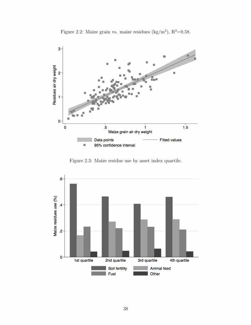
Figure 2.2: Maize grain vs. maize residues (kg/m2), R2=0.58.

Figure 2.3: Maize residue use by asset index quartile.

38

Table 2.1: Summary statistics of variables used.

Standard Minimum MaximumVariable Mean Deviation Value Value

Gender of household head: 1=male* 0.81Household head age 51.41 15.35 20.00 90.00Household head years of education 6.75 4.53 0.00 18.00Household size 6.06 2.46 1.00 13.00Asset index 0.00 1.00 -1.00 5.95Estimate of household annual income (KES) 146,610 262,733 0 3,674,650Total land area farmed (acres) 4.53 9.82 0.05 110.00Land in maize as share of total 0.42 0.27 0.01 1.00No chemical fertilizer applied* 0.36No maize residues applied* 0.17Soil pH 5.82 (Low) 0.52 4.35 7.13Soil nitrogen (% by weight) 0.16 (Very low) 0.09 0.06 0.87Average plot altitude (m) 1,606 330 1,205 2,258Herd size (TLU) 2.38 2.71 0.00 17.66Own livestock* 0.94

Household-level, across two seasonsMaize grain harvest (kg) 1,001.81 1,283.24 11.50 10,453.52Maize land (acres) 1.58 1.22 0.08 7.14Labor (person-days) 94.14 67.97 11.00 406.00NPK (kg) 25.28 41.33 0.00 315.00Fertilizer (kg) 48.26 81.32 0.00 700.00N (kg) 10.79 18.71 0.00 154.00Maize residues (kg) 1,521.08 1,579.88 0.00 9,561.73Fraction of acres planted with hybrid maize 0.58 0.46 0.00 1.00Fraction of acres intercropped with legumes 0.74 0.39 0.00 1.00

Note: * indicates binary variable. N=309 households.

39

Table 2.2: Sample soils data by key indicator (N=309).

Indicator Mean (Ranking) St. Dev. Min Max

Organic carbon content (% by weight) 2.45 (Good) 1.30 0.81 9.45Total nitrogen content (% by weight) 0.16 (Very Low) 0.09 0.06 0.87Extractable P (g/kg) 0.013 (Good) 0.015 0.0006 0.1321Extractable K (g/kg) 0.36 (Good) 0.22 0.05 1.34Soil pH 5.82 (Low) 0.52 4.35 7.13

Table 2.3: Allocation of maize residues across the main uses.

Variable Mean St. Dev. Min Max

Share of maize residues to soil fertility management 0.47 0.31 0 1Share of maize residues to animal feed 0.25 0.27 0 0.9Share of maize residues to residential fuel 0.22 0.15 0 1Share of maize residues to other uses 0.05 0.17 0 0.8

Note: N=309 households.

40

Table 2.4: Household-level maize production function.

Maize grain (kg) Coe�cient Std. Err.

Maize land (acres) 65.79 (182.7)Labor days -0.251 (2.509)NPK (kg) 0.659 (4.751)Residues (kg) 0.217** (0.102)1/2 Maize land sq. 252.6** (100.1)1/2 Labor days sq. -0.0125 (0.0233)1/2 NPK sq. 0.0823 (0.0685)1/2 Residues sq. 0.000133** (5.27e-05)Interaction: Land * Labor -0.135 (1.132)Interaction: Land * NPK 1.177 (2.006)Interaction: Land * Residues -0.250*** (0.0503)Interaction: Labor * NPK 0.00997 (0.0367)Interaction: Labor * Residues 0.00127 (0.000856)Interaction: NPK * Residues 0.000979 (0.00110)Average plot altitude (m) 0.649*** (0.150)Soil pH 92.72 (67.85)Soil nitrogen (% by weight) 125.5 (307.1)Herd size (TLU) 66.31*** (19.39)Fraction of acres intercropped with legumes -26.62 (90.32)Fraction of acres planted with hybrid maize -105.9 (87.55)Gender of household head: 1=male -79.48 (75.93)Household head age -1.464 (2.072)Household head years of education 1.574 (6.802)Constant -1,285** (540.3)

Observations 309R-squared 0.852

Wald tests �

2 Prob> �

2

Coe�cients for land: ↵1 = ↵11 = ↵12 = ↵13 = ↵14 = 0 38.66 0.00Coe�cients for labor: ↵2 = ↵12 = ↵22 = ↵23 = ↵24 = 0 3.04 0.69Coe�cients for NPK: ↵3 = ↵13 = ↵23 = ↵33 = ↵34 = 0 50.24 0.00Coe�cients for residues: ↵4 = ↵14 = ↵24 = ↵34 = ↵44 = 0 35.42 0.00All second-order terms: = 0 61.06 0.00

Note: Bootstrapped standard errors in parentheses (1,000 replications). *** p<0.01, ** p<0.05, * p<0.1.

41

Table 2.5: Household-level marginal physical productivities (MPP), marginalvalue productivities (MVP), and benefit/cost estimates.

Variable MPP (kg maize/ MVP Input price Marginal benefit/costunit input) (KES) (KES) (MVP/input price)

Maize land (acres) 103.36 (335.03) 2,997.44 (9,715.87) 2,110 1.42 (4.60)Labor (person-days) 0.54 (1.91) 15.74 (55.31) 138 0.01 (0.40)NPK (kg) 8.11 (5.93) 235.29 (172.04) 146 1.61 (1.18)Maize residues (kg) 0.21 (0.18) 6.03 (5.33) 5.49 1.10 (0.97)

Note: Standard errors are in parentheses. MPP of NPK and MPP of maize residues are reported onlyfor households with positive input values (N=198 and N=257, respectively). Sample average maize price is29 KES. Input prices are based on the mean reported prices from the household survey (price of land is thesample average rental price of 1 acre of land, price of labor is the sample average price of 1 person-day of hiredlabor, and price of NPK is the household-level sample average price of 1 kilogram of NPK (expenditure onchemical fertilizer divided by the quantity of N, P, K in kg). Input price for maize residues is the estimatedaverage shadow value (not adjusted for travel cost). 84 KES = 1 USD (average 2011-2012 exchange rate).

Table 2.6: Shadow price of maize residues (KES/kg).

Variable Mean St. Dev. N

Using market price of NPKValue for full sample 6.29 7.43 162Value for full sample, excluding top and bottom 5% 5.49 4.34 144

Using market price of NPK adjusted for travel costValue for full sample 6.90 9.07 162Value for full sample, excluding top and bottom 5% 6.05 5.06 144

Note: Calculated using household-specific price of 1 kg of NPK. 84 KES = 1 USD (average 2011-2012exchange rate).

42

Table 2.7: Economic value of maize residues in Kenyan shillings (KES) andUS dollars (USD).

Variable Value in KES Value in USD

Maize residues for soil fertility management per farm 8,351 (8,674) 99 (103)All maize residues per farm 17,458 (19,526) 208 (232)

Value per acreMaize residues per acre 11,239 (6,567) 134 (78)Maize grain per acre 19,426 (14,924) 231 (178)

Value per hectareMaize residues per acre 27,760 (16,219) 330 (193)Maize grain per acre 47,982 (36,863) 571 (439)

Note: Calculated using 5.49 KES as value of 1 kg of maize residues and 29 KES as price of 1 kg ofmaize grain. Standard errors are in parentheses. N=309 households. 84 KES = 1 USD (average 2011-2012exchange rate).

43

Table 2.8: Household- and farm-level determinants of the shadow value ofmaize residues.

Value of cropresidues (KES/kg) (1) (2)

Gender of household head: 1=male 2.717* 0.520(1.535) (1.027)

Asset index from first PC -1.191* -1.158***(0.638) (0.394)

Herd size (TLU) -1.146** -0.204(0.501) (0.312)

Herd size squared 0.0799 0.0122(0.0556) (0.0323)

Household size -0.611** -0.222(0.293) (0.186)

Total land area farmed (acres) -0.0904 -0.0685(0.225) (0.150)

Land in maize as share of total -6.663*** -3.220*(2.187) (1.690)

Average plot altitude (m) 0.0762** 0.0298**(0.0379) (0.0129)

Soil nitrogen (% by weight) 15.55 1.194(14.22) (7.392)

Soil pH 3.463* 1.522(1.800) (1.043)

Constant -115.3** -42.39**(57.80) (21.01)

Observations 162 144Village fixed e↵ects YES YESR-squared 0.359 0.384

Note: Bootstrapped standard errors in parentheses (1,000 replications). *** p<0.01, ** p<0.05, *p<0.1. Sample size is the households that used both chemical fertilizer and maize residues for soil fertilitymanagement in positive quantities. Column (2) excludes the households with the shadow value in the topand bottom tails (5 percent of the distribution).

44

APPENDIX

2.A Additional tables

45

Table 2.A.1: Scoring coe�cients (weights) for asset index.

Variable Weight

Durables: number ofHouse 0.411Radio 0.389Telephone (mobile) 0.649Fridge/freezer 0.620Television 0.688Electronic equipment 0.559Air conditioning 0.339Furniture 0.743Kettle/iron 0.446Mosquito net 0.602Computer 0.529Internet access 0.351Electric/gas stove 0.526Improved stove 0.217Bicycle 0.332Motorcycle 0.483Car/truck 0.568Bank account 0.699Generator 0.291Large battery 0.177Solar panel 0.338LPG 0.636

Characteristics: indicator forBrick/cement walls 0.700Mabati (corrugated iron) roof 0.379Cement/wood floor 0.666Private piped water 0.447Water from neighbor -0.068Borehole water 0.036River/stream water -0.184No toilet -0.279Traditional toilet -0.293Improved toilet 0.703Kerosene light -0.717Electricity light 0.763Solar light 0.112

Observations 309

46

Tab

le2.A.2:Specification

sof

thehou

seholdmaize

productionfunction.

(1)

(2)

(3)

(4)

(5)

(6)

Maize

grain(kg)

Parsimon

ious

Quad

ratic

Environ

.va

rsAllco

ntrols

Block

dummies

Village

dummies

Maize

land(acres)

318.8*

**17

6.9

80.63

65.79

75.70

45.51

(95.02)

(195.2)

(184.2)

(190.5)

(189

.7)

(191.5)

Laborday

s-0.922

-2.031

-0.0931

-0.251

-0.508

0.0175

(0.888)

(2.797)

(2.542)

(2.533)

(2.644

)(2.537)

NPK

(kg)

19.98*

**4.76

10.30

90.65

90.29

20.72

3(2.299)

(5.147)

(4.563)

(4.663)

(4.753

)(4.560)

Residues

(kg)

0.0538

0.186*

0.203**

0.217**

0.221**

0.220**

(0.0676)

(0.109)

(0.0938)

(0.0978)

(0.103)

(0.104)

1/2Maizelandsq.

225.1**

243.7**

252.6**

255.7**

267.1**

(114.3)

(97.78

)(99.56)

(99.53)

(104.5)

1/2Laborday

ssq.

-0.00586

-0.0129

-0.0125

-0.0106

-0.0131

(0.0248)

(0.0237)

(0.0239)

(0.024

3)

(0.0226)

1/2NPK

sq.

0.1000

0.0859

0.0823

0.0811

0.0806

(0.0721)

(0.0649)

(0.0687)

(0.068

2)

(0.0684)

1/2Residues

sq./1,000

0.151***

0.133***

0.133***

0.131*

*0.136***

(0.0537)

(0.0513)

(0.0501)

(0.052

1)

(0.0507)

Interaction:Land*Labor

-0.0326

-0.109

-0.135

-0.239

-0.257

(1.216)

(1.149

)(1.159)

(1.128)

(1.085)

Interaction:Land*NPK

0.416

1.210

1.177

1.085

1.121

(2.240)

(1.956

)(2.004)

(1.946)

(2.046)

Interaction:Land*Residues

/1,000

-253.3***

-246.6***

-249.6***

-244.6***

-243.3***

(55.71)

(48.50

)(48.35)

(49.44)

(51.94)

Interaction:Labor*NPK

0.0162

0.00875

0.00997

0.0142

0.0110

(0.0397)

(0.0345)

(0.0356)

(0.039

0)

(0.0359)

Interaction:Labor*Residues

/1,000

1.150

1.281

1.27

31.211

1.139

(0.916)

(0.833

)(0.825)

(0.832)

(0.818)

Interaction:NPK

*Residues

/1,000

0.588

0.976

0.979

0.972

0.893

(1.191)

(1.051

)(1.113)

(1.058)

(1.131)

Averag

eplotaltitu

de(m

)0.60

1***

0.64

9***

0.38

5-0.120

(0.141)

(0.158)

(0.333)

(0.555)

SoilpH

85.88

92.72

149.1

245.1*

(60.60)

(68.09)

(111.8)

(136.4)

Soilnitrogen

(%byweight)

95.07

125.5

203.5

269.6

(309.2)

(302.1)

(339.3)

(349.6)

Herdsize

(TLU)

59.96*

**66

.31*

**68

.90*

**66

.12*

**(17.99)

(19.15)

(19.28)

(20.14)

Fractionof

acres

intercropped

withlegumes

-26.62

-67.30

-90.71

(92.18)

(98.79)

(95.46)

Fractionof

acres

plantedwithhybridmaize

-105.9

-76.11

-179.5

(95.16)

(111.6)

(125.6)

Gen

der

ofhousehold

hea

d:1=male

-79.48

-86.98

-74.84

(76.87)

(76.52)

(85.96)

Hou

seholdhea

dag

e-1.464

-2.014

-2.425

(2.085)

(2.077)

(2.463)

Hou

seholdhea

dyea

rsof

educa

tion

1.57

4-0.658

1.61

3(7.121)

(6.838)

(8.012)

Constant

-3.355

216.2**

-1,366***

-1,285**

-1,339

-1,202

(73.59)

(108.9)

(495.6)

(541.7)

(1,071

)(1,129)

R-squared

0.722

0.826

0.850

0.852

0.854

0.863

Note:

Boo

tstrap

ped

stan

darderrors

inparentheses

(1,000

replication

s).***p<0.01,**

p<0.05,*p<0.1.

47

Table 2.A.3: Quadratic maize production function: NPK, nitrogen (N), andtotal fertilizer.

(1) (2) (3)Maize grain (kg) NPK N Fertilizer

Maize land (acres) 65.79 129.8 78.40(188.1) (193.2) (187.9)

Labor days -0.251 -0.364 -0.448(2.603) (2.183) (2.404)

NPK/N/Fertilizer (kg) 0.659 2.004 0.766(4.808) (8.407) (2.424)

Residues (kg) 0.217** 0.199** 0.202**(0.102) (0.0919) (0.0938)

1/2 Maize land sq. 252.6*** 385.2*** 286.4***(97.62) (103.3) (95.16)

1/2 Labor days sq. -0.0125 0.0154 -0.00299(0.0234) (0.0204) (0.0214)

1/2 NPK/N/Fertilizer sq. 0.0823 0.645** 0.0163(0.0666) (0.320) (0.0154)

1/2 Residues sq. / 1,000 0.133*** 0.181*** 0.158***(0.0489) (0.0445) (0.0464)

Interaction: Land * Labor -0.135 -1.749* -0.542(1.132) (1.027) (1.097)

Interaction: Land * NPK/N/Fertilizer 1.177 -2.737 0.664(1.953) (5.181) (0.977)

Interaction: Land * Residues / 1,000 -249.6*** -281.4*** -258.5***(48.75) (53.38) (44.76)

Interaction: Labor * NPK/N/Fertilizer 0.00997 0.00442 0.00416(0.0364) (0.0495) (0.0176)

Interaction: Labor * Residues / 1,000 1.273 0.885 1.037(0.840) (0.584) (0.740)

Interaction: NPK/N/Fertilizer * Residues / 1,000 0.979 2.911 0.398(1.007) (2.379) (0.543)

Average plot altitude (m) 0.649*** 0.783*** 0.654***(0.157) (0.153) (0.149)

Soil pH 92.72 63.10 87.96(68.46) (64.62) (68.81)

Soil nitrogen (% by weight) 125.5 210.4 225.3(313.0) (299.5) (309.4)

Herd size (TLU) 66.31*** 53.25*** 62.47***(19.45) (15.31) (16.89)

Fraction of acres intercropped with legumes -26.62 -46.76 -14.12(87.73) (90.78) (92.45)

Fraction of acres planted with hybrid maize -105.9 -61.70 -110.7(92.07) (81.47) (85.57)

Gender of household head: 1=male -79.48 -71.18 -87.21(76.55) (74.16) (75.49)

Household head age -1.464 -0.262 -1.489(2.083) (2.028) (2.170)

Household head years of education 1.574 4.787 2.704(7.052) (7.107) (7.485)

Constant -1,285** -1,450*** -1,281**(550.0) (520.9) (527.5)

R-squared 0.852 0.861 0.858Shadow price of residues (KES/kg) 6.29 (7.43) 9.74 (17.50) 5.28 (5.43)Shadow price of residues (KES/kg), excl. top and bottom 5% 5.49 (4.34) 8.81 (8.33) 5.00 (3.74)

Note: Bootstrapped standard errors in parentheses (1,000 replications). *** p<0.01, ** p<0.05, *p<0.1. Column (1) is the same as Table 3. Column (2) repeats the estimation with N (kg) instead of NPK(kg); shadow price is calculated using household-specific price of nitrogen (depending on the fertilizer type).Column (3) repeats the estimation with Total fertilizer (kg) instead of NPK (kg); household-specific priceof fertilizer is calculated as price of fertilizer divided by fertilizer amount in kg.

48

Table 2.A.4: Cobb-Douglas and translog maize production functions.

(1) (2)LN(Maize grain (kg)) Cobb-Douglas Translog

LN(Maize land (acres)) 0.450*** 1.473**(0.0975) (0.642)

LN(Labor days) 0.160* -0.641(0.0911) (0.947)

LN(NPK (g)) 0.107** -1.059*(0.0447) (0.590)

LN(Residues (g)) 0.313*** -0.515(0.0895) (1.196)

1/2 Maize land sq. 0.112(0.145)

1/2 Labor days sq. 0.150(0.210)

1/2 NPK sq. 0.130**(0.0606)

1/2 Residues sq. 0.0706(0.0860)

Interaction: Land * Labor -0.119(0.134)

Interaction: Land * NPK 0.00638(0.0191)

Interaction: Land * Residues -0.0655***(0.0136)

Interaction: Labor * NPK -0.0149(0.0208)

Interaction: Labor * Residues 0.0203(0.0143)

Interaction: NPK * Residues -0.00181(0.00206)

Average plot altitude (m) 0.000757*** 0.000583***(0.000175) (0.000186)

Soil pH -0.0890 -0.125(0.0969) (0.0943)

Soil nitrogen (% by weight) 0.589 0.615(0.562) (0.577)

Herd size (TLU) 0.0616*** 0.0706***(0.0150) (0.0143)

Fraction of acres intercropped with legumes 0.0968 0.0441(0.128) (0.120)

Fraction of acres planted with hybrid maize 0.297** 0.180(0.125) (0.125)

Gender of household head: 1=male 0.00388 -0.0389(0.108) (0.104)

Household head age -0.00162 -0.00158(0.00291) (0.00285)

Household head years of education 0.00322 0.00239(0.0107) (0.0110)

No chemical fertilizer applied: =1 0.590 -4.161*(0.382) (2.224)

No maize residue applied: =1 3.871*** 0.843(1.180) (7.068)

Constant -0.832 11.23(1.530) (9.087)

R-squared 0.665 0.714Shadow price of residues (KES/kg) 11.46 (17.74) 20.00 (120.00)Shadow price of residues (KES/kg), excl. top and bottom 5% 8.72 (7.17) 7.97 (12.44)

Note: Bootstrapped standard errors in parentheses (1,000 replications). *** p<0.01, ** p<0.05, * p<0.1.Column (1) is the Cobb-Douglas specification with maize grain harvest, land, labor, NPK and residues inlog forms. Column (2) is the translog specification. LN(NPK (g)) = LN(NPK (g) if NPK>0), =1 otherwiseand LN(Residues (g))=LN(Residues (g) if Residues>0), =1 otherwise.

49

CHAPTER 3

AGRICULTURAL PRODUCTIVITY AND SOIL CARBON DYNAMICS: A

BIOECONOMIC MODEL

3.1 Natural resources, poverty, and climate

The world’s poorest billion people mostly live in rural areas, where their livelihoods depend

directly on natural capital (Hassan, Scholes, and Ash 2005). They derive a substantial por-

tion of their livelihoods from farmland, forests, and waterways, so that the natural capital

is not only an amenity but also a primary factor of production. While natural resources

are typically renewable, overuse or mismanagement leads to their depletion and deteriora-

tion (Dasgupta 2010). Crop lands stop responding to applications of fertilizer, inland and

coastal fisheries become depleted, and excessive deforestation leads to loss of biodiversity.

For the poor, especially in fragile environments in Africa and some parts of Latin America

and Asia, the reduced stocks and the deteriorated ecosystem services they provide lead to

lower land productivity and stagnating incomes, as well as discourage investments in main-

taining the natural resource base or in new agricultural technologies needed for su�cient

food production. Improving the management of natural resources is, therefore, fundamental

to addressing rural poverty.

Management of soil resources in smallholder agriculture of Sub-Saharan Africa (SSA) is

of particular concern as depletion of soil fertility is considered to be one of the major bio-

physical causes of low per capita food production (Sanchez 2002). About 414 million people

in the region—up from 290 million people in 1990—live in extreme poverty, and Sub-Saharan

Africa remains the region with the highest prevalence of undernourishment (UN 2014). The

neglect of the rural sector by governments and the collapse of traditional societies and their

practices (e.g., fallowing) over many decades have resulted in the removal of large quanti-

50

ties of nutrients from soils without su�cient quantities of fertilizer or organic resources to

replenish them. Almost 40 percent of land across SSA su↵er from nutrient depletion, mak-

ing it the primary source of soil degradation across the continent (Tully et al. 2015). As

soils depleted of organic matter and nutrients are less responsive to mineral fertilizers and

changing climate, more and more resources are needed to maintain food production. As a

result, smallholder farmers in SSA “cultivate marginal soils with marginal inputs, produce

marginal yields, and perpetuate marginal living and poverty” (Lal 2004, p. 1626). In addi-

tion, degradation of soil resources in SSA leads to numerous environmental concerns, such as

water pollution and conversion of natural environments and marginal lands to agriculture,

among many others. And some estimates suggest that across SSS climate change will lead

to a further 36 percent decline in cereal yields by the end of the century (Ward, Florax, and

Flores-Lagunes 2014).

Soil resources also play a major role in the global carbon cycle. Soils and the biomass

therein contain about 2,500 petagrams (1 Pg is equal to one billion metric tons) of carbon

within a one-meter depth, making soils the largest terrestrial pool of carbon (Woodward

et al. 2009). And while agriculture accounts for 20-30 percent of total global greenhouse

gas emissions, agricultural soils and biomass also sequester carbon out of the atmosphere

(WB 2012). “Climate-smart” farming practices can take advantage of the soil role as a

carbon sink and a carbon store and simultaneously reduce emissions. These practices include

mulching, retention of crop residues, use of manures, agroforestry, and many others. Lal

(2004) estimates that soil carbon sequestration from sustainable use and agriculture could

sequester 0.4-1.2 Pg of carbon per year. This amount is equivalent to 5-15 percent of global

emissions from fossil fuels.

In this paper, we ask the following questions: what is the optimal management of soil

resources in smallholder agriculture in the tropics, what is the potential for increasing yields

and sequestering carbon, and what is the value of soil carbon? To answer these questions,

51

we develop a dynamic bioeconomic model of agricultural households in the western Kenyan

highlands. Our theoretical bioeconomic modeling framework extends the traditional eco-

nomic agricultural household model to incorporate the dynamic nature of natural resource

management and to integrate biophysical processes through soil carbon management. Using

an eight-year panel dataset from an agronomic “chronosequence” experiment in Vihiga and

Nandi districts in Kenya and data from household and market surveys, our model combines

an econometrically estimated production function and a calibrated soil carbon flow equation

in a maximum principle framework. The unique nature of our dataset—a “false” time series,

comparable to a quasi-natural experiment and not often available for economic research—

allows for estimation of site-specific dynamic relationships between agronomic productivity,

land use management decisions, and soil carbon.

We use the model to determine the optimal management of the farming system over

time in terms of the application rates of mineral fertilizer and crop residues, taking into

consideration initial resource endowments and prices. The combined application of mineral

fertilizer and organic resources is required to overcome soil fertility depletion across SSA

(Vanlauwe and Giller 2006) and to sequester carbon (Lal 2014). The two inputs fulfill

di↵erent functions. While the main role of mineral fertilizer is to supply nutrients, organic

resources replenish soil carbon and soil organic matter stocks that enhance soil physical,

chemical, and biological processes and properties, fundamental for long-term soil fertility and

nutrient use e�ciency (Blanco-Canqui et al. 2013). The improvement of soil properties not

only sustains yields, but also enhances the inherent capacity of soils to bu↵er against extreme

climatic events such as droughts, heat waves, and floods. Moreover, the limited availability

and high cost of external inputs, as well as competing uses for on-farm organic resources (fuel

and fodder) often discourage the applications of either in su�cient quantities (Vanlauwe and

Giller 2006). At the same time, decomposition of crop residues into soil carbon may require

additional nutrients, such as nitrogen, phosphorus, and sulfur (Richardson et al. 2014).

Understanding how soil resources respond to the combined applications and determining the

52

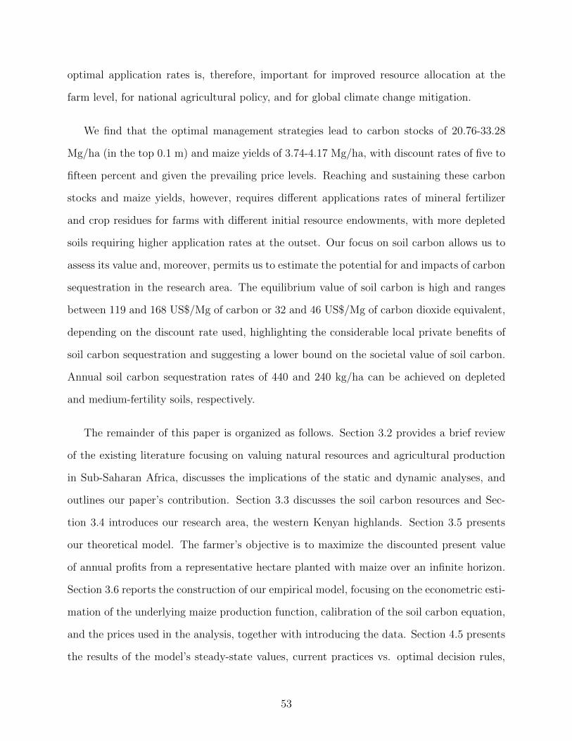
optimal application rates is, therefore, important for improved resource allocation at the

farm level, for national agricultural policy, and for global climate change mitigation.

We find that the optimal management strategies lead to carbon stocks of 20.76-33.28

Mg/ha (in the top 0.1 m) and maize yields of 3.74-4.17 Mg/ha, with discount rates of five to

fifteen percent and given the prevailing price levels. Reaching and sustaining these carbon

stocks and maize yields, however, requires di↵erent applications rates of mineral fertilizer

and crop residues for farms with di↵erent initial resource endowments, with more depleted

soils requiring higher application rates at the outset. Our focus on soil carbon allows us to

assess its value and, moreover, permits us to estimate the potential for and impacts of carbon

sequestration in the research area. The equilibrium value of soil carbon is high and ranges

between 119 and 168 US$/Mg of carbon or 32 and 46 US$/Mg of carbon dioxide equivalent,

depending on the discount rate used, highlighting the considerable local private benefits of

soil carbon sequestration and suggesting a lower bound on the societal value of soil carbon.

Annual soil carbon sequestration rates of 440 and 240 kg/ha can be achieved on depleted

and medium-fertility soils, respectively.

The remainder of this paper is organized as follows. Section 3.2 provides a brief review

of the existing literature focusing on valuing natural resources and agricultural production

in Sub-Saharan Africa, discusses the implications of the static and dynamic analyses, and

outlines our paper’s contribution. Section 3.3 discusses the soil carbon resources and Sec-

tion 3.4 introduces our research area, the western Kenyan highlands. Section 3.5 presents

our theoretical model. The farmer’s objective is to maximize the discounted present value

of annual profits from a representative hectare planted with maize over an infinite horizon.

Section 3.6 reports the construction of our empirical model, focusing on the econometric esti-

mation of the underlying maize production function, calibration of the soil carbon equation,

and the prices used in the analysis, together with introducing the data. Section 4.5 presents

the results of the model’s steady-state values, current practices vs. optimal decision rules,

53

and sensitivity analyses. Section 4.6 concludes the paper.

3.2 Value of soil resources in agricultural production

A number of qualitative studies focusing on the implications of rural environmental degra-

dation have shed light on how the incomes of rural communities are a↵ected by resource

degradation. Yet, there is limited empirical work demonstrating the quantitative impor-

tance of natural resources as factors of production (Lopez 1997). Valuing the local natural

resource base in the developing world is a challenging task. The subsistence nature of

smallholder agriculture means that farmers make production, consumption, and resource

allocation decisions subject to considerable temporal uncertainty, both in terms of the bio-

physical environment (soil quality, rainfall, adverse weather conditions, pests, etc.) and the

economic environment (output and input prices, input availability, etc.). Hence, farming

systems in developing countries are very complex; they include a large number of interlinked

activities, outcomes of which frequently depend directly on the conditions of local natural

resources rather than on external input use. Since natural resources a↵ect farming activities

through complex biophysical processes, their e↵ects may not be entirely understood and

are di�cult to quantify. In addition, natural resource management in developing countries

has environmental implications that often go beyond farm boundaries, both temporally and

geographically, and volatility in markets and prices complicate the analysis (Barbier and

Bergeron 2001).

Interest in the impacts of soil resource management on agricultural output dates back

to at least the Dust Bowl era of the 1930s in the American Midwest (Thampapillai and

Anderson 1994). Recognizing the e↵ects of land use practices and agricultural technologies

on agricultural productivity, a rich body of literature in agricultural economics addresses

these issues in a static production framework. Specifically for Sub-Saharan Africa, numerous

54

studies address crop responses to fertilizer use, hybrid seeds, and other external inputs or

reasons for their limited applications (see, for example, recent studies in Kenya by Marenya

and Barrett (2009a), Suri (2011), Duflo, Kremer, and Robinson (2011), and Sheahan, Black,

and Jayne (2013)).

At the same time, relatively few studies explicitly recognize the direct impacts of man-

agement practices on soil fertility beyond including indicators for farmers’ perception of soil

quality. Several studies consider the e↵ects of decreasing common pools of biomass or leaving

land fallow. Lopez (1997) examines the common village-level stock of biomass and its decline

due to reductions in the fallow periods in Ghana. By incorporating village-level biomass as

an input in agricultural production, he finds that it is an important factor of production and

is often exploited beyond the socially optimal level. Goldstein and Udry (2008) demonstrate

the importance of fallows for on-farm soil quality, and hence, profits from agricultural plots

left fallow, also in Ghana. As applications of animal manure deliver not only nutrients neces-

sary for plant growth but also help maintain long-term soil fertility, Gavian and Fafchamps

(1996) and Sheahan, Black, and Jayne (2013), for example, include indicator variables for

manure use, while Marenya and Barrett (2009b) consider the value of livestock as a proxy

for manure applications. Only two papers from SSA, to our knowledge, include quantities of

animal manure as inputs in crop response models (Teklewold 2012; Matsumoto and Yamano

2011), and only one considers the quantities of crop residues (Chapter 2).

Soil degradation in the current period imposes a reduction in net benefits on the future

generation (i.e., user cost); therefore, it ideally needs to be evaluated within an intertemporal

framework. Some of the earlier work treating soil as a renewable resource comes from the

U.S. For example, Burt (1981) employs a dynamic programming framework to model soil

conservation in the U.S. Northwest, using depth of topsoil and the percentage of organic

matter therein as the state variables and cropping practices as the control variables. Mc-

Connell (1983) uses soil loss as the state variable in a theoretical model of soil conservation

55

to argue that the private and social rates of soil erosion are the same under most institutional

arrangements.

Yet, the paucity of detailed information available to economists, such as technical data on

rates of soil fertility loss, as well as the inherent complexity of farming systems, has limited

the dynamic analysis of soils in developing countries. Some past studies focus on qualitative

analysis (see, for example, French (1986)), while others include biophysical variables such as

soil nutrients (carbon, nitrogen, phosphorus), organic matter depletion and soil erosion and

simulate the e↵ects of land degradation by incorporating parameters estimated in a separate

biophysical model into a model of economic behavior. Barbier (1998), for example, combines

a linear programming model of economic behavior with agricultural production parameters

obtained from the results of the Erosion Productivity Impact Calculator (EPIC) model to

study land degradation in Burkina Faso. Wise and Cacho (2011) use the Soil Changes Under

Agriculture, Agroforestry, and Forestry (SCUAF) model to derive soil-carbon changes, crop-

yield dynamics and tree-biomass accumulation as functions of management variables in a

dynamic simulation model to assess the financial viability of agroforestry systems as carbon

sinks in Indonesia.

Specifically for western Kenya, two simulation models examine the links between bio-

physical and economic processes at the farm scale. Shepherd and Soule (1998) develop

a simulation model to predict the long-term e↵ects of farming systems on nutrient cycling,

plant production and farm income, while Stephens et al. (2012) use a system dynamics model

to examine the interactions between natural resource-based poverty traps and food security

for small farms in Kenya. Both of these models, however, are descriptive or predictive (not

optimization problems), and do not allow for changes in management practices in response

to physical changes in soil.

Only when detailed biophysical data from the research area are available and allow for

estimation of crop productivity responses and soil condition changes, however, can bioeco-

56

nomic models truly internalize the e↵ects of land degradation on household intertemporal

decisions. In one such example, using plot-level data from field experiments in the Ethiopian

highlands, Holden, Shiferaw, and Pender (2005) assess the impacts of land degradation, pop-

ulation growth, market imperfections, and increased risk of drought on household production,

food security, and welfare.

Our paper contributes to both static and dynamic strands of the literature. Our dynamic

bioeconomic model treats soil fertility as an input in agricultural production and a renew-

able resource, while the rich agronomic and socio-economic datasets we use allow for the

model’s precise estimation. We explicitly recognize that agricultural outcomes depend on

the conditions of local natural resources and consider soil fertility as a factor of agricultural

production. At the same time, we model farm household intertemporal management prac-

tices and their e↵ects on current and future agricultural productivity. By doing so, we are

also able to assign monetary value to soil fertility and specifically soil carbon, thus quanti-

tatively demonstrating the importance of natural resources as primary factors of production

in smallholder agriculture.

3.3 Focus on soil carbon

We focus on soil carbon as the interface between the social and biophysical processes. There

are several compelling reasons for doing so. First, there is a strong relation between soil

organic carbon (SOC) and soil fertility, on the one hand, and crop productivity and soil

fertility, on the other. Although SOC is not essential to plant growth per se and its ben-

efits can be to a degree substituted by applying external inputs, the SOC pool is related

to the amount of soil organic matter (SOM) with multiple benefits to soil productivity,

such as nutrient availability, water-holding capacity, and soil biota, and therefore, on agro-

nomic/biomass productivity (Lal 2006; Blanco-Canqui et al. 2013). Increases in SOC, in

57

addition, not only increase average yields, but also decrease the susceptibility of yields to

weather shocks (Gra↵-Zivin and Lipper 2008).

Land use decisions, such as the conversion of forests to agricultural land, have a major

influence on the level of the SOC pool. By removing the bulk of aboveground biomass,

conversion to agricultural land breaks the carbon movement cycle in the ecosystem as soil

carbon is not replenished fast enough to keep up with decomposition. A large fraction of

the accumulated carbon and soil nutrients thus become lost; this generally happens most

rapidly in the years immediately after agricultural conversion (Murty et al. 2002). Current

agricultural practices in resource-poor economies also deplete the SOC and SOM pools, and

by doing so degrade soil quality and have an adverse e↵ect on agronomic productivity. At

the same time, agricultural management practices that alter the inputs of organic matter or

the decomposition rate of SOM can build up the stock of soil organic carbon. Such practices

include leaving land fallow, no-till farming, residue retention, manuring, composting, N

fertilization, mulching, incorporation of grass and legumes in the rotation cycle, and the use

of agroforestry systems (Lal 2006; WB 2012).

The second reason for our focus on soil carbon is found in the potential of carbon seques-

tration to simultaneously achieve two sustainability goals: the improvement of agricultural

productivity and climate change mitigation (Antle and Stoorvogel 2008). Land use changes

and agricultural practices can transfer atmospheric carbon dioxide (CO2) to soil. With the

continuing use of these practices over 20-50 years, observed rates of SOC sequestration can

range from 0 to 150 kg C/ha per year in dry and warm regions, and up to 100-1,000 kg C/ha

per year in humid and cool climates, depending on soil texture, characteristics and climate

(Lal 2004). As a result, it is estimated that soil carbon sequestration from sustainable land

use and agriculture could potentially o↵set the emissions from fossil fuels by 0.4-1.2 Gt C

per year, or 5 to 15 percent of the global fossil fuel emissions (Lal 2004).

The third reason for focusing on soil carbon, as Antle and Stoorvogel (2008) note, is the

58

fact that despite great interest in the international community and among national policy-

makers, there is little available information about the potential for and impacts of payments

for agricultural carbon sequestration from actual projects. By estimating the potential for

carbon sequestration and valuing carbon on the western Kenyan farms, we provide such

empirical evidence.

3.4 Study area: western Kenyan highlands

The western Kenyan highlands provide our case study. Surrounding Lake Victoria on the

Kenyan side, this is one of the most densely populated regions of the country, with over 55

percent of the population living below the national rural poverty line (about US$0.59 per

day) (WRI 2007). The complexity of smallholder farming systems in developing countries,

as discussed above, also characterizes this research area. Rural households engage in a range

of agricultural activities. While their main objective is increasing food supplies (Waithaka

et al. 2006), subsistence farmers also strive to earn income and satisfy household energy

needs.

Average farms are about 0.5-2 hectares in size and originally formed part of the Guineo-

Congolese forest system that became converted to agricultural land in the 20th century.

Farms have medium to high agricultural potential (WRI 2007), but su↵er from severe soil

degradation. The incorporation of crop residues at plowing, crop rotations and short fallows

were some of the main means of maintaining soil fertility in crop fields in western Kenya

until the 1960s (Crowley and Carter 2000). As population increased and farm areas declined,

however, crop rotations and fallowing periods were reduced and most farmers have stopped

planting woodlots, making cereal residues the principal on-farm source of fuel. Only wealthier

households with larger land holdings have continued fallowing and/or using crop rotations

(Crowley and Carter 2000). As a result, the amount of organic material returned to the soil

59

after harvest has significantly declined in the area and maize monoculture has hastened soil

deterioration (Solomon et al. 2007).

We examine one of the main agricultural activities of households in rural western Kenya—

production of a subsistence crop, maize (Zea mays L.). Maize is the most commonly grown

and consumed grain in the area, having established itself as a dominant food crop in Kenya

at the beginning of the 20th century (Crowley and Carter 2000). Despite its significant

contribution to satisfying household food needs and cultivation by most smallholders on

the largest proportion of farm area, maize production often results in low yields. Farmer-

reported average maize yields are in the range of 1.65 and 2.7 Mg/ha1 (Sheahan, Black,

and Jayne 2013). The potential yields in response to water and nutrient availability for this

environmental range, however, are found to be much higher, between 10.8 and 11.4 Mg/ha

(Tittonell and Giller 2013).

Low yields correspond to current agricultural practices—no fallowing, limited use of

hybrid seeds and mineral fertilizer, as well as organic resources, such as crop residues, animal

manures, compost, etc. In fact, the use of maize residues as soil organic amendments is traded

o↵ against other applications. Less than half of all residues is left on the field for soil fertility

management; the other half is roughly equally split between household energy and animal

feed (Chapter 2). Soil carbon stocks, as a result, are heavily depleted (Solomon et al. 2007).

Data from several sources are used to build the bioeconomic model described below.

Plot-level maize yields and carbon stocks come from a long-term agronomic experiment in

Vihiga and Nandi districts of western Kenya in 2005-2012, while socio-economic household-

level data and prices are from the household and market surveys in the districts surrounding

the agronomic sites in 2011-2013. The data sources are shown in Figure A.1.2 and further

discussed in the sections that follow. Our soil analysis reported the total stocks of soil carbon,

which are equivalent to total organic carbon since the soils in the research site are acidic and

11 megagram (Mg) = 1,000 kilogram (kg) = 1 metric tonne. 1 hectare (ha) = 10,000 square meters.

60

do not contain carbonates.

3.5 Economic model

Our model is similar to that of Burt (1981): the farmer’s objective is to maximize the dis-

counted present value of net returns from the land resource over an infinite planning horizon.

Instead of focusing on the depth of topsoil and percentage of soil organic matter to capture

soil fertility, however, we use soil carbon as a state variable that influences agronomic pro-

ductivity, and its flow depends on the choice of farming practices. Adopting the model

to a developing-country setting requires some additional considerations. When markets for

agricultural outputs or inputs are missing, or when transaction costs are excessive, rural

households respond by linking their production and consumption decisions to satisfy multi-

ple objectives of food security, income generation, and risk reduction (de Janvry, Fafchamps,

and Sadoulet 1991). This nonseparability in consumption and production also implies that

consumption needs and asset distribution have significant impacts on production decisions

and thus the management of natural resources (Holden and Binswanger 1998). While small-

scale farmers in our study area may face large transaction costs, similar to Wise and Cacho

(2011), we argue that profit is an important part of the farmers’ objectives. Moreover, we

explicitly account for opportunity cost of household labor, land, and organic resources. In

addition, we use farmer-reported prices that reflect potential transaction costs and availabil-

ity constraints and perform price sensitivity analysis. We also only focus on production of

maize, the staple cereal, and the practices to manage soil fertility and increase maize yields,

abstracting from the farmer’s decisions in terms of the amount of land and the choice of

crops to cultivate.

Assuming away the variation in farm size (and thus imposing constant returns to scale),

suppose a representative farmer cultivates a hectare of land of homogenous quality with

61

maize. Let ct

represent the state of farmer’s land in year t, defined by a single soil-quality

indicator—soil carbon content. The farmer grows maize by employing a range of land use

and management decisions: let ft

be the quantity of mineral nitrogen applied and ↵t

2 [0, 1]

be the share of maize residues left on the field for soil fertility at the end of year t that

influences the stock of soil carbon in t+ 1. Maize production (Mg/ha) is then a function of

soil carbon and nitrogen fertilizer: yt

= y(ct

, ft

). The change in soil carbon content depends

not only on the carbon content in the previous period, but also on the farmer’s management

decisions: ct+1 � c

t

= g(ct

, ft

,↵t

), where g(·) is a function describing soil carbon dynamics.

The initial level of soil carbon, c0 = a > 0, is given. The farmer earns profit from growing

maize and also derives value from having maize residues to be used as cooking fuel, animal

feed, or soil organic amendment. Let ⇡t

= ⇡(ct

, ft

,↵t

) = py(ct

, ft

) + qrt

� nft

� qrt

↵t

�m

be the annual profit obtained from a hectare planted with maize, where p is the price of

maize ($/Mg), q is the per unit value of crop residues in highest household use ($/Mg), rt

is

the total quantity of maize residues produced in year t (Mg/ha), n is the price of nitrogen

($/Mg), and m is the per-hectare cost of preparing the land, planting, and harvesting maize

($/ha).

3.5.1 Farmer’s objective

The farmer’s objective is then to maximize the discounted present value of annual profits

by growing maize on a hectare of land over an infinite horizon, with a discount factor ⇢ =

62

1/(1 + �) for the discount rate �:

max{ft,↵t}

⇡ =1X

t=0

⇢t[py(ct

, ft

) + qrt

� nft

� qrt

↵t

�m]

subject to

ct+1 � c

t

= g(ct

, ft

,↵t

),

c0 = a > 0, given. (3.1)

We assume that total crop residues produced in period t are a fraction of maize yield

in period t, so that rt

= kyt

, where k is the time-independent conversion parameter (maize

residue to grain ratio).2 Then assuming that ft

, ↵t

, ct

and �t

, the multiplier on the soil carbon

constraint, are restricted to being nonnegative, the discrete-time current value Hamiltonian

can be written as

H = py(ct

, ft

) + qky(ct

, ft

)� nft

� qky(ct

, ft

)↵t

�m+ ⇢�t+1g(ct, ft,↵t

) (3.2)

= (p+ qk(1� ↵t

))y(ct

, ft

)� nft

�m+ ⇢�t+1g(ct, ft,↵t

), (3.3)

where the multiplier �t+1 can be interpreted as the current-value shadow price of the soil

2Residue or straw to grain ratio is a standard conversion parameter to estimate the production of cropresidues (Smil 1999).

63

carbon stock at time t+ 1. The first order conditions require that

@H

@ft

= (p+ qk(1� ↵t

))@y(·)@f

t

� n+ ⇢�t+1

@g(·)@f

t

= 0, (3.4)

@H

@↵t

= �qky(·) + ⇢�t+1

@g(·)@↵

t

= 0, (3.5)

⇢�t+1 � �

t

= �@H

@ct

= �(p+ qk(1� ↵

t

))@y(·)@c

t

+ ⇢�t+1

@g(·)@c

t

�, (3.6)

ct+1 � c

t

=@H

@[⇢�t+1]

= g(ct

, ft

,↵t

). (3.7)

Re-writing the first order conditions, we have the following results:

(p+ qk(1� ↵t

))@y(·)@f

t

+ ⇢�t+1

@g(·)@f

t

= n, (3.8)

⇢�t+1

@g(·)@↵

t

= qky(·), (3.9)

�t

= ⇢�t+1

1 +

@g(·)@c

t

�+ (p+ qk(1� ↵

t

))@y(·)@c

t

, (3.10)

ct+1 � c

t

= g(ct

, ft

,↵t

). (3.11)

Equations 3.8 and 3.9 equate “full marginal value” to marginal cost for the two man-

agement variables, f and ↵. Full marginal value is the marginal value product in current

production plus the marginal value based on the discounted shadow price for carbon in t+1.

Equation 3.10 is a form of the co-state equation relating the shadow price on carbon in

period t to its discounted future marginal value in t+ 1 plus the marginal value product of

carbon in production in period t. Equation 3.11 is a restatement of the state equation.

64

3.6 Empirical model

The construction of the empirical model used to estimate the farmer’s maximization problem

(Equation 3.1) consists of several steps. We first specify and econometrically estimate the

maize yield equation (y(·)) as a function of soil carbon stock (to a depth of 0.1 m) (c)

and nitrogen fertilizer (f). We then specify and calibrate the soil carbon equation (g(·))

to approximate the annual change in soil carbon stock from maize residues left on the field

and carbon loss from mineralization. Two management variables of interest are, then, the

application rates of nitrogen fertilizer (f) and the share of maize residues left on the field as

soil amendments to replenish soil carbon (↵). The two equations interactively describe crop-

yield dynamics and soil-carbon changes and provide parameters for our biophysical model.

As a last step, we describe the economic variables used in the empirical model and their

sources before proceeding to the discussion of our results.

3.6.1 Maize yield function

The biophysical data used to estimate the maize yield function come from agronomic exper-

imental sites in Vihiga and Nandi districts of western Kenya. The sites were established in

2005 and maintained until 2012 as a part of a chronosequence experiment designed to ana-

lyze the long-term e↵ects of land conversion from primary forest to continuous agriculture

(Ngoze et al. 2008; Kinyangi 2008; Kimetu et al. 2008; Guerena 2014). A chronosequence—a

set of sites that share similar attributes but are of di↵erent ages—was established on twenty-

eight farms of di↵erent age since conversion from forest to agricultural land.3 Prior to the

establishment of the experimental sites, soils had received very little or no mineral fertilizer

since forest clearing, no animal manure, and had been cropped with maize for 5, 20, 35, 80,

3A chronosequence is an important tool for studying temporal dynamics of soil development across mul-tiple time-scales (Stevens and Walker 1970).

65

and 105 years (Kinyangi 2008).

Each year experimental plots received nitrogen mineral fertilizer at a rate of 0 and 120

kg per hectare, and in 2011 and 2012 the nitrogen (N) application rate varied at 0, 80,

120, 160, 200, and 240 kg per hectare. In addition, organic inputs (Tithonia diversifolia

leaves, wood charcoal, and sawdust) were applied at a rate of 18 Mg of carbon per hectare

over three seasons in 2005 and 2006 (6 Mg/ha per season). All other management variables

(e.g., type of maize hybrid seed, timing of weeding and harvesting, etc.) were maintained

the same across the sites. The four treatments include control (with and without N input),

Tithonia diversifolia (with and without N input), charcoal (with and without N input), and

sawdust (with and without N input). Maize grain yield data (oven-dry measurements) are

available for each farm, treatment and year from 2005 to 2012. While the soil samples were

collected at 0.1 m depth from experimental plots each year, not all were analyzed for soil

carbon stock given the large number of samples involved and therefore the high time and

financial cost of soil chemical analysis. A sub-sample, representing three major age groups,

each treatment and year (177 samples), was analyzed for total soil carbon after ball milling

using a Dumas combustion analyzer. Bulk density was measured using three rings per plot

in order to calculate carbon stocks. Following Kinyangi (2008), the resulting data were fitted

using a three-parameter exponential decay model, y = y0+ae�bx, where y0 is the final carbon

equilibrium level, a is the amount of carbon lost (Mg/ha), b is the rate of loss, and x is years

since conversion from forest, for each of treatment-fertilizer sub-samples. The established

relationships were then used to predict plot-specific soil carbon stocks.4

The heterogeneity of soil fertility and the di↵ering impacts of inputs on individual plants

on otherwise homogenous farms have been shown to imply a smooth aggregate production

function (Berck and Helfand 1990). We use a quadratic specification to approximate the

4Soil samples were collected at harvest of the long rains season, so that in the final predictions a laggedvariable is used: e.g., a soil carbon stock measured during the harvest of 2005 is used as c

t=2006, a soil carbonstock relevant for maize production in 2006. The sampling procedure and the construction of soil carbonstock variable are described in Appendix 3.A.

66

unknown true relationship between maize yields, soil carbon stocks and nitrogen applica-

tions, and to capture the interactions between soil fertility and nitrogen inputs. The same

functional form is also used in recent studies focusing on maize production and soils across

Sub-Saharan Africa (see, for example, Sheahan, Black, and Jayne (2013) and Harou et al.

(2014)). We estimate

ykit

= �0 + �c

ckit

+ �cc

c2kit

+ �f

fkit

+ �ff

f 2kit

+ �cf

ckit

fkit

+ ⌘k

+ ⇣i

+ ✓t

+ ⇠kt

+ ✏kit

, (3.12)

where ykit

is maize yield (Mg/ha) for treatment k on farm i at time t, ckit

is the soil carbon

stock (Mg/ha), fkit

is the nitrogen fertilizer input (Mg/ha), �0, �c, �cc, �f , �ff and �cf

are

coe�cients to be estimated, ⌘k

is a treatment fixed e↵ect, ⇣i

is a farm-level fixed e↵ect, ✓t

is

a year fixed e↵ect, ⇠kt

is a treatment-year interaction fixed e↵ect, and ✏kit

is the i.i.d., mean

zero, normally distributed regression error.

Pooling observations across the eight years, twenty-eight farms, and four treatments,

there are 1,450 observations.5 Table 3.1 shows summary statistics for the variables used.6

Similarly to Harou et al. (2014), our data and, therefore, estimations focus on locally at-

tainable yield levels, which are defined as the yields from researcher-managed plots or the

maximum yields achievable by resource-endowed farmers in their most productive fields

(95th-percentile yields in a farmer field survey) (Tittonell and Giller 2013). The average

maize yields from the chronosequence experiment are 4.5 Mg/ha, while they are 4.38 Mg/ha

for the 95th-percentile of farmers in the household survey conducted in the same area. Our

detailed dataset spanning eight years allows us to make credible estimates of the yield re-

5The number of observations di↵ers by farm. Several farms exited the chronosequence experiment becauseof their change in land ownership or farmers decided to discontinue working with the researchers. Some otherobservations are missing due to outlier status in grain yield measurements or other recording issues. Weomit observations with the values of maize yield in the top and bottom one percent of the distribution.

6Nitrogen content of maize roots and residues is very low; it averages around 1 percent (for example,0.7 percent in Gentile et al. (2011), 1.06 percent in Kinyangi (2008), or 1.27 percent in Latshaw and Miller(1924)). We do not add nitrogen in maize residues to nitrogen from mineral fertilizer.

67

sponse rates to the additions of mineral fertilizer and soil carbon stocks. It does not allow,

however, for the incorporation of legume intercropping and additions of animal manure as

soil amendments that are also characteristic of the western Kenyan highlands.

Table 3.2 shows the estimated coe�cients of the maize yield function, as well as the

average marginal productivities for carbon stock and nitrogen fertilizer. The estimation

includes farm, year and treatment fixed e↵ects, which control for initial conditions and

time-invariant farm heterogeneity (i.e., slope, drainage, etc.), annual changes in rainfall and

other weather e↵ects, and the treatments, respectively. Since rainfall may have di↵erential

impacts on plots with di↵erent treatments, we also include the year-treatment interaction.

Column (1) shows the standard errors clustered at the farm level, while column (2) shows

bootstrapped standard errors.

The quadratic specification seems to fit the data quite well; the R-squared of the estimated

model is 0.50, and we cannot reject the joint significance of the second order terms (a Wald

test statistic of 8.16 and a P-value of zero against the �2(3) distribution). For every additional

Mg of soil carbon stock, maize yield increases by 0.06 Mg,7 while an addition of 100 kg of

nitrogen fertilizer results in the yield increase of 1,039 kg. Figure 3.2 shows the distribution

of the estimated returns to soil carbon and nitrogen application, with the estimated returns

to nitrogen being shown for observations with f > 0. Of particular interest is the negative

coe�cient on the interaction term between carbon stock and nitrogen fertilizer. The negative

sign suggests substitutability between the two inputs, which is similar to the findings of

a comprehensive meta analysis of Chivenge, Vanlauwe, and Six (2011). Synthesizing the

results from the 57 agronomic studies of maize yields on smallholder farms across Sub-

Saharan Africa, the authors find that overall, the combined addition of organic resources

and nitrogen fertilizer results in negative interactive e↵ects on maize yields (about 445 kg/ha

as compared to 218 kg/ha in our sample). They argue that the negative interaction e↵ects

7Diaz-Zorita, Duarte, and Grove (2002) find a similar relationship: a 1 Mg/ha decrease in SOC is asso-ciated with a 0.04 Mg/ha yield loss across 134 farmers’ wheat fields in Argentina.

68

can be explained by an excess amount of nitrogen added: over 70 percent of the studies

included in their meta analysis applied at least 100 kg of nitrogen per hectare, which can

reduce the agronomic N use e�ciency and conceal the possible positive interactions.8 The

N application rate in our sample is 120 kg N/ha for most observations and we find similar

agronomic N use e�ciency: 12.3 kg of maize grain per 1 kg of nitrogen added, similar to the

13.6 kg of maize grain estimated by Chivenge, Vanlauwe, and Six (2011).9 Our data and

estimation also support the finding of Chivenge et al. (2007) and Chivenge, Vanlauwe, and

Six (2011) that the combined applications of organic resources and nitrogen results in lower

soil organic carbon than the addition of organic resources alone. This may be attributed to

enhanced decomposition of the added organic resources (Knorr, Frey, and Curtis 2005; Khan

et al. 2007; Kimetu et al. 2009).10

3.6.2 Soil carbon equation

Annual changes in soil carbon stock reflect the balance between carbon outflows and inflows.

Outflows are losses through gas fluxes associated with microbial and plant respiration, wa-

ter and wind erosion, and deep leaching. Inflows include carbon in crop residues, animal

manure, compost, and other organic resources (Blanco-Canqui et al. 2013). As a first-step

approximation, we model the annual change in soil carbon, �c = ct+1 � c

t

, as a sum of

carbon losses in the form of carbon mineralization and carbon additions in the form of maize8Marenya and Barrett (2009b), in contrast, find complementaries between soil carbon and nitrogen fer-

tilizer in the same research area as ours. N applications in their study are much lower—average of 5.21 kgfor an average plot size of 0.33 ha (about 16 kg N/ha, similar to farmer-reported application rates in ourhousehold survey), while soil carbon is measured as percent by weight as determined by lab analyses.

9Agronomic N use e�ciency is calculated for the sample averages according to the following formula: Nuse e�ciency = (maize yield on treatment plots—maize yield on control plots)/total N applied.

10Our data corroborate this finding. The average maize yield following the addition of organic resourcesand nitrogen fertilizer is 4.52 Mg/ha as opposed to 3.33 Mg/ha following the addition of organic resourcesalone; while average total soil carbon stock is lower: 43.69 Mg/ha vs. 48.68 Mg/ha. These di↵erences arealso statistically significant (with the p-value=0.0000).

69

residues left on the field for soil fertility:

ct+1 � c

t

= �Dct

+ A(↵t

Fky(ct

, ft

))B, (3.13)

where D is rate of annual soil carbon loss, A and B are parameters calibrated using the

Rothamsted Carbon Model for turnover of carbon in soil (Coleman and Jenkinson 1999), F

is carbon content of maize residues, and k is maize residue to grain ratio.

According to the Intergovernmental Panel on Climate Change (IPCC) guidelines, the

relative soil carbon stock change factor is 0.91 (±4%) for tropical wet soils with low residue

return due to their removal, which implies an average 10 percent annual decrease in soil

carbon stock (IPCC 2003). The main loss of soil carbon is carbon dioxide (CO2) release

from the soil surface, referred to as carbon mineralization. This process is mainly a result of

microbial decomposition of soil organic matter. While soil organic matter (SOM) is crucial for

maintaining overall soil fertility, higher levels of SOM induce greater microbial decomposition

rates, leading to higher rates of carbon loss through carbon dioxide mineralization. Using a

laboratory experiment to study the impacts of pre-existing SOM on soil mineralization after

addition of organic matter in soils from the chronosequence farms, Kimetu et al. (2009) show

that carbon losses are greater in the carbon-rich soils than in carbon-poor soils regardless of

the quality of the applied organic resource. Total CO2-C annual mineralization (C loss to C

stock ratio) is found to depend on the time in continuous cultivation: it is between 8 and 12

percent over the course of one year. D is assumed to be 0.11.

The main source of soil carbon inputs is maize residues left on the field from previous

seasons. Parameters A and B are chosen to fit the equilibrium levels of soil carbon, shown

by the Rothamsted Carbon Model for turnover of carbon in soil (Coleman and Jenkinson

1999), calibrated for the geographic location of the chronosequence farms, as well as the

70

equilibrium levels of maize yields.11 Parameter k is the median value of maize residue to

grain ratio in the chronosequence data, while F , carbon content of maize residues, is the

weighted carbon content of leaves, stems, and cobs from Latshaw and Miller (1924).

3.6.3 Prices

Economic variables used in the empirical model are prices of maize grain (p) and nitrogen (n),

the per-hectare cost of preparing the land, planting, and harvesting maize (m), opportunity

cost of maize residues (q), and the discount rate (�). Socio-economic farm-level data to

derive the economic variables come from the detailed household and production survey in

the Nyando and Yala river basins of western Kenya in 2011-2012. Price, cost and market

data were collected from public sources and interviews with farmers, as well as market sellers

and buyers in 2011, 2012, and 2013.

The empirical distributions of prices reported in the household survey are summarized

in Table 3.3. They reflect small quantity premiums, travel costs, local availability, and other

potential transaction costs. The median price of maize grain (p) is 331 $/Mg, while the av-

erage maize price reported in market surveys is slightly higher, 410 $/Mg. The main sources

of nitrogen in western Kenya are found in the fertilizer mixes: Di-ammonium phosphate

(DAP) with a nitrogen content of 18 percent is commonly applied during planting, while

urea (N content 46 percent) and calcium ammonium nitrate (CAN) (N content 26 percent)

are applied as top dressing. The cheapest source of nitrogen is urea fertilizer (2,070 $/Mg);

all three fertilizer types, however, are commonly applied. To represent local availability and

preferences, similar to Sheahan, Ariga, and Jayne (2013), we construct a composite price

of nitrogen from the prices of the main fertilizer types, using their relative shares in the

11The procedure used to calibrate the Rothamsted Carbon Model and estimate the equilibrium levels ofsoil carbon in the research area is developed by Dominic Woolf. This procedure and our choice of A and B

are described in Appendix 3.B.

71

household survey as weights.12 The composite median price of nitrogen (n) is 4,434 $/Mg

(its equivalent from the market surveys is 4,390 $/Mg).

The per-hectare cost of preparing the land, planting, and harvesting maize (m) includes

the additional monetary and opportunity costs incurred during maize production—the cost of

seeds, transportation, equipment, sacks for storage, etc. as well as paid and household labor

and land rental value. The opportunity cost of household labor is calculated by multiplying

the number of days worked by household members and an average agricultural daily wage of

100 Kenyan shillings. To account for the opportunity cost of land, we run a hedonic analysis

of land characteristics using the reported land rental value for the households that rented in

or rented out parcels during the household survey. Parcel characteristics include perceived

soil type and quality, as well as measured soil carbon content and parcel altitude. We then

use the estimated coe�cients to calculate the average land rental value in the entire sample

of surveyed households.13

The use of maize residues for soil fertility management among western Kenyan farmers

is traded o↵ against two other competing uses of biomass: household energy and livestock

feed. The household survey shows that currently about a quarter of maize residues is used

as fuel, another quarter is allocated for feeding animals, and the remaining half is left on

the field, mulched, or collected to apply as organic soil amendments. Chapter 2 estimates

the value of maize residues left on the fields for soil fertility management, using the same

household survey. The median value (q) is 58 $/Mg and it is similar to the value of crop

residues in other household uses. While very few households in the survey purchased livestock

feed, many bought fuelwood. Specific energy, energy per unit mass that is often used for

12The formula used is the following: n=price of DAP/0.18 ⇥ 0.69 + price of urea/0.46 ⇥ 0.16 + priceof CAN /0.26 ⇥ 0.15. The weights (0.69 for DAP, 0.16 for urea and 0.15 for CAN) are derived from thehousehold survey.

13The hedonic regression and the distribution of all prices used in the analysis are reported in Appendix 3.C.While we recognize the di↵erence between land rental value and the longer-term value of owned land, as wellas other limitations of the hedonic analysis (Palmquist 2005), it is not the primary focus of our analysis. Weuse this strategy to approximate average opportunity cost of land in the area.

72

comparing fuels, of mixed fuel and maize stover and cobs in western Kenya is very similar

(Torres-Rojas et al. 2011).14 The mean (median) price of fuelwood in the household survey

is 77 (61) $/Mg.

Another critical factor a↵ecting farmers’ investment in soil resource conservation is the

extent to which they discount the future. Higher discount rates lead to lower than opti-

mal steady-state stocks of renewable resources and faster depletion rates of non-renewable

resources (Hotelling 1931; Clark 1990). Previous empirical research suggests that the dis-

count rates implied by behavior in field studies or in experimental settings exceed market

interest rates, yet they show significant variability in the estimates and su↵er from numerous

challenges that tend to bias the estimates upward (Frederick, Loewenstein, and O’Donoghue

2002). While there are fewer studies in developing countries, the ones that exist point to ad-

ditional challenges of constrained credit markets and their implications for discounting and

borrowing (Pender 1996). To approximate smallholders’ discount rates in western Kenya

we surveyed lending institutions—banks, micro-finance institutions, market traders, etc.—in

the research area. The survey also showed significant variability: the annual interest rate

ranges from 3 to 24 percent, depending on the type of loan, amount, and lending institution.

We use the discount rate of ten percent and check the results for the discount rates of five

and fifteen percent.

All prices are quoted in US dollars using the 2011-2012 average exchange rate of 84

Kenyan Shillings (KES) per 1 US dollar (USD). Values for the agronomic and economic

variables and prices used in the model together with their sources are summarized in Ta-

ble 3.4.14It is 17.2 MJ/kg for mixed wood, 17.3 MJ/kg for maize stover and 16.9 MJ/kg for maize cobs.

73

3.6.4 Di↵erence in resource endowments: three soil fertility levels

The wealth of a household can also be measured by its natural resource endowment. Farms

with better soil fertility enjoy higher maize yields that may translate to higher profits and

assets. Moreover, richer households are found to be more patient (implying lower discount

rates) (Pender 1996; Tanaka, Camerer, and Nguyen 2010). To account for the di↵erence in

resource endowments, we vary the initial soil carbon stock: c0 = 14.00, 19.12, and 36.13

Mg/ha. The values correspond to farms with depleted, medium-fertility, and fertile soils.

They are the 5th, 50th, and 99th-percentile of the distribution of soil carbon stocks on maize

plots in the three household survey villages closest to the chronosequence sites.

3.7 Results and discussion

The empirical implementation of the model described in Section 3.5 and parametrized in

Section 3.6 maximizes the discounted net present value of maize production over a 50-year

horizon, which is defined as the sum of the discounted net revenue from maize production over

the interval t = 0, 1, ..., T�1 and a final function in period t = T . We assume that the infinite-

horizon problem asymptotically converges to the full steady-state values. We approximate

this convergence in a finite-horizon problem with the final function (cT

) = �1+�

�

(css

� cT

)2.

The final function penalizes any actions that would deplete soil carbon as t gets closer to T .

The solution of our bioeconomic model results in the optimal decision rules for the two

management variables—nitrogen input (ft

) and share of residues (↵t

)—and the associated

values of soil carbon (ct

) and maize yield (yt

). Prior to solving the finite-horizon problem,

with final function, we determine the steady state of the infinite-horizon problem which can

be compared to the terminal carbon stock in the finite-horizon problem, cT

. We then discuss

the sensitivity of the infinite-horizon steady state to discount rate and prices.

74

3.7.1 Steady-state analysis

We first look at the steady-state equilibrium to answer the question whether the optimal

management strategies would ever be sustainable ad infinitum. For the steady-state equilib-

rium to exist, we need ft

= f > 0 and ↵t

= ↵ > 0. The functional forms in Equations 3.12

and 3.13 and ct+1 = c

t

= c imply the following first order conditions:

�ABF (↵Fky(c, f))B�1 � (1 + �)q = 0, (3.14)

[p+ qk(1� ↵) + ⇢�AB(↵Fky(c, f))B�1↵Fk][�f

+ 2�ff

f + �cf

c]� n = 0, (3.15)

[p+ qk(1� ↵) + ⇢�AB(↵Fky(c, f))B�1↵Fk][�c

+ 2�cc

c+ �cf

f ]� (� +D)⇢� = 0,

(3.16)

A(↵Fky(c, f))B �Dc = 0. (3.17)

It can be shown that css

will be locally stable if and only if |✓0(css

)| < 1, where

✓(ct

; ft

,↵t

) ⌘ (1 � D)ct

+ A(↵t

Fky(ct

, ft

))B (Conrad 2010). Given the parameters in Ta-

ble 3.4, we can simultaneously solve Equations 3.14, 3.15, 3.16, and 3.17 to get the endoge-

nously determined equilibrium values for share of maize residues to leave on the field for soil

fertility, rate of nitrogen application, and soil carbon stock (Table 3.5). For � = 10%, ↵ss

= 0.54, fss

= 0.13 Mg/ha, css

= 25.63 Mg/ha, and the corresponding yss

= 3.91 Mg/ha.

The equilibrium value of soil carbon stock, css

= 25.63 Mg/ha, is the same as the long-term

equilibrium value of soil carbon obtained with the Rothamsted Carbon Model. Both ↵ss

=

0.54 and fss

= 0.13 Mg/ha are higher than the current farming practices in western Kenya.

The average application rates in the household survey are 0.47 for maize residues and 0.018

Mg/ha for nitrogen fertilizer. Higher steady-state ↵ss

also corresponds to higher maize grain

and residue yield. The equilibrium maize yield (yss

) is 3.91 Mg/ha, which is almost double

the average yield reported in the household survey.

75

The steady-state analysis suggests that the optimal management strategies can be

achieved and will be sustainable, leading to high levels of soil carbon stock and associ-

ated increases in maize production. These levels of soil carbon and maize yield are, however,

dependent on the discount rate (Table 3.5). A lower discount rate (� = 5%) results in a

higher steady-state stock of soil carbon and maize yield (css

= 33.28 Mg/ha and yss

= 4.17

Mg/ha, respectively). This is consistent with other empirical studies that demonstrate the

inverse relationship between discount rates and household profits and assets (Pender 1996;

Tanaka, Camerer, and Nguyen 2010).

The price of maize grain, nitrogen and maize residues used are the median values of the

respective empirical distributions of prices reported in the household survey and estimated in

Chapter 2. They are subject to small quantity premiums, travel costs, local availability, and

other potential transaction costs. To explore the sensitivity of the steady-state results to the

changes in prices, we use additional information from the empirical distributions. Assuming

� = 10%, the top panel of Table 3.6 shows the steady-state values of ↵ss

, fss

, css

, yss

, and

�ss

when we simultaneously change the values of p, n and q: use either median or mean

value, as well as decrease the average values by subtracting or adding 50 or 25 percent of

the respective standard deviations (µ � 0.5�, µ � 0.25�, µ + 0.25�, µ + 0.5�). Our results

hold up to the price values in the range of µ � 0.5� to µ + 0.5�. As all prices go up, the

steady-state share of maize residues (↵ss

) decreases, and so do the value of carbon stock

(css

) and maize yield (yss

). In the bottom panel, we alter one prices at a time. We keep

the price of maize (p) at its median value, and increase or decrease either price of nitrogen

(n) or value of crop residues (q) (by 25 percent from its median value). There is a clear

trade-o↵ between nitrogen fertilizer and maize residues. As the price of nitrogen increases,

the steady-state value of fss

goes down and the steady-state value of ↵ss

goes up (and the

other way around). Higher values of ↵ss

also correspond to the higher carbon stock (css

)

and the corresponding yield (yss

). They can be achieved either with a lower price of crop

residues or a higher price of nitrogen.

76

3.7.2 Value of carbon

In steady state the shadow price of soil carbon is given by Equation 3.16. When � = 10%

and with median prices, Equation 3.16 implies �ss

= 137.93 $/Mg (Table 3.5). The shadow

price of soil carbon is the present value of one Mg of soil carbon when maintained for the

rest of time. And it is considerably higher than the net marginal benefit of an additional

unit of soil carbon in maize production, p(�c

+ 2�cc

css

+ �cf

fss

) = 21 $/Mg, thus confirming

the benefit of the dynamic analysis.

Our steady-state shadow price of soil carbon, 138 $/Mg of carbon or 38 $/Mg of carbon

dioxide equivalent (CO2e),15 is substantially higher than the majority of the existing national

and sub-national carbon pricing instruments. Carbon dioxide prices in the European Union

Emissions Trading System remained in the range of 5-9 $/Mg of CO2e in 2013 (WB 2014),

and the average price for forestry o↵sets in 2012 was 7.8 $/Mg of CO2e (Peters-Stanley,

Gonzalez, and Yin 2013). At the same time, our price is closer to the global shadow cost of

carbon based on the estimates of future climate change damages. Two recent estimates of

the social cost of carbon are 35.8 $/Mg of CO2e for the preferred 3 percent constant discount

rate (IWG 2010, 2013) and 18.6 $/Mg of CO2e for declining discount rates (Nordhaus 2014).

It is also similar to 35 $/Mg of CO2e, the inherent value of soil organic carbon, estimated as

the “hidden cost” of soil carbon restoration though biochemical transformation of biomass

carbon in Lal (2014).

Our estimates of soil carbon value highlight the considerable local private benefits of

carbon sequestration in the form of soil fertility improvements and increased maize yields.

They also suggest a lower bound on the societal value of soil carbon, which should also include

the monetary equivalent of all ecosystem services provisioned by a unit of soil carbon (Lal

2014).

15Conversion from carbon to carbon dioxide is done by multiplying the amount of carbon by 3.667 (WB2012).

77

3.7.3 Current practices vs. optimal decision rules

We start by running the model with the average values for f and ↵ from the household

survey to approximate the current practices of farmers in western Kenya. This simulation

is instructive for the calibration of the model and to observe the change in soil carbon if

current practices are preserved. Not surprisingly the soil carbon stock rapidly declines from

the initial levels to the steady state of 11-14 Mg/ha and the corresponding maize yield of

0.78-1.11 Mg/ha (see Figure 3.3). Similar carbon stocks and maize yields are observed in the

household survey. Soil carbon stocks are lower than 19 Mg/ha and maize yields are lower

than 1.26 Mg/ha for half of the households in the three villages closest to the chronosequence

farms.

We then allow the model to maximize the discounted profit over 50 years with � = 10%.

Soil carbon stocks reach the steady-state level (css

= 26 Mg/ha) for the three farm types in

35 years (Table 3.7, Figure 3.5 shows the time paths for the first 35 years). For farms with

depleted and medium-fertility soils, soil carbon stock increases; for farms with fertile soils,

however, it declines from c0 = 36 Mg/ha to css

= 26 Mg/ha, with the largest decrease in the

first ten years. This is consistent with the results of Kinyangi (2008) from the same sites.

Following land conversion from forests to agricultural land, Kinyangi (2008) finds significant

loss of soil carbon pool during the first 11 years of continuous maize cultivation even with

additions of mineral fertilizer. On a global scale, Davidson and Ackerman (1993) find that

between 20 and 40 percent of soil carbon is lost following conversion to agriculture in various

ecosystems worldwide, with most of this loss occurring within the first few years following

conversion.

The World Bank Report “Carbon Sequestration in Agricultural Soils” finds that soil

carbon sequestration reaches saturation for most of the land management technologies in

the first 25 years (WB 2012). This is true in our analysis. Over first 25 years, the soil carbon

78

stock on farms with depleted soils increases by 11 Mg/ha, with an average annual increase

of 440 kg/ha of carbon. And for farms with medium soil fertility the average annual increase

is 240 kg/ha. These two rates are similar to 375 kg/ha of annual soil carbon sequestration

found from the use of crop residues for soil fertility management across the 46 studies in Sub-

Saharan Africa (WB 2012).16 And this average rate is similar to the rates from applying

mulches, planting cover crops, and practicing no-tillage.

Reaching and sustaining the steady-state values of soil carbon and corresponding maize

yields requires di↵erent initial management strategies for the farms with di↵erent soil fertility

(Figure 3.4). For farms with depleted and medium-fertility soils, the optimal rate of nitrogen

input and share of residues are high from the beginning: f0 = 0.16 Mg/ha and ↵0 = 0.64 for

farms with depleted soils and f0 = 0.15 and ↵0 = 0.59 for farms with medium-soil fertility.

Maintaining high maize yields on farms with fertile soils is, however, initially possible with

much lower rates: f0 = 0.10 Mg/ha and ↵0 = 0.47. As soil carbon stock declines, higher

applications rates are required (see Table 3.7).

The equilibrium maize yield due to the optimal decision rules in our model is similar to

the average yields from the researcher-managed chronosequence plots. Using the data from

the nearby Vihiga, Kakamega, and Teso districts and simulations of the soil-crop dynamic

model of nutrient balances (DYNBAL), Tittonell et al. (2006, 2007) also find that maize

grain yields increase with increasing contents of soil carbon and nitrogen, with the potential

maize grain yields varying between 10.8 and 11.4 Mg/ha. Their yields are much higher than

the yields shown by our model. In addition to the soil-crop interactions, we also consider

the socio-economic constraints, such as high prices of external inputs, competing uses for

maize residues, and farmers’ time preferences. Our results, hence, are more reflective of both

biophysical and socio-economic constraints on production.

16The report’s calculation of the average carbon sequestration rate is based on estimating the cost-e↵ectiveness of the land management practices, assuming the discount rate of 9 percent and the adoptionperiod of 25 years (WB 2012).

79

The di↵erence in the present value of profit from a representative hectare of land is also

observed between the farms with di↵erent initial soil fertility (Table 3.7). The profit is

greatest for the farms with the best initial conditions (6,870 $/ha)—farms with high starting

values of soil carbon stock. This finding highlights the importance of initial natural resource

base for maize yields and consequent farmer livelihoods: high initial carbon stocks allow for

maintaining soil fertility over time with lower initial rates of costly external inputs, while low

initial carbon stocks require substantial fertilizer applications from the start, in the range

of 150-160 kg/ha, and in their absence may give rise to “soil degradation poverty traps”

(Marenya and Barrett 2009b; Stephens et al. 2012).

3.8 Conclusion

We examine the link between natural resources and agricultural production in smallholder

systems of western Kenya. Our findings show that regardless of the initial soil fertility levels

it is agronomically possible to double maize yields and increase and maintain large stocks of

soil carbon. The optimal management strategies lead to maize yields of 3.74-4.17 Mg/ha and

carbon stocks of 20.76-33.28 Mg/ha (in the top 0.1 m), with discount rates of five to fifteen

percent and given the prevailing price levels. Reaching and sustaining these high maize

yields and soil carbon stocks, however, requires considerable application rates of mineral

fertilizer and organic resources. Combining applications of both mineral fertilizer and organic

resources takes advantage of the positive e↵ects on soil quality, and this has future benefits

in the form of increased productivity. The process of transformation of crop residues into soil

carbon also requires additional nutrients such as nitrogen (Lal 2014). Application rates also

depend on the initial condition of soil fertility. For farms with depleted and medium-fertility

soils, the optimal rates of nitrogen input and share of residues are high from the beginning

(0.15-0.16 Mg/ha and 0.47-0.59, respectively), while fertile soils permit lower applications

80

rates initially. Better initial natural resource endowment (more fertile soils) also translates to

higher profits: the discounted net present value of agricultural profits from a representative

hectare of land is US$6,870 for farms with fertile soils, and reduces to $4,537 and $3,814 for

farms with medium-fertility and degraded soils, respectively.

The question remains why the optimal practices as shown by our model diverge from

the current practices of western Kenyan farmers. We believe there are several explanations.

Farmers’ investment in long-term soil resource conservation is necessarily influenced by their

time and risk preferences. High rates of time preference, for example, can lead to lower

than optimal steady-state stocks of renewable resources and faster depletion rates of non-

renewable resources (Hotelling 1931; Clark 1990). In our model, the equilibrium value of

soil carbon stock is the lowest with the highest discount rate (20.76 Mg/ha for the discount

rate of 15 percent). High rates of time preference lead to lower application rates of organic

resources and mineral fertilizer, lower yields, and agricultural profits, thus perpetuating soil

degradation and poverty. Uninsured risk has also been shown to be a binding constraint on

farmer investment (Shively 2001; Karlan et al. 2012).

Another explanation is in imperfect capital markets and farmers’ liquidity constraints.

Our model does not impose any constraints on capital—it assumes that farmers can purchase

nitrogen fertilizer in required quantities. There are reasons to believe, however, that financial

market imperfections can hinder optimal agricultural investments by smallholder farmers

(Beaman et al. 2014). Moreover, cash liquidity constraints and poverty in assets can also

be correlated with higher rates of time preference (Holden, Shiferaw, and Wik 1998). In

our household survey, richer farmers17 apply, on average, 23 Kg/ha of nitrogen fertilizer,

with some plots receiving 100-130 kg/ha, similar to the optimal rate. The richer farmers,

therefore, are more likely to invest in soil conservation.

17Richer farmers are those with the asset index, derived from a factor analysis on household durables andhousing quality (Sahn and Stifel 2003), in the top quartile of the distribution.

81

Yet, another explanation can be due to information-related barriers (Foster and Rosen-

zweig 1995). Some recent evidence suggests that farmers across Sub-Saharan Africa do not

significantly vary input application rates according to perceived soil quality (Sheahan and

Barrett 2014). Smallholder farmers may not possess the information about sustainable soil

fertility management. Public agricultural extension programs, one of the main sources of

agricultural information in Kenya, have been found to have limited impact on agricultural

technology adoption and have also been criticized for their poor quality (Aker 2011). Since

information is rarely costless and symmetric in developing countries, information constraints

can be an important barrier to adopting soil fertility management practices.

Moreover, high application rates of maize residues can be achieved in smallholder systems

only if alternative sources for competing uses are identified and made available. Removing

crop residues for fodder and fuel are prevailing practices throughout the developing world

in the tropics and subtropics (Lal 2006). In the absence of readily available and a↵ord-

able substitutes, removing crop residues from agricultural fields contributes to depletion of

soil fertility, thus decreasing agronomic productivity and reducing fertilizer e�ciency. Sus-

tainable management of soil resources that are fundamental in agrarian societies, therefore,

needs to become part of any government policy or program aimed at improving agricultural

productivity, achieving food security, and eliminating poverty. Such strategies could include

fertilizer subsidies, extension services, establishment of biofuel plantations on degraded and

marginal lands, and improving access to credit.

Our analysis also has implications for global climate policy debates in terms of under-

standing the potential of soil carbon sequestration in mitigating climate change. Our find-

ings show that in the western Kenyan highlands considerable amounts of carbon can be

sequestered over 25 years. The soil carbon stock changes for depleted and medium-fertility

soils equate to an average annual increase in soil carbon of 440 and 240 kg C/ha, respectively.

Our findings also show high equilibrium on-farm value of soil carbon: it ranges between 119

82

and 168 US$/Mg of carbon or 32 and 46 US$/Mg of carbon dioxide equivalent, depending

on the discount rate used. These estimates highlight the considerable local private benefits

of carbon in the form of soil fertility improvements and increased maize yields and suggest

a lower bound on the societal value of soil carbon.

In this paper we consider profit maximization as the only objective of farming households

and soil carbon as the state variable. To account for other objectives of farming households

and the existing socio-economic and biophysical constraints, the objective function could

be further extended to incorporate, for example, the objective of food security; additional

constraints and farming practices can also be included. The model set-up also allows us to

introduce participation in a Clean Development Mechanism project to receive payments for

carbon sequestration services, as in Wise and Cacho (2011). The income provided by carbon

payments could partially counteract the e↵ects of high discount rates and we expect in this

scenario it would be possible to achieve even higher soil carbon stocks and corresponding

maize yields.

83

Figure 3.1: Map of the research farms and villages.

84

Figure 3.2: Estimated returns to soil carbon, dYdC, (N=1,450) and nitrogenfertilizer, dYdF, (N=882 observations with f > 0).

Figure 3.3: Current practices: f=0.018 Mg/ha and ↵=0.47 for depleted,medium-fertility, and fertile soils.

85

Figure 3.4: Optimal decision rules: time paths for nitrogen input, ft

, andshare of residues for soil fertility management, ↵

t

(�=10%).

Figure 3.5: Optimal decision rules: time paths for soil carbon stock, ct

, andmaize yield, y

t

(�=10%).

86

Table 3.1: Summary statistics for maize production function (N=1,450).

Variable Unit Mean St. deviation Min Max

Grain yield Mg/ha 4.05 2.47 0.16 12.14Carbon stock Mg/ha 45.64 18.53 31.79 182.49Nitrogen fertilizer Mg/ha 0.08 0.07 0 0.24

Table 3.2: Maize yield as a function of soil carbon stock and nitrogen fertil-izer.

(1) (2)Maize yield (Mg/ha) Clustered Bootstrapped

Soil carbon stock (Mg/ha) 0.113*** 0.113***(0.0354) (0.0264)

Squared: Soil carbon stock (Mg/ha) -0.000413** -0.000413***(0.000157) (0.000126)

Nitrogen fertilizer (Mg/ha) 27.04*** 27.04***(4.704) (3.119)

Squared: Nitrogen fertilizer (Mg/ha) -41.30*** -41.30***(10.12) (10.46)

Interaction: Carbon stock and Nitrogen fertilizer (Mg/ha) -0.218*** -0.218***(0.0632) (0.0564)

Constant -1.461 -1.461(1.215) (0.910)

Observations 1,450 1,450R-squared 0.500 0.500Farmer, Year, Treatment Fixed E↵ects YES YESYear-Treatment Interaction YES YES

Return to soil carbon stock mean (st.dev.) 0.06 (0.02) 0.06 (0.02)Return to nitrogen fertilizer mean (st.dev.) 10.39 (6.58) 10.39 (6.58)

*** p<0.01, ** p<0.05, * p<0.1. Column (1) shows standard errors clustered at farm level (28 farms).Column (2) shows bootstrapped standard errors (1,000 replications).

87

Table 3.3: Summary statistics: price of maize, p, nitrogen, n, value ofresidues, q, and per-hectare production cost, m.

Price Unit Mean Median St. dev. 25% 75% Nµ 50% �

p $/Mg 349 331 95 265 397 120n $/Mg 4,346 4,434 1,737 3,251 5,291 190q $/Mg 65 58 52 24 94 144m $/ha 445 375 283 290 516 309

Table 3.4: Baseline parameter values for economic and agronomic variables.

Variable Description Value Unit Source

Maize yield function�0 Constant -0.810* – Chronosequence data�

c

Coe�cient on c

t

0.113 – Chronosequence data�

cc

Coe�cient on c

2t

-0.000413 – Chronosequence data�

f

Coe�cient on f

t

27.038 – Chronosequence data�

ff

Coe�cient on f

2t

-41.295 – Chronosequence data�

cf

Coe�cient on c

t

f

t

-0.218 – Chronosequence data

Soil carbon equationD Rate of soil carbon loss 0.11 – IPCC (2003); Kimetu et al. (2009)A Carbon plant input parameter 2.4 – Chronosequence data, ROTHC-26.3B Carbon plant input parameter 0.52 – Chronosequence data, ROTHC-26.3k Maize residues to grain ratio 1.5 – Chronosequence dataF Carbon content of maize residues 0.43 – Latshaw and Miller (1924)

Pricesp Price of maize 331 $/Mg Market and household surveysn Price of nitrogen fertilizer 4,434 $/Mg Market and household surveysq Value of crop residues 58 $/Mg Household surveym Maize production cost 375 $/ha Household survey� Discount rate 5, 10, 15 % Market survey

Initial conditionsc0 C stock in depleted soils 14.00 Mg/ha Household survey

C stock in medium-fertility soils 19.12 Mg/ha Household surveyC stock in fertile soils 36.13 Mg/ha Household survey

.

*To account for fixed e↵ects in the estimation of the production function, we add the average of coe�-cients for each of the fixed e↵ects category (farm, year, treatment, year-treatment) to the coe�cient on theconstant term: �1.461 + 0.651 = �0.810

88

Table 3.5: Steady-state values: changing discount rate.

Variable Unit � = 5% � = 10% � = 15%

Share of residues, ↵ss

0� 1 0.84 0.54 0.38Nitrogen input, f

ss

Mg/ha 0.11 0.13 0.14Carbon stock, c

ss

Mg/ha 33.28 25.63 20.76Maize yield, y

ss

Mg/ha 4.17 3.91 3.74Value of carbon, �

ss

$/Mg 167.55 137.93 118.71

Table 3.6: Steady-state values: changing prices (� = 10%).

Variable µ� 0.5� µ� 0.25� median µ µ+ 0.25� µ+ 0.50�

Price of maize, p 302 325 331 349 373 397Price of nitrogen, n 3,478 3,912 4,434 4,346 4,780 5,215Value of crop residues, q 39 52 58 65 78 91

Share of residues, ↵ss

0.73 0.56 0.54 0.46 0.39 0.35Nitrogen input, f

ss

0.13 0.14 0.13 0.15 0.15 0.16Carbon stock, c

ss

31.28 26.49 25.63 23.58 21.61 20.20Maize yield, y

ss

4.24 4.05 3.91 3.97 3.85 3.86Value of carbon, �

ss

111.49 127.50 137.93 143.13 158.48 173.69

Variable n " 25% n # 25% median q " 25% q # 25%

Price of maize, p 331 331 331 331 331Price of nitrogen, n 5,543 3,326 4,434 4,434 4,434Value of crop residues, q 58 58 58 73 44

Share of residues, ↵ss

0.71 0.41 0.54 0.38 0.82Nitrogen input, f

ss

0.09 0.17 0.13 0.15 0.11Carbon stock, c

ss

28.42 22.86 25.63 21.04 32.55Maize yield, y

ss

3.60 4.11 3.91 3.82 4.12Value of carbon, �

ss

151.74 124.11 137.93 144.69 130.48

Mean (µ), median, and standard deviation (�) of prices are from their empirical distributions.

89

Table 3.7: Time paths for share of residues, ↵t

, nitrogen input, ft

, soil car-bon stock, c

t

, maize yield, yt

, and discounted annual profit, ⇢t⇡t

,over 35 cycles for the farms with di↵erent resource endowments(�=10%, median prices).

Depleted soils Medium-fertility soils Fertile soils

t ↵t ft ct yt ⇢

t⇡t ↵t ft ct yt ⇢

t⇡t ↵t ft ct yt ⇢

t⇡t

0 0.64 0.16 14.00 3.49 170.74 0.59 0.15 19.12 3.68 315.10 0.47 0.10 36.13 4.27 774.62

1 0.63 0.16 15.36 3.54 190.38 0.59 0.15 19.88 3.71 305.78 0.48 0.11 34.90 4.23 674.92

2 0.62 0.16 16.56 3.58 201.16 0.58 0.14 20.56 3.73 293.45 0.48 0.11 33.81 4.19 589.96

3 0.61 0.15 17.63 3.62 205.32 0.58 0.14 21.15 3.75 279.15 0.49 0.11 32.85 4.16 517.30

4 0.60 0.15 18.56 3.66 204.60 0.57 0.14 21.67 3.77 263.69 0.50 0.11 32.01 4.13 454.95

5 0.59 0.15 19.39 3.69 200.36 0.57 0.14 22.14 3.79 247.66 0.50 0.12 31.26 4.11 401.25

6 0.58 0.15 20.12 3.72 193.63 0.56 0.14 22.55 3.80 231.51 0.50 0.12 30.60 4.08 354.84

7 0.58 0.14 20.77 3.74 185.22 0.56 0.14 22.91 3.82 215.57 0.51 0.12 30.02 4.06 314.59

8 0.57 0.14 21.34 3.76 175.74 0.56 0.14 23.23 3.83 200.06 0.51 0.12 29.50 4.05 279.57

9 0.57 0.14 21.84 3.78 165.66 0.56 0.14 23.51 3.84 185.15 0.52 0.12 29.05 4.03 248.98

10 0.57 0.14 22.28 3.79 155.33 0.55 0.14 23.76 3.85 170.94 0.52 0.12 28.65 4.02 222.19

11 0.56 0.14 22.67 3.81 144.99 0.55 0.14 23.97 3.85 157.51 0.52 0.12 28.29 4.00 198.65

12 0.56 0.14 23.02 3.82 134.84 0.55 0.14 24.17 3.86 144.88 0.52 0.13 27.98 3.99 177.91

13 0.56 0.14 23.33 3.83 125.02 0.55 0.13 24.34 3.87 133.07 0.52 0.13 27.71 3.98 159.58

14 0.56 0.14 23.60 3.84 115.60 0.55 0.13 24.49 3.87 122.06 0.53 0.13 27.46 3.98 143.34

15 0.55 0.14 23.83 3.85 106.66 0.55 0.13 24.62 3.88 111.83 0.53 0.13 27.25 3.97 128.92

16 0.55 0.14 24.04 3.86 98.21 0.55 0.13 24.74 3.88 102.37 0.53 0.13 27.06 3.96 116.08

17 0.55 0.13 24.23 3.86 90.29 0.55 0.13 24.84 3.88 93.62 0.53 0.13 26.89 3.96 104.63

18 0.55 0.13 24.39 3.87 82.89 0.55 0.13 24.94 3.89 85.56 0.53 0.13 26.74 3.95 94.40

19 0.55 0.13 24.54 3.87 76.00 0.54 0.13 25.02 3.89 78.14 0.53 0.13 26.61 3.95 85.24

20 0.55 0.13 24.67 3.88 69.61 0.54 0.13 25.09 3.89 71.33 0.53 0.13 26.50 3.94 77.02

21 0.55 0.13 24.78 3.88 63.70 0.54 0.13 25.15 3.90 65.08 0.53 0.13 26.39 3.94 69.65

22 0.55 0.13 24.88 3.89 58.24 0.54 0.13 25.21 3.90 59.35 0.53 0.13 26.30 3.94 63.01

23 0.54 0.13 24.97 3.89 53.21 0.54 0.13 25.26 3.90 54.10 0.54 0.13 26.23 3.93 57.05

24 0.54 0.13 25.04 3.89 48.59 0.54 0.13 25.30 3.90 49.30 0.54 0.13 26.15 3.93 51.67

25 0.54 0.13 25.11 3.89 44.35 0.54 0.13 25.34 3.90 44.92 0.54 0.13 26.09 3.93 46.81

26 0.54 0.13 25.17 3.90 40.45 0.54 0.13 25.37 3.90 40.91 0.54 0.13 26.04 3.93 42.43

27 0.54 0.13 25.22 3.90 36.89 0.54 0.13 25.40 3.90 37.25 0.54 0.13 25.99 3.92 38.48

28 0.54 0.13 25.27 3.90 33.62 0.54 0.13 25.43 3.91 33.92 0.54 0.13 25.95 3.92 34.90

29 0.54 0.13 25.31 3.90 30.64 0.54 0.13 25.45 3.91 30.87 0.54 0.13 25.91 3.92 31.66

30 0.54 0.13 25.35 3.90 27.91 0.54 0.13 25.47 3.91 28.10 0.54 0.13 25.88 3.92 28.73

31 0.54 0.13 25.38 3.90 25.42 0.54 0.13 25.49 3.91 25.57 0.54 0.13 25.85 3.92 26.08

32 0.54 0.13 25.41 3.90 23.14 0.54 0.13 25.51 3.91 23.27 0.54 0.13 25.82 3.92 23.67

33 0.54 0.13 25.44 3.91 21.07 0.54 0.13 25.52 3.91 21.17 0.54 0.13 25.80 3.92 21.50

34 0.54 0.13 25.46 3.91 19.18 0.54 0.13 25.53 3.91 19.26 0.54 0.13 25.78 3.92 19.52

35 0.54 0.13 25.48 3.91 17.45 0.54 0.13 25.54 3.91 17.52 0.54 0.13 25.76 3.92 17.73

Total net revenue $3,814.09 Total net revenue $4,536.93 Total net revenue $6,869.55

Total net revenue is calculated as the sum of the discounted net revenue from t = 0 to t = 34 and⇢

34⇡

ss

/�, the present value of net revenue if the steady state is maintained from t = 35 to infinity.

90

APPENDIX

3.A Soil carbon stock value

The chronosequence dataset contains 1,450 observations across 28 farms, eight years (2005,

2006, 2007, 2008, 2009, 2010, 2011, 2012) and four treatments, each with and without

nitrogen fertilizer (control with and without N, Tithonia diversifolia leaves with and without

N, wood charcoal with and without N, and sawdust with and without N). In addition, for

2011 and 2012 we have varied rates of N application on control plots—0, 0.08, 0.12, 0.16, 0.20

and 0.24 N Mg/ha. Since the soil analysis of all observations was cost- and time-prohibitive,

we used the following sampling design to select a sub-sample for detailed soil chemistry

analysis. Three farms at each conversion group—old, medium-age, young—were chosen for

their close geographic proximity.18 Prior to analysis we mixed soil of the three farms at each

conversion group for each year and treatment to create representative soil samples at each

conversion group for the total number of 177 soil samples.

The soil samples were analyzed at the Cornell Nutrient Analysis Laboratory (CNAL)

in May 2014 for total nitrogen and carbon as percentage by dry weight. To calculate soil

carbon stocks on an equal mass basis, we follow the procedure described in Betemariam

et al. (2011). Soil carbon stock is calculated by multiplying the carbon concentration of an

oven-dry weight with bulk density and soil depth:

SC =C

100⇥ ⇢⇥D ⇥ (1� frag)⇥ 100, (3.18)

where SC is soil carbon stock (Mg C/ha), C is soil carbon concentration of soil fines deter-

mined in the laboratory (%), ⇢ is soil bulk density (g/cm3), D is depth of the sampled soil

18Three farms in Kechire converted in 1950, three farms in Kereri/Bonjoge converted in 1986, and threefarms in Sik Sik converted in 2000.

91

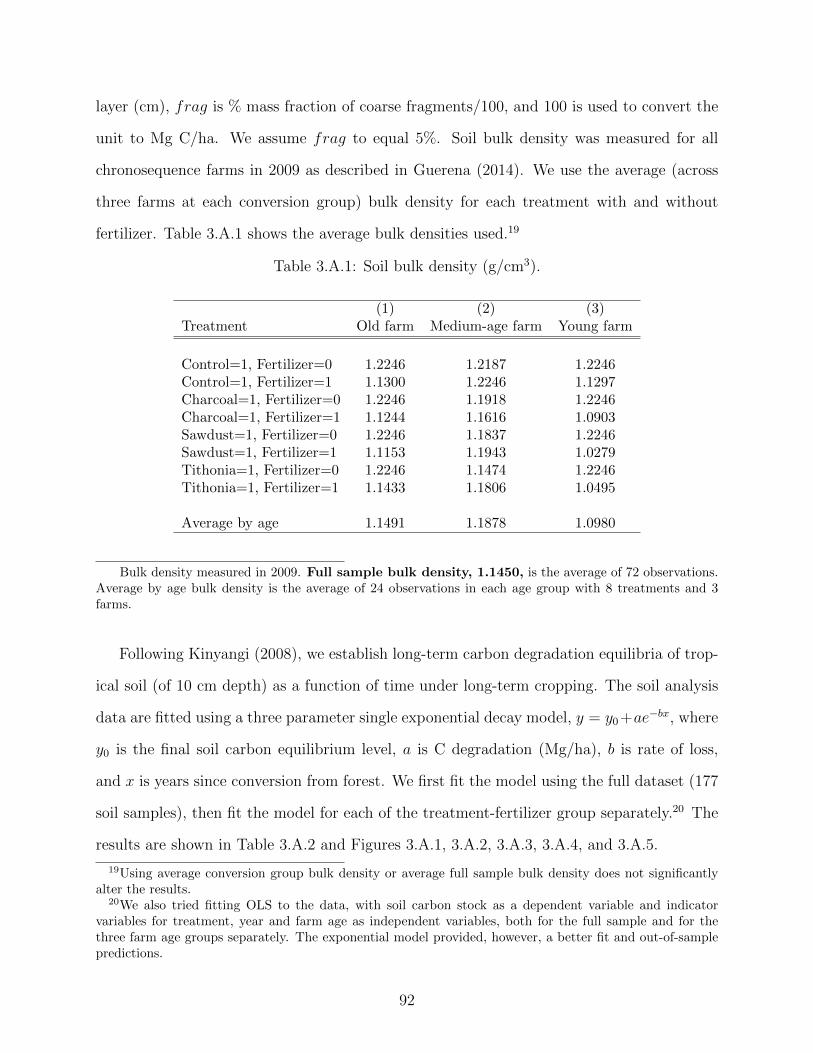
layer (cm), frag is % mass fraction of coarse fragments/100, and 100 is used to convert the

unit to Mg C/ha. We assume frag to equal 5%. Soil bulk density was measured for all

chronosequence farms in 2009 as described in Guerena (2014). We use the average (across

three farms at each conversion group) bulk density for each treatment with and without

fertilizer. Table 3.A.1 shows the average bulk densities used.19

Table 3.A.1: Soil bulk density (g/cm3).

(1) (2) (3)Treatment Old farm Medium-age farm Young farm

Control=1, Fertilizer=0 1.2246 1.2187 1.2246Control=1, Fertilizer=1 1.1300 1.2246 1.1297Charcoal=1, Fertilizer=0 1.2246 1.1918 1.2246Charcoal=1, Fertilizer=1 1.1244 1.1616 1.0903Sawdust=1, Fertilizer=0 1.2246 1.1837 1.2246Sawdust=1, Fertilizer=1 1.1153 1.1943 1.0279Tithonia=1, Fertilizer=0 1.2246 1.1474 1.2246Tithonia=1, Fertilizer=1 1.1433 1.1806 1.0495

Average by age 1.1491 1.1878 1.0980

Bulk density measured in 2009. Full sample bulk density, 1.1450, is the average of 72 observations.Average by age bulk density is the average of 24 observations in each age group with 8 treatments and 3farms.

Following Kinyangi (2008), we establish long-term carbon degradation equilibria of trop-

ical soil (of 10 cm depth) as a function of time under long-term cropping. The soil analysis

data are fitted using a three parameter single exponential decay model, y = y0+ae�bx, where

y0 is the final soil carbon equilibrium level, a is C degradation (Mg/ha), b is rate of loss,

and x is years since conversion from forest. We first fit the model using the full dataset (177

soil samples), then fit the model for each of the treatment-fertilizer group separately.20 The

results are shown in Table 3.A.2 and Figures 3.A.1, 3.A.2, 3.A.3, 3.A.4, and 3.A.5.

19Using average conversion group bulk density or average full sample bulk density does not significantlyalter the results.

20We also tried fitting OLS to the data, with soil carbon stock as a dependent variable and indicatorvariables for treatment, year and farm age as independent variables, both for the full sample and for thethree farm age groups separately. The exponential model provided, however, a better fit and out-of-samplepredictions.

92

Table 3.A.2: Exponential fit for full sample vs. for each treatment-fertilizergroup.

(1) (2) (3) (4) (5)Treatment y0 a b N R2

Full sample 35.60 117.00 0.194 177 0.69

Control=1, Fertilizer=0 33.26 85.21 0.149 21 0.78Control=1, Fertilizer=1 31.79 76.69 0.128 21 0.79Charcoal=1, Fertilizer=0 40.20 262.93 0.307 21 0.75Charcoal=1, Fertilizer=1 35.58 117.56 0.149 24 0.83Sawdust=1, Fertilizer=0 36.08 230.11 0.275 21 0.82Sawdust=1, Fertilizer=1 34.34 69.52 0.136 24 0.78Tithonia=1, Fertilizer=0 37.61 106.26 0.178 21 0.64Tithonia=1, Fertilizer=1 35.75 64.65 0.177 24 0.59

Based on y = y0+a⇥ e

�bx, where y is soil carbon stock (Mg/ha), y0 is the equilibrium soil carbon level,a is carbon degradation, b is rate of loss, and x is years since conversion from forest.

Figure 3.A.1: Exponential fit for full sample.

Using parameters of the exponential decay model summarized in Table 3.A.2, we predict

soil carbon stocks for the entire sample of 1,450 observations. The density of predicted soil

93

Figure 3.A.2: Exponential fit for control with and without N fertilizer.

Figure 3.A.3: Exponential fit for charcoal with and without N fertilizer.

94

Figure 3.A.4: Exponential fit for sawdust with and without N fertilizer.

Figure 3.A.5: Exponential fit for Tithonia with and without N fertilizer.

95

carbon stocks (Mg/ha) is shown in Figure 3.A.6, with the correlation coe�cient of the two

predictions being 0.93. Given a slightly better fit of the model for each treatment-fertilizer

group, we use the predictions shown on the right-hand side panel of Figure 3.A.6 in our

estimation of the production function.

Figure 3.A.6: Density of predicted soil carbon stocks (Mg/ha).

96

3.B Calibrating soil carbon equation

The Rothamsted Carbon Model (ROTHC-26.3) is one of the most widely used models to

study the turnover of soil organic carbon. The model estimates the carbon dynamics for

decades or centuries under di↵erent management and requires few inputs that are easily

available for the chronosequence farms: the carbon inputs into the soil, as well as soil clay

content and monthly weather conditions (rainfall, temperature, and open pan evaporation)

(Coleman and Jenkinson 1999). The data requirements, their values and sources used for

calibration of the Rothamsted carbon model are described in Table 3.B.1.21

Table 3.B.1: Data requirements for the ROTHC-26.3 model.

Variable Data Source

Average monthly mean air 18.2 (J), 18.2 (F), 18.5 (M), 19.6 (A), 19.7 (M), 19.5 (J),

temperature (�C)* 20 (J), 20.2 (A), 20.3 (S), 20.2 (O), 18.8 (N), 18.6 (D) New locClim, FAO (2005)

Monthly precipitation (mm)* 129 (J), 201 (F), 170 (M), 150 (A), 97 (M), 80 (J),

58 (J), 117 (A), 127 (S), 243 (O), 207 (N), 150 (D) New locClim, FAO (2005)

Monthly evaporation (mm)* 132 (J), 144 (F), 146.13 (M), 158 (A),

145.07 (M), 160.27 (J), 163.73 (J), 154.80 (A),

172.53 (S), 144.13 (O), 138.27 (N), 130.27 (D) New locClim, FAO (2005)

Soil depth (cm) 10

Clay content of the soil (%) 47 Kimetu et al. (2009)

DPM/RPM ratio for maize** 1.44 Coleman and Jenkinson (1999)

Soil cover Fallow only in July and August

Monthly input of plant residues In February and June

Amount of inert organic matter Unknown, obtained as described in the modeling section

*The weather data are displaced by six months so that the soil is at field capacity at the start of themodel run, as suggested by Coleman and Jenkinson (1999). **Ratio of decomposable plant material toresistant plant material. Value suggested by Coleman and Jenkinson (1999).

The weather data come from New LocClim: Local Climate Estimator, an FAO software

program and database, which provides estimates of average climatic conditions at locations

for which no observations are available (FAO 2005). The monthly long-term mean tempera-

ture, precipitation and evaporation are interpolated for the chronosequence farms—00� 09’

34”N, 34� 57’ 37”E, 1,780 m altitude (Kinyangi 2008).

21The procedure used to calibrate the Rothamsted Carbon Model and estimate the equilibrium levels ofsoil carbon in the research area is developed by Dominic Woolf.

97

ROTHC-26.3 is first run to estimate the equilibrium values for tropical forest with the

climate data and soil clay content described in Table 3.B.1, and assuming annual inputs to the

tropical forest soil equal to the mean net primary production of carbon for broadleaf evergreen

forest specified in Potter (1999)—1,075.4 g/m2/year which translates to 0.896 Mg/ha/month.

The initial level of measured total soil carbon is 65 Mg C/ha (Kinyangi 2008) and the

DPM/RPM ratio, ratio of decomposable plant material to resistant plant material, is 0.25,

the default for deciduous and tropical woodland (Coleman and Jenkinson 1999). Running the

model in “inverse,” when inputs are calculated from known changes in soil organic matter,

we obtain the amount of inert organic matter (IOM), 5.6899 Mg/ha, and monthly input of

plant residues, 0.4996 Mg C/ha. Now running the model “forward,” we obtain the starting

values in Mg/ha for decomposable plant material (DPM)—0.1410, resistant plant material

(RPM)—13.9892, microbial biomass (BIO)—1.1866, humidified organic matter (HUM)—

43.9959, and inert organic matter (IOM)—5.6899, to be used in the model simulations for

di↵erent management scenarios.

To simulate the soil carbon equilibrium levels under di↵erent management scenarios, we

run ROTHC-26.3 “forward” for di↵erent levels of plant carbon inputs (0, 0.5, 1, 1.5, 2, 2.5,

3, 3.5, 4, 4.5, 5, 5.5, 6, 6.5, 7, 7.5, 8 Mg C/ha) applied in February, the end of the main

Long Rains season, and assuming the constant rate of plant carbon inputs, 1 Mg C/ha, in

June to reflect the crop residues left on the field in the end of the Short Rains season. The

resulting equilibrium levels of soil carbon (after 10,000 years) for di↵erent levels of plant

carbon inputs are shown in Figure 3.B.1 that suggests a linear relationship: equilibrium soil

carbon = 14.12431 + 8.247451 * plant carbon input.

To find values for the parameters A and B in the soil carbon equation, g(·) = ct+1 � c

t

=

�Dct

+ A(↵t

Fky(ct

, ft

))B, we use the data predicted by the RothC model. In equilibrium,

equation 3.17 implies that A(↵Fky(c, f))B = Dc, or ln(c) = ln(A)� ln(D) +B ln(↵kFy(·))

in logs, where D, soil carbon mineralization rate, F , carbon content of maize residues, and

98

Figure 3.B.1: Equilibrium levels of soil carbon from ROTHC-26.3 as a func-tion of plant carbon inputs.

k, maize residue to grain ratio, are given. The data predicted by RothC suggest a linear

relationship between the equilibrium soil carbon content (c) and plant carbon input (x)

(Figure 3.B.1) such that ln(c) = 3.08 + 0.52 ln(x). Since x is also equal to ↵kFy(·) in

equation 3.17, we assume that 3.08 = ln(A)� ln(D) and 0.52 = B, giving values for A = 2.4

and B = 0.52. Although equation 3.17 is non-linear, for x 2 (1, 3] that is a reasonable range

of plant carbon input in maize systems in western Kenya, equation 3.17 closely mirrors the

data predicted by the RothC model as can be seen in Figure 3.B.2.

99

Figure 3.B.2: Calibrating the soil carbon function.

100

3.C Prices

The following figures show the empirical distributions of prices as reported in the household

survey or estimated in Chapter 2, using the same household survey data. Table 3.C.1 shows

the estimation of the hedonic price function used to approximate land rental values in the

research area.

Figure 3.C.1: Maize grain price in the household survey.

Note: N=120, households that sold maize. The average market price in 2011-2012 is 410

$/Mg.

101

Figure 3.C.2: Composite nitrogen price in the household survey.

Note: N=190, households that bought DAP, urea, and/or CAN. 2,070 $/Mg is the price of

nitrogen in urea, 4,390 $/Mg is the composite price of nitrogen from the market surveys.

n = price of DAP/0.18⇥ 0.69 + price of urea/0.46⇥ 0.16 + price of CAN/0.26⇥ 0.15.

Figure 3.C.3: Per-hectare maize production costs in the household survey.

Note: N=309. Production costs include the cost of preparing the land, planting, and

harvesting maize, including household and paid labor and land rental value.

102

Figure 3.C.4: Value of maize residues left on the fields for soil fertility man-agement.

Note: N=144. Estimated in Chapter 2.

103

Table 3.C.1: Hedonic regression of land rental value.

Rent (USD/ha) (1) (2)

Indicator for loam soil -19.66 -10.30(13.92) (8.585)

Indicator for clay soil -19.58 -22.98*(16.87) (12.09)

Indicator for murram soil -42.52*** -28.19***(15.08) (9.694)

Indicator for moderate or fertile soil 26.83** 29.90***(11.42) (8.502)

Organic soil carbon (% by weight) 1.543(4.843)

Plot GIS altitude (m) 0.0637***(0.0172)

Constant 62.12*** -42.20(15.08) (29.71)

Observations 53 45R-squared 0.170 0.481Mean predicted value (st.dev.) 64.70 (17.18) 65.06 (24.66)Median predicted value 69.29 59.19

Robust standard errors in parentheses. *** p<0.01, ** p<0.05, * p<0.1. Indicator for sandy soil omitted.

104

CHAPTER 4

SMALL-SCALE BIOENERGY PRODUCTION IN SUB-SAHARAN AFRICA:

THE ROLE OF FEEDSTOCK PROVISION IN ECONOMIC VIABILITY

4.1 Introduction

Renewable energy from materials derived from biological sources—bioenergy—accounts for

about ten percent of global primary energy demand, and some recent estimates suggest a

considerable potential for expansion (IEA 2014). Most existing traditional bioenergy use is in

developing countries in the form of burning solid biomass for residential cooking. Fuelwood

and charcoal, for example, account for more than 60 percent of total energy use in Sub-

Saharan Africa (SSA) (Eisentraut 2010). Access to modern energy in developing countries,

however, remains limited. More than 620 million people in SSA are without access to

electricity, with nearly 80 percent of those lacking access living in rural areas. Two-thirds

of total energy consumption in SSA is in the residential sector (mostly for cooking), while

transport accounts for only 11 percent of final energy consumption, and industry, agriculture,

and service sectors together account only for 21 percent (IEA 2014).

Modern, reliable and high quality energy, however, is necessary to provide lighting, heat-

ing, communication, transport, and mechanical power to support education, better health,

and higher household incomes. Not surprisingly, there is growing interest in SSA, as else-

where in the developing world, to establish modern bioenergy sectors to supplement existing

traditional energy reserves. While for many industrial countries the main drivers for devel-

oping the bioenergy sector are reducing greenhouse gas (GHG) emissions and diversifying

energy sources, developing countries have additional objectives. Bioenergy sector expan-

sion is also viewed as a means of stimulating economic development—providing biofuel for

powering agricultural machinery, transporting goods to markets, accessing medical services,

105

and creating jobs (Kojima and Johnson 2005; Jumbe, Msiska, and Madjera 2009; Lynd and

Woods 2011).

Expansion of the modern bioenergy sector, in general, and biofuels, in particular, is,

however, not without tradeo↵s. Many of the challenges are centered on the provisioning of

raw materials, or feedstocks, for biofuel production. These include competition with food

production for land resources, environmental concerns, and increasing GHG emissions (see,

for example, Fargione et al. (2008) and Tilman et al. (2011)). Second-generation biofuels,

however, o↵er potential solutions for some of the sustainability issues often associated with

biofuels from food crops (Hammond and Seth 2013). They use cellulosic biomass from non-

edible feedstocks that do not compete with food production and can be produced with lower

life-cycle GHG emissions than traditional fossil fuels. Such feedstocks include agricultural

residues, sustainably harvested wood and forest residues, perennial plants grown on degraded

lands, double cropped and mixed cropping systems, and municipal and industrial wastes

(Tilman et al. 2009).

Crop residues (cereal and legume straws, leaves, stalks, tops of vegetables, sugar, and oil

crops, etc.), in particular, are of great potential interest as biofuel feedstocks, because they

do not require additional land cultivation, do not compete with food production, and are

already found in considerable quantities (Eisentraut 2010). There are, however, several im-

portant competing uses for crop residues. Crop residues are used as animal fodder, especially

in developing countries. They are also essential for maintaining many soil properties and

processes, such as storing and recycling nutrients, stabilizing soil structure, reducing risks of

soil erosion, improving water retention, and enhancing agronomic productivity, among many

others (Lal 2005). So the removal of crop residues from fields can lead to a decline in soil

fertility with long-term adverse impacts on the environment.

The existing studies that assess bioenergy expansion potential in SSA mostly focus on the

technical feedstock provision potential of entire countries or they make assumptions about

106

the percentage of residues that is “safe” to use for bioenergy (see, for example, Senelwa

and Hall (1993) in Kenya, Jingura and Matengaifa (2008) in Zimbabwe, Milbrandt (2009)

in Liberia, Duku, Gu, and Hagan (2011) in Ghana, and Ackom et al. (2013) in Cameroon).

It is, however, important to understand the true economic cost of using crop residues as

bioenergy feedstocks. There are major economic and environmental tradeo↵s associated

with alternative uses of crop residues. And in many places, markets for crop residues do not

exist, complicating the assessment of the true costs of residues to smallholder farmers. It is

also important to recognize the challenges in scaling up bioenergy infrastructure (Richard

2010). Overall, understanding the security of biomass supply in developing countries and

accounting for its various challenges (sourcing from small farms, seasonality of availability,

etc.) is essential to correctly estimate the feasibility of bioenergy production and profitability

(Eisentraut 2010).1

In this paper, we analyze the ex ante economic viability of small-scale bioenergy pro-

duction in rural SSA, specifically focusing on one challenge—feedstock provision costs. We

consider the availability and cost of purchasing maize residues from smallholder farmers,

as well as the cost of transporting them to a small-scale pyrolysis-biochar plant in rural

western Kenya. We account for maize residue yield risk and its e↵ect on feedstock prices,

and the pyrolysis-biochar plant’s potential power to exercise monopsony prices. We o↵er the

first detailed estimates of feedstock provision costs for SSA, and assess whether producing

bioenergy is economically viable or whether initial government subsidies would be necessary

to account for the social and environmental benefits of rural bioenergy production.

A pyrolysis-biochar plant producing ethanol and biochar, a soil amendment, is chosen for

several reasons. Ethanol is one of the most promising biofuels. In principle, it can be derived

from any lignocellulosic biomass and then blended with gasoline for transportation fuels, thus

1Other challenges associated with bioenergy development in poor and remote regions, such as technicalknow-how, capital availability, lack of private sector capacity, market development, land tenure security,poor infrastructure, lack of skilled labor, and limited financing possibilities are described elsewhere (see, forexample, Ewing and Msangi (2009), Eisentraut (2010)).

107

allowing the countries to retain the existing transportation infrastructure (e.g., refueling

stations). In western Kenya, for example, Kisumu already has facilities for ethanol-gasoline

blending, and similar facilities are being completed in Eldoret and Nakuru (MOE 2015).

Biochar also o↵ers several benefits. Once incorporated in soils, biochar has been shown

to increase crop yields and reduce fertilizer requirements, and its high carbon content and

stability o↵er soil carbon sequestration and climate change mitigation potential (Lehmann

2007b; Stavi and Lal 2013).

Our focus on small-scale production with the end goal of local bioethanol and biochar

use is an opportunity to consider an alternative model to large-scale, monoculture-oriented

production, and the benefits it can bring to smallholder farmers. There is growing evidence

that smallholder farmers can benefit from small-scale bioenergy production if production,

marketing, and distribution networks are designed with the view to help the poor (e.g.,

Woods (2006), Ewing and Msangi (2009), von Maltitz and Sta↵or (2011)). The evidence

from existing small-scale bioenergy projects is, however, scarce and points to the challenges

to their economic feasibility without considerable donor support (von Maltitz and Sta↵or

2011).

Using detailed household-level and market data from the western Kenyan highlands, we

provide a detailed ex ante assessment of one particular case and draw implications for the

small-scale bioenergy development in other rural settings. We demonstrate that feedstock

provision costs strongly depend on regionally specific agro-ecological and socio-economic

conditions. Crop yields, planting density, and value of crop residues to farmers exhibit a

high degree of heterogeneity even in the limited geographic area considered. They result in

highly varying feedstock purchase and transportation costs, depending on the location of the

pyrolysis-biochar system. Only under the best-case scenario (that with the lowest provision

costs), do we find that a pyrolysis-biochar plant with 15 Mg of feedstock per hour capacity

has a positive estimated net present value (NPV). Initial capital investment, feedstock cost,

108

final product prices, and interest rates have the greatest impacts on NPV estimates. To help

promote small-scale bioenergy production, initial government support may be required to

account for the social and environmental benefits of rural bioenergy production.

In the following section, we discuss the available technologies for bioenergy production

in Sub-Saharan Africa, focusing on one in particular—a pyrolysis-biochar system to produce

bioethanol and biochar. In section 4.3 we discuss the implications of sourcing feedstock

from small-scale farmers. We describe the study area, and explain our methods to derive

feedstock availability, price, and transport costs. In section 4.4 we present the metrics to

assess the economic viability of the pyrolysis-biochar system, while in section 4.5 we discuss

our results. Section 4.6 concludes the paper and discusses the implications of our findings

for the small-scale bioenergy development in other rural settings.

4.2 Bioenergy production technologies in SSA and pyrolysis-

biochar system

The available technologies for bioenergy production in Sub-Saharan Africa are numerous.

They are applicable at di↵erent scales, for diverse purposes, under various climatic condi-

tions, and with multiple feedstock sources (Rutz and Janssen 2012). Bioenergy technologies

range from small-scale household cookstoves to village-level medium-enterprise applications

to large-scale industrial plants. For all scales, di↵erent conversion technologies (biological,

mechanical, thermal, chemical processes) produce liquid, gaseous, and solid bioenergy, which

can be converted into electricity, heat, cooking and lighting energy, and transportation fuels.

The most common traditional technology for biomass conversion into bioenergy is a

three-stone fire or “open fire” cookstove, with wood fuels (charcoal and firewood) as the

dominant biomass feedstock. Smoke from burning of solid biomass fuels on open fire stoves is

109

responsible for high concentrations of health-damaging pollutants such as particulate matter

and carbon monoxide, while incomplete combustion of fuels releases black carbon (soot),

contributing to poor health outcomes and climate change (Rehfuess, Mehta, and Pruss-

Ustun 2006; Adkins et al. 2010). Where on-farm biomass is scarce, the o↵-farm fuelwood

collection burden often falls on women and children, while the cutting down of trees for

firewood or to make charcoal contributes to deforestation (Arnold, Kohlin, and Persson

2006; Hosonuma et al. 2012).

Another common technology for biomass conversion into bioenergy is a farm-size biogas

digester. Their use has been rapidly increasing since the 1970s; there are now more than

30 million household digesters in China, about 3.8 million in India, and tens of thousands

in both Nepal and Bangladesh (Rajendran, Aslanzadeh, and Taherzadeh 2012). The use of

farm biogas digesters in Sub-Saharan Africa is, however, still limited, and among those that

exist many do not function due to often high capital costs and laborious maintenance and

repair requirements (Bond and Templeton 2011; Austin et al. 2012).

Modern energy technologies that utilize numerous biomass feedstocks to produce elec-

tricity and heat, however, are also in use, albeit much less widespread. Most of the existing

ones form part of large-scale plants (e.g., use of bagasse to provide heat energy for a sugar

mill), while technologies for stand-alone production of biofuels for transport in SSA are still

in nascent stages. The government of Kenya, for example, lists inadequate research and

development on alternative biofuel feedstocks and technologies as one of the main challenges

confronting its national biofuel policy (MOE 2015). It also recognizes that producing energy

crops for biofuel production carries the threat of competing with production of food.

One of the promising technologies for the sustainable production of renewable energy is

pyrolysis—a process that involves thermal decomposition of biomass at elevated tempera-

tures with a limited supply of oxygen (Lehmann and Joseph 2009). Pyrolysis can generate

liquid and gaseous energy sources from a large diversity of biomass feedstocks, including

110

woody and herbaceous materials, agricultural and food processing residues, municipal waste,

as well as other waste products (Yaman 2004; Lehmann 2007a). During pyrolysis, biomass is

converted into a liquid product (i.e., bio-oil), a solid char (i.e., biochar), and non-condensable

gases such as carbon monoxide, carbon dioxide, hydrogen, methane and higher hydrocarbons

(i.e., “syngas” or “pyrolysis gas”) (Brown 2009). While pyrolysis gas is mostly suitable for

process heat and power generation and unsuitable for long-distance distribution or residential

applications, bio-oil can be refined into drop-in “green” transportation fuels—fuels that can

substitute for petroleum gasoline and can be distributed in the same fueling infrastructure

(Brown, Wright, and Brown 2011).

Biochar, a major product of pyrolysis, has many appealing properties. It can be sold

as charcoal briquettes, used to pre-dry biomass, or employed in water purification and gas

cleaning; its novel value, however, has been found in its application as a soil amendment

(Lehmann 2007b). Biochar has high carbon content and may contain up to half of the

total carbon of the original organic matter. Biochar is also highly stable against decay and

retains nutrients better than other forms of soil organic matter (Lehmann 2007a). As a

result, once incorporated into soils, biochar can enhance soil fertility, resulting in improved

crop yields, and reduce applications of energy-intensive agricultural inputs like nitrogen

fertilizer. Furthermore, it can reduce environmental pollution by retaining nutrients such as

nitrogen and phosphorus in the soil and reducing the leaching of nutrients into groundwater

or their erosion into surface waters (Lehmann 2007b). In contrast to crop residues and

other organic resource applications, biochar’s stability in terms of carbon storage over a long

timescale allows for removing carbon dioxide from the atmosphere. Once assimilated by

plant growth, carbon dioxide can be stored in a stable soil-carbon form rather than returned

to the atmosphere through decomposition (Roberts et al. 2010).

While the engineering studies of pyrolysis and biochar production are many, economic

feasibility analysis is rare and, to our knowledge, exists only for industrial-scale systems and

111

in a developed-country setting. Several studies in the US carefully consider both fast and

slow pyrolysis technologies using maize residues as a feedstock (see, for example, McCarl

et al. (2009), Roberts et al. (2010), and Brown, Wright, and Brown (2011)). While the

existing technologies are found unprofitable, the authors point to many assumptions relying

on highly uncertain data and show that their results are most sensitive to feedstock costs,

biochar benefits, and plant costs, as well as policies on GHGs and energy prices. To our

knowledge, there are no studies analyzing the profitability of a pyrolysis-biochar project in

Sub-Saharan Africa.

While still hypothetical, the pyrolysis-biochar system can become an attractive technol-

ogy for the production of bioenergy. Since biomass is the feedstock that people in developing

countries already know how to grow, its use in the pyrolysis-biochar system could be a key

ingredient in generating additional incomes and improving agricultural productivity through

biochar applications. Unlike cookstoves and biogas digesters, the system can use any non-

edible lignocellulosic biomass. Its robust nature allows for considerable flexibility in the

quality and type of the biomass feedstock. The system’s larger scale will also require sub-

stantial capital investment and maintenance and operating costs. It can, however, tap into

private domestic and foreign investment and potential government subsidies. Moreover, with

soil carbon sequestration through biochar applications and the displacement of fossil fuels

in the production of inorganic fertilizer and associated emissions, pyrolysis-biochar systems

may o↵er a way forward for participation in international o↵set mechanisms or voluntary

emissions o↵set markets (Whitman and Lehmann 2009). Thus, the technology deserves

careful consideration for a developing-country setting.

112

4.3 Feedstock provision (biomass supply) costs

There are several categories of direct economic costs associated with the adoption of

pyrolysis-biochar systems: feedstock provision costs, capital costs, and operating and main-

tenance costs of the system. The most uncertain and geographically varied of these are

feedstock provision, or biomass supply, costs. These include both feedstock purchase and

transportation costs. Not surprisingly, the costs depend heavily on regionally specific con-

ditions such as feedstock availability, its price, and available infrastructure with respect to

transport networks and their use (Eisentraut 2010).

To assess the availability of biomass for energy production, both existing and future,

a number of studies focus on global, regional, and country-level estimates. Most of these

studies analyze either geographic or technical potential. The geographic potential refers to

the theoretical potential of growing biomass in a given area that is considered available and

suitable for biomass production. Technical potential also includes losses during the harvest-

ing process (Eisentraut 2010). Many of the existing estimates, however, ignore economic

constraints to biomass availability and accordingly demonstrate higher available amounts

of biomass that could be produced cost-competitively in practice. Moreover, regional and

country-level estimates inevitably mask a high degree of geographic variation in biomass pro-

duction. Both of these factors contribute to considerable uncertainty in estimating feedstock

provision costs.

The other challenge lies in calculating the purchase price of feedstocks. Markets for many

agricultural residues do not exist since processing technologies have not yet emerged. As a

result, there are often no reliable data for the purchase price of feedstock. When data do

exist, the available estimates vary significantly between di↵erent types and locations.2 At

the same time, since bioenergy sector expansion in developing countries is also meant to

2Eisentraut (2010), for example, reports the following price ranges for freshly harvested sugar cane topsand leaves: 3-8 $/Mg in Brazil, 8-15 $/Mg in Thailand, and 20-30 $/Mg in India.

113

stimulate rural development (Kojima and Johnson 2005), the purchase price of feedstock

needs to internalize social costs (Gallagher et al. 2003). Ideally, residue prices should reflect

the opportunity costs for the private benefits of leaving crop residues on the fields, thus

imitating a government policy of sustainable land use.

Typically, biomass transportation costs increase with larger plant sizes that exhibit higher

feedstock demands and, consequently, increased transport distances and more complex logis-

tics associated with storage and handling (Eisentraut 2010). Moreover, agricultural residues

(even when naturally air-dried) have low bulk density (e.g., 0.1 Mg/m3 for straw) that

contributes to higher costs of moving biomass and requires significant investments in trans-

portation. While the local sourcing of feedstock can help overcome the diseconomies of scale

associated with long-distance transportation of biomass (Richard 2010), infrastructure and

road maintenance especially in rural areas of developing countries is often precarious, further

increasing feedstock provision costs. Reflecting these considerations, Eisentraut (2010) sug-

gests that feedstock transport costs are approximately 10-25 percent of total biomass costs,

but can be as high as 65 percent under unfavorable conditions. This wide range of estimates

makes the general determination of the economic feasibility of bioenergy systems problematic

and reinforces the importance of focusing on the specific biophysical and economic circum-

stances characterizing local areas. For these reasons, having access to micro-level data and

doing a meticulous assessment of a specific case can reduce the uncertainty of accurately

estimating feedstock provision costs.

4.3.1 Study area

We focus on one geographic area—the western Kenyan highlands (Western, Nyanza, and

Uasin Gishu provinces)—to estimate the availability and provision costs as one particular

example. The research area is one of the most densely populated regions of Kenya (100-

114

300 people per square kilometer), with over 55 percent of the population living below the

national rural poverty line (WRI 2007). Our estimates are based on several micro-level

datasets collected between 2011 and 2013 in the Yala and Nyando river basins, two of the

major seven influent rivers feeding Lake Victoria in Kenya. The five research sites (Lower

Yala, Mid Yala, Upper Yala, Lower Nyando, and Mid Nyando) are similar in terms of

agricultural practices, but vary in altitude, rainfall, soils, and socio-economic characteristics,

and thus represent the diversity of the East African highlands (Figure A.1.2).3

A household-level survey collected information on biomass availability and uses, as well

as agricultural production over the 2011 calendar year. It covered 21 randomly sampled

households in three villages in each of the research sites, comprising a total sample of about

315 households. Average farms are about 1-2 hectare in size and originally formed part of

the tropical forest that became converted to agricultural land. Farmers practice subsistence

agriculture with maize being the main food commodity. Plot-level data included farmer-

reported annual and perennial crop harvest, chemical and organic inputs, seeds, household

and hired labor, as well as GPS-measured plot size and farmers perceptions of soil quality.

Access to electricity (about 11 percent of the sample population) and use of transportation

fuels (12 percent) is slightly higher than Kenya averages (WB 2015).

In addition, a survey of 56 commercial centers in April-June 2012 described the demand

and supply patterns of available energy and transportation in rural western Kenya (Cadogan

and O’Sullivan 2012; Lane 2013). This survey collected market price data from energy sellers

and buyers, as well as estimated the demand for modern energy services from small businesses

in each of the commercial centers.3The sites formed part of the original geographic coverage of the Western Kenya Integrated Ecosystem

Management Project, implemented between 2005-2010 by the Kenya Agricultural Research Institute andthe World Agroforestry Center and funded from the Global Environmental Facility of the World Bank. The10x10 km sites were chosen to satisfy the GEF criteria of carbon sequestration and biodiversity incrementpotential, severity of land degradation, and the proximity to reserves with significant degradation becauseof external pressure.

115

4.3.2 Crop residue availability

The standard procedure to estimate the technical potential of cereal crop residues for energy

production consists of multiplying country-level average cereal grain yields by a product-to-

residue ratio (see, for example, Jingura and Matengaifa (2008), Milbrandt (2009), and Duku,

Gu, and Hagan (2011)). Some of the studies also consider selected economic constraints on

technical availability, and assume fixed percentages of residues that can be safely removed

from the fields (e.g., Ackom et al. (2013)). Without having access to micro-level data, these

country-level studies and the estimates they produce, however, may underestimate or, more

likely, overestimate both the technical and economic potential of biomass for local bioenergy

production.

In rural western Kenya, maize residues are one of the main on-farm biomass sources

(Torres-Rojas et al. 2011). We use maize grain yields (Mg/ha/year)4 data from the household

survey. To convert maize grain yields to maize residue yields, we use the product-to-residue

ratio observed in the research area. Crop residues in the study area, as elsewhere in Sub-

Saharan Africa, are used for di↵erent purposes: about a quarter of maize residues is fed to

domestic animals, another quarter is used as household fuel, and the remaining residues are

left on the fields for soil fertility management (Chapter 2). Therefore, we use 50 percent as

the estimated proportion of economically available residues for bioenergy production.

4.3.3 Feedstock cost

As discussed above, there are several challenges surrounding the estimation of feedstock cost.

The cost of maize residues and their delivery to the plant is likely to be influenced by residue

production density that is in turn determined by maize yields, their volatility across space

41 megagram (Mg) = 1,000 kilogram (kg) = 1 metric tonne. 1 hectare (ha) = 10,000 square meters =2.47 acres.

116

and time, and the land area around the plant under maize cultivation. Moreover, there are

reasons to expect that the pyrolysis-biochar plant will be able to exercise monopsony power

when it comes to purchasing residues from smallholder farmers.

Similar to Gallagher et al. (2003), Caputo et al. (2005), and Sesmero and Sun (2015), we

assume that maize residues feeding the pyrolysis-biochar plant are collected over a circular

geographic area centered on the plant with uniform yield and harvest practices. Therefore,

additional residues can only be procured from an expanding circle around the plant, from

the extensive margin only. In contrast to previous literature, however, we combine both

the e↵ects of yield volatility on residue price and partial spatial price discrimination on

transportation cost.

Let p be the farm-gate price of residues ($/Mg). Since markets for agricultural residues

in western Kenya do not exist, we can estimate their value using either a production or

a substitution approach. As applied to non-marketed sources of biomass, the production

approach demonstrates the value of residues by calculating changes in farm profits or pro-

duction output by including residues as a production input (see for example, Lopez (1997)

and Klemick (2011)), while the substitution approach derives the value of residues from

the observed prices for marketed substitutes (Teklewold 2012; Magnan, Larson, and Taylor

2012).

Given the focus on sourcing from smallholders, we rely on household-level data to estimate

the farm-gate feedstock price. The value of maize residues is assessed on the basis of monetary

worth of the equivalent amount of fertilizer required to compensate for the loss of crop

residues, as estimated in Chapter 2. It reflects the private benefit of leaving crop residues

on the fields and should be similar to the social value of sustainable land use.

This farm-gate price is, however, can also be influenced by yield volatility. Adverse

weather and other production shocks can lead to lower residue yields, thus increasing the

117

value of residues harvested. The higher value can be a result of harvesting cost that is fixed

per unit of area or due to increased risk of soil erosion. On the other hand, high residue

yields may increase the prevalence of pests and disease, thus potentially lowering the value

of residues to the farmer. Following Sesmero and Sun (2015), we allow for the link between

residue price and yield by a linear relationship:

p = ↵� �y, (4.1)

where p is the farm-gate price of residues ($/Mg) and y is the maize residue yield (Mg/ha).

The parameter � captures the e↵ect of changes in residue yield on price. We calibrate

�, following Sesmero and Sun (2015), so that the elasticity of residue price with respect to

yield is equal to one at the median yield and residue values in the data.5 It is calculated

as dp

dy

y

p

= �� y

p

= 1, which implies � = � p

y

= �58.242.99 = �19.48, meaning that a reduction

in residue yield of one Mg per ha is associated with a decrease of value of maize residues

to farmers of 19.48 $/Mg. Then, ↵ is calculated from the equation above and it is equal to

116.49 $/Mg.6

Feedstock transport cost is determined to account for intrinsic feedstock characteristics

such as scattered geographic distribution. The procurement area and, therefore, the trans-

port distance from the point of feedstock production to a bioenergy plant depend on several

factors. These include the capacity of the plant and the quantity of feedstock required, as

well as local crop yields, and planting density around the bioenergy plant.

5As suggested by some estimates, a ten percent reduction in residue yield can lead to a seven percentincrease in on-farm per unit harvest cost of maize residues, due to existing cost factors that are fixed per unitof area. Sesmero and Sun (2015) argue that a value of 0.7 is, therefore, a lower bound on the elasticity ofresidue price with respect to yield and it is probably higher once soil erosion risk is taken into consideration.

6The farm-gate value of maize residues is also spatially and temporally heterogeneous. In fact, the value isdi↵erent across households in our dataset and, controlling for natural capital, is higher for poorer households(Chapter 2). In this paper we use the median value of maize residues and focus our attention on the e↵ectof yield volatility on feedstock prices.

118

The transportation component of residue cost increases with the distance traveled (r) and

the amount of feedstock procured (Q). It can be approximated by Q = ⇡r2�y, which is the

product of the circular area around the plant and the density of residues (Gallagher et al.

2003; Caputo et al. 2005; Sesmero and Sun 2015). Inside this collection area, the actual

plots with maize cultivation are only a fraction of total land area and may be unevenly

distributed. Therefore we measure �, the density of planted maize in the total area, as the

share of total farm size assuming a uniform biomass distribution density over the entire area

of the collection basin. Since Q represents the capacity of the biochar-pyrolysis plant, the

maximum distance to procure the required feedstock is, therefore, r =q

Q

⇡�y

. As shown

by Gallagher et al. (2003), the average transport cost can then be derived as 23tr, where

t is the freight rate in $/Mg/km, the unit cost of trucking feedstock from farms to the

biochar-pyrolysis plant. Hence, the transportation cost increases with the freight rate and

the maximum distance traveled, while the supply radius increases with plant capacity and

decreases with residue density.

Given the geographic distribution and a large number of small farms producing maize

residues, the biochar-pyrolysis plant is likely to have monopsony power in the maize residue

market. Agricultural and natural resource markets are often characterized by spatially dis-

tributed supply and significant transport costs, so that the processing facilities can exercise

price discrimination in the form of partial or complete absorption of freight charges (Lofgren

1985; Graubner, Balmann, and Sexton 2011). To account for this possibility and similar to

Lofgren (1985), let � 2 [0, 1] measure the degree of spatial price discrimination. Then, when

� = 1, the plant bears the entire transportation cost and the producers of maize residues

receive the same price irrespective of their location relative to the plant (uniform delivered

pricing). But when � < 1, the plant can pass along some of the transportation cost to

producers (partial freight absorption).

Putting these elements together, the per-unit feedstock cost (c) can then be calculated

119

as

c = p+ �2

3tr = ↵� �y + �

2

3t

sQ

⇡�y, (4.2)

where c depends on the maize residue yield (y), freight rate (t), plant capacity (Q), residue

density (�), and the market power of the biochar-pyrolysis plant (�).

4.4 Economic viability of small-scale bioenergy production

In order to assess the economic viability of small-scale bioenergy production in rural Sub-

Saharan Africa and the relative magnitude of the feedstock provision costs and their variabil-

ity, we focus on a hypothetical pyrolysis-biochar plant in western Kenya. The plant operates

on the thermochemical conversion platform and uses maize residues from the surrounding

farms as feedstock. The feedstock is gasified to produce syngas that is then converted into

ethanol by a biological reaction (fermentation) using microbial catalysts (the process is de-

scribed in Piccolo and Bezzo (2009)). In addition to ethanol, the plant coproduces biochar.

While there is a trade-o↵ between ethanol and biochar yields (Woolf et al. 2014), both prod-

ucts are valuable and need to be considered to take full advantage of environmental and

social benefits of the pyrolysis-biochar system.

Given our focus on small-scale bioenergy production in a rural setting, we analyze a plant

that can process 15 Mg of dry feedstock per hour and operates at 75 percent capacity,7 so that

the annual biomass required is 98,550 Mg. As common in other techno-economic analyses

of bioenergy projects, we also assume the life of plant of 20 years and interest rate of 10

785 percent is often assumed as a levelized capacity factor, an average capacity over the life of a plant,while historic data show that the annual average capacity factor for a coal-fired plant in the US variesbetween 65 and 75 percent (Rubin 2012). Given the developing country setting, we assume a lower capacityfactor of 75 percent.

120

percent. To approximate total capital and operating costs, we use the recent estimates from

the literature. The pyrolysis capital cost comes from McCarl et al. (2009) who analyze the

costs and benefits of fast and slow pyrolysis technologies using maize residues as a feedstock.

The biofuel conversion capital cost is from Piccolo and Bezzo (2009) who present the first

comprehensive analysis of the gasification and fermentation process. Annual operating and

maintenance costs are assumed to be four percent of total capital costs as in Shabangu et al.

(2014).

The direct economic benefits of the pyrolysis-biochar plant are bioethanol and biochar

sales. Given the infant nature of the pyrolysis bioethanol markets, we assign the value to

pyrolysis ethanol as an equivalent to a conventional product. Brazil is one of the worlds

largest producers of ethanol, with a substantial domestic market and considerable exports.

Since Brazil’s sugarcane-based ethanol is cheaper to produce than the US corn-based ethanol,

we use the five-year average of Brazil’s producer prices—0.55 US$ per liter (OECD/FAO

2015).8

The price of biochar is often estimated in comparison to a conventional fertilizer price,

its value in terms of increased yields, or its combustion value (McCarl et al. 2009; Galinato,

Yoder, and Granatstein 2011). In Kenya, conventional charcoal is the primary energy source

for 82 percent of urban and 34 percent of rural households. The producer price of charcoal is

estimated at 85 US$/Mg, with market prices ranging between 306 US$/Mg (wholesale) to 952

US$/Mg (consumer retail) (KFS 2013). We assume biochar’s combustion value (the producer

price of charcoal, 85 US$/Mg) as the lowest price. Its total value, however, comes from

soil improvements and associated agricultural productivity increases, and climate change

mitigation (Lehmann and Joseph 2009). Thus, our base value is higher—115 US$/Mg.

These and other assumptions used, as well as their assumed variability, are summarized in

8http://www.agri-outlook.org [Accessed 07/05/2015]. For comparison, the five-year average of

ethanol wholesale free on board price in Omaha, Nebraska is 0.62 US$ per liter (http://www.neo.ne.gov/statshtml/66.html).

121

Table 4.1.

We then derive three economic decision criteria used in the analysis of investments eco-

nomic viability—net present value (NPV), payback period (PBP), and internal rate of return

(IRR). Net present value (NPV) compares the value of money now with the value of money

in the future. Assuming that total annual economic benefits (TAB) and total annual oper-

ating costs (TOC) do not change over the projects lifetime (t), we calculate the NPV ($)

from the expression:

NPV =TX

t=1

(TAB � TOC)t

(1 + �)t� TCIC, (4.3)

where � is the annual interest rate and TCIC is the total overnight capital and installation

costs (the sum of pyrolysis capital cost and the biofuel conversion capital cost).

Payback period (PBP) refers to the number of years required to return the project’s orig-

inal investment. Assuming that initial investment is the total capital and installation costs

(TCIC) and that annual net profits are constant over time, we calculate the undiscounted

UPBP ($) as follows:

UPBP =TCIC

(TAB � TOC). (4.4)

Internal rate of return (IRR) estimates the interest rate needed to make the present value

of a stream of net revenues equal to zero. It is calculated as IRR that solves the following

equation:

NPV =TX

t=1

(TAB � TOC)t

(1 + IRR)t

.TCIC. (4.5)

122

If IRR is higher than the discount rate, investment is considered profitable. For a high risk

project such a pyrolysis-biochar system, the suggested IRR is usually 15 percent (Piccolo

and Bezzo 2009).

4.5 Results

We first present the estimates of feedstock availability and provision costs using the micro-

level data from the research area and focusing on a high degree of variability between the

five research sites. We use the median values; however, report the empirical distributions of

maize residue yield that proxy for spatial and temporal variability. The site-level estimates of

maize residue yields, maize planting density, and residue cost suggest a range of purchasing

and transportation costs that can be expected now if a pyrolysis-biochar plant was placed

in one of the research sites. We then calculate the economic decision criteria (net present

value, internal rate of return, and payback period), using the lowest estimate of the feedstock

provision costs, and perform sensitivity analysis of this net present value to several economic

variables. Then, to account for yield volatility and following Sesmero and Sun (2015), we

estimate the probability distributions of maize residue yield in five research sites and model

the cost of feedstock as a function of that distribution.

4.5.1 Maize residues availability in western Kenya

Following the standard procedure to estimate the technical potential of maize crop residues

for energy production, we first present country-level and province-level average cereal grain

yields (Table 4.2). For country-level estimates (second row) we use the 2000-2011 average

maize production from FAOSTAT, while for province-level estimates (third row) we use the

data from the Kenya Agricultural Sector Data Compendium reported in Sheahan, Ariga,

123

and Jayne (2013). Estimates in the last row are based on the household-level data from

western Kenya. Grain yield averages (Mg/ha) vary across the three data sources. The

three province averages are higher than the country-level average, which is not surprising

given that Nyanza, Western, and Rift Valley provinces have some of the most favorable

agro-climatic conditions in Kenya. The province averages, however, are higher than average

yields reported by farmers in the household survey. Yet, even averages from the household

survey hide a great degree of variation in both technical and economic availability of residues.

Figure 4.2 shows the distribution of maize residue yields in the five research sites, as well as

for the whole sample.9 The median harvest is the highest in Upper Yala (4.15 Mg/ha) and

the lowest is in Lower Yala (2.25 Mg/ha).

Despite the low technical potential for feedstock from maize residues in the research area,

its economic potential is even lower. Crop residues are an important resource in smallholder

agriculture, providing feed for domestic animals and used as household fuel. Leaving crop

residues on the fields as a soil amendment is also essential to enhancing, maintaining, and

sustaining long-term soil fertility and agricultural productivity. Their removal for other uses

has led to the depletion of the soil organic pool in the tropics and subtropics, accelerating

soil degradation, severe erosion, and water pollution (Lal 2006). It is di�cult to imagine

the removal of all residues for bioenergy production since such a move, together with its

environmental implications, would require a major change in farming and biomass utilization

systems (Senelwa and Hall 1993). As the household survey reported, we use 50 percent of

maize residues as the amount of residues available for bioenergy production.

9For the 186 households (out of 309) that cultivated maize twice in 2011, the sum of yields from bothseasons (long rains and short rains) is shown.

124

4.5.2 Feedstock provision costs: price and transport

The estimates for non-marketed maize residue value are from Chapter 2. Using the same

household data, the household-specific shadow value of maize residues used for soil fertility

management is estimated using coe�cients from a maize production function and household-

specific fertilizer prices. For the sustainable bioenergy production, the social cost included in

the supply analysis must involve opportunity costs associated with alternative residue uses

(Gallagher et al. 2003). And since we assume that only 50 percent of maize residues can be

included in supply to avoid soil degradation, our estimates approximate farmers’ decisions

under a policy of sustainable land use.

The median value for the whole sample is 58.24 $/Mg. This is close to the value of cereal

stubble in Morocco estimated by Magnan, Larson, and Taylor (2012). Similar to maize

residue yields, however, there is a high degree of variability in the value of maize residues

to western Kenyan farmers (Table 4.3). The lowest median residue value is observed in

Upper Yala (27.09 $/Mg), the site with the highest yields. For Mid Yala, the site with the

second highest median residue yield (3.95$/Mg), however, the median residue value is very

high: 101.72 $/Mg. A very high population density and small sized farms characterize this

research site, placing a greater demand on residues from alternative uses.

To calculate the cost of transporting maize residues to a pyrolysis-biochar plant, we also

need to know the distribution of maize residues over the entire area of the collection basin.

Assuming that households in our survey are representative of the research area, we scale

maize residue yields available for bioenergy by the share of land under maize cultivation in

each of the research sites in total farm area (maize planting density).10 This means that

our feedstock planting density is not the residue yield of the maize-producing plots, but the

10For households that planted maize twice in 2011, we estimate the feedstock distribution density asfollows: maize residues yield in long rains multiplied by the share of land planted with maize in long rainsin total farm area + maize residues yield in short rains multiplied by the share of land planted with maizein short rains in total farm area.

125

average equivalent yield of the entire geographic area around the plant to define the average

feedstock transport distance.

The estimate of the freight rate ($/Mg/km), the unit cost of trucking feedstock from farms

to the biochar-pyrolysis plant, is the average freight rate reported in the commercial center

survey ($/Mg/km average for 5, 7, 10, and 12 Mg capacity trucks, including the minimum

charge). Some other estimates from Kenya suggest that the operational cost for semi-trailers

is 1 $/Mg/km (similar to the costs in Europe), while the trucking businesses charge 1.20

$/Mg/km to the client (WB 2005). The degree of freight cost absorption is assumed to

be 80 percent, i.e., the pyrolysis-biochar plant bears 80 percent of the transportation cost

and passes 20 percent to the farmers. Similar practices are observed in the sugarcane and

tea growing industries in the research area. Sugarcane mills, for example, pick up cane at

the farms and then deduct a portion of the transportation costs from the final payments to

farmers.

Table 4.3 summarizes the variables used for the calculation of the feedstock cost for the

five research sites and for the whole sample. Given the di↵erence in maize planting density

(maize residue yield times maize land as a share of total land) and value, both feedstock

purchase and transport cost significantly vary between the sites. The highest feedstock unit

cost is observed in the Mid Yala region (101.72 $/Mg), while the transportation unit cost

in this region is one of the lowest (13.43 $/Mg) because of the relatively high density of

maize residues. The transportation cost as a share of feedstock purchase cost also varies

between 13 and 40 percent, similar to the shares suggested by Eisentraut (2010). The

geographically varied agro-ecological and socio-economic conditions are reflected in the highly

variable feedstock provision costs among the five research sites and can only be seen with

the micro-level data. The sample averages necessary mask this heterogeneity, and suggest

the average total provision costs almost double than the costs estimated for Upper Yala.

The highest maize residue yield and maize land share, and the lowest residue unit price are

126

observed in Upper Yala (4.15 Mg/ha/year, 0.55, and 29.97 $/Mg at the median, respectively).

As a result, the Upper Yala site has the smallest radius of the catchment area necessary to

provide feedstock to the pyrolysis-biochar plant. For a plant with 15 Mg of feedstock per

hour capacity, such a radius is 16.57 km. The total feedstock provision cost (both feedstock

cost and transport cost) is also, therefore, the lowest—3,654,000 $/year. It is this value that

we use in the economic viability estimations.

4.5.3 Economic viability and sensitivity analysis

Using the feedstock cost from the Upper Yala research site, Table 4.4 summarizes the costs

and benefits of the 15 Mg/hr pyrolysis-biochar system, and shows the three economic via-

bility indicators: net present values (NPV), internal rate of return (IRR), and undiscounted

payback period (UPBP). At the assumed discount rate of 10 percent, NPV is positive

($1,643,513), and the initial capital investment can be paid o↵ in 8.25 years. And although

IRR exceeds the assumed interest rate, it is, however, below the recommended 15 percent

value for high-risk investments.

The key variables with the most significant impact on the profitability of the pyrolysis-

biochar plant are similar to other studies: initial capital investment, feedstock cost, final

product prices, and interest rates (the variables, as well as their baseline, low, and high

values are summarized in Table 4.5). Figure 4.3 shows the impact of varying the baseline

values on the economic viability of the pyrolysis-biochar plant indicated by the net present

value (NPV).

Ethanol and biochar prices have the highest impact on profitability. Brazil’s sugarcane-

based ethanol was, on average, 0.38 $/liter in 2009 and 0.69 $/liter in 2011 (OECD/FAO

2015). The ethanol unit price of 0.35 to 0.75 Mg/liter varies the net present value from

-$22,436,187 to $25,723,084. Given the absence of biochar markets in Eastern Africa, we

127

also assume a high spread in the biochar unit price: from 85 $/Mg to 230 $/Mg, with

consequent changes to net present value (from -$7,662,030 to $37,314,451). This high degree

of ethanol price volatility and uncertainty in the value of biochar may require initial private

or government support (in the form of guaranteed ethanol or biochar prices).

When feedstock purchase cost is increased to 65 $/Mg (similar to the second highest

value of maize residues in the five research sites), the net present value of the plant becomes

negative: -$30,163,485. The ability of the plant to pass some of the transportation cost to

the farmers is also important: when the plant takes the full responsibility for transportation,

the net present value falls to -$451,486. Similar to other techno-economic studies of the

bioenergy production, the baseline value for interest rate is assumed to be 10 percent. Given

the developing-country additional objectives for bioenergy development, however, a lower

interest rate may be more appropriate. The interest rate of five percent changes the net

present value to $26,326,339, suggesting considerable benefits of the pyrolysis-biochar plant

in Upper Yala.

4.5.4 Varying yields and residue cost

To explicitly model both geographic and temporal yield volatility and its e↵ect on residue

prices, we follow the procedure outlined in Sesmero and Sun (2015). We first fit empirical

yield distributions for the whole sample and five research sites (blue lines over distributions

in Figure 4.2). Yields are best approximated by the gamma distribution, �, with shape and

rate parameters di↵ering for each site.11 We now also allow for the link between residue price

and yield by a linear relationship: p = ↵ � �y, where p is the farm-gate price of residues

($/Mg) and y is the maize residue yield (Mg/ha). Parameters ↵ and � are calibrated as

discussed above using the site-specific median yield and residue values, so that ↵ and � are

11Whole sample �(2.104,0.591), Lower Nyando �(1.502,0.492), Mid Nyando �(2.668,0.867), Lower Yala�(3.181,1.235), Mid Yala �(2.342,0.477), Upper Yala �(2.955,0.707).

128

di↵erent for each site (Table 4.3). Therefore, randomness in yields has two e↵ects on the

feedstock provision costs and the calculations of the net present value. First, it introduces

risk in maize harvest density and thus influences the transportation cost. Second, it adds

risk to the farm-gate price of residues.

We then calculate net present values (10,000 iterations for each location) based on fitted

yield distributions. These simulations result in a probability distribution of NPVs for each

of the five research sites and for the whole sample. Figure 4.4 shows the cumulative density

functions (CDFs) and the first two moments of the distributions are reported in Table 4.6.

Similarly to the deterministic analysis, the mean of the net present value is positive only

for one research site—Upper Yala ($740,924), with all other sites and the whole sample

showing the average negative net present values. Placing a pyrolysis-biochar plant in Upper

Yala is also a less risky investment. Upper Yala is preferred to all other locations by both

risk-neutral and risk-averse investors. Its NPV distribution displays higher mean and lower

standard deviation than other sites, and simple visual inspection of Figure 4.4 confirms that

the Upper Yala CDF dominates all other CDFs in a second-order stochastic sense (both

high and low values are less likely, but the reduction in the probability of low values is large

enough to o↵set the reduction in probability of high values).

4.5.5 Non-monetary benefits

Production of both bioethanol and biochar can result in net greenhouse gas (GHG) o↵sets

that we do not consider in this paper. Biofuels are considered potentially “carbon neutral”

since biomass feedstock absorbs the carbon dioxide which is released when biofuels are burnt.

The extent of the GHG reductions, however, depends on land use changes associated with

biomass production, conversion technologies, and often on methodological assumptions. The

GHG savings estimates range from about +85 percent to -30 percent (Hammond and Seth

129

2013), and for ethanol from sugarcane, for example, they are +70-100 percent (Bringezu

et al. 2009). Moreover, while credits for renewable energy calculated from the displacement

of fossil fuel energy are common in emissions trading schemes, the production of biochar can

also o↵er additional emissions credits.

Soil carbon is primarily derived from plant matter. In the tropics, however, biomass

decomposes quickly, and about 80 to 90 percent of carbon from biomass added to soil can be

lost after 5-10 years (Jenkinson and Ayanaba 1977). In contrast, pyrolysis stabilizes carbon

in biochar in a form that is resistant to further decomposition and the stored carbon in

soil is not susceptible to release due to changes in management practices (Lehmann 2007b).

In addition, biochar applications can enhance agronomic e�ciency and even substitute di-

rectly for fertilizer and other agricultural inputs, thus decreasing fertilizer applications and

increasing yields (Gaunt and Cowie 2009).

Several studies include a complete life-cycle analysis of the GHG emissions from a

pyrolysis-biochar system. McCarl et al. (2009), for example, estimate the net GHG o↵set

for slow pyrolysis with maize residue feedstock to be 1.112 Mg of carbon dioxide equiva-

lent (CO2e) for each Mg of feedstock. Their analysis of GHG o↵sets includes both GHG

emissions (fossil fuels used during residue harvest, transportation, and processing, plant op-

erations, carbon consequences of biomass removal and nutrient replacement, and biochar

transportation and application) and GHG emissions avoided (fossil fuel o↵set, reduction in

inputs, and sequestration enhancement). Although the existing carbon pricing instruments

are below 10 $/Mg of CO2e,12 even a modest payment for the GHG o↵sets can increase the

pyrolysis-biochar system’s profitability.

We also do not account for other potential environmental benefits of the pyrolysis-biochar

system (e.g., changes in water and air quality) and for the dynamic nature of the crop-

12Carbon dioxide prices in the European Union Emissions Trading System remained in the range of 5-9$/Mg of CO2e in 2013 (WB 2014), and the average price for forestry o↵sets in 2012 was 7.8 $/Mg of CO2e(Peters-Stanley, Gonzalez, and Yin 2013).

130

biochar production relationship. Biochar applications on farms that supply feedstock to the

pyrolysis-biochar plant can enhance maize yields and thus availability and cost of feedstock.

Since bioenergy production in developing countries is also viewed as a means of stimulating

economic development (Kojima and Johnson 2005), other non-monetary benefits may include

increased access to markets, educational and medical facilities, agricultural machinery, and

new jobs.

4.6 Conclusion

Conversion technologies for most second-generation biofuels are still at early stages of de-

velopment, with multiple technological and economic challenges impeding their commercial

deployment (Hammond and Seth 2013). In this paper, we consider one of these challenges—

feedstock supply. We analyze the cost of purchasing maize residues from smallholder farmers

and the cost of transporting them to a small-scale pyrolysis-biochar plant in rural western

Kenya. Using micro-level data from five research sites, we show how the di↵erences in maize

residue yields, maize planting density, and value of residues to farmers drive a great degree

of variability in feedstock provision costs even in the limited geographic area considered.

The pyrolysis-biochar plant with the 15 Mg of feedstock per hour capacity is found to have

positive net present value only in one research site—Upper Yala, with the lowest feedstock

provision costs. At the assumed discount rate of 10 percent, NPV is $1,643,513, and the

initial capital investment can be paid o↵ in 8.25 years. And although the internal rate of

return index exceeds the assumed interest rate, it is, however, below the recommended 15

percent value for high-risk investments. We also show that, in addition, Upper Yala research

site with the highest maize yield and maize planting density, as well as the lowest value of

maize residues to farmers, would be preferred to all other locations by both risk-neutral and

risk-averse investors.

131

Our results also suggest a range of purchasing and transportation costs of maize residues

that can be expected now if a pyrolysis-biochar plant were to be placed in western Kenya.

We would, however, expect significant adjustments in feedstock availability and provision

costs, as well as the associated spillovers to local biomass and fuel markets, with an actual

placement of such a pyrolysis-biochar plant. If biochar were to be used on the farms sup-

plying feedstock for the plant, for example, higher maize yields could result both in greater

availability and lower cost of feedstock, thus lowering the feedstock provision costs for the

plant. Pyrolysis-based fuel production could also influence the household demand for resi-

dential fuel by o↵ering new fuel alternatives and changing the current allocation shares of

maize residues to di↵erent uses. Moreover, we use 50 percent of maize residues as the amount

of residues available for bioenergy production to approximate farmers’ current practices. A

private market for residues as feedstocks for bioenergy production could, however, alter these

practices, inducing higher supply of residues for bioenergy production and potentially higher

social costs if not enough residues were to be left on the fields for soil fertility management.

Such general equilibrium e↵ects are of great interest and deserve careful analysis in future

research.

There are several implications of our results for small-scale bioenergy production in other

rural settings. First, the country-level statistics that are so common to the past literature

hide a great degree of heterogeneity in terms of both the agro-ecological environment and

socio-economic conditions. Even if we were to analyze the economic viability of the bioenergy

plant using the average values from our dataset, we would not capture all the variability that

exists. Therefore, having access to micro-level data helps resolve some of the uncertainty in

terms of the feedstock provision costs and to locate areas where small-scale bioenergy pro-

duction can be profitable. Second, given the high sensitivity of net present value estimates to

final product prices and feedstock provision costs, initial government support—in the form

of guaranteed ethanol or biochar prices, subsidies for feedstock purchase, etc.—would likely

be required to assure economic viability (but that dependence itself would be a drawback).

132

To help promote small-scale bioenergy development, national biofuel policies should focus

on raising financial resources for infrastructure development, investing in research and de-

velopment, and establishing regulatory and institutional frameworks (Jumbe, Msiska, and

Madjera 2009). Finally, since for many developing countries bioenergy carries multiple de-

velopment objectives, including non-monetary benefits as well as using a lower discount rate

in the analysis may be more appropriate. Accounting for diversity of agro-ecological and

socio-economic constraints is necessary to match the global enthusiasm about bioenergy and

its potential to deliver access to modern energy services, spur economic growth, and mitigate

climate change.

133

Figure 4.1: Five research sites: Lower Nyando, Mid Nyando, Lower Yala,Mid Yala, and Upper Yala.

134

Figure 4.2: Maize residue yields in western Kenya: distributions of maizeresidue yields from the household survey data, by research siteand for the whole sample.

Whole sample

Maize residue yield Mg/ha

Den

sity

0 5 10 15

0.0

0.1

0.2

0.3

0.4

Lower Nyando

Maize residue yield Mg/ha

Den

sity

0 5 10 15

0.0

0.1

0.2

0.3

0.4

Mid Nyando

Maize residue yield Mg/haD

ensi

ty

0 5 10 15

0.0

0.1

0.2

0.3

0.4

Mid Yala

Maize residue yield Mg/ha

Den

sity

0 5 10 15

0.0

0.1

0.2

0.3

0.4

Upper Yala

Maize residue yield Mg/ha

Den

sity

0 5 10 15

0.0

0.1

0.2

0.3

0.4

Lower Yala

Maize residue yield Mg/ha

Den

sity

0 5 10 15

0.0

0.1

0.2

0.3

0.4

Note: The blue line shows fitted Gamma distributions.

135

Figure 4.3: Sensitivity analysis for a pyrolysis-biochar plant size of 15 Mg/hr.

!$37,000,000' !$27,000,000' !$17,000,000' !$7,000,000' $3,000,000' $13,000,000' $23,000,000' $33,000,000'

Degree'of'freight'cost'absorption''

Plant'size'(Mg/hr)'

Capacity'factor'

Pyrolysis'capital'unit'cost'($/(Mg/hr))'

Maize'residue'unit'cost'($/Mg)'

Biofuel'conversion'capital'unit'cost'($/(Mg/hr))'

Interest'rate'(%)'

Biochar'unit'price'($/Mg)'

Ethanol'unit'price'($/L)'

Net$present$value$of$the$pyrolysis2biochar$system$

high'

low'

Note: Net present value at the baseline is $1,643,513, for the parameters in Table 4.4.

Table 4.5 shows the low, baseline, and high values for each of the sensitivity variables used

in the calculations.

136

Figure 4.4: Cumulative density functions of the net present value simula-tions.

−200 −100 0 100 200 300

0.0

0.2

0.4

0.6

0.8

1.0

Net present value across blocks

million US$

cdf

Whole sample

Lower Nyando

Mid Nyando

Lower Yala

Mid Yala

Upper Yala

Note: CDFs are based on fitted maize residue yields (10,000 iterations for each location),

site-specific residue value and share of maize land in total land. All other parameters are

at the baseline values as appear in Table 4.1 and 4.3.

137

Table 4.1: Values of main economic parameters.

Variable Unit Value

Pyrolysis-biochar plantPlant size Mg DM/hr 15Capacity factor % 75Interest rate % 10Life of plant Years 20

Capital and operating costsPyrolysis capital unit cost $/(Mg DM/hr) 1,240,000Biofuel conversion capital unit cost $/(Mg DM/hr) 2,198,309Operating and maintenance (4% of capital costs) $/year 2,062,985

Annual revenueBiochar yield, including ash Mg/Mg feedstock 0.3697Biochar price $/Mg 115Biochar produced Mg/year 36,434Biochar revenue $/year 4,189,910Biofuel yield, in L L/Mg feedstock 143.50Biofuel price, in L $/L 0.55Biofuel produced, in L L/year 14,141,925Biofuel revenue, in L $/year 7,778,059Total annual revenue $/year 11,967,969

Data sources: Shabangu et al. (2014), McCarl et al. (2009), Piccolo and Bezzo (2009), authors’ estimates.

138

Table 4.2: Maize grain yields (Mg/ha).

Data source Country Nyanza Western Rift ValleyProvince Province Province

FAO, 2000-2011 average 1.61KASDC, 2000, 2004, 2007, 2010 average 1.74 2.16 2.50 2.42Household survey, 2011 1.13 1.68 2.23

For household survey data, average estimates are based on 6 villages in Nyanza province, 3 villagesin Western province, and 6 villages in Rift Valley province. Data sources: FAOSTAT, Kenya AgriculturalSector Data Compendium (as reported in Sheahan et al. (2013)), authors’ household survey.

Table 4.3: Feedstock provision costs by research site.

Variable Unit All Lower Mid Lower Mid Upper

Nyando Nyando Yala Yala Yala

N=309 N=62 N=61 N=62 N=62 N=62

Plant capacity (Q) Mg/year 98,550 98,550 98,550 98,550 98,550 98,550

Freight cost (t) $/Mg/km 1.13 1.13 1.13 1.13 1.13 1.13

Maize residue yield Mg/ha/year 2.99 2.45 2.61 2.25 3.95 4.15

Maize residue for bioenergy (y) Mg/ha/year 1.49 1.23 1.31 1.12 1.97 2.08

Maize land as share of total land (d) 0-1 0.35 0.20 0.31 0.40 0.32 0.55

Transportation radius (r) km 24.50 35.76 27.84 26.42 22.28 16.57

Maize residue unit cost (p) $/Mg 58.24 53.43 46 63.49 101.72 27.09

↵ 116.48 106.86 92.00 126.98 203.44 54.18

� 19.51 21.79 17.61 28.27 25.76 6.52

Degree of freight cost absorption (�) 0-1 0.8 0.8 0.8 0.8 0.8 0.8

Feedstock cost $/Mg 58.24 53.43 46.00 63.49 101.72 27.09

Transportation cost $/Mg 14.77 21.55 16.78 15.93 13.43 9.99

Transportation cost/feedstock cost 0.25 0.40 0.36 0.25 0.13 0.37

Total provision cost $/year 7,194,851 7,389,621 6,186,536 7,826,391 11,347,967 3,654,000

We use site-specific median values for maize residue yield, maize land as share of total land, and maizeresidue unit cost. We assume that half of maize residue yield is available for bioenergy production. Datasources: Authors’ household survey and estimates.

139

Table 4.4: Net present value, internal rate of return, and payback periodwith the lowest total provision cost (Upper Yala estimates).

Variable Unit Baseline

Plant size Mg DM/hr 15Capacity factor 0-1 0.75Interest rate % 10Life of plant Years 20

Operating and maintenance (4% of capital costs) $/year 2,062,985Total provision cost $/year 3,654,000Total annual cost $/year 5,716,986

Biochar price $/Mg 115Biochar produced Mg/year 36,434Biochar revenue $/year 4,189,910Biofuel price $/L 0.55Biofuel produced L/year 14,141,925Biofuel revenue $/year 7,778,059Total annual revenue $/year 11,967,969

Total capital cost $ 51,574,635Total annual profit $/year 6,250,984

Net present value $ 1,643,513Internal rate of return % 10.46Payback period Years 8.25

Table 4.5: Sensitivity analysis inputs.

Variable Unit Low Baseline High

Plant size Mg DM/hr 10 15 20Capacity factor 0-1 0.65 0.75 0.85Interest rate % 5 10 15Pyrolysis capital unit cost $/(Mg DM/hr) 620,000 1,240,000 1,860,000Biofuel conversion capital unit cost $/(Mg DM/hr) 1,099,155 2,198,309 3,297,464Maize residue unit cost $/Mg 15 27.09 65Degree of freight cost absorption 0-1 0.6 0.8 1Biochar unit price $/Mg 85 115 230Biofuel unit price $/L 0.35 0.55 0.75

140

Table 4.6: Mean and standard deviation of the net present value distributionsto account for maize residue yield volatility.

Location Unit Mean St.dev.

Whole sample $ -20,512,774 45,808,233Lower Nyando $ -23,049,850 55,590,411Mid Nyando $ -14,158,779 32,889,395Lower Yala $ -27,391,758 38,418,434Mid Yala $ -44,615,208 72,404,285Upper Yala $ 740,924 16,374,118

141

CHAPTER 5

CONCLUSIONS

5.1 Overview

Understanding the link between natural resources, poverty, and environment, and recon-

ciling the potential tradeo↵s among them, is necessary to meet the competing demands of

poverty alleviation, energy su�ciency, and environmental conservation in Africa. Biological

resources and crop residues, in particular, play a significant role in smallholder agriculture

and, together with land and labor, constitute much of farmers’ productive resources. Their

management not only satisfies immediate objectives such as providing livestock feed or res-

idential fuel, but these resources can also enhance longer-term agricultural productivity,

support a range of ecosystem services, and mitigate climate change through carbon seques-

tration. Each of the three foregoing essays on the economics of biomass management in

western Kenya suggests conclusions and policy recommendations that might lead to more

e↵ective management of natural resources, both in Kenya and in other rural developing

regions. Some of the broader lessons learned regarding natural resource management and

future research directions are discussed below.

5.2 Lessons learned

In the western Kenyan highlands, an average farm produces 3.2 Mg of maize residues annu-

ally (or 5.06 Mg per hectare). Maize residues constitute critical productive resources, and

few of them are wasted. Nearly half (47 percent) of maize residues on the farms in the

household survey are allocated to soil fertility management, about 25 percent are used for

animal feed, and 22 percent are used for household fuel. A minor amount of the remaining

142

residues are allocated to miscellaneous uses, such as building materials, livestock bedding,

etc. Furthermore, over 60 percent of households use animal manure as organic fertilizer—an

additional outcome of feeding crop residues to cattle—with positive impacts on soil quality

and crop yields. As a result, the total value of maize residues to smallholder farmers is

substantial. While the economic literature has devoted significant attention to the values of

other critical resources in smallholder agriculture such as land, labor, and external inputs,

there have been few attempts to value non-marketed residues. The first essay (Chapter 2)

estimates the shadow value of maize residues left on the fields for soil fertility management.

The resulting value of annual maize residue production per farm is estimated at US$208

(22 percent of the median income). Put it di↵erently, maize residues constitute about 37

percent of the total value of cereal production (both grain and residues) in western Kenya.

While the estimated value (the most conservative of which is 5.49 Kenyan shillings or $0.06

per kilogram) is high, it is surprisingly close to the price of fuelwood in the area—which is

substitutable for residues when used as a fuel for cooking in the household—and to estimates

of the value of agricultural residues from Ethiopia and Morocco (Teklewold 2012; Magnan,

Larson, and Taylor 2012).

The amounts of crop residues produced, their allocation to di↵erent uses, and their values,

however, di↵er among households. Average maize residue yields, for example, range from

2.15 Mg/ha to 9.12 Mg/ha between the 15 villages in the household survey. This di↵erence

in yields, as well as in maize planting density (the area devoted to maize as a share of

total area), consequently determines residue availability for bioenergy production and helps

determine where to locate a bioenergy producing plant (Chapter 4). Richer households

with more livestock allocate more residues as animal feed, while poorer households with

the lowest quantities of purchased fertilizer allocate the largest share of maize residues for

soil fertility management. The value of maize residues (per kilogram) is also higher for

poorer households (Chapter 2). As a result, the promotion of agricultural technologies and

bioenergy alternatives centering on crop residues cannot presume their wide availability and

143

no or low cost across all households.

As suggested by both the theoretical and empirical results in the first essay (Chapter 2),

the value of maize residues used for soil fertility management extends beyond fertilizer substi-

tution and likely includes the longer-term benefits of leaving crop residues on the fields. This

is consistent with a meta-analysis from 57 studies across Sub-Saharan Africa by Chivenge,

Vanlauwe, and Six (2011) who demonstrate that the addition of organic resources in one

season also have residual e↵ects in the subsequent seasons. Similarly, the second essay

(Chapter 3) demonstrates the longer-term benefits of leaving crop residues on the fields

through their contribution to soil carbon. The shadow price of soil carbon is the private

benefit of carbon sequestration to the farmer in the form of soil fertility improvements and

increased maize yields and is estimated at 138 $/Mg. This price is more than six times

higher than the value of one unit of soil carbon in maize production during one year, thus

confirming the benefit of evaluating natural resources in an intertemporal framework.

The second essay (Chapter 3) also evaluates the potential ability to increase yields and se-

quester carbon in the research area, once the agro-ecological environment and socio-economic

conditions are taken into consideration. The results show that regardless of the initial soil

fertility levels the optimal management strategies (mineral fertilizer and maize residue appli-

cation rates) lead to maize yields of 3.74-4.17 Mg/ha—more than double the yields observed

in the household survey—and carbon stocks of 20.76-33.28 Mg/ha (in the top 0.1 m), with

discount rates of five to fifteen percent and given the prevailing price levels. These optimal

application rates, however, are significantly higher than those observed in the household

survey.

The question why the optimal practices as predicted by the model in the second essay

(Chapter 3) diverge from the current practices of western Kenyan farmers deserves special

attention. The potential explanations suggested in Chapter 3—farmers’ time and risk pref-

erences, imperfect markets and liquidity constraints, and information-related barriers—have

144

important implications both for policy and future research. First, investments in any sus-

tainable agricultural practice with long-term benefits are necessarily influenced by farmers’

time and risk preferences. High rates of time preference, for example, can lead to lower or in-

complete adoption of such practices; uninsured risk has also been shown to be a binding con-

straint on long-term investments (Shively 2001; Karlan et al. 2012). Second, financial market

imperfections can delay optimal agricultural investments by smallholder farmers (Beaman

et al. 2014), while cash liquidity constraints and poverty in assets can also be correlated

with higher rates of time preference (Holden, Shiferaw, and Wik 1998). Third, information

constraints also play a role; smallholder farmers may simply not possess adequate informa-

tion about sustainable agricultural practices. Since the traditional sources of information

such as public agricultural extension programs have been found to have limited impacts

on agricultural technology adoption (Aker 2011), other means to provide farmers access to

and higher quality of information in the form of technical assistance from NGOs, electronic

communications, and other mechanisms can help surmount obstacles to the adoption and

practice of sustainable agricultural practices.

The current socio-economic and policy environments of Kenya and most other nations

do not fully support the adoption of sustainable agricultural practices such as the retention

of crop residues, use of manure and compost, no-till farming, agroforestry, and other prac-

tices that enhance soil fertility. To improve agricultural productivity, achieve food security

and address rural poverty, it is imperative that, going forward, climate-smart agricultural

practices that focus on soil resource management become an integral component of national

policies and practical actions (Powlson et al. 2011). These practices and interventions must

guarantee that farmers have reliable access to agricultural inputs and develop institutional

environments that support rural communities (Vanlauwe et al. 2015). They could include a

combination of agricultural extension, information provision, economic incentives, fertilizer

subsidies, improved access to credit, development of rural infrastructure and output markets,

and government regulations. Finding alternative sources for animal feed and household fuel

145

is also important (Lal 2005).

The second essay (Chapter 3) also finds a considerable scope for agricultural carbon se-

questration in the research area. The bioeconomic model shows that over the first 25 years

the average rate of annual carbon sequestration is 440 kg/ha of carbon on farms with de-

pleted soils and 240 kg/ha of carbon on farms with medium soil fertility. These sequestration

rates are close to 375 kg/ha, the average rate from the use of crop residues for soil fertility

management, found across 46 studies in Sub-Saharan Africa (WB 2012). In general, sustain-

able agricultural practices have the potential to sequester 0.4-1.2 Pg of carbon per year on

the world’s agricultural and degraded soils, an amount equivalent to 5-15 percent of global

emissions from fossil fuels (Lal 2004). This is an additional incentive for national policies

and programs to promote sustainable agricultural practices. Payments for agricultural car-

bon sequestration, for example, can stimulate adoption of sustainable practices and increase

rural incomes (Antle and Stoorvogel 2008). By tapping into international carbon markets,

such policies can also partially counteract the other challenges associated with the adoption

of climate-smart practices discussed above.

Participation in the international and national carbon mechanisms can also be used

for promotion of second-generation bioenergy and biochar production. Production of both

bioethanol and biochar can result in net greenhouse gas (GHG) o↵sets, as the third essay

(Chapter 4) suggests. While conversion technologies for most second-generation biofuels

are still at early stages of development, there is increasing interest in SSA, as elsewhere

in the developing world, in establishing modern bioenergy sectors to supplement existing

traditional energy reserves and stimulate rural economic growth. Numerous technological

and economic challenges, however, remain. One of the challenges has to do with accounting

for the true economic availability of crop residues as a feedstock for bioenergy production.

The third essay (Chapter 4) explores how the di↵erences in maize residue yields, maize

planting density, and crop residue values to farmers drive a great degree of variability in

146

feedstock provision costs in western Kenya, even in the limited geographic area examined.

The pyrolysis-biochar plant with a 15 Mg of feedstock per hour capacity is found to have

positive net present value only in one location (Upper Yala research site), with the lowest

feedstock provision costs.

The heterogeneity of feedstock provision costs, as well as the high sensitivity of net present

value estimates to final product prices, o↵er several lessons for second-generation bioenergy

projects, both in Kenya and other developing countries. To promote small-scale bioenergy

production that can benefit the rural areas and farmers supplying feedstock, such projects

need to account for multiple development objectives, include non-monetary benefits, and

take advantage of net GHG o↵sets. They may also require initial government support in

the form of guaranteed product prices, subsidies, or tax breaks. In general, national biofuel

policies should focus on raising financial resources for infrastructure development, investing in

research and development, and establishing regulatory and institutional frameworks (Jumbe,

Msiska, and Madjera 2009).

5.3 Future research

The findings of the three essays suggest several directions for future research. Due to data

constraints the first essay (Chapter 2), for example, assumes time invariance in the use of

crop residues. Farming practices and the values of natural resources, however, can change in

response to outside shocks and changes in market and environmental conditions. Magnan,

Larson, and Taylor (2012), for instance, find di↵erent values for cereal stubble in normal

rainfall and drought years. Therefore, this assumption, while plausible in the research area,

needs to be rigorously tested. Understanding how farmers form perceptions about the quality

of their natural resources is also important for promotion of sustainable agricultural prac-

tices. Some recent evidence, for example, suggests that farmers across Sub-Saharan Africa

147

do not significantly vary input application rates according to perceived soil quality (Sheahan

and Barrett 2014). The household survey used in the three essays supports this finding.

And similar to farmers in Ethiopia (Karltun, Lemenih, and Tolera 2013), farmers in western

Kenya instead use crop yields to judge the fertility of their soils. Whether these percep-

tions translate into improved management practices, and whether existing data collection

methods accurately capture them, are still questions to be answered. Finally, time and risk

preferences can dictate farmers’ choices of agricultural practices and their management of

natural resources. These preferences, however, are di�cult to measure. While many stud-

ies in developing countries have traditionally relied on simple choice experiments to elicit

preferences, some recent work in Vietnam, for example, uses more sophisticated techniques

(Tanaka, Camerer, and Nguyen 2010).

More and better data are required to answer these and other research questions. The

fieldwork for this project involved several innovative methods: we collected biophysical data

such as soil samples and tree measurements, used hand-held GPS devices to accurately calcu-

late farm and plot area, and used audio recordings to ensure data quality (Berazneva 2014).

Going forward, panel and experimental data, best suited to the question at hand, may be

required. Moreover, collaborations with soil scientists, agronomists, and engineers have al-

lowed me to explore questions about human-environment interactions. These collaborations,

both in research and implementation, will be important to improve agricultural productivity

and assure environmental sustainability and resilience to climate change, and thereby help

address food security in Sub-Saharan Africa.

148

APPENDIX A

FIELDWORK DESCRIPTION

A.1 Research area

The research sites are in the Nyando and Yala river basins, two of the major seven influent

rivers feeding Lake Victoria in the Kenya sector (Figures A.1.1 and A.1.2). The five research

sites—Lower Nyando, Mid Nyando, Lower Yala, Mid Yala, and Upper Yala—formed part of

the original geographic coverage of the Western Kenya Integrated Ecosystem Management

Project (WKIEMP), implemented between 2005-2010 by the Kenya Agricultural Research

Institute (KARI) and the World Agroforestry Center (ICRAF) and funded from the Global

Environmental Facility (GEF) of the World Bank. In 2005 the 10x10 km sites were chosen to

satisfy the GEF criteria of carbon sequestration and biodiversity increment potential, severity

of land degradation, and the proximity to reserves with significant degradation because of

external pressure (WB 2010).

Within each 10x10 km site, three sub-locations (Kenyan lowest administrative units at

the time of the household survey) were chosen at random to ensure geographic coverage.

A list of villages in each chosen sub-location was gathered in consultation with the local

authorities from which three villages in each sub-location were chosen at random. A list of

households for each chosen village (as well as the village boundary) was determined with

the help of the village elders and twenty-one households in each village were then randomly

chosen for an interview. In total, the sample comprises of about 315 households—twenty-

one households in most of the fifteen villages in the sample (three villages in each of the five

research sites).1

Table A.1.1 lists the villages, their administrative locations, and the dates of visits. The

1In one of the villages, Nyangera B, we surveyed two additional households; two households refused toallow soil sampling.

149

Figure A.1.1: East Africa.

Note: Research provinces are highlighted in purple.

changed order of village visits during the second round reflects seasonal constraints (e.g.,

timing of planting, start of short rains, road conditions, etc.).

150

Figure A.1.2: Map of the research area.

151

Tab

leA.1.1:Villagesin

thesample.

Village

Sub-location

Location

District

Province

Dateof

firstvisit

Dateof

secondvisit

Lower-Nyando

Kan

yiban

aA

Awach

North-E

astNyakach

Kisumu

Nya

nza

11-14Oct

2011

23-24,

27-28Feb

2012

Tab

etB

Kap

lelartet

Kap

lelartet

Kericho

RiftValley

19,24

-26Oct

2011

29Feb

,1-2,

5Mar

2012

Ratunw

etLekwenyi

Kap

sorok

Kericho

RiftValley

17-18,

20-21Oct

2011

6,8-9Mar

2012

Mid-N

yando

Ogw

edhiB

KoruCentral

Koru

Kisumu

Nyanza

27,29

,31

Oct,1Nov

2011

29-31Mar

2012

Kag

aiKan

dege

FortTen

anKisumu

Nyanza

2-4,

7Nov

2011

12-14Mar

2012

Kures

Siwot

Chilchila

Kericho

RiftValley

8-11

Nov

2011

26-28March

2012

Mid-Y

ala

Cham

akan

gaCham

akan

gaBusaliWest

Vihiga

Western

16-18,

21Nov

2011

17-20Apr20

12Jeveleli

Shiveye

Iguhu

Kakam

ega

Western

22-25Nov

2011

13-14,

16Apr20

12BumiraB

Jivololi

Sham

akhok

ho

Vihiga

Western

28-30Nov,1Dec

2011

10-12Apr20

12Lower-Yala

Kan

yilajiB

Ngu

geWestGem

Siaya

Nyanza

2,5-7Dec

2011

2-4Apr20

12Nyangera

BOny

inyo

reSou

thGem

Siaya

Nyanza

8-9,

12-13Dec

2011

30Apr,

1-3May

2012

Kasag

omaB

Ndori

Sou

thGem

Siaya

Nyanza

14-15,

19-20Dec

2011

23-26Apr20

12Upper-Yala

Tulwet

West

Tulwet

Tulwet

Uasin

Gishu

RiftValley

4-6,

9Ja

n20

1221

-23Mar,5May

2012

Lelmolok

AKesses

Kesses

Uasin

Gishu

RiftValley

9-12

Jan20

1215

-17Mar

2012

Chep

kitinB

Tarak

wa

Tarak

wa

Uasin

Gishu

RiftValley

16-18Ja

n20

1219

-21Mar

2012

152

A.2 Data collection

The fieldwork focused on collecting both socio-economic and biophysical data. The sur-

vey instrument was developed in consultation with scientists at Cornell University and the

World Agroforestry Center, and also reflected input from qualitative interviews and field

testing, both of which facilitated the incorporation of knowledge and opinions of local farm

households. Once the survey instrument was finalized, it was reviewed and approved by the

Institutional Review Board of Cornell’s O�ce of Research Integrity and Assurance (Protocol

ID number 1107002353 was found to be exempt from a full IRB review on 08/12/2011).

The research team included three interviewers to administer the questionnaire to sample

farmers, three field technicians to collect biophysical and geo-referenced data, three o�ce

sta↵ members at ICRAF’s field o�ce in Kisumu to check, clean, and input the collected

data into a program specifically designed for data entry, and a driver to transport the team

to the survey villages and assist with the project implementation. Figure A.2.1 shows the

timeline of the project’s activities.

The data collection e↵orts consisted of (i) an agricultural and socio-economic household

survey, (ii) biophysical measurements, (iii) spatial (geo-referenced) data, and (iv) village and

market surveys.

A.2.1 Household survey

To account for the bi-modal rain pattern and consequent two distinct cropping seasons in

several of the research sites, the household survey was split into two rounds and covered a

wide range of standard World Bank Living Standards Measurement Survey topics. The first

round of the survey (October 2011—January 2012) collected the following data: household

production activities of the first completed cropping season of 2011 (long rains), income

153

sources, household resource endowments in terms of land, labor, and biomass, and socio-

economic characteristics such as household composition, educational background, and labor

market participation. The second round (February 2012—May 2012) re-visited the same

households to collect information on household production activities of the second cropping

season of 2011 (short rains), residential energy use, access to information, household assets,

recent shocks, and attitudes towards changing climate.2

2The first round included 317 households and the second round included 313 households. Three householdsthat had taken part in the first round moved before our second visit (to Nairobi or Mombasa), and onehousehold refused to take part in the second round.

154

Figure

A.2.1:Tim

eline.

2011

2013

Janu

ary

Biomassresearch

July

Survey

preparation

September

Con

versationswithkeyinform

ants

andexperts,method

sdevelop

ment,fieldtesting,

trainingof

team

Octob

er

Started

ROUND

I,Datachecking—

audio

Augu

st

IRB

filing,

A-exa

m,trip

toKenyaDecem

ber

Started

dataentry

June

Biomassusesresearch,conv

ersation

sat

Cornell

February

Field

testingof

ROUND

II,Started

ROUND

II

June

Backto

Ithaca,

starteddataprocessing

May

Resultsto

farm

ers

Novem

ber

Descriptive

statistics

155

A typical interview took 2–2.5 hours to complete and the data were recorded by enumer-

ators on the field sheets provided. The interviews were also audio recorded using Olympus

VN-8100PC Digital Voice Recorders with consent from participants to check accuracy of the

written information and for training purposes. The data were first checked by an enumerator

at the end of each household visit, then checked again in the field o�ce. When questions

came up, the data were checked against the audio recording. The data were then double-

entered using the Census and Survey Processing System (CSPro), a public domain software

package developed and supported by the U.S. Census Bureau.

A.2.2 Biophysical measurements

Since one of the project’s goals was to accurately measure on-farm biomass availability, we

supplemented the data collected via household surveys with our own measurements. A list

of trees and shrubs present in the area was developed in September 2011, based on Maundu

and Tengnas (2005) and Kindt et al. (2011), as well as conversations with ICRAF scientists.

The list included about 100 species and contained their scientific names, as well as names in

English, Kiswahili, and, when available, names in the local languages (Luo, Luhya, Nandi, or

Kipsigis). During farm visits, field technicians identified and counted the trees and shrubs,

and measured diameter at breast height (DBH) for all trees with DBH over 10 centimeters

(31.5 centimeters in circumference).

Tree diameter is an easy to record proxy for many tree structural properties, including

above-ground tree biomass (Dietz and Kuyah 2011). It is often used as a key component

in allometric equations for tree biomass assessment, which were developed and extensively

field tested by ICRAF in western Kenya (Kuyah et al. 2012). To determine DBH, the

circumference of the tree about 1.3 meter above the ground was measured using a regular

metric tape. Where the trunk or large branches were divided, we measured the circumference

156

of all sub-sections. Assuming a circular cross-section, measurements of tree circumference

can be transformed into diameter (DBH = circumference/⇡).

Stand-alone (scattered) trees around the homestead, agricultural plots, as well as trees in

windrows or hedgerows along plot boundaries, were identified and their count was recorded

by species. The recording was divided into trees with DBH less than 5 cm, trees with

DBH between 5 and 10 cm, and trees with DBH over 10 cm, for which the exact DBH was

recorded. The number of scattered shrubs was recorded by species, and for shrubs along

boundaries we recorded the number of shrubs along a 4 m long sample, up to three species

found, and the exact length of the boundary in meters (measured using GPS). Trees on

woodlots most often belonged to one species (e.g., Eucalyptus saligna or Sydney blue gum)

and were counted based on the area of each woodlot (measured using GPS) and the number

of trees in a 2x2 m random sample. If woodlot trees had DBH greater than 10 cm, then

DBH was recorded for all the trees found in a 2x2 m random sample.

Soil samples were taken from the largest maize plot on each farm. Only several households

did not cultivate maize during the long rains season of 2011. For these farms, soil samples

were taken from the largest cultivated plot. Topsoil (0–20 cm) was collected from four

randomly chosen positions within the maize plot using a soil auger. The depth of any

restricted layer while augering, as well as a GPS reading of the center point of the plot

(coordinates, elevation, and accuracy of GPS) were recorded in the field sheet. The four

samples were thoroughly mixed, then air dried at the ICRAF field o�ce in Kisumu, and

passed through a 2-mm sieve. The samples were taken to the ICRAF Nairobi Soil-Plant

Spectral Diagnostics Laboratory in January 2012 and analyzed using near infrared (NIR)

spectroscopy, a rapid nondestructive technique for analyzing the chemical composition of

materials. The analysis predicted some key soil properties such as organic carbon (C),

nitrogen content (N), extractable phosphorous (P) and potassium (K), and soil pH, which

were later used for a three-tiered soil fertility classification scheme. The three tiers used were

157

“good,” “low,” and “very low,” and were created based on thresholds and recommendations

for soils in the area from the Kenya Agricultural Research Institute (Mukhwana and Odera

2009) and from the Cornell Soil Health Test (Moebius-Clune et al. 2011).

A.2.3 Spatial data

The spatial data were collected using GPSMAP 60 CSX (one unit) and eTrex Vista HCx

(two units) during the first round of the survey, October 2011–January 2012. The following

waypoints were taken during each household visit: location of homestead, location of water

source (if available), location of soil sample taken from the largest maize plot, corner of

each plot and parcel,3 and hedge/boundary tracked. We also tracked the perimeter of each

parcel, the perimeter of each plot, and the length of each hedge (shrubs along boundaries).

All parcels and plots were identified by the primary farmer (who often accompanied a field

technician during tracking).

Some additional spatial data were collected during the second household visit (February–

May 2012). The GPS measurements were taken from parcels/plots located farther than a

10 minute walk from a household (they were not measured during our first visit). On

several occasions, we had to drive to reach additional land parcels/plots. Some parcel/plots

measurements were still missing. Those were the land units either located farther than

a 30 minute drive away from a household or impenetrable due to thick vegetation (e.g.,

thick forest). The new GPS measurements were also taken from plots that were split from

previously recorded plots for cultivation during the short rains season. In addition, some

GPS measurements were confirmed during the second visit if the previous measurements

3A “parcel” was defined as a unit of land defined by its acquisition as a single contiguous unit, so that itis under a single title (ownership or lease). A parcel often included several plots. A “plot” was defined as acontiguous piece of land on which a unique crop or a mixture of crops is grown, under a uniform, consistentcrop management system. It must be continuous and should not be split by a path of more than one meterin width. Plot boundaries are defined according to the crops grown and the operator.

158

were deemed unclear or inaccurate due to the GPS unit malfunctioning or poor satellite

connection.

Figure A.2.2: Example of farm sketches.

The spatial data were saved on the GPS units and downloaded from the units to a PC

on a daily basis (in .txt, .xls, and .shp formats) using DNR Garmin Version 5.4.1 software

(copyright of the Minnesota Department of Natural Resources). In addition, the data were

recorded by hand in household survey/biophysical measurement field sheets: area of parcels

and plots, length of hedges, and waypoints of parcel/plot corners. For a homestead, water

source, and soil sample waypoints, we additionally recorded elevation and accuracy (in me-

ters). The primary use of each plot during the last completed cropping season was recorded

and was categorized into food crops, cash crops, kitchen garden, grazing/pasture land, wood-

159

lot, forest, fallow land, cover crop, or uncultivated. These data were recorded in an Excel

spreadsheet. We also sketched each farm/homestead: location of the homestead and water

source (if available) within the farm, approximate location of each plot with respect to the

house, its perimeter, label, and location of hedges (farm sketches were scanned) (see, for

example, Figure A.2.2).

Figure A.2.3: Example of spatial data collected: Kagai and Kures.

All the spatial data were confirmed against the farm sketches and the QuickBird im-

ages of the research sites. Five high-resolution multispectral images (2.44–2.88 meter pixel

resolution) were taken from the QuickBird earth observation satellite (owned by Digital-

Globe) in the early 2010 and acquired by the World Agroforestry Center. Lower Nyando

and Mid Nyando images are dated 27 January 2010, Upper Yala—9 February 2010, Mid

160

Yala—18 February 2010, and Lower Yala—12 March 2010. The data collected in the field

were transferred to ArcGIS, a geographic information system (GIS) for working with maps

and geographic information, overlaid the QuickBird images and, having confirmed with each

farm’s sketch, adjusted (e.g., plot polygon) when necessary. Figure A.2.3 shows waypoints

and tracks in two sample villages—Kagai and Kures—overlaid the Mid Nyando QuickBird

remote sensing image.

A.2.4 Village and market surveys

Village-level data were collected during both rounds. Village elders were interviewed to

gather information about village infrastructure and access to basic services: distance from

roads and nearest towns; availability of markets, post o�ce, banking facility, cell phone

coverage, electricity, piped water access, agricultural extension services; etc. We visited

local primary and secondary schools to get reliable estimates of the cost of sending a child

to school (school fees, books and materials, extra tuition, uniforms, meals, etc.).

In addition, during each round we collected price data on locally available agricultural

commodities (including measurements of local units).

A.3 Households and their resources

A typical household in the sample has about 6 household members (Table A.3.1), with a

dependency ratio, defined as the number of household members aged less than 15 or over 65

divided by the number of household members aged between 15 and 65, of 1.13.4 The head

of household, the main income earner and decision maker, is on average 51 years old, and,

4A “household” was defined as a person or a group of people living in the same compound, answerableto the same head and sharing a common source of food and/or income.

161

for over 80 percent households in the sample, is male. However, for 8 percent of households

the male household head lives and/or works away (e.g., as a factory laborer in Nairobi or a

shop keeper in Mombasa), leaving his spouse to run their rural home and make agricultural

decisions on their farm. On average, the household head has about 7 years of schooling, which

corresponds to incomplete primary school (in Kenya, primary school is currently 8 years).

However, for 16 percent of households in the sample the head has no formal education, and

for nine percent the head has more than secondary education (college or university). Most

households (85 percent) are engaged in o↵-farm employment, with two household members

working o↵-farm per household on average. Most o↵-farm jobs are still in agriculture (33

percent of all jobs in the sample)—preparing land, planting, weeding and harvesting on other

farms, or local trade (19 percent) and services (ten percent).

Table A.3.1: Sample summary statistics—demographics.

Variable Mean St. Dev. Min Max N

Household size 6.03 2.46 1 13 317Dependency ratio 1.13 0.94 0 6 311Head age 51.06 15.44 20 90 317Head is male, with a wife or wives (%) 68.45 – – – 317Head is male, divorced, single or widowed (%) 3.79 – – – 317Head is female, divorced, single or widowed (%) 19.56 – – – 317Head is female, husband lives/works away (%) 8.20 – – – 317Head years of education 6.86 4.59 0 20 317Head has no education (%) 16.40 – – – 317Head has more than secondary education (%) 9.46 – – – 317Household with o↵-farm employment (%) 85.49 – – – 317Household members with o↵-farm jobs 1.93 1.03 1 6 271

Virtually all dwellings in the sample are owned by households. A two- or three-room

house (2.85 is the average number of rooms in the sample) is typically built with mud and

poles or mud and stones (81 percent of main dwellings in the sample), and has sturdy sheets

of corrugated iron (mabati) for the roof (74 percent of houses) (Table A.3.2). Mud used

for walls is often mixed with cow dung and requires periodic re-plastering. Other popular

materials include cement and baked or burnt bricks (8 percent and 5 percent, respectively).

162

While most households build traditional pit toilets, about 19 percent of households in the

sample have no toilet facility. When it comes to household assets, households on average

have 14 pieces of furniture and one radio. About 40 percent of households in the sample

own a bicycle, and only 7 percent and 4 percent own a motorcycle and a car, respectively.

However, the majority of households owns at least one mobile phone (1.7 is the sample

average). The prevailing agricultural assets include hand hoes and pangas, large knifes used

for cutting vegetation (an East African variant of the machete). Households in the sample

own three hand hoes and two pangas, on average, suggesting widespread use of hoe-farming.

Ownership of ploughs—either ox/donkey or tractor ploughs—is not as common: only 58

households in the sample own ox ploughs and six households own tractor ploughs. However,

a greater percentage of households rent these tools: 51 percent of households either owned

or rented an ox plough and 23 percent of households either owned or rented a tractor plough

for the agricultural seasons of 2011.

Table A.3.2: Sample summary statistics—household assets.

Variable Mean St. Dev. Min Max N

House walls made of mud and poles (% households) 81.47 – – – 313House roof made of corrugated iron (% households) 74.12 – – – 313No toilet facility (% households) 18.53 – – – 313

Radio 1.18 0.93 0 10 313Mobile phone 1.70 1.34 0 10 313Furniture/furnishings 14.21 8.96 0 51 313Bicycle 0.49 0.61 0 2 313Motorcycle 0.07 0.27 0 2 313Car 0.06 0.31 0 3 313

Hand hoe 3.39 1.86 0 10 313Panga 1.68 0.88 0 6 313Ox/donkey plough 0.21 0.48 0 3 313Tractor plough 0.02 0.14 0 1 313

The most common source of agricultural information in the area appears to be radio—74

percent of households reported receiving information/advice for their agricultural activities

163

in 2011 from radio. Only 74 households (24 percent of the 313 households surveyed) reported

receiving information from the government agricultural extension service, and 45 households

(14 percent) reported receiving information from an NGO or a research organization. This

last source of agricultural information is not surprising given a considerable presence of large

agricultural NGOs and research organizations in western Kenya. Thirty-one households in

the sample (almost 10 percent) also reported taking part in an agricultural project run by an

NGO and/or a research organization. Most of these projects happened in the last ten years,

were often run by CARE Kenya, ICRAF, Kenya Agricultural Research Institute (KARI),

and VI-Agroforestry, or their partnerships, and focused on tree planting, agroforestry and its

benefits, as well as in some cases on horticulture and livestock-rearing activities. Agricultural

information sharing also appears to be widespread among farmers in each of the surveyed

villages. About 20 percent of households reported receiving advice from lead farmers in

their village and 41 percent of households reported receiving advice from peer farmers—

neighbors, relatives, and friends. Forty households (13 percent of the 313 households asked)

also participated in farmer groups (for the total of 44 groups). These farmer groups had 41

members in each, on average, and focused on savings and/or credit (19 groups), marketing

of agricultural products (11 groups), animal husbandry (11 groups), tree nursery and tree

planting (10 groups), and/or productivity enhancement (10 groups), as reported by our

respondents. When asked about the main benefits of farmer group participation, households

mostly mentioned access to loans, free agricultural inputs (e.g., seeds or seedlings), and labor

sharing.

A typical farm in western Kenya is about 2.5-5 acres in size (Tittonell et al. 2005),

with our sample average being 3.64 acres (Figure A.3.3).5 A household often owns and/or

cultivates several parcels of land (with 1.51 parcels being the sample average). Most land

is inherited or received as gift from parents (63 percent of 482 parcels in the sample), while

5Farm area size is based on farmers’s estimates and is the average from 310 farms. Several farms are notcounted as their owners did not know the size of their land holding; and 3 farms are excluded due to theiroutlier status. 1 acre = 4,047 square meters = 0.405 hectares.

164

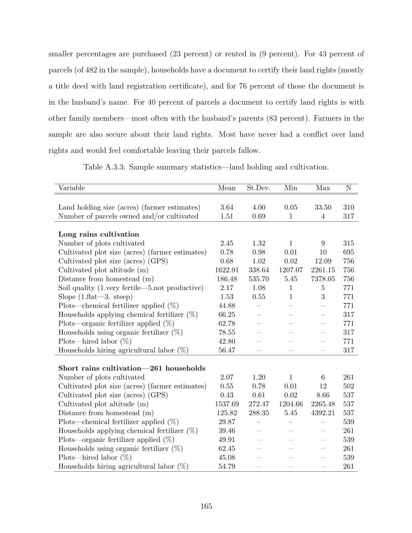
smaller percentages are purchased (23 percent) or rented in (9 percent). For 43 percent of

parcels (of 482 in the sample), households have a document to certify their land rights (mostly

a title deed with land registration certificate), and for 76 percent of those the document is

in the husband’s name. For 40 percent of parcels a document to certify land rights is with

other family members—most often with the husband’s parents (83 percent). Farmers in the

sample are also secure about their land rights. Most have never had a conflict over land

rights and would feel comfortable leaving their parcels fallow.

Table A.3.3: Sample summary statistics—land holding and cultivation.

Variable Mean St.Dev. Min Max N

Land holding size (acres) (farmer estimates) 3.64 4.00 0.05 33.50 310Number of parcels owned and/or cultivated 1.51 0.69 1 4 317

Long rains cultivationNumber of plots cultivated 2.45 1.32 1 9 315Cultivated plot size (acres) (farmer estimates) 0.78 0.98 0.01 10 695Cultivated plot size (acres) (GPS) 0.68 1.02 0.02 12.09 756Cultivated plot altitude (m) 1622.91 338.64 1207.07 2261.15 756Distance from homestead (m) 186.48 535.70 5.45 7378.05 756Soil quality (1.very fertile—5.not productive) 2.17 1.08 1 5 771Slope (1.flat—3. steep) 1.53 0.55 1 3 771Plots—chemical fertilizer applied (%) 44.88 – – – 771Households applying chemical fertilizer (%) 66.25 – – – 317Plots—organic fertilizer applied (%) 62.78 – – – 771Households using organic fertilizer (%) 78.55 – – – 317Plots—hired labor (%) 42.80 – – – 771Households hiring agricultural labor (%) 56.47 – – – 317

Short rains cultivation—261 householdsNumber of plots cultivated 2.07 1.20 1 6 261Cultivated plot size (acres) (farmer estimates) 0.55 0.78 0.01 12 502Cultivated plot size (acres) (GPS) 0.43 0.61 0.02 8.66 537Cultivated plot altitude (m) 1537.69 272.47 1204.66 2265.48 537Distance from homestead (m) 125.82 288.35 5.45 4392.21 537Plots—chemical fertilizer applied (%) 29.87 – – – 539Households applying chemical fertilizer (%) 39.46 – – – 261Plots—organic fertilizer applied (%) 49.91 – – – 539Households using organic fertilizer (%) 62.45 – – – 261Plots—hired labor (%) 45.08 – – – 539Households hiring agricultural labor (%) 54.79 – – – 261

165

The homestead on a typical farm is usually located upslope near a road and is surrounded

by scattered trees and living fences to define the housing compound (Tittonell et al. 2005).

Agricultural plots are most often located around the homestead (as close as 5.45 m), however,

some parcels are further away from the homestead (at times more than 7 km away). An

average distance of a cultivated plot from the homestead during the long rains was 186.48

m6 (Table A.3.3). On average, a household cultivated 2.45 plots during the long rains season

and 2.07 plots during the short rains season of 2011. While all households in the sample

cultivated their land during the long rains, only 261 households did so in the short rains.

The diversity of agroecosystems across the 15 villages dictates some di↵erences in rainfall

availability, altitude, and the possibility of two cropping seasons and their length. An average

plot size during the long rains was 0.78 acre according to farmers’ estimates, or 0.68 acre

according to the GPS measurement. Cultivated plots during the short rains are smaller

on average—0.55 acre according to farmers’ estimates, or 0.43 acre according to the GPS

measurement.

All plots in the sample are rainfed. Even in those areas where two cropping seasons

are possible, since the short rains are shorter in length and the amount of rainfall is less

predictable, most households opt to reduce their cultivation e↵orts. This explains a smaller

average number of plots cultivated and a reduced plot size during the second cropping season,

as well as decreased input application. Thirty nine percent of households applied some

chemical fertilizer (e.g., di-ammonium phosphate and urea) and 62 percent applied organic

fertilizer (mostly animal manure or compost) in the short rains, as opposed to 66 percent

and 79 percent, respectively, during the long rains. Although most farmers in the sample

are subsistence farmers and cultivate their own land, more than half of the households also

6The distance between the center point of each plot and the corresponding homestead was calculated basedon the GPS data collected during household visits (geographic coordinates) using an accurate ellipsoidalmodel of the Earth and assuming elevation above the ellipsoid is zero. The distance was calculated only forplots for which geographic coordinates were available. Several plots were not measured as they were locatedmore than 30 minutes drive from homesteads. Twenty-four plots among those measured were located furtherthan one km away from the homestead. If we were to exclude these 24 plots, the average distance woulddecrease to 110.52 m.

166

hired agricultural labor for planting, weeding, or harvesting (56 percent in the long rains

and 55 percent in the short rains).

Along the Yala and Nyando river basins, the dominant soil types are acrisols, ferralsols

and nitisols (Jaetzold and Schmidt 1982). While nitisols can be of high fertility, acrisols

and ferralsols are strongly leached or weathered. Farmers in the sample identified their soil

fertility as mostly moderate. Table A.3.4 summarizes the results from the near infrared (NIR)

spectroscopy soil analysis. Organic carbon content is an indicator of soil organic matter that

is readily available as a carbon and energy source for the soil microbial community (i.e.,

food for the soil food web) and averages 2.45 percent (by volume) in the sample. Nitrogen,

phosphorus, and potassium are critical nutrients for plant growth and yield; nitrogen content

seems to be very low across the sample. Soil pH measures the degree of soil acidity or

alkalinity (from 0 to 14); neutral pH is 7 and optimum pH for plant growth is 6.5. Average

pH in the sample is 5.82, which is lower than optimal.

Table A.3.4: Sample soils data by key indicator (N=315).

Indicator Mean (Ranking) St. Dev. Min Max

Organic carbon content (% by volume) 2.45 (Good) 1.30 0.81 9.45Total nitrogen content (% by volume) 0.16 (Very Low) 0.09 0.06 0.87Extractable P (g/kg) 0.0134 (Good) 0.0153 0.0006 0.1321Extractable K (g/kg) 0.36 (Good) 0.22 0.05 1.34Soil pH 5.82 (Low) 0.52 4.35 7.13

Farms in the sample are often very diversified: households grow annual crops for home

consumption, perennial cash crops for sale, and trees to satisfy residential energy needs. Over

80 percent of all cultivated plots during both seasons were occupied by food crops—grains

and tubers (maize, maize and beans, cassava, sorghum, sweet potatoes, millet), with two

annual crops grown on each farm on average (Table A.3.5). Maize is the most popular grain

in the area, having quickly established itself as a dominant food crop in the beginning of the

20th century due to its relatively higher yields per unit of land and two crops per calendar

167

year in many villages (Crowley and Carter 2000). Most sample households (312 households)

grew maize during the long rains and 187 households grew maize during the short rains season

as well. Annual crops are often intercropped (e.g., maize and beans) to maximize land use.

Many households also devote small plots around the homestead to growing vegetables, such

as collard greens, cowpea, pumpkin leaves, and indigenous vegetable plants, among others.

The farthest plots are found on the slopes towards the waterways and are often dedicated to

cash crops and woodlots, or left for pasture. Almost 40 percent of households grow perennial

cash crops such as tea and sugarcane, as well as the increasingly market-oriented crops of

bananas and Napier grass. Requiring inputs and relatively high investments, cash crops are

predominantly grown for sale and in most cases are not consumed by the household. Most

households in the Mid Yala villages also have a banana plot to provide food, a storage area

for cattle fodder, as well as, at various times, a protected place for childbearing and other

household rituals (Crowley and Carter 2000).

Table A.3.5: Sample summary statistics—production.

Variable Mean St. Dev. Min Max N

Number of annual crops grown in LR 2.19 0.78 1 5 317Number of annual crops grown in SR 2.19 1.02 1 5 247Households with perennial crops (%) 38.80 – – – 317Households with woodlots (%) 15.77 – – – 317Households with trees (%) 97.79 – – – 317Number of farm trees (farmer estimates) 324.56 1,312.10 0 11,020 317Number of farm trees (measured) 128.93 127.69 0 976 317Number of farm tree species 9.79 4.67 0 23 317Households own animals (%) 93.38 – – – 317Number of local cows 1.89 2.86 0 19 297Number of improved cows 1.04 2.42 0 20 297Number of chickens 11.25 25.51 0 300 297

Trees from woodlots—small plantations of cultivated trees—play an important role on

many farms, serving as on-farm sources of fuel and/or construction wood and, at times,

households sell wood in the market. About 16 percent of households in the sample have

woodlots, with an average woodlot size of 0.17 acres (693 m2). But almost all households

168

(98 percent) have trees on their farms. Linear tree formations or windrows are largely mono-

specific, with three species dominating their composition: Cupressus lusitanica, Eucalyptus

salinga, and Pinus patula (Bradley 1988). Hedgerows are deliberately planted homogenous

bushes, trees, and other vegetation types along the edge of various plots. They are often

dominated by one or two species, chosen for specific purposes, such as the demarcation

of plot boundaries, provision of firewood, fruits or livestock feed, use as soil amendments,

ornamental purposes, etc. For example, sturdy hedges of Tithonia diversifolia or Lantana

camara are planted due to their rapid growth and impenetrability to livestock (Bradley

1988). Moreover, a wide variety of isolated trees is found on each farm. A typical farm in

the sample has about 129 trees (or 325 according to farmers’ estimates).7 Some are planted

specifically for their fruit or wood, for shade, or medicinal or ornamental purposes; while

others are left from land clearing or grow naturally. On average, farms have 10 di↵erent tree

species, with Eucalyptus saligna and Markhamia lutea being the most popular species. More

than half (212) of households in the sample grow Eucalyptus saligna and 168 households

grow Markhamia lutea. Other popular tree species are Psidium guajava or guava, Cupressus

lusitanica or Mexican cypress, and Grevillea robusta or silky oak, among others. Over 93

percent of households keep farm animals. Each household has, on average, two local cows

(Zebu breeds), one improved dairy cow, and eleven chickens.

A.4 On-farm biological resources in western Kenya

Following Bari et al. (1998), on-farm non-edible biomass can be broadly categorized into

four major types according to its source: crop residues and other plant materials, trees and

hedgerows, animal and household waste. These major categories loosely correspond to the

di↵erent land use types: crop residues are collected from growing annual food crops and

7We did not count trees on several farms that had large areas of thick forests. This could explain a largedivergence in the estimates.

169

perennial cash crops, while trees and bushes are found on woodlots and throughout the farm

as windrows, hedgerows and isolated trees. Table A.4.1 shows the main biomass sources in

western Kenya. For each source of biomass, Table A.4.1 also shows percentage of households

in the sample producing it, the month the biomass source is most abundant, and the main

three uses (with the percentage of households dedicating the biomass source to each use).

Most biomass is used for several di↵erent purposes, leaving none wasted. The main three

uses are feeding domestic animals (either collecting biomass or grazing animals on the fields

after harvest), kitchen or household fuel, and for soil fertility management (leaving crop

residues in the fields, mulching or collecting biomass to apply as organic amendment later

on).

More than 93 percent of households in the sample own domestic animals, but only 36

households purchased feed for their cows as a supplement, stating that their cattle primary

grazed on their land. Twenty-seven percent of households, for example, left some maize

stover in the fields for grazing cattle, while 33 percent collected maize stover as animal feed.8

Crop residues from other annual (e.g., sorghum) and perennial (e.g., sugarcane and banana)

crops are also used as cattle feed, while some households (7 percent in the sample) specifically

grow fodder grasses (Pennisetum purpureum, or Elephant or Napier grass). Woody biomass

(defined as biomass from woody or ligneous plants, including shrubs), on the other hand,

satisfies most of domestic cooking energy needs. Only a small portion of woody biomass

(as charcoal) is dedicated to heating an iron or other household chores. Most households

cook on traditional open fire stoves and use twigs and branches (71 percent of households)

and/or wood (42 percent) from their own farms. Almost all households, after shelling their

maize, use maize cobs as fuel (96 percent). Some others supplement their cooking needs

with cereal straw (30 percent of households that produce it) or tea prunings (31 percent).

Di↵erent sources of biomass are also widely used for soil fertility management (leaving crop

residues on the fields as organic soil amendment, mulching, applying animal manure, or ash

8Biomass uses are not exclusive. We asked about three main uses for each biomass source.

170

from burning biomass for kitchen fuel, etc.)—most households in the sample reported using

all di↵erent sources of crop residues for soil improvement measures.

Several uses of source-specific biomass are also widespread. For example, ash from burn-

ing the bean plants in an outside fire is collected and stored to be used in cooking to make

vegetable dishes more palatable (25 percent of households reported doing so). Cow dung—

mixed with ash and soil or by itself—is used to re-plaster the outside walls of homes or

other mud structures (63 percent of households). Apart from being collected as firewood,

woody biomass is also used in construction and furniture making, as well as to demarcate

land use units and farms (18 percent of households use twigs and brunches and 35 percent

of households use wood from their farms as building materials). Moreover, medicinal, or-

namental uses, and shade provision are also common uses of tree biomass (Kindt, Simons,

and Van Damme 2004). Eighty-nine households (29 percent of the sample) reported mak-

ing charcoal mostly from their own trees, with about 206 kg of charcoal made in 2011 per

household on average. Fifty-eight households reported selling their charcoal.

It is worth noting that biomass production and utilization patterns vary according to

agricultural season, farm size, land use practices, soil fertility, as well as household size

and socio-economic characteristics, and prevailing cultural practices. Annual crop residue

availability follows the agricultural season. For example, legume residues are most abundant

in June and maize stover in August—the respective harvesting months of the long rains

agricultural season. The higher productivity of maize crops on more fertile soils or on farms

more recently converted from forest leads to higher productivity (per acre) of maize residues

(Torres-Rojas et al. 2011). Wealthy households use inorganic fertilizers, practice fallowing

on a portion of their farm and incorporate maize stover for soil management to achieve

higher crop yields, while poor households get higher returns from using maize residues as

fuel (Crowley and Carter 2000).

Only several biomass sources (twigs/branches, wood, timber o↵cuts) are commonly

171

traded in local markets. However, although markets for other sources of biomass do not

exist, households engage in the collection or barter of biomass to satisfy their needs. For

example, 34 households in the sample reported acquiring additional maize stover, with 24

households getting stover from their neighbors for feeding livestock. Forty households ac-

quired maize cobs from their neighbors to supplement their energy sources (of those, 34

households collected maize cobs for free). One hundred thirty-eight households acquired

twigs and branches, while 4 households sold some twigs and branches from their farm. Of

those who acquired woody biomass, 81 households collected it on community areas or a

neighboring farm for free, and 32 purchased it mostly at local markets.

172

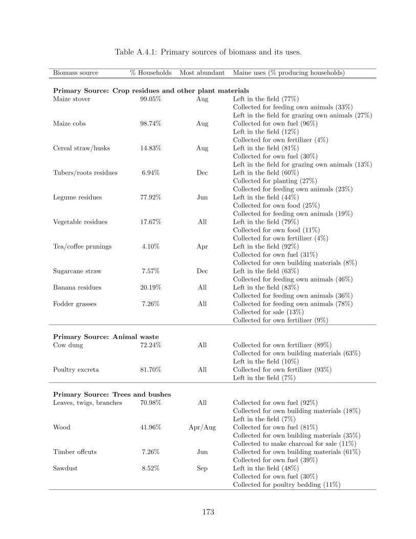
Table A.4.1: Primary sources of biomass and its uses.

Biomass source % Households Most abundant Maine uses (% producing households)

Primary Source: Crop residues and other plant materialsMaize stover 99.05% Aug Left in the field (77%)

Collected for feeding own animals (33%)Left in the field for grazing own animals (27%)

Maize cobs 98.74% Aug Collected for own fuel (96%)Left in the field (12%)Collected for own fertilizer (4%)

Cereal straw/husks 14.83% Aug Left in the field (81%)Collected for own fuel (30%)Left in the field for grazing own animals (13%)

Tubers/roots residues 6.94% Dec Left in the field (60%)Collected for planting (27%)Collected for feeding own animals (23%)

Legume residues 77.92% Jun Left in the field (44%)Collected for own food (25%)Collected for feeding own animals (19%)

Vegetable residues 17.67% All Left in the field (79%)Collected for own food (11%)Collected for own fertilizer (4%)

Tea/co↵ee prunings 4.10% Apr Left in the field (92%)Collected for own fuel (31%)Collected for own building materials (8%)

Sugarcane straw 7.57% Dec Left in the field (63%)Collected for feeding own animals (46%)

Banana residues 20.19% All Left in the field (83%)Collected for feeding own animals (36%)

Fodder grasses 7.26% All Collected for feeding own animals (78%)Collected for sale (13%)Collected for own fertilizer (9%)

Primary Source: Animal wasteCow dung 72.24% All Collected for own fertilizer (89%)

Collected for own building materials (63%)Left in the field (10%)

Poultry excreta 81.70% All Collected for own fertilizer (93%)Left in the field (7%)

Primary Source: Trees and bushesLeaves, twigs, branches 70.98% All Collected for own fuel (92%)

Collected for own building materials (18%)Left in the field (7%)

Wood 41.96% Apr/Aug Collected for own fuel (81%)Collected for own building materials (35%)Collected to make charcoal for sale (11%)

Timber o↵cuts 7.26% Jun Collected for own building materials (61%)Collected for own fuel (39%)

Sawdust 8.52% Sep Left in the field (48%)Collected for own fuel (30%)Collected for poultry bedding (11%)

173

BIBLIOGRAPHY

Ackom, E.K., D. Alemagi, N.B. Ackom, P.A. Minang, and Z. Tchoundjeu. 2013. “Modern

bioenergy from agricultural and forestry residues in Cameroon: Potential, challenges and

the way forward.” Energy Policy 63:101–113.

Adkins, E., E. Tyler, J. Wang, D. Siriri, and V. Modi. 2010. “Field testing and survey evalua-

tion of household biomass cookstoves in rural sub-Saharan Africa.” Energy for Sustainable

Development 14:172–185.

Aker, J.C. 2011. “Dial “A” for agriculture: a review of information and communication

technologies for agricultural extension in developing countries.” Agricultural Economics

42:631–647.

Amacher, G., W. Hyde, and B. Joshee. 1993. “Joint production and consumption in tra-

ditional households: Fuelwood and crop residues in two districts in Nepal.” Journal of

Development Studies 30:206–225.

Antle, J., and J. Stoorvogel. 2008. “Agricultural carbon sequestration, poverty, and sustain-

ability.” Environment and Development Economics 13:327–352.

Arnold, J.M., G. Kohlin, and R. Persson. 2006. “Woodfuels, livelihoods, and policy inter-

ventions: Changing perspectives.” World Development 34:596–611.

Arslan, A., and J.E. Taylor. 2009. “Farmers’ subjective valuation of subsistence crops: The

case of traditional maize in Mexico.” American Journal of Agricultural Economics 91:956–

972.

Austin, G., G. Morris, R. Janssen, and D. Rutz. 2012. “Biogas production in Africa.” In

Bioenergy for Sustainable Development in Africa. Dordrecht: Springer Netherlands, pp.

103–115.

174

Barbier, B. 1998. “Induced innovation and land degradation: Results from a bioeconomic

model of a village in West Africa.” Agricultural Economics 19:15–25.

Barbier, B., and G. Bergeron. 2001. “Natural resource management in the hillsides of Hon-

duras: bioeconomic modeling at the micro-watershed level.” Research Report No. 123,

International Food Policy Research Institute (IFPRI), Washington, D.C.

Bari, M., D. Hall, N. Lucas, and S. Hossain. 1998. “Biomass energy use at the household

level in two villages of Bangladesh: assessment of field methods.” Biomass and Bioenergy

15:171–180.

Battese, G.E. 1997. “A note on the estimation of Cobb-Douglas production functions when

some explanatory variables have zero values.” Journal of Agricultural Economics 48:250–

252.

Beaman, L., D.S. Karlan, B. Thuysbaert, and C.R. Udry. 2014. “Self-selection into credit

markets: Evidence from agriculture in Mali.” Working Paper No. 377, Center for Global

Development, Washington, D.C.

Berazneva, J. 2014. “Audio recording of household interviews to ensure data quality.” Journal

of International Development 26:290–296.

Berck, P., and G. Helfand. 1990. “Reconciling the von Liebig and di↵erentiable crop produc-

tion functions.” American Journal of Agricultural Economics 72:985–996.

Betemariam, E., T.G. Vagen, K. Shepherd, and L. Winowiecki. 2011. “A protocol for mea-

surement and monitoring soil carbon stocks in agricultural landscapes.” Version 1.1, World

Agroforestry Centre (ICRAF), Nairobi, Kenya.

Blanco-Canqui, H., C.A. Shapiro, C.S. Wortmann, R.A. Drijber, M. Mamo, T.M. Shaver,

and R.B. Ferguson. 2013. “Soil organic carbon: The value to soil properties.” Journal of

Soil and Water Conservation 68:129A–134A.

175

Boko, M., I. Niang, A. Nyong, C. Vogel, A. Githeko, M. Medany, B. Osman-Elasha, R. Tabo,

and P. Yanda. 2007. “Africa.” In M. Parry, O. Canziani, J. Palutikof, P. van der Linden,

and C. Hanson, eds. Climate Change 2007: Impacts, Adaptation and Vulnerability. Con-

tribution of Working Group II to the Fourth Assessment Report of the Intergovernmental

Panel on Climate Change. Cambridge, UK: Cambridge University Press, pp. 433–467.

Bond, T., and M.R. Templeton. 2011. “History and future of domestic biogas plants in the

developing world.” Energy for Sustainable Development 15:347–354.

Bradley, P. 1988. “Survey of Woody Biomass on Farms in Western Kenya.” Ambio 17:40–48.

Bringezu, S., H. Schtz, M. O’Brien, L. Kauppi, R. Howarth, and J. McNeely. 2009. “To-

wards sustainable production and use of resources: assessing biofuels.” Report of the

International Panel for Sustainable Resource Management, United Nations Environment

Programme (UNEP), Paris, France.

Brown, R. 2009. “Biochar production technology.” In J. Lehmann and S. Joseph, eds. Biochar

for Environmental Management: Science and Technology . London, UK: Earthscan Publi-

cations Ltd., pp. 127–146.

Brown, T., M. Wright, and R. Brown. 2011. “Estimating profitability of two biochar pro-

duction scenarios: slow pyrolysis vs. fast pyrolysis.” Biofuels, Bioproducts and Biorefining

5:54–68.

Burt, O.R. 1981. “Farm level economics of soil conservation in the Palouse area of the

Northwest.” American Journal of Agricultural Economics 63:83 –92.

Cadogan, S., and L. O’Sullivan. 2012. “Commercial center energy survey in Western Kenya.”

Working paper, World Agroforestry Centre (ICRAF), Nairobi, Kenya.

Caputo, A.C., M. Palumbo, P.M. Pelagagge, and F. Scacchia. 2005. “Economics of biomass

176

energy utilization in combustion and gasification plants: E↵ects of logistic variables.”

Biomass and Bioenergy 28:35–51.

Chivenge, P., B. Vanlauwe, and J. Six. 2011. “Does the combined application of organic and

mineral nutrient sources influence maize productivity? A meta-analysis.” Plant and Soil

342:1–30.

Chivenge, P.P., H.K. Murwira, K.E. Giller, P. Mapfumo, and J. Six. 2007. “Long-term impact

of reduced tillage and residue management on soil carbon stabilization: Implications for

conservation agriculture on contrasting soils.” Soil and Tillage Research 94:328–337.

Clark, C.W. 1990. Mathematical Bioeconomics: The Optimal Management of Renewable

Resources , 2nd ed. Pure and applied mathematics, New York: John Wiley & Sons.

Coleman, K., and D. Jenkinson. 1999. “ROTHC-26.3. A model for the turnover of carbon

in soil.” November 1999 issue (modified August 2008), Rothamsted Research, Harpenden,

Herts, UK.

Conrad, J. 2010. Resource Economics , 2nd ed. New York, NY: Cambridge University Press.

Cooke, P., G. Kohlin, and W. Hyde. 2008. “Fuelwood, forests and community management?

Evidence from household studies.” Environment and Development Economics 13:103–135.

Cozzolino, D., and A. Moron. 2003. “The potential of near-infrared reflectance spectroscopy

to analyse soil chemical and physical characteristics.” The Journal of Agricultural Science

140:65–71.

Crowley, E., and S. Carter. 2000. “Agrarian change and the changing relationships between

toil and soil in Maragoli, Western Kenya (1900–1994).” Human Ecology 28:383–414.

Dasgupta, P. 2010. “The place of nature in economic development. Chapter 74.” In D. Ro-

drik and M. Rosenzweig, eds. Handbook of Development Economics . Elsevier, vol. 5 of

Handbooks in Economics , pp. 4977–5046.

177

Davidson, E., and I. Ackerman. 1993. “Changes in soil carbon inventories following cultiva-

tion of previously untilled soils.” Biogeochemistry 20:161–193.

de Janvry, A., M. Fafchamps, and E. Sadoulet. 1991. “Peasant household behaviour with

missing markets: Some paradoxes explained.” Economic Journal 101:1400–1417.

Diaz-Zorita, M., G.A. Duarte, and J.H. Grove. 2002. “A review of no-till systems and soil

management for sustainable crop production in the subhumid and semiarid Pampas of

Argentina.” Soil and Tillage Research 65:1–18.

Dietz, J., and S. Kuyah. 2011. “Guidelines for establishing regional allometric equations for

biomass estimation through destructive sampling.” Carbon Benefits Project: Modelling,

Measurement and Monitoring, World Agroforestry Centre (ICRAF), Nairobi, Kenya.

Duflo, E., M. Kremer, and J. Robinson. 2011. “Nudging farmers to use fertilizer: Theory

and experimental evidence from Kenya.” American Economic Review 101:2350–2390.

Duku, M.H., S. Gu, and E.B. Hagan. 2011. “A comprehensive review of biomass resources

and biofuels potential in Ghana.” Renewable and Sustainable Energy Reviews 15:404–415.

Eisentraut, A. 2010. “Sustainable production of second-generation biofuels.” IEA Energy Pa-

pers, Organisation for Economic Co-operation and Development (OECD), Paris, France.

Ewing, M., and S. Msangi. 2009. “Biofuels production in developing countries: assessing

tradeo↵s in welfare and food security.” Environmental Science & Policy 12:520–528.

FAO. 2005. “New\ LocClim: Local Climate Estimator.”

FAOSTAT. 2015. FAOSTAT Database Query . Available from

http://faostat3.fao.org/home/E, Rome, Italy: Food and Agriculture Organization

of the United Nations Statistics Division (FAOSTAT).

Fargione, J., J. Hill, D. Tilman, S. Polasky, and P. Hawthorne. 2008. “Land clearing and the

biofuel carbon debt.” Science 319:1235–1238.

178

Foster, A.D., and M.R. Rosenzweig. 1995. “Learning by doing and learning from others: Hu-

man capital and technical change in agriculture.” Journal of Political Economy 103:1176–

1209.

Frederick, S., G. Loewenstein, and T. O’Donoghue. 2002. “Time discounting and time pref-

erence: A critical review.” Journal of Economic Literature 40:351–401.

French, D. 1986. “Confronting an unsolvable problem: Deforestation in Malawi.” World

Development 14:531–540.

Galinato, S.P., J.K. Yoder, and D. Granatstein. 2011. “The economic value of biochar in

crop production and carbon sequestration.” Energy Policy 39:6344–6350.

Gallagher, P., M. Dikeman, J. Fritz, E. Wailes, W. Gauthier, and H. Shapouri. 2003. “Supply

and social cost estimates for biomass from crop residues in the United States.” Environ-

mental and Resource Economics 24:335–358.

Gaunt, J., and A. Cowie. 2009. “Biochar, greenhouse gas accounting and emissions trading.”

In J. Lehmann and S. Joseph, eds. Biochar for Environmental Management: Science and

Technology . London, UK: Earthscan Publications Ltd., pp. 317–340.

Gavian, S., and M. Fafchamps. 1996. “Land tenure and allocative e�ciency in Niger.” Amer-

ican Journal of Agricultural Economics 78:460–471.

Gentile, R., B. Vanlauwe, P. Chivenge, and J. Six. 2011. “Trade-o↵s between the short- and

long-term e↵ects of residue quality on soil C and N dynamics.” Plant and Soil 338:159–169.

Goldstein, M., and C. Udry. 2008. “The profits of power: Land rights and agricultural

investment in Ghana.” Journal of Political Economy 116:981–1022.

Gra↵-Zivin, J., and L. Lipper. 2008. “Poverty, risk, and the supply of soil carbon sequestra-

tion.” Environment and Development Economics 13:353–373.

179

Graubner, M., A. Balmann, and R.J. Sexton. 2011. “Spatial price discrimination in agri-

cultural product procurement markets: A computational economics approach.” American

Journal of Agricultural Economics 93:949–967.

Guerena, D. 2014. “Anthropogenic and Natural Pyrogenic Carbon in Tropical Environments:

From the Rhizosphere to the Landscape.” PhD Dissertation, Cornell University, Ithaca,

NY.

Hammond, G.P., and S.M. Seth. 2013. “Carbon and environmental footprinting of global

biofuel production.” Applied Energy 112:547–559.

Harou, A., Y. Liu, C.B. Barrett, and L. You. 2014. “Variable returns to fertilizer use and

its relationship to poverty.” IFPRI Discussion Paper 01373, International Food Policy

Research Institute (IFPRI), Washington, D.C.

Hassan, R., R. Scholes, and N. Ash, eds. 2005. Ecosystems and Human Well-being: Current

State and Trends, Volume 1 . Washington, DC: Island Press.

Holden, S., and H. Binswanger. 1998. “Small farmers, market imperfections, and natural re-

source management.” In E. Lutz, H. Binswanger, P. Hazell, and A. McCalla, eds. Agricul-

ture and the Environment: Perspectives on Sustainable Rural Development . Washington,

D.C.: The World Bank (WB), pp. 50–70.

Holden, S., B. Shiferaw, and J. Pender. 2005. “Policy analysis for sustainable land manage-

ment and food security in Ethiopia: A bioeconomic model with market imperfections.”

Research Report No. 140, International Food Policy Research Institute (IFPRI), Wash-

ington, DC.

Holden, S.T., B. Shiferaw, and M. Wik. 1998. “Poverty, market imperfections and time

preferences: of relevance for environmental policy?” Environment and Development Eco-

nomics 3:105–130.

180

Hosonuma, N., M. Herold, V.D. Sy, R.S.D. Fries, M. Brockhaus, L. Verchot, A. Angelsen,

and E. Romijn. 2012. “An assessment of deforestation and forest degradation drivers in

developing countries.” Environmental Research Letters 7:044009.

Hotelling, H. 1931. “The economics of exhaustible resources.” Journal of Political Economy

39:137–175.

IEA. 2014. World Energy Outlook 2014 . Paris, France: International Energy Agency (IEA).

IPCC. 2003. Intergovernmental Panel on Climate Change Good Practice Guidance for Land

Use, Land-Use Change and Forestry . Institute for Global Environmental Strategies (IGES)

for the Intergovernmental Panel on Climate Change (IPCC).

IWG. 2010. Interagency Working Group on Social Cost of Carbon, US Government, technical

support document: Social cost of carbon for regulatory impact analysis under Executive

Order 12866 . Interagency Working Group (IWG).

—. 2013. Interagency Working Group on Social Cost of Carbon, US Government, technical

support document: Technical update of the social cost of carbon for regulatory impact

analysis under Executive Order 12866, May 2013 . Interagency Working Group (IWG).

Jacoby, H.G. 1993. “Shadow wages and peasant family labour supply: An econometric ap-

plication to the Peruvian Sierra.” Review of Economic Studies 60:903–921.

Jaetzold, R., and H. Schmidt. 1982. Farm Management Handbook of Kenya. Vol. II. Natural

Conditions and Farm Management Information. Nairobi, Kenya: Ministry of Agriculture.

Jayne, T., and S. Rashid. 2013. “Input subsidy programs in sub-Saharan Africa: a synthesis

of recent evidence.” Agricultural Economics 44:547–562.

Jenkinson, D.S., and A. Ayanaba. 1977. “Decomposition of carbon-14 labeled plant material

under tropical conditions.” Soil Science Society of America Journal 41:912–915.

181

Jingura, R.M., and R. Matengaifa. 2008. “The potential for energy production from crop

residues in Zimbabwe.” Biomass and Bioenergy 32:1287–1292.

Jumbe, C.B.L., F.B.M. Msiska, and M. Madjera. 2009. “Biofuels development in Sub-

Saharan Africa: Are the policies conducive?” Energy Policy 37:4980–4986.

Karlan, D.S., R. Osei, I. Osei-Akoto, and C. Udry. 2012. “Agricultural decisions after relaxing

credit and risk constraints.” Working Paper 18463, National Bureau of Economic Research

(NBER).

Karltun, E., M. Lemenih, and M. Tolera. 2013. “Comparing farmers’ perception of soil

fertility change with soil properties and crop performance in Beseku, Ethiopia.” Land

Degradation & Development 24:228–235.

KFS. 2013. “Analysis of the charcoal value chain in Kenya.” Final report, Kenya Forest

Service (KFS), Nairobi, Kenya.

Khan, S.A., R.L. Mulvaney, T.R. Ellsworth, and C.W. Boast. 2007. “The myth of nitrogen

fertilization for soil carbon sequestration.” Journal of Environment Quality 36:1821.

Kimetu, J., J. Lehmann, J. Kinyangi, C. Cheng, J. Thies, D. Mugendi, and A. Pell. 2009.

“Soil organic C stabilization and thresholds in C saturation.” Soil Biology & Biochemistry

41:2100–2104.

Kimetu, J., J. Lehmann, S. Ngoze, D. Mugendi, J. Kinyangi, S. Riha, L. Verchot, J. Recha,

and A. Pell. 2008. “Reversibility of soil productivity decline with organic matter of di↵ering

quality along a degradation gradient.” Ecosystems 11:726–739.

Kindt, R., D. Osino, C. Orwa, A. Nzisa, P. Van Breugel, L. Graudal, J.P. Lilleso, K. Kehlen-

beck, J. Dietz, M. Nyabenge, R. Jamnadass, and H. Neufeld. 2011. “Useful tree species

for Africa.” Interactive vegetation maps and species composition tables based on the Veg-

etation Map of Africa, World Agroforestry Centre (ICRAF), Nairobi, Kenya.

182

Kindt, R., A.J. Simons, and P. Van Damme. 2004. “Do farm characteristics explain dif-

ferences in tree species diversity among Western Kenyan farms?” Agroforestry Systems

63:63–74.

Kinyangi, J. 2008. “Soil Degradation, Thresholds and Dynamics of Long-Term Cultivation:

from Landscape Biogeochemistry to Nanoscale Biogeocomplexity.” PhD Dissertation, Cor-

nell University, Ithaca, New York.

Klemick, H. 2011. “Shifting cultivation, forest fallow, and externalities in ecosystem ser-

vices: Evidence from the Eastern Amazon.” Journal of Environmental Economics and

Management 61(1):95–106.

Knorr, M., S.D. Frey, and P.S. Curtis. 2005. “Nitrogen additions and litter decomposition:

a meta-analysis.” Ecology 86:3252–3257.

Kojima, M., and T. Johnson. 2005. Potential for Biofuels for Transport in Developing Coun-

tries . Energy Sector Management Assistance Programme (ESMAP), United Nations En-

vironment Programme (UNDP), World Bank.

Kuyah, S., J. Dietz, C. Muthuri, R. Jamnadass, P. Mwangi, R. Coe, and H. Neufeldt. 2012.

“Allometric equations for estimating biomass in agricultural landscapes: I. Aboveground

biomass.” Agriculture, Ecosystems & Environment 158:216–224.

Lal, R. 2006. “Enhancing crop yields in the developing countries through restoration of the

soil organic carbon pool in agricultural lands.” Land Degradation & Development 17:197–

209.

—. 2014. “Societal value of soil carbon.” Journal of Soil and Water Conservation 69:186A–

192A.

—. 2004. “Soil carbon sequestration impacts on global climate change and food security.”

Science 304:1623 –1627.

183

—. 2009. “Soil quality impacts of residue removal for bioethanol production.” Soil and Tillage

Research 102:233–241.

—. 2005. “World crop residues production and implications of its use as a biofuel.” Environ-

ment International 31:575–584.

Lane, G. 2013. “Energy Markets in Kenya: The Impacts of Imperfect Markets on Rural

Households.” Unpublished M.S. Thesis, Dyson School of Applied Economics and Manage-

ment, Cornell University, Ithaca, New York.

Latshaw, W., and E. Miller. 1924. “Elemental composition of the corn plant.” Journal of

Agricultural Research XXVII:845–860.

Le, K.T. 2009. “Shadow wages and shadow income in farmers’ labor supply functions.”

American Journal of Agricultural Economics 91:685–696.

Lee, D., and C. Barrett, eds. 2001. Tradeo↵s or Synergies? Agricultural Intensification,

Economic Development and the Environment . Wallingford, U.K.: CABI Press.

Lee, D., P. Ferraro, and C. Barrett. 2001. “Introduction: Changing perspectives on agricul-

tural intensification, economic development and the environment.” In D. Lee and C. Bar-

rett, eds. Tradeo↵s or Synergies? Agricultural Intensification, Economic Development and

the Environment . Wallingford, UK: CABI Press, pp. 1–16.

Lehmann, J. 2007a. “Bio-energy in the black.” Frontiers in Ecology and the Environment

5:381–387.

—. 2007b. “A handful of carbon.” Nature 447:143–4.

Lehmann, J., and S. Joseph. 2009. “Biochar for environmental management: An introduc-

tion.” In J. Lehmann and S. Joseph, eds. Biochar for Environmental Management: Science

and Technology . London, UK: Earthscan Publications Ltd., pp. 1–12.

184

Lofgren, K.G. 1985. “The pricing of pulpwood and spatial price discrimination: Theory and

practice.” European Review of Agricultural Economics 12:283–293.

Lopez, R. 1997. “Environmental externalities in traditional agriculture and the impact of

trade liberalization: the case of Ghana.” Journal of Development Economics 53:17–39.

Lynd, L.R., and J. Woods. 2011. “Perspective: A new hope for Africa.” Nature 474:S20–S21.

Magnan, N., D.M. Larson, and J.E. Taylor. 2012. “Stuck on stubble? The non-market

value of agricultural byproducts for diversified farmers in Morocco.” American Journal of

Agricultural Economics 94:1055–1069.

Marenya, P., and C. Barrett. 2007. “Household-level determinants of adoption of improved

natural resources management practices among smallholder farmers in western Kenya.”

Food Policy 32:515–536.

—. 2009a. “Soil quality and fertilizer use rates among smallholder farmers in western Kenya.”

Agricultural Economics 40:561–572.

—. 2009b. “State-conditional fertilizer yield response on eestern Kenyan farms.” American

Journal of Agricultural Economics 91:991–1006.

Mathenge, M.K., M. Smale, and J. Olwande. 2014. “The impacts of hybrid maize seed on

the welfare of farming households in Kenya.” Food Policy 44:262–271.

Matsumoto, T., and T. Yamano. 2011. “Optimal fertilizer use on maize production in East

Africa.” In T. Yamano, K. Otsuka, and F. Place, eds. Emerging Development of Agriculture

in East Africa. Springer Netherlands, pp. 117–132.

Maundu, P., and B. Tengnas, eds. 2005. Useful Trees and Shrubs for Kenya. Technical

Handbook No. 35, Nairobi, Kenya: World Agroforestry Centre - Eastern and Central

Africa Regional Programme (ICRAF-ECA).

185

McCarl, B., C. Peacocke, R. Chrisman, K. Chih-Chun, and R. Sands. 2009. “Economics

of biochar production, utilisation and emissions.” In J. Lehmann and S. Joseph, eds.

Biochar for Environmental Management: Science and Technology . London, UK: Earthscan

Publications Ltd., pp. 341–358.

McConnell, K. 1983. “An economic model of soil conservation.” American Journal of Agri-

cultural Economics 65:83.

Mekonnen, A., and G. Kohlin. 2008. “Biomass fuel consumption and dung use as manure:

Evidence from rural households in the Amhara region of Ethiopia.” EfD Discussion Pa-

per No. 08-17, Environment for Development Initiative and Resources for the Future,

Washington, D.C.

Milbrandt, A. 2009. “Assessment of biomass resources in Liberia.” Technical Report

NREL/TP-6a2-44808, National Renewable Energy Laboratory (NREL), Golden, Col-

orado, USA.

MOE. 2015. “National Energy and Petroleum Policy.” Draft, Republic of Kenya Ministry of

Energy and Petroleum (MOE).

Moebius-Clune, B., H. van Es, O. Idowu, R. Schindelbeck, J. Kimetu, S. Ngoze, J. Lehmann,

and J. Kinyangi. 2011. “Long-term soil quality degradation along a cultivation chronose-

quence in western Kenya.” Agriculture, Ecosystems & Environment 141:86–99.

Moebius-Clune, B.N. 2010. “Applications of Integrative Soil Quality Assessment in Research,

Extension, and Education.” PhD dissertation, Cornell University, Ithaca, New York.

Mukhwana, E., and J. Odera. 2009. “Best-bet comparison of soil fertility management rec-

ommendations in western Kenya: Independent testing by NGOs.” 10th KARI Biennial

Scientific Conference Volume I, Kenya Agricultural Research Institute (KARI), Nairobi,

Kenya.

186

Murty, D., M. Kirschbaum, R. Mcmurtrie, and H. Mcgilvray. 2002. “Does conversion of forest

to agricultural land change soil carbon and nitrogen? A review of the literature.” Global

Change Biology 8:105–123.

Ngoze, S., S. Riha, J. Lehmann, L. Verchot, J. Kinyangi, D. Mbugua, and A. Pell. 2008.

“Nutrient constraints to tropical agroecosystem productivity in long-term degrading soils.”

Global Change Biology 14:2810–2822.

Nordhaus, W. 2014. “Estimates of the social cost of carbon: Concepts and results from the

DICE-2013R model and alternative approaches.” Journal of the Association of Environ-

mental and Resource Economists 1:273–312.

OECD/FAO. 2015. “OECD-FAO Agricultural Outlook.” OECD Agriculture statistics

(database), http://dx.doi.org/10.1787/agr-outl-data-en.

Pagan, A. 1984. “Econometric issues in the analysis of regressions with generated regressors.”

International Economic Review 25:221–247.

Palm, C., C. Gachengo, R. Delve, G. Cadisch, and K. Giller. 2001. “Organic inputs for

soil fertility management in tropical agroecosystems: application of an organic resource

database.” Agriculture, Ecosystems and Environment 83:27–42.

Palmquist, R.B. 2005. “Property value models. Chapter 16.” In K.-G. Maler and J. R.

Vincent, eds. Handbook of Environmental Economics . Elsevier, vol. 2 of Valuing Environ-

mental Changes , pp. 763–819.

Pender, J.L. 1996. “Discount rates and credit markets: Theory and evidence from rural

india.” Journal of Development Economics 50:257–296.

Peters-Stanley, M., G. Gonzalez, and D. Yin. 2013. Covering New Ground: State of the

Forest Carbon Markets 2013 . Washington, D.C.: Forest Trends’ Ecosystem Marketplace.

187

Piccolo, C., and F. Bezzo. 2009. “A techno-economic comparison between two technologies

for bioethanol production from lignocellulose.” Biomass and Bioenergy 33:478–491.

Potter, C.S. 1999. “Terrestrial biomass and the e↵ects of deforestation on the global carbon

cycle: Results from a model of primary production using satellite observations.” BioScience

49:769–778.

Powlson, D.S., P.J. Gregory, W.R. Whalley, J.N. Quinton, D.W. Hopkins, A.P. Whitmore,

P.R. Hirsch, and K.W.T. Goulding. 2011. “Soil management in relation to sustainable

agriculture and ecosystem services.” Food Policy 36, Supplement 1:S72–S87.

Rajendran, K., S. Aslanzadeh, and M.J. Taherzadeh. 2012. “Household biogas rigesters – A

review.” Energies 5:2911–2942.

Rehfuess, E., S. Mehta, and A. Pruss-Ustun. 2006. “Assessing household solid fuel use: Mul-

tiple omplications for the Millennium Development Goals.” Environmental Health Per-

spectives 114:373–378.

Richard, T.L. 2010. “Challenges in scaling up biofuels infrastructure.” Science 329:793–796.

Richardson, A.E., C.A. Kirkby, S. Banerjee, and J.A. Kirkegaard. 2014. “The inorganic

nutrient cost of building soil carbon.” Carbon Management 5:265–268.

Roberts, K.G., B.A. Gloy, S. Joseph, N.R. Scott, and J. Lehmann. 2010. “Life cycle as-

sessment of biochar systems: Estimating the energetic, economic, and climate change

potential.” Environmental Science & Technology 44:827–833.

Rubin, E.S. 2012. “Understanding the pitfalls of CCS cost estimates.” International Journal

of Greenhouse Gas Control 10:181–190.

Rutz, D., and R. Janssen. 2012. “Keynote introduction: Biomass technologies and markets

in Africa.” In R. Janssen and D. Rutz, eds. Bioenergy for Sustainable Development in

Africa. Dordrecht: Springer Netherlands, pp. 63–73.

188

Sahn, D.E., and D. Stifel. 2003. “Exploring alternative measures of welfare in the absence

of expenditure data.” Review of Income and Wealth 49:463–489.

Sanchez, P. 2002. “Soil fertility and hunger in Africa.” Science 295:2019–2020.

Senelwa, K.A., and D.O. Hall. 1993. “A biomass energy flow chart for Kenya.” Biomass and

Bioenergy 4:35–48.

Sesmero, J., and X. Sun. 2015. “The influence of feedstock supply risk on location of stover-

based bio-gasoline plants.” GCB Bioenergy , pp. In press.

Shabangu, S., D. Woolf, E.M. Fisher, L.T. Angenent, and J. Lehmann. 2014. “Techno-

economic assessment of biomass slow pyrolysis into di↵erent biochar and methanol con-

cepts.” Fuel 117, Part A:742–748.

Sheahan, M., J. Ariga, and T. Jayne. 2013. “Modeling the e↵ects of input market reforms on

fertilizer demand and maize production: A case study of Kenya.” Selected Paper prepared

for presentation at the Agricultural & Applied Economics Associations 2013 AAEA &

CAES Joint Annual Meeting, Washington, DC, August 4-6, 2013, Michigan State Univer-

sity.

Sheahan, M., and C.B. Barrett. 2014. “Understanding the agricultural input landscape in

Sub-Saharan Africa: recent plot, household, and community-level evidence.” Working

paper No. WPS7014, The World Bank (WB), Washington, D.C.

Sheahan, M., R. Black, and T. Jayne. 2013. “Are Kenyan farmers under-utilizing fertilizer?

Implications for input intensification strategies and research.” Food Policy 41:39–52.

Shepherd, K., and M. Walsh. 2002. “Development of reflectance spectral libraries for char-

acterization of soil properties.” Soil Science Society of America Journal 66:988–998.

Shepherd, K.D., and M.J. Soule. 1998. “Soil fertility management in west Kenya: dynamic

189

simulation of productivity, profitability and sustainability at di↵erent resource endowment

levels.” Agriculture, Ecosystems & Environment 71:131–145.

Shiferaw, B., and H. Freeman, eds. 2003. Methods for assessing the impacts of natural re-

source management research. A summary of the proceedings of an International Workshop,

6-7 December 2002, Patancheru, Andhra Pradesh, India: International Crops Research In-

stitute for the Semi-Arid Tropics (ICRISAT).

Shively, G.E. 2001. “Poverty, consumption risk, and soil conservation.” Journal of Develop-

ment Economics 65:267–290.

Skoufias, E. 1994. “Using shadow wages to estimate labor supply of agricultural households.”

American Journal of Agricultural Economics 76:215–227.

Smil, V. 1999. “Crop residues: Agriculture’s largest harvest.” BioScience 49:299–308.

Solomon, D., J. Lehmann, J. Kinyangi, W. Amelung, I. Lobe, A. Pell, S. Riha, S. Ngoze,

L. Verchot, D. Mbugua, J. Skjemstad, and T. Schfer. 2007. “Long-term impacts of an-

thropogenic perturbations on dynamics and speciation of organic carbon in tropical forest

and subtropical grassland ecosystems.” Global Change Biology 13:511–530.

Stavi, I., and R. Lal. 2013. “Agroforestry and biochar to o↵set climate change: A review.”

Agronomy for Sustainable Development 33:81–96.

Stephens, E.C., C.F. Nicholson, D.R. Brown, D. Parsons, C.B. Barrett, J. Lehmann,

D. Mbugua, S. Ngoze, A.N. Pell, and S.J. Riha. 2012. “Modeling the impact of natu-

ral resource-based poverty traps on food security in Kenya: The Crops, Livestock and

Soils in Smallholder Economic Systems (CLASSES) model.” Food Security 4:423–439.

Stevens, P.R., and T.W. Walker. 1970. “The chronosequence concept and soil formation.”

The Quarterly Review of Biology 45:333–350.

190

Suri, T. 2011. “Selection and comparative advantage in technology adoption.” Econometrica

79:159–209.

Tanaka, T., C.F. Camerer, and Q. Nguyen. 2010. “Risk and time preferences: Linking exper-

imental and household survey data from Vietnam.” American Economic Review 100:557–

571.

Teklewold, H. 2012. “The impact of shadow prices and farmers’ impatience on the alloca-

tion of a multipurpose renewable resource in Ethiopia.” Environment and Development

Economics 17:479–505.

Thampapillai, D., and J. Anderson. 1994. “A review of the socio-economic analysis of soil

degradation problems for developed and developing countries.” Review of Marketing and

Agricultural Economics 62.

Thornton, P.K., M. Herrero, and R.S. DeFries. 2010. “Potential for reduced methane and car-

bon dioxide emissions from livestock and pasture management in the tropics.” Proceedings

of the National Academy of Sciences 107:19667–19672.

Tilman, D., C. Balzer, J. Hill, and B. Befort. 2011. “Global food demand and the sustainable

intensification of agriculture.” Proceedings of the National Academy of Sciences 108:20260–

20264.

Tilman, D., R. Socolow, J.A. Foley, J. Hill, E. Larson, L. Lynd, S. Pacala, J. Reilly,

T. Searchinger, C. Somerville, and R. Williams. 2009. “Beneficial biofuels – The food,

energy, and environment trilemma.” Science 325:270–271.

Tittonell, P., and K. Giller. 2013. “When yield gaps are poverty traps: The paradigm of

ecological intensification in African smallholder agriculture.” Field Crops Research 143:76–

90.

191

Tittonell, P., P.A. Le↵elaar, B. Vanlauwe, M.T. van Wijk, and K.E. Giller. 2006. “Exploring

diversity of crop and soil management within smallholder African farms: A dynamic model

for simulation of N balances and use e�ciencies at field scale.” Agricultural Systems 91:71–

101.

Tittonell, P., B. Vanlauwe, N. de Ridder, and K.E. Giller. 2007. “Heterogeneity of crop

productivity and resource use e�ciency within smallholder Kenyan farms: Soil fertility

gradients or management intensity gradients?” Agricultural Systems 94:376–390.

Tittonell, P., B. Vanlauwe, P. Le↵elaar, E. Rowe, and K. Giller. 2005. “Exploring diversity

in soil fertility management of smallholder farms in western Kenya: I. Heterogeneity at

region and farm scale.” Agriculture, Ecosystems & Environment 110:149–165.

Torres-Rojas, D. 2015. “Biomass Resource Inventory and Selection for Biochar Production

using Manual and Object Based Image Analysis.” PhD Dissertation, Cornell University,

Ithaca, New York.

Torres-Rojas, D., J. Lehmann, P. Hobbs, S. Joseph, and H. Neufeldt. 2011. “Biomass

availability, energy consumption and biochar production in rural households of Western

Kenya.” Biomass and Bioenergy 35:3537–3546.

Tully, K., C. Sullivan, R. Weil, and P. Sanchez. 2015. “The state of soil degradation in

Sub-Saharan Africa: Baselines, trajectories, and solutions.” Sustainability 7:6523–6552.

UN. 2014. The Millennium Development Goals Report . New York, NY: United Nations (UN).

Vanlauwe, B., J. Diels, N. Sanginga, and R. Merckx. 2002. Integrated Plant Nutrient Man-

agement in Sub-Saharan Africa: From Concept to Practice. Wallingford, Oxon, UK; New

York, NY, USA: CABI.

Vanlauwe, B., and K. Giller. 2006. “Popular myths around soil fertility management in

sub-Saharan Africa.” Agriculture, Ecosystems & Environment 116:34–46.

192

Vanlauwe, B., J. Six, N. Sanginga, and A.A. Adesina. 2015. “Soil fertility decline at the base

of rural poverty in sub-Saharan Africa.” Nature Plants 1:15101.

von Maltitz, G., and W. Sta↵or. 2011. “Assessing opportunities and constraints for biofuel

development in sub-Saharan Africa.” Working paper No. CIFOR Working Paper no. 58,

Center for International Forestry Research (CIFOR), Bogor, Indonesia.

Waithaka, M., P. Thornton, M. Herrero, and K. Shepherd. 2006. “Bio-economic evaluation of

farmers’ perceptions of viable farms in western Kenya.” Agricultural Systems 90:243–271.

Ward, P.S., R.J.G.M. Florax, and A. Flores-Lagunes. 2014. “Climate change and agricultural

productivity in Sub-Saharan Africa: a spatial sample selection model.” European Review

of Agricultural Economics 41:199–226.

WB. 2012. Carbon Sequestration in Agricultural Soils . REPORT NO. 67395-GLB, Washing-

ton, D.C.: The World Bank (WB).

—. 2010. “Implementation Completion and Results Report (TF-054250) for a Western Kenya

Integrated Ecosystem Management Project (WKIEMP).” Environmental and Natural Re-

sources Management Unit, Sustainable Development Department, Country Department

AFCE2, Africa Region, The World Bank (WB), Washington, D.C., Nairobi, Kenya.

—. 2005. “Kenya: Issues in trade logistics.” Report, The World Bank (WB), Washington,

D.C.

—. 2014. State and trends of carbon pricing 2014 . REPORT NO. 88284, Washington, D.C.:

The World Bank (WB).

—. 2015. World Development Indicators (WDI). Washington, D.C.: The World Bank.

Whitman, T., and J. Lehmann. 2009. “Biochar – One way forward for soil carbon in o↵set

mechanisms in Africa?” Environmental Science & Policy 12:1024–1027.

193

Wise, R., and O. Cacho. 2011. “A bioeconomic analysis of the potential of Indonesian agro-

forests as carbon sinks.” Environmental Science & Policy 14:451–461.

Woods, J. 2006. “Science and technology options for harnessing bioenergy’s potential.”

Bioenergy and Agriculture: Promises and Challenges No. Focus 14, Brief 6 of 12, In-

ternational Food Policy Research Institute (IFPRI), Washington, DC.

Woodward, F.I., R.D. Bardgett, J.A. Raven, and A.M. Hetherington. 2009. “Biological

approaches to global environment change mitigation and remediation.” Current Biology

19:R615–R623.

Woolf, D., J. Lehmann, E.M. Fisher, and L.T. Angenent. 2014. “Biofuels from pyrolysis in

perspective: Trade-o↵s between energy yields and soil-carbon additions.” Environmental

Science & Technology 48:6492–6499.

WRI. 2007. Nature’s Benefits in Kenya: An Atlas of Ecosystems and Human Well-being .

Washington, D.C., Nairobi, Kenya: World Resources Institute (WRI); Department of

Resource Surveys and Remote Sensing, Ministry of Environment and Natural Resources,

Kenya; Central Bureau of Statistics, Ministry of Planning and National Development,

Kenya; International Livestock Research Institute.

Yaman, S. 2004. “Pyrolysis of biomass to produce fuels and chemical feedstocks.” Energy

Conversion and Management 45:651–671.

194