Three essays on economics and information shocks

Thesis by

Kyle Carlson

In Partial Fulfillment of the Requirements

for the Degree of

Doctor of Philosophy

California Institute of Technology

Pasadena, California

2015

(Defended 5/15/2015)

ii

c⃝ 2015

Kyle Carlson

All Rights Reserved

iii

Acknowledgments

Numerous people helped make this work possible and otherwise contributed to the time I spent at Caltech.

Colin Camerer supported and encouraged all the projects in this thesis (and more) from the most nascent

stages to the final changes requested by reviewers. If not for Colin, my time here would have been more

fraught and much less interesting. I am thankful that we still have more research to do. He also con-

tributed by assembling and mentoring, in an outstandingly earnest, rigorous, and intellectually curious way,

an amazing and amazingly varied group of researchers in his lab. Each week we had the opportunity to

discuss research with Colin, and, in an important sense, see him doing research. This form of interaction

is incredibly valuable. It is very unfortunate that this arrangement is not a widely held norm. By working

with Colin I also had the great chance to meet and collaborate with numerous other people, including Alice,

Annamaria, Josh, Stephen, and Zach. Other lab members I had the fortune to meet are Alec, Deb, Gidi,

Klavdia, Mathieu, Matt, Meghana, Rahul, Romann, and Taisuke. Deb and Rahul were great office mates.

Gui generously gave me advice on serval occasions. Thanks to Laurel for cutting me some slack and keeping

everything running (along with Barbara).

Matt Shum encouraged me to do the second chapter in particular. When I was unsure whether I should or

not, he said to just do it. Fortunately, I listened because it turned out to be my first publication. Otherwise,

Matt was very generous with his time and advice. I thank Erik Snowberg for accepting my invitation to

attend my second year talk where I presented an early version of the second chapter (to a small audience).

Much thanks go to Michael Ewens for generously providing thoughts on the thesis.

I would never have been here without the support of Lorenz, a great researcher who refuses to do

anything the easy way. Others mentors who encouraged me include Suzanne along with Bill, Cyril, David,

Julie, K.K., and Volodymyr.

I am grateful that Carl very carefully read the second chapter and critiqued it with the full force of his

economics training. More importantly I finally made it to dinner with his family. I greatly appreciate that

Ali and Kata traveled from very far away to visit me in Pasadena. Thanks to my parents for unwavering

support. Innumerable thanks to Cheryl.

iv

Abstract

A person living in an industrialized society has almost no choice but to receive information daily

with negative implications for himself or others. His attention will often be drawn to the ups and

downs of economic indicators or the alleged misdeeds of leaders and organizations. Reacting to

new information is central to economics, but economics typically ignores the affective aspect of

the response, for example, of stress or anger. These essays present the results of considering how

the affective aspect of the response can influence economic outcomes.

The first chapter presents an experiment in which individuals were presented with information

about various non-profit organizations and allowed to take actions that rewarded or punished those

organizations. When social interaction was introduced into this environment an asymmetry be-

tween rewarding and punishing appeared. The net effects of punishment became greater and more

variable, whereas the effects of reward were unchanged. The individuals were more strongly influ-

enced by negative social information and used that information to target unpopular organizations.

These behaviors contributed to an increase in inequality among the outcomes of the organizations.

The second and third chapters present empirical studies of reactions to negative information

about local economic conditions. Economic factors are among the most prevalent stressors, and

stress is known to have numerous negative effects on health. These chapters document localized,

transient effects of the announcement of information about large-scale job losses. News of mass

layoffs and shut downs of large military bases are found to decrease birth weights and gestational

ages among babies born in the affected regions. The effect magnitudes are close to those estimated

in similar studies of disasters.

v

Contents

Acknowledgments iii

Abstract iv

Overview 1

Discussion of the motivation . . . . . . . . . . . . . . . . . . . . . . . . . . . . . . . . 1

Discussion of what was learned . . . . . . . . . . . . . . . . . . . . . . . . . . . . . . . 6

1 Punishing and rewarding in an experimental media environment 11

1.1 Introduction . . . . . . . . . . . . . . . . . . . . . . . . . . . . . . . . . . . . . . 12

1.2 Background . . . . . . . . . . . . . . . . . . . . . . . . . . . . . . . . . . . . . . 15

1.2.1 Mechanisms of media influence . . . . . . . . . . . . . . . . . . . . . . . 15

1.2.2 Negative publicity . . . . . . . . . . . . . . . . . . . . . . . . . . . . . . 16

1.2.3 Motivations for sharing and punishment . . . . . . . . . . . . . . . . . . . 18

1.3 Experimental design . . . . . . . . . . . . . . . . . . . . . . . . . . . . . . . . . 19

1.3.1 Motivation . . . . . . . . . . . . . . . . . . . . . . . . . . . . . . . . . . 19

1.3.2 Overview . . . . . . . . . . . . . . . . . . . . . . . . . . . . . . . . . . . 20

1.3.3 Payoffs to non-profits . . . . . . . . . . . . . . . . . . . . . . . . . . . . . 20

1.3.4 Design of the news website . . . . . . . . . . . . . . . . . . . . . . . . . . 21

1.3.5 Multiple-worlds structure and experimental conditions . . . . . . . . . . . 22

1.3.6 Similar studies . . . . . . . . . . . . . . . . . . . . . . . . . . . . . . . . 23

1.3.7 Instructions to the participants . . . . . . . . . . . . . . . . . . . . . . . . 24

1.3.8 Technical aspects of recruitment . . . . . . . . . . . . . . . . . . . . . . . 25

1.4 Models and statistical procedures . . . . . . . . . . . . . . . . . . . . . . . . . . . 26

vi

1.4.1 Model of individual choices . . . . . . . . . . . . . . . . . . . . . . . . . 26

1.4.2 Statistical procedures for the world-level analysis . . . . . . . . . . . . . . 28

1.4.2.1 Motivation of the metrics . . . . . . . . . . . . . . . . . . . . . 28

1.4.2.2 Definitions of metrics . . . . . . . . . . . . . . . . . . . . . . . 30

1.4.2.3 Estimators of world-level metrics . . . . . . . . . . . . . . . . . 31

1.5 Results . . . . . . . . . . . . . . . . . . . . . . . . . . . . . . . . . . . . . . . . . 33

1.5.1 Analysis at the level of individual participants . . . . . . . . . . . . . . . . 33

1.5.1.1 Characteristics of the sample . . . . . . . . . . . . . . . . . . . 33

1.5.1.2 Predictors of individual-level behavior . . . . . . . . . . . . . . 34

1.5.2 Analysis at the level of worlds . . . . . . . . . . . . . . . . . . . . . . . . 37

1.5.3 Analysis at the level of choices . . . . . . . . . . . . . . . . . . . . . . . . 40

1.5.4 Number of organizations with leverage on the net metrics . . . . . . . . . . 46

1.5.4.1 Social influence vs. attention manipulation by algorithm . . . . . 51

1.6 Conclusion . . . . . . . . . . . . . . . . . . . . . . . . . . . . . . . . . . . . . . 54

1.7 Appendix of chapter 1 . . . . . . . . . . . . . . . . . . . . . . . . . . . . . . . . 56

1.7.1 Examples of real Internet punishment . . . . . . . . . . . . . . . . . . . . 56

1.7.2 Description and images of experimental news site . . . . . . . . . . . . . . 61

1.7.3 Simulation study of the re-sampling estimator . . . . . . . . . . . . . . . . 67

1.7.4 Additional results . . . . . . . . . . . . . . . . . . . . . . . . . . . . . . . 69

1.7.5 Open-ended descriptions of experienced anger (raw questionnaire data) . . 99

1.7.6 Open-ended general comments (raw questionnaire data) . . . . . . . . . . 112

2 Fear itself: The effects of distressing economic news on birth outcomes 117

2.1 Introduction . . . . . . . . . . . . . . . . . . . . . . . . . . . . . . . . . . . . . . 117

2.2 Background . . . . . . . . . . . . . . . . . . . . . . . . . . . . . . . . . . . . . . 120

2.2.1 Stress due to economic conditions . . . . . . . . . . . . . . . . . . . . . . 120

2.2.2 Prenatal stress . . . . . . . . . . . . . . . . . . . . . . . . . . . . . . . . . 121

2.3 Data . . . . . . . . . . . . . . . . . . . . . . . . . . . . . . . . . . . . . . . . . . 123

2.3.1 Layoffs and plant closings . . . . . . . . . . . . . . . . . . . . . . . . . . 124

2.3.1.1 Description . . . . . . . . . . . . . . . . . . . . . . . . . . . . 124

vii

2.3.2 Natality data . . . . . . . . . . . . . . . . . . . . . . . . . . . . . . . . . 128

2.3.3 Other data . . . . . . . . . . . . . . . . . . . . . . . . . . . . . . . . . . . 129

2.4 Empirical model . . . . . . . . . . . . . . . . . . . . . . . . . . . . . . . . . . . . 130

2.4.1 County-level model . . . . . . . . . . . . . . . . . . . . . . . . . . . . . . 130

2.4.2 Individual-level analysis on natality micro-data . . . . . . . . . . . . . . . 133

2.4.3 State-to-state heterogeneity of effects . . . . . . . . . . . . . . . . . . . . 134

2.5 Results . . . . . . . . . . . . . . . . . . . . . . . . . . . . . . . . . . . . . . . . . 135

2.5.1 County-level results for birth weight and gestational age . . . . . . . . . . 135

2.5.2 Effects over broader geographic regions . . . . . . . . . . . . . . . . . . . 137

2.5.3 Dynamic features of the birth weight response . . . . . . . . . . . . . . . . 138

2.5.4 Individual-level results using birth micro-data . . . . . . . . . . . . . . . . 141

2.6 Conclusion . . . . . . . . . . . . . . . . . . . . . . . . . . . . . . . . . . . . . . 143

2.7 Appendix of chapter 2 . . . . . . . . . . . . . . . . . . . . . . . . . . . . . . . . 145

2.7.1 Data description . . . . . . . . . . . . . . . . . . . . . . . . . . . . . . . 145

3 Red alert: Prenatal stress and plans to close military bases 153

3.1 Introduction . . . . . . . . . . . . . . . . . . . . . . . . . . . . . . . . . . . . . . 153

3.2 Background . . . . . . . . . . . . . . . . . . . . . . . . . . . . . . . . . . . . . . 156

3.2.1 Statutory requirements of BRAC . . . . . . . . . . . . . . . . . . . . . . . 156

3.2.2 The BRAC list and results . . . . . . . . . . . . . . . . . . . . . . . . . . 158

3.2.3 Public reactions to BRAC as reported by the news media . . . . . . . . . . 160

3.2.4 Previous research on stress . . . . . . . . . . . . . . . . . . . . . . . . . . 161

3.3 Data and model . . . . . . . . . . . . . . . . . . . . . . . . . . . . . . . . . . . . 164

3.3.1 BRAC data . . . . . . . . . . . . . . . . . . . . . . . . . . . . . . . . . . 164

3.3.2 Community lobbying data . . . . . . . . . . . . . . . . . . . . . . . . . . 164

3.3.3 Natality data . . . . . . . . . . . . . . . . . . . . . . . . . . . . . . . . . 165

3.3.4 Additional data . . . . . . . . . . . . . . . . . . . . . . . . . . . . . . . . 166

3.3.5 Empirical model . . . . . . . . . . . . . . . . . . . . . . . . . . . . . . . 166

3.4 Results . . . . . . . . . . . . . . . . . . . . . . . . . . . . . . . . . . . . . . . . . 168

3.4.1 Lobbying intensity in the GAO-6 . . . . . . . . . . . . . . . . . . . . . . 168

viii

3.4.2 Birth outcomes . . . . . . . . . . . . . . . . . . . . . . . . . . . . . . . . 169

3.4.2.1 Pre-treatment trends . . . . . . . . . . . . . . . . . . . . . . . . 169

3.4.2.2 Main results for gestational age . . . . . . . . . . . . . . . . . . 170

3.4.2.3 Main results for birth weight . . . . . . . . . . . . . . . . . . . 173

3.4.2.4 Month-by-month results for gestational age . . . . . . . . . . . . 173

3.4.2.5 Distributional effects on gestational age . . . . . . . . . . . . . . 175

3.4.2.6 Randomization inference for gestational age effect . . . . . . . . 176

3.4.2.7 Individual-level estimates . . . . . . . . . . . . . . . . . . . . . 177

3.4.3 Additional mechanisms . . . . . . . . . . . . . . . . . . . . . . . . . . . . 179

3.4.3.1 Unemployment rates . . . . . . . . . . . . . . . . . . . . . . . . 179

3.4.3.2 Selection . . . . . . . . . . . . . . . . . . . . . . . . . . . . . . 179

3.4.4 Effects beyond the GAO-6 . . . . . . . . . . . . . . . . . . . . . . . . . . 182

3.5 Conclusion . . . . . . . . . . . . . . . . . . . . . . . . . . . . . . . . . . . . . . 182

3.6 Appendix of chapter 3 . . . . . . . . . . . . . . . . . . . . . . . . . . . . . . . . 185

3.6.1 Background . . . . . . . . . . . . . . . . . . . . . . . . . . . . . . . . . . 185

3.6.2 Data . . . . . . . . . . . . . . . . . . . . . . . . . . . . . . . . . . . . . . 186

3.6.3 Results . . . . . . . . . . . . . . . . . . . . . . . . . . . . . . . . . . . . 189

ix

List of Tables

1.1 Summary statistics of the individual participants . . . . . . . . . . . . . . . . . . . 35

1.2 Individual characteristics as predictors of behavior in the experiment . . . . . . . . . 36

1.3 Summary statistics for world-level metrics: Social vs. Independent . . . . . . . . . . 39

1.4 Simple effects of punishment/reward on individual behavior (page controls omitted) 43

1.5 Coefficient estimates from punish/reward logit models (page controls omitted) . . . 44

1.6 Share effects of punishment/reward on individual behavior (social vs. independent) . 45

1.7 Leverage of an organization on the net punishment metric . . . . . . . . . . . . . . 47

1.8 Coefficient estimates from models of the participant-wise probabilities of affecting

net punishment and reward . . . . . . . . . . . . . . . . . . . . . . . . . . . . . . . 49

1.9 Social effects on behavior when controlling for page position . . . . . . . . . . . . . 51

1.10 48 selected cases of punishment and shaming involving the Internet . . . . . . . . . 56

1.11 Stories and organizations used in the experiment . . . . . . . . . . . . . . . . . . . 66

1.12 Alternative specifications of social influence on probability of punishing . . . . . . . 76

1.13 Coefficient estimates of models for affecting net outcomes (panel data) . . . . . . . 78

1.14 Effects of social condition on individual behavior and net outcomes . . . . . . . . . 79

1.15 Effects of social condition on net punishment (conditional on points ≤ 30) . . . . . . 80

1.16 Effects of social condition on net reward (conditional on points ≥ 30) . . . . . . . . 81

1.17 Individual characteristics as predictors of behavior in the experiment (clustering

standard errors by world) . . . . . . . . . . . . . . . . . . . . . . . . . . . . . . . . 82

1.18 Average marginal effects of added and subtracted points (clustering by user vs. world) 83

1.19 Average marginal effects of added and subtracted points (controlling for page posi-

tion, clustering by user vs. world) . . . . . . . . . . . . . . . . . . . . . . . . . . . 83

1.20 Linear effects of prior punishment/reward (cond. on viewing) . . . . . . . . . . . . 85

x

1.21 Binary effects of prior punishment/reward (cond. on viewing) . . . . . . . . . . . . 86

1.22 Log effects of prior punishment/reward on individual behavior (cond. on viewing) . 87

1.23 Linear effects of prior punishment/reward on individual behavior (unconditional) . . 88

1.24 Binary effects of prior punishment/reward on individual behavior (unconditional) . . 89

1.25 Log effects of prior punishment/reward on individual behavior (unconditional) . . . 90

1.26 Effects on punish/reward choices conditional on viewing (social vs. independent) . . 91

1.27 The questionnaire . . . . . . . . . . . . . . . . . . . . . . . . . . . . . . . . . . . . 116

2.1 Summary of dataset . . . . . . . . . . . . . . . . . . . . . . . . . . . . . . . . . . . 124

2.2 Example timeline of WARN notice in July of 250 layoffs in October . . . . . . . . . 131

2.3 Estimated anticipation effects on birth weight and gestational age . . . . . . . . . . 136

2.4 Inter-county effects of dislocations over wider geographic areas . . . . . . . . . . . 139

2.5 Dynamics of the anticipatory response . . . . . . . . . . . . . . . . . . . . . . . . . 140

2.6 Individual-level effects of advance notices during pregnancy . . . . . . . . . . . . . 143

2.7 Natality data summary statistics . . . . . . . . . . . . . . . . . . . . . . . . . . . . 146

2.8 Account of WARN notices, 1999–2009 . . . . . . . . . . . . . . . . . . . . . . . . 147

2.9 Potential of dislocation-months as a percentage of working-age population . . . . . 147

2.10 Previously estimated effects of prenatal exposures . . . . . . . . . . . . . . . . . . . 148

2.11 Micro-data IV estimates of effects of advance notices in each state . . . . . . . . . . 151

2.12 Alternative specifications for micro-data models . . . . . . . . . . . . . . . . . . . . 152

3.1 Sites facing significant negative effects from BRAC 2005 (GAO-6) . . . . . . . . . 160

3.2 Summary statistics for birth data, 2000–2005 . . . . . . . . . . . . . . . . . . . . . 166

3.3 Estimated citizen lobbying intensities from BRAC-affected areas . . . . . . . . . . . 169

3.4 Estimated effects of BRAC list announcement on gestational age and birth weight

in the GAO-6 . . . . . . . . . . . . . . . . . . . . . . . . . . . . . . . . . . . . . . 171

3.5 Estimated effects of BRAC list announcement on unemployment in the GAO-6 . . . 180

3.6 Effects on mothers’ characteristics: Age, race, education, marital status . . . . . . . 183

3.7 Key dates in BRAC 2005 process . . . . . . . . . . . . . . . . . . . . . . . . . . . 185

3.8 Control groups used in estimation . . . . . . . . . . . . . . . . . . . . . . . . . . . 185

3.9 Summary statistics of natality data . . . . . . . . . . . . . . . . . . . . . . . . . . . 186

xi

3.10 Estimated effects of BRAC list on mean birth weight (grams), alternate trend speci-

fications . . . . . . . . . . . . . . . . . . . . . . . . . . . . . . . . . . . . . . . . . 189

3.11 Sensitivity of estimates to the specification of demographic controls . . . . . . . . . 192

3.12 Sensitivity of estimates to the specification of demographic controls (military control) 193

3.13 Estimated effects of BRAC list major closure announcement . . . . . . . . . . . . . 194

3.14 Effects on gestational age (days), additional control variables printed . . . . . . . . . 195

3.15 Effects on birth weight (grams), additional control variables printed . . . . . . . . . 196

3.16 Monthly estimates for 2006, gestational age and birth weight . . . . . . . . . . . . . 197

3.17 Individual-level estimates of effects of exposure to the BRAC announcement . . . . 201

3.18 Individual-level estimates of effects of exposure to the BRAC announcement (preterm

birth and low birth weight) . . . . . . . . . . . . . . . . . . . . . . . . . . . . . . . 202

3.19 Individual-level estimates of effects of exposure to the BRAC announcement (preg-

nancy characteristics) . . . . . . . . . . . . . . . . . . . . . . . . . . . . . . . . . . 203

3.20 Individual-level estimates of effects of exposure to the BRAC announcement (race

and education) . . . . . . . . . . . . . . . . . . . . . . . . . . . . . . . . . . . . . 204

3.21 Estimated effects of BRAC list announcement on complications and abnormalities

in the GAO-6 . . . . . . . . . . . . . . . . . . . . . . . . . . . . . . . . . . . . . . 205

3.22 Estimated effects of BRAC list announcement on unemployment in the GAO-6 . . . 206

3.23 Effects on mothers’ characteristics: Age . . . . . . . . . . . . . . . . . . . . . . . . 207

3.24 Effects on mothers’ characteristics: Educational attainment . . . . . . . . . . . . . . 208

3.25 Effects on mothers’ characteristics: Race/ethnicity . . . . . . . . . . . . . . . . . . 209

3.26 Effects on mothers’ characteristics: Total birth order . . . . . . . . . . . . . . . . . 210

3.27 Effects on mothers’ characteristics: Tobacco use . . . . . . . . . . . . . . . . . . . 211

3.28 Effects on mothers’ characteristics: Prenatal visits, weight gain, obstetrics . . . . . . 212

3.29 Birth rates around the BRAC 2005 announcement . . . . . . . . . . . . . . . . . . . 213

xii

List of Figures

1.1 Screenshot of the top of the news website in the social condition. . . . . . . . . . . . 22

1.2 Illustration of the three world-level metrics (stylized data) . . . . . . . . . . . . . . 29

1.3 Probability that participant ever punished and ever rewarded versus anger rating . . . 37

1.4 Evolution of net reward and punishment in the 16 worlds . . . . . . . . . . . . . . . 38

1.5 Mean world-level outcomes: Social versus independent conditions . . . . . . . . . . 40

1.6 Resampling tests: Social vs. independent . . . . . . . . . . . . . . . . . . . . . . . 41

1.7 Additional characteristics of punishment . . . . . . . . . . . . . . . . . . . . . . . . 46

1.8 Effect of the social condition on choices that affect net punishment/reward . . . . . . 50

1.9 Effect of previous punishment and reward on individual behavior . . . . . . . . . . . 53

1.10 Instructions to the participants (social and independent). . . . . . . . . . . . . . . . 61

1.11 Reminder to participants after quiz. . . . . . . . . . . . . . . . . . . . . . . . . . . 62

1.12 Headlines page (social condition). . . . . . . . . . . . . . . . . . . . . . . . . . . . 63

1.13 One of the news stories. . . . . . . . . . . . . . . . . . . . . . . . . . . . . . . . . 64

1.14 One of the news stories (after choosing to punish). . . . . . . . . . . . . . . . . . . 65

1.15 Net reward: Performance of conventional vs. re-sampling estimator. . . . . . . . . . 68

1.16 Net punishment: Performance of conventional vs. re-sampling estimator. . . . . . . 68

1.17 Histogram of time spent by participants on the news site . . . . . . . . . . . . . . . 69

1.18 Participant age vs. browsing time . . . . . . . . . . . . . . . . . . . . . . . . . . . 70

1.19 Headline items’ time on screen by visual position and condition . . . . . . . . . . . 71

1.20 Social:independent odds ratios for viewing stories . . . . . . . . . . . . . . . . . . . 72

1.21 Distribution of story views for each world . . . . . . . . . . . . . . . . . . . . . . . 73

1.22 Evolution of points actions and views . . . . . . . . . . . . . . . . . . . . . . . . . 74

1.23 Headline items’ time on screen and click probability by page position . . . . . . . . 75

xiii

1.24 Binary effect of previous punishment and reward on individual behavior . . . . . . . 77

1.25 Probability that participant i punishes story k over the course of a social world . . . 84

1.26 Bivariate histogram of 50,000 resampled independent worlds vs. observed social

worlds . . . . . . . . . . . . . . . . . . . . . . . . . . . . . . . . . . . . . . . . . . 92

1.27 Additional tests for world-level outcomes . . . . . . . . . . . . . . . . . . . . . . . 93

1.28 Search behavior of 12 individuals on the headlines page . . . . . . . . . . . . . . . 94

1.29 Mean total reward by story . . . . . . . . . . . . . . . . . . . . . . . . . . . . . . . 95

1.30 Mean total punishment by story . . . . . . . . . . . . . . . . . . . . . . . . . . . . 96

1.31 Mean controversy by story . . . . . . . . . . . . . . . . . . . . . . . . . . . . . . . 97

1.32 Mean net change in points by story . . . . . . . . . . . . . . . . . . . . . . . . . . 98

2.1 Distributions of days of advance notice and media coverage . . . . . . . . . . . . . 127

2.2 Monthly frequency of WARN notices by state, 1999–2009 . . . . . . . . . . . . . . 128

2.3 Birth weight decreases in context with other studies . . . . . . . . . . . . . . . . . . 144

2.4 County-month carpet plot of WARN dislocations; blue=AN, red=SN, purple=both . 149

2.5 Anticipatory effects for varying LBW & PTB cutoffs (95% CIs plotted) . . . . . . . 150

3.1 Public attention to the BRAC process . . . . . . . . . . . . . . . . . . . . . . . . . 158

3.2 Year-to-year trends in gestational age and birth weight . . . . . . . . . . . . . . . . 170

3.3 Estimated gestational age effects by month . . . . . . . . . . . . . . . . . . . . . . 174

3.4 Effects on the gestational age distribution in the GAO-6 . . . . . . . . . . . . . . . . 176

3.5 Histograms of randomization test results, May–Aug. coefficients and equality test . . 178

3.6 Adjusted year-to-year trends in gestational age and birth weight . . . . . . . . . . . 187

3.7 Unemployment rates by area type, 2000–2005 . . . . . . . . . . . . . . . . . . . . . 188

3.8 Histogram of randomization test results, Jan.–Apr. ’05 . . . . . . . . . . . . . . . . 189

3.9 Histogram of randomization test results, Sept.–Dec. ’05 . . . . . . . . . . . . . . . 190

3.10 Estimated birth weight effects by month . . . . . . . . . . . . . . . . . . . . . . . . 191

3.11 Estimated birth rate effects by month . . . . . . . . . . . . . . . . . . . . . . . . . 198

1

Overview

Discussion of the motivation

Each of these three papers reveals a new relationship between variables of long-standing economic

interest. Two of them show links between mass job losses and government policy, on the one

hand, and health at birth, on the other. The first paper shows how the introduction of a new

media technology influences third-party punishment and the relative success of different non-profit

organizations. The existence of these relationships was in each case suggested by considering

how new pieces of economic information (information shocks) could generate strong emotional

reactions. In one case the health and psychology literature said news of job losses should generate

stress in the people near the site of job losses, which should in turn decrease birth weights and

gestational age. In the other case, the research on punishment, anger, gossip, and communication

suggested that the deployment of social media technology could increase punishment. It should be

noted that in none of the studies is the emotion itself the direct object of study. First, data on the

emotions themselves is valuable but often not available. Second, that data is not always necessary

to make a connection of economic interest. The approach of using the literature on emotion to

make a connection between non-emotion data is the one used profitably in these papers.1

1Other economics papers use a similar approach. One example is the study of clock games by Kang et al. (2010),in which the basic features of anxiety are used to predict how a game’s form will affect behavior in the game. Standardeconomic theory predicts no effect, but a clear prediction about the direction of the effect can be obtained by consid-ering anxiety to be a psychological flow cost that is incurred as long as some salient economic uncertainty remainsunresolved. That prediction can be obtained whether or not some otherwise valuable, emotion-related measurementis obtained during the experiment. Studies comparing the strategy method and direct-response method rely on similarthinking (see, for example, Brosig et al. 2003).

A second example is the model of surprise and suspense developed by Ely et al. (2013). They suppose that an agenthas preferences over his own experiences of the emotions of surprise and suspense. However, the authors suggesttesting this model by examining the relationship between the design of a surprise-suspense good—a book, movie, orsport—and the consumption (audience) of the good.

2

Economists have studied emotion before2, but, as noted by Loewenstein (2000), they have

focused on the anticipation of emotions to be experienced in the future. Loewenstein (2000) ad-

vises economists to pay more attention to what he calls immediate emotions (or visceral factors),

especially negative ones. Such emotions include those considered in these papers.

Loewenstein (2000) argues that the dominance of visceral factors in human behavior is one of

the most important reasons that economists are so reluctant to consider them. Visceral factors can

override deliberation to generate behavior that is contrary to long-run self-interest. He prescribes

models with state-dependent preferences. This scheme allows, for example, an otherwise money-

interested person to become angry over another’s unfairness and prefer to throw away his own

money simply to hurt the offender. However, even in situations where no economic model exists,

we can still propose and test important economic relationships or develop simple empirical models

by considering emotional reactions.

Emotional reactions and economic news fit together in ways that give the researcher several

advantages. These advantages add up to tell the researcher when and where to look for some

interesting behavior, what that behavior should be, and that, with some luck, there should be a lot

of it.

First, the emotional reaction occurs at a time that can be identified with a useful degree of

precision. That is, the reaction occurs just after the information arrives because emotional reactions

occur quickly and without effort or volition.3 Emotional reactions are also transient, so they can

be reasonably assumed to begin and end at some point. This advantage is exploited in the two

chapters on health and job losses.

Second, the emotional reaction to any given type of situation or information is fairly regular

(Frijda 1988). For example, being cheated out of a desired goal almost invariably gives rise to

anger. Therefore, the type of emotion experienced by the subjects of research may be understood

by generalizing findings from related research and, to some extent, by introspection or theory of

mind. In addition, those people who experience an emotion often express it openly. The third

chapter makes use of data on lobbying messages sent by community members to policy makers,

which provides information about the intensity and valence of the emotional reaction to news about

2In particular, the early economists Jeremy Bentham and Adam Smith devoted substantial attention to emotion.3However, there is always the possibility that some people may be privy to important information before it becomes

publicly known.

3

a local change in economic policy.

Third, emotions have well-studied and regular behavioral and physiological effects (Frijda

1988). For example, anger gives rise to the desire to hurt the agent whose behavior triggered the

anger. This regularity, which effectively characterizes emotions, is referred to as an “action ten-

dency” or “action readiness.” The experience of stress is accompanied by an extensively-studied

physiological reaction discussed in chapters 2 and 3. The advantage of the regularity in both the

input and output sides of emotion is that the researcher can consider a helpfully stable mapping

between the information shock and observable outcomes (behavior or otherwise).

Fourth, the combination of the first three advantages gives the researcher some justification for

suspecting that the reaction will be present in a detectable amount. Due to the speed and input-

regularity of emotions, the same form of emotional reaction will often be experienced by a large

group of people at the same time. In addition, the reactors often tend to have the same interests and

characteristics (common environment and homophily). For example, everyone in a town has an

interest in the general economic conditions of the town. Alternatively, some people may express

their reaction and persuade others to agree with them (social influence). These factors tend to

concentrate the effects of the emotional reaction, or even amplify the effects, which may make the

effects easier to detect and study. This last advantage plays a key role in all three chapters.

These advantages serve as a counterargument to the view that emotions are unimportant be-

cause they are transient. One piece of the counterargument, already articulated by Loewenstein

(2000), is that visceral factors can influence people to take “extreme actions” (p. 429). But, poten-

tially more importantly, emotional reactions may also influence many people to all take an extreme

action at the same time. The regular input-output mapping involved in behavior, along with corre-

lated individual characteristics, means that any emotionally-charged broadcast to a group of people

is likely to generate highly correlated behaviors. In one such example, Deaton (2012) suggests that

during the recent financial crisis, the stock market indices may have been an especially salient

form of information about economic conditions, which then generated a strong correlation be-

tween market movements and self-reported, subjective well-being as measured by daily surveys.

Social interactions may also serve to amplify and prolong the reaction. Finally, the chapters on

birth outcomes suggest that even transient responses may have permanent effects on the next gen-

eration. These points show that emotional reactions may be especially important when an authority

4

considers how it will release (broadcast) information to a large audience.

The remainder of the section discusses some additional and more domain-specific ways in

which incorporating emotional reactions contributed to the papers.

The second and third chapters were first inspired by an observation made by Matthew Rabin

in his short course at Caltech in 2011. He commented that in economic models the loss of a

job has almost no effect on the worker’s the present discounted value of lifetime earnings yet in

reality many people are terrified of job loss. This same puzzle is tackled in an extensive study

by Davis and von Wachter (2011). They show that even very recent, sophisticated models of the

labor market generate earnings losses far less than those seen in actual data. Using representative

survey data, they also document that workers’ worries about their economic futures are highly

attuned to economic conditions. Davis and von Wachter’s (2011) take-away is a great disconnect

between the standard models and the attention that unemployment receives: Unemployment is of

little consequence to a worker in a model, but it is among the most concerning issues in politics and

economics. Along the same lines, the strength of the emotional reaction to unemployment should

be a warning to anyone who would discount the costs of job loss, even if the emotion is regarded

as an inconsequential by-product—where there’s smoke, there’s fire.

The notion that something about the costs of job loss failed to add up is not new. In his short

paper “The Private and Social Costs of Unemployment,” Feldstein (1978) worked through a simple

numerical example in which he shows that, due to tax policies and benefits, unemployment would

have only a small negative effect on the net income of a worker. Regarding this “low private cost

of unemployment” (p. 156) as proven, he speculated that unemployment would be higher if not

for some puzzling force (possibly, social norms) dissuading people from taking transfer payments.

However, at that time research on the links between economic conditions and physical and

mental health was well under way. The short review “Health and Social Costs of Unemployment”

(Liem and Rayman 1982) covers the research in the 1970s and early 1980s with particular attention

on stressful life events and mental health. This line of research grew into a very large literature

with contributions from researchers in economics, health, and psychology. A recent meta-analysis

included over 300 studies on unemployment and mental health outcomes such as distress, de-

pression, anxiety, and subjective well-being (Paul and Moser 2009). Stress features prominently

in Sullivan and von Wachter’s (2009) report of enormous effects of job loss on mortality. Thus,

5

aside from the debate over the magnitude of earnings losses, this research indicates that there are

substantial psychological and physiological costs to job loss.

Finally, we turn to the chapter on punishment and social media. Being a relatively new technol-

ogy, social media is the subject of only a nascent literature. A variety of “real-life” events suggested

the importance of punishment. Appendix Table 1.10 (on page 56 of the main matter) describes 48

selected cases of punishment and public shaming that substantially involved the Internet. These

examples show social media being used to pressure prominent leaders, demand changes in business

practices, and to publicly shame individuals for small transgression. Executives have been forced

to resign, and companies have been shut down. These examples are not isolated incidents but

rather pieces of a pattern to which businesses are now responding. For example, the online review

site Yelp has adapted its moderating operations and scans for potentially viral news events in order

to mitigate the problem of attacks against specific restaurants, which have frequently overwhelmed

legitimate reviews (McKeever 2015). Yelp’s business model depends on voluntary contributions to

a public good, which forces the company to handle a double-edged sword: cooperative individuals

are also highly punitive against those who violate norms (Falk et al. 2005).

These events are characterized by very intense, rapidly-forming, punitive responses by a large

number of individuals. The responses often arise from relatively inconsequential or localized viola-

tions. It is difficult to reconcile this behavior with theories based entirely on stable, self-interested

preferences. However, the speed, intensity, and sociality of the responses strongly suggest that

emotion is critical.

The literature on punishment, even in economics, often attributes the behavior to anger or a

similar emotion, for example, indignation. These findings appear in self-reported data (Fehr and

Gachter 2002) and in experimental manipulations (Grimm and Mengel 2011). However, without

some theory of what makes people angry, it is difficult to make predictions based on the relationship

between anger and punishment. The first chapter instead makes use of research showing that

communication and social media are also linked to anger. Anger spreads especially well through

social media (Fan et al. 2014; Berger and Milkman 2012; Berger 2011). Moreover, individuals who

see an antisocial behavior tend to experience negative emotions and can relieve those emotions by

sharing information about the antisocial behavior with a third-party (Feinberg et al. 2012b).

Putting these findings together suggests that introducing social media will have some facilitat-

6

ing effect on punishment. The experiment found support for this prediction by exposing individuals

to new information about organizations (information shocks) either with or without social media.

The apparent asymmetry between punishing and rewarding behavior seems especially unlikely to

have been predicted without reflecting on the research about emotional motivations. Like the other

two chapters, a substantive economic relationship between two variables was found without having

to measure emotions. Nevertheless, better measurements of emotion-related variables would add

greatly to any similar studies conducted in the future.

Discussion of what was learned

The previous section lists several reasons why studying emotion-mediated effects is promising.

However, despite those reasons and the fact that economy-related stress may be the top stressor

among Americans, the effects reported in chapters 2 and 3 are fairly modest. The announcement

of a very large job loss event is associated with a decrease in the mean birth weight of less than

1 percent. These effects show little sign of extending beyond the county of the employer. In one

sense the effects are large and in another small. The effects from announcements of job losses

appear large when we note that they are similar in size to effects estimated in studies of natural and

man-made disasters (see Figure 2.3). This finding adds another piece of evidence that the costs of

job loss and economic change are greater than once thought.

In contrast, all of these seemingly extreme shocks appear to have smaller effects than several

more mundane factors, for example, maternal smoking and black race (also in Figure 2.3). How-

ever, it should not be concluded that the effects of shocks are unimportant. First, the largest effects

on birth weight (all losses > 100 grams) are associated with exposures measured at the individual

level, for example, the mother smoking, the mother being black, or birth after the father has lost

employment. The average effects in the area-wide shock studies probably mask large degrees of

heterogeneity.

Second, the effects on birth outcomes are just one piece of the (population-wide) stress re-

sponse. The fact that many papers in economics look at birth outcomes reflects the easy availabil-

ity of high quality birth data and economists’ long-standing interest in intergenerational mobility

7

and human capital.4 A more complete accounting of the costs of any shock or stressor requires

considering more outcomes. Furthermore, these other outcomes or costs of a shocks may not be

highly correlated with the effects on birth outcomes. Figure 2.3 shows effects from a wide variety

of shocking events yet the birth weight losses are surprisingly similar. A very recent working paper

reports a few grams of lost birth weight in association Super Bowl wins—likely due to increased

tobacco and alcohol consumption (Duncan et al. 2015). Thus, one might conclude from the liter-

ature that almost any emotionally charged event with widespread attention will arrive along with

a small (a few grams or low double-digit grams) decrease in average birth weight within the af-

fected area regardless of the wider material and social consequences of the shock. This apparent

invariance is itself a puzzle to be explained.

An additional problem with studying average effects on birth outcomes is that these effects

are small relative to differences between different locations—even within the same country—and

unexplained time-trends (Donahue et al. 2010). Separating interesting effects from these large and

murky sources of variation can be statistically difficult. Finally, estimating these average effects is

of limited practical use. It is impractical to advise people to avoid disasters. Health care workers

might be usefully warned of an increase in the risk of poor birth outcomes in the aftermath of a

shock. But, it would be far more useful to provide information on which individuals are at the

greatest risk of a bad outcome and how they might avoid one.

These issues could be addressed with finer data on individuals’ responses. The traditional

way of collecting such data is a survey. However, when the event of interest is a surprise, a

prospective survey is almost impossible. A retrospective survey will be subject to recall errors.

Either case will suffer from the typical problems with self-reported data, which may be exacerbated

by stressful situations. Surveys are also expensive, and large sample sizes may be needed to find

the individuals that have strong responses to the stressor. One promising approach to understand

these responses—and the inputs to fetal development more broadly—is to collect relatively cheap,

high resolution data through mobile devices. Methods are being developed to allow inference

of emotional states from smartphone usage, for example, typing rates and shaking movements

4The enormous number of papers written based on birth data from the U.S. and elsewhere demonstrates the valueof systematically collecting data that covers every instance of some important phenomenon (in this case births). Thecoverage of the data allows it to be merged with any other data source without worrying about selection. This hasallowed researchers document a great variety of different factors that influence birth outcomes.

8

(Graham-Rowe 2012). Instrumented mobile devices may also allow researchers to understand how

pollution and other environmental exposures interact with stress and economic circumstances.5

Birth data may eventually be linked with large amounts of high-resolution data on activity, location,

noise levels, pollution, and other personal variables, but privacy concerns will certainly emerge.

One take-away from the last two chapters is that the effects of large-scale shocks on average

measurements of health may be smaller than expected. We see something similar in the chapter

on social media and punishment. One might predict that introducing social interaction would lead

to an enormous increase in punishing (or rewarding) behavior. However, the social condition only

had about 21 percent more instances of individuals inflicting punishment and 12 percent more

instances of reward, and neither difference is statistically significant. However, on average, the

net losses generated by punishment almost doubled. This increase depended on the emergence

of unpopular organizations that, due to social information, received concentrated punishment and

relatively few rewards. The social condition showed some evidence of an increase in the net effects

of rewards. Together these effects generated large increases in inequality across the organizations.

The substantial effects on the distribution of points but modest effect on the overall propensity

to punish or reward gives away the fact that attention is the main mechanism. The social effects

on rewarding behavior appear to result almost entirely from the attention-manipulating algorithm

used to dynamically construct the web page. Punishing behavior has some social influence that

goes beyond the algorithm, but these effects appear to relate largely to helping potential punishers

seek out unpopular organizations. The social condition also had no significant effect on the average

degree of self-reported anger. It is—at least in this setting—much easier to manipulate people’s

attention and where they direct their efforts than to persuade them to do more or less of some

action. Attention-related choices, to the extent that they can be called choices, are made under

weak incentives. The value of any potential object of attention cannot even be determined until

some attention has been directed to it. Without any information to distinguish the various objects

on a screen, attention will be determined by very weak influences, for example, small differences

in effort costs related to manipulating the window. Since potentially important choices follow

from where attention is directed, the ultimate consequences of small influences on attention may

5Small, inexpensive mobile devices for measuring pollution exposure are in development (Handwerk 2015), whichcould help understand the effects of pre-natal exposure to air pollution (Currie et al. 2009) and the interaction ofmaternal pollution exposure and poverty (Vishnevetsky et al. 2015).

9

be disproportionate.

The role of attention also suggests an interpretation of two common tropes about the Internet

and society that seem incompatible: One is that social media has caused people to spend an in-

creasing amount of time looking at viral trivia like baby videos and humorous listicles. The other

is that social media encourages unending outrage and abuse (Thompson 2014). The results of

this experiment suggest instead that social media may function mostly to concentrate attention and

thereby increase the intensity and salience of any reaction, be it favorable or unfavorable. A more

subtle conclusion is that Internet use involves numerous choices made rapidly with little reflection

and little directly at stake, which makes factors like search costs—even miniscule ones—and vi-

sual presentation (“display effects”) relatively important and gives substantial influence to those

who design online interfaces and algorithms. The distribution of behavior will be shaped by the

incentives of the designers, the incentives and psychological characteristics of the users, and how

these variables interact to determine the design of online mechanisms. But, the importance of un-

predictable social events and interactions means the realizations of behavior may still be highly

variable and difficult for a designer to control.6

An important methodological lesson from the social media experiment is that it is possible

to create an experimental model of a complex media environment that is surprisingly realistic in

several ways. A couple of technical features stand out. First, the click rates of items on the page

show a pattern that is very similar to real Facebook data reported by Bakshy et al. (2015). Second,

the social treatment increased the total amount of time spent on the news page and increased the

probability that a participant would visit more than one news story. The business case for social

media is that it should increase the engagement of users. A failure to find this effect in the exper-

iment would raise doubts about whether the participants experienced experimental social media

in the same way they do real social media. Third, the participants’ behavior is broadly consistent

with related research. More educated participants viewed more news stories, which is a pattern

that also exists in the general population. College-educated participants were also more likely to

punish, a result also reported by Carpenter and Seki (2011) and Carpenter et al. (2004) (based

on Japanese fishermen and Thai and Vietnamese slum dwellers, respectively). Overall, about 50

6For example, in the setting of the experiment here, a designer wishing to increase average page views wouldimplement the social media condition rather than the independent condition. This choice would, as a “side effect,”increase the mean and the variance of the distribution of net punishment.

10

percent of participants in the present study punished at all during the experiment, which compares

well to the results from Fehr and Fischbacher (2004a), where about 45–60 percent of a sample of

Zurich college students punished.7 As discussed above, anger is thought to be an important cause

of punishment, and the participants in this experiment who reported experiencing more anger were

also more likely to have punished during the experiment.8 Finally, the participants who reported

engaging in some kind of protest activity before were more likely to inflict punishment in the

experiment.

This success is important because algorithms that infer preferences and guide choices are ubiq-

uitous and a topic of growing research (Kramer et al. 2014, for example,). However, few re-

searchers have sufficient access to social media data to conduct research, and the algorithms them-

selves are often secret (Lazer 2015). Chapter 1 demonstrates that simple tools and participants

recruited inexpensively can be used to create a useful model of these situations. The behavior

of the model agrees with important aspects of behavior in social media, in lab experiments, and

among the general population.

7However, see Guala (2012) for extensive discussion about the rate of punishers.8Anthropological evidence shows a positive relation between market integration and the propensity to punish (Hen-

rich et al. 2010). An analogue to their market integration variable in industrialized societies is not obvious. However,the present experiment’s results do show a suggestive (but not statistically significant) association between propen-sity to punish and owning a smartphone, which might be thought of as a tool allowing much easier access to manyeconomic services.

11

Chapter 1

Punishing and rewarding in anexperimental media environment

Abstract

The economic and political outcomes of organizations and leaders can be affected positively or

negatively by media coverage. The existing economics literature on media production and bias

treats media firms as producers and the public as consumers. However, social media technology

incorporates consumer behavior directly into the production of news coverage. The interactions

and preferences of numerous individuals can attract attention to specific events and frame the

coverage in a way that is helpful or harmful to the subject of coverage. This study experimentally

investigates individual choices to monetarily reward or punish non-profit organizations in response

to media coverage and how those choices influence the aggregate outcomes of the organizations.

In the control condition all participants are independent and receive news content from a static,

centralized source. The manipulation introduces a stylized form of social media in which (1)

the most attention-getting news content is made even more salient and (2) individuals’ reward-or-

punish behavior is made public. The introduction of social media is found to increase inequality

across the organizations along with the net effect and variability of punishment. These effects

are strongly driven by the attention-manipulating effects of the page construction algorithm which

tend to concentrate positive and negative actions. However, social information about punishment

generates additional effects by allowing participants to effectively target unpopular organizations.

12

1.1. Introduction

Leaders, companies, and other organizations can be adversely affected by negative media cover-

age. Exposure of corrupt politicians can damage their electoral prospects (Ferraz and Finan 2008).

Hermitage Capital Management successfully pursues a “shaming” strategy to pressure corpora-

tions to correct governance violations (Dyck et al. 2008). The Catholic church’s sexual abuse

scandal caused substantial numbers of members to leave (Hungerman 2013). Media firms’ behav-

ior reflects an understanding of these effects. For example, media firms bias their coverage in favor

of the advertisers on which they depend for revenue (Di Tella and Franceschelli 2011; Gurun and

Butler 2012). Thus, to understand the prospects of influential leaders and organizations, we must

understand the production of media coverage. In particular, we should know how media processes

cause a particular organization to (1) receive more or less attention from the public and (2) be de-

picted in a more positive or negative way. Social media is a new technology with great capacity to

draw attention to events and shape discussion about them. This study experimentally investigates

how introducing a stylized form of social media into a news environment affects the organizations

which are subject to coverage. The topic of technological development in the media market is first

on the list of promising research agendas in Prat and Stromberg’s (2011) survey of the political

economy of media. Their survey notes specifically the lack of research on news media and the

Internet.

Research on media and political economy predominantly takes the approach of treating media

outlets as producers and members of the public as consumers. Often, in addition to choosing media

consumption, each consumer has some other decision to make related to policy outcomes, e.g.,

voting. A common concern is bias, that is, selection by a media outlet of what issues are covered,

what aspects of the issues are covered, how facts are framed, and how to comment on issues (Prat

and Stromberg 2011). This framework gives the decision about bias to the firm, although it will be

subject to equilibrium effects.

However, the standard framework is challenged by the Internet media market with social media.

Decisions about bias are no longer solely the domain of the media outlet. Consumers and large

portals, e.g., aggregators and social networks, are integral parts of the Internet media market, and

they influence all aspects of bias listed above. In this context, we can identify two important

13

features that are missing from the standard framework.

First, consumers’ behavior directly enters into the production function of web news. That is,

consumers contribute to media products by adding commentary to content on news websites or to

links posted on social networks. These comments typically add a positive or negative perspective.

Some sites provide features designed to allow users to display their opinion, for example, “Likes”

on Facebook or voting on Reddit. In addition, many media sites publicly display aggregate mea-

sures of their users’ behavior, e.g., by publishing “trending” topics or listing the most-viewed or

most-shared stories. Audience data is also used to dynamically change particular pieces of content

or their salience on the site. For example, a popular news story may be made more salient by

increasing its size and changing its position on the site. Features which draw attention to certain

items and make them easy to encounter are especially important because the amount of content

produced is far greater than anyone can consume. When numerous options are available, the visual

accessibility of the options is known to influence attention and choice (display effects) (Reutskaja

et al. 2011).

Second, media consumers often access media content suggested by third parties, which can

influence the relative attention given to different events or perspectives. News sites receive about

20 percent of their traffic from links on Facebook, which are posted by users or displayed by

a “personalized” recommender system (Somaiya 2014). This dynamic reduces the news site’s

ability to influence the audience’s attention. Instead, the audience’s attention will be influenced by

social sharing of links and complex, opaque algorithms. The sharing behavior depends on millions

of interacting individuals, making it potentially much more complicated than bias produced by a

single firm.

These facts mean that to understand the political and economic roles of the media, we must

understand how social media technology and individual behavior interact. The relevant consumer

behaviors are often made subject to unusual types of motivations that are difficult to model or

predict. That is, the choice to share or consume a piece of news content is subject to emotions,

such as surprise, anger, or boredom and also concerns for social image, political preferences, and

social norms (Berger and Milkman 2012; Berger 2011; Barasch and Berger 2014). In particu-

lar, negative news coverage of leaders and organizations often generates consumer responses that

resemble third-party punishment as studied in the social preferences literature, which further in-

14

volves emotional and social motivations (Carpenter and Matthews 2012; Fehr and Fischbacher

2004a; Coffman 2011).

This study aims to shed light on the role of social media technology using model societies that

are simple enough to remain tractable yet still incorporate several important features of the actual

media market. First, each model society is composed of numerous individuals with access to me-

dia content. Second, each society includes prominent organizations which are subject to coverage

in the media. Third, in addition to consuming media content, each consumer can take actions that

have positive or negative effects on the organizations. The experimental manipulation introduces

a stylized form of social media with two features: (1) the behavior of users determines the relative

salience of the pieces of news content, and (2) the users’ positive and negative actions towards each

organization are made public. In addition, the study runs multiple instances of each society with

identical initial conditions but a different random sample of participants. This method, dubbed

“multiple worlds” by Salganik et al. (2006), allows examination of the distribution of aggregate

outcomes. By experimenting on these model societies, the study addresses several questions. First,

how does the technology used to provide media content influence the outcomes of the organiza-

tions? Second, how does the technology influence the behavior of the individual consumers? Third,

how does individual behavior interact with technology? In particular, the study helps us understand

differences between positive and negative behaviors towards the organizations.

The results reveal that the addition of social information into the media environment has two

main effects. First, the organizations covered by the news content become more unequal in their

outcomes. This effect occurs mainly because the social condition concentrates positive and nega-

tive actions. Organizations that have been affected by positive or negative behavior are more likely

to be the subject of further actions. At the individual level this herding-like behavior is mostly

driven by the page-construction algorithm, which sorts the most viewed stories to the top of the

page where they receive more attention. The social effects of punishment and reward are almost en-

tirely eliminated once the effect of the sorting algorithm is accounted for. Second, under the social

condition the net effects of punishment in a given world tend to be greater on average but also more

variable. At the individual level two behaviors contribute to the increase in net punishment. Social

information allows individuals to seek out and target relatively unpopular organizations even when

they are rare in comparison to popular organizations. In addition, negative social information has

15

some strong effects that go beyond the sorting algorithm. Participants that view any given story are

significantly more likely to punish and less like to reward if that story was punished by previous

participants. A similar social effect of reward is not found, which suggests that negative actions

can have special social effects.

1.2. Background

1.2.1. Mechanisms of media influence

Media may influence behavior through several mechanisms. The most obvious is a simple infor-

mation and learning effect. Media coverage provides new information to an individual who then

updates their beliefs and behaves differently. Another similar mechanism, which can be difficult to

distinguish, is persuasion. Persuasion can be modeled with rational, Bayesian agents (Kamenica

and Gentzkow 2011), which is not distinct from an information and learning mechanism. Per-

suasion as a distinct mechanism is sometimes considered to be learning that is erroneous in some

way, for example, by failing to correctly account for the incentives or bias of a persuader (Cain

et al. 2005; DellaVigna and Kaplan 2007). Persuasion can also be conceptualized as a change in

preferences (see, for example, Yanagizawa-Drott 2014). Another mechanism is limited attention.

Individuals may have a limited capacity to be influenced by new information, and the media may

bias attention towards certain pieces of information and away from others.

Rational learning and persuasion are two candidate mechanisms for media influence, particu-

larly in the political economy literature. However, definitively distinguishing the two mechanisms

is difficult. DellaVigna and Kaplan (2007) exploit geographic variation in the rollout of Fox News

to show that access before the year 2000 resulted in greater vote share for Republican candidates.

They attribute this effect chiefly to ideological persuasion. In a small field experiment Gerber

et al. (2009) document an ideologically leftward shift when the voter is offered a free newspaper

subscription. Their evidence is more consistent with a learning effect than persuasion. Pure in-

formation or learning mechanisms also appear in research on financial markets and the timing of

local media coverage (Engelberg and Parsons 2011). Research in finance has also looked at the

“sentiment” of media content—the positive or negative orientation of the text—which may operate

16

in a similar way to learning and persuasion (see, for example, Tetlock 2007). Finally, Stromberg

(2004) show that U.S. counties with greater radio broadcast audiences received more federal fund-

ing under the New Deal. This effect may reflect self-interested policy makers perceiving radio

listeners as being more informed.

The attentional mechanism is also supported by numerous studies. In an event-based design,

Eisensee and Stromberg (2007) study the effects of competition between newsworthy events for

public attention. Using two empirical designs, they show that disasters receive less aid from the

United States when they face greater competition for television airtime. Gentzkow (2006) argues

that the introduction of television, “crowded out” consumption of local radio and newspapers,

which in turn decreased turnout in local elections. The nationwide marketing of the New York

Times may have had similar effects (George and Waldfogel 2006). Olkean (2009) reports that

improved television access decreased social capital and community activities in Javan villages.

These effects may be viewed as manifestations of limited attention. Research in finance documents

similar effects. Even highly incentivized and experienced investors have limited attention. Market

behavior is sensitive to the timing of important announcements made at publicly known times

(Dellavigna and Pollet 2009; Hirshleifer et al. 2009). Shifting the attention of investors appears

to be one of the important roles of media coverage in financial markets (Barber and Odean 2008).

Huberman and Regev (2001) document a stark case in which a news article drew attention to

previously published cancer research and thereby generated enormous effects in biotech trading.

Unlike the present experiment, these studies do not consider whether positive and negative news

might have different effects on attention.

1.2.2. Negative publicity

Research indicates that negative media coverage can generate substantial effects across a variety of

political and economic domains, including elected and autocratic leaders, corporations, and non-

profit organizations. Negative publicity is often interpreted in terms of ethics or morality. However,

media coverage may also simply convey negative information about the quality of a product. The

literature offers limited evidence about whether negative publicity functions by attracting attention,

persuading individuals to take action, or some other mechanism.

17

Ferraz and Finan (2008) provide evidence on the effects of publicizing corruption by exploit-

ing a government policy that published randomized audits of elected officials. Officials revealed

as corrupt are significantly and substantially less likely to be re-elected. These effects are ampli-

fied by the presence of local radio broadcasters. The authors attribute this effect to the voters’

new information about the officials, which leads them to punish corrupt officials by voting against

them. The study cannot say whether the voters were motivated by an interest in the quality of

government (potentially purely self-interested) or retribution (social preferences). Several studies

examine the effects of “name and shame” campaigns against human rights abuses by governments.

These campaigns are reported to (1) decrease violence and abuse (Krain 2012; Murdie and Davis

2012), (2) decrease foreign direct investment in the target countries (Barry et al. 2013), (3) increase

the probability of humanitarian intervention (Murdie and Peksen 2014), and (4) increase the prob-

ability of economic sanctions (Murdie and Peksen 2013; Peksen et al. 2014). It should, however,

be noted that these studies do not have exogenous variation on shaming campaigns. Human rights

organizations and media are unlikely to launch randomized shaming campaigns but rather behave

in a strategic manner (Wright and Escriba-Folch 2009; DeMeritt 2012). Media can also serve to

increase levels of violence. Yanagizawa-Drott’s (2014) study of the Rwandan Genocide reports

that villages with better radio reception engaged in greater levels of militia violence, which is at-

tributed to (1) a propaganda-fueled boost in preference for ethnic violence or (2) information about

the (low) likelihood of punishment by authorities. Dellavigna et al. (2014) also report that radio

broadcasts can trigger ethnic hatred.

Dyck et al. (2008) analyze Hermitage Capital Management’s “shaming” attacks against Rus-

sian corporations. They report that Hermitage’s actions drew media attention to corporate gover-

nance violations, which then prompted action by the corporation or the intervention of a regulator.

The mechanism depended on international media coverage, as opposed to domestic, which sug-

gests that the relevant leaders aim to protect their reputations with international lenders or business

partners. These results are robust to using Hermitage’s portfolio as an instrument for shaming

attacks. Another study from the finance literature uses content analysis of Wall Street Journal

analysis to show a link between pessimistic sentiment and decreases in the Dow Jones index (Tet-

lock 2007).

18

Hungerman (2013) shows that scandals can also have substantial effects on non-profit organiza-

tions. They report that membership in the Catholic church stopped growing following widespread

allegations of child sexual abuse. Surprisingly, the members shifted predominantly to Baptist

churches. The scandal may have also decreased the number of Catholic schools and enrollment in

them (Dills and Hernandez-Julian 2012).

Research on consumer goods provides evidence that negative publicity can decrease demand.

Although product reviews generally do not have the ethical or moral component involved in scan-

dals, these results still show that consumers are responsive to negative information (Brown et al.

2012; Chevalier and Mayzlin 2006; Basuroy et al. 2003; Reinstein and Snyder 2005). However,

Berger et al. (2010) argue that negative publicity can sometimes benefit a company if the effect of

added publicity outweighs the negativity.

1.2.3. Motivations for sharing and punishment

The topic negative publicity is especially important when considering the possibility that infor-

mation transmitted over social media could spur individuals to action. Both social information

transmission and punishment behavior are motivated by negative emotions. Media content with

emotional charge, especially anger, is more likely to be shared (Berger and Milkman 2012), and

anger is especially contagious between social media users (Fan et al. 2014). Generally, emotion

and physical arousal increase sharing of media content (Stieglitz and Dang-Xuan 2013; Berger

2011).

Similarly, research from several angles shows close links between punishment and negative

emotion. In economics experiments, numerous researchers have linked punishment behavior to

negative emotions, especially anger, spite, and indignation (Fehr and Fischbacher 2004b; Bosman

et al. 2001; Bosman and Van Winden 2002; Carpenter and Matthews 2012; Frank 1988; Sanfey

et al. 2003). The strongest evidence of a causal effect comes from adding “cooling off” periods

to punishment games, which reduces the propensity to punish (Grimm and Mengel 2011; Neo

et al. 2013; Wang et al. 2011). Individuals also make trade-offs between costly punishment and

“costless” verbal punishment, indicating that the underlying motivation may be to express negative

emotions about a norm violation or inflict psychological pain on the transgressor (Xiao and Houser

19

2005). Dictators (in the dictator game) are also willing to make larger offers in order to avoid being

subjected to verbal punishment by the receiver (Xiao and Houser 2009).

Research in marketing links punitive consumer behaviors, for example, boycotts, to “consumer

outrage,” a reaction involving moral emotions and perceived violations of norms (Lindenmeier

et al. 2012).

Finally, sharing negative information about a particular individual (or organization) can serve

as a form of punishment against that individual. Sharing can be seen simply as increasing the

audience and effectiveness of negative publicity. This interpretation fits well within the literature

on norm enforcement, where gossip can be considered a form of low-cost punishment (Feinberg

et al. 2012a). However, an individual may inflict punishment by spreading negative publicity even

without the intention of actually punishing. Sharing may be motivated by a desire for attention or

to provide useful information to friends. This situation is similar to a news company that publishes

a damaging expose or Hermitage Capital Management, both of which are ultimately motivated by

profit. Thus, we might view negative publicity targeting a corrupt leader as a form of collective

action. The collective action problem can be solved as a side effect of news outlets or individuals

responding to private incentives (Olson 1965).

1.3. Experimental design

1.3.1. Motivation

The experiment is designed to capture individuals’ positive and negative behavior toward non-

profit organizations. The environment is tractable but rich enough to involve both attention and

social influence, which are the two main mechanisms identified in the political economic literature

on media. First, limited attention is relevant because the number of participants and stories is fairly

large. Reutskaja et al. (2011) find substantial attention-related effects with 16 options whereas the

present experiment has 24 stories. Second, persuasion is potentially operative because participants

can send positive and negative signals. In addition, the stories were selected to be controversial

and unusual, which leaves room for the participants to be swayed. However, it must be noted

that the experiment is not designed to disentangle the mechanisms involved in social influence and

20

attention. That goal would require a set of much narrower and more tightly controlled experi-

ments. Instead the design is intended to test how the introduction of social media affects economic

outcomes when attention and social influence are at work.

The wealth (in points) of the organizations is the main economic outcome. The presence of

these organizations also constitutes an important contribution over studies that examine only the

behavior of media consumers or social media users. The individuals are only allowed to influence

points by punishing or rewarding (by 10 points) or doing nothing. This design is the simplest

one that captures variation in the motivation to take action at all and the polarity of the action.

The points correspond to real monetary payoffs so that the participants are incentivized under

other-regarding preferences. The addition and subtraction of points is conceptualized as a highly

stylized form of reward and punishment. Corresponding naturally-occurring behaviors include

fund-raising campaigns, public praise, politically-motivated patronization of businesses, boycotts,

vigilante activities, harassment, shaming, posting negative reviews, and protesting.

1.3.2. Overview

Participants in the experiment were recruited from Amazon Mechanical Turk. Each participant

was informed that completion of the experiment consisted of: (1) viewing a news web page with

headlines of 24 real stories about non-profit organizations, (2) visiting 1–9 of the 24 stories,1 and

(3) completing a brief questionnaire. Subjects could optionally make choices to affect the payoffs

of the 24 distinct non-profit organizations discussed in the stories. However, each subject that

completed the study, which takes about 3–10 minutes, received only a fixed payment of exactly

$0.75.

1.3.3. Payoffs to non-profits

Each of the 24 non-profit organizations was endowed with 300 points. At the end of the experiment

a single organization was selected uniformly at random. That organization’s points were converted

to money at the rate of 10 points = $0.30 and sent to the organization as a donation. The participants

1The most important part of this requirement is that the participant visit at least one story. The upper bound of ninewas intended to prevent any one participant from having a large influence on a given world. Based on pilot testing, theupper bound was expected to bind for very few participants.

21

could change each organization’s amount of points without incurring a cost (other than a very

small amount of time and effort). Specifically, each news story contained a menu which allowed

the reader to optionally add or subtract exactly 10 points from the organization described in the

story. Since each participant was allowed to read up to nine stories, a participant could affect, at

most, the expected payoff of nine organizations. The parameters were designed such that within

any independent session (world) no organization could go below 0 points or above 600 points.

1.3.4. Design of the news website

The stories used in the website were taken from a variety of popular news websites. A preliminary

sample of recent stories about non-profit organizations was collected. These stories were rated by

a separate group on Mechanical Turk on various dimensions, for example, the extent to which the

subject experienced anger and interestingness. These ratings were used to construct the final set

of stories posted on the website. The stories were selected so that interestingness was moderate to

high and within-story anger ratings had moderate to high variance. High within-story variance in

anger ratings is interpreted as an indicator of controversy. Since choices from a visual menu are

strongly influenced by the position of the items, the initial order of the stories was randomized.

Just as at a normal website, subjects could view a news story by clicking the headline. The

full-text of each story would then be displayed.2 Unlike a typical news site, each story was ac-

companied by a sidebar with the name of the non-profit organization and neutral description of the

organization, which was usually adapted from wikipedia.org. Below the description the subject

could click a button to add 10 points or a button to subtract 10 points from the named organization.

Subjects could also cancel or reverse this decision.

The website’s menu bar contained a drop-down display where the participant could check how

many stories he had viewed and how many points he had added and subtracted. After viewing at

least one story, a “Survey” button would become available. This button allowed the participant to

go to the final step of the experiment, which was to complete a questionnaire.

The news website was created using Meteor (https://www.meteor.com/), which is a

cutting-edge framework for developing web applications, and hosted on a DigitalOcean server.

2Some stories were truncated so that the typical length was about 500 words. Truncation was done so as to avoidchanging interpretation of the story.

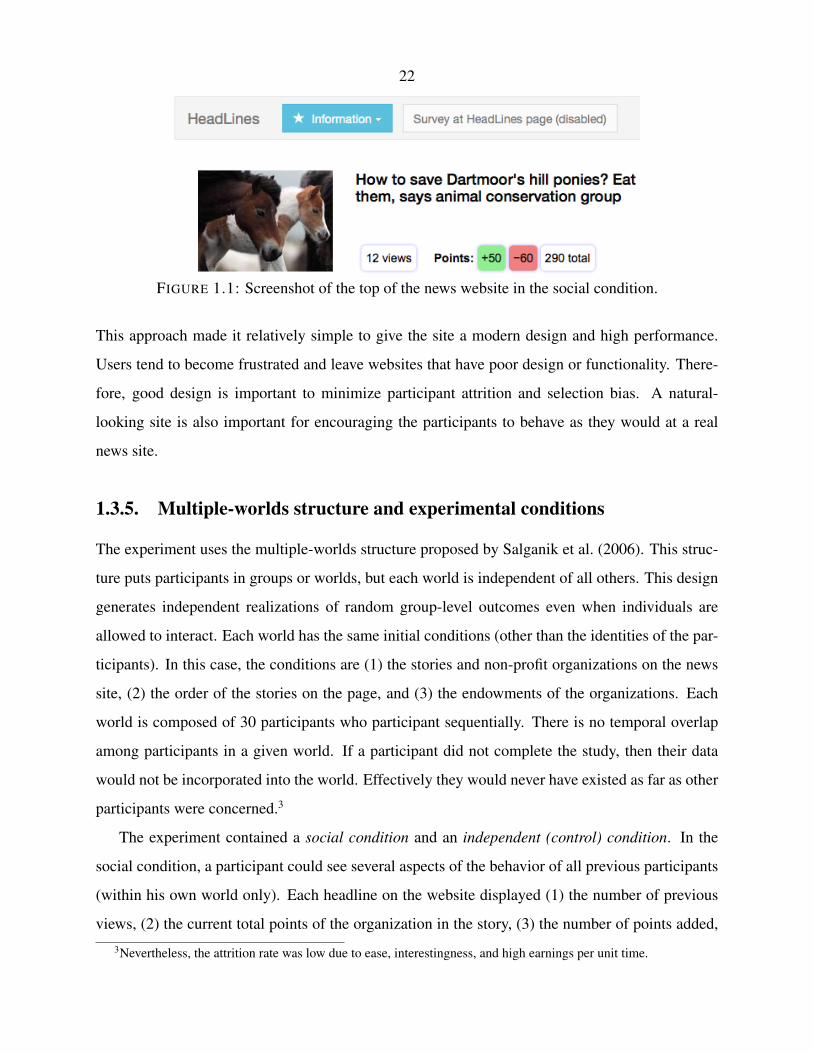
22

FIGURE 1.1: Screenshot of the top of the news website in the social condition.

This approach made it relatively simple to give the site a modern design and high performance.

Users tend to become frustrated and leave websites that have poor design or functionality. There-

fore, good design is important to minimize participant attrition and selection bias. A natural-

looking site is also important for encouraging the participants to behave as they would at a real

news site.

1.3.5. Multiple-worlds structure and experimental conditions

The experiment uses the multiple-worlds structure proposed by Salganik et al. (2006). This struc-

ture puts participants in groups or worlds, but each world is independent of all others. This design

generates independent realizations of random group-level outcomes even when individuals are

allowed to interact. Each world has the same initial conditions (other than the identities of the par-

ticipants). In this case, the conditions are (1) the stories and non-profit organizations on the news

site, (2) the order of the stories on the page, and (3) the endowments of the organizations. Each

world is composed of 30 participants who participant sequentially. There is no temporal overlap

among participants in a given world. If a participant did not complete the study, then their data

would not be incorporated into the world. Effectively they would never have existed as far as other

participants were concerned.3

The experiment contained a social condition and an independent (control) condition. In the

social condition, a participant could see several aspects of the behavior of all previous participants

(within his own world only). Each headline on the website displayed (1) the number of previous

views, (2) the current total points of the organization in the story, (3) the number of points added,3Nevertheless, the attrition rate was low due to ease, interestingness, and high earnings per unit time.

23

and (4) the number of points subtracted. Each subject was also informed about how many partic-

ipants had gone before them. In addition, during the social condition the position of the headlines

on the page was determined by the number of views. The headlines were arranged in decreas-

ing order, so that the most-viewed story was at the top. Ties were broken according to the initial

random ordering. The organizations’ points had no role in ordering the headlines.

In the independent condition no participant received any information about the behavior of

other participants. Each participant was presented with an identical version of the webpage. The

study is based on 12 social worlds and 4 independent worlds.

1.3.6. Similar studies

The design of this experiment draws on that of Salganik et al. (2006). They created a website where

individuals could download music without charge. Their experiment involved a social condition

in which (1) each participant could see how many times each song had been downloaded and (2)

the songs were sorted so that the most popular songs appeared at the top of the screen. In the

independent condition the participants had no information about downloads by other users, and

the order of the songs was randomized for each participant. Multiple instances, or “worlds,” of

the website under both conditions were run independently. The main result is that in the social

condition the popularity of songs was more unequal and unpredictable than in the independent

condition.

The present study provides an extension and addresses a confound in Salganik et al. (2006).

The extension is to allow for both positive and negative behavior (rewarding and punishing) instead

of just a positive behavior (downloading a song). In addition, Salganik et al. (2006) link popularity

to the positive behavior, whereas the present study uses page views as a measure of popularity. My

design is therefore symmetric with respect to the positive and negative behaviors. The confounding

issue in Salganik et al. (2006) is that the visual ordering of the songs within a given world was far

more stable under the social condition than under the independent condition. This occurs because

the social condition sorted songs by popularity whereas the independent condition sorted songs

randomly across subjects. In a social world, most subjects towards the later part of the run saw

the songs in a very similar order. The stability itself can greatly increase inequality across songs

24

because a few songs will tend to remain at the top of the page where they will receive more

attention. The present design fixes the news story order across all subjects in the independent

condition. In that way, the design is actually somewhat biased against finding greater inequality in

social condition. Nevertheless, that result still appears.

My design also draws on common features in the experimental economics literature. In typical

experiments on punishment the participants are given an endowment by the experimenter. Pun-

ishment corresponds to a participant destroying the endowment of another (see, for example, Fehr

and Fischbacher 2004a), which is precisely how punishment occurs in this design. Finally, in my

design some players are organizations which have no choice to make. This feature is borrowed

from the “representative dictator game” of Carpenter et al. (2008), in which participants play as a

dictator with a non-profit organization.

1.3.7. Instructions to the participants

Participants were informed that they would view the news site as part of a “group” of 30 individ-

uals. That is, they were told that their points over choices would be summed with those of the

29 others in the group to determine the final total points for each organization. They were fully

informed about the payoff structure for the non-profit organizations.

An important difference from many lab experiments is that the instruction page was identical

for both experimental conditions. In a web experiment the risk of attrition is higher than in a lab,

and participants might select out of the experiment due to the content or length of the instructions.4

To mitigate this problem, all participants saw the same instructions page, which informed them of

(1) the basic nature of the news page, (2) the payoff structure of organizations, (3) the fact that they

were in a group of 30, and (4) the necessary and sufficient conditions to complete the study, that

is, visit 1–9 stories and then complete the questionnaire. Additional information about the social

condition was provided through tooltips attached to the objects that displayed the organizations

points. The social conditional also included a small, collapsible banner explaining succinctly how

the headlines were sorted.

Some participants on Mechanical Turk select out of tasks because they worry that their per-

4A total of 549 users entered the experiment. Of those, 506 reached the news headline page, and 480 subsequentlyfinished. Therefore, the attrition rate upon reaching the headline page was 5.1 percent.

25

formance and pay may be low. This behavior could introduce selection on confidence or risk

preferences. Therefore, the instructions also emphasized that the experiment does not have “right”

or “wrong” answers and that each participant would be paid so long as they completed the basic

requirements. Each subject had to also answer three questions about the instructions to demon-

strate understanding of the payoffs and conditions of completion. Upon proceeding to the news

headline page, a pop-up window reiterated that the subject had only to visit 1–9 stories and that it

was entirely optional to add or subtract points.

1.3.8. Technical aspects of recruitment

Several aspects of the study, including recruitment, were designed so that subjects could not repeat-

edly participate in the study nor begin the study and then complete it at a later time. The purpose

of this design is to make the study resemble a situation where many individuals participate a single

time, each within one brief interval of time.

Several methods were used to control the recruitment process. Amazon’s built-in filter was

used to allow only participants located in the United States. However, some subjects outside the

United States are able to deceive Amazon’s system. Therefore, the server hosting the experiment

also geocoded each participant’s IP address using two different geocoding services. Any visitor

with a foreign IP address was blocked from participating. In addition, most Turkers from outside

the U.S. are based in India. So the study was run only during the day in the U.S., when people in

India were sleeping. Pilot studies and monitoring of the server indicated that these measures were

very effective at preventing illegitimate participation. Inspection of the open-ended responses on

the survey revealed little sign of anyone who was not a native speaker of American English.

Each potential participant at Mechanical Turk was given a one-time use link to the study’s

website. They were advised that if they followed the link, they would not be able to make any

other attempt on the study and would not be able to leave the site and return later. Any subject

that followed the link would have their Amazon Worker ID and IP address logged. Any future

participant with a matching ID or IP address would be prevented from participating.

26

1.4. Models and statistical procedures

1.4.1. Model of individual choices

The analysis of choices is conducted using pooled logit models. For expositional simplicity, con-

sider that the dataset generated by a single world is structured as a participant-by-story panel with

Nw ×K data points, where Nw = 30 is the number of participants in a single world and K = 24

is the number of stories. Note that in the analysis the worlds will be pooled. Let Yik ∈ {0, 1} be

a binary outcome variable for the i-th participant in the world. For example, we may have that

Yik indicates if participant i viewed story k. At the time that participant i visits the news headline

page, each headline item k can be characterized by a vector xik potentially consisting of: (1) the

position of the headline on the page, (2) the number of previous views of the corresponding story,

(3) the number of points added, and (4) the number of points subtracted. Each participant i is then

modelled as making 24 binary choices with the characteristics xi = (xik)k=1,...,24. We specify the

model

P(Yik = 1|xik) = Λ(sk + x′ikβ), (1.1)

where sk is a story-specific parameter (estimated by including dummy variables in the regression).

A typical component of xik will be the position xi,k,1 of headline k on the news page when

viewed by participant i. The case xi,k,1 = 1 means that story k was at the top of the page when

viewed by i, while xi,k,1 = 24 means the story was at the bottom of the page. Note that the series

{xi,k,1 : i = 1, . . . , 30} represents the position of a particular story k on the web page over time,

which will potentially change according the the viewing choices of the 30 participants. The coef-

ficient on xi,k,1 represents the influence of the headline’s visual position. We expect that headlines

at the bottom of the page are less likely to be viewed, so the coefficient should be negative. In the

social condition, the positions of the headlines can change from subject to subject depending on

the number of views for each story. This feature allows the effect of position to be identified even

when the story-specific parameters {sk : k = 1, . . . , 24} are included in the model. However, in

independent condition the stories do not vary in position. Therefore, the position effect cannot be

estimated using only data from the independent condition. This limitation is operative in several

of the models used but does not cause any serious problems.

27

The vector of story characteristics xik will also include some components that represent, in

aggregate, the points-related choices of all the participants in the world prior to i. For example,

xi,k,2 might represent the sum of all rewards to story k. That is

xi,k,2 :=i−1∑j=1

rjk, (1.2)

where rjk = 10 if participant j rewarded the organization in story k (added 10 points).5 A similar

measure can be defined based on the variable pjk, which equals 10 if and only if participant j

punished the organization in story k (subtracted 10 points). The coefficients on these variables are

designed to represent social influences. For example, we would like a positive coefficient on xi,k,2

to reflect that previous decisions to reward k will (causally) influence a subsequent participant

to also reward k. However, in order to have this interpretation, we must include the story-specific

effects sk in the model. If the statistical model omitted these effects, the estimates of the coefficient

on xi,k,2 (or any other points-related effect) might merely reflect the story-specific effect. This bias

would be equivalent to claiming to identify an effect of social influence when in fact the effect is

caused by a common environment. In this context, the “environment” is the news story itself.

One concern is that the model requires that each participant i makes independent choices

(Yi,1, . . . , Yi,24). However, in this application we might suspect that a participant may sample a

variety of choices. In addition, the requirement that the participant read at least one story may

induce dependence between the choices. To mitigate this concern, we estimate standard errors

which are robust to within-subject clustering. The analysis will show that social influences can be

“diluted,” that is, the social effect of punishment/reward (on any particular story) decreases when

other stories have also been punished or rewarded. To account for this effect many of the models

will include terms that allow for a decay of social effects over the course of the experiment. That

approach can be thought of as modeling the contextual effects on each subject’s choices.

Another concern regards inference when participants interact in groups, which creates depen-

dencies between the participants. The typical solution is to use standard errors clustered by the

group. However, in this design we have only 4, 12, or 16 groups, which does not meet conven-

5In some models we will also use an indicator variable like xi,k,2 := I{∑i−1

j=1 rjk > 0}, which is simply a dummyvariable that indicates if any previous participant rewarded story k.

28

tional levels for the quality of the asymptotic approximations. The alternative approach is again to

model the dependencies by incorporating variables accounting for the interactions and then assum-

ing independence conditional on the covariates. Appendix Tables 1.18 and 1.19 compare standard

errors that are clustered by participant and by world. The models are the same ones displayed

in Table 1.4 below. These results show that the standard errors clustered by world can be larger

or smaller than those clustered by participant. In general, standard errors clustered by world are

somewhat larger but similar in magnitude. The second table (1.19) includes page position controls,

which should further control for subject inter-dependencies. That modification makes the two sets

of standard errors even closer, supporting the argument that modeling the dependencies can im-

prove inference. The analysis will use clustering by participant because the two approaches give

similar results and the number of worlds is small.

1.4.2. Statistical procedures for the world-level analysis

1.4.2.1. Motivation of the metrics

We aim to define a few simple metrics that characterize the overall state of the organizations in a

given world. These metrics can be calculated after each participant (“time period”) of a world or

at the end of the world as a final summary outcome. This passage provides some motivation and

intuition for the metrics used in the study. The next sub-section provides mathematical definitions

for the metrics.

An important characteristic of a world is the inequality of the organizations’ points. Salganik

et al. (2006) report a large, positive effect of social information on the inequality of downloads

across songs within a given instance of a market. Their design is similar to this study. The songs

correspond to organizations, and the downloads correspond to points. This suggests that the social

condition should increase inequality. Figure 1.2 shows the distribution of points using a realistic

but stylized data set. The data can be taken to represent (1) the final points after all 30 participants

in the world or (2) an intermediate “snapshot” of the data before the world has been completed.

The case of zero inequality corresponds to a perfectly flat, black line, which indicates that all

organizations have the same number of points. As the black line diverges from zero, the inequality

increases. The measure of inequality used is the Theil index as described below.

29

However, Salganik et al.’s (2006) study included only one type of behavior, downloading a

song. The present study has two types of behavior, punishing and rewarding, which can each con-

tribute to inequality. Therefore, we would like to have measures of the overall effects of punishing

and rewarding which relate to inequality. The metrics net punishment and net reward quantify the

contributions of punishment and reward to changes in wealth levels and, therefore, to inequality.6

Another interpretation of the net metrics is that they reflect clustering of behavior with respect

to stories. For example, suppose that reward choices are uniformly distributed over the 24 stories.

If many participants “coordinated” to punish a particular story k, then the net punishment against k

would probably be large because the total points subtracted from k would be larger than the points

added to k. However, if the participants distributed the same number of punishment choices over

many different stories, then it is likely that in many cases the subtractions will be “canceled out”

by the additions. Then the net punishment could be zero.

1 4 7 10 13 16 19 22 24

Organization #(ranked based on final points or mid-session "snapshot")

150.0

200.0

250.0

300.0

350.0

400.0

450.0

Curr

ent

wealt

h (

poin

ts)

of

org

aniz

ati

on

Net punishment =absolute value(sum of red bars)

Net reward =sum of green bars

Inequality:The inequality metric increases as the

black, wealth plot diverges from a flat line.

Wealth (points)

Negative deviation from endowment

Positive deviation from endowment

FIGURE 1.2: Illustration of the three world-level metrics (stylized data)

6The total amounts of punishment and reward do not reflect how punishment and reward can nullify each other’seffects. Therefore, the total amounts have an ambiguous relation to inequality.

30

1.4.2.2. Definitions of metrics

Let w = 1, . . . ,W index worlds in the experiment and iw = 1, . . . , 30 index the players in world

w. Let the reward and punishment variables be riw,k and piw,k, respectively. They represent the

amount of points added or subtracted by a subject. The variable riw,k takes the value 10 (ten) if

participant iw rewarded story k and 0 otherwise. The variable piw,k is defined analogously.

Definition 1 The wealth (points) inequality of the organizations in a given world is measured by

the Theil index, which is given by

Th(v) :=1

24

24∑k=1

(vkvlog

vkv

), (1.3)

where v = (vk)k=1,...,24 is the vector of points for each of the 24 organizations. The mean of

points is v = 124

∑24k=1 vk. A larger Theil index indicates that the distribution of points among the

organizations is more unequal.

Definition 2 The net reward of story k is given by

Rk :=

(30∑i=1

riw,k − piw,k

)+

, (1.4)

where the notation (x)+ means the positive part of x. The (interim) net reward after n participants

can be calculated in the same way by summing over i = 1, . . . , n.

Definition 3 The net punishment of story k is given by

Pk :=

(30∑i=1

piw,k − riw,k

)+

. (1.5)

Note that for any given story k, at most one of Rk and Pk can be non-zero. The (interim) net

punishment after n participants can be calculated in the same way by summing over i = 1, . . . , n.

Definition 4 The net reward in world w is given by

Rw :=24∑k=1

Rk. (1.6)

31

Notice that the net reward in a particular world is the net increase in wealth (points) among the

set of stories that were rewarded more than they were punished (story-wise).

Definition 5 The net punishment in world w is given by

Pw :=24∑k=1

Pk. (1.7)

The net reward is the net loss of wealth (points) among the set of stories that were punished more

than they were rewarded (story-wise).

1.4.2.3. Estimators of world-level metrics

The distribution of aggregate outcomes of independent-condition worlds can be estimated by re-

sampling individual participants. Let there be data for W independent worlds. Then there is a data

set D composed of 30×W independent participants. For any world-level metric M let F ∗M be the

distribution of M generated by drawing a subsample of size 30 from D without replacement.

The re-sampling estimator of the expected value of metricM is computed fromB sub-sampled

worlds {M∗b : b = 1, . . . , B} whereM∗

biid∼ F ∗

M . The estimator is µ∗M = 1

B

∑Bb=1M

∗b . The estimator

of the variance is σ2M∗ = 1

B

∑Bb=1(M

∗b − µ∗

M)2. The simulation results in the appendix show that,

compared to the conventional estimators, the re-sampling estimator of the mean is somewhat more

efficient and the re-sampling estimator of the variance much more so. The conventional estimator

of the standard error (of the mean) does not apply to the re-sampling estimator. Therefore, the stan-

dard error is estimated by the bootstrap which requires two levels of iteration. That is, J bootstrap

data sets are created by drawing with replacement from the independent-condition participants.

For each bootstrap data set j = 1, . . . , J , we compute the re-sampling estimate of the mean µ∗M,j .

The estimator of the standard error is then se(µ∗M) :=

√1J

∑Jj=1(µ

∗M,j − µ∗

M)2.

Since the individuals participating in the social-condition worlds can influence each other, it

is not appropriate to re-sample social-worlds. Therefore, the means and standard deviations of

outcomes in the social worlds are estimated using the conventional estimators: the sample mean

and sample standard deviation treating each world as an independent observation (rather than each

individual).

32

To test the null hypothesis that the means of a world-level metric M are equal in the two

conditions, H0 : µM,soc = µM,ind, I use a simple percentile bootstrap procedure.7 The test statistic

is the difference of the two means

dobs = µM,soc − µ∗M . (1.8)

The null distribution of the statistic is estimated by bootstrapping each of the means. For bootstrap

replicates j = 1, . . . , J , the social-world mean µ∗M,soc,j is generated by drawing with replacement

from the 12 social worlds and then computing the mean of M in the replicate sample j. The

bootstrap distribution of µ∗M is generated as described above, creating replicate samples of 120

individuals. Each replicate of 120 individuals is then used to compute a realization of the sub-

sampling estimator µ∗∗M,j . The j-th bootstrap realization of the test statistic is

d∗j := (µ∗M,soc,j − µM,soc)− (µ∗∗

M,j − µ∗M). (1.9)

The two-tailed p-value of the test is then pM := 1J+1

(1 +

∑Jj=1{|d∗j | ≥ dobs}

).

An alternative approach to hypothesis testing follows that of Salganik et al. (2006), in which

the value of a statistic observed in the social worlds is compared to the distribution generated by

re-sampling individuals from the independent worlds (effectively creating synthetic independent

worlds). Let Ms = {Mw : w = 1, . . . , s} represent outcomes of some metric M from s social

worlds. Let Ms∗ be a vector of the same metric M in s worlds generated by re-sampling from F ∗M .

Let Ts(Ms) be some statistic, for example, the sample mean or sample standard deviation of the

metric M . For the null hypothesis Ts(Ms)iid∼ Ts(M

s∗), we can conduct a test by comparing the

observed value from the social worlds Ts(m) to the distribution of Ts(M∗) re-sampled from the

independent data. Let {t∗b : b = 1, . . . , B} be a set of B re-sampled realizations of Ts(Ms∗). Then

we can estimate the probability p that the re-sampling distribution would generate a value at least

as large as the one observed in the social worlds. That estimator is

p = 1B+1

(1 +

B∑b=1

{Ts(ms) ≥ t∗s}

)(1.10)

7The advantage of this approach over a bootstrap t-test is that the standard error does not need to be computed foreach bootstrap replicate, which would require an additional level of computationally-intensive iteration.

33

wher ms is the observed vector of the metric M observed in the s social worlds. This approach to

testing ignores sampling variation in F ∗M itself but is still presented for comparison.

1.5. Results

1.5.1. Analysis at the level of individual participants

1.5.1.1. Characteristics of the sample

Table 1.1 shows summary statistics for the two groups of participants. Some variables are demo-

graphic characteristics reported in the questionnaire, and others are based on recorded behavior

during the experiment. In general, the participants are young, highly educated, and heavily female.

The mean age is about 35.2 with a standard deviation of 11.3. Over half of the participants received

a college degree (56.2 percent). The percentage female is 58.9 percent.

The participants are similar to a representative sample of U.S. households in terms of their

ability to withstand a negative income shock. The variable designated “low wealth” indicates if the

participant answered negatively to the following question: “If you were to lose your main source of

income (e.g., job, government benefits), could you cover your expenses for 3 months by borrowing

money, using savings, selling assets, or borrowing from friends/family?” The question was taken

from a household survey by the Federal Reserve where 42.2 percent of respondents answered that

they could not cover the expenses (Reserve 2014). In the present experiment the subjects reported

being in slightly better condition, with 37 percent and 38 percent of the individual and social groups

being unable to cover expenses.

The variable designated “has smartphone” indicates if the participant answered affirmatively

to the following question: “Do you have a smartphone like an iPhone, Samsung Galaxy phone, or

Windows Phone?” The independent and social groups reported having a smartphone at the rates of

78.5 and 81.6 percent, respectively. The question was adopted from the Pew Internet & American

Life Project Poll, where 65 percent reported having a smartphone (Center 2014).

The variable “engaged in political protest” indicates if the participant answered affirmatively

to the following question: “Have you ever done any of the following forms of political action?

Joining in boycotts, attending peaceful demonstrations, joining strikes.”

34

The variable designated “degree of belief in donation” was asked to check whether the subjects

believe that the donations will be paid to the non-profit organizations. The question text was:

“How much confidence do you have that we will pay out the points as explained?” The response

was a scale with the points (1=“No confident at all”), (2=“Not too much confidence”), (3=“Some

confidence”), and (4=“A lot of confidence”). The empirical probabilities are (0.0252, 0.0943,

0.4151, 0.4654). Therefore, the modal participant has “a lot of confidence” in the third-parties’

payoffs.

The summary statistics indicate that many participants found the study interesting. Most par-

ticipants (71 percent) visited more than one news story and therefore spent more time than required

on study (in exchange for no additional earnings). The mean (median) number of stories visited

was 3.25 (2). The maximum number of stories (9) was viewed by 8.75 percent of participants.

The mean (median) amount of time browsing the news site was 5.27 (4.21) minutes. The fact that

participants would spend more time than necessary on the study is not surprising because the study

is designed to replicate a behavior that many people do in their leisure time.

1.5.1.2. Predictors of individual-level behavior

Table 1.2 shows several regressions that quantify how subjects’ characteristics predict their behav-

ior in the experiment. The binary outcomes are modeled using linear probability models, while the

number of stories viewed is modelled using Poisson regression. A broad conclusion is that behav-

ior in the experiment is predicted well by demographic characteristics, while technology adoption

has somewhat less predictive power.

The variable “ever punished” indicates if the participant subtracted points from any of the or-

ganizations. Punishment is predicted by three demographic variables but none of the technological

variables. In particular, engaging in political or economic protest activity is estimated to increase

the probability of punishment by 0.122. Being female and being college-educated increased the

probability of punishment by 0.117 and 0.093, respectively. This suggests that the propensity to

punish in the experiment reflects general characteristics of the individuals rather than a technology-

or domain-specific characteristic.

The variable “ever rewarded” is not strongly linked to any of the observed demographic vari-

ables. The only significant predictor is where the participant uses the social network Twitter.

35

TABLE 1.1: Summary statistics of the individual participants

Independent condition Social condition

Mean Std. Dev. Median Mean Std. Dev. Median

Age (years) 35.475 11.641 33 35.192 11.185 33Male 0.370 0.485 0 0.425 0.495 0College degree 0.622 0.487 1 0.542 0.499 1Low wealth 0.370 0.485 0 0.380 0.486 0Has smartphone 0.782 0.415 1 0.816 0.388 1Uses Facebook 0.808 0.395 1 0.833 0.373 1Uses Twitter 0.425 0.496 0 0.378 0.486 0Has engaged in protest activity 0.227 0.421 0 0.226 0.419 0Hours/week on MTurk 10.933 10.357 8 12.081 12.263 10Dollars/week on MTurk 38.437 47.058 25 35.277 43.396 20Behavior in experiment:- Stories viewed 2.992 2.413 2 3.339 2.449 3- Viewed > 1 story 0.633 0.484 1 0.739 0.440 1- Browsing time (minutes) 4.652 3.368 4 5.471 4.230 4- Points subtracted 7.667 11.132 0 9.306 12.279 10- Points added 17.333 16.840 10 19.389 16.662 10- Ever punished 0.458 0.500 0 0.517 0.500 1- Ever rewarded 0.792 0.408 1 0.853 0.355 1- Anger level (1–9) 2.487 1.904 1 2.522 1.919 2- Degree of belief in donations 3.303 0.720 3 3.327 0.757 3

Observations 120 360

Another important outcome is whether the participant visited more than one news story. Since

each participant was only required to visit one story, any additional visits represent a choice by

the subject to spend more time on the experiment without earning any additional money. Possible

reasons for visiting additional stories include a simple desire to get information about the story, a

desire to add or subtract more points, or an interest in how a story relates to the behavior of others.

The last two factors appear to be important because the social treatment has a statistically signif-

icant positive effect on the probability of reading additional stories. The demographic variables

are also important predictors. College education and previous protest behavior are predictors of

visiting additional stories. However, different variables predict total browsing time. Men spend

on average about 22 percent less time browsing. Older people also spend less time browsing. The

social treatment is associated with a 17.5 percent increase in browsing time.

36

TABLE 1.2: Individual characteristics as predictors of behavior in the experiment

Binary measures of behavior

Total storiesviewed

Log totalbrowsing

time

Read> 1 story

Everpunished

Everrewarded

College graduate 0.121∗ 0.083 0.113∗∗∗ 0.093∗∗ 0.005(0.070) (0.062) (0.043) (0.047) (0.035)

Male -0.025 -0.217∗∗∗ 0.022 -0.117∗∗ 0.002(0.070) (0.065) (0.042) (0.048) (0.035)

Has engaged in protest activity 0.134∗ -0.056 0.145∗∗∗ 0.122∗∗ 0.057(0.078) (0.073) (0.044) (0.054) (0.037)

Age 0.003 0.018∗∗∗ 0.001 0.000 -0.000(0.003) (0.003) (0.002) (0.002) (0.002)

Has low wealth 0.090 0.083 0.031 -0.009 0.032(0.072) (0.065) (0.043) (0.049) (0.034)

Uses Facebook -0.003 -0.017 -0.101∗∗ 0.076 0.008(0.085) (0.082) (0.051) (0.061) (0.049)

Uses Twitter 0.035 -0.064 0.050 -0.010 0.113∗∗∗

(0.071) (0.061) (0.041) (0.048) (0.032)Owns smartphone -0.014 -0.078 0.049 0.064 0.010

(0.093) (0.079) (0.056) (0.061) (0.047)Social treatment 0.121 0.175∗∗ 0.113∗∗ 0.075 0.061

(0.081) (0.069) (0.049) (0.052) (0.042)

Obs. 477 477 477 477 477

Notes. The first two columns show semi-elasticities. The remaining columns show coefficient estimates (averagemarginal effects) from linear probability models. Heteroscedasticity robust standard errors are in parentheses. ∗

p < 0.10, ∗∗ p < 0.05, ∗∗∗ p < 0.01

The standard errors in Table 1.2 are heteroscedasticity-robust. The results are in general robust

to clustering the standard errors by world. In some cases this approach provides stronger evi-

dence of effects (see Appendix Table 1.17). For example, clustering the standard errors by world

moderately shrinks the standard errors on the social treatment effect in all 5 models.

Figure 1.3 groups all participants according to their self-reported anger rating, which is in-

tended to capture the degree of anger experienced overall during the experiment. The probabilities

that the user “ever punished” and “ever rewarded” within each bin are displayed. Higher anger

ratings are correlated with increasing probability of ever punishing. However, there is little rela-

tionship between rewarding and anger. Since participants on average visit more than one story,

this result indicates that anger at one story does not tend to decrease the probability that the par-

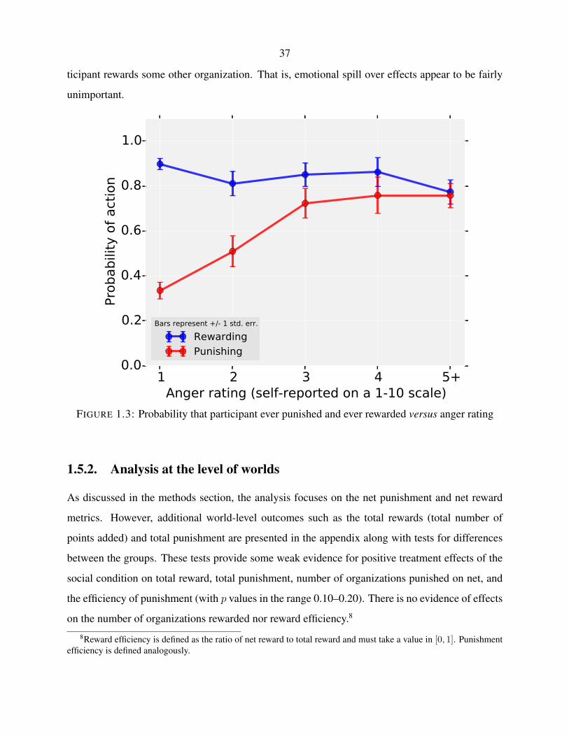
37

ticipant rewards some other organization. That is, emotional spill over effects appear to be fairly

unimportant.

1 2 3 4 5+Anger rating (self-reported on a 1-10 scale)

0.0

0.2

0.4

0.6

0.8

1.0

Pro

babili

ty o

f act

ion

Bars represent +/- 1 std. err.

Rewarding

Punishing

FIGURE 1.3: Probability that participant ever punished and ever rewarded versus anger rating

1.5.2. Analysis at the level of worlds

As discussed in the methods section, the analysis focuses on the net punishment and net reward

metrics. However, additional world-level outcomes such as the total rewards (total number of

points added) and total punishment are presented in the appendix along with tests for differences

between the groups. These tests provide some weak evidence for positive treatment effects of the

social condition on total reward, total punishment, number of organizations punished on net, and

the efficiency of punishment (with p values in the range 0.10–0.20). There is no evidence of effects

on the number of organizations rewarded nor reward efficiency.8

8Reward efficiency is defined as the ratio of net reward to total reward and must take a value in [0, 1]. Punishmentefficiency is defined analogously.

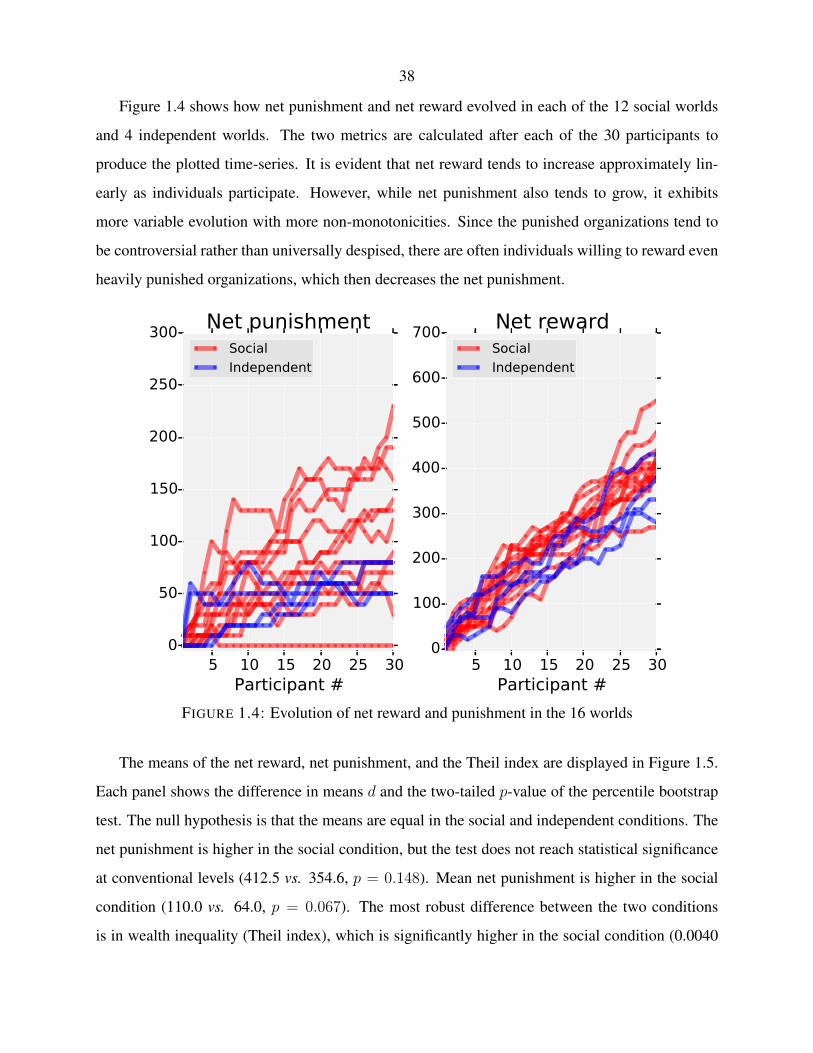
38

Figure 1.4 shows how net punishment and net reward evolved in each of the 12 social worlds

and 4 independent worlds. The two metrics are calculated after each of the 30 participants to

produce the plotted time-series. It is evident that net reward tends to increase approximately lin-

early as individuals participate. However, while net punishment also tends to grow, it exhibits

more variable evolution with more non-monotonicities. Since the punished organizations tend to

be controversial rather than universally despised, there are often individuals willing to reward even

heavily punished organizations, which then decreases the net punishment.

5 10 15 20 25 30Participant #

0

50

100

150

200

250

300Net punishment

Social

Independent

5 10 15 20 25 30Participant #

0

100

200

300

400

500

600

700Net rewardSocial

Independent

FIGURE 1.4: Evolution of net reward and punishment in the 16 worlds

The means of the net reward, net punishment, and the Theil index are displayed in Figure 1.5.

Each panel shows the difference in means d and the two-tailed p-value of the percentile bootstrap

test. The null hypothesis is that the means are equal in the social and independent conditions. The

net punishment is higher in the social condition, but the test does not reach statistical significance

at conventional levels (412.5 vs. 354.6, p = 0.148). Mean net punishment is higher in the social

condition (110.0 vs. 64.0, p = 0.067). The most robust difference between the two conditions

is in wealth inequality (Theil index), which is significantly higher in the social condition (0.0040

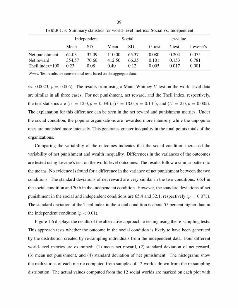
39

TABLE 1.3: Summary statistics for world-level metrics: Social vs. Independent

Independent Social p-value

Mean SD Mean SD U -test t-test Levene’s

Net punishment 64.03 32.09 110.00 65.37 0.080 0.204 0.075Net reward 354.57 70.60 412.50 66.35 0.101 0.153 0.781Theil index*100 0.23 0.08 0.40 0.12 0.005 0.017 0.001

Notes. Test results are conventional tests based on the aggregate data.

vs. 0.0023, p = 0.005). The results from using a Mann-Whitney U test on the world-level data

are similar in all three cases. For net punishment, net reward, and the Theil index, respectively,

the test statistics are (U = 12.0, p = 0.080), (U = 13.0, p = 0.101), and (U = 2.0, p = 0.005).

The explanation for this difference can be seen in the net reward and punishment metrics. Under

the social condition, the popular organizations are rewarded more intensely while the unpopular

ones are punished more intensely. This generates greater inequality in the final points totals of the

organizations.

Comparing the variability of the outcomes indicates that the social condition increased the

variability of net punishment and wealth inequality. Differences in the variances of the outcomes

are tested using Levene’s test on the world-level outcomes. The results follow a similar pattern to

the means. No evidence is found for a difference in the variance of net punishment between the two

conditions. The standard deviations of net reward are very similar in the two conditions: 66.4 in

the social condition and 70.6 in the independent condition. However, the standard deviations of net

punishment in the social and independent conditions are 65.4 and 32.1, respectively (p = 0.075).

The standard deviation of the Theil index in the social condition is about 55 percent higher than in

the independent condition (p < 0.01).

Figure 1.6 displays the results of the alternative approach to testing using the re-sampling tests.

This approach tests whether the outcome in the social condition is likely to have been generated

by the distribution created by re-sampling individuals from the independent data. Four different

world-level metrics are examined: (1) mean net reward, (2) standard deviation of net reward,

(3) mean net punishment, and (4) standard deviation of net punishment. The histograms show

the realizations of each metric computed from samples of 12 worlds drawn from the re-sampling

distribution. The actual values computed from the 12 social worlds are marked on each plot with

40

0

100

200

300

400

500 d=57.91, p=0.148

Net reward

0

20

40

60

80

100

120

140

160

d=45.54, p=0.067 *

Net punishment

0.000

0.001

0.002

0.003

0.004

0.005

0.006

d=0.0017, p=0.005 ***

Wealth inequality

Means plottedwith +/- SE

Social

Independent

FIGURE 1.5: Mean world-level outcomes: Social versus independent conditions

a vertical line. For three of the four metrics, the observed statistic in the social worlds is far

out into the tail of the re-sampling distribution. For example, among the 12 social worlds the

sample standard deviation of net punishment is 65.4. However, this value is larger than any of

those generated by re-sampling 12 independent worlds and then computing the sample standard

deviation from those 12 values. In the fourth metric, standard deviation of net reward, the observed

value in the social worlds is very close to the center of the re-sampling distribution.

1.5.3. Analysis at the level of choices

The final section of the analysis examines how individual participants’ choices result in the ag-

gregate effects observed in the social condition. This analysis uses participant-by-story panel data

where each participant contributes an observation for each of the 24 stories (organizations). The

social condition data has 8,640 observations while the independent condition data has 2,880 ob-

servations. Individuals are modelled as making 24 binary decisions (about each decision type:

punishing, rewarding, and viewing). These decisions are allowed to depend on the features of the

stories at the time that the relevant participant views the news page. The most important features

are the points added and subtracted by previous participants. Functions of these points are included

in the model to allow for social influences of punishment and reward. The initial models simply in-

41

0 20 40 60 80 100 120 140Sample mean of net punishment

0.00

0.02

0.04

0.06

0.08

0.10

Pro

port

ion

Social condition:Observed = 110.0p = 0.0002

Resampled independent data, 12 worlds

0 10 20 30 40 50 60 70 80 90Sample standard deviation of net punishment

0.00

0.02

0.04

0.06

0.08

0.10

Pro

port

ion

Social condition:Observed = 65.4p = 0.0001

Resampled independent data, 12 worlds

250 300 350 400 450Sample mean of net reward

0.00

0.02

0.04

0.06

0.08

0.10

Pro

port

ion

Social condition:Observed = 412.5p = 0.0033

Resampled independent data, 12 worlds

0 20 40 60 80 100 120 140 160Sample standard deviation of net reward

0.00

0.02

0.04

0.06

0.08

0.10

Pro

port

ion

Social condition:Observed = 66.3p = 0.5748

Resampled independent data, 12 worlds

FIGURE 1.6: Resampling tests: Social vs. independent

clude binary variables that indicate whether a given story was punished at all or rewarded at all by

the previous participants in the world. However, the results indicate that this binary effect decays

rapidly over the course of a given world. Therefore, the models also include the interaction of the

dummy variables with the logarithm of the participant’s number within the world (from 1 to 30).

This feature is called logarithmic decay. The logit coefficient estimates in Table 1.5 show a signif-

icant negative effect on the interaction variable, which strongly supports a decaying social effect.

A behavioral interpretation of this feature is that social information preferentially attracts attention

to those stories that have been previously punished or rewarded. However, the social information

may not increase the overall propensity of a participant to punish or reward. Such a model would

generate an effect that decays over the course of the experiment as more stories are punished or

rewarded. An example specification with binary effects of points added and subtracted that decay

42

logarithmically would have the form

P (i punishes story k) =

Λ(sk + β1PagePositionik

+ β2PagePosition2ik

+ β3 log(Participant #)

+ δ1AnyPointsAddedik + γ1AnyPointsAddedik × log(Participant #)

+ δ2AnyPointsSubtractedik + γ2AnyPointsSubtractedik × log(Participant #)),

where Λ is the logistic function. The variable AnyPointsAddedik takes the value one if any par-

ticipant before i added points to (rewarded) organization k and zero otherwise. The variable

AnyPointsSubtractedik takes the value one if any participant before i subtracted points from (pun-

ished) organization k and zero otherwise.

Average marginal effects using the binary definition of social effects appear in Table 1.4. The

logit coefficient estimates appear in Table 1.5. These models do not yet include terms for the page

position of the headlines. Data from only the social condition is used to estimate the models in the

first three columns, which are logit models of the probability of any given participant punishing,

rewarding, or viewing any given story. The point estimates are the average marginal effects of

the social effect variables. All three models show that if a participant punishes or rewards a story,

then subsequent participants are significantly more likely to punish, reward, or view that story.

For example, the average marginal effect of punishment on a given story is to increase, for each

subsequent participant, that story’s (1) probability of punishment by 0.027± 0.008, (2) probability

of reward by 0.020 ± 0.008, and (3) probability of being viewed by 0.049 ± 0.012. The average

marginal effect of prior reward is to increase the probability of subsequent punishment by 0.016±

0.005 and the probability of subsequent reward by 0.034 ± 0.009. These social effects therefore

tend to concentrate more punishment on stories that have been punished before and more reward on

those that have been rewarded before. This pattern tends to increase inequality across the stories,

which is the result seen in the aggregate data. It may be surprising to see that both punishment

and reward tend to increase later punishment and reward. However, both behaviors strongly draw

additional attention (views), which drives the additional punishment and reward. Later analyses

43

TABLE 1.4: Simple effects of punishment/reward on individual behavior (page controls omitted)

Social conditionIndividual behavior:

Independent condition(placebo test)

Individual behavior:

Punish Reward View Punish Reward View

Social effect:Points sub’ed (dummy) 0.027∗∗∗ 0.020∗∗ 0.049∗∗∗ -0.042∗∗∗ 0.009 -0.018

(0.008) (0.008) (0.012) (0.013) (0.017) (0.019)Points added (dummy) 0.016∗∗∗ 0.034∗∗∗ 0.059∗∗∗ -0.019 -0.011 -0.022

(0.005) (0.009) (0.011) (0.014) (0.018) (0.020)

Individuals 360 360 360 120 120 120Obs. 8, 640 8, 640 8, 640 2, 400 2, 760 2, 760Avg. log-likelihood -0.145 -0.256 -0.367 -0.143 -0.241 -0.340

Notes. Average marginal effects of previous punishment (points sub’ed) and reward (points added) printed. Effectsare specified in binary form with logarithmic decay. Estimates come from a logit model with a dummy variable foreach story but no controls for page position. Standard errors, in parentheses, are clustered by participant. Standarderrors, in parentheses, are clustered by participant. ∗ p < 0.10, ∗∗ p < 0.05, ∗∗∗ p < 0.01

show that this attentional effect predominantly accounts for the social effects in the present models.

Table 1.4 also shows the results from estimating identical models using only data from the

independent condition (columns 4–6) as a placebo test. These models reveal little evidence of

social effects, and most of the point estimates are negative. This result starkly shows that the social

condition causes any activity towards a particular story to attract additional attention towards the

same story. This effect is the main underlying mechanism for the increase in points inequality in

the social condition. In particular, these models show that rewards have a relatively large effect on

attracting attention (0.059± 0.014).

The placebo tests indicate a significant negative effect of punishment on subsequent punish-

ment. This estimate is not robust to plausible alternative specifications of the social effect that also

fit the data well (Table 1.6). One such case is to treat the social effects as shares of punishment

and reward. This specification explicitly represents the idea of social effects being diluted and

decaying as more stories are punished and rewarded. In this specification, if n stories have been

punished, then the punishment variable for those stories is set to 1n

. The remaining 24 − n stories

will have the punishment variable set to 0. The reward variable is defined analogously. This defi-

nition allows the social effects to be diluted. An interpretation of this definition is that any existing

punishment generates one unit of additional propensity to punish, which is distributed uniformly

44

TABLE 1.5: Coefficient estimates from punish/reward logit models (page controls omitted)

Punishment Reward

(1) (2) (3) (4)Social Independent Social Independent

Points sub’ed (dummy) 2.222∗∗∗ -0.545 -0.670 0.512(0.562) (1.199) (0.546) (0.858)

Points sub’ed × Log(participant #) -0.661∗∗∗ -0.215 0.375∗∗ -0.156(0.202) (0.445) (0.185) (0.305)

Points added (dummy) 0.621 -2.067 1.360∗∗∗ -0.611(0.591) (1.379) (0.364) (0.849)

Points added × Log(participant #) -0.070 0.585 -0.373∗∗∗ 0.179(0.218) (0.502) (0.139) (0.297)

Individuals 360 120 360 120Obs. 8, 640 2, 400 8, 640 2, 760Avg. log-likelihood -0.14450 -0.14308 -0.25634 -0.24144

Notes. Table displays coefficients from logit models using participant-by-story panel data and no controls for pageposition. The points subtracted (added) dummy indicates if the story was punished (rewarded) by any previous partic-ipant. Standard errors, in parentheses, are clustered by individual. ∗ p < 0.10, ∗∗ p < 0.05, ∗∗∗ p < 0.01

over all stories that have been punished. The average marginal effect of such a social variable can

be complicated to interpret. In terms of a social effect of punishment, the marginal effect could

be viewed as the change in the outcome probability for a story when it has been punished and no

other story has been punished. Analogous social and placebo results for the share specification

appear in Table 1.6. These again reveal substantial positive effects of punishment and reward on

all behaviors in the social condition. As expected, no social effects are found in the independent

condition.

Returning attention to the binary specification in Table 1.4, one might note that the average

marginal (social) effects of punishment on punishment and rewarded are similar in magnitude.

It may therefore appear that these effects will cancel out and therefore the effect on net punish-

ment may be difficult to account for. These results highlight the difficulty in understanding the

experiment by looking only at average marginal effects over the entire data set or at model coeffi-

cients. Much of the remaining analysis will present marginal effects in graphical form in order to

understand how the effects vary over the course of a world.

Further understanding the relationship between individual behavior and overall outcomes re-

quires a more subtle analysis along with careful consideration of the punishment and reward pre-

45

TABLE 1.6: Share effects of punishment/reward on individual behavior (social vs. independent)

Social conditionIndividual behavior:

Independent condition(placebo test)

Individual behavior:

Punish Reward View Punish Reward View

Social effect:Points sub’ed (share) 0.055∗∗∗ 0.057∗∗ 0.131∗∗∗ -0.084 0.080 0.035

(0.014) (0.025) (0.033) (0.085) (0.073) (0.099)Points added (share) 0.086∗∗∗ 0.190∗∗∗ 0.372∗∗∗ -0.029 -0.027 0.086

(0.023) (0.040) (0.061) (0.102) (0.114) (0.100)

Individuals 360 360 360 120 120 120Obs. 8, 640 8, 640 8, 640 2, 400 2, 760 2, 760Avg. log-likelihood -0.145 -0.257 -0.368 -0.146 -0.241 -0.340

Notes. Average marginal effects of previous punishment (points sub’ed) and reward (points added) printed. Effects arespecified in the share form. Estimates come from a logit model with a dummy variable for each story but no controlsfor page position. Standard errors, in parentheses, are clustered by participant. Standard errors, in parentheses, areclustered by participant. ∗ p < 0.10, ∗∗ p < 0.05, ∗∗∗ p < 0.01

dictor variables. First, it is possible to further divide the stories into those that have been punished

only and not rewarded. Therefore, alternative models were estimated where the observations are

partitioned into those that have been (1) neither punished nor rewarded, (2) punished only, (3) re-

warded only, or (4) both punished and rewarded, each interacted with a logarithmic decay. The

probabilities of punishment and reward over the course of a world for group 2 (punished only) are

printed in the first panel of Figure 1.7. This result shows that among stories that have been only

punished the probability of subsequent punishment is always greater than or equal to the probabil-

ity of reward. Therefore, among these stories the net punishment will tend to increase. A second

factor to consider is that the average marginal effects in Table 1.4 do not account for the actual pat-

terns of punishment. Since this model is non-linear, the effect of punishment can vary depending

on the values of the covariates (in this case, the story dummy variables). Panel two of Figure 1.7

shows the average marginal effect of punishment on subsequent punishment but with the effects

broken out into two groups: (1) those observations (stories) that were actually punished during the

experiment and (2) those observations that were not punished. That is, the marginal effects were

computed separately over the two corresponding sets of observations in the panel data. This re-

sult shows that the marginal effect of punishment is greater among those stories that were actually

punished, typically by a factor of 2. In effect, the participants selectively targeted the stories where

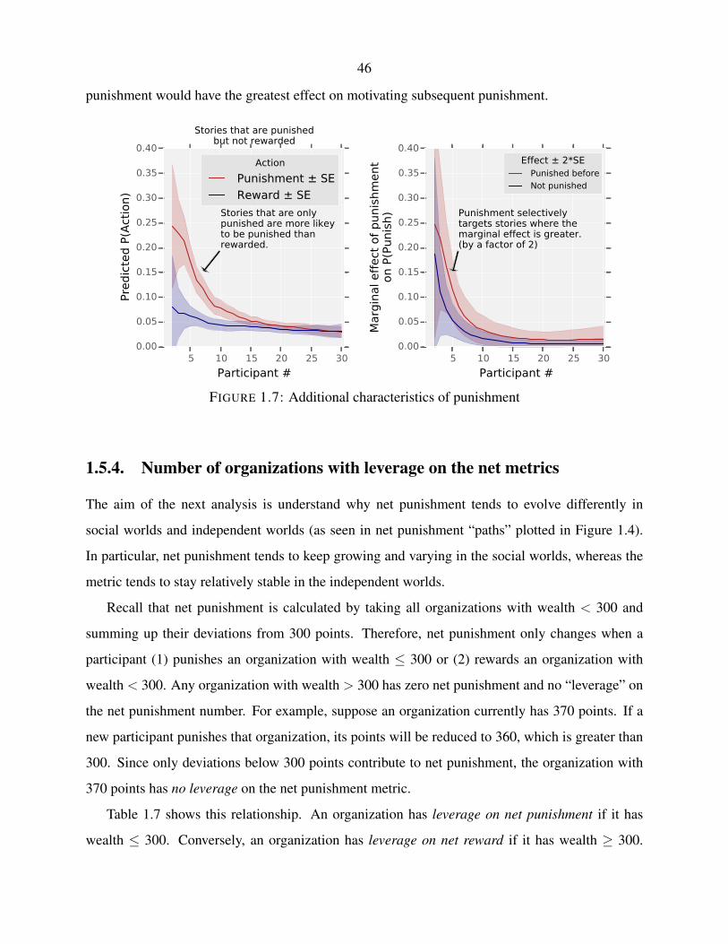
46

punishment would have the greatest effect on motivating subsequent punishment.

5 10 15 20 25 30

Participant #

0.00

0.05

0.10

0.15

0.20

0.25

0.30

0.35

0.40

Pre

dic

ted P

(Act

ion)

Stories that are onlypunished are more likeyto be punished thanrewarded.

Stories that are punishedbut not rewarded

Action

Punishment ± SE

Reward ± SE

5 10 15 20 25 30

Participant #

0.00

0.05

0.10

0.15

0.20

0.25

0.30

0.35

0.40

Marg

inal eff

ect

of

punis

hm

ent

on P

(Punis

h) Punishment selectively

targets stories where themarginal effect is greater.(by a factor of 2)

Effect ± 2*SEPunished before

Not punished

FIGURE 1.7: Additional characteristics of punishment

1.5.4. Number of organizations with leverage on the net metrics

The aim of the next analysis is understand why net punishment tends to evolve differently in

social worlds and independent worlds (as seen in net punishment “paths” plotted in Figure 1.4).

In particular, net punishment tends to keep growing and varying in the social worlds, whereas the

metric tends to stay relatively stable in the independent worlds.

Recall that net punishment is calculated by taking all organizations with wealth < 300 and

summing up their deviations from 300 points. Therefore, net punishment only changes when a

participant (1) punishes an organization with wealth ≤ 300 or (2) rewards an organization with

wealth < 300. Any organization with wealth > 300 has zero net punishment and no “leverage” on

the net punishment number. For example, suppose an organization currently has 370 points. If a

new participant punishes that organization, its points will be reduced to 360, which is greater than

300. Since only deviations below 300 points contribute to net punishment, the organization with

370 points has no leverage on the net punishment metric.

Table 1.7 shows this relationship. An organization has leverage on net punishment if it has

wealth ≤ 300. Conversely, an organization has leverage on net reward if it has wealth ≥ 300.

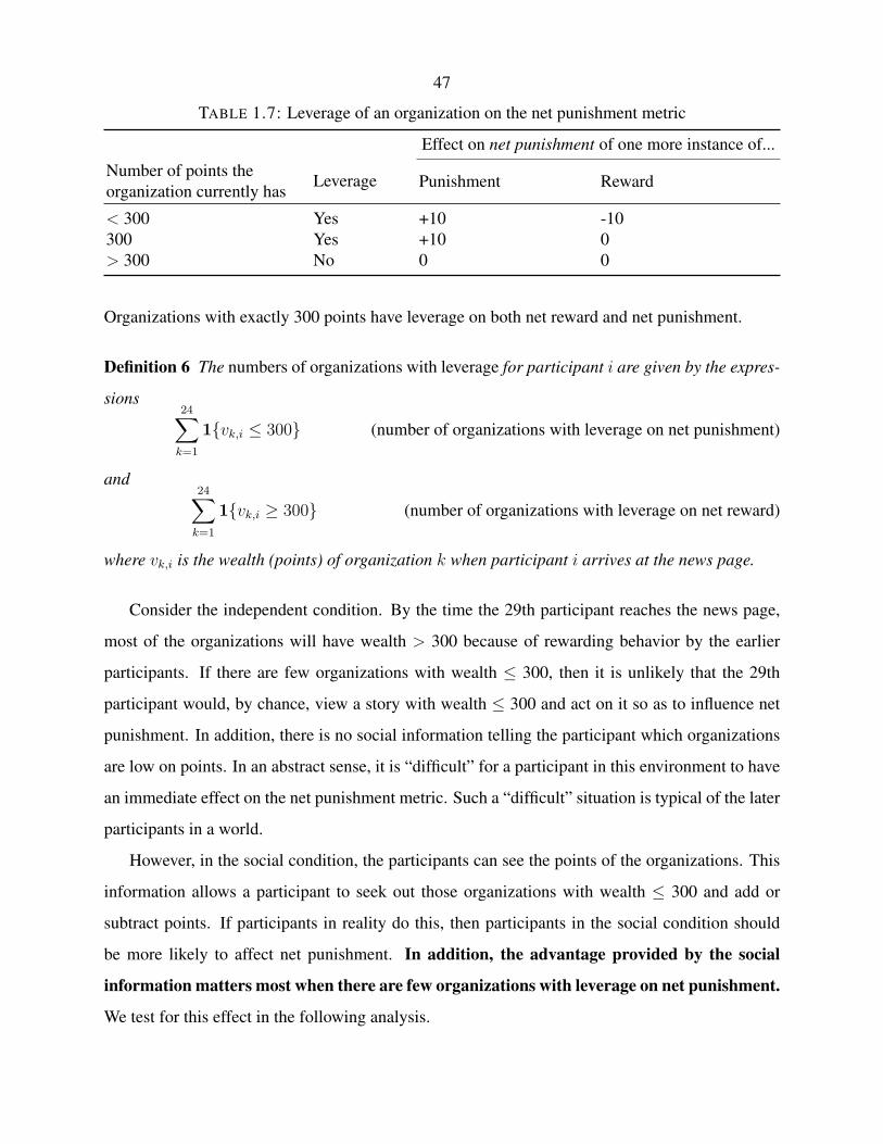
47

TABLE 1.7: Leverage of an organization on the net punishment metric

Effect on net punishment of one more instance of...

Number of points theorganization currently has

Leverage Punishment Reward

< 300 Yes +10 -10300 Yes +10 0> 300 No 0 0

Organizations with exactly 300 points have leverage on both net reward and net punishment.

Definition 6 The numbers of organizations with leverage for participant i are given by the expres-

sions24∑k=1

1{vk,i ≤ 300} (number of organizations with leverage on net punishment)

and24∑k=1

1{vk,i ≥ 300} (number of organizations with leverage on net reward)

where vk,i is the wealth (points) of organization k when participant i arrives at the news page.

Consider the independent condition. By the time the 29th participant reaches the news page,

most of the organizations will have wealth > 300 because of rewarding behavior by the earlier

participants. If there are few organizations with wealth ≤ 300, then it is unlikely that the 29th

participant would, by chance, view a story with wealth ≤ 300 and act on it so as to influence net

punishment. In addition, there is no social information telling the participant which organizations

are low on points. In an abstract sense, it is “difficult” for a participant in this environment to have

an immediate effect on the net punishment metric. Such a “difficult” situation is typical of the later

participants in a world.

However, in the social condition, the participants can see the points of the organizations. This

information allows a participant to seek out those organizations with wealth ≤ 300 and add or

subtract points. If participants in reality do this, then participants in the social condition should

be more likely to affect net punishment. In addition, the advantage provided by the social

information matters most when there are few organizations with leverage on net punishment.

We test for this effect in the following analysis.

48

To test for this relationship a simple logit model was estimated on the participant-level data

(480 observations).9 The model predicts whether or not the participant had any effect on net

punishment during his visit to the page. Alternatively, we could think of the model as describing

whether the participant made the net punishment path in Figure 1.4 tick up or down. The right-hand

side variables were (1) an indicator for the social condition, (2) a scalar term showing the number

of organizations with leverage on net punishment at the time the participant arrived at the page, and

(3) the interaction of variables 1 and 2. The coefficients from estimating this model appear in Table

1.8. The average marginal effects are plotted in Figure 1.8. The table also includes the analogous

but “inverted” model for net reward. This model replaces the left-hand side with an indicator

for influencing net reward and the second predictor variable with a term showing the number of

organizations with leverage on net reward. The first two columns show coefficient estimates for

affecting net punishment. The scalar term has a positive effect, which means that a participant

is more likely to influence net punishment when there are more organizations with leverage on

net punishment. The other way of viewing this is that a participant is less likely to influence

net punishment when few organizations have leverage on the metric. However, this relationship

is inverted when looking at the social condition. The interaction term is negative and larger in

magnitude than the simple scalar term. In addition, the effect of the social condition dummy is

positive and significant.

The overall result is that when the number of organizations with points ≤ 300 is small, the

participants in the social condition are more likely than those in the independent condition to

influence net punishment. This relationship is depicted in Figure 1.8 which shows average marginal

effects of the social condition evaluated at different values of the scalar variable in the regression.

The low end of the x-axis corresponds to the later part of a world. The positive marginal effects

at the low end of the x-axis confirms the idea that social information can help participants to

target actions on the few organizations with leverage. The average marginal effects from the net

reward model are also plotted. These results do not reveal any effect of the social condition on the

probability of influencing net reward. This finding makes sense because there are usually many

9This deliberately simplified for illustrative purposes. The appendix includes a corresponding analysis using thepanel data, where page position and story effects can be incorporated into the model to control for dependencies. SeeAppendix Table 1.13. These results provide even stronger evidence that the leverage variable and its interaction withthe social dummy should be in the model along with the social dummy. The joint test of those three variables issignificant at level 0.001.

49

TABLE 1.8: Coefficient estimates from models of the participant-wise probabilities of affectingnet punishment and reward

Left-hand side variable (binary):The participant changed the netmetric listed below during his

visit to the news page.

Net punishment Net reward

(1) (2) (3) (4)

Social condition (dummy) 0.552∗∗ 1.814∗∗ 0.370 -0.111(0.219) (0.851) (0.287) (3.415)

State of the news pagewhen visited by the participant:

Number of organizations w/ points ≤ 300 0.061[i.e., with leverage on net punishment] (0.050)

Social dummy × (# orgs. w/ points ≤ 300) -0.086(0.055)

Number of organizations w/ points ≥ 300 -0.064[i.e., with leverage on net reward] (0.149)

Social dummy × (# orgs. w/ points ≥ 300) 0.022(0.163)

Average marginal effect of social cond. 0.133 0.138 0.047 0.044Significance of AME of social cond. (p) 0.009 0.006 0.225 0.253Joint sig. of 3 coefs. above (p) . 0.032 . 0.523Individuals 480 480 480 480

Notes. Coefficient estimates from logit models with standard errors in parentheses. The average marginal effect is theaverage effect on the probability of the modeled outcome. The printed p-value of the AME corresponds to a test withthe null hypothesis that the AME is 0. The joint significance test has the null hypothesis that all 3 coefficients in thecolumn are zero. ∗ p < 0.10, ∗∗ p < 0.05, ∗∗∗ p < 0.01.

organizations with leverage on net reward. They are not “difficult” to find, so social information is

less important for finding them. The supports of the data on the x-axis correspond to the heavily

shaded areas of the plot. For example, the number of organizations with leverage on net reward

never dropped below 15.

The consequence of this result at the aggregate level is that as a social world evolves we see

net punishment continue to change (mainly increasing), which leads to the higher levels of net

punishment and higher variance of net punishment observed in the aggregate results. Another way

to interpret this result is to note that net punishment evolves like a random walk with drift. The

50

social condition allows this “random walk” to have a greater number of time steps because each

participant has a greater probability of making the walk transition to a new state (as shown in this

analysis). A higher number of steps translates to higher variance at the end of the world. However,

the results for net reward do not show the increasing marginal effect seen for net reward. No

significant advantage is seen for the social condition in changing net reward. This finding agrees

with the world-level results where there is no evidence of a difference between the two conditions

in the variance of net reward.

0 4 8 12 16 20 24

Number of organizations with leverage on the metric(when the participant arrives at the news page)

0.2

0.0

0.2

0.4

0.6

Advanta

ge o

f th

e s

oci

al co

ndit

ion

Marg

inal eff

ect

on P

(Part

icip

ant

changes

net

metr

ic)

Here there are few organizationswith leverage on net punishment,and participants in the socialcondition are more likely toact on those few organizations.Social information is useful tofind those few organizationswith wealth 300.

Here there are few organizationswith leverage on net punishment,and participants in the socialcondition are more likely toact on those few organizations.Social information is useful tofind those few organizationswith wealth 300.

Metric

Net reward ± SE

Net punishment ± SE

p < 0.10

p < 0.05

FIGURE 1.8: Effect of the social condition on choices that affect net punishment/reward

51

TABLE 1.9: Social effects on behavior when controlling for page position

Not controlling for pageposition

Controlling for pageposition

Punish Reward View Punish Reward View

Social effect:Points sub’ed (dummy) 0.027∗∗∗ 0.020∗∗ 0.049∗∗∗ 0.006 -0.016∗∗ -0.017

(0.008) (0.008) (0.012) (0.008) (0.008) (0.011)Points added (dummy) 0.016∗∗∗ 0.034∗∗∗ 0.059∗∗∗ -0.002 -0.019∗ -0.020

(0.005) (0.009) (0.011) (0.007) (0.011) (0.013)

Individuals 360 360 360 360 360 360Obs. 8, 640 8, 640 8, 640 8, 640 8, 640 8, 640Avg. log-likelihood -0.145 -0.256 -0.367 -0.142 -0.250 -0.356

Notes. Average marginal effects of previous punishment (points sub’ed) and reward (points added) printed. Effectsare specified in the binary form with logarithmic decay. Estimates come from a logit model with a dummy variablefor each story. Page position is controlled for by a quadratic function. Standard errors, in parentheses, are clustered byparticipant. Standard errors, in parentheses, are clustered by participant. ∗ p < 0.10, ∗∗ p < 0.05, ∗∗∗ p < 0.01

1.5.4.1. Social influence vs. attention manipulation by algorithm

The previous analyses of the effects of points subtracted and added in the social condition did

not include controls for the effect of page position. Therefore, the social effects represented a

combination of any direct social influence and the attentional effect of shifting the location of a

story on the page. That is, because punishing and rewarding imply viewing a story, the social

variables are highly correlated with the story being near the top of the news page, which itself

greatly increases the probability of being viewed. To disentangle these effects I estimated the same

models with the addition of a quadratic control for page position. The results of this exercise

appear in Table 1.9. The estimates from Table 1.4 are reprinted for convenience. Once page

position controls are added, many of the social effects become small and insignificant. This finding

indicates that the mechanical page position effects dominate the social effects. Once they are

accounted for, the participants put little additional weight on points added and subtracted overall.

Negative effects are also consistent with a preference for fairness wherein participants prefer to

reward organizations that have not yet been rewarded.

The evidence indicates that participants are, in some sense, passive and highly subject to the

algorithm that constructs the page (in this case, sorting by views). However, the participants do

not entirely disregard social information. The results indicate that social information does have

52

direct effects (controlling for page position), but these effects occur very early in the course of

a world. First, alternative specifications using the share definition of social effects reveal robust

positive effects of points subtracted on subsequent punishment (see Appendix Table 1.12). These

specifications essentially overweight the effects that occur early in a world. Second, these social

effects appear when we explicitly examine average marginal effects over the course of a world.

To explore individual behavior in greater detail I estimated the familiar logit models predicting

punishment, reward, and viewing. Each model again includes story dummies, quadratic page po-

sition controls, linear specifications of the points added and subtracted, and those points variables

interacted with a quadratic function of the log participant number. The exact specification of the

points and the function of the participant number make relatively little difference to the results.

Analogous models using binary points effects are printed in the appendix (see Appendix Figure

1.24).

In addition, a model of each behavior was estimated with quadratic controls for the page po-

sition, linear terms for added and subtracted points, and quadratic logarithmic decay interactions.

This particular specification was chosen based on fit statistics, but a model with binary social ef-

fects gives similar results (see Appendix Table 1.24). The average marginal effects of punishment

and reward were evaluated at each participant number and are displayed in Figure 1.9. Since these

models are based on the entire social data set they are called the unconditional estimates. These

results reveal little evidence of social effects. Punishment and, to some extent, reward are found to

have some negative effects on rewarding among early and middle participants. The negative effects

of reward on rewarding are quantitatively small and not entirely robust to alternative specifications

(see additional results in the appendix). These effects are largely accounted for by the increase in

exploration among participants in the middle range of a world. However, the effects of punishment

show some true social influence. Even controlling for page position, punished organizations are

significantly less likely to be rewarded (by a few percentage points) during the first third of a world.

Figure 1.9 also shows results from models estimated using only the participant-by-story obser-

vations where the participant viewed the story. These models are called “conditional on viewing.”

The estimated coefficients for punishment and reward are printed in Table 1.26. These results

show significant effects on punishment, which increases the probability of punishing (conditional

on viewing) by up to 20 percentage points. The probability of rewarding (conditional on viewing)

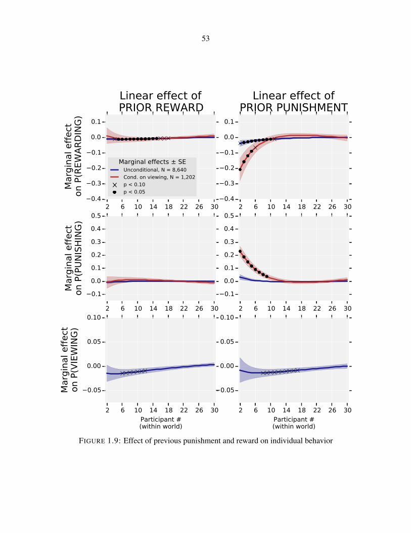
53

2 6 10 14 18 22 26 300.4

0.3

0.2

0.1

0.0

0.1

Marg

inal eff

ect

on P

(REW

AR

DIN

G)

Linear effect ofPRIOR REWARD

Marginal effects ± SEUnconditional, N = 8,640

Cond. on viewing, N = 1,202

p < 0.10

p < 0.05

2 6 10 14 18 22 26 300.4

0.3

0.2

0.1

0.0

0.1

Linear effect ofPRIOR PUNISHMENT

2 6 10 14 18 22 26 30

0.1

0.0

0.1

0.2

0.3

0.4

0.5

Marg

inal eff

ect

on P

(PU

NIS

HIN

G)

2 6 10 14 18 22 26 30

0.1

0.0

0.1

0.2

0.3

0.4

0.5

2 6 10 14 18 22 26 30

Participant #(within world)

0.05

0.00

0.05

0.10

Marg

inal eff

ect

on P

(VIE

WIN

G)

2 6 10 14 18 22 26 30

Participant #(within world)

0.05

0.00

0.05

0.10

FIGURE 1.9: Effect of previous punishment and reward on individual behavior

54

is decreased by a similar amount. The similarity of the two effect magnitudes suggests that punish-

ment may persuade those who would otherwise reward to punish instead. The models’ estimated

coefficients are printed in Table 1.26, which again shows that punishment has effects on punish-

ment and reward that are similar in magnitude but opposite in sign. However, it is likely that, in

addition to persuasive effects, selection also plays a role. Punished stories may attract the attention

of individual participants that have a high propensity to punish and low propensity to reward. The

decaying form of the effect also suggests an important role for selection.

The same conditional-on-viewing models do not show any social effects of reward on subse-

quent reward or punishing. Therefore, punishment seems to be special in generating social effects

that go beyond algorithmic manipulation of attention.

1.6. Conclusion

The experiment revealed that adding social information to the media environment had two main

effects on aggregate outcomes. First, the inequality in points across the organizations became more

unequal. Effectively, the popular organizations tended to be more popular while the unpopular

organizations tended to be more unpopular. Second, the expected net punishment in a given world

became greater but also more variable.

A further investigation of the individual behavior during the experiment provided some answers

about why the aggregate outcomes were affected by social information. The page-construction al-

gorithm, which sorted the most-viewed stories to the top of the headlines page, played a dominant

role in concentrating attention in a herding-like way. That is, participants always had to view a story

before punishing or rewarding. These views tended to push that story to the top of the page where

it was more likely to be viewed, which in turned caused the story to receive more punishment or

reward. This mechanism generated a strong positive correlation between being punished/rewarded

in the past and being punished/rewarded in the future. However, once the models accounted for

the position of the headline on the page, the effects of social information about punishment and

reward were greatly diminished. This result suggests that participants offloaded a substantial por-

tion of their decision making process to the page-constructing algorithm. The actual effect of the

algorithm on choices depends on how well it aligns with the participants’ own preferences. If they

55

are perfectly aligned, then the participants would, by some measure, make better choices or make

choices as if they had zero search costs or “thinking aversion” (Ortoleva 2013). Alternatively, if

the participants incur search costs, then the choices of participants could be systematically manip-

ulated by the algorithm. One such example is the herding experiment on an artificial music market

by Salganik and Watts (2008), in which social information about song popularity was deceptively

inverted.

That finding gives a different impression from recent research by Bakshy et al. (2015) on news

consumption through Facebook. Those researchers argue that political bias in news consumption

was driven more by individuals’ own choices than through the Facebook News Feed algorithm. In

practice, the degree of selection through the two sources will be highly dependent on the particular

context and algorithm used. Future research might investigate this topic by varying the page/menu-

construction algorithm in a way somewhat like Salganik and Watts (2008) along with the types

of social information available. The present experiment provided a fairly sparse form of social

information. Richer forms of communication may lead to stronger selection through individual

choice.

The present results also reveal an asymmetry in positive and negative social effects (reward and

punishment). This finding is consistent with research showing that negative events and information

tend to have greater effects than positive (Baumeister et al. 2001). Punishment was found to have

two substantive social effects, whereas reward had little. Participants used social information to

selectively target unpopular organizations (mostly for punishment but also reward). It could be

argued that this result only occurred because unpopular organizations tended to be much rarer than

popular. If popular organizations were rare instead, it is possible that participants would then use

social information to target them. However, a second unique effect of punishment is that it had

a significant social effect even after controlling for the effect of the page-construction algorithm.

When participants viewed a story about a previously punished organization, they were significantly

more likely to punish that organization instead of reward. These findings suggest that, compared

to positive activity, negative activity may be more dependent on herding-like behavior.

56

1.7. Appendix of chapter 1

1.7.1. Examples of real Internet punishment

TABLE 1.10: 48 selected cases of punishment and shaming involving the Internet

Case Time Situation Consequences

George & Dragon British Pub,Orlando, FL1

May 2015 Owner accused of racist threatwith gun.

Angry Yelp reviews posted.Owner arrested.

Melbourne Man, Melbourne,Australia2

May 2015 Mother posted photo of man onFacebook with accusation thathe was sex offender.

Man received death threats butwas cleared by police.

Rubbin Buttz BBQ, Milliken,CO3

May 2015 Enacted 10% discount for whitepeople.

Angry Yelp reviews posted.Discount extended to allcustomers.

PLOS ONE4 May 2015 Reviewer asked female authorsto add a male co-author.

Authors posted reviewer reportson Twitter. Reviewer wasbanned by PLOS ONE.

Cigars & Stripes Bar, Berwyn,IL5

April 2015 Two-way mirror allows lookinginto women’s restroom.

Angry Yelp reviews posted.Police investigated.

Alphagraphics, Suwanee, GA6 April 2015 Refused to print invitations fora gay wedding.

Angry Yelp reviews posted.

Popeyes Chicken, Channelview,TX7

April 2015 Fired employee that wasrobbed.

Angry Yelp reviews. Employeewas offered job back.

Dieseltec, Grandville, MI8 April 2015 Announced policy of notserving gay clients.

Angry Yelp reviews posted.

Clorox9 April 2015 Accused of a racist tweet. Attacked by Twitter users.

New York University10 April 2015 Facebook user accused campusstore of having sexist babyclothing.

Attacked on social media bystudents and almuni.

Memories Pizza, Walkerton,IN11

April 2015 Announced policy of notserving gay clients.

Attacked on Yelp. GoFundMecampaign launched in support.

Days Inn, Pine Bluff, AR12 March 2015 Fired employee for speaking toa reporter about a minimumwage bill.

Attacked on Yelp and socialmedia.

F&R Auto Sales, Westport,MA13

Jan. 2015 Leaked video of argument withpizza delivery man.

Attacked on Yelp/Googlereviews. Website went down.

Indian men on a bus (Rohtak,India)14

Dec. 2014 Three men allegedly harassedtwo sisters on a bus.

The sisters hit the men withbelts. A cell phone videospread. The men were arrested.The sisters were accused ofmisrepresenting the incident.

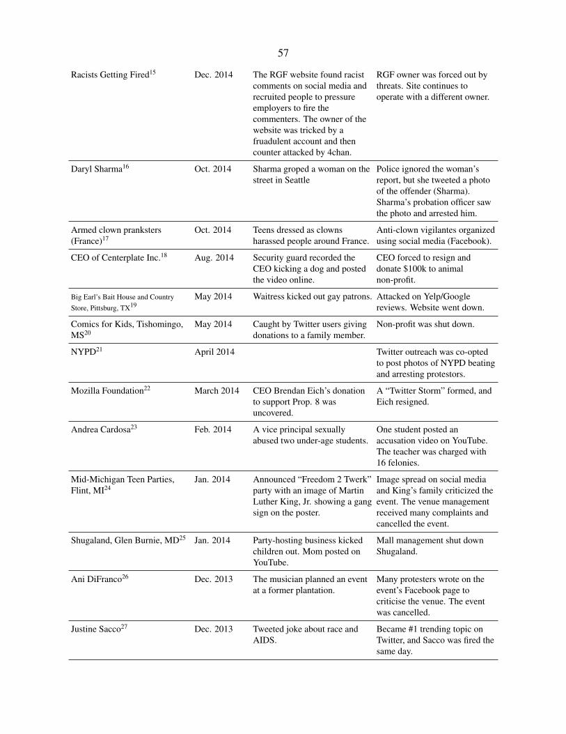
57

Racists Getting Fired15 Dec. 2014 The RGF website found racistcomments on social media andrecruited people to pressureemployers to fire thecommenters. The owner of thewebsite was tricked by afruadulent account and thencounter attacked by 4chan.

RGF owner was forced out bythreats. Site continues tooperate with a different owner.

Daryl Sharma16 Oct. 2014 Sharma groped a woman on thestreet in Seattle

Police ignored the woman’sreport, but she tweeted a photoof the offender (Sharma).Sharma’s probation officer sawthe photo and arrested him.

Armed clown pranksters(France)17

Oct. 2014 Teens dressed as clownsharassed people around France.

Anti-clown vigilantes organizedusing social media (Facebook).

CEO of Centerplate Inc.18 Aug. 2014 Security guard recorded theCEO kicking a dog and postedthe video online.

CEO forced to resign anddonate $100k to animalnon-profit.

Big Earl’s Bait House and CountryStore, Pittsburg, TX19

May 2014 Waitress kicked out gay patrons. Attacked on Yelp/Googlereviews. Website went down.

Comics for Kids, Tishomingo,MS20

May 2014 Caught by Twitter users givingdonations to a family member.

Non-profit was shut down.

NYPD21 April 2014 Twitter outreach was co-optedto post photos of NYPD beatingand arresting protestors.

Mozilla Foundation22 March 2014 CEO Brendan Eich’s donationto support Prop. 8 wasuncovered.

A “Twitter Storm” formed, andEich resigned.

Andrea Cardosa23 Feb. 2014 A vice principal sexuallyabused two under-age students.

One student posted anaccusation video on YouTube.The teacher was charged with16 felonies.

Mid-Michigan Teen Parties,Flint, MI24

Jan. 2014 Announced “Freedom 2 Twerk”party with an image of MartinLuther King, Jr. showing a gangsign on the poster.

Image spread on social mediaand King’s family criticized theevent. The venue managementreceived many complaints andcancelled the event.

Shugaland, Glen Burnie, MD25 Jan. 2014 Party-hosting business kickedchildren out. Mom posted onYouTube.

Mall management shut downShugaland.

Ani DiFranco26 Dec. 2013 The musician planned an eventat a former plantation.

Many protesters wrote on theevent’s Facebook page tocriticise the venue. The eventwas cancelled.

Justine Sacco27 Dec. 2013 Tweeted joke about race andAIDS.

Became #1 trending topic onTwitter, and Sacco was fired thesame day.

58

Murdoch’s Range & HomeSupply, Evansville, WY28

Dec. 2013 Two employees killed araccoon, which was reported onFacebook.

The two employees resigned.

Specialized Bicycle29 Dec. 2013 Specialized accused a smallbike shop of trademarkinfringement.

After social media criticism,Specialized dropped the suit,and the CEO personallyapologized to the shop owner.

Duck Dynasty (TV show)30 Dec. 2013 GQ magazine published aninterview in which Robertson(actor on the show) expressedanti-gay opinions.

The interview spread on socialmedia. A&E suspendedRobertson. Duck Dynastymerchandise was removed fromstores.

Devin Barnes + Red Lobster,Franklin, TN31

October 2013 Waitress claimed Barnes wrotea slur on the receipt.

Barnes received death threats.Waitress received $10,000 indonations. Barnes sued RedLobster and waitress.

FedEx32 July 2013 Video of delivery driverthrowing packages spread onthe web.

Driver was fired.

Golden Corral, Port Orange,FL33

July 2013 Pictures purported to be of adirty kitchen at GC were postedon Reddit.

GC manager was fired forimproper food handling.

Taco Bell34 June 2013 Picture of employee lickingtaco shells (for an internal photocontest) spread on the net.

The employee was fired.

Sunil Tripathi + Reddit35 April 2013 Reddit users crowdsourcing thesearch for the Boston Marathonbombers mistakenly accusedseveral people.

The accusations were spread bymainstream media. Severalinnocent people werethreatened and harassed.

Adria Richards36 March 2013 Richards posted a photo of aman making sexual jokes at aprogramming conference inorder to shame him.

The man was fired. Hackersattacked Richards and heremployer. Richards was fired.

SeaWorld37 2013-2015 Accused of mistreating whalesin a documentary and on socialmedia.

Attendance and stock price fell.CEO resigned. Layoffs.

Thai Noodles Etc., Austin,TX38

Dec. 2012 Restaurant owner posted racistmessage on Facebook about theSandy Hook shooting.

Attacked on Yelp. Ownerreceived death threats.Restaurant deleted Facebookpage.

Lindsey Stone39 Oct. 2012 Stone appeared in an imagegiving the middle finger in jestat the Arlington NationalCemetery.

The image spread on socialmedia. A Facebook pageappeared with the goal ofhaving Stone fired. She wasfired.

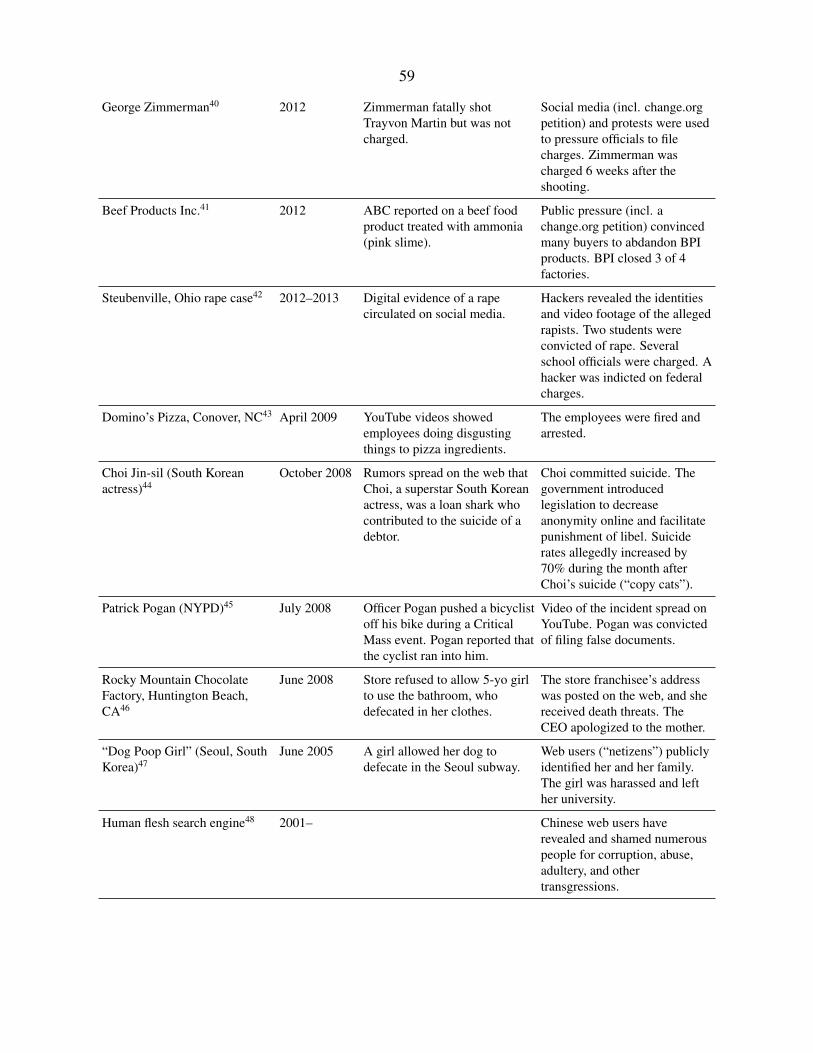
59

George Zimmerman40 2012 Zimmerman fatally shotTrayvon Martin but was notcharged.

Social media (incl. change.orgpetition) and protests were usedto pressure officials to filecharges. Zimmerman wascharged 6 weeks after theshooting.

Beef Products Inc.41 2012 ABC reported on a beef foodproduct treated with ammonia(pink slime).

Public pressure (incl. achange.org petition) convincedmany buyers to abdandon BPIproducts. BPI closed 3 of 4factories.

Steubenville, Ohio rape case42 2012–2013 Digital evidence of a rapecirculated on social media.

Hackers revealed the identitiesand video footage of the allegedrapists. Two students wereconvicted of rape. Severalschool officials were charged. Ahacker was indicted on federalcharges.

Domino’s Pizza, Conover, NC43 April 2009 YouTube videos showedemployees doing disgustingthings to pizza ingredients.

The employees were fired andarrested.

Choi Jin-sil (South Koreanactress)44

October 2008 Rumors spread on the web thatChoi, a superstar South Koreanactress, was a loan shark whocontributed to the suicide of adebtor.

Choi committed suicide. Thegovernment introducedlegislation to decreaseanonymity online and facilitatepunishment of libel. Suiciderates allegedly increased by70% during the month afterChoi’s suicide (“copy cats”).

Patrick Pogan (NYPD)45 July 2008 Officer Pogan pushed a bicyclistoff his bike during a CriticalMass event. Pogan reported thatthe cyclist ran into him.

Video of the incident spread onYouTube. Pogan was convictedof filing false documents.

Rocky Mountain ChocolateFactory, Huntington Beach,CA46

June 2008 Store refused to allow 5-yo girlto use the bathroom, whodefecated in her clothes.

The store franchisee’s addresswas posted on the web, and shereceived death threats. TheCEO apologized to the mother.

“Dog Poop Girl” (Seoul, SouthKorea)47

June 2005 A girl allowed her dog todefecate in the Seoul subway.

Web users (“netizens”) publiclyidentified her and her family.The girl was harassed and lefther university.

Human flesh search engine48 2001– Chinese web users haverevealed and shamed numerouspeople for corruption, abuse,adultery, and othertransgressions.

60

Notes1Silverstein (2015)2Pearlman (2015)3Associated Press (2015)4Woolston (2015)5Ward and Gutowski (2015)6Markiewicz (2015)7Wagner (2015)8Zoladz (2015)9CNN (2015)

10Firstpost.com (2015)11TMZ.com (2015)12Moran (2015)13Spargo (2015)14Arya (2015)15McDonald (2014)

16News (2014)17Goldhammer (2014)18Garrett (2014)19Shah (2014)20Johnston (2014)21McKechnie (2014)22Kim (2014)23Goff and Shin (2015)24DeJohn (2014)25Scharper (2014)26Anderson (2013)27Ronson (2015)28Associated Press (2013)29Babin (2013)30Ford (2013)31Wagner (2014)32Jacobson (2013)

33Ward (2013)

34Sun (2013)

35Levenson (2015)

36Martin (2013)

37Lomax (2015)

38Kuruvilla (2012)

39Sieczkowski (2012)

40Selter (2012)

41Blaney (2012)

42Kushner (2013)

43Hutchinson (2009)

44Sang-Hun (2008)

45Yaniv (2010)

46Burris (2008)

47Krim (2005)

48Hatton (2014)

61

1.7.2. Description and images of experimental news site

FIGURE 1.10: Instructions to the participants (social and independent).

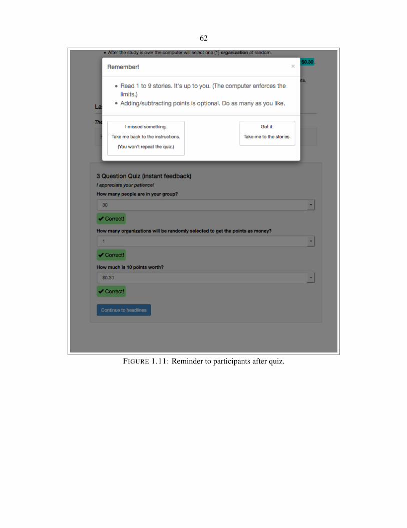
62

FIGURE 1.11: Reminder to participants after quiz.

63

FIGURE 1.12: Headlines page (social condition).

64

FIGURE 1.13: One of the news stories.

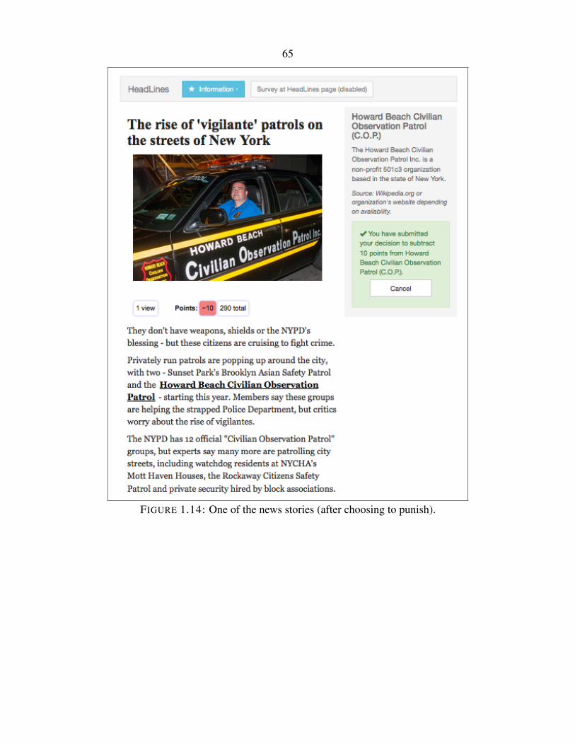
65

FIGURE 1.14: One of the news stories (after choosing to punish).

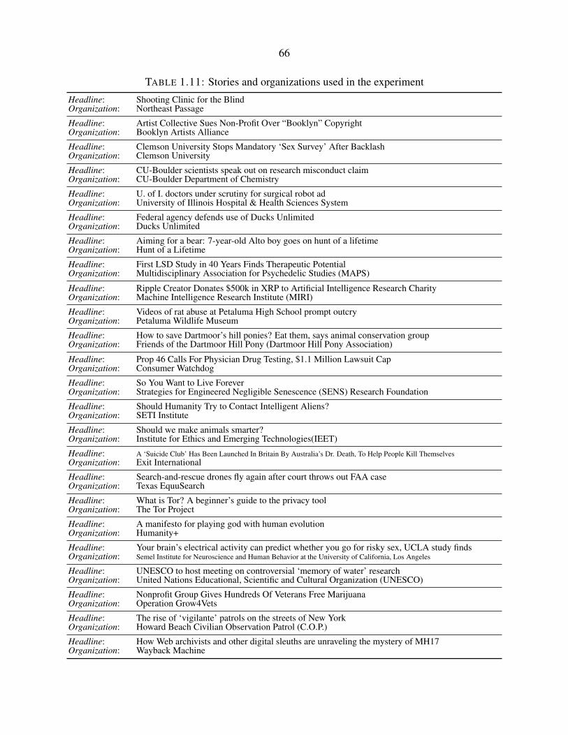
66

TABLE 1.11: Stories and organizations used in the experiment

Headline: Shooting Clinic for the BlindOrganization: Northeast Passage

Headline: Artist Collective Sues Non-Profit Over “Booklyn” CopyrightOrganization: Booklyn Artists Alliance

Headline: Clemson University Stops Mandatory ‘Sex Survey’ After BacklashOrganization: Clemson University

Headline: CU-Boulder scientists speak out on research misconduct claimOrganization: CU-Boulder Department of Chemistry

Headline: U. of I. doctors under scrutiny for surgical robot adOrganization: University of Illinois Hospital & Health Sciences System

Headline: Federal agency defends use of Ducks UnlimitedOrganization: Ducks Unlimited

Headline: Aiming for a bear: 7-year-old Alto boy goes on hunt of a lifetimeOrganization: Hunt of a Lifetime

Headline: First LSD Study in 40 Years Finds Therapeutic PotentialOrganization: Multidisciplinary Association for Psychedelic Studies (MAPS)

Headline: Ripple Creator Donates $500k in XRP to Artificial Intelligence Research CharityOrganization: Machine Intelligence Research Institute (MIRI)

Headline: Videos of rat abuse at Petaluma High School prompt outcryOrganization: Petaluma Wildlife Museum

Headline: How to save Dartmoor’s hill ponies? Eat them, says animal conservation groupOrganization: Friends of the Dartmoor Hill Pony (Dartmoor Hill Pony Association)

Headline: Prop 46 Calls For Physician Drug Testing, $1.1 Million Lawsuit CapOrganization: Consumer Watchdog

Headline: So You Want to Live ForeverOrganization: Strategies for Engineered Negligible Senescence (SENS) Research Foundation

Headline: Should Humanity Try to Contact Intelligent Aliens?Organization: SETI Institute

Headline: Should we make animals smarter?Organization: Institute for Ethics and Emerging Technologies(IEET)

Headline: A ‘Suicide Club’ Has Been Launched In Britain By Australia’s Dr. Death, To Help People Kill ThemselvesOrganization: Exit International

Headline: Search-and-rescue drones fly again after court throws out FAA caseOrganization: Texas EquuSearch

Headline: What is Tor? A beginner’s guide to the privacy toolOrganization: The Tor Project

Headline: A manifesto for playing god with human evolutionOrganization: Humanity+

Headline: Your brain’s electrical activity can predict whether you go for risky sex, UCLA study findsOrganization: Semel Institute for Neuroscience and Human Behavior at the University of California, Los Angeles

Headline: UNESCO to host meeting on controversial ‘memory of water’ researchOrganization: United Nations Educational, Scientific and Cultural Organization (UNESCO)

Headline: Nonprofit Group Gives Hundreds Of Veterans Free MarijuanaOrganization: Operation Grow4Vets

Headline: The rise of ‘vigilante’ patrols on the streets of New YorkOrganization: Howard Beach Civilian Observation Patrol (C.O.P.)

Headline: How Web archivists and other digital sleuths are unraveling the mystery of MH17Organization: Wayback Machine

67

1.7.3. Simulation study of the re-sampling estimator

The simulation creates identical, independent agents that make decisions over 24 stories. Each

agent punishes each story with probability 148

and rewards each story with probability 248

, which

are similar to the observed probabilities. This parametrization gives simulated means and standard

deviations that are close to the actual data. The simulation creates 1,000 data sets composed of

n worlds for each n = 2, 4, 8, 16, 32, 64. Each world is composed of 30 such agents as in the

experiment. The net punishment in each world is calculated as described in the methods section.

The conventional estimators are the sample mean and sample standard deviation. The re-sampling

estimator is computed as described in the paper. In this case, each simulated data set is sub-sampled

400 times to create 400 worlds. The mean and standard deviation of the sub-sampled worlds are the

estimates. The simulation results show that the re-sampling standard deviation estimator has much

less variance (smaller standard error) than the conventional estimator. Fairly precise estimates are

available even for 2 worlds, where the conventional estimator is highly erratic. The bias of the

re-sampling estimator is similar to that of the conventional estimator. The re-sampling estimator of

the mean has somewhat less variance than the sample mean, but the advantage is much less than in

the case of estimating the standard deviation. The re-sampling estimator of the mean has a small

downward bias that decreases with the sample size. The sample mean is, of course, unbiased.

Figure 1.16 shows box and whiskers plots of the results from the 1,000 simulated data sets in

each box. The box shows the interquartile range with a line at the median. The whiskers extend

1.5 × (the interquartile range) beyond the box edges. The plus signs are outliers.

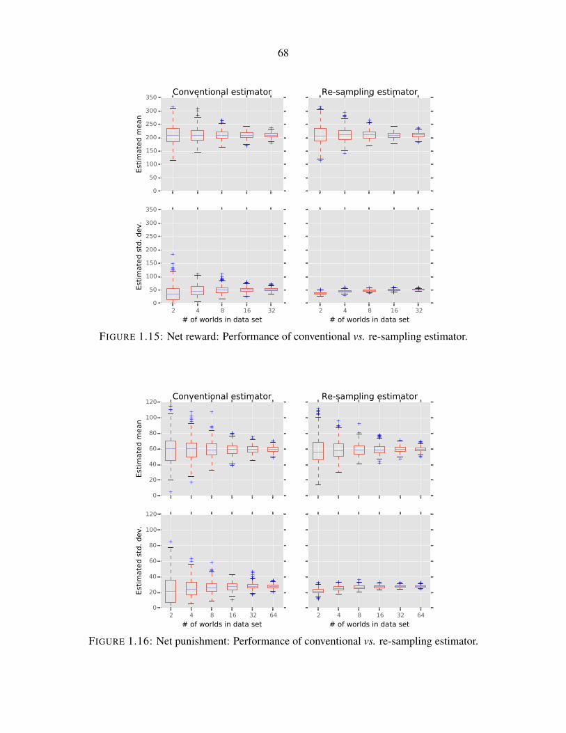
68

0

50

100

150

200

250

300

350

Est

imate

d m

ean

Conventional estimator Re-sampling estimator

2 4 8 16 32

# of worlds in data set

0

50

100

150

200

250

300

350

Est

imate

d s

td.

dev.

2 4 8 16 32

# of worlds in data set

FIGURE 1.15: Net reward: Performance of conventional vs. re-sampling estimator.

0

20

40

60

80

100

120

Est

imate

d m

ean

Conventional estimator Re-sampling estimator

2 4 8 16 32 64

# of worlds in data set

0

20

40

60

80

100

120

Est

imate

d s

td. dev.

2 4 8 16 32 64

# of worlds in data set

FIGURE 1.16: Net punishment: Performance of conventional vs. re-sampling estimator.

69

1.7.4. Additional results

0 5 10 15 20 25 30 35Total browsing time (minutes)

0.00

0.02

0.04

0.06

0.08

0.10

0.12

0.14

0.16

0.18Pro

port

ion

FIGURE 1.17: Histogram of time spent by participants on the news site

70

10 20 30 40 50 60 70 80Age (years)

10-1

100

101

102

Bro

wsi

ng t

ime (

min

ute

s)

FIGURE 1.18: Participant age vs. browsing time

71

1 4 7 10 13 16 19 22 24Position of headline (1 = top of page)

0

5

10

15

20

25

30

Mean t

ime o

n s

creen (

seco

nds,

Win

sori

zed)

Mean w/ IQR shaded

Social

Independent

FIGURE 1.19: Headline items’ time on screen by visual position and condition

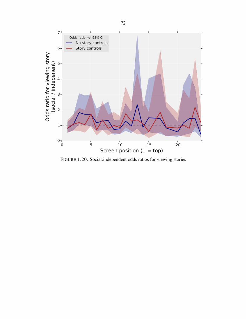
72

0 5 10 15 20

Screen position (1 = top)

0

1

2

3

4

5

6

7

Odds

rati

o f

or

vie

win

g s

tory

(soci

al /

indepenent)

Odds ratio +/- 95% CI

No story controls

Story controls

FIGURE 1.20: Social:independent odds ratios for viewing stories

73

1 4 7 10 13 16 19 22 24Rank of story (by # views, jittered)

0

5

10

15

20

# v

iew

s

Social

Independent

FIGURE 1.21: Distribution of story views for each world

74

1 6 11 16 21 26 300

5

10

15

20

Mean #

org

s. p

unis

hed o

r re

ward

ed

1 6 11 16 21 26 30Participant #

0

20

40

60

80

100

Mean #

sto

ry-v

iew

s

Social

Independent

FIGURE 1.22: Evolution of points actions and views

75

1 4 7 10 13 16 19 22 24Position of headline (1 = top of page)

0.0

0.5

1.0

1.5

2.0

2.5

3.0

Rati

o:

soci

al /

independent

Odds ratio of viewing story +/- SE

Ratio of mean screen time +/- SE

FIGURE 1.23: Headline items’ time on screen and click probability by page position

76

TABLE 1.12: Alternative specifications of social influence on probability of punishing

Not controlling forpage position

Includes quadraticin page position

Includes pageposition dummy

variablesSocialeffect:Linear

Socialeffect:

Quadratic

Socialeffect:Linear

Socialeffect:

Quadratic

Socialeffect:Linear

Socialeffect:

Quadratic

Social effect:Points sub’ed 0.055∗∗∗ 0.158∗∗∗ 0.029∗∗ 0.106∗∗∗ 0.031∗∗ 0.113∗∗∗

(0.014) (0.033) (0.015) (0.038) (0.015) (0.039)Points added 0.086∗∗∗ 0.149∗∗∗ 0.021 0.054 0.018 0.049

(0.023) (0.046) (0.029) (0.055) (0.029) (0.056)

Individuals 360 360 360 360 360 360Obs. 8, 640 8, 640 8, 640 8, 640 8, 640 8, 640Avg. log-likelihood -0.145 -0.144 -0.143 -0.142 -0.141 -0.140

Notes. Average marginal effects of previous punishment (points sub’ed) and reward (points added) printed. Effectsare specified in the share form. Estimates come from a logit model with a dummy variable for each story. Standarderrors, in parentheses, are clustered by participant. ∗ p < 0.10, ∗∗ p < 0.05, ∗∗∗ p < 0.01

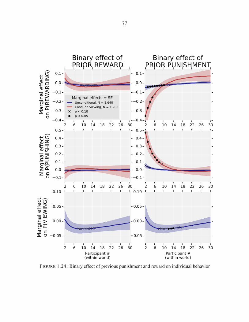
77

2 6 10 14 18 22 26 300.4

0.3

0.2

0.1

0.0

0.1

Marg

inal eff

ect

on P

(REW

AR

DIN

G)

Binary effect ofPRIOR REWARD

Marginal effects ± SEUnconditional, N = 8,640

Cond. on viewing, N = 1,202

p < 0.10

p < 0.05

2 6 10 14 18 22 26 300.4

0.3

0.2

0.1

0.0

0.1

Binary effect ofPRIOR PUNISHMENT

2 6 10 14 18 22 26 30

0.1

0.0

0.1

0.2

0.3

0.4

0.5

Marg

inal eff

ect

on P

(PU

NIS

HIN

G)

2 6 10 14 18 22 26 30

0.1

0.0

0.1

0.2

0.3

0.4

0.5

2 6 10 14 18 22 26 30

Participant #(within world)

0.05

0.00

0.05

0.10

Marg

inal eff

ect

on P

(VIE

WIN

G)

2 6 10 14 18 22 26 30

Participant #(within world)

0.05

0.00

0.05

0.10

FIGURE 1.24: Binary effect of previous punishment and reward on individual behavior

78

TABLE 1.13: Coefficient estimates of models for affecting net outcomes (panel data)

Left-hand side variable (binary):The participant acted on story k such

that the net outcome was affectedNet punishment Net reward

Social condition (dummy) 1.278∗ -0.700(0.776) (1.468)

State of the news pagewhen visited by the participant:Number of organizations w/ points ≤ 300 0.003

(0.049)Social dummy × (# orgs. w/ points ≤ 300) -0.066

(0.051)Number of organizations w/ points ≥ 300 -0.053

(0.066)Social dummy × (# orgs. w/ points ≥ 300) 0.038

(0.070)

Average marginal effect of social cond. 0.013 0.006Significance of AME of social cond. (p) 0.090 0.511Joint sig. of 3 coefs. above (p) 0.001 0.651Observations 6, 497 9, 860Individuals 480 480

Notes. Table displays coefficient estimates from pooled logit models and participant-by-storypanel data. The data used for the “punish” model includes only observations where the organizationhad wealth ≤ 30. The data used for the “reward” model includes only observations where theorganization had wealth ≥ 30. Models include dummy variables for each story and a quadraticeffect of page position. Standard errors, in parentheses, are clustered by individual. ∗ p < 0.10, ∗∗

p < 0.05, ∗∗∗ p < 0.01

79

TABLE 1.14: Effects of social condition on individual behavior and net outcomes

∆Net punishment ∆Net reward Views (exploration)Effect SE Effect SE Effect SE

Difficulty0 −0.0132 (0.0222) 0.0069 (0.0219) −0.0085 (0.0229)1 −0.0072 (0.0171) 0.0073 (0.0132) −0.0475∗ (0.0283)2 −0.0028 (0.0139) 0.0075 (0.0097) −0.0717∗ (0.0384)3 0.0009 (0.0117) 0.0076 (0.0094) −0.0752∗ (0.0417)4 0.0041 (0.0101) 0.0077 (0.0107) −0.0611 (0.0378)5 0.0069 (0.0089) 0.0078 (0.0126) −0.0363 (0.0310)6 0.0094 (0.0081) 0.0079 (0.0146) −0.0079 (0.0255)7 0.0117 (0.0076) 0.0080 (0.0165) 0.0190 (0.0227)8 0.0139∗ (0.0075) 0.0081 (0.0183) 0.0414∗ (0.0217)9 0.0159∗∗ (0.0075) 0.0081 (0.0199) 0.0579∗∗∗ (0.0213)10 0.0178∗∗ (0.0078) 0.0082 (0.0215) 0.0681∗∗∗ (0.0210)11 0.0196∗∗ (0.0082) 0.0082 (0.0230) 0.0719∗∗∗ (0.0206)12 0.0212∗∗ (0.0087) 0.0083 (0.0243) 0.0695∗∗∗ (0.0201)13 0.0228∗∗ (0.0093) 0.0083 (0.0256) 0.0614∗∗∗ (0.0199)14 0.0244∗∗ (0.0099) 0.0083 (0.0268) 0.0484∗∗ (0.0207)15 0.0258∗∗ (0.0105) 0.0084 (0.0280) 0.0319 (0.0229)16 0.0272∗∗ (0.0111) 0.0084 (0.0291) 0.0141 (0.0261)17 0.0286∗∗ (0.0117) 0.0085 (0.0301) −0.0013 (0.0286)18 0.0299∗∗ (0.0124) 0.0085 (0.0311) −0.0089 (0.0301)19 0.0311∗∗ (0.0130) 0.0085 (0.0321) −0.0028 (0.0357)20 0.0324∗∗ (0.0136) 0.0085 (0.0330) 0.0208 (0.0491)21 0.0335∗∗ (0.0142) 0.0086 (0.0339) 0.0610 (0.0601)22 0.0347∗∗ (0.0148) 0.0086 (0.0347) 0.1122∗ (0.0629)23 0.0358∗∗ (0.0154) 0.0086 (0.0355) 0.1728∗∗ (0.0873)24 0.0369∗∗ (0.0160) 0.0086 (0.0363) 0.2569 (0.1633)

Individuals 480 480 473Obs. 6, 497 9, 860 4, 614Avg. log-like. −0.171 −0.284 −0.269BIC 2458.15 5864.37 2555.97

Notes. Table displays estimated marginal effects of the social condition on the probability of changing net punish-ment, changing net reward, or viewing a story, respectively. Marginal effects are based on pooled logit models andparticipant-by-story panel data. The data used for estimation contains only the observations such that the organizationhad wealth≤ 30, wealth ≥30, and wealth= 30, respectively. Difficulty means the number of observations for a givenparticipant that were dropped due to the aforementioned conditioning. Models include dummy variables for each storyand a quadratic effect of page position. Standard errors, in parentheses, are clustered by individual. ∗ p < 0.10, ∗∗

p < 0.05, ∗∗∗ p < 0.01

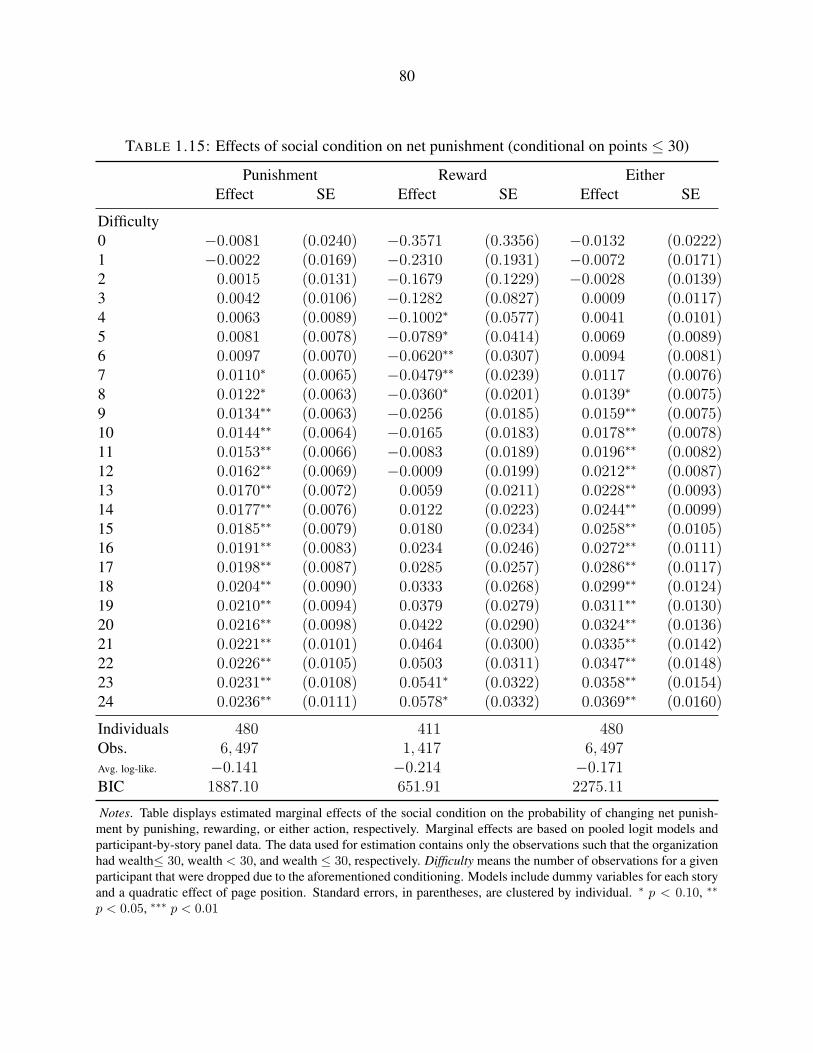
80

TABLE 1.15: Effects of social condition on net punishment (conditional on points ≤ 30)

Punishment Reward EitherEffect SE Effect SE Effect SE

Difficulty0 −0.0081 (0.0240) −0.3571 (0.3356) −0.0132 (0.0222)1 −0.0022 (0.0169) −0.2310 (0.1931) −0.0072 (0.0171)2 0.0015 (0.0131) −0.1679 (0.1229) −0.0028 (0.0139)3 0.0042 (0.0106) −0.1282 (0.0827) 0.0009 (0.0117)4 0.0063 (0.0089) −0.1002∗ (0.0577) 0.0041 (0.0101)5 0.0081 (0.0078) −0.0789∗ (0.0414) 0.0069 (0.0089)6 0.0097 (0.0070) −0.0620∗∗ (0.0307) 0.0094 (0.0081)7 0.0110∗ (0.0065) −0.0479∗∗ (0.0239) 0.0117 (0.0076)8 0.0122∗ (0.0063) −0.0360∗ (0.0201) 0.0139∗ (0.0075)9 0.0134∗∗ (0.0063) −0.0256 (0.0185) 0.0159∗∗ (0.0075)10 0.0144∗∗ (0.0064) −0.0165 (0.0183) 0.0178∗∗ (0.0078)11 0.0153∗∗ (0.0066) −0.0083 (0.0189) 0.0196∗∗ (0.0082)12 0.0162∗∗ (0.0069) −0.0009 (0.0199) 0.0212∗∗ (0.0087)13 0.0170∗∗ (0.0072) 0.0059 (0.0211) 0.0228∗∗ (0.0093)14 0.0177∗∗ (0.0076) 0.0122 (0.0223) 0.0244∗∗ (0.0099)15 0.0185∗∗ (0.0079) 0.0180 (0.0234) 0.0258∗∗ (0.0105)16 0.0191∗∗ (0.0083) 0.0234 (0.0246) 0.0272∗∗ (0.0111)17 0.0198∗∗ (0.0087) 0.0285 (0.0257) 0.0286∗∗ (0.0117)18 0.0204∗∗ (0.0090) 0.0333 (0.0268) 0.0299∗∗ (0.0124)19 0.0210∗∗ (0.0094) 0.0379 (0.0279) 0.0311∗∗ (0.0130)20 0.0216∗∗ (0.0098) 0.0422 (0.0290) 0.0324∗∗ (0.0136)21 0.0221∗∗ (0.0101) 0.0464 (0.0300) 0.0335∗∗ (0.0142)22 0.0226∗∗ (0.0105) 0.0503 (0.0311) 0.0347∗∗ (0.0148)23 0.0231∗∗ (0.0108) 0.0541∗ (0.0322) 0.0358∗∗ (0.0154)24 0.0236∗∗ (0.0111) 0.0578∗ (0.0332) 0.0369∗∗ (0.0160)

Individuals 480 411 480Obs. 6, 497 1, 417 6, 497Avg. log-like. −0.141 −0.214 −0.171BIC 1887.10 651.91 2275.11

Notes. Table displays estimated marginal effects of the social condition on the probability of changing net punish-ment by punishing, rewarding, or either action, respectively. Marginal effects are based on pooled logit models andparticipant-by-story panel data. The data used for estimation contains only the observations such that the organizationhad wealth≤ 30, wealth < 30, and wealth ≤ 30, respectively. Difficulty means the number of observations for a givenparticipant that were dropped due to the aforementioned conditioning. Models include dummy variables for each storyand a quadratic effect of page position. Standard errors, in parentheses, are clustered by individual. ∗ p < 0.10, ∗∗

p < 0.05, ∗∗∗ p < 0.01

81

TABLE 1.16: Effects of social condition on net reward (conditional on points ≥ 30)

Punishment Reward EitherEffect SE Effect SE Effect SE

Difficulty0 0.0321∗∗ (0.0154) −0.0036 (0.0214) 0.0069 (0.0219)1 0.0196∗ (0.0109) 0.0026 (0.0119) 0.0073 (0.0132)2 0.0100 (0.0087) 0.0061 (0.0086) 0.0075 (0.0097)3 0.0017 (0.0080) 0.0085 (0.0083) 0.0076 (0.0094)4 −0.0056 (0.0090) 0.0104 (0.0094) 0.0077 (0.0107)5 −0.0123 (0.0113) 0.0119 (0.0109) 0.0078 (0.0126)6 −0.0185 (0.0142) 0.0131 (0.0123) 0.0079 (0.0146)7 −0.0242 (0.0174) 0.0142 (0.0137) 0.0080 (0.0165)8 −0.0297 (0.0207) 0.0152 (0.0150) 0.0081 (0.0183)9 −0.0348 (0.0241) 0.0160 (0.0161) 0.0081 (0.0199)10 −0.0397 (0.0275) 0.0168 (0.0171) 0.0082 (0.0215)11 −0.0444 (0.0308) 0.0174 (0.0181) 0.0082 (0.0230)12 −0.0489 (0.0342) 0.0181 (0.0190) 0.0083 (0.0243)13 −0.0532 (0.0375) 0.0187 (0.0198) 0.0083 (0.0256)14 −0.0573 (0.0407) 0.0192 (0.0206) 0.0083 (0.0268)15 −0.0613 (0.0439) 0.0197 (0.0213) 0.0084 (0.0280)16 −0.0652 (0.0471) 0.0202 (0.0220) 0.0084 (0.0291)17 −0.0690 (0.0502) 0.0206 (0.0226) 0.0085 (0.0301)18 −0.0726 (0.0532) 0.0210 (0.0232) 0.0085 (0.0311)19 −0.0761 (0.0562) 0.0214 (0.0237) 0.0085 (0.0321)20 −0.0796 (0.0592) 0.0218 (0.0243) 0.0085 (0.0330)21 −0.0829 (0.0621) 0.0221 (0.0248) 0.0086 (0.0339)22 −0.0862 (0.0649) 0.0225 (0.0253) 0.0086 (0.0347)23 −0.0894 (0.0677) 0.0228 (0.0257) 0.0086 (0.0355)24 −0.0925 (0.0704) 0.0231 (0.0262) 0.0086 (0.0363)

Individuals 459 480 480Obs. 4, 482 9, 860 9, 860Avg. log-like. −0.147 −0.255 −0.284BIC 1369.73 5087.06 5655.68

Notes. Table displays estimated marginal effects of the social condition on the probability of changing net reward bypunishing, rewarding, or either action, respectively. Marginal effects are based on pooled logit models and participant-by-story panel data. The data used for estimation contains only the observations such that the organization had wealth>30, wealth ≥30, and wealth≥ 30, respectively. Difficulty means the number of observations for a given participant thatwere dropped due to the aforementioned conditioning. Models include dummy variables for each story and a quadraticeffect of page position. Standard errors, in parentheses, are clustered by individual. ∗ p < 0.10, ∗∗ p < 0.05, ∗∗∗

p < 0.01

82

TABLE 1.17: Individual characteristics as predictors of behavior in the experiment (clusteringstandard errors by world)

Binary measures of behavior

Total storiesviewed

Log totalbrowsing

time

Read> 1 story

Everpunished

Everrewarded

College graduate 0.121∗ 0.083 0.113∗∗∗ 0.093∗ 0.005(0.071) (0.065) (0.030) (0.047) (0.031)

Male -0.025 -0.217∗∗ 0.022 -0.117∗∗ 0.002(0.082) (0.078) (0.046) (0.049) (0.035)

Has engaged in protest activity 0.134 -0.056 0.145∗∗ 0.122∗∗ 0.057(0.089) (0.090) (0.053) (0.056) (0.033)

Age 0.003 0.018∗∗∗ 0.001 0.000 -0.000(0.004) (0.002) (0.003) (0.003) (0.002)

Has low wealth 0.090 0.083 0.031 -0.009 0.032(0.074) (0.056) (0.044) (0.056) (0.032)

Uses Facebook -0.003 -0.017 -0.101∗ 0.076 0.008(0.104) (0.105) (0.056) (0.057) (0.049)

Uses Twitter 0.035 -0.064 0.050 -0.010 0.113∗∗∗

(0.053) (0.054) (0.041) (0.040) (0.028)Owns smartphone -0.014 -0.078 0.049 0.064 0.010

(0.085) (0.068) (0.073) (0.059) (0.066)Social treatment 0.121∗∗∗ 0.175∗∗∗ 0.113∗∗ 0.075∗ 0.061∗

(0.043) (0.058) (0.042) (0.041) (0.035)

Obs. 477 477 477 477 477

Notes. The first two columns show semi-elasticities. The remaining columns show coefficient estimates (averagemarginal effects) from linear probability models. Standard errors, in parentheses, are clustered by world. ∗ p < 0.10,∗∗ p < 0.05, ∗∗∗ p < 0.01

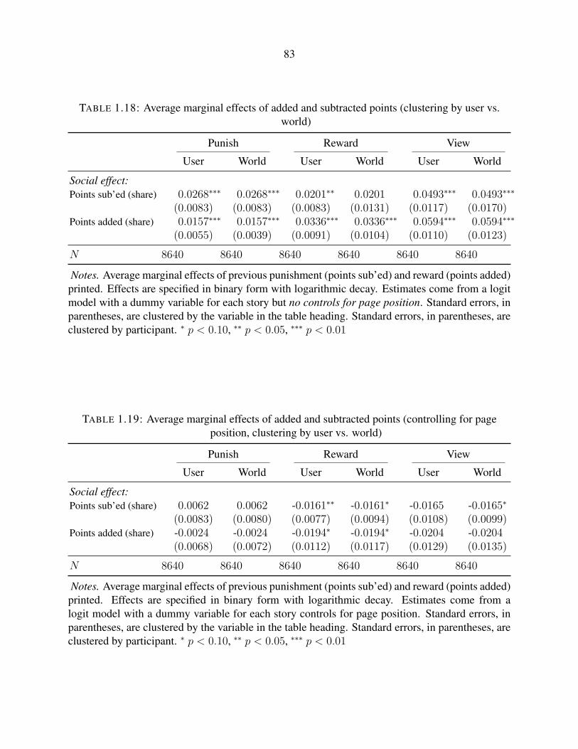
83

TABLE 1.18: Average marginal effects of added and subtracted points (clustering by user vs.world)

Punish Reward View

User World User World User World

Social effect:Points sub’ed (share) 0.0268∗∗∗ 0.0268∗∗∗ 0.0201∗∗ 0.0201 0.0493∗∗∗ 0.0493∗∗∗

(0.0083) (0.0083) (0.0083) (0.0131) (0.0117) (0.0170)Points added (share) 0.0157∗∗∗ 0.0157∗∗∗ 0.0336∗∗∗ 0.0336∗∗∗ 0.0594∗∗∗ 0.0594∗∗∗

(0.0055) (0.0039) (0.0091) (0.0104) (0.0110) (0.0123)

N 8640 8640 8640 8640 8640 8640

Notes. Average marginal effects of previous punishment (points sub’ed) and reward (points added)printed. Effects are specified in binary form with logarithmic decay. Estimates come from a logitmodel with a dummy variable for each story but no controls for page position. Standard errors, inparentheses, are clustered by the variable in the table heading. Standard errors, in parentheses, areclustered by participant. ∗ p < 0.10, ∗∗ p < 0.05, ∗∗∗ p < 0.01

TABLE 1.19: Average marginal effects of added and subtracted points (controlling for pageposition, clustering by user vs. world)

Punish Reward View

User World User World User World

Social effect:Points sub’ed (share) 0.0062 0.0062 -0.0161∗∗ -0.0161∗ -0.0165 -0.0165∗

(0.0083) (0.0080) (0.0077) (0.0094) (0.0108) (0.0099)Points added (share) -0.0024 -0.0024 -0.0194∗ -0.0194∗ -0.0204 -0.0204

(0.0068) (0.0072) (0.0112) (0.0117) (0.0129) (0.0135)

N 8640 8640 8640 8640 8640 8640

Notes. Average marginal effects of previous punishment (points sub’ed) and reward (points added)printed. Effects are specified in binary form with logarithmic decay. Estimates come from alogit model with a dummy variable for each story controls for page position. Standard errors, inparentheses, are clustered by the variable in the table heading. Standard errors, in parentheses, areclustered by participant. ∗ p < 0.10, ∗∗ p < 0.05, ∗∗∗ p < 0.01

84

5 10 15 20 25 30

Participant #

0.0

0.1

0.2

0.3

0.4

0.5

Pre

dic

ted P

(Punis

h)

Raw means

5 10 15 20 25 30

Participant #

0.0

0.1

0.2

0.3

0.4

0.5

Predicted P(Punishment)Binary social effects

(covariates balanced)

5 10 15 20 25 30

Participant #

0.0

0.1

0.2

0.3

0.4

0.5

Predicted P(Punishment)Proportional social effects

(covariates balanced)

Prediction ± 2*SEPunished before

Not punished

FIGURE 1.25: Probability that participant i punishes story k over the course of a social world

85

TABLE 1.20: Linear effects of prior punishment/reward (cond. on viewing)Punishment Reward

Effect SE Effect SE

Effect of prior punishmentParticipant #1 0.2779∗∗∗ (0.0341) −0.2767∗∗∗ (0.0875)2 0.2307∗∗∗ (0.0367) −0.2081∗∗∗ (0.0727)3 0.1869∗∗∗ (0.0358) −0.1574∗∗∗ (0.0601)4 0.1490∗∗∗ (0.0325) −0.1190∗∗ (0.0493)5 0.1173∗∗∗ (0.0283) −0.0892∗∗ (0.0406)6 0.0911∗∗∗ (0.0244) −0.0658∗ (0.0338)7 0.0695∗∗∗ (0.0214) −0.0472 (0.0287)8 0.0517∗∗∗ (0.0192) −0.0323 (0.0250)9 0.0372∗∗ (0.0177) −0.0204 (0.0224)10 0.0254 (0.0166) −0.0109 (0.0204)11 0.0160 (0.0156) −0.0035 (0.0190)12 0.0087 (0.0148) 0.0023 (0.0178)13 0.0031 (0.0140) 0.0067 (0.0168)14 −0.0011 (0.0133) 0.0100 (0.0159)15 −0.0042 (0.0126) 0.0123 (0.0149)16 −0.0063 (0.0119) 0.0139 (0.0141)17 −0.0075 (0.0113) 0.0148 (0.0132)18 −0.0081 (0.0108) 0.0151 (0.0125)19 −0.0081 (0.0104) 0.0149 (0.0118)20 −0.0076 (0.0101) 0.0144 (0.0114)21 −0.0067 (0.0099) 0.0135 (0.0111)22 −0.0055 (0.0100) 0.0123 (0.0111)23 −0.0039 (0.0102) 0.0109 (0.0114)24 −0.0020 (0.0107) 0.0093 (0.0120)25 0.0000 (0.0113) 0.0074 (0.0128)26 0.0024 (0.0121) 0.0055 (0.0138)27 0.0048 (0.0130) 0.0034 (0.0150)28 0.0075 (0.0140) 0.0011 (0.0163)29 0.0103 (0.0151) −0.0012 (0.0178)30 0.0132 (0.0162) −0.0036 (0.0193)

Effect of prior rewardParticipant #1 −0.0180 (0.0552) 0.0242 (0.0658)2 −0.0086 (0.0455) 0.0112 (0.0503)3 −0.0015 (0.0375) 0.0027 (0.0392)4 0.0037 (0.0312) −0.0030 (0.0314)5 0.0074 (0.0264) −0.0069 (0.0259)6 0.0100 (0.0228) −0.0094 (0.0220)7 0.0116 (0.0201) −0.0111 (0.0192)8 0.0125 (0.0181) −0.0120 (0.0172)9 0.0129 (0.0165) −0.0124 (0.0158)10 0.0128 (0.0152) −0.0123 (0.0146)11 0.0123 (0.0141) −0.0119 (0.0137)12 0.0116 (0.0131) −0.0113 (0.0128)13 0.0107 (0.0122) −0.0105 (0.0120)14 0.0097 (0.0115) −0.0096 (0.0113)15 0.0086 (0.0107) −0.0085 (0.0107)16 0.0074 (0.0101) −0.0074 (0.0101)17 0.0062 (0.0095) −0.0062 (0.0096)18 0.0049 (0.0090) −0.0049 (0.0091)19 0.0036 (0.0086) −0.0037 (0.0088)20 0.0023 (0.0084) −0.0024 (0.0085)21 0.0010 (0.0082) −0.0011 (0.0084)22 −0.0003 (0.0082) 0.0002 (0.0085)23 −0.0017 (0.0084) 0.0015 (0.0087)24 −0.0030 (0.0087) 0.0029 (0.0090)25 −0.0044 (0.0091) 0.0042 (0.0094)26 −0.0058 (0.0097) 0.0055 (0.0100)27 −0.0071 (0.0103) 0.0068 (0.0106)28 −0.0085 (0.0110) 0.0081 (0.0113)29 −0.0098 (0.0117) 0.0093 (0.0120)30 −0.0111 (0.0125) 0.0106 (0.0128)

Avg. log-like. −0.50844 −0.59997

Notes. Table displays estimated marginal effects. Models (1,202 obs., 480 individuals) include dummy variables for each story and a quadraticeffect of page position. Standard errors, in parentheses, are clustered by individual. ∗ p < 0.10, ∗∗ p < 0.05, ∗∗∗ p < 0.01

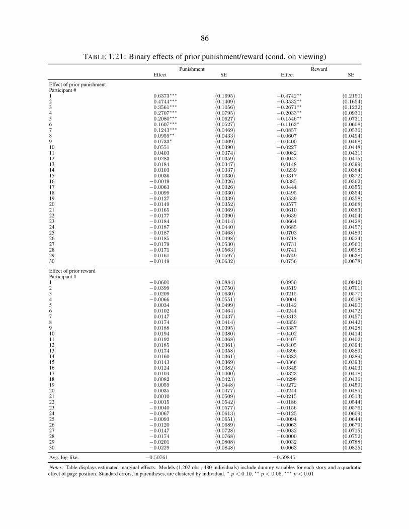
86

TABLE 1.21: Binary effects of prior punishment/reward (cond. on viewing)Punishment Reward

Effect SE Effect SE

Effect of prior punishmentParticipant #1 0.6373∗∗∗ (0.1695) −0.4742∗∗ (0.2150)2 0.4744∗∗∗ (0.1409) −0.3532∗∗ (0.1654)3 0.3561∗∗∗ (0.1056) −0.2671∗∗ (0.1232)4 0.2707∗∗∗ (0.0795) −0.2033∗∗ (0.0930)5 0.2080∗∗∗ (0.0627) −0.1546∗∗ (0.0731)6 0.1607∗∗∗ (0.0527) −0.1163∗ (0.0608)7 0.1243∗∗∗ (0.0469) −0.0857 (0.0536)8 0.0959∗∗ (0.0433) −0.0607 (0.0494)9 0.0733∗ (0.0409) −0.0400 (0.0468)10 0.0551 (0.0390) −0.0227 (0.0448)11 0.0403 (0.0374) −0.0082 (0.0431)12 0.0283 (0.0359) 0.0042 (0.0415)13 0.0184 (0.0347) 0.0148 (0.0399)14 0.0103 (0.0337) 0.0239 (0.0384)15 0.0036 (0.0330) 0.0317 (0.0372)16 −0.0019 (0.0326) 0.0385 (0.0362)17 −0.0063 (0.0326) 0.0444 (0.0355)18 −0.0099 (0.0330) 0.0495 (0.0354)19 −0.0127 (0.0339) 0.0539 (0.0358)20 −0.0149 (0.0352) 0.0577 (0.0368)21 −0.0165 (0.0369) 0.0610 (0.0383)22 −0.0177 (0.0390) 0.0639 (0.0404)23 −0.0184 (0.0414) 0.0664 (0.0428)24 −0.0187 (0.0440) 0.0685 (0.0457)25 −0.0187 (0.0468) 0.0703 (0.0489)26 −0.0185 (0.0498) 0.0718 (0.0524)27 −0.0179 (0.0530) 0.0731 (0.0560)28 −0.0171 (0.0563) 0.0741 (0.0598)29 −0.0161 (0.0597) 0.0749 (0.0638)30 −0.0149 (0.0632) 0.0756 (0.0678)

Effect of prior rewardParticipant #1 −0.0601 (0.0884) 0.0950 (0.0942)2 −0.0399 (0.0750) 0.0519 (0.0701)3 −0.0209 (0.0630) 0.0215 (0.0577)4 −0.0066 (0.0551) 0.0004 (0.0518)5 0.0034 (0.0499) −0.0142 (0.0490)6 0.0102 (0.0464) −0.0244 (0.0472)7 0.0147 (0.0437) −0.0313 (0.0457)8 0.0174 (0.0414) −0.0359 (0.0442)9 0.0188 (0.0395) −0.0387 (0.0428)10 0.0194 (0.0380) −0.0402 (0.0414)11 0.0192 (0.0368) −0.0407 (0.0402)12 0.0185 (0.0361) −0.0405 (0.0394)13 0.0174 (0.0358) −0.0396 (0.0389)14 0.0160 (0.0361) −0.0383 (0.0389)15 0.0143 (0.0369) −0.0366 (0.0393)16 0.0124 (0.0382) −0.0345 (0.0403)17 0.0104 (0.0400) −0.0323 (0.0418)18 0.0082 (0.0423) −0.0298 (0.0436)19 0.0059 (0.0448) −0.0272 (0.0459)20 0.0035 (0.0477) −0.0244 (0.0485)21 0.0010 (0.0509) −0.0215 (0.0513)22 −0.0015 (0.0542) −0.0186 (0.0544)23 −0.0040 (0.0577) −0.0156 (0.0576)24 −0.0067 (0.0613) −0.0125 (0.0609)25 −0.0093 (0.0651) −0.0094 (0.0644)26 −0.0120 (0.0689) −0.0063 (0.0679)27 −0.0147 (0.0728) −0.0032 (0.0715)28 −0.0174 (0.0768) −0.0000 (0.0752)29 −0.0201 (0.0808) 0.0032 (0.0788)30 −0.0229 (0.0848) 0.0063 (0.0825)

Avg. log-like. −0.50761 −0.59845

Notes. Table displays estimated marginal effects. Models (1,202 obs., 480 individuals) include dummy variables for each story and a quadraticeffect of page position. Standard errors, in parentheses, are clustered by individual. ∗ p < 0.10, ∗∗ p < 0.05, ∗∗∗ p < 0.01

87

TABLE 1.22: Log effects of prior punishment/reward on individual behavior (cond. on viewing)Punishment Reward

Effect SE Effect SE

Effect of prior punishmentParticipant #1 0.5885∗∗ (0.2434) −0.9459∗∗ (0.4775)2 0.4732∗∗∗ (0.1300) −0.6429∗∗ (0.2906)3 0.3864∗∗∗ (0.1141) −0.4712∗∗ (0.1943)4 0.3061∗∗∗ (0.1036) −0.3544∗∗ (0.1477)5 0.2349∗∗∗ (0.0879) −0.2629∗∗ (0.1187)6 0.1748∗∗ (0.0720) −0.1880∗∗ (0.0956)7 0.1257∗∗ (0.0593) −0.1269 (0.0772)8 0.0863∗ (0.0509) −0.0775 (0.0640)9 0.0549 (0.0461) −0.0379 (0.0559)10 0.0301 (0.0436) −0.0066 (0.0514)11 0.0106 (0.0423) 0.0180 (0.0491)12 −0.0047 (0.0414) 0.0372 (0.0478)13 −0.0165 (0.0404) 0.0519 (0.0466)14 −0.0255 (0.0394) 0.0630 (0.0453)15 −0.0322 (0.0382) 0.0711 (0.0437)16 −0.0369 (0.0369) 0.0767∗ (0.0419)17 −0.0400 (0.0356) 0.0802∗∗ (0.0400)18 −0.0418 (0.0344) 0.0820∗∗ (0.0383)19 −0.0424 (0.0335) 0.0822∗∗ (0.0368)20 −0.0420 (0.0330) 0.0813∗∗ (0.0359)21 −0.0408 (0.0329) 0.0792∗∗ (0.0357)22 −0.0387 (0.0334) 0.0762∗∗ (0.0364)23 −0.0361 (0.0347) 0.0724∗ (0.0381)24 −0.0328 (0.0365) 0.0679∗ (0.0408)25 −0.0290 (0.0390) 0.0628 (0.0444)26 −0.0248 (0.0420) 0.0571 (0.0487)27 −0.0201 (0.0455) 0.0510 (0.0535)28 −0.0151 (0.0495) 0.0444 (0.0589)29 −0.0098 (0.0537) 0.0375 (0.0646)30 −0.0042 (0.0582) 0.0303 (0.0707)

Effect of prior rewardParticipant #1 −0.0127 (0.1576) −0.0641 (0.2411)2 −0.0029 (0.1250) −0.0592 (0.1574)3 0.0030 (0.1014) −0.0556 (0.1131)4 0.0063 (0.0823) −0.0523 (0.0868)5 0.0076 (0.0677) −0.0483 (0.0698)6 0.0073 (0.0574) −0.0436 (0.0587)7 0.0061 (0.0506) −0.0383 (0.0517)8 0.0043 (0.0461) −0.0329 (0.0474)9 0.0020 (0.0431) −0.0276 (0.0447)10 −0.0006 (0.0409) −0.0223 (0.0428)11 −0.0033 (0.0392) −0.0173 (0.0413)12 −0.0061 (0.0377) −0.0125 (0.0398)13 −0.0090 (0.0363) −0.0079 (0.0384)14 −0.0119 (0.0351) −0.0035 (0.0370)15 −0.0149 (0.0339) 0.0007 (0.0356)16 −0.0178 (0.0329) 0.0046 (0.0344)17 −0.0208 (0.0322) 0.0085 (0.0333)18 −0.0238 (0.0317) 0.0121 (0.0326)19 −0.0267 (0.0315) 0.0157 (0.0322)20 −0.0297 (0.0316) 0.0191 (0.0322)21 −0.0326 (0.0322) 0.0223 (0.0328)22 −0.0355 (0.0331) 0.0255 (0.0338)23 −0.0383 (0.0344) 0.0286 (0.0353)24 −0.0412 (0.0361) 0.0316 (0.0372)25 −0.0440 (0.0381) 0.0345 (0.0394)26 −0.0468 (0.0403) 0.0373 (0.0420)27 −0.0496 (0.0428) 0.0400 (0.0449)28 −0.0523 (0.0454) 0.0426 (0.0480)29 −0.0551 (0.0482) 0.0452 (0.0512)30 −0.0577 (0.0512) 0.0477 (0.0546)

Avg. log-like. −0.51108 −0.59925

Notes. Table displays estimated marginal effects. Models (1,202 obs., 480 individuals) include dummy variables for each story and a quadraticeffect of page position. Standard errors, in parentheses, are clustered by individual. ∗ p < 0.10, ∗∗ p < 0.05, ∗∗∗ p < 0.01

88

TABLE 1.23: Linear effects of prior punishment/reward on individual behavior (unconditional)Punishment Reward Viewing

Effect SE Effect SE Effect SE

Effect of prior punishmentParticipant #1 0.0470 (0.0305) −0.0438 (0.0275) −0.0023 (0.0354)2 0.0331 (0.0202) −0.0379∗ (0.0201) −0.0077 (0.0256)3 0.0233 (0.0146) −0.0325∗∗ (0.0155) −0.0108 (0.0193)4 0.0158 (0.0109) −0.0278∗∗ (0.0124) −0.0126 (0.0151)5 0.0104 (0.0082) −0.0238∗∗ (0.0102) −0.0135 (0.0122)6 0.0065 (0.0063) −0.0204∗∗ (0.0086) −0.0139 (0.0102)7 0.0037 (0.0051) −0.0175∗∗ (0.0075) −0.0139 (0.0089)8 0.0016 (0.0043) −0.0150∗∗ (0.0066) −0.0137∗ (0.0080)9 0.0002 (0.0038) −0.0129∗∗ (0.0060) −0.0133∗ (0.0073)10 −0.0009 (0.0034) −0.0110∗∗ (0.0056) −0.0128∗ (0.0068)11 −0.0017 (0.0032) −0.0094∗ (0.0052) −0.0122∗ (0.0064)12 −0.0022 (0.0030) −0.0079 (0.0050) −0.0116∗ (0.0061)13 −0.0026 (0.0028) −0.0067 (0.0047) −0.0109∗ (0.0058)14 −0.0028 (0.0027) −0.0056 (0.0045) −0.0103∗ (0.0055)15 −0.0029 (0.0025) −0.0046 (0.0043) −0.0095∗ (0.0053)16 −0.0030 (0.0024) −0.0038 (0.0040) −0.0088∗ (0.0050)17 −0.0029 (0.0023) −0.0031 (0.0038) −0.0081∗ (0.0047)18 −0.0028 (0.0022) −0.0024 (0.0036) −0.0074 (0.0045)19 −0.0027 (0.0022) −0.0019 (0.0035) −0.0067 (0.0043)20 −0.0025 (0.0021) −0.0014 (0.0033) −0.0060 (0.0041)21 −0.0022 (0.0021) −0.0009 (0.0032) −0.0053 (0.0040)22 −0.0020 (0.0020) −0.0006 (0.0031) −0.0046 (0.0039)23 −0.0017 (0.0020) −0.0003 (0.0031) −0.0039 (0.0038)24 −0.0014 (0.0020) 0.0000 (0.0032) −0.0033 (0.0038)25 −0.0010 (0.0021) 0.0002 (0.0033) −0.0026 (0.0039)26 −0.0007 (0.0021) 0.0004 (0.0035) −0.0020 (0.0040)27 −0.0004 (0.0022) 0.0006 (0.0038) −0.0014 (0.0042)28 0.0000 (0.0023) 0.0007 (0.0040) −0.0008 (0.0044)29 0.0004 (0.0025) 0.0008 (0.0044) −0.0002 (0.0046)30 0.0008 (0.0026) 0.0009 (0.0047) 0.0004 (0.0049)

Effect of prior rewardParticipant #1 −0.0094 (0.0155) −0.0063 (0.0105) −0.0120 (0.0221)2 −0.0070 (0.0123) −0.0088 (0.0083) −0.0145 (0.0170)3 −0.0052 (0.0098) −0.0102 (0.0069) −0.0154 (0.0135)4 −0.0038 (0.0078) −0.0110∗ (0.0060) −0.0155 (0.0112)5 −0.0027 (0.0064) −0.0113∗∗ (0.0054) −0.0151 (0.0095)6 −0.0019 (0.0053) −0.0113∗∗ (0.0050) −0.0145∗ (0.0083)7 −0.0013 (0.0046) −0.0111∗∗ (0.0047) −0.0137∗ (0.0075)8 −0.0008 (0.0041) −0.0108∗∗ (0.0045) −0.0129∗ (0.0069)9 −0.0005 (0.0037) −0.0104∗∗ (0.0043) −0.0120∗ (0.0064)10 −0.0002 (0.0034) −0.0099∗∗ (0.0042) −0.0111∗ (0.0060)11 −0.0000 (0.0032) −0.0094∗∗ (0.0040) −0.0102∗ (0.0057)12 0.0001 (0.0030) −0.0088∗∗ (0.0039) −0.0092∗ (0.0054)13 0.0003 (0.0028) −0.0082∗∗ (0.0038) −0.0083 (0.0051)14 0.0004 (0.0026) −0.0076∗∗ (0.0036) −0.0075 (0.0048)15 0.0004 (0.0025) −0.0070∗∗ (0.0035) −0.0066 (0.0046)16 0.0005 (0.0023) −0.0064∗ (0.0034) −0.0058 (0.0044)17 0.0005 (0.0022) −0.0058∗ (0.0032) −0.0049 (0.0042)18 0.0006 (0.0021) −0.0051∗ (0.0031) −0.0042 (0.0039)19 0.0006 (0.0020) −0.0045 (0.0030) −0.0034 (0.0038)20 0.0006 (0.0019) −0.0039 (0.0029) −0.0026 (0.0036)21 0.0006 (0.0018) −0.0033 (0.0028) −0.0019 (0.0034)22 0.0006 (0.0018) −0.0027 (0.0027) −0.0012 (0.0033)23 0.0006 (0.0018) −0.0021 (0.0026) −0.0006 (0.0032)24 0.0005 (0.0018) −0.0016 (0.0025) 0.0001 (0.0032)25 0.0005 (0.0018) −0.0010 (0.0025) 0.0007 (0.0032)26 0.0005 (0.0018) −0.0005 (0.0025) 0.0013 (0.0032)27 0.0004 (0.0019) 0.0001 (0.0025) 0.0019 (0.0032)28 0.0004 (0.0020) 0.0006 (0.0025) 0.0025 (0.0033)29 0.0004 (0.0021) 0.0011 (0.0026) 0.0031 (0.0035)30 0.0003 (0.0022) 0.0016 (0.0027) 0.0036 (0.0036)

Avg. log-like. −0.14184 −0.24959 −0.35528

Notes. Table displays estimated marginal effects. Models (8,640 obs., 480 individuals) include dummy variables for each story and a quadraticeffect of page position. Standard errors, in parentheses, are clustered by individual. ∗ p < 0.10, ∗∗ p < 0.05, ∗∗∗ p < 0.01

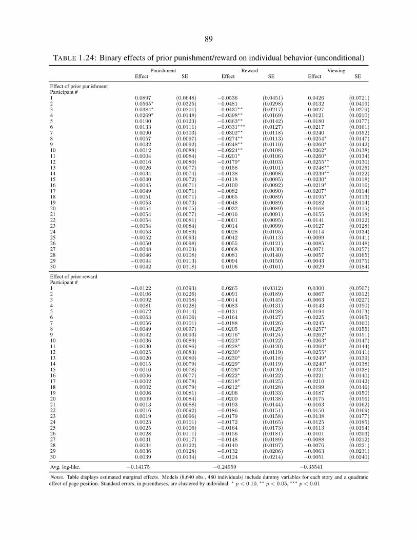
89

TABLE 1.24: Binary effects of prior punishment/reward on individual behavior (unconditional)Punishment Reward Viewing

Effect SE Effect SE Effect SE

Effect of prior punishmentParticipant #1 0.0897 (0.0648) −0.0536 (0.0451) 0.0426 (0.0721)2 0.0565∗ (0.0325) −0.0481 (0.0298) 0.0132 (0.0419)3 0.0384∗ (0.0201) −0.0437∗∗ (0.0217) −0.0027 (0.0279)4 0.0269∗ (0.0148) −0.0398∗∗ (0.0169) −0.0121 (0.0210)5 0.0190 (0.0123) −0.0363∗∗ (0.0142) −0.0180 (0.0177)6 0.0133 (0.0111) −0.0331∗∗∗ (0.0127) −0.0217 (0.0161)7 0.0090 (0.0103) −0.0302∗∗ (0.0118) −0.0240 (0.0152)8 0.0057 (0.0097) −0.0274∗∗ (0.0113) −0.0254∗ (0.0147)9 0.0032 (0.0092) −0.0248∗∗ (0.0110) −0.0260∗ (0.0142)10 0.0012 (0.0088) −0.0224∗∗ (0.0108) −0.0262∗ (0.0138)11 −0.0004 (0.0084) −0.0201∗ (0.0106) −0.0260∗ (0.0134)12 −0.0016 (0.0080) −0.0179∗ (0.0103) −0.0255∗∗ (0.0130)13 −0.0026 (0.0077) −0.0158 (0.0101) −0.0248∗∗ (0.0126)14 −0.0034 (0.0074) −0.0138 (0.0098) −0.0239∗∗ (0.0122)15 −0.0040 (0.0072) −0.0118 (0.0095) −0.0230∗ (0.0118)16 −0.0045 (0.0071) −0.0100 (0.0092) −0.0219∗ (0.0116)17 −0.0049 (0.0071) −0.0082 (0.0090) −0.0207∗ (0.0114)18 −0.0051 (0.0071) −0.0065 (0.0089) −0.0195∗ (0.0113)19 −0.0053 (0.0073) −0.0048 (0.0089) −0.0182 (0.0114)20 −0.0054 (0.0075) −0.0032 (0.0089) −0.0168 (0.0115)21 −0.0054 (0.0077) −0.0016 (0.0091) −0.0155 (0.0118)22 −0.0054 (0.0081) −0.0001 (0.0095) −0.0141 (0.0122)23 −0.0054 (0.0084) 0.0014 (0.0099) −0.0127 (0.0128)24 −0.0053 (0.0089) 0.0028 (0.0105) −0.0114 (0.0134)25 −0.0052 (0.0093) 0.0042 (0.0113) −0.0099 (0.0141)26 −0.0050 (0.0098) 0.0055 (0.0121) −0.0085 (0.0148)27 −0.0048 (0.0103) 0.0068 (0.0130) −0.0071 (0.0157)28 −0.0046 (0.0108) 0.0081 (0.0140) −0.0057 (0.0165)29 −0.0044 (0.0113) 0.0094 (0.0150) −0.0043 (0.0175)30 −0.0042 (0.0118) 0.0106 (0.0161) −0.0029 (0.0184)

Effect of prior rewardParticipant #1 −0.0122 (0.0393) 0.0265 (0.0312) 0.0300 (0.0507)2 −0.0106 (0.0226) 0.0091 (0.0189) 0.0067 (0.0312)3 −0.0092 (0.0158) −0.0014 (0.0145) −0.0063 (0.0227)4 −0.0081 (0.0128) −0.0083 (0.0131) −0.0143 (0.0190)5 −0.0072 (0.0114) −0.0131 (0.0128) −0.0194 (0.0173)6 −0.0063 (0.0106) −0.0164 (0.0127) −0.0225 (0.0165)7 −0.0056 (0.0101) −0.0188 (0.0126) −0.0245 (0.0160)8 −0.0049 (0.0097) −0.0205 (0.0125) −0.0257∗ (0.0155)9 −0.0042 (0.0093) −0.0216∗ (0.0124) −0.0262∗ (0.0151)10 −0.0036 (0.0089) −0.0223∗ (0.0122) −0.0263∗ (0.0147)11 −0.0030 (0.0086) −0.0228∗ (0.0120) −0.0260∗ (0.0144)12 −0.0025 (0.0083) −0.0230∗ (0.0119) −0.0255∗ (0.0141)13 −0.0020 (0.0080) −0.0230∗ (0.0118) −0.0249∗ (0.0139)14 −0.0015 (0.0079) −0.0229∗ (0.0119) −0.0240∗ (0.0138)15 −0.0010 (0.0078) −0.0226∗ (0.0120) −0.0231∗ (0.0138)16 −0.0006 (0.0077) −0.0222∗ (0.0122) −0.0221 (0.0140)17 −0.0002 (0.0078) −0.0218∗ (0.0125) −0.0210 (0.0142)18 0.0002 (0.0079) −0.0212∗ (0.0128) −0.0199 (0.0146)19 0.0006 (0.0081) −0.0206 (0.0133) −0.0187 (0.0150)20 0.0009 (0.0084) −0.0200 (0.0138) −0.0175 (0.0156)21 0.0013 (0.0088) −0.0193 (0.0144) −0.0163 (0.0162)22 0.0016 (0.0092) −0.0186 (0.0151) −0.0150 (0.0169)23 0.0019 (0.0096) −0.0179 (0.0158) −0.0138 (0.0177)24 0.0023 (0.0101) −0.0172 (0.0165) −0.0125 (0.0185)25 0.0025 (0.0106) −0.0164 (0.0173) −0.0113 (0.0194)26 0.0028 (0.0111) −0.0156 (0.0181) −0.0101 (0.0203)27 0.0031 (0.0117) −0.0148 (0.0189) −0.0088 (0.0212)28 0.0034 (0.0122) −0.0140 (0.0197) −0.0076 (0.0221)29 0.0036 (0.0128) −0.0132 (0.0206) −0.0063 (0.0231)30 0.0039 (0.0134) −0.0124 (0.0214) −0.0051 (0.0240)

Avg. log-like. −0.14175 −0.24959 −0.35541

Notes. Table displays estimated marginal effects. Models (8,640 obs., 480 individuals) include dummy variables for each story and a quadraticeffect of page position. Standard errors, in parentheses, are clustered by individual. ∗ p < 0.10, ∗∗ p < 0.05, ∗∗∗ p < 0.01

90

TABLE 1.25: Log effects of prior punishment/reward on individual behavior (unconditional)Punishment Reward Viewing

Effect SE Effect SE Effect SE

Effect of prior punishmentParticipant #1 0.1019 (0.0827) −0.0816 (0.0785) 0.0815 (0.1401)2 0.0660 (0.0559) −0.0709 (0.0590) 0.0492 (0.0981)3 0.0434 (0.0361) −0.0598 (0.0448) 0.0274 (0.0704)4 0.0285 (0.0245) −0.0498 (0.0347) 0.0126 (0.0519)5 0.0180 (0.0177) −0.0410 (0.0274) 0.0024 (0.0394)6 0.0104 (0.0137) −0.0333 (0.0224) −0.0045 (0.0312)7 0.0047 (0.0115) −0.0267 (0.0190) −0.0093 (0.0258)8 0.0004 (0.0102) −0.0210 (0.0169) −0.0125 (0.0224)9 −0.0030 (0.0094) −0.0161 (0.0155) −0.0144 (0.0202)10 −0.0055 (0.0089) −0.0117 (0.0146) −0.0155 (0.0188)11 −0.0075 (0.0085) −0.0080 (0.0139) −0.0159 (0.0178)12 −0.0090 (0.0081) −0.0046 (0.0134) −0.0158 (0.0169)13 −0.0101 (0.0078) −0.0017 (0.0128) −0.0154 (0.0162)14 −0.0109 (0.0075) 0.0008 (0.0122) −0.0146 (0.0154)15 −0.0115 (0.0072) 0.0031 (0.0116) −0.0136 (0.0147)16 −0.0119∗ (0.0070) 0.0051 (0.0110) −0.0124 (0.0140)17 −0.0120∗ (0.0068) 0.0068 (0.0104) −0.0111 (0.0134)18 −0.0121∗ (0.0066) 0.0084 (0.0099) −0.0097 (0.0128)19 −0.0120∗ (0.0064) 0.0098 (0.0094) −0.0082 (0.0123)20 −0.0118∗ (0.0064) 0.0110 (0.0090) −0.0066 (0.0119)21 −0.0116∗ (0.0064) 0.0121 (0.0088) −0.0050 (0.0116)22 −0.0112∗ (0.0064) 0.0131 (0.0087) −0.0034 (0.0116)23 −0.0108∗ (0.0066) 0.0139 (0.0089) −0.0018 (0.0117)24 −0.0104 (0.0068) 0.0147 (0.0092) −0.0001 (0.0120)25 −0.0099 (0.0071) 0.0154 (0.0096) 0.0015 (0.0125)26 −0.0094 (0.0074) 0.0159 (0.0102) 0.0031 (0.0131)27 −0.0088 (0.0078) 0.0165 (0.0110) 0.0047 (0.0139)28 −0.0082 (0.0082) 0.0169 (0.0118) 0.0063 (0.0147)29 −0.0076 (0.0087) 0.0173 (0.0127) 0.0079 (0.0157)30 −0.0070 (0.0092) 0.0177 (0.0137) 0.0094 (0.0167)

Effect of prior rewardParticipant #1 −0.0267 (0.0372) −0.0315 (0.0337) −0.0563 (0.0629)2 −0.0200 (0.0246) −0.0303 (0.0265) −0.0487 (0.0465)3 −0.0156 (0.0177) −0.0278 (0.0210) −0.0413 (0.0353)4 −0.0125 (0.0137) −0.0248 (0.0172) −0.0346 (0.0279)5 −0.0102 (0.0114) −0.0219 (0.0148) −0.0288 (0.0232)6 −0.0085 (0.0100) −0.0190 (0.0133) −0.0237 (0.0203)7 −0.0071 (0.0093) −0.0163 (0.0124) −0.0192 (0.0185)8 −0.0060 (0.0088) −0.0138 (0.0118) −0.0152 (0.0173)9 −0.0051 (0.0084) −0.0114 (0.0114) −0.0117 (0.0164)10 −0.0043 (0.0082) −0.0092 (0.0111) −0.0086 (0.0156)11 −0.0037 (0.0079) −0.0072 (0.0107) −0.0058 (0.0150)12 −0.0032 (0.0077) −0.0054 (0.0103) −0.0033 (0.0143)13 −0.0027 (0.0074) −0.0037 (0.0100) −0.0010 (0.0136)14 −0.0023 (0.0072) −0.0021 (0.0096) 0.0011 (0.0130)15 −0.0020 (0.0069) −0.0006 (0.0092) 0.0030 (0.0124)16 −0.0017 (0.0067) 0.0008 (0.0088) 0.0047 (0.0118)17 −0.0014 (0.0065) 0.0021 (0.0084) 0.0063 (0.0113)18 −0.0012 (0.0063) 0.0032 (0.0081) 0.0078 (0.0108)19 −0.0010 (0.0062) 0.0043 (0.0079) 0.0091 (0.0105)20 −0.0009 (0.0061) 0.0054 (0.0077) 0.0103 (0.0103)21 −0.0007 (0.0061) 0.0063 (0.0076) 0.0115 (0.0102)22 −0.0006 (0.0062) 0.0072 (0.0077) 0.0125 (0.0102)23 −0.0005 (0.0063) 0.0081 (0.0078) 0.0135 (0.0104)24 −0.0004 (0.0064) 0.0088 (0.0080) 0.0144 (0.0107)25 −0.0004 (0.0066) 0.0096 (0.0082) 0.0153 (0.0111)26 −0.0003 (0.0069) 0.0103 (0.0086) 0.0161 (0.0117)27 −0.0002 (0.0072) 0.0109 (0.0090) 0.0168 (0.0123)28 −0.0002 (0.0075) 0.0115 (0.0095) 0.0175 (0.0129)29 −0.0002 (0.0079) 0.0121 (0.0100) 0.0181 (0.0136)30 −0.0001 (0.0082) 0.0126 (0.0106) 0.0187 (0.0144)

Avg. log-like. −0.14195 −0.24975 −0.35554

Notes. Table displays estimated marginal effects. Models (8,640 obs., 480 individuals) include dummy variables for each story and a quadraticeffect of page position. Standard errors, in parentheses, are clustered by individual. ∗ p < 0.10, ∗∗ p < 0.05, ∗∗∗ p < 0.01

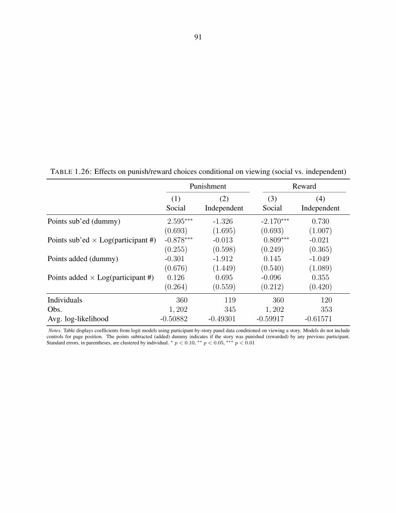
91

TABLE 1.26: Effects on punish/reward choices conditional on viewing (social vs. independent)

Punishment Reward

(1) (2) (3) (4)Social Independent Social Independent

Points sub’ed (dummy) 2.595∗∗∗ -1.326 -2.170∗∗∗ 0.730(0.693) (1.695) (0.693) (1.007)

Points sub’ed × Log(participant #) -0.878∗∗∗ -0.013 0.809∗∗∗ -0.021(0.255) (0.598) (0.249) (0.365)

Points added (dummy) -0.301 -1.912 0.145 -1.049(0.676) (1.449) (0.540) (1.089)

Points added × Log(participant #) 0.126 0.695 -0.096 0.355(0.264) (0.559) (0.212) (0.420)

Individuals 360 119 360 120Obs. 1, 202 345 1, 202 353Avg. log-likelihood -0.50882 -0.49301 -0.59917 -0.61571Notes. Table displays coefficients from logit models using participant-by-story panel data conditioned on viewing a story. Models do not include

controls for page position. The points subtracted (added) dummy indicates if the story was punished (rewarded) by any previous participant.Standard errors, in parentheses, are clustered by individual. ∗ p < 0.10, ∗∗ p < 0.05, ∗∗∗ p < 0.01

92

FIGURE 1.26: Bivariate histogram of 50,000 resampled independent worlds vs. observed socialworlds

Figure 1.26 shows the results of drawing 50,000 worlds from the independent worlds re-

sampling distribution. The distribution of net reward and net punishment is plotted as a bivariate

histogram (heatmap). The observed values from the 12 social worlds at overlaid as red points.

The most evident pattern is that the realizations of net punishment in the social worlds are highly

dispersed, with many of the observations lying in regions where the re-sampling distribution has

low density.

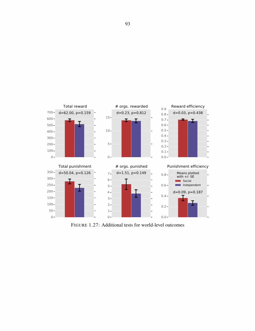
93

0

100

200

300

400

500

600

700 d=62.00, p=0.159

Total reward

0

5

10

15d=0.23, p=0.812

# orgs. rewarded

0.0

0.1

0.2

0.3

0.4

0.5

0.6

0.7

0.8

0.9d=0.03, p=0.438

Reward efficiency

0

50

100

150

200

250

300

350 d=50.04, p=0.126

Total punishment

0

1

2

3

4

5

6

7 d=1.51, p=0.149

# orgs. punished

0.0

0.2

0.4

0.6

0.8

d=0.09, p=0.187

Punishment efficiency

Means plottedwith +/- SE

Social

Independent

FIGURE 1.27: Additional tests for world-level outcomes

94

0 1 2 3 4 5 6

0.0

0.2

0.4

0.6

0.8

1.0

0.0 0.5 1.0 1.5 2.0 2.5

0.0

0.2

0.4

0.6

0.8

1.0

0.0 0.2 0.4 0.6 0.8 1.0 1.2 1.4

0.0

0.2

0.4

0.6

0.8

1.0

0.0 0.1 0.2 0.3 0.4 0.5 0.6

0.0

0.2

0.4

0.6

0.8

1.0

0 1 2 3 4 5 6 7 8

0.0

0.2

0.4

0.6

0.8

1.0

0 2 4 6 8 10 12

0.0

0.2

0.4

0.6

0.8

1.0

0.0 0.5 1.0 1.5 2.0 2.5 3.0

0.0

0.2

0.4

0.6

0.8

1.0

0 1 2 3 4 5

0.0

0.2

0.4

0.6

0.8

1.0

0.0 0.5 1.0 1.5 2.0

0.0

0.2

0.4

0.6

0.8

1.0

0.0 0.5 1.0 1.5 2.0 2.5 3.0 3.5

0.0

0.2

0.4

0.6

0.8

1.0

Dis

tance

fro

m t

op o

f headlin

es

page (

norm

aliz

ed)

0 1 2 3 4

Time elapsed since entering news site (minutes)[Breaks are visits to news stories]

0.0

0.2

0.4

0.6

0.8

1.0

0.0 0.5 1.0 1.5 2.0 2.5 3.0 3.5

0.0

0.2

0.4

0.6

0.8

1.0

FIGURE 1.28: Search behavior of 12 individuals on the headlines page

95

01

02

03

04

05

06

07

08

09

0

Mean t

ota

l re

ward

Art

ist

colle

ctiv

e s

ues

non p

rofit

over

"bookl

yn"

copyri

ght

A m

anifest

o f

or

pla

yin

g g

od w

ith h

um

an e

volu

tion

Cu b

ould

er

scie

nti

sts

speak

out

on r

ese

arc

h m

isco

nduct

cla

im

Unesc

o t

o h

ost

meeti

ng o

n c

ontr

overs

ial 'm

em

ory

of

wate

r' r

ese

arc

h

U.

of

i. d

oct

ors

under

scru

tiny f

or

surg

ical ro

bot

ad

Vid

eos

of

rat

abuse

at

peta

lum

a h

igh s

chool pro

mpt

outc

ry

Federa

l agency

defe

nds

use

of

duck

s unlim

ited

How

to s

ave d

art

moor'

s hill

ponie

s? e

at

them

, sa

ys

anim

al co

nse

rvati

on g

roup

So y

ou w

ant

to liv

e f

ore

ver

How

web a

rchiv

ists

and o

ther

dig

ital sl

euth

s are

unra

velin

g t

he m

yst

ery

of

mh1

7

Searc

h a

nd r

esc

ue d

rones

fly a

gain

aft

er

court

thro

ws

out

faa c

ase

Shooti

ng c

linic

for

the b

lind

Your

bra

in's

ele

ctri

cal act

ivit

y c

an p

redic

t w

heth

er

you g

o f

or

risk

y s

ex,

ucl

a s

tudy f

inds

Cle

mso

n u

niv

ers

ity s

tops

mandato

ry 'se

x s

urv

ey' aft

er

back

lash

Rip

ple

cre

ato

r donate

s $

50

0k

in x

rp t

o a

rtific

ial in

telli

gence

rese

arc

h c

hari

ty

Pro

p 4

6 c

alls

for

physi

cian d

rug t

est

ing,

$1

.1 m

illio

n law

suit

cap

What

is t

or?

a b

egin

ner'

s guid

e t

o t

he p

rivacy

tool

Should

we m

ake

anim

als

sm

art

er?

A 'su

icid

e c

lub' has

been launch

ed in b

rita

in b

y a

ust

ralia

's d

r. d

eath

, to

help

people

kill

them

selv

es

Aim

ing f

or

a b

ear:

7 y

ear

old

alt

o b

oy g

oes

on h

unt

of

a lifeti

me

Should

hum

anit

y t

ry t

o c

onta

ct inte

lligent

alie

ns?

Firs

t ls

d s

tudy in 4

0 y

ears

fin

ds

thera

peuti

c pote

nti

al

The r

ise o

f 'v

igila

nte

' patr

ols

on t

he s

treets

of

new

york

Nonpro

fit

gro

up g

ives

hundre

ds

of

vete

rans

free m

ari

juana

Headline

FIG

UR

E1.

29:

Mea

nto

talr

ewar

dby

stor

y

96

05

10

15

20

25

30

35

40

45

Mean t

ota

l punis

hm

ent

How

web a

rchiv

ists

and o

ther

dig

ital sl

euth

s are

unra

velin

g t

he m

yst

ery

of

mh1

7

What

is t

or?

a b

egin

ner'

s guid

e t

o t

he p

rivacy

tool

Rip

ple

cre

ato

r donate

s $

50

0k

in x

rp t

o a

rtific

ial in

telli

gence

rese

arc

h c

hari

ty

Unesc

o t

o h

ost

meeti

ng o

n c

ontr

overs

ial 'm

em

ory

of

wate

r' r

ese

arc

h

Cu b

ould

er

scie

nti

sts

speak

out

on r

ese

arc

h m

isco

nduct

cla

im

Art

ist

colle

ctiv

e s

ues

non p

rofit

over

"bookl

yn"

copyri

ght

Federa

l agency

defe

nds

use

of

duck

s unlim

ited

Your

bra

in's

ele

ctri

cal act

ivit

y c

an p

redic

t w

heth

er

you g

o f

or

risk

y s

ex,

ucl

a s

tudy f

inds

U.

of

i. d

oct

ors

under

scru

tiny f

or

surg

ical ro

bot

ad

Searc

h a

nd r

esc

ue d

rones

fly a

gain

aft

er

court

thro

ws

out

faa c

ase

Firs

t ls

d s

tudy in 4

0 y

ears

fin

ds

thera

peuti

c pote

nti

al

Vid

eos

of

rat

abuse

at

peta

lum

a h

igh s

chool pro

mpt

outc

ry

A m

anifest

o f

or

pla

yin

g g

od w

ith h

um

an e

volu

tion

Nonpro

fit

gro

up g

ives

hundre

ds

of

vete

rans

free m

ari

juana

Should

hum

anit

y t

ry t

o c

onta

ct inte

lligent

alie

ns?

Pro

p 4

6 c

alls

for

physi

cian d

rug t

est

ing,

$1

.1 m

illio

n law

suit

cap

Should

we m

ake

anim

als

sm

art

er?

So y

ou w

ant

to liv

e f

ore

ver

Shooti

ng c

linic

for

the b

lind

A 'su

icid

e c

lub' has

been launch

ed in b

rita

in b

y a

ust

ralia

's d

r. d

eath

, to

help

people

kill

them

selv

es

Aim

ing f

or

a b

ear:

7 y

ear

old

alt

o b

oy g

oes

on h

unt

of

a lifeti

me

The r

ise o

f 'v

igila

nte

' patr

ols

on t

he s

treets

of

new

york

How

to s

ave d

art

moor'

s hill

ponie

s? e

at

them

, sa

ys

anim

al co

nse

rvati

on g

roup

Cle

mso

n u

niv

ers

ity s

tops

mandato

ry 'se

x s

urv

ey' aft

er

back

lash

Headline

FIG

UR

E1.

30:

Mea

nto

talp

unis

hmen

tby

stor

y

97

05

10

15

20

25

30

35

40

Wit

hin

-worl

d c

ontr

overs

y

How

web a

rchiv

ists

and o

ther

dig

ital sl

euth

s are

unra

velin

g t

he m

yst

ery

of

mh1

7

Art

ist

colle

ctiv

e s

ues

non p

rofit

over

"bookl

yn"

copyri

ght

Unesc

o t

o h

ost

meeti

ng o

n c

ontr

overs

ial 'm

em

ory

of

wate

r' r

ese

arc

h

Cu b

ould

er

scie

nti

sts

speak

out

on r

ese

arc

h m

isco

nduct

cla

im

Federa

l agency

defe

nds

use

of

duck

s unlim

ited

U.

of

i. d

oct

ors

under

scru

tiny f

or

surg

ical ro

bot

ad

Rip

ple

cre

ato

r donate

s $

50

0k

in x

rp t

o a

rtific

ial in

telli

gence

rese

arc

h c

hari

ty

What

is t

or?

a b

egin

ner'

s guid

e t

o t

he p

rivacy

tool

Searc

h a

nd r

esc

ue d

rones

fly a

gain

aft

er

court

thro

ws

out

faa c

ase

A m

anifest

o f

or

pla

yin

g g

od w

ith h

um

an e

volu

tion

Your

bra

in's

ele

ctri

cal act

ivit

y c

an p

redic

t w

heth

er

you g

o f

or

risk

y s

ex,

ucl

a s

tudy f

inds

Vid

eos

of

rat

abuse

at

peta

lum

a h

igh s

chool pro

mpt

outc

ry

So y

ou w

ant

to liv

e f

ore

ver

Firs

t ls

d s

tudy in 4

0 y

ears

fin

ds

thera

peuti

c pote

nti

al

Pro

p 4

6 c

alls

for

physi

cian d

rug t

est

ing,

$1

.1 m

illio

n law

suit

cap

Shooti

ng c

linic

for

the b

lind

How

to s

ave d

art

moor'

s hill

ponie

s? e

at

them

, sa

ys

anim

al co

nse

rvati

on g

roup

Should

hum

anit

y t

ry t

o c

onta

ct inte

lligent

alie

ns?

Should

we m

ake

anim

als

sm

art

er?

Nonpro

fit

gro

up g

ives

hundre

ds

of

vete

rans

free m

ari

juana

A 'su

icid

e c

lub' has

been launch

ed in b

rita

in b

y a

ust

ralia

's d

r. d

eath

, to

help

people

kill

them

selv

es

Cle

mso

n u

niv

ers

ity s

tops

mandato

ry 'se

x s

urv

ey' aft

er

back

lash

Aim

ing f

or

a b

ear:

7 y

ear

old

alt

o b

oy g

oes

on h

unt

of

a lifeti

me

The r

ise o

f 'v

igila

nte

' patr

ols

on t

he s

treets

of

new

york

Headline

FIG

UR

E1.

31:

Mea

nco

ntro

vers

yby

stor

y

98

40

20

02

04

06

08

0

Mean o

f re

ward

- p

unis

hm

ent

(net

poin

ts)

How

to s

ave d

art

moor'

s hill

ponie

s? e

at

them

, sa

ys

anim

al co

nse

rvati

on g

roup

Cle

mso

n u

niv

ers

ity s

tops

mandato

ry 'se

x s

urv

ey' aft

er

back

lash

A m

anifest

o f

or

pla

yin

g g

od w

ith h

um

an e

volu

tion

Vid

eos

of

rat

abuse

at

peta

lum

a h

igh s

chool pro

mpt

outc

ry

Art

ist

colle

ctiv

e s

ues

non p

rofit

over

"bookl

yn"

copyri

ght

Cu b

ould

er

scie

nti

sts

speak

out

on r

ese

arc

h m

isco

nduct

cla

im

Unesc

o t

o h

ost

meeti

ng o

n c

ontr

overs

ial 'm

em

ory

of

wate

r' r

ese

arc

h

U.

of

i. d

oct

ors

under

scru

tiny f

or

surg

ical ro

bot

ad

So y

ou w

ant

to liv

e f

ore

ver

Shooti

ng c

linic

for

the b

lind

Federa

l agency

defe

nds

use

of

duck

s unlim

ited

The r

ise o

f 'v

igila

nte

' patr

ols

on t

he s

treets

of

new

york

A 'su

icid

e c

lub' has

been launch

ed in b

rita

in b

y a

ust

ralia

's d

r. d

eath

, to

help

people

kill

them

selv

es

Pro

p 4

6 c

alls

for

physi

cian d

rug t

est

ing,

$1

.1 m

illio

n law

suit

cap

Aim

ing f

or

a b

ear:

7 y

ear

old

alt

o b

oy g

oes

on h

unt

of

a lifeti

me

Searc

h a

nd r

esc

ue d

rones

fly a

gain

aft

er

court

thro

ws

out

faa c

ase

How

web a

rchiv

ists

and o

ther

dig

ital sl

euth

s are

unra

velin

g t

he m

yst

ery

of

mh1

7

Your

bra

in's

ele

ctri

cal act

ivit

y c

an p

redic

t w

heth

er

you g

o f

or

risk

y s

ex,

ucl

a s

tudy f

inds

Rip

ple

cre

ato

r donate

s $

50

0k

in x

rp t

o a

rtific

ial in

telli

gence

rese

arc

h c

hari

ty

Should

we m

ake

anim

als

sm

art

er?

What

is t

or?

a b

egin

ner'

s guid

e t

o t

he p

rivacy

tool

Should

hum

anit

y t

ry t

o c

onta

ct inte

lligent

alie

ns?

Firs

t ls

d s

tudy in 4

0 y

ears

fin

ds

thera

peuti

c pote

nti

al

Nonpro

fit

gro

up g

ives

hundre

ds

of

vete

rans

free m

ari

juana

Headline

FIG

UR

E1.

32:

Mea

nne

tcha

nge

inpo

ints

byst

ory

99

1.7.5. Open-ended descriptions of experienced anger (raw questionnaire data)

Responses to the prompt: “Please use this text box to describe any feelings of anger or indignation

that you experienced during the study.”’

+-----------------------------------------------------------------------------------------------------+

— experience —

—-----------------------------------------------------------------------------------------------------—

1. — People were too uptight about a survey. —

2. — I didn’t have any feelings of anger or indignation. —

3. — I didn’t experience any anger at all even when I might be in possible opposition to the story/fun.. —

4. — I did not feel any anger. —

5. — one story did affect mw —

—-----------------------------------------------------------------------------------------------------—

6. — —

7. — None —

8. — I thought the hunting story was ridiculous. Killing animals for sport is worthless. —

9. — Reading about the students abusing the rats in the museum was frustrating, saddening, and made me.. —

10. — Not at all. The stories do not really pertain to my immediate situation. —

—-----------------------------------------------------------------------------------------------------—

11. — —

12. — I did not experience anger or indignation in any way. —

13. — Thought it was weird about the handing out of marijuana —

14. — none —

15. — Civilian patrols are a good idea but beating up on minorities is a dick move. —

—-----------------------------------------------------------------------------------------------------—

16. — I find it hard to believe that some scientists think that altering animal intelligence is benefic.. —

17. — no anger —

18. — —

19. — —

20. — I was a bit angry at the story that proposed the eating of pony meat, but I am not a very angry p.. —

—-----------------------------------------------------------------------------------------------------—

21. — A bit of anger at some of the stories. —

22. — —

23. — i was calm while reading the stories —

24. — I experienced no feelings of anger. —

25. — —

—-----------------------------------------------------------------------------------------------------—

26. — —

27. — —

28. — —

29. — The suicide story made me angry because it seemed as if someone was profiting off of people’s suf.. —

30. — None —

—-----------------------------------------------------------------------------------------------------—

31. — I was angry at seeing all the crimes committed and it took a civilian to make a vigilante force t.. —

100

32. — none, i like reading about medicine and neuroscience —

33. — I’m amazed at the things people think are good ideas. It’s as if things are never thought through.. —

34. — —

35. — none - I purposely avoided the story (rats) that I felt would make me angry —

—-----------------------------------------------------------------------------------------------------—

36. — none —

37. — I was not angry, I was intrigued. —

38. — I didn’t experience any anger, or at least I don’t think I did. —

39. — I was an am intrested on how New York in particular would handle the recent decline in funding Po.. —

40. — I thought that Clemson UNiversity was being unnecessarily invasive and overstepping their bounds .. —

—-----------------------------------------------------------------------------------------------------—

41. — N/A —

42. — I was angry at the fact that medical practicioners are not subjected to random drug tests and at .. —

43. — Anger mostly at accounts of invasion of personal privacy by an institution. —

44. — I hard a hard time believing what one organization wanted to do. I could understand their motivat.. —

45. — I really didn’t feel any type of anger reading these two stories. —

—-----------------------------------------------------------------------------------------------------—

46. — The reason I gave it a 4 is because in the second story I was not happy with the way the civilian.. —

47. — Interesting what kind of programs people fund. —

48. — How can companies get away with some of those things? —

49. — I thought it was not okay for the Clemson survey to ask such invasive questions —

50. — I didn’t experience any anger because I completely agree with testing doctors who are off duty fo.. —

—-----------------------------------------------------------------------------------------------------—

51. — I feel that I did not really experience too much anger because I always look at the positive side.. —

52. — I was a bit angry when reading about the vigilante patrols. —

53. — i did not experience any anger —

54. — One particular story was about the ponies.They had a solution to save them by eating them!!They d.. —

55. — no anger, just interst —

—-----------------------------------------------------------------------------------------------------—

56. — When I read about lab rats being abused by students at Petaloma High School, I became very angry... —

57. — The hunting article and the horse eating article made me angry. It shows a disrespect for other .. —

58. — Anger at being labeled —

59. — The suicide article got to me. I am strongly against euthanasia. I knew someone that lived reckle.. —

60. — —

—-----------------------------------------------------------------------------------------------------—

61. — No anger from this story. I found it to be interesting idea of neighbors helping neighbors, espec.. —

62. — Vigilantism can go horribly wrong. —

63. — Surprised at some of organizations and their goals much less excepting donations . How could you.. —

64. — I get upset when personal privacy isn’t respected. —

65. — —

—-----------------------------------------------------------------------------------------------------—

66. — —

67. — none —

68. — I was very angry at the thought of a shooting school for the blind. Americans with eyesight are a.. —

69. — Not really anger. Amazed at what people will do —

101

70. — —

—-----------------------------------------------------------------------------------------------------—

71. — I didn’t like the that the sources were from wikipedia. —

72. — —

73. — It was bad that one of the vigilante groups beat a gay black man. —

74. — I was not surprised, we live in 1984 now —

75. — I read about how LSD is making a comeback for use with cancer patients. Drugs kill so I am a bit .. —

—-----------------------------------------------------------------------------------------------------—

76. — —

77. — —

78. — none —

79. — the suicide club really angered me i think it would take a persons choice away, much like the ore.. —

80. — I didn’t feel anger. —

—-----------------------------------------------------------------------------------------------------—

81. — All of the stories I read made me slightly anger because the abuse of power in them. —

82. — No anger experienced. —

83. — i didn’t feel anything. —

84. — —

85. — I experienced some indignation, particularly with the story regarding the sex survey that the sch.. —

—-----------------------------------------------------------------------------------------------------—

86. — —

87. — When I read about the Jewish Orthodox patrol group beating a gay black man, I felt a little indig.. —

88. — I read the story about the patrol groups for neighborhoods and I did experience some anger about .. —

89. — —

90. — I felt angry when reading the story about the students abusing the rats at the museum. Regardless.. —

—-----------------------------------------------------------------------------------------------------—

91. — not really angry, but annoyed at times at the things people feel are important, and the things pe.. —

92. — none whatspever —

93. — —

94. — I was angry at the vigilantes that had harmed people and not reported a missing child and at the .. —

95. — I did not experience anger. —

—-----------------------------------------------------------------------------------------------------—

96. — Didnt really feel angry at all. —

97. — didnt like that students were abusing rats. —

98. — I experienced indignation with a couple articles. Especially accepting suicide as a right and it.. —

99. — —

100. — I didn’t feel much anger. It just seemed law enforcement does not understand that other people ca.. —

—-----------------------------------------------------------------------------------------------------—

101. — I feel that people need to stop trying to play God. If animals were meant to be smarter, then the.. —

102. — Really, they were kind of mild-mannered, even-keeled stories. —

103. — This made me feel angry because I don’t think that this is the right way to go about assisted sui.. —

104. — I want to be able to trust the law enforcement in an area but also understand feelings of concern.. —

105. — I didn’t feel anything. —

—-----------------------------------------------------------------------------------------------------—

106. — none experienced —

102

107. — —

108. — I did not experience any anger. —

109. — I really only clicked on the links I liked. I was mildly angry at the Clemson university story, b.. —

110. — None —

—-----------------------------------------------------------------------------------------------------—

111. — I thought that some of the stories did not warrant the attention that they were getting. —

112. — Curiosity, I only read the SETI article. —

113. — No anger feelings —

114. — I did not experience any type of anger —

115. — —

—-----------------------------------------------------------------------------------------------------—

116. — While I read the one on the MIRI, many of the titles seemed to be written to aggravate the reader. —

117. — The article I read about was overall positive. There was no display of anger or indignation. —

118. — None —

119. — —

120. — pissed me off. Might as well try to sell the eponymous bridge too. —

—-----------------------------------------------------------------------------------------------------—

121. — I felt that this was very intrusive. —

122. — I disagreed with some of the news items. —

123. — Veterans looking for additional medical help for pain and suffering. Ponies being killed for food.. —

124. — I didn’t feel any anger. At most, I felt mild bemusement. —

125. — I didn’t feel any anger in the stories I had read. —

—-----------------------------------------------------------------------------------------------------—

126. — —

127. — The thought of eating ponies kind of made me angry —

128. — I have no anger at all. —

129. — Some stories’ headlines made me feel mostly appalled rather than angry. I chose to ignore some of.. —

130. — Of all the thousands of nonprofits in the world that could use support and address issues that I .. —

—-----------------------------------------------------------------------------------------------------—

131. — I was very anger and upset over one of the articles. —

132. — Even though I detest rats and mice, it’s wrong to mistreat them in that museum. Also, civilians .. —

133. — I thought that the Clemson survey was distasteful and I would have been very angry if I had been .. —

134. — —

135. — —

—-----------------------------------------------------------------------------------------------------—

136. — n/a —

137. — —

138. — —

139. — n/a —

140. — I felt a tiny bit angry at an organization advocating euthanasia. —

—-----------------------------------------------------------------------------------------------------—

141. — i had none —

142. — I felt just slightly upset that raising the lawsuit amount would increase medical costs for every.. —

143. — —

144. — I didn’t understand why there would ever be a gun range for the blind. —

103

145. — Neutral —

—-----------------------------------------------------------------------------------------------------—

146. — Very slight anger that social conventions and governmental laws are restricting the study of pote.. —

147. — I had no feelings of anger. —

148. — —

149. — None of these stories made me very angry. I was slightly annoyed at the vigilante cops, but not e.. —

150. — It really bothered me that we are a nation so completely obsessed with firearms that we are putti.. —

—-----------------------------------------------------------------------------------------------------—

151. — I felt a little angry that we have to worry about doctors using illegal drugs and misusing prescr.. —

152. — —

153. — I didn’t really experience any anger —

154. — I had no anger or any aggressive emotions during the study. —

155. — No anger-just thought the topic at hand was very intrusive to the students who participated. Majo.. —

—-----------------------------------------------------------------------------------------------------—

156. — Moderately angry at the thought that there is an organization sharing suicide methods and tips to.. —

157. — U felt a little angry that some Dr. S don’t feel they need to be regulated. —

158. — I felt joy learning that veterans can cure symptoms of ptsd by using marijuana —

159. — I believe that the group that is trying to contact extraterrestrial life is putting everyone on e.. —

160. — I felt anger over the mistreatment of animals and the stripping of rights from our veterans. —

—-----------------------------------------------------------------------------------------------------—

161. — —

162. — I was partially angered at the fact that some of the organizations asking for money were ridiculo.. —

163. — The only thing that upset me was eating ponies to save the species. That seems silly. Also, I w.. —

164. — None —

165. — I did not feel any anger. It was just a medical article about LSD. —

—-----------------------------------------------------------------------------------------------------—

166. — I didn’t have any anger —

167. — I did not feel angry or feel any indignation over reading the news. It was not personal. —

168. — —

169. — The story I read had a small boy that is dying allowed to fulfill his hunting dream. Even though .. —

170. — I did not feel any anger. I picked topics that did not anger me. —

—-----------------------------------------------------------------------------------------------------—

171. — I did not experience any anger during the study. —

172. — I felt almost no feelings of anger. The one time I felt a little uneasy maybe edging towards ange.. —

173. — Mainly about the story I read regarding physicians being under the influence of drugs while prefo.. —

174. — The feelings of anger an indignation were during the reading of the story about the school with t.. —

175. — —

—-----------------------------------------------------------------------------------------------------—

176. — I did not feel angry. —

177. — and while I didn’t agree with many of the stories (helping people kill themselves? could never l.. —

178. — I was very angry at the thought of doctors performing surgery while they are under the influence .. —

179. — —

180. — I did not like the use of Student ID numbers in the survey I read about in the article —

—-----------------------------------------------------------------------------------------------------—

181. — I read about the horses being used for meat and the thought is angering but when you hear that it.. —

104

182. — none —

183. — Was upset over impropriety in an academic setting —

184. — I can see that some of the stories were meant to provoke different kind of anger. I had more curi.. —

185. — Only the general anger that happens when one realizes how weird and potentially terrible the worl.. —

—-----------------------------------------------------------------------------------------------------—

186. — why do people not think ahead, animals are animals and humans are humans, there are so many probl.. —

187. — .. —

188. — —

189. — —

190. — I did not feel any anger. —

—-----------------------------------------------------------------------------------------------------—

191. — I didn’t feel any anger. —

192. — I felt angry that people are so judgmental concerning the articles. I even felt that I was fallin.. —

193. — I think some of the science articles were ridiculous, people playing god —

194. — I was moldy angry reading the story of vigilantes in new York city. It arouses my suspicions when.. —

195. — I was disturbed by the rat abuse story on a couple of levels, both the abusive treatment they rec.. —

—-----------------------------------------------------------------------------------------------------—

196. — I find it a little maddening that vets aren’t taken care of the way they should be. We send thes.. —

197. — —

198. — none —

199. — Anger at FAA regulation. —

200. — —

—-----------------------------------------------------------------------------------------------------—

201. — The story of humanistic advance and playing God angered me. —

202. — I didn’t feel too much anger. I didn’t like the fact that the Clemson students needed to sign in.. —

203. — It was a ridiculous survey that the university did. It is none of their business and very intrusi.. —

204. — I experienced absolutely no anger or indignation. —

205. — —

—-----------------------------------------------------------------------------------------------------—

206. — NO FEELINGS —

207. — I didn’t feel anger at all while reading these stories. In fact, I felt more curious than anythin.. —

208. — angry at one of the articles —

209. — —

210. — I felt no anger —

—-----------------------------------------------------------------------------------------------------—

211. — No real feelings of anger —

212. — I did not feel any emotions related to anger. —

213. — No anger, just boring headlines. —

214. — I did not experience any feelings of anger or indignation during the study, I enjoyed the stories.. —

215. — I got somewhat upset at the mandatory drug testing law —

—-----------------------------------------------------------------------------------------------------—

216. — —

217. — —

218. — —

219. — I had no feeling sof anger, just sympathy for the veterans. —

105

220. — skeptical about the story about citizens patrols. —

—-----------------------------------------------------------------------------------------------------—

221. — —

222. — —

223. — It amazes me that people have the right intentions, but go about it in a wrong way. That is just.. —

224. — None except for mild disagreement with Hawkings contention that contact with aliens might jeopard.. —

225. — Eating the horses was pretty gross and made me mad. —

—-----------------------------------------------------------------------------------------------------—

226. — I didn’t really feel any. The two stories I read were both very interesting. —

227. — Coming for a state that pot is legal I can see people trying to legalize the use of LSD for medic.. —

228. — I did not have any feelings of anger. —

229. — —

230. — I thought that the articles I read were interesting —

—-----------------------------------------------------------------------------------------------------—

231. — —

232. — The reading about aliens was as annoying as articles I read in the news paper everyday. —

233. — I felt angry that citizens have to do the work that police are paid to do. What is even the point.. —

234. — Bear hunting story and Ukrainian plane story were a bit maddening. —

235. — —

—-----------------------------------------------------------------------------------------------------—

236. — I did not feel any anger or indignation. —

237. — The story about the rats being abused filled me with anger. Animal abuse is ugly, ugly behavior. —

238. — I mostly felt anger at the idiotic students that somehow think killing animals is fun. And who w.. —

239. — I didn’t like the celebration of an animal’s death. —

240. — I was angry that some people are too focused on changing things don’t need to be changed. —

—-----------------------------------------------------------------------------------------------------—

241. — I felt indignation at the sex survey article. It was invasive and assumptive. —

242. — none. —

243. — It makes me a little bit upset when I read about animal being test subjects. —

244. — I never felt angry. —

245. — Reading the eating ponies angered me. —

—-----------------------------------------------------------------------------------------------------—

246. — —

247. — —

248. — I experienced no anger. —

249. — I didn’t see anything to get actually angry about. —

250. — i didnt really feel to much of anything during the study, neutral feelings. i wasnt angry or happ.. —

—-----------------------------------------------------------------------------------------------------—

251. — —

252. — —

253. — some of the articles I wasnt interested in —

254. — The Dr. Death guy really made me angry. And also those presumptuous stoners handing out maryjane.. —

255. — Pets being made smarter is neutral with me. I read about doctors being drug tested. I think it’s .. —

—-----------------------------------------------------------------------------------------------------—

256. — I was not angry at all —

106

257. — —

258. — None experienced. —

259. — I felt anger when reading the story about the abused rats. It’s disturbing that children, or anyb.. —

260. — None —

—-----------------------------------------------------------------------------------------------------—

261. — did not experience anger —

262. — Some of the stories were quite biased and I did not agree with them. —

263. — I didn’t experience any anger but I did experience slight indignation. —

264. — I read a story about blind people shooting guns. I got a little angry hearing that at least one .. —

265. — —

—-----------------------------------------------------------------------------------------------------—

266. — I really didnt think eating the ponies was a good idea. It made me angry to read this. —

267. — I don’t think it’s right to allow kids who are terminally sick to go out hunting. It seems hypocr.. —

268. — I didn’t experience any anger, I found the survey interesting and informative. —

269. — —

270. — I do not have any feelings of anger, but only feel more knowledgeable after reading such informat.. —

—-----------------------------------------------------------------------------------------------------—

271. — I felt a little annoyed that there is a whole organization committed to saving Dartmoor ponies by.. —

272. — I was indignant at a few of the headlines. I also was disgusted by the article about eating ponie.. —

273. — frustrating about news on government and politics and heatlh etc. —

274. — I felt a little irritation, especially with regard to the articles about guns. —

275. — More than anger I felt outraged. These are public funds. Palladium is an important resource, and .. —

—-----------------------------------------------------------------------------------------------------—

276. — but then I ended up giving then points for helping kids. —

277. — I didn’t feel any of the articles I read were meant to invoke anger or indignation. They were al.. —

278. — I didn’t feel any anger or indignation really, maybe more interest and perplexity —

279. — I usually don’t trust the media. The story I read about weed was interesting but annoyed me a lit.. —

280. — I was somewhat angered about the lack of disclosure in the ad for robotic surgery. —

—-----------------------------------------------------------------------------------------------------—

281. — n/a —

282. — I could not really understand why the blind need to shoot guns, did not get the point. —

283. — I got angry when I read the story about Clemson University because of the types of questions they.. —

284. — none —

285. — When reading about the drones, I felt angered at how much fuss people make over them. Seriously, .. —

—-----------------------------------------------------------------------------------------------------—

286. — I did not experience any feelings of anger —

287. — The whole suicide club article got me pretty angry —

288. — —

289. — There was information within one of the articles I read that brought up anger from prior knowledg.. —

290. — —

—-----------------------------------------------------------------------------------------------------—

291. — I was angered about the unjust deaths of animals, especially the rats. —

292. — while reading the stories about eating ponies i was horrified and angry. where do we draw the lin.. —

293. — A few made me angry like hunting trips for kids but overall it was more mild disapproval like the.. —

294. — I experienced no anger. —

107

295. — I was slightly indignant at the abrupt halt to lsd research since I believe it has benefits. —

—-----------------------------------------------------------------------------------------------------—

296. — i read different story about people try to help other but the government get involve and miss thi.. —

297. — None —

298. — I felt anger concerning the vigilante/crime watch article in which a group beat a black gay man. —

299. — I had no anger. I read the article at first with no bias and then made my own decisions. —

300. — —

—-----------------------------------------------------------------------------------------------------—

301. — no anger —

302. — response. —

303. — I felt that there was a lot of irresponsible behavior described in most of the articles I read, a.. —

304. — —

305. — —

—-----------------------------------------------------------------------------------------------------—

306. — I did not like the idea of making meat out of the ponies. I also was angry at the treatment of t.. —

307. — I always feel upset when I learn that anyone is mistreated or treated unfairly. For the most part.. —

308. — N/A —

309. — I did not feel any feelings of anger. —

310. — I am vegetarian so stories about hurting animals made me unhappy. —

—-----------------------------------------------------------------------------------------------------—

311. — The sex survey article was pretty ridiculous and sort of funny. —

312. — —

313. — —

314. — none —

315. — I was annoyed in particular at the Clemson story. There is a problem on campus, but I’m not sure .. —

—-----------------------------------------------------------------------------------------------------—

316. — —

317. — Some of the organizations, in my opinion are just plain stupid. That they would actually garner .. —

318. — I was shocked that Clemson would publish a study that would allow confidential information to be .. —

319. — I felt angry after seeing an image of a pig that was hunted and killed by a little boy. —

320. — I did not really experience any anger or indignation. I thought the articles and organizations we.. —

—-----------------------------------------------------------------------------------------------------—

321. — I was angry to see the meat market approach to saving Hill ponies. —

322. — I didn’t really feel angry, although I disagreed with some of the ethics. —

323. — I was a bit angry with the LSD and marijuana legalization efforts, knowing how damaging these dru.. —

324. — I felt angry about the scientists at Colorado Boulder that may have been falsifying their results.. —

325. — There were little amounts of anger in reading the article about Dr.Death and his attempt to allow.. —

—-----------------------------------------------------------------------------------------------------—

326. — I was a little angry about the article that said to save horses we should eat them. —

327. — I felt angry at a story about animal abuse reported at a school, as well as a story about researc.. —

328. — there was a story about hunting which made me a bit angry but i did not read the story after seei.. —

329. — —

330. — and on transhumanism, because I felt that they did not deal very well with the science involved. —

—-----------------------------------------------------------------------------------------------------—

331. — no anger or indignation —

108

332. — Not very much anger. More like confusion. —

333. — There were a lot of stories that were not real news or beneficial. —

334. — I experienced some anger toward doctors who would treat patients while ’under the influence’ ther.. —

335. — I was angry about one of the articles I read and how the study participants in it were treated. —

—-----------------------------------------------------------------------------------------------------—

336. — I didn’t experience any anger. —

337. — —

338. — Nothing made me angry. —

339. — Some of the stories made me angry at the organizations that were unethical and abused their powers. —

340. — I felt it was ridiculous to teach blind people to shoot guns, and wondered why the State of New H.. —

—-----------------------------------------------------------------------------------------------------—

341. — none —

342. — I was perfectly at peace during the study. —

343. — I did not feel angry at all doing the readings —

344. — I got angry when I read about Drs. performing surgery with drug problems. —

345. — —

—-----------------------------------------------------------------------------------------------------—

346. — No anger —

347. — —

348. — —

349. — —

350. — No anger at all —

—-----------------------------------------------------------------------------------------------------—

351. — Did not have any anger. —

352. — —

353. — It made me slightly angry to read that Congress has mandated that a third of military forces are .. —

354. — I did not experience anger or indignation. —

355. — none really —

—-----------------------------------------------------------------------------------------------------—

356. — I didn’t feel any anger. I felt the Doctor’s decision is justified. If someone wants to end their.. —

357. — The thought of eating horses is disgusting —

358. — I had some anger at Clemson University for their questions about how many times the students had .. —

359. — There were none. —

360. — —

—-----------------------------------------------------------------------------------------------------—

361. — I felt indignation because none of the news stories were inspirational. None of the organizations.. —

362. — I did think the pony eating was a little disgusting, but I didn’t feel anger or indignation. Also.. —

363. — I felt no real anger. I am not keen on some of the subjects, but I wouldn’t call what I felt as a.. —

364. — —

365. — I don’t recall feeling any anger. —

—-----------------------------------------------------------------------------------------------------—

366. — most of the studys in these news story where just bull i just got mad about the waste of time and.. —

367. — —

368. — I felt some anger from the euthanasia article when at the end of the article they quoted someone .. —

369. — No anger...maybe a little fear. (the alien one) —

109

370. — N/A I don’t get angry easily —

—-----------------------------------------------------------------------------------------------------—

371. — Well, i was not angry, but there are a couple of stories that really make you re-think beliefs an.. —

372. — No anger felt. I had a position in my mind while reading but they didn’t cause any agitation or a.. —

373. — Slight anger over those who can’t see being allowed to use firearms. Moderate anger over eating h.. —

374. — —

375. — I fully understood each article and nothing anger me. —

—-----------------------------------------------------------------------------------------------------—

376. — I thought it was a little strange that someone would think that everyone living forever would be .. —

377. — none —

378. — No feelings of anger. I did think there was a potential for the vigilante justice workers to go .. —

379. — none —

380. — No anger, but I didn’t like the story about the vigilants in Howard Beach —

—-----------------------------------------------------------------------------------------------------—

381. — I felt anger when I read the rat story. I hate animal abuse. I believe all animals should have ri.. —

382. — Just don’t fancy horse eating. —

383. — —

384. — its bad that their are not enough cops —

385. — Not so sure about the vigilante’s in NY. Are the police officers that overwhelmed there? I think .. —

—-----------------------------------------------------------------------------------------------------—

386. — —

387. — —

388. — i dont like untrained people in squad cars —

389. — I didn’t experience any anger. —

390. — I was a bit angered and disturbed by the story about the organization promoting selling and eatin.. —

—-----------------------------------------------------------------------------------------------------—

391. — I didn’t read any stories that would make me feel any anger. There is too much sad and disgustin.. —

392. — —

393. — no anger —

394. — That a group who is supposed to save horses says to eat them, that kind of makes me angry. A scho.. —

395. — —

—-----------------------------------------------------------------------------------------------------—

396. — None —

397. — —

398. — Hunters kids? I don’t like —

399. — I felt indignant at the irresponsible methods some Pro-Euthenasia groups go about things. —

400. — I had no anger I was just reading news stories who gets angry at the news? —

—-----------------------------------------------------------------------------------------------------—

401. — I felt a little angry because I do not agree with vigilante groups and it brought up old feelings.. —

402. — I felt no feelings of anger toward the articles I read. —

403. — i felt very little anger because i had a level head —

404. — I did not like the story about ponies and eating them. I also did not like TOR because I felt th.. —

405. — Anger that children are taught to slaughter wild animals. Anger that ponies would be killed for m.. —

—-----------------------------------------------------------------------------------------------------—

406. — I was angered just a tiny bit because the headlines weren’t necessarily ones I wanted to donate to —

110

407. — none —

408. — —

409. — I had no feelings of anger —

410. — Calmness and interest —

—-----------------------------------------------------------------------------------------------------—

411. — is a ridiculous notion to have more ponies....if you’re having more for them to be eaten, I fail.. —

412. — Most of the causes seems to be fairly liberal with the goal of playing God or defeating tradition.. —

413. — I’m just kind of confused with the points system. —

414. — None —

415. — Reading some of the stories the topics made me angry. Like eating horses and abusing mice —

—-----------------------------------------------------------------------------------------------------—

416. — —

417. — —

418. — Some of the articles presented ugly sides of humanity, such as dishonest physicians and the use o.. —

419. — I did not experience much anger. The only slight feeling of indignation was when I was reading a.. —

420. — No feelings of anger! —

—-----------------------------------------------------------------------------------------------------—

421. — I didn’t feel any. —

422. — I don’t think people should have to disclose their personal lives unless help is granted afterward. —

423. — I was somewhat disappointed by this research. There were so many discrepancies in whether or not .. —

424. — The only story that upset me was about the assisted suicide. It has been a hot topic lately, so I.. —

425. — Some of those people are so stupid! —

—-----------------------------------------------------------------------------------------------------—

426. — Slightly upset —

427. — —

428. — Hunting is one thing, but just torturing animals is another. —

429. — —

430. — I just disagreed with the two stories I read. I found them very absurd! —

—-----------------------------------------------------------------------------------------------------—

431. — —

432. — I read the article on eating Dartmoor ponies to save them. As the article says, I see horses as c.. —

433. — —

434. — I was angry at eating the horses and helping people commit suicide. —

435. — I think it’s pathetic how people think animals should be treated. I can’t stand reading about peo.. —

—-----------------------------------------------------------------------------------------------------—

436. — None of the stories that I chose made me feel angry. I avoided the ones that would have, like the.. —

437. — —

438. — n/a —

439. — I was very interested in some of the stores. —

440. — I did not feel any anger or indignation. Perhaps it was my choice of articles. —

—-----------------------------------------------------------------------------------------------------—

441. — The stories about gun use were particularly bothersome to me. —

442. — —

443. — I did not experience anger. —

444. — —

111

445. — none —

—-----------------------------------------------------------------------------------------------------—

446. — I am really feeling that the vets deserve medical marijuana. —

447. — I didn’t really have any feelings of anger. Some disappointment in things a story reported, but n.. —

448. — —

449. — I think it’s wrong —

450. — a hard time. I believe individuals who are suffering should be allowed to end their lives in a d.. —

—-----------------------------------------------------------------------------------------------------—

451. — I was frustrated that humans would either want to experiment on animals or take it upon themselve.. —

452. — I had no angry feelings. —

453. — I felt angry that the rebels in the story tried to boast on min, then when they found out it was .. —

454. — I had no feelings of anger while doing this study. —

455. — I thought that people are stupid a lot which makes me mildly angry but not tremendously angry tho.. —

—-----------------------------------------------------------------------------------------------------—

456. — Not angry as much disturb by the thought of trying to live forever from the article I read. —

457. — It made me a little angry when I read they ate the horses. —

458. — —

459. — I felt very angry about the story of the rats being abused —

460. — The story was more information and not an issue that would generate a lot of emotional response —

—-----------------------------------------------------------------------------------------------------—

461. — I chose articles that were not the type that causes anger —

462. — I had no anger just curiosity in the subjects at hand. —

463. — I experienced anger when reading the stories related to the animals - the abuse and mistreatment .. —

464. — I think it is ridiculous that anyone would even consider training a blind person to shoot a gun. .. —

465. — none —

—-----------------------------------------------------------------------------------------------------—

466. — No anger —

467. — I wasn’t angry, I found the news article interesting. —

468. — Some of the stories just touch home to me and bother me quite a bit. Although Im not furiously an.. —

469. — I was slightly angry reading about the Clemson University story. It upset me that students were .. —

470. — Some of the titles of the articles I did not want to read. I chose not to read those...I think I .. —

—-----------------------------------------------------------------------------------------------------—

471. — Not really anger. Just the stories I read seemed rather bizarre and foolish, if not outright dang.. —

472. — The sex survey story made me angry. nobody has any right to make people disclose this type of inf.. —

473. — Some of the stories made me cringe because of their beliefs within the stories. —

474. — The story I read was about MD’s not diclosing financial ties to the DaVinci. It’s angering becaus.. —

475. — I experienced anger while reading the story of the 7 year old boy whose bear hunt was sponsored b.. —

—-----------------------------------------------------------------------------------------------------—

476. — I thought it was ridiculous that the Howard Beach Civilian Patrol was not appreciated by NYPD. —

477. — I was upset that no matter what you do on the internet, it can never really be kept secret. Altho.. —

478. — I can just imagine the rise of many George Zimmerman type crimes taking place with the vigilante .. —

479. — —

480. — —

+-----------------------------------------------------------------------------------------------------+

112

1.7.6. Open-ended general comments (raw questionnaire data)3. — I have a lot of confidence because you put it in writing. If you don’t then your credibility is s.. —

7. — none —

12. — This was an interesting and unique study. I look forward to hearing about the results. —

16. — I enjoyed it. —

17. — none, thank you —

—-----------------------------------------------------------------------------------------------------—

18. — thanks —

20. — N/A —

24. — Good luck with your research! I have some good friends at CalTech. —

27. — Interesting articles, some I’ve heard of and some I will look up after survey completion. —

38. — It was interesting to have so much control over what to read and how to influence how much money .. —

—-----------------------------------------------------------------------------------------------------—

39. — program where you and a few people ellect to talk to some one i.e a sophmore would talk to a sen.. —

41. — This was a fun and interesting Hit. Thanks, have a great day!! —

51. — Thank you, this was very nicely put together and the topics were great. —

57. — I just started Mechanical Turk so the weekly amounts above are estimates. —

58. — NA —

—-----------------------------------------------------------------------------------------------------—

63. — none —

75. — I believe some of these stories are made up for research purposes. —

82. — None —

90. — I enjoyed participating in your study and reading the articles. —

92. — ty —

—-----------------------------------------------------------------------------------------------------—

96. — I like turtles —

98. — I just started using mechanical turk so my average time and amount earned are not entirely accura.. —

100. — It was a little confusing at first, but I soon got the hang of what was required. —

103. — Interesting survey! —

114. — thank you —

—-----------------------------------------------------------------------------------------------------—

120. — What a great study presentation. Low stress, made me want to read the articles. This is a better .. —

123. — I feel very fortunate that I am well. —

124. — n/a —

130. — Very interesting study, rather unique. I appreciate the opportunity to participate. —

134. — I enjoyed reading the articles. —

—-----------------------------------------------------------------------------------------------------—

137. — Some of the headlines seemed to not be real. —

146. — none. neat new survey tool —

148. — Interesting! —

149. — Excellent HIT, thanks a ton! —

151. — Interesting and fun study. —

—-----------------------------------------------------------------------------------------------------—

154. — n/a —

162. — I doubt there will be any actual money paid even though the 10 points are merely 30 cents. I sti.. —

113

165. — I stated that I didn’t feel any anger but the next question was how you define your anger. —

167. — Fun study. I like to read the news, you had a nice selection of different topics. I’ll look for.. —

170. — No problems. —

—-----------------------------------------------------------------------------------------------------—

175. — thanks —

185. — Wish I could have read more articles. Interesting selections! —

186. — , so I don’t really have a proper weekly hours time or earnings amount. —

192. — I really enjoyed this type of survey, very unique. —

193. — na —

—-----------------------------------------------------------------------------------------------------—

196. — good luck with your research! —

201. — real purpose?? —

204. — The news stories were varied and interesting. —

214. — N/A, thank you very much. —

225. — Feel free give out bonuses to us sub-minimum wage folks. ;-) —

—-----------------------------------------------------------------------------------------------------—

228. — Very interesting articles! —

235. — none —

241. — None. —

250. — no additional comments. —

254. — the articles were interesting and informative —

—-----------------------------------------------------------------------------------------------------—

255. — This has been simple to understand. —

256. — There were a lot of editing errors in the articles on this site. —

259. — n/a —

270. — I really enjoyed taking this survey. —

276. — I’m not certain all those news articles are actually real. Just a comment, not a complaint. —

—-----------------------------------------------------------------------------------------------------—

277. — The articles were not that interesting overall. They were regarding subjects that are very much .. —

278. — Interesting study! —

279. — thank you for the study, it was interesting —

281. — n/a —

284. — none —

—-----------------------------------------------------------------------------------------------------—

285. — This was interesting. —

289. — This was an interesting survey. I did enjoy taking it. I love to read. —

294. — Thank you! —

296. — none —

299. — none —

—-----------------------------------------------------------------------------------------------------—

302. — Good luck--good variety of articles and I learned something new today!!! That’s a BIG plus when y.. —

309. — Very interesting, thank you! —

311. — It was a fun exercise. Thanks! —

318. — None, thanks! —

329. — thank you —

114

—-----------------------------------------------------------------------------------------------------—

330. — Some of the articles seemed to have grammatical mistakes, although this may not be your fault. Al.. —

337. — Thank you! —

338. — I liked the variety of headlines that were available to choose from. —

340. — I thought it was interesting, and different (in a good way) —

346. — None —

—-----------------------------------------------------------------------------------------------------—

347. — Some of the news articles were interesting to read. —

350. — No complaints or concerns... —

353. — n/a —

355. — none —

356. — Interesting choice of stories. —

—-----------------------------------------------------------------------------------------------------—

359. — I liked this study. —

361. — not any —

364. — Thanks for the articles, there were a few I wasn’t aware of. —

365. — Interesting survey! —

370. — none but thanks for the survey —

—-----------------------------------------------------------------------------------------------------—

375. — interesting and different —

377. — was very interesting the two stories I read were very informative —

380. — Interesting survey. Thanks! —

390. — The stories were cool! A lot of random information and organizations I didn’t know about. —

391. — I found this survey very interesting. This is a lot different than most hits on Mturk which is w.. —

—-----------------------------------------------------------------------------------------------------—

394. — I wish I could read more or that it explains (and maybe it does) that the headlines do not need t.. —

398. — Interesting —

400. — I love the design of this site, wish I had more time to play around on it but I have to go to din.. —

410. — Thank you. —

423. — I have no other comments about this study except that I find that there are some disturbing thing.. —

—-----------------------------------------------------------------------------------------------------—

431. — none —

439. — Vary insightful!! —

441. — I really like the way this survey was designed. It was fun and easy to use. I’d love to do some m.. —

451. — No other comments. —

452. — none —

—-----------------------------------------------------------------------------------------------------—

453. — Thank You —

459. — have a nice day —

461. — No comment —

462. — N/A —

467. — None —

—-----------------------------------------------------------------------------------------------------—

475. — It was interesting reading the articles but I feel like the instructions were a little hard to un.. —

476. — None. —

115

+-----------------------------------------------------------------------------------------------------+

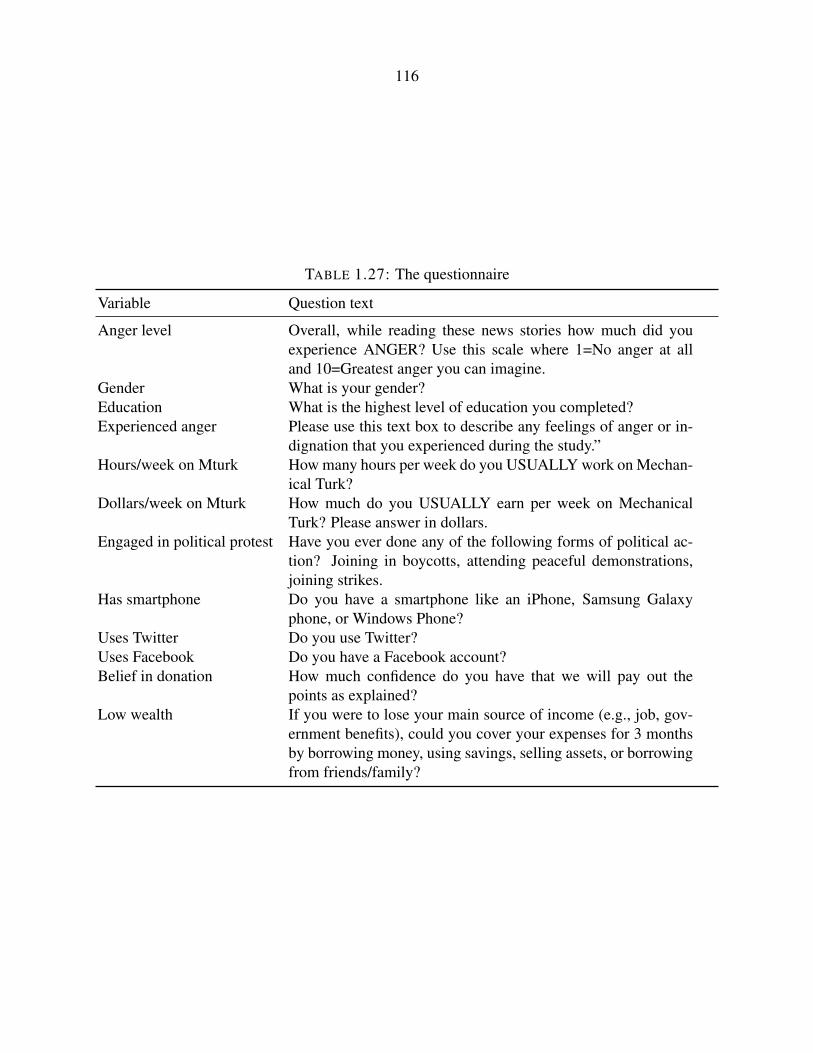
116

TABLE 1.27: The questionnaire

Variable Question text

Anger level Overall, while reading these news stories how much did youexperience ANGER? Use this scale where 1=No anger at alland 10=Greatest anger you can imagine.

Gender What is your gender?Education What is the highest level of education you completed?Experienced anger Please use this text box to describe any feelings of anger or in-

dignation that you experienced during the study.”Hours/week on Mturk How many hours per week do you USUALLY work on Mechan-

ical Turk?Dollars/week on Mturk How much do you USUALLY earn per week on Mechanical

Turk? Please answer in dollars.Engaged in political protest Have you ever done any of the following forms of political ac-

tion? Joining in boycotts, attending peaceful demonstrations,joining strikes.

Has smartphone Do you have a smartphone like an iPhone, Samsung Galaxyphone, or Windows Phone?

Uses Twitter Do you use Twitter?Uses Facebook Do you have a Facebook account?Belief in donation How much confidence do you have that we will pay out the

points as explained?Low wealth If you were to lose your main source of income (e.g., job, gov-

ernment benefits), could you cover your expenses for 3 monthsby borrowing money, using savings, selling assets, or borrowingfrom friends/family?

117

Chapter 2

Fear itself: The effects of distressingeconomic news on birth outcomes

Published as “Fear itself: The effects of distressing economic news on birth outcomes” in the

Journal of Health Economics. Vol. 41, May 2015, pp. 117–132.

Abstract

I use new administrative data on mass layoffs and plant closings to study the effects of distressing

economic news. Exposure to stressful events during pregnancy can impair fetal development. I find

that announcement of impending job losses leads to a transient decrease in the mean birth weight

within the firm’s county one to four months before the job losses. A loss of 500 jobs corresponds

roughly to a decrease of 15–20 grams and 16 percent greater risk of low birth weight. Layoffs

announced late in pregnancy are most strongly linked to decreased birth outcomes.

2.1. Introduction

Each year in the United States some 20 million jobs are lost through layoffs or discharges. Workers

who lose employment face serious problems, including long-term loss of earnings and damaged

health, which have been documented in the economics literature.1 However, each time someone1Displaced workers’ long-term earnings losses can range from 10 to 25 percent (Ruhm 1991; Jacobson et al. 1993;

Couch and Placzek 2010). Recently displaced workers are likely to drop out of the labour force (Huttunen et al. 2011)

118

loses employment, he first receives the unfortunate news of the impending event. And each time a

firm announces the decision to lay off workers or shut down, those residing nearby must consider

how the change might affect the local economy and their future livelihoods. Many forms of dis-

tressing news appear as a part of the normal course of economic activity, but we know relatively

little about the effects and costs associated with these messages.

Economic research on bad news and distress is nascent and promising. For example, Deaton

(2012) reports a surprisingly strong relationship between negative hedonic experience and the S&P

500 index during the recent financial crisis. He conjectures that the index functioned as a highly

salient channel for pessimistic news, which drove up mental and physical symptoms on a large

scale. The present study investigates a similar relationship but focuses on many, localized news

shocks rather than a nationwide crisis. These news shocks are announcements of mass layoffs and

plant closings at specific sites. Such events are considered in light of the human capital literature

which studies the damaging effects of stress experienced by women during pregnancy. Shocking

events, such as terrorism and natural disasters, can decrease birth weights and shorten gestation

(see, for example, Camacho 2008a or Simeonova 2011). These findings suggest that brief events

can have serious health consequences that may even affect the next generation. However, these

studies’ quasi-experimental designs exploit very unusual events that may have effects different

from those of common economic stressors.

The conjunction of stress and economic news is exceptionally appropriate. Perhaps the most

common stressors are personal finances, jobs, and economic conditions (American Psychological

Association 2012). To address the question of causal identification, I construct a novel data set

containing the dates of major job loss events and information about the amount of forewarning

given to the local community. These data allow me to analyze the particularly interesting period in

which news of job losses is taking effect, but the job losses themselves have not yet occurred. My

empirical model is constructed to rule out the direct consequences of job loss and isolate anticipa-

tory effects. Such effects include the immediate, physiological effects of stress but also behavioral

and can experience enormously elevated mortality risk (Sullivan and von Wachter 2009). A parent’s job loss can alsoreduce the health of subsequently born children (Lindo 2011).

119

responses in anticipation of economic change. For example, pregnant women who receive negative

information about the future might decrease consumption of healthful goods, increase consump-

tion of unhealthful goods, become more neglectful of their health in other ways, experience stress

as a result of initiating a job search, or be burdened with extra responsibilities when another mem-

ber of the household initiates a job search. Many of these channels cannot be isolated with the

present data.

I study mass layoffs and plant closings using administrative data from Alabama, New York,

Texas, and Washington. These data, derived from notices filed under the Worker Adjustment and

Retraining Notification (WARN) Act, are merged with natality data at the county-by-month level

to link each birth with job losses occurring in the mother’s community. The results indicate that

mean birth weights drop by 15–20 grams during a brief period before a large job loss event (defined

as one at the 95th percentile or approximately 500 workers in an average U.S. county). However,

the effect is almost entirely restricted to job losses where the firm in question provides a large

amount of forewarning rather than little, suggesting that bad news is the driving factor. These

negative effects also appear in analyses of individual-level birth data, which reveal that WARN

notices occurring in the mother’s county of residence just around the time of birth are linked to

significant decreases in birth weight and gestational age. The strongest effects are associated with

exposure to notices in the third trimester.

The study has several limitations. Births and dislocations are linked only by time and place, be-

cause the identities of the mothers and the people affected by WARN notices are unknown. There-

fore like other studies of wide-scale stressors, the estimates represent only effects averaged over

the affected community. In addition, the arrival time of the bad news about worker dislocations is

only approximately known, which “blurs” the estimated form of the response. Finally, caution is

required when interpreting the results and considering policy implications. One should not con-

clude that WARN notices or worker notification laws are harmful on the basis of this study. Others

have found that displaced workers can find new jobs more quickly when protected by notification

laws (Friesen 1997; Jones and Kuhn 1995). Compared to job losses without any notice, notices

120

might have some negative effects upfront but provide benefits over a longer time span. Any policy

is bound to have unintended consequences. My results should instead be considered evidence that

announcements of common business decisions are associated with substantial psychological and

physiological costs that occur before the decision takes effect.

2.2. Background

2.2.1. Stress due to economic conditions

Several studies report that workers’ physical and mental conditions deteriorate in anticipation of

job loss events. Evidence from quasi-experimental designs with large samples is reported by

Hamilton et al. (1990a) and Ferrie et al. (1995, 2002). The latter presents strong evidence from

longitudinal data on self-reported and physiological measures of health in about 3,500 workers.

Earlier studies, although smaller and weaker in some design aspects, also report physiological ef-

fects before job loss events (Kasl and Cobb 1970a, 1980a). Overall, these studies cover a variety

of workers, including both blue collar and white collar workers along with both sexes. However, a

notable shortcoming is that each study considers only one employer.

Individuals who do not lose employment can still suffer from layoffs. Workers remaining at

firms that have conducted layoffs can exhibit worsened health and increased absenteeism as evi-

denced by studies of survey data (Moore et al. 2004), administrative records (Vahtera et al. 1997),

and interviews with managers (Maki et al. 2005). Although these studies also examine just one

employer each, the link between pessimistic job expectations and poor health is broad enough to

appear in representative survey data (Kalimo et al. 2003). Finally, numerous studies of a variety of

sizes report that a wife may feel stress due to her husband’s layoff or job troubles (Dew et al. 1987;

Rook et al. 1991; Vinokur et al. 1996; Westman et al. 2001). For example, Dew et al. (1987) re-

port that wives of laid-off steel workers experience stress increases which depend on the husband’s

mental health. However, direct, person-to-person transmission—sometimes called contagion—is

generally difficult to isolate from empirically similar effects, such as the effect of a common envi-

121

ronment. This caveat is important: A community’s economic and social characteristics can have

especially strong effects on mental health and subjective well-being, as found in the well-known

Moving to Opportunity experiment (Ludwig et al. 2012). However, to support the hypothesis of

this study it is enough to document that the effects of layoffs can spread broadly. In general, it

is likely that news of layoffs will spread and induce stress through a variety of channels, which

include being at a directly affected employer, having a household member or family member af-

fected, word-of-mouth, or local media coverage.

2.2.2. Prenatal stress

Research from a large variety of approaches links stress experienced by the mother during preg-

nancy with effects on fetal development, birth outcomes, and health later in life. Causal effects

of prenatal stress are well-supported by evidence from animal experiments (for a review, see We-

instock 2005). Ethics strongly constrain exogenous stress manipulations in human subjects, but

there are converging lines of evidence to support effects in humans.

Birth weight and gestational age are the most commonly studied outcomes in this literature be-

cause they are easily available and indicative of health.2 Several studies take a simple observational

approach and document that stress reported by pregnant women is negatively associated with birth

weight and gestational age (see Copper et al. 1996; Dole et al. 2003; and Rondo et al. 2003 for

studies with relatively large samples). However, these generally provide weak evidence of causal-

ity because a third factor may cause both stress and low birth weight. Other clinical studies focus

on the mechanisms linking stress and birth outcomes, which are thought to involve neuroendocrine

processes, immune-inflammatory activity, and behavior (Wadhwa et al. 2001b,a; Wadhwa 2005;

Dunkel Schetter 2011). Clinical research on birth outcomes and stress hormones—cortisol and

corticotropin-releasing hormone (CRH)—typically report negative correlations between hormone

2The literature’s narrow focus on these variables is a well-known limitation (Currie 2011). Nevertheless, birthweight and gestational age are important intermediate outcomes (Cunha and Heckman 2007) that consistently predicthealth and socioeconomic success (Behrman and Rosenzweig 2004; Black et al. 2007; Currie and Moretti 2007a;Royer 2009). A broad review of child health and socioeconomic status is provided by Currie (2009).

122

levels and birth outcomes (Hobel et al. 1999; Inder et al. 2001; Wadhwa et al. 2004). Such stud-

ies still lack exogenous variation,3 but they provide additional evidence of causality by examining

mechanisms that are well-supported by basic neuroendocrinology (Wadhwa et al. 2011; Welberg

and Seckl 2001; Weinstock 2005; Seckl and Holmes 2007; Glover et al. 2010; Erickson et al. 2001;

McLean et al. 1995; De Weerth and Buitelaar 2005). The role of infection as a link between stress

and birth outcomes has received somewhat less study than endocrinology (Wadhwa et al. 2001b,

2011), but intrauterine infection is a heavily-studied risk factor for preterm birth (Goldenberg et al.

2008).

To address the lack of exogenous variation in the clinical research, some studies use quasi-

experiments generated by plausibly exogenous, stressful events, for example, natural disasters or

terrorist attacks. As an added advantage, such studies can use large administrative data sets. These

studies typically report that prenatal exposure to the stressor decreases the expected birth weight

and gestational age. Effects in terms of mean birth weight are typically a few grams up to about

30 grams while average effects on gestational age are roughly a day (Camacho 2008a; Simeonova

2011; Eccleston 2011; Brown 2014). However, one study reports no effects of a “near miss”

by a hurricane on birth weight nor on gestational age (Currie and Rossin-Slater 2013a). Some

studies only consider low birth weight as an outcome, making comparisons across the literature

more difficult, but these studies consistently report elevated risk of low birth weight (Catalano

and Hartig 2001; Lauderdale 2006; Eskenazi et al. 2007). The use of exogenous stressors is both

the main advantage and disadvantage of this research.4 The events are typically extraordinary,

3However, Aizer et al. (2009) investigate the role of cortisol using a novel design that exploits within-mother—between-pregnancy variation in cortisol measurements taken during the third trimester. They report that higher levelspredict worse cognitive and health outcomes in the child. Aizer et al. (2009) do not find evidence of an effect on birthoutcomes but attribute this to the way the sample was selected.

4An additional concern that applies to the entire literature is the inconsistency in the evidence related to the timingof stress during pregnancy. Laboratory studies using artificial stress tests report both decreasing (De Weerth andBuitelaar 2005) and increasing (Entringer et al. 2010) sensitivity. Associations between stress tests and pregnancyoutcomes are also mixed (McCubbin et al. 1996; Vythilingum et al. 2010). These studies are small, and the relationshipbetween laboratory stress tests and naturally-occurring stressors in this context is unknown. Large-scale studies basedon administrative data and exogenous stressors are similarly inconclusive. These have reported that the strongesteffects occur due to exposure during early and middle pregnancy (Eskenazi et al. 2007), middle and late pregnancy(Class et al. 2011; Catalano and Hartig 2001; Simeonova 2011), the first trimester (Torche 2011), and the secondtrimester (Camacho 2008b).

123

meaning the generalizability of the findings is questionable. In addition, the stress-related causal

mechanism is often poorly isolated because the stressors involve violence and destruction that

could have independent health effects or drive selective migration. Some studies do attempt to

address these issues, for example, by using location instruments (Currie and Rossin-Slater 2013a)

or analyzing birth rates (Quintana-Domeque and Rodenas 2014).

My study mitigates these concerns by examining a common stressor before there is likely to

be a significant material effect. The empirical model used for this analysis is like that used by

Currie and Schmieder (2009) to study pollution releases. Following their approach, I aggregate the

data at the county level and estimate how births respond to within-county variation in a continuous

treatment variable. This approach has the advantages of (1) isolating the period before a worker

dislocation, (2) allowing for estimation of birth rates, and (3) describing the process that would

occur in a community during the period before a dislocation. However, the county-level approach

does not describe the effects of WARN notices appearing at different time points in pregnancy. That

question involves some complications in defining the trimesters of pregnancy, which the county-

level approach avoids. However, the question is still important, so I also analyze the natality micro-

data by estimating models where birth outcomes depend on variables that represent exposure to

notices during each trimester of pregnancy.

2.3. Data

This study examines births from 1999 to 2008 using a county-month panel data set that includes

all 422 counties in Alabama, New York, Texas, and Washington. These states were selected based

on the histories of WARN notices available from state-level agencies. I traded off geographic

coverage against panel length while forming a balanced panel. The core of the dataset is composed

of 7,113,083 births and 2,626 WARN notices. Extended summary statistics for all data are available

in the appendix.

124

TABLE 2.1: Summary of dataset

Births % Births Counties Advance notices

Alabama 546,870 7.7 67 282New York 2,327,954 32.7 62 891Texas 3,476,622 48.9 254 1,142Washington 761,637 10.7 39 311Total 7,113,083 100.0 422 2,626

2.3.1. Layoffs and plant closings

2.3.1.1. Description

The United States Congress enacted the Worker Adjustment and Retraining Notification Act of

1988 in order to help individuals and communities anticipate worker dislocations. Under this

law, private employers must notify workers and authorities (the chief elected official in the local

government where the employer is located) at least 60 days in advance of a plant closing or mass

layoff. Closings and layoffs trigger the law only if they meet certain criteria, which mainly specify

thresholds for the number of workers involved. If a worksite with at least 50 workers will close,

then the employer must provide notice. Similarly, the law applies to (1) layoffs of 500 or more

workers and (2) layoffs of 50–499 workers when they constitute at least 33 percent of a site’s

workforce.5 When one of these conditions applies, the employer must give detailed, written notices

to (1) the affected workers, (2) the workers’ representatives, (3) the local government, and (4)

the state’s dislocated worker unit (DWU). Upon receipt of a notice, the DWU’s Rapid Response

team contacts workers and the employer to arrange meetings and provide services to the affected

workers. Typical services include guidance on unemployment insurance, career counseling, and

job search assistance.

Several DWUs have provided electronic records of WARN notices for this study. Each notice

specifies several key pieces of information: (1) the employer’s name and address, (2) the number of

5For a complete description of the criteria in the Act, see the guide published by the Employment and TrainingAdministration (2003).

125

workers affected, (3) the date on which the DWU was notified,6 and (4) the date on which worker

dislocations were to occur or begin. This combination of details allows me to identify distressing

events that are locally salient, something not possible with other data. For example, the BLS Mass

Layoff Statistics program lacks information about the amount of forewarning given by employers

and provides coarser temporal and geographic resolution.

Based on the difference between the notice date and dislocation date, I categorize each notice

into one of two types: Advance notices (ANs) provide at least 60 days’ notice, while short notices

(SNs) provide less. The analysis here focuses on advance notices because they indicate situations

where an anticipatory effect can be isolated. In the case of short notices it is difficult to isolate

births that could be affected by an anticipatory effect but not by the job losses themselves. The next

paragraphs describe the two types of notices and argue that they are substantially similar except

for the fact that advance notices provide much greater forewarning about an impending dislocation

and appear to receive greater coverage in the media.

Advance notices make up about 40 percent of the total, a finding like those of U.S. government

studies (U.S. General Accounting Office 1993, 2003). A small portion of notices, about 5 percent,

arrived more than 30 days after the dislocation or more than 120 days early. These were regarded

as erroneous or atypical situations and discarded. Nevertheless, the inclusion of these notices has

no substantial effect on the results. Advance notices provide on average 70 days of forewarning,

while short notices provide on average 31. Figure 2.1 shows a histogram of the distribution of

amounts of forewarning given in the notices.

There are several reasons why notices giving less than 60 days’ notice can appear. Employers

are suspected to violate the WARN Act’s requirements because of confusion, weak enforcement,

and small penalties (U.S. General Accounting Office 1993). No government agency is directly

responsible for enforcement of the Act. Following a violation, workers or local governments may

file suit against employers in U.S. District Court to extract back pay. Such lawsuits can be costly

6The Alabama and New York records include just the date of the notification document, but the data from Wash-ington include just the date on which the DWU received the notification. Only Texas includes both dates. I use thedate of receipt in the analysis, but the results are not substantially changed by using the other date.

126

and uncertain because the criteria in the act are complicated and courts have interpreted the WARN

Act inconsistently. These factors also contribute to underreporting. It is estimated that employers

fail to file a notice for one-half to two-thirds of events that should be reported (U.S. General Ac-

counting Office 1993, 2003). However, the WARN Act also encourages employers to file notices

even if they are not obligated to do so, and these notices are not distinguished in the data. Finally,

I contacted DWU staff to ask about differences between the two types. They denied that there is

any clear difference (Faraone 2012; Jordan 2012).

A key feature of the notices is that the two types implicitly attribute different amounts of bad

news to the months before dislocations. The notice date represents an important point in the pro-

cess that disperses information about the impending job losses. However, the notice date should

not be viewed as the single point at which full information about the job losses is instantaneously

revealed to all. First, the notice date is generally the latest date at which workers would learn of the

planned job losses. Employers want to break the news before Rapid Response makes contact with

the workers. The U.S. General Accounting Office (1993) reports that workers generally receive

somewhat more forewarning than DWUs. Second, workers also receive informal signals of the

impending notice filing and dislocation. Previous studies of worker notification laws have consid-

ered this “spillover” problem (Friesen 1997; Jones and Kuhn 1995). Finally, the employer must

also notify the community’s authorities, and local media often report WARN notices. Some state

governments, including all four in the study, publish WARN notices online as they receive them,

which provides another way for people to learn about them. Thus, when a dislocation follows

an advance notice rather than a short one, the news of the impending job losses will have had a

relatively long time to spread throughout the community and exert an effect.

An important factor that determines the effect of a notice is how much attention it receives. A

notice that is reported by the media will have a greater potential to generate stress than a notice

that is not reported and remains little known. The WARN notice data do not report whether a

notice received media coverage. To determine the amount of coverage, a random sample of 220

notices was hand-coded according to whether media coverage relating to the notice could be found

127

using a search engine.7 Media coverage typically announces that the worker dislocation has just

occurred or reports, shortly before the notice, that a company is preparing to lay off workers or

shut down. The results of this analysis appear in Figure 2.1. Overall 45 percent of the notices have

media coverage. The notices are grouped into bins (of width 1 day), and the points represent the

proportion of notices in each bin having media coverage. The smoothed (LOWESS) plot indicates

that notices with a medium amount of forewarning receive the least amount of coverage. The

probability of coverage increases sharply as the amount of warning approaches 60 days, which

suggests that notices with 60 days or more forewarning may be more consequential. The greater

amount of news coverage could directly increase the effects of these notices by making them more

widely known. Alternatively, the greater amount of news coverage may simply reflect a belief that

such notices are likely to have a greater impact on economic activity.

020

040

060

0F

requ

ency

−50 0 50 100 150Days of notice

(Layoff date − Notice date)

Short noticeAdvance notice

0

.2

.4

.6

.8

1

Pro

babi

lity

of m

edia

cov

erag

e

0 20 40 60 80Days of notice

(Layoff date − Notice date)

SmoothedRaw mean

FIGURE 2.1: Distributions of days of advance notice and media coverage

A dislocation’s potential impact depends in part on the number of workers affected and the size

7This method is imperfect but still reveals an important feature of the data. The random sample was stratifiedaccording to the amount of notice given, and the statistics were weighted by the actual sample frequencies. Thismethod was chosen so that a sufficient amount of notices in the middle range would be included in the sample. Thecoding was done by searching for the company name along with the year of the notice and the location in GoogleNews search. A notice was classified as having media coverage if any articles were found that directly mentioned thenotice or that discussed plans for layoffs or shut down around the time of the notice. The coding was done blind to theamount of forewarning and with the notices sorted in a random order.

128

of the community. Thus, I operationalize this potential as the ratio of (a) the number of workers

affected to (b) the population of working-age people in the county of the employer. In the set of

county-month cells with at least one AN dislocation, the mean (median) potential is 0.124 (0.024)

percent.8

WARN notices are rare in the sense that about 6 percent of county-month cells contain one.

However, 67 percent of counties have at least one at some point in time. The second percentage

would be above 90 if not for Texas, where 50 percent of the counties have no notices. The WARN

Act applies only to employers with at least 100 employees in total, regardless of how many workers

lose employment at a single worksite operated by the employer, and there may be few or no such

large employers in the many small counties of Texas. Figure 2.2 shows that WARN notices are

highly dispersed over the study period. No single year has more than 13 percent of the notices nor

less than 7 percent.

0

50

0

50

0

50

0

50

1999m1 2002m1 2005m1 2008m1 2009m12

Alabama

New York

Texas

Washington

FIGURE 2.2: Monthly frequency of WARN notices by state, 1999–2009

2.3.2. Natality data

The National Center for Health Statistics at the Centers for Disease Control (CDC) has provided

a confidential version of the Vital Statistics natality data that identifies each mother’s county of

8AN and SN dislocations have very similar distributions of potential. The corresponding mean (median) for SNdislocations is 0.125 (0.026) percent. The first and third quartiles are also nearly equal across the two types. The meannumber of workers affected by an AN notice is 114, while SN notices affect 117 on average.

129

residence. Practically all births in the United States appear in these data. The available variables

include the birth weight (BWT) in grams, the gestational age (GA) in weeks, the month of birth,

and the mother’s demographic characteristics. Births were included based on these criteria: (1)

the birth was a singleton, (2) the mother resided and gave birth within the same state, and (3) the

mother was 18 to 45 years of age. If a record had a missing value in the birth weight, gestational

age, plurality, or location variables, then it was dropped before analysis. The mean age of mothers

at the time of birth is 27.6 years. Births to Hispanic, white, black, and “other” mothers make up

33, 47, 14, and 6 percent of the sample. The means of birth weight and gestational age are 3,318

grams and 38.7 weeks.

By convention, babies born at a weight below 2,500 grams are classified as low birth weight

(LBW), and births before 37 weeks are classified as preterm (PTB). I also consider age-conditional

z-scores and the proportion of babies that are both LBW and PTB. The z-scores indicate how

much a baby’s birth weight deviates from the median birth weight given the length of gestation,

so they are sensitive to changes in fetal growth but not changes in gestational age. The z-scores

are calculated using the tables and reference population provided by Oken et al. (2003). Z-scores

are only defined for gestational ages between 22 and 44 weeks, so births outside this range, which

make up less than one percent of the sample, are dropped when z-scores are analyzed.

2.3.3. Other data

The Bureau of Labor Statistics provides unemployment data at the county-by-month level through

the Local Area Unemployment Statistics program. Finally, birth rates and working-age populations

are calculated using intercensal population estimates from the U.S. Census and National Cancer

Institute/SEER. The Census estimates July populations for each county, so linear interpolation

provides figures for the remaining months.

130

2.4. Empirical model

2.4.1. County-level model

In order to estimate how birth outcomes respond to dislocations, I use a county fixed effects model

that incorporates the following key features. First, each month’s outcomes are allowed to depend

on AN dislocations up to 6 months in the future. For a depiction of this structure consider the

timeline in Table 2.2. This table gives an example of how the key variables relate to the timing

of a notice and layoff. This example depicts a typical case in the sense that within a given county

most layoffs will be isolated in time. In this example, a layoff of 250 workers occurs in October,

the last column. However, the notice was given in July, and the period between the notice and the

dislocation is shaded. Note that the row “# jobs lost in month t” has the value 250 in October, and

the row “# layoffs announced in month t” has the value 250 in July. In addition, note that in July the

distributed lead variable “# number jobs lost in month t+3” has the value 250. This variable along

with the other distributed leads is the key to the anticipation effect because it allows outcomes in

the earlier months to depend on the impending job losses. The regression coefficients on these

distributed leads quantify the deviations in birth outcomes occurring during the 6 months before

the job loss. For example, if the coefficient on the three-month lead is -20 grams, then it should

be interpreted to mean that births occurring about 3 months before a unit-sized layoff are expected

to be 20 grams lower than if there was no layoff (all else equal). Importantly, the model allows

birth outcomes to respond to a dislocation up to six months before the job losses actually occur.

As discussed above, the small number of WARN notices providing more than 120 days of advance

notice were dropped from the data set. To demonstrate how this relates to the model, suppose that

a notice was filed in June for a layoff occurring 120 days (4 months) later in October. It is possible

that an anticipatory response appears in May, 5 months before the dislocation. This could occur

if the firm made a pre-announcement in May stating that it was planning to formally announce

layoffs in the next few weeks. By including the full set of 6 months of distributed leads of job loss

variables, the model allows for such a situation. In principle, any number of distributed leads could

131

TABLE 2.2: Example timeline of WARN notice in July of 250 layoffs in OctoberMonth Apr May June July Aug Sept OctMonths before layoff 6 5 4 3 2 1 0Months after notice -3 -2 -1 0 1 2 3# layoffs announced in month t . . . 250 . . .# jobs lost in month t . . . . . . 250# jobs lost in month t+ 1 . . . . . 250 .# jobs lost in month t+ 2 . . . . 250 . .# jobs lost in month t+ 3 . . . 250 . . .# jobs lost in month t+ 4 . . 250 . . . .# jobs lost in month t+ 5 . 250 . . . . .# jobs lost in month t+ 6 250 . . . . . .

be included, but 6 months is used because it is expected to encompass almost all anticipatory effects

related to job losses. The second key feature is that dislocations enter the model as a proportion of

the working-age population in the county.

The estimated equation is

Yi,t =6∑

τ=0

βτ (AN)i,(t+τ) + Zi,tδδδ + ϵi,t,

where for each county i and month t

• Yi,t is the mean of a birth outcome,

• (AN)i,t is the proportion of the working-age population dislocated under an advance notice.9

In the example above, if t =July, then

(AN)i,t+3 =250

working-age population of county i

(up to a scaling factor). If the corresponding coefficient β3 is negative, then the presence of

job losses in October (month t + 3) will have a negative effect on the mean birth outcome

in July (month t). This relationship is precisely the “anticipatory effect” whereby women

respond to impending job loss events. Since layoffs are rare, the (AN)i,t are sparse. That is,

it is unlikely for more than one of the (AN)i,t to be non-zero in any given case (i, t).

9Summary statistics for the variable (AN) are printed in appendix Table 2.9. This variable corresponds to the rowin the above table labelled “# jobs lost in month t” except that the population normalization is applied. For example,the mean value taken over county-month cells is 0.124 percent.

132

• Zi,t is a vector that potentially includes the means of characteristics of women giving birth

and county-specific quadratic time trends along with indicators for county of birth, year of

birth, and calendar month of birth.10

Each observation is weighted by the number of births to increase efficiency, and standard errors

are adjusted for clustering at the county level. Some specifications also include a window of

unemployment rates, which is detailed in the results section. The dislocation effect variables are

scaled so as to represent the effect of a 95th percentile layoff. The scaling factor was obtained by

examining the 6% of county-month cells in which any worker dislocations resulted from WARN

notices. From these cells, the 95th percentile of the dislocation potential (the percentage of the

working-age population dislocated by a WARN notice) was extracted giving the number 0.0067.

Note that since the percentile is determined by only a small subset of the cells, the use of the 95th

percentile does not mean that a unit-sized or larger layoff occurs in 5% of county-month cells.

During the period from 1999 through 2009, only 176 county-month cells, or about 0.32%, reach

the threshold of 0.0067. Thus, the effects in this paper are scaled so as to represent very extreme

dislocation events.

While it may seem counter-intuitive to use the month of the job losses as a reference point,

this specification is a natural result of the identification strategy. The statistical model must be

designed so as to clearly separate the effects of job loss from the anticipatory effects caused by bad

news. If the model were to use the month of the notice as a reference point, the anticipatory effects

could be confounded with the effects of job losses. For example, suppose the results showed that

birth weight tends to be lower than normal about three months after a notice. There could be

two explanations. One is that people are anticipating layoffs that had 3–4 months of notice. The

other is that some layoffs, which had two months of notice, are generating effects one month after10Mother characteristics enter as proportions of mothers in groups defined following Currie et al. (2011). The age

groups are “Less than 20”, “20 to 34”, “Over 34”, and “Missing”. The race and ethnicity groups are “Hispanic”,“White”, “Black”, “Other”, and “Missing”. The educational attainment groups are “Less than high school”, “Highschool”, “Some college”, “College or higher”, and “Missing”. The marital status groups are “Married” and “Notmarried”. Finally, the categories for total birth order are 1, 2, 3, 4, 5 or more, and “Missing”. However, these maternalvariables are omitted from birth rate models because they are undefined in months with no births. Smoking variablesare omitted because of possible endogeneity, but their inclusion has minimal effect on the results. Birth rates arecalculated as the number of births per 1,000 women aged 18–45.

133

the job losses—which is three months after the notice. Therefore, the county-level analysis uses

the approach which sharply separates the pre- and post-job loss periods. However, the individual-

level analysis (explained below) allows notices to directly enter the model, which provides the

perspective of explicitly looking at responses to notices.

2.4.2. Individual-level analysis on natality micro-data

The second set of results uses birth-level micro-data to estimate the effects of exposure to notices

at different points during the pregnancy. This approach presents some complications because ex-

posure during the last trimester of pregnancy is partially determined by the length of pregnancy. A

birth occurring at 40 weeks rather than 39 will have one extra week in which to accumulate expo-

sure. This relation creates an upward (positive) bias in the effect of exposure in the third trimester

even if the true effect is null or negative. Currie and Rossin-Slater (2013a) call this complication

a “mechanical correlation” between the exposure and outcome, and they propose instrumenting

for exposure using the potentially counterfactual exposure that would have resulted if the birth

occurred at 39 weeks. That is, the instrument represents exposure as-if the pregnancy lasted 39

weeks. The instrument can be viewed as the result of making a small but critical adjustment to

the endogenous exposure variable. I apply the “full-term instrument” method in this analysis. The

individual-level results using this approach are consistent with results from the county-level data.

Each pregnancy is first divided into three trimesters corresponding to 13-week periods relative

to conception. The date of conception is estimated by taking the midpoint of the birth month and

subtracting the gestational age. Two weeks are added because conception normally occurs two

weeks after the date of the last normal menstrual period, which is used to compute gestational age.

Based on this conception date the trimesters of pregnancy are defined. In each trimester I compute

the total amount of workers dislocated and affected by WARN notices by summing all those within

the county of residence of the mother and falling within the appropriate time period. The third

trimester ends at birth and may be longer than 13 weeks. The instrument is constructed using the

same method except under the assumption that the birth occurred at 39 weeks gestational age. As

134

a result, for births occurring at 39 weeks the instrument and the actual exposure are identical.

In addition to the three trimesters of pregnancy I define three additional trimesters for use in

the analysis. Trimester 0 is the 13-week window just before conception. For births that occur at

39 weeks, trimester 4 is the 13 weeks after birth. Otherwise, trimester 4 is the window following

trimester 3 up to 52 weeks after conception. 11 Finally, trimester 5 is weeks 53–65. This last period

is included in the spirit of a placebo test, meaning it is expected to have relatively little effect.12

2.4.3. State-to-state heterogeneity of effects

Estimates using only data from individual states reveal heterogeneity in the effects of WARN

notices. The two large states, New York and Texas, show the strongest evidence of anticipatory

effects of notices on birth outcomes. However, the smaller states show more equivocal results. The

estimates from Washington suggest moderate effects on birth outcomes, while Alabama shows no

evidence of a decrease. State-by-state results from micro-data are in Table 2.11.

This heterogeneity demands some conceptual and methodological consideration before the

analysis can proceed. Differences in anticipatory effects might arise from variation in regional

labor market features or policies, locals’ prior beliefs about job losses, spatial relationships among

employers and employees, or numerous other factors. Alabama is the only state that shows no

evidence of effects, and it is an outlier from the other states in several ways. First, the mean birth

weight is substantially lower than in the other states. For example, it is 86 grams lower than the

mean of New York. This difference dwarfs the estimated effects in this paper, which are already

scaled to represent a very large loss of jobs. Second, Alabama is substantially more rural than the

other three states.13 Third, relative to these small counties, the worker dislocations in Alabama tend11Trimester 4 ideally is the one following birth, but it will in reality slightly overlap with pregnancy in some cases

because only the month of birth is known. In addition, because the exact timing at which people learn of an impendingdislocation is not known, the inclusion of trimester 4 allows testing for anticipation of events occurring just after birth.

12Note that constructing the regressors requires 4 trimesters of notice data before the birth, so it is not possible touse births from 1999. Therefore, the individual-level analysis focuses on 2000–2008.

13The distribution in Alabama stands out with much fewer births in large metropolitan areas compared to the otherstates. However, the effects of notices does not appear to vary systematically between rural and urban areas. Theseresults are available from the author.

135

to be large relative to the local population, although they are not unusually large in absolute terms.

In the other three states about 0.1 percent of the working age population is affected by a WARN

notice in an average month. However in Alabama, this value is over 0.3 percent, which suggests

that the effects of dislocations are likely to be dispersed outside the county. Future research should

investigate how people in different environments vary in their reaction to economic news.

Heterogeneity of treatment effects presents some complications when estimating average treat-

ment effects. Angrist (1998) shows that when treatment effects are heterogeneous across groups

an OLS estimator which allows just one treatment effect will not in general estimate the average

treatment effect. Instead, the estimator will estimate a weighted average of the group-specific

treatment effects where each weight is proportional to the group-specific variance of the treatment

variable. The estimator then depends on the marginal distribution of the treatment variable within

each group. In this case the estimator overweights Alabama because the notice variables have high

variance relative to the other states. Morgan and Winship (2007) propose addressing this problem

by a simple stratification method which estimates the group-specific treatment effects and then av-

erages them using weights proportional to the number of observations in each group. I implement

this estimator by computing one regression which allows each state to have a separate set of effects.

A single treatment effect is then estimated by averaging these four state-specific effects using the

proportion of births in each state as weights. This approach is applied to both the county-level es-

timates and the individual-level estimates. Estimates from models that estimate single, unstratified

effects are available in appendix Table 2.12 along with estimates based on raw counts of workers

affected by notices.

2.5. Results

2.5.1. County-level results for birth weight and gestational age

Table 2.3 presents the main results for birth weight and gestational age. The estimates show that

both variables selectively decrease in anticipation of dislocations. During the period four months

136

to one month before dislocations, the mean birth weight is depressed by 15–20 grams and the mean

gestational age by roughly one half to one day.

TABLE 2.3: Estimated anticipation effects on birth weight and gestational age

Birth weight (grams) Gestational age (days)

(1) (2) (3) (4) (1) (2) (3) (4)

Timing of birth(relative to job losses)6 mos. before 0.26 -1.89 -3.55 -3.54 -0.17 -0.19 -0.04 -0.06

(4.77) (4.45) (5.12) (5.17) (0.21) (0.21) (0.22) (0.22)5 mos. before 0.83 -2.73 -4.74 -4.98 -0.18 -0.23 -0.10 -0.10

(6.52) (5.75) (5.86) (5.87) (0.21) (0.20) (0.23) (0.23)4 mos. before -17.32∗∗ -18.24∗∗ -18.81∗∗ -19.15∗∗ -0.86∗∗ -0.93∗∗ -0.77∗∗ -0.79∗∗

(6.06) (5.89) (5.93) (5.91) (0.20) (0.21) (0.20) (0.21)3 mos. before -16.71∗ -18.89∗ -20.18∗∗ -20.81∗∗ -0.29 -0.33 -0.18 -0.21

(7.58) (7.48) (7.45) (7.43) (0.22) (0.22) (0.20) (0.19)2 mos. before -10.66+ -14.63∗∗ -16.00∗∗ -16.94∗∗ -0.57∗ -0.61∗ -0.48∗ -0.53∗

(5.88) (5.44) (5.61) (5.65) (0.24) (0.24) (0.22) (0.22)1 mo. before -11.83+ -14.30∗ -16.07∗ -17.27∗ -0.23 -0.25 -0.12 -0.16

(7.06) (6.87) (6.81) (6.75) (0.27) (0.28) (0.24) (0.24)Same month 4.46 1.42 1.05 -0.08 -0.04 -0.09 0.08 0.06

(7.55) (7.62) (7.38) (7.59) (0.26) (0.28) (0.26) (0.26)County, yr., mo. FEs Yes Yes Yes Yes Yes Yes Yes YesMoms’ characteristics . Yes Yes Yes . Yes Yes YesCounty quad. trends . . Yes Yes . . Yes YesUnemp. rates . . . Yes . . . Yes

Cells 49, 123 49, 123 49, 123 49, 123 49, 123 49, 123 49, 123 49, 123Adj. R-sq. 0.655 0.665 0.674 0.674 0.536 0.539 0.561 0.561

Notes. Average treatment effects of a 95th percentile layoff printed with standard errors in parentheses. FE=Fixedeffects. Statistical significance symbols: + p < 0.10, ∗ p < 0.05, ∗∗ p < 0.01.

Estimates from four specifications allow us to consider the potential influence of omitted vari-

ables. The most basic specification includes just county fixed effects and state-specific year and

calendar month fixed effects. This relatively simple model is sufficient to show the basic form of

the anticipatory response to dislocations. The addition of the mothers’ demographic characteristics

increases the magnitude of the birth weight coefficients associated with advance notice and tends

to increase the precision of the estimates. These additional covariates also slightly increase the

magnitude of the gestational age coefficients. This result suggests that the effects are not driven by

changes in the demographic composition of mothers.

Since the study period spans ten years, one might be concerned that the counties underwent

heterogeneous drift in some unobserved factors related to birth outcomes and job loss activity,

137

which could bias the estimates. This problem appears unlikely because the birth outcomes show

transient responses. Nevertheless, the third specification includes county-specific quadratic time

trends. These trends should capture the effects of unobserved influences that vary in a smooth way

within each county. This change adds over 800 parameters to the model, but has little effect on the

estimated coefficients and standard errors. The birth weight effects slightly increase in magnitude,

while the gestational age effects slightly decrease in magnitude.

Finally, it might also be suspected that dislocation activity simply reflects more general eco-

nomic conditions. The state-by-year fixed effects in the basic model should control for economic

activity varying at the state level. However, county-level heterogeneity might still be a source of

bias. The quadratic trends might not properly account for varying economic activity since two

recessions occured during the study period. So, the last specification includes a 19-month win-

dow of county-level unemployment rates. Twelve months of lags are included to capture effects

occuring around the time of conception and during pregnancy. Six months of leads are included

to allow for pregnant women to react to expectations about future economic activity. Inclusion

of unemployment rates slightly increases the magnitude of the birth weight and gestational age

effects, suggesting that local fluctations in general economic activity are not a serious problem.

2.5.2. Effects over broader geographic regions

The effects of job losses and their announcements might extend beyond the county where they

occur. This subsection shows that such effects are unlikely to be large, which justifies the paper’s

focus on within-county effects. To check for the possibility of such inter-county spillover effects

the model is augmented with variables that represent, for each county, the job losses in a group

of nearby counties. The model retains variables representing same-county notices. Therefore, the

model allows us to answer the question, ‘How do birth outcomes in a particular county i respond

to increasing the amount of WARN notices in i’s group (holding constant notices within i itself)?’

For the moment, assume that all counties have been partitioned into contiguous groups. The

variables that represent inter-county influences are constructed analogously to those that represent

138

within-county influences and use the same scaling factor. The variable representing the inter-

county influences on i is

# of workers being laid off by advance notices in i’s group (but not in i itself)the working-age population of the group (excluding i’s population)

.

Just like the baseline specification, these inter-county variables enter the model as distributed leads.

Four methods of grouping counties are analyzed: Metro- and micro-politan areas, commuter

zones (as defined by the US Department of Agriculture’s Economic Research Service), component

economic areas, and economic areas. The last two groupings are defined by the U.S. Bureau of

Economic Analysis. Some counties are not part of a metro- or micro-politan area, so these counties

have zeros for all inter-county influence variables.

The results of this approach appear in Table 2.4. Same-county effects from the previous table

are reprinted in the first column for the purpose of comparison. In contrast to the same-county esti-

mates, which show a consistent, statistically significant negative effect, the inter-county estimates

have widely varying signs and do not reach significance at conventional levels. Based on these

results the remainder of the analysis will consider only within-county effects.

2.5.3. Dynamic features of the birth weight response

The four-month period before dislocations shows a fairly stable depression in birth weights, but this

stability hides interesting dynamics. In particular, the initial response is marked by a precipitation

of babies born too early and too small. Later parts of the response show decreased fetal growth and

possibly some selection. With these two mechanisms in mind, I now consider several additional

variables.

The main physiological contributors to birth weight are the length of gestation and the rate of

intrauterine growth. These contributions can be partially disentangled by considering the joint dis-

tribution of birth weight and gestational age. Decreased birth weights caused by shorter gestation

should be reflected in the proportion of babies born both preterm and with low weight. However,

139

TABLE 2.4: Inter-county effects of dislocations over wider geographic areas

Surrounding area (inter-county effects only)

Samecounty Metro area Commuter

zoneComponenteconomic area

Economicarea

Timing of birth(relative to job losses)6 mos. before -3.55 -4.87 -3.63 1.13 12.33

(5.12) (10.01) (8.15) (10.80) (9.39)5 mos. before -4.74 2.33 -1.04 10.07 7.12

(5.86) (7.11) (7.99) (10.65) (18.40)4 mos. before -18.81** 19.73+ -6.50 20.84 8.47

(5.93) (11.36) (9.35) (16.86) (17.02)3 mos. before -20.18** -0.68 -1.69 -3.41 -15.19

(7.45) (10.55) (10.70) (13.96) (14.25)2 mos. before -16.00** -16.16 -19.45 -12.86 -23.00

(5.61) (15.62) (12.57) (18.97) (21.07)1 mo. before -16.07* -0.87 -5.95 -11.74 15.74

(6.81) (10.31) (9.84) (11.69) (15.08)Same month 1.05 -9.09 -11.96 -1.78 13.23

(7.38) (6.43) (9.75) (9.43) (13.54)

# geographic units 422 323 108 57 36

Notes. Average treatment effect of a 95th percentile layoff printed with standard errors (clustered at the level ofgeographic grouping) in parentheses. All models include county, year, and month fixed effects along with county-specific trends. Only advance notices included. Statistical significance symbols: + p < 0.10, ∗ p < 0.05, ∗∗ p < 0.01.

this variable is not sensitive to a change merely in fetal growth rates. Alternatively, birth weights

caused by lower growth rates can be detected in age-conditional z-scores, which are sensitive to

changes in birth weight conditional on gestational age.

Table 2.5 displays the estimated effects of a dislocation on the (1) mean birth weight, (2) birth

rate, (3) proportion low birth weight, (4) proportion both low birth weight and preterm, and (5)

mean age-conditional z-score of birth weight. Several results suggest that the initial decrease

in birth weight at month four can be attributed to reduced gestational age. First, at this point

the proportion LBW is increased by one percentage point, or 16 percent of the overall rate, and

the proportion LBW & PTB increases by 0.76 percentage points, or 20 percent of the overall

rate, revealing that the additional low weight births are largely also additional preterm births.14

Second, the contemporaneous effects (“four months before”) in the main results above show that

the decreases in birth weight and gestational age are consistent with each other. To a first-order

approximation, a 0.8 day decrease in gestational age implies a decrease of 18.9 grams, which is

14The LBW and PTB cutoffs are somewhat arbitrary, so it is reasonable to vary the cutoffs and recalculate theeffects. That analysis is presented in Appendix Figure 2.5 and is consistent with the results in this subsection.

140

almost exactly the estimated change in mean birth weight.15

TABLE 2.5: Dynamics of the anticipatory response

BWT BR LBW LBW & PTB Z-score

ATE SE ATE SE ATE SE ATE SE ATE SE

Timing of birth(relative to job losses)6 mos. before −3.55 (5.12) −0.03 (0.07) 0.19 (0.29) 0.01 (0.19) −0.19 (1.04)5 mos. before −4.74 (5.86) −0.09 (0.07) 0.06 (0.23) −0.01 (0.20) −1.05 (1.09)4 mos. before −18.81∗∗ (5.93) −0.01 (0.06) 1.01∗∗ (0.28) 0.76∗∗ (0.23) −0.76 (1.06)3 mos. before −20.18∗∗ (7.45) −0.14+ (0.07) 0.88∗∗ (0.28) 0.34+ (0.18) −3.61∗∗ (1.39)2 mos. before −16.00∗∗ (5.61) 0.01 (0.05) 0.20 (0.29) 0.01 (0.21) −2.02+ (1.09)1 mo. before −16.07∗ (6.81) −0.22∗∗ (0.07) 0.28 (0.28) 0.16 (0.19) −3.24∗∗ (1.13)Mo. of layoff 1.05 (7.38) −0.09 (0.07) −0.19 (0.35) −0.24 (0.27) −0.52 (1.26)

Cells 49, 123 50, 640 49, 123 49, 123 49, 108Adj. R-sq. 0.674 0.840 0.254 0.177 0.572

Notes. Average treatment effect of a 95th percentile layoff printed with standard errors in parentheses. Outcomemodels include county, year, and month fixed effects along with county-specific trends. BR model is a Poisson modelwith coefficients reported. BWT=Birth weight (grams). BR=Monthly birth rate: Births per 1,000 women of childbearing age. LBW=Proportion low birth weight × 100. PTB=Proportion preterm birth × 100. Z-score representsBWT conditional on gestational age and is multiplied by 100 for display. Statistical significance symbols: + p < 0.10,∗ p < 0.05, ∗∗ p < 0.01.

Closer to the dislocation month, there appear changes in intrauterine growth. The effect on the

proportion LBW progressively diminishes from month four onwards while the decrease in mean

birth weight is about 16 grams. Months three through one show rescaled z-scores decreased by

2.02–3.61, suggesting that retarded intrauterine growth is reducing birth weights. Converting the

z-score effect to grams gives a decrease of 11–17 grams.16 This result indicates that decreased

growth, due to physiological stress responses or increased levels of unhealthful behaviour by preg-

nant women, can account for most or all of the estimated change in birth weight.

One concern is that average birth outcomes could change if women migrated out of areas where

job losses are about to occur. Immigration is also possible but less likely in this context. Estimates

of changes in birth rates before job losses suggest that selection is unlikely to account for the

estimated effects on birth outcomes. Table 2.5 also shows changes in the monthly birth rate using

a model like those used to estimate changes in average birth outcomes. These results show that the

15Oken et al.’s (2003) supplemental tables indicate that a median baby born at 38 weeks should weigh 165 gramsmore than one born at 37 weeks. The calculation (3, 301 − 3, 136) × 1

7 × 0.8 ≈ 18.9 suggests that around this pointin pregnancy a decrease of 0.8 days in GA should result in a 18.9 gram decrease in birth weight.

16For a birth at 39 weeks, Oken et al.’s (2003) supplemental tables associate a loss of 11 grams with a decrease of0.03 in z-score. Alternatively, the standard deviation of birth weight in the data is 562 grams. So, a change of 0.03standard deviations corresponds to 17 grams.

141

changes in birth outcomes do not coincide with changes in the birth rate. Recall that birth weight

is consistently depressed from 4 months to 1 month before the job loss event. However, the birth

rate is decreased only in months 3 and 1 and by less than 5%. This discrepancy in timing indicates

that a simple pattern of selection cannot account for the decrease in birth weight.17

2.5.4. Individual-level results using birth micro-data

The last analysis approaches the problem differently by modeling individual-level birth outcomes

in the manner commonly used to study prenatal exposures in the economics literature. Linear mod-

els are estimated which allow the expected outcome of each birth to depend on exposure—notices

occurring in the mother’s county—during each trimester of the pregnancy. This approach provides

the advantage of explicitly allowing the effect of an exposure to depend on when in pregnancy it

occurred. However, this approach also complicates the identification of the effects of notices them-

selves because a given pregnancy is often exposed to both the notice and the subsequent pregnancy.

Nevertheless, these new results are consistent with anticipatory effects. Exposure to notices late in

pregnancy is associated with significant decreases in both birth weight and gestational age.

The estimated individual-level effects of exposure to WARN notices are displayed in Table 2.6.

Like the previous set of results these include only advance notices.18 Each IV column shows esti-

mates from a model using the full-term instruments, while the OLS columns show reduced-form

estimates. The notice exposure variables are scaled so that they are comparable to the county-level

results. That is, a unit of exposure in a particular trimester corresponds to WARN notices directly

affecting approximately 0.67% of the county’s working-age population during that trimester. In

the birth weight columns, the negative coefficients on third and fourth trimester exposure indicate

that the occurrence of notices in those periods—just around birth—is associated with a strong de-

crease in birth weight. The point estimates for these two trimesters are around -30 and -21 grams,

17Additional analysis that consider subgroups of mothers and mothers’ characteristics also fail to show clear evi-dence of selection. These results are available from the author.

18The analysis in this section gives similar results if all notices are included. However, the estimates are smaller inmagnitude because the short notices “dilute” the effect. These results are available from the author.

142

respectively. These estimates are somewhat more negative than the county-level results, which

are about -20 grams. This difference likely occurs because the county-level effects isolate births

that are before layoffs, but the individual-level results include many births occurring after a layoff.

For example, the third trimester coefficients may be picking up additional negative effects of lay-

offs that are both announced and carried out during the third trimester. However, the differences

between the county-level and individual-level models are not especially large compared to the stan-

dard errors of about 6. Additionally, this same concern applies to all of the trimester coefficients,

which may be contributing to a small downward bias across all trimesters. Taking the evidence all

together, the effects of notices are likely closer to 20 grams.

These results provide additional evidence that birth outcomes deteriorate in anticipation of

job losses. The effects are concentrated in the third and fourth trimesters rather than earlier in

pregnancy. If the effects were actually driven by the consequences of job losses themselves, for

example, lost income or migration, then we should expect to see the strongest effects from notices

early in pregnancy. For example, if women tend to selectively migrate away from areas that are

losing jobs, then the effect of selection should increase as time passes, which would result in larger

effects for earlier notices rather than later ones. In addition, significant effects are estimated from

notices occurring in the fourth trimester, which covers the period just following pregnancy and

possibly the very end of pregnancy.19 There is little opportunity for job losses associated with

fourth trimester notices to directly affect the pregnancy. These effects are likely due to both the

brief overlap between the fourth trimester and pregnancy along with anticipation of the notice itself.

Finally, the fourth trimester estimates are uniformly smaller than the third trimester estimates,

suggesting that the strongest effects result from notices occurring at the end of pregnancy.

19Separate analyses were run where job losses enter the individual-level models instead of notices. The results showthat birth weight and gestational age are significantly lower among births that occur just before a job loss event, whichalso suggests anticipatory effects. These results are available upon request.

143

TABLE 2.6: Individual-level effects of advance notices during pregnancy

Time of exposurerelative to conception

Birth weight Gestational age Low birth weight Preterm birth

OLS IV OLS IV OLS IV OLS IV

Trimester 0 -7.99 -8.02 -0.59∗ -0.59∗ 0.33 0.33 0.83+ 0.83+

[1–13 weeks before] (5.83) (5.80) (0.29) (0.29) (0.24) (0.24) (0.50) (0.50)Trimester 1 -10.07 -10.10 -0.47 -0.47 0.21 0.21 0.37 0.37

[weeks 1–13] (7.92) (7.88) (0.30) (0.30) (0.34) (0.34) (0.50) (0.50)Trimester 2 -6.94 -6.93 -0.78∗∗ -0.78∗∗ 0.29+ 0.29+ 0.59 0.59

[weeks 14–26] (4.73) (4.70) (0.28) (0.28) (0.16) (0.16) (0.39) (0.39)Trimester 3 -29.62∗∗ -30.32∗∗ -1.16∗∗ -1.17∗∗ 0.92∗∗ 0.94∗∗ 1.29∗∗ 1.30∗

[weeks 27–39] (5.70) (6.00) (0.36) (0.37) (0.21) (0.23) (0.49) (0.51)Trimester 4 -21.47∗∗ -21.07∗∗ -1.08∗∗ -1.07∗∗ 0.68∗∗ 0.67∗∗ 1.04∗∗ 1.02∗

[weeks 40–52] (4.35) (4.51) (0.26) (0.26) (0.17) (0.18) (0.39) (0.40)Trimester 5 -4.62 -4.62 -0.53∗ -0.53∗ 0.28 0.28+ 0.71∗ 0.71∗

[weeks 53–65] (4.30) (4.27) (0.22) (0.22) (0.17) (0.17) (0.35) (0.35)

Notes. Estimates from micro-data. OLS column shows reduced-form estimates. IV column shows instrumentalvariables estimates. Coefficients for LBW and PTB models are multiplied by 100 so as to represent percentage pointeffects. All models have 6,332,304 observations. Average treatment effect of a 95th percentile layoff printed withstandard errors (clustered by county) in parentheses. All models include county, year, and month fixed effects alongwith mother covariates. Statistical significance symbols: + p < 0.10, ∗ p < 0.05, ∗∗ p < 0.01.

2.6. Conclusion

Analyzed in variety of ways, the data reveal that birth outcomes deteriorate in anticipation of

job loss events that are announced with substantial forewarning. That is, several months before

mass layoffs and plant closings, birth weights transiently decrease by 15–20 grams within the

affected community. Results from individual-level data show that birth outcomes are affected

by announcements of worker dislocations made late in pregnancy or around the time of birth as

well as by worker dislocations occurring just after birth. These effects are largely restricted to

exposures that occur late in pregnancy rather than early in pregnancy. The results are robust to the

instrumental variables approach of Currie and Rossin-Slater (2013b). Thus, both approaches to the

data indicate significant anticipatory effects of job losses on birth outcomes in the local community.

These results suggest that the arrival of commonplace bad news about the local economy can

generate a wave of stress or unhealthful coping behaviors that in turn decrease birth weights. In

addition, the response of birth weights has an intuitive dynamic. The curtailment of pregnan-

cies can affect birth weights abruptly, while changes in growth rates require time to integrate up

to a significant effect. This pattern appears in the results. The initial response to bad news ap-

pears to be babies born too early and too small, while later decreases are associated mostly with

144

slower intrauterine growth. Nevertheless further research should probe the mechanisms related

to the anticipation of negative economic events. This study cannot disentangle direct physiolog-

ical responses to stress from behavioral responses that might also generate deterioration of birth

outcomes. Future research should look at data with fine-grained temporal resolution to determine

exactly when and how behavior and physiology begin to anticipate shocks. Mobile and wearable

technology or social media may provide an especially useful source of such data (see, e.g., An-

tenucci et al. 2014). In general, one important matter is how disclosure policy, media coverage,

and social networks influence the anticipatory response to economic events.

FIGURE 2.3: Birth weight decreases in context with other studies

The results in this study are similar in magnitude to those reported in studies of prenatal stress

and destructive events. This similarity may seem surprising, but recall that the effects in this

study are scaled to represent very extreme job loss events. The unconditional probability of such

a job loss event occurring within the county-month sample is 0.0032. Figure 2.3 displays reported

effects on birth outcomes from a wide variety of studies. The effect attributed to the current study

was obtained by averaging the county-level anticipatory effects 1–4 months before a dislocation

event. An important takeaway from this figure is that the effects of even fairly extreme stressors,

such as terrorist attacks, tend to be small, typically in the single- or low double-digits. These

145

effects are quite small compared to the effect of smoking, race-related differences, the difference

between Alabama and New York, or even the decrease in the mean U.S. birth weight since the

1990s—which is largely unexplained (Donahue et al. 2010). Of particular interest are the findings

of Lindo (2011), which show that babies fathered by men who have lost employment are 142 grams

lighter. This treatment effect is probably the largest one attributed to a specific event but is likely

to include substantial income effects along with stress and other mechanisms. If one supposes

that stress makes up a small but significant fraction of that decrease, then the present results on

layoff notices would require that a fairly large portion of a county’s population be stressed. Since

most layoff events dislocate only a very small portion of the local population, it is likely that many

people are indirectly affected by dislocations.

Although the mean effects on birth weight and gestational age associated with this study and

others on extreme events are fairly small, the risk of falling below critical thresholds can be sub-

stantial. For example, the individual-level results above indicate that large layoffs can increase the

risk of preterm birth by 10 percent. Future research might try to determine who is most at risk of

a strong negative reaction to bad news. Finally, policy makers might consider the possibility of

offering health assessments or counselling to workers facing imminent job loss or others who are

at significant risk.

2.7. Appendix of chapter 2

2.7.1. Data description

146

TABLE 2.7: Natality data summary statistics

Alabama New York Texas Washington All

Mother’s age (years) 26.27 28.94 26.85 27.99 27.61(5.56) (5.96) (5.76) (5.83) (5.90)

Married 0.664 0.628 0.668 0.711 0.659(0.47) (0.48) (0.47) (0.45) (0.47)

Hispanic 0.0565 0.224 0.479 0.165 0.330(0.23) (0.42) (0.50) (0.37) (0.47)

Non-Hispanic white 0.629 0.501 0.372 0.663 0.465(0.48) (0.50) (0.48) (0.47) (0.50)

Non-Hispanic black 0.300 0.173 0.108 0.0401 0.137(0.46) (0.38) (0.31) (0.20) (0.34)

Non-Hispanic other 0.0143 0.0873 0.0382 0.107 0.0598(0.12) (0.28) (0.19) (0.31) (0.24)

Less than high school 0.193 0.180 0.281 0.160 0.228(0.39) (0.38) (0.45) (0.37) (0.42)

High school 0.328 0.287 0.304 0.260 0.296(0.47) (0.45) (0.46) (0.44) (0.46)

Some college 0.252 0.233 0.208 0.282 0.227(0.43) (0.42) (0.41) (0.45) (0.42)

College 0.225 0.292 0.197 0.260 0.237(0.42) (0.45) (0.40) (0.44) (0.43)

Female 0.489 0.488 0.489 0.487 0.488(0.50) (0.50) (0.50) (0.50) (0.50)

Birthweight (grams) 3244.0 3329.7 3298.8 3422.1 3317.9(588.4) (568.9) (553.1) (551.6) (562.5)

Low birthweight 0.0802 0.0602 0.0618 0.0447 0.0609(0.27) (0.24) (0.24) (0.21) (0.24)

Gestational age (weeks) 38.43 38.90 38.63 39.02 38.74(2.66) (2.40) (2.41) (2.23) (2.42)

Preterm birth 0.138 0.0980 0.116 0.0847 0.108(0.34) (0.30) (0.32) (0.28) (0.31)

Low weight and preterm 0.0507 0.0373 0.0382 0.0280 0.0377(0.22) (0.19) (0.19) (0.17) (0.19)

Births 546,870 2,327,954 3,476,622 761,637 7,113,083

Standard deviations in parentheses. Categories specified as proportions.

147

TABLE 2.8: Account of WARN notices, 1999–2009

Alabama New York Texas Washington TotalNo. % No. % No. % No. % No. %

CompletenessComplete 857 99.8 2,443 99.0 2,840 99.8 760 96.9 6,900 99.2Incomplete 2 0.2 25 1.0 6 0.2 24 3.1 57 0.8Total 859 100.0 2,468 100.0 2,846 100.0 784 100.0 6,957 100.0

Type>30 days late 37 4.3 73 3.0 56 2.0 9 1.1 175 2.5Short 488 56.8 1,428 57.9 1,576 55.4 441 56.2 3,933 56.5Advance 282 32.8 899 36.4 1,144 40.2 324 41.3 2,649 38.1>120 days early 52 6.1 68 2.8 70 2.5 10 1.3 200 2.9Total 859 100.0 2,468 100.0 2,846 100.0 784 100.0 6,957 100.0

In analysis?Included 768 89.4 2,302 93.3 2,715 95.4 741 94.5 6,526 93.8Excluded 91 10.6 166 6.7 131 4.6 43 5.5 431 6.2Total 859 100.0 2,468 100.0 2,846 100.0 784 100.0 6,957 100.0

TABLE 2.9: Potential of dislocation-months as a percentage of working-age population

Mean Max Q1 Median Q3

State AN SN AN SN AN SN AN SN AN SN

Alabama 0.345 0.343 8.205 5.028 0.037 0.045 0.121 0.135 0.424 0.411New York 0.065 0.061 1.333 1.936 0.008 0.008 0.020 0.019 0.069 0.053Texas 0.111 0.085 3.440 5.350 0.007 0.004 0.018 0.015 0.067 0.052Washington 0.085 0.097 1.431 1.543 0.009 0.011 0.021 0.031 0.065 0.096Total 0.124 0.125 8.205 5.350 0.009 0.008 0.024 0.026 0.091 0.092

Note: Each statistic is calculated separately on the set of county-month cells with a positive number of ANdislocations and the set of cells with a positive number of SN dislocations.Abbreviations: AN=Advance notice, SN=Short notice, Q#=Quartile #

148

TABLE 2.10: Previously estimated effects of prenatal exposures

Study Location Exposure Timing† BWT effect GA effect

Camacho (2008b) Colombia Landmine Trimester 3 -0.4g ns .Camacho (2008b) Colombia Landmine Trimester 2 -0.8g ns .Camacho (2008b) Colombia Landmine Trimester 1 -2.0g .

Catalano & Hartig (2001) Sweden Estonia sunk Trimester 3 -18 vLWBs ns .Catalano & Hartig (2001) Sweden Estonia sunk Trimester 2 +26 vLWBs .Catalano & Hartig (2001) Sweden Estonia sunk Trimester 1 -15 vLWBs ns .

Catalano & Hartig (2001) Sweden Palme murder Trimester 3 +44 vLWBs .Catalano & Hartig (2001) Sweden Palme murder Trimester 2 +13 vLWBs ns .Catalano & Hartig (2001) Sweden Palme murder Trimester 1 +16 vLWBs ns .

Deschenes et al. (2009) USA Temp.>85F Trimester 3 -0.009 % .Deschenes et al. (2009) USA Temp.>85F Trimester 2 -0.008 % .Deschenes et al. (2009) USA Temp.>85F Trimester 1 -0.003 % .

Eccleston (2011) NYC 9/11 attack Trimester 3 ns nsEccleston (2011) NYC 9/11 attack Trimester 2 -14.3g -0.12 ws.Eccleston (2011) NYC 9/11 attack Trimester 1 -11.9g -0.22 ws.

Eskenazi et al. (2007) NYC 9/11 attack +0–1 ws. 1.44a, vLWB 1.30a, vPTB nsEskenazi et al. (2007) NYC 9/11 attack +0–1 ws. 1.67a, mLBW .Eskenazi et al. (2007) NYC 9/11 attack +13–16 ws. 1.36a, vLWB nsEskenazi et al. (2007) NYC 9/11 attack +17–20 ws. 1.28a, vLWB ∼1.20a, vPTB

Eskenazi et al. (2007) NYC 9/11 attack +33–36 ws. 1.29a, vLWB nsEskenazi et al. (2007) Upstate NY 9/11 attack +17–20 ws. 1.46a, vLWB ∼1.10a, mPTB

Eskenazi et al. (2007) Upstate NY 9/11 attack +33–36 ws. 1.32a, vLWB nsEskenazi et al. (2007) NYC 9/11 attack +0–8 ws. ns 0.87a, mPTB

Eskenazi et al. (2007) Upstate NY 9/11 attack +0–4 ws. ns 0.89a, mPTB

Khashan et al. (2008) Denmark Relative dies Trimester 3 -29g .Khashan et al. (2008) Denmark Relative dies Trimester 2 -47g .Khashan et al. (2008) Denmark Relative dies Trimester 1 -27g .

Khashan et al. (2008) Denmark Relative ill Trimester 3 -10g .Khashan et al. (2008) Denmark Relative ill Trimester 2 -13g .Khashan et al. (2008) Denmark Relative ill Trimester 1 -15g .

Simeonova (2011) USA Ext. weather Birth−1 mo. -0.7g ns nsSimeonova (2011) USA Ext. weather Birth−2 mo. -1.6g nsSimeonova (2011) USA Ext. weather Birth−3 mo. -1.6g -0.01 ws.

Simeonova (2011) USA Strong storm Birth−1 mo. -1.8g -0.01 ws. nsSimeonova (2011) USA Strong storm Birth−2 mo. -2.2g -0.20 ws.Simeonova (2011) USA Strong storm Birth−3 mo. -1.1g ns -0.01 ws. ns

Smits et al. (2006) Netherlands 9/11 attack Trimester 3 -71g -0.5 days nsSmits et al. (2006) Netherlands 9/11 attack Trimester 2 -67g -1.1 daysSmits et al. (2006) Netherlands 9/11 attack Trimester 1 +2g ns +0.7 days

Torche (2011) Chile Earthquake Trimester 3 +2.6g ns +0.03 ws. nsTorche (2011) Chile Earthquake Trimester 2 +17g ns +0.01 ws. nsTorche (2011) Chile Earthquake Trimester 1 -51g -0.19 ws.

† Large plus symbol indicates timing of observed effect relative to exposure. Notation: BWT=Birthweight;(v,m)LBW=(very,moderately)Low birthweight; GA=Gestational age; (v,m)PTB=(very,moderately)Preterm birth; a ad-justed odds ratio; ns=Reported as statisically non-significant; ws.=weeks; g=grams

149

1999

m01

2002

m01

2005

m01

2008

m01

2009

m12

AL

NY

TX

WA

FIG

UR

E2.

4:C

ount

y-m

onth

carp

etpl

otof

WA

RN

disl

ocat

ions

;blu

e=A

N,r

ed=S

N,p

urpl

e=bo

th

150

●

● ●●

●

●

● ●

●●

●● ●

●

●●

● ●●

●

● ● ●

● ●

●

●

●

●

●

●

−0.01

0.00

0.01

0.02

0.03

2000 2500 3000 3500

Born 1 mos. before job losses

● ●● ●

● ●●

●

●

●●

● ●

●

●

●

●● ●

● ●

●●

● ●●

● ●

●

●

●

−0.01

0.00

0.01

0.02

0.03

2000 2500 3000 3500

Born 2 mos. before job losses

● ● ● ●

●●

●● ● ●

●

●

●●

● ●●

●

●

● ● ●

●

●

●

●

●

●

●

●

●

−0.01

0.00

0.01

0.02

0.03

2000 2500 3000 3500

Born 3 mos. before job losses

● ● ●●

●●

● ●

● ●● ●

●●

●

●●

●

●

●

●

●

●

● ●

●

●

● ●

●●

−0.01

0.00

0.01

0.02

0.03

2000 2500 3000 3500

Born 4 mos. before job losses

Cutoff for low birth weight (grams)

Cha

nge

in p

ropo

rtio

nbe

low

cut

off

●● ● ● ●

● ● ● ●● ●

●

●●

●

●

● ●

●

●

●

● ●

−0.02

0.00

0.02

0.04

20 25 30 35 40

Born 1 mos. before job losses

● ● ● ● ● ● ● ● ● ● ● ●

●

●

●

●

●

●

●

●

●● ●

−0.02

0.00

0.02

0.04

20 25 30 35 40

Born 2 mos. before job losses

● ● ● ● ● ●● ● ●

● ● ●

● ●

●●

●

● ●

●

●

● ●

−0.02

0.00

0.02

0.04

20 25 30 35 40

Born 3 mos. before job losses

● ● ● ●● ● ● ● ●

● ●●

●

●●

●

●

●

●

●

●

● ●

−0.02

0.00

0.02

0.04

20 25 30 35 40

Born 4 mos. before job losses

Cutoff for preterm birth (weeks)

Cha

nge

in p

ropo

rtio

nbe

low

cut

off

FIGURE 2.5: Anticipatory effects for varying LBW & PTB cutoffs (95% CIs plotted)

151

TABLE 2.11: Micro-data IV estimates of effects of advance notices in each state

Birth weight (grams) Gestational age (days)

AL NY TX WA AL NY TX WA

Trimester 0 -2.39 -12.50 -6.97 -3.00 -0.09 -1.12 -0.36 -0.35(2.32) (11.77) (8.74) (8.88) (0.09) (0.71) (0.36) (0.34)

Trimester 1 3.64∗ -11.42 -14.71 5.49 0.11 -0.76 -0.48 0.01(1.75) (19.39) (9.69) (5.80) (0.07) (0.74) (0.36) (0.27)

Trimester 2 -0.46 -6.69 -6.86 -12.68+ -0.00 -1.48∗ -0.48+ -0.60(1.81) (9.22) (7.30) (6.43) (0.08) (0.73) (0.29) (0.36)

Trimester 3 -1.09 -42.92∗∗ -26.13∗∗ -25.64 0.06 -2.66∗∗ -0.33 -1.34(2.29) (12.94) (6.92) (16.79) (0.10) (0.92) (0.35) (0.83)

Trimester 4 0.95 -45.63∗∗ -13.74∗ 0.27 -0.10 -2.62∗∗ -0.39 -0.24(2.14) (9.99) (5.57) (8.74) (0.11) (0.69) (0.24) (0.29)

Trimester 5 -4.63∗ -8.82 -2.71 -0.64 -0.10 -1.57∗∗ -0.02 0.01(2.04) (10.45) (5.09) (7.58) (0.08) (0.57) (0.22) (0.22)

Births 483, 908 2, 056, 626 3, 112, 455 679, 315 483, 908 2, 056, 626 3, 112, 455 679, 315Adj. R-sq. 0.057 0.036 0.035 0.028 0.017 0.015 0.013 0.011

Notes. Effects of exposure a 95th percentile notice with at least 60 days forewarning. Standard errors (clustered bycounty) in parentheses. All models include county, year, and month fixed effects along with county-specific trends.Estimates are multiplied by 100 so as to represent percentage point changes. Statistical significance symbols: +

p < 0.10, ∗ p < 0.05, ∗∗ p < 0.01.

152

TABLE 2.12: Alternative specifications for micro-data models

Birth weight (grams) Gestational age (days)

Proportion Levels Proportion Levels

Trimester 0 -2.91 -0.23 -0.24+ -0.08(2.46) (0.70) (0.14) (0.06)

Trimester 1 -0.24 -2.05 -0.10 -0.11*(2.92) (1.44) (0.13) (0.05)

Trimester 2 -2.70 -0.33 -0.29 -0.11**(2.37) (0.70) (0.18) (0.04)

Trimester 3 -10.42+ -2.58* -0.35 -0.10(5.45) (1.05) (0.25) (0.08)

Trimester 4 -4.57 -0.41 -0.35* -0.06(3.51) (0.79) (0.18) (0.04)

Trimester 5 -2.85 0.65 -0.19+ -0.01(2.27) (0.58) (0.11) (0.03)

Births 6,332,304 6,332,304 6,332,304 6,332,304Adj. R-sq. 0.041 0.041 0.019 0.019

Notes. All treatment variables included without stratification by state. Proportion column uses the standard treatmentvariable used throughout the paper: the proportion of the working-age population affected by WARN notices. Thelevels column uses the number of workers affected by WARN notices and is scaled to represent the effect of 500 work-ers. All models include county, year, and month fixed effects. Standard errors clustered by county are in parentheses.Statistical significance symbols: + p < 0.10, ∗ p < 0.05, ∗∗ p < 0.01.

153

Chapter 3

Red alert: Prenatal stress and plans to closemilitary bases

Abstract

In May 2005 the U.S. military announced a restructuring plan called Base Realignment and Closure

(BRAC). Some areas were projected to lose 20 percent of employment, sparking much distress.

Previous research shows that stress affects pregnancy and fetal development. I find that immedi-

ately following the announcement, the mean gestational age in the most-affected areas dropped by

1.5 days for a period of 1–2 months. Births shifted from 39+ to 37–38 weeks, a period linked to

health risks. Similar changes appear in birth weight. Local changes in employment and mothers’

characteristics do not account for these effects.

3.1. Introduction

The effects of government policies are the subject of much economics research. However, less

attention focuses on the effects of the decision process during which a potential policy is publicly

discussed and announced. When the costs of a potential policy change will be highly concentrated

in specific areas, their residents may react to the decision process with a great deal of distress.

This stress may affect people’s mental or physical well-being before any policy changes are im-

plemented. The relevant situations typically involve large, lumpy, localized projects, for example,

154

U.S. domestic military activities. In many communities military operations make up a major por-

tion of economic activity, which makes these communities especially sensitive to actual or planned

changes in military policy.1 For example, as a result of the 2013 budget sequestration, the De-

partment of Defense announced tentative plans to furlough almost all civilian employees for 22

days (Carroll 2013).2 These plans threatened to have extremely concentrated, negative effects at

places like Newport News, Virginia, where the shipyard for nuclear-powered aircraft carriers em-

ploys some 21,000 people. In a high-profile speech at the shipyard, President Obama attributed

significant harm to the mere threat of furloughs and spending cuts (Shear and Shanker 2005).

To study these announcement effects in a specific and tractable way, I focus on a major military

reorganization process called Base Realignment and Closure 2005 (BRAC 2005). It is the most

recent and best documented reorganization of the U.S. military. Another round of BRAC may

occur in the next few years. BRAC 2005 involved a secretive decision process surrounded by much

speculation and anxiety, during which the Department of Defense (DoD) announced a preliminary

plan that involved hundreds of military sites throughout the United States. Some major bases were

designated for closure or reduction in size, and projected losses of local employment reached as

high as 20 percent. However, the implementation of this plan was to begin only long after the

announcement and was not certain. An independent commission reviewed the DoD’s plan, heard

communities’ concerns, and ultimately canceled several parts of the plan. This study focuses on

May–August 2005, the period starting with the DoD’s announcement of its plans and ending with

the BRAC commission’s final revisions. This period was marked by highly salient uncertainty and

much public distress.

The announcement’s effects are examined using the human capital literature that considers the

effects of stress experienced by women during pregnancy. The condition of the baby at birth is

important because it predicts the offspring’s later life outcomes such as earnings, education, IQ,

and pregnancy outcomes in adulthood (Behrman and Rosenzweig 2004; Black et al. 2007; Royer

1Military spending, Medicare-Medicaid, and Social Security each consume similar portions of the federal budget.However, military spending is relatively concentrated in specific areas, a characteristic which is the subject of its ownliterature (see Braddon 1995).

2The initial plans called for 22 days of furlough, which was later cut to 11.

155

2009).3 We can better understand the intergenerational evolution of outcomes by studying how

conditions during pregnancy affect the offspring (Currie and Moretti 2007b). Several studies have

shown that disasters and other extreme events can decrease birth weights and shorten pregnancies

in the surrounding area (see, for example, Camacho 2008a or Simeonova 2011). Such findings

raise the possibility that stressful events experienced during a critical phase of development might

have long-lasting effects on human capital. However, it remains unclear how stress related to

violent and destructive events compares to stress caused by changes in economic conditions. This

study helps to fill that gap by relating a stress-inducing announcement about economic policy to

birth outcomes.

The results presented here show that, in some areas, the BRAC 2005 announcement had effects

quite similar to those reported in studies of prenatal stress and natural or man-made disasters. In a

few communities that were projected to lose 10–20 percent of employment due to BRAC, the DoD

announcement was associated with a significant decrease in mean gestational age. Gestational

age trended downward in the months preceding the announcement, and the effect reached a peak

just after the announcement of the BRAC list. The month of the announcement and the following

month show a brief, sharp drop in gestational age of about 1.5 days in magnitude. The drop is

characterized by a shift in births from 39 weeks and above to 37–38 weeks, a period called early-

term and associated with long-lasting, negative effects on health and cognitive function. This result

is supported by auxiliary, individual-level analyses using a full-term exposure instrument (Currie

and Rossin-Slater 2013a), which reveal a strong negative link between expected gestational age and

BRAC exposure during the third trimester. Over the key period between the DoD announcement

and the commission’s decision, the mean gestational age was about half a day lower. These results

are robust to many alternative specifications of the control group. The effects on the mean birth

weight are more difficult to estimate but are consistent with the effects seen in gestational age.

These results suggest that researchers and officials should pay greater attention to the negative

psychological and health effects of major policy announcements.

3However, the degree of importance of birth outcomes is still a subject of debate (Almond et al. 2005).

156

Further investigation shows that these effects are unlikely to be explained by economic changes

or selection by potential mothers. Unemployment rates show little evidence of a BRAC effect on

local economic conditions during 2004–2005. The BRAC-affected areas show some evidence of

changes in the characteristics of women giving birth, but these changes are generally small in size,

in a direction that cannot account for the effect, or temporally inconsistent with the changes in

gestational age. Finally, the main results for gestational age and birth weight are affected little by

the inclusion or exclusion of demographic control variables and by highly flexible specifications

of the control variables.

The next section of the paper explains the BRAC process and findings from previous studies

of stress. The following section covers the data and empirical model. Afterwards the results are

presented along with a variety of robustness checks.

3.2. Background

3.2.1. Statutory requirements of BRAC

The BRAC 2005 process was a major restructuring of the United States military in which many

military sites were closed or “realigned,” that is, had personnel and functions removed and re-

located to other sites. The overall effect was mainly a consolidation of operations rather than a

reduction in total military size. The procedures for BRAC are specified in the Defense Base Clo-

sure and Realignment Act of 1990. Previous rounds of BRAC were carried out in 1988, 1991,

1993, and 1995, which reduced the military’s installation inventory by about 21 percent (Base

Realignment and Closure Commission 2005a, p. 314).

The requirements of the Act are as follows. The Department of Defense must prepare an

inventory of military installations and develop a 20-year plan for national security as a part of the

fiscal year 2005 budget process (Base Realignment and Closure Commission 2005b, Appendix C.

Section 2912). The Secretary of Defense must then decide whether the military needs to close or

realign military installations in order to follow the 20-year plan.

157

If so, the Secretary must publicly certify the need for BRAC and publish a list of recommended

closures and realignments by May 16, 2005 (Base Realignment and Closure Commission 2005b,

Appendix C. Section 2914(a)). These recommendations must be made according to two sets of

criteria. The military value criteria have four components: (1) the current and future mission ca-

pabilities of the Department of Defense for fighting and training, (2) the availability of land, facil-

ities, and airspace at military sites, (3) the ability to accommodate contingencies and mobilization,

and (4) the cost of operations and personnel implications. The other criteria are: (1) the extent and

timing of costs and savings from closures and realignments, (2) the economic impact of changes

on communities near military installations, (3) the ability of community infrastructure to support

operational changes, and (4) environmental impact, including restoration and waste management.

The Act instructs the Secretary to place higher priority on the military value criteria.

The Act also requires the President to nominate, by March 15, 2005, nine members for the

Defense Base Closure and Realignment Commission, which are subject to appointment by the

Senate (Base Realignment and Closure Commission 2005b, Appendix C. Section 2912(d)). The

Commission is required to review the list of recommendations published by the DoD and prepare

a report on its findings and conclusions, which must be sent to the President by September 8,

2005. The review process must include public hearings on the recommendations. In addition,

the Government Accountability Office (GAO) must assist in the review process by publishing a

report analyzing the recommendations by July 1, 2005. The Commission’s report must include a

revised set of recommendations. The Commission can modify or strike recommendations that are

judged to deviate from the 20-year plan and final criteria. However, new closures and realignments

or expansions of realignments require additional procedures, including public hearings and the

support of 7 of the 9 commissioners. The President must approve or disapprove the Commission’s

recommendations by September 23, 2005.

158

3.2.2. The BRAC list and results

For this study, the two key BRAC events are the public announcement of the Secretary’s recom-

mended closings and realignments—commonly called “the BRAC list”—on May 13, 2005 and the

final deliberations of the BRAC Commission, broadcast live on August 24–27, 2005. The May

13 announcement was very salient and the subject of great anticipation because the communities

near military installations feared reductions in employment following realignment or closure. On

May 14, 2005 the New York Times covered the list in a front page story (Schmidt 2005). Figure 3.1

shows the intensity of Google searches for “BRAC 2005”, which indicates that attention began to

increase in late 2004 and built up to a sharp spike in May 2005. A smaller peak occurs in August

2005, the month of the final vote. During this May–August period, the communities subject to

closures and realignments lobbied the BRAC Commission fiercely, arguing that their base should

be removed from the list.

Final selectioncriteria announcedFebruary 12, 2004

BRAC listannounced by DoD

May 13, 2005

BRAC commission voteson DoD’s recommendations

August 24−27, 2005

0

20

40

60

80

100

Nor

mal

ized

sea

rch

volu

me

for

"BR

AC

200

5"

2004m1 2005m1 2006m1 2007m1Month

Jan−Apr: Before list announcementMay−Aug: List public; vote unresolvedSept−Dec: After commission’s vote

Significant periods in 2005

Source of search data: www.google.com/trends

FIGURE 3.1: Public attention to the BRAC process

159

The DoD’s BRAC list proposed 837 closures and realignment actions. Included were 33 major

closures and 30 major realignments. The DoD designates a closure as “major” if the facility has a

plant replacement value of at least $100 million.4 A realignment is designated as “major” if it will

result in a net reduction of at least 400 military or civilian personnel at the installation (Government

Accountability Office 2005). The DoD’s designations are not ideal indicators of the local economic

impact of BRAC. First, major closures are defined only by the value of physical plant and in some

cases affect a small number of personnel. Second, they do not take into account the size of the

installation relative to the local economy.

Instead, I focus on six actions singled out by the GAO, which publishes many studies to support

the BRAC decision process and audits the results of BRAC implementation. For the statutorily-

mandated report released on July 1, 2005, the Government Accountability Office analyzed the

potential negative economic impact of the BRAC actions and found that six areas faced “fairly

significant impact” (Government Accountability Office 2005, p. 48). These are the communities

associated with (1) Cannon Air Force Base, New Mexico; (2) Hawthorne Army Depot, Nevada;

(3) Naval Support Activity Crane, Indiana; (4) Submarine Base New London, Connecticut; (5)

Eielson Air Force Base, Alaska; and (6) Ellsworth Air Force Base, South Dakota. The estimated,

combined direct and indirect losses of area employment ranged from 8.5 percent to 20.5 percent.

These areas (“the GAO-6”) are listed in table 3.1.

In five of these cases, the Commission modified the recommendation. The Commission can-

celed the realignment of Hawthorne Army Depot and the closure of Ellsworth Air Force Base.

Cannon Air Force base was assigned to enclave status, in which it would remain open while a new

use was found for it. The closure of Submarine Base New London was reduced to a realignment,

and the realignment of Eielson Air Force Base was partially canceled. Only the realignment of

Naval Support Activity Crane stood without modification.

4Plant replacement value of a facility is the cost, in current year dollars, of designing and constructing a replacementof the facility at the same site (Office of the Deputy Under Secretary of Defense 2003).

160

TABLE 3.1: Sites facing significant negative effects from BRAC 2005 (GAO-6)1

Military installation DoD’s recommended ac-tion

Result2 County Percentageemployment loss

projected

PopulationY2004

Cannon AFB Close Enclave Curry, NM 20.5 45,951Hawthorne Army Depot Realign Struck Mineral, NV 13.6 4,827NSA Crane Realign Realign Martin, IN 11.6 10,220SUBASE New London Close Struck/R New London, CT 9.4 266,890Eielson AFB Realign Struck/R FNSB, AK 8.6 92,301Ellsworth AFB Close Struck Pennington, SD 8.5 92,890

1 “Of those communities facing potential negative economic impact, six communities face the potential for a fairlysignificant impact. They include the communities surrounding Cannon Air Force Base, New Mexico; HawthorneArmy Depot, Nevada; Naval Support Activity Crane, Indiana; Submarine Base New London, Connecticut; EielsonAir Force Base, Alaska; and Ellsworth Air Force Base, South Dakota, where the negative impact on employment as apercent of area employment ranges from 8.5 percent to 20.5 percent.” (GAO-05-785, pp. 48–49)2 The BRAC commission spared five of the installations by voting to strike or modify the DoD’s recommended action.Abbreviations: AFB=Air Force Base, NSA=Naval Support Activity, SUBASE=Submarine Base, FNSB=FairbanksNorth Star Borough

3.2.3. Public reactions to BRAC as reported by the news media

News coverage of the BRAC process frequently reported anxiety, fear, and local efforts to prepare

to lobby the Commission. Before the announcement of the list, local papers ran headlines like

“A Good Navy Town, Submarines Run Deep In Groton’s Soul, And So Does Fear For The Naval

Base’s Future” (Hamilton 2005). The local paper in Clovis, New Mexico reported that closure of

Cannon Air Force Base could “devastate” the community with over 7,000 jobs lost (Irvin 2005).

Hoax emails claiming to leak the list were circulating by late 2004 (Linn 2004). Some community

groups sought to retain law firms for assistance in lobbying the Commission (Gargulinski 2005).

Economic impact analyses were also commissioned in order to challenge BRAC decisions on the

economic impact criterion (see, e.g., State of Connecticut 2005).

The New York Times, in a front page story, characterized the day of the BRAC announcement

by saying, “On military bases across the country and in the communities that depend on them, all

the dread and anxiety comes into high focus today, when the Pentagon plans to release a new list

of recommended base closings and consolidations” (Semple 2005). Civilian employees at military

sites crowded around televisions waiting for the press conference in which the list would be an-

nounced (Hartz 2004).5 Residents in the GAO-6 were variously reported to react with “engaged

5“When defense officials announced Cannon was recommended for closure, a sense of unbelief crashed throughthe crowd [watching the press conference]. ‘We were all very upset and shocked,’ said Wike, a manager of dining

161

anger,” “denial”, and “shock” (Semple 2005; Hartz 2004).

3.2.4. Previous research on stress

This study’s hypothesis depends on two key relationships. First, the announcement of the BRAC

recommendations should cause a broad increase in stress levels among residents of the GAO-6.

Media reports and data on community lobbying both support this point, and studies discussed

below report evidence that people are sensitive to anticipated changes in economic conditions.

Second, stress experienced by a woman during pregnancy tends to cause an earlier birth and lower

birth weight.

Economic matters are important sources of stress according to representative survey data. In

recent surveys by the American Psychological Association (2012), “the economy” is the third most

commonly reported stressor, after “money” and “work.” Anxiety levels reported by workers are

highly responsive to cyclical changes in labor market conditions (Davis and von Wachter 2011).

Finally, self-reported negative hedonic experience is sensitive to short-term changes in the S&P 500

index (Deaton 2012). At a finer level numerous studies by health researchers link deterioration of

workers’ physical and mental health to anticipation of negative workplace events, for example,

layoffs, plant closures, and restructuring (Kasl and Cobb 1970b, 1980b; Hamilton et al. 1990b;

Ferrie et al. 1995; Grunberg et al. 2001).6

A wide variety of research links stress experienced during pregnancy to effects on fetal devel-

opment and birth outcomes. The risks of low birth weight and preterm birth are positively asso-

ciated with self-reported stress (see Copper et al. 1996; Dole et al. 2003; and Rondo et al. 2003

for clinical studies with samples sizes on the order of 1,000). The biological mechanisms under-

lying these links involve neuroendocrine processes, immune/inflammatory activity, and behavior

(Wadhwa et al. 2001b,a; Wadhwa 2005; Dunkel Schetter 2011). Two commonly studied hor-

mones in this context are cortisol and corticotropin-releasing hormone (CRH), which are involved

facilities and clubs at Cannon” (Hartz 2004).6Carlson (2015) provides a more detailed discussion of stress in this context.

162

in the physiological stress response and pregnancy. Cortisol is implicated in “programming” of the

hypothalamic-pituitary-adrenal (HPA) axis, a proposed prenatal mechanism that permanently al-

ters physiology with consequences for cognitive, emotional, and physiological health (Welberg

and Seckl 2001; Weinstock 2005; Seckl and Holmes 2007; Glover et al. 2010). Aizer et al.

(2009) investigate cortisol using within-mother—between-child variation and report that higher

levels predict worse cognitive and health outcomes in the child. Corticotropin-releasing hormone

plays a critical role in both the stress response and determining the timing of birth (Erickson et al.

2001). Some researchers propose that CRH functions as a “clock” that determines the onset of

birth (McLean et al. 1995). Numerous studies positively associate levels of maternal CRH with the

risk of preterm birth (see, for example, Hobel et al. 1999; Inder et al. 2001; Wadhwa et al. 2004;

Sandman et al. 2006). Stress can also raise the mother’s risk of infection or level of inflammatory

processes, which in turn increase the possibility of preterm birth (Wadhwa et al. 2001b). Finally,

mothers experiencing stress may cope by using substances or altering diet (Dunkel Schetter 2011).

These studies are critically important for establishing the biological plausibility of a causal link

between stressful experiences and effects on fetal development. The main shortcoming of this line

of research in humans is a lack of exogenous variation in stress.

That shortcoming is partially addressed by the research that studies pregnant women who were

exposed to an exogenous, stressful event, typically a disaster or similar extreme situation. A variety

of disasters have been studied including earthquakes (Glynn et al. 2001; Tan et al. 2009; Torche

2011), extreme weather (Xiong et al. 2008; Deschenes et al. 2009; Simeonova 2011; Currie and

Rossin-Slater 2013a), armed conflict (Catalano and Hartig 2001; Camacho 2008a; Mansour and

Rees 2012; Quintana-Domeque and Rodenas 2014), a nation-wide blackout (Burlando 2012), and

the September 11, 2001 attacks (Berkowitz et al. 2003; Lederman et al. 2004; Lauderdale 2006;

Smits et al. 2006; Eskenazi et al. 2007; Lipkind et al. 2010; Eccleston 2011; Brown 2014). The

designs of these studies are highly variable in terms of the sophistication of statistical methods

and origin of data, with some using small, convenience samples and others using comprehensive

administrative data. Studies typically report that exposure to extreme events modestly decreases

163

mean birth weight or gestational age and increases the risk of low birth weight or preterm birth.7

Studies using large administrative data sets have reported birth weight decreases such as 8.7g (Ca-

macho 2008a, landmine exposure), 8–19g (Eccleston 2011, 2001-09-11 in NYC), 5–15g (Brown

2012, 2001-09-11 outside NYC/DC), ∼2g and ∼30g (Simeonova 2011, storms and floods), 51g

(Torche 2011, earthquake), and ∼0.3g (Deschenes et al. 2009, per day >85F). Reported decreases

in mean gestational age are typically on the order of a day (see, for example, Eccleston 2011; Sime-

onova 2011; Torche 2011). However, even in careful studies there are still concerns. The physical

destruction caused by extreme disasters could impede access to food, water, or medical services.

Women may leave or be forced from disaster-affected areas or may experience an abortion. These

influences could introduce selection bias.

To study some of these concerns Currie and Rossin-Slater (2013a) utilize a dataset that links

births to mother identifiers and precise location data. With this data they can use a mother’s lagged

location to instrument for hurricane exposure during subsequent pregnancies. An instrumental

variables approach is also used to correct for the fact that longer pregnancies are more likely to be

exposed to a hurricane. The authors report no effect of hurricane exposure on gestational age nor

birth weight. However, they do find exposure to increase the risk of abnormal conditions.

This paper also relates to research on economic changes and birth outcomes. Dehejia and

Lleras-Muney (2004) report a countercyclical relationship between economic conditions and birth

outcomes in the United States. Babies conceived when unemployment is high are at lower risk of

low birth weight. However, Bozzoli and Quintana-Domeque (2014) study Argentina during 2001–

2003 and report that low economic activity in the month of birth predicts a lower birth weight.

However, the effects of economic conditions are strongest in low-education women. The high-

education women appear to be sensitive only to economic conditions in early pregnancy. Finally,

Lindo (2011) finds evidence that a man’s displacement from work can negatively impact the birth

weight of his wife’s babies.

7However, Lipkind et al. (2010) reports no difference in mean birth weight and gestational age between pregnantwomen in the immediate vicinity of the World Trade Center on 2001-09-11 and other pregnant women in New YorkCity more than 5 miles from the towers.

164

3.3. Data and model

3.3.1. BRAC data

The BRAC process is heavily documented. The DoD’s main report is a volume of about 650

pages, while eleven additional volumes provide supporting documentation (United States Depart-

ment of Defense 2005a,b). Appendix B details the 449 sites where BRAC actions would have

a net, non-zero effect on area employment.8 The BRAC Commission’s report is over 700 pages

and indicates all changes to the DoD’s original list (Base Realignment and Closure Commission

2005a,b). The last key document is GAO report 05-785 (Government Accountability Office 2005),

which identifies the major closures, major realignments, and the GAO-6 sites.

3.3.2. Community lobbying data

There are two separate sets of data on community lobbying: web comments and postal letters.

The web comments were obtained from the site BRAC.gov, which was created by the BRAC

Commission. Members of the public were able to submit anonymous, public comments at this site

without charge. The comments were submitted in 2005 between May 21 and September 16. A

total of 13,249 comments are posted at the site. Commenters were able to fill in a field specifying

the base on which they were commenting, and about 89 percent of the comments contain this

information. The analysis focuses on a subset of 5,884 messages that meet the following criteria:

(1) the comment was associated with one of the 444 domestic installations on which the BRAC list

had a net personnel effect, (2) the comment was submitted before the Commission’s final votes on

August 24–27, and (3) the comment was not associated with a set of nine bases that were added to

the list by the Commission in July.9

8Each site was assigned an area according to the following rule. If the site was in a metropolitan division (MD),then it was assigned to that MD. Otherwise, if the site was in a metropolitan or micropolitan statistical area, then itwas assigned to that area. If neither of the above applied, then the site was assigned to its county.

9These bases were actually on the original list, but the Commission voted on July 19 to make the effects morenegative. For example, Naval Air Station Oceana was changed from a minor realignment to a major closure (DefenseBase Closure and Realignment Commission 2005a).

165

Data on lobbying via postal letter was derived from an archive of BRAC documents. The Com-

mission scanned and archived all documentation, including letters sent from community members.

Metadata on these files is maintained by the University of North Texas Digital Library. These

metadata files were used to estimate the number of letters sent by members of each community.10

The analysis includes the 157,661 letters that met the same selection criteria used for the web

comments.

3.3.3. Natality data

The data on births come from the National Center for Health Statistics at the Centers for Disease

Control (CDC). Almost all births in the United States are recorded in this data set. The key vari-

ables are the birth weight (BWT) in grams, the gestational age (GA) in weeks, the month of birth,

and the mother’s county of residence. For the purpose of this study, births are assigned to the

county in which the mother resides, rather than the county of birth, so as to capture the effect of

the mother’s environment. Births meeting the following criteria were included: (1) The birth was

a singleton, (2) the mother resided and gave birth within the same state, and (3) the mother was 18

to 45 years of age. If a record had a missing value in the birth weight, gestational age, plurality, or

location variables, then it was dropped before analysis.

Summary statistics of the birth data appear in table 3.2. Several differences appear between the

GAO-6 and control areas. Births in the GAO-6 are more likely to be to non-Hispanic white moth-

ers. These mothers are slightly younger and more likely to be married. The education distribution

of mothers in the GAO-6 is more tightly clustered around high school and some college. Finally,

births in the GAO-6 have a higher mean weight, by about 44 grams, and gestational age, by about

0.12 weeks.10Standard text processing techniques were used to process metadata entries like: “‘Community Correspondence -

214 Individual Letters from Cannon AFB’, ’2005 BRAC Commission”’. However, in some cases the exact number ofletters could not be determined. These cases were counted as one letter. The responses likely contain some measure-ment error, but this appears to be small. For example, the data contain 125,699 letters from the Niagara Falls area, andlocal news coverage on the letter campaign reported that more than 123,000 letters had been sent by August 16, 2005(Buckley 2005).

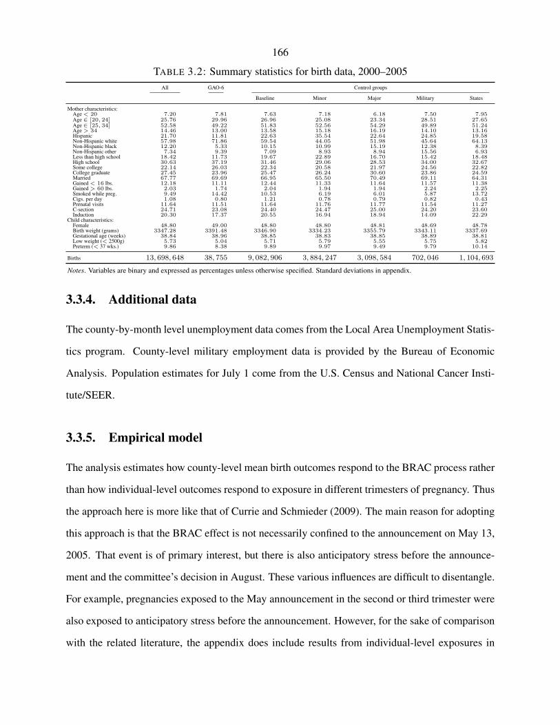
166

TABLE 3.2: Summary statistics for birth data, 2000–2005All GAO-6 Control groups

Baseline Minor Major Military States

Mother characteristics:Age < 20 7.20 7.81 7.63 7.18 6.18 7.50 7.95Age ∈ [20, 24] 25.76 29.96 26.96 25.08 23.34 28.51 27.65Age ∈ [25, 34] 52.58 49.22 51.83 52.56 54.29 49.89 51.24Age > 34 14.46 13.00 13.58 15.18 16.19 14.10 13.16Hispanic 21.70 11.81 22.63 35.54 22.64 24.85 19.58Non-Hispanic white 57.98 71.86 59.54 44.05 51.98 45.64 64.13Non-Hispanic black 12.20 5.33 10.15 10.99 15.19 12.38 8.39Non-Hispanic other 7.34 9.39 7.09 8.93 8.94 15.56 6.93Less than high school 18.42 11.73 19.67 22.89 16.70 15.42 18.48High school 30.63 37.19 31.46 29.06 28.53 34.00 32.67Some college 22.14 26.03 22.34 20.58 21.97 24.56 22.82College graduate 27.45 23.96 25.47 26.24 30.60 23.86 24.59Married 67.77 69.69 66.95 65.50 70.49 69.11 64.31Gained < 16 lbs. 12.18 11.11 12.44 11.33 11.64 11.57 11.38Gained > 60 lbs. 2.03 1.74 2.04 1.94 1.94 2.24 2.25Smoked while preg. 9.49 14.42 10.53 6.19 6.01 5.87 13.72Cigs. per day 1.08 0.80 1.21 0.78 0.79 0.82 0.43Prenatal visits 11.64 11.51 11.64 11.76 11.77 11.54 11.27C-section 24.71 23.08 24.40 24.47 25.00 24.20 23.60Induction 20.30 17.37 20.55 16.94 18.94 14.09 22.29

Child characteristics:Female 48.80 49.00 48.80 48.80 48.81 48.69 48.78Birth weight (grams) 3347.28 3391.48 3346.90 3334.23 3355.79 3343.11 3337.69Gestational age (weeks) 38.84 38.96 38.85 38.83 38.85 38.89 38.81Low weight (< 2500g) 5.73 5.04 5.71 5.79 5.55 5.75 5.82Preterm (< 37 wks.) 9.86 8.38 9.89 9.97 9.49 9.79 10.14

Births 13, 698, 648 38, 755 9, 082, 906 3, 884, 247 3, 098, 584 702, 046 1, 104, 693

Notes. Variables are binary and expressed as percentages unless otherwise specified. Standard deviations in appendix.

3.3.4. Additional data

The county-by-month level unemployment data comes from the Local Area Unemployment Statis-

tics program. County-level military employment data is provided by the Bureau of Economic

Analysis. Population estimates for July 1 come from the U.S. Census and National Cancer Insti-

tute/SEER.

3.3.5. Empirical model

The analysis estimates how county-level mean birth outcomes respond to the BRAC process rather

than how individual-level outcomes respond to exposure in different trimesters of pregnancy. Thus

the approach here is more like that of Currie and Schmieder (2009). The main reason for adopting

this approach is that the BRAC effect is not necessarily confined to the announcement on May 13,

2005. That event is of primary interest, but there is also anticipatory stress before the announce-

ment and the committee’s decision in August. These various influences are difficult to disentangle.

For example, pregnancies exposed to the May announcement in the second or third trimester were

also exposed to anticipatory stress before the announcement. However, for the sake of comparison

with the related literature, the appendix does include results from individual-level exposures in

167

the three different trimesters. Those results include estimates using the counterfactual full-term

pregnancy instrument proposed by Currie and Rossin-Slater (2013a).

To estimate how birth outcomes respond to the BRAC announcement, I use a linear model with

county fixed effects. The mean birth outcome Yi,t for each county i and month t is modeled by

Yi,t = αi +

(6∑

τ=1

βτTτi,t + γτt

)+Z ′

i,tδ + ϵi,t,

where

• the six treatment variables T τi,t indicate if county i is in the GAO-6 and month t is in the

period τ = (1) Jan–Apr 2004, (2) May–Aug 2004, (3) Sept–Dec 2004, (4) Jan–Apr 2005, (5)

May–Aug 2005, and (6) Sept–Dec 2005;

• γτt indicates when t is in period τ as defined above; and

• Zi,t is a vector of other covariates, including year indicators, seasonality indicators, and

means of mothers’ characteristics.11 The seasonality indicators are interacted with the treat-

ment group so that the treatment effect estimates are not biased by differences in seasonal

patterns between the groups. This specification is strongly supported by tests of the restric-

tion that the seasonal patterns are equal in the two groups.12

The key parameter is β5, which gives the average effect of the BRAC announcement on birth

outcomes in the GAO-6 during May–August 2005. The corresponding estimate along with those

for the other five periods of interest are reported in the results section. The regressions weight each11The mothers’ characteristics are proportions of mothers falling in various groups. The age categories are “Less

than 20”, “20 to 24”, “25 to 34”, “Over 34”, and “Missing”. The race and ethnicity categories are “Hispanic”, “White”,“Black”, “Other”, and “Missing”. The educational attainment categories are “Less than high school”, “High school”,“Some college”, “College or higher”, and “Missing”. The marital status categories are “Married” and “Not married”.The categories for total birth order are 1, 2, 3, 4, 5 or more, and “Missing”. Tobacco use variables are not included inthe main results because they are reported irregularly across states and over time. These self-reported variables are alsogenerally suspected to contain significant measurement error. Nevertheless additional results reported in the appendixshow that inclusion of tobacco use variables has no substantial effect on the results. The variables included are “non-smoker”, “smokes 1–5 cigarettes per day”, “smokes 6–10 cigarettes per day”, “smokes 11-20 cigarettes per day”,“smokes 21 or more cigarettes per day”, “smokes an unknown amount”, “smoking status unknown”, and “smokingvariables not reported.”

12The p value from the seasonality interaction test (SIT) is reported in the regression tables.

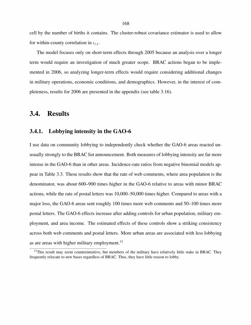
168

cell by the number of births it contains. The cluster-robust covariance estimator is used to allow

for within-county correlation in ϵi,t.

The model focuses only on short-term effects through 2005 because an analysis over a longer

term would require an investigation of much greater scope. BRAC actions began to be imple-

mented in 2006, so analyzing longer-term effects would require considering additional changes

in military operations, economic conditions, and demographics. However, in the interest of com-

pleteness, results for 2006 are presented in the appendix (see table 3.16).

3.4. Results

3.4.1. Lobbying intensity in the GAO-6

I use data on community lobbying to independently check whether the GAO-6 areas reacted un-

usually strongly to the BRAC list announcement. Both measures of lobbying intensity are far more

intense in the GAO-6 than in other areas. Incidence-rate ratios from negative binomial models ap-

pear in Table 3.3. These results show that the rate of web comments, where area population is the

denominator, was about 600–900 times higher in the GAO-6 relative to areas with minor BRAC

actions, while the rate of postal letters was 10,000–50,000 times higher. Compared to areas with a

major loss, the GAO-6 areas sent roughly 100 times more web comments and 50–100 times more

postal letters. The GAO-6 effects increase after adding controls for urban population, military em-

ployment, and area income. The estimated effects of these controls show a striking consistency

across both web comments and postal letters. More urban areas are associated with less lobbying

as are areas with higher military employment.13

13This result may seem counterintuitive, but members of the military have relatively little stake in BRAC. Theyfrequently relocate to new bases regardless of BRAC. Thus, they have little reason to lobby.

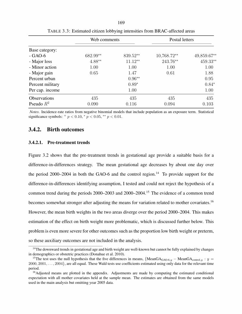
169

TABLE 3.3: Estimated citizen lobbying intensities from BRAC-affected areas

Web comments Postal letters

Base category:- GAO-6 682.99∗∗ 839.52∗∗ 10,768.72∗∗ 49,859.67∗∗

- Major loss 4.88∗∗ 11.12∗∗ 243.76∗∗ 459.33∗∗

- Minor action 1.00 1.00 1.00 1.00- Major gain 0.65 1.47 0.61 1.88Percent urban 0.96∗∗ 0.95Percent military 0.89∗ 0.84∗

Per cap. income 1.00 1.00

Observations 435 435 435 435Pseudo R2 0.090 0.116 0.094 0.103

Notes. Incidence-rate ratios from negative binomial models that include population as an exposure term. Statisticalsignificance symbols: + p < 0.10, ∗ p < 0.05, ∗∗ p < 0.01.

3.4.2. Birth outcomes

3.4.2.1. Pre-treatment trends

Figure 3.2 shows that the pre-treatment trends in gestational age provide a suitable basis for a

difference-in-differences strategy. The mean gestational age decreases by about one day over

the period 2000–2004 in both the GAO-6 and the control region.14 To provide support for the

difference-in-differences identifying assumption, I tested and could not reject the hypothesis of a

common trend during the periods 2000–2003 and 2000–2004.15 The evidence of a common trend

becomes somewhat stronger after adjusting the means for variation related to mother covariates.16

However, the mean birth weights in the two areas diverge over the period 2000–2004. This makes

estimation of the effect on birth weight more problematic, which is discussed further below. This

problem is even more severe for other outcomes such as the proportion low birth weight or preterm,

so these auxiliary outcomes are not included in the analysis.

14The downward trends in gestational age and birth weight are well-known but cannot be fully explained by changesin demographics or obstetric practices (Donahue et al. 2010).

15The test uses the null hypothesis that the five differences in means, {MeanGAGAO-6,y − MeanGAcontrol,y : y =2000, 2001, . . . , 2004}, are all equal. These Wald tests use coefficients estimated using only data for the relevant timeperiod.

16Adjusted means are plotted in the appendix. Adjustments are made by computing the estimated conditionalexpectation with all mother covariates held at the sample mean. The estimates are obtained from the same modelsused in the main analysis but omitting year 2005 data.

170

H0: Parallel pre−treatment, p = 0.27

38.7

38.8

38.9

39

39.1M

ean

gest

atio

nal a

ge (

wee

ks)

2000 2001 2002 2003 2004 2005 2006 2007 2008Year

GAO−6Control

Standard errorsprinted as bands.

(A)

H0: Parallel pre−treatment, p = 0.003300

3350

3400

3450

Mea

n bi

rth

wei

ght (

gram

s)

2000 2001 2002 2003 2004 2005 2006 2007 2008Year

GAO−6Control

Standard errorsprinted as bands.

(B)

FIGURE 3.2: Year-to-year trends in gestational age and birth weight

3.4.2.2. Main results for gestational age

The main regression results for gestational age appear in Table 3.4. In each of the five models, there

are six estimates, which correspond to the six four-month periods of 2004–2005. Across all models

the pattern is a decrease in gestational age that is strongest in May–August 2005 followed by an

insignificantly positive effect after August 2005. The first column shows results using the baseline

control group. In 2005, the January–April and May–August effects reach -0.42 (SE=0.27) and

-0.60 (SE=0.20) days, respectively. However, the September–December effect is +0.31 (SE=0.24)

days. Below the regression estimates is the p value of the equality test, which has the null hypothe-

sis that the three effects in 2005 are equal but not necessarily equal to zero. Thus, the test has some

robustness to a violation of parallel trends. The test strongly rejects that the three coefficients are

equal. In addition, note that the coefficient estimates do not change monotonically over time. The

mean deviation test is designed to test for a linear relationship among the three coefficients. The

null hypothesis is that the May–August 2005 effect is equal to the average of the January–April

2005 and September–December 2005 effects. This test also rejects strongly as seen in bottom of

Table 3.4.

The other four columns show that the pattern of results is robust to the use of alternative control

groups. The minor control group is the set of 144 counties that were affected by a minor BRAC

171

TAB

LE

3.4:

Est

imat

edef

fect

sof

BR

AC

lista

nnou

ncem

ento

nge

stat

iona

lage

and

birt

hw

eigh

tin

the

GA

O-6

Ges

tatio

nala

ge(d

ays)

Bir

thw

eigh

t(gr

ams)

(1)

(2)

(3)

(4)

(5)

(6)

(7)

(8)

(9)

(10)

Jan.

–Apr

.’04

0.252

0.065

0.151

0.178

0.473

9.052

7.626

11.496

5.751

10.025

(0.410)

(0.467)

(0.402)

(0.461)

(0.405)

(13.609)

(14.206)

(14.600)

(14.532)

(13.922)

May

–Aug

.’04

-0.186

-0.333

-0.294

-0.340

-0.172

4.395

4.196

8.739

1.414

4.623

(0.441)

(0.456)

(0.456)

(0.506)

(0.446)

(9.730)

(9.930)

(11.455)

(12.506)

(10.530)

Sept

.–D

ec.’

04-0.452

∗-0.477

∗-0.486

∗-0.254

-0.459

∗-24.676∗

∗-28.084∗

∗-20.899∗

-22.512∗

-19.896∗

(0.189)

(0.207)

(0.204)

(0.257)

(0.209)

(6.982)

(6.882)

(8.095)

(10.425)

(8.576)

Jan.

–Apr

.’05

-0.421

-0.595

+-0.594

∗-0.404

-0.306

-17.829

-21.381

-20.024

-23.781

-9.470

(0.271)

(0.313)

(0.298)

(0.341)

(0.277)

(16.505)

(16.019)

(16.970)

(17.746)

(17.034)

May

–Aug

.’05

-0.603

∗∗-0.831

∗∗-0.804

∗∗-0.739

∗∗-0.590

∗-35.164∗

-37.267∗

∗-44.666∗

∗-44.729∗

-29.975+

(0.204)

(0.183)

(0.206)

(0.272)

(0.246)

(15.163)

(13.941)

(13.717)

(17.719)

(16.899)

Sept

.–D

ec.’

050.306

0.236

0.217

0.353

0.391

-19.596

-26.137

-28.800

-33.438

-8.532

(0.235)

(0.268)

(0.234)

(0.276)

(0.262)

(22.386)

(21.711)

(23.678)

(27.880)

(23.220)

Con

trol

grou

pB

asel

ine

Min

orM

ajor

Mili

tary

Stat

esB

asel

ine

Min

orM

ajor

Mili

tary

Stat

esQ

uadr

atic

tren

dN

oN

oN

oN

oN

oY

esY

esY

esY

esY

esPT

T,20

00–2

003:p

0.664

0.781

0.699

0.803

0.721

0.039

0.121

0.177

0.045

0.044

SIT:p

0.000

0.000

0.000

0.000

0.000

0.000

0.000

0.000

0.012

0.015

Equ

ality

test

:p0.000

0.000

0.000

0.000

0.000

0.000

0.008

0.000

0.013

0.001

Mea

nde

viat

ion

test

:p0.000

0.000

0.000

0.001

0.000

0.044

0.091

0.013

0.080

0.023

Cel

ls115,708

6,764

9,991

3,236

16,524

115,708

6,764

9,991

3,236

16,524

Clu

ster

s1,646

94139

45240

1,646

94139

45240

Adj

.R2

0.341

0.601

0.626

0.478

0.273

0.514

0.792

0.759

0.777

0.468

Not

es.

Diff

eren

ce-i

n-di

ffer

ence

ses

timat

esdi

spla

yed.

Stan

dard

erro

rs,i

npa

rent

hese

s,ar

ecl

uste

red

byB

RA

C-d

efine

dec

onom

icar

eas.

All

mod

els

incl

ude

year

and

cale

ndar

mon

th-b

y-tr

eatm

entg

roup

indi

cato

rs.S

ymbo

lsof

sign

ifica

nce

atle

velp

:+p<

0.10

,∗p<

0.05

,∗∗p<

0.01

.

172

action.17 They satisfied these criteria: (1) A military installation in the county was put on the DoD’s

BRAC list, (2) no major closure, major realignment, nor major gain occurred in the county, and (3)

the employment changes associated with the county’s BRAC activities were less than one percent

of the county’s employment. The major control group is the set of 171 counties that fell in an

economic area that was slated to have a major closure or major realignment (where economic area

is defined as described in the background section above). The minor and major control groups are

disjoint. The military control group is the set of 56 counties where military employment made up

5–25% of employment in 2004. The military control group is not a strict subset of the minor control

group nor of the major control group. Finally, the states control group includes only counties in

the same states as the GAO-6 areas. The alternate control groups give statistically significant

May–August 2005 estimates in the range of -0.59 to -0.83, an interval which includes the estimate

obtained from the baseline model. In addition the equality and deviation tests are rejected in all

cases.

Only the May–August 2005 estimate is statistically robust across all models, but the results

suggest that gestational age was already trending downward before May 2005. The trend can be

seen to start in late 2004, which suggests that something was influencing gestational age in the

GAO-6 areas before the announcement in May 2005. One possibility is a change in economic

conditions. This topic is considered further below, and the unemployment rate data do not reveal

any significant changes over 2004–2005. Another possibility is selection or migration by potential

parents, also considered in more detail below. The results do not show unusual changes in the

characteristics of mothers giving birth during 2004–2005 nor the number of births. Finally, there

is the possibility that the decrease in gestational age is due to a process of anticipatory stress

that built up and peaked just after the BRAC list was announced. The coefficient estimates on the

gestational age effects steadily decrease and appear to be part of a single process that reaches a peak

and terminates in May–Aug. 2005. Gestational age then abruptly returned to a baseline level. An

anticipatory stress process is consistent with the local press reports discussed above, which indicate

17The number of counties is not equal to the number of clusters in the table because some counties are combinedaccording the military’s definition of an economic area.

173

a significant amount of anxiety before the BRAC announcement. However, this explanation also

requires that the GAO-6 areas were affected more severely than other military areas. Unfortunately

there is no data on beliefs about the relative likelihood of different military sites being assigned

to the BRAC list. Research on BRAC or other policy changes should consider the possibility that

medical or physiological data might reflect aggregate beliefs about the likelihood of stressful future

events.

3.4.2.3. Main results for birth weight

The results for birth weight must be interpreted with caution because, as shown in Figure 3.2, the

pre-treatment trends diverge. Table 3.4 displays regression results analogous to those for gesta-

tional age, but these birth weight models include treatment group-specific quadratic time trends.

This functional form appears most plausible in appendix Figure 3.6. Nevertheless, regression re-

sults for alternative specifications are presented in appendix table 3.10. The birth weight results are

in qualitative agreement with the gestational age results and suggest a decrease in growth during

May–August 2005 relative to the other parts of the year. The May–August 2005 effect estimates

range from -30 to -45 grams, but the estimates are somewhat imprecise with standard errors in

the range of 14 to 18. Across all the control group specifications the equality tests and deviation

tests are rejected, indicating an unusual change in birth weights over the course of the 2005. The

results from alternative specifications of the time trend also indicate a decrease in birth weight

during May–August 2005 and rejection of the equality test. Ultimately, the results here suggest the

same pattern of changes seen in gestational age, but the lack of well-behaved pre-treatment trends

precludes a sharp conclusion about the size of the birth weight effects.

3.4.2.4. Month-by-month results for gestational age

Examining the effects on a monthly basis provides additional evidence that the BRAC announce-

ment decreased the mean gestational age in the GAO-6. To investigate the effects of the announce-

ment in finer detail, I estimated a model with separate effects for each month of 2005 instead of

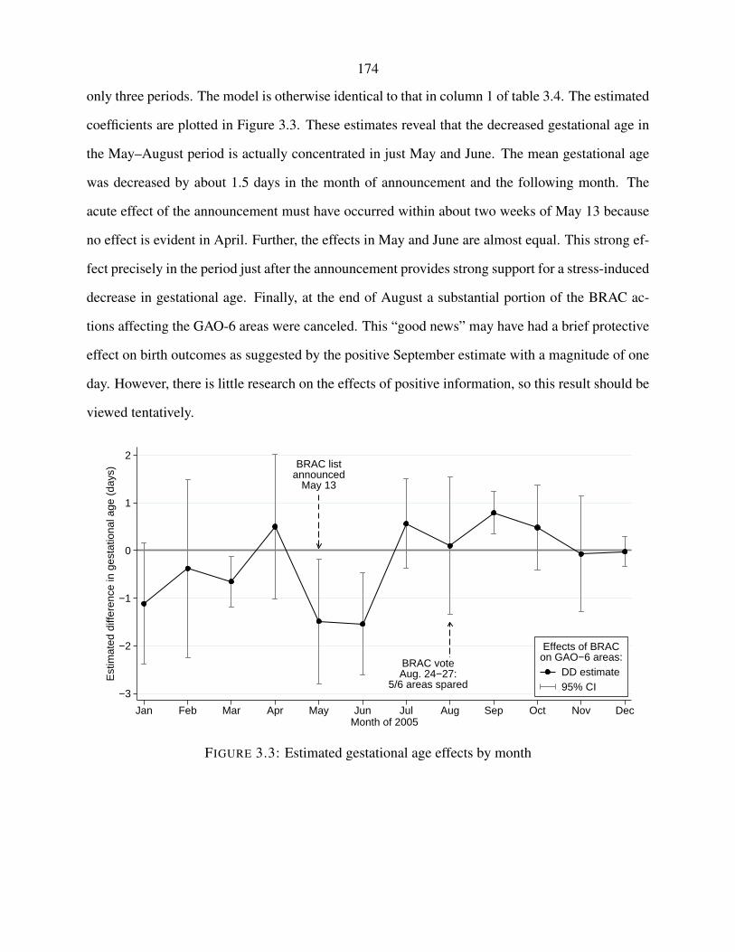
174

only three periods. The model is otherwise identical to that in column 1 of table 3.4. The estimated

coefficients are plotted in Figure 3.3. These estimates reveal that the decreased gestational age in

the May–August period is actually concentrated in just May and June. The mean gestational age

was decreased by about 1.5 days in the month of announcement and the following month. The

acute effect of the announcement must have occurred within about two weeks of May 13 because

no effect is evident in April. Further, the effects in May and June are almost equal. This strong ef-

fect precisely in the period just after the announcement provides strong support for a stress-induced

decrease in gestational age. Finally, at the end of August a substantial portion of the BRAC ac-

tions affecting the GAO-6 areas were canceled. This “good news” may have had a brief protective

effect on birth outcomes as suggested by the positive September estimate with a magnitude of one

day. However, there is little research on the effects of positive information, so this result should be

viewed tentatively.

BRAC listannounced

May 13

BRAC voteAug. 24−27:

5/6 areas spared−3

−2

−1

0

1

2

Est

imat

ed d

iffer

ence

in g

esta

tiona

l age

(da

ys)

Jan Feb Mar Apr May Jun Jul Aug Sep Oct Nov DecMonth of 2005

DD estimate95% CI

Effects of BRACon GAO−6 areas:

FIGURE 3.3: Estimated gestational age effects by month

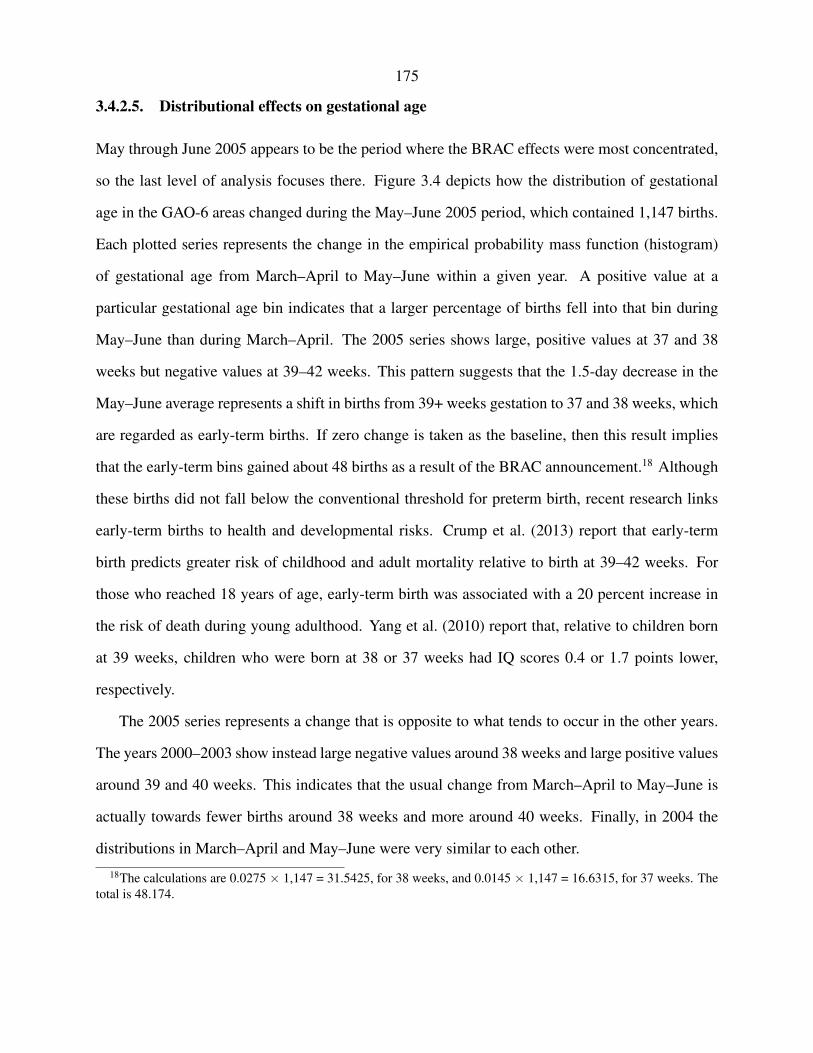
175

3.4.2.5. Distributional effects on gestational age

May through June 2005 appears to be the period where the BRAC effects were most concentrated,

so the last level of analysis focuses there. Figure 3.4 depicts how the distribution of gestational

age in the GAO-6 areas changed during the May–June 2005 period, which contained 1,147 births.

Each plotted series represents the change in the empirical probability mass function (histogram)

of gestational age from March–April to May–June within a given year. A positive value at a

particular gestational age bin indicates that a larger percentage of births fell into that bin during

May–June than during March–April. The 2005 series shows large, positive values at 37 and 38

weeks but negative values at 39–42 weeks. This pattern suggests that the 1.5-day decrease in the

May–June average represents a shift in births from 39+ weeks gestation to 37 and 38 weeks, which

are regarded as early-term births. If zero change is taken as the baseline, then this result implies

that the early-term bins gained about 48 births as a result of the BRAC announcement.18 Although

these births did not fall below the conventional threshold for preterm birth, recent research links

early-term births to health and developmental risks. Crump et al. (2013) report that early-term

birth predicts greater risk of childhood and adult mortality relative to birth at 39–42 weeks. For

those who reached 18 years of age, early-term birth was associated with a 20 percent increase in

the risk of death during young adulthood. Yang et al. (2010) report that, relative to children born

at 39 weeks, children who were born at 38 or 37 weeks had IQ scores 0.4 or 1.7 points lower,

respectively.

The 2005 series represents a change that is opposite to what tends to occur in the other years.

The years 2000–2003 show instead large negative values around 38 weeks and large positive values

around 39 and 40 weeks. This indicates that the usual change from March–April to May–June is

actually towards fewer births around 38 weeks and more around 40 weeks. Finally, in 2004 the

distributions in March–April and May–June were very similar to each other.

18The calculations are 0.0275 × 1,147 = 31.5425, for 38 weeks, and 0.0145 × 1,147 = 16.6315, for 37 weeks. Thetotal is 48.174.

176

−0.02

0.00

0.02

0.04

19 22 25 28 31 34 37 40 43 46Gestational age (weeks)

Cha

nge

in p

roba

bilit

y m

ass

from

Mar

ch−

Apr

il to

May

−Ju

neYear

200520042003200220012000

FIGURE 3.4: Effects on the gestational age distribution in the GAO-6

3.4.2.6. Randomization inference for gestational age effect

Additional analysis shows that the changes in birth weights in the GAO-6 are unusual relative to

those found in other areas. I conducted a randomization inference test similar to that discussed by

Bertrand et al. (2002) and Donohue and Ho (2007). This test holds all covariates constant except

for the BRAC treatment variables, which are randomly assigned to other areas. After random

assignment, the effects of the randomly assigned treatments are estimated. Under the sharp null

hypothesis of no treatment effect in every unit, repetition of this procedure N times delivers an

estimate of the randomization distribution of the test statistic of interest, {tn : n = 1, . . . , N}.19

Observing an extreme test statistic relative to the randomization distribution provides evidence

against the null hypothesis.

This test is constructed such that it parallels the research design and incorporates informa-

tion about the treatment assignment mechanism. Intuitively it answers the question, “If many

researchers conducted studies of BRAC by randomly choosing six counties with a large military

presence and then conducted the usual analysis, what would be the distribution of results?” In

19Calculation of all possible permutations is infeasible.

177

each realization of the test, the placebo treatments are randomly assigned so as to create a group

of six counties that are similar to the GAO-6. These random groups are drawn from the set of 62

counties where military employment made up 5–25 percent of local employment.20 The test statis-

tic used is the t statistic on the May–August 2005 effect, the same statistic used for inference in

the conventional analysis. If the BRAC list announcement truly has no effect, then the observed t

statistic is unlikely to be unusual relative to the randomization distribution. Finally, one additional

step is included to address the problem of pre-treatment trends and the difference-in-differences

identifying assumption. Some randomly formed treatment groups do not share a common trend

with the control group. Ignoring this problem would cause potentially severely biased estimates

to enter the randomization distribution. To address this problem, the random groups are filtered

through the parallel trends test used elsewhere in the paper. Each realization is only included if

this test has p > 0.05 over 2000–2004.21

A total of 5,000 randomizations were attempted, which yielded 922 statistics after filtering. The

p-value on the May–August 2005 estimate had a 95 percent confidence interval which fell entirely

below 0.05, thus satisfying a simple stopping rule. A histogram of these realizations appears in

figure 3.5. The observed t = −2.91 has a one-tailed p-value of 0.027. Thus, the real result was

unlikely to be generated under the null hypothesis of no BRAC effect. The equality test of the

three key coefficients is also rejected under the randomization implementation with a p-value of

0.014. The January–April and September–December coefficients however are not significant at

conventional levels. These additional results are plotted in the appendix.

3.4.2.7. Individual-level estimates

For comparison with the literature, estimates on individual-level natality data are presented in the

appendix. These models treat the BRAC announcement on May 13, 2005 as a point source of

stress like studies of disaster exposure. Exposures are treated both in the conventional way and

20This includes the GAO-6 counties. Two of the GAO-6 sites, Martin, Indiana, and Mineral, Nevada, were reportedto have less than 5 percent military employment in the Bureau of Economic Analysis data. But these data conflict withmilitary figures and appear to be unreliable due to the small populations.

21The trends are tested over 2000-2004 and only the treatment variables for 2005 are included.

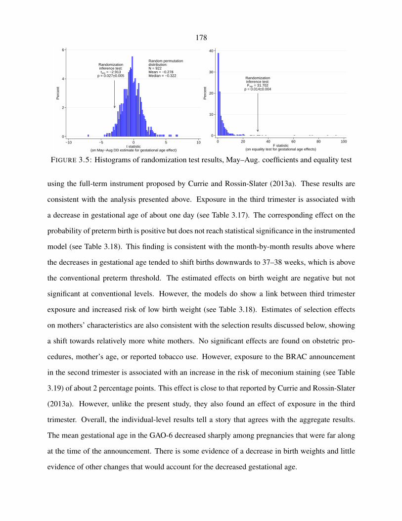
178

Randomizationinference test:tobs = −2.913

p = 0.027±0.005

Random permutationdistribution:N = 922Mean = −0.278Median = −0.322

0

2

4

6

Per

cent

−10 −5 0 5 10t statistic

(on May−Aug DD estimate for gestational age effect)

Randomizationinference test:Fobs = 31.702

p = 0.014±0.004

0

10

20

30

40

Per

cent

0 20 40 60 80 100F statistic

(on equality test for gestational age effects)

FIGURE 3.5: Histograms of randomization test results, May–Aug. coefficients and equality test

using the full-term instrument proposed by Currie and Rossin-Slater (2013a). These results are

consistent with the analysis presented above. Exposure in the third trimester is associated with

a decrease in gestational age of about one day (see Table 3.17). The corresponding effect on the

probability of preterm birth is positive but does not reach statistical significance in the instrumented

model (see Table 3.18). This finding is consistent with the month-by-month results above where

the decreases in gestational age tended to shift births downwards to 37–38 weeks, which is above

the conventional preterm threshold. The estimated effects on birth weight are negative but not

significant at conventional levels. However, the models do show a link between third trimester

exposure and increased risk of low birth weight (see Table 3.18). Estimates of selection effects

on mothers’ characteristics are also consistent with the selection results discussed below, showing

a shift towards relatively more white mothers. No significant effects are found on obstetric pro-

cedures, mother’s age, or reported tobacco use. However, exposure to the BRAC announcement

in the second trimester is associated with an increase in the risk of meconium staining (see Table

3.19) of about 2 percentage points. This effect is close to that reported by Currie and Rossin-Slater

(2013a). However, unlike the present study, they also found an effect of exposure in the third

trimester. Overall, the individual-level results tell a story that agrees with the aggregate results.

The mean gestational age in the GAO-6 decreased sharply among pregnancies that were far along

at the time of the announcement. There is some evidence of a decrease in birth weights and little

evidence of other changes that would account for the decreased gestational age.

179

3.4.3. Additional mechanisms

3.4.3.1. Unemployment rates

Employers in the GAO-6 areas might have reacted to BRAC by slowing hiring or laying off work-

ers. The unemployment data provide little evidence of this effect. Appendix figure 3.7 plots the

unemployment rates in the two areas, which shows that unemployment in the GAO-6 was lower

throughout the study period. However, the gap between the two areas grew after the 2001 recession

and then steadily shrank.22 To account for that approximately linear change in the gap from 2002

onwards, the unemployment models in Table 3.5 are estimated on the 2002–2005 data and include

group-specific linear trends. The negative coefficients reflect that unemployment in the GAO-6 is

lower even after taking into account the linear drift in the gap, although the coefficients are not

significant at conventional levels. If anticipation or the consequences of the BRAC announcement

had increased unemployment in the GAO-6, then we would expect an upward trend in the coeffi-

cients. However, the coefficients show a downward trend with time. In addition, this trend is fairly

steady, whereas the changes in birth outcomes show a sharp reversal within 2005. Overall, these

results show little evidence of unusual changes in employment activity in the GAO-6.

3.4.3.2. Selection

The means of gestational age and birth weight are also influenced by the composition of mothers.

Several additional checks show that changes in the composition of mothers are unlikely to explain

the decrease in gestational age and birth weight. The first check is to estimate a model of the birth

rate. The estimates from a Poisson conditional fixed-effects model are displayed in the last column

of Table 3.6. The results show little evidence of changes in the birth rate, and the usual equality

test does not reject the hypothesis that the Jan.–Apr., May–Aug., and Sept.–Dec. coefficients

from 2005 are equal. The same results hold for the alternative control groups (see appendix Table

3.29). These results leave little room for women to select out of giving birth in the GAO-6 on

net. The second check simply allows the demographic control variables to enter the models of22The militarized areas may have been insulated from the business cycle.

180

TABLE 3.5: Estimated effects of BRAC list announcement on unemployment in the GAO-6

(1) (2) (3) (4) (5)

Jan.–Apr. 2004 -0.012 -0.063 -0.115 -0.169 -0.092(0.175) (0.180) (0.178) (0.184) (0.197)

May–Aug. 2004 -0.150 -0.134 -0.247 -0.315 -0.196(0.339) (0.346) (0.347) (0.350) (0.359)

Sept.–Dec. 2004 -0.421 -0.345 -0.495 -0.594 -0.522(0.499) (0.506) (0.508) (0.517) (0.529)

Jan.–Apr. 2005 -0.204 -0.176 -0.438 -0.578 -0.607(0.493) (0.506) (0.502) (0.511) (0.535)

May–Aug. 2005 -0.181 -0.130 -0.401 -0.630 -0.577(0.546) (0.564) (0.553) (0.564) (0.593)

Sept.–Dec. 2005 -0.292 -0.268 -0.539 -0.778 -0.657(0.616) (0.629) (0.626) (0.636) (0.671)

Control group Baseline Minor Major Military StatesEquality, p 0.674 0.572 0.479 0.450 0.783Deviation, p 0.381 0.299 0.227 0.529 0.485Cells 79, 008 7, 200 8, 496 2, 976 11, 520Adj. R2 0.836 0.864 0.859 0.884 0.794

Notes. All models include year fixed effects, calendar month indicator variables interacted with treatment group, and group-specific linear trends.Cells are weighted by the size of the labor force. The equality test has the null hypothesis that all three coefficients in 2005 are equal. Deviationtest explained in main text. Standard errors, in parentheses, are clustered by county. Statistical significance symbols: + p < 0.10, ∗ p < 0.05, ∗∗

p < 0.01.

mean gestational age and birth weight more flexibly. The estimated decreases in gestational age

and birth weight are robust to excluding the demographic controls or simultaneously interacting

them with treatment group, calendar month, and year indicator variables. The May–Aug. 2005

estimate of the decrease in gestational age is -0.517 (SE=0.25) when demographic controls are

omitted. Including the controls results in an estimate of -0.602 (SE=0.204). Finally, interacting

the demographic controls with indicators for treatment group, calendar month, and year results in

an estimate of -0.567 (SE=0.226). These robustness results are available for both the baseline and

military control groups in the appendix (Tables 3.11 and 3.12).

Further checks for selection are implemented by estimating models of the proportions of moth-

ers falling into various demographic categories. These models are like those used for the main

results above but exclude mothers’ demographics as covariates. This check was run for a variety of

characteristics including age categories, educational attainment, marital status, and smoking status.

181

The results are presented in Table 3.6 and the appendix. The mothers’ characteristics show some

evidence of changes over 2004–2005, but these changes appear unlikely to explain the changes

in gestational age and birth weight. The magnitudes of the demographic changes are small, and

the period-to-period timing of the changes in demographics does not match well with changes in

gestational age. Finally, these demographic results are sensitive to the specification of the control

group, whereas the main results are quite robust.

For example, during 2005 and especially the crucial May–August period, there is evidence of

a moderate increase in the percentages of mothers who are white and married. Comparing the

three race/ethnicity columns suggests that births shifted from Hispanic and black mothers to white

mothers. This shift appears unlikely to account for the gestational age results because on average

births to white mothers and Hispanic mothers have similar gestational ages. Births to black mothers

have significantly lower gestational age than the two other groups, and births to married women

tend to have higher gestational ages (see appendix Table 3.14). Finally, marriage tends to have a

positive effect on gestational age.

The education results in Table 3.6 suggest that the mean educational attainment of mothers in

the GAO-6 decreased during 2005 with a shift from college education to high school and partial

college. This change would tend to decrease the mean gestational age, but the effects are quite

small at about 1–2 percentage points. More importantly the pattern of education changes does not

match the pattern of gestational age changes. The proportion of college-educated mothers remains

depressed throughout 2005, but the gestational age was depressed only during the first two periods

of the year and elevated in the last period. In addition, the decrease in college-education is greatest

during Jan.–Apr. 2005, with an estimate of -1.87 percentage points, and then rises to -1.03 during

May–Aug. 2005. However, the gestational age decrease was greatest during the May–Aug. period.

Furthermore, if the model is estimated using the military control group, then the decrease in the

proportion of college-educated mothers is substantially smaller and not statistically-significant. In

contrast, the gestational age effect of BRAC appears larger when switching from the baseline to

military control group. Finally, in the individual-level models there is no significant association

182

between the mother’s education and third trimester BRAC exposure (see appendix Table 3.20).

Estimates for additional variables, including weight gain, prenatal visits, birth method, tobacco

use, and birth order, are available in the appendix (see Table 3.23 and the following tables). Like

the results discussed above, these additional variables overall do not exhibit patterns of changes

that can explain the decreases in gestational age and birth weight.

3.4.4. Effects beyond the GAO-6

The GAO-6 areas represent a small portion of those affected by BRAC. Other areas that were

targeted by major closures or realignments may have experienced similar stress-related effects. A

supplementary analysis here suggests the possibility of small negative effects on gestational age.

To examine other areas, I use the same models as in the main analysis (see Table 3.4). However,

treatment is redefined to be any major closure or realignment. More precisely, a county was defined

as treated if it contained a military site that was assigned to undergo a “major closure” or “major

realignment” as defined by the DoD. The GAO-6 areas were entirely excluded from this analysis.

The results appear in appendix Table 3.13. First, in some specifications the parallel trends tests

reject or nearly reject, so the results are subject to bias. However, there is still some evidence

of an effect in May–August 2005 because, like the main GAO-6 results, that period shows lower

gestational ages than preceding and following periods. However, the size of the difference is small

relative to the GAO-6 results and generally not significant at conventional levels. Thus, the results

here are qualitatively consistent with the stress hypothesis, but the effects, if any, are small and

strong conclusions cannot be reached.

3.5. Conclusion

In May 2005 the Department of Defense announced plans to close or shrink military sites across the

United States. In six communities that were expected to experience serious losses of employment

as a result of the policy change, the announcement was met with much anxiety and distress. In

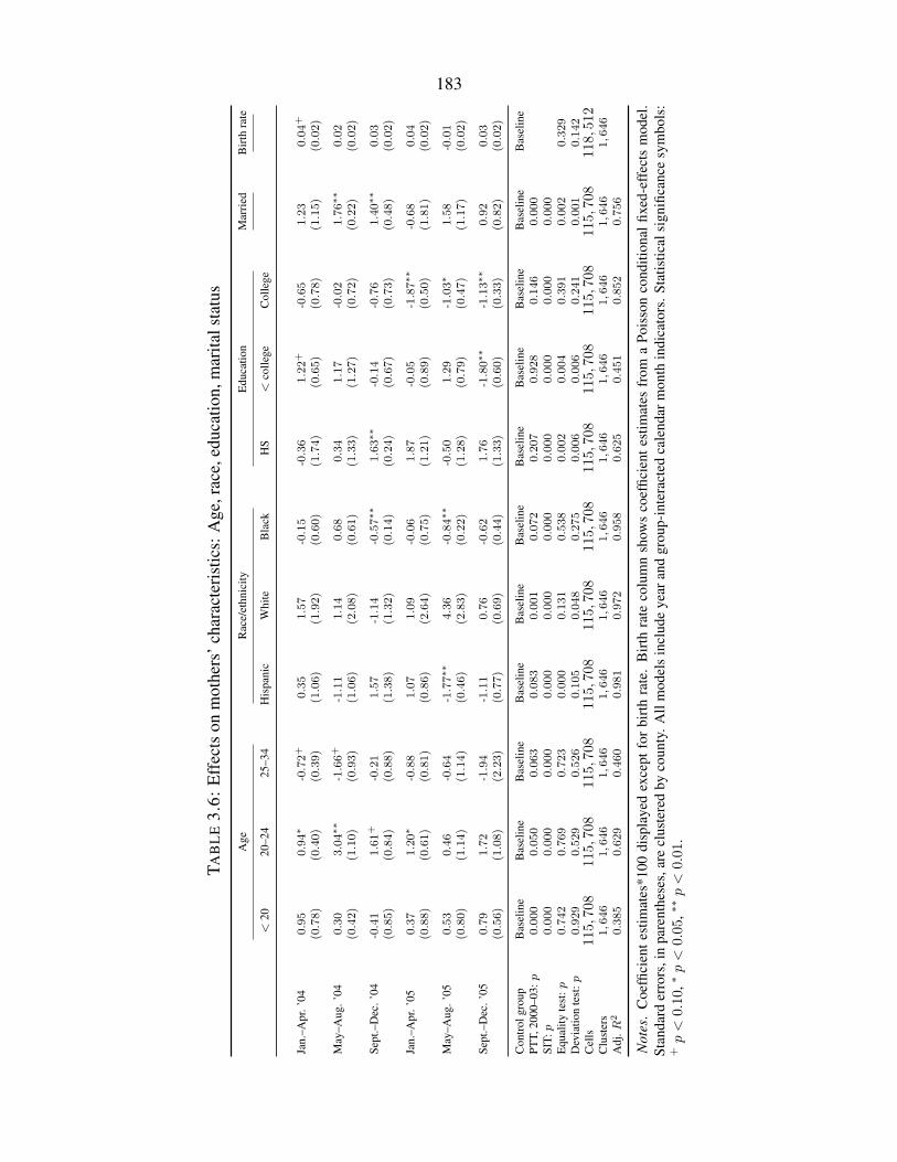
183

TAB

LE

3.6:

Eff

ects

onm

othe

rs’c

hara

cter

istic

s:A

ge,r

ace,

educ

atio

n,m

arita

lsta

tus

Age

Rac

e/et

hnic

ityE

duca

tion

Mar

ried

Bir

thra

te

<20

20–2

425

–34

His

pani

cW

hite

Bla

ckH

S<

colle

geC

olle

ge

Jan.

–Apr

.’04

0.95

0.94∗

-0.72+

0.35

1.57

-0.15

-0.36

1.22+

-0.65

1.23

0.04+

(0.78)

(0.40)

(0.39)

(1.06)

(1.92)

(0.60)

(1.74)

(0.65)

(0.78)

(1.15)

(0.02)

May

–Aug

.’04

0.30

3.04∗∗

-1.66+

-1.11

1.14

0.68

0.34

1.17

-0.02

1.76∗∗

0.02

(0.42)

(1.10)

(0.93)

(1.06)

(2.08)

(0.61)

(1.33)

(1.27)

(0.72)

(0.22)

(0.02)

Sept

.–D

ec.’

04-0.41

1.61+

-0.21

1.57

-1.14

-0.57∗∗

1.63∗∗

-0.14

-0.76

1.40∗∗

0.03

(0.85)

(0.84)

(0.88)

(1.38)

(1.32)

(0.14)

(0.24)

(0.67)

(0.73)

(0.48)

(0.02)

Jan.

–Apr

.’05

0.37

1.20∗

-0.88

1.07

1.09

-0.06

1.87

-0.05

-1.87∗∗

-0.68

0.04

(0.88)

(0.61)

(0.81)

(0.86)

(2.64)

(0.75)

(1.21)

(0.89)

(0.50)

(1.81)

(0.02)

May

–Aug

.’05

0.53

0.46

-0.64

-1.77∗∗

4.36

-0.84∗∗

-0.50

1.29

-1.03∗

1.58

-0.01

(0.80)

(1.14)

(1.14)

(0.46)

(2.83)

(0.22)

(1.28)

(0.79)

(0.47)

(1.17)

(0.02)

Sept

.–D

ec.’

050.79

1.72

-1.94

-1.11

0.76

-0.62

1.76

-1.80∗∗

-1.13∗∗

0.92

0.03

(0.56)

(1.08)

(2.23)

(0.77)

(0.69)

(0.44)

(1.33)

(0.60)

(0.33)

(0.82)

(0.02)

Con

trol

grou

pB

asel

ine

Bas

elin

eB

asel

ine

Bas

elin

eB

asel

ine

Bas

elin

eB

asel

ine

Bas

elin

eB

asel

ine

Bas

elin

eB

asel

ine

PTT,

2000

–03:

p0.000

0.050

0.063

0.083

0.001

0.072

0.207

0.928

0.146

0.000

SIT:

p0.000

0.000

0.000

0.000

0.000

0.000

0.000

0.000

0.000

0.000

Equ

ality

test

:p0.742

0.769

0.723

0.000

0.131

0.538

0.002

0.004

0.391

0.002

0.329

Dev

iatio

nte

st:p

0.929

0.529

0.526

0.105

0.048

0.275

0.006

0.006

0.241

0.001

0.142

Cel

ls115,708

115,708

115,708

115,708

115,708

115,708

115,708

115,708

115,708

115,708

118,512

Clu

ster

s1,6

46

1,6

46

1,6

46

1,6

46

1,6

46

1,6

46

1,6

46

1,6

46

1,6

46

1,6

46

1,6

46

Adj

.R2

0.385

0.629

0.460

0.981

0.972

0.958

0.625

0.451

0.852

0.756

Not

es.

Coe

ffici

ente

stim

ates

*100

disp

laye

dex

cept

for

birt

hra

te.

Bir

thra

teco

lum

nsh

ows

coef

ficie

ntes

timat

esfr

oma

Pois

son

cond

ition

alfix

ed-e

ffec

tsm

odel

.St

anda

rder

rors

,in

pare

nthe

ses,

are

clus

tere

dby

coun

ty.A

llm

odel

sin

clud

eye

aran

dgr

oup-

inte

ract

edca

lend

arm

onth

indi

cato

rs.S

tatis

tical

sign

ifica

nce

sym

bols

:+p<

0.10

,∗p<

0.05,

∗∗p<

0.01.

184

these areas, the mean gestational age decreased by 1.5 days for a period of 1–2 months following

the announcement. This decrease was driven by a greater risk of early-term birth, a factor which

predicts decreased cognitive function and higher risk of childhood and adult mortality. The mean

birth weight showed changes that are consistent with the decreases in gestational age. A smaller

decreasing trend in gestational age appeared in the months before the announcement. Alternative

models were estimated that treat the BRAC announcement as a point source of stress exposure for

individual pregnancies. These results are consistent with the aggregate results and are robust to the

use of the full-term instrument proposed by Currie and Rossin-Slater (2013a). The effects on birth

outcomes are not accounted for by changes in unemployment rates or demographic features of the

mothers in the BRAC-affected areas during 2004–2005.

This result suggests that policy announcements can have substantial effects in areas where

many people expect to suffer losses from the policy change. In addition, anxiety about impending

economic changes may be revealed by medical or physiological changes in the relevant population.

This study focused on areas where effects were concentrated, but there are also people working in

relatively small sites who may fear being furloughed or having their work place closed. It is unclear

how these isolated workers will differ. They might be less distressed by announcements if they

believe that they can easily find another job in their area. They might also be less affected if the

results of this study depend on social interactions to amplify distress. However, social interactions

might also provide a protective effect, which would make isolated workers even worse off. These

questions can only be addressed with additional research using individual-level data.

Nevertheless, these results are highly relevant because many policy changes and business de-

cisions have strongly concentrated effects. As shown here, the mere announcement of a policy is

followed by responses similar to those seen following disasters. In addition, the health effects are

unlikely to be restricted to just birth outcomes, so further research on additional outcomes would

be valuable. Cardiovascular and mental health variables are likely candidates. Officials in areas

facing strong impacts from policy changes should be cognizant of health effects. They may want

to provide interventions to help employees or citizens manage stress levels and maintain healthful

185

behaviors during uncertain times.

3.6. Appendix of chapter 3

3.6.1. Background

TABLE 3.7: Key dates in BRAC 2005 process

Date Event

November 15, 2002 BRAC process initiated by SECDEF.1

February 12, 2004 Final base selection criteria published by SECDEF.2

March 23, 2004 Need for BRAC 2005 certified by SECDEF.3

April 1, 2005 BRAC commissioners appointed by President Bush.4

May 13, 2005 Recommendations (BRAC list) announced by SECDEF.July 1, 2005 GAO reported analysis of DoD’s recommendations.5

August 24–27, 2005 Final deliberations and vote by BRAC commission6

2006– BRAC actions implemented

SECDEF=Secretary of Defense Donald Rumsfeld 1 Government Accountability Office (2005, p. 2)2 United States Department of Defense (2005a, p. 18) 3 United States Department of Defense (2005a, p. 2)4 United States Department of Defense 5 Government Accountability Office (2005) 6 Defense Base Closure andRealignment Commission (2005b)

TABLE 3.8: Control groups used in estimation

Control group Definition

Baseline All non-GAO-6 areas where no major closure, realignment, or gain occurred.Minor BRAC All non-GAO-6 areas affected by BRAC where (1) no major closure, realignment,

or gain occurred; and (2) projected changes in local employment (due to BRAC)were less than one percent.

Major BRAC All non-GAO-6 areas where a major closure or realignment occurred.Military All non-GAO-6 areas where military employment is 5–25% of total employment.States Alaska, Connecticut, Indiana, Nevada, New Mexico, South Dakota

Notes. Major closures are closures of installations of at least $100 million in plant replacement value. Major realign-ments (gains) are actions that would remove (add) at least 400 jobs at an installation.

186

3.6.2. Data

TABLE 3.9: Summary statistics of natality dataAll GAO-6 Control groups

Baseline Minor Major Military States

Age < 20 7.20 7.81 7.63 7.18 6.18 7.50 7.95(25.84) (26.83) (26.54) (25.81) (24.09) (26.34) (27.05)

Age ∈ [20, 24] 25.76 29.96 26.96 25.08 23.34 28.51 27.65(43.73) (45.81) (44.38) (43.35) (42.30) (45.15) (44.72)

Age ∈ [25, 34] 52.58 49.22 51.83 52.56 54.29 49.89 51.24(49.93) (49.99) (49.97) (49.93) (49.82) (50.00) (49.98)

Age > 34 14.46 13.00 13.58 15.18 16.19 14.10 13.16(35.17) (33.63) (34.26) (35.88) (36.84) (34.80) (33.81)

Hispanic 21.70 11.81 22.63 35.54 22.64 24.85 19.58(41.22) (32.27) (41.84) (47.86) (41.85) (43.21) (39.68)

Non-Hispanic white 57.98 71.86 59.54 44.05 51.98 45.64 64.13(49.36) (44.97) (49.08) (49.64) (49.96) (49.81) (47.96)

Non-Hispanic black 12.20 5.33 10.15 10.99 15.19 12.38 8.39(32.73) (22.47) (30.20) (31.28) (35.89) (32.94) (27.72)

Non-Hispanic other 7.34 9.39 7.09 8.93 8.94 15.56 6.93(26.08) (29.17) (25.66) (28.52) (28.53) (36.24) (25.39)

Less than high school 18.42 11.73 19.67 22.89 16.70 15.42 18.48(38.76) (32.18) (39.75) (42.01) (37.30) (36.11) (38.82)

High school 30.63 37.19 31.46 29.06 28.53 34.00 32.67(46.10) (48.33) (46.44) (45.40) (45.15) (47.37) (46.90)

Some college 22.14 26.03 22.34 20.58 21.97 24.56 22.82(41.52) (43.88) (41.65) (40.43) (41.40) (43.04) (41.97)

College graduate 27.45 23.96 25.47 26.24 30.60 23.86 24.59(44.63) (42.68) (43.57) (44.00) (46.08) (42.62) (43.06)

Married 67.77 69.69 66.95 65.50 70.49 69.11 64.31(46.73) (45.96) (47.04) (47.54) (45.61) (46.20) (47.91)

Gained < 16 lbs. 12.18 11.11 12.44 11.33 11.64 11.57 11.38(32.71) (31.42) (33.00) (31.69) (32.07) (31.99) (31.76)

Gained > 60 lbs. 2.03 1.74 2.04 1.94 1.94 2.24 2.25(14.10) (13.09) (14.12) (13.80) (13.78) (14.80) (14.82)

Smoked while preg. 9.49 14.42 10.53 6.19 6.01 5.87 13.72(29.31) (35.13) (30.70) (24.10) (23.77) (23.50) (34.41)

Cigs. per day 1.08 0.80 1.21 0.78 0.79 0.82 0.43(3.81) (3.05) (4.04) (3.21) (3.22) (3.21) (2.36)

Prenatal visits 11.64 11.51 11.64 11.76 11.77 11.54 11.27(3.85) (3.26) (3.80) (3.91) (3.86) (3.94) (4.05)

Induction 20.30 17.37 20.55 16.94 18.94 14.09 22.29(40.22) (37.89) (40.40) (37.51) (39.18) (34.80) (41.62)

C-section 24.71 23.08 24.40 24.47 25.00 24.20 23.60(43.13) (42.13) (42.95) (42.99) (43.30) (42.83) (42.46)

Female 48.80 49.00 48.80 48.80 48.81 48.69 48.78(49.99) (49.99) (49.99) (49.99) (49.99) (49.98) (49.99)

Birth weight (grams) 3347.28 3391.48 3346.90 3334.23 3355.79 3343.11 3337.69(566.19) (561.60) (564.56) (560.75) (565.74) (566.39) (561.03)

Gestational age (weeks) 38.84 38.96 38.85 38.83 38.85 38.89 38.81(2.37) (2.21) (2.37) (2.37) (2.33) (2.40) (2.37)

Births 13, 698, 648 38, 755 9, 082, 906 3, 884, 247 3, 098, 584 702, 046 1, 104, 693

Notes. Variables are binary and expressed as percentages unless otherwise specified. Standard deviations in parentheses.

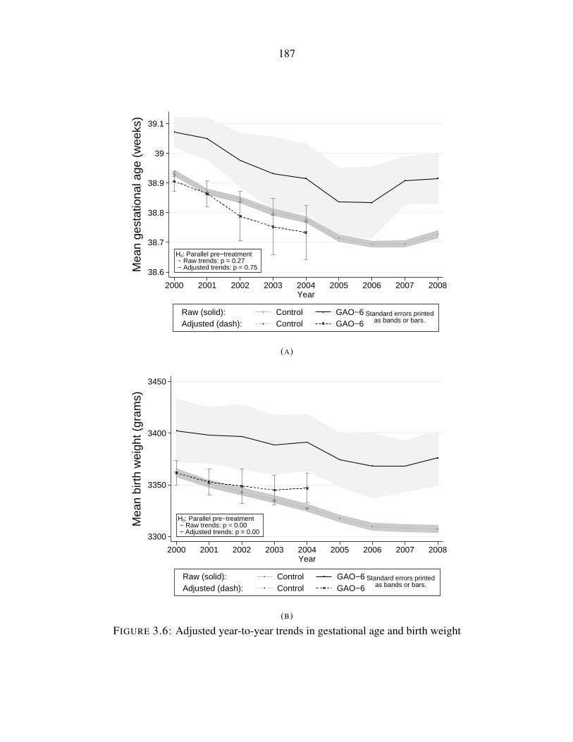
187

H0: Parallel pre−treatment − Raw trends: p = 0.27 − Adjusted trends: p = 0.75

38.6

38.7

38.8

38.9

39

39.1

Mea

n ge

stat

iona

l age

(w

eeks

)

2000 2001 2002 2003 2004 2005 2006 2007 2008Year

Raw (solid): Control GAO−6Adjusted (dash): Control GAO−6

Standard errors printedas bands or bars.

(A)

H0: Parallel pre−treatment − Raw trends: p = 0.00 − Adjusted trends: p = 0.00

3300

3350

3400

3450

Mea

n bi

rth

wei

ght (

gram

s)

2000 2001 2002 2003 2004 2005 2006 2007 2008Year

Raw (solid): Control GAO−6Adjusted (dash): Control GAO−6

Standard errors printedas bands or bars.

(B)

FIGURE 3.6: Adjusted year-to-year trends in gestational age and birth weight

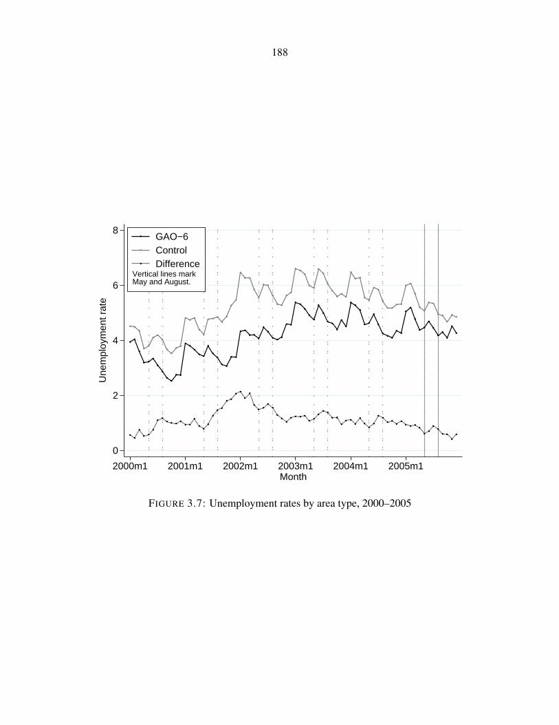
188

0

2

4

6

8

Une

mpl

oym

ent r

ate

2000m1 2001m1 2002m1 2003m1 2004m1 2005m1Month

GAO−6ControlDifference

Vertical lines markMay and August.

FIGURE 3.7: Unemployment rates by area type, 2000–2005

189

3.6.3. Results

Randomizationinference test:tobs = −1.807

p = 0.185±0.013

Random permutationdistribution:N = 922Mean = −0.381Median = −0.221

0

2

4

6

8

Per

cent

−15 −10 −5 0 5t statistic

(on Jan−Apr DD estimate for gestational age effect)

FIGURE 3.8: Histogram of randomization test results, Jan.–Apr. ’05

TABLE 3.10: Estimated effects of BRAC list on mean birth weight (grams), alternate trendspecifications

1 2 3

Jan.–Apr. ’04 24.657∗∗ 15.641 9.052(7.62) (13.95) (13.61)

May–Aug. ’04 23.474∗∗ 14.404∗∗ 4.395(6.87) (4.63) (9.73)

Sept.–Dec. ’04 -2.315 -11.339 -24.676∗∗

(10.83) (9.12) (6.98)Jan.–Apr. ’05 12.276 -0.461 -17.829

(18.52) (16.56) (16.51)May–Aug. ’05 -0.226 -13.010 -35.164∗

(16.01) (15.25) (15.16)Sept.–Dec. ’05 19.967∗ 7.237 -19.596

(7.96) (9.90) (22.39)County FE Yes Yes YesLinear trend . Yes YesQuad. trend . . Yes

Trend test: p 0.000 0.000 0.007Equality test, p 0.0236 0.0243 0.0004Cells 115, 708 115, 708 115, 708Adj. R-sq. 0.514 0.514 0.514

Notes. All models include year and calendar month fixed effects. Standard errors in parentheses. Statistical significance symbols: + p < 0.10, ∗

p < 0.05, ∗∗ p < 0.01.

190

Randomizationinference test:

tobs = 1.975p = 0.116±0.011

Random permutationdistribution:N = 922Mean = 0.047Median = 0.063

0

2

4

6

Per

cent

−10 −5 0 5t statistic

(on Sept−Dec DD estimate for gestational age effect)

FIGURE 3.9: Histogram of randomization test results, Sept.–Dec. ’05

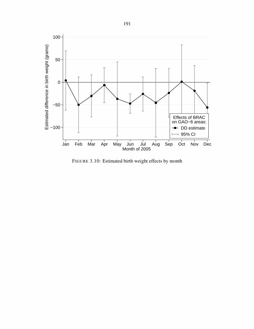
191

−100

−50

0

50

100

Est

imat

ed d

iffer

ence

in b

irth

wei

ght (

gram

s)

Jan Feb Mar Apr May Jun Jul Aug Sep Oct Nov DecMonth of 2005

DD estimate95% CI

Effects of BRACon GAO−6 areas:

FIGURE 3.10: Estimated birth weight effects by month

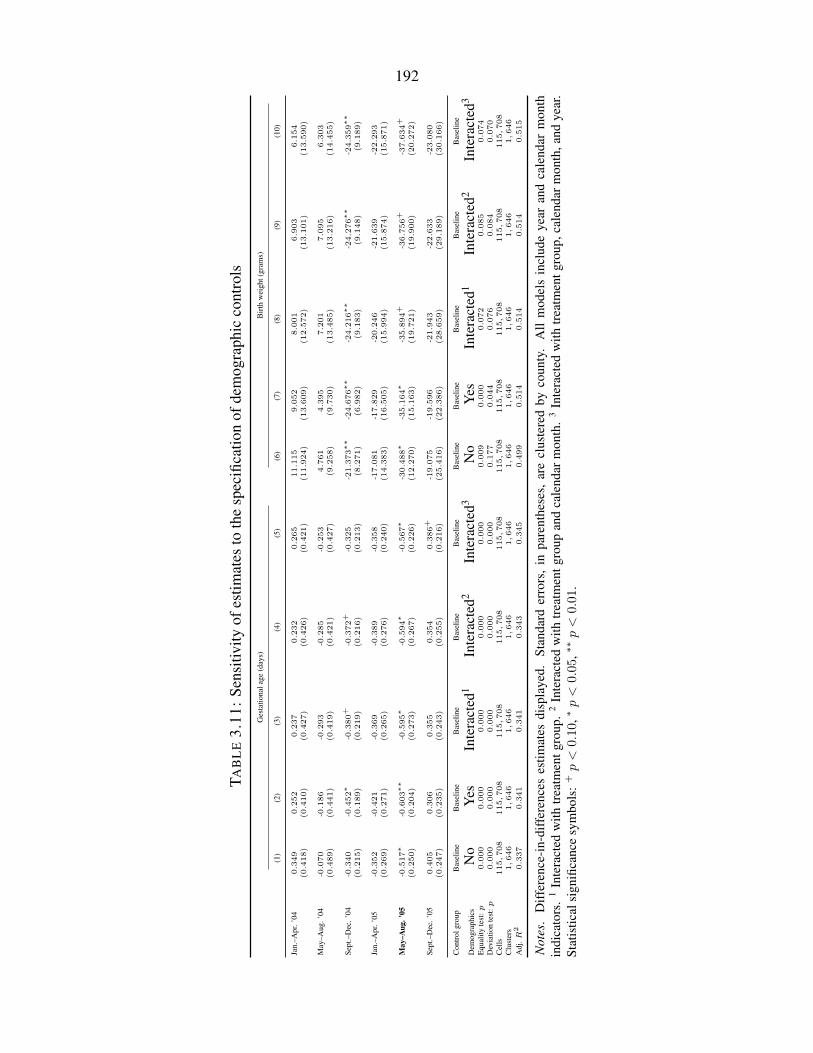
192

TAB

LE

3.11

:Se

nsiti

vity

ofes

timat

esto

the

spec

ifica

tion

ofde

mog

raph

icco

ntro

lsG

esta

tiona

lage

(day

s)B

irth

wei

ght(

gram

s)

(1)

(2)

(3)

(4)

(5)

(6)

(7)

(8)

(9)

(10)

Jan.

–Apr

.’04

0.349

0.252

0.237

0.232

0.265

11.115

9.052

8.001

6.903

6.154

(0.418)

(0.410)

(0.427)

(0.426)

(0.421)

(11.924)

(13.609)

(12.572)

(13.101)

(13.590)

May

–Aug

.’04

-0.070

-0.186

-0.293

-0.285

-0.253

4.761

4.395

7.201

7.095

6.303

(0.489)

(0.441)

(0.419)

(0.421)

(0.427)

(9.258)

(9.730)

(13.485)

(13.216)

(14.455)

Sept

.–D

ec.’

04-0.340

-0.452∗

-0.380+

-0.372+

-0.325

-21.373∗∗

-24.676∗∗

-24.216∗∗

-24.276∗∗

-24.359∗∗

(0.215)

(0.189)

(0.219)

(0.216)

(0.213)

(8.271)

(6.982)

(9.183)

(9.148)

(9.189)

Jan.

–Apr

.’05

-0.352

-0.421

-0.369

-0.389

-0.358

-17.081

-17.829

-20.246

-21.639

-22.293

(0.269)

(0.271)

(0.265)

(0.276)

(0.240)

(14.383)

(16.505)

(15.994)

(15.874)

(15.871)

May

–Aug

.’05

-0.517∗

-0.603∗∗

-0.595∗

-0.594∗

-0.567∗

-30.488∗

-35.164∗

-35.894+

-36.756+

-37.634+

(0.250)

(0.204)

(0.273)

(0.267)

(0.226)

(12.270)

(15.163)

(19.721)

(19.900)

(20.272)

Sept

.–D

ec.’

050.405

0.306

0.355

0.354

0.386+

-19.075

-19.596

-21.943

-22.633

-23.080

(0.247)

(0.235)

(0.243)

(0.255)

(0.216)

(25.416)

(22.386)

(28.659)

(29.189)

(30.166)

Con

trol

grou

pB

asel

ine

Bas

elin

eB

asel

ine

Bas

elin

eB

asel

ine

Bas

elin

eB

asel

ine

Bas

elin

eB

asel

ine

Bas

elin

e

Dem

ogra

phic

sN

oY

esIn

tera

cted

1In

tera

cted

2In

tera

cted

3N

oY

esIn

tera

cted

1In

tera

cted

2In

tera

cted

3E

qual

ityte

st:p

0.000

0.000

0.000

0.000

0.000

0.009

0.000

0.072

0.085

0.074

Dev

iatio

nte

st:p

0.000

0.000

0.000

0.000

0.000

0.177

0.044

0.076

0.084

0.070

Cel

ls115,708

115,708

115,708

115,708

115,708

115,708

115,708

115,708

115,708

115,708

Clu

ster

s1,646

1,646

1,646

1,646

1,646

1,646

1,646

1,646

1,646

1,646

Adj

.R2

0.337

0.341

0.341

0.343

0.345

0.499

0.514

0.514

0.514

0.515

Not

es.

Diff

eren

ce-i

n-di

ffer

ence

ses

timat

esdi

spla

yed.

Stan

dard

erro

rs,

inpa

rent

hese

s,ar

ecl

uste

red

byco

unty

.A

llm

odel

sin

clud

eye

aran

dca

lend

arm

onth

indi

cato

rs.

1In

tera

cted

with

trea

tmen

tgro

up.

2In

tera

cted

with

trea

tmen

tgro

upan

dca

lend

arm

onth

.3

Inte

ract

edw

ithtr

eatm

entg

roup

,cal

enda

rm

onth

,and

year

.St

atis

tical

sign

ifica

nce

sym

bols

:+p<

0.10

,∗p<

0.05

,∗∗p<

0.01

.

193

TAB

LE

3.12

:Se

nsiti

vity

ofes

timat

esto

the

spec

ifica

tion

ofde

mog

raph

icco

ntro

ls(m

ilita

ryco

ntro

l)G

esta

tiona

lage

(day

s)B

irth

wei

ght(

gram

s)

(1)

(2)

(3)

(4)

(5)

(6)

(7)

(8)

(9)

(10)

Jan.

–Apr

.’04

0.101

0.178

0.161

0.249

0.261

8.302

5.751

4.231

2.536

-14.971

(0.469)

(0.461)

(0.473)

(0.563)

(0.597)

(12.551)

(14.532)

(13.338)

(16.058)

(17.569)

May

–Aug

.’04

-0.438

-0.340

-0.496

-0.616

-0.530

2.934

1.414

3.205

4.454

-8.875

(0.544)

(0.506)

(0.476)

(0.454)

(0.466)

(10.501)

(12.506)

(14.710)

(17.835)

(18.487)

Sept

.–D

ec.’

04-0.417

-0.254

-0.267

-0.399+

-0.478

-20.055+

-22.512∗

-23.298∗

-16.945

-30.665

(0.258)

(0.257)

(0.256)

(0.205)

(0.369)

(10.020)

(10.425)

(11.147)

(15.480)

(19.501)

Jan.

–Apr

.’05

-0.535+

-0.404

-0.391

-0.423

-0.826∗

-22.014

-23.781

-25.758

-28.016

-46.272+

(0.301)

(0.341)

(0.307)

(0.364)

(0.390)

(15.526)

(17.746)

(17.279)

(23.503)

(24.529)

May

–Aug

.’05

-0.833∗

-0.739∗∗

-0.737∗

-0.823∗

-1.242∗

-38.139∗

-44.729∗

-46.010∗

-41.835

-50.821

(0.327)

(0.272)

(0.361)

(0.404)

(0.468)

(14.360)

(17.719)

(21.692)

(28.427)

(31.038)

Sept

.–D

ec.’

050.182

0.353

0.319

0.400

-0.071

-31.234

-33.438

-36.896

-26.654

-36.944

(0.288)

(0.276)

(0.291)

(0.268)

(0.364)

(27.588)

(27.880)

(30.861)

(38.625)

(42.352)

Con

trol

grou

pM

ilita

ryM

ilita

ryM

ilita

ryM

ilita

ryM

ilita

ryM

ilita

ryM

ilita

ryM

ilita

ryM

ilita

ryM

ilita

ry

Dem

ogra

phic

sN

oY

esIn

tera

cted

1In

tera

cted

2In

tera

cted

3N

oY

esIn

tera

cted

1In

tera

cted

2In

tera

cted

3E

qual

ityte

st:p

0.000

0.000

0.000

0.000

0.000

0.054

0.013

0.086

0.222

0.674

Dev

iatio

nte

st:p

0.000

0.001

0.001

0.013

0.016

0.237

0.080

0.099

0.127

0.382

Cel

ls3,236

3,236

3,236

3,236

3,236

3,236

3,236

3,236

3,236

3,236

Clu

ster

s45

45

45

45

45

45

45

45

45

45

Adj

.R2

0.465

0.478

0.478

0.478

0.498

0.770

0.777

0.777

0.779

0.780

Not

es.

Diff

eren

ce-i

n-di

ffer

ence

ses

timat

esdi

spla

yed.

Stan

dard

erro

rs,

inpa

rent

hese

s,ar

ecl

uste

red

byco

unty

.A

llm

odel

sin

clud

eye

aran

dca

lend

arm

onth

indi

cato

rs.

1In

tera

cted

with

trea

tmen

tgro

up.

2In

tera

cted

with

trea

tmen

tgro

upan

dca

lend

arm

onth

.3

Inte

ract

edw

ithtr

eatm

entg

roup

,cal

enda

rm

onth

,and

year

.St

atis

tical

sign

ifica

nce

sym

bols

:+p<

0.10

,∗p<

0.05

,∗∗p<

0.01

.

194

TAB

LE

3.13

:E

stim

ated

effe

cts

ofB

RA

Clis

tmaj

orcl

osur

ean

noun

cem

ent

Ges

tatio

nala

ge(d

ays)

Bir

thw

eigh

t(gr

ams)

(1)

(2)

(3)

(4)

(5)

(6)

(7)

(8)

(9)

(10)

Jan.

–Apr

.’04

0.049

-0.049

-0.156

0.039

0.240+

-3.771

-3.811

-3.542

-3.077

-4.851

(0.108)

(0.121)

(0.131)

(0.284)

(0.136)

(2.959)

(3.612)

(3.748)

(5.300)

(3.427)

May

–Aug

.’04

-0.031

-0.149

-0.297∗

-0.058

0.003

-5.458+

-7.083∗

-5.028

-8.360

-7.596+

(0.115)

(0.125)

(0.120)

(0.302)

(0.155)

(3.019)

(3.449)

(3.772)

(5.908)

(4.322)

Sept

.–D

ec.’

040.014

-0.038

-0.155

0.192

0.005

-4.279

-6.675∗

0.500

4.717

-3.054

(0.083)

(0.095)

(0.097)

(0.188)

(0.125)

(2.757)

(3.327)

(3.246)

(4.569)

(4.262)

Jan.

–Apr

.’05

0.221∗

0.078

0.057

0.094

0.298∗

-3.546

-4.787

-3.402

-10.560∗

-0.897

(0.106)

(0.119)

(0.133)

(0.216)

(0.147)

(3.195)

(3.555)

(3.678)

(5.210)

(4.384)

May

–Aug

.’05

0.116

-0.029

-0.265∗

-0.160

0.074

-0.377

-1.276

-4.829

-3.230

-1.937

(0.097)

(0.111)

(0.128)

(0.323)

(0.129)

(3.044)

(3.859)

(3.612)

(5.956)

(3.874)

Sept

.–D

ec.’

050.214∗

0.117

0.154

0.106

0.278+

2.781

-1.193

4.612

0.400

5.534

(0.099)

(0.131)

(0.130)

(0.205)

(0.154)

(3.182)

(3.903)

(3.627)

(5.176)

(4.512)

Con

trol

grou

pB

asel

ine

Min

orM

ajor

Mili

tary

Stat

esB

asel

ine

Min

orM

ajor

Mili

tary

Stat

esPT

T,20

00–2

003:

p0.145

0.167

0.002

0.105

0.682

0.076

0.079

0.601

0.320

0.152

SIT:

p0.121

0.235

0.039

0.065

0.074

0.147

0.661

0.055

0.015

0.282

Equ

ality

test

:p0.518

0.471

0.008

0.464

0.217

0.261

0.537

0.082

0.263

0.321

Mea

nde

viat

ion

test

:p0.252

0.229

0.003

0.258

0.092

0.998

0.567

0.102

0.682

0.273

Cel

ls118,733

9,789

10,496

5,757

19,333

118,733

9,789

10,496

5,757

19,333

Clu

ster

s1,688

136

146

80

279

1,688

136

146

80

279

Adj

.R2

0.381

0.672

0.651

0.679

0.498

0.548

0.825

0.777

0.825

0.649

Not

es.

Diff

eren

ce-i

n-di

ffer

ence

ses

timat

esdi

spla

yed.

Stan

dard

erro

rs,

inpa

rent

hese

s,ar

ecl

uste

red

byco

unty

.A

llm

odel

sin

clud

eye

aran

dca

lend

arm

onth

indi

cato

rs.S

tatis

tical

sign

ifica

nce

sym

bols

:+p<

0.10

,∗p<

0.05

,∗∗p<

0.01

.

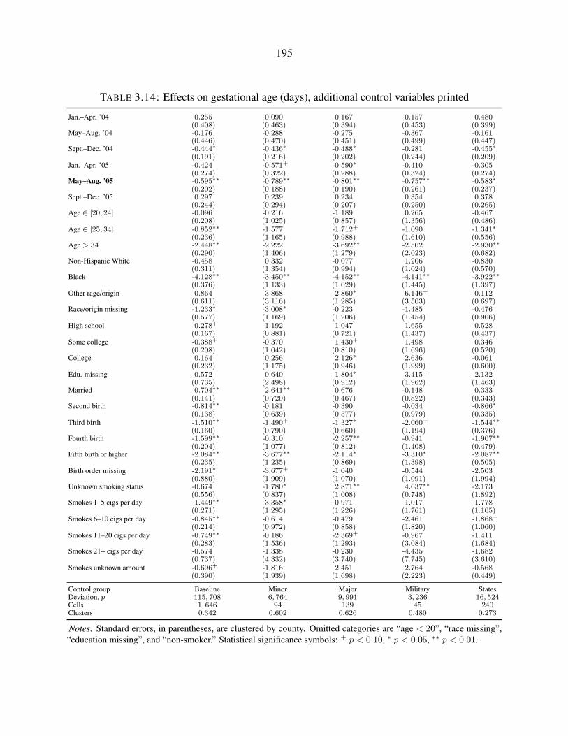
195

TABLE 3.14: Effects on gestational age (days), additional control variables printed

Jan.–Apr. ’04 0.255 0.090 0.167 0.157 0.480(0.408) (0.463) (0.394) (0.453) (0.399)

May–Aug. ’04 -0.176 -0.288 -0.275 -0.367 -0.161(0.446) (0.470) (0.451) (0.499) (0.447)

Sept.–Dec. ’04 -0.444∗ -0.436∗ -0.488∗ -0.281 -0.455∗(0.191) (0.216) (0.202) (0.244) (0.209)

Jan.–Apr. ’05 -0.424 -0.571+ -0.590∗ -0.410 -0.305(0.274) (0.322) (0.288) (0.324) (0.274)

May–Aug. ’05 -0.595∗∗ -0.789∗∗ -0.801∗∗ -0.757∗∗ -0.583∗(0.202) (0.188) (0.190) (0.261) (0.237)

Sept.–Dec. ’05 0.297 0.239 0.234 0.354 0.378(0.244) (0.294) (0.207) (0.250) (0.265)

Age ∈ [20, 24] -0.096 -0.216 -1.189 0.265 -0.467(0.208) (1.025) (0.857) (1.356) (0.486)

Age ∈ [25, 34] -0.852∗∗ -1.577 -1.712+ -1.090 -1.341∗(0.236) (1.165) (0.988) (1.610) (0.556)

Age > 34 -2.448∗∗ -2.222 -3.692∗∗ -2.502 -2.930∗∗(0.290) (1.406) (1.279) (2.023) (0.682)

Non-Hispanic White -0.458 0.332 -0.077 1.206 -0.830(0.311) (1.354) (0.994) (1.024) (0.570)

Black -4.128∗∗ -3.450∗∗ -4.152∗∗ -4.141∗∗ -3.922∗∗(0.376) (1.133) (1.029) (1.445) (1.397)

Other rage/origin -0.864 -3.868 -2.860∗ -6.146+ -0.112(0.611) (3.116) (1.285) (3.503) (0.697)

Race/origin missing -1.233∗ -3.008∗ -0.223 -1.485 -0.476(0.577) (1.169) (1.206) (1.454) (0.906)

High school -0.278+ -1.192 1.047 1.655 -0.528(0.167) (0.881) (0.721) (1.437) (0.437)

Some college -0.388+ -0.370 1.430+ 1.498 0.346(0.208) (1.042) (0.810) (1.696) (0.520)

College 0.164 0.256 2.126∗ 2.636 -0.061(0.232) (1.175) (0.946) (1.999) (0.600)

Edu. missing -0.572 0.640 1.804∗ 3.415+ -2.132(0.735) (2.498) (0.912) (1.962) (1.463)

Married 0.704∗∗ 2.641∗∗ 0.676 -0.148 0.333(0.141) (0.720) (0.467) (0.822) (0.343)

Second birth -0.814∗∗ -0.181 -0.390 -0.034 -0.866∗(0.138) (0.639) (0.577) (0.979) (0.335)

Third birth -1.510∗∗ -1.490+ -1.327∗ -2.060+ -1.544∗∗(0.160) (0.790) (0.660) (1.194) (0.376)

Fourth birth -1.599∗∗ -0.310 -2.257∗∗ -0.941 -1.907∗∗(0.204) (1.077) (0.812) (1.408) (0.479)

Fifth birth or higher -2.084∗∗ -3.677∗∗ -2.114∗ -3.310∗ -2.087∗∗(0.235) (1.235) (0.869) (1.398) (0.505)

Birth order missing -2.191∗ -3.677+ -1.040 -0.544 -2.503(0.880) (1.909) (1.070) (1.091) (1.994)

Unknown smoking status -0.674 -1.780∗ 2.871∗∗ 4.637∗∗ -2.173(0.556) (0.837) (1.008) (0.748) (1.892)

Smokes 1–5 cigs per day -1.449∗∗ -3.358∗ -0.971 -1.017 -1.778(0.271) (1.295) (1.226) (1.761) (1.105)

Smokes 6–10 cigs per day -0.845∗∗ -0.614 -0.479 -2.461 -1.868+(0.214) (0.972) (0.858) (1.820) (1.060)

Smokes 11–20 cigs per day -0.749∗∗ -0.186 -2.369+ -0.967 -1.411(0.283) (1.536) (1.293) (3.084) (1.684)

Smokes 21+ cigs per day -0.574 -1.338 -0.230 -4.435 -1.682(0.737) (4.332) (3.740) (7.745) (3.610)

Smokes unknown amount -0.696+ -1.816 2.451 2.764 -0.568(0.390) (1.939) (1.698) (2.223) (0.449)

Control group Baseline Minor Major Military StatesDeviation, p 115, 708 6, 764 9, 991 3, 236 16, 524Cells 1, 646 94 139 45 240Clusters 0.342 0.602 0.626 0.480 0.273

Notes. Standard errors, in parentheses, are clustered by county. Omitted categories are “age < 20”, “race missing”,“education missing”, and “non-smoker.” Statistical significance symbols: + p < 0.10, ∗ p < 0.05, ∗∗ p < 0.01.

196

TABLE 3.15: Effects on birth weight (grams), additional control variables printed

Jan.–Apr. ’04 10.892 8.302 12.170 6.519 11.905(13.063) (13.615) (14.213) (13.812) (13.374)

May–Aug. ’04 6.672 4.474 9.396 1.931 6.656(10.234) (10.403) (11.952) (12.509) (10.666)

Sept.–Dec. ’04 -22.256∗∗ -28.334∗∗ -21.263∗ -22.385∗ -18.047∗(7.797) (7.775) (8.742) (10.232) (8.908)

Jan.–Apr. ’05 -16.726 -22.711 -21.188 -23.612 -8.784(16.896) (16.271) (17.161) (17.756) (17.076)

May–Aug. ’05 -32.263∗ -37.982∗∗ -44.928∗∗ -43.625∗ -27.658+(14.736) (13.090) (13.123) (16.495) (16.066)

Sept.–Dec. ’05 -20.359 -29.911 -31.153 -34.121 -10.563(24.397) (22.641) (24.745) (27.802) (25.000)

Age ∈ [20, 24] 5.914 26.508 9.435 39.277 -21.474(6.384) (28.717) (23.531) (32.259) (17.212)

Age ∈ [25, 34] 19.997∗∗ 36.622 22.694 44.567 -6.268(7.095) (31.386) (24.904) (37.617) (19.435)

Age > 34 -2.123 2.654 52.335+ 63.681 -31.083(8.554) (37.645) (28.302) (51.297) (22.279)

Non-Hispanic White 9.423 -21.650 62.909∗∗ 35.430 17.983(8.170) (24.578) (19.481) (25.700) (19.153)

Black -233.944∗∗ -267.033∗∗ -212.612∗∗ -216.154∗∗ -212.789∗∗(11.789) (32.386) (22.060) (40.860) (41.766)

Other rage/origin -1.536 -113.182∗∗ -120.877∗∗ -34.356 58.311∗

(12.793) (33.662) (37.153) (50.207) (25.694)Race/origin missing -17.706 -43.434 44.928 -29.558 15.651

(15.856) (31.090) (41.143) (38.989) (29.833)High school 26.563∗∗ -24.361 12.474 72.394∗ 23.033

(5.448) (26.386) (18.365) (29.286) (14.379)Some college 55.133∗∗ 7.423 64.045∗∗ 84.243∗ 66.382∗∗

(6.293) (32.850) (19.914) (31.895) (16.355)College 86.273∗∗ 29.177 88.400∗∗ 80.645∗ 75.414∗∗

(6.958) (32.927) (20.306) (36.185) (17.879)Edu. missing -21.401 -135.547∗ 18.188 3.170 -61.176

(19.562) (56.823) (35.993) (37.884) (47.589)Married 41.181∗∗ 84.388∗∗ 14.265 14.860 40.124∗∗

(4.187) (19.408) (16.178) (24.454) (11.095)Second birth 74.575∗∗ 76.754∗∗ 90.432∗∗ 93.847∗∗ 87.004∗∗

(4.400) (18.007) (14.632) (26.292) (11.696)Third birth 85.641∗∗ 84.925∗∗ 80.878∗∗ 71.601∗ 85.325∗∗

(5.213) (18.459) (19.182) (29.585) (12.408)Fourth birth 82.650∗∗ 131.506∗∗ 91.884∗∗ 74.049+ 82.172∗∗

(6.416) (27.047) (25.606) (42.418) (15.496)Fifth birth or higher 86.626∗∗ 75.285∗∗ 70.622∗∗ 47.977 89.514∗∗

(7.115) (27.519) (25.566) (38.152) (16.337)Birth order missing 40.127+ 103.683∗∗ -11.445 48.962+ 12.469

(23.128) (34.714) (35.216) (25.718) (32.831)Unknown smoking status -35.385∗∗ -22.725+ 63.045∗ 36.728∗ -29.377

(7.201) (11.686) (28.765) (18.030) (36.860)Smokes 1–5 cigs per day -171.140∗∗ -186.345∗∗ -196.978∗∗ -169.708∗∗ -158.584∗∗

(7.915) (31.582) (34.066) (43.746) (28.092)Smokes 6–10 cigs per day -220.913∗∗ -180.154∗∗ -200.615∗∗ -195.778∗∗ -247.434∗∗

(6.757) (34.455) (24.517) (46.281) (28.591)Smokes 11–20 cigs per day -260.817∗∗ -313.414∗∗ -267.910∗∗ -260.923∗∗ -266.078∗∗

(8.719) (47.149) (36.934) (73.408) (44.702)Smokes 21+ cigs per day -277.677∗∗ -495.309∗∗ -203.458+ -298.916 -301.618∗

(23.473) (134.987) (116.722) (213.243) (122.666)Smokes unknown amount -200.448∗∗ -115.091∗ -49.268 -110.725∗ -212.003∗∗

(11.265) (54.589) (51.007) (49.774) (12.907)

Control group Baseline Minor Major Military StatesDeviation, p 115, 708 6, 764 9, 991 3, 236 16, 524Cells 1, 646 94 139 45 240Clusters 0.524 0.796 0.762 0.780 0.479

Notes. Standard errors, in parentheses, are clustered by county. Omitted categories are “age < 20”, “race missing”,“education missing”, and “non-smoker.” Statistical significance symbols: + p < 0.10, ∗ p < 0.05, p < 0.01.

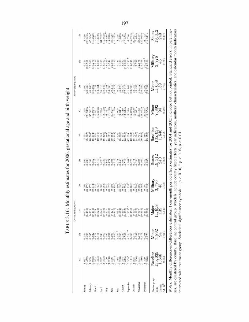
197

TAB

LE

3.16

:M

onth

lyes

timat

esfo

r200

6,ge

stat

iona

lage

and

birt

hw

eigh

tG

esta

tiona

lage

(day

s)B

irth

wei

ght(

gram

s)

(1)

(2)

(3)

(4)

(5)

(6)

(7)

(8)

(9)

(10)

Janu

ary

1.027

-0.154

0.070

0.004

0.199

3.951

-0.295

1.400

-5.914

8.420

(0.452)

(0.496)

(0.431)

(0.470)

(0.438)

(25.507)

(23.979)

(20.969)

(23.501)

(26.888)

Febr

uary

1.935

0.385

0.539

0.278

0.889

40.788∗

35.381+

40.168∗

25.003

45.364∗

(0.983)

(0.522)

(0.491)

(0.511)

(0.552)

(18.174)

(17.947)

(18.167)

(19.270)

(19.222)

Mar

ch0.592

-0.871

-0.778

-0.539

-0.119

0.970

-2.501

-4.627

-14.511

4.421

(0.474)

(0.811)

(0.823)

(0.858)

(0.810)

(12.510)

(12.303)

(14.661)

(14.738)

(13.669)

Apr

il2.227

0.630

0.848

0.809

1.229+

20.049

18.224

15.819

12.819

31.702+

(1.363)

(0.569)

(0.598)

(0.668)

(0.633)

(16.420)

(18.122)

(18.146)

(18.307)

(17.002)

May

1.700

0.192

0.327

0.280

0.849

41.264∗

38.331∗

36.988∗

41.530∗

48.818∗∗

(1.280)

(0.791)

(0.803)

(0.870)

(0.777)

(16.071)

(16.190)

(14.363)

(16.544)

(17.276)

June

0.566

-0.603

-0.421

-0.603

-0.408

30.383∗

30.627∗

29.116∗

22.603

35.428∗

(0.491)

(0.840)

(0.817)

(0.855)

(0.913)

(13.218)

(14.195)

(14.177)

(15.115)

(14.232)

July

0.314

-1.154+

-1.052

-1.395∗

-0.971

2.620

7.005

-0.979

-7.784

1.228

(0.223)

(0.686)

(0.674)

(0.680)

(0.749)

(5.320)

(7.311)

(6.128)

(9.838)

(6.679)

Aug

ust

1.334

0.229

0.296

0.157

0.494

11.155

11.419

10.439

8.697

16.100

(0.679)

(0.542)

(0.507)

(0.554)

(0.519)

(16.716)

(17.974)

(17.916)

(18.906)

(16.859)

Sept

embe

r0.308∗

-1.224∗∗

-1.225∗∗

-1.232∗

-1.101∗

-17.658

-18.379

-11.869

-24.222+

-8.746

(0.141)

(0.460)

(0.456)

(0.469)

(0.475)

(12.033)

(12.056)

(12.809)

(12.825)

(12.794)

Oct

ober

1.265

0.175

0.106

-0.077

0.371

18.737∗∗

16.200∗∗

12.053∗

9.363

22.061∗∗

(0.366)

(0.289)

(0.287)

(0.294)

(0.334)

(4.697)

(5.981)

(5.452)

(7.798)

(6.624)

Nov

embe

r0.501

-0.778

-0.717

-0.609

-0.605

-35.771

-39.153

-31.912

-32.678

-35.587

(0.216)

(0.471)

(0.462)

(0.567)

(0.469)

(26.495)

(28.852)

(30.689)

(29.566)

(26.045)

Dec

embe

r1.399

0.208

0.251

0.000

0.352

27.180+

26.835∗

28.792∗

25.206+

31.762∗

(0.320)

(0.278)

(0.269)

(0.322)

(0.285)

(13.970)

(12.954)

(13.032)

(14.160)

(14.911)

Con

trol

grou

pB

asel

ine

Min

orM

ajor

Mili

tary

Stat

esB

asel

ine

Min

orM

ajor

Mili

tary

Stat

esC

ells

135,039

7,892

11,658

3,776

19,312

135,039

7,892

11,658

3,776

19,312

Clu

ster

s1,646

94139

45240

1,646

94

139

45

240

Adj

.R2

0.351

0.611

0.643

0.498

0.290

0.518

0.795

0.765

0.781

0.477

Not

es.M

onth

lydi

ffer

ence

-in-

diff

eren

ces

estim

ates

.Fou

r-m

onth

peri

odef

fect

ses

timat

esfo

r200

4an

d20

05in

clud

edbu

tnot

prin

ted.

Stan

dard

erro

rs,i

npa

rent

he-

ses,

are

clus

tere

dby

coun

ty.

Bas

elin

eco

ntro

lgro

up.

Mod

els

incl

ude

coun

tyfix

edef

fect

s,ye

arin

dica

tors

,mot

hers

’ch

arac

teri

stic

s,an

dca

lend

arm

onth

indi

cato

rsin

tera

cted

with

trea

tmen

tgro

up.S

tatis

tical

sign

ifica

nce

sym

bols

:+p<

0.10

,∗p<

0.05

,p<

0.01

.

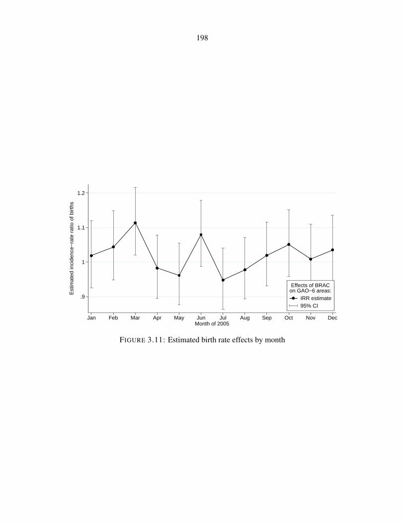
198

.9

1

1.1

1.2

Est

imat

ed in

cide

nce−

rate

rat

io o

f birt

hs

Jan Feb Mar Apr May Jun Jul Aug Sep Oct Nov DecMonth of 2005

IRR estimate95% CI

Effects of BRACon GAO−6 areas:

FIGURE 3.11: Estimated birth rate effects by month

199

Explanation of individual-level estimates — The individual-level estimates use the same sam-

ples as the main analysis except that the data are not aggregated into county-month cells and the

year 2006 is included.23 The states and military samples are used for computational tractability.

Each birth is assigned a birth date corresponding to the midpoint of the month of birth. A nom-

inal start date is assigned by subtracting the gestational age from the birth date (without adding

two weeks). Exposure to the BRAC announcement for each birth was calculated by comparing

the nominal start date with May 13, 2005. Exposure in the first trimester was defined as having a

nominal start date within the period starting 13 weeks before May 13, 2005 and ending on May

13, 2005. Exposure in the second trimester was defined as having a nominal start date within the

period starting 26 weeks before May 13, 2005 and ending 13 weeks before May 13, 2005. Expo-

sure in the third trimester was defined as having a nominal start date more than 26 weeks before

May 13, 2005 and being born after May 13, 2005. In addition, exposure calculations also required

that the pregnancy reached the trimester in question. The full-term instrument is defined for each

birth by calculating the exposure for a pregnancy that started on the same date and ended with a

gestational age of 39 weeks.

For each birth indexed by (i, c, y,m), which means birth i in county c in year y in calendar

month m, the outcome x is modeled by

xi,c,y,m =3∑

t=1

(βtDti,c,y,m+ψtB

ti,c,y,m)+ϕ′Zi,c,y,m+αc+ γy + δm+∆m×{c ∈ GAO-6}+ ϵi,c,y,m

(3.1)

where

• Bt indicates if the pregnancy was in trimester t on May 13, 2005,

• Dti,c,y,m indicates if the pregnancy was in trimester t on May 13, 2005 and c ∈ GAO-6,

• αc, γy, δm,∆m are county, year, month, and interacted month fixed effects, and

• Z is a vector of mother characteristics (as described in the main text).23South Dakota contains a GAO-6 site and switched to the revised birth certificate in 2006. So some non-comparable

items related to complications and abnormalities are not considered in the individual-level results.

200

Thus, the estimate of βt is an estimate of effect of exposure to the BRAC announcement in trimester

t. These estimates are reported in table 3.17. In the instrumented models, the variables Bt and Dt

are instrumented for by the full-term instruments Bt and Dt, respectively. That is, Bti,c,y,m takes

the value that Bti,c,y,m would have if birth (i, c, y,m) occurred at exactly 39 weeks gestational

age. The two variables are identical for all births that actually had a gestational age of 39 weeks.

Models that put any characteristic of the mother on the left-hand side do not put any demographic

characteristics on the right-hand side.

201

TAB

LE

3.17

:In

divi

dual

-lev

eles

timat

esof

effe

cts

ofex

posu

reto

the

BR

AC

anno

unce

men

t

Ges

tatio

nala

ge(d

ays)

Bir

thw

eigh

t(gr

ams)

Sim

ple

expo

sure

Inst

rum

ente

dSi

mpl

eex

posu

reIn

stru

men

ted

Sim

ple

expo

sure

Inst

rum

ente

dSi

mpl

eex

posu

reIn

stru

men

ted

Trim

este

r10.533∗

0.493+

0.447∗

0.445∗

6.922

6.390

12.612

12.695

(0.262)

(0.259)

(0.224)

(0.221)

(9.154)

(9.289)

(8.748)

(8.933)

Trim

este

r20.060

0.075

0.286

0.299

21.122

21.102

22.073+

22.019+

(0.390)

(0.384)

(0.351)

(0.349)

(13.044)

(13.005)

(12.451)

(12.536)

Trim

este

r3-1.609∗∗

-1.104∗

-1.243∗∗

-0.917∗

-22.416

-24.948

-16.162

-21.595

(0.395)

(0.462)

(0.329)

(0.452)

(16.547)

(20.915)

(16.419)

(21.002)

Con

trol

grou

pM

ilita

ryM

ilita

rySt

ates

Stat

esM

ilita

ryM

ilita

rySt

ates

Stat

esB

irth

s87

2,037

872,03

71,345

,383

1,34

5,383

872,03

787

2,037

1,34

5,38

31,345,383

Clu

ster

s45

45

240

240

45

45

240

240

Adj

.R2

0.017

0.014

0.016

0.013

0.044

0.044

0.039

0.039

Not

es.

Diff

eren

ce-i

n-di

ffer

ence

ses

timat

esdi

spla

yed

(raw

coef

ficie

nts)

.St

anda

rder

rors

,in

pare

nthe

ses,

are

clus

tere

dby

coun

ty.

Sym

bols

ofsi

gnifi

canc

eat

leve

lp

:+p<

0.10

,∗p<

0.05,

∗∗p<

0.01.

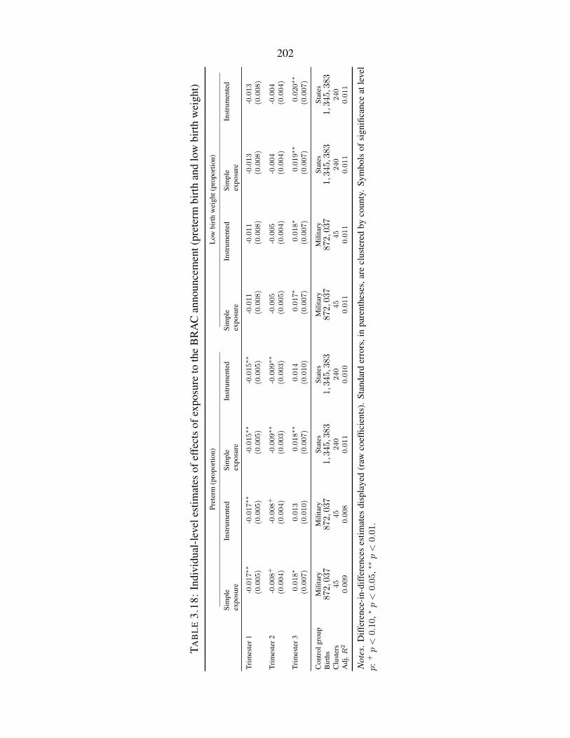
202

TAB

LE

3.18

:In

divi

dual

-lev

eles

timat

esof

effe

cts

ofex

posu

reto

the

BR

AC

anno

unce

men

t(pr

eter

mbi

rth

and

low

birt

hw

eigh

t)

Pret

erm

(pro

port

ion)

Low

birt

hw

eigh

t(pr

opor

tion)

Sim

ple

expo

sure

Inst

rum

ente

dSi

mpl

eex

posu

reIn

stru

men

ted

Sim

ple

expo

sure

Inst

rum

ente

dSi

mpl

eex

posu

reIn

stru

men

ted

Trim

este

r1-0.017∗∗

-0.017∗∗

-0.015∗∗

-0.015∗∗

-0.011

-0.011

-0.013

-0.013

(0.005)

(0.005)

(0.005)

(0.005)

(0.008)

(0.008)

(0.008)

(0.008)

Trim

este

r2-0.008+

-0.008+

-0.009∗∗

-0.009∗∗

-0.005

-0.005

-0.004

-0.004

(0.004)

(0.004)

(0.003)

(0.003)

(0.005)

(0.004)

(0.004)

(0.004)

Trim

este

r30.018∗

0.013

0.018∗∗

0.014

0.017∗

0.018∗

0.019∗∗

0.020∗∗

(0.007)

(0.010)

(0.007)

(0.010)

(0.007)

(0.007)

(0.007)

(0.007)

Con

trol

grou

pM

ilita

ryM

ilita

rySt

ates

Stat

esM

ilita

ryM

ilita

rySt

ates

Stat

esB

irth

s87

2,037

872,03

71,345

,383

1,34

5,383

872,03

787

2,037

1,34

5,38

31,345,383

Clu

ster

s45

45

240

240

45

45

240

240

Adj

.R2

0.009

0.008

0.011

0.010

0.011

0.011

0.011

0.011

Not

es.

Diff

eren

ce-i

n-di

ffer

ence

ses

timat

esdi

spla

yed

(raw

coef

ficie

nts)

.St

anda

rder

rors

,in

pare

nthe

ses,

are

clus

tere

dby

coun

ty.

Sym

bols

ofsi

gnifi

canc

eat

leve

lp

:+p<

0.10

,∗p<

0.05,

∗∗p<

0.01.

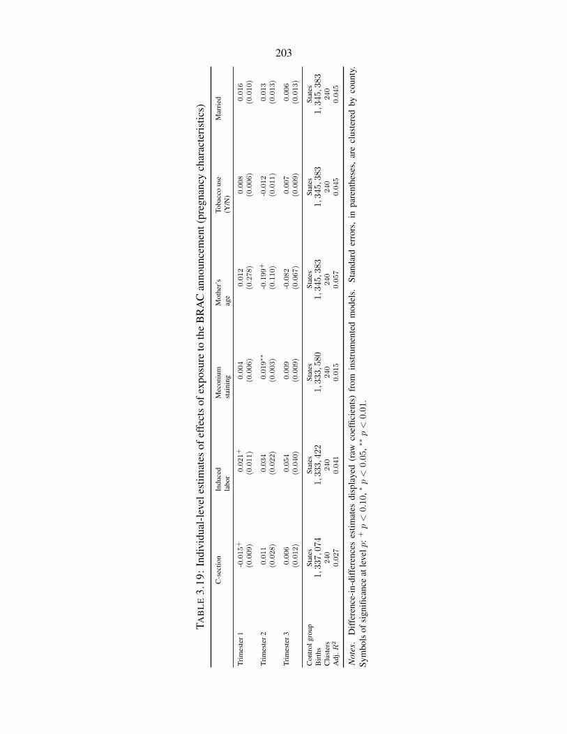
203

TAB

LE

3.19

:In

divi

dual

-lev

eles

timat

esof

effe

cts

ofex

posu

reto

the

BR

AC

anno

unce

men

t(pr

egna

ncy

char

acte

rist

ics)

C-s

ectio

nIn

duce

dla

bor

Mec

oniu

mst

aini

ngM

othe

r’s

age

Toba

cco

use

(Y/N

)M

arri

ed

Trim

este

r1-0.015+

0.021+

0.004

0.012

0.008

0.016

(0.009)

(0.011)

(0.006)

(0.278)

(0.006)

(0.010)

Trim

este

r20.011

0.034

0.019∗∗

-0.199+

-0.012

0.013

(0.028)

(0.022)

(0.003)

(0.110)

(0.011)

(0.013)

Trim

este

r30.006

0.054

0.009

-0.082

0.007

0.006

(0.012)

(0.040)

(0.009)

(0.067)

(0.009)

(0.013)

Con

trol

grou

pSt

ates

Stat

esSt

ates

Stat

esSt

ates

Stat

esB

irth

s1,337,074

1,333,422

1,33

3,580

1,345

,383

1,34

5,383

1,345,383

Clu

ster

s240

240

240

240

240

240

Adj

.R2

0.027

0.041

0.015

0.057

0.045

0.045

Not

es.

Diff

eren

ce-i

n-di

ffer

ence

ses

timat

esdi

spla

yed

(raw

coef

ficie

nts)

from

inst

rum

ente

dm

odel

s.St

anda

rder

rors

,in

pare

nthe

ses,

are

clus

tere

dby

coun

ty.

Sym

bols

ofsi

gnifi

canc

eat

leve

lp:+

p<

0.10

,∗p<

0.05

,∗∗p<

0.01

.

204

TAB

LE

3.20

:In

divi

dual

-lev

eles

timat

esof

effe

cts

ofex

posu

reto

the

BR

AC

anno

unce

men

t(ra

cean

ded

ucat

ion)

Rac

e/et

hnic

ityE

duca

tion

His

pani

cW

hite

Bla

ck<

HS

Hig

hsc

hool

Som

eco

lleg

Col

lege

Trim

este

r1-0.009

-0.005

0.003

0.004

0.030

-0.014

-0.020+

(0.011)

(0.015)

(0.011)

(0.006)

(0.019)

(0.012)

(0.011)

Trim

este

r2-0.014∗

0.025

-0.017∗

0.000

0.011

0.001

-0.011

(0.007)

(0.018)

(0.007)

(0.009)

(0.014)

(0.011)

(0.011)

Trim

este

r3-0.019∗∗

0.035

-0.006+

-0.011

0.007

0.007

-0.005

(0.005)

(0.024)

(0.003)

(0.007)

(0.017)

(0.011)

(0.009)

Con

trol

grou

pSt

ates

Stat

esSt

ates

Stat

esSt

ates

Stat

esSt

ates

Bir

ths

1,34

5,383

1,34

5,38

31,34

5,38

31,345

,383

1,34

5,38

31,34

5,383

1,345,383

Clu

ster

s240

240

240

240

240

240

240

Adj

.R2

0.206

0.220

0.094

0.046

0.022

0.009

0.077

Not

es.

Diff

eren

ce-i

n-di

ffer

ence

ses

timat

esdi

spla

yed

(raw

coef

ficie

nts)

from

inst

rum

ente

dm

odel

s.St

anda

rder

rors

,in

pare

nthe

ses,

are

clus

tere

dby

coun

ty.

Sym

bols

ofsi

gnifi

canc

eat

leve

lp:+

p<

0.10

,∗p<

0.05

,∗∗p<

0.01

.

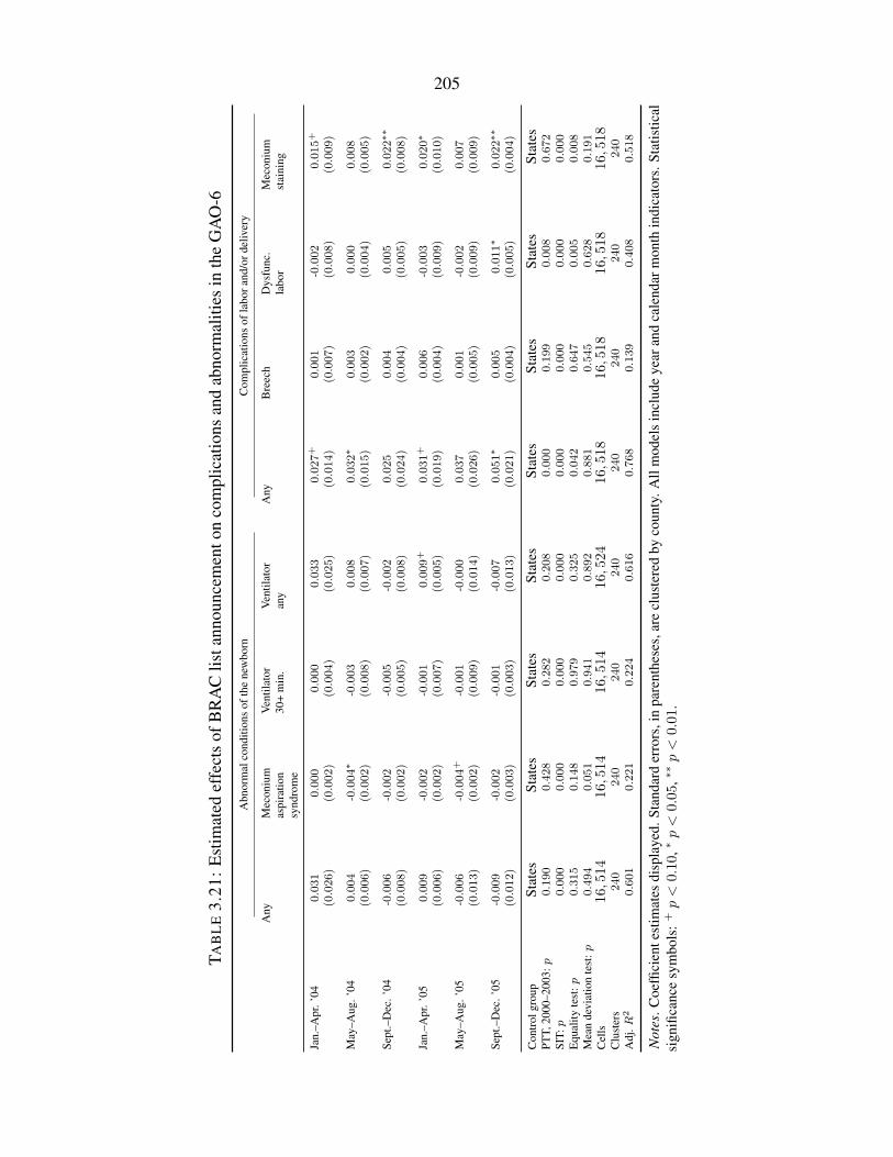
205

TAB

LE

3.21

:E

stim

ated

effe

cts

ofB

RA

Clis

tann

ounc

emen

ton

com

plic

atio

nsan

dab

norm

aliti

esin

the

GA

O-6

Abn

orm

alco

nditi

ons

ofth

ene

wbo

rnC

ompl

icat

ions

ofla

bora

nd/o

rdel

iver

y

Any

Mec

oniu

mas

pira

tion

synd

rom

e

Ven

tilat

or30

+m

in.

Ven

tilat

oran

yA

nyB

reec

hD

ysfu

nc.

labo

rM

econ

ium

stai

ning

Jan.

–Apr

.’04

0.031

0.000

0.000

0.033

0.027+

0.001

-0.002

0.015+

(0.026)

(0.002)

(0.004)

(0.025)

(0.014)

(0.007)

(0.008)

(0.009)

May

–Aug

.’04

0.004

-0.004∗

-0.003

0.008

0.032∗

0.003

0.000

0.008

(0.006)

(0.002)

(0.008)

(0.007)

(0.015)

(0.002)

(0.004)

(0.005)

Sept

.–D

ec.’

04-0.006

-0.002

-0.005

-0.002

0.025

0.004

0.005

0.022∗∗

(0.008)

(0.002)

(0.005)

(0.008)

(0.024)

(0.004)

(0.005)

(0.008)

Jan.

–Apr

.’05

0.009

-0.002

-0.001

0.009+

0.031+

0.006

-0.003

0.020∗

(0.006)

(0.002)

(0.007)

(0.005)

(0.019)

(0.004)

(0.009)

(0.010)

May

–Aug

.’05

-0.006

-0.004+

-0.001

-0.000

0.037

0.001

-0.002

0.007

(0.013)

(0.002)

(0.009)

(0.014)

(0.026)

(0.005)

(0.009)

(0.009)

Sept

.–D

ec.’

05-0.009

-0.002

-0.001

-0.007

0.051∗

0.005

0.011∗

0.022∗∗

(0.012)

(0.003)

(0.003)

(0.013)

(0.021)

(0.004)

(0.005)

(0.004)

Con

trol

grou

pSt

ates

Stat

esSt

ates

Stat

esSt

ates

Stat

esSt

ates

Stat

esPT

T,20

00–2

003:

p0.190

0.428

0.282

0.208

0.000

0.199

0.008

0.672

SIT:

p0.000

0.000

0.000

0.000

0.000

0.000

0.000

0.000

Equ

ality

test

:p0.315

0.148

0.979

0.325

0.042

0.647

0.005

0.008

Mea

nde

viat

ion

test

:p0.494

0.051

0.941

0.892

0.881

0.545

0.628

0.191

Cel

ls16,51

416,514

16,514

16,524

16,518

16,518

16,518

16,518

Clu

ster

s240

240

240

240

240

240

240

240

Adj

.R2

0.601

0.221

0.224

0.616

0.768

0.139

0.408

0.518

Not

es.C

oeffi

cien

test

imat

esdi

spla

yed.

Stan

dard

erro

rs,i

npa

rent

hese

s,ar

ecl

uste

red

byco

unty

.All

mod

els

incl

ude

year

and

cale

ndar

mon

thin

dica

tors

.Sta

tistic

alsi

gnifi

canc

esy

mbo

ls:+

p<

0.10

,∗p<

0.05

,∗∗p<

0.01

.

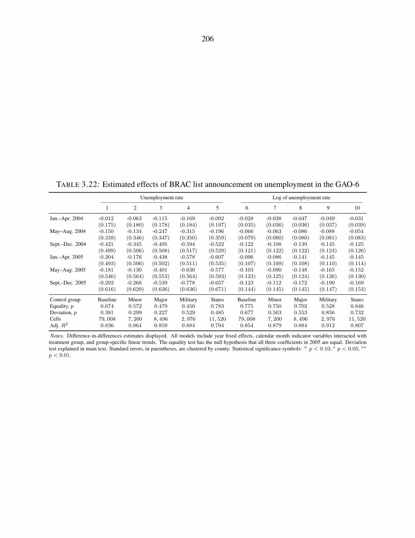
206

TABLE 3.22: Estimated effects of BRAC list announcement on unemployment in the GAO-6

Unemployment rate Log of unemployment rate

1 2 3 4 5 6 7 8 9 10

Jan.–Apr. 2004 -0.012 -0.063 -0.115 -0.169 -0.092 -0.028 -0.038 -0.047 -0.049 -0.031(0.175) (0.180) (0.178) (0.184) (0.197) (0.035) (0.036) (0.036) (0.037) (0.039)

May–Aug. 2004 -0.150 -0.134 -0.247 -0.315 -0.196 -0.066 -0.063 -0.086 -0.088 -0.054(0.339) (0.346) (0.347) (0.350) (0.359) (0.079) (0.080) (0.080) (0.081) (0.083)

Sept.–Dec. 2004 -0.421 -0.345 -0.495 -0.594 -0.522 -0.122 -0.108 -0.139 -0.145 -0.125(0.499) (0.506) (0.508) (0.517) (0.529) (0.121) (0.122) (0.122) (0.124) (0.126)

Jan.–Apr. 2005 -0.204 -0.176 -0.438 -0.578 -0.607 -0.096 -0.086 -0.141 -0.145 -0.145(0.493) (0.506) (0.502) (0.511) (0.535) (0.107) (0.109) (0.108) (0.110) (0.114)

May–Aug. 2005 -0.181 -0.130 -0.401 -0.630 -0.577 -0.103 -0.090 -0.148 -0.165 -0.152(0.546) (0.564) (0.553) (0.564) (0.593) (0.123) (0.125) (0.124) (0.126) (0.130)

Sept.–Dec. 2005 -0.292 -0.268 -0.539 -0.778 -0.657 -0.123 -0.112 -0.172 -0.190 -0.169(0.616) (0.629) (0.626) (0.636) (0.671) (0.144) (0.145) (0.145) (0.147) (0.153)

Control group Baseline Minor Major Military States Baseline Minor Major Military StatesEquality, p 0.674 0.572 0.479 0.450 0.783 0.775 0.750 0.702 0.528 0.846Deviation, p 0.381 0.299 0.227 0.529 0.485 0.677 0.563 0.553 0.856 0.732Cells 79, 008 7, 200 8, 496 2, 976 11, 520 79, 008 7, 200 8, 496 2, 976 11, 520Adj. R2 0.836 0.864 0.859 0.884 0.794 0.854 0.879 0.884 0.912 0.807

Notes. Difference-in-differences estimates displayed. All models include year fixed effects, calendar month indicator variables interacted withtreatment group, and group-specific linear trends. The equality test has the null hypothesis that all three coefficients in 2005 are equal. Deviationtest explained in main text. Standard errors, in parentheses, are clustered by county. Statistical significance symbols: + p < 0.10, ∗ p < 0.05, ∗∗

p < 0.01.

207

TAB

LE

3.23

:E

ffec

tson

mot

hers

’cha

ract

eris

tics:

Age

Age

<20

Age

20–2

4A

ge25

–34

Age

>34

Jan.

–Apr

.200

40.95

1.15

0.94∗

0.29

-0.72+

-0.79

-1.17∗∗

-0.66+

(0.78)

(0.81)

(0.40)

(0.45)

(0.39)

(0.48)

(0.32)

(0.36)

May

–Aug

.200

40.30

0.41

3.04∗∗

2.06+

-1.66+

-1.43

-1.68∗∗

-1.05+

(0.42)

(0.47)

(1.10)

(1.13)

(0.93)

(0.97)

(0.57)

(0.60)

Sept

.–D

ec.2

004

-0.41

-0.44

1.61+

1.00

-0.21

-0.20

-1.00∗

-0.36

(0.85)

(0.88)

(0.84)

(0.88)

(0.88)

(0.93)

(0.47)

(0.51)

Jan.

–Apr

.200

50.37

0.68

1.20∗

0.66

-0.88

-1.07

-0.68

-0.27

(0.88)

(0.91)

(0.61)

(0.65)

(0.81)

(0.88)

(0.47)

(0.52)

May

–Aug

.200

50.53

0.57

0.46

0.14

-0.64

-0.56

-0.35

-0.15

(0.80)

(0.83)

(1.14)

(1.17)

(1.14)

(1.18)

(0.55)

(0.59)

Sept

.–D

ec.2

005

0.79

0.97

1.72

1.46

-1.94

-2.61

-0.57

0.18

(0.56)

(0.58)

(1.08)

(1.13)

(2.23)

(2.30)

(1.45)

(1.47)

Con

trol

grou

pB

asel

ine

Mili

tary

Bas

elin

eM

ilita

ryB

asel

ine

Mili

tary

Bas

elin

eM

ilita

ryPT

T,20

00–2

003:

p0.000

0.037

0.050

0.204

0.063

0.356

0.001

0.211

SIT:

p0.000

0.000

0.000

0.000

0.000

0.000

0.000

0.000

Equ

ality

test

:p0.742

0.735

0.769

0.740

0.723

0.487

0.871

0.962

Mea

nde

viat

ion

test

:p0.929

0.669

0.529

0.575

0.526

0.324

0.742

0.907

Cel

ls115,7

08

3,2

36

115,7

08

3,2

36

115,7

08

3,2

36

115,7

08

3,2

36

Clu

ster

s1,6

46

45

1,6

46

45

1,6

46

45

1,6

46

45

Adj

.R2

0.385

0.558

0.629

0.786

0.460

0.582

0.673

0.786

Not

es.

Coe

ffici

ent

estim

ates

*100

disp

laye

d.St

anda

rder

rors

,in

pare

nthe

ses,

are

clus

tere

dby

coun

ty.

All

mod

els

incl

ude

year

and

cale

ndar

mon

thin

dica

tors

.St

atis

tical

sign

ifica

nce

sym

bols

:+p<

0.10,

∗p<

0.05

,∗∗p<

0.01

.

208

TAB

LE

3.24

:E

ffec

tson

mot

hers

’cha

ract

eris

tics:

Edu

catio

nala

ttain

men

t

<H

igh

scho

olH

igh

scho

olSo

me

colle

geC

olle

geM

issi

ng

Jan.

–Apr

.200

40.28

1.47

-0.36

0.35

1.22+

1.80+

-0.65

-0.21

-0.49∗

-3.40+

(0.85)

(1.24)

(1.74)

(1.80)

(0.65)

(1.03)

(0.78)

(0.84)

(0.24)

(1.83)

May

–Aug

.200

4-0.82

0.57

0.34

0.91

1.17

1.82

-0.02

0.68

-0.66+

-3.99+

(0.52)

(1.07)

(1.33)

(1.44)

(1.27)

(1.45)

(0.72)

(0.75)

(0.38)

(2.06)

Sept

.–D

ec.2

004

-0.36

1.06

1.63∗∗

2.44∗∗

-0.14

0.31

-0.76

-0.46

-0.37

-3.35

(0.78)

(1.18)

(0.24)

(0.50)

(0.67)

(0.96)

(0.73)

(0.77)

(0.29)

(2.03)

Jan.

–Apr

.200

50.74

2.55+

1.87

2.15

-0.05

0.18

-1.87∗∗

-0.94

-0.69+

-3.94+

(0.90)

(1.49)

(1.21)

(1.31)

(0.89)

(1.05)

(0.50)

(0.61)

(0.41)

(2.23)

May

–Aug

.200

50.43

2.02+

-0.50

0.69

1.29

1.75

-1.03∗

-0.22

-0.19

-4.25

(0.54)

(1.06)

(1.28)

(1.50)

(0.79)

(1.10)

(0.47)

(0.66)

(0.14)

(2.73)

Sept

.–D

ec.2

005

1.56

2.90+

1.76

3.49∗

-1.80∗∗

-1.92+

-1.13∗∗

0.02

-0.38

-4.50

(1.21)

(1.63)

(1.33)

(1.44)

(0.60)

(1.05)

(0.33)

(0.59)

(0.24)

(2.74)

Con

trol

grou

pB

asel

ine

Mili

tary

Bas

elin

eM

ilita

ryB

asel

ine

Mili

tary

Bas

elin

eM

ilita

ryB

asel

ine

Mili

tary

PTT,

2000

–200

3:p

0.000

0.003

0.207

0.147

0.928

0.960

0.146

0.364

0.000

0.006

SIT:

p0.000

0.000

0.000

0.000

0.000

0.000

0.000

0.000

0.000

0.000

Equ

ality

test

:p0.410

0.572

0.002

0.082

0.004

0.003

0.391

0.472

0.324

0.380

Mea

nde

viat

ion

test

:p0.193

0.294

0.006

0.032

0.006

0.004

0.241

0.606

0.163

0.935

Cel

ls115,7

08

3,2

36

115,7

08

3,2

36

115,7

08

3,2

36

115,7

08

3,2

36

115,7

08

3,2

36

Clu

ster

s1,6

46

45

1,6

46

45

1,6

46

45

1,6

46

45

1,6

46

45

Adj

.R2

0.806

0.850

0.625

0.757

0.451

0.593

0.852

0.852

0.456

0.537

Not

es.

Coe

ffici

ent

estim

ates

*100

disp

laye

d.St

anda

rder

rors

,in

pare

nthe

ses,

are

clus

tere

dby

coun

ty.

All

mod

els

incl

ude

year

and

cale

ndar

mon

thin

dica

tors

.St

atis

tical

sign

ifica

nce

sym

bols

:+p<

0.10,

∗p<

0.05

,∗∗p<

0.01

.

209

TAB

LE

3.25

:E

ffec

tson

mot

hers

’cha

ract

eris

tics:

Rac

e/et

hnic

ity

His

pani

cW

hite

Bla

ckO

ther

Mis

sing

Jan.

–Apr

.200

40.35

1.12

1.57

1.75

-0.15

0.35

0.45

1.68∗

-2.23

-4.89∗

(1.06)

(1.18)

(1.92)

(2.22)

(0.60)

(0.64)

(0.38)

(0.67)

(2.02)

(2.39)

May

–Aug

.200

4-1.11

-0.14

1.14

1.04

0.68

0.86

1.39+

2.56∗

-2.10

-4.31+

(1.06)

(1.19)

(2.08)

(2.38)

(0.61)

(0.65)

(0.82)

(1.06)

(1.82)

(2.23)

Sept

.–D

ec.2

004

1.57

2.57+

-1.14

-2.81

-0.57∗∗

-0.26

1.21

2.29∗

-1.07

-1.79

(1.38)

(1.42)

(1.32)

(1.68)

(0.14)

(0.20)

(0.88)

(1.07)

(0.82)

(1.44)

Jan.

–Apr

.200

51.07

1.80+

1.09

-0.02

-0.06

0.58

0.50

1.36

-2.60

-3.72

(0.86)

(0.94)

(2.64)

(2.94)

(0.75)

(0.77)

(0.87)

(1.11)

(2.25)

(2.63)

May

–Aug

.200

5-1.77∗∗

-0.94

4.36

3.38

-0.84∗∗

-0.49+

0.80

1.78+

-2.55

-3.73

(0.46)

(0.56)

(2.83)

(3.17)

(0.22)

(0.29)

(0.67)

(0.91)

(2.16)

(2.65)

Sept

.–D

ec.2

005

-1.11

-0.05

0.76

-0.22

-0.62

-0.37

1.47∗

2.36∗

-0.50∗∗

-1.73

(0.77)

(0.85)

(0.69)

(1.46)

(0.44)

(0.49)

(0.60)

(0.92)

(0.18)

(1.44)

Con

trol

grou

pB

asel

ine

Mili

tary

Bas

elin

eM

ilita

ryB

asel

ine

Mili

tary

Bas

elin

eM

ilita

ryB

asel

ine

Mili

tary

PTT,

2000

–200

3:p

0.083

0.230

0.001

0.048

0.072

0.064

0.267

0.398

0.000

0.026

SIT:

p0.000

0.000

0.000

0.000

0.000

0.000

0.000

0.350

0.000

0.000

Equ

ality

test

:p0.000

0.005

0.131

0.146

0.538

0.437

0.000

0.002

0.479

0.573

Mea

nde

viat

ion

test

:p0.105

0.117

0.048

0.057

0.275

0.232

0.882

0.949

0.299

0.319

Cel

ls115,7

08

3,2

36

115,7

08

3,2

36

115,7

08

3,2

36

115,7

08

3,2

36

115,7

08

3,2

36

Clu

ster

s1,6

46

45

1,6

46

45

1,6

46

45

1,6

46

45

1,6

46

45

Adj

.R2

0.981

0.986

0.972

0.954

0.958

0.976

0.951

0.988

0.462

0.436

Not

es.

Coe

ffici

ent

estim

ates

*100

disp

laye

d.St

anda

rder

rors

,in

pare

nthe

ses,

are

clus

tere

dby

coun

ty.

All

mod

els

incl

ude

year

and

cale

ndar

mon

thin

dica

tors

.St

atis

tical

sign

ifica

nce

sym

bols

:+p<

0.10,

∗p<

0.05

,∗∗p<

0.01

.

210

TAB

LE

3.26

:E

ffec

tson

mot

hers

’cha

ract

eris

tics:

Tota

lbir

thor

der

Firs

tSe

cond

Thi

rdFo

urth

Fift

h+M

issi

ng

Jan.

–Apr

.200

42.08

1.62

-0.86

-0.95

-1.41∗

-0.76

1.17

1.67

-0.83

-0.45

-0.15

-1.13

(1.67)

(1.78)

(1.33)

(1.41)

(0.57)

(0.64)

(1.00)

(1.03)

(0.88)

(0.91)

(0.17)

(1.05)

May

–Aug

.200

43.80

3.67

0.29

0.20

-1.26

-0.55

-2.05∗∗

-1.84∗

-0.75

-0.48

-0.04

-0.99

(2.71)

(2.79)

(0.98)

(1.07)

(1.18)

(1.23)

(0.73)

(0.76)

(0.62)

(0.71)

(0.15)

(1.06)

Sept

.–D

ec.2

004

2.16∗∗

1.80∗∗

0.65

0.23

-1.08

-0.93

-0.99

-0.76

-0.68

-0.41

-0.07

0.07

(0.49)

(0.60)

(1.85)

(1.91)

(0.93)

(1.03)

(1.12)

(1.14)

(0.44)

(0.51)

(0.10)

(0.20)

Jan.

–Apr

.200

51.32

0.94

0.35

0.02

-0.28

0.26

-0.28

-0.38

-0.95

-0.84

-0.15

-0.00

(1.51)

(1.55)

(0.97)

(1.07)

(0.94)

(0.99)

(0.65)

(0.67)

(0.59)

(0.64)

(0.14)

(0.23)

May

–Aug

.200

51.20

0.83

0.33

-0.11

1.03

1.27

-1.66

-1.46

-0.85+

-0.67

-0.05

0.14

(1.77)

(1.85)

(0.72)

(0.77)

(0.87)

(0.93)

(1.11)

(1.13)

(0.46)

(0.51)

(0.09)

(0.29)

Sept

.–D

ec.2

005

2.43∗

1.82+

0.71

0.31

-0.74∗

-0.79+

-1.22∗∗

-0.99∗∗

-1.13+

-0.44

-0.05

0.09

(0.94)

(1.02)

(0.44)

(0.49)

(0.33)

(0.41)

(0.20)

(0.24)

(0.66)

(0.70)

(0.10)

(0.29)

Con

trol

grou

pB

asel

ine

Mili

tary

Bas

elin

eM

ilita

ryB

asel

ine

Mili

tary

Bas

elin

eM

ilita

ryB

asel

ine

Mili

tary

Bas

elin

eM

ilita

ryPT

T,20

00–2

003:

p0.001

0.004

0.001

0.140

0.466

0.222

0.000

0.000

0.600

0.914

0.076

0.145

SIT:

p0.000

0.000

0.000

0.000

0.000

0.000

0.000

0.000

0.000

0.000

0.000

0.000

Equ

ality

test

:p0.220

0.456

0.807

0.855

0.056

0.013

0.398

0.705

0.852

0.912

0.356

0.314

Mea

nde

viat

ion

test

:p0.554

0.648

0.840

0.789

0.224

0.256

0.480

0.558

0.652

0.952

0.151

0.140

Cel

ls115,7

08

3,2

36

115,7

08

3,2

36

115,7

08

3,2

36

115,7

08

3,2

36

115,7

08

3,2

36

115,7

08

3,2

36

Clu

ster

s1,6

46

45

1,6

46

45

1,6

46

45

1,6

46

45

1,6

46

45

1,6

46

45

Adj

.R2

0.265

0.479

0.102

0.155

0.060

0.116

0.111

0.223

0.360

0.539

0.213

0.360

Not

es.

Coe

ffici

ent

estim

ates

*100

disp

laye

d.St

anda

rder

rors

,in

pare

nthe

ses,

are

clus

tere

dby

coun

ty.

All

mod

els

incl

ude

year

and

cale

ndar

mon

thin

dica

tors

.St

atis

tical

sign

ifica

nce

sym

bols

:+p<

0.10,

∗p<

0.05

,∗∗p<

0.01

.

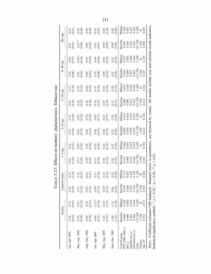
211

TAB

LE

3.27

:E

ffec

tson

mot

hers

’cha

ract

eris

tics:

Toba

cco

use

Smok

erU

nkno

wn

stat

us1–

5ci

gs6–

10ci

gs11

–20

cigs

21–4

0ci

gs40

+ci

gs

Jan.

–Apr

.200

4-0.28

-0.73

0.20

0.15

-0.01

-0.13

-0.15

-0.21

0.01

-0.17

0.03

0.00

-0.01

-0.01

(0.93)

(0.97)

(0.16)

(0.23)

(0.33)

(0.35)

(0.38)

(0.40)

(0.48)

(0.50)

(0.06)

(0.07)

(0.01)

(0.01)

May

–Aug

.200

4-0.23

-0.87

0.13

0.10

0.71∗

0.65∗

-0.65

-0.97

-0.22

-0.33

-0.01

-0.08+

0.01∗∗

-0.00

(0.68)

(0.72)

(0.15)

(0.24)

(0.28)

(0.32)

(0.73)

(0.76)

(0.22)

(0.24)

(0.04)

(0.04)

(0.00)

(0.00)

Sept

.–D

ec.2

004

-0.08

-0.70

-0.05

-0.04

0.50∗

0.38

-0.62

-0.72

-0.40

-0.66∗

-0.00

-0.05

0.00

0.00

(0.46)

(0.51)

(0.11)

(0.21)

(0.25)

(0.29)

(0.54)

(0.56)

(0.28)

(0.29)

(0.05)

(0.05)

(0.00)

(0.00)

Jan.

–Apr

.200

5-0.60

-1.17+

0.30∗

0.17

-0.13

-0.23

0.09

-0.03

-0.24

-0.47

0.10

0.06

-0.01

-0.02

(0.51)

(0.59)

(0.14)

(0.25)

(0.16)

(0.20)

(0.67)

(0.71)

(0.37)

(0.40)

(0.08)

(0.09)

(0.01)

(0.01)

May

–Aug

.200

50.45

-0.33

0.22+

0.15

0.48

0.44

0.08

-0.27

-0.07

-0.33

0.00

-0.06

0.00∗

0.00

(0.97)

(1.01)

(0.12)

(0.24)

(0.42)

(0.45)

(0.75)

(0.77)

(0.37)

(0.39)

(0.04)

(0.05)

(0.00)

(0.00)

Sept

.–D

ec.2

005

-1.09

-1.31

0.04

0.03

0.35

0.47

-0.51

-0.56

-0.11

-0.30

0.01

-0.04

0.00∗

0.00

(1.21)

(1.26)

(0.12)

(0.20)

(0.35)

(0.39)

(0.80)

(0.82)

(0.41)

(0.43)

(0.05)

(0.05)

(0.00)

(0.00)

Con

trol

grou

pB

asel

ine

Mili

tary

Bas

elin

eM

ilita

ryB

asel

ine

Mili

tary

Bas

elin

eM

ilita

ryB

asel

ine

Mili

tary

Bas

elin

eM

ilita

ryB

asel

ine

Mili

tary

PTT,

2000

–200

3:p

0.000

0.002

0.679

0.112

0.374

0.166

0.009

0.073

0.000

0.074

0.259

0.677

0.304

0.438

SIT:

p0.000

0.000

0.036

0.081

0.000

0.035

0.000

0.024

0.000

0.108

0.000

0.097

0.459

0.684

Equ

ality

test

:p0.281

0.612

0.072

0.235

0.121

0.073

0.039

0.504

0.911

0.934

0.377

0.300

0.595

0.447

Dev

iatio

nte

st:p

0.162

0.344

0.124

0.130

0.504

0.573

0.013

0.887

0.701

0.830

0.365

0.254

0.338

0.252

Cel

ls115,7

08

3,2

36

115,7

08

3,2

36

115,7

08

3,2

36

115,7

08

3,2

36

115,7

08

3,2

36

115,7

08

3,2

36

115,7

08

3,2

36

Clu

ster

s1,6

46

45

1,6

46

45

1,6

46

45

1,6

46

45

1,6

46

45

1,6

46

45

1,6

46

45

Adj

.R2

0.784

0.871

0.317

0.262

0.481

0.705

0.613

0.722

0.513

0.554

0.147

0.109

0.009

0.001

Not

es.

Coe

ffici

ent

estim

ates

*100

disp

laye

d.St

anda

rder

rors

,in

pare

nthe

ses,

are

clus

tere

dby

coun

ty.

All

mod

els

incl

ude

year

and

cale

ndar

mon

thin

dica

tors

.St

atis

tical

sign

ifica

nce

sym

bols

:+p<

0.10,

∗p<

0.05

,∗∗p<

0.01

.

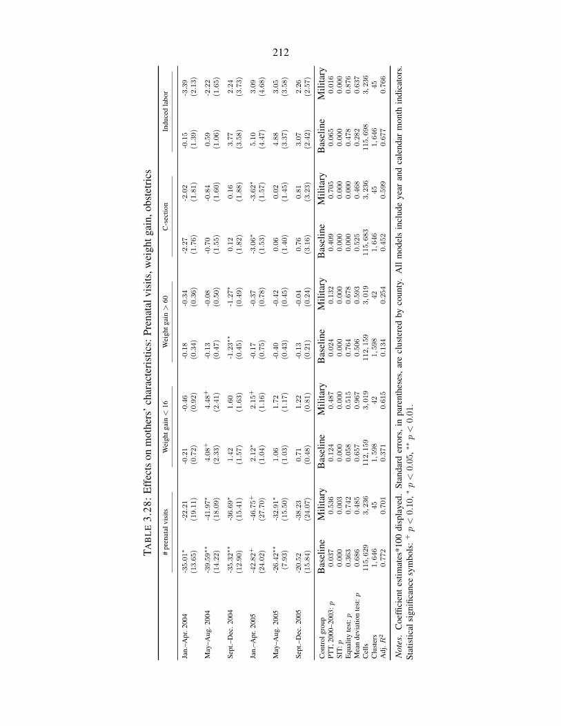
212

TAB

LE

3.28

:E

ffec

tson

mot

hers

’cha

ract

eris

tics:

Pren

atal

visi

ts,w

eigh

tgai

n,ob

stet

rics

#pr

enat

alvi

sits

Wei

ghtg

ain<

16W

eigh

tgai

n>

60C

-sec

tion

Indu

ced

labo

r

Jan.

–Apr

.200

4-35.01∗

-22.21

-0.21

-0.46

-0.18

-0.34

-2.27

-2.02

-0.15

-3.39

(13.65)

(19.11)

(0.72)

(0.92)

(0.34)

(0.36)

(1.76)

(1.81)

(1.39)

(2.13)

May

–Aug

.200

4-39.59∗∗

-41.97∗

4.08+

4.48+

-0.13

-0.08

-0.70

-0.84

0.59

-2.22

(14.22)

(18.09)

(2.33)

(2.41)

(0.47)

(0.50)

(1.55)

(1.60)

(1.06)

(1.65)

Sept

.–D

ec.2

004

-35.32∗∗

-36.69∗

1.42

1.60

-1.23∗∗

-1.27∗

0.12

0.16

3.77

2.24

(12.90)

(15.41)

(1.57)

(1.63)

(0.45)

(0.49)

(1.82)

(1.88)

(3.58)

(3.73)

Jan.

–Apr

.200

5-42.82+

-46.75+

2.12∗

2.15+

-0.17

-0.37

-3.06∗

-3.62∗

5.10

3.09

(24.02)

(27.70)

(1.04)

(1.16)

(0.75)

(0.78)

(1.53)

(1.57)

(4.47)

(4.68)

May

–Aug

.200

5-26.42∗∗

-32.91∗

1.06

1.72

-0.40

-0.42

0.06

0.02

4.88

3.05

(7.93)

(15.50)

(1.03)

(1.17)

(0.43)

(0.45)

(1.40)

(1.45)

(3.37)

(3.58)

Sept

.–D

ec.2

005

-20.52

-38.23

0.71

1.22

-0.13

-0.04

0.76

0.81

3.07

2.26

(15.84)

(24.07)

(0.48)

(0.81)

(0.21)

(0.24)

(3.16)

(3.23)

(2.42)

(2.57)

Con

trol

grou

pB

asel

ine

Mili

tary

Bas

elin

eM

ilita

ryB

asel

ine

Mili

tary

Bas

elin

eM

ilita

ryB

asel

ine

Mili

tary

PTT,

2000

–200

3:p

0.037

0.536

0.124

0.487

0.024

0.132

0.409

0.705

0.065

0.016

SIT:

p0.000

0.003

0.000

0.000

0.000

0.000

0.000

0.000

0.000

0.000

Equ

ality

test

:p0.363

0.742

0.058

0.515

0.764

0.678

0.000

0.000

0.478

0.876

Mea

nde

viat

ion

test

:p0.686

0.485

0.657

0.967

0.506

0.593

0.525

0.468

0.282

0.637

Cel

ls115,6

29

3,2

36

112,1

59

3,0

19

112,1

59

3,0

19

115,6

83

3,2

36

115,6

98

3,2

36

Clu

ster

s1,6

46

45

1,5

98

42

1,5

98

42

1,6

46

45

1,6

46

45

Adj

.R2

0.772

0.701

0.371

0.615

0.134

0.254

0.452

0.599

0.677

0.766

Not

es.

Coe

ffici

ent

estim

ates

*100

disp

laye

d.St

anda

rder

rors

,in

pare

nthe

ses,

are

clus

tere

dby

coun

ty.

All

mod

els

incl

ude

year

and

cale

ndar

mon

thin

dica

tors

.St

atis

tical

sign

ifica

nce

sym

bols

:+p<

0.10,

∗p<

0.05

,∗∗p<

0.01

.

213

TABLE 3.29: Birth rates around the BRAC 2005 announcement

1 2 3 4 5

Jan.–Apr. 2004 0.042+ 0.055∗ 0.045+ 0.036 0.027(0.024) (0.024) (0.024) (0.025) (0.024)

May–Aug. 2004 0.023 0.033 0.027 0.012 0.017(0.024) (0.024) (0.024) (0.024) (0.024)

Sept.–Dec. 2004 0.030 0.035 0.034 0.008 0.027(0.024) (0.024) (0.024) (0.025) (0.024)

Jan.–Apr. 2005 0.037 0.047+ 0.043+ 0.030 0.032(0.024) (0.024) (0.024) (0.025) (0.024)

May–Aug. 2005 -0.010 0.002 -0.004 -0.008 -0.010(0.024) (0.024) (0.024) (0.024) (0.024)

Sept.–Dec. 2005 0.028 0.041+ 0.026 0.014 0.020(0.024) (0.024) (0.024) (0.025) (0.024)

Control group Baseline Minor Major Military StatesEquality test: p 0.329 0.363 0.369 0.553 0.444Mean deviation test: p 0.142 0.158 0.185 0.323 0.217Cells 118, 512 6, 768 10, 008 3, 240 17, 280Clusters 1, 646 94 139 45 240

Notes. Coefficient estimates from Poisson conditional fixed-effects models. Models include terms for year and group-interacted calendar month.The equality test has the null hypothesis that all three coefficients in 2005 are equal. Deviation test explained in main text. Standard errors, inparentheses, are clustered by county. Statistical significance symbols: + p < 0.10, ∗ p < 0.05, ∗∗ p < 0.01.

214

Bibliography

Aizer, A., Stroud, L., and Buka, S. (2009). Maternal stress and child well-being: Evidence from

siblings. Unpublished manuscript, Brown University, Providence, RI.

Almond, D., Chay, K. Y., and Lee, D. S. (2005). The costs of low birth weight. The Quarterly

Journal of Economics, 120(3):1031–1083.

American Psychological Association (2012). Stress in America.

http://www.apa.org/news/press/releases/stress/2011/final-2011.pdf.

Anderson, S. (2013). Ani difranco cancels artist retreat at former slave plantation.

Rolling Stone, http://www.rollingstone.com/music/news/ani-difranco-cancels-artist-retreat-at-

former-slave-plantation-20131230.

Angrist, J. D. (1998). Estimating the labor market impact of voluntary military service using social

security data on military applicants. Econometrica, 66(2):249–288.

Antenucci, D., Cafarella, M., Levenstein, M. C., Re, C., and Shapiro, M. D. (2014). Using social

media to measure labor market flows. Technical report, National Bureau of Economic Research.

Arya, D. (2015). India ’fightback’ sisters: Has the fight gone out of them? BBC.com,

http://www.bbc.com/news/world-asia-india-32579895.

Associated Press (2013). Raccoon beaten to death at wyoming murdoch’s. Scottsbluff Star Her-

ald, http://www.starherald.com/news/wyoming/raccoon-beaten-to-death-at-wyoming-murdoch-

s/article 75fdddd8-6504-11e3-9c73-001a4bcf887a.html.

215

Associated Press (2015). Bbq joint rubbin’ buttz extends white customer discount to all diners.

The Denver Post.

Babin, T. (2013). War veteran forced to change bike shop’s name after threat from u.s bike giant

specialized. Calgary Herald, http://calgaryherald.com/news/local-news/war-veteran-forced-to-

change-bike-shops-name-after-threat-from-u-s-bike-giant-specialized.

Bakshy, E., Messing, S., and Adamic, L. (2015). Exposure to ideologically diverse news and

opinion on Facebook. Science, Published online May 7 2015.

Barasch, A. and Berger, J. (2014). Broadcasting and narrowcasting: How audience size affects

what people share. Journal of Marketing Research, 51(3):286–299.

Barber, B. M. and Odean, T. (2008). All that glitters: The effect of attention and news on the buying

behavior of individual and institutional investors. Review of Financial Studies, 21(2):785–818.

Barry, C. M., Chad Clay, K., and Flynn, M. E. (2013). Avoiding the spotlight: Human rights

shaming and foreign direct investment. International Studies Quarterly, 57(3):532–544.

Base Realignment and Closure Commission (2005a). 2005 Defense Base Closure and Realignment

Commission report. Volume 1.

Base Realignment and Closure Commission (2005b). 2005 Defense Base Closure and Realignment

Commission report. Volume 2.

Basuroy, S., Chatterjee, S., and Ravid, S. A. (2003). How critical are critical reviews? the box

office effects of film critics, star power, and budgets. Journal of Marketing, 67(4):103–117.

Baumeister, R. F., Bratslavsky, E., Finkenauer, C., and Vohs, K. D. (2001). Bad is stronger than

good. Review of general psychology, 5(4):323.

Behrman, J. R. and Rosenzweig, M. R. (2004). Returns to birthweight. Review of Economics and

Statistics, 86(2):586–601.

216

Berger, J. (2011). Arousal increases social transmission of information. Psychological Science,

22(7):891–893.

Berger, J. and Milkman, K. L. (2012). What makes online content viral? Journal of Marketing

Research, 49(2):192–205.

Berger, J., Sorensen, A. T., and Rasmussen, S. J. (2010). Positive effects of negative publicity:

When negative reviews increase sales. Marketing Science, 29(5):815–827.

Berkowitz, G. S., Wolff, M. S., Janevic, T. M., Holzman, I. R., Yehuda, R., and Landrigan, P. J.

(2003). The World Trade Center disaster and intrauterine growth restriction. Jama, 290(5):595–

596.

Bertrand, M., Duflo, E., and Mullainathan, S. (2002). How much should we trust differences-in-

differences estimates? Technical report, National Bureau of Economic Research.

Black, S. E., Devereux, P. J., and Salvanes, K. G. (2007). From the cradle to the labor market? The

effect of birth weight on adult outcomes. Quarterly Journal of Economics, 122(1):409–439.

Blaney, B. (2012). ’Pink slime’ maker halts production at some plants. USA

Today, http://usatoday30.usatoday.com/news/health/story/health/story/2012-03-26/Pink-slime-

maker-halts-production-at-some-plants/53786918/1.

Bosman, R., Sonnemans, J., and Zeelenberg, M. (2001). Emotions, rejections, and cooling off in

the ultimatum game. Technical report, working paper.

Bosman, R. and Van Winden, F. (2002). Emotional hazard in a power-to-take experiment. The

Economic Journal, 112(476):147–169.

Bozzoli, C. and Quintana-Domeque, C. (2014). The weight of the crisis: Evidence from newborns

in Argentina. Review of Economics and Statistics, forthcoming.

Braddon, D. (1995). The regional impact of defense expenditure. volume 1 of Handbook of

Defense Economics, chapter 17, pages 491 – 521. Elsevier.

217

Brosig, J., Weimann, J., and Yang, C.-L. (2003). The hot versus cold effect in a simple bargaining

experiment. Experimental Economics, 6(1):75–90.

Brown, A. L., Camerer, C. F., and Lovallo, D. (2012). To review or not to review? Limited strategic

thinking at the movie box office. American Economic Journal: Microeconomics, 4(2):1–26.

Brown, R. (2012). The intergenerational impact of terror: Does the 9/11 tragedy reverberate into

the outcomes of the next generation? Technical report, Working paper.

Brown, R. (2014). The intergenerational impact of terror: Does the 9/11 tragedy reverberate into

the outcomes of the next generation? Technical report, Households in Conflict Network.

Buckley, E. (August 16, 2005). BRAC letter writing campaign a success. In WBFO News.

http://news.wbfo.org/post/brac-letter-writing-campaign-success.

Burlando, A. (2012). Transitory shocks and birth weights: Evidence from a blackout in Zanzibar.

Technical report, University of Oregon Working Paper.

Burris, A. (2008). Child’s restroom emergency puts store on defensive. Orange County Register,

http://www.ocregister.com/news/mother-128012-store-overturf.html.

Cain, D. M., Loewenstein, G., and Moore, D. A. (2005). The dirt on coming clean: Perverse effects

of disclosing conflicts of interest. The Journal of Legal Studies, 34(1):1–25.

Camacho, A. (2008a). Stress and birth weight: Evidence from terrorist attacks. American Eco-

nomic Review, 98(2):511–515.

Camacho, A. (2008b). Stress and birth weight: Evidence from terrorist attacks. American Eco-

nomic Review, 98(2):511–515.

Carlson, K. (2015). Fear itself: The effects of distressing economic news on birth outcomes.

Journal of Health Economics, 41(0):117 – 132.

218

Carpenter, J., Connolly, C., and Myers, C. K. (2008). Altruistic behavior in a representative dictator

experiment. Experimental Economics, 11(3):282–298.

Carpenter, J. and Seki, E. (2011). Do social preferences increase productivity? field experimental

evidence from fishermen in toyama bay. Economic Inquiry, 49(2):612–630.

Carpenter, J. P., Daniere, A. G., and Takahashi, L. M. (2004). Cooperation, trust, and social capital

in southeast asian urban slums. Journal of Economic Behavior & Organization, 55(4):533 –

551. Trust and Trustworthiness.

Carpenter, J. P. and Matthews, P. H. (2012). Norm enforcement: Anger, indignation, or reciprocity?

Journal of the European Economic Association, 10(3):555–572.

Carroll, C. (2013). DOD furlough plan to affect 9 in 10 civilians.

http://www.stripes.com/news/sequestration/dod-furlough-plan-to-affect-9-in-10-civilians-

1.220844.

Catalano, R. and Hartig, T. (2001). Communal bereavement and the incidence of very low birth-

weight in Sweden. Journal of Health and Social Behavior, 42(4):333–341.

Center, P. R. (2014). E-reading rises as device ownership jumps. Technical report.

Chevalier, J. A. and Mayzlin, D. (2006). The effect of word of mouth on sales: Online book

reviews. Journal of marketing research, 43(3):345–354.

Class, Q. A., Lichtenstein, P., Langstrom, N., and D’Onofrio, B. M. (2011). Timing of prenatal

maternal exposure to severe life events and adverse pregnancy outcomes: A population study of

2.6 million pregnancies. Psychosomatic Medicine, 73(3).

CNN (2015). Clorox apologizes, deletes tweet after racial uproar. money.cnn.com,

http://money.cnn.com/2015/04/09/technology/clorox-emoji-tweet/.

Coffman, L. C. (2011). Intermediation reduces punishment (and reward). American Economic

Journal: Microeconomics, pages 77–106.

219

Copper, R. L., Goldenberg, R. L., Das, A., Elder, N., Swain, M., Norman, G., Ramsey, R., Cotro-

neo, P., Collins, B. A., and Johnson, F. (1996). The preterm prediction study: Maternal stress

is associated with spontaneous preterm birth at less than thirty-five weeks’ gestation. American

Journal of Obstetrics and Gynecology, 175(5):1286–1292.

Couch, K. A. and Placzek, D. W. (2010). Earnings losses of displaced workers revisited. American

Economic Review, 100(1):572–589.

Crump, C., Sundquist, K., Winkleby, M. A., and Sundquist, J. (2013). Early-term birth (37–38

weeks) and mortality in young adulthood. Epidemiology, 24(2):270–276.

Cunha, F. and Heckman, J. J. (2007). The technology of skill formation. American Economic

Review, 97(2):31–47.

Currie, J. (2009). Healthy, wealthy, and wise: Socioeconomic status, poor health in childhood, and

human capital development. Journal of Economic Literature, 47(1):87–122.

Currie, J. (2011). Inequality at birth: Some causes and consequences. American Economic Review,

101(3):1–22.

Currie, J., Greenstone, M., and Moretti, E. (2011). Superfund cleanups and infant health. American

Economic Review, 101(3):435–41.

Currie, J. and Moretti, E. (2007a). Biology as destiny? Short-and long-run determinants of inter-

generational transmission of birth weight. Journal of Labor Economics, 25(2):231–263.

Currie, J. and Moretti, E. (2007b). Biology as destiny? Short-and long-run determinants of inter-

generational transmission of birth weight. Journal of Labor Economics, 25(2):231–263.

Currie, J., Neidell, M. J., and Schmieder, J. F. (2009). Air pollution and infant health: Lessons

from New Jersey. Journal of Health Economics, 28(3):688–703.

Currie, J. and Rossin-Slater, M. (2013a). Weathering the storm: Hurricanes and birth outcomes.

Journal of health economics, 32(3):487–503.

220

Currie, J. and Rossin-Slater, M. (2013b). Weathering the storm: Hurricanes and birth outcomes.

Journal of health economics, 32(3):487–503.

Currie, J. and Schmieder, J. F. (2009). Fetal exposures to toxic releases and infant health. American

Economic Review, 99(2):177–83.

Davis, S. J. and von Wachter, T. M. (2011). Recessions and the cost of job loss. NBER working

paper.

De Weerth, C. and Buitelaar, J. K. (2005). Physiological stress reactivity in human pregnancy—a

review. Neuroscience & Biobehavioral Reviews, 29(2):295–312.

Deaton, A. (2012). The financial crisis and the well-being of Americans 2011 OEP Hicks lecture.

Oxford economic papers, 64(1):1–26.

Defense Base Closure and Realignment Commission (2005b). Hearing transcripts and additional

information. http://brac.gov.

Defense Base Closure and Realignment Commission (July 19, 2005a). Considerations for addition

record of vote. http://brac.gov/docs/VoteTally 19July.pdf.

Dehejia, R. and Lleras-Muney, A. (2004). Booms, busts, and babies’ health. Quarterly Journal of

Economics, 119(3):1091–1130.

DeJohn, I. (2014). Martin luther king jr.’s family outraged over image used for ’freedom 2 twerk’

party. New York Daily News, http://www.nydailynews.com/news/national/michigan-promoters-

martin-luther-king-jr-s-image-promote-freedom-2-twerk-article-1.1580654.

Dellavigna, S., Enikolopov, R., Mironova, V., Petrova, M., and Zhuravskaya, E. (2014). Cross-

border media and nationalism: Evidence from serbian radio in croatia. American Economic

Journal: Applied Economics, 6(3):103–132.

DellaVigna, S. and Kaplan, E. D. (2007). The Fox News effect: Media bias and voting. The

Quarterly Journal of Economics, 122(3):1187–1234.

221

Dellavigna, S. and Pollet, J. M. (2009). Investor inattention and Friday earnings announcements.

The Journal of Finance, 64(2):709–749.

DeMeritt, J. H. (2012). International organizations and government killing: Does naming and

shaming save lives? International Interactions, 38(5):597–621.

Deschenes, O., Greenstone, M., and Guryan, J. (2009). Climate change and birth weight. American

Economic Review, 99(2):211–217.

Dew, M. A., Bromet, E. J., and Schulberg, H. C. (1987). A comparative analysis of two commu-

nity stressors’ long-term mental health effects. American Journal of Community Psychology,

15(2):167–184.

Di Tella, R. and Franceschelli, I. (2011). Government advertising and media coverage of corruption

scandals. American Economic Journal: Applied Economics, 3(4):119–51.

Dills, A. K. and Hernandez-Julian, R. (2012). Negative publicity and catholic schools. Economic

Inquiry, 50(1):143–152.

Dole, N., Savitz, D. A., Hertz-Picciotto, I., Siega-Riz, A. M., McMahon, M. J., and Buekens, P.

(2003). Maternal stress and preterm birth. American Journal of Epidemiology, 157(1):14–24.

Donahue, S. M., Kleinman, K. P., Gillman, M. W., and Oken, E. (2010). Trends in birth weight

and gestational length among singleton term births in the united states: 1990–2005. Obstetrics

and gynecology, 115(2 Pt 1):357.

Donohue, J. J. and Ho, D. E. (2007). The impact of damage caps on malpractice claims: Random-

ization inference with difference-in-differences. Journal of Empirical Legal Studies, 4(1):69–

102.

Duncan, B., Mansour, H., Rees, D. I., et al. (2015). Prenatal stress and low birth weight: Evidence

from the super bowl. Technical report, Institute for the Study of Labor (IZA).

222

Dunkel Schetter, C. (2011). Psychological science on pregnancy: Stress processes, biopsychoso-

cial models, and emerging research issues. Annual review of psychology, 62:531–558.

Dyck, A., Volchkova, N., and Zingales, L. (2008). The corporate governance role of the media:

Evidence from russia. The Journal of Finance, 63(3):1093–1135.

Eccleston, M. (2011). In utero exposure to maternal stress: Effects of 9/11 on birth and early

schooling outcomes in New York City. Working paper.

Eisensee, T. and Stromberg, D. (2007). News droughts, news floods, and US disaster relief. The

Quarterly Journal of Economics, pages 693–728.

Ely, J., Frankel, A., and Kamenica, E. (2013). Suspense and surprise. Journal of Political Economy,

forthcoming.

Employment and Training Administration (2003). The Worker Adjustment and Retraining Notifi-

cation (WARN) Act. Employer’s guide to advance notice of closings and layoffs. U.S. Depart-

ment of Labor.

Engelberg, J. E. and Parsons, C. A. (2011). The causal impact of media in financial markets. The

Journal of Finance, 66(1):67–97.

Entringer, S., Buss, C., Shirtcliff, E. A., Cammack, A. L., Yim, I. S., Chicz-DeMet, A., Sandman,

C. A., and Wadhwa, P. D. (2010). Attenuation of maternal psychophysiological stress responses

and the maternal cortisol awakening response over the course of human pregnancy. Stress,

13(3):258–268. PMID: 20067400.

Erickson, K., Thorsen, P., Chrousos, G., Grigoriadis, D. E., Khongsaly, O., McGregor, J., and

Schulkin, J. (2001). Preterm birth: Associated neuroendocrine, medical, and behavioral risk

factors. Journal of Clinical Endocrinology & Metabolism, 86(6):2544–2552.

Eskenazi, B., Marks, A. R., Catalano, R., Bruckner, T., and Toniolo, P. G. (2007). Low birthweight

223

in New York City and upstate New York following the events of September 11th. Human Re-

production, 22(11):3013–3020.

Falk, A., Fehr, E., and Fischbacher, U. (2005). Driving forces behind informal sanctions. Econo-

metrica, 73(6):2017–2030.

Fan, R., Zhao, J., Chen, Y., and Xu, K. (2014). Anger is more influential than joy: Sentiment

correlation in Weibo. PloS one, 9(10):e110184.

Faraone, J. M. (2012). Personal communication. New York State Department of Labor.

Fehr, E. and Fischbacher, U. (2004a). Third-party punishment and social norms. Evolution and

Human Behavior, 25(2):63–87.

Fehr, E. and Fischbacher, U. (2004b). Third-party punishment and social norms. Evolution and

Human Behavior, 25(2):63–87.

Fehr, E. and Gachter, S. (2002). Altruistic punishment in humans. Nature, 415(6868):137–140.

Feinberg, M., Cheng, J. T., and Willer, R. (2012a). Gossip as an effective and low-cost form of

punishment. Behavioral and Brain Sciences, 35:25–25.

Feinberg, M., Willer, R., Stellar, J., and Keltner, D. (2012b). The virtues of gossip: reputa-

tional information sharing as prosocial behavior. Journal of personality and social psychology,

102(5):1015.

Feldstein, M. (1978). The private and social costs of unemployment. The American Economic

Review, pages 155–158.

Ferraz, C. and Finan, F. (2008). Exposing corrupt politicians: The effects of Brazil’s publicly

released audits on electoral outcomes. The Quarterly Journal of Economics, 123(2):703–745.

224

Ferrie, J. E., Shipley, M. J., Marmot, M., Stansfeld, S., and Smith, G. D. (1995). Health effects of

anticipation of job change and non-employment: Longitudinal data from the Whitehall II study.

British Medical Journal, 311(7015):1264–1269.

Ferrie, J. E., Shipley, M. J., Stansfeld, S., and Marmot, M. (2002). Effects of chronic job insecurity

and change in job security on self reported health, minor psychiatric morbidity, physiological

measures, and health related behaviours in British civil servants: The Whitehall II study. Journal

of Epidemiology and Community Health, 56(6):450–454.

Firstpost.com (2015). After outrage, baby clothing brand takes down onesies that said ’i hate

my thighs’. Firstpost.com, http://www.firstpost.com/living/outrage-baby-clothing-brand-takes-

onesies-said-hate-thighs-2191171.html.

Ford, D. (2013). ’duck dynasty’ star suspended for anti-gay remarks. CNN,

http://www.cnn.com/2013/12/18/showbiz/duck-dynasty-suspension/.

Frank, R. H. (1988). Passions within reason. Norton New York.

Friesen, J. (1997). Mandatory notice and the jobless durations of displaced workers. Industrial

and Labor Relations Review, 50(4):652–666.

Frijda, N. H. (1988). The laws of emotion. American psychologist, 43(5):349.

Gargulinski, R. (April 20, 2005). Cannon backers hire BRAC advisers. In Clovis News Journal.

http://cnjonline.com/cms/news/story-556047.html.

Garrett, R. (2014). Centerplate ceo ousted in dog-kicking elevator incident. Eater SF,

http://sf.eater.com/2014/9/3/6161897/centerplate-ceo-ousted-in-dog-kicking-elevator-incident.

Gentzkow, M. (2006). Television and voter turnout. The Quarterly Journal of Economics,

121(3):931–972.

George, L. M. and Waldfogel, J. (2006). The New York Times and the market for local newspapers.

American Economic Review, 96(1):435–447.

225

Gerber, A. S., Karlan, D., and Bergan, D. (2009). Does the media matter? a field experiment mea-

suring the effect of newspapers on voting behavior and political opinions. American Economic

Journal: Applied Economics, 1(2):35–52.

Glover, V., O’Connor, T., and O’Donnell, K. (2010). Prenatal stress and the programming of the

HPA axis. Neuroscience & Biobehavioral Reviews, 35(1):17–22.

Glynn, L. M., Wadhwa, P. D., Dunkel-Schetter, C., Chicz-DeMet, A., and Sandman, C. A. (2001).

When stress happens matters: Effects of earthquake timing on stress responsivity in pregnancy.

American journal of obstetrics and gynecology, 184(4):637–642.

Goff, K. and Shin, T. (2015). Teacher who admitted sex abuse in youtube vid gets 10 years. NBC

Los Angeles, http://www.nbclosangeles.com/news/local/Teacher-Who-Admitted-Sex-Abuse-in-

YouTube-Video-to-Be-Sentenced-291304121.html.

Goldenberg, R. L., Culhane, J. F., Iams, J. D., and Romero, R. (2008). Epidemiology and causes

of preterm birth. The Lancet, 371(9606):75 – 84.

Goldhammer, Z. (2014). Scary clowns are terrorizing france. The Atlantic,

http://www.theatlantic.com/international/archive/2014/10/clown-killer-quest-ce-que-

cest/382092/.

Government Accountability Office (2005). Analysis of DOD’s 2005 selection process and recom-

mendations for base closures and realignments. Technical Report GAO-05-785.

Graham-Rowe, D. (2012). A smart phone that knows you’re angry. MIT Technology Review,

http://www.technologyreview.com/news/426560/a-smart-phone-that-knows-youre-angry/.

Grimm, V. and Mengel, F. (2011). Let me sleep on it: Delay reduces rejection rates in ultimatum

games. Economics Letters, 111(2):113–115.

Grunberg, L., Moore, S. Y., and Greenberg, E. (2001). Differences in psychological and physical

226

health among layoff survivors: The effect of layoff contact. Journal of Occupational Health

Psychology, 6(1):15–25.

Guala, F. (2012). Reciprocity: Weak or strong? what punishment experiments do (and do not)

demonstrate. Behavioral and Brain Sciences, 35:1–15.

Gurun, U. G. and Butler, A. W. (2012). Don’t believe the hype: Local media slant, local advertis-

ing, and firm value. The Journal of Finance, 67(2):561–598.

Hamilton, J. (May 8, 2005). A good navy town: Submarines run deep in Groton’s soul, and so

does fear for the naval base’s future. In Hartford Courant.

Hamilton, V. L., Broman, C. L., Hoffman, W. S., and Renner, D. S. (1990a). Hard times and

vulnerable people: Initial effects of plant closing on autoworkers’ mental health. Journal of

Health and Social Behavior, 31(2):123–140.

Hamilton, V. L., Broman, C. L., Hoffman, W. S., and Renner, D. S. (1990b). Hard times and

vulnerable people: Initial effects of plant closing on autoworkers’ mental health. Journal of

Health and Social Behavior, 31(2):123–140.

Handwerk, B. (2015). With wearable devices that monitor air quality, scientists can crowdsource

pollution maps. Smithsonian Magazine, http://www.smithsonianmag.com/innovation/with-

wearable-devices-that-monitor-air-quality-scientists-can-crowdsource-pollution-maps-

180954556/?no-ist.

Hartz, M. (December 10, 2004). Area residents look back on BRAC. In Clovis News Journal.

http://www.cnjonline.com/cms/news/story-550343.html.

Hatton, C. (2014). China’s internet vigilantes and the ’human flesh search engine’. BBC.com,

http://www.bbc.com/news/magazine-25913472.

Henrich, J., Ensminger, J., McElreath, R., Barr, A., Barrett, C., Bolyanatz, A., Cardenas, J. C.,

227

Gurven, M., Gwako, E., Henrich, N., et al. (2010). Markets, religion, community size, and the

evolution of fairness and punishment. science, 327(5972):1480–1484.

Hirshleifer, D., Lim, S. S., and Teoh, S. H. (2009). Driven to distraction: Extraneous events and

underreaction to earnings news. The Journal of Finance, 64(5):2289–2325.

Hobel, C. J., Dunkel-Schetter, C., Roesch, S. C., Castro, L. C., and Arora, C. P. (1999). Ma-

ternal plasma corticotropin-releasing hormone associated with stress at 20 weeks’ gestation

in pregnancies ending in preterm delivery. American Journal of Obstetrics and Gynecology,

180(1):S257–S263.

Huberman, G. and Regev, T. (2001). Contagious speculation and a cure for cancer: A nonevent

that made stock prices soar. The Journal of Finance, 56(1):387–396.

Hungerman, D. M. (2013). Substitution and stigma: Evidence on religious markets from the

catholic sex abuse scandal. American Economic Journal: Economic Policy, 5(3):227–253.

Hutchinson, B. (2009). Youtube-exposed domino’s pizza castoff finding it hard to get new job. New

York Daily News, http://www.nydailynews.com/news/money/youtube-exposed-domino-pizza-

castoff-finding-hard-new-job-article-1.172881.

Huttunen, K., Møen, J., and Salvanes, K. G. (2011). How destructive is creative destruction?

Effects of job loss on job mobility, withdrawal and income. Journal of the European Economic

Association, 9(5):840–870.

Inder, W. J., Prickett, T. C. R., Ellis, M. J., Hull, L., Reid, R., Benny, P. S., Livesey, J. H., and

Donald, R. A. (2001). The utility of plasma CRH as a predictor of preterm delivery. Journal of

Clinical Endocrinology & Metabolism, 86(12):5706–5710.

Irvin, D. (March 13, 2005). Politics, BRAC go hand in hand. In Clovis News Journal.

http://www.cnjonline.com/cms/news/story-556520.html.

228

Jacobson, K. (2013). Fedex employee fired after package throwing video goes viral.

WMC-TV, http://apmobile.worldnow.com/story/22941867/fedex-employee-fired-after-package-

throwing-video-goes-viral.

Jacobson, L. S., LaLonde, R. J., and Sullivan, D. G. (1993). Earnings losses of displaced workers.

American Economic Review, 83(4):685–709.

Johnston, R. (2014). Comics for kids - but are they related? Bleeding Cool,

http://www.bleedingcool.com/2014/05/29/comics-for-kids-but-are-they-are-related/.

Jones, S. R. G. and Kuhn, P. (1995). Mandatory notice and unemployment. Journal of Labor

Economics, 13(4):599–622.

Jordan, R. (2012). Personal communication. Alabama Department of Economic and Community

Affairs.

Kalimo, R., Taris, T. W., and Schaufeli, W. B. (2003). The effects of past and anticipated future

downsizing on survivor well-being: An equity perspective. Journal of Occupational Health

Psychology, 8(2):91–109.

Kamenica, E. and Gentzkow, M. (2011). Bayesian persuasion. American Economic Review,

101(6):2590–2615.

Kang, M. J., Ray, D., and Camerer, C. F. (2010). Anxiety and learning in dynamic and static clock

game experiments. Technical report, California Institute of Technology.

Kasl, S. V. and Cobb, S. V. (1970a). Blood pressure changes in men undergoing job loss: A

preliminary report. Psychosomatic Medicine, 32(1):19–38.

Kasl, S. V. and Cobb, S. V. (1970b). Blood pressure changes in men undergoing job loss: A

preliminary report. Psychosomatic Medicine, 32(1):19–38.

Kasl, S. V. and Cobb, S. V. (1980a). The experience of losing a job: Some effects on cardiovascular

functioning. Psychotherapy and Psychosomatics, 34(2-3):88–109.

229

Kasl, S. V. and Cobb, S. V. (1980b). The experience of losing a job: Some effects on cardiovascular

functioning. Psychotherapy and Psychosomatics, 34(2-3):88–109.

Khashan, A. S., McNamee, R., Abel, K. M., Pedersen, M. G., Webb, R. T., Kenny, L. C.,

Mortensen, P. B., and Baker, P. N. (2008). Reduced infant birthweight consequent upon ma-

ternal exposure to severe life events. Psychosomatic Medicine, 70(6):688–694.

Kim, S. (2014). Mozilla ceo brendan eich resigns after protests from gay marriage support-

ers. ABC News, http://abcnews.go.com/Business/mozilla-ceo-resigns-calif-gay-marriage-ban-

campaign/story?id=23181711.

Krain, M. (2012). J’accuse! Does naming and shaming perpetrators reduce the severity of geno-

cides or politicides? International Studies Quarterly, 56(3):574–589.

Kramer, A. D. I., Guillory, J. E., and Hancock, J. T. (2014). Experimental evidence of massive-

scale emotional contagion through social networks. Proceedings of the National Academy of

Sciences, 111(24):8788–8790.

Krim, J. (2005). Subway fracas escalates into test of the internet’s

power to shame. Washington Post, http://www.washingtonpost.com/wp-

dyn/content/article/2005/07/06/AR2005070601953.html.

Kuruvilla, C. (2012). Manager of thai restaurant in texas attacked online after post-

ing racist facebook rant about sandy hook shootings. New York Daily News,

http://www.nydailynews.com/news/national/racist-sandy-hook-rant-hurts-tx-restaurant-article-

1.1223001.

Kushner, D. (2013). Anonymous vs. steubenville. Rolling Stone,

http://www.rollingstone.com/culture/news/anonymous-vs-steubenville-20131127.

Lauderdale, D. S. (2006). Birth outcomes for Arabic-named women in California before and after

September 11. Demography, 43(1):185–201.

230

Lazer, D. (2015). The rise of the social algorithm. Science.

Lederman, S. A., Rauh, V., Weiss, L., Stein, J. L., Hoepner, L. A., Becker, M., and Perera, F. P.

(2004). The effects of the World Trade Center event on birth outcomes among term deliveries

at three lower Manhattan hospitals. Environmental Health Perspectives, pages 1772–1778.

Levenson, E. (2015). Reddit’s find boston bombers thread moderator is full of re-

grets. Boston.com, http://www.boston.com/entertainment/movies/2015/04/11/reddit-find-

boston-bombers-thread-moderator-full-regrets/dT6akA04BwcSuoAIJVCMSM/story.html.

Liem, R. and Rayman, P. (1982). Health and social costs of unemployment: Research and policy

considerations. American Psychologist, 37(10):1116.

Lindenmeier, J., Schleer, C., and Pricl, D. (2012). Consumer outrage: Emotional reactions to

unethical corporate behavior. Journal of Business Research, 65(9):1364–1373.

Lindo, J. M. (2011). Parental job loss and infant health. Journal of Health Economics, 30(5):869–

879.

Linn, M. (December 10, 2004). Base-closing list nothing more than hoax. In Clovis News Journal.

http://www.cnjonline.com/cms/news/story-556520.html.

Lipkind, H. S., Curry, A. E., Huynh, M., Thorpe, L. E., and Matte, T. (2010). Birth outcomes

among offspring of women exposed to the September 11, 2001, terrorist attacks. Obstetrics &

Gynecology, 116(4):917–925.

Loewenstein, G. (2000). Emotions in economic theory and economic behavior. American eco-

nomic review, pages 426–432.

Lomax, A. (2015). What seaworld’s sinking stock really means. Time,

http://time.com/money/3847251/seaworld-stock/.

231

Ludwig, J., Duncan, G. J., Gennetian, L. A., Katz, L. F., Kessler, R. C., Kling, J. R., and San-

bonmatsu, L. (2012). Neighborhood effects on the long-term well-being of low-income adults.

Science, 337(6101):1505–1510.

Maki, N., Moore, S., Grunberg, L., and Greenberg, E. (2005). The responses of male and fe-

male managers to workplace stress and downsizing. North American Journal of Psychology,

7(2):297–314.

Mansour, H. and Rees, D. I. (2012). Armed conflict and birth weight: Evidence from the al-Aqsa

intifada. Journal of Development Economics, 99(1):190–199.

Markiewicz, D. (2015). Parent co. to print gay wedding invites after franchisee refuses. At-

lanta Journal Constitution, http://www.ajc.com/news/news/suwanee-printer-wont-do-wedding-

invitations-for-ga/nk4Kx/.

Martin, J. (2013). Techie adria richards fired after tweeting about men’s com-

ments. CBS News, http://www.cbsnews.com/news/techie-adria-richards-fired-after-tweeting-

about-mens-comments/.

McCubbin, Lawson, Cox, Sherman, Norton, and Read (1996). Prenatal maternal blood pressure

response to stress predicts birth weight and gestational age: A preliminary study. American

Journal of Obstetrics and Gynecology, 175(3, Part 1):706 – 712.

McDonald, S. N. (2014). ‘racists getting fired’ exposes weaknesses of internet vigilantism, no

matter how well-intentioned. Washington Post, http://www.washingtonpost.com/news/morning-

mix/wp/2014/12/02/racists-getting-fired-exposes-weaknesses-of-internet-vigilantism-no-

matter-how-well-intentioned/.

McKechnie, B. (2014). Nypd twitter campaign hijacked with photos of police brutal-

ity. globalnews.ca, http://globalnews.ca/news/1285215/nypd-twitter-campaign-hijacked-with-

photos-of-police-brutality/.

232

McKeever, A. (2015). Why Yelp emerged as a site for social protest. Eater.com,

http://www.eater.com/2015/5/19/8588185/yelp-social-protest-trolling-memories-pizza.

McLean, M., Bisits, A., Davies, J., Woods, R., Lowry, P., and Smith, R. (1995). A placental clock

controlling the length of human pregnancy. Nature medicine, 1(5):460–463.

Moore, S., Grunberg, L., and Greenberg, E. (2004). Repeated downsizing contact: The effects of

similar and dissimilar layoff experiences on work and well-being outcomes. Journal of Occu-

pational Health Psychology, 9(3):247–257.

Moran, L. (2015). Arkansas hotel worker claims she was fired over mini-

mum wage quotes after manager suggested interview. New York Daily News,

http://www.nydailynews.com/news/national/ark-hotel-worker-claims-fired-wage-quotes-

article-1.2167983.

Morgan, S. and Winship, C. (2007). Counterfactuals and causal inference: Methods and principles

for social research. Cambridge University Press.

Murdie, A. and Peksen, D. (2013). The impact of human rights ingo activities on economic sanc-

tions. The Review of International Organizations, 8(1):33–53.

Murdie, A. and Peksen, D. (2014). The impact of human rights ingo shaming on humanitarian

interventions. The Journal of Politics, 76(01):215–228.

Murdie, A. M. and Davis, D. R. (2012). Shaming and blaming: Using events data to assess the

impact of human rights ingos1. International Studies Quarterly, 56(1):1–16.

Neo, W. S., Yu, M., Weber, R. A., and Gonzalez, C. (2013). The effects of time delay in reciprocity

games. Journal of Economic Psychology, 34:20–35.

News, Q. F. (2014). Woman groped by stranger in seattle fights back on social me-

dia. q13fox.com, http://q13fox.com/2014/10/15/woman-groped-by-stranger-in-seattle-fights-

back-on-social-media/.

233

Office of the Deputy Under Secretary of Defense (2003). Report of the plant replacement value

(PRV) panel.

Oken, E., Kleinman, K., Rich-Edwards, J., and Gillman, M. (2003). A nearly continuous measure

of birth weight for gestational age using a United States national reference. BMC Pediatrics,

3(1):6.

Olkean, B. A. (2009). Do television and radio destroy social capital? evidence from indonesian

villages. American Economic Journal: Applied Economics, 1(4):1–33.

Olson, M. (1965). The logic of collective action: Public goods and the theory of group. Harvard

University Press Cambridge.

Ortoleva, P. (2013). The price of flexibility: Towards a theory of thinking aversion. Journal of

Economic Theory, 148(3):903–934.

Paul, K. I. and Moser, K. (2009). Unemployment impairs mental health: Meta-analyses. Journal

of Vocational Behavior, 74(3):264–282.

Pearlman, J. (2015). Mother falsely accuses ’devastated’ aus-

tralian man of photographing her children. The Telegraph,

http://www.telegraph.co.uk/news/worldnews/australiaandthepacific/australia/11600245/Mother-

falsely-accuses-devastated-Australian-man-of-photographing-her-children.html.

Peksen, D., Peterson, T. M., and Drury, A. C. (2014). Media-driven humanitarianism? news

media coverage of human rights abuses and the use of economic sanctions. International Studies

Quarterly, 58(4):855–866.

Prat, A. and Stromberg, D. (2011). The political economy of mass media. Technical report.

Quintana-Domeque, C. and Rodenas, P. (2014). Fear in the womb: The effects of terrorism on

birth outcomes in Spain. Technical report, Working paper.

234

Reinstein, D. A. and Snyder, C. M. (2005). The influence of expert reviews on consumer demand

for experience goods: A case study of movie critics*. The journal of industrial economics,

53(1):27–51.

Reserve, F. (2014). Report on the economic well-being of U.S. households in 2013. Technical

report, Consumer and Community Development Research Section, Board of Governors of the

Federal Reserve System.

Reutskaja, E., Nagel, R., Camerer, C. F., and Rangel, A. (2011). Search dynamics in consumer

choice under time pressure: An eye-tracking study. The American Economic Review, pages

900–926.

Rondo, P. H. C., Ferreira, R. F., Nogueira, F., Ribeiro, M. C. N., Lobert, H., and Artes, R. (2003).

Maternal psychological stress and distress as predictors of low birth weight, prematurity and

intrauterine growth retardation. European Journal of Clinical Nutrition, 57(2):266–272.

Ronson, J. (2015). How one stupid tweet blew up Justine Sacco’s life. The

New York Times, http://www.nytimes.com/2015/02/15/magazine/how-one-stupid-tweet-ruined-

justine-saccos-life.html.

Rook, K., Dooley, D., and Catalano, R. (1991). Stress transmission: The effects of husbands’ job

stressors on the emotional health of their wives. Journal of Marriage and Family, 53(1):165–

177.

Royer, H. (2009). Separated at girth: US twin estimates of the effects of birth weight. American

Economic Journal: Applied Economics, 1(1):49–85.

Ruhm, C. J. (1991). Are workers permanently scarred by job displacements? American Economic

Review, 81(1):319–324.

Salganik, M. J., Dodds, P. S., and Watts, D. J. (2006). Experimental study of inequality and

unpredictability in an artificial cultural market. Science, 311(5762):854–856.

235

Salganik, M. J. and Watts, D. J. (2008). Leading the herd astray: An experimental study of self-

fulfilling prophecies in an artificial cultural market. Social Psychology Quarterly, 71(4):338–

355.

Sandman, C. A., Glynn, L., Schetter, C. D., Wadhwa, P., Garite, T., Chicz-DeMet, A., and Ho-

bel, C. (2006). Elevated maternal cortisol early in pregnancy predicts third trimester levels

of placental corticotropin releasing hormone (CRH): Priming the placental clock. Peptides,

27(6):1457–1463.

Sanfey, A. G., Rilling, J. K., Aronson, J. A., Nystrom, L. E., and Cohen, J. D. (2003). The neural

basis of economic decision-making in the ultimatum game. Science, 300(5626):1755–1758.

Sang-Hun, C. (2008). Web rumors tied to Korean actress’s suicide. The New York Times,

http://www.nytimes.com/2008/10/03/world/asia/03actress.html.

Scharper, J. (2014). Six-year-old’s ’ruined’ fashion show birthday party goes viral. The Bal-

timore Sun, http://articles.baltimoresun.com/2014-01-15/features/bal-little-girls-fashion-show-

birthday-party-fiasco-sparks-law-suit-20140114 1 party-goody-bags-marley-station-mall.

Schmidt, E. (2005). Pentagon seeks to shut dozens of bases across nation. In The New York Times.

14 May 2005.

Seckl, J. R. and Holmes, M. C. (2007). Mechanisms of disease: Glucocorticoids, their placental

metabolism and fetal ‘programming’ of adult pathophysiology. Nature clinical practice En-

docrinology & metabolism, 3(6):479–488.

Selter, B. (2012). In slain teenager’s case, a long route to national attention. The

New York Times, http://www.nytimes.com/2012/03/26/business/media/for-martins-case-a-long-

route-to-national-attention.html.

Semple, K. (May 13, 2005). Military base, awaiting future, tries hard to assure it has one. In The

New York Times. http://www.nytimes.com/2005/05/13/national/13close.html.

236

Shah, K. (2014). Yelpers slam texas restaurant for asking gay couple to not return.

Eater.com, http://www.eater.com/2014/5/29/6216059/yelpers-slam-texas-restaurant-for-asking-

gay-couple-to-not-return.

Shear, M. and Shanker, T. (2005). With Virginia shipyard as backdrop, Obama warns again on

cuts. In The New York Times. 26 February 2013.

Sieczkowski, C. (2012). Lindsey stone, plymouth woman, takes photo at arlington national ceme-

tery, causes facebook fury. Huffington Post, http://www.huffingtonpost.com/2012/11/20/lindsey-

stone-facebook-photo-arlington-national-cemetery-unpaid-leave n 2166842.html.

Silverstein, J. (2015). Florida pub owner held black couple at gunpoint after dispute about a

drink: cops. New York Daily News, http://www.nydailynews.com/news/national/florida-pub-

owner-held-black-couple-gunpoint-cops-article-1.2221507.

Simeonova, E. (2011). Out of sight, out of mind? Natural disasters and pregnancy outcomes in the

USA. CESifo Economic Studies, 57(3):403–431.

Smits, L., Krabbendam, L., de Bie, R., Essed, G., and van Os, J. (2006). Lower birth weight of

Dutch neonates who were in utero at the time of the 9/11 attacks. Journal of Psychosomatic

Research, 61(5):715–717.

Somaiya, R. (2014). How Facebook is changing the way its users consume journalism. New York

Times.

Spargo, C. (2015). ’the internet has your back bro’: Car dealership cruelly shames pizza delivery

man by calling him back and taking away his tip and then posts the video - which backfires

spectacularly. Daily Mail, http://www.dailymail.co.uk/news/article-2911009/The-Internet-

bro-Car-dealership-cruelly-shames-pizza-delivery-man-taking-away-tip-posts-video-backfires-

spectacularly.html.

237

State of Connecticut (May 3, 2005). The contribution of the Groton naval sub base and

the Electric Boat Company to the economies of Connecticut and southeastern Connecticut.

http://www.ct.gov/ecd/lib/ecd/Sub Base EIA 5.4.05.pdf.

Stieglitz, S. and Dang-Xuan, L. (2013). Emotions and information diffusion in social media—

Sentiment of microblogs and sharing behavior. Journal of Management Information Systems,

29(4):217–248.

Stromberg, D. (2004). Radio’s impact on public spending. The Quarterly Journal of Economics,

pages 189–221.

Sullivan, D. and von Wachter, T. (2009). Job displacement and mortality: An analysis using

administrative data. Quarterly Journal of Economics, 124(3):1265–1306.

Sun, J. (2013). Taco bell employee busted for licking tacos on facebook. Eater.com,

http://www.eater.com/2013/6/3/6426329/taco-bell-employee-busted-for-licking-tacos-on-

facebook.

Tan, C. E., Li, H. J., Zhang, X. G., Zhang, H., Han, P. Y., An, Q., Ding, W. J., and Wang, M. Q.

(2009). The impact of the Wenchuan earthquake on birth outcomes. PLoS One, 4(12):e8200.

Tetlock, P. C. (2007). Giving content to investor sentiment: The role of media in the stock market.

The Journal of Finance, 62(3):1139–1168.

Thompson, D. (2014). The facebook effect on the news. The Atlantic,

http://www.theatlantic.com/business/archive/2014/02/the-facebook-effect-on-the-

news/283746/.

TMZ.com (2015). Indiana pizza place forced to close doors after refusing to cater gay wed-

ding. TMZ.com, http://www.tmz.com/2015/04/01/memories-pizza-closes-indiana-deny-service-

gay-wedding/.

238

Torche, F. (2011). The effect of maternal stress on birth outcomes: Exploiting a natural experiment.

Demography, 48(4):1473–1491.

United States Department of Defense. Base realignment and closure 2005.

http://www.defense.gov/brac/faqs001.html.

United States Department of Defense (2005a). Base closure and realignment report. Technical

Report Volume 1. Part 1.

United States Department of Defense (2005b). Base closure and realignment report. Technical

Report Volume 1. Part 2.

U.S. General Accounting Office (1993). Worker Adjustment and Retraining Notification Act not

meeting its goals. GAO/HRD-93-18. United States Congress.

U.S. General Accounting Office (2003). The Worker Adjustment and Retraining Notification Act.

GAO-03-1003. United States Congress.

Vahtera, J., Kivimaki, M., and Pentti, J. (1997). Effect of organisational downsizing on health of

employees. The Lancet, 350(9085):1124–1128.

Vinokur, A. D., Price, R. H., and Caplan, R. D. (1996). Hard times and hurtful partners: How

financial strain affects depression and relationship satisfaction of unemployed persons and their

spouses. Journal of Personality and Social Psychology, 71(1):166–179.

Vishnevetsky, J., Tang, D., Chang, H.-W., Roen, E. L., Wang, Y., Rauh, V., Wang, S., Miller,

R. L., Herbstman, J., and Perera, F. P. (2015). Combined effects of prenatal polycyclic aromatic

hydrocarbons and material hardship on child {IQ}. Neurotoxicology and Teratology, 49(0):74 –

80.

Vythilingum, B., Geerts, L., Fincham, D., Roos, A., Faure, S., Jonkers, J., and Stein, D. J. (2010).

Association between antenatal distress and uterine artery pulsatility index. Archives of women’s

mental health, 13(4):359–364.

239

Wadhwa, P. D. (2005). Psychoneuroendocrine processes in human pregnancy influence fetal de-

velopment and health. Psychoneuroendocrinology, 30(8):724–743.

Wadhwa, P. D., Culhane, J. F., Rauh, V., and Barve, S. S. (2001a). Stress and preterm birth:

Neuroendocrine, immune/inflammatory, and vascular mechanisms. Maternal and child health

journal, 5(2):119–125.

Wadhwa, P. D., Culhane, J. F., Rauh, V., Barve, S. S., Hogan, V., Sandman, C. A., Hobel, C. J.,

Chicz-DeMet, A., Dunkel-Schetter, C., Garite, T. J., et al. (2001b). Stress, infection and preterm

birth: A biobehavioural perspective. Paediatric and Perinatal Epidemiology, 15(s2):17–29.

Wadhwa, P. D., Entringer, S., Buss, C., and Lu, M. C. (2011). The contribution of maternal stress

to preterm birth: Issues and considerations. Clinics in perinatology, 38(3):351–384.

Wadhwa, P. D., Garite, T. J., Porto, M., Glynn, L., Chicz-DeMet, A., Dunkel-Schetter, C., and

Sandman, C. A. (2004). Placental corticotropin-releasing hormone (CRH), spontaneous preterm

birth, and fetal growth restriction: A prospective investigation. American Journal of Obstetrics

and Gynecology, 191(4):1063–1069.

Wagner, M. (2014). Man accused of leaving racist receipt at red lobster sues waitress, restaurant.

New York Daily News, http://www.nydailynews.com/news/national/man-accused-racist-receipt-

fiasco-sues-waitress-restaurant-article-1.1804250.

Wagner, M. (2015). Texas popeyes manager fired for not paying back $400 robber stole at gun-

point, she says. New York Daily News.

Wang, C. S., Sivanathan, N., Narayanan, J., Ganegoda, D. B., Bauer, M., Bodenhausen, G. V., and

Murnighan, K. (2011). Retribution and emotional regulation: The effects of time delay in angry

economic interactions. Organizational Behavior and Human Decision Processes, 116(1):46–54.

Ward, A. (2013). Golden corral dumpster food: Gross out video prompts response. Newsmax.com,

http://www.newsmax.com/TheWire/golden-corral-dumpster-food/2013/07/09/id/514087/.

240

Ward, C. and Gutowski, C. (2015). Police investigate two-way mirror in berwyn club’s bath-

room. Chicago Tribune, http://www.chicagotribune.com/news/ct-berwyn-two-way-mirror-met-

20150427-story.html.

Weinstock, M. (2005). The potential influence of maternal stress hormones on development and

mental health of the offspring. Brain, Behavior, and Immunity, 19(4):296–308.

Welberg, L. and Seckl, J. R. (2001). Prenatal stress, glucocorticoids and the programming of the

brain. Journal of neuroendocrinology, 13(2):113–128.

Westman, M., Etzion, D., and Danon, E. (2001). Job insecurity and crossover of burnout in married

couples. Journal of Organizational Behavior, 22(5):467–481.

Woolston, C. (2015). Sexist review causes twitter storm. Nature, 521(9).

Wright, J. and Escriba-Folch, A. (2009). Are dictators immune to human rights shaming?

Xiao, E. and Houser, D. (2005). Emotion expression in human punishment behavior. Proceedings

of the National Academy of Sciences of the United States of America, 102(20):7398–7401.

Xiao, E. and Houser, D. (2009). Avoiding the sharp tongue: Anticipated written messages promote

fair economic exchange. Journal of Economic Psychology, 30(3):393–404.

Xiong, X., Harville, E. W., Mattison, D. R., Elkind-Hirsch, K., Pridjian, G., and Buekens, P.

(2008). Exposure to Hurricane Katrina, post-traumatic stress disorder and birth outcomes. The

American journal of the medical sciences, 336(2):111.

Yanagizawa-Drott, D. (2014). Propaganda and conflict: Evidence from the Rwandan genocide.

The Quarterly Journal of Economics.

Yang, S., Platt, R. W., and Kramer, M. S. (2010). Variation in child cognitive ability by week of

gestation among healthy term births. American Journal of Epidemiology, 171(4):399–406.

241

Yaniv, O. (2010). Patrick Pogan, NYPD cop who pushed a critical mass cyclist to the ground, gets

no jail time. New York Daily News, http://www.nydailynews.com/news/patrick-pogan-nypd-

pushed-critical-mass-cyclist-ground-no-jail-time-article-1.464247.

Zoladz, C. (2015). Anti-gay mich. business targeted by vandals. USA Today,

http://www.usatoday.com/story/news/nation/2015/04/22/michigan-business-owner-gay-

facebook-vandalism/26174937/.