
Essays on the Economics of Structural Change - Humboldt ...
151
E SSAYS ON THE E CONOMICS OF S TRUCTURAL C HANGE Evidence from the Division and Reunification of Germany D ISSERTATION zur Erlangung des akademischen Grades doctor rerum politicarum (Doktor der Wirtschaftswissenschaft) eingereicht an der Wirtschaftswissenschaftlichen Fakultät Humboldt-Universität zu Berlin von Hannah Liepmann, M.Sc. Economics Präsidentin der Humboldt-Universität zu Berlin: Prof. Dr.-Ing. Dr. Sabine Kunst Dekan der Wirtschaftswissenschaftlichen Fakultät: Prof. Dr. Daniel Klapper Gutachter: 1. Prof. Dr. Alexandra Spitz-Oener 2. Prof. Bernd Fitzenberger, Ph.D. Tag des Kolloquiums: 29. Januar 2019
-
Upload
khangminh22 -
Category
Documents
-
view
0 -
download
0
Transcript of Essays on the Economics of Structural Change - Humboldt ...

E S S A Y S O N T H E E C O N O M I C S O FS T R U C T U R A L C H A N G E
Evidence from the Division and Reunification of Germany
D I S S E R T A T I O N
zur Erlangung des akademischen Grades
doctor rerum politicarum
(Doktor der Wirtschaftswissenschaft)
eingereicht an der
Wirtschaftswissenschaftlichen Fakultät
Humboldt-Universität zu Berlin
von
Hannah Liepmann, M.Sc. Economics
Präsidentin der Humboldt-Universität zu Berlin:Prof. Dr.-Ing. Dr. Sabine Kunst
Dekan der Wirtschaftswissenschaftlichen Fakultät:Prof. Dr. Daniel Klapper
Gutachter:1. Prof. Dr. Alexandra Spitz-Oener2. Prof. Bernd Fitzenberger, Ph.D.
Tag des Kolloquiums: 29. Januar 2019


Abstract
In the context of structural change, how do economic factors impact socio-economic
outcomes? In this thesis, I leverage the division and reunification of Germany to
investigate two specific topics pertaining to this fundamental question.
In the first essay, I analyze how a negative labor demand shock impacts fertility.
I analyze this question in the context of the East German fertility decline after the
fall of the Berlin Wall in 1989. I exploit differential pressure for restructuring across
East German industries which led to unexpected, exogenous, and permanent changes
to labor demand. I find that throughout the 1990s, women more severely impacted
by the demand shock had relatively more children than their less-severely-impacted
counterparts. Thus, the demand shock not only depressed the aggregate fertility level,
but also changed the composition of mothers. My paper shows that these two effects do
not necessarily operate in the same direction.
The second essay of this thesis explores the question of how refugee-specific aid
impacts the medium-term economic success of refugees who migrate as children and
young adults. We address this question in the historical context of German Democratic
Republic (GDR) refugees who escaped to West Germany between 1946 and 1961,
exploiting the facts that only the subgroup of “political refugees” was granted refugee-
targeted aid, and that this only occurred after 1953. The quasi-experiment allows us to
combine several approaches to address identification difficulties resulting from the fact
that refugees eligible for aid are both self-selected and screened by local authorities. We
find positive effects of aid-eligibility on educational attainment, job quality and income
among the refugees who migrated as young adults. We do not find similar effects of
aid-eligibility for refugees who migrated as children.
The final chapter of this thesis presents results of a project which partially closes
a gap that currently exists for East Germans in the data from German social security
notifications and the internal procedures of the Federal Employment Agency. By linking
these data with the GDR’s “Data Fund of Societal Work Power” from 1989, we have
created a new data set that permits the analysis of phenomena such as unemployment,
job mobility, and regional mobility. The new data set can also be used to refine existing
knowledge of the individual-level labor market consequences of German reunification.
Keywords:
Fertility, Labor Demand Shock, Industrial Restructuring;
Refugees, Government Aid, Economic Success;
Labor Market Trajectories, Administrative Data, Record Linkage;
Division and Reunification of Germany, Structural Change


Zusammenfassung
Wie wirken sich, im Kontext strukturellen Wandels, ökonomische Einflussfaktoren
auf sozio-ökonomische Ergebnisse aus? Basierend auf der Teilung und Wiedervereini-
gung Deutschlands, untersuche ich in dieser Dissertation zwei spezifische Themen, die
sich auf diese fundamentale Frage beziehen.
Im ersten Aufsatz analysiere ich, wie sich ein negativer Arbeitsmarktnachfrage-
Schock auf Fertilität auswirkt. Ich analysiere diese Frage im Kontext des ostdeutschen
Fertilitätsrückgangs nach dem Fall der Berliner Mauer im Jahr 1989. Meine empirische
Strategie stützt sich auf unterschiedliche Grade der Restrukturierung auf Industrie-
Ebene, welche unerwartete, exogene, und permanente Anpassungen der Arbeitsnachfra-
ge zur Folge hatten. Ich zeige, dass in den 1990er Jahren ostdeutsche Frauen, welche
stärker vom negativen Arbeitsnachfrage-Schock betroffen waren, relativ mehr Kinder
bekommen haben als Frauen, die weniger stark von dem Schock betroffen waren. Dies
impliziert, dass der Arbeitsnachfrage-Schock nicht nur das aggregierte Fertilitätsniveau
gesenkt hat, sondern auch Auswirkungen auf die Zusammensetzung (Komposition) der
Mütter hatte. Meine Analyse zeigt, dass diese beiden Effekte nicht notwendigerweise in
die gleiche Richtung wirken.
Der zweite Aufsatz dieser Dissertation betrifft die Frage, wie sich Flüchtlings-
spezifische staatliche Hilfen auf den mittelfristigen ökonomischen Erfolg von Flüchtlin-
gen, die als Kinder und junge Erwachsene geflohen sind, auswirken. Wir untersuchen
diese Frage im historischen Kontext ostdeutscher Flüchtlinge, die zwischen 1946 und
1961 aus der Deutschen Demokratischen Republik (DDR) nach Westdeutschland geflo-
hen sind; und nutzen empirisch aus, dass nur der Untergruppe “politischer Flüchtlinge”
Anspruch auf Flüchtlings-spezifische Hilfen gewährt wurde sowie lediglich erst ab
dem Jahr 1953. Dieses Quasi-Experiment ermöglicht es uns, verschiedene Ansätze zu
verfolgen, welche Identifikations-Probleme adressieren, die daraus resultieren, dass für
Flüchtlingshilfen berechtigte Personen sowohl selbst-selektiert waren als auch von den
Behörden ausgewählt wurden. Im Ergebnis zeigen sich positive Effekte der Flüchtlings-
spezifischen Hilfen auf die Bildungsabschlüsse, die Qualität der Jobs, und auf das
Einkommensniveau von Flüchtlingen, die als junge Erwachsene migriert sind. Wir
finden keine vergleichbaren Ergebnisse für Flüchtlinge, die als Kinder migriert sind.
Das letzte Kapitel dieser Dissertation präsentiert Ergebnisse eines Projektes, das
partiell die Lücke schließt, welche derzeit für Ostdeutsche in den Daten der deutschen
Sozialversicherung sowie der internen Datenerfassung der Bundesagentur für Arbeit
existiert. Durch die Verknüpfung dieser Daten mit den Daten des “Datenspeichers Ge-
sellschaftliches Arbeitsvermögen” der DDR aus dem Jahr 1989 haben wir einen neuen
Datensatz geschaffen, welcher Analysen von Phänomenen wie Arbeitslosigkeit, berufli-
che Mobilität, und regionale Mobilität ermöglicht. Der neue Datensatz kann auch dazu

beitragen, das existierende Wissen über die individuellen Arbeitsmarktkonsequenzen
des Mauerfalls zu erweitern.
Schlagwörter:
Fertilität, Arbeitsnachfrage-Schock, Industrielle Restrukturierung;
Flüchtlinge, Staatliche Hilfen, Ökonomischer Erfolg;
Berufliche Verläufe, Administrative Daten, Datenverknüpfung (Record Linkage);
Teilung und Wiedervereinigung Deutschlands, Strukturwandel
vi

Acknowledgements
I would like to begin by thanking my advisor, Alexandra Spitz-Oener, for her support of this
dissertation. She gave me the opportunity to pursue my research ideas and provided decisive
guidance on both intellectual and professional issues. I also thank Bernd Fitzenberger whom
I could always approach with questions and who gave in-depth feedback.
I am grateful to all former and current team members at Humboldt-University Berlin
for the cooperative work atmosphere. This includes in particular Benjamin Bruns, Julian
Emmler, Albrecht Glitz, Lukas Mergele, Jessica Oettel, Kai Priesack, Camille Remigereau,
Kristin Schwier, Felix Weinhardt, and Hanna Zwiener.
During my doctoral studies I had the opportunity to spend five months at the Institute for
Research on Labor and Employment at UC Berkeley. I thank Jesse Rothstein and Daniel
Schneider for making this stay possible and for their extremely helpful comments and
suggestions.
I learned a lot from working with Sandra E. Black, Camille Remigereau, and Alexandra
Spitz-Oener on our joint project that is presented in Chapter 3 of this thesis. To obtain access
to the data used in this project, I went to Mannheim for several short research visits at the
GESIS Leibniz Institute for the Social Sciences, where Bernhard Schimpl-Neimanns has
been very supportive.
As part of my doctoral studies, I also spent time at the Institute for Employment Research
(IAB) in Nuremberg. I thank Dana Müller for her hospitality during this time. Our stimulating
collaboration has led to Chapter 4 of this thesis. I also thank Manfred Antoni of the IAB for
interesting discussions.
My dissertation was made possible by the financial support of the German Research Foun-
dation (DFG), through the Research Training Group “Interdependencies in the Regulation of
Markets” (RTG 1659), the Collaborative Research Center “Economic Risk” (CRC 649), and
the Collaborative Research Center/Trans Regio “Rationality and Competition” (CRC/TRR
190). Moreover, the graduate program of the RTG 1659 and the Berlin Doctoral Program
in Management and Economics (BDPEMS) provided an excellent research environment. I
am grateful for the financial support as well as for the opportunity to engage in inspiring
research networks.
vii

An invaluable experience over the past few years have been the intense conversations with
Niko de Silva, Friederike Lenel, and Arne Thomas. We spent many evenings and weekends
discussing our respective projects from the first vague ideas to completed final drafts. I am
grateful for their feedback and the great time we had discussing research (and many other
topics).
I also thank Eileen Appelbaum and Heidi Hartmann for their encouraging advice and
generous support. They are inspiring role models for me. Knut Gerlach was kind enough to
provide detailed comments on Chapter 2 of this thesis, when it was still at an early stage.
Flora Budianto and I have supported each other ever since we started our graduate program
together. I am also grateful to Ariane Hegewisch who has been an important mentor even
before and also after I started this dissertation.
Finally, I wish to thank Beate, Peter, Klaus, and Jean-François: for their patience, empathy,
critical perspectives, and for their humor.
Contents
1 Introduction 1
2 The Impact of a Negative Labor Demand Shock on Fertility 7
2.1 Introduction . . . . . . . . . . . . . . . . . . . . . . . . . . . . . . . . . . 7
2.2 Background and Empirical Strategy . . . . . . . . . . . . . . . . . . . . . 12
2.2.1 Selection Into Industries . . . . . . . . . . . . . . . . . . . . . . . 12
2.2.2 Employment Development by Economic Sector . . . . . . . . . . . 13
2.2.3 Industry-Level Variation of the Labor Demand Shock . . . . . . . . 15
2.3 Data and Sample . . . . . . . . . . . . . . . . . . . . . . . . . . . . . . . 18
2.3.1 Main Data: BASiD . . . . . . . . . . . . . . . . . . . . . . . . . . 18
2.3.2 Sample Selection . . . . . . . . . . . . . . . . . . . . . . . . . . . 19
2.4 Baseline Estimation . . . . . . . . . . . . . . . . . . . . . . . . . . . . . . 22
2.5 Analysis of Labor Market Outcomes . . . . . . . . . . . . . . . . . . . . . 24
2.6 Baseline Fertility Analysis: The Composition Effect . . . . . . . . . . . . . 26
2.6.1 Annual Births . . . . . . . . . . . . . . . . . . . . . . . . . . . . . 26
2.6.2 Persistence over Time . . . . . . . . . . . . . . . . . . . . . . . . 28
2.6.3 Robustness . . . . . . . . . . . . . . . . . . . . . . . . . . . . . . 30
2.6.4 Interpretation . . . . . . . . . . . . . . . . . . . . . . . . . . . . . 31
2.7 Extended Fertility Analysis: Composition versus Level Effect . . . . . . . 33
2.7.1 Using Older Cohorts as a Control Group . . . . . . . . . . . . . . . 33
2.7.2 Difference-in-Differences Results . . . . . . . . . . . . . . . . . . 34
2.7.3 Common Trends Assumption . . . . . . . . . . . . . . . . . . . . 37
2.8 Effect Heterogeneity by Age . . . . . . . . . . . . . . . . . . . . . . . . . 38
2.9 Conclusions . . . . . . . . . . . . . . . . . . . . . . . . . . . . . . . . . . 39
3 Refugee-Specific Government Aid and Child Refugees’ Economic Suc-
cess Later in Life 41
3.1 Introduction . . . . . . . . . . . . . . . . . . . . . . . . . . . . . . . . . . 41
ix

CONTENTS
3.2 Historical Background . . . . . . . . . . . . . . . . . . . . . . . . . . . . 46
3.2.1 General Background . . . . . . . . . . . . . . . . . . . . . . . . . 46
3.2.2 State of the West German Economy and Welfare State . . . . . . . 50
3.2.3 Criteria Determining GDR Refugees’ Eligibility for Additional Ben-
efits . . . . . . . . . . . . . . . . . . . . . . . . . . . . . . . . . . 51
3.2.4 Benefits for Political GDR-Refugees . . . . . . . . . . . . . . . . . 52
3.2.5 West German Educational System . . . . . . . . . . . . . . . . . . 53
3.3 Data, Sample, and Definition of Main Variables . . . . . . . . . . . . . . . 54
3.3.1 Data . . . . . . . . . . . . . . . . . . . . . . . . . . . . . . . . . . 54
3.3.2 Samples . . . . . . . . . . . . . . . . . . . . . . . . . . . . . . . . 55
3.3.3 Definition of Main Variables . . . . . . . . . . . . . . . . . . . . . 56
3.4 Empirical Specifications and Identification Strategy . . . . . . . . . . . . . 57
3.5 Results . . . . . . . . . . . . . . . . . . . . . . . . . . . . . . . . . . . . . 65
3.5.1 Education and Other Economic Outcomes in 1971 . . . . . . . . . 65
3.5.2 Robustness . . . . . . . . . . . . . . . . . . . . . . . . . . . . . . 68
3.5.3 Interpretation . . . . . . . . . . . . . . . . . . . . . . . . . . . . . 71
3.6 Conclusions . . . . . . . . . . . . . . . . . . . . . . . . . . . . . . . . . . 71
4 A Proposed Data Set for Analyzing the Labor Market Trajectories of
East Germans around Reunification 73
4.1 Introduction . . . . . . . . . . . . . . . . . . . . . . . . . . . . . . . . . . 73
4.2 Original Data Sources . . . . . . . . . . . . . . . . . . . . . . . . . . . . . 75
4.2.1 GAV Data . . . . . . . . . . . . . . . . . . . . . . . . . . . . . . . 75
4.2.2 IEB Data . . . . . . . . . . . . . . . . . . . . . . . . . . . . . . . 78
4.3 Newly Created Data Source . . . . . . . . . . . . . . . . . . . . . . . . . . 80
4.3.1 Procedure for the Merge of the GAV Data and the IEB Data . . . . 80
4.3.2 Evaluation of the Merging Procedure . . . . . . . . . . . . . . . . 83
4.4 Conclusions and Next Steps . . . . . . . . . . . . . . . . . . . . . . . . . 87
A Appendix to Chapter 2: The Impact of a Negative Labor Demand
Shock on Fertility 89
A.1 Employment by Sector and More Detailed Industries, Additional Figures . . 89
A.2 Initially Unemployed Women . . . . . . . . . . . . . . . . . . . . . . . . . 92
A.3 Women Employed in Social Security Agencies . . . . . . . . . . . . . . . 93
A.4 Description of Variables . . . . . . . . . . . . . . . . . . . . . . . . . . . 95
x

CONTENTS
A.5 Robustness of the Composition Effect . . . . . . . . . . . . . . . . . . . . 97
A.5.1 Migration to West Germany . . . . . . . . . . . . . . . . . . . . . 97
A.5.2 Placebo Test for Education . . . . . . . . . . . . . . . . . . . . . . 98
A.5.3 Child Care and Regional Spillover Effects . . . . . . . . . . . . . . 98
A.5.4 Missing Information on Industry . . . . . . . . . . . . . . . . . . . 99
A.5.5 Assortative Mating . . . . . . . . . . . . . . . . . . . . . . . . . . 101
A.5.6 Industries with Strong Employment Growth . . . . . . . . . . . . . 104
A.5.7 Placebo Test based on Previous Births . . . . . . . . . . . . . . . . 105
A.6 Effect Heterogeneity by Qualification Group . . . . . . . . . . . . . . . . . 107
B Appendix to Chapter 3: Refugee-specific Government Aid and Child
Refugees’ Economic Success Later in Life 109B.1 Additional Tables . . . . . . . . . . . . . . . . . . . . . . . . . . . . . . . 109
B.2 Additional Figures . . . . . . . . . . . . . . . . . . . . . . . . . . . . . . 114
xi


List of Figures
1.1 Conceptual Approach and Specific Research Topics . . . . . . . . . . . . . 2
2.1 Total Fertility Rates by Region and Year, 1980-2012 . . . . . . . . . . . . . 8
2.2 Employment in East Germany (in Thousands), By Economic Sector, 1970-
2007 (Selected Years) . . . . . . . . . . . . . . . . . . . . . . . . . . . . . 13
2.3 Employment in East Germany Relative to 1989 (in Percent), By Economic
Sector . . . . . . . . . . . . . . . . . . . . . . . . . . . . . . . . . . . . . 14
2.4 Correlation between the Relative East German Employment Change 1989 to
1993 (in Percent) and Relative Excess Supply in 1989, By Industry . . . . . 17
2.6 Quarterly Number of Births per 1,000 East German Women, By Six Cohort
Groups . . . . . . . . . . . . . . . . . . . . . . . . . . . . . . . . . . . . . 20
2.7 RES and Total Number of Births/End of Period Childlessness, Graphical
Illustration of OLS Estimates (Cross-Sectional Regressions), Years 1991 to
2007 . . . . . . . . . . . . . . . . . . . . . . . . . . . . . . . . . . . . . . 29
3.1 Migration between East and West Germany, in Thousands, 1944/45 to 2014 47
3.2 Schematic Overview of the Emergence Reception Procedure in Marienfelde
in 1960 . . . . . . . . . . . . . . . . . . . . . . . . . . . . . . . . . . . . 49
3.3 Definition of Samples and Historical Time Line . . . . . . . . . . . . . . . 55
3.4 Share of Aid-Eligible Refugees, by Year of Arrival in West Germany . . . . 64
A.1 Employment in West Germany (in Thousands), By Economic Sector, 1970-
2007 (Selected Years) . . . . . . . . . . . . . . . . . . . . . . . . . . . . . 90
A.2 Correlation between the Relative West German Employment Change 1989
to 1993 (in Percent) and Relative Excess Supply in 1989, By Industry . . . 91
A.3 Female versus Male Unemployment and Non-Employment Rates in East
Germany 1993 and Relative Excess Supply in 1989, by Industry . . . . . . 91
A.5 Annual Number of Births per 1,000 East German Women, By Employment
Status at the Beginning of 1991 . . . . . . . . . . . . . . . . . . . . . . . . 92
xiii

LIST OF FIGURES
A.6 Correlation between Women’s RES-Values (by Industry) and Average RES-
Values of their Husbands, 1991, Married Women Only . . . . . . . . . . . 101
A.8 Unemployment Rates in East Germany, 1991-2015, By Gender . . . . . . . 103
B.1 Father’s Educational Attainment . . . . . . . . . . . . . . . . . . . . . . . 115
B.2 Father’s Employment Status . . . . . . . . . . . . . . . . . . . . . . . . . 116
B.3 Father’s Industry of Employment . . . . . . . . . . . . . . . . . . . . . . . 117
xiv

List of Tables
2.1 Summary Statistics for the RES Measure and the Control Variables . . . . . 23
2.2 Relative Excess Supply (RES) and Various Labor Market Outcomes, OLS
Estimates (Panel Regressions) . . . . . . . . . . . . . . . . . . . . . . . . 25
2.3 RES and Annual Births, OLS Estimates (Panel Regressions) . . . . . . . . 27
2.4 RES and Total Number of Births/End of Period Childlessness, OLS Estimates
(Cross-Sectional Regressions) . . . . . . . . . . . . . . . . . . . . . . . . 28
2.5 RES and Fertility Relative to the Control Group of Older East German
Cohorts, Difference-in-Differences Estimates (based on cross-sections) . . . 35
2.6 RES and Predetermined Fertility Outcomes Relative to the Control Group of
Older East German Cohorts, Test of the Common Trend Assumption (based
on cross-sections) . . . . . . . . . . . . . . . . . . . . . . . . . . . . . . . 37
2.7 RES and Total Number of Births, OLS Estimates (Cross-Sectional Regres-
sions), By Age Groups . . . . . . . . . . . . . . . . . . . . . . . . . . . . 38
3.1 Summary Statistics for Main Variables . . . . . . . . . . . . . . . . . . . . 57
3.2 Summary Statistics for Unconditional Potential Years of Exposure (EXP),
by Arrival Sample and Time . . . . . . . . . . . . . . . . . . . . . . . . . 61
3.3 Summary Statistics for Potential Years of Exposure Conditional on Aid-
Eligibility, by Arrival Sample and Time . . . . . . . . . . . . . . . . . . . 62
3.4 Comparison of Age-at-Arrival and Father’s Education Differences for Refugees
who Arrived before 1953 and Thereafter . . . . . . . . . . . . . . . . . . 63
3.5 The Impact of Refugee-Specific Government Aid on Educational Attainment
and other Socio-Economic Outcomes, Men who arrived in West Germany
aged 15 to 25, Cross-Sectional OLS Regression Results (AID specification) 66
3.6 The Impact of Refugee-Specific Government Aid on Educational Attainment
and other Socio-Economic Outcomes, Men who arrived in West Germany
aged 15 to 25, Cross-Sectional OLS Regression Results (EXP specification) 67
xv

LIST OF TABLES
3.7 The Impact of Refugee-Specific Government Aid on Educational Attainment
and other Socio-Economic Outcomes, Men who arrived in West Germany
aged 1 to 14, Cross-Sectional OLS Regression Results (AID specification) . 69
3.8 The Impact of Refugee-Specific Government Aid on Educational Attainment
and other Socio-Economic Outcomes, Men who arrived in West Germany
aged 1 to 14, Cross-Sectional OLS Regression Results (EXP specification) . 70
4.1 Number of Observations and Persons in the GAV Data and Merging Quotas 82
4.2 OLS Regression Results Assessing the Success of the Merge by Age, Quali-
fication Level, and Marital Status . . . . . . . . . . . . . . . . . . . . . . . 85
4.3 Summary Statistics (in Percent) . . . . . . . . . . . . . . . . . . . . . . . . 86
A.1 Fertility Statistics, By Employment Status and Non-Missing vs. Missing
Industry Information on January 1st, 1991 . . . . . . . . . . . . . . . . . . 93
A.2 Extreme Cases: Social Security Agencies Compared With Insurance and
Financial Intermediation, Various Outcomes, OLS Estimates (Panel Regres-
sions, Unweighted) . . . . . . . . . . . . . . . . . . . . . . . . . . . . . . 94
A.3 Variables and Underlying Concepts . . . . . . . . . . . . . . . . . . . . . . 95
A.4 List of Industries in Ascending Order of RES . . . . . . . . . . . . . . . . 96
A.5 RES and Total Number of Births/End of Period Childlessness, OLS Estimates
(Cross-Sectional Regressions), By Migration Status . . . . . . . . . . . . . 97
A.6 RES and Qualification in 1991, OLS Estimates (Cross-Sectional Regressions) 98
A.7 RES and Total Number of Births/End of Period Childlessness, OLS Estimates
(Cross-Sectional Regressions), Controlling for Regional Spillover Effects . 99
A.8 RES and Total Number of Births/End of Period Childlessness, OLS Estimates
(Cross-Sectional Regressions), Including Firm-Level Control Variables . . . 100
A.9 RES and Total Number of Births/End of Period Childlessness, OLS Estimates
(Cross-Sectional Regressions), Including Imputed Control Variables for
Labor Market Prospects of Spouses . . . . . . . . . . . . . . . . . . . . . 102
A.10 RES and Total Number of Births/End of Period Childlessness, OLS Es-
timates (Cross-Sectional Regressions), Excluding Industries with Strong
Employment Growth . . . . . . . . . . . . . . . . . . . . . . . . . . . . . 104
A.11 RES and Total Number of Births, OLS Estimates (Cross-Sectional Regres-
sions), Excluding Industries with Strong Employment Growth and Including
Imputed Control Variables for Spouses . . . . . . . . . . . . . . . . . . . . 105
xvi

LIST OF TABLES
A.12 RES and Predetermined Fertility Outcomes, Placebo Test (Cross-Sectional
Regressions) . . . . . . . . . . . . . . . . . . . . . . . . . . . . . . . . . . 106
A.13 RES and Total Number of Births, OLS Estimates (Cross-Sectional Regres-
sions), By Qualification in 1991 . . . . . . . . . . . . . . . . . . . . . . . 107
B.1 Description of Governmental Aid Programs Covered by C-Status . . . . . . 110
B.2 Additional Information on Variable Definitions and Underlying Concepts . 112
B.3 Summary Statistics for Years of Exposure (EXP) . . . . . . . . . . . . . . 113
xvii


1 Introduction
What are the consequences of structural change? And, in the context of structural change,
how do economic factors impact socioeconomic outcomes? In this thesis, I approach these
fundamental questions by exploring two particular issues in the context of a stark period of
structural change: the division and reunification of Germany. I leverage this historical context
to investigate the causal nexus between economic factors and socio-economic outcomes.
Specifically, I analyze, first, how women’s labor market situations affect their childbearing
decisions; and second, the impact of government aid on refugee children’s medium-term
economic success.
Of course, structural change is a broadly defined phenomenon that can refer to pronounced
adjustments in the economic sphere; or that is initially caused by substantial shifts in the
social and political arenas. The interdependencies between these aspects of society imply
that the consequences of structural change will reverberate throughout society, affecting the
lives of the population in myriad ways.
The examples of the German division and reunification clearly illustrate this point: The
fall of the Berlin Wall in 1989, and the subsequent collapse of communism, profoundly and
permanently changed the lives of around 16 million East Germans (see for instance Huinink
and Mayer, eds., 1995; Mayer and Solga, 2010). Due to the introduction of democracy and
the market economy, citizens of the former German Democratic Republic (GDR) had to
adapt to a new systemic order, which brought about new basic freedoms. At the same time,
their society experienced a severe economic crisis (Akerlof et al., 1991; Burda and Hunt,
2001).
Structural change was similarly complex before 1961, when the planned economy was
introduced in East Germany. Aiming to achieve a more egalitarian society, the totalitarian
regime in East Germany focused on political oppression and severe economic restrictions
and disappropriations that targeted, in particular, those citizens who formerly enjoyed a
privileged socio-economic status. As a result, before the Berlin Wall was built in 1961, at
least 3.6 million East Germans escaped to West Germany, where they would need time to
become integrated into society and the labor market (Bethlehem, 1982; Heidemeyer, 1994;
Ackermann, 1995; Van Melis, 2006).
1
1 INTRODUCTION
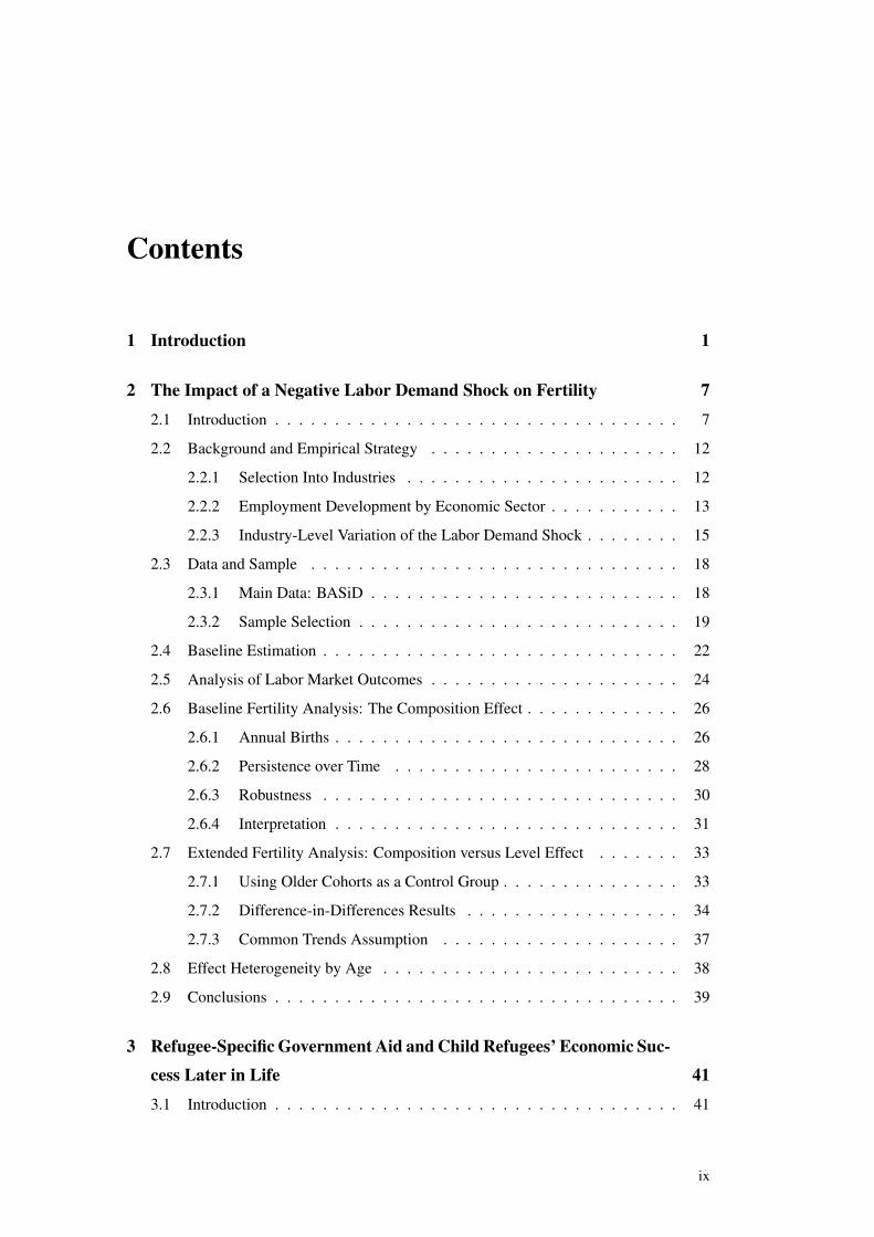
Figure 1.1: Conceptual Approach and Specific Research Topics
Conceptual Approach:
Structural change causesEconomic change(exogenous vari-ation is isolated)
impacts Social and/or eco-nomic outcomes
Topic of Chapter 2:
Fall of the Wallcauses
Negative labordemand shock(variation at
industry level)
impacts Labor marketoutcomes, child-bearing decisions
Topic of Chapter 3:
East-Westmigration due toGerman division
causesPublic spending(variation by ref-ugee subgroup,
exposure effects)
impacts Refugee children’ssocio-economic
outcomes
Because of the complexity of structural change, I pay careful attention to isolating exoge-
nous variation in economic factors. In the context of my two specific research questions, the
methodological approach allows me to assess the causal nexus between economic factors
and socio-economic outcomes (see Figure 1.1 for a summary). In this sense, my thesis
is methodologically inspired by previous studies that have interpreted the same historical
frame as a quasi-experiment in order to uncover causal effects. These studies have focused
on a range of causal relationships regarding phenomena such as solidarity (Ockenfels and
Weimann, 1999), occupational choice (Fuchs-Schündeln and Schündeln, 2005), preferences
for redistribution (Alesina and Fuchs-Schündeln, 2007), saving behavior (Fuchs-Schündeln,
2008), market access (Redding and Sturm, 2008), occupational entry regulation (Prantl
and Spitz-Oener, 2009), social networks (Burchardi and Hassan, 2013), migration (Prantl
and Spitz-Oener, 2014), city structures (Ahlfeldt et al., 2015), consumption (Bursztyn and
Cantoni, 2016), and gender norms (Beblo and Görges, 2018).
Figure 1.1 summarizes the conceptual approach that I employ as well as the specific
topics that I analyze. In Chapter 2, I revisit the question of how women’s labor market
situations impact childbearing decisions. I analyze the question in the context of the dramatic
2

decline in aggregate East German fertility after the fall of the Berlin Wall. To circumvent the
endogeneity of women’s labor market situations, I exploit variation in the labor demand shock
which hit East Germany during this time. The variation stems from differential pressure for
restructuring across industries. This empirical strategy is particularly suited for the purposes
of my research question, since industrial restructuring in East Germany was unexpected and
therefore exogenous to prior selection into industries. Furthermore, industrial restructuring
led to permanent changes to women’s labor market situations.
My paper makes two contributions to the literature. First, I build on previous evidence
by Chevalier and Marie (2017) on the East German fertility decline, but in contrast to these
authors, I exploit exogenous variation in women’s labor market situations and assess how
these impact childbearing decisions. Second, my study is related to Schaller (2016) and Autor
et al. (2018) who also exploit industry-level variation of demand shocks. Whereas the level of
analysis in these two studies is the regional level, I analyze fertility at the individual level and
follow selected cohorts of women over time. I argue that it is important to understand such
individual-level mechanisms, as they have implications for women’s life courses and labor
market trajectories. These mechanisms can also have implications for children to the extent
that parent’s labor market situations are associated with an intergenerational transmission of
inequalities (see the review by Brand, 2015).
My analysis is based on rich panel data from German unemployment and pension in-
surance records, called BASiD. I find that the demand shock impacted the composition of
mothers: Throughout the 1990s women more severely impacted by the demand shock had rel-
atively more children than their less-severely impacted counterparts and this effect persisted
over time. My results thus point to a trade-off between female careers and childbearing. In
the uncertain economic environment in East Germany after reunification, women with more
favorable labor market situations had relatively fewer children because they apparently were
less willing to put their jobs and labor market prospects at risk. More generally, I show that
demand shocks not only depress aggregate fertility levels but also change the composition of
mothers. Indeed, my study demonstrates that, perhaps surprisingly, level and composition
effects of labor demand shocks on fertility do not necessarily operate in the same direction.
Therefore, composition effects should also be investigated in other contexts, particularly
because they entail consequences of economic and social relevance for women and their
families.
Chapter 3 of this thesis is jointly written with Sandra E. Black, Camille Remigereau, and
Alexandra Spitz-Oener. It analyses the impact of refugee-specific government aid on child
3

1 INTRODUCTION
refugees’ economic success later in life (see Figure 1.1). The chapter is motivated by the fact
that there is surprisingly little research on how welfare affects the success of refugees, with
the notable exceptions of Andersen et al. (2018) and LoPalo (2018).
We focus on refugees escaping from the GDR to West Germany between 1946 and 1961
and examine a range of economic outcomes measured 10 years after the migration stream
ceased. The GDR refugees were not welcomed with open arms, leading to a situation in
which merely the subgroup acknowledged as genuine “political refugees” was eligible for
refugee-specific aid (and only from 1953 onward). This allows us to compare refugees
eligible for aid with their non-eligible counterparts. Using rich Microcensus data collected in
West Germany in 1971, we are able to control for detailed parental background characteristics
that the authorities relied on when distinguishing aid-eligible from non-eligible individuals.
Furthermore, we exploit variation in years of exposure to aid. We find that refugee-specific
government aid had an economically significant impact on the educational attainment, job
quality, and income among those refugees who migrated as young adults. In contrast, we do
not find similar effects of aid eligibility for refugees who migrated as children.
Our findings demonstrate the importance of age-at-arrival and the institutional link to the
host country. In the medium-term, non-eligible refugees migrating as children were able to
catch up with their aid-eligible counterparts. We argue that this was due to their natural inte-
gration in the host country’s educational institutions, and emphasize that the refugee-specific
aid was granted in addition to the comprehensive West German social welfare net that all
GDR refugees were covered by. However, refugees arriving as young adults were vulnerable
to a lack of refugee-specific aid. Faced with the decision of entering the labor market and
earning a wage immediately, and given their families’ severe liquidity constraints, young
adults lacking refugee-specific aid were not able to invest in higher education and suffered
the economic consequences this entailed in the medium term. Our findings thus point to a
need for policy makers to consider the specific circumstances of young refugees who are
above the compulsory schooling age.
The final Chapter 4 is coauthored with Dana Müller. It is a methodological report that
relates to Chapter 2. An empirical challenge that I had to tackle in Chapter 2 was the issue
that for East Germans, data from social security records are only fully available from 1992
onward.1 This is due to the fact that the East German labor market administration was
integrated into the West German administration through a complex process. It took time
before all East German firms reported to the social security system (Schmid and Oschmiansky,
1In Chapter 2, I worked with a sample for which earlier information was available and constructed weightsto make the sample representative by industry. See Section 2.3.2 below for details.
4

2007). By 1992, considerable fractions of East Germans had already lost their jobs, had
changed their occupations and industries, or had moved to West Germany. A large number
of firms had closed (see e.g., Diewald et al., 1995; Burda and Hunt, 2001; Hunt, 2006). For
many research questions, 1992 is thus too late in time as a starting point for analysis.
The report presented in Chapter 4 provides results from a project that partially closes the
gap for East Germans in the social security data. From the Federal Archive of Germany we
obtained a cross-section of the GDR’s “Data Fund of Societal Work Power” (for previous
descriptions of these data see Solomon, 1981; Dietz and Rudolph, 1990; Rathje, 1996;
Gebauer et al., 2004). The cross-section contains information on around 7 million East
German workers in 1989, which amounts to 72 percent of the East German labor force at
that time. Based on names, exact dates of birth, and gender information, we merged the 1989
data with data from social security records that start in 1992. In Chapter 4 we describe the
original data sources that we merged, provide details on the merging procedure, and evaluate
its quality. The evaluation shows that we were able to obtain a comparatively high merging
quota of 82 percent for workers younger than 60 in 1989. It furthermore reveals that the
merge was less successful for older workers, who dropped out of the labor force, or initially
single women, who often changed their names after marriage.
Overall, we have created a unique and promising new data set that has two major ad-
vantages. First, it allows researchers to study mechanisms behind phenomena of general
relevance, such as unemployment, occupational mobility, mobility across industries, and
regional mobility. Second, it permits the analysis of East German labor market trajectories
around reunification based on a sample size that is considerably larger than the sample sizes
of currently existing data sources with panel structure. This is particularly relevant because
differences between the former East and West Germany remain an important dimension
of the persistent socio-economic disparities in Germany. This implies a need for further
scientific investigations that are thorough and transparent (recent evidence on the need for
further research is provided in Goschler and Böick, 2017).
To summarize, the three chapters of this thesis are self-contained and can be read inde-
pendently, but they all address topics that pertain to the consequences of structural change
induced by the division and reunification of Germany. Of course, this context influences
how the empirical results are interpreted. At the same time, the context is particularly
appropriate for empirically exploiting exogenous variation in economic factors. Therefore,
this thesis refines the existing knowledge on two specific questions that concern the causal
nexus between economic factors and socio-economic outcomes: the impact of women’s
5

1 INTRODUCTION
labor market situations on childbearing decisions as well as the effect of refugee-specific
government aid on child refugees’ economic success later in life.
6
2 The Impact of a Negative Labor Demand
Shock on Fertility
This chapter has been published as:
Liepmann, Hannah (2018), The Impact of a Negative Labor Demand Shock on Fertility -
Evidence from the Fall of the Berlin Wall, Labour Economics (54), 210–224,
with DOI: https://doi.org/10.1016/j.labeco.2018.07.003.1
2.1 Introduction
In this paper, I revisit the question of how women’s labor market situations impact child-
bearing decisions. From a neoclassical point of view, this is an empirical question, as
there are opposing income and substitution effects (e.g., Becker, 1965; Gronau, 1977). Yet
the endogeneity of individuals’ labor market outcomes poses a key empirical challenge.
I analyze the question in the context of East Germany after the fall of the Berlin Wall in
1989. Fertility in the formerly communist country plummeted after 1989 and recovered only
slowly in later years (Figure 2.1).2 The magnitude of this decline in East German fertility is
unprecedented (Eberstadt, 1994). It stands in contrast to the relatively constant and already
low West German fertility level.
The East German setting is particularly suited to study the effect of women’s labor market
prospects on fertility. To tackle the endogeneity problem, I exploit exogenous variation in the
negative labor demand shock which hit East Germany as a consequence of the introduction
of the market economy. The variation stems from differential pressure for restructuring
across East German industries. A unique advantage of my empirical strategy results from
the unexpectedness of the demand shock. In the former German Democratic Republic self-
selection into industries was independent of later industrial restructuring. Instead, prior to
German reunification, East German workers were accustomed to remarkably stable industrial
1The thesis chapter and Liepmann (2018) are identical, with the exception of minor editorial adjustments.2The decline was due to postponement of childbearing (Conrad et al., 1996; Lechner, 2001), but completed
fertility also declined (Kreyenfeld, 2003; Goldstein and Kreyenfeld, 2011).
7

2 THE IMPACT OF A NEGATIVE LABOR DEMAND SHOCK ON FERTILITY
Figure 2.1: Total Fertility Rates by Region and Year, 1980-2012
.5
1
1.5
2
Tot
al F
ertil
ity R
ate
1980 1985 1990 1995 2000 2005 2010
East Germany West Germany
Source: Human Fertility Database, Max Planck Institute for Demographic Research (Germany) and Vienna Institute of De-mography (Austria), available at www.humanfertility.org (data downloaded in March, 2015). See Goldstein and Kreyenfeld(2011, p. 454) for a similar graph. The total fertility rates are defined for each year as the unweighted sum of all age-specificbirth rates for women in their childbearing years.
employment structures, full employment guaranteed by the state, and constrained job choice
under central planning.
The nature of the labor demand shock represents another distinguishable feature of the East
German setting. The shock is a one-time event which led to sharp and permanent structural
changes to labor demand. This allows me to isolate how the effects of the shock evolved
over time. Specifically, I show that in 1989, the East German employment distribution over
industries strongly differed from economic structures in market economies. Within only a
few years after reunification East German industrial employment structures converged to the
market economy benchmark provided by West Germany. I exploit this fact to abstract from
endogenous supply-side adjustments and to measure the varying intensity of the negative
labor demand shock. The East German setting is an interesting test case, because the
rapid shifts in East German industrial employment structures resemble changes to industrial
employment structures in market economies. In market economies, these changes were
considerably more gradual, but they likewise implied the decline of the manufacturing (Autor
et al., 2003, 2013) and the rise of the services sector (Autor and Dorn, 2013).
My analysis is based on rich administrative data from German unemployment and pension
insurance records, called BASiD. The panel structure of these data permits a detailed
8

2.1 INTRODUCTION
individual-level analysis of fertility over a relatively long time period of seventeen years.
Moreover, in the BASiD data I am able to identify the significant fraction of East German
women who migrated to West Germany. This allows me to study childbearing decisions of
East German women rather than of women living in East Germany.
To preview the results, I first establish that the industry-level labor demand shock generated
exogenous variation in individuals’ labor market outcomes by increasing unemployment and
inducing mobility across industries. I then show that this had an impact on the composition of
mothers: Throughout the 1990s, women more severely impacted by the labor demand shock
had relatively more children than their counterparts who were less severely impacted. This
composition effect is economically significant and it persists over the seventeen year period.
The composition effect is moreover robust to evaluating the influence of migration to West
Germany, qualification levels, child care, regional spill over effects, firm-level characteristics,
and the presence of assortative mating. Furthermore, the composition effect is robust when
older cohorts of East German women are used as a control group. Finally, my empirical
estimates suggest a small permanent effect on completed fertility.
My results point to a trade-off between female careers and childbearing: In the uncertain
economic environment in East Germany after reunification, women with more favorable
labor market outcomes had relatively fewer children because they apparently were less
willing to put their current jobs and future labor market prospects at risk. This mechanism
affected the composition of mothers against the backdrop of a low aggregate fertility level.
In terms of neoclassical theory, the substitution effect dominated over the income effect in
determining the composition of mothers. The results suggest that the compatibility between
female careers and childbearing is crucial. During downturns in particular, the availability
of high-quality childcare might, for example, help avoiding a higher birth reduction among
women with relatively better labor market prospects.
As a general implication of my results, it is important to distinguish between the level
effect and the composition effect of a labor demand shock on fertility. It is a stylized fact
that the aggregate fertility level tends to decline in industrialized countries during recessions
(Sobotka et al., 2011). In East Germany, this negative level effect was very pronounced
and aggregate fertility declined strongly for all groups of East German women (see Figure
2.1). The negative level effect was due to rapid systemic change after German reunification
(Frejka, 2008). While the level effect was not caused by a single factor alone, a major
contributing factor was the aggregate negative labor demand shock. Many researchers have
therefore attributed the fertility decline to economic uncertainty.3 However, contrarily to
3In particular, Chevalier and Marie (2017) emphasize the importance of elevated economic uncertainty incausing the decline in aggregate fertility (see also Eberstadt, 1994; Conrad et al., 1996; Sobotka et al., 2011).
9

2 THE IMPACT OF A NEGATIVE LABOR DEMAND SHOCK ON FERTILITY
what one might expect intuitively, my paper shows that this does not imply that those women
most severely impacted by the demand shock had the lowest birth rates. On the contrary,
women more severely impacted by the demand shock had relatively more children than
their less-severely-impacted counterparts.4 Therefore, the level and composition effect of
the labor demand shock did not operate in the same direction. It is generally important to
understand such composition effects. These individual-level dynamics have implications
for the life courses and labor market trajectories of women. They can also have long-term
consequences for the next generation, since parents’ labor market outcomes affect children
to the extent that socio-economic inequalities persist across generations.
My paper is related to three strands of literature. First, I build on previous studies on the
East German fertility decline. Chevalier and Marie (2017) find that East German women who
had children after the fall of the Berlin Wall were negatively selected in terms of observable
characteristics. They show that these selection effects caused poor educational outcomes of
East Germans born during this time. Moreover, these authors stress feelings of economic
uncertainty as a determinant for childbearing decisions after reunification. In particular,
the authors demonstrate that East German women who had reported to be highly worried
about the economy were less likely to subsequently have children. My results highlight
another mechanism explaining the selection into motherhood. In contrast to Chevalier
and Marie (2017), I exploit exogenous variation in women’s employment situations and
show that women more severely impacted by the labor demand shock had relatively more
children than their less-severely-impacted counterparts. This result can potentially give an
additional explanation why Chevalier and Marie (2017) find worse outcomes for children
born after reunification. Parents’ labor market outcomes affect children to the extent that
socio-economic inequalities persist across generations (see the review by Brand, 2015).
For married couples in Norway, Rege et al. (2011) find negative effects of paternal but
not maternal job loss on children’s school performance. However, maternal job loss is
detrimental for children in contexts where maternal employment and female breadwinner
roles are more normative (Brand and Simon Tomas, 2014). Given the high labor force
attachment of East German women (Rosenfeld et al., 2004; Klenner et al., 2012), women’s
labor market situations presumably entailed intergenerational spill-over effects also in the
East German context after reunification.
Other studies on the East German fertility decline include Arntz and Gathmann (2014) who
In contrast, Arntz and Gathmann (2014) stress the importance of new opportunities. In my view, these twoexplanations are not mutually exclusive.
4Earlier research shows that aggregate economic conditions lead to such composition effects (Dehija andLleras-Muney, 2004; Chevalier and Marie, 2017); whereas I focus on the causal impact of individuals’ labormarket outcomes.
10
2.1 INTRODUCTION
focus on returns to experience in market economies and find that predicted motherhood wage
penalties led to lower birth rates among East German women. Bhaumik and Nugent (2011)
and Kreyenfeld (2010) document a negative impact of perceived employment uncertainty on
birth rates of East German women. Women’s perceived employment uncertainty of partners
(Bhaumik and Nugent, 2011) or actual unemployment (Kreyenfeld, 2010) had no impact.
Finally, in accordance with my findings, Kohler and Kohler (2002) show that in Russia
during the mid 1990s, less favorable labor market outcomes were in several cases positively
correlated with fertility.
Second, this paper is related to two previous studies which exploit industry-level variation
of changes to labor demand in the United States.5 Schaller (2016) uses a Bartik-type
instrumental variable strategy. Autor et al. (2018) focus on import competition from China.6
With regard to fertility, both studies find that fertility tends to increase in regions where
female labor market prospects decline. My contribution to this literature is twofold. To begin
with, compared to the shift-share approaches employed in these previous studies, my measure
for the demand shock exploits variation at the industry level but not based on geographic
differences in initial industry concentration. Thus, my approach is not affected by serial
correlation which is a potential concern in the context of shift-share analysis. In addition,
the level of analysis in both previous studies is the regional level, whereas I investigate
individual-level fertility. Specifically, I follow selected cohorts of women over time and
analyze their childbearing decisions for the extensive and intensive margins of fertility. This
enables me to show that the labor demand shock impacted the timing of childbearing, but
also had a persistent impact on individual-level fertility in the long term.
Finally, this paper is related to studies analyzing plant closures, which arrive at different
conclusions. For Finland, Huttunen and Kellokumpu (2016) show that female job loss
decreases fertility. Del Bono et al. (2015) also find negative effects of job loss on the fertility
of female white-collar workers in Austria, which they attribute to career disruptions.7 This
demonstrates the importance of the type of demand shock investigated. Mass layoffs have
severe implications at individual and regional levels, but a significant fraction of displaced
workers move into new jobs relatively quickly (Gathmann et al., 2017). Thus, after a plant
closure, women seem to prioritize their reentry into employment before they have children.
By contrast, a structural demand shock affecting entire industries may impact previously
5See also Perry (2004) who explores heterogeneity depending on women’s qualification. Early contributionsin this area are Schultz (1985) and Heckman and Walker (1990).
6Methodologically similar studies analyze shocks to family income or wealth. These studies exploit jobdisplacement of husbands (Lindo, 2010), energy price shocks which increased male wages (Black et al., 2013),or real estate price changes (Lovenheim and Mumford, 2013; Dettling and Kearney, 2014).
7Similarly, De la Rica and Iza (2005) show that the high prevalence of fixed-term contracts and a higherthreat of job loss were associated with delayed childbearing in Spain.
11

2 THE IMPACT OF A NEGATIVE LABOR DEMAND SHOCK ON FERTILITY
acquired human capital more permanently, thereby causing the composition effects I analyze
in this paper.
The paper proceeds as follows. In the next section, I provide background information on
the labor demand shock and its variation across industries. Section 2.3 contains a description
of the data and sample. Section 2.4 includes the baseline empirical model. In Section 2.5, I
establish that the labor demand shock impacted labor market outcomes. I analyze its effect
on fertility in Section 2.6. In Section 2.7, I introduce older cohorts of East German women
as a control group to demonstrate the robustness of the results. Section 2.8 assesses the effect
on completed fertility. Section 2.9 concludes.
2.2 Background and Empirical Strategy
2.2.1 Selection Into Industries
For my empirical strategy it is important that the self-selection of GDR citizens into jobs was
exogenous to the industry-level variation of the negative labor demand shock that I exploit.
In this context, two institutional aspects are crucial. First, the reunification and economic
integration of Germany were not anticipated. As a result, GDR citizens self-selected into
jobs and industries independently of conditions that later prevailed in the market economy.
The same argument has been made in the migration literature with regard to pre-determined
occupational choices of migrants (Friedberg, 2001; Borjas and Doran, 2012; Prantl and
Spitz-Oener, 2014).
Second, under central planning individuals’ job choices were heavily constrained (Köhler
and Stock, 2004; Baker et al., 2007; Fuchs-Schündeln and Masella, 2016; Prantl and Spitz-
Oener, 2014). When Erich Honecker came to power in 1971, access to higher education
was severely restricted. Very few students were allowed to obtain the school diploma which
qualified for direct university admission. Apart from good performance in school, the
demonstration of political loyalty towards the GDR regime and active membership in the
“Free German Youth” were necessary prerequisites for being accepted to this school track.
Career counseling was meant to influence individuals from an early age onwards to ensure
that their occupational choices were made in accordance with available positions. In the
sixth school year at the latest, students had to define their desired occupation for the first
time. Applications for multiple apprenticeship positions were officially not possible. In sum,
self-selection into industries was exogenous to the labor demand shock studied in this paper
because German reunification was not anticipated and because job choices in the GDR were
12

2.2 BACKGROUND AND EMPIRICAL STRATEGY
Figure 2.2: Employment in East Germany (in Thousands), By Economic Sector, 1970-2007(Selected Years)
0
500
1000
1500
2000
2500
3000
3500
Em
ploy
men
t (in
100
0s)
1970 1975 1980 1985 1990 1995 2000 2005
Manufacturing Services, loc/reg authorities, non-prof org.
Agric., forestry, fishing Retail
Construction Transport, information transm.
Mining, energy + water supp. Finance, insurance
Source: 1970-1989: Federal Statistical Office (1994), which recoded data for the universe of all GDR establishments (the so-called Berufstätigenerhebung) according to West German classification schemes, and additionally included persons workingfor the army, Ministry of the Interior, Socialist Unity Party, and the Ministry of State Security as these did not appear inofficial GDR statistics. 1990: Bernien et al. (1996, p. 16) based on the last Berufstätigenerhebung which also covered theuniverse of all East German establishments and refers to November 30th, 1990. 1991-2004: Author’s calculations based onScientific Use Files of the Microcensus (a 0.7 percent sample of the population) for persons aged 15 and older living in EastGermany (including East Berlin) at their main residence.
constrained.
2.2.2 Employment Development by Economic Sector
As the market economy was introduced in the formerly communist country, East Germany
experienced a sharp reduction in labor demand. This affected individual East German
industries differently. I now discuss the differential impact of the labor demand shock across
broadly defined economic sectors. At this level of aggregation I could compile reliable and
consistently classified employment data spanning several decades. For 1970 to 1990, these
data are based on the universe of all East German establishments, and for 1991 to 2007 the
data source is the German Microcensus. The time series illustrates that the demand shock is
particularly suited to the purposes of my research question.
Figure 2.2 shows absolute East German employment by sector from 1970 to 2007. The
13

2 THE IMPACT OF A NEGATIVE LABOR DEMAND SHOCK ON FERTILITY
Figure 2.3: Employment in East Germany Relative to 1989 (in Percent), By Economic Sector
-100
-75
-50
-25
0
25
50
75
100
125
150
175E
mpl
. Rel
. to
1989
(in
Per
cent
)
1990 1995 2000 2005
Manufacturing Loc/reg authorities, Soc. Ins.
Agric., forestry, fishing Retail
Construction Transport, information transm.
Mining, energy+water supp. Finance, insurance
Services Non-prof. org.
Source: As in the previous figure. From 1989 onwards it is possible to split up the large category of services, local andregional authorities, and non-profit organizations.
figure reveals that before 1989 sectoral employment structures were remarkably stable in the
GDR. This stability reflects that central planners pursued an extensive growth strategy, which
was based on a mere expansion of production. There was no transition to an intensive growth
strategy, which would have fostered productivity increases and corresponding adjustments of
the sectoral structure. In the 1980s, the political authorities of the GDR failed to reallocate
workers across sectors. One reason was that firms engaged in labor hoarding. Also, workers
were reluctant to leave their firms as these had an important social function. The resulting
sectoral stability was possible only because full employment was guaranteed by the state.
This included full employment of women (Grünert, 1996; Ritter, 2007).
There was a structural break due to German reunification, which unexpectedly and per-
manently changed the East German employment distribution over sectors. This is further
illustrated in Figure 2.3, which displays relative employment changes by sector after 1989.
Employment losses were especially drastic in agriculture, manufacturing, and “mining,
energy and water supply” where employment declined by up to 75 percent until 1993. The
second highest relative employment losses were in local and regional authorities, and in
14

2.2 BACKGROUND AND EMPIRICAL STRATEGY
transport and information transmission. Much less pronounced employment losses occurred
in retail, not-for-profit organizations, and services. The service sector even grew from
1993 onwards. Finally, the rather small finance and insurance sector grew strongly, and the
construction sector experienced a boom which lasted until 1996.8
The East German employment decline after the fall of the wall and its variation across
sectors were driven by three main phenomena (Lutz and Grünert, 1996). First and most im-
portantly, the former GDR economy had to adjust to the fact that there were clear differences
in economic structures between the GDR and market economies such as West Germany.
It is crucial for my empirical strategy that, between East and West Germany, there were
pronounced differences in the distribution of workers across broad sectors and more detailed
industries. Second, employment declined due to migration to West Germany, early retirement
schemes, and layoffs of workers with low performance who had been guaranteed jobs in the
GDR. Finally, many workers in the so-called “Sector X” lost their jobs. These workers had
previously been employed by the army, the Ministry of the Interior, the Ministry of State
Security, and the Socialist Unity Party. Personnel replacements also impacted academic
disciplines related to the economic and social system of the GDR.
2.2.3 Industry-Level Variation of the Labor Demand Shock
In the analysis, I will rely on variation of the labor demand shock at a level that is more
detailed than broad sectors and will distinguish between 48 different industries. To give
examples within the manufacturing sector, employment in the textiles and wearing apparel
industries declined by more than 80 percent between 1989 and 1993, compared with a 57
percent employment decline in the food production industry, and a 41 percent decline in
the chemical industry. Within services, the category “other services (consulting and related
activities)” had declined by 19 percent by 1993, whereas the category “accommodation,
homes, laundry, cleaning, waste collection” had increased by 40 percent.9
These relative changes in employment reflect both demand-side and supply-side adjust-
ments. A credible identification strategy, however, should circumvent supply-side adjust-
ments, as they are potentially endogenous. In particular, supply-side adjustments could
be related to childbearing decisions. Thus, I derive an exogenous measure for the varying
intensity of the labor demand shock where I exploit that the employment distribution over
8To compare the East German case to a market economy, in Appendix Figure A.1 I plot the development ofWest German employment by economic sector. In West Germany, changes to the sectoral structure started earlierand were more gradual. There was no structural break after 1989.
91993 was chosen as the reference year, because the major employment changes occurred up until 1993; alsoafter 1993 there was a change in the classification scheme of these more detailed industries.
15

2 THE IMPACT OF A NEGATIVE LABOR DEMAND SHOCK ON FERTILITY
industries differed strongly between East and West Germany in 1989. Specifically, I define
the following measure of relative excess supply (RES):
RES j,89 =(Empl_East j,89/Empl_East89)− (Empl_West j,89/Empl_West89)
Empl_East j,89/Empl_East89, (2.1)
where Empl_East j,89 denotes the number of East German workers employed in an industry j
in 1989, and Empl_East89 stands for total East German employment in 1989. Empl_West j,89
and Empl_West89 are defined analogously for West Germany. The numerator accounts for
percentage point differences in East and West German industry shares in 1989. The larger
the numerator is, the greater is the excess supply of East German workers in an industry
j relative to the West German market economy benchmark. Accordingly, one can expect
East German employment in j to decline. The denominator of the RES measure relates
this percentage point difference to the relative size of an East German industry, since a
given percentage point difference should matter the more, the smaller is an East German
industry. Importantly for identification, the RES measure is entirely based on differences in
industrial employment structures that emerged because of divergent economic developments
in East and West Germany during the separation of the country.10 Thus, the RES variable is
exogenous to supply side adjustments after the fall of the wall, such as potentially selective
fertility decisions, migration to West Germany, or other movements out of the East German
labor force.
In panel (A) of Figure 2.4, I regress relative employment changes by industry on the RES
measure. The figure illustrates the strength of the RES measure as a predictor for the relative
employment decline of East German industries after 1989. Relative employment changes are
captured by the percentage change in employment of an East German industry between 1989
and 1993. The figure confirms that relative employment changes of East German industries
are indeed negatively correlated with 1989 employment differences in East and West German
employment structures, as measured by the RES variable.11 As shown in Panel (B) of the
same figure, where the four most extreme RES values are excluded, this negative relationship
is not driven by outliers.12
10To emphasize that the East German employment changes were indeed the result of reunification, in aplacebo test I regress West German employment changes on the RES measure. These two variables are notsystematically correlated (Appendix Figure A.2).
11Due to a lack of female GDR-employment statistics, the RES-measure includes both genders. A measurebased on women alone might be more precise, implying that I present lower bound effects. In particular, EastGerman women were more likely than men to lose their jobs after reunification (Hunt, 2002). In Appendix FigureA.3, I confirm that, across industries, job losses were more severe for women in 1993. There is some, albeit veryimprecisely estimated, evidence that female relative to male job loss was stronger in industries developing morefavorably (with low RES-values).
12 ‘Social insurance agencies’ are excluded from the analysis but discussed in the Appendix. In 1989, only0.07 percent of East German workers were employed in this industry. Most workers initially employed in this
16

2.2 BACKGROUND AND EMPIRICAL STRATEGY
Figure 2.4: Correlation between the Relative East German Employment Change 1989 to1993 (in Percent) and Relative Excess Supply in 1989, By Industry
Coeff. = -45.99Robust s.e. = 9.51T-stat = -4.84
-150
-100
-50
0
50
100
150
200
250
300
350
400
Em
pl. C
hang
e 19
89-9
3, E
ast G
erm
any
(in P
erce
nt)
-8 -7 -6 -5 -4 -3 -2 -1 0 1RES = (Share East 1989 - Share West 1989) / Share East 1989
A. All industries (N=48)
Coeff. = -43.04Robust s.e. = 11.74T-stat = -3.67
-125
-100
-75
-50
-25
0
25
50
75
Em
pl. C
hang
e 19
89-9
3, E
ast G
erm
any
(in P
erce
nt)
-1.5 -1 -.5 0 .5 1RES = (Share East 1989 - Share West 1989) / Share East 1989
B. Excluding the four most extreme RES-values
Source: For East Germany in 1989 and 1993, the data sources are the same as in Figures 2.2 and 2.3. For West Germanyin 1989, the data source is the Microcensus. See Appendix Table A.4 for a list of the industries. The regression modelsare weighted using 1989 East German employment shares of industries as analytical weights. The y-axis displays changein percent, i.e., 100 ∗ Empl_East j,93−Empl_East j,89
Empl_East j,89. In panel (B), the four most extreme RES-values are excluded (these are the
finance and insurance industries, “printing & reproduction,” and “finishing trade”) to emphasize that the relationship in panel(A) is not driven by outliers.
The economic rationale why the RES measure predicts East German employment changes
after 1989 is twofold. First, market forces led to a convergence of the distribution of East
German employees to the West German standard. After all, West German industry structures
had evolved such that the West German economy was relatively successful internationally.
Second, as part of the massive privatization of East German firms by the “Trust Agency,”
decisions were made on a case-by-case basis, while industrial policy concerns such as
regional spill-over effects played a subordinate role. In this context, East German firms
were frequently taken over by and integrated into West German firms belonging to the
same industry. The East German firms were, for example, then established as suppliers of
intermediary input goods (Wahse, 2003; Federal Institute for Special Tasks Arising From
Unification, 2003). Essential for the identification strategy is the fact that East Germans
did not anticipate any of these developments. At the point in time when former GDR
citizens sorted into industries, industrial employment structures were stable, employment
was guaranteed by the state, and sorting into industries was constrained as a result of limited
job choice under central planning.
industry were replaced (Bernien et al., 1996), and the drastic expansion of this industry had no positive impacton their later labor market success.
17

2 THE IMPACT OF A NEGATIVE LABOR DEMAND SHOCK ON FERTILITY
2.3 Data and Sample
2.3.1 Main Data: BASiD
The “Biographical Data of Social Security Insurance Agencies in Germany 1951-2009”
(BASiD) combine data from the German Statutory Pension Insurance Scheme (RV), the
Federal Employment Agency (BA) and the Institute for Employment Research (IAB).
The basis of BASiD is the Sample of Insured Persons and their Insurance Accounts 2007
(Versichertenkontenstichprobe, VSKT) from the RV, which is merged with data from the BA
and the IAB. The VSKT 2007 is a 1 percent sample of insured persons aged 15 to 67 at
December 31, 2007 who are still alive and have an active pension insurance account. This
refers to persons who are covered by the pension insurance scheme but are not currently
receiving pensions.13 Insured persons contribute to their pension entitlements by means of
employment, child care or elderly care, by receiving health insurance in case of long-term
illness, or by receiving social benefits such as unemployment insurance (for more details
about the data see Hochfellner et al. (2011, 2012)).
The BASiD data have a rich panel structure. Up until 2007, they provide retrospective
information on all spells and events which are relevant to the pension insurance, the un-
employment insurance, or both. For the purposes of my study, the BASiD data have three
major advantages. First, I can identify former GDR citizens in the data even if they moved to
West Germany after the fall of the wall. As large proportions of young East German women
migrated to West Germany during the 1990s (Hunt, 2006; Fuchs-Schündeln and Schündeln,
2009), this is an important feature. It enables me to include East German women who
migrated to West Germany in my analysis. Second, the data provide accurate information
on the month of birth of a woman’s children, because childbearing entails contributions to
pension entitlements. This is also true for births before 1989. Finally, sample sizes of BASiD
are considerably larger than in alternative German panel data sources, which allows me to
analyze the extensive and the intensive margin of fertility over a relatively long time period
of 17 years.
The BASiD data are well suited to study how women’s labor market situations impact
childbearing decisions. By contrast, information on births is unfortunately not available
for men. A potential concern in this context is assortative mating. However, I later add
imputed control variables for the presence and labor market prospects of spouses and show
that the results are not driven by assortative mating. Moreover, it is a priori reasonable to
13German pension data have high coverage rates (Richter and Himmelreicher, 2008), but, as is typically thecase for German administrative data, the self-employed and civil servants are not included.
18

2.3 DATA AND SAMPLE
expect that the labor market situation of East German women had a significant impact on
their childbearing decisions. East German women and mothers have traditionally had a high
labor force attachment (Rosenfeld et al., 2004). Among East German mothers with minor
children in 1996, only 7.7 percent of mothers with partners and 2.2 percent of single mothers
reported transfers from current partners, former partners or other relatives as their main
income source (the corresponding figures for West Germany are 50.2 and 9.8 percent). While
West German mothers relied much more often on their partners’ incomes, for East German
mothers the most important income sources were their own wages and salaries, followed
by public transfers (Federal Statistical Office, 2010, p. 26). Adler (1997) emphasizes the
reluctance of East German women to economically depend on their partners. Providing
qualitative evidence, she even argues that economic independence from men would be a
prerequisite for East German women to have children.
2.3.2 Sample Selection
Identification of East Germans
The selection of the sample of East German women requires three steps. In the first step,
I identify East Germans by exploiting the fact that contributory periods in East and West
Germany yield different pension entitlements. Specifically, the sample includes women
who prior to 1989 had at least one spell related to work or training in the dual system of
apprenticeship in the GDR, but had no such spells in West Germany prior to 1989.14 These
criteria ensure that the selected women were integrated in the East German labor market and
that the labor demand shock studied in this paper was relevant to them. Note that women
who migrated to West Germany after the fall of the wall are kept in the sample to rule out
selective attrition resulting from migration to the West.
Cohort Choice
The second selection criterion concerns the cohorts included in the analysis. Women in the
former GDR had their children at young ages, particularly in comparison with West German
women (Huinink and Wagner, 1995; Goldstein and Kreyenfeld, 2011). This is confirmed in
Figure 2.6, where I display the number of quarterly births per 1,000 East German women
born between 1944 and 1973, based on the BASiD data and for six different cohort groups.
The fertility of women who were older than 31 in 1990 (or born before 1959) was largely
14I am grateful to Dana Müller whose Stata-routine I use to distinguish between East and West German spells.See also Grunow and Müller (2012).
19

2 THE IMPACT OF A NEGATIVE LABOR DEMAND SHOCK ON FERTILITY
Figure 2.6: Quarterly Number of Births per 1,000 East German Women, By Six CohortGroups
0
10
20
30
40
50
0
10
20
30
40
50
0
10
20
30
40
50
0
10
20
30
40
50
0
10
20
30
40
50
0
10
20
30
40
50
1960q1 1970q1 1980q1 1990q1 2000q1 2010q1 1960q1 1970q1 1980q1 1990q1 2000q1 2010q1 1960q1 1970q1 1980q1 1990q1 2000q1 2010q1
1960q1 1970q1 1980q1 1990q1 2000q1 2010q1 1960q1 1970q1 1980q1 1990q1 2000q1 2010q1 1960q1 1970q1 1980q1 1990q1 2000q1 2010q1
1st group: born 1944-48 2nd group: born 1949-53 3rd group: born 1954-58
4th group: born 1959-63 5th group: born 1964-68 6th group: born 1969-73
Qua
rter
ly B
irths
, per
1,0
00 W
omen
Source: BASiD; based on women who, prior to November 1989, worked or did apprenticeship training in the GDR but notin West Germany, and including women who migrated to West Germany after November 1989. N = 22,572. Due to dataprotection, less than 20 absolute births per quarter had to be censored and are displayed here as zero births. The vertical linestands for the third quarter of 1990. See Section 2.3.1 for details on the data and Section 2.3.2 for details on the identificationof East Germans.
completed even before the wall fell (groups 1-3 in Figure 2.6). By contrast, childbearing
decisions of women born between 1959 and 1973 were impacted by the fall of the wall
(groups 4-6). Therefore, I include groups 4 to 6, who were aged 17 to 31 at the end of 1990,
in the main sample.
Final Selection Step
The final step in the selection of the sample arises from a peculiarity of the BASiD data. In
this step, the sample is additionally restricted to women who on January 1st, 1991, worked
in East Germany and have non-missing industry information. This is the first point in time
for which industry information is known for a subsample of East Germans. The final sample
consists of 4,234 women.
To explain the final step, after reunification the East German labor administration was
integrated into the West German administration as part of a complex process (Schmid and
20

2.3 DATA AND SAMPLE
Oschmiansky, 2007). For some firms industry information was reported already in 1991,
whereas it is available for all East German firms from 1992 onwards. It is, however, crucial
to infer industry information for the earliest point in time possible, since industries are only
observed for employed persons. Unemployment rapidly increased from 9.5 percent among
East German women in mid-January of 1991 to 20.5 percent a year later (Federal Employment
Agency, 2015) and a significant fraction of workers likely changed industries after they
became unemployed. Figure 2.3 above shows that the most pronounced employment losses
took place after 1990 (in this figure, the information for 1990 refers to the end of November).
Using industry information from January 1st, 1991, thus seems to be a good approximation
of industries prior to the fall of the wall. As far as the fertility analysis is concerned, it is also
reasonable to exclude the year 1990. Fertility can respond to economic conditions only with
a time lag of nine months, and during 1990 births were largely independent of the fall of the
wall in November of 1989.
It needs to be emphasized that industry information for January 1st, 1991, is missing for
a large fraction of women who work on this day (there are 4,234 employed women with
non-missing and 4,783 employed women with missing industry information). It is important
that the missing information on industries is driven by firms not yet integrated into the social
security system rather than by workers not reporting their industry. Workers sorted into firms
prior to reunification and independently of later labor demand conditions. Nevertheless,
the fact that information on industry is missing for a large fraction of firms requires further
investigation.
To begin with, the representativeness of the sample distribution over industries is a concern.
For example, at the sectoral level, the sample share of women working in mining is suspi-
ciously large and the sample share working in services appears to be too small. To correct
for these discrepancies between the sample distribution and the population distribution, I
use the Microcensus of 1991. In the Microcensus, I identify women born between 1959 and
1973 who live in East Germany and compile their distribution over industries.15 For each
woman from an industry j, I then calculate the following simple post-stratification weight:
w j =share_Microcensus j
share_sample j, (2.2)
where share_Microcensus j is an estimate of the population share of this industry. Throughout
the paper, I apply w j as probability weights.16
15I use the Scientific Use File, which is a 0.7 percent representative sample of the population. The Microcensuswas conducted in April, when unemployment was already high. Therefore the distribution is based on the currentindustry of employed women and the last industry of non-employed women.
16Weighted and unweighted results are consistent in a qualitative sense, but effects in unweighted estimations
21

2 THE IMPACT OF A NEGATIVE LABOR DEMAND SHOCK ON FERTILITY
In addition, it is possible that the firms included in the analysis are not a random sample.
However, in a robustness test I control for a set of firm-level characteristics and show that
these characteristics do not confound the impact of the labor demand shock on fertility.
Finally, there might be selective sample attrition because some women have already lost
their jobs by January 1st, 1991. 8 percent of women are unemployed on this day and I discuss
this specific group in Appendix A.2. It turns out that the initially unemployed women are
indeed a selective subgroup, since they include a high share of mothers with young children
who were born immediately before the fall of the wall. At the same time, this corresponds
to the intuition behind the findings for the main analysis, as it indicates that in these times
of elevated uncertainty, childbearing was related to the risk of job loss. In Appendix A.2, I
also provide fertility statistics for employed women with missing and non-missing industry
information for January 1st, 1991. Overall, fertility statistics for these two groups compare
well. Relative to these two groups, it is again the case that women who had already lost their
jobs by the beginning of 1991 had relatively many children on average.
2.4 Baseline Estimation
For woman i from industry j = 1, ...,48 and years t, the following panel regression is
estimated:
Yit j = β0 +β1RES j,89 +X ′itβ2 +X ′i β3 + γt + εit j. (2.3)
The model is estimated for three separate time periods containing years 1991 to 1994, 1995
to 1999, and 2000 to 2007, respectively. RES j,89 is the measure for the intensity of the
unexpected and exogenous labor demand shock as derived in Section 2.2.3. γt are time
fixed-effects. Since the treatment is time invariant within industries, throughout the paper
robust standard errors are clustered at the industry level (the number of clusters is 48).
I first establish that the RES demand shock impacted different labor market outcomes,
which are discussed in the next section. I then analyze the impact on fertility, where Yit j is a
dummy variable equal to one if a woman gave birth in a given year.
To assess how the impact of the demand shock evolves over time, I focus on three distinct
time periods. The first period of years 1991 to 1994 refers to the short term and includes
the years during which aggregate East German fertility plummeted. The second period
captures medium-term effects. It includes years 1995 to 1999 during which aggregate East
German fertility increased again (for these aggregate fertility trends recall Figure 2.1 above).
Finally, the third period is defined as years 2000 to 2007 and refers to the long term. The
tend to be somewhat smaller and their statistical significance tends to be weaker.
22

2.4 BASELINE ESTIMATION
Table 2.1: Summary Statistics for the RES Measure and the Control Variables
Panel A: RES MeasureMean -.204 P90, P10 interval [.583, -.911]Standard deviation (.993) P75, P25 interval [.324, -.391]
Panel B: Control variablesAge (here: in 1991) 25.68 2 children bf. 91 .264S.d. of age (4.11) 3 children bf. 91 .034Low Qualification, 91 .255 Privileges in GDR .057Med. Qualification, 91 .706 Appr. Training, 91 .062High Qualification, 91 (reference) .039 Large city, 91 .0990 children bf. 91 (reference) .386 Very large city, 91 .1411 child bf. 91 .316
Sample size; i.e., individuals observed each year (1991-2007) 4,234
Notes: Panel A refers to the industry a woman worked in on January 1st, 1991. In Panel B all control variables are defined asdummy variables (except for age). The sample is balanced with N = 4,234 individuals.
main parameter of interest, β1, measures the average annual impact of the unexpected and
exogenous labor demand shock during the respective time periods. β1 thus summarizes
annual effects in a way that is straightforward to interpret. I later augment the baseline
specification to investigate how the effects accumulate over time.
Across specifications, time variant control variables are age and age squared. The other
control variables are time constant. These include two qualification dummy variables
referring to women who in 1991 had no formal qualification and to women who in 1991
had completed apprenticeship training, respectively. Women who in 1991 had graduated
from university are the reference category. It is important to control for qualification, since
the qualification level of the employed in an industry might have influenced both the RES-
variable and the fertility rate. Further control variables are dummy variables for the number
of children a woman had prior to 1991 (one child, two children and three or more children),
and two dummy variables for whether a woman worked in a large city or very large city at
the beginning of the 1990s, because fertility patterns as well as industry structures might
differ in rural versus urban areas. Another dummy variable for persons who in the GDR were
entitled to privileged pensions serves as a proxy for closeness to the regime. This variable
addresses the concern that for some workers labor market trajectories after reunification
were shaped by their prior regime closeness rather than their initial industry. A final dummy
variable captures whether a woman was still in apprenticeship training in 1991. A more
detailed description of the definition and in some cases of the imputation of variables is
provided in Appendix Table A.3. Summary statistics for the RES demand shock measure
23

2 THE IMPACT OF A NEGATIVE LABOR DEMAND SHOCK ON FERTILITY
and for the control variables are shown in Table 2.1. Summary statistics of the dependent
variables are included in the respective tables below.
2.5 Analysis of Labor Market Outcomes
I now establish that the RES demand shock generated exogenous variation in individuals’
labor market outcomes (Table 2.2).17 The first outcome variable is the incidence of unem-
ployment, which is captured by a dummy variable equal to one if a women experienced
an unemployment spell in a given year. The second outcome variable is the duration of
unemployment expressed in months per year, which is set to zero for women without any
unemployment spell. Third, industry changes are defined as a dummy variable equal to one
if a woman started to work in a new industry in a given year. Finally, migration to West
Germany is accounted for by a dummy variable equal to one in the year migration took place.
To facilitate the interpretation of results, I compare estimated effects for women who
initially worked in industries subject to a severe labor demand shock with estimated effects
for women who initially worked in industries which were less severely hit. Specifically, I
compare women at the 90th percentile of the RES measure (which is 0.58 and stands for a
severe labor demand shock) with women at the 10th percentile (which is -0.91 and implies
the industry was not negatively impacted by the shock). In terms of actual industries, the 90th
percentile coincides with textile manufacturing, whereas the 10th percentile corresponds to
lower-skilled services including cleaning and laundry workers. Throughout the paper, tables
include rows labeled “P90 vs P10.” In these rows, the difference in estimated effects between
the 90th and the 10th percentile is reported.
As shown in Table 2.2, the impact of the RES demand shock on unemployment is positive,
significant, and it persists over time. In the short term of years 1991 to 1994, the implied
differential increase in the incidence of unemployment is 7.0 percentage points on average
per year when comparing a worker at the 90th percentile with a worker at the 10th percentile
(Table 2.2, panel a, column 1). The average implied increase in unemployment duration per
year is 0.48 months (panel b, column 1). When additional controls are added, the effect on
unemployment is only slightly smaller (panels a and b, column 2). Over time, the effect
decreases, but it remains positive even in the long term (panels a and b, columns 5 and 6).
Besides unemployment, the RES demand shock also impacted mobility across industries. For
the short-term period, a worker at the 90th percentile is estimated to be around 3.3 percentage
points more likely to change industries in a given year than a worker at the 10th percentile17Note that I now refer to the “RES demand shock” or the “RES measure” to distinguish the industry-level
variation from the aggregate demand shock.
24

2.5 ANALYSIS OF LABOR MARKET OUTCOMES
Table 2.2: Relative Excess Supply (RES) and Various Labor Market Outcomes, OLS Esti-mates (Panel Regressions)
(1) (2) (3) (4) (5) (6)1991-94 1995-99 2000-07
(a) Dep. Var.: Unemployment Spell in t (0/1)RES .047*** .040*** .039*** .033*** .021** .017**
(.015) (.013) (.009) (.008) (.008) (.007)P90 vs P10 .070 .059 .058 .050 .031 .025Mean of dep. var. .364 .364 .299 .299 .213 .213
(b) Dep. Var.: Unemployment Duration in t (months)RES .319*** .264*** .286*** .240*** .174** .140**
(.101) (.087) (.057) (.047) (.072) (.059)P90 vs P10 .475 .394 .426 .358 .260 .208Mean of dep. var. 2.431 2.431 2.101 2.101 1.505 1.505
(c) Dep. Var.: Industry Change in t (0/1)RES .022*** .021*** .015*** .015*** .008*** .007***
(.008) (.008) (.005) (.005) (.002) (.002)P90 vs P10 .033 .032 .023 .022 .012 .010Mean of dep. var. .182 .182 .120 .120 .059 .059
(d) Dep. Var.: Migration West in t (0/1)RES -.002 -.002 .000 .000 .002** .002***
(.002) (.002) (.001) (.001) (.001) (.001)P90 vs P10 -.003 -.003 .000 .000 .003 .003Mean of dep. var. .032 .032 .016 .016 .022 .022
Basic controls only yes - yes - yes -Main controls - yes - yes - yesTime FEs yes yes yes yes yes yesN (each year) 4,234 4,234 4,234 4,234 4,234 4,434
Notes: Each coefficient is from a separate regression. “Basic controls” are age, age squared and two dummy variables for1991 qualification (no formal qualification and apprenticeship training; university graduates are the omitted category). “Maincontrols” additionally include dummy variables for the number of children born prior to 1991, for living in a large or very largecity in 1991, for GDR regime closeness, and for apprenticeship training in January 1991. Robust standard errors clustered atthe industry level are in parentheses; ***, **, * refers to significance at the 1, 5, and 10 percent level, respectively. “P90 vsP.10” columns report the differences in the estimated effects between the 90th and the 10th percentile. The 90th percentileof the RES measure equal 0.58 and stands for a severe labor demand shock; the 10th percentile equals -0.91 and implies thatthe industry was not negatively impacted by the shock. Hence, the difference between the 90th and 10th percentile equals“coefficient” multiplied by 0.58-(-0.91)=1.49. Results are weighted using post-stratification weights as explained in Section2.3.2.
(panel c, columns 1 and 2). Again, this effect decreases over time but remains positive.18
Finally, there is no systematic association between the RES measure and the decision to
migrate to West Germany (panel d of Table 2.2).19 This implies that the results on fertility
18Participation in retraining programs could be another adjustment mechanism, but information on suchprograms is not available before 2000. Wage effects are also neglected, because after reunification East Germanwages were determined as part of a political process influenced by West German unions. Thus, wages exceededmarket equilibria (Krueger and Pischke, 1995).
19Note that I did not find a systematic association between RES and the duration of the time spent in West
25

2 THE IMPACT OF A NEGATIVE LABOR DEMAND SHOCK ON FERTILITY
presented below are not confounded by migration to West Germany.
The impact of the RES demand shock on unemployment and mobility across industry
is economically significant. This is particularly true if one keeps in mind that the RES
measure exploits only one dimension of the labor demand shock. Moreover, it impacted
unemployment and mobility across industries over a relatively long time period.
2.6 Baseline Fertility Analysis: The Composition
Effect
2.6.1 Annual Births
Based on the previous section, it follows that for women who initially worked in industries
subject to a relatively severe labor demand shock, labor market outcomes were less favorable
and stable compared with their counterparts who initially worked in industries less strongly
affected. I now assess how the demand shock impacted fertility and regress annual births
on the RES demand shock measure. A distinction is again made between the short term,
medium term, and long term. The results are reported in Table 2.3.
Throughout the 1990s, the RES demand shock affected the composition of mothers, which
I refer to as the “composition effect.” In particular, during the short-term period of years
1991 to 1994, East German women more severely impacted by the labor demand shock had
relatively more children than their counterparts who were less severely impacted. Again, I
compare the two extremes of women at the 90th percentile of the RES measure with women
at the 10th percentile of the RES measure. Between those extremes, in the short-term period,
the annual likelihood of having a child was 0.53 percentage points higher for women more
severely impacted by the demand shock (Table 2.3, panel a, column 1). This effect is robust
when further control variables are added (panel a, column 2). In the medium term of years
1995 to 1999, the RES demand shock had an even larger positive effect: During these years,
women more severely impacted by the demand shock (90th percentile) were 0.76 percentage
points more likely to have a child in a given year than women employed in industries not
negatively impacted by the demand shock (10th percentile; see panel a, columns 3 and
4). Thus, throughout the 1990s, the RES labor demand shock affected the composition of
mothers. This composition effect is economically significant. To put it into perspective, the
average annual birth rate during these years was 4 percent. Finally, in the long term of years
2000 to 2007, point estimates suggest a negative, though statistically insignificant, impact
Germany, either; as measured in terms of months spent in West Germany in a given year.
26

2.6 BASELINE FERTILITY ANALYSIS: THE COMPOSITION EFFECT
Table 2.3: RES and Annual Births, OLS Estimates (Panel Regressions)
(1) (2) (3) (4) (5) (6) N (each1991-94 1995-99 2000-07 year)
(a) Dep. Var: Birth in t (0/1)RES .0036*** .0037*** .0051*** .0051*** -.0010 -.0009 4,234
(.0009) (.0012) (.0007) (.0007) (.0009) (.0011)P90 vs P10 .0053 .0055 .0076 .0076 -.0015 -.0013Mean, dep. var. .040 .040 .041 .041 .019 .019
(b) Dep. Var: First Birth in t (0/1)RES .0053** .0053* .0046*** .0042*** -.0035*** -.0033*** 1,597
(.0022) (.0029) (.0008) (.0009) (.0007) (.0008)P90 vs P10 .0079 .0079 .0068 .0063 -.0052 -.0049Mean, dep. var. .058 .058 .051 .051 .019 .019
(c) Dep. Var: Higher-Order Birth in t (0/1)RES .0014* .0016** .0034*** .0034*** .0005 .0005 4,234
(.0008) (.0007) (.0008) (.0008) (.0008) (.0009)P90 vs P10 .0021 .0023 .0050 .0051 .0007 .0007Mean, dep. var. .018 .018 .021 .021 .012 .012
Basic contr. only yes - yes - yes -Main controls - yes - yes - yesTime FEs yes yes yes yes yes yes
Notes: Explanations are analogous to Table 2.2. The dependent variables are equal to one whenever a woman gave birthin a given year and equal to zero otherwise. In Panel a, this refers to all births, in Panel b to first births, and in Panel c tohigher-order births. Results on first births are for women who on January 1st, 1991 were still childless.
of the RES demand shock on annual births: According to point estimates, women more
severely impacted by the demand shock were on average 0.13 percentage points less likely
to have a child in a given year (panel a, column 6).
To assess whether these results differ by birth order, I separately regress first births and
higher-order births on the RES measure (Table 2.3, panels b and c). With regard to first
births, the RES demand shock had a pronounced positive effect throughout the 1990s (panel
b, columns 1-4), but in the long-term period, this effect turns negative (panel b, columns 5-6).
Thus, the RES demand shock appears to have impacted the timing of first births, and some
of the effects that are found for the 1990s are later compensated for.
As far as higher-order births are concerned, there is a positive impact of the RES demand
shock throughout the short and medium terms (panel c, columns 1-4). In the long term, point
estimates are positive but statistically insignificant (panel c, columns 5-6), which indicates
that shifting across time mattered less for higher-order births. This suggests a persistent
impact of the RES demand shock on higher-order births.
27

2 THE IMPACT OF A NEGATIVE LABOR DEMAND SHOCK ON FERTILITY
Table 2.4: RES and Total Number of Births/End of Period Childlessness, OLS Estimates(Cross-Sectional Regressions)
(1) (2) (3)1994 1999 2007
(a) Dep. Var: End of Period Childlessness (0/1)RES -.0215* -.0422*** -.0162
(.0119) (.0110) (.0112)P90 vs P10 -.0320 -.0629 -.0241Mean of dep. var. .766 .509 .355
N 1,597 1,597 1,597
(b) Dep. Var: Total Number of Births (#)RES .0146*** .0406*** .0334***
(.0045) (.0044) (.0100)P90 vs P10 .0217 .0605 .0497Mean of dep. var. .163 .367 .522
N 4,234 4,234 4,234
Main controls yes yes yes
Notes: Each regression is based on a single cross-section referring only to the year of 1994, or 1999, or 2007, respectively.Regarding “total number of births,” the dependent variable is the number of children born 1991-94 (column 1), born 1991-99(column 2), and born 1991-2007 (column 3). “End of period childlessness” refers to a dummy variable equal to 1 if a womanis still childless at the end of a given year; here the sample is restricted to women who were childless at the beginning of1991. The estimations contain all main control variables, which are defined as in Table 2.2. Robust standard errors are againclustered at the industry level.
2.6.2 Persistence over Time
Since the industry-level demand shock caused more-severely-affected women to have rel-
atively more children throughout the 1990s, a subsequent question is whether this pattern
accumulates to persistent differences in fertility. To investigate this further, I adjust the
empirical model to only include one cross-section at a time, namely the cross-sections of
1994, 1999, or 2007. The choice of these years is motivated as before, when I defined 1994
as the end of the short term, 1999 as the end of the medium term, and 2007 as the end of the
long term.20 For woman i, industry j = 1, ...,48, and year t equal to 1994, 1999, or 2007, the
cross-sectional regression model has the following form:
Yit j = β0 +β1RES j,89 +X ′itβ2 +X ′i β3 + εit j. (2.4)
20The year of 2007 is exogenously determined by the right censoring of the data. While the choice of 1994and 1999 as cutoffs is somewhat arbitrary, the aim is to analyze how the effects accumulate over time and thechosen approach is suitable to reveal this.
28

2.6 BASELINE FERTILITY ANALYSIS: THE COMPOSITION EFFECT
Figure 2.7: RES and Total Number of Births/End of Period Childlessness, Graphical Illustra-tion of OLS Estimates (Cross-Sectional Regressions), Years 1991 to 2007
-.07-.065-.06
-.055-.05
-.045-.04
-.035-.03
-.025-.02
-.015-.01
-.0050
.005.01
Effe
ct o
f RE
S E
valu
ated
at P
90 v
s P
10
1991 1994 1997 2000 2003 2006
Significant (1% level) Significant (5% level)
Significant (10% level) Not significant (at 10%)
A. Dep. Var: End of year childlessness(0/1); initially childless women only
-.01-.005
0.005.01
.015.02
.025.03
.035.04
.045.05
.055.06
.065.07
Effe
ct o
f RE
S E
valu
ated
at P
90 v
s P
10
1991 1994 1997 2000 2003 2006
Significant (1% level) Significant (5% level)
Significant (10% level) Not significant (at 10%)
B. Dep. Var: Total Number of Births(#); all women
Notes: Analogue to Table 2.4. This time, the underlying model (equation 2.4) is estimated separately for all seventeen years.Control variables, standard errors, and “P90 vs P10”-effects are defined as in Table 2.4. “End of year childlessness” refers toa dummy variable equal to one whenever an initially childless woman is still childless at the end of a given year (Panel A).Regarding “total number of births,” the dependent variable is the number of children born between the beginning of 1991 andthe end of a respective year (Panel B).
To analyze the extensive margin of fertility, the sample is restricted to initially childless
women and Yit j is a dummy variable equal to one whenever a woman is still childless at the
end of a given year (panel (a) of Table 2.4). As one would expect based on the previous
results, over time the RES demand shock decreases the likelihood that a woman is still
childless. At the end of 1999, a woman at the 90th percentile of the RES measure is around
6 percentage points less likely to still be childless than a woman at the 10th percentile (panel
a, column 2). However, up until the end of 2007, the difference in childlessness becomes
smaller and is no longer statistically significant (panel a, column 3). This implies that with
regard to the decision of initially childless women to become mothers, the demand shock
mostly impacted the timing of births. Those women more severely impacted by the demand
shock had their first children earlier after they experienced the shock; whereas those less
severely impacted postponed childbearing more and became mothers at a later point in time.
By contrast, there is a persistent positive impact on the total number of children born even
in the long term. This can be seen in panel (b) of Table 2.4, which refers to the intensive
margin of fertility. The sample now includes all women and the outcome variable Yit j is
the total number of children a woman had between the beginning of 1991 and the end of
1994, 1999, and 2007, respectively. By the end of 2007, there still is a persistent effect of the
demand shock on the total number of children born. Between years 1991 to 2007, women
more severely impacted by the demand shock have 0.050 children more on average (panel
29

2 THE IMPACT OF A NEGATIVE LABOR DEMAND SHOCK ON FERTILITY
b, column 3). This effect is economically meaningful, since the average number of births
between 1991 and 2007 is 0.522.
Finally, Figure 2.7 complements the analysis, by illustrating estimates of equation 2.4 for
all of the available years. Panel (A) shows how the demand shock impacted the timing of first
births: While the difference in childlessness at first increases significantly between women
more severely impacted by the demand shock and their less-severely-impacted counterparts,
from 1999 onward, the same difference becomes smaller. Panel (B) confirms the long-term
persistence of the composition effect for the total number of births over the seventeen-year
period. From 1992 through 1999 annual birth rates are relatively higher for women more
severely impacted by the shock. This leads to accumulated differences in the total number
of children born. While this difference does not increase any further from 2000 onward, it
persists until the end of the seventeen-year period in 2007.
2.6.3 Robustness
In the two previous sections, I have established that the RES demand shock altered the
composition of mothers. I now investigate the robustness of this composition effect. For the
sake of brevity, I provide a summary here and include more detailed explanations and results
in Appendix A.5.
First, as far as migration to West Germany is concerned, I find evidence for the composition
effect among women who stayed in East Germany and women who migrated to West
Germany, but the effect is less pronounced for the latter group. Due to new economic
opportunities post-migration, for migrants initial industry affiliations likely became less
decisive. Note, however, that throughout the analysis I include migrants in the sample,
thereby comprehensively assessing the overall effect.
Second, previous research has shown that low-skilled East German women disproportion-
ately lost their jobs after reunification (Hunt, 2002). A concern in this context is that the
skill-level of the employed in an industry influenced the RES-measure and also impacted
fertility decisions. While I control for qualification throughout the analysis, I additionally
conduct a placebo test, where I regress qualification levels on the RES-measure. Reassuringly,
there is no systematic association between these variables.
Third, the availability of child care could have an effect on my results. Post-reunification,
public child care became the responsibility of local municipalities and its availability declined
in East Germany (p. 310 in Kreyenfeld, 2003; Rosenfeld et al., 2004). However, this is not a
plausible cause for the composition effect, since in municipalities more severely impacted
by the demand shock the availability of childcare should be relatively lower. This should
30

2.6 BASELINE FERTILITY ANALYSIS: THE COMPOSITION EFFECT
have a negative effect on birth rates. Moreover, when including municipality fixed effects,
I demonstrate that regional spill-over effects merely play a small role in explaining the
composition effect.
Fourth, since my sample only includes women employed in firms who reported to the
social security system at the beginning of 1991, a concern is that these firms are a selective
sample. My results are very robust to the inclusion of firm-level control variables, which
suggests that characteristics of firms do not confound my results.
Fifth, the labor demand shock experienced by women could in systematic ways be corre-
lated with their spouses’ employment prospects. Because the East German economy was
characterized by large firms, assortative mating may have played a role. Yet microeconomic
theory and recent empirical evidence suggest that negative shocks to male employment
prospects operate through the income effect and therefore depress fertility (Lindo, 2010;
Black et al., 2013; Schaller, 2016; Autor et al., 2018). Given that these insights apply to
the East German context, the presence of assortative mating should then downward bias the
estimated effect of the RES demand shock on the composition of mothers. I present tentative
evidence that this is indeed the case, by using imputed control variables for employment
prospects of spouses. While I can test these relationships only imperfectly, at the very least
my findings cannot be reconciled with the view that the presence of assortative mating drives
the effect the demand shock had on the composition of mothers.
Sixth, I investigate non-linearity and exclude the industries with the strongest employment
growth (namely the finance and insurance industries, “printing and reproduction” and “fin-
ishing trade”; see Figure 2.4 above). The composition effect remains robust, but becomes
smaller in the long term. However, once I account for assortative mating, the effect again
becomes persistent in the long term.
Finally, I investigate births which occurred before 1991 and hence before the RES demand
shock. I find no evidence for unobservable characteristics that are systematically associated
with the RES demand shock and fertility. I address the concern of unobservable characteris-
tics more rigorously in Section 2.7 below, when I evaluate the composition effect against a
control group of older cohorts.
2.6.4 Interpretation
Throughout the 1990s, East German women more severely impacted by the labor demand
shock had relatively more children than their counterparts who experienced a less severe
labor demand shock. In terms of neoclassical theory, the substitution effect dominated the
income effect in determining the composition of mothers. An interpretation that rationalizes
31

2 THE IMPACT OF A NEGATIVE LABOR DEMAND SHOCK ON FERTILITY
this finding is that after reunification there was a high degree of general economic uncertainty
in East Germany. Up until 2006, the unemployment rates of East German men and women
were at dramatic levels (see Appendix Figure A.8). The prevalence of unemployment was
also high among the cohorts of women included in my analysis (see Table 2.1). Those
women with relatively better labor market prospects might have been less willing to put their
jobs at further risk. As a consequence, they had relatively fewer children.
After reunification, the West German system of unemployment compensation was intro-
duced in East Germany (Schmid and Oschmiansky, 2007). Under this system, unemployed
persons were first eligible for unemployment insurance (Arbeitslosengeld) for several months,
provided that their previous employment episodes were sufficiently long. Unemployed
persons, who were not eligible for unemployment insurance or who had exhausted their
unemployment insurance entitlements, received means-tested unemployment assistance
(Arbeitslosenhilfe; for details see Hunt (1995); Fitzenberger and Wilke (2004)).
Until 1994, for persons with children unemployment insurance amounted to 68 percent of
past earnings; and unemployment assistance to 58 percent. In 1994, the two replacement
ratios were each reduced by one percentage point. For persons without children, the two ratios
were somewhat lower.21 After reunification, almost all unemployed East Germans received
unemployment compensation payments and were first eligible for the higher unemployment
insurance (Schmid and Oschmiansky, 2007, p. 463). As part of the transition process, East
German earnings increased significantly (Krueger and Pischke, 1995), which implies that the
basis for the determination of unemployment compensation also increased. Overall, during
the time that is relevant for my study, unemployment compensation can be considered as
relatively generous. This might be one institutional factor explaining why women with less
favorable labor market outcomes had relatively more children.
The fact that the RES demand shock had a positive impact on the composition of mothers
is puzzling given that East Germany experienced an unprecedented decline in aggregate
fertility. In the analysis below, I resolve this apparent contradiction by demonstrating that
the labor demand shock impacted both the level of fertility and the composition of mothers.
The composition and level effects need to be distinguished, since they did not operate in the
same direction.
2163 percent and 56 percent until 1994; 60 and 53 percent after 1994.
32

2.7 EXTENDED FERTILITY ANALYSIS: COMPOSITION VERSUS LEVEL EFFECT
2.7 Extended Fertility Analysis: Composition versus
Level Effect
2.7.1 Using Older Cohorts as a Control Group
As previously discussed, it is still possible that, across industries, women differ in unob-
servable characteristics correlated with fertility. To account for this possibility, I define the
main sample of women born between 1959 to 1973 as treated cohorts and use older East
German women born between 1944 and 1958 as a control group. The fertility of this control
group was completed before the fall of the Berlin Wall (recall Figure 2.6) and serves as a
benchmark. The identifying assumption requires that the potential endogeneity of industries
is constant between treated cohorts and their older counterparts. Thus, the approach accounts
for systematic unobserved differences among women in highly affected versus less affected
industries under the assumption that these differences are the same for the treatment and the
control group. The control group is a natural choice, because the socialization of treatment
and control group took place in the GDR and both groups selected into industries within
the same institutional environment. The comparison to this control group is moreover in-
formative as it clarifies that the labor demand shock impacted fertility through a level and a
composition effect.
To explain the approach in more detail, I also define three time periods for the control
group: 1976 to 1979 (short term), 1980 to 1984 (medium term), and 1985 to 1992 (long
term). During these intervals, women in the control group were of the same ages as the
treated cohorts during the time periods included in the baseline analysis (1991 to 1994, 1995
to 1999, and 2000 to 2007). The following difference-in-differences model is then estimated
separately for the respective short-, medium-, and long-term periods:
Yit j = β0 +β1RES j,89 +β2treated_ci +β3treated_ci ∗RES j,89 +X ′itβ4 +X ′i β5 + εit j. (2.5)
For treated cohorts, t stands for 1994, 1999, or 2007; for control cohorts it refers to 1979,
1984, or 1992. treated_ci is equal to one if a woman belongs to the treatment group and
equal to zero otherwise. Control variables are analogous to the main controls used in the
baseline analysis.22
j denotes the industry a woman worked in, which for both treatment and control groups
22Note that in the following, I no longer include imputed control variables for husbands (as I have donein Section 2.6.3), since these variables are not available for the control group. Thus, I provide lower-boundestimates of the composition effect.
33

2 THE IMPACT OF A NEGATIVE LABOR DEMAND SHOCK ON FERTILITY
is defined as her industry on January 1st, 1991. As in the previous section, I distinguish
between the extensive and the intensive margins of fertility. The first outcome is end of
period childlessness, which is a dummy variable equal to one whenever an initially childless
woman is still childless at the end of the short-, medium- or long-term period. The second
outcome is the total number of children a woman had between the beginning of the short-term
period and the end of a given period.
Regarding main coefficients, β1 controls for unobserved differences across industries that
are correlated with fertility. β2 captures differences in fertility between the treatment and
control group when the two groups were of the same ages. This reflects the impact of the
aggregate labor demand shock as well as any other factor changing general fertility trends.23
Finally, β3 measures the impact of the RES demand shock on the fertility of treated cohorts
relative to the control group. Under the identifying assumption stated above, β3 estimates the
impact of the RES demand shock on fertility net of the influence of a presumed endogeneity
of industries. Therefore, β3 is the crucial parameter when assessing the robustness of the
baseline results (specifically the results presented in Table 2.4 of Section 2.6; which I will
refer to in the discussion below).
2.7.2 Difference-in-Differences Results
The results of the difference-in-differences analysis are shown in Table 2.5. The table reveals
pronounced differences in fertility between treatment and control groups at the same ages.
Among initially childless women, women in the treatment group are 25 percentage points
more likely to still be childless at the end of the short-term period than their older counterparts
(Table 2.5, panel a, column 1, β̂2). By the end of the long-term period, the difference in
childlessness between treated and control groups has become smaller (panel a, column 3,
β̂2). This is in line with the finding that part of the East German fertility decline after the fall
of the wall was caused by postponement of first births (Conrad et al., 1996; Goldstein and
Kreyenfeld, 2011).
In addition, there are strong differences in the total number of births. Compared with the
control group, by the end of the long-term period, women in the treatment group had on
average 0.279 children less (panel b, column 3, β̂2). This clearly shows the relevance of the
negative level effect on aggregate fertility. The level effect can be attributed to the aggregate
demand shock and to systemic change after German reunification more generally. The results
23For example, pro-natalist policies took effect in 1972 and 1976 in East Germany and coincided with higherbirth rates among women in the control group (Huinink and Wagner, 1995). This does not invalidate the choice ofthe control group, as long as these policies - or other factors impacting fertility trends - did not have a differentialimpact across industries.
34

2.7 EXTENDED FERTILITY ANALYSIS: COMPOSITION VERSUS LEVEL EFFECT
Table 2.5: RES and Fertility Relative to the Control Group of Older East German Cohorts,Difference-in-Differences Estimates (based on cross-sections)
(1) (2) (3)Short term Med. Term Long Term N
(a) Dep. Var: End of Period Childlessness (0/1)RES (β̂1) .0040 .0015 .0046 3,190
(.0222) (.0131) (.0048)
Treated Cohorts (β̂2) .2509*** .2256*** .1215***(.0210) (.0193) (.0151)
RES x Treated Cohorts (β̂3) -.0209 -.0457*** -.0223**(.0214) (.0122) (.0087)
P90 vs P10 -.0311 -.0681 -.0332
|P90 vs P10| / β̂2 .1240 .3019 .2733
(b) Dep. Var: Total Number of Births (#)RES (β̂1) -.0106* .0007 .0063 8,878
(.0057) (.0068) (.0112)
Treated Cohorts (β̂2) -.2419*** -.3220*** -.2791***(.0108) (.0157) (.0257)
RES x Treated Cohorts (β̂3) .0227*** .0381*** .0258(.0060) (.0067) (.0165)
P90 vs P10 .0338 .0568 .0385
P90 vs P10 / |β̂2| .1397 .1764 .1379
Main Controls yes yes yes
Notes: “Short term” stands for years 1991-94 for treated cohorts born 1973-59; and for years 1976-79 for the control groupborn 1944-58. “Medium term” refers to 1995-99 (treatment) and 1980-84 (control); and “long term” to 2000-07 (treatment)and 1985-92 (control). Only the final year of each of the three time periods is included. In panel a, “end of period childless-ness” refers to a dummy variable equal to one whenever an initially childless woman is still childless at the end of a givenperiod. In panel b, “Total Number of Births” refers to the number of children born between the beginning of the first periodand the end of the final year of the short, medium, and long term period, respectively. Control variables are defined as before,except for qualification now standing for the highest qualification a woman achieved (since 1976 qualification variables arenot available for the control group). For the sake of comparability, I use the same post-stratification weights as before.
presented here even seem to indicate that the level effect was so pronounced that it reduced
completed fertility among women in the treatment group. Due to the right-censoring of
the data in 2007, however, it is beyond the scope of this paper to analyze comprehensively
whether this is indeed the case.
Importantly, the results on the impact of the RES demand shock on fertility are robust.
Recall that β̂1 captures the presumed endogeneity of industries. The parameter is small
according to point estimates and almost always statistically insignificant. Thus, a potential
35

2 THE IMPACT OF A NEGATIVE LABOR DEMAND SHOCK ON FERTILITY
endogeneity of industries is not a concern. The only exception is the impact of the RES
measure on the total number of births during the initial period (panel b, column 1, β̂1). In
this case β̂1 is in fact negative. If anything, the positive impact of the RES demand shock
on the fertility of the treatment group in the short term has been slightly underestimated in
Table 2.4 of Section 2.6.2.
The other parameter of interest reflects the differential impact of the RES demand shock
on the fertility of the treatment group relative to the control group, and net of a presumed
endogeneity of industries (β̂3, see the interaction terms in Table 2.5). β̂3 thus captures the
composition effect identified in the baseline analysis. According to the composition effect,
the intensity of the labor demand shock experienced by women shaped the composition of
mothers. Reassuringly, the conclusions drawn are similar to those discussed before. I again
find that women more severely impacted by the industry-level demand shock had relatively
more children. One difference worth noting is that the negative impact of the RES demand
shock on childlessness at the end of the long-term period is now slightly stronger and the
statistical significance of this effect has increased compared with the baseline analysis (β̂3,
panel b, column 3). The opposite is true with regard to the positive impact of the RES
demand shock on the total number of children born until the end of the long-term period
(β̂3, panel a, column 3). The results now suggest that in the long term a woman at the 90th
percentile of the demand shock measure had 0.039 births more on average than a women
at the 10th percentile of the measure (compared with the previously estimated difference
of 0.050 births, see Table 2.4). The statistical significance decreased (the p-value is now
0.125). While the difference-in-differences analysis thus changes some details of a nuanced
interpretation of the effects, overall it confirms the persistence of the positive impact of
the demand shock on fertility.24 This shows that the main results are not invalidated by
endogeneity.
Finally, a direct comparison of the estimates for β̂2 and β̂3 in Table 2.5 leads to a more
differentiated interpretation. First, the level effect (captured by β̂2) and the composition
effect (captured by β̂3) operate in different directions. The RES demand shock changed the
composition of mothers, but against the backdrop of a generally low fertility level. This
makes the distinction between the composition effect and the level effect particularly relevant.
Second, the level effect is in general relatively large in comparison to the composition effect
(as evaluated at the 90th versus 10th percentile). With regard to the total number of births,
and depending on the time period analyzed, the magnitude of the composition effect amounts
24The interpretation is the same when I right censor the data three years earlier for both treatment and controlgroups to avoid that the control group is observed after 1989 (not shown). Note, however, that the control grouphad almost completed their fertility in 1989 (Figure 2.6); and was therefore included until 1992.
36

2.7 EXTENDED FERTILITY ANALYSIS: COMPOSITION VERSUS LEVEL EFFECT
Table 2.6: RES and Predetermined Fertility Outcomes Relative to the Control Group ofOlder East German Cohorts, Test of the Common Trend Assumption (based oncross-sections)
(1) (2)Prior Prior total
childlessness (0/1) no of births (#)
RES (β̂1) -.0015 .0148(.0061) (.0121)
Treated Cohorts (β̂2) .1085*** -.1896***(.0098) (.0226)
RES x Treated Cohorts (β̂3) .0019 .0045(.0106) (.0246)
P90 vs P10 .0029 .0067
N 8,878 8,878
Main Controls yes yes
Notes: The model has the same difference-in-differences structure as in Table 2.5. To test the common trends assumption, theoutcome variable in column (1) is a dummy variable equal to 1 whenever a women was still childless before the beginning ofthe respective short term period (for women in the treatment group this refers to the beginning of 1991 and for women in thecontrol group this refers to the beginning of 1976). In column (2), the outcome is the total number of children born before therespective short term period. Control variables for the number of children born before the short term are obviously dropped;otherwise explanations and control variables are the same as in Table 2.5.
to 14 to 18 percent of the magnitude of the level effect. As far as first births are concerned,
and again depending on the time period analyzed, the composition effect amounts to 12 to
30 percent of the level effect (see Table 2.5). While the composition effect was economically
significant, it was not strong enough to counterbalance the low aggregate fertility level after
the fall of the wall.
2.7.3 Common Trends Assumption
In the last section, β3 measured the differential impact of the RES demand shock on fertility
of the treatment group relative to the control group. The approach requires that estimates
for β3 are driven by the intensity of the negative labor demand shock after 1991. β3 should
not be confounded by any unobservable trend affecting women in the treatment and control
groups differently across industries. To test and support this assumption, I repeat the previous
analysis for predetermined birth outcomes (childlessness at the beginning of the short term
period as well as the total number of children born up until this point). This test should yield
small and insignificant estimates for β3. Results reported in Table 2.6 highlight that this is
37

2 THE IMPACT OF A NEGATIVE LABOR DEMAND SHOCK ON FERTILITY
Table 2.7: RES and Total Number of Births, OLS Estimates (Cross-Sectional Regressions),By Age Groups
(1) (2) (3)1994 1999 2007 N
(a) Aged 34-38 at the end of 2007RES .0276** .0797*** .0597* 1,144
(.0112) (.0148) (.0314)P90 vs P10 .0433 .1251 .0937Mean of dep. var. .269 .668 1.087
(b) Aged 39-43 at the end of 2007RES .0017 .0270* .0227 1,457
(.0113) (.0135) (.0164)P90 vs P10 .0025 .0402 .0338Mean of dep. var. .204 .431 .531
(c) Aged 44-48 at the end of 2007RES .0091* .0172*** .0149** 1,633
(.0048) (.0052) (.0064)P90 vs P10 .0136 .0256 .0222Mean of dep. var. .056 .107 .130
Main controls yes yes yes
Notes: Explanations are analogous to Table 2.4. As before, “Total Number of Births” means the number of children bornbetween 1991 and the end of 1994, 1999, or 2007.
indeed the case and support the validity of the difference-in-differences approach.
2.8 Effect Heterogeneity by Age
In the final part of the analysis, I investigate effect heterogeneity by age. Since, in the last
section, endogeneity of industries was shown not the be a major concern, I return to the main
sample of women born between 1959 and 1973 and distinguish between three different age
groups. This analysis is informative as it helps assess to what extent the composition effect
impacted completed fertility.
So far, I have found that the composition effect persists even after a relatively long period
of 17 years. At the end of this period in 2007, the cohorts I focused on are 34 to 48 years old.
While it is possible that some of the identified effects are counterbalanced by later births,
childbearing among East German women is not very common after age 34 (recall Figure
2.6 above). It is therefore unlikely that the composition effect completely vanished after the
analyzed time period.
38

2.9 CONCLUSIONS
Table 2.7 shows that the effect of the RES demand shock on fertility is decreasing in
age. Intuitively, this can be rationalized by the fact that the younger women were, the fewer
children they tended to have prior to 1991. Therefore, the impact on fertility was stronger
for younger women. However, a small persistent effect is found even for the oldest group of
women who were aged 44 to 48 in 2007 (Table 2.7, panel c). This last result is of particular
interest, because it is impossible that many women belonging to the oldest age group had
children after 2007. The result suggests that the RES demand shock had a small impact on
their completed fertility.25
2.9 Conclusions
In this paper, I analyze how women’s labor market situations impact childbearing decisions.
I analyze this question in the context of East Germany after the fall of the Berlin Wall. To
circumvent the endogeneity of individuals’ labor market outcomes, I exploit exogenous
variation of the negative labor demand shock which hit East Germany as a result of the
introduction of the market economy. The variation stems from differential pressure for
restructuring across industries. Industrial restructuring in East Germany was pronounced
and entirely unexpected. It led to permanent shifts in employment structures and it generated
exogenous variation in individuals’ labor market outcomes. Moreover, industrial restructuring
occurred independently of previous sorting of East German workers into industries. This
makes industrial restructuring in East Germany an interesting test case. It resembles shifts in
industrial employment structures in market economies, which were more gradual but also
implied a decline in manufacturing and a rise of the services sector.
I find that the negative labor demand shock had an impact on the composition of mothers.
Throughout the 1990s, East German women more severely impacted by industrial restruc-
turing had relatively more children than their counterparts who were less severely impacted
(composition effect). The comparison with older cohorts of East German women reveals that
the composition effect was not strong enough to counterbalance the pronounced negative
level effect the aggregate labor demand shock had on the aggregate East German fertility
level after the fall of the Berlin Wall (level effect). However, the composition effect was
meaningful in an economic sense.
A priori, it is theoretically ambiguous how women’s labor market situations impact
childbearing decisions. From a neoclassical point of view, there are opposing income and
25In Online Appendix Table A.13, I similarly assess heterogeneity by qualification groups. This analysisshows that the composition effect pertains to all qualification groups, but is more pronounced for initiallylow-skilled and high-skilled women.
39

2 THE IMPACT OF A NEGATIVE LABOR DEMAND SHOCK ON FERTILITY
substitution effects. The findings presented in this paper point to the dominance of the
substitution effect in determining the composition of mothers. This suggests a trade-off
between pursuing a career and raising children. After the fall of the wall, economic prospects
were generally uncertain in East Germany. In this situation, childbearing likely increased
the actual or at least the perceived risk of job loss. As a result, it appears that East German
women with more favorable employment conditions were relatively less willing to give up
their current labor market situations.
Finally, a general implication of my results is that labor demand shocks impact fertility both
through a level effect and a composition effect and that these two effects do not necessarily
operate in the same direction. Two questions remain, which concern the generalizability
of my findings. First, can we expect the level effect to prevail over the composition effect
also in other contexts? This is likely the case, since existing empirical evidence largely
finds that fertility is pro-cyclical. Thus, it is generally true that aggregate fertility levels
tend to decline during recessions (Sobotka et al., 2011). Second, can we expect to observe
the same composition effect also in other contexts? This could be an interesting question
for future research, since the answer is a priori not clear. The composition effect might be
contingent upon institutional arrangements such as the relatively generous unemployment
benefits in Germany prior to the Hartz reforms. However, my paper has demonstrated that,
perhaps surprisingly, there are contexts in which level and composition effects of labor
demand shocks on fertility do not operate in the same direction. Therefore, composition
effects should be carefully investigated also in other contexts, particularly because they entail
consequences of economic and social relevance for women and their families.
40

3 Refugee-Specific Government Aid and
Child Refugees’ Economic Success Later
in Life
Joint with Sandra E. Black, Camille Remigereau, and Alexandra Spitz-Oener
3.1 Introduction
Refugees are a particular class of immigrant who tend to be more highly educated than
the average immigrants and who arrive with fewer resources, having fled from political
upheaval. Refugees have received a lot of attention in the current political climate, where
there is vigorous debate about the large influx of refugees from countries such as Syria and
Afghanistan. Many destination countries have programs designed to help these refugees
adjust to their new environments, often providing financial support to meet basic needs as
well as job-search assistance. By doing so, they acknowledge the challenges of the refugees’
experience. At the same time, however, there is growing concern about welfare expenditures
on refugees.
Against this background, there is surprisingly little research on how welfare affects the
success of refugees.1 One exception is Andersen et al. (2018), who study a 2002 reform of
social assistance in Denmark that cut refugee benefit levels up to 50 percent and changed
the modalities of how social assistance is paid. The authors find large and immediate jumps
in male employment owing to the reform. However, the change reduced female labor force
participation, and the reform made it less likely for children to attend daycare. Another
exception is work by LoPalo (2018), who analyzes the effects of cash aid paid to refugees as
part of the United States’ refugee resettlement program. She finds that cash aid increases
wages for the employed but does not alter employment. The highly educated saw the largest
wage effect.
1By contrast, there is sophisticated knowledge on refugee settlement policies and the consequences of ethnicenclave formation (Edin et al., 2003; Damm, 2009).
41

3 REFUGEE-SPECIFIC GOVERNMENT AID AND CHILD REFUGEES’ ECONOMIC SUCCESS LATER
IN LIFE
The existing research focuses primarily on refugees who arrive as adults, not their children,
despite widespread concern that children may face development challenges if their parents
start anew with few resources in an unfamiliar country. Similarly, government aid might
affect child refugees differently than it does adult refugees. This would be consistent with
research in other contexts that shows that age is important when it comes to the success of
welfare programs, both theoretically (Mayer and Lopoo, 2008; Del Boca et al., 2016) and
empirically (Dahl and Lochner, 2012; Chetty et al., 2016; Chetty and Hendren, 2018). It
would also be consistent with results of the previously mentioned study by Andersen et al.
(2018), which found that the Danish reform negatively affected the test scores of refugee
children.
A divided Germany in the post-WWII era provides us with an opportunity to examine the
impact of refugee aid on refugees who arrive as children and young adults. From the end
of the war in 1945 until the Berlin Wall was built in 1961, an estimated 3.6 million to 4.5
million East Germans escaped from the communist German Democratic Republic (GDR)2
and migrated to the Federal Republic of Germany (FRG), or West Germany. Like refugees
from other countries, East Germans left behind their belongings and social ties when they
escaped from the East. Upon arrival in West Germany, they faced the economic, social, and
psychological hardship brought about by flight experiences. But, of course, those newcomers
were physically indistinguishable from the West Germans, shared the same language, culture,
religious background and - before 1945 - lived in the same country and were involved in the
same war, that is, they also shared similar war and other historical experiences.
Despite those similarities, the political climate at the time was such that the GDR refugees
were not welcomed with open arms. In contrast, the authorities in West Germany saw the
GDR refugees as potential threads to social stability because of common fears that the
newcomers were criminals, smugglers, and Communist agents (see Limbach, 2011). Thus,
institutions for refugee reception were implemented that involved hosting the refugees first in
camps where they underwent severe screening from West German, U.S., British and French
authorities (the Allied countries typically involved their intelligence units with the goal to
detect communist spies or learn about strategic information the refugees might have). As
Limbach (2011, p. 3) states “. . . there is little difference how the FRG treated East Germans
in 1952, and how they came to treat Croatian refugees in 1992 or Afghan refugees in 2010.”
At the end of this screening which could take several weeks, GDR refugees were classified
as either economic or political GDR refugees. Only the later were considered genuine
refugees which - after 1953 - made them eligible for refugee-specific support programs,
2We refer to the East German part that in 1949 became the German Democratic Republic as “GDR”throughout the manuscript for ease of exposition. Before 1949 it was the Soviet Occupation Zone.
42

3.1 INTRODUCTION
while both groups could stay in the West. The fact that both groups of refugees could remain
in the West is important for our analysis, because it enables us to observe the entire pool of
applicants, and not just those refugees who were eligible for aid.
We analyze how refugee-specific government spending impacts the medium-term eco-
nomic success of refugees who arrived as children (1-14 years old) and as young adults
(15-24 years old). Age-at-arrival is an important determinant of integration success, typically
for reasons that have to do with language proficiency (Bleakley and Chin, 2010). In our
context, given that refugees speak the same language as natives, the institutional connection
to the host country is the most important reason for distinguishing the newcomers by age-
at-arrival. Children below 15 were subject to compulsory schooling, so they were readily
integrated in the West German education system and were then naturally connected to the
institutions of their new home country. Those who were 15-24 upon arrival were much less
naturally institutionally integrated in West Germany. In principle, they could continue going
to school, do an apprenticeship degree, attend university, or immediately start working.3
We observe outcomes of the refugee children at least 10 years after arrival. We therefore
focus on their medium-term success. It could, for example, be that the impact of refugee-
specific government aid is only important for refugee children in the short term and then
dissipates with time in the country - particularly in countries where schooling is mandatory
and tuition-free, and the social safety net is comprehensive. In contrast with children,
young adults might be more vulnerable to an absence of refugee-specific government aid
since, again, they are less naturally linked to the educational institutions of the host country.
Economic necessity combined with a lack of government assistance may preclude these
young adult refugees from pursuing higher education, which might have been beneficial for
their long-term well-being.
Our data capture the father’s education, the mother’s education, the father’s industry, and
the father’s occupational status. These are the most important observable characteristics
that the GDR regime tapped to identify potential “class enemies” who needed re-education
and other intervention to form “good socialist citizens.” Accordingly, the West German
and Allied authorities also used these observable characteristics to select genuine political
refugees. In addition, the FRG wanted to discourage East Germans from fleeing the GDR
in general. One important concern was that if refugee-targeted support programs were
implemented for all East Germans fleeing the GDR, this would encourage more to come. As
3Note that differences by age-at-arrival in institutional connection to the host country is also important in thecontext of other refugee groups. The refugee children from Syria, for example, who arrived in Germany belowthe age of 16 have an immediate institutional connection to their new home country because of mandatory schoolrequirements, whereas this is not the case for older refugees.
43

3 REFUGEE-SPECIFIC GOVERNMENT AID AND CHILD REFUGEES’ ECONOMIC SUCCESS LATER
IN LIFE
a result, only in 1953 were refugee-specific aid programs implemented for the GDR refugees,
this came as a surprise, and only genuine political refugees became eligible for aid.
Thus, the general difficult task of identifying the effect of government aid on outcomes
owing to self-selection and screening effects is facilitated in our historical setting: we observe
the whole pool of applicants, we know the most important variables used by the authorities
to select those eligible for aid, and the timing of the refugee-targeted aid program is such
that it provides us with exogeneous variation in potential years of exposure to aid, generated
by variation in age-at-arrival and year of arrival in West Germany.
Overall, our data are particularly well-suited for studying the effect of government aid on
refugees. Using rich micro-census data collected in West Germany in 1971, we can identify
refugees directly rather than relying on country of origin as an indicator of “likely refugees,”
as is typically done in this context.4 In addition, we observe the pool of applicants. We know
eligibility for government aid on the individual level, and we know the age and year of arrival
in the FRG as well as a range of outcome variables in 1971.
The refugee-targeted government support programs were implemented in addition to the
FRG’s welfare and social security system at the time and were intended to compensate for the
hardship of the refugee experience. The supports - including cash, eligibility for education
allowance, job-search assistance, access to credit for businesses, and access to real estate
loans - sought to improve the refugees’ chances of economic and social integration.
Interestingly, the East Germans fleeing to the FRG represented various socio-economic
backgrounds, and overall, compare well with the West German population at the time.
Certain groups are overrepresented, including families with fathers who were self-employed,
who were farmers, or who had a university degree. This occurred because the oppression by
the GDR government was rooted in communist ideology aiming at increasing social equality
and forming socialist personalities. To achieve that goal, the regime used parents’ education
levels and occupations to identify families that needed intervention and re-education.
This specific setting allows us to bypass factors that often distort the integration of migrants,
among them language barriers, mismatch of educational and vocational degrees, and legal
issues related to residence or work permits. While this might constrain the one-to-one
generalizability of results to other (more typical) groups of refugees when they arrive as adults,
this is less of a concern when focusing on child refugees since they learn the host country
language quite fast and, depending on their age at arrival, are readily integrated into the host
country educational system. However, parents’ obstacles to integration, including proficiency
in the host country language, might matter for the outcomes of children. The analysis of our
4See for example Borjas (2000), Cortes (2004), and LoPalo (2018).
44

3.1 INTRODUCTION
specific group of refugee children allows us to pin down the effects of government aid on
families who must start anew - with the involuntary displacement, economic hardship, and
social and psychological consequences that might be involved - while abstracting from other
parental characteristics that potentially impede integration. The latter include host country
language deficiencies, educational mismatch, and certain legal restrictions.
For refugees migrating as young adults (age-at-migration: 15-24), we find that immediate
eligibility for government aid significantly improved the likelihood that they completed a
higher level of education by 1971. Each additional potential year of aid-eligibility increases
the probability of graduating from university by 1.2 percentage points, making those at the
75th percentile of the treatment distribution 6 percentage points more like to graduate from
university than those at the 25th percentile. This is a large effect: only 14.2 percent of West
German men aged 20-50 in 1971 had graduated from university. In line with this effect on
human capital accumulation, these refugees also had higher-status jobs in 1971 and higher
net monthly incomes.
Interestingly, these findings do not apply to aid-eligible refugees who migrated as children
(age-at-migration: 1-14). For these refugees, schooling was compulsory, so they were readily
integrated in the new host country educational institutions, and they faced no trade-off
between investing in human capital or start working right away.
Our results suggest that government spending makes a difference in situations where par-
ents have very few resources at their disposal and, therefore, are highly liquidity constrained.
If the children in those families are at ages in which they face trade-offs between investing
in human capital and starting to work, government aid that alleviates the family’s financial
constraints leads those children to invest more in human capital, and, ultimately, be more
successful in the labor market. We find this to be true even when parents are highly skilled
and even in a system where education is tuition-free.
Beyond the studies referred to above, we build on scholarship that analyzed the same
historical setting that we use. The GDR refugees we focus on are the foundation of the
social ties between East and West Germans analyzed by Burchardi and Hassan (2013) and
Dorner et al. (2016) in the context of German reunification. Lüttinger (1986, 1989) provides
a detailed descriptive comparison of native West Germans, people expelled from Central and
Eastern Europe, and GDR refugees, finding that qualification levels and occupational status
were higher among GDR refugees. Also related are studies on expellees from Central and
Eastern European countries, groups that have received more attention in the economic litera-
ture than the GDR refugees. Falck et al. (2012) suggest that expellees did not improve their
situation relative to West German natives, while Bauer et al. (2013) find that they experienced
45

3 REFUGEE-SPECIFIC GOVERNMENT AID AND CHILD REFUGEES’ ECONOMIC SUCCESS LATER
IN LIFE
economic penalties (except for those who moved from agriculture into other sectors). Braun
and Kvasnicka (2014) analyze the effect on sectoral change and productivity, while Braun
and Mahmoud (2014) show that the influx of expellees decreased native employment in the
short term. Note, however, that the influx of expellees from Central and Eastern European
countries to West Germany was completed before 1950, whereas the influx of GDR refugees
had its peak after 1950 and continued until the Berlin wall was built in 1961.
This paper is structured as follows: Section 3.2 explains the historical background; Section
3.3 describes the data, samples, and main variables; Section 3.4 presents the empirical
framework and Section 3.5 includes the analyses and results. We conclude in Section 3.6.
3.2 Historical Background
3.2.1 General Background
After the defeat of Nazi Germany in 1945, the Potsdam Treaty divided the remaining German
territory west of the Oder-Neisse line into four occupation zones under the United States,
the United Kingdom, France, and the Soviet Union. In 1949, the Soviet Occupation Zone
in the east of Germany became the German Democratic Republic (GDR), organized as a
communist state with a planned economy. The three other zones in the west became the
Federal Republic of Germany (FRG), founded as a democracy with a market economy.
Even though there was no free movement between the different occupation zones, the
authorities could not prevent the mass migration from the East to the West that we focus on in
this paper. Between 1944 and 1961, at least 3.6 million refugees (Flüchtlinge or Zuwanderer
in German) from East Germany are estimated to have arrived in West Germany.5 This stream
of East Germans to West Germany is depicted in Figure 3.1, together with the migration
between East and West Germany until 2015. The figure illustrates this migration in net terms
(East-West migration minus West-East migration). At the height of the outflow in 1954, for
example, 400,000 East Germans fled to the West. The historical migration from East to West
is even more important than the migration experience after the fall of the Berlin Wall in
1989.6 To get a sense of the magnitude, the West German population was 39 million in 1939
(thus, the GDR refugees represented 9 percent of the West German population at the time)
and the East German population was 17 million in 1939 (i.e. an estimated 21 percent of the
5This estimate is based on the Census of 1961. It excludes all expellees from Eastern Europe who movedto West Germany via the GDR. If Eastern European expellees who left the GDR between 1950 and 1961 (andlikely did so because of the communist regime) are included, the estimated number of refugees increases to 4.5million. (Authors’ compilation is based on Heidemeyer (1994, pp. 43ff.).)
6Hunt (2006), Fuchs-Schündeln and Schündeln (2009), and Prantl and Spitz-Oener (2014) focus on the latter.
46

3.2 HISTORICAL BACKGROUND
Figure 3.1: Migration between East and West Germany, in Thousands, 1944/45 to 2014
0
50
100
150
200
250
300
350
400
Per
sons
Mig
ratin
g (1
'000
s)
1945 1950 1955 1960 1965 1970 1975 1980 1985 1990 1995 2000 2005 2010 2015Year
East-West West-East
Sources: 1945-1949, East to West: Based on retrospective information from the Census of 1961, excluding Eastern Europeanexpellees who arrived in West Germany via the Soviet Occupation Zone, and taken from Heidemeyer (1994, p. 44). “1945”combines figures for both 1944 and 1945. 1950-61, both directions: Mobility statistics provided by the Federal StatisticalOffice, obtained from Heidemeyer (1994, p. 45). 1962-2015, both directions: Mobility statistics provided by the FederalStatistical Office upon request. Note that all data from 1950 onward stem from registration offices.
East German population fled between 1944 and 1961).7
The historical literature names three main drivers that pushed people to escape the GDR
(see, for example Heidemeyer, 1994; Van Melis, 2006). One group of refugees were
regime opponents who fled for directly political reasons. These included members of the
Protestant church youth organization, the so-called Junge Gemeinde (Young Parish), which
was oppressed by the communist regime. In this category were also people forced to work in
uranium mining or for the East German police.
A second driver was the centrally planned communist system’s economic oppression and
downgrading. Farmers and agricultural workers, for example, fled as a consequence of the
expropriation and reorganization of their farms for use as agricultural production cooperatives,
corresponding to Soviet kolkhoz. Expropriations also affected owners of industrial firms.
Shopkeepers and self-employed skilled trades workers faced discriminatory taxation and
7These population figures refer to the territories of the later FRG and GDR, respectively; see FederalStatistical Office (1952, p. 12) and Governmental Central Office for Statistics (1955, p. 8).
47

3 REFUGEE-SPECIFIC GOVERNMENT AID AND CHILD REFUGEES’ ECONOMIC SUCCESS LATER
IN LIFE
restricted access to markets for inputs. The academic elite and technical specialists left
because their children were blocked from higher education and from freely choosing their
occupations.
More general situations, including shortages of goods and limited housing opportunities,
prompted the other group of refugees to leave the GDR. Reunification with family members
in the West was also a reason.8
From today’s perspective, persons who left the GDR and moved to West Germany can,
in large part, be viewed as refugees. Had the regime been a different one, they would have
stayed. They felt forced to flee the GDR, escaping secretly and illegally, while leaving behind
most of their belongings, their property, and their social network. They risked monetary
penalties and imprisonment, and they exposed family members left behind to punishment. In
addition, upon arrival in West Germany, GDR refugees were first confined to refugee camps,
from which they were then allocated to the different West German regions (Kimmel, 2005;
Van Melis, 2006; Limbach, 2011). While during the immediate first years after the war there
were no common procedures in the different occupation zones, the refugee management
process became more and more harmonized and standardized across West Germany, with
the Emergency Reception Procedures (Notaufnahmegesetz) becoming the FRG-wide legal
basis from September 1950 to June 1990. Figure 3.2 includes a schematic overview of the
screening and examination process the Emergency Reception Procedures involved.
Starting in 1952, the communist regime stepped up efforts to deter migration. It established
a very effective 5-kilometer-wide exclusion zone along the more than 1,000-kilometer-long
border between West and East Germany, which was heavily fortified and patrolled by armed
police. As a result, refugees had to cross into West Berlin via train after 1952. Before being
allocated to the different West German regions (and flown there by plane), they lived in a
refugee camp in West Berlin, where they were registered, examined and interrogated (see
Figure 3.2, again). In 1961, that final path to the West was ultimately blocked by the erection
of the Berlin Wall (see, for example Van Melis, 2006). Migration to West Germany was not
possible again for 28 years, when the Berlin Wall fell, and communism collapsed.
8GDR refugees also included a group of spies and criminals which, despite its small size, received consider-able attention in the West German debate (ibid, see also Ackermann, 1995).
48

3.2H
IST
OR
ICA
LB
AC
KG
RO
UN
D
Figure 3.2: Schematic Overview of the Emergence Reception Procedure in Marienfelde in 1960
Emergengy Emergengy Admittance Representatives of Allied Forces Representatives of Allied Forces constantly prensent. constantly prensentIssuance of a route card and documenation of personal details documenation of personal details of individuals arriving. Notification of individuals arriving. Notification of responsible US officier in case an of responsible US officier in case individual might possess important individual might possess important information about the GDR.
Medical Services Health certificate
sick healthy
US officials Interrogation
Relevant
information
US Intelligence Service in Berlin
Interrogation
Determination of date of appearance before
final committee
X-ray examination (to detect
tuberculosis) infections)
Committee for Final Admittance
Residence Permit
Board of Complaint Assessment of decision
concerning residence permit
Hospital or quarantine in emergency admittance
camp
British officials Interrogation
Relevant
information
French officials Interrogation
Relevant information
Assessment of competency
Germans from the GDR?
State Welfare Agency - Counseling - Accomadation in main emergency admittance camp or in one of the supplementary camps - Provision of food - Provosion of clothing - Provision of hygiene products
Police Registration,
Assessment of criminal records
Pre-Assessment A Application for
emergency admittance
Pre-Assessment B-III Federal Intelligence Service
Interrogation
Pre-Assessment B-II “Minsitry for inner German
relations” Interrogation
Pre-Assessment B-I Federal Office for the
Protection of the Constitution Interrogation
Charitable organizations, organizations offering counselling services to refugees, offices of the political parties from the GDR (parliamentary opposition in exile)
Federal State Allocation
Allocation Process involving representatives
of the Federal States
Transportation to Federal States other
than Berlin
Legal Procedures Lawsuit possible
Berlin
British Intelligence Service in Berlin
Interrogation
French Intelligence Service in Berlin
Interrogation
Seperate procedures for non-German
nationals
no
yes
no
yes
Agencies in Charge
Government Agency of Berlin
Offices of the Allied Forces
Director of Emergency Admittance Procedure Other
Source: Replication from Kimmel (2005, p. 121)
49

3 REFUGEE-SPECIFIC GOVERNMENT AID AND CHILD REFUGEES’ ECONOMIC SUCCESS LATER
IN LIFE
3.2.2 State of the West German Economy and Welfare State
From the end of World War II through the beginning of the 1970s, West German society
was shaped by two phenomena. The first was the key societal challenge brought by unem-
ployment, housing shortages, the mass in-migration of expellees and GDR refugees, and
the re-integration of war victims. The policy response in the immediate years after the war
included food stamps, massive investments in social housing programs and, as we explain in
more detail in the next sections, programs targeting expellees and GDR refugees (Schulz,
2005a; Löffler, 2007).
The second phenomenon was the exceptional GDP growth in the 1950s and 1960s. Be-
tween 1950 and 1960, annual GDP increased by 127 percent; between 1960 and 1970, it
swelled another 53 percent (Lampert and Althammer, 2001, p. 88). West Germany was able
to overcome the hardship of the immediate years after 1945 relatively fast so that increased
real incomes reached broad levels of the population and inflation rates were stable and
moderate. By the end of the 1950s, West Germany had achieved full employment (Schulz,
2005a; Löffler, 2007). This implies that the socio-economic integration of GDR refugees
in the 1950s and 1960s occurred against the backdrop of particularly favorable economic
development.
West Germany was organized as a social market economy that combined liberal (but
regulated) markets with a comprehensive welfare state supported by two pillars (Esping-
Andersen, 1990): the social security system and welfare benefits. The social security system
includes mandatory health, accident, pension, and unemployment insurance schemes. Social
security coverage is tied to employment and co-financed by employers and employees.
Contributions are determined as a function of employees’ wages, and benefits depend
on prior contributions (Schulz, 2005b). Welfare benefits, the second pillar, are paid to
individuals or families in need who are otherwise uninsured and do not have sufficient
personal financial means. Welfare benefits are funded through taxes and include a monthly
allowance that covers basic costs. Although the monthly allowance previously existed, it
became an enforceable right only in 1962, the same year that welfare benefits were introduced
for persons experiencing illness, depending on care, or facing other difficult circumstances
(Boldorf, 2007).
At that time, the male breadwinner model was the norm in West Germany. Married women
- especially mothers - tended to be housewives who relied on their husbands’ incomes.
Female employment increased only gradually. Among married women below the age of 65,
only 26 percent of women worked outside the home in 1950. By 1961, that figure rose to 37
percent; in 1970, it was 41 percent (Schulz, 2005b, p. 43). With social security coverage tied
50

3.2 HISTORICAL BACKGROUND
to employment, West German housewives were disadvantaged.9 To partially compensate for
this gender inequality and to fight poverty among families with many children, child benefits
were introduced in 1955.10 These benefits came in tandem with income tax deductions for
families (Münch, 2005, 2007).
All refugees from the GDR had access to social security and welfare benefits, irrespective
of legal status. In 1953, they were integrated into the West German health, accident, and
pension insurance schemes and, in 1956, into the unemployment insurance scheme. This
process involved acknowledgment of social security entitlements based on periods of em-
ployment in the GDR (Heidemeyer, 1994, pp. 232-241). They were also entitled to child
benefits and family tax deductions (Nahm, 1967, p. 8).
3.2.3 Criteria Determining GDR Refugees’ Eligibility for
Additional Benefits
Beyond the social security and welfare benefits, large-scale redistribution schemes were
implemented in West Germany to partially compensate those who incurred losses during
World War II. From the early 1950s through 1966, some 63 billion Deutsche Mark were
redistributed under the Equalization of Burdens Act. This remains one of the biggest
economic and financial transactions in German history, with roughly 25 percent of the 1966
GDP redistributed over about 15 years.11 Funding came through designated taxes (Nahm
(1967, p. 20), Abelshauser (2011, p. 335)).
There was a broad political consensus that expellees from Eastern and Central Europe
should benefit from the redistribution programs (Werber et al., 1954; Heidemeyer, 1994).
The question whether GDR refugees should also benefit sparked a major and controversial
political debate. Until the Berlin Wall was built in 1961, the debate revolved around the
question of whether East Germans were genuine refugees, as discussed before. In this context,
influential members of the governing Christian Democratic Party opposed the inclusion of
GDR refugees in the redistribution programs. Their underlying motive was to discourage
further migration from East Germany, although program costs were also a consideration
(Heidemeyer, 1994; Ackermann, 1995).12
9Women and children are, however, entitled to health insurance through their husbands’ or fathers’ insurance.Within the pension insurance scheme, widows receive surviving dependents’ pensions.
10Child benefits were paid per child from the third child onward and, after 1961, from the second childonward. From 1955 through 1965, the child benefits were raised multiple times. In principle, the benefits weredesigned at a flat-rate, but they were reduced for families with incomes exceeding a certain threshold. Initially,the child benefits were financed by employers and the self-employed. In later years, they were funded throughtaxes (Münch, 2005, 2007).
11West German annual GDP in 1966 was 249 billion deutsche mark. The figures cited here are in 1966 prices.12The parliamentary opposition, the Social Democrats, advocated a more liberal response to the refugee
51
3 REFUGEE-SPECIFIC GOVERNMENT AID AND CHILD REFUGEES’ ECONOMIC SUCCESS LATER
IN LIFE
In the end, only a subgroup of East German migrants was given status on par with the
expellees and made eligible for financial and other aid that addressed their specific needs
as refugees. And that was true only from 1953 forward. Those “political GDR refugees”
received so-called “C-status” that was documented in refugee-passports, and that is the legal
background of the government aid we analyze here.13 C-status was decided in refugee offices
at the regional level. Refugees who migrated before 1953 could apply retroactively. Children
were automatically assigned the same status as their parents (Werber et al., 1954; Ackermann,
1995).
3.2.4 Benefits for Political GDR-Refugees
GDR migrants who were acknowledged as political refugees became eligible for an additional
set of governmental programs (Lüder, 1957, for an overview see our compilation in Appendix
Table B.1), including cash benefits and access to loans. Lump-sum cash benefits were
paid for the purchase of household goods and personal effects that might have been lost.
A monthly cash allowance was extended to refugees and their relatives who wanted to
complete a vocational qualification or university degree but lacked the financial means.
Loans, meanwhile, were provided for the purchase of real estate used for private purposes and
for professionals, farmers, and business owners who had lost their capital. Rent-controlled
apartments were available through yet another program.14 There also existed the possibility
of a publicly subsidized job (Lüder, 1957; Nahm, 1967). Indeed, various measures were
intended to boost the refugees’ labor market integration. Among the target groups were
farmers or agricultural workers (via affordable loans and cash benefits), the self-employed
(via affordable loans, debt guarantees, co-partnerships, tax cuts, cash benefits, and other
privileges), and employees (via privileged treatment by employment agencies, privileged
re-entry into previous occupations, and privileged access to apprenticeships). Moreover, the
benefits included generous regulations governing past debts (Werber et al., 1954; Lüder,
1957).
In other words, the refugee-specific aid granted political refugees access to the social
security and welfare system of the FRG while also making them eligible for additional
programs that aimed to provide partial compensation for the losses they had incurred. Most
components of the refugee-specific aid alleviated current needs and cannot be characterized
inflow but lacked the political power to put it into action.13The specific law is the Federal Expellee Law (Bundesvertriebenengesetz, BVFG) of 1953.14Two laws formed the basis for the benefits, the Hardship Fund of the Equalization of Burdens Act (Las-
tenausgleichsgesetz, LAG) and the Federal Expellee Law (Bundesvertriebenengesetz, BVFG). Until 1966, 2.5billion deutsche mark were distributed under the Hardship Fund (Nahm, 1967, p. 32)
52

3.2 HISTORICAL BACKGROUND
as direct investments in refugee children. However, there is one important exception: student
allowances. Student allowances may allow young adults who face trade-offs between
investing in human capital and starting to work to overcome the financial constraints that
make their decisions myopic. Overall, and in contrast with children, young adults might
be more vulnerable to an absence of refugee-specific government aid since, again, they are
less naturally linked to the educational institutions of the host country. Economic necessity
combined with a lack of government assistance may preclude these young adult refugees from
pursuing higher education, which might have been beneficial for their long-term well-being.
Policymakers sought to improve the refugees’ socio-economic status while moving toward
equality of opportunities between refugees and West German natives (Werber et al., 1954;
Heidemeyer, 1994). Accordingly, eligibility for benefits ended once the individual recipients
reached a sufficient degree of social and economic integration. East German migrants
who were not acknowledged as political refugees were excluded from these comprehensive
programs.
The benefits paid to political refugees were economically significant. For example,
adolescents and young adults willing to tolerate modest living standards were able to be
full-time university students or apprentices thanks to the monthly education or vocational
training allowance (Gillner, 1955).
3.2.5 West German Educational System
Primary, secondary, and tertiary education is generally free of charge in Germany, implying
that there is no tuition. In the time span relevant to our study, compulsory schooling covered
eight years in a system that had three school “tracks:” the lowest track that ended after eight
grade (and encompassed the majority of students), an intermediate track to which student
switched after fourth grade, and the college-bound Gymnasium track. In the early years
of the Federal Republic of Germany, few students moved to the intermediate school track
(3.3 percent in 1951) or to the highest school track, the Gymnasium (9.7 percent in 1951),
which qualified students for direct university admission (the remaining 87 percent attended
the lowest school track). In the years that followed, enrollment in the intermediate and
Gymnasium tracks rose (Schulz, 2005a, p. 60).
As part of this general expansion in education, a national student-aid program was in-
troduced in the winter term of 1957/58. Students with good academic records but without
the financial means to attend university were paid a monthly education allowance so they
could study. Half of the allowance was stipend-based, and half was financed through student
loans (Anweiler, 2005). In 1971, the year when our data were sampled, 14.2 percent of West
53
3 REFUGEE-SPECIFIC GOVERNMENT AID AND CHILD REFUGEES’ ECONOMIC SUCCESS LATER
IN LIFE
German men aged 20 to 50 had obtained a university degree, 63.7 an apprenticeship degree,
and 22.0 percent had no formal qualification.15
3.3 Data, Sample, and Definition of Main Variables
3.3.1 Data
Our analysis is based on the Supplementary Microcensus of 1971, the so-called Mikrozen-
suszusatzerhebung (MZU 1971), conducted by the German Federal Statistical Office in April
1971. It is a 1 percent representative sample of the West German native population aged 15
and older, and its aim was to elicit economic and social transformations in post-war Germany.
Respondents were required by law to participate in the survey (for a detailed description, see
Tegtmeyer, 1979).
For the purposes of our study, the MZU 1971 has three major advantages. First, these
data contain information on a person’s region of origin and population group, allowing us to
identify refugees from the GDR. We also know their age at arrival and the year of arrival in
the West; and we can see whether former GDR citizens were eligible for government aid. A
second advantage of the data is its detailed parental background characteristics for refugees
at age 15. This information, collected for all persons born in 1920 or later, includes the
father’s detailed occupational status (13 categories), the father’s industry (16 categories), the
father’s qualification level (6 categories), and the mother’s qualification level (6 categories).16
They were the most important characteristics used in distinguishing political refugees from
economic refugees. The third advantage is that the data provide detailed information on
individuals’ socio-economic outcomes in 1971. These variables refer to a person’s education,
employment, type of employment, and income. Overall, the MZU 1971 is an ideal data
source for studying the impact of governmental support programs on child and young adult
refugees’ economic success.
The MZU 1971 has a clustered survey design. Throughout the analysis, we account for
15Authors’ estimates based on the data described in the next section. The corresponding shares for womenare 7.8 percent (university graduates), 63.7 percent (women with completed apprenticeship training), and 49.0percent (no formal qualification).
16The survey also includes mothers’ occupational status and industry at age 15. However, in many casesmothers dropped out of the labor force and this information is either missing or not very meaningful. Therefore,we focus on fathers’ occupational status and industry. The occupational status variable is influenced byMax Weber’s concept of social stratification (Lüttinger, 1989, p. 73). On the one hand, the variable dividesoccupational status into horizontal categories (for example, by distinguishing among the self-employed, theemployed, civil servants, workers, etc.). On the other hand, the variable elicits status differences within thesecategories (for example, by distinguishing among low, medium, and high-level civil employees). Because thisstatus variable is crucial for our analysis, our main samples exclude all observations for which the father’soccupation status was missing. We return to this restriction later when we assess the robustness of our results.
54

3.3 DATA, SAMPLE, AND DEFINITION OF MAIN VARIABLES
Figure 3.3: Definition of Samples and Historical Time Line
t
1939:Beginning
WWII
1945:End
WWII
1961:Wallbuilt
1971:Data
sampled
Children sample: migr. at ages 1-14
Youth sample: migr. at ages 15-24
Migration from GDRto West Germany
a potential dependence of observations within the same sampling units by clustering our
standard errors accordingly (cf. Deaton, 1997, p. 71ff.).17
3.3.2 Samples
Our analysis is based on refugees from East Germany who migrated to West Germany
before the Berlin wall was built in 1961.18 We begin with individuals migrating from 1946
(bypassing 1945, which was marked by the turmoil and chaos of the end of the war). In
addition, we restrict our analysis to men. Our goal is an examination of outcomes that capture
refugees’ economic success in 1971. Since the male breadwinner model dominated in West
Germany and women - especially mothers - dropped out of the labor force, it is reasonable
to focus on men. Indeed, only 55 percent of East German women who migrated as young
adults (at ages 15 to 24) and 50 percent of women who migrated as children (at ages 1 to 15)
were employed in 1971.19
17In the first sampling stage, 10 percent of all sampling districts were randomly selected. In the secondstage, 10 percent of the population aged 15 and older was randomly selected within the sampled districts. Sincesampling districts were relatively small, there are several hundred clusters (for details see Schimpl-Neimanns,2016).
18We exclude former expellees from Eastern European territories who arrived in West Germany via EastGermany. These former expellees form a distinct group that was forced to migrate twice and, hence, was entitledto different governmental support programs than East German refugees who migrated only once. By onlyincluding persons living at their main residence, we also impose restrictions that make our sample representative.Furthermore, we exclude observations classified as supplemental and duplicated observations (for details seeSchimpl-Neimanns, 2016).
19Authors’ calculations. One consequence of the low female employment rates was that significant shares ofwomen did not report important economic indicators like their income.
55

3 REFUGEE-SPECIFIC GOVERNMENT AID AND CHILD REFUGEES’ ECONOMIC SUCCESS LATER
IN LIFE
Since the economic success of migrants likely depends on the age at which a refugee
arrives in the country of destination, we focus our analysis on two different samples. The
sample definitions and the historical time line are summarized in Figure 3.3. We call our
samples the children sample and the youth sample (=young adults). The children sample
consists of refugees who arrived in West Germany at ages 1 to 14, a time frame in which
they are subject to compulsory school attendance. (School was mandatory through eighth
grade, when students were typically 15 years old.) Therefore, the children sample comprises
first generation migrants who arrived in the destination country before they left high school.
We exclude those who were born in West Germany because we want to make sure that they
were born in the GDR and experienced the flight experience.
The youth sample, meanwhile, includes refugees who migrated at ages 15 to 24 and,
because of their age at arrival in West Germany, were not obligated to attend school. They
had to decide whether to continue going to school, pursue an apprenticeship degree, attend
university, or immediately search for a job.
3.3.3 Definition of Main Variables
To capture medium-term outcomes of refugee children and young adults in 1971, we focus
on two sets of outcome variables. First, we place emphasis on variables capturing educational
attainment. This is due to the fact that the education allowance was the component of the
refugee aid program targeting refugees migrating at young ages. Specifically, we assess how
refugee-specific aid impacted the likelihood of obtaining a high qualification (i.e., graduating
from university), a medium qualification (i.e., completing an apprenticeship training degree),
or a low qualification (i.e., not obtaining a formal qualification). For the children sample, we
also assess whether refugees are in the process of receiving higher education or of completing
an apprenticeship training degree.
Second, we complement the analysis of educational attainment by looking at a set of
additional economic outcome variables. In terms of employment outcomes, we include
an indicator variable for being employed, as well as a variable capturing job quality. The
latter is an indicator variable for a person employed as a high-level civil servant, high-level
employee, or elite worker (i.e., a worker with managerial responsibilities). Furthermore, we
assess individuals’ total monthly net income from all income sources. The income variable
is not to be confused with (labor market) wages, but it does constitute a proxy variable for
socio-economic status.
In Table 3.1, we report summary statistics for the children and the youth samples. About
57 percent of our overall sample belongs to the youth sample and about 43 percent to the
56
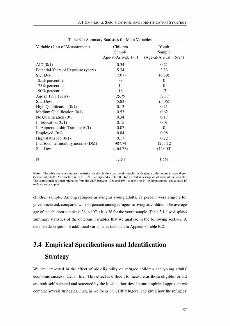
3.4 EMPIRICAL SPECIFICATIONS AND IDENTIFICATION STRATEGY
Table 3.1: Summary Statistics for Main Variables
Variable (Unit of Measurement) Children YouthSample Sample
(Age-at-Arrival: 1-14) (Age-at-Arrival: 15-24)
AID (0/1) 0.34 0.21Potential Years of Exposure (years) 5.34 3.23Std. Dev. (7.67) (6.39)
25% percentile 0 075% percentile 14 090% percentile 18 17
Age in 1971 (years) 25.79 37.77Std. Dev. (5.83) (5.06)High Qualification (0/1) 0.13 0.21Medium Qualification (0/1) 0.53 0.62No Qualification (0/1) 0.34 0.17In Education (0/1) 0.15 0.01In Apprenticeship Training (0/1) 0.07 0Employed (0/1) 0.84 0.98High status job (0/1) 0.17 0.22Ind. total net monthly income (DM) 987.74 1253.12Std. Dev. (464.75) (423.00)
N 1,151 1,551
Notes: The table contains summary statistics for the children and youth samples, with standard deviations in parentheses(where indicated). All variables refer to 1971. See Appendix Table B.2 for a detailed description of some of the variables.The sample includes men migrating from the GDR between 1946 and 1961 at ages 1 to 14 (children sample) and at ages 15to 24 (youth sample).
children sample. Among refugees arriving as young adults, 21 percent were eligible for
government aid, compared with 34 percent among refugees arriving as children. The average
age of the children sample is 26 in 1971; it is 38 for the youth sample. Table 3.1 also displays
summary statistics of the outcome variables that we analyze in the following section. A
detailed description of additional variables is included in Appendix Table B.2.
3.4 Empirical Specifications and Identification
Strategy
We are interested in the effect of aid-eligibility on refugee children and young adults’
economic success later in life. This effect is difficult to measure as those eligible for aid
are both self-selected and screened by the local authorities. In our empirical approach we
combine several strategies. First, as we focus on GDR refugees, and given how the refugees’
57

3 REFUGEE-SPECIFIC GOVERNMENT AID AND CHILD REFUGEES’ ECONOMIC SUCCESS LATER
IN LIFE
admission in West Germany was managed by the authorities, our analyses consider the
pool of aid applicants, and we control for the most important characteristics that the local
authorities used to select aid-eligible persons from the pool of applicants. In addition, we
take advantage of the fact that the refugee-targeted aid was only available after 1953.
We restrict our analyses to GDR refugees who all wanted to be legally acknowledged to
build their new life, that is, they reflect the applicant pool. The applicants were thoroughly
screened, in a specific refugee screening process that involved West German authorities and
those of the Allied countries.
All refugees were first hosted in refugee camps, rigorously interrogated by both West
German authorities and by the Allies (represented in general by members of the different
countries’ intelligence institutions). The whole screening process took several weeks, and all
refugees had to go through it. At the end, there was a committee with three members who
took all stages of the screening process into account when summarizing the escape motives
and making the decision about the legal status of the refugees. So, we are comparing two
groups of people who - by fleeing the GDR - have both strongly indicated that they want to
build a new life in West Germany permanently. That is, both groups had a strong incentive
to be legally acknowledged, independently from the additional refugee-targeted aid. While
the application for government aid was nominally voluntary, once refugees had gone through
the screening process, it was largely a minor formality.
The data analyzed here includes the most important characteristics that the authorities
used to screen refugee families, namely parental background characteristics, allowing us to
reduce the selection bias introduced by the screening process of the authorities.
Against this background, and considering that the refugee-targeted aid was only introduced
in 1953, our basic specification takes the following form:
Yi = α +β1AIDi +β2Ti +β3AIDi ∗Ti +β4Xbasici +β5X par
i + εi. (3.1)
Yi captures medium-term economic outcomes of refugees measured in 1971. Specifically,
Yi includes variables on education outcomes, employment outcomes and income. Because
age-at-arrival determines the integration of young refugees into the West German education
system, we separately analyze two different groups of GDR refugees: children (age-at-arrival:
1-14) and young adults (age-at-arrival: 15-24). See previous discussions.
The variable AIDi is a dummy variable indicating refugees’ eligibility for government aid
at any point after arrival, Ti is a dummy variable for having arrived in West Germany in 1953,
or later, and AIDi ∗Ti is an interaction term indicating GDR refugees who were eligible for
aid and arrived in 1953, or thereafter. This specification reflects the basic institutional details
58

3.4 EMPIRICAL SPECIFICATIONS AND IDENTIFICATION STRATEGY
of the government aid program that we analyze. The program was introduced in 1953, which
rationalizes the separation of those who arrived before 1953, and those who arrived thereafter.
At the same time, refugees who arrived before 1953 and who were acknowledged as legal
refugees were also eligible for aid, that is AIDi has values of one and zero for refugees
arriving between 1946 and 1961.
The coefficient β1 captures the average difference between those who were eligible for
government aid and those who were not, whereas coefficient β3 on the interaction term
AIDi ∗ Ti indicates whether this average effect is systematically different for those who
arrived after 1953.
Conceptually, we differentiate the effects of those who became aid eligible immediately
after arrival (Ti = 1), from those who arrived in the same “age-at-arrival” range but became
eligible later (i.e. when they were older, Ti = 0). For example, refugee children who were
younger than 15 at arrival in West Germany and arrived before 1953 were on average 11.8
years old in 1953, when the refugee-targeted aid was introduced. The counterpart of children
who were also younger than 15 at arrival, but arrived in 1953, or later, were 4.2 years old on
average when they became eligible for the refugee-specific aid (note that the average age
at arrival for children, who arrived below the age of 15, was 7.6 for both those who arrived
before 1953 and those who arrived thereafter).
Analogously, young adults who were between 15 and 24 at arrival and arrived before
1953 were on average 24.3 years old in 1953, when the refugee-targeted aid was introduced,
whereas those who arrived in 1953, or later, were on average 19.9 years old when they
became eligible (even though those who arrived before 1953 and those who arrived thereafter
were on average about 20 years old when they arrived).
In the basic specification, we address the age difference in two ways. First, Ti captures level
differences in the outcome variable between the early and late arrivals, including differences
in outcomes that arise because of differences in age when they became eligible. Ti also
picks up unobserved heterogeneity between the early and late arrivals if this unobserved
heterogeneity is time-invariant.
In addition, we take the age difference into account by controlling for the age of individuals
in 1971. Specifically, Xbasici includes age in 1971 and its square. It also includes the year of
migration which is important as it accounts for aggregate, year-specific differences between
1946 and 1961 that may affect the outcome variables in 1971 for all individuals in the same
way.
X pari in Specification (3.1) includes the refugees’ parental background characteristics, the
most important observable characteristics that the authorities used to screen the refugees, and
59

3 REFUGEE-SPECIFIC GOVERNMENT AID AND CHILD REFUGEES’ ECONOMIC SUCCESS LATER
IN LIFE
which allow us to reduce selection bias introduced by the screening process of the authorities.
As described earlier, in West Germany the authorities focused on background characteristics
of the adults in a family because those are the characteristics that the GDR regime used to
identify potential “class enemies.” So, both sides used the same “profiling” characteristics
to predict likely political refugees (who became eligible for government aid) as opposed to
likely economic refugee (who did not become eligible for government aid). The advantage
of our data is that we do observe parental background characteristics when the refugee
children and young adults were 15 years old, among them the father’s occupational status
(13 categories), father’s industry (16 categories), and father and mother’s qualification levels
(6 categories, respectively).20 Of course, those characteristics are important control variables
by themselves, given our research question.
Up to this point, we have treated AIDi as a dummy variable. But the institutional set up
of our experiment allows us to go one step further and use differences in treatment dose as
the identifying variation. The coefficient on the dummy variable specification represents
a weighted average of the per-unit causal effect along the length of the causal response
function. As we will show below, there is large variation in the number of potential years of
aid-eligibility, making a specification that exploits this variation more persuasive.
When constructing the treatment dose measure, we exploit the fact that GDR refugees
differed in terms of when they arrived, in combination with the fact that refugee-targeted
government support programs were only implemented for the GDR refugees in 1953.
We take explicitly into account that refugees’ year of arrival and therefore the potential
number of years of exposure to aid-eligibility varied within the “age-at-arrival” groups.
Specifically, we define a variable capturing potential years of exposure (EXPi) to government
aid as follows:
EXPi =
0 if AIDi = 0
1971− year_migrationi if AIDi = 1 and year_migrationi > 1953
1971−1953 if AIDi = 1 and year_migrationi ≤ 1953
(3.2)
That is, for those who are not eligible, EXPi is still zero. However, for those who arrived
after the introduction of the refugee-targeted government aid in 1953, the potential number
of years of eligibility is 1971 (the year of the survey and in which we measure our outcomes)
minus the year of arrival (year_migrationi) in West Germany (which is also equal to the
difference in age in 1971 and age at arrival). For those who arrived before 1953, aid-eligibility
20See Appendix Table B.2 for a detailed definition of the variables included in X pari .
60

3.4 EMPIRICAL SPECIFICATIONS AND IDENTIFICATION STRATEGY
Table 3.2: Summary Statistics for Unconditional Potential Years of Exposure (EXP), byArrival Sample and Time
(1) (2) (3) (4) (5) (6) (7)Mean Std. Dev. Median 75% 90% 95% N
Pctile Pctile Pctile
Children Sample, Age at Arrival: 1-14
Before 1953EXP 4.92 8.03 0 18 18 18 5421953 and laterEXP 5.72 7.32 0 13 17 18 609
Youth Sample, Age at Arrival: 15-24
Before 1953EXP 3.11 6.81 0 0 18 18 6771953 and laterEXP 3.33 6.04 0 0 14 16 874
Notes: The table contains unconditional summary statistics for the variable “Potential Years of Exposure” (EXP) by arrivaltime and arrival sample. The sample includes men migrating from the GDR between 1946 and 1961 at ages 1 to 14 (childrensample) and at ages 15 to 24 (youth sample).
only started after 1953 when they had already lived in West Germany for a couple of years
and were older compared to their age-at-arrival cohort that arrived in 1953, or later (see the
example above when we discuss the role of Ti). While aid-eligibility did not start for this
group immediately after arrival in West Germany, it potentially lasted for 18 years, from
1953 to 1971.
Overall, we find considerable variation in treatment dose. As Table 3.1 shows, in the
children sample, the average potential years of exposure is 5.3 (std. dev. 7.7); in the young
adult sample, it is 3.2 (std. dev. 6.4). Tables 3.2 and 3.3 show further details of this variable,
both unconditionally (Table 3.2) and conditionally on aid-eligibility (Table 3.3). As is clear
from those statistics, those who arrived earlier had more years of potential aid-eligibility but
it started when they were older. Table B.3 in the Appendix shows in detail how EXPi varies
by “age in 1971.”
Against this background, we estimate the following model:
Yi = a+θ1EXPi +θ2Ti +θ3EXPi ∗Ti +θ4Xbasici +θ5X par
i + εi. (3.3)
Our coefficients of main interest are θ1 and θ3, the average impact of an additional potential
year of aid-eligibility on the outcome variable (θ1) and the difference in the effect for those
aid-eligible who arrived in 1953, or later (θ3). All other variables in Specification (3.3)
61

3 REFUGEE-SPECIFIC GOVERNMENT AID AND CHILD REFUGEES’ ECONOMIC SUCCESS LATER
IN LIFE
Table 3.3: Summary Statistics for Potential Years of Exposure Conditional on Aid-Eligibility,by Arrival Sample and Time
(1) (2) (3) (4) (5) (6) (7) (8)Mean Std. Dev. 5% 25% Median 75% 95% N
Pctile Pctile Pctile Pctile
Children Sample, Age at Arrival: 1-14
Before 1953EXP 18 0 18 18 18 18 18 1481953 and laterEXP 14.5 2.9 10 11 15 17 18 240
Youth Sample, Age at Arrival: 15-24
Before 1953EXP 18 0 18 18 18 18 18 1171953 and laterEXP 13.8 2.6 10 11 14 16 18 211
Notes: The table contains summary statistics for the variable “Potential Years of Exposure” (EXP) by arrival time and arrivalsample, conditional on being aid-eligible. The sample includes men migrating from the GDR between 1946 and 1961 at ages1 to 14 (children sample) and at ages 15 to 24 (youth sample).
are defined as in Specification (3.1), and the interpretation of estimated coefficients is as
discussed before.
Given the variation in the data we use for effect identification in all specifications, it is
important to examine whether there are systematic differences between GDR refugees across
age-at-arrival and year of arrival. To do so, we show empirical evidence that suggests that
there is no systematic difference between the key observable characteristics of those who
arrived before 1953 - when neither the refugees nor people involved in the screening process
knew that the refugee-targeted government aid program would be introduced - and those
who arrived in 1953, or later.
First, we focus on age-at-arrival differences. It could for example be that the authorities
who screened the refugee families systematically treated families with kids in certain age
ranges differently, because, for example, the access to student allowances was important
at the time for the family. Table 3.4 shows mean age at arrival for both the children and
youth samples. Furthermore, we distinguish between “before 1953,” the time before the
refugee-specific aid was implemented and before invested parties knew about it, and 1953
onward. Had there been strategic sorting based on age at arrival, we would expect to observe
changes in age at arrival by refugee status and over time. This is clearly not the case. For
refugees of the children sample who received aid, the mean age at arrival before 1953 was
7.6 years (column 1(a)). It was virtually the same - 7.7 years - for those arriving in 1953
62

3.4 EMPIRICAL SPECIFICATIONS AND IDENTIFICATION STRATEGY
Table 3.4: Comparison of Age-at-Arrival and Father’s Education Differences for Refugeeswho Arrived before 1953 and Thereafter
(1) (2) (3) (4) (5) (6)Children sample Youth sample
(Age-at-Arrival: 1-14) (Age-at-Arrival: 15-24)Mean Mean Difference Mean Mean DifferenceAID NO AID (2)-(1) AID NO AID (5)-(4)
(a) Arrival before 1953
Age at arrival 7.6 7.7 0.1 19.8 20.1 0.3N 148 394 117 560Father’s educationHigh qualif. 0.07 0.09 0.02 0.02 0.05 0.03Med. qualif 0.66 0.72 0.06 0.60 0.60 0.00No qualif. 0.27 0.19 -0.08* 0.38 0.35 -0.03N 130 345 99 532
(b) Arrival in 1953 or later
Age at arrival 7.7 7.6 -0.1 19.9 19.9 0.0N 240 369 211 663Father’s educationHigh qualif. 0.08 0.05 -0.03 0.08 0.05 -0.03Med. qualif 0.73 0.73 0.00 0.65 0.69 0.03No qualif. 0.19 0.22 0.03 0.27 0.26 -0.01N 206 338 194 637
Notes: The table refers to men who migrated from East to West Germany between 1946 and 1961. Columns (1) and (4) reportmean characteristics for those who were eligible for aid. Columns (2) and (5) report the same statistic for those not eligible.Columns (3) and (6) report the differences in means. We conducted two-sided t-tests to evaluate the statistical significance ofthe difference, where one star * refers to significance at the 10 percent level. The absence of any stars (*) indicates that thedifferences are not statistically different at conventional levels.
and later (column 1(b)). Moreover, the age of arrival for those not receiving aid was not
statistically different (column 3 (a) and (b)). The same applies to refugees arriving as young
adults. Before 1953, the mean age at arrival for those receiving aid was 19.8 (column 4 (a)),
while it was 19.9 from 1953 onward (column 4 (b)). Again, the mean age at arrival for those
not receiving aid was not statistically different (column 6 (a) and (b)).
Similarly, we assess whether from 1953 onward there was strategic sorting into the
program based on fathers’ educational attainment. Moving through the table in the same
way as we did for “age at arrival,” there are no systematic differences. Only one difference
is statistically significant at the 10 percent level: Fathers of refugee children who were
aid-eligible and who arrived before 1953 were more likely to have no formal qualification
level, suggesting that, if anything, there was negative selection into aid-eligibility based on
63

3 REFUGEE-SPECIFIC GOVERNMENT AID AND CHILD REFUGEES’ ECONOMIC SUCCESS LATER
IN LIFE
Figure 3.4: Share of Aid-Eligible Refugees, by Year of Arrival in West Germany
0
.05
.1
.15
.2
.25
.3
.35
.4
.45
.5
.55
.6
.65
.7
.75
.8
.85
.9
.95
1
Sha
re
1946
1947
1948
1949
1950
1951
1952
1953
1954
1955
1956
1957
1958
1959
1960
1961
Year of arrival in West Germany
Sources: This figure shows the share of aid-eligible refugees who arrived in West Germany at ages 1-25, by year of arrival.
fathers’ educational attainment.
Figure 3.4 shows the share of GDR refugees who were eligible for aid by year of arrival in
West Germany. For arrival years before 1951, the yearly share was about 20 percent. It was
higher for the years adjacent to 1953, in line with the GDR policies at the time (e.g., there
was a wave of expropriations in agriculture), and mirroring the historical reasons for the
introduction of the refugee-targeted aid in 1953. It was about 20 percent in the mid-1950s
again, but increased for arrivals after 1957, reflecting again the changes in GDR policies
(such as worsening conditions in schools and universities as well as for certain professional
persons, see Ackermann, 1995).
We complement the previous analysis by examining the refugees’ parental background
characteristics in detail for each year of arrival in West Germany. We focus on the father’s
education, employment status, and industry; display the distributions of these variables for
(1) all GDR refugees, (2) only those acknowledged as political refugees, and also show (3)
the shares within each category who were acknowledged as political refugees (see Figures
B.1, B.2, and B.3 in the Appendix). Two conclusions can be drawn from this analysis. First,
there are fluctuations by year of arrival in West Germany.21 Second, and importantly for our
21To give an example, consistent with the wave of expropriations in agriculture, the share of all GDR refugeeswhose fathers were farmers increased around 1953 and a high share of refugees whose fathers were farmers wereacknowledged as political refugees around this year (see Figure B.2, Panels A to C). Similarly, and consistent
64

3.5 RESULTS
purposes, there are no patterns suggesting that the selectivity of persons acknowledged as
political refugees systematically changed for those arriving from 1953 onwards. This further
corroborates the variation we exploit for effect identification.
Finally, we should stress that our estimate on AIDi and EXPi captures the effect on the
outcomes of aid eligibility rather than aid receipt. That is, we are estimating an intention-to-
treat effect. We see this as the relevant policy measure since policymakers may decide upon
the offer of aid but not take-up. Moreover, the intention-to-treat effect is not confounded by
potentially endogenous take-up of aid.
3.5 Results
3.5.1 Education and Other Economic Outcomes in 1971
Youth Sample (Age-at-Arrival: 15-24)
Each row of Table 3.5 includes the results for the outcome variables listed in the first column.
Columns (1) to (3) show the results for β1, β2, and β3 from Specification (3.1) when only
the basic controls - age, its square, and year of migration to West Germany - are included in
the specification; columns (4) to (6) show the respective results when parental backgrounds
characteristics are additionally controlled for. The coefficient of interest is β3, presented
in columns (3) and (6), which captures the effect of aid eligibility for those who became
eligible immediately upon arrival in the destination country.
A broad comparison of results in columns (1) to (3) and columns (4) to (6) shows that the
inclusion of parental background characteristics does not change the main pattern in the data.
They appear to be important nevertheless, when it comes to the size and statistical significance
of the coefficients. We therefore focus on discussing the results shown in columns (4) to (6),
given we know that there is selection of aid eligibility on parental characteristics.
Those who arrived in 1953 and thereafter and were eligible for government aid are 16.9
percentage points more likely to have graduated from university. As 98 percent of those who
arrived as young adults worked in 1971 (see Table 3.1) eligibility for government aid had no
impact on the probability of being employed. However, it significantly increased the chances
of working in a good job: those eligible for aid are 18.3 percentage points more likely to
work in a high-status job in 1971, and they enjoy on average about 14 percent higher net
monthly income (results for the different outcome variables when moving down column 6).
with the worsening conditions in the education sector as well as for certain professional persons such as doctorsand lawyers, after 1957 high proportions of refugees were acknowledged as political refugees whose fathersworked in qualified services, culture and religion, or in the public sector (see Figure B.3, Panel C).
65

3 REFUGEE-SPECIFIC GOVERNMENT AID AND CHILD REFUGEES’ ECONOMIC SUCCESS LATER
IN LIFE
Table 3.5: The Impact of Refugee-Specific Government Aid on Educational Attainment andother Socio-Economic Outcomes, Men who arrived in West Germany aged 15 to25, Cross-Sectional OLS Regression Results (AID specification)
(1) (2) (3) (4) (5) (6)AID Arrival aft. Arrival aft. AID Arrival aft. Arrival aft.
1953 ‘53 * AID 1953 ‘53 * AID
Qualification variablesHigh Qualif. .055 -.195** .155*** -.012 -.142 .169***(0/1) (.046) (.095) (.059) (.040) (.089) (.052)
Med Qualif. -.102* .315*** -.078 -.047 .237** -.085(0/1) (.052) (.111) (.065) (.052) (.108) (.064)
Low Qualif. .049 -.113 -.075 .059 -.088 -.082(0/1) (.044) (.090) (.053) (.045) (.086) (.053)
Other Socio-Economic VariablesEmployed (0/1) -.008 -.033 .020 .001 -.048 .012
(.016) (.040) (.019) (.015) (.038) (.019)
High-status .070 -.170* .170*** .011 -.110 .183***Job (0/1) (.047) (.094) (.061) (.041) (.091) (.056)
Log Net Inc./ .047 -.106 .136*** .003 -.072 .139***Month (DM) (.032) (.075) (.043) (.027) (.069) (.038)
Basic Controls Yes Yes Yes Yes Yes YesParental Controls No No No Yes Yes YesN 1,551 1,551 1,551 1,551 1,551 1,551
Notes: Coefficients in columns (1) and (4) show the effect of being eligible for refugee-specific aid on the respective de-pendent variable. Coefficient in columns (2) and (5) show the effect of having migrated in 1953, or later. Coefficients incolumns (3) and (6) show the effect of being eligible for refugee-specific aid and having migrated in 1953, or later. Basiccontrol variables account for age and its square, gender, and year of migration. Parental background characteristics at age15 capture the father’s occupational status (13 categories), the father’s industry (16 categories), the father’s and the mother’squalification level (6 categories, respectively). Robust standard errors are clustered at the level of the sampling units; thereare several hundred clusters. ***, **, and * denote significance at the 1 percent, 5 percent, and 10 percent level, respectively.
So, overall, the refugee-specific government aid had a sizable positive impact on educational
outcomes (the average university graduation rate in the group is 21 percent, see Table 3.1)
and economic and social integration.
The level effects for AIDi (column 4) are all statistically insignificant, suggesting no
general systematic differences between the treatment group and control group once we have
controlled for parents’ characteristics. This is the effect for the group who arrived before
1953. If anything, potential selection effects should be larger for these early arrivals than for
66

3.5 RESULTS
Table 3.6: The Impact of Refugee-Specific Government Aid on Educational Attainment andother Socio-Economic Outcomes, Men who arrived in West Germany aged 15 to25, Cross-Sectional OLS Regression Results (EXP specification)
(1) (2) (3) (4) (5) (6)EXP Arrival aft. Arrival aft. EXP Arrival aft. Arrival aft.
1953 ‘53 * EXP 1953 ‘53 * EXP
Qualification variablesHigh Qualif. .003 -.168* .011*** -.001 -.122 .012***(0/1) (.003) (.094) (.004) (.002) (.088) (.003)
Med Qualif. -.006* .292*** -.007 -.003 .220** -.006(0/1) (.003) (.111) (.004) (.003) (.107) (.004)
Low Qualif. .003 -.116 -.005 .003 -.091 -.005(0/1) (.002) (.089) (.003) (.002) (.086) (.003)
Other Socio-Economic VariablesEmployed (0/1) -.000 -.031 .001 .000 -.046 .001
(.001) (.040) (.001) (.001) (.038) (.001)
High-status .004 -.142 .013*** .001 -.089 .013***job (0/1) (.003) (.093) (.004) (.002) (.089) (.003)
Log Net Inc./ .003 -.083 .010*** .000 -.056 .010***Month (DM) (.002) (.074) (.003) (.001) (.069) (.002)
Basic Controls Yes Yes Yes Yes Yes YesParental Controls No No No Yes Yes YesN 1,551 1,551 1,551 1,551 1,551 1,551
Notes: Coefficients in columns (1) and (4) show the effect of years of exposure (EXP) to governmental aid. Coefficient incolumns (2) and (5) show the level effect of having migrated in 1953, or later. Coefficients in columns (3) and (6) show theeffect of years of exposure to governmental aid for those who migrated in 1953, or later. Basic control variables accountfor age and its square, gender, and year of migration. Parental background characteristics at age 15 capture the father’soccupational status (13 categories), the father’s industry (16 categories), the father’s and the mother’s qualification level (6categories, respectively). Robust standard errors are clustered at the level of the sampling units; there are several hundredclusters. ***, **, and * denote significance at the 1 percent, 5 percent, and 10 percent level, respectively.
those who arrived in 1953 and thereafter, because the early arrivals had to apply retroactively
for AIDi, sometimes years after they underwent the screening process of the authorities,
whereas for the late arrivals the application for AIDi was a natural step at the end of the
screening process upon arrival.
We find that those who arrived in 1953 and thereafter are 23.7 percentage points more
likely to have a degree from the dual system of apprenticeship which is consistent with the
general educational upgrading at the time (column 5).
67

3 REFUGEE-SPECIFIC GOVERNMENT AID AND CHILD REFUGEES’ ECONOMIC SUCCESS LATER
IN LIFE
Table 3.6 shows the results when identification relies on variation in the treatment intensity,
that is, the potential years of exposure to aid-eligibility (EXPi) generated through the differ-
ences in age-at-arrival and year of arrival, in combination with the fact that the government
program only started in 1953. This allows us to ask whether the effects on the outcome
variables varies across treatment levels in the expected direction, and the answer is yes. For
those who arrive in 1953, and later, each additional year of potential aid-eligibility increases
the probability of graduating from university by 1.2 percentage points, the probability of
having a high-status job by 1.3 percentage points, and the net monthly income by about 1
percent.
To put these estimates into perspective, the difference between the 75th percentile and
25th percentile in the potential length of exposure distribution for young adults eligible
for aid and who arrived after 1953 is 5 years (see Table 3.3, last row), which translates
into a 6 percentage point difference in university graduation as a result of aid-eligibility
(.012∗5 = .06), a 6.5 percentage point difference in the probability of holding a high-status
job, and a 5 percent higher net monthly income.
Children Sample (Age-at-Arrival: 1-14)
Tables 3.7 and 3.8 show the results of the same specifications and the same outcome variables
as those in Table 3.5 and 3.6, but this time for the sample that includes refugees who arrived
at ages 1 to 14. At the time of arrival, they were all subject to compulsory schooling, that
is, they were naturally integrated in the host country educational institutions. As additional
outcome variables, we assess whether in 1971 an individual is enrolled in school or university
or participates in apprenticeship training. Basically, none of the coefficients of interest is
statistically significant, indicating the refugee-specific aid of this group of refugee kids did
not improve educational outcomes or labor market integration.
3.5.2 Robustness
We have dropped respondents who did not report their fathers’ occupational status. To assess
how this impacts our findings, we replicated our analysis and re-estimated equations (3.1)
and (3.3). This time we included all individuals and captured missing occupational status of
the fathers by incorporating an additional category in our regression analysis.
In addition, and because the share of AID-eligible refugees increased after 1957, we test
the robustness of our results to restricting the sample to the period 1946-1957, instead of
1946-1961 that we use in the main sample. The results for both exercises are similar to those
68

3.5 RESULTS
Table 3.7: The Impact of Refugee-Specific Government Aid on Educational Attainment andother Socio-Economic Outcomes, Men who arrived in West Germany aged 1 to14, Cross-Sectional OLS Regression Results (AID specification)
(1) (2) (3) (4) (5) (6)AID Arrival aft. Arrival aft. AID Arrival aft. Arrival aft.
1953 ‘53 * AID 1953 ‘53 * AID
Qualification variablesHigh Qualif. -.045 -.066 .025 -.045 -.017 -.008(0/1) (.046) (.065) (.050) (.043) (.065) (.049)
Med Qualif. .012 .073 -.001 .024 -.013 .032(0/1) (.053) (.098) (.065) (.051) (.099) (.064)
Low Qualif. .033 -.007 -.024 .021 .030 -.024(0/1) (.042) (.089) (.055) (.042) (.092) (.056)
In School/ .002 -.010 -.072* .016 .096 .016University (0/1) (.026) (.074) (.043) (.025) (.071) (.041)
In Apprenticeship .004 -.038 -.013 .004 -.046 -.004Training (0/1) (.010) (.065) (.028) (.012) (.067) (.027)
Other Socio-Economic VariablesEmployed (0/1) -.022 .024 -.045 -.037 -.071 .011
(.028) (.075) (.045) (.028) (.071) (.043)
High-status .004 -.166*** -.002 .003 -.116* -.033Job (0/1) (.045) (.063) (.050) (.044) (.066) (.049)
Log Net Inc./ -.009 -.137 -.052 -.009 -.128 -.074Month (DM) (.039) (.124) (.063) (.040) (.129) (.064)
Basic Controls Yes Yes Yes Yes Yes YesParental Controls No No No Yes Yes YesN 1,151 1,151 1,151 1,151 1,151 1,151
Notes: Coefficients in columns (1) and (4) show the effect of being eligible for refugee-specific aid on the respective de-pendent variable. Coefficient in columns (2) and (5) show the effect of having migrated in 1953, or later. Coefficients incolumns (3) and (6) show the effect of being eligible for refugee-specific aid and having migrated in 1953, or later. Basiccontrol variables account for age and its square, gender, and year of migration. Parental background characteristics at age15 capture the father’s occupational status (13 categories), the father’s industry (16 categories), the father’s and the mother’squalification level (6 categories, respectively). Robust standard errors are clustered at the level of the sampling units; thereare several hundred clusters. ***, **, and * denote significance at the 1 percent, 5 percent, and 10 percent level, respectively.
presented earlier.22
22Results are available from the authors.
69
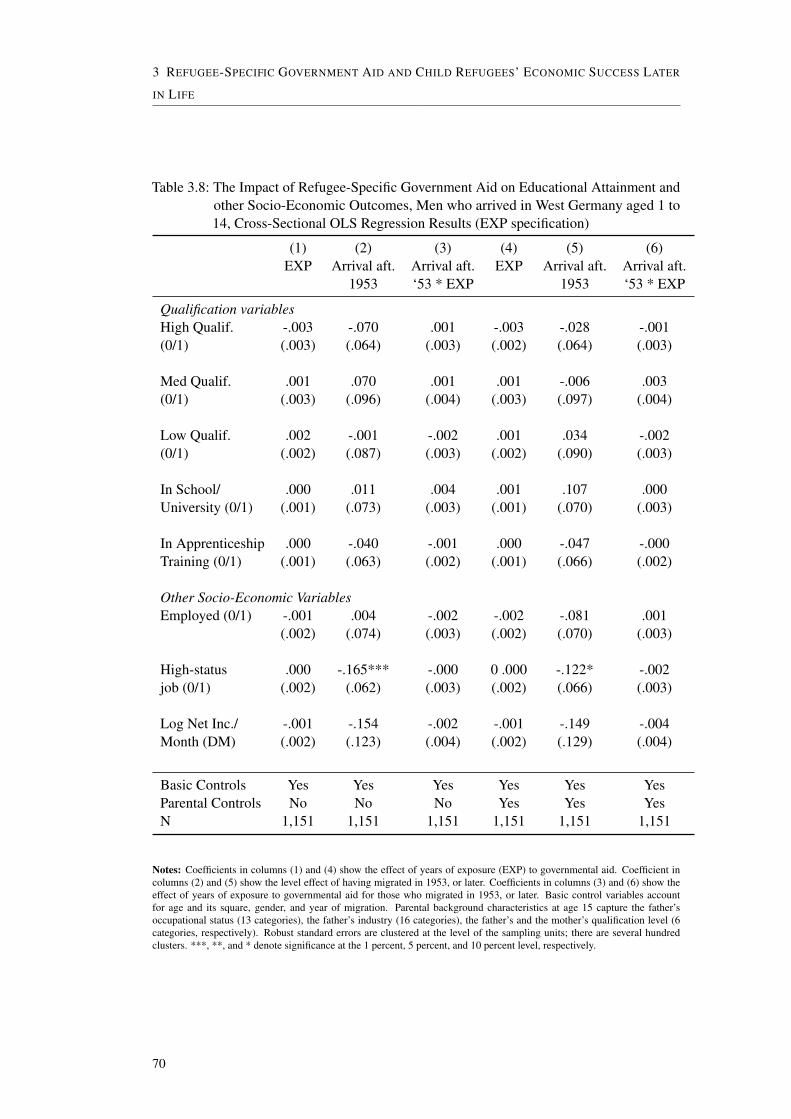
3 REFUGEE-SPECIFIC GOVERNMENT AID AND CHILD REFUGEES’ ECONOMIC SUCCESS LATER
IN LIFE
Table 3.8: The Impact of Refugee-Specific Government Aid on Educational Attainment andother Socio-Economic Outcomes, Men who arrived in West Germany aged 1 to14, Cross-Sectional OLS Regression Results (EXP specification)
(1) (2) (3) (4) (5) (6)EXP Arrival aft. Arrival aft. EXP Arrival aft. Arrival aft.
1953 ‘53 * EXP 1953 ‘53 * EXP
Qualification variablesHigh Qualif. -.003 -.070 .001 -.003 -.028 -.001(0/1) (.003) (.064) (.003) (.002) (.064) (.003)
Med Qualif. .001 .070 .001 .001 -.006 .003(0/1) (.003) (.096) (.004) (.003) (.097) (.004)
Low Qualif. .002 -.001 -.002 .001 .034 -.002(0/1) (.002) (.087) (.003) (.002) (.090) (.003)
In School/ .000 .011 .004 .001 .107 .000University (0/1) (.001) (.073) (.003) (.001) (.070) (.003)
In Apprenticeship .000 -.040 -.001 .000 -.047 -.000Training (0/1) (.001) (.063) (.002) (.001) (.066) (.002)
Other Socio-Economic VariablesEmployed (0/1) -.001 .004 -.002 -.002 -.081 .001
(.002) (.074) (.003) (.002) (.070) (.003)
High-status .000 -.165*** -.000 0 .000 -.122* -.002job (0/1) (.002) (.062) (.003) (.002) (.066) (.003)
Log Net Inc./ -.001 -.154 -.002 -.001 -.149 -.004Month (DM) (.002) (.123) (.004) (.002) (.129) (.004)
Basic Controls Yes Yes Yes Yes Yes YesParental Controls No No No Yes Yes YesN 1,151 1,151 1,151 1,151 1,151 1,151
Notes: Coefficients in columns (1) and (4) show the effect of years of exposure (EXP) to governmental aid. Coefficient incolumns (2) and (5) show the level effect of having migrated in 1953, or later. Coefficients in columns (3) and (6) show theeffect of years of exposure to governmental aid for those who migrated in 1953, or later. Basic control variables accountfor age and its square, gender, and year of migration. Parental background characteristics at age 15 capture the father’soccupational status (13 categories), the father’s industry (16 categories), the father’s and the mother’s qualification level (6categories, respectively). Robust standard errors are clustered at the level of the sampling units; there are several hundredclusters. ***, **, and * denote significance at the 1 percent, 5 percent, and 10 percent level, respectively.
70

3.6 CONCLUSIONS
3.5.3 Interpretation
The divergent results for the two samples are noteworthy. Why do we find positive and
economically significant effects for the youth sample but reach very different conclusions
for the children sample? Upon arrival in West Germany, refugees and their families had few
resources at hand. They were also liquidity constrained. That meant refugees arriving as
young adults had to consider whether to enter the labor force and immediately earn wages.
Our results indicate that refugee-specific aid made a decisive difference. It enabled young
adults to postpone their entry into the labor market and, instead, pursue higher education.
In the medium-term, this higher education was associated with working in a higher-status
job and having higher monthly incomes. These results deserve the attention of policymakers
who are addressing refugee issues.
For younger children arriving in West Germany, the economic incentives were quite
different. Not only were these refugees too young to start working immediately, but it
appears that time spent in the destination country allowed them to catch up with their
counterparts who received aid. Presumably, this catch up-process was smoothed by the
general expansion of higher education and the exceptional period of economic growth that
West Germany experienced. We would like to emphasize that we do not view our results as
evidence that aid for young children would be ineffective in general. After all, in the German
context that we analyze, all refugees and their children were covered by social security and
had access to tuition-free education (Section 3.2). However, the results demonstrate that
refugees migrating as children and young adults face different challenges which play an
important role in shaping medium-term outcomes.
3.6 Conclusions
This paper examines whether refugees’ economic success is linked to government aid. We
investigate the impact on refugees who migrated as children (at ages 1 to 14) and on refugees
who migrated as young adults (at ages 15 to 24) and assess medium-term outcomes (i.e., at
least 10 years after the refugee stream ceased). The analysis focuses on male GDR refugees
who migrated to West Germany from the end of World War II until the Berlin Wall was built
in 1961. We exploit the fact that West German authorities distinguished between political
and economic refugees from the GDR, providing aid only to political refugees. Receipt of
this refugee-specific aid, which was meant to compensate for the losses stemming from the
refugee experience, did not affect refugees’ ability to also receive standard welfare and social
security benefits in West Germany. The quasi-experimental nature of this historical setting
71

3 REFUGEE-SPECIFIC GOVERNMENT AID AND CHILD REFUGEES’ ECONOMIC SUCCESS LATER
IN LIFE
allows us to combine several approaches to address identification concerns.
Refugee-specific aid engendered positive and economically meaningful effects for refugees
migrating as young adults. For refugees who migrated as children, we find no similar positive
effects of the refugee-specific aid on education, employment outcomes, and incomes.
We conclude that age-at-arrival and the institutional link to the host country is important.
Refugees migrating as children can catch up with their counterparts who were aid-eligible.
This catch-up process, presumably, is related to their natural integration in the host countries
education institutions through compulsory schooling laws, the general expansion of higher
education and the exceptional period of economic growth that West Germany underwent
during the period we study. By contrast, refugees migrating as young adults were more
vulnerable to a lack of immediate refugee-specific aid. Faced with the trade-off between
entering the labor market and gaining income right away or investing in education, those
young adults who were not eligible for refugee-specific aid bypassed investments in education
- not surprisingly, given their and their families’ severe liquidity constraints. This finding
suggests that policymakers need to consider the specific needs of young refugees who are
above the compulsory schooling age.
72

4 A Proposed Data Set for Analyzing the
Labor Market Trajectories of East
Germans around Reunification
Joint with Dana Müller
This chapter has been published as Methodology Report No. 03/2018 of the Research
Data Centre of the German Federal Employment Agency (Liepmann and Müller, 2018),
available at: http://doku.iab.de/fdz/reporte/2018/MR_03-18_EN.pdf.1
4.1 Introduction
The fall of the Berlin Wall in 1989 and the reunification of Germany in 1990 fundamentally
and permanently changed the lives of around 16 Million East Germans (Huinink and Mayer,
eds., 1995). These unanticipated events overturned the political, economic, and social
systems of the former German Democratic Republic (GDR) at a rapid pace. For East
Germans, this resulted in new freedoms and opportunities. At the same time, East Germans
had to adapt to the new systemic order and were forced to cope with the economic crisis that
was caused by the introduction of the market economy (Akerlof et al., 1991; Burda and Hunt,
2001).
In the GDR, labor market trajectories were remarkably stable up until 1989. Full employ-
ment was guaranteed by the state and GDR citizens had the right, as well as the duty, to work
(Grünert, 1996; Ritter, 2007). After 1989, prolonged unemployment in East Germany meant
that drastic job changes (Diewald et al., 1995, p. 322 et seq.) and regional mobility (Hunt,
2006; Fuchs-Schündeln and Schündeln, 2009) became the norm, rather than the exception.
1We are grateful to Chris Bertold of the Federal Archive of Germany for supporting this project and formaking it possible. We thank Manfred Antoni for intense discussions, Florian Zimmermann for excellent researchassistance, and Niko de Silva and Matthias Umkehrer for valuable suggestions. Financial support by the GermanResearch Foundation (DFG) through the CRC/TRR 190, as well as the support of Bernd Fitzenberger andAlexandra Spitz-Oener, principal investigators of the project A07 of the CRC/TRR, is gratefully acknowledged.
73

4 A PROPOSED DATA SET FOR ANALYZING THE LABOR MARKET TRAJECTORIES OF EAST
GERMANS AROUND REUNIFICATION
Even today, differences between the former East and the former West remain an important
dimension of the persistent socio-economic disparities in Germany. Therefore, thorough
and transparent scientific investigations of the individual-level labor market consequences
of German reunification are still important today. This need for further research has, for
example, been documented in a recent study about perceptions concerning the privatization
of East German firms after 1989 (Goschler and Böick, 2017).
Administrative data, in particular those stemming from social security notifications and
internal procedures of the Federal Employment Agency, are invaluable for analyzing the
labor market trajectories of East Germans around reunification. These data are processed
at the Institute for Employment Research (IAB) into a biographical dataset, the so-called
“Integrated Employment Biographies” (IEB data), which has a panel structure and large
sample size. Moreover, these data provide highly reliable information on a number of
key variables, such as average daily wages as well as types and durations of labor market
episodes.
However, for East Germans data from social security records are only fully available from
1992 onwards. This is due to the fact that the East German labor market administration was
integrated into the West German administration, as part of a complex process. It took time
before all firms in East Germany started to report to the social security system (Schmid and
Oschmiansky, 2007). The resulting gap in the data poses a key empirical challenge. After
1989, significant fractions of East Germans lost their jobs, changed their occupations and
industries, or moved to West Germany. A large number of firms closed (e.g., Diewald et al.,
1995; Burda and Hunt, 2001; Hunt, 2006). For many research questions, 1992 is thus too
late in time as a starting point for analysis.
Our project “Labor Market Trajectories of East Germans around Reunification” partially
closes the gap in the data. For this purpose, we obtained the so-called “Data Fund of Societal
Work Power” (in German Datenspeicher Gesellschaftliches Arbeitsvermögen, which we
abbreviate by GAV data) from the Federal Archive of Germany. The GAV data are a cross-
section that provides information on labor market relevant characteristics of around 7 million
persons for the year of 1989. This amounts to 72 percent of the East German labor force
at that time. Based on names, exact dates of birth, and gender, we merged the 1989 data
with data from social security records that start in 1992. We thus created a unique and
very promising new data set that has two major advantages. First, it allows researchers to
study mechanisms behind phenomena of general relevance, such as unemployment, regional
mobility, occupational mobility, and mobility across industries. Second, it permits the
analysis of East German labor market trajectories around reunification based on a sample size
74

4.2 ORIGINAL DATA SOURCES
that is considerably larger than currently existing data sources. From a historical perspective,
the new data therefore enhance the analysis of German reunification. From a political
perspective, the new data help refine our knowledge of the causes and consequences of the
socio-economic disparities between East and West Germany. These disparities constitute a
major dimension of inequality that is still extremely relevant in Germany. Note, however, that
at this time, the linked data may only be used within the project “Labor Market Trajectories
of East Germans around Reunification.”
This report is structured as follows. In the next section, we present details on the two
original data sources that we merged. In Section 4.3, we describe the merging procedure and
evaluate its quality. Section 4.4 concludes and summarizes the next steps.
4.2 Original Data Sources
4.2.1 GAV Data
The so-called “Data Fund of Societal Work Power” constitutes our data source from GDR
times. Its German name is Datenspeicher Gesellschaftliches Arbeitsvermögen, which we
abbreviate by GAV data. “Societal Work Power” is derived from Marxist thought. The
authorities in the GDR wanted to refer to a society’s combined knowledge, abilities, and
skills that are relevant to economic production (Solomon, 1981).
The GAV data were collected in a decentralized way. At the firm and establishment level,
human resource departments were required to report information on the characteristics of all
employees and had to update these data on a monthly basis. From this source, the councils of
each of the fifteen districts of the GDR obtained and combined the information relevant for
the GAV data. The councils then transferred this information to the government agency for
labor and wages (Staatssekretariat für Arbeit und Löhne), which was ultimately responsible
for the collection of the GAV data (Gebauer et al., 2004). The quality of these data meets high
standards. In particular, the information reported by establishments was fact checked and
had to be revised when implausible (Rathje, 1996), though in a few instances this revision
did not take place and thus resulted in missing information (Dietz and Rudolph, 1990).
Neither the original GAV data nor analytical results based on these data were publicly
made available. Instead, government agencies in the GDR relied on the GAV data as part
of the process of central planning. For example, the data were used to identify and recruit
experts demanded in specific circumstances. However, the full potential of the data for
central planning purposes was never exploited (Gebauer et al., 2004).
75

4 A PROPOSED DATA SET FOR ANALYZING THE LABOR MARKET TRAJECTORIES OF EAST
GERMANS AROUND REUNIFICATION
Around 7 million persons are included in the GAV data. Specifically, the data cover the
following groups (Dietz and Rudolph, 1990; Rathje, 1996; Gebauer et al., 2004):
• Workers and employees with a permanent or temporary work contract
• Members of producers’ cooperative societies (Produktionsgenossenschaften) and law
firms (Rechtsanwaltskollegien)
• Retired persons still working
• Men performing compulsory military service or alternative civilian service
As is typically the case with GDR official statistics, the GAV data exclude the so-called
“Sector X,” which was an integral part of the GDR regime. For these employees, separate
databases existed. Specifically, the following groups are excluded from the GAV data (ibid):
• Persons working for the Ministry of the Interior, the Ministry of State Security, the
Socialist Unity Party, the army, or customs authorities (“Sector X”)
Separate databases also existed for specific subgroups, such as certain types of teachers
and child care workers. Therefore, some groups are only partially included in the GAV data
(ibid):
• The data exclude teachers in schools and child care workers; but include teachers at
vocational schools, professors at universities, and employees in nurseries.
• The data exclude the self-employed and their employees; though the majority of
craftsmen were members of producers’ cooperative societies and are therefore included
in the data.
• The data include apprentices; but only those who started apprenticeship training in the
year before December 1989.
• The data exclude foreigners temporarily working in the GDR under the coverage of
intergovernmental agreements; but include foreign GDR residents.
For the workers who are included in the GAV data, rich information was elicited. The
variables can be divided into four categories:
1. Demographic characteristics include age, gender, place of residence, the number of
children under 14 and the number of persons in need of care in the household, disability
status, marital status, and nationality.
76

4.2 ORIGINAL DATA SOURCES
2. Qualification characteristics include high school education, current apprenticeship
training, and university degree.
3. Employment characteristics include the type of employment, place of employment,
leave of absence, main job task, job status, work hours, and occupation.
4. Firm characteristics include firm type and industry.
In our project, we use a cross-section of the GAV data that refers to December 31 in
1989. The history of these data demonstrates that their survival was not self-evident: In fact,
the GAV data had been collected on an annual basis.2 However, due to limited computer
capacities in the GDR, only data from the current year were kept while data from previous
years were deleted (Gebauer et al., 2004). The Federal Archive of Germany obtained the
1989 GAV data in November of 1991 on magnetic tape. In 1998, the data were for the first
time saved on CD-ROM. In addition to the GAV data, detailed wage information had been
collected for 2.3 Million employees in the GDR. Unfortunately, because of data protection
regulations, these wage data were deleted in 1991 in reunified Germany (Rathje, 1999). The
data that we use in our project therefore do not contain any information on pre-unification
wages.
The vast majority of historians and other scientists conducting research in the Federal
Archive of Germany do not employ quantitative methods (Rathje and Wettengel, 1999).
Therefore, up until today, few researchers have analyzed the GAV data. The studies that
we are aware of include Solomon (1981) and Groebel (1997). Solomon (1981) provides
a technical report concerning the processing and analysis of the GAV data. This report
reflects the information technology available in the GDR in the early 1980s.3 Groebel (1997)
explores reasons for the divergence of sectoral employment structures in market economies
and planned economies. Among other data sources Groebel (1997) relies on the GAV data to
provide descriptive statistics that illustrate her theoretical arguments. Additionally, from 2001
through 2012, a subproject of the Collaborative Research Center 580 studied GDR elites and
used the GAV data, though only as a supplementary source of information (Gebauer et al.,
2004; Salheiser, 2006).
2The GAV data project was initiated in 1975, though it took until 1986 before the data were made fullyavailable to the government agencies interested in them (Gebauer et al., 2004).
3Solomon (1981) constitutes a dissertation written at Humboldt-University Berlin (East). During GDR times,this dissertation was classified as confidential. After reunification, a copy was retrieved by the Federal Archiveof Germany such that the dissertation can now be accessed by the public.
77
4 A PROPOSED DATA SET FOR ANALYZING THE LABOR MARKET TRAJECTORIES OF EAST
GERMANS AROUND REUNIFICATION
4.2.2 IEB Data
We merged the GAV data with data from the so-called “Integrated Employment Biographies”
(IEB data). The IEB data are a natural choice for our project, because they contain labor
market relevant information that resembles the GAV data. The IEB data include informa-
tion from two sources: social security notifications and internal processes of the Federal
Employment Agency. We discuss each of these sources in turn.
First, social security notifications involve an integrated notification procedure for the
health, pension, and unemployment insurance programs, which is known by the abbreviation
DEÜV (for more details see Wermter and Cramer (1988) and Bender et al. (1996, p. 4 et
seq.)). It has been mandatory since 1973 in West Germany and since 1991 in East Germany.
The notifications include several pieces of information on all insurable employment episodes
reported by every employer. Section 28 of the Social Code Act IV determines what kind of
information needs to be notified. In general, a notification includes information about the
beginning and end of each employment episode that is subject to social security contributions,
as well as corresponding information about gross wages, education, employment status,
occupation and nationality. In addition, there is a mandatory notification for every employer
liable to social security contributions at least once a year. Since 1999 employment episodes
of marginal part-time employees and family workers have also been recorded. Importantly,
the social security notifications do not include civil servants, self-employed individuals and
regular students.
The following will give a more detailed idea of the notification procedure. The data are
recorded by the health insurance companies first, and then are transmitted to the German
pension insurance, which in turn forwards the data to the Federal Employment Agency.
The data are collected and processed by the Federal Employment Agency, particularly for
generating employment statistics. Subsequently the data are processed into employment
histories at the Data and IT-Management Department of the IAB. These employment histories
constitute the so-called Employee History File, which starts in 1975 for West Germany and
includes East Germans from 1992 onwards.
Second, internal processes of the Federal Employment Agency are the other source of the
IEB data. These data are collected to fulfill legal requirements, to inform the public and in
the preparation of statistics. The data are then prepared at the IAB and organized in four
different history files:
1. The Benefit Recipients History includes all periods during which unemployed indi-
viduals received earnings replacement benefits from the Federal Employment Agency
within the scope of Social Code Book III (SGB III). The data start in 1975.
78

4.2 ORIGINAL DATA SOURCES
2. The Unemployment Benefit II Recipient History covers all periods during which unem-
ployed individuals received benefits in accordance with the Social Code Book II (SGB
II). It was implemented in 2005 and captures the pooling of unemployment benefits
and social assistance. The difference compared with SGB III is that unemployment
benefits are not determined individually but depend on the so-called “benefit commu-
nity” (which includes certain household members, such as spouses and children). This
data source only contains information about individuals who are capable of working
or are under the age of 64, and about the benefit community’s members in accordance
with Section 7 of SGB II. However, the Federal Employment Agency is not the only
responsible authority for administering the benefits that fall under Social Code Book
II. There are three possible types of institutions the data can stem from:
• Joint facilities of employment agencies and municipalities since 2011 (before
2011 cooperation of employment agencies and municipalities in the context of
so-called working partnerships);
• separated responsibilities until 2011 with divided tasks between the Federal
Employment Agency and the municipality; and,
• authorized municipalities which are responsible for all tasks regarding the SGB
II.
The data originate from different reporting procedures. In particular, authorized
municipalities can use their own IT procedures and transmit the data to the Federal
Employment Agency. The data have been collected since 2005 but the data are
complete only from 2007 onwards.
3. The Participation-in-Measure History Files include active labor market policy measures
within the scope of SGB III and in accordance with SGB II if these measures are
reported in Federal Employment Agency IT procedures. The data are available from
2000 onwards.
4. The Jobseeker History contains information on jobseekers who are registered with
employment agencies. The data are available from 2000 onwards and were expanded
in 2005 to also include jobseekers receiving Unemployment Benefit II.
Finally, the data from the social security notifications (i.e., the Employment History File)
and the data from the internal processes of the Federal Employment Agency (i.e., the four
other history files just described) are combined. Together, these data sources represent the
Integrated Employment Biographies (IEB data).
79

4 A PROPOSED DATA SET FOR ANALYZING THE LABOR MARKET TRAJECTORIES OF EAST
GERMANS AROUND REUNIFICATION
Note that the IEB data could not directly be used for the linkage procedure with the GAV
data, because the IEB data lack direct identifiers like names for reasons of data privacy. As
we explain in more detail in the next section, we instead used information from the data ware
house of the Statistics Department of the Federal Employment Agency. This information
includes all individuals from the IEB data as well as their direct identifiers. Variables from
the IEB data will then later be merged to the linked new data set.
4.3 Newly Created Data Source
4.3.1 Procedure for the Merge of the GAV Data and the IEB
Data
For the purposes of merging the GAV data and the IEB data, the Federal Archive of Germany
provided us with the non-anonymized version of the 1989 GAV data. We received fifteen
Excel documents, each referring to one of the districts in the GDR, which we transformed
into a single file in Stata format. Based on the non-anonymized version of the GAV data, we
were able to exploit the following information for the merge: first name, last name, exact
date of birth, and gender. In principle, it would have been possible to rely on additional
information pertaining to occupations, industries, and regions. However, the IEB data are
fully available for East Germans only from 1992 onwards. Between 1989 and 1992, a
significant fraction of East Germans changed jobs and moved between regions. Hence, using
this additional information would have led to oversampling of persons who did not move
across regions or did not change jobs. In order to avoid such biases, we deliberately decided
not to use the additional information for the merge and relied on names, date of birth, and
gender only.
From the data warehouse of the Statistics Department of the Federal Employment Agency
we similarly obtained information on names, date of birth, and gender for persons covered
by the IEB data. In addition, we obtained their anonymized personal IDs that will later allow
us to merge further IEB variables. Our aim was to identify workers from the GDR and to
reduce the complexity of the data. Therefore, when drawing from the universe of individuals
included in the IEB data we imposed three restrictions. First, we focused on persons born
between 1929 and 1976 who were aged 13 to 70 in 1989. Second, we only included persons
for whom at least one episode is recorded in the IEB data between 1990 and 1996 in East or
West Germany. Third, we imposed that for these persons no such episodes were recorded in
West Germany before 1990. Because of the third criterion, a large number of West Germans
80

4.3 NEWLY CREATED DATA SOURCE
are excluded from the merging procedure. This reduces the likelihood of false matches.
At the same time, it implies that we neglect individuals who migrated from West to East
Germany before the wall fell. However, only few West Germans moved to the GDR during
this period (see for example the graph in Hunt, 2006, p. 1017). Note that, for the individuals
who we match, selected variables on their entire history from the IEB records will ultimately
be included in the data set.
We conducted the merge in collaboration with Manfred Antoni who describes the technical
details of the procedure in Antoni (2018). We began by preprocessing the GAV data.
Duplicates in the GAV data were one issue we needed to address (see Table 4.1). On the
one hand, this concerns pure duplicates, where all variables are identical to an original
observation. We dealt with these cases by dropping all 166,604 pure duplicates. On the
other hand, there are cases of data entries that contain information on multiple jobs held by
the same individual. Specifically, there are 194,916 data entries which refer to individuals’
second or higher order observations (Table 4.1). We do not know with certainty whether these
are observations referring to individuals performing several jobs in parallel or observations
referring to individuals’ previous jobs. The latter case would refer to situations in which
the data were not updated after job changes. We were, however, able to code a variable
ordering multiple data entries per person by the date the data were collected. One possibility
is therefore to restrict the analysis to each individual’s most recent job spell, which we did
when merging.4 This left us with a sample size of more than 7 million persons included in
the GAV data (Table 4.1).
We next preprocessed the information on names. In the original GAV data, information
on names is presented in the format of “last_name, first_name”. While this is true for the
majority of names, we had to account for the fact that some names deviated from the intended
format. To ensure comparability across data sources, identical preprocessing steps were
applied to both the GAV data and the IEB data. In particular, the following steps were
necessary:
• Special characters, which appeared in various formats and at varying places in the name
variable, were deleted or replaced by a comma to separate first and last names (for
example when the name was in the format of “„last_name, first_name” or “last_name.
first_name” etc.).
• Name suffixes, which appeared in various formats and at varying places in the name
4When we performed the merge, we also encountered the issue of duplicates in the IEB data. These are caseswhere we found matches based on exact names and date of birth but where we could not identify a unique IEBperson ID. However, this concerns few cases (<1%) which we treat as unsuccessful matches.
81
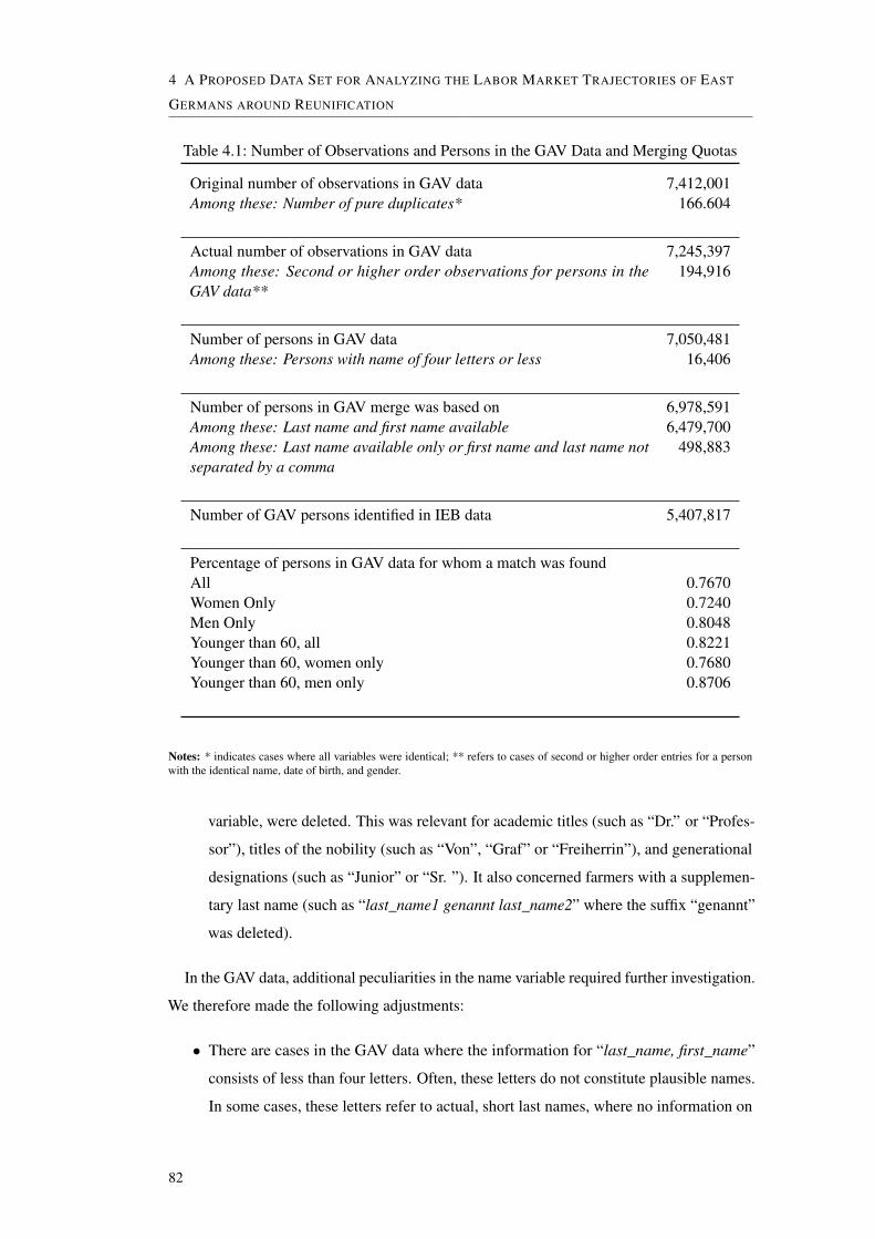
4 A PROPOSED DATA SET FOR ANALYZING THE LABOR MARKET TRAJECTORIES OF EAST
GERMANS AROUND REUNIFICATION
Table 4.1: Number of Observations and Persons in the GAV Data and Merging Quotas
Original number of observations in GAV data 7,412,001Among these: Number of pure duplicates* 166.604
Actual number of observations in GAV data 7,245,397Among these: Second or higher order observations for persons in theGAV data**
194,916
Number of persons in GAV data 7,050,481Among these: Persons with name of four letters or less 16,406
Number of persons in GAV merge was based on 6,978,591Among these: Last name and first name available 6,479,700Among these: Last name available only or first name and last name notseparated by a comma
498,883
Number of GAV persons identified in IEB data 5,407,817
Percentage of persons in GAV data for whom a match was foundAll 0.7670Women Only 0.7240Men Only 0.8048Younger than 60, all 0.8221Younger than 60, women only 0.7680Younger than 60, men only 0.8706
Notes: * indicates cases where all variables were identical; ** refers to cases of second or higher order entries for a personwith the identical name, date of birth, and gender.
variable, were deleted. This was relevant for academic titles (such as “Dr.” or “Profes-
sor”), titles of the nobility (such as “Von”, “Graf” or “Freiherrin”), and generational
designations (such as “Junior” or “Sr. ”). It also concerned farmers with a supplemen-
tary last name (such as “last_name1 genannt last_name2” where the suffix “genannt”
was deleted).
In the GAV data, additional peculiarities in the name variable required further investigation.
We therefore made the following adjustments:
• There are cases in the GAV data where the information for “last_name, first_name”
consists of less than four letters. Often, these letters do not constitute plausible names.
In some cases, these letters refer to actual, short last names, where no information on
82
4.3 NEWLY CREATED DATA SOURCE
the first name is provided. According to experience from previous data record linkages
performed at the Research Data Center of the Federal Employment Agency, it is highly
unlikely to find matches in the IEB data based on name information of four letters or
less. Therefore, we decided to exclude these cases from the merge. This concerned
around 16,000 persons (see Table 4.1).
• In the GAV data, for around 500,000 persons, the information “last_name, first_name”
consists of one word only. In the majority of cases, one-word-names refer to last
names. We therefore interpreted these names as last names and used this information
for the merge. Additionally, there are one-word-names including a last name and a
first name which lack a separating comma. In order to distinguish between first and
last names, we used a routine that identified and separated common first names. We
then fact checked these results manually, since additional corrections were required
that could not be automated (for example when a common first name was in fact part
of a last name as in “Franke” , “Schubert” or in more exotic semantic combinations).
After preprocessing, we based the merge on 6.98 million persons included in the GAV
data. For 93 percent of these, we used information of first and last names, whereas for the
remaining 7 percent either the last name was available only or first and last names were
not separated (Table 4.1). To put these figures into perspective, the GDR labor force of
1989 consisted of 9.75 million persons (Federal Statistical Office, 1994). Thus, our merge
encompasses 72 percent of the East German labor force.
4.3.2 Evaluation of the Merging Procedure
For 77 percent of persons from the GAV data we found a match in the IEB data (Table 4.1).
According to experience from previous merges performed at the Research Data Center of
the Federal Employment Agency, this is a good quota. For the vast majority of matches (88
percent), the information on first and last names, date of birth, and gender was identical in
both the GAV and the IEB data (data not shown). The remaining fraction was matched using
record linkage techniques that tolerate a justifiable degree of error while at the same time
keeping the likelihood of false matches as small as possible. Three steps were particularly
relevant in increasing the merge quota. First, we tolerated small spelling or coding mistakes
in the name information and in the day of birth, but imposed that the other identifiers (gender,
month and year of birth) were matched accurately. Second, we required a perfect match
between last names, birth date, and gender but dropped first names. This step was especially
important; as a significant fraction of persons in the GAV data lack a first name (see Table
83

4 A PROPOSED DATA SET FOR ANALYZING THE LABOR MARKET TRAJECTORIES OF EAST
GERMANS AROUND REUNIFICATION
4.1). Third, we repeated the previous step but relied on first names while neglecting last
names. We only kept cases where a unique match was found. Manfred Antoni performed
these steps and provides more details on the exact implementation in Antoni (2018).
We next use OLS-regression analysis to investigate how the success of the merge correlates
with key observable characteristics in 1989. Specifically, we regress a dummy variable that is
equal to one in case of a successful merge on key observable characteristics. Key observable
characteristics are measured as categorical variables and refer to gender, age intervals, type of
school diploma obtained, and marital status. The regression results are displayed in Table 4.2.
For reference, we display corresponding summary statistics for the independent variables in
Table 4.3.
Based on column (1) in Table 4.2, three phenomena should be emphasized. First, the
merge quota is considerably lower for individuals older than 60 in 1989. Indeed, we were
not able to find any matches above the age threshold of 61 (data not shown). This is due to
the fact that for the IEB data the information on names stems from the late 1990s. By this
time, older East Germans had dropped out of employment. Most analyses based on the new
data set should therefore be limited to persons younger than 60. If these are dropped, the
quota of successful merges increases to 82 percent (see Table 4.1). Below the age threshold
of 50 in 1989, the same quota increases further to 86 percent (data not shown). In our view,
these are high merge quotas that speak for the quality of the new data set. At the same time,
these quotas highlight that the data are more reliable for persons younger than 60 or even 50
in 1989.
Second and reassuringly, there are only negligible differences by qualification level in
the success of the merge. This can be seen in column (1) of Table 4.2, where we measure
qualification in terms of four different levels of school diploma obtained. We used these
categories because the usual distinction between an apprenticeship degree and no formal
vocational qualification cannot be made in the GAV data. The only noteworthy difference by
qualification level is the significantly lower merge quota for persons with missing information
about the school diploma obtained. However, this concerns very few cases (< 0.5 percent,
see Table 4.3).
Third, the merge quota is considerably lower for women than for men. For women younger
than 60 in 1989, this quota amounts to 77 percent, which is around 10 percentage points
lower than the merge quota of their male counterparts (see Table 4.1). We investigate this
further in columns (2) and (3) of Table 4.2, where we perform regression analysis as before
but this time split the sample by gender. Furthermore, we exclude persons older than 59.
We show that the likelihood of finding a match among women is lowest for initially single
84
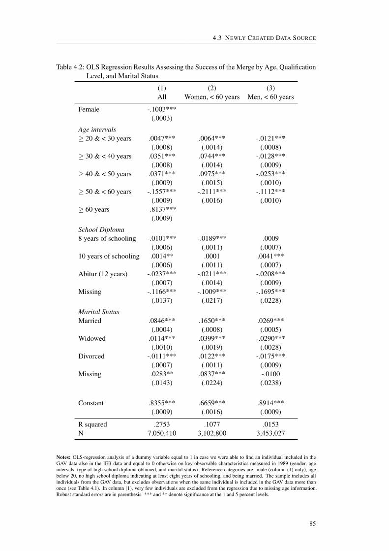
4.3 NEWLY CREATED DATA SOURCE
Table 4.2: OLS Regression Results Assessing the Success of the Merge by Age, QualificationLevel, and Marital Status
(1) (2) (3)All Women, < 60 years Men, < 60 years
Female -.1003***(.0003)
Age intervals≥ 20 & < 30 years .0047*** .0064*** -.0121***
(.0008) (.0014) (.0008)≥ 30 & < 40 years .0351*** .0744*** -.0128***
(.0008) (.0014) (.0009)≥ 40 & < 50 years .0371*** .0975*** -.0253***
(.0009) (.0015) (.0010)≥ 50 & < 60 years -.1557*** -.2111*** -.1112***
(.0009) (.0016) (.0010)≥ 60 years -.8137***
(.0009)
School Diploma8 years of schooling -.0101*** -.0189*** .0009
(.0006) (.0011) (.0007)10 years of schooling .0014** .0001 .0041***
(.0006) (.0011) (.0007)Abitur (12 years) -.0237*** -.0211*** -.0208***
(.0007) (.0014) (.0009)Missing -.1166*** -.1009*** -.1695***
(.0137) (.0217) (.0228)
Marital StatusMarried .0846*** .1650*** .0269***
(.0004) (.0008) (.0005)Widowed .0114*** .0399*** -.0290***
(.0010) (.0019) (.0028)Divorced -.0111*** .0122*** -.0175***
(.0007) (.0011) (.0009)Missing .0283** .0837*** -.0100
(.0143) (.0224) (.0238)
Constant .8355*** .6659*** .8914***(.0009) (.0016) (.0009)
R squared .2753 .1077 .0153N 7,050,410 3,102,800 3,453,027
Notes: OLS-regression analysis of a dummy variable equal to 1 in case we were able to find an individual included in theGAV data also in the IEB data and equal to 0 otherwise on key observable characteristics measured in 1989 (gender, ageintervals, type of high school diploma obtained, and marital status). Reference categories are: male (column (1) only), agebelow 20, no high school diploma indicating at least eight years of schooling, and being married. The sample includes allindividuals from the GAV data, but excludes observations when the same individual is included in the GAV data more thanonce (see Table 4.1). In column (1), very few individuals are excluded from the regression due to missing age information.Robust standard errors are in parenthesis. *** and ** denote significance at the 1 and 5 percent levels.
85

4 A PROPOSED DATA SET FOR ANALYZING THE LABOR MARKET TRAJECTORIES OF EAST
GERMANS AROUND REUNIFICATION
Table 4.3: Summary Statistics (in Percent)
(1) (2) (3)All Women, Men,
< 60 years < 60 years
Female 46.73
Age intervals< 20 years 4.58 4.81 5.02≥ 20 & < 30 years 23.29 25.95 24.24≥ 30 & < 40 years 24.77 26.32 26.92≥ 40 & < 50 years 19.67 21.04 21.25≥ 50 & < 60 years 20.68 21.88 22.57≥ 60 years 7.01Missing (excluded from regressions) 0.00
School Diploma< 8 years of schooling 6.84 4.92 9.108 years of schooling 40.74 37.22 37.5510 years of schooling 44.38 50.28 44.26Abitur (12 years) 7.84 7.31 8.94Missing 0.20 0.26 0.16
Marital StatusSingle 22.34 19.50 27.46Married 67.18 68.46 64.92Widowed 2.35 2.46 0.64Divorced 7.95 9.33 6.83Missing 0.19 0.25 0.14
N 7,050,481 3,102,800 3,453,027
Notes: Summary statistics for independent variables used in the repression analysis presented in Table 4.2. All variables referto 1989.
women. In particular, the merge quota is considerably higher for those who are married
in 1989 compared with those who are single initially.5 This indicates that the lower merge
quota among women can be rationalized by the fact that initially single women changed
their names after marriage and are then more difficult to identify in the IEB data.6 Our
5With 68 and 20 percent, respectively, initially married and initially single women are the largest group; 9percent of women are divorced, and 2 percent are widowed (Table 4.3, column (2)).
6 In general, when East German women married for the first time, they usually adopted the husband’s familyname, but kept this name after a divorce. Thus, for our merge we are particularly concerned about women’stransitions from initially being single to being married, while we are less concerned about transitions from initialmarriages into divorce. Our reasoning is based on anecdotal evidence from discussions with former employeesof the former population registration office in Karl-Marx-Stadt (now Chemnitz). We are not aware of systematic
86
4.4 CONCLUSIONS AND NEXT STEPS
recommendation is therefore that future analyses should include robustness tests concerning
women’s initial marital status. It might for example be appropriate to add marital status as a
control variable or to investigate whether main effects differ by marital status category.
4.4 Conclusions and Next Steps
This report summarizes our linkage of the GDR’s “Data Fund of Societal Work Power” from
1989 with the Integrated Employment Biographies from later years. The merge was based
on around 7 million East German workers, which amounts to 72 percent of the East German
labor force at that time. We were able to obtain a comparatively high merge quota of 82
percent among persons younger than 60 in 1989. However, the merge was somewhat less
successful for older workers, who dropped out of the labor force, and for initially single
women, who often changed their names after marriage.
Before the linked data can be used in the project “Labor Market Trajectories of East
Germans around Reunification,” different processing steps are still necessary. First of all, the
direct identifiers such as names have to be deleted and will be replaced by a pseudo-identifier.
Variables from the IEB, which are normally contained in the linked standard data products of
the Research Data Center (FDZ), such as PASS-ADIAB (see Antoni and Bethmann, 2018),
will be added to the new data set. In addition, we need to develop crosswalks in order
to harmonize variables that are similar in the GAV and IEB data, such as the occupation,
industry, and region variables. Finally, a sample needs to be conceptualized and drawn from
the linked data.
The linked data will allow the analysis of research questions about East German em-
ployment biographies around reunification based on sample sizes that are much larger than
those of currently existing data sources with panel structure. However, our legally binding
agreement with the Federal Archive of Germany requires that the data will have to be deleted
after the end of our project. Therefore, the Research Data Center (FDZ) of the Federal Em-
ployment Agency will develop a concept in order to convince the Federal Archive to make
the linked data available to the research community via the FDZ. We believe that the new
data have considerable potential to answer research questions of general scientific interest,
as well as to enhance the understanding of differences between East and West Germany,
which still constitute a major dimension of the persistent socio-economic disparities in this
country.
studies that analyze norms concerning female names for East Germany.
87


A Appendix to Chapter 2: The Impact of a
Negative Labor Demand Shock on
Fertility
A.1 Employment by Sector and More Detailed
Industries, Additional Figures
89

A APPENDIX TO CHAPTER 2: THE IMPACT OF A NEGATIVE LABOR DEMAND SHOCK ON
FERTILITY
Figure A.1: Employment in West Germany (in Thousands), By Economic Sector, 1970-2007(Selected Years)
0
2500
5000
7500
10000
12500
15000
Em
ploy
men
t (in
100
0s)
1970 1975 1980 1985 1990 1995 2000 2005
Manufacturing Services, loc/reg authorities, non-prof. org.
Agric., forestry, fishing Retail
Construction Transport, information transm.
Mining, energy + water supp. Finance, insurance
Source: 1970, 1975, 1980: Provided by Federal Statistical Office and based on the (West German) Microcensus. 1985 andlater: Author’s calculations based on the Scientific Use Files of the Microcensus (a 0.7 percent sample of the population) forpersons aged 15 and older living in West Germany at their main residence; weighted by Microcensus weights. The increaseand decline in manufacturing employment between 1989 and 1995 can be explained by new investment opportunities in EastGermany, followed by the impact of a now more competitive environment in which firms could move production to centraland eastern European countries (see, e.g., Dustmann et al., 2014, p. 182).
90

A.1 EMPLOYMENT BY SECTOR AND MORE DETAILED INDUSTRIES, ADDITIONAL FIGURES
Figure A.2: Correlation between the Relative West German Employment Change 1989 to1993 (in Percent) and Relative Excess Supply in 1989, By Industry
Coeff. = -2.23Robust s.e. = 0.89T-stat = -2.49
-150
-100
-50
0
50
100
150
200
250
300
350
400E
mpl
. Cha
nge
1989
-93,
Wes
t Ger
man
y (in
Per
cent
)
-8 -7 -6 -5 -4 -3 -2 -1 0 1RES = (Share East 1989 - Share West 1989) / Share East 1989
Source: West German analogue for Figure 2.4, panel (A). N = 48, the regression model is weighted using 1989 WestGerman employment shares of industries as analytical weights. The y-axis displays change in percent, i.e., 100 ∗Empl_West j,93−Empl_West j,89
Empl_West j,89.
Figure A.3: Female versus Male Unemployment and Non-Employment Rates in East Ger-many 1993 and Relative Excess Supply in 1989, by Industry
Coeff. = -.1611Robust s.e. = .1699T-stat = -.95
0
1
2
3
4
5
6
Sha
re u
nem
pl. f
emal
e 93
/ S
hare
une
mpl
. mal
e 93
-8 -6 -4 -2 0 2RES = (Share East 1989 - Share West 1989)/Share East 1989
A. Female versus Male Unemployment Rates in1993
Coeff. = -.0400Robust s.e. = .0060T-stat = -.61
1
2
3
4
5
6
Sha
re n
on-e
mpl
. fem
ale
93 /
Sha
re n
on-e
mpl
. mal
e 93
-8 -6 -4 -2 0 2RES = (Share East 1989 - Share West 1989)/Share East 1989
B. Female versus Male Non-employment Rates in1993
Source: The analysis is based on the Scientific Use File of German Microcensus of 1993 and on persons aged 15 to 54 livingin East Germany at their main residence. On the y-axes, I display female unemployment (non-employment) rates divided bymale unemployment (non-employment) rates by industry. These ratios are regressed on the RES measure. The regressionmodel is weighted using the 1993 shares of the industries as weights.
91

A APPENDIX TO CHAPTER 2: THE IMPACT OF A NEGATIVE LABOR DEMAND SHOCK ON
FERTILITY
A.2 Initially Unemployed Women
Figure A.5: Annual Number of Births per 1,000 East German Women, By EmploymentStatus at the Beginning of 1991
0
50
100
150
200
Ann
ual B
irths
, per
1,0
00 W
omen
1975 1980 1985 1990 1995 2000 2005 2010
Employed, all Employed, ind. knownUnemployed
Notes: Group definitions and sample sizes are: (1) 9,017 women were employed on January 1st, 1991 (“employed, all”).(2) Of those employed on January 1st, 1991, 4,234 women had non-missing industry information (“employed, industryknown”). This is the main sample used in the analysis. (3) An additional 807 women were unemployed on January 1st, 1991(“unemployed”). The discrepancy between the first two groups motivates the use of weights in order to make the samplerepresentative by industry; whereas weighting cannot address any selective attrition resulting from unemployment. Note alsothat 2 percent of women had already migrated to West Germany by January 1st, 1991. Unfortunately, due to its small samplesize (N=223), I was not allowed to display birth data for this group. This is because results based on less than 20 absolutebirths per year and subgroup were censored. For the same reason, the line for initially unemployed women is for years 1980to 1998 only.
Eight percent of women had already become unemployed by January 1st, 1991, the day for
which the sample was drawn. Across and within industries, these women should be among
those workers with the highest risk of job loss. Since their initial industry is not known, it is
unfortunately not possible to include them in the main analysis. Nevertheless, interesting
fertility patterns are found for this subgroup.
To illustrate this further, in Figure A.5, annual births per 1,000 women are displayed for
women who work at the beginning of 1991 as well as for women who have already lost their
jobs by then. It turns out that the initially unemployed women have disproportionately high
birth rates in the three years prior to reunification (1987 to 1989). Those East German women
who were among the first losing their jobs were relatively likely to have young children below
the age of four. This corresponds to legal regulations: The comprehensive job guarantee for
all workers in the GDR was officially abolished in June of 1990 (Richardi, 2007, p. 356);
whereas special dismissal protection and job guarantees for pregnant women and for women
on maternity leave (which originate from the West German labor law) were introduced in
East Germany only at the beginning of 1991 (ibid, p. 359). Overall, the association in Figure
A.5 suggests that in these times of elevated economic uncertainty, childbearing was related
92

A.3 WOMEN EMPLOYED IN SOCIAL SECURITY AGENCIES
Table A.1: Fertility Statistics, By Employment Status and Non-Missing vs. Missing IndustryInformation on January 1st, 1991
(1) (2)Children born Children bornbf. 1991 (#) 1991-2007 (#) N
(a) Main sample: employed, industry known (Jan.1st, 1991)
0.952 0.522 4,234
(b) Employed, industry not known (Jan. 1st,1991)
0.965 0.531 4,066
(c) Employed, industry not known OR on leave(Jan. 1st, 1991)
1.056 0.534 4,783
(d) Unemployed (Jan. 1st, 1991) 1.159 0.560 807
Notes: Means of the number of children born before 1991 (column (1)) and between 1991 and 2007 (column (2)). Note thatthe group referred to in panel (b) is a sub-group of the group referred to in panel (c).
to the risk of job loss.1
Table A.1 presents further fertility statistics for women with missing and non-missing
industry information. Fertility statistics for the main sample (panel a) compare well to
statistics for women who on January 1st, 1991, were employed but for whom no industry
information is known (panel b). By construction, the mean of the number of children born
before 1991 increases once women are included who on January 1st, 1991, were on maternity
or sick leave (panel c).2 Finally, as has been discussed before, women who had already lost
their jobs by January 1st, 1991, up until 1991 had more children on average than the other
groups of women (panel d).
A.3 Women Employed in Social Security Agencies
My analysis excludes women initially employed in social security agencies. Social security
agencies practically did not exist in the GDR. Employment in this industry therefore increased
by more than 850 percent between 1989 and 1993. The corresponding RES value is similarly
extreme. Despite this strong employment growth, women initially employed in social
security agencies were frequently replaced by new workers. This was part of the complete
reorganization of social security agencies after the reunification of Germany (Bernien et al.,
1From 1991 onwards, dismissal protection for mothers only covered the time of maternity leave; it moreoverdid not apply to women employed in firms which closed down.
2In this context, it is a concern that some women referred to in panel (c) became pregnant after the wall felland gave birth before 1991; such that these births are not captured by my analysis. However, this is not the casefor 94 percent of women referred to in panel (c) or for 97 percent of women referred to in panels (a) and (c)combined.
93

A APPENDIX TO CHAPTER 2: THE IMPACT OF A NEGATIVE LABOR DEMAND SHOCK ON
FERTILITY
Table A.2: Extreme Cases: Social Security Agencies Compared With Insurance and Fi-nancial Intermediation, Various Outcomes, OLS Estimates (Panel Regressions,Unweighted)
(1) (2) (3) (4) (5) (6)1991-94 1995-99 2000-07
(a) Dep. Var.: Unemployment Spell in t (0/1)Soc. Sec. Agencies .0211 .0219 .0817*** .0515 .0430* .0214
(.0321) (.0371) (.0291) (.0322) (.0222) (.0243)
(b) Dep. Var.: Industry Change in t (0/1)Soc. Sec. Agencies .1468*** .1196*** .0333 .0421* .0273** .0232*
(.0294) (.0321) (.0205) (.0242) (.0107) (.0125)
(c) Dep. Var.: Birth in t (0/1)Soc. Sec. Agencies .0210 .0064 .0286*** .0299*** -.0035 -.0006
(.0140) (.0178) (.0101) (.0093) (.0081) (.0076)
Age controls only yes - yes - yes -Main controls - yes - yes - yesTime FEs yes yes yes yes yes yesN (each year) 228 228 228 228 228 228
Notes: Each coefficient is from a separate regression. It refers to a dummy variable equal to one for women who worked insocial security agencies on January 1st, 1991; this dummy variable is equal to zero for women who worked in insurance orfinancial intermediation on January 1st, 1991. Control variables are analogous to Table 2.2. Robust standard errors are inparentheses; ***, **, * refers to significance at the 1, 5, and 10 percent level, respectively. No weights were used.
1996).
Once I include women initially employed in social security agencies, the economic
significance of the RES demand shock decreases somewhat. To illustrate this, in Table A.2 I
compare outcomes of women initially employed in social security agencies with outcomes
of women initially employed in insurance and monetary intermediation industries. These are
two other examples of industries which expanded strongly after reunification, although less
so than social security agencies. Table A.2 reveals that women initially employed in social
security agencies comparatively often experienced unemployment and, in particular, changed
industries often. Their medium-term birth rates were relatively high. In this sense, for women
initially employed in social security agencies, less favorable or stable labor market outcomes
are again associated with higher medium-term birth rates; but, this stands in contrast to the
exceptional employment development of their initial industry.
94

A.4 DESCRIPTION OF VARIABLES
A.4 Description of Variables
Table A.3: Variables and Underlying Concepts
Unemployment:Because unemployment transfers are in part means tested (Fitzenberger and Wilke, 2004),unemployment refers to spells with such transfers (unemployment benefits or assistance)or to spells merely entailing contributions towards pensions. Unemployment variables aredefined for calendar years; unemployment spells covering multiple calendar years were thussplit.
Industry Change:Defined as occurring whenever a woman works in a new industry for the first time.
Migration West:Based on a Stata-routine by Dana Müller. East or West German residence is inferred fromemployment and unemployment spells and related pension entitlements. There may be gapsin the data; thus, the point of time of migration is determined as the last day of the last spellin East Germany.
Birth: Inferred from month of birth of a woman’s children.
Age: Inferred from a woman’s month of birth.
Qualification: Imputed and defined following Fitzenberger et al. (2006).
Children Born Before 1991:Inferred from month of birth of a woman’s children.
Large/very large city:Cities are based on the 2009 regional classification scheme; in several cases the definition ofcity boundaries is broader than at the beginning of the 1990s. Moreover based on the firstentry when regional information was non-missing. Large cities are defined as Chemnitz,Halle, Magdeburg, Erfurt and Rostock; very large cities are Berlin, Leipzig, and Dresden.
GDR regime closeness:Proxied by GDR pension privileges. Around one third of these pensions were paid to “SectorX” employees and two-thirds to persons in positions considered important, including part ofthe intellectual elite and pedagogues (Schmähl, 2007).
Apprenticeship Training:Dummy variable equal to one for women who on January 1st, 1991, participated in anapprenticeship training program.
95

A APPENDIX TO CHAPTER 2: THE IMPACT OF A NEGATIVE LABOR DEMAND SHOCK ON
FERTILITY
Table A.4: List of Industries in Ascending Order of RES
Industries j=1,...,48:Insurance; Monetary intermediation; Printing, reproduction; Finishing trade; Construction& repair of road vehicles etc.; Drawing & cold-rolling of metals, custom steel forming;Accommodation, homes, laundry, cleaning, waste collection etc.; Wholesale, wholesaleon a fee or contract basis; Chemical industry, manufacturing & processing of fissible &fertile material; Manuf. of iron, sheet metal & metal products; Retail sale; Manuf. ofplastics products, processing of rubber products; German Federal Postal Administration;Precision mechanics, optics, Manuf. of watches & clocks; Local & regional authorities;Human health activities, veterinary activities; Other services (consulting & related activities);Other transport; Manuf. & processing of pulp, groundwood pulp, paper, paperboards; Iron& steel producing industry; Manufacturing & processing of wood; Facture of structuralmetal products, Manuf. of railway vehicles; Non-profit organizations; Manuf. of non-ferrous & semi-finished non-ferrous metal products; Manuf. of tobacco products; Electricalengineering, repair of domestic appliances; Main construction; Manuf. of food products;Fine ceramics, Manuf. & processing of glass; Mechanical engineering; Inland, sea &coastal water transport; Education, science, culture, publishing; Manuf. of wearing apparel;Manuf. of beverages; Distribution of electricity, gas, water, long-distance heating & relatedactivities; Industrial market gardening & farming, forestry, fishing; Quarrying & processingof stone & minerals; Foundry; Coal mining; Manuf. of office machinery, accounting &computing machinery; Manuf. of musical instruments, games, toys, fountain pens etc.;Manuf. of textiles; Manuf. of leather; Building & repairing of ships; Agriculture; Railwayorganizations; Manuf. of refined petroleum products; Other mining
The industry classification scheme corresponds to the German 1979 Classification of Eco-nomic Activities.
96
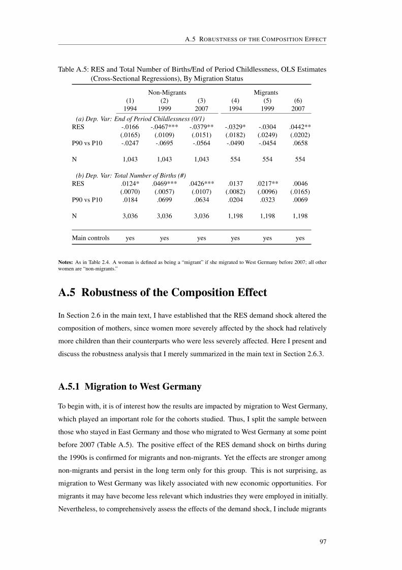
A.5 ROBUSTNESS OF THE COMPOSITION EFFECT
Table A.5: RES and Total Number of Births/End of Period Childlessness, OLS Estimates(Cross-Sectional Regressions), By Migration Status
Non-Migrants Migrants(1) (2) (3) (4) (5) (6)
1994 1999 2007 1994 1999 2007(a) Dep. Var: End of Period Childlessness (0/1)
RES -.0166 -.0467*** -.0379** -.0329* -.0304 .0442**(.0165) (.0109) (.0151) (.0182) (.0249) (.0202)
P90 vs P10 -.0247 -.0695 -.0564 -.0490 -.0454 .0658
N 1,043 1,043 1,043 554 554 554
(b) Dep. Var: Total Number of Births (#)RES .0124* .0469*** .0426*** .0137 .0217** .0046
(.0070) (.0057) (.0107) (.0082) (.0096) (.0165)P90 vs P10 .0184 .0699 .0634 .0204 .0323 .0069
N 3,036 3,036 3,036 1,198 1,198 1,198
Main controls yes yes yes yes yes yes
Notes: As in Table 2.4. A woman is defined as being a “migrant” if she migrated to West Germany before 2007; all otherwomen are “non-migrants.”
A.5 Robustness of the Composition Effect
In Section 2.6 in the main text, I have established that the RES demand shock altered the
composition of mothers, since women more severely affected by the shock had relatively
more children than their counterparts who were less severely affected. Here I present and
discuss the robustness analysis that I merely summarized in the main text in Section 2.6.3.
A.5.1 Migration to West Germany
To begin with, it is of interest how the results are impacted by migration to West Germany,
which played an important role for the cohorts studied. Thus, I split the sample between
those who stayed in East Germany and those who migrated to West Germany at some point
before 2007 (Table A.5). The positive effect of the RES demand shock on births during
the 1990s is confirmed for migrants and non-migrants. Yet the effects are stronger among
non-migrants and persist in the long term only for this group. This is not surprising, as
migration to West Germany was likely associated with new economic opportunities. For
migrants it may have become less relevant which industries they were employed in initially.
Nevertheless, to comprehensively assess the effects of the demand shock, I include migrants
97

A APPENDIX TO CHAPTER 2: THE IMPACT OF A NEGATIVE LABOR DEMAND SHOCK ON
FERTILITY
Table A.6: RES and Qualification in 1991, OLS Estimates (Cross-Sectional Regressions)
(1) (2) (3)Low qualif. (0/1) Med. qualif. (0/1) High qualif. (0/1)
RES -.0051 .0014 .0038(.0155) (.0200) (.0054)
P90 vs P10 -.0076 .0020 .0056Mean of dep. var. .255 .706 .039
Main Controls yes yes yesN 4,234 4,234 4,234
Notes: Each coefficient is from a separate regression. The dependent variables are dummy variables capturing no formalqualification (column 1), completed apprenticeship training (column 2), and university graduation (column 3). They all referto the beginning of 1991. Standard errors and control variables are defined as before (see Table 2.4), but control variablesexclude qualification variables.
throughout the analysis.
A.5.2 Placebo Test for Education
Previous research has shown that low-skilled East German women disproportionately lost
their jobs after reunification (Hunt, 2002). In this context, the skill-level of the employed
in an industry could be a characteristic which might have influenced the RES-measure and
which could also be related to fertility rates. While I control for education throughout the
analysis, I additionally conduct a placebo test where I regress women’s initial qualification
levels in 1991 on the RES-measure (see Table A.6). Reassuringly, it turns out that there is no
systematic association between the RES-measure and qualification levels.
A.5.3 Child Care and Regional Spillover Effects
Next, I investigate whether the results are driven by regional spillover effects. The availability
of childcare could be relevant in this context. The GDR was a state incentivizing and even
requiring full-time employment of mothers through comprehensive public child care (Rosen-
feld et al., 2004). Post-reunification, public child care became the responsibility of local
municipalities. Its availability declined in East Germany, even though it was still markedly
higher than in West Germany (Kreyenfeld, 2003, p. 310). However, in municipalities more
severely impacted by the demand shock, one would expect the availability of child care to
be relatively lower. This should decrease regional birth rates and lead to underestimation
of the effect of the RES demand shock on the composition of mothers. While the reduced
availability of child care is one plausible reason for the East German fertility decline as a
98

A.5 ROBUSTNESS OF THE COMPOSITION EFFECT
Table A.7: RES and Total Number of Births/End of Period Childlessness, OLS Estimates(Cross-Sectional Regressions), Controlling for Regional Spillover Effects
(1) (2) (3)1994 1999 2007 N
(a) Dep. Var: End of Period Childlessness (0/1)RES -.0189* -.0417*** -.0179* 1,516
(.0110) (.0093) (.0090)P90 vs P10 -.0281 -.0621 -.0267
(b) Dep. Var: Total Number of Births (#).0107*** .0373*** .0286*** 4,088(.0031) (.0040) (.0084)
P90 vs P10 .0159 .0555 .0425
Main Controls yes yes yesMunicipality FEs yes yes yes
Notes: As in Table 2.4. The regressions now contain detailed fixed effects accounting for the municipality a woman lived inat the beginning of the 1990s (Kreise in German). In a few cases, this information was missing, which explains the slightlysmaller sample sizes.
whole; it is less plausible as a cause for the finding that women more severely impacted by
the demand shock had more children on average.
Independent of child care, it could still be the case that the RES demand shock impacted
fertility through the channel of regional spillover effects. Such spillover effects would be
a consequence of the labor demand shock, but one that would indirectly operate through
differential changes in regional economic prospects. To assess whether this channel impacts
the results, in Table A.7 I include detailed fixed effects accounting for the municipalities
women lived in at the beginning of the 1990s (Kreise in German). The inclusion of these fixed
effects does not change the results significantly. Point estimates for results on childlessness
are very similar to those presented earlier, and point estimates for the total number of children
born become only slightly smaller. This suggests that the channel of regional spillover effects
played only a small role in explaining the results.
A.5.4 Missing Information on Industry
My sample includes women whose firms were integrated into the social security system and
reported their industry affiliation already at the beginning of 1991. A potential concern is
that firm-level characteristics, such as firm size, determined which firms were more likely to
report their industry affiliation earlier. I therefore analyze whether firm-level characteristics
confound the results. In Table A.8, I control for the set of 1991 firm-level characteristics
99

A APPENDIX TO CHAPTER 2: THE IMPACT OF A NEGATIVE LABOR DEMAND SHOCK ON
FERTILITY
Table A.8: RES and Total Number of Births/End of Period Childlessness, OLS Estimates(Cross-Sectional Regressions), Including Firm-Level Control Variables
Dep. Var: End of Period Dep. Var: Total NumberChildlessness (0/1) of Births (#)
(1) (2) (3) (4) (5) (6)1994 1999 2007 1994 1999 2007
RES -.0275** -.0458*** -.0204* .0158*** .0407*** .0367***(.0118) (.0103) (.0105) (.0038) (.0045) (.0098)
P90 vs P10 -.0410 -.0682 -.0304 .0235 .0606 .0547
Firm-Level Control VariablesShare Female -.1661** -.2000*** -.2006*** .0996*** .1296*** .2062***
(.0724) (.0648) (.0563) (.0287) (.0303) (.0545)Share low-skilled -.0899** -.1402* -.1043* .0380** .0641 .1181**> 5% (0/1) (.0389) (.0755) (.0532) (.0184) (.0473) (.0581)Share younger 30 .1659 -.0007 -.1525 -.0068 .0222 .2087*
(.1130) (.0871) (.1177) (.0701) (.0753) (.1214)Share older 50 -.0591 -.2135 -.2843 .1357 .2480 .3373*
(.1659) (.1862) (.1180) (.0905) (.1707) (.1826)Firm Size 1.06E-05 4.89E-06 5.33E-06 -4.97E-06 -7.74E-06 -1.2E-05
(8.80E-06) (1.24E-05) (9.27E-06) (5.97E-06) (7.75E-06) (9.79E-06)Firm Size Sq. -3.45E-10 -2.87E-11 -4.80E-11 2.54E-10 4.97E-10 4.70E-10
(3.23E-10) (5.10E-10) (3.83E-10) (2.25E-10) (3.18E-10) (3.85E-10)
N 1,582 1,582 1,582 4,196 4,196 4,196
Main controls yes yes yes yes yes yes
Notes: As in Table 2.4, but controlling for 1991 firm-level characteristics. Coefficients on firm size are in scientific notation,where for example E-05 denotes 10−5. Firm size is defined as the number of employees.
included in the BASiD data. These characteristics are the number of employees working at a
firm and its square, the share of female workers, a dummy variable capturing whether a firm
employed more than 5 percent of low-skilled workers, the share of workers younger than 30,
and the share older than 50. Some of the firm-level characteristics are correlated with fertility.
In particular, fertility was higher among women employed in female-dominated firms or in
firms with a relatively large share of low-skilled workers. Importantly, the impact of the
RES demand shock on fertility is qualitatively and quantitatively robust to the inclusion of
the firm-level control variables. This suggests that the potential selectivity of firms does not
confound my results.
100

A.5 ROBUSTNESS OF THE COMPOSITION EFFECT
Figure A.6: Correlation between Women’s RES-Values (by Industry) and Average RES-Values of their Husbands, 1991, Married Women Only
Coeff. = 0.120Robust s.e. = 0.027T-stat = 4.50
-8
-7
-6
-5
-4
-3
-2
-1
0
1
Mea
n R
ES
-val
ue h
usba
nds
-8 -7 -6 -5 -4 -3 -2 -1 0 1RES-value of women's industries
A. All industries (N=48)
Coeff. = 0.266Robust s.e. = 0.050T-stat = 5.36
-2
-1
0
1
Mea
n R
ES
-val
ue h
usba
nds
-2 -1 0 1RES-value of women's industries
B. Excluding the four most extreme RES-values
Notes: Based on the Microcensus of 1991. The sample includes East German women born 1959 to 1973 who have a husband.The regression model is weighted using industry shares.
A.5.5 Assortative Mating
The previous analysis has focused on women while neglecting their spouses. This could be
a problem if the labor demand shock experienced by women was correlated in systematic
ways with employment prospects of their spouses. Because the East German economy was
characterized by large firms, it is implausible to assume that assortative mating played no
role. Drawing on the Microcensus and focusing on East German women who were married
in 1991, I find that there is indeed some evidence of assortative mating. This is shown in
Figure A.6, where, at the industry level, average RES-values for husbands are regressed
on women’s RES-values. On average, the RES measure for husbands increases by 0.12 if
women’s RES-values are increased by a factor of 1 (panel A).
However, microeconomic theory as well as several recent empirical studies (Lindo, 2010;
Black et al., 2013; Autor et al., 2018; Schaller, 2016), suggest that negative shocks to men’s
labor market prospects merely operate through the income effect and hence decrease fertility.
Given that these insights apply to the East German context, the presence of assortative mating
should lead to an underestimation of the positive effect the RES demand shock had on the
composition of mothers.
To the extent possible, I test these expectations empirically. In Table A.9 I include control
variables for husbands. I again relied on the German Microcensus. Using this auxiliary data
source, at the industry level I compiled the fraction of women living with a spouse in 1991.
Additionally, for married women I inferred the 1991 RES-value of their spouses. At the
industry-level, I then calculated the average RES-value of spouses. I merged the two industry-
101

A APPENDIX TO CHAPTER 2: THE IMPACT OF A NEGATIVE LABOR DEMAND SHOCK ON
FERTILITY
Table A.9: RES and Total Number of Births/End of Period Childlessness, OLS Estimates(Cross-Sectional Regressions), Including Imputed Control Variables for LaborMarket Prospects of Spouses
(1) (2) (3)1994 1999 2007
(a) Dep. Var: End of Period Childlessness (0/1)RES -.0182 -.0458*** -.0308**
(.0156) (.0153) (.0150)P90 vs P10 -.0271 -.0683 -.0459
Mean RES-value of spouses -.0059 .0382 .1182(.0855) (.1062) (.0972)
P90 vs P10 -.0025 .0161 .0497
Share living with spouse -.3113** -.1453 -.0455(.1458) (.2179) (.1891)
N 1,596 1,596 1,596
(b) Dep. Var: Total Number of Births (#)RES .0131* .0421*** .0664***
(.0067) (.0080) (.0123)P90 vs P10 .0195 .0628 .0990
Mean RES-value of spouses .0110 -.0097 -.2655**(.0419) (.0616) (.1179)
P90 vs P10 .0046 -.0041 -.1115
Share living with spouse .0199 -.0642 -.1151(.0926) (.1254) (.1682)
N 4,229 4,229 4,229
Main controls yes yes yes
Notes: As in Table 2.4, but adding imputed control variables for husbands. These variables are based on the Scientific UseFile of the 1991 Microcensus, from which women born 1959 to 1973 living in East Germany were selected. For these, theshare living with a spouse as well as average RES-values of spouses (calculated for married women only) was imputed at theindustry level. These two imputed variables were merged to the main sample according to a woman’s initial industry.
level variables - the fraction living with a spouse in 1991 and average 1991 RES-values
of spouses - with the main BASiD data.3 These control variables were imputed for 1991
only, because partnership formation in later years could have been influenced by the labor
demand shock. It turns out that average RES-values of spouses have an insignificant effect in
the short-term period. In the medium- and long-term periods, point estimates suggest that
average RES-values of spouses operate in the expected direction. This is tentative evidence
3This is inspired by Perry (2004) and Raute (2017) who similarly impute information about spouses.
102

A.5 ROBUSTNESS OF THE COMPOSITION EFFECT
Figure A.8: Unemployment Rates in East Germany, 1991-2015, By Gender
5
10
15
20
25
Une
mpl
oym
ent R
ate
1990 1992 1994 1996 1998 2000 2002 2004 2006 2008 2010 2012 2014
East German Men East German Women
Source: Federal Employment Agency (2015). Unemployment rates refer to June 30th of a given year and are defined relativeto the dependent labor force.
that indeed negative shocks to male employment prospects decrease fertility. As a result, the
impact of female labor market prospects, as captured by the RES demand shock experienced
by women, increases. By 2007, women at the 90th percentile of the demand shock are now
estimated to have had 0.099 children more on average than their counterparts at the 10th
percentile (panel (b) of Table A.9, column (3)). The effect on long-term childlessness also
becomes larger in magnitude. At the end of 2007, women experiencing a more severe labor
demand shock are on average 4.6 percentage points less likely to still be childless (panel (a),
column (3)).
Why should male labor market prospects only impact fertility in the medium- and long-
term periods? A possible reason is that East German men were most strongly hit by the
labor demand shock only from the mid-1990s onwards. After 1995 and up until 2006, male
unemployment rates increased to dramatic levels. By contrast, unemployment rates among
East German women reached dramatic levels already in 1992 (see Figure A.8 as well as Hunt
(2002) who analyzes the gender gap in employment levels post-reunification). Particularly in
the medium- and long-term periods, not accounting for male employment prospects seems to
lead to a downward bias of the effect of female labor market prospects on the composition of
mothers.
Average RES-values are only an imperfect approximation of the labor demand shock
spouses experienced. For example, this proxy variable could capture both the labor market
situation of actual spouses of married women and the labor market situation of potential
partners of single women. A comprehensive analysis of how men’s labor market situations
103

A APPENDIX TO CHAPTER 2: THE IMPACT OF A NEGATIVE LABOR DEMAND SHOCK ON
FERTILITY
Table A.10: RES and Total Number of Births/End of Period Childlessness, OLS Estimates(Cross-Sectional Regressions), Excluding Industries with Strong EmploymentGrowth
(1) (2) (3)1994 1999 2007
(a) Dep. Var: End of Period Childlessness (0/1)RES -.0647*** -.0639** -.0175
(.0185) (.0260) (.0226)P90 vs P10 -.0983 -.0971 -.0266
N 1,557 1,557 1,557
(b) Dep. Var: Total Number of Births (#)RES .0188* .0420*** .0115
(.0095) (.0112) (.0331)P90 vs P10 .0192 .0428 .0117
N 4,135 4,135 4,135
Main contr. yes yes yesFirm contr. yes yes yes
Notes: As in Table 2.4, but excluding women initially employed in one of the four industries with the strongest employ-ment growth. After weighting, the share of women employed in these industries is 3.2 percent. I include 1991 firm-levelcharacteristics (as in Table A.8).
impact childbearing decisions is beyond the scope of this paper. At the very least, however,
the findings presented in Table A.9 cannot be reconciled with the view that the presence of
assortative mating drives the positive effect the demand shock had on the composition of
mothers.
A.5.6 Industries with Strong Employment Growth
Four East German industries were subject to a strong positive labor demand shock.4 Because
these industries were small in the GDR, their employment growth after reunification was
pronounced. A natural question is how this impacts my results.
In Table A.10 I exclude women who were initially employed in one of these industries.
The patterns of the results are similar to those presented earlier. But an important difference
is that the persistence of the effect on the total number of children born until 2007 becomes
smaller. It appears that for the majority of women the shock mostly impacted the timing
of births. To investigate this further, in Table A.11 I include imputed control variables for
4These industries include the finance and insurance industries, “printing & reproduction,” and “finishingtrade.”
104

A.5 ROBUSTNESS OF THE COMPOSITION EFFECT
Table A.11: RES and Total Number of Births, OLS Estimates (Cross-Sectional Regressions),Excluding Industries with Strong Employment Growth and Including ImputedControl Variables for Spouses
(1) (2) (3) (4) (5) (6)1994 1999 2007 1994 1999 2007
Dep. Var: Total Number of Births (#)RES .0013 .0402 .0721* .0157 .0515* .1215***
(.0196) (.0294) (.0404) (.0175) (.0261) (.0347)P90 vs P10 .0013 .0410 .0735 .0160 .0525 .1239
N 4,167 4,167 4,167 4,130 4,130 4,130
Main Controls yes yes yes yes yes yesHusb. Control Variables yes yes yes yes yes yesFirm Control Variables - - - yes yes yes
Notes: As in Table 2.4, but excluding women initially employed in one of the four industries with the strongest employmentgrowth. I include imputed control variables for spouses (as in Table A.9). In columns 4 to 6, I additionally include firm-levelcontrol variables (as in Table A.8).
spouses (see the previous section for details). Now the effect on the total number of children
born becomes persistent in the long term as well.5 Assortative mating seems to exert a
relatively strong downward bias, potentially because assortative mating plays a stronger role
when the industries with particularly favorable employment growth are excluded (panel (B)
of Figure A.6). Therefore, the results remain robust, but the persistence of the effect on the
total number of children born now depends on whether I account for assortative mating.
A.5.7 Placebo Test based on Previous Births
Finally, even though the negative labor demand shock was unexpected and exogenous, a
natural concern is the potential impact of unobserved differences associated with the intensity
of the labor demand shock. This would be a problem if these characteristics, and not the
demand shock, caused differences in fertility. As one approach to addressing this objection,
in panel (a) of Table A.12 I display the results of a placebo test. The test investigates births
before the labor demand shock. The outcome variables are a dummy capturing childlessness
at the end of 1990 as well as the total number of children born up until this point. When these
predetermined variables are regressed on the RES measure, the coefficients are statistically
insignificant. The point estimates are moreover relatively small in comparison to the mean
of the outcome variables. This suggests that the labor demand shock was not associated with
5In this specification with husband control-variables, coefficients are imprecisely estimated (Table A.11,columns 1-3), but the precision increases with the inclusion of firm-level control variables (columns 4-6).
105

A APPENDIX TO CHAPTER 2: THE IMPACT OF A NEGATIVE LABOR DEMAND SHOCK ON
FERTILITY
Table A.12: RES and Predetermined Fertility Outcomes, Placebo Test (Cross-SectionalRegressions)
(1) (2)Prior Prior total
childlessness (0/1) no of births (#)
(a) All women born 1959-1973RES -.0020 .0213
(.0058) (.0163)P90 vs P10 -.0029 .0317
Mean of dep. var. .3860 .9515N 4,234 4,234
(b) Women born 1959-1963RES -.0086 .0468
(.0133) (.0312)P90 vs P10 -.0135 .0735
Mean of dep. var. .1182 1.5250N 1,633 1,633
(c) Women born 1964-1968RES .0247** -.0252
(.0120) (.0162)P90 vs P10 .0368 -.0376
Mean of dep. var. .3257 .9148N 1,457 1,457
(d) Women born 1969-1973RES -.0157 .0192
(.0121) (.0132)P90 vs P10 -.0233 .0285
Mean of dep. var. .0856 .1561N 1,144 1,144
Main Controls yes yes
Notes: The model has the same structure as Table 2.4. The outcome variable in column (1) is a dummy variable equalto 1 whenever a women was still childless at the beginning of 1991. In column (2), the outcome is the total number ofchildren born before 1991. Control variables for the number of children born before 1991 are obviously dropped; otherwiseexplanations and control variables are the same as in Table 2.4.
106

A.6 EFFECT HETEROGENEITY BY QUALIFICATION GROUP
unobservable factors causing systematic differences in childbearing.
In panels (b) to (d) of the sample table, I repeat the placebo test but split the main sample
into three different cohort groups. Again, I find that there are no systematic differences
in predetermined births. In particular, point estimates for women born 1959-63 and 1964-
68 have opposing signs (these cohorts are of particular interest because they were old
enough such that a significant share of women had children prior to reunification). The
only statistically significant effect concerns the pre-determined childlessness of women born
1964-68, but in this case, women employed in industries that were later subject to a severe
labor demand shock were in fact more likely to be childless in 1990. Note also that the
placebo test yields similar results if I only include main control variables, or if I additionally
control for imputed variables for husbands, firm-level characteristics, and regional fixed
effects (details are available from the author).
A.6 Effect Heterogeneity by Qualification Group
Table A.13: RES and Total Number of Births, OLS Estimates (Cross-Sectional Regressions),By Qualification in 1991
(1) (2) (3)1994 1999 2007 N
(a) Low qualificationRES .0322*** .0637*** .0695*** 1,147
(.0092) (.0133) (.0203)P90 vs P10 .0480 .0949 .1036
(b) Medium qualificationRES .0073 .0285*** .0165 2,929
(.0085) (.007) (.0115)P90 vs P10 .0109 .0425 .0246
(c) High qualificationRES .0306** .1156*** .1203*** 158
(.0131) (.0139) (.0145)P90 vs P10 .0236 .0890 .0926
Main controls yes yes yes
Notes: Explanations are analogous to Table 2.4. I refer to women without formal qualification, with apprenticeship degrees,and to graduates, respectively. As before, “Total Number of Births” means the number of children born between 1991 andthe end of 1994, 1999, or 2007. I no longer control for qualification.
107


B Appendix to Chapter 3: Refugee-specific
Government Aid and Child Refugees’
Economic Success Later in Life
B.1 Additional Tables
109

B APPENDIX TO CHAPTER 3: REFUGEE-SPECIFIC GOVERNMENT AID AND CHILD REFUGEES’
ECONOMIC SUCCESS LATER IN LIFE
Table B.1: Description of Governmental Aid Programs Covered by C-Status
Category ofSpecific Pro-gram
Specific Rights and Entitlements Legal Basis
Employment Privileged access to occupations and industrybranches with barriers to entry
§§ 69-71BVFG
Employment Acknowledgement of certified qualifications ob-tained before May 1945
§ 92 BVFG
Employment Simplified procedure for replacing lost certificates § 93 BVFGEmployment Possibility to be assigned a job subsidized by the
governmentLAG
Employment,Apprenticeshiptraining
Support of employees through privileged treat-ment by employment agencies, privileged re-entryinto previous occupations, privileged access toapprenticeships and to public funds supporting ap-prenticeship training programs, provision of cheaploans and debt guarantees used for the creation ofpermanent jobs for refugees
§§ 77-79BVFG
Family reunion Granted right to reunite with family members § 94 BVFGFinancial As-sets
Exchange of financial assets in former Germancurrency
Other
General support Counseling by organizations for expellees andrefugees, free of charge
§ 95 BVFG
Geographiclocation
Participation in geographical reallocation process §§ 26-34BVFG
Housing Privileged access to rent-controlled flats built aspart of public social housing programs and to flatssubsidized via tax cuts, cheap loans and cash bene-fits
§ 80 BVFG
Housing Access to real estate loans, in case previous realestate was lost
$ 301 LAG
Housing Possibility to be assigned a flat that has been spon-sored through a governmental program (Wohn-raumhilfe)
LAG
Reparations Reparations paid to victims of the Nazi regime BEG and othersSelf-employment
Cheap loans and cash benefits for tenants or buyersof agricultural businesses / farms. (West Germansellers and landlords of farms and agricultural landreceived tax cuts if they sold/rented to individualswith C-status).
§§ 35-68BVFG
Self-employment
Support for self-employed persons (outside agri-culture) through access to loans, low interest rates,debt guarantees, co-partnerships, tax cuts and cashbenefits, privileged access to public contracts, privi-leged access to public real estate and other property
§§ 72-76BVFG
110
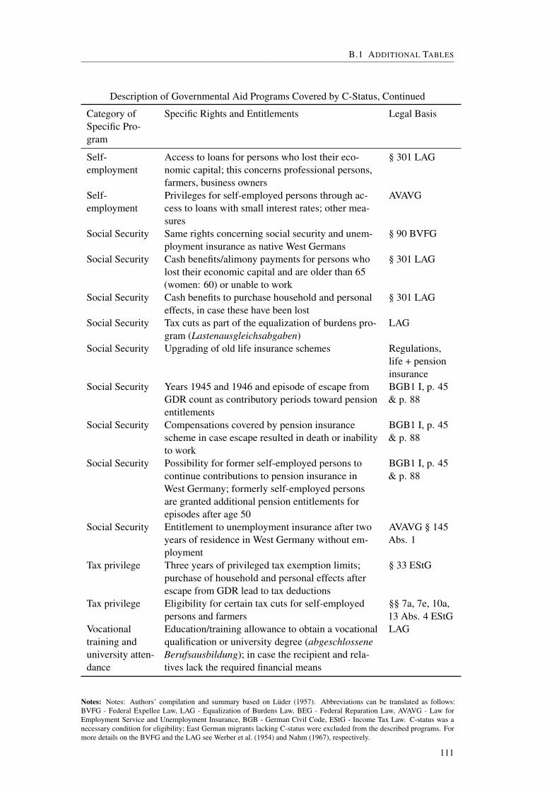
B.1 ADDITIONAL TABLES
Description of Governmental Aid Programs Covered by C-Status, Continued
Category ofSpecific Pro-gram
Specific Rights and Entitlements Legal Basis
Self-employment
Access to loans for persons who lost their eco-nomic capital; this concerns professional persons,farmers, business owners
§ 301 LAG
Self-employment
Privileges for self-employed persons through ac-cess to loans with small interest rates; other mea-sures
AVAVG
Social Security Same rights concerning social security and unem-ployment insurance as native West Germans
§ 90 BVFG
Social Security Cash benefits/alimony payments for persons wholost their economic capital and are older than 65(women: 60) or unable to work
§ 301 LAG
Social Security Cash benefits to purchase household and personaleffects, in case these have been lost
§ 301 LAG
Social Security Tax cuts as part of the equalization of burdens pro-gram (Lastenausgleichsabgaben)
LAG
Social Security Upgrading of old life insurance schemes Regulations,life + pensioninsurance
Social Security Years 1945 and 1946 and episode of escape fromGDR count as contributory periods toward pensionentitlements
BGB1 I, p. 45& p. 88
Social Security Compensations covered by pension insurancescheme in case escape resulted in death or inabilityto work
BGB1 I, p. 45& p. 88
Social Security Possibility for former self-employed persons tocontinue contributions to pension insurance inWest Germany; formerly self-employed personsare granted additional pension entitlements forepisodes after age 50
BGB1 I, p. 45& p. 88
Social Security Entitlement to unemployment insurance after twoyears of residence in West Germany without em-ployment
AVAVG § 145Abs. 1
Tax privilege Three years of privileged tax exemption limits;purchase of household and personal effects afterescape from GDR lead to tax deductions
§ 33 EStG
Tax privilege Eligibility for certain tax cuts for self-employedpersons and farmers
§§ 7a, 7e, 10a,13 Abs. 4 EStG
Vocationaltraining anduniversity atten-dance
Education/training allowance to obtain a vocationalqualification or university degree (abgeschlosseneBerufsausbildung); in case the recipient and rela-tives lack the required financial means
LAG
Notes: Notes: Authors’ compilation and summary based on Lüder (1957). Abbreviations can be translated as follows:BVFG - Federal Expellee Law, LAG - Equalization of Burdens Law, BEG - Federal Reparation Law, AVAVG - Law forEmployment Service and Unemployment Insurance, BGB - German Civil Code, EStG - Income Tax Law. C-status was anecessary condition for eligibility; East German migrants lacking C-status were excluded from the described programs. Formore details on the BVFG and the LAG see Werber et al. (1954) and Nahm (1967), respectively.
111

B APPENDIX TO CHAPTER 3: REFUGEE-SPECIFIC GOVERNMENT AID AND CHILD REFUGEES’
ECONOMIC SUCCESS LATER IN LIFE
Table B.2: Additional Information on Variable Definitions and Underlying Concepts
Refugees:Persons who migrated from East Germany to West Germany between 1946 and 1961,excluding expellees from Eastern European territories.
Qualification Variables:Low: no formal vocational qualification; medium: completed apprenticeship training; high:graduates from universities or institutions of applied sciences, as well as engineers andtechnicians
Individuals’ total monthly net income 1971:“Income” in the Microcensus is defined as an individual person’s net monthly total incomefrom all income sources. This income definition provides a suitable variable for our purposes,as it captures a person’s socio-economic status; but should not be confused with (labormarket) wages which are not elicited in the Microcensus. The income variable is measuredin seven income brackets, which reach from [1, 150 German Marks) to [1800, + infinity).We performed interval regression analysis with logged income values referring to the intervalendpoints and a missing value at the censored upper end (based on men observed in WestGermany; i.e., not only the GDR refugees). The dependent variables were age and its square,qualification (6 categories), economic status (13 categories; which distinguish betweendifferent categories among the self-employed, civil servants, employees, workers, and non-employed workers), and region (35 categories referring to administrative regions calledRegierungsbezirke). Based on this approach, we predicted log income values. (We adjustedthe transformation to levels such that the information is meaningful also in the top-incomebracket, see Cameron and Trivedi (2010, p. 108)). Note that the income variable excludesfarmers and agricultural workers.
High employment status:Dummy variable equal to 1 whenever a person is employed as a high-level civil servants oremployee or belongs to the worker elite.
Father’s occupational status, list of categories included in analysisSelf-employed outside of agriculture; high-level civil servants; medium-level civil servants;low-level civil servants; high-level employees; medium-level employees; low-level employee;worker elite; qualified workers; workers with on the job and no training; farmers and helpingfamily members; in training or school/university; non-employed
Father’s industry, list of categories included in analysisAgriculture; energy and mining; manufacturing; construction; retail; transport and infor-mation transmission; finance and insurance; hotels and restaurants; low-skilled services;science, education, art; health; qualified services; churches and other organizations; privatehouseholds; public administration; missing industry.
Father’s and mother’s qualification, list of categories included in analysisNo vocational qualification and at most a basic school education; no vocational qualifica-tion and an intermediate or higher school education; vocational qualification and at mosta basic school education; vocational qualification and an intermediate or higher schooleducation; technician, graduate from professional school (Fachschule); engineer, graduatefrom university; missing information
112
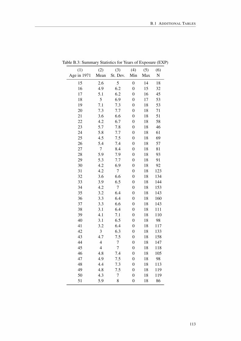
B.1 ADDITIONAL TABLES
Table B.3: Summary Statistics for Years of Exposure (EXP)
(1) (2) (3) (4) (5) (6)Age in 1971 Mean St. Dev. Min Max N
15 2.6 5 0 14 1816 4.9 6.2 0 15 3217 5.1 6.2 0 16 4518 5 6.9 0 17 5319 7.1 7.3 0 18 5320 7.3 7.7 0 18 7121 3.6 6.6 0 18 5122 4.2 6.7 0 18 5823 5.7 7.8 0 18 4624 5.8 7.7 0 18 6125 4.5 7.5 0 18 6926 5.4 7.4 0 18 5727 7 8.4 0 18 8128 5.9 7.9 0 18 9329 5.3 7.7 0 18 9130 4.2 6.9 0 18 9231 4.2 7 0 18 12332 3.6 6.6 0 18 13433 3.9 6.5 0 18 14434 4.2 7 0 18 15335 3.2 6.4 0 18 14336 3.3 6.4 0 18 16037 3.3 6.6 0 18 14338 3.1 6.4 0 18 11139 4.1 7.1 0 18 11040 3.1 6.5 0 18 9841 3.2 6.4 0 18 11742 3 6.3 0 18 13343 4.7 7.5 0 18 15844 4 7 0 18 14745 4 7 0 18 11846 4.8 7.4 0 18 10547 4.9 7.5 0 18 9848 4.4 7.3 0 18 11349 4.8 7.5 0 18 11950 4.3 7 0 18 11951 5.9 8 0 18 86
113

B APPENDIX TO CHAPTER 3: REFUGEE-SPECIFIC GOVERNMENT AID AND CHILD REFUGEES’
ECONOMIC SUCCESS LATER IN LIFE
B.2 Additional Figures
114

B.2 ADDITIONAL FIGURES
Figure B.1: Father’s Educational Attainment
0
.05
.1
.15
.2
.25
.3
.35
.4
.45
.5
.55
.6
.65
.7
.75
Sha
re
1946
1947
1948
1949
1950
1951
1952
1953
1954
1955
1956
1957
1958
1959
1960
1961
Year of arrival in West Germany
High qualification
Medium qualification
No qualification
A. Distribution of Refugee Children and Young AdultsAcross Fathers’ Education, by Year of Arrival
0.05
.1.15
.2.25
.3.35
.4.45
.5.55
.6.65
.7.75
.8
Sha
re
1946
1947
1948
1949
1950
1951
1952
1953
1954
1955
1956
1957
1958
1959
1960
1961
Year of arrival in West Germany
High qualification
Medium qualification
No qualification
B. Share of Aid-Eligible Refugee Children and YoungAdults, by Year of Arrival in West Germany and byFathers’ Education
0.05
.1.15
.2.25
.3.35
.4.45
.5.55
.6.65
.7.75
.8
Sha
re
1946
1947
1948
1949
1950
1951
1952
1953
1954
1955
1956
1957
1958
1959
1960
1961
Year of arrival in West Germany
High qualification
Medium qualification
No qualification
C. Distribution of Aid-Eligible Refugee Children andYoung Adults Across Fathers’ Education, by Year ofArrival in West Germany
Notes: Panel (A): This figure shows the distribution across fathers’ educational attainment of refugees who arrived in WestGermany at ages 1-25, by year of arrival. The values for each education class by year of arrival sum to 1. Panel (B): Thisfigure shows the share of aid-eligible refugees who arrived in West Germany at ages 1-25, by year of arrival and by fathers’educational attainment. Panel (C): This figure shows the distribution of aid-eligible refugees who arrived in West Germanyat ages 1-25 across fathers’ educational attainment, by year of arrival.
115

B APPENDIX TO CHAPTER 3: REFUGEE-SPECIFIC GOVERNMENT AID AND CHILD REFUGEES’
ECONOMIC SUCCESS LATER IN LIFE
Figure B.2: Father’s Employment Status
0
.05
.1
.15
.2
.25
.3
.35
.4
.45
.5
.55
Sha
re
1946
1947
1948
1949
1950
1951
1952
1953
1954
1955
1956
1957
1958
1959
1960
1961
Year of arrival in West Germany
Self employed Civil servant
Employee Worker
Unemployed Farmer
A. Distribution of Refugee Children and Young AdultsAcross Fathers’ Employment Status, by Year of Arrival
0.05
.1.15
.2.25
.3.35
.4.45
.5.55
.6.65
.7.75
.8
Sha
re
1946
1947
1948
1949
1950
1951
1952
1953
1954
1955
1956
1957
1958
1959
1960
1961
Year of arrival in West Germany
Self employed Civil servant
Employee Worker
Unemployed Farmer
B. Share of Aid-Eligible Refugee Children and YoungAdults, by Year of Arrival in West Germany and byFathers’ Employment Status
0
.05
.1
.15
.2
.25
.3
.35
.4
.45
.5
.55
.6
Sha
re
1946
1947
1948
1949
1950
1951
1952
1953
1954
1955
1956
1957
1958
1959
1960
1961
Year of arrival in West Germany
Self employed Civil servant
Employee Worker
Unemployed Farmer
C. Distribution of Aid-Eligible Refugee Children andYoung Adults Across Fathers’ Employment Status, byYear of Arrival in West Germany
Notes: Panel (A): This figure shows the distribution across fathers’ occupational status of refugees who arrived in WestGermany at ages 1-25, by year of arrival. The values for each employment status group by year of arrival sum to 1. Panel(B): This figure shows the share of aid-eligible refugees who arrived in West Germany at ages 1-25, by year of arrival andby fathers’ employment status. Panel (C): This figure shows the distribution of aid-eligible refugees who arrived in WestGermany at ages 1-25 across fathers’ employment status, by year of arrival.
116

B.2 ADDITIONAL FIGURES
Figure B.3: Father’s Industry of Employment
0
.05
.1
.15
.2
.25
.3
.35
.4
.45
Sha
re
1946
1947
1948
1949
1950
1951
1952
1953
1954
1955
1956
1957
1958
1959
1960
1961
Year of arrival in West Germany
Construction Manufacturing Retail and transport
Low qualified services Culture and religion Qualified services
Public services Energy and mining Agriculture
A. Distribution of Refugee Children and Young AdultsAcross Fathers’ Employment Status, by Year of Arrival
0.05
.1.15
.2.25
.3.35
.4.45
.5.55
.6.65
.7.75
.8.85
.9.95
1
Sha
re
1946
1947
1948
1949
1950
1951
1952
1953
1954
1955
1956
1957
1958
1959
1960
1961
Year of arrival in West Germany
Construction Manufacturing Retail and transport
Low qualified services Culture and religion Qualified services
Public services Energy and mining Agriculture
B. Share of Aid-Eligible Refugee Children and YoungAdults, by Year of Arrival in West Germany and byFathers’ Employment Status
0
.05
.1
.15
.2
.25
.3
.35
.4
.45
.5
Sha
re
1946
1947
1948
1949
1950
1951
1952
1953
1954
1955
1956
1957
1958
1959
1960
1961
Year of arrival in West Germany
Construction Manufacturing Retail and transport
Low qualified services Culture and religion Qualified services
Public services Energy and mining Agriculture
C. Distribution of Aid-Eligible Refugee Children andYoung Adults Across Fathers’ Employment Status, byYear of Arrival in West Germany
Notes: Panel (A): This figure shows the distribution across fathers’ industry of employment of refugees who arrived in WestGermany at ages 1-25, by year of arrival. The values for each employment status group by year of arrival sum to 1. Panel(B): This figure shows the share of aid-eligible refugees who arrived in West Germany at ages 1-25, by year of arrival and byfathers’ industry of employment. Panel (C): This figure shows the distribution of aid-eligible refugees who arrived in WestGermany at ages 1-25 across fathers’ industry of employment, by year of arrival.
117


Bibliography
Abelshauser, Werner (2011). Deutsche Wirtschaftsgeschichte, Von 1945 bis zur Gegenwart.
München: C.H. Beck.
Ackermann, Volker (1995). Der ‘echte’ Flüchtling - Deutsche Vertriebene und Flüchtlinge
aus der DDR 1945-1961. Osnabrück: Universitätsverlag Rasch.
Adler, Marina (1997). Social Change and Declines in Marriage and Fertility in Eastern
Germany. Journal of Marriage and the Family 59(1), 37–49.
Ahlfeldt, Gabriel, Stephen Redding, Daniel Sturm, and Nikolaus Wolf (2015). The Eco-
nomics of Density: Evidence from the Berlin Wall. Econometrica 83(6), 2127–2189.
Akerlof, George, Andrew Rose, Janet Yellen, and Helga Hessenius (1991). East Germany
in from the Cold: The Economic Aftermath of Currency Union. Brookings Papers on
Economic Activity 1, 1–105.
Alesina, Alberto, and Nicola Fuchs-Schündeln (2007). Goodbye Lenin (or not?): The Effect
of Communism on People’s Preferences. American Economic Review 97(4), 1507–1528.
Andersen, Lars Højsgaard, Christian Dustmann, and Rasmus Landersø (2018). Lowering
Welfare Benefits: Intended and Unintended Consequences for Migrants and their Families.
Mimeo.
Antoni, Manfred (2018). Record linkage of GDR’s “Data Fund of Societal Work Power”
with administrative labour market biography data of the German Federal Employment
Agency. German RLC Working Paper No. wp-grlc-2018-02.
Antoni, Manfred, and Arne Bethmann (2018). PASS-ADIAB - Linked Survey and Ad-
ministrative Data for Research on Unemployment and Poverty. Jahrbücher für Nation-
alökonomie und Statistik online first.
Anweiler, Oskar (2005). Bildungspolitik. In G. Schulz and Federal Ministry of Labour and
Social Affairs and The Federal Archive (Eds.), Geschichte der Sozialpolitik in Deutschland
119

BIBLIOGRAPHY
seit 1945, Band 3, Bundesrepublik Deutschland 1949-1957, pp. 653–686. Baden Baden:
Nomos Verlag.
Arntz, Melanie, and Christina Gathmann (2014). Permanent Changes in the Wage Struc-
ture and the East German Fertility Crisis. Beiträge zur Jahrestagung des Vereins für
Socialpolitik 2014: Evidenzbasierte Wirtschaftspolitik - Session: Marriage and Children,
No. B02-V2.
Autor, David, and David Dorn (2013). The Growth of Low-Skill Service Jobs and the
Polarization of the US Labor Markt. American Economic Review 103(5), 1553–1597.
Autor, David, David Dorn, and Gordon Hanson (2013). The China Syndrome: Local
Labor Market Effects of Import Competition in the United States. American Economic
Review 103(6), 2121–2168.
Autor, David, David Dorn, and Gordon Hanson (2018). When Work Disappears: Manu-
facturing Decline and the Falling Marriage-Market Value for Men. American Economic
Review: Insights, forthcoming.
Autor, David, Frank Levy, and Richard Murnane (2003). The Skill Content of Recent
Technological Change: An Empirical Exploration. Quarterly Journal of Economics 118(4),
1279–1333.
Baker, David, Helmut Köhler, and Manfred Stock (2007). Socialist Ideology and the
Contraction of Higher Education: Institutional Consequences of State Manpower and
Education Planning in the Former East Germany. Comparative Education Review 51(3),
353–377.
Bauer, Thomas, Sebastian Braun, and Michael Kvasnicka (2013). The Economic Integration
of Forced Migrants: Evidence for Post-War Germany. The Economic Journal 123(571),
998–1024.
Beblo, Miriam, and Luise Görges (2018). On the Nature of Nurture. The Malleability of Gen-
der Differences in Work Preferences. Journal of Economic Behavior & Organization 151,
19–41.
Becker, Gary (1965). A Theory of the Allocation of Time. The Economic Journal 75(299),
493–517.
Bender, Stefan, Jürgen Hilzendegen, Götz Rohwer, and Helmut Rudolph (1996). Die IAB-
Beschäfigtenstichprobe 1975 - 1990. Beiträge zur Arbeitsmarkt- und Berufsforschung 197.
120
BIBLIOGRAPHY
Bernien, Maritta, Vera Dahms, Reinhard Schaefer, Frank Schiemann, and Jürgen Wahse
(1996). Der Arbeitsmarkt in Ostdeutschland, 1989-1994. Berlin: Graue Reihe der KSPW
bei der GSFP.
Bethlehem, Siegfried (1982). Heimatvertreibung, DDR-Flucht, Gastarbeiterzuwanderung.
Stuttgart: Klett-Cotta.
Bhaumik, Sumon, and Jeffrey Nugent (2011). Real Options and Demographic Decisions:
Empirical Evidence from East and West Germany. Applied Economics 43(11), 2739–2749.
Black, Dan, Natalia Kolesnikova, Seth Sanders, and Lowell Taylor (2013). Are Children
‘Normal’? Review of Economics and Statistics 95(1), 21–33.
Bleakley, Hoyt, and Aimee Chin (2010). Age at Arrival, English Proficiency, and Social As-
similation among US Immigrants. American Economic Journal: Applied Economics 2(1),
165–192.
Boldorf, Marcel (2007). Sozialpolitische Denk- und Handlungsfelder. In M. Ruck,
M. Boldorf, and Federal Ministry of Labour and Social Affairs and The Federal Archive
(Eds.), Geschichte der Sozialpolitik in Deutschland seit 1945, Band 4, Bundesrepublik
Deutschland 1957-1966, pp. 85–150. Baden Baden: Nomos Verlag.
Borjas, George (2000). Ethnic Enclaves and Assimilation. Swedish Economic Policy
Review 7, 89–122.
Borjas, George, and Kirk Doran (2012). The Collapse of the Soviet Union and the Productiv-
ity of American Mathematicians. Quarterly Journal of Economics 127(3), 1143–1203.
Brand, Jennie (2015). The Far-Reaching Consequences of Job Loss and Unemployment.
Annual Review of Sociology 41, 359–375.
Brand, Jennie, and Juli Simon Tomas (2014). Job Displacement Among Single Mothers: Ef-
fects on Children’s Outcomes in Young Adulthood. American Journal of Sociology 119(4),
955–1001.
Braun, Sebastian, and Michael Kvasnicka (2014). Immigration and Structural Change:
Evidence from Post-War Germany. Journal of International Economics 93(2), 253–269.
Braun, Sebastian, and Toman Omar Mahmoud (2014). The Employment Effects of Immigra-
tion: Evidence from the Mass Arrival of German Expellees in Postwar Germany. Journal
of Economic History 74(1), 69–108.
121

BIBLIOGRAPHY
Burchardi, Konrad, and Tarek Hassan (2013). The Economic Impact of Social Ties: Evidence
from German Reunification. Quarterly Journal of Economics 128(3), 1219–1271.
Burda, Michael, and Jennifer Hunt (2001). From Reunification to Economic Integration:
Productivity and the Labor Market in Eastern Germany. Brookings Papers on Economic
Activity 32(2), 1–92.
Bursztyn, Leonardo, and Davide Cantoni (2016). A Tear in the Iron Curtain: The Impact of
Western Television on Consumption Behavior. Review of Economics and Statistics 98(1),
25–41.
Cameron, Colin, and Pravin Trivedi (2010). Microeconometrics Using Stata. College Station,
Texas: Stata Press Publication.
Chetty, Raj, and Nathaniel Hendren (2018). The Impacts of Neighborhoods on Intergenera-
tional Mobility I: Childhood Exposure Effects. Quarterly Journal of Economics 133(3),
1107–1162.
Chetty, Raj, Nathaniel Hendren, and Lawrence Katz (2016). The Effects of Exposure to
Better Neighborhoods on Children: New Evidence from the Moving to Opportunity
Experiment. American Economic Review 106(4), 855–902.
Chevalier, Arnaud, and Olivier Marie (2017). Economic Uncertainty, Parental Selection,
and the Educational Outcomes of the ‘Children of the Wall’. Journal of Political Econ-
omy 125(2), 393–430.
Conrad, Christoph, Michael Lechner, and Welf Werner (1996). East German Fertility After
Unification: Crisis of Adaptation? Population and Development Review 22(2), 331–358.
Cortes, Kalena (2004). Are Refugees different from Economic Immigrants? Some Empirical
Evidence on the Heterogeneity of Immigrant Groups in the United States. Review of
Economics and Statistics 86(2), 465–480.
Dahl, Gordon, and Lance Lochner (2012). The Impact of Family Income on Child Achieve-
ment: Evidence from the Earned Income Tax Credit. American Economic Review 102(5),
1927–1956.
Damm, Anna Piil (2009). Ethnic Enclaves and Immigrant Labour Market Outcomes: Quasi-
Experimental Evidence. Journal of Labor Economics 27(2), 281–314.
De la Rica, Sara, and Amaia Iza (2005). Career Planning in Spain: Do Fixed-term Contracts
Delay Marriage and Parenthood? Review of Economics of the Household 3, 49–73.
122

BIBLIOGRAPHY
Deaton, Angus (1997). The Analysis of Household Surveys. Baltimore: The Johns Hopkins
University Press.
Dehija, Rajeev, and Adriana Lleras-Muney (2004). Booms, Busts, and Babies’ Health.
Quarterly Journal of Economics 119(3), 1091–1130.
Del Boca, Daniela, Christopher Flinn, and Matthew Wiswall (2016). Transfers to Households
with Children and Child Development. The Economic Journal 126(596), 136–183.
Del Bono, Emilia, Andrea Weber, and Rudolf Winter-Ebmer (2015). Fertility and Economic
Instability: The Role of Unemployment and Job Displacement. Journal of Population
Economics 28(2), 463–478.
Dettling, Lisa, and Melissa Kearney (2014). House Prices and Birth Rates: The Impact of
the Real Estate Market on the Decision to Have a Baby. Journal of Public Economics 110,
82–100.
Dietz, Frido, and Helmut Rudolph (1990). Berufstätigenerhebung und der Datenspeicher
“Gesellschaftliches Arbeitsvermögen”. Mitteilungen aus der Arbeitsmarkt- und Berufs-
forschung 4, 511–518.
Diewald, Martin, Johannes Huinink, Heike Solga, and Annemette Sorensen (1995). Um-
brüche und Kontinuitäten – Lebensverläufe und die Veränderung von Lebensbedingungen
seit 1989. In J. Huinink and K. U. Mayer (Eds.), Kollektiv und Eigensinn. Lebensverläufe
in der DDR und danach, pp. 307–348. Berlin: Akademie Verlag.
Dorner, Matthias, Dietmar Harhoff, Tina Hinz, Karin Hoisl, and Stefan Bender (2016). Social
Ties for Labor Market Access - Lessons from the Migration of East German Inventors.
IAB Discussion Paper 41/2016.
Dustmann, Christian, Bernd Fitzenberger, Uta Schönberg, and Alexandra Spitz-Oener (2014).
From Sick Man of Europe to Economic Superstar: Germany’s Resurgent Economy.
Journal of Economic Perspectives 28(1), 167–188.
Eberstadt, Nicholas (1994). Demographic Shocks After Communism: Eastern Germany,
1989-93. Population and Development Review 20(1), 137–152.
Edin, Per-Anders, Peter Fredriksson, and Olof Åslund (2003). Ethnic Enclaves and the
Economic Success of Immigrants - Evidence from a Natural Experiment. Quarterly
Journal of Economics 118(1), 329–357.
123

BIBLIOGRAPHY
Esping-Andersen, Gøsta (1990). The Three Worlds of Welfare Capitalism. Cambridge:
Polity Press.
Falck, Oliver, Stephan Heblich, and Susanne Link (2012). Forced Migration and the Effects
of an Integration Policy in Post-WWII Germany. The B.E. Journal of Economic Analysis
& Policy 12(1), 1–27.
Federal Employment Agency (2015). Arbeitsmarkt in Zahlen, Arbeitslosigkeit im Zeitverlauf.
Nürnberg: Bundesagentur für Arbeit Statistik.
Federal Institute for Special Tasks Arising From Unification (2003). Teil 1. In Schnell pri-
vatisieren, entschlossen sanieren, behutsam stilllegen - Ein Rückblick auf 13 Jahre Arbeit
der Treuhandanstalt und der Bundesanstalt für vereinigungsbedingte Sonderaufgaben, pp.
1–202. Berlin: Wegweiser.
Federal Statistical Office (1952). Statististisches Jahrbuch für die Bundesrepublik Deutsch-
land. Stuttgart: Verlag W. Kohlhammer.
Federal Statistical Office (1994). Sonderreihe mit Beiträgen für das Gebiet der ehemaligen
DDR, Heft 14, Erwerbstätige, 1950 bis 1989. Wiesbaden.
Federal Statistical Office (2010). Alleinerziehende in Deutschland, Ergebnisse des Mikrozen-
sus 2009. Wiesbaden.
Fitzenberger, Bernd, Aderonke Osikominu, and Rober Völter (2006). Imputation Rules to
Improve the Education Variable in the IAB Employment Subsample. Journal of Applied
Social Science Studies (Schmollers Jahrbuch) 126(3), 405–436.
Fitzenberger, Bernd, and Ralf Wilke (2004). Unemployment Durations in West-Germany
Before and After the Reform of the Unemployment Compensation System During the
1980s. ZEW Discussion Paper No. 04-24.
Frejka, Tomas (2008). Determinants of Family Formation and Childbearing During the
Societal Transformation in Central and Eastern Europe. Demographic Research 19(7),
139–170.
Friedberg, Rachel (2001). The Impact of Mass Migration on the Israeli Labor Market.
Quarterly Journal of Economics 116(4), 1373–1408.
Fuchs-Schündeln, Nicola (2008). The Response of Household Saving to the Large Shock of
German Reunification. American Economic Review 98(5), 1798–1828.
124

BIBLIOGRAPHY
Fuchs-Schündeln, Nicola, and Paolo Masella (2016). Long-Lasting Effects of Socialist
Education. Review of Economics and Statistics 98(3), 428–441.
Fuchs-Schündeln, Nicola, and Matthias Schündeln (2005). Precautionary Savings and Self-
Selection: Evidence from the German Reunification “Experiment”. Quarterly Journal of
Economics 120(3), 1085–1120.
Fuchs-Schündeln, Nicola, and Matthias Schündeln (2009). Who Stays, Who Goes, Who
Returns? East-West Migration within Germany since Reunification. Economics of
Transition 17(4), 703–738.
Gathmann, Christina, Ines Helm, and Uta Schönberg (2017). Spillover Effects of Mass
Layoffs. Working Paper.
Gebauer, Ronald, Dietmar Remy, and Axel Salheiser (2004). Der Datenspeicher
“Gesellschaftliches Arbeitsvermögen”: prozessproduzierte Daten als Quelle für die quanti-
tative historische Sozialforschung und eine Soziologie des DDR-Sozialismus. Historical
Social Research 29(4), 196–219.
Gillner, Karl (1955). Beihilfen zur Ausbildung für jugendliche Flüchtlinge aus der sowjetis-
chen Besatzungszone. Flüchtlingsberater, Bundesminister für Vertriebene, Flüchtlinge
und Kriegsgeschadigte (ed.) 1, 7–14.
Goldstein, Joshua, and Michaela Kreyenfeld (2011). Has East Germany Overtaken West
Germany? Recent Trends in Order-Specific Fertility. Population and Development
Review 37(3), 453–472.
Goschler, Constantin, and Marcus Böick (2017). Wahrnehmung und Bewertung der Arbeit
der Treuhandanstalt. Study commissioned by the Federal Ministry for Economic Affairs
and Energy, http://www.bmwi.de/Redaktion/DE/Publikationen/Studien/wahrnehmung-
bewertung-der-arbeit-der-treuhandanstalt-lang.html (accessed January 2018).
Governmental Central Office for Statistics (1955). Statistisches Jahrbuch der Deutschen
Demokratischen Republik. Berlin (East): Staatsverlag der Deutschen Demokratischen
Republik.
Groebel, Annegret (1997). Strukturelle Entwicklungsmuster in Markt- und Planwirtschaften,
Vergleich der sektoralen Erwerbsstrukturen von BRD und DDR. Heidelberg: Physica
Verlag.
125

BIBLIOGRAPHY
Gronau, Reuben (1977). Leisure, Home Production, and Work - the Theory of the Allocation
of Time Revisited. Journal of Political Economy 85(6), 1099–1124.
Grünert, Holle (1996). Das Beschäftigungssystem der DDR. In B. Lutz, H. Nickel,
R. Schmidt, and A. Sorge (Eds.), Arbeit, Arbeitsmarkt und Betriebe, pp. 17–68. Opladen:
Leske+Budrich.
Grunow, Daniela, and Dana Müller (2012). Kulturelle und strukturelle Faktoren bei der
Rückkehr in den Beruf, Ostdeutsche, westdeutsche und ost-west-mobile Mütter im Ver-
gleich. In J. Huinink, M. Kreyenfeld, and H. Trappe (Eds.), Familie und Partnerschaft in
Ost- und Westdeutschland. Sonderheft der Zeitschrift für Familienforschung, pp. 55–78.
Opladen, Berlin, Toronto: Barbara Bulich.
Heckman, James, and James Walker (1990). The Relationship Between Wages and In-
come and the Timing and Spacing of Births: Evidence from Swedish Longitudinal Data.
Econometrica 58(6), 1411–1441.
Heidemeyer, Helge (1994). Flucht und Zuwanderung aus der SBZ/DDR 1945/49-1961.
Düsseldorf: Droste Verlag.
Hochfellner, Daniela, Dana Müller, and Anja Wurdack (2011). BASiD - Biographical Data
of Selected Social Security Agencies in Germany. Data Report of the German Federal
Employment Agency 09/2011.
Hochfellner, Daniela, Dana Müller, and Anja Wurdack (2012). Biographical Data of So-
cial Insurance Agencies in Germany - Improving the Content of Administrative Data.
Schmollers Jahrbuch 132(2), 443–451.
Huinink, Johannes, and Karl Ulrich Mayer, eds. (1995). Kollektiv und Eigensinn. Lebensver-
läufe in der DDR und danach. Berlin: Akademie Verlag.
Huinink, Johannes, and Michaela Wagner (1995). Partnerschaft, Ehe und Familie in der
DDR. In J. Huinink and K. U. Mayer (Eds.), Kollektiv und Eigensinn. Lebensverläufe in
Ostdeutschland vor der Wende und danach, pp. 145–188. Berlin: Akademie Verlag.
Hunt, Jennifer (1995). The Effect of Unemployment Compensation on Unemployment
Duration in Germany. Journal of Labor Economics 13(1), 88–120.
Hunt, Jennifer (2002). The Transition in East Germany: When Is a Ten-Point Fall in the
Gender Gap Bad News? Journal of Labor Economics 20(1), 148–169.
126

BIBLIOGRAPHY
Hunt, Jennifer (2006). Staunching Emigration from East Germany: Age and the Determinants
of Migration. Journal of the European Economic Association 4(5), 1014–1037.
Huttunen, Kristiina, and Jenni Kellokumpu (2016). The Effect of Job Displacement on
Couples’ Fertility Decisions. Journal of Labor Economics 34(2), 403–442.
Kimmel, Elke (2005). Das Notaufnahmeverfahren. In B. Effner and H. Heidemeyer (Eds.),
Flucht im geteilten Deutschland, pp. 115–134. Berlin: Bebra Verlag.
Klenner, Christina, Katrin Menke, and Svenja Pfahl (2012). Flexible Familienernährerinnen.
Moderne Geschlechterarrangements oder prekäre Konstellationen? Opladen, Berlin,
Toronto: Verlag Barbara Budrich.
Köhler, Helmut, and Manfred Stock (2004). Bildung nach Plan? Bildungs- und Beschäfti-
gungssystem in der DDR 1949 bis 1989. Opladen: Leske und Budrich.
Kohler, Hans-Peter, and Iliana Kohler (2002). Fertility Decline in Russia in the Early and
Mid 1990s: The Role of Economic Uncertainty and Labor Market Crises. European
Journal of Population 18(3), 233–262.
Kreyenfeld, Michaela (2003). Crisis or Adaptation - Reconsidered: A Comparison of East
and West German Fertility Patterns in the First Six Years after the ‘Wende’. European
Journal of Population 19(3), 303–329.
Kreyenfeld, Michaela (2010). Uncertainties in Female Employment Careers and the Post-
ponement of Parenthood in Germany. European Sociological Review 26(3), 351–366.
Krueger, Alan, and Jörn-Steffen Pischke (1995). A Comparative Analysis of East and
West German Labor Markets: Before and After Unification. In R. Freeman and L. Katz
(Eds.), Differences and Changes in Wage Structures, pp. 405–446. Chicago: University of
Chicago Press.
Lampert, Heinz, and Jörg Althammer (2001). Lehrbuch der Sozialpolitik. Berlin-Heidelberg-
New York: Springer.
Lechner, Michael (2001). The Empirical Analysis of East German Fertility after Unification:
An Update. European Journal of Population 17(1), 61–74.
Löffler, Bernhard (2007). Rahmenbedingungen. In M. Ruck, M. Boldorf, and Federal
Ministry of Labour and Social Affairs and The Federal Archive (Eds.), Geschichte der
Sozialpolitik in Deutschland, Band 4, Bundesrepublik Deutschland 1957-1966, pp. 1–84.
Baden Baden: Nomos Verlag.
127

BIBLIOGRAPHY
Liepmann, Hannah (2018). The Impact of a Negative Labor Demand Shock on Fertility -
Evidence from the Fall of the Berlin Wall. Labour Economics 54, 210–224.
Liepmann, Hannah, and Dana Müller (2018). A Proposed Data Set for Analyzing the Labor
Market Trajectories of East Germans around Reunification. Nuremberg: Methodology
Report, Research Data Centre of the German Federal Employment Agency 03/2018.
Limbach, Eric H. (2011). Unsettled Germans: The Reception and Resettlement of East
German Refugees in West Germany, 1949-1961. Dissertation, Michigan State University,
https://d.lib.msu.edu/etd/1605 (retrieved October 2018).
Lindo, Jason (2010). Are Children Really Inferior Goods? Evidence from Displacement-
Driven Income Shocks. Journal of Human Resources 45(2), 301–327.
LoPalo, Melissa (2018). The Effects of Cash Assistance on Refugee Outcomes. Working
Paper.
Lovenheim, Michael, and Kevin Mumford (2013). Do Family Wealth Shocks Affect Fertility
Choices? Evidence from the Housing Market. Review of Economics and Statistics 95(2),
464–475.
Lüder, Rudolf (1957). Die Rechte und Vergünstigungen aus dem Flüchtlingsausweis C. Der
Fachberater, Bundesminister für Vertriebene, Flüchtlinge und Kriegsgeschädigte (ed.) 12,
353–360.
Lüttinger, Paul (1986). Der Mythos der schnellen Integration. Zeitschrift für Soziologie 15(1),
20–36.
Lüttinger, Paul (1989). Integration der Vertriebenen. Frankfurt/Main, New York: Campus
Verlag.
Lutz, Burkhart, and Holle Grünert (1996). Der Zerfall der Beschäftigungsstrukturen der DDR,
1989-1993. In B. Lutz, H. Nickel, R. Schmidt, and A. Sorge (Eds.), Arbeit, Arbeitsmarkt
und Betriebe, pp. 69–118. Opladen: Leske+Budrich.
Mayer, Karl Ulrich, and Heike Solga (2010). Lebensverläufe im deutsch-deutschen Vereini-
gungsprozess. In P. Krause and I. Ostner (Eds.), Leben in Ost- und Westdeutschland - Eine
sozialwissenschaftliche Bilanz der deutschen Einheit 1990-2010, pp. 39–56. Frankfurt/M.
and New York, NY: Campus Verlag.
Mayer, Susan, and Leonard Lopoo (2008). Government Spending and Intergenerational
Mobility. Journal of Public Economics 92(1-2), 139–158.
128

BIBLIOGRAPHY
Münch, Ursula (2005). Familien-, Jugend-, und Altenpolitik. In G. Schulz and Federal
Ministry of Labour and Social Affairs and The Federal Archive (Eds.), Geschichte der
Sozialpolitik in Deutschland, Band 3, Bundesrepublik Deutschland 1949-1957, pp. 597–
652. Baden Baden: Nomos Verlag.
Münch, Ursula (2007). Familien-, Jugend-, und Altenpolitik. In M. Ruck, M. Boldorf, and
Federal Ministry of Labour and Social Affairs and The Federal Archive (Eds.), Geschichte
der Sozialpolitik in Deutschland, Band 4, Bundesrepublik Deutschland 1957-1966, pp.
549–610. Baden Baden: Nomos Verlag.
Nahm, Peter (1967). Der Lastenausgleich. Stuttgart: Verlag W. Kohlhammer.
Ockenfels, Axel, and Joachim Weimann (1999). Types and Patterns - An Experimental
East-West German Comparison of Cooperation and Solidarity. Journal of Public Eco-
nomics 71(2), 275–287.
Perry, Cynthia (2004). How Do Female Earnings Affect Fertility Decisions? PhD Thesis,
MIT.
Prantl, Susanne, and Alexandra Spitz-Oener (2009). How does Entry Regulation influence
Entry into Self-Employment and Occupational Mobility? Economics of Transition 17(4),
769–802.
Prantl, Susanne, and Alexandra Spitz-Oener (2014). Interacting Product and Labor Market
Regulation and the Impact of Immigration on Native Wages. IZA Discussion Paper, No.
7882.
Rathje, Ulf (1996). Der Datenspeicher “Gesellschaftliches Arbeitsvermögen” der DDR.
Historical Social Research 21(2), 113–117.
Rathje, Ulf (1999). Bestand DQ 3 MD, Datenspeicher Gesellschaftliches Arbeitsvermögen.
Internal Document, Bundesarchiv Koblenz, 104 pages.
Rathje, Ulf, and Michael Wettengel (1999). Digitale Datenbestände von Behörden und
Einrichtungen der DDR im Bundesarchiv. Historical Social Research 24(4), 70–101.
Raute, Anna (2017). Can Financial Incentives Reduce the Baby Gap? Evidence from a
Reform in Maternity Leave Benefits. NBER Working Paper No. 23793.
Redding, Stephen, and Daniel Sturm (2008). The Costs of Remoteness: Evidence from
German Division and Reunification. American Economic Review 98(5), 1766–1797.
129
BIBLIOGRAPHY
Rege, Mari, Kjetil Telle, and Mark Votruba (2011). Parental Job Loss and Children’s School
Performance. Review of Economic Studies 78(4), 1462–1489.
Richardi, Reinhard (2007). Arbeitsverfassung und Arbeitsrecht. In G. Ritter and Federal
Ministry of Labour and Social Affairs and The Federal Archive (Eds.), Geschichte der
Sozialpolitik in Deutschland, Band 11, Bundesrepublik Deutschland 1989-1994, pp. 343–
395. Baden Baden: Nomos Verlag.
Richter, Maria, and Ralf Himmelreicher (2008). Die Versicherungskontenstichprobe als
Datengrundlage für Analysen von Versicherungsbiografien unterschiedlicher Alters-
jahrgänge. DRV Schriften 79, pp. 34-36.
Ritter, Gerhard (2007). Rahmenbedingungen der innerdeutschen Einigung. In G. Ritter and
Federal Ministry of Labour and Social Affairs and The Federal Archive (Eds.), Geschichte
der Sozialpolitik in Deutschland, Band 11, Bundesrepublik Deutschland 1989-1994, pp.
1–107. Baden Baden: Nomos Verlag.
Rosenfeld, Rachel, Heike Trappe, and Janet Gornick (2004). Gender and Work in Germany:
Before and after Reunification. Annual Review of Sociology 30, 103–124.
Salheiser, Axel (2006). Der Datenspeicher “Gesellschaftliches Arbeitsvermögen” (DS
GAV) des Staatssekretariats für Arbeit und Löhne. In H. Best and D. Remy (Eds.), Die
geplante Gesellschaft, Analysen personenbezogener Datenspeicher der DDR, pp. 117–128.
SFB-580-Mitteilungen, Heft 18.
Schaller, Jessamyn (2016). Booms, Busts, and Fertility: Testing the Becker Model Using
Gender-Specific Labor Demand. Journal of Human Resources 51(1), 1–29.
Schimpl-Neimanns, Berndhard (2016). Mikrozensus Zusatzerhebung berufliche und soziale
Umschichtung der Bevölkerung, April 1971 - Revision der Ordnungsnummern und Hin-
weise zur Hochrechnung. Mimeo, GESIS.
Schmähl, Winfried (2007). Sicherung bei Alter, Invalidität und für Hinterbliebene. In
G. Ritter and Federal Ministry of Labour and Social Affairs and The Federal Archive
(Eds.), Geschichte der Sozialpolitik in Deutschland, Band 11, Bundesrepublik Deutschland
1989-1994, pp. 393–514. Baden Baden: Nomos Verlag.
Schmid, Günther, and Frank Oschmiansky (2007). Arbeitsmarktpolitik und Arbeitslosenver-
sicherung. In G. Ritter and Federal Ministry of Labour and Social Affairs and The Federal
Archive (Eds.), Geschichte der Sozialpolitik in Deutschland, Band 11, Bundesrepublik
Deutschland 1989-1994, pp. 435–491. Baden Baden: Nomos Verlag.
130

BIBLIOGRAPHY
Schultz, T. Paul (1985). Changing World Prices, Women’s Wages, and the Fertility Transi-
tion: Sweden, 1860-1910. Journal of Political Economy 93(6), 1126–1154.
Schulz, Günther (2005a). Rahmenbedingungen. In G. Schulz and Federal Ministry of
Labour and Social Affairs and The Federal Archive (Eds.), Geschichte der Sozialpolitik in
Deutschland, Band 3, Bundesrepublik Deutschland 1945-1957, pp. 1–72. Baden Baden:
Nomos Verlag.
Schulz, Günther (2005b). Sozialpolitische Denk- und Handlungsfehler. In G. Schulz and
Federal Ministry of Labour and Social Affairs and The Federal Archive (Eds.), Geschichte
der Sozialpolitik in Deutschland, Band 3, Bundesrepublik Deutschland 1945-1957, pp.
73–178. Baden Baden: Nomos Verlag.
Sobotka, Tamáš, Vegard Skirbekk, and Dimiter Philipov (2011). Economic Recession and
Fertility in the Developed World. Population and Development Review 37(2), 267–306.
Solomon, Jürgen (1981). Probleme bei der Genauigkeit bei der Massendatenverar-
beitung unter besonderer Berücksichtigung der Fehlerbereinigung und der Fortschreibung,
dargestellt am Beispiel des Projektes Gesellschaftliches Arbeitsvermögen. PhD Thesis,
Humboldt-University Berlin (East).
Tegtmeyer, Heinrich (1979). Berufliche und soziale Umschichtung der Bevölkerung: Method-
ische Anmerkungen zur Planung, Durchführung und Aufbereitung der Befragung. In
H. Tegtmeyer (Ed.), Soziale Strukturen und Mobilität. Beiträge zur sozio-demographischen
Analyse der Bundesrepublik Deutschland, pp. 17–47. Boldt.
Van Melis, Damian (2006). Republikflucht - Flucht und Abwanderung aus der SBZ/DDR
1945 bis 1961. München: Oldenbourg Verlag.
Wahse, Jürgen (2003). Das gegenwärtige Beschäftigungs- und Wirtschaftspotential pri-
vatisierter ehemaliger Treuhandunternehmen. In F. I. for Special Tasks Arising From Uni-
fication (Ed.), Schnell privatisieren, entschlossen sanieren, behutsam stilllegen - Ein
Rückblick auf 13 Jahre Arbeit der Treuhandanstalt und der Bundesanstalt für vereini-
gungsbedingte Sonderaufgaben, pp. 119–150. Berlin: Wegweiser.
Werber, Klemens, Günter Bode, and Werner Ehrenforth (1954). Bundesvertriebenengesetz,
Kohlhammer Kommentare. Stuttgart: Verlag W. Kohlhammer.
Wermter, Winfried, and Ulrich Cramer (1988). Wie hoch war der Beschäftigtenanstieg seit
1983? Ein Diskussionsbeitrag aus der Sicht der Beschäftigtenstatistik der Bundesanstalt
für Arbeit. Mitteilungen aus der Arbeitsmarkt- und Berufsforschung 4(8), 468–482.
131


Selbstständigkeitserklärung
Ich erkläre, dass ich die vorliegende Arbeit selbstständig und nur unter Verwendung der
angegebenen Literatur und Hilfsmittel angefertigt habe.
Ich bezeuge durch meine Unterschrift, dass meine Angaben über die bei der Abfassung
meiner Dissertation benutzten Hilfsmittel, über die mir zuteil gewordene Hilfe sowie über
frühere Begutachtungen meiner Dissertation in jeder Hinsicht der Wahrheit entsprechen.
Genf, den 11. November 2018 Hannah Liepmann