
Color Reproduction with Juxtaposed Halftoning - EPFL
138
POUR L'OBTENTION DU GRADE DE DOCTEUR ÈS SCIENCES acceptée sur proposition du jury: Dr R. Boulic, président du jury Prof. R. Hersch, directeur de thèse Dr J. Morovic, rapporteur Dr P. Zolliker, rapporteur Prof. S. Süsstrunk, rapporteuse Color Reproduction with Juxtaposed Halftoning THÈSE N O 6703 (2015) ÉCOLE POLYTECHNIQUE FÉDÉRALE DE LAUSANNE PRÉSENTÉE LE 7 AOÛT 2015 À LA FACULTÉ INFORMATIQUE ET COMMUNICATIONS LABORATOIRE DE SYSTÈMES PÉRIPHÉRIQUES PROGRAMME DOCTORAL EN INFORMATIQUE ET COMMUNICATIONS Suisse 2015 PAR Vahid BABAEI
-
Upload
khangminh22 -
Category
Documents
-
view
1 -
download
0
Transcript of Color Reproduction with Juxtaposed Halftoning - EPFL
POUR L'OBTENTION DU GRADE DE DOCTEUR ÈS SCIENCES
acceptée sur proposition du jury:
Dr R. Boulic, président du juryProf. R. Hersch, directeur de thèse
Dr J. Morovic, rapporteurDr P. Zolliker, rapporteur
Prof. S. Süsstrunk, rapporteuse
Color Reproduction with Juxtaposed Halftoning
THÈSE NO 6703 (2015)
ÉCOLE POLYTECHNIQUE FÉDÉRALE DE LAUSANNE
PRÉSENTÉE LE 7 AOÛT 2015
À LA FACULTÉ INFORMATIQUE ET COMMUNICATIONSLABORATOIRE DE SYSTÈMES PÉRIPHÉRIQUES
PROGRAMME DOCTORAL EN INFORMATIQUE ET COMMUNICATIONS
Suisse2015
PAR
Vahid BABAEI

ii

iii
First, I would like to thank my supervisor, Roger Hersch, for giving me the opportunity to complete a PhD at EPFL. His enthusiasm for research, attention to the finest details, and exceptional modesty among his many other qualities inspired me profoundly.
I thank my thesis committee: Professor Sabine Süsstrunk, Dr Jan Morovic and Dr Peter Zolliker for their efforts in examining my thesis and their insightful comments.
I express my gratitude to the Swiss National Science Foundation for its financial support, grant n° 200021-143501.
I am deeply grateful to Romain Rossier for his continuous support during my PhD studies. I was new to the field and he kindly answered my never-ending questions. Romain, I wish you a lot of success in your adventure.
LSP wouldn’t be such a wonderful place without its friendly atmosphere. Thank you Maria Anitua, Isaac Amidror, Thomas Bugnon, Petar Pjanic, Julien Andrès, Thomas Walger, Marjan Shahpaski, Sergiu Gaman, Udaranga Wickramasinghe, Alex Nyemeck and Youri Marko. Thank you Xavier Jimenez and Florent Garcin for contributing to our wonderful breaks.
I thank the Cordey family for receiving me in Switzerland and making me feel at home. Merci infiniment pour votre gentillesse Evelyne, Michel, Coralie et Raynald.
My love and heartfelt thanks go to my family who accompanied me emotionally during these years: my father Mohsen, my mother Shahnaz and my siblings Saeed, Mehri, Hamid and Fatemeh.
Finally, life wouldn’t be so much joyful without you Azadeh. I love you.
Acknowledgement

iv

v
Les encres non-standards sont de plus en plus utilisées dans l’imprimerie. Les encres non-
standards sont des encres ayant des effets inhabituels tels que la dépendance angulaire des
couleurs, la texture et la fluorescence. Elles peuvent contenir des pigments à effets spéciaux.
Ceux-ci sont utilisés pour la fabrication de peintures, de plastiques et de cosmétiques. Dans le
domaine de l’impression, les applications sont encore très limitées.
L’impression traditionnelle est fondée sur l’hypothèse que les encres sont transparentes. Cette
hypothèse simplifie le processus d’impression et permet à plusieurs couches d’encres d’être
superposées sur le substrat en tout négligeant leurs interactions spatiales. Néanmoins, il existe
de nombreuses encres non-standard qui ne sont pas transparentes ou se neutralisent en mode de
surimpression. Ces encres sont appliquées sous la forme d’aplat ou en demi-teintes. Grâce au
procédé de tramage, plusieurs encres non-standards peuvent être utilisées ensembles ou en
combinaison avec des encres classiques pour créer de nouveaux effets. Un algorithme efficace
pour tramage juxtaposé est nécessaire.
La solution au problème de l’impression en demi-teintes par encres opaques est simple. Nous
plaçons les différentes encres les unes à côté des autres afin d’éviter qu'elles ne se chevauchent.
Nous proposons une nouvelle méthode de tramage juxtaposé basé sur des droites discrètes.
Plusieurs encres peuvent être placées sur un élément de trame. Le tramage juxtaposé par droites
discrètes crée des zones distinctes avec une précision plus élevée que le pixel. En outre, nous
proposons des super-tuiles juxtaposées en une et deux dimensions. De manière similaire aux
super-tuiles classiques, les super-tuiles juxtaposées basées sur droites discrètes offrent une
palette plus large de teintes sans réduire la linéature du point de trame. De plus, les super-tuiles
Résumé

vi
réduisent l’automoiré — un artefact qui est dû à l'interaction des points de trame et de la grille
du dispositif.
Le tramage juxtaposé a pour conséquence d’élargir de champ de la reproduction couleur.
Certaines hypothèses présentes en reproduction couleur sont invalidées. Par exemple, la plupart
des modèles de prédiction de couleurs reposent sur la superposition indépendante des
différentes trames encrées. Il n'est plus possible de compter sur ce paradigme puisque le tramage
juxtaposé empêche la superposition de couches. Nous proposons l'utilisation du modèle de
centrage de point de trame 2×2 pour la prédiction de couleurs en tramage juxtaposé. Nous
introduisons une méthode qui permet de réduire considérablement le nombre des échantillons
d’étalonnage nécessaires avec une perte négligeable de la précision de prédiction.
Afin de mettre en pratique les méthodes développées, nous étudions l’impression par encres
métalliques dont tous les colorants sont métalliques. Nous étudions notamment le modèle
spectral de Neugebauer modifié par Yule et Nielsen pour la prédiction de couleur des points de
trame métalliques sous divers angles d’illumination et d’observation. Nous étudions
l’interaction de la lumière avec les trames métalliques et expliquons les différences de précision
du modèle ainsi que ses paramètres pour les différentes géométries d’illumination et
d’observation. Comme nous n’utilisons pas de surimpression, nous avons besoin d’un nombre
d’encres plus élevé que pour l’impression classique. Cela introduit des nouveaux défis
notamment pour la caractérisation inverse et la séparation des couleurs. Nous décrivons le
problème de séparation de n-couleurs dans le contexte du tramage juxtaposé. Nous comparons
les propriétés des imprimés obtenus par différentes stratégies de séparation des couleurs.
Mots-clefs: reproduction couleur, tramage juxtaposé, Yule-Nielsen, modèle de centrage de
point de trame 2×2, encres non-standard, encre métallique, sécurité optique de documents.

vii
Recently, non-standard inks have begun to make their way into the world of printing. Non-
standard inks are printing materials which exhibit unusual effects such as angular color
dependence, texture, or fluorescence. They are made of special-effect pigments that play an
increasingly important role in the paint, plastic, and cosmetic industries. In the printing industry,
due to the challenges they pose, they have restricted applications.
A long-held assumption in classic printing is the transparency of standard inks. This simplifies
the printing process in which different layers of halftone patterns can be laid out on top of each
other without much caution about their spatial interaction. However, many non-standard inks
either are not transparent or counteract each other’s effect while overprinting. Currently, these
inks are used for different purposes mainly as single-ink fulltones or halftones. Non-standard
multi-ink halftones could however be used together, or in combination with classic inks, to open
new design spaces. Halftoning enables, for example, the creation of color images made of
colored metallic-inks, which could be very useful in art, decoration and document security.
The solution to the problem of opaque-ink halftoning is fairly intuitive. We can place different
inks next to each other to prevent them from overlapping. There is therefore a need for a well-
executed, scalable juxtaposed halftoning algorithm. In this dissertation, we propose a new
juxtaposed color-halftoning method based on discrete lines. As many inks as desired can be
placed within a single screen-element. Discrete-line halftones provide colorant segments that
have subpixel precision. Furthermore, we introduce discrete-line juxtaposed superscreens in one
and two dimensions. Like classic superscreen, discrete-line juxtaposed superscreens offer a
larger number of tones without decreasing the screen frequency of halftone dots. Moreover,
Abstract

viii
superscreens can eliminate or reduce the automoiré— an artifact that is due to the interaction of
the halftone dots and the device grid.
Juxtaposed halftoning, however, introduces new aspects to color reproduction. It partially
invalidates current assumptions about the color-reproduction workflow. For example, many of
the existing color-prediction models rely on the independent superposition of different ink
layers. We cannot rely on this paradigm because juxtaposed halftones prevent the colorants
from being superposed. We propose the application of the two-by-two dot-centering model for
the color prediction of juxtaposed halftones. We introduce an enhancement to this model by
proposing a solution that significantly reduces the number of required calibration pixel-tiles
with a negligible loss in prediction accuracy.
In order to put the developed method into practice, we study the creation of metallic-ink prints
whose contributing colorants are made of metallic inks. We study the application of the Yule-
Nielsen spectral Neugebauer model on color prediction of metallic-ink halftones at multiple
illumination and observation angles. We study the interaction of light and the metallic halftones
and explain the differences in model accuracy and parameters at different geometries. As we do
not superpose the inks, we need more inks than in a traditional printing system. This introduces
new challenges especially for backward characterization of metallic-ink prints. The problem is
similar to n-color separation. We therefore describe the problem of n-color separation in the
context of juxtaposed halftoning. We compare different print characteristics obtained different
color-separation formulations.
Keywords: color reproduction, juxtaposed halftoning, Yule-Nielsen, two-by-two dot-centering
model, non-standard inks, metallic ink, optical document security.

ix
Acknowledgement ...................................................................................................................................... iii
Résumé ........................................................................................................................................................ v
Abstract ...................................................................................................................................................... vii
Table of Contents ........................................................................................................................................ ix
List of Figures ........................................................................................................................................... xiii
List of Tables ........................................................................................................................................... xvii
1 Introduction .......................................................................................................................................... 1
1.1 Motivations ................................................................................................................................ 1
1.2 Color Reproduction Workflow ................................................................................................... 2
1.3 Scope and Objective ................................................................................................................... 3
1.4 Contributions and Outline .......................................................................................................... 4
2 Discrete-Line Juxtaposed Halftoning ................................................................................................... 7
2.1 Introduction ................................................................................................................................ 7
2.2 Digital Halftoning ...................................................................................................................... 8
2.3 Prior Art ................................................................................................................................... 10
2.4 Discrete Lines ........................................................................................................................... 11
2.5 Discrete-Line Plotting .............................................................................................................. 13
2.6 Bilevel Screen-Element Generation ......................................................................................... 15
2.6.1 Holladay’s algorithm ........................................................................................................... 16
2.7 Synthesis of Juxtaposed Color Screens .................................................................................... 18
2.7.1 Size of the color screen-element library ............................................................................... 18
Table of Contents

x
2.7.2 Fast juxtaposed color-halftone-screen generation ................................................................ 18
2.8 Results ...................................................................................................................................... 20
2.9 Summary .................................................................................................................................. 22
3 Superscreen and Automoiré in Discrete-Line Juxtaposed Halftoning ............................................... 25
3.1 Introduction .............................................................................................................................. 25
3.2 Discrete-Line Juxtaposed Screen Properties ............................................................................. 26
3.3 Discrete-Line Juxtaposed Superscreen ..................................................................................... 29
3.4 Automoiré in Discrete-Line Juxtaposed Halftoning ................................................................. 30
3.5 Reducing the Automoiré ........................................................................................................... 32
3.6 2D Discrete-Line Superscreen .................................................................................................. 38
3.6.1 2D discrete-line plotting ....................................................................................................... 39
3.6.2 2D superscreen ..................................................................................................................... 42
3.7 Summary .................................................................................................................................. 44
4 Predictive Two-by-Two Dot-Centering Model .................................................................................. 47
4.1 Introduction .............................................................................................................................. 47
4.2 Two-by-Two Dot-Centering Model ......................................................................................... 49
4.3 Two-by-Two Pattern Tile Reflectance Prediction .................................................................... 50
4.4 Accuracy Results ...................................................................................................................... 55
4.4.1 Two-by-two pattern reflectance estimation .......................................................................... 55
4.4.2 Two-by-two model performance using predicted patterns ................................................... 56
4.4.3 Limitations ........................................................................................................................... 57
4.5 Summary .................................................................................................................................. 59
5 Color Prediction of Juxtaposed Halftones .......................................................................................... 61
5.1 Introduction .............................................................................................................................. 61
5.2 Neugebauer and Demichel ........................................................................................................ 62
5.3 Prediction Models for Juxtaposed Halftones ............................................................................ 64
5.3.1 Yule-Nielsen spectral Neugebauer model ............................................................................ 65
5.3.2 Ink spreading ........................................................................................................................ 65
5.4 Color-Prediction Accuracy of Juxtaposed Halftones ................................................................ 68
5.4.1 Applying the two-by-two model to discrete line juxtaposed halftones ................................ 68
5.4.2 Performance of the two-by-two model compared to YNSN ................................................ 68
5.4.3 Two-by-two versus YNSN n-Value ..................................................................................... 71
5.4.4 Testing prediction models on halftones with freely chosen area coverages ......................... 71

xi
5.4.5 Testing prediction models on halftones with custom inks ................................................... 72
5.5 Summary .................................................................................................................................. 73
6 Yule-Nielsen Based Multi-Angle Color Prediction of Metallic Halftones ........................................ 75
6.1 Introduction .............................................................................................................................. 75
6.2 Experimental Setup .................................................................................................................. 76
6.2.1 Printing metallic inks ........................................................................................................... 76
6.2.2 Gonio-spectral measurements .............................................................................................. 76
6.3 Color Prediction of Metallic Halftones with Nominal YNSN .................................................. 80
6.4 Yule-Nielsen Analysis of Metallic-Ink Halftones .................................................................... 84
6.5 Summary .................................................................................................................................. 88
7 Color Separation for Juxtaposed Halftoning ...................................................................................... 91
7.1 Introduction .............................................................................................................................. 91
7.2 Prediction Accuracy of the Forward Characterization ............................................................. 93
7.3 Color Separation ....................................................................................................................... 95
7.3.1 Direct color inversion........................................................................................................... 95
7.3.2 Color separation relying on formulas ................................................................................... 97
7.4 Print Attributes from Different Color-Separation Schemes ..................................................... 99
7.4.1 Gamut volume ...................................................................................................................... 99
7.4.2 Maximum number of inks per color ................................................................................... 101
7.4.3 Color constancy ................................................................................................................. 102
7.4.4 Halftone visibility .............................................................................................................. 103
7.5 Summary ................................................................................................................................ 107
8 Conclusions and Future Work ......................................................................................................... 109
8.1 Conclusions ............................................................................................................................ 109
8.2 Future Work ........................................................................................................................... 111
9 Bibliography .................................................................................................................................... 113
10 Curriculum Vitae ........................................................................................................................ 119

xii
xiii
Figure 1.1 The color reproduction workflow. .............................................................................................. 3
Figure 2.1 A gray-level image (center) halftoned with clustered-dot (left) and Floyd-Steinberg [15] error diffusion (right) methods. ............................................................................................................................ 9
Figure 2.2 A clustered-dot color halftone image as a result of superimposing three halftone layers........... 9
Figure 2.3 Discrete lines with a = 4, b = 7 and γ = -3 having different thicknesses: (a) thin w = 4, (b) naive w = 7, and (c) thick w = 17. ....................................................................................................................... 12
Figure 2.4 Illustration of the b-periodicity of discrete lines. A discrete line with a slope equal to a/b repeats the same structure every b pixels; here a = 4 and b = 7. ................................................................ 13
Figure 2.5 (a) Parallelogram screen element and its associated vectors and (b) paving a 20×12 output image with that screen element. Area coverage is 45%. The vertical thickness T is 4 and the slope is m = 2/5. The equivalent Holladay tile and its replications are also shown. The discrete line and Holladay’s tile parameters are a = 2, b = 5, L = 10, H = 2, and tx = 5. ............................................................................... 17
Figure 2.6 Example of creation of the magenta part of a screen element by subtracting the tile of surface coverage c from the tile of surface coverage c + m. ................................................................................... 19
Figure 2.7 (a) A juxtaposed halftone screen with orientation a = 4, b = 7 and vertical thickness T = 10 with area coverages of green: 20/70, yellow: 5/70, white: 9/70, magenta: 8/70, red: 10/70, black: 7/70, blue: 0/70 and cyan: 11/70. (b) Synthesis of three colorants within the screen element by accessing the black/white screen element library: green is directly taken from the library, yellow is synthesized from the sum of green and yellow area coverages minus the area coverage of green, and magenta is synthesized from the sum of green, yellow and magenta area coverages minus the area coverage of green and yellow. ................................................................................................................................................................... 20
Figure 2.8 The “Fruits” and “Orchestra” halftone images reproduced by discrete-line juxtaposed halftoning. Discrete-line screen-element parameters are a = 4, b = 7 and T = 15. The image is produced at a resolution of 600 dpi (for more details, see the electronic version). ................................................... 21
Figure 2.9 An example of a highly textured image with the same halftoning parameters as in Figure 2.8 (see the electronic version). ....................................................................................................................... 22
List of Figures

xiv
Figure 2.10 Cyan-yellow 2D color gradient image with cyan-yellow varying from 0 to 75%, halftoned using surface coverages of the cyan, yellow and green colorants obtained from the Demichel equations (see the electronic version)......................................................................................................................... 22
Figure 3.1 A classic superscreen where the original tile with 5 dither values is expanded to a superscreen of 20 dither values. ..................................................................................................................................... 26
Figure 3.2 An output halftone image and the parallelogram screen-element. The vertical thickness T is 4 and the slope is a/b = 2/5. Current rational area coverage is 9/20. ............................................................. 27
Figure 3.3 (a) A juxtaposed halftone screen of orientation a = 4, b = 7 and vertical thickness T = 10 with area coverages of green: 20/70, yellow: 5/70, white: 9/70, magenta: 8/70, red: 10/70, black: 7/70, blue: 0/70 and cyan: 11/70. (b) Another screen with the same parameters but with a smaller vertical thickness T = 6. The corresponding parallelogram screen tiles are also shown. ........................................................ 28
Figure 3.4 Screen parallelogram orientation α, vertical thickness T, and screen period h. ........................ 29
Figure 3.5 A discrete line superscreen composed of two smaller, slightly different subscreens filled with two colorants. Within the subscreens, respective colorants may have slightly different area coverages. .. 30
Figure 3.6 Three halftone patches and their corresponding bitmaps. The discrete-line slope is a/b = 4/7 and the vertical thickness for figures (a), (b) and (c) is 10, 8 and 6, respectively. The chosen area coverage for each patch corresponds to a discrete line with thickness w/b = 1 + 1/b, i.e. at a certain location the discrete line is two pixels thick. The bottom row shows the halftone patches at the real size at 600 dpi and also enlarged by a factor of 5×5 (see the electronic version). .................................................................... 31
Figure 3.7 The order of discretization of a naive digital-line segment (a = 4, b = 7). Discrete lines with all possible thicknesses are drawn................................................................................................................... 33
Figure 3.8 Effect of displacing a discrete line (a = 4, b = 7). The first pixels of the discrete lines are shown with a dashed square. (a) The top line is displaced by a rational distance of 28/7 (= 4). Both discrete lines are identical. (b) The top discrete line is displaced with a rational distance of 33/7 (= 4 5/7). Both discrete lines are identical except that their order of formation is different because of their different remainder functions.................................................................................................................................... 35
Figure 3.9 Staircase repetition-vectors, supertile (solid line) and subscreens (dashed line) of the halftone with a/b = 4/7, T1 = 52/7 and T2 = 53/7. The right-hand view shows the halftone patches at the real size at 600 dpi and also enlarged by a factor of 5×5 (see the electronic version). ................................................ 36
Figure 3.10 Automoiré in the vertical direction for the halftone with line slope a/b = 13/18 and T = 7. We show also the parallelogram screen element. The right-hand view shows the halftone patches at the real size at 600 dpi and also enlarged by a factor of 5×5 (see the electronic version). ..................................... 37
Figure 3.11 Automoiré in new direction for the halftone with line slope a/b = 13/18 and two rational periods T1 = T2 = 135/18. The automoiré orientation is shown by the repetition vector v21 = (9, –1). The right-hand view shows the halftone patches at the real size at 600 dpi and also enlarged by a factor of 5×5 (see the electronic version)......................................................................................................................... 38
Figure 3.12 Halftone with line slope a/b = 13/18 and two rational periods T1 = 134/18 and T2 = 136/18. The repetition vectors are v12 = (2, –6) and v21 = (–2, –9). The right-hand view shows the halftone patches at the real size at 600 dpi and also enlarged by a factor of 5×5 (see the electronic version). ..................... 38
Figure 3.13 1D superscreen with line slope a/b = 11/15 and T = 35. There are 5 subscreens with 5 rational periods T1 = 103/15, T2 = 109/15, T3 = 104/15 and T4 = 108/15 and T5 = 101/15. The resulting
xv
halftone shows severe automoiré due to the large pixel staircase structures that repeat along the discrete-line slope (see the electronic version). ....................................................................................................... 39
Figure 3.14 The intersection of two thick discrete lines D1 (a, b, γ, w) and D2 (c, d, µ, υ) results in w pixels of the parallelogram with vertical thickness w/b. ............................................................................ 40
Figure 3.15 A 2D discrete-line superscreen with sides t = (1, 13) and m = (15, 8) shown with dotted lines. Vector t is composed of two sub-vectors t1 = (3, 7) and t2 = (–2, 6) and m is composed of two sub-vectors m1 = (7, 3) and m2 = (8, 5). ........................................................................................................................ 43
Figure 3.16 A 2D discrete line superscreen with sides t = (3, –14) and m = (14, –7). Vector t is composed of two sub-vectors t1 = (1, –7) and t2 = (2, –7) and m is composed of two sub-vectors m1 = (7, –3) and m2 = (7, –4) (see the electronic version). ........................................................................................................ 44
Figure 3.17 A few superscreens of different sizes: 1×2, 1×3 and 2×2 from left to right, respectively (see the electronic version). ............................................................................................................................... 45
Figure 4.1 (a) The seven calibration patterns for the black and white two-by-two model. (b) Example of a halftone with the corresponding mapped two-by-two patterns. ................................................................. 50
Figure 4.2 Predicting the reflectance of two-by-two calibration tile patterns by: (left) setting up a matrix that establishes a relation between tile area coverages and tile absorptances of the training set and (right) computing the reflectances of any test two-by-two pattern. ...................................................................... 51
Figure 4.3 Two examples of two-by-two tiles. .......................................................................................... 53
Figure 5.1 Schematic representation of the Neugebauer and Demichel equations. The color of magnified halftone on top is a weighted average of the color of 8 Neugebauer primaries (shown on the bottom-right). The weights are area coverages of these primaries which depend on the area coverages of the base inks and are calculated using Demichel equations. .................................................................................... 63
Figure 5.2 Prediction model with ink spreading in all superposition conditions. ...................................... 68
Figure 5.3 A simple discrete line juxtaposed halftone with three colorants and halftone parameters a/b = 2/5 and T = 4. The original parallelogram screen element and the equivalent rectangular tile are shown using thick solid and dashed lines, respectively. The two-by-two patterns occurring inside the equivalent rectangular tile are shown by thin solid lines. This repetitive tile may be located anywhere within the halftone. ..................................................................................................................................................... 69
Figure 6.1 The fulltone metallic magenta reflectance spectra at all available capturing geometries of the MA98 for the 45° illumination. ................................................................................................................. 78
Figure 6.2 The fulltone metallic magenta CIELAB color-coordinates for all in-plane geometries and the 45° illumination. Each geometry has its own reference white, i.e. the reflectance of silver for that geometry. The black arrow shows the direction of incident light. The numbers in black around the circle give the aspecular capturing angle. The numbers in red inside the circle give the values of color coordinates. ................................................................................................................................................ 79
Figure 6.3 The fulltone metallic magenta CIELAB color-coordinates for all in-plane geometries and 45° illumination. All geometries use a unique diffuse white measured at 45 as 45 (45°:0°) as the reference white. The black arrow shows the direction of incident light. The numbers in black around the circle give the aspecular capturing angle. The numbers in red inside the circle give the values of the color coordinates. ................................................................................................................................................ 79
Figure 6.4 The lightness, chroma and hue angle of fulltone metallic magenta at all in-plane geometries with 45° illumination. For aspecular angles -15°, 0°, 15° and 25°, the reflectance of silver at each

xvi
corresponding geometry is used as the reference white. Other geometries use a unique diffuse white measured at 45 as 45 (45°:0°). ................................................................................................................... 80
Figure 6.5 A juxtaposed halftone line screen comprising four colorants with different area-coverages: C 25%, M 20%, Y 25% and S (in white) 30%. The corresponding parallelogram screen elements boundaries are shown with a solid line. ........................................................................................................................ 82
Figure 6.6 The mean ΔE00 accuracy of the YNSN prediction for 56 metallic-ink halftones (see Table 6.2). The white reference is either silver ink for near specular or diffuse Spectralon for far from specular geometries. The NED is also shown inside parentheses for each geometry. ............................................. 83
Figure 6.7 The Yule-Nielsen graph for different n-values for the non-silver halftone area coverage of a= 0.6. Note that the n= 100 and n= -100 curves nearly coincide. .................................................................. 85
Figure 6.8 Measured halftone attenuation and Yule-Nielsen graphs for different geometries. The YN function graphs are plotted for n = 1(dotted line), n = 2 (dashed line) and the fitted n (solid line) of the halftone (m = 0.6, s = 0.4). The fitted n-value for each graph is written inside the plots. .......................... 86
Figure 6.9 The microscopic image of 100% metallic magenta taken in transmission mode. (a) Printed in one pass. (b) Printed in four passes by printing several discrete lines side by side. (c) The layout of one halftone screen used for generating the multi-pass solid magenta sample. ................................................ 87
Figure 6.10 The spectral reflectances for solid 100% magenta (solid line) and for the multi-pass 100% magenta (dashed line) for some representative geometries. The measurements have taken place with our default setup, i.e., the MA98 plane of incidence is parallel to the horizontal axis of the halftones. .......... 88
Figure 7.1 Schematic representation of a dot-on-dot screen from the top (left) and from the side (right). In this drawing, c < m < y. .............................................................................................................................. 98
Figure 7.2 Photographs of two full metallic-ink prints produced by our workflow viewed under the 45 as 25 (45°:20°) geometry. The only difference between these two images is the separation formula. The top image is generated by the Kueppers formula and the bottom image with the Demichel formula (see the electronic version). ................................................................................................................................... 105
Figure 7.3 Photographs of a full metallic-ink print under 45 as 25 geometry with optimized halftone visibility (see the electronic version). ...................................................................................................... 106
Figure 7.4 Hierarchy of subgamuts during color separation of a small region of an image. The subgamuts used for color separation of the gray pixel are sorted according to their vicinity to this pixel. ................ 106
Figure 7.5 Photographs of a full metallic-ink print under 45 as 25 geometry with neighborhood subgamut processing (see the electronic version). .................................................................................................... 107

xvii
Table 4.1. The color difference error for predicted two-by-two tile patterns. ............................................ 56
Table 4.2 The prediction accuracy of the two-by-two dot centering model for predicting 125 clustered-dot and dispersed-dither halftones using fully and partially measured calibration two-by-two tile patterns. .. 58
Table 5.1 Demichel area coverages of the 8 Neugebauer primaries for a subset of ink area-coverages. The resulting colors corresponding to different area-coverages are also shown. .............................................. 70
Table 5.2 Prediction accuracy of the two-by-two and the YNSN models for discrete-line juxtaposed halftoning for 125 test halftones obeying the Demichel equations, on a Canon PIXMA Pro9500 at 600 dpi. ............................................................................................................................................................. 70
Table 5.3 As a reference, prediction accuracy of the two-by-two and the YNSN model variants for 125 classic clustered-dot halftones, on a Canon PIXMA Pro9500 at 600 dpi. ................................................. 71
Table 5.4 Prediction accuracy of the two-by-two and the YNSN model variants for 125 juxtaposed halftones with non-Demichel area coverages, on a Canon PIXMA Pro9500 at 600 dpi. .......................... 72
Table 5.5 Non-Demichel area coverages of the 8 Neugebauer primaries obtained by exchanging the area coverages of cyan and blue and of yellow and red. The colors resulted from corresponding area coverages are also shown. ........................................................................................................................................... 72
Table 5.6 Prediction accuracy of the two-by-two and the YNSN model variants for 125 juxtaposed halftones with cyan, magenta, yellow, blue, green, red and pure black custom inks of the same area-coverages as those in Table 5.4 on a Canon PIXMA Pro9500 at 600 dpi. ................................................ 73
Table 6.1 Measuring geometries provided by the X-Rite MA98. .............................................................. 77
Table 6.2 The prediction accuracy of the YNSN model calibrated separately for each measuring geometry under the D65 illuminant for a test set of 56 discrete line juxtaposed halftones. The white reference is either the diffuse white of a Spectralon measured at 45 as 45 (45°:0°) or the solid silver ink measured at each corresponding geometry. ................................................................................................................... 83
Table 6.3 The prediction accuracy of the YNSN model for a single discrete line juxtaposed halftone (m 0.6, s 0.4) calibrated separately for each measuring geometry. ................................................................. 84
Table 7.1 The prediction accuracy of the YNSN model calibrated separately for each measuring geometry under the D65 illuminant for a test set of 125 discrete-line juxtaposed halftones. The white reference is
List of Tables

xviii
either the diffuse white of a spectralon sample measured at 45 as 45 (45°:0°) or the solid silver ink measured at each corresponding geometry. ............................................................................................... 95
Table 7.2 The coverage of 8 Neugebauer colorants, according to the Kueppers separation formula. The area coverages depend on the respective area-coverages of the CMY inks. .............................................. 98
Table 7.3 The coverage of 8 Neugebauer colorants according to the Demichel separation formula. ........ 99
Table 7.4 The volume of the concave gamut achievable with different color-separation strategies (in kilo CIELAB). ................................................................................................................................................. 100
Table 7.5 List of all subgamuts accessible with different color separation strategies. ............................. 101
Table 7.6 The CMCCON97 Color-Inconstancy-Index of 125 metallic-ink test-halftones color separated using different separation strategies. ........................................................................................................ 103
Table 7.7 The halftone visibility score based on S-CIELAB for 125 test halftones color separated using different separation schemes. ................................................................................................................... 103

1 Introduction
1
1.1 Motivations
Almost seventy years ago, Hardy and Wurzburg [1] concluded with the following their work on
color correction in printing.
“It is of interest in this connection to note again that, regardless of the number of impressions,
the inks may be selected solely on the basis of their color gamut. Their colors need not be cyan,
magenta, and yellow; nor is it required that they be transparent. The way is therefore opened
for entirely new printing processes.”
Although there have been many efforts on achieving custom prints with inks other than cyan,
magenta and yellow, Hardy and Wurzburg’s long-standing vision of prints with non-transparent
inks has not been completely realized. One important reason is that the classic printing
frameworks with conventional halftoning methods are efficient, reliable and well-established. It
has therefore been more straightforward to modify rather than to change such a validated
system. With the growing invention of non-standard inks, it is no longer possible to use the
classic color reproduction framework without major modifications.
In recent years, non-standard inks have begun to progressively make their way into the world of
printing. Non-standard inks are printing inks that exhibit unusual effects such as angular color
dependence, texture or fluorescence, to name only a few [2]. A concrete example is the metallic
1 1 Introduction

1 Introduction
2
ink that shows a metal-like luster due to the presence of metallic particles. These opaque
particles hide the underlying ink or substrate while overprinting.
The restrictions caused by overprinting are not confined to opaque inks. Many transparent non-
standard inks should be treated as opaque because of their optical behavior. Pearlescent inks, for
example, are made of transparent pearl-luster pigments. They show additional colors due to
interference phenomenon known as iridescence. The superposition of these inks might result in
counteracting each other’s effect. The same is true for fluorescent inks where the superposition
of the inks reduces the intensity of the emission spectrum, an effect called quenching [3].
Another example is the Kinegram [4]. A Kinegram is a diffraction-based security device
embossed into a substrate. The superposition of Kinegrams can change or diminish the expected
diffraction patterns.
In all applications with such non-standard inks, in order to obtain predictable halftone colors,
we need to create halftone dots of different colors side by side without overlapping. A robust
and precise juxtaposed halftoning method is therefore imperative. But the circumstances
associated with juxtaposed halftones either modify or completely invalidate many assumptions
generally made for the color reproduction workflow. The goal of this dissertation is to create a
new juxtaposed halftoning algorithm and study its color reproduction.
1.2 Color Reproduction Workflow
A common element present in all printing applications is the color reproduction of original
images. A color reproduction workflow is a succession of processes that converts an input
image into the printer’s command language [5]. Almost all existing reproduction workflows
follow the same steps as is shown in Figure 1.1. Briefly, we first convert input colors from a
source color space, such as sRGB, to a device-independent color space such as CIELAB [6]. By
performing gamut mapping [7], we map the input colors into the colors of the usually narrower
print gamut. We then carry out the color separation by converting the gamut-mapped printable
colors into amounts of printer inks. The separated layers are then halftoned [8] and printed.
Two important tasks in the workflow, i.e. gamut mapping and color separation, require the
characterization of the printer. Forward printer characterization determines the printer’s color
response to a given input control value. We need the forward characterization in order to

1 Introduction
3
determine the color gamut of a printer. Backward characterization is required during color
separation to deduce the amounts of inks that are needed to print a specific color.
Figure 1.1 The color reproduction workflow.
Printer characterization can be achieved by printing and measuring a number of different color
patches. By interpolation, we can then find, for any amounts of inks, the corresponding printed
color. Spectral1 prediction models [9, 10], however, are a more flexible way of characterizing a
printer. Based on a calibration step requiring a few dozens of measurements, they enable us to
vary input parameters and predict the corresponding colors.
1.3 Scope and Objective
This dissertation is focused on a color reproduction workflow for juxtaposed halftones. We
especially consider juxtaposed halftoning and spectral prediction models. Throughout the
manuscript, we assume familiarity with the basics of colorimetry. This includes color matching
functions, color spaces, color mixing and color difference formulas. Interested readers are
encouraged to consult one of the many excellent references such as [6]. Although we pay
particular attention to juxtaposed halftoning, classic halftoning methods are also occasionally
used for the purpose of comparison.
Among spectral prediction models, we work exclusively with the Yule-Nielsen modified
spectral Neugebauer model (YNSN) [11] and the two-by-two dot-centering model [12]. In order
1 Note that, in this monograph, the use of spectral prediction model and color prediction model is interchangeable.
1 Introduction
4
to improve the YNSN accuracy, we sometimes benefit from an ink spreading model accounting
for dot gain [13]. Note that gamut mapping algorithms, although occasionally used, are not
within the scope of this dissertation.
Regarding the scope of experiments, we work mainly with colors printed with inkjet
technology. Towards the end of the thesis and in order to print with metallic inks, we use also a
dye-sublimation printer. In most experiments, we use classic CMY inks and sometimes a larger
number of custom transparent inks. Metallic inks are used in final experiments to demonstrate a
proof of concept.
In this dissertation we present a set of tools and concepts useful for color reproduction with
juxtaposed halftones. First we propose a general purpose juxtaposed halftoning method that is
robust and efficient. New halftone configuration requires new deliberation, specifically for
printer characterization. Also, working with metallic inks involves specific considerations about
printing, measurement and reproduction.
Lastly, as a cautionary note, the reproduction of certain images in Chapters 2, 3 and 7 should be
exact. Since they are halftone images, re-halftoning by the printer introduces unwanted effects
that distort the intended content. If exact printing is not possible, the electronic version should
be consulted.
1.4 Contributions and Outline
Our contributions in this thesis are the following:
- In Chapter 2, we present a new juxtaposed color halftoning method based on discrete
lines. As many colorants as desired can be juxtaposed within a single screen element.
Discrete line halftones provide colorant segments having subpixel precision. This is one
of the original contributions of this thesis.
- In Chapter 3, we introduce discrete-line juxtaposed superscreens. Discrete-line
juxtaposed superscreens offer larger number of tones without decreasing the screen
frequency of halftone dots. Furthermore, we show that superscreens can eliminate or
reduce the automoiré— a moiré like artifact due to the interaction of the halftone dots
and the device grid.
- In Chapter 4, after presenting the two-by-two dot centering model, we introduce an
enhancement to this model by proposing a solution that reduces the number of required

1 Introduction
5
calibration pixel tiles by more than 90% compared with the original method, with a
negligible loss in the prediction accuracy.
- In Chapter 5, we study the application of the standard as well as the enhanced two-by-
two dot centering model for color prediction of juxtaposed halftones. For the sake of
comparisons, we compare the accuracy results with those of the Yule-Nielsen spectral
Neugebauer model and its different variants. We discuss the effect of Yule-Nielsen
factor n shared by both class of models and explain why the n-values behave differently
in the two models.
- In Chapter 6, we study the application of the Yule-Nielsen spectral Neugebauer
(YNSN) model on metallic halftones in order to predict their reflectances. The model is
calibrated at multiple illumination and observation angles. We try to understand the
interaction of light and the metallic halftones.
- In Chapter 7, we describe the problem of color separation when dealing with juxtaposed
halftoning. Juxtaposed halftones enable us to use template ink-to-colorant formulations
that provide an efficient color separation. Using different color separation formulas, we
compare different print characteristics.
- We draw the conclusions and discuss possible avenues for future research in Chapter 8.

1 Introduction
6

2 Discrete-Line Juxtaposed Halftoning
7
2.1 Introduction
Halftoning algorithms try to reproduce the visual impression of a continuous tone image by
taking advantage of the low-pass filtering property of the human visual system. In classic color-
halftoning algorithms, such as clustered dot and blue noise dithering, a halftone layer is created
for each ink separately. The final color-halftone image is formed by the superposition of all the
layers. The screen dot layers partially overlap. Overlapped screen dots form new colorants1
under the assumption that the inks are transparent, i.e. they do not scatter light back to the
surface. There are applications however with strongly scattering inks, such as opaque inks or
inks providing special effects such as fluorescent inks and pearlescent inks. In such applications,
in order to obtain predictable halftone colors, we need to print different colorant halftone dots
side by side without overlapping.
1 We use the term “colorant” for unprinted paper, solid inks and the superposition of solid inks printed on paper. Classic halftones made with cyan, magenta and yellow inks comprise 8 colorants, also called Neugebauer primaries: paper white, cyan, magenta, yellow, blue as the superposition of cyan and magenta, green as the superposition of cyan and yellow, red as the superposition of magenta and yellow, and black as the superposition of cyan, magenta and yellow.
2 2 Discrete-Line Juxtaposed Halftoning

2 Discrete-Line Juxtaposed Halftoning
8
In this chapter, we introduce a new juxtaposed halftoning algorithm that creates side by side laid
out colorant halftone-lines without limiting the number of colorants. The proposed method
relies on discrete line geometry, which provides subpixel precision for creating discrete thick
lines. The screen elements are formed by parallelograms made of discrete line segments whose
relative subpixel thicknesses are set according to the desired colorant area coverages. The
parallelogram screen elements form a library that comprises all possible discrete line thickness
variations. The final color halftone screen is created by accessing and combining binary screen
elements stored within the library.
After a short introduction to digital halftoning in Section 2.2, we review the prior art in
juxtaposed halftoning in Section 2.3. We introduce the discrete line which is the building block
of our juxtaposed halftoning algorithm in Section 2.4. In Section 2.5, we describe the discrete
line drawing algorithm. Section 2.6 outlines the procedure of creating bilevel screen elements.
Multi-colorant juxtaposed halftoning and its efficient implementation are presented in
Section 2.7. In Section 2.8 we show experimental results.
2.2 Digital Halftoning
Most printers are restricted to printing all or nothing at a pixel location. Before printing, a
continuous-tone digital image therefore needs to be transformed into a binary image. Digital
halftoning aims at creating bilevel images conveying the visual illusion of a continuous tone
image. Groups of colored and white pixels are printed with certain ratio and structure so that,
when viewed by the eye, give the impression of continuous color [14].
Clustered-dot screening and error diffusion are the two fundamental halftoning methods. In
clustered-dot method, a set of deterministic threshold values are arranged in a threshold matrix.
The threshold values are compared with gray levels of the input continuous image. If the gray
level at a certain output pixel is less than the corresponding dither matrix value, a microdot is
printed. Otherwise, the pixel remains unprinted. A clustered-dot screen is designed such that
individual printer microdots are grouped into clusters.
Error-diffusion halftoning works on a pixel-by-pixel basis and sequentially converts each pixel
in the image to one of two levels, either black or white. As input image pixels are originally
gray, an error is made when setting them to black or white. This error is diffused to the
unprocessed neighboring pixels. The halftone-image quality depends on the number of the

2 Discrete-Line Juxtaposed Halftoning
9
neighboring pixels affected by the process and also on the ratio and directions of the diffused
error. Figure 2.1 shows a gray-level image halftoned with the two mentioned halftoning
techniques.
Figure 2.1 A gray-level image (center) halftoned with clustered-dot (left) and Floyd-Steinberg [15] error diffusion (right) methods.
In color halftoning, three or four color layers are halftoned separately. The final color halftone is
the result of the color mixing of different halftone layers by overlaying them on top of each
other. Clustered-dot halftones can suffer from moiré [16] due to the interference between
periodic structures of different layers. The conventional solution to minimize moiré is to rotate
the three main halftone screens with angles that are 30° apart from each other. Figure 2.2 shows
a color halftone image as a result of the superposition of three halftone layers. Note that the
halftone dots of different layers overlap.
Figure 2.2 A clustered-dot color halftone image as a result of superimposing three halftone layers.

2 Discrete-Line Juxtaposed Halftoning
10
2.3 Prior Art
Previous attempts related to side by side printing of colorants comprise Kueppers’ approach of
multi-color printing [17], error diffusion in color space [18, 19, 20], multi-color dithering [21],
juxtaposed halftoning using screen libraries [22] and error diffusion of Neugebauer primaries
[23, 24].
Ostromoukhov and Hersch [21] present a juxtaposed multi-color dithering technique where
amounts of colorants are converted into dither value intervals. The resulting colorant surfaces
form colorant rings that follow the level lines of the dither function. More specifically, within
the framework of invisible fluorescent imaging, Hersch et al. [22] created a new juxtaposed
halftoning algorithm for printing images with fluorescent inks. Morovič et al. [23, 24] propose
an approach for printing with freely chosen amounts of Neugebauer primaries by relying on
error diffusion halftoning.
Previous juxtaposed halftoning methods were designed for specific applications and have
limitations when extending them in order to serve general purposes. The methods based on error
diffusion have the drawback of generating many singular microdots. This is clearly undesirable
for many printing technologies capable of printing with non-standard inks.
Let us have a closer look at the state-of-the-art juxtaposed halftoning algorithm described in
[22]. This method creates clustered-dot juxtaposed halftones. The resulting halftone screen
enables three colorants to be printed side by side. The algorithm is based on partitioning the
surface of a halftone screen into geometrical sub-surfaces. The area of each sub-surface is
proportional to the area coverages of the contributing inks. As generating the sub-surfaces
inside the halftone screen is not possible in real time, they are computed and saved in a screen
library for all combinations of three colorants’ area coverages.
There are several limitations to this method. First, it is constrained to three colorants. Although
this is sufficient for its specific purpose (invisible fluorescent imaging), in some applications
more colorants are desired. Trying to extend this method to handle more colorants is not
practical. When the number of colorants increases, the possible combinations of area coverages
of these colorants grows unwieldy. We compute this number in Section 2.7.1. Furthermore, with
a greater number of colorants, the quantization errors affect the results significantly due to
rasterizing the geometrical shapes and to the floating point computations.

2 Discrete-Line Juxtaposed Halftoning
11
Ideally, juxtaposed halftoning should have properties similar to conventional halftoning. It
should provide the possibility of printing with a sufficient number of colorants and tone
variations. It should also provide some clustering behavior, be able to reproduce image details at
a frequency higher than the screen frequency, exhibit as least artifacts as possible, and offer
support for an efficient implementation.
2.4 Discrete Lines
In this section, we introduce the concept and definition of discrete lines. Discrete lines have
interesting properties that make them an attractive mathematical tool for a general-purpose
juxtaposed halftoning. Discrete lines enable subpixel precision. With a single parameter, we can
sequentially vary the thicknesses in one-pixel steps. As we see later in Section 2.7, this property
helps creating any number of juxtaposed colorant-lines in a very efficient way. Furthermore,
since it is based on rational numbers, the discrete-line plotting function does not propagate
errors as is the case with floating point algorithms.
The arithmetic definition of a discrete line introduced by Reveillès is a fundamental notion in
digital geometry [25, 26, 27]. A set D of points (x, y) in ℤ2 belongs to the discrete line if and
only if each member of this set satisfies
.ax by wγ γ≤ − < + ( 2.1)
In other words,
{ }2( , , , ) ( , ) |D a b w x y ax by wγ γ γ= ∈ ≤ − < +
( 2.2)
where parameters a, b, γ and w are integers, a/b is the line slope, γ defines the affine
offset indicating the line position in the plane and w determines its thickness.
In this work, pixels are represented by unit squares centered on integer points. A discrete line
with 0 < |a| < |b| has two Euclidean support lines. The superior support line is given by
supay xb b
γ= − ( 2.3)
and the inferior support line is given by
2 Discrete-Line Juxtaposed Halftoning
12
inf .a wy xb b
γ=
+− ( 2.4)
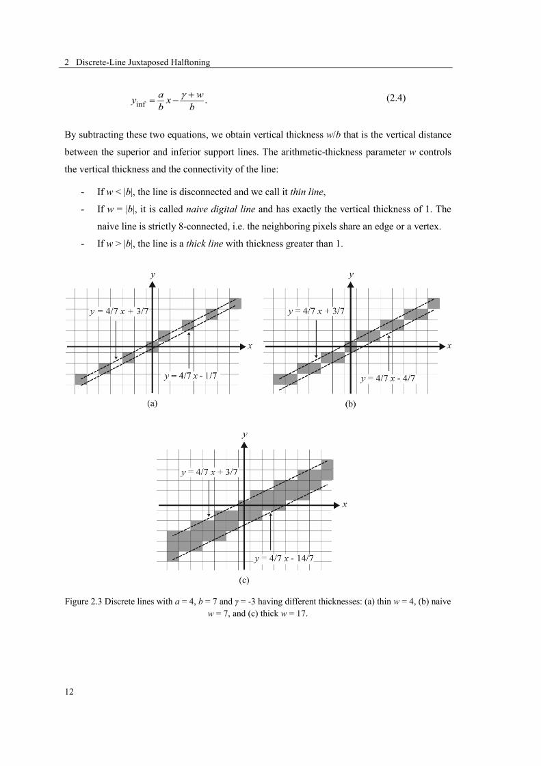
By subtracting these two equations, we obtain vertical thickness w/b that is the vertical distance
between the superior and inferior support lines. The arithmetic-thickness parameter w controls
the vertical thickness and the connectivity of the line:
- If w < |b|, the line is disconnected and we call it thin line,
- If w = |b|, it is called naive digital line and has exactly the vertical thickness of 1. The
naive line is strictly 8-connected, i.e. the neighboring pixels share an edge or a vertex.
- If w > |b|, the line is a thick line with thickness greater than 1.
Figure 2.3 Discrete lines with a = 4, b = 7 and γ = -3 having different thicknesses: (a) thin w = 4, (b) naive w = 7, and (c) thick w = 17.

2 Discrete-Line Juxtaposed Halftoning
13
Figure 2.4 Illustration of the b-periodicity of discrete lines. A discrete line with a slope equal to a/b repeats the same structure every b pixels; here a = 4 and b = 7.
Figure 2.3 shows discrete lines having different thicknesses.
Another interesting property of a discrete line is its b-periodicity. As shown in Figure 2.4, for a
given naive digital line in the first octant with parameters a and b, after b pixels in the horizontal
direction, the same line segment is repeated. Therefore, the discrete line is invariant under the
translation k [b a]T, for any integer k. The main advantage of b-periodicity is that we can limit
our study to pixels x ϵ [0, b – 1]. Furthermore, we can use this property for efficient discrete-line
plotting.
2.5 Discrete-Line Plotting
The first step towards discrete-line halftoning is the ability of generating discrete lines with any
desired rational thickness and orientation. Due to the symmetry properties of discrete lines,
without loss of generality, we limit our study to the first octant where 0 < a < b with a and b
being mutually prime1. The plotting algorithm is explained for the naive line D(a, b, γ, b) and
can be extended to thin and thick discrete lines. It has been first described by Reveillès [25].
A naive digital line is a single-valued function along one of the main axes. With 0 < a < b, for a
given value of x, there is one single value of y such that
axybγ
−= ( 2.5)
1 Horizontal, vertical and 45° oriented discrete lines can have thicknesses only in integer steps. They are therefore not usable for discrete line juxtaposed halftoning.

2 Discrete-Line Juxtaposed Halftoning
14
where the square bracket denotes the quotient of the Euclidean division. The value of y selects
the pixels whose centers are located on or below the superior continuous line (Equation (2.3))
and not located on or below the inferior continuous line (Equation (2.4), with w = b). In order to
derive an incremental formulation for drawing the naive lines, y (x + 1) can be written as
( 1) .ax ay xb bγ
−+ = + ( 2.6)
Using the classic identity
δ υ
δ υ δ υ ε εε ε ε ε
++ = + + ( 2.7)
where δ, υ and ε are integer numbers and the curly bracket denotes the Euclidean remainder, we
get
( 1) .
ax aax a b by x
b b b
γγ
− +−+ = + + ( 2.8)
Since b > a, [a/b = 0] and {a/b = a}, we obtain
( )( 1) ( ) r x ay x y xb
++ = + ( 2.9)
where
( ) .axr xbγ
−= ( 2.10)
Therefore, an increment in x results in an increment of one unit in y or in no change. The
corresponding remainder function r(x) is either increased by a or, respectively, increased by a
and decreased by b. See Algorithm 2.1 for the naive-line incremental plotting algorithm.
In a similar manner to Bresenham’s algorithm [28], this algorithm generates incrementally a set
of integer coordinates that compose a digital line with a single pixel height.

2 Discrete-Line Juxtaposed Halftoning
15
Algorithm 2.1. Incremental plotting algorithm of a naive line.
y = Div (a * x - γ, b) Integer division
r = Rem (a * x - γ, b) Integer remainder
for x = 0 to x = b - 1 do
Plot Pixel (x, y)
r = r + a
if r >= b
r = r - b
y = y + 1
end if
end for
When plotting a thin or thick discrete line of a thickness other than unity, instead of directly
plotting the discrete line D (a, b, γ, w), we synthesize a top and a bottom naive line with
parameters (a, b, γ, b) and (a, b, γnew, b) respectively, such that
new btγ γ= + ( 2.11)
where t is the vertical thickness of the desired discrete line. It is a rational number with a
denominator equal to b (see the next chapter). The plotted thin or thick discrete line is composed
of pixels with pixel centers located between these two naive lines. Pixels that belong to the top
naive line and, at the same time, do not belong to the bottom naive line as well as all pixels in
between are plotted. For a thin line, a pixel can belong to both the top and the bottom naive line.
In this case, the pixel is left blank.
2.6 Bilevel Screen-Element Generation
Classic ordered-dither halftoning methods rely on dithering with dither matrices. In contrast to
dithering methods, we create a library of predefined screen elements [29] obtained by
synthesizing discrete lines. Library entries are screen elements corresponding to the different
area coverages. Once the screen-element library is created, halftoning is performed by
traversing the output halftone-image scanline by scanline and pixel by pixel and by finding the

2 Discrete-Line Juxtaposed Halftoning
16
corresponding location in the input continuous-tone image. The color at this location determines
an entry within the screen element library. The current output pixel location determines the
location within the screen element whose colorant is to be copied into a current output pixel. Let
us first present the generation of screen elements for black and white halftoning and then, in
Section 2.7, extend the algorithm to color halftones.
We want to generate screen elements made of discrete lines and to halftone an input image by
paving the output-image plane with these discrete screen-elements. The screen element is a
discrete parallelogram whose surface is segmented into black and white parts according to the
desired black/white area coverages. These parallelogram screen-elements are created by discrete
lines of appropriate subpixel thicknesses. The parallelogram forming the screen element is
defined by its sides, given by vectors [0 T]T and [b a]T, where T is the vertical thickness of the
discrete line that forms a complete discrete parallelogram and a/b is the discrete-line slope.
Hence, within the parallelogram screen, a discrete-line segment may have a vertical thickness
between 0 and T. As an example, Figure 2.5 shows a parallelogram screen with 45% area
coverage.
In order to establish the monochrome screen-element library, the bilevel screen-elements are
generated level-by-level by creating each time within the parallelogram tile a “black” discrete
line with a vertical thickness from 0 to T, with b∙T different possible thicknesses. A discrete line
with a thickness of 0 (an empty set of pixels) corresponds to the screen element with 0 area
coverage. A discrete line with vertical thickness T corresponds to the screen element with an
area coverage of 1, i.e. a black parallelogram. Therefore, discrete-line thicknesses are 0 for a
surface coverage of 0, 1/b for a surface coverage of (1/b) ∙T, 2/b for a surface coverage of (2/b)
∙T, …, 1 for a surface coverage of 1/T, … and T for a surface coverage of 1.
In order to create the halftoned output image, the image plane is paved by replicating the
parallelogram screen-element along its side vectors [b a]T and [0 T]T. In this chapter, we restrict
our attention to the discrete parallelograms given by vectors [b a]T and [0 T]T. In the next
chapter, we introduce a method that creates parallelograms with any given side vectors.
2.6.1 Holladay’s algorithm
Instead of using parallelogram screen elements, we can produce equivalent rectangular screen-
elements that tile the plane according to Holladay’s algorithm [30]. Given a discrete
parallelogram with sides [px py]T and [qx qy]T, Holladay’s algorithm yields an equivalent L by H

2 Discrete-Line Juxtaposed Halftoning
17
rectangular tile (Figure 2.5). Paving the image plane with this rectangular tile is equivalent to
paving the plane with the original discrete parallelogram. Parameters of the equivalent
rectangular tile are
GCD( , ); .x y x yy y
p q q pH p q L
H−
= = ( 2.12)
Note that the discrete parallelogram surface is S = px qy – qx py. The L by H Holladay rectangular
tile paves the plane by being replicated horizontally, as well as diagonally, with replication
vector (tx, ty) where
; .xy x
y
v S H pt H tp
− ⋅ + ⋅= = ( 2.13)
For our special case with parallelogram side vectors [0 T]T and [b a]T the replication vector (tx,
ty) is
GCD( , ); .y xt T a t v b= = ⋅ ( 2.14)
In Equation (2.13) and (2.14), v is an integer that must be determined such that 0 < tx ≤ L. Note
that all Holladay tile parameters L, H, tx and ty are integers.
Figure 2.5 (a) Parallelogram screen element and its associated vectors and (b) paving a 20×12 output image with that screen element. Area coverage is 45%. The vertical thickness T is 4 and the slope is m = 2/5. The equivalent Holladay tile and its replications are also shown. The discrete line and Holladay’s tile
parameters are a = 2, b = 5, L = 10, H = 2, and tx = 5.
In order to create an L by H equivalent rectangular tile, the discrete parallelogram screen-
element is repeated several times along the parallelogram vectors until it covers the surface
inside the L by H rectangle. The final screen-element library size is L × H × (S+1), where L and
2 Discrete-Line Juxtaposed Halftoning
18
H are derived from Holladay’s algorithm and S+1 is the number of possible area coverage levels
(see Section 3.2).
2.7 Synthesis of Juxtaposed Color Screens
2.7.1 Size of the color screen-element library
Juxtaposed color halftoning relying on discrete lines enables creating parallelogram screen-
elements within which successive discrete-line segments are associated to different colorants.
However, trying to create a screen-element library containing the screens for each combination
of colorants at every area coverage level would require a huge memory.
To compute the number of combinations of K colorant values, including paper white, such that
each colorant can take an integer surface portion between 0 and N, where the addition of these
surface portions is equal to N, we solve the following equality
1 2 Kx x x N+ + + =
( 2.15)
where paper white is considered as the Kth colorant. The total number of solutions is the number
of non-negative solutions of Equation (2.15), which is known as the number of ways to
distribute N indistinguishable balls into K distinguishable boxes [31]
1.
N KN
+ − ( 2.16)
For example, if we consider a screen with 8 colorants and each colorant takes the value between
0 and 255, there are 13255 8 11.55 10
255+ −
≅ ×
possible combinations.
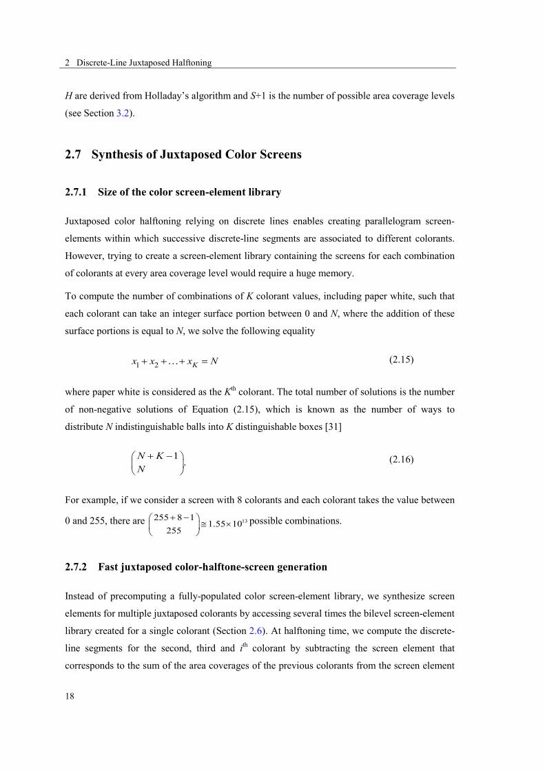
2.7.2 Fast juxtaposed color-halftone-screen generation
Instead of precomputing a fully-populated color screen-element library, we synthesize screen
elements for multiple juxtaposed colorants by accessing several times the bilevel screen-element
library created for a single colorant (Section 2.6). At halftoning time, we compute the discrete-
line segments for the second, third and ith colorant by subtracting the screen element that
corresponds to the sum of the area coverages of the previous colorants from the screen element

2 Discrete-Line Juxtaposed Halftoning
19
that corresponds to the sum of the area coverages of the new and the previous colorants. Note
that screen elements are bilevel arrays containing 1 and 0, which in the present work, represent
black and white pixels, respectively.
As an example, let us consider a screen of 25% cyan, 20% magenta and 10% yellow area
coverages with the halftoning order cyan, magenta and yellow. The cyan tile is chosen directly
from the bilevel screen element library by finding the screen tile corresponding to its area
coverage of 25%. The magenta screen is obtained by subtracting the screen tile associated with
the area coverage of cyan (25%) from the screen tile corresponding to the addition of the area
coverages of cyan and magenta, i.e. 45%. This yields the magenta part of the halftone
(Figure 2.6). Similarly, the subtraction of the screen tile assigned to cyan and magenta (45%)
from the screen tile of cyan, magenta and yellow (55%) yields the screen tile for the yellow
layer.
Figure 2.6 Example of creation of the magenta part of a screen element by subtracting the tile of surface coverage c from the tile of surface coverage c + m.
More formally, multi-colorant juxtaposed halftoning is performed by calculating the sequence
of screen colorant tiles S1(c1), S2(c2), … SK(cK)
1 1 1
2 2 1 2 1
11 1
( ) ( )( ) ( ) ( )
( ) ( ) ( )
B
B B
K Ki ii iK K B B
S c S cS c S c c S c
S c S c S c−= =
=
= + −
= −∑ ∑
( 2.17)
where we assume that the current output-image location is to be printed with c1, c2, …, cK area
coverages of the K colorants and SB(c) is the screen tile associated with area coverage c stored in
the bilevel screen-element library. This approach does not limit the number of colorants and
does not introduce any accumulated error. Figure 2.7 shows an example of a juxtaposed

2 Discrete-Line Juxtaposed Halftoning
20
halftone screen, printed with the cyan, magenta, yellow, blue, green, red, black and white
Neugebauer primaries. Also, we demonstrate the synthesis of discrete lines associated with the
first three colorants present in this halftone screen.
Figure 2.7 (a) A juxtaposed halftone screen with orientation a = 4, b = 7 and vertical thickness T = 10 with area coverages of green: 20/70, yellow: 5/70, white: 9/70, magenta: 8/70, red: 10/70, black: 7/70, blue: 0/70 and cyan: 11/70. (b) Synthesis of three colorants within the screen element by accessing the black/white screen element library: green is directly taken from the library, yellow is synthesized from the sum of green and yellow area coverages minus the area coverage of green, and magenta is synthesized from the sum of green, yellow and magenta area coverages minus the area coverage of green and yellow.
2.8 Results
In this section, we evaluate discrete-line juxtaposed halftoning with a few examples. The
selected parameters are m = 4/7 and T = 15. The halftone images are printed with the 8
Neugebauer primaries whose area coverages are calculated from amounts of cyan, magenta and
yellow inks. For the sake of simplicity, color management and gamut mapping are excluded
from the present analysis. Therefore, the reproduced colors might differ from the original image
colors. The presented examples are printed with classic inks on paper. We start with an input
image with given amounts of cyan (c), magenta (m) and yellow (y) inks and calculate the area
coverages of the 8 Neugebauer primaries according to the Demichel equations [11] as follows
(see Section 7.3.2 for more details about the use of the Demichel equations)

2 Discrete-Line Juxtaposed Halftoning
21
(1 )(1 )(1 )(1 )
(1 )(1 )(1 )(1 )(1 )
(1 )(1 )(1 )
c
m
y
b
g
r
k
w
a c m ya m c ya y c ma cm ya cy ma my ca cmya c m y
= − −= − −= − −
= −
= −
= −=
= − − −
( 2.18)
where ac, am, ay, ab, ag, ar, ak, and aw are the area coverages of the colorants cyan, magenta,
yellow, blue, green, red, black and white, respectively.
Figure 2.8 The “Fruits” and “Orchestra” halftone images reproduced by discrete-line juxtaposed halftoning. Discrete-line screen-element parameters are a = 4, b = 7 and T = 15. The image is produced
at a resolution of 600 dpi (for more details, see the electronic version).
Figure 2.8, Figure 2.9 and Figure 2.10 show the results on different images. As can be seen
from these figures, discrete-line juxtaposed halftoning enables printing with many different
colorants, preserves the edges, reproduces textures at frequencies higher than the screen
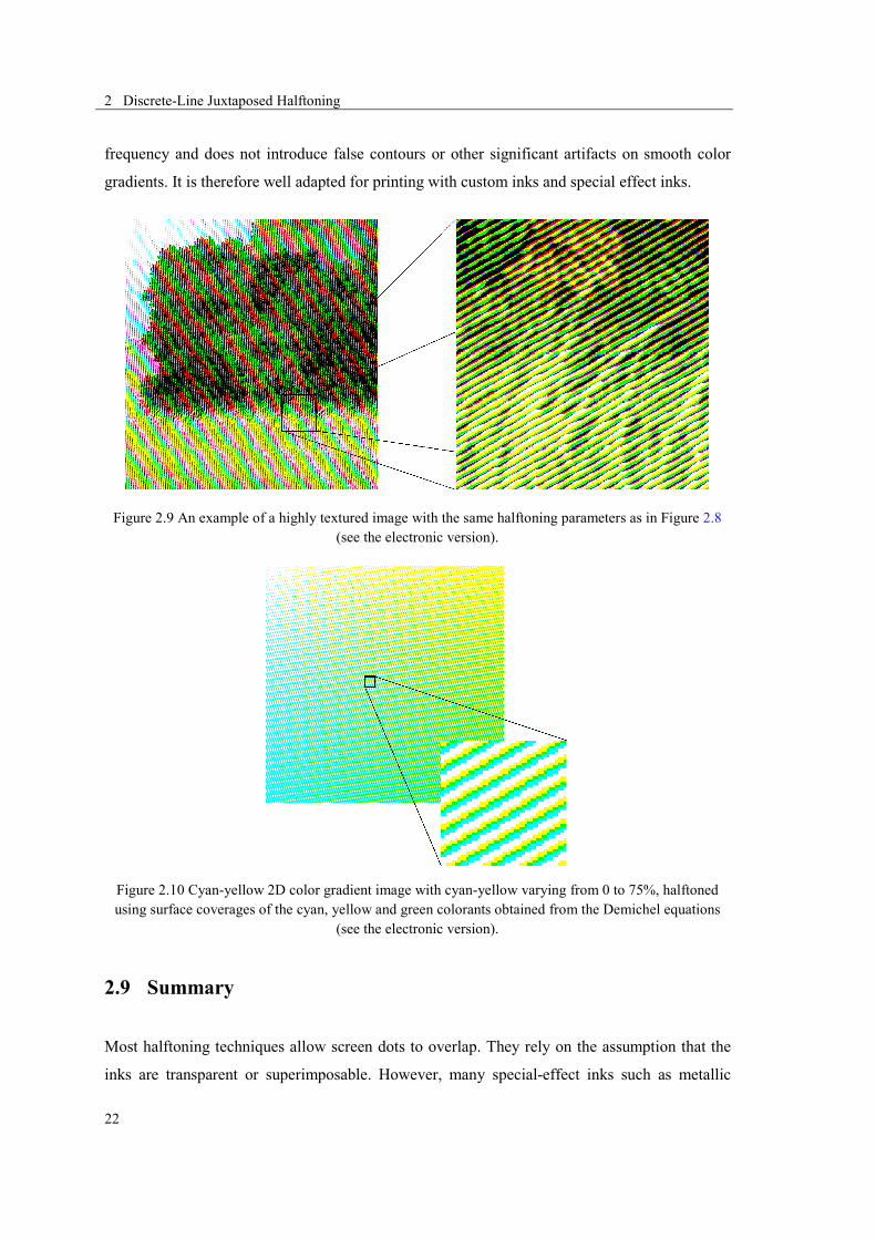
2 Discrete-Line Juxtaposed Halftoning
22
frequency and does not introduce false contours or other significant artifacts on smooth color
gradients. It is therefore well adapted for printing with custom inks and special effect inks.
Figure 2.9 An example of a highly textured image with the same halftoning parameters as in Figure 2.8 (see the electronic version).
Figure 2.10 Cyan-yellow 2D color gradient image with cyan-yellow varying from 0 to 75%, halftoned using surface coverages of the cyan, yellow and green colorants obtained from the Demichel equations
(see the electronic version).
2.9 Summary
Most halftoning techniques allow screen dots to overlap. They rely on the assumption that the
inks are transparent or superimposable. However, many special-effect inks such as metallic
2 Discrete-Line Juxtaposed Halftoning
23
inks, pearlescent inks or pigmented inks are either opaque or cannot be superposed. In order to
create halftone images, halftone dots formed by such inks should be juxtaposed, i.e. printed side
by side.
In this chapter, we presented a new juxtaposed-color halftoning method based on discrete lines.
Discrete line halftones provide colorant segments with subpixel precision made of discrete lines
with rational thicknesses. It relies on a library of bilevel screen-elements created by successions
of discrete lines. Discrete-line juxtaposed-color halftoning is performed efficiently by multiple
accesses to the screen-element library. As many colorants as desired can be juxtaposed within a
single screen-element. The quality of the resulting halftones is comparable to classic line screen
halftones. However, juxtaposed halftoning requires a high registration accuracy. Such a high
registration accuracy between colorant layers can be achieved on modern printers.
Juxtaposed halftoning can be a solution to many problems. It enables printing with partially or
fully opaque inks. Therefore, printing halftone images with metallic inks and pearlescent inks
becomes possible. Application domains comprise flexible packaging, poster design, document
security and art. In addition, the area coverages of all colorants are directly controlled, i.e. freely
chosen amounts of custom inks can be reproduced. If the halftone screen is too small, the
method might suffer from a quantization error after the continuous values of colorants to integer
number of pixels inside the screen are assigned. Whereas, large screens have the drawback of
creating visible halftones. In the next chapter, we address this trade-off by introducing
superscreens.

2 Discrete-Line Juxtaposed Halftoning
24

3 Superscreen and Automoiré in Discrete-Line Juxtaposed Halftoning
25
3.1 Introduction
Angled screens are highly desirable in clustered-dot halftoning method. However, there is an
inherent limitation in achieving all angles on a digital grid. There are only a finite set of screen
directions that are represented by vectors with integer values. Because the angles of these
vectors are the arc tangent of the ratio of two integers, the screens are referred to as rational
tangent screens [14].
Although all rotation angles cannot be produced precisely, we can achieve close approximations
with large direction vectors. The key trade-off in digital halftoning is therefore the number of
intensity levels versus the halftone frequency. Large vectors lead to larger screens that have
more gray levels hence a better tone reproduction. However, they replicate at a lower frequency
and are therefore more visible.
Superscreens or supercells are a solution to this classic trade-off. They are very large screens
that contain a number of individual halftone cells. They produce rational-tangent screens with
large integers, which generate almost perfect angles. The number of intensity levels is the
3 3 Superscreen and Automoiré in
Discrete-Line Juxtaposed Halftoning

3 Superscreen and Automoiré in Discrete-Line Juxtaposed Halftoning
26
number of pixels inside the large superscreen. Whereas, the screen frequency appearing to the
eye comes from the smaller halftone cells inside superscreen.
Classic superscreens can be created by replicating a dither tile a number of times, for example 4,
by multiplying accordingly the dither threshold levels, and by distributing intermediate
threshold values among the replicated tiles. Figure 3.1 shows an example of a dither tile with
originally 5 dither levels, which due to the superscreen construction, is expanded to 20 levels.
As we see in this simple example, the corners of the larger cell define the rational tangent angle.
Note that it is not necessary for the individual dither cells to be congruent. Each has a slightly
different shape and contains a slightly different number of dither values.
In this chapter, we first discuss the discrete-line juxtaposed-halftone screen properties. We show
that characteristics of a discrete-line screen are controlled mainly by its two parameters: line
slope and vertical thickness. We also introduce the method for constructing a superscreen for
discrete-line juxtaposed halftones. In addition to the classic benefits of a superscreen, we
demonstrate that the superscreen can be a solution to automoiré, an objectionably visible artifact
due to the interaction between the halftone grid and the device grid. For this purpose, we
analyze how discrete-line segments are formed and how a discrete line grows inside a screen
when its thickness is increased. When the number of subscreens in a discrete-line superscreen
increases, the artifacts begin to intensify even more severely than in single screens. Therefore,
we introduce 2D discrete-line juxtaposed superscreens.
Figure 3.1 A classic superscreen where the original tile with 5 dither values is expanded to a superscreen of 20 dither values.
3.2 Discrete-Line Juxtaposed Screen Properties
Let us first calculate the number of possible area coverages (or gray levels) inside a discrete-line
halftone screen. Recall from the Chapter 2 that our juxtaposed screen-element is formed by a

3 Superscreen and Automoiré in Discrete-Line Juxtaposed Halftoning
27
parallelogram made of a discrete-line segment with a given thickness and orientation. The
parallelogram forming the screen element is defined by its sides given by vectors [0 T] and [b a]
where T is the vertical thickness of the discrete line and a/b is the discrete line slope
(Figure 3.2).
Figure 3.2 An output halftone image and the parallelogram screen-element. The vertical thickness T is 4 and the slope is a/b = 2/5. Current rational area coverage is 9/20.
The number of possible area-coverages inside a discrete line screen is determined by the area of
the discrete parallelogram tile. It is the cross product of the parallelogram vectors plus one level
that refers to zero area-coverage where nothing is printed:
T T#Levels 1 ([0 ] [ ] ) 1 .T b a bT= + × = + ( 3.1)
The classic trade-off of the number of levels versus the halftone frequency is also present in
discrete-line juxtaposed halftoning. A large parallelogram tile provides many variations of area
coverages, hence a precise tone reproduction; but depending on the output device resolution, it
might become visible to the naked eye.
For a fixed line slope m = a/b, let us investigate the role of the vertical thickness T. The number
of possible area coverages increases proportionally with the vertical screen tile thickness T,
yielding a larger number of discrete colors and larger screen dots. With a large screen thickness
T, small area coverages still yield connected lines. With a smaller thickness T, the same area
coverages result in thin, disconnected lines. Compare Figure 3.3a that shows a screen tile with a
vertical thickness of T = 10 and Figure 3.3b that shows a screen tile with T = 6 where the same
colorant area coverages are reproduced. In the smaller screen tile of Figure 3.3b, the line
colorants are thin thus less clustered. This can cause a problem on some printers where single
isolated pixels of a given colorant either have a major dot gain or tend to disappear.

3 Superscreen and Automoiré in Discrete-Line Juxtaposed Halftoning
28
Figure 3.3 (a) A juxtaposed halftone screen of orientation a = 4, b = 7 and vertical thickness T = 10 with area coverages of green: 20/70, yellow: 5/70, white: 9/70, magenta: 8/70, red: 10/70, black: 7/70, blue:
0/70 and cyan: 11/70. (b) Another screen with the same parameters but with a smaller vertical thickness T = 6. The corresponding parallelogram screen tiles are also shown.
The main drawback of a large vertical thickness T is the low halftone-frequency. According to
Figure 3.4, the screen frequency is
2 2
cosd d d a bfh T b Ta
+= = =⋅
( 3.2)
where f is the screen frequency in screen elements per inch (lpi), d is the printer resolution in
pixels per inch (dpi) and α is the angle of the screen-element parallelogram support-line with
. Due to symmetry, it is enough to consider 0 < α < 45°. Increasing T leads
to a decrease of the halftone frequency hence to more visible halftones.
The influence of angle α = arctan(a/b) is another interesting factor. According to Equation (3.2),
angles close to 45° deliver the highest halftone frequencies. This is of great interest as the
human visual system has less acuity for diagonal lines than for vertical and horizontal lines.
However, an angle of exactly 45° is a special case in which a = b = 1 where only integer vertical
thicknesses are possible, therefore the number of different colorants’ area coverages is limited
to T. Nevertheless, angles close to 45° have a relatively high frequency, offer bT different
thicknesses and are less visible to the human visual system.
2 2cos /b a ba = +

3 Superscreen and Automoiré in Discrete-Line Juxtaposed Halftoning
29
Figure 3.4 Screen parallelogram orientation α, vertical thickness T, and screen period h.
3.3 Discrete-Line Juxtaposed Superscreen
As discussed in Section 3.2, a large vertical screen thickness T and/or large values of b (and
consequently of a) result in a large number of area coverages and a small surface color
discretization-error. This term is coined to describe the difference between the intended area
coverage of a particular colorant and the actual generated area-coverage that is limited by the
screen-element surface, i.e., the number of cells inside the screen-element.
There is a trade-off between a low surface color discretization-error achievable with large
values of T and/or b and the visibility of the screen element. In order to keep the surface color
discretization-error small, it is desirable to increase the number of area coverages without
making the screen element more visible. This can be obtained by extending the current discrete
parallelogram-screens to superscreens. Superscreens in discrete-line juxtaposed halftoning
follow the same principles as clustered-dot multicenter superscreens [14].
In order to create a superscreen for discrete-line halftoning, we create a large discrete-line
parallelogram-tile containing the desired number of area coverages. We split the parallelogram
superscreen vertically into a desired number of subscreens (e.g. two). The intended area-
coverage of each colorant is then distributed as equally as possible between the subscreens of
the superscreen. For this purpose, the vertical thickness of the superscreen is split into rational
vertical sub-thicknesses of similar sizes. We explain in Section 3.5 how a rational sub-thickness
can create cells with different phases inside a superscreen. Note that if the subscreens have
significantly different areas, they can generate a beating effect visible on smooth color surfaces.
Figure 3.5 shows a parallelogram superscreen with vertical thickness of T = 9 divided into two
subscreens. The screen frequency that appears to the human eye is the screen frequency of the

3 Superscreen and Automoiré in Discrete-Line Juxtaposed Halftoning
30
subscreen, whereas the number of area coverages is given by the area of the superscreen. Within
different sub-tiles, same colorants have slightly different area coverages.
Figure 3.5 A discrete line superscreen composed of two smaller, slightly different subscreens filled with two colorants. Within the subscreens, respective colorants may have slightly different area coverages.
3.4 Automoiré in Discrete-Line Juxtaposed Halftoning
In classic color halftoning methods, moiré generally results from the superposition of two or
more periodic superposed ink-layers. A well-known solution for avoiding the moiré produced
by the superposition of layers is to rotate them by 30° with respect to each other [16].
Juxtaposed halftoning does not create superposition moiré, because ink layers are laid-out side
by side. However there are aliasing effects that occur during line discretization on the output
device grid. The repetition of these effects creates undesired low-frequency components called
automoiré [32].
Automoiré, also called internal moiré, results from the interference between the halftone and the
device grid. In general, methods for reducing automoiré break the regular patterns by
randomization. They either try to vary the period of halftone dots [33, 34] or to correct
quantization errors by an error diffusion process [35, 36]. It is also possible to suppress
automoiré artifacts with antialiasing filters [37, 38].
In discrete-line juxtaposed halftoning, the parallelogram screens made of discrete-line segments
repeat themselves in both directions within the discrete plane. To achieve less visible halftones
on a device with limited resolution, the screen frequency can be increased by decreasing the
vertical period T. However, an increased screen frequency can result in automoiré artifacts.
When the device resolution is high compared to the screen frequency, the artifacts tend to

3 Superscreen and Automoiré in Discrete-Line Juxtaposed Halftoning
31
vanish. These artifacts occur both in black-and-white and color halftones. For the sake of
simplicity, we limit our analysis to black and white halftones. Solutions for black-and-white
halftones also apply to color halftones.
Figure 3.6 shows three discrete-line halftones and their magnified bitmaps having identical line
slope (a/b = 4/7) but different vertical periods T, specifically 10, 8 and 6. To make the example
clear, an area-coverage was chosen at which the vertical thickness of the discrete line is 8/7,
hence it has a discrete thickness of two pixels at a certain location. When printing these bitmaps
at 600 dpi, we obtain three patches of different appearances. While the patch with the lowest
frequency (T = 10) exhibits no perceptually strong artifacts, the two other patches show a
vertically disturbing visual effect, more visible at positions where the discrete line has a
thickness of two pixels. On displays, anti-aliasing methods avoid this artifact by adapting the
gray levels of neighboring pixels [39]. On a binary printer, however, this solution is not
applicable.
Figure 3.6 Three halftone patches and their corresponding bitmaps. The discrete-line slope is a/b = 4/7 and the vertical thickness for figures (a), (b) and (c) is 10, 8 and 6, respectively. The chosen area coverage
for each patch corresponds to a discrete line with thickness w/b = 1 + 1/b, i.e. at a certain location the discrete line is two pixels thick. The bottom row shows the halftone patches at the real size at 600 dpi and
also enlarged by a factor of 5×5 (see the electronic version).

3 Superscreen and Automoiré in Discrete-Line Juxtaposed Halftoning
32
3.5 Reducing the Automoiré
When replicating the discrete lines with an integer vertical offset, the same staircase belonging
to different discrete lines is repeated at a certain vertical distance. From Figure 3.6, we can see
that this vertical repetition of identical discrete-line segments yields automoiré. The automoiré
becomes more visible when the vertical distance is reduced, i.e. when the screen frequency is
increased. In contrast to a single screen, in a superscreen there is a rational vertical distance
between a discrete line and its immediate top or down neighbor. Successive rational distances
inside a superscreen induce a zigzag replication path that breaks the visually objectionable
frequency induced by a straight vertical path. In this section, we will explain how the rational
distance between discrete lines replicates the identical line-segments in a direction different
from the vertical.
Let us have a closer look at the formation of the discrete line superscreen. By displacing the
discrete lines with a rational value, we are able to choose different locations on the plane where
the identical staircases of the repeated discrete lines occur. According to the naive-line drawing
algorithm [40], the pixels are drawn by rounding down the y coordinate of their superior
support-line given by the following equation
sup .ay xb b
γ= − ( 3.3)
The corresponding remainder function r(x) of the discrete line is defined by
( )axr x
bγ−
=
( 3.4)
where the curly bracket denotes the Euclidean remainder.
The remainders function r (x) characterizes the formation of the digital line. The vertical
distance between the superior support-line and the discrete pixel center located just below is r
(x) / b. The remainder-function range includes the set of integers between 0 and b − 1. The first
pixel occurs at an abscissa where the vertical distance is zero, i.e. the discrete pixel center is on
the superior support-line. Hence, the first pixel of a naive line occurs at abscissa x1 where r (x1)
= 0, the second at x2 where r (x2) = 1, and so on, until the last pixel xb where r (xb) =b – 1.

3 Superscreen and Automoiré in Discrete-Line Juxtaposed Halftoning
33
The sequence of remainders characterizes the succession of segments forming the digital line
and depends only on a and b. The coefficient γ determines the order of this sequence [26].
Figure 3.7 clarifies the order of discretization of a naive digital line. This figure shows 7
possible discrete thicknesses for a line with a/b = 4/7. If we consider the right-hand side period
of the discrete line in Figure 3.7, the first staircase pixel forms at the location of r (x) = 0, i.e. x =
1. When increasing the discrete-line thickness, the second staircase pixel occurs at x = 3 where r
(x) = 1 and so on. Note that, due to b-periodicity, the same sequence of remainders occurs after
each set of b pixels in the x direction.
The discretization of a thick discrete line follows the same order of a digital naive line. In the
current example, if we continue increasing the line thickness, the (b +1)th pixel would occur at
the same abscissa of the first pixel of the naive line (x = 1) but in an ordinate just below it, the (b
+2)th pixel would occur at the same abscissa of the second pixel of the naive line (x = 3), and so
on.
Figure 3.7 The order of discretization of a naive digital-line segment (a = 4, b = 7). Discrete lines with all possible thicknesses are drawn.
In Figure 3.7 the lines are vertically displaced with 1-pixel shifts. A discrete line can be shifted
by a rational vertical thickness that is a multiple of 1/b. Therefore, the discrete-line segment
replicate at a vertical offset t/b, where t ∊ ℤ. The remainder function of the replicated line is
2( )
( ) .ax t ax tr x
b b bγ γ− + −
= = −
( 3.5)

3 Superscreen and Automoiré in Discrete-Line Juxtaposed Halftoning
34
Using the identity (2.7), we obtain
2 ( ) .
ax tax t b br x b
b b b
γγ
− −+
− −= + −
( 3.6)
When t is a multiple of b, i.e. we have an integer displacement, 0t
b−
=
and the remainder
function r2(x) is the same for the original and the replicated discrete line. If t is not a multiple of
b, the remainder function differs from the original one according to the value of t.
Consequently, the discretization of the original line and that of the replicated line will be shifted
in respect to each other.
Figure 3.8 shows an example where a discrete line is displaced by an integer and also a rational
vertical shift.
When replicating the discrete lines with an integer vertical offset, i.e. when t is a multiple of b,
each staircase is repeated at a certain vertical distance. In case the discrete line is repeated with a
rational displacement t/b, with t ≠ kb, the staircase is replicated in a direction different from the
vertical. We look for successive staircase repetition-vectors that break the visually
objectionable base frequency induced by a single repetition-vector.
Staircase repetition-vectors define the relative position of corresponding staircases in successive
colorant lines. The vector pointing from the first pixel of the original discrete line to the
corresponding first pixel of the next discrete line is the repetition vector. To compute the
staircase repetition-vectors, the coordinates of the first pixels of the successive lines are
computed. We define the first pixel of the discrete line D (a, b, γ, w) as a pixel whose center
p1(x1, y1) intersects the superior support-line. By definition, the remainder function given by
Equation (3.4) at the integer x coordinate of this pixel has a value of zero. In other words
( ).ax k b kγ− = ⋅ ∈ ( 3.7)
This equation is equivalent to the following linear congruence.
(mod )ax bγ≡ ( 3.8)

3 Superscreen and Automoiré in Discrete-Line Juxtaposed Halftoning
35
(a) (b)
Figure 3.8 Effect of displacing a discrete line (a = 4, b = 7). The first pixels of the discrete lines are shown with a dashed square. (a) The top line is displaced by a rational distance of 28/7 (= 4). Both
discrete lines are identical. (b) The top discrete line is displaced with a rational distance of 33/7 (= 4 5/7). Both discrete lines are identical except that their order of formation is different because of their different
remainder functions.
This linear congruence can be solved for x and among many solutions we choose the one that is
less than b (x1). The first pixel of the original discrete line, according to Equation (3.3), has the
integer ordinate
11 .
axy
bγ−
= ( 3.9)
We choose a new value of γ for the replicated discrete line. Then we compute its first pixel
coordinate p2(x2, y2) with the same procedure as for the original line. Having computed the first
pixels of two successive discrete lines, the first to second discrete-line repetition-vector is
computed by subtracting the two coordinates, i.e. v12 = p2 – p1.
The supertile screen-element paves the plane by two vectors with integer components: (b, a) and
(0, T). We fragment the vertical distance T into several rational distances. For the sake of
simplicity, we are interested in a few rational displacements, for example, an integer
displacement divided into two rational displacements. Let us consider a discrete supertile
parallelogram with a slope of 4/7 and a vertical period T = 15. We can divide the supertile
vertical thickness T = 15 into two rational thicknesses, for example T1 = 52/7 and T2 = 53/7.
This results in two subscreen tiles of slightly different vertical thicknesses. As shown in

3 Superscreen and Automoiré in Discrete-Line Juxtaposed Halftoning
36
Figure 3.9, because of the rational vertical displacements between one subscreen tile and the
next, the second discrete line is horizontally shifted in respect to the first one. As the sum of the
two rational displacements yields an integer displacement, the third discrete colorant line has
exactly the same staircase layout as the first discrete colorant line at a vertical distance T = 15
pixels from it. Although the actual screen frequency of the halftone is close to those shown in
Figure 3.6 b and c, the visible automoiré is considerably reduced.
Figure 3.9 Staircase repetition-vectors, supertile (solid line) and subscreens (dashed line) of the halftone with a/b = 4/7, T1 = 52/7 and T2 = 53/7. The right-hand view shows the halftone patches at the real size at
600 dpi and also enlarged by a factor of 5×5 (see the electronic version).
Replicating discrete lines with two arbitrary selected vertical rational displacements does not
automatically solve the problem of automoiré. For example, consider the halftone with a line
slope composed of large a and b, a/b = 13/18. Figure 3.10 shows the magnified pixel-map as
well, as the patch in real size, for an integer vertical thickness T = 7. It exhibits a clearly visible
automoiré artifact in form of vertical dotted lines. In order to reduce this automoiré, we could
try to bisect the vertical period T = 15 to obtain a screen-element vertical period almost equal to
7 (15/2), by using two rational periods T1 = T2 = 135/18. As shown in Figure 3.11, the resulting
halftone patch still incorporates the same automoiré intensity but at an orientation different from
the vertical orientation. As the two rational vertical displacements T1 and T2 are identical, the

3 Superscreen and Automoiré in Discrete-Line Juxtaposed Halftoning
37
displacement vector v21 repeats itself between successive discrete lines. The orientation of this
repetition vector defines the orientation of the automoiré in the halftone patches.
Figure 3.10 Automoiré in the vertical direction for the halftone with line slope a/b = 13/18 and T = 7. We show also the parallelogram screen element. The right-hand view shows the halftone patches at the real
size at 600 dpi and also enlarged by a factor of 5×5 (see the electronic version).
In order to avoid the automoiré in a new orientation, the challenge is to find the optimum pair of
staircase displacement-vectors. The only parameter that can be changed to obtain different
staircase repetition-vectors is the rational distance between the original discrete colorant line
and its replicated instance. For the latter case of a/b = 13/18, by choosing two different
repetition vectors, such as T1 = 134/18 and T2 = 136/18, the artifacts are significantly reduced
but not completely eliminated (Figure 3.12). When b (and consequently a) is a large number,
one period of a discrete line is composed of several distinct pixel staircases. Hence, even when
avoiding identical repetition-vectors, new dot configurations may appear and produce a visible
automoiré. With small slope-parameters, there are potentially less moiré generating
configurations [41].
We can also create a superscreen with more than two cells. An integer vertical period can be
divided into several rational numbers. This results in a sequence of staircase repetition-vectors
that forms a path showing the relative position of corresponding pixels on different discrete
lines inside the superscreen. We notice that, regardless of the staircase path, the automoiré
persists and even intensifies with a larger number of screens within the superscreen. The reason
is that with more subscreens, we have larger structures in the vertical direction that repeat in the
horizontal direction every b pixels. As b increases, the repetition period is lower and the
automoiré becomes more visible.

3 Superscreen and Automoiré in Discrete-Line Juxtaposed Halftoning
38
Figure 3.11 Automoiré in new direction for the halftone with line slope a/b = 13/18 and two rational periods T1 = T2 = 135/18. The automoiré orientation is shown by the repetition vector v21 = (9, –1). The
right-hand view shows the halftone patches at the real size at 600 dpi and also enlarged by a factor of 5×5 (see the electronic version).
Figure 3.12 Halftone with line slope a/b = 13/18 and two rational periods T1 = 134/18 and T2 = 136/18. The repetition vectors are v12 = (2, –6) and v21 = (–2, –9). The right-hand view shows the halftone patches
at the real size at 600 dpi and also enlarged by a factor of 5×5 (see the electronic version).
3.6 2D Discrete-Line Superscreen
The main cause of automoiré is the repetition of identical line-segments along a fixed direction.
We showed that breaking this regular pattern along the direction (0, T) can reduce the

3 Superscreen and Automoiré in Discrete-Line Juxtaposed Halftoning
39
automoiré. When we generate superscreens with a large number of screens, we observe that
moiré artifacts also occur due to the repetition along the discrete line slope (b, a).
Figure 3.13 shows an example of a vertical superscreen with 5 subscreens. This supertile
exhibits strong artifacts in the direction of the line slope. As the repeated structure is large, the
artifact is more pronounced. The situation deteriorates with larger slopes, as the structures
repeat with a lower frequency. This was the trigger for our idea to create superscreens that do
not repeat in a regular manner along the second direction (hence the name 2D superscreens).
Figure 3.13 1D superscreen with line slope a/b = 11/15 and T = 35. There are 5 subscreens with 5 rational periods T1 = 103/15, T2 = 109/15, T3 = 104/15 and T4 = 108/15 and T5 = 101/15. The resulting
halftone shows severe automoiré due to the large pixel staircase structures that repeat along the discrete-line slope (see the electronic version).
3.6.1 2D discrete-line plotting
In Section 2.5, we explained how to plot a discrete line of any thickness. As halftone screens
were limited to strictly vertical screens, parallelogram screens could be represented as discrete
lines with different thicknesses. In this section, we first introduce a method of creating single
parallelogram halftone-screens with two arbitrarily oriented side vectors. Recall that up to now,

3 Superscreen and Automoiré in Discrete-Line Juxtaposed Halftoning
40
the screens always have a vertical side (0, T). Then, in the next section, we illustrate the
synthesis of 2D superscreens by placing several single screens adjacent to each other.
Let m = (b, a) and t = (d, c) be the two sides of a parallelogram screen-element. In order to
discretize the parallelogram with thickness w/b assigned to the side with slope m, it is sufficient
to intersect two discrete lines D1 (a, b, γ, w) and D2 (c, d, µ, υ). D1 and D2 are each represented
with a pair of analytical lines illustrated as dotted and dashed lines in Figure 3.14. Parameters γ,
µ and υ are calculated knowing the point at the origin of vectors t and m. The only varying
parameter w belongs to D1 and is equal to the number of pixels resulting from the intersection.
This can be verified by calculating the area of a parallelogram formed by D2 and D1 with
thickness w/b. Note that we could grow the screen in another direction by building it on line D2.
Figure 3.14 The intersection of two thick discrete lines D1 (a, b, γ, w) and D2 (c, d, µ, υ) results in w pixels of the parallelogram with vertical thickness w/b.
The following method describes the intersection of two discrete lines [42]. The intersection is
the solution of the following equation system in ℤ2:
ax by wcx dy
γ γµ µ υ
≤ − < +≤ − < +
( 3.10)
where the two thick discrete lines are not parallel, i.e. ad – bc ≠ 0. Furthermore, the orientation
coefficients need not to be mutually prime thereby allowing any size for the screen element.
If g = GCD (a, b), a´ = a/g and b´= b/g, we can rewrite the Equation (3.10) in matrix form:
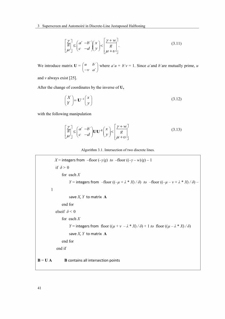
3 Superscreen and Automoiré in Discrete-Line Juxtaposed Halftoning
41
´ ´ .wxa bg g
yc d
γγ
µ µ υ
+−
≤ <− +
( 3.11)
We introduce matrix U = ´´
u bv a
−
where a´u + b´v = 1. Since a´and b´are mutually prime, u
and v always exist [25].
After the change of coordinates by the inverse of U,
1 xXyY
−
=U ( 3.12)
with the following manipulation
´ ´ wxa bg gyc d
γγ
µ µ υ
+−
≤ <− +
-1UU ( 3.13)
Algorithm 3.1. Intersection of two discrete lines.
X = integers from –floor (–γ/g) to –floor ((–γ – w)/g) – 1
if δ > 0
for each X
Y = integers from –floor ((–µ + λ * X) / δ) to –floor ((–µ – v + λ * X) / δ) –
1
save X, Y to matrix A
end for
elseif δ < 0
for each X
Y = integers from floor ((µ + v – λ * X) / δ) + 1 to floor ((µ – λ * X) / δ)
save X, Y to matrix A
end for
end if
B = U A B contains all intersection points
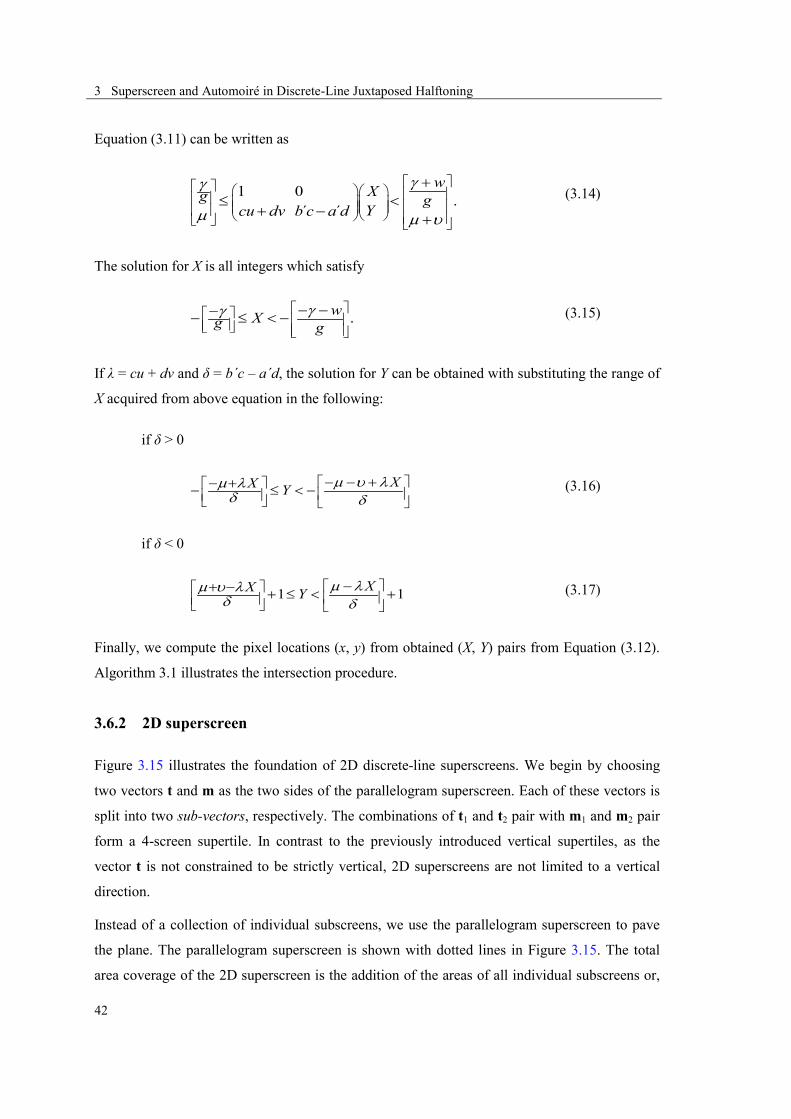
3 Superscreen and Automoiré in Discrete-Line Juxtaposed Halftoning
42
Equation (3.11) can be written as
1 0 .´ ´
wXg gYcu dv b c a d
γγ
µ µ υ
+≤ <
+ − +
( 3.14)
The solution for X is all integers which satisfy
.wXg gγγ
− −−− ≤ < − ( 3.15)
If λ = cu + dv and δ = b´c – a´d, the solution for Y can be obtained with substituting the range of
X acquired from above equation in the following:
if δ > 0
XX Y µ υ λµ λδ δ
− − +− +− ≤ < − ( 3.16)
if δ < 0
1 1XX Y µ λµ υ λδ δ
−+ − + ≤ < + ( 3.17)
Finally, we compute the pixel locations (x, y) from obtained (X, Y) pairs from Equation (3.12).
Algorithm 3.1 illustrates the intersection procedure.
3.6.2 2D superscreen
Figure 3.15 illustrates the foundation of 2D discrete-line superscreens. We begin by choosing
two vectors t and m as the two sides of the parallelogram superscreen. Each of these vectors is
split into two sub-vectors, respectively. The combinations of t1 and t2 pair with m1 and m2 pair
form a 4-screen supertile. In contrast to the previously introduced vertical supertiles, as the
vector t is not constrained to be strictly vertical, 2D superscreens are not limited to a vertical
direction.
Instead of a collection of individual subscreens, we use the parallelogram superscreen to pave
the plane. The parallelogram superscreen is shown with dotted lines in Figure 3.15. The total
area coverage of the 2D superscreen is the addition of the areas of all individual subscreens or,

3 Superscreen and Automoiré in Discrete-Line Juxtaposed Halftoning
43
equivalently, the area of the corresponding supertile parallelogram, i.e. the cross product of
vectors t and m.
Figure 3.15 A 2D discrete-line superscreen with sides t = (1, 13) and m = (15, 8) shown with dotted lines. Vector t is composed of two sub-vectors t1 = (3, 7) and t2 = (–2, 6) and m is composed of two sub-vectors
m1 = (7, 3) and m2 = (8, 5).
The dot growth inside a superscreen should also be carefully controlled. The first black pixel
corresponding to the first gray level can be located in any of the subscreens. Its exact location
inside the cell is determined according to the plotting algorithm that we described in
Section 3.6.1. The second black pixel is preferred to be in a different vertical level from that of
the first subscreen. If we place both pixels in a subscreen that shares the same vertical sub-
vector, the halftone will be more visible because the pixels replicate in a longer vertical
distance. Taking the supertile of Figure 3.15 as an example, the first pixel can be placed inside
the subscreen built by m1 and t1, the second inside the subscreen with m2 and t2, the third in the
subscreen made of m1 and t2 and the fourth in the subscreen with m2 and t1 as sides. The
subsequent pixels follow the same order as the first four pixels.
Subscreens inside a superscreen are not identical. The ensembles of two slopes that build each
single parallelogram subscreen are not identical. The subscreens therefore have a slightly
different shape but should not contain a significantly different numbers of pixels.
In Figure 3.16 we show a discrete-line juxtaposed halftone produced using a 2D superscreen.
We place four subscreens inside a superscreen of sides m = (14, –7) and t = (3, –14). The side
m of the superscreen is decomposed into m1 = (7, –3) and m2 = (7, –4) and side t is decomposed
into t1 = (1, –7) and t2 = (2, –7). The total area coverage of the supertile is the sum of the areas
of each individual subscreen. The decomposition of the large side vectors into sub-vectors

3 Superscreen and Automoiré in Discrete-Line Juxtaposed Halftoning
44
should be carried out such that the areas of the four subscreens remain similar but not identical.
The resulting halftone patch does not show a significant artifact, especially when compared to a
screen of the same size like Figure 3.6c.
Figure 3.16 A 2D discrete line superscreen with sides t = (3, –14) and m = (14, –7). Vector t is composed of two sub-vectors t1 = (1, –7) and t2 = (2, –7) and m is composed of two sub-vectors m1 = (7, –3) and m2
= (7, –4) (see the electronic version).
The superscreen in Figure 3.16 is a 2×2 supertile with 4 screens inside. With our proposed
method, it is straightforward to create superscreens with a different number of screens.
Figure 3.17 shows a few examples of superscreens without significant automoiré artifacts. The
parameters have been selected in a heuristic way and keep the different subscreen areas similar.
When expanding the superscreens in order to achieve a larger number of subscreens, e.g. 3×3
superscreen, severe artifacts appear. The space of solutions expands quickly and it is not easy to
find by trial and error appropriate parameters for the subscreen. In the future, it would be
interesting to find the parameters of a superscreen of any size, automatically, using an
optimization procedure. For this purpose, a well-defined quality metric is needed.
3.7 Summary
The properties of discrete-line juxtaposed halftone-screens are governed by a few parameters,
namely line slope and vertical thickness. Discrete-line halftone superscreens, similar to their
clustered-dot counterparts, offer more gray levels for tone reproduction without decreasing the
halftone screen frequency.

3 Superscreen and Automoiré in Discrete-Line Juxtaposed Halftoning
45
Figure 3.17 A few superscreens of different sizes: 1×2, 1×3 and 2×2 from left to right, respectively (see the electronic version).
Automoiré in discrete-line halftoning is caused by the periodic occurrence of staircases along a
fixed direction. It occurs when paving the plane with discrete parallelogram screen-elements. In
order to reduce automoiré artifacts, we divide a supertile into two screen-element tiles. By
selecting different rational distances between successive discrete lines of the same colorant, we
ensure that they have different phases with respect to the device grid. For two screen-elements
within one supertile, we select a repetition vector that is different from one discrete line to the
next discrete line of the same colorant. This breaks the monodirectional automoiré artifact into
two less visible artifacts with different orientations.
When the size of a discrete-line superscreen increases, there are potentially more artifacts. We
therefore propose 2D halftone superscreens, where the exact repetition of discrete-line segments
is perturbed along both directions.
In summary, in the absence of automoiré, halftones generated by single screen-elements yield
the best visual quality and smoothest texture. Therefore, single-screen discrete-line juxtaposed
halftones are recommended when they yield the desired tonal variations and screen frequency.
They start to generate artifacts when we increase the screen frequency significantly.
Superscreens in one direction help producing more gray levels without decreasing the halftone
frequency. The quality however deteriorates with a larger number of subscreens. Two-
dimensional superscreens reduce the decline in quality by perturbing the distributions of
subscreens along both dimensions. In other words, a valid option is to place four subscreens in a
2D superscreen rather than in a 1D superscreen. In order to create the superscreens with a larger
number of subscreens, a quality criterion is necessary to obtain optimal screen parameters.

3 Superscreen and Automoiré in Discrete-Line Juxtaposed Halftoning
46

4 Predictive Two-by-Two Dot-Centering Model
47
4.1 Introduction
As we mentioned at the beginning of this dissertation (Section 1.2), printer characterization is
the key step in a color-reproduction workflow. A flexible means for characterizing a printer is a
color-prediction model. The color-prediction model specifies the color response of a given
printer when it prints with a given amount of ink. Most color prediction models are established
by learning from a set of color measurements called a calibration set. Once calibrated, the
models predict the reflectances of halftones printed with known nominal area coverages of the
inks. In general, a model is calibrated for a fixed combination of paper, inks, halftones and
measurement geometry. Changing one of these parameters requires a change in the whole or
part of the calibration step.
A particular model, which is of great interest in the context of this dissertation, is the two-by-
two dot-centering model. In this chapter, we explain this model in detail and introduce an
improvement that facilitates its calibration. We propose a solution that reduces the size of the
calibration set to less than 10% of the original size with a negligible loss in the model accuracy.
We describe our proposed improvement and test it on classic halftoning methods. We dedicate a
4 4 Predictive Two-by-Two Dot-Centering
Model

4 Predictive Two-by-Two Dot-Centering Model
48
chapter to this method as it can be used independently of other contexts of this thesis. In the
next chapter, we apply the two-by-two dot-centering model for the color prediction of
juxtaposed halftones.
Color-prediction models need to account for the dot gain. The area of deposited ink dot in a
print is generally larger than its nominal area coverage, which leads to the ink spreading
phenomenon responsible for physical dot-gain. In addition, the lateral scattering of light within
the paper substrate and the internal reflections at the interface between the print and the air are
responsible for what is called optical dot-gain, also known as the Yule-Nielsen effect. The two-
by-two dot centering model [12] accounts for both the physical and optical dot gain in an
explicit manner. It uses as primaries the measured reflectance of all different two-by-two pixel
configurations. In order to create patches large enough to be measured with a
spectrophotometer, each two-by-two pattern is replicated and printed. We call these macro
patches two-by-two tile patterns. The model is therefore able to capture the physical and optical
dot-gain within its set of primaries, also called calibration patterns. The reflectance of any
halftone is then predicted by determining, at each position of the halftone, the corresponding
two-by-two tile patterns and by averaging their measured reflectances with the Yule-Nielsen
formula.
This halftone-independent spectral prediction model has the drawback of requiring a very large
number of measurements for characterizing a given 3- or 4-ink print setup. In this chapter, we
propose to estimate the reflectances of most two-by-two tile patterns by using only a small
subset of measured two-by-two tile reflectances. Assuming the area coverages of the two-by-
two tiles to be equivalent to colorant concentrations, we build a linear relationship between the
area coverages of the measured two-by-two tile patterns and their corresponding absorptances
derived from the reflectances. We compute a transformation matrix mapping the colorant area-
coverages to their absorptance spectra by performing a linear regression. By feeding the area
coverages of non-measured two-by-two tile patterns to this transformation matrix, we predict
their absorptances and compute their reflectances. Using these estimated reflectances, we can
predict the reflectances of color-halftone patches with the standard two-by-two dot-centering
model.
To test the performance of this predictive method, we compare the prediction accuracy of a two-
by-two dot-centering model calibrated on a fully-measured set with the prediction accuracy of a
model calibrated on a set mainly composed of predicted tile-pattern reflectances. For a cyan,
magenta and yellow inkjet print at 600 dpi, with 72 two-by-two measured calibration tile
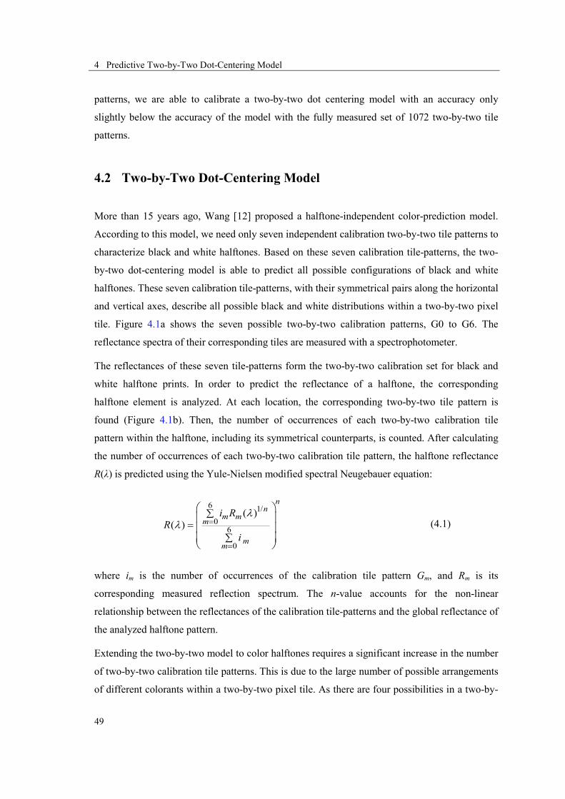
4 Predictive Two-by-Two Dot-Centering Model
49
patterns, we are able to calibrate a two-by-two dot centering model with an accuracy only
slightly below the accuracy of the model with the fully measured set of 1072 two-by-two tile
patterns.
4.2 Two-by-Two Dot-Centering Model
More than 15 years ago, Wang [12] proposed a halftone-independent color-prediction model.
According to this model, we need only seven independent calibration two-by-two tile patterns to
characterize black and white halftones. Based on these seven calibration tile-patterns, the two-
by-two dot-centering model is able to predict all possible configurations of black and white
halftones. These seven calibration tile-patterns, with their symmetrical pairs along the horizontal
and vertical axes, describe all possible black and white distributions within a two-by-two pixel
tile. Figure 4.1a shows the seven possible two-by-two calibration patterns, G0 to G6. The
reflectance spectra of their corresponding tiles are measured with a spectrophotometer.
The reflectances of these seven tile-patterns form the two-by-two calibration set for black and
white halftone prints. In order to predict the reflectance of a halftone, the corresponding
halftone element is analyzed. At each location, the corresponding two-by-two tile pattern is
found (Figure 4.1b). Then, the number of occurrences of each two-by-two calibration tile
pattern within the halftone, including its symmetrical counterparts, is counted. After calculating
the number of occurrences of each two-by-two calibration tile pattern, the halftone reflectance
R(λ) is predicted using the Yule-Nielsen modified spectral Neugebauer equation:
6 1/0
6
0
( )( )
nn
m mm
mm
i RR
i
λλ =
=
∑
∑=
( 4.1)
where im is the number of occurrences of the calibration tile pattern Gm, and Rm is its
corresponding measured reflection spectrum. The n-value accounts for the non-linear
relationship between the reflectances of the calibration tile-patterns and the global reflectance of
the analyzed halftone pattern.
Extending the two-by-two model to color halftones requires a significant increase in the number
of two-by-two calibration tile patterns. This is due to the large number of possible arrangements
of different colorants within a two-by-two pixel tile. As there are four possibilities in a two-by-

4 Predictive Two-by-Two Dot-Centering Model
50
two tile, the number of possible colorant arrangements per two-by-two pixel tile is N4, where N
is the number of colorants. Colorants are formed by single inks, all possible superpositions of
single inks and white paper. For example, in the case of a CMY print, we have 8 colorants and
there are 84 = 4096 possible color arrangements. After removing the horizontally and vertically
symmetric two-by-two tiles, 1072 independent tile patterns remain. For N colorants, the total
number of independent patterns P(N) is given by Equation (4.2). See [14], pp. 470-479.
! ! ! !( ) 6 9 5
( 4)!4! ( 3)!3! ( 2)!2! ( 1)!N N N N
P NN N N N
= + + +− − − −
( 4.2)
where for N = 3 and for N = 2 the first term and the first two terms are omitted, respectively. For
black and white halftones there are P (2) = 7 independent tile patterns and for CMY halftones,
there are P (8) = 1072 independent tile patterns. For a 4-ink print, the two-by-two dot-centering
model becomes intractable with P (16) = 16576 tile patterns. We therefore seek a method for
inferring the reflectances of a large number of tile patterns, given the measured reflectances of a
small subset of them.
(a) (b) Figure 4.1 (a) The seven calibration patterns for the black and white two-by-two model. (b) Example of a
halftone with the corresponding mapped two-by-two patterns.
4.3 Two-by-Two Pattern Tile Reflectance Prediction
We intend to estimate the spectral reflectance of unknown two-by-two tile patterns from known,
measured tile patterns (Figure 4.2). We propose to estimate the reflectances of most two-by-two
tile patterns by relying only on a small subset of measured two-by-two tile reflectances. We
assume that within the two-by-two tiles, area coverages of colorants are equivalent to relative
concentrations. We therefore work in the absorptance space and establish a linear relationship
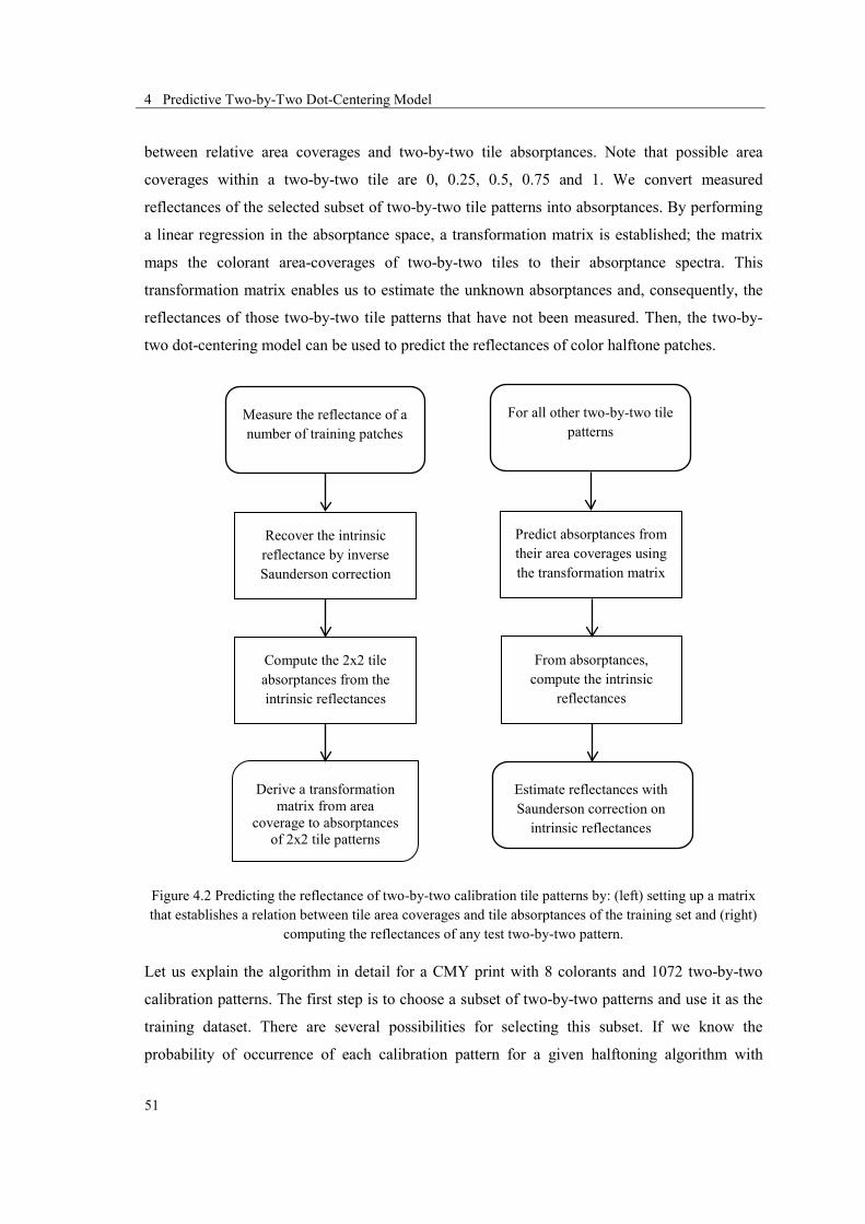
4 Predictive Two-by-Two Dot-Centering Model
51
between relative area coverages and two-by-two tile absorptances. Note that possible area
coverages within a two-by-two tile are 0, 0.25, 0.5, 0.75 and 1. We convert measured
reflectances of the selected subset of two-by-two tile patterns into absorptances. By performing
a linear regression in the absorptance space, a transformation matrix is established; the matrix
maps the colorant area-coverages of two-by-two tiles to their absorptance spectra. This
transformation matrix enables us to estimate the unknown absorptances and, consequently, the
reflectances of those two-by-two tile patterns that have not been measured. Then, the two-by-
two dot-centering model can be used to predict the reflectances of color halftone patches.
Figure 4.2 Predicting the reflectance of two-by-two calibration tile patterns by: (left) setting up a matrix that establishes a relation between tile area coverages and tile absorptances of the training set and (right)
computing the reflectances of any test two-by-two pattern.
Let us explain the algorithm in detail for a CMY print with 8 colorants and 1072 two-by-two
calibration patterns. The first step is to choose a subset of two-by-two patterns and use it as the
training dataset. There are several possibilities for selecting this subset. If we know the
probability of occurrence of each calibration pattern for a given halftoning algorithm with
Recover the intrinsic reflectance by inverse Saunderson correction
Compute the 2x2 tile absorptances from the intrinsic reflectances
From absorptances, compute the intrinsic
reflectances
Measure the reflectance of a number of training patches
Estimate reflectances with Saunderson correction on
intrinsic reflectances
For all other two-by-two tile patterns
Derive a transformation matrix from area
coverage to absorptances of 2x2 tile patterns
Predict absorptances from their area coverages using the transformation matrix

4 Predictive Two-by-Two Dot-Centering Model
52
known parameters, we can include the most probable two-by-two tile patterns in the training set
and estimate all others. Another approach consists in selecting two-by-two tile patterns that are
well distributed across the printer color gamut and have different pattern configurations. Here,
in order to apply our approach and verify its accuracy on a non-optimized set of learning
patterns, we randomly select the two-by-two tile-pattern training set.
We also verify the impact of the size of the training set. When the number of measurements
increases, we expect a decrease in the prediction error of the resulting two-by-two model.
The measured reflectance Rm(λ) is composed of the intrinsic reflectance ρ(λ), and of the Fresnel
reflectances at the print-air interface. As we are interested in the absorptance of the two-by-two
tile patterns, we apply an inverse Saunderson correction on the measured reflectance spectra of
the training set in order to first recover the intrinsic reflectances. The expression for the
Saunderson correction is [43]
(1 )(1 ) ( )( )
1 ( )s i
m si
r rR K r
rr λ
λr λ
− −= ⋅ +
− ⋅ ( 4.3)
where rs is the Fresnel specular reflection at the air-print interface, K is the portion of specular
reflection captured by the spectrophotometer and ri is the Fresnel reflection at the print-air
interface, averaged over all incident angles. The overall Fresnel reflection at the print-air
interface has been calculated by Judd [44] as ri = 0.6 for an index of refraction of 1.5. For a
given incident angle, rs is constant and depends on the refractive index of the print. At 45° and
for a refractive index of 1.5, rs = 0.04. We obtain the intrinsic reflectance of the two-by-two
pattern by applying the inverse Saunderson correction, derived from Equation (4.3)
( )( )
1 (1 ) ( ).m s
i s i m i s
R K rK r r r R r r
λr λ
λ
− ⋅=
+ − ⋅ + ⋅ − − ( 4.4)
Within the narrow space of a two-by-two tile, we assume that area coverages are equivalent to
colorant concentrations. As proposed by Berns [45], we select the absorptance space as the
space in which we establish a linear relationship between area coverages and absorptances.
Let us now calculate the absorptance from the previously calculated intrinsic reflectance. If we
assume that light travels twice through the halftone colorant layer, we can express the intrinsic
two-by-two tile reflectance ρi(λ) as

4 Predictive Two-by-Two Dot-Centering Model
53
2( ) ( ) ( )i p Tr λ r λ λ= ( 4.5)
where T2 is the attenuation of light traversing twice the colorant halftone layer and ρp is the
intrinsic reflectance of paper. The attenuation T of the colorant halftone layer can be expressed
by the Beer-Bouguer law
( )( ) c dT e ε λλ − ⋅ ⋅= ( 4.6)
where ε(λ) is the molar extinction coefficient, c is the concentration and d is the thickness of the
colorant halftone layer. Since the absorptance is defined as K(λ) = ε(λ)·c·d, we obtain from
Equations (4.5) and (4.6)
.2 ( )( ) ( ) K
i p e λr λ r λ −= ( 4.7)
By inverting Equation (4.7), we obtain the spectral absorptance K(λ)
( )1( ) ln( ).
2 ( )i
pK
r λλ
r λ= − ( 4.8)
Since for a print with cyan, magenta and yellow inks we have 8 colorants, an 8-component
vector characterizes the area coverage of a two-by-two pattern. As an example, Figure 4.3
shows two examples of two-by-two calibration tile-patterns. The left-hand side tile is composed
of area coverage of 25% cyan, 25% magenta, 25% yellow and 25% black and the right-hand
side is composed of area coverages of 25% white, 25% cyan and 50 % blue. These area
coverages can be expressed as vectors a = (0, 0.25, 0.25, 0.25, 0, 0, 0, 0.25) and b = (0.25, 0.25,
0, 0, 0.50, 0, 0, 0), respectively. The order of colorants in the vector is white (w), cyan (c),
magenta (m), yellow (y), blue (b), green (g), red (r), and black (k).
Figure 4.3 Two examples of two-by-two tiles.
The stated linear relationship in absorptance space implies that a given two-by-two tile
absorptance is a linear combination of base-tile absorptances:

4 Predictive Two-by-Two Dot-Centering Model
54
1 1 2 2 8 8= c + c +…+ ck k k k ( 4.9)
where k is a column vector expressing absorptances at visible wavelengths, e.g., 36 discrete
wavelengths between 380 nm and 730 nm at 10 nm intervals, and c1 to c8 are the area coverages
of the considered 8 colorants, and ki are the colorant absorptances derived from the training set.
Equation (4.9) can be formulated in vector-matrix form
1,1 1,2 1,81 1
2,1 2,2 2,82 2
36 836,1 36,2 36,8
k k kk ck k kk c
k ck k k
=
( 4.10)
or equivalently
k = Mc ( 4.11)
where c is the area coverage 8-component vector of a two-by-two pattern and M is the 36-by-8
matrix, composed of the colorant vectors ki. Matrix M gives the relationship between colorant
area coverages and spectral absorptance. We can derive the coefficients of matrix M with a set
of training two-by-two tiles significantly larger than the number of unknowns. With a set of m
training-tile patterns with known area-coverage vectors ci and absorptances ki, we obtain an
overdetermined linear system
[ ] [ ]m m1 2 1 2k ,k ,…,k = M c ,c ,…,c ( 4.12)
or in short form
.K = MC ( 4.13)
Matrix K is the absorptivity matrix with a size of 36 by m, C is an 8 by m matrix containing the
colorant area-coverages and M is the 36-rows-by-8-columns transformation matrix. We can
solve this linear system by minimizing ║K - MC║
1( )T T −=M KC CC ( 4.14)

4 Predictive Two-by-Two Dot-Centering Model
55
where superpose T stands for matrix transpose. See [46] for more details. Having obtained
matrix M, we can compute by applying Equation (4.11) the absorptance of any two-by-two tile
from its area coverages.
For predicting the reflectance of a new two-by-two tile, we calculate first the absorptance with
the transformation matrix obtained by linear regression. We then convert absorptances to
intrinsic reflectances. This is accomplished by Equation (4.7). Finally, by applying the
Saunderson correction given by Equation (4.3), we obtain the predicted reflectance on the air
side of the two-by-two tile.
4.4 Accuracy Results
4.4.1 Two-by-two pattern reflectance estimation
In this sub-section, we give the reconstruction accuracy that results when we apply the proposed
predictive method of reducing the number of calibration two-by-two patterns. We verify how
accurate the non-measured two-by-two tile reflectances have been reconstructed. In the next
sub-section, we present the prediction accuracy of the color-prediction model by testing the
two-by-two dot-centering model on different halftones with a calibration set that is partly
measured and partly predicted.
All samples were printed with a Canon PIXMA Pro9500 inkjet printer at 600 dpi on Canon MP-
101 paper. Two-by-two tile patterns were printed on a single A4 sheet. The spectral reflectance
measurements were carried out with a Datacolor MF45 spectrophotometer having a 0°:45°
measuring geometry. The repeatability of the printing and measuring devices was verified. In
order to build the training dataset, we select from the 1072 two-by-two tile patterns a subset
whose reflectances are measured. We are interested in the minimum number of measurements.
As stated before, we pick these patterns randomly. We know that the most important two-by-
two calibration patterns are the 8 fulltone two-by-two colorant tiles, namely white, cyan,
magenta, yellow, blue, green, red and black. These tile patterns are therefore included in all
selections of training patterns. The other training tile patterns are randomly selected from the
two-by-two patterns set.
Table 4.1 demonstrates the accuracies of the proposed algorithm in predicting the reflectances
of those two-by-two tile patterns that do not belong to the training set. It gives the mean
prediction error in terms of ΔE94 values, the maximum prediction-error and the 95%-quantile

4 Predictive Two-by-Two Dot-Centering Model
56
prediction-error under the D65 illuminant. Three different training set sizes were chosen. These
prediction-accuracy tests were performed for 20 different randomly chosen training sets.
Table 4.1. The color difference error for predicted two-by-two tile patterns.
Training set Test set
size
ΔE94
mean 95% max
36 (8 fulltones + 28 random samples) 1036 2.05 4.46 9.53
72 (8 fulltones + 64 random samples) 1000 1.97 4.57 8.33
100 (8 fulltones + 92 random samples) 972 1.97 4.43 7.59
As shown in Table 4.1, we use three different numbers for the training data size: 36, 72 and 100
of which 8 are fulltone colorants. Despite the fact that only a small fraction of two-by-two
calibration patterns is measured, the two-by-two tile reflectance prediction accuracy is relatively
high. In addition, the size of training set does not have a strong effect on the prediction
accuracy.
4.4.2 Two-by-two model performance using predicted patterns
The two-by-two dot-centering model predicts the spectral reflectances of halftone prints by
making use of all possible two-by-two pixel configurations. In this sub-section, in order to
verify the performance of our predictive approach, we test the two-by-two model with a
calibration set whose reflectances have, to a very large extent, been predicted. Also, we compare
the prediction accuracies of the two-by-two model where all two-by-two calibration tiles are
measured and where these both measured and predicted are mixed.
The testing set for obtaining the accuracy of the two-by-two model is comprised of mutually
rotated clustered-dot halftones at 3 screen frequencies, namely 75 lpi, 100 lpi and 125 lpi and of
blue-noise diffused-dither halftones. They were printed with all combinations of cyan, magenta
and yellow area coverages of 0, 0.25, 0.5, 0.75 and 1, i.e., we consider 125 test patches per set.
We analyze the target halftones by calculating the number of repetitions of each calibration tile-
pattern within the color halftone. We then predict the color-halftone reflectance spectrum by
using the Yule-Nielsen modified spectral Neugebauer equation:

4 Predictive Two-by-Two Dot-Centering Model
57
1071 1/
01071
0
( )( )
nn
m mm
mm
i RR
i
λλ =
=
∑=
∑
( 4.15)
where the only difference with Equation (4.1) is the number of calibration two-by-two tiles,
which is larger for a CMY color-halftone (1072 patterns) compared to a black and white
halftone (7 patterns). The performance of the two-by-two model both when using fully
measured and when using predicted two-by-two pattern reflectances is shown Table 4.2. The
prediction accuracy using the predicted calibration tile pattern reflectances is very close to the
accuracy obtained with a fully measured calibration set. Therefore, a major reduction in the
number of two-by-two pattern measurements does not significantly reduce the prediction
accuracy of the two-by-two model.
For clustered-dot halftoning, the low difference between the prediction accuracy of the fully and
partially measured calibration two-by-two tiles can be explained by the fact that in clustered-dot
halftoning a large portion of two-by-two tile patterns are solid colorants. To see how significant
this effect is, we performed the comparison of prediction accuracy also on blue noise diffused
dither halftones where many different two-by-two tile patterns occur. The prediction accuracy is
still high and demonstrates the validity of our approach.
To have a “ground truth” in Table 4.2, we also include the spectral prediction accuracy of the
superposition-dependent ink-spreading enhanced Yule-Nielsen spectral Neugebauer model
(SDIS-YNSN) that is calibrated with 44 calibration patches. We will explain this model and its
calibration in the next chapter. Note that, in contrast to the two-by-two dot centering model, the
training samples for SDIS-YNSN should be printed with the same halftoning method and at the
same orientation and screen frequencies as the test samples. Moreover, the reflectances of 44
out of 125 samples used for obtaining the accuracy of SDIS-YNSN are known, whereas in the
case of the two-by-two dot-centering model the whole set of 125 samples are pure test samplers.
4.4.3 Limitations
An ambiguity that comes up when using the two-by-two dot centering model is related to its
halftone-invariant property. This model is halftone invariant in the sense that a unique
calibration set can be used for different halftone configurations, i.e. different screen frequencies,
shapes, and orientations. However, the Yule-Nielsen n present in the model (Equation (4.15))
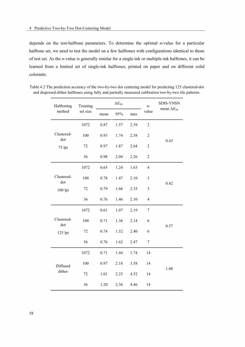
4 Predictive Two-by-Two Dot-Centering Model
58
depends on the test-halftone parameters. To determine the optimal n-value for a particular
halftone set, we need to test the model on a few halftones with configurations identical to those
of test set. As the n-value is generally similar for a single-ink or multiple-ink halftones, it can be
learned from a limited set of single-ink halftones, printed on paper and on different solid
colorants.
Table 4.2 The prediction accuracy of the two-by-two dot centering model for predicting 125 clustered-dot and dispersed-dither halftones using fully and partially measured calibration two-by-two tile patterns.
Halftoning method
Training set size
ΔE94 n-value
SDIS-YNSN mean ΔE94
mean 95% max
Clustered-dot
75 lpi
1072 0.87 1.57 2.39 2
0.43 100 0.93 1.74 2.58 2
72 0.97 1.87 2.64 2
36 0.98 2.04 2.26 2
Clustered-dot
100 lpi
1072 0.65 1.24 1.63 4
0.42 100 0.78 1.47 2.10 3
72 0.79 1.66 2.35 3
36 0.76 1.46 2.10 4
Clustered-dot
125 lpi
1072 0.61 1.07 2.19 7
0.57 100 0.71 1.36 2.14 6
72 0.74 1.52 2.40 6
36 0.76 1.62 2.47 7
Diffused dither
1072 0.71 1.44 1.74 14
1.08 100 0.97 2.18 3.58 14
72 1.01 2.25 4.52 14
36 1.20 2.36 4.46 14
4 Predictive Two-by-Two Dot-Centering Model
59
Moreover, for the two-by-two dot centering model, the calibration and the test samples are
printed and measured separately. Therefore, the accuracy results of the two-by-two model are
slightly affected by the repeatability of the printing and measuring devices. This is not true for
the YNSN model where all 125 calibration and test samples are printed on a single paper sheet.
There is also a limitation that is specific to our predictive approach. In order to estimate the
reflectances of two-by-two patterns, using Beer’s law, we build a linear relationship between
their area coverages and their absorptances. One of the requirements for using Beer’s law is that
the inks should not significantly scatter the light. The inkjet inks satisfy this requirement as
confirmed from the accurate results obtained in Table 4.1. The two-by-two tile prediction
approach cannot be applied to laser printers that use toners that do not obey Beer’s law. In order
to estimate the two-by-two patterns printed with toners, an entity other than pure absorptance is
needed for establishing our proposed framework. It should take into account the scattering of
particles. Opaque metallic inks are another example where Beer’s law is invalid.
4.5 Summary
The two-by-two dot-centering model predicts the halftone spectral reflectances without
knowledge of the halftoning method. However, for a color-halftone print it requires as input the
reflectances of a large number of two-by-two calibration tile-patterns. Spectral measurement of
hundreds or thousands of tile patterns is cumbersome and time consuming. As an alternative,
with a small measured subset of the two-by-two calibration-patterns, we learn a matrix that
gives the linear relationship between calibration-pattern colorant area-coverages and the
corresponding calibration-pattern spectral-absorptance. This relationship is then used to predict
the absorptance and deduce the reflectance of all other two-by-two calibration patterns. The
accuracy of the proposed method is verified by comparing the reflectance predictions relying on
the two-by-two dot-centering model based either on the measured full set or on the
measurement of a small subset of the two-by-two calibration tile-patterns.
The mean color-prediction error of the two-by-two model for a clustered-dot halftone at 100 lpi
for a fully measured set of 1072 two-by-two calibration patterns is ΔE94 = 0.65. When the two-
by-two model is calibrated with only 72 two-by-two spectral measurements, the mean
prediction-error becomes ΔE94 = 0.74. The accuracy of the proposed method is slightly lower
for blue-noise diffuse-dither halftones where the fully measured calibration set yields a
prediction error of ΔE94 = 0.71 and the subset with the 72 measurements yields a prediction

4 Predictive Two-by-Two Dot-Centering Model
60
error of ΔE94 = 1.01. Predicting a very large fraction of the two-by-two tile patterns facilitates
the use of the two-by-two dot-centering model for 3- or possibly 4-ink printing setups.

5 Color Prediction of Juxtaposed Halftones
61
5.1 Introduction
In Chapter 2 we introduce discrete-line juxtaposed halftoning. Colorants formed by inks and ink
superpositions form side-by-side discrete lines. Juxtaposed halftoning is necessary when
printing with opaque or special-effect inks. To our knowledge, color prediction of juxtaposed
halftones has never been investigated. Color-prediction models are useful for establishing the
correspondence between ink area-coverages and resulting halftoned color in a color-
reproduction workflow (Section 1.2). They enable us to calculate the color gamut and to
establish the color separation tables. Generally, prediction models are calibrated by considering
specific halftone characteristics.
The primary difficulty associated with color prediction of juxtaposed halftones is determining
the effective area-coverages of contributing colorants. To overcome this difficulty, we propose
the two-by-two dot-centering spectral prediction model. This model enables us to capture the
reflectance of slightly overlapping colorants by relying on halftone configurations instead of
colorant area-coverages.
5 5 Color Prediction of Juxtaposed
Halftones

5 Color Prediction of Juxtaposed Halftones
62
In this chapter, we adapt the two-by-two dot-centering model to discrete-line juxtaposed
halftones. A comparison between the two-by-two model and different variants of the Yule-
Nielsen spectral Neugebauer model (YNSN) is also provided. We also explain the relationship
between the n-values used by the two-by-two model and by the YNSN model. Furthermore, we
extend the spectral predictions to a larger number of custom inks, i.e. cyan, magenta, yellow,
custom blue, custom red, custom green and custom achromatic black.
5.2 Neugebauer and Demichel
Early color-prediction models were developed by being inspired by the layout of the halftones.
This is the case of the well-known Neugebauer model [47] and its close connection with
Demichel equations [48].
The Neugebauer model relies on a statistically independent superposition of ink dots. Printing N
superposed dot-screens gives rise to 2N possible combinations of ink superpositions at each
point of the printed paper [49]. In our discussion we set N = 3 as is the case with classic CMY
prints. The Neugebauer equations for calculating the XYZ color-coordinates of a halftone (Xh,
Yh, Zh) can be expressed as
000 000 100 100 111 111
000 000 100 100 111 111
000 000 100 100 111 111
,
,
.
X a X a X a XhY a Y a Y a YhZ a Z a Z a Zh
= + + +
= + + +
= + + +
( 5.1)
where Xijk, Yijk and Zijk denote the XYZ color-coordinates of the inks and all their possible
superpositions. The binary indices i, j and k determine the presence of the first, second and third
halftone layer in a specific position of a given halftone. The weight aijk of each possible color in
the Neugebauer equations is the relative area of that color in the halftone.
For a CMY print with cyan, magenta and yellow inks, the halftone is composed of 8 colorants:
white, cyan, magenta, yellow, blue, green, red and black. These are the Neugebauer primaries.
The color of Neugebauer primaries (Xijk, Yijk, Zijk) can easily be measured with a measurement
device. To determine the area coverages (aijk) of the colorants, we can count the number of
pixels covered by each primary. We can also calculate them by applying a probabilistic method
and by accounting for certain assumptions.

5 Color Prediction of Juxtaposed Halftones
63
Figure 5.1 Schematic representation of the Neugebauer and Demichel equations. The color of magnified halftone on top is a weighted average of the color of 8 Neugebauer primaries (shown on the bottom-
right). The weights are area coverages of these primaries which depend on the area coverages of the base inks and are calculated using Demichel equations.
Let us denote by c, m, and y the fractions of the area of a CMY halftone. We assume that cyan,
magenta, and yellow ink dots are laid out independently from one another1. From a statistical
point of view, c, m and y can be considered as the probability of any particular point within the
halftone to be covered by the C, M or Y ink, respectively. Hence, the probability of not being
covered by an ink, say cyan, is 1 − c. It follows that the probability of any randomly chosen
point being covered by all three colors is the multiplication of their probabilities, i.e., cmy.
By similar reasoning, the area coverages of all 8 possible colorants can be obtained from the
relative area-coverages of the base inks. This provides a set of equations known as the Demichel
equations:
000 100
010 001
110 101
011 111
: (1 )(1 )(1 ) : (1 )(1 )(1 ) (1 ) (1 )(1 )
(1 ) (1 )
(1 )
: :: :: :
a a c m y a a c m yw ca c m y a c m ym ya cm y a c m ygba c my a cmyr k
a aa aa a
= − − − = − −= − − = − −
= − = −
= − =
( 5.2)
1 Amidror and Hersch [49] extensively discuss the validity of this assumption and to what extent it holds.

5 Color Prediction of Juxtaposed Halftones
64
where aw, ac, am, ay, ab, ag, ar, and ak are the probabilistic area-coverages of the resulting
colorants white, cyan, magenta, yellow, blue, green, red and black, respectively. We can use the
Demichel equations to calculate the weights in the Neugebauer formula (Equation 5.1). This
enables us to predict the printed color of a given halftone patch. Figure 5.1 illustrates the
relation between the Demichel and the Neugebauer equations.
5.3 Prediction Models for Juxtaposed Halftones
Many of the existing color-prediction models are either derived from Neugebauer equations or
use Demichel equations for calculating colorant area-coverages [10]. As we discussed in the
previous section, these two interrelated set of equations rely on the assumption of an
independent superposition of different ink layers. This is an acceptable assumption for classic
halftoning methods such as rotated clustered-dot halftoning and blue-noise dithering [49]. For
juxtaposed halftones, the use of these equations is invalid because juxtaposed halftones prevent
the colorants from being superposed. There is no established model specifying how to compute
the physical dot-gain of the individual colorants and the area of newly formed colorants in case
of overlapping of the individual inks.
In this section, we review the spectral-prediction models that can predict the color of juxtaposed
halftones. This includes the two-by-two dot-centering model [12] and its predictive variant [50]
that relies on a smaller set of calibration samples (Chapter 4). The two-by-two dot-centering
spectral prediction model enables us to predict the reflectance of slightly overlapping colorants
and can therefore be appropriate for predicting the color of juxtaposed halftones. As this model
requires a large calibration set, we use also an estimation technique that predicts more than 90%
of the two-by-two calibration patterns reflectances by measuring less than 10% of them. Note
that the predictive version is based on the same principles as the “full” version of the two-by-
two model. It only reduces the tedious calibration work.
In addition to the two-by-two dot-centering model, in order to predict the color of juxtaposed
halftones, we test the well-known Yule-Nielsen modified spectral Neugebauer model. This
model is extensively used for color prediction of classic halftones.

5 Color Prediction of Juxtaposed Halftones
65
5.3.1 Yule-Nielsen spectral Neugebauer model
The Neugebauer model (Equation (5.1)) has been extended to work with spectral reflectances.
The spectral Neugebauer model predicts the overall reflectance R(λ) of a halftone as a weighted
average of the colorant reflectances Ri(λ). Yule and Nielsen [51] and Viggiano [52] proposed to
replace this linear relationship with a non-linear power function whose value n is optimized
according to a limited number of measured patch reflection-spectra:
1/( ) ( )i
nn
iiaR Rλ λ ∑
= ( 5.3)
where ai is the fractional area-coverage of Neugebauer primary i, Ri(λ) is its reflectance
spectrum and R(λ) is the predicted reflectance of the halftone patch. The power functions with
values 1/n and n account for the optical dot-gain due to lateral propagation of light and to
multiple internal reflections between the paper bulk and the print-air interface.
The prediction accuracy of the YNSN model depends on our knowledge of the effective area-
coverages ai of the contributing colorants. Effective area-coverages depend on the inks, on the
paper, and on their superposition condition. Variants of the YNSN model differentiate
themselves according to the approach for calculating the area coverages of the Neugebauer
primaries.
We consider three variants. The first variant called nominal YNSN consists in applying nominal
area-coverages. The second variant called independent ink spreading YNSN (IIS-YNSN)
considers, for each single ink, a curve that maps nominal to effective area-coverages. These
curves are obtained by linear interpolation between fitted area-coverages of halftones printed on
paper. The third approach called superposition-dependent ink-spreading YNSN (SDIS-YNSN),
relies on ink spreading curves that map nominal to effective area-coverages for each
superposition condition. Let us explain the ink spreading models more detailed.
5.3.2 Ink spreading
The ink-spreading model accounts for ink spreading in different ink-superposition conditions
[13]. It relies on ink-spreading curves that map nominal area coverages to effective area
coverages. The ink-spreading model takes into account (a) the area coverages of single-ink

5 Color Prediction of Juxtaposed Halftones
66
halftones, (b) the area coverages of single-ink halftones superposed with one solid ink and (c)
the surface coverages of single-ink halftones superposed with two solid inks.
During calibration of the model, the effective area-coverages of a single-ink halftone printed in
superposition with paper white, with one solid ink or with two solid inks can be obtained. We
first measure the reflectance spectra of these halftones at a few nominal area-coverages. Then,
effective area-coverages are fitted by minimizing the sum of square differences between
predicted reflectance using the YNSN model (Equation (5.3)) and the measured reflectance. By
linear interpolation between the fitted effective area-coverages, we can obtain the ink-spreading
curves for each ink and in each ink-superposition condition.
For cyan, magenta and yellow inks with nominal coverages c, m and y, the ink spreading
functions (curves) for single-ink halftones are fc(c), fm(m) and fy(y). For independent ink-
spreading YNSN (IIS-YNSN), we only use these three ink-spreading curves.
The functions that map nominal coverages of an ink to effective coverages of that ink, for single
ink halftones superposed with a second solid-ink and for single-ink halftones superposed with
two solid inks are, respectively, fc/m(c), fc/y(c), fm/c(m), fm/y(m), fy/c(y), fy/m(y) and fc/my(c), fm/cy(m),
fy/cm(y), where fi/j(i) indicates an ink halftone i superposed with solid ink j. fi/jk(i) indicates an ink
halftone i superposed with solid inks j and k. In the case of three inks, these 9 ink-spreading
functions as well as 3 single-ink functions are obtained by fitting 36 patches, i.e., 3 patches
(25%, 50% and 75% nominal area-coverages) per function. Superposition-dependent ink
spreading YNSN (SDIS-YNSN) uses all 12 ink-spreading curves to calculate the effective area-
coverages.
In order to obtain the effective area-coverages c’, m’ and y’ of a color-halftone patch with c, m
and y nominal coverages, it is necessary to weight the contributions of the corresponding ink-
spreading curves. For example, for deducing the effective cyan-ink coverage, we weight the
contributions of the ink spreading curves fc, fc/m, fc/y and fc/my. The weighting functions depend on
the effective area-coverages of the colorants on which the considered ink halftone is
superposed. Let us assume that inks are printed independently from each other. For the
considered 3-ink system and assuming the independence of halftone layers, Equations (5.4)
weight each ink-spreading curve with the corresponding relative area of its underlying
colorants.
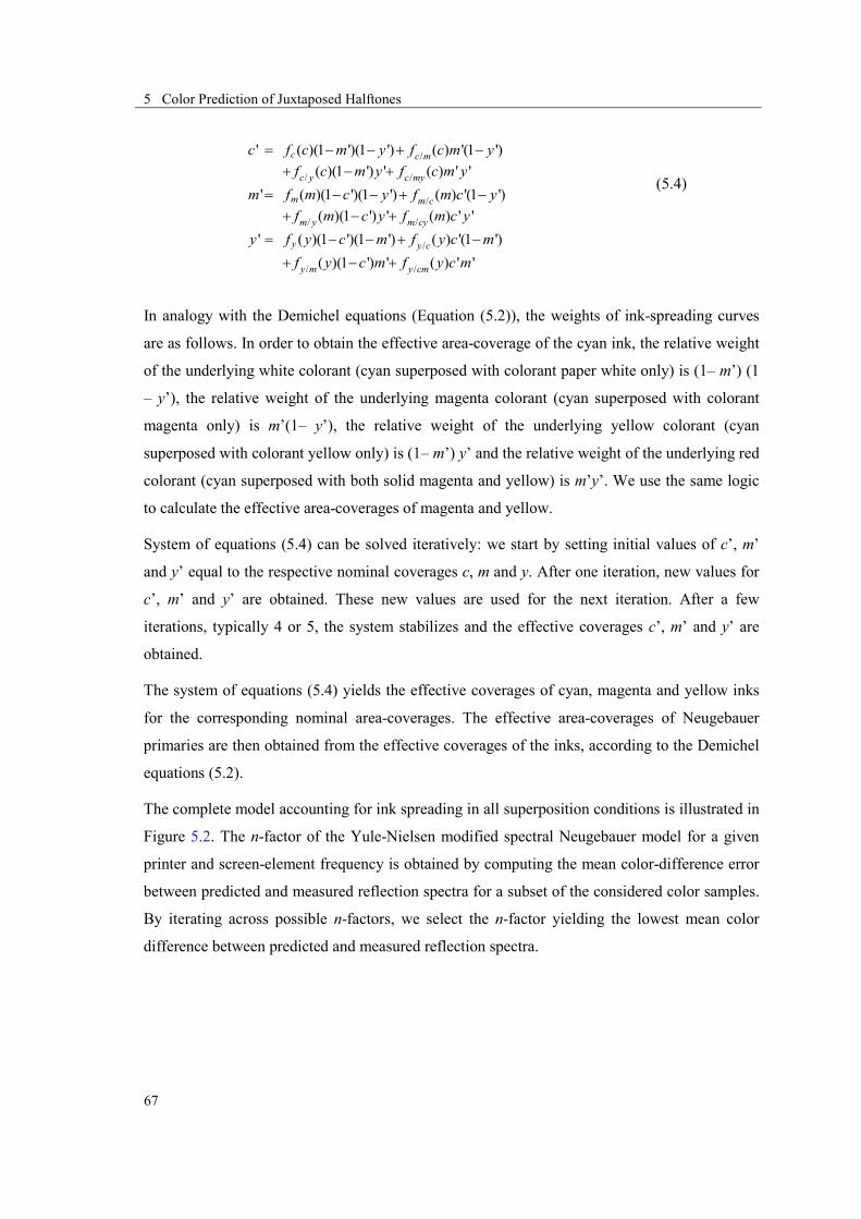
5 Color Prediction of Juxtaposed Halftones
67
/
/ /
/
/ /
/
/ /
' ( )(1 ')(1 ') ( ) '(1 ')( )(1 ') ' ( ) ' '
' ( )(1 ')(1 ') ( ) '(1 ')( )(1 ') ' ( ) ' '
' ( )(1 ')(1 ') ( ) '(1 ')( )(1 ') ' ( ) ' '
c c m
c y c my
m m c
m y m cy
y y c
y m y cm
c f c m y f c m yf c m y f c m y
m f m c y f m c yf m c y f m c y
y f y c m f y c mf y c m f y c m
= − − + −+ − +
= − − + −+ − +
= − − + −
+ − +
( 5.4)
In analogy with the Demichel equations (Equation (5.2)), the weights of ink-spreading curves
are as follows. In order to obtain the effective area-coverage of the cyan ink, the relative weight
of the underlying white colorant (cyan superposed with colorant paper white only) is (1– m’) (1
– y’), the relative weight of the underlying magenta colorant (cyan superposed with colorant
magenta only) is m’(1– y’), the relative weight of the underlying yellow colorant (cyan
superposed with colorant yellow only) is (1– m’) y’ and the relative weight of the underlying red
colorant (cyan superposed with both solid magenta and yellow) is m’y’. We use the same logic
to calculate the effective area-coverages of magenta and yellow.
System of equations (5.4) can be solved iteratively: we start by setting initial values of c’, m’
and y’ equal to the respective nominal coverages c, m and y. After one iteration, new values for
c’, m’ and y’ are obtained. These new values are used for the next iteration. After a few
iterations, typically 4 or 5, the system stabilizes and the effective coverages c’, m’ and y’ are
obtained.
The system of equations (5.4) yields the effective coverages of cyan, magenta and yellow inks
for the corresponding nominal area-coverages. The effective area-coverages of Neugebauer
primaries are then obtained from the effective coverages of the inks, according to the Demichel
equations (5.2).
The complete model accounting for ink spreading in all superposition conditions is illustrated in
Figure 5.2. The n-factor of the Yule-Nielsen modified spectral Neugebauer model for a given
printer and screen-element frequency is obtained by computing the mean color-difference error
between predicted and measured reflection spectra for a subset of the considered color samples.
By iterating across possible n-factors, we select the n-factor yielding the lowest mean color
difference between predicted and measured reflection spectra.

5 Color Prediction of Juxtaposed Halftones
68
Figure 5.2 Prediction model with ink spreading in all superposition conditions.
5.4 Color-Prediction Accuracy of Juxtaposed Halftones
5.4.1 Applying the two-by-two model to discrete line juxtaposed halftones
To obtain the reflectance of a halftone using the two-by-two dot-centering model, we need to
count the number of occurrences of each representative two-by-two pattern inside a halftone-
screen element. The screen element generated by our discrete-line juxtaposed halftoning is a
parallelogram tile whose size depends on two parameters: slope a/b and vertical period T, as
shown in Figure 5.3. Any b×T rectangle forms a repetitive tile equivalent to the parallelogram
screen-element. This can be beneficial to a rapid implementation of the two-by-two dot-
centering model. For a classic halftone such as blue-noise dithering, we need to analyze an
arbitrarily large segment of a halftone when counting the two-by-two patterns, in order to reach
an unbiased number of occurrences. As it is repetitive, for discrete-line juxtaposed halftoning,
analyzing a usually small b×T rectangle is sufficient.
5.4.2 Performance of the two-by-two model compared to YNSN
In order to assess the performance of the two-by-two spectral prediction model on discrete-line
juxtaposed halftones, we compare it with the Yule-Nielsen spectral Neugebauer model. To
perform a fair comparison, we create juxtaposed halftones with colorant area-coverages meeting

5 Color Prediction of Juxtaposed Halftones
69
the constraints of the YNSN model. Although juxtaposed halftoning enables us to directly set
the area coverages of input colorants independently of each other, we chose the 8 colorant area
coverages so as to respect the Demichel equations. We convert all combinations of 0, 0.25, 0.5,
0.75 and 1 of cyan, magenta and yellow inks into area coverages of the 8 colorants using
Equation (5.2). This results in 125 test patches. Table 5.1 shows a few examples of colorant-
area coverages calculated according to the Demichel equations. Colorant area-coverages are
generated using discrete-line juxtaposed halftoning.
Figure 5.3 A simple discrete line juxtaposed halftone with three colorants and halftone parameters a/b = 2/5 and T = 4. The original parallelogram screen element and the equivalent rectangular tile are shown
using thick solid and dashed lines, respectively. The two-by-two patterns occurring inside the equivalent rectangular tile are shown by thin solid lines. This repetitive tile may be located anywhere within the
halftone.
The generated 125 test-halftone patches are printed on Canon MP-101 paper. The experiments
were carried out on an inkjet printer Canon PIXMA Pro9500 at 600 dpi driven in high-quality
mode, with a droplet size of 3 producing saturated ink colors. The corresponding solid cyan,
magenta and yellow densities are respectively 1.00, 0.80 and 1.08. The halftones were generated
at vertical screen-period T = 7 pixels yielding a screen frequency of 99 lpi, and at vertical period
T = 11 pixels yielding a screen frequency of 63 lpi for a single discrete-line slope m = 4/7. The
order in which colorant lines are placed next to each other is yellow, green, cyan, blue, black,
red, magenta and white.
Table 5.2 shows the prediction accuracy for juxtaposed-line halftones obeying the Demichel
equations. We considered the variants of the YNSN model, as well as the two-by-two dot-
centering model whose calibration set comprises either completely measured or partly measured
and partly predicted patch-reflectances. All colors are calculated under the D65 illuminant.

5 Color Prediction of Juxtaposed Halftones
70
Table 5.1 Demichel area coverages of the 8 Neugebauer primaries for a subset of ink area-coverages. The resulting colors corresponding to different area-coverages are also shown.
Inks Colorants
c m y ac am ay ab ag ar ak aw color
0 0 0 0 0 0 0 0 0 0 1
1/4 3/4 3/4 1/64 9/64 9/64 3/64 3/64 27/64 9/64 3/64 1/2 1/2 1/2 1/8 1/8 1/8 1/8 1/8 1/8 1/8 1/8 3/4 1/4 2/4 18/64 2/64 6/64 6/64 18/64 2/64 6/64 6/64 1 1 1 0 0 0 0 0 0 1 0
In order to better appreciate the achievable accuracy of the printing system, Table 5.3 shows the
prediction accuracy of the same prediction models for a 3-ink classic clustered-dot rotated-
screen halftone at 100 lpi. The test set is composed of 125 test patches with the same nominal
area-coverages as those used for the tests in Table 5.2. For predictions made by the two-by-two
dot-centering model, we either measure all 1072 representative patterns or measure 100
randomly selected representative patterns and predict the remaining ones.
Table 5.2 Prediction accuracy of the two-by-two and the YNSN models for discrete-line juxtaposed halftoning for 125 test halftones obeying the Demichel equations, on a Canon PIXMA Pro9500 at 600
dpi.
Halftone
parameters Prediction model # Calib.
set
ΔE94 n-value mean 95% max
Juxtaposed
T = 7, m = 4/7,
99 lpi
Nominal YNSN 8 2.32 6.94 12.33 10
IIS-YNSN 17 1.50 6.03 10.13 10
SDIS-YNSN 44 1.48 6.24 10.53 10
Predictive 2-by-2 100 1.39 3.32 3.99 2.4
Full 2-by-2 1072 0.70 1.68 4.27 2.5
Juxtaposed
T = 11, m = 4/7,
63 lpi
Nominal YNSN 8 1.84 6.26 9.52 3.9
IIS-YNSN 17 1.63 7.00 8.60 3.8
SDIS-YNSN 44 1.51 6.51 8.47 3.9
Predictive 2-by-2 100 1.34 2.89 4.64 1.6
Full 2-by-2 1072 0.91 2.08 4.61 1.6
The results shown in Table 5.2 and Table 5.3 demonstrate that the accuracy of the YNSN model
is improved when using single-ink dot-gain curves. Applying the SDIS-YNSN model with a
separate ink-spreading curve per superposition condition does not significantly improve the

5 Color Prediction of Juxtaposed Halftones
71
accuracy, because for the Canon Pro9500 printer the ink-spreading curves are similar in the
different superposition conditions. Moreover, juxtaposed halftones do not satisfy the conditions
assumed by ink-spreading equations.
Table 5.3 As a reference, prediction accuracy of the two-by-two and the YNSN model variants for 125 classic clustered-dot halftones, on a Canon PIXMA Pro9500 at 600 dpi.
Halftone
parameters Prediction model # Calib.
set
ΔE94 n-value mean 95% max
Clustered dot
100 lpi
Nominal YNSN 8 1.29 2.28 2.87 10
IIS-YNSN 17 0.41 0.99 1.46 9
SDIS -YNSN 44 0.36 0.81 0.99 9.9
Predictive 2-by-2 100 1.41 3.38 3.85 2.4
Full 2-by-2 1072 0.64 1.21 1.72 2.4
5.4.3 Two-by-two versus YNSN n-Value
The last column of Table 5.2 shows the n-value used for the considered models. To obtain the
best value, we vary n from 1 to 10 with steps of 0.1 (n-values greater than 10 change the results
negligibly). The n-value is known to be responsible for the optical dot-gain, which occurs when
light is propagated from one colorant to other colorants. As the calibration patterns of the two-
by-two model are halftones comprising all possible arrangements of colorants, they
automatically account for the optical dot-gain with neighboring colorants. Hence, the n-value
fitted for the two-by-two model is responsible mainly for further nonlinear relationships
between target halftone reflectance and representative two-by-two pattern reflectances such as
variations in dot thickness [53]. In contrast, the n-value of YNSN model accounts for all
phenomena including the optical dot-gain. Therefore it is larger than the two-by-two n-value.
5.4.4 Testing prediction models on halftones with freely chosen area coverages
Juxtaposed halftones with arbitrary colorant area-coverages do not satisfy the Demichel
equations. In this case, for predictions with the YNSN model, we cannot use ink-spreading
variants but we can use the nominal YNSN that assumes the area coverages of the colorants are
equal to the input nominal coverages. In Table 5.4, we show the prediction accuracy of the
nominal YNSN and the two-by-two prediction models for 125 juxtaposed halftones with non-
Demichel area-coverages of the 8 Neugebauer primaries. The area coverages of this test set are

5 Color Prediction of Juxtaposed Halftones
72
obtained by exchanging the old area-coverages of the colorants. We exchanged the area
coverages of cyan and blue, as well as of yellow and red, thereby invalidating the Demichel
equations. See Table 5.5 for examples of non-Demichel area-coverages of Neugebauer
primaries.
As expected, the YNSN model with nominal ink-area-coverages does not yield a high
prediction accuracy. The two-by-two model performs accurately and offers a slightly increased
prediction accuracy compared with predictions on patches that obey the Demichel equations.
The two-by-two model directly captures the halftone configuration and does not need explicit
knowledge about area coverages and ink spreading.
Table 5.4 Prediction accuracy of the two-by-two and the YNSN model variants for 125 juxtaposed halftones with non-Demichel area coverages, on a Canon PIXMA Pro9500 at 600 dpi.
Halftone parameters Prediction model # Calib.
set
ΔE94 n-value mean 95% max
Juxtaposed T = 11, m
= 4/7, 63 lpi with non-
Demichel area
Nominal YNSN 8 2.63 6.77 8.72 4.7
Predictive 2-by-2 100 1.58 3.36 4.33 1.5
Full 2-by-2 1072 0.76 1.84 2.94 1.6
Table 5.5 Non-Demichel area coverages of the 8 Neugebauer primaries obtained by exchanging the area coverages of cyan and blue and of yellow and red. The colors resulted from corresponding area coverages
are also shown.
5.4.5 Testing prediction models on halftones with custom inks
Finally, in order to show the prediction accuracy of a real-life example, we test the
aforementioned spectral prediction models on the same non-Demichel area-coverages as in the
previous section but for custom inks. In the previous test sets, the blue, green, red and black
primaries were obtained by superposition of the original cyan, magenta and yellow inks. In the
ac am ay ab ag ar ak aw color 0 0 0 0 0 0 0 1
3/64 9/64 27/64 1/64 3/64 9/64 9/64 3/64 1/8 1/8 1/8 1/8 1/8 1/8 1/8 1/8 6/64 2/64 2/64 18/64 18/64 6/64 6/64 6/64 0 0 0 0 0 0 1 0
5 Color Prediction of Juxtaposed Halftones
73
present test set, in addition to cyan, magenta and yellow we use the custom blue, green, red and
black inks.
As can be seen from Table 5.6, the results are similar to those from the previous test sets. The
two-by-two model offers more accurate predictions than the nominal YNSN model. However,
the predictions obtained by the two-by-two model with all calibration patterns measured (full 2-
by-2) are slightly worse than the predictions of the corresponding two-by-two model for the
three-ink prints. With a larger number of inks, there is more variation in the halftones. The
overlaps of neighboring colorants are produced by two different inks and not by two colorants
that have in many cases one ink in common.
Table 5.6 Prediction accuracy of the two-by-two and the YNSN model variants for 125 juxtaposed halftones with cyan, magenta, yellow, blue, green, red and pure black custom inks of the same area-
coverages as those in Table 5.4 on a Canon PIXMA Pro9500 at 600 dpi.
Halftone parameters Prediction model # Calib.
set
ΔE94 n-value mean 95% max
Juxtaposed T = 11, m
= 4/7, 63 lpi
7 custom inks
Nominal YNSN 8 2.36 6.65 8.57 3.9
Predictive 2-by-2 100 1.41 3.70 7.10 1.5
Full 2-by-2 1072 1.24 3.20 6.91 1.6
5.5 Summary
Due to dot gain, it is difficult to estimate the effective area-coverages of the juxtaposed-halftone
colorants. Also, small overlaps of neighboring colorants due to misregistration, as well as
variations in colorant ink thicknesses, make it difficult to estimate their effective area-
coverages. The two-by-two dot-centering model does not require explicit knowledge of
effective area-coverages and is therefore a reliable model for predicting the reflection spectra
and colors of juxtaposed halftones.
Ink-spreading variants of the Yule-Nielsen modified spectral Neugebauer models cannot be
used for predicting the color of juxtaposed halftones. The reason is that ink-spreading equations
are directly based on the Demichel equations. Even on juxtaposed test-samples specially
conceived to satisfy the Demichel equations, the two-by-two dot-centering model offers
prediction accuracies higher than the YNSN model variants. The two-by-two spectral prediction
model offers accurate predictions on juxtaposed inkjet halftones both for classic cyan, magenta

5 Color Prediction of Juxtaposed Halftones
74
and yellow inks and for custom inks and outperforms the different variants of the Yule-Nielsen
spectral Neugebauer model.
6 Yule-Nielsen Based Multi-Angle Color Prediction of Metallic Halftones
75
6.1 Introduction
Spectral prediction models are widely used for color prediction of classic, almost transparent
ink-halftones printed on a diffuse substrate. Metallic-ink prints, however, reflect most of the
light in the specular direction. This chapter is dedicated to predicting the reflectances and colors
of metallic halftone prints for different illumination and observation geometries. Due to their
opaque nature, multi-color metallic halftones require juxtaposed halftoning methods.
To the best of our knowledge, no prior work addresses the color prediction of halftone prints
composed of multi-chromatic metallic inks. Existing technologies comprise prints with
transparent inks deposited on a silver ink [54] or on a metallic sheet [55]. For such prints there
have been attempts to establish color prediction models for viewing the prints at traditional
observation angles [56, 57]. In a specular viewing mode, Pjanic and Hersch [55] use a cellular
Yule-Nielsen modified spectral Neugebauer model in order to characterize metallic color prints
made of transparent inks deposited on a metallic sheet.
In an experimental setup similar to ours, Matusik et al. [58] present a general method in order to
reproduce the BRDF of flat surfaces. By halftoning, they linearly combined the BRDFs of input
6 6 Yule-Nielsen Based Multi-Angle Color
Prediction of Metallic Halftones

6 Yule-Nielsen Based Multi-Angle Color Prediction of Metallic Halftones
76
metallic and non-metallic inks with the aim of reproducing a given appearance. The present
chapter addresses the problem of exact color reproduction in a single bi-directional geometry.
For this purpose, we study the Yule-Nielsen modified spectral Neugebauer model (YNSN) for
predicting the reflectances of metallic halftones at different pairs of illumination and
observation directions. We observe the model prediction accuracy, as well as the best Yule-
Nielsen n-value for different measuring geometries. For traditional prints on paper, the n-value
expresses the amount of optical dot-gain. With an experimental setup designed to minimize
optical dot-gain, we seek a better understanding of the interaction of light and halftones of
multi-chromatic metallic prints.
6.2 Experimental Setup
6.2.1 Printing metallic inks
Current printing technologies, such as offset and gravure, are capable of printing with metallic
inks. However experimenting with these technologies is prohibitively expensive. As in [58], we
use the OKI DP-7000 printer (also known as ALPS MD) to print metallic inks. The printer can
print with up to nine ink cartridges at once. The inks include process, metallic and spot colors.
The printer uses a thermal transfer technology where the inks are transferred to the substrate by
heating a ribbon. In this work, we use only the four available metallic inks: metallic cyan (C),
metallic magenta (M), gold (Y) and silver (S). In order to generate metallic halftones, we apply
discrete line juxtaposed halftoning (Chapter 2) [40].
The OKI DP-7000 can nominally print up to a resolution of 1200 dpi. However, our registration
tests indicated that for high-frequency patterns, even the minimum resolution (300 dpi) does not
prevent considerable overlaps between juxtaposed ink layers. Therefore, in all our experiments
we consider an effective resolution of 100 dpi by forming pixels made of 3×3 squares at 300 dpi
nominal resolution.
6.2.2 Gonio-spectral measurements
Multi-angle spectral measurement devices enable us to measure the reflectances at their
supported set of illumination and observation geometries. To perform spectrophotometric
measurements for different illumination and viewing geometries, we used the MA98, a multi-
angle spectrophotometer from X-Rite. It has two illuminants at 15° and 45° with respect to the

6 Yule-Nielsen Based Multi-Angle Color Prediction of Metallic Halftones
77
surface normal and sensors inside and outside of the plane of incidence located at the angles
proposed by Alman [59]. In the present experiments, we consider only the 45° incident-
illumination. The available measurement geometries of the MA98 device are summarized in
Table 6.1. Following related works, we use the term aspecular (as) to express the signed angle
between the specular-reflection orientation and the actual light capturing orientation [60].
Table 6.1 Measuring geometries provided by the X-Rite MA98.
Illumination Viewing
(aspecular, azimuth) Illumination
Viewing
(aspecular, azimuth)
45 0, 0 15 -45, 0
45 -15, 0 15 -15, 0
45 15, 0 15 15, 0
45 25, 0 15 45, 0
45 45, 0 15 80, 0
45 75, 0 15 38.3, 43
45 110, 0 15 38.3, -43
45 25, 90 15 46.9, 104.5
45 25, -90 15 46.9, -104.5
45 60, 125.3 -- --
45 60, -125.3 -- --
To observe the spectral and color behavior of the metallic inks, we perform spectrophotometric
measurements according to different illumination and viewing geometries. For example,
Figure 6.1 shows the fulltone metallic magenta-ink spectra illuminated by the 45° light source
for all 11 capturing geometries shown in Table 6.1. As expected, the spectrum resulting from
the 45 as 0 geometry (specular reflection) has the highest intensity. The spectra acquired at the
two geometries 45 as 15 and 45 as -15 (also called cis- and trans-) have significant differences,
despite their equivalent angular distance from specular reflection. Kirchner and Cramer [61]
explain this phenomenon by considering the measurement geometry with respect to the normal
vector of the metal flakes inside the ink, instead of the normal of the surface.

6 Yule-Nielsen Based Multi-Angle Color Prediction of Metallic Halftones
78
Figure 6.1 The fulltone metallic magenta reflectance spectra at all available capturing geometries of the
MA98 for the 45° illumination.
The perceptual color changes of the same sample (i.e., metallic magenta ink) expressed in
CIELAB as a function of the capturing angle is shown in Figure 6.2. With a 45° illuminant and
for all in-plane capturing angles, we use an angular plot to show the results. We use the silver
ink as a white reference to which the eye adapts. We use the silver spectrum measured
separately for each geometry in order to compute the CIELAB colors for that geometry.
Figure 6.3 shows the importance of the selection of the adapting white reference in calculating
CIELAB colors for different capturing geometries. We use the same spectral data as in
Figure 6.2 to compute the CIELAB colors, but we set the quasi-Lambertian Spectralon
measured at 45 as 45 (45°:0°) as the white reference. As a result, we see completely different
color coordinates compared to Figure 6.2.

6 Yule-Nielsen Based Multi-Angle Color Prediction of Metallic Halftones
79
Figure 6.2 The fulltone metallic magenta CIELAB color-coordinates for all in-plane geometries and the 45° illumination. Each geometry has its own reference white, i.e. the reflectance of silver for that
geometry. The black arrow shows the direction of incident light. The numbers in black around the circle give the aspecular capturing angle. The numbers in red inside the circle give the values of color
coordinates.
Figure 6.3 The fulltone metallic magenta CIELAB color-coordinates for all in-plane geometries and 45° illumination. All geometries use a unique diffuse white measured at 45 as 45 (45°:0°) as the reference
white. The black arrow shows the direction of incident light. The numbers in black around the circle give the aspecular capturing angle. The numbers in red inside the circle give the values of the color
coordinates.
In principal, the white reference is the whitest point on which the eye adapts (see [6] page 156-
157). For near-specular geometries, the silver ink is the brightest point on which the eye adapts.
For far-from-specular geometries, the silver is dark and we use a typical diffuse white as the
white reference. Although there is no paper in our setup, we assume the eye will find a diffuse
white in the scene.
Figure 6.4 shows the angular plot of lightness, chroma and hue angle of the fulltone metallic
magenta with proper white adaptation at each geometry. More specifically, in our current setup,
for aspecular angles -15°, 0°, 15° and 25° we adopt the silver ink measured separately for each
geometry. For aspecular angles 45°, 60°, 75° and 110° the Spectralon at 45 as 45 (45°:0°) is
used as the white reference.

6 Yule-Nielsen Based Multi-Angle Color Prediction of Metallic Halftones
80
As we can see from Figure 6.4, the lightness of the metallic sample drops abruptly at far-from-
specular geometries. The chromaticity is the highest for near-specular geometries except for
specular geometry where the color is desaturated with a large portion of top surface reflection
[62]. However, we still can observe well-saturated colors at specular geometry, especially when
compared with other inks such as Pantone metallic inks. As could be expected, the hue angle is
constant over the whole range of capturing angles.
Figure 6.4 The lightness, chroma and hue angle of fulltone metallic magenta at all in-plane geometries with 45° illumination. For aspecular angles -15°, 0°, 15° and 25°, the reflectance of silver at each
corresponding geometry is used as the reference white. Other geometries use a unique diffuse white measured at 45 as 45 (45°:0°).
6.3 Color Prediction of Metallic Halftones with Nominal YNSN
In a color-reproduction workflow, spectral-prediction models enable us to calculate the color
gamut and to establish the color-separation tables without requiring many measurements. A
prediction model is especially interesting for metallic halftones because it allows us to
characterize metallic prints at different illumination and observing angles by multi-angle
measurement of a limited number of calibration samples. In this section, we study the
application of the well-known YNSN for predicting the color of metallic halftones. This surface
model [10] is easy to calibrate and does not require the inks to be transparent.
As we discussed in the previous chapter [63], as juxtaposed halftones do not satisfy the
prerequisites for ink-spreading models, we cannot take advantage of these models together with
20
40
60
80
100
-15
15
45
75
105
135 -45
L*
20
40
60
-15
15
45
75
105
135 -45
C*
90°
180°
270°
360°
-15
15
45
75
105
135 -45
H*

6 Yule-Nielsen Based Multi-Angle Color Prediction of Metallic Halftones
81
the YNSN. Therefore, we use the nominal YNSN. This choice has been made also with respect
to our printing system that works at a low resolution (100 dpi). At such a low resolution, the
physical dot gain is very small.
Let us recall the Yule-Nielsen equation here. The Yule-Nielsen modified spectral Neugebauer
model predicts the overall reflectance R(λ) of a halftone as a weighted average of the colorant
reflectances Ri(λ) in a power function space:
1/( ) ( )i
nn
iiaR Rλ λ ∑
= ( 6.1)
where ai is the fractional area-coverage of fulltone colorant i. For opaque metallic inks, we
consider as colorants only the fulltone inks. For classic prints on paper, the n-value accounts for
the optical dot-gain due to lateral propagation of light inside the substrate and to multiple
internal reflections between the paper bulk and the print-air interface. The n-value is optimized
by considering a limited number of measured sample spectra.
In order to examine the prediction accuracy of the nominal YNSN model for metallic-ink
halftones, we consider a test set formed by variations of the nominal area-coverages of the four
metallic inks in 20% intervals, while constraining them such that the sum of the area coverages
remains one, i.e. c + m + y + s = 100%, where c, m, y and s denote the respective area-coverages
of the cyan, magenta, yellow and silver inks. This yields 56 combinations of four area-
coverages that are rendered using discrete-line juxtaposed halftoning. As a reminder, Figure 6.5
shows a discrete-line juxtaposed halftone screen (Chapter 2). It shows the repetitive halftone
screen-element formed by a parallelogram composed of discrete-line segments. Note that for
our spectral measurements, the plane of incidence is horizontal, i.e. parallel to the x-axis.
Table 6.2 summarizes the prediction accuracies for all 11 geometries. Note that the best n-value
for each geometry is obtained by minimizing the average RMS difference between the 56
spectral-reflectance measurements and their predicted counterparts for the considered measuring
geometry. We allowed the n-value to vary between -10 to 10 at 0.1 intervals. Values greater
than 10 or less than -10 do not change the results significantly and can be considered as infinity
[64].

6 Yule-Nielsen Based Multi-Angle Color Prediction of Metallic Halftones
82
Figure 6.5 A juxtaposed halftone line screen comprising four colorants with different area-coverages: C 25%, M 20%, Y 25% and S (in white) 30%. The corresponding parallelogram screen elements boundaries
are shown with a solid line.
As shown in Table 6.2, the prediction accuracy of the YNSN model, expressed as CIEDE2000
color difference [65], is within an acceptable range. The color accuracy varies according to the
measuring geometry. This is partially due to the magnitudes of the reflectance factors of the
metallic inks that vary greatly between different measuring geometries. When using the
diffusing white Spectralon at 45 as 45 (45°:0°) as white reference for computing the CIELAB
color coordinates, for near specular geometries, we reach higher CIELAB values. Whereas, for
small reflectance values (compared to the reference white) of far-from-specular geometries, we
obtain systematically low CIELAB values. Hence, the color differences are biased and depend
on the relative amplitude of the reflectances. We also use as white reference the silver
reflectance measured at each corresponding geometry. Although this is reasonable for near-
specular geometries, for far-from-specular geometries the silver reflectance is low.
As we discussed previously, depending on the measuring geometry we can use either silver ink
or a diffuse white as the white reference. In Table 6.2, we have two separate columns for color
difference values, each calculated by choosing either of the white references. The highlighted
values show the color differences that reflect well the reality. They are calculated according to
our proposed adaptation scheme where geometries with aspecular angles -15°, 0°, 15° and 25°
use the corresponding silver ink reflectance and other geometries use the diffuse Spectralon
measured at 45 as 45 (Figure 6.6).
In addition, in Table 6.2, we propose a metric based on the Euclidean distance between two
spectral reflectance vectors normalized in respect to the measured spectral reflectance. We call
it normalized Euclidean difference (NED) and define it as
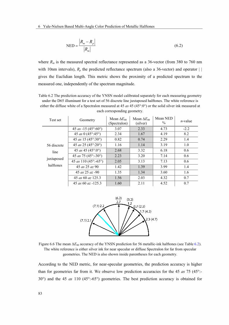
6 Yule-Nielsen Based Multi-Angle Color Prediction of Metallic Halftones
83
NEDm p
m
R RR
=−
( 6.2)
where Rm is the measured spectral reflectance represented as a 36-vector (from 380 to 760 nm
with 10nm intervals), Rp the predicted reflectance spectrum (also a 36-vector) and operator | |
gives the Euclidian length. This metric shows the proximity of a predicted spectrum to the
measured one, independently of the spectrum magnitude.
Table 6.2 The prediction accuracy of the YNSN model calibrated separately for each measuring geometry under the D65 illuminant for a test set of 56 discrete line juxtaposed halftones. The white reference is
either the diffuse white of a Spectralon measured at 45 as 45 (45°:0°) or the solid silver ink measured at each corresponding geometry.
Test set Geometry Mean ΔE00 (Spectralon)
Mean ΔE00 (silver)
Mean NED % n-value
56 discrete
line
juxtaposed
halftones
45 as -15 (45°:60°) 3.07 2.33 4.73 -2.2 45 as 0 (45°:45°) 2.34 1.67 4.19 8.2
45 as 15 (45°:30°) 0.82 0.74 2.29 1.4 45 as 25 (45°:20°) 1.16 1.14 3.19 1.0 45 as 45 (45°:0°) 2.68 3.32 6.18 0.6
45 as 75 (45°:-30°) 2.23 3.20 7.14 0.6 45 as 110 (45°:-65°) 2.05 3.13 7.13 0.6
45 as 25 az 90 1.42 1.39 3.99 1.4 45 as 25 az -90 1.35 1.34 3.60 1.6
45 as 60 az 125.3 1.56 2.03 4.32 0.7 45 as 60 az -125.3 1.60 2.11 4.52 0.7
Figure 6.6 The mean ΔE00 accuracy of the YNSN prediction for 56 metallic-ink halftones (see Table 6.2). The white reference is either silver ink for near specular or diffuse Spectralon for far from specular
geometries. The NED is also shown inside parentheses for each geometry.
According to the NED metric, for near-specular geometries, the prediction accuracy is higher
than for geometries far from it. We observe low prediction accuracies for the 45 as 75 (45°:-
30°) and the 45 as 110 (45°:-65°) geometries. The best prediction accuracy is obtained for

6 Yule-Nielsen Based Multi-Angle Color Prediction of Metallic Halftones
84
capturing angles between the specular (45°:45°) and the normal (45°:0°) orientation such as 45
as 15 (45°:30°) and 45 as 25 (45°:20°).
6.4 Yule-Nielsen Analysis of Metallic-Ink Halftones
Let us analyze how the optimal n-values behave as a function of the measuring geometry. We
examine one halftone sample with 60% metallic magenta and 40% silver. The prediction
accuracies for this particular halftone are collected in Table 6.3. As shown in this table, there are
different optimal n-values for different geometries. Also, extending our study to negative n-
values proved to be helpful as shown for the 45 as -15 geometry. In addition, 5 out of the 11
geometries have an optimized n-value in the interval (0, 1) which is rather unusual.
Table 6.3 The prediction accuracy of the YNSN model for a single discrete line juxtaposed halftone (m 0.6, s 0.4) calibrated separately for each measuring geometry.
Test set Geometry ΔE00 (Spectralon)
ΔE00 (silver) NED % n-value
A halftone
sample
composed of
60% magenta
and 40%
silver
45 as -15 (45°:60°) 2.67 2.22 5.38 -2.1 45 as 0 (45°:45°) 0.32 0.28 0.71 2.5
45 as 15 (45°:30°) 0.87 0.78 1.92 2.1 45 as 25 (45°:20°) 0.44 0.44 0.79 1.2 45 as 45 (45°:0°) 0.85 0.90 2.95 0.8
45 as 75 (45°:-30°) 1.81 2.19 4.87 0.6 45 as 110 (45°:-65°) 1.91 2.34 5.34 0.6
45 as 25 az 90 0.53 0.51 1.52 1.1 45 as 25 az -90 0.59 0.59 1.44 1.5
45 as 60 az 125.3 1.70 1.95 4.21 0.7 45 as 60 az -125.3 0.69 0.83 2.12 0.8
In order to better understand the effect of different n-values on the prediction of halftone
reflectances, we use the graphical representation of the Yule-Nielsen (YN) function [66]. For a
two-colorant metallic halftone, we denote Ra(λ) the spectral reflectance of the halftone patch
composed of the metallic non-silver ink with coverage a (0<a<1) and the silver ink with area
coverage (1 – a). R1(λ) is the spectral reflectance of the non-silver metallic ink with full area-
coverage. The silver ink is assimilated to the “white” background with reflectance R0(λ). The
Yule-Nielsen function for this halftone is

6 Yule-Nielsen Based Multi-Angle Color Prediction of Metallic Halftones
85
( ) ( ) ( ) ( )1/ 1/0 11 .
nn naR a R aR λ = − λ + λ ( 6.3)
By dividing Eq. (3) by R0(λ) we obtain for each wavelength
( )1/0 1 01 .
nnaR R a a R R
= − + ( 6.4)
The relative attenuation of the halftone Ra/R0 as a function of the relative attenuation of the
fulltone R1/R0 can be plotted according to the spectral measurements of R0(λ), Ra(λ) and R1(λ).
These reflectances provide as many Ra/R0 and R1/R0 attenuations as discrete values contained in
the measured spectra.
Figure 6.7 The Yule-Nielsen graph for different n-values for the non-silver halftone area coverage of a= 0.6. Note that the n= 100 and n= -100 curves nearly coincide.
In Figure 6.7 we show the YN function for a halftone area-coverage of a = 0.6 and for different
values of n. The straight line with n = 1 represents the “Neugebauer function”, a linear
relationship between no attenuation and attenuation by the fulltone ink according to the area
coverage of that ink. Varying the n-value has the effect of making the YN function nonlinear.
The traditional interval of n-values [1, 100] covers a small portion of the function’s range. In
this interval, the reflectance of halftones is lower than the one predicted by the Neugebauer
function. Extending this interval to negative values helps us span a greater portion of the range.

6 Yule-Nielsen Based Multi-Angle Color Prediction of Metallic Halftones
86
The most interesting case is the interval (0, 1) where the YN function yields an inverse effect,
i.e. the halftone exhibits a higher reflectance than the one predicted by the Neugebauer function.
Let us study the metallic halftone (m= 0.6, s= 0.4) using the fitted YN function along with
measured data for some representative geometries. Figure 6.8 shows the function for three n-
values: n = 1 which represents the Neugebauer function, n = 2 as recommended by Yule and
Nielsen [51], and the best fitted n-value according to Table 6.3. Depending on the measuring
geometry, the value R1/R0 can be larger than 1. Also, some Ra/R0 values can be above the
Neugebauer line, yielding fitted n-values between 0 and 1.
We observe that for all geometries the measured attenuations follow a straight line. This is in
contrast with a traditional print on paper where, due to optical dot-gain, the halftone attenuation
follows a curve similar to the n = 2 Yule-Nielsen curve. This might be an indication of a very
moderate or no optical dot-gain.
In traditional prints with transparent inks on a diffusely reflecting paper, the n-value accounts
for the nonlinear effects that occur due to subsurface scattering and multiple reflections between
the paper bulk and the print-air interface. For such prints, the halftone attenuation forms a curve
similar to the Yule-Nielsen function, generally with 1 < n < 100.
Figure 6.8 Measured halftone attenuation and Yule-Nielsen graphs for different geometries. The YN function graphs are plotted for n = 1(dotted line), n = 2 (dashed line) and the fitted n (solid line) of the
halftone (m = 0.6, s = 0.4). The fitted n-value for each graph is written inside the plots.
In our experiments the metallic flakes reflect strongly at specular angles and weakly at non-
specular angles. They are printed at a very low print resolution and cover the full surface.
Therefore, optical dot-gain induced by scattering of light in the paper substrate is not likely to
0 0.5 10
0.2
0.4
0.6
0.8
145 as -15
0 0.5 10
0.2
0.4
0.6
0.8
145 as 0
0 0.5 10
0.2
0.4
0.6
0.8
1
45 as 25 az 90
R1
/R0
0 0.5 1
Ra/R
0
0
0.5
1
45 as 110
0 0.5 10
0.2
0.4
0.6
0.8
1
45 as 45
0 0.5 10
0.2
0.4
0.6
0.8
1
45 as 15
n = 0.8
NED = 2.95
n = -2.1NED = 5.38
n = 2.5
NED = 0.71
n = 2.1
NED = 1.92
n = 0.6
NED = 5.34
n = 1.1
NED = 1.52

6 Yule-Nielsen Based Multi-Angle Color Prediction of Metallic Halftones
87
occur. A simple Neugebauer model could therefore be enough for predicting these halftone
reflectances. But why do we have n-values different from 1? And, why are the n-values
different for different measuring geometries?
To investigate these questions, we designed an experiment that demonstrates the effect of
juxtaposed halftoning on the texture of a metallic sample and on its multi-angle reflection
behavior. Figure 6.9 shows the microscopic image of two samples. In Figure 6.9a we have a
fulltone (100%) metallic magenta sample printed in a single pass. To simulate the effect of
halftoning, in Figure 6.9b, we try to generate the same fulltone magenta sample but by
sequentially printing several halftone lines of metallic magenta side by side.
Figure 6.9 The microscopic image of 100% metallic magenta taken in transmission mode. (a) Printed in one pass. (b) Printed in four passes by printing several discrete lines side by side. (c) The layout of one
halftone screen used for generating the multi-pass solid magenta sample.
Without the effects of multi-pass printing, the two samples would have the same reflection
spectra at all illumination and observation angles. However, from the microscopic images we
can observe the differences. In the “multi-pass” fulltone magenta, the misregistration between
successive printed lines generates small unprinted white areas. In addition, the partial
superposition of the halftone lines due to misregistration makes the surface of the multi-pass
solid magenta uneven and prone to shadowing.
Figure 6.10 shows the reflectance spectra of the two samples depicted in Figure 6.9. The
difference between the two reflectance spectra depends on the measuring geometry. Note that in
the case of the traditional 45 as 45 (45°:0°) geometry, there is an identical spectrum for both
samples. This indicates that, at this non-specular geometry, the multi-pass artifacts have no
effect. For measurement geometries close to specular, the texturing effect of multi-pass printing
is important.

6 Yule-Nielsen Based Multi-Angle Color Prediction of Metallic Halftones
88
Figure 6.10 The spectral reflectances for solid 100% magenta (solid line) and for the multi-pass 100% magenta (dashed line) for some representative geometries. The measurements have taken place with our
default setup, i.e., the MA98 plane of incidence is parallel to the horizontal axis of the halftones.
Slight shifts between the colorant layers can explain the need for Yule-Nielsen n-values that
vary in function of the measurement geometry. Note that misregistration also occurs in classic
prints. However, as classic inks are transparent and their halftone dots partially overlap, the
effect of misregistration is weak compared to opaque metallic-ink juxtaposed halftones.
Depending on the measuring geometry, the metallic halftones exhibit different contributions of
shadowing and white interstices. Misregistration creates shadowing effects that result in darker
measurements and unprinted space between halftone dots that lighten the reflectance. The n-
value seems to account for these two inverse effects. As the effects of shadowing and white
interstices are different for each geometry, the n-value also differs.
6.5 Summary
In order to create a color reproduction workflow for metallic inks, we need to characterize the
metallic halftones, possibly accounting for several illumination and observation geometries.
Such a characterization enables simulating the appearance of the final print at different
observation conditions.
The printer characterization is performed with a spectral prediction model. We investigated the
Yule-Nielsen spectral Neugebauer spectral prediction model for the different measurement
geometries. This prediction model, calibrated separately for each geometry, shows good color-
400 500 600 700100
200
30045 as -15
400 500 600 700100
200
30045 as 0
400 500 600 70050
100
150
20045 as 15
400 500 600 700
Ref
lect
ance
fact
or %
0
20
40
Wavelength400 500 600 7000
10
2045 as 110
400 500 600 7000
50
100

6 Yule-Nielsen Based Multi-Angle Color Prediction of Metallic Halftones
89
prediction accuracy. For each measuring geometry, there is a different Yule-Nielsen n-value.
For traditional prints on paper, the n-value expresses the amount of optical dot-gain. In the case
of the metallic prints, the optical dot gain is much smaller than in paper prints. With the fitted n-
values, we explain the interaction of light and metallic halftones. Our experiments suggest that
the Yule-Nielsen n-value accounts for effects induced by colorant misregistration such as
shadows and white interstices at halftone-dot borders.

6 Yule-Nielsen Based Multi-Angle Color Prediction of Metallic Halftones
90

7 Color Separation for Juxtaposed Halftoning
91
7.1 Introduction
In spite of their potential applications, metallic inks have a limited usage in the printing
industry. They are either used as spot colors in luxury designs or printed below classic inks to
give a shiny look to the printout. In this chapter, we create metallic-ink images: prints whose
contributing colorants are all made of metallic inks. One of the main advantages of metallic-ink
prints, compared to prints with classic inks printed on top of silver, is their anti-counterfeiting
capacity. They are not copyable by classic inks. In addition, counterfeiters cannot easily create
fully metallic images. From a technical point of view, printing high amounts of classic inks on
top of silver is not always possible because of the trapping effect. Obtaining well-saturated
metallic-colors with overprinting is therefore not easy.
Metallic-ink prints require more than four inks to generate a significant color gamut. The
opaque particles inside the metallic inks mask the layers beneath them and prevent the
formation of new colorants. If we want a gamut similar to a standard CMY gamut, 8 metallic
inks corresponding to 8 colorants of CMY prints are needed (see Section 5.2). With 8 inks, there
will be more than a single ink-combination that reproduces a desired color. The problem of
7 7 Color Separation for Juxtaposed
Halftoning

7 Color Separation for Juxtaposed Halftoning
92
printing with a large number of inks is also known in standard printing and is referred to as n-
color printing [67].
In traditional prints with transparent inks, the reasons behind the so-called n-color printing are
various. The main purpose is to increase the color gamut of CMYK prints as it is narrower than
the gamut of a color display. Spectral reproduction is another objective where an exact color
reproduction under more than one illuminant is desired. Additional inks sometimes are simply
used as spot colors that are very popular in packaging industry.
The main challenge in n-color printing is the redundancy introduced with the addition of new
inks. For a 4-ink CMYK printer, this problem has been known for long time. In these printers, a
target color can be produced by one CMY ink-combination or many CMYK ink-combinations.
For four-ink systems, there are well-established methods to address this one-to-many problem.
These methods rely on under-color removal (UCR) or gray-component replacement (GCR)
[46].
The problem of n-color separation (n > 4) has been studied in many works [17, 68, 69, 70, 71,
72, 73, 74]. Usually, these works divide the ink set into smaller subsets, making the color
separation simpler. When there are multiple choices between different ink subsets, they might
select the solution that optimizes one or more print attributes. These attributes include halftone
visibility, color constancy, amount of consumed inks, etc. [24]. Chen et al. [72] devise an
approach towards a multi-ink color separation by using color lookup tables. For one color, they
generate several ink combinations matching that color and choose one that performs the best
according to a multi-criteria print-quality metric. This metric is a weighted combination of
chromaticity of the print, print color-constancy and graininess. However, they do not offer
access to their halftoning method and no printed image is included in their results. Son and Park
[73], convert the CMYK digital values into CMYKLcLm ink amounts. During this conversion
they take into account print-quality measures such as dot visibility and spatial smoothness of the
image. Another method for color separation is halftone area Neugebauer separation (HANS)
[24]. This method does not impose a limit on the number of contributing inks.
This chapter addresses the problem of n-color separation for juxtaposed halftones. Many print
attributes that can be taken into account during color separation are pertinent to the halftoning
method. For example, discrete-line halftone dots might be visible because of their line-screen
nature. Therefore, it is worth trying to obtain halftones with minimal dot-visibility. More
specifically, we focus on metallic-ink prints that are made of halftones with juxtaposed metallic

7 Color Separation for Juxtaposed Halftoning
93
inks (Chapter 6). As mentioned above, n-color printing is a requirement, rather than an option,
for printing metallic-ink images. Therefore, our efforts in this chapter are oriented towards
introducing a simple method of color separation that can be used efficiently and in a
straightforward way.
7.2 Prediction Accuracy of the Forward Characterization
We follow closely the experimental framework introduced in Chapter 6. In short, we use a dye-
sublimation OKI printer that is capable of printing simultaneously with 9 cartridges among
which four are metallic: metallic cyan (C), metallic magenta (M), gold or metallic yellow (Y)
and silver (S). There are also transparent process and spot inks available for this printer. In
Chapter 6, we carried out our experiments using metallic inks only. In order to have a metallic-
ink print with a reasonable color gamut volume, we add four more inks to the previous setup.
We “synthesize” three new metallic colorants: metallic blue (B) by superposing transparent
cyan on metallic magenta, metallic green (G) by superposing transparent cyan on gold and
metallic red (R) by superposing transparent magenta on gold. Finally, as black is highly
absorbant, we add a process black ink (K) to form a CMYKRGBS metallic-ink system that is
similar to heptatone multi-color printing [17, 68, 69] except that the silver in metallic prints (S)
serves as the equivalent of paper in standard prints. In this chapter we use the names silver (S)
and white (W) interchangeably. Also, the colorants in classic prints are equivalent to metallic-
inks in our juxtaposed setup. In order to have an accurate registration, we use again the 100 dpi
print resolution. As in the past chapter, we use the X-Rite MA98 to perform spectrophotometric
measurements for different illumination and viewing geometries.
To be able to print full-color images using metallic inks, we first need a color prediction model
that predicts the spectral reflectance of metallic-ink halftones with acceptable accuracy.
Generally, with more than four inks, the forward characterization of a printer becomes more
complicated and data intensive. For example, to characterize a CMYKRGB printer with
transparent inks, we can use the cellular Yule-Nielsen spectral Neugebauer model (CYNSN). If
we have cells with area coverages only at 0, 50% and 100%, for 7 inks, the model requires
37=2187 samples for calibration. Juxtaposition of inks decreases the number of calibration
patches required for a spectral prediction model. For characterizing the same printer but with
juxtaposed halftoning, a two-by-two dot centering model for 8 opaque colorants requires 1072
calibration samples.

7 Color Separation for Juxtaposed Halftoning
94
As in Chapter 6, we use the nominal Yule-Nielsen spectral Neugebauer model (YNSN) for
predicting the color of metallic-ink halftones under different illumination and observation
geometries. The model needs only 8 measured Neugebauer primaries as the calibration set. The
YNSN prediction equation in the vector-matrix form can be written as
1/ 1/n n⊗ ⊗=r A a ( 7.1)
where r is a 31-vector representing the halftone reflectance comprising discrete wavelengths
from 400 to 700 nm in 10 nm intervals. A is the matrix of primaries whose rows are the
reflectance vectors of Neugebauer primaries (31×8) and a is the vector of nominal area-
coverages, an 8-vector. The symbol ⊗ stands for an element-by-element matrix operation. For
classic prints, the value n accounts for the optical dot-gain due to lateral propagation of light
inside the substrate. For metallic halftones, this parameter is responsible for shadowing and
misregistration between different colorants. We extensively discussed the role of the n-value in
metallic prints in the previous chapter.
In order to examine the predication accuracy of the YNSN model for metallic halftones, we
consider a test set formed by 125 halftones with variations of the nominal area-coverages of the
8 metallic inks that are constrained such that the sum of their area coverages is 1. Table 7.1
summarizes the prediction accuracies for the 11 geometries available at the 45° illumination.
We allowed the n-value to vary between -10 to 10 at 0.1 intervals. As shown in Table 7.1, the
prediction accuracy of the YNSN model, expressed as CIEDE2000 color-difference formulae
[65], is within an acceptable range. The color accuracy varies according to the measuring
geometry. The analysis of this model and the role of the n-value, according to the observation
and illumination angles, are thoroughly discussed in Chapter 6. For the white reference, we use
either the diffusing white Spectralon measured at the 45°:0° geometry or the silver reflectance
measured at each corresponding geometry. We evaluate the accuracy of the model according to
a spectral difference metric, i.e., the normalized Euclidean distance (NED) between the
predicted and measured spectral reflectance-vectors normalized to the measured reflectance-
vector.
In the present work, we limit ourselves to measurements for a single measuring geometry, i.e.
45 as 25 (45°:20°). The main reason is that the color prediction at this geometry is accurate. As
the purpose of this chapter is to perform color separation, the accuracy of forward model is
important in order to have an accurate color reproduction.
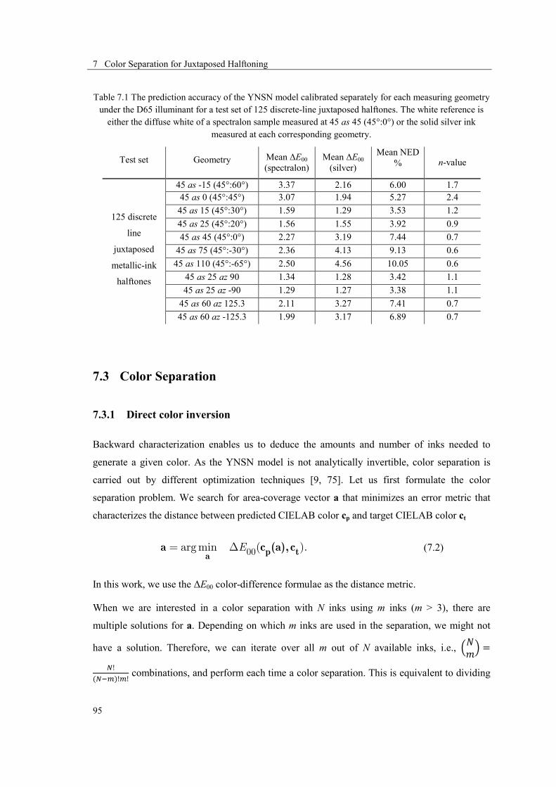
7 Color Separation for Juxtaposed Halftoning
95
Table 7.1 The prediction accuracy of the YNSN model calibrated separately for each measuring geometry under the D65 illuminant for a test set of 125 discrete-line juxtaposed halftones. The white reference is
either the diffuse white of a spectralon sample measured at 45 as 45 (45°:0°) or the solid silver ink measured at each corresponding geometry.
Test set Geometry Mean ΔE00 (spectralon)
Mean ΔE00 (silver)
Mean NED % n-value
125 discrete
line
juxtaposed
metallic-ink
halftones
45 as -15 (45°:60°) 3.37 2.16 6.00 1.7 45 as 0 (45°:45°) 3.07 1.94 5.27 2.4
45 as 15 (45°:30°) 1.59 1.29 3.53 1.2 45 as 25 (45°:20°) 1.56 1.55 3.92 0.9 45 as 45 (45°:0°) 2.27 3.19 7.44 0.7
45 as 75 (45°:-30°) 2.36 4.13 9.13 0.6 45 as 110 (45°:-65°) 2.50 4.56 10.05 0.6
45 as 25 az 90 1.34 1.28 3.42 1.1 45 as 25 az -90 1.29 1.27 3.38 1.1
45 as 60 az 125.3 2.11 3.27 7.41 0.7 45 as 60 az -125.3 1.99 3.17 6.89 0.7
7.3 Color Separation
7.3.1 Direct color inversion
Backward characterization enables us to deduce the amounts and number of inks needed to
generate a given color. As the YNSN model is not analytically invertible, color separation is
carried out by different optimization techniques [9, 75]. Let us first formulate the color
separation problem. We search for area-coverage vector a that minimizes an error metric that
characterizes the distance between predicted CIELAB color cp and target CIELAB color ct
00argmin ( ).E= E p taa c (a), c ( 7.2)
In this work, we use the ΔE00 color-difference formulae as the distance metric.
When we are interested in a color separation with N inks using m inks (m > 3), there are
multiple solutions for a. Depending on which m inks are used in the separation, we might not
have a solution. Therefore, we can iterate over all m out of N available inks, i.e., �𝑁𝑚� =
𝑁!(𝑁−𝑚)!𝑚!
combinations, and perform each time a color separation. This is equivalent to dividing

7 Color Separation for Juxtaposed Halftoning
96
the N-ink gamut into multiple sub-gamuts of m inks. For example, if we limit the use of m = 4
inks per screen in the case of our 8-ink printing system, there will be �84� = 70 sub-gamuts.
For traditional halftoning with transparent inks, the color separation is usually performed in a
similar manner, except that it takes place in a limited number of subgamuts, e.g., 20 out of 70
for m = 4, see [72]. This is due to the exhaustive calibration effort that would be required for a
global forward prediction-model comprising all N inks. For example, calibrating a cellular
YNSN requires at least 3N measurements of the calibration samples, at 0, 50% and 100% area
coverages of each ink. If a higher accuracy is desired, we can use additional nodes at 25% and
75% giving rise to 5N calibration samples. Therefore, a limited number of m-ink (usually 4-ink)
forward models characterizing m-ink subgamuts are established. The computational and
measurement effort is increased when considering more subgamuts. With fewer subgamuts, new
possibilities for optimizing the print attributes are lost. Hence, there is a trade-off between the
calibration effort and the solution space for optimizing the print attributes.
In contrast to most halftoning methods, in juxtaposed halftoning we are free to choose the
number of contributing inks for rendering a desired color. Adding inks does not induce
computational overhead and does not introduce moiré-like artifacts. Moreover, for their color
prediction, establishing an N-ink model is possible with an affordable number of calibration
samples. Although in this chapter we use the nominal YNSN with only 8 primaries, for high-
accuracy reproduction the two-by-two dot-centering model with 1072 calibration pattern can be
used.
Having calibrated a global N-ink color-prediction model, an m-color separation can be done by
using an optimization formula (7.2) with additional constraints:
00
1
argmin ( )
subject to 1
and [0,1]
qm
E= E
=
Î
p taa c (a), c
a
a
( 7.3)
where ||.||1 stands for the 1-norm of a vector, which is the sum of its elements. We execute
multiple times the minimization (7.3) on all possible subgamuts of m inks. Each time, we set the
sum of ink area-coverages inside the qth subgamut to 1. Consequently, all non-participating inks
that do not belong to this subgamut (but are used in the global model for optimization) have
zero area-coverage. Because a color is reproducible inside more than 1 subgamut, the

7 Color Separation for Juxtaposed Halftoning
97
optimization yields multiple answers. For the final solution, we can choose the answer that
produces the lowest error. However, this is not a correct approach as the error associated with
the selected answer might be only slightly lower than the error produced by other solutions. A
better way is to define a set of solutions according to an error criterion, e.g., the set of solutions
that satisfy ΔE00 < 1.
7.3.2 Color separation relying on formulas
In most of previous works on n-color separation, the total color gamut of all participating inks is
divided into a number of smaller subgamuts. Then, a forward characterization is carried out for
each subgamut. During color separation, the inversion takes place at the subgamut where the
most faithful reproduction can be obtained. If there are multiple subgamuts satisfying the
reproduction criterion, one of them is selected based on other criteria. The main disadvantage of
these methods is that they are often computationally expensive.
We seek a rapid color separation for metallic-ink image reproduction. We are inspired by the
gray component replacement (GCR) that is used for printing with CMYK. In this method, first
the color separation for three chromatic inks is obtained. Then, during the black generation step,
the amount of black ink is obtained using a unique transform from CMY to CMYK. In a similar
approach, we first accomplish a color separation for a pseudo-CMY-ink system. We call it
pseudo-ink system because not all colors are reproducible with juxtaposed CMY inks.
Therefore, we consider an ink-to-colorant formulation mapping the pseudo-CMY-inks to all
contributing colorants (CMYKRGBS) in the forward model and also during the color
separation. The CMY inks play the role of the interface that separates the input from the set of
available colorants.
The color separation relying on a formula results in pseudo area-coverages of cyan, magenta
and yellow that are then mapped to the working area-coverages of colorants using the
considered ink-to-colorant mapping. As we rely on juxtaposed halftoning, such a mapping
should result in area coverages that sum up to 1. In this chapter, we consider two mappings for
the color separation of metallic-ink prints.
The Kueppers color separation formula: Harald Kueppers [17] uses a CMYKRGB ink set to
create heptatone prints. In his approach, every color in the color space is reproduced by up to
four inks, two of which are black and white. In other words, in every color separation there exist
at most two chromatic inks. The proposed formulation can best be described by considering

7 Color Separation for Juxtaposed Halftoning
98
CMY transparent inks superposed as in dot-on-dot screens [76], see Figure 7.1. The outcome of
the superposition depends on the respective CMY area-coverages (c, m, y). In Figure 7.1, c ≤ m
≤ y, hence ay = y – m, ar = m – c, ak = c and aw = 1 – y. Note that we are using the notations
introduced in Section 5.2.
Figure 7.1 Schematic representation of a dot-on-dot screen from the top (left) and from the side (right). In this drawing, c < m < y.
Table 7.2 lists all possible colorant outcomes generated as a result of different respective area-
coverages of cyan, magenta and yellow in a dot-on-dot screen. Note that the sum of all primary
area-coverages in each column in the Table 7.2 is 1. It is important to note that the dot-on-dot
approach here is only used to explain Kueppers’ color-separation formula. In this work, as the
inks are opaque, the area coverages of any formulations are halftoned in a perfectly juxtaposed
manner.
Table 7.2 The coverage of 8 Neugebauer colorants, according to the Kueppers separation formula. The area coverages depend on the respective area-coverages of the CMY inks.
c ≤ m ≤ y c ≤ y < m m < c ≤ y m ≤ y < c y < c ≤ m y < m < c
ac 0 0 0 c – y 0 c – m am 0 m – y 0 0 m – c 0 ay y – m 0 y – c 0 0 0 ak c c m m y y ar m – c y – c 0 0 0 0 ag 0 0 c – m y – m 0 0 ab 0 0 0 0 c – y m – y aw 1 – y 1 – m 1 – y 1 – c 1 – m 1 – c
The Demichel color separation formula: In Section 5.2 we discussed the Demichel equations
and their extensive use in halftone printing. As a reminder, Table 7.3 summarizes the Demichel

7 Color Separation for Juxtaposed Halftoning
99
equations. Given the dot area of CMY inks, the Demichel equations compute the area coverages
of the 8 Neugebauer primaries. They rely on the statistically independent superposition of ink
dots. We can verify that the sum of all area coverages in the Demichel equations is 1. Here also,
using the Demichel pseudo-ink to colorant mapping does not imply that the colorants should be
laid out independently to satisfy the Demichel equations.
Table 7.3 The coverage of 8 Neugebauer colorants according to the Demichel separation formula.
ac c (1 – m) (1 – y) ar (1 – c) m y am (1 – c) m (1 – y) ag c (1 – m) y ay (1 – c) (1 – m) y ab c m (1 – y) ak c m y aw (1 – c) (1 – m) (1 – y)
7.4 Print Attributes from Different Color-Separation Schemes
The separation formulas provide a relationship between the contributing inks in n-color printing.
This is equivalent to the division of the overall gamut into a number of subgamuts, except that
the ink-to-colorant formulas accomplish this task implicitly by using a mathematical formula
that is computed very rapidly. Depending on the employed separation formula, a given color in
the gamut uses a specific subgamut. Let us compare the different print characteristics of test
patches color-separated according to different separation schemes.
7.4.1 Gamut volume
The first step in evaluating every separation formula is its resulting gamut volume. If the gamut
volume is significantly smaller than the maximum volume achievable with a given printing
system, then the corresponding separation formula fails to cover all regions in the gamut and
therefore it is not suitable for high quality color reproduction. To calculate the gamut volume
for a given set of printer, paper and inks, we use the YNSN model with the parameters acquired
in Section 7.2. For our metallic-ink prediction framework, we use n = 0.9 as the Yule-Nielsen
factor. As we use nominal area-coverages, the model is run by only the spectra of the 8
participating metallic inks.
To create the largest possible color gamut, the area coverages of all 8 metallic inks are changed
in small intervals and the resulting spectra are predicted using the nominal YNSN model. Each
spectrum is then converted to CIEXYZ, and subsequently to CIELAB under the D65 illuminant.

7 Color Separation for Juxtaposed Halftoning
100
From the set of CIELAB colors synthesized using the prediction model, the volume of the
concave color-gamut can be obtained [77].
In order to calculate the gamut volume covered by the separation formulas, we change only the
area coverages of three CMY inks. There is no limitation on the area coverages of three inks
and they can take any amounts from 0 to 1. Using either the Kueppers or the Demichel
separation formula, we compute the area coverages of the 8 metallic inks. Following the same
steps above for calculating the maximal gamut, we obtain the gamut volume corresponding to
each separation formula. Table 7.4 shows the calculated gamut volume for each separation
strategy. Kueppers’ and Demichel’s formulas cover 93% and 88% of the largest possible gamut,
respectively.
Table 7.4 The volume of the concave gamut achievable with different color-separation strategies (in kilo CIELAB).
Kueppers’ formula Demichel’s formula Largest gamut
156.02 148.39 168.78
Note that as we use the same inks and the same prediction model, the differences in gamut
volume arise from the differences in separation formulations only. Different formulas cover
different regions in the area-coverage domain. Table 7.5 lists the subgamuts accessible by each
separation formula. For the sake of completeness, we count every single ink as a subgamut. In
Table 7.5, a subgamut named A1A2 …AN is formed by combinations of non-zero amounts of
inks A1, A2… AN where the sum of their corresponding area coverages is unity, i.e.
a1+a2+…+aN = 1. The non-zero condition implies that larger subgamuts cannot be reduced to
subgamuts with a lower number of inks. For example, with Demichel’s formula, a 3-ink
subgamut, such as CMW, cannot be achieved by setting to zero the value of the blue ink in the
4-ink subgamut CMBW.
Both Kueppers’ and Demichel’s separation formulas are nonlinear transformations from [0, 1]3
to [0, 1]8. Each formula, spans a specific range in [0, 1]8. Note that, in addition to the general
limitation of the sum of area coverages, there are other limitations specific to each formula. For
example, inks in the 8-ink gamut accessible by the Demichel formula cannot take any arbitrary
non-zero values. If they could, the gamut volume generated by the Demichel color separation
would be equal to the largest gamut (Table 7.4). There are constraints caused by the Demichel
equations, which limit the range of accessible area coverages. For example, increasing the value

7 Color Separation for Juxtaposed Halftoning
101
of cyan colorant independently of other colorants is not possible. If we increase the value of the
cyan pseudo-ink, it also results in increased values of blue, green and black colorants.
Table 7.5 List of all subgamuts accessible with different color separation strategies.
Subgamut Kueppers (52) Demichel (27)
1-ink 8 (C, M, Y, K, R, G, B, W) 8 (C, M, Y, K, R, G, B, W) 2-ink 19 (WK, CG, CB, CW, CK,
MR, MB, MW, MK, YR, YG,
YW, YK, RW, RK, GW, GK,
BW, BK)
12 (CG, CB, CW, MR, MB, MW,
YR, YG, YW, RK, GK, BK)
3-ink 19 (CWK, CBW, CBK, BWK,
MWK, MBW, MBK, MRW,
MRK, YWK, YRW, YRK,
RKW, YGW, YGK, GWK,
CGW, CGK, GWK)
0
4-ink 6 (CGWK, CBWK, MRWK,
MBWK, YRWK, YGWK)
6 (CMBW, CYGW, CGBK,
MYRW, MRBK, YRGK)
5-ink 0 0 6-ink 0 0 7-ink 0 0 8-ink 0 1 (CMYRGBKW)
Table 7.5 explains why the Demichel separation strategy offers a gamut volume smaller than the
Kueppers separation. For example, with the Demichel equations, we can verify that any 2-ink
combinations comprising black ink and one ink selected from cyan, magenta and yellow inks is
not possible. These combinations represent colors in the border of the gamut and have a direct
influence on the gamut volume. The Kueppers formula, however, can produce these
combinations of colorants.
7.4.2 Maximum number of inks per color
This criterion determines the maximum number of inks that can be placed in a halftone screen-
element to reproduce a given color. For direct color separation, it can be set to any number.
When using separation formulas, the maximum number of inks per screen is known beforehand.
The Kueppers separation formula uses at most 4 inks to reproduce a color. The Demichel
separation equations need a maximum of 8 inks per color. The number of inks per color has an

7 Color Separation for Juxtaposed Halftoning
102
important influence on halftone properties. A small number of inks in a halftone yields for each
ink a larger dot, thus leading to more clustering. This can be advantageous for some printing
technologies where small dots tend to disappear. Furthermore, with larger dots, the color shift
induced by the misregistration of the different layers has less undesirable effects [78].
7.4.3 Color constancy
The CMCCON97 Color-Inconstancy-Index is used to evaluate the color constancy of samples
generated by different color separation strategies. In order to compute this index for any color
sample we perform the following steps [79]:
(1) We measure or calculate the CIEXYZ values of the sample under a test (XYZt) and a
reference illuminant (XYZr)
(2) A chromatic adaptation transform (e.g. CMCCAT97 [79]) is used to compute the
corresponding color of the sample when taken from the test to the reference illuminant
(XYZCAT).
(3) The Color Inconstancy Index is defined as the color difference between the actual color
(XYZr) and the transformed color of the sample (XYZCAT) under the reference illuminant.
We first perform the color separation on 125 color patches printed with metallic inks by using
either the Kueppers formula or the Demichel formula. As these colors are inside the printer
gamut, no gamut clipping occurs. Having obtained the area coverage of a halftone, we predict
its spectral reflectance. Tristimulus values are then calculated from the predicted spectral
reflectance for the test illuminant and the reference illuminant. We set fluorescent F11 (also
known under the name TL84) and D65 as the test and reference illuminants, respectively. The
CIE2000 color-difference formula is then employed to evaluate the difference between pairs of
corresponding colors. Table 7.6 shows the statistics of the CMCCON97 Color Inconstancy
Index for 125 representative test colors separated according to the two separation formulas.
Halftones separated using the Kueppers formula show a higher color constancy when moving
between different illuminants. This is due to the presence of higher amounts of achromatic black
and silver inks compared to the halftones color-separated with the Demichel formulation.

7 Color Separation for Juxtaposed Halftoning
103
Table 7.6 The CMCCON97 Color-Inconstancy-Index of 125 metallic-ink test-halftones color separated using different separation strategies.
CII Kueppers’ formula Demichel’s formula
mean 3.14 4.24 0.95 quantile 5.65 7.41
max 7.24 9.07
7.4.4 Halftone visibility
Halftone visibility is particularly interesting for us as the discrete-line juxtaposed halftoning
tends to produce 1D lines that are more visible than other dot shapes. The metric we use for
halftone visibility is the standard deviation of the lightness in an S-CIELAB halftone tile [73].
Let us call this metric std-SL*. In order to compute it for a halftone with a certain area-coverage
vector a, we generate the halftone tile using discrete-line juxtaposed halftoning. We then create
a CIEXYZ image-tile with the CIEXYZ values of the ink assigned to each pixel. From the XYZ
halftone-tile we can generate the S-CIELAB halftone image as explained in [80]. The standard
deviation of the L* channel of the S-CIELAB halftone-image is adopted as the visibility score.
The higher the score, the higher the visibility of the halftone.
Table 7.7 shows the std-SL* statistics for the 125 representative halftone-patches with separated
area-coverages according to different color-separation formulas. The Kueppers formula leads to
slightly more visible halftones. Although the mean visibility-score for both methods is almost
equal, the Kueppers formulation results in a higher standard deviation of the std-SL* visibility
score. This is because the visibility increases for halftone patches with large amounts of black
and silver and decreases for other halftones with less black and silver inks.
Table 7.7 The halftone visibility score based on S-CIELAB for 125 test halftones color separated using different separation schemes.
Visibility score Kueppers’ formula Demichel’s formula
mean 12.8 12.3 0.95 quantile 27.5 24.9
max 29.4 29.3 standard dev. 9.8 7.4
Figure 7.2 shows the photographs of two printed images reproduced using our reproduction
workflow (Section 1.2) for metallic inks. The only difference between these two images is the

7 Color Separation for Juxtaposed Halftoning
104
formulation used for their color separation. For both images, we use a discrete-line halftone
screen with m = 4/7, T = 45/7 + 46/7. We use the YNSN with n = 0.9 to establish the gamuts
and perform the color separation. As shown in this figure, the image generated using the
Kueppers formula looks more vivid. This is due to the high-contrast screens resulting from
screens with a lower number of inks and the presence of the black ink. The gamut is also
slightly larger. The image generated by the Demichel separation template tends to be smoother.
The higher standard-deviation in the visibility of screens generated by the Kueppers formulation
leads to a grainier image because the fluctuations in halftone visibility are higher. Furthermore,
according to Table 7.5, the number of accessible subgamuts is larger when color separation
using the Kueppers formula (52) compared with the Demichel formula (27). We will discuss
this issue in more detail.
As halftone visibility is an important attribute in prints with discrete-line juxtaposed halftones,
we try to minimize the visibility by optimizing the candidate subgamuts of the YNSN model.
For this purpose, we perform a color separation for all possible subgamuts of our 8-ink system.
Using the binominal theorem, we can verify that there are
1 22 1NN N N
N++ +
æ ö æ ö æ ö÷ ÷ ÷ç ç ç÷ ÷ ÷ç ç ç÷ ÷ ÷ç ç ç÷ ÷ ÷÷ ÷ ÷ç ç çè ø è ø=
ø è- ( 7.4)
subgamuts in an N-ink printing system. Therefore, there are 255 subgamuts in an 8-ink system.
After choosing the candidate subgamuts capable of reproducing the desired color with high
accuracy, we can select the subgamut with the lowest visibility score.
A brute-force approach for visiting all 255 subgamuts is computationally expensive. In order to
hasten the procedure, we first exclude the subgamuts that certainly do not contain the desired
color. This can be achieved with bounding cubes of all subgamuts in CIELAB. In order to
separate a given color, we exclude the subgamuts that do not include it. Furthermore, we sort
the valid subgamuts based on a rough visibility metric: the standard deviation of the L*
component of the participating inks in each subgamut with equal area-coverages.
We set two thresholds: accuracy and halftone visibility are set to 1.5 ΔE00 color difference and
10, respectively. For a given color, we search among the valid subgamuts sorted according to
the rough visibility metric. Beginning with the first valid subgamut with the least L* deviation,
we perform the color separation. If the accuracy threshold is met, we calculate the halftone
visibility-score (std-SL*) of the separation solution according to the procedure described earlier.
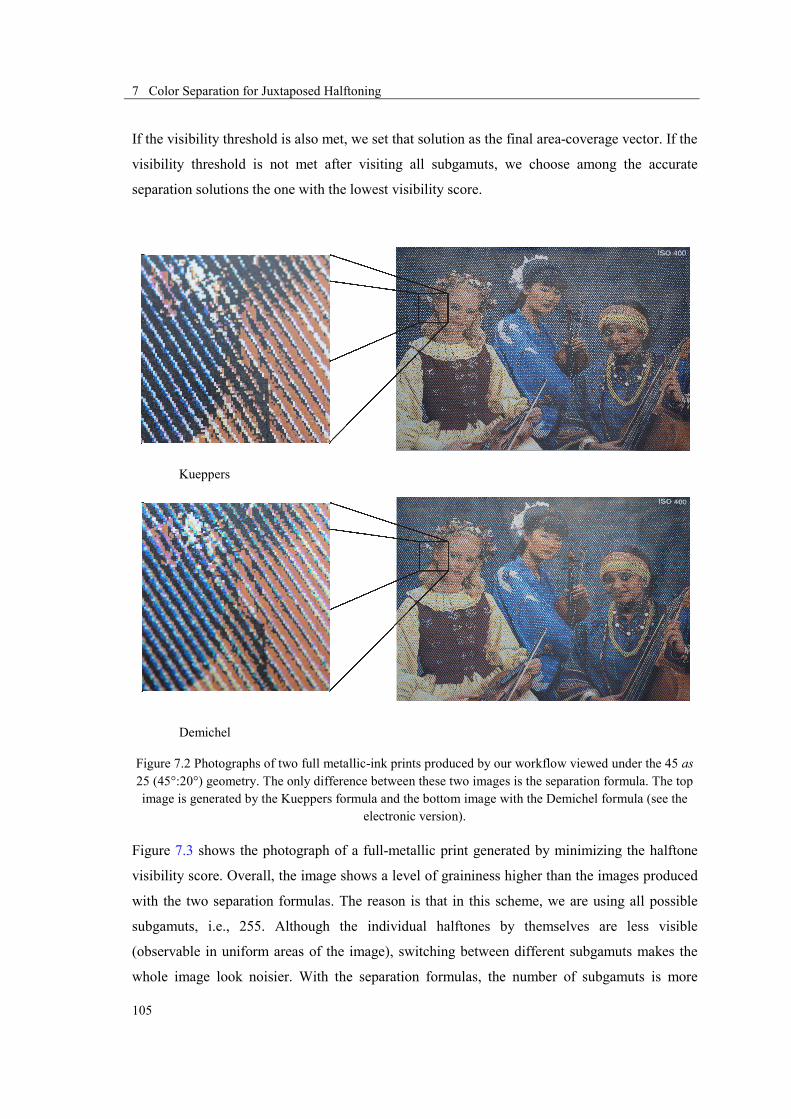
7 Color Separation for Juxtaposed Halftoning
105
If the visibility threshold is also met, we set that solution as the final area-coverage vector. If the
visibility threshold is not met after visiting all subgamuts, we choose among the accurate
separation solutions the one with the lowest visibility score.
Kueppers
Demichel
Figure 7.2 Photographs of two full metallic-ink prints produced by our workflow viewed under the 45 as 25 (45°:20°) geometry. The only difference between these two images is the separation formula. The top image is generated by the Kueppers formula and the bottom image with the Demichel formula (see the
electronic version).
Figure 7.3 shows the photograph of a full-metallic print generated by minimizing the halftone
visibility score. Overall, the image shows a level of graininess higher than the images produced
with the two separation formulas. The reason is that in this scheme, we are using all possible
subgamuts, i.e., 255. Although the individual halftones by themselves are less visible
(observable in uniform areas of the image), switching between different subgamuts makes the
whole image look noisier. With the separation formulas, the number of subgamuts is more

7 Color Separation for Juxtaposed Halftoning
106
limited and, although the halftone visibility is higher, the image graininess is lower. The
halftone-visibility thresholding method could be used to minimize the visibility of uniform
halftones, for example for reproducing spot colors with N inks [75].
Figure 7.3 Photographs of a full metallic-ink print under 45 as 25 geometry with optimized halftone visibility (see the electronic version).
Color-separation induced image-graininess is a local property and increases with an increased
dissimilarity of the subgamuts at each neighborhood. In order to limit the accessible subgamuts
within a small area in the image, when performing pixel by pixel color separation, we give the
preference to the subgamuts visited by adjacent pixels. Inspired by the Stucki weights for error-
diffusion halftoning [81], we set the preferences using the order shown in Figure 7.4. To
perform the color separation for the current pixel (shown by the gray square in the Figure 7.4),
we use the subgamut used by the adjacent pixel number 1. If the threshold accuracy is met, we
proceed to the next pixel. Otherwise, we try other subgamuts in the specified order. If none of
the 12 subgamuts give a satisfactory color separation, we test all remaining subgamuts sorted by
their rough visibility metric.
Figure 7.4 Hierarchy of subgamuts during color separation of a small region of an image. The subgamuts used for color separation of the gray pixel are sorted according to their vicinity to this pixel.
Figure 7.5 shows the same image color-separated by neighborhood-subgamut processing. In this
example, we use only 5-ink subgamuts and set the accuracy threshold to 1.5 ΔE00 color

7 Color Separation for Juxtaposed Halftoning
107
difference. The generated image is visibly smoother than all other examples of color separation
shown in this chapter.
Figure 7.5 Photographs of a full metallic-ink print under 45 as 25 geometry with neighborhood subgamut processing (see the electronic version).
7.5 Summary
The backward characterization of a printer or “color separation” is required in order to deduce
the amount and number of inks that generate a specific color. Although the main purpose of the
color separation is accuracy in printing the desired color, there are other print attributes that
depend on the color separation method. These attributes also relate to the halftoning method
applied to the separated ink-layers.
Discrete-line juxtaposed halftoning, used for working with non-standard inks, has its own
properties. This method is applicable with any number of inks within a screen-element. Each m-
ink combination of N available inks represents a subgamut. Juxtaposed halftoning enables us to
consider any desired number of subgamuts for color separation.
As n-color printing is necessary for printing metallic-ink images, we can rely on fast separation
formulations for implicitly partitioning the gamut. We compared different print characteristics
for two proposed separation formulas: Kueppers and Demichel. The Kueppers formula shows
generally better properties, except that it leads to grainier color-images. We have shown that
generating less visible halftones does not necessarily lead to spatially smooth color images. The
image graininess induced by color separation is a local property and can be reduced at the cost
of more computation. We have presented a color-separation method that accounts for pixels
already color-separated in the neighborhood. The visited subgamuts in each pixel’s

7 Color Separation for Juxtaposed Halftoning
108
neighborhood have the priority for its color separation. In the majority of cases, this prevents
having two neighbor pixels with similar colors being separated with different subgamuts.

8 Conclusions and Future Work
109
8.1 Conclusions
The emergence of non-standard inks and their wide availability creates opportunities for novel
printing processes. In this dissertation, we have addressed an obstacle in printing that is shared
by many non-standard inks, i.e. the superposition constraint. Most non-standard inks are not
designed to be printed on top of each other. In contrast, the conventional printing relies on the
superposition of inks. We propose a new juxtaposed-halftoning method that places different
inks next to each other without allowing them to overlap. Relying on discrete line-geometry, we
have presented a robust, efficient and scalable implementation that is based on rational numbers.
We can use as many inks as necessary providing subpixel precision without adding significant
complexity. Discrete-line juxtaposed halftoning forms partial clusters, preserves the edges,
reproduces textures at frequencies higher than the screen frequency and does not introduce false
contours or other significant artifacts on smooth color-gradients.
Discrete-line juxtaposed halftoning inherits the classic trade-off of screen-based halftoning: the
number of tonal levels versus halftone frequency. In this thesis, to cope with this trade-off, we
have introduced discrete-line superscreens that offer a larger number of tones without
decreasing the screen frequency of halftone dots. By choosing the right parameters,
8 8 Conclusions and Future Work
8 Conclusions and Future Work
110
superscreens can also eliminate or reduce the low frequency artifacts due to the repetition of
self-similar halftone-dot segments.
Juxtaposed halftoning is a suitable solution for printing with many non-standard inks that
interact unpredictably when printed in superposition. It opens the way for printing with any
number of inks. This is an important property as the juxtaposition of inks prevents the formation
of “secondary” colors. Therefore, more inks are needed to obtain a large color gamut.
Furthermore, the clustering behavior of the discrete-line juxtaposed halftoning method is of
great interest especially in the context of non-standard inks. Non-standard inks are significantly
more sensitive to slight overlapping compared to classic, transparent inks. Clustering is a first
precaution against unwanted effects due to misregistration. Apart from non-standard inks,
discrete-line juxtaposed halftoning provides support for printing with any number of custom
inks. The area coverages of custom inks can directly be controlled.
Producing exact and reliable halftones is not the only prerequisite for color reproduction with
juxtaposed halftoning. Regardless of the different inks’ distinct properties, the fact that
juxtaposed halftones are not free to overlap changes the traditional reproduction paradigm. One
important aspect, independent from the type of inks, is that classic spectral prediction models
[10] are not suitable for juxtaposed halftoning. Most of these models assume a statistically
independent superposition of ink halftones. In this thesis, we have shown that the two-by-two
dot-centering model can efficiently be employed to predict the color of juxtaposed halftones.
Furthermore, we have introduced a method that significantly reduces the cumbersome
calibration of the two-by-two model.
The practical part of this thesis was dedicated to a case study of reproducing full metallic-ink
prints. As metallic inks contain opaque particles, they mask the inks or substrate beneath them
and are therefore not reproducible with traditional overprinting. We first studied the color
prediction of multi-color metallic-ink halftones by using the Yule-Nielsen spectral Neugebauer
prediction model. As these inks have illumination-observation dependency, we considered their
color prediction separately at different measurement configurations. We observed interesting
differences in the prediction accuracy and model parameters at each geometry and have
explained these differences.
For generating full-color metallic-ink images, we have used 8 metallic inks. This introduces
new challenges for the color separation. We have formulated the color separation problem in the
context of juxtaposed halftoning. Ink-to-colorant formulations can be used for the color

8 Conclusions and Future Work
111
separation of multi metallic-ink system. Different color-separation formulations result in
different print characteristics. We have shown several trade-offs when using different strategies
for the color separation of metallic-ink images.
8.2 Future Work
Discrete-line juxtaposed halftoning is a flexible tool that can be used in many situations. Being
able to print with any given number of inks, regardless of their limitations, can pave the way for
interesting future research.
The framework for juxtaposed halftoning assumes high registration-accuracy. Misregistration of
colorant layers might yield significant color shifts, especially when printing with non-standard
inks. Future research is needed to analyze the effect of misregistration. Depending on the
employed ink and specified application, we can minimize the misregistration effects.
Concerning the automoiré, for specific screen-element periods and orientations, we have been
able to reduce the automoiré artifact. By finding an appropriate optimization criterion, future
work will be able to automatically find the superscreen parameters for a larger set of screen-
element periods and orientations.
Regarding the color prediction of juxtaposed halftones, extending the current two-by-two
predictive framework to CMYK inks is interesting. The added black ink increases the number of
required two-by-two calibration patterns significantly: from 1072 for CMY to 16576 for CMYK
inks. The predictive framework can benefit from the redundancy introduced by the black ink to
select the training dataset, efficiently. Furthermore, in the future, an ink-spreading model for
juxtaposed halftones is highly desirable. Similar to ink-spreading models for dot-on-dot and
randomly superposed halftones [76, 13], such a model would predict the effective area-
coverages of contributing inks and the degree to which neighboring colorants overlap.
The inversion of the two-by-two model, to perform a color-separation based on this model, is
another interesting avenue of future research. The large number of two-by-two model
parameters (1072), poses a great challenge for an efficient solution. Finally, to create plausible
color images at multiple illumination-observation geometries, future work can address a color
reproduction for mixed metallic inks and transparent inks.

8 Conclusions and Future Work
112
9 Bibliography
113
[1] A. C. Hardy and F. L. Wurzburg, "Color correction in color printing," Journal of the Optical Society of America, vol. 38, no. 4, pp. 300-307, 1948.
[2] G. Pfaff, Special Effect Pigments, 2nd ed., Hannover: Vincentz Network, 2008.
[3] K. NASSAU, The Physics and Chemistry of Color, New York: John Wiley & Sons, 1983, pp. 70, 400-405.
[4] R. L. van Renesse, Optical Document Security, Boston: Artech House, 2005, pp. 202-205.
[5] J. Morovič and J. Lammens, "Colorimetry: Understanding the CIE System," in Color management, John Wiley, 2007, p. 159–206.
[6] G. Wyszecki and W. S. Stiles, Color Science, 2nd ed., New York: Wiley, 1982, p. 130–175.
[7] J. Morovič and M. R. Luo, "The fundamentals of gamut mapping: A survey," Journal of Imaging Science and Technology, vol. 45, no. 3, p. 283–290, 2001.
[8] F. A. Baqai, J. H. Lee, A. U. Agar and J. P. Allebach, "Digital color halftoning," Signal Processing Magazine, IEEE, vol. 22, no. 1, p. 87–96, 2005.
[9] R. Balasubramanian , "Optimization of the spectral Neugebauer model for printer characterization," Journal of Electronic Imaging, vol. 8, p. 156–166, 1999.
9 Bibliography

9 Bibliography
114
[10] M. Hébert and R. D. Hersch, "Review of spectral reflectance models for halftone prints: Principles, Calibration, and prediction accuracy," Color Research and Application Journal, vol. 40, no. 4, p. 383–397, 2015.
[11] D. R. Wyble and R. S. Berns, "A critical review of spectral models applied to binary color printing," Color Research and Application Journal, vol. 25, no. 1, p. 4–19, 2000.
[12] S. G. Wang, "Two-by-two centering printer model with Yule-Nielsen equation," in IS&T International Conference on Digital Printing Technologies, 1998.
[13] R. D. Hersch and F. Crété, "Improving the Yule-Nielsen modified spectral Neugebauer model by dot surface coverages depending on the ink superposition conditions," IS&T/SPIE Electronic Imaging Symposium, Conf. Imaging X: Processing, Hardcopy and Applications, Vols. SPIE, 5667, p. 434–445, 2005.
[14] C. Hains, S. G. Wang and K. Knox, "Digital Color Halftones," in Digital Color Imaging Handbook, CRC Press, 2003, pp. 385-490.
[15] R. W. Floyd and L. Steinberg, "An adaptive algorithm for spatial grey scale," Proc. Soc. Inf. Display, vol. 17, pp. 75-77, 1976.
[16] I. Amidror , The Theory of the Moiré Phenomenon, vol. I, Springer, 2009, pp. 59-64.
[17] H. Kueppers, "Printing process where each incremental area is divided into a chromatic area and an achromatic area and wherein the achromatic areas are printed in black and white and the chromatic areas are printed in color sub-sections". US Patent 4812899, 14 March 1989.
[18] R. V. Klassen, R. Eschbach and K. Bharat, "Vector error diffusion in a distorted colour space," in IS&T 47th Annual Conference (Reprinted in Recent Progress in Digital Halftoning, R. Eschbach Ed.), 1994.
[19] Z. Fan and S. Harrington, "Improved quantization methods in color error diffusion,," Journal of Electronic Imaging, vol. 8, no. 4, p. 430–438, 1999.
[20] Z. He, "Hierarchical error diffusion," IEEE Transactions on Image Processing, vol. 18, no. 7, p. 1524–1535, 2009.
[21] V. Ostromoukhov and R. D. Hersch, "Multi-color and artistic dithering,," Proc. SIGGRAPH, in Computer Graphics Proceedings, Annual Conference Series, p. 425–432, 1999.
[22] R. D. Hersch, P. Donzé and S. Chosson, "Color images visible under UV light," ACM Transactions on Graphics (Proc. ACM SIGGRAPH), vol. 22, no. 3, p. 427–436, 2007.
[23] J. Morovič, P. Morovič and J. Arnabat, "HANS – A new color separation and halftoning paradigm," in Proc. IS&T 18th Color Imaging Conference, p. 359–364, 2010.

9 Bibliography
115
[24] J. Morovič, P. Morovič and J. Arnabat, "HANS: Controlling ink-jet print attributes via Neugebauer primary area coverages," IEEE Transactions on Image Processing, vol. 21, no. 2, p. 688–696, 2012.
[25] J. P. Reveillès, Géométrie discrète, calcul en nombres entiers et algorithmique, Strasbourg: Ph.D. dissertation, University of Louis Pasteur, 1991.
[26] J. P. Reveillès, "Combinatorial pieces in digital lines and planes," SPIE Vision Geometry IV, vol. 2573, p. 23–34, 1995.
[27] R. Klette and A. Rosenfeld, Digital Geometry, San Francisco: Elsevier, 2004, pp. 309-341.
[28] J. Bresenham, "Algorithm for computer control of a digital plotter," IBM Systems Journal, vol. 4, no. 1, p. 25–30, 1965.
[29] P. Li and J. P. Allebach , "Look-up-table based halftoning," IEEE Transactions on Image Processing, vol. 9, no. 9, p. 1593–1603, 2000.
[30] T. M. Holladay , "An optimum algorithm for halftone generation for displays and hard copies," in Proc. SID, vol. 21, p. 185–192, 1980.
[31] K. H. Rosen, Discrete Mathematics and Its Applications, 6th ed., New York: McGraw-Hil, 2007, p. 370–382.
[32] P. R. Jones , "Evolution of halftoning technology in the United States patent literature," Journal of Electroninc Imaging, vol. 3, no. 3, p. 257–275, 1994.
[33] K. Ikuta and K. Yamada , "Halftone dot formation". U.S. Patent 4673971, 1987.
[34] W. Gall , "Method and apparatus for producing half-tone printing forms with rotated screens on the basis of randomly selected screen threshold values". U.S. Patent 4700235, 1987.
[35] Z. Fan, "Dot-to-dot error diffusion," Journal of Electronic Imaging, vol. 2, no. 1, p. 62–66, 1992.
[36] K. Ikuta , "Method of producing halftone images by choosing a conversion function based on virtual and reference solid pixels". U.S. Patent 4977464, 1990.
[37] R. Levin, "Well tempered screening technology," Proc. IS&T 3rd Tech. Symp. Prepress, Proofing and Printing, p. 98–101, 1993.
[38] R. Kenneth , "Suppression of automoiré in multi-level supercell halftone screen design," Proc. NIP23 and Digital Fabrication, p. 201–204, 2007.
[39] X. Wu, "An efficient antialiasing technique," Proc. SIGGRAPH 1991, Computer Graphics, vol. 25, no. 4, p. 143–152, 1991.

9 Bibliography
116
[40] V. Babaei and R. D. Hersch, "Juxtaposed color halftoning relying on discrete lines," IEEE Transactions on Image Processing, vol. 22, no. 2, p. 679–686, 2013.
[41] V. Babaei and R. D. Hersch, "Reducing auto moiré in discrete line juxtaposed halftoning," SPIE Electronic Imaging, vol. 8652, pp. 86520N1-9, 2013.
[42] O. Figueiredo, "Advances in Discrete Geometry Applied to the Extraction of Planes and Surfaces from 3D Volumes," Lausanne: Ph.D. dissertation, Ecole Polytechnique Fédérale de Lausanne, pp. 36-38, 1999.
[43] J. L. Saunderson, "Calculation of the color of pigmented plastics," Journal of Optical Society of America, vol. 32, pp. 727-736, 1942.
[44] D. B. Judd, "Fresnel reflection of diffusely incident light," Journal of Research of the National Bureau of Standards, vol. 29, pp. 329-332, 1942.
[45] R. S. Berns, "A generic approach to color modeling," Color Research and Application Journal, vol. 22, no. 5, pp. 318-325, 1997.
[46] R. Bala, "Device characterization," in Digital Color Imaging Handbook, G. Sharma, Ed., CRC Press, 2003, pp. 269-382.
[47] W. Rhodes, "Fifty years of the Neugebauer equations," SPIE: Neugebauer memorial seminar on colour reproduction, vol. 1184, p. 7–18, 1989.
[48] E. Demichel, "Le procédé," vol. 26, pp. 17–21, 26–27, 1924.
[49] I. Amidror and R. D. Hersch, "Neugebauer and Demichel:Dependence and independence in n-screen superpositions for colour printing," Color Research and Application Journal, vol. 25, no. 4, pp. 267-277, 2000.
[50] V. Babaei, R. Rossier and R. D. Hersch, "Reducing the number of calibration patterns for the two-by-two dot centering model," SPIE Electronic Imaging, vol. 8292, pp. 829208-1_9, 2012.
[51] J. A. C. Yule and W. J. Nielsen, "The penetration of light into paper and its effect on halftone reproductions," Proc. TAGA, vol. 3, p. 65–76, 1951.
[52] J. A. S. Viggiano, "Modeling the color of multi-colored halftones," Proc. TAGA, p. 44–62, 1990.
[53] M. Hébert and R. D. Hersch, "Analyzing halftone dot blurring by extended spectral prediction models," Journal of Optical Society of America A, vol. 27, p. 6–12, 2010.
[54] A. Ainge, "Improvements in printing processes using metallic inks". European Patent Application Patent EP1517797, 2003.
9 Bibliography
117
[55] P. Pjanic and R. D. Hersch, "Specular color imaging on a metallic substrate," in IS&T 21st Color Imaging Conference, p. 61–68, 2013.
[56] R. D. Hersch, F. Collaud and P. Emmel, "Reproducing color images with embedded metallic patterns," Proc. SIGGRAPH, ACM Transactions on Graphics, vol. 22, no. 3, p. 427–436, 2003.
[57] T. Bugnon, A. Maesani and R. D. Hersch, "Enhancing the specular effect of metallic color prints by reducing the use of yellow ink," Journal of Imaging Science and Technnology, vol. 55, no. 6, pp. 060506-1–060506-9, 2011.
[58] W. Matusik, B. Ajdin, J. Gu, J. Lawrence, H. P. A. Lensch, F. Pellacini and S. Rusinkiewicz, "Printing spatially-varying reflectance," ACM Transactions on Graphics, vol. 28, no. 3, p. 128:1–128:9, 2009.
[59] D. H. Alman, "Directional color measurement of metallic flake finishes," in Inter-Society Color Council Conference on Appearance, Williamsburg, 1987.
[60] V. Babaei and R. D. Hersch, "Yule-Nielsen based multi-angle reflectance prediction of metallic halftones," SPIE Electronic Imaging, vol. 9395, pp. 93950H-1_10, 2015.
[61] E. Kirchner and W. Cramer, "Making sense of measurement geometries for multi-angle spectrophotometers," Color Research and Application, vol. 37, no. 3, p. 186–198, 2012.
[62] M. Mikula, M. Ceppan and K. Vasko, "Gloss and goniocolorimetry of printed materials," Color Research and Application Journal, vol. 28, no. 5, pp. 335-342, 2003.
[63] V. Babaei and R. D. Hersch, "Spectral prediction of juxtaposed halftones relying on the two-by-two dot centering model”," Journal of Imaging Science and Technology, vol. 57, no. 4, pp. 040501-1–9, 2013.
[64] A. Lewandowski, M. Ludl, G. Byrne and G. Dorffner, "Applying the Yule-Nielsen equation with negative n," Journal of Optical Society of America A, vol. 23, no. 8, p. 1827–1834, 2006.
[65] M. R. Luo, G. Cui and B. Rigg, "The development of the CIE 2000 colour-difference formula: CIEDE2000," Color Research and Application Journal, vol. 26, no. 5, p. 340–350, 2001.
[66] M. Hébert, "Yule-Nielsen effect in halftone prints: graphical analysis method and improvement of the Yule-Nielsen transform," SPIE Color Imaging XIX: Displaying, Processing, Hardcopy, and Applications, vol. 9015, pp. 9015-27, 2014.
[67] K. Deshpande, P. Green and M. R. Pointer, "Gamut evaluation of an n-colour printing with the minimum number of measurements," Color Research and Application Journal, vol. 40, no. 4, p. 408–415, 2015.
[68] V. Ostromoukhov, "Chromaticity gamut enhancement by heptatone multi-color printing," SPIE

9 Bibliography
118
proc., vol. 1909, p. 139–151, 1993.
[69] H. Boll, "A color to colorant transformation for a seven ink process," in Device Independent Color Imaging (Ed. E. Walowit), SPIE Proceedings, vol. 2170, p. 108–118, 1994.
[70] D. Tzeng, "Spectral-based color separation algorithm development for multi-ink color reproduction," Ph.D. dissertation (Rochester Institute of Technology), 1999.
[71] P. Urban and R. R. Grigat, "Spectral-based color separation using linear regression iteration," Color Research and Application Journal, vol. 31, p. 229–238, 2006.
[72] Y. Chen, R. Berns, L. Taplin and F. Imai, "Multi-ink color separation algorithm improving image quality," Journal of Imaging Science and Technology , vol. 52, pp. 020604-1–9, 2008.
[73] C. H. Son and H. M. Park, "Improved color separation based on dot-visibility modeling and color mixing rule for six-color printers," Journal of Imaging Science and Technology, vol. 55, no. 1, pp. 010505-1–16, 2011.
[74] Q. Liu, X. Wan and D. Xie, "Optimization of spectral printer modeling based on a modified cellular Yule–Nielsen spectral Neugebauer model," Journal of Optical Society of America A, vol. 31, no. 6, p. 1284–1294, 2014.
[75] K. Deshpande, P. Green and M. R. Pointer, "Color separation of an n-color printing process using inverse printer models," Journal of Imaging Science and Technology, vol. 58, no. 5, pp. 050504-1_050504-8, 2014.
[76] R. D. Hersch and A. K. Singla, "An ink spreading model for dot-on-dot spectral prediction," in Proc. IS&T/SID 14th Color Imag. Conf., p. 38–43, 2006.
[77] F. Bernardini, J. Mittleman, H. Rushmeier, C. Silva and G. Taubin, "The ballpivoting algorithm for surface reconstruction," IEEE Transactions on Visualization and Computer Graphics, vol. 5, p. 349–359, 1999.
[78] B. Oztan, G. Sharma and R. P. Loce, "Misregistration sensitivity in clustered-dot color halftones,”," Journal of Electronic Imaging, vol. 17, no. 2, pp. 023004, 1–30, 2008.
[79] M. R. Luo and R. W. G. Hunt, "A chromatic adaptation transform and a colour inconstancy index," Color Research and Application Journal, vol. 23, no. 3, pp. 154-158, 1998.
[80] X. Zhang and B. A. Wandell, "A spatial extension of CIELAB for digital color image reproduction," in Proc. Soc. Information Display Symp., 1996.
[81] R. Ulichney, Digital Halftoning, Cambridge: MIT Press, 1987, pp. 239-265.

10 Curriculum Vitae
119
Vahid Babaei is a PhD student at the Peripheral Systems Laboratory (Ecole Polytechnique
Fédérale de Lausanne, EPFL) in Lausanne, Switzerland. Prior to joining EPFL, he completed
his Master studies at Color Science Laboratory of Amirkabir University of Technology (Tehran
Polytechnic). His main research interest is appearance reproduction.
Personal bibliography
Journal papers:
1- Vahid Babaei, Cédric Pelvet and Roger D. Hersch, “Color reproduction on shrink sleeves,”
Color Research and Application Journal, Early view, 2015.
2- Vahid Babaei, Roger D. Hersch, “Spectral prediction of juxtaposed halftones relying on the
two-by-two dot centering model,” Journal of Imaging Science and Technology, Vol. 57 (4), p.
040501-1–9, 2013.
3- Vahid Babaei, Roger D. Hersch, “Juxtaposed color halftoning relying on discrete lines,”
IEEE Transaction on Image Processing, Vol. 22 (2), p. 679–686, 2013.
4- Abolfazl Aghanouri, Niloofar Eslahi and Vahid Babaei, “Performances of classic and
weighted versions of some selected methods in estimation of spectral data from camera
responses,” Journal of Textiles and Polymers, Vol. 1 (1), p. 9–18, 2013.
10 Curriculum Vitae
10 Curriculum Vitae
120
5- Vahid Babaei, Seyed Hossein Amirshahi and Farnaz Agahian, “Using weighted pseudo-
inverse method for reconstruction of reflectance spectra and analyzing the dataset in terms of
normality,” Color Research and Application Journal, Vol. 36 (4), p. 296–305, 2011.
Conference proceedings:
6- Vahid Babaei, Roger D. Hersch, “Yule-Nielsen based multi-angle reflectance prediction of
metallic halftones,” Proc. of SPIE, Color Imaging XX, Vol. 9395, 93950H-1–10, San Francisco,
2015.
7- Vahid Babaei, Roger D. Hersch, “Reducing auto moiré in discrete line juxtaposed
halftoning,” Proc. of SPIE, Color Imaging XVIII, Vol. 8652, p. 86520N-1–9, Burlingame,
California, 2013.
8- Vahid Babaei, Romain Rossier and Roger D. Hersch, “Reducing the number of calibration
patterns for the two-by-two dot centering model,” Proc. of SPIE, Color Imaging XVII, Vol.
8292, p. 829208-1–9, Burlingame, California, 2012.
9- Vahid Babaei, Seyed Hossein Amirshahi and Farnaz Agahian, “Reflectance reconstruction
by adapting Wiener restoration method: using color difference values as weighting matrix,”
11th Congress of the International Colour Association, Sydney, 2009.