NanoScope Analysis 1.50 User Manual - EPFL
355
NanoScope Analysis1.50 NanoScope Analysis 1.50 provides offline analysis functions for NanoScope and SpmLab captured data files. The NanoScope Analysis 1.50 manual consists of the following main areas: l What's New in NanoScope Analysis l The NanoScope Analysis User Interface (page 9) l Installation and Basic Requirements (page 11) l File Commands (page 13) l Analysis Functions (page 59) l Filter Commands (page 163) l Force Curve & Ramping Analysis (page 207) l Time-Based Analysis (page 267) l MIRO (page 293) 1
-
Upload
khangminh22 -
Category
Documents
-
view
1 -
download
0
Transcript of NanoScope Analysis 1.50 User Manual - EPFL

NanoScope Analysis1.50
NanoScope Analysis 1.50 provides offline analysis functions for NanoScope and SpmLab captured data files.
The NanoScope Analysis 1.50manual consists of the followingmain areas:
l What's New in NanoScope Analysisl The NanoScope Analysis User Interface (page 9)l Installation and Basic Requirements (page 11)l File Commands (page 13)l Analysis Functions (page 59)l Filter Commands (page 163)l Force Curve & Ramping Analysis (page 207)l Time-Based Analysis (page 267)l MIRO (page 293)
1

NanoScope Analysis 1.50 User Manual
About the PDF version of this manual
This manual was written in and for html presentation but a PDF version was prepared for users who requestedit. Screen images in the PDFmanual will sometimes be less clear than those in the html manual but a printedversionmay be better than the screen versions. Pagination, particularly that of tables, may be less thanoptimal.
2

Chapter 1: Welcome to NanoScope Analysis 1.50
Chapter1:Welcome to NanoScope Analysis 1.50
NanoScope Analysis 1.50 comes with some great new functionality to expand your experimental capabilitiesand to improve the user experience. Click on the topics below for brief explanations and links tomoreinformation.
1.1 Online HelpBruker's help manuals are linked directly to the NanoScope Analysis software, accessible from themenutoolbar. Better yet, use the F1 key to open the online help to an area related to your current operations. Pleasenote that themanual will look at the active panel in the software, so try clicking on the area of the screen thatyou're most interested in knowing about before using the F1 key. Not the right information? The online help isalso indexed and fully searchable.
1.2 New features for NanoScope Analysis 1.50 r2:
Enhancements to the Color ScaleA new feature, Add Color Point has been added to the Color Scale function, increasing your colordisplay options.
24 bit bitmaps24 bit bitmaps replaced 256 color bitmaps, resulting in higher quality image display.
1.3 New features for NanoScope Analysis 1.50 r1:
Offline analysis has been removed from NanoScope software version 9 and laterand has been replaced by equivalent functions in NanoScope Analysis.
Support for Windows 7® 64-bitNanoScope Analysis 1.50 supports Windows 7 64 bit as well as Windows 7 andWindows XP 32 bitsystems. TheWindows 7 64-bit architecture provides access tomore physical memory, paving the wayfor faster data processing.
The Run History dialog is now called Run AutoProgram, and has enhancements.
3
NanoScope Analysis 1.50 User Manual
3D Lighting in the 2D ViewAllows you tomakemore detailed, vivid images.
Expanded Export FunctionalityExport is now called Journal Quality Export with more options to control exported images andmovies.
Images with 3D lighting can also be exported and placed intomovies.
3D images can now be exported with all the options of Journal Quality Export, including 3D movies.
Support for MIROMIRO support has been added to NanoScope Analysis 1.50.
S Parameters added to the Roughness analysisNanoScope Analysis 1.50 adds calculation of S parameters.
Patterned Sample Analysis ImprovedPatterned Sample Analysis no longer requires aMATLAB® runtime library, is written in C++ and is over10 times faster.
Flatten ImprovedFlatten now includes a histogram with amovable cursor that allows you tomore easily set the thresholdheight for excluded data.
1.4 Previous Software Releasesl NanoScope Analysis 1.40 New Features (page 5)l NanoScope Analysis 1.30 New Features (page 7)
4
Chapter 1: Welcome to NanoScope Analysis 1.50
1.5 Join the Conversation at The Nanoscale World
This online forum allows you unprecedented access to AFM experts around the world, at Bruker andbeyond. Post your questions, browse for advice, and share your own knowledge with AFM peers. Thisis also your portal for Applications Notes documentation and feature requests. We look forward tohearing from you!
1.6 More Questions?See Technical Support at Bruker (page 337) to contact us directly with your questions, comments, or concerns.
1.7 NanoScope Analysis 1.40 New FeaturesNanoScope Analysis 1.40 introducedmany new functions, some of which include enhanced nanomechanicalproperty analysis. Click on the topics below for brief explanations and links tomore information.
1.7.1 New features for NanoScope Analysis 1.40 r3:
Force VolumeForce VolumeMapping now includes quantitative nanomechanical property calculations. ForceVolume has been used for many years by researchers to collect an array of force curves over animage area. Many users have created their own analysis routines to analyze these force curvesand present maps of the calculated sample stiffness, modulus and tip-sample adhesion. Nowthese calculations can be done within the NanoScope software in real-time and offline in Nan-oScope Analysis. Calculations include Hertz and Sneddonmodulus models and tip-sample adhe-sion.
1.7.2 New features for NanoScope Analysis 1.40 r2:
Modify Force ParametersTheModify Force Parameters function lets you change theDeflection Sensitivity, SpringConstant, Tip Radius, Tip Half Angle and theSample's Poisson Ratio.
5

NanoScope Analysis 1.50 User Manual
Indentation AnalysisThe Indentation function lets you fit various indentationmodels to measured force curves.
Baseline CorrectionTheBaseline Correction functionmeasures baseline tilt and applies a linear correction to thewhole force curve.
Boxcar filterTheBoxcar filter applies amoving average filter to your data.
MATLAB utilitiesMATLAB utilities included with NanoScope Analysis allow you to interfaceMATLAB withNanoScope force and force volume data.
1.7.3 New features for NanoScope Analysis 1.40:
Run HistoryOnce one image has been analyzed, filtered and/or exported, the same sequence of actions canbe applied tomultiple images.
Image ExportAllows you to export publication quality images from NanoScope Analysis.
Make moviesWhen usingRun History, a movie can be created from exported images.
Patterned Sample Analysis (optional)
6
Chapter 1: Welcome to NanoScope Analysis 1.50
Allows you to characterize regularly patterned samples.
Support for more data typesElectrochemistry (EC) data channels are now supported, as well as TIFF-directed point-and-shoot.
Support for SIS FilesNanoScope Analysis fully supports SIS files created by Bruker ScanPanel software.
1.8 NanoScope Analysis 1.30 New FeaturesNanoScope Analysis 1.30 introduced several new functions. Click on the topics below for brief explanationsand links tomore information.
1.8.1 New features for NanoScope Analysis 1.30:
Color table editorThis new dialog allows you to choose a color table and customize it according to your preferences. Youcan optimize the color scheme for a given image and save that color scheme for use on future analyses.
Synchronized analysis and cursorsCursors and analyses can now be applied across multiple data channels and files, improvingproductivity and enabling easier comparison of data across data types and files.
Small monitor supportAdditional monitor size support now includes netbooks, laptops, andmultiple monitors.
High-resolution 3D renderingNanoScope Analysis can now render up to 2048 points per line by default with the capability to rendereven higher resolution images as required.
7

NanoScope Analysis 1.50 User Manual
Linearity verificationYou can now verify scanner performance within NanoScope Analysis.
8
Chapter 2: The NanoScope Analysis User Interface
Chapter2:The NanoScope Analysis User Interface
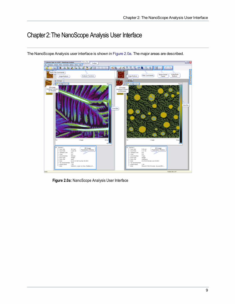
The NanoScope Analysis user interface is shown in Figure 2.0a. Themajor areas are described.
Figure 2.0a: NanoScope Analysis User Interface
9


Chapter 3: Installation and Basic Requirements
Chapter3:Installation and Basic Requirements
3.1 Basic RequirementsTo use NanoScope Analysis1.50, a computer with the following capabilities is needed:
l 2GHz minimum, 3GHz recommendedl 1GB RAM required, 2GB RAM recommendedl 50GB Hard Driveminimuml Windows XP, Vista, orWindows 7.
NOTE: 64 bit versions of NanoScope Analysis requireWindows 7.
3.2 InstallationTo install NanoScope Analysis1.50, follow the directions below:
1. Login as an Administrator inWindows. Copy NanoScope Analysis installer to the hard disk. Theinstaller for 1.50 is approximately 600MB.
2. Double click the installer to begin the installation process. AWelcomewindow will immediately appear.Click Next.
3. The next window asks you to select a database server and authenticationmethod. Selecting the defaultserver and authenticationmethod are the preferredmethods for the vast majority of NanoScope Ana-lysis users. A few users may want to select their own SQL servers. Click Next.
4. The next window will be the end user license agreement. Choose I Accept and Next to continue install-ation. The licensemay also be Printed for future reference, if required.
5. Enter the username, company name and click Next.6. Choose the destination location where setup will install the files. Once the correct path has been iden-
tified, click Next and Install to proceed.7. At this point, NanoScope Analysis setup will check prerequisites behind the scenes. Setup will install
the following list of packages, if the necessary versions are not found on the system.l .Net framework 4.0l Visual Studio 8.0mergemodules.
NOTE: If the above packages are not installed correctly, a ‘NsDataAnalysisExt.dll failed to register’ errormessage will appear. If this error message appears, uninstall NanoScope Analysis and reinstall it.
11

Chapter 4: File Commands
Chapter4:File Commands
The NanoScope Analysis user interface includes aMenu bar at the top of the program window. Manycommands accessed from themenu bar are similar to what youmight find in other word processing and SPMsoftware programs. File commands enable the user to perform frequent tasks in NanoScope Analysissoftware.
The following File Command sections are included in NanoScope Analysis 1.50:
l Basic File Commands (page 13)l The BrowseWindow (page 16)l Converting Data (page 22)l Set Units (page 24)l Set Sensitivity (page 24)l Common Image Control Actions (page 25)l Color Scale (page 29)l CommonGrid Controls (page 42)l Workspaces (page 42)l File Context Commands (page 43)l Auto-scale Data Option (page 49)l Exporting Images (page 50)l Data History (page 51)l Run AutoProgram (page 54)
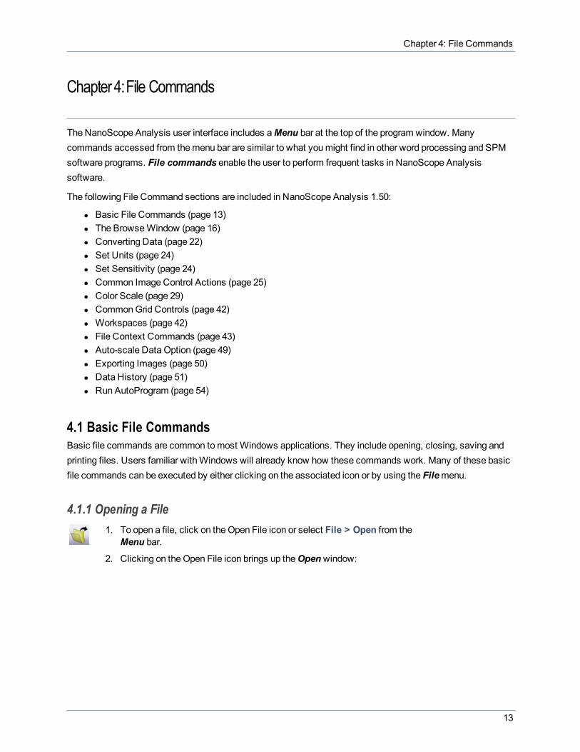
4.1 Basic File CommandsBasic file commands are common tomost Windows applications. They include opening, closing, saving andprinting files. Users familiar withWindows will already know how these commands work. Many of these basicfile commands can be executed by either clicking on the associated icon or by using the Filemenu.
4.1.1 Opening a File1. To open a file, click on the Open File icon or select File > Open from the
Menu bar.
2. Clicking on theOpen File icon brings up theOpenwindow:
13

NanoScope Analysis 1.50 User Manual
3. Choose the preferred file and clickOpen.
4. The chosen file will open in 2DImage view.
4.1.2 Closing a FileTo close a file, click on theClose File icon or click on the FileMenu and select Close (open filename) orClose All.
4.1.3 Saving a FileTo save a file, click on the Filemenu and select Save (open filename) or Save As (open filename) tosave the file with a different name. Additionally, clicking on theSave icon will save a file.
4.1.4 Printing a FileTo print a file, click on the Filemenu and select Print. To view a print preview in advance of printing, chooseFile > Print Preview from the Filemenu. Print settings may also be changed by selecting File > Print Setupfrom the Filemenu.
4.1.5 Display File PropertiesTo display the properties of a given file, first open that file in NanoScope Analysis. Once the file is open, selectFile > Display Properties from the Filemenu. The Parameters window for the particular image will open:
14

Chapter 4: File Commands
Click on the +/- signs to expand or collapse each data field.
4.1.6 Add a NoteA Note can be added to any open image by right clicking on the area adjacent to the image or by selecting File> Add a Note To... from theMenu bar. When right clicking adjacent to an image, a dialog appears withNoteas a choice:
SelectingNote opens theEdit Notewindow where theNote can be added:
15
NanoScope Analysis 1.50 User Manual
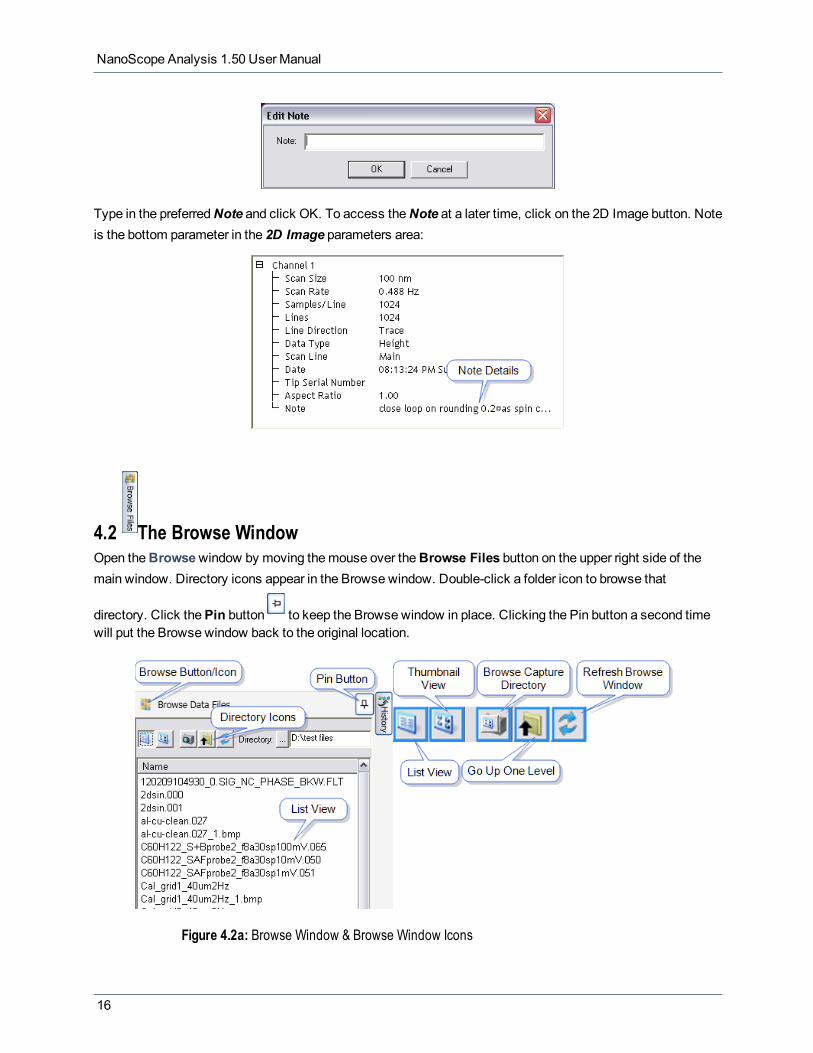
Type in the preferredNote and click OK. To access theNote at a later time, click on the 2D Image button. Noteis the bottom parameter in the 2D Image parameters area:
4.2 The Browse WindowOpen theBrowsewindow by moving themouse over theBrowse Files button on the upper right side of themain window. Directory icons appear in the Browse window. Double-click a folder icon to browse that
directory. Click thePin button to keep the Browse window in place. Clicking the Pin button a second timewill put the Browse window back to the original location.
Figure 4.2a: Browse Window & Browse Window Icons
16

Chapter 4: File Commands
4.2.1 List ViewSelecting the first icon of the Browse window initiates a List View of file information:
Figure 4.2b: List View
Right clicking the on a file and clicking on properties allows for viewing of several SPM parameters for thatparticular file. See Figure 4.2c.
Figure 4.2c: File Parameters
Configuring the List ViewRight-clicking in the List View (but not on a file name) opens a dialog that allows you to choose the displayedNanoScope fields. See Figure 4.2d.
17

NanoScope Analysis 1.50 User Manual
Figure 4.2d: Configure List View Fields
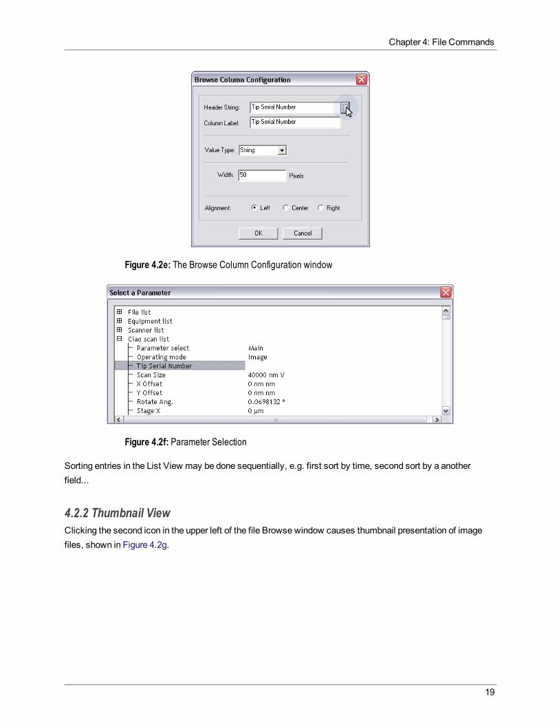
Click User Definable to open theBrowse Column Configuration window, show in Figure 4.2e, that allowsyou to select a user-defined field. Click the ... button to the right of theHeader String field to open theSelect aParameterwindow, shown in Figure 4.2f, and select a parameter from the drop-down lists. Set theWidth tomore than 0 pixels to view it.
NOTE: The parameter choices in theSelect a Parameterwindow are determined by the first file in theBrowse Window List View.
18
Chapter 4: File Commands
Figure 4.2e: The Browse Column Configuration window
Figure 4.2f: Parameter Selection
Sorting entries in the List View may be done sequentially, e.g. first sort by time, second sort by a anotherfield...
4.2.2 Thumbnail ViewClicking the second icon in the upper left of the file Browse window causes thumbnail presentation of imagefiles, shown in Figure 4.2g.
19

NanoScope Analysis 1.50 User Manual
Figure 4.2g: Thumbnail Images in the Browse Window
If no images are selected, right-clicking in the image Browse window (but not on an image icon) allows you toSort the image icons in the Browse window. See Figure 4.2h. Double-click on a thumbnail to open the image forfurther analysis.
Figure 4.2h: Sorting Thumbnails
Image DisplayIf no images are selected, right-clicking in the Browse window (but not on an image icon) allows you to select adisplay channel and a color table for the image icons in the Browse window. See Figure 4.2i.
20

Chapter 4: File Commands
Figure 4.2i: Browse Display / Color Table Selection and Properties
4.2.3 Capture DirectoryClicking theCapture Directory icon in the upper left of the Browse window displays file information, in eithertext or thumbnail presentations, of theCapture Directory (default is D:\capture).
4.2.4 Go Up One LevelClicking on theGo Up One Level icon in the upper left of the Browse window lets the user browse for files ontheir computer or network(s).
4.2.5 Refresh Browse WindowClicking theRefresh Browse Window icon in the upper left of the Browse window refreshes the icons (or list)in the Browse window.
4.2.6 Drag & DropImages can be dragged and dropped from theBrowse Fileswindow and opened automatically in NanoScopeAnalysis. This can be done from the List view or the Thumbnail view.
Select the file or multiple files (by using Shift+click) from theBrowse Fileswindow in either the List view orThumbnail view. Drag the selected files into theWorkspace. The selected files will open.
21

NanoScope Analysis 1.50 User Manual
4.3 Converting DataRefer to the following sections for preparing file data:
Preparing Data for Spreadsheets (Summary) (page 22)
Preparing Data for Image Processing (Summary) (page 22)
Converting Data Files into ASCII (page 22)
4.3.1 Preparing Data for Spreadsheets (Summary)Youmay load data files into third-party, spreadsheet software (e.g., Excel, Igor Pro, Mathematica, etc.). Toconvert data in to a spreadsheet program, complete the following:
1. Convert the data into ASCII format—for example, by using the File > Export > ASCII command fromThe BrowseWindow (page 16).
NOTE: This may increase the size of the file substantially.
2. Select desired settings (see Converting Data Files into ASCII (page 22)), thenSave.3. Load the file into a suitable editor where it may be prepared for third-party applications.4. Load the raw data into the third-party software program and, if needed, condition the data according to
important header parameters and requirements of third-party software applications.5. Analyze or modify the conditioned data as required.
4.3.2 Preparing Data for Image Processing (Summary)Youmay convert data files into third-party, image processing software (e.g., Photoshop, CorelDraw). Toconvert the data into image processing software, complete the following:
1. Convert the data into TIFF format—for example, by right-clicking on the image thumbnail in The BrowseWindow (page 16) and selectingExport > Tiff > 8-bit Color, 8-bit Gray Scale or 16-bit Gray Scale.
2. Load the TIFF file directly into the third-party, image processing software.3. Process the image file. This may include cropping the image, filtering the image, adjusting contrast,
brightness, color, etc.
4.3.3 Converting Data Files into ASCIIWhenNanoScope image files are captured and stored, they are in 2-byte, binary (LSB—least significant bit)form. Although some programs import raw, binary files, most users find they must convert the files into ASCIIform first to use them. The converted file allows users to read the header information directly and works withmany third-party programs requiring ASCII formatting. (Some users prefer to download the original, raw binaryfiles into their third-party program, while using their ASCII version of the file as a guidemap.)
NOTE: Depending upon the software version used during capture of the image data, the actual file formatand file size varies. Headers may includemore than 2000 parameters, followed by Ctrl-Z, data padding,and raw data.
22

Chapter 4: File Commands
Convert captured data in to ASCII format by using the File > Exportmenu command from The BrowseWindow (page 16). To convert files, complete the following:
1. Make a backup copy of the file to be converted and save it to a safeguarded archive. 2. Select a directory, then an image file within it, from the file browse window at the right of the NanoScope
Analysis main window. Right-click in the thumbnail image to open themenu shown in Figure 4.3a.
Figure 4.3a: The ASCII Export Command
3. Click Export > ASCII to open theExport dialog box, shown in Figure 4.3b.4. Select the dataChannels to be exported.5. Choose theColumn format.
Figure 4.3b: The File Export Dialog Box
6. Select the units (nm, V, Deg...) in which to record the data in the new file by checking the appropriateboxes. Export the image header, ramp, or time information by selecting those check boxes.
NOTE: In order to convert the ASCII data from binary (LSB) data to useful values (Phase, Fre-quency, Current, etc.), youmust save the information in the header.
7. Click Save As..., designate a directory path and filename, and click Save.
23
NanoScope Analysis 1.50 User Manual
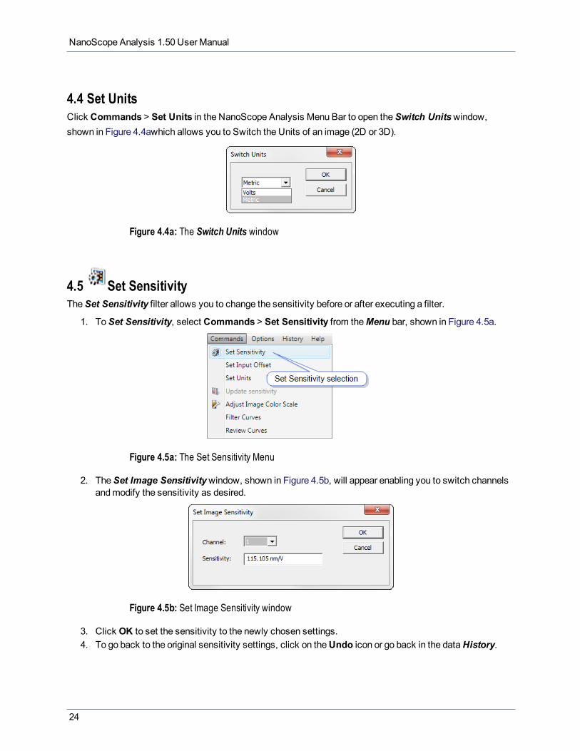
4.4 Set UnitsClick Commands > Set Units in the NanoScope Analysis Menu Bar to open theSwitch Unitswindow,shown in Figure 4.4awhich allows you to Switch the Units of an image (2D or 3D).
Figure 4.4a: The Switch Units window
4.5 Set SensitivityTheSet Sensitivity filter allows you to change the sensitivity before or after executing a filter.
1. ToSet Sensitivity, select Commands > Set Sensitivity from theMenu bar, shown in Figure 4.5a.
Figure 4.5a: The Set Sensitivity Menu
2. TheSet Image Sensitivitywindow, shown in Figure 4.5b, will appear enabling you to switch channelsandmodify the sensitivity as desired.
Figure 4.5b: Set Image Sensitivity window
3. Click OK to set the sensitivity to the newly chosen settings.4. To go back to the original sensitivity settings, click on theUndo icon or go back in the dataHistory.
24

Chapter 4: File Commands
4.6 Common Image Control Actions
4.6.1 Image ButtonsClicking the Image buttons above a captured image performs the following functions:
l Measure - Left click, hold, and drag out a line. The length of the line appears in a box near the line any-time the cursor is on the line.
l Pan - From a zoomed image, pan around to other areas of the original image.l Data Zoom - Left click, hold, and drag out a box. Release themouse button and the image will auto-
matically zoom in to the area of the box. The zoomed region will be centered about the point originallyselected.
l Resize Up - Resizes the image up to the precious zoom level.l Resize Down - Resized the image down to the previous zoom level.l 3D Lighting - Illuminates the image by uniform light whose anglemay be varied. See 3D Lighting Para-
meters.
Figure 4.6a: Image Buttons
4.6.2 Right-clicking On an ImageRight clicking on an image will bring up amenu, shown in Figure 4.6b.
Figure 4.6b: Depiction of Dialog When Image is Right Clicked
The following tasks are available by right clicking on an image:
l Rotating Line - Left click, hold, and drag out a line. Release themouse button to end the line.l Box (for some analyses) - Left click, hold, and drag out a box and release themouse button.
NOTE: Left clicking in the center of the box allows you to translate. Left clicking on edges allows you tochange the box size.
25
NanoScope Analysis 1.50 User Manual
l Copy Clipboard - copies the image, in bmp format, to theWindows clipboard.l Tooltip Level:
l Basicl Mediuml Advancedl None
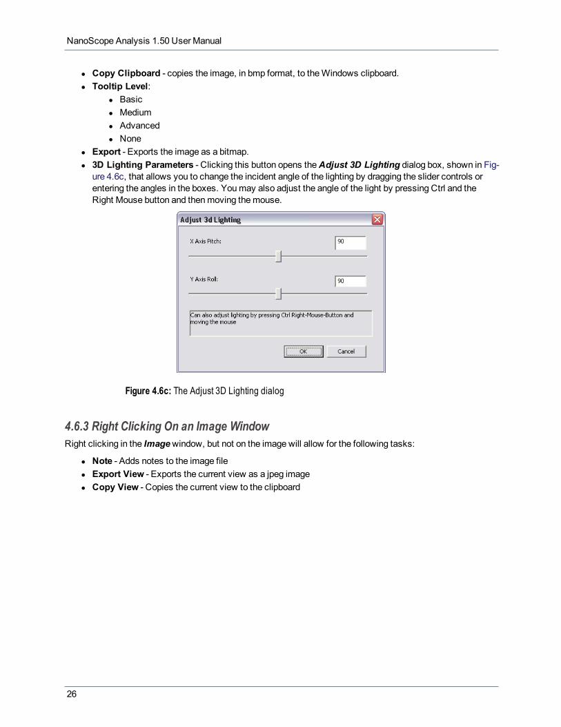
l Export - Exports the image as a bitmap.l 3D Lighting Parameters - Clicking this button opens theAdjust 3D Lighting dialog box, shown in Fig-
ure 4.6c, that allows you to change the incident angle of the lighting by dragging the slider controls orentering the angles in the boxes. Youmay also adjust the angle of the light by pressing Ctrl and theRight Mouse button and thenmoving themouse.
Figure 4.6c: The Adjust 3D Lighting dialog
4.6.3 Right Clicking On an Image WindowRight clicking in the Imagewindow, but not on the image will allow for the following tasks:
l Note - Adds notes to the image filel Export View - Exports the current view as a jpeg imagel Copy View - Copies the current view to the clipboard
26

Chapter 4: File Commands
Figure 4.6d: Depiction of Right-clicking on an Image Window
4.6.4 Color TablesThe Color Scale (page 29) page shows how to change the image appearance.
4.6.5 Using the Mouse Within a Captured ImageThe following functions are available by using your mouse within a captured image:
27

NanoScope Analysis 1.50 User Manual
l Left click anywhere in an image window, drag line out and release - Creates a line of X length, at0° angle in the image window.
l Place cursor on line - Displays the length and angle values of line in the image window.l Place cursor on line, click and hold left button, and drag - Allows you to drag the line anywhere in
the image window.l Click and hold either end of line and drag - Changes length and/or angle of the line.l Right click - Clicking the right mouse button when the cursor is on the line accesses the Image Cursor
menu.
Figure 4.6e: Image Cursor Menu
The Image Cursormenu enables the following functions:
l Delete - deletes the line.l Flip Direction - switches the line end to end.l Show Direction - Adds a small arrowhead to the line to indicate direction.l Set Color - Allows you to change the color of the line.l Clear All - Deletes all lines.
28
Chapter 4: File Commands
4.7 Color Scale
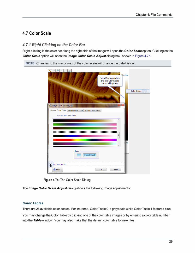
4.7.1 Right Clicking on the Color BarRight-clicking in the color bar along the right side of the image will open theColor Scale option. Clicking on theColor Scale option will open the Image Color Scale Adjust dialog box, shown in Figure 4.7a.
NOTE: Changes to themin or max of the color scale will change the data history.
Figure 4.7a: The Color Scale Dialog
The Image Color Scale Adjust dialog allows the following image adjustments:
Color TablesThere are 26 available color scales. For instance, Color Table 0 is grayscale while Color Table 1 features blue.
Youmay change the Color Table by clicking one of the color table images or by entering a color table numberinto the Tablewindow. Youmay alsomake that the default color table for new files.
29

NanoScope Analysis 1.50 User Manual
Figure 4.7b displays a list of the 26 NanoScope color tables withContrast = 0 andOffset = 0.
Color Table ID Colors
0
1
2
3
4
5
6
7
8
9
10
11
12
13
14
15
16
17
18
19
20
21
22
23
24
25
Figure 4.7b: NanoScope Color Tables
30

Chapter 4: File Commands
Header Color Table vs. Default Color TableNanoScope can now (since version 8.00) save the color table number (for each data channel) that was usedwhen the image was captured in the file header. NanoScope Analysis can use these color tables or they can beoverridden by theDefault Color Table. Click Options > Default Color Table choose to use either the colortable stored in the image file header or theDefault Color Table. See Figure 4.7c. Changing this selectioncauses the browser to change display modes. Images that are already open will not changemodes, but newlyopened files will open in the new mode. All thumbnails should reflect the selectedmode.
Figure 4.7c: Select Default Color Table or Header Color Table
4.7.2 Edit Color TableClick theEdit Color Table button, shown in Figure 4.7a, to open theColor Table Editor panel, shown inFigure 4.7d.
31

NanoScope Analysis 1.50 User Manual
Figure 4.7d: The Color Table Editor
TheColor Table Editor displays a histogram of the data and cubic spline histograms of the Red, Green andBlue channels.
Youmay addEdit Points to a channel by highlighting that channel, right-clicking and selectingAdd EditPoint. See Figure 4.7e. Youmay moveEdit Points by left-clicking the point and dragging it. DeleteEditPoints by right-clicking on the point and selectingDelete Point.
Figure 4.7e: Edit Point added to the red channel
32

Chapter 4: File Commands
Youmay also addColor Points to a channel by highlighting that channel, right-clicking and selectingAddColor Point. See Figure 4.7f. Youmay move aColor Point by left-clicking the point and dragging it. ConvertColor Points toEdit Points by right-clicking on the point and selectingRemove Link.
Figure 4.7f: Color Points added
Change from cubic spline to linear interpolation by checkingUse linear interpolation.
Youmay alsoChoose a Color by right-clicking one of the RGB (Red, Green, Blue) curves and selectingChoose Color. See Figure 4.7d. This opens theColor selection window, shown in Figure 4.7g.
Figure 4.7g: The Color selection window
33

NanoScope Analysis 1.50 User Manual
TheColor selection window allows you to choose a color for the selected (by cursor) X value. TheColorselection window allows you to drag a cursor to select Hue and Saturation and drag the right cursor to selectLightness. Themapping from HSL (Hue, Saturation, Lightness) to RGB is also displayed. Youmay also selectfrom a palate of predefined basic colors.
Data ScaleTheModify Data Scale tab provides several methods to scale your data.
Figure 4.7h: The data scale dialog box
Clicking theColor Bar Scale Relative to Minimum Data Cursor button sets the top label of the Data Scaleto the data range and removes the bottom label.
NOTE: This function is unavailable in MIRO because the layers do not have a real data scale.
Dragging the red cursors in theData Histogram will set theScaling Mode toCustom and clip the data. Themodified values will be reflected in theDisplay fields.
Youmay also enterMinimum andMaximum values in theDisplay fields to clip the data.
TheDisplay fields correspond to theminimum andmaximum values of the data that is mapped to the colortable.
TheData fields display theminimum andmaximum values of the stored data.
TheReal-time fields display theminimum andmaximum vales of the scales stored in the header when thedata was captured. This data is centered at 0. Click theReal-time radio button to use these values.
TheAutoscale option sets the data scale to be (Range Factor)*(range of data after clipping) where (RangeFactor)=1.5.
34
Chapter 4: File Commands
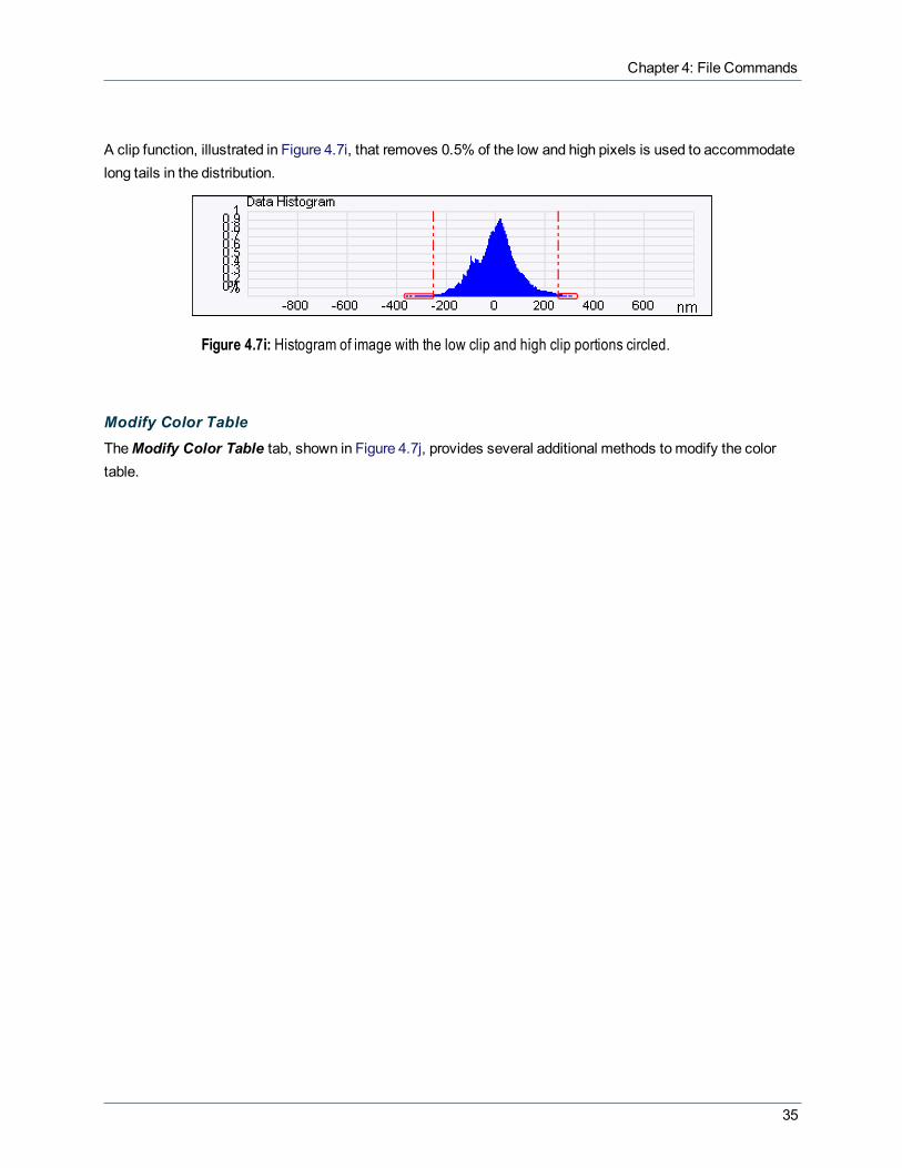
A clip function, illustrated in Figure 4.7i, that removes 0.5% of the low and high pixels is used to accommodatelong tails in the distribution.
Figure 4.7i: Histogram of image with the low clip and high clip portions circled.
Modify Color TableTheModify Color Table tab, shown in Figure 4.7j, provides several additional methods tomodify the colortable.
35

NanoScope Analysis 1.50 User Manual
Figure 4.7j: The Modify Color Table tab
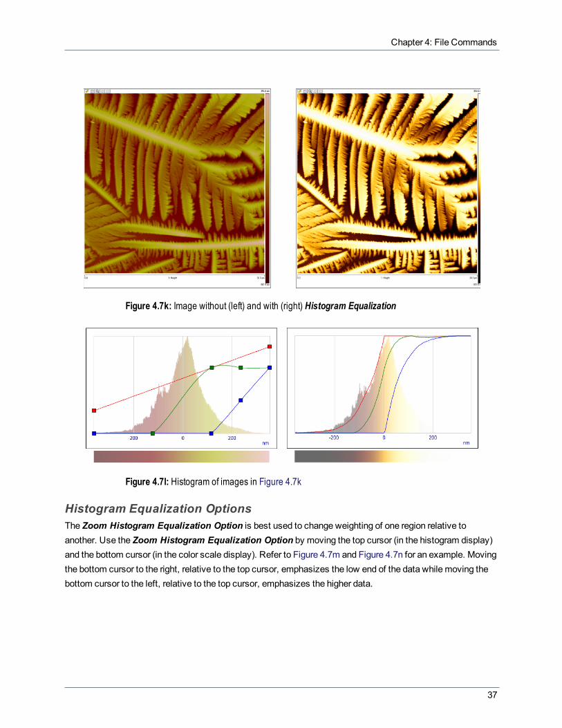
Histogram EqualizationHistogram Equalization is perhaps themost powerful of NanoScope Analysis color functions. HistogramEqualization converts the RGB values to HSL andmodifies the normalized Lightness based on thecumulative histogram. This has the effect of associating the largest lightness change with the largest datachange, increasing the contrast in rapidly changing areas. See Figure 4.7k for an example.
36
Chapter 4: File Commands
Figure 4.7k: Image without (left) and with (right) Histogram Equalization
Figure 4.7l: Histogram of images in Figure 4.7k
Histogram Equalization OptionsThe Zoom Histogram Equalization Option is best used to change weighting of one region relative toanother. Use the Zoom Histogram Equalization Option by moving the top cursor (in the histogram display)and the bottom cursor (in the color scale display). Refer to Figure 4.7m and Figure 4.7n for an example. Movingthe bottom cursor to the right, relative to the top cursor, emphasizes the low end of the data while moving thebottom cursor to the left, relative to the top cursor, emphasizes the higher data.
37

NanoScope Analysis 1.50 User Manual
Figure 4.7m: Image without (left) and with (right) Zoom Histogram Equalization
Figure 4.7n: The histogram of the right image in Figure 4.7m.
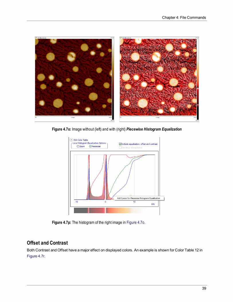
ThePiecewise Histogram Equalization Option is particularly useful when the data histogram is bimodal.Use thePiecewise Histogram Equalization Option by right-clicking to add cursors (see Figure 4.7p).
38
Chapter 4: File Commands
Figure 4.7o: Image without (left) and with (right) Piecewise Histogram Equalization
Figure 4.7p: The histogram of the right image in Figure 4.7o.
Offset and ContrastBoth Contrast andOffset have amajor effect on displayed colors. An example is shown for Color Table 12 inFigure 4.7r.
39

NanoScope Analysis 1.50 User Manual
Offset—Number (-128 to +128)— designates offset colors in the displayed image (e.g., 120 showsilluminated background on image). Offset effectively changes the color value around which the color scale ismapped.
Contrast—Number (-10 to +10)— designates contrast of colors in displayed image (e.g., -10 shows littlechange while 10 shows highest contrast)
Figure 4.7q: The Offset and Contrast dialog box
40

Chapter 4: File Commands
Figure 4.7r: Effect of Contrast and Offset on displayed color for Color Table 12
41
NanoScope Analysis 1.50 User Manual
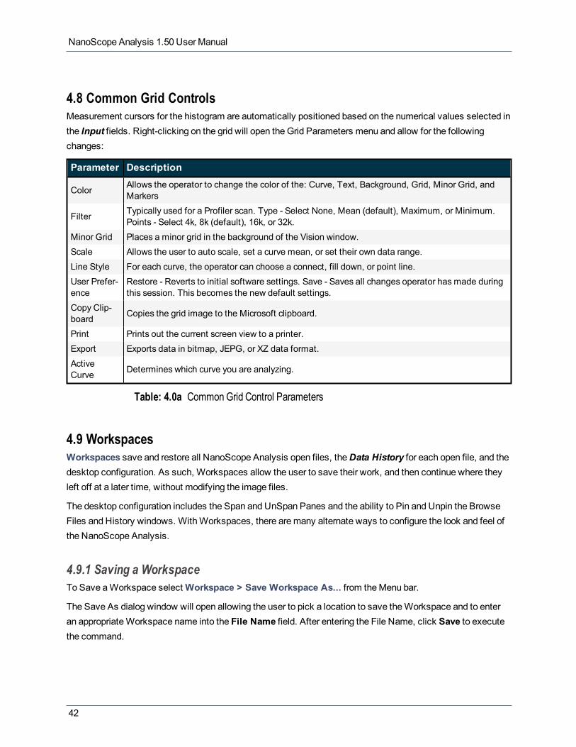
4.8 Common Grid ControlsMeasurement cursors for the histogram are automatically positioned based on the numerical values selected inthe Input fields. Right-clicking on the grid will open the Grid Parameters menu and allow for the followingchanges:
Parameter Description
Color Allows the operator to change the color of the: Curve, Text, Background, Grid, Minor Grid, andMarkers
Filter Typically used for a Profiler scan. Type - Select None, Mean (default), Maximum, or Minimum.Points - Select 4k, 8k (default), 16k, or 32k.
Minor Grid Places a minor grid in the background of the Vision window.Scale Allows the user to auto scale, set a curve mean, or set their own data range.Line Style For each curve, the operator can choose a connect, fill down, or point line.User Prefer-ence
Restore - Reverts to initial software settings. Save - Saves all changes operator has made duringthis session. This becomes the new default settings.
Copy Clip-board Copies the grid image to the Microsoft clipboard.
Print Prints out the current screen view to a printer.Export Exports data in bitmap, JEPG, or XZ data format.ActiveCurve Determines which curve you are analyzing.
Table: 4.0a CommonGrid Control Parameters
4.9 WorkspacesWorkspaces save and restore all NanoScope Analysis open files, theData History for each open file, and thedesktop configuration. As such, Workspaces allow the user to save their work, and then continue where theyleft off at a later time, without modifying the image files.
The desktop configuration includes the Span and UnSpan Panes and the ability to Pin and Unpin the BrowseFiles and History windows. WithWorkspaces, there aremany alternate ways to configure the look and feel ofthe NanoScope Analysis.
4.9.1 Saving a WorkspaceTo Save aWorkspace selectWorkspace > Save Workspace As... from theMenu bar.
The Save As dialog window will open allowing the user to pick a location to save theWorkspace and to enteran appropriateWorkspace name into the File Name field. After entering the File Name, click Save to executethe command.
42

Chapter 4: File Commands
4.9.2 Opening a WorkspaceToOpen a previously savedWorkspace, selectWorkspace > Open Workspace... from theMenu bar. TheOpen dialog window will open allowing the user to choose the preferredWorkspace to open. Choose thepreferredWorkspace and click on theOpen button. The selectedWorkspace will open.
4.10 File Context CommandsFile Context commands enable different views and aid in applying cursors to images. File Contextcommands can be accessed by right clicking on any tabbed image. The dialog shown in Figure 4.10a willappear.
Figure 4.10a: File Context Commands Window
4.10.1 Span/UnSpan PanesTheSpan Panes andUnSpan Panes commands allow you to choose 1 or 2 panes in the NanoScope
Analysis view. TheSpan Panes andUnSpan Panes buttons are located on the Icon toolbar. TheSpan Panes andUnSpan Panes commands can also be accessed in the Tab Contextmenu by right clickingon any tabbed image, as shown below.
WhenUnSpan Panes is chosen and 2 panes are showing, the active pane is indicated by the darker graybackground. See Figure 4.10b and Figure 4.10c for details.
43

NanoScope Analysis 1.50 User Manual
Figure 4.10b: Span Panes Enabled
44

Chapter 4: File Commands
Figure 4.10c: UnSpan Panes Enabled (Note Active Pane in Dark Gray)
UnSpan Panes ExampleThe following example demonstrates the use of theUnSpan Panes function to simultaneously apply anAnalysis function to different channels of the same image.
1. Load an image file into NanoScope Analysis.
2. Click theUnSpan Panes icon to open two analysis windows.
3. Load the same file into the other analysis window.4. Choose a second image channel (Potential in this example).5. Shift +Click or Ctrl+Click on the appropriate image thumbnail on the left side of the image to activ-
ate multiple channels.6. Select and run an analysis function from the NanoScope Analysis toolbar (Section in this
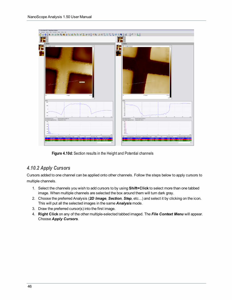
example).7. The results, shown in Figure 4.10d, will appear in both windows.
45
NanoScope Analysis 1.50 User Manual
Figure 4.10d: Section results in the Height and Potential channels
4.10.2 Apply CursorsCursors added to one channel can be applied onto other channels. Follow the steps below to apply cursors tomultiple channels.
1. Select the channels you wish to add cursors to by usingShift+Click to select more than one tabbedimage. Whenmultiple channels are selected the box around them will turn dark gray.
2. Choose the preferred Analysis (2D Image, Section, Step, etc...) and select it by clicking on the icon.This will put all the selected images in the sameAnalysismode.
3. Draw the preferred cursor(s) into the first image.4. Right Click on any of the other multiple-selected tabbed imaged. The File Context Menuwill appear.
ChooseApply Cursors.
46

Chapter 4: File Commands
Figure 4.10e: Apply Cursors
5. The cursors added to the first image will now be added to the other selected images. See Figure 4.10f.
47

NanoScope Analysis 1.50 User Manual
Figure 4.10f: Cursors Applied to Other Channels
4.10.3 Synchronized Cursors/AnalysesSynchronized cursors (mouse events) allow you to select multiple channels (viaShift+click orCtrl+click) insingle or multiple files regardless of which pane or tab they appear. Operations will be carried out on all theseselected channels.
TheMultiple Tabs is Onmessage, shown in Figure 4.10g, will appear in the lower right corner of theNanoScope Analysis screen when you have selectedmore than on channel.
Figure 4.10g:Multiple Tabs is On message
l Synchronized cursors allow you to draw onemarker (box, line..) in an open image and have that markerdrawn in all selected channels.
48

Chapter 4: File Commands
l Synchronized cursors can be applied only across the same type of NanoScope Analysis view (e.g. 2D,3D, Depth...) and image aspect ratio.
l If the view includes anExecute button, it is necessary to click Execute in each view.l Synchronized cursors work with the 3D Image function. If you select multiple files in/for a 3D Image,
rotating, changing the lighting... on one changes all.
The synchronized cursor function enables easy comparison of data in different channels/files, therebyimproving productivity.
4.10.4 CloseThe File Contextmenu can also be used toClose a file. Right-click on any tabbed image and select Close toshut down that particular file.
4.10.5 Move to Next/Previous Tab GroupTheMove to Next/Previous Tab Group is a convenient way to view files already open in NanoScopeAnalysis. TheMove to Next/Previous Tab Group selection is only functional when you are in theUnSpanPanes view with 2 panes showing and with more than 1 file open. Selecting theMove to Next Tab Groupwillopen the next tabbed image group and push the current tabbed group to the second pane. Conversely,selecting theMove to Previous Tab Groupwill reload the previous tab group in the second pane and open thecurrent tab group in the first pane.
4.11 Auto-scale Data OptionTheAuto-scale Data option allows for automatic scaling of data usingminimum andmaximum values from thefile dataset.
The default forAuto-scale Data is On. TurningOffAuto-scale Datawill enable the NanoScope Analysissoftware to use the data scale found in the header file. To turnAuto-scale DataOff, select Options > Auto-scale Data from theMenu bar. The check mark next toAuto-scale Datawill disappear. TheAuto-scale Dataoption only affects the file when it is first opened. If the user changes the data scale in the dialog, the auto-scaling will be turnedOff and cannot be turned back Onwithout re-opening the file.
49

NanoScope Analysis 1.50 User Manual
Figure 4.11a: Auto-scale data menu
TheAutoscale option sets the data scale to be (Range Factor)*(range of data after clipping) where (RangeFactor)=1.5.
A clip function, illustrated in Figure 4.11b, that removes 0.5% of the low and high pixels is used toaccommodate long tails in the distribution.
Figure 4.11b: Histogram of image with the low clip and high clip portions circled.
4.12 Exporting Images
4.12.1 Exporting from the Browse windowYoumay export images, in eitherASCII, Bitmap, JPEG or Tiff formats from theBrowsewindow by right-clicking single or multiple images (shift right-click), shown in Figure 4.12a. After the export format has beenselected, a new window, shown in Figure 4.12b, will open allowing selection of theChannel andColor Table.
50

Chapter 4: File Commands
Figure 4.12a: Exporting Multiple Images from the Image Browse window
Figure 4.12b: Selecting the Channel and/or Color Table
4.13 Data HistoryData History enables the user to restore previous raw data with the click of a button. This command can beuseful, if at any point, the user prefers to revert to data from an earlier time an analysis session.
Executing a Filter:
l Causes the Filter icon and/or Filter name to be displayed in theHistorymenul Creates a new history item and view containing themodified raw datal Saves the unmodified raw data in theData History so the user can restore it, if required.
4.13.1 ProcedureData History can be accessed by selectingHistory > (Particular History Item) from theMenu bar or byopening theHistorywindow by clicking on theHistory icon on the right side of the NanoScope Analysis view.
Press thePin button to keep theHistorywindow in place. Then double click on the appropriateDataHistory item to access it. Pressing thePin button a second time will put theHistorywindow back to theoriginal location.
51

NanoScope Analysis 1.50 User Manual
Figure 4.13a: Data History Menu
4.13.2 Undo/Redo Buttons
TheUndo andRedo buttons provide a simple option tomove backward or forward in theDataHistory. Clicking on theUndo button will remove the top item in theData History. Clicking on theRedobutton will restore the next Data History item. If noData History item has been selected or undone, theUndoandRedo buttons will remain un-selectable. In addition to using the icons on the Icon toolbar, one can alsoselect History > Undo orHistory > Redo from theMenu bar to execute these commands.
4.13.3 Modifying the Data HistoryYoumay Close data history items by selecting that item in the History window, right-clicking and choosingClose as shown in Figure 4.13b.
52

Chapter 4: File Commands
Figure 4.13b: Close a History item
Youmay insert Filter and Analysis functions after an existing item into the data history by highlighting that itemand then selecting the new function. See Figure 4.13c.
Figure 4.13c: Bearing Analysis function inserted into the Data History after Patterned SampleAnalysis. Before (left) and After (right).
If you execute or delete a Filter Command, you will be asked, via a pop-up window, shown in Figure 4.13d, ifyou wish to undo the changes done to the file by the filter and delete items after that filter or accept the datamodifications and rerun the entire history list.
Figure 4.13d: The Modify History Options window.
53

NanoScope Analysis 1.50 User Manual
4.14 Run AutoProgramTheRun AutoProgram, formerly namedRun History, function allows you to perform a sequence ofoperations that may be applied automatically to at least one previously captured image. Typically, RunAutoPropram is used to rapidly analyze a large number of images taken under similar conditions. Applying afixed Data Scale (page 34) to multiple images is a good example of the Run AutoProgram function. Any Offlinecommand except for XY Drift (page 153) may be included inRun AutoProgram.
4.14.1 Configuring Run AutoProgram To configure Run AutoProgram within NanoScope Analysis:
1. Click theRun AutoProgram icon on the NanoScope Analysis toolbar or click History > RunAutoProgram as shown in Figure 4.14a.
Figure 4.14a: The History Menu
2. This opens theRun AutoProgram window, shown in Figure 4.14b.
54

Chapter 4: File Commands
Figure 4.14b: The Run AutoProgram window
3. Select an existing AutoProgram file (*.apg) or use the current history list, shown below theOpenAutoProgram button.
4. Click theAdd button in theRun AutoProgram window. TheSelect Multiple Files dialog box, shownin Figure 4.14c, appears.
55

NanoScope Analysis 1.50 User Manual
Figure 4.14c: The Add Files dialog box
5. Add individual files by clicking, a range of files by Shift-clicking or select multiple files by Ctrl-clicking.Youmay also add selected files by dragging them from The BrowseWindow (page 16) or from aWin-dows Explorer window into theSelect Multiple Files orDrag files from Browse Window here dialogboxes.
6. Select whichChannels you wish to be analyzed.7. Select theReport Directory to store the output files.8. TheRun AutoProgram window, shown in Figure 4.14b, will display the files which are to be operated
on. Youmay remove files from this list by highlighting the file and clickingRemove. Youmay alsoselect or deselect a file by checking theRun box.
9. Click theSave List box to save your file list so that this list will appear the next time you openRunAutoProgram.
NOTE: AutoPrograms created within NanoScope software will not run in NanoScope Analysis software.
56
Chapter 4: File Commands
4.14.2 Running an AutoProgramOnce all commands are included in a Run AutoProgram list and their action specified, you are ready to RunAutoProgram. Use this command tomakemovies.
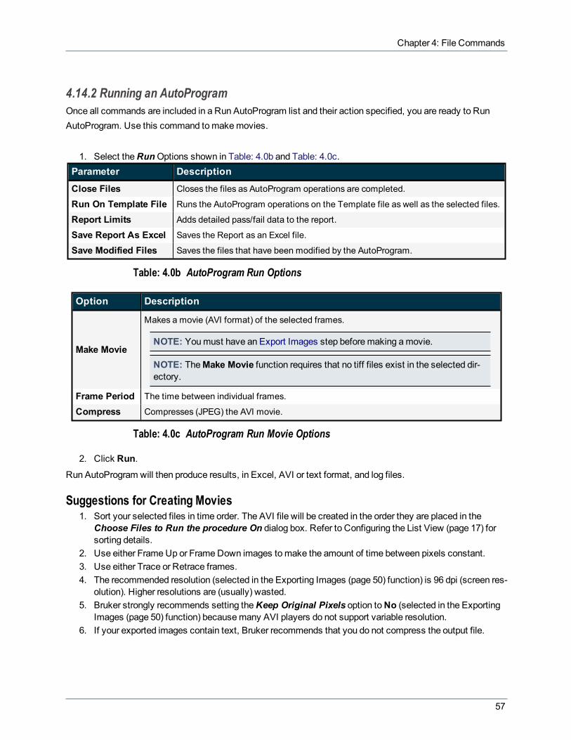
1. Select theRunOptions shown in Table: 4.0b and Table: 4.0c.Parameter Description
Close Files Closes the files as AutoProgram operations are completed.
Run On Template File Runs the AutoProgram operations on the Template file as well as the selected files.
Report Limits Adds detailed pass/fail data to the report.
Save Report As Excel Saves the Report as an Excel file.
Save Modified Files Saves the files that have been modified by the AutoProgram.
Table: 4.0b AutoProgram Run Options
Option Description
Make Movie
Makes a movie (AVI format) of the selected frames.
NOTE: Youmust have an Export Images step beforemaking amovie.
NOTE: TheMake Movie function requires that no tiff files exist in the selected dir-ectory.
Frame Period The time between individual frames.
Compress Compresses (JPEG) the AVI movie.
Table: 4.0c AutoProgram Run Movie Options
2. Click Run.Run AutoProgram will then produce results, in Excel, AVI or text format, and log files.
Suggestions for Creating Movies1. Sort your selected files in time order. The AVI file will be created in the order they are placed in the
Choose Files to Run the procedure On dialog box. Refer to Configuring the List View (page 17) forsorting details.
2. Use either FrameUp or FrameDown images tomake the amount of time between pixels constant.3. Use either Trace or Retrace frames.4. The recommended resolution (selected in the Exporting Images (page 50) function) is 96 dpi (screen res-
olution). Higher resolutions are (usually) wasted.5. Bruker strongly recommends setting theKeep Original Pixels option toNo (selected in the Exporting
Images (page 50) function) becausemany AVI players do not support variable resolution.6. If your exported images contain text, Bruker recommends that you do not compress the output file.
57

NanoScope Analysis 1.50 User Manual
Run AutoProgram TroubleshootingThe Run AutoProgram function uses aMicrosoft SQL Server database to store and retrieve NanoScopeAnalysis history. This database, stored on the local computer, grows with use. If you would like to reduce thesize of the file associated with this database, you can clear unused records from the database:
1. Click Help > About NanoScope Analysis to open theAboutwindow, shown in Figure 4.14d.2. Click theClear Database button to remove unused records.
Figure 4.14d: Clear Database
58

Chapter 5: Analysis Functions
Chapter5:Analysis Functions
Analysis Functions relate to analyzing surface behavior of materials on images captured in Realtimemode.These commands are known as image processing or analysis commands. The commands contain views,options and configurations for analysis, modifications, and storage of the collected data. The analysis may beautomated (i.e. in auto programs) or completedmanually. In general, the analysis commands providemethodsfor quantifying the surface properties of samples.
Analysis Functions can be opened using theMenu bar or by clicking on the appropriate icon from the IconToolbar. TheseAnalysis icons are identical to the icons used in NanoScope V8 software.
Figure 5.0a: Analysis Icons Toolbar and Menu
The followingAnalysis Functions are available in NanoScope Analysis 1.50:
l 2D Image (page 60)l 3D Image (page 65)l Bearing Analysis (page 73)
59

NanoScope Analysis 1.50 User Manual
l Depth (page 80)l Journal Quality Export (page 84)l Linearity Verification (page 88)l Particle Analysis (page 90)l Patterned Sample Analysis (page 98)l Power Spectral Density (PSD) (page 105)l Roughness (page 112)l Section (page 123)l Step (page 131)l Tip Qualification (page 135)l Width (page 147)l XY Drift (page 153)l Electrochemistryl Force Volume (page 226)
5.1 2D ImageThe 2D Image analysis displays the selected image with color-coded height information in a two-dimensionalperspective. 2D Image analysis is the default analysis of NanoScope Analysis such that when an image isinitially opened it is always rendered in 2D Image.
5.1.1 2D Image Procedure1. Select the 2D Image analysis by selecting Analysis > 2D Image from the Toolbarmenu or by clicking
on the 2D Image icon from the Icon toolbar.2. The file is opened in the 2D Imagewindow, shown in Figure 5.1a.
60

Chapter 5: Analysis Functions
Figure 5.1a: 2D Image Menu and Window
3. Right click in theChannel Parameters area and select Show All. TheChannel Parameters appearwith checkboxes next to them. By un-checking the boxes, you can determine whichChannelParameters are shown and which parameters are hidden. This is a convenient way to hide rarely-usedparameters. When satisfied with the checked and un-checked boxes, right-click theChannelParameters area and select Show All again. Only the checked parameters will now show in theChannel Parameters area.
61

NanoScope Analysis 1.50 User Manual
Figure 5.1b: Channel Parameters Hide / Show Selection
4. Right click in theChannel Parameters area and select Copy Text.5. A new dialog, shown in Figure 5.1c, will appear notifying the user that the data from theChannel
Parameters area has been copied to the clipboard. The user can now save the data into their preferredmedium.
Figure 5.1c: Dialog Indicating Text has been Copied to the Clipboard
6. To determine length and anglemeasurements, use themouse to draw a cursor in the preferred locationon the 2D Image rendering.
7. Length and anglemeasurements are show next to themouse icon when themouse is placed over thedrawn cursor.
8. After a cursor has been drawn it is possible to get more detailed information on the length and anglemeasurements. Right click anywhere in the 2D Image rendering (except on the drawn cursor). ChooseTooltip Level > Basic, Medium, Advanced, or None. See Figure 5.1d.
62

Chapter 5: Analysis Functions
Figure 5.1d: Cursor Length and Angle Measurements
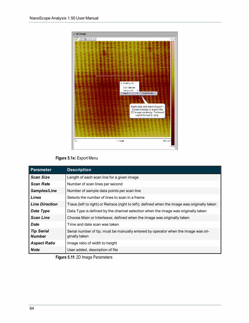
9. To export the 2D Image rendering, right click anywhere in the 2D Image rendering and select Export >Screen Display. Name the file and choose the location to save it. The preferred file for saving exportedimages is .bmp. See Figure 5.1e.
63
NanoScope Analysis 1.50 User Manual
Figure 5.1e: Export Menu
Parameter Description
Scan Size Length of each scan line for a given image
Scan Rate Number of scan lines per second
Samples/Line Number of sample data points per scan line
Lines Selects the number of lines to scan in a frame
Line Direction Trace (left to right) or Retrace (right to left); defined when the image was originally taken
Data Type Data Type is defined by the channel selection when the image was originally taken
Scan Line Choose Main or Interleave; defined when the image was originally taken
Date Time and date scan was taken
Tip SerialNumber
Serial number of tip; must be manually entered by operator when the image was ori-ginally taken
Aspect Ratio Image ratio of width to height
Note User added, description of file
Figure 5.1f: 2D Image Parameters
64
Chapter 5: Analysis Functions
5.2 3D ImageThe 3D Image view displays the selected image with color-coded height information in a three-dimensional,oblique perspective. 3D Image allows selection of the viewing angle and illumination angle for amodeled lightsource.
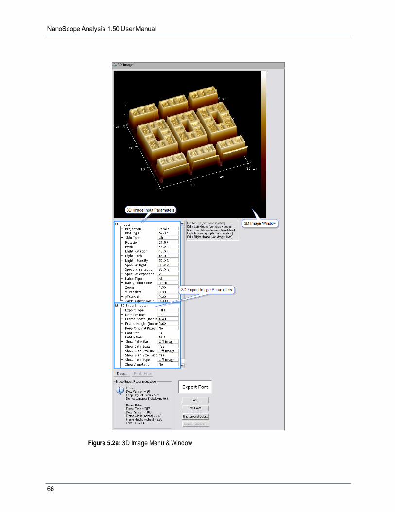
3D Image Procedure1. Select the 3D Image analysis by selectingAnalysis > 3D Image from the Toolbarmenu or by clicking
on the 3D Image icon from the Icon toolbar.2. TheProjection, Plot Type, Skin Type, Label Type, andBackground Color parameters can be
changed by clicking in the related window and selecting from the drop-downmenus. The remaining para-meters may be changed by typing the desired information in the related window or by use of the key-board andmouse keys.
3. To zoom in or out on the image, hold the control key down and slide themouse up and down on theimage while holding the left mouse button.
4. To pan, hold the shift key down andmove themouse up, down, left, or right on the image while holdingthe left mouse button.
5. Clicking and holding the right mouse button downwhile moving themouse left and right changes thelight rotation on the image. This is only available whenPlot Type is set toMixed.
6. Clicking and holding the right button while moving themouse up and down changes the light pitch. Thisis only available whenPlot Type is set toMixed.
65
NanoScope Analysis 1.50 User Manual
Figure 5.2a: 3D Image Menu & Window
66

Chapter 5: Analysis Functions
NOTE: NanoScope Analysis versions prior to 1.30 rendered amaximum of 512 points/line in 3D. Version1.30 and later render up to 2048 points/line by default, with aRender Hires button to render higher res-olution images.
Skin Type ExampleSkin Type allows you to paint the 3D surface with colors taken from an alternative channel. This is useful forcomparing property channels with the surface topography.
The following example demonstrates the use of Skin Type, Color Scale and other commonly used 3Dparameters using a SRAM/SCM sample.
1. After the image is opened, click on the 3D Image icon. Change theProjection parameter toPerspective and thePlot Type toHeight.
Figure 5.2b: Image opened in 3D Image view
2. Click on the tab for the alternative channel to be painted onto the surface of the 3D Image. Change theColor Scale to #17.
67

NanoScope Analysis 1.50 User Manual
NOTE: The top of the color table at 44.1 degrees is violet. The bottom pixels in the image are red at about -18 degrees.
Figure 5.2c: Color Table 17 Selected on Alternative Channel
3. Return to the original channel and choose theSkin Type of the alternative channel. The data of thealternative channel will now be painted onto the 3D surface.
68

Chapter 5: Analysis Functions
Figure 5.2d: Skin Type of Original Channel Modified to Color Scale 17
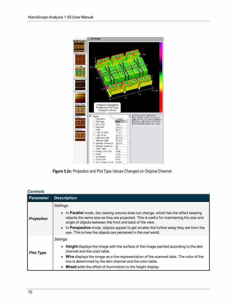
4. Return to the original channel and changeProjection toParallel andPlot Type toMixed.
69
NanoScope Analysis 1.50 User Manual
Figure 5.2e: Projection and Plot Type Values Changed on Original Channel
ControlsParameter Description
Projection
Settings:
l In Parallel mode, the viewing volume does not change, which has the effect keepingobjects the same size as they are projected. This is useful for maintaining the size andangle of objects between the front and back of the view.
l In Perspectivemode, objects appear to get smaller the further away they are from theeye. This is how the objects are perceived in the real world.
Plot Type
Setings:
l Height displays the image with the surface of the image painted according to the skinchannel and the color table.
l Wire displays the image as a line representation of the scanned data. The color of theline is determined by the skin channel and the color table.
l Mixed adds the effect of illumination to the height display.
70

Chapter 5: Analysis Functions
Parameter Description
Skin TypeBy default, Skin Type is determined by the current channel. Selecting a different channel paintsthe 3D surface with the data from the selected channel. The range of the color table used isdetermined by the range shown in the chosen skin channel.
RotationThe Rotation parameter changes as the viewing angle by rotating the displayed image aboutthe Z axis relative to its captured orientation. Zero degrees indicates the image is rendered ascaptured (straight on).
PitchThe Pitch parameter changes the viewing angle by manually changing the pitch of the Y axis inthe three-dimensional surface plot image. Zero degreed indicates a top down view of the cap-tured image.
LightRotation
The Light Rotation parameter rotates the light source in the horizontal plane (xy plane). This isonly available when the Plot Type is set toMixed. 90 degrees of Light Rotation indicates thelight source is on the right.
Light PitchThe Light Pitch parameter changes the viewing angle by selecting the pitch of the Z axis in thethree-dimensional surface plot image. This is only available when the Plot Type is set toMixed. 90 degrees indicates the light pitch is coming from above (high noon).
LightIntensity
Selects the percentage of the imaginary light source mixed with the color-encoded heightinformation when the Plot Type is set toMixed.
SpecularLight
Specular Light, Specular Reflection, and Specular Exponent all control the reflection of light(shininess) on the 3D image.
Label Type
Label Type - The Label Type parameter selects whether labels or axes are displayed with theimage.All displays the axes with labels.Axis displays all the axes without labeling.None displays the image without labels.
BackgroundColor Changes the background color to black or white
Zoom Zooms in on the image. Larger numbers increase the zoom level and smaller numbersdecrease the zoom level. 1.5 will typically come close to filling the image frame.
xTranslate Moves the image up or down in the image window.
yTranslate Moves the image left or right in the image window.
ZaxisAspectRatio
Allows you to control the relative height of the Z axis display
Range:
0.0 to 1.0 where 0.0 produces a flat display while 1.0 produces a display whose Z axis is equalis size to the X and Y axes.
Table: 5.0d 3D Image Parameters
71

NanoScope Analysis 1.50 User Manual
Button Description
ExportAllows you to export a publication quality image. The Export function allows you to make 3Dmovies. Refer to Journal Quality Export (page 84) for a discussion of 3D Export InputParameters.
LoadSkin
Loads a file (channel) to be used as a skin. Used only for NanoDrive files because each NanoDrivechannel is a separate file.
UnloadSkin Unloads a skin. Used only for NanoDrive files because each NanoDrive channel is a separate file.
RenderHires Re-renders the image at higher resolution. Applies to images greater or equal to 2048 samples/line.
Table: 5.0e 3D Image Buttons
72

Chapter 5: Analysis Functions
5.3 Bearing AnalysisBearing Analysis provides amethod of plotting and analyzing the distribution of surface height over a sample.Bearing Analysis may be applied to the entire image, or to selected areas of the image, using a rubber bandbox. Moreover, regions within the selected area can be blocked out by using “stop bands” to remove unwanteddata from the analysis.
Bearing Analysis TheoryBearing Analysis reveals how much of a surface lies above or below a given height. This measurementprovides additional information beyond standard roughness measurements. (Surface roughness is generallyrepresented in terms of statistical deviation from average height; however, this gives little indication of heightdistribution over the surface.) By using bearing analysis, it is possible to determine what percentage of thesurface (the “bearing ratio”) lies above or below any arbitrarily chosen height. In industries wherematerials arepolished or chemically etched, this is a particularly useful tool. For example, bearing analysis is frequently usedin silicon etching processes to observe changes in etched features over an interval of time.
Figure 5.3a: Bearing Analysis Illustration
Figure 5.3a represents how Bearing Analysis generates a histogram of feature height based upon theoccurrence of pixels at various Z heights. At Z height “A,” virtually all of the surface is included (correspondingto a Bearing ratio of 100, or 100 percent of the area). At Z height “D,” the pixel count is much reduced,representing a smaller Bearing ratio (approximately 2-5 percent of the area).
Bearing Analysis Procedure1. Select an image file from the file Browse window at the right of themain window. Double-click or drag
73
NanoScope Analysis 1.50 User Manual
the thumbnail image to select and open the image.2. Open the Bearing Analysisby selectingAnalysis > Bearing Analysis from theMenu bar or by clicking
theBearing Analysis icon in the Icon toolbar.
3. Use the Filters > Plane Fit function to remove all tilt before running Bearing Analysis.
The Bearing Analysis function displays a top view of the image, then calculates and displays bearing areacurves and surface height histograms for lines or areas drawn on the image. See Figure 5.3b.
74
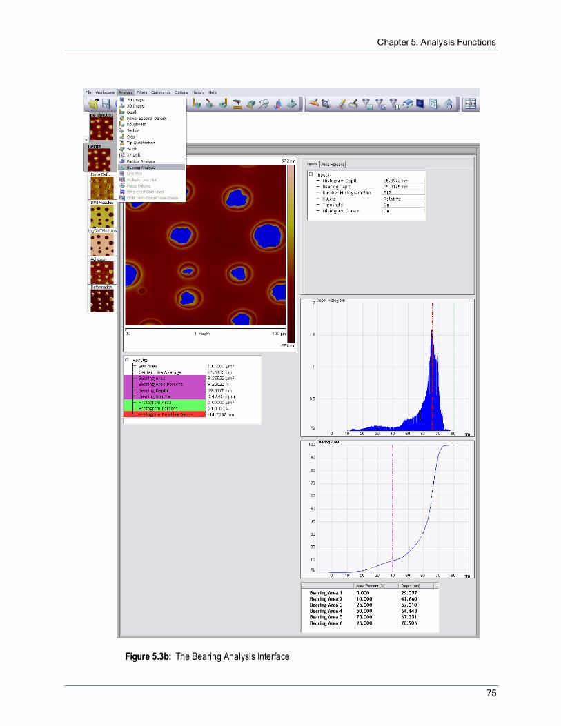
Chapter 5: Analysis Functions
Figure 5.3b: The Bearing Analysis Interface
75

NanoScope Analysis 1.50 User Manual
The word bearingmeans the relative roughness of a surface in terms of high and low areas. The bearing areacurve is the integral of the surface height histogram and plots the percentage of the surface above a referenceplane as a function of the depth of that plane below the highest point in the image.
4. Plotted data includes all data points, noise spikes and holes. If noise is to be filtered out, it should beremoved before using the Bearing Analysis function by executing one of the filtering commands (e.g.,Gaussian (page 176), Lowpass (page 187), Median (page 190)).
5. Using themouse, left-click and drag a box on the area of the image to analyze. TheDepth Histogramdisplays the depth information about this specified area.
6. Move the cursors to select theBearing Depth and set theX Axis, Threshold andHistogram inputparameters.
NOTE: If no box is drawn, by default, the entire image is selected.
Bearing Analysis InterfaceThe Bearing Analysis interface includes a captured image, Input parameters, Results parameters, aDepthHistogram and aBearing Area plot as shown in the image above.
Parameter Description
HistogramDepth
User input field that corresponds to the red cursor in the Depth Histogram display and the redboxes in the Results parameters.Moving the red cursor in the Depth Histogram display will modify the Histogram Depthinput parameter while changing the Histogram Depth input parameter will move the redcursor.
BearingDepth
The Bearing Depth reference plane. User input that corresponds to the magenta cursor in theBearing Area display.Moving the magenta cursor in the Bearing Area display will modify the Bearing Depth inputparameter while changing the Bearing Depth input parameter will move the magenta cursor.
Number ofHistogramBins
The number of data points which result from the filtering calculation.
NOTE: Havingmore histogram bins than pixels is unnecessary.
X AxisRelative: Plots the data relative to the highest point. Points that are lower than the highestpoint will have higher depths.Absolute: Plots the real (i.e., measured) numbers.
Threshold
On: Points higher than the Bearing Depth (magenta cursor) in the Bearing Area plot are dis-played as blue in the image.Off: Points higher than the Bearing Depth (magenta cursor) in the Bearing Area plot are not dis-played in the image.
HistogramCursor Turns the green Histogram cursor On and Off.
Table: 5.0f Bearing Analysis Input Parameters
NOTE: Clicking in the image will reset all the cursors and their corresponding input parameters.
76

Chapter 5: Analysis Functions
Parameter Description
Box Area The area of the selected analysis region.
Center LineAverage The height at which half the points in the selected area are above and half are below.
Bearing Area Area covered by all of the points above the selected Bearing Depth.
Bearing AreaPercent The percentage of the surface above the Bearing Depth reference plane.
Bearing Depth The Bearing Depth reference plane. Identical to the Bearing Depth input parameter.
Bearing Volume Sample volume defined above the bearing depth plane.
Histogram Area The area of the histogram bin covered by the points at the depth indicated by the redhistogram cursor.
Histogram Percent The percentage of the total number of points in the histogram bin at the depth indic-ated by the red histogram cursor.
Histogram Depth The depth of the red histogram cursor position relative to highest point in the image.
Histogram RelativeDepth
The Histogram Depth (red cursor) relative to the Histogram (green) Cursor. Active whenthe Histogram Cursor is On.
Table: 5.0g Bearing Analysis Results Parameters
Patterned Sample Analysis ResultsIf you have previously run Patterned Sample Analysis (page 98), theBottom Result is used as an Input toBearing Analysis and additional PSA results parameters, shown in Figure 5.3c and Table: 5.0h, arecomputed.
Figure 5.3c: Results panel with Patterned Sample Analysis
Parameter Description
PSA Bottom Depth The Bottom Depth Area.
PSA Bottom Area Percent The percentage of the total area occupied by the Bottom Depth.
77

NanoScope Analysis 1.50 User Manual
Parameter Description
PSA Top Depth The Top Depth Area.
PSA Top Area Percent The percentage of the total area occupied by the Top Depth.
Table: 5.0h PSA parameters in Bearing Analysis Results
Area percentTheArea Percent tab allows the input of Bearing ratios:
Figure 5.3d: The Area Percent input
TheArea Percent tab allows input of up to six different bearing ratios. For example, if 50% is entered for theratio, the box displayed in theBearing Area Results window, shown in Figure 5.3e, measures the depthabove which 50% of the data points are above.
Figure 5.3e: The Bearing Area Results window
TheBearing Area results window, shown in Figure 5.3e, displays depth data for specifically entered bearingratios.
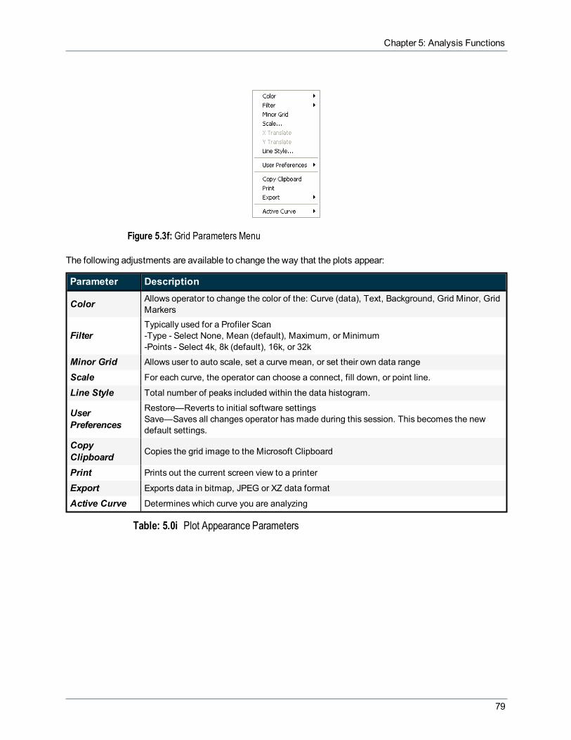
Using the Grid DisplayRight-clicking in the plot area will bring up theGrid Parametersmenu.
78
Chapter 5: Analysis Functions
Figure 5.3f: Grid Parameters Menu
The following adjustments are available to change the way that the plots appear:
Parameter Description
Color Allows operator to change the color of the: Curve (data), Text, Background, Grid Minor, GridMarkers
FilterTypically used for a Profiler Scan-Type - Select None, Mean (default), Maximum, or Minimum-Points - Select 4k, 8k (default), 16k, or 32k
Minor Grid Allows user to auto scale, set a curve mean, or set their own data range
Scale For each curve, the operator can choose a connect, fill down, or point line.
Line Style Total number of peaks included within the data histogram.
UserPreferences
Restore—Reverts to initial software settingsSave—Saves all changes operator has made during this session. This becomes the newdefault settings.
CopyClipboard Copies the grid image to the Microsoft Clipboard
Print Prints out the current screen view to a printer
Export Exports data in bitmap, JPEG or XZ data format
Active Curve Determines which curve you are analyzing
Table: 5.0i Plot Appearance Parameters
79

NanoScope Analysis 1.50 User Manual
5.4 DepthTo analyze the depth of features you have numerous choices whichmeasure the height difference betweentwo dominant features that occur at distinct heights. Depth analysis was primarily designed for automaticallycomparing feature depths at two similar sample sites (e.g., when analyzing etch depths on large numbers ofidentical silicon wafers).
TheoryTheDepth command accumulates depth data within a specified area, applies a Gaussian low-pass filter to thedata to remove noise, then obtains depth comparisons between two dominant features.
Although this method of depth analysis does not substitute for direct, cross-sectioning of the sample, it affordsameans for comparing feature depth between two similar sites in a consistent, statistical manner.
TheDepthwindow includes a top view image and a histogram; depth data is displayed in theResultswindowand in the histogram. Themouse is used to resize and position the box cursor over the area to be analyzed. Thehistogram displays both the raw and an overlaid, Gaussian-filtered version of the data, distributed proportionalto its occurrence within the defined bounding box.
Depth HistogramFigure 5.4a displays a histogram from raw depth data. Data points A and B are the twomost dominant features,and therefore would be compared in Depth analysis. Depending upon the range and size of depth data, thecurvemay appear jagged in profile, with noticeable levels of noise.
NOTE: Color of cursor, data, and grid may change if user has changed the settings. Right-click on thegraph and go toColor if you want to change the default settings.
80

Chapter 5: Analysis Functions
Figure 5.4a: Depth Image and Corresponding Histogram
Correlation CurveTheCorrelation Curve is a filtered version of theRaw Data Histogram and is located on theRaw DataHistogram represented by a red line. Filtering is done using theHistogram Filter Cutoff parameter in theInputs parameters box.The larger the filter cutoff, themore data is filtered into a Gaussian (bell-shaped) curve.Large filter cutoffs average somuch of the data curve that peaks corresponding to specific features becomeunrecognizable. On the other hand, if the filter cutoff is too small, the filtered curvemay appear noisy.
TheCorrelation Curve portion of the histogram presents a low-pass, Gaussian-filtered version of the rawdata. The low-pass Gaussian filter removes noise from the data curve and averages the curve’s profile. Peakswhich are visible in the curve correspond to features in the image at differing depths.
Peaks do not show on the correlation curve as discrete, isolated spikes; instead, peaks are contiguous withlower and higher regions of the sample, and with other peaks. This reflects the reality that features do not allstart and end at discrete depths.
When using theDepth view for analysis, each peak on the filtered histogram is measured from its statisticalcentroid (i.e., its statistical center of mass).
Depth Procedures1. Select an image file from the fileBrowsewindow at the right of themain window. Double click the
thumbnail image to select and open the image.2. Open theDepth analysis by selecting Analysis > Depth from theMenu bar or by clicking on the Depth
icon in the Icon toolbar.
81

NanoScope Analysis 1.50 User Manual
Figure 5.4b: Depth Analysis Menu & Window
3. Using themouse, left-click and drag a box on the area of the image to analyze. The Histogram displaysthe depth correlation on this specified area.
NOTE: If no box is drawn, by default, the entire image is selected.
4. Adjust theMinimum Peak to Peak to exclude non relevant depths.5. Adjust the Histogram Filter Cutoff parameter to filter noise in the histogram as desired. Note the results.
Depth InterfaceTheDepth interface includes a captured image, Grid Markers, Input parameters, Results parameters and a
82

Chapter 5: Analysis Functions
correlationHistogram shown in Figure 5.4b.
Parameter Description
Number ofHistogramBins
The number of data points which result from the filtering calculation.
NOTE: Havingmore histogram bins than pixels is unnecessary.
HistogramFilter Cutoff
Lowpass filter which smoothes out the data by removing wavelength components below thecutoff. Use to reduce noise in the Correlation histogram.
MinimumPeak To Peak
Sets the minimum distance between the maximum peak and the second peak marked by acursor. The second peak is the next largest peak to meet this distance criteria.
Left PeakCutoff
The left (smaller in depth value) of the two peaks chosen by the cursors. Value used to definehow much of the left peak is included when calculating the centroid.Note: At 0%, only the maximum point on the curve is included. At 25%, only the maximum25% of the peak is included in the calculation of the centroid.
Right PeakCutoff
The right (larger in depth value) of the two peaks marked by the cursors. Value used to definehow much of the right peak is included when calculating the centroid.Note: At 0%, only the maximum point on the curve is included. At 25%, only the maximum25% of the peak is included in the calculation of the centroid.
Data RangePad Creates a buffer region at either end of the histogram.
X AxisRelative: Plots the data relative to the highest point. Points that are lower than the highestpoint will have higher depths.Absolute: Plots the real (i.e., measured) numbers.
Table: 5.0j Depth Parameters
Parameter Description
Peak to Peak Distance Depth between the two data peak centroidsas selected using the line cursors.
Minimum Peak Depth The depth of the deeper of the two features.
Maximum Peak Depth The depth of the shallower of the two fea-tures.
Depth at HistogramMaximum
Depth at the maximum peak on the his-togram.
Number of Peaks Found Total number of peaks included within thedata histogram.
Table: 5.0k Depth Results Parameters
Using the Grid DisplayRight-clicking on the grid will bring up theGrid Parametersmenu.
83

NanoScope Analysis 1.50 User Manual
Figure 5.4c: Grid Parameters Menu
The following adjustments are available to change the way that the plots appear:
Parameter Description
Color Allows operator to change the color of the: Curve (data), Text, Background, Grid Minor, GridMarkers
FilterTypically used for a Profiler Scan-Type - Select None, Mean (defualt), Maximum, or Minimum-Points - Select 4k, 8k (default), 16k, or 32k
Minor Grid Allows user to auto scale, set a curve mean, or set their own data range
Scale For each curve, the operator can choose a connect, fill down, or point line.
Line Style Total number of peaks included within the data histogram.
UserPreferences
Restore—Reverts to initial software settingsSave—Saves all changes operator has made during this session. This becomes the newdefault settings.
CopyClipboard Copies the grid image to the Microsoft Clipboard
Print Prints out the current screen view to a printer
Export Exports data in bitmap, JPEG or XZ data format
Active Curve Determines which curve you are analyzing
Table: 5.0l Plot Appearance Parameters
5.5 Journal Quality ExportThe Journal Quality Export function allows you to export publication quality images from NanoScopeAnalysis. The image will be exported to the same directory with as OriginalFileName_Channel#.ExportType.
The Journal Quality Export function retains settings from the last use of this function.
To Export a high quality image:
84

Chapter 5: Analysis Functions
1. Click the Journal Quality Export icon on the NanoScope Analysis toolbar or select Analysis >Journal Quality Export from themenu.
2. Choose appropriate Export options in the Inputs panel, shown in Table: 5.0m.
Figure 5.5a: Export image options
3. Click Export. The file will be exported to the same directory as the original image file.Export options are described in Table: 5.0m.
Parameter Description
Export Type
Settings:l Bitmapl Tiffl Jpegl Png
Dots PerInch The resolution of the output file.
FrameWidth(inches)
The width, in inches, of the output file.
NOTE: This includes the Color Bar and associated Data Scale.
FrameHeight(inches)
The height, in inches, of the output file.
NOTE: This includes the Scan Size Bar, Data Type label and off-image annotation.
85

NanoScope Analysis 1.50 User Manual
Parameter Description
KeepOriginalPixels
Settings:l Nol Yes
Font Size
Selects the font size used for the Data Scale, Scan Size and Data Type display.
NOTE: Bruker recommends lossless (Tiff or Png) or no (Bitmap) compression forimages that include text.
Show ColorBar
Settings:
l Nol Off Image: Displays the color scale to the right of the image.l On Image: Displays the color scale on the image.
Show DataScale
Settings:
l Nol Yes: Displays the data scale
NOTE: Show Color Barmust be set toOff or On Image to enableShow Data Scale.
Show ScanSize Bar
Settings:
l Nol Off Image: Displays the scan size bar below the scan.l On Image: Displays the scan size bar on the image.
Show DataType
Settings:
l Nol Off Image: Displays the Data Type below the Scan Size barl On Image: Displays the Data Type below the Scan Size bar
ShowAnnotation
Displays user-selected annotation.
Settings:
l Nol Off Imagel On Image
AnnotationType
Selects the type of annotation.
Settings:
l File Namel Timel Datel Parameter
AnnotationParameterLabel
Clicking the Select Parameter button, shown in Figure 5.5a, opens the Select a Parameterwindow, shown in Figure 5.5b, that allows you to chose a selected parameter that will appear inthe annotation. Click the + sign to expand the list and then click a parameter. Close the windowto apply your selection.
86

Chapter 5: Analysis Functions
Parameter Description
Font Opens a window that allows you to chose a font, style and size
Text Color Opens a window that allows you to chose a font color.
BackgroundColor Opens a window that allows you to chose the color of the background that surrounds the image.
Table: 5.0m ExportOptions
Figure 5.5b: The Select a Parameter window
Figure 5.5c shows an image that has been exported.
Figure 5.5c: Exported Image with no annotation
87

NanoScope Analysis 1.50 User Manual
5.6 Linearity VerificationThe Linearity Verification function requires an image of a Bruker calibration standard. If you run LinearityVerification on an unsuitable sample, you will receive an error message "Linear Verification Analysis requiresdata from a calibration standard."
The Linearity Verification function is used by Bruker personnel for quality control.
NOTE: The Linearity Verification function requires images that are tilted less than 3 degrees.
5.6.1 Linearity Verification Procedure1. Open the image and click Analysis > Linearity
Verification.
2. The Linearity Verificationwindow, shown in Figure 5.6a,opens.
3. Enter theSpecified Pitch in the Inputswindow.
Figure 5.6a: The Linearity Verification window
88

Chapter 5: Analysis Functions
4. TheCalculated Pitch and thePercent Differential and Integral Errors are displayed in theResultswindow, shown in Figure 5.6b.
Figure 5.6b: The Linearity Verification Results window
5.6.2 Linearity Verification ResultsThe Linearity Verification function produces a plot as well as several calculated results:
Result Description
CalculatedPitch The average pitch
% Diff LinErr
Root mean square of the differential error (i.e. error at point i vs error at point i + 1 or i - 1) as apercent of the mean pitch.
% Int Err Maximum absolute error - the largest individual error value - as a percent of scan size
89

NanoScope Analysis 1.50 User Manual
5.7 Particle AnalysisTheParticle Analysis command defines features of interest based on the height of pixel data. This commandwas designed for analyzing well isolated particles or features of interest. Particles may be analyzed singly or inquantities. Particles in this context, are conjoined pixels above or below a given threshold height.
The analysis includes a histogram of particle size, which can be used to identify specific particles by size.Measurements on this analysis include: themean area and standard deviation of the particle sizes, the totalnumber of particles, a correlation histogram, and a depth histogram.
Figure 5.7a illustrates how particles can be isolated by height. This type of analysis works well onmaterials inwhich particle size or type is linked to height.
Figure 5.7a: Particles Isolated by Height
Dilate & Erode As applied to theParticle Analysis command on NanoScope Analysis images, Dilate is used to clump grainstogether andErode is used to separate grains. Pixels comprising an image are evaluated in squarematrices(i.e., neighborhoods), sized according to theNeighborhood Size andNumber Pixels Off parameters.ExecutingDilatewill increase the size of particles. Conversely, executingErodewill decrease the size ofparticles.
Dilate—The effect of digital dilation is to conjoin otherwise separate grains, and tomend broken grains. If theNumber Pixels Off forDilate parameter is set to 1, the dilation process is triggered if even one pixel is off,making dilationmore sensitive at a setting of 1. Furthermore, if theDilateNeighborhood Size is large, dilation
90

Chapter 5: Analysis Functions
Neighborhood Size Neighborhood Size setting and a small Number Pixels Off forDilate setting.Minimum dilation is attained with a small DilateNeighborhood Size setting and a largeNumber Pixels OffforDilate setting.
Erode—The effect of digital erosion is to separate grains which otherwise touch or conjoin one another. If theNumber Pixels Off forErode parameter is set to 1, the erosion process is triggered if even one pixel is off,making erosionmore sensitive at a setting of 1. Furthermore, if theErode Neighborhood Size is large,erosion is applied to larger areas of the image. Therefore, maximum erosion is obtained with a largeErodeNeighborhood Size setting and a small Number Pixels Off forErode setting. Minimum erosion is attainedwith a small ErodeNeighborhood Size setting and a largeNumber Pixels Off forErode setting.
Particle Analysis ProcedureTheParticle Analysis command is designed to detect andmeasure the lateral and vertical dimensions ofisolated particles on the sample surfaces. The procedure for usingParticle Analysis is as follows:
1. Open an image in NanoScope Analysis.2. Select Analysis > Particle Analysis from theMenu bar or click on theParticle Analysis icon from the
Icon toolbar. The file opens in theParticle Analysiswindow with theDetect tab showing.
91

NanoScope Analysis 1.50 User Manual
Figure 5.7b: Particle Analysis Menu & Window
3. ChooseAbove orBelow from the Feature Direction parameter in theDetect tab. If the interested fea-tures are above the surface, chooseAbove. If they are below the surface, for example pits, chooseBelow.
4. Adjust the threshold by moving the red vertical cursor in theDepth Histogram to the preferred location(usually between the twomost defined peaks). The particles (features of interest) will turn to sky blue intheParticle Analysiswindow. Data for the selected particles is captured at the bottom of the window intheDetect tabData Box.
92

Chapter 5: Analysis Functions
5. When satisfied with the particles selected in theParticle Analysiswindow, click theNext button at thebottom of theDetect tab. NanoScope Analysis opens theModify tab.
Figure 5.7c:Modify Tab
6. Adjust theErode andDilate parameters as preferred. For details on the Erode and Dilate parameters,please click on the following link: Dilate & Erode. Once completed, click theNext button. NanoScopeAnalysis opens theSelect tab.
93

NanoScope Analysis 1.50 User Manual
Figure 5.7d: Select Tab
7. Modify the Select tab parameters to get the desired results. For details on the Select tab parameters,click on the following link Select Tab Parameters. TheSelect tab also contains 3 histograms: Diameter,Height, and Area. Each histogram provides a different way to analyze particles. Slide the cursor laterallyalong the bottom of each histogram to highlight each particle plotted. The corresponding data for eachparticle is displayed in the Data Box at the bottom of the window.
Particle Analysis InterfaceParameter Description
Threshold:ThresholdHeight
Sets the threshold height. Unlike the slider cursor, this parameter allows for precise pinpointingof threshold values.
FeatureDirection
Select Above or Below, depending if particles are in high or low-lying (e.g. pits) areas of theimage.
Depth
94

Chapter 5: Analysis Functions
Parameter Description
Histogram:
X Axis Choose Relative (to highest) orAbsolute.
Number ofHistogramBins
The number of data points which result from the filtering calculation.
NOTE: Note: Havingmore histogram bins than pixels is unnecessary.
HistogramFilterCutoff
Lowpass filter which smoothes out the wavelengths that lie below the cutoff in the depth cor-relation histogram. Used to reduce noise in the Correlation histogram.
Min Peakto Peak
Sets the minimum distance between the maximum peak and the second peak marked by acursor. The second peak is the next largest peak to meet this distance criteria.
Left PeakCutoff
The left (smaller in depth value) of the two peaks chosen by the cursors. Value used to definehow much of the left peak is included when calculating the centroid. Note: At 0%, only the max-imum point on the curve is included. At 25%, only the maximum 25% of the peak is included inthe calculation of the centroid.
Right PeakCutoff
The right (larger in depth value) of the two peaks marked by the cursors. Value used to definehow much of the right peak is included when calculating the centroid. Note: At 0%, only the max-imum point on the curve is included. At 25%, only the maximum 25% of the peak is included inthe calculation of the centroid.
Table: 5.0n Detect Tab Parameters
Parameter Mean Minimum Maximum Sigma
TotalCount
Average count ofparticles in data set
Minimum count ofparticles in data set
Maximum count ofparticles in data set
Standard deviation oftotal count of particles indata set
Density Average density of allparticles in data set
Minimum density ofall particles in dataset
Maximum density ofall particles in dataset
Standard deviation ofdensity of all particles indata set
Height
Average height of allparticles in data setrelative to theThreshold Height.
Minimum height of allparticles in data setrelative to theThreshold Height.
Maximum height ofall particles in dataset relative to theThreshold Height.
Standard deviation ofheight of all particles indata set relative to theThreshold Height.
Area Average area of allparticles in data set
Minimum area of allparticles in data set
Maximum area of allparticles in data set
Standard deviation ofarea of all particles indata set
DiameterAverage diameter ofall particles in dataset
Minimum diameter ofall particles in dataset
Maximum diameterof all particles in dataset
Standard deviation of dia-meter of all particles indata set
Table: 5.0o Detect Tab Data Box
95
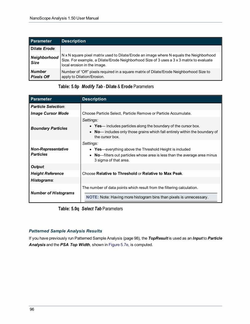
NanoScope Analysis 1.50 User Manual
Parameter Description
Dilate Erode:
NeighborhoodSize
N x N square pixel matrix used to Dilate/Erode an image where N equals the NeighborhoodSize. For example, a Dilate/Erode Neighborhood Size of 3 uses a 3 x 3 matrix to evaluatelocal erosion in the image.
NumberPixels Off
Number of “Off” pixels required in a square matrix of Dilate/Erode Neighborhood Size toapply to Dilation/Erosion.
Table: 5.0p Modify Tab -Dilate & Erode Parameters
Parameter Description
Particle Selection:Image Cursor Mode Choose Particle Select, Particle Remove or Particle Accumulate.
Boundary Particles
Settings:l Yes— includes particles along the boundary of the cursor box.l No— includes only those grains which fall entirely within the boundary of
the cursor box.
Non-RepresentativeParticles
Settings:l Yes—everything above the Threshold Height is includedl No—filters out particles whose area is less than the average area minus
3 sigma of that area.
Output:Height Reference Choose Relative to Threshold orRelative to Max Peak.Histograms:
Number of HistogramsThe number of data points which result from the filtering calculation.
NOTE: Note: Havingmore histogram bins than pixels is unnecessary.
Table: 5.0q Select Tab Parameters
Patterned Sample Analysis ResultsIf you have previously run Patterned Sample Analysis (page 98), the TopResult is used as an Input toParticleAnalysis and thePSA Top Width, shown in Figure 5.7e, is computed.
96
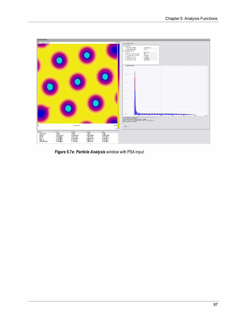
Chapter 5: Analysis Functions
Figure 5.7e: Particle Analysis window with PSA input
97
NanoScope Analysis 1.50 User Manual
5.8 Patterned Sample AnalysisPatterned Sample Analysis is an optional NanoScope Analysis feature that allows you to characterizeregularly patterned samples. Typical samples include image sensors and LED arrays.
Patterned Sample Analysis automatically corrects the tilt of each line and then finds peaks (objects). Partialobjects are screened out. Remaining objects are numbered from left to right, bottom to top. The user selectsthe shape of the base of each object (circular, ellipsoidal or rectangular) and selects locations for anglecalculation. The analysis displays the height and location of each found object, maximum base width and top,middle and bottom angles on the left and right sides of each object. Statistics over all found objects are alsoreported.
Patterned Sample Analysis Procedure1. Open an image in NanoScope Analysis.
2. Execute a 1st order Plane Fit (page 192) onthe data.
Some samples may require that you exclude the patterned objects and use just the sample base for the planefit correction calculation. Do this by:
3. Set Plane Fit Mode toXY.4. Set Plane Fit Order to 1st.5. Set Plane Fit Z Thresholding Direction toUse Z < .6. Set Plane Fit Z Threshold Percent. to exclude the patterned objects. Excluded data will be
shown in blue.
98

Chapter 5: Analysis Functions
Figure 5.8a: Plane Fit to PSA Example. Plane Fit Z Threshold Percent. was set to 18%
7. Click Execute.8. Select Analysis > Patterned Sample Analysis from theMenu bar or click thePatterned
Sample Analysis icon in the NanoScope Analysis toolbar. The file opens in thePatternedSample Analysiswindow.
9. Select a Feature Type in the Inputs panel, shown in Figure 5.8d. Available inputs areEllipse,Rectangle, Sphere andCone.
l Select Rectangle for objects that have a rectangular in-plane shape, Sphere for objectsthat have a circular in-plane shape, Ellipse for objects that have an elliptical in-planeshape andCone for objects with a circular in-plane shape and a conical (but with anessentially flat top) X-Z and/or Y-Z cross-section. Figure 5.8b displays a 3D Image of asample suitable for theCone option while Figure 5.8c displays a 3D Image of a samplesuitable for theSphere option.
99

NanoScope Analysis 1.50 User Manual
Figure 5.8b: 3D Image of typical Cone objects
100

Chapter 5: Analysis Functions
Figure 5.8c: 3D Image of a sample suitable for the Sphere option.
10. Define locations for the anglemeasurements in the Inputs panel, shown in Fig-ure 5.8d.
Figure 5.8d: Inputs for Patterned Sample Analysis
Definitions of geometrical parameters that are used to compute theResults are shown in Figure 5.8eand described in Table: 5.0r.
101

NanoScope Analysis 1.50 User Manual
Figure 5.8e: Inputs description
11. Define aHeight Screen and Top Height. See Table: 5.0r fordefinitions.
Input Description
Feature Type
Settings:
l Ellipsel Rectanglel Spherel Cone
Top AngleLocation Defined as a percentage of the Height down from the peak.
Top AngleBandwidth
The width, defined as a percentage of the peak, of the height used for computation of theTop Angles.
Middle AngleBandwidth
The width, defined as a percentage of the peak, of the height used for computation of theMiddle Angles.
Bottom AngleLocation Defined as a percentage of the Height up from the substrate.
Bottom AngleBandwidth
The width, defined as a percentage of the peak, of the height used for computation of theBottom Angles.
Height Screen Excludes objects if they are lower byHeight Screen%of maximum height.
Top Height The Top Height input is a percentage of the Height down from the peak and is used to cal-culate the Top Width (shown as Top in the Results table).
Bottom Height The Bottom Height input is a percentage of the Height up from the substrate.
Tip Width User input that is subtracted from the Width results.
Table: 5.0r Inputs description
102

Chapter 5: Analysis Functions
NOTE: TheMiddle Location is defined as themid-point (50%) between the substrate and object peak.
NOTE: A line that connects the edge at the bottom point of theBandwidth to the top point of theBandwidth defines the angle with respect to horizontal at that location.
12. The peak locations and angle calculations are computed whenever an Input parameter ischanged.
NOTE: The computation time is approximately proportional to the number of pixels in the image.
Figure 5.8f: Patterned Sample Analysis image showing found peaks
Figure 5.8g: Patterned Sample Analysis Results table
103

NanoScope Analysis 1.50 User Manual
Patterned Sample Analysis ResultsPatterned Sample Analysis results from the image shown in Figure 5.8f are shown in Figure 5.8g.
Result Description
N The number of the found peak, shown in Figure 5.8f.
Width (µm) The width at the base of that peak.
Height (µm) The height of the peak.
X Axis (µm) Diameter of the elliptical or spherical fit in the X direction.
Y Axis (µm) Diameter of the elliptical or spherical fit in the Y direction.
Z Axis (µm) Diameter of the elliptical or spherical fit in the Z direction.
RMS Err (µm) RMS error between the measured surface and the fit.
Top Left (°) Angle, in degrees, at the Top Left of the peak.
Top Right (°) Angle, in degrees, at the Top Right of the peak.
Middle Left (°) Angle, in degrees, at the Middle Left of the peak.
Middle Right (°) Angle, in degrees, at the Middle Right of the peak.
Bottom Left (°) Angle, in degrees, at the Bottom Left of the peak.
Bottom Right (°) Angle, in degrees, at the Bottom Right of the peak.
X Center (µm) The X location of the peak.
Y Center (µm) The Y location of the peak.
Pitch Angle (°) The angle, with respect to horizontal (X axis) of the peaks.
Pitch (µm) The pitch of the peaks along the line that is closest to 0 degrees.
Bottom (µm) The mean baseline Z value.
Top (µm) The maximum Z value.
Table: 5.0s Patterned Sample Analysis Results description
SomePatterned Sample Analysis results, e.g. Bottom and Top, are used in subsequent Bearing Analysis(page 73), Particle Analysis (page 90) and Roughness (page 112) Analysis.
104
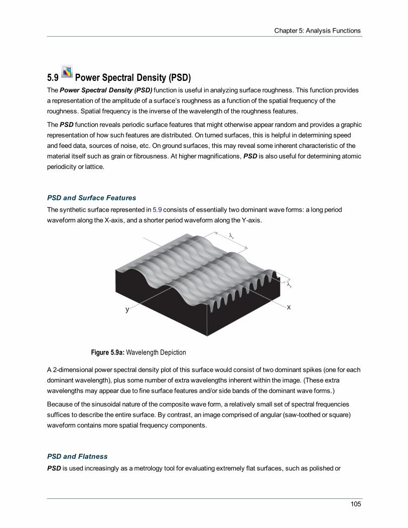
Chapter 5: Analysis Functions
5.9 Power Spectral Density (PSD)ThePower Spectral Density (PSD) function is useful in analyzing surface roughness. This function providesa representation of the amplitude of a surface’s roughness as a function of the spatial frequency of theroughness. Spatial frequency is the inverse of the wavelength of the roughness features.
ThePSD function reveals periodic surface features that might otherwise appear random and provides a graphicrepresentation of how such features are distributed. On turned surfaces, this is helpful in determining speedand feed data, sources of noise, etc. On ground surfaces, this may reveal some inherent characteristic of thematerial itself such as grain or fibrousness. At higher magnifications, PSD is also useful for determining atomicperiodicity or lattice.
PSD and Surface FeaturesThe synthetic surface represented in 5.9 consists of essentially two dominant wave forms: a long periodwaveform along the X-axis, and a shorter period waveform along the Y-axis.
Figure 5.9a:Wavelength Depiction
A 2-dimensional power spectral density plot of this surface would consist of two dominant spikes (one for eachdominant wavelength), plus some number of extra wavelengths inherent within the image. (These extrawavelengths may appear due to fine surface features and/or side bands of the dominant wave forms.)
Because of the sinusoidal nature of the composite wave form, a relatively small set of spectral frequenciessuffices to describe the entire surface. By contrast, an image comprised of angular (saw-toothed or square)waveform contains more spatial frequency components.
PSD and FlatnessPSD is used increasingly as ametrology tool for evaluating extremely flat surfaces, such as polished or
105

NanoScope Analysis 1.50 User Manual
epitaxial silicon. Generally, the desired surface is expected to adhere to certain PSD thresholds, signifying itmeets a specified flatness criterion.
Themain advantage gained over traditional RMS specifications is that PSD flatness is qualified through the fullspectral range of interest. For example, onemay specify spectral thresholds at frequencies measured on theatomic scale, thus ensuring surfaces consist largely of uniform lattices. Setting the precise thresholds forvarious materials remains amatter of debate.
Figure 5.9b: Epitaxial Gallium Arsenide
This surface above is comprised of “terraces” formed from thematerial’s natural lattice structure; each terraceis one atomic monolayer thick and is spaced at fairly regular intervals. This degree of flatness is handilyevaluated withPSD, as the terraces produces a spectral spike corresponding to their spacing wavelength.
Figure 5.9c: PSD Analysis of Epitaxial Gallium Arsenide
106
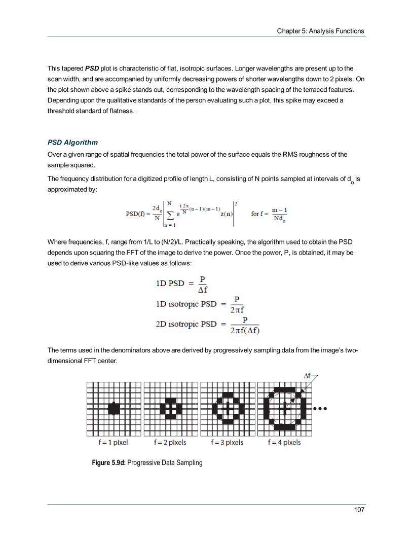
Chapter 5: Analysis Functions
This taperedPSD plot is characteristic of flat, isotropic surfaces. Longer wavelengths are present up to thescan width, and are accompanied by uniformly decreasing powers of shorter wavelengths down to 2 pixels. Onthe plot shown above a spike stands out, corresponding to the wavelength spacing of the terraced features.Depending upon the qualitative standards of the person evaluating such a plot, this spikemay exceed athreshold standard of flatness.
PSD AlgorithmOver a given range of spatial frequencies the total power of the surface equals the RMS roughness of thesample squared.
The frequency distribution for a digitized profile of length L, consisting of N points sampled at intervals of do isapproximated by:
Where frequencies, f, range from 1/L to (N/2)/L. Practically speaking, the algorithm used to obtain the PSDdepends upon squaring the FFT of the image to derive the power. Once the power, P, is obtained, it may beused to derive various PSD-like values as follows:
The terms used in the denominators above are derived by progressively sampling data from the image’s two-dimensional FFT center.
Figure 5.9d: Progressive Data Sampling
107

NanoScope Analysis 1.50 User Manual
Each sampling swings a “data bucket” of given frequency f. Since samples are taken from the image center,the sampling frequency, f, is limited to (N/2)/L, where N is the scan size in pixels. This forms the upperbandwidth limit (i.e., the highest frequency or Nyquist frequency) of the PSD plot. The lower bandwidth limit isdefined at 1/L.
Power Spectral Density Procedure1. Select an image file from theBrowsewindow at the right of themain window. Double click the thumb-
nail image to select and open the image.2. Open thePSD analysis by selecting Analysis > PSD from theMenu bar or by clicking on the PSD icon
in the Icon toolbar. ThePSD window, shown in Figure 5.9e, opens to allow PSD plotting.
Figure 5.9e: PSD Menu & Window
108

Chapter 5: Analysis Functions
PSD Interface
Compute PSD ButtonsOnce thePSD analysis window is opened, select the type of spectral density analysis you wish to perform byclicking the appropriate button in theCompute PSD window.
l 2D Isotropic—Executes a two-dimensional PSD analysis.l Horizontal Axis—Executes a one-dimensional PSD analysis along the X-axis.l Vertical Axis—Executes a one-dimensional PSD analysis along the Y-axis.
The calculation begins as soon as one of these buttons is selected. ThePSD and a table of values from thegraph are shown in theResultswindow. Completion of the analysis will also result in a topographicalhistogram in the spectrum plot window.
Results DisplayTheResultswindow displays the Name and Value of the procedures performed during aPSD analysis. Theteal shaded area in the display window corresponds to the area designated by the teal cursor on the PowerSpectral Density histogram, and themagenta shaded area corresponds to themagenta cursor. You cangenerate a report by right-clicking in theResultswindow, selectingCopy Text and pasting the clipboard intoanother application (e.g. Notepad, Word...).
Select Displayed ParametersThe operator can select which Results will or will not be displayed in theResultswindow by right-clicking intheResultswindow, selecting Show All from the popupmenu, and checking or un-checking the appropriateboxes.
Figure 5.9f: PSD Results Window
109

NanoScope Analysis 1.50 User Manual
Parameter Description
Wavelength The wavelength at current cursor positions. See λx and λy in the Figure:Wavelength Depiction
Frequency The spatial frequency, 1/(λ), at current cursor positions.
Power Power measured in nm2 at current cursor positions.
1D PSD One-dimensional power spectral density measured in nm2; P/(Δf)
1DIsotropicPSD
One-dimensional isotropic power spectral density measured in nm2; P/(2πf)
2DIsotropicPSD
Two-dimensional isotropic power spectral density measured in nm4; P/2πf(Δf)
TotalPower The sum of the power contained in the entire spectrum.
EquivalentRMS
The root mean square (RMS) roughness of the sample. It is calculated as the square root of thetotal power.
PowerBetweenCursors
The sum of the power contained in the portion of the spectrum between the cursors.
EquivalentRMS
The root mean square (RMS) roughness of the sample contained by the frequencies betweenthe cursors. It is calculated as the square root of the integral of the power between the cursors.
Table: 5.0t PSDParameters
Exporting TextSelectingCopy Text from the popupmenu will copy the text from theResultswindow, in tab-delimited textformat, to theWindows clipboard. Youmay then paste it into a text or word processing program.
Changing Parameters of the Spectrum PlotTheSpectrum Plotwindow displays results of thePSD analysis. The window has two cursors whose colorcorresponds to the shaded areas in theResultswindow. Move either of the cursors within theSpectrum Plotwindow by placing the cross hair cursor directly over the cursor, clicking and holding the left mouse button, anddragging themouse to the left or right. Both cursors can bemoved simultaneously by left-clicking themousewith the cross hair cursor anywhere between the two cursors and dragging to the left or right.
To change the parameters of theSpectrum Plot, right-click in theSpectrum Plotwindow at the bottom of thedisplay and choose from the popupmenu.
110

Chapter 5: Analysis Functions
Figure 5.9g: Spectrum Plot Window, Right-click to Change Parameters
111

NanoScope Analysis 1.50 User Manual
5.10 RoughnessTheRoughness command generates a variety of statistics of surfaces, including classical Roughnessvalues andPeak and Zero Crossing data. “Image” statistics are reported for the entire image. “Box” statisticsare reported only for the region you define within a cursor box. In addition, the data can be augmented with stopbands (excluding features).
Most industrial standards for roughness measurement call forPlane fitting data before calculating values.Plane fitting applies a temporary first-order plane fit before calculating statistics. Onmany surfaces,especially those which are tilted, this yields different values from those seen in raw (un plane fitted) data.Moreover, peripheral features included within the analyzed regionmay produce cumulative resultsuncharacteristic of the feature(s) of interest. To ensure the best results, observe the following rules when usingRoughness analysis:
l If the image shows signs of second- or third-order distortion (e.g., bow due to large scans on large scan-ners), apply a second- or third-order Flatten orPlane fit to the image before usingRoughness analysis.
l Isolate your analysis to specific areas of the image. This may be accomplished by using the box cursorinRoughness to analyze only select portions of the image.
Roughness TheoryRegarding the effects of Plane fitting on Roughness statistics—whenRoughness analysis is applied to animage, statistical values are calculated according to the heights of each pixel in the image. Plane fitting andFlattening (used to correct images for tilt and bow) reorient these pixels in amanner which can affectroughness statistics dramatically on some surfaces. This is especially true of surfaces having broad, coplanarfeatures. For more information onPlane fitting, see Plane Fit (page 192).
WhenRoughness analysis is applied to an image or a portion of an image, the data is automatically plane fit(first order) beforehand. This is done to accord with ASME and ISOmetrological standards. (Only the RawMean andMean parameters are exempt from this operation, being calculated from raw data only.) To avoidunexpected results due to plane fitting, be certain to apply Roughness analysis only to the surface(s) ofinterest by utilizing a cursor box, or by scanning just the specific site of interest. Including peripheral featureswithin an analyzed areamay produce cumulative results uncharacteristic of the feature(s) of interest.
Many Roughness results are affected by theOL Plane Fit parameter that was previously set during imagecapture. There are three options for this parameter: None, Offset, and Full. The Full option automaticallysubtracts a first order plane in order to make the average value and the average slope zero. TheOffset optionsubtracts a constant in order to make the average value of the image zero. TheNone option leaves the dataunaltered; thus, theMean equals theRaw Mean.
Regarding Basic RoughnessMeasurements—Average Roughness (Ra) is one of themost commonly usedroughness statistics. Figure 5.10a represents two surfaces having the same average roughness.
112

Chapter 5: Analysis Functions
Figure 5.10a: Roughness Depiction
Similarly, a number of other roughness values are based upon least-squares calculations (e.g., RMSroughness, or Rq), and their algorithms aremore concerned with a best fit of all height points than with thespatial frequency of features.
The surface of image A is represented as having a high frequency profile of features. Image B represents aseparate surface having the same average feature height, but distributed at wider (lower-frequency) intervals.In terms of average and RMS roughness, both surfaces are equally rough. If you are interested in differentiatingbetween the two, youmust rely upon other statistical parameters such as Power Spectral Density.
Roughness Procedure1. Select an image file from the fileBrowsewindow at the right of themain window. Double click the
thumbnail image to select and open the image.2. Open theRoughness analysis by selecting Analysis > Roughness from theMenu bar or by clicking on
theRoughness icon from the Icon toolbar. TheRoughness view, shown in Figure 5.10b, appearsshowing the results for the entire image.
113
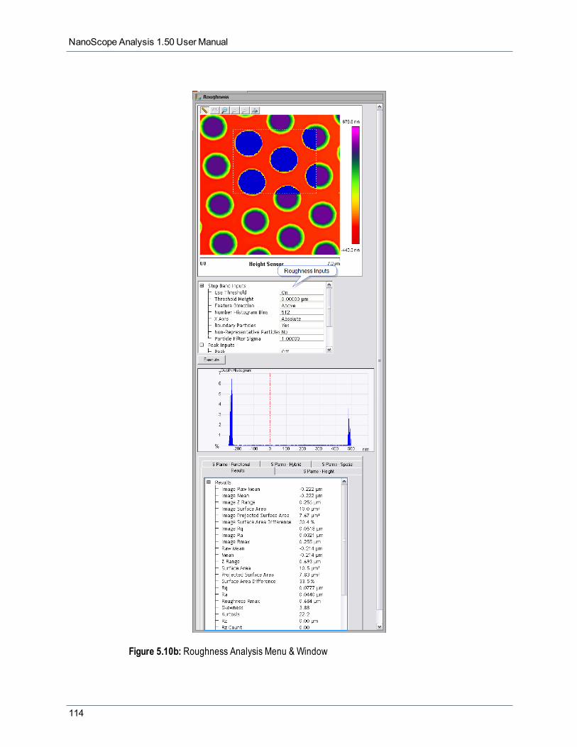
NanoScope Analysis 1.50 User Manual
Figure 5.10b: Roughness Analysis Menu & Window
114

Chapter 5: Analysis Functions
3. To perform Roughnessmeasurements within an area, left-click andmove themouse to draw ameas-urement box. Click on theExecute button to calculate theRoughness inside the box.
4. To exclude an area:l Right-click in the image to access a pop-upmenu and select Stop Band.l Using themouse, draw a box around the area to be excluded by the stop band command.
5. To exclude an area not defined by boxes:l Set Use Threshold toOn.l Set the Feature Direction as needed.l Move the Depth Histogram cursor to exclude the data you wish to exclude as shown in the
image.6. Click theExecute button to calculate theRoughness outside the box.
Input parameters for roughness are discussed in Roughness Parameters (page 116).
115

NanoScope Analysis 1.50 User Manual
5.10.1 Roughness Parameters
Stop Band Input ParametersStop band inputs allow you to exclude parts of the image from Roughness (page 112) Analysis.
Parameter Description
Use Threshold
Uses the Threshold Height to exclude data from the analysis.
NOTE: Use Threshold is, by default, set toOnwhen Patterned Sample Analysis(page 98) has been run.
ThresholdHeight
Height used for threshold.
NOTE: Moving theDepth Histogram cursor will modify the Threshold Height.
NOTE:When Patterned Sample Analysis (page 98) has been run, theBottom res-ult from Patterned Sample Analysis is used for Threshold Height
FeatureDirection
Select Above or Below, depending if features are in high or low-lying (e.g. pits) areas ofthe image.
NumberHistogram Bins
The number of data points which result from the filtering calculation.
NOTE: Note: Havingmore histogram bins than pixels is unnecessary.
X Axis
Applies to the Depth Histogram X axis.
Settings:
l Absolute—data remains unchanged.l Relative—data is relative to the top point.
BoundaryParticles
Settings:
l Yes— includes particles along the boundary of the cursor box.l No— includes only those grains which fall entirely within the boundary of the cursor
box.
Non-RepresentativeParticles
Settings:
l Yes—everything above the Threshold is includedl No—filters out small particles based on the Particle Filter Sigma.
Particle FilterSigma Large sigma values filter out less while small sigma values filter out more.
Table: 5.0u Stop Band Input Parameters
Peak Input ParametersThere are two important configurations for the input parameters that control the way that Roughness calculate
116

Chapter 5: Analysis Functions
statistics: Peak and Zero Crossing.
Figure 5.10c: Roughness Inputs
Some parameters are reported only when certain subroutines are turned on.
PeakThePeak feature, when switchedOn, isolates specified height portions of the image (peaks) from backgrounddata.
Peaks are specified using thePeak Threshold parameters, either in terms of their absolute height or theirdeviation from the RMS value of all surface data, and relative to either the highest data point (Peak) or themean (Zero).
WhenPeak is turnedOn, portions of the image contained within the box cursor and falling within the specifiedboundaries are retained; all other data is removed.
Range or SettingsWhenPeak is turnedOn, the following subcommands are activated:
Command Definition
Peakthresholdreference
The Reference buttons select whether the threshold is defined relative to the Zero (lowest)value, or the tallest Peak in the selected region.
Peakthresholdvalue type
The Value Type determines whether the threshold is defined as an absolute distance from thereference point in nanometers (Absolute value) or a percentage of the root-mean-square (Rms%) of the Z values.
Peakthresholdvalue
The Value is an absolute distance from the reference point in nanometers (Absolute value) or apercentage of the root-mean-square (Rms%) of the Z values.
117

NanoScope Analysis 1.50 User Manual
Table: 5.0v Peak Settings
WhenPeak is turnedOn, the following statistical parameters are turned on. All Peak parameters are calculatedfrom the thresholds you define with thePeak subcommands.
l Rzl Rz countl Peak Countl Valley Countl Max peak ht (Rp)l Av. Max ht (Rpm)l Max depth (Rv)l Av. max depth (Rvm)
WhenPeak is turnedOff, statistics are not calculated.
Zero CrossingA zero crossing is a point where the Z values go through zero regardless of slope. This value is the total numberof zero crossings along both the X and Y center lines divided by the sum of the box dimensions.
Range or SettingsWhen Zero crossing is turnedOn and you click theExecute button, the number of zero crossings along the Xand Y center lines of the box cursor is determined. The number of zero crossings is divided by the sum of thelengths of the X and Y center lines and reported as the Line Density.
When Zero crossing is turnedOff, the Zero crossing determination is not performed.
Results ParametersStatistics used by theRoughness routine are defined in this section. The terms are listed alphabetically. Mostare derived from ASME B46.12 (“Surface Texture: Surface Roughness, Waviness and Lay”) available from theAmerican Society of Mechanical Engineers.
NOTE: The parameters that begin with "Image" are calculated from the entire image excludingStopBandswhen theExecute button is clicked. The other parameters are only calculated for the region withinaBoxwhen theExecute button is clicked.
Parameter Description
ImageRaw Mean
Mean value of data contained within the whole image, except for stop bands. This is calculatedas if the OL Plane fit were set to None during image capture.
ImageMean
Mean value of data contained within the whole image, except for stop bands. This is calculatedafter the OL Plane fit set during image capture has been applied.
118
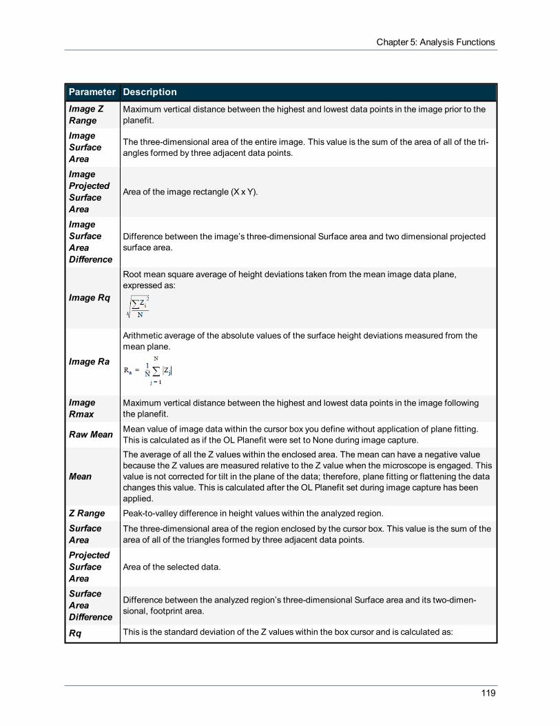
Chapter 5: Analysis Functions
Parameter Description
Image ZRange
Maximum vertical distance between the highest and lowest data points in the image prior to theplanefit.
ImageSurfaceArea
The three-dimensional area of the entire image. This value is the sum of the area of all of the tri-angles formed by three adjacent data points.
ImageProjectedSurfaceArea
Area of the image rectangle (X x Y).
ImageSurfaceAreaDifference
Difference between the image’s three-dimensional Surface area and two dimensional projectedsurface area.
Image Rq
Root mean square average of height deviations taken from the mean image data plane,expressed as:
Image Ra
Arithmetic average of the absolute values of the surface height deviations measured from themean plane.
ImageRmax
Maximum vertical distance between the highest and lowest data points in the image followingthe planefit.
Raw Mean Mean value of image data within the cursor box you define without application of plane fitting.This is calculated as if the OL Planefit were set to None during image capture.
Mean
The average of all the Z values within the enclosed area. The mean can have a negative valuebecause the Z values are measured relative to the Z value when the microscope is engaged. Thisvalue is not corrected for tilt in the plane of the data; therefore, plane fitting or flattening the datachanges this value. This is calculated after the OL Planefit set during image capture has beenapplied.
Z Range Peak-to-valley difference in height values within the analyzed region.
SurfaceArea
The three-dimensional area of the region enclosed by the cursor box. This value is the sum of thearea of all of the triangles formed by three adjacent data points.
ProjectedSurfaceArea
Area of the selected data.
SurfaceAreaDifference
Difference between the analyzed region’s three-dimensional Surface area and its two-dimen-sional, footprint area.
Rq This is the standard deviation of the Z values within the box cursor and is calculated as:
119

NanoScope Analysis 1.50 User Manual
Parameter Description
where Zi is the current Z value, and N is the number of points within the box cursor. This value isnot corrected for tilt in the plane of the data; therefore, plane fitting or flattening the datachanges this value.
Ra
Arithmetic average of the absolute values of the surface height deviations measured from themean plane within the box cursor:
Rmax
Skewness
Measures the symmetry of surface data about a mean data profile, expressed as:
where Rq is the Rms roughness. Skewness is a non dimensional quantity which is typically eval-uated in terms of positive or negative. Where Skewness is zero, an even distribution of dataaround the mean data plane is suggested. Where Skewness is strongly non-zero, an asymmetric,onetailed distribution is suggested, such as a flat plane having a small, sharp spike (> 0), or asmall, deep pit (< 0).
Kurtosis
This is a non-dimensional quantity used to evaluate the shape of data about a central mean. It iscalculated as
Graphically, kurtosis indicates whether data are arranged flatly or sharply about the mean.
Rz This is the average difference in height between the (RZ Count value) highest peaks and valleysrelative to the Mean Plane.
Rz Count Number of peak/valley pairs that are used to calculate the value Rz.
PeakCount The number of peaks taller than the Threshold Value.
ValleyCount The number of valleys shorter than the Threshold Value.
Max Peakht (Rp) Maximum peak height within the analyzed area with respect to the mean data plane.
AverageMaxHeight(Rpm)
Average distance between the (Peak Count value) highest profile points and the mean dataplane.
MaximumDepth (Rv) Lowest data point in examined region.
120
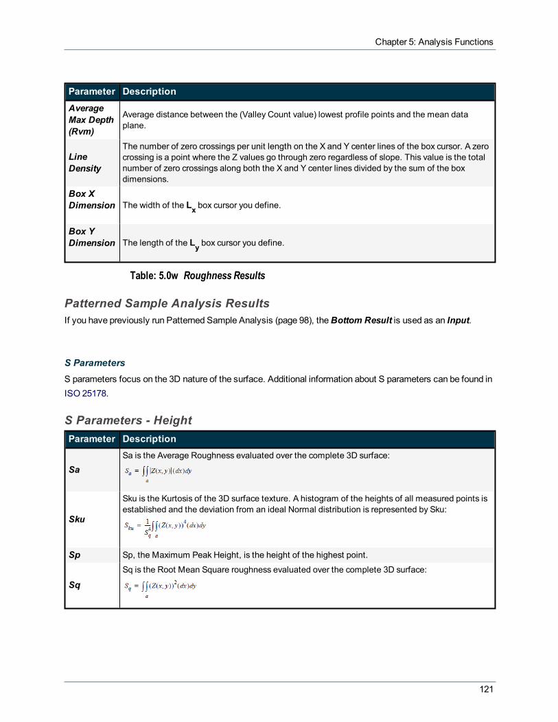
Chapter 5: Analysis Functions
Parameter Description
AverageMax Depth(Rvm)
Average distance between the (Valley Count value) lowest profile points and the mean dataplane.
LineDensity
The number of zero crossings per unit length on the X and Y center lines of the box cursor. A zerocrossing is a point where the Z values go through zero regardless of slope. This value is the totalnumber of zero crossings along both the X and Y center lines divided by the sum of the boxdimensions.
Box XDimension The width of the Lx box cursor you define.
Box YDimension The length of the Ly box cursor you define.
Table: 5.0w Roughness Results
Patterned Sample Analysis Results If you have previously run Patterned Sample Analysis (page 98), theBottom Result is used as an Input.
S ParametersS parameters focus on the 3D nature of the surface. Additional information about S parameters can be found inISO 25178.
S Parameters - HeightParameter Description
SaSa is the Average Roughness evaluated over the complete 3D surface:
Sku
Sku is the Kurtosis of the 3D surface texture. A histogram of the heights of all measured points isestablished and the deviation from an ideal Normal distribution is represented by Sku:
Sp Sp, the Maximum Peak Height, is the height of the highest point.
SqSq is the Root Mean Square roughness evaluated over the complete 3D surface:
121

NanoScope Analysis 1.50 User Manual
Parameter Description
Ssk
Ssk is the Skewness of the 3D surface texture. A histogram of the heights of all measured pointsis established and the deviation from an ideal Normal distribution is represented by Ssk:
Sv Sv, the Maximum Valley Depth, is the depth of the lowest point.
Sz Sz, the Maximum Height of the Surface; Sz = Sp - Sv.
S Parameters - FunctionalParameter Description
SbiSbi, is the Surface Bearing Index:
SciSci, is the Core Fluid Retention Index:
SviSvi, is the Valley Fluid Retention Index:
SmSm is the Surface Material Volume – Volume from top to 10% bearing area:
ScSc is the Core Void Volume – Volume enclosed:
VvSv is the Surface Void Volume – Volume from 80% to 100% bearing area:
S Parameters - HybridParameter Description
Sdq
Sdq, the Root Mean Square Surface Slope comprising the surface, evaluated overall directions:
SdrSdr, the Developed Interfacial Area Ratio, is expressed as the percentage of addi-tional surface area contributed by the texture as compared to an ideal plane thesize of the measurement region:
122

Chapter 5: Analysis Functions
Parameter Description
Sds
Sds, the Density of Summits, is the number of summits per unit area. Summits arederived from peaks. A peak is defined as any point, above all 8 nearest neighbors.Summits are constrained to be separated by at least 1% of the minimum “X” or “Y”dimension comprising the 3D measurement area. Additionally, summits are onlyfound above a threshold that is 5% of Sz above the mean plane.
Ssc
Ssc is the Mean Summit Curvature for the various peak structures. Ssc is evaluatedfor each summit and then averaged over the area:
S Parameters - SpatialParameter Description
Sal
Sal, the Auto-Correlation Length, is a measure of the distance over the surfacesuch that the new location will have minimal correlation with the original location.Sal = Length_Of_Fastest_Decay_Of_Auto_Correlation_Function_To_0.2_In_Any_Direction.
StdStd, the texture direction, is determined by the Angular Power Spectral DensityFunction and is a measure of the angular direction of the dominant lay comprising asurface. Std is defined relative to the Y axis.
Std Minor Std Minor shows the 2nd most conspicuous direction of texture.
Str Str, the Texture Aspect Ratio, is a measure of the spatial isotropy or directionalityof the surface texture.
Previous topic: Roughness (page 112)
5.11 SectionTheSection command displays a top view image, upon which up to three reference lines may be drawn. Thecross-sectional profiles and fast Fourier transform (FFT) of the data along the reference lines are shown inseparate windows. Roughness measurements aremade of the surface along the reference lines you define.
Section is probably themost commonly used Analysis command; it is also one of the easiest commands touse. To obtain consistently accurate results, ensure your image data is corrected for tilt, noise, etc. beforeanalyzing with Section.
123

NanoScope Analysis 1.50 User Manual
Sectioning of SurfacesSamples are sectioned to learn about their surface profiles. The Section command does not reveal what isbelow the surface—only the profile of the surface itself. When sectioning samples, it is important to ascertainsurface topology before applying the Section analysis. Depending upon the topology and orientation of thesample, the results of Section analysis may vary tremendously.
Figure 5.11a: Examples of Section Analysis
The sample surface above (a diffraction grating) is sectioned along three axes. Sections 1 and 2 aremadeperpendicular to the grating’s rules, revealing their blaze and spacings. (Sections 1 and 2may be comparedsimultaneously using two fixed cursor lines, or checked individually with amoving cursor.) Section 3 is madeparallel to the rules, and reveals amuch flatter profile because of its orientation.
The Section command produces a profile of the surface, then presents it in the Cross Section Plot.
124

Chapter 5: Analysis Functions
Figure 5.11b: Cross Section Plot Profile
Generally, Section analysis proves most useful for making direct depthmeasurements of surface features. Byselecting the type of cursor (Rotating Line, Rotating Box, orHorizontal Line), and its orientation tofeatures, youmay obtain:
l Vertical distance (depth), horizontal distance and angle between two or more points.l Roughness along section line: RMS, Ra, Rmax, Rz.l FFT spectrum along section line.
Features are discussed below. See Roughness (page 112) for additional information regarding roughnesscalculations.
Section Procedures & InterfaceBefore doing a Section analysis, ensure that the image is properly oriented by removing any tilt or bow. This isespecially important if a high level of precision is to be employed inmeasuring the blaze angle. To remove anytilt whichmight be present, use thePlanefitmodification feature. See Plane Fit (page 192) for moreinformation.
To perform Section analysis:
1. Select an image file from the file Browse window at the right of themain window. Double-click thethumbnail image to select and open the image.
2. Open the Section analysis by selectingAnalysis > Section from theMenu bar or by clicking on the Sec-tion icon in the Icn toolbar.
125

NanoScope Analysis 1.50 User Manual
Figure 5.11c: Section Analysis Menu & Window
3. Draw a line across the image by clicking and dragging the cursor.
Figure 5.11d: Depiction of Mouse-Line Dragging to Insert Cursor(s)
4. When a line is drawn on the image, the cross section is displayed in themain plot and a FFT spectrum isdisplayed directly below this.
5. Move the grid cursors left and right along the section by clicking and dragging the plot markers on thesection plot.
126
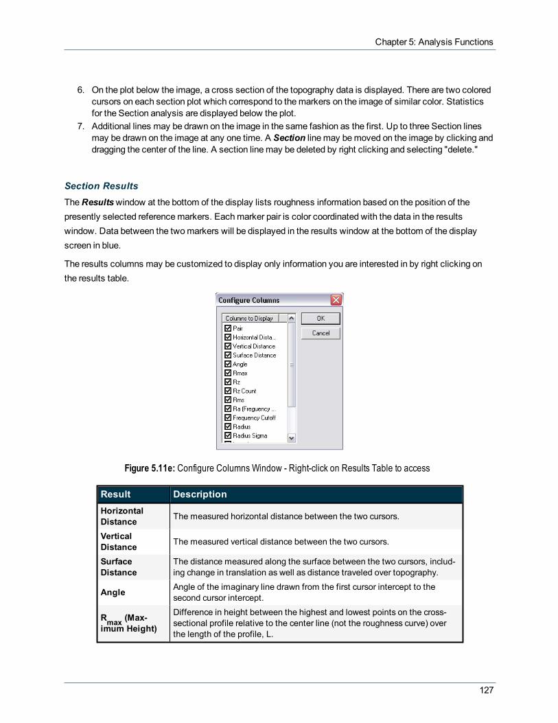
Chapter 5: Analysis Functions
6. On the plot below the image, a cross section of the topography data is displayed. There are two coloredcursors on each section plot which correspond to themarkers on the image of similar color. Statisticsfor the Section analysis are displayed below the plot.
7. Additional lines may be drawn on the image in the same fashion as the first. Up to three Section linesmay be drawn on the image at any one time. A Section linemay bemoved on the image by clicking anddragging the center of the line. A section linemay be deleted by right clicking and selecting "delete."
Section ResultsTheResultswindow at the bottom of the display lists roughness information based on the position of thepresently selected referencemarkers. Eachmarker pair is color coordinated with the data in the resultswindow. Data between the twomarkers will be displayed in the results window at the bottom of the displayscreen in blue.
The results columns may be customized to display only information you are interested in by right clicking onthe results table.
Figure 5.11e: Configure Columns Window - Right-click on Results Table to access
Result DescriptionHorizontalDistance The measured horizontal distance between the two cursors.
VerticalDistance The measured vertical distance between the two cursors.
SurfaceDistance
The distance measured along the surface between the two cursors, includ-ing change in translation as well as distance traveled over topography.
Angle Angle of the imaginary line drawn from the first cursor intercept to thesecond cursor intercept.
Rmax (Max-imum Height)
Difference in height between the highest and lowest points on the cross-sectional profile relative to the center line (not the roughness curve) overthe length of the profile, L.
127

NanoScope Analysis 1.50 User Manual
Result Description
Rz (Ten-PointMean Rough-ness)
Average difference in height between the five highest peaks and five low-est valleys relative to the center line over the length of the profile, L. Incases where five pairs of peaks and valleys do not exist, this is based onfewer points.
RMS (StandardDeviation)
Standard deviation of the Z values between the reference markers, cal-culated as:
where Zi is the current Z value, Zave is the average of the Z valuesbetween the reference markers, and N is the number of points between thereference markers.
Rz Count The number of peaks used for the Rz computation.
Ra (MeanRoughness)
Mean value of the roughness curve relative to the center line, calculatedas:
where L is the length of the roughness curve and f(x) is the roughness curverelative to the center line.
FrequencyCutoff (um)
Frequency Cutoff measured in terms of a percentage of the root meansquare.Changing the cursor on the FFT changes lc, the cutoff length of the high-pass filter applied to the data. The filter is applied before the roughnessdata is calculated; therefore, the position of the cutoff affects the cal-culated roughness values.
Radius Radius of circle fitted to the data between the cursors.Radius Sigma Mean square error of radius calculation.Length Length of the roughness curve.Spectral Period Spectral period at the cursor position.Spectral Fre-quency Spectral frequency at the cursor position.
SpectralRMS Amplitude Amplitude at the cursor position.
Table: 5.0x Section Results Columns
Mouse Operations for a Rotating Line Cursorl Mouse down, drag—Anchors the origin of a line segment and expands from the selected position, allow-
ing a line segment to be drawn in any direction.l Mouse up—Anchors the terminal point of the first (dashed) line segment and draws amoving reference
line perpendicular to the fixed-line segment. The cross-sectional profile and the FFT along the referenceline are displayed at this time. The position of themoving reference line tracks themovements of the
128

Chapter 5: Analysis Functions
mouse. When themouse is stationary, the cross-sectional profile and the FFT of the data along themov-ing reference line is updated.
l Clicking on the center of the line and draggingmoves the line on the image.l Clicking on either end of the line rotates the line.
Mouse Operations for Rotating Box Cursor (Right-Click Selection):l 1st click—Anchors the origin of a box and “rubber bands” out from the center of the selected position.l As a reference, the cursor positions show up on the center line in the box.l Clicking on the box—Allows the box to bemoved (cursor inside box), or resized (cursor on edge of box).
Clicking on the corner allows the box to be resized in two directions.l Holding the Shift button downwhile clicking on the box and dragging in a circular direction rotates the
box.
Mouse Operations for a Horizontal Line Cursor:l Mouse down—Draws a horizontal line segment at that location.l Clicking on the line and draggingmoves the line on the image.
Using the Grid DisplayMeasurement cursors for histogram and cross section views inDepth andSection are provided to the left andright of theGrid Display. You can bring the cursors into the grid by placing themouse cursor onto themeasurement cursors, clicking and holding the left mouse button, and dragging them onto the grid. When youplace themouse cursor onto ameasurement cursor, the cursor will change to a horizontal or vertical double-arrow cursor , which indicates you can grab and drag this cursor.
Right-clicking on the grid will bring up theGrid Parametersmenu and allow you tomake the followingchanges:
Grid Para-meter Description
Color
Allows operator to change the color of the:-Curve-Text-Background-Grid-Minor-Marker
FilterTypically uses a Profiler Scan.Type - Select None, Mean (default), Maximum, or MinimumPoints - Select 4k, 8k (default), 16k or 32k
Minor Grid Places a minor grid in the background of the Graph WindowScale Allows user to auto scale, set a curve mean, or set their own data rangeLine Style For each curve, the operator can choose a connect, fill down, or point line.User Prefer-ence
Restore—Reverts to initial software settings Save—Saves all changes operator has made duringthis session. This becomes the new default settings.
129

NanoScope Analysis 1.50 User Manual
Grid Para-meter Description
Copy Clip-board Copies the grid image to the Microsoft Clipboard
Print Prints out the current screen view to a printerExport Exports data in bitmap, JPEG or XZ data formatActiveCurve Determines which curve you are analyzing
Table: 5.0y Grid Parameters
130
Chapter 5: Analysis Functions
5.12 StepTheStep analysis makes relative height measurements between two regions (steps) on sample surfaces.Typical applications includemeasuring film thickness and etch depths. Step works similarly to aSectionanalysis with an averaging box cursor, but its operation is simplified.
Step displays a top view of the image, then the user draws a reference line across the regions to bemeasured.A height profile is generated from averaged data on either side of the reference line in the box. Cursors—whicharemoved along the profile—define specific regions (steps). Thesemay bemeasured (Measure button) relativeto each other, with or without data leveling (Level button).
5.12.1 Step Procedure1. Select an image file from the fileBrowsewindow at the right of themain window. Double-click the
thumbnail image to select and open the image.2. Open theStep analysis by selecting Analysis > Step from theMenu bar or by clicking on the Step icon
from the Icon toolbar. TheStepwindow appears showing the results for the entire image.3. To run theStep Analysis for a region of the image, use themouse to draw a rotating box in the desired
location. TheStep interface includes a captured image and a graph of averaged height within a selectedbox.
4. By holding down the shift key while dragging the edge of the box, it can be rotated. Rotation is some-times required when features of interest are not horizontal.
5. In the height graph area below the image, two pairs of cursors (one black and one red) can bemovedacross this profile to define the steps to bemeasured. To insert cursors, move themouse in the heightgraph to the left of the Y axis. The cursor will change to a double-headed arrow. Using the left mouse but-ton, drag the double-headed arrow to the desired step location. This can be repeated for a secondcursor. The region between each pair of cursors defines a “step.” Themarker position is shown belowthe height graph.
6. Once the two pairs of cursors are added to the height graph, the system will report the vertical distancebetween the average heights of the two steps in the Results area.
131

NanoScope Analysis 1.50 User Manual
Figure 5.12a: Step Analysis Unleveled
7. If the profile is tilted, click on the Level button and, using the cursors, select two steps that should havethe same height. The slope of the profile changes to level the two steps.
132
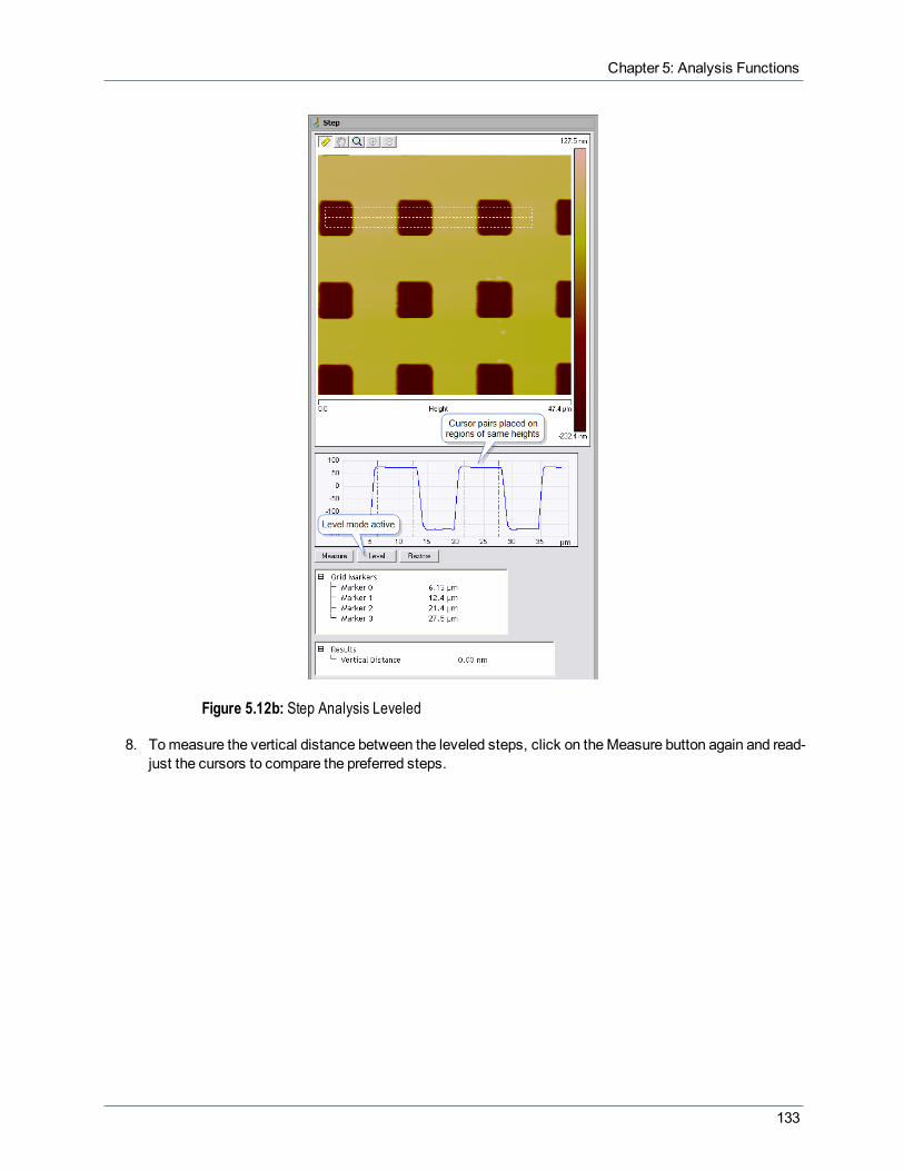
Chapter 5: Analysis Functions
Figure 5.12b: Step Analysis Leveled
8. Tomeasure the vertical distance between the leveled steps, click on theMeasure button again and read-just the cursors to compare the preferred steps.
133

NanoScope Analysis 1.50 User Manual
Figure 5.12c: Step Analysis in Measure Mode
5.12.2 Step Display Menu Commands & ResultsParameter Description
Measure Displays the relative height between steps
Level Re-orients the profile so that the average height of each step region (between cursor pairs) isequal
Restore Returns the profile to its original, unleveled form (De-selects the Level option)
StepResults:
VerticalDistance
Displays the distance between the average height of each region (between cursor pairs). If theheight of the region between the second pair of cursors is lower than the firsts's, this will be a neg-ative value.
134
Chapter 5: Analysis Functions
5.13 Tip QualificationTip Qualification refers to estimating tip shape from appropriate characterizer samples and rating tips asgood, worn, bad, suspect, or no tip. The Tip Qualification function incorporates the two separate capabilities:Tip Estimation and Tip Qualification.
Tip EstimationTip Estimation generates amodel of the tip based on an image of a standard characterizer sample. Acharacterizer refers to a sample whose surface is well suited to deducing tip condition when imaged using anSPM probe.
In Tip Estimation, local peaks in a topographic image are successively analyzed, refining a 3-dimensional tipmodel. At each peak, the slope away from the peak in all directions is measured, determining theminimum tipsharpness (no data in the image can have a slope steeper than the slope of the tip). As this process is repeatedfor each local peak, any steeper slope than was found from all previously analyzed peaks causes the tip modelto update to a new, sharper tip estimate.
Tip QualificationTip Qualification uses the tip estimate to determine whether the tip is acceptable for use. This feature can beused to check tips periodically for signs of wear, and to exchange unacceptably worn tips. By using tipqualification to enforce tip acceptance criteria, metrological values can be compared from image to image,ensuring consistent, long-term comparability of samples.
Theoretical Foundation for Tip QualificationIt is not useful to qualify a probe tip that is poorly matched to the sample to be imaged. Specifically, a tip cannotresolve the linear and angular aspects of any sample feature sharper than the tip itself. (However, even a blunttip can resolve height accurately on a surface with shallow slopes.) Therefore, select a tip sharp enough toresolve the features of interest.
Tip ArtifactsAtomic ForceMicroscope (AFM) images depend on the shape of the tip used to probe the sample. Tip artifactsrefer to either the occurrence of features or the absence of features in an image that are not in the sample, butdue to the tip used as compared (hypothetically) with an ideal tip of near-zero tip radius. In the simplest case,the finite size of the AFM tip does not allow it to probe narrow, deep fissures in a sample where the tip radius isgreater than the radius of the recess.
135

NanoScope Analysis 1.50 User Manual
Figure 5.13a: Tip Artifact Depiction
Also, sharp sample features scanned with a dull tip are broadened in AFM images. Consequently, imagemeasurements such as surface roughness and surface area depend on probe tip shape. An image generatedwith a sharp tip shows greater roughness and larger surface area than an image produced with a dull tip.
Figure 5.13b: Effects of Tip Sharpness
Sample Dependence of Tip QualificationThemodel generated by tip estimation is not, in general, the actual shape of the tip. Because the tip model isconstructed by analyzing the shapes of peaks in the image data, the accuracy of themodel is limited by thesharpness of features on the characterizer.
Characterizer samples that provide themost accurate estimate of tip size and shape are those with many fineprotrusions, since they typically have very sharp features. Even these samples are not perfect, and only asurface with infinitely sharp features can produce an perfectly accuratemodel of the tip:
136

Chapter 5: Analysis Functions
Figure 5.13c: Characterizer - Dull Tip on Sharp Characterizer
A surface having only large rounded features provide the least useful estimate of tip shape:
Figure 5.13d: Sharp Tip on Rounded Characterizer
Similar feature size of the characterizer and tip will yield a combined geometry for the tip shape:
Figure 5.13e: Typical Characterizer
Despite the dependence on characterizer characteristics, Tip Estimation and Tip Qualification can oftenprovide a reliable method of tracking tip wear and ensuring that probes are changed when they become dull. Forexample, whenmaking repeatedmeasurements on suitable rough samples, Tip Estimation can provide veryreproducible estimates of tip size and shape, which change in a predictable and consistent fashion as the tipwears.
Tip Quality ThresholdsBased on thresholds set by the user, Tip Qualification software usually finds the tip status to beGood, Worn, orBad.
l A tip status of Good indicates that the tip is still sufficiently sharp and that the image data should beacceptable.
l A tip status of Worn indicates that the tip is becoming dull and should be changed, but previous imagedata taken with this tip should still be acceptable.
l If a Bad status is returned, the tip should be changed and the current image data discarded.l In cases where imaging errors are suspected, Tip Qualificationmay assign a status of Suspect or No
Tip.
137

NanoScope Analysis 1.50 User Manual
Characterizer Sample SelectionJust as probe selection influences imaging results, characterizer sample selection influences probe tipcharacterization. An ideal characterizer sample for tip diagnosis has isolated extremely sharp peaks.
Bruker provides a characterizer sample that is recommended for tip evaluation. The polycrystalline titaniumroughness sample (part number RS, available at http://www.brukerafmprobes.com) has jagged featuressuitable for obtaining an accurate tip model.
Figure 5.13f: Polycrystalline Titanium Roughness Sample
Operating Principles of Tip QualificationThe result of running Tip Qualification is a display similar to that shown in Figure 5.13g.
138

Chapter 5: Analysis Functions
Figure 5.13g: A typical Tip Qualification window
The top-left frame is the image analyzed to evaluate the tip. The top-right frame, labeled Tip, is a top viewimage of the softwaremodel of the tip (looking into its apex).
Once a tip model has been generated, Tip Estimation extracts an estimate of the tip geometry in cross-sections at two different distances from the tip apex, as seen in Figure 5.13h.
139

NanoScope Analysis 1.50 User Manual
Figure 5.13h: Tip Estimation Cross-Sections Depiction
The cross-section diagrams on the right in Figure 5.13g show the apparent size and shape of the tip at twodifferent distances from its apex (labeled Level 1 ETD and Level 2 ETD. In the Level 1 cross-section, theroughly circular tip diameter is shown in light gray. In the lower-right frame of Figure 5.13g, the Level 1 cross-section is shown again in light gray and the Level 2 cross-section is shown darker. (The actual colors of the tipcross-sections depend on the color table selected.)
Tip Estimation then provides, at each cross section, two numerical measures of tip size and shape: effectivetip diameter (ETD) and aspect ratio (AR). The effective tip diameter is defined as the diameter of a circle havingthe same area as themeasured tip cross-section (see Figure 5.13i). The ETD is shown below as a circle to theright.
Figure 5.13i: ETD Depiction
Aspect Ratio is defined as the ratio of themaximum vertical (Y) dimension to themaximum horizontal (X)dimension of a tip cross section as seen in Figure 5.13j.
140

Chapter 5: Analysis Functions
Figure 5.13j: Aspect Ratio Depiction
Control of Tip Qualification StatusTip Qualification generates a tip status based on the calculated values of ETD, AR and on threshold and limitvalues selected. There are two ETD thresholds that affect tip status:
l Good/Worn ETD Threshold—If the ETD is smaller than this number, the tip will usually be char-acterized as Good. The threshold diameters are shown as green circles in the ETD windows.
l Worn/Bad ETD Threshold—If the ETD is smaller than this threshold, but bigger than theGood/WornETD Threshold, it is characterized asWORN. If the ETD is larger than this number, it is characterizedas Bad. These threshold diameters are shown as red circles in the ETD windows.
There are separate sets of ETD thresholds for the two tip levels (ETD 1 at HEIGHT 1, and ETD 2 at HEIGHT2). There are alsominimum andmaximum limits for tip AR at each level. These limits detect when the imagedata produces a tip model of an oblong shape that is unlikely to accurately represent the tip. Usually an oblongtip model is induced by an imaging artifact, such as a noise streak not removed by discontinuity rejection. TheAR limits should not be adjusted.
It takes some experimentation with a particular tip and characterizer sample type to find appropriate values forthe various thresholds. The basic idea is to find themaximum ETDs (the diameters of the dullest tips) thatprovide reliable image data for your samples, then set theWorn/Bad ETD Thresholds based on thesediameters. Then set theGood/Worn ETD Thresholds slightly smaller than theWorn/Bad ETD Thresholds.
An additional limit,Min ETD Size, is used to reject Tip Qualification results if the estimated tip is unreasonablysmall (indicating a tip that is sharper than physically likely). This is usually induced by imaging artifacts, suchas noise spikes not removed by spike rejection. In most cases,Min ETD Size can be set at or near the samevalue as the height from the tip apex for both cross sections. So, if Height 1 = 10NM, a reasonable value fortheMin ETD Size is also 10NM.
NOTE: A tip estimate rejected in this way returns Tip Status of Suspect.
Because the tip estimate is valid only where the tip contacts the characterizer sample, cross section heightsshould be selected to ensure that the tip makes “frequent” contact with the characterizer sample at thoseheights. Thus, the cross section heights should be below the sample peak-to-valley values. If the cross sectionheights are too high for the characterizer sample, the resultant ETD will tend to be very large andmultipleapparent peaks will be found at that height.
141

NanoScope Analysis 1.50 User Manual
Tip Qualification Procedures1. Scan (contact mode) the characterizer sample. Set the scan size to approximately 2.5um.
Characterizer image size is important because, along with Tip Image Size (page 144) and feature dens-ity, it determines how many peaks are used for the tip estimation. To accurately estimate the tip shape,theremust bemany peaks (greater than 10 is good).
2. Select the captured image file of the characterizer sample from the file browsing window at the right ofthemain window. Double click the thumbnail image to select and open the image.
3. Open the Tip Qualification Analysis by selectingAnalysis >Tip Qualification from theMenu bar orby clicking on the Tip Qualification icon in the Icon toolbar. The initial Tip Qualification view appears.
4. Enter the Tip Image Size desired for the currently loaded tip and characterization image.5. Select whether to apply a low pass filter to the image by selecting eitherYes orNo for parameter LPF
for Max Select.
NOTE: It is generally a good idea to use a low pass filter to ensure that small noise artifacts are removedbefore Tip Estimation. Noisemistaken for an imaged feature renders amisleading tip model. Additionally,large noise artifacts can be selectively removed by adjustingSigma Mult for Spike Rejection andSigma Mult for Discontinuity Rejection.
6. Enter the number of Low Pass Filter Iterations.
NOTE: This applies a Lowpass (page 187) Filter to the image n times. peak and slope finding are per-formed on the filtered data. You should use this filter for images taken at Scan Rates greater than 5 Hz.Bruker recommends that you set LPF for Max Select to No when you use this filter.
7. Enter values for all parameters in theCross Section panels.8. Click Estimate Tip.9. Click Qualify Tip.10. View the Tip Status in theResults panel.11. If the end radius of the tip is required, click Save Tip and then open the saved file. Click theSection
icon to open the file and draw a cursor through the tip center. The radius of a circle fitted to the databetween the cursors is displayed in the bottom of theSectionwindow. Refer to Section (page 123) formore information.
Tip Qualification Interface
Tip Qualification ButtonsButton Description
EstimateTip
Performs a new tip assessment. A bottom-to-top, plan view rendering of the tip, labeled Tip, isshown in the middle-top image. The original image appears in the upper-left corner of the screen,with green markers (+) indicating the data peaks used for the estimation. If the Save Tip button isselected, the estimated tip image is saved to a file. This image can be loaded and analyzed in thesame ways as other NanoScope images.
QualifyTip
Results:
l If any “Tip Estimation” parameter or the analysis region has been changed, a new tip estim-ation is performed.
142
Chapter 5: Analysis Functions
Button Descriptionl The tip cross sections and qualification results appear in the Results panel.l Tip status is determined based on the estimated tip shape.
Save TipStores the estimated tip image as a NanoScope image file, allowing it to be analyzed using the
standard NanoScope Analysis Functions (page 59) and Filter Commands (page 163). A tip imageis approximately the size specified by the Tip Image Size parameter and thus has fewer datapoints than a standard image.
Table: 5.0z Tip Qualification buttons
143

NanoScope Analysis 1.50 User Manual
Group Parameter Description
TipEstimation
Tip ImageSize
Sets the size of the image displayed in the upper-left corner of the TipQualification window. Calculated tip diameters are not expected to exceed TipImage Size. For example, Tip Image Size = 120 nm will result in a tip imageapproximately 120 nm square. A reported ETD is the smallest odd integermultiple of the sample data resolution that is greater than or equal to thecalculated tip diameter.
Tip Image Size also defines in a characterizer image the neighborhood sizeused to select the topographic maxima points used for Tip Estimation. Forexample, for Tip Image Size = 120 nm, each selected maximum pixel is thetallest point topographically within an approximately 120 nm square centered on
the point. Therefore, a larger Tip Image Sizemay result in fewer selectedmaxima. More points provide more tip information, so select Tip Image Size tobe as small as possible while also satisfying two other conditions:
1) Tip Image Size should exceed the ETD at as tall a height above the tip apexas is contacted imaging the characterizer sample. Determine this experimentally
by varying Tip Image Size and observing the resultant top-middle image in theTip Qualification window.NOTE: A good starting point for Tip Image Size is the sum of the maximumallowable tip diameter plus the diameter of a typical feature in the characterizer.2) If and when “double tip” peaks appear in the image due to tip wear, their
apexes should be no farther apart than one-half Tip Image Size. This ensuresthat multiple peaks from a “double tip” feature are not treated as separatefeatures from the same peak (which would produce erroneous results and nolonger guarantee an outside tip envelope).
NOTE: Characterizer image size and feature density also affect the number ofselected maxima.
LPF for maxselect
Determines whether a lowpass filter is applied to the data before identifyingselected points. The filtered data is only used for point selection, not for theactual tip calculation. This filter has the effect of reducing noise sensitivity. It isrecommended that the filter be turned on (Yes) unless you use the Low PassFilter Iterations function.
Low PassFilterIterations
Number of times to apply the Lowpass (page 187) filter to the data before find-ing peaks and slopes.
Sigma Multfor SpikeRejection
Sets a threshold for rejection of isolated upwards-oriented noise spikes. At eachpoint (x,y) in an image, a difference Δ(x,y) is calculated between the pixel valueat that point and the average value of the surrounding eight pixels. The average,μ, and standard deviation, σ, of all positive Δ(x,y)s in the image are then cal-culated. The normal (Gaussian) distribution with average value, μ, and standarddeviation, σ, is then used to represent the actual distribution of positive Δ(x,y)
144
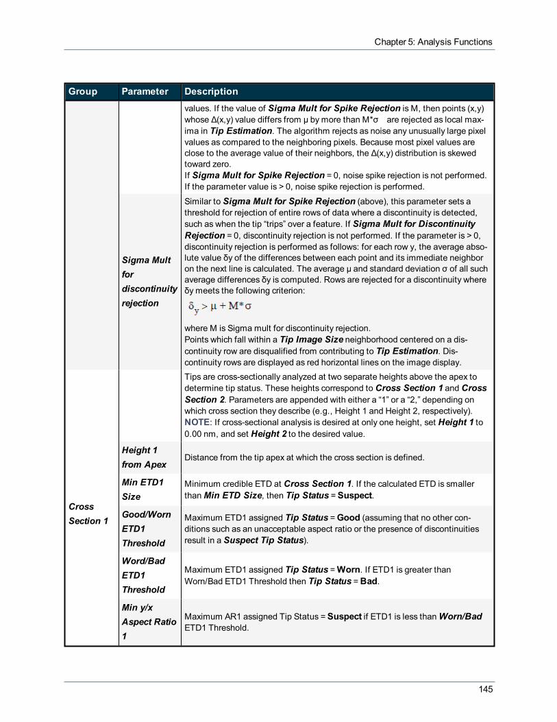
Chapter 5: Analysis Functions
Group Parameter Description
values. If the value of Sigma Mult for Spike Rejection is M, then points (x,y)whose Δ(x,y) value differs from μ by more than M*σ are rejected as local max-ima in Tip Estimation. The algorithm rejects as noise any unusually large pixelvalues as compared to the neighboring pixels. Because most pixel values areclose to the average value of their neighbors, the Δ(x,y) distribution is skewedtoward zero.If Sigma Mult for Spike Rejection = 0, noise spike rejection is not performed.If the parameter value is > 0, noise spike rejection is performed.
Sigma Multfordiscontinuityrejection
Similar to Sigma Mult for Spike Rejection (above), this parameter sets athreshold for rejection of entire rows of data where a discontinuity is detected,such as when the tip “trips” over a feature. If Sigma Mult for DiscontinuityRejection = 0, discontinuity rejection is not performed. If the parameter is > 0,discontinuity rejection is performed as follows: for each row y, the average abso-lute value δy of the differences between each point and its immediate neighboron the next line is calculated. The average μ and standard deviation σ of all suchaverage differences δy is computed. Rows are rejected for a discontinuity whereδy meets the following criterion:
where M is Sigma mult for discontinuity rejection.Points which fall within a Tip Image Size neighborhood centered on a dis-continuity row are disqualified from contributing to Tip Estimation. Dis-continuity rows are displayed as red horizontal lines on the image display.
CrossSection 1
Tips are cross-sectionally analyzed at two separate heights above the apex todetermine tip status. These heights correspond to Cross Section 1 and CrossSection 2. Parameters are appended with either a “1” or a “2,” depending onwhich cross section they describe (e.g., Height 1 and Height 2, respectively).NOTE: If cross-sectional analysis is desired at only one height, set Height 1 to0.00 nm, and set Height 2 to the desired value.
Height 1from Apex
Distance from the tip apex at which the cross section is defined.
Min ETD1Size
Minimum credible ETD at Cross Section 1. If the calculated ETD is smallerthanMin ETD Size, then Tip Status =Suspect.
Good/WornETD1Threshold
Maximum ETD1 assigned Tip Status =Good (assuming that no other con-ditions such as an unacceptable aspect ratio or the presence of discontinuitiesresult in a Suspect Tip Status).
Word/BadETD1Threshold
Maximum ETD1 assigned Tip Status =Worn. If ETD1 is greater thanWorn/Bad ETD1 Threshold then Tip Status =Bad.
Min y/xAspect Ratio1
Maximum AR1 assigned Tip Status =Suspect if ETD1 is less thanWorn/BadETD1 Threshold.
145

NanoScope Analysis 1.50 User Manual
Group Parameter Description
Max y/xAspect Ratio1
Minimum AR1 signed Tip Status =Suspect if ETD1 is less thanWorn/BadETD1 Threshold.
CrossSection 2
Height 2from Apex
Distance from the tip apex at which the cross section is defined.
Min ETD2Size
Minimum credible ETD at Cross Section 2. If the calculated ETD is smallerthan Min ETD Size, then Tip Status =Suspect.
Good/WornETD2Threshold
Maximum ETD2 assigned Tip Status =Good (assuming that no other con-ditions such as an unacceptable aspect ratio or the presence of discontinuitiesresult in a Suspect Tip Status).
Word/BadETD2Threshold
Maximum ETD2 assigned Tip Status =Worn. If ETD2 is greater thanWorn/Bad ETD2 Threshold then Tip Status =Bad.
Min y/xAspect Ratio2
Maximum AR2 assigned Tip Status =Suspect if ETD2 is less thanWorn/BadETD2 Threshold.
Max y/xAspect Ratio2
Minimum AR2 signed Tip Status =Suspect if ETD2 is less thanWorn/BadETD2 Threshold.
Table: 5.0aa Tip Estimation Panel Parameters
TipStatus Result
1.Suspect
Tips will be qualified as SUSPECT under any of the following conditions:
l A discontinuity exceeding the Sigma mult for discontinuity rejection has been found in thedata.
l One of the aspect ratios of the tip is outside the range (Min y/x Aspect Ratio, Max y/x AspectRatio).
l ETD1 or ETD2 is smaller than its Min ETD1 [ETD2] Size.
2. Good Both ETDs are less than the Good/Worn ETD Threshold parameter setting.
3. Bad At least one of the ETDs is greater than its Worn/Bad ETD Threshold or one of the cross-sectionsintersects a large portion of the tip image boundary.
4.Worn At least one of the ETDs falls between its Good/Worn ETD Threshold and Worn/Bad ETDThreshold.
Table: 5.0ab Tip Status Results - Evaluated in the order listed
146

Chapter 5: Analysis Functions
5.14 WidthTo analyze the width of features you have numerous choices whichmeasure the height difference between twodominant features that occur at distinct heights.Widthwas primarily designed for automatically comparingfeature widths at two similar sample sites (e.g., when analyzing etch depths on large numbers of identicalsilicon wafers).
TheWidth command is designed to automatically measure width between features distinguished by height,such as trenches and raised features.
TheWidth command is best applied when comparing similar features on similar sites. Widthmeasurement ondissimilar sites is better performed using theSection command.
Width TheoryTheWidth algorithm utilizes many of the same functions found inDepth analysis by accumulating height datawithin a specified area, applying aGaussian low-pass filter to the data (to remove noise), then rapidly obtainingheight comparisons between two dominant features. For example, 1) the depth of a single feature and itssurroundings; or, 2) depth differences between two or more dominant features. Although this method of widthmeasurement does not substitute for direct, cross-sectioning of the sample, it does afford ameans forcomparing feature widths between two or more similar sites in a consistent, statistical manner.
TheWidthwindow includes a top view image and a histogram; depth data is displayed in the results windowand in the histogram. Themouse is used to resize and position the box cursor over the area to be analyzed. Thehistogram displays both the raw and an overlaid, Gaussian-filtered version of the data, distributed proportionallyto its occurrence within the defined bounding box.
5.14.1 Histogram
Raw DataHistograms for depth data are presented on the bottom of theWidthwindow. The histogram peaks correspondto the distribution of depths of analyzed regions of the image (see Figure 5.14a).
147

NanoScope Analysis 1.50 User Manual
Figure 5.14a:Width Image and Corresponding Histogram
NOTE: Color of cursor, data, and grid may change if user has changed the settings. Right-click on thegraph and go toColor if you want to change the default settings.
Correlation CurveTheCorrelation Curve is a filtered version of theRaw Data Histogram and is represented by a red line on theDepth Histogram. Filtering is done using theHistogram filter cutoff parameter in the Inputs parameterbox.The larger the filter cutoff, themore data is filtered into a Gaussian (bell shaped) curve. Large filter cutoffsaverage somuch of the data curve that peaks corresponding to specific features are unrecognizable. On theother hand, if the filter cutoff is too small, the filtered curvemay appear noisy.
TheCorrelation Curve portion of the histogram presents a lowpass, Gaussian-filtered version of the raw data.The low-pass Gaussian filter removes noise from the data curve and averages the curve’s profile. Peaks whichare visible in the curve correspond to features in the image at differing widths.
Peaks do not show on the correlation curve as discrete, isolated spikes; instead, peaks are contiguous withlower and higher regions of the sample, and with other peaks. This reflects the reality that features do not allstart and end at discrete depths.
When using theWidthview for analysis, each peak on the filtered histogram is measured from its statisticalcentroid (i.e., its statistical center of mass).
Width Procedures1. Select an image file from the fileBrowsewindow at the right of themain window. Double-click the
thumbnail image to select and open the image.2. Open theWidth analysis by selecting Analysis > Width from theMenu bar or by clicking on theWidth
icon in the Icon toolbar.3. TheWidth view, shown in Figure 5.14b, appears showing results for the entire image.
148
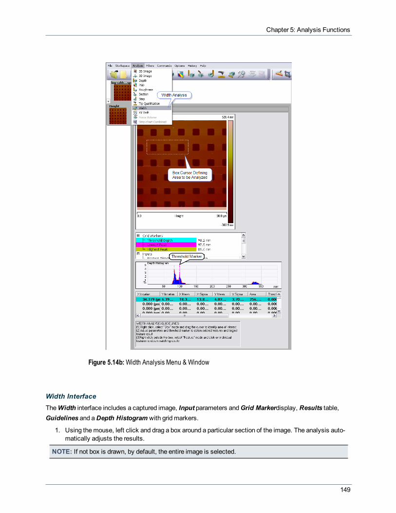
Chapter 5: Analysis Functions
Figure 5.14b:Width Analysis Menu & Window
Width InterfaceTheWidth interface includes a captured image, Input parameters andGrid Markerdisplay, Results table,Guidelines and aDepth Histogram with grid markers.
1. Using themouse, left click and drag a box around a particular section of the image. The analysis auto-matically adjusts the results.
NOTE: If not box is drawn, by default, the entire image is selected.
149
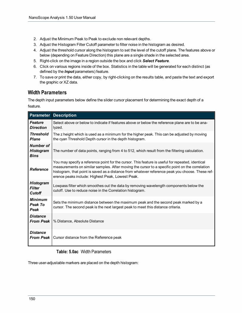
NanoScope Analysis 1.50 User Manual
2. Adjust theMinimum Peak to Peak to exclude non relevant depths.3. Adjust the Histogram Filter Cutoff parameter to filter noise in the histogram as desired.4. Adjust the threshold cursor along the histogram to set the level of the cutoff plane. The features above or
below (depending on Feature Direction) this plane are a single shade in the selected area.5. Right-click on the image in a region outside the box and click Select Feature.6. Click on various regions inside of the box. Statistics in the table will be generated for each distinct (as
defined by the Input parameters) feature.7. To save or print the data, either copy, by right-clicking on the results table, and paste the text and export
the graphic or XZ data.
Width ParametersThe depth input parameters below define the slider cursor placement for determining the exact depth of afeature.
Parameter Description
FeatureDirection
Select above or below to indicate if features above or below the reference plane are to be ana-lyzed.
ThresholdPlane
The z height which is used as a minimum for the higher peak. This can be adjusted by movingthe cyan Threshold Depth cursor in the depth histogram.
Number ofHistogramBins
The number of data points, ranging from 4 to 512, which result from the filtering calculation.
Reference
You may specify a reference point for the cursor. This feature is useful for repeated, identicalmeasurements on similar samples. After moving the cursor to a specific point on the correlationhistogram, that point is saved as a distance from whatever reference peak you choose. These ref-erence peaks include: Highest Peak, Lowest Peak.
HistogramFilterCutoff
Lowpass filter which smoothes out the data by removing wavelength components below thecutoff. Use to reduce noise in the Correlation histogram.
MinimumPeak ToPeak
Sets the minimum distance between the maximum peak and the second peak marked by acursor. The second peak is the next largest peak to meet this distance criteria.
DistanceFrom Peak %Distance, Absolute Distance
DistanceFrom Peak Cursor distance from the Reference peak
Table: 5.0ac Width Parameters
Three user-adjustable markers are placed on the depth histogram:
150
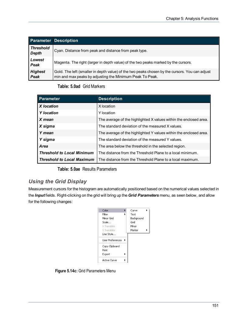
Chapter 5: Analysis Functions
Parameter Description
ThresholdDepth Cyan. Distance from peak and distance from peak type.
LowestPeak Magenta. The right (larger in depth value) of the two peaks marked by the cursors.
HighestPeak
Gold. The left (smaller in depth value) of the two peaks chosen by the cursors. You can adjustmin and max peaks by adjusting theMinimum Peak To Peak.
Table: 5.0ad Grid Markers
Parameter Description
X location X location
Y location Y location
X mean The average of the highlighted X values within the enclosed area.
X sigma The standard deviation of the measured X values.
Y mean The average of the highlighted Y values within the enclosed area.
Y sigma The standard deviation of the measured Y values.
Area The area below the threshold in the selected region.
Threshold to Local Minimum The distance from the Threshold Plane to a local minimum.
Threshold to Local Maximum The distance from the Threshold Plane to a local maximum.
Table: 5.0ae Results Parameters
Using the Grid DisplayMeasurement cursors for the histogram are automatically positioned based on the numerical values selected inthe Input fields. Right-clicking on the grid will bring up theGrid Parametersmenu, as seen below, and allowfor the following changes:
Figure 5.14c: Grid Parameters Menu
151

NanoScope Analysis 1.50 User Manual
Parameter Description
Color Allows the operator to change the color of the: Curve, Text, Background, Grid, Minor Grid, andMarkers
Filter Typically used for a Profiler scan. Type - Select None, Mean (default), Maximum, or Minimum.Points - Select 4k, 8k (default), 16k, or 32k.
Minor Grid Places a minor grid in the background of the Vision window.
Scale Allows the user to auto scale, set a curve mean, or set their own data range.
Line Style For each curve, the operator can choose a connect, fill down, or point line.
UserPreference Restore - Reverts to initial software settings. Save - Saves all changes operator has made during
this session. This becomes the new default settings.
CopyClipboard Copies the grid image to the Microsoft clipboard.
Print Prints out the current screen view to a printer.
Export Exports data in bitmap, JEPG, or XZ data format.
ActiveCurve Determines which curve you are analyzing.
Table: 5.0af Plot Appearance Parameters
152

Chapter 5: Analysis Functions
5.15 XY DriftDue to temperature differences, thermal lateral drift can occur between two successive images whilescanning. XY Drift analysis, an optional feature of NanoScope Analysis, can calculate the lateral shiftbetween two images. You can alsomanually enter the drift.
RequirementsTwo images captured sequentially with the same scan direction are required. The capture and trace directionsmust be the same for both images (up/down, Trace/Retrace), and the images must have the samemicroscopeconfiguration and scanner calibration properties.
XY Drift ProcedureTo calculateXY Drift using NanoScope Analysis:
1. Identify the two images to be compared withXY Drift analysis, and open the first (chronologically) ofthe two images.
2. Open theXY Drift analysis view by selecting Analysis > XY Drift from themenu bar or by clicking onthe XY Drift icon in the Icon toolbar.
3. TheXY Drift view, shown in Figure 5.15a, opens showing the selected image.
153

NanoScope Analysis 1.50 User Manual
Figure 5.15a: XY Drift Analysis Menu & Window
154

Chapter 5: Analysis Functions
4. Use the Load Image button to browse for the subsequent image and open it.5. Click the Calculate Shift button. The software will calculate the shift of the second image relative to the
first image.6. The results display in theResults panel.7. To apply the corrections in the Inputs box, click the Apply Correction button.8. You can alsomanually enter the correction values in the Inputs box. Click the Apply Correction button.
NOTE: Apply Correction affects RealTime by applying a drift correction to the RealTime images. Do notuseApply Correction if this is not your intent.
XY Drift ParametersStatistics used by theXY Drift analysis are defined in this section.
Parameter Description
Number of scanlines Specifies the number of lines to calculate.
Flatten Flattens both images before the shift is calculated. (Use the Undo Flattenbutton toreverse the flatten).
X Correction Specifies the amount of correction to apply to the X-axis of the scanner.
Y Correction Specifies the amount of correction to apply to the Y-axis of the scanner.
Second Image Defines the location of the second image used in the analysis.
Image resizefactor Speeds up the shift calculation by averaging for images larger than 512 pixels
Table: 5.0ag XY Drift Parameters
Results of theXY Drift analysis are presented in this section.
Parameter Description
X Shift Specifies the amount of calculated shift along the X-axis of the second image relative to the first.
Y Shift Specifies the amount of calculated shift along the Y-axis of the second image relative to the first.
TestedCorrelation
Coefficient
Reports the correlation coefficient after correcting for the detected shift. A perfect correlation is1.0. If the tested correlation coefficient is too low, then the calculation is not valid and should notbe applied. You may need features that have more distinct contrast.
RawCorrelation
Coefficient
Reports the correlation coefficient between the two images prior to processing.
Table: 5.0ah Results Parameters
155

NanoScope Analysis 1.50 User Manual
Parameter Description
Load Image Browse to open the second image in the right box.
Calculate Shift Compares left image to right image, and reports the shift statistics in the Results box.
Apply Correction Applies the correction in the Inputs box to the second image.
Undo Flatten Undo Flatten restores the image to its original form.
Table: 5.0ai XY Drift Buttons
156

Chapter 5: Analysis Functions
5.16 Electrochemical SPMThe electrochemical display environment, shown in Figure 5.16a, displays one channel of the image, threeplots and a plot control panel.
Figure 5.16a: The NanoScope Analysis Electrochemistry display window showing a PeakForceDMTmodulus image
TheVoltammogram (top plot) plots current along the vertical axis versus potential along the horizontal axis.This can be Itip vs. Etip (STM) or I vs. E or one of the calculated values, current density, charge, etc. vs., E.
NOTE: The calculated values are all based on the electrochemical cell current, I, and not on STM tip cur-rent, Itip.
157
NanoScope Analysis 1.50 User Manual
In the Temporal (bottom two) plots, the horizontal axis is always time. A voltage (top) and a current (bottom)are plotted versus time. The voltage can be the electrochemical cell potential, E, or the potential of the STM tip,Etip. The current can be electrochemical cell current, I, one of its derivative quantities; e.g., charge, currentdensity, etc., or it can be the current flowing through the STM tip, Itip.
The time scale on the Temporal graph does not necessarily correspond to the time required to capture an SPMimage for the following reasons:
1. The total number of data points is limited to 62,254. Hence, the product of theSample Rate and Timerange is limited to 62,254. For example, when one attempts to collect 1000 seconds of data, themax-imum Sample Rate is 62 Hz.
2. If the time to capture an image exceeds the time to record themaximum of the 62,254 electrochemicaldata points that can be stored, only the last 62,254 data points are saved. The data points prior to thelast 62,254 data points are lost. Time zero on the Temporal graph reflects the start of the last 62,254data points.
3. To display on the Temporal graph only a portion of the stored data points, for example, the last 30,000of 62,254 data points recorded using aSample Rate of 100 Hz, define Time Start equal 300 seconds(roughly one-half of themaximum of 623 seconds for this case) and Time End equal 623 seconds in theplot controls dialog box for the NanoScope Analysis software. In this case, time zero on the Temporalgraph would actually be the first data point after the 300-secondmarker.
CursorsA mouse click-and-hold-and-dragmay be used in the Temporal plot windows to display data at any point in theexperiment.
Themarkers in all three plots will follow the position of the cursor as themouse is dragged (click and hold) inthe plot. The electrochemical cell data (E, I, Time) at the position of themarker is displayed in the Temporalpanel of the plot controls dialog box in the lower left of the EC window.
A marker on theVoltammogram will indicate the corresponding data as potential vs. current. The vertical linein the Temporal plot indicates, in time, when the first line of the SPM image was captured. As the Temporalmarker is moved, a horizontal line on the SPM image will move to the scan line that was captured atapproximately the same time. See Figure 5.16a. In addition, themousemay drag (click-and-hold) the line onthe image to any scan line, and this will move the Temporal andVoltammogrammarkers to the appropriatepositions and update the electrochemical cell data display.
Note that it is possible to have data displayed in the Temporal plot across such a time window that it does notcorrespond to any of the data in the SPM image. This is because when an SPM image is captured, the last62,254 electrochemical data points are also recorded in the file, and only a portion of the electrochemical datarecordedmay correspond to the time required to capture the SPM image; i.e., the imagemay have taken lesstime to capture than the last 62,254 electrochemical data points.
A mouse Ctrl-click-and-hold-and-dragmay be used in the plot windows to zoom in on a portion of the data.Clicking themagnifying glass in the lower left corner of the plot window resets the plot.
158

Chapter 5: Analysis Functions
Plot Controls Dialog BoxThe parameters in the plot controls dialog box, shown in Figure 5.16b and described in Table: 5.0aj, allow youto scale and clip the electrochemical data.
Figure 5.16b: The electrochemistry plot control dialog box
159

NanoScope Analysis 1.50 User Manual
ParameterGroup Parameter Description
Voltam
VoltamFunction
Indicates the quantities plotted along horizontal and vertical axes of thevoltammogram.
Settings:
l Chargel Chrg Densl Currentl Cur Densl Log Curl Lg Cur Densl Tip Current
When this parameter is Itip, the current through STM tip is plotted vs. Etip. Allother settings (e.g., current, charge) have the electrochemical cell parameter
plotted vs. E.
I Range Controls the vertical scale of the Voltammogram graph.
VoltMinimum Voltage corresponding to left edge of Voltammogram graph.
VoltMaximum Voltage corresponding to the right edge of the Voltammogram graph.
RampRate Indicates the ramp rate at the time of capture.
SampleRate The rate of electrochemical data recording at the time of capture.
TipReference
STM only. Indicates whether the STM tip potential, Etip, or tip bias, Ebias, is keptconstant during ramping.
RampElectrode Indicates which electrode (working or STM tip) was ramped at time of capture.
TemporalTemporalFunction
Indicates what parameter is plotted along the vertical axis vs. time along horizontalaxis.
Settings:
l Chargel Chrg Densl Currentl Cur Densl Log Curl Lg Cur Densl Tip Current
I Range Controls the current scale of the Temporal graph.
160
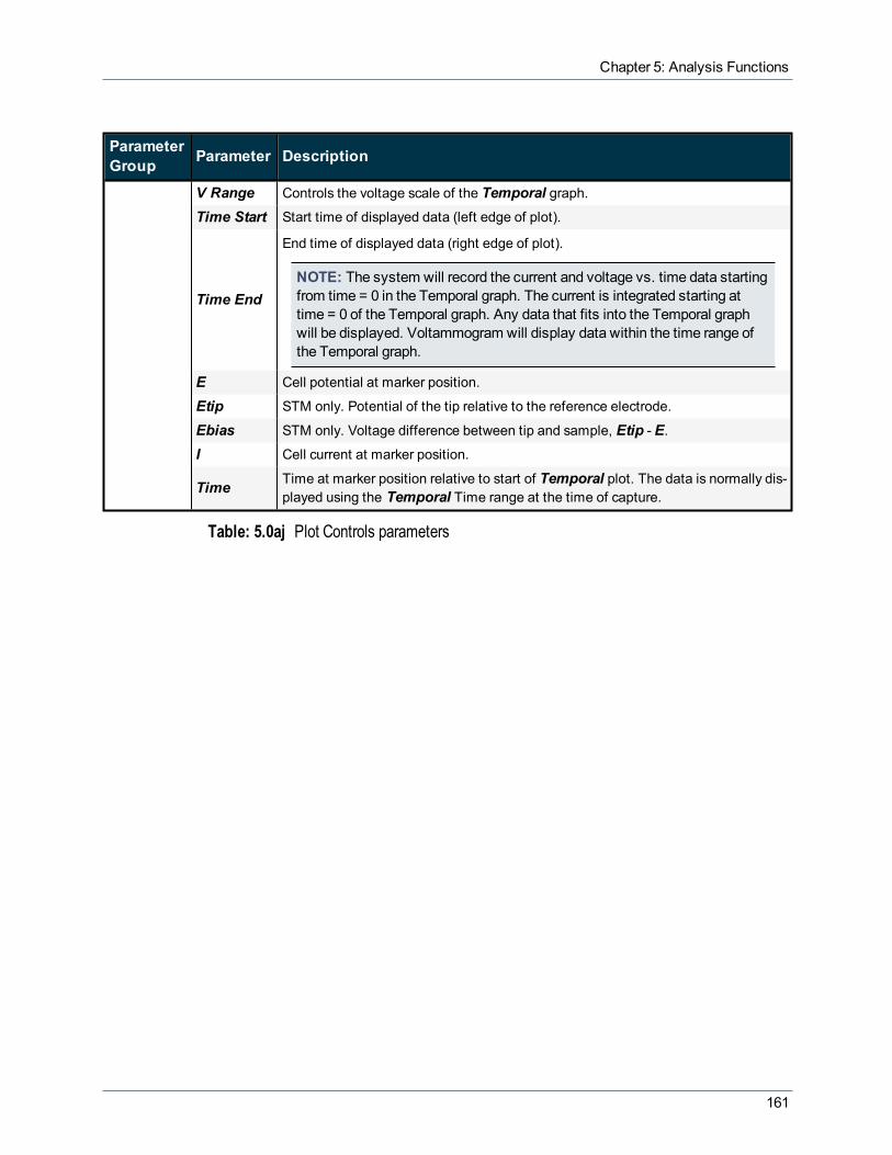
Chapter 5: Analysis Functions
ParameterGroup Parameter Description
V Range Controls the voltage scale of the Temporal graph.Time Start Start time of displayed data (left edge of plot).
Time End
End time of displayed data (right edge of plot).
NOTE: The system will record the current and voltage vs. time data startingfrom time = 0 in the Temporal graph. The current is integrated starting attime = 0 of the Temporal graph. Any data that fits into the Temporal graphwill be displayed. Voltammogram will display data within the time range ofthe Temporal graph.
E Cell potential at marker position.
Etip STM only. Potential of the tip relative to the reference electrode.
Ebias STM only. Voltage difference between tip and sample, Etip - E.I Cell current at marker position.
Time Time at marker position relative to start of Temporal plot. The data is normally dis-played using the Temporal Time range at the time of capture.
Table: 5.0aj Plot Controls parameters
161


Chapter 6: Filter Commands
Chapter6:Filter Commands
All Filter Commandsmodify the file data and/or metadata and will cause a new view to be opened with theresults of the chosen filter. The user can restore the previous data by going to the previous step in the dataHistory or by executing theUndo command.
Filter Commands can be opened using theMenu bar or by clicking on the appropriate icon from the Icontoolbar. These Filter icons are identical to the icons used in NanoScope V8 software.
Figure 6.0a: Filter Icon Toolbar & Menu Commands
The following Filter Commands are available in NanoScope Analysis 1.50:
l Clean Image (page 164)l Crop & Split (page 167)l Erase (page 170)l Flatten (page 172)l Gaussian (page 176)l ImageMath (page 184)l Lowpass (page 187)l Median (page 190)l Plane Fit (page 192)l Rotate (page 197)l Spectrum 2D (page 198)
163
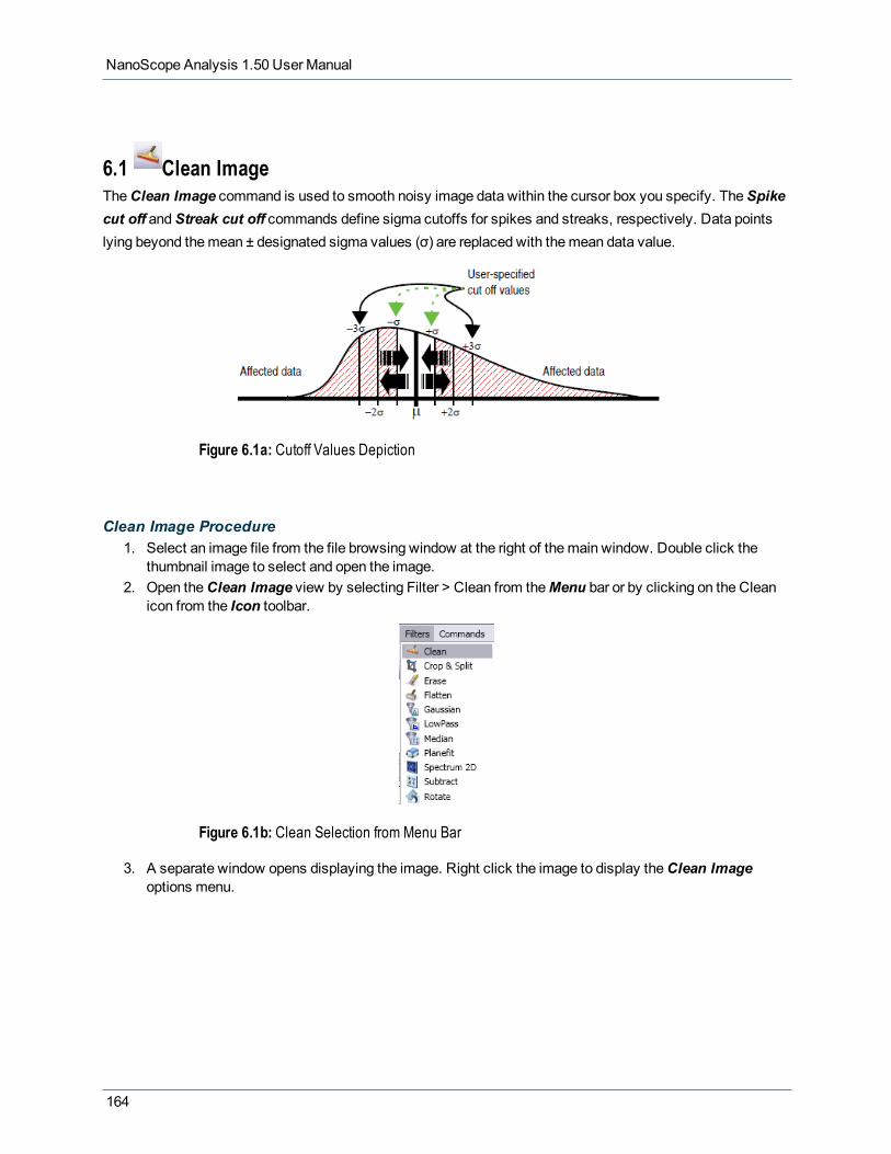
NanoScope Analysis 1.50 User Manual
6.1 Clean ImageTheClean Image command is used to smooth noisy image data within the cursor box you specify. TheSpikecut off andStreak cut off commands define sigma cutoffs for spikes and streaks, respectively. Data pointslying beyond themean ± designated sigma values (σ) are replaced with themean data value.
Figure 6.1a: Cutoff Values Depiction
Clean Image Procedure1. Select an image file from the file browsing window at the right of themain window. Double click the
thumbnail image to select and open the image.2. Open theClean Image view by selecting Filter > Clean from theMenu bar or by clicking on the Clean
icon from the Icon toolbar.
Figure 6.1b: Clean Selection from Menu Bar
3. A separate window opens displaying the image. Right click the image to display theClean Imageoptions menu.
164

Chapter 6: Filter Commands
Figure 6.1c: Clean Image Window
4. Click and drag in the image to define a box.5. Configure the Input parameters.6. Click Execute to perform the operation.7. To restore the unprocessed image, click on the Undo icon. From here one can go back in the data his-
tory to get to the preferred image.
Clean Image InterfaceParameter Description
RemoveSpikes
Settings:
l On: Enables the Spike cut off value and applies it to data within the cursor box you spe-cify.
l Off: DisablesSpike cut off value.
165
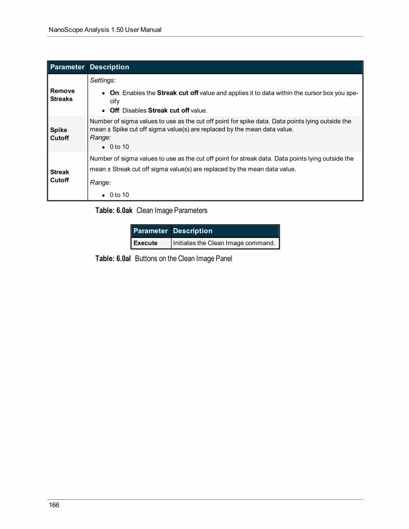
NanoScope Analysis 1.50 User Manual
Parameter Description
RemoveStreaks
Settings:
l On: Enables the Streak cut off value and applies it to data within the cursor box you spe-cify
l Off: DisablesStreak cut off value.
SpikeCutoff
Number of sigma values to use as the cut off point for spike data. Data points lying outside themean ± Spike cut off sigma value(s) are replaced by the mean data value.Range:
l 0 to 10
StreakCutoff
Number of sigma values to use as the cut off point for streak data. Data points lying outside themean ± Streak cut off sigma value(s) are replaced by the mean data value.
Range:
l 0 to 10
Table: 6.0ak Clean Image Parameters
Parameter DescriptionExecute Initiates the Clean Image command.
Table: 6.0al Buttons on the Clean Image Panel
166

Chapter 6: Filter Commands
6.2 Crop & SplitTheCrop & Split function replaces and expands the Zoom function used in version 7.0 and earlier releases ofNanoScope software. Use theCrop & Split function to extract an image from a large Version 7 image forVersion 5 analysis or to inspect only part of an image. NanoScope Version 5 software features a number ofOffline functions currently not available in Versions 7 and 8 NanoScope software. Crop & Splitwill producethe largest Version 5 image size possible within the bounded region (128 x 128, 256 x 256 or 512 x 512).
NOTE: The image produced by this analysis is Version 5 compatible, however, if the image is later pro-cessed by a Version 7 analysis, the imagemay no longer be Version 5 compatible.
Crop and Split ProcedureUse theCrop & Split function to isolate a portion of a high resolution image.
1. Open an image that you wish to crop. (larger than 512 x 512).2. Open theCrop & Split view by selecting Filter > Crop & Split from theMenu bar or by clicking on the
Crop & Split icon in the Icon toolbar.3. The selected image opens in theCrop & Split dialog box.
167

NanoScope Analysis 1.50 User Manual
Figure 6.2a: Crop & Split Window
4. Create a bounding box by dragging themouse in the image. Place the cursor inside the box, and whileholding themouse button, move the box to the location of interest. If Crop V5 Compatible is selected,the box is restricted to the largest possible Version 5-compatible image size (usually 512 x 512).
5. Click the Create File(s) button.6. Choose Filename in theSave As dialog.
Crop and Split InterfaceParameter Description
Crop V5Compatible
Settings:-Yes - A V5 compatible file (128x128, 256x256, or 512x512 is created from the image.-No - Crops to arbitrary sizes.
Method Available with Crop V5 Compatible set to Yes.
168

Chapter 6: Filter Commands
Parameter Description
Settings:-Interpolate - Data points will be interpolated to create new image.-Replicate - Data points will be used as is to create a new image.
V5 Numberof Samples
Available with Crop V5 Compatible set to Yes.Settings:-128, 256, 512
SaveChannelsSeparately
Settings:-Yes - Individual files, named OriginalFileName_crop and splitN.f07, where N is the channelnumber (1 through 8), are created.-No - One file with all selected channels will be created.
SaveSubset File
Settings:-Yes - Individual files, named OriginalFileName_crop and splitN.f07, where N is the channelnumber (1 through 8), are created.-No - One file with all selected channels will be created.You must select Yes for either the Save Channels Separately or the Save Subset File com-mands.
IncludeChannels
Settings:-Yes - The channel is included in the output file(s)-No - This channel is not included in the output file(s).
Number ofX Points Number of x points in the new image.
Number ofY Points Number of y lines in the new image.
AspectRatio Aspect ratio of the new image.
Scan SizeScan size of the new image. The units of this parameter are volts if the Units parameter (OtherControls panel) is set to Volts. The units are linear distance (nm or μm) if the Units parameter isset to Metric.
Error
Possible errors:-No Error - (Default)-Not Enough X Points - Original image has less than 512 points/line-Invalid Aspect Ratio - Zoomed image results in an aspect ration greater than 256:1-File Write - A disk error occurred-Unknown - An unknown error as occurred.
Table: 6.0am Crop & Split Parameters
Button Description
Create File(s)
An image is created from the portion of the high resolution image that is contained in the bound-ing box.
Table: 6.0an Crop & Split Buttons
169

NanoScope Analysis 1.50 User Manual
6.3 EraseTheErase command is a retouching function for editing images. This function allows horizontal lines or areasto be replaced with an interpolation from the adjacent lines.
6.3.1 Erase Procedure1. Select an image file from the file browsing window at the right of themain window. Double click the
thumbnail image to select and open the image.2. Open theEraseView by selecting Filter > Erase or by clicking on the Erase icon in the Icon toolbar. A
separate window opens, also displaying the image.
Figure 6.3a: Erase Window
3. Right-click in the image to display theErase Optionsmenu. Select eitherHorizontal Line orArea anda check mark will appear. The option chosen will remain checked until another selection is made.
l Area - Selects a region to be erasedl Horizontal Line - Selects a single line to be erased.
4. Click anywhere within the image to define a horizontal line, or click and drag in the image to define a boxto be replaced. When selecting a line, the line applies to the entire scan line of the image, regardless ofwhether you are zoomed into a region on the image.
5. Click theExecute button to perform the interpolation.
170
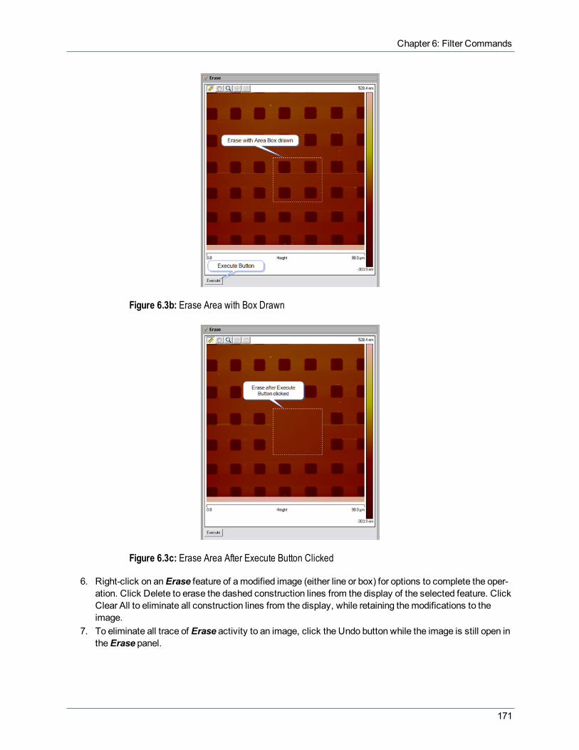
Chapter 6: Filter Commands
Figure 6.3b: Erase Area with Box Drawn
Figure 6.3c: Erase Area After Execute Button Clicked
6. Right-click on anErase feature of amodified image (either line or box) for options to complete the oper-ation. Click Delete to erase the dashed construction lines from the display of the selected feature. ClickClear All to eliminate all construction lines from the display, while retaining themodifications to theimage.
7. To eliminate all trace of Erase activity to an image, click the Undo button while the image is still open intheErase panel.
171

NanoScope Analysis 1.50 User Manual
6.4 FlattenThe Flatten command eliminates unwanted features from scan lines (e.g., noise, bow and tilt). It uses allunmasked portions of scan lines to calculate individual least-square fit polynomials for each line.
Flatten is useful prior to image analysis commands (e.g., Depth, Roughness, Section, etc.) where the imagedisplays a tilt, bow or low frequency noise, which appear as horizontal shifts or stripes in the image.
Figure 6.4a: Image with Bow
Figure 6.4b: Image with Bow Removed
172

Chapter 6: Filter Commands
Flatten TheoryThe Flatten command is a filter that modifies the data to delete low frequency noise and remove tilt from animage. Each line is fit individually to center data (0th order) and remove tilt (1st order), or 2nd or 3rd order bow. Abest fit polynomial of the specified order is calculated from each data line and then subtracted out. In somecases, the stopband (box cursor to exclude features) can be used to remove regions of the image from the dataset used for the polynomial fits. Click on the image to start drawing a stopband box. Right-click on a box todelete it or change its color.
Flatten PolynomialsThe polynomial equations calculate the offset and slope, and higher order bow of each line for the data as perthe table below.
Order Polynomial Explanation0 z=a Centers data along each line.
1 z=a+bx Centers data and removes tilt on each line (i.e. calculates and removes offset (a) andslope (b).
2 z=a+bx+cx2 Centers data and removes the tilt and bow in each scan line, by calculating a secondorder, least-squares fit for the selected segment then subtracting it from the scan line.
3 z=a+bx+cx2+dx3
Centers data and removes the tilt and bow in each scan line, by calculating a thirdorder, least -squares fit for the selected segment then subtracting it from the scan line.
Table: 6.0ao Flatten Polynomials
Flatten ProcedureFor an image that contains a number of noisy scan lines, use the Flatten command to correct the problem.
Figure 6.4c: Raw Image of Syndiatatic Polystyrene (500nm)
173

NanoScope Analysis 1.50 User Manual
1. Open the image. Note disjointed scan lines which aremisaligned along the Z-axis (some are high andsome are low). This effect somewhat resembles an unshuffled deck of cards when viewed on-edge orappears as horizontal streaks or bands. The imagemay have bow along its Y-axis.
2. Select Filters > Flatten on theMenu bar or click on the Flatten Icon from the Icon toolbar.3. Set the flatten order to 0th. This removes the scan linemisalignment.4. Click Execute to initiate the Flatten command. The flattened image appears on the display screen.
Figure 6.4d: Flattened Image of Syndiatatic Polystyrene (500 nm)
5. To see the variety of effects using the Flatten command, enter different Flatten Order values. Eachnew changemay be undone by clicking on theReload button.
Flatten InterfaceA series of parameters appear in the Flatten view, allowing the order of the Flatten polynomial to be selectedand display parameters to be adjusted to preference.
Input ParametersParameter Description
Flatten Order Select 0th, 1st, 2nd, or 3rd
Flatten ZThresholdingDirection
Specifies the range of data to be used for the polynomial calculation based on thedistribution of the data in Z:
Settings:
l Use Z >=: Uses the data whose Z values are greater than or equal to the valuespecified by the Z thresholding %.
l Use Z <: Uses the data whose Z values are less than the value specified by theZ thresholding %.
l No thresholding: Disables all thresholding parameters.
174

Chapter 6: Filter Commands
Parameter Description
Find Threshold for
Applies the Thresholding values for the whole image or each line independently.
Settings:
l The whole imagel Each line
Mark Excluded Data Displays (in blue) data that has been excluded (by the Z Thresholding operation) fromthe calculation.
Number HistogramBins The number of data points in the histogram.
Threshold Height Defines a Z value relative to the lowest data point.
Use Histogram
Displays a histogram of the height allowing you to, more easily, using the dashed red
cursor, set the Threshold Height for excluded data.
Settings:
l Onl Off
Table: 6.0ap Flatten Range, Settings and Buttons
Button Description
Execute Initiates the Flatten operation.
Table: 6.0aq Buttons on the Flatten Panel
175

NanoScope Analysis 1.50 User Manual
6.5 GaussianGaussian filter applies either a Lowpass or aHighpass digital filter to an image along either theHorizontal ortheVertical axis.
Lowpass Gaussian FilterThe Lowpass Gaussian Filter eliminates high frequency (sharp) features oriented along either the X or Y axisof the scan. The practical effect upon the image is a loss of detail or "blurring" effect.
TheGaussian filter can average features running parallel to an image’s Y scan axis while leaving featuresrelatively unchanged along the X axis, or vice versa. This is a similar capability to theSpectrum 2D function,although applied to only the X or Y axis.
Consider the scan of the grating below, with prominent features oriented along the x axis.
Figure 6.5a: Grating with Prominent X-Axis Features
Applying a Lowpass Gaussian Filter along theVertical (Y) axis results in elimination of noise in the image.
Figure 6.5b: Noise Removed by Applying Lowpass Gaussian Filter to Y Axis
176

Chapter 6: Filter Commands
NOTE: Notice that rulings running parallel to the Y axis are smoothed along their length by the filter, whilefeatures oriented orthogonal to the Y axis remain relatively unchanged. This results in an idealized (aver-aged) profile of the X axis.
Applying the Lowpass Gaussian Filter to theHoriztonal (X) axis destroys the ruling features in the image byaveraging across their profile.
Figure 6.5c: Lowpass Gaussian Filter Applied to Horizontal X Axis
NOTE: Notice how the filter has eliminated the prominent high frequency features along the axis which thefilter has been applied, resulting in an almost flat surface.
Highpass Gaussian FilterTheHighpass Gaussian Filter eliminates low frequency (dull) features oriented along either the X or Y axis ofthe scan. The "DC" (average) value is also eliminated, resulting in an image containing only the transitions fromone region to the next. This filter is typically used for edge detection of different regions or grain bounders.
One example of applying aGaussian Highpass filter is themagnetic domains in a permalloy specimen, asshown below.
177

NanoScope Analysis 1.50 User Manual
Figure 6.5d: Permalloy Specimen
NOTE: The figure shows themagnetic forcemicroscopy (MFM) image in its original form. This is an earlyMFM image of a permalloy specimen, and contains artifacts which are significantly reduced in phase ana-lyzed images. Magnetic force is represented in the image as height data. Suppose themicroscopistwanted to highlight themagnetic boundaries without regard tomagnetic force (height data). A GaussianHighpass filter would be appropriate.
When the image is filtered using theHorizontal setting, the high frequency features along the X-axis arehighlighted.
Figure 6.5e: Highpass Gaussian Filter Using Horizontal Setting
NOTE: Notice that features running parallel to the X-axis (e.g., the tips of each oval area) are washed out,while features running perpendicular to the X-axis are enhanced.
When the image is filtered using the Vertical setting, the high frequency features along the Y-axis arehighlighted.
178

Chapter 6: Filter Commands
Figure 6.5f: Highpass Gaussian Filter Using Vertical Setting
NOTE: Notice that features running parallel to the Y-axis (e.g., the sides of each oval area) are washedout, while features running perpendicular to the Y-axis are enhanced.
A composite of the two images shows the domain boundaries clearly. All of the low frequency features havebeen removed, leaving only the transitions between the grain boundaries.
Figure 6.5g: Highpass Gaussian Filter Using Horizontal & Vertical Settings
NOTE: To construct a composite image of the twoGaussian-filtered images, add them together. (This canbe accomplished by using the subtract feature with an inverted image) See ImageMath (page 184) for fur-ther details.
Gaussian Kernel AlgorithmGaussian filters utilize a 1 x N matrix, where N is determined by the filter size parameter. In this instance,image data is analyzed in two-dimensional matrices which are shaped to aGaussian curve where the sigmavalue (σ) is determined by the filter size parameter.
179

NanoScope Analysis 1.50 User Manual
Figure 6.5h: Gaussian Filter Depiction
The general equation used to generate a 1-by-(N+1) Gaussian kernel is:
Where i is in units of pixels, and σ is set by the Filter size value. Using this kernel, the filter output is:
Gaussian Filter SizeThe Filter Size value corresponds to the sigma (σ) value of the Gaussian curve, encompassing approximately68 percent of the data with the symmetric Gaussian curve centered over the operated-upon pixel.
Larger Filter size values distribute the curve broadly.
During Lowpass filtering, this lends greater weight to values farther away from the pixel and increases theGaussian filter’s averaging effects upon the image.
DuringHighpass filtering, this subtracts a decreased average from each pixel, lessening the filter’s impact.
Figure 6.5i: Larger Filter Size
180

Chapter 6: Filter Commands
Smaller Filter size values concentrate curve data around the center value
Figure 6.5j: Smaller Filter Size
During Lowpass filtering, this lends less weight to pixels distant from the center, decreasing the Gaussianfilter’s ability to average local pixels with distant ones—the filter’s impact is lessened.
DuringHighpass filtering, the larger andmore localized pixel average being subtracted from the operated-uponpixel value yields an enhanced impact upon the image.
Filter size is specified in units of Distance, Spatial Frequency, Time, Temporal Frequency, and #pixels.
Gaussian Filtering Procedure1. Select an image file from the file browsing window at the right of themain window Double click the
thumbnail image to select and open the image.2. Open theGaussian view by selecting Filter > Gaussian from theMenu bar or by clicking on the
Gaussian icon in the Icon toolbar.
181

NanoScope Analysis 1.50 User Manual
Figure 6.5k: Gaussian Window
3. Configure the Input parameters.4. Click Execute to perform theGaussian filtering operation.5. To restore the unprocessed image, click theReload button or go back in the dataHistory.
6.5.1 Gaussian Filter InterfaceParameter Description
Filter Size
Size of the scan line to be operated upon by the Gaussian filter kernel. This value is expressed inthe Cutoff Units specified below.
Range and Settings:
l Minimum = 3 pixelsl Maximum = one-half scan size
Filter AxisSettings:
l Horizontal - Applies the one dimensional Gaussian filter along the X axis.l Vertical - Applies the one dimensional Gaussian filter along the Y axis.
182

Chapter 6: Filter Commands
Parameter Description
CutoffUnits
Selected units are applied simultaneously to the Filter size. (The #pixelsfield displays the pixelequivalent of the current Filter size value.)
Range and Settings:
l Distancel Spatial Frequencyl Timel Temporal Frequency
Filter Type
Range and Settings:
l Lowpass - filtering allows longer wavelength features through while filtering out shorterwavelength features. The net effect is to remove noise in the form of spikes and fuzz onthe image.
l Highpass - filtering allows shorter wavelength features through while filtering out longerwavelength features.
#pixels
The current Filter Size in pixel units. This value may be used to both enter and monitor the FilterSize.
Range and Settings:
l Minimum = 3 pixelsl Maximum = one-half scan size
Table: 6.0ar Gaussian Parameters
183
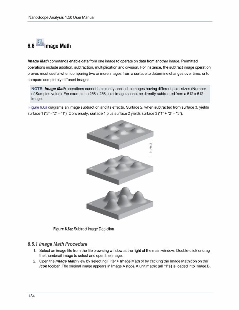
NanoScope Analysis 1.50 User Manual
6.6 Image Math
Image Math commands enable data from one image to operate on data from another image. Permittedoperations include addition, subtraction, multiplication and division. For instance, the subtract image operationproves most useful when comparing two or more images from a surface to determine changes over time, or tocompare completely different images.
NOTE: Image Math operations cannot be directly applied to images having different pixel sizes (Numberof Samples value). For example, a 256 x 256 pixel image cannot be directly subtracted from a 512 x 512image.
Figure 6.6a diagrams an image subtraction and its effects. Surface 2, when subtracted from surface 3, yieldssurface 1 (“3” - “2” = “1”). Conversely, surface 1 plus surface 2 yields surface 3 (“1” + “2” = “3”).
Figure 6.6a: Subtract Image Depiction
6.6.1 Image Math Procedure1. Select an image file from the file browsing window at the right of themain window. Double-click or drag
the thumbnail image to select and open the image.2. Open the Image Math view by selecting Filter > ImageMath or by clicking the ImageMathicon on the
Icon toolbar. The original image appears in Image A (top). A unit matrix (all "1"s) is loaded into Image B.
184

Chapter 6: Filter Commands
Figure 6.6b: Image Math Window
185

NanoScope Analysis 1.50 User Manual
3. Click the Load Image button to browse for a second file.4. If necessary, right click on the second image panel to change the channel (see Figure 6.6b). The chan-
nel may also be changed by entering the channel number into the Image Math dialog box, shown inFigure 6.6c.
5. Select theOperator (+, -, *, /) andScaling Factors
Figure 6.6c: The Image Math dialog box
6. Click the Execute button to perform the operation on Image A. The result, which overrides the data inthe active (A) channel, is shown in the top panel of the Image Math view. Error are displayed the inImageMath dialog box shown in Figure 6.6c.
7. Youmay invert (multiply by -1) either image without clickingExecute by clicking the Invert Image but-tons.
NOTE:WhenData types are not the same, the calculation is performed as follows: First Image Relative Zscale * first (left) image - Second image Relative Z scale * second (right) image = new image. The RelativeZ scalemust be greater than - 32767 and less than 32767.
8. Click Undo or useHistory to restore the originally loaded file .
186

Chapter 6: Filter Commands
6.7 LowpassThe Lowpass command effectively suppresses the high spatial frequency component by averaging the 3x3pixel region centered on each pixel.
Data is analyzed in kernels (matrices), with every pixel individually recalculated based upon the values of itsneighboring pixels.
Figure 6.7a: Lowpass Data Analysis Depiction
The Lowpass filter always uses a 3x3 kernel.
Because of long reaching legacy reasons, we call this filter Lowpass. Yes, it would have been better if namedwe had called itMean orAverage filter. If you are looking for a "real" lowpass filter, see the Gaussian (page176) or Spectrum 2D (page 198) imagemodification functions.
6.7.1 Lowpass Procedure1. Select an image file from theBrowsewindow at the right of themain window. Double-click the thumb-
nail image to select and open the image.2. Open the LowPass view by selecting Filter > Lowpass from theMenu bar or by clicking on the Lowpass
icon from the Icon toolbar.
187

NanoScope Analysis 1.50 User Manual
Figure 6.7b: LowPass Window
3. Click theExecute button to apply the filter to the image.4. To restore the unprocessed image, click theUndo button or go back in the dataHistory.5. The filter always applies a 3x3 filter to the image. The filter may be appliedmultiple times for increased
blurring effects, as seen below.
188
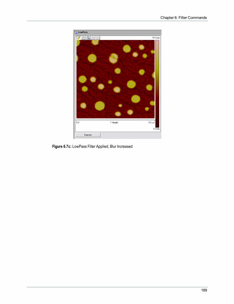
Chapter 6: Filter Commands
Figure 6.7c: LowPass Filter Applied, Blur Increased
189

NanoScope Analysis 1.50 User Manual
6.8 MedianTheMedianmodify command is similar to Lowpass; it reduces the contributions of high spatial frequency,reducing contrast in regions of high contrast. The advantage ofMedian over Lowpass (averaging) filter is thattheMedian will eliminate lone "bad pixels" without significantly affecting the resolution of the image.
6.8.1 Median TheoryIn theMedian command, data is analyzed in kernels (matrices), with every pixel individually recalculatedbased upon its neighboring values. For example, data which is undergoing aMedian filter applies a 3x3 or 5x5matrix operation to each image pixel.
Figure 6.8a:Median Data Analysis Depiction
NOTE: Each pixel is individually evaluated within its own local, 5x5 “neighborhood.” Neighborhood A haspixel a2a3 at its center. For aMedian filter, the 25 pixels in neighborhood A are evaluated to locate themedian value pixel. Themedian value of neighborhood A is thenmapped to a new pixel a2a3 in a separatedata set. Thematrix is shifted over one column to define a new neighborhood (“B”) with pixel a2a4 at its cen-ter. Themedian value for neighborhood “B” is found, thenmapped to pixel a2a4 in the separate data set.The filtering process is repeated until all pixels have been remapped.
In this and all other matrix operations, pixels aremapped to the new, separate data set without changing pixelvalues in the original image data until saved. (Matrices do not operate cumulatively on previously filtered data.)
The size of the filter’s sliding window pixel array is set under Inputs > Median Order. Increasing theMedianOrder increases the pool of pixels from which each value is calculated, and effectively increases the blurringeffects of the filter.
NOTE: The effects of three different size pixel arrays (3x3, 7x7, 11x11, left to right) applied to the sameimage are shown below.
190

Chapter 6: Filter Commands
Figure 6.8b:Median Pixel Array Effects
6.8.2 Median Procedure1. Select an image file from theBrowsewindow at the right of themain window. Double click the thumb-
nail image to select and open the image.2. Open theMedian filter by selecting Filter > Median from theMenu bar or clicking on theMedian icon
from the Icon toolbar.3. Select theMedian Order from the Inputs menu: 3x3, 5x5, 7x7, 9x9, or 11x11.4. Click Execute to apply theMedian filter.
191

NanoScope Analysis 1.50 User Manual
6.9 Plane FitThePlane Fit command computes a single polynomial of a selectable order for an image and subtracts it fromthe image. ThePlane Fit operation can be applied to either or both of the XY directions.
Box cursors or passbands allow specific points to be used in the calculation of the polynomial. Click on theimage to start drawing a passband box. Right-click on a box to delete it or change its color.
Figure 6.9a depicts an image with tilt and bow which could affect the analysis of the surface data.
Figure 6.9a: Visual Representation of Planefit
Fitted PolynomialsRefer to Table: 6.0as to view the polynomials that calculate the best plane fit for the images in thePlane Fitfunction.
Order Variable Polynomial Equation0 X z = a
Y z = aXY (Add Higher Order CrossTerms for XYOFF) z = a
XY (Add Higher Order CrossTerms for XY on) z = a
1 X z = a+bxY z = a+byXY (Add Higher Order CrossTerms for XYOFF) z = a+bx+cy
XY (Add Higher Order CrossTerms for XY on) z = a+bx+cy+dxy
2 X z = a+bx+cx2
Y z = a+by+cy2
192

Chapter 6: Filter Commands
Order Variable Polynomial EquationXY (Add Higher Order CrossTerms for XYOFF) z = a+bx+cy+dxy+ex2+fy2
XY (Add Higher Order CrossTerms for XY on) z = a+bx+cy+dxy+ex2+fy2+gxy2+hx2y+ix2y2
3 X z = a + bx + cx2 + dx3
Y z = a + by + cy2 + dy3
XY (Add Higher Order CrossTerms for XYOFF) z = a+ bx + cy + dxy + ex2 + fy2 + gxy2 + hx2y + jx3 + ky3
XY (Add Higher Order CrossTerms for XY on)
z = a + bx + cy + dxy + ex2 + fy2+ gxy2 + hx2y + ix2y2 + jx3 + ky3 +lxy3 +mx2y3 +nx3y3 +ox3y + px3y2
Table: 6.0as Fitted Polynomials
Plane Fit ProcedureUsePlane Fit to correct an image for distortion as follows:
1. Select an image file from the fileBrowsewindow. Double click the thumbnail image to open the image.2. Select Filters > Plane Fitfrom theMenu bar or click on thePlane fit icon from the Icon toolbar.3. ThePlane Fit input parameters appear along with the top view image.4. Select X, Y, or XY as thePlane Fit Mode.5. Select thePlane fit Order as Oth, 1st, 2nd, or 3rd.6. Click Execute7. Notice that the image distortion is removed, reflecting a flat, planar profile.
193

NanoScope Analysis 1.50 User Manual
Figure 6.9b: Plane Fit View
Figure 6.9c: Saddle Image Before Plane fit
194

Chapter 6: Filter Commands
Figure 6.9d: Image after Plane Fit
Now, experiment with an image to explore the range of Plane Fit capabilities. Try the following:
l Change thePlane Fit Order value to see its effects. Notice that there is a vast difference between avalue of 1, 2 or 3.
l Try planefitting in one axis (for example, X), but not the other. This generally keeps whatever distortionsare presently oriented along the unused axis. For example, the image can be straightened along its Yaxis, while leaving the X axis strongly bowed.
l Try using a different Planefit Order for the X and Y axis (for example, a setting of 3 for X, but a settingof 1 for Y.) This is similar to using one axis, but not the other.
l Compare the effect of Plane Fitwith Flatten. Notice that each command has a significantly differentimpact; although, the difference is less noticeable for some types of images.
Plane Fit InterfaceThePlane Fit dialog box allows the display parameters and thePlane Fit Order to be adjusted to yourpreferences.
Parameter Description
Plane Fit Mode X, Y, XY
Plane Fit Order
Selects the order of the plane calculated and subtracted from the image.
Settings:
l 0th—centers data.l 1st—removes tilt.l 2nd—removes 2nd order bow.l 3rd—removes 3rd order bow.
195
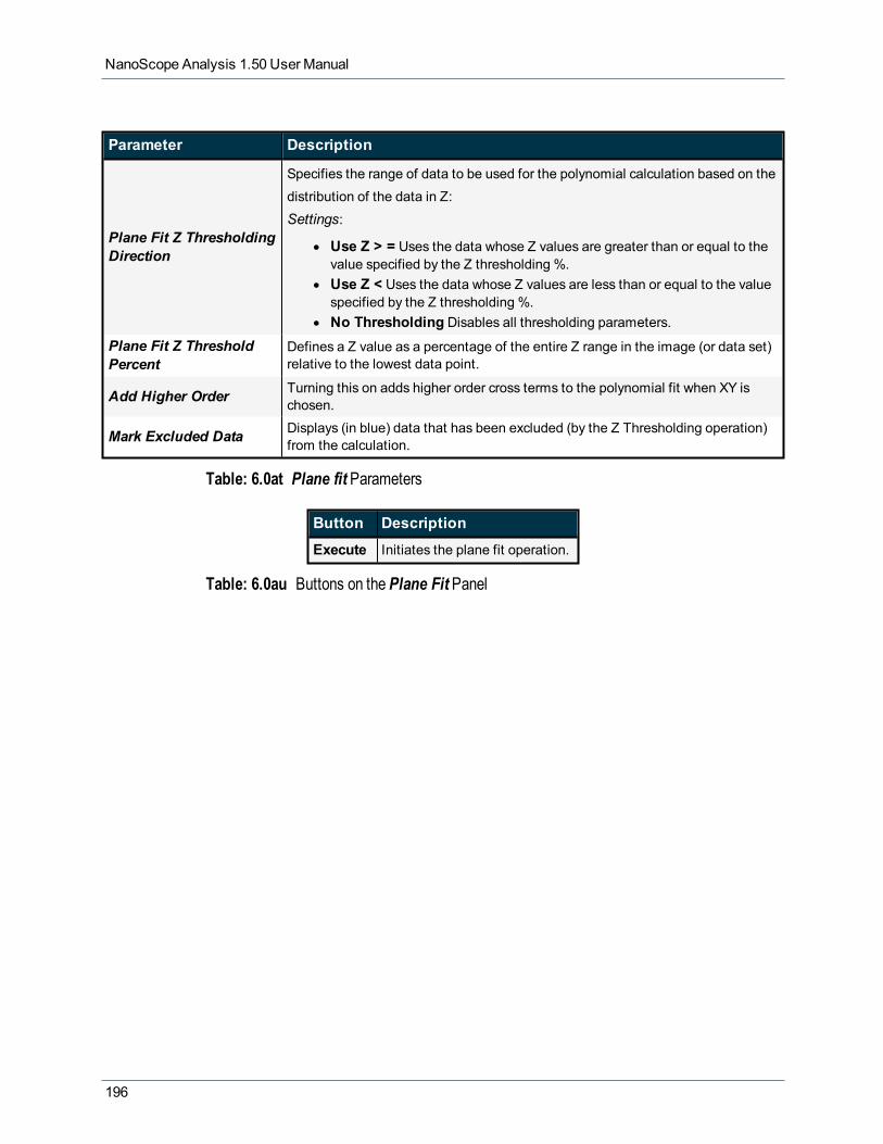
NanoScope Analysis 1.50 User Manual
Parameter Description
Plane Fit Z ThresholdingDirection
Specifies the range of data to be used for the polynomial calculation based on thedistribution of the data in Z:
Settings:
l Use Z > = Uses the data whose Z values are greater than or equal to thevalue specified by the Z thresholding %.
l Use Z < Uses the data whose Z values are less than or equal to the valuespecified by the Z thresholding %.
l No Thresholding Disables all thresholding parameters.Plane Fit Z ThresholdPercent
Defines a Z value as a percentage of the entire Z range in the image (or data set)relative to the lowest data point.
Add Higher Order Turning this on adds higher order cross terms to the polynomial fit when XY ischosen.
Mark Excluded Data Displays (in blue) data that has been excluded (by the Z Thresholding operation)from the calculation.
Table: 6.0at Plane fit Parameters
Button Description
Execute Initiates the plane fit operation.
Table: 6.0au Buttons on the Plane Fit Panel
196

Chapter 6: Filter Commands
6.10 RotateTheRotate filter command allows for the arbitrary rotation of images.
6.10.1 Rotate Procedure & Interface1. Select an image file from the file browsing window at the right of themain window. Double-click or drag
the thumbnail image to select and open the image.2. Open theRotate filter by selecting Filter > Rotate from theMenu bar or by clicking the Rotate icon in the
Icon toolbar. TheRotatewindow, shown in Figure 6.10a,opens.
Figure 6.10a: Rotate Menu & Window
3. In the Input box, enter the preferred rotation angle and click theExecute button. The image is rotated tothe desired angle. Use theUndo andRedo buttons to go back and forth, as desired.
197
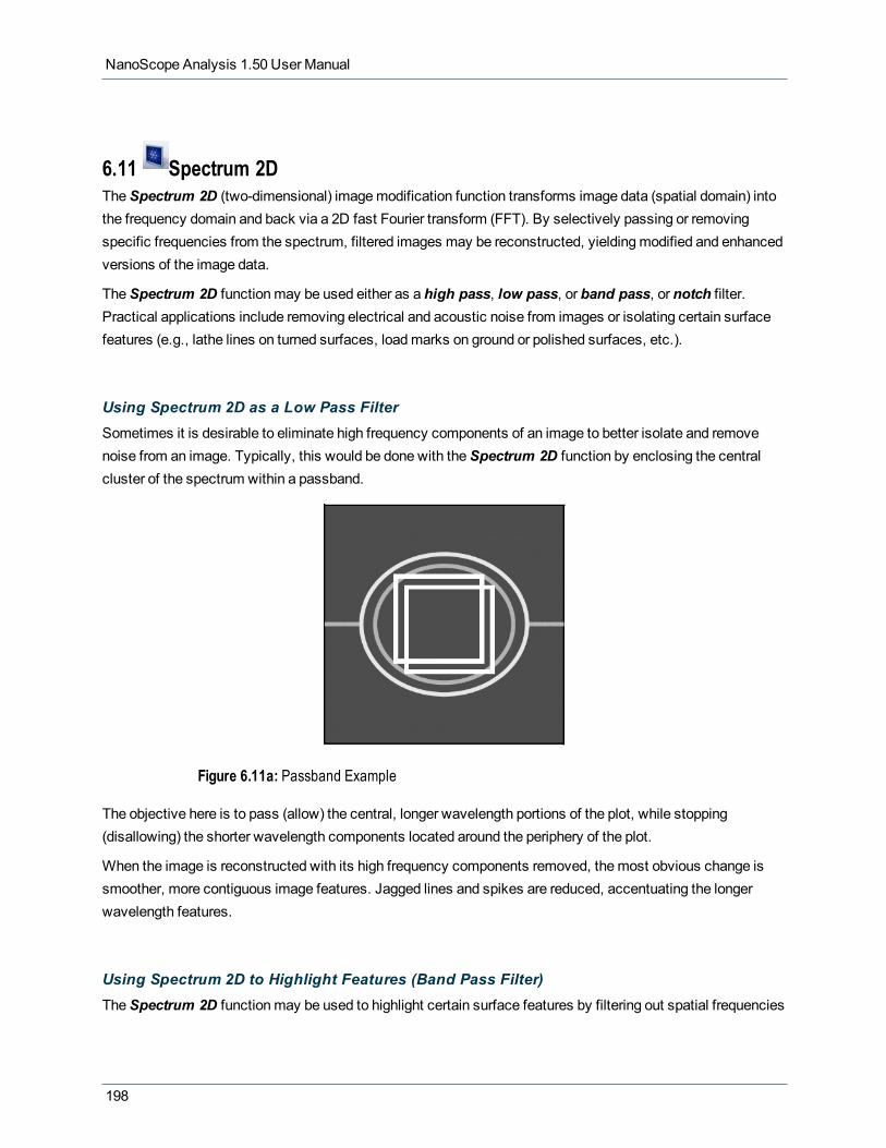
NanoScope Analysis 1.50 User Manual
6.11 Spectrum 2DTheSpectrum 2D (two-dimensional) imagemodification function transforms image data (spatial domain) intothe frequency domain and back via a 2D fast Fourier transform (FFT). By selectively passing or removingspecific frequencies from the spectrum, filtered images may be reconstructed, yieldingmodified and enhancedversions of the image data.
TheSpectrum 2D functionmay be used either as a high pass, low pass, or band pass, or notch filter.Practical applications include removing electrical and acoustic noise from images or isolating certain surfacefeatures (e.g., lathe lines on turned surfaces, loadmarks on ground or polished surfaces, etc.).
Using Spectrum 2D as a Low Pass FilterSometimes it is desirable to eliminate high frequency components of an image to better isolate and removenoise from an image. Typically, this would be done with theSpectrum 2D function by enclosing the centralcluster of the spectrum within a passband.
Figure 6.11a: Passband Example
The objective here is to pass (allow) the central, longer wavelength portions of the plot, while stopping(disallowing) the shorter wavelength components located around the periphery of the plot.
When the image is reconstructed with its high frequency components removed, themost obvious change issmoother, more contiguous image features. Jagged lines and spikes are reduced, accentuating the longerwavelength features.
Using Spectrum 2D to Highlight Features (Band Pass Filter)TheSpectrum 2D functionmay be used to highlight certain surface features by filtering out spatial frequencies
198

Chapter 6: Filter Commands
along a particular axis. It is possible to do this by drawing a band pass region over a particular region of thespectrum. This might be useful in isolating and accentuating smaller surface features inherent within linesoriented along a particular axis.
To filter out vertcially oriented features, a passband should be drawn on with horizontal orientation on thespectrum. Horizontally distributed features would be passed, while vertically oriented features would befiltered.
Figure 6.11b: Horizontal Passband
Conversely, the vertically distributed features may be similarly examined by drawing a passband vertically,thus filtering out the horizontal components.
Figure 6.11c: Vertical Passband
Using Spectrum 2D to Remove Noise (Notch Filter)If high frequency surface noise is evenly distributed across the spectrum, a passband around the center of the
199

NanoScope Analysis 1.50 User Manual
spectral plot could be used as low pass filter to removemulti-spectral high frequency features. However, if theimage contains high frequency noise of a particular frequency, thenSpectrum 2D may also be used as aNotch Filter to remove only the offending frequency.
If the noise source is a particular electrical or vibrational frequency, the frequency shows up in theFFT spectrum as spectral "hot spots". These spots may be removed by drawing a stop band over just theseregions and then performing an InverseFFT.
Figure 6.11d: Example of Hot Spots
Depending upon the distribution and orientation of the noise bands, the hot spots should be distributed at thesame angle in the spectral plot as they are on the image. Theremay also exist other spectral hot spots whichare actually part of the surface features; however, these are usually distributed at some other orientation.
If the surface is anisotropic and includes some type of banding features naturally, isolating the noise bandsproves more difficult, especially if they run parallel to the noise bands.
Spectrum 2D ProceduresTheSpectrum 2D command allows filtering of images in the frequency domain through the 2-dimensional FastFourier transform (FFT). As the cursor is moved through the 2D plot, instantaneous results are displayed.
UseSpectrum 2D to correct the image distortion as follows:
1. Select an image file from the file browsing window at the right of themain window. Doubleclick thethumbnail image to select and open the image.
2. Open theSpectrum 2D view by selecting Filter > Spectrum 2D or by clicking on the Spectrum 2D iconfrom the Icon toolbar.
200

Chapter 6: Filter Commands
Figure 6.11e: Spectrum 2D Window
3. Click on the FFT button to perform a two dimensional Fast Fourier Transform on the data. The frequencyspectrum image will appear in the image view.
4. Sometimes the finer high frequency features of the transformed image are not visible without adjustingthe color settings. Experiment with the color mapping using the Offset and Scale values (right click onthe color scale) to best view the FFT spectrum's finer features. Refer toColor Scale (page 29) fordetails.
201
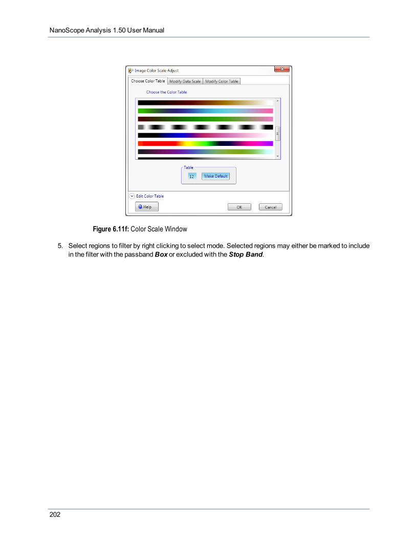
NanoScope Analysis 1.50 User Manual
Figure 6.11f: Color Scale Window
5. Select regions to filter by right clicking to select mode. Selected regions may either bemarked to includein the filter with the passbandBox or excluded with theStop Band.
202

Chapter 6: Filter Commands
Figure 6.11g: Passband Boxes Drawn Into Image
6. Due to the symmetry of the transformed data about the line fx = -fy, all Stopband andPassband boxesdrawn actually produce two boxes on the display.
7. If any Passband boxes exist on the display, then data outside thePassband boxes is deleted. Thus, itis superfluous to have aStopband box completely outside the confines of aPassband box.
8. Individual boxes and stopbands may be deleted by right clicking on an individual box and selecting theDelete command. The entire field of boxes and stopbands may be cleared with theClear All command.
9. When the desired regions are selected, press the InverseFFT to return to the spatial domain.
203

NanoScope Analysis 1.50 User Manual
Figure 6.11h: Spatial Domain
10. Youmay pass back and forth between the spatial and frequency domains, or youmay reload the imageto start over by clicking on the original image in the dataHistory.
Parameter Description
X Period Spatial frequency in the x direction. The lowest frequency is at the center of the plot.
Y Period Spatial frequency in the y direction. The lowest frequency is at the center of the plot.
R Period Spatial frequency in the radial direction.
Angle Arctangent of (y/x).
Max Amp The maximum amplitude (0-peak) of the transformed image.
Max The maximum of the RMS amplitude of the transformed image.
204

Chapter 6: Filter Commands
Parameter Description
RMS AmpMax Power The maximum power of the transformed image.
Max Psd The maximum power spectral density of the transformed image.
Amp The amplitude of the 2D FFT at that spatial frequency.
RMS Amp Amp/(sqrt(2))
Power Amplitude2 = (2D FFT)2
Psd Normalized power spectrum per number of points = (2DFFT * # x_points * # y_points)2/(# x_points * # y_points)
Rel Amp Amplitude / (Max Amplitude)
Rel Psd PSD / (Max PSD)
Table: 6.0av Results Parameters in Spectrum 2D
205


Chapter 7: Force Curve & Ramping Analysis
Chapter7:Force Curve & Ramping Analysis
Force Curve analysis functions display the results of experiments where the tip-sample separation is varied ateach XY position. Ramping analysis functions are two-dimensional data sets where up to three data channelsaremeasured simultaneously while a control parameter (z-position, tip bias, sample bias, etc...) is varied.During the Ramping, the XY position is held constant.
Force Commands can be opened using theMenu bar or by clicking on the appropriate icon from the Icontoolbar.
Figure 7.0a: The Force icons (above) and the Analysis Force menu (bottom left) and Filters Forcemenu (bottom right)
The following Force Curve analysis andRamping analysis commands are available in NanoScope Analysis1.50:
l Line Plot & Multiple Line Plotl Line Plot - Update Sensitivityl Indentation Analysis (page 244)l Force Volumel Review Force Curves (page 236)l FilteringMultiple Force Curves (page 237)l Multiple Curve analysis (MCA)l Modify Force Parameters (page 243)
207
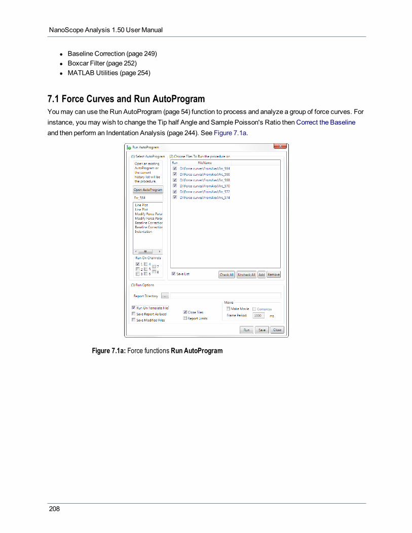
NanoScope Analysis 1.50 User Manual
l Baseline Correction (page 249)l Boxcar Filter (page 252)l MATLAB Utilities (page 254)
7.1 Force Curves and Run AutoProgramYoumay can use the Run AutoProgram (page 54) function to process and analyze a group of force curves. Forinstance, youmay wish to change the Tip half Angle and Sample Poisson's Ratio then Correct the Baselineand then perform an Indentation Analysis (page 244). See Figure 7.1a.
Figure 7.1a: Force functions Run AutoProgram
208

Chapter 7: Force Curve & Ramping Analysis
7.2 Line Plot & Multiple Line Plot
TheoryLine Plots andMultiple Line Plots allow visualization of two-dimensional data sets such as Ramps, Strip-charts, andHigh Speed Data Capture (HSDC). Ramps are two-dimensional data sets where up to three datachannels aremeasured simultaneously while a control parameter (z-position, tip bias, sample bias, etc...) isvaried. Strip-charts record up to 8 channels of data versus time. HSDC is a special kind of strip-chart thatallows up to 2 high speed channels and twomedium speed channels to be compared versus time.
A Force Curve is a type of rampwhereby scanner’s vertical position is typically plotted versus either thecantilever deflection (Contact AFM), or the amplitude of the cantilever oscillation (TappingMode). The X, Yposition is held constant at the center of the previous scan.
Other types of ramps are used in STM (current vs. sample bias), SCM (dC/dV vs. sample bias), PFM (PRamplitude or Phase vs. tip bias), etc.
Force Curve ProcedureTo use the Line Plot analysis in the NanoScope Analysis, open the preferred force curve image in the softwareby clicking on theOpen File button or by clicking on the Browse Files button. Once the image is open followthese steps:
1. When the image is opened it should look similar to the image below. Themarker data is non-existent asnomarkers have been added to the Line Plot.
209

NanoScope Analysis 1.50 User Manual
Figure 7.2a: The Line Plot Window
2. To addmarkers to the Line Plot, position themouse in the Line Plot graph area to the left of the Y axis.The standard cursor will change to a double-headed cursor (see Figure 7.2b). When the double-headedcursor appears, left-click themouse, and drag the cursor to the desired position on the Line Plot. Thedata for the position is automatically updated in theMarker Pair Results area.
210

Chapter 7: Force Curve & Ramping Analysis
Figure 7.2b: Adding Markers to a Line Plot
3. To open aMultiple Line Plot, click on theMultiple Line Plot icon from the Analysis toolbar.See theMultiple Line Plotwindow shown in Figure 7.2c.
211
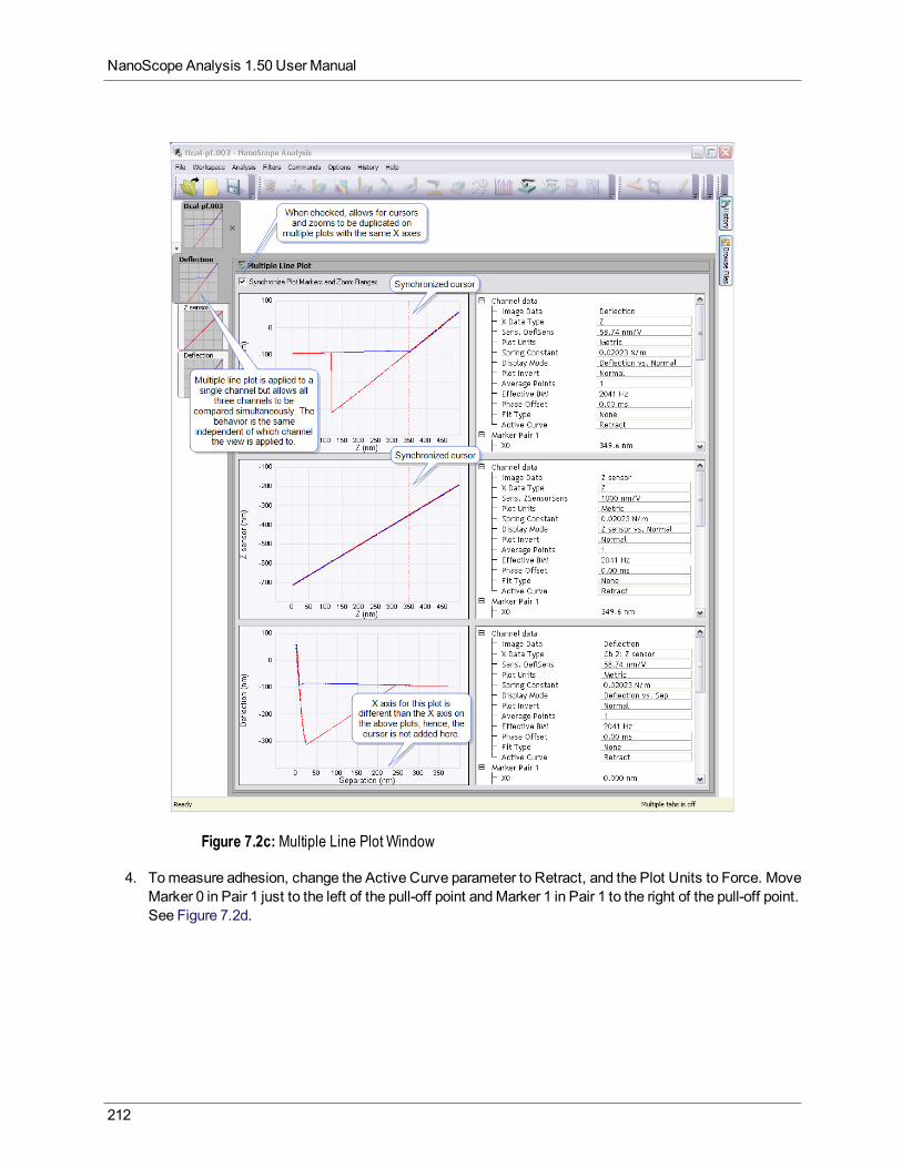
NanoScope Analysis 1.50 User Manual
Figure 7.2c:Multiple Line Plot Window
4. Tomeasure adhesion, change the Active Curve parameter to Retract, and the Plot Units to Force. MoveMarker 0 in Pair 1 just to the left of the pull-off point andMarker 1 in Pair 1 to the right of the pull-off point.See Figure 7.2d.
212

Chapter 7: Force Curve & Ramping Analysis
Figure 7.2d: Adhesion Measurement Example
5. To Zoom in on the area of interest hold down the Control key and draw a box in the preferred area of theLine Plot. To zoom back out, double-click on the image or click on themagnifying glass icon.
213

NanoScope Analysis 1.50 User Manual
Figure 7.2e: Zoom Example
6. To re-center the Y-axis drag a horizontal cursor from the top or bottom of the Line Plot. Once the cursoris positioned in the preferred location, right click in the plot and select Y-Translate.
Figure 7.2f: Y-Translate Example
214

Chapter 7: Force Curve & Ramping Analysis
Figure 7.2g: Y-Translate In Effect
7. It is often advantageous to change the color of many of the items in the Line Plot so that they can be dif-ferentiated. To change the color of the Curves, Text, Background, Grid, or Markers, right click in theLine Plot and select Color > Preferred item to change. See Figure 7.2h.
NOTE: Curve 1 is called the Trace curve and curve 2 is called the Retrace curve. The Trace curve is donefirst and the Retrace second. In a Force Curve, the Trace curve is always bringing the tip and sampletogether, while the Retrace is separating them.
Figure 7.2h: Options to Change Color of Plot Items
215
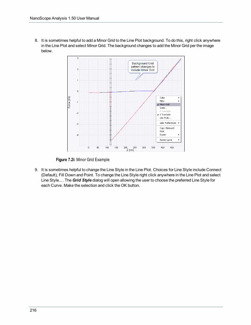
NanoScope Analysis 1.50 User Manual
8. It is sometimes helpful to add aMinor Grid to the Line Plot background. To do this, right click anywherein the Line Plot and select Minor Grid. The background changes to add theMinor Grid per the imagebelow.
Figure 7.2i:Minor Grid Example
9. It is sometimes helpful to change the Line Style in the Line Plot. Choices for Line Style include Connect(Default), Fill Down and Point. To change the Line Style right click anywhere in the Line Plot and selectLine Style.... TheGrid Style dialog will open allowing the user to choose the preferred Line Style foreach Curve. Make the selection and click the OK button.
216

Chapter 7: Force Curve & Ramping Analysis
Figure 7.2j: Line Style Selection
10. Line Plot data or images are often required for Export. To Export, right click anywhere in the Line Plotand select Export > Graphic or XZ Data. TheSave As dialog will open allowing the user to choose thelocation and filename for the exported file. The preferred graphic file to save images in is .bmp.
NOTE:When exporting XZ data, the data consists of amulti-column text file that represents the data asplotted (including X and Y translate, etc).
Figure 7.2k: Export Example
217

NanoScope Analysis 1.50 User Manual
Display Mode & Hertzian Fit ExampleThe purpose of a separation plot is to show the force versus the tip-sample separation. This type of plot isnecessary when fitting contact mechanics and pullingmodels.To create this type of plot requires an accuratedeflection sensitivity and one of the data channels to be either deflection or TM deflection.
Figure 7.2l: Deflection vs. Z, Prior to Separation
1. Choose the separationmode.
218

Chapter 7: Force Curve & Ramping Analysis
Figure 7.2m: Deflection vs. Separation
2. Place the cursors on the Plot in the unloading region. Zoom if for additional accuracy.3. Active Curve should be set to Retract.4. Set the Fit Type to Hertzian.
219

NanoScope Analysis 1.50 User Manual
Figure 7.2n: Hertzian Fit Example
General Ramping: Piezoresponse Force Microscopy (PFM) Example1. In PFM the tip or sample bias is ramped while observing the amplitude and/or phase of the cantilever
deflection. In this case, the tip bias was ramped from -5V to +5V. PFM ramping is a powerful tool forobserving the ferro-electric properties of materials.
220

Chapter 7: Force Curve & Ramping Analysis
Figure 7.2o: PFM Example
Force Curve InterfaceParameter Description
ImageData Type of data originally taken for the particular channel (Y-axis).
X DataType
Type of data that the channel data is being plotted against. This data displays on the X axis.Choices include Time, Ramp Channel (e.g. Z), or any of the other collected data channels.
Sens.Deflection
Sensitivity of the data channel. The name depends on the mode and what channel is being col-lected. Some examples include Sens. TM Deflection, Sens. DeflSens, etc...
Plot Units Selects the units for the Y-axis of the plot. Switches parameters in the Results panel betweenunits of Volts (V), Metric (nm or μm), or Force (nN).
SpringConstant Used to calculate the Force if Plot Units are Force.
221

NanoScope Analysis 1.50 User Manual
Parameter Description
DisplayMode
Changes the X-axis data to separation (including the effect of cantilever bending). Two options:Deflection vs. Ramp Channel (e.g. Z) or Deflection vs. Sep. Separation = deflection - Z position +constant (determined such that the separation is Zero at the turn around point)
Plot Invert Inverts data along the Y-axis, effectively turning valleys into mounds and vice versa.
AveragePoints Averages multiple points to smooth the curve.
EffectiveBW
A display (you cannot input a value to it) representing the sampling frequency with display aver-aging taken into account:Effective BW = (force plot sampling rate)/(Average Points)
PhaseOffset Shift horizontal position of plot to compensate for averaging of endpoint data.
Fit Type Choose from None, Line, Hertzian, or WLC (Worm-like Chain - pulling model)
ActiveCurve Choose from Approach or Retract
Table: 7.0aw Channel Data Input Parameters
Parameter Description
Marker Pair 1:X0 Horizontal position of first marker, Marker Pair 1
X1 Horizontal position of second marker, Marker Pair 1
Y0 Vertical position of first marker, Marker Pair 1
Y1 Vertical position of second marker, Marker Pair 1
X1 - X0 Horizontal distance between markers in Marker Pair 1
Y1 - Y0 Vertical space between markers in Marker Pair 1
dY/dX Slope of Marker Pair 1; calculated from endpoints
dX/dY 1/Slope of Marker Pair 1; calculated from endpoints
Least Squares Equation Equation of the fit
Root Mean Square RMS deviation from the fit
Average Deviation Average deviation from the fit
Marker Pair 2:X2 Horizontal position of first marker, Marker Pair 2
X3 Horizontal position of second marker, Marker Pair 2
Y2 Vertical position of first marker, Marker Pair 2
Y3 Verticaln position of second marker, Marker Pair 2
X3 - X2 Horizontal distance between markers in Marker Pair 2
Y3 - Y2 Vertical space between markers in Marker Pair 2
222

Chapter 7: Force Curve & Ramping Analysis
Parameter Description
dY/dX Slope of Market Pair 2; calculated from endpoints
dX/dY 1/Slope of Marker Pair 2; calculated from endpoints
Least Squares Equation Equation of the fit
Root Mean Square RMS deviation from the fit
Average Deviation Average deviation from the fit
Table: 7.0ax Marker Pair Parameters
Force Curve - Update SensitivityNanoScope Analysis allows for the updating of sensitivity on Line Plot files. To learn about this capability, goto the following link: Line Plot - Update Sensitivity
7.3 Force Curve - Update SensitivityNanoScope Analysis allows for the updating of sensitivity on Force Curves files. The goal of updating thesensitivity of a Force Curve is to calibrate the Y axis (Cantilever Deflection for Contact Mode or Amplitude forTappingMode).
7.3.1 Update Sensitivity Procedure1. When updating sensitivity it is important to use the Z sensor channel (Height sensor) if available and to
set the Active Curve to Retract. When placing cursors, it is preferred to place them such that they areover a linear section of the plot (not too close to the pull off or peak force). Additionally, select as long ofa section as possible.
NOTE:When using the Update Sensitivity function, it is assumed that there is no deformation of the tip orsample. This requires a hard sample for the results to be valid.
2. After the Force Curve file has already been opened in NanoScope Analysis, select Command >Update Sensitivity from theMenu Bar, as shown in the image below.
223
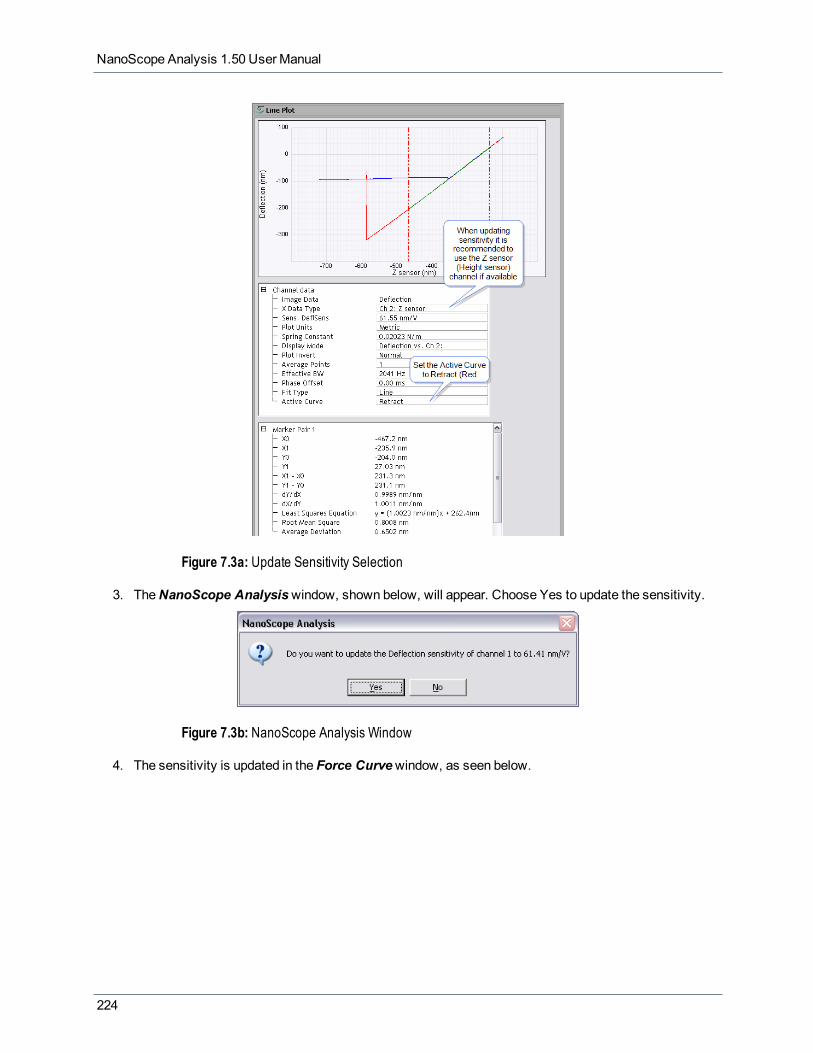
NanoScope Analysis 1.50 User Manual
Figure 7.3a: Update Sensitivity Selection
3. TheNanoScope Analysiswindow, shown below, will appear. Choose Yes to update the sensitivity.
Figure 7.3b: NanoScope Analysis Window
4. The sensitivity is updated in the Force Curvewindow, as seen below.
224

Chapter 7: Force Curve & Ramping Analysis
Figure 7.3c: Sensitivity Updated
225

NanoScope Analysis 1.50 User Manual
7.4 Force VolumeNanoScope Force Volume (FV) imaging with the atomic forcemicroscope (AFM) combines forcemeasurement with topographic imaging. Typical AFM images depict the topography of a surface by measuringthe action of a feedback loop tomaintain a constant tip/sample interaction as the tip is scanned across thesurface. The force volume data set combines nearly simultaneously measured topographic and forceinformation into a single data set allowing themicroscopist to test for correlations between forces and surfacefeatures.
TheoryA single force curve records the force on the tip as it approaches and retracts from a point on the samplesurface. When the Force reaches a user specified "trigger" value, the system records the height for that pixeland the tip retracts. Force volume imaging associates each (X,Y) position with a force curve in Z for someselected range. By plotting these values along X and Y coordinates, youmay view stratified layers of force atvarious Z-axis heights above the sample surface. The value at a point (X,Y,Z) in the volume is the deflection(force) of the cantilever at that position in space. The height image is composed of the relative Z positions ofthe trigger points.
A force volume data set can be used tomap in two or three dimensions the interaction forces between asample and the AFM probe tip. Possible applications include studies of elasticity, adhesion, electric andmagnetic fields. Force volume imaging enables themeasurement of forces at various Z-positions and atthousands of (X,Y) positions during a single image scan.
7.4.1 Force Volume Procedure1. Display individual force curves by first opening the file and then selecting theSingle radio button from
the Force Curve Mode selection dialog. Click the left mouse button on a specific pixel in any of the 3images to display the associated Force Curve in the Force Plot region (see Figure 7.4a).
NOTE: The pixels in the images aremarked with white crosses.
2. The Z value of theDeflection Error is displayed in the force volume image as a red vertical cursor atthat particular Z value. Adjust the red cursor in the Force Plot region to find the position in theDeflection Error image that shows good contrast.
226
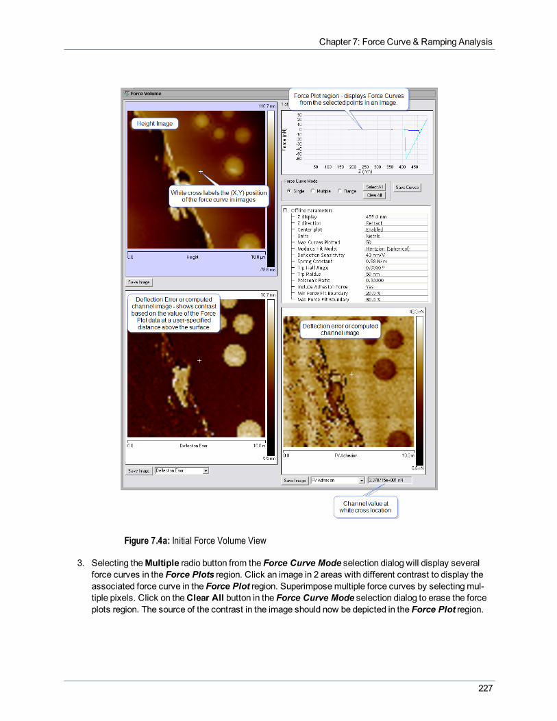
Chapter 7: Force Curve & Ramping Analysis
Figure 7.4a: Initial Force Volume View
3. Selecting theMultiple radio button from the Force Curve Mode selection dialog will display severalforce curves in the Force Plots region. Click an image in 2 areas with different contrast to display theassociated force curve in the Force Plot region. Superimposemultiple force curves by selectingmul-tiple pixels. Click on theClear All button in the Force Curve Mode selection dialog to erase the forceplots region. The source of the contrast in the image should now be depicted in the Force Plot region.
227

NanoScope Analysis 1.50 User Manual
Figure 7.4b: Selecting Appropriate Z Display
4. Selecting the range radio button from the Force Curve Mode selection dialog will display all of the forcecurves in a selected box in the Force Plots region. To draw a box, place the cursor in an image, clickthe left mouse button and drag the box to the desired size. The Force Plots region will be automaticallyupdated with the data for the chosen area.
5. Individual force curves can be analyzed separately from the height and volume data; select SaveCurves and the standard force curve analysis view is saved and can be opened from theBrowsewin-dow. Oncemodified and analyzed, select File > Save to save the image andmodified force curve. If
228

Chapter 7: Force Curve & Ramping Analysis
multiple force curves are displayed, clickingSave Curves saves each curve as its own standard ForceCurve file.
Figure 7.4c: Using the Range Box
Force Volume InterfaceParameter Description
Single Displays the associated force curve for the selected pixel chosen in an image.
Multiple Displays several force curves in the force plots region for the selected pixels chosen in an image.
229

NanoScope Analysis 1.50 User Manual
Parameter Description
Range Displays several force curves in the force plots region for the selected area chosen in an image.
Select All Plots all Force Curves in the Force Plots region.
Clear All Erases the Force Curves shown in the Force Plots region.
SaveCurves
Saves each Force Curve as its own standard Force Curve file that can be opened separately inNanoScope Analysis.
Table: 7.0ay Force Curve Mode Selections & Buttons
Parameter Description
Z display
The Z display parameter determines the Z position of the Slice to be displayed in the DeflectionError image. The Z display can be set in two ways. The first is to enter the desired Z value of theslice in the control panel. The second is to use the mouse to change the horizontal position (thatis, the Z position) of the cursor in the force plot region. For example, a Z display of 30 nm causesthe force volume image region to depict forces on the tip when it is at a Z position of 30 nmabove the piezoelectric actuator position at the Trig threshold. The Z display parameter may bethought of as defining bands of force at fixed distances from the sample surface.
Z direction The Z direction parameter determines which portion of the force curve, Extend or Retract, isshown in the bottom 2 images. For example, if adhesion forces are probed, then the Retract por-tion should be used.
Centerplot
When Center Plot isOn, any additional Force Curves added to the Force Plot will be translatedvertically so that the leftmost data points in the curve are Zero. If Center Plot isOff, added ForceCurves are not translated.
Units Choose: Volts or Metric
MaxCurvesPlotted
The maximum number of force curves that will be plotted.
ModulusFit Model
The model type used to analyze the force curves:
l Hertz model (spherical indenter) (page 231)l Sneddon (conical indenter) (page 232)
DeflectionSensitivity The cantilever deflection per unit of separation.
SpringConstant The cantilever spring constant.
Tip HalfAngle The half angle of the probe tip.
Tip Radius The radius of the probe tip.
PoissonRatio The sample's Poisson ratio.
IncludeAdhesionForce
Including Adhesion Force means that calculations are performed based on forces relative to theadhesion force.
230
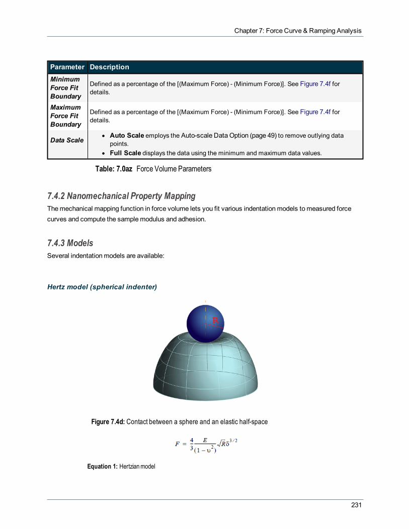
Chapter 7: Force Curve & Ramping Analysis
Parameter Description
MinimumForce FitBoundary
Defined as a percentage of the [(Maximum Force) - (Minimum Force)]. See Figure 7.4f fordetails.
MaximumForce FitBoundary
Defined as a percentage of the [(Maximum Force) - (Minimum Force)]. See Figure 7.4f fordetails.
Data Scalel Auto Scale employs the Auto-scale Data Option (page 49) to remove outlying data
points.l Full Scale displays the data using the minimum and maximum data values.
Table: 7.0az Force Volume Parameters
7.4.2 Nanomechanical Property MappingThemechanical mapping function in force volume lets you fit various indentationmodels to measured forcecurves and compute the samplemodulus and adhesion.
7.4.3 ModelsSeveral indentationmodels are available:
Hertz model (spherical indenter)
Figure 7.4d: Contact between a sphere and an elastic half-space
Equation 1: Hertzianmodel
231

NanoScope Analysis 1.50 User Manual
F = force (from force curve)
E = Young's modulus (fit parameter)
ν = Poisson's ratio (sample dependent, typically 0.2 - 0.5)
R = radius of the indenter (tip)
δ = indentation
Equation 1may be linearized in separation by taking both sides to the 2/3 power, shown in Equation 2.
Equation 2: LinearizedHertzequation
Sneddon (conical indenter)
Figure 7.4e: Contact between a cone and an elastic half-space
Equation 3: Sneddonmodel
where
F = force (from force curve)
232

Chapter 7: Force Curve & Ramping Analysis
E = Young's modulus (fit parameter)
ν = Poisson's ratio (sample dependent, typically 0.2 - 0.5)
α = half-angle of the indenter
δ = indentation
Equation 3may be linearized in separation by taking both sides to the 1/2 power, shown in Equation 4.
Equation 4: LinearizedSneddon equation
Depending on themodel, Young's modulus is computed from the slope of either Equation 2 or Equation 4.
Stiffness (linear)The stiffness model extrapolates a straight line fit to themaximum indentation.
Nanomechanical Property Mapping Procedure1. If you are using theHertzianmodel, enter the probe Tip Radius.2. If you are using theSneddonmodel, enter the probe Tip Half Angle.3. Enter theSample's Poisson Ratio.4. Decide if you wish to Include Adhesion Force.
Including Adhesion Forcemeans that calculations are performed based on forces relative to the adhe-sion force. Otherwise, calculations are performed on absolute force values.
5. Enter a value for theMinimum Force Fit Boundary. TheMinimum Force Fit Boundary is defined asa percentage of the [(Maximum Force) - (Minimum Force)]. See Figure 7.4f.
6. Enter a value for theMaximum Force Fit Boundary. TheMaxmimum Force Fit Boundary is definedas a percentage of the [(Maximum Force) - (Minimum Force)].These boundaries define the region through which the fit model is computed.
233

NanoScope Analysis 1.50 User Manual
Figure 7.4f:Minimum and Maximum Force Fit Boundaries defined
7. Select aModulus Fit Model:l Hertz model (spherical indenter) (page 231)l Sneddon (conical indenter) (page 232)8. Select the Z direction that you wish to use for theModulus Fit Model: Extend orRetract.
NOTE: You choice of Z direction here also determines which portion of the Real-time force curve cycle,Extend orRetract, is shown in the force volume image.
8. Enter theSpring Constant.9. Select which property you wish to display in each of the two force volume images:
l Deflection Errorl FV Modulus: Maps themodulus using the selectedModulus Fit Model.l FV Log Modulus: Maps the log of themodulus using the selectedModulus Fit Model.l FV Stiffness: Maps the Stiffness (linear) (page 233).l FV Adhesion: The peak force below the baseline. See Figure 7.4g.
Figure 7.4g: Adhesion
234

Chapter 7: Force Curve & Ramping Analysis
NOTE: 1st order baseline correction, which removes baseline tilt as well as offset, is performed beforeadhesionmapping.
10. TheSave Image button, found at the bottom of each image, saves the selected display (see above).
235

NanoScope Analysis 1.50 User Manual
7.5 Review Force CurvesA force spectroscopy session can yield dozens if not hundreds of individual force plots.
1. To facilitate comparison of plots and deletion of files deemed unworthy of inclusion, click Commands >Review Curves.
2. TheReview Force Curves window, shown in Figure 7.5a, opens.a. Enter the path to theDirectorywhose contents are the force plot files of interest.b. Select aSort category: Date, TMR (scanning TraceMinus Retrace) orName.
NOTE: The TMR values are proportional to the area between the approach and retract curves.
c. Select aSort order: Ascending (box checked) orDescending (box unchecked).d. Select thePlot Units (vertical axis) units: Volts,Metric or Force.e. Select thePlot number.f. Select the Trace(s) to plot: Extend, Retract orBoth.
Figure 7.5a: The Review Force Curves window for reviewing multiple force plot files
3. Advance through the ordered set of files by clicking the arrow buttons in the bottom left of the File textbox or using the keyboard arrow keys.a. Click Mark for Delete, d, or the keyboard Delete key for any force plot you wish to discard from
the set.
NOTE: Files marked for deletion are not sent to the recycling bin until theDelete Files button is clicked.Youmay remove the check from theMark for Delete at any time prior to this.
4. Zooming on a plot is accomplished by pressing Ctrl, left-clicking and dragging in the plot. Zooming out isdone by double-clicking in the plot area.
236

Chapter 7: Force Curve & Ramping Analysis
7.6 Filtering Multiple Force CurvesAnother way to quickly delete force curves uses the Filter Curves function.
1. Youmay apply selection criteria to delete force curves by selecting, from themainmenu, Commands >Filter Curves.
2. The Filter Force Curveswindow, shown in Figure 7.6a, opens.a. Enter the path to theDirectorywhose contents are the force plot files of interest.b. Enter thePlot number that you wish to analyze.c. Enter aMinimum Distance from the contact point below which data will be ignored.d. Enter aMinimum Force from the contact point to qualify peaks.e. Enter the number of Average Points to use. To reduce noise, peak values are computed by aver-
aging ±(Average Points)/2 around a point.
Figure 7.6a: The Filter Force Curves window
3. Click Delete Curves to analyze, using the criteria in the Filter Force Curves window, the force curvesin the selected directory. Click Cancel to abort the process.
4. Files meeting the deletion criteria will be shown in the left window, shown in Figure 7.6a, and ames-sage, Confirm File Delete, will be displayed asking if you wish to send the specified file to the RecycleBin.
237

NanoScope Analysis 1.50 User Manual
7.7 Multiple Curve Analysis (MCA)Multiple Curve Analysis enables the evaluation of multiple force plots.
MCA ProcedureTo open aMCA file in NanoScope Analysis, double click on a NanoScopeMCA file in theBrowse Files view
or navigate to the preferredMCA file from theOpen File icon . If the file is indeed anMCA file, it will beopened in theMCA window automatically.
Click Add Files... in theMCA window to open a file selection window and click the files to be analyzed.Choose the preferred files and click Add. These files are then added to the file list in theMCA FileInformation Register. Files in that list may be removed individually or multiply by clicking the file name andthen clickingRemove Files. Files may be selectively displayed by clicking in the Plot field— an X will bedisplayed— of theMCA File Information Register.
238
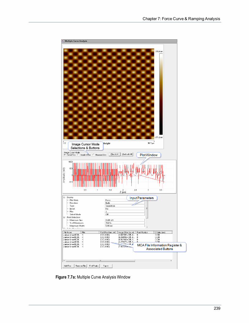
Chapter 7: Force Curve & Ramping Analysis
Figure 7.7a:Multiple Curve Analysis Window
239
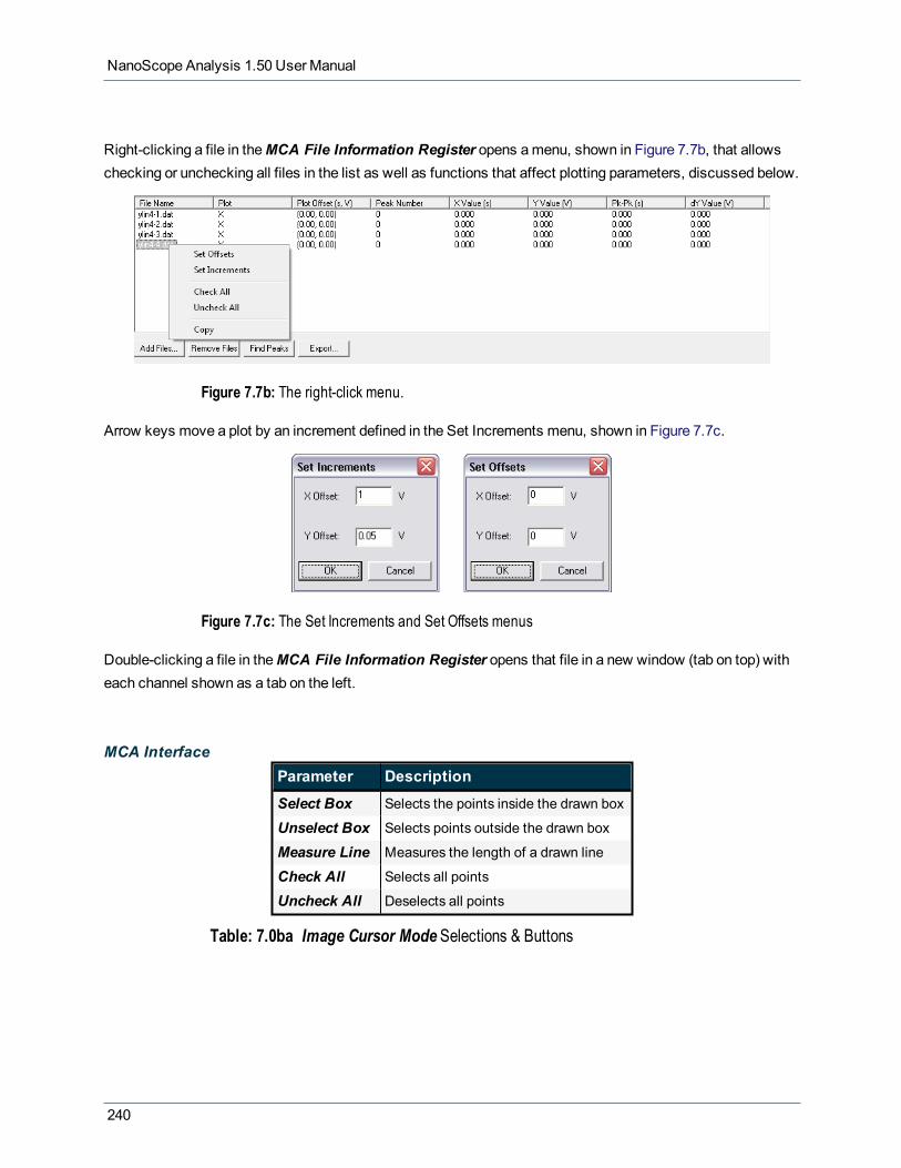
NanoScope Analysis 1.50 User Manual
Right-clicking a file in theMCA File Information Register opens amenu, shown in Figure 7.7b, that allowschecking or unchecking all files in the list as well as functions that affect plotting parameters, discussed below.
Figure 7.7b: The right-click menu.
Arrow keys move a plot by an increment defined in the Set Increments menu, shown in Figure 7.7c.
Figure 7.7c: The Set Increments and Set Offsets menus
Double-clicking a file in theMCA File Information Register opens that file in a new window (tab on top) witheach channel shown as a tab on the left.
MCA InterfaceParameter Description
Select Box Selects the points inside the drawn box
Unselect Box Selects points outside the drawn box
Measure Line Measures the length of a drawn line
Check All Selects all points
Uncheck All Deselects all points
Table: 7.0ba Image Cursor Mode Selections & Buttons
240

Chapter 7: Force Curve & Ramping Analysis
Group Parameter Description
Display
Plot Units The user can choose either Force, Volt or distance (Metric) on the Y axis.
Direction The Extend option plots and looks for peaks only in the Extend direction. TheRetract option plots and looks for peaks only in the Retract direction.
Type Either Z or Separation. Z displays the Z position of the piezo measured by a capa-citive sensor. Separation displays the corrected (for cantilever deflection) Z data.
Invert The Y axis is inverted when Yes is selected.
Plot Enter the channel to be plotted, and hit Enter.
SelectMode On turns all curves to color number one and the selected (by mouse or arrow key)curve to its plot color.
PeakDetection
Minimumsize Finds peaks greater than the value entered here.
Percentageof Max The Y variable must fall by this percentage to be considered a peak.
MinimumWidth at %Max
A peak must have a width (at Percentage of Max of the peak’s absolute value)greater than the Minimum Width at %Max to be considered a peak.
AutoAlignCurves
X-axis auto-zero Either On (at the contact point), Off or User.
Y-axis auto-zero
Either On, Off, User or Cascade which increments the Y offset of each plot by theCascade Offset.
CascadeOffset Define the Y offset to be used here when the Y Axis Auto-zero is set to Cascade.
Table: 7.0bb MCA Parameters
Parameter Description
Add Files Opens a file selection window that allows files to be added in the Multiple Force window.
RemoveFiles Deletes selected (by clicking) files from the Multiple Force window
FindPeaks
Finds peaks using the filters (rules) selected in the Peak Detection functions in the Input Para-meters window. The XOffset and YOffset, Peak Number, X Value, Y Value, Peak-To-Peak andDY Values are shown in the table below the plot window, as shown in Figure 7.7b.
Export Saves the results from Find Peaks in a tab-delimited text file.
Table: 7.0bc MCA File Information Register
Creating MCA FilesMCA files are automatically created by NanoScope Point and Shoot rampmode. MCA files may also be
241

NanoScope Analysis 1.50 User Manual
created by combiningmultiple force curves. This is required for files created by NanoDrive software.
Youmay create anmca file by selectingmultiple .dat files (using Shift or Ctrl), right-clicking and selectingCurve Analysis as shown in Figure 7.7d.
Figure 7.7d: Select Curve Analysis
This opens a window, shown in Figure 7.7e, that allows you to choose themca file name and directory.
Figure 7.7e: Create an MCA file
Choose a directory, a file name and click Save.
242

Chapter 7: Force Curve & Ramping Analysis
7.8 Modify Force ParametersTheModify Force Parameters function lets you change theDeflection Sensitivity, Spring Constant, TipRadius, Tip Half Angle and theSample's Poisson Ratio.
7.8.1 Cases where you might use this functionl You forget to enter your spring constant before collecting data and later want to correct the saved force
curve files.l When using a functionalized probe you often want to calibrate the deflection sensitivity at the end of the
experiment. You then need to update all of your saved data with the correct value.
7.8.2 Modify Force Parameters ProcedureEither:
l Click theChange check box next to the parameter that you wish tomodify, then click in the appropriateNew Value field, edit and click Execute.
or
l Click in the appropriateNew Value field and enter the new value (theChange check box will bechecked) and click Execute.
See Figure 7.8a.
Figure 7.8a: The Modify Force Parameters window
NOTE: Themodified values will be used in subsequent NanoScope Analysis functions but will not besaved to the file unless youSave the file.
243
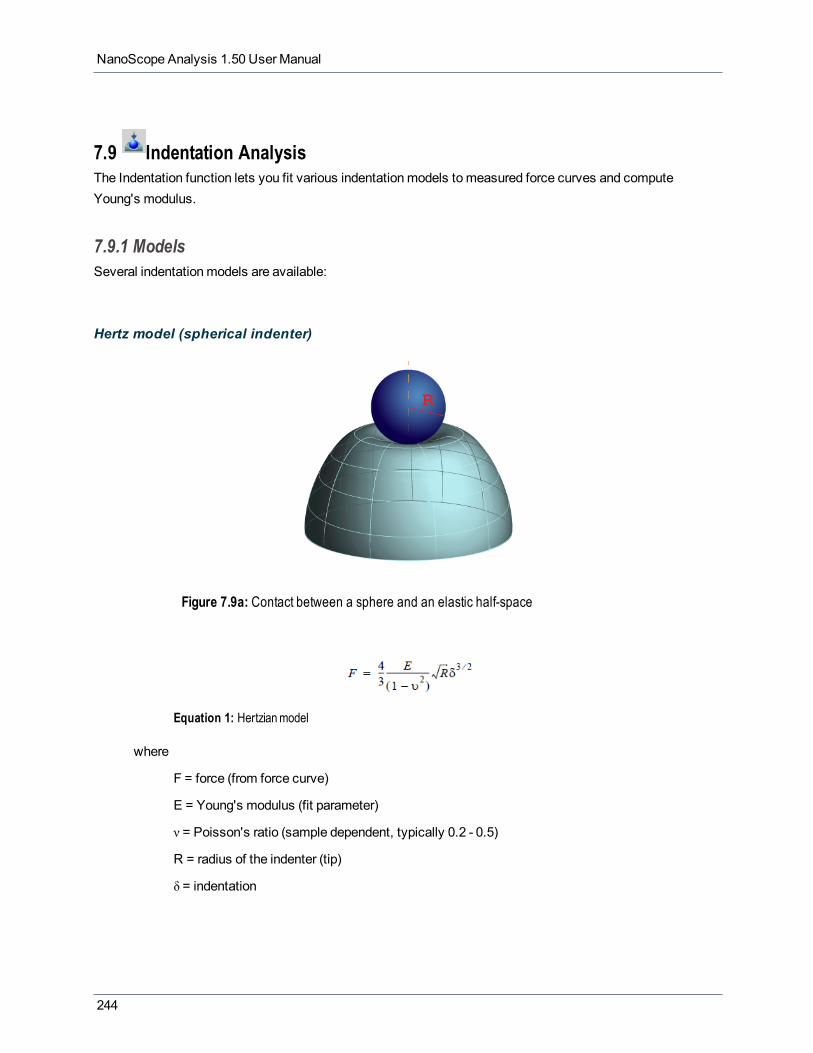
NanoScope Analysis 1.50 User Manual
7.9 Indentation AnalysisThe Indentation function lets you fit various indentationmodels to measured force curves and computeYoung's modulus.
7.9.1 ModelsSeveral indentationmodels are available:
Hertz model (spherical indenter)
Figure 7.9a: Contact between a sphere and an elastic half-space
Equation 1: Hertzianmodel
where
F = force (from force curve)
E = Young's modulus (fit parameter)
ν = Poisson's ratio (sample dependent, typically 0.2 - 0.5)
R = radius of the indenter (tip)
δ = indentation
244
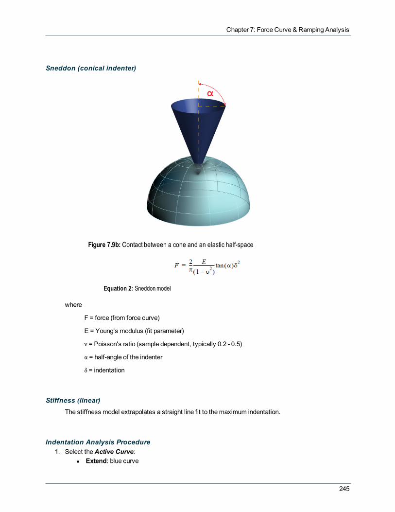
Chapter 7: Force Curve & Ramping Analysis
Sneddon (conical indenter)
Figure 7.9b: Contact between a cone and an elastic half-space
Equation 2: Sneddonmodel
where
F = force (from force curve)
E = Young's modulus (fit parameter)
ν = Poisson's ratio (sample dependent, typically 0.2 - 0.5)
α = half-angle of the indenter
δ = indentation
Stiffness (linear)The stiffness model extrapolates a straight line fit to themaximum indentation.
Indentation Analysis Procedure1. Select theActive Curve:
l Extend: blue curve
245

NanoScope Analysis 1.50 User Manual
l Retract: red curve2. Select the Fit Method:
l Contact Point Based:Uses a nonlinear least squares fit to either the Hertz or Sneddonmodels, above, and goesthrough the contact point, determined in Step 4.
l Linearized ModelEquation 1 (Hertz model) may be linearized in separation by taking both sides to the 2/3 power,shown in Equation 3, and Equation 2may be linearized by taking both sides to the 1/2 power,shown in Equation 4.
Equation 3: LinearizedHertzequation
Equation 4: LinearizedSneddon equation
Because these equations are linear, they no longer are forced through the origin so that the con-tact point is not needed. In the Linearized Model case, Young's modulus is computed from theslope of these equations.TheMinimum Force, shown in Figure 7.9d, is determined as follows:
Starting a the lowest separation, a straight line is least squares-fitted to 5% of the pointson the curve and its slope is calculated.Another straight line is drawnwith the starting point incremented by one using the abovemethod.This process is repeated and stopped when the local slope becomes positive.TheMinimum Force is subtracted before the force curves are linearized.
Youmay manually move theMinimum Force point by dragging the dashed blue line, shown in Fig-ure 7.9d.
NOTE: Baseline Correction (page 249) should be applied before this model is used.
3. Decide if you wish to Include Adhesion ForceIncluding Adhesion Forcemeans that calculations are performed based on forces relative to the adhe-sion force. Otherwise, calculations are performed on absolute force values.
4. Select theContact Point Algorithm available for Fit Method = Contact Point Based:l Best Estimate:
A line drawn between the first and last points of the force curve is subtracted from each point inthe force curve, effectively rotating it. The point with the resultingminimum value is selected asthe contact point. This method emphasizes theminimum force at the contact point while de-emphasizing forces due to noise or interference in the non-contact region, reducing the likelihoodthat the wrong point is selected.
l Treat as Fit Variable:
246
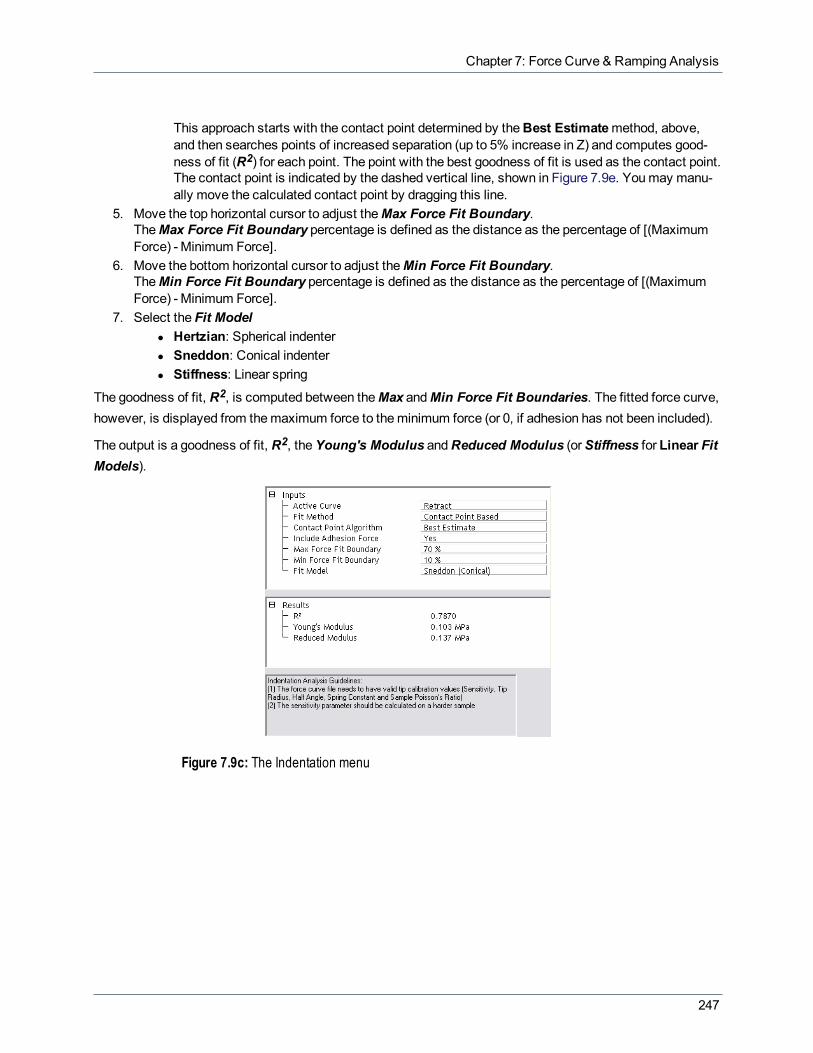
Chapter 7: Force Curve & Ramping Analysis
This approach starts with the contact point determined by theBest Estimatemethod, above,and then searches points of increased separation (up to 5% increase in Z) and computes good-ness of fit (R2) for each point. The point with the best goodness of fit is used as the contact point.The contact point is indicated by the dashed vertical line, shown in Figure 7.9e. Youmay manu-ally move the calculated contact point by dragging this line.
5. Move the top horizontal cursor to adjust theMax Force Fit Boundary.TheMax Force Fit Boundary percentage is defined as the distance as the percentage of [(MaximumForce) - Minimum Force].
6. Move the bottom horizontal cursor to adjust theMin Force Fit Boundary.TheMin Force Fit Boundary percentage is defined as the distance as the percentage of [(MaximumForce) - Minimum Force].
7. Select the Fit Modell Hertzian: Spherical indenterl Sneddon: Conical indenterl Stiffness: Linear spring
The goodness of fit, R2, is computed between theMax andMin Force Fit Boundaries. The fitted force curve,however, is displayed from themaximum force to theminimum force (or 0, if adhesion has not been included).
The output is a goodness of fit, R2, theYoung's Modulus andReduced Modulus (orStiffness for Linear FitModels).
Figure 7.9c: The Indentation menu
247

NanoScope Analysis 1.50 User Manual
Figure 7.9d: Force plot with a linearized fit
Figure 7.9e shows a Hertzian fit (green curve) to a force curve.
Figure 7.9e: Hertzian fit to a force curve
248

Chapter 7: Force Curve & Ramping Analysis
7.10 Baseline CorrectionThe Baseline Correction functionmeasures baseline tilt and offset and applies a linear correction to the wholeforce curve.
7.10.1 Cases where you might use this functionForce curves can have a small amount of baseline tilt caused by the detector configuration. Thoughinsignificant in many measurements, it’s sometimes desirable to remove this artifact in force curves involvingvery low forces.
7.10.2 Baseline Correction Procedure1. Select the force curveDirection that you wish to correct.:
l Extend: blue curvel Retract: red curvel Both: blue and red curves
2. Choose the Y-axis Plot Units:l Voltl Metricl Force
3. Choose the X-axis plot Type:l Zl Separation
4. Choose theCorrection Order:l 0thRemoves offsetl 1stRemoves tilt as well as offset (0th order)
5. Choose theExtend Baseline Source:Selects which baseline to use for the Extend direction of the force curve:
l Extendl Retract
6. Choose theRetract Baseline SourceSelects which baseline to use for the Retract direction of the force curve:
l Extendl Retract
7. Move the cursors to select theBaseline Start andStop percentages.
NOTE: The cursor colors match their associated baseline sources, blue corresponds toExtendwhile redcorresponds toRetract.
8. Click Execute to apply the correction. See Figure 7.10a.
249

NanoScope Analysis 1.50 User Manual
Figure 7.10a: The Baseline filter window
NOTE: Themodified values will be used in subsequent NanoScope Analysis functions but will not besaved to the file unless youSave the file.
Figure 7.10b shows a force curve before and after application of the Baseline Correction filter.
250
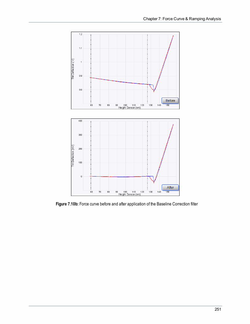
Chapter 7: Force Curve & Ramping Analysis
Figure 7.10b: Force curve before and after application of the Baseline Correction filter
251

NanoScope Analysis 1.50 User Manual
7.11 Boxcar FilterThe Boxcar filter applies amoving average filter with weight of 0 or 1 (over a selectable number of points) toyour data. A boxcar filter is frequently employed to reducemeasurement noise.
7.11.1 Boxcar Filter Procedure1. Select theDirection:l Extend: blue curvel Retract: red curve:l Both: blue and red curves:2. Select the number of Average Points to use in themoving average.
The filter will be centered about the current point of theAverage Points is odd. If Average Points is even,there will be onemore trailing point than leading point.
3. Click Execute to apply the filter. See Figure 7.11a.
Figure 7.11a: The Boxcar filter window
NOTE: Themodified values will be used in subsequent NanoScope Analysis functions but will not besaved to the file unless youSave the file.
Figure 7.11b shows a force curve before and after application of the Boxcar filter (10 points) which was used toremove thermal noise.
252
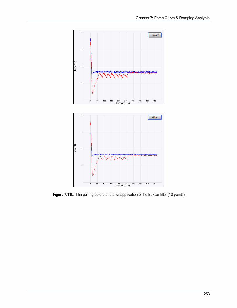
Chapter 7: Force Curve & Ramping Analysis
Figure 7.11b: Titin pulling before and after application of the Boxcar filter (10 points)
253

NanoScope Analysis 1.50 User Manual
7.12 MATLAB UtilitiesNanoScope Analysis includes aMATLAB utility, NSMatLabUtilities.m (in the root directory of NanoScopeAnalysis), that extracts force curves, force volume data, HSDC data and image data from NanoScope files foruse by MATLAB. This allows you to, for instance, compare arbitrary forcemodels with measured data.
Bruker also provides MATLAB examples, NSMatLabExamples.m (in the root directory of NanoScopeAnalysis), that demonstrate the use of MATLAB to analyze NanoScope force curves.
NOTE: 64 bit windows users will need to install Microsoft Windows SDK (Software Development Kit) forWindows 7 in order to use thematlab toolbox with 64bit matlab. Additional information is available fromMathWorks at MATLABWindows 64-bit support. The SDK can be downloaded fromWindows 7 SDKdownload.
7.12.1 NSMatlabUtilitiesThe NSMatlabUtilities class implements NanoScope file I/O utilities.
The NSMatlabUtilities class has 6 properties:
1. FileName –Current file name2. IsOpen – A value indicating whether the file is open3. METRIC –Option to retrieve data in metric units4. VOLTS –Option to retrieve data in volts5. FORCE –Option to retrieve data in force units6. RAW –Option to retrieve data in LSB
NSMatlabUtilitiesConstructs the NSMatlabUtilities class.
Example:
NSMU = NSMatlabUtilities();
Open(FileName)Opens the file whose name is specified in the parameter FileName
Example:
NSMU.Open(‘Example.spm');
Close()Closes the file
Example:
NSMU.Close();
254

Chapter 7: Force Curve & Ramping Analysis
GetForceCurveDataReturns force curve data from a force curve file.
Syntax:
[trace, retrace, scaleUnit, dataTypeDesc] = GetForceCurveData(ChannelNumber, UnitType)
Input:
ChannelNumber ranges from 1 to Number of Channels in the file.UnitType: this.METRIC, this.VOLTS, this.FORCE, this.RAW
Output:
trace: array of trace dataretrace: array of retrace datascaleUnit: scale unit stringdataTypeDesc: data type dscription
Example:
[trace, retrace, scale_units, type_desc] = NSMU.GetForceCurveData(1, NSMU.METRIC);
GetHSDCDataReturns HSDC data from aHSDC file.
Syntax:
[data, scaleUnit, dataTypeDesc] = GetHSDCData(ChannelNumber, UnitType)
Input:
ChannelNumber ranges from 1 to Number of Channels in the file.UnitType: this.METRIC, this.VOLTS, this.RAW
Output:
data: array of hsdc channel datascaleUnit: scale unit stringdataTypeDesc: data type dscription
Example:
[data, scale_units, type_desc] = NSMU.GetHSDCData(1, NSMU.METRIC );
GetForceVolumeImageDataReturns force volume image data from a force volume file.
Syntax:
[data, scaleUnit, dataTypeDesc] = GetForceVolumeImageData(UnitType)
Input:
UnitType: this.METRIC, this.VOLTS, this.RAW
Output:
255

NanoScope Analysis 1.50 User Manual
data: array of hsdc channel datascaleUnit: scale unit stringdataTypeDesc: data type dscription
Example:
[data, scale_units, type_desc] = NSMU.GetForceVolumeImageData(NSMU.RAW);
GetForceVolumeForceCurveDataReturns force volume force curve data from a force volume file.
Syntax:
[trace, retrace, scaleUnit, dataTypeDesc] = GetForceVolumeForceCurveData(CurveNumber,UnitType)
Input:
ChannelNumber ranges from 1 to Number of Channels in the file.UnitType: this.METRIC, this.VOLTS, this.FORCE, this.RAW
Output:
trace: array of force volume force curve trace dataretrace: array of force volume force curve retrace datascaleUnit: scale unit stringdataTypeDesc: data type dscription
Example:
[trace, retrace, scale_units, type_desc] = NSMU.GetForceVolumeForceCurveData(1, NSMU.VOLTS);
GetImageDataReturns image channel data from an image file
Syntax:
[data, scaleUnit, dataTypeDesc] = GetImageData( ChannelNumber, UnitType )
Input:
ChannelNumber ranges from 1 to Number of Channels in the file.UnitType: this.METRIC, this.VOLTS, this.RAW
Output:
data: array of image datascaleUnit: scale unit stringdataTypeDesc: data type dscription
Example:
[data, scale_units, type_desc] = NSMU.GetImageData(1, NSMU.RAW);
256

Chapter 7: Force Curve & Ramping Analysis
GetZSensitivityUnitsReturns Z Sensitivity unit for a specific ChannelNumber
Syntax:
[unit] = GetZSensitivityUnits(ChannelNumber)
Input:
ChannelNumber ranges from 1 to Number of Channels in the file.
Output:
Unit: Z sensitivity units
Example:
ZSensitivityUnits1 = NSMU.GetZSensitivityUnits(1);
GetScalingFactorReturns the Scaling factor for a specific ChannelNumber
Syntax:
[factor] = GetScalingFactor(ChannelNumber, isMetric)
Input:
ChannelNumber ranges from 1 to Number of Channels in the file.If IsMetric is 1, the function returns the scaling factor to convert the LSB data tometric units.If IsMetric is 0, the function returns the scaling factor to convert the LSB data to volts units.
Output:
factor: Scaling factor
Example:
ZScalingFactorVolt = NSMU.GetScalingFactor(1,0);
GetBufferSizeReturns the buffer size for a specific ChannelNumber
Syntax:
[size] = GetBufferSize(ChannelNumber)
Input:
ChannelNumber ranges from 1 to Number of Channels in the file.
Output:
size: Buffer size
Example:
BufferSize = NSMU.GetBufferSize(1);
257

NanoScope Analysis 1.50 User Manual
GetSamplesPerLineReturns the samples per line in an image file.
Syntax:
[samps] = GetSamplesPerLine(ChannelNumber)
Input:
ChannelNumber ranges from 1 to Number of Channels in the file
Output:
samps: samples per line
Example:
SamplesPerLine = NSMU.GetSamplesPerLine(1);
GetNumberOfLinesReturns the number of lines in an image file
Syntax:
[lines] = GetNumberOfLines(ChannelNumber)
Input:
ChannelNumber ranges from 1 to Number of Channels in the file
Output:
lines: number of lines
Example:
NumberOfLines = NSMU.GetNumberOfLines(1);
GetImageAspectRatioReturns the Aspect Ratio in an image file
Syntax:
[AspectRatio] = GetImageAspectRatio(ChannelNumber)
Input:
ChannelNumber ranges from 1 to Number of Channels in the file
Output:
AspectRatio: Aspect ratio
Example:
AspectRatio = NSMU.GetImageAspectRatio(1);
258

Chapter 7: Force Curve & Ramping Analysis
GetNumberOfForceCurvesReturns the number of force curves in the file
Syntax:
[number] = GetNumberOfForceCurves()
Output:
number: number of force curves
Example:
NumberOfForceCurves = NSMU.GetNumberOfForceCurves();
GetNumberOfPointsPerCurveReturns the number of points for a specific force curve
Syntax:
[number] = GetNumberOfPointsPerCurve(ChannelNumber)
Input:
ChannelNumber ranges from 1 to Number of Channels in the file
Output:
number: number of points in the force curve
Example:
NumberOfPoints = NSMU.GetNumberOfPointsPerCurve(1);
GetRampSizeReturns the ramp size of a specific force curve ChannelNumber
Syntax:
[RampSize, RampUnits] = GetRampSize(ChannelNumber, isMetric)
Input:
ChannelNumber ranges from 1 to Number of Channels in the fileIf IsMetric is 1, the function returns the RampSize tometric unitIf IsMetric is 0, the function returns the RampSize to volts unit.
Output:
Ramp size and units
Example:
[RampSize, RampUnits] = NSMU.GetRampSize(1, 0);
259
NanoScope Analysis 1.50 User Manual
GetZScaleInSwUnitsReturns the ZScale of a specific force curve ChannelNumber
Syntax:
[ZScale] = GetZScaleInSwUnits( ChannelNumber)
Input:
ChannelNumber ranges from 1 to Number of Channels in the file
Output:
Z scale in sw units
Example:
SWZScale = NSMU.GetZScaleInSwUnits(ChannelNumber);
GetZScaleInHwUnitsReturns the ZScale of a specific force curve ChannelNumber
Syntax:
[ZScale] = GetZScaleInHwUnits( ChannelNumber)
Input:
ChannelNumber ranges from 1 to Number of Channels in the file
Output:
Z scale in hw units
Example:
HWZScale = NSMU.GetZScaleInHwUnits(ChannelNumber);
GetNumberOfTracePointsReturns the number of points in trace
Syntax:
[NumTrace] = GetNumberOfTracePoints(ChannelNumber)
Input:
ChannelNumber ranges from 1 to Number of Channels in the file
Output:
the number of points in trace curve
Example:
NumTrace = NSMU.GetNumberOfTracePoints(1);
260

Chapter 7: Force Curve & Ramping Analysis
GetNumberOfRetracePointsReturns the number of points in retrace
Syntax:
[NumRetrace] = GetNumberOfRetracePoints(ChannelNumber)
Input:
ChannelNumber ranges from 1 to Number of Channels in the file
Output:
the number of points in retrace
Example:
NumRetrace = NSMU.GetNumberOfRetracePoints(1);
GetPoissonRatioReturns the Poisson ratio from the header file
Syntax:
[Ratio] = GetPoissonRatio()
Output:
Poisson ratio
Example:
PoissonRatio = NSMU.GetPoissonRatio();
GetTipRadiusReturns the Tip radius from the header file
Syntax:
[Radius] = GetTipRadius()
Output:
Tip Radius
Example:
Radius = NSMU.GetTipRadius();
GetForwardRampVelocityReturns the Forward ramp velocity from the header file
Syntax:
[Velocity] = GetForwardRampVelocity( ChannelNumber, isMetric)
261

NanoScope Analysis 1.50 User Manual
Input:
ChannelNumber ranges from 1 to Number of Channels in the fileIsMetric is 1 or 0
Output:
Forward ramp velocity
Example:
VelocityMetric = NSMU.GetForwardRampVelocity(1,1);
GetReverseRampVelocityReturns the Reverse ramp velocity from the header file
Syntax:
[Velocity] = GetReverseRampVelocity(ChannelNumber, isMetric)
Input:
IsMetric is 1 or 0ChannelNumber ranges from 1 to Number of Channels in the file
Output:
Reverse ramp velocity
Example:
VelocityMetric = NSMU.GetReverseRampVelocity(1,1);
GetSpringConstantReturns the Spring constant
Syntax:
[SpringConst] = GetSpringConstant(ChannelNumber)
Input:
ChannelNumber ranges from 1 to Number of Channels in the file
Output:
Spring constant
Example:
Springcst = NSMU.GetSpringConstant(1);
GetNumberOfChannelsReturns the Number of Channels in an Image file
Syntax:
262

Chapter 7: Force Curve & Ramping Analysis
[NumberOfChannels] = GetNumberOfChannels()
Output:
Number of Channels in the Image file
Example:
channels = NSMU.GetNumberOfChannels();
GetHsdcRateReturns the Hsdc rate from the header
Syntax:
[HsdcRate] = GetHsdcRate(ChannelNumber)
Input:
ChannelNumber ranges from 1 to Number of Channels in the file
Output:
Hsdc Rate in Hsdc file
Example:
hsdcRate = NSMU.GetHsdcRate(1);
CreateForceTimePlotReturns force curve data vs time and their labels.
Syntax:
[xData, yData, xLabel, yLabel] = CreateForceTimePlot(ChannelNumber, UnitType)
Input:
ChannelNumber: ranges from 1 to Number of Channels in the file.UnitType: this.METRIC, this.VOLTS, this.FORCE, this.RAW
Output:
xData: an array of time datayData: an array of force dataxLabel: x LabelyLabel: y Label
Example:
[xData, yData, xLabel, yLabel] = NSMU.CreateForceTimePlot(1, NSMU.METRIC);Youmay use the output data for other MATLAB functions, e.g. plotting the data:
plot(xData, yData);
xlabel(xLabel);
ylabel(yLabel);
263
NanoScope Analysis 1.50 User Manual
CreateForceZPlotReturns force curve data vs Z range and their labels
Syntax:
[xTrace, xRetrace, yTrace, yRetrace, xLabel, yLabel] = CreateForceZPlot(ChannelNumber, UnitType,isSeparation)
Input:
ChannelNumber: ranges from 1 to Number of Channels in the file.UnitType: this.METRIC, this.VOLTS, this.FORCE, this.RAWisSeperation: 1 if you want a separation plot
Output:
xTrace: an array of Z data for plotting yTracexRetrace: an array of Z data for plotting yRetraceyTrace: an array of force Trace datayRetrace: an array of force Retrace dataxLabel: x LabelyLabel: y Label
Example:
[xTrace, xRetrace, yTrace, yRetrace, xLabel, yLabel] = NSMU.CreateForceZPlot(1, NSMU.FORCE,0);
plot the dataplot(xTrace, yTrace);hold on;plot(xRetrace, yRetrace);xlabel(xLabel);ylabel(yLabel);
CreateForceVolumeForceCurveZplotReturns x, y trace and retrace values and their labels of Force curve Z plot in a Force volume file
Syntax:
[xTrace, xRetrace, yTrace, yRetrace, xLabel, yLabel] = CreateForceVolumeForceCurveZplot(Chan-nelNumber, UnitType)
Input:
ChannelNumber: ranges from 1 to Number of Channels in the file.UnitType: this.METRIC, this.VOLTS, this.FORCE, this.RAW
Output:
xTrace: an array of Z data for plotting yTracexRetrace: an array of Z data for plotting yRetraceyTrace: an array of force volume force curve trace datayRetrace: an array of force volume force curve Retrace dataxLabel: x Label
264

Chapter 7: Force Curve & Ramping Analysis
yLabel: y Label
Example:
[xTrace, xRetrace, yTrace, yRetrace, xLabel, yLabel] = NSMU.CreateForceVolumeForceCurveZplot(1, NSMU.METRIC);
CreateHSDCTimePlotReturns HSDC data vs. time and their labels
Input:
ChannelNumber: ranges from 1 to Number of Channels in the file.UnitType: this.METRIC, this.VOLTS, this.RAW
Output:
xData: an array of time datayData: an array of hsdc dataxLabel: x LabelyLabel: y Label
Example:
[xData, yData, xLabel, yLabel] = NSMU.CreateHSDCTimePlot(1, NSMU.METRIC);
265


Chapter 8: Time-Based Analysis
Chapter8:Time-Based Analysis
Time-Based analysis functions display experimental results as a function of time. Unlike Ramps, Time-Based analyses work with data sets that do not involve changing a control variable (Z or bias).
The following Time-Based Analysis commands are available in NanoScope Analysis 1.50:
l QNMHsdc-ForceCurve-Imagel High Speed Data Capture (HSDC)l Strip-chartl Strip-chart Combined Channels
8.1 QNM HSDC Force Curve/Image
8.1.1 IntroductionReal-time PeakForce QNM saves images of processed data likemodulus and adhesion. There are times whenone would like to compare these processed data images with the associated force curves. For this reason, aPeakForce QNMmode off-line analysis function is included in the NanoScope Analysis package. Themainintention of this function is to allow you to view and analyze force curves from areas wherematerial propertiesaremost likely to change. You are given options to export raw force curves that can then be analyzed in theNanoScope Analysis or third party analysis programs.
You should collect an image and then, at a region of interest during the capture, click theCapture Line button.This ensures capture of the raw high speed data capture (HSDC) in the DSP buffers. Remember that totransfer the data to the computer and into a file, youmust click theUpload Data button in theHigh SpeedData Capture interface.
TheQNM Force Curve Procedure (page 268) page shows you how to use the NanoScope Analysis package toanalyze captured force curves.
TheQNM Force Curve Controls and Settings (page 272) page describes the controls and settings used in thePeakForce QNM function.
The Exported Force Curves (page 275) page describes additional functionality available for exported forcecurves.
267

NanoScope Analysis 1.50 User Manual
8.1.2 QNM Force Curve Procedure
1. Start the NanoScope Analysis package by double clicking the offline icon on theWindowsdesktop.
2. Open the PeakForce QNMHSDC file.
3. Click the QNM-Hsdc Force Curve-Image icon to open theQNM Hsdc Force Curve-Imagewin-dow, shown in Figure 8.1a.
Figure 8.1a: The QNM Hsdc Force Curve Image window.
268

Chapter 8: Time-Based Analysis
4. Click the Load Image button, circled in Figure 8.1a, and select the image file associated with your highspeed data capture file.
5. The solid blue horizontal line, shown in Figure 8.1b, displays the captured line.
Figure 8.1b: The Height channel of the image file
6. Two vertical dashed blue cursors, shown in Figure 8.1c, display the X position of the displayed forcecurves whenPair is checked in the Force Curve Selection box. The associated number boxes displaythe Z piezo tap number. Youmay move the force position by either dragging the dashed blue cursors inthe image, the dashed red cursors (see Step 7) in the time display or entering the numbers in the ForceCurve Selection panel. Youmay select the channel of the captured image by right-clicking in the imageas shown in Figure 8.1c.
269

NanoScope Analysis 1.50 User Manual
Figure 8.1c: Vertical cursors display X position
7. The position of the force curves is also represented by the red dashed cursors in theDeflection Errorvs. Time display, shown in Figure 8.1d.To Zoom in on an area of interest in the graphs, hold down theControl key and draw a box in the preferred area. To Zoom back out, double-click the image or click themagnifying glass icon in the lower left corner of the plot.
270

Chapter 8: Time-Based Analysis
Figure 8.1d: The QNM Hsdc Force Curve-Image window
271

NanoScope Analysis 1.50 User Manual
8.1.3 QNM Force Curve Controls and Settings
Image Line SelectionRange and Settings::
l All: Displays all captured lines.l One Line: Displays one captured scan line of taps.
The arrow in the Image Line Selection panel and the solid blue line, shown in Figure 8.1b, display thescan direction. The counters are displayed in the Force Curve Selection panel.
Figure 8.1e: PeakForce QNM Controls
Force Curve SelectionRange and Settings:
l Pair: Displays one force curve for each cursor. See Figure 8.1d (in QNM Force Curve Procedure (page268)) for an example. The red cursors snap to the closest peak in the Deflection Error vs. Time plot. Theexported force curves encompass a full cycle around the selected peaks. Force curve number 1 will bethe first curve that has a full cycle. This may be the second peak in the time plot. The location of the pairof force curves can be controlled by moving either the dashed blue cursors in the image, the dashed redcursors (see Step 7 in the QNM Force Curve Procedure (page 268)) in the time display or entering thenumbers in the Force Curve Selection panel.
NOTE: Youmay select one (rather than two) curve by entering the same curve number in both fields.
l Multiple: Displays all the force curves between the vertical cursors. The location of the force curvescan be controlled by dragging either the dashed blue cursors in the image, the dashed red cursors (seeStep 7 in the QNM Force Curve Procedure (page 268) page) in the time display or entering the numbersin the Force Curve Selection panel. See Figure 8.1f.
272

Chapter 8: Time-Based Analysis
Figure 8.1f:Multiple Force Curve Selection
Force Curve TypeRange and Settings:
l Both: Display both the extend and retract portions of the Z piezo ramp.l Trace: Displays the extend portion of the Z piezo ramp.l Retrace: Displays the retract portion of the Z piezo ramp.
Exporting Force CurvesClick theExport Curves button to export either
l aPair of force curves. One force curve will be exported for each vertical cursor. The red cursors snap tothe closest peak in the Deflection Error vs. Time plot. The exported force curves encompass a full cycle
273

NanoScope Analysis 1.50 User Manual
around the selected peaks.
NOTE: Youmay select one (rather than two) curve by entering the same curve number in both fields.
l orMultiple curves in a directory FrcExport.One file will be created for each force curve. This binary file (header is ASCII) can be opened by the Nan-oScope Analysis package.
Because off-line plots (either NanoScope or NanoScope Analysis) featuremore display options for exportedcurves (FrcExport) than HSDC files, youmay wish to export your curves and then open the FrcExport files.See the Exported Force Curves (page 275) section for details.
PeakForce QNM Input ParametersThe parameters appearing in the PeakForce QNM Input Parameters window have been collected in real-timebut may bemodified for off-line analysis here.
l Deformation Sensitivityl Deflection Sensitivityl Spring Constantl Hsdc Display Channel
274

Chapter 8: Time-Based Analysis
8.1.4 Exported Force CurvesExported force curves (file names begin with FrcExport) can be viewed in NanoScope software or NanoScopeAnalysis software. Off-line plots featuremore display options for exported curves than are available for HSDCfiles. These additional options are listed below.
Time Domain PlotsChange the X Data Type from Z Height to Time to transform the original force curve, shown in Figure 8.1g, toa Force vs. Time plot (a.k.a. heartbeat), shown in Figure 8.1h
Figure 8.1g: Exported force curve.
275
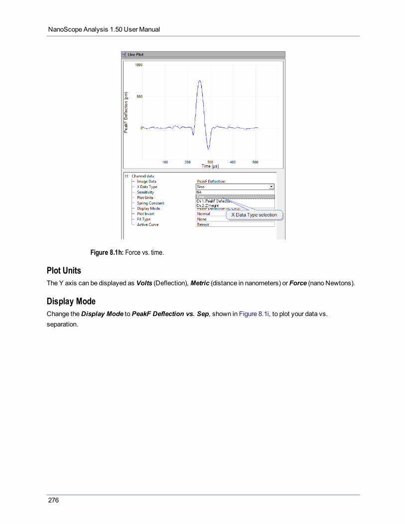
NanoScope Analysis 1.50 User Manual
Figure 8.1h: Force vs. time.
Plot UnitsThe Y axis can be displayed as Volts (Deflection),Metric (distance in nanometers) or Force (nano Newtons).
Display ModeChange theDisplay Mode toPeakF Deflection vs. Sep, shown in Figure 8.1i, to plot your data vs.separation.
276
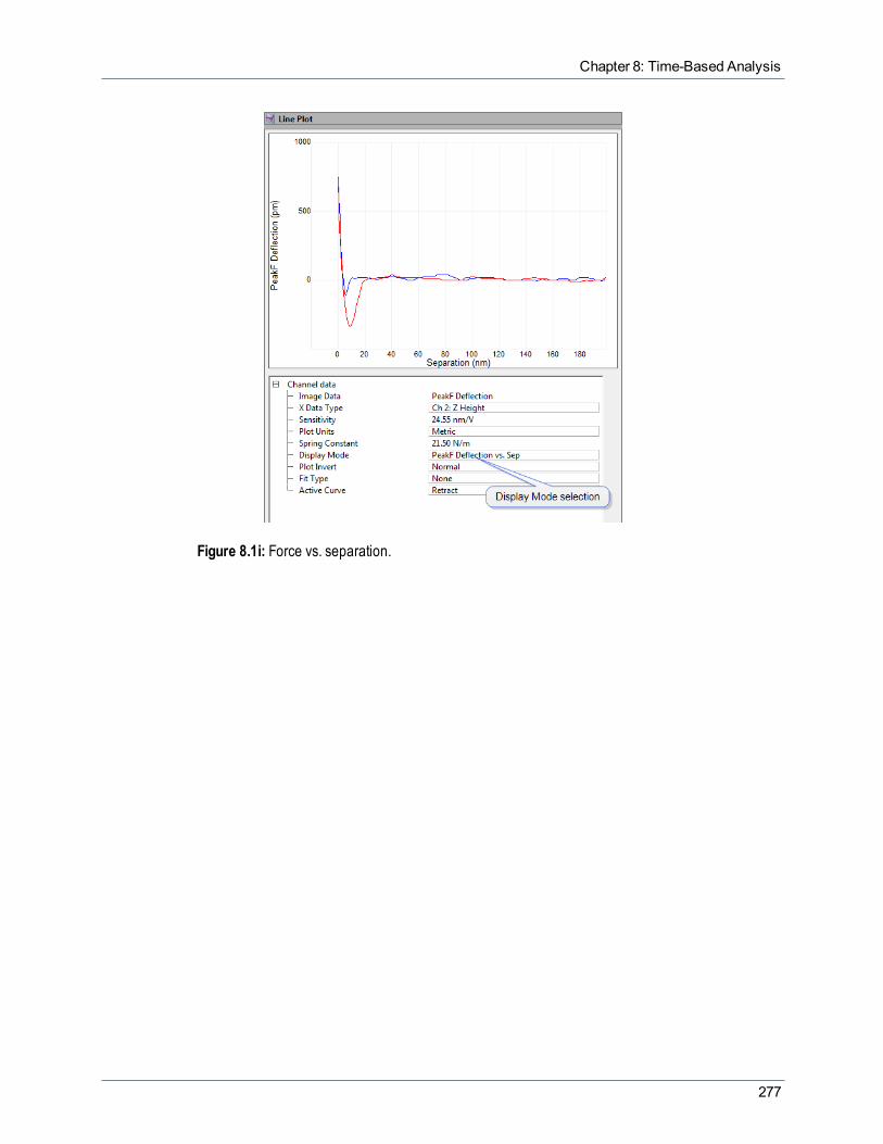
Chapter 8: Time-Based Analysis
Figure 8.1i: Force vs. separation.
277

NanoScope Analysis 1.50 User Manual
8.2 High Speed Data Capture (HSDC)High Speed Data Capture files allow for the capturing and storing of many signals.
8.2.1 HSDC ProcedureTo open aHSDC file in NanoScope Analysis, double click on a NanoScopeHSDC file in theBrowse Files
view or navigate to the preferredHSDC file from theOpen File icon . If the file is indeed anHSDC file, itwill be opened in theHSDC window automatically.
When theHSDC image is opened it should look similar to the image shown in Figure 8.2a. The data forMarkerPair 2 is non-existent as that marker has not yet been added to theHSDC image.
To addmarkers to theHSDC image, position themouse in the Force Curve graph area to the left of the Y axis.The standard cursor will change to a double-headed arrow cursor. When the double-headed cursor appears,left-click themouse, and drag the cursor to the desired position on the Force Curve. The data for the position isautomatically updated in theMarker Pair Results area.
In addition to displaying the captured data plotted vs. time, youmay also perform a Fast Fourier Transform ofthe data by changing theDisplay Type toAmplitude vs Frequency.
278

Chapter 8: Time-Based Analysis
Figure 8.2a: HSDC Window
8.2.2 HSDC InterfaceParameter Description
Display TypeChoose:-Channel vs Time or-Amplitude vs Frequency
Frequency Bin Width Automatically determined
Number of Time Segments Automatically determined
X scale Automatically determined
Y scale Automatically determined
High Speed Data Type Automatically determined
Units Choose: Metric or Volts
Fit Type Choose: None or Line
Table: 8.0bd Channel Data Parameters
279

NanoScope Analysis 1.50 User Manual
Parameter Description
Marker Pair 1:X0 Z position of first marker, Marker Pair 1
X1 Z position of second marker, Marker Pair 1
Y0 Deflection/oscillation position of first marker, Marker Pair 1
Y1 Deflection/oscillation position of second marker, Marker Pair 1
X1 - X0 Z distance between markers in Marker Pair 1
Y1 - Y0 Deflection/oscillation space between markers in Marker Pair 1
dY/dX Slope of Marker Pair 1
dX/dY 1/Slope of Marker Pair 1
Least Squares EquationRoot Mean SquareAverage Deviation
Marker Pair 2:X2 Z position of first marker, Marker Pair 2
X3 Z position of second marker, Marker Pair 2
Y2 Deflection/oscillation position of first marker, Marker Pair 2
Y3 Deflection/oscillation position of second marker, Marker Pair 2
X3 - X2 Z distance between markers in Marker Pair 2
Y3 - Y2 Deflection/oscillation space between markers in Marker Pair 2
dY/dX Slope of Market Pair 2
dX/dY 1/Slope of Marker Pair 2
Least Squares EquationRoot Mean SquareAverage Deviation
Table: 8.0be Marker Pair Results
280

Chapter 8: Time-Based Analysis
8.3 Strip-chartA Strip-chart file plots a channel versus time.
8.3.1 Strip-chart Procedure1. To open aStrip-chart file in NanoScope Analysis, double click on the file in theBrowse Files view or
navigate to the preferred file from theOpen File icon . If the file is indeed aStrip-chart file, it will beopened in theStrip-chartwindow automatically. When the image is opened it should look similar to theimage below.
2. To addmarkers to the image, position themouse in the graph area to the left of the Y axis. The standardcursor will change to a double-headed arrow cursor. When the double-headed cursor appears, left-clickthemouse, and drag the cursor to the desired position on the graph. The data for the position is auto-matically updated in theMarker Pair Results area.
281

NanoScope Analysis 1.50 User Manual
Figure 8.3a: Strip-chart Window
8.3.2 Strip-chart InterfaceParameter Description
Image Data Determined by original data
Sens. ZsensFit Type Choose: None, Line, Hertzian, WLC
Table: 8.0bf Channel Data Input Parameters
Parameter Description
Marker Pair 1:X0 Z position of first marker, Marker Pair 1
282
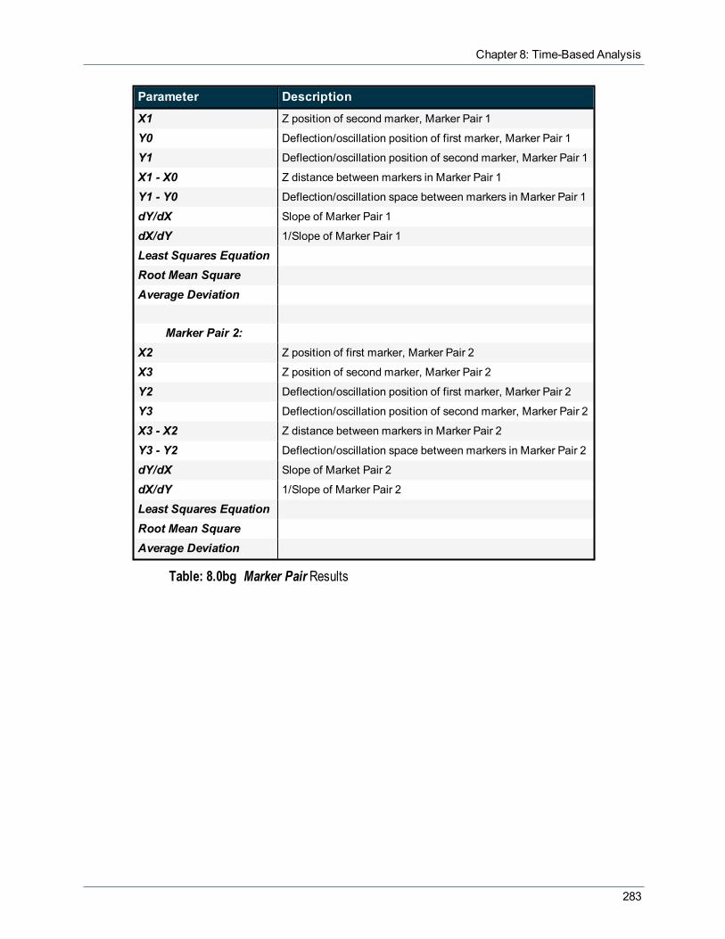
Chapter 8: Time-Based Analysis
Parameter Description
X1 Z position of second marker, Marker Pair 1
Y0 Deflection/oscillation position of first marker, Marker Pair 1
Y1 Deflection/oscillation position of second marker, Marker Pair 1
X1 - X0 Z distance between markers in Marker Pair 1
Y1 - Y0 Deflection/oscillation space between markers in Marker Pair 1
dY/dX Slope of Marker Pair 1
dX/dY 1/Slope of Marker Pair 1
Least Squares EquationRoot Mean SquareAverage Deviation
Marker Pair 2:X2 Z position of first marker, Marker Pair 2
X3 Z position of second marker, Marker Pair 2
Y2 Deflection/oscillation position of first marker, Marker Pair 2
Y3 Deflection/oscillation position of second marker, Marker Pair 2
X3 - X2 Z distance between markers in Marker Pair 2
Y3 - Y2 Deflection/oscillation space between markers in Marker Pair 2
dY/dX Slope of Market Pair 2
dX/dY 1/Slope of Marker Pair 2
Least Squares EquationRoot Mean SquareAverage Deviation
Table: 8.0bg Marker Pair Results
283
NanoScope Analysis 1.50 User Manual
8.4 Strip-chart Combined ChannelsTheStrip-chart Combined plots a channel versus time and two different channels versus each other. Bycomparing the two different charts it is possible to correlate multiple channels against time.
8.4.1 Strip-chart Combined Procedure1. To open aStrip-chart file in NanoScope Analysis, double click on a NanoScope Timed file in the
Browse Files view or navigate to the preferred Timed file from theOpen File icon . If the file isindeed a Timed file, it will be opened in theStrip-chartwindow automatically. When the image isopened it should look similar to the image below. The data forMarker Pair 2 is non-existent, as thatmarker has not yet been added to theStrip-chart image.
2. Now, to open theStrip-chart Combinedwindow, click on the Strip-chart Combined icon from the Icontoolbar. TheStrip-chart Combinedwindow will open.
3. To addmarkers to the image, position themouse in the graph area to the left of the Y axis. The standardcursor will change to a double-headed arrow cursor. When the double-headed cursor appears, left-clickthemouse, and drag the cursor to the desired position on the graph. The data for the position is auto-matically updated in theMarker Pair Results area.
284
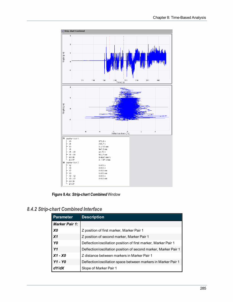
Chapter 8: Time-Based Analysis
Figure 8.4a: Strip-chart CombinedWindow
8.4.2 Strip-chart Combined InterfaceParameter Description
Marker Pair 1:X0 Z position of first marker, Marker Pair 1
X1 Z position of second marker, Marker Pair 1
Y0 Deflection/oscillation position of first marker, Marker Pair 1
Y1 Deflection/oscillation position of second marker, Marker Pair 1
X1 - X0 Z distance between markers in Marker Pair 1
Y1 - Y0 Deflection/oscillation space between markers in Marker Pair 1
dY/dX Slope of Marker Pair 1
285
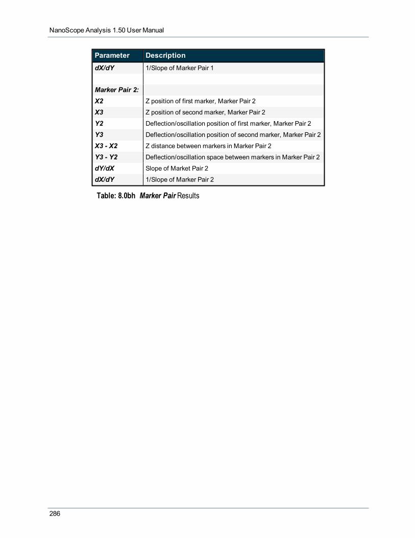
NanoScope Analysis 1.50 User Manual
Parameter Description
dX/dY 1/Slope of Marker Pair 1
Marker Pair 2:X2 Z position of first marker, Marker Pair 2
X3 Z position of second marker, Marker Pair 2
Y2 Deflection/oscillation position of first marker, Marker Pair 2
Y3 Deflection/oscillation position of second marker, Marker Pair 2
X3 - X2 Z distance between markers in Marker Pair 2
Y3 - Y2 Deflection/oscillation space between markers in Marker Pair 2
dY/dX Slope of Market Pair 2
dX/dY 1/Slope of Marker Pair 2
Table: 8.0bh Marker Pair Results
286
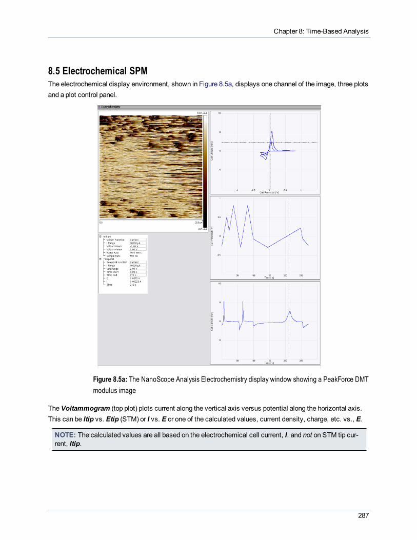
Chapter 8: Time-Based Analysis
8.5 Electrochemical SPMThe electrochemical display environment, shown in Figure 8.5a, displays one channel of the image, three plotsand a plot control panel.
Figure 8.5a: The NanoScope Analysis Electrochemistry display window showing a PeakForce DMTmodulus image
TheVoltammogram (top plot) plots current along the vertical axis versus potential along the horizontal axis.This can be Itip vs. Etip (STM) or I vs. E or one of the calculated values, current density, charge, etc. vs., E.
NOTE: The calculated values are all based on the electrochemical cell current, I, and not on STM tip cur-rent, Itip.
287

NanoScope Analysis 1.50 User Manual
In the Temporal (bottom two) plots, the horizontal axis is always time. A voltage (top) and a current (bottom)are plotted versus time. The voltage can be the electrochemical cell potential, E, or the potential of the STM tip,Etip. The current can be electrochemical cell current, I, one of its derivative quantities; e.g., charge, currentdensity, etc., or it can be the current flowing through the STM tip, Itip.
The time scale on the Temporal graph does not necessarily correspond to the time required to capture an SPMimage for the following reasons:
1. The total number of data points is limited to 62,254. Hence, the product of theSample Rate and Timerange is limited to 62,254. For example, when one attempts to collect 1000 seconds of data, themax-imum Sample Rate is 62 Hz.
2. If the time to capture an image exceeds the time to record themaximum of the 62,254 electrochemicaldata points that can be stored, only the last 62,254 data points are saved. The data points prior to thelast 62,254 data points are lost. Time zero on the Temporal graph reflects the start of the last 62,254data points.
3. To display on the Temporal graph only a portion of the stored data points, for example, the last 30,000of 62,254 data points recorded using aSample Rate of 100 Hz, define Time Start equal 300 seconds(roughly one-half of themaximum of 623 seconds for this case) and Time End equal 623 seconds in theplot controls dialog box for the NanoScope Analysis software. In this case, time zero on the Temporalgraph would actually be the first data point after the 300-secondmarker.
CursorsA mouse click-and-hold-and-dragmay be used in the Temporal plot windows to display data at any point in theexperiment.
Themarkers in all three plots will follow the position of the cursor as themouse is dragged (click and hold) inthe plot. The electrochemical cell data (E, I, Time) at the position of themarker is displayed in the Temporalpanel of the plot controls dialog box in the lower left of the EC window.
A marker on theVoltammogram will indicate the corresponding data as potential vs. current. The vertical linein the Temporal plot indicates, in time, when the first line of the SPM image was captured. As the Temporalmarker is moved, a horizontal line on the SPM image will move to the scan line that was captured atapproximately the same time. See Figure 8.5a. In addition, themousemay drag (click-and-hold) the line on theimage to any scan line, and this will move the Temporal andVoltammogrammarkers to the appropriatepositions and update the electrochemical cell data display.
Note that it is possible to have data displayed in the Temporal plot across such a time window that it does notcorrespond to any of the data in the SPM image. This is because when an SPM image is captured, the last62,254 electrochemical data points are also recorded in the file, and only a portion of the electrochemical datarecordedmay correspond to the time required to capture the SPM image; i.e., the imagemay have taken lesstime to capture than the last 62,254 electrochemical data points.
A mouse Ctrl-click-and-hold-and-dragmay be used in the plot windows to zoom in on a portion of the data.Clicking themagnifying glass in the lower left corner of the plot window resets the plot.
288

Chapter 8: Time-Based Analysis
Plot Controls Dialog BoxThe parameters in the plot controls dialog box, shown in Figure 8.5b and described in Table: 8.0bi, allow you toscale and clip the electrochemical data.
Figure 8.5b: The electrochemistry plot control dialog box
289

NanoScope Analysis 1.50 User Manual
ParameterGroup Parameter Description
Voltam
VoltamFunction
Indicates the quantities plotted along horizontal and vertical axes of thevoltammogram.
Settings:
l Chargel Chrg Densl Currentl Cur Densl Log Curl Lg Cur Densl Tip Current
When this parameter is Itip, the current through STM tip is plotted vs. Etip. Allother settings (e.g., current, charge) have the electrochemical cell parameter
plotted vs. E.
I Range Controls the vertical scale of the Voltammogram graph.
VoltMinimum Voltage corresponding to left edge of Voltammogram graph.
VoltMaximum Voltage corresponding to the right edge of the Voltammogram graph.
RampRate Indicates the ramp rate at the time of capture.
SampleRate The rate of electrochemical data recording at the time of capture.
TipReference
STM only. Indicates whether the STM tip potential, Etip, or tip bias, Ebias, is keptconstant during ramping.
RampElectrode Indicates which electrode (working or STM tip) was ramped at time of capture.
TemporalTemporalFunction
Indicates what parameter is plotted along the vertical axis vs. time along horizontalaxis.
Settings:
l Chargel Chrg Densl Currentl Cur Densl Log Curl Lg Cur Densl Tip Current
I Range Controls the current scale of the Temporal graph.
290

Chapter 8: Time-Based Analysis
ParameterGroup Parameter Description
V Range Controls the voltage scale of the Temporal graph.Time Start Start time of displayed data (left edge of plot).
Time End
End time of displayed data (right edge of plot).
NOTE: The system will record the current and voltage vs. time data startingfrom time = 0 in the Temporal graph. The current is integrated starting attime = 0 of the Temporal graph. Any data that fits into the Temporal graphwill be displayed. Voltammogram will display data within the time range ofthe Temporal graph.
E Cell potential at marker position.
Etip STM only. Potential of the tip relative to the reference electrode.
Ebias STM only. Voltage difference between tip and sample, Etip - E.I Cell current at marker position.
Time Time at marker position relative to start of Temporal plot. The data is normally dis-played using the Temporal Time range at the time of capture.
Table: 8.0bi Plot Controls parameters
291


Chapter 9: MIRO
Chapter9:MIRO
Bruker's Microscope Image Registration andOverlay (MIRO) software integrates AFM imaging with opticalmicroscopy. This optional software allows the user to automatically import and rescale light microscopeimages, which can then be used to direct the location of AFM imaging and forcemeasurements. Correlateddatasets can be captured and analyzed with the powerful offline functionality.
Figure 9.0a: Fixed macrophage cell labeled with Alexa Fluor phalloidin (red) and DAPI (blue) withAFM inset. Image courtesey of Peter Hanley, Institute fro Physiology II, University of Muenster,Germany.
If you would likemore information or would like to purchaseMIRO, please contact Bruker.
MIRO™ (Microscope Image Registration andOverlay) user-guided interactive software allows you to do thefollowing:
l Register optical and AFM imagesl Import and overlay multiple optical and AFM imagesl Adjust and fine-tune the registration parameters of both optical and AFM imagesl Store and restore profiles for different system configurations (e.g. multiple objective lenses)l Adjust image color, transparency and overlay options—individually for each channell Export overlaid imagesl Save each overlay and associated image parameters for further analysis in offlinemodel MIRO 2.0 adds multipleRegion of Interest views which allow you tomore easily compare overlaid
images
Refer to the following sections for information about MIRO:
293
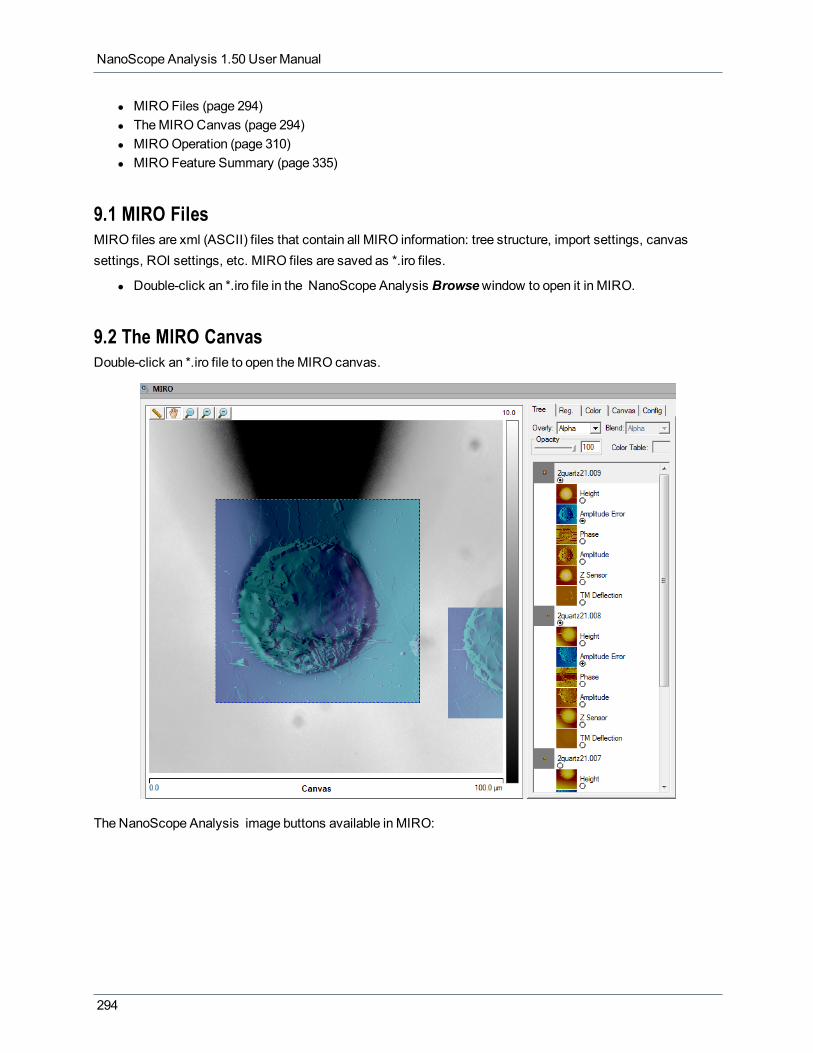
NanoScope Analysis 1.50 User Manual
l MIRO Files (page 294)l TheMIROCanvas (page 294)l MIROOperation (page 310)l MIRO Feature Summary (page 335)
9.1 MIRO FilesMIRO files are xml (ASCII) files that contain all MIRO information: tree structure, import settings, canvassettings, ROI settings, etc. MIRO files are saved as *.iro files.
l Double-click an *.iro file in the NanoScope Analysis Browsewindow to open it in MIRO.
9.2 The MIRO CanvasDouble-click an *.iro file to open theMIRO canvas.
The NanoScope Analysis image buttons available in MIRO:
294

Chapter 9: MIRO
The first three buttons represent "modes" in which you will be able to interact differently with the imageshowing on the canvas:
Cursor Mode:Allows the user to draw a box, line, or place amarker to obtain measurements from theimage displayed in the canvas.
l With theCursor Mode button selected, click the right mouse button to select Box, Rotatingline, orCross.
l Left-click and drag on the image to draw the box, line, or cross on the element you wish tomeas-ure.
l Information about the box dimensions or line length and angle will appear in a tool tip at the bot-tom left-hand-side of the canvas.
Pan Mode: From a zoomed canvas, allows the user to drag other areas of the canvas into view.
l With thePan Mode button selected, click the left mouse button and drag the canvas around asdesired.
Zoom Mode:Allows the user to draw a zoom in box on the canvas.
l With the Zoom Mode button selected, click the left mouse button and drag to create a zoombox.
l Note that the box will be drawn from the center (click point) outward.
Additional buttons andmouse functions control other interactions with the image:
l Zoom In:Button is active for one click only; zooms in by 40%, relative to the current screen center.l Zoom Out:Button is active for one click only; zooms out by 40%, relative to the current screen center.l Mouse Wheel: Turn themouse wheel to zoom in (roll away from yourself) or zoom out (roll towards your-
self) in 20% increments.l Current position of themouse cursor (arrow) is used as the anchor point of the zoom when using
themouse wheell Enabled regardless of the activemode in the canvas (Cursor Mode, PanMode, or ZoomMode)
l Mouse Double Click:Centers the view on the clicked spot.l Does not zoom in or outl Enabled regardless of the activemode in the canvas (Cursor Mode, PanMode, or ZoomMode)
TheMIRO Toolbar (page 309), which appears in the NanoScopemain window whenMIRO is active, offersadditional imaging options.
TheMIRO canvas contains all of the following tabs, each with its respective functionality:
l The Tree Tab (page 296)l The Registration Tab (page 298)
295

NanoScope Analysis 1.50 User Manual
l The Color Tab (page 299)l The Canvas Tab (page 308)l The Configuration Tab (page 308)
9.2.1 The Tree TabThe Tree tab allows you to select the AFM and optical channels to be overlaid, change their tree structure,adjust their overlay and blend properties, color, and opacity.
Figure 9.2a:MIRO Canvas with Lines and Buttons selected
Functions Performed on a Selected Image:l Show/Hide: Click the radio button below the image name to show/hide the image (as demonstrated in
Figure 9.2a).l Change Order in tree: Drag the image to change its order in the tree. The order of images in the tree
determines the overlay order on the canvas.l Overlay: Specifies the overlay method for the images. Define α as the opacity and "n" as the layer num-
ber.
Settings:
l Alpha: Colorn = ColornOriginal* αn + Colorn–1 * (1–αn)l Add: Colorn = ColornOriginal * αn + Colorn–1l Max: Max[ColornOriginal* αn, Colorn–1]
296

Chapter 9: MIRO
l Blend:Specifies the overlay method for the channels. Define n as the layer number with n = 1 the bot-tom layer and αn as the opacity of the n
th layer.
Settings:
l Alpha:Colorn = ColornOriginal * αn + Colorn–1 * (1–αn)l Add:Colorn = ColornOriginal * αn + Colorn–1l Max:Max[ColornOriginal * αn, Colorn–1]
l Opacity:Move theOpacity slider, enter a number or use the arrow keys to change the opacity of animage. This function aids image alignment.
l Color Table:Selects the color table. See List of Color Tables.
Canvas Formatting Functions:Right-click the Tree on the right-hand side of the canvas to access most of the Tree Tab functions:
Figure 9.2b: Example of function options available by right-clicking on the tree
l Enable Label Edit:When selected, allows the user to change the image labell Lines and Buttons: The Lines and Buttons function, shown in Figure 9.2a, displays the image tree
structure. Clicking a button collapses that portion of the tree.l Import Images to Top:Sets default to import an image to the top of the selected imagel Import Images to Bottom:Sets default to import an image to the bottom of the selected imagel Add new Group to Top:Adds a new group to the top of the selected imagel Add new Group to Bottom:Adds a new group to the bottom of the selected imagel Delete Selected:Deletes the selected image fromMIROl Delete All:Deletes all images fromMIRO
297

NanoScope Analysis 1.50 User Manual
9.2.2 The Registration TabTheRegistration tab is used to adjust the registration overlay.
Once the initial registration process has been performed, you can expand, shrink, translate or rotate a selectedimage so that it more accurately overlaps a correlating area of an AFM image.
CAUTION: Adjustments to the registration are usually done on optical images.AFM images always import according to their registration-associated scan inform-ation.
Figure 9.2c: The Registration tab in the MIRO window
298
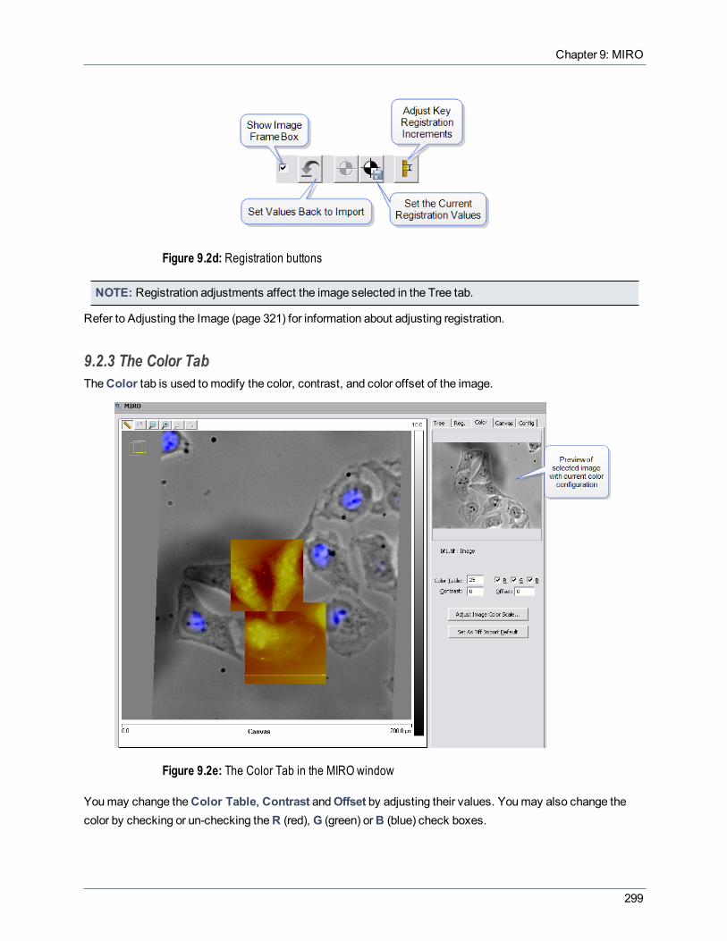
Chapter 9: MIRO
Figure 9.2d: Registration buttons
NOTE: Registration adjustments affect the image selected in the Tree tab.
Refer to Adjusting the Image (page 321) for information about adjusting registration.
9.2.3 The Color TabTheColor tab is used tomodify the color, contrast, and color offset of the image.
Figure 9.2e: The Color Tab in the MIRO window
Youmay change theColor Table, Contrast andOffset by adjusting their values. Youmay also change thecolor by checking or un-checking theR (red), G (green) orB (blue) check boxes.
299

NanoScope Analysis 1.50 User Manual
NOTE: Color adjustments affect the image selected in the Tree tab.
Color Tab Parameters
Color TableChoose among the standard NanoScope color tables
Range and Settings: 0 to 25 (see List of Color Tables).
RGBTurns On/Off Red, Green and Blue in the image (see Figure 9.2f, Figure 9.2g, Figure 9.2h, and Figure 9.2i,below for examples).
Figure 9.2f: Original Image in Color Table 25
300

Chapter 9: MIRO
Figure 9.2g: Image of Figure 9.2f with only R (Red) selected
301

NanoScope Analysis 1.50 User Manual
Figure 9.2h: Image of Figure 9.2f with only G (Green) selected
302

Chapter 9: MIRO
Figure 9.2i: Image of Figure 9.2f with only B (Blue) selected
ContrastAdjusts image contrast
Range and Settings: –10 to +10. See below for examples and for a plot of the respective image intensity levels.
303

NanoScope Analysis 1.50 User Manual
Figure 9.2j: Contrast set to –10
304

Chapter 9: MIRO
Figure 9.2k: Contrast set to +10
Figure 9.2l: Plots of image intensity from Figure 5 (left) and Figure 6 (right)
OffsetAdds or subtracts a constant offset from each color table index, shifting the color scale up or down.
Offset effectively changes the color value around which the color scale is mapped.
Range and Settings: –128 to +128. See below for examples and a plot of the respective image intensity levels.
305

NanoScope Analysis 1.50 User Manual
Figure 9.2m: Offset set to –128
306

Chapter 9: MIRO
Figure 9.2n: Offset set to +128
Figure 9.2o: Plots of image intensity in Figure 8 (left) and Figure 9 (right)
Adjust Image Color ScaleOpens the Color Scale (page 29) function.
Set As Tiff Import DefaultSets the above parameters as the default tiff image import parameters.
NOTE: This function is available only when you import a tiff image.
307

NanoScope Analysis 1.50 User Manual
9.2.4 The Canvas TabTheCanvas tab is used to adjust the canvas size, location and angle.
Figure 9.2p: The Canvas Tab in the MIRO window
Canvas ControlsShow Image Frame Box: Indicates, using a blue dashed line, which image is selected and can bemanipulated. If this option is not selected, adjustments to the images can not bemade using themouse.
9.2.5 The Configuration TabTheConfiguration tab is used to select the camera and overlay methods as well as set up defaults for theimport of images.
308

Chapter 9: MIRO
Figure 9.2q: The Configuration Tab in the MIRO window
Configuration Controls
Interpolation ModeSettings:
l Nearest Neighbor—Selects the value of the nearest pointl Bi-Linear—Two dimensional linear interpolation
SPM import channels limit:Limits themaximum number of channels that can be imported in one image.
Range: 1 - 8
Image Import ConfigAllows setting defaults for importing images such as registration profiles, etc.
9.2.6 The MIRO ToolbarTheMIRO toolbar appears whenMIRO is active. The following functions are available through theMIROtoolbar:
309

NanoScope Analysis 1.50 User Manual
Import images. When optical images are imported, you will be prompted to select a registrationprofile to use from the Image Import Configuration window. See Importing Images (page 313) for moreinformation.
Export From the Canvas View (page 331)
Create Region Of Interest (page 318)
Refresh Region Of Interest (page 318)
Configure Region Of Interest (page 318)
Undo Image Change:SeeUndo/Redo (page 328) for a discussion of the Undo function.Redo Image Change:SeeUndo/Redo (page 328) for a discussion of theRedo function.
9.3 MIRO OperationThere are several helpful topics for MIRO camera operations:
l Introduction to Optical Image Registration (page 310)l Placing Images on theMIROCanvas (page 313)
l Importing Images (page 313)l Region Of Interest (page 318)l Adjusting the Image (page 321)l Moving Images (page 322)l Undo/Redo (page 328)l Export From the Canvas View (page 331)l MIRO Import/Export (page 329)
9.3.1 Introduction to Optical Image RegistrationIn order to import and overlay an optical image to theMIRO canvas, the following information is needed:
l Rotation Anglel X Scalel Y Scalel X Offsetl Y Offsetl Image Flipsl Non-linear correction data
310

Chapter 9: MIRO
MIRO saves this data as *.irc files in theMirc directory. When an optical image is imported, the data in theselected *.irc file is used.
You can view, edit, create and delete these *.irc files using the Image Import Configurations window. Toaccess the Image Import Configurations window, click the Image Import Config button in theConfig tab:
The Image Import Configurationswindow will open:
311

NanoScope Analysis 1.50 User Manual
There are several ways to create or modify the registration *.irc file:
1. Estimate or calculate the registration data and enter it in the Image Import Configurations Win-dow.
2. After the optical image is “tweaked” (see Adjusting the Image (page 321)) the registration datacan be set/saved (*.irc file) by clicking theSet the current values as import registration iconon The Registration Tab (page 298).
The Image Import Configurationswindow is also used to configure Import Z Order andDialog ShowOptions:
Import Z Order Parametersl Import To Top: Imports selected images to the top of the image tree.l Import To Bottom: Imports selected images to the bottom of the image tree. Imported images may not
be visible if they are beneath another image with high opacity.
Dialog Show Optionsl On Every File:Opens the Configurations for Import window (see Importing Images (page 313)) each
time a file is opened.l On 1st File Only:Opens the Configurations for Import window for the first file whenmultiple optical
images are selected (select multiple images by holding down the CTRL key while clicking each filename).
l Don’t Show:Does not open the Configurations for Import window when optical images are imported.
NOTE: If you have turned theDon’t Show option "On" and wish to display the Configurations forImport window, you will have to access it through the Image Import Config. button in theConfigtab.
312
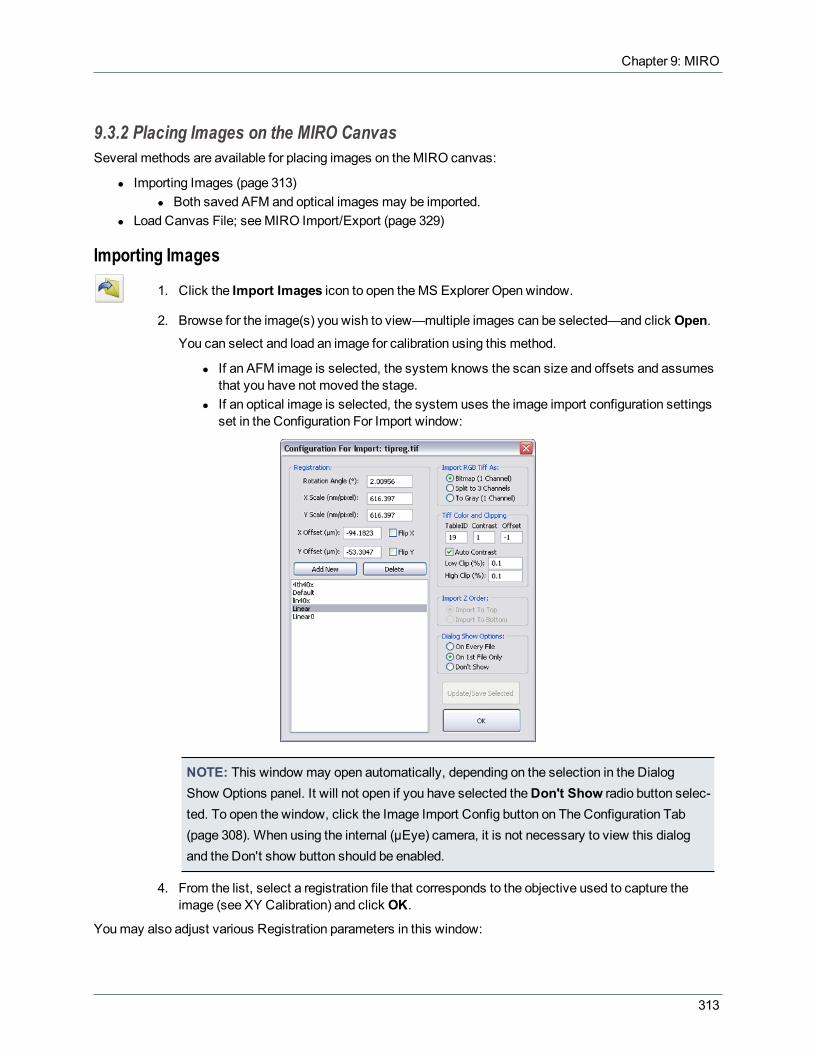
Chapter 9: MIRO
9.3.2 Placing Images on the MIRO CanvasSeveral methods are available for placing images on theMIRO canvas:
l Importing Images (page 313)l Both saved AFM and optical images may be imported.
l Load Canvas File; seeMIRO Import/Export (page 329)
Importing Images
1. Click the Import Images icon to open theMS Explorer Open window.
2. Browse for the image(s) you wish to view—multiple images can be selected—and click Open.You can select and load an image for calibration using this method.
l If an AFM image is selected, the system knows the scan size and offsets and assumesthat you have not moved the stage.
l If an optical image is selected, the system uses the image import configuration settingsset in the Configuration For Import window:
NOTE: This window may open automatically, depending on the selection in the DialogShow Options panel. It will not open if you have selected theDon't Show radio button selec-ted. To open the window, click the Image Import Config button on The Configuration Tab(page 308). When using the internal (μEye) camera, it is not necessary to view this dialogand the Don't show button should be enabled.
4. From the list, select a registration file that corresponds to the objective used to capture theimage (see XY Calibration) and click OK.
Youmay also adjust various Registration parameters in this window:
313
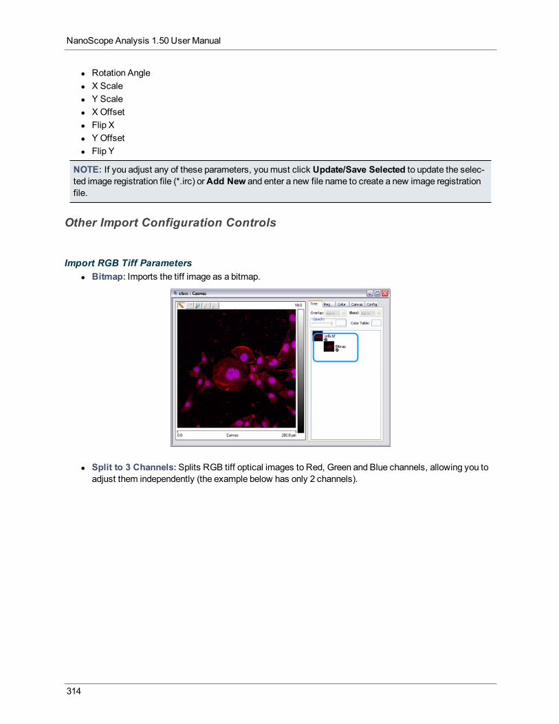
NanoScope Analysis 1.50 User Manual
l Rotation Anglel X Scalel Y Scalel X Offsetl Flip Xl Y Offsetl Flip Y
NOTE: If you adjust any of these parameters, youmust click Update/Save Selected to update the selec-ted image registration file (*.irc) orAdd New and enter a new file name to create a new image registrationfile.
Other Import Configuration Controls
Import RGB Tiff Parametersl Bitmap: Imports the tiff image as a bitmap.
l Split to 3 Channels:Splits RGB tiff optical images to Red, Green and Blue channels, allowing you toadjust them independently (the example below has only 2 channels).
314

Chapter 9: MIRO
l To Gray: Imports the tiff image as a 16 bit gray-scale image.
Tiff Color and Clipping Parameters
NOTE: These parameters, with the exception of Auto Contrast, can be pre-set using theSet As TiffImport Default button in the Color tab (see Color Tab Parameters (page 300) for more information).
l Color Table ID:Chose a standard NanoScope color table.l Range and Settings: 0 to 25.l See List of Color Tables
l Contrast: Image contrast.l Range and Settings: –10 to +10.l SeeContrast (page 303) for more information and examples.
l Offset:Adds or subtracts a constant offset from each color table index, shifting the color scale up ordown. Offset effectively changes the color value around which the color scale is mapped.
l Range and Settings: –128 to +128.l SeeOffset (page 305) for more information and examples.
315

NanoScope Analysis 1.50 User Manual
l Auto Contrast:Auto Contrast automatically adjusts the image contrast by first clipping a small, user-adjustable, number of pixels, Low Clip and High Clip, to accommodate long tails in the contrast dis-tribution. Auto Contrast is turned on if checked.
Figure 9.3a shows the original tiff image and Figure 9.3b shows a graph of its intensity (long tails arecircled):
Figure 9.3a: Original Tiff Image
Figure 9.3b: Graph of Image Intensity of image in Figure 1 showing the tails in the distribution
Auto Contrast removes the long tails in the distribution then adjusts the dynamic range to fill the range.
Figure 9.3c shows the original tiff image before import and Figure 9.3d shows a graph of thecorresponding image intensity:
316

Chapter 9: MIRO
Figure 9.3c: Original Tiff Image Before Import
Figure 9.3d: Graph of Image Intensity of image in Figure 3
Figure 9.3e shows the same tiff image after Auto Contrast adjustment, and Figure 9.3f shows a graph ofthe corresponding image intensity:
Figure 9.3e: Image After Import with Auto Contrast On
317
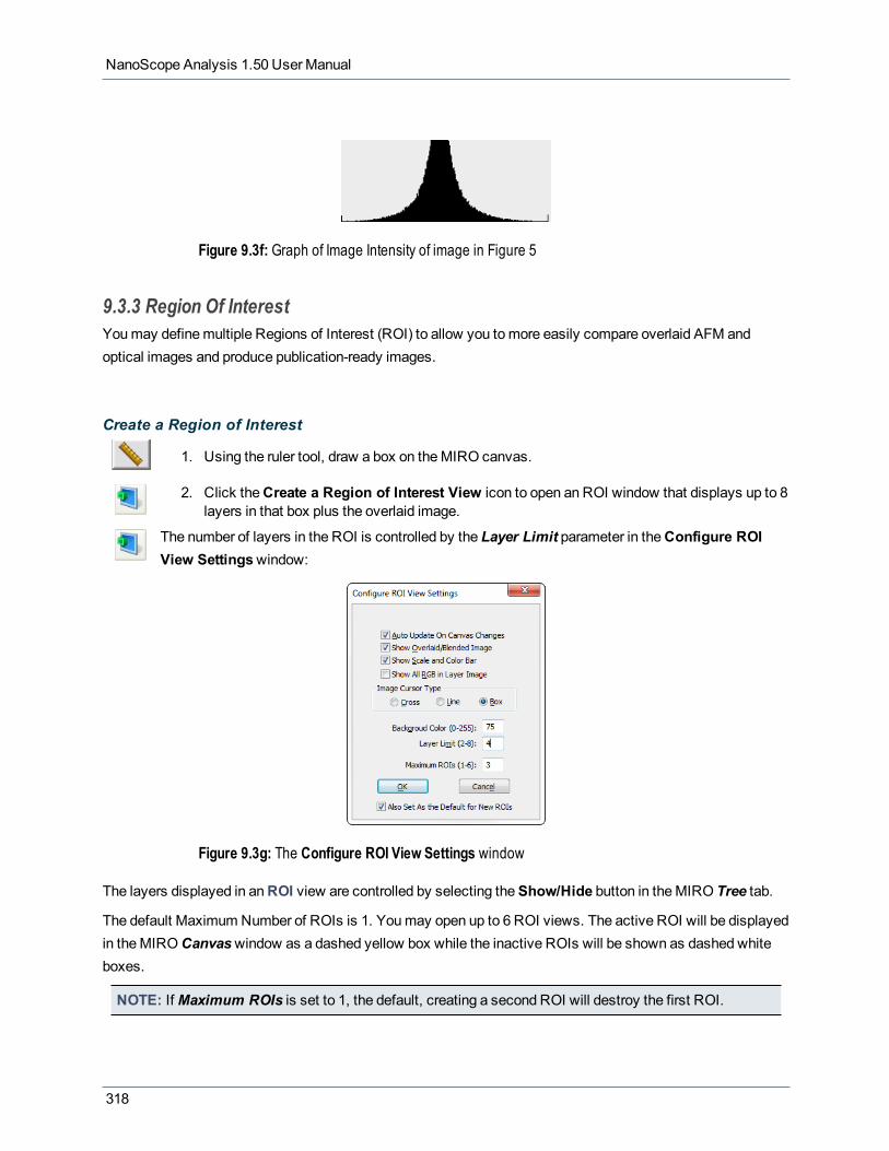
NanoScope Analysis 1.50 User Manual
Figure 9.3f: Graph of Image Intensity of image in Figure 5
9.3.3 Region Of InterestYoumay definemultiple Regions of Interest (ROI) to allow you tomore easily compare overlaid AFM andoptical images and produce publication-ready images.
Create a Region of Interest
1. Using the ruler tool, draw a box on theMIRO canvas.
2. Click theCreate a Region of Interest View icon to open an ROI window that displays up to 8layers in that box plus the overlaid image.
The number of layers in the ROI is controlled by the Layer Limit parameter in theConfigure ROIView Settingswindow:
Figure 9.3g: The Configure ROI View Settings window
The layers displayed in anROI view are controlled by selecting theShow/Hide button in theMIRO Tree tab.
The default Maximum Number of ROIs is 1. Youmay open up to 6 ROI views. The active ROI will be displayedin theMIROCanvaswindow as a dashed yellow box while the inactive ROIs will be shown as dashed whiteboxes.
NOTE: IfMaximum ROIs is set to 1, the default, creating a second ROI will destroy the first ROI.
318

Chapter 9: MIRO
The default ROI window displays 2 layers plus the overlaid image:
NOTE: Regions of interest are square. If you draw a rectangle, the narrowest side will be used to definethe square.
319
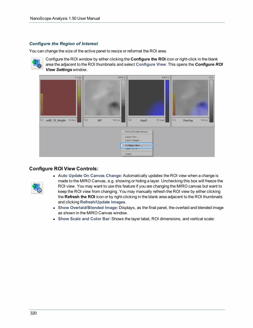
NanoScope Analysis 1.50 User Manual
Configure the Region of InterestYou can change the size of the active panel to resize or reformat the ROI area.
Configure the ROI window by either clicking theConfigure the ROI icon or right-click in the blankarea the adjacent to the ROI thumbnails and select Configure View. This opens theConfigure ROIView Settingswindow.
Configure ROI View Controls:l Auto Update On Canvas Change:Automatically updates the ROI view when a change is
made to theMIROCanvas, e.g. showing or hiding a layer. Unchecking this box will freeze theROI view. Youmay want to use this feature if you are changing theMIRO canvas but want tokeep the ROI view from changing. Youmay manually refresh the ROI view by either clickingtheRefresh the ROI icon or by right-clicking in the blank area adjacent to the ROI thumbnailsand clickingRefresh/Update Images.
l Show Overlaid/Blended Image:Displays, as the final panel, the overlaid and blended imageas shown in theMIROCanvas window.
l Show Scale and Color Bar:Shows the layer label, ROI dimensions, and vertical scale:
320

Chapter 9: MIRO
l Show All RGB in Layer Image:Shows Red (R), Green (G) and Blue (B) regardless of thesettings in the Color tab.
l Image Cursor Type:May be a Cross, Line or Box (default). The same cursor will appear in allimages in that ROI window.
l Background Color: The intensity of the areas of the ROI that have no image with 0 being thedarkest and 255 the lightest.
l Layer Limit: The number of layers displayed is set in the Layer Limit box. Youmay displayup to 8 layers in an ROI window.
l Maximum ROIs: Themaximum number of ROIs.l Also Set As the Default for New ROIs: Sets new ROI default to these values.
Click OK to accept your changes orCancel to return to the unchanged ROI window.
Regions of interest are saved when you saveMIRO (*.iro) files. The Regions of Interest will open when youopen the savedMIRO file.
9.3.4 Adjusting the ImageTheMIRO canvas offers a wide range of options in terms of image contrast, color, opacity…Beyond theaesthetic aspect, it can be very useful to check if the AFM and optical images exactly overlap each other, byselecting an AFM channel—deflection or amplitude usually gives the best contrast—and setting the opacityparameter to zero. Then progressively increase this value to see the AFM image appear.
Save the registration file once the optical images have been adjusted for optimal registration.
Another helpful option is to select two AFM channels (for instance Amplitude Error and Phase) anduse this function to alternately switch from one channel to the other.
321
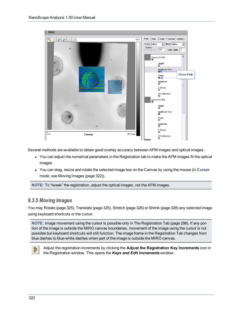
NanoScope Analysis 1.50 User Manual
Several methods are available to obtain good overlay accuracy between AFM images and optical images:
l You can adjust the numerical parameters in the Registration tab tomake the AFM images fit the opticalimages.
l You can drag, resize and rotate the selected image box on the Canvas by using themouse (inCursormode; seeMoving Images (page 322)).
NOTE: To “tweak” the registration, adjust the optical images, not the AFM images.
9.3.5 Moving ImagesYoumay Rotate (page 325), Translate (page 325), Stretch (page 326) or Shrink (page 328) any selected imageusing keyboard shortcuts or the cursor.
NOTE: Imagemovement using the cursor is possible only in The Registration Tab (page 298). If any por-tion of the image is outside theMIRO canvas boundaries, movement of the image using the cursor is notpossible but keyboard shortcuts will still function. The image frame in the Registration Tab changes fromblue dashes to blue-white dashes when part of the image is outside theMIRO canvas.
Adjust the registration increments by clicking the Adjust the Registration Key Increments icon inthe Registration window. This opens theKeys and Edit Incrementswindow:
322

Chapter 9: MIRO
Change theXY Offset Adjusting Increment, theRotation Adjusting Increment and/or theXY ScaleAdjusting Ratio Increment and click OK.
Select the image you wish tomanipulate in the Tree Tab. A blue-white dashed line will surround and bisect theactive image. Then select theRegistration Tab to modify the registration image.
NOTE: If you wish to use themouse, ensure that you are inCursor mode and in the Registration Tab. Themouse cannot be used for Rotate, Translate, Shrink, and Stretch operations in Zoommode.
NOTE: To adjust X and Y independently, uncheck theX-Y Size check box, shown in the RegistrationTab. If the X-Y check box remains checked, the image will stretch proportionately in X and Y.
323

NanoScope Analysis 1.50 User Manual
324
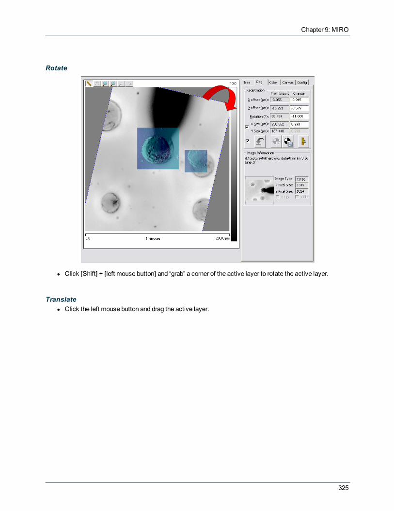
Chapter 9: MIRO
Rotate
l Click [Shift] + [left mouse button] and “grab” a corner of the active layer to rotate the active layer.
Translatel Click the left mouse button and drag the active layer.
325
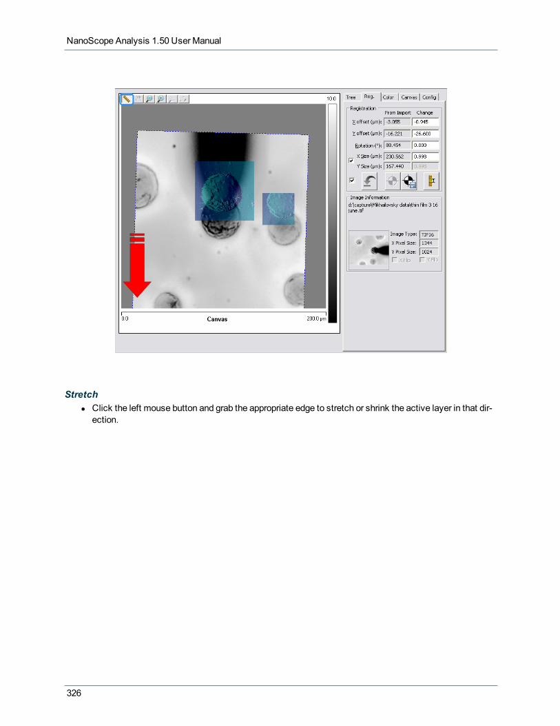
NanoScope Analysis 1.50 User Manual
Stretchl Click the left mouse button and grab the appropriate edge to stretch or shrink the active layer in that dir-
ection.
326

Chapter 9: MIRO
327

NanoScope Analysis 1.50 User Manual
Shrink
l Click the left mouse button and grab an edge to stretch or shrink the active layer.
9.3.6 Undo/RedoTheUndo andRedo functions allow unlimited undo and redo of the following operations withinan image (where the image is defined as the root of a tree):
l Image registration changes: offset, size, rotation, translation, X-Y linking.l Color table, overlay and blend types, opacity, contrast, offset, RGB.l Layer (channel) selection changes.
328

Chapter 9: MIRO
9.3.7 MIRO Import/ExportRight-click in the border of theMIROwindow to open aGUI with options toSave/Load the MIRO File (*.iro) orExport the MIRO View.
329

NanoScope Analysis 1.50 User Manual
Save MIRO File saves the image tree as an *.iro file that can be retrieved later using the Load MIRO Filecommand or by double-clicking on the .iro file in the NanoScope browse window.
NOTE: The image registration file (*.irc) is embedded in the saved *.iro file.
Import Images: refer to Placing Images on theMIROCanvas (page 313) for details.
Export Images: refer to Export From the ROI View (page 332) for details.
Export View saves a JPEG image of the entire MIROCanvas window. This is the same as theExport theView button in the Export Images from Canvas View window.
NOTE:When closing the canvas, the system will prompt you to save the current MIRO con-figuration.
NOTE: Clicking theSave icon with MIRO in focus will also save the .iro file.
For other Export options see Export From the Canvas View (page 331) and Export From the ROI View (page332).
330
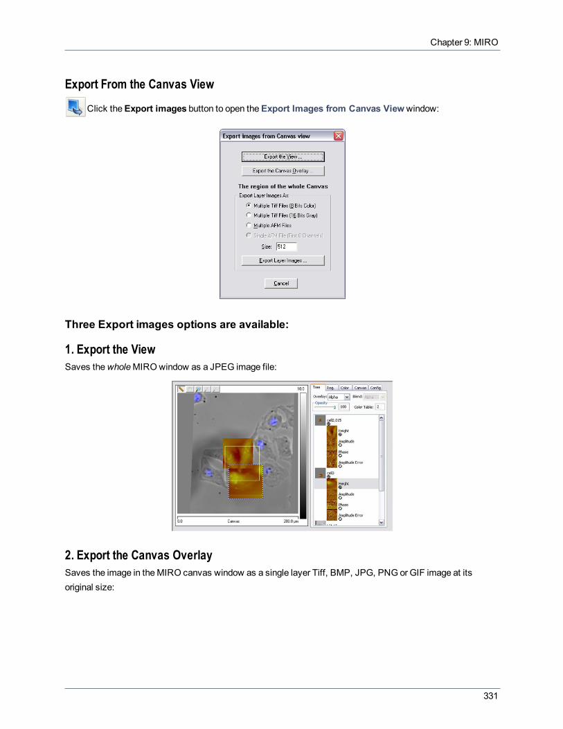
Chapter 9: MIRO
Export From the Canvas View
Click theExport images button to open theExport Images from Canvas Viewwindow:
Three Export images options are available:
1. Export the ViewSaves thewholeMIROwindow as a JPEG image file:
2. Export the Canvas OverlaySaves the image in theMIRO canvas window as a single layer Tiff, BMP, JPG, PNG or GIF image at itsoriginal size:
331

NanoScope Analysis 1.50 User Manual
3. Export Layer ImagesExports, in order of priority, selected layers in either the region inside the select box, the zoomed region or theentire MIRO canvas.
Use theShow/Hide button to control which layers will be exported. Youmay also adjust the exported imagesize by changing theSize parameter (in theExport Layer Images As section of the Export Images From theCanvas View window, above). The image interpolationmode is determined by the InterpolationMode setting inThe Configuration Tab (page 308). Several export options are available:
l Individual layers are exported as 8-bit RGB uncompressed tiff files.l Individual layers are exported as 16-bit gray-scale uncompressed tiff files.l Individual layers, including optical images, are exported as *.spm files.
Export From the ROI ViewIt is possible to export images from anROI view by either clicking theExport images icon when theROI window is active, or by right-clicking in the border and selectingExport Images:
332
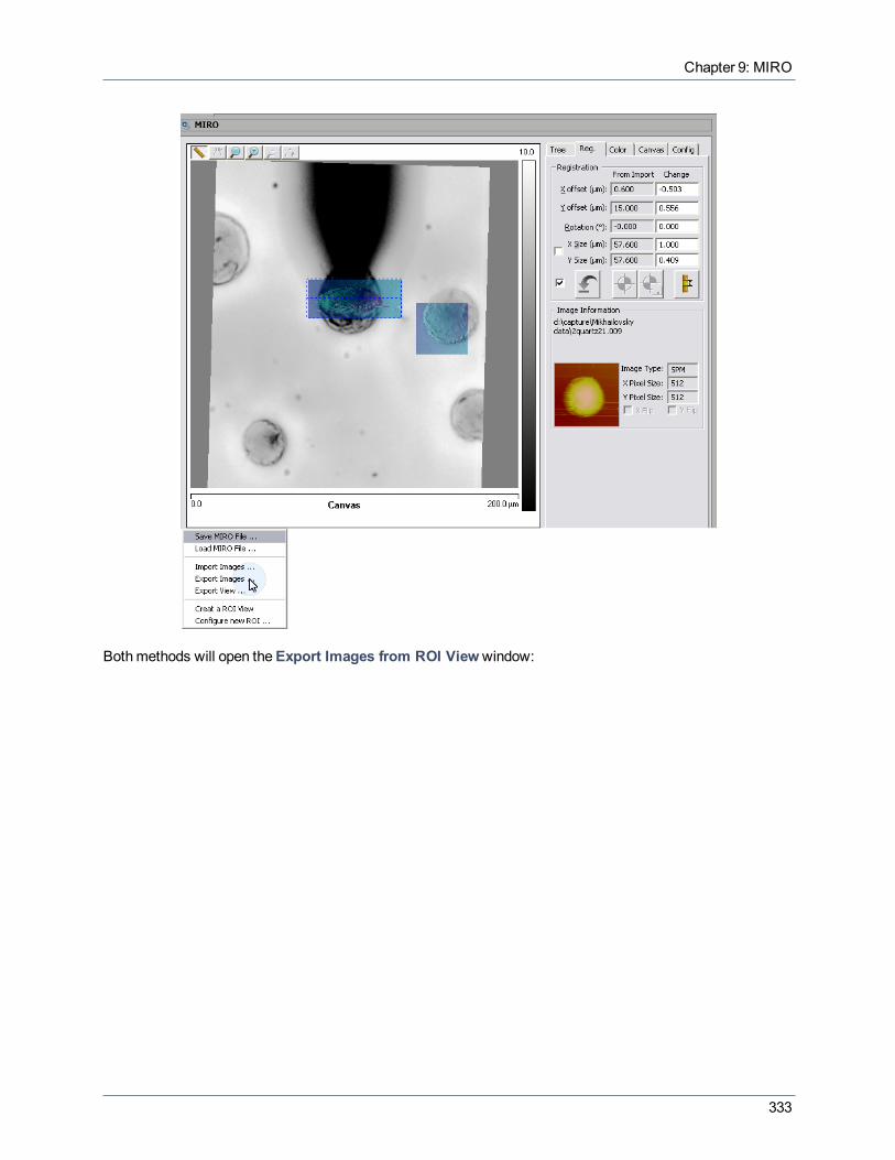
Chapter 9: MIRO
Bothmethods will open theExport Images from ROI Viewwindow:
333

NanoScope Analysis 1.50 User Manual
Three Export ROI options are available:
1. Export the ViewSaves thewholeROI window as a JPEG image file:
2. Export Displayed ROI ImagesSaves the ROI images as single layer Tiff, BMP, JPG, PNG, or GIF images at their original size:
3. Export Layer ImagesExports ROI images with preserved layers. Layers are either exported to separate files or a single mult-channelfile is created.
Youmay adjust the exported image size by changing theSize parameter (in theExport Layer Images Assection of the Export Images From the ROI View window, above). The image interpolationmode is determinedby the InterpolationMode setting in The Configuration Tab (page 308). Several export options are available:
334

Chapter 9: MIRO
l Individual layers are exported as 8-bit RGB uncompressed tiff files.l Individual layers are exported as 16-bit gray-scale uncompressed tiff files.l Individual layers, including optical images, are exported as *.spm files.
9.4 MIRO Feature Summary
ImportThe following file types may be imported:
l Tiffl BMPl JPG (JPEG)l PNGl GIF
CanvasThe Canvas view allows the following functions:
l Zooml Panl Resizel Scalel Rotatel Offsetl Pixel sizel File tree
Overlay and Color Controll Check box of the tree nodes to toggle show/hidel Drag and drop tree nodes to change the overlay orderl Change image or channel opacity to affect overlay and blendl Manipulate color by color table, contrast and offsetl Individual red, green, blue On/Off controlsl Two interpolationmethods: Bi-Linear and Nearest Neighbor
Position and Scale Re-registrationl Drag, resize and rotate the image (inCursormode only)l Registration tab with edit-box registration, undo and use informationl Update or save the selected non-AFM image registration as Import Registration
335
NanoScope Analysis 1.50 User Manual
Exportl Export the Canvas window as a single layer Tiff, BMP, JPG, PNG or GIF imagel Export selected channel image files into a new directoryl Export the Canvas view
Region of Interestl Up to 5 ROI viewsl Re-sizablel Auto update and frozen optionsl Scale and color bar show/no show optionsl Configurable background colorl Synchronized cursorsl Show the ROI boxes in the Canvas view, with the active ROI solid line
ROI Exportl Export as jpegl Export as 8 bit color tiffl Export as 16 bit gray tiffl Export as the shown size and colorl Export as multiple AFM images
Undo/Redol Unlimited image level changesl Image registration changes: offset, size, rotation, translation, X-Y linking.l Color table, overlay and blend types, opacity, contrast, offset, RGB.l Layer (channel) selection changes.
336

Chapter 10: Technical Support at Bruker
Chapter10:Technical Support at Bruker
Your satisfaction and productivity regarding Bruker products and documentation are absolutely essential.
Click Help > Technical Support for Bruker SPM technical support contact information.
10.1 Regional Technical SupportSelect your geographic region for the nearest service and support locations and contact information:
l Asia-Pacific (page 337)l Japan (page 341)l Europe, Africa, and theMiddle East (page 341)l North America (page 347)l Latin America (page 347)
10.2 Web-Based Technical Support Resourcesl http://www.bruker-axs.com/nano_surfaces_support.htmll http://www.bruker.coml http://www.brukerafmprobes.coml http://nanoscaleworld.bruker-axs.com
10.3 Asia-PacificSelect your country or region to obtain local technical support contact information:
World Wide Webl http://www.bruker-axs.com/nano_surfaces_support.htmll http://www.bruker.coml http://www.brukerafmprobes.coml http://nanoscaleworld.bruker-axs.com
Asia-Pacific (APAC)Bruker AXS Pte Ltd
l Address:11 Biopolis Way #10-05/08
The Helios
SINGAPORE 138667
l Telephone: +65 6773 9688l Fax: +65 6773 9662
337

NanoScope Analysis 1.50 User Manual
Australia/New ZealandNewSpec PTY. LTD.
l Address:134Gilbert Street
Adelaide, SA 5000
AUSTRALIA
l Telephone: +61 8 8273 3040
IndiaM/s Icon Analytical Equipment Pvt. Ltd.
l Address:554, G.M.Bhosale Marg, Worli
Mumbai 400 018
INDIA
l Telephone: +91 22 6663 3911l Fax: +91 22 6663 3914
MalaysiaBruker Malaysia SDN Bhd
l Address:303 Block A, Menatari Business Park No2
Jalan PJS 8/5
DataranMentari 46150 Petaling Jaya
46150 Selangor
MALAYSIA
l Telephone: +603 5621 8303l Fax: +603 5621 9303
PakistanNoor (Private) Limited
l Address:2nd Floor, Naqi Market
338

Chapter 10: Technical Support at Bruker
75-Shahrah-e-Quaid-e-Azam
Lahore 54000
PAKISTAN
l Telephone: +92 42 3636 2211l Fax: +92 42 3637 3320
PR ChinaBruker Beijing (Rep Office of KHE)
l Address:Suite A329
First No. 8 Guanghua Road
Chaoyang Distric, Beijing 100026
China
l Telephone: +86 10 8251 2606l Fax: +86 10 6581 6755
Bruker Shanghai
l Address:Suite 505, Building 7
1888 Xinjinqiao Road
Shanghai, 201206
China
l Telephone: +(86) 21 5531 8005l Fax: +(86) 21 3872 0056
South KoreaBruker BioSciences Korea Co. Ltd. (AAFM)
l Address:Bundang-gu, Seongnam-si
KINS Tower 15F, 25-1 Jeongja-dong
Gyeonggi-do 463-847
SOUTH KOREA
TecSco (AFMI & SOM)
l Address:
339

NanoScope Analysis 1.50 User Manual
#1811GwanghwamunOfficia
163 Sinmunno1ga Jongnogu
Seoul, 110-999
SOUTH KOREA
l Telephone: +82 2 3276 3660 1l Fax: +82 2 3276 3662
TaiwanBruker Taiwan Co., Ltd.
l Address:3F-5, No.5 Taiyuan 1st St.
Zhubei City
Hsinchu County 302
TAIWAN R.O.C.
l Telephone: +886 2 869 81212
ThailandBruker Biospin AG
l Address:41 Soi Lertpanya
Sri Ayuthaya Rd. - Lertpanya Bldg. Suite 1407
Bangkok 10400
THAILAND
l Telephone: +66 2 642 6900l Fax: +66 2 642 6901
Lite-Tech International Co. LTD
l Address:10 Ruamchitt Road, Tanonnakornchaisri
Dusit Bangkok 10300
THAILAND
l Telephone: +662 667 45019l Fax: +662 667 4506
340

Chapter 10: Technical Support at Bruker
10.4 JapanSelect your country or region to obtain local technical support contact information:
World Wide Webl http://www.bruker-axs.com/nano_surfaces_support.htmll http://www.bruker.coml http://www.brukerafmprobes.coml http://nanoscaleworld.bruker-axs.com
Bruker AXS K.K.l Address:
BanchoM Building
2-8 Rokubancho
Chiyoda-ku
Tokyo, 102-0085
JAPAN
l Telephone: +81 3 3265 1190l Fax: +81 3 3265 1198
10.5 Europe, Africa, and the Middle EastSelect your country or region to obtain local technical support contact information:
World Wide Webl http://www.bruker-axs.com/nano_surfaces_support.htmll http://www.bruker.coml http://www.brukerafmprobes.coml http://nanoscaleworld.bruker-axs.com
Belarus, Kazakhstan, Kyrgyzstan, Russia, Tajikistan, Ukraine, Uzbekistan, Turkmenistan,Georgia, Moldova, & ArmeniaOPTEC
l Address:Department of Nanotechnology Systems & ElectronMicroscopy (NTS)
Denisovski per., 26
105005Moscow
RUSSIA
341

NanoScope Analysis 1.50 User Manual
l Telephone: +7 495 933 5151l http://optec.zeiss.ru
BENELUX (Belgium, Denmark, Finland, Luxembourg, Netherlands, Norway, Sweden)Bruker Nederlands BV
l Address:Bruynvisweg 16-18
1531AZWormer
THE NETHERLANDS
l Telephone: +31 75 628 5251l Fax: +31 75 628 9771l Mailing Address:
P.O. Box 88
NL 1530ABWormer
THE NETHERLANDS
Bosnia, Bulgaria, Croatia, Hungary, Serbia, & SloveniaLABCO
l Address:Vadgalamb u.1
H-3519Miskolc
HUNGARY
l Telephone: +36 4656 2466
Czech Republic & SlovakiaMeasurement Technic Moravia Ltd.
l Address:Nádražní 267,
66441, Omice
CZECH REPUBLIC
l Telephone: +420 733 727 920l www.mt-m.eu/
342
Chapter 10: Technical Support at Bruker
Estonia & LatviaBruker Baltic OÜ
l Address:Pärnumnt. 141
11314 Tallinn
ESTONIA
l Telephone: +372 689 9000l www.bruker.com/lv.html
France & SwitzerlandBruker AXS S.A.S.
l Address:7, rue de la Croix Martre
91120 PALAISEAU
FRANCE
l Telephone: +33 1 72 86 61 00l Fax: +33 1 72 86 61 20
Germany & SwitzerlandBruker Nano GmbH
l Address:Östliche Rheinbrückenstraße 49
76187 Karlsruhe
GERMANY
l Telephone: +49 (0721) 50997 5950l Fax: +49 (0721) 50997 5952
GreeceAnalytical Instruments
l Address:9, Tzavella St.
Chalandri 152 31
Athens
343

NanoScope Analysis 1.50 User Manual
GREECE
l Telephone: +30 210 674 8973l www.analytical.gr/en/
IsraelNew Technology R.K. Ltd.
l Address:11 Tuval Street, 7th floor
Ramat Gan 52522
ISRAEL
l Telephone: +972 3 679 2000l www.newtech.co.il/
Ireland & United KingdomBruker UK Limited
l Address:Nanotech House, Anderson Road
Buckingway Business Park
Swavesey, Cambridge CB24 4UQ
UNITED KINGDOM
l Telephone: +44 1954 233 900l Fax: +44 1954 231 300
Italy2M Strumenti SRL
l Address:Via G. Pontano, 9
Roma, I-00141
ITALY
l Telephone: +39 06 8689 5319l www.2mstrumenti.com
344

Chapter 10: Technical Support at Bruker
LithuaniaLinea Libera
l Address:Akademijos str. 2
Vilnius LT-08412
LITHUANIA
l Telephone: + 370 52 63 8748l www.linealibera.lt
North Africa, Algeria, Morocco, & TunisiaOpexcel
l Address:3 rue Ruhmkorff
75 017 Paris
FRANCE
l Telephone: +33 144 83 0221
PolandLabSoft
l Address:ul. Bażancia 45A
02-892Warszawa
POLAND
l Telephone: +48 22 644 9750l www.labsoft.pl/
RomaniaRonexprim SRL
l Address:5 Cotiturii Street
010855 Bucharest-1
ROMANIA
345

NanoScope Analysis 1.50 User Manual
l Telephone: +40 21 314 3599l www.ronexprim.com
Saudi Arabia, United Arab Emirates, Qatar, BahrainNaizak Labsystems
l Address:POBox 57792
Al Sulaimaniya District
PrinceMusaid Bin Abdul Aziz Road
11584 Riyadh
SAUDI ARABIA
l Telephone: +966 1 479 0484l www.naizak.com
South AfricaCarl Zeiss (Pty) Limited
l Address:363Oak Avenue, Ferndale
Randburg, 2194
REPUBLIC OF SOUTH AFRICA
l Telephone: +27 11 886 9510l www.zeiss.co.za
Spain, PortugalTELSTAR Instrumat, S.L.
l Address:Avda. Alcalde Barnils, 70 - PTA. 3
08190 Sant Cugat del Valles
SPAIN
l Telephone: +34 93 544 2320l www.telstar-instrumat.com/
TurkeyCeyhun Atuf Kansu Caddesi
346

Chapter 10: Technical Support at Bruker
l Address:No: 112, Kat: 4, Daire: 26
06520 Balgat - Cankaya / Ankara
TURKEY
l Telephone: +90 312 472 6108l www.anatek.com.tr
10.6 North AmericaTechnical Support for North America is located at the factory where the Bruker SPMs are designed andmanufactured. Customers outside of North America are also welcome to contact the factory for service orsupport inquiries.
l Phone:l 1-800-873-9750l 1-805-967-1400
l Fax: 1-805-967-7717l E-mail: [email protected]
Mailing AddressTechnical Documents, Technical Support or Bug Reports at Bruker
Bruker Inc.
112 Robin Hill Rd.
Santa Barbara, CA 93117
World Wide Webl http://www.bruker-axs.com/nano_surfaces_support.htmll http://www.bruker.coml http://www.brukerafmprobes.coml http://nanoscaleworld.bruker-axs.com
10.7 Latin AmericaSelect your country or region to obtain local technical support contact information:
World Wide Webl http://www.bruker-axs.com/nano_surfaces_support.htmll http://www.bruker.coml http://www.brukerafmprobes.coml http://nanoscaleworld.bruker-axs.com
347
NanoScope Analysis 1.50 User Manual
ArgentinaBio Analitica Argentina S.A
l Address:Florida 835, 1º piso Of. 104A
C1005AAQBuenos Aires
ARGENTINA
l Telephone: +54 11 4515 0117l Fax: +54 11 4515 0142
BrazilAltmann S.A. Importação e Comércio
l Address:Ave das Nacoes Unidad 13.771
Bloco 1, 7th Floor
Sao Paulo, SP 04794-000
BRAZIL
l Telephone: +55 11 2198 7198l Fax: +55 11 5507 4196
ChileArquimed S.A.
l Address:Arturo Prat 828,
Santiago de Chile
CHILE
l Telephone: +56 (2) 674 30 14l Fax: +56 (2) 634 46 33
IGMO Ltda
l Address:Santo Domingo 1083Of. 1114
52612 Santiago
CHILE
l Telephone: +56 (9) 9 895 3089
348

Chapter 10: Technical Support at Bruker
ColumbiaArotec Colombiana S.A.
l Address:Cra. 16, No 35-56
Bogota
COLUMBIA
l Telephone: +57 (1) 288 7799l Fax: +57 (1) 285 3604
EquadorIng. Jose M. Jalil Haas
l Address:Fray Joaquín Auz # 181 (E7-08) y Últimas Noticias
Quito
ECUADOR
l Telephone: +593 (2) 244 2388
MexicoAlta Tecnologia en Laboratorios
l Address:Comoporis #43
Col. El Caracol
Del. Coyoacan
04739Mexico D.F.
MEXICO
l Telephone: +52 (55) 5606 7525
PeruScience and Technology Training EIRL
l Address:Calle Independencia 521
Urbanizacion Pando 7ma Etapa
349
NanoScope Analysis 1.50 User Manual
SanMiguel, Lima32
PERU
l Telephone: +51 1628 1840l Fax: +51 1628 1841
UruguayLabimed S.A.
l Address:La Cumparsita 1373Of 803
11200Montevideo
URUGUAY
l Telephone: +59829032902l Fax: +59829031772
VenezuelaBusiness Electronics International C.A.
l Address:Av. La Salle c/c Lima
Torre Phelps, Piso 18Oficina 18-B
Caracas 1050
VENEZUELA
l Telephone: +58 2127931496
350

Index
Rev. A NanoScope Analysis 1.50 - 351 -
Index
2
2D image 60
2D isotropic 109
3
3D image 65
3D Lighting 25-26
A
Active pane 43
Add a note 15
Add higher order 196
add image 184
adhesion 212
Analysis functions 59
Analyze 22
Apply correction 156
Apply cursors 46
Auto-scale data 49
AutoProgram 54
B
backgournd color 71
Basic file commands 13
Bearing Analysis 73
bow removed 172
Box; Cursors
box 25
Browse files button 16
Browse window 16
C
Calculate shift 156
Capture directory 21
clean image 164
Clear database 58
Closing a file 14
Color bar 29
Color Scale 29
Color table 29
contact mechanics 218
Contrast 39-40
Converting data 22
Copy clipboard 26
Copy view 26
Correlation curve 81, 148
crop & split 167
Cursor 295
Cursors 46
double-headed 210, 284
grid controls 42
image 27
line plot 214
synchronized 48
D
Data history 51
Data scale 34
Data zoom 25
Default color table 31
Depth 80
Depth histogram 80
Dilate 90
Display file properties 14
divide image 184
Drag & drop 21
E
Electrochemical SPM 157, 287
erase 170
erase area 170
erase horizontal line 170
Erode 90

Index
- 352 - NanoScope Analysis 1.50 Rev. A
Estimate Tip 142
Export 26
journal quality 84
Export images
MIRO 310, 329, 331-332, 336
Export view 26
exported force curves 275
Exporting images 50
F
File commands 13
File context commands 43
File Formats 22
Filter commands 163
Fitted polynomials 192
flatten 172
Flatten 112
flatten order 174
flatten polynomials 173
flatten theory 173
flatten threshold 175
flatten z threshold% 175
flatten z thresholding direction 174
Force curve 223
force curve controls and settings 272
Force Curve Selection 269
force volume 226
Force Volume 231
G
gaussian 176
Gaussian low pass filter 80
Go up one level 21
grid controls 42
grid parameters 42
H
Header color table 31
Hertz model 231, 244
high speed data capture 278
Highest peak 151
highpass gaussian filter 177
History menu 51
Horizontal axis 109
HSDC 267, 278
I
Image buttons 25, 294
Image control actions 25
Image cursor 28
Image display 20
ImageMath 184
Imagemodification 59
Image processing 59
Image resize factor 155
Import images
MIRO 308, 310, 313, 329
Installation 11
J
Journal Quality Export 84
L
label type 71
light intensity 71
light pitch 71
light rotation 71
Linearity verification 88
List view 17
Load image 156, 269
Lowest peak 151
lowpass 187
lowpass gaussian filter 176
M
MATLAB 254
MCA 238

Index
Rev. A NanoScope Analysis 1.50 - 353 -
Measure button 25
Measurement 295
median 190
MIRO 293
blend layers 297
canvas 294, 296, 298-299, 308, 313, 331,335
canvas tab 308
color tab 299
color table 297, 299
configuration tab 308
contrast 299
create region of interest (ROI) 310
export images 310, 329, 331-332, 336
features 335
file format 294
image adjustments 321
imagemodification 322
image opacity 297
image overlay 296
import images 308, 310-311, 313, 329, 335
move images 322
offset 299
operation 310, 313, 318, 321
optical image registration 310
redo 328
region of interest 318, 336
registration tab 298
rotate images 325
show/hide images 296
shrink images 328
stretch images 326
toolbar 309
translate images 325
tree tab 296
undo 328
Move to next tab group 49
Move to previous tab group 49
Movie 57
multiple curve analysis 238
multiple line plot 209
multiply image 184
N
Navigate 295
Neighborhood size 91
Note 26
Number pixels off 91
O
Offset 39-40
Opening a file 13
P
Pan 295
Pan button 25
Particle Analysis 90
Patterned Sample Analysis 77, 96, 98, 121
Peak 112
Peak threshold reference 117
Peak threshold value 117
Peak threshold value type 117
PeakForce QNM 267
Pin button 16
pitch 71
Plane fit 98, 192
Plane fit mode 195
Plane fit order 195
Plane fitting 112
plot type 70
Power spectral density 105
Printing a file 14
Procedure
MIRO 310
projection 70

Index
- 354 - NanoScope Analysis 1.50 Rev. A
PSD 105
PSD and flatness 105
pull-off point 212
pullingmodels 218
Q
QNM 272, 275
Qualify Tip 142
R
Ramping 207
Raw correlation coefficient 155
Redo button 52
Refresh 21
remove spikes 165
remove streaks 166
Requirements 11
Resize down 25
Resize up 25
rotate 197
Rotate Images
MIRO 325
Rotating line; Cursors
rotating line 25
rotation 71
Roughness 112
parameters 116
Run AutoProgram 54
RunHistory 54
S
S parameters 121
functional 122
height 121
hybrid 122
spatial 123
Save Tip 143
Saving a file 14
Section 123
set sensitivity 24
Set Units 24
Shrink Images
MIRO 328
skin type 71
Skin type 67
Sneddonmodel 232, 245
Sorting thumbnails 20
Span panes 43
Span/unspan panes 43
spectrum 2D 198
spectrum 2D band pass filter 198
spectrum 2D low pass filter 198
spectrum 2D notch filter 199
specular light 71
spike cut off 164
Step 131
Stop band 116
streak cut off 164
Stretch Images
MIRO 326
strip-chart combined channels 284
strip chart 281
subtract image 184
Switch Units 24
Synchronized cursors 48
T
Technical support 337
Africa 341
Asia-Pacific 337
Australia and New Zealand 338
China 339
Europe 341
India 338
Latin America 347

Index
Rev. A NanoScope Analysis 1.50 - 355 -
Malaysia 338
Middle East 341
North America 347
Pakistan 338
South Korea 339
Taiwan 340
Thailand 340
Tested correlation coefficient 155
Threshold depth 151
Thumbnail view 19
time-based analysis 267
Tip artifacts 135
Tip characterizer 136
Tip estimation 135
Tip qualification 135
Tip quality threshold 137
Tooltip level 26
Translate Images
MIRO 325
Troubleshooting
Run history 58
U
Undo button 52
Undo flatten 156
Undo/redo buttons 52
Unspan panes 43
uodate sensivity 223
Update sensitivity 223
User interface 9, 13
V
Vertical axis 109
Voltammogram 157, 287
W
Width 147
Workspace 21
Workspaces 42
X
X correction 155
X shift 155
xtranslate 71
XY drift 153
Y
Y correction 155
Y shift 155
ytranslate 71
Z
Z thresholding% 196
Z thresholding direction 196
Zero crossing 112
zoom 71, 213
Zoom 295