
Essays on information and networks
181
Essays on information and networks Bassel Tarbush Wolfson College University of Oxford A thesis submitted for the degree of Doctor of Philosophy Trinity 2013
-
Upload
khangminh22 -
Category
Documents
-
view
1 -
download
0
Transcript of Essays on information and networks

Essays on information and networks
Bassel Tarbush
Wolfson College
University of Oxford
A thesis submitted for the degree ofDoctor of Philosophy
Trinity 2013


Acknowledgments
I feel very lucky to have been supervised by John Quah whose support goes well beyondwhat I could ever hope to repay. I am grateful for his insightful comments and tirelessguidance in every aspect of writing this dissertation. I would also like to extend mygratitude to Francis Dennig and to my co-author Alex Teytelboym. They both con-tributed substantially to the content of this dissertation, but I am mostly thankful fortheir healthy injections of sanity into our lives in Oxford. The process of writing wasprobably far less efficient than it otherwise might have been, but I can’t imagine it tohaving been much more fun. My thanks go to Dan Beary, Vincent Crawford, Péter Eső,Marcel Fafchamps, Bernie Hogan, Rachel Kranton, Meg Meyer, Iyad Rahwan, BurkhardSchipper, Nicolas Stefanovitch, and Peyton Young for their various comments and help-ful suggestions. For its generous funding I thank the Royal Economic Society. Lastlymy fondest thoughts go to my parents, Nada, and Cameron.

Essays on information and networksBassel Tarbush
Wolfson College, University of Oxford
A thesis submitted for the degree of Doctor of Philosophy, Trinity 2013
This thesis consists of three independent and self-contained chapters regarding informationand networks. The abstract of each chapter is given below.
Chapter 1: The seminal “agreeing to disagree” result of Aumann (1976) was general-ized from a probabilistic setting to general decision functions over partitional informationstructures by Bacharach (1985). This was done by isolating the relevant properties of con-ditional probabilities that drive the original result – namely, the “Sure-Thing Principle” and“like-mindedness” – and imposing them as conditions on the decision functions of agents.Moses & Nachum (1990) identified conceptual flaws in the framework of Bacharach (1985),showing that his conditions require agents’ decision functions to be defined over events thatare informationally meaningless for the agents. In this paper, we prove a new agreementtheorem in information structures that contain “counterfactual” states, and where decisionfunctions are defined, inter-alia, over the beliefs that agents hold at such states. We showthat in this new framework, decisions are defined only over information that is meaningfulfor the agents. Furthermore, the version of the Sure-Thing Principle presented here, whichaccounts for beliefs at counterfactual states, sits well with the intuition of the original versionproposed by Savage (1972). The paper also includes an additional self-contained appendix inwhich our framework is re-expressed syntactically, which allows us to provide further insights.
Chapter 2: We develop a parsimonious and tractable dynamic social network forma-tion model in which agents interact in overlapping social groups. The model allows us toanalyze network properties and homophily patterns simultaneously. We derive closed-formanalytical expressions for the distributions of degree and, importantly, of homophily indices,using mean-field approximations. We test the comparative static predictions of our modelusing a large dataset from Facebook covering student friendship networks in ten Americancolleges in 2005, and we calibrate the analytical solutions to these networks. We find goodempirical support for our predictions. Furthermore, at the best-fitting parameters values,the homophily patterns, degree distribution, and individual clustering coefficients resultingfrom the simulations of our model fit well with the data. Our best-fitting parameter valuesindicate how American college students allocate their time across various activities whensocializing.
Chapter 3: We examine three models on graphs – an information transmission mecha-nism, a process of friendship formation, and a model of puzzle solving – in which the evolutionof the process is conditioned on the multiple edge types of the graph. For example, in themodel of information transmission, a node considers information to be reliable, and thereforetransmits it to its neighbors, if and only if the same message was received on two distinct com-munication channels. For each model, we algorithmically characterize the set of all graphsthat “solve” the model (in which, in finite time, all the nodes receive the message reliably, allpotentially close friendships are realized, and the puzzle is completely solved). Furthermore,we establish results relating those sets of graphs to each other.


Contents
1 Agreeing on decisions: an analysis with counterfactuals 1
1.1 Introduction . . . . . . . . . . . . . . . . . . . . . . . . . . . . . . . . . . . 2
1.2 Information structures . . . . . . . . . . . . . . . . . . . . . . . . . . . . . 5
1.2.1 General information structures . . . . . . . . . . . . . . . . . . . . 5
1.2.2 Partitional structures . . . . . . . . . . . . . . . . . . . . . . . . . . 8
1.2.3 Belief structures . . . . . . . . . . . . . . . . . . . . . . . . . . . . 10
1.3 Agreeing on decisions . . . . . . . . . . . . . . . . . . . . . . . . . . . . . . 12
1.3.1 The original result . . . . . . . . . . . . . . . . . . . . . . . . . . . 12
1.3.2 Conceptual flaws . . . . . . . . . . . . . . . . . . . . . . . . . . . . 14
1.4 Counterfactual structures . . . . . . . . . . . . . . . . . . . . . . . . . . . 16
1.4.1 Set-up with counterfactual states . . . . . . . . . . . . . . . . . . . 17
1.4.2 The agreement theorem . . . . . . . . . . . . . . . . . . . . . . . . 21
1.4.3 Solution to the conceptual flaws . . . . . . . . . . . . . . . . . . . . 23
1.4.4 Interpretation . . . . . . . . . . . . . . . . . . . . . . . . . . . . . . 24
1.5 Relation to the literature . . . . . . . . . . . . . . . . . . . . . . . . . . . . 30
1.5.1 Other solutions . . . . . . . . . . . . . . . . . . . . . . . . . . . . . 30
1.5.2 Action models . . . . . . . . . . . . . . . . . . . . . . . . . . . . . . 32
1.5.3 Counterfactuals . . . . . . . . . . . . . . . . . . . . . . . . . . . . . 33
1.6 Conclusion . . . . . . . . . . . . . . . . . . . . . . . . . . . . . . . . . . . . 34
1.7 Appendix A: The syntactic approach . . . . . . . . . . . . . . . . . . . . . 36
1.7.1 New definitions . . . . . . . . . . . . . . . . . . . . . . . . . . . . . 36
1.7.2 Syntactic results . . . . . . . . . . . . . . . . . . . . . . . . . . . . 42
1.7.3 Alternative construction of counterfactuals . . . . . . . . . . . . . . 48
1.8 Appendix B: Proofs . . . . . . . . . . . . . . . . . . . . . . . . . . . . . . 53
1.9 References . . . . . . . . . . . . . . . . . . . . . . . . . . . . . . . . . . . . 59
i

ii CONTENTS
2 Friending: a model of online social networks 612.1 Introduction . . . . . . . . . . . . . . . . . . . . . . . . . . . . . . . . . . . 62
2.1.1 Homophily . . . . . . . . . . . . . . . . . . . . . . . . . . . . . . . 622.1.2 Socializing on Facebook . . . . . . . . . . . . . . . . . . . . . . . . 632.1.3 Our contribution . . . . . . . . . . . . . . . . . . . . . . . . . . . . 64
2.2 Literature review . . . . . . . . . . . . . . . . . . . . . . . . . . . . . . . . 662.3 Model . . . . . . . . . . . . . . . . . . . . . . . . . . . . . . . . . . . . . . 68
2.3.1 Characteristics of agents . . . . . . . . . . . . . . . . . . . . . . . . 682.3.2 Network formation process . . . . . . . . . . . . . . . . . . . . . . . 692.3.3 Interpretation of the model . . . . . . . . . . . . . . . . . . . . . . 702.3.4 Discussion of the model . . . . . . . . . . . . . . . . . . . . . . . . 712.3.5 Relationship to affiliation networks . . . . . . . . . . . . . . . . . . 73
2.4 Theoretical results . . . . . . . . . . . . . . . . . . . . . . . . . . . . . . . 742.4.1 Degree distribution . . . . . . . . . . . . . . . . . . . . . . . . . . . 752.4.2 Assortativity . . . . . . . . . . . . . . . . . . . . . . . . . . . . . . 792.4.3 Homophily . . . . . . . . . . . . . . . . . . . . . . . . . . . . . . . 80
2.5 Simulation results . . . . . . . . . . . . . . . . . . . . . . . . . . . . . . . . 842.6 Data . . . . . . . . . . . . . . . . . . . . . . . . . . . . . . . . . . . . . . . 852.7 Tests and empirical observations . . . . . . . . . . . . . . . . . . . . . . . 86
2.7.1 A representative college . . . . . . . . . . . . . . . . . . . . . . . . 862.7.2 All colleges . . . . . . . . . . . . . . . . . . . . . . . . . . . . . . . 86
2.8 Model calibration . . . . . . . . . . . . . . . . . . . . . . . . . . . . . . . . 892.8.1 Empirical strategy . . . . . . . . . . . . . . . . . . . . . . . . . . . 892.8.2 Results . . . . . . . . . . . . . . . . . . . . . . . . . . . . . . . . . 92
2.9 Discussion . . . . . . . . . . . . . . . . . . . . . . . . . . . . . . . . . . . . 962.9.1 Arrival of new nodes . . . . . . . . . . . . . . . . . . . . . . . . . . 962.9.2 Endogenous probability of idleness . . . . . . . . . . . . . . . . . . 982.9.3 Preferential attachment . . . . . . . . . . . . . . . . . . . . . . . . 992.9.4 Endogenous characteristics . . . . . . . . . . . . . . . . . . . . . . 100
2.10 Conclusion . . . . . . . . . . . . . . . . . . . . . . . . . . . . . . . . . . . . 1012.11 Appendix . . . . . . . . . . . . . . . . . . . . . . . . . . . . . . . . . . . . 103
2.11.1 Proofs . . . . . . . . . . . . . . . . . . . . . . . . . . . . . . . . . . 1032.11.2 Simulation algorithm . . . . . . . . . . . . . . . . . . . . . . . . . . 1072.11.3 Algorithm for finding robust points in the grid search . . . . . . . . 1082.11.4 Data description . . . . . . . . . . . . . . . . . . . . . . . . . . . . 1092.11.5 Further baseline observations on homophily . . . . . . . . . . . . . 1102.11.6 Results . . . . . . . . . . . . . . . . . . . . . . . . . . . . . . . . . 113

CONTENTS iii
2.11.7 Degree distributions in cleaned and raw data . . . . . . . . . . . . 1142.11.8 Test of Proposition 1 with an unrestricted set of agents . . . . . . 1152.11.9 Dynamics of homophily across the grid space . . . . . . . . . . . . 116
2.12 References . . . . . . . . . . . . . . . . . . . . . . . . . . . . . . . . . . . . 118
3 Processes on graphs with multiple edge types 1233.1 Introduction . . . . . . . . . . . . . . . . . . . . . . . . . . . . . . . . . . . 124
3.1.1 Motivation . . . . . . . . . . . . . . . . . . . . . . . . . . . . . . . 1243.1.2 Outline of the paper . . . . . . . . . . . . . . . . . . . . . . . . . . 129
3.2 Literature review . . . . . . . . . . . . . . . . . . . . . . . . . . . . . . . . 1313.3 Preliminary results on trees and reduced trees . . . . . . . . . . . . . . . . 1333.4 Characterization of assemblable graphs . . . . . . . . . . . . . . . . . . . . 137
3.4.1 Growth algorithm for minimally assemblable graphs . . . . . . . . 1403.4.2 Splitting algorithm for minimally assemblable graphs . . . . . . . . 1423.4.3 Discussion of the algorithms for generating minimally assemblable
graphs . . . . . . . . . . . . . . . . . . . . . . . . . . . . . . . . . . 1453.4.4 Algorithm for assemblable graphs . . . . . . . . . . . . . . . . . . . 146
3.5 Characterization of combinable graphs . . . . . . . . . . . . . . . . . . . . 1463.6 Characterization of transmissible graphs . . . . . . . . . . . . . . . . . . . 148
3.6.1 Transmissible graph growth . . . . . . . . . . . . . . . . . . . . . . 1503.6.2 Discussion of the algorithm for generating transmissible graphs . . 151
3.7 Conclusion . . . . . . . . . . . . . . . . . . . . . . . . . . . . . . . . . . . . 1523.8 Appendix . . . . . . . . . . . . . . . . . . . . . . . . . . . . . . . . . . . . 1543.9 References . . . . . . . . . . . . . . . . . . . . . . . . . . . . . . . . . . . . 169

iv CONTENTS

Chapter 1
Agreeing on decisions: an analysis
with counterfactuals
Abstract: The seminal “agreeing to disagree” result of Aumann (1976) was general-ized from a probabilistic setting to general decision functions over partitional informationstructures by Bacharach (1985). This was done by isolating the relevant properties ofconditional probabilities that drive the original result – namely, the “Sure-Thing Princi-ple” and “like-mindedness” – and imposing them as conditions on the decision functionsof agents. Moses and Nachum (1990) identified conceptual flaws in the framework ofBacharach (1985), showing that his conditions require agents’ decision functions to bedefined over events that are informationally meaningless for the agents. In this paper, weprove a new agreement theorem in information structures that contain “counterfactual”states, and where decision functions are defined, inter-alia, over the beliefs that agentshold at such states. We show that in this new framework, decisions are defined onlyover information that is meaningful for the agents. Furthermore, the version of the Sure-Thing Principle presented here, which accounts for beliefs at counterfactual states, sitswell with the intuition of the original version proposed by Savage (1972). The paper alsoincludes an additional self-contained appendix in which our framework is re-expressedsyntactically, which allows us to provide further insights.1
1Parts of this chapter appear in Tarbush (2013).
1

2 CHAPTER 1. AGREEING ON DECISIONS
1.1 Introduction
Aumann (1976) proved that agents endowed with a common prior cannot agree to
disagree. This means that if agents’ posterior beliefs over some event (a subset of some
state space), which are obtained from updating over private information, are commonly
known, then these beliefs must be the same. Aumann’s result was derived in a proba-
bilistic framework, in which agents’ beliefs are expressed as probabilities and in which a
particular “partitional” structure is imposed on the state space. Bacharach (1985) and
Cave (1983) (independently) were the first to generalize Aumann’s seminal result to the
non-probabilistic case. Essentially, they replaced probability functions, which map from
events to probabilities in [0, 1], with more general “decision functions”, which map from
events to some arbitrary space of “actions”. Specifically, Bacharach isolated the relevant
properties that hold both of conditional probabilities and of the common prior assump-
tion – which drive the original result –, and imposed them as independent conditions
on general decision functions in partitional information structures. As such, he was able
to isolate and interpret the assumptions underlying Aumann’s original result as (i) an
assumption of “like-mindedness”, which requires agents to take the same action given the
same information, and (ii) an assumption that he claimed is analogous to requiring the
agents’ decision functions to satisfy Savage’s Sure-Thing Principle (Savage (1972)). This
principle is understood as capturing the intuition that
If an agent i takes the same action in every case when i is more informed, itakes the same action in the case when i is more ignorant. (STP 1)
Moses and Nachum (1990) found conceptual flaws in Bacharach’s analysis, show-
ing that his interpretations of “like-mindedness” and of the Sure-Thing Principle are
problematic. Indeed, given that Bacharach (like Aumann, 1976) is operating within par-
titional information structures, the information of agents is modeled as partitions of the
state space.2 The partition elements are therefore the primitives of the structure that2An agent i considers states that belong to the same partition element of i’s partition to be indis-
tinguishable.

1.1. INTRODUCTION 3
define the information of an agent. Furthermore, decision functions are defined over
sets of states in a manner that is supposed to be consistent with the information that
each agent has – in this way, decisions can be interpreted as being functions of agents’
information. In Bacharach’s set-up, like-mindedness requires the decision function of an
agent i to be defined over elements of the partitions of other agents j. But, except for
the trivial case in which agent i’s partition element corresponds exactly to that of agent
j, there is no sense in requiring i’s function to be defined over j’s partition element since
that element is informationally meaningless to agent i. That is, there is no primitive in
the structure that represents what i’s information is in this case. The Sure-Thing Prin-
ciple is also problematic. An agent’s decision function is said to satisfy the Sure-Thing
Principle if, whenever the decision over each element of a set of disjoint events is x, the
decision over the union of all those events is also x. Notably, this implies that an agent
i’s decision function must be defined over the union of i’s partition elements, but again,
this is informationally meaningless for that agent since there is no partition element of
that agent that corresponds to a union of i’s partition elements. To sum up, Moses and
Nachum show that Bacharach’s set-up is such that the domains of the agents’ decision
functions contain elements that are informationally meaningless for the agents.
In this paper, we develop a method of transforming any given partitional structure
into a richer information structure that explicitly includes counterfactual states. We
interpret these “counterfactual structures” as being more complete pictures of the situ-
ation that is being modeled in the original partitional structure. Within counterfactual
structures, one can provide a formal definition of the information that agents have in par-
ticular counterfactual situations, which turns out to be crucial in resolving the conceptual
issues raised by Moses and Nachum (1990).3 Furthermore, we prove a new “agreeing to
disagree” result in counterfactual structures.
3Counterfactual information is important in many areas of research in economics and in game theory.For example, one must determine what agents would do at histories of a game that are never reached(that is, in counterfactual situations) in order to fully specify a backwards induction solution.

4 CHAPTER 1. AGREEING ON DECISIONS
Most importantly, we show that our set-up resolves the conceptual issues raised by
Moses and Nachum (1990), in the sense that, within counterfactual structures, decision
functions are defined only over events that are informationally meaningful for the agents.
Furthermore, our set-up allows us to provide new formal definitions of the Sure-Thing
Principle and of like-mindedness that sit well with intuition. Indeed, we have a version
of like-mindedness that does not require an agent i’s decision function to be defined over
the partition elements of another agent j. Regarding the Sure-Thing Principle, we show
that our version of this principle captures the intuition that
If the agent i takes the same action in every case when i is more informed, iwould take the same action if i were secretly more ignorant. (STP 2)
The conditional statement originally expressed in (STP 1) is now expressed as a
counterfactual (in (STP 2)), and the agent’s ignorance is “secret” in the sense that the
other agents’ information regarding this agent remains unchanged in the counterfactual
situation. We show that this is closer to the original version of the Sure-Thing Principle,
which was developed by Savage (1972) in a single-agent decision theory setting. Indeed,
Bacharach’s Sure-Thing Principle requires taking the union of partition elements, but
doing so for an agent modifies the primitives of the structure in a manner that can also
change other agents’ information about this agent. Ignorance is therefore not “secret” in
Bacharach’s version, which surely does not adequately capture the single-agent setting
version of Savage (1972). Other than the issue of secrecy, the distinction between ex-
pressing the Sure-Thing Principle as a counterfactual (STP 2) rather than as a simple
conditional (STP 1) turns out to be important in resolving the conceptual issues raised
by Moses and Nachum (1990), but could not be captured within Bacharach’s framework.
Indeed, the analysis in Bacharach (1985) is carried out in partitional structures, and all
information in those structures must be factual (in the sense that any event that an
agent believes must be true), whereas information need not be factual in counterfactual
structures.

1.2. INFORMATION STRUCTURES 5
In Section 1.2 we present the formal definitions required to analyze information struc-
tures in general, and in Section 1.3 we set up Bacharach’s framework, prove his version
of the agreement theorem, and present Moses’s and Nachum’s arguments regarding the
conceptual flaws. In Section 1.4 we develop a method for constructing counterfactual
structures, provide new definitions for the Sure-Thing Principle and for like-mindedness,
and prove a new agreement theorem within such structures. Furthermore, we show that
our approach resolves the conceptual flaws. Finally, in Section 1.5 we relate our approach
to other results and proposed solutions to the conceptual flaws found in the “agreeing to
disagree” literature, and Section 1.6 concludes.
This papers contains two appendices. Appendix A (Section 1.7) is an additional, self-
contained section, in which we express our framework syntactically so that information
is no longer merely modeled by a state space and some relation over it, but also by a
syntactic language. This new framework allows us to provide several interesting results
and further insights into the “agreeing to disagree” literature. The proofs of all the results
in the paper are in Appendix B (Section 1.8).
1.2 Information structures
This section introduces the formal apparatus that will be used to derive the agreement
theorem. In large part, the formal definitions given are completely standard.
1.2.1 General information structures
Let Ω denote a finite set of states and N a finite set of agents. A subset e ⊆ Ω is
called an event. For every agent i ∈ N , define a binary relation Ri ⊆ Ω × Ω, called a
reachability relation. So, we say that the state ω ∈ Ω reaches the state ω′ ∈ Ω if ωRiω′.4
It terms of interpretation, if ωRiω′, then at ω, agent i considers the state ω′ possible.
An information structure S = (Ω, N, Rii∈N ) is entirely determined by the state space,
4In our notation, we alternate between ωRiω′ and (ω, ω′) ∈ Ri, whenever it is convenient to do so.

6 CHAPTER 1. AGREEING ON DECISIONS
the set of agents, and the reachability relations.
The reachability relations Rii∈N are said to be:
1. Serial if ∀i ∈ N, ∀ω ∈ Ω,∃ω′ ∈ Ω, ωRiω′.
2. Reflexive if ∀i ∈ N, ∀ω ∈ Ω, ωRiω.
3. Transitive if ∀i ∈ N, ∀ω, ω′, ω′′′ ∈ Ω, if ωRiω′&ω′Riω′′, then ωRiω′′.
4. Euclidean if ∀i ∈ N, ∀ω, ω′, ω′′′ ∈ Ω, if ωRiω′&ωRiω′′, then ω′Riω′′.
A possibility set at state ω for agent i ∈ N is defined by
bi(ω) = ω′ ∈ Ω|ωRiω′ (1.1)
A possibility set bi(ω) is therefore, simply the set of all states that i considers possible
at ω. For any event e ⊆ Ω, whenever bi(ω) ⊆ e, we say that i believes that e is true at
ω. Indeed, at ω, every state that i considers possible is included in this event. In terms
of notation, let us have Bi = bi(ω)|ω ∈ Ω. For any e ⊆ Ω, a belief operator is given by
Bi(e) = ω ∈ Ω|bi(ω) ⊆ e (1.2)
Therefore, Bi(e) is the set of all states in Ω at which i believes that e is true. Note
that we have not yet imposed any particular restrictions on the reachability relations.
But it is precisely the restrictions on these relations that will determine the properties
that the belief operator satisfies and that will therefore allow us to provide a proper
interpretation for this operator. There are several sets of restrictions that are commonly
found in the literature. For example, the class of structures in which the reachability
relations are equivalence relations (i.e. reflexive and Euclidean) is known as the S5
class. As we demonstrate Section 1.2.2, in this class, the set Bi partitions the state
space, and the possibility sets are the partition elements of this set. We therefore obtain
the standard structures of Aumann (1976) (and of Bacharach, 1985), and the belief

1.2. INFORMATION STRUCTURES 7
operator is interpreted as a knowledge operator. Another common class is the class
of structures in which the reachability relations are serial, transitive, and Euclidean,
and which is known as the KD45 class. We discuss this class in Section 1.2.3 below.
Finally, the class of structures in which the reachability relations are serial and transitive
is known as the KD4 class. The terminology employed here in naming the classes of
structures is standard in the modal logic and epistemic logic literatures, with textbook
treatments including Fagin et al. (1995), Chellas (1980) and van Benthem (2010). Note
that although we have defined these classes here, we are not yet imposing any restrictions
on the reachability relations, so the definitions below are provided in a general setting,
with the understanding that they will only be applied in S5, KD45, and a subset of
KD4 structures.
For any e ⊆ Ω, and any G ⊆ N , a mutual belief operator is given by
MG(e) = ∩i∈GBi(e) (1.3)
This operator can be iterated by letting M1G(e) = MG(e) and Mm+1
G (e) = MG(MmG (e))
for m ≥ 1. For any e ⊆ Ω, and any G ⊆ N , we can thus define a common belief operator,
CG(e) = ∩∞m=1MG(e) (1.4)
Therefore, CG(e) is the set of all states in Ω in which all the agents in G believe that e,
all agents in G believe that all agents in G believe that e, and so on, ad infinitum.
Finally, we say that a state ω′ ∈ Ω is reachable among the agents in G from a
state ω ∈ Ω if there exists a sequence of states ω ≡ ω0, ω1, ω2, ..., ωn ≡ ω′ such that
for each k ∈ 0, 1, ..., n − 1, there exists an agent i ∈ G such that ωkRiωk+1. The
component TG(ω) (among the agents in G) of the state ω is the set of all states that are
reachable among the agents in G from ω. Common belief can now be given an alternative

8 CHAPTER 1. AGREEING ON DECISIONS
characterization,
CG(e) = ω ∈ Ω|TG(ω) ⊆ e (1.5)
This is standard and for example follows Hellman (2013, p. 12).
1.2.2 Partitional structures
Consider an information structure S = (Ω, N, Rii∈N ) and suppose that the reach-
ability relations Rii∈N are equivalence relations. Then, we say that S is a partitional
structure. Indeed, the remark below shows that in this case, the information structure
S becomes a standard “partitional”, or S5, or “knowledge” structure (for example, see
Aumann, 1976).
Remark 1. Suppose S = (Ω, N, Rii∈N ) is a partitional structure. For any agent
i ∈ N , ω ∈ bi(ω), and any bi(ω) and bi(ω′) are either identical or disjoint; and, Bi is a
partition of the state space.
Note that in a partitional structure, at any state ω, an agent i considers any of the
states in bi(ω) (including ω itself) possible. The belief operator becomes the standard
“knowledge” operator, and it satisfies the following properties, which are well-known in
the literature (for example, see Fagin et al., 1995):5
K Bi(¬e ∪ f) ∩Bi(e) ⊆ Bi(f) Kripke
D Bi(e) ⊆ ¬Bi(¬e) Consistency
T Bi(e) ⊆ e Truth
4 Bi(e) ⊆ Bi(Bi(e)) Positive Introspection
5 ¬Bi(e) ⊆ Bi(¬Bi(e)) Negative Introspection
The Kripke property, K, states that if an agent i knows that e and knows that e implies
f , then i must also know that f . The Consistency property D states that if an agent i5Note that for any e ⊆ Ω, ¬e denotes the set Ω\e.

1.2. INFORMATION STRUCTURES 9
knows that e, then i cannot also know that not e. The Truth property, T, states that if
an agent i knows that e, then e must be true. The Positive Introspection property states
that if an agent i knows that e, then i knows that i knows that e, and the Negative
Introspection property states that if an agent i does not know that e, then i knows
that i does not know that e. These five properties are thought of as characterizing
the properties of knowledge (Aumann, 1999). In structures in which the reachability
relations are required to satisfy restrictions that are weaker than equivalence relations –
as in KD45 or KD4 –, the belief operator does not satisfy all the above properties and
can then no longer be interpreted as a “knowledge” operator, but simply as a “belief”
operator (The KD45 case is examined in Section 1.2.3 below).
Note that in a partitional structure, the operator CG has the familiar interpretation of
being the “common knowledge” operator. Furthermore, since this reduces to a completely
standard framework, we can obtain familiar technical results, such as the proposition
below, which will be useful in later sections.
Proposition 1. Suppose S = (Ω, N, Rii∈N ) is a partitional structure. Then, for any
ω ∈ Ω and any i ∈ G, ∪ω′∈TG(ω)bi(ω′) = TG(ω).
That is, any component is equal to the union of the possibility sets that it includes.
Example. Figure 1.1 illustrates a very simple S5 structure. Panel (1) and panel
(2) are equivalent representations of the same structure. The state space is given by
Ω = ω1, ω2, and the set of agents is given by N = a, b. The reachability re-
lations, which are shown in panel (1), are given by Ra = (ω1, ω1), (ω2, ω2), and
Rb = (ω1, ω1), (ω1, ω2), (ω2, ω1), (ω2, ω2). Note that the reachability relations here
are equivalence relations. So, given Remark 1, we can provide an alternative representa-
tion of this information structure in panel (2), which shows the agents’ partitions of the
state space: Ba = ba(ω1), ba(ω2) = ω1, ω2, and Bb = bb(ω1) = Ω.
Now, let us consider the event e = ω1. Since ba(ω1) ⊆ e, we have that Ba(e) 6= ∅,
so a knows that e. (Note that ba(ω1) ⊆ e would be read as “a knows that e at ω1”).

10 CHAPTER 1. AGREEING ON DECISIONS
However, there is no possibility set for agent b that is a subset of e, so b does not know
that e (which can be written as ¬Bb(e)). This can be complicated further: For example,
since ¬Bb(e) = Ω, and since ba(ω1) ⊆ Ω, we have that, at ω1, a knows that b does not
know that e. In fact, Ba(¬Bb(e)) = Ω. One can verify that the belief (or in this case
“knowledge”) operator in this structure satisfies properties K, D, T, 4, and 5.
Finally, note that TN (ω1) = Ω since ω1 reaches ω2 by some sequence of reachability
relations belonging to the agents in N (In this case, ω1Rbω2). Similarly, TN (ω2) = Ω.
In particular, this means that CN (¬Bb(e)) = Ω, so it is common knowledge that b does
not know that e. Finally, as an illustration of Proposition 1, notice that TN (ω1) =
ba(ω1) ∪ ba(ω2) = bb(ω1).
ω1
a
ω2
ba
b
a, b
a, b
ω1
a
ω2
ba
a, b
ω2
ba
(1) (2)
Figure 1.1: Example of an S5 structure
1.2.3 Belief structures
Suppose now that the reachability relations Rii∈N in an information structure
S = (Ω, N, Rii∈N ) are serial, transitive, and Euclidean. Then, say we that S is a belief
structure. Indeed, the information structure S becomes a standard KD45 structure. A
similar presentation of such structures can be found in Hellman (2013).

1.2. INFORMATION STRUCTURES 11
Remark 2. Suppose S = (Ω, N, Rii∈N ) is a belief structure. For any agent i ∈ N ,
and any ω ∈ Ω, bi(ω) 6= ∅, and if ω ∈ bi(ω′), then bi(ω) = bi(ω′).
It is important to note that, although every possibility set must be non-empty, it can
be the case that ω 6∈ bi(ω). This means that at the state ω, agent i considers states other
than ω to be possible, and does not consider ω to be possible. The agent is therefore
“deluded”. (In fact, this terminology is directly borrowed from Hellman, 2013, p. 5). An
example may help to illustrate this point.
Example. Consider the simple belief structure S = (Ω, N, Rii∈N ), illustrated in
Figure 1.2, in which Ω = ω1, ω2, N = a, and Ra = (ω1, ω1), (ω2, ω1). This
reachability relation is now not an equivalence relation (it is only serial, transitive, and
Euclidean), and this will affect the properties that the belief operator satisfies. Indeed,
consider the event e = ω1. Since ba(ω2) = ω1, it follows that a believes that e at ω2,
even though the state at which this is evaluated is ω2. At the state ω2, a only considers
the state ω1, but not ω2 itself to be possible. That is, at ω2, a falsely believes that the
state is, in fact, ω1. And notably, since ba(ω1) ⊆ e we have that Ba(e) = ω1, ω2, so
Ba(e) 6⊆ e. So the property T of the belief operator does not hold. In this case, the
set of states at which a believes that e (Ba(e)) can include states outside of e, so a can
falsely believe that e.
ω1
ω2
a
a
Figure 1.2: Example of a KD45 structure
The example above shows that the belief operator no longer satisfies the Truth prop-

12 CHAPTER 1. AGREEING ON DECISIONS
erty T, but it does satisfy K, D, 4, and 5. So this describes a belief system in which the
beliefs satisfy the Kripke property, Consistency, and the Introspection properties, but
not the Truth property. There exist weaker systems of belief, such as KD4, which in
addition to dropping the Truth property, also drop the Negative Introspection property
of the belief operator. We return to these in Section 1.4.
The salient point here is that the set-up presented has very close analogues in the
literature, and it allows us to drop – among other things – the property T of the belief
operator, as compared with partitional structures. This will be important when including
counterfactual states since, by their very nature, these will be used to model information
that can be false.
1.3 Agreeing on decisions
In this section, we present the original set-up of Bacharach (1985), derive his version
of the agreement theorem, and then outline its inherent conceptual flaws which were
originally raised in Moses and Nachum (1990).
1.3.1 The original result
The original result was derived in a partitional information structure. The set-up
in this entire section therefore assumes that we are working with a partitional structure
S = (Ω, N, Rii∈N ). Notably, this means that Bi is taken to be a partition of the state
space for every agent i ∈ N (see Remark 1).
For every agent i ∈ N , an action function δi : Ω → A, which maps from states to
actions, specifies agent i’s action at any given state. A decision function Di for agent i,
maps from a field F of subsets of Ω into a set A of actions. That is,
Di : F → A (1.6)

1.3. AGREEING ON DECISIONS 13
Following the terminology of Moses and Nachum (1990), we say that the agent i using
the action function δi follows the decision function Di if for all states ω ∈ Ω, δi(ω) =
Di(bi(ω)). That is, δi specifies agent i’s action at any given state as a function of i’s
possibility set at that state (which is intended to represent i’s “information” at that
state); so the value of the action function will fully depend on the partition Bi
Bacharach imposes two main restrictions in order to derive his result, namely, the
Sure-Thing Principle and like-mindedness. The definitions of these terms are given
below.
Definition 1. The decision function Di of agent i satisfies the Sure-Thing Principle if
whenever for all e ∈ E, Di(e) = x then Di(∪e∈Ee) = x, where E ⊆ F is a non-empty set
of disjoint events.
In terms of interpretation, we can think of an event as representing some information
and a of decision over that event as determining the action that is taken as a function of
that information. The union of events is intended to capture some form of “coarsening”
of the information. So, following Moses and Nachum (1990), the Sure-Thing Principle is
intended to capture the intuition that If an agent i takes the same action in every case
when i is more informed, i takes the same action in the case when i is more ignorant.
For example, if agent i decides to take an umbrella when i knows that it is raining and
decides to take an umbrella when i knows that it is not raining, then according to the
principle, i also decides to take an umbrella when i does not know whether it is raining
or not. Regarding like-mindedness, we have the following definition.
Definition 2. Agents are said to be like-minded if they have the same decision function.
That is, over the same subsets of states, the agents take the same action if they are
like-minded. This is intended to capture the intuition that given the same information,
the agents would take the same action.
Theorem 1 (Bacharach, 1985). Let S = (Ω, N, Rii∈N ) be a partitional structure. If
the agents i ∈ N are like-minded (as defined in Definition 2) and follow the decision

14 CHAPTER 1. AGREEING ON DECISIONS
functions Dii∈N (as defined in (1.6)) that satisfy the Sure-Thing Principle (as defined
in Definition 1), then for any G ⊆ N , if CG(∩i∈Gω′ ∈ Ω|δi(ω′) = xi) 6= ∅, then xi = xj
for all i, j ∈ G.
This theorem states that if the action taken by each member of a group of like-
minded agents who follow decision functions that satisfy the Sure-Thing Principle is
common knowledge among that group, then the members of the group must all take the
same action. That is, the agents cannot “agree to disagree” about which action to take.
1.3.2 Conceptual flaws
Moses and Nachum (1990) find conceptual flaws in the set-up of Bacharach (1985)
outlined above. In broad terms, they find that the requirements that Bacharach imposes
on the decision functions force them to be defined over sets of states, the interpretation
of which is meaningless within the information structure he is operating in. Formally,
consider the following definition.
Definition 3. Let S = (Ω, N, Rii∈N ) be some arbitrary information structure. We
say that an event e is a possible belief for agent i in S if there exists a state ω ∈ Ω such
that e = bi(ω).
When S is a partitional structure, this definition corresponds exactly to e being what
Moses and Nachum (1990) call a “possible state of knowledge”. In Moses and Nachum
(1990), it is shown that
1. The Sure-Thing Principle forces decisions to be defined over unions of possibility
sets, but no union of possibility sets can be a possible belief for any agent (see
Moses and Nachum, 1990, Lemma 3.2).
2. The assumption of like-mindedness forces the decision function of an agent i to be
defined over the possibility sets of agents j 6= i, but – other than the case when

1.3. AGREEING ON DECISIONS 15
the sets correspond trivially – these are not possible beliefs for agent i (see Moses
and Nachum, 1990, Lemma 3.3).
In other words, Bacharach’s framework requires the decision functions to be defined over
events that are not possible beliefs for the agents (given the primitives of the information
structure). More specifically, the primitives in partitional information structures are the
partition elements of each agent’s partition over the state space. It is precisely those
primitives that describe the information that an agent has in the structure. However,
in Bacharach’s set-up, like-mindedness requires the decision function of an agent i to be
defined over elements of the partitions of other agents j. But, except for the trivial case
in which agent i’s partition element corresponds exactly to that of agent j, there is no
sense in requiring i’s function to be defined over j’s partition element since that element
is informationally meaningless to agent i. That is, there is no primitive in the structure
that represents what i’s information is in this case. The Sure-Thing Principle is also
problematic. An agent’s decision function is said to satisfy the Sure-Thing Principle if
whenever the decision over each element of a set of disjoint events is x, the decision over
the union of all those events is also x. Notably, this implies that an agent i’s decision
function must be defined over the union of i’s partition elements, but again, this is
informationally meaningless for that agent since there is no partition element of that
agent that corresponds to a union of i’s partition elements.
Example. Consider Figure 1.1 on page 10. Like-mindedness in Bacharach’s framework
would require agent b’s decision function to be defined over the event ba(ω1) = ω1.
However, there is no primitive in this structure (that is, there is no possibility set in this
structure) for agent b that corresponds to ω1. Therefore, b’s information at ω1 is
not defined. Similarly, the Sure-Thing Principle in Bacharach’s framework would require
agent a’s decision function to be defined over the event ba(ω1)∪ ba(ω2). But once again,
there is no primitive in this structure for agent a that corresponds to this union. So a’s
information at ba(ω1) ∪ ba(ω2) is not defined.

16 CHAPTER 1. AGREEING ON DECISIONS
Moses’s and Nachum’s point is therefore that Bacharach’s assumptions force the
decision function of an agent i to be defined not only over the primitives of this agent,
but also over events (such as the union of partition elements) that do not correspond to
any primitive, and that were therefore not given any well-defined informational content.6
To resolve this problem, in Section 1.4 below (and in particular in Section 1.4.3), we
preserve assumptions that are similar in spirit to Bacharach’s, but we guarantee that
the domain of the decision functions only contains information that is meaningful for
the agents. Notably, our version of the Sure-Thing Principle will still require taking
the union of partition elements and our decision functions will still be defined on such
unions, but this is all set within a framework (counterfactual structures) in which unions
of partition elements will have meaningful informational content.
1.4 Counterfactual structures
The main point of this paper is that the Sure-Thing Principle ought to be understood
as an inherently counterfactual notion, and so any analysis that involves this principle,
but is carried out in an information structure that does not explicitly model the counter-
factuals, must be lacking in some way. Indeed, one could reformulate the intuition that
the Sure-Thing Principle is intended to capture as: If an agent i takes the same action
in every case when i is more informed, i would take the same action if i were more igno-
rant (where “more ignorant” has a well-defined meaning). This is counterfactual in the
sense that there is no requirement for the agent to actually be more ignorant. Rather,
the requirement is that the agent would take the same action in the situation where i
imagines him/herself, counterfactually, to be more ignorant.
This distinction is important, but cannot be captured within Bacharach’s framework.
Indeed, the analysis in Bacharach (1985) is carried out in partitional structures. However,
since the Truth property T holds in such structures, every conceivable belief must be
6We further elaborate on this criticism in Appendix A (Section 1.7).

1.4. COUNTERFACTUAL STRUCTURES 17
factual, and so by definition, counterfactual situations cannot be considered.7 Thus, in
an S5 structure, agents cannot counterfactually imagine themselves to be more ignorant;
they would have to actually be more ignorant.
In this section, we therefore develop a method of transforming any given partitional
structure into an information structure that explicitly includes the relevant counter-
factual states. We interpret such “counterfactual structures” as being more complete
pictures of the situation being modeled in the original partitional structure. We then
provide new formal definitions for the Sure-Thing Principle and for like-mindedness and
derive a new agreement theorem within these new structures. Ultimately, this will re-
solve the conceptual issues raised by Moses and Nachum (1990) in the sense that, within
counterfactual structures, decision functions are defined only over events that are possi-
ble beliefs for the agents (in other words, decision functions are defined only over events
that are informationally meaningful for the agents).
1.4.1 Set-up with counterfactual states
In this section we define a method of transforming any given partitional structure
into an information structure that explicitly includes the relevant counterfactual states.
It will be useful to introduce some new definitions. Suppose S = (Ω, N, Rii∈N ) is
a partitional structure. For every agent i ∈ N , define Ii(ω) = ω′ ∈ Ω|ωRiω′. Trivially,
Ii(ω) is the equivalence class of the state ω, and for each i ∈ N , Ii = Ii(ω)|ω ∈ Ω is a
partition of the state space (by Remark 1). Finally, let us define,
Γi = ∪e∈Ee|E ⊆ Ii, E 6= ∅ (1.7)
That is, Γi consists of all the partition elements of i, and of all the possible unions across
those partitions elements.
7An agent i’s belief in an event e is factual if Bi(e) ⊆ e.

18 CHAPTER 1. AGREEING ON DECISIONS
Construction of counterfactuals. Let S = (Ω, N, Rii∈N ) be a partitional structure.
We can immediately define Ii(ω) = ω′ ∈ Ω|ωRiω′, the partition Ii = Ii(ω)|ω ∈ Ω,
and the set Γi (described above) for every i ∈ N . From S, we can create a new structure
S ′ = (Ω′, N, R′ii∈N ), which we call the counterfactual structure of S, where Ω′ = Ω∪Λ,
Λ is a set of states distinct from Ω, and R′i ⊆ Ω′ × Ω is a reachability relation for every
i ∈ N . The construction of the set Λ and of the reachability relations R′ii∈N is
described below.
• For every i ∈ N , and for every e ∈ Γi, create a set Λei of new states, which contains
exactly one duplicate λei,ω of the state ω for every ω ∈ Ω (so |Λei | = |Ω|). We say
that the counterfactual state λei,ω is the counterfactual of ω for agent i with respect
to the event e. The set of states Λ is simply the set of all counterfactual states.
Namely, Λ = ∪i∈N ∪e∈Γi Λei .a
• We now describe the process to construct the reachability relations R′ii∈N . For
every agent i ∈ N , start with R′i = Ri. We will add new elements to R′i according
to the following method: For every λ ∈ Λ, if λ = λei,ω for some ω ∈ Ω and e ∈ Γi,
then (i) if ω ∈ e (that is, if λei,ω is the duplicate of a state in e), then for every
ω′ ∈ e, add (λei,ω, ω′) as an element to R′i, and (ii) if ω 6∈ e, then for every ω′ ∈ Ii(ω),
add (λei,ω, ω′) as an element to R′i. Finally, if λ = λej,ω for some ω ∈ Ω, and e ∈ Γj
where j ∈ N\i, then for every ω′ ∈ Ii(ω), add (λej,ω, ω′) as an element to R′i.
Nothing else is an element of R′i.aNote that the indexing of the sets Λei by both e and i is crucial. Indeed, one must note that for
any i ∈ N , and for any e, e′ ∈ Γi such that e 6= e′, Λei ∩Λe′i = ∅. Furthermore, for any i, j ∈ N such that
i 6= j, if e ∈ Γi and e′ ∈ Γj , Λei ∩ Λe′j = ∅ (even if e = e′).
This is best explained by means of an example.
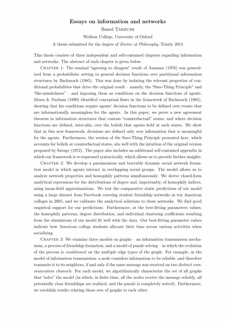
Example. Consider a partitional structure S with Ω = ω1, ω2, ω3, ω4, ω5, N = a, b,
and partitions Ia and Ib as represented in Figure 1.3. In Figures 1.4-1.6, we represent

1.4. COUNTERFACTUAL STRUCTURES 19
a selection of substructures of the counterfactual structure S ′ of S.8 Figure 1.4 shows
the set of counterfactual states Λω4,ω5a , as well as Ω, and the reachability relations,
R′i ⊆ Λω4,ω5a × Ω, of both agents across these two sets. The reachability relations
R′i ⊆ Ω× Ω are left out, but they are unchanged (relative to S) and therefore identical
to what is shown in Figure 1.3. Note that each state in Λω4,ω5a is simply a duplicate
of a corresponding state in Ω. For agent b, every state λω4,ω5a,ω simply points to all
the states ω′ ∈ Ib(ω) (and nothing else). For agent a, every state λω4,ω5a,ω such that
ω ∈ ω1, ω2, ω3 simply points to all the states ω′ ∈ Ia(ω) (and nothing else). However,
for a state ω ∈ ω4, ω5, every state λω4,ω5a,ω points to both ω4 and ω5 (and nothing
else), even though Ia(ω4) ∩ Ia(ω5) = ∅. A similar pattern holds in Figures 1.5 and 1.6
which are there as additional examples for the reader. For practical reasons, we do not
represent the full sets Λ and R′i ⊆ Ω′ ×Ω in a single diagram; and, note that even when
taken together Figures 1.3-1.6 do not offer a complete picture of S ′.
ω1
a
ω2
b
ω3
ba
ω4
a
ω5
ba
Figure 1.3: Ω and the partitions Ia and Ib
The counterfactual structure of a partitional structure has several interesting prop-
erties, which we derive below.8Consider any two information structures S+ = (Ω+, N, R+
i i∈N ) and S− = (Ω−, N, R−i i∈N ).We say that S− is a substructure of S+ if Ω− ⊆ Ω+ and R−i ⊆ R
+i for every i ∈ N .
20 CHAPTER 1. AGREEING ON DECISIONS
ω1
ω2
ω3
ω4
ω5
λω4,ω5a,ω1
λω4,ω5a,ω2
λω4,ω5a,ω3
λω4,ω5a,ω4
λω4,ω5a,ω5
a b
b
b
a b
a
a
a b
ab
a
ba
b
ab
Figure 1.4: Λω4,ω5a ∪ Ω and R′i ⊆ Λ
ω4,ω5a × Ω for i ∈ a, b
ω1
ω2
ω3
ω4
ω5
λω4,ω5b,ω1
λω4,ω5b,ω2
λω4,ω5b,ω3
λω4,ω5b,ω4
λω4,ω5b,ω5
a b
b
b
a b
a
a
a b
ab
b
b
ab
Figure 1.5: Λω4,ω5b ∪ Ω and R′i ⊆ Λ
ω4,ω5b × Ω for i ∈ a, b
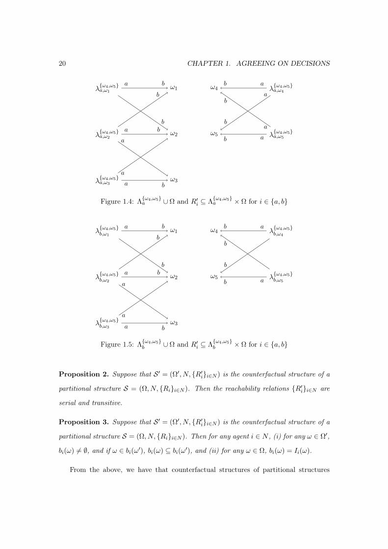
Proposition 2. Suppose that S ′ = (Ω′, N, R′ii∈N ) is the counterfactual structure of a
partitional structure S = (Ω, N, Rii∈N ). Then the reachability relations R′ii∈N are
serial and transitive.
Proposition 3. Suppose that S ′ = (Ω′, N, R′ii∈N ) is the counterfactual structure of a
partitional structure S = (Ω, N, Rii∈N ). Then for any agent i ∈ N , (i) for any ω ∈ Ω′,
bi(ω) 6= ∅, and if ω ∈ bi(ω′), bi(ω) ⊆ bi(ω′), and (ii) for any ω ∈ Ω, bi(ω) = Ii(ω).
From the above, we have that counterfactual structures of partitional structures

1.4. COUNTERFACTUAL STRUCTURES 21
ω1
ω2
ω3
ω4
ω5
λω1,ω2,ω3b,ω1
λω1,ω2,ω3b,ω2
λω1,ω2,ω3b,ω3
λω1,ω2,ω3b,ω4
λω1,ω2,ω3b,ω5
a b
b
b
b
a b
a
b
b
a
b
a b
ab
a
ba
b
ab
Figure 1.6: Λω1,ω2,ω3b ∪ Ω and R′i ⊆ Λ
ω1,ω2,ω3b × Ω for i ∈ a, b
belong to the class of KD4 structures. In particular, the belief operator now only
satisfies properties K, D, and 4; so Negative Introspection no longer holds, relative to
belief structures. (See Section 1.5.2 for further discussion of this point). Note however
that within the counterfactual structure S ′ = (Ω′, N, R′ii∈N ) of a partitional structure
S = (Ω, N, Rii∈N ), the substructure (Ω, N, Rii∈N ) of S ′ corresponds exactly to the
original structure S and is therefore partitional. A further result will be useful.
Proposition 4. Suppose that S ′ = (Ω′, N, R′ii∈N ) is the counterfactual structure of a
partitional structure S = (Ω, N, Rii∈N ). Then for any ω ∈ Ω′ and any G ⊆ N , (i) if
ω′ ∈ TG(ω), then ω′ ∈ Ω, and (ii) for any i ∈ G, ∪ω′∈TG(ω)bi(ω′) = TG(ω).
1.4.2 The agreement theorem
We will now adapt the main definitions required to derive the agreement theorem
within the counterfactual structure of a partitional structure.
Throughout this section, we consider a partitional structure S = (Ω, N, Rii∈N ),
and the counterfactual structure S ′ = (Ω′, N, R′ii∈N ) of S. As before, we can define
Ii(ω) = ω′ ∈ Ω|ωRiω′, the partition Ii = Ii(ω)|ω ∈ Ω, and the set Γi for every
i ∈ N .

22 CHAPTER 1. AGREEING ON DECISIONS
A decision function Di for an agent i ∈ N maps from Γi to a set of actions A. That
is,
Di : Γi → A (1.8)
We now say that an action function δi : Ω′ → A follows decision function Di if for
all states ω ∈ Ω′, δi(ω) = Di(bi(ω)). The following proposition guarantees that this is
well-defined.
Proposition 5. Suppose that S ′ = (Ω′, N, R′ii∈N ) is the counterfactual structure of a
partitional structure S = (Ω, N, Rii∈N ). Then for any ω ∈ Ω′, bi(ω) ∈ Γi.
Below, we provide definitions for the Sure-Thing Principle and like-mindedness that
are analogous to the ones proposed by Bacharach. We elaborate on their interpretations
in Section 1.4.4.
Definition 4. The decision function Di of agent i satisfies the Sure-Thing Principle if
for any non-empty subset E of Ii, whenever for all e ∈ E, Di(e) = x then Di(∪e∈Ee) = x.
The domain Γi includes all possible unions of elements of the partition Ii, so this is
well-defined. Furthermore, note that E must be a set of disjoint events.9
Definition 5. Agents i and j are said to be like-minded if for any e ∈ Γi and any e′ ∈ Γj,
if e = e′ then Di(e) = Dj(e′).10
Theorem 2. Let S ′ = (Ω′, N, R′ii∈N ) be the counterfactual structure of a partitional
structure S = (Ω, N, Rii∈N ).9Note that we impose the Sure-Thing Principle only on events in Ii, which happen to be disjoint
because of the partitionality of the information structure. We do not impose the condition on allevents and do not impose a requirement that the events be disjoint. This contrasts with Moses andNachum (1990) who, in their solution, propose adopting a version of the Sure-Thing Principle thatis imposed on possibly non-disjoint events. The disjointness of events arises naturally if we think ofdecision functions as being conditional probabilities. Indeed, if we index a decision function by anevent e and let De
i (f) = Pri(e|f), then such a decision function will satisfy the Sure-Thing Principle,since conditional probabilities satisfy Pr(e|f ∪ f ′) = x if Pr(e|f) = Pr(e|f ′) = x when f ∩ f ′ = ∅ (seeBacharach, 1985, p. 180). In fact, Cave (1983) notes that conditional probabilities, expectations, andactions that maximize conditional expectations all naturally satisfy the Sure-Thing Principle.
10In contrast with the previous definition, we do not simply say that agents are like-minded if theyhave the “same” decision functions since the domains of the decision functions will now typically bedifferent for different agents.

1.4. COUNTERFACTUAL STRUCTURES 23
If the agents i ∈ N are like-minded (as defined in Definition 5) and follow the decision
functions Dii∈N (as defined in (1.8)) that satisfy the Sure-Thing Principle (as defined
in Definition 4), then for any G ⊆ N , if CG(∩i∈Gω′ ∈ Ω′|δi(ω′) = xi) 6= ∅ then xi = xj
for all i, j ∈ G.
Although this agreement theorem might appear to have many similarities with the
previous one, it is conceptually entirely distinct.11 In particular, we show below (in
Section 1.4.3) that we were able to obtain the result while avoiding the conceptual flaws
that were discussed in Section 1.3.2. We also provide an interpretation of Theorem 2
and of counterfactual structures of partitional structures more generally in Section 1.4.4.
1.4.3 Solution to the conceptual flaws
As discussed in Section 1.3.2, Bacharach’s framework requires the decision functions
to be defined over events that are not possible beliefs for the agents. The proposition
below shows that this is not the case in our set-up.
Proposition 6. Suppose that S ′ = (Ω′, N, R′ii∈N ) is the counterfactual structure of a
partitional structure S = (Ω, N, Rii∈N ). Then for any e ∈ Γi, there exists an ω ∈ Ω′
such that bi(ω) = e. (In fact, there exists a state λei,ω ∈ Λ for some ω ∈ e such that
bi(λei,ω) = e).
This proposition, in conjunction with Proposition 5, shows that in our set-up, the
domain of the decision function of every agent is exactly the set of all possible beliefs for
that agent. Indeed, our decision functions are defined over unions of partition elements,
but these are possible beliefs for the agents because, for every such union, there exists
a counterfactual state at which the possibility set is precisely that union. We therefore
11Note that the proof of the theorem itself does not have to rely on the counterfactual structure.Indeed, with the appropriate restrictions, we could have stated the result as holding in standard parti-tional structures. However, it is the fact that the decision functions are embedded in the larger structurewhich will allow us to provide a proper interpretation of the information over which the decisions aredefined.

24 CHAPTER 1. AGREEING ON DECISIONS
avoid the first point in the conceptual flaws raised by Moses and Nachum (1990). Re-
garding the second point, the decision function Di of agent i is now defined only over
events in Γi. There is therefore no requirement for the function to determine the agent’s
action in the case where the event corresponds to another agent’s possible belief.
Example. To illustrate this, let us once again revisit Figure 1.1 on page 10. Like-
mindedness in Bacharach’s framework would require agent b’s decision function to be
defined over the event ba(ω1) = ω1, which is not a possible belief for b. In our frame-
work however, the domain of b’s decision function is given by Γb = Ω, so there is no
requirement for b’s decision function to be defined over ω1. Similarly, The Sure-Thing
Principle in Bacharach’s framework would require agent a’s decision function to be de-
fined over the event ba(ω1)∪ ba(ω2) = ω1, ω2, which once again, is not a possible belief
for agent a. In contrast, in the counterfactual structure of the partitional structure rep-
resented in Figure 1.1, there will a counterfactual state, namely the state λω1,ω2a,ω1 , such
that ba(λω1,ω2a,ω1 ) = ω1, ω2. Therefore, in our framework, ω1, ω2 is a possible belief
for agent a.
1.4.4 Interpretation
In this section, we provide an interpretation of our assumptions, showing that the
formal definitions of the Sure-Thing Principle and of like-mindedness match well with
intuition. We also provide an interpretation both of the agreement theorem in counter-
factual structures and of those structures more generally.
Our notion of like-mindedness is straightforward: Over the same information, like-
minded agents take the same action. However, our definition has an advantage over
Bacharach’s because an agent i is not required to consider which action to take over the
possible belief of another agent j.
The proposition below, in particular part (ii), allows us to interpret our version of
the Sure-Thing Principle as capturing the intuition that: If an agent i takes the same

1.4. COUNTERFACTUAL STRUCTURES 25
action in every case when i is more informed, i would take the same action if i were
secretly “just” more ignorant.
Proposition 7. Suppose that S ′ = (Ω′, N, R′ii∈N ) is the counterfactual structure of
a partitional structure S = (Ω, N, Rii∈N ). Then, (i) for any e ⊆ Ω′, and ω, ω′ ∈ Ω′,
bi(ω) ⊆ e and bi(ω′) ⊆ e if and only if bi(λbi(ω)∪bi(ω′)i,ω′′ ) ⊆ e (for some ω′′ ∈ Ω). (ii) For
any e ⊆ Ω′, and ω, ω′ ∈ Ω, bi(ω) ⊆ e and bi(ω′) ⊆ e if and only if bi(λbi(ω)∪bi(ω′)i,ω ) ⊆ e.
Indeed, suppose S ′ = (Ω′, N, R′ii∈N ) is the counterfactual structure of a partitional
structure S = (Ω, N, Rii∈N ). Now consider an agent i and two partition elements
Ii(ω), Ii(ω′) ∈ Ii (where ω, ω′ ∈ Ω) and suppose that i’s decision function is such
that Di(Ii(ω)) = Di(Ii(ω′)) = x. The Sure-Thing Principle requires that Di(Ii(ω) ∪
Ii(ω′)) = x. Proposition 6 shows that the possibility set that corresponds to Ii(ω) ∪
Ii(ω′) is bi(λ
Ii(ω)∪Ii(ω′)i,ω ). Proposition 7 part (ii) shows that for any event e, i believes
that e at the counterfactual state λIi(ω)∪Ii(ω′)i,ω if and only if i also believes that e at
the states within each of those partition elements. Informally, if we can call a belief
in an event “information”, then the information that i has at the counterfactual state
preserves only the information that is the same across both the partition elements. In
this sense, the information that i has at the counterfactual state is the information that
i would have if i were “just” more ignorant than at a state in either of the partition
elements.12 Furthermore, by the construction of counterfactual structures, there is no
state ω′′′ ∈ Ω′ and no j ∈ N such that (ω′′′, λIi(ω)∪Ii(ω′)i,ω ) ∈ R′j ; and, for any j 6= i,
(λIi(ω)∪Ii(ω′)i,ω , ω′′′) ∈ R′j for every ω′′′ ∈ Ij(ω) only. In words, this means that at this
counterfactual state, i may have become “more ignorant”, but the information of all
other agents is unchanged. The information at this state therefore truly captures the
fact that i is imagining him/herself “secretly” to be more ignorant. The situation is
counterfactual since all other agents still believe that i has the information that she does
in the partition Ii.
12In fact, it corresponds to being “just” less informed, in a sense similar to that given in Samet (2010).

26 CHAPTER 1. AGREEING ON DECISIONS
We believe that this interpretation of the Sure-Thing Principle matches well with
intuition. In particular, given that the principle finds its origins in single-agent deci-
sion theory (see Savage (1972)), it makes sense that the requirement on the decisions
in cases where the agents are more ignorant is imposed only when ignorance is secret
– in the sense that the information of all other agents is unchanged. One can contrast
this with Bacharach’s version of the Sure-Thing Principle, which requires us to take the
union of partition elements: Since there is no primitive that corresponds to this union,
under a naive interpretation, one could replace the union of partition elements by an-
other partition element that corresponds precisely to this union. But implementing this
modification over the partition elements of some agent i directly implies modifying the
primitives of the structure, which affects the information of the other agents j regarding
i. In this sense, ignorance in Bacharach’s version of the Sure-Thing Principle is not
secret. Furthermore, we can show that the information that the agent has in this union
does not correspond to being “just” more ignorant. We elaborate on the distinction be-
tween this naive method of modeling ignorance and the method we have developed (by
constructing counterfactual structures) in the example below.13
Example. Panel (1) of Figure 1.7 illustrates a partitional structure, S = (Ω, N, Rii∈N ),
in which Ω = ω1, ω2, N = a, b, and the partitions of the agents are given by
Ia = Ib = ω1, ω2. Let e1 and e2 denote the events ω1 and ω2 respec-
tively. Note that in panel (1), Bb(e1) = ω1 and Bb(e2) = ω2. So we also have
that Bb(e1) ∪ Bb(e2)) = ω1, ω2. That is, agent b knows whether e1 or e2 is true. Fur-
thermore, Ba(Bb(e1) ∪ Bb(e2)) = ω1, ω2, so a knows that b knows whether e1 or e2 is
true. Finally, one can also verify that Bb(Ba(Bb(e1) ∪ Bb(e2))) = ω1, ω2. That is, b
knows that a knows that b knows whether e1 or e2 is true. In fact, we have that at each
state of each of b’s partition elements, b knows that a knows that b knows whether e1 or
e2 is true.
13We also elaborate on this point in Appendix A (Section 1.7).

1.4. COUNTERFACTUAL STRUCTURES 27
Now, let us consider two alternative ways in which we can make b no longer know
whether e1 or e2 is true. That is, let us consider two alternative ways in which to make
b more ignorant. According to the naive method described above, we can replace b’s
partition of the state space by a coarser one, in which we take the union of b’s original
partition elements. That is, let us now have that Ib = ω1, ω2. This situation is
represented in panel (2) of Figure 1.7. It is indeed the case that b is more ignorant
since Bb(e1) = ∅ and Bb(e2) = ∅, and so Bb(e1) ∪ Bb(e2) = ∅. That is, in panel (2), b
no longer knows whether e1 or e2 is true. However, b is (i) neither “secretly” ignorant
(ii) nor is b “just” more ignorant relative to the original situation. Indeed, regarding
point (i), Ba(Bb(e1) ∪ Bb(e2)) = ∅, so a no longer knows that b knows whether e1 or
e2 is true. That is, in panel (2), a’s information was not left unchanged relative to the
structure represented in panel (1). So, in this sense, making b more ignorant was not
secret. Regarding point (ii), Bb(Ba(Bb(e1) ∪ Bb(e2))) = ∅ in panel (2), so b no longer
knows that a knows that b knows whether e1 or e2 is true, even though b did know this at
each state of each of b’s partition elements in the original information structure. In this
sense, b has lost too much information, and it therefore cannot be said that b is “just”
more ignorant than in the original structure. Note that this feature, as well as the loss
of secrecy, is driven by the fact that the structure illustrated in panel (2) is partitional,
and therefore all the information in it must be factual. In other words, b must indeed
genuinely be made more ignorant, which implies that a cannot have false beliefs about
b’s ignorance (loss of secrecy), which in turn implies that b cannot have false beliefs
about a’s information (and since a’s information changes, b’s information changes in a
manner that does not result in b being “just” more ignorant).
In contrast, we show that in the counterfactual structure S ′ = (Ω ∪ Λ, N, R′ii∈N ) of
the partitional structure S, which is partly represented in panel (3), there is a state in
which b is secretly “just” more ignorant than in the original structure of panel (1). Panel
(3) of Figure 1.7 shows the original structure S, the counterfactual states in Λω1,ω2b

28 CHAPTER 1. AGREEING ON DECISIONS
(which are the states in which b is made more ignorant regarding the states ω1 and ω2),
and the reachability relations linking these counterfactual states to the original ones. In
this panel, the original structure is preserved intact so a’s and b’s original information is
left unchanged. Indeed, one can verify that Bb(e1) and Bb(e2) are not empty, so b does
indeed either believe that e1 is true or believe that e2 is true. (Notice that we have now
switched from “knowledge” to “belief” because, as shown in Proposition 2, the counter-
factual structure is a KD4 structure, so the belief operator must therefore properly be
interpreted as belief ). Furthermore, Ba(Bb(e1)∪Bb(e2)) is also not empty, so a believes
that b has this belief. And finally, Bb(Ba(Bb(e1)∪Bb(e2))) is also not empty, so b believes
that a believes that b has this belief. It appears as though nothing has changed relative
to panel (1), and this is fully intended: The primitives of the original structure should
not be altered. However, there is also an important difference: At the state λω1,ω2b,ω1
, it
is not the case that b believes that e1 is true, and it is not the case that b believes that e2
is true. In fact, b can no longer distinguish between these events, and has therefore been
made more ignorant. But b’s ignorance is secret because even at that state, which is a
duplicate of state ω1, a still believes that b either believes that e1 is true or believes that
e2 is true. Furthermore, b is “just” more ignorant since it is still true, for example, that at
that state, b believes that a believes that b either believes that e1 is true or believes that
e2 is true. In fact, Proposition 7 shows that b’s beliefs at this counterfactual state will
consist precisely of those beliefs that b held at both partition elements ω1 and ω2.
And, since b believes that a believes that b either believes that e1 is true or believes that
e2 is true at both ω1 and ω2, b preserves this belief at the counterfactual state.14
14We can take this example as an opportunity to also show the manner in which the belief operatorno longer satisfies the properties T and 5 in counterfactual structures of partitional structures. For anyi ∈ N and e ⊆ Γi, let us define Λ(ω) = ∪i∈N ∪e∈Γi λ
ei,ω, so Λ(ω) is the set of all counterfactual states that
are duplicates of the state ω ∈ Ω. Now, note that in panel (3) of Figure 1.7, Bb(e1) = ω1 ∪ (Λ(ω1) \λω1,ω2b,ω1
). Indeed, agent b reaches only ω1 from ω1, and reaches only ω1 from every counterfactual statethat is a duplicate of ω1 except for the duplicate state λω1,ω2
b,ω1, in which b reaches both ω1 and ω2.
From this it follows that Bb(e1) 6⊆ e1, thus violating the Truth property, T. Essentially, this fact tells usthat agent b believes ω1 at the state ω1 but also at counterfactual states, at which, in principle, thebelief could be false. For a somewhat starker example, note that λω1,ω2
b,ω1∈ Ba(Bb(e1) ∪ Bb(e2)) but
λω1,ω2b,ω1
6∈ Bb(e1) ∪Bb(e2). That is, a actually entertains a false belief regarding b’s beliefs at the state
1.4. COUNTERFACTUAL STRUCTURES 29
ω1
ω2
a, b
a, b
ω1
ω2
b
a, b
a, b
ω1
ω2
λω1,ω2b,ω1
λω1,ω2b,ω2
ab
b
b
ab
a, b
a, b
(1) (2) (3)
Figure 1.7: Secret counterfactual ignorance
More generally, our interpretation of the counterfactual structure S ′ of a partitional
structure S is therefore that it is simply a more complete picture of the situation being
modeled by the structure S since it also includes states in which the agents imagine
themselves (secretly and counterfactually) to be more ignorant. Indeed, consider the fol-
lowing analogy with backwards induction: In order to fully specify a backwards induction
solution in a game, one must determine what each player would do at each history of
the game, including histories that are never reached given the history that would be
played under the specified profile. The specification therefore requires determining the
actions of agents both along the actual path and also along paths that are not played.
In our case, the counterfactual structures allow us to speak not only about the actions
of the agents in the “actual” situation, but also about their actions in counterfactual
situations that do not actually occur (but which nevertheless matter for what happens
λω1,ω2b,ω1
. Regarding the property 5, note that ¬Bb(e1) = ω2 ∪ Λ(ω2) ∪ Λω1,ω2b , which is simply the
complement of Bb(e1). And Bb(¬Bb(e1)) = ω2∪ (Λ(ω2) \λω1,ω2b,ω2
). Indeed, agent b cannot reach anyof the states in Λ(ω2)∪Λ
ω1,ω2b from any state; and agent b reaches only ω2 from ω2, and reaches only
ω2 from every counterfactual state that is a duplicate of ω2 except for the duplicate state λω1,ω2b,ω2
, inwhich b reaches both ω1 and ω2. However, this shows that ¬Bb(e1) 6⊆ Bb(¬Bb(e1)), thus violating theNegative Introspection property, 5.

30 CHAPTER 1. AGREEING ON DECISIONS
in the actual situation). Indeed, we can think of the substructure S = (Ω, N, Rii∈N ) of
S ′ = (Ω ∪ Λ, N, R′ii∈N ) as representing the “actual” situation, and the counterfactual
states Λ are essentially “fake” in the sense that they do not actually occur. However, they
are connected (via the reachability relations) to the “actual” states in Ω15 in a manner
that captures every possible way in which every agent could be secretly more ignorant
relative to the “actual” situation; and although the “fake” states do not occur, the decision
functions are defined at such states (more precisely, they are defined over possibility sets
that are defined as such states). This turns out to be crucial: Theorem 2 is derived by
showing that when the actions of agents are commonly known, the Sure-Thing Principle
and like-mindedness imply that the actions must be the same precisely in the case when
the decision functions are based on the information at some counterfactual (or “fake”)
states. The equality of the actions over information at counterfactual states then carries
over to the decisions over the information in the “actual” situation, and therefore agents
cannot agree to disagree.
1.5 Relation to the literature
We now discuss our approach in relation to other solutions that were proposed regard-
ing the conceptual flaws. We then also compare our construction of the counterfactual
states to other models that are designed to represent counterfactual information.
1.5.1 Other solutions
Moses and Nachum (1990) propose a solution to the conceptual flaws that they found
in the result of Bacharach (1985). Essentially, they define a “relevance projection”, which
maps from sets of states to the “relevant information” at that set of states (Moses and
Nachum, 1990, p. 158). They then impose conditions on this projection and on the
decision functions to derive a new agreement theorem. However, it is not always obvious15Notice that this shows that our counterfactual structures are particular “impossible-world” struc-
tures (e.g. see Wansing (1990)). We return to this point in Section 1.5.

1.5. RELATION TO THE LITERATURE 31
how a projection satisfying their conditions ought to be found. In contrast, the approach
presented here offers a constructive method of obtaining a structure in which the analysis
can be carried out.16
Aumann and Hart (2006) also propose a solution using a purely syntactic approach.
Unlike the semantic framework presented in the previous sections, in which informa-
tion is modeled purely with states and relations over those states, a syntactic framework
expresses information by means of a syntactic language comprising purely syntactic state-
ments such as propositions. To derive their result, Aumann and Hart (2006) impose a
condition, which we do not impose here, that higher-order information must be irrele-
vant to the agents’ decisions.17 If first-order information refers to the information that
agents have about the “basic facts”, such as “It is raining” or “Socrates is a man”, then
second-order information refers to the information that an agent i has about an agent j’s
information about the “basic facts”, and third-order information refers to the information
that i has about j’s information about k’s information about the “basic facts”, and so on.
The restriction of Aumann and Hart (2006) requires agents’ decision functions to not
depend on anything above first-order information. But one can easily imagine scenarios
in which higher-order information is relevant. Indeed, any situation in which an agent’s
decision depends on the information of another agent will suffice.18
Finally, Samet (2010) presented a very interesting solution to the conceptual flaws
by redefining the Sure-Thing Principle entirely. Roughly, Samet’s “Interpersonal Sure-
Thing Principle” states that if agent i knows that agent j is more informed than i is, and
knows that j’s action is x, then i takes action x. Combining this with the assumption of
the existence of an “epistemic dummy” – an agent who is less informed than every other
agent – Samet (2010) proves a new agreement theorem in paritional structures. Other
16Note that our counterfactual structures along with our decision functions does satisfy propertiesthat resemble, in spirit, the conditions imposed on the relevance projection.
17The relation between their result and ours is made clear in Appendix A (Section 1.7).18For example, consider the situation in which agent a is an analyst, and agent b requires some advice.
Agent b is willing to pay a to obtain some advice if and only if b knows that a is more informed than bis. Here, b’s decision does not depend on the “basic facts”, but on high-order knowledge; namely, on bknowing that a is more informed than b.

32 CHAPTER 1. AGREEING ON DECISIONS
than the fact that, unlike our version of the Sure-Thing Principle (Definition 4), the
interpersonal Sure-Thing Principle does not have a straightforward single-agent version,
the large differences in the assumptions make a formal comparison between the approach
here and in Samet (2010) difficult.
1.5.2 Action models
Loosely speaking, it was shown that the information at the counterfactual states in
a counterfactual structure corresponds to secretly “losing” information. It turns out that
secretly “gaining” information is well-studied in the dynamic epistemic logic literature
(e.g. Baltag and Moss, 2005). Action models formalize how the underlying structure
(both the state space and the reachability relations) must be modified to model various
protocols by which agents may gain some new information.
It was shown, in Van Eijck (2008, Theorem 17), that in the case of secretly gaining
new information, a partitional structure (S5) would have to be transformed into a belief
structure (KD45). In this paper, we have defined a method of modeling secret loss
of information by transforming a partitional structure into a (counterfactual) structure
that belongs to the KD4 class. In particular, this means that Negative Introspection is
dropped as a property of the belief operator. We have not shown that it is necessary to
drop Negative Introspection in order to model secret loss of information, so in principle,
it remains an open question as to whether it is possible to define a purely semantic trans-
formation of a partitional structure (i.e. involving only the states and the reachability
relations) that can model secret loss of information such that the resulting structure is
a belief structure in which the primitives of the original structure (i.e. the original state
space and partitions over them) are unchanged.19,20
19Stalnaker (1996) analyzes counterfactuals inKD45 structures. But his initial structures areKD45,whereas we are looking for a method that would transform a partitional structure into a KD45 struc-ture while building relevant counterfactual states and leaving the primitives of the original structureunchanged.
20Note that in contrast with the purely semantic approach, it is not particularly difficult to findsuch a transformation within a syntactic framework to model the relevant counterfactual states whilepreserving KD45 information (i.e. Negative Introspection). For this, see Section 1.7.3 of Appendix A.

1.5. RELATION TO THE LITERATURE 33
1.5.3 Counterfactuals
General set-theoretic information structures have been proposed to model counter-
factuals (e.g. see Halpern, 1999), especially in relation to the literature on backwards
induction. In extensive form games, to implement the backwards induction solution,
agents must consider what they would do at histories of the game that might never be
reached. They must therefore be able to define what they would do in situations that
never occur. Although this bears some resemblance to our set-up in which agents are
required to have decisions that are defined over information at counterfactual (or “fake”)
states that never actually occur, there are important differences.
There is a multitude of ways in which counterfactuals can be modeled, and we cannot
hope to survey the literature here. However, it will suffice to say that, in general, the
approach to modeling counterfactuals proceeds in roughly the following manner (again,
see Halpern, 1999): One defines a “closeness” relation on states and then says that a state
ω belongs to the event “If f were the case, then e would be true” if e is true in all the closest
states to ω where f is true. It is possible to then augment this approach with epistemic
operators and decisions, but the salient point is simply that the standard approach to
counterfactuals aims to be quite general, in capturing all possible hypothetical situations.
In contrast, we only model counterfactuals for a very particular set of hypothetical
situations, namely, every possible situation (relative to the “actual” situation) in which
every agent imagines him/herself to be secretly more ignorant. This is not done by
imposing a closeness relation, but by creating a new set of “fake” counterfactual states
and carefully re-wiring them to the “actual” states. (Note however, that the resulting
information at the counterfactual states was shown to be interpretable as being secretly
“just” more ignorant than in the “actual” situation being considered, so in this sense, the
counterfactual state can be seen as being “close” to the actual situation). As a result,
it is unfortunately not obvious to see how the method developed here can be applied
to studying backwards induction, which requires considering a richer set of hypothetical

34 CHAPTER 1. AGREEING ON DECISIONS
situations. We are not aware of any papers that model counterfactuals in quite the same
way as is done here, but the method is well-adapted for the analysis of the agreement
theorems carried out in this paper.
Note that there is another approach that is related to our counterfactual structures.
What is known as the “impossible-worlds” approach (e.g. Wansing, 1990) augments
information structures with a new set of states and with modified reachability relations.
The set of states in the original structure are then referred to as “possible”, or “normal”,
worlds, while the ones in the new set are referred to as “impossible”, or “non-normal”.
In our framework, these actually correspond to our “actual” states Ω and to our “fake”
states Λ (and the reachability relations are modified from Ri to some R′i for every i).
The counterfactual structures presented here can therefore be seen as specific “impossible-
worlds” structures. However, we are not aware of any paper that use impossible-worlds
structures as a tool for modeling counterfactuals in the manner presented here.
1.6 Conclusion
We provided a constructive method for creating an information structure that in-
cludes the relevant counterfactual states starting from a partitional structure. This new
counterfactual structure is interpreted as providing a more complete picture of the sit-
uation that is being modeled by the original partitional structure. Our analysis of the
agreement theorem is carried out in such structures.
Having provided new formal definitions for the Sure-Thing Principle and for like-
mindedness, we prove an agreement theorem within such structures and show that we
can interpret our version of the Sure-Thing principle as capturing the intuition that: If
an agent i takes the same action in every case when i is more informed, i would take
the same action if i were secretly (just) more ignorant. We also show that our version of
like-mindedness has more desirable properties than Bacharach’s. Furthermore, we show
that our approach resolves the conceptual issues raised by Moses and Nachum (1990), in

1.6. CONCLUSION 35
the sense that within counterfactual structures, decision functions are defined only over
events that are possible beliefs or, equivalently, that are informationally meaningful for
the agents.
Therefore, in providing a constructive method for creating counterfactual structures,
our approach achieves the goal of maintaining an interpretation of the underlying as-
sumptions of the agreement theorem that fits well with intuition, while simultaneously
resolving the conceptual issues, identified in Moses and Nachum (1990), regarding the
domain of the decision functions.

36 CHAPTER 1. AGREEING ON DECISIONS
1.7 Appendix A: The syntactic approach
In this self-contained appendix, we express our framework syntactically. This allows
us to provide further insights into the “agreeing to disagree” result. To do this, we intro-
duce Kripke information structures. These are essentially identical to the information
structures we defined in Section 1.2, but are augmented with a valuation map, which
determines the truth of syntactic statements at each state.
1.7.1 New definitions
Definitions 6 to 9 are standard in the epistemic logic literature (e.g. for general
reference, see Chellas, 1980, and van Benthem, 2010).
Definition 6. Define a finite set of atomic propositions, P . Let N denote the set of all
agents. We then inductively create all the formulas in our language, L, as follows:
(i) Every p ∈ P is a formula.
(ii) If ψ is a formula, so is ¬ψ.
(iii) If ψ and φ are formulas, then so is ψ φ, where is one of the following Boolean
operators: ∧, ∨, →, or ↔.
(iv) If ψ is a formula, then so is •ψ, where • is one of the modal operators βi∈N or
CG⊆N .
(v) Nothing else is a formula.
“It is raining” and “Socrates is a man” are examples of atomic propositions. They are
propositions that cannot be reduced (in the sense that they do not contain a negation, a
Boolean operator, or a modal operator), and they express “basic facts”. From a finite set
of such atomic propositions, the definition above generates all the syntactic “formulas” –
which are, technically, simply strings of symbols – that are admissible in the language.
“It is raining and Socrates is a man” is an example of such a formula. The following
defines Kripke information structures.

1.7. APPENDIX A: THE SYNTACTIC APPROACH 37
Definition 7. As before, an information structure is a triple (Ω, N, Rii∈N ), where Ω
is a finite, non-empty set of states, and Ri ⊆ Ω × Ω is a binary relation for each agent
i ∈ N , also called the reachability relation for agent i. A Kripke information structure
over an information structure (Ω, N, Rii∈N ), is a tupleM = (Ω, N, Rii∈N ,V), where
V : P × Ω→ 0, 1 is a valuation map.
A Kripke information structure is, therefore, an information structure augmented
with a valuation map. For each state in Ω, the map assigns a value of one or zero to each
proposition in P . This will be interpreted as a proposition being true or false respectively
at the state in question. This is then extended to every formula in our language in the
manner shown in the definition below.
Definition 8. We say that a proposition p ∈ P is true at state ω in a Kripke information
structureM = (Ω, N, Rii∈N ,V), denotedM, ω |= p, if and only if V(p, ω) = 1. Truth
is then extended inductively to all other formulas ψ as follows:
(i)M, ω |= ¬ψ if and only if it is not the case thatM, ω |= ψ.
(ii)M, ω |= (ψ ∧ φ) if and only ifM, ω |= ψ andM, ω |= φ.
(iii)M, ω |= (ψ ∨ φ) if and only ifM, ω |= ψ orM, ω |= φ.
(iv)M, ω |= (ψ → φ) if and only if, if M, ω |= ψ thenM, ω |= φ.
(v)M, ω |= (ψ ↔ φ) if and only if,M, ω |= ψ if and only ifM, ω |= φ.
(vi)M, ω |= βiψ if and only if ∀ω′ ∈ Ω, if ωRiω′ thenM, ω′ |= ψ.
(vii)M, ω |= CGψ if and only if ∀ω′ ∈ TG(ω),M, ω′ |= ψ.
Note that the syntactic operator βi and our notion of possibility sets bi(ω) are closely
related since we could have defined: M, ω |= βiψ if and only if ∀ω′ ∈ bi(ω),M, ω′ |= ψ.
In this sense, we readM, ω |= βiψ as “Agent i believes that ψ at state ω in the Kripke
structureM”, andM, ω |= CGψ as “It is commonly believed among the agents in G that
ψ (at state ω in the Kripke structureM)”.
Note that the syntactic operator βi inherits properties (K, D, T, 4, and 5) that are
entirely analogous to those of belief operators, depending on the restrictions imposed on

38 CHAPTER 1. AGREEING ON DECISIONS
the reachability relations. For example, whenever the reachability relations are equiva-
lence relations in some Kripke information structure M, then for any formula ψ ∈ L,
any agent i, and at any state of the structure, it is true that: (βi(ψ → φ) ∧ βiψ)→ βiφ
(Kripke, K), βiψ → ¬βi¬ψ (Consistency, D), βiψ → ψ (Truth, T), βiψ → βiβiψ (Pos-
itive Introspection, 4), and finally, ¬βiψ → βi¬βiψ (Negative Introspection, 5). We
therefore interpret βi as “knowledge” in an S5 structure. Similarly, βi satisfies all the
above properties but Truth in a KD45 structure, and additionally does not satisfy Neg-
ative Introspection in a KD4 structure; and therefore βi is interpreted as “belief” in the
latter two structures.
Definition 9. The modal depth md(ψ) of a formula ψ is the maximal length of a nested
sequence of modal operators. This can be defined by the following recursion on our syntax
rules: (i) md(p) = 0 for any p ∈ P , (ii) md(¬ψ) = md(ψ), (iii) md(ψ ∧ φ) = md(ψ ∨
φ) = md(ψ → φ) = md(ψ ↔ φ) = max(md(ψ),md(φ)), (iv) md(βiψ) = 1 + md(ψ), (v)
md(CGψ) = 1 + md(ψ).
Finally, note that for any formula ψ ∈ L such that md(ψ) ≥ 1, we say that the
“outermost modal operator” of ψ is βi if, reading the symbols of ψ from left to right, the
first modal operator encountered is βi.
The central concept that we introduce in this appendix is that of a ken of an agent i
at state ω, which is the set of all formulas ψ, such that md(ψ) ≥ 1, that are true at that
state (within a Kripke structure) where the outermost modal operator of ψ is βi.
Definition 10. In any Kripke information structure M = (Ω, N, Rii∈N ,V), the ken
of agent i at the state ω is defined by
kenMi (ω) = •ψ ∈ L|ω |= •ψ, • ∈ βi,¬βi
This is extended to subsets W ⊆ Ω as follows: KMi (W ) = kenMi (ω)|ω ∈W.
A ken kenMi (ω) is therefore simply a set of formulas. It does not exhaust all the

1.7. APPENDIX A: THE SYNTACTIC APPROACH 39
formulas that are true at state ω in the Kripke structure M, but it does contain all
the relevant formulas that describe i’s information at state ω. Indeed, for any formula
ψ ∈ L, and at any state ω of any Kripke structure M, it must be the case that either
βiψ is true at ω or that ¬βiψ is true at ω.
Example. We illustrate these concepts in the simple Kripke information structure
M = (Ω, N, Rii∈N ,V) represented in Figure 1.8. Here, Ω = ω1, ω2, N = a, b,
Ra = (ω1, ω1), (ω2, ω2), and Rb = (ω1, ω1), (ω1, ω2), (ω2, ω1), (ω2, ω2). Note that this
structure is partitional, and we will therefore interpret βi as “knowledge”. Furthermore,
let P = p, and suppose V(p, ω1) = 1 and V(p, ω2) = 0. That is, p is the only atomic
proposition in the language, and p is true at the state ω1 and false at the state ω2. Now,
since ω1 only reaches ω1 via Ra, and ω1 |= p, it follows that ω1 |= βap. That is, agent
a knows that p at ω1. Also, note that at ω1, agent b considers the state ω2 possible,
in which p is not true. Therefore, ω1 |= ¬βbp. That is, agent b does not know that p
(is true) at ω1, because at ω1, there is a state that b considers possible (namely ω2) at
which p is false. It follows that ω1 |= βa¬βbp, so a knows that b does not know that p.
(Similarly, it also follows that ω1 |= βa(¬(βbp∨βb¬p)), so a knows that b does not know
whether p at ω1).
The modal depth of the formula βa¬βbp is two, and its outermost modal operator is βa.
The outermost modal operator of the formula ¬βbp is βb.
Note finally that, among many others, the formulas βap and βa¬βbp and βa(¬(βbp ∨
βb¬p)) are members of the ken kenMa (ω1). Similarly, among many others, the formula
¬βbp is in the ken kenMb (ω1).
We can now define an (incomplete) order% over the kens of an agent i that determines
their relative informativeness.
Definition 11. Consider any Kirpke information structure M and ki,k′i ∈ KMi (Ω).
The ken ki is more informative than the ken k′i, denoted ki % k′i, if for each formula

40 CHAPTER 1. AGREEING ON DECISIONS
ω1 |= p
ω2 6|= p
b
a, b
a, b
Figure 1.8: A Kripke structure
ψ ∈ L, if βiψ ∈ k′i, then βiψ ∈ ki.21
Definition 12. Consider any Kirpke information structure M and any Z ⊆ KMi (Ω).
The infimum of the set of kens Z, denoted infZ, is the most informative ken (according
to %) that is less informative than each of the kens in Z. It is defined by: For any formula
ψ ∈ L, βiψ ∈ infZ if and only if βiψ ∈ ki for each ki ∈ Z.
Example. Suppose that Z = ka,k′a and that ka % k′a. Then, any formula that
agent a believes in the ken k′a, a also believes in the ken ka (but a might also believe
more formulas in the latter than in the former). In the case in which βi is interpreted
as “knowledge”, this means that a knows at least as many formulas in ka as in k′a.
Regarding the infimum of these kens, infZ preserves only the information in ka and
k′a that these sets agree on. For example, if “Agent a knows that Socrates is a man” is
an element of both ka and k′a, then it will also be an element of the infimum. On the
other hand, if “Agent a knows that Socrates is a man” is an element of ka but “Agent a
does not know that Socrates is a man” is an element of k′a, then “Agent a does not know
that Socrates is a man” will be an element of the infimum.
For any information structure M, and any W ⊆ Ω, let IMi (W ) be the set of kens21In spirit, this is the same order as the one found in Samet (2010).

1.7. APPENDIX A: THE SYNTACTIC APPROACH 41
defined by: For any Z ⊆ KMi (W ), inf(Z) ∈ IMi (W ). One can verify that this set has the
following important properties: (1) KMi (W ) ⊆ IMi (W ), and (2) for any Z ⊆ IMi (W ),
infZ ∈ IMi (W ). In words, IMi (W ) is the set of all kens at the states in W , as well
as all the all the possible infima across such kens. In fact, it is the closure under infima
of the kens at states in W , and it is the syntactic analogue of the set Γi introduced in
Section 1.4.1.
We can now provide the definition of a decision function for an agent.
Definition 13. For any Kripke information structureM and any i ∈ N , Di : IMi (Ω)→
A, is a decision function for agent i, where A is a set of actions.
The decision function Di determines what agent i does given every ken in IMi (Ω).
The Sure-Thing Principle over such decisions functions is defined below.
Definition 14. Consider the counterfactual structure S ′ = (Ω′, N, R′ii∈N ) of a parti-
tional structure S = (Ω, N, Rii∈N ), and letM′ be a Kripke information structure over
S ′. For all i ∈ N , the decision function Di of agent i satisfies the Sure-Thing Principle
if all Z ⊆ KM′i (Ω), if for every ki ∈ Z, Di(ki) = x then Di(infZ) = x.22,23
This states that whenever an agent takes the same decision over every ken ki in Z,
then the agent also takes the same decision over the infimum of those kens. Note that
the Sure-Thing Principle is well-defined by the properties of the set IMi (Ω).
The order % is defined for a given agent i. However, we can compare the relative
informativeness of kens across different agents with the following relation.
Definition 15. Consider any Kirpke information structureM and any ki ∈ IMi (Ω) and
kj ∈ IMj (Ω). We say that the kens ki and kj are equally informative, denoted ki ∼ kj,
22Note that the Sure-Thing Principle is not imposed on all kens, but only on those at states withinΩ. Futhermore, note for any ω, ω′ ∈ Ω, if i’s ken at ω is distinct from i’s ken at ω′, then it must be thecase that bi(ω)∩ bi(ω′) = ∅. So in a sense, just as for the semantic definition of the Sure-Thing Principle(Definition 4), we are once again applying the Sure-Thing Principle on information that happens to be“disjoint” (in a manner that is analogous to the semantic approach), and this disjointness is derived fromthe fact that the substructure S is partitional.
23Note that the value of the valuation map at the counterfactual states in a Kripke structure over acounterfactual structure is irrelevant since no counterfactual state is reachable from any state.

42 CHAPTER 1. AGREEING ON DECISIONS
if for any formula ψ ∈ L, βiψ ∈ ki if and only if βjψ ∈ kj.
Example. This example clarifies what it means to say that the kens ka and kb of agents
a and b are equally informative. If βaψ ∈ ka, then it must be the case that βbψ ∈ kb.
If the modal depth of ψ is zero, then ka ∼ kb simply means that a and b have the
same beliefs regarding the “basic facts”. However, this becomes more nuanced when the
modal depth of ψ is one. Indeed, suppose ψ ∈ βaφ,¬βaφ, βbφ,¬βaφ for some φ with
md(φ) = 0. Then, ka ∼ kb means that a and b must have the same beliefs about a’s
beliefs about the “basic facts” and must have the same beliefs about b’s beliefs about the
“basic facts”. Furthermore, suppose there is a third agent c and that ψ ∈ βcφ,¬βcφ
for some φ. Then, ka ∼ kb means that a and b must have the same beliefs about any
other agent c’s beliefs about the “basic facts”. This reasoning extends to higher modal
depths of ψ.
The concept of kens being “equally informative” allows us to provide a definition for
like-mindedness in this context.
Definition 16. Consider the counterfactual structure S ′ = (Ω′, N, R′ii∈N ) of a parti-
tional structure S = (Ω, N, Rii∈N ), and letM′ be a Kripke information structure over
S ′. Agents i, j ∈ N are said to be like-minded if for any ki ∈ IM′i (Ω) and kj ∈ IM′j (Ω),
if ki ∼ kj then Di(ki) = Dj(kj).
1.7.2 Syntactic results
Proposition 8 shows that the infimum of kens has the correct interpretation when the
underlying structure is the counterfactual structure of a partitional structure. Namely
it represents being secretly “just” more ignorant (relative to the kens over which the
infimum is taken).
Proposition 8. Consider the counterfactual structure S ′ = (Ω′, N, R′ii∈N ) of a parti-
tional structure S = (Ω, N, Rii∈N ), and letM′ be a Kripke information structure over

1.7. APPENDIX A: THE SYNTACTIC APPROACH 43
S ′. Then, for any i ∈ N , W ⊆ Ω, and Z ⊆ KM′i (W ), infZ = kenM′
i (λWi,ω) for some
ω ∈ Ω.
To see why the infimum of kens represents being secretly “just” more ignorant, we
present an example below, which briefly repeats the example given on page 26, but within
a syntactic framework.
Example. Suppose that S = (Ω, N, Rii∈N ) is a partitional structure and thatM is a
Kripke information structure over S, as represented in panel (1) of Figure 1.9. Suppose
Ω = ω1, ω2, N = a, b, and that the partitions are given by Ia = Ib = ω1, ω2.
Furthermore, suppose that P = p and that V(p, ω1) = 1 and V(p, ω2) = 0.
Suppose also that Db(Ib(ω1)) = Db(Ib(ω2)) = x. Bacharach’s Sure-Thing Principle
requires that Db(Ib(ω1) ∪ Ib(ω2)) = x. But what is the information contained in
Ib(ω1) ∪ Ib(ω2)? It is clear that, in panel (1) of Figure 1.9, ω1 |= βbp and ω2 |= βb¬p.
Also, ω1 |= βa(βbp ∨ βb¬p) and ω2 |= βa(βbp ∨ βb¬p), so at each state, a knows that
b knows whether p is true. Furthermore, note that ω1 |= βb(βa(βbp ∨ βb¬p)) and
ω2 |= βb(βa(βbp ∨ βb¬p)). That is, in each state, b knows that a knows that b knows
whether p is true. But in a Kripke information structure, b’s information is not de-
fined at the union of the partition elements. Under a naive method, one could replace
Ib(ω1)∪Ib(ω2) with a new partition element which is equal to this union. That is, we could
consider the structure shown in panel (2) of Figure 1.9, in which Ia = ω1, ω2 and
Ib = ω1, ω2. However, in this case, ω1 |= ¬βb(βa(βbp∨βb¬p)). So the ken kenM′
b (ω1)
in this new structure contains a formula in which b does not know that a knows whether
b knows that p. This ken therefore, surely cannot correspond to b becoming “just” more
ignorant since it does not preserve the information that b knew at every state of the orig-
inal structure. Furthermore, this ignorance is not secret since now a’s information has
changed to ω1 |= βa(¬(βbp∨ βb¬p)). On the other hand, Proposition 8 above does show
that kenM′
b (λω1,ω2b,ω2
) = kenM′
b (λω1,ω2b,ω1
) = infkenM′b (ω1),kenM′
b (ω2) in the Kripke
structure M′ over the counterfactual structure of the partitional structure S shown in

44 CHAPTER 1. AGREEING ON DECISIONS
panel (3) of Figure 1.9. Therefore, the infimum of b’s kens in the original structure
does precisely correspond to being “just” more ignorant – by the very definition of the
infimum. Furthermore, the ignorance is now secret since a’s reachability relations point
back only into the original structure while leaving a’s information unchanged.
ω1 |= p
ω2 6|= p
a, b
a, b
ω1 |= p
ω2 6|= p
b
a, b
a, b
ω1 |= p
ω2 6|= p
λω1,ω2b,ω1
λω1,ω2b,ω2
ab
b
b
ab
a, b
a, b
(1) (2) (3)
Figure 1.9: Ignorance in a Kripke structure
The example above shows that in a partitional structure S, if one were to replace
the union of partition elements of an agent with a new partition element that is equal to
this union, then the information “contained” in this union (in the corresponding Kripke
information structure over S) does not correspond to the agent being “just” more igno-
rant. On the other hand, in the Kripke structure over the counterfactual structure S ′
of S, the ken at the agent’s counterfactual state of those partition elements corresponds
exactly to the infimum of the kens at each of those partition elements, and therefore
corresponds precisely to being secretly “just” more ignorant.
We should note that Aumann and Hart (2006) proved an agreement theorem in a
syntactic framework (see Section 1.5). However, they required their decision functions to
depend only on formulas of modal depth at most one, and to not depend on higher-order
information. Remarkably, we can show, in the proposition below, that if we restrict the

1.7. APPENDIX A: THE SYNTACTIC APPROACH 45
language L to comprise only formulas of modal depth at most one, then the information
“contained” in a partition element that is equal to the union of partition elements is the
same as the infimum of the kens at each of those partition elements. Therefore, the
union of partition elements does correspond to being secretly “just” more ignorant when
the language does not contain formulas of modal depth greater than one.24
Proposition 9. Consider the counterfactual structure S ′ = (Ω′, N, R′ii∈N ) of a parti-
tional structure S = (Ω, N, Rii∈N ), and letM′ be a Kripke information structure over
S ′, where L only comprises formulas ψ such that md(ψ) ≤ 1.
Consider i ∈ N , and suppose that for ω, ω′ ∈ Ω, Ii(ω) and Ii(ω′) are disjoint. Further-
more, supposeM′′ is a Kripke information structure that is identical toM′, except that
i’s partition over Ω is modified such that Ii(ω) and Ii(ω′) are replaced by a partition
element Ji(ω), which is equal to their union.
Then, we have that kenM′′
i (ω) = kenM′
i (λIi(ω)∪Ii(ω′)i,ω ).
We can now present our agreement theorem within this framework. To do this,
whenever we have that Di(kenMi (ω)) = x, we add a new proposition dxi to our language
that we set as being true at state ω (in M) and that is interpreted as the statement
“Agent i performs action x”. With this, we can provide a formal syntactic definition of
agreeing to disagree.
Definition 17. In a Kripke information structureM, the agents in G ⊆ N cannot agree
to disagree if it is the case that if CG(∧i∈G d
xii ) is true at some ω ∈ Ω, then xi = xj for
all i, j ∈ G.
We can therefore state our agreement theorem in the syntactic framework below.
Theorem 3. Consider the counterfactual structure S ′ = (Ω′, N, R′ii∈N ) of a partitional
structure S = (Ω, N, Rii∈N ), and letM′ be a Kripke information structure over S ′.24We can easily provide some intuition for the reason why the union of partition elements preserves
secrecy when the language is restricted to comprise only formulas of modal depth at most one: Theignorance of an agent i can be secret only if the information of other agents regarding i’s information isunchanged. Secrecy is therefore defined only if the language contains formulas of modal depth strictlygreater than one.

46 CHAPTER 1. AGREEING ON DECISIONS
If the agents i ∈ N are like-minded (as defined in Definition 16) and follow the decision
functions Dii∈N (as defined in Definition 13) that satisfy the Sure-Thing Principle (as
defined in Definition 14), then for any G ⊆ N , the agents in G cannot agree to disagree.
In what remains of this section, we prove a result that diverges somewhat from the
rest of the paper’s content, but that might be considered to be sufficiently interesting
nonetheless.
Definition 18. A Kripke information structure M is said to satisfy “pairwise equal
information” if and only if, for all non-singleton G ⊆ N , ω ∈ Ω, and for each i ∈ G, there
is some j ∈ G\i such that ki ∼ kj for some ki ∈ IMi (TG(ω)) and kj ∈ IMj (TG(ω)).
That is, a Kripke information structure satisfies “pairwise equal information” if, in ev-
ery component and for every agent, there is some other agent with an equally informative
ken (from within the closure under infima of kens in the component).
Example. The structure in Figure 1.10 does not satisfy pairwise equal information.
Indeed, a believes that p is true at every state, so p must also be true in every infimum
of a’s kens, and b believes that p is false at every state, so p must be false in every
infimum of b’s kens.
ω1 |= p ∧ ¬q
ω2 |= ¬p ∧ ¬q
ω3 |= ¬p ∧ q
ω4 |= p ∧ q
b
a
b
a
a
b
b
a
Figure 1.10: A structure that does not satisfy pairwise equal information

1.7. APPENDIX A: THE SYNTACTIC APPROACH 47
It turns out that the impossibility of agents agreeing to disagree in a Kripke infor-
mation structure is equivalent to the structure satisfying pairwise equal information, as
stated below.
Theorem 4. For any Kripke information structureM = (Ω, N, Rii∈N ,V),M satisfies
pairwise equal information if and only if for any non-singleton G ⊆ N , and any decision
functions Dii∈G (as defined in Definition 13) satisfying the Sure-Thing Principle (as
defined in Definition 14) and like-mindedness (as defined in Definition 16), agents cannot
agree to disagree in the structureM.
Roughly speaking, this characterization result states that agents cannot agree to
disagree if and only if the information structure is such that for any pair of agents i and
j, agent i has a ken in the domain of his/her decision function that is equally informative
to some ken in the domain of agent j. Note that the interpretation of the information
contained in these kens will depend on the particular restrictions that are imposed on the
reachability relations since it is these relations that determine the interpretation of the
syntactic operator βi. So we cannot provide a proper interpretation of the information
over which the decision functions are defined in Theorem 4 unless we first impose some
more structure onM. To resolve this, consider the following definition.
Definition 19. A Kripke information structureM = (Ω, N, Rii∈N ,V) is said to sat-
isfy “quasi-coherence” if and only if, for every G ⊆ N and every component TG(ω),
there is a sub-component TG(ω′) ⊆ TG(ω) such that for all ω′′ ∈ TG(ω′) and all i ∈ G,
(ω′′, ω′′) ∈ Ri.
That is, a Kripke structure is quasi-coherent if (roughly) every component has a
reflexive sub-component. One can verify that a Kripke structure over the counterfactual
structure of a partitional structure satisfies quasi-coherence. And, as the proposition
below shows, quasi-coherent Kripke structures also satisfy pairwise equal information.
Therefore, the kens over which the decision functions are defined in Theorem 4 will be

48 CHAPTER 1. AGREEING ON DECISIONS
well-interpreted if we further assume that the structureM, referred to in the theorem,
is a Kripke structure over the counterfactual structure of a partitional structure.
Proposition 10. If a Kripke information structure satisfies quasi-coherence then it sat-
isfies pairwise equal information.
Bonanno and Nehring (1998) present a characterization of “agreeing to disagree”
within a semantic framework in which agents are endowed with “qualitative” belief indices
satisfying conditions analogous to, but stronger than Bacharach’s Sure-Thing Principle.
Specifically, in a framework in which the underlying structure belongs to the KD45
class, they show that agents cannot agree to disagree if and only if the structure satisfies
a condition that is technically very close to quasi-coherence.25,26 Theorem 4 above can
be seen as a syntactic counterpart to their result.
1.7.3 Alternative construction of counterfactuals
We end this appendix with an aside regarding of one substantive difference between
the syntactic approach presented above and the semantic approach presented in pre-
vious sections of the paper. In Section 1.4.1, we developed a method for constructing
counterfactual states within a purely semantic framework, which leaves the primitives of
the original partitional structure unchanged, but which results in a structure in which
the belief operator no longer satisfies Negative Introspection (among other things – see
Proposition 2). It remains an open question as to whether it is possible to construct
counterfactual states in a manner that satisfactorily leaves the primitives of the origi-
nal structure unchanged and preserves Negative Introspection within a purely semantic
framework. In contrast, it is not particularly difficult to find such a transformation
within the syntactic framework; and this is driven by the fact that unlike under the
25In fact, the term “quasi-coherence” is borrowed from Bonanno and Nehring (1998), and in theirsetting it is the condition that agents consider it jointly possible that they commonly believe that whatthey believe is true.
26For characterizations of agreeing to disagree type results in probabilistic settings, see Bonanno andNehring (1999), Feinberg (2000), Heifetz (2006) and references therein.

1.7. APPENDIX A: THE SYNTACTIC APPROACH 49
semantic framework, it is possible to create multiple events that are informationally in-
distinguishable. That is, whereas the βi operator does not satisfy Negative Introspection
in the Kripke structure over the counterfactual structure of a partitional structure, we
show below how to construct, within the syntactic framework, a counterfactual Kripke
structure in which the operator βi does satisfy Negative Introspection.
We will say that a structureM = (Ω, N, Rii∈N ,V) is a partitional Kripke structure
if the reachability relations are equivalence relations. We can immediately define Ii(ω) =
ω′ ∈ Ω|ωRiω′, the partition Ii = Ii(ω)|ω ∈ Ω, and the set Γi = ∪e∈Ee|E ⊆
Ii, E 6= ∅ for every i ∈ N . From any partitional Kripke structure M, we construct
the counterfactual Kripke structure M∗ = (Ω∗, N, R∗i i∈N ,V∗) as follows: As for the
construction of counterfactual structure over partitional structures, let Ω∗ = Ω∪Λ where
Λ is a set of states distinct from Ω, and R∗i ⊆ Ω∗ ×Ω is a reachability relation for every
i ∈ N . The construction of the set Λ and of the reachability relations R∗i i∈N is
described below.
• For every i ∈ N and for every e ∈ Γi, create a set Λei of counterfactual states (fol-
lowing the description for constructing counterfactual structures over partitional
structures). In addition, create an extra set of new states Σei which contains exactly
one duplicate σei,ω of the state ω for every ω ∈ Ω (so |Σei | = |Ω|). Furthermore,
for any e ∈ Γi, any ω ∈ Ω, and any p ∈ P , let V(p, ω) = V(p, σei,ω). We say that
the alternative state σei,ω ∈ Σei is the alternative of ω for agent i with respect to
the event e. The state σei,ω is the alternative of ω because it verifies the same
“basic facts” as ω. The set of states Λ is simply the set of all counterfactual and
alternative states. Namely, Λ = ∪i∈N ∪e∈Γi (Λei ∪ Σei ).
• We now describe the process to construct the reachability relations R∗i i∈N . For
every agent i ∈ N , start with R∗i = Ri. We will add new elements to R∗i according
to the following method: Firstly, for any e ∈ Γi, add (σei,ω, σei,ω′) to R∗i if and only
if (ω, ω′) ∈ Ri. Also, for any λei,ω, (i) if ω ∈ e, then for every ω′ ∈ e, add (λei,ω, σei,ω′)

50 CHAPTER 1. AGREEING ON DECISIONS
as an element to R∗i , and (ii) if ω 6∈ e, then for every ω′ ∈ Ii(ω), add (λei,ω, σei,ω′) as
an element to R∗i . Furthermore, impose the following closure: If (λei,ω, σei,ω′) ∈ R∗i
and (λei,ω, σei,ω′′) ∈ R∗i , then add (σei,ω′ , σ
ei,ω′′) as an element to R∗i . That is, make
agent i more ignorant by appropriately adding i-arrows from i’s counterfactual
state to the alternative states (which copy the original partitional substructure),
while guaranteeing that these new connections are transitive and Euclidean (and
therefore satisfy Negative Introspection). To keep the information of every agent
j ∈ N\i unchanged, add the following: For any e ∈ Γi, any ω ∈ Ω, and any
ω′ ∈ Ij(ω), add (λei,ω, ω′) as an element to R∗j .
One can verify that the counterfactual Kripke structureM∗ = (Ω∗, N, R∗i i∈N ,V∗)
is a KD45 structure. Notice the terminology: a counterfactual Kripke structure is an
object that is entirely different from a Kripke structure over the counterfactual structure
of a partitional structure.
Example. This example illustrates the construction of a counterfactual Kripke struc-
ture. Consider the partitional Kripke structure shown in panel (1) of Figure 1.11, where
Ω = ω1, ω2, N = a, b, Ia = Ia = ω1, ω2, and V(p, ω1) = 1 and V(p, ω2) = 0.
In panel (2) of Figure 1.11, we represent a substructure of the counterfactual Kripke
structure over this partitional Kripke structure. In fact, we consider only the event
ω1, ω2 ∈ Γb, and its related counterfactual and alternative states. That is, we consider
only the situation in which agent b is made “more ignorant”.
Here, at the counterfactual states λω1,ω2b,ω1
and λω1,ω2b,ω2
, b’s reachability relations point
only to the alternative states, whereas a’s reachability relations point only to the original
structure. In this way, we have modeled a situation in which a’s information remains
completely unchanged relative to the original structure, while b imagines him/herself to
be in the alternative situation. In this alternative situation, b imagines him/herself to be
more ignorant and is imagining that a knows that b is more ignorant (whereas, in fact,
a still believes that b is informed). The ignorance modeled here is therefore somewhat
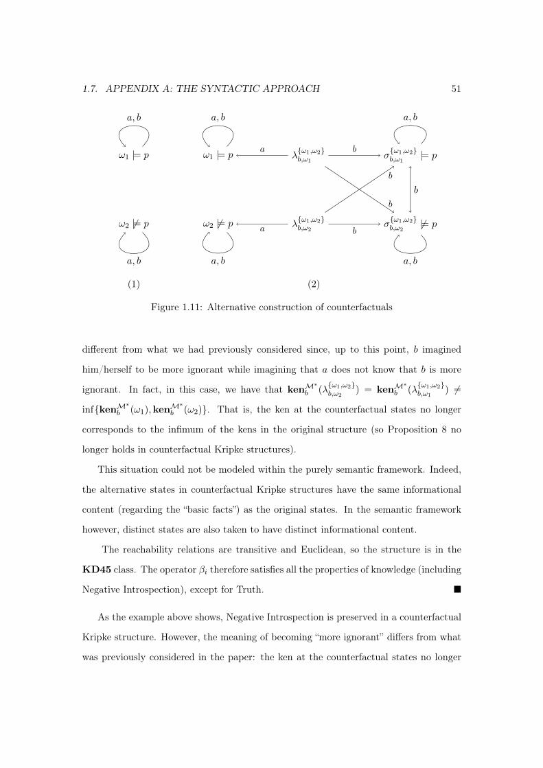
1.7. APPENDIX A: THE SYNTACTIC APPROACH 51
ω1 |= p
ω2 6|= p
a, b
a, b
ω1 |= p
ω2 6|= p
λω1,ω2b,ω1
λω1,ω2b,ω2
σω1,ω2b,ω1
|= p
σω1,ω2b,ω2
6|= p
a
a
a, b
a, b
a, b
a, b
b
b
b
b
b
(1) (2)
Figure 1.11: Alternative construction of counterfactuals
different from what we had previously considered since, up to this point, b imagined
him/herself to be more ignorant while imagining that a does not know that b is more
ignorant. In fact, in this case, we have that kenM∗
b (λω1,ω2b,ω2
) = kenM∗
b (λω1,ω2b,ω1
) 6=
infkenM∗b (ω1),kenM∗
b (ω2). That is, the ken at the counterfactual states no longer
corresponds to the infimum of the kens in the original structure (so Proposition 8 no
longer holds in counterfactual Kripke structures).
This situation could not be modeled within the purely semantic framework. Indeed,
the alternative states in counterfactual Kripke structures have the same informational
content (regarding the “basic facts”) as the original states. In the semantic framework
however, distinct states are also taken to have distinct informational content.
The reachability relations are transitive and Euclidean, so the structure is in the
KD45 class. The operator βi therefore satisfies all the properties of knowledge (including
Negative Introspection), except for Truth.
As the example above shows, Negative Introspection is preserved in a counterfactual
Kripke structure. However, the meaning of becoming “more ignorant” differs from what
was previously considered in the paper: the ken at the counterfactual states no longer

52 CHAPTER 1. AGREEING ON DECISIONS
corresponds to the infimum of the kens in the original structure. Furthermore, in the
counterfactual structure of a partitional structure, ignorance was easily expressed syn-
tactically as the infimum of kens, but there does not appear to be any obvious syntactic
operation to capture the type of ignorance modeled in counterfactual Kripke structures.

1.8. APPENDIX B: PROOFS 53
1.8 Appendix B: Proofs
Proof of Remark 1. Since the reachability relations are equivalence relations, they are
reflexive and Euclidean. One can easily verify that transitivity of the relations is implied.
By reflexivity, we have that for all i ∈ N and every ω ∈ Ω, ω ∈ bi(ω). By transitivity,
we have that for all i ∈ N and ω, ω′ ∈ Ω, if ω ∈ bi(ω′), bi(ω) ⊆ bi(ω
′). Finally, by
Euclideaness, we have that for all i ∈ N , and ω, ω′ ∈ Ω, if ω ∈ bi(ω′), bi(ω′) ⊆ bi(ω). It
follows that if ω ∈ bi(ω′), then bi(ω) = bi(ω′). The rest follows easily.
Proof of Proposition 1. Let ω′′ ∈ ∪ω′∈TG(ω)bi(ω′). So, ω′′ ∈ bi(ω′) for some ω′ ∈ TG(ω).
So ω′Riω′′, and by definition of TG, ω′ is reachable from ω. It follows that ω′′ is reachable
from ω, so ω′′ ∈ TG(ω). For the converse, suppose ω′′ ∈ TG(ω). Since S is partitional,
ω′′ ∈ bi(ω′′), so for some ω′′′ ∈ TG(ω), ω′′ ∈ bi(ω′′′). That is, ω′′ ∈ ∪ω′∈TG(ω)bi(ω′).
Proof of Remark 2. Since the reachability relations are serial, we have that for all i ∈ N
and every ω ∈ Ω, bi(ω) 6= ∅. By transitivity, we have that for all i ∈ N and ω, ω′ ∈ Ω,
if ω ∈ bi(ω′), bi(ω) ⊆ bi(ω′). Finally, by Euclideaness, we have that for all i ∈ N , and
ω, ω′ ∈ Ω, if ω ∈ bi(ω′), bi(ω′) ⊆ bi(ω). It follows that if ω ∈ bi(ω
′), then bi(ω) =
bi(ω′).
Proof of Theorem 1. Suppose that ω ∈ CG(∩i∈Gω′ ∈ Ω|δi(ω′) = xi). Then, for every
i ∈ G, TG(ω) ⊆ ω′ ∈ Ω|δi(ω′) = xi. Let us focus on agent i. This means that
δi(ω′) = xi for every ω′ ∈ TG(ω). By Proposition 1, ∪ω′∈TG(ω)bi(ω
′) = TG(ω). This
implies that TG(ω) is a (non-empty) set of disjoint possibility sets bi(ω′) such that ω′ ∈
TG(ω). This implies that Di(bi(ω′)) = xi for every possibility set bi(ω′) that is a subset of
TG(ω). By the Sure-Thing Principle, we have that Di(TG(ω)) = xi. A similar argument
for any other agent j would lead us to conclude that Dj(TG(ω)) = xj . But since any
agents i, j ∈ G are like-minded, we have that xi = Di(TG(ω)) = Dj(TG(ω)) = xj for all
i, j ∈ G.

54 CHAPTER 1. AGREEING ON DECISIONS
Proof of Proposition 2. Consider an arbitrary i ∈ N , and suppose z ∈ Ω′. If z ∈ Ω, then
z belongs to some equivalence class within Ii. If z ∈ Λ, then by construction of R′i, there
exists some ω ∈ Ω such that zR′iω. In either case, there exists some ω ∈ Ω′ such that
zR′iω. To establish transitivity, suppose z, ω′, ω′′ ∈ Ω′ such that zR′iω′ and ω′R′iω
′′. If
z ∈ Ω, then z, ω′, and ω′′ all belong to the same equivalence class, and therefore zR′iω′′.
If z ∈ Λ, then since zR′iω′, it follows that z is the duplicate of some state ω ∈ Ω such
that ω′ ∈ Ii(ω); and since ω′R′iω′′, we have that ω′′ ∈ Ii(ω). Since by construction, z
must reach every state in Ii(ω), it follows that zR′iω′′.
Proof of Proposition 3. (i) Since the reachability relations are serial, we have that for
all i ∈ N and every ω ∈ Ω′, bi(ω) 6= ∅. By transitivity, we have that for all i ∈ N and
ω, ω′ ∈ Ω′, if ω ∈ bi(ω′), bi(ω) ⊆ bi(ω′). (ii) It suffices to note that over Ω× Ω, R′i = Ri
by construction. And since Ri ⊆ Ω× Ω is an equivalence relation, we have that for any
ω ∈ Ω, bi(ω) = Ii(ω).
Proof of Proposition 4. Let ω ∈ Ω′. (i) Suppose ω′ ∈ TG(ω). Since by construction of the
counterfactual structure, no counterfactual state reaches itself, and every counterfactual
state must reach a state within Ω, it must be the case that ω′ ∈ Ω. (ii) Suppose that
ω′′ ∈ ∪ω′∈TG(ω)bi(ω′). Then, ω′′ ∈ bi(ω
′) for some ω′ ∈ TG(ω). So ω′Riω′′, and by
definition of TG, ω′ is reachable from ω. It follows that ω′′ is reachable from ω, so ω′′ ∈
TG(ω). For the converse, suppose ω′′ ∈ TG(ω). By part (i), ω′′ ∈ Ω. From Proposition
3 part (ii), it follows that ω′′ ∈ bi(ω′′). So, for some ω′′′ ∈ TG(ω), ω′′ ∈ bi(ω′′′). That is,
ω′′ ∈ ∪ω′∈TG(ω)bi(ω′).
Proof of Proposition 5. Suppose ω ∈ Ω′. If ω ∈ Ω, then bi(ω) = Ii(ω) (Proposition 3
part (ii)), and since by definition, Ii(ω) ∈ Γi, it follows that bi(ω) ∈ Γi. Now suppose
ω ∈ Λ. Then, by construction of the counterfactual structure, ω reaches either all the
states in a single element of the partition Ii, or it reaches all the states in multiple
elements of the partition Ii. In the first case, bi(ω) = Ii(ω′) for some ω′ ∈ Ω, and in the

1.8. APPENDIX B: PROOFS 55
second case, bi(ω) is the union of several partition elements; that is, bi(ω) = ∪ω′∈EIi(ω′)
for some E ⊆ Ω. Either way, bi(ω) ∈ Γi by definition of Γi.
Proof of Theorem 2. Suppose that ω ∈ CG(∩i∈Gω′ ∈ Ω′|δi(ω′) = xi). Then, for every
i ∈ G, TG(ω) ⊆ ω′ ∈ Ω′|δi(ω′) = xi. Let us focus on agent i. This means that
δi(ω′) = xi for every ω′ ∈ TG(ω). By Proposition 4 part (ii), ∪ω′∈TG(ω)bi(ω
′) = TG(ω).
This implies that TG(ω) is a (non-empty) set of disjoint possibility sets bi(ω′) such
that ω′ ∈ TG(ω). This implies that Di(bi(ω′)) = xi for every possibility set bi(ω′)
that is a subset of TG(ω). Note that for any ω′ ∈ TG(ω), ω′ ∈ Ω (Proposition 4 part
(i)), and that for any ω′ ∈ Ω, bi(ω′) = Ii(ω′) (Proposition 3 part (ii)). From this, it
follows that bi(ω′)|ω′ ∈ TG(ω) ⊆ Ii, and by the Sure-Thing Principle, we have that
Di(TG(ω)) = xi. A similar argument for any other agent j would lead us to conclude
that Dj(TG(ω)) = xj . But since any agents i, j ∈ G are like-minded, we have that
xi = Di(TG(ω)) = Dj(TG(ω)) = xj for all i, j ∈ G.
Proof of Proposition 6. By construction of the counterfactual structure, for any i ∈ N
and for any e ∈ Γi, there exists a state λei,ω ∈ Λ for some ω ∈ e. Furthermore, λei,ωR′iω′
for every ω′ ∈ e, and λei,ω reaches no other states. It follows that bi(λei,ω) = e.
Proof of Proposition 7. (i) Suppose bi(ω) ⊆ e and bi(ω′) ⊆ e. So, bi(ω) ∪ bi(ω′) ⊆ e. By
Proposition 5, bi(ω), bi(ω′) ∈ Γi. By definition of Γi, it is also the case that bi(ω)∪bi(ω′) ∈
Γi. By construction of the counterfactual structure, for some ω′′ ∈ Ω, there exists a state
λbi(ω)∪bi(ω′)i,ω′′ ∈ Λ which reaches (via R′i) every state in bi(ω) ∪ bi(ω′) and no other state.
Therefore, bi(λbi(ω)∪bi(ω′)i,ω′′ ) = bi(ω)∪bi(ω′), from which it follows that bi(λ
bi(ω)∪bi(ω′)i,ω′′ ) ⊆ e.
The converse is proved similarly. (ii) For this, simply follow the proof for part (i) but
note that since ω ∈ Ω, we have that ω ∈ bi(ω) by Proposition 3 part (ii). So the relevant
counterfactual state is λbi(ω)∪bi(ω′)i,ω′′ where ω′′ = ω.
Proof of Proposition 8. Suppose that S ′ = (Ω′, N, R′ii∈N ) is the counterfactual struc-
ture of a partitional structure S = (Ω, N, Rii∈N ), and letM′ be a Kripke information

56 CHAPTER 1. AGREEING ON DECISIONS
structure over S ′. Consider i ∈ N and Z ⊆ KM′i (W ) for some W ⊆ Ω. Suppose that for
an arbitrary ψ ∈ L, βiψ ∈ infZ. Then for each ki ∈ Z, βiψ ∈ ki. Since the reacha-
bility relations over Ω are equivalence relations, it follows that ψ is true at every state
ω ∈W . Note that by construction, λWi,ω reaches (via R′i) precisely every state ω ∈W . It
follows that βiψ ∈ kenM′
i (λWi,ω). Similarly, suppose that ¬βiψ ∈ infZ. Then for some
ki ∈ Z, ¬βiψ ∈ ki. Again, it follows that ¬ψ is true at some state in W , from which it
follows that ¬βiψ ∈ kenM′
i (λWi,ω).
Proof of Proposition 9. Suppose that βiψ ∈ kenM′′
i (ω) for some ψ ∈ L (where md(ψ) =
0). Then M′′, ω′′ |= ψ for every ω′′ ∈ Ji(ω). This implies that M′, ω′′ |= ψ for every
ω′′ ∈ Ii(ω) ∪ Ii(ω′). This implies that βiψ is also true at all such states. Therefore,
βiψ ∈ kenM′
i (λIi(ω)∪Ii(ω′)i,ω ). The converse is proved similarly.
Proof of Theorem 3. Consider the counterfactual structure S ′ = (Ω′, N, R′ii∈N ) of a
partitional structure S = (Ω, N, Rii∈N ), and let M′ be a Kripke information struc-
ture over S ′. Suppose that CG(∧i∈G d
xii ) is true at some ω ∈ Ω. Then
∧i∈G d
xii is
true at every state ω′ ∈ TG(ω). Consider agent i. Then for every ki ∈ KM′i (TG(ω)),
Di(ki) = xi. By the Sure-Thing Principle, Di(infKM′i (TG(ω))) = xi. However, note
that infKM′i (TG(ω)) ∼ infKM′j (TG(ω)) for any i, j ∈ G. To see this, notice that
βiψ ∈ infKM′i (TG(ω)) if and only if βiψ ∈ ki for every ki ∈ KM′i (TG(ω)), which
implies that ψ is true at every state ω′ ∈ TG(ω). It then follows that βjψ ∈ kj for
every kj ∈ KM′j (TG(ω)), so βjψ ∈ infKM′j (TG(ω)). By like-mindedness, it follows that
Di(infKM′i (TG(ω))) = Dj(infKM′j (TG(ω))), so xi = xj for all i, j ∈ G.
Proof of Theorem 4. For an arbitrary ω ∈ Ω and G = 1, ..., k ⊆ N , suppose that
ω |= CG(∧i∈G d
xii ). It follows that at every state in the component ω′ ∈ TG(ω), ω′ |=∧
i∈G dxii . Take agent i. It follows that for every ken ki ∈ KMi (TG(ω)), Di(ki) = xi. By
the Sure-Thing Principle, we have that for any k′i ∈ IMi (TG(ω)), Di(k′i) = xi. Reasoning
similarly for any other agent j, we have that for any kj ∈ IMj (TG(ω)), Dj(kj) = xj . But,

1.8. APPENDIX B: PROOFS 57
since pairwise equal information implies that there is (k1, ...,kk) ∈ ×i∈GIMi (TG(ω)) such
that k1 ∼ ... ∼ kk, then since the agents are like-minded, x1 = ... = xk.
For the other direction, suppose that at ω there is some i ∈ G = 1, ..., k such that
for all j ∈ G\i, ki 6∼ kj for all ki ∈ IMi (TG(ω)) and kj ∈ IMj (TG(ω)). Without
loss of generality, divide the agents into the sets 1, ..., s and s + 1, ..., k, where for
any i ∈ 1, ..., s, every ki ∈ IMi (TG(ω)) is such that ki 6∼ kj for all j ∈ G\i and
all kj ∈ IMj (TG(ω)); while agents in the set s + 1, ..., k do have kens that are the
equally informative as other agents in s + 1, ..., k (according to ∼). For each agent
i ∈ G = 1, ..., k, and any ken ki ∈ IMi (TG(ω)) define the following decision function:
Di(ki) =
i if i ∈ 1, ..., s
0 if i ∈ s+ 1, ..., k
Suppose i ∈ 1, ..., s. Then for any pair of kens ki and k′i such thatDi(ki) = Di(k′i), it is
true that Di(infki,k′i) = Di(ki), so the Sure-Thing Principle is satisfied. Furthermore,
like-mindedness is trivially satisfied since for every i ∈ 1, ..., s, there is no other agent
with an equally informative ken. Now, suppose i ∈ s + 1, ..., k. Once again, one
can easily verify that the Sure-Thing Principle is satisfied. Furthermore, the only other
agents that have a ken in the domain of their decision function that is equally informative
to i’s are also in s+ 1, ..., k, and all such agents make the same decision (namely, take
action 0), therefore like-mindedness is also satisfied.
Finally, since every agent i ∈ 1, ..., s takes action i at every ken in the component
TG(ω), it follows that this is commonly believed, and since every agent i ∈ s+ 1, ..., k
takes action 0 at every ken in the component, it also follows that this is commonly
believed. However, the actions are not the same (i 6= 0). That is, the agents can agree
to disagree.
Proof of Proposition 10. Suppose thatM = (Ω, N, Rii∈N ,V) is a Kripke structure sat-
isfying quasi-coherence, so for every component TG(ω), there is a reflexive sub-component

58 CHAPTER 1. AGREEING ON DECISIONS
TG(ω′) ⊆ TG(ω). Let Zi = KMi (TG(ω′)) for every i ∈ G, and note that for any i ∈ G
and ψ ∈ L, either (i) βiψ ∈ infZi or (ii) ¬βiψ ∈ infZi. Suppose case (i) is true.
Then βiψ ∈ ki for every ki ∈ Zi, and by reflexivity of TG(ω′), it follows that ψ is true at
every state in TG(ω′). And, for any state ω′′ ∈ TG(ω′), if (ω′′, ω′′′) ∈ Rj , for any agent
j ∈ G, then ω′′′ ∈ TG(ω′). So whatever state j considers to be possible from ω′′, ψ will
be true at that state. This implies that for any kj ∈ Zj , βjψ ∈ kj . So, for all j ∈ G\i,
βjψ ∈ infZj. Now suppose case (ii) is true. Then ¬βiψ ∈ ki for some ki ∈ Zi. This
could not be true if there were not at least one state ω′′ ∈ TG(ω′) such that ¬ψ is true at
ω′′. But since TG(ω′) is reflexive for all j ∈ G\i, it follows that ¬βjψ for all j ∈ G\i
at that state. So for each of these agents, ¬βjψ ∈ kj for some kj ∈ Zj . Therefore, for
all j ∈ G \ i, ¬βjψ ∈ infZj. The above implies that there are sets of kens Zii∈G
such that for all pairs of agents i, j ∈ G, infZi ∼ infZj. Clearly, this implies that
for each i ∈ G, there is some j ∈ G \ i such that ki ∼ kj for some ki ∈ IMi (TG(ω))
and kj ∈ IMj (TG(ω)).
Note that the converse is not true since the Kripke structure M = (Ω, N, Rii∈N ,V)
with Ω = ω1, ω2, N = a, b, Ra = Rb = (ω1, ω2), (ω2, ω1), P = p, and
V(p, ω1) = 1 and V(p, ω2) = 0 trivially satisfies pairwise equal information but not
quasi-coherence.
1.9. REFERENCES 59
1.9 References
Aumann, R. (1976). Agreeing to disagree. The Annals of Statistics 4 (6), 1236–1239.
Aumann, R. (1999). Interactive epistemology (i): Knowledge. International Journal of
Game Theory 28 (3), 263–300.
Aumann, R. and S. Hart (2006). Agreeing on decisions. Unpublished manuscript, The
Einstein Institute of Mathematics, Jerusalem, Israel. http://math.huji.ac.il/~hart/
papers/agree.pdf.
Bacharach, M. (1985). Some extensions of a claim of aumann in an axiomatic model of
knowledge. Journal of Economic Theory 37 (1), 167–190.
Baltag, A. and L. Moss (2005). Logics for epistemic programs. Information, Interaction
and Agency 139 (2), 1–60.
Bonanno, G. and K. Nehring (1998). Assessing the truth axiom under incomplete infor-
mation. Mathematical social sciences 36 (1), 3–29.
Bonanno, G. and K. Nehring (1999). How to make sense of the common prior assumption
under incomplete information. International Journal of Game Theory 28 (3), 409–434.
Cave, J. (1983). Learning to agree. Economics Letters 12 (2), 147–152.
Chellas, B. (1980). Modal logic: an introduction. Cambridge, UK: Cambridge University
Press.
Fagin, R., J. Halpern, Y. Moses, and M. Vardi (1995). Reasoning about knowledge.
Cambridge, MA: MIT Press.
Feinberg, Y. (2000). Characterizing common priors in the form of posteriors. Journal of
Economic Theory 91 (2), 127–179.

60 CHAPTER 1. AGREEING ON DECISIONS
Halpern, J. (1999). Hypothetical knowledge and counterfactual reasoning. International
Journal of Game Theory 28 (3), 315–330.
Heifetz, A. (2006). The positive foundation of the common prior assumption. Games
and Economic Behavior 56 (1), 105–120.
Hellman, Z. (2013). Deludedly agreeing to agree. In Proceedings of the 14th Conference
on Theoretical Aspects of Rationality and Knowledge, pp. 105–110.
Moses, Y. and G. Nachum (1990). Agreeing to disagree after all. In Proceedings of the
3rd Conference on Theoretical Aspects of Reasoning about Knowledge, pp. 151–168.
Samet, D. (2010). Agreeing to disagree: The non-probabilistic case. Games and Eco-
nomic Behavior 69 (1), 169–174.
Savage, L. (1972). The Foundations of Statistics. Mineola, NY: Dover Publications.
Stalnaker, R. (1996). Knowledge, belief and counterfactual reasoning in games. Eco-
nomics and Philosophy 12, 133–164.
Tarbush, B. (2013). Agreeing on decisions: an analysis with counterfactuals. Theoretical
Aspects of Rationality & Knowledge XIV .
van Benthem, J. (2010). Modal Logic for Open Minds. Chicago, IL: University of Chicago
Press.
Van Eijck, J. (2008). Advances in dynamic epistemic logic. Unpublished manuscript,
CWI and ILLC, Amsterdam, Netherlands. http://homepages.cwi.nl/~jve/papers/
08/ae/38-anininlijc.pdf.
Wansing, H. (1990). A general possible worlds framework for reasoning about knowledge
and belief. Studia Logica 49 (4), 523–539.
Chapter 2
Friending: a model of online social
networks
Abstract: We develop a parsimonious and tractable dynamic social network for-mation model in which agents interact in overlapping social groups. The model allowsus to analyze network properties and homophily patterns simultaneously. We deriveclosed-form analytical expressions for the distributions of degree and, importantly, ofhomophily indices, using mean-field approximations. We test the comparative staticpredictions of our model using a large dataset from Facebook covering student friend-ship networks in ten American colleges in 2005, and we calibrate the analytical solutionsto these networks. We find good empirical support for our predictions. Furthermore, atthe best-fitting parameters values, the homophily patterns, degree distribution, and indi-vidual clustering coefficients resulting from the simulations of our model fit well with thedata. Our best-fitting parameter values indicate how American college students allocatetheir time across various activities when socializing.1
1Parts of this chapter appear in Tarbush and Teytelboym (2012).
61

62 CHAPTER 2. FRIENDING
2.1 Introduction
Friendships are an essential part of economic life and social networks affect many
areas of public policy.2 Friendships create externalities, which impact educational per-
formance (Sacerdote, 2001), health (Kremer and Levy, 2008), group lending (Banerjee
et al., 2012), and productivity at work (Falk and Ichino, 2006). Recently, online social
networks have become a global record of naturally occurring social ties. The world’s
largest online social network – Facebook – is increasingly becoming the main platform
for interacting with friends and documenting friendships.3 Launched in 2004 and at first
exclusive to American colleges, it now has over a billion active users worldwide.4 An av-
erage user spends 405 minutes on Facebook per month.5 Facebook allows users to share
pictures, videos, links, as well as organize events, play games, and develop professional
contacts though numerous third-party applications. On Facebook, users have access to
a huge amount of information about other users, which influences the network formation
process (Lewis et al., 2008, 2012). In this paper, we propose a social network formation
model which uses this information to explain who befriends whom on Facebook.
2.1.1 Homophily
A particular focus of this paper is homophily – the tendency of individuals to as-
sociate with those who are similar to themselves – which has been well documented in
sociology.6 Homophily patterns, for example, play an important role in school segrega-2The best recent summaries of applications of networks in the social sciences are by Jackson (2008),
Goyal (2009), Easley and Kleinberg (2010), and Newman (2010).3Since 2011 Facebook has become the dominant online social network in almost every country in
the world except China, Russia, Belarus, Ukraine, Iran, Armenia, Kazakhstan, Latvia, and Vietnam.4Active users are those who logged on to their Facebook profile at
least once in the previous month. See SEC Form 10-Q 2012Q2 filing:http://www.sec.gov/Archives/edgar/data/1326801/000119312512325997/d371464d10q.htm.
5This is far more than on any other social networking website: on average users spent17 minutes on LinkedIn, 8 minutes on MySpace, 21 minutes on Twitter, and 3 minuteson Google+ per month. These data come from a Bloomberg report based on a comScorestudy: http://www.bloomberg.com/news/2012-02-28/google-users-spent-less-time-on-site-in-january-comscore-finds.html. Pempek et al. (2009) found similar Facebook use intensity for college students.
6The two classic studies of homophily in humans by Kandel (1978) and Shrum et al. (1988) foundracial and gender homophily in adolescent social groups. McPherson et al. (2001) provide an excellent

2.1. INTRODUCTION 63
tion (Currarini et al., 2009) and information transmission (Golub and Jackson, 2012).
There are also many studies regarding the causes of homophily. Some empirical studies
in economics (Mayer and Puller, 2008) and sociology (Moody, 2001, Mouw and Entwisle,
2006) find that most of the homophily can be explained by a bias in people’s preferences.
More recently, Currarini et al. (2009, 2010) proposed a rigorous model explaining several
striking patterns of homophily in ethnicity in high-school peer groups. Yet Currarini
et al. (2009) make it clear that the observed racial homophily patterns do not necessar-
ily arise from an exogenous bias in preferences towards people of the same type. Rather,
similar people may be simply more likely to meet. Wimmer and Lewis (2010) provide
some support for that idea by studying racial homophily in a small Facebook dataset.
They find that sharing the same physical environment7 and reciprocal friendships are
far more important in explaining homophily than race preference.
2.1.2 Socializing on Facebook
In social networks the characteristics of the agents constitute the identity of the
person they represent. As Sen (2006) emphasizes, a person’s identity is necessarily mul-
tidimensional: one can simultaneously identify oneself as a woman, a student, a Catholic,
a vegetarian, and a rower. An identity is then a collection of characteristics drawn from
social categories.8 In the preceding example, the social categories are: gender, employ-
ment status, religion, dietary practice, and sport activity. A social group is a collection
of persons sharing a characteristic from a particular social category.
Let us immediately make these ideas more concrete and think about two students –
Mark and Eduardo – who are “friends” on the Facebook network of a prestigious American
university. Mark and Eduardo live in the same dorm, but Mark is a computer science
major, whereas Eduardo studies finance. There are many processes that explain how
Mark and Eduardo became friends on Facebook. In our model, we propose that Mark and
survey of the literature and cite numerous examples of homophily among humans and other animals.7The authors call this “propinquity”.8Akerlof and Kranton (2010) summarize the importance of identity in economics.

64 CHAPTER 2. FRIENDING
Eduardo allocate time across their various social categories, such as attending lectures
and class and spending time in their dorm. Naturally, a lot of the time-allocation is
determined institutionally by timetables or geographical locations. The overlap between
their social groups (and their relative sizes) determines how frequently they interact with
each other socially and their chance of meeting in person. If Mark and Eduardo were
also members of the same fraternity, their chance of meeting would be even higher. Their
eventual friendship is then documented online via Facebook.
2.1.3 Our contribution
This paper makes several contributions. We develop an intuitive and parsimonious
dynamic social network formation model. The process governing friendship formation
resembles our description of how Mark and Eduardo become friends on Facebook. That
is, agents allocate time across various social categories thus determining how frequently
they interact with others in each social group. When interacting with others in a social
group, an agent forms a friendship with another agent chosen at random from among
those in the group who are not yet his/her friends and who are still actively using
Facebook.
We are interested in the structural properties of the resulting network. We are
able to obtain closed-form analytical expressions for the degree distribution and for
various measures of homophily. Importantly, we are able to derive the full distribution
of individual homophily indices.
The entire process is governed by the allocation of time and the relative sizes of the
groups to which the agents belong. Since agents with certain sets of characteristics may
interact more often, homophily may emerge with respect to particular social categories.
As such, the biases in the frequency of interaction between agents in our model can
either be seen as a pure bias in meeting opportunities, or as the manifestation of agents’
preferences over how they allocate their time. Our model, therefore, does not distinguish

2.1. INTRODUCTION 65
these two possible effects. Furthermore, since choices are made stochastically, we bypass
strategic considerations for friendship formation. However, this simplification allows us
to develop a dynamic network formation model in which agents’ characteristics determine
the formation process.
In this paper, we focus on homophily for immutable social categories, such as gender
or – in the context of a university – year of graduation, because no feedback mecha-
nism exists that would allow agents to change their characteristics within these social
categories on the basis of their friendships.
The empirical part of this paper provides striking support for our model. We find
the best-fitting parameter values, which determine the allocation of time across social
categories, and best fit the degree and homophily distribution in gender and year of
graduation for ten separate student Facebook networks. Students’ friendships reveal
that they spend more time socializing in class than in their dorms. The model fits the
data extremely well despite its parsimony (there are only three degrees of freedom).
Remarkably, the simulations run at the best-fitting parameter values show that the
individual clustering coefficient distributions also match the clustering patterns in all
the networks.
Following a brief literature review in the next section, the outline of this paper is
as follows. In Section 2.3, we formally present and discuss the social network formation
model. In Section 2.4, we derive the degree distribution and homophily indices using
a mean-field approximation method (as well as other properties of the network) and
test this approximation in Section 2.5 against simulation results. Sections 2.6 and 2.7
present the Facebook dataset and explore some baseline tests and empirical patterns.
In Section 2.8, we calibrate the model to the data and present our empirical results.
Section 2.9 discusses four possible extensions to the model, and Section 2.10 concludes.
The Appendix contains the proofs, the algorithms and methods used for calibration, a
full description of the data, the results table, and further empirical tests of the model.

66 CHAPTER 2. FRIENDING
2.2 Literature review
In many dynamic social network formation models, agents (represented by nodes
in a graph) are anonymous. The formation of new friendships (edges or links) then
depends entirely on the existing links in the network. In a seminal paper, Barabási and
Albert (1999) proposed a model in which every node receives a link with a probability
proportional to its existing number of links. In this preferential attachment framework,
Mark would be more likely to send a “friend request” to Eduardo if the latter is already
popular. We discuss this approach further in Section 2.9.3. Jackson and Rogers (2007)
additionally suggested that “friends of friends” are more likely to link. Hence, if Mark
knows that he and Eduardo have a Facebook friend in common, then he and Eduardo are
likely to establish a direct Facebook link with each other. These types of models provide
analytical expressions and comparative statics for the macroscopic properties of the
network: degree distribution, clustering, diameter, average distance, and assortativity.
However, these models are unable to explain homophily patterns because node char-
acteristics are not taken into account. Node characteristics can play a big role in ex-
plaining the topology of a network (Bianconi et al., 2009). One branch of the economics
literature explores the equilibria and stability of static networks, where node characteris-
tics determine the linking process (de Marti and Zenou, 2011, Iijima and Kamada, 2013).
We contribute to another branch, which considers dynamic processes. Currarini et al.
(2009) originally proposed a dynamic matching model with a biased meeting process in
which agents prefer to link to those who are similar to themselves. Agents were endowed
with a characteristic from one social category, and the biased meeting process was deter-
mined by an exogenous parameter. Given the nature of the model, it cannot account for
the properties of the resulting network of friendships.9 Bramoullé et al. (2012) extended
9They use data from The National Longitudinal Study of Adolescent Health (Add Health), whichrepresents a relatively restricted network structure. Students were asked to name their ten “best friends”and around three quarters of students choose to nominate fewer than ten “best friends.” Additionally,at most 5 of them could be of the same sex. This means that a deep analysis of the network propertiesis not usually possible.

2.2. LITERATURE REVIEW 67
the model of Jackson and Rogers (2007) to consider homophily in a random growing
network with multidimensional node characteristics and tested the comparative static
predictions of their model against a dataset of empirical citation networks. Our ap-
proach is similar in spirit to their paper, but complements it in several important ways.
As in our paper, networks form through the creation of new links over time. However,
most of the results given in Bramoullé et al. (2012) are in the limit as time approaches
infinity. Some results are also given for any time period for the case in which there are
only two relevant social groups. In contrast, our paper offers new theoretical results
for any time period. In particular, we replicate the result Bramoullé et al. (2012) in
the case of two social groups (showing that homophily becomes a decreasing function of
time and degree), but we also show how this result breaks down in the case of multiple
social groups. In addition, although the authors are able to derive properties of the re-
sulting networks and obtain comparative statics on the relationship between homophily
and degree, they do not obtain a closed-form solution for the degree distribution. Since
we are able to obtain closed-form solutions for our expressions, we are able not only to
test the comparative static predictions of our model, but also to calibrate the model to
our dataset, thereby isolating the best-fitting parameter values of our model. We are
not aware of any studies that carry out such a calibration. Finally, in fitting the model
to the data, we consider entire distributions of degree, homophily indices, and cluster-
ing coefficients rather than simply fitting averages; this is also something we have not
encountered in the literature.
Our model is also conceptually related to affiliation networks introduced in sociology
by Breiger (1974) and Feld (1981). We discuss this relationship further in Sections 2.3.5
and 2.9.4. An affiliation network is described by a set of agents and a set of memberships,
such as clubs, online fora, research topics, or social groups (Newman et al., 2002). These
models have found wide-spread application in online social networks (Botha and Kroon,
2010, Kumar et al., 2010, Xiang et al., 2010). In more recent evolving models of affiliation

68 CHAPTER 2. FRIENDING
networks, new memberships may emerge over time, and the likelihood of meeting new
agents can depend on their memberships (Lattanzi and Sivakumar, 2009, Zheleva et al.,
2009). However, these models typically contain a large number of parameters and most,
such as those by Leskovec et al. (2005, 2008), rely entirely on simulations.
2.3 Model
2.3.1 Characteristics of agents
Let K = [K0, ...,KR] be a finite ordered list of social categories. An element Kr is
the rth category and k ∈ Kr is a characteristic within that category. Let R = 0, ..., R
and R+ = R \ 0. The identity of every agent i ∈ N is represented by a vector
ki = (k0i , ..., k
Ri ) of characteristics, where for each r ∈ R, kri ∈ Kr. For any pair i, j ∈ N ,
let k0i = k0
j .10 For each r ∈ R, define a social group Γri = j ∈ N |kri = krj\i, which
is the set of all agents (other than i) that share the characteristic kri within the social
category r with i. Note that Γ0i = N\i. Finally, for each non-empty S ⊆ R, define
πi(S) =⋂r∈S
Γri \⋃
r∈R\(S∪0)
Γri (2.1)
which induces a partition Πi = πi(S)|S ⊆ R, S 6= ∅ on N\i.11 Therefore, πi(S)
is the set of agents (other than i) that share only the characteristics within the set of
categories indexed by S with i.
Example. Consider an online social network at a university in which we can observe the
class, dorm, gender, and year of graduation for each student. Then using our notation
K = [K0,K1,K2,K3,K4] = [student, class, dorm, gender, year of graduation]
10This does not restrict the characteristics space in any way. The zeroth category, which greatlysimplifies notation, is one in which all agents share the same characteristic.
11Note that πi(S) = πi(S ∪ 0) for all non-empty S ⊆ R. Furthermore, since Γri = ∪π∈πi(S)|r∈Sπ,a social group is a union of disjoint partition elements.

2.3. MODEL 69
All agents are students (k0i = k0
j for all i, j ∈ N). The class social category, K1, can
include k ∈ maths, computer science, psychology. Let the identity of a student i be
represented by the vector
ki = (student, computer science,KirklandHouse,male, 2006)
Let us consider S = 1, 3. Now, i’s social group Γ1i is the set of all computer science
students and Γ3i is the set of all male students (other than i). Then, πi(S) is the
set of male students other than i, who take the computer science class, but do not
share any other characteristics with i. πi(0) would be the set of all female non-
computer-scientists, who do not live in Kirkland House and are not graduating in 2006.
Πi represents the partition into disjoint sets of students who share exactly 1, 2, 3, 4 or
5 social categories with i.
2.3.2 Network formation process
We model our network as a simple, undirected graph, with a finite set of nodes (which
represent agents) and a finite set of edges (which represent friendships). The degree of
an agent i is the number of i’s friends. At time period t = 0 all agents are active and
have no friends. Let q = (q0, ..., qR) and∑
r∈R qr = 1. In each period t ∈ 1, 2, 3 . . .,
an active agent interacts with agents in the social group Γri with probability qr ≥ 0.
One can think of Γ0i = N\i as the social group that i interacts with during i’s “free
time”. We can thus interpret qr as the proportion of time in any period t that agent i
spends with agents in the social group Γri . During the interaction in a social group, an
agent i is linked to an another active agent in that group chosen uniformly at random
with whom i is not yet a friend. If the agent is already linked to every other active
agent in that social group, the agent makes no friends in that period. Friendships are
always reciprocal so all links are undirected. Finally, in every period, agent i remains
active with a given probability pi ∈ (0, 1) until the following period and becomes idle

70 CHAPTER 2. FRIENDING
with probability 1− pi. If the agent i becomes idle, i retains all his/her friendships, but
can no longer form any links with other agents in all subsequent periods.12
2.3.3 Interpretation of the model
We can interpret our model in the context of an online social network, such as
Facebook. We imagine that the online social network has users who interact with each
other either online or offline. Users can meet each other physically in real-world social
groups: for example, university students could meet in class, in their dorm, or at parties
during their free time. This was particularly relevant in the earlier stages of Facebook
when it was open only to selected American colleges. Additionally, most social networks
allow users to browse profiles of other users according their memberships in particular
social groups (Facebook, for example, facilitates direct browsing of users’ profiles by
characteristic).
In our model, we interpret q as the fraction of time that students physically spend
within various social categories or their propensity to browse for other students of these
social categories online. Note that, although Mark and Eduardo may spend the same time
in class (since q is the same for both of them), they will be meeting different social groups
of people since Mark is attending a computer science lecture (Mark’s class is computer
science) and Eduardo is taking a finance course (Eduardo’s class is finance). When Mark
is interacting with other computer scientists, he befriends them (at random) and then
documents these friendships via the online social network (for example, by sending a
“friend request” on Facebook).13 Even after every computer scientist in Mark’s lecture
becomes his friend, Mark still attends the lecture. Henceforth, whenever Mark spends
time in the class, he does not make any more friends with the lecture attendees. However,
Mark could still be making friends with students in his other social groups: for example,
with finance majors in his fraternity.
12Naturally, i cannot make a link to him/herself.13Our model assumes that all “friend requests” are accepted.

2.3. MODEL 71
Social categories are, technically, just the names of variables which we can observe
about the users of an online social network. Since these social categories can be virtually
anything, it does not always make sense to impose a positive probability qr of spending
time in every social category r. For example, gender and graduation year can be social
categories, but it is not very meaningful to say that Mark specifically allocates time to
spend it only with men or only with students of his graduation year. Rather, Mark may
be more or less likely to meet these students because of the classes he takes or the dorm
he lives in. This point will be relevant when we fit the model to the data, and we return
to it in Section 2.8.
There are several ways of interpreting 1−pi, the probability of becoming idle. There
must be reasons, other than having linked with every user in the network, for why peo-
ple stop adding new friends online: losing interest, finding an alternative online social
network, reaching a cognitive capacity for social interaction, and so on. Including all
these explanations would require a much richer model, so we simply capture them as a
random process with the idleness probability 1− pi. One is to imagine that it represents
the probability that, in any period, Eduardo stops sending or accepting “friend requests”
even though he may still be actively using the online platform to stay in touch with his
current friends.14
Example. (cont.) Figure 2.1 succinctly summarizes the link formation process in our
example and its interpretation for agent i. This process happens simultaneously for all
agents in every period. Furthermore it is assumed that q3 = q4 = 0.
2.3.4 Discussion of the model
Many dynamic social network formation models are growing random network models
in which new nodes arrive in every period and link to existing ones (e.g. Price, 1976,14We think of the fixed probability 1− pi as a somewhat crude manner of allowing agents to become
idle at different times. Embedding the model with a (possibly time-varying) probability of idleness foreach agent that is a function that agent’s current state and characteristics could be a fruitful area forfurther research. See a further discussion in Section 2.9.2.

72 CHAPTER 2. FRIENDING
t
t+ 1
Agent i
q1
Γ1i
Agents ini’s class
q2
Γ2i
Agents ini’s dorm
q0
N \ iAgents other
than i
The agents that i interacts with are chosen according to q.Suppose Γ2
i is realized.
If the number of active agents that i is not linked with in Γ2i is
zero, go to Step 3.Otherwise, make a link with an active agent that i is not alreadylinked to in Γ2
i chosen uniformly at random.
Agent i becomes idle with probability 1− pi and remains activeuntil the next period with probability pi.
Step 1
Step 2
Step 3
Figure 2.1: Network formation process in the Example
Barabási and Albert, 1999, Jackson and Rogers, 2007). In contrast, we chose to present
a model with a fixed number of nodes, which become idle while retaining their links.
This choice is not intellectual curiosity alone. One can, of course, think of Facebook as
a growing network (new users join every day); however, our model allows us to focus on
the formation of links among the existing users. Naturally, it is possible to extend our
model to accommodate for the arrival of new users, and we discuss this in Section 2.9.1.
Our model has a unique theoretical feature. For every agent in every social group,
we derive an “expected stopping time” at which the agent has become friends with every
active agent in that group. This highlights the idea that all interactions within social
groups are inherently local. Yet we are able to characterize the macroscopic properties
of the network in terms of these expected stopping times and (pi)i∈N alone.
We have set up our model in a manner that does not require the agents to make any
optimal decisions. In our model, agents do not maximize a utility function, but rather

2.3. MODEL 73
all their choices are fully stochastic. However, we could reformulate our model such that
the observed friendship choices result from the optimal decisions of utility-maximizing
agents (Currarini et al., 2009, take this approach). Indeed, endow every agent i ∈ N
with a utility function Ui(di) = vi(di)− cidi where di is the number of i’s friends and ci
is the marginal cost of creating a new friendship. Suppose that in every period, every
agent i “spends time” in some social group and can choose one “active” agent within
that social group with whom i makes a new friendship. Since the characteristics of that
agent are irrelevant to i’s utility, the specific agent that is chosen does not matter, and
so can be chosen uniformly at random. If we also assume that the benefit function vi(·)
is strictly increasing, twice-differentiable and concave in its argument, then there will be
a finite number of friends d∗i satisfying v′i(d∗i ) = ci.15 Agent i will therefore keep adding
friends in every period up to the point at which i has d∗i friends. We can then find a
family of utility functions Ui(·)i∈N such that the distribution of d∗i matches G(d) in
Equation (2.13) below, and we obtain a model equivalent to the one we outlined in the
previous sections.
2.3.5 Relationship to affiliation networks
Our network formation process can be reinterpreted as a dynamic affiliation network.
An affiliation network is initialized by a bipartite graph consisting of two sets of nodes:
agents and memberships. In our framework, memberships correspond to characteristics,
for example, computer science class or Kirkland House dorm. At the beginning, the only
links in this graph are between agents and memberships. New links can be formed by
closing transitive triples: if two agents are linked to the same membership, there is a
positive probability that a link will form between them. Easley and Kleinberg (2010,
p. 97) call this focal closure.
More specifically within our framework, the set of all memberships is k ∈ Kr|r ∈ R
and a link between an agent i and a membership k ∈ Kr is given the weight qr for all15Ignoring the slight complication that d∗i must be an integer.

74 CHAPTER 2. FRIENDING
i ∈ N . Figure 2.2(a) represents our Example as an initialized bipartite graph of an
affiliation network. The formation of new links via focal closure happens in the following
way: in every period, every agent i is assigned a membership k ∈ Kr at random according
to q, and the agent forms a link with another agent j chosen uniformly at random from
among the remaining active agents that have a link with k ∈ Kr. For example, Mark and
Eduardo could become friends in some period because Mark was assigned to Kirkland
House with which Eduardo also has a membership. This is shown in Figure 2.2(b).
Mark
Eduardo
Free
Computer Science
Kirkland House
Finance
q0
q1
q2
q0
q2
q1
Mark
Eduardo
Free
Computer Science
Kirkland House
Finance
q0
q1
q2
q0
q2
q1
(a) (b)
Figure 2.2: Model as an affiliation network
2.4 Theoretical results
We are interested in analyzing properties of the network generated by the model. In
order to derive closed-form expressions for the degree distribution and homophily indices,
we use the mean-field approximation method used in statistical mechanics. According
to this method, we assume that the realization of a random variable in any period
is its expected value. Hence, the dynamic system generated by our model does not
evolve stochastically, but rather deterministically at the rate proportional to the expected
change. The method has been adopted by the economics literature, and our analysis here
is similar to the one carried out in Jackson and Rogers (2007). In general, the mean-field

2.4. THEORETICAL RESULTS 75
approximation method is not without its drawbacks. The accuracy of its predictions
must be tested against simulations (Jackson, 2008, p. 137). In Section 2.5, we show that
the approximation works well for our model.
2.4.1 Degree distribution
In order to derive the degree distribution, we first analyze the meeting process of
agents across social groups. The probability with which agent i interacts with an agent
from πi(S) is given by
qπi(S) = |πi(S)|
∑r∈S∪0
qr
|Γri |
(2.2)
and by definition∑
π∈Πiqπ = 1.
Example. (cont.) To understand Equation (2.2), let us derive qπi(1) in our example.
We interpret this as the proportion of time that i spends with students that are in his
class, but not in his dorm. There are |Γ1i | students in i’s class in total, and there are
|πi(1)| who are both in his class but not in his dorm. He can encounter students in his
class but not in his dorm either during the time he spends in class or during his free time.
When in class, which happens with probability q1, he encounters students who are in his
class but not in his dorm with probability |πi(1)||Γ1i |
. Similarly, during his free time, which
happens with probability q0, he encounters students who are in his class but not in his
dorm with probability |πi(1)||N |−1 . Hence, the proportion of time that i spends with students
that are in his class, and not in his dorm is given by qπi(1) = |πi(1)|[q1
|Γ1i |
+ q0
|N |−1
].
Let di(t) be the degree of agent i in period t. Analogously, dπi (t) is the number of
friends i has in period t with agents in π ∈ Πi. If T π is the expected time it takes i
to make a link with every other active agent in π (expected stopping time), then the
mean-field approximation of the degree change of i with agents in π between periods t
and t+ 1 is
∆dπi (t) = qπ(
1 +Rπ(t)
Rπ(t)
)1(t ≤ T π) = 2qπ1(t ≤ T π) (2.3)

76 CHAPTER 2. FRIENDING
where Rπ(t) is the total number of remaining active agents in π (other than i) with whom
i is not yet linked at time t, and 1 is an indicator function. In other words, conditional
on being in π, i makes a link to an agent in π. Agent i also receives one link on average
from an agent in π at t: there are Rπ(t) other active agents (with whom i is not linked)
in π, and each is linked with i with probability 1Rπ(t) .
16 Hence, on average i makes 2qπ
friends in π in every period until T π.
The partition Πi induced on N \ i allows us to consider the links made between
agents of any element π separately. Hence, we determine the link formation process
within each element π ∈ Πi and then weigh it by qπ – the proportion of time spent in
π. Despite this analytical trick, the actual network formation process certainly allows
agents to receive links from outside the social group they are currently interacting in.
This fact also justifies our ignoring the possibility that any two agents make the same
link simultaneously, which is negligible for large N .
Recall that, in period t = 0, every agent i has no friends. Solving Equation (2.3)
with our initial condition dπi (0) = 0 gives
dπi (t) = 2qπ [t1(t ≤ T π) + T π1(t > T π)] (2.4)
In order to obtain the expected stopping time T π for any π ∈ Πi, we solve the following
difference equation
Rπ(t+ 1) = Rπ(t)− [2qπ + (1− pπ)Rπ(t)− (1− pπ)2qπ] (2.5)
= pπ [Rπ(t)− 2qπ]
where pπ = 1|π|∑
i∈π pi. The interpretation of Equation (2.5) is straightforward. The
16Technically, this assumes that every agent is interacting in every element of the partition in everyperiod, but the interaction is simply weighted by q. Hence, there is a positive probability that i receivesa link from every agent in i’s social group in every period despite the fact that they may not actuallybe interacting in that social group in that period. Furthermore, to derive Equation (2.3) we implicitlyassume that agents in π have the same degree as i at t.

2.4. THEORETICAL RESULTS 77
number of remaining active agents in π at t + 1 is simply the number of active agents
in π at t less the number of agents that have either become idle or were linked with i.
This includes the agents who were linked with i at t (2qπ) and those who have become
idle at t ((1 − pπ)Rπ(t)) and excludes the ones who were linked with i at t and have
become idle at t ((1− pπ)2qπ). For any agent i and any π ∈ Πi, we can solve this with
Rπ(0) = |π| to get
Rπ(t) = |π|(pπ)t +2qπpπ((pπ)t − 1)
1− pπ(2.6)
Solving Equation (2.6) for Rπ(T π) = 0, gives us the expected number of periods it takes
i to form links with every agent in π ∈ Πi, namely
T π =
ln(
2qπpπ
2qπpπ+(1−pπ)|π|
)ln(pπ) if qπ > 0
0 otherwise(2.7)
The degree of agent i in period t is therefore given by Equation (2.8) below
di(t) =∑π∈Πi
dπi (t)
= 2∑π∈Πi
qπ [t1(t ≤ T π) + T π1(t > T π)] (2.8)
Note that di(t) is a concave, piecewise linear function that is strictly increasing in the
range [0,maxπ∈ΠiT π]. This means that in our model, an active agent makes friends
at a decreasing rate over time. Given that preferences do not enter into our model, this
feature is not exhibited because agents have decreasing marginal utility of friendships
(unlike Currarini et al., 2009), but rather because elements of the partitions Πi, for every
i, are gradually exhausted over time.
Since di(t) is increasing, we can find its inverse in the range [0, di(maxπ∈ΠiT π)],

78 CHAPTER 2. FRIENDING
which is given by
d−1i (d) = ti(d) =
d− 2∑
π∈ΠiqπT π1(d > di(T
π))
2∑
π∈Πiqπ1(d ≤ di(T π))
(2.9)
We now obtain Gi(d) – the probability that agent i has degree at most d (degree
distribution of agent i).
Pr(di(t) ≤ d) = Pr(d−1i (di(t)) ≤ d−1
i (d)) = Pr(t ≤ ti(d)) = Gi(d) (2.10)
Since an agent i remains active exactly x periods with probability pxi (1 − pi), we have
that
Pr(t ≤ x) =t=x∑t=0
pti(1− pi) = 1− px+1i (2.11)
Therefore, the degree distribution of agent i is given by
Gi(d) = Pr(t ≤ ti(d)) = 1− pti(d)+1i (2.12)
Finally, the overall degree distribution G(d) is the average of the degree distributions
across all agents and is given by
G(d) =1
|N |∑i∈N
(1− pti(d)+1
i
)(2.13)
Note that the overall degree distribution is approximately exponential.17 We discuss the
implications of this in Section 2.9.3. Henceforth, in order to keep the model parsimonious
and reduce the number of parameters when it comes to calibrating it to the data, we
shall assume that pi = p for all i.
The results derived above allow us to obtain a relationship between the size of the
social group and degree. The following proposition shows that, under some technical
17The degree distribution of agent i is in fact geometric but the exponential distribution is thecontinuous analogue of the geometric distribution.

2.4. THEORETICAL RESULTS 79
conditions, agents in larger social groups, ceteris paribus, have a higher degree.
Proposition 1. Consider any agent i ∈ N and suppose |πi(r)| increases by δ and
|πi(0)| decreases by δ (so that |Γri | increases by δ). If δ is small,18 then there is some
t∗ ≥ T πi(r), such that di(t) is larger for every t ≤ t∗.
That is, for any given t within an (empirically) “large” interval in the domain of di(t),
agent i’s degree di(t) is larger if i’s social group Γri is larger (when this is at the expense
of people outside any of i’s social groups). Note that this proposition allows for the
somewhat counter-intuitive situation in which, following an increase in the size of one of
i’s social groups, i’s degree after t∗ is smaller than it otherwise would have been.
2.4.2 Assortativity
We can derive a further property of the resulting social network which is related to
standard results on assortativity in growing random networks.
Proposition 2. If for every S ⊆ R and any pair of agents i, j ∈ N , |πi(S)| = |πj(S)|,
then for any agent i, the average degree of agent i’s friends is increasing in agent i’s
degree.
This proposition unveils an interesting feature about assortativity in our model. Since
di(t) is increasing in t, if i becomes idle at a later time period t, i’s friends will have a
higher degree at this later t, and therefore the total degree of i’s friends will be larger.
If all agents were making friends at the same rate as i, then this would also imply
that the average degree of i’s friends will be larger. This fact is essentially what drives
assortativity results in models in which agents do not differ in their characteristics. On
in the other hand, in our model, is it in principle possible for the average degree of
i’s friends to be decreasing in i’s degree if i makes friends at a rate that is faster than
his/her friends. The restriction in the proposition to situations in which all agents have18The change in must small enough such that the order of the expected stopping times remains
unchanged.

80 CHAPTER 2. FRIENDING
partition elements that are of the same size rules out this possibility. This is a strong
restriction, but in practice we should expect to observe positive assortativity if group
sizes and partition element sizes are not too different across individuals, or if there is
a positive enough correlation between the sizes of corresponding partition elements of
friends.
2.4.3 Homophily
Homophily captures the tendency of agents to form links with those similar to them-
selves. We now present definitions for two measures of homophily and show the rela-
tionship between them (McPherson et al., 2001). We then express homophily within the
context of our model and derive several results that describe the dynamics of homophily
in the link formation process.
Individual homophily
For any agent i, the individual homophily index in social category r ∈ R is given by
Hri =
number of friends of i that share krinumber of friends of i
(2.14)
Let W rk = j ∈ N |krj = k be the set of all agents that have characteristic k ∈ Kr.
We say that an agent exhibits no individual homophily in social category r if the in-
dividual homophily index equals the fraction of agents in the population who have the
characteristic k = kri i.e. if Hri =
|W rk ||N | .
Group homophily
We now present a definition of group homophily which corresponds to Definition 1 in
Currarini et al. (2009). For any characteristic k in social category r, the group homophily

2.4. THEORETICAL RESULTS 81
index is given by
Hrk =
∑i∈W r
knumber of friends of i that share kri∑i∈W r
knumber of friends of i
(2.15)
which is the fraction of the total number of friendships that agents with characteristic
k have made with agents who also have characteristic k. We say that a group exhibits
homophilious behavior in social category r if the group homophily index exceeds the
fraction of agents in the population who have characteristic k i.e. if Hrk >
|W rk ||N | . Het-
erophilious behavior is defined analogously as Hrk <
|W rk ||N | (Definition 5 in Currarini et al.,
2009).19
It is easy to verify the following relationship between individual and group homophily
∑i∈W r
k
Hri
[number of friends of i∑
i∈W rknumber of friends of i
]= Hr
k (2.16)
Homophily in our model
Let us define Πri = πi(S) ∈ Πi|r ∈ S. This is the set of partition elements that
contain agents who share i’s characteristic in social category r. Using Equation (2.14),
the individual homophily index in social category r of agent i in period t is
Hri (t) =
∑π∈Πri
dπi (t)∑π∈Πi
dπi (t)=
∑π∈Πri
dπi (t)
di(t)(2.17)
19In a similar vein, we can define inbreeding homophily (Currarini et al., 2009). First, for any agenti, the individual inbreeding homophily index (IHr
i ) in social category r ∈ R is given by
IHri =
Hri −
|Wrk ||N|
1− |Wrk|
|N|
which captures how homophilious an agent i is relative to how homophilious i could be given the numberof agents who have characteristic kri in the population. Now, for any characteristic k in social categoryr, the group inbreeding homophily index (Definition 6 in Currarini et al., 2009) is given by
IHrk =
Hrk −
|Wrk ||N|
1− |Wrk|
|N|
which captures how homophilious a group of agents is relative to how homophilious the group could be.We do not focus on this measure of homophily in this paper.

82 CHAPTER 2. FRIENDING
Following Equations (2.15) and (2.16), we obtain the group homophily index for
characteristic k in social category r in period t
∑i∈W r
k
Hri (t)
[di(t)∑
i∈W rkdi(t)
]=
∑i∈W r
k
[∑π∈Πri
dπi (t)
di(t)
][di(t)∑
i∈W rkdi(t)
]=
∑i∈W r
k
[∑π∈Πri
dπi (t)∑i∈W r
kdi(t))
]= Hr
k(t) (2.18)
Finally, it will be useful to define a composition function hri (d) ≡ (Hri ti)(d) which
expresses individual homophily as a function of degree rather than as a function of time.
Dynamics of homophily
We now explore the properties ofHri (t). Let TLi = minπ∈ΠiT π, TMi = maxπ∈Πri
T π,
and THi = maxπ∈ΠiT π. Note that TLi ≤ TMi ≤ THi for all i.20
Proposition 3. The function Hri (t) has the following form: (1) For t ∈ (0, TLi ), Hr
i (t) is
a constant. (2) For t ∈ [TLi , TMi ), the slope of Hr
i (t) is ambiguous. (3) For t ∈ [TMi , THi ),
Hri (t) is decreasing. (4) For t ∈ [THi ,∞), Hr
i (t) is a constant.
Remark 1. hri (d) ≡ (Hri ti)(d) has a similar shape to Hr
i (t). For this, it suffices to
note that ti(d) is an increasing, piecewise linear function.
Figure 2.3 illustrates the general relationships between Hri (t), hri (d), and di(t) or
ti(d), depending on whether we want to take degree or time as the exogenous variable.
Note that this figure is merely a sketch, and the representation given in Figure 2.3
illustrates the most commonly encountered shape for the homophily function within the
20One can verify that TLi is the number of periods it takes i to exhaust the partition which consistsof the people who share the greatest number of characteristics with i, TMi is the number of periods ittakes i to exhaust the social group Γri , and finally THi is the number of periods it takes i to exhausteveryone.

2.4. THEORETICAL RESULTS 83
parameter space that we explore in Section 2.8.21 A tighter characterization of homophily
patterns cannot be given in the general case.
Hri (t) d, di(t)
t, ti(d)
hri (d)
TLi
TMi
THi
di(TLi ) di(T
Mi ) di(T
Hi )
Figure 2.3: Relationship between degree and individual homophily indices
In order to give a feel for the dynamics of homophily in our model, we can provide
tighter analytical results for the case where qr > 0 for only one r ∈ R+.
Corollary 1. Consider the case where qr > 0 for only one r ∈ R+. Then
(1) Hri (t) and hri (d) are (weakly) decreasing in their respective arguments.
(2) Suppose |πi(r)| increases by δ and |πi(0)| decreases by δ (so that |Γri | increases
21Unlike in the representation given in Figure 2.3, it is possible for the limiting value of homophily(namely, Hr
i (THi ))) to be above the initial value Hri (1). Furthermore, it is also possible for Hr
i (t) tobe weakly increasing everywhere since the decreasing range [TMi , THi ) can be empty (This is possible inprinciple, but unlikely in practice). However, in the large majority of cases, homophily has a “hump”shape, as represented in Figure 2.3. The evidence for this can be found in Section 2.11.9 of the Appendix.

84 CHAPTER 2. FRIENDING
by δ). If δ is small,22 then there is some t∗ ≥ T πi(r), such that individual homophily
for agent i in social category r is smaller for every t ≤ t∗.
The result above shows that when agenti’s partition Πi consists of only two elements
(those who share characteristics r with i and those who do not), homophily is decreasing
in i’s degree and, under the same technical conditions as Proposition 1, i’s homophily in
social category r is decreasing in the size of the social group Γri .
2.5 Simulation results
We used a mean-field approximation method to derive the analytical expressions
for the dynamics of the network formation process. As we mentioned in Section 2.4,
the accuracy of the mean-field approximation must first be tested against simulations.
The simulation algorithm, which emulates the theoretical network formation process,
is summarized in Section 2.11.2 of the Appendix. We tested the analytical expressions
for the degree distribution and the individual homophily index distribution against an
average of 100 runs of the simulation for multiple parameter values. Our analytical
degree distribution matches the simulated version exceptionally well. There is, however,
some loss of accuracy at extreme values of the cumulative distribution of the individual
homophily index. Nevertheless, we anticipated this in the theoretical model. Equation
(2.17) makes it clear that the individual homophily index is unlikely to be 0 or 1. The
individual homophily index is 0 when∑
π∈Πridπi (t) = 0 i.e. only if Γri = ∅. This can only
happen when an agent is alone in her social group. The individual homophily index could
be 1 for the case of, say, gender in a women’s college (i.e.∑
π∈Πridπi (t) = di(t)). This is
purely an artifact of the mean-field approximation of the individual degree. Despite these
problems at the extremes, if the model is correct, we should expect a good prediction
of the average of the individual homophily indices. Head-to-head plots and numerical
22The change in must small enough such that the order of the expected stopping times remainsunchanged.

2.6. DATA 85
results for both the degree distribution and homophily patterns are provided in Section
2.8.2 below.23
2.6 Data
We use Facebook data first analyzed by Traud et al. (2010, 2012). The data repre-
sent a September 2005 cross-section of the complete structures of social connections on
www.facebook.com within (but not across) the first ten American colleges and univer-
sities that joined Facebook. The raw data contain over 130,000 nodes (users) and over
5.6 million links (friendships). In order to join Facebook, each user had to have a valid
college email address. We observe six social categories for each user: gender, year of
graduation, major, minor, dorm, and high school. In order to protect personal identity,
all the data were anonymized by Adam D’Angelo (former CTO of Facebook) and are
represented by number codes.
Since all personal data were provided voluntarily, some users did not submit all their
information. Testing our model requires us to observe major, minor, dorm, gender, and
year of graduation for every user. We therefore dropped any user (and their links), who
had not provided all the personal characteristics other than high school.24 In addition,
some users were listed as faculty members and some students listed graduation years that
were probably untruthful (e.g. 1926). We therefore dropped all faculty members and
every user whose year of graduation is outside 2006-2009. Hence, in our data, we look
only at students graduating between 2006 and 2009, who have supplied all the relevant
personal characteristics (except high school).25
23The plots in Section 2.8.2 show only a representative example, but the tests of the analyticalapproximations against the simulations were run for a broad range of values.
24High school is also an interesting social category, however, the relative group sizes within collegesare too small to allow for a meaningful analysis.
25Technically, this means we consider a non-random subsample of the data since there might beselection biases in data disclosure preferences. However, in Section 2.11.7 of the Appendix, we show thatthe degree distributions in the cleaned datasets are very similar to the original datasets. Hence, we expectthat our calibrated parameters should not be unreasonably far from the unbiased parameter estimatesand that our comparative statics results should remain unchanged. More precise point estimates andstructural estimation of our model using the full data is a potential area of future research.

86 CHAPTER 2. FRIENDING
There are 27,454 users and 492,236 links in our cleaned dataset. The individual
college names were provided in abbreviated form; however, we managed to back out the
names of all colleges using their tags from the order in which they appear in our dataset
and the order in which they joined Facebook.26 The summary of the data is given in
Section 2.11.4 of the Appendix.
2.7 Tests and empirical observations
2.7.1 A representative college
Before we calibrate the model to the data, let us first get a feel for the general empir-
ical patterns and the information contained in our dataset. Since there are ten separate
networks, it is impractical to give the visual representations and detailed statistics for
every college. Instead, whenever it is necessary, we focus on a representative college.27
For example, Figure 2.4(a) shows the network for Harvard University (the first college to
have Facebook) with nodes in the graph colored by graduation year.28 We can see that
students from the same year group tend to cluster together. Another way of illustrating
this would be by considering the adjacency matrix directly. In Figure 2.4(b), we plot
the adjacency matrix with the students sorted by the year of graduation, each point
representing a link (as in Newman, 2010, p. 227). In Section 2.11.9 of the Appendix,
we also show that that the dynamics of homophily presented in Figure 2.3 hold quite
generally.
2.7.2 All colleges
We also offer some tentative support for the dynamic predictions of our model. While
the dataset is a cross section, we can look at the homophily degree patterns across year
26Using, inter alia, a community edited public list:http://www.quora.com/Facebook-Company-History/In-what-order-did-Facebook-open-to-college-and-university-campuses
27The Matlab and Python code and analogous results for any college are available upon request.28This was generated with the ForceAtlas 2 algorithm using the open-source Gephi graph visualisation
software.

2.7. TESTS AND EMPIRICAL OBSERVATIONS 87
(a) Year of graduation: Red - 2009; Purple - 2008; Blue - 2007; Green - 2006
(b) Assortative matching by year of graduation
Figure 2.4: Harvard University

88 CHAPTER 2. FRIENDING
groups by year of graduation. This is clearly imperfect, but it provides some indication
of whether the model will be able to match data in a panel dataset. Figure 2.5(a) shows
that, on average, degree is non-decreasing across year groups (over time). Degree seems
to fall for the students graduating in 2006, but the behavior of seniors may have differed
slightly from the other cohorts since they were about to leave college when Facebook
was introduced. Figure 2.5(c) shows that on average, the individual homophily index
in year of graduation falls sharply as students enter later years. Figure 2.5(d) shows
that gender homophily is roughly stable across the years. These plots do not appear
to contradict our main result regarding degree over time, or the gist of Corollary 1
and Proposition 3 regarding the shape of homophily.29 Figure 2.5(b) shows that more
popular students are friends with other more popular students. This is in accordance with
the discussion following Proposition 2; namely, that we if expect agents’ corresponding
partition elements to be of approximately similar sizes, then in practice, we should
observe positive assortativity in degree. Further plots for baseline empirical results on
homophily patterns in the ten colleges can be found in Section 2.11.5 of the Appendix.
We provide a more rigorous test of test Proposition 1 below. Let S = 0, 1, 2
with 0 representing student, 1 representing class, and 2 representing dorm. Technically,
the proposition only holds for time periods within a particular range. Since we cannot
observe time periods in our dataset, we instead identify the set of agents whose degree
is within the relevant range in degree space. To identify these agents, we carried out the
following procedure: In the case where “class” (that is, Γ1i ) is the social group that is being
expanded, we compared the empirical degree of each agent i with the analytical value
di(Tπi(1)), and only retained those agents whose empirical degree is below di(T
πi(1)).
Call the set of retained agents X. In the case where “dorm” (that is, Γ2i ) is the social
group being expanded, we preformed a similar exercise and retained a set of agents Y .
To test Proposition 1, for each college, we regressed the degree of each agent i ∈ X ∩ Y
29Dashed lines represent 99% Chebyshev confidence intervals.

2.8. MODEL CALIBRATION 89
Dependent variable: agent’s degree|Γ1
i | s.e. |Γ2i | s.e. |πi(S)| s.e. const. N
Harvard 0.267*** (0.019) 0.142*** (0.021) -0.332** (0.178) -0.922 771Columbia 0.245*** (0.012) 0.010 (0.007) -0.189*** (0.066) 8.270 1551Stanford 0.472*** (0.018) 0.032** (0.014) -0.771*** (0.238) 3.335 1211
Yale 0.297*** (0.027) 0.006 (0.015) 0.214 (0.278) 5.096 645Cornell 0.107*** (0.012) 0.010*** (0.002) 0.054 (0.061) 7.486 1605
Dartmouth 0.428*** (0.022) 0.026 (0.022) -0.549** (0.275) 4.077 811UPenn 0.301*** (0.011) -0.003 (0.004) -0.244*** (0.075) 8.866 1796
MIT 0.204*** (0.023) 0.088*** (0.015) -0.069 (0.169) 4.801 957NYU 0.139*** (0.007) 0.013*** (0.002) -0.086** (0.034) 9.773 4295
Boston U. 0.171*** (0.007) 0.006*** (0.001) -0.154*** (0.026) 8.656 4004Comment: Standard OLS regression with robust standard errors in parentheses
∗∗∗/∗∗/∗ denote rejection of H0 : β = 0 at the 1/5/10% significant level respectively
Table 2.1: Regression results
on the size of i’s class, and dorm, and on the size of the intersection of class and dorm.
di = α+ β1|Γ1i |+ β2|Γ2
i |+ β3|πi(S)|+ ε (2.19)
Table 2.1 reports the results for all ten colleges. In support of our model, we find
that most coefficients are positive or not significantly different from zero.30
2.8 Model calibration
2.8.1 Empirical strategy
We calibrate our model against the data using the social categories identified in the
Example. Using the available information in our data, we define agents i and j to be in
the same class if and only if they have the same year of graduation and major or have the
same year of graduation and minor. We assume that every agent i interacts in his/her
class and dorm with respective probabilities q1 and q2. The probability of interacting
with the gender and year of graduation social categories are set to zero (q3 = q4 = 0;
30Section 2.11.8 in the Appendix provides results from the same regression run on the unrestrictedset of agents. The results there show that the relationship between group size and degree hold quitegenerally.
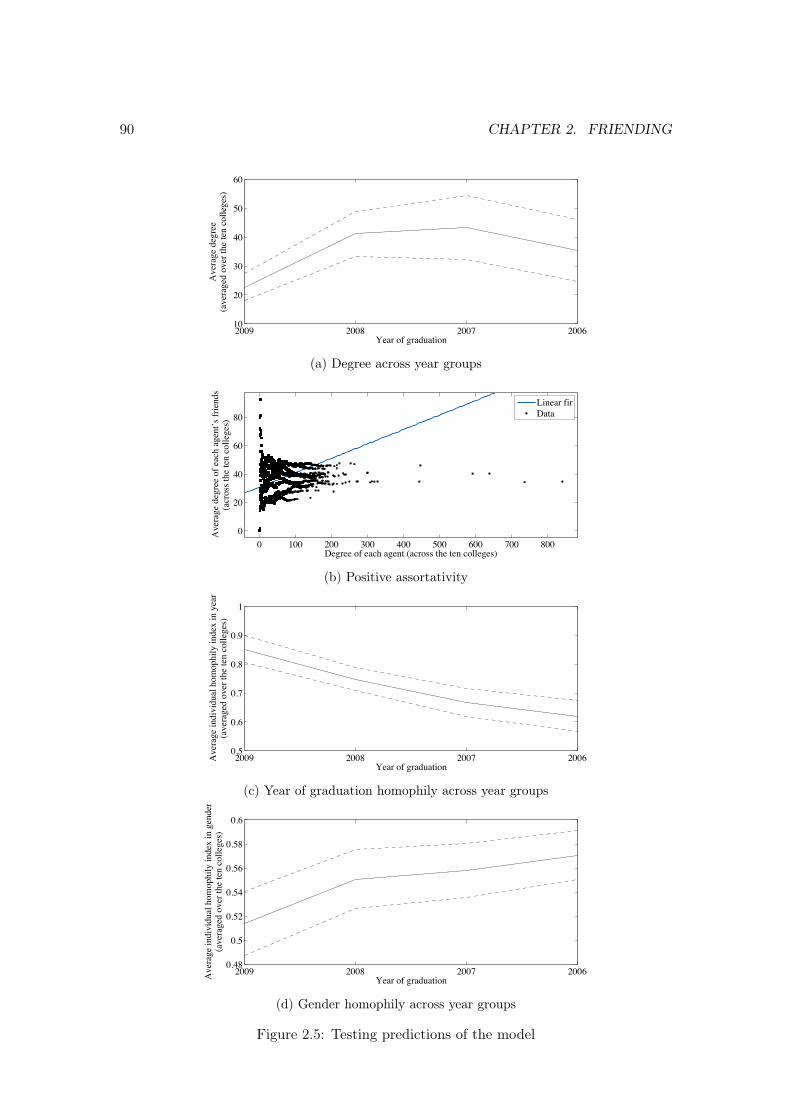
90 CHAPTER 2. FRIENDING
2009 2008 2007 200610
20
30
40
50
60
Year of graduation
Ave
rage
deg
ree
(ave
rage
d ov
er th
e te
n co
llege
s)
(a) Degree across year groups
0 100 200 300 400 500 600 700 8000
20
40
60
80
Degree of each agent (across the ten colleges)
Ave
rage
deg
ree
of e
ach
agen
t’s fr
iend
s(a
cros
s the
ten
colle
ges)
Linear firData
(b) Positive assortativity
2009 2008 2007 20060.5
0.6
0.7
0.8
0.9
1
Year of graduation
Ave
rage
indi
vidu
al h
omop
hily
inde
x in
yea
r(a
vera
ged
over
the
ten
colle
ges)
(c) Year of graduation homophily across year groups
2009 2008 2007 20060.48
0.5
0.52
0.54
0.56
0.58
0.6
Year of graduationAve
rage
indi
vidu
al h
omop
hily
inde
x in
gen
der
(ave
rage
d ov
er th
e te
n co
llege
s)
(d) Gender homophily across year groups
Figure 2.5: Testing predictions of the model

2.8. MODEL CALIBRATION 91
see Section 2.3.3 for a justification). Finally, q0 = 1 − q1 − q2 is the proportion of time
spent interacting with all other agents (free time). Hence, the model has 4 parameters
(namely q0, q1, q2, and p) but only 3 degrees of freedom.
In order to fit the model to the data (degree distribution and homophily patterns),
we used a grid search on parameters q0, q1, q2, and p. For q0, q1, and q2, we took values
from 0 to 1 in steps of 0.05. For p, we took values from 0.90 to 0.9975 in steps of 0.0025.
For the degree distribution, we computed the analytical degree distribution, and, for
homophily, we found the analytical homophily index of every agent i in gender and year
of graduation as a function of i’s empirical degree at each point in the grid. Our goal
is to fit the degree distribution and vectors of individual homophily indices as closely as
possible to the actual data.
Since there may be a trade-off in fitting homophily patterns and degree distribution,
we found best-fitting values q0, q1, q2, and p, which minimize an intuitive loss function
that measures the “overall error” in our model.31 For each point (q, p) =(q0, q1, q2, p)
in the grid, we define the distance ∆d(q, p) between the empirical degree distribution
G(x;q, p) and the analytical degree distribution G(x;q, p) as
∆d(q, p) =
x=maxi∈Ndi∑x=0
(G(x;q, p)− G(x;q, p)
)2(2.20)
and let ∆d = (∆d(q, p))(q,p). Similarly, for each point in the grid, we define the
distance between the empirical (hri (q, p))i∈N and the analytical (hri (q, p))i∈N vectors of
individual homophily indices as follows
∆r(q, p) =∑i∈N
(hri (q, p)− hri (q, p)
)2(2.21)
31In principle, one could define any sensible loss function. We opted for a Cobb-Douglas functionalform with equal weights on the arguments. We could have also used the Generalized Method of Mo-ments (GMM). However, the vectors of individual homophily indices for any college are of length |N |,whereas the analytical cumulative degree distributions may be of a different length. Implementing GMMappropriately would require the moment vectors to be of equal length, but reducing the vectors to thesame length coarsens data and worsens fit.

92 CHAPTER 2. FRIENDING
as well as ∆r = (∆r(q, p))(q,p). We would like to minimize the following loss function
with respect to (q, p)
L(q, p) =
(∆d(q, p)
‖∆d‖
)(∆3(q, p)
‖∆3‖
)(∆4(q, p)
‖∆4‖
)(2.22)
where ‖∆‖ is the Euclidean norm of ∆. The normalizations guarantee that the
distances are comparable across the various components of the loss function. Further-
more, note that the loss function puts equal weight on the normalized distances between
the empirical and analytical degree distribution and between vectors of the individual
homophily indices.
We ranked the 8680 grid points (q, p) starting with the one that minimizes L(q, p).
Since the grid search is necessarily coarser than a full optimization, we wanted to avoid
the possibility of finding the highest ranked point by chance. That is, an isolated point
could have been picked as a global minimum simply because of the way in which the grid
was overlaid on the loss function. We developed a robust grid search algorithm to pin
down the global minimum with more confidence. Our algorithm identified sets of points
(among the top 100 of the possible 8680) that are “near” each other in the grid. These
sets were ranked according to value of loss function at the points within each set. We
selected the best point within the highest ranking set. The algorithm always selected
one of the top two points among the top 100 possible points. The method is outlined in
Section 2.11.3 of the Appendix.
2.8.2 Results
We are interested in the structural properties of Facebook networks, such as degree
distribution and clustering, as well as in homophily in gender and year group, and finally
in testing how closely our model reproduces these properties. Technically, our model
and the various definitions of homophily allow us to measure homophily in any social
category. However, characteristics within certain categories could, in principle, be chosen

2.8. MODEL CALIBRATION 93
endogenously by the agents. For example, students can change their major depending on
which major their friends have chosen (see our discussion of endogenous characteristics
in Section 2.9.4). Since our model does not account for such a feedback mechanism
within the characteristics, we consider our homophily results only for immutable social
categories in our dataset. These happen to be gender and year of graduation.
We ran model simulations for every network at its best-fitting parameter values,
which minimized its loss function L(q, p) according to the robust grid search algorithm.
The table in Section 2.11.6 of the Appendix presents the results for the first ten colleges
that joined Facebook. It shows that our model fits average individual homophily and the
average individual clustering coefficient very well.32,33 Remarkably, the clustering results
from our simulations fit the empirical results even though clustering does not enter into
the loss function. A simple visual representation of the results table in Section 2.11.6 is
given in Figure 2.6.34
Despite differences in the collegiate life of American universities, the best-fitting pa-
rameter values suggest that students spend a larger proportion of time interacting with
students in their class than in their dorm. Nevertheless, there are observable hetero-
geneities in the best-fitting parameter values across the colleges, which indicates that
the model is sufficiently flexible to accommodate for them. For example, MIT students
appear to spend more time making friends in their dorms relative to Harvard students. It
is worth noting that recently Shaw et al. (2011) also obtained this qualitative result using
different methods (from machine learning in computer science) on the same dataset.
We also look at how the best-fitting parameter values change across year groups.
Figure 2.7 shows that as students go through college, less time is allocated to making
friends in class and more to making friends in dorm.35 This is intuitive: most fresh-
32The individual clustering coefficient of agent i is the fraction of i’s friends who are friends with eachother. See Jackson (2008, p. 35).
33The simulated values are taken as an average over 100 runs of the model.34In order to avoid making any assumptions about the distributions, we estimated standard errors
around the empirical averages non-parametrically. Figure 2.6 therefore represents the Chebyshev confi-dence intervals at the 95% and 99% levels.
35Figure 2.7 was obtained by finding the values of (q, p) that minimize the loss function when the

94 CHAPTER 2. FRIENDING
men are allocated dorms randomly, while many seniors self-select into dorms with their
friends.
The table in Section 2.11.6 reports results on average statistics and by itself pro-
vides no indication of how well our model fits the full distributions of degree, individual
homophily indices, and individual clustering coefficients. For this, we need to look at
individual representative colleges. Plots in Figure 2.8 show the empirical, analytical,
and simulated degree, individual homophily, and individual clustering distributions for
Harvard University. The figures make it clear that our model does not fit only the av-
erage statistics, but also entire distributions surprisingly well. Furthermore, the fits are
representative of the analogous plots for the other colleges.
imputed arguments are ∆d(q, p), ∆3(q, p), and ∆4(q, p), but where the homophily vectors are restrictedto indices of students of a particular year of graduation. This was done for each of the ten colleges.Figure 2.7 shows the average of these vectors (q, p) across the ten colleges.
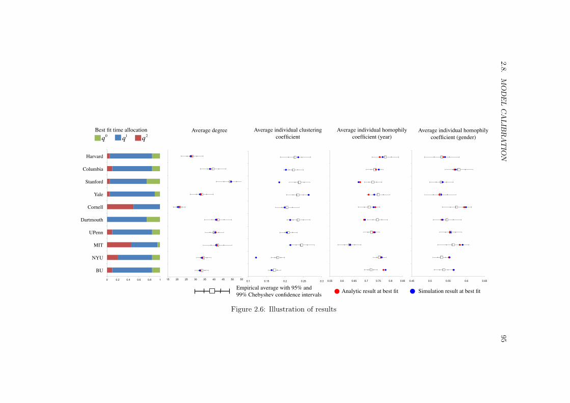
2.8.M
OD
EL
CA
LIBR
AT
ION
95
Harvard!
Columbia!
Stanford!
Yale!
Cornell!
Dartmouth!
UPenn!
MIT!
NYU!
BU!0 0.2 0.4 0.6 0.8 1 0.1 0.15 0.2 0.25 0.3
1
2
3
4
5
6
7
8
9
10
0.55 0.6 0.65 0.7 0.75 0.8 0.85
1
2
3
4
5
6
7
8
9
10
0.45 0.5 0.55 0.6 0.65
1
2
3
4
5
6
7
8
9
10
Best fit time allocation! Average individual clustering coefficient!
Average degree! Average individual homophily coefficient (year)!
Average individual homophily coefficient (gender)!
€
q0
€
q1
€
q2
Empirical average with 95% and 99% Chebyshev confidence intervals! Analytic result at best fit! Simulation result at best fit!
15 20 25 30 35 40 45 50 55
1
2
3
4
5
6
7
8
9
10
Figure 2.6: Illustration of results
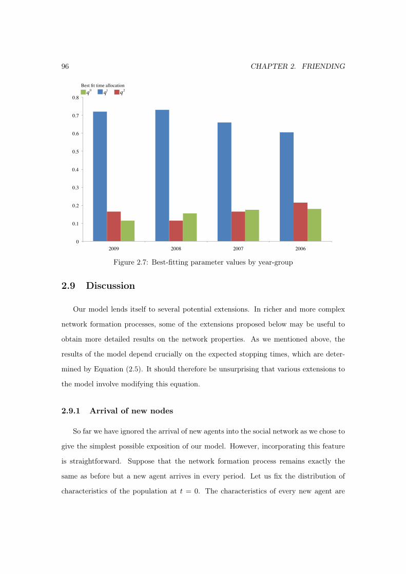
96 CHAPTER 2. FRIENDING
0!
0.1!
0.2!
0.3!
0.4!
0.5!
0.6!
0.7!
0.8!
2009! 2008! 2007! 2006!
Best fit time allocation!
€
q0
€
q1
€
q2
Figure 2.7: Best-fitting parameter values by year-group
2.9 Discussion
Our model lends itself to several potential extensions. In richer and more complex
network formation processes, some of the extensions proposed below may be useful to
obtain more detailed results on the network properties. As we mentioned above, the
results of the model depend crucially on the expected stopping times, which are deter-
mined by Equation (2.5). It should therefore be unsurprising that various extensions to
the model involve modifying this equation.
2.9.1 Arrival of new nodes
So far we have ignored the arrival of new agents into the social network as we chose to
give the simplest possible exposition of our model. However, incorporating this feature
is straightforward. Suppose that the network formation process remains exactly the
same as before but a new agent arrives in every period. Let us fix the distribution of
characteristics of the population at t = 0. The characteristics of every new agent are
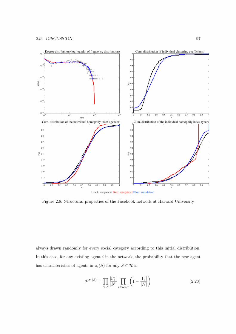
2.9. DISCUSSION 97
100 101 102 10310−6
10−5
10−4
10−3
10−2
10−1
ln(x)
ln(f(x))
0 0.1 0.2 0.3 0.4 0.5 0.6 0.7 0.8 0.9 10
0.1
0.2
0.3
0.4
0.5
0.6
0.7
0.8
0.9
1
x
F(x)
0 0.1 0.2 0.3 0.4 0.5 0.6 0.7 0.8 0.9 10
0.1
0.2
0.3
0.4
0.5
0.6
0.7
0.8
0.9
1
x
F(x)
0 0.1 0.2 0.3 0.4 0.5 0.6 0.7 0.8 0.9 10
0.1
0.2
0.3
0.4
0.5
0.6
0.7
0.8
0.9
1
x
F(x)
Degree distribution (log-log plot of frequency distribution)! Cum. distribution of individual clustering coefficients!
Cum. distribution of the individual homophily index (gender) ! Cum. distribution of the individual homophily index (year) !
Black: empirical Red: analytical Blue: simulation!
Figure 2.8: Structural properties of the Facebook network at Harvard University
always drawn randomly for every social category according to this initial distribution.
In this case, for any existing agent i in the network, the probability that the new agent
has characteristics of agents in πi(S) for any S ∈ R is
Pπi(S) =∏r∈S
|Γri ||N |
∏r∈R\S
(1− |Γ
ri ||N |
)(2.23)

98 CHAPTER 2. FRIENDING
Using this fixed probability, Equation (2.5) becomes
Rπ(t+ 1) = Rπ(t) + Pπ − [2qπ + (1− p)(Rπ(t) + Pπ)− (1− p)2qπ] (2.24)
= p [Rπ(t) + Pπ − 2qπ] (2.25)
The intuition for this is that the remaining active agents in π ∈ Πi are the ones that
remain active from: (i) those that were active in the previous period, as well as (ii) the
new node (arriving with probability Pπ into this partition element), less (iii) the agents
to which i linked in the previous period. Solving this once again for Rπ(0) = |π| yields
Rπ(t) = |π|pt +(2qπ − Pπ)p(pt − 1)
1− p(2.26)
Finally, we can obtain the expected stopping time in π by solving Rπ(t) = 0
T π =
ln(
(2qπ−Pπ)p(2qπ−Pπ)p+(1−p)|π|
)ln(p) if 2qπ − Pπ > 0
0 otherwise(2.27)
It is worth observing that the system is well defined only if the new nodes arrive at a
slow enough rate (Pπ < 2qπ). If the new nodes arrive too quickly, stopping times become
infinite. The rest of the model can be solved using methods from Section 2.4.
2.9.2 Endogenous probability of idleness
In the model, we have assumed that the probability 1− pi of an agent becoming idle
in any given period is constant. It is reasonable to suppose that this probability depends
on time, so that pi(t). This would modify Equations (2.5) and (2.11) respectively as

2.9. DISCUSSION 99
follows
Rπ(t+ 1) = pπ(t) [Rπ(t)− 2qπ] (2.28)
Pr(t ≤ x) =
t=x∑t=0
z=x∏z=0
pi(z) [1− pi(x+ 1)] (2.29)
Although this introduces some difficulties for deriving the analytical expressions for
the degree distribution for a general pi(t), these expressions will easily generate the
appropriate numerical solutions.
2.9.3 Preferential attachment
Since the degree distribution in many networks follows a power law, Price (1976),
Barabási and Albert (1999), and Jackson and Rogers (2007) suggested introducing pref-
erential attachment into the network formation process in order to reproduce this prop-
erty. This means that nodes in a network link to each other with a probability that is
proportional to their degree.
We find that our model with uniform random attachment performs well against the
data. In fact, Jackson (2008, p. 65) observes that
“some of the more purely social networks have parameters that indicate muchhigher levels of random link formation, which are very far from satisfying apower law. In fact, the degree distribution of the romance network amonghigh school students is essentially the same as that of a purely random net-work.”
The above quote suggests that “more purely social networks” tend to have degree
distributions that are closer to exponential. It is nevertheless possible to induce a power
law distribution by introducing preferential attachment into our model. Equation (2.3)
becomes
∆dπi (t) = qπ(
1 + dπi (t)Rπ(t)
Rπ(t)
)1(t ≤ T π) = (1 + dπi (t))qπ1(t ≤ T π) (2.30)

100 CHAPTER 2. FRIENDING
Even though agent i’s out-link is made according to preferential attachment, it does
not matter to whom it is made. However, the in-link is no longer made uniformly with
probability 1Rπ(t) , but instead with probability dπi (t)
Rπ(t) , which is proportional to i’s degree.
As before, solving with dπi (0) = 0 yields
dπi (t) = (1 + qπ)[t1(t≤Tπ)+Tπ1(t>Tπ)] − 1 (2.31)
Now the analogue of Equation (2.5) is
Rπ(t+ 1) = pπ[Rπ(t)− (1 + qπ)t + 1
](2.32)
assuming for simplicity that pi = p for all i. Setting Rπ(0) = |π| produces a rather
unwieldy result
Rπ(t) =pt+2|π|−pt+1[(2+qπ)|π|+qπ ]+pt(1+qπ)|π|+p2[(1+qπ)t−1]+p[1+qπ−(1+qπ)t]
(p−1)(p−qπ−1)(2.33)
Solving for Rπ(T π) = 0, is possible numerically, and the rest of derivation, once
again, follows the steps outlined in Section 2.4.
2.9.4 Endogenous characteristics
Perhaps the most interesting extension of the model is to consider what happens
when ki is made endogenous (Bramoullé et al., 2012, and Boucher, 2012, also make this
point). Let us, once again, think about the model as the affiliation network discussed
in Section 2.3.5. New links can form in ways other than by focal closure. If an agent i
is linked to another agent j who has a particular membership k ∈ Kr, then there is a
positive probability that a link will form between i and k ∈ Kr. Figure 2.9 shows that
Mark wants to join the Finance membership because his friend Eduardo is already a
member. This is called membership closure.
The endogenous determination of characteristics in our model would be neatly cap-
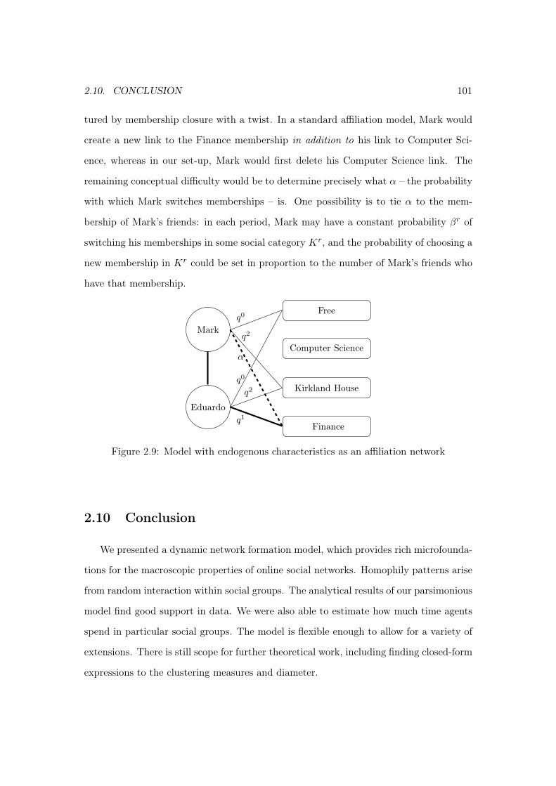
2.10. CONCLUSION 101
tured by membership closure with a twist. In a standard affiliation model, Mark would
create a new link to the Finance membership in addition to his link to Computer Sci-
ence, whereas in our set-up, Mark would first delete his Computer Science link. The
remaining conceptual difficulty would be to determine precisely what α – the probability
with which Mark switches memberships – is. One possibility is to tie α to the mem-
bership of Mark’s friends: in each period, Mark may have a constant probability βr of
switching his memberships in some social category Kr, and the probability of choosing a
new membership in Kr could be set in proportion to the number of Mark’s friends who
have that membership.
Mark
Eduardo
Free
Computer Science
Kirkland House
Finance
q0
q2
α
q0
q2
q1
Figure 2.9: Model with endogenous characteristics as an affiliation network
2.10 Conclusion
We presented a dynamic network formation model, which provides rich microfounda-
tions for the macroscopic properties of online social networks. Homophily patterns arise
from random interaction within social groups. The analytical results of our parsimonious
model find good support in data. We were also able to estimate how much time agents
spend in particular social groups. The model is flexible enough to allow for a variety of
extensions. There is still scope for further theoretical work, including finding closed-form
expressions to the clustering measures and diameter.

102 CHAPTER 2. FRIENDING
The model has some interesting implications for policy design. Suppose that the
policy objective is to diffuse information about the quality of a particular product as
quickly as possible and that agents learn by averaging signals about product quality from
their neighbors (this is known as DeGroot learning). Golub and Jackson (2012) showed
that homophily in a random network slows down the speed of DeGroot learning. In our
model, agents who have been in the network the longest have the highest degree and
are most heterophilious; therefore, information about the product would travel fastest if
the diffusion process began with these agents. Alternatively, it may indeed be effective
to target the newest arrivals to the network because their homophily often increases as
they make their first friendships.

2.11. APPENDIX 103
2.11 Appendix
2.11.1 Proofs
Proof of Proposition 1. We compare the original scenario with the one in which |πi(r)|
is increased by δ and |πi(0)| is decreased by δ (so |Γri | is increased by δ). We represent
all variables after the change with a “hat”, so for example, |Γri | = |Γri |+ δ.
Using Equations (2.2) and (2.7), we obtain
T πi(S) =
ln
2p
[∑r∈S∪0
qr
|Γri|
]2p
[∑r∈S∪0
qr
|Γri|
]+(1−p)
ln(p)
(2.34)
This equation shows that (i) if S′ ⊆ S, then∑
r∈S′qr
|Γri |≤∑
r∈Sqr
|Γri |and therefore
T πi(S′) ≥ T πi(S) (since ln(p) < 0). Secondly, the equation also shows that (ii) T πi(S) is
increasing in |Γri | for every S such that r ∈ S.
Without loss of generality, we can order the expected stopping times before the
change, for some sequence of sets Sk with k ∈ 1, ..., 2|R|, as:
T πi(S1) ≤ T πi(S2) ≤ · · · ≤ T πi(Sk) (2.35)
The order of expected stopping times after the change is then
T πi(S1) ≤ T πi(S2) ≤ · · · ≤ T πi(Sk) (2.36)
where the sequence of the sets Sk is unchanged (which is true by virtue of δ being small
– an assumption of the proposition). Now, by point (i) above, we know that for any
Sk, T πi(Sk) ≥ T πi(Sk). For an arbitrary k, let us consider the interval [T πi(Sk−1), T πi(Sk)]
before the change, and the corresponding interval [T πi(Sk−1), T πi(Sk)] after the change.
According to the definition of di(t) (see Equation (2.8)), the slope of di(t) within this
interval is given by 2∑2|R|
j=k qπi(Sj) before the change, and by 2
∑2|R|
j=k qπi(Sj) after the

104 CHAPTER 2. FRIENDING
change. According to Equation (2.2), one can verify the following:
qπi(S) =
q0 |πi(0)|−δ|N |−1 if S = 0
q0 |πi(S)||N |−1 + qr |πi(S)|
|Γri |+δ+∑
s∈S\r qs |πi(S)||Γsi |
if r ∈ S and S 6= r
q0 |πi(S)|+δ|N |−1 + qr |πi(S)|+δ
|Γri |+δif S = r
q0 |πi(S)||N |−1 +
∑s∈S q
s |πi(S)||Γsi |
if r 6∈ S
(2.37)
Naturally, for any S, qπi(S) is simply qπi(S) with δ = 0. The difference is between the
slopes in the interval after the change and before the change is given by
2|R|∑j=k
qπi(Sj) −2|R|∑j=k
qπi(Sj) (2.38)
=2|R|∑j=k
qπi(Sj) − qπi(Sj) (2.39)
Now, suppose for reference, that Sk∗ = r.
Case A: Consider any k ≤ k∗. Then the set S = Sj |j < k must include 0 and
may include sets Sj such that r ∈ Sj (Given our ordering of the expected stopping times,
this is true by point (i) above). It may also includes sets Sj such that r 6∈ Sj , but for all
such sets, qπi(Sj) = qπi(Sj). This implies that Equation (2.39) becomes:
qr
[(∑S∈S′∈S|r∈S′ |πi(S)|+ δ
|Γri |+ δ
)−
(∑S∈S′∈S|r∈S′ |πi(S)|
|Γri |
)](2.40)
Since |Γri | ≥∑
S∈S′∈S|r∈S′ |πi(S)|, this is positive, which implies that the slope of di(t)
in any time period preceding T πi(Sk∗ ), that is T πi(r) must be greater after the change
than before the change.
Case B: Consider any k > k∗. Then every Sj such that j ≥ k must be a set
not containing r (otherwise, this would contradict point (i) above). This implies that
the aggregation in Equation (2.39) is only over set of categories not containing r. By

2.11. APPENDIX 105
Equation (2.37), Equation (2.39) becomes: − δ|N |−1 which is negative. This implies
that the slope of di(t) in any time period after T πi(r) and before T πi(0) must be
greater before the change than after the change. This means that within the interval
[T πi(r), T πi(0)] it is in principle possible for the degree before to change to reach a
higher value than after the change.
Proof of Proposition 2. If we denote the set of i’s friends at t by the set Ni(t), then the
average degree of i’s friends at t is given by
∑j∈Ni(t) dj(t)
di(t)(2.41)
We expect i’s degree to be larger is i becomes idle at a later t, therefore the average
degree of i’s friends is increasing in di(t) if it is increasing in t. By Equations (2.2), (2.7),
and (2.8), one can note that if |πi(S)| = |πj(S)| for all S, then di(t) = dj(t). Under this
restriction, the average degree of i’s friends at t simply becomes |Ni(t)| ≡ di(t), which is
increasing in t.
Proof of Proposition 3. First of all, note that both the numerator and the denominator
are concave, non-decreasing, piecewise linear functions, and for any given t, the slope of
the numerator is always less than that of the denominator. (1) For t ∈ (0, TLi ), both
the numerator and the denominator are linear functions starting at the origin, with the
denominator having a steeper slope than the numerator. Hence, Hri (t) is a constant. (2)
At TLi , there is a kink either (a) in the denominator alone or (b) both in the numerator
and the denominator. In case (a),Hri (t) would increase since the slope of the denominator
falls, but in case (b), it is ambiguous (it is easy to find an example where Hri (t) increases
before decreasing again in this range). This reasoning applies every time there is such a
kink, which occurs at every expected stopping time in the interval [TLi , TMi ). (3) At TM
the numerator becomes flat, while the denominator is still increasing. This implies that
Hri (t) is decreasing in the interval [TMi , THi ). (4) Finally, at THi , the denominator also

106 CHAPTER 2. FRIENDING
becomes flat, which means that for every t ≥ THi , Hri (t) is simply a constant divided by
another constant.
Proof of Corollary 1. (1) Since qr > 0 for only one r ∈ R+, one can verify that (i)
T πi(S) ∈ T πi(r), 0 for any S such that r ∈ S, and (ii) T πi(S) ∈ T πi(0), 0 for any S
such that r /∈ S. Note that if S′ ⊆ S, then∑
r∈S′qr
|Γri |≤∑
r∈Sqr
|Γri |and therefore from
Equation (2.34), we obtain T πi(S′) ≥ T πi(S) (since ln(p) < 0). Hence, maxπ∈ΠiT π =
T πi(0), maxπ∈ΠriT π = T πi(r) and minπ∈ΠiT π ∈ T πi(r), 0. From this, it follows
that: either TLi = TMi = T πi(r) and THi = T πi(0); or TLi = 0, TMi = T πi(r) and
THi = T πi(0). From Proposition 3, we have that Hri (t) has the following form: (i) For
t ∈ [0, TMi ), Hri (t) is a constant. (ii) For t ∈ [TMi , THi ), Hr
i (t) is decreasing. (iii) For
t ∈ [THi ,∞), Hri (t) is a constant. The shape of hri (d) follows from this and from Remark
1.
(2) This follows immediately from part (1) of this corollary and Proposition 1.

2.11. APPENDIX 107
2.11.2 Simulation algorithm
Input:|N | ×R matrix M where each row is the vector of characteristics ki.Vector q.
Initialise:Empty adjacency matrix A with elements aij.Let L be the list of all agents.Using M, find Γr
i |r ∈ R for all i ∈ N.
1. while L is non-empty do
2. every agent in L becomes idle with probability p
3. L is now the list of remaining active agents in random order
4. for every i in L do
5. select an r ∈ R at random according to q
6. if Z = Γri ∩ L ∩ j ∈ N |aij = 0 6= ∅ then
7. pick an agent j uniformly at random from Z
8. create edges ij and ji in A
9. else continue to next agent in L
10. end if
11. end for
12. return A

108 CHAPTER 2. FRIENDING
2.11.3 Algorithm for finding robust points in the grid search
Input:Q where each row is a vector (q, p), and the rows are ordered by the value
they induce in L(q, p), from lowest at the top to highest at the bottom. Q isthe 100-by-4 matrix consisting of the top 100 row vectors of Q.(q, p)k = (q0k, q
1k, q
2k, pk) ∈ Q denotes the kth row vector in Q.
Initialise:S is a 1-by-100 vector of scores, δq = 0.1, δp = 0.05.
1. for k from 1 to 100 do
2. S(k) = |(q, p)j ∈ Q|pj ∈ [pk − δp, pk + δp] &∀i ∈ 0, 1, 2, qij ∈ [qik − δq, qik + δq]|
3. end for
4. for k from 1 to 99 do
5. if S(k) > S(k + 1) then
6. break
7. else
8. continue
9. end if
10. end for
11. return (q, p)k

2.11.A
PP
EN
DIX
1092.11.4 Data description
College
Raw
number
of nodes
Raw
number
of edges Nodes Edges
Average
degree Women Men
Avg.
major
size
Avg.
minor
size
Avg.
dorm
size
Avg.
class
size
Harvard U. 15126 824617 1325 18608 28.1 567 758 23.2 22.5 42.7 46.9
Columbia U. 11770 444333 2663 52697 39.6 1573 1090 29.6 29.9 54.3 65.7
Stanford U. 11621 568330 2254 55,124 48.9 1043 1211 30.9 30.1 25.6 55.0
Yale U. 8578 405450 1431 23847 33.3 639 792 19.6 19.1 68.1 38.2
Cornell U. 18660 790777 2509 26653 21.2 1078 1431 27.6 24.6 20.6 51.6
Dartmouth College 7694 304,076 1612 34030 42.2 780 832 29.9 29.3 23.0 45.0
U. of Penn. 14916 686501 3006 60516 40.3 1417 1589 28.4 27.1 50.9 77.0
M.I.T. 6440 251252 1563 32751 41.9 626 937 44.7 37.2 26.1 58.2
New York U. 21679 715715 5581 95968 34.4 3345 2236 53.7 52.2 105.5 99.7
Boston U. 19700 637528 5510 92042 33.4 3355 2155 37.5 34.7 91.8 90.8
Average 13618 562858 2745 49224 36.3 1442 1303 32.5 30.7 50.5 62.8

110 CHAPTER 2. FRIENDING
2.11.5 Further baseline observations on homophily
Figure 2.10 shows the group homophily index in gender and in year of graduation
across the ten colleges. Figures 2.11 and 2.12 show a histogram of individual homophily
indices for each college in gender and in year of graduation, respectively. The horizontal
lines show the empirical fractions of students sharing a particular characteristic in the
population ( |Wrk ||N | in the notation of the population). The plots show that for gender,
students tend to distribute themselves roughly symmetrically around the fraction of
students who share their characteristic, while for year of graduation, most students tend
to exhibit much stronger individual homophily (a feature which our model replicates).
Harvard Columbia Stanford Yale Cornell Dartmouth UPenn MIT NYU BostonU0.4
0.45
0.5
0.55
0.6
0.65
Gro
up h
omop
hily
in g
ende
r
boysgirls
Harvard Columbia Stanford Yale Cornell Dartmouth UPenn MIT NYU BostonU0.5
0.55
0.6
0.65
0.7
0.75
0.8
0.85
0.9
0.95
Gro
up h
omop
hily
in y
ear o
f gra
duat
ion
2006200720082009
Figure 2.10: Group homophily in gender and in year of graduation across the ten colleges
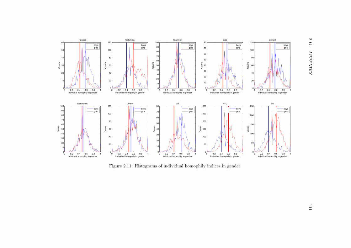
2.11.A
PP
EN
DIX
111
0 0.2 0.4 0.6 0.8 10
10
20
30
40
50
60
Cou
nts
Individual homophily in gender
Harvard
boysgirls
0 0.2 0.4 0.6 0.8 10
20
40
60
80
100
120
Cou
nts
Individual homophily in gender
Columbia
boysgirls
0 0.2 0.4 0.6 0.8 10
10
20
30
40
50
60
70
80
90
100
Cou
nts
Individual homophily in gender
Stanford
boysgirls
0 0.2 0.4 0.6 0.8 10
10
20
30
40
50
60
70
80
Cou
nts
Individual homophily in gender
Yale
boysgirls
0 0.2 0.4 0.6 0.8 10
20
40
60
80
100
120
Cou
nts
Individual homophily in gender
Cornell
boysgirls
0 0.2 0.4 0.6 0.8 10
10
20
30
40
50
60
70
80
90
100
Cou
nts
Individual homophily in gender
Dartmouth
boysgirls
0 0.2 0.4 0.6 0.8 10
20
40
60
80
100
120C
ount
s
Individual homophily in gender
UPenn
boysgirls
0 0.2 0.4 0.6 0.8 10
10
20
30
40
50
60
70
80
Cou
nts
Individual homophily in gender
MIT
boysgirls
0 0.2 0.4 0.6 0.8 10
50
100
150
200
250
300
Cou
nts
Individual homophily in gender
NYU
boysgirls
0 0.2 0.4 0.6 0.8 10
50
100
150
200
250
Cou
nts
Individual homophily in gender
BU
boysgirls
Figure 2.11: Histograms of individual homophily indices in gender
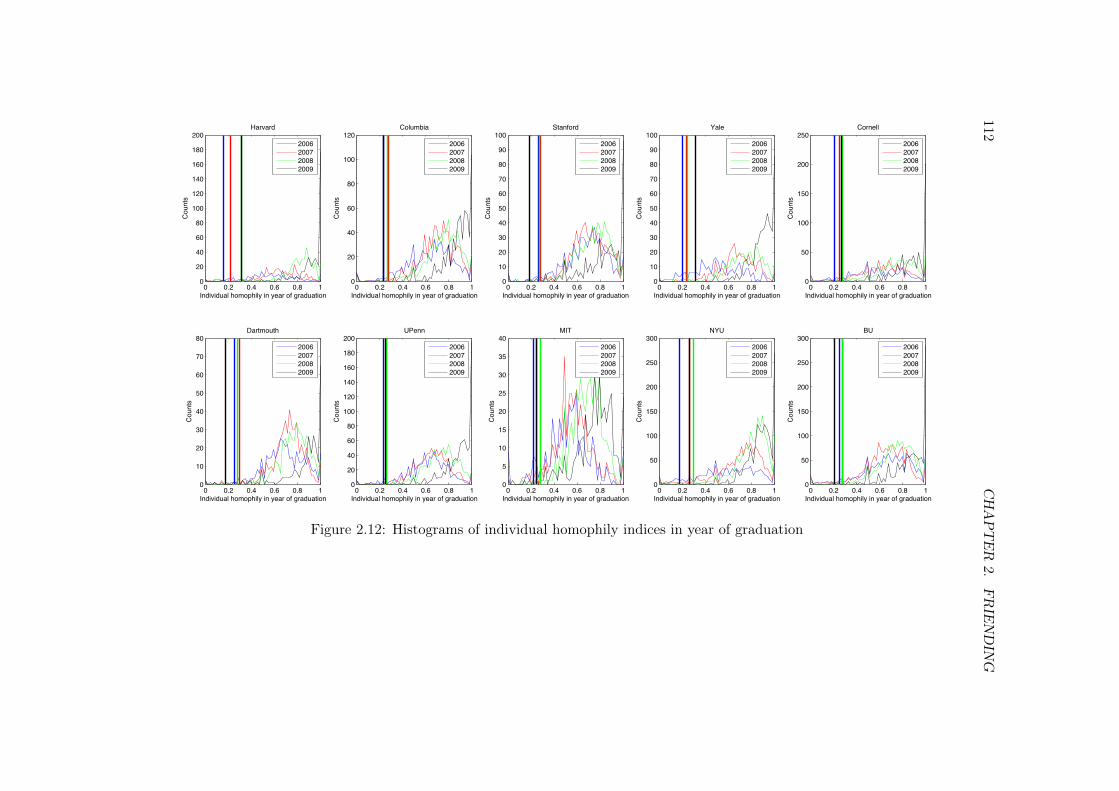
112C
HA
PT
ER
2.FR
IEN
DIN
G
0 0.2 0.4 0.6 0.8 10
20
40
60
80
100
120
140
160
180
200
Cou
nts
Individual homophily in year of graduation
Harvard
2006200720082009
0 0.2 0.4 0.6 0.8 10
20
40
60
80
100
120
Cou
nts
Individual homophily in year of graduation
Columbia
2006200720082009
0 0.2 0.4 0.6 0.8 10
10
20
30
40
50
60
70
80
90
100
Cou
nts
Individual homophily in year of graduation
Stanford
2006200720082009
0 0.2 0.4 0.6 0.8 10
10
20
30
40
50
60
70
80
90
100
Cou
nts
Individual homophily in year of graduation
Yale
2006200720082009
0 0.2 0.4 0.6 0.8 10
50
100
150
200
250
Cou
nts
Individual homophily in year of graduation
Cornell
2006200720082009
0 0.2 0.4 0.6 0.8 10
10
20
30
40
50
60
70
80
Cou
nts
Individual homophily in year of graduation
Dartmouth
2006200720082009
0 0.2 0.4 0.6 0.8 10
20
40
60
80
100
120
140
160
180
200C
ount
s
Individual homophily in year of graduation
UPenn
2006200720082009
0 0.2 0.4 0.6 0.8 10
5
10
15
20
25
30
35
40
Cou
nts
Individual homophily in year of graduation
MIT
2006200720082009
0 0.2 0.4 0.6 0.8 10
50
100
150
200
250
300
Cou
nts
Individual homophily in year of graduation
NYU
2006200720082009
0 0.2 0.4 0.6 0.8 10
50
100
150
200
250
300
Cou
nts
Individual homophily in year of graduation
BU
2006200720082009
Figure 2.12: Histograms of individual homophily indices in year of graduation

2.11.A
PP
EN
DIX
1132.11.6 Results
College q1 q2 q0 p 〈h3i 〉 〈h3i 〉 〈h3i 〉 〈h4i 〉 〈h4i 〉 〈h4i 〉 C C
Harvard U. 0.80 0.05 0.15 0.9625 0.53 0.54 0.54 0.78 0.76 0.77 0.23 0.24
Columbia U. 0.75 0.10 0.15 0.9700 0.58 0.57 0.57 0.74 0.74 0.75 0.22 0.20
Stanford U. 0.70 0.05 0.25 0.9775 0.53 0.53 0.54 0.73 0.67 0.67 0.24 0.18
Yale U. 0.85 0.05 0.10 0.9775 0.53 0.53 0.53 0.75 0.71 0.73 0.24 0.26
Cornell U. 0.50 0.50 0.00 0.9400 0.57 0.59 0.60 0.71 0.74 0.73 0.21 0.20
Dartmouth College 0.75 0.00 0.25 0.9705 0.55 0.53 0.53 0.75 0.69 0.69 0.24 0.21
U. of Penn. 0.75 0.10 0.15 0.9725 0.56 0.55 0.56 0.72 0.73 0.73 0.21 0.20
M.I.T. 0.50 0.45 0.05 0.9700 0.56 0.58 0.59 0.63 0.63 0.63 0.25 0.21
New York U. 0.65 0.20 0.15 0.9550 0.53 0.55 0.55 0.75 0.76 0.76 0.18 0.12
Boston U. 0.75 0.10 0.15 0.9575 0.54 0.56 0.57 0.72 0.77 0.78 0.17 0.16
q1: best-fitting proportion of time spent in class
q2: best-fitting proportion of time spent in dorm
q0: best-fitting proportion of time spent as free time
p: best-fitting probability of remaining active in any given period
C: average of empirical individual clustering coefficients
C: average of simulated individual clustering coefficients
〈h3i 〉: average of empirical individual homophily indices for gender
〈h3i 〉: average of analytical individual homophily indices for gender
〈h3i 〉: average of simulated individual homophily indices for gender
〈h4i 〉: average of empirical individual homophily indices for graduation year
〈h4i 〉: average of analytical individual homophily indices for graduation year
〈h4i 〉: average of simulated individual homophily indices for graduation year
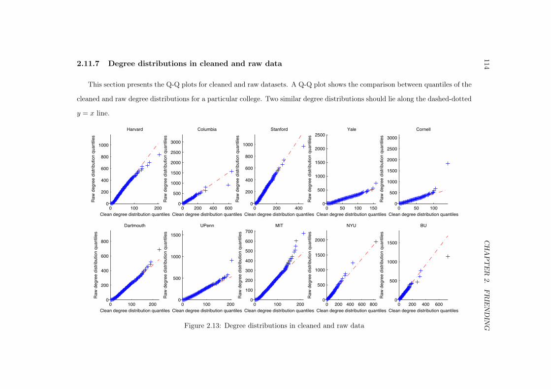
114C
HA
PT
ER
2.FR
IEN
DIN
G2.11.7 Degree distributions in cleaned and raw data
This section presents the Q-Q plots for cleaned and raw datasets. A Q-Q plot shows the comparison between quantiles of the
cleaned and raw degree distributions for a particular college. Two similar degree distributions should lie along the dashed-dotted
y = x line.
0 100 2000
200
400
600
800
1000
Clean degree distribution quantiles
Raw
deg
ree
dist
ribut
ion
quan
tiles
Harvard
0 200 400 6000
500
1000
1500
2000
2500
3000
Clean degree distribution quantiles
Raw
deg
ree
dist
ribut
ion
quan
tiles
Columbia
0 200 4000
200
400
600
800
1000
Clean degree distribution quantiles
Raw
deg
ree
dist
ribut
ion
quan
tiles
Stanford
0 50 100 1500
500
1000
1500
2000
2500
Clean degree distribution quantiles
Raw
deg
ree
dist
ribut
ion
quan
tiles
Yale
0 50 1000
500
1000
1500
2000
2500
3000
Clean degree distribution quantiles
Raw
deg
ree
dist
ribut
ion
quan
tiles
Cornell
0 100 2000
200
400
600
800
Clean degree distribution quantiles
Raw
deg
ree
dist
ribut
ion
quan
tiles
Dartmouth
0 100 2000
500
1000
1500
Clean degree distribution quantiles
Raw
deg
ree
dist
ribut
ion
quan
tiles
UPenn
0 100 2000
100
200
300
400
500
600
700
Clean degree distribution quantiles
Raw
deg
ree
dist
ribut
ion
quan
tiles
MIT
0 200 400 600 8000
500
1000
1500
2000
Clean degree distribution quantilesR
aw d
egre
e di
strib
utio
n qu
antil
es
NYU
0 200 400 6000
500
1000
1500
Clean degree distribution quantiles
Raw
deg
ree
dist
ribut
ion
quan
tiles
BU
Figure 2.13: Degree distributions in cleaned and raw data

2.11. APPENDIX 115
2.11.8 Test of Proposition 1 with an unrestricted set of agents
Table 2.4 presents the results from running the regression shown in equation (2.19) on
all agents in each college rather than on the restricted set X ∩ Y . Once again, although
the values are not quite as stark as previously, all relevant coefficients are positive or not
significantly different from zero which suggests that the relationship between group size
and degree appears to hold quite generally.
Dependent variable: agent’s degree|Γ1
i | s.e. |Γ2i | s.e. |πi(S)| s.e. const. N
Harvard 0.170*** (0.032) 0.239*** (0.034) -0.273 (0.308) 9.002 1325Columbia 0.149*** (0.022) 0.012 (0.012) -0.627*** (0.141) 33.94 2663Stanford 0.319*** (0.031) 0.071*** (0.021) -1.995*** (0.429) 35.53 2254
Yale 0.035 (0.043) 0.056** (0.023) 0.518 (0.458) 25.06 1431Cornell 0.034** (0.017) 0.002 (0.003) -0.308*** (0.096) 21.07 2509
Dartmouth 0.200*** (0.037) -0.035 (0.036) -0.689 (0.512) 37.04 1612UPenn 0.153*** (0.018) -0.018*** (0.005) -0.427*** (0.128) 37.55 3006
MIT 0.063** (0.032) -0.028 (0.018) -0.328 (0.274) 42.38 1563NYU 0.085*** (0.012) 0.020*** (0.003) -0.218*** (0.061) 23.98 5581
Boston U. 0.091*** (0.011) 0.008*** (0.002) -0.274*** (0.044) 26.02 5510Comment: Standard OLS regression with robust standard errors in parentheses
∗∗∗/∗∗/∗ denote rejection of H0 : β = 0 at the 1/5/10% significant level respectively
Table 2.4: Regression results on the unrestricted set of agents
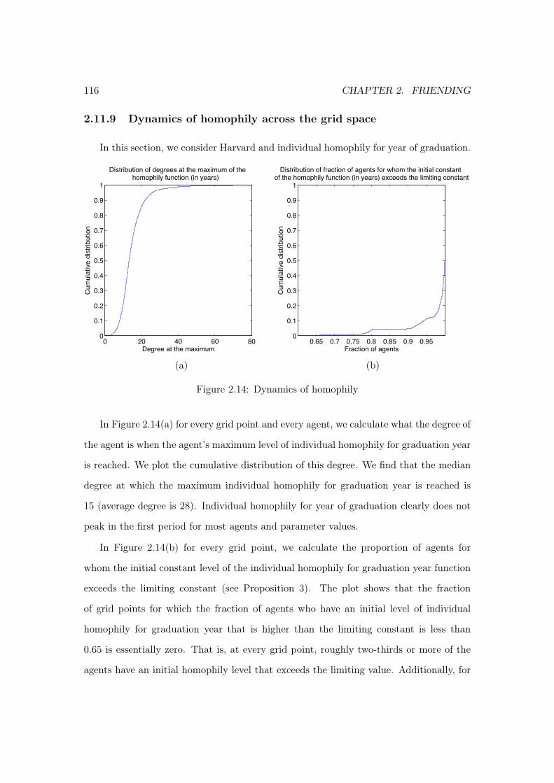
116 CHAPTER 2. FRIENDING
2.11.9 Dynamics of homophily across the grid space
In this section, we consider Harvard and individual homophily for year of graduation.
0 20 40 60 800
0.1
0.2
0.3
0.4
0.5
0.6
0.7
0.8
0.9
1
Degree at the maximum
Cum
ulat
ive
dist
ribut
ion
Distribution of degrees at the maximum of the homophily function (in years)
0.65 0.7 0.75 0.8 0.85 0.9 0.950
0.1
0.2
0.3
0.4
0.5
0.6
0.7
0.8
0.9
1
Fraction of agents
Cum
ulat
ive
dist
ribut
ion
Distribution of fraction of agents for whom the initial constant of the homophily function (in years) exceeds the limiting constant
(a) (b)
Figure 2.14: Dynamics of homophily
In Figure 2.14(a) for every grid point and every agent, we calculate what the degree of
the agent is when the agent’s maximum level of individual homophily for graduation year
is reached. We plot the cumulative distribution of this degree. We find that the median
degree at which the maximum individual homophily for graduation year is reached is
15 (average degree is 28). Individual homophily for year of graduation clearly does not
peak in the first period for most agents and parameter values.
In Figure 2.14(b) for every grid point, we calculate the proportion of agents for
whom the initial constant level of the individual homophily for graduation year function
exceeds the limiting constant (see Proposition 3). The plot shows that the fraction
of grid points for which the fraction of agents who have an initial level of individual
homophily for graduation year that is higher than the limiting constant is less than
0.65 is essentially zero. That is, at every grid point, roughly two-thirds or more of the
agents have an initial homophily level that exceeds the limiting value. Additionally, for

2.11. APPENDIX 117
approximately 90 percent of the grid points, 95 percent of agents start out with a higher
level of individual homophily for graduation year than the limiting constant. Results for
any other college and for individual homophily for gender are comparable.

118 CHAPTER 2. FRIENDING
2.12 References
Akerlof, G. A. and R. E. Kranton (2010). Identity Economics: How Our Identities Shape
Our Work, Wages, and Well-Being . Princeton University Press.
Banerjee, A., A. G. Chandrasekhar, E. Duflo, and M. O. Jackson (2012). The diffusion
of microfinance. Working Paper 17743, NBER. http://www.nber.org/papers/w17743.
pdf.
Barabási, A.-L. and R. Albert (1999). Emergence of scaling in random networks. Sci-
ence 286, 509–512.
Bianconi, G., P. Pin, and M. Marsili (2009). Assessing the relevance of node features for
network structure. Proceedings of the National Academy of Sciences 106 (28), 11433–
11438.
Botha, L. and S. Kroon (2010). A community-based model of online social networks. In
The 4th SNA-KDD Workshop on Social Network Mining and Analysis.
Boucher, V. (2012). Structural homophily. Working paper, Université de Montréal.
http://www.vincentbouchereconomist.com/SH5juillet.pdf.
Bramoullé, Y., S. Currarini, M. O. Jackson, P. Pin, and B. W. Rogers (2012). Homophily
and long run integration in social networks. Journal of Economic Theory 147, 1754–
1786.
Breiger, R. L. (1974). The duality of persons and groups. Social Forces 53 (2), 181–190.
Currarini, S., M. O. Jackson, and P. Pin (2009). An Economic Model of Friendship:
Homophily, Minorities, and Segregation. Econometrica 77 (4), 1003–1045.
Currarini, S., M. O. Jackson, and P. Pin (2010). Identifying the roles of race-based choice
and chance in high school friendship network formation. Proceedings of the National
Academy of Sciences 107 (11), 4857–4861.

2.12. REFERENCES 119
de Marti, J. and Y. Zenou (2011, March). Identity and social distance in friendship for-
mation. Working paper, Stockholm University. http://www.econ.upf.edu/~demarti/
Articles/identity.pdf.
Easley, D. and J. Kleinberg (2010). Networks, Crowds, and Markets: Reasoning about a
highly connected world. Cambridge, UK: Cambridge University Press.
Falk, A. and A. Ichino (2006). Clean evidence on peer effects. Journal of Labor Eco-
nomics 24 (1), 39–57.
Feld, S. L. (1981). The focused organization of social ties. American Journal of Sociol-
ogy 86 (5), 1015–1035.
Golub, B. and M. O. Jackson (2012). How homophily affects diffusion and learning in
networks. Quarterly Journal of Economics 127 (3), 1287–1338.
Goyal, S. (2009). Connections: An Introduction to the Economics of Networks. Princeton,
NJ: Princeton University Press.
Iijima, R. and Y. Kamada (2013). Social distance and network structures. Working
paper, Harvard University. http://www.ykamada.com/pdf/Clustering.pdf.
Jackson, M. O. (2008). Social and Economic Networks. Princeton, NJ: Princeton Uni-
versity Press.
Jackson, M. O. and B. W. Rogers (2007). Meeting strangers and friends of friends: How
random are social networks? American Economic Review 70 (3), 890–915.
Kandel, D. B. (1978). Homophily, selection, and socialization in adolescent friendships.
American Journal of Sociology 84 (2), 427–436.
Kremer, M. and D. Levy (2008). Peer effects and alcohol use among college students.
Journal of Economic Perspectives 22 (3), 189–206.

120 CHAPTER 2. FRIENDING
Kumar, R., J. Novak, and A. Tomkins (2010). Structure and evolution of online social
networks. In Proceedings of the 11th ACM International Conference on Knowledge
Discovery and Data Mining, pp. 611–617.
Lattanzi, S. and D. Sivakumar (2009). Affiliation networks. In Proceedings of the 41st
annual ACM symposium on Theory of computing, pp. 427–434.
Leskovec, J., J. Kleinberg, and C. Faloutsos (2005). Graphs over time: Densification
laws, shrinking diameters and possible explanations. In Proceedings of the 11th ACM
SIGKDD international conference on Knowledge Discovery in Data Mining, pp. 177–
187.
Leskovec, J., K. J. Lang, A. Dasgupta, and M. W. Mahoney (2008). Statistical properties
of community structure in large social and information networks. In Proceedings of
the 17th international conference on World Wide Web, pp. 695–704.
Lewis, K., M. Gonzalez, and J. Kaufman (2012). Social selection and peer influence in
an online social network. Proceedings of the National Academy of Sciences 109 (1),
68–72.
Lewis, K., J. Kaufman, M. Gonzalez, A. Wimmer, and N. Christakis (2008). Tastes, ties,
and time: A new social network dataset using Facebook.com. Social Networks 30 (4),
330–342.
Mayer, A. and S. L. Puller (2008). The old boy (and girl) network: Social network
formation on university campuses. Journal of Public Economics 92 (1-2), 329–347.
McPherson, M., L. Smith-Lovin, and J. M. Cook (2001). Birds of a feather: Homophily
in social networks. Annual Review of Sociology 27, 415–444.
Moody, J. (2001). Race, school integration, and friendship segregation in america. Amer-
ican Journal of Sociology 107 (3), 679–716.

2.12. REFERENCES 121
Mouw, T. and B. Entwisle (2006). Residential segregation and interracial friendship in
schools. American Journal of Sociology 112 (2), 394–441.
Newman, M. E. J. (2010). Networks: An Introduction. Oxford, UK: Oxford University
Press.
Newman, M. E. J., D. J. Watts, and S. H. Strogatz (2002). Random graph models of
social networks. Proceedings of the National Academy of Sciences 99 (Supplement 1),
2566–2572.
Pempek, T. A., Y. A. Yermolayeva, and S. L. Calvert (2009). College students’ social net-
working experiences on Facebook. Journal of Applied Developmental Psychology 30 (3),
227–238.
Price, D. D. S. (1976). A general theory of bibliometric and other cumulative advantage
processes. Journal of the American Society for Information Science 27 (5), 292–306.
Sacerdote, B. (2001). Peer Effects with Random Assignment: Results for Dartmouth
Roommates. Quarterly Journal of Economics 116 (2), 681–704.
Sen, A. (2006). Identity and Violence: Illusion of Destiny. London, UK: Penguin Books.
Shaw, B., B. Huang, and T. Jebara (2011). Learning a distance metric from a network. In
Proceedings of the 25th annual conference on Neural Information Processing Systems,
pp. 1899–1907.
Shrum, W., N. H. Cheek Jr., and S. M. Hunter (1988). Friendship in school: Gender
and racial homophily. Sociology of Education 61 (4), 227–239.
Tarbush, B. and A. Teytelboym (2012). Homophily in online social networks. In Internet
and Network Economics, pp. 512–518. Springer.
Traud, A. L., E. D. Kelsic, P. J. Mucha, and M. A. Porter (2010). Comparing community

122 CHAPTER 2. FRIENDING
structure to characteristics in online collegiate social networks. SIAM Review 53 (3),
526–543.
Traud, A. L., P. J. Mucha, and M. A. Porter (2012). Social structure of Facebook
networks. Physica A 391 (16), 4165–4180.
Wimmer, A. and K. Lewis (2010). Beyond and below racial homophily: Erg models of a
friendship network documented on facebook. American Journal of Sociology 116 (2),
583–642.
Xiang, R., J. Neville, and M. Rogati (2010). Modeling relationship strength in online
social networks. In Proceedings of the 19th international conference on World Wide
Web, pp. 981–990.
Zheleva, E., H. Sharara, and L. Getoor (2009). Co-evolution of social and affiliation net-
works. In Proceedings of the 15th ACM SIGKDD international conference on Knowl-
edge Discovery and Data Mining, pp. 1007–1016.

Chapter 3
Processes on graphs with multiple
edge types
Abstract: We examine three models on graphs – an information transmission mech-anism, a process of friendship formation, and a model of puzzle solving – in which theevolution of the process is conditioned on the multiple edge types of the graph. Forexample, in the model of information transmission, a node considers information to bereliable, and therefore transmits it to its neighbors, if and only if the same message wasreceived on two distinct communication channels. For each model, we algorithmicallycharacterize the set of all graphs that “solve” the model (in which, in finite time, allthe nodes receive the message reliably, all potentially close friendships are realized, andthe puzzle is completely solved). Furthermore, we establish results relating those sets ofgraphs to each other.
123

124 CHAPTER 3. MULTIPLE EDGE TYPES
3.1 Introduction
3.1.1 Motivation
Despite the abundance of research on games and diffusion processes in graphs (for ref-
erence, see Goyal, 2009, Jackson, 2008, or Easley and Kleinberg, 2010), there is relatively
very little research done on such processes in multiple interacting graphs. However, one
can imagine many situations in which agents will often not act within a single graph in
isolation, but rather across multiple interacting graphs. Below, we present three stylized
models in which the interaction of multiple graphs is key. The presentation here is some-
what informal, but we revisit each model more formally in the rest of the paper where we
eventually characterize the set of all graphs that “solve” each model, and establish results
regarding the relation between the sets of graphs that “solve” each of these models.
Model 1 - Reliable message transmission Define two sets of undirected edges, Es
(solid edges) and Ed (dashed edges), over a set of nodes N (|N | = n). We interpret
the different sets of edges as two different channels of communication across the agents
in N . For example xx′ ∈ Es could represent radio communication between x and x′,
while xx′ ∈ Ed can represent written communication between x and x′. Now, suppose
that each agent transmits a message it receives from these channels if and only if the
message it receives is reliable, and a message is reliable if and only if the same message
was received on two distinct channels.
We say that a graph Gn = (N,Es, Ed) solves Model 1 if and only if there is
some node such that at the end of a reliable message transmission process starting from
that node, all the nodes in the graph receive the message reliably in a finite number of
periods. Later in the paper, we will also say that such graphs are transmissible (from
some node).
We illustrate the process in Figure 3.1. In the first period, agent x1 has a message
to transmit (panel (1)). Agents x2, x3 and x4 all receive the message by radio; however,
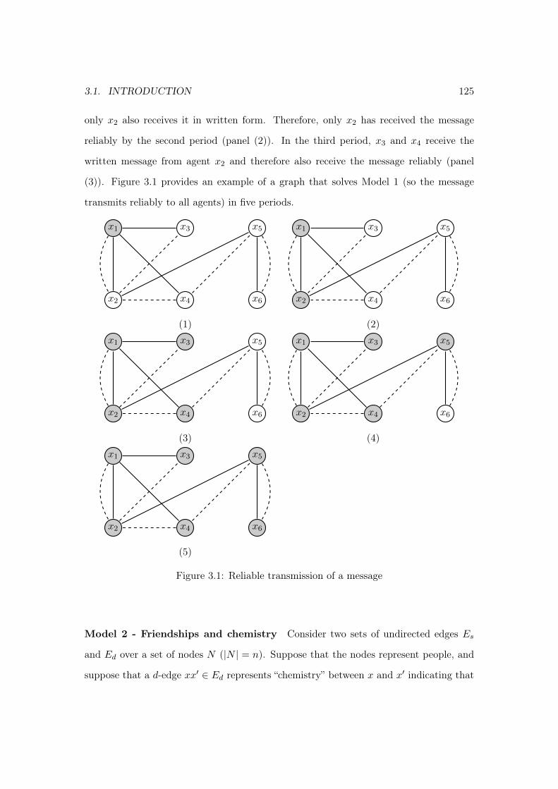
3.1. INTRODUCTION 125
only x2 also receives it in written form. Therefore, only x2 has received the message
reliably by the second period (panel (2)). In the third period, x3 and x4 receive the
written message from agent x2 and therefore also receive the message reliably (panel
(3)). Figure 3.1 provides an example of a graph that solves Model 1 (so the message
transmits reliably to all agents) in five periods.
x1
x2
x3
x4
x5
x6
x1
x2
x3
x4
x5
x6
(1) (2)x1
x2
x3
x4
x5
x6
x1
x2
x3
x4
x5
x6
(3) (4)x1
x2
x3
x4
x5
x6
(5)
Figure 3.1: Reliable transmission of a message
Model 2 - Friendships and chemistry Consider two sets of undirected edges Es
and Ed over a set of nodes N (|N | = n). Suppose that the nodes represent people, and
suppose that a d-edge xx′ ∈ Ed represents “chemistry” between x and x′ indicating that

126 CHAPTER 3. MULTIPLE EDGE TYPES
if x and x′ were to be acquainted then they would get along together, and finally suppose
that an s-edge xx′ ∈ Es represent x and x′ as being acquainted with each other. A
close friendship between x and x′ is represented by xx ∈ Es ∩ Ed. That is, x and x′
are close friends if they are acquainted with each other and there is chemistry between
them. Now, consider the following friendship formation process: In every period, every
agent introduces its close friends to its acquaintances. That is, if an agent x is close
friends with some other agent x′ but is merely acquainted with some agent x′′, then x
will create an s-edge x′x′′. Of course, it is possible that there is no chemistry between x′
and x′′, but if there is chemistry between them, then this will prompt them to introduce
each other to their own respective sets of acquaintances in the following period. New
close friendships are therefore created as a function of existing close friendships in this
process.1
We say that a graph Gn = (N,Es, Ed) solves Model 2 if after a finite number of
periods, all pairs of agents who would get along if they were to be acquainted actually
do become acquainted and, furthermore, each agent has at least one close friend. Later
in the paper, we will also say that such graphs are combinable.
Figure 3.2 illustrates this process. In the first period (panel (1)), agents x1 and x2 are
close friends. Therefore, x1 introduces x2 to all of its acquaintances (thereby creating the
1Note that this model could easily have been presented as a game theoretic model. Indeed, denotethe s-neighborhood of an agent x ∈ N by Ns(x) = x′ ∈ N |xx′ ∈ Es. The d-neighborhood can besimilarly defined, and finally define the sd-neighborhood of x as Nsd(x) = Ns(x)∩Nd(x). Suppose thatthe utility of agent x ∈ N is increasing in the size of its sd-neighborhood and in the utility of eachof its sd-neighbors. Furthermore, suppose that in every period, every agent x ∈ N can create s-edgesyy′ such that y, y′ ∈ Ns(x), and each such edge is created at a small cost ε > 0. Finally, assume thatany d-edge xx′ ∈ Ed is “latent”, in the sense that it is completely unknown to all the agents, unless itis also the case that the s-edge xx′ ∈ Es exists, in which case the d-edge xx′ is known to x and x′.Now, assuming that for any x ∈ N , and any number of close friends of x, and any number of theirclose friends, the expected marginal benefit of creating an s-edge yy′ where y′ ∈ Ns(x) is greater thanε, we can derive the optimal strategy of an agent in any period as follows: Clearly, an agent x ∈ Nwill never have an incentive to create an s-edge between y ∈ Ns(x) and y′ ∈ Ns(x) if neither of themis a close friend of x. If, however, y ∈ Ns(x) is a close friend of x, given our assumption regarding thesize of ε, x will introduce y to all of its s-neighbors. That is, we have a game in which the optimalstrategy in every period for every agent x ∈ N is to create an s-edge yy′ if and only if y ∈ Nsd(x)and y′ ∈ Ns(x). This corresponds precisely to the friendship formation presented in the text. Notefurthermore, that this game could equally be interpreted as a model of business partnerships wherenodes represent entrepreneurs, a d-edge xx′ represents a potentially fruitful business venture between xand x′, and an s-edge xx′ represents x and x′ being acquainted with each other.

3.1. INTRODUCTION 127
s-edges x2x3 and x2x4), and x2 introduces x1 to all of its acquaintances (thereby creating
the s-edge x1x5). Also, x5 introduces its close friend x6 to x2 thereby creating the edge
x2x6. Note that in the second period (panel (2)), there are now close friendships that
did not previously exist, namely, between x2 and x3, and between x2 and x4. In panel
(3), the final close friendship is created between x4 and x5. Figure 3.2 therefore provides
an example of a graph that solves Model 2 (in which all potentially close friendships are
realized, and each agent has at least one close friend) in three periods.
x1
x2
x3
x4
x5
x6
x1
x2
x3
x4
x5
x6
(1) (2)
x1
x2
x3
x4
x5
x6
(3)
Figure 3.2: Formation of close social ties
Model 3 - Distributed puzzle assembly This model is due to Brummitt et al.
(2012): Consider two sets of undirected edges Es and Ed over a set of nodes N (|N | = n).

128 CHAPTER 3. MULTIPLE EDGE TYPES
Each node x ∈ N is interpreted as a person, and it is assumed that each person holds a
piece of an n-piece jigsaw puzzle. A d-edge xx′ ∈ Ed is interpreted as x and x′ holding
puzzle pieces that are “clickable” together, and an s-edge xx′ ∈ Es is interpreted as x
and x′ communicating with each other. An assembly process governs how the jigsaw
puzzle is assembled over time: Let us call any set of assembled puzzle pieces a cluster.
Then, at every step, any disjoint clusters X and Y are assembled together into a larger
cluster if and only if X and Y can be clicked together (that is, there is a person holding
a puzzle piece x ∈ X and a person holding a puzzle piece y ∈ Y such that x and y are
clickable) and there is a communication link across the people belonging to the disjoint
clusters (that is, there is a person x′ holding a puzzle piece in X and a person y′ holding
a puzzle piece in Y such that x′ and y′ communicate with each other).2
We say that a graph Gn = (N,Es, Ed) solves Model 3 if after a finite number of
assembly steps, the set of assembled puzzle pieces is equal to N . Later in the paper, we
will also say that such graphs are assemblable.
The above is interpreted as a model of innovation: A jigsaw puzzle being solved is
seen as a process of innovation, or as a problem being solved, in which compatible ideas
– or clickable puzzle pieces – are brought together over time; the model can therefore,
in principle, allow us to identify the connectivity conditions under which a set of people
can jointly solve a global problem. Figure 3.3 illustrates this process.
In panel (1) of Figure 3.3, agent x1 has a puzzle piece that can be assembled with
agent x2. Furthermore, x1 and x2 can communicate with each other and therefore
assemble their puzzle pieces. Note that in the first period, although x2’s puzzle piece
can also be clicked with x3’s, they do not immediately assemble their pieces because they
do not communicate with each other. However, once x1 and x2 have assembled their
pieces together (panel (2)), x1 – who does communicate with x3 – can see that the joint
(x1, x2) piece can be assembled with x3’s puzzle piece, and these are therefore assembled
2Formally, at every step, a set of nodes X ⊆ N can be assembled with another set Y ⊆ N if andonly if there is x ∈ X and y ∈ Y such that xy ∈ Es, and there is x′ ∈ X and y′ ∈ Y such that x′y′ ∈ Ed.

3.1. INTRODUCTION 129
x1
x2
x3
x4
x5
x6
x3
x4x1, x2
x5, x6
(1) (2)
x1, x2, x3, x4 x5, x6
x1, x2, x3, x4, x5, x6
(3) (4)
Figure 3.3: Assembly of a distributed puzzle
in the following period (panel (3)). Figure 3.3 provides an example of a graph that solves
Model 3 (completely assembles the puzzle) in four periods.
3.1.2 Outline of the paper
In this paper, we algorithmically characterize the set of all graphs Gn = (N,Es, Ed)
that solve Models 1, 2 and 3. Furthermore, we show that the set of graphs that solve
Models 2 and 3 are identical and that the set of graphs that solve Model 1 is a strict
subset of the set of graphs that solve Model 3.
In each case, the characterization of the set of all graphs that solve Model X is
done by providing an algorithm X ′ that is sound and complete for generating graphs
that solve Model X. That is, we present an algorithm X ′ for generating graphs and
show that every graph that the algorithm X ′ returns solves Model X (soundness), and
furthermore, we show that the algorithm X ′ can return every graph that solves Model

130 CHAPTER 3. MULTIPLE EDGE TYPES
X (completeness). We therefore say that we have algorithmically characterized the set
of all graphs that solve Model X (by means of algorithm X ′).
We therefore present an algorithm that can generate precisely every graph in which,
starting from some node, all agents receive the message reliably in a finite number of
steps (Model 1), and we present an algorithm that can generate precisely every graph
in which all potentially close friendships are realized in a finite number of steps and
each agent ends up with at least one close friend (Model 2), and in which the puzzle is
completely assembled in a finite number of steps (Model 3).
It will be useful to provide some intuition regarding the approach that we use in
proving the characterizations. In general, once an algorithm is proposed, it is relatively
easy to prove that it is sound. Completeness, on the other hand, is usually harder to
establish. We adopt the same general approach to prove completeness for each of the
three models presented above: Roughly, the main algorithms proposed in the paper
generate graphs sequentially “block by block”, where a “block” will typically be some
subset of nodes possibly connected by some edges. That is, an algorithm will create
a block, then connect a second block to the existing one in a particular manner, and
then connect a third block to the existing blocks in a particular manner, and so on. To
prove soundness, it suffices to show that at every step of the algorithm (at every newly
added block), the graph that was generated up to that step has the desired property of
solving a particular model. To prove completeness, we show that every graph that has
this desired property contains a subset of nodes and edges that corresponds to one of the
blocks of the proposed algorithm, such that if this block is deleted from the graph, the
resulting subgraph also has this desired property. If this can be shown, then a simple
proof by induction over the number of blocks will show that the proposed algorithm can
generate every graph with the desired property.
Following a brief literature review in Section 3.2, the outline of this paper is as follows.
In Section 3.3, we provide some general results on algorithms to generate trees and a

3.2. LITERATURE REVIEW 131
related type of graph which we call reduced trees. These results will be useful for the
following sections. In Section 3.4 we provide the algorithmic characterization of graphs
that solve Model 3. In Section 3.5 we show that the set of graphs that solve Model 2
is identical to the set of graphs that solve Model 3. Finally, in Section 3.6 we provide
the algorithmic characterization of graphs that solve Model 1, and show that this set of
graphs is a strict subset of the set of graphs that solve Model 3. We conclude in Section
3.7. All proofs (and some lemmas) are in the Appendix.
3.2 Literature review
Granovetter (1978) introduced linear threshold models for the analysis of diffusion
on networks. In such models, every agent has a threshold representing the fraction of its
neighbors that would have to be in a given state for the agent to also switch to that state.
This model has been explored and extended in various ways (see Kleinberg, 2013, and
references therein), however the models always involve a single quantitative threshold
per agent on a single network. In contrast, Model 1 (described in the introduction) can
be seen as a qualitative threshold process in which a certain number of each edge type
must be “activated” in order for an agent to be activated. In the simple case considered
in Model 1, just a single edge of each type must be activated, but one can easily imagine
generalizations.
Like Granovetter (1978), Model 1 is not a strategic model of information transmission.
There are games of strategic (and deterministic) information transmission on a single
fixed network (Hagenbach, 2011), but we are not aware of any models in which the
transmission is in any way conditional on different edge types.
There is a growing literature on networks with multiple edge types (often called
multiplex networks). There are physics and civil engineering papers concerned with
suppressing failures in interdependent networks. For example, an electricity network can
fail in some locations thereby also affecting the telecommunications network. These are

132 CHAPTER 3. MULTIPLE EDGE TYPES
typically dynamic statistical models where the failure of one node will usually directly
affect the failure rate of its neighbors, in various degrees, across all the different networks
(see Newman et al., 2005, Rosato et al., 2008, Buldyrev et al., 2010, Brummitt et al.,
2012, Gómez et al., 2013). Another literature exists on community detection in multiplex
networks (e.g. see Mucha et al., 2010), and yet another extends various well-known
network measures to multiplex networks (e.g. see Halu et al., 2013). Finally, there
are some studies in economics and sociology that empirically assess the externalities
exhibited by various “layers” – or edge types – of a school faculty network (Baccara
et al., 2012), or that detect the importance of the various edge types in a network and
evaluate the different roles that agents play within each network (Szell et al., 2010, in an
online gaming community; Lee and Monge, 2011, within an organizational structure).
A particularly interesting study on assessing the value to trade of canal and railroad
networks is found in Swisher (2013).
The only paper we are aware of that fully leverages the existence of qualitatively dis-
tinct edges such that the process on the network is crucially conditioned on the multiple
edge types is Brummitt et al. (2012). We have described their model in the introduction.
However, their analysis of the model differs significantly from the one carried out here.
Concretely, Brummitt et al. (2012) take a fixed set of d-edges Ed and let the s-edges be
generated by an Erdős and Rényi (1959) random graph process with linking probability
p. They then determine a cut-off value on p above which the puzzle solves completely
with high probability. In this sense, their paper asks whether a random graph (in the
Erdős and Rényi (1959) sense) can solve a puzzle. In contrast, we characterize the sets
of all possible fixed configurations of edges Ed and Es over a set of nodes such that the
puzzle solves completely. One of the upshots of our results is that any graph that is
formed as a growth procedure (and this can include random models such as Barabási
and Albert (1999)) will solve with certainty.

3.3. PRELIMINARY RESULTS ON TREES AND REDUCED TREES 133
3.3 Preliminary results on trees and reduced trees
In this section, we present algorithmic characterizations of trees and of related graphs
which we call reduced trees. These results will be useful for the sections to come.
Most of the definitions introduced in this section are entirely standard in the graph
theory literature (for example, see Bondy and Murty, 2008). We repeat some of them
here: A graph Gn = (N,E) consists of a set of nodes N and a set of edges E (sometimes
there will be multiple edge sets). In any graph, a path from x ∈ N to y ∈ N is a sequence
of edges x0x1, x1x2, ..., xk−1xk such that x0 = x and xk = y and there are no repeating
nodes in the sequence. A cycle is a path in which x0 = xk. A graph is connected if there
is a path from any node to any other node. A graph is acyclic if it contains no cycles.
The degree of a node x ∈ N is the number of edges in E that are incident to x. A leaf
is a node with degree one. Throughout the paper, we consider only undirected graphs
(in which edges have no orientation, so the edge xy is identical to the edge yx) with no
self-loops (so there is no node x ∈ N such that xx is an edge).
Definition 1. A tree over n nodes, denoted Tn, is a connected acyclic graph.
The following two theorems regarding trees are entirely standard (see Bondy and
Murty, 2008). Note that their proofs are therefore omitted in the Appendix.
Theorem 1. The graph Tn is a tree if and only if Tn is connected and has n− 1 edges.
Theorem 2. Every tree has at least two leaves.
The following is a simple algorithm that generates trees. Essentially, the algorithm
starts with a single node and adds nodes sequentially, one at a time, connecting each
new node by a single edge to some node that came before it in the sequence.

134 CHAPTER 3. MULTIPLE EDGE TYPES
Algorithm 1 [Tree growth]
1. Let N := x1, ..., xn be a set of nodes and E := .2. Add the node x1, and let r := 1.3. While r < n,
• Add xr+1, select a pre-existing node xj<r+1, and E := E ∪ xr+1xj.• r := r + 1
4. Return Gn := (N,E)
We can show that the algorithm stated above is sound and complete for generat-
ing trees; that is, every graph that the algorithm generates is a tree (soundness), and
furthermore, every tree can be generated by the algorithm (completeness).
Proposition 1. Algorithm 1 is sound and complete for generating trees.
Proof of this result as well as all the other results presented in this paper can be
found in the Appendix.
Hereafter, we focus our attention on graphs with multiple edge types. More specifi-
cally, we consider graphs Gn = (N,Es, Ed) with a set of nodes, N , and two edge types.
Namely, Es is a set of s-edges (which are always represented by solid lines in figures),
which we also sometimes refer to as solid edges or as solid lines; and Ed is a set of d-edges
(which are always represented by dashed lines in figures), which we also sometimes refer
to as dashed edges or as dashed lines.
Definition 2. For any graph Gn = (N,Es, Ed), the s-graph of Gn is the graph (N,Es),
and the d-graph of Gn is the graph (N,Ed). We say that Gn is s-connected if the
s-graph is connected (and similarly for d-connected).
Definition 3. For any graph Gn = (N,Es, Ed) and any X ⊆ N , the graph Gn induced
on X, denoted Gn[X], is the graph (X,E′s, E′d) where E′s = xy ∈ Es|x, y ∈ X and
E′d = xy ∈ Ed|x, y ∈ X.
Definition 4. Consider any graph Gn = (N,Es, Ed), and let U ⊆ N with |U | = u.
Suppose that Π is a partition of the set U . The reduced graph over Π, denoted GΠu =

3.3. PRELIMINARY RESULTS ON TREES AND REDUCED TREES 135
(U,EΠs , E
Πd ), is defined as follows: The set of edges EΠ
s is Es restricted to nodes that
are connecting distinct elements of the partition. That is EΠs = xy ∈ Es|X,Y ∈ Π, x ∈
X, y ∈ Y,&X 6= Y , and EΠd is similarly defined.
Definition 5. Consider any graph Gn = (N,Es, Ed), and let U ⊆ N with |U | = u.
Suppose that Π is a partition of the set U . The reduced graph over Π, GΠu = (U,EΠ
s , EΠd ),
is a reduced tree over Π if the following conditions hold:
1. |EΠs | = |EΠ
d | = |Π| − 1
2. Any element of the partition is connected to some other element of the partition
by both an s-edge and a d-edge. That is, for any X ∈ Π there is a Y ∈ Π (with
Y 6= X) such that there is an x ∈ X and y ∈ Y and xy ∈ EΠs , and there is an
x′ ∈ X and y′ ∈ Y and x′y′ ∈ EΠd .
x1
x2
x3
x4
x5
x6 x7
x8 x9
x1
x2
x3
x4
x5
x6 x7
x8 x9
(1) Gn (2) GΠn
Figure 3.4: Example of a reduced tree
A reduced tree over some partition Π of a subset of nodes is essentially a graph in
which, if we were to consider each element of the partition to be a node, there would
be a tree consisting of solid lines across those nodes and an identical tree consisting of
dashed lines across those nodes.

136 CHAPTER 3. MULTIPLE EDGE TYPES
Example. Figure 3.4 provides an example of a reduced tree over a partition Π starting
from some graph Gn = (N,Es, Ed). The set of nodes is N = x1, ..., x9, the edges are
represented, and the partition ofN is given by Π = x1, x2, x3, x4, x5, x6, x7, x8, x9.
The reduced tree over Π is then GΠn = (N,EΠ
s , EΠd ), where EΠ
s = x2x7, x5x9 and
EΠd = x3x8, x4x9. Note that if we take the elements of the partition Π to be nodes,
then there is a solid edge connecting x1, x2, x3 to x6, x7, x8, x9 and a solid edge con-
necting x6, x7, x8, x9 to x4, x5, so there is a solid line tree over these three nodes.
Furthermore, there is an identical dashed line tree over these three nodes since there is
a dashed edge connecting x1, x2, x3 to x6, x7, x8, x9 and a dashed edge connecting
x6, x7, x8, x9 to x4, x5.
The following algorithm will be shown to be sound and complete for generating
reduced trees. The algorithm operates in a manner that is similar to Algorithm 1: It
selects a subset U of nodes and generates a partition Π of U . It then starts with a single
partition element and adds partition elements sequentially, one at a time, connecting
each new partition element to another that came before it in the sequence as follows:
It selects a pre-existing partition element. It then selects a node in the new partition
element and another in the selected pre-existing partition element and connects them
by a solid edge, and it selects a node in the new partition element and another in the
selected pre-existing partition element and connects them by a dashed edge.
Algorithm 2 [Reduced tree growth]
1. Let N := x1, ..., xn be a set of nodes and U ⊆ N such that |U | = u, and createa partition Π := X1, ..., Xk over U . Let EΠ
s := and EΠd := .
2. Add the element X1, and let r := 1.3. While r < k,
• Add the element Xr+1, and select a pre-existing element Xj<r+1.
• Select a x ∈ Xr+1 and y ∈ Xj and EΠs := EΠ
s ∪ xy.• Select a x′ ∈ Xr+1 and y′ ∈ Xj and EΠ
d := EΠd ∪ x′y′.
• r := r + 1
4. Return GΠu := (U,EΠ
s , EΠd )

3.4. CHARACTERIZATION OF ASSEMBLABLE GRAPHS 137
Proposition 2. For any set N , and any partition Π of N , Algorithm 2 is sound and
complete for generating reduced trees over Π.
3.4 Characterization of assemblable graphs
In this section we provide a formal description of Model 3 (presented in the intro-
duction). We then present two algorithmic characterizations of graphs that solve Model
3 (a “growth” algorithm and a “splitting” algorithm).
The following assembly process provides a formal description of Model 3:
Definition 6. Consider a graph Gn = (N,Es, Ed) where N is a set of nodes (|N | = n),
Es is a set of s-edges, and Ed is a set of d-edges. Define the following assembly process:
1. Initially, C0 is the set of singletons x|x ∈ N.
2. At the first step, C1 is the set of connected components in the graph (N,Es ∩ Ed).
3. After step t ≥ 1, we have a set of clusters Ct that partitions the set of nodes N . At
step (t+ 1), we merge every pair of clusters in Ct that are both s- and d-adjacent.
Clusters X and Y are s-adjacent if there exists x ∈ X, y ∈ Y such that xy ∈ Es.
Similarly, clusters X and Y are d-adjacent if there exists x ∈ X, y ∈ Y such that
xy ∈ Ez. The graph solves Model 3, or is assemblable, according to the assembly
process, if there is a step T <∞ such that CT = N.
Example. To illustrate the assembly process, consider the two graphs in Figure 3.5.
Notice that the graphs represented in panel (1) and panel (2) of Figure 3.5 are both s-
and d-connected. However, the graph represented in panel (1) is assemblable, but the
one in panel (2) is not. Indeed, the graph shown in panel (1) is the same as the one that
was shown in Figure 3.3 in the introduction. Formally, we can represent the assembly

138 CHAPTER 3. MULTIPLE EDGE TYPES
x1
x2
x3
x4
x5
x6
x1
x2
x3
x4
x5
x6
(1) (2)
Figure 3.5: (1) An assemblable graph, and (2) a graph that is not assemblable
process on this graph as follows:
C0 = x1, x2, x3, x4, x5, x6
C1 = x1, x2, x3, x4, x5, x6
C2 = x1, x2, x3, x4, x5, x6
C3 = x1, x2, x3, x4, x5, x6
We start with a set of nodes N = x1, x2, x3, x4, x5, x6 and the set of singletons C0.
Since x1 and x2 are s- and d-adjacent, they are merged into a single cluster. Similarly,
x5 and x6 merge into a single cluster. We therefore obtain C1. Now, since x3 and x4
are each s- and d-adjacent to x1, x2, they merge with it to form a single cluster, thus
yielding C2. And finally, x5, x6 are s- and d- adjacent to x1, x2, x3, x4. The process
thus terminates with C3 = N and the graph is assemblable.
In contrast, the graph represented in panel (2) of Figure 3.5 is not assemblable. We
can show this formally below, as well as representing it graphically by gathering every
cluster into a single node as shown in Figure 3.6. Formally, the assembly on the graph
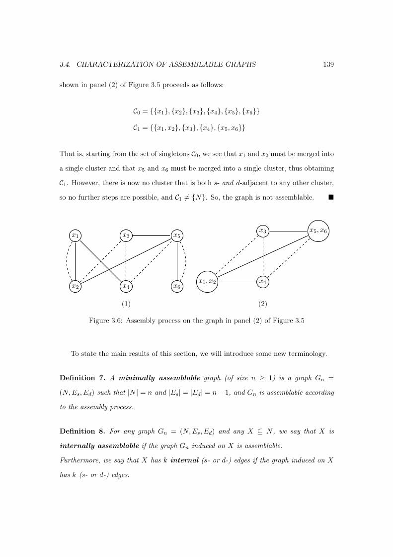
3.4. CHARACTERIZATION OF ASSEMBLABLE GRAPHS 139
shown in panel (2) of Figure 3.5 proceeds as follows:
C0 = x1, x2, x3, x4, x5, x6
C1 = x1, x2, x3, x4, x5, x6
That is, starting from the set of singletons C0, we see that x1 and x2 must be merged into
a single cluster and that x5 and x6 must be merged into a single cluster, thus obtaining
C1. However, there is now no cluster that is both s- and d-adjacent to any other cluster,
so no further steps are possible, and C1 6= N. So, the graph is not assemblable.
x1
x2
x3
x4
x5
x6
x3
x4x1, x2
x5, x6
(1) (2)
Figure 3.6: Assembly process on the graph in panel (2) of Figure 3.5
To state the main results of this section, we will introduce some new terminology.
Definition 7. A minimally assemblable graph (of size n ≥ 1) is a graph Gn =
(N,Es, Ed) such that |N | = n and |Es| = |Ed| = n− 1, and Gn is assemblable according
to the assembly process.
Definition 8. For any graph Gn = (N,Es, Ed) and any X ⊆ N , we say that X is
internally assemblable if the graph Gn induced on X is assemblable.
Furthermore, we say that X has k internal (s- or d-) edges if the graph induced on X
has k (s- or d-) edges.

140 CHAPTER 3. MULTIPLE EDGE TYPES
Definition 9. A subgraph G′n = (N,E′s, E′d) of Gn = (N,Es, Ed) is a graph such that
E′s ⊆ Es and E′d ⊆ Ed.
In what follows, we present two algorithms that are sound and complete for generating
minimally assemblable graphs. The “growth” algorithm is presented in Section 3.4.1 and
the “splitting” algorithm is presented in Section 3.4.2. We discuss their merits in Section
3.4.3. We then show that any assemblable graph must have a minimally assemblable
subgraph which easily allows us (in Section 3.4.4) to present an algorithm that is sound
and complete for generating assemblable graphs.
3.4.1 Growth algorithm for minimally assemblable graphs
We now present an algorithm which we prove to be sound and complete for generating
minimally assemblable graphs. Roughly, the algorithm proceeds as follows: It partitions
the set of nodes and builds reduced trees over disjoint subsets of this partition. It then
creates a new partition of the set of nodes which is coarser than the previous one and
builds reduced trees over disjoint subsets of this new partition. The procedure is repeated
until the final partition contains a single element, namely, the entire set of nodes itself.
Algorithm 3 [Minimally assemblable graph growth]
1. Let N := x1, ..., xn be a set of nodes, and let S := x1, ..., xn be the set ofsingletons.
2. Let Π be a non-trivial partition of S.a Let Es := and Ed := .3. While S 6= N,
• Create a reduced tree over each X ∈ Π using Algorithm 2, and add the newedges to Es and Ed.
• Let S := ∪x∈Xx|X ∈ Π, and let Π be a non-trivial partition of S.
4. Return Gn := (N,Es, Ed)
aSuch that |Π| < |S|, to guarantee that the algorithm terminates.
Example. The following example shows how the algorithm generates minimally assem-
blable graphs by showing how it would generate the graph shown in panel (1) of Figure

3.4. CHARACTERIZATION OF ASSEMBLABLE GRAPHS 141
3.5 (which we know is assemblable). To start with, let N = x1, ..., x6 (see Figure 3.7
panel (1)), and initialize the algorithm with S0 and Π0 as follows:
S0 =x1, x2, x3, x4, x5, x6
Π0 =
x1, x2
,x3
,x4
,x5, x6
Note that S0 is a partition of the set of nodes, while Π0 is a partition of S0, so a fortiori
it is a set of disjoint subsets of S0. The algorithm therefore creates a reduced tree over
each element of Π0. In this case, we create the s-edges x1x2 and x5x6 as well as the
d-edges x1x2 and x5x6 (see Figure 3.7 panel (2)). At the following step of the algorithm,
we can obtain:
S1 =x1, x2, x3, x4, x5, x6
Π1 =
x1, x2, x3, x4
,x5, x6
Now, the algorithm creates a reduced tree over each element of Π1. For the element,
x1, x2, x3, x4 ∈ Π1, we can let x1, x2 enter first (according to the reduced
tree algorithm). Then, x3 can enter second, and must connect with the first entrant
with an s-edge and a d-edge. So, we could create the s-edge x1x3, and the d-edge x2x3.
Similarly, we can let x4 be the third entrant. It must connect with one of the pre-
existing entrants with an s-edge and with one of the pre-existing entrants with a d-edge.
Suppose that the created s-edge is x1x4 and that the created d-edge is x2x4 (see Figure
3.7 panel (3)).
As a brief aside, let us note here that there are multiple stages within the algo-
rithm that are not fully determined. For example, we have chosen the set Π1 to bex1, x2, x3, x4
,x5, x6
, but we equally could have chosen a different parti-
tion of S1. For example, we could have set Π1 to bex1, x2, x3,
x4, x5, x6
.
Naturally, this would ultimately result in an assemblable graph that might different from

142 CHAPTER 3. MULTIPLE EDGE TYPES
the one shown in panel (1) of Figure 3.5. Similarly, in creating the reduced tree over
x1, x2, x3, x4, we created an s-edge x1x4 and a d-edge x2x4. So in this case, x4
happens to connect only with nodes in the element x1, x2, but it could have also been
the case that instead of creating the s-edge x1x4, we could have had, say, x3x4. Once
again, the resulting assemblable graph would have been different from the one shown in
panel (1) of Figure 3.5.
Continuing our example, at the following step of the algorithm, we can obtain:
S2 =x1, x2, x3, x4, x5, x6
Π2 =
x1, x2, x3, x4, x5, x6
The algorithm must create a reduced tree over x1, x2, x3, x4, x5, x6. So, letting
x1, x2, x3, x4 enter first, we can let x5, x6 enter second, and we must connect some
element of the second entrant to some element of the first entrant with an s-edge, and
we must connect some element of the second entrant to some element of the first entrant
with a d-edge. For sake of argument, suppose that the s-edge is x2x5 and that the d-edge
is x4x5 (see Figure 3.7 panel (4)). In the following step, S3 = x1, x2, x3, x4, x5, x6,
and so the algorithm terminates.
Theorem 3. Algorithm 3 is sound and complete for generating minimally assemblable
graphs.
3.4.2 Splitting algorithm for minimally assemblable graphs
In contrast with the “growth” algorithm presented in the previous section, we now
present a “splitting” algorithm, which we show is also sound and complete for generating
minimally assemblable graphs. It will be necessary to introduce some terminology.
Definition 10. To contract an edge e ∈ Es ∩ Ed of a graph Gn = (N,Es, Ed) is to
delete the edge, and take its ends x, x′ ∈ N and replace them by a single node y incident

3.4. CHARACTERIZATION OF ASSEMBLABLE GRAPHS 143
x1
x2
x3
x4
x5
x6
x1
x2
x3
x4
x5
x6
(1) (2)x1
x2
x3
x4
x5
x6
x1
x2
x3
x4
x5
x6
(3) (4)
Figure 3.7: Steps of a run of Algorithm 3
to all the edges e′ ∈ Es ∪ Ed which were incident in Gn to either x or x′.
Definition 11. To split a node x in Gn = (N,Es, Ed) is to replace x by two s- and
d-adjacent nodes y and y′, and to replace each edge e′ ∈ Es ∪ Ed incident to x by an
edge incident to either y or y′ (but not both), the other end of the edge e′ remaining
unchanged.
Note that these definitions are adaptations of their counterparts for graphs with sin-
gle edge types (Bondy and Murty, 2008).3
Algorithm 4 [Minimally assemblable graph by node splitting]
1. Let N := x.2. While |N | < n,
• Choose an existing node in N and split it.
3. Return Gn := (N,Es, Ed)
3For an interesting application of node splitting to the generation of random trees see David et al.(2009).

144 CHAPTER 3. MULTIPLE EDGE TYPES
Example. This example shows how the algorithm generates minimally assemblable
graphs by showing how it would generate the graph shown in panel (1) of Figure 3.5
(which we know is assemblable). Initialize the algorithm with N = a and n = 6 (see
Figure 3.8 panel (1)). We can split a into b and b′, and connect by both an s- and a
d-edge. We therefore have N = b, b′ (see panel (2)). At the next step, we can then split
b into c and c′, and connect these by an s- and a d-edge. We can also replace the former
bb′ s-edge with cb′, and the former bb′ d-edge with c′b′. We now have N = c, c′, b′ (see
panel (3)). At the next step of the algorithm, we can split c into d and d′, and connect
these by an s- and a d-edge. Then for any edge cx, we replace c with d to obtain the
edge dx. The set of nodes is now N = d, d′, c′, b′ (see panel (4)). At the next step, we
split the node d into e and e′, and connect these by an s- and a d-edge, and we re-wire
some edges accordingly. The new set of nodes is now N = e, e′, d′, c′, b′ (see panel (5)).
Finally, at the last step, we split the node b′ into f and f ′ and re-wire accordingly. The
algorithm terminates because |N | = |e, e′, d′, c′, f, f ′| = 6. Notice that the graph in
panel (6) of Figure 3.8 corresponds precisely to the graph shown in panel (1) of Figure
3.5.
Just as for the “growth” algorithm that was presented in the previous section, there
are stages of the “splitting” algorithm that are not fully determined.4 Indeed, whenever a
node is split, we are left with a choice regarding how the edges are to be re-wired. More
generally, all the algorithms presented in this paper share a similar feature. Namely,
they all specify some subset of nodes from which one is allowed to select the node with
which to connect an edge (at any step), but the precise node from among this subset is
never fully determined.
Theorem 4. Algorithm 4 is sound and complete for generating minimally assemblable
graphs.
4See the aside in the example given on page 140.
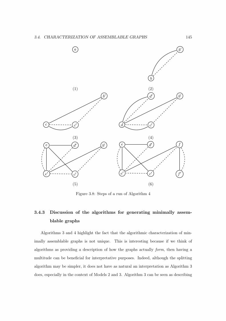
3.4. CHARACTERIZATION OF ASSEMBLABLE GRAPHS 145
x1
x2
a
x4
x5
x6
x1
x2
x3
b
b′
x6
(1) (2)x1
c
x3
c′
b′
x6
x1
d
d′
c′
b′
x6
(3) (4)
e
e′
d′
c′
b′
x6
e
e′
d′
c′
f
f ′
(5) (6)
Figure 3.8: Steps of a run of Algorithm 4
3.4.3 Discussion of the algorithms for generating minimally assem-
blable graphs
Algorithms 3 and 4 highlight the fact that the algorithmic characterization of min-
imally assemblable graphs is not unique. This is interesting because if we think of
algorithms as providing a description of how the graphs actually form, then having a
multitude can be beneficial for interpretative purposes. Indeed, although the splitting
algorithm may be simpler, it does not have as natural an interpretation as Algorithm 3
does, especially in the context of Models 2 and 3. Algorithm 3 can be seen as describing

146 CHAPTER 3. MULTIPLE EDGE TYPES
the manner in which graphs that solve Model 3 (and Model 2 as we see in Section 3.5)
form: In the context of Model 3 for example, Algorithm 3 allows clusters to form in
disparate parts of an overall graph. And, if whenever a communication link exists across
two clusters, the clusters are also clickable together, then the resulting graph must be
assemblable.
3.4.4 Algorithm for assemblable graphs
Up to now, we have presented algorithms that are sound and complete for generating
minimally assemblable graphs. In this section, we show that any assemblable graph has
a minimally assemblable subgraph, which will allow us to easily provide an algorithm
that is sound and complete for generating assemblable graphs.
Proposition 3. A graph Gn is assemblable if and only if it has a minimally assemblable
subgraph.
Algorithm 5 [Assemblable graph algorithm]
1. Return a graph Gn using either Algorithm 3 or 4.2. Add s-edges and d-edges to Gn as desired to obtain G′n3. Return G′n
Corollary 1. Algorithm 5 is sound and complete for generating assemblable graphs.
3.5 Characterization of combinable graphs
In this section we provide a formal description of Model 2 (presented in the intro-
duction), and show that the set of graphs that solve Model 2 is identical to the set of
graphs that solve Model 3. Algorithm 5 is therefore shown to algorithmically character-
ize the set of graphs that solve Model 2. It will first be necessary to introduce some new
terminology.

3.5. CHARACTERIZATION OF COMBINABLE GRAPHS 147
Definition 12. A team in a graph Gn = (N,Es, Ed) is a set of nodes X ⊆ N such that
the induced graph (X,Ed[X]) is connected and Ed[X] ⊆ Es[X].
Here, we have that Es[X] = xy ∈ Es|x, y ∈ X, and similarly for Ed[X].
Example. For example, in panel (2) of Figure 3.2 in the introduction, the nodes
x1, x2, x3, x4 are a team, and the nodes x5, x6 are another team.
The following combination process provides a formal description of the edge for-
mation process of Model 2 described in the introduction:
Definition 13. Consider a graph Gn = (N,Es, Ed) where N is a set of nodes (|N | = n),
Es is a set of s-edges, and Ed is a set of d-edges. Define the following combination
process:
1. T0 is the set of singleton nodes x|x ∈ N.5 And let E1s = Es.
2. At the first step, T1 is the set of connected components in the graph (N,E1s ∩ Ed).
3. At step t ≥ 1, we have a set of teams Tt that partitions the set of nodes N . At step
(t+ 1), go through every node x ∈ N , and for every y ∈ N ts(x) ∩N t
d(x) and every
z ∈ N ts(x), add the s-edge yz (if it does not already exist). After cycling through
all the nodes, we thus obtain Et+1s . (Note that for any period t, N t
s(x) = y ∈
N |xy ∈ Ets, and N td(x) is similarly defined).
We then let Tt+1 denote the set of all teams in the new graph Gt+1n = (N,Et+1
s , Ed).
The graph solves Model 2, or is combinable, according to the combination process, if
there is a step T <∞ such that TT = N.
5Since there are no edges in the graph induced on a singleton, we will also call any singleton a team.

148 CHAPTER 3. MULTIPLE EDGE TYPES
Example. We can illustrate the process represented in Figure 3.2 formally as follows:
T0 = x1, x2, x3, x4, x5, x6
T1 = x1, x2, x3, x4, x5, x6
T2 = x1, x2, x3, x4, x5, x6
T3 = x1, x2, x3, x4, x5, x6
Namely, we start off with T0 and immediately create the set T1 by noting that x1 and
x2 are connected by both an s- and a d-edge (and similarly for x5 and x6). Now, at step
2, we can go through each node in turn and establish new edges, starting with x1. Since
N 1s (x1) ∩ N 1
d (x1) = x2, and N 1s (x1) = x2, x3, x4, we add the edges x2x3 and x2x4.
Moving on to node x2, since N 1s (x2) ∩ N 1
d (x2) = x1, and N 1s (x2) = x1, x5, we add
the edge x1x5. Going through the node x3 and x4 adds no edges. Finally, for x5, since
N 1s (x5) ∩ N 1
d (x5) = x6, and N 1s (x5) = x2, x6, we add the edge x2x6. We have now
cycled through all the nodes, and since x2x3, x2x4 ∈ E2s ∩ Ed, the new set of teams is
therefore now given by T2. Applying the same procedure in step 3, we obtain T3.
Theorem 5. A graph Gn is assemblable according to the assembly process defined in
Definition 6 if and only if Gn is combinable according to the combination process defined
in Definition 13.
Corollary 2. Algorithm 5 is sound and complete for generating combinable graphs.
3.6 Characterization of transmissible graphs
In this section we provide a formal description of Model 1 (presented in the intro-
duction). We then present an algorithmic characterization of graphs that solve Model 1,
and show that this set of graphs is a subset of the set of graphs that solve Models 2 and
3.
The following transmission process provides a formal description of Model 1:

3.6. CHARACTERIZATION OF TRANSMISSIBLE GRAPHS 149
Definition 14. Consider a graph Gn = (N,Es, Ed) where N is a set of nodes (|N | = n),
Es is a set of s-edges, and Ed is a set of d-edges. Define the following transmission
process:
1. Initially, S0 = x, where x ∈ N .
2. At step t ≥ 1, St is the union of St−1 and every node y ∈ N \ St−1 such that for
some x ∈ St−1 yx ∈ Es, and for some x′ ∈ St−1, yx′ ∈ Ed.
The graph solves Model 1, or is transmissible (from some initial node), according
to the transmission process, if there is a step T < ∞ and some node x ∈ N with the
message originating at that node, such that ST = N .6
Example. We can illustrate the process represented in Figure 3.1 (in the introduction)
formally as follows:
S0 = x1
S1 = x1, x2
S2 = x1, x2, x3, x4
S3 = x1, x2, x3, x4, x5
S4 = x1, x2, x3, x4, x5, x6
In what follows, we present Algorithm 6 which we show generates a set of graphs
that is a strict subset of the set of graphs generated by Algorithm 5. Furthermore, we
show that Algorithm 6 characterizes the set of graphs that are transmissible from some
node (in Section 3.6.1). We provide a brief discussion of the new algorithm in Section
3.6.2.
6Note that at any step t, St is the set of all agents who have received a reliable message.

150 CHAPTER 3. MULTIPLE EDGE TYPES
3.6.1 Transmissible graph growth
Below, we present a growth procedure for generating graphs which proceeds as fol-
lows: The algorithm starts with a single node and sequentially adds new nodes, one at a
time, connecting each new node by an s-edge to some pre-existing node that came before
it in the sequence and by a d-edge to some pre-existing node that came before it in the
sequence.
Algorithm 6 [Transmissible graph growth]
1. Let N := x1, ..., xn, and let X := x1 enter (and suppose x1 initiates themessage). Let r := 1.
2. While r < n,
• Connect xr+1 by an s-edge to some node in X, and by a d-edge to some nodein X.
• X := X ∪ xr+1 and r := r + 1.
3. Return Gn := (N,Es, Ed)4. Add s-edges and d-edges to Gn as desired to obtain G′n5. Return G′n
Example. This example shows how the algorithm generates graphs that are transmis-
sible (from some node) by showing how it would generate the transmissible graph shown
in panel (1) of Figure 3.1 in the introduction. Let N = x1, ..., x6, and start with
X = x1, as in panel (1) of Figure 3.9. At the following step, the algorithm connects
x2 by both an s-edge and a d-edge to x1 and adds x2 to X (panel (2)). At the next
step, the algorithm connects x3 by an s-edge to x1 and a d-edge to x2 and adds x3 to
X (panel (3)). In the following steps, the algorithm connects x4, then x5, then x6 to
pre-existing nodes as shown in the remaining panels of Figure 3.9.
Proposition 4. The set of graphs generated by Algorithm 6 is a strict subset of the set
of graphs generated by Algorithm 5.
Theorem 6. Algorithm 6 is sound and complete for generating graphs that are trans-
missible from some node.
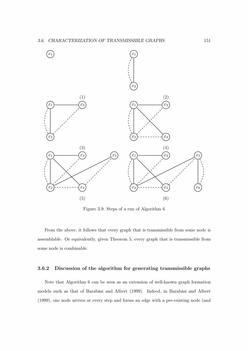
3.6. CHARACTERIZATION OF TRANSMISSIBLE GRAPHS 151
x1
x2
x3
x4
x5
x6
x1
x2
x3
x4
x5
x6
(1) (2)x1
x2
x3
x4
x5
x6
x1
x2
x3
x4
x5
x6
(3) (4)x1
x2
x3
x4
x5
x6
x1
x2
x3
x4
x5
x6
(5) (6)
Figure 3.9: Steps of a run of Algorithm 6
From the above, it follows that every graph that is transmissible from some node is
assemblable. Or equivalently, given Theorem 5, every graph that is transmissible from
some node is combinable.
3.6.2 Discussion of the algorithm for generating transmissible graphs
Note that Algorithm 6 can be seen as an extension of well-known graph formation
models such as that of Barabási and Albert (1999). Indeed, in Barabási and Albert
(1999), one node arrives at every step and forms an edge with a pre-existing node (and

152 CHAPTER 3. MULTIPLE EDGE TYPES
it selects the node with which it forms the edge with a probability that is proportional
to the current degree of the latter). In the case of Algorithm 6, one node arrives at
every step and forms one s-edge with a pre-existing node and one d-edge with a pre-
existing node (and the selection of the nodes is, as we explained in Section 3.4.2, not
fully determined, but can therefore be done according to whichever stochastic process
one desires).
Note that the process governing Model 1 is essentially a non-simultaneous version
of the processes governing Models 2 and 3. Indeed, in Model 1, the information has
a unique initial source and eventually propagates through the graph. However, if the
same information could be initialized at multiple sources (at any node x ∈ N such
that xy ∈ Es ∩ Ed for some y ∈ N), then Algorithm 5 would characterize the set of
transmissible graphs.
3.7 Conclusion
This paper presents three models on graphs in which the evolution of the process is
conditioned on the multiple edge types of the graph. For each model, we algorithmically
characterize the set of graphs that solve the model and we establish the relationships
across those sets of graphs. The algorithmic characterizations provide a way to interpret
the manner in which graphs could form to exhibit the desired property (of solving a
particular model).
A particularly interesting point to note regarding Algorithm 6 is that although the
connections across nodes can be made at random, the structure of the network forma-
tion as a growth procedure forces the resulting graph to be transmissible (and therefore
assemblable). This is in contrast with Brummitt et al. (2012) since the Erdős and Rényi
(1959) link formation process yields an assemblable graph only with some probability.
A further point to note here is that in graphs with single edge types, the set of
graphs generated by Algorithm 1 (which is a growth procedure) is identical to the set

3.7. CONCLUSION 153
of graphs generated by the standard notion of nodes splitting (see David et al. (2009));
namely, they both generate trees. In contrast, with multiple edge types, Algorithm 6
(which extends standard tree growth to graphs with multiple edge types) generates a set
of graphs that is a strict subset of the set of graphs generated by Algorithm 4 (which
extends standard node splitting to graphs with multiple edge types).
Given the relatively small literature on graphs with multiple edge types, the results
and methods presented in this paper provide an interesting contribution and open up
several areas of potential future research. Admittedly, the models studied in this paper
are rather rigid, deterministic, and highly stylized and it may be fruitful to relax some
of their underlying assumptions. For example, graphs with only two edge types were
considered here, but we could extend the analysis to graphs with more than two edge
types. And, we could also consider more general processes that are conditioned not only
on the type but also on the number of each edge type.

154 CHAPTER 3. MULTIPLE EDGE TYPES
3.8 Appendix
Proof of Proposition 1. It is trivial to see that every graph that the algorithm generates
is connected and has n− 1 edges. Therefore, by Theorem 1 the graph must be a tree.
For the converse, note that by Theorem 2, we can take any tree Tn and delete a
node (namely, one of its leaves), and obtain a tree Tn−1. Given this, we can show that
every tree can be generated by the algorithm by induction on n. Indeed, the algorithm
generates every tree of size n = 2. Now suppose it can generate any tree Tk of size k.
Then, consider any tree, Tk+1, of size k + 1. We can delete a node of Tk+1 to obtain a
tree Tk of size k, which the algorithm can generate, and it then suffices for the algorithm
to re-insert the last node at the desired place.
Lemma 1. Suppose that U is a subset of nodes with |U | = u, that Π is a partition of
U with |Π| = k, and that GΠu = (U,EΠ
s , EΠd ) is a reduced tree over Π. Then there is
an element X ∈ Π that we can delete from GΠu along with all its connections (that is,
we can delete all pairs in EΠs and EΠ
d containing an x ∈ X) such that the graph GΠ′w =
(W,EΠ′s , E
Π′d ) is a reduced tree over Π′, where Π′ = Π \ X (so clearly |Π′| = k − 1),
and W = U \X with |W | = w.
Proof of Lemma 1. Suppose GΠu = (U,EΠ
s , EΠd ) is a reduced tree over Π. Now consider
the graph Gk = (Π, Es[Π], Ed[Π]) where for any X,Y ∈ Π, XY ∈ Es[Π] if and only
if there is an x ∈ X and y ∈ Y such that xy ∈ EΠs , and Ed[Π] is similarly defined.
It is trivial to see that Gk must have exactly k − 1 s-edges and that it is connected.
Therefore Gk is a tree. From Theorem 2, Gk must have a leaf. This is true for the
s-edges, but since Es[Π] = Ed[Π] it is also true for the d-edges. We can therefore delete
the leaf to obtain a tree Gk−1. A leaf in Gk corresponds to an element of the partition
Π. Call this element X. So Gk−1 corresponds to the reduced tree GΠu = (U,EΠ
s , EΠd )
with X deleted. Reversing the construction of Gk−1 we therefore easily obtain a reduced
tree GΠ′w = (W,EΠ′
s , EΠ′d ) over Π′, where Π′ = Π \ X (so clearly |Π′| = k − 1), and

3.8. APPENDIX 155
W = U \X with |W | = w.
Example. The procedure used in the proof of Lemma 1 is illustrated in Figure 3.10.
Here, we have a graph Gn with n = 9. We then obtain the reduced tree with Π =
x1, x2, x3, x4, x5, x6, x7, x8, x9, so k = 3. We then obtain Gk in panel (3). We
can then delete a leaf of Gk to obtain Gk−1. We have Π′ = x1, x2, x3, x6, x7, x8, x9,
and W = x1, x2, x3, x6, x7, x8, x9, so w = 7. We reverse the construction of Gk−1 to
obtain the reduced tree GΠ′w in panel (5), and finally, we can also obtain Gn[W ] (the
graph Gn induced on W ), which represents what remains of the graph Gn in panel (6)
– although this last step is not required in the proof.
Proof of Proposition 2. The algorithm creates precisely |Π| − 1 s-edges and |Π| − 1 d-
edges. Furthermore, every element of the partition must be connected to some other
element of the partition by both edge types. Therefore the returned graph is a reduced
tree over the partition Π.
We show the converse by induction on the size of the partition. Suppose |Π| = 2.
Then, we can write Π = U,W, and suppose that |U | = u and |W | = w. Since the
algorithm is not restricted with regards to the nodes within U or W that it selects to
connect these two elements of the partition, it can select any one of the uw possible pairs
of nodes. Furthermore, there will be precisely one s-edge and one d-edge across these
elements. The reduced graph over Π is therefore a reduced tree over Π.
For an inductive step, suppose the algorithm can generate all reduced trees over all
possible partitions Π, where |Π| = k over some subset of nodes U . It suffices to consider
an arbitrary reduced tree over Π where |Π| = k + 1 and to show that the algorithm can
generate it. We can apply Lemma 1 to delete an element X ∈ Π, and let Π′ = Π \ X
and obtain a reduced tree over Π′. Since |Π′| = k, the algorithm can generate it, and it
suffices for the algorithm to then add a new partition element X and to connect some
node x ∈ X by an s-edge to some node y ∈ Y in an existing partition element Y ∈ Π′,
and also to connect some node x′ ∈ X by a d-edge to some node y′ ∈ Y .

156 CHAPTER 3. MULTIPLE EDGE TYPES
x1
x2
x3
x4
x5
x6 x7
x8 x9
x1
x2
x3
x4
x5
x6 x7
x8 x9
(1) Gn (2) GΠn
x1
x2
x3
x4
x5
x6 x7
x8 x9
x1
x2
x3
x4
x5
x6 x7
x8 x9
(3) Gk (4) Gk−1
x1
x2
x3
x4
x5
x6 x7
x8 x9
x1
x2
x3
x4
x5
x6 x7
x8 x9
(5) GΠ′w (6) Gn[W ]
Figure 3.10: Illustration for proof of Lemma 1

3.8. APPENDIX 157
Lemma 2. Let Gn = (N,Es, Ed) be a minimally assemblable graph, and let Ct denote
the set of clusters during period t of the assembly process. Then,
1. For any t ≥ 0, Ct is a partition of the set of nodes N .
2. For any t ≥ 1 and every X ∈ Ct, there is a subset Y1, ..., Yk ⊆ Ct−1 that is a
partition of X. Denote this partition by Π.
3. The reduced graph over Π, GΠ|X| = (X,EΠ
s , EΠd ), is a reduced tree over Π.
Proof of Lemma 2. Let T denote the time at which CT = N. Obviously, CT partitions
N . Suppose that Ct is a partition of N , and suppose that X ∈ Ct. Then, by the assembly
process, X is the result of merging clusters Y1,...,Yk from the previous period in Ct−1.
Since a node cannot belong to two distinct clusters, all such clusters must be disjoint.
Furthermore, their union must exhaust X. Since this is true for each X ∈ Ct, the union
of all the clusters in Ct−1 must equal the entire set of nodes N , and distinct clusters
must be disjoint. This completes parts 1 and 2. These simple facts are also found in
Brummitt et al. (2012).
For part 3, consider CT = N. Then CT−1 = X1, ..., Xk, where the clusters in
CT−1 are disjoint and their union equals N . Now, note that any cluster appearing in Ct
for any period t of the assembly process must be internally assemblable because what
determines whether any nodes within a cluster merge depends only on the links across
such nodes, and not on any other nodes outside of the cluster (That is, whether Xi is
internally solvable cannot depend on how it is connected to Xj for i 6= j. See Brummitt
et al., 2012, p. 7, for a similar remark). This implies that for every i ∈ 1, ..., k, Xi is
internally assemblable. Since being connected is a necessary condition for assemblability,
it must be the case that Xi internally has at least |Xi|−1 s-edges and at least |Xi|−1 d-
edges. This means that, noting that∑k
i=1 |Xi| = n, the total number of internal s-edges

158 CHAPTER 3. MULTIPLE EDGE TYPES
in the elements of CT−1 must be at least
k∑i=1
(|Xi| − 1) = n− k (3.1)
Now, consider the edges across (but not internal to) the elements of CT−1. Since all the
clusters in CT−1 must merge together in one period, it must be the case that every Xi
is s- and d-adjacent to some Xj . Given this connectedness across the clusters, we must
have at least k − 1 s-edges across them. Since the total number of edges must be n− 1
(because the graph is minimally assemblable), we have that there must be exactly k− 1
s-edges across the clusters and exactly n − k s-edges in total that are internal to the
clusters in CT−1.
Now, since there are exactly k − 1 s-edges across the clusters in CT−1, and by similar
argument, k − 1 d-edges across them as well, and since the clusters must be connected,
both the s-graph and the d-graph induced on those clusters are trees. However, since
all the clusters merge in exactly one period, it must be the case that the intersection of
those trees is equal to one of the trees itself. That is, the reduced graph over CT−1 is a
tree.
Now consider Ct, and for an inductive step, suppose that for any Π = X1, ..., Xk ⊆ Ct
such that Π is a partition of some cluster W ∈ Ct+1 with |W | = w, the total number of
s-edges internal to the clusters in Π is exactly w− k (similarly for d-edges) and that the
reduced graph over Π is a reduced tree. Now consider Ct−1. We know that we must have
Y X11 , Y X1
2 , ..., Y X1z1 , ..., Y Xk
1 , Y Xk2 , ..., Y Xk
zk ⊆ Ct−1, where the notation indicates that for
all i ∈ 1, ..., k, Π(Xi) = Y Xi1 , ..., Y Xi
zi is a partition of Xi. It remains for us to show
that the total number of s- (or d-) edges internal to all the elements in each such partition
must be |Xi| − zi and that the reduced graph over each Π(Xi) is a reduced tree. Now,
for every i and j, Y Xij is internally assemblable. Since being connected is a necessary
condition for assemblability, it must be the case that Y Xij internally has at least |Y Xi
j |−1
s-edges and at least |Y Xij | − 1 d-edges. This implies that the total number of s-edges

3.8. APPENDIX 159
internal to the clusters in Π(Xi) = Y Xi1 , ..., Y Xi
zi must be at least
zi∑j=1
(|Y Xij | − 1) =
zi∑j=1
|Y Xij | − zi = |Xi| − zi (3.2)
Now, consider the edges across (but not internal to) the elements of Y Xi1 , ..., Y Xi
zi .
Since all the clusters in Π(Xi) must merge together in one period to form Xi, it must
be the case that every Y Xij is s- and d-adjacent to some Y Xi
j′ . Given this connectedness
across the clusters, we must have at least zi − 1 s-edges across them. This implies that
the total number of edges internal to Xi must be at least |Xi| − zi + (zi − 1) = |Xi| − 1.
Therefore, noting that∑k
i=1 |Xi| = w, the total number of edges in W must be at least
k∑i=1
(|Xi| − 1) = w − k (3.3)
But, since the total number of edges must be exactly w − k, we have, by the inductive
step, that there must be exactly |Xi| − 1 edges in each of the clusters Xi. From this,
it follows that there must be exactly zi − 1 s-edges across the clusters in each Π(Xi),
and finally that there must be exactly |Xi| − zi s-edges internal to each of the clusters
in Π(Xi).
Finally, since there are exactly zi − 1 s-edges across the clusters in Π(Xi) for each i,
and by similar argument, zi− 1 d-edges across them as well, and since the clusters must
be connected, both the s-graph and the d-graph induced on those clusters are trees.
However, since all the clusters merge in exactly one period to form Xi, it must be the
case that the intersection of those trees is equal to one of the trees itself. That is, the
reduced graph over Π(Xi) is a tree.
Example. We illustrate the main approach used the proof of Lemma 2 in Figure
3.11. Suppose CT−1 = X1, ..., X4. Then we show that there is a reduced tree over
X1, ..., X4. Furthermore, we show that if we “zoom in” on any element of CT−1, say
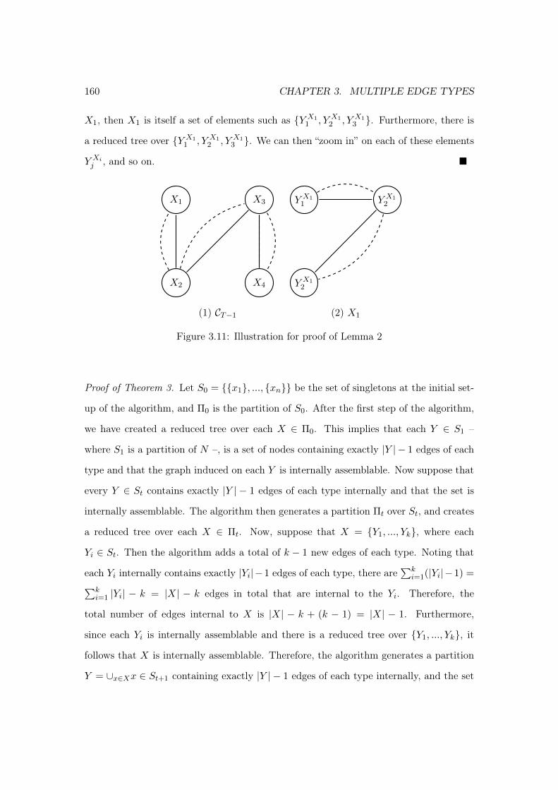
160 CHAPTER 3. MULTIPLE EDGE TYPES
X1, then X1 is itself a set of elements such as Y X11 , Y X1
2 , Y X13 . Furthermore, there is
a reduced tree over Y X11 , Y X1
2 , Y X13 . We can then “zoom in” on each of these elements
Y Xij , and so on.
X1
X2
X3
X4
Y X11
Y X12
Y X12
(1) CT−1 (2) X1
Figure 3.11: Illustration for proof of Lemma 2
Proof of Theorem 3. Let S0 = x1, ..., xn be the set of singletons at the initial set-
up of the algorithm, and Π0 is the partition of S0. After the first step of the algorithm,
we have created a reduced tree over each X ∈ Π0. This implies that each Y ∈ S1 –
where S1 is a partition of N –, is a set of nodes containing exactly |Y | − 1 edges of each
type and that the graph induced on each Y is internally assemblable. Now suppose that
every Y ∈ St contains exactly |Y | − 1 edges of each type internally and that the set is
internally assemblable. The algorithm then generates a partition Πt over St, and creates
a reduced tree over each X ∈ Πt. Now, suppose that X = Y1, ..., Yk, where each
Yi ∈ St. Then the algorithm adds a total of k − 1 new edges of each type. Noting that
each Yi internally contains exactly |Yi|−1 edges of each type, there are∑k
i=1(|Yi|−1) =∑ki=1 |Yi| − k = |X| − k edges in total that are internal to the Yi. Therefore, the
total number of edges internal to X is |X| − k + (k − 1) = |X| − 1. Furthermore,
since each Yi is internally assemblable and there is a reduced tree over Y1, ..., Yk, it
follows that X is internally assemblable. Therefore, the algorithm generates a partition
Y = ∪x∈Xx ∈ St+1 containing exactly |Y | − 1 edges of each type internally, and the set

3.8. APPENDIX 161
is internally assemblable. Since the algorithm terminates at the T such that ST = N,
we have that the graph generated by the algorithm contains precisely |N | − 1 = n − 1
edges of each type and is internally assemblable.
For the converse, note that by definition, a graph Gn is minimally assemblable if and only
if it has n−1 of each edge type and assembles according to a sequence C0, C1, ..., CT such
that CT = N. We now show that any such sequence can be reproduced by the algorithm
and, furthermore, that every graph producing such a sequence can be generated by the
algorithm. The algorithm always starts at S0 which corresponds precisely to C0. Now
suppose the algorithm can reproduce the set of clusters Ct−1. Then, by Lemma 2, Ct is
obtained by producing reduced trees over disjoint sets of clusters in Ct−1. By Proposition
2, every such tree can be produced by Algorithm 2. Therefore, Algorithm 3 can reproduce
Ct (and furthermore, it can generate every possible set of reduced trees to generate Ct
from Ct−1).
Proof of Theorem 4. It is easy to verify that the node splitting will generate a graph
with exactly n − 1 of each edge type. Furthermore, it is assemblable because a split at
any step can be reversed by a contraction, and contractions – as we have defined them
– correspond to clusters merging.
For the converse, suppose that Gn is a minimally assemblable graph. Note that a contrac-
tion in a graph Gn results in a graph Gn−1 with precisely n−1 nodes. By assemblability
of Gn, there must exist a sequence of contractions Gn, Gn−1,...,G1. Therefore, we can
contract an edge in Gn to obtain a graph Gn−1, and Gn−1 must be assemblable since
we can apply the same sequence of contractions starting from Gn−1. Finally, Gn−1 must
have precisely n−2 edges of each type because any contraction deletes precisely one edge
of each type and Gn had exactly n− 1 edges of each type. Given this, we can use a sim-
ple inductive argument to show that any minimally assemblable graph can be generated
by the splitting algorithm. Indeed, it is trivial to see that any minimally assemblable
graph with one node can be generated by the algorithm. For an inductive step, suppose

162 CHAPTER 3. MULTIPLE EDGE TYPES
that the algorithm can generate any minimally assemblable graph Gn. Now consider
any minimally assemblable graph Gn+1. Contracting an edge in Gn+1 results in a graph
Gn that is minimally assemblable and can therefore be generated by the algorithm. It
now suffices for the algorithm to reverse the edge contraction with a node split to obtain
Gn+1.
Proof of Proposition 3. If Gn is a minimally assemblable graph, then it is trivial to see
that adding any number of edges of any type to it will still result in a graph that is
assemblable.
For the converse, supposeGn is an assemblable graph. Consider the sequence C0, C1, ..., CT
according to which it reaches CT = N. Lemma 2 parts 1 and 2 still apply in this case,
so suppose that X ∈ Ct, and that Y1, ..., Yk ⊆ Ct−1 is a partition of X. Since all the
clusters in Ct−1 must merge together in one period to form X, it must be the case that
every Yi is s- and d-adjacent to some Yj . Given this connectedness across the clusters, we
must have at least k− 1 s-edges across them. In fact, the reduced graph over Y1, ...Yk
must have a subgraph that is a reduced tree over Y1, ...Yk. Now, if we delete edges
from the reduced graph over Y1, ...Yk until it becomes a reduced tree over Y1, ...Yk
with exactly k − 1 of each edge type, the graph remains assemblable. This is the case
because all the edges we would be deleting are internal to X and provided that the graph
induced over X is assemblable, Gn remains assemblable. If we repeat this deletion, or
“trimming”, procedure in every cluster, at every t, we are left with precisely n− 1 edges
of each type and therefore obtain a minimally assemblable graph (following the counting
exercise carried out in the proof of Lemma 2).
Example. We illustrate the trimming procedure used in the proof of Proposition 3.
Panel (1) in Figure 3.12 shows a reduced graph over Y1, ..., Y4. We can delete the
s-edge from the reduced graph connecting the sets of nodes Y1 and Y3, and we can delete
the d-edge from the same graph connecting the sets of nodes Y2 and Y3. This leaves us
with a reduced tree over Y1, ..., Y4, as shown in panel (2). We can then consider each

3.8. APPENDIX 163
set Yi separately, and carry out the same trimming exercise within each one of them.
Y1
Y2
Y3
Y4
Y1
Y2
Y3
Y4
(1) (2)
Figure 3.12: Illustration for proof of Proposition 3
Proof of Corollary 1. Follows from Theorems 3 and 4 and Proposition 3.
Proof of Theorem 5. Consider C1 = X1, ..., Xr. Suppose that all the nodes in Xi (for
each i) belong to the same team. Suppose furthermore that, by some step t <∞ of the
assembly process, ∪i∈1,...,rXi ∈ Ct. That is, all the nodes in ∪i∈1,...,rXi belong to the
same cluster. We can show that there exists a τ < ∞ of the combination process by
which all the nodes in ∪i∈1,...,rXi belong to the same team. We do this by considering
the sequence C1, ..., Ct. We show that at every step t′, if the nodes in every element of
Ct′ belong to the same team by some finite step τ ′ of the combination process, then the
nodes in every element of Ct′+1 belong to the same team by some finite step τ ′′ of the
combination process. So, suppose Ct′ = Y1, ..., Ym and Ct′+1 = Z1, ..., Zm′ where all
the nodes in each Yj for j ∈ 1, ...,m belong to the same team by some finite step τ ′ of
the combination process. Note that each Zk (for k ∈ 1, ...,m′) is the union of possibly
multiple sets Yj (so that each Zk is a cluster of merged Yjs from the previous step).
Without loss of generality, suppose that Y1, ..., Yz partition Z1, so Z1 = ∪zi=1Yi. Also,
let us denote the partition Y1, ..., Yz by Π(Z1). That is, all the elements of Z1 have
merged together at step t′ of the assembly process. We show below that all the nodes in
Z1 must belong to the same team by some finite step of the combination process. Since
Y1,...,Yz all merge together at step t′ of the assembly process, every element Yi ∈ Π(Z1)

164 CHAPTER 3. MULTIPLE EDGE TYPES
is s- and d-adjacent to some element Yj ∈ Π(Z1) (for i 6= j and i, j ∈ 1, ..., z). For
simplicity, suppose that Y1 is s- and d-adjacent to Y2 so that there is x ∈ Y1 and y ∈ Y2
such that xy ∈ Es(= E1s ) and there is a x∗ ∈ Y1 and y∗ ∈ Y2 such that x∗y∗ ∈ Ed.
For an illustration of the argument that is about to follow, see Figure 3.13 starting with
panel (1). Now, suppose that we are at step τ ′ of the combination process, and run
through each node in Y1 starting with node x. Every s-neighbor of x in Y1 becomes an
s-neighbor of y according to the combination process because the s-neighbors of x are
also d-neighbors (since Y1 is a team by step τ ′ of the combination process). Moving to
the neighbors x′ of x, every neighbor of x′ in Y1 becomes an s-neighbor of y, and so on.
Therefore, after a number of steps of the combination process, every node in Y1 will be
an s-neighbor of y (See panel (2) of Figure 3.13). A similar argument now applies if
we run through the nodes in Y2 starting with node y. This time, every s-neighbor of y
in Y2 becomes an s-neighbor of every node in Y1 because the s-neighbors of y are also
d-neighbors (since Y2 is a team by step τ ′ of the combination process). Moving on to the
neighbors y′ of y, and so on, we have that, after a number of steps of the combination
process, every node in Y1 is an s-neighbor of every node in Y2. From this, it follows
that x∗y∗ ∈ E τs for some τ (See panel (3) of Figure 3.13). Furthermore, τ <∞ because
|Y1| <∞ and |Y2| <∞. That is, by some step τ , the nodes in Y1 and Y2 belong to the
same team. This is true for all pairs of elements in Z1; therefore, by some finite step of
the combination process, all the nodes in Z1 belong to the same team. This argument
applies to all sets Zk, and therefore each of them is a set of nodes that will all belong to
the same team by some finite step τ ′′ of the combination process.
For the converse, again consider C1 = X1, ..., Xr, and suppose that all the nodes
in Xi (for each i) belong to the same team, but suppose that there is no finite step
t of the assembly process by which all the nodes in ∪i∈1,...,rXi belong to the same
cluster. Then, we can show that there is no finite step τ of the combination process
by which all the nodes in ∪i∈1,...,rXi belong to the same team. Indeed, suppose there
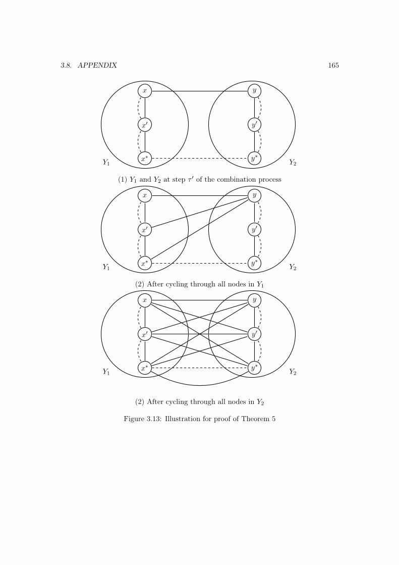
3.8. APPENDIX 165
x′
x
x∗Y1
y′
y
y∗Y2
(1) Y1 and Y2 at step τ ′ of the combination process
x′
x
x∗Y1
y′
y
y∗Y2
(2) After cycling through all nodes in Y1
x′
x
x∗Y1
y′
y
y∗Y2
(2) After cycling through all nodes in Y2
Figure 3.13: Illustration for proof of Theorem 5

166 CHAPTER 3. MULTIPLE EDGE TYPES
is some step t′ of the assembly process such that Y1, ..., Ym ⊆ Ct′ and Y1,...,Ym never
merge in any subsequent step. This implies that the intersection of the s- and d-graphs
induced over them is empty. Now consider specifically, Y1 and Y2. We know that Y1 is
not s- and d-adjacent to Y2 and, furthermore, any cluster containing Y1 will never be s-
and d-adjacent to any cluster containing Y2 (according to the assembly process). This
trivially implies that it can never be the case that xy ∈ Eτs ∩ Ed for any τ according to
the combination process. It follows that Y1 and Y2 can never belong to the same team.
For the main result, it suffices to note that at step 1 of both the assembly and the
combination process, we have that T1 = C1 = X1, ..., Xr, and each element of T1 and
of C1 is a team. Now, suppose the graph Gn is assemblable according to the assembly
process, then there is a step T <∞ by which all of the nodes in ∪i∈1,...,rXi belong to
the same cluster. By the above, this is true if and only if there is a step T ′ <∞ of the
combination process by which all of the nodes in ∪i∈1,...,rXi belong to the same team.
That is, Gn is combinable according to the combination process.
Proof of Corollary 2. Follows from Corollary 1 and Theorem 5.
Proof of Proposition 4. We can show that, up to part 3 of Algorithm 6 (where it returns
Gn), the algorithm is a special case of Algorithm 3, and the rest simply follows. In
Algorithm 3, let S0 = x1, ..., xn, Π0 = x1, x2, x3, ..., xn, and suppose
that the successive coarsening operations follow the structure below in which in every
step a single node is joined with the set of previously joined nodes:
S1 = x1, x2, x3, ..., xnΠ1 = x1, x2, x3, x4, ..., xnS2 = x1, x2, x3, x4, ..., xnΠ2 = x1, x2, x3, x4, x5, ..., xnS3 = x1, x2, x3, x4, x5, ..., xn...
ST = x1, x2, ..., xn
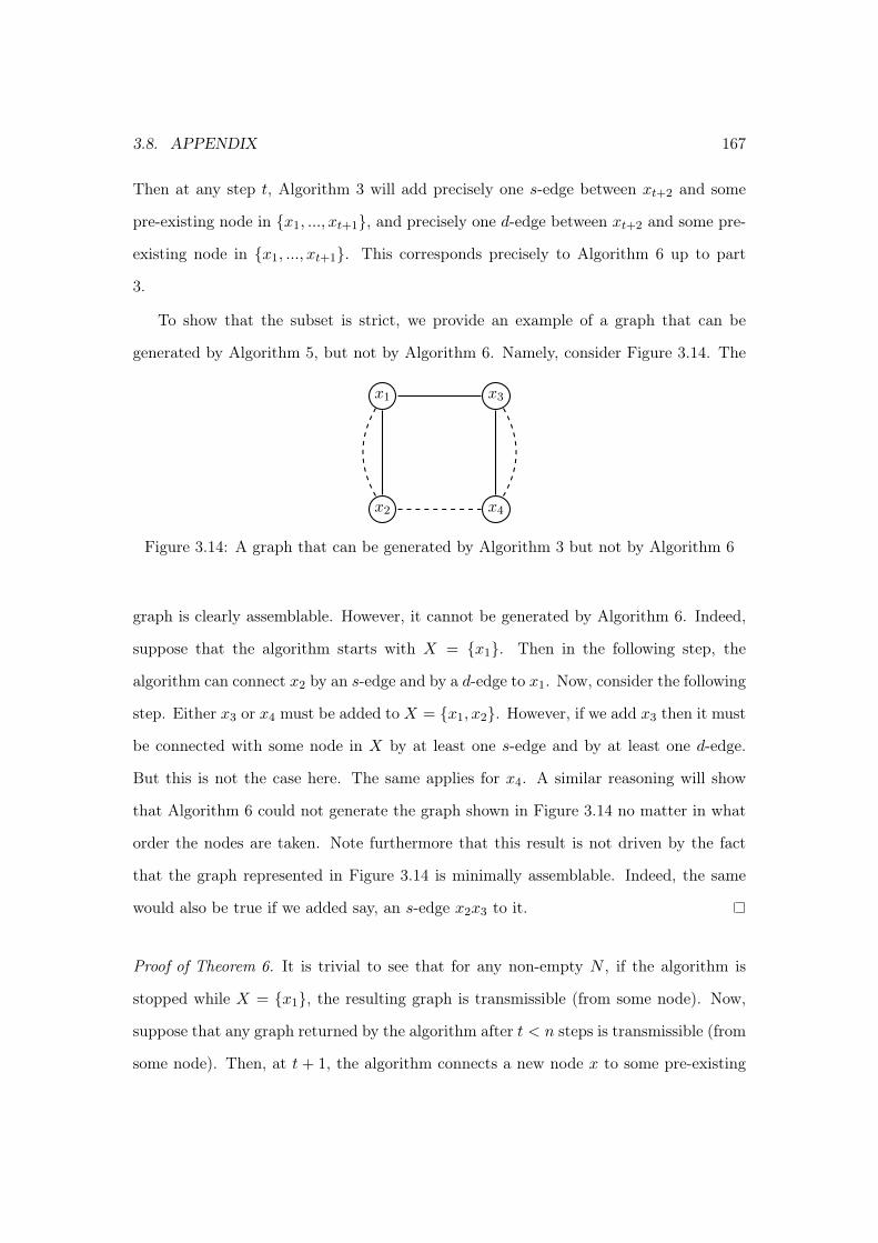
3.8. APPENDIX 167
Then at any step t, Algorithm 3 will add precisely one s-edge between xt+2 and some
pre-existing node in x1, ..., xt+1, and precisely one d-edge between xt+2 and some pre-
existing node in x1, ..., xt+1. This corresponds precisely to Algorithm 6 up to part
3.
To show that the subset is strict, we provide an example of a graph that can be
generated by Algorithm 5, but not by Algorithm 6. Namely, consider Figure 3.14. The
x1
x2
x3
x4
Figure 3.14: A graph that can be generated by Algorithm 3 but not by Algorithm 6
graph is clearly assemblable. However, it cannot be generated by Algorithm 6. Indeed,
suppose that the algorithm starts with X = x1. Then in the following step, the
algorithm can connect x2 by an s-edge and by a d-edge to x1. Now, consider the following
step. Either x3 or x4 must be added to X = x1, x2. However, if we add x3 then it must
be connected with some node in X by at least one s-edge and by at least one d-edge.
But this is not the case here. The same applies for x4. A similar reasoning will show
that Algorithm 6 could not generate the graph shown in Figure 3.14 no matter in what
order the nodes are taken. Note furthermore that this result is not driven by the fact
that the graph represented in Figure 3.14 is minimally assemblable. Indeed, the same
would also be true if we added say, an s-edge x2x3 to it.
Proof of Theorem 6. It is trivial to see that for any non-empty N , if the algorithm is
stopped while X = x1, the resulting graph is transmissible (from some node). Now,
suppose that any graph returned by the algorithm after t < n steps is transmissible (from
some node). Then, at t + 1, the algorithm connects a new node x to some pre-existing

168 CHAPTER 3. MULTIPLE EDGE TYPES
node in X by an s-edge and to some pre-existing node in X by a d-edge. Since the graph
induced over X is transmissible from some node (and |X| = t), it follows that, within a
finite number of periods, all the nodes in X will receive the message reliably. But then
it also follows that x must receive the message reliably.
To prove completeness, consider a transmissible graph Gn. Then there is a finite T
such that ST = N . Each node x ∈ N \ST−1 must receive the message reliably in the final
period (but not before), and every node in ST−1 has already received the message reliably.
So each x ∈ N \ ST−1 must have at least one s-edge connected to some y ∈ ST−1 and at
least one d-edge connected to some y′ ∈ ST−1. Suppose we delete such a node x along
with all its edges. All the other nodes x′ ∈ N \ST−1 will still receive the message reliably
in the final period, and all the nodes in ST−1 will also already have received the message
reliably (that is, no node depends on x to receive its message reliably). Therefore, if we
delete x as well as all its edges, we obtain a graph Gn−1 that is transmissible. Given this,
a simple induction will show that Algorithm 6 can generate every transmissible graph.
Indeed, the algorithm can trivially generate every transmissible graph G1 of size 1. For
an inductive hypothesis, suppose that the algorithm can generate every transmissible
graph Gn of size n. Now, consider a transmissible graph Gn+1 of size n+ 1. If we delete
an appropriate node from Gn+1 (according to the process described above), then we
obtain a transmissible graph of size n. It suffices for the algorithm to re-insert the node
at the desired place to obtain Gn+1.

3.9. REFERENCES 169
3.9 References
Baccara, M., A. Imrohorolu, A. J. Wilson, and L. Yariv (2012). A field study on matching
with network externalities. The American Economic Review 102 (5), 1773–1804.
Barabási, A.-L. and R. Albert (1999). Emergence of scaling in random networks. Sci-
ence 286 (5439), 509–512.
Bondy, J. and U. Murty (2008). Graph theory (Graduate texts in mathematics, Vol. 244).
New York, NY: Springer.
Brummitt, C. D., S. Chatterjee, P. S. Dey, and D. Sivakoff (2012). Jigsaw percolation:
Can a random graph solve a puzzle? arXiv preprint arXiv:1207.1927 .
Brummitt, C. D., R. M. D’Souza, and E. Leicht (2012). Suppressing cascades of load in
interdependent networks. Proceedings of the National Academy of Sciences 109 (12),
680–689.
Buldyrev, S. V., R. Parshani, G. Paul, H. E. Stanley, and S. Havlin (2010). Catastrophic
cascade of failures in interdependent networks. Nature 464 (7291), 1025–1028.
David, F., W. Dukes, T. Jonsson, and S. Ö. Stefánsson (2009). Random tree growth by
vertex splitting. Journal of Statistical Mechanics: Theory and Experiment 2009 (04),
P04009.
Easley, D. and J. Kleinberg (2010). Networks, crowds, and markets. Cambridge, UK:
Cambridge University Press.
Erdős, P. and A. Rényi (1959). On random graphs. Publicationes Mathematicae Debre-
cen 6, 290–297.
Gómez, S., A. Díaz-Guilera, J. Gómez-Gardeñes, C. J. Perez-Vicente, Y. Moreno, and
A. Arenas (2013). Diffusion dynamics on multiplex networks. Physical review let-
ters 110 (2), 028701.

170 CHAPTER 3. MULTIPLE EDGE TYPES
Goyal, S. (2009). Connections: an introduction to the economics of networks. Princeton,
NJ: Princeton University Press.
Granovetter, M. (1978). Threshold models of collective behavior. American journal of
sociology 83, 1420–1443.
Hagenbach, J. (2011). Centralizing information in networks. Games and Economic
Behavior 72 (1), 149–162.
Halu, A., R. J. Mondragon, P. Pansaraza, and G. Bianconi (2013). Multiplex pagerank.
arXiv preprint arXiv:1306.3576 .
Jackson, M. O. (2008). Social and economic networks. Princeton, NJ: Princeton Univer-
sity Press.
Kleinberg, J. (2013). Cascading behavior in social and economic networks. In Proceedings
of the fourteenth ACM conference on Electronic Commerce, pp. 1–4.
Lee, S. and P. Monge (2011). The coevolution of multiplex communication networks in
organizational communities. Journal of Communication 61 (4), 758–779.
Mucha, P. J., T. Richardson, K. Macon, M. A. Porter, and J.-P. Onnela (2010).
Community structure in time-dependent, multiscale, and multiplex networks. Sci-
ence 328 (5980), 876–878.
Newman, D. E., B. Nkei, B. A. Carreras, I. Dobson, V. E. Lynch, and P. Gradney (2005).
Risk assessment in complex interacting infrastructure systems. In Proceedings of the
38th Annual Hawaii International Conference on System Sciences.
Rosato, V., L. Issacharoff, F. Tiriticco, S. Meloni, S. Porcellinis, and R. Setola (2008).
Modelling interdependent infrastructures using interacting dynamical models. Inter-
national Journal of Critical Infrastructures 4 (1), 63–79.

3.9. REFERENCES 171
Swisher, S. (2013). Reassessing railroads and growth: Accounting for transport network
endogeneity. Working paper. https://mywebspace.wisc.edu/sswisher/web/documents/
Swisher_JMP_Railroads%26Growth_10-2013.pdf.
Szell, M., R. Lambiotte, and S. Thurner (2010). Multirelational organization of large-
scale social networks in an online world. Proceedings of the National Academy of
Sciences 107 (31), 13636–13641.