Modelling Videos of Physically Interacting Objects

University of Heidelberg

Department of Physics and Astronomy

MASTER’S THESIS

in Physics

in the year 2020

submitted by

Jannik Lukas Kossen,

born in Nordhorn, Germany.

Modelling Videos of Physically

Interacting Objects

This thesis has been carried out by

Jannik Lukas Kossen

under the supervision of

First Supervisor Prof. Dr. Daniel DurstewitzTheoretical NeuroscienceDepartment of Physics and AstronomyUniversity of Heidelberg and Central Institute ofMental Health

&

Second Supervisor Prof. Dr. Kristian KerstingArtificial Intelligence and Machine Learning LabDepartment of Computer ScienceDarmstadt University of Technology.

Modelling Videos of PhysicallyInteracting Objects

A strong prior in human cognition is the notion of objects. Humans exhibit excellentpredictive capabilities in dynamical settings, precisely estimating future object trajec-tories despite complex physical interactions. In machine learning, designing modelscapable of making similarly accurate estimates about future states and obtaininga useful representation of the world in an unsupervised fashion is a challengingresearch question. Building models with inductive biases inspired by those of humanperception presents a promising path towards solving these problems. This thesispresents STOVE, a novel machine learning architecture capable of modelling videosof physically interacting objects. STOVE combines recent advances in unsupervisedobject-aware image modelling and relational physics modelling to yield a non-linearstate space model, which explicitly reasons about objects and their interactions. Itis trained from pixels without any external supervision. We demonstrate STOVEon simulated videos of physically interacting objects, where it clearly improvesupon previous unsupervised and object-aware approaches to video modelling, evenapproaching the performance of a supervised baseline. STOVE’s predictions ex-hibit long-term stability, and it correctly conserves the kinetic energy in one ofthe prediction scenarios. Additionally, STOVE is extended to action-conditionedvideo prediction, advancing video models towards more general interactions beyondphysical simulations.

v

Modellierung von Videosphysikalisch interagierenderObjekte

Objekte sind ein wichtiger Prior menschlicher Wahrnehmung. Zusätzlich zeigenMenschen exzellente prädiktive Fähigkeiten in dynamischen Situationen. Selbstbei komplexen physikalischen Interaktionen treffen wir präzise Vorhersagen überdie Trajektorien von Objekten. Im maschinellen Lernen ist die Konstruktion vonModellen, die nützliche Repräsentationen der Welt hervorbringen und zu akkuratenVorhersagen fähig sind, Gegenstand aktueller Forschung. Das Design von Model-len mit induktiven Biases, ähnlich derer menschlicher Wahrnehmung, stellt hierbeieinen vielversprechenden Weg dar. Diese Arbeit präsentiert STOVE, einen neuartigenAnsatz des maschinellen Lernens, um Videos physikalisch interagierender Objekte zumodellieren. STOVE kombiniert Fortschritte unüberwachter objektorientierter Bild-modelle und relationaler Physikmodelle, um ein nichtlineares Zustandsraummodellzu bilden, welches explizit Objekte und ihre Interaktionen miteinbezieht. Das Modellwird vollständig unüberwacht auf Bildpixeln trainiert. Wir zeigen anhand von Videosphysikalischer Simulationen, dass STOVE die Ergebnisse vorheriger unüberwachterModelle verbessern kann und sogar an die Performanz einer überwachten Base-line herankommt. Die Vorhersagen von STOVE sind über lange Zeiträume stabilund in einer der Anwendungsszenarien lernt STOVE korrekterweise die Erhaltungder kinetischen Energie. Darüber hinaus wird STOVE um die aktionskonditionierteVideovorhersage erweitert, was einen wichtigen Schritt zur Entwicklung von Video-modellen für allgemeinere Interaktionen jenseits strikter physikalischer Simulationendarstellt.

vii

AcknowledgementsI am grateful to Prof. Kristian Kersting for supervising this thesis. I have greatlyenjoyed our conversations, whose impact spreads beyond this document, and whichhave had a lasting effect on my personal thoughts and convictions.

I would like to extend a special thank you to Prof. Daniel Durstewitz. Without yourtrust and agreement to the supervision, this thesis would have been impossible.

I would like to thank Karl Stelzner for his excellent supervision and keen mathemati-cal insights. I truly learnt a lot from our countless discussions, and I am grateful forall the useful feedback.

Thank you Karl, Claas, and Marcel for the incredible teamwork leading up to the ICLRdeadline. I still cannot believe how much we got done in those few weeks. Thankyou for believing in our model and thank you for your contributions, without which,I am certain, successful publication would have been much less likely. Septemberwas easily the most fun and gratifying month of this thesis.

Finally, I want to thank all the researchers and students in the Artificial Intelligenceand Machine Learning Lab at Technical University Darmstadt for the perfect balanceof thought-provoking conversations and distracting chatter in the office kitchen andbeyond.

ix

Contents

1 Introduction 11.1 Motivation . . . . . . . . . . . . . . . . . . . . . . . . . . . . . . . . . 11.2 Contribution . . . . . . . . . . . . . . . . . . . . . . . . . . . . . . . . 31.3 Outline . . . . . . . . . . . . . . . . . . . . . . . . . . . . . . . . . . . 5

2 Concepts 72.1 Recurrent Neural Networks . . . . . . . . . . . . . . . . . . . . . . . . 72.2 Variational Inference and Variational Autoencoders . . . . . . . . . . . . 102.3 State Space Models . . . . . . . . . . . . . . . . . . . . . . . . . . . . 15

2.3.1 Classical State Space Models . . . . . . . . . . . . . . . . . . . 152.3.2 Neural State Space Models . . . . . . . . . . . . . . . . . . . . 18

2.4 Sum-Product Networks . . . . . . . . . . . . . . . . . . . . . . . . . . 24

3 Related Work 293.1 Object-Aware Image Modelling . . . . . . . . . . . . . . . . . . . . . . 29

3.1.1 Motivation and Overview . . . . . . . . . . . . . . . . . . . . . 293.1.2 Sum-Product Attend-Infer-Repeat . . . . . . . . . . . . . . . . 313.1.3 Tangential Developments . . . . . . . . . . . . . . . . . . . . . 34

3.2 Physics Modelling . . . . . . . . . . . . . . . . . . . . . . . . . . . . . 353.2.1 Motivation and Overview . . . . . . . . . . . . . . . . . . . . . 353.2.2 Relational Physics using Graph Neural Networks . . . . . . . . . 363.2.3 Tangential Developments . . . . . . . . . . . . . . . . . . . . . 38

3.3 Video Modelling . . . . . . . . . . . . . . . . . . . . . . . . . . . . . . 393.3.1 General-Purpose Video Models . . . . . . . . . . . . . . . . . . 393.3.2 Object-Aware Approaches . . . . . . . . . . . . . . . . . . . . . 403.3.3 Tangential Developments . . . . . . . . . . . . . . . . . . . . . 42

4 Structured Object-Aware Physics Prediction for Video Modelling and Planning 434.1 Sum-Product Attend Infer Repeat for Image Modelling . . . . . . . . . 464.2 Graph Neural Networks for Physics Modelling . . . . . . . . . . . . . . 474.3 Joint State Space Model . . . . . . . . . . . . . . . . . . . . . . . . . 504.4 Conditioning on Actions . . . . . . . . . . . . . . . . . . . . . . . . . . 53

5 Evaluation and Discussion 555.1 Introducing the Environments . . . . . . . . . . . . . . . . . . . . . . 555.2 Training Details . . . . . . . . . . . . . . . . . . . . . . . . . . . . . . 585.3 Video and State Modelling . . . . . . . . . . . . . . . . . . . . . . . . 585.4 Action-Conditioned Prediction . . . . . . . . . . . . . . . . . . . . . . . 625.5 Energy Conservation . . . . . . . . . . . . . . . . . . . . . . . . . . . . 655.6 Noisy Supervision . . . . . . . . . . . . . . . . . . . . . . . . . . . . . 675.7 Chaos in the Billiards Environment . . . . . . . . . . . . . . . . . . . . 70

xi

5.8 Stability of Predictions . . . . . . . . . . . . . . . . . . . . . . . . . . . 745.9 Flexibility of the Object Model . . . . . . . . . . . . . . . . . . . . . . 755.10 Ablation Study . . . . . . . . . . . . . . . . . . . . . . . . . . . . . . . 755.11 Scaling to Additional Objects . . . . . . . . . . . . . . . . . . . . . . . 77

6 Concluding Thoughts 796.1 Discussion and Future Work . . . . . . . . . . . . . . . . . . . . . . . . 796.2 Summary . . . . . . . . . . . . . . . . . . . . . . . . . . . . . . . . . . 82

Appendix A Model Details 85A.1 Recognition Model Architecture . . . . . . . . . . . . . . . . . . . . . . 85A.2 Generative Model Architecture . . . . . . . . . . . . . . . . . . . . . . 85A.3 Model Initialisation . . . . . . . . . . . . . . . . . . . . . . . . . . . . 86A.4 Hyperparameter Settings . . . . . . . . . . . . . . . . . . . . . . . . . 87

Appendix B Baselines 89

Bibliography 93

xii

1Introduction

1.1 MotivationHumans are remarkable. Every day we solve a multitude of complex and diversetasks with incredible skill. When picking up new tasks, we efficiently leverage priorexperience to accelerate the learning process. We possess a complex mental modelof the world, allowing us to reason about our decisions. Human intelligence faroutranks any artificial intelligence today (Chollet, 2019; Lake et al., 2017).

Many problems of artificial intelligence may be approached with machine learning.Over the last decade, such machine learning based approaches have seen greatprogress with the advent of deep learning based architectures. Following the ex-cellent overview of LeCun et al. (2015): In many areas of machine learning thatrequire highly non-linear function approximation, such as computer vision or naturallanguage processing, deep learning based approaches have been able to improveupon state-of-the-art performance significantly. While previous approaches relied onhand-designed feature extractors as input to shallow models, deep learning basedarchitectures can, in many cases, automatically extract complex non-linear features.However, deep learning is not one thing, not a single model with which to solveevery problem. It is a general concept, a buzzword, which best encapsulates theapproaches taken by many machine learning models of the current wave. Its progresshas been enabled by a mix of new model architectures, advances in optimisationmethods, faster processors, and the availability of large amounts of curated data.Current state-of-the-art deep learning architectures outperform humans on sometasks. Considerable media attention was given to the cases of ATARI video games(Mnih et al., 2015) or the board game GO (Silver et al., 2016, 2017).

However, as lamented by Chollet (2019), many of these models are extremely faraway from true intelligence. As defined by Legg and Hutter (2006),

“Intelligence measures an agent’s ability to achieve goals in a wide rangeof environments.” (Legg and Hutter (2006))

If the goal of the artificial intelligence community truly is to achieve intelligentsystems, the current modus operandi of large parts of the community seems prob-lematic: Intelligence has primarily been measured as skill. Skill is measured asperformance on some success metric, such as accuracy, on a narrowly defined taskfor which the model has been specifically trained. In some parts of the community,this has downright led to benchmarking races: State-of-the-art results on popularbenchmarking tasks were released by one group and then beaten by others in quicksuccession.1 To be fair, this has lead to impressive improvements on these tasks.

1See paperswithcode.com/sota/image-classification-on-imagenet to get an idea of the amount ofpapers and their timing on the ImageNet classification task (last accessed on 25th March, 2020).

1

http://paperswithcode.com/sota/image-classification-on-imagenet

However today, arguably, performance on many of the popular benchmarks is satu-rated. We may be close to the point where beating the previous state-of-the-art mayonly be achieved by implicitly overfitting the model architecture to the data set, seee. g. Recht et al. (2019).

Chollet (2019) finds fault with a different consequence of this benchmarking men-tality. He argues that few of the improvements of the last years have resulted inmodels that are more intelligent as defined above. They often require large amountsof carefully curated and labelled data to allow for learning, are limited in theircapability to generalise knowledge to new tasks, and have no deeper understandingof their actions, i. e. they cannot reason about their decisions or act in logically soundways. This is problematic beyond a philosophical debate about what high-levelgoals the community should aim for. Instead, it has real-world consequences. Inmany use cases, current state-of-the-art machine learning models may not be appli-cable. For example, the creation of high-quality data sets with sufficient labelleddata may be prohibitively expensive. Of course, the problems mentioned abovehave been given attention by the community – some relevant areas are transferlearning, multi-task learning, explainable or interpretable models, learning fromweak supervisory signals, semi-supervised learning, data-efficient reinforcementlearning, or neuro-symbolic approaches combining reasoning and data – but Chollet(2019) argues that time is ripe for a widespread disruptive change in the communitytowards building more intelligent models.

It should be obvious that none of the current machine learning models can matchthe versatility of human intelligence. However, Chollet (2019) proposes that weshould focus research efforts on models with similarly desirable properties. Addingto the definition of Legg and Hutter (2006), he posits that intelligence, in the contextof artificial intelligence research, should be measured as follows:

“The intelligence of a system is a measure of its skill-acquisition effi-ciency over a scope of tasks, with respect to priors, experience, andgeneralization difficulty.” (Chollet (2019))

Lake et al. (2017) argue that seeking inspiration from humans is the way to buildsuch models. The artificial intelligence community may be far from creating trueintelligence, but cognitive science, neuroscience, psychology, and related disciplineshave a good understanding of many processes related to human intelligence. Withcareful design, such priors of human cognition may be translated into mathematicsand computer code. In this way, machine learning models inspired by powerfulhuman priors can be built, going beyond the strained biological motivations of neuralnetworks. The manifest of Lake et al. (2017) is called “Building machines that learnand think like people”, and we see the work presented here directly following itsphilosophy.

Human vision is inherently based on the notion of objects. This strong innateprior can already be found in infants (Zelazo and Johnson, 2013). From a physicsperspective, our vision apparatus, the eyes, is constantly bombarded with largeamounts of photons. From a machine learning perspective, this photon showercorresponds to vast amounts of unstructured data as input to our vision model. Ashumans, we do not perceive this unstructured data. Instead, we perceive a highlystructured and complex representation of our world. A fundamental entity of thisrepresentation is the object. We perceive objects and endow them with properties or

2 Chapter 1 Introduction

argue about relations between them. The notion of objects is a central ingredientto intelligence, intricately connected to human vision. Recently, this has lead to thedevelopment of machine learning models of images which include this notion ofobjects at their core, see Section 3.1. Such models hold the promise of extracting avariety of knowledge in an unsupervised fashion. They can infer segmentation masks,obtain latent object representations useful for reasoning in downstream tasks, orlearn to count the total number of objects present in a scene. Importantly, they havebeen shown to improve upon the generalisation capabilities of previous approaches,e. g. generalising to unseen numbers of objects without requiring any extra training(Eslami et al., 2016).

Another strong innate prior to human cognition is intuitive physics (McCloskey,1983). Humans intuitively anticipate the outcome of collisions between objects orthe movement of a ball falling in gravity. In other words, we effortlessly make precisepredictions about future trajectories of physically acting objects. These physicalreasoning capabilities are essential to our successful navigation of the world. Weshould therefore seek to create machine learning models, which can likewise predictthe outcomes of complex physical interactions. In the machine learning community,a mountain of research trying to teach physics to machines has been establishedover the last years, see Section 3.2. Examples of physics scenarios include teaching amodel to play billiards, non-linear physics simulations, fluid dynamics, rigid bodyphysics, or even real-life robotics applications. As with object-based image models,critical innovations in model architectures were necessary to obtain models suited tophysical predictions. However, many of these approaches rely on strong supervisorysignals, such as ground truth trajectories or a simulator. While their performance isimpressive, such work often does not scale efficiently to many interesting real-worldapplications, e. g. robotics, because the collection of sufficient supervisory signals isnot feasible.

Our work combines the priors of object-based vision and intuitive physics to yield agenerative model of videos trained directly on raw pixels. It seems obvious that theinclusion of an object-based representation for image modelling is helpful for thetask of physics prediction and vice versa. Rather than restricting our modelling capa-bilities in comparison to more general approaches, the inclusion of these inductivebiases seems to empower the performance of the model.

1.2 ContributionThis thesis presents a machine learning model which learns about objects and theirinteractions from raw pixels in an unsupervised fashion. We call the model STOVE,loosely abbreviating Structured Object-Aware Physics Prediction for Video Modellingand Planning. A first overview of its capabilities is given in Fig. 1.1. More specifically,a generative model of videos is proposed as a non-linear state space model. Weconstruct the video model as the composition of a generative unsupervised modelof static images and a graph neural network for modelling the relational dynamicsbetween object states. Skipping many critical details, one may give an intuitivelyappealing description of this model in three sentences: The image model infersobject-specific states from single images. The dynamics model can propagate thesestates forward in time, predicting future object trajectories. The image model canalso render future frames of video from the predicted states. Model training is

1.2 Contribution 3

PhysicalVideo

Modelling

Object-Based Image Modelling Flexible

Object Model

Multiple ScenariosExtract

Trajectories

Non-LinearState Space

Model

RelationalDynamics Modelling

ExplicitLatents

Figure 1.1.: This thesis introduces STOVE, a generative model of videos of physically in-teracting objects. STOVE models images in terms of their constituent objectsusing a Sum-Product Attend-Infer-Repeat image model. The image model infersobject-specific latent states, part of which explicitly correspond to object posi-tions, velocities, and sizes. From this interpretable latent space, future latentstates may be predicted using a relational dynamics model, a graph neuralnetwork. Image and object appearance are not hard coded but learned instead.Likewise, STOVE can accommodate a variety of physical simulation scenarios.The STOVE architecture corresponds to a probabilistic non-linear state spacemodel. Learning in this model is made tractable using amortised variationalinference.

accomplished using amortised variational inference in the probabilistic state spacemodel. This conceptually simple approach significantly improves upon previouswork in future frame or state prediction tasks. Notably, in one of the tasks, ourmodel manages to correctly preserve the kinetic energy of the system, leading topredictions with impressive stability over long timeframes. This is in stark contrast toprevious approaches whose predictions quickly diverge to unrealistic trajectories.

More philosophically speaking and connecting to the previous discussion, STOVEpresents a counterpoint to the prevailing wisdom of approaching complex problemswith large unstructured models and lots of data. While the achievements of deepand mostly unstructured neural networks on classic tasks of computer vision ornatural language processing are impressive, the explicit specification of modelstructure informed by prior knowledge massively benefits performance and trainingefficiency. Discovering structure in data remains central to machine learning, andone may not always want to predefine models as much as we have done withSTOVE. However, STOVE demonstrates that with minimal model building, we canachieve predictive performance drastically superior to unstructured approaches.Note that this approach to structured problem-solving is undoubtedly distinct fromold-fashioned, hand-crafted machine learning. STOVE consists entirely of flexibleneural networks and deep probabilistic models and is adaptable to a wide rangeof scenarios. It is the careful delegation of tasks among these components, thedesign of the communication interfaces between them, and the formulation of theprobabilistic model, that are key components of a new wave of structured machine

4 Chapter 1 Introduction

learning architectures, of which STOVE is an example.

Part of my work on this thesis resulted in the publication Structured Object-AwarePhysics Prediction for Video Modeling and Planning (Kossen et al., 2020), whichis to be published in the proceedings of the Eighth International Conference ofLearning Representations (ICLR), a highly-ranked conference in machine learning.I am grateful for the work of my co-authors, without whom successful publicationwould not have been possible. Some of the results in the publication can also befound in this thesis. However, unless otherwise mentioned, they were obtained byme. To avoid any uncertainties, I will attribute my co-authors whenever I discussresults from the paper which cannot be unambiguously attributed to my own work.Additionally, since the publication in the proceedings coincides with the submissionof this thesis, and a preprint of the paper has been available since 25th September,2019, I will cite the paper whenever necessary to avoid self-plagiarism. The thesiscan be seen as an extended version of the paper, containing additional experimentsand insights, as well as a more thorough treatment of the theoretical background,related works, and derivations.

1.3 OutlineChapter 2 introduces generally useful concepts from machine learning crucial tothis thesis, focussing on machine learning for sequences, variational inference, andsum-product networks. The chapter lays the theoretical foundation for STOVE andthe discussed related work. Chapter 3 then serves as an introduction to image,physics, and video modelling. Previous approaches influential and tangential tothis thesis are discussed. Of special importance is Section 3.1.2, which introducesSuPAIR, a modified version of which is used as the image model in STOVE. Likewise,Section 3.2.2 introduces relational physics modelling using graph neural networks, avariant of which comprises our dynamics model. Chapter 4 then formally introducesSTOVE with all the components of its non-linear state space model. Chapter 5presents a thorough experimental evaluation of STOVE with a comparison againstbaselines, an ablation study, as well as more model-specific considerations. Chapter 6then discusses some exciting ideas for future research, before closing this thesis witha final summary.

1.3 Outline 5

2Concepts

This chapter introduces recurrent neural networks, variational inference and thevariational autoencoder, latent state space models, as well as sum-product networks.These concepts present the essential theoretical foundation for STOVE as well as thediscussed related works. Throughout this chapter, we will assume that the reader isfamiliar with machine learning on the level of an introductory university course, i. e.foundational knowledge of probability theory as well as basic classification, regres-sion, clustering, and dimensionality reduction methods. Additionally, some basicknowledge of fully connected neural networks and their training by backpropagationis helpful. This information may be found in any machine learning textbook, e. g.Bishop (2006) or Barber (2012).

Rather than introducing each concept wherever it appears first, we introduce themall together here. While this leads to a more structured approach, it also results in adecently long chapter on machine learning methods without constantly visible linksto this thesis. You may of course skip parts you are familiar with. You may even skipconcepts you are not acquainted with, as they will be referenced when needed, suchthat you can then come back here.

2.1 Recurrent Neural NetworksFeed-forward neural networks are powerful function approximators. Given a singleinput x ∈ RD, they learn to approximate the desired output y = f(x) ∈ RM , wherey might be the prediction for a regression or classification task. However, they haveno natural way to process a sequence of observations x1:T = {xt}Tt=1 ∈ RT×D. Whileone could reshape the sequence to form a single observation x ∈ RT ·D, this approachdoes not scale to long sequences, cannot handle sequences of varying length, anddiscards temporal structure. Recurrent Neural Networks (RNNs) remedy this byintroducing recurrent connections, i. e. self-connections, to neural networks (Elman,1990). Now, input sequences are consumed sequentially, e. g. such that

ht = g(xt, ht−1) (2.1)

yt = f(ht) , (2.2)

where f and g are non-linear transformations as in a feed-forward network. Often,this is a single linear transformation followed by a non-linearity. Figure 2.1a showsa graphical depiction of such a network. At each timestep t, the mapping g updatesa hidden state ht by considering the current position of the input xt as well as theprevious hidden state ht−1. An output yt may be produced from the hidden statewith the mapping f . This hidden state allows the RNN to model dependencies overtime, retaining and accessing information from previous timesteps. If the desiredoutput is again a sequence, y = {yt}Tt=1 may be concatenated, if not, y = yT doesthe trick. Of course, RNNs may also be applied when the input is not a sequence but

7

xt

ht

yt

g

f

(a)

tanhtanh

(b)

Figure 2.1.: (a) Illustration of a simple Recurrent Neural Network (RNN). At time t, thefunction g uses the input xt to update a hidden state ht−1. Output yt is producedusing f and the current hidden state ht. (b) Procedural flow of a Long-ShortTerm Memory (LSTM) network: The previous hidden state ht−1 and currentinput xt are used to construct the gates ft, it, and ot, which are then used toupdate the hidden and cells states ht−1 and ct−1. Figure adapted from Bonse(2019).

the output should be, by setting xt = x, ∀t. See Goodfellow et al. (2016, Chap. 10)or Lipton et al. (2015) for excellent ground-up introductions to RNNs, the latterincluding a more thorough review of current literature.

LSTMs. While immediately intriguing, early implementations of RNNs were plaguedwith problems, preventing their widespread use. Mainly, they struggled to modellong-term dependencies. As the hidden state is propagated through time, it is mul-tiplied with the state transition matrix. In many cases, this will either shrink (orincrease) the modulus of the hidden state. Repeated applications will lead to ex-ponentially decaying (or exploding) states and gradients. This became known asthe “vanishing gradient problem” in RNNs (Hochreiter, 1991, 1998). The intro-duction of the Long-Short Term Memory (LSTM) (Hochreiter and Schmidhuber,1997) architecture essentially solved this problem by introducing fixed unit-weightrecurrent edges (Lipton et al., 2015). Now, for the first time, RNNs could successfullymodel long-term dependencies (Hochreiter and Schmidhuber, 1997). The use ofLSTM-based models in time series modelling, natural language processing, and evencomputer vision exploded. They became the de-facto standard for dealing withsequences in neural networks, achieving state-of-the-art performance on many tasks(Lipton et al., 2015). Formally, the update equations of the LSTM are given as

ct = ft � ct−1 + it � tanh(Whcht−1 + Wxcxt + bc)

ht = ot � tanh(ct) , (2.3)

8 Chapter 2 Concepts

where � signifies element-wise multiplication. Here, ft, it, and ot implement gatingmechanisms, given by

ft = σ(Wxfxt +Whfht−1 +bf )

it = σ(Wxixt +Whiht−1 +bi)

ot = σ(Wxoxt +Whoht−1 +bo) , (2.4)

where all matrices W and vectors b in the above Eqs. (2.3) and (2.4) are learnableparameters and σ(x) = (1 + exp(−x))−1 is the sigmoid function. Figure 2.1bvisualises the above operations. The gates ft, it, and ot explicitly control the flow ofinformation between all cells of the LSTM. The forget gate ft controls the amount ofinformation kept from the previous cell state, the input gate it controls how muchis added to the cell state, and the output gate ot controls how much of the currentcell state is copied to the hidden state. This architecture mitigates the problem ofvanishing gradients, because the cell state is no longer subject to an exponentialdecrease due to repeated multiplication with weights w < 1. Instead, the forgetgate ft dynamically modulates, how much of the previous cell state is kept. Infact, the original LSTM did not have a forget gate, i. e. ft = 1. This formulationmakes the constant connection between cell states across time, and thereby thenon-vanishing of the gradients, more visible. The forget gate was added later byGers et al. (1999). The capability to explicitly forget states was found to be beneficialto learning, without reintroducing vanishing gradients. See Lipton et al. (2015) fora further discussion of this.

Many variations of the above Eqs. (2.3) and (2.4) exist. The exact form displayed wasintroduced by Zaremba and Sutskever (2014). Other, similarly designed architecturessuch as Bidirectional Recurrent Neural Networks (BRNNs) (Schuster and Paliwal,1997), Neural Turing Machines (NTMs) (Graves et al., 2014), and Gated RecurrentUnits (GRUs) (Cho et al., 2014) exist. GRUs simplify the design of the LSTMby discarding the output gate, which may sometimes speed up learning but hasadversarial effects on modelling complexity (Chung et al., 2014). GRUs have neverreached the popularity of LSTMs.

Only recently has the reign of LSTM-supremacy in natural language processingbegun to topple as purely self-attention-based architectures, introduced by the Trans-former (Vaswani et al., 2017), have been able to surpass previous performancerecords. However, LSTMs are still frequently used, e. g. as building blocks in largerarchitectures, where they are often employed to model factorisations of distributionsp(z) =

∏j p(zj | z1:j−1), where j indexes dimensions, as is the case in this thesis.

Section 2.3 below will give some examples of LSTMs as part of probabilistic sequencemodels.

Data from many domains are inherently stochastic. The RNNs discussed so far aredeterministic architectures, and as such, they struggle to model naturally stochasticprocesses, such as speech (Chung et al., 2015). Embracing this stochasticity inmodel building leads to more expressive and powerful models. Recently, hybridarchitectures combining probabilistic modelling and the flexibility of RNNs havebeen proposed. These approaches are enabled by recent advances in VariationalInference (VI), which we will introduce now, before returning to our discussion ofsequence models in Section 2.3.

2.1 Recurrent Neural Networks 9

2.2 Variational Inference and Variational Autoencoders

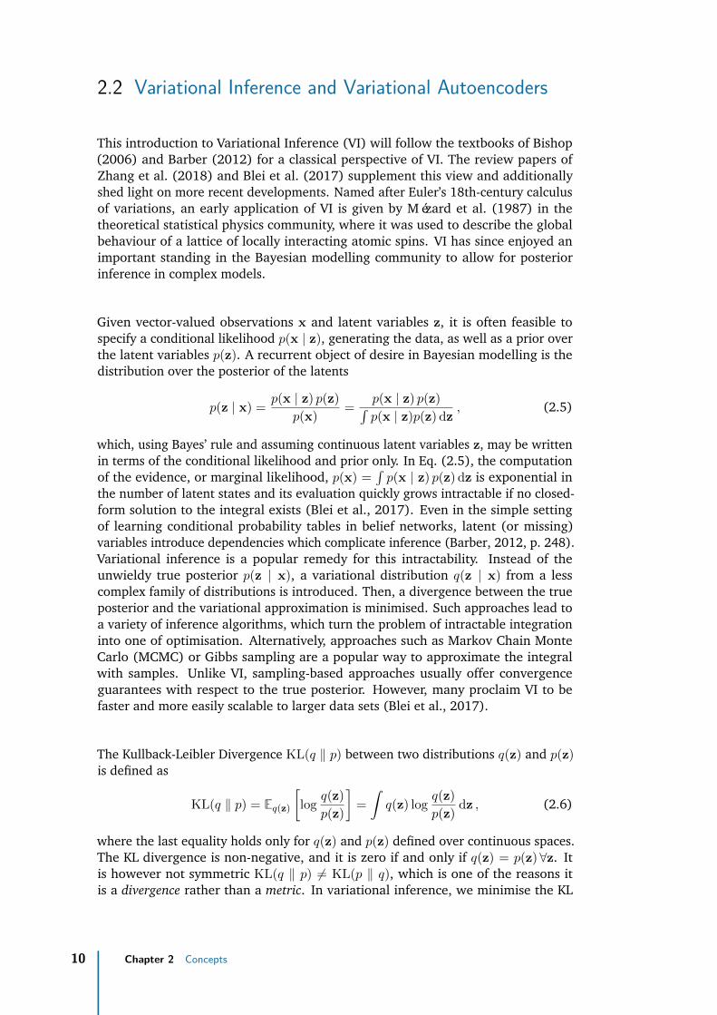
This introduction to Variational Inference (VI) will follow the textbooks of Bishop(2006) and Barber (2012) for a classical perspective of VI. The review papers ofZhang et al. (2018) and Blei et al. (2017) supplement this view and additionallyshed light on more recent developments. Named after Euler’s 18th-century calculusof variations, an early application of VI is given by Mézard et al. (1987) in thetheoretical statistical physics community, where it was used to describe the globalbehaviour of a lattice of locally interacting atomic spins. VI has since enjoyed animportant standing in the Bayesian modelling community to allow for posteriorinference in complex models.

Given vector-valued observations x and latent variables z, it is often feasible tospecify a conditional likelihood p(x | z), generating the data, as well as a prior overthe latent variables p(z). A recurrent object of desire in Bayesian modelling is thedistribution over the posterior of the latents

p(z | x) =p(x | z) p(z)

p(x)=

p(x | z) p(z)∫p(x | z)p(z) dz

, (2.5)

which, using Bayes’ rule and assuming continuous latent variables z, may be writtenin terms of the conditional likelihood and prior only. In Eq. (2.5), the computationof the evidence, or marginal likelihood, p(x) =

∫p(x | z) p(z) dz is exponential in

the number of latent states and its evaluation quickly grows intractable if no closed-form solution to the integral exists (Blei et al., 2017). Even in the simple settingof learning conditional probability tables in belief networks, latent (or missing)variables introduce dependencies which complicate inference (Barber, 2012, p. 248).Variational inference is a popular remedy for this intractability. Instead of theunwieldy true posterior p(z | x), a variational distribution q(z | x) from a lesscomplex family of distributions is introduced. Then, a divergence between the trueposterior and the variational approximation is minimised. Such approaches lead toa variety of inference algorithms, which turn the problem of intractable integrationinto one of optimisation. Alternatively, approaches such as Markov Chain MonteCarlo (MCMC) or Gibbs sampling are a popular way to approximate the integralwith samples. Unlike VI, sampling-based approaches usually offer convergenceguarantees with respect to the true posterior. However, many proclaim VI to befaster and more easily scalable to larger data sets (Blei et al., 2017).

The Kullback-Leibler Divergence KL(q ‖ p) between two distributions q(z) and p(z)is defined as

KL(q ‖ p) = Eq(z)

[log

q(z)

p(z)

]=

∫q(z) log

q(z)

p(z)dz , (2.6)

where the last equality holds only for q(z) and p(z) defined over continuous spaces.The KL divergence is non-negative, and it is zero if and only if q(z) = p(z)∀z. Itis however not symmetric KL(q ‖ p) 6= KL(p ‖ q), which is one of the reasons itis a divergence rather than a metric. In variational inference, we minimise the KL


divergence between the variational distribution and the true posterior1

KL(q(z | x) ‖ p(z | x)) (2.7)

= Eq(z|x)

[log

q(z | x)

p(z | x)

](2.8)

= Eq(z|x) [log q(z | x)]− Eq(z|x) [log p(x, z)] + log p(x) , (2.9)

where we have used p(x)’s independence of z for the last term. We want to minimisethe LHS of the equation but cannot evaluate it directly due to the intractabilities inp(z | x). Likewise, the RHS of the equation contains p(x), which, lest we forget, isthe reason for this mathematical endeavour in the first place. However, because p(x)is irrelevant to our optimisation in z, we may omit it and instead maximise

ELBO(q) = Eq(z|x) [log p(x, z)]− Eq(z|x) [log q(z | x)] , (2.10)

where we introduce the Evidence Lower Bound (ELBO). The negative ELBO isequivalent to the KL divergence we seek to minimise up to a constant. Maximisingthe ELBO therefore corresponds to minimising an upper bound to the above KLdivergence.

A different but equally popular derivation for this lower bound is given by maximumlikelihood learning in models with unobserved latent variables: We seek to maximisethe marginal likelihood, or evidence, p(x) of the data under our model. This requiresmarginalisation over the latent variables z. Again, one introduces the variationaldistribution q(z | x) to modify the intractable integral

log p(x) = log

∫p(x, z) dz (2.11)

= log

∫q(z | x)

p(x, z)

q(z | x)dz (2.12)

= log

(Eq(z|x)

[p(x, z)

q(z | x)

])(2.13)

≥ Eq(z|x)

[log

p(x, z)

q(z | x)

](2.14)

= ELBO(q) , (2.15)

where Eq. (2.14) results from Jensen’s inequality (Jensen et al., 1906). We seethat both the minimisation of the KL divergence between the true posterior and thevariational approximation, as well as the maximisation of the marginal likelihood,may be used as motivation to derive the ELBO, Eq. (2.10).

By rewriting Eq. (2.9)

log p(x) = ELBO(q) + KL(q(z | x) ‖ p(z | x)) , (2.16)

we see that the lower bound is tight if the KL divergence is 0, and therefore q = p. Inpractice, this may only occur if the variational approximation q(z | x) is expressiveenough to model the true posterior p(z | x). This will often not be the case. Forexample, the popular mean field approach specifies q(z | x) =

∏j qj(zj | x), where j

1The asymmetry of the KL divergence results in various subtleties not discussed here but e. g. inBarber (2012, Sec. 28.3).

2.2 Variational Inference and Variational Autoencoders 11

indexes the latent space dimensions. This leads to tractable inference but cannotaccount for dependencies between the latent dimensions. Mean-field VariationalInference (MFVI) leads to iterative optimisation algorithms, which require iterationover the complete data set and therefore do not scale well to large data settings(Zhang et al., 2018). Stochastic Variational Inference (SVI) (Hoffman et al., 2013)eliminates this constraint by applying stochastic optimisation to variational inference,essentially yielding a mini-batch compatible VI variant. However, in all of the above,a variational distribution has to be computed for each input datum x, either byevaluating expectations with respect to q(z | x), if they are tractable, or performingoptimisations, if they are not. Therefore, scaling MFVI to large data and complexarchitectures is not without problems, i. e. see discussions in Zhang et al. (2018),Farquhar et al. (2020), or Wu et al. (2019a).

Amortised variational inference presents a promising proposal to solve these issues.Instead of optimising the variational distribution for each data point separately, inamortised VI, a powerful model fφ(x) directly predicts the variational distribution.If q(z | x;λ) is parametrised by λ, e. g. λ = {µ,σ} for a mean-field Gaussian,evaluation of fφ directly yields fφ(x) = λ. Here, φ are the parameters of fφ tobe optimised. As the parameters φ are shared over all data instances, variationalinference is said to be amortised. Amortised VI hinges on the assumption that fφ isflexible enough to predict the correct distribution for all x reliably. Neural networksare a popular choice for such approximators, and amortised VI has quickly becomethe default approach to combine neural networks and probabilistic frameworks(Zhang et al., 2018). The parameters φ then correspond to the weights and biasesof the network fφ.

The Variational Autoencoder. Amortised VI was first proposed by Dayan et al.(1995), see Marino et al. (2019), while the term was coined in Gershman andGoodman (2014). However, its use in the Variational Autoencoder (VAE), attributedto both Kingma and Welling (2014) and Rezende et al. (2014), popularised it. Tra-ditionally, VI is used to allow for inference in complex probabilistic models, whichspecify intricate dependencies between variables. The VAE formulates a simple prob-abilistic model and pushes complexities into encoding and decoding networks. SeeDoersch (2016) for a welcoming and easy-to-digest tutorial on VAEs and Tschannenet al. (2018) for a more recent review paper focussed on unsupervised representationlearning. VAEs are a probabilistic architecture relying on two neural networks, aprobabilistic encoder q(z | x) and a probabilistic decoder p(x | z), where x ∈ RD,z ∈ RL, and usually D � L. Usually, a normally distributed prior p(z) = N (0,1) onthe latent space is assumed, and both the encoder and the decoder parametrise themeans µ and variances σ2 of factorised Gaussian distributions,

qφ(z | x) = N(z; µφ(x),σ2

φ(x))

and (2.17)

pθ(x | z) = N(x; µθ(z),σ2

θ(z)), (2.18)

where φ (and θ) are the parameters of the encoding (and decoding) networks.2

VAEs may be used for unsupervised representation learning as well as generative

2We often omit the parameters {θ,φ} for the sake of readability. Neural networks have been usedto parametrise conditional distributions well before the introduction of VAEs. An early example of thisare Mixture Density Networks (MDNs) (Bishop, 1994), which already share a lot of the philosophy ofamortised inference, i. e. for each incoming data point, a neural network directly infers the parametersof a probabilistic model. However, MDNs predict deterministic estimates of the latent parameters.


x

zφ θ

N

(a)

Encoder Decoder

(b)

Figure 2.2.: (a) Graphical model of a Variational Autoencoder (VAE). Black edges indicatethe generative model p(x, z) = pθ(x | z)p(z) and red ones the inference modelqφ(z | x). Solid lines indicate dependency structures between random variables,dashed lines the dependencies on parameters. Shaded nodes indicate observedvariables, transparent nodes latent variables. Plate notation is used to indicateamortisation, i. e. sharing of φ over all data instances N . For the sake ofsimplicity, we will not display plate notation or dependencies on parameters infuture graphical models in this thesis. Figure adapted from Kingma and Welling(2014). (b) Illustration of a typical VAE architecture and computational flow.Given an input image x, the encoder infers the latent distribution qφ(z | x).From this, we sample a latent state z, which the decoder uses to predict pθ(x | z).Next, a reconstruction x of the input image may be obtained by sampling. Infully generative mode, samples from the prior z ∼ p(z) are used as input to thedecoder. Figure inspired by Tschannen et al. (2018).

modelling of complex data.

In the setting of image modelling, a VAE may be employed to (a) produce a low-dimensional encoding z ∼ q(z | x) given an image x, and (b) to generate an imageby sampling z ∼ p(z) from the prior and decoding it to an image x ∼ p(x | z).Depending on the scenario, one or both of these applications may be desirable.Figure 2.2 displays the graphical model of to the VAE as well as an additionalillustration of a typical architecture. VAE training proceeds by stochastic optimisationof the ELBO, Eq. (2.10), for the parameters of the encoding and decoding networksjointly. In the context of VAEs, the ELBO is often rewritten as

ELBO(q) = Eq(z|x) [log p(x | z)]−KL(q(z | x) ‖ p(z)) , (2.19)

which highlights the VAE components more clearly. As the expectations with respectto q(z | x) are not tractable, they are usually approximated with a single sample.3

The first term Eq(z|x) [log p(x | z)] can be interpreted as a reconstruction loss of thecurrent image x given the latent code z ∼ q(z | x) and resulting decoding p(x | z).To see this more clearly, let x be an image and p(x | z) a pixel-wise independent

3Approaches such as the IWAE (Burda et al., 2015) or AESMC (Le et al., 2018) use multiplesamples z to approximate the expectations with respect to q. If q is flexible enough, this results intighter bounds with respect to the true posterior. However, the interplay between the encoding anddecoding networks is complex and “tighter variational bounds are not necessarily better” (Rainforthet al., 2018). See Rainforth et al. (2018) for an excellent discussion of why more samples may hinderlearning of the inference network.

2.2 Variational Inference and Variational Autoencoders 13

Gaussian distribution with fixed variances. Then

log p(x | z) =∑j

(µθ(zj)− xj)2

2σ2+ C , (2.20)

which is the common squared loss between predicted and observed pixel values.Maximising the ELBO minimises KL(q(z | x) ‖ p(z)), which penalises deviationsbetween q(z | x) and p(z). If the KL divergence is minimal and therefore 0, thenq(z | x) = p(z) and the encodings are pure noise and cannot contain any information.This is, of course, detrimental to achieving good reconstructions from z. On theother hand, without the KL-penalty, the network will not learn encodings whichresemble the prior distribution p(z), and therefore makes sampling from p(z) toobtain images p(x | z) impossible. Intuitively the ELBO can be seen as representinga trade-off between good reconstructions and conforming to the prior distribution ofthe latent space.4

Optimisation of VAEs usually proceeds via (mini-batch) gradient descent, i. e. arandom subset of the data {xi}Nb

i=1 is propagated through the VAE and the parame-ters {φ,θ} of the encoding and decoding distributions qφ(z | x) and pθ(x | z) areupdated using the cumulative gradient N−1b

∑i∇φ,θ ELBOi, e. g. with the ADAM

optimiser (Kingma and Ba, 2015).

This then finally leads us to the computation of

∇φ,θ ELBO = ∇φ,θ Eqφ(z|x) [log pθ(x | z)]−∇φ,θ KL(qφ(z | x) ‖ p(z)) . (2.21)

For the encoding distribution, the gradient with respect to φ is problematic because

∇φ Eqφ(z) [fφ(z)] = ∇φ

∫qφ(z)fφ(z) dz (2.22)

6=∫qφ(z)∇φfφ(z) dz (2.23)

= Eqφ(z) [∇φfφ(z)] . (2.24)

This means that, in the current form, we may not sample z ∼ q, evaluate theELBO, and calculate its gradient, because this would correspond to a calculation ofEqφ [∇φfφ(z)]. In other words, generally, the gradient of an expectation is not thesame as the expectation of a gradient. One way of solving this, is writing

∇φEqφ(z|x) [fφ(z)] =

∫ ((∇φqφ)

qφqφfφ + qφ(∇φfφ)

)dz (2.25)

=

∫qφ (fφ∇φ log qφ +∇φfφ) dz (2.26)

= Eqφ [fφ∇φ log qφ +∇φfφ] , (2.27)

4Again, many subtleties beyond the scope of this thesis are involved here. Many works on theeffects and side-effects of the KL-divergence and reconstruction loss exist, and in turn, many modelshave been proposed to overcome their limitations. This discussion is often tightly linked with the aimto construct VAEs which learn disentangled representations. A disentangled representation in a VAE isloosely defined as a representation for which the individual dimensions of the latent space correspondto the true generative factors of the data. The interested reader may consult Higgins et al. (2017),Burgess et al. (2017), Mathieu et al. (2019), or Zhao et al. (2019) for a further discussion of thesetopics.


which does however have a high variance (Krishnan et al., 2015).

This is where the reparametrisation trick (Kingma and Welling, 2014) comes into play.For some distributions, we may reparametrise z ∼ q(z | x), such that the inequalityin Eqs. (2.22) to (2.24) becomes an equality. For example, if z ∼ N (µ(x),σ2(x)),we may write z as a deterministic function, where noise is injected via the auxiliaryvariable ε,

z = µ(x) + ε� σ(x) = g(x, ε) , where ε ∼ N (0,1) = p(ε) . (2.28)

Note that for vector-valued z and ε, multiplication is element-wise. This allows us torewrite the expectation Eq. (2.22) as

∇φ Eqφ(z) [fφ(z)] = ∇φ

∫qφ(z)fφ(z) dz (2.29)

= ∇φ

∫p(ε)fφ(z) dε, using q(z) dz = p(ε) dε , (2.30)

=

∫p(ε)∇φfφ(z) dε (2.31)

= Ep(ε) [∇φfφ(z)] . (2.32)

This is the Stochastic Gradient Variational Bayes (SGVB) estimator (Kingma andWelling, 2014). We may therefore now sample ε ∼ p(ε), compute the ELBO, andevaluate its gradient, obtaining a correct estimate Eq. (2.21).5 See Kingma andWelling (2014) for a discussion of other distributions for which this is possible. Notethat this problem does not arise for the gradient with respect to θ for the decodingnetwork because q does not depend on θ and the above inequality Eq. (2.22)becomes an equality. For the calculation of the KL divergence in Eq. (2.19), thisproblem may be circumvented entirely if closed-form solutions of the KL divergenceexist, e. g. if both p and q are Gaussian. Such closed-form solutions additionally leadto lower variance estimates of the gradient, which may benefit training, see e. g.Burda et al. (2015).

2.3 State Space Models

2.3.1 Classical State Space Models

Before the rise of LSTMs, Probabilistic Graphical Models (PGMs) were the dominantapproach for modelling sequences. The presentation below largely follows theworks of Barber (2012), Bishop (2006), and Murphy (2012). Given a sequence ofobservations x1:T = {xt}Tt=1 and latent states z1:T = {zt}Tt=1, we formulate a joint

5The reparametrisation trick was explained in detail because of the apparent confusion surroundingit. Often, the question of “Why do we need the reparametrisation trick?” is answered with “BecauseTensorFlow, PyTorch, etc. cannot backpropagate through stochastic variables. The reparametrisationtrick makes the latent variables deterministic and automatic backpropagation will then work fine.” Thisanswer is incomplete, as it reduces the reparametrisation trick to an implementation detail, when, infact, it is a neat and necessary mathematical trick. Without it, we would either (a) naïvely and wronglyevaluate Eq. (2.24), which is not the desired quantity, or (b) need to resort to the high-varianceestimator Eq. (2.27).

2.3 State Space Models 15

z1

x1

z2

x2

. . .

. . .

zT−1 zT

xT−1 xT

(a)

zt−1

xt−1

zt

xt

(b)

Figure 2.3.: Graphical model of the Hidden Markov Model (HMM) and Linear GaussianState-Space Model (LG-SSM) in (a) full and (b) compact representation. Thedynamics of the latent state zt are given by the transition distribution p(zt | zt−1).Observations xt may be generated from latent states via the emission distributionp(xt | zt). The latent state zt fully explains xt, such that xt is independentof all other variables given zt. For the HMM, the latent states are discrete,giving a transition matrix, while the emission distribution may be specified withrespect to discrete or continuous variables. For the LG-SSM, both transition andemission distributions are Gaussian. From now on, we will only draw graphicalmodels in their compact representation.

probability distribution over both as

p(x1:T , z1:T ) = p(x1 | z1) p(z1)T∏t=2

p(xt | zt) p(zt | zt−1) . (2.33)

This factorisation encodes a variety of conditional (in-)dependence assumptionsbetween variables, which can be displayed as a graphical model, see Fig. 2.3. Namely,at time t and given zt, the observation xt is independent of all other observationsx1:t−1,t+1:T and latent states z1:t−1,t+1:T , i. e. p(xt | x1:t−1,t+1:T , z1:T ) = p(xt | zt).Likewise, zt−1 and zt+1 are conditionally independent given zt. In other words,the latent state zt fully explains the current observation xt. The model is 1storder Markov in the latent states, i. e. the latent state zt suffices to predict thedistribution over future latent states and observations. Previous latent states zt′<t

provide no additional information. However, without knowledge of the latents,the observations xt on their own do not exhibit such independence structure, i. e.p(xt | x1:t−1) may not be simplified any further. We can sample a sequence of latentstates from this model if the transition distribution p(zt | zt−1) is known. For each zt,we may then sample an observation xt ∼ p(xt | zt) from the emission distribution.The prior p(z1) encodes assumptions about the distribution of states in absence ofprevious observations.

For discrete latent states, the above model is known as a Hidden Markov Model(HMM),6 which has been successful in many sequence modelling applications suchas object tracking, bioinformatics, or speech recognition (Barber, 2012). In speechrecognition, the observations correspond to a representation of a snippet of audioand the latent states represent the phonemes needed to transcribe the audio. InHMMs, the transition distribution is given by a matrix p(zt = i | zt−1 = j) = At(i, j).If this matrix is independent of time, the sequence is called stationary. Note that

6Sometimes, the term Hidden Markov Model is used to describe all sequence models with Marko-vian latent states. However, most often, such as in the textbooks of Barber (2012), Bishop (2006), andMurphy (2012), the term is used solely for models with discrete latent states. This is the conventionthat we will conform to.


HMMs are capable of modelling long-range dependencies because no independenceassumptions on the observations exist, i. e. the predictive distribution p(xt | x1:t−1)depends on all previous observations. This dependency is mediated by the latentstates. Without the inclusion of latent states, long-term dependency modelling couldonly be achieved by adding many individual dependencies – additional backwardsarrows {xt → xt−b}Bb=2 in the graphical model – which would lead to a combinatorialexplosion in the conditional distribution p(xt | xt−1:t−B) (Bishop, 2006, p. 608).

For continuous latent states, the above factorisation is called a Linear Gaussian State-Space Model (LG-SSM), also called Linear Dynamical System (LDS). It corresponds tothe same graphical model, Fig. 2.3, only this time, continuous Gaussian latent statesare assumed and linear equations govern the transition and emission distributions,such that, following Murphy (2012, Chap. 18),

zt = Atzt−1 + εt, εt ∼ N (0, Qt) (2.34)

xt = Btzt + δt, δt ∼ N (0, Rt) . (2.35)

The matrices At and Bt give the transition and emission behaviour, and noiserepresenting the uncertainty of observations δt and noise intrinsic to the process εtis included (Durstewitz, 2017, p. 152f.). It follows from Eqs. (2.34) and (2.35) thatp(xt | zt) and p(zt | zt−1) are also Gaussian. Often, the LG-SSM is formulated inadditional dependency on an external control parameter or action at. One of the LG-SSM’s main application is the estimation of the state zt given a sequence of uncertainmeasurements x1:t, i. e. the position of a rocket given only noisy estimates (Barber,2012). Estimation of p(zt | x1:t) is referred to as filtering. Given the parametersof the system γt = {At,Bt,Qt,Rt}, filtering in LG-SSMs is tractable and leads tothe Kalman filter equations. The LG-SSM is colloquially referred to as the Kalmanfilter, as filtering is its predominant use. LG-SSMs are also used heavily in traditionalforecasting, even though they might be called by a different name. For example, thepopular Autoregressive-Moving Average (ARMA) models used in time series analysiscan be represented as a special case of the LG-SSM (Murphy, 2012, p. 640).

Table 2.1 lists classic inference tasks for both HMMs and LG-SSMs. Given theparameters of the model, all tasks are tractable for both models, assuming the size ofthe HMM’s state space is reasonable. This means that, if the model assumptions hold,the HMM and LG-SSM perform these inference tasks optimally. Often for LG-SSMs,a physical model describing the measurement and transition process exists, and allparameters in Eqs. (2.34) and (2.35) are known. However, parameter learning ofall or some parameters in the above equations may be performed. Learning in bothmodels is trivial if x1:T and z1:T are observed during training. For example, whentraining an HMM for speech recognition, one may create a training set that containsboth the audio recordings (observations) and the corresponding correct phonemes(latents). If only x1:T is observed, algorithms such as expectation maximisation maybe used to estimate stationary parameters.

Both HMMs and LG-SSMs present a classical alternative to modern RNNs such asthe LSTM. However, HMMs do not scale well to larger state spaces, as the transitionmatrix and inference is quadratic in the size of the latent space (Lipton et al.,2015). Furthermore, LG-SSMs are unsuited for applications where the assumptionof linear transitions does not hold. Extensions of LG-SSMs to non-linear transitionand emission functions exist (Wan and Van Der Merwe, 2000). However, they


Table 2.1.: Relevant inference tasks in probabilistic sequence modelling. Exact estimationof the below distributions is tractable in the Hidden Markov Model (HMM) andLinear Gaussian State-Space Model (LG-SSM). Adapted from Barber (2012).

Filtering p(zt | x1:t)Prediction p(zt | x1:t′) t′ < tSmoothing p(zt | x1:t′) t′ > tLikelihood Estimation p(x1:T )Most Probable Latent Sequence argmaxz1:T p(z1:T | x1:T )

rely on sampling and assume that a linearisation of the functions up to first orsecond order is sufficient. Additionally, they either demand emission and transitionmatrices to be known upfront or require a tractable posterior to allow for learning(Karl et al., 2017a). LSTMs on the other hand, allow for learning highly non-lineartransition functions and can model long-term dependencies between latent states.The relationship between RNNs and state space models have been discussed as earlyas in DeCruyenaere and Hafez (1992). Until recently, it mostly seemed like the twoapproaches were opposing. In the following section, we will give an introduction torecent architectures that defy this assumption.

2.3.2 Neural State Space ModelsWe concluded the last section by remarking that LG-SSMs and HMMs may beunsuited to model complex processes in large data settings. However, LSTMs oftencan accommodate such scenarios. Why would we want to combine recurrent neuralnetworks and state space models? As discussed at the end of Section 2.1, RNNsare not well suited to modelling processes where stochasticity is inherent anddominant. While we may interpret the output of an RNN as the parametrisation ofa probability distribution, the hidden state transitions in the RNN remain entirelydeterministic. Chung et al. (2015) note that the introduction of stochasticity helpsthe LSTM to model “the kind of variability observed in highly structured sequentialdata”. Adding to that, LSTMs are not well suited to the unconditional generation ofnovel sequences. Principled approaches to generate novel sequences require a priordistribution, from which to draw samples, which standard LSTMs lack. The abovestatements are supported by the fact that the works introduced below routinelyoutperform deterministic recurrent approaches or classical state space models.

Over the last years, a cornucopia of approaches marrying state space models andrecurrent neural networks have been proposed. This has lead to sequence models ca-pable of dealing with non-linear, stochastic, and high-dimensional data such as audioor video in a fully probabilistic way. The topic of this thesis is object-aware modellingof physical video sequences. By specialising general-purpose sequence models tobe better suited to physical video modelling, e. g. by including object-based imagemodels and physical prediction modules, approaches such as ours, STOVE, may beobtained. The non-linear sequence models presented below therefore correspondto important baselines, but may also yield inspiration for further developments inobject-aware modelling of physical video sequences. Examples of such models thatwe are aware of include Bayer and Osendorfer (2014), Fabius and van Amersfoort(2015), Chung et al. (2015), Watter et al. (2015), Krishnan et al. (2015), Johnsonet al. (2016), Karl et al. (2017a), Krishnan et al. (2017), Maddison et al. (2017),and Rangapuram et al. (2018). They enjoy the advantage of using neural networks


to model highly non-linear functions, while simultaneously benefitting from thestochasticity, structure, interpretability, data-efficiency, and the explicit inclusion ofstructure in state space models (Rangapuram et al., 2018).

Such models can be obtained by modifying the emission and transition behaviourof the LG-SSM in numerous ways. Regarding the emission function, it is commonto replace the linear model with (a) a complex non-linear likelihood model, e. g.a neural network. Additionally, most approaches implement one of the followingtactics to allow for more flexible transition models: (b) model the latent transitionwith a neural network, (c) keep the transition dynamics linear but predict theirparameters with a (recurrent) neural network, or (d) introduce a separate deter-ministic RNN which interfaces with stochastic latent states. The approaches alsodiffer by how many of the strict independence assumptions of the LG-SSM theyretain. Many of the above approaches leverage amortised variational inference,see Section 2.2, to achieve tractable learning in these highly non-linear hybrid ap-proaches between state space models and neural networks. VI is usually applied formodels which implement strategies (a), (b), or (d), because the resulting non-lineartransition models make classical inference intractable. For future reference, STOVE,our approach, falls into the categories (a) and (b), where (a) is achieved by usingSum-Product Attend-Infer-Repeat (SuPAIR), Section 3.1.2, and (b) is realised with aGraph Neural Network (GNN), Section 3.2.2. The above approaches may be framedin terms of a variety of applications, such as time series prediction, modelling ofspeech, handwriting, or videos. While this may have informed model design, anyapproach is relevant for this section as long as it is a general approach capable ofmodelling high-dimensional data with complex dependencies. Here, modelling refersto the specification of a fully generative model as well as the capability to performinference therein.

A useful strategy for understanding neural state space models is to seek answers tothe following questions.

(i) How are images xt generated?(ii) How are future latent states zt+1 predicted?

(iii) How are present latent state zt inferred?

Questions (i) and (ii) are directed at the form of the emission and transition distri-butions, the generative model, Eq. (2.33) for the LG-SSM. As posterior inferenceof latent variables zt is intractable in non-linear state space models, some form ofamortised approximation is usually employed, the exact form of which is asked byquestion (iii).

Due to different ways of interlacing the RNNs and SSMs, the cited approachesimplement observation likelihoods, transition functions, or inference networks indifferent ways. Note that the above approaches may have been designed withdifferent applications in mind. While one might focus on accurate inference of latentstates, e. g. by designing a neural smoother, another might focus on obtaining a goodgenerative model.

VRNNs. While all of the above approaches have reached some level of popularityin the community, the Variational Recurrent Neural Network (VRNN) (Chung et al.,2015) is most common. In our evaluation in Chapter 5, as well as in other papersin the literature, it is the chosen representative of general-purpose non-linear and


stochastic sequence models. Let us quickly introduce the defining characteristicsof the VRNN. The VRNN employs the strategies (a) and (d) mentioned above. Itintroduces an LSTM whose hidden state ht = f1(ht−1,xt, zt) depends on boththe current observation xt, the current latent state zt, and the previous hiddenstate ht. At time t, the LSTM therefore expresses dependencies on all previousimages x1:t−1 and latents z1:t−1 through its hidden state. This hidden state is usedas input to Multilayer Perceptrons (MLPs) to predict the means and variances of therelevant Gaussian conditional distributions. In all subsequent approaches and unlessotherwise mentioned, distributions are likewise to be assumed factorised Gaussians,whose means and variances are predicted by neural networks. To answer questions(i) through (iii), let us assume that we have inferred, observed, or calculated allprevious variables zt−1, xt−1, and ht−1. To ease notation, we will also assumethat the VRNN and all subsequent approaches correctly handle prior distributions.Figures 2.4a to 2.4d illustrate the following operations. (i) Following Fig. 2.4a,to generate an image xt, we require the previous hidden state ht−1, available byassumption, and current latent state zt, which is available from (ii) or (iii). Thisgives us xt ∼ p(xt | x1:t−1, z1:t) = f2(ht−1, zt), where f2 and all following fi arerealised as MLPs. (ii) Still looking at Fig. 2.4a, we can sample future latent states aszt ∼ p(zt | x1:t−1, z1:t−1) = f3(ht−1) from the previous hidden state of the RNN. (iii)Following Fig. 2.4b, given the current observation xt and previous hidden state ht−1,we may infer zt ∼ q(zt | xt,x1:t−1, z1:t−1) = f4(xt,ht−1) without any extra steps.Here, q is the amortised variational approximation of the true posterior. Now thatwe have obtained both xt and zt, we can update the hidden state and move onto the next timestep, see Fig. 2.4c. As ht−1 can realise a dependence on all paststates and observations, the recognition model’s estimate of zt may be seen as aneural and implicit version of the Kalman filtering algorithm. The deterministictransition of hidden states is shared over inference and generation. The VRNN doesnot implement a way to obtain smoothed estimates of zt. The above procedures andFigs. 2.4a to 2.4d correspond to the generative and inference models

p(x1:T , z1:T ) =∏t

p(xt | x1:t−1, z1:t) p(zt | x1:t−1, z1:t−1) (2.36)

q(z1:T | x1:T ) =∏t

q(zt | x1:t, z1:t−1) , (2.37)

from which the ELBO may be assembled for parameter learning. In contrast to theLG-SSM, the VRNN includes no conditional independence assumptions on previousobservations or latent states.7

STORN. The Stochastic Recurrent Network (STORN) (Bayer and Osendorfer, 2014)is one of the first approaches combining SSMs and LSTMs. It is a predecessor toVRNNs, also uses strategies (a) and (d), and its graphical model is given in Figs. 2.4eto 2.4h. STORN’s approach of integrating RNNs and LSTMs is straightforward.STORN includes two RNNs f1 and f2. They realise the time-factorisation of thegenerating and recognition distributions, where the output of the RNN at time t

7While not immediately relevant to this thesis, I find it instructive to briefly discuss some otherapproaches to neural state space models. Sadly, a comprehensive review and comparison of thesemodels does currently not exist. The only thing that comes close is Lesort et al. (2018), which has aheavy focus on reinforcement learning/control and misses many of the works cited herein. The busyreader may skip these last paragraphs. In addition to presenting interesting background knowledge,their primary relevance is for the discussion of STOVE and future work in Section 6.1.


ht−1 ht

zt

xt

(a) VRNN: Generation

ht−1 ht

zt

xt

(b) Inference

ht−1 ht

zt

xt

(c) Deterministic

ht−1 ht

zt

xt

(d) Full

h1t

h2t

zt

xt

(e) STORN: Generation

h1t

h2t

zt

xt

(f) Inference

h1t−1 h1

t

h2t−1 h2

t

zt

xtxt−1

(g) Deterministic

h1t−1 h1

t

h2t−1 h2

t

zt

xtxt−1

(h) Full

h1t

h2t

ztzt−1

xt

(i) SRNN: Generation

h1t

h2t

ztzt−1

xt

(j) Inference

h1t−1 h1

t

h2t−1 h2

t

zt

xtxt−1

(k) Deterministic

h1t−1 h1

t

h2t−1 h2

t

zt

xtxt−1

zt−1

(l) Full

Figure 2.4.: Graphical models for (a-d) Variational Recurrent Neural Networks (VRNNs),(e-h) Stochastic Recurrent Networks (STORNs), and (i-l) Stochastic RecurrentNeural Networks (SRNNs). The first column illustrates the generation of novelobservations and/or latents. Observed variables are shaded, latents transparent,and deterministic variables are displayed as diamonds. Inference operationsare drawn with red arrows. Deterministic nodes refer to hidden states of RNNs,which model dependencies on all of their previous input variables. Emission andtransition distribution of stochastic nodes are realised by MLPs. In the originalpapers, the dependence on external control variables is sometimes considered,which is omitted here. Figures (a-c) adapted from Chung et al. (2015).


directly gives the current conditional distribution

p(x1:T | z1:T ) =∏t

p(xt | x1:t−1, z1:t) p(xt | x1:t−1, z1:t) = f1(zt,xt−1,h1t−1)

(2.38)

q(z1:T | x1:T ) =∏t

q(zt | x1:t) q(zt | x1:t2) = f2(xt,h2t−1) . (2.39)

Similar to the procedure for the VRNN, one may check how the questions (i-iii) areanswered for STORN. (i) xt is generated from Eq. (2.38), requiring the previousimages and current latent state, and (iii) zt is inferred from Eq. (2.39), requiringonly the current observation to update the hidden state. Unlike the VRNN, STORNinfers latent state zt independent of all previous latent states. (ii) A major drawbackof STORN is, that it provides no way to predict future latent states zt. The updatedlatent zt would also be needed to update h1

t to generate a new observation xt. In theabsence of such a mechanism, we sample z ∼ p(z) from the prior at each step of theprediction, which leads to lower quality predictions, as the amount of stochasticityis fixed and is independent of all previous states and observations (Chung et al.,2015).

DMMs. To generate an observation xt, the generative model of the VRNN, Eq. (2.36),depends on both the stochastic variable zt as well as the history ht−1, encompassingall previous observations x1:t−1 and latents z1:t−1. Likewise, the generation of novellatent states zt depends on all x1:t−1 and z1:t−1 through the hidden state ht−1. Thisbreaks with Markovian assumptions of the LG-SSM, which the authors of the DeepMarkov Model (DMM) (Krishnan et al., 2017) retain.8 DMMs employ strategies (a)and (b), and their generative model is identical in factorisation to the LG-SSM,

p(x1:T , z1:T ) =∏t

p(xt | zt) p(zt | zt−1) , (2.40)

where the emission distribution is parametrised by an MLP and the transitiondistribution is inspired by the Gated Recurrent Unit. Notably, they formulate theinference network as

q(z1:T | x1:T ) =∏t

q(zt | zt−1,x1:T ) , (2.41)

using all previous and future observations to infer the latent states. This is unlikeVRNNs and STORNs, which make the simplifying assumption that zt is inferredusing only past information.9 Unlike the VRNN, the DMM relies on all observa-tions, including future observations xt+1:T , to infer zt. Both formulations are valid,however, without any further additions, this smoothing-like formulation requires

8DMMs were previously published as Deep Kalman Filters (DKFs) by Krishnan et al. (2015). Aless fitting name, especially given that the Deep Kalman Filter performs smoothing in its defaultconfiguration.

9In addition to (zt−1, x1:T ), the authors also consider other dependencies of the inference networkon the observations, such as conditioning on (x1:T ), (x1:t), (zt−1, x1:T ), (zt−1, x1:t), or (zt−1, xt:T ).From the perspective of a Markovian state space model, the previous latent state and all futureobservations should lead to optimal smoothing inference given the independence assumptions. Indeed,they show that the inclusion of past observations is negligible if the last latent state is included. If it isnot included, then past observations contribute significantly to the overall performance. Conditioningon all observations is performed using a bi-directional RNN, see e. g. (Salehinejad et al., 2017).


the entire sequence to be available at inference time and complicates the reuse oftransition functions as in the VRNN, which shares its LSTM between inference andgeneration. The authors show strong performance of the DMM inference modelcompared to STORN and others, but show no comparisons for the generative model.One may assume that their generative performance will deteriorate if the assumedindependencies no longer hold. However, the simplified generative model Eq. (2.40)does lead to tractable evaluation of the KL divergence in the ELBO.

SRNNs. Fraccaro et al. (2016) provide yet another variant of stochastic recurrentnetworks with strategies (a) and (d), which more clearly separates stochastic fromdeterministic nodes, i. e. separately models transitions for deterministic and stochas-tic nodes. All distributions are then predicted by MLPs with dependence on boththe stochastic as well as the deterministic nodes. They have found this to givebetter performance and to be easier to train. They name their approach StochasticRecurrent Neural Network, which should not be confused with Stochastic RecurrentNetworks (STORNs), but mercifully choose the more distinct abbreviation SRNN.Like Krishnan et al. (2017), they use information from future observations duringinference. We have displayed them in Figs. 2.4i to 2.4l alongside the others forcomparison, but will not go into any more detail.

DVBF. Indeed, the reuse of the generative transition in the inference model, as inVRNNs, is paramount according to the authors of Deep Variational Bayes (DVBF)(Karl et al., 2017a), who claim that it leads to favourable gradients during trainingand therefore improves performance. Like the DMM, they keep the independenceassumptions Eqs. (2.40) and (2.41) of the generative model. Additionally, Karlet al. (2017a) claim that many sequence models are stuck in local optima of goodreconstruction but bad transition behaviour because optimal reconstructions maybe obtained without incorporating knowledge about the transition. This biasesthe latents towards reconstruction and not transition. The transition function thencannot modify the latents because this would decrease the reconstruction quality,leading to a model biased towards reconstruction. To instead bias the model towardsuseful transition functions, they posit a special form of the transition function andinference network. Instead of directly inferring latent states, the inference networkinfers parameters of the transition function, making it deterministic, from theprevious latent state and current observation. A Bayesian treatment of the inferredparameters makes it possible to penalise the heavy use of the current observationto predict the parameters of the current latent state, ensuring that the transitionfunction is used as intended. Karl et al. (2017a) observe that their model can recoverderivative quantities, such as velocities, in the latent space, while Krishnan et al.(2017) fail to do so. As our model, STOVE, also reuses the generative transitionmodel during inference and strictly enforces latent space assumptions, we willdiscuss the effect of these assumptions further in Chapter 4.

Quasi-Linear Approaches. Other recent approaches using strategies (c), such asFraccaro et al. (2017) and Rangapuram et al. (2018), are of special interest becausethey retain the ability to tractably compute all quantities in Table 2.1. Fraccaroet al. (2017) achieve this by predicting time-dependent parameters γ1:T of a LG-SSM using (recurrent) neural networks. As the equations of Table 2.1 also applyto non-stationary processes, once the linear transition and emission parametershave been inferred, this model is identical to a time-dependent LG-SSM. Here,


zt−1 zt

at−1 at

xt−1 xt

LGSSM

VAE

ht−1 htγt−2

γt−1

γt−1

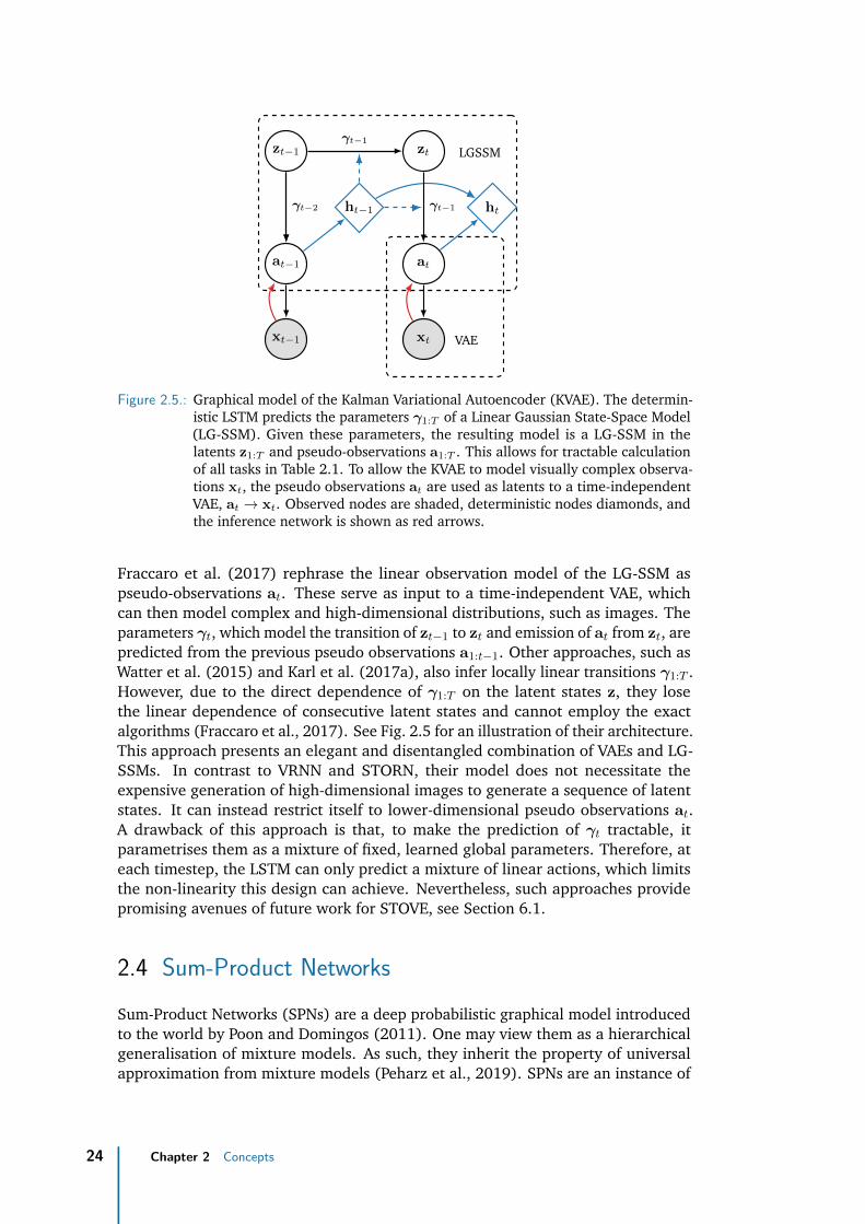
Figure 2.5.: Graphical model of the Kalman Variational Autoencoder (KVAE). The determin-istic LSTM predicts the parameters γ1:T of a Linear Gaussian State-Space Model(LG-SSM). Given these parameters, the resulting model is a LG-SSM in thelatents z1:T and pseudo-observations a1:T . This allows for tractable calculationof all tasks in Table 2.1. To allow the KVAE to model visually complex observa-tions xt, the pseudo observations at are used as latents to a time-independentVAE, at → xt. Observed nodes are shaded, deterministic nodes diamonds, andthe inference network is shown as red arrows.

Fraccaro et al. (2017) rephrase the linear observation model of the LG-SSM aspseudo-observations at. These serve as input to a time-independent VAE, whichcan then model complex and high-dimensional distributions, such as images. Theparameters γt, which model the transition of zt−1 to zt and emission of at from zt, arepredicted from the previous pseudo observations a1:t−1. Other approaches, such asWatter et al. (2015) and Karl et al. (2017a), also infer locally linear transitions γ1:T .However, due to the direct dependence of γ1:T on the latent states z, they losethe linear dependence of consecutive latent states and cannot employ the exactalgorithms (Fraccaro et al., 2017). See Fig. 2.5 for an illustration of their architecture.This approach presents an elegant and disentangled combination of VAEs and LG-SSMs. In contrast to VRNN and STORN, their model does not necessitate theexpensive generation of high-dimensional images to generate a sequence of latentstates. It can instead restrict itself to lower-dimensional pseudo observations at.A drawback of this approach is that, to make the prediction of γt tractable, itparametrises them as a mixture of fixed, learned global parameters. Therefore, ateach timestep, the LSTM can only predict a mixture of linear actions, which limitsthe non-linearity this design can achieve. Nevertheless, such approaches providepromising avenues of future work for STOVE, see Section 6.1.

2.4 Sum-Product NetworksSum-Product Networks (SPNs) are a deep probabilistic graphical model introducedto the world by Poon and Domingos (2011). One may view them as a hierarchicalgeneralisation of mixture models. As such, they inherit the property of universalapproximation from mixture models (Peharz et al., 2019). SPNs are an instance of


tractable probabilistic models. In contrast to most other graphical models, they allowfor tractable and exact evaluation of many relevant inference tasks. All tractablegraphical models have a SPN-representation (Poon and Domingos, 2011), and everySPN may be converted into a Bayesian Network in linear time (Zhao et al., 2015).They have successfully been employed to on complex tasks, such as modellingimages (Poon and Domingos, 2011; Dennis and Ventura, 2012), speech (Peharzet al., 2014), or language (Cheng et al., 2014), and classification e. g. of images(Gens and Domingos, 2012), often producing state-of-the-art results at the time ofpublication. SPNs are relevant to this thesis because STOVE employs a variant ofSum-Product Attend-Infer-Repeat (SuPAIR) to model the distribution over individualimages. SuPAIR uses Random Sum-Product Networks (Random SPNs) (Peharz et al.,2019) to achieve this. Random SPNs are a variant of SPNs fully amendable to end-to-end differentiable optimisation. Historically, SPNs are an instance of ArithmeticCircuits (Darwiche, 2003), for which parameters are traditionally specified and notlearned. The interested reader is referred to Vergari et al. (2019) for a recent andextensive review of SPNs.

A Sum-Product Network (SPN) may be represented by a rooted directed acyclicgraph, containing sum nodes, product nodes, and leaf distributions. The scope ofan SPN is given by the set of variables over which it is defined. Following this, arecursive definition of SPNs is given:

“(1) A tractable distribution is an SPN; (2) a product of SPNs definedover different scopes is an SPN; and (3), a convex combination of SPNsover the same scope is an SPN.” (Molina et al. (2018))

While this definition should technically suffice, we will illustrate SPNs and their prop-erties a bit further. At the root, the joint probability p(x) over all x = (x1, . . . , xD) ∈ Xis obtained. Each leaf defines a distribution over a subset of the input variables.Any other node in the tree is either a sum node or a product node. Sum nodespropagate (upwards) a weighted sum over their children, which all have identicalscope. In other words, each sum node is a mixture model over its children. Themixture weights are learned during training, and Peharz et al. (2015) show thatthey may be normalised locally for each sum node without losing expressiveness.Product nodes compute the product over inputs from different, non-overlappingscopes. This allows the SPN to implement hierarchies over variables by modellingindependencies between them. As we traverse the tree of a typical SPN, going downfrom the full joint distribution at the root, product nodes are used to iteratively splitthe joint distribution into less complex distributions over fewer variables. Intuitively,we want to use product nodes whenever we can find disjoint subsets of statisticallyindependent variables at the current node. If we cannot find such independencies,we use sum nodes to model more complex distributions. These may then, in turn,induce further independencies. Usually, sum and product nodes are employed inan alternating pattern. Evaluation of an SPN is performed bottom-up, i. e. givenan input x, we evaluate all leaf distributions at the corresponding subvectors of xand then pass up the results, performing weighted summation over the children atsum nodes and multiplication of children at product nodes. Figure 2.6 shows anillustration of a simple SPN, where each leaf node defines a distribution over a singlevariable only. Note that for SPNs, the graph structure may be seen as a deterministiccomputation graph of summation and multiplication operations from the leavesto the root. In contrast, in graphical depictions of other models, such as Bayesian

2.4 Sum-Product Networks 25

+

× ×

x0 + × x2

××

x1 x2 x1 x2

x0 x1

0.40.6

0.3

0.7

Figure 2.6.: Illustration of a simple SPN. Sum nodes implement normalised mixtures overtheir child distributions and product nodes model independencies. The jointprobability over all variables p(x) is obtained at the root by evaluating the leafnode distributions and propagating the results up through sum and productnodes. In this illustration, the leaves contain the univariate distributions of thevariables x = (x0, x1, x2). Figure adapted from Molina et al. (2019).

Networks, graph nodes usually directly illustrate random variables. In an SPN, thisis only true for the leaf nodes. See the original publication (Poon and Domingos,2011) for further information, as well as an airtight theoretical introduction of SPNs.

An attractive property of SPNs is that they are capable of performing many inferencetasks in linear time with respect to the size of the model. Computation of marginalsp(x−y) =

∫p(x)dy simply corresponds to marginalisation at the respective leaf

nodes, where y ∈ Y ⊂ X , x−y ∈ X−y ⊂ X , and Y ∪X−y = X , Y ∩X−y = ∅.10 Eachleaf node is defined over a subvector y′ of x. If all y′ ∈ Y ′ are in the marginalisationset for a specific leaf node Y ′ ⊂ Y, then marginalisation simply corresponds tosetting this node to 1. Similarly, any conditional p(y | x−y) may be constructedvia marginalisation p(y,x−y)/p(x−y) and is therefore obtained in linear time. Alinear-time approximation exists for MPE-inference y∗ = argmaxy p(X−y = x−y,y),for which exact computation is NP-hard. Vergari et al. (2018) demonstrate that SPNshave built-in autoencoding and unsupervised representation learning capabilities.

If the structure of an SPN is given, e. g. because it is designed with prior knowledge ofthe data or specific applications in mind, the weights of an SPN may be learned usingexpectation maximisation or gradient-based approaches (Poon and Domingos, 2011).However, often, the tree structure of an SPN is learned from data using specialisedalgorithms such as in Gens and Pedro (2013), Poon and Domingos (2011), Dennisand Ventura (2012), or Adel et al. (2015). To obtain a valid SPN, the algorithmsneed to ensure that the structure obeys the completeness (i. e. for each sum node, allchildren have identical scope) and decomposability (i. e. for each product node, allchildren have non-overlapping scope) properties, see Poon and Domingos (2011)and Peharz et al. (2015) for further details.

10Set operations are meant as operations on the dimensionality of the input vectors, i. e. the ∪operator corresponds to concatenation.


Figure 2.7.: Illustration of a Random Sum-Product Network (Random SPN) over sevenvariables (X1, . . . , X7) with hyperparameters D = 2, R = 2, C = 3, S = 2, andI = 2. Here, D is the number of times the scope is partitioned (downwards inthe tree), R the number of times we repeat partitioning from full scope, C thenumber of sum nodes at the root, S the number of sum nodes at intermediatelevels, and I the number of leaf distributions. Figure from Peharz et al. (2019),where further details may be found.

Random SPNs. Peharz et al. (2019) argue that the need for structure learningmay have hindered widespread adoption of SPNs, as their learning algorithms areincompatible with the prevalent notion of general-purpose architectures and learn-ing using Stochastic Gradient Descent (SGD). They propose Random Sum-ProductNetworks (Random SPNs), which forego structure learning entirely. Instead, alarge set of random structures is generated, which essentially represent an over-parametrisation of the problem, similar in spirit to deep neural networks. Afterrandom initialisation, Random SPNs are fully end-to-end trainable using SGD. Suchsimple-to-use deep probabilistic architectures are desirable because they retain thecapabilities of SPNs – exact likelihood evaluation, efficient computation of arbitraryconditioning or marginalisation queries, and a principled treatment of uncertaintiesand missing data – while eliminating the need for structure learning. In addition,Random SPNs, also called Random Tensorised SPNs (RATs), integrate naturally intopopular deep learning frameworks and are easily combinable with other end-to-end differentiably trainable architectures such as neural networks. Peharz et al.(2019) demonstrate that Random SPNs are capable of modelling complex distri-butions, allow for a continuous trade-off between discriminative and generativelearning, maintain well-calibrated predictive uncertainties, and can be used in hybridneural-SPN architectures.

We will briefly discuss the construction of a Random SPN and direct the interestedreader to the original publication by Peharz et al. (2019) for further details. RandomSPNs abandon structure learning in favour of a randomly created graph structure, theregion graph. The creation of the region graph can be defined succinctly recursively,see Peharz et al. (2019, Algorithm 2). The overarching idea is that, starting at theroot, the full scope X is randomly divided into two disjunct and equally-sized regionsX1 and X2, such that X1 ∪ X2 = X and X1 ∩ X2 = ∅, a 2-partition. These are thenfurther and randomly subdivided down the tree, where a hyperparameter D governs

2.4 Sum-Product Networks 27

how often this splitting procedure is recursively repeated. The whole procedure itself(partitioning from full scope) is also repeated a specified number of times R. Giventhese regions, a Random SPN may then be created. A region will either be a sumregion or a leaf region, where each sum region will be equipped with S sum nodesand each leaf region with I leaf nodes. For class-conditional distribution modellingp(X | C), C different roots may be used in parallel. Between two sum regions (ora leaf and a sum region), product regions are created which realise all possibleproducts between the sum nodes of their child regions (the outer product of the childregions). Figure 2.7 shows an example of a Random SPN. Instead of learning thecorrect partitioning of variables from data, the Random SPN contains many differentdeep hierarchical mixtures over the variables. If sufficiently large random structuresare generated, SGD-training automatically reinforces useful substructures, such thatRandom SPNs can successfully model complex data.


3Related Work

While the previous chapter has introduced general concepts, relevant to the ma-chine learning community at large, this chapter focuses on related work in morespecific subfields. Our approach, STOVE, mainly combines two related topics: imagemodelling and physics prediction. The combination of these necessarily yields amodel capable of reasoning over sequences, i. e. videos. While we have presentedgeneral-purpose sequence models in Sections 2.1 and 2.3, this chapter will alsodevote a section to models catered to sequence prediction, albeit with a focus onvideos, object-awareness, or physics. Each of the three sections below will first givea high-level overview of related works. Then, some approaches will be presentedin-depth as they provide direct inspiration for STOVE, are used as components inSTOVE, or are compared to as baselines. Specifically, STOVE uses Sum-ProductAttend-Infer-Repeat (SuPAIR), Section 3.1.2, as its vision model and a Graph Neu-ral Network (GNN), Section 3.2.2, as its physics model. Lastly, each section thencontains a few words on tangential but nevertheless related developments in therespective fields.

3.1 Object-Aware Image Modelling3.1.1 Motivation and OverviewTeaching machines to see as humans do is the ultimate goal of computer vision.Ideally, this entails learning a model which can adapt to and solve a wide varietyof tasks in real-world visual environments with little supervision using a complexmental representation of the world. In practice, however, this ambitious goal is oftenbroken down into a variety of narrow tasks, which necessitate the expensive curationof labelled training data for supervised learning. Most popular is image classification,where each image is an instance of a class to be determined by the model, see e. g.Rawat and Wang (2017). Also prevalent are segmentation task, where each pixelbelongs to a class in the image, see e. g. Ronneberger et al. (2015). Then, thereare hybrid tasks between computer vision and natural language processing, such asimage captioning, wherein the model describes the contents of a given image with ashort sentence. Other tasks of computer vision, such as object tracking (e. g. Redmonet al. (2016)) or motion estimation (e. g. Dosovitskiy et al. (2015)), are related tovideos rather than singular images.

Classically, hand-designed approaches, such as designing specific filter kernels todetect edges, were used to engineer solutions to some of the above tasks. However,currently, many state-of-the-art models in computer vision rely on some form ofmachine learning. Of those, many use (deep) convolutional neural networks (CNNs).This applies to all examples cited above. CNNs specifically have been an instrumentalcomponent in achieving state-of-the-art performance over the last decade, wherethe publication of Krizhevsky et al. (2012) marks a starting point. Only recently

29

have purely self-attention-based architectures begun to take off in computer vision(Ramachandran et al., 2019), challenging the prevalent dominance of convolutionalarchitectures.

Because the collection of supervised data for the models above is expensive and time-consuming, the computer vision community has put approaches forward to alleviatethis problem, such as data augmentation, weak supervision, semi-supervision, ortraining on surrogate tasks. However, generally speaking, the problem remainsunsolved. A promising avenue of research is that of image (and video) modelling.

Image Models. An image model aims to learn a probabilistic model of the likelihooddistribution p(x) of images x in unsupervised fashion from a data set (x1, . . . ,xN ).Ideally, such a model then allows for both sampling of novel images x ∼ p(x) andexact evaluation of the likelihood p(x). Additionally, the model might extract alatent representation z ∼ p(z | x), or a variational approximation thereto, whichmay be useful for reasoning in downstream tasks. At first inspection, image modelsseem unrelated to the tasks of computer vision mentioned above. However, as weshall soon see, depending on their specification, they may directly or indirectly helpsolve tasks entirely without supervisory signals. In fact, generative modelling-basedapproaches to computer vision have a longstanding history in the community andare known as vision as inverse graphics (Grenander, 1976). Such approaches requirethe formulation of an image generating process, such as a renderer, and visionthen corresponds to parameter inference in the renderer. Classically, this rendereris non-differentiable, and parameter inference is attempted using sampling–basedapproaches. We will not discuss such models here. Instead, we focus on modelsthat learn the data-generating process. Generally, image models are trained in anunsupervised fashion, although learning may be conditioned on supervisory signalsif desired.

Before we focus on object-centric approaches to image modelling, we briefly discussthe use of general-purpose probabilistic models for image modelling. VariationalAutoencoders (VAEs) are a popular example of deep generative models, which maybe used for image modelling, and have been introduced in detail in Section 2.2.They allow for the generation of novel images in a two-step process: First, a latentsample z is drawn from the prior z ∼ p(z), after which an image x is generated fromthe conditional likelihood x ∼ p(x | z). VAEs do not allow for direct evaluation of thelikelihood p(x), although sampling-based approximations exist (Kingma and Welling,2014). However, a latent representation z ∼ q(z | x) may be obtained. GenerativeAdversarial Networks (GANs) allow for the generation of highly realistic samplesbut lack an explicit likelihood as well as posterior inference (Goodfellow, 2016).Autoregressive approaches, such as Van den Oord et al. (2016), omit the latent spacebut allow for tractable likelihood evaluation. We employ a Random Sum-ProductNetwork (Random SPN), which allows for tractable density estimation, sampling,and encoding, but is, in essence, a linear architecture, see Section 2.4. Recently,flow-based approaches, see Rezende and Mohamed (2015), Kobyzev et al. (2019),or Papamakarios (2019), have shown promise. They use a series of non-linearinvertible transformations to yield neural density estimators that allow for sampling,tractable likelihood evaluation, and inference of latent states. However, dependingon the flow architecture, either sampling is slow and likelihood evaluation is fast,sampling is fast and likelihood evaluation is slow, or both are fast but at the cost ofdecreased modelling flexibility (Papamakarios, 2019). That being said, most image

30 Chapter 3 Related Work

models relevant to this thesis are VAE-based architectures. Although there are noobvious obstacles for using flows or other approaches for image modelling, we arenot aware of many works that do so. One may specualte that this is due to thewealth of work dealing with interpretable or disentangled latent spaces in VAEs, seeSection 2.2, compared to only very few works that discuss this in the context offlows, see Sorrenson et al. (2020) for a rare example.

Attend-Infer-Repeat. As motivated in Chapter 1, the notion of objects is an elemen-tary building block to human cognition (Lake et al., 2017). This strong human priorof object-oriented vision motivated Eslami et al. (2016) to introduce the Attend-Infer-Repeat (AIR) model. Unlike the previously discussed unstructured generative models,AIR has a baked-in notion of objects. This object-centrality is achieved using a specialarchitecture, entirely unlike the predominant approaches to supervised scene seg-mentation (Burgess et al., 2019). We employ a variant of the AIR-successor SuPAIR(Stelzner et al., 2019), which we introduce in full detail below in Section 3.1.2, inour approach to object-aware video modelling. In addition to SuPAIR, many othervariants of AIR have since been introduced, some of which are mentioned in Sec-tion 3.1.3. Before that, we would like to give a brief and non-technical introductionto the idea behind the AIR image models.

For AIR, an image is modelled as a superposition of objects. An LSTM, see Section 2.1,the attention network, is given the image as input and iteratively attends to eachof the objects, inferring their positions and sizes. These are used as input to spatialtransformer layers (Jaderberg et al., 2015), which obtain rectangular, differentiablecutouts at the proposed object locations. A VAE is then used to model the appearancesof these cutouts individually. To obtain image reconstructions, first, reconstructionsof the object cutouts are obtained from the object VAE and then pasted one by oneto the correct position at the correct scale on the, initially empty, image canvas usingthe inverse transformation for the spatial transformer. Therefore, AIR is also referredto as a cut-and-paste image model (Stelzner et al., 2019).

The original AIR has some fairly restricting assumptions: Rectangular boundingboxes are assumed, the total number of objects is assumed small, and the backgroundis assumed to be black. Additionally, AIR is only demonstrated to work on visuallysimple data. However, it is in many ways closer to the elementary goal of computervision than the supervised, task-specific approaches discussed above. Instead oftraining on a specially curated data set for a narrow task, AIR obtains a general-purpose, object-oriented representation of a given scene. This representations maybe used directly for object localisation, (rudimentary) image segmentation, or objectcounting, and is easily adaptable to other downstream tasks. Scaling AIR-likeapproaches to more natural scenes of higher visual complexity may provide solutionsto key problems in computer vision. Motivated by this, there is a large interest fromthe robotics and reinforcement learning community, where the creation of manuallylabelled datasets is often infeasible.

3.1.2 Sum-Product Attend-Infer-RepeatWith Sum-Product Attend-Infer-Repeat (SuPAIR), Stelzner et al. (2019) suggesta variation to the original AIR architecture: Instead of using a VAE to model theappearance over the objects, SuPAIR employs a Random Sum-Product Network(Random SPN), see Section 2.4, to model the object distributions directly. We will

3.1 Object-Aware Image Modelling 31

now thoroughly introduce SuPAIR, relying heavily on the formalism and motivationof Section 2.2, and then discuss improvements over the original AIR. Although theoriginal formulations of AIR and SuPAIR can handle varying numbers of objects, inthis work, a fixed and given object count will be assumed throughout for simplicity.SuPAIR with fixed object count is used as the vision component in STOVE, aspresented in Chapter 4.

Like AIR, SuPAIR is framed as a Bayesian scene model: A data generating processp(x, z) = p(x | z)p(z) is assumed, where x is an image and z are latent vari-ables. Maximum likelihood learning of p(x) =

∫p(x, z)dz and posterior inference

p(z | x) = p(x, z)/p(x) are intractable, and the recognition network q(z | x) is intro-duced as the amortised variational approximation to the true posterior. Learningis performed jointly in the generative process and the recognition distribution bymaximising the ELBO, Eq. (2.10), as a lower bound to the true image likelihood. Sofar, this is identical to the VAE. The specification of the generative and recognitiondistributions will now give the formalism by which the notion of objects is includedin the model. SuPAIR is illustrated in Fig. 3.1a.

The recognition network q(z | x) infers a distribution over the per-object latent states(z1, . . . , zO) = {zo}Oo=1 = z1:O. Each object is characterised by a two-dimensionalposition and size parameters for the horizontal and vertical scale of the objectzo = (zopos, z

osize) = (zox-pos, z

oy-pos, z

ox-size, z

oy-size). The size parameters give the scale of

the object’s bounding box with respect to the size of the canvas, i. e. 0 ≤ zox/y-size ≤ 1.The posterior approximation q(z | x) is given by a factorised Gaussian

q(z | x) = N (z;µ(x),σ2(x)) , (3.1)

whose means and variances are predicted by the attention network, an LSTM. It isgiven the image x as constant input and outputs the parameters (µ(x)o,σ2(x)o) forthe latent state zo distribution at each iteration o = (1, . . . , O).

Let us now turn towards the specification of the generative distribution p(x | z)p(z).The prior

p(z) =O∏

o=1

p(zopos) p(zosize) (3.2)

is assumed to be a simple uniform distribution over the object positions and sizes.The conditional likelihood p(x | z) also factorises over objects as

p(x | z) = pbg-SPN(xbg | z1:O)

O∏o=1

pobj-SPN(ST(x; zo, A) | z1:o)zox-sizez

oy-size . (3.3)

This equation warrants a longer explanation. The conditional likelihood of an im-age x is given by the product of the background likelihood and the individual objectlikelihoods. The likelihood of an object is modelled directly using the obj-SPN, a Ran-dom Sum-Product Network (Random SPN), see Section 2.4. Likewise, the likelihoodof the background is modelled using the bg-SPN. Object sizes may vary betweenobjects and images, but the obj-SPN expects a fixed number of input variables, orequivalently, a fixed object pixel resolution. Therefore, for each object o, a spatialtransformer layer ST(x; zo, A) extracts the contents of x at zopos via a rectangularbounding box with size zosize and scales them to fixed quadratic resolution (A,A).


sample

GenerativeInference

ST

ObjectSPN

BGSPN

InputImage

LSTM

(a)

AIR SuPAIR MONet

(b)

Figure 3.1.: (a) Overview of the Sum-Product Attend-Infer-Repeat (SuPAIR) architecturefor image modelling. An attention LSTM attends to one object after the other,inferring their latent positions and sizes z ∼ q(z | x). A spatial transformerlayer (ST) extracts rectangular object patches from the image x. The objectand background SPNs directly assign patch likelihoods from which we assem-ble p(x | z). Generative and inference model are trained jointly by maximisingthe ELBO. (b) Example images from AIR, SuPAIR, and MONet. Unlike AIR,SuPAIR can handle structured backgrounds and accommodate noisy inputs.The spatial mixture model formulation of MONet allows for modelling of morecomplex scenes, although MONet relies heavily on colour cues. Images for (b)reassembled from Eslami et al. (2016), Stelzner et al. (2019), and Burgess et al.(2019).

The object likelihoods may then be directly evaluated using the obj-SPN. In Eq. (3.3),they need to be rescaled by an exponent of zox-sizez

oy-size in order to account for the

transformation. As we expect the overall image sizes to be constant throughout thedata, no such rescaling is needed for the evaluation of the background likelihood inEq. (3.3). The evaluation of any object likelihood component is always conditionedon all previous latent variables. This becomes necessary when the bounding boxesof different objects overlap. If this is the case, we must avoid modelling the samepixels twice, once for object o1 and again for o2 > o1. Therefore, pixels that havebeen modelled in o1 need to be marginalised over when evaluating the likelihoodpobj-SPN(ST(x; zo2 , A) | zo1:o2), implementing explaining away. This marginalisationis trivial to achieve in random SPNs, see Section 2.4. Essentially, if we evaluatean object o2 > 1, we need to check if any of the pixels of its bounding box in x,parametrised by zo2 , have been part previous of bounding boxes oi < o2, and if thisis the case, we must marginalise over these pixels when evaluating the conditionallikelihood. Here, we let the order of the objects as discovered by the attention LSTMinduce a natural ordering. For the background, we must marginalise over all pixelswhich are part of object bounding boxes, to ensure that the bg-SPN does in fact modelbackground pixels only. In Stelzner et al. (2019), the generative model, Eq. (3.3), iswritten down using a formulation relying on mask and indicator matrices, so thatthey can explicitly handle the marginalisation information that we have dealt onlyinformally with here. Otherwise, their presentation of the algorithm is identical.

The parameters of the inference network, i. e. the parameters of the LSTM atten-tion network, and the generative network, i. e. the weights and leaf distributionparameters of the object and background random SPNs, are optimised jointly us-

3.1 Object-Aware Image Modelling 33

ing mini-batch gradient descent on the standard ELBO, Eq. (2.10). Single sam-ples z ∼ q(z | x) and the reparametrisation trick are used to approximate thegradient of the expectation, as presented in Section 2.2.

While SuPAIR uses amortised variational inference to obtain the position and sizeparameters of the objects, unlike AIR, it does not use a variational autoencoder tomodel the appearances over the objects. In the original AIR, an encoder networkextracts a latent description zowhat from the object glimpse, from which a decoder thengenerates a reconstruction. Much of the model complexity of AIR lies in this encoding-decoding detour to obtain the loss on the generative model p(x | z) (Stelzner et al.,2019). By explicitly modelling the distribution over the objects, SuPAIR is able toassign conditional likelihoods directly, without resorting to expensive reconstructions.The authors find that this improves the speed of learning in SuPAIR by an order ofmagnitude in comparison to AIR. AIR assumes the background to be black, whileSuPAIR explicitly models the distribution over the background. Therefore, withSuPAIR, one obtains a fully probabilistic model over the conditional likelihoods.Stelzner et al. (2019) demonstrate that this leads to more robust performance inscenarios with non-uniform backgrounds or observation noise. Note that, whileSuPAIR does not need a per-object latent encoding, if desired, such an encoding canstill be obtained directly using the autoencoding procedure specified in Vergari et al.(2018). Figure 3.1b showcases applications of AIR and SuPAIR.

3.1.3 Tangential DevelopmentsWe will briefly touch on some historical and recent developments related to AIR andSuPAIR, some of which may inspire future work.

Preceding AIR, models such as RAM (Mnih et al., 2014) and DRAM (Gregor et al.,2015) have used attention-based mechanisms for modelling images as a sequentialdrawing process. In each drawing step, the attention model selects a region of theimage canvas upon which the model then draws. Unlike in AIR, these steps are notsupposed to correspond to objects but rather separate strokes of a pen, mimickingthe human drawing process.

Succeeding AIR, a variety of approaches have been proposed that aim to overcomeits limitations. Crawford and Pineau (2019) target AIR’s inability to accommodatescenes with large and varying amounts of objects by replacing the recurrent attentionmechanism with a convolutional architecture. MONet (Burgess et al., 2019) relaxesAIR’s assumption of rectangular bounding boxes. Instead of predicting bounding boxparameters, MONet postulates each image as a pixel-wise mixture of components.For this, MONet uses a U-Net-like (Ronneberger et al., 2015) architecture to predictpixel-wise masks for each object iteratively and in an unsupervised fashion. Theimage components, or objects, are then modelled with a component-VAE at fullresolution, where the masks are used to block out unrelated pixels for the currentcomponent. While the number of components C, also called slots, is fixed for MONet,the approach is able to handle a variable number of objects C ′ ≤ C by ignoringthe superfluous slots using the masking mechanism. In addition to modelling morecomplex sceneries, this allows MONet to accommodate partially occluded objects,see Fig. 3.1b. MONet is shown to generalise to unseen numbers of objects as wellas novel feature combinations and object co-occurences (Burgess et al., 2019). Theextracted latent scene representation corresponds to interpretable quantities suchas object shape, position, scale, or colour. However, MONet’s attention mechanism


is deterministic, and it lacks a proper probabilistic treatment. Specifically, thereis no principled way to allow for unconditional generation of scenes because thecomponent latent states are assumed to be independent. Two approaches thatremedy this are GENESIS (Engelcke et al., 2020) and IODINE (Greff et al., 2019).With IODINE, Greff et al. (2019) introduce an iterative inference scheme. At eachstep, component latents are inferred jointly over all objects. However, the iterativeprocedure allows for interactions between the latents and, therefore, unconditionalscene generation. GENESIS takes a different route and introduces dependenciesbetween the object-wise latents through an autoregressive formulation using aRNN. Most recently, SPACE (Lin et al., 2020) has proposed a combination of spatialattention and scene mixture model, attempting to solve scaling issues in MONet andits derivatives, similar to how Crawford and Pineau (2019) did for AIR.

3.2 Physics Modelling

3.2.1 Motivation and OverviewAs with the previous section, we will now give a brief introduction to physicsmodelling in the machine learning community. Sometimes the lines between a physicsmodel and video model become blurry because both may be able to predict futureobservations. For us, physics models are those (a) whose main motivation comesfrom modelling physics, (b) explicitly use a physics engine, or (c) rely on strongsupervisory signals such as object positions and properties, or the pre-specificationof the governing types of physics (e. g. gravity or collisions).

Humans are capable of robustly and precisely predicting the result of intricatephysical processes, such as objects falling under gravity, colliding with walls orother objects, or rolling down slopes. We can do this with incredible flexibility for avariety of scenarios and objects. This facet of human ability is not only relevant forchildren playing with toy bricks. Instead, it seems to be a core component of humanintelligence, relevant for a variety of every-day tasks. It is called intuitive physics. Fora long time, the predominant explanation of this phenomenon has been that humansrely on a broad set of heuristics (McCloskey, 1983). However, recent developmentsin the cognitive and psychological sciences suggest that a better explanation is givenby assuming that we possess some variant of a mental Newtonian physics simulator(Hamrick et al., 2011; Sanborn et al., 2013; Battaglia et al., 2013). To predict futuretrajectories, we perform probabilistic inference in this mental physics engine givenour noisy sensory observations.

Simulator-Based Approaches. Early approaches in physics modelling, such as Galileo(Wu et al., 2015), were heavily driven by such cognitive motivations, designingmachine learning models to mimic this newfound explanation of intuitive physics.Galileo proposes a model which can infer the parameters of a single object – such asmass, position, or shape – from observations of real videos of physics experiments.While certainly impressive, early approaches, such as Galileo, often contain a lotof hand-designed structure and supervision: A standard tracking algorithm is usedto infer the object trajectories, e. g. of an object rolling down a slope. A physicssimulation software is initialised with the type and geometry of the experiment, suchthat it matches the observed experiment exactly. The parameters of the simulationcorrespond to the object properties, we wish to infer. Then, Markov Chain Monte

3.2 Physics Modelling 35

Carlo (MCMC) is used to find the parameters of the simulator which result in simula-tions that best fit the observations. Once a good fit is obtained, the parameters maybe compared to ground truth or the simulator is used to predict future trajectories.

Robotics. In Fragkiadaki et al. (2016) and later Agrawal et al. (2016), the cognitiveroots are overshadowed and replaced by hopes of intuitive physics in robotics,teaching an agent to predict the effects of its actions in novel environments. InFragkiadaki et al. (2016), the effects of hitting billiard balls on a simulated two-dimensional table are predicted. Object positions and applied forces are given. Topredict the effect of collisions, a glimpse around the current object position is taken,from which a CNN extracts useful visual information about nearby objects or walls.The approach struggles to simulate scenarios with more than one ball realistically. InAgrawal et al. (2016) a similar approach is used to teach a real robot to push objectsto goal locations from video input alone.

3.2.2 Relational Physics using Graph Neural NetworksNeural Prediction Engine. Chang et al. (2017) present the Neural Prediction Engine(NPE), which uses a neural network to predict future states for each object indi-vidually. Instead of relying on visual attention via glimpses, the NPE models theinteractions for object o by applying an interaction network to each nearby object o′.While not explicitly written down by the original authors, the next-state predictionfor each object o is given by

∆vo = A

∑o′ 6=o

1[‖ro − ro

′‖ < d]I(zo, zo

′), zo

, (3.4)

the sum of its interactions I(·) and the previous state zo aggregated by A(·), whereboth functions are parametrised using MLPs. Here, ro ⊂ zo are two-dimensionalposition vectors, and the states zo contain extrinsic properties (positions, velocities,orientations, angular velocity) and intrinsic properties (mass, object type, objectsize). The result ∆vo is the change in velocity for object o between two consecutive,fixed-length timesteps. The neighbourhood mask 1 [·] is a hard and prespecifiedselection criterion, which posits that only interactions between objects that are withinEuclidean distance d of one another are considered. This hard masking allows NPEto scale to many-object scenarios. The approach relies on complete state supervisionand does not feature any visual component.

Interaction Networks. On the very same day as NPE, Battaglia et al. (2016) intro-duced Interaction Networks (INs). Like, NPE they process object states and notvisual input, and they require full supervision with respect to object properties andphysics parameters. Unlike NPE, the authors demonstrate that INs can handle avariety of physics scenarios in addition to the bouncing ball data of NPE, such asn-body gravitational simulations, invisible springs between objects, or non-rigiddynamics (soft strings – realised as a chain of springs – falling under gravity andwrapping around hard objects). Gravitational interactions and invisible springs actat a distance, such that NPE’s local neighbourhood assumption necessarily leadsto modelling failure. Instead, INs require the supervised specification of a O × O,non-symmetric, binary interaction matrix, indicating which objects interact with oneanother. Again, INs rely on complete state supervision and do not feature a visual


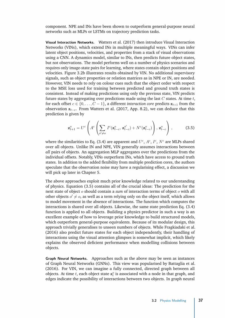
component. NPE and INs have been shown to outperform general-purpose neuralnetworks such as MLPs or LSTMs on trajectory prediction tasks.

Visual Interaction Networks. Watters et al. (2017) then introduce Visual InteractionNetworks (VINs), which extend INs in multiple meaningful ways. VINs can inferlatent object positions, velocities, and properties from a stack of visual observationsusing a CNN. A dynamics model, similar to INs, then predicts future object states,but not observations. The model performs well on a number of physics scenarios andrequires only image-state pairs for learning, where states contain object positions andvelocities. Figure 3.2b illustrates results obtained by VIN. No additional supervisorysignals, such as object properties or relation matrices as in NPE or IN, are needed.However, VIN needs to rely on colour cues such that the object order with respectto the MSE loss used for training between predicted and ground truth states isconsistent. Instead of making predictions using only the previous state, VIN predictsfuture states by aggregating over predictions made using the last C states. At time t,for each offset c ∈ {0, . . . , C − 1}, a different interaction core predicts zt+1 from theobservation zt−c. From Watters et al. (2017, App. 8.2), we can deduce that thisprediction is given by

zot+1 = U c

Ac

∑o′ 6=o

Ic(zot−c, zo′t−c) +N c(zot−c)

, zot−c

, (3.5)

where the similarities to Eq. (3.4) are apparent and U c, Ac, Ic, N c are MLPs sharedover all objects. Unlike IN and NPE, VIN generally assumes interactions betweenall pairs of objects. An aggregation MLP aggregates over the predictions from theindividual offsets. Notably, VINs outperform INs, which have access to ground truthstates. In addition to the added flexibility from multiple prediction cores, the authorsspeculate that the observation noise may have a regularising effect, a discussion wewill pick up later in Chapter 5.

The above approaches exploit much prior knowledge related to our understandingof physics. Equation (3.5) contains all of the crucial ideas: The prediction for thenext state of object o should contain a sum of interaction terms of object o with allother objects o′ 6= o, as well as a term relying only on the object itself, which allowsto model movement in the absence of interactions. The function which computes theinteractions is shared over all objects. Likewise, the same state prediction Eq. (3.4)function is applied to all objects. Building a physics predictor in such a way is anexcellent example of how to leverage prior knowledge to build structured models,which outperform general-purpose equivalents. Because of its modular design, thisapproach trivially generalises to unseen numbers of objects. While Fragkiadaki et al.(2016) also predict future states for each object independently, their handling ofinteractions using the visual attention glimpses is somewhat implicit, which likelyexplains the observed deficient performance when modelling collisions betweenobjects.

Graph Neural Networks. Approaches such as the above may be seen as instancesof Graph Neural Networks (GNNs). This view was popularised by Battaglia et al.(2016). For VIN, we can imagine a fully connected, directed graph between allobjects. At time t, each object state zot is associated with a node in that graph, andedges indicate the possibility of interactions between two objects. In graph neural

3.2 Physics Modelling 37

InputGraph

: Node: Interaction: Aggregation

FunctionsGNN

(a)

Frame True Prediction

Spri

ngs

Gra

vity

Mag

net

icB

oun

cin

g

(b)

Figure 3.2.: (a) Overview of the Graph Neural Network (GNN) architecture for relationalphysics modelling. In our case, a fully connected graph between all objectstates (z1t , z

2t , z

3t ) is assumed. The GNN makes future state predictions using

the same set of functions for each object, where each object is chosen to bethe focus node once. The node function N(zot ) is applied to the focus node o,and for each neighbour of the focus node, the interaction function I(zot , z

o′

t )is applied for all focus-node–neighbour-node pairs (o, o′). The aggregationfunction yields the next state by aggregating over the results of I and N , zot+1 =

A(N(zot ),∑

o′ I(zot , zo′

t )). While the procedure is depicted as a sequence in thegraphic, i. e. one object is predicted after the other, prediction can easily beparallelised in implementation. (b) Example simulations obtained from theVisual Interaction Network (VIN). The left column shows an example inputframe to the VIN architecture, the centre column visualises true trajectoriestaken by the balls in the various physics simulations, and the final column showsVIN’s well-matching predictions. Simulation images in (b) reconstructed fromWatters et al. (2017).

networks, the same set of operations is applied locally at each node zo. A set of GNNoperations matching the above would be: (a) the neural network N(zo) is applied tothe node itself, (b) then I(zo, zo

′) is applied for each neighbour o′ of o on the graph,

and (c) the results of the operations (a) and (b) are aggregated with A(·), whichfinally yields the output of the GNN at node zo. This architecture is demonstratedin Fig. 3.2a. Comparing this to the above models, we can now clearly see how VINcorresponds to a GNN with edges between all objects, IN corresponds to a GNN withedges specified by the interaction matrix, and NPE corresponds to a GNN whereedges are assigned dynamically depending on the current distances between objects.For a thorough introduction and review of GNNs, the reader is referred to eitherZhou et al. (2018) or Wu et al. (2019b). STOVE uses a GNN similar to Eq. (3.5) asits physics prediction module, which we will present in Section 4.2.

3.2.3 Tangential DevelopmentsZheng et al. (2018) extend INs to extract physical properties from object state tra-jectories. Simulator-based approaches remain popular, and Wu et al. (2016, 2017)make Galileo more efficient and performant by replacing expensive sampling-basedinference routines with neural networks. Jaques et al. (2020) use a differentiablephysics engine, which enables end-to-end gradient-based learning. Interaction mech-anisms similar to I(·, ·) in Eq. (3.5) present a useful inductive bias to other tasks inmachine learning which require reasoning about relations between entities. Santoro


et al. (2017) introduce Relation Networks (RNs) and show that such interactionmechanisms are useful to solve a variety of visual or text-based question answeringtasks.

Physical Tracking. Ehrhardt et al. (2018) learn a multi object-tracker using the phys-ically motivated principles of causality and equivariance, resulting in an adversarialstyle training with data augmentation. For each stack of input frames, a randomlywarped version is created. Equivariance then ensures that the warped version of theinput images results in an appropriately warped trajectory. Causality is motivated bythe desired smoothness of the obtained trajectories. Random permutations of realtrajectories, which violate smoothness, are generated, and a discriminator is trainedto discern between real and permutated trajectories produced by the tracker. Alsorelevant is their later work (Ehrhardt et al., 2019), where a single model learns toaccommodate a variety of physics simulations by explicitly inferring the currentlyactive scenario from a stack of past observations.

GNNs for Particle Simulations. GNNs have been applied to physical simulationsof increasing complexity in supervised scenarios. Sanchez-Gonzalez et al. (2018)propose a generalisation of INs and apply it to the DeepMind Control Suite (Tassaet al., 2018). Recently, Li et al. (2019) and Sanchez-Gonzalez et al. (2020) haveused large GNNs with up to ten-thousand particles to obtain realistic simulations offluids, rigid objects, or deformable objects in three-dimensional environments.

Neural ODEs. Another interesting and related line of work are Neural OrdinaryDifferential Equations (Neural ODEs) (Chen et al., 2018), where neural networksare used to parametrise the time derivative of some unknown dynamical systemdf(z(t))/dt = NN(z(t), t;θ). This ODE is then solved using differentiable versions ofstandard ODE integrators and gradient-based learning optimises the parameters θ ofthe network to produce time derivatives which result in trajectories z(t) in agreementwith the training set. Neural ODEs can model continuous-time processes and easilyincorporate irregularily sampled data. They can be seen as infinite depth normalisingflows. Lutter et al. (2019), Cranmer et al. (2020), Greydanus et al. (2019), andToth et al. (2020) explicitly constrain neural ODEs to modelling physical systems byinterpreting the neural ODE in relation to a physical Hamiltonian or Lagrangian.They show successful application on dynamical systems such as chaotic pendulums orn-body systems, where they achieve energy conservation. Kolter and Manek (2019)similarly constrain a neural ODE to produce stable dynamics using the concept ofLyapunov functions from chaos theory. The above approaches will likely fail, ifthe underlying dynamics may not be well approximated by an ODE. It is unclearhow well they scale to discontinuous dynamics or more general scenarios. However,extensions of neural ODEs to stochastic processes exist (Jia and Benson, 2019).

3.3 Video Modelling3.3.1 General-Purpose Video ModelsWe refer to video prediction as the conditional prediction of future frames xt+1

from a history of observations (x1, . . . ,xt), where observations correspond to high-dimensional images. Often, such models are trained in self-supervised fashionby comparing the prediction xt+1 to the true and readily observable xt+1. Video

3.3 Video Modelling 39

modelling is treated akin to image modelling, where, depending on the application,unconditional sampling of new videos, tractable video likelihood evaluation, orthe inference of informative sequence- or image-level latents is desired. General-purpose non-linear latent state sequence models, such as the VRNN (Chung et al.,2015), see Section 2.3.2, may of course also be used to process and predict futureframes in videos. In fact, the VRNN is a popular baseline in the object-aware videomodelling community. However, other architectures purpose-built for videos alsoexist. They are often motivated by applications in (model-based) reinforcementlearning, prediction, classification, or content creation.

The discussion of generative models of video is similar to that for sequence models,see Chapter 2, and image models in Section 3.1 above. Srivastava et al. (2015)present an early approach to multi-step video prediction. Simple enough, they usean LSTM which consumes the sequence of images and is trained in a self-supervisedfashion. The fully connected layers of a standard LSTM are unsuited to accommodatecomplex visual scenarios. This motivates Xingjian et al. (2015) to introduce theConvolutional LSTM (ConvLSTM), combining CNNs and LSTMs, which they applyto precipitation forecasting, outperforming state-of-the-art alternatives. Oh et al.(2015) extend this and feed a small stack of frames to a CNN-based autoencodingarchitecture to produce action-conditioned frame predictions in ATARI video games.For up to 100 frames, they achieve stable predictions useful for applications inmodel-based control. Multiple models (Finn et al., 2016; Liu et al., 2017; Mathieuet al., 2016) reframe video prediction as pixel-wise motion prediction, i. e. opticalflow. A MSE-based loss does not differentiate well between a model that has learnedvisually appealing behaviour and one that has not. Likewise, MSE-style losses areincompatible with multiple futures, i. e. multiple plausible future frame predictionsgiven the history of observations. This can lead to blurry or implausible output. Toapproach these problems Vondrick et al. (2016), Mathieu et al. (2016), and Leeet al. (2018) employ a GAN-style adversarial loss. Similar to our argument forthe advantage of including stochasticity in sequence models, many have arguedthat deterministic models fail to capture the stochasticity inherent to videos as well.Therefore, many in the community have shifted towards probabilistic models ofvideos such as Kalchbrenner et al. (2017), Babaeizadeh et al. (2018), Lee et al.(2018), or Denton and Fergus (2018). Many of these approaches can be set inrelation to the non-linear sequence models of Section 2.3. Finally and recently,Kumar et al. (2020) apply normalising flows to video modelling, while Weissenbornet al. (2019) present an autoregressive approach based on self-attention networks.

3.3.2 Object-Aware ApproachesAn object-based representation of videos learned in an unsupervised fashion couldbe hugely beneficial to applications, for example in reinforcement learning androbotics. Reasoning about the effects of actions and understanding the interactionsbetween the objects present is crucial to learning intelligent agents. While suchreasoning capability is difficult to obtain from raw pixels directly, object-based videomodels and their latent representations might provide a compelling inductive bias.This argument for object-aware video models is similar to that made for object-aware image models. For object-aware video models, one can additionally makethe case that future frame predictions should be superior to unstructured models insuitable scenarios. If the objects are clearly discernible and move predictably, e. g.determined by physical laws or external actions, it is much easier to understand


and predict the movement of a limited number of objects rather than that of manyindividual, unstructured pixels. This idea is at the core of object-aware imagemodelling. Additionally, learning object-based representations from video should infact be simpler than learning them from single images. Compared to object-awareimage models, the presence of time in video has been argued to be a helpful bias forobject detection in video models (Kosiorek et al., 2018). After all, if a mass of pixelsmoves coherently and predictably throughout the frames of the video, it is likely tobe part of the same object. Kosiorek et al. (2018) and Hsieh et al. (2018) presenttwo approaches which extend the Attend-Infer-Repeat framework to sequences. Bothare highly related work to our approach, and we will compare against them inChapter 5.

SQAIR. Kosiorek et al. (2018) propose Sequential Attend-Infer-Repeat (SQAIR)to extend AIR to sequences. Much of the complexity in SQAIR is in its aspirationto handle a varying number of objects between different frames of the same video.At each timestep, SQAIR not only has to discover all objects, but it has to decide ifany object can be matched with an object from the previous frame, or if it insteadbelongs to a new object which has just appeared in the video. While AIR usesa single LSTM to attend to the objects of a static image, SQAIR uses a total ofthree different LSTMs for its inference routine: One updates object states betweenframes, another models relations between objects, and lastly, a third LSTM is usedto discover new objects. This mesh of RNNs across time and space leads to O(O · T )algorithmic complexity. The processes of old-object propagation and new-objectdiscovery are likewise present in the generative model. The authors find that SQAIRis indeed more successful than AIR at discerning partially or heavily occluded objects,demonstrating that video does indeed have a regularising effect on object detection.SQAIR is applied to a simulated dataset of moving handwritten numbers – ananimated version of MNIST (LeCun et al., 1998) – and simple but realistic CCTVvideo footage of walking pedestrians.

DDPAE. Concurrently to SQAIR, Hsieh et al. (2018) introduce the DecompositionalDisentangled Predictive Autoencoder (DDPAE). Like SQAIR, DDPAE presents anextension of AIR to videos. Compared to SQAIR, the architecture of DDPAE isconceptually simpler. It does not include a fully generative model of videos andfocuses on conditional generation instead. Also, it lacks the complex discoveryand propagation networks, instead assuming a constant number of objects withconstant appearance per sequence. The constant appearance is inferred from anaggregation RNN which smoothes over all appearance vectors from the individualframes. This mechanism results in good modelling of overlapping objects. Forinference, DDPAE also uses a two-dimensional recurrence over objects and time,such that they arrive at the same algorithmic complexity as SQAIR. For future stategeneration, a RNN-based model is proposed, which the authors claim is able tohandle interactions. Here, the DDPAE is again a bit more explicit than SQAIR,as future states are predicted as offsets to previous states. Like the original AIR,the authors demonstrate generalisation to novel numbers of objects. DDPAE isdemonstrated on moving MNIST data and bouncing balls.

NEM. A distinctive approach is presented by Greff et al. (2017). Neural ExpectationMaximisation (NEM) learns a pixel-wise mixture model, using a neural variant ofthe expectation maximisation (EM) algorithm. Essentially, a neural network predicts

3.3 Video Modelling 41

the pixel-wise mixture distribution from latent cluster representations. They unrolland backpropagate through the EM steps. Unlike in AIR, objects in NEM do notnecessarily correspond to a localised collection of pixels. Its iterative procedureneeds multiple steps, about ten, for the clusters to converge, which is undesirablefor many applications. Additionally, NEM requires binarised input with added noiseto avoid unstable behaviour. Notably, the successor, Relational Neural ExpectationMaximisation (R-NEM), employs a relational reasoning module between objectssimilar to the approaches of Battaglia et al. (2016) and Santoro et al. (2017).

Object-aware sequence models have not been shown to be capable of modellingrealistic videos. However, currently, unstructured approaches show only limitedperformance in this domain as well. Nevertheless, on low-complexity videos withclearly defined objects, object-based approaches regularly outperform unstructuredmodels. This is currently restricted to simulated and visually simple, two- or three-dimensional environments. One can only speculate that some sort of object-inspiredstructure should also be beneficial in modelling real videos. Therefore, scalingobject-aware approaches to such environments presents a fruitful avenue of futurework. We will now discuss some recent and tangential developments related toobject-aware video models.

3.3.3 Tangential DevelopmentsApproaches such as Finn et al. (2016) and Goel et al. (2018) model the move-ment between two frames of video in terms of the movement of a fixed number ofpixel-wise movement masks. While these approaches are not necessarily motivatedby future frame prediction, they may still obtain an object-like representation andsegmentation, which they demonstrate to be beneficial to reinforcement learningin ATARI video games and robotics. As many approaches to object-oriented videoprediction are motivated by such applications, a rising amount of work fuses rein-forcement learning models and object-based representations. For example, Watterset al. (2019) use object-representations obtained from a MONet-like vision mod-ule for data-efficient model-based reinforcement learning in a simple, sprite-based,two-dimensional simulation.

Since the proposal of our model, a number of new and related approaches have beenpublished. Jiang et al. (2020) parallelise the attention mechanism in SQAIR, suchthat they are able to demonstrate the successful application of their method to sceneswith more than 60 objects. Another recent proposal by Akhundov et al. (2019),assumes a Markovian state space for dynamics modelling, similar to our approach.Kipf et al. (2020) learn an object-oriented latent embedding on sequences withoutrelying on pixel reconstructions using a contrastive loss objective, which solelyapplies to the latent space embeddings. They employ a GNN to model transitionsin this latent space. In Fuchs et al. (2019), the authors use GNNs to extend theirattention-based tracking algorithm (Kosiorek et al., 2017) to the multi-object setting.Veerapaneni et al. (2019) introduce OP3, making first steps towards generalising aMONet-like image model to sequences with a GNN-based transition model. OP3 isapplied for planning in a discrete prediction task.


4Structured Object-AwarePhysics Prediction for VideoModelling and Planning

After the previous chapters have introduced the motivation for object-aware videomodelling, relevant concepts, and related works, we may finally turn our attentionto Structured Object-Aware Physics Prediction for Video Modelling and Planning(STOVE).1,2 The theoretical formulation of STOVE in this chapter and its experimen-tal evaluation in the following chapter comprise the main contribution of this thesis.STOVE presents a self-supervised approach to learning models of videos of physicallyinteracting objects. Given a sequence of images {xt}Tt=1, we assume the existenceof Markovian latent states {zt}Tt=1, which fully explain the observations and, giventhe right transition function, allow for the prediction of future states and observa-tions. STOVE is obtained as the composition of a Sum-Product Attend-Infer-Repeat(SuPAIR) image model, see Section 3.1.2, and a Graph Neural Network (GNN) forrelational physics modelling, predicting transitions in latent space, see Section 3.2.2.The above combination gives a non-linear latent state space model (SSM), see Sec-tion 2.3. Unlike in linear state space models, the conditional distributions are notparametrised by linear operations but rather neural networks or deep probabilisticmodels. To allow for tractable learning, we introduce an amortised variational ap-proximation to the true posterior and optimise all model components jointly via theresulting ELBO. The SuPAIR-like image model interfaces with the observations xt inpixel space, inferring latent state distributions q(zt | xt) and evaluating conditionalimage likelihoods p(xt | zt). The physics model then propagates these states forwardin time, realising the transition distribution p(zt+1 | zt). At the time of publication,STOVE presented the first extension of AIR image models to relational physicalreasoning in videos. While reading this chapter, the reader is referred to the Figs. 4.1and 4.2 for reference. Figure 4.1 gives a detailed overview of the workings of STOVE,while Fig. 4.2 displays the underlying graphical model and the structure of the latentspace. For a first overview of STOVE, let us introduce its defining characteristics:structure, object-awareness, physics prediction, video modelling, and planning.

Structure. In comparison to other approaches, STOVE exhibits a large amount ofpredefined structure. For one, the assumption of Markovian latent states in boththe generative model and inference routine is decidedly restricting, compared tomany of the much more general approaches in Section 2.3 and Chapter 3, such

1A PyTorch implementation of STOVE is provided at github.com/jlko/STOVE.2Concurrently to this thesis, a paper on STOVE will be published in the proceedings of the Eighth

International Conference of Learning Representations. This thesis and the paper share some of theresults and figures presented. While the work of my co-authors has been immeasurably important forthe creation of the paper, unless otherwise mentioned, the figures presented and experiments describedin this thesis have been created and performed by me.

43

http://github.com/jlko/STOVE

STsample

ObjectSPN

BGSPN

GenerativeIn

fere

nce

predict σ

Dynamics Model – GNN

Image Model – SuPAIRInference

Legend

Generative

LSTM

Axes

Time

Computation

to nexttimestep

fromprevioustimestep

InputImage

fix σ

Figure 4.1.: Overview of STOVE’s architecture. (Centre left) At time t, the input image xt

is processed by an LSTM in order to obtain a proposal distribution over objectstates q(zt | xt). (Top left) A separate proposal q(zt | zt−1) is obtained bypropagating the previous state zt−1 using the dynamics model. (Centre) Themultiplication of both proposal distributions yields the final variational distribu-tion q(zt | zt−1,xt). (Right) We sample zt from this distribution to evaluate thegenerative distribution p(zt | zt−1)p(xt | zt), where p(zt | zt−1) shares means –but not variances – with q(zt | zt−1), and p(xt | zt) can be obtained by directevaluation of xt in the sum-product networks, using the spatial transformeroperations, ST, for the objects. Not shown is the dependence on xt−1 in theinference routine, which allows for the explicit inference of velocities fromposition differences. Figure and caption also appearing in Kossen et al. (2020).

as VRNN and SQAIR. Additionally, the latent space itself is structured. Competingapproaches in video prediction often assume a largely unstructured latent space,usually with a normally-distributed prior. After training their models, they then lookfor meaning in the resulting latent space. In contrast to this, we directly specify ameaningful latent space, consisting of per object positions, velocities, and sizes. Thisfurther injects prior knowledge into the model, directly benefitting model stability,performance, and interpretability. In our experiments, this structure does not hindergeneralisation on the data explored. Instead, the right kind of structure benefitsperformance and interpretability due to a clear allocation of responsibilities betweenmodel components. As the SuPAIR-like image model does not rely on latent statesto model the object appearances, appearance information does not compete withdynamics information in the latent space. Of course, the assumptions of clearlydefined object positions, velocities, and sizes hold in all our experiments and would,depending on the application, have to be revisited. The following paragraph lists afurther structural constraint of STOVE.

44 Chapter 4 Structured Object-Aware Physics Prediction for Video Modelling and Planning

Object-Awareness. STOVE reasons about the world in terms of objects. As is com-mon for AIR-derivatives, see Section 3.1, images are constructed as the superpositionof objects atop a background. An image may be described in terms of object-specificlatent states zt = {zot}

Oo=1. A video is a sequence of T images, which likewise has a

corresponding sequence of latent states z = {zt}Tt=1. At each timestep, per objectpositions, velocities, and sizes are inferred from the given images using the scenemodel or propagated from previous latent states by the dynamics model. Whileobject-centric modelling of images is a novelty, object-centrality in physics modelling,where the goal is to approximate a sequence of object states, is an obvious pre-requisite. For videos, only few approaches to object-oriented modelling exist, seeChapter 3.

Physics Prediction. The movement of a single object in a video is rarely independentof its surrounding. Instead, complex interactions between objects affect individualobject trajectories. This is true for real-world scenarios such as the movements ofa self-driving car, as well as simpler applications such as video games. In physicsprediction and unsupervised video modelling, toy data sets of physically interactingobjects, such as bouncing or gravitationally attracted balls, are often used to mimicsome of this complexity. In such simulations, the trajectories of the individual objectsare highly non-linear and dependent on interactions with other objects. In STOVE,the transition of the per-object latent states p(zot | zt−1) is realised by a state-of-the-art physics prediction model, a Graph Neural Network (GNN). GNNs are specialrelational architectures which can be used to facilitate the modelling of interactivebehaviour in physics simulations. At the time of publication and to the best of ourknowledge, STOVE is the first AIR-video model capable of generatively modellingcomplex physical interactions. Our experiments show that models which do notinclude such a relational component in their transition model fail to appropriatelymodel interactions between objects and exhibit unrealistic trajectory predictions. Wesuspect that such relational modelling has meaning beyond toy datasets and willlikely be important for applications in real-world scenarios.

Video Modelling. A video model naturally arises from the components above. Theimage model allows STOVE to infer latent states from images q(zt | xt) as well asto render images from states p(xt | zt), while the sequence model allows for thepropagation of latent states through time p(zt | zt+1). Therefore, the combinationof the model over the images and the physics model over the states yields a modelover a sequence of images – a model of videos. The dynamics model and the imagemodel only interface via the object positions and velocities, see discussion below.While STOVE is expressive enough for the scenarios which we investigate, it wouldneed to be adapted for more complex situations where objects may change theirvisual appearance during the video sequence.

Planning. We propose an extension of STOVE from videos to video games, i. e. tothe setting of model-based control. For this, we modify STOVE such that it canpredict future frames, states, and rewards conditioned on external control inputs, oractions. In other words, STOVE is employed as a world model, a full simulation of theinteractive environment. One can then use STOVE in tandem with planning methods,acting in the environment to maximise rewards. The extension of STOVE beyondstrict physical simulation is an important step towards obtaining video models formore general scenarios with wider varieties of interactions and dynamics.

45

By simply going over the main characteristics that, more or less, spell out the lettersof STOVE, we have already introduced a significant proportion of what sets STOVEapart from other approaches. We will now introduce the details of the STOVEarchitecture.

4.1 Sum-Product Attend Infer Repeat for ImageModelling

We use a variation of the Sum-Product Attend-Infer-Repeat (SuPAIR) image model,as introduced in Section 3.1.2 and by Stelzner et al. (2019), to model the distributionof images x in object-aware fashion. The focus of STOVE is the proposal of a videomodel capable of modelling complex interactions between objects. We thereforeavoid the complexities of dealing with a varying number of objects during thesequence, see SQAIR (Kosiorek et al., 2018) and Section 3.3 for further details. Theoriginal SuPAIR architecture is simplified by constraining SuPAIR to a fixed numberof objects O. In Section 3.1.2, we have directly proposed this constrained SuPAIRvariant. The assumption of constant O simplifies inference, as we do not need toevaluate the expectation with respect to O in the ELBO during training. ExtendingSTOVE to a varying object count, which stays constant over the sequence, similar toHsieh et al. (2018), would be possible without much effort. Additionally, the originalSuPAIR employs an auxiliary loss term, which penalises overlapping bounding boxesbetween objects. Without it, SuPAIR can predict superfluous objects without beingpenalised. This is not needed in the O-constrained version of SuPAIR.3

Otherwise, there are deliberately few changes from the original SuPAIR architecture.Therefore, the components in STOVE take on clearly designed roles and have few butmeaningful interactions between each other. In Section 3.1.2, we have introduced theconditional likelihood model p(x | z), Eq. (3.3), which models the appearance of animage x using an SPN to assess object likelihoods, an SPN for background likelihoods,and spatial transformer layers. Likewise, we have introduced the recognition modelq(z | x), Eq. (3.1), which infers object latent positions and sizes zo(pos, size) in recurrentfashion. For STOVE, we use these components without any further changes. However,as we are now considering sequences of images, we endow the variables with anindex t, writing p(xt | zt), q(zt | xt), and zot,(pos, size) instead.

As a further inductive bias, we want to introduce velocities zot,velo to the latent state.While the experiments presented in Section 5.10 show that STOVE can indeeddiscover velocities and does not need them a priori, explicit velocities do provide animportant bias to improve model training. Also, they are straightforward for us to

3In the original SuPAIR, if a superfluously predicted object o′ is completely on top of a previousbounding box, all pixels of o′ are marginalised over, such that it does not contribute to the ELBO, butleads to a wrong object count. One therefore needs an auxiliary loss term to combat this behaviour.In the O-constrained version, such behaviour may not occur because each bounding box needs tocover an object. If a bounding box completely overlaps with a previous box, such that it is completelymarginalised over, an object of the scene is missed by the attention model. This object, which isnecessarily not covered by any bounding box, then causes a loss because it must be part of thebackground, and the background SPN is likely to assign a low background likelihood.


implement from position differences as

q(zot,velo | xt,xt−1) = N (zot,velo;µot, pos, i − µo

t−1, pos, i,

(σ2)ot, pos, i + (σ2)ot−1, pos, i) , (4.1)

where the uncertainty results from the additive combination of the two independentGaussian position variables in a principled probabilistic way. The subscript i refersto the fact that the mean and variance proposals for the latent state are inferred bythe image and not the dynamics model.

A few hyperparameters guide the predictions of SuPAIR. A possible failure mode ofSuPAIR is that the background model may learn to model full scenes on its own,disregarding the object mechanism. To avoid this behaviour, Stelzner et al. (2019)have found it helpful to bias the structure of the background SPN towards lesscomplex appearances. Another possible failure is the prediction of a single image-sized object or the prediction of zero-sized objects. To avoid such problems, the sizeof objects are lower- and upper-bounded to be 10 % and 90 % of the total image size.See Appendix A.4 for an exhaustive list of hyperparameters and default values.

In addition to training speed, there is an unexpected advantage of using SuPAIR overAIR in the context of physics prediction. We require the obtained object positionsfrom the attention network to be as precise as possible. For this, it is essential that theobject is always well-centred within the bounding box. In SuPAIR, we can observethis property and notice a decrease in likelihood for off-centre bounding boxes.In other AIR-like models, this is not necessarily the case. Due to the un-structureof the latent space, AIR may learn latent states which encode the position of theobject within the bounding box, yielding accurate reconstructions even for off-centreboxes. While additional information in the latent state will incur a loss in the KLdivergence, such behaviour is still observed in AIR models. Because SuPAIR avoidsthe unstructured appearance latent, it cannot encode object positions within thebounding box and consequently learns to predict well-centred bounding boxes.

As SuPAIR is already a probabilistic model framed in terms of amortised varia-tional inference, its integration into the STOVE architecture is almost effortless, seeSection 4.3.

4.2 Graph Neural Networks for Physics Modelling

In Section 3.2.2, relational physics modelling was presented from the perspective ofsupervised machine learning, where learning is usually accomplished by minimisinga squared loss between predicted and observed trajectories from the training set. InSTOVE, we need to embed such a physics model into the probabilistic state spacemodel. Instead of directly predicting future states zt+1, the physics model needs topredict transition probabilities p(zt+1 | zt). A simple approach to accomplish this isto use the predictions from the physics model as means of a factorised Gaussian with

4.2 Graph Neural Networks for Physics Modelling 47

fixed standard deviations

µot+1, (pos, velo, latent) = A

N(zot ) +∑o′ 6=o

α(zot , zo′t ) I(zot , z

o′t )

(4.2)

µot+1, (pos, velo, latent) = U

(µot+1, (pos, velo, latent), z

ot

). (4.3)

We have introduced the governing ideas behind relational physics modelling alreadyin Section 3.2.2. The prediction of the future latent state is given by a concatenationof functions, Eqs. (4.2) and (4.3), which is applied to each object independently.For each object, the prediction is given by a function N(zot ) applied to the currentfocus node, modelling object movement independent of interactions, plus a sumover its interactions I(zot , z

o′t ) with neighbouring objects o′. The function A(·) is used

to aggregate over these terms. Similarly, U(·) represents aggregation in addition toa skip connection to the input state and, for reasons that will become obvious in Sec-tion 4.4, we introduce the intermediate results µo

t+1, (pos, velo, latent). The interactionfunction is reused over all objects pairs. The different functions are parametrisedby MLPs. In addition to the familiar functions mentioned above, we introduce anattention term α(zot , z

o′t ) > 0. Like the interaction module, it is applied to each

pair of focus object o and neighbouring object o′ and shared over predictions for allobjects o ∈ (1, . . . , O). The attention term strictly increases the modelling flexibilityof STOVE. In simulation settings where not all possible interactions between objectsmight be relevant at all times, α(zot , z

o′t ) presents a learned version of the hard and

prespecified mechanism employed by NPE in Eq. (3.4). This allows STOVE to modelscenarios with discrete interactions, such as collisions, in a similar fashion as NPE,where intuitively, the attention term can switch these interactions on and off, whilethe interaction term models their outcome. However, STOVE can also accommo-date scenarios where a hard attention mechanism is not appropriate, combiningthe advantages of VIN and NPE. A similar attention mechanism is used by R-NEM,introduced in Section 3.3. Unlike VIN, we find that a single prediction core sufficesfor convincing performance.

Instead of predicting new states directly, NPE predicts velocity differences and usesthose to update states, see Section 3.3. Similarly, we bias STOVE towards predictingnew positions as offsets to old ones. This inductive bias is useful for scenarios withsmoothly moving objects. However, this offset is not given by zt,velo, as our velocityestimate at time t relies on past information from t− 1 and is therefore inaccurateduring collisions, i. e. at the time of collision, the true, instantaneous velocity changesare not yet reflected in our observational velocity. Instead, the offset to the lastposition is predicted directly by the GNN. Otherwise, much of the structure of theMLPs of the dynamics GNN is straightforward. They consist of a couple of layers offully connected neural networks, with skip connections and ReLU non-linearities.Equation (4.3) is implemented efficiently and computed for all objects in parallelusing tensorised code. This is true also for the interactions, which are computedin parallel using stacking and replicating operations. Appendix A.2 gives the fulldetails.

So far, we have introduced the object position, velocity, and size as latent spacecomponents. For physics modelling, we extend the latent space by unstructured


zt−1 zt

xt−1 xt

(a)

zot,velo

zot,size

zot,pos

zot,latent

q(zot,pos | zt−1) · q(zot,pos | xt)

q(zot,velo | zt−1) · q(zot,velo | xt,xt−1)

q(zot,size | xt)

q(zot,latent | zt−1)

(b)

Figure 4.2.: (a) Depiction of the graphical model underlying STOVE. Black arrows denote thegenerative mechanism and red arrows the inference procedure. The variationaldistribution q(zt | zt−1,xt,xt−1) is formed by combining predictions from thedynamics model q(zt | zt−1) and the object detection network q(zt | xt,xt−1).(b) Components of the per-object latent state zot and corresponding variationaldistributions. Note that the velocities are estimated based on the change inpositions between timesteps, inducing a dependency on xt−1. Figures adaptedfrom the original graphics by Karl Stelzner. Figures and caption first producedfor Kossen et al. (2020).

latent space zot,latent. In VAE fashion, this latent space is regularised towards

zo1,latent ∼ p(zo1,latent) = N (zo1,latent;0,1) . (4.4)

In essence, the motivation for this latent space is to give the GNN extra modellingcapabilities: Additional information about the object states not included in position,approximate velocity, or size can be stored in the latent space by the GNN. Forexample, the latent state space may be used to account for different dynamicalbehaviour between objects. This may be needed because the same function Eq. (4.3)is used to predict the dynamics of all objects. Therefore, without the latent space,if two objects have the same position, velocity, and size, the GNN must predict thesame future state distribution. It cannot account for differences between objectsthat are not present in the latent state. With the introduction of unstructuredlatent space, such differences can now be reflected, which then allows the GNNto account for them as well. Experiments have indicated that the unstructuredlatent is indeed essential for modelling performance. In addition, preliminaryexperiments have shown that the unstructured latents may contain higher orderderivatives, i. e. accelerations. The following reflections indicate that this mayindeed be necessary: We have already mentioned issues with the observationalvelocity during collisions. Because we observe a discretised sequence of images,the position differences observed during collisions usually do not correspond tothe true, instantaneous object velocities. It follows that the original latent space ofpositions and observational velocities is, in a first order Markov model, not enough toaccurately model the dynamics because we cannot predict the outcome of collisions.The unstructured latent space allows to account for that. See Section 5.10 forfurther discussion. Even in the worst case, if the model does not need the latentspace in some scenario, it can easily be ignored and should not negatively affectperformance.

4.2 Graph Neural Networks for Physics Modelling 49

4.3 Joint State Space ModelAbove, we have established the two defining components of STOVE, the Sum-Product Attend-Infer-Repeat (SuPAIR) image module and the Graph Neural Network(GNN) relational physics module. We now identify them with the correspondingdistributions in our non-linear state space model, see Fig. 4.2.

For the generative model, we decompose the joint likelihood over observations andlatent states as

p(x1:T , z1:T ) = p(x1 | z1)p(z1)T∏t=2

p(xt | zt) p(zt | zt−1) , (4.5)

using the chain rule of probability and the Markov property of the latent states. Here,p(xt | zt) is given by the generative model of SuPAIR, Eq. (3.3), and p(zt | zt−1) is asdescribed by Eq. (4.3). The prior p(z0) is assembled from the uniform priors overobject positions and sizes of SuPAIR and the normal prior over the unstructuredlatents of the dynamics model.

As inference in the non-linear state space model is intractable, we formulate arecognition model for amortised inference of z ∼ q(z | x), see Section 2.2. Attime t, we can use SuPAIR’s inference routine to infer latent states q(z | xt,xt−1).4

Such an approach is common in non-linear state space models, see the detaileddiscussion in Section 2.3. However, in doing so, we would disregard all informationfrom the dynamics model. Instead, we can construct a joint estimate of the currentlatent state position and velocity using information from both the image and thedynamics model, by introducing a variational approximation to the dynamics modelq(zt, (pos, velo) | zt−1). A naïve approach to do this would be to construct a seconddynamics model with identical architecture but separate parameters. Instead, we effi-ciently reuse the generative GNN for inference, i. e. the means of q(zt, (pos, velo) | zt−1)and p(zt, (pos, velo) | zt−1) are identical and as given by Eq. (4.3). The benefits of thisreuse are discussed below. The joint estimate from both models is given as

q(zt, pos | xt,xt−1, zt−1)

∝ q(zt, pos | xt,xt−1) · q(zt, pos | zt−1) (4.6)

= N (zt, pos; µt, pos, i, σ2t, pos, i) · N (zt, pos; µt, pos, d, σ

2t, pos ,d)

∝ N (zt, pos;µt, pos, σ2t, pos) (4.7)

µt, pos =σ2t, pos, d µt, pos, i + σ2

t, pos, i µt, pos, d

σ2t, pos, d + σ2

t, pos, i(4.8)

1

σ2t, pos

=1

σ2t, pos, d

+1

σ2t, pos, i

, (4.9)

where the subscripts i and d denote the respective parameters from the imageand dynamics model, and we proceed the same way for q(zt, velo | xt,xt−1, zt−1).5

4Dependence on xt−1 serves as a reminder that we use the position distribution previouslypredicted by SuPAIR to assemble an estimate of the velocity, see Eq. (4.1). As xt−1 is not used anyfurther, e. g. for filtering estimates about the current position or size, we might sometimes omit thedependency to avoid confusion.

5In principle, one could also obtain estimates of zt,size in identical fashion. However, as this seemedto impact model training negatively, we rely on SuPAIR only for the estimate of the object sizes.


Because both models output factorised Gaussian distributions, their product is againproportional Gaussian with means and variances as given by Eqs. (4.8) and (4.9).Equation (4.6) presents a principled probabilistic way to combine uncertain Gaussianinformation from two sources, similar to the measurement step in a Kalman filter(Murphy, 2012, p. 641). The predicted state mean in Eq. (4.8) is weighted by theuncertainty in the two source distributions, naturally preferring certain informationwith small variances over uncertain information. Uncertainty in one measurementincreases the overall uncertainty. For the generative dynamics model p(zt | zt−1),means are predicted by Eq. (4.3) and variances fixed. To allow the dynamics modelto make use of the probabilistic combination, we predict variances for q(zt | zt−1) asadditional outputs of the GNN, Eq. (4.3).

This approach is inspired by Becker-Ehmck et al. (2019) and Karl et al. (2017b),who have, however, used it in single-object settings only. In addition to modellingefficiency and more precise estimates of zt, they give another justification for thereuse of the generative dynamics model for inference: The dependency of zt on thedynamics model leads to a favourable backpropagation of the image model throughthe dynamics model. In other words, because the quality of the samples zt nowdepends on the dynamics model, the dynamics model becomes crucial for obtaininga well-working model. If the dynamics model provides bad or uncertain estimates,samples are bad, and learning is significantly hindered for all model components,including the image model. Without this mechanism, a bad dynamics model wouldlead to a penalty in the transition prior, Eq. (4.5), but the image model could stillbe trained well, as samples would be unaffected. Furthermore, this mechanismis an algorithmically efficient way to couple inference for dynamics and imagemodels without introducing computational burden, as SuPAIR inference may stillbe performed for all images in parallel. SQAIR and DDPAE instead introduce acostly double recurrence, with complexity O(O · T ) over objects and time to formestimates zt, see Section 3.3.2. STOVE instead requires O inference operations forall images in parallel, followed by T prediction steps for the dynamics model for allobjects in parallel, keeping the total complexity to only O(O + T ).

For the sequence of observations x1:T and corresponding latent states z1:T , wedecompose the recognition distribution as

q(z1:T | x1:T ) = q(z1 | x1)

T∏t=2

q(zt | xt,xt−1, zt−1) , (4.10)

where q(zt | xt,xt−1, zt−1) is given by Eq. (4.6). Note that similar to the discussionin Section 2.3, we would also be allowed to condition on future observations in therecognition network. However, similar to Krishnan et al. (2017), we have foundthe above formulation to be sufficient. The initialisation of the model is given byq(z1 | x1), which is obtained from the image model only, see Appendix A.3 for fulldetails of model initialisation.

We train the generative model and the recognition model jointly by maximising the

4.3 Joint State Space Model 51

ELBO, Eq. (2.10), which for a sequence of images x1:T is given by

log p(x1:T ) ≥ Eq(z1:T |x1:T )

{log

p(x1:T , z1:T )

q(z1:T | x1:T )

}= Eq(z1:T |x1:T )

{log

{p(x1 | z1) p(z1)q(z1 | x1)

}

+

T∑t=2

log

{p(xt | zt) p(zt | zt−1)q(zt | xt,xt−1, zt−1)

}}, (4.11)

where we approximate expectations Eq(z1:T |x1:T ){·} with a single chain of sam-ples z1:T . In practice, STOVE is trained using mini-batch gradient descent, i. e.gradients from Eq. (4.11) are accumulated over multiple sequences {(x1:T )n}Nb

n=1

before parameter updates are applied. We use the reparametrisation trick (Kingmaand Welling, 2014; Rezende et al., 2014), see Section 2.2, to correctly evaluate thegradient with respect to the expectation over q(z1:T | x1:T ). Equation (4.11) is notmodified with ad-hoc auxiliary losses, as are common practice in supervised physicsmodels, and all model components are trained from scratch without pretraining.

The attention LSTM of STOVE’s image model is not guaranteed to preserve the objectorder between individual timesteps. We therefore face the challenge of matchingthe order of the object proposals between dynamics and image model and timesteps.A simple but effective solution to this is to match states based on the Euclideandistance ‖·‖ between their positions. More precisely, we first ensure a consistentobject order in the recognition distributions q(zt | xt) = N (zt; µt,i,σ

2t,i) from the

image model i by matching objects between timesteps such that ‖µot,pos,i−µo′

t−1,pos,i‖is minimised. Because the dynamics model is initialised from states inferred with theattention LSTM, see Appendix A.3, we now have consistently sorted states over timebetween the dynamics and object model. A naïve implementation of this sortingproblem has complexity O(O!). However, using the Hungarian algorithm (Kuhn,1955), the assignment problem can be solved exactly in polynomial time O(O3). Forsmall O ≤ 3, the naïve implementation suffices. For large O, a greedy approximationto the exact solution can be obtained in O(O2), which may however lead to adverseeffects on model training. Even for an exact implementation of matching, the solu-tions obtained are correct only if objects move sufficiently little between timesteps,which should, however, be a fair assumption for any reasonable discretisation ofcontinuous physics simulations. Note that many supervised approaches such as VIN(Watters et al., 2017) circumvent the need for matching by assigning the objects afixed order based on their, presumed to be distinctive, visual appearance. This is notrequired for STOVE, although we will investigate appearance-based matching, inaddition to the position distances, see Section 4.4. Section 6.1 discusses ways ofmodifying the model structure to omit the need for matching.

As part of our attempt to fully disentangle dynamics and visuals, STOVE, like e. g.DDPAE (Hsieh et al., 2018), cannot model changes in object appearance over time.During rollouts, approximate MPE in the SPNs is used to render novel images(Vergari et al., 2018). Karl et al. (2017a) have argued that a latent space whichcompetes between modelling visuals and dynamics is a significant cause for flaweddynamics performance. STOVE does not struggle with this per construction, asthe latent space does not model object appearances. Extensions to STOVE that do


zt−1 zt

xt−1 xt

at−1 rt

Figure 4.3.: (a) Depiction of the graphical model underlying the action-conditioned variantof STOVE. State predictions of the dynamics model p(zt | zt−1,at−1) are nowconditioned on actions at−1 of the agent. The dynamics model is extended topredict a distribution over the reward p(rt | zt−1,at−1). Black arrows denotethe generative mechanism and red arrows the inference procedure. The varia-tional distribution q(zt | zt−1,at−1,xt,xt−1) is formed by combining predictionsfrom the dynamics model q(zt | zt−1,at−1) and the object detection networkq(zt | xt,xt−1). Figure adapted from original graphic by Karl Stelzner. Figureand caption first produced for Kossen et al. (2020).

consider dynamically changing visuals are left for future work, although first stepshave already been taken by Voelcker (2020).

4.4 Conditioning on ActionsIn reinforcement learning, an agent executes actions at to maximise an expectationover future rewards r in an environment with observations xt. Recently, muchattention has been given to model-based approaches to reinforcement learningin visually complex domains, see e. g. Schrittwieser et al. (2019), Kaiser et al.(2020), Watters et al. (2019), or Veerapaneni et al. (2019). For such approaches, asophisticated simulator of the environment, or other relevant quantities, is required.After such a simulator has been learned, it can, for example, be used for planning:The simulator is used to predict the cumulative rewards of many different possiblesequences of actions, after which the most promising action is executed in the realenvironment. This is in contrast to model-free approaches, which learn to act directlyin the environment. The acquisition of observation samples xt is often expensive inreal-world settings. A main motivation for model-based approaches is their presumedsample efficiency, see the citations above for support of this.

An extension of STOVE allows its use as a world model in model-based control.6 Fig-ure 4.3 reflects the changes to the graphical model of STOVE for action-conditioning.

6Model-based reinforcement learning remains a footnote in this thesis. The extension of STOVE asan action-conditioned world-model was done in collaboration between all co-authors. The experimentson STOVE’s predictive capabilities presented in this thesis were performed by me. Kossen et al. (2020)contains additional experiments, where Monte-Carlo Tree Search (MCTS) (Coulom, 2006) was usedfor planning with STOVE as a world-model and its performance compared to suitable baselines. Thoseexperiments were performed by Claas Voelcker and Marcel Hussing, and they are not presented in thisthesis. Further experiments with STOVE in the context of model-based reinforcement learning maybe found in Voelcker (2020) and Hussing (2020). For the scope of this thesis, we will only evaluateSTOVE’s capabilities as a generative action-conditioned video model, isolated from applications inreinforcement learning.

4.4 Conditioning on Actions 53

STOVE’s dynamics prediction is extended to consider actions p(zt | zt−1,at−1),and likewise for the variational approximation q(zt | zt−1,at−1). The dynamicsmodel predicts states per object, Eq. (4.3), but we want STOVE to make no a prioriassumptions about which objects are affected by actions. Therefore, actions areconcatenated to the state representations of all objects in Eq. (4.3). This allowsthe GNN to infer when actions are relevant for accurate prediction. Additionally,the dynamics model is extended to provide predictions of rewards p(rt | zt−1,at−1)via

µt+1, reward = R2

(O∑

o=1

R1

(µot+1, (pos, velo, latent)

)). (4.12)

In other words, we reuse intermediate results µot+1, (pos, velo, latent) from the dynamics

GNN, Eq. (4.2). The agent receives a reward per observation, not per observationand object. We therefore need to transform the per-object predictions of the GNN toa single reward prediction per observation. A simple and order-invariant mechanismto achieve this is the summation over all per-object terms. For added modellingflexibility, R1 transforms the intermediate prediction before and R2 after summation,see Appendix A.2 for details. It may seem like an arbitrary decision to reuse partsof the dynamics model for reward prediction. However, similar to the prediction ofobject dynamics, the observed reward is likely to depend on interactions between ob-jects. It is therefore plausible that an intermediate representation µo

t+1, (pos, velo, latent)presents a suitable starting point for both reward and dynamics prediction. Theweight of the reward loss in the total ELBO is linearly increased during training untila maximum weight is reached. This corresponds to a decrease in the variance of thedistribution p(rt | zt−1,at−1).

We stress that this extension of STOVE to action-conditioned video predictionpresents a departure from its original use for modelling of videos of physicallyinteracting objects. In physics simulation, all objects are subject to the same lawsof motion. In reinforcement learning environments, interactions between objectsare more general. Even for the simple application of action-conditioned videoprediction presented in Chapter 5, actions discretely affect the motion of a singleobject, upsetting the balance of physical simulations. This presents a challenge to thedynamics GNN, which models the motion of each object individually using the samefunction. To lighten the burden on the GNN, we extend the object-representationzot, (pos, velo, latent) in the dynamics model with visual input vo

t , such that the GNN maydirectly discern if objects have different visual appearances. This latent appearanceencoding may be obtained from the representation encoded in the object SPN ofSuPAIR, see Vergari et al. (2018). Alternatively, a VAE, possibly with convolutionallayers, may be trained on the object glimpses to extract a latent encoding, as donein AIR. We opt for a simple alternative and construct vo

t from simple summarystatistics: the mean pixel value per colour channel of the object glimpse defined bythe bounding box.


5Evaluation and Discussion

This chapter contains a thorough experimental evaluation of STOVE. As introducedin Chapter 4, STOVE’s primary capabilities are the inference of object states from asequence of observed images, the reconstruction of a sequence of observed images,the prediction of future object state trajectories, and the prediction of future videoframes conditioned on a sequence of observed images. The prediction of future ob-ject positions or video frames is a much more demanding task than reconstructing orinferring from observations, as it much more relies on an adequate dynamics modelin addition to the image model. Therefore, the centrepiece of this evaluation will be acomparison of STOVE’s predictive performance to previously proposed unsupervisedvideo prediction models, upon which STOVE can improve.1 We evaluate STOVEon three tasks. Two of those tasks, billiards and gravity, are common benchmarksfor evaluating the capabilities of physics models. Additionally, we extend STOVEto consider action-conditioned state transitions, evaluating STOVE’s capabilities asa world model for planning. We further show that STOVE is able to conserve theaverage kinetic energy in the billiards scenario. This leads to visually convincingrollouts for extremely long timeframes, which have not been demonstrated by pre-vious approaches. Also, experimental considerations suggest that STOVE performsoptimally given the chaoticity of the billiards environment. We come to relevantconclusions concerning the general applicability of the billiards environment as abenchmark for physics models. A discussion of the effect of observation noise onthe supervised baseline is followed by a qualitative illustration of the stability ofthe predictions, STOVE’s performance on scenarios with different object visuals, anablation study, and some considerations with respect to STOVE’s scaling behaviour.The environments are fully introduced in the following section.

5.1 Introducing the Environments2

Figure 5.1 shows frames of videos from all environments.

Billiards Environment. The billiards environment consists of multiple objects movingon a bounded, quadratic, (two-dimensional) plane. The objects are circular and,going with the metaphor of billiards, will be referred to as balls. Unless a collisionoccurs, balls move in straight lines with constant velocities, since no frictional forcesare considered. If the distance between two balls is less than their combined radius,elastic collisions occur, preserving the total momentum and kinetic energy of thesystem. The boundaries of the canvas are modelled as walls. If the outer radius

1The repository at github.com/jlko/STOVE contains animated versions of the static sequencesdisplayed here. The reader is strongly encouraged to watch them, as they much better convey a visualimpression of STOVE’s qualitative performance.

2Our implementation of the environments is released as part of the official STOVE repository andbuilds on the original code by Sutskever et al. (2009). I want to thank my co-authors Karl Stelzner,Claas Voelcker, and Marcel Hussing for contributing valuable code to the environment’s codebase.

55


Act

ion-

Con

d.G

ravi

tyB

illia

rds

Figure 5.1.: Exemplary future frame predictions from STOVE for the relevant environments.The first two rows show consecutive frames from the billiards environment,followed by frames from the gravity simulations, and the action-conditionedsetting. To save space, the above frames show 1 out of every 3 frames inthe simulation and 8 of the above frames correspond to 1 second of video.See github.com/jlko/STOVE for animated versions. For the action-conditionedsettings, we artificially invert the pixel values, whenever STOVE predicts areward of −1.

of a ball reaches one those boundaries, it is reflected without losing momentum orenergy. This can be seen as an elastic collision where the boundary is modelled withinfinite mass and zero velocity. Objects are initialised with random positions drawnfrom a uniform distribution over the area of the billiards table. If object positionsshould overlap, the initialisation is invalid, and new positions are drawn until avalid initialisation is produced. Object velocity components are initialised as drawsfrom a zero-mean normal distribution. Velocities are normalised so that the totalkinetic energy of the system is constant across all sequences, as is standard in theliterature, see e. g. Sutskever et al. (2009). Average velocities are such that the entirelength of the canvas may be crossed in about 20 simulation steps. Unless otherwisementioned, the billiards environment is rendered at a resolution of 32 by 32 pixels,with ball radii of about 8 pixels. While this environment can be seen as the top viewof a quadratic billiards table without pockets and friction, it really does not bear anyresemblance to the game of billiards. This may be why it is sometimes also given themore descriptive, albeit somewhat silly, name of bouncing balls.

Gravity Environment. The gravity environment consists of multiple, gravitationallyinteracting objects on a (two-dimensional) plane. Objects are modelled as pointmasses but rendered with finite and circular size. They interact gravitationally, i. e.any pair of objects is subject to a force proportional to the inverse square of theirdistance and proportional to the product of their masses. No hard object-objector object-wall collisions are modelled. Compared to the billiards environment,reliably obtaining stable sequences of gravitationally interacting objects requires afairly large amount of additional modifications to the system. In line with Watterset al. (2017), we apply a small additional parabolic force towards the centre toprevent objects from drifting apart. The simulation is also transformed such thatthe centre of mass of the system always corresponds to the centre of the frame to

56 Chapter 5 Evaluation and Discussion


account for object configurations whose centre of mass drifts. As gravitational forcesdiverge for object distances tending to zero, great accelerations may occur duringthe simulation. These accelerations are too large to be stabilised using the parabolicattraction towards the centre. We therefore additionally clip the gravitational forceto dampen the impact of such events. We allow objects to partially leave the frame.However, sequences where objects fully leave the frame or occlude each other aredropped from the data sets. The gravity environment is highly sensitive to theinitialisation of object positions and velocities. This complicates the search fora broad range of parameters to which we can randomly and safely initialise thesystem. After extensive experimentation, we opted for a random initialisation ofpositions, avoiding points too close to the centre, the boundary of the frame, or toother objects. Velocities are initialised as orthogonal to the object’s position vectormeasured from the centre of the frame and corrupted by component-wise randomnoise. This initialises the objects on a rotating path around the centre of the frame.Unless otherwise mentioned, the gravity environment is rendered at a resolution of50 by 50 pixels, with ball radii of about 7 pixels.

Action-Conditioned Environment. The billiards scenario is extended for applicationto model-based control. One of the balls is now actively steered by the actionsof an agent; the others continue to move according to the physics of the billiardsenvironment. When one of the two passive balls collides with a ball controlled by theagent, the active ball is simulated as having infinite mass and zero velocity, and theircollision is identical to that of a physical ball and a wall: The passive ball is elasticallyreflected, leaving its absolute momentum and energy unchanged, while the activeball’s state is unchanged. The agent may choose between 9 discrete actions: Movingthe ball in one of 4 cardinal directions (up, down, left, right), one of the 4 diagonals,or not moving the ball at all. Excluding the non-action, the actions result in aninstantaneous movement of the active ball in that direction. Unlike a physical force,the action does not additively modify previous velocity values. Instead, an actionsets the velocity of the active ball to a fixed value, resulting in a direct movementof the ball in that direction for one timestep only. Therefore, the active ball doesnot exhibit constant velocity motion. In other words, to move it across the screenleft-to-right, the “right” action has to be chosen not once but on each frame. Thisscheme was chosen because it proved to be the most natural and easiest to play fromthe perspective of a human player. All 8 movements are normalised to equal length.A game is obtained by the construction of the following reward function: Negativereward of −1 is given when the active ball collides with one of the passive balls. If nocollisions occur, a reward of 0 is returned. The goal of the game is therefore to steerthe active ball such that collisions with the passive balls are avoided. The size of themovements are such that the active ball may cross the entire length of the canvaswith about 10 actions. Successful multi-step planning is needed to avoid collisions.A random action selection policy is used to generate data for training STOVE inthis setting. At time t = 0, a random action a0 is chosen uniformly from the set ofavailable actions. At time t, action at = at−1 is chosen with probability 1− α, andwith probability α, a random action is chosen uniformly from the set of all actions.

The environments support a varying numbers of objects, as well as different massesor sizes between objects of the same sequence. Unless otherwise mentioned, exper-iments are performed with three identically sized, circular objects of equal mass.The environment also offers the option to render objects from a set of prespecifiedsprites. While the environment supports colour images, unless otherwise mentioned,

5.1 Introducing the Environments 57

greyscale-transformed images were used as input to the models. This results inimages, for which all balls are white, while the background is black. The ballsare rendered using a Gaussian kernel smoother for anti-aliasing, which results insmooth-looking objects at low resolutions. Coloured images are usually for illus-trative purposes only, although we do use colour input for the action-conditionedscenario. While the laws governing the billiards and gravity environments arestraightforward to describe, their emulation using a function approximator, e. g. aneural network, is not trivial, as the objects’ overall behaviour is highly non-linearand chaotic.

5.2 Training DetailsFor all video modelling tasks, 1000 test and 300 training sequences with 100 frameseach are generated. A random subset of 8 frames is used to train STOVE via thesequence ELBO, Eq. (4.11). Unless otherwise stated, STOVE was trained for a totalof 83 000 steps with a batch size of 256. We used the ADAM optimizer (Kingma andBa, 2015) with a learning rate schedule of 2× 10−3 exp(−4× 10−2 · step). STOVEis implemented using the PyTorch library (Paszke et al., 2019). Training of a defaultSTOVE model on a single desktop machine with an AMD Ryzen 7 3800X processorand a Nvidia Geforce RTX 2080 Ti converges in about 10 hours. See Appendix A.4for an exhaustive list of hyperparameters and their settings.

5.3 Video and State ModellingWe compare the rollout performance of STOVE to relevant and recently publishedbaselines. As rollout, we define the prediction of future frames of video or objectstates conditional on a sequence of observed images. Here, the models observe andreconstruct 8 frames of video from the test set. Conditioned on those, a predictionfor the following 92 frames is made and compared to the ground truth. For modelswhich are able to extract object positions, we obtain a position prediction error asthe mean Euclidean distance between the predicted and the ground truth positionsaveraged over all objects. For models able to render future video frames, we obtaina prediction error as the mean squared error between predicted and ground truthpixel values.

Introducing Baselines. We choose VRNN (Chung et al., 2015), DDPAE (Hsieh et al.,2018), and SQAIR (Kosiorek et al., 2018), which have been introduced in Sec-tions 2.3 and 3.3, as baselines against which we compare.3 VRNNs are an establishedbaseline for unstructured non-linear state space models and present the non-AIRbaseline in the experiments. SQAIR and DDPAE are obvious contenders because, likeus, they extend AIR to videos. To allow for a fair comparison to STOVE, we fix thenumber of objects in both DDPAE and SQAIR to the correct amount. A supervisedbaseline is constructed by isolating STOVE’s dynamics core and directly using groundtruth object positions and velocities as input. As this baseline does not suffer fromany visual uncertainties, it serves as an upper bound to the performance obtainablewith the dynamics core. Additionally, a linear ablation is constructed by using STOVEto infer object states from the first 8 observable frames of video. For future frame and

3The experiments with SQAIR have been performed by Karl Stelzner.


Real STOVE SQAIR SupervisedSTOVE SQAIRSupervised Real

Figure 5.2.: Visualisation of object positions from the real environment and predictionsmade by STOVE, SQAIR, and the supervised baseline for the billiards andgravity environments after the first 8 frames were given. STOVE achievesrealistic behaviour, outperforms the unsupervised models, and approaches thequality of the supervised baseline, despite being fully unsupervised. For fulleffect, the reader is encouraged to watch animated versions of the sequences atgithub.com/jlko/STOVE. Objects coloured for illustrative purposes only. Figureand caption first produced for Kossen et al. (2020).

state prediction, the dynamics core is substituted by a linear model which fixes thevelocity of each object to the last observed values, resulting in straight trajectories.In the billiards environment, this model will predict sensible behaviour until the firstcollision occurs or an object reaches a frame boundary. For the linear baseline, weclip maximum positions to the dimensions of the canvas. This results in pixel andposition error curves, which serve as lower bounds that should be outperformed byany well-functioning dynamics model. A similar linear baseline has been used byBattaglia et al. (2016). As VRNNs have no inherent notion of objects, one cannotdirectly obtain object positions from them. Therefore, for VRNN, we only comparethe pixel MSE. As DDPAE and SQAIR are both object-aware AIR-derived models, wecan obtain pixel and position errors. The supervised baseline directly operates onstates, and therefore only position errors can be specified. As the linear ablation is amodification of STOVE, pixel and position errors may be calculated. For additionaldetails on the training and hyperparameter selection of the baselines, the reader isreferred to Appendix B.

Result Summary. The qualitative behaviour of the rollouts is visualised in Fig. 5.2.Figure 5.3 displays the rollout errors for STOVE in comparison to the baselines.Table 5.1 underlines the results with concrete numbers. STOVE is able to clearlyimprove upon the baselines against which we compare. In addition, STOVE performsstrikingly close to the supervised model.

Reconstructions. STOVE, DDPAE, SQAIR, and VRNN all reconstruct the observedframes with similarly high accuracy. The same holds for the positions inferred bySTOVE, DDPAE, and SQAIR. STOVE’s average accuracy for inferred positions is at1/3 pixel accuracy. As previously, the accuracy of the object positions obtained bySuPAIR (Stelzner et al., 2019) or AIR (Eslami et al., 2016) has not been reported, thisresult in itself is an encouraging addition to the literature. However, as no notabledifferences between STOVE and the baselines may be found in the reconstructiontasks, our focus on a predictive evaluation of the models is further motivated. Notethat the position error for the observed frames for the supervised baseline is 0, asthe model directly observes object positions and velocities.

Predictions. In the predictive regime, Fig. 5.3 clearly shows that STOVE is ableto improve upon previous approaches. No model is significantly outperformed bythe linear baseline. Notably, in the billiards scenario STOVE’s performance comesclose to that of the upper bound given by the supervised baseline. The gravity task

5.3 Video and State Modelling 59


0.00

0.10

0.20Pi

xel E

rror

Billiards

0.00

0.02

0.04

0.06

Gravity

STOVELinearVRNNSQAIRDDPAE

0 20 40 60 80 100Frame Number

0.00

0.20

0.40

0.60

Posi

tion

Err

or

0 20 40 60 80 100Frame Number

0.00

0.20

0.40

0.60 STOVELinearSQAIRDDPAESupervised

Figure 5.3.: Mean test set performance of STOVE compared to baselines. STOVE clearlyoutperforms all unsupervised baselines and is almost indistinguishable from thesupervised dynamics model on the billiards task. (Top) Mean squared errorsover all pixels in the video prediction setting (the lower, the better). (Bottom)Mean Euclidean distances between predicted and true positions (the lower, thebetter). All position and pixel values are in [0, 1]. In all experiments, the firsteight frames are given, all remaining frames are then conditionally generated.The shading indicates the min and max values over multiple training runs withidentical hyperparameters. Figure and caption first produced for Kossen et al.(2020).

seems easier, because even though the objects move at similar speeds, predictionerrors grow slower for STOVE and the supervised baseline. Here, larger differencesbetween STOVE and the supervised baseline are observable, suggesting that thegravity task may further benefit from the precise inference of ground truth states.

Qualitative Discussion. A visual inspection of the produced animated rollouts con-firms STOVE’s improvements over the baselines.4 DDPAE, SQAIR, and VRNN areable to model freely drifting objects and objects colliding with walls. However, theyare unable to correctly and consistently account for interactions between objects.The videos they predict quickly show unstable and unphysical behaviour. Amongthe baselines, DDPAE performs best and sometimes produces interactions betweenobjects which resemble realistic collisions. In contrast, STOVE’s predictions lookstrikingly similar to the true underlying simulation. Indeed, preliminary experimentshave shown that the quality of STOVE’s rollouts is such that humans struggle toconsistently discriminate between STOVE’s predictions and simulations from theenvironment. STOVE is able to uphold this prediction quality for a large number oftimesteps. We tested this for up to 100 000 prediction steps in the billiards environ-ment. This already hints at STOVE’s capability of correctly preserving the kineticenergy in the billiards environment, as discussed in Section 5.5.

Additional Observations. It seems worth discussing some general observations con-cerning the error curves. All models exhibit similarly shaped error curves, resemblinglogistic growth. Errors for the fully observed initial frames are low. With the onset of

4We invite the reader to watch the animated rollouts in the repository at github.com/jlko/STOVE.



Table 5.1.: Predictive performance of our approach, the baselines, and ablations (the lower,the better, best unsupervised values are bold). STOVE outperforms all unsuper-vised baselines and is almost indistinguishable from the supervised model onthe billiards task. The values are computed by summing the prediction errorspresented in Fig. 5.3 in the time interval t ∈ [9, 18], i. e. the first 10 predictedtimesteps. In parentheses, standard deviations across multiple training runs aregiven. The ablations are further discussed in Section 5.10. Table and caption firstproduced for Kossen et al. (2020).

Billiards (pixels) Billiards (positions) Gravity (pixels) Gravity (positions)

STOVE (ours) 0.240(14) 0.418(20) 0.040(3) 0.142(7)VRNN 0.526(14) – 0.055(12) –SQAIR 0.591 0.804 0.070 0.194DDPAE 0.405 0.482 0.120 0.298Linear 0.844(5) 1.348(15) 0.196(2) 0.493(4)Supervised – 0.232(37) – 0.013(2)Abl: Double Dynamics 0.262 0.458 0.042 0.154Abl: No Velocity 0.272 0.460 0.053 0.174Abl: No Latent 0.338 0.050 0.089 0.235

prediction, the error rises until a maximum value is reached. This plateau must bereached, as the environments are inherently chaotic and accurate prediction overlong time periods is impossible, as further discussed in Section 5.7. The maximumvalue for the pixel errors is due to the boundedness of pixel values, while the maxi-mum value of the position error can be explained by the bounds on the allowed orpractically observed object positions in the billiards and gravity environment. Whenthis plateau is reached, none of the predictions contain any more useful informationwith respect to the true positions of the objects. For a reader unacquainted withthe problem at hand, the differences between models based on the position errorcurves may look unremarkable. However, a visual inspection of the animated rolloutgraphics clearly shows substantial differences between the models, as discussedabove. Section 5.5 therefore proposes an additional measure of performance toaccount for STOVE’s ability to predict visually convincing rollouts over long periodsof time. Section 5.7 then discusses the chaoticity of the billiards environment asa factor for the curve shapes and the implications this has for the environment’spopular application as a benchmark for machine learning models.

Additionally, peculiarities for the different models may be revealed from the errorcurves. For example, the pixel error curve for DDPAE reaches a higher plateaucompared to the other models. A simple explanation can be given: DDPAE tends toincrease the object sizes during rollouts in both scenarios, which leads to a largerpixel error when the highly incorrect object predictions are compared to a blackbackground. Furthermore, SQAIR and VRNN display a decrease of the long-termpixel error, which is most pronounced for the gravitational data. This decrease is dueto a tendency of the models to merge objects, i. e. to decrease the total object countor predict completely overlapping objects. This leads to less area where incorrectobject predictions are compared to the background and therefore to lower pixelerror values. Without knowledge of the peculiarities of the environment and thepixel error, one may erroneously conclude that VRNN and SQAIR outperform DDPAE,when actually, DDPAE’s non-merging behaviour should be seen as preferable andmore realistic, even though it leads to higher pixel errors in the chaotic regime. Theposition error for the linear baseline converges to a higher plateau than all othermodels. Its predictions quickly stick to the boundary, which results in higher average

5.3 Video and State Modelling 61

Rig

htLe

ftD

own

Up

Figure 5.4.: Visualisation of action-conditioned video prediction in STOVE. STOVE correctlyand precisely predicts the effect of the actions corresponding to movementsin cardinal directions on the active ball, displayed in red. Actions are repeat-edly applied on each frame. Images are rendered by STOVE and coloured forillustrative purposes.

distances to the uniformly distributed ground truth positions than for the othermodels.

5.4 Action-Conditioned PredictionThe action-conditioned variant of STOVE, introduced in Section 4.4, is applied to theavoidance game in the billiards environment. Given a list of actions, STOVE predictsfuture rewards of the environment in addition to the object states. STOVE thereforelearns a full simulation of the environment, which is combined with a planningalgorithm to obtain a policy. In Kossen et al. (2020), we show that competitiveand data-efficient performance is obtained when using STOVE’s action-conditionedreward prediction with MCTS (Coulom, 2006) for planning in comparison to state-of-the-art model-free reinforcement learning baselines. MCTS with STOVE achievesa performance of about 1 collision per 100 frames of video.5 We will give a detaileddiscussion of the predictive performance of STOVE when conditioned on actions. Forthe action-conditioned experiments, the environment was used in full RGB colourmode, where each ball is given a different colour, and appearance information isappended to the object states for dynamics modelling, as described in Section 4.4.However, the SPNs continue to model greyscale images for simplicity.

The first experiment demonstrates that STOVE successfully learns the effect ofactions on the active ball. The model is initialised with 4 frames, null action, and theactive ball placed in the centre of the frame. Then follows a sequence of repeatinga single action 10 times. The passive balls were initialised such that collisionsbetween the active ball and one of the passive balls were prevented. ConditioningSTOVE’s prediction on a sequence of a single action, repeated over time, yields aprecise movement of the active ball in that direction, while the passive balls moveunaffected. For the four cardinal directions, this is displayed in Fig. 5.4. Figure 5.5(left) demonstrates this for all 9 available actions. The precision with which themovements are predicted is high, especially given the low resolution of the input

5A detailed discussion of this application in the context of reinforcement learning is out of scopefor this thesis, as the corresponding experiment in the publication has mainly been performed by myco-authors, see Kossen et al. (2020) for details.


0.5 0.0 0.5x Position

0.5

0.0

0.5

y Po

siti

on

0 50Frame Number

0.0

0.2

0.4

0.6

Posi

tion

Err

or

ActivePassivePassiveSTOVE

0 50Frame Number

0.0

0.2

0.4

0.6

Posi

tion

Err

or

Action-Cond. STOVEDefault STOVE

Figure 5.5.: Further visualisation of STOVE conditioned on actions. (Left) STOVE preciselypredicts the effects of all 9 actions on the movement of the controlled ball atsub-pixel resolution. Actions are applied for 10 steps, the first of which is notdisplayed, such that the effect of the null action is clearly visible. 9 separateexperiments were performed and combined in a single plot. The movement ofthe controlled ball as a result of the action sequences is both rendered as pixels(yellow, normalised sum of images displayed) as well as plotted in terms of thepredicted positions (red). The passive balls are not displayed and did not affectthe movement of the active ball. (Centre) Per-object prediction errors for theaction-conditioned STOVE on the test set with random actions. The positionerror for the controlled ball on the test set is far lower than the error for thepassive balls, suggesting that STOVE fully exploits the available information.(Right) The total position error averaged over all objects for action-conditionedSTOVE (red-green-blue) is similar to STOVE in the default billiards scenario(dashed-grey). Additional information about the experiments may be found inthe text.

images. Figure 5.5 (centre) demonstrates that predicting the movement of the activeball can be achieved with much lower error than the prediction of the passive balls.This is unsurprising, since, given a list of actions, the movement of the active ballis largely deterministic. That is, it is deterministic until its trajectory is affected bya passive ball, whose position is chaotically determined. We speculate that suchcollisions mostly account for the prediction errors of the active ball.

Figure 5.5 (right) shows that the performance of STOVE in the action-conditionedscenario is similar to the performance of STOVE in the default billiards scenario. Thisis surprising. As presented in Chapter 4, in STOVE, a graph neural network modelsthe transition function. By design, this graph neural network uses the same functionto predict the state transition for all objects. This is an intuitive approach for physicssimulations where, usually, all objects follows the same laws of physics, i. e. in thebilliards and gravity environments the implicit assumption holds that the predictionfunction is identical for each object. Differences between the objects which affectthe transition function, such as different masses, are usually assumed to be smalland reflected in the latent state. However, in the action-conditioned environment,these assumptions of largely equal dynamics are violated: The controlled ball movesentirely dependent on actions, while the passive balls continue to bounce around.Excitingly, the dynamics function continues to predict correct behaviour for all ofthe balls in the simulation. The single function of the GNN is therefore able toapproximate multiple entirely different dynamics. Essentially, the dynamics modellearns to map characteristics of the specific object’s latent state to indicator functionsin the GNN, which then determine the dynamics. Note that this behaviour is learned

5.4 Action-Conditioned Prediction 63

0 10Frame Number

0.00

0.01

0.02

0.03

0.04

Ener

gy

0 100Frame Number

0 70000Frame Number

STOVESQAIRDDPAEreal

Figure 5.6.: Comparison of kinetic energies in the rollouts predicted by the models, com-puted based on position differences between successive states. Only STOVE’spredictions reflect the conservation of total kinetic energy in the billiards dataset. This is a quantitive measure of the convincing physical behaviour in therollout videos. (Left) All models recover noisy but roughly correct estimates ofthe system’s energy. (Dashed vertical line demarcates the end of observations.)(Centre) STOVE continues to predict trajectories with constant energy, whilethe energies of SQAIR and DDPAE quickly diverge. (Right) STOVE managesto predict these constant energy rollouts for possibly infinite amounts of time– displayed here are 100 000 frames. (Left & Centre) Averages are over 300trajectories from the test set. Shaded regions indicate one standard deviation.(Right) Rolling average over a single, extremely long-term run. Figure andcaption first produced for Kossen et al. (2020).

and not pre-specified. Such behaviour is only possible if the latent space allows forreliable differentiation between the object types, e. g. by including object masses,appearance information, or other distinctive properties. As we append a visualrepresentation to each object state, here, the GNN can differentiate between passiveand active objects from the input representations. However, preliminary experimentshave shown that even without such appearance information, i. e. when objects arenot discernable a priori, the model learns to predict adequately different dynamicsfor active and passive objects. This is only possible if the GNN learns to assigndifferent signatures in the unstructured latent zot, latent to different object dynamics.However, model performance does deteriorate in this scenario, such that we choseto append appearance information in the default case.

In the context of physics simulations, the action-conditioned environment may seema bit contrived and without real-world relevance. However, the application of graphneural networks as transition functions in broader contexts such as reinforcementlearning or robotics is interesting. There, it is never the case that all objects followthe same dynamical laws: The paddles in Pong behave differently than the ball, andMario’s interaction with Princess Peach is different from Donkey Kong’s. Our simpleextension of the billiards environment to action-conditioning can be seen as a firstproof of concept that relational dynamics models continue to function well, even ifimplicit assumptions are broken. This further motivates their use outside of physicsmodelling domains, and Section 6.1 contains a further discussion of possible futuredirections of research implied by theses results.


5.5 Energy ConservationSTOVE predicts visually convincing rollouts for extremely long timeframes, whilethe predictions from DDPAE, SQAIR, and VRNN quickly show unrealistic behavioursuch as teleporting, decelerating, wobbling, or overlapping balls. For the billiardsscenario, a reliable quantification of this observation is demonstrated. Here, theenergy of the system should be conserved, as no friction is modelled and collisionsare fully elastic. Because no potential energies are present, the total energy E isequal to the kinetic energy K and

E = K =∑o

1

2mo(vo)2 , (5.1)

where mo and vo are the object masses and velocities. As DDPAE and SQAIR do notexplicitly model the object velocities, the velocity is approximated for all models bythe differences in positions between consecutive frames zot, pos − zot−1, pos = vo ·∆t.

STOVE correctly conserves the total kinetic energy, while the other models exhibitdivergent behaviour after only few predicted frames. Note that, while the energyshould be strictly conserved for any given sequence, STOVE achieves this conser-vation on average – rolling average over the sequence or average over differentsequences. This is displayed in Fig. 5.6. STOVE’s qualitative superiority in termsof visual rollout quality is clearly reflected by its ability to preserve the averagekinetic energy of the system. We therefore find energy conservation to be a quantitywell-reflective of the qualitative model behaviour. We have experimentally verifiedthe constancy of STOVE’s energy predictions for up to 100 000 frames, althoughwe see no reason why this behaviour should not continue indefinitely given theMarkovian properties of STOVE’s underlying graphical model. Note that we have nomeasures in place to directly optimise for a conservation of energy. This is furtherdiscussed in Section 5.6.

During the initial iterations of training, the rollout position error decreases quicklyand reliably. Figure 5.7 shows that the convergence to the correct energy value takesmuch longer, converging only in the late stages of training. This is in line with theobservation that STOVE often predicts decelerating objects in the initial phase oftraining, leading to a near standstill of the dynamics.

The above result contains a caveat. As is common in the literature, but not oftenstated, the randomly initialised velocities of the objects are normalised such thatthe total kinetic energy of the system is constant over all sequences.6 Therefore, inthe above experiments, STOVE does not need to actually observe the velocities ofany given sequence with high accuracy, as long as it internalises the total kineticenergy shared by all sequences in the test and training set. Still, regressing to thecorrect energy is impressive and certainly preferable to the catastrophic breakdownof other methods. As far as we are aware, this constant energy choice has never beenexplicitly discussed. This is partially explained by the fact that learning generativesequence models which exhibit energy conservation has likewise not been a focusin the video modelling community. A hint that this regression to the mean doesindeed occur, is given by the fact that in Fig. 5.6, the standard deviation over theenergies is higher for observed values than for future predictions. The only sensible

6See e. g. code for simulations of Sutskever et al. (2009).

5.5 Energy Conservation 65

0 50000 100000Training Steps

0.0

0.2

0.4

0.6

0.8

1.0

1.2

1.4

1.6M

ean

Rol

lout

Ene

rgy

1e 2

True Energy

0 200 400Frame Number

0.0

0.2

0.4

0.6

0.8

1.0

1.2

1.4

1.6

Mea

n R

ollo

ut E

nerg

y

1e 2

0 50000 100000Training Steps

0.2

0.5

0.8

1.0

1.2

1.5

1.8

Std. over Sequences

1e 3

Figure 5.7.: Emergence of energy conservation during the training of STOVE for a single,reproducible run. Mean energies slowly converge to the correct value indicatedby the grey dashed line. (Left) Mean energies over the 300 test set sequencesof lengths 100 during training. As the mean energies converge, their standarddeviations over the different sequences likewise decrease, converging to a lowvalue. (Displayed in dashed blue, y-axis on the right.) (Right) Quantitativebehaviour of the rollout energy over the number of predicted frames. During theinital stages of training (blue), the predicted energies quickly decrease over therollout duration, corresponding to a near stand still of the objects, as if frictionalforces were at work. This behaviour is remedied later in training (yellow) whenenergies are correctly conserved. Per curve, a mean was computed over the 300sequences in the test set. The colourbar maps each curve to a training step.

explanation for this is that these prediction energies are actually not conditioned onthe observed sequence at all and instead stem from internalised behaviour learnedover all sequences. Therefore, due to the peculiarities of the model and data, wepredict the energy of the system with lower variance than we can observe.

This then leaves the question of whether STOVE is able to observe and predictsequences of varying energies when (a) trained on a set of single energy sequences,as is default, or (b) trained on a set of sequences with energies sampled uniformly ina reasonable interval. Note that the physics of the environment remain unchangedsuch that the kinetic energy remains constant throughout a sequence. Questions (a)and (b) are answered in Fig. 5.8 (left and right). If STOVE is trained on constantenergy data (left), it is able to infer new energies from observed frames, albeit withsome negative bias and decent amount of noise at high energies. However, stableforward predictions of these energies are not possible, and the predicted energiesquickly (after around 10 frames) diverge to the training set value. This value is thenstably propagated without any regard for the input sequence. This behaviour furthersupports the hypothesis that STOVE learns and internalises a global kinetic energy.If STOVE is trained on a diverse set of energies, said energies can be observed moreaccurately and precisely. Prediction also improves, and after 10 predicted framesonly small divergences from the input energies are visible. However, after predicting100 frames, the model seems to again converge to some non-zero energy regardlessof the input energy. The conservation of arbitrary energies cannot be achieved andis left for future work. Nevertheless, the improved behaviour for the diverse set of


0.00 0.01 0.02 0.03 0.04True Energy

0.00

0.02

0.04

STO

VE

Ener

gy

Trained on Constant Energy

0.00 0.01 0.02 0.03 0.04True Energy

Trained on Diverse EnergiesConstant EnergyShort PredictionLong PredictionObserved

Figure 5.8.: Mean kinetic energy observed/predicted by STOVE over true energy of thesequences. (All) The dashed diagonal line represents perfect predictive be-haviour. The observed values refer to energies obtained as the mean energyvalue over the six initially observed frames. The short (long) timeframe refersto the mean energy over the first 10 (100) frames of prediction. 300 points perlabel are displayed. (Left) STOVE is trained on sequences of constant kineticenergy. This is the default procedure for other experiments of this thesis andin the literature. As can be seen from the blue scatter points, STOVE predictssequences which comply with energy conservation, when the sequence energyexactly equals the single energy observed during training. All 300 points areconcentrated at (0.01, 0.01). When STOVE is applied to sequences of differentenergies – but trained on sequences with a single energy – it manages to inferthese energies from observed frames fairly well, with inaccuracies compoundingat larger energies (red). In conditional prediction, however, the mean predictedenergies quickly diverge to the energy value observed in the training set (orangeand green scatters). (Right) STOVE is now trained on sequences of varyingenergies. Compared to the constant energy training, energy observation andprediction improves drastically. Energy observation (red) does not exhibit astrong bias at larger energies anymore. The short-term predictions (orange) nolonger immediately regress towards a specific value. However, after 100 frames,the predicted energies still regress to a wrong value (green). Figure and captionfirst produced for Kossen et al. (2020).

training energies is promising.

5.6 Noisy SupervisionThis section investigates the influence of observation noise on the prediction errorand energy conservation capabilities on the billiards data set. The initial motivationfor this experiment was the inability to obtain supervised baselines which conservethe kinetic energy of the rollouts. As previously introduced, the supervised model isobtained by isolating SuPAIR’s dynamics model and inputting ground truth objectpositions and velocities. In STOVE, SuPAIR passes object positions and velocities tothe dynamics model. It is therefore initially unclear why STOVE’s dynamics modelshould achieve energy conservation while the dynamics model on its own, referredto as the supervised baseline, does not. A difference between the two is the factthat, while the supervised baseline has access to the floating point precise groundtruth positions from the simulation, STOVE observes positions uncertainly fromlow-resolution images. We therefore investigate the hypothesis that adding noise tothe ground truth data makes the supervised baseline behave more similar to STOVE.Normally distributed noise with zero mean and standard deviations equal to STOVE’s

5.6 Noisy Supervision 67

0 100000Training Steps

0.00

0.25

0.50

0.75

1.00M

ean

Ener

gy1e 2 No Noise

0 100000Training Steps

With Noise

Figure 5.9.: Mean predicted energies as training progresses for the supervised dynamicsprediction of six different runs. For the three blue runs, no noise was addedto the ground truth data. For the three orange runs, noise the size of STOVE’sobservation uncertainty has been added. Adding noise seems to benefit thedecrease of the standard deviation of the mean energy predictions. Energyconservation for the supervised baseline could not be achieved. Rolling meansand standard deviations over the training steps are plotted alongside in blackand grey. True energy is shown with the dashed horizontal lines.

observational uncertainty is applied to the training set.

Figure 5.9 visualises the effect of adding noise to the input data on the meanpredicted energies during rollout as training progresses. Without noise, the meanpredicted energies of the supervised model are far from the true value, which isagain constant over all sequences. Additionally, a large variance over the meanpredicted energies between training steps is observed (dashed grey lines). For thesupervised models trained with noise, this variance decreases and additionally, themean predicted energies edge closer to the real value. The model trained with noisedoes indeed appear to behave closer to STOVE than the model trained without noise.Experiments were repeated three times to highlight differences between runs due torandom model initialisation. Again, variances between models are higher for themodels trained without noise than for those trained with. An explanation for thedifference in variance is suggested as follows: For a chaotic environment such asbilliards, see Section 5.7, exact prediction over long periods is impossible for anymodel. However, a model which observes the uncorrupted object states may still tryto predict future states exactly rather than capture general environment behaviour,as this is possible to some extent for shorter timeframes. However, over the longrollouts presented here, small deviations in the predictions add up exponentially,creating predictions with large variations in object states and therefore energies.As noise is added to the training data, it becomes harder for the model to predictfuture states exactly. This may be beneficial to the regression to the mean energyeffect observed. In the face of uncertain data, the model quickly regresses to itsinternalised mean dynamics. This suggests that adding noise may indeed benefit thereliable conservation of a single mean energy.

Figure 5.10 (left) corroborates this result. It displays the progression of the averagepredicted energies over the number of predicted rollout frames for the modelstrained with (orange) and without (blue) noise from Fig. 5.9. The models trainedwithout noise display a tendency of slowly decreasing energies during rollout. Thisleads to a visual impression similar to frictional forces acting on the objects. As canbe seen from Fig. 5.7, similar behaviour is observed during the initial training phases


0 100 200 300 400 500Frame Number

0.5

1.0

Rol

lout

Ene

rgy

1e 2

No Noise With Noise (Training Only)0.0

0.5

1.0

Posi

tion

Err

or

1e 1

No NoiseWith NoiseTrainingTesting

Figure 5.10.: (Left) Progression of predicted energies over rollout frames. The supervisedmodels without noisy data (blue) display a slow but steady decrease in thepredicted energies. Adding noise (orange) increases the average predictedenergies, which edge closer to the true value. Energies now decrease sharplyonce at the beginning of prediction, and then they stay constant. The dashedgrey line indicates the true, constant energy of all sequences in the data.Standard deviations are given over the 300 runs in the test set. Eight runs aredisplayed, a superset of those in Fig. 5.9. (Right) Average train and test setposition error for supervised models trained without (blue) and with (orange)noise. Without noise, train and test set errors are low. With noise, train errors(measured against noisy training set) are higher due to the noisy observations.Test errors (not corrupted with noise) are considerably lower than training seterrors. This suggests that the model is able to extrapolate from noisy data. Testerrors do, however, not quite reach the level of the model without noise. Errorbars indicate the min/max values over four runs each.

of STOVE. The supervised model can however not escape this undesirable behaviouras training progresses. Adding noise to the training data noticeably affects the shapeof this curve. Instead of the slow, steady decrease of the predicted energies, a sharpdecrease in energy is observed in the transition from reconstruction to prediction,after which the mean predicted energies stay constant. This suggests that addingnoise does indeed benefit a conservation of energy during rollout. That being said,the supervised models predict energies lower than the true energy in both scenarios.Additionally, the initial sharp energy decrease for the model trained with noise isnoticeable in animations and appears unrealistic. The energies predicted by themodels augmented with noise are, however, closer to the true energies comparedto the noiseless variant. Figure 5.10 (right) shows a comparison of the positionprediction errors for the two supervised baselines with and without noise on thetraining and test sets. As was to be expected, the model without noisy training dataoutperforms its noisy equivalent on the position error. However, if the model trainedwith noise is benchmarked on the uncorrupted test data, its prediction error is muchlower than the training error against the noisy data. This suggests that, in additionto producing rollouts with energetic properties closer to that of STOVE, this modelsuccessfully learns to generalise model behaviour beyond the noise in the trainingset, since the prediction error significantly drops when the model is applied to datawithout noise.

Some experimental steps towards closing the gap between the behaviour differencesof the supervised dynamics model and the unsupervised STOVE have been taken.Often in the literature, a suspicion towards the beneficial effects of observation noiseon training models from visual data is voiced, see e. g. in Watters et al. (2017).

5.6 Noisy Supervision 69

This assumption is rarely tested. The strict compositionality of STOVE allowed usto realize specific experiments testing the effects of observation noise on modelbehaviour. Adding noise to the training data does indeed seem to benefit theprediction of a stable mean energy over prolonged rollout periods. However, wewere unable to achieve a mean predicted energy equal the true energy of the data inthe supervised setting. Future work could alleviate this difference by further tuningthe artificial noise, the training procedure, or model hyperparameters.

5.7 Chaos in the Billiards EnvironmentThe billiard environment is chaotic. This implies that, on average, states which areinitially infinitesimally close show exponentially diverging trajectories. The sameholds for the gravity environment. Yet, the billiards environment is more commonlyused in the literature, and stable simulations may be obtained without much effort.For the purposes of brevity, we therefore restrict ourselves to a discussion of thebilliards environment. The chaoticness of the environments entails that it is virtuallyimpossible to learn a model which perfectly emulates training set trajectories, be-cause even noise with magnitudes as small as the limits of floating-point precisionwill lead to an exponential divergence of states. Here, this exponential growth is,of course, limited by the boundedness of the simulation due to the hard collisionswith the walls of the environment. This section studies the effects of noise on thechaotic environment, i. e. the data generating program itself, and not directly theperformance of any model, such as STOVE, trying to emulate it. The insights ob-tained here have, as far as we are aware, not been discussed in the machine learningcommunity so far. They have implications on the use of the billiards environment asa benchmark for learning physics simulators.

Perfect Simulator with Observation Noise. The main result of this investigation isobtained by answering the following question: How does the rollout error behave,assuming the model’s dynamics prediction has learned a perfect simulation, butits initial observation is subject to noise? To answer this question, we investigatethe effect of artificial observational noise purely in simulation. We first create arandom reference trajectory from the simulation, remembering the initial state ofthe environment. The environment is then reinitialised using the same initial state.However, this time, the initial state is corrupted by adding normally distributednoise, before rerunning the simulation from this minimally altered state. We thencompare the trajectories of the two curves and produce the familiar position errorrollout plots. This procedure is repeated to obtain summary statistics. The size of thenoise added is identical to the observation noise to which STOVE is subject to, i. e.roughly 1/3 of a pixel. Surprising results are obtained and displayed in Fig. 5.11 (topleft). Alongside the error curve obtained from the experiment, a reference curve forSTOVE’s rollout error is plotted. The two curves look almost identical. STOVE’s errorcurves are indiscernible from those of a perfect model of the environment corruptedby appropriately sized initial observation noise. As is discussed further below, thisdoes not imply that STOVE’s dynamics model is perfect, only that it is good enoughto not drastically affect the error curves. Reductions of the observation noise mayonly be achieved by increasing the pixel resolution of the data, assuming that SuPAIRas STOVE’s image model performs optimally. As the observational error is already inthe subpixel regime, we think it fair to judge this assumption to be approximately


0 25 50 75Frame Number

0.0

0.2

0.4

Posi

tion

Err

or

STOVEInitial Noise

0 20 40 60 80 100Frame Number

0.0

0.2

0.4

0.6

0.8

Posi

tion

Err

or

Initial Noise Mean


0.0

0.2

0.4

Posi

tion

Err

or


1e-3

1e-7

1e-11Posi

tion

Err

or Noise1e-31e-51e-71e-91e-111e-13

ObservationPrediction

1e-3 1e-7 1e-11Prediction Noise

1e-3

1e-7

1e-11

Obs

erva

tion

Noi

se

1e-3 1e-7 1e-11max(Observation, Prediction) Noise

0

200

400

Tim

e to

Vis

ible

Cha

os

100

200

300

Time to V

isible Chaos

Figure 5.11.: The environment’s chaoticness is a direct cause of the familiar shape of theposition error curve. This is revealed by investigating the effect of artificialnoise on the trajectories generated by the environment. (Top left) A perfectsimulation of the environment with added initial noise results in a meanerror curve strikingly similar to that of STOVE. (Top right) The familiar shapeof the error curve is obtained only by averaging, and individual trajectories(displayed with transparency) are heavily influenced by collisions. (Centre left)Decreasing the initial observation errors only shifts the time until visible chaos.(Centre right) A logarithmic plot reveals that the errors do in fact accumulatein exponential fashion. The initial observation noise merely determines theinitial position error, after which the rate of exponential growth is inherentto the simulation. (Centre and bottom) There are two types of noise whichmay be applied to the simulation: (a) noise applied once, corresponding tothe noise of an initial observation, conditioned on which predictions are made,and (b) predictive noise applied continuously at each timestep, correspondingto the errors of the dynamics model. Whichever noise is larger dominates theshape of the error curve, succinctly described by the time until visible chaos. Ifthe observation error dominates the dynamics error, the performance of thedynamics prediction cannot be assessed from the position error curve. Thecurves are averaged over 300/100/10 individual sequences for the curves in thetop/centre/bottom. Description is displayed here in abbreviated form. See textfor a full discussion of all figures displayed. Legend in centre right plot indicatesthe standard deviation of the applied zero-mean Gaussian noise. Colours forcentre and bottom right plot are consistent with the legend. Dashed grey linein centre left plot indicates the threshold used to estimate the time until visiblechaos for the bottom plots.

5.7 Chaos in the Billiards Environment 71

true. In other words, at the given resolution, the billiards environment may beconsidered solved optimally by STOVE with respect to the rollout error, simply dueto the lower limit on the observation noise and the chaoticity of the environment.The standard deviation displayed corresponds to the standard deviation between theindividual error curves over 300 sequences. This standard deviation is fairly large, asthe process of error accumulation in the individual sequences is highly stochasticand dependent on when exactly collisions take place. This is illustrated by Fig. 5.11(top right), which displays the progression of individual error curves alongside themean value. The impact of individual collisions on the error is clearly visible, andeven though the initial observational error is small, individual trajectories divergequickly and result in entirely different error curves. The familiar shape of the errorcurve emerges only by mean aggregation. Note that in previous rollout plots, thestandard deviation between the average rollout errors over different training runswere displayed.

Decreasing the Observation Noise. One could argue, that a simple increase in resolu-tion should alleviate the problem, as it allows for higher resolution position inferencewhich in turn allows for lower error curves. The solid lines in Fig. 5.11 (centre left,matching legend on centre right) show the error curves which emerge for differentlevels of the simulated observation noise. Between each solid line displayed inFig. 5.11 (centre left), the initial noise is decreased 100-fold. This decrease can beconsidered extreme, as a similarly sized increase in the video resolution would beneeded to achieve these lower observational errors in practice. Even initial noiseas low as 1× 10−13 leads to the same familiar chaotic error curve after about 500prediction steps. Decreasing the level of noise merely shift the curves right, delayingthe time to the apparent chaotic explosion. This may be counterintuitive, as thenaïve expectation may be that error curves with smaller noise show slower errorgrowth, i. e. smaller gradients in the error curves. An explanation to this is givenby Fig. 5.11 (centre right). Indeed, in line with chaos theory, the average positionerrors grow exponentially. That is, until the state divergence reaches the order of thesimulation boundary and errors converge to their maximum value. The gradient ofthe log-transformed curves seems to be an intrinsic property of the simulation, andthe initial value of the error merely shifts its initial value, setting a baseline valuefrom which the exponential growth proceeds. Therefore, the size of the error ofobservation merely affects the time until chaotic explosion becomes visible in thelinear plot (centre left). This confirms our observation in Fig. 5.3 that the shape ofthe error curve is largely independent of model choice.

Adding Prediction Noise. Besides initial observational errors, additional predictionerrors can occur with each step. We visually observe these errors clearly, e. g. in therollouts of the unsupervised baselines. However, it is fair to assume that STOVEalso does not perfectly emulate the physics environment given noisy observations, aswas assumed for Fig. 5.11 (top left). We qualitatively validate this assumption inSection 5.8. What is the effect of the errors of the dynamics simulation on the shapeof the error curves? As these errors are incurred anew at each prediction step, we callthem prediction errors in Fig. 5.11. Figure 5.11 (centre) shows with dashed lines theerror curves resulting from applying additional noise to the predicted states at eachstep of the prediction. The size of this continuous noise was assumed to be the sameas the initial uncertainty for the sake of simplicity. Again, an initially surprising resultis obtained. The added continuous noise barely affects the time to visible chaos. We


define the time until visible chaos by the time when the position error exceeds avalue of 0.1 as indicated by the dashed grey line in Fig. 5.11 (centre left). Adding1× 10−3 dynamics noise to a process which incurred 1× 10−3 initial noise reducesthe time to visible chaos only by about 10 frames. These numbers do not change fora process with noise levels of 1× 10−11. This is especially surprising as the dynamicsnoise is applied each step along the simulation. Again, these observations may beexplained by the chaotic behaviour of the environment. As the states are alreadyexponentially diverging with a rate inherent to the environment, the additional noisedoes not have a large impact on the time until visible chaos. In the logarithmic viewof the error curve, each additional dynamical prediction error simply contributes aconstant offset to the curve.

Observation versus Dynamics Noise. If the two noises, observation and dynam-ics noise, have different magnitude, the time until visible chaos is dominated bywhichever noise is larger. Figure 5.11 (bottom left) compares a grid of combinationsof initial and dynamical noise with respect to their time to visible chaos. The aboveassumption that the larger uncertainty dominates the time to chaos is validated bythe relation found in Fig. 5.11 (bottom right). This investigation of the environmentshows that a perfect simulation of the environment subject to no uncertainty in thedynamics prediction but initial observation noise equal to that of STOVE resultsin error curves indiscernible from those produced by STOVE. Unless the dynamicserror becomes significantly larger than the observational error, it does not influencethe shape of the error curve, as this is dominated by the larger of the two errors.To improve the shape of the error curve, one must first decrease the observationerror.

Model Comparison in Chaotic Environments. More generally, the shape of the errorcurves is largely a product of the environment characteristics. Without additionalmetrics such as the conservation of energy, the dynamics prediction error is our onlyproxy for assessing the quality of the generated trajectories. The pixel resolutionpresents a lower bound to the observation error. As the observation and predictionerrors of the presented models likely do not differ over magnitudes, they all exhibitsimilar error curves. We find this experimentally corroborated in Fig. 5.3, as errorsfor the different unsupervised models look strikingly similar, even though the visualappeal of their predictions differs drastically. For STOVE, good reconstructions canbe obtained after a few thousand iterations of training. However, for good futurestate predictions, it is necessary to train up to 100 000 steps. In this respect, the aboveresults are somewhat disappointing, as we spent most of the training on improvingthe prediction error, which will have little effect on the shape of the error curve.

We consider the above results useful to anyone reading about or performing experi-ments on chaotic environments. Maybe the experiments presented herein inspirefuture work to consider and investigate the effects that chaos has on prediction errorsand model comparison. The dominating behaviour of the observational error sug-gests that supervised approaches may be preferred when testing dynamics prediction.As supervised approaches do not suffer any observational noise, the error obtainedby them directly corresponds to the error of the dynamics prediction. However, manymodels, such as SQAIR and VRNN, do not possess the strict compositional structureof STOVE, and it is not possible to obtain a dynamics module, which can be trainedin isolation, from them. While STOVE’s performance may be considered optimalunder the above assumptions, this does not imply the obsolescence of the billiards

5.7 Chaos in the Billiards Environment 73

Figure 5.12.: STOVE’s rollouts appear visually convincing to the naked eye. Here, a setup istested which should result in the balls moving infinitely up and down, withoutdrifting off to either side. The trajectories generated by STOVE do not meet thisrequirement. (Left) Example trajectory generated by STOVE given the setup.(Right) Rendered sequence of 64 frames corresponding to the trajectories onthe left. Images are displayed with a frame skip of 2.

task. Instead, the shortcomings of the position error strongly motivate the defaultuse of additional metrics, such as conservation of energy, to assess the performanceof physics prediction models applied to chaotic dynamical systems. Other quantitiesof global or local conservation may be equally suited. Besides, such metrics aremore in line with long-term goals of the field: discovering general truths, such asconservation laws, from the data, instead of solely solving prediction tasks.

5.8 Stability of PredictionsIn the previous sections, we have established the insufficiencies of the rollout errorto fully assess the performance of the dynamics model. STOVE’s conservation ofthe kinetic energy is a quantitative measure to demonstrate the stability of therollouts. However, STOVE exhibits this stability only on average. And even forexact energy conservation, one can imagine a variety of scenarios which conserveenergy but do not conform to realistic physical behaviour. Therefore, we presentan additional qualitative investigation into the physical plausibility of the predictedtrajectories. We initialise STOVE with a simple constellation of object states, forwhich the ideal behaviour is obvious: Three balls are placed equidistant (x-axis)at equal height (y-axis) and with identical velocity of v = (vx, vy) = (0, vy), wherevy is chosen such that the total energy results in the familiar value. Given thisinitial state, the behaviour of a perfect simulation are vertically bouncing balls thatdo not drift horizontally and keep constant absolute vertical velocity. As is visiblefrom Fig. 5.12, STOVE does not meet this expectation. Here, STOVE predicts futurestates zt+1 directly from the means of p(zt+1 | zt) without sampling. Of course,STOVE’s predictions are subject to observation noise of the initial state as discussedextensively before. However, the errors made are not attributable to observationnoise alone. If they were, the objects would continue on straight paths and otherwisefully obey the physics of elastic collisions. From Fig. 5.12 (left) it is obvious thatthis is not the case. Instead, the trajectories contain distortions. Especially collisionswith the walls seem to set the objects on wrong paths. Additionally, the velocityconstancy is violated, as the objects are on different heights after 64 frames, whilekeeping trajectories relatively straight, see Fig. 5.12 (right). While this demonstrates


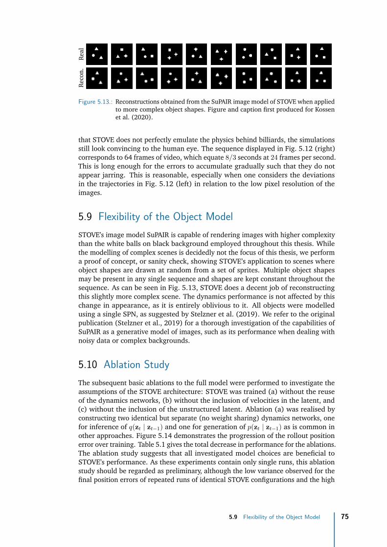
Reco

n.Re

al

Figure 5.13.: Reconstructions obtained from the SuPAIR image model of STOVE when appliedto more complex object shapes. Figure and caption first produced for Kossenet al. (2020).

that STOVE does not perfectly emulate the physics behind billiards, the simulationsstill look convincing to the human eye. The sequence displayed in Fig. 5.12 (right)corresponds to 64 frames of video, which equate 8/3 seconds at 24 frames per second.This is long enough for the errors to accumulate gradually such that they do notappear jarring. This is reasonable, especially when one considers the deviationsin the trajectories in Fig. 5.12 (left) in relation to the low pixel resolution of theimages.

5.9 Flexibility of the Object ModelSTOVE’s image model SuPAIR is capable of rendering images with higher complexitythan the white balls on black background employed throughout this thesis. Whilethe modelling of complex scenes is decidedly not the focus of this thesis, we performa proof of concept, or sanity check, showing STOVE’s application to scenes whereobject shapes are drawn at random from a set of sprites. Multiple object shapesmay be present in any single sequence and shapes are kept constant throughout thesequence. As can be seen in Fig. 5.13, STOVE does a decent job of reconstructingthis slightly more complex scene. The dynamics performance is not affected by thischange in appearance, as it is entirely oblivious to it. All objects were modelledusing a single SPN, as suggested by Stelzner et al. (2019). We refer to the originalpublication (Stelzner et al., 2019) for a thorough investigation of the capabilities ofSuPAIR as a generative model of images, such as its performance when dealing withnoisy data or complex backgrounds.

5.10 Ablation StudyThe subsequent basic ablations to the full model were performed to investigate theassumptions of the STOVE architecture: STOVE was trained (a) without the reuseof the dynamics networks, (b) without the inclusion of velocities in the latent, and(c) without the inclusion of the unstructured latent. Ablation (a) was realised byconstructing two identical but separate (no weight sharing) dynamics networks, onefor inference of q(zt | zt−1) and one for generation of p(zt | zt−1) as is common inother approaches. Figure 5.14 demonstrates the progression of the rollout positionerror over training. Table 5.1 gives the total decrease in performance for the ablations.The ablation study suggests that all investigated model choices are beneficial toSTOVE’s performance. As these experiments contain only single runs, this ablationstudy should be regarded as preliminary, although the low variance observed for thefinal position errors of repeated runs of identical STOVE configurations and the high

5.9 Flexibility of the Object Model 75

0 20000 40000 60000Step

0.2

0.3

0.4

0.5

Posi

tion

Err

or

Billiards

0 20000 40000 60000Step

0.1

0.2

0.3

0.4Gravity

STOVEAbl: Double DynamicsAbl: No VelocityAbl: No Latent

Figure 5.14.: Displayed is the mean predicted position error over a rollout length of 8 framesas training progresses for the billiards (left) and gravity (right) scenario forSTOVE and its ablations: STOVE trained (orange) without the reuse of thedynamics networks, (green) without inclusion of velocities in the latent, and(red) without the inclusion of the unstructured latent. All ablated componentsare likely beneficial to STOVE’s performance. A similar figure and caption werefirst produced for Kossen et al. (2020).

computational efforts of training multiple models somewhat justify this choice. Wenow offer some thoughts regarding the results of the ablation study.

a) No Dynamics Reuse. Even if the performance of this approach should come closeto the original configuration, as is maybe the case for the gravity environment, asingle, reused dynamics network should be preferred as it reduces the number ofparameters of the model as well as the complexity of the model structure.

b) No Explicit Velocities. The final performance of STOVE without the explicitinclusion of velocities is not far away from the full model, which implies that STOVElearns to account for velocities in the unstructured latent space. Perfect velocityinformation is valuable to future state prediction. However, the observational velocityincluded in STOVE is not perfect, as discussed below, and the unstructured latentspace likely has to make up some of the difference even for the full STOVE model.It is therefore not completely surprising that the unstructured latent can also learnto account for all of the velocity. The authors of Karl et al. (2017a) also show thesuccessful recovery of velocities in a non-linear state space model, albeit for singleobject scenarios. Training does, however, progress much slower without velocities,justifying the choice of their inclusion.

c) No Unstructured Latent. STOVE’s performance suffers worst from the omissionof the unstructured latent space in the dynamics prediction. Strictly speaking,object positions and velocities fully describe the state of the billiards and gravitysystem. But, as discussed before in Chapter 4, the velocities obtained by STOVEare mere approximations to the true velocity. Especially around collisions, thesevalues are imprecise, and additional latent information is necessary to predict thenext object state. For example, if an object collides perpendicularly with a wall inthe billiards environment, this is observed by STOVE as two snapshots at t0 and t1from the simulation. Let the true component velocities be v0 before and v1 = −v0after the collision. Assuming that the ball moves with constant velocity before thecollision, i. e. x−1 = x0 − v0∆t, STOVE’s estimate of v0 ∝ x0 − x−1 is accurate.However, at t1, STOVE will not be able to accurately estimate the velocity v1 from


Figure 5.15.: Scaling of STOVE to scenes with six objects. Shown are frames of rolloutpredicted by STOVE. We display every third frame. Rollouts exhibit realis-tic collisions at all times, although a decrease in the kinetic energy of thesystem is noticeable. This is best seen in the animated version available atgithub.com/jlko/STOVE.

the difference in positions because a collision occurred. A collision between t0 andt1 will lead to x1 − x0 6= ∆t v1 because the collision abruptly changes the ball’sposition and velocity. In the extreme case, the snapshot at t1 may be taken such,that the ball is in the exact same position before and after the collision, i. e. in thetime t′ ∈ [t0, t1] the ball moves away from its original position, collides with thewall, and then moves back to its original position. An analysis of the billiards datadoes in fact show these patterns. STOVE’s estimates of the velocities are tightlylinked to the position differences observed by SuPAIR. As x1 = x0 it follows thatSTOVE’s estimate of v1 must incorrectly conclude v1 ∝ x1 − x0 = 0. While theapproximated velocity information is generally helpful for predicting future states, itprovides wrong information around collisions, which demonstrates the need for anabstract latent space. This abstract latent may at t1 choose to remember v0 from t0and help the dynamics network to predict the collision v1 = −v0 correctly. The aboveargument for ball-wall collisions holds similarly for collisions between balls. Thisline of reasoning should also make it clear, why we do not predict new positionsfrom offsets given by the observed velocities in STOVE, but rather opt for the moregeneral formulation described in Chapter 4.

5.11 Scaling to Additional ObjectsLastly, we briefly explore the scaling capabilities of STOVE to scenes with moreobjects. We create a new billiards data set with six objects, increasing the resolutionto 50 by 50 pixels to fit all objects on the screen. Adaptations to STOVE werenecessary to model this scenario successfully: The exact matching routine betweentimesteps was replaced with a greedy matching routine, which is computationallycheaper. However, the main bottleneck for STOVE in this scenario seems to be theimage model, which tends to merge nearby objects, predicting one large boundingbox for two or more balls. To avoid this, we restrict the maximum allowable objectsize to 1/5 of the image size. We also reintroduce an overlap penalty for the boundingboxes as in Stelzner et al. (2019). With these modifications, STOVE successfullyscales to six objects, producing rollouts which do not merge objects and displayconvincing collision behaviour. Figure 5.15 displays example frames of the obtainedmodel rollouts. A conservation of energy could not be obtained in this scenario, and

5.11 Scaling to Additional Objects 77


the object velocities decrease noticeably during rollouts. The problems with mergingobjects are likely an indication of the limits of the sequential attention mechanism inthe image model. The number of parameters in the dynamics network is independentof the number of objects. However, the size of the tensors propagated through theGNN scales with O(O2). While the above scaling test of STOVE may be consideredsuccessful, it is also likely that any scaling of STOVE to scenes with more objects orlarger canvasses will require further adaptations to the model architecture.


6Concluding Thoughts

This final chapter contains a closing discussion of the main findings of the thesiswith a particular emphasis on resulting directions for future work, as well as asummary.

6.1 Discussion and Future WorkMany of the previous unstructured sequence prediction work focuses on scenariosof high visual dimensionality but with simple dynamics. This remains true even formany of the object-specific approaches such as SQAIR and DDPAE. Conversely, muchof the previous work on physics prediction targets low observation dimensionality butcomplicated dynamics. The novelty and strength of STOVE lies in the combination ofhigh-dimensional visual input and non-linear relational dynamics in an unsupervisedfashion.

As observed by Kosiorek et al. (2018), the extension of AIR to videos is natural, andthe sequential nature of videos aids the consistent discovery of objects. With theintroduction of STOVE, this thesis has demonstrated the successful combination ofAIR-like image models and powerful relational physics modelling. Capable transitionmodels are an important component of video modelling. They allow for accuratefuture state predictions and planning in downstream applications. However, if thetransition model underfits the true dynamics of the environment, a model may stillobtain decent reconstructions in the simple scenarios presented in this thesis andmany other publications. In other words, here, dynamics information is not crucialto obtaining good reconstructions. Nevertheless, in future applications and morecomplex modelling scenarios, powerful transition models may prove essential forinference of noisy and complex observations. This further motivates the reuse ofthe dynamics model for both generation and inference. As interactions with theenvironment are important in almost all real-world applications, we argue for theproliferation of relational reasoning mechanisms in video models.

Many preceding video models have not concentrated on the quality of rollout predic-tions, preferring to investigate reconstructions instead. Furthermore, if they do showrollouts, often, the absence of animated visualisations makes it hard to judge thepredictive performance of the model. Likewise, the presented timeframes should belong enough to allow the viewer to come to a conclusion concerning the predictionstability. Additionally, our discussion of the chaoticness of the frequently used bil-liards environment has exposed subtleties with regards to simple error metrics basedon the prediction performance. Most notably, rollout error curves look strikinglysimilar between models with entirely different dynamics performance. For example,STOVE, with convincing and stable predictions, exhibits error curves closely relatedto the linear baseline, a most unrealistic model, simply because they have the same

79

initial observation uncertainty. Therefore, we argue for the inclusion of other quanti-tative measures, such as physical conservation laws, when applicable to demonstratethe plausibility of the learned model. Alternatively, the model’s usefulness may bedemonstrated by applying it on downstream tasks such as planning.

A challenge in many object-aware models is the need for careful design of modelcomplexity. If the object models are made too powerful, they may learn to approxi-mate the whole scene instead of single objects. Only by introducing artificial capacitybottlenecks in the object model can we entice the architecture to use the objectmechanism. This reliance on bottlenecks to elicit objects is unsatisfactory, and wehope that videos, together with capable transition models, provide a strong enoughobject prior to break the above failure modes. Our work has provided first steps inthis direction. However, so far, reliable object-aware video modelling and futurestate prediction remain unsolved in scenarios with complex visuals.

SQAIR in particular has a very complex and overparametrised structure, as theauthors themselves note (Kosiorek et al., 2018). Where STOVE performs a simplemultiplication of distributions, see Eq. (4.6), SQAIR uses general-purpose MLPs thatare provided with as much information as available. Similarly contrasting designchoices are made in almost all other components of STOVE and SQAIR, see Kosioreket al. (2018, Algorithm 2-3). While this might make SQAIR hard to train, debug,or interpret, STOVE contains many assumptions which are too restricting for someapplications. How can we build models whose structure guides them with usefulprior knowledge but does not restrict them? For STOVE, we may have achieved thiswith respect to the simple physical simulation data. However, it is unclear, how tosuccessfully extend this to more complex settings. We will now present some moreconcrete directions for future work. They are loosely sorted from easy to implementand likely to succeed to challenging or vague albeit interesting.

Varying Object Counts. Extending STOVE to accommodate sequences with varyingobject numbers should be straightforward, as long as the number of objects persequence is fixed. This extension would reintroduce the total number of objects O asa random variable, and we could proceed similarly as in SuPAIR. If the number ofobjects should be allowed to vary within the sequence, additional complexity dueto modules for re-recognising objects from previous frames and discovering newobjects, similar to SQAIR, could likely not be avoided. For an extension to largeobject counts, parallel attention mechanisms such as in Crawford and Pineau (2019)or Jiang et al. (2020) would need to be adopted.

Object Matching. While the object state matching routine of STOVE is a simple andeffective solution, its algorithmic complexity of O(O3) may present a limiting factorin future applications. Also, matching states based on Euclidean position distances isnot desirable when objects overlap heavily. Since the conception of STOVE, differentapproaches to handling similar problems have emerged. Inspired by Miladinovic et al.(2019), the matching problem could be solved by first creating state proposals froman unchanged dynamics model. Then, the image model could get these proposalsas input and predict correctional offsets to the proposed states, conditioned on boththe proposal and the observation. An explicit matching is not required anymore,because the image model is aware of the object order proposed by the dynamicsmodel. Veerapaneni et al. (2019) proceed similarly, using the image model torefine predictions from the dynamics model. Instead of directly predicting offsets to

80 Chapter 6 Concluding Thoughts

states, Veerapaneni et al. (2019) refine parameter guesses using iterative variationalinference. By entangling the image and dynamics model, we could proceed similarlyto the above for STOVE and obviate the need for a matching routine. However, thetrade-off between matching complexity and component entanglement needs to beinvestigated.

Extensions to the SSM. The position estimates obtained by the SuPAIR imagemodel of STOVE are completely independent of all previous observations. Whilethese strict independence assumptions are first and foremost a strength of STOVEand lead to a fast inference routine, it is likely that the inclusion of smoothing orfiltering mechanisms is necessary for scenarios with high observation noise or visualcomplexity. Section 2.3 has introduced many ways of constructing such non-linearstate space models. Even VRNN, which is an early example of such models andwhich has flaws that have been discussed by subsequent work, has shown somewhatadmirable performance in Chapter 5 on complex data that it was not designed for.We are therefore confident that the approaches of Section 2.3 would likely yieldstrong results when adapted to object-based image modelling and relational physics.Because these approaches already expect highly non-linear emission and transitiondistributions, the extension of STOVE to such models should be straightforward.That being said, the discussions in Section 2.3 and Karl et al. (2017a) reveal that theinteraction of appearance and dynamics modelling is non-trivial. Thus, approachessuch as Karl et al. (2017a) or Fraccaro et al. (2017), which can regularise the use ofthe dynamics model, are particularly promising.

Conservation of Energy. Section 5.5 has shown that STOVE correctly conserves theaverage kinetic energy of the rollouts. Unfortunately, we can only offer speculationas to how STOVE achieves this conservation and must leave everything else for thefuture. More importantly, future work should focus on building models which reliablyachieve a conservation of relevant physical quantities. Neural ODEs, introduced inChapter 3, offer a promising path towards specifying models, which, depending onthe exact specification, may conserve relevant quantities by design. Successfullyapplying these models to videos of discontinuous processes, such as the billiardsenvironment, or more general and complex dynamics has not been done, but is afruitful avenue for future work.

More Complex Object Models. The SuPAIR-like image model in STOVE is derivedfrom AIR and therefore limited to rectangular object bounding boxes. While SuPAIRalready presents some improvements over AIR, such approaches are not appropriatefor more complex data encountered in real-world applications. In Chapter 3, weintroduced MONet and follow-up work, which presents a more flexible approachto object-aware image modelling, predicting pixel-wise object masks. Extensionsof such models to relational video prediction are interesting future work. Afterthe publication of Kossen et al. (2020), Voelcker (2020) performed experimentswith an adaptation of STOVE to MONet-like image models. While the results arepromising, in general, the approach is brittle and requires careful hyperparametertuning. Unlike STOVE, MONet features object-wise unstructured latents, which leadsto the entangling of appearance and dynamics information in the latent space. Thismay be a reason for the observed instabilities and, therefore, the approaches ofSection 2.3 may provide inspiration on how to move forward. Other recent workby Veerapaneni et al. (2019) or Watters et al. (2019) extends MONet to discrete

6.1 Discussion and Future Work 81

dynamics, e. g. block-stacking tasks or moving sprites. Scaling object-aware imagemodels and relational physics modules to realistic videos is an excellent challengefor future work.

Low-Dimensional Dynamics. For applications in reinforcement learning or robotics,full-scale video modelling of future frames in complex visual settings might not bethe only research direction. Depending on the application, it might be preferable todirectly focus dynamics modelling efforts on lower-dimensional latents, from whichquantities relevant to acting in the environment can directly be predicted, similar toDosovitskiy and Koltun (2017), Farquhar et al. (2018), or Schrittwieser et al. (2019).These quantities should be easier to model than high-dimensional visuals. Here,relational dynamics models could prove beneficial to obtaining good transitionalmodels. However, it is not always obvious, what should constitute an object in suchabstract transition models. A possible answer to this question is provided by Kipfet al. (2020), who learn a useful object-specific latent embedding without relying ona reconstruction loss.

General Relational Prediction. The application of Graph Neural Networks (GNNs)for learning physics simulations is well-established. However, in Section 5.4, wewere able to show that, excitingly, the GNN continues to perform well even when notall objects follow the same dynamical laws. This could pave the way for relationalreasoning modules for more general kinds of interactions. In the real world or videogames, object trajectories are often determined by interactions with the environmentor between objects. Relational reasoning modules in object-aware video modelsmay provide a way to efficiently learn about these interactions, even when theyare more abstract than physical laws and dynamics are allowed to differ betweenobjects. For example, future models may be able to learn the interactions thatgovern the movement of objects in ATARI video games. In turn, knowledge ofthese interactions is then invaluable for acting in the environment. While ourinitial experiments in Section 5.4 proved successful without any modifications tothe architecture, it seems likely that modifications to the GNN are needed in morecomplex settings. For example, one could explicitly introduce latent variables thatassign different dynamics submodules, inspired by work on continual or multi-tasklearning. Alternatively, the modelling choice could be made implicit by includingadditional attention or gating mechanisms, which let the GNN infer the appropriatedynamics mode between object pairs. A similar approach is chosen in Ehrhardt et al.(2019), albeit not in the context of relational physics prediction.

6.2 SummaryObjects and intuitive physics are of central importance to human reasoning. Withthe motivation to bring such capabilities to machine learning models, we haveintroduced STOVE. STOVE presents a structured, object-aware approach to videomodelling, extending attend-infer-repeat models to videos of physically interactingobjects. We assemble STOVE as a non-linear state space model: The transitiondistribution is given by a relational physics module, a graph neural network, and theemission distribution is realised with a SuPAIR-like image module. STOVE is trainedin a self-supervised fashion directly from pixels. Unlike generic approaches, STOVEmakes use of a variety of structuring assumptions, such as the object-awareness,explicit positions, velocities, and object sizes in the latent space, the reuse of the

82 Chapter 6 Concluding Thoughts

generative dynamics model for inference, as well as the structural assumptionsimposed by the graph neural network. These assumptions seem to empower ratherthan restrict STOVE, as the experimental evaluation has shown clear improvementsover previous, less structured video models. In addition, STOVE produces remarkablystable rollouts, which correctly conserve the kinetic energy of the simulation in thebilliards scenario. There, investigations into the chaoticness of the environmentsuggest that STOVE is close to optimal performance considering the resolution ofthe data.

Many exciting directions for future work have been presented. While some strivefor increased visual modelling complexity, others attempt generalisations of the dy-namics model. However, they all share the overarching vision that object-awarenessand relational reasoning present important inductive biases. They should be seenas general-purpose mechanisms with broad relevancy for many areas of machinelearning. STOVE presents a valuable contribution to this vision.

6.2 Summary 83

AModel Details1

A.1 Recognition Model ArchitectureThe object detection network for q(zt, (pos, size) | xt) is realised by an LSTM (Hochre-iter and Schmidhuber, 1997) with 256 hidden units, which outputs the means andvariances of the object’s latent state, i. e. 2 · 2 · 2 = 8 parameters per object.

The Random SPN for the objects is created with parameters (R = 6, D = 2, S =10, C = 1, I = 10), see Section 2.4. Similarly, the Random SPN for the backgroundis created with parameters (R = 3, D = 1, S = 6, C = 1, I = 3). Leaf distributionsare modelled as factorised Gaussians, where means and variances are learnableparameters. The structure for the background SPN is simpler to avoid STOVE relyingentirely on the background model for reconstructions, neglecting object-abstractionsentirely, see Stelzner et al. (2019). The above values are similar to those in Stelzneret al. (2019) and are valid for all experiments of the thesis. Appendix A.4 listsfurther hyperparameter choices.

A.2 Generative Model ArchitectureFor zot,latent, we choose dimensionality 12, such that a full state

zot =(zot, pos, z

ot, size, z

ot, velo, z

ot, latent

)(A.1)

is 18-dimensional.

The dynamics prediction is given by the following series of transformations appliedto each input state of shape (Nb, O, l), where Nb is the batch size, O the number ofobjects, and L = 16 the total size of the latent space per object for the dynamicsprediction without the size parameters.

• S1: Encode input state with linear layer [L, 2L].• S2: Apply linear layer [2L, 2L] to S1 followed by ReLU non-linearity.• S3: Apply linear layer [2L, 2L] to S2 and add result to S2. This gives the

dynamics prediction without relational effects, corresponding to N(zot ) inEq. (4.3).

• C1: The following steps obtain the relational aspects of dynamics prediction,corresponding to I(zot , z

o′t ) in Eq. (4.3). Concatenate the encoded state So

1

pairwise with all state encodings, yielding a tensor of shape (Nb, O,O, 4L).• C2: Apply linear layer [4L, 4L] to C1 followed by ReLU.• C3: Apply linear layer [4L, 2L] to C2 followed by ReLU.• C4: Apply linear layer [2L, 2L] to C3 and add to C3.

1Appendices A.1 to A.3 appear in similar form in the concurrently published Kossen et al. (2020).

85

• A1: To obtain attention coefficients α(zot , zo′t ), apply linear layer [4L, 4L] to C1

followed by ReLU.• A2: Apply linear layer [4L, 2L] to A1 followed by ReLU.• A3: Apply linear layer [2L, 1] to A2 and apply exponential function.• R1: Multiply C4 with A3, where diagonal elements of A3 are masked out to

ensure that R1 only covers cases where o 6= o′.• R2: Sum over R1 for all o′, to obtain tensor of shape (Nb, O, 2L). This is the

relational dynamics prediction.• D1: Sum relational dynamics R2 and self-dynamics S3, obtaining the input toA in Eq. (4.3).

• D2: Apply linear layer [2L, 2L] to D1 followed by tanh non-linearity.• D3: Apply linear layer [2L, 2L] to D2 followed by tanh non-linearity and add

result to D2.• D4: Concatenate D3 and S1, see U in Eq. (4.3), and apply linear layer [4L, 2L]

followed by tanh.• D5: Apply linear layer [2L, 2L] to D4 and add result to D4 to obtain the final

dynamics prediction.

The output D5 has shape (Nb, O, 2L), twice the size of L to account for the vari-ances of the variational state prediction q(zt+1 | zt). For the generative dynamicsp(zt+1 | zt), the predicted variances are ignored and fixed ones used instead.

For the model-based control scenario, the one-hot encoded actions of shape (Nb, A),where A is the number of actions, are transformed with a linear layer [A,O · E],where E is the size of the action-encoding, and reshaped to (A,O,E). We setA = 9 and E = 4 for the experiments in this thesis. The action embedding and theobject appearances (Nb, O, 3) are then concatenated to the input state. The rest ofthe dynamics prediction follows as above. The reward prediction consists of thefollowing steps:

• H1: Apply linear layer [2L, 2L] to D1 followed by ReLU.• H2: Apply linear layer [2L, 2L] to H1.• H3: Sum over object dimension to obtain tensor of shape (Nb, 2L).• H4: Apply linear layer [2L,L] to H3 followed by ReLU.• H5: Apply linear layer [L,L/2] to H4 followed by ReLU.• H5: Apply linear layer [L/2, 1] to H4 followed by a sigmoid non-linearity.

H5 then gives the final reward prediction.

A.3 Model InitialisationIn the first two timesteps, we cannot yet apply STOVE’s main inference stepq(zt | zt−1,xt,xt−1) as described above. In order to initialise the latent state overthe first two frames, we apply a simplified architecture and only use a partial stateat t = 0.

At t = 0, z0 ∼ q(z0, (pos, size) | x0) is given purely by the image model, since noprevious states which could be propagated, exist. This initial z0 is incompleteinsofar as it does not contain velocity information or unstructured latents. At t = 1,q(z1, (pos, size) | x1,x0) is still given purely based on the object attention network.Note that for a dynamics prediction of z1, velocity information at t = 0 wouldneed to be available. However, at t = 1, velocities can be constructed based on

86 Chapter A Model Details

the differences between the previously inferred object positions. We sample z1,latentfrom the normally distributed prior to assemble the first full initial state z1. Att ≥ 2, the full inference network can be run: States are inferred both from theattention network q(zt | xt,xt−1) as well as propagated using the dynamics modelq(zt | zt−1).

In the generative model, similar adjustments are made: p(z0, (pos, size)) is given by auniform prior, velocities and latents are omitted. At t = 1, velocities are sampledfrom a uniform distribution in planar coordinates p(z1, velo) and positions are givenby a simple linear dynamics model

p(z1,pos | z0,pos, z1,velo) = N (z0,pos + z1,velo,σ2) . (A.2)

Latents z1,latent are sampled from a Gaussian prior. Starting at t = 2, the fulldynamics model is used.

A.4 Hyperparameter SettingsThe following list gives the default settings for hyperparameters in STOVE. They arealso part of config.py in the provided code base.

Data Parameters:

num_visible = 8 # Number of visible frames per sequence.num_episodes = 1000 # Number of generated sequences.num_frames = 100 # Number of frames per sequence.channels = 1 # Use black and white images.num_obj = 3 # Number of objects.

Training Configuration:

batch_size = 256cl = 32 # Twice the latent space dimension for the dynamics model.# See adjust_learning_rate() in train.py for further information.learning_rate = 0.002 # Inital and maximum learning rate.min_learning_rate = 0.0002 # Minimum learning rate, see above.debug_anneal_lr = 40000.0 # Learning rate decrease, see above.num_epochs = 400 # Total number of epochs.debug_amsgrad = True # Fix Adam gradients.

Model Config: Action-Conditioned:

# Reward trade-off for combined loss, inverse to variance on reward dist.debug_reward_factor = 15000# No. of steps during which reward loss linearly increases.debug_reward_rampup = 20000# Add object appearance to dynamics prediction.debug_core_appearance = Falsedebug_appearance_dim = 3

Model Config – Dynamics:

A.4 Hyperparameter Settings 87

# Standard deviations on the generative dynamics model.transition_lik_std = [0.01, 0.01, 0.01, 0.01]debug_nonlinear = 'relu' # Nonlinearity used in dynamics core.# Bound on inferred standard deviation on latents.debug_latent_q_std = 0.04

Model Config – SPN:

debug_bw = True # Do not model colours in SPN.# No. of pixels used to model objects in SPN.patch_height = 10patch_width = 10# Bounds on variance for leaves in object-SPN.obj_min_var = 0.12obj_max_var = 0.35# Bounds on variance for leaves in background-SPN.bg_min_var = 0.002bg_max_var = 0.16# Maximum object variances for SuPAIR q-distributions.scale_var = 0.3pos_var = 0.3# Bounds for mean of width of bounding box relative to canvas width.min_obj_scale = 0.1max_obj_scale = 0.8# Bounds for mean of height of bounding box relative to width.min_y_scale = 0.75max_y_scale = 1.25# Max and min object position relative to canvas.obj_pos_bound = 0.9# Number of leaf distributions and sums.obj_spn_num_gauss = 10obj_spn_num_sums = 10

88 Chapter A Model Details

BBaselines1

Following Kosiorek et al. (2018), we experimented with different hyperparameterconfigurations for VRNNs. We varied the sizes of the hidden and latent states[h, z], experimenting with the values [256, 16], [512, 32], [1024, 64], and [2048, 32].We found that increasing the model capacity beyond [512, 32] did not yield largeincreases in performance, which is why we chose the configuration [512, 32] forour experiments. Our VRNN implementation is written in PyTorch and based ongithub.com/emited/VariationalRecurrentNeuralNetwork. VRNN and all modelsbelow were trained until convergence.

SQAIR can handle a variable number of objects in each sequence. However, toallow for a fairer comparison to STOVE, we fixed the number of objects to thecorrect number. This means that in the first timestep, exactly three objects arediscovered, which are then propagated in all following timesteps, without furtherdiscoveries. Our implementation is based on the original implementation providedby the authors at github.com/akosiorek/sqair. Experiments with SQAIR in this thesiswere performed by Karl Stelzner. We thank Adam Kosiorek for his help with theimplementation.

The DDPAE experiments were performed using the implementation available atgithub.com/jthsieh/DDPAE-video-prediction from the original authors. Defaultparameters for training DDPAE with the billiards datasets are provided by the authors.However, the resolutions of our billiards (32 pixels) and gravity (50 pixels) data aredifferent from the resolution DDPAE expects (64 pixels). While we experimentedwith adjusting DDPAE parameters, such as the latent space dimension, to fit ourdifferent resolutions, the best results were obtained when bilinearly scaling ourdata to the resolution DDPAE expects. DDPAE was trained for 400 000 steps, whichsufficed for convergence of the models’ test set error.

The linear baseline was obtained as follows: For the first 8 frames, we infer thefull model state using a fully trained STOVE model. We then take the last inferredpositions and velocities of each object and predict future positions by assumingconstant uniform motions for each object. We do not allow objects to leave theframe, i. e. when objects reach the canvas boundary after some timesteps, they stickto it.

Since our dynamics model requires only object positions and velocities as input, itis trivial to construct a supervised baseline for physics prediction by replacing theSuPAIR-inferred states with real, ground-truth states from the environment. On these,the model can then be trained in a supervised fashion. As with STOVE, we allow thesupervised baseline extra modelling capabilities by introducing unstructured latent

1Chapter appears in similar form in the concurrently published Kossen et al. (2020).

89

https://github.com/emited/VariationalRecurrentNeuralNetwork

https://github.com/akosiorek/sqair

https://github.com/jthsieh/DDPAE-video-prediction

space in addition to the ground-truth input. The loss function per input sequence isgiven by

1

T

T∑t=1

γt ‖zt − zt‖2 , (B.1)

where zt are position and velocity predictions for all objects, zt true states, γ = 0.98exponentially discounts predictions, and T = 8 as for the full STOVE.

90 Chapter B Baselines

Acronyms

AESMC Auto-Encoding Sequential Monte Carlo.

AIR Attend-Infer-Repeat.

ARMA Autoregressive-Moving Average.

BRNN Bidirectional Recurrent Neural Network.

CNN Convolutional Neural Network.

ConvLSTM Convolutional LSTM.

DDPAE Decompositional Disentangled Predictive Autoencoder.

DKF Deep Kalman Filter.

DMM Deep Markov Model.

DVBF Deep Variational Bayes.

ELBO Evidence Lower Bound.

EM Expectation Maximisation.

GAN Generative Adversarial Network.

GNN Graph Neural Network.

GRU Gated Recurrent Unit.

HMM Hidden Markov Model.

IN Interaction Network.

IWAE Importance-Weighted Autoencoder.

KL divergence Kullback-Leibler Divergence.

KVAE Kalman Variational Autoencoder.

LDS Linear Dynamical System.

LG-SSM Linear Gaussian State-Space Model.

LHS Left-Hand Side.

LSTM Long-Short Term Memory.

MCMC Markov Chain Monte Carlo.

MCTS Monte-Carlo Tree Search.

91

MDN Mixture Density Network.

MFVI Mean-field Variational Inference.

MLP Multilayer Perceptron.

MONet Multi-Object Network.

MPE Most Probable Explanation.

MSE Mean Squared Error.

NEM Neural Expectation Maximisation.

Neural ODE Neural Ordinary Differential Equation.

NPE Neural Prediction Engine.

NTM Neural Turing Machine.

PGM Probabilistic Graphical Model.

R-NEM Relational Neural Expectation Maximisation.

Random SPN Random Sum-Product Network.

RHS Right-Hand Side.

RN Relation Network.

RNN Recurrent Neural Network.

SGD Stochastic Gradient Descent.

SGVB Stochastic Gradient Variational Bayes.

SPN Sum-Product Network.

SQAIR Sequential Attend-Infer-Repeat.

SRNN Stochastic Recurrent Neural Network.

SSM State-Space Model.

STORN Stochastic Recurrent Network.

STOVE Structured Object-Aware Physics Prediction for Video Modelling and Plan-ning.

SuPAIR Sum-Product Attend-Infer-Repeat.

SVI Stochastic Variational Inference.

VAE Variational Autoencoder.

VI Variational Inference.

VIN Visual Interaction Network.

VRNN Variational Recurrent Neural Network.

92 Acronyms

Bibliography

T. Adel, D. Balduzzi, and A. Ghodsi. Learning the structure of sum-product networksvia an svd-based algorithm. In Proceedings of the Conference on Uncertainty inArtificial Intelligence, pages 32–41, 2015.

P. Agrawal, A. V. Nair, P. Abbeel, J. Malik, and S. Levine. Learning to poke by poking:Experiential learning of intuitive physics. In Advances in Neural InformationProcessing Systems, pages 5074–5082, 2016.

A. Akhundov, M. Soelch, J. Bayer, and P. van der Smagt. Variational trackingand prediction with generative disentangled state-space models. arXiv preprintarXiv:1910.06205, 2019.

M. Babaeizadeh, C. Finn, D. Erhan, R. H. Campbell, and S. Levine. Stochasticvariational video prediction. In Proceedings of the International Conference onLearning Representations, 2018.

D. Barber. Bayesian reasoning and machine learning. Cambridge University Press,2012.

P. Battaglia, R. Pascanu, M. Lai, D. J. Rezende, et al. Interaction networks for learningabout objects, relations and physics. In Advances in Neural Information ProcessingSystems, pages 4502–4510, 2016.

P. W. Battaglia, J. B. Hamrick, and J. B. Tenenbaum. Simulation as an engine ofphysical scene understanding. Proceedings of the National Academy of Sciences, 110(45):18327–18332, 2013.

J. Bayer and C. Osendorfer. Learning stochastic recurrent networks. arXiv preprintarXiv:1411.7610, 2014.

P. Becker-Ehmck, J. Peters, and P. Van Der Smagt. Switching linear dynamics forvariational bayes filtering. In Proceedings of the International Conference on MachineLearning, pages 553–562, 2019.

C. M. Bishop. Mixture density networks. Neural Computing Research Group Report,1994.

C. M. Bishop. Pattern recognition and machine learning. springer, 2006.D. M. Blei, A. Kucukelbir, and J. D. McAuliffe. Variational inference: A review for

statisticians. Journal of the American statistical Association, 112(518):859–877,2017.

M. Bonse. Machine larning based atmosphere prediction for extreme adaptive optics.Master Thesis, Technical University Darmstadt, 2019.

Y. Burda, R. Grosse, and R. Salakhutdinov. Importance weighted autoencoders. arXivpreprint arXiv:1509.00519, 2015.

C. P. Burgess, I. Higgins, A. Pal, L. Matthey, N. Watters, G. Desjardins, and A. Lerchner.Understanding disentangling in β-vae. In Neural Information Processing SystemsWorkshop on Learning Disentangled Representations, 2017.

93

C. P. Burgess, L. Matthey, N. Watters, R. Kabra, I. Higgins, M. Botvinick, and A. Lerch-ner. Monet: Unsupervised scene decomposition and representation. arXiv preprintarXiv:1901.11390, 2019.

M. B. Chang, T. Ullman, A. Torralba, and J. B. Tenenbaum. A compositional object-based approach to learning physical dynamics. In Proceedings of the InternationalConference on Learning Representations, 2017.

T. Q. Chen, Y. Rubanova, J. Bettencourt, and D. K. Duvenaud. Neural ordinarydifferential equations. In Advances in Neural Information Processing Systems, pages6571–6583, 2018.

W.-C. Cheng, S. Kok, H. V. Pham, H. L. Chieu, and K. M. A. Chai. Language modelingwith sum-product networks. In Fifteenth Annual Conference of the InternationalSpeech Communication Association, 2014.

K. Cho, B. Van Merriënboer, C. Gulcehre, D. Bahdanau, F. Bougares, H. Schwenk,and Y. Bengio. Learning phrase representations using rnn encoder-decoder forstatistical machine translation. In Conference on Empirical Methods in NaturalLanguage Processing, 2014.

F. Chollet. The measure of intelligence. arXiv preprint arXiv:1911.01547, 2019.J. Chung, C. Gulcehre, K. Cho, and Y. Bengio. Empirical evaluation of gated recurrent

neural networks on sequence modeling. In Neural Information Processing SystemsWorkshop on Learning Disentangled Representations, 2014.

J. Chung, K. Kastner, L. Dinh, K. Goel, A. C. Courville, and Y. Bengio. A recurrentlatent variable model for sequential data. In Advances in Neural InformationProcessing Systems, pages 2980–2988, 2015.

R. Coulom. Efficient selectivity and backup operators in monte-carlo tree search.In Proceedings of International Conference on Computers and Games, pages 72–83.Springer, 2006.

M. Cranmer, S. Greydanus, S. Hoyer, P. Battaglia, D. Spergel, and S. Ho. Lagrangianneural networks. In International Conference on Learning Representations Workshopon Deep Differential Equations Workshop, 2020.

E. Crawford and J. Pineau. Spatially invariant unsupervised object detection withconvolutional neural networks. In Proceedings of the AAAI Conference on ArtificialIntelligence, volume 33, pages 3412–3420, 2019.

A. Darwiche. A differential approach to inference in bayesian networks. Journal ofthe ACM (JACM), 50(3):280–305, 2003.

P. Dayan, G. E. Hinton, R. M. Neal, and R. S. Zemel. The helmholtz machine. Neuralcomputation, 7(5):889–904, 1995.

J. DeCruyenaere and H. Hafez. A comparison between kalman filters and recurrentneural networks. In IJCNN International Joint Conference on Neural Networks,volume 4, pages 247–251. IEEE, 1992.

A. Dennis and D. Ventura. Learning the architecture of sum-product networks usingclustering on variables. In Advances in Neural Information Processing Systems,pages 2033–2041, 2012.

E. Denton and R. Fergus. Stochastic video generation with a learned prior. InProceedings of the International Conference on Machine Learning, pages 1174–1183,2018.

C. Doersch. Tutorial on variational autoencoders. arXiv preprint arXiv:1606.05908,2016.

A. Dosovitskiy and V. Koltun. Learning to act by predicting the future. In Proceedingsof the International Conference on Learning Representations, 2017.

A. Dosovitskiy, P. Fischer, E. Ilg, P. Hausser, C. Hazirbas, V. Golkov, P. Van Der Smagt,

94 Bibliography

D. Cremers, and T. Brox. Flownet: Learning optical flow with convolutionalnetworks. In Proceedings of the IEEE Conference on Computer Vision and PatternRecognition, pages 2758–2766, 2015.

D. Durstewitz. Advanced data analysis in neuroscience. Springer InternationalPublishing, 2017.

S. Ehrhardt, A. Monszpart, N. Mitra, and A. Vedaldi. Unsupervised intuitive physicsfrom visual observations. In Proceedings of the Asian Conference on Computer Vision,pages 700–716. Springer, 2018.

S. Ehrhardt, A. Monszpart, N. J. Mitra, and A. Vedaldi. Unsupervised intuitive physicsfrom past experiences. arXiv preprint arXiv:1905.10793, 2019.

J. L. Elman. Finding structure in time. Cognitive science, 14(2):179–211, 1990.M. Engelcke, A. R. Kosiorek, O. P. Jones, and I. Posner. Genesis: Generative scene

inference and sampling with object-centric latent representations. In Proceedingsof the International Conference on Learning Representations, 2020.

S. A. Eslami, N. Heess, T. Weber, Y. Tassa, D. Szepesvari, G. E. Hinton, et al. Attend,infer, repeat: Fast scene understanding with generative models. In Advances inNeural Information Processing Systems, 2016.

O. Fabius and J. R. van Amersfoort. Variational recurrent auto-encoders. In Interna-tional Conference on Machine Learning Workshop Track, 2015.

G. Farquhar, T. Rocktäschel, M. Igl, and S. Whiteson. Treeqn and atreec: Differen-tiable tree-structured models for deep reinforcement learning. In Proceedings ofthe International Conference on Learning Representations, 2018.

S. Farquhar, M. Osborne, and Y. Gal. Radial bayesian neural networks: Robustvariational inference in big models. In Proceedings of International Conference onArtificial Intelligence and Statistics, 2020.

C. Finn, I. Goodfellow, and S. Levine. Unsupervised learning for physical interactionthrough video prediction. In Advances in Neural Information Processing Systems,pages 64–72, 2016.

M. Fraccaro, S. K. Sønderby, U. Paquet, and O. Winther. Sequential neural modelswith stochastic layers. In Advances in Neural Information Processing Systems, pages2199–2207, 2016.

M. Fraccaro, S. Kamronn, U. Paquet, and O. Winther. A disentangled recognitionand nonlinear dynamics model for unsupervised learning. In Advances in NeuralInformation Processing Systems, pages 3601–3610, 2017.

K. Fragkiadaki, P. Agrawal, S. Levine, and J. Malik. Learning visual predictive modelsof physics for playing billiards. In Proceedings of the International Conference onLearning Representations, 2016.

F. B. Fuchs, A. R. Kosiorek, L. Sun, O. P. Jones, and I. Posner. End-to-end recurrentmulti-object tracking and trajectory prediction with relational reasoning. arXivpreprint arXiv:1907.12887, 2019.

R. Gens and P. Domingos. Discriminative learning of sum-product networks. InAdvances in Neural Information Processing Systems, pages 3239–3247, 2012.

R. Gens and D. Pedro. Learning the structure of sum-product networks. In Interna-tional Conference on Machine Learning, pages 873–880, 2013.

F. A. Gers, J. Schmidhuber, and F. Cummins. Learning to forget: Continual predictionwith lstm. In Proceedings of International Conference on Artificial Neural Networks.IET, 1999.

S. Gershman and N. Goodman. Amortized inference in probabilistic reasoning. InProceedings of the Annual Meeting of the Cognitive Science Society, 2014.

V. Goel, J. Weng, and P. Poupart. Unsupervised video object segmentation for deep

Bibliography 95

reinforcement learning. In Advances in Neural Information Processing Systems,pages 5683–5694, 2018.

I. Goodfellow. Generative adversarial networks. In Advances in Neural InformationProcessing Systems Tutorial, 2016.

I. Goodfellow, Y. Bengio, and A. Courville. Deep Learning. MIT Press, 2016.A. Graves, G. Wayne, and I. Danihelka. Neural turing machines. arXiv preprint

arXiv:1410.5401, 2014.K. Greff, S. Van Steenkiste, and J. Schmidhuber. Neural expectation maximization.

In Advances in Neural Information Processing Systems, pages 6691–6701, 2017.K. Greff, R. L. Kaufmann, R. Kabra, N. Watters, C. Burgess, D. Zoran, L. Matthey,

M. Botvinick, and A. Lerchner. Multi-object representation learning with iterativevariational inference. In Proceedings of the International Conference on LearningRepresentations, pages 2424–2433, 2019.

K. Gregor, I. Danihelka, A. Graves, D. J. Rezende, and D. Wierstra. Draw: A recurrentneural network for image generation. In Proceedings of the International Conferenceon Machine Learning, pages 1462–1471, 2015.

U. Grenander. Lectures in Pattern Theory: Vol. 2 Pattern Analysis. Springer-Verlag,1976.

S. Greydanus, M. Dzamba, and J. Yosinski. Hamiltonian neural networks. In Advancesin Neural Information Processing Systems, pages 15353–15363, 2019.

J. Hamrick, P. Battaglia, and J. B. Tenenbaum. Internal physics models guideprobabilistic judgments about object dynamics. In Proceedings of the 33rd annualconference of the cognitive science society, volume 2. Cognitive Science SocietyAustin, TX, 2011.

I. Higgins, L. Matthey, A. Pal, C. Burgess, X. Glorot, M. Botvinick, S. Mohamed,and A. Lerchner. beta-vae: Learning basic visual concepts with a constrainedvariational framework. In Proceedings of the International Conference on LearningRepresentations, 2017.

S. Hochreiter. Untersuchungen zu dynamischen neuronalen netzen. Diploma, Tech-nische Universität München, 91(1), 1991.

S. Hochreiter. The vanishing gradient problem during learning recurrent neuralnets and problem solutions. International Journal of Uncertainty, Fuzziness andKnowledge-Based Systems, 6(02):107–116, 1998.

S. Hochreiter and J. Schmidhuber. Long short-term memory. Neural computation, 9(8):1735–1780, 1997.

M. D. Hoffman, D. M. Blei, C. Wang, and J. Paisley. Stochastic variational inference.The Journal of Machine Learning Research, 14(1):1303–1347, 2013.

J.-T. Hsieh, B. Liu, D.-A. Huang, L. F. Fei-Fei, and J. C. Niebles. Learning to decomposeand disentangle representations for video prediction. In Advances in NeuralInformation Processing Systems, pages 517–526, 2018.

M. Hussing. Object-aware state representation learning. Master Thesis, TechnicalUniversity Darmstadt, 2020.

M. Jaderberg, K. Simonyan, A. Zisserman, et al. Spatial transformer networks. InAdvances in Neural Information Processing Systems, pages 2017–2025, 2015.

M. Jaques, M. Burke, and T. Hospedales. Physics-as-inverse-graphics: Joint unsuper-vised learning of objects and physics from video. In Proceedings of the InternationalConference on Learning Representations, 2020.

J. L. W. V. Jensen et al. Sur les fonctions convexes et les inégalités entre les valeursmoyennes. Acta mathematica, 30:175–193, 1906.

J. Jia and A. R. Benson. Neural jump stochastic differential equations. In Advances

96 Bibliography

in Neural Information Processing Systems, pages 9843–9854, 2019.J. Jiang, S. Janghorbani, G. De Melo, and S. Ahn. Scalor: Generative world models

with scalable object representations. In Proceedings of the International Conferenceon Learning Representations, 2020.

M. J. Johnson, D. K. Duvenaud, A. Wiltschko, R. P. Adams, and S. R. Datta. Compos-ing graphical models with neural networks for structured representations and fastinference. In Advances in Neural Information Processing Systems, pages 2946–2954,2016.

L. Kaiser, M. Babaeizadeh, P. Milos, B. Osinski, R. H. Campbell, K. Czechowski,D. Erhan, C. Finn, P. Kozakowski, S. Levine, et al. Model-based reinforcementlearning for atari. In Proceedings of the International Conference on LearningRepresentations, 2020.

N. Kalchbrenner, A. van den Oord, K. Simonyan, I. Danihelka, O. Vinyals, A. Graves,and K. Kavukcuoglu. Video pixel networks. In Proceedings of the InternationalConference on Machine Learning-Volume 70, pages 1771–1779, 2017.

M. Karl, M. Soelch, J. Bayer, and P. Van der Smagt. Deep variational bayes filters:Unsupervised learning of state space models from raw data. In Proceedings of theInternational Conference on Learning Representations, 2017a.

M. Karl, M. Soelch, P. Becker-Ehmck, D. Benbouzid, P. van der Smagt, and J. Bayer.Unsupervised real-time control through variational empowerment. arXiv preprintarXiv:1710.05101, 2017b.

D. P. Kingma and J. Ba. Adam: A method for stochastic optimization. In Proceedingsof the International Conference on Learning Representations, 2015.

D. P. Kingma and M. Welling. Auto-encoding variational bayes. In Proceedings of theInternational Conference on Learning Representations, 2014.

T. Kipf, E. van der Pol, and M. Welling. Contrastive learning of structured worldmodels. In Proceedings of the International Conference on Learning Representations,2020.

I. Kobyzev, S. Prince, and M. A. Brubaker. Normalizing flows: Introduction and ideas.arXiv preprint arXiv:1908.09257, 2019.

J. Z. Kolter and G. Manek. Learning stable deep dynamics models. In Advances inNeural Information Processing Systems, pages 11126–11134, 2019.

A. Kosiorek, A. Bewley, and I. Posner. Hierarchical attentive recurrent tracking. InAdvances in Neural Information Processing Systems, pages 3053–3061, 2017.

A. Kosiorek, H. Kim, Y. W. Teh, and I. Posner. Sequential attend, infer, repeat: Gener-ative modelling of moving objects. In Advances in Neural Information ProcessingSystems, pages 8606–8616, 2018.

J. Kossen, K. Stelzner, M. Hussing, C. Voelcker, and K. Kersting. Structured object-aware physics prediction for video modeling and planning. In Proceedings of theInternational Conference on Learning Representations, 2020.

R. G. Krishnan, U. Shalit, and D. Sontag. Deep kalman filters. arXiv preprintarXiv:1511.05121, 2015.

R. G. Krishnan, U. Shalit, and D. Sontag. Structured inference networks for nonlinearstate space models. In Proceedings of AAAI Conference on Artificial Intelligence,2017.

A. Krizhevsky, I. Sutskever, and G. E. Hinton. Imagenet classification with deepconvolutional neural networks. In Advances in Neural Information ProcessingSystems, pages 1097–1105, 2012.

H. W. Kuhn. The hungarian method for the assignment problem. Naval researchlogistics quarterly, 2(1-2):83–97, 1955.

Bibliography 97

M. Kumar, M. Babaeizadeh, D. Erhan, C. Finn, S. Levine, L. Dinh, and D. Kingma.Videoflow: A conditional flow-based model for stochastic video generation. InProceedings of the International Conference on Learning Representations, 2020.

B. M. Lake, T. D. Ullman, J. B. Tenenbaum, and S. J. Gershman. Building machinesthat learn and think like people. Behavioral and brain sciences, 40, 2017.

T. A. Le, M. Igl, T. Rainforth, T. Jin, and F. Wood. Auto-encoding sequential montecarlo. In Proceedings of the International Conference on Learning Representations,2018.

Y. LeCun, L. Bottou, Y. Bengio, and P. Haffner. Gradient-based learning applied todocument recognition. Proceedings of the IEEE, 86(11):2278–2324, 1998.

Y. LeCun, Y. Bengio, and G. Hinton. Deep learning. nature, 521(7553):436–444,2015.

A. X. Lee, R. Zhang, F. Ebert, P. Abbeel, C. Finn, and S. Levine. Stochastic adversarialvideo prediction. arXiv preprint arXiv:1804.01523, 2018.

S. Legg and M. Hutter. A formal measure of machine intelligence. In Proceedings of15th Annual Machine Learning Conference of Belgium and The Netherlands, 2006.

T. Lesort, N. Díaz-Rodríguez, J.-F. Goudou, and D. Filliat. State representationlearning for control: An overview. Neural Networks, 108:379–392, 2018.

Y. Li, J. Wu, R. Tedrake, J. B. Tenenbaum, and A. Torralba. Learning particle dynamicsfor manipulating rigid bodies, deformable objects, and fluids. In Proceedings of theInternational Conference on Learning Representations, 2019.

Z. Lin, Y.-F. Wu, S. V. Peri, W. Sun, G. Singh, F. Deng, J. Jiang, and S. Ahn. Space:Unsupervised object-oriented scene representation via spatial attention and decom-position. In Proceedings of the International Conference on Learning Representations,2020.

Z. C. Lipton, J. Berkowitz, and C. Elkan. A critical review of recurrent neuralnetworks for sequence learning. arXiv preprint arXiv:1506.00019, 2015.

Z. Liu, R. A. Yeh, X. Tang, Y. Liu, and A. Agarwala. Video frame synthesis using deepvoxel flow. In Proceedings of the IEEE International Conference on Computer Vision,pages 4463–4471, 2017.

M. Lutter, C. Ritter, and J. Peters. Deep lagrangian networks: Using physics as modelprior for deep learning. In International Conference on Learning Representations,2019.

C. J. Maddison, J. Lawson, G. Tucker, N. Heess, M. Norouzi, A. Mnih, A. Doucet,and Y. Teh. Filtering variational objectives. In Advances in Neural InformationProcessing Systems, pages 6573–6583, 2017.

J. Marino, Y. Yue, and S. Mandt. Iterative amortized inference. In Proceedings of theInternational Conference on Machine Learning, pages 3403–3412, 2019.

E. Mathieu, T. Rainforth, N. Siddharth, and Y. W. Teh. Disentangling disentanglementin variational autoencoders. In Proceedings of the International Conference onLearning Representations, 2019.

M. Mathieu, C. Couprie, and Y. LeCun. Deep multi-scale video prediction beyondmean square error. In Proceedings of the International Conference on LearningRepresentations, 2016.

M. McCloskey. Intuitive physics. Scientific american, 248(4):122–131, 1983.M. Mézard, G. Parisi, and M. Virasoro. Spin glass theory and beyond: An Introduction

to the Replica Method and Its Applications, volume 9. World Scientific PublishingCompany, 1987.

Ð. Miladinovic, W. Gondal, B. Schölkopf, J. M. Buhmann, and S. Bauer. Disentangledstate space models: Unsupervised learnign of dynamics across heterogenous

98 Bibliography

environments. In International Conference on Learning Representations Workshop,2019.

V. Mnih, N. Heess, A. Graves, et al. Recurrent models of visual attention. In Advancesin Neural Information Processing Systems, pages 2204–2212, 2014.

V. Mnih, K. Kavukcuoglu, D. Silver, A. A. Rusu, J. Veness, M. G. Bellemare, A. Graves,M. Riedmiller, A. K. Fidjeland, G. Ostrovski, et al. Human-level control throughdeep reinforcement learning. Nature, 518(7540):529–533, 2015.

A. Molina, A. Vergari, N. Di Mauro, S. Natarajan, F. Esposito, and K. Kersting. Mixedsum-product networks: A deep architecture for hybrid domains. In Proceedings ofthe AAAI Conference on Artificial Intelligence, 2018.

A. Molina, A. Vergari, K. Stelzner, R. Peharz, P. Subramani, N. D. Mauro, P. Poupart,and K. Kersting. Spflow: An easy and extensible library for deep probabilisticlearning using sum-product networks, 2019.

K. P. Murphy. Machine learning: a probabilistic perspective. MIT press, 2012.J. Oh, X. Guo, H. Lee, R. L. Lewis, and S. Singh. Action-conditional video prediction

using deep networks in atari games. In Advances in Neural Information ProcessingSystems, pages 2863–2871, 2015.

G. Papamakarios. Neural density estimation and likelihood-free inference. arXivpreprint arXiv:1910.13233, 2019.

A. Paszke, S. Gross, F. Massa, A. Lerer, J. Bradbury, G. Chanan, T. Killeen, Z. Lin,N. Gimelshein, L. Antiga, et al. Pytorch: An imperative style, high-performancedeep learning library. In Advances in Neural Information Processing Systems, pages8024–8035, 2019.

R. Peharz, G. Kapeller, P. Mowlaee, and F. Pernkopf. Modeling speech with sum-product networks: Application to bandwidth extension. In 2014 IEEE InternationalConference on Acoustics, Speech and Signal Processing, pages 3699–3703. IEEE,2014.

R. Peharz, S. Tschiatschek, F. Pernkopf, and P. Domingos. On theoretical propertiesof sum-product networks. In Artificial Intelligence and Statistics, pages 744–752,2015.

R. Peharz, A. Vergari, K. Stelzner, A. Molina, M. Trapp, K. Kersting, and Z. Ghahra-mani. Probabilistic deep learning using random sum-product networks. In Pro-ceedings of the Conference on Uncertainty in Artificial Intelligence, 2019.

H. Poon and P. Domingos. Sum-product networks: A new deep architecture. InIEEE International Conference on Computer Vision Workshops, pages 689–690. IEEE,2011.

T. Rainforth, A. R. Kosiorek, T. A. Le, C. J. Maddison, M. Igl, F. Wood, and Y. W.Teh. Tighter variational bounds are not necessarily better. In Proceedings of theInternational Conference on Machine Learning, pages 116–124, 2018.

P. Ramachandran, N. Parmar, A. Vaswani, I. Bello, A. Levskaya, and J. Shlens. Stand-alone self-attention in vision models. In Advances in Neural Information ProcessingSystems, pages 68–80, 2019.

S. S. Rangapuram, M. W. Seeger, J. Gasthaus, L. Stella, Y. Wang, and T. Januschowski.Deep state space models for time series forecasting. In Advances in Neural Infor-mation Processing Systems, pages 7785–7794, 2018.

W. Rawat and Z. Wang. Deep convolutional neural networks for image classification:A comprehensive review. Neural computation, 29(9):2352–2449, 2017.

B. Recht, R. Roelofs, L. Schmidt, and V. Shankar. Do imagenet classifiers generalizeto imagenet? In Proceedings of the International Conference on Machine Learning,pages 5389–5400, 2019.

Bibliography 99

J. Redmon, S. Divvala, R. Girshick, and A. Farhadi. You only look once: Unified,real-time object detection. In Proceedings of the IEEE Conference on Computer Visionand Pattern Recognition, pages 779–788, 2016.

D. J. Rezende and S. Mohamed. Variational inference with normalizing flows. InInternational Conference on Machine Learning, pages 1530–1538, 2015.

D. J. Rezende, S. Mohamed, and D. Wierstra. Stochastic backpropagation and ap-proximate inference in deep generative models. In Proceedings of the InternationalConference on Machine Learning, pages 1278–1286, 2014.

O. Ronneberger, P. Fischer, and T. Brox. U-net: Convolutional networks for biomedi-cal image segmentation. In International Conference on Medical Image Computingand Computer-assisted Intervention, pages 234–241. Springer, 2015.

H. Salehinejad, S. Sankar, J. Barfett, E. Colak, and S. Valaee. Recent advances inrecurrent neural networks. arXiv preprint arXiv:1801.01078, 2017.

A. N. Sanborn, V. K. Mansinghka, and T. L. Griffiths. Reconciling intuitive physicsand newtonian mechanics for colliding objects. Psychological review, 120(2):411,2013.

A. Sanchez-Gonzalez, N. Heess, J. T. Springenberg, J. Merel, M. Riedmiller, R. Had-sell, and P. Battaglia. Graph networks as learnable physics engines for inferenceand control. In Proceedings of the International Conference on Machine Learning,pages 4470–4479, 2018.

A. Sanchez-Gonzalez, J. Godwin, T. Pfaff, R. Ying, J. Leskovec, and P. W. Battaglia.Learning to simulate complex physics with graph networks. arXiv preprintarXiv:2002.09405, 2020.

A. Santoro, D. Raposo, D. G. Barrett, M. Malinowski, R. Pascanu, P. Battaglia, andT. Lillicrap. A simple neural network module for relational reasoning. In Advancesin Neural Information Processing Systems, pages 4967–4976, 2017.

J. Schrittwieser, I. Antonoglou, T. Hubert, K. Simonyan, L. Sifre, S. Schmitt, A. Guez,E. Lockhart, D. Hassabis, T. Graepel, et al. Mastering atari, go, chess and shogi byplanning with a learned model. arXiv preprint arXiv:1911.08265, 2019.

M. Schuster and K. K. Paliwal. Bidirectional recurrent neural networks. IEEETransactions on Signal Processing, 45(11):2673–2681, 1997.

D. Silver, A. Huang, C. J. Maddison, A. Guez, L. Sifre, G. Van Den Driessche, J. Schrit-twieser, I. Antonoglou, V. Panneershelvam, M. Lanctot, et al. Mastering the gameof go with deep neural networks and tree search. nature, 529(7587):484, 2016.

D. Silver, J. Schrittwieser, K. Simonyan, I. Antonoglou, A. Huang, A. Guez, T. Hubert,L. Baker, M. Lai, A. Bolton, et al. Mastering the game of go without humanknowledge. Nature, 550(7676):354–359, 2017.

P. Sorrenson, C. Rother, and U. Köthe. Disentanglement by nonlinear ica with generalincompressible-flow networks (gin). In Proceedings of the International Conferenceon Learning Representations, 2020.

N. Srivastava, E. Mansimov, and R. Salakhudinov. Unsupervised learning of videorepresentations using lstms. In Proceedings of the International Conference onMachine Learning, pages 843–852, 2015.

K. Stelzner, R. Peharz, and K. Kersting. Faster attend-infer-repeat with tractableprobabilistic models. In Proceedings of the International Conference on MachineLearning, 2019.

I. Sutskever, G. E. Hinton, and G. W. Taylor. The recurrent temporal restrictedboltzmann machine. In Advances in Neural Information Processing Systems, pages1601–1608, 2009.

Y. Tassa, Y. Doron, A. Muldal, T. Erez, Y. Li, D. d. L. Casas, D. Budden, A. Ab-

100 Bibliography

dolmaleki, J. Merel, A. Lefrancq, et al. Deepmind control suite. arXiv preprintarXiv:1801.00690, 2018.

P. Toth, D. J. Rezende, A. Jaegle, S. Racanière, A. Botev, and I. Higgins. Hamiltoniangenerative networks. In Proceedings of the International Conference on LearningRepresentations, 2020.

M. Tschannen, O. Bachem, and M. Lucic. Recent advances in autoencoder-basedrepresentation learning. In Neural Information Processing Systems Workshop onBayesian Deep Learning, 2018.

A. Van den Oord, N. Kalchbrenner, L. Espeholt, O. Vinyals, A. Graves, et al. Condi-tional image generation with pixelcnn decoders. In Advances in Neural InformationProcessing Systems, pages 4790–4798, 2016.

A. Vaswani, N. Shazeer, N. Parmar, J. Uszkoreit, L. Jones, A. N. Gomez, Ł. Kaiser,and I. Polosukhin. Attention is all you need. In Advances in Neural InformationProcessing Systems, pages 5998–6008, 2017.

R. Veerapaneni, J. D. Co-Reyes, M. Chang, M. Janner, C. Finn, J. Wu, J. B. Tenenbaum,and S. Levine. Entity abstraction in visual model-based reinforcement learning. InProceedings of the International Conference on Robot Learning, 2019.

A. Vergari, R. Peharz, N. Di Mauro, A. Molina, K. Kersting, and F. Esposito. Sum-product autoencoding: Encoding and decoding representations using sum-productnetworks. In Proceedings of the AAAI Conference on Artificial Intelligence, 2018.

A. Vergari, N. Di Mauro, and F. Esposito. Visualizing and understanding sum-productnetworks. Machine Learning, 108(4):551–573, 2019.

C. Voelcker. Unsupervised object detection and sequence modeling for control.Master Thesis, Technical University Darmstadt, 2020.

C. Vondrick, H. Pirsiavash, and A. Torralba. Generating videos with scene dynamics.In Advances in Neural Information Processing Systems, pages 613–621, 2016.

E. A. Wan and R. Van Der Merwe. The unscented kalman filter for nonlinearestimation. In Proceedings of the IEEE 2000 Adaptive Systems for Signal Processing,Communications, and Control Symposium, pages 153–158. IEEE, 2000.

M. Watter, J. Springenberg, J. Boedecker, and M. Riedmiller. Embed to control: Alocally linear latent dynamics model for control from raw images. In Advances inNeural Information Processing Systems, pages 2746–2754, 2015.

N. Watters, D. Zoran, T. Weber, P. Battaglia, R. Pascanu, and A. Tacchetti. Visualinteraction networks: Learning a physics simulator from video. In Advances inNeural Information Processing Systems, pages 4539–4547, 2017.

N. Watters, L. Matthey, M. Bosnjak, C. P. Burgess, and A. Lerchner. Cobra: Data-efficient model-based rl through unsupervised object discovery and curiosity-driven exploration. arXiv preprint arXiv:1905.09275, 2019.

D. Weissenborn, O. Täckström, and J. Uszkoreit. Scaling autoregressive video models.In Proceedings of the International Conference on Learning Representations, 2019.

A. Wu, S. Nowozin, E. Meeds, R. E. Turner, J. M. Hernández-Lobato, and A. L.Gaunt. Deterministic variational inference for robust bayesian neural networks.In Proceedings of the International Conference on Learning Representations, 2019a.

J. Wu, I. Yildirim, J. J. Lim, B. Freeman, and J. Tenenbaum. Galileo: Perceivingphysical object properties by integrating a physics engine with deep learning. InAdvances in Neural Information Processing Systems, pages 127–135, 2015.

J. Wu, J. J. Lim, H. Zhang, J. B. Tenenbaum, and W. T. Freeman. Physics 101:Learning physical object properties from unlabeled videos. In Proceedings of theBritish Machine Vision Conference, 2016.

J. Wu, E. Lu, P. Kohli, B. Freeman, and J. Tenenbaum. Learning to see physics via

Bibliography 101

visual de-animation. In Advances in Neural Information Processing Systems, pages153–164, 2017.

Z. Wu, S. Pan, F. Chen, G. Long, C. Zhang, and P. S. Yu. A comprehensive survey ongraph neural networks. arXiv preprint arXiv:1901.00596, 2019b.

S. Xingjian, Z. Chen, H. Wang, D.-Y. Yeung, W.-K. Wong, and W.-c. Woo. Convolu-tional lstm network: A machine learning approach for precipitation nowcasting.In Advances in Neural Information Processing Systems, pages 802–810, 2015.

W. Zaremba and I. Sutskever. Learning to execute. arXiv preprint arXiv:1410.4615,2014.

P. D. Zelazo and S. P. Johnson. Object Perception. Oxford University Press, 2013.C. Zhang, J. Bütepage, H. Kjellström, and S. Mandt. Advances in variational inference.

In IEEE Transactions on Pattern Analysis and Machine Intelligence, volume 41, pages2008–2026. IEEE, 2018.

H. Zhao, M. Melibari, and P. Poupart. On the relationship between sum-productnetworks and bayesian networks. In Proceedings of the International Conference onMachine Learning, pages 116–124, 2015.

S. Zhao, J. Song, and S. Ermon. Infovae: Balancing learning and inference invariational autoencoders. In Proceedings of the AAAI Conference on ArtificialIntelligence, pages 5885–5892, 2019.

D. Zheng, V. Luo, J. Wu, and J. B. Tenenbaum. Unsupervised learning of latentphysical properties using perception-prediction networks. In Proceedings of theConference on Uncertainty in Artificial Intelligence, 2018.

J. Zhou, G. Cui, Z. Zhang, C. Yang, Z. Liu, L. Wang, C. Li, and M. Sun. Graph neuralnetworks: A review of methods and applications. arXiv preprint arXiv:1812.08434,2018.

102 Bibliography

Declaration

Ich versichere, dass ich diese Arbeit selbstständig verfasst habe und keine anderenals die angegebenen Quellen und Hilfsmittel benutzt habe.

Berlin, den 20. April 2020 . . . . . . . . . . . . . . . . . . . . . . . . . . . . .

Jannik Lukas Kossen

103

Modelling Videos of Physically Interacting Objects

Documents

Transcript of Modelling Videos of Physically Interacting Objects