Semantic Representations of Images and Videos - Eurecom
151
-
Upload
khangminh22 -
Category
Documents
-
view
5 -
download
0
Transcript of Semantic Representations of Images and Videos - Eurecom


S E M A N T I C R E P R E S E N TAT I O N S O F I M A G E S A N D V I D E O S
danny francis
Credits: xkcd.com
Supervisors: Prof. Bernard Merialdo & Prof. Benoit Huet
November 2019 – version 1.0

Danny Francis: Semantic Representations of Images and Videos, © Novem-ber 2019

D E C L A R AT I O N O F A U T H O R S H I P
I declare that this thesis has been composed solely by myself. Exceptwhere states otherwise by reference or acknowledgment, the workpresented is entirely my own.
Biot, France, November 2019
Danny Francis


A B S T R A C T
Describing images or videos is a task that we all have been able totackle since our earliest childhood. However, having a machine auto-matically describe visual objects or match them with texts is a toughendeavor, as it requires to extract complex semantic information fromimages or videos. Recent research in Deep Learning has sent the qual-ity of results in multimedia tasks rocketing: thanks to the creation ofbig datasets of annotated images and videos, Deep Neural Networks(DNN) have outperformed other models in most cases.
In this thesis, we aim at developing novel DNN models for auto-matically deriving semantic representations of images and videos. Inparticular we focus on two main tasks : vision-text matching and im-age/video automatic captioning.
Addressing the matching task can be done by comparing visualobjects and texts in a visual space, a textual space or a multimodalspace. In this thesis, we experiment with these three possible meth-ods. Moreover, based on recent works on capsule networks, we definetwo novel models to address the vision-text matching problem: Recur-rent Capsule Networks and Gated Recurrent Capsules. We find thatreplacing Recurrent Neural Networks usually used for natural lan-guage processing such as Long Short-Term Memories or Gated Re-current Units by our novel models improve results in matching tasks.On top of that, we show that intrinsic characteristics of our modelsshould make them useful for other tasks.
In image and video captioning, we have to tackle a challengingtask where a visual object has to be analyzed, and translated into atextual description in natural language. For that purpose, we proposetwo novel curriculum learning methods. Experiments on captioningdatasets show that our methods lead to better results and faster con-vergence than usual methods. Moreover regarding video captioning,analyzing videos requires not only to parse still images, but also todraw correspondences through time. We propose a novel LearnedSpatio-Temporal Adaptive Pooling (L-STAP) method for video cap-tioning that combines spatial and temporal analysis. We show thatour L-STAP method outperforms state-of-the-art methods on the videocaptioning task in terms of several evaluation metrics.
Extensive experiments are also conducted to discuss the interestof the different models and methods we introduce throughout thisthesis, and in particular how results can be improved by jointly ad-dressing the matching task and the captioning task.
v

R É S U M É E N F R A N Ç A I S
Décrire des images ou des vidéos est une tâche que nous sommestous en mesure d’accomplir avec succès depuis notre plus tendre en-fance. Toutefois pour une machine, générer automatiquement des de-scriptions visuelles ou bien associer des images ou vidéos à des textesdescriptifs est une tâche ardue, car elle nécessite d’extraire des in-formations sémantiques complexes à partir de ces images ou vidéos.Des recherches récentes en apprentissage profond ont fait monter enflèche la qualité des résultats dans les tâches multimédias : grâce àla création de grands ensembles de données d’images et de vidéosannotées, les réseaux de neurones profonds ont surpassé les autresmodèles dans la plupart des cas. En particulier, nous pouvons citerle jeu de données ImageNet [16], constitué d’images réparties selondifférentes catégories sémantiques. L’utilisation de cet immense jeude données a permis de tirer profit des capacités des réseaux deneurones convolutionnels, et d’obtenir à partir de 2012 en classifica-tion d’images des résultats dépassant très largement ceux de l’étatde art de l’époque [50]. Suite à cela, l’engouement pour les tech-niques d’apprentissage profond a été à l’origine d’un réel bascule-ment dans les problèmes liés à l’intelligence artificielle, notammentconcernant la vision par ordinateur ou le traitement du langage na-turel. Ainsi, dans de nombreux problèmes multimédias, les solutionsles meilleures actuellement font souvent appel aux réseaux de neu-rones convolutionnels en vision par ordinateur, ou aux réseaux deneurones récurrents [13, 38] en traitement du langage naturel. Cepen-dant, la recherche de nouveaux modèles plus performants n’est pasau point mort, et de nouvelles idées semblent aujourd’hui promet-teuses. Citons notamment les réseaux de capsules en vision par ordi-nateur, ou les transformateurs (Transformers en anglais) en traitementdu langage naturel.
Dans ce travail de recherche, nous visons à développer de nou-veaux modèles de réseaux de neurones profonds permettant de générerautomatiquement des représentations sémantiques d’images et devidéos. En particulier, nous nous concentrons sur deux tâches prin-cipales : la mise en relation de la vision et du langage naturel et lagénération automatique de descriptions visuelles.
Nos contributions ont été les suivantes :
• nous avons défini, testé et validé deux modèles nouveaux pourl’appariement texte-vision :
– les réseaux de capsules récurrentes ;
– les Gated Recurrent Capsules ;
vi

• nous avons défini, testé et validé un modèle nouveau pour lagénération de descriptions visuelles de vidéos, et proposé unenouvelle méthode d’entraînement des modèles de générationde descriptions :
– un modèle fondé sur une nouvelle méthode de pooling
adaptatif spatio-temporel que nous proposons, permettantd’obtenir des représentations sémantiques fines des vidéos;
– une méthode d’apprentissage par curriculum adaptatif.
Ce résumé se présente ainsi : nous commençons par dresser un étatde l’art du sujet. Nous présentons ensuite nos contributions. Enfin,nous expliquons de quelle manière nos modèles ont été évalués pouren justifier la pertinence.
état de l’art
Appariements vision-texte
L’appariement d’images et de textes ou de vidéos et de textes sup-pose de trouver une représentation commune aux deux modalités enquestion. Plusieurs travaux ont en particulier cherché à construire desreprésentations vectorielles communes aux images ou vidéos et auxtextes descriptifs. Dans [73], Frome et al. ont construit de telles re-présentations vectorielles à l’aide d’un modèle de type skip-gram [65]pour la partie textuelle, et à l’aide d’un réseau convolutionnel Alex-Net [50] pour la partie visuelle. Karpathy et al. quant à eux ont pro-posé l’utilisation de représentations vectorielles par fragments [44].L’idée sous-jacente est la suivante : comme les différentes partiesd’une phrase descriptive correspondent à différentes parties d’uneimage, ils ont construit un modèle dressant des correspondances entredes bouts de phrases et des fragments d’images. Le modèle proposépar Kiros et al. dans [47] fonctionne de la manière suivante : lesphrases descriptives sont traitées par une LSTM produisant des repré-sentations vectorielles, lesquelles sont projetées dans un espace mul-timodal vers lequel sont également projetées des représentations vi-suelles générées à l’aide d’un réseau convolutionnel. Les deux projec-tions (textuelle et visuelle) sont mises en correspondance par l’optimi-sation d’une fonction objectif visant à maximiser la similarité cosinusentre un vecteur d’image et un vecteur de description textuelle corres-pondante. La plupart des travaux sur l’appariement vision-langageportent sur des images ; il convient cependant de noter que des tra-vaux sur les vidéos existent également, et qu’ils sont dans le principeassez similaires aux travaux existants sur les images [66].
D’autres travaux reposent sur l’utilisation de vecteurs de Fisher[73]. Dans [48], Klein et al. calculent des vecteurs de Fisher pour des
vii

phrases en se fondant sur un modèle de mélange gaussien (MMG) etun modèle de mélange hybride laplacien-gaussien (MMHLG). Dans[54], Lev et al. proposent un réseau récurrent faisant office de mo-dèle génératif, utilisé en lieu et place des modèles probabilistes ci-tés précédemment. Dans les deux derniers travaux cités, les relationsentre vision et texte sont établies à l’aide d’un algorithme d’analysecanonique des corrélations [40]. Dans [24], Eisenschtat et Wolf cal-culent également des vecteurs de Fisher à l’aide d’un MMG et d’unMMHLG. Cependant, l’originalité de leur travail repose sur l’utilisa-tion d’un réseau de neurones "2-Way" au lieu d’un algorithme d’ana-lyse canonique des corrélations.
Des architectures plus complexes ont également été proposées pard’autres auteurs. Niu et al. [68] ont défini une LSTM hiérarchiquemultimodale, représentant les phrases sous forme d’arbres, ce quipermet d’établir des correspondances entre groupes de mots et ré-gions d’une image. Nam et al. [67] ont proposé un réseau à attentionduale (Dual Attention Network) reposant sur un mécanisme d’atten-tion conjointe entre régions d’une image et mots d’une phrase des-criptive. Plus récemment en 2018, Gu et al. [31] ont montré que l’en-traînement conjoint de modèles génératifs (génération de phrases àpartir d’images et génération d’images à partir de phrases) et de mo-dèles d’appariement d’images et de textes permettait d’augmentersignificativement l’efficacité de ces modèles d’appariement d’imageset de textes. Enfin, il convient de noter que les derniers travaux endate reposent sur l’utilisation de caractéristiques locales extraites àl’aide d’un Faster R-CNN [75], un modèle de détection d’objets [53].
Génération de descriptions visuelles
La génération de descriptions visuelles peut être vue comme unetâche de traduction : une image ou une séquence d’images doiventêtre traduites dans un langage cible.
Certains travaux d’avant-garde comme [77] ont fait usage de mé-thodes de traduction automatique statistique pour générer des des-criptions visuelles de vidéos. Cependant aujourd’hui, la plupart destravaux en génération de descriptions textuelles d’images ou de vi-déos font usage de techniques d’apprentissage profond, en particu-lier fondées sur une architecture de type encodeur-décodeur telle quecelle proposée dans [85] pour de la traduction d’un langage sourcevers un langage cible. Par ailleurs, l’emploi d’un mécanisme d’atten-tion lors de la phase de décodage sur les états cachés de l’encodeura permis de remarquables progrès en traduction automatique neuro-nale [60], ce qui a été confirmé par [101] pour la génération de textesdescriptifs.
Pour les images, les principales améliorations de l’architecture ba-sique encodeur-decodeur avec mécanisme d’attention font usage de
viii

techniques d’apprentissage par renforcement [76] ou de vecteurs dedétections d’objets [3].
Concernant la génération de descriptions visuelles de vidéos, il està noter que dans certains travaux, les vidéos sont sont divisées entrames, des caractéristiques globales sont calculées par trame à l’aidede réseaux convolutionnels [35, 50, 81, 86], et les vecteurs de caracté-ristiques ainsi obtenus sont traités séquentiellement par un encodeur[33, 55, 59, 69, 93, 96]. Le défaut de telles approches est qu’en secontentant de caractéristiques globales, elles perdent les informationsd’ordre local, et donc de la précision.
D’autres approches permettent de pallier ce problème de perte d’in-formations locales. Dans [101], les auteurs divisent leur model endeux parties : un encodeur-décodeur usuel traite des caractéristiquesglobales, tandis qu’un réseau convolutionnel à trois dimensions estutilisé pour calculer des caractéristiques locales aidant à améliorerla générations des phrases descriptives. Dans [103], les auteurs fontusage de caractéristiques locales pour suivre les trajectoires des diffé-rents objets présents dans les vidéos. Dans [97] également, les auteursproposent une méthode permettant de suivre la trajectoire des objetsau long de la vidéo. Dans les deux cas, les trajectoires sont combinéesavec des vecteurs de caractéristiques globales afin de calculer des re-présentations sémantiques vectorielles des vidéos. Dans [94], des vec-teurs de caractéristiques locales sont calculés et utilisés pour générerdes phrases descriptives à l’aide d’un mécanisme d’attention. Enfin,d’autres travaux ont tenté d’utiliser des réseaux convolutionnels àtrois dimensions [95] ou des réseaux récurrents convolutionnels [94]pour dresser des correspondances temporelles entre caractéristiqueslocales.
nos contributions
Il est possible de traiter la tâche d’appariement en comparant desimages ou vidéos et des textes dans un espace visuel, un espace tex-tuel ou un espace multimodal. Dans cette thèse, nous expérimentonsces trois méthodes. De plus, sur la base de travaux récents sur lesréseaux de capsules, nous définissons deux nouveaux modèles pourrésoudre le problème de correspondance vision-texte : les réseaux decapsules récurrentes (Recurrent Capsule Networks) et les Gated Recur-
rent Capsules, inspirées des Gated Recurrent Units. Nous constatonsque le remplacement des réseaux de neurones récurrents habituel-lement utilisés pour le traitement du langage naturel, tels que lesLong Short-Term Memories ou les Gated Recurrent Units, par nos nou-veaux modèles améliore les résultats des tâches de mise en relationvision-texte. De plus, nous expliquons que les caractéristiques intrin-sèques de nos modèles pourraient potentiellement les rendre utilespour d’autres tâches.
ix

Figure 1 : Une caspsule générique pour vision par ordinateur
Appariement vision-langage
Une partie significative des modèles d’appariement vision-texte au-jourd’hui utilisés sont constitués d’une partie en charge de l’analysevisuelle et d’une autre partie en charge de l’analyse textuelle (sou-vent un réseau de neurones récurrent). Nous nous sommes attachésà tenter d’améliorer les réseaux de neurones récurrents usuellementemployés pour effectuer des tâches de traitement du langage naturel.
Comme expliqué précédemment, il a été montré que les réseaux decapsules avaient des résultats prometteurs en vision par ordinateur.Nous nous sommes demandés si l’idée de l’utilisation de capsulespouvait également améliorer les résultats obtenus en traitement dulangage naturel. L’idée derrière les capsules telles que décrites dans[80] pour la vision par ordinateur est représentée dans la Figure 1. Envision par ordinateur, une capsule a pour rôle d’effectuer des calculscomplexes et de renvoyer en sortie un vecteur de position et une ac-tivation (au lieu d’une simple activation pour un neurone classique).Ce vecteur de sortie est ensuite dirigé vers les capsules suivantes parle biais d’un algorithme de routage prédéfini. Le but de cette archi-tecture est que chaque capsule apprenne à reconnaître un type de ca-ractéristique visuelle, indépendamment des transformations qui luiont été appliquées. Par exemple, certaines capsules pourraient recon-naître des yeux, un nez, une bouche et leur positions respectives. Ellesenverraient ensuite leurs activations et vecteurs de positions vers unecapsule suivante qui aurait pour but de reconnaître un visage en-tier. La sortie d’une capsule contenant non seulement une activationmais aussi des informations positionnelles, elles ne subissent pas les
x

Figure 2 : Notre modèle. Les capsules sont représentées par des boîtes enpointillés. Les phrases sont représentées par des séquences d’en-codages dits one-hot (w1, ...,wn). Elles sont ensuite transforméesen des séquences de vecteurs de mots de dimensions plus pe-tites par le biais d’une multiplication par une matrice d’enco-dages Ww. Les phrases sont ensuite traitées par notre réseaude capsules récurrentes, qui finit par générer une représentationvectorielle v. Cette représentation vectorielle est comparée à unereprésentation vectorielle d’image appartenant au même espacemultimodal.
défauts des opérations de pooling, qui sont obligatoires dans un ré-seau convolutionnel, et qui entraînent une perte d’information spa-tiale. Les deux modèles que nous avons imaginés sont inspirés desréseaux de capsules, et sont adaptés au traitement du langage natu-rel. Nous ne présenterons pas ici comment nous traitons les imagespour les apparier avec des phrases car nous le faisons de façon trèsclassique : nous extrayons des vecteurs de caractéristiques à l’aided’un réseau convolutionnel, que nous projetons dans le même espacemultimodal que les représentations vectorielles de phrases que nousgénérons. Les sections qui suivent font état de nos contributions, quiont consisté en la définition de modèles nouveaux pour le traitementdu langage naturel.
Réseaux de capsules récurrentes (voir Figure 2)
Le premier de ces modèles est un réseau de capsules récurrentes. Ici,chaque capsule contient deux GRU. Le rôle de la première est d’ex-traire ce que nous appelons un "masque" (l’équivalent d’une activa-tion pour les capsules en vision par ordinateur). La seconde produitune représentation vectorielle de phrase, que nous pouvons assimilerau vecteur de position. La sortie de la première GRU de la i-ème cap-sule est notée GRUmaski
(input) et la sortie de la deuxième GRU dela i-ème capsule est notée GRUembi
(input). Dans la première GRU, lafonction tanh est remplacée par une sigmoïde, de telle sorte que lesmasques soient constitués uniquement de nombres positifs entre 0 et1. Ces masques jouent le rôle d’un mécanisme d’attention.
xi

De façon plus formelle, si s est une phrase, nous codons chaquemot de s à l’aide d’un encodage one-hot : nous avons s = (w1, ...,wL)
avec L la longueur de s, et w1, ...,wL appartenant à RD, où D est
la taille de notre vocabulaire. Soit Ww ∈ RD×V une matrice de re-
présentations vectorielles de mots. On notera dans la suite x = Wws
au lieu de (x1, ..., xL) = (Www1, ...,WwwL) pour simplifier les nota-tions. Si m est un vecteur de dimension V , alors on notera égalementm⊙ x au lieu de (m⊙ x1, ...,m⊙ xL). Dans la suite, m est un masqueet v est une représentation vectorielle de phrase. Ces représentationsvectorielles sont calculées ainsi :
v(t)i = GRUembi
(m(t−1)i ⊙ x). (1)
Les masques sont calculés en deux étapes. Tout d’abord, les cap-sules produisent un masque en fonction de leur phrase d’entrée etdes masques calculés à l’étape précédente :
m(t)i = GRUmaski
(m(t−1)i ⊙ x). (2)
Ensuite, les mi sont calculés en effectuant une somme pondérée deces masques :
m(t)i =
Nc∑
j=1
α(t)ij m
(t)i (3)
et les représentations vectorielles finales sont calculées ainsi :
v(t) =
Nc∑
i=1
Nc∑
j=1
β(t)ij v
(t)i . (4)
Les coefficients des sommes pondérées sont calculés selon les for-mules suivantes (〈v1|v2〉 représente le produit scalaire usuel entredeux vecteurs v1 et v2) :
α(t)ij =
⟨
v(t)i |v
(t)j
⟩
∑Nc
k=1
⟨
v(t)i |v
(t)k
⟩ , (5)
β(t)ij =
⟨
v(t)i |v
(t)j
⟩
∑Nc
k=1
∑Nc
l=1
⟨
v(t)k |v
(t)l
⟩ . (6)
Nous attirons l’attention du lecteur sur le fait que pour t = 0, lesmasques sont des vecteurs dont toutes les coordonnées sont égales à
xii

1 : cela revient à simplement entrer les phrases dans les GRU sans leurappliquer de masque. Les formules que nous avons définies peuventêtre interprétées de façon intuitive : des capsules contribuent d’au-tant plus au calcul des masques et des représentations vectoriellesfinales qu’elles produisent des représentations vectorielles similaires.C’est en quelque sorte une variante du routage par accord (routing-
by-agreement) tel que défini dans [80].
Gated Recurrent Capsules (GRC, voir Figure 3)
Schématiquement, notre but avec les GRC est de produire différentesreprésentations sémantiques pour une même phrase mettant l’accentsur ses différents éléments. Ainsi, une phrase est en quelque sorte di-visée en sous-phrases, dont chacune prêterait attention à un élémentparticulier d’une image. Ces représentations de sous-phrases sont en-suite traitées pour construire une représentation globale de la phraseentière.
Dans notre modèle, toutes les capsules partagent les mêmes para-mètres et sont similaires à des GRU. Dans la suite, nous allons expli-quer les différences principales entre celles-ci et les GRU. Formelle-ment, si nous considérons la k-ème capsule avec k dans {1, ...,Nc}, leséquations des portes des update gates et des reset gates sont les mêmesque pour une GRU :
u(k)t = σ(Wxuxt +Whuh
(k)t−1 + bu), (7)
r(k)t = σ(Wxrxt +Whrh
(k)t−1 + br), (8)
Nous calculons également h(k)t comme nous le ferions dans uneGRU :
h(k)t = tanh(Wxhxt +Whh(r
(k)t ⊙ h
(k)t−1) + bh), (9)
Nous supposons maintenant que pour chaque capsule, pour unmot donné wt, nous avons un coefficient p(k)t ∈ [0, 1] tel que :
h(k)t = (1− p
(k)t )h
(k)t−1 + p
(k)t h
(k)t (10)
avec
h(k)t = u
(k)t ⊙ h
(k)t + (1− u
(k)t )⊙ h
(k)t−1, (11)
ce qui correspond en fait à la mise à jour de l’état caché telle qu’elleest effectuée dans une GRU. Le coefficient p(k)t est un coefficient deroutage, décrivant à quel point une capsule donnée doit voir son état
xiii

caché être mis à jour par le mot entré. De la même manière que dans[37], le routage peut être vu comme un mécanisme d’attention ; dansnotre cas, l’attention est portée sur les mots considérés comme étantpertinents. Cependant, contrairement aux auteurs de [37], qui fontusage de gaussiennes déterminées par espérance-maximisation pourcalculer ce coefficient, nous proposons de le calculer d’une manièreplus simple, comme nous l’expliquons un peu plus loin. Finalement,nous obtenons l’équation suivante :
h(k)t = (1− p
(k)t u
(k)t )⊙ h
(k)t−1 + p
(k)t u
(k)t ⊙ h
(k)t . (12)
Nous pouvons remarquer que cela revient à multiplier les update gates
u(k)t par un coefficient p(k)t . Il nous reste ensuite à calculer p(k)t . Pour
ce faire, nous définissons un coefficient d’activation a(k)t pour chaquecapsule :
a(k)t = |αk|+ log(P(k)t ). (13)
Dans la dernière équation, les αk sont des nombres aléatoires tirésd’une distribution gaussienne de moyenne 0,1 et d’écart-type 0,001.Ces αk sont importants car les capsules partagent les mêmes para-mètres : si toutes les activations sont les mêmes au début, elles reste-ront les mêmes en fin de calcul. Ces nombres aléatoires cassent la sy-métrie existant de facto entre les différentes capsules. P(k)t a pour rôlede représenter la similarité sémantique entre l’état caché actuel de lacapsule h(k)t−1 et le mot en entrée xt : si celui-ci est sémantiquement
proche de l’état caché précédent, alors P(k)t doit être haut, et s’il esttrès différent cette grandeur doit être faible. On peut intuitivement
imaginer que la similarité cosinus cos(h(k)t−1, h(k)t ) =
⟨
h(k)t−1|h
(k)t
⟩
‖h(k)t−1‖2×‖h(k)
t ‖2correspond à une définition pertinente de la similarité sémantiqueentre l’état caché actuel de la capsule et le mot en entrée : si le moten entrée a un sens différent des mots précédents, on peut s’attendreà ce que h(k)t reflètera cette différence de sens. C’est pourquoi nousdéfinissons P(k)t de la façon suivante :
P(k)t = cos(h(k)t−1, h(k)t ). (14)
Nous pouvons ensuite calculer p(k)t à l’aide de la formule suivante :
pt =softmax(a
(1)t
T , ..., a(N)t
T )
M(15)
oùM est la coordonnée de valeur maximale du vecteur softmax(a(1)t
T , ..., a(N)t
T )
et T est un hyperparamètre contrôlant la finesse de la procédure deroutage : plus T est grand, plus le plus grand poids de routage estproche de 1 et les autres proches de 0.
xiv

Figure 3 : Gated Recurrent Capsules : toutes les capsules partagent lesmêmes paramètres appris θ. Les entrées de la capsule i au tempst sont des vecteurs de mots xt et son état caché au temps t− 1est h(i)t−1. Sa sortie est h(i)t . Cette procédure de routage peut êtrevue comme un mécanisme d’attention : chaque sortie dépend dessimilarités sémantiques des mots de la phrase traitée avec les pré-cédents mots de cette même phrase. Elle permet que chaque cap-sule génère une représentation vectorielle de phrase mettant l’ac-cent sur un élément particulier de la phrase..
Le routage que nous proposons est différent de celui qui a été pré-senté dans [37, 80] : les sorties des capsules ne sont pas des combinai-sons de toutes les précédentes capsules. Seuls les poids de routagedépendent de ces précédentes capsules.
Génération de descriptions visuelles (voir Figure 4)
Concernant la tâche de génération de descriptions visuelles, nous de-vons nous attaquer à un problème difficile dans lequel une imageou une vidéo doivent être analysés et traduits en une descriptiontextuelle en langage naturel. À cette fin, nous proposons deux nou-velles méthodes d’apprentissage par curriculum. Les expériences surles jeux de données de génération de textes descriptifs montrent quenos méthodes conduisent à de meilleurs résultats et à une conver-gence plus rapide que les méthodes habituelles. En outre, en ce quiconcerne la génération de descriptions de vidéos, l’analyse de celles-ci implique non seulement l’analyse d’images fixes, mais égalementl’établissement de correspondances dans le temps entre les différentestrames. Nous proposons une nouvelle méthode de regroupement adap-tatif spatio-temporel (Spatio-Temporal Adaptive Pooling ou L-STAP) pourla génération de descriptions de vidéos, qui combine une analysespatiale et une analyse temporelle de caractéristiques sémantiquesvisuelles de ces vidéos. Nous montrons que notre méthode L-STAPsurpasse les méthodes de l’état de l’art en matière de génération dedescriptions de vidéos selon plusieurs métriques d’évaluation.
xv

Figure 4 : Illustration de notre modèle, fondé sur la méthode L-STAP quenous proposons. Les trames sont traitées séquentiellement parun réseau convolutionnel (un ResNet-152 dans notre cas). Ce-pendant, au lieu d’appliquer un regroupement par moyennage(average pooling) sur les caractéristiques locales comme cela sefait dans de nombreux travaux récents, nous faisons usage d’uneLSTM pour détecter les dépendances temporelles. Des états ca-chés locaux sont calculés pour obtenir un tenseur de dimen-sions 7x7x1024. Ces états cachés locaux sont ensuite regroupésensemble, soit en les moyennant soit en faisant usage d’un mé-canisme d’attention, et traités par une LSTM permettant de pro-duire une phrase descriptive.
Learned Spatio-Temporal Adaptive Pooling
La première étape est de générer une représentation vectorielle de lavidéo dont nous voulons obtenir une description textuelle.
Étant donnée une vidéo V = (v(1), ..., v(T)), nous devons calculerdes vecteurs de caractéristiques pour chaque trame v(t). Une façonusuelle de faire est de traiter chaque trame à l’aide d’un réseau convo-lutionnel pré-entraîné sur un grand jeu de données. Dans des travauxtels que [59], la sortie de l’avant-dernière couche d’un ResNet-152 aété choisie comme représentation de trame (il s’agit d’un vecteur dedimension 2048). Cependant, de telles représentations font abstrac-tions des caractéristiques locales des trames, ce qui cause une perted’information. C’est la raison pour laquelle nous avons choisi de ré-cupérer plutôt la sortie de la dernière couche convolutionnelle d’unResNet-152. Cela nous a permis d’obtenir des vecteurs de caractéris-tiques locales (x(1), ..., x(T)) = X, avec x(t) ∈ R
7×7×2048 pour toutt. L’étape suivante est de combiner ces représentations locales, afind’obtenir une représentation plus fine qu’avec un simple moyennagede vecteurs de caractéristiques locales.
Le but de la méthode L-STAP que nous proposons est de rempla-cer en fait l’opération de regroupement par moyennage (average poo-
ling) après la dernière couche convolutionnelle du ResNet-152, et deprendre en considération dans notre regroupement l’évolution à la
xvi

fois temporelle et spatiale des caractéristiques visuelles. Ainsi, on es-père récupérer les endroits et moments de la vidéo où des actionsimportantes arrivent, et rejeter les endroits et moments n’étant paspertinents pour générer une description textuelle concise de la vidéo.Pour ce faire, nous faisons usage d’une LSTM, prenant les caractéris-tiques locales comme entrées, ce qui nous permet d’obtenir des étatscachés locaux ceux-ci sont combinés à l’aide d’une somme pondéréeque nous décrivons en fin de section. Plus formellement, soient lescaractéristiques locales x(t)ij ∈ R
2048. Les caractéristiques locales re-
groupées h(t)ij sont calculées de la façon suivante :
i(t)ij = σ(Wixx
(t)ij +Wihh
(t−1)+ bi) (16)
f(t)ij = σ(Wfxx
(t)ij +Wfhh
(t−1)+ bf) (17)
o(t)ij = σ(Woxx
(t)ij +Wohh
(t−1)+ bo) (18)
c(t)ij = f
(t)ij ◦ c
(t−1) + i(t)ij tanh(Wcxx
(t)ij +Wchh
(t−1)+ bc) (19)
h(t)ij = o
(t)ij ◦ tanh(c(t)ij ) (20)
où Wix, Wih, bi, Wfx, Wfh, bf, Wox, Woh, bo, Wcx, Wch et bc sontdes paramètres définis par descente de gradient, et c(t−1) et h
(t−1)
sont respectivement la mémoire et l’état caché de la LSTM. Notonsque les mémoires et états cachés sont partagés en chaque endroit dela vidéo à l’instant t. La mémoire et l’état caché à l’instant t sontcalculés ainsi :
c(t) =
7∑
i=1
7∑
j=1
α(t)ij c
(t)ij (21)
h(t)
=
7∑
i=1
7∑
j=1
α(t)ij h
(t)ij (22)
où les α(t)ij sont des poids locaux. Nous avons testé deux types de
poids locaux. Les premiers sont des poids uniformes :
α(t)ij =
1
7× 7(23)
xvii

ce qui correspond en fait à un moyennage arithmétique simple desmémoires et des états cachés. Les deuxièmes types de poids ont étécalculés à l’aide d’un mécanisme d’attention, comme suit :
α(t)ij = wT tanh(Wαxx
(t)ij +Wαhh
(t−1)+ bα). (24)
α(t)ij =
exp(α(t)ij )
∑7k=1
∑7l=1 exp(α(t)
kl ), (25)
où Wαx, Wαh, bα sont des paramètres définis lors de l’entraînementpar descente de gradient.
Nous obtenons ainsi des représentations locales agrégées des vi-déos, lesquelles sont utilisées en entrée d’une LSTM pour générerdes phrases descriptives.
Apprentissage par curriculum
L’apprentissage par curriculum s’intéresse à la façon dont des don-nées doivent être présentées pendant l’entraînement d’une intelligenceartificielle. De la même manière qu’un professeur suit un programme(curriculum en anglais) pour enseigner à ses élèves, il peut être perti-nent de prédéfinir des règles selon lesquelles l’apprentissage d’une in-telligence artificielle doit être mené. Il a été montré que dans certainscas, l’apprentissage par curriculum pouvait accélérer la convergenced’un modèle, voire améliorer ses résultats [9].
Nous avons défini deux méthodes d’apprentissage par curriculumpermettant d’entraîner des modèles de génération de textes descrip-tifs. La première méthode est une simple adaptation de [9]. La com-plexité d’une image ou d’une vidéo annotée par des phrases descrip-tives a été évaluée en calculant le score self-BLEU [108] du corpusde phrases descriptives correspondantes. En effet, le score self-BLEUpermet de mesurer la diversité d’un corpus de textes : si les phrasesdescriptives correpsondant à une même image ou une même vidéosont très diverses, on peut en déduire que le contenu de cette imageou de cette vidéo est sémantiquement complexe. Nous avons ensuiteutilisé ce score pour présenter les données d’entraînement en intro-duisant petit à petit des éléments plus complexes.
La deuxième méthode que nous avons proposée est une méthoded’apprentissage par curriculum adaptatif : les données d’entraîne-ment ont d’autant plus de chances d’être présentées au modèle quecelui-ci est peu performant sur celles-ci. Pour calculer la performanced’un modèle sur une image ou une vidéo, nous avons procédé de lafaçon suivante. Soit V un objet visuel (image ou vidéo), s une phrasedescriptive de la réalité-terrain, et s une phrase générée par notre mo-dèle. Nous supposons que la fonction r : V , s 7→ r(V , s) associe unscore numérique à un couple objet visuel-phrase descriptive ; dans
xviii

notre cas, nous avons utilisé la métrique CIDEr. Le score associé à(V , s) pour notre modèle est défini de la manière suivante :
P(V , s, s) = min(1, exp(λ(−α+ r(V , s) − r(V , s)))), (26)
où λ et α sont des hyperparamètres. P(V , s, s) correspond à la pro-babilité que le couple (V , s) soit présenté au modèle comme donnéed’entraînement.
évaluer nos résultats
Différents jeux de données et différentes métriques ont été utiliséspour évaluer nos modèles par rapport à l’état de l’art. Les principauxjeux de données utilisés sont Flickr8k, Flickr30k et MSCOCO pourles tâches de type image-texte et MSVD et MSR-VTT pour les tâchesde type video-texte. Pour les tâches d’appariement, nos résultats sontévalués en termes de rappel, et pour les tâches de génération de textesdescriptifs, nous avons fait usage des métriques BLEU, ROUGE, ME-TEOR et CIDEr usuellement employées pour évaluer de telles tâches.
conclusions
Notre travail a été l’occasion de proposer de nouveaux modèles etde nouvelles méthodes pour la création de représentations séman-tiques d’images ou de vidéos : représentations vectorielles multimo-dales, utiles pour les tâches d’appariement vision-langage, et aussides représentations textuelles en langage naturel générées automati-quement. En particulier, il convient d’avoir à l’esprit les points sui-vants :
• Les modèles que nous avons proposés ont été comparés auxmodèles usuellement employés. Nous avons montré que ceux-ci permettaient d’obtenir de meilleurs résultats qu’avec les mé-thodes usuelles.
• Par ailleurs, les modèles que nous avons proposés ont été ap-pliqués à des tâches très spécifiques, mais nous estimons qu’ilspourraient également être utilisés dans un cadre plus général.
• Des expériences approfondies sont également menées pour dis-cuter de l’intérêt des différents modèles et méthodes que nousavons présentés tout au long de cette thèse, et en particulier dela façon dont les résultats peuvent être améliorés en abordantconjointement la tâche de mise en correspondance et la tâche degénération de descriptions visuelles.
Les modèles et méthodes que nous avons proposés ont été appli-qués dans le cadre du sujet de cette thèse ; néanmoins nous pensons
xix

que leur intérêt pourrait aller au-delà de ce sujet car ceux-ci sontconceptuellement généralisables à d’autres applications, notammentliées au traitement du langage naturel pour les réseaux de capsulesrécurrentes et les gated recurrent capsules, ou au traitement des vidéospour notre méthode L-STAP.
xx

C O N T E N T S
1 introduction 1
2 prolegomena to vision and natural language pro-cessing 5
2.1 Tackling Complexity with Deep Learning . . . . . . . . 5
2.1.1 Artificial Neural Networks . . . . . . . . . . . . 5
2.1.2 The Learning Process . . . . . . . . . . . . . . . 8
2.1.3 Convolutions for Vision . . . . . . . . . . . . . . 12
2.1.4 Recurrences for Sentences . . . . . . . . . . . . . 18
2.2 Ties Between Vision and Language . . . . . . . . . . . . 22
2.2.1 Training Models to Match Vision and Language 22
2.2.2 Dealing with Images... . . . . . . . . . . . . . . . 23
2.2.3 ... and Videos . . . . . . . . . . . . . . . . . . . . 24
2.3 Tell Me What You See . . . . . . . . . . . . . . . . . . . 25
2.3.1 Captioning as a Neural Machine Translation Task 25
2.3.2 Training Captioning Models . . . . . . . . . . . 26
2.3.3 Image Captioning . . . . . . . . . . . . . . . . . . 28
2.3.4 Video Captioning . . . . . . . . . . . . . . . . . . 28
3 matching vision and language 31
3.1 Introduction . . . . . . . . . . . . . . . . . . . . . . . . . 31
3.2 Visual vs Textual Embeddings . . . . . . . . . . . . . . 31
3.2.1 EURECOM Runs at TRECVid AVS 2016 . . . . . 33
3.2.2 Experimental Results . . . . . . . . . . . . . . . . 35
3.2.3 Discussion . . . . . . . . . . . . . . . . . . . . . . 36
3.2.4 Conclusion of Section 3.2 . . . . . . . . . . . . . 40
3.3 Recurrent Capsule Networks for Multimodal Embed-dings . . . . . . . . . . . . . . . . . . . . . . . . . . . . . 41
3.3.1 Related Work . . . . . . . . . . . . . . . . . . . . 43
3.3.2 A Recurrent CapsNet for Visual Sentence Em-bedding . . . . . . . . . . . . . . . . . . . . . . . 43
3.3.3 Results and Discussion . . . . . . . . . . . . . . 48
3.3.4 Conclusion of Section 3.3 . . . . . . . . . . . . . 50
3.4 Gated Recurrent Capsules . . . . . . . . . . . . . . . . . 51
3.4.1 Related Work . . . . . . . . . . . . . . . . . . . . 53
3.4.2 Visual Sentence Embeddings . . . . . . . . . . . 53
3.4.3 Experimental Results . . . . . . . . . . . . . . . . 59
3.4.4 Comparison Image Space vs Multimodal Space 61
3.4.5 Conclusion of Section 3.4 . . . . . . . . . . . . . 63
3.5 GRCs for the Video-to-Text (VTT) task . . . . . . . . . . 63
3.5.1 Our Model . . . . . . . . . . . . . . . . . . . . . . 63
3.5.2 Our runs . . . . . . . . . . . . . . . . . . . . . . . 65
3.6 Limits of Multimodal Spaces: Ad-Hoc Video Search . . 67
3.6.1 Related Works . . . . . . . . . . . . . . . . . . . . 69
xxi

xxii contents
3.6.2 Cross-Modal Learning . . . . . . . . . . . . . . . 70
3.6.3 Fusion Strategy . . . . . . . . . . . . . . . . . . . 71
3.6.4 Experiments . . . . . . . . . . . . . . . . . . . . . 73
3.6.5 Results on TRECVid AVS 2019 . . . . . . . . . . 75
3.6.6 Conclusion . . . . . . . . . . . . . . . . . . . . . . 76
3.7 General Conclusion of Chapter 3 . . . . . . . . . . . . . 76
4 attention and curriculum learning for caption-ing 79
4.1 Introduction . . . . . . . . . . . . . . . . . . . . . . . . . 79
4.2 Video Captioning with Attention . . . . . . . . . . . . . 80
4.2.1 L-STAP: Our Model . . . . . . . . . . . . . . . . 81
4.2.2 Training . . . . . . . . . . . . . . . . . . . . . . . 86
4.2.3 Experiments . . . . . . . . . . . . . . . . . . . . . 87
4.2.4 Conclusion of Section 4.2 . . . . . . . . . . . . . 91
4.3 Curriculum Learning for Captioning . . . . . . . . . . . 92
4.3.1 Image Captioning with Attention . . . . . . . . 93
4.3.2 Curriculum Learning with Self-BLEU . . . . . . 94
4.3.3 Adaptive Curriculum Learning . . . . . . . . . . 95
4.3.4 Experiments . . . . . . . . . . . . . . . . . . . . . 97
4.3.5 Conclusion . . . . . . . . . . . . . . . . . . . . . . 99
4.4 General Conclusion of Chapter 4 . . . . . . . . . . . . . 100
5 general conclusion 103
bibliography 105

L I S T O F F I G U R E S
Figure 1 Une caspsule générique pour vision par ordi-nateur . . . . . . . . . . . . . . . . . . . . . . . . x
Figure 2 Notre modèle. Les capsules sont représentéespar des boîtes en pointillés. Les phrases sontreprésentées par des séquences d’encodages ditsone-hot (w1, ...,wn). Elles sont ensuite transfor-mées en des séquences de vecteurs de mots dedimensions plus petites par le biais d’une mul-tiplication par une matrice d’encodages Ww.Les phrases sont ensuite traitées par notre ré-seau de capsules récurrentes, qui finit par gé-nérer une représentation vectorielle v. Cette re-présentation vectorielle est comparée à une re-présentation vectorielle d’image appartenant aumême espace multimodal. . . . . . . . . . . . . xi
Figure 3 Gated Recurrent Capsules : toutes les capsulespartagent les mêmes paramètres appris θ. Lesentrées de la capsule i au temps t sont des vec-teurs de mots xt et son état caché au tempst − 1 est h(i)t−1. Sa sortie est h(i)t . Cette procé-dure de routage peut être vue comme un mé-canisme d’attention : chaque sortie dépend dessimilarités sémantiques des mots de la phrasetraitée avec les précédents mots de cette mêmephrase. Elle permet que chaque capsule génèreune représentation vectorielle de phrase met-tant l’accent sur un élément particulier de laphrase.. . . . . . . . . . . . . . . . . . . . . . . . xv
xxiii

xxiv List of Figures
Figure 4 Illustration de notre modèle, fondé sur la mé-thode L-STAP que nous proposons. Les tramessont traitées séquentiellement par un réseauconvolutionnel (un ResNet-152 dans notre cas).Cependant, au lieu d’appliquer un regroupe-ment par moyennage (average pooling) sur lescaractéristiques locales comme cela se fait dansde nombreux travaux récents, nous faisons usaged’une LSTM pour détecter les dépendances tem-porelles. Des états cachés locaux sont calculéspour obtenir un tenseur de dimensions 7x7x1024.Ces états cachés locaux sont ensuite regrou-pés ensemble, soit en les moyennant soit enfaisant usage d’un mécanisme d’attention, ettraités par une LSTM permettant de produireune phrase descriptive. . . . . . . . . . . . . . . xvi
Figure 5 Illustration of the matching task. Given an im-age of an old train, and a text saying "this is anold train", a matching model should be able tosay that the image and the text match. . . . . . 2
Figure 6 Illustration of the captioning task. Given animage of an old train, a captioning model shouldbe able to output a describing sentence such as"this is an old train". . . . . . . . . . . . . . . . 2
Figure 7 A sketch of a real neuron. Electrical signals (inorange) go to the cell body through dendrites.If the sum of signals is above a given threshold,then another electrical signal (in green) goes toother neurons through the axon. . . . . . . . . 6
Figure 8 A sketch of an artificial neuron. Dendrites arereplaced by three inputs x1, x2 and x3. The ar-tificial neuron makes a weighted sum of theseinputs, and applies a transfer function f to com-pare it to a threshold b. The output y if actu-ally the output of f: y is high when the weightedsum of inputs is high, and low if that weightedsum is low. . . . . . . . . . . . . . . . . . . . . . 7
Figure 9 Illustration of the Gradient Descent algorithm.Starting from a random point correspondingto a certain value of the loss function (here theheight), computing the gradient at this pointgives an information on where the slope is go-ing down. . . . . . . . . . . . . . . . . . . . . . . 8

List of Figures xxv
Figure 10 An illustration of the backpropagation algo-rithm. We give here an example with two in-puts, one output and one hidden layer. First,the partial derivatives of the loss with respectto the loss are computed. Then, these par-tial derivatives are backpropagated to the hid-den layer, to compute the partial derivatives ofthe weights leading to intermediate neurons.Eventually, these weights are also backprop-agated to obtain weight updates for the firstlayer of the neural network. . . . . . . . . . . . 11
Figure 11 Graphs of the functions f (in blue), x 7→ K(−x)
(in black) and f ∗K (in red). As one can notice,the convolution f ∗ K corresponds to patternrecognition: the graph of f ∗ K reaches max-imums when the graph of f is similar to thegraph of x 7→ K(−x). . . . . . . . . . . . . . . . 13
Figure 12 Illustration of a convolution on an image. Thepattern to be recognized is the matrix repre-sented at the right of the ∗ sign, the image isat the left and the rightmost matrix is the re-sult of the convolution. In this example, thedetected pattern is a type of edge. . . . . . . . 13
Figure 13 An illustration of pooling in CNNs. In thisexample, we perform max-pooling: the widthand the height of an image is divided by twoby pooling together four neighboring pixels. . 15
Figure 14 Result of classification using a state-of-the-artResNet-152 trained on ImageNet. A simple ro-tation can lead to extremely bad results. . . . . 15
Figure 15 Illustration of an Inception unit. Inception unitscontain 1× 1 convolutions, which increase thedepth of the CNN without increasing a lot itsnumber of trainable weights . . . . . . . . . . . 16
Figure 16 Illustration of a Residual Block. If X is the in-put of a Residual Block, and f(X) is the resultof the convolutions included in this ResidualBlock, its final output is X + f(X). Residualblocks allow a better backpropagation of errorsduring gradient descent training. . . . . . . . . 17
Figure 17 The skip-gram model from [65]. A vector rep-resentation is derived from a word. That rep-resentation is optimized so that it can predictsurrounding words. . . . . . . . . . . . . . . . . 18

xxvi List of Figures
Figure 18 Illustration of a simple RNN. The output at agiven iteration depends on the input, but alsoin the previous output. . . . . . . . . . . . . . . 19
Figure 19 Illustration of an LSTM. . . . . . . . . . . . . . 21
Figure 20 Illustration of a GRU. . . . . . . . . . . . . . . . 21
Figure 21 The encoder-decoder scheme. A text in a sourcelanguage is input to an encoder (usually anLSTM or a GRU), which derives a vector rep-resentation of that text. That representation isthen used by the decoder (also an LSTM or aGRU) to generate a sentence in a target language. 25
Figure 22 EURECOM Runs at TRECVid AVS 2016: GenericArchitecture. The two strategies we mentionedare represented in this figure: either topics areinput to Google Images to retrieve correspond-ing images that are compared to keyframes ina visual space, or keyframes are converted intotextual annotations that are compared to topicin a textual space. . . . . . . . . . . . . . . . . . 34
Figure 23 Behavior of our strategies (X-Axis: min = -0.223, max = 0.041, σ = 0.065; Y-Axis: min =-0.007, max = 0.011, σ = 0.003) . . . . . . . . . . 36
Figure 24 Influence of L2-normalization . . . . . . . . . . 37
Figure 25 Influence of GloVe vectors dimensions . . . . . 37
Figure 26 Topics cannot be easily separated into two groups(X-Axis: min = -0.465, max = 0.555, σ = 0.244;Y-Axis: min = -0.434, max = 0.526, σ = 0.217) . 39
Figure 27 Overview of our RCN model: A first part com-putes image embeddings, a second one com-putes sentence embeddings through a Recur-rent CapsNet. The two parts are constrainedby a loss function to produce embeddings inthe same multimodal space. . . . . . . . . . . . 42
Figure 28 A generic capsule for computer vision . . . . . 44

List of Figures xxvii
Figure 29 Our model. Capsules are represented with dashedboxes. In the sentence embedding part, a sen-tence is represented by a sequence of one-hotvectors (w1, ..., wn). It is transformed into alist of word embeddings (x1, ..., xn) througha multiplication by a word embedding matrixWw. The sentence then goes through the Re-current CapsNet a pre-defined number of times,and eventually the RCN outputs a sentenceembedding v. In the image embedding part, anaffine transformation is applied to a featuresvector to obtain an image embedding. Bothembeddings belong to the same multimodalspace. . . . . . . . . . . . . . . . . . . . . . . . . 45
Figure 30 Performance of GRUs on Flickr8k according tothe size of their hidden states. The x-axis rep-resents the size of hidden states, the y-axis rep-resents the performance of the GRUs. This per-formance is the sum of R@1, R@5 and R@10 forboth Image Annotation and Image Retrievaltasks. The line corresponds to the performanceof our best model (RCN-0.05 with hidden statesof dimension 1024). . . . . . . . . . . . . . . . . 50
Figure 31 Our hypothesis. The cross corresponds to animage, circles correspond to sentence embed-dings output by an RCN and triangles corre-spond to sentence embeddings output by a GRU.In that case, both the RCN and the GRU out-put sentence embeddings for a given imagearound the same point, but even if the RCNgenerates worse embeddings on average, itsbest sentence embedding is better than the bestsentence embedding output by the GRU. . . . 50
Figure 32 Word2VisualVec and our variant with a GRC.In Word2VisualVec, three sentence representa-tions (Word2Vec, BoW and GRU) are concate-nated and then mapped to a visual featuresspace. In our model, we replaced the final hid-den state of the GRU by the average of all finalhidden states of a GRC. . . . . . . . . . . . . . 54

xxviii List of Figures
Figure 33 A Gated Recurrent Unit: for each input xt, anew value ht is computed, based on xt, rt andht−1, where rt expresses how much of ht−1
should be reset to compute ht. Eventually, htis computed based on ht, ht−1 and ut, whereut expresses how much of ht should be usedto update ht−1 to ht . . . . . . . . . . . . . . . 55
Figure 34 Gated Recurrent Capsules: all capsules sharethe same learned parameters θ. The inputsof capsule i at time t are a word embeddingxt and its hidden state at time t− 1 h(i)t−1. Its
output is h(i)t , and it is computed through therouting procedure described in Section 3.2. Thisrouting procedure can be seen as an attentionmodel: each output depends on how seman-tically similar the incoming word is to previ-ously processed words. It ensures that eachcapsule generates a sentence embedding cor-responding to one important visual element ofthe sentence. . . . . . . . . . . . . . . . . . . . . 58
Figure 35 Compared results of Word2VisualVec and ourmodel on three images. . . . . . . . . . . . . . . 62
Figure 36 Our model. RNN can be a GRU, a GRC or abidirectional GRU. . . . . . . . . . . . . . . . . 65
Figure 37 Results on subset A . . . . . . . . . . . . . . . . 67
Figure 38 Results on subset B . . . . . . . . . . . . . . . . 67
Figure 39 Results on subset C . . . . . . . . . . . . . . . . 67
Figure 40 Results on subset D . . . . . . . . . . . . . . . . 68
Figure 41 Results on subset E . . . . . . . . . . . . . . . . 68
Figure 42 Principle of AVS. Video Features are derivedfrom videos and processed by a Video Modelto obtain a vector representation. At the sametime, a text query is processed by a Text Modelthat also derives a vector representation. Thesetwo vector representations are then comparedto list all relevant videos with respect to thetext query. . . . . . . . . . . . . . . . . . . . . . 69
Figure 43 Proposed model. We extract embeddings fromthree modules: a counting module, an activ-ity module and a concepts module. These em-beddings are then concatenated and input toFully-Connected layers to obtain new embed-dings. That model is also trained using a tripletloss. . . . . . . . . . . . . . . . . . . . . . . . . . 72
Figure 44 Best result for each team at TRECVid AVS 2019.We performed poorly, as we finished last. . . . 76

List of Figures xxix
Figure 45 Overview of our L-STAP method. Frame-levellocal features are derived using a ResNet-152.Then, an LSTM processes these local features,and updates its hidden state by attending tothem based on previous frames. The result isthat space and time are jointly taken into ac-count to build video representations. . . . . . . 81
Figure 46 Illustration of our model, based on the pro-posed L-STAP method. Frames are processedsequentially by a CNN (a ResNet-152 in thiscase). However, instead of applying an averagepooling on local features as some recent worksdo, we make use of an LSTM to capture timedependencies. Local hidden states are com-puted to obtain a 7x7x1024-dimensional ten-sor. These local hidden states are then pooledtogether (using average pooling or soft atten-tion), and processed by an LSTM decoder tooutput a sentence. . . . . . . . . . . . . . . . . . 82
Figure 47 Overview of our training losses. The first train-ing loss is the Cross-Entropy loss, which aimsto make the probability distribution of sentencesin the training set and the probability distri-bution of the inferred sentences match. Thesecond one is a ranking loss, aiming to bridgethe semantic gap between video representa-tions and sentences. . . . . . . . . . . . . . . . . 86
Figure 48 Some qualitative results of L-STAP on MSR-VTT. 90
Figure 49 Our second interpretation about the efficiencyof the second term of our loss function. Skipconnections between video representations andground-truth sentences improve results. . . . . 91
Figure 50 The image captioning model we employed. AFaster-RCNN derives features vectors correspond-ing to object detection boxes from an input im-age. These features vectors are then used bya decoder through a soft-attention mechanismto produce a caption for the input image. . . . 93
Figure 51 Examples of images taken from the MSCOCOdataset and their corresponding self-BLEU scores.Images that contain few elements and that areeasily described have a high score, whereascomplex images have a low score. . . . . . . . 94

xxx List of Figures
Figure 52 Plot of validation scores of the baseline trainedwith simple mini-batch gradient descent (in blue)and using self-BLEU-based Curriculum Learn-ing (in red). We can notice that CurriculumLearning make training a bit faster, even thoughthe best validation loss is eventually nearly thesame for both methods. . . . . . . . . . . . . . . 99

L I S T O F TA B L E S
Table 1 Results of Our Models on AVS 2016 Data . . . 35
Table 2 Results of the Best Model and the Best Combi-nation of Two Models . . . . . . . . . . . . . . . 38
Table 3 Examples of visual weights for some words.It appears that words corresponding to some-thing that can be visualized have higher weightsthan the others. . . . . . . . . . . . . . . . . . . 40
Table 4 Results of our new implementation of our sec-ond strategy on AVS 2016 data. Visual weightslead to better results. . . . . . . . . . . . . . . . 40
Table 5 Results of our new implementation of our sec-ond strategy on AVS 2017 data. Surprisingly,visual weights lead to better results. . . . . . . 41
Table 6 Results of our experiments on Flickr8k. R@Kdenotes Recall at rank K (higher is better). Bestresults among other models and among ourmodels are in bold. Best results among allmodels are underlined . . . . . . . . . . . . . . 49
Table 7 Results of our experiments on MSCOCO. R@Kdenotes Recall at rank K (higher is better). Bestresults among all models are in bold. . . . . . 61
Table 8 For each model: number of sentences rankedin top 9 for the right image by one model andabove rank 100 by the other model. Ten sen-tences are ranked in top 9 by Word2VisualVecwhile ranked above rank 100 by our model,and seventeen sentences are ranked in top 9
by our model while ranked above rank 100 byWord2VisualVec. We also reported these num-bers of sentences without counting sentencescontaining "UNK" tokens. This table showsthat GRCs are performing better than GRUs onmuch more sentences than GRUs compared toGRCs. . . . . . . . . . . . . . . . . . . . . . . . . 61
Table 9 Results of our experiments on MSCOCO: com-parison between image space and multimodalspace. R@K denotes Recall at rank K (higheris better). Best results among all models are inbold. . . . . . . . . . . . . . . . . . . . . . . . . . 62
Table 10 Our results in terms of Mean Inverse Rank . . 66
Table 11 Results on the MSR-VTT test dataset of threemodules. . . . . . . . . . . . . . . . . . . . . . . 74
xxxi

xxxii List of Tables
Table 12 Results on the V3C1 dataset of three modules. 74
Table 13 Results on the MSR-VTT test dataset of fusionsof modules. Sum of best is the sum of M1 +
M2 +M3 and F(M1,M2,M3). . . . . . . . . . 75
Table 14 Results on the V3C1 dataset of fusions of mod-ules. . . . . . . . . . . . . . . . . . . . . . . . . . 75
Table 15 Results on the MSVD dataset. The * sign meansthat the model is using reinforcement learningtechniques to optimize over the CIDEr metric.Best results are in bold characters. . . . . . . . 88
Table 16 Results on the MSR-VTT dataset. The * signmeans that the model is using reinforcementlearning techniques to optimize over the CIDErmetric. Best results are in bold characters. . . . 89
Table 17 Results of ablation study on MSVD. Resultsshow that a significant improvement can bereached using our Learned Spatio-Temporal Adap-tive Pooling instead of the usual average pool-ing. Pooling hidden states of the encoder usingsoft-attention (line 4) instead of average pool-ing (line 3) does not always improve results.Our interpretation of that outcome is that theLSTM actually performs a kind of attentionon local features before local hidden states arepooled together. . . . . . . . . . . . . . . . . . . 92
Table 18 Our results on the MSCOCO dataset. As onecan notice, the self-BLEU-based Curriculum Learn-ing algorithm leads to nearly the same resultsas the baseline. To the contrary, the AdaptiveCurriculum Learning algorithm improves theresults of the baseline in terms of all metrics.However, it does not induce as much improve-ment as a Reinforcement Learning loss induces. 99

A C R O N Y M S & N O TAT I O N S
acronyms
CNN Convolutional Neural Network
GRU Gated Recurrent Unit
LSTM Long Short-Term Memory
NLP Natural Language Processing
RNN Recurrent Neural Network
SGD Stochastic Gradient Descent
operations
⊙ Hadamard product
AT Transpose matrix of A
f ◦ g Function composition of f and g
〈u|v〉 Scalar product of u and v∂f∂x Partial derivative of f with respect to x
∇f Gradient of f
J(f) Jacobian matrix of f
functions
exp Exponential function
log Natural logarithm function
cos Cosine similarity function
σ Sigmoid function
tanh Hyperbolic tangent function
softmax Softmax function
xxxiii


2 introduction
Figure 5: Illustration of the matching task. Given an image of an old train,and a text saying "this is an old train", a matching model shouldbe able to say that the image and the text match.
Figure 6: Illustration of the captioning task. Given an image of an old train,a captioning model should be able to output a describing sentencesuch as "this is an old train".
The second task on which we worked is the captioning task (see Fig-ure 6 for an illustration). The captioning task is the following: givenan image or a video, our goal is to generate a describing sentence innatural language, which should be as close as possible to the descrip-tion that a human would have done. It means that giving a vague butaccurate description is not sufficient : that description should also beas precise as a human description would be.
As we will see, deep neural networks can successfully addressthese tasks. In this thesis, we proposed several models or methodsimproving usual ones. The outline of this thesis is the following: inChapter 2, we give an introduction to deep learning and present ex-isting works in vision-text matching and in captioning. In Chapter 3,we introduce our work on the vision-text matching task. In Chapter 4,we introduce our work on the captioning task. We conclude the thesisin Chapter 5.
Our contributions in this work are as follows:
• In Chapter 3:

introduction 3
– We proposed a method to weigh words in a sentence withrespect to how the contribute to a visual description (Sec-tion 3.2.3.4).
– We architectured a novel Recurrent Capsule Network forsentences embeddings. We showed that it outperformedusual models for sentences embeddings (Section 3.3).
– We architectured a novel Gated Recurrent Capsule modelfor sentences embeddings. The model that we designedat Section 3.3 was efficient but was too computationallyintensive. That novel model is much lighter, and we alsoshowed that it outperformed usual models for sentencesembeddings (Section 3.4).
– We proposed a video-to-text matching model at Section3.5 in the context of TRECVid VTT 2018, an evaluationcampaign for video-to-text matching models. Our modelscored third out of eleven competitors.
– We proposed a fusion model for Ad-Hoc Video Search (Sec-tion 3.6).
• In Chapter 4:
– We introduced at Section 4.2 a novel learned spatio-temporaladaptive pooling method that we designed for video pro-cessing and applied in the context of video captioning.We showed that a model based on this method outper-formed state-of-the-art models on a standard video cap-tioning dataset in terms of several metrics. We also as-sessed the interest of each element of our method throughan ablation study.
– We proposed an extension of a Curriculum Learning al-gorithm for captioning, and showed that it improved thetraining speed (Section 4.3.2).
– We proposed a novel Adaptive Curriculum Learning algo-rithm for captioning. We showed on a standard dataset thatour algorithm outperformed the usual gradient descent al-gorithm in the context of image captioning (Section 4.3.3).


2P R O L E G O M E N A T O V I S I O N A N D N AT U R A LL A N G U A G E P R O C E S S I N G
In this chapter, we will give some preliminary insights on Deep Learn-ing and its applications in Computer Vision and Natural LanguageProcessing. Then, we will explain how Deep Learning techniqueshave been used for matching vision and language, and for generat-ing descriptions of images and videos in natural language.
2.1 tackling complexity with deep learning
Understanding photos and videos or texts in natural language isnot straightforward for computers. However, Deep Neural Networkshave had appalling results in these fields, even if they rely on artificialneurons, which are extremely simple mathematical objects, as we will In this thesis,
"artificial neuron"
and "perceptron"
will designate the
same objects
see later in this section. How such simple objects can be used to solvesuch difficult problems? This is what we will explain in this section.
2.1.1 Artificial Neural Networks
The idea of using mathematical objects inspired by neurons to mod-elize problems is not new: in 1943, McCulloch and Pitts make a linkbetween real neuron networks and propositional logic [62]. In this sec-tion, we will define artificial neurons and how they can be combinedto form artificial neural networks.
2.1.1.1 The Perceptron
Before defining artificial neurons (or perceptrons), let us describebriefly how real neurons work. Neurons are the main cells of thenervous system of all animals 1. As shown on Figure 7, they are com-posed of dendrites, propagating electrochemical signals towards thecell body. If the sum of signals is above a certain threshold, then a re-sulting electrochemical signal is propagated in the axon towards sub-sequent neurons. According to stimuli from their environments, con-nections between their neurons, called synapses, are strengthened orweakened: this phenomenon is called Neuroplasticity. It allows themto act accordingly to environmental stimuli.
Perceptrons have been designed by Frank Rosenblatt in 1958 [78].They are inspired by real neurons. As shown on Figure 8, exter-nal stimuli are represented by numerical values. A weighted sum
1 Apart from sponges and trichoplaxes...
5

6 prolegomena to vision and natural language processing
Figure 7: A sketch of a real neuron. Electrical signals (in orange) go to thecell body through dendrites. If the sum of signals is above a giventhreshold, then another electrical signal (in green) goes to otherneurons through the axon.
combines them; weights correspond to the strength of synapses. Abias, corresponding to the threshold of real neurons, is added to theweighted sum. The numerical value thus obtained is then processedthrough an activation function, which defines the signal that is out-put by the perceptron. This activation function is generally a non-decreasing function. It is assumed to be differentiable, for reasons wewill develop later.
Mathematically, a perceptron corresponds to an affine function fromR
d to R, where d is the number of incoming signals:
y = f(〈w|x〉+ b). (27)
Perceptrons are often combined to deliver multi-dimensional signals.In that case, the previous equation become:
y = f(Wx+ b) (28)
where y is not a numerical value anymore but a real vector. Such acombination of perceptrons is called a layer of perceptrons.
A single perceptron, or even a layer of perceptrons are not suffi-cient to solve complex problems: even simple ones such as the XORProblem cannot be solved by perceptrons, which are linear classifiers.We will see in next section how to combine layers of perceptrons tosolve more complex problems.
2.1.1.2 Multi-Layer Perceptrons
As we stated in the previous section, if the sum of the electrochemicalsignals that enter a real neuron is above a certain threshold, it triggers

2.1 tackling complexity with deep learning 7
Figure 8: A sketch of an artificial neuron. Dendrites are replaced by threeinputs x1, x2 and x3. The artificial neuron makes a weighted sumof these inputs, and applies a transfer function f to compare it toa threshold b. The output y if actually the output of f: y is highwhen the weighted sum of inputs is high, and low if that weightedsum is low.
another signal that is also transferred to other neurons. One layer ofperceptrons cannot solve complex problems: that is where the interestof Multi-Layer Perceptrons (or MLPs) relies. In MLPs, the output of alayer of perceptrons is used as the input of another layer. In that case,the mathematical expression of the output of an MLP is the following:
y = fn(Wn...f2(W2f1(W1x+ b1) + b2) + ... + bn), (29)
where Wi, bi and fi correspond to the weights, the bias and the acti-vation of layer i, respectively. Biases can be removed for convenienceby including it in the weights and assuming that the inputs for theweights corresponding to biases are set to 1. We obtain the followingformula:
y = fn(Wn...f2(W2f1(W1x))...). (30)
We will stick to that convention in the rest of this chapter.In 1989, George Cybenko showed that MLPs were able to approx-
imate any real-valued function under some hypotheses [14]: MLPscan potentially solve nearly any complex problem if they are well-formulated. However, even though an efficient MLP can exist for agiven complex task, how to find it? How to determine the right pa-rameters? In Section 2.1.2, we explain how to train neural networks,including MLPs.

8 prolegomena to vision and natural language processing
Figure 9: Illustration of the Gradient Descent algorithm. Starting from a ran-dom point corresponding to a certain value of the loss function(here the height), computing the gradient at this point gives aninformation on where the slope is going down.
2.1.2 The Learning Process
Training a neural network is not always self-evident, and simple algo-rithms such as gradient descent are often insufficient to obtain rele-vant results. In this section, we define the gradient descent algorithm,and explain how it has been improved for efficient neural networktraining.
2.1.2.1 Gradient Descent
We usually try to formulate AI-related problems as unconstrainedoptimization problems, with a differentiable function as the objec-tive function. The gradient descent algorithm can be used to solvethis kind of problems. As this algorithm is based on gradient com-putations, we must assume that all functions that we use are differ-entiable almost everywhere, including activation functions of neuralnetworks. First of all, we define a loss function (also called "cost func-tion"), which is an objective function to be minimized. Let us call it

2.1 tackling complexity with deep learning 9
LX, where X is the input of the neural network. The gradient descentalgorithm is an iterative algorithm whose goal is to find optimal pa-rameters, based on an input X. If W(t) are the weights of a neuralnetwork at iteration t, weights at iteration t+ 1 are derived based onthe following update formula:
W(t+1) =W(t) − λ∇WLX(W(t)), (31)
where λ is a hyperparameter called the learning rate.Training is usually performed on a dataset containing multiple pos-
sible inputs. When the loss function is averaged over the set X all pos-sible samples X ∈ X, the algorithm is called Batch Gradient Descent,and the update formula is the following:
W(t+1) = W(t) − λ∇WLX(W(t))
where LX(W(t)) = 1
|X|
∑X∈XLX(W
(t)).(32)
However Batch Gradient Descent is too slow if the training datasetis big: there are too many operations performed before updating theweights of the neural network. Therefore, Stochastic Gradient De-scent is preferred: it consists in picking randomly one sample X(t)
at each iteration t and updating weights after every random choice.The Stochastic Gradient Descent update formula is the following one:
W(t+1) =W(t) − λ∇WLX(t)(W(t)). (33)
The drawback of Stochastic Gradient Descent is that it is too noisy,and requires making computations on small pieces of data, whichis not efficient for hardware-related reasons. Therefore, the GradientDescent version that is employed in most cases is the Minibatch Gra-dient Descent. It is a trade-off between Batch Gradient Descent andStochastic Gradient Descent: at each iteration t, a small subset X(t)
of X is sampled randomly, and weights are updated based on thatsample of data:
W(t+1) =W(t) − λ∇WLX(t)(W(t)). (34)
The convergence speed of Gradient Descent algorithms can furtherbe improved a lot. The three methods that we will introduce are basedon the first and second raw moments of weight updates. For simplic-ity, L will designate the loss function in the following.
The momentum method [74] consists in adding to the weight up-date a fraction of previous weight updates: it is based on the first rawmoment of weight updates. It can be compared to Newton’s principleof inertia: previous updates induce an "inertia" to following updates.

10 prolegomena to vision and natural language processing
It accelerates convergence if many gradients point at a similar di-rection. Mathematically, the momentum method can be described asfollows:
W(t+1) = W(t) − λM(t+1)
M(t+1) = (1−α)×M(t) +α×∇WL(W(t))(35)
where α is a hyperparameter between 0 and 1. If α is high, then inertiais low, and vice versa.
The RMSProp method [87] is based on the second raw momentof weight updates. It consists in adapting the learning rate for eachparameter: when a parameter is often updated, its learning rate isreduced, and vice versa. Mathematically, the learning rate for a givenweight is divided by the root mean square of the updates for thatweight, as explained in the following formulas:
W(t+1) = W(t) − λ∇WL(W(t))√
G(t+1)
G(t+1) = (1−α)×G(t) +α× (∇WL(W(t)))2(36)
where α is a hyperparameter controlling the importance of last stepsin the moving average of square weight updates.
The Adam method [46] is a combination of Momentum and RM-SProp. It can be described by the following formulas:
W(t+1) = W(t) − λ∇WL(M(t+1))√
G(t+1)
G(t+1) = (1−αG)×G(t) +αG × (∇WL(W(t)))2
M(t+1) = (1−αM)×M(t) +αM ×∇WL(W(t))
(37)
where αG and αM are hyperparameters.Neural networks can contain a lot of layers, and computing weight
updates of early layers can be computationally intensive if done naively.In the next section, we explain how weight updates can be computedefficiently, using the backpropagation algorithm.
2.1.2.2 Backpropagation
The backpropagation algorithm consists in applying recursively thechain rule to compute weight updates from the last layer of a neuralnetwork to the first one. We will describe the backpropagation algo-rithm for the standard SGD, but it can be used with no modificationsfor the other optimization methods we introduced previously (Mo-mentum, RMSProp and Adam). First, we define the loss function LX
for an input X as follows:
LX(W) = L(fn(Wn(fn−1Wn−1...f1(W1X)...))), (38)
where L : Rd 7→ R is a differentiable function (d is the dimension of
the output of the neural network). For the t-th iteration, the updateformula is:
W(t+1) =W(t) − λ∇LX(t)(W), (39)

2.1 tackling complexity with deep learning 11
Figure 10: An illustration of the backpropagation algorithm. We give herean example with two inputs, one output and one hidden layer.First, the partial derivatives of the loss with respect to the loss arecomputed. Then, these partial derivatives are backpropagated tothe hidden layer, to compute the partial derivatives of the weightsleading to intermediate neurons. Eventually, these weights arealso backpropagated to obtain weight updates for the first layerof the neural network.
where X(t) is the input at iteration t.Let us also define X(t)
i for i in {1, ...,n} as follows:
X(t)1 = X(t), X
(t)i+1 = fi(WiX
(t)i ). (40)
As the backpropagation algorithm computes weight updates recur-sively, we define a loss function for each layer:
Ln,X(t)(Wn) = L(
fn
(
WnX(t)n
))
Li,X(t)(Wi) = ϕ(t)i+1
(
fi
(
WiX(t)i
))(41)
where ϕ(t)i is defined as follows:
ϕ(t)n (Xn) = L
(
fn
(
W(t)n Xn
))
ϕ(t)i (Xi) = ϕ
(t)i+1
(
fi
(
W(t)i Xi
))(42)
where W(t)i is the weights matrix of layer i at iteration t. We also
define the following helper functions:
g(t)i (Xi) = fi
(
W(t)i Xi
)
h(t)i (Wi) = fi
(
WiX(t)i
). (43)
Let us now compute the weights updates for each layer:
W(t+1)i =W
(t)i − λ∇Li,X(t)
(
W(t)i
)
. (44)

12 prolegomena to vision and natural language processing
The partial loss function Li,X(t) can be rewritten as follows:
∇Li,X(t)
(
W(t)i
)
= ∇(
ϕ(t)i+1 ◦ h
(t)i
)(
W(t)i
)
(45)
This gradient can be computed using the chain rule. Mathematically,if g and f are multivariate real functions and g ◦ f is a real-valuedfunction, then the gradient ∇(g ◦ f) is:
∇(g ◦ f)(x) = ∇g(f(x))TJ(f)(x) (46)
where J(f) is the Jacobian matrix of f. Using that rule, we can computethe gradient of ϕ(t)
i+1 ◦ h(t)i :
∇(
ϕ(t)i+1 ◦ h
(t)i
)
=[
∇ϕ(t)i+1
(
X(t)i+1
)]T [
J(
h(t)i
)(
W(t)i
)]
. (47)
In the last expression, J(
h(t)i
)(
W(t)i
)
can be easily computed, as
h(t)i and W(t)
i are known. Now, we need to derive an expression for
∇ϕ(t)i+1
(
X(t)i+1
)
. We notice that we have the following relation between
ϕ(t)i+1 and ϕ(t)
i+2:
ϕ(t)i+1
(
X(t)i+1
)
=(
ϕ(t)i+2 ◦ g
(t)i+1
)(
X(t)i+1
)
. (48)
This leads us to the final expression of ∇ϕ(t)i+1
(
X(t)i+1
)
by applyingthe chain rule:
∇ϕ(t)i+1
(
X(t)i+1
)
=[
∇ϕ(t)i+2
(
X(t)i+2
)]T [
J(
g(t)i+1
)(
X(t)i+1
)]
. (49)
The backpropagation algorithm can be used to train any kind ofneural networks. In the next sections, we will describe ConvolutionalNeural Networks (CNNs) and Recurrent Neural Networks (RNNs).
2.1.3 Convolutions for Vision
Convolutions are operations that have been widely used in signalprocessing, and in particular in image processing. What are they, andwhy do they work well with images and videos? In this section, wewill define them and relate them to Convolutional Neural Networks.
2.1.3.1 What are Convolutions?
Initially, convolutions have been designed as mathematical operationsbetween functions. The convolution of two numerical functions f andK is defined by the following formula:
(f ∗K)(x) =
∫
R
f(x− t)K(t)dt. (50)

2.1 tackling complexity with deep learning 13
Figure 11: Graphs of the functions f (in blue), x 7→ K(−x) (in black) and f ∗K(in red). As one can notice, the convolution f ∗ K corresponds topattern recognition: the graph of f ∗ K reaches maximums whenthe graph of f is similar to the graph of x 7→ K(−x).
Figure 12: Illustration of a convolution on an image. The pattern to be rec-ognized is the matrix represented at the right of the ∗ sign, theimage is at the left and the rightmost matrix is the result of theconvolution. In this example, the detected pattern is a type ofedge.
That convolution can be intuitively interpreted as a pattern recogni-tion operation. If we imagine that the graph of the function t 7→ K(−t)
is a pattern, then (f ∗ K)(x) is high if that pattern is present aroundx in the graph of f, and low otherwise. Let us give an example. Iff(x) = sin(x), and K(x) = −2x/π for x ∈ [−π/2,π/2] and K(x) = 0
otherwise, then we find that (f ∗ K)(x) =4 cos(x)
π . We represented f,x 7→ K(−x) and (f ∗ K) on Figure 11. As one can notice, f ∗ K reachesmaximums when the graph of f is similar to the graph of x 7→ K(−x),ie for x = 0 [2π].
Pattern recognition is a way to understand the content of images.Therefore convolutions have intuitively been adapted to image pro-cessing, similarly to the convolution operation we defined previously.If I is an image, represented by a matrix, and F is the pattern that wewant to recognize in I, the convolution of I and F is defined as:
(I ∗ F)(x,y) =W−1∑
i=0
H−1∑
j=0
I (x−X+ i,y− Y + j) F(i, j) (51)

14 prolegomena to vision and natural language processing
where W is the width of the pattern F, H its height, X =⌊
W−12
⌋
andY =
⌊
H−12
⌋
. A straightforward application of convolutions is edgedetection, as represented on Figure 12.
The convolution operation for images that we defined is based on1-channel images. However, images have usually three channels, asusual images are RGB images. Convolutions have been adapted in3D fashion, as follows (C is the total number of channels of images):
(I ∗ F)(x,y) =W−1∑
i=0
H−1∑
j=0
C∑
c=1
I (x−X+ i,y− Y + j, c) F(i, j, c). (52)
Convolutions as we defined them are not sufficient to detect pat-terns that are more complex than simple edges. Tackling complexityneeds to combine these patterns: this is where the interest of Convo-lutional Neural Networks lies.
2.1.3.2 From Handcrafted Features to Learned Features
In Convolutional Neural Networks (CNNs), convolution filters arenot predefined but learned. CNNs are special cases of artificial neuralnetworks, where some weights are set to zero and others are shared:the backpropagation algorithm used to compute weight updates dur-ing the gradient descent can be easily extended to train CNNs.
The problem induced by CNNs is that they need a lot of data tograsp all possible patterns that are relevant to understand images.Good results on simple datasets such as MNIST have been reachedsince 1998 by LeCun et al. [52]. However, results of CNNs on "real-world datasets" remained very poor until recently because of the lackof data to train them. At that time, CNNs had to remain shallow andto be used only on handcrafted features to obtain decent results. In2012, in the context of the ImageNet Large Scale Visual RecognitionChallenge (ILSVRC) [79], a fully-trained CNN using raw images as in-puts instead of handcrafted features outperformed by a large marginits competitors [50]. What had changed at that time? The challengewas based on ImageNet [16], a huge dataset of annotated images al-lowed for the first time to train successfully a deep CNN on rawimages. Since then, CNNs are considered as the best models for Com-puter Vision in most applications.
CNNs are not only composed of learned convolutions detectingpatterns. They also contain pooling operations to pool visual informa-tion together, as shown on Figure 13. Convolutions in the first layersof a CNN detect low-level patterns such as edges and simple geomet-ric shapes. Recognized patterns become more and more complex innext layers. The last layers of a CNN recognize high-level features,which become more semantic than only geometric.
Even though CNNs lead to state-of-the-art results in most Com-puter Vision tasks, they are not perfect. In particular, pooling op-erations raise the problem of the loss of spatial information: when

2.1 tackling complexity with deep learning 15
Figure 13: An illustration of pooling in CNNs. In this example, we performmax-pooling: the width and the height of an image is divided bytwo by pooling together four neighboring pixels.
Figure 14: Result of classification using a state-of-the-art ResNet-152 trainedon ImageNet. A simple rotation can lead to extremely bad results.

16 prolegomena to vision and natural language processing
Figure 15: Illustration of an Inception unit. Inception units contain 1× 1 con-volutions, which increase the depth of the CNN without increas-ing a lot its number of trainable weights
outputs of convolutional layers are pooled together, they do not con-tain anymore information on how pooled features were located inthe image with respect to the others. On Figure 14, we give an ex-ample of how a state-of-the-art ResNet-152 [35] image classifier canbe deceived by a simple rotation. Some works have tried to solvethat problem. In particular, Sabour et al. and Hinton et al. proposedCapsule Networks that get rid of these pooling layers. In CapsuleNetworks, neurons are replaced by capsules, that are actually smallneural networks outputting an activation as neurons do, but also apose vector containing spatial information. Even though that kindof architecture has shown promising results, it has not been appliedyet on large-scale problems, because of the computationally intensiverouting algorithms that they need to transfer outputs of one layer ofcapsules to the following one.
In the next section, we will give a description of some of the CNNarchitectures that we use in our research work.
2.1.3.3 CNN Architectures
In 2014 and 2015, the ILSVRC saw new architectures of CNNs im-proving the results that had been obtained in 2012. Let us describethese architectures, that we have been using in our research work.
In 2014, the first runner-up team came from the Visual GeometryGroup (VGG) of the University of Oxford. The model they proposefor the challenge was the VGG16 network, and consisted in a stack of16 convolutional layers, with pooling layers inserted at some points.The problem that raises this network is that it is very long to train,because of its 138 millions of weights. The winner of the 2014 ILSVRChas proposed an architecture tackling that issue.


18 prolegomena to vision and natural language processing
Figure 17: The skip-gram model from [65]. A vector representation is de-rived from a word. That representation is optimized so that it canpredict surrounding words.
2.1.4 Recurrences for Sentences
Dealing with texts in natural language raises different issues thanComputer Vision. The first one is that words are not easily repre-sented by numbers. Applying convolutions to images to recognizepatterns is intuitive, as we stated in Section 2.1.3.1, because they canbe represented by matrices or tensors of numbers. What can be donewith words? The second issue is that texts in natural language aresequences of words of undefined length, with complex dependencesbetween them. How to deal with these sequences?
In this section, we will introduce word embeddings that deal withthe first issue, and Recurrent Neural Networks that deal with thesecond one.
2.1.4.1 Word Embeddings
The simplest vector representation that we could think of for wordsis the one-hot encoding: each word is assigned an index, and is repre-sented by a one-hot encoding corresponding to that index. However,even though that representation is simple, it reflects neither syntac-tic nor semantic information. Some better vector representations ofwords, called word embeddings, have been proposed.
Word2vec is one of them. It has been proposed by Mikolov et
al. in [65]. It consists in using a skip-gram model that predicts sur-rounding words from an input word. More precisely, given the one-hot encoding of a word, an affine transform reduces the dimensionof that encoding to obtain an embedding, which is used throughother affine transforms to predict surrounding words, as shown onFigure 17. Another word embedding is GloVe [72]. It derives wordembeddings based on global and local statistics of a text corpus. Inthis work, we also used PDC-HDC word embeddings [84], that arelearned by jointly modeling syntagmatic and paradigmatic relationsbetween words.

2.1 tackling complexity with deep learning 19
Figure 18: Illustration of a simple RNN. The output at a given iteration de-pends on the input, but also in the previous output.
Recently, word embeddings such as BERT [18] are based on a newTransformer architecture [88], but we did not use them in this thesiswork.
How to process whole sentences? Making averages of word embed-dings could be a simple solution, but it does not take into accountrelations between words in a sentence. This is where the interest ofRecurrent Neural Networks (RNNs) lies.
2.1.4.2 RNNs
Sentences can be seen as sequences of words. We saw how to makeword vector representations, but we need to combine them in a cleverway. For that purpose, the use of Recurrent Neural Networks hasshown good results. Recurrent Neural Networks are neural networkswhose output depends not only on its current input but also on pre-vious ones. A simple RNN with input x(t+1) and output h(t+1) canbe described through the following equation:
h(t+1) = f(
Whh(t) +W
(t+1)x x(t+1) + b
)
(53)
where Wh, Wx and b are trainable parameters. That architecture isrepresented on Figure 18. The output of an RNN is also called a hid-den state, because it is used to compute its next output: RNNs canbe seen as state machines whose inputs induce transitions to otherstates. This simple RNN however does not give good results on natu-ral language processing tasks: why? We will see that some tricks arenecessary to obtain desired results.
2.1.4.3 LSTMs and GRUs
The problem that is raised by the simple RNN architecture that weintroduced in Section 2.1.4.2 is the vanishing or exploding gradi-ent problem: with long sequences of words, during gradient descenttraining, it happens that very often, updates become very big or verysmall. In that case, the neural network does not train. Why is that

20 prolegomena to vision and natural language processing
happening? Let us understand this problem with a toy example. Weassume that we are considering the architecture we defined in Section2.1.4.2, with inputs and outputs of dimension 1, Wh = 0 and x(t) = 1for all t. The partial derivative of the output with respect to Wx isthen the following:
∂h(t+1)
∂Wx=
t∏
i=1
f ′(Wx + b) = f ′(Wx + b)t (54)
where f ′ is the derivative of f. We can see that the gradient can bevery big if |f ′(Wx + b)| > 1 and very small if |f ′(Wx + b)| < 1. How todeal with the vanishing or exploding gradient problem?
In [38], the Long Short-Term Memory (LSTM) network has beenproposed. A memory cell is introduced to keep long-term dependen-cies between words, and is also architectured to avoid the gradientproblems we described previously. An illustration of an LSTM canbe seen on Figure 19. An LSTM can be described by the followingequations:
i(t) = σ(
Wihh(t−1) +Wixx
(t) + bi)
o(t) = σ(
Wohh(t−1) +Woxx
(t) + bo)
f(t) = σ(
Wfhh(t−1) +Wfxx
(t) + bf)
h(t)
= tanh(
Whhh(t−1) +Wixx
(t) + bi)
c(t) = i(t) ⊙ h(t)
+ f(t) ⊙ c(t)
h(t) = o(t) ⊙ c(t)
(55)
where Wih, Wix, Woh, Wox, Wfh, Wfx, bi, bo and bf are trainableparameters.
Let us see with the same toy example as in 2.1.4.2 if the gradientproblem is still raised. We assume that Whh = 0, and all inputs areequal to 1:
∂h(t+1)
∂Whx= o(t)
(
i(t) tanh (Whx + b) + f(t)∂c(t+1)
∂whx
)
. (56)
As one can see, the vanishing or exploding gradient problem doesnot appear anymore with that toy example.
Another type of Recurrent Neural Network called the Gated Re-current Unit (GRU) has been proposed in [13]. We illustrated it onFigure 20. It usually leads to similar results, but contains less train-able parameters because the output gate has been removed. It can bedescribed through the following equations:
i(t) = σ(
Wihh(t−1) +Wixx
(t) + bi)
f(t) = σ(
Wfhh(t−1) +Wfxx
(t) + bf)
h(t)
= tanh(
Whh
(
h(t−1) ⊙ f(t))
+Wixx(t) + bi
)
h(t) = i(t) ⊙ h(t)
+(
1− i(t))
⊙ h(t−1)
(57)
where Wih, Wix, Wfh, Wfx, bh and bx are trainable parameters.

2.1 tackling complexity with deep learning 21
Figure 19: Illustration of an LSTM.
Figure 20: Illustration of a GRU.

22 prolegomena to vision and natural language processing
2.1.4.4 Non-Recurrent Neural Networks for NLP
Some non-recurrent neural networks have been proposed for NLP.For instance, CNNs for sentence classification have been proposedin [45], and a Transformer model for neural machine translation hasbeen presented in [88]. Even though these models give sometimesbetter results than LSTMs or GRUs on NLP tasks, we did not havethe opportunity to experiment with them in this thesis work.
2.2 ties between vision and language
In Section 2.1, we explained how Deep Learning techniques couldallow to deal with complex problems of Computer Vision and Nat-ural Language Processing. However, in this thesis work, our goal isto derive semantic representations of images and videos. Therefore,we have to relate vision and language. What kind of semantic repre-sentations can we derive for images and videos? How to combine theadvantages of CNNs and RNNs to deal with that problem?
In this section, we will give an overview of existing works dealingjointly with vision and language. The semantic representations thatwe will introduce are first vector representations, and then textualdescriptions in natural language.
2.2.1 Training Models to Match Vision and Language
The vision-language matching task consists in designing models tellingwhether a given text describes accurately a given image or a givenvideo. It requires being able to compare visual objects with sentences.For that purpose, a usual way to make that task feasible is to repre-sent each modality with a vector belonging to a same space. Using asimilarity metric allows then to compare them. Let S be a similaritymetric such that S(u, v) is high when vectors u and v are close, andlow otherwise. The first intuition would be to try to maximize S, andso use −S as a loss function. When the model is only trained to con-struct one of the two vectors, that loss function works well. Howeversuch a loss function is not relevant if both vectors are constructed byour model: an obvious minimum for that loss function is to projectall inputs to the same vector. In that case, adding contrastive exam-ples in the training loss function is essential. In most works in vision-language matching such as [44], a triplet loss is used. If s is a sentenceand v is an image or a video, φW(s) the vector derived by our modelfor s and ψW(v) the vector for v (W is the set of all trainable weights),the triplet loss is defined as:
L(W) = max(0,α− S(φW(s),ψW(v)) + S(φW(s),ψW(v))) (58)
where v is a contrastive example for v and α is a hyperparameter.Please note that instead of taking a contrastive example for v, a con-

2.2 ties between vision and language 23
trastive example for s could also have been chosen. The first versionactually optimizes a model for image or video retrieval whereas thesecond would optimize a model for sentence retrieval. Both losses canalso be summed if both tasks need to be achieved.
Several similarity metrics can be used. The most employed onesare based on the cosine similarity, and on the mean square error. Thecosine similarity is defined as:
cos(u, v) =〈u|v〉
‖u‖‖v‖. (59)
The cosine similarity is already a similarity metric, so in that case, wehave S(u, v) = cos(u, v). The mean square error (or MSE) is definedas:
MSE(u, v) = ‖u− v‖22 (60)
and in that case, we have S(u, v) = −MSE(u, v). Some other similar-ity metrics have been proposed such as the order similarity relyingon the intrinsic asymmetry existing between vision and text as a de-scriptive text is always less precise than the image or the video it isdescribing [90]. However we did not experiment on these other simi-larity metrics in our thesis work.
When should we use the cosine similarity and when should we usethe mean square error? The cosine similarity is interesting because ofits normalizing terms: if the vectors of both modalities are derivedby our model, the MSE loss leads to an unwanted situation wherevector norms are minimized, because the lower the norm the lowerthe MSE. However, when the vectors of only one modality are builtby our model, the MSE should be preferred as it keeps the geometryof the other modality.
2.2.2 Dealing with Images...
Several works have been done on building visual-semantic embed-dings. In [73], Frome et al. made such embeddings through a modelbased on a skip-gram text modeling architecture [65] for the semanticpart, and on AlexNet [50] for the visual part. Karpathy et al. proposedfragment embeddings in [44]: as the different parts of a descriptivesentence correspond to different parts of an image, they designed amodel that would draw matches between image fragments and textfragments. The model proposed by Kiros et al. in [47] is similar tothe models we will present in Section 3.3 and Section 3.4: they de-rive a sentence embedding with an LSTM and a features vector fora corresponding image through a CNN. Their objective function im-poses a constrain on the two modalities so that they belong to thesame space. The main difference between our models and [47] is thatwe make use of novel RNN architectures that we designed. More in-formation is given in Section 3.3 and Section 3.4. Variations of Kiros’

24 prolegomena to vision and natural language processing
model have been suggested. Vendrov et al. have tried to induce an or-der between images and sentences by replacing the cosine similarityin the loss function by an order penalty [90]. More recently, Faghri et
al. have shown that emphasizing hard negatives in the loss functionwould lead to high improvements [25].
Some other works are based on Fisher Vectors [73]. In [48], Klein et
al. derive Fisher Vectors for sentences from a Gaussian Mixture Model(GMM) and a Hybrid Laplacian-Gaussian Mixture Model (HLGMM).In [54], Lev et al. propose an RNN that is used as a generative proba-bilistic model. In these last two works, matches between images andtexts are made through the Canonical Correlation Analysis algorithm[40]. In [24], Eisenschtat and Wolf also derive Fisher Vectors for sen-tences from a GMM and an HLGMM, but they do not use CCA tomatch images and sentences. They designed a 2-Way neural networkthat projects the two modalities onto a common space.
More complex architectures have also been designed in some pa-pers. Niu et al. [68] have proposed a hierarchical multimodal LSTM:a sentence is parsed as a tree and correspondences between phrasesand image regions are drawn. Nam et al. [67] proposed a Dual At-tention Network that is designed to attend jointly to image regionsand corresponding words in text. Gu et al. [31] proposed a model thatwould match texts and images by learning high-level global features,but also low-level local features thanks to two generative models: oneof them generates sentences from images and the other one gener-ates images from sentences. More recently, the use of local featuresderived through an object detection model has shown good results inimage-sentence matching [53].
2.2.3 ... and Videos
There is less existing research work on video-text matching than inimage-text matching. The principle of works in video-text matchingare often similar to those we find in image-text matching. For instance,the Word2VisualVec model [20] has been designed for image but hasbeen very simply extended to video. In [66], authors propose to buildtwo multimodal spaces to match videos and texts: a first one is basedon a CNN deriving features for video frames (they call it the objectspace) whereas a second one is based on an I3D model [11], whichis a 4D-convolutional neural network trained to detect activities invideos (they call that second space the activity space). Some workshave also been conducted in video search, where multiple videosneed to be retrieved for one given natural language query; in theseworks, best results are usually obtained using concept detectors [23,61]. Some other works have also investigated how natural languagequeries could be used to detect moments in videos. These works arebased on the DiDeMo dataset [4], but we considered it was out of the

2.3 tell me what you see 25
Figure 21: The encoder-decoder scheme. A text in a source language is inputto an encoder (usually an LSTM or a GRU), which derives a vectorrepresentation of that text. That representation is then used bythe decoder (also an LSTM or a GRU) to generate a sentence in atarget language.
scope of this thesis work: therefore we did not conduct research workon it.
2.3 tell me what you see
In the previous section, we explained how images and videos couldbe compared to texts. This can be useful for indexing and retrievaltasks. In this section, we make a review of works in captioning: howto generate descriptive sentences from images and videos?
2.3.1 Captioning as a Neural Machine Translation Task
Captioning can be seen as a translation task: an image or a sequenceof frames, which can be compared to a sequence of words in a sourcelanguage, have to be translated in a target language. Some pioneer-ing works in image captioning such as [26] and in video captioningsuch as [77] make use of Statistical Machine Translation techniquesto generate captions from images or videos, respectively. Howevernowadays, most of recent works on image or video captioning relyon Deep Learning techniques, and more particularly on the encoder-decoder framework that has been developed in [85] for text transla-tion [19], and that we represented on Figure 21. Moreover, attendingto the hidden states of the encoder during the decoding phase hasshown to give significant improvements in Neural Machine Transla-tion [60], which have been confirmed by [99] and [101] in the contextof image captioning and video captioning, respectively.
Let us focus a little on attention mechanisms. The attention mecha-nisms that are usually employed in captioning tasks work as follows:the t-th generated word is used as a reference to help the decoder togenerate the following t+ 1-th word. More formally, if x is the wordembedding of the last generated word, and v1, ..., vn are n visual fea-tures vectors (corresponding to image regions or video regions), then

26 prolegomena to vision and natural language processing
the features vector that will be input to the decoder to help it generatethe next word is:
v =
n∑
i=1
αivi, (61)
where the αi are non-negative weights. These weights are derivedthrough the following computations:
(α1, ...,αn) = softmax(r1, ..., rn), (62)
where ri for i ∈ {1, ...,n} is defined as:
ri = f(Wvvi +Wxx+ b), (63)
where f is an activation function. In the last equation, Wv, Wx andb are trainable parameters that are derived training by gradient de-scent. The weighted sum of features vectors that is thus obtainedemphasizes important regions for word prediction, and obliteratesnon-relevant ones. Let us now describe how captioning models aretrained.
2.3.2 Training Captioning Models
In this section, we will explain how to train a captioning model, andhow to evaluate it.
2.3.2.1 Loss Functions
The goal of a captioning model is to output a descriptive sentencegiven an image or video input. That task is usually performed usinga cross-entropy function. Mathematically, given an image or video V ,and a ground-truth sentence s = (x1, ..., xL) of length L, the cross-entropy loss is defined as:
L(W) = −
L∑
l=1
log (pW (xl|x1, ..., xl−1,V)) (64)
where W is the set of trainable weights of our captioning model. Theproblem of the cross-entropy loss is that there is a discrepancy withthe metric that is used for evaluation. For that reason, some workssuch as [76] introduced a Reinforcement Learning loss aiming at di-rectly optimizing the captioning model with respect to its evaluationmetric. More formally, let r(s) be the score assigned to a descriptivesentence s for a given input image or video (r(s) is high when thesentence is good and low otherwise). Then, the new loss function is:
L(W) = −r(s), s ∼ pW . (65)

2.3 tell me what you see 27
That loss function is not differentiable, therefore it is not usable di-rectly for gradient descent. However the expectation of L can be writ-ten as:
∇E [L(W)] = ∇E [−r(s)]
= −∑
s r(s)∇pW(s)
= −∑
s r(s)pW(s)∇ log(pW(s))
= −E [r(s)∇ log(pW(s))]
= ∇E [−r(s) log(pW(s))]
(66)
Therefore, it boils down to optimizing on the loss function L ′, definedas:
L ′(W) = −r(s) log(pW(s)), s ∼ pW
= −r(s)∑L
l=1 log (pW (xl|x1, ..., xl−1,V)) .(67)
Let us now describe the evaluation metrics that are used for evaluat-ing captioning models.
2.3.2.2 Evaluation Metrics
Several metrics have been designed to evaluate translation tasks orcaptioning models. As we explained before, the captioning task canbe seen as a translation task: evaluation metrics for translation tasksare actually widely used to evaluate captioning. Let us describe theones we used in this thesis work.
The BLEU-n metric has been defined in [70]. It counts the propor-tion of n-grams in the reference sentences that appear in the candi-date sentence, which is called the n-gram precision. If an n-gram isnot more than p times in any reference sentence, we count it not morethan p times in the candidate, even if there are more occurrences ofthat n-gram in the candidate sentence. Let us give an example:Candidate sentence: "a cat is lying on a blue couch"Reference sentence 1: "there is a black cat on a couch"Reference sentence 2: "the cat is lying on the couch"BLEU-1 = 0.875 (a cat is lying on a blue couch)BLEU-2 = 0.429 (a cat, cat is, is lying, lying on, on a, a blue, bluecouch).
The ROUGEL [57] metric is based on the longest common subse-quence (LCS) between the candidate sentence and a reference sen-tence. It is computed as follows:
ROUGEL(c, r) =(1+β2)RP
R+β2P, (68)
where c is the candidate sentence, r a reference, P =LCS(c,r)length(c) , R =
LCS(c,r)length(r) and β = P
R . In the previous example, the ROUGEL score of

28 prolegomena to vision and natural language processing
the candidate sentence with respect to the first reference sentence is0.625, its ROUGEL score with respect to the second candidate sen-tence is 0.661. Therefore, its global ROUGEL score is 0.643.
The METEOR [17] and CIDErD [89] metrics are more computation-ally intensive: therefore we will not do the computations here by handbut only give the idea behind.
The METEOR metric is computed by first aligning candidate andreference sentences based on synonyms, stemming and phrase corre-spondences. Once the alignment done, a similarity score is computedbetween both sentences.
The CIDErD metric is derived as an average of cosine similarities ofTF-IDF vectors of references and candidate based on 1-gram, 2-gram,3-gram and 4-gram tokenizations.
For convenience, the ROUGEL and the CIDErD metrics will be des-ignated as ROUGE and CIDEr in the rest of this work.
2.3.3 Image Captioning
First works in image captioning were based on the simple Encoder-Decoder scheme we described, with no attention mechanism. Neu-ralTalk by Karpathy et al. [43] and Show and Tell by Vinyals et al. [92]fall into this category. After the image captioning model proposed by[99], using an attention mechanism to improve that Encoder-Decoderscheme has quickly become a standard in image captioning. Fromthat Encoder-Decoder with attention baseline, different models forimage captioning have been proposed, often taking into account localfeatures [32] or object detections [3] instead of only global features.
2.3.4 Video Captioning
In some works, videos are split into frames, global features are de-rived for each frame using a CNN [35, 50, 81, 86], and the obtainedfeatures vectors are sequentially processed by the encoder [33, 55, 59,69, 93, 96]. The drawback in such approaches is that spatial informa-tion is lost. In the approach we proposed in [27], we aim at takinginto account this spatial information.
Other approaches take into account locality. However, these ap-proaches have some significant differences with our approach. In[101], the authors separate their model into two parts: a usual encoder-decoder based on global features of frames, and a 3D-CNN that de-rives a single representation for a whole video. The 3D-CNN theyemploy does take into account locality, but it has two major concep-tual differences with respect to our work in [27]. First, it is basedon handcrafted features, which do not provide as much semantic in-formation as CNN features. Moreover, the pooling operations thatare used to get their video representations are neither learned nor

2.3 tell me what you see 29
adaptive. In our approach, pooling takes into account the relevanceof local features in a frame with respect to previous frames. In [103],authors use local features to trace semantic concepts along videos,which is conceptually different from our approach, as we aim to de-rive a video representation based on these local features. In [97], au-thors propose another method to compute trajectories through videos.In both papers, these trajectories are combined with global featuresto build video representations. In [94], local features are used to gen-erate video representations. However, local features from differentspatial locations are not related together, contrary to the work we con-ducted in 4.2 and that we will introduce in 4.2, which proposes to at-tend to local features based on all local features from previous frames.Eventually, some other works used 3D-CNN architectures [95] or con-volutional RNNs [94] to relate local features through time. However,due to the nature of convolution operations, relations drawn throughthese methods remain local: they are not able to spatially relate ob-jects from the video which are far from each other in a video forinstance.
2.3.4.1 Dense Captioning
Some works we did not cite yet focused on what is called ImageDense Captioning and Video Dense Captioning. The goal of the Im-age Dense Captioning task is to extracts all regions of interest of animage and to annotate them with natural language sentences. Oneof the pioneering works in Image Dense Captioning is DenseCap byJohnson et al. [42]. Video Dense Captioning is similar to Image DenseCaptioning, but instead of annotating regions of interest, models aimat annotating moments of interest [107]. We did not have the oppor-tunity to experiment with these kinds of models, even though theycould have fallen in the category of image captioning or video cap-tioning.


3M AT C H I N G V I S I O N A N D L A N G U A G E
In this chapter, the subject of study is the vision-language matchingtask: how to tell whether texts describe accurately images or videos?
3.1 introduction
Humans can intuitively match sensorial perceptions such as visionwith language. For instance, one can easily describe a landscape, orimagine how one looks like after reading its description in a novel.For a computer, that seemingly mundane task raises some questions:how to represent sentences and images and how to link these repre-sentations of two different modalities? Some successful works havebeen done in that field, such as automatic image captioning [43] orvisual question answering [2].
How has that been possible? As we explained in Section 2.1.3.2,big annotated databases of multimedia contents such as ImageNet[16] were built recently, and these collections permitted the emer-gence of deep neural networks, because they can perform very wellif they are trained with a sufficient amount of training examples. Incomputer vision, convolutional neural networks (CNN) [35, 50] arenow widely used. In natural language processing, recurrent neuralnetworks (RNN) such as long short-term memory units (LSTM) [38]or gated recurrent units (GRU) [13] are a common choice. As men-tioned in Chapter 2, these neural networks can learn representationsof images and texts, and some works have shown that these repre-sentations can be used as a basis for comparisons [25, 31, 47, 67, 68,90].
In this chapter, we will present our results in image-sentence match-ing and in video-sentence matching.
3.2 visual vs textual embeddings
Our work for this thesis has started in 2016, in the context of theTRECVid Ad-hoc Video Search (AVS) campaign. But before introduc-ing AVS, let us have some words about video retrieval. Managinglarge databases of multimedia content such as videos is more andmore a topical issue. The problem is that in such databases, videocontent cannot be manually annotated. Therefore, searching videos inbig video databases is especially a matter of using self-contained in-formation. In addition, the lack of structure in such databases impliesthat queries must be built as freely as possible; preferably in natural
31
32 matching vision and language
language. Pattern Recognition techniques seem to be nowadays oneof the most adapted to such problems: they offer great performancein both natural language and computer vision.
Natural Language Processing and Computer Vision problems canbe addressed with Deep Learning techniques. In Natural LanguageProcessing, Recurrent Neural Networks (RNN) [64] are now widelyused to model languages: sentences are divided into word vectors [65,72] that are processed one after the other by such networks. Convo-lutional Neural Network are well-adapted to Computer Vision tasks.After being trained they can detect visual concepts with very highprecision [35, 50, 81]. Recent works have shown that these networkscould be combined to match visual content with text content. For in-stance neural networks such as NeuralTalk [43] or DenseCap [42] canproduce sentences to describe visual content and some combinationsof techniques make it possible to perform zero-shot video search withsimple text descriptions [15, 34].
The National Institute of Standards and Technology (NIST) orga-nizes every year TRECVID [6], an international evaluation campaignon video information retrieval. In 2016, a new task called “Ad-HocVideo Search” (AVS) was proposed. The goal was to process Natu-ral Language queries to retrieve relevant shots from a large databasecontaining about 600 hours of video, representing 300,000 shots. Par-ticipating teams were provided with 30 test topics, and could submitup to four runs. Each run had to be a list of 1,000 shots, ranked fromthe most relevant shot to the least one. The NIST performed a manualevaluation of the runs and gave the Mean Inferred Average Precision(an approximation of the Mean Average Precision) for each of them.
Our work for this thesis started at the end of the AVS TRECVid cam-paign of 2016. EURECOM took part in that AVS task and even thoughparticipants were allowed to submit only four runs many possiblesystems have been implemented. The data that were used to evaluateruns were published after the campaign, therefore we could evaluateall these systems. In this section, we present and analyze the perfor-mances of all the approaches EURECOM implemented for the AVStask. These approaches were built upon two orthogonal strategies:
• Strategy 1: use the natural language queries to take images froma web search engine, and compare keyframes with these imagesto select the best ones.
• Strategy 2: generate a text-based description of the keyframesand compare them to the queries.
These strategies have been implemented using tools that are freelyavailable from the Internet.
• We got images from the Google ImageSearch engine to imple-ment Strategy 1: we entered a text query and the search engine

3.2 visual vs textual embeddings 33
returned a list of images related to it. The implementation ofthis search engine is not open-source, but we think that it islikely to be based on the textual content that surrounds images.
• To get a text description from an image, we used several tools:
– the VGG Deep Networks [81], which have been trainedon part of the ImageNet [16] database and can analyze animage to provide scores for 1,000 predefined concepts,
– the ImageNet Shuffle [63], which provides classifiers trainedon a larger share of the ImageNet database, and analyzeimages to produce scores for up to 13,000 concepts,
– the NeuralTalk [43] model, which generates sentences de-scribing the visual content of images.
• To compare visual contents, we compute a visual feature vec-tor for an image by applying the VGG Deep Network to eachimage and extracting the outputs of the one-before-last and two-before-last layers, to build visual vectors. The similarity betweenvisual vectors is computed as the usual scalar product, some-times with normalization.
• To compare textual content, we use the GloVe vector represen-tations of words [72], to build a textual vector from either thetopic description, the concept name or the descriptive sentence.The similarity between textual vectors is again computed as theusual scalar product.
We implemented several types of runs inasmuch as many combina-tions of these modules are possible, as well as different values of theparameters involved. These runs boil down to three types: runs basedon Strategy 1, runs based on Strategy 2 and runs mixing both strate-gies. We noticed that performances where not the same dependingon topics and on some other parameters. We will elaborate on whatworked and what did not.
3.2.1 EURECOM Runs at TRECVid AVS 2016
In this section, we will describe how EURECOM runs were built.
3.2.1.1 Generic Architecture
The Figure 22 illustrates the generic architecture that we have putin place, corresponding modules. The green modules represent text-based information, the blue modules contain visual information, theyellow modules represent similarity computations. We tried variouscombinations to define the four runs that we submitted to the finalevaluation.

34 matching vision and language
Figure 22: EURECOM Runs at TRECVid AVS 2016: Generic Architecture.The two strategies we mentioned are represented in this figure:either topics are input to Google Images to retrieve correspond-ing images that are compared to keyframes in a visual space, orkeyframes are converted into textual annotations that are com-pared to topic in a textual space.
All our runs are of the “Fully Automatic” category, since no manualprocessing was done at any stage, and with the “D” training type, aswe are using tools which were trained on data external to TRECVID.
3.2.1.2 Runs Using the First Strategy
For each of the topic, we performed a search using the Google Im-ages engine, and retained the first 100 pictures of the ranked list. Toeach image, we applied the VGG Deep network, and kept either thelast, the penultimate or the antepenultimate layer as feature vectorof dimension 4K. Thus we obtained vectors for each of the 100 pic-tures. We tried to normalize them using L2-normalization and notto normalize them. We applied the same visual processing to eachof the TRECVID keyframes in the test collection, and ranked themaccording to a Nearest Neighbor distance from Google images.
3.2.1.3 Runs Using the Second Strategy
We implemented two types of systems based on the second approach.The first one uses 13,000 ImageShuffle concepts. The second one isbased on NeuralTalk. In both case we make a comparison betweenvectors. We tried to normalize them using L2-normalization and notto normalize them.With ImageNet Shuffle Concepts – We used the ImageShuffle sys-tem to obtain scores for 13,000 concepts, which we used as featurevectors for each TRECVID keyframe. We used these scores as weightsto compute a semantic vector of dimension 50 (resp. 100, 200 or 300)by a linear combination of the GloVe vectors corresponding to the

3.2 visual vs textual embeddings 35
concepts. For each topic, we constructed a semantic vector of dimen-sion 50 (resp. 100, 200 or 300) by averaging the GloVe vectors of thewords appearing in the topic. Then we used the cosine similarity tofind the images whose semantic vectors were most similar to the top-ics.With NeuralTalk – We used the NeuralTalk system to generate textdescriptions for each of the TRECVID keyframes. Then, we built asemantic vector of dimension 50 (resp. 100, 200 or 300) by averagingthe GloVe vectors of dimension 50 (resp. 100, 200 or 300) of the wordsappearing in these descriptions. We did the same for the test topics.Finally, we used again the cosine similarity to find the images whosesemantic vectors were most similar to the topics.
3.2.1.4 Runs Combining both Approaches
During the development phase, we experimented with a number ofcombinations of the modules that we have described, using differentdimensions, different projections, different layers, different similaritymeasures. We tried several combinations of our previous approachesand computed a score for each image by averaging its inverse ranksin all results lists.
3.2.2 Experimental Results
We evaluated all our models. Their results are summed up in Table 1.
Type Best MAP Average MAP
Strategy 1 0.0173 0.0098
Strategy 2 (ImageNet Shuffle) 0.0285 0.0219
Strategy 2 (NeuralTalk) 0.0021 0.0016
Mix of both strategies 0.0167 0.0113
Table 1: Results of Our Models on AVS 2016 Data
The best strategy seems to be the second one, with ImageShuffleconcepts. But we also found out that the efficiency of our strategiesdepended on the topic. The graph that is represented on Figure 23
is a PCA of the different runs: we built a vector for each run, whosecoordinates are the AP corresponding to the different topics.
As one can notice on Figure 23, the two strategies seem to have or-thogonal behaviors, and the mix of both strategies seems to be a “mid-dle ground”. Therefore, we argue that trying to find the best strategyfor a given topic instead of mixing strategies would be worthwhile.We will elaborate on that later on.

36 matching vision and language
Figure 23: Behavior of our strategies (X-Axis: min = -0.223, max = 0.041, σ =0.065; Y-Axis: min = -0.007, max = 0.011, σ = 0.003)
3.2.3 Discussion
Let us now discuss the effect of different settings, and how one strat-egy performs with respect to the other.
3.2.3.1 Effect of L2-Normalisation
As said in the introduction, all our runs were based on vectors, andwe wondered if it was worth normalizing them. Therefore we madetests with raw vectors and with L2-normalized vectors. In Figure 24,each point corresponds to a model. Its abscissa corresponds to itsMean Average Precision (MAP) without L2-normalization and its or-dinate corresponds to its MAP with L2-normalization. The red line isthe line of equation y = x.
As one can notice, L2-normalization often improves our results,and never deteriorates them.
3.2.3.2 Dimension of GloVe Vectors
Our models based on Strategy 2 need a word embedding. We usedGloVe vectors, and tried different dimensions (50, 100, 200 and 300).In Figure 25 we give the MAP for the best five models based on Strat-egy 2, according to the dimension of the GloVe vectors we chose.
As expected the higher the dimension is, the higher the MAP.

3.2 visual vs textual embeddings 37
Figure 24: Influence of L2-normalization
Figure 25: Influence of GloVe vectors dimensions

38 matching vision and language
3.2.3.3 How to Choose the Right Strategy?
As we said in Section 3.2.2, Strategy 1 and Strategy 2 are orthogonal inthat they do not have good results on the same topics. It would be aninteresting challenge to find a way to decide whether we should usethe first or the second strategy. More precisely our goal is to choosethe best combination of two models from the ones we implementedand use a binary classifier to use the most adapted to a given topic.As expected, we found out that the best combination for the 30 topicsof TRECVID was composed of one model based on Strategy 1 andone model based on Strategy 2:
• the first one uses the penultimate layer of the VGG Deep Net-work, with L2-normalization, to compute the vectors for Googleimages;
• the second one uses GloVe vectors of dimension 300 to representImageShuffle concepts (with L2 normalization).
The results we obtained are reported in Table 2.
Model MAP
Best Model among All 0.0285
Best Combination of Two Models 0.0371
Table 2: Results of the Best Model and the Best Combination of Two Models
As one can notice the MAP increases by 30% if we choose the bestcombination of two models, and then apply the most relevant one fora given topic: it would be a significant improvement.
We tried to check if such a system was feasible. For each groupof 29 topics, we found the best combination of two models. Thenfor each topic, we averaged the GloVe vectors of their words, thusgetting an overall vector. Next we trained a linear SVM to classifytopics according to which model is the most adapted. We eventuallyapplied the SVM on the remaining topic.
Unfortunately we did not get good results, as the MAP of the re-sulting system was only 0.0084. We think that there are two mainreasons explaining these bad results:
• as we only had 30 topics it was difficult to build a general modelthat would generalize to new topics;
• averaging GloVe vectors to obtain topic vectors may not be adapted,as one can see on Figure 26, representing a PCA of the topic vec-tors.

3.2 visual vs textual embeddings 39
Figure 26: Topics cannot be easily separated into two groups (X-Axis: min =-0.465, max = 0.555, σ = 0.244; Y-Axis: min = -0.434, max = 0.526,σ = 0.217)
3.2.3.4 Boosting the Second Strategy with Visual Weights
After our participation in TRECVid AVS in 2016, we noticed that sim-ply averaging word embeddings to make a sentence embedding wasless efficient when sentences contained visually ambiguous wordssuch as articles, pronouns or general concepts. As a result of thatobservation we decided to derive weights associated to their visualexplicitness. For that purpose we used the MSCOCO database, con-taining 40k images with five sentence labels each. We computed 1kImageNet scores for each image using a VGG Deep Network, thusobtaining 1k-dimensional vectors. If I is an image, let VI denote itscorresponding vector of ImageNet scores. Let w be a word and letSw be the set of all image-sentence couples (I, s) in MSCOCO with scontaining w. Eventually let V be the average vector of all images inMSCOCO. Then we derived word scores according to the followingformula:
score(w) =
∥
∥
∥
∥
∥
∥
V −1
|Sw|
∑
(I,s)∈Sw
VI
∥
∥
∥
∥
∥
∥
2
. (69)
We found that these scores worked like a visual tf-idf weighting:they were high both when words were uncommon and when theywere explicitly designating a visual element of an image, as shown

40 matching vision and language
Word Visual weight
a 0.12
while 0.53
make 0.61
plenty 1.03
stuff 1.08
cat 1.22
piano 1.23
banana 1.29
clock 1.31
Table 3: Examples of visual weights for some words. It appears that wordscorresponding to something that can be visualized have higherweights than the others.
Model Mean Average Precision
Without weights 0.039
With weights 0.047
Table 4: Results of our new implementation of our second strategy on AVS2016 data. Visual weights lead to better results.
on Table 3. We wondered if making a weighted average of words em-beddings based on these visual weights could lead to better results.
For that purpose, we replicated our second strategy based on 1kImageNet concepts. To improve our results, we used a better conceptextractor, released by [61] after AVS 2016, and PDC word embeddings[84] giving better results than GloVe word embeddings. We evaluatedthat new implementation of the second strategy with and withoutvisual weights. As shown in the results we report in Table 4, visualweights seemed to improve results significantly.
Therefore, we decided to participate in AVS 2017 using these visualweights. Unfortunately, as shown on Table 5, the improvement we sawon AVS 2016 data did not appear on AVS 2017 data.
3.2.4 Conclusion of Section 3.2
We evaluated different models based on two main strategies, aimingat doing ad-hoc video search. The result of any of these models is avector space that we use to compare queries and keyframes. We stud-ied the importance of two factors: the suitability of L2-normalizationand the dimension of word embeddings if they are needed. We alsoshowed that our two strategies were orthogonal: they do not givegood results on the same topics. We proposed visual weights, that

3.3 recurrent capsule networks for multimodal embeddings 41
Model Mean Average Precision
Without weights 0.094
With weights 0.090
Table 5: Results of our new implementation of our second strategy on AVS2017 data. Surprisingly, visual weights lead to better results.
lead to a significant improvement on AVS 2016 data, but not on AVS2017 data.
Would it be possible to improve results by embeddings sentencesand images or videos in a same multimodal space? State-of-the-artworks seem to show that it is the case. This is the reason why wedecided to focus on multimodal embeddings, as we did in the nextsection.
3.3 recurrent capsule networks for multimodal embed-dings
In the previous section, we discussed methods for comparing visualobjects and text using visual or textual embeddings. Another way ofcomparing them is by representing them in a common multimodalspace, with multimodal embeddings. This can be done by defininga constraint on the neural networks that are used to represent thetwo different modalities, so that they learn the same representationfor them: in that case they would output a vector representation ofimages or texts so that an image and a corresponding text are closeaccording to some similarity measure. This is what the model we in-troduce in this part is doing: we use a first neural network to computean image embedding, a second one to compute a sentence embed-ding, and we train them jointly to make images and correspondingsentences match together.
At the end of 2017, a novel architecture of neural networks called“capsule” [80] has shown promising results on some computer visiontasks. A capsule is a group of neurons whose role is to make somecomplex computations, and to output a simple vector as a result ofthese computations. These outputs are then routed towards higher-level capsules. During training they are supposed to specialize in therecognition of specific patterns; lower capsules learn to recognize sim-ple shapes and higher capsules use the results of the computation ofthe lower capsules to recognize complex shapes. The advantage ofcapsules with respect to more common CNNs is that they do not con-tain pooling operations losing spatial information in high-level layers.We think that the idea of capsule-like units can be generalized to otherfields than computer vision. The model we introduce here uses cap-sule units to analyze sentences – we expect each capsule to performwell on a certain type of sentences. In our model, outputs of capsules

42 matching vision and language
Figure 27: Overview of our RCN model: A first part computes image em-beddings, a second one computes sentence embeddings througha Recurrent CapsNet. The two parts are constrained by a lossfunction to produce embeddings in the same multimodal space.
are not routed towards higher level capsules but towards capsules ofthe same layer in a recurrent fashion: Figure 27 depicts our proposedrecurrent capsule network (Recurrent CapsNet or RCN) architecture.We will elaborate on this new deep model in subsequent parts of thissection.
In this section, we present the model for visual sentence embed-dings that we described in [28]. It is divided into two parts: the firstpart computes sentence embeddings thanks to an RCN – each cap-sule contains two GRUs as we will explain later on. The second partcomputes image embeddings based on feature vectors obtained witha ResNet-152 [35] (ResNet-152 often provides state-of-the-art resultsin computer vision tasks). We compare our model with some state ofthe art models used for image captioning and retrieval on the Flickr8kdataset [39] and show that our RCN performs better than most ap-proaches and better than a simple GRU. Our contributions are thedefinition of the RCN, and the presentation of its results on an ImageAnnotation task and on an Image Retrieval task when it is used toproduce sentence embeddings.
The rest of the presentation is organized as follows: in Section 3.3.1we present some recent and related works. In Section 3.3.2 we give aformal definition of our model. In Section 3.3.3 we present the resultsof experiments we made on our model. We conclude our presentationin Section 3.3.4.

3.3 recurrent capsule networks for multimodal embeddings 43
3.3.1 Related Work
The model we propose here is inspired by a kind of neural networkarchitecture called “capsule” [36, 80]. A capsule is a group of neuronsthat is supposed to do some complex and very specific computations,and then output a low dimensional vector as a result of these compu-tations. In computer vision, this architecture is worthy of interest be-cause it could overcome the problem of pooling operations in CNNsthat lose all spatial information in higher layers. As far as we know,capsules have only been proposed in computer vision. Our modelis the first one using capsules in natural language processing. Ourarchitecture is also the first recurrent one: CapsNet have only beenproposed in a feed-forward fashion.
3.3.2 A Recurrent CapsNet for Visual Sentence Embedding
Let us now describe our novel Recurrent CapsNet (RCN) model indetail.
3.3.2.1 Gated Recurrent Units (GRU)
As stated in Section 2.1.4.3, Gated Recurrent Units were introducedby Cho et al. in [13]. They are similar to LSTMs: they have similarperformances and are well adapted to NLP because they can handlelong-term dependencies in sentences. We preferred GRUs to LSTMsbecause they have less parameters for similar performances. Moreformally, a GRU is composed of an update gate is and a reset gate fs,and can be described with the following expressions:
is = σ (Wihhs−1 +Wixxs + bi)
fs = σ (Wfhhs−1 +Wfxxs + bf)
hs = tanh (Whh (hs−1 ⊙ fs) +Wixxs + bi)
hs = is ⊙ hs + (1− is)⊙ hs
(70)
with xs the s-th input and hs the s-th output of the GRU. Here andthroughout the presentation, ⊙ denotes the Hadamard product and σdenotes the sigmoid function. For more informations on the interestof GRUs, please refer to Section 2.1.4.3.
3.3.2.2 Our Model
Our model can be divided into two parts: a first part aims at derivingsentence embeddings based on an RCN and the second part is de-signed to project an image features vector onto the same space as theaforementioned sentence embeddings. Let us first describe the firstpart of our model.

44 matching vision and language
Figure 28: A generic capsule for computer vision
The idea behind capsules as they were designed by [80] for imageprocessing is represented on Figure 28. It consists in making com-plex computations and outputting a pose vector and an activation.This output is then routed towards subsequent capsules according tosome predefined routing algorithm. The goal of that architecture isto have each capsule learning to recognize a visual feature based onwhat previous capsules have recognized before. For instance, somecapsules could recognize eyes, a nose, a mouth and their respectivepositions. Then they would send their outputs to another capsuleaiming at recognizing a whole face. It is architectured to avoid losingspatial information as common CNN do due to pooling operations.We think that capsules can also successfully perform other tasks suchas NLP-related tasks, as our proposed model does.
In our case, each capsule contains two GRUs. The role of the firstGRU is to output what we call a “mask” (the equivalent of the acti-vation for computer vision) and the second one outputs a sentenceembedding (the equivalent of the pose). The output of the first GRUof the i-th capsule is denoted by GRUmaski
(input) and the output ofthe second GRU of the i-th capsule is denoted by GRUembi
(input).In the first GRU, the tanh function is replaced by a sigmoid functionso that masks are composed of positive numbers. The mask that isoutput plays the role of an attention mechanism; we will give moredetails in the following. The biggest difference with capsules as theywere described in [80] is that they are applied in a recurrent fash-ion: masks that are produced at time step t are applied to the inputsentence, which is then fed into the same capsules at time step t+ 1.Sentence embeddings are built according to the following steps:
• we represent each word of a given sentence by a one-hot vector;

3.3 recurrent capsule networks for multimodal embeddings 45
Figure 29: Our model. Capsules are represented with dashed boxes. In thesentence embedding part, a sentence is represented by a sequenceof one-hot vectors (w1, ...,wn). It is transformed into a list ofword embeddings (x1, ..., xn) through a multiplication by a wordembedding matrix Ww. The sentence then goes through the Re-current CapsNet a pre-defined number of times, and eventuallythe RCN outputs a sentence embedding v. In the image embed-ding part, an affine transformation is applied to a features vectorto obtain an image embedding. Both embeddings belong to thesame multimodal space.
• we multiply each one-hot vector by a word embedding matrix;
• at each time step we apply masks onto the initial input sentence,and produce new masks based on the new input;
• we eventually output a sentence embedding.
Let us describe more formally how we compute that sentence em-bedding. Let s be a sentence. We encode each word of s with a one-hot vector: we have s = (w1, ...,wL) with L the length of s, andw1, ...,wL belonging to R
D with D the size of our vocabulary. LetWw ∈ R
D×V be the word embedding matrix. Then x = Wws willdenote (x1, ..., xL) = (Www1, ...,WwwL) in the following. If m is aV-dimensional vector, then m⊙ x will denote (m⊙ x1, ...,m⊙ xL). Inwhat follows m denotes a mask and v denotes an embedding. Embed-dings are computed according to the following:
v(t)i = GRUembi
(m(t−1)i ⊙ x). (71)
Masks are computed in two steps. First, capsules compute a maskaccording to the input sentence and the masks that were computedat the previous step:
m(t)i = GRUmaski
(m(t−1)i ⊙ x). (72)

46 matching vision and language
Then, the mi are computed as linear combinations of these masks,as follows:
m(t)i =
Nc∑
j=1
α(t)ij m
(t)i (73)
and the final embeddings are computed in a similar way:
v(t) =
Nc∑
i=1
Nc∑
j=1
β(t)ij v
(t)i . (74)
The coefficients of the linear combinations are computed accordingto the following formulas (〈v1|v2〉 denotes the scalar product betweentwo vectors v1 and v2):
α(t)ij =
⟨
v(t)i |v
(t)j
⟩
∑Nc
k=1
⟨
v(t)i |v
(t)k
⟩ , (75)
β(t)ij =
⟨
v(t)i |v
(t)j
⟩
∑Nc
k=1
∑Nc
l=1
⟨
v(t)k |v
(t)l
⟩ . (76)
Please note that for t = 0, the masks are vectors whose coordinatesare all equal to one: we actually just input sentences in the GRUs with-out applying any masks to them. These formulas can be interpretedin an intuitive way: if there are many capsules whose embeddings aresimilar to its own embedding, then they contribute a lot in the com-putation of masks and embeddings. If the embedding of a capsuleis very different from other embeddings, its participation remainsmarginal. It can be viewed as a variation of the routing-by-agreementthat is proposed in [80]: when other capsules output a sentence em-bedding that is very similar to the output of a given capsule, then thisparticular capsule plays an important role in the computation of thefinal embedding. If other capsules “do not agree”, then it becomesmore marginal. Regarding masks that are assigned to capsules, onecan notice that a capsule contributes to the derivation of the mask ofanother capsule only if both capsules output a similar embedding. Inthat sense, embeddings that are output by capsules can be related tothe pose vectors and masks can be viewed as activations as they weredescribed in [80]: capsules send their activations to capsules agreeingto their pose. However, masks are not simple activations: multiplyingterm-by-term input words vectors by masks composed of positivenumbers is more an attention mechanism that attends to a particulardomain of the word embedding space.

3.3 recurrent capsule networks for multimodal embeddings 47
The second part of our model is much simpler. First, we computefeatures vectors of images by keeping the output of the penultimatelayer of a ResNet-152 that has been pre-trained on ImageNet 1000
classes and finetuned on MSCOCO [25]. More precisely we makenine crops of an image in the same way as it has been done in [90],and we compute the average of the corresponding features vectors ofthese crops. Then, we just apply an affine transform to these vectors.The parameters of that affine transform are derived during training.Figure 29 gives a summary of how our model has been defined.
3.3.2.3 Loss Function
The loss function that we apply is the hard-negative-based triplet lossthat has been presented in [25]. If Nb is the number of samples in themini-batch then we draw Nb image-sentence pairs in the trainingdataset. Then, for each pair of the mini-batch we take the contrastiveimage and the contrastive sentence for which our model is less effi-cient, and apply a penalty for these contrastive image and sentence.More formally the loss function is defined as follows (ε is a hyperpa-rameter):
L1 =
Nb∑
k=1
maxul 6=uk
max(−ε,− cos(uk, vk) + cos(ul, vk))
Nb(77)
L2 =
Nb∑
k=1
maxvl 6=vk
max(−ε,− cos(uk, vk) + cos(uk, vl))
Nb(78)
L = L1 + L2 (79)
Optimizing the model boils down to finding parameters that min-imize L. More information on triplet losses can be found in Section2.2.1.
3.3.2.4 Regularization
Since we want to avoid having the same masks in each capsule, andwe do not want a capsule to output only zero-masks, we added thefollowing regularization term to the loss function
V =
(∑Nc
i=1 ‖mi −m‖22
Nc‖m‖22mini‖mi‖2
)−1
(80)

48 matching vision and language
where m denotes the average mask. The new loss function is then
L ′ = L+ λV , (81)
with λ a hyperparameter. As we will see in the next section, thatregularization term can lead to better results.
3.3.3 Results and Discussion
We will now present the experimental results of our model and dis-cuss on them.
3.3.3.1 Parameters and implementation
We evaluated how our models performed on both the image annota-tion and the image retrieval tasks on the Flickr8k dataset [39]. Thisdataset comes with a predefined split between training, validationand testing samples; we use that split in our experiments. This datasetis composed of 8000 images with 5 sentences each: there are 6000 im-ages in the training set, 1000 images in the validation set and 1000
images in the testing set.Regarding the sentence embedding part of our model, we set its
parameters as follows: we set the maximum sentence length to 16 (iflonger the sentence is cut after the 16-th word), D = 5000 (we keptonly the 5000 most common words and replaced all the other wordsby an “UNK” token) and V = 300. Ww was initialized according toprecomputed Word2Vec embeddings [65]. Regarding the RCN, wefound that a model with four capsules performed well. For a givensentence we kept v(5) as its corresponding embedding. For the im-age embedding part of our model, the dimension of image featuresvectors was 2048. The final embeddings dimension was 1024.
In the loss function, we set ǫ = 0.2 and we tried different valuesfor λ. We found that λ = 0.05 was giving good results. We trainedour models using the Adam method [46] with mini-batches of 16
image-sentence pairs. The learning rate was 0.0002. We made all ourimplementations using the TensorFlow [1] library for Python.
3.3.3.2 Experiments
We compared our results on Flickr8k with some recent state-of-the-artmodels. In addition, we trained two different models on the Flickr8kdataset.
GRU. That model is simply the one we described in Section 3.3.2,but with a simple GRU instead of the RCN. It is also a special caseof our model where the number of capsules is 1 and the number ofrecursions is 0.
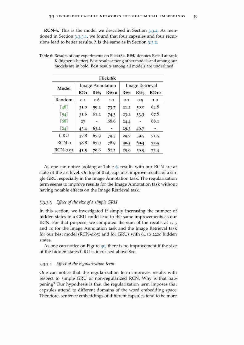
3.3 recurrent capsule networks for multimodal embeddings 49
RCN-λ. This is the model we described in Section 3.3.2. As men-tioned in Section 3.3.3.1, we found that four capsules and four recur-sions lead to better results. λ is the same as in Section 3.3.2.
Table 6: Results of our experiments on Flickr8k. R@K denotes Recall at rankK (higher is better). Best results among other models and among ourmodels are in bold. Best results among all models are underlined
Flickr8k
ModelImage Annotation Image Retrieval
R@1 R@5 R@10 R@1 R@5 R@10
Random 0.1 0.6 1.1 0.1 0.5 1.0
[48] 31.0 59.2 73.7 21.2 50.0 64.8
[54] 31.6 61.2 74.3 23.2 53.3 67.8
[68] 27 - 68.6 24.4 - 68.1
[24] 43.4 63.2 - 29.3 49.7 -
GRU 37.8 67.9 79.3 29.7 59.5 71.5
RCN-0 38.8 67.0 78.9 30.3 60.4 72.5
RCN-0.05 41.5 70.6 81.2 29.9 59.9 72.4
As one can notice looking at Table 6, results with our RCN are atstate-of-the-art level. On top of that, capsules improve results of a sin-gle GRU, especially in the Image Annotation task. The regularizationterm seems to improve results for the Image Annotation task withouthaving notable effects on the Image Retrieval task.
3.3.3.3 Effect of the size of a simple GRU
In this section, we investigated if simply increasing the number ofhidden states in a GRU could lead to the same improvements as ourRCN. For that purpose, we computed the sum of the recalls at 1, 5
and 10 for the Image Annotation task and the Image Retrieval taskfor our best model (RCN-0.05) and for GRUs with 64 to 2200 hiddenstates.
As one can notice on Figure 30, there is no improvement if the sizeof the hidden states GRU is increased above 800.
3.3.3.4 Effect of the regularization term
One can notice that the regularization term improves results withrespect to simple GRU or non-regularized RCN. Why is that hap-pening? Our hypothesis is that the regularization term imposes thatcapsules attend to different domains of the word embedding space.Therefore, sentence embeddings of different capsules tend to be more

50 matching vision and language
Figure 30: Performance of GRUs on Flickr8k according to the size of theirhidden states. The x-axis represents the size of hidden states, they-axis represents the performance of the GRUs. This performanceis the sum of R@1, R@5 and R@10 for both Image Annotation andImage Retrieval tasks. The line corresponds to the performance ofour best model (RCN-0.05 with hidden states of dimension 1024).
Figure 31: Our hypothesis. The cross corresponds to an image, circles corre-spond to sentence embeddings output by an RCN and trianglescorrespond to sentence embeddings output by a GRU. In thatcase, both the RCN and the GRU output sentence embeddings fora given image around the same point, but even if the RCN gener-ates worse embeddings on average, its best sentence embeddingis better than the best sentence embedding output by the GRU.
different than for a GRU or an RCN without normalization. As theImage Annotation task consists in retrieving one of five sentences foran image, the distribution that capsules induce may lead to have oneout of these five sentences being closer to its corresponding image.We summarized our hypothesis in Figure 31.
3.3.4 Conclusion of Section 3.3
In [28], we proposed the RCN (Recurrent Capsule Network), a noveldeep architecture for visual sentence embedding. It is based on the

3.4 gated recurrent capsules 51
CapsNet architecture that was recently proposed in [80], but it differsfrom it in three important ways: we applied it to natural language pro-cessing, it is built in a recurrent fashion whereas the original CapsNetwas built in a fully-connected fashion and the routing is performedusing one of the GRUs.
We obtained some promising results, especially for the Image An-notation task where our RCN performs better than GRUs. We ex-plained these performances improvements by the distribution thatthe capsules induced in the computation of sentence embeddings. Inaddition, we showed that the results of our capsules could not onlybe explained by the fact that they had more parameters than their cor-responding GRUs: Figure 30 showed that increasing the size of GRUshidden states did not result in as good results as our models.
The main drawback of our model is that it is very large, and verylong to train on bigger datasets such as MSCOCO [58]. Therefore, wearchitectured Gated Recurrent Capsules, requiring much less train-able parameters than the RCN we introduced in this section. Thenext section is dedicated to these Recurrent Gated Capsules.
3.4 gated recurrent capsules
In [29], we proposed another novel deep network architecture for thecaption retrieval task: given a set of images and a set of sentences,we build a model that ought to find the closest sentence to an inputimage. As stated in Section 2.2.2, numerous works have attempted toaddress that task; most of them are making use of a multimodal spacewhere sentences and images are projected and compared [25, 31, 44,53]. Word2VisualVec [20, 21] relies on another approach, the authorsbuilt a model to project sentences directly in a space of visual features:as the quality of visual features is constantly improving, the authorsstated that learning visual sentence embeddings rather than project-ing them in a more complicated multimodal space was a promisingapproach. In our paper [29], a model following this unconventionalapproach is proposed.
Projecting images and sentences in the same space, whether mul-timodal or simply visual, implies that representations of images andsentences as mathematical objects must be derived. Since the recentbreakthrough of deep learning, Convolutional Neural Networks (CNNs)have shown compellingly good performances in computer vision tasks.In particular, some of them [35, 50] are able to learn visual featuresthat they use to classify images from a big dataset such as ImageNet[16]. Most recent works on caption retrieval have used features com-ing from a ResNet [35] which had been trained on ImageNet for aclassification task [25, 31]. In our work, we extract features thanksto a ResNet that had been finetuned on MSCOCO [58] by the au-thors of [25], as we did for the RCN in Section 3.3. Deriving visual

52 matching vision and language
sentence representations is the main part of our work. RecurrentNeural Networks (RNNs) such as Long Short-Term Memory units(LSTMs) [38] and Gated Recurrent Units (GRUs) [13] have provedto deliver state-of-the-art results on various language modeling taskssuch as translation [85], automatic image captioning [92] or captionretrieval [25]. In the last version of Word2VisualVec [21], the authorsshowed that concatenating a representation derived by a GRU witha Word2Vec [65] representation and a bag-of-words representationto get a multi-scale sentence representation lead to better results invisual sentence embedding for caption retrieval. However, we arguethat using these kinds of representations cannot be optimal: pool-ing all words together without putting attention on relevant parts ofthe sentence does not reflect the complexity of images; and the cur-rent state-of-the-art model for image and caption retrieval is basedon object-detection and cross-attention [53], which corroborates ourstatement that sentences should be processed in a finer way. Our workaims at proposing a new architecture corresponding to and address-ing that issue: how to analyze a sentence so that important visualelements are emphasized?
As for the RCN, our research has been inspired by recent workson capsule networks [37, 80]. This new architecture shows promisingresults in computer vision. In capsule networks, the routing proce-dure can be seen as an attention mechanism that routes the outputof capsules from one layer to the relevant ones in the next layer. Wethink that this principle can be successfully used in Recurrent NeuralNetworks, and the Gated Recurrent Capsule that we introduce in thissection is a novel architecture, and is to our best knowledge the veryfirst occurrence of recurrent unit using capsules.
The contributions that we presented in [29] are three-fold:
• we introduce Gated Recurrent Capsules (GRCs), a novel RNNarchitecture which extents conventional GRUs so that informa-tion flow focuses on critical data items;
• we propose to address the caption retrieval task using the newlyproposed GRCs architecture;
• we demonstrate experimentally that GRC enable higher perfor-mance when compared to state of the art Word2VisualVec (em-ploying GRUs) in the MSCOCO caption retrieval task.
Our presentation is divided in five sections. Having introduced theextent of the work we published in [29] in the current section, wewill describe related works in Section 3.4.1. In Section 3.4.2 we willdescribe our model for caption retrieval. Section 3.4.3 details resultsobtained by our model. We will conclude our presentation in Section3.4.5.

3.4 gated recurrent capsules 53
3.4.1 Related Work
Several works have been done on building visual-semantic embed-dings. Most of them are based on the construction of a multimodalspace where sentences and images are projected and compared. In[25], Faghri et al. used a GRU to map sentences to a multimodalspace; images were simply mapped to that space through a lineartransform. They obtained good results by finetuning the ResNet theyused to produce visual features: that is the reason why we used oneof their finetuned ResNets to produce visual features in our model.Another more complex model proposed by Gu et al. [31] showed thatresults could be boosted by the use of two generative models (onegenerating images and one generating sentences) in addition to aGRU and a ResNet. More recently, [53] has shown that even betterperformances could be reached by processing images with an objectdetection model combined with cross-attention instead of derivingglobal visual features.
Another approach has been proposed recently: instead of mappingimages and sentences to a multimodal space, [20, 21] proposed to de-rive visual features from images and to map directly sentences to thespace of visual features. This approach is promising as the qualityof visual features is constantly increasing. Moreover, it avoids map-ping images to a more complex space. Our work follows that uncon-ventional approach. It has been inspired by recent works on capsulenetworks [37, 80]. Capsule networks have shown promising results incomputer vision. However to our best knowledge they have not beenused yet in a recurrent fashion for natural language processing apartfrom the work we introduced in Section 3.3 that we published in [28];however, the architecture presented in [28] is using a complex GRUssetup to process and route the information, leading to much morelearnable parameters, which is a drawback that our architecture doesnot have.
3.4.2 Visual Sentence Embeddings
Word2VisualVec is a non-conventional approach to caption retrieval,as it maps sentences directly to a visual features space. We decidedto test that approach. We eventually compare it to the multimodalapproach.
3.4.2.1 Word2VisualVec
In [20], a first version of Word2VisualVec was proposed. It consistedin applying a multilayer perceptron on vectorized sentences to projectthese sentences in a space of visual features. Three vectorization meth-ods were discussed in that paper: bag-of-words, word hashing and av-eraging Word2Vec embeddings. In [21], the authors of [20] improved

54 matching vision and language
Figure 32: Word2VisualVec and our variant with a GRC. In Word2VisualVec,three sentence representations (Word2Vec, BoW and GRU) areconcatenated and then mapped to a visual features space. In ourmodel, we replaced the final hidden state of the GRU by the av-erage of all final hidden states of a GRC.
Word2VisualVec by concatenating three sentence representations. Inthat paper, a sentence representation was produced by concatenatinga bag-of-words, a Word2Vec and a GRU representation of the sen-tence. Then, it was projected in a space of visual features through amultilayer perceptron. Figure 32 shows how Word2VisualVec worksin practice.
On top of good performances in caption retrieval, this visual repre-sentation of sentences showed an interest in multimodal query com-position: the authors showed that visual words features could beadded or subtracted to images features and form multimodal queries.Authors also stated that further gains could be expected by includinglocality in Word2VisualVec representations.
3.4.2.2 Gated Recurrent Capsules
Gated Recurrent Units were introduced by Cho et al. in [13]. Theyare similar to LSTMs: they have similar performances and are welladapted to NLP because they can handle long-term dependenciesin sentences. We preferred GRUs to LSTMs because they have lessparameters for similar performances. More formally, a GRU is com-posed of an update gate ut and a reset gate rt, and can be describedwith the following expressions:
ut = σ(Wxuxt +Whuht−1 + bu), (82)

3.4 gated recurrent capsules 55
Figure 33: A Gated Recurrent Unit: for each input xt, a new value ht iscomputed, based on xt, rt and ht−1, where rt expresses howmuch of ht−1 should be reset to compute ht. Eventually, ht iscomputed based on ht, ht−1 and ut, where ut expresses howmuch of ht should be used to update ht−1 to ht
rt = σ(Wxrxt +Whrht−1 + br), (83)
ht = tanh(Wxhxt +Whh(rt ⊙ ht−1) + bh), (84)
ht = (1− ut)⊙ ht−1 + ut ⊙ ht, (85)
with xt the t-th input and ht the t-th output or hidden state of theGRU. The equations above can be explained as follows: for each in-put xt, the GRU computes rt and ut based on the input and theprevious state ht−1. It computes a new value ht based on xt, rt andht−1, and rt expresses how much of ht−1 should be reset to computeht. Eventually, ht is computed based on ht, ht−1 and ut, and ut ex-presses how much of ht should be used to update the hidden stateht of the GRU. Learned parameters are Wxu, Whu, bu, Wxr, Whr, br,Wxh, Whh, and bh. GRUs are described with more details in Section2.1.4.3.
In our case, the xt correspond to word embeddings: if s is a sen-tence of length L, then it is first converted into a list (w1, ...,wL) ofone-hot vectors, and each one-hot vector is mapped to a word em-bedding using a lookup matrix We. Therefore, we have (x1, ..., xL) =(Wew1, ...,WewL). The coefficients ofWe are learned, but they are ini-tialized to precomputed word embeddings to avoid overfitting prob-lems.
Capsules were designed by [80] for image processing. The idea be-hind capsules for computer vision consists in making complex com-putations and outputting a pose vector and an activation. This outputis then routed towards subsequent capsules according to some prede-fined routing algorithm. The goal of that architecture is to have eachcapsule learning to recognize a visual feature based on what previouscapsules have recognized before. For instance, some capsules couldrecognize eyes, a nose, a mouth and their respective positions. Then

56 matching vision and language
they would send their outputs to another capsule aiming at recogniz-ing a whole face. It is architectured to avoid losing spatial informationas common CNN do due to pooling operations. We think that cap-sules can also successfully perform other tasks such as NLP-relatedtasks, as our proposed model does.
In a nutshell, what we would like to do is to produce different em-beddings that would attend to different semantic sides of the inputsentence. A sentence would be divided into sub-sentences, and eachof those sub-sentences would attend to a particular element of an im-age. These sub-sentences representations are then processed to buildan embedding for the whole sentence.
In our model, all capsules share the same parameters and are simi-lar to GRUs. In the following, we will explain the differences betweenthem and actual GRUs. A recurrent capsule layer should process asentence word-by-word and make updates in a way that would putattention on important words: the hidden state of each capsule shouldreflect one semantic side of the input sentence. Therefore, we need todefine a routing procedure depending on current states and incom-ing words. For that purpose, we will use hidden states of capsules attime t− 1 and the incoming word xt to find how relevant a word is toa given capsule. More formally, if we consider the k-th capsule withk ∈ {1, ...,Nc}, update gates and reset gates will be the same as for aGRU:
u(k)t = σ(Wxuxt +Whuh
(k)t−1 + bu), (86)
r(k)t = σ(Wxrxt +Whrh
(k)t−1 + br), (87)
We also compute h(k)t as we do in a GRU:
h(k)t = tanh(Wxhxt +Whh(r
(k)t ⊙ h
(k)t−1) + bh), (88)
We would like to make our routing procedure trainable via gradi-ent descent, so we need to define differentiable operations. For thatpurpose, we will assume that for each capsule, for a given word wt,we have a coefficient p(k)t ∈ [0, 1] such that
h(k)t = (1− p
(k)t )h
(k)t−1 + p
(k)t h
(k)t (89)
with
h(k)t = u
(k)t ⊙ h
(k)t + (1− u
(k)t )⊙ h
(k)t−1, (90)
which is the actual update computed in a GRU. The coefficient p(k)t isa routing coefficient, describing to what extent a given capsule needs

3.4 gated recurrent capsules 57
to be updated by the incoming word. As in [37], routing can be seenas an attention mechanism, putting attention on relevant words in ourcase. However, while the authors of [37] use Gaussians determined byEM-routing to compute this coefficient, we propose to compute it ina simpler manner. More details are provided in the next section. Wecan expand the last equation to get the following update:
h(k)t = (1− p
(k)t u
(k)t )⊙ h
(k)t−1 + p
(k)t u
(k)t ⊙ h
(k)t (91)
We can notice that it boils down to multiplying the update u(k)t bya coefficient p(k)t . Then, how to compute p(k)t ? For that purpose, wedefine an activation coefficient a(k)t for each capsule:
a(k)t = |αk|+ log(P(k)t ). (92)
In the last equation, the αk are random numbers drawn from a nor-mal probability distribution (we found that 0.1 and 0.001 were goodvalues for the mean and the standard deviation of the normal prob-ability distribution). The αk are important to our model because allcapsules share the same parameters: if all activations are the samewhen they start processing a sentence, they will be all the same at theend. These random numbers break the symmetry between capsules;this is needed for our model to work properly. We assume P(k)t oughtto represent the semantic similarity between the current hidden stateof the capsule h(k)t−1 and the incoming word xt: if the incoming word is
semantically similar to the previous hidden state, P(k)t should be high,and if it is different, then it should be low. One can intuitively imag-
ine that the cosine similarity cos(h(k)t−1, h(k)t ) =
⟨
h(k)t−1|h
(k)t
⟩
‖h(k)t−1‖2×‖h(k)
t ‖2corre-
sponds to a relevant definition of the semantic similarity between thecurrent hidden state of the capsule and the incoming word: if the in-coming word has a different meaning than previous words, then onecan expect that h(k)t will reflect that different meaning. Therefore wedefine P(k)t as:
P(k)t = cos(h(k)t−1, h(k)t ). (93)
Then we can compute p(k)t according to the following formula:
pt =softmax(a
(1)t
T , ..., a(N)t
T )
M(94)
whereM is the maximal coordinate of the vector softmax(a(1)t
T , ..., a(N)t
T )
and T is a hyperparameter controlling the sharpness of the routingprocedure (the higher T , the more we have one routing weight equalto 1 and all others equal to 0).

58 matching vision and language
Figure 34: Gated Recurrent Capsules: all capsules share the same learnedparameters θ. The inputs of capsule i at time t are a word em-bedding xt and its hidden state at time t− 1 h(i)t−1. Its output is
h(i)t , and it is computed through the routing procedure described
in Section 3.2. This routing procedure can be seen as an attentionmodel: each output depends on how semantically similar the in-coming word is to previously processed words. It ensures thateach capsule generates a sentence embedding corresponding toone important visual element of the sentence.
Our routing is different from those that were introduced in [37, 80]:the outputs of capsules are not combinations of all previous capsulesoutputs. Only the weights of the routing procedure depend on theseprevious capsules outputs.
Please note that if T → +∞, then all capsules receive the sameinputs and produce the same hidden states: it is strictly equivalent toa GRU. Therefore, GRCs are an extension of the GRUs. The interestof GRCs over GRUs is that they can provide different representationsof the same sentence, with attention put on some relevant parts ofit. This idea is shown on Figure 34. Moreover, a GRC has the samenumber of trainable parameters as a GRU, but it has the ability tomake more complex computations: for that reason we think that thisarchitecture could be successfully used for other tasks than captionretrieval.
The model we propose for caption retrieval is similar to Word2VisualVec,but we replace the GRU by a GRC, as shown on Figure 32. Insteadof concatenating the last hidden state of a GRU to a Word2Vec and abag-of-words representations, we concatenate the average of the lasthidden states of a GRC. We also tried to derive a weighted averageof the hidden states of a GRC based on a soft-attention mechanismdescribed in [22] but results did not improve. We reported our resultsin Section 3.4.3 for information.
3.4.2.3 Improving Word2VisualVec with GRC
As we said in Section 3.4.2.1, Word2VisualVec relies on three represen-tations of sentences: bag-of-words, average of Word2Vec embeddingsand GRU. GRCs provide another representation that we can concate-nate to the three previous ones. More precisely, let us assume that weprocessed a sentence of length L with a GRC containing Nc capsules.Then, if h(1)L , ...,h(Nc)
L are the final hidden states of its capsules, the

3.4 gated recurrent capsules 59
corresponding representation vGRC of the sentence is the average ofall these hidden states:
vGRC =1
Nc
Nc∑
k=1
h(k)L . (95)
This representation is intermediate between the GRU and the Word2Vecrepresentations: it is the sum of Nc different hidden states, each ofthem corresponding to a particular part of a whole sentence.
Our goal is to map sentences to corresponding images in a spaceof visual features. One way to measure the efficiency of that kindof mappings is to evaluate the model on caption retrieval. When themodel projects both images and sentences in a common multimodalspace, recent works have shown that triplet ranking losses were ef-ficient [25]. However in our case, sentences are directly mapped toa space of visual features, no transformation is made on image fea-ture vectors. We found, in accordance with [21], that using the meansquared error (MSE) gave better results than a triplet ranking loss.Therefore, considering a mini-batch B = ((s1, x1), ..., (sNb
, xNb)) of
sentence-image pairs (Nb is the size of the mini-batch), we definedthe loss function LMSE(B) as follows:
LMSE(B) =1
Nb
Nb∑
k=1
‖fθ(sk) −φ(xk)‖22 , (96)
where φ is a function mapping images to image features and fθ is afunction mapping sentences to image features where θ is the set of alltrainable parameters. Our objective is to find a θ minimizing LMSE:
θ = argminθ(LMSE(B)) (97)
where B is the set of all possible image-sentence pairs. We detail theadvantages of the MSE loss in Section 2.1.2 for more information. Weuse the RMSProp method to optimize fθ, following the procedure wedescribe in Section 2.1.2.1.
3.4.3 Experimental Results
In this section, we present our experimental results. We first introducethe dataset we used to perform our experiments, then we give someimplementation details, and eventually we present and discuss ourresults with respect to the actual Word2VisualVec model, and withrespect to a multimodal version of our model.
3.4.3.1 Dataset
We evaluated how our models performed on the caption retrieval taskon the MSCOCO dataset [58]. This dataset contains 123000 images

60 matching vision and language
with 5 captions each, and we split it into a training set, a validationset and a test set according to [43]. The training set contains 113000
images, the validation set contains 5000 images and the test set con-tains 5000 images.
As for data preprocessing, we converted all sentences to lowercaseand removed special characters (apart from spaces and hyphens). Welimited the vocabulary to 5000 most used words, and replaced allother words by an "UNK" token. Regarding images, we projectedthem to a space of visual features. For that purpose, we used thepenultimate layer of the ResNet-152 from [25] to get 2048-dimensionalfeatures vectors.
3.4.3.2 Parameters
Regarding the sentence embedding part of our model, we set its pa-rameters as follows: we set the maximum sentence length to 24 (iflonger the sentence is cut after the 24-th word). We initialized We
using 500-dimensional Word2Vec embeddings trained on Flickr. Wealso used these embeddings to compute the Word2Vec part of sen-tences representations. These embeddings are the same as the onesthat the authors of Word2VisualVec used in [21]. Regarding the GRC,we found that a model with 4 capsules and T = 0.4 performed well.The GRU in Word2VisualVec and the GRC capsules in our modelhave 1024-dimensional hidden states.
We trained our models using the RMSProp method [87] with mini-batches of 25 image-sentence pairs during 25 epochs. We followed thesame learning rate decay procedure as in [21]: the learning rate wasinitially 0.0001 and we divided it by 2 when the performance of themodel on the validation set did not increase during three consecutiveepochs. We made all our implementations using the TensorFlow [1]library for Python and used the default parameters of the RMSPropoptimizer: decay = 0.9, momentum = 0.0 and epsilon = 1e-10.
3.4.3.3 Results and Discussion
To prove the interest of our model, we compared it to Word2VisualVec.We compared the two versions we described in Section 3.4.2.2: theone with the average of final hidden states of capsules and the onewith the soft-attention mechanism proposed in [22]. We reported ourresults in Table 7. They show that our model performs better thanWord2VisualVec, and that the attention mechanism does not providemuch improvement.
Moreover, we also wanted to see on which kind of sentences GRCswere more efficient than GRUs. For that purpose, we listed all thesentences that our model ranked in the top 9 sentences and that wereranked worse than rank 100 by Word2VisualVec. We also listed sen-

3.4 gated recurrent capsules 61
Table 7: Results of our experiments on MSCOCO. R@K denotes Recall atrank K (higher is better). Best results among all models are in bold.
MSCOCO
ModelCaption Retrieval
R@1 R@5 R@10
Word2VisualVec 32.4 61.3 73.4
W2V + BoW + GRC 33.4 62.2 74.0
W2V + BoW + GRC + Attention 32.8 62.3 74.2
tences ranked by Word2VisualVec in the top 9 that were ranked worsethan rank 100 by our model. Our results are summarized in Table 8.
Table 8: For each model: number of sentences ranked in top 9 for theright image by one model and above rank 100 by the othermodel. Ten sentences are ranked in top 9 by Word2VisualVec whileranked above rank 100 by our model, and seventeen sentences areranked in top 9 by our model while ranked above rank 100 byWord2VisualVec. We also reported these numbers of sentences with-out counting sentences containing "UNK" tokens. This table showsthat GRCs are performing better than GRUs on much more sen-tences than GRUs compared to GRCs.
Word2VisualVec Our model
Total 10 17
Total without UNK tokens 3 11
We noticed that sentences on which GRCs were outperformingGRUs were more likely sentences containing multiple visual concepts.We provide some examples in Figure 35. We think that this observa-tion implies that GRCs could be used efficiently to derive finer visualsentence embeddings, taking into account important local elements.
3.4.4 Comparison Image Space vs Multimodal Space
We have also trained a multimodal version of our model, replacingthe visual features extractor by the visual embedding model we pre-sented in Section 3.4.2.1. The results we obtained are reported in Table9.
As one can notice, the multimodal model is much more efficientthan the visual model on the caption retrieval task.

62 matching vision and language
Figure 35: Compared results of Word2VisualVec and our model on threeimages.
Table 9: Results of our experiments on MSCOCO: comparison between im-age space and multimodal space. R@K denotes Recall at rank K(higher is better). Best results among all models are in bold.
MSCOCO
ModelCaption Retrieval
R@1 R@5 R@10
Image Space 33.4 62.2 74.0
Multimodal Space 33.5 64.1 77.0

3.5 grcs for the video-to-text (vtt) task 63
3.4.5 Conclusion of Section 3.4
In [29], we introduced a novel RNN architecture called Gated Re-current Capsules (GRCs). We built a model to address the captionretrieval task by mapping images and sentences to a visual featuresspace. We showed in our experimental work that the models obtainedusing the proposed GRCs are surpassing those from earlier works(employing GRUs). Moreover, we stated that GRCs could potentiallybe used in any typical RNN tasks, as they are an extension of GRUs.Eventually, we showed that a multimodal version of our model wasmore efficient than the visual one. Therefore, as we wanted to assessour results at the TRECVid VTT Matching task that we will describein Section 3.5, aiming at performing video caption retrieval, we de-cided to focus on multimodal models.
3.5 grcs for the video-to-text (vtt) task
EURECOM participated in the Sentence Matching subtask of the TRECVid2018 [7] Video-to-Text (VTT) task for the first time. The approachwe followed was to adapt the model we presented in Section 3.4 forvideo-sentence matching, following the setup of the winning team of2017 [22]. The Sentence Matching subtask of the VTT task requiresto link videos and sentences describing these videos. Testing data iscomposed of 1,000 videos, and five datasets of 1,000 sentences, eachsentence corresponding to one video. For each video and for eachdataset of sentences, teams are asked to rank sentences from the clos-est to the most dissimilar. Evaluation is performed on each sentencedataset using the Mean Inverse Rank measure.
3.5.1 Our Model
In this section, we will present the model that we used at TRECVidVTT and some variations we also submitted.
3.5.1.1 Definition of our model
As stated in the introduction of Section 3.5, our model aims at adapt-ing the model we presented in Section 3.4 for video-sentence match-ing, following the setup of the winning team of 2017 [22]. In [22],video embeddings are derived as follows:
- frames are extracted every 0.5 second for each video;
- features vectors (v1, ..., vn) are derived from these frames usingthe penultimate layer of a ResNet-152 [35];
- these features vectors are then fed sequentially into a GRU [13],whose hidden states (h1, ...,hn) are concatenated to correspond-

64 matching vision and language
ing features vectors, to obtain contextualized features vectors(s1, ..., sn) = (v1‖h1, ..., vn‖hn);
- these contextualized features vectors are combined through asoft attention mechanism to form a vector v, which is actually aweighted sum of s1, ..., sn;
- this vector v is then projected into a vector space after two fully-connected layers with ReLU activations, where each activationis preceded by a batch normalization.
In our model, the same process is applied for computing videoembeddings. However, before feeding v into the two fully-connectedlayers, we concatenated it with a vector that we derived from thevideo using the last layer of an RGB-I3D [11]. Moreover, [22] used aResNet-152 trained on ImageNet [16] whereas we used the ResNet-152 trained on ImageNet and finetuned on MSCOCO [58] proposedby [25].
In [22], text-embeddings are derived as follows:
- three text representations are derived (one using an average ofWord2Vec [65] embeddings, a second one is a BoW representa-tion and a third one is derived by taking the last hidden state ofa GRU) and concatenated;
- the resulting vector is then fed into two consecutive fully-connectedlayers following the same process as for videos.
Regarding the text-embeddings part of our model, we tried to re-place the GRU by GRCs [29] or a bidirectional GRU. GRCs are exten-sions of GRUs that we proposed in [29], where we showed that theycould improve results of GRUs on multimodal matching tasks. Ourmodel is summarized by Figure 36.
3.5.1.2 Training
We trained our model using a common hard-negative triplet rankingloss [25]. More formally, if v is the embedding computed for a video, sthe embedding computed for a sentence corresponding to that video,then the loss l(v, s) corresponding to the couple (v, s) is defined asfollows:
l(v, s) = maxs 6=s
(max(0,α− cos(v, s) + cos(v, s))), (98)
where α is a hyperparameter that we set to 0.2.We used several datasets for training and validation:
- MSVD [12];
- MSR-VTT [98];

3.5 grcs for the video-to-text (vtt) task 65
Figure 36: Our model. RNN can be a GRU, a GRC or a bidirectional GRU.
- TGIF [56] (for computer memory problems, we only used 60,000
sentence-video pairs from TGIF);
- TrecVid VTT 2016 test data [5];
- TrecVid VTT 2017 test data [6].
Our validation set was composed of 200 videos from TrecVid VTT2016 test data and 200 videos from TrecVid VTT 2017 test data withcorresponding sentences. Therefore, the validation set contained 400
different videos. We used MSVD, MSR-VTT and TGIF for training,for a total of 65,782 different videos with all corresponding sentences.Eventually, we used the remaining data from TrecVid VTT 2016 andTrecVid VTT 2017 to form a finetuning dataset of 3,088 videos.
We trained our models using the RMSProp method [87] with Ten-sorFlow default parameters and gradient clipping between -5 and 5.We first trained our model on the training set, applying a learningrate of 0.00003 during 20 epochs (dividing the learning rate by twoif validation loss did not improve during three consecutive epochs),with mini-batches of size 25. Then, we set the learning rate to 0.00002,and finetuned our model on the finetuning dataset during 60 epochs,dividing the learning rate by two if validation loss did not improveduring three consecutive epochs.
3.5.2 Our runs
Now, we will describe the runs we actually submitted to TRECVidVTT, and the results we obtained with respect to other teams.

66 matching vision and language
Table 10: Our results in terms of Mean Inverse Rank
Runs Subset A Subset B Subset C Subset D Subset E
Run 1 0.194 0.190 0.194 0.193 0.199
Run 2 0.197 0.197 0.197 0.184 0.204
Run 3 0.202 0.209 0.206 0.186 0.212
Run 4 0.231 0.240 0.234 0.224 0.241
3.5.2.1 Definition of runs
EURECOM submitted four different runs to the VTT Sentence Match-ing subtask. The runs are numbered from 1 to 4, with the expectedbest runs having the highest numbers. For each run and for eachvideo, sentences are ranked by decreasing cosine similarity.
run 1 : We apply the model we described in Section 3.5.1. TheRNN we used for computing sentence embeddings was a simpleGRU.
run 2 : This run was similar to RUN 1, but we replaced the GRUby a GRC.
run 3 : In this run, the GRU of RUN 1 is replaced by a bidirectionalGRU.
run 4 : This final run is a merge of previous runs. The merge isperformed by summing the cosine similarities of the three previousruns, to obtain a new score for each sentence.
3.5.2.2 Results
We reported our results in Table 10. Our runs are ranked as we ex-pected on subsets A, B, C and E. It is not the case for subset D, asthe simple GRU obtained better results than the GRC and the bidirec-tional GRU.
In Figures 37-41, all results on different sentences subsets are pre-sented. Our results are in red. As one can see, our ensemble methoddid better than other methods.
Our results were very encouraging, as we ended third out of eleventeams. Thinking of our tries at AVS 2016 and AVS 2017 with textualand visual embeddings, we planned to participate in AVS 2019 withmultimodal embeddings. However, results were not as good as weexpected.

3.6 limits of multimodal spaces : ad-hoc video search 67
Figure 37: Results on subset A
Figure 38: Results on subset B
Figure 39: Results on subset C
3.6 limits of multimodal spaces : ad-hoc video search
As mentioned in Section 3.2, Ad-Hoc Video Search (AVS) is a chal-lenging task consisting in using natural language queries to retrieverelevant video segments from large datasets (see Figure 42). “Ad-Hoc”implies that the query follows no pattern, and the terms are drawnfrom an open vocabulary that is not restricted to any particular do-main. Due to this nature, a query can be very specific (e.g., "find shotsof a surfer standing on a surfboard, not in the water") or open ended

68 matching vision and language
Figure 40: Results on subset D
Figure 41: Results on subset E
(e.g., "find shots inside a moving car"). Therefore, a "good" model forAVS should be able to extract relevant high-level features from videos,parse text queries, and find a common representation of both modal-ities for relevance judgement. TRECVID, an evaluation campaign, isorganized yearly by the NIST to evaluate state-of-the-art models fordifferent video processing tasks, including the AVS task [6]. In thissection, the focus of study is automatic AVS using external trainingdata.
Most recent works in image and video processing and in text pro-cessing rely on Deep Learning techniques. For image processing, com-monly used feature extractors or concepts detectors are deep Convo-lutional Neural Networks (CNNs) which have been pretrained on Im-ageNet 1000 categories [16]. For video processing, I3D trained on theKinetics dataset has shown excellent results in activity detection [11].Regarding text processing, recent works have shown that RNNs suchas LSTMs [38] or GRUs [13] could be used to build efficient languagemodels.
In [30], we proposed using a fusion of three multimodal modulestrained on different datasets to tackle the AVS task. Our contributionsin that work are two-fold:

3.6 limits of multimodal spaces : ad-hoc video search 69
Figure 42: Principle of AVS. Video Features are derived from videos andprocessed by a Video Model to obtain a vector representation. Atthe same time, a text query is processed by a Text Model that alsoderives a vector representation. These two vector representationsare then compared to list all relevant videos with respect to thetext query.
- joint exploitation of object counting, activity detection and se-mantic concept annotation for query interpretation;
- a new fusion method that combines three modules trained ondifferent datasets and shows competitive performance.
We also show the limits of the use of multimodal spaces to tackle theAVS task with respect to methods based on visual spaces or wordspaces.
Our presentation is organized as follows. Section 3.6.2 introducesthe related works in AVS. Section 3.6.3 introduces the cross-modallearning employed for training three different modules, while Section3.6.3 describes the proposed fusion method. Section 3.6.4 providesempirical insights and Section 3.6.6 concludes this presentation.
3.6.1 Related Works
From AVS 2018 [7], the general approaches from the participants canbe summarized as follows: linguistic analysis for query understand-ing combining different techniques for concept selection and fusion;or learning joint embedding space of textual queries and images; orthe integration of two mentioned approaches. From the results of tenparticipants, we conclude that the approach of learning the embed-ding space is the key of success for AVS task. Following up this direc-tion, we propose to learn three embedding spaces including objects

70 matching vision and language
counting, activities and semantic concepts separately, and a fusionmethod to incorporate these models.
3.6.2 Cross-Modal Learning
In this section we will describe the multimodal models we employed.More precisely we will first define their architecture and then howwe trained them. Please note that in this section, we will considerimages and videos, even though our models will be used for Ad-HocVideo Search. The reason is that some of our models will be trainedon images and applied at frame-level on videos. More informationswill be given at Section 3.6.4.2.
3.6.2.1 Feature Representation
Let Q be a textual query and V an image or a video. We want to builda model so that Q and V can be compared. More precisely, we wantto be able to assign a score to any (Q,V) to describe the relevance ofV with respect to Q. For that purpose, we use a similar model to [25].
For processing textual queries, we represent any query Q of lengthL as a sequence (w1, ...,wL) of one-hot vectors of dimension N, whereN is the size of our vocabulary. These one-hot vectors are then em-bedded in a vector space of dimension D. More formally, we obtain asequence of word embeddings (x1, ..., xL) where xk = wkWe for eachk in {1, ...,L}. The weights of the embedding matrix We ∈ R
D×N aretrainable.
The obtained sequence of word embeddings is then processed by aGRU, whose last hidden state is kept and input to a Fully-Connectedlayer to get a sentence embedding. Formally, a GRU is defined by thefollowing equations:
ut = σ(htWuh + xt+1Wux + bu) (99)
rt = σ(htWrh + xt+1Wrx + br) (100)
ht = tanh((ht ⊙ rt)Whh + xt+1Whx + bu) (101)
ht+1 = (1− ut)⊙ ht + ut ⊙ ht (102)
where Wuh, Wux, Wrh, Wrx, Whh, Whx, bu, br and bu are trainableparameters. More information on GRU is given in Section 2.1.4.3. Ifthe length of the input sequence is L, then the final sequence embed-ding vs is defined as:
vs = hLWs + bs (103)

3.6 limits of multimodal spaces : ad-hoc video search 71
where Ws and bs are trainable parameters.Regarding visual objects, the generic process we employ is to ex-
tract a vector representation ϕ(V) of a visual object V where ϕ corre-sponds to any relevant concepts or features extractor. Then, we inputϕ(V) to a Fully-Connected layer to obtain a visual embedding vv:
vv = ϕ(V)Wv + bv (104)
where Wv and bv are trainable parameters.Our goal is to train these models to be able to compare vs and vv.
We will explain how these models are trained in Section 3.6.2.2.
3.6.2.2 Model Training
The objective is to learn a mapping such that the relevancy of a pairof a query and a video (Q,V) can be evaluated. As explained in Sec-tion 3.6.2.1, our model derives a query representation vs from Q anda video representation vv from V . Triplet loss is used as the loss func-tion for model training. Mathematically, if we consider a query repre-sentation vs, a positive video representation vv (corresponding to vs)and a negative video representation vv (that does not correspond tovs), the triplet loss L for (vs, vv, vv) to minimize is defined as follows:
L(vs, vv, vv) = max(0,α− cos(vs, vv) + cos(vs, vv)) (105)
where α is a margin hyperparameter. We chose to employ the hard-margin loss presented in [25], where vv is chosen to be the representa-tion of the negative video with the highest similarity with the queryrepresentation vs among all videos in the current training mini-batch.
3.6.3 Fusion Strategy
In this section we will describe the three multimodal modules weused and how we fused them.
3.6.3.1 Multimodal Modules
Our model relies on three multimodal modules: a counting module,an activity module and a concepts module (see Figure 43). Each ofthem has the architecture we described in Section 3.6.2.1 and has beentrained according to the optimization scheme we defined in Section3.6.2.2.
The counting module is based on a Faster-RCNN [75] trained onthe OpenImagesv4 dataset [51]. It takes images as inputs. For eachinput, it detects objects belonging to the 600 classes of OpenImagesv4
and counts them to obtain a vector of dimension 600, where the valueat index i corresponds to the number of detected objects of class i.Embeddings are then derived from that vector.

72 matching vision and language
Figure 43: Proposed model. We extract embeddings from three modules:a counting module, an activity module and a concepts mod-ule. These embeddings are then concatenated and input to Fully-Connected layers to obtain new embeddings. That model is alsotrained using a triplet loss.
The activity module relies on an I3D trained on Kinetics-600 andtakes video inputs. Each input is processed by the I3D, which re-turns a vector of 600 logits corresponding to the 600 activities of theKinetics-600 dataset. That vector is then processed as described inSection 3.6.2.1 to obtain an embedding.
The concepts module takes as input concepts detections comingfrom four different concept detectors. These concept detectors areResNet [35] models trained on ImageNet1k, Places-365 [106], TRECVIDSIN [105] and HAVIC [83]. Following the same process as for othertwo modules, we generate embeddings from the concatenation of theconcept detections coming from these four detectors.
3.6.3.2 Fusion Model
Instead of simply averaging similarity scores to compare videos andqueries, we chose to train a model to draw finer similarities betweenthem. For that purpose, we derived embeddings from our modulesfor videos and queries, and passed them through Fully-Connectedlayers to obtain new embeddings. More formally, if v1v, v2v and v3v arevideo embeddings respectively generated by the counting module,the activity module and the concepts module, we derived the newvideo embedding vv as follows:
vv = concat(v1v, v2v, v3v)Wfusev + bfuse
v (106)
where Wfusev and bfuse
v are trainable parameters. Similarly, if v1s , v2sand v3s are query embeddings, we obtain a new query embedding asfollows:
vs = concat(v1s , v2s , v3s)Wfuses + bfuse
s (107)
where Wfuses and bfuse
s are trainable parameters.

3.6 limits of multimodal spaces : ad-hoc video search 73
We trained our fusion models using the same triplet loss as we didfor multimodal modules, as decribed in Section 3.6.2.2.
3.6.4 Experiments
In this section, we describe how we implemented and trained ourmodels, and present our experimental results.
3.6.4.1 Datasets
We used the MSCOCO [58] dataset to train the counting module (notthe Faster-RCNN itself) and the concepts module. MSCOCO is com-posed of about 120k images, and five captions per image. We trainedmodules on the whole dataset, using 1k images for validation: we didnot employ the usual train/validation/test split.
Regarding the activity module, it has been trained on the TGIF[56] dataset (containing about 100k animated GIF images and 125kcaptions) and on the MSVD [12] dataset (containing 1970 videos andabout 70k captions).
Fusion models have been trained on the MSR-VTT [98] dataset, con-taining 10k videos with 20 captions each. We used the usual split:6513 videos for training, 497 for validation and 2990 for testing.
Our models have also been evaluated in terms of mean averageprecision based on 10,000 retrieved shots on V3C1 [10], containing7475 videos split into 1,082,657 shots, using the provided ground-truth results for six queries.
3.6.4.2 Implementation details
We implemented our models using the Tensorflow [1] framework forPython. Each of them has been trained for 150k iterations with mini-batches of size 64. We used the RMSProp [87] algorithm, with gradi-ents capped to values between -5 and 5 and a learning rate of 10−4.Hidden dimensions of GRUs are always 1024, and embeddings out-put by multimodal modules and fusion models are of dimension 512.The size of vocabularies has been set to 20k. We applied dropout [82]with rate 0.3 to all outputs of Fully-Connected layers, and batch nor-malization [41] to the inputs of our models. In triplet losses, the αparameter has been set to 0.2.
Modules trained on images (counting and concepts modules) areused for videos during testing in two different ways. For tests onMSR-VTT, we extracted uniformly one frame every fifteen frames, ap-plied the extractor on each frame (Faster-RCNN for the counting mod-ule or concepts extractors for the concepts module) and averaged ob-tained vectors. For tests on V3C1, we processed provided keyframesinstead of entire videos.

74 matching vision and language
3.6.4.3 Performance of Modules
Model R@1 R@5 R@10 medR
M1 (Counting) 2.95% 7.16% 11.40% 264
M2 (Activity) 2.83% 8.80% 13.59% 167
M3 (Concepts) 3.88% 10.69% 15.44% 168
Table 11: Results on the MSR-VTT test dataset of three modules.
Model mAP
M1 (Counting) 2.15%
M2 (Activity) 0.00%
M3 (Concepts) 2.15%
Table 12: Results on the V3C1 dataset of three modules.
In this section, we report results of each module on the uniquevideo retrieval task (evaluated on MSR-VTT) and the multiple videosretrieval task (evaluated on V3C1). Results are reported in Table 11
and Table 12.One can notice that relative results of modules are completely dif-
ferent with respect to the task. On the unique video retrieval task, thecounting module has the worst results, and the concepts module hasthe best results. On the multiple videos retrieval task, the countingmodule and the concepts module perform similarly, and the activitymodule has very bad results.
We think that these results are due to the fact that shots in the V3C1
datasets are much shorter than the videos on which the I3D activityextractor has been trained. For that reason, we will not report resultsof fusions involving the I3D on V3C1 in the following. Regarding thefact that the counting module performs as well as the concepts mod-ule on the multiple videos retrieval task, our hypothesis is that themultiple videos retrieval task requires less precision than the uniquevideo retrieval task: the concepts module covers a large range of vi-sual concepts, which is useful when looking for a specific video, butless useful when the goal is to retrieve as many videos as possible.
In the next section, we will present results of fusions
3.6.4.4 Performance of Fusions
Results of fusion models are reported in Table 13 and Table 14. Twotypes of fusions have been tested : Mi +Mj means that we summedup similarity scores between modules Mi and Mj, and F(Mi,Mj)
means that we applied the fusion scheme we described in Section3.6.3.

3.6 limits of multimodal spaces : ad-hoc video search 75
Model R@1 R@5 R@10 medR
M1 +M2 3.91% 11.31% 16.87% 133
M1 +M3 4.29% 11.56% 16.22% 149
M2 +M3 4.69% 13.31% 19.19% 105
M1 +M2 +M3 5.00% 13.70% 19.37% 104
F(M1,M2) 5.20% 15.78% 23.69% 59
F(M1,M3) 4.80% 14.70% 22.09% 70
F(M2,M3) 5.90% 18.00% 26.39% 49
F(M1,M2,M3) 6.48% 19.27% 27.99% 42
Sum of best 6.72% 17.80% 24.72% 67
Table 13: Results on the MSR-VTT test dataset of fusions of modules. Sumof best is the sum of M1 +M2 +M3 and F(M1,M2,M3).
Model mAP
M1 +M3 4.54%
F(M1,M3) 4.01%
F(M1,M3) +M1 +M3 5.41%
Table 14: Results on the V3C1 dataset of fusions of modules.
In each case, the best model involves a fusion according to ourfusion method. In the unique video retrieval task, the fusion aloneperforms better than other models whereas in the multiple videosretrieval task, the sum of similarity scores of modules and of theirfusion has the best results. The reason may be that our fusion schememakes finer representations of videos, which is less useful for multi-ple videos retrieval than for unique video retrieval.
3.6.5 Results on TRECVid AVS 2019
For AVS 2019, we submitted three runs: one was based on our count-ing module, another one on our concepts module and the last onewas a fusion of both modules. Best results of each team have beenreported on Figure 44.
As one can notice, we performed very poorly, as we ended as thelast team. It seems that using concepts detectors without multimodalembeddings and big ensemble methods leads to better results. Look-ing at these results, we think that the approach to AVS must be dif-ferent from the approach to VTT. In the VTT task, we have the priorknowledge that there is one and only one textual description corre-sponding to a given video. However for AVS, we just need to retrieveas many videos possible corresponding to one given query. Traininga model on matching data may induce too much attention to details,

76 matching vision and language
Figure 44: Best result for each team at TRECVid AVS 2019. We performedpoorly, as we finished last.
which can be relevant when the task is to find the only correspondingtext to a video. However, even though transforming a textual queryinto a list of visual concepts may be less precise, it is probably moreinclined to find a high number of videos that are related to a giventextual query.
3.6.6 Conclusion
In [30], we proposed to tackle the AVS problem using three modules:a counting module, an activity module and a concepts module. Eachof these modules analyzes videos and derives embeddings in a mul-timodal space. We showed that jointly taking advantage of countingobjects, detecting activities and detecting semantic concepts in videosallowed to deal efficiently with the complexity of the AVS task. More-over, we proposed a method to fuse modules trained on differentdatasets that appeared to lead to significantly better results than sim-pler fusion methods.
However, we also showed that using fully learned multimodal spaceswas not efficient for the AVS task, even though it was efficient for theVTT task, as mentioned in Section 3.6.5.
3.7 general conclusion of chapter 3
In this chapter, we tackled several tasks related to matching imagesand texts or videos and texts. For that purpose, we architectured twoneural network models inspired by capsule networks: the RecurrentCapsule Network and the Gated Recurrent Capsules. We also showed

3.7 general conclusion of chapter 3 77
that for matching a single image or a single video to a single text,embedding both modalities in a multimodal space was more efficientthan embedding them in a visual space. We assessed our results usingcommon datasets such as Flickr 8k and MSCOCO.
However, we found that the multimodal approach was not as ef-ficient for the AVS task, where multiple videos need to be retrievedbased on one natural language query. We think that in that case, amethod based on concepts extraction would be a better idea, and wethink that it should be the right research direction to improve resultson the AVS task.


4AT T E N T I O N A N D C U R R I C U L U M L E A R N I N G F O RC A P T I O N I N G
4.1 introduction
In Chapter 3, we introduced models for image-sentence matching andvideo-sentence matching. The semantic representations that we usedfor these matching tasks were mostly multimodal embeddings. In thischapter, we propose to generate descriptive sentences from imagesand videos, which is another type of semantic representation. Theserepresentations can be useful for other applications than multimodalembeddings. Automatic image captioning can be useful for visuallyimpaired people, to give automatically a textual descriptions of im-ages they cannot see, on websites for instance. Automatic video cap-tioning can be used for instance to enrich TV programs with textualinformation on scenes, that can improve the user experience. Mul-timodal embeddings are not straightforwardly readable by humans,therefore they are mostly useful for back-end applications, such asmultimedia indexing and retrieval.
The image captioning task and the video captioning task consistin automatically generating short textual descriptions for images andvideos respectively. They are challenging multimedia tasks as they re-quire to grasp all information contained in a visual document, suchas objects, persons, context, actions, location, and to translate this in-formation into text. This task can be compared to a translation task:except instead of translating a sequence of words in a source languageinto a sequence of words in a target language, the aim is to translate aphotograph or a sequence of frames into a sequence of words. There-fore, most of recent works in captioning rely on the encoder-decoderframework proposed in [85], initially for text translation. In imageor video captioning, the encoder aims at deriving an image or videorepresentation, respectively. Recent advances in deep learning haveshown to fit very well to that task. In particular, Convolutional Neu-ral Networks (CNNs) have proved to give excellent results in produc-ing highly descriptive image representations or video representations.The decoder part aims at generating a sentence based on the repre-sentation produced by the encoder. Long Short-Term Units (LSTMs)[38] and Gated Recurrent Units (GRUs) [13] are usually chosen forthat task. Image captioning [92] and video captioning can seem tobe similar tasks, as both of them require to "translate" a visual objectinto a textual one. However, video captioning poses a problem that
79

80 attention and curriculum learning for captioning
makes it more challenging than image captioning: it requires to takeinto account temporality.
Our contributions in that chapter are two-fold:
• we propose a Learned Spatio Temporal Pooling (L-STAP) methodto tackle both temporal and spatial complexity in videos to gen-erate video captions;
• we propose two Curriculum Learning algorithms to improveresults in captioning.
Section 4.2 deals with the L-STAP method. In Section 4.3, we in-troduce our two Curriculum Learning algorithms. We conclude thechapter in Section 4.4.
4.2 video captioning with attention
In the work we will introduce in this section, we aim at attending torelevant regions of a video based on previous frames, because the rele-vance of objects, persons or actions relies on the context in which theyappear; and that context should be inferred from previous frames.More precisely, after deriving frame-level local features using the lastconvolutional layer of a ResNet-152 [35], we do not apply an averagepooling to pool these local features. We process them by Learned Spa-tio Temporal Adaptive Pooling (L-STAP). L-STAP attends to specificregions of a frame based on what occurred previously in the video.Our pooling method is learned because it is based on an LSTM whoseparameters are learned. It is spatio-temporal because it takes into ac-count space and time in a joint fashion. In addition, it is adaptivebecause the attention paid to local regions is based on previous hid-den states of the LSTM; pooling depends not only on the processedframe but also on previous ones. A high-level schematic view of ourproposed model is depicted in Figure 45.
We evaluated our results on two common datasets used for bench-marking video captioning tasks: MSVD [12] and MSR-VTT [98]. Re-sults show that our model based on L-STAP outperforms state-of-the-art models in terms of several metrics. An ablation study also showsthat our method leads to significant improvements with respect tostate-of-the-art methods.
Our contributions can be summarized as follows: we propose anovel pooling method for video processing, which we evaluate onthe video captioning task, even though it could be applied to anyother task involving video processing, such as video classification.Moreover, we demonstrate the interest of our pooling method overusual approaches.

4.2 video captioning with attention 81
Figure 45: Overview of our L-STAP method. Frame-level local features arederived using a ResNet-152. Then, an LSTM processes these localfeatures, and updates its hidden state by attending to them basedon previous frames. The result is that space and time are jointlytaken into account to build video representations.
4.2.1 L-STAP: Our Model
Let us first formulate the problem we are to deal with. Given a videoV , which is a sequence of T frames (v(1), ..., v(T)), our goal is to derivea descriptive sentence Y = (y1, ...,yL). The approach that we havefollowed is based on the encoder-decoder framework. The encoderfirst derives frame-level representations (x(1), ..., x(T)) = X, and thenpool these representations together to form frame-level video repre-
sentations (h(1)
, ...,h(T)
). Based on these representations, the decoderreconstructs a descriptive sentence in a recurrent fashion. Figure 46
summarizes the important steps our model. In the following section,we will describe it in detail and report how we train it.
4.2.1.1 Grasping Spatio-Temporal Dependencies with L-STAP
As we stated above, the first step is to produce a representation of theinput video. In the following subsections, we will explain how wederive frame-level features, and how we pool them together.
Given a video V = (v(1), ..., v(T)), we need to derive features foreach frame v(t). A common way to do so is to process each frameusing a CNN, which has been previously pretrained on a large-scaledataset. In works such as [59], the outputs of the penultimate layerof a ResNet-152 have been chosen as frames representations, whichconsist of 2048-dimensional vectors. However, such representations

82 attention and curriculum learning for captioning
Figure 46: Illustration of our model, based on the proposed L-STAP method.Frames are processed sequentially by a CNN (a ResNet-152 inthis case). However, instead of applying an average pooling on lo-cal features as some recent works do, we make use of an LSTM tocapture time dependencies. Local hidden states are computed toobtain a 7x7x1024-dimensional tensor. These local hidden statesare then pooled together (using average pooling or soft attention),and processed by an LSTM decoder to output a sentence.
discard locality, which results in loss of information. Therefore, inthis work, we choose to take the output of the last convolutionallayer of a ResNet-152. Thus, we obtain frame-level representations(x(1), ..., x(T)) = X, where x(t) ∈ R
7×7×2048 for all t. The next stepis to process these dense frame-level representations to derive com-pact frame-level representations, using the proposed L-STAP methodinstead of conventional pooling.
L-STAP aims at replacing the average pooling operation after thelast convolutional layer in a CNN, and to pool local features accord-ing to previous frames. The goal is to capture where important ac-tions are occurring, and to discard locations that are not relevant tosummarize what is happening in a video. For that purpose, we usean LSTM, taking local features as inputs, resulting in local hiddenstates, which are then combined in a way we will describe later inthis subsection. More formally, given local features x(t)ij ∈ R
2048, the
aggregated local features h(t)ij are computed recursively as follows:
i(t)ij = σ(Wixx
(t)ij +Wihh
(t−1)+ bi) (108)
f(t)ij = σ(Wfxx
(t)ij +Wfhh
(t−1)+ bf) (109)
o(t)ij = σ(Woxx
(t)ij +Wohh
(t−1)+ bo) (110)

4.2 video captioning with attention 83
c(t)ij = f
(t)ij ◦ c
(t−1) + i(t)ij tanh(Wcxx
(t)ij +Wchh
(t−1)+ bc) (111)
h(t)ij = o
(t)ij ◦ tanh(c(t)ij ) (112)
where Wix, Wih, bi, Wfx, Wfh, bf, Wox, Woh, bo, Wcx, Wch andbc are trainable parameters, and c(t−1) and h
(t−1)are respectively
the memory cell and the hidden state of the LSTM. Please note thatmemory cells and hidden states are shared for computing all aggre-gated local features. The memory cell and the hidden state at time tare computed as follows:
c(t) =
7∑
i=1
7∑
j=1
α(t)ij c
(t)ij (113)
h(t)
=
7∑
i=1
7∑
j=1
α(t)ij h
(t)ij (114)
where α(t)ij are local weights. In our work, we experimented with two
types of local weights. We first tried to use uniform weights:
α(t)ij =
1
7× 7(115)
which actually correspond to an average pooling of aggregated localfeatures. The second solution that we tried was to derive local weightsusing an attention mechanism, as follows:
α(t)ij = wT tanh(Wαxx
(t)ij +Wαhh
(t−1)+ bα). (116)
α(t)ij =
exp(α(t)ij )
∑7k=1
∑7l=1 exp(α(t)
kl ), (117)
where Wαx, Wαh, bα are trainable parameters.
4.2.1.2 Encoding Videos
In our model, we encode videos using the L-STAP method we pre-sented previously. We initialized the memory cell and the hiddenstate of the LSTM using the output of an I3D [11] (before the final

84 attention and curriculum learning for captioning
softmax) which had been trained on Kinetics-600 [11]. More formally,if V is an input video:
c(0)ij = tanh(We
ce(V) + bec) (118)
h(0)ij = tanh(We
he(V) + beh) (119)
where Wec, be
c, Weh and be
h are trainable parameters. The decoder pro-
duces c(T) and h(T)
as outputs, where T is the length of the inputvideo. These outputs will be used to initialize the sentence decoderthat we will introduce in the next section.
4.2.1.3 Decoding Sentences
For decoding sentences, we chose to use an LSTM. In the following,we assume that sentences Y are represented by sequences of one-hotvectors y1, ...,yL ∈ R
N where N is the vocabulary size. The aim ofthe LSTM is to compute the probabilities P(yl|yl−1, ...,y1,V ; θ) forl ∈ {1, ...,L}, where θ is the set of all parameters in the encoder andthe decoder, and V an input video. In the following, we will describeformally how we compute these probabilities.
We initialize the memory cell and the hidden state of the decoderLSTM using the last memory cell and the last hidden state of theencoder:
cd0 = c(T), (120)
hd0 = h(T)
. (121)
It has been shown in [60] for text translation tasks that attendingto hidden states of the encoder during the decoding phase improvedresults. Some works in video captioning have followed that approachsuccessfully [100, 101]. We followed a similar approach for our decod-ing phase. More precisely, at each step l, we compute a weighted sumof hidden states of the encoder:
ϕ(h,hdl−1) =
T∑
t=1
β(t)l h
(t)(122)
where β(1)l , ..., β(T)
l are computed as follows:
β(t)l = wT
β tanh(Wβeh(t)
+Wβhhdl−1 + bβ), (123)

4.2 video captioning with attention 85
β(t)l =
exp(β(t)l )
∑Lk=1 exp(β(t)
k ), (124)
where Wβe, Wβh, bβ are trainable parameters. Assuming that theword yl−1 has been decoded at step l− 1, we aim to decode yl basedon yl−1 and ϕ(h,hdl−1). For that purpose, we first compute a wordembedding xdl :
wdl =Wembyl−1, (125)
where Wemb is a learned embedding matrix. Then, we concatenatewd
l and ϕ(h,hdl−1) to obtain and xdl :
xdl = [wdl ;ϕ(h,hdl−1)] (126)
Eventually, we input xdl to the decoder LSTM:
idl = σ(Wdixx
dl +Wd
ihhdl−1 + b
di ) (127)
fdl = σ(Wdfxx
dl +Wd
fhhdl−1 + b
df ) (128)
odl = σ(Wdoxx
dl +Wd
ohhdl−1 + b
do) (129)
cdl = fdl ◦ cdl−1 + i
dl tanh(Wd
cxxdl +Wd
chhdl−1 + b
dc ) (130)
hdl = odl ◦ tanh(cdl ) (131)
where Wdix, Wd
ih, bdi , Wdfx, Wd
fh, bdf , Wdox, Wd
oh, bdo , Wdcx, Wd
ch andbdc are trainable parameters.
The last step is to infer a word yl. For that purpose, we derive ylas follows:
yl = softmax(Wdhdl ) (132)
where Wd is a trainable parameter. We state that yl is the one-hotvector corresponding to the maximum coordinate of yl.

86 attention and curriculum learning for captioning
Figure 47: Overview of our training losses. The first training loss is theCross-Entropy loss, which aims to make the probability distribu-tion of sentences in the training set and the probability distribu-tion of the inferred sentences match. The second one is a rankingloss, aiming to bridge the semantic gap between video represen-tations and sentences.
4.2.2 Training
Assuming that y1, ...,yL correspond to ground-truth words, we aimto minimize the following cross-entropy loss:
Ld(θ) = −
L∑
l=1
log P(yl|yl−1, ...,y1,V ; θ) (133)
where V is a video corresponding to the caption (y1, ...,yL). Moreinformation is given on the cross-entropy loss in Section 2.3.
In addition to that, some works have shown that regularizing thecross-entropy loss with a matching loss between video encodingsand ground-truth sentences could improve results by bridging thesemantic gap between them [33, 59]. As reported in Section 4.2.2,such improvement has been noticed in our experiments. The match-ing model we employed is described in the following. Let us assumethat Y = (y1, ...,yL) is a sentence corresponding to a video V . First, wetranslate this sequence of one-hot vectors into a sequence of word em-beddings (xs1, ..., xsL) using the matrixWemb from Section 4.2.1.3. Then,we compute a sentence embedding ψ(Y) by processing this sequenceof word embeddings into another LSTM: each word embedding isentered sequentially as an input to that LSTM, and ψ(Y) is defined tobe its last hidden state. We want the initialization of the decoder tobe as close as possible to an accurate representation of its correspond-
ing sentence. Therefore, if ϕ(V) = h(T)
is the initial hidden state of

4.2 video captioning with attention 87
the decoder, we will aim to minimize the following ranking loss from[25]:
Lm(θ) = maxV 6=V
(
max(0,α− S(ϕ(V),ψ(Y)) + S(ϕ(V),ψ(Y))))
+ maxY 6=Y
(
max(0,α− S(ϕ(V),ψ(Y)) + S(ϕ(V),ψ(Y)))) (134)
where V is a negative video sample, and Y is a negative sentence sam-ple coming from another video than V . More information on rankinglosses is given in Section 2.2.1 The final loss is the following:
L(θ) = Ld(θ) + λLm(θ) (135)
where λ is a hyperparameter that we set to 0.4 according to results onvalidation.
4.2.3 Experiments
In this section, we will deal with our experimental results.
4.2.3.1 Datasets
We evaluated our models on two video captioning datasets: MSVD[12] and MSR-VTT [98]. MSVD is a dataset composed of 1,970 videosfrom YouTube, which have been annotated by Amazon MechanicalTurks (AMT). Each video has approximately 40 captions in English.We split that dataset following [91]: 1,200 videos for training, 100
videos for validation and 670 videos for testing. MSR-VTT is a similardataset, but with much more videos, and less captions per video. Itis composed of 10,000 videos, and 20 captions per video. Following[98], we split that dataset into 6,513 videos for training, 497 videos forvalidation and 2,990 videos for testing.
For both datasets, we uniformly sampled 30 frames per video asdone in [104], and extracted features for each frame based on the lastconvolutional layer of a ResNet-152 [35], which had been trained onthe image-text matching task on MSCOCO [58], after pre-training onImageNet-1000 [16] following [25]. In addition, we extracted activityfeatures for each video using an I3D pretrained on Kinetics-600 [11].For MSVD, we converted sentences to lowercase and removed specialcharacters, which lead to a vocabulary of about 14k words. We con-verted each word into an integer, and cut sentences after the thirtiethword if their lengths were higher than thirty. The same approach forMSR-VTT lead to a much bigger vocabulary size of about 29k words.Therefore, we kept only the 15k most common words, and replacedall the others by an <UNK> token. We applied the same process oth-erwise.

88 attention and curriculum learning for captioning
4.2.3.2 Implementation Details
Our models have been implemented with the TensorFlow framework[1]. We use 1024-dimensional LSTMs in both encoder and decoder.Soft attention spaces are 256-dimensional. Word embeddings are 300-dimensional.
We trained our model using the RMSProp algorithm [87], with de-cay = 0.9, momentum = 0.0 and epsilon = 1e-10. Batch size is set to64. Learning rate is 1e-4, and we apply gradient clipping to a thresh-old of 5. Eventually, we apply dropout on the output of the decoder(before the prediction layer) with a rate of 0.5 to avoid overfitting.
4.2.3.3 Results on MSVD and MSR-VTT
Model Bleu-4 ROUGE METEOR CIDEr
TSL [97] 51.7 - 34.0 74.9
RecNet [93] 52.3 69.8 34.1 80.3
mGRU [71] 53.8 - 34.5 81.2
AGHA [104] 55.1 - 35.3 83.3
SAM [94] 54.0 - 35.3 87.4
E2E* [55] 50.3 70.8 34.1 87.5
SibNet [59] 54.2 71.7 34.8 88.2
L-STAP (Ours) 55.1 72.7 35.4 86.7
Table 15: Results on the MSVD dataset. The * sign means that the modelis using reinforcement learning techniques to optimize over theCIDEr metric. Best results are in bold characters.
We evaluated our models in terms of BLEU [70], ROUGE [57], ME-TEOR [17] and CIDEr [89] scores, which are metrics commonly usedto evaluate automated captioning tasks. We compared them to thefollowing recent models for video captioning. Our results on MSVDare presented in Table 15. Results on MSR-VTT are presented in Table16.
On MSVD, it can be noticed that L-STAP achieves the best resultson three out of four metrics. It is also relevant to mention that E2E[55], which achieves better CIDEr results than our model, has beentrained using reinforcement learning techniques to be optimized re-garding that CIDEr metric. Works on image captioning and videocaptioning have shown that significant improvements could be doneusing such techniques [3, 76, 96], at the price of much longer trainingtimes. We did not use reinforcement learning to train our models, in-stead we use cross-entropy minimization which has the advantage ofbeing fast and simpler to implement.
Results on MSR-VTT show that our model outperforms modelstrained using a cross-entropy loss on two metrics out of four (ME-

4.2 video captioning with attention 89
TEOR and ROUGE). HRL [96] obtains better results overall, howeverit makes use of reinforcement learning techniques, which leads tobetter results as stated in the previous paragraph.
We report some qualitative results of our model on MSR-VTT inFigure 48. On the second video, the man who is singing appears dur-ing a very limited amount of time. This shows that our model hasbeen able to attend to important frames to identify what the main ac-tion of the video was. In the first video, a woman starts talking aboutmakeup, and then puts some lipstick on her lips. The caption gen-erated by our model shows that it has been able to draw a relationbetween the first and the second parts of the video. Moreover, thelipstick is applied on a very localized part of the video frames: wecan infer that our model could efficiently attend to the right part ofthe frame to generate a caption. The fourth video shows that resultscould be improved by adding sound processing to our model: it wasnot possible from the video only to know that colors were said.
Model Bleu-4 ROUGE METEOR CIDEr
RecNet [93] 39.1 59.3 26.6 42.7
E2E* [55] 40.1 61.0 27.0 48.3
SibNet [59] 40.9 60.2 27.5 47.5
HRL* [96] 41.3 61.7 28.7 48.0
L-STAP (Ours) 40.7 61.2 27.6 44.8
Table 16: Results on the MSR-VTT dataset. The * sign means that the modelis using reinforcement learning techniques to optimize over theCIDEr metric. Best results are in bold characters.
4.2.3.4 Ablation Study
Results of an ablation study on the MSVD dataset are reported in Ta-ble 17. The encoder we used in our baseline model is an Long-termRecurrent Convolutional Network (LRCN) [19]. As shown in previ-ous works such as [33, 59], adding a component to the training loss tomake video representations match sentence representations improvesresults. Two interpretations can be given to these results. A first oneis that adding a ranking loss to match video representations and sen-tence representations helps bridging the semantic gap between thesetwo modalities. A second one could be that propagating the gradi-ent across all the layers of the decoder could make it vanish throughdepth. Thus, adding a matching loss to the cross-entropy loss couldbe seen as a skip-connection between the sentence to be generatedand the video representation used by the decoder. We illustrate thatsecond interpretation in Figure 49.
Replacing the average pooling at the end of a CNN by our L-STAPinduces a major improvement with respect to all metrics as reported

90 attention and curriculum learning for captioning
Figure 48: Some qualitative results of L-STAP on MSR-VTT.

4.2 video captioning with attention 91
Figure 49: Our second interpretation about the efficiency of the second termof our loss function. Skip connections between video representa-tions and ground-truth sentences improve results.
in Table 17. On top of that, results shown in Table 15 demonstratethat L-STAP leads to better results than other models based on localfeatures such as AGHA and SAM, and results shown in both Table15 and Table 16 show the interest of L-STAP over average pooling.
We can notice in Table 17 that using a soft-attention mechanism topool local hidden states in the encoder does not provide significantimprovements over average pooling for all metrics except from CIDEr.Our interpretation is that the LSTM of the encoder can learn to attendto relevant local features by itself: before applying the average pool-ing, attention has already been drawn quite efficiently.
4.2.4 Conclusion of Section 4.2
In [27], we presented a novel Learned Spatio-Temporal Adaptive Pool-ing (L-STAP) method for video captioning. It consists in taking intoaccount spatial and temporal information jointly in a video to pro-duce good video representations. As we have shown, these video rep-resentations can be successfully used to perform automated videocaptioning. We demonstrated the quality of our models based onL-STAP by comparing them with state-of-the-art models on MSVDand MSR-VTT, which are two video captioning datasets. On top ofthat, we assessed the interest of L-STAP through an ablation study.Although this presentation concentrates on video captioning we be-

92 attention and curriculum learning for captioning
Model Bleu-4 ROUGE METEOR CIDEr
Baseline 52.7 71.4 34.1 79.5
Baseline + matching 53.3 71.2 34.5 82.2
L-STAP (avg) + matching 55.1 72.3 35.4 84.3
L-STAP (att) + matching 55.1 72.7 35.4 86.8
Table 17: Results of ablation study on MSVD. Results show that a significantimprovement can be reached using our Learned Spatio-TemporalAdaptive Pooling instead of the usual average pooling. Poolinghidden states of the encoder using soft-attention (line 4) insteadof average pooling (line 3) does not always improve results. Ourinterpretation of that outcome is that the LSTM actually performsa kind of attention on local features before local hidden states arepooled together.
lieve that the proposed L-STAP method could be also applied to othervideo-related tasks such as video classification.
4.3 curriculum learning for captioning
In [9], Bengio et al. proposed a training method called CurriculumLearning. Instead of training models based on randomly drawn mini-batches from a training set, their method incrementally widens thetraining set, starting from easiest samples, and adding some harderones after each epoch. They showed that training could get faster,and sometimes lead to better results. In this section, we propose twoCurriculum Learning methods for captioning. The first one is a sim-ple adaptation of the algorithm that has been introduced in [9]: wepropose to evaluate the complexity of training samples based on theself-BLEU [108] metric. The second one is an Adaptive CurriculumLearning algorithm: instead of using a predefined curriculum, wepropose an algorithm that adapts the content of the training set tothe actual performances of our model. We apply our method to im-age captioning, but it can also be straightforwardly adapted to videocaptioning.
Our contributions in this section are two-fold:
• we show in the context of curriculum learning that the self-BLEU metric that has initially been proposed to evaluate di-versity can also be used to assess the complexity of captionedimages;
• we propose an Adaptive Curriculum Learning algorithm andwe show experimentally that it performs better than the usualmini-batch gradient descent algorithm.
The rest of this section is organized as follows: in Section 4.3.1, wedefine the image captioning model we use in our experiments. In Sec-

4.3 curriculum learning for captioning 93
Figure 50: The image captioning model we employed. A Faster-RCNN de-rives features vectors corresponding to object detection boxesfrom an input image. These features vectors are then used by adecoder through a soft-attention mechanism to produce a captionfor the input image.
tion 4.3.2, we explain how self-BLEU can assess the complexity of acaptioned image. In Section 4.3.3, we present our novel Adaptive Cur-riculum Learning algorithm. We show and discuss our experimentalresults in Section 4.3.4, and we conclude in Section 4.3.5.
4.3.1 Image Captioning with Attention
The model that we use for image captioning is the one on Figure 50. AFaster-RCNN [75] pretrained on VisualGenome [49] is used to extractdetection boxes and corresponding features vectors. These featuresvectors are then used as the input of a decoder GRU via an attentionmechanism to guide the generation of a caption. More formally, let(v1, ..., vn) be n object detections features vectors obtained by a Faster-RCNN on a given image. Let wt be the t-th decoded word. Then, theinput xt+1 of the decoder GRU for decoding the t+ 1-th word is asfollows:
xt+1 =
n∑
i=1
αi,t+1vi, (136)
where the αi,t+1 are non-negative weights. These weights are derivedthrough a soft-attention mechanism:
(α1,t+1, ...αn,t+1) = softmax(r1,t+1, ..., rn,t+1), (137)
where for each i ∈ {1, ...,n}, ri,t+1 is derived as:
ri,t+1 = 〈Wvvi|Wwxt〉 , (138)
where Wv and Ww are trainable parameters. The output of the de-coder GRU is then converted into a word through an affine transform,as we did in Section 4.2.
Let us now describe the two Curriculum Learning methods that wepropose.

94 attention and curriculum learning for captioning
Figure 51: Examples of images taken from the MSCOCO dataset and theircorresponding self-BLEU scores. Images that contain few ele-ments and that are easily described have a high score, whereascomplex images have a low score.
4.3.2 Curriculum Learning with Self-BLEU
BLEU [70] has initially been proposed as a metric to assess the qualityof automatic translations. It has been also widely used for evaluatingcaptioning models. In [108], Zhu et al. propose self-BLEU, a methodto evaluate the diversity of generated text data. It consists in averag-ing the BLEU scores of all generated texts with respect to the others.More formally, let S = {s1, ..., sp} a corpus of generated texts, and letBLEUA(s) be the BLEU score of s with respect to the set A. Then, theself-BLEU score of S is derived as follows:
self-BLEU(S) =1
p
p∑
i=1
BLEUS\{si}(si). (139)
As shown on Figure 51, this self-BLEU metric can also be used tomeasure the complexity of visual contents that have been captionedby human beings. If there is a big diversity in captions for a givenimage, it means that describing this image is not a straightforwardtask. Conversely, if the self-BLEU score is high, it means that inde-pendent humans use approximately the same sentences to describe it:the content is easily understandable.
We propose then an algorithm to train an image captioning modelwith Curriculum Learning based on the self-BLEU score. The princi-ple is simple: training starts with a subset of easy samples from thetraining set (with a high self-BLEU score), and after each epoch, weadd a fixed number of samples of increasing difficulty from the train-

4.3 curriculum learning for captioning 95
ing set to the training subset we mentioned. That training process isdescribed in the following algorithm. In that algorithm, we define a
Algorithm 1 Curriculum Learning with self-BLEU (α is a hyperpa-rameter)
Ensure: self-BLEU(si) > self-BLEU(si+1) ∀i ∈ {1, ...,n− 1}
train_set← {s1, ..., sn}k← k0for epoch ∈ {1, ..., #epochs} do
train_subset← {s1, ..., sk}k← min(k+α,n)Train model on train_subset
end for
hyperparameter α corresponding to how much we increase the sizeof the training subset after each epoch.
4.3.3 Adaptive Curriculum Learning
The idea of Curriculum Learning comes from an analogy between astudent and an artificial intelligence: in both cases, they are taughtthanks to data that they are provided with in an increasing order ofdifficulty. However, even though [9] has showed that training couldbe made significantly faster with Curriculum Learning, it is not clearthat final results of models trained with that method obtain system-atically better results than with a simple mini-batch gradient descent.We think that the reason is that after all, a model ends by being pro-vided with all training data, and therefore it is always optimized tofit the same data distribution.
How to avoid that issue? We think that despite these problems, theidea of Curriculum Learning should be further investigated: using afixed curriculum is only one possible way of providing a model withtraining data. In this section, we propose an Adaptive CurriculumLearning algorithm, that adapts a curriculum to the model that istraining. The idea behind our algorithm is simple. If our model isdoing well on some data, that data should not be often shown to it.However, if its results on that data is bad, then it should be providedmore often to it.
An analogy between our Adaptive Curriculum Learning algorithmand flashcard-based spaced repetition [8] could be made: it has beenshown that humans could learn efficiently and in the long term ifthey were provided with difficult data frequently, and less frequentlywith easy data. For a neural network model, we made the assumptionthat easy data correspond to frequent data in the training set, anddifficult data correspond to rare data: neural networks perform betteron data containing features they are often provided with because they

96 attention and curriculum learning for captioning
are optimized to fit their training data. Applying that principle toneural networks training using our Adaptive Curriculum Learningalgorithm can be seen as compensating imbalance in training data.
More formally, at each iteration t, we draw randomly a mini-batchfrom the training set. In the following, the expression CIDErA(s) de-notes the CIDEr score [89] of a sentence s based on a reference setA, and model(I) denotes the sentence generated by our captioningmodel for an image I. Each sample xi = (Ii, si,Si) from that mini-batch (Ii is an image, si is a corresponding sentence randomly drawnfrom the set Si of annotations) is then assigned a score ai, defined asfollows:
ai = CIDErSi\si(si) − CIDErSi\si(model(Ii)). (140)
That score ai if then used to compute the probability pi that thecorresponding sample is actually used for training:
pi = min(
exp(
ai − µ
σ
)
, 1)
, (141)
where µ and σ are two hyperparameters. The more our model isdoing well on a given sample, the more that sample has a chanceto be dismissed during training. The algorithm, that we called theFlashcard Algorithm accordingly to the analogy we made before, isdescribed below (p is the size of mini-batches).
Algorithm 2 The Flashcard algorithm: an Adaptive CurriculumLearning algorithm (µ and σ are hyperparameters)
train_set← {s1, ..., sn}for epoch ∈ {1, ..., #epochs} do
while Training data is remaining do
minibatch← {(I1, s1,S1), ..., (Ip, sp,Sp)}for i ∈ {1, ...,p} do
ai = CIDErSi\si(si) − CIDErSi\si(model(Ii))pi = min
(
exp(
ai−µσ
)
, 1)
minibatch← minibatch \ (Ii, si,Si) with probability 1− piend for
Train model on resulting minibatchend while
end for
Let us now describe how we trained our image captioning models.
4.3.3.1 Optimization
Assuming that y1, ...,yL correspond to ground-truth words for a givenimage, we aim to minimize the following cross-entropy loss:
L(θ) = −
L∑
l=1
log P(yl|yl−1, ...,y1, I; θ) (142)

4.3 curriculum learning for captioning 97
where I is an image corresponding to the caption (y1, ...,yL) and ylis the output of the decoder at iteration l. More information is givenon the cross-entropy loss in Section 2.3.
We use the Curriculum Learning algorithms that we defined pre-viously to guide training. In Section 2.3, we also stated that an al-ternative to the usual cross-entropy loss to train captioning modelswas using reinforcement learning. Reinforcement learning has shownto lead to very significant improvements in image or video caption-ing. We wondered if using one of our Curriculum Learning methodscould compensate the drawbacks of the cross-entropy loss that thereinforcement learning loss do not have. Therefore, we also train ourimage captioning model using reinforcement learning with CIDErreward. The reinforcement learning loss to minimize is defined asfollows:
LRL(θ) = −r(s), s ∼ pθ (143)
where r(s) is the reward for a sentence s. As neural networks aretrained by gradient descent, that loss needs to be adapted to be differ-entiable with respect to θ. As we showed in Section 2.3, minimizingthe reinforcement learning loss was equivalent to minimizing the fol-lowing loss:
L ′RL(θ) = −r(s) log(pθ(s)), s ∼ pθ
= −r(s)∑L
l=1 log (pθ (yl|y1, ..., xl−1, I; θ)) .(144)
4.3.4 Experiments
In this section, we give our experimental results. First, we explainhow we implemented our models, then we describe the dataset onwhich we train them, and eventually we give our results and discussthem.
4.3.4.1 Implementation Details
All our models have been implemented using the Tensorflow frame-work for Python [1]. We use 1024-dimensional LSTMs in both encoderand decoder. Soft attention spaces are 256-dimensional. Word embed-dings are 300-dimensional.
We trained our model using the RMSProp algorithm [87], with de-cay = 0.9, momentum = 0.0 and epsilon = 1e-10. Batch size is set to 64.Learning rate is 8e-5, and we apply gradient clipping to a thresholdof 5. Neither dropout nor batch normalization have been applied. Re-garding the hyperparameters of the Adaptive Curriculum Learningalgorithm, we found by cross-validation that µ = −0.6 and σ = 1.0lead to the best results.

98 attention and curriculum learning for captioning
4.3.4.2 Dataset
We evaluated how our models performed on the caption retrieval taskon the MSCOCO dataset [58]. This dataset contains 123,000 imageswith 5 captions each, and we split it into a training set, a validationset and a test set according to [43]. The training set contains 113000
images, the validation set contains 5000 images and the test set con-tains 5000 images.
As for data preprocessing, we converted all sentences to lowercaseand removed special characters (apart from spaces and hyphens). Welimited the vocabulary to 10,000 most used words, and replaced allother words by an "<UNK>" token. Regarding images, we utilized theResNet-101 features of object detections that have been released by[3]. These object detections have been derived using a Faster-RCNNwhich has been trained on the VisualGenome dataset. For each image,we utilized a fixed amount of 36 object detections.
4.3.4.3 Results and Discussion
We reported the experimental results we obtained on MSCOCO in Ta-ble 18. As one can notice, the self-BLEU-based Curriculum Learningalgorithm leads to nearly the same results as the baseline. We thinkthat the reason why results do not improve is that eventually, with orwithout a simple Curriculum Learning algorithm, models are trainedon the same data distributions: therefore we can intuitively deducethat they obtain on average nearly the same results.
The Adaptive Curriculum Learning algorithm leads to an improve-ment in terms of all metrics with respect to the baseline. The maindifference between the usual Curriculum Learning algorithm basedon self-BLEU and our Adaptive Curriculum Learning algorithm isthat the latter does not always lead to training a model on the samedistribution of training data, but on a more balanced distribution asit adapts the probability to deliver training data to the actual resultsof the model.
However, results using a Reinforcement Learning loss are still aboveour Adaptive Curriculum Learning algorithm. But both methods arenot exclusive, and there is no reason why the Reinforcement Learningmethod cannot be combined with our Adaptive Curriculum Learningalgorithm. We think that an interesting direction of research would beto investigate to what extent Adaptive Curriculum Learning can im-prove results of Reinforcement Learning in captioning.
We also plotted the validation curves of the baseline model trainedwith a simple mini-batch gradient descent, and using the self-BLEU-based Curriculum Learning algorithm. That plot has been reportedon Figure 52. We can see that training is slightly faster using Cur-riculum Learning, accordingly to the findings of [9]. However, bothcurves end with similar validation scores. An interesting direction of

4.3 curriculum learning for captioning 99
Model BLEU-4 ROUGE METEOR CIDEr
Baseline 30.9 53.8 25.2 98.5
Baseline + Self-BLEU 31.1 53.7 25.0 97.3
Baseline + Adaptive 31.1 54.1 25.7 100.4
Baseline + Reinforcement 32.2 54.8 25.8 108.5
Table 18: Our results on the MSCOCO dataset. As one can notice, the self-BLEU-based Curriculum Learning algorithm leads to nearly thesame results as the baseline. To the contrary, the Adaptive Cur-riculum Learning algorithm improves the results of the baseline interms of all metrics. However, it does not induce as much improve-ment as a Reinforcement Learning loss induces.
Figure 52: Plot of validation scores of the baseline trained with simple mini-batch gradient descent (in blue) and using self-BLEU-based Cur-riculum Learning (in red). We can notice that Curriculum Learn-ing make training a bit faster, even though the best validation lossis eventually nearly the same for both methods.
research would be to define a metric making the training of a caption-ing model with Curriculum Learning even faster.
4.3.5 Conclusion
In this section, we introduced our results in image captioning usingtwo methods of Curriculum Learning we designed: the first one issimilar to [9] using the self-BLEU metric to measure the complexityof annotated images, whereas the second one is an Adaptive Curricu-lum Learning method, that adapts the distribution of training data tothe actual performances of the captioning model during training. Weexperimented with these methods on the MSCOCO dataset for im-

100 attention and curriculum learning for captioning
age captioning, but our methods can be easily extended also to videocaptioning.
We found that, even though results on test data for the self-BLEU-based Curriculum Learning algorithm were similar to the usual mini-batch gradient descent, training could be made faster, accordinglyto the findings of [9]. We also found that our Adaptive CurriculumLearning algorithm lead to an improvement in terms of all the met-rics we used with respect to the mini-batch gradient descent baseline.However, this improvement is not as big as the improvement inducedby a reinforcement learning loss.
We think that two interesting directions of research would be to tryto find a complexity metric making the usual Curriculum Learning al-gorithm even faster for captioning, and to find a way to combine ourAdaptive Curriculum Learning algorithm with reinforcement learn-ing to further improve results.
4.4 general conclusion of chapter 4
In this chapter, we introduced models we developed for image andvideo captioning. In particular, we proposed the Learned Spatio Tem-poral Adaptive Pooling (L-STAP) method for video captioning, thatcan be used to replace the final global pooling in a CNN when usedto process videos. With that pooling method, one can derive local em-beddings where temporality is taken into account. Our video caption-ing model based on the L-STAP method outperforms state-of-the-artvideo captioning models according to our experiments. An ablationstudy has been able to show to what extent each component of ourmethod contributes to improving results. We think that the interestof our L-STAP method is not restricted to video captioning: the samemethod can be applied to any other task related to video processing.
We also proposed two Curriculum Learning algorithms. The firstone is based on the self-BLEU score, that we used to measure thecomplexity of an annotated image: if the self-BLEU score of such anannotated image is high, it means that annotators agreed a lot on thecaptions they proposed. In that case, we can infer that describing theimage was straightforward: the complexity of the image is low. Tothe contrary, if the self-BLEU score is low, it means that annotatorsdid not agree on the captions, which allows us to say that the imagewas complex. Using the self-BLEU score with a usual CurriculumLearning algorithm improved the speed of training, but not the finalresult. We proposed an explanation to that: with the usual Curricu-lum Learning algorithm, models are eventually trained to fit the samedistribution of data as models trained without Curriculum Learning.Therefore, to tackle that issue, we proposed a novel Adaptive Cur-riculum Learning algorithm that we called the Flashcard algorithm.It consists in showing data to the model with high probability when

4.4 general conclusion of chapter 4 101
it does not perform well on it, and with low probability if it does.With that Flashcard algorithm, results improved with respect to asimple mini-batch gradient descent. However, we also showed that itdid not improve results as much as Reinforcement Learning did. Aninteresting direction of research would be to find how to combine ourAdaptive Curriculum Learning algorithm with Reinforcement Learn-ing to further improve results in captioning.


5G E N E R A L C O N C L U S I O N
Our research work was the occasion to propose novel models andnovel methods for the creation of semantic representations of imagesor videos: multimodal vector representations that are useful in thecontext of vision-text matching, and also textual representations innatural language that are automatically generated. In particular, wewould like to emphasize the following points:
• The models that we proposed in this thesis work have beencompared to models usually employed for the same tasks. Weassessed that our models lead to better results than usual mod-els through experiments on standard datasets evaluated usingstandard metrics.
• Moreover, the models that we proposed have been applied tospecific tasks, but we think that they can also be applied in amore general context.
• Extensive experiments have been conducted throughout thiswork to assess the interest of each element of our models andmethods.
The models and methods we have proposed have been applied inthe context of this thesis research work; nevertheless we think thattheir interest could go beyond our research topic because they areconceptually generalizable to other applications, in particular relatedto natural language processing regarding our Recurrent Capsule Net-works and our Gated Recurrent Capsules, or related to video process-ing regarding our L-STAP method. Our work could for instance beextended to tasks that we did not have the opportunity to deal within that thesis work, such as Dense Captioning, or Visual QuestionAnswering.
We think that the main idea to be remembered from our work isthat, as says [88], "Attention Is All You Need". The models we pro-posed throughout this thesis are actually based on attention mech-anisms, emphasizing relevant data and obliterating irrelevant data.Also, the Curriculum Learning algorithms that we proposed can beseen as attention in a certain way: the right data is attended to dur-ing mini-batch selection, and given to the model we train. We startedthis manuscript with a citation of John Locke: "Reading furnishes themind only with materials of knowledge; it is thinking that makeswhat we read ours." This is exactly the message we would like toconvey: big datasets have given birth to the current AI trend, mak-
103

104 general conclusion
ing it grow up will need that models "think" and "understand" thesedatasets.
That leads us to the future perspectives of our work. We showed inSection 3.4 with our Gated Recurrent Capsules that focusing on sub-parts of a sentence was a way to improve results in image-sentencematching. We also showed in Section 4.2 that our L-STAP method,based on local features, was more efficient than using global features.Locality in both text and vision improved our results: would it bealso beneficial to study how sub-parts of sentences and local featuresof images or videos match? We think that this perspective should befurther investigated.
We showed in Chapter 3 that even though multimodal models wereefficient for matching vision and text, they lost their efficiency in taskssuch as Ad-Hoc Video Search (AVS), and concept detectors seemedto be more efficient. We think that it is worth focusing on what kindof information should preferably be extracted from vision-text datato address the AVS task.
We have showed in Section 4.3 how our Adaptive Curriculum Learn-ing algorithm was able to improve image captioning. However, theimprovement induced by Reinforcement Learning is bigger. How couldwe combine both Adaptive Curriculum Learning and ReinforcementLearning?
The matching term of the loss function of the model we imple-mented and tested, based on out L-STAP method induced an im-provement of our results. What are the links between vision-text match-ing and captioning? How solving one task can provide informationto help solving the second one?
As a conclusion and a general summary, we showed that attentionwas a key to success to derive semantic representations for imagesand videos. We think that a right direction for pursuing our researchwould be to focus on attention models on one hand, and on analyzinghow and what training data is fed to models during optimization onthe other hand.

B I B L I O G R A P H Y
[1] Martín Abadi, Paul Barham, Jianmin Chen, Zhifeng Chen, AndyDavis, Jeffrey Dean, Matthieu Devin, Sanjay Ghemawat, Geof-frey Irving, Michael Isard, et al. “Tensorflow: A system forlarge-scale machine learning.” In: 12th {USENIX} Symposium
on Operating Systems Design and Implementation ({OSDI} 16).2016, pp. 265–283.
[2] Aishwarya Agrawal, Jiasen Lu, Stanislaw Antol, Margaret Mitchell,C Lawrence Zitnick, Devi Parikh, and Dhruv Batra. “Vqa: Vi-sual question answering.” In: International Journal of Computer
Vision 123.1 (2017), pp. 4–31.
[3] Peter Anderson, Xiaodong He, Chris Buehler, Damien Teney,Mark Johnson, Stephen Gould, and Lei Zhang. “Bottom-upand top-down attention for image captioning and visual ques-tion answering.” In: Proceedings of the IEEE Conference on Com-
puter Vision and Pattern Recognition. 2018, pp. 6077–6086.
[4] Lisa Anne Hendricks, Oliver Wang, Eli Shechtman, Josef Sivic,Trevor Darrell, and Bryan Russell. “Localizing moments invideo with natural language.” In: Proceedings of the IEEE In-
ternational Conference on Computer Vision. 2017, pp. 5803–5812.
[5] George Awad, Jonathan Fiscus, David Joy, Martial Michel, AlanSmeaton, Wessel Kraaij, Maria Eskevich, Robin Aly, RoelandOrdelman, Marc Ritter, et al. “Trecvid 2016: Evaluating videosearch, video event detection, localization, and hyperlinking.”In: 2016.
[6] George Awad, Jonathan Fiscus, David Joy, Martial Michel, AlanF Smeaton, Wessel Kraaij, Georges Quénot-Georges, Maria Eskevich-M, Roeland Ordelman, Marc Ritter, et al. “TRECVID 2016:Evaluating Video Search, Video Event Detection, Localization,and Hyperlinking.” In: (2017).
[7] George Awad, Asad Butt, Keith Curtis, Yooyoung Lee, JonathanFiscus, Afzad Godil, David Joy, Andrew Delgado, Alan Smeaton,Yvette Graham, et al. “Trecvid 2018: Benchmarking video ac-tivity detection, video captioning and matching, video story-telling linking and video search.” In: 2018.
[8] Alan D Baddeley. Human memory: Theory and practice. Psychol-ogy Press, 1997.
[9] Yoshua Bengio, Jérôme Louradour, Ronan Collobert, and Ja-son Weston. “Curriculum learning.” In: Proceedings of the 26th
annual international conference on machine learning. ACM. 2009,pp. 41–48.
105

106 Bibliography
[10] Fabian Berns, Luca Rossetto, Klaus Schoeffmann, ChristianBeecks, and George Awad. “V3C1 Dataset: An Evaluation ofContent Characteristics.” In: Proceedings of the 2019 on Inter-
national Conference on Multimedia Retrieval. ICMR ’19. OttawaON, Canada: ACM, 2019, pp. 334–338. isbn: 978-1-4503-6765-3. doi: 10.1145/3323873.3325051. url: http://doi.acm.org/10.1145/3323873.3325051.
[11] Joao Carreira and Andrew Zisserman. “Quo vadis, action recog-nition? a new model and the kinetics dataset.” In: proceedings of
the IEEE Conference on Computer Vision and Pattern Recognition.2017, pp. 6299–6308.
[12] David L Chen and William B Dolan. “Collecting highly paral-lel data for paraphrase evaluation.” In: Proceedings of the 49th
Annual Meeting of the Association for Computational Linguistics:
Human Language Technologies-Volume 1. Association for Com-putational Linguistics. 2011, pp. 190–200.
[13] Kyunghyun Cho, Bart Van Merriënboer, Caglar Gulcehre, DzmitryBahdanau, Fethi Bougares, Holger Schwenk, and Yoshua Ben-gio. “Learning phrase representations using RNN encoder-decoderfor statistical machine translation.” In: arXiv preprint arXiv:1406.1078
(2014).
[14] George Cybenko. “Approximation by superpositions of a sig-moidal function.” In: Mathematics of control, signals and systems
2.4 (1989), pp. 303–314.
[15] Jeffrey Dalton, James Allan, and Pranav Mirajkar. “Zero-shotvideo retrieval using content and concepts.” In: Proceedings of
the 22nd ACM international conference on Information & Knowl-
edge Management. ACM. 2013, pp. 1857–1860.
[16] Jia Deng, Wei Dong, Richard Socher, Li-Jia Li, Kai Li, and LiFei-Fei. “Imagenet: A large-scale hierarchical image database.”In: 2009 IEEE conference on computer vision and pattern recogni-
tion. Ieee. 2009, pp. 248–255.
[17] Michael Denkowski and Alon Lavie. “Meteor universal: Lan-guage specific translation evaluation for any target language.”In: Proceedings of the ninth workshop on statistical machine trans-
lation. 2014, pp. 376–380.
[18] Jacob Devlin, Ming-Wei Chang, Kenton Lee, and Kristina Toutanova.“Bert: Pre-training of deep bidirectional transformers for lan-guage understanding.” In: arXiv preprint arXiv:1810.04805 (2018).
[19] Jeffrey Donahue, Lisa Anne Hendricks, Sergio Guadarrama,Marcus Rohrbach, Subhashini Venugopalan, Kate Saenko, andTrevor Darrell. “Long-term recurrent convolutional networksfor visual recognition and description.” In: Proceedings of the

Bibliography 107
IEEE conference on computer vision and pattern recognition. 2015,pp. 2625–2634.
[20] Jianfeng Dong, Xirong Li, and Cees GM Snoek. “Word2visualvec:Image and video to sentence matching by visual feature pre-diction.” In: arXiv preprint arXiv:1604.06838 (2016).
[21] Jianfeng Dong, Xirong Li, and Cees GM Snoek. “Predicting vi-sual features from text for image and video caption retrieval.”In: IEEE Transactions on Multimedia 20.12 (2018), pp. 3377–3388.
[22] Jianfeng Dong, Shaoli Huang, Duanqing Xu, and DachengTao. “Dl-61-86 at TRECVID 2017: Video-to-text description.”In: 2017.
[23] Jianfeng Dong, Xirong Li, Chaoxi Xu, Shouling Ji, Yuan He,Gang Yang, and Xun Wang. “Dual Encoding for Zero-ExampleVideo Retrieval.” In: Proceedings of the IEEE Conference on Com-
puter Vision and Pattern Recognition. 2019, pp. 9346–9355.
[24] Aviv Eisenschtat and Lior Wolf. “Linking image and text with2-way nets.” In: Proceedings of the IEEE conference on computer
vision and pattern recognition. 2017, pp. 4601–4611.
[25] Fartash Faghri, David J Fleet, Jamie Ryan Kiros, and SanjaFidler. “Vse++: Improving visual-semantic embeddings withhard negatives.” In: arXiv preprint arXiv:1707.05612 (2017).
[26] Hao Fang, Saurabh Gupta, Forrest Iandola, Rupesh K Srivas-tava, Li Deng, Piotr Dollár, Jianfeng Gao, Xiaodong He, Mar-garet Mitchell, John C Platt, et al. “From captions to visualconcepts and back.” In: Proceedings of the IEEE conference on
computer vision and pattern recognition. 2015, pp. 1473–1482.
[27] Danny Francis and Benoit Huet. “L-STAP : Learned Spatio-Temporal Adaptive Pooling for Video Captioning.” In: First
International Workshop on AI for Smart TV Content Production
(AI4TV)@MM19. ACM. 2019.
[28] Danny Francis, Benoit Huet, and Bernard Merialdo. “Embed-ding images and sentences in a common space with a recur-rent capsule network.” In: 2018 International Conference on Content-
Based Multimedia Indexing (CBMI). IEEE. 2018, pp. 1–6.
[29] Danny Francis, Benoit Huet, and Bernard Merialdo. “GatedRecurrent Capsules for Visual Word Embeddings.” In: Interna-
tional Conference on Multimedia Modeling. Springer. 2019, pp. 278–290.
[30] Danny Francis, Phuong Anh Nguyen, Benoit Huet, and Chong-Wah Ngo. “Fusion of Multimodal Embeddings for Ad-HocVideo Search.” In: Proceedings of the IEEE International Confer-
ence on Computer Vision Workshops. IEEE. 2019.

108 Bibliography
[31] Jiuxiang Gu, Jianfei Cai, Shafiq R Joty, Li Niu, and Gang Wang.“Look, imagine and match: Improving textual-visual cross-modalretrieval with generative models.” In: Proceedings of the IEEE
Conference on Computer Vision and Pattern Recognition. 2018, pp. 7181–7189.
[32] Jiuxiang Gu, Jianfei Cai, Gang Wang, and Tsuhan Chen. “Stack-captioning: Coarse-to-fine learning for image captioning.” In:Thirty-Second AAAI Conference on Artificial Intelligence. 2018.
[33] Zhao Guo, Lianli Gao, Jingkuan Song, Xing Xu, Jie Shao, andHeng Tao Shen. “Attention-based LSTM with semantic consis-tency for videos captioning.” In: Proceedings of the 24th ACM
international conference on Multimedia. ACM. 2016, pp. 357–361.
[34] Amirhossein Habibian, Thomas Mensink, and Cees GM Snoek.“Composite concept discovery for zero-shot video event detec-tion.” In: Proceedings of International Conference on Multimedia
Retrieval. ACM. 2014, p. 17.
[35] Kaiming He, Xiangyu Zhang, Shaoqing Ren, and Jian Sun.“Deep residual learning for image recognition.” In: Proceedings
of the IEEE conference on computer vision and pattern recognition.2016, pp. 770–778.
[36] Geoffrey E Hinton, Alex Krizhevsky, and Sida D Wang. “Trans-forming auto-encoders.” In: International Conference on Artifi-
cial Neural Networks. Springer. 2011, pp. 44–51.
[37] Geoffrey E Hinton, Sara Sabour, and Nicholas Frosst. “Matrixcapsules with EM routing.” In: (2018).
[38] Sepp Hochreiter and Jürgen Schmidhuber. “Long short-termmemory.” In: Neural computation 9.8 (1997), pp. 1735–1780.
[39] Micah Hodosh, Peter Young, and Julia Hockenmaier. “Fram-ing image description as a ranking task: Data, models andevaluation metrics.” In: Journal of Artificial Intelligence Research
47 (2013), pp. 853–899.
[40] Harold Hotelling. “Relations between two sets of variates.” In:Breakthroughs in statistics. Springer, 1992, pp. 162–190.
[41] Sergey Ioffe and Christian Szegedy. “Batch Normalization: Ac-celerating Deep Network Training by Reducing Internal Co-variate Shift.” In: International Conference on Machine Learning.2015, pp. 448–456.
[42] Justin Johnson, Andrej Karpathy, and Li Fei-Fei. “Densecap:Fully convolutional localization networks for dense caption-ing.” In: Proceedings of the IEEE Conference on Computer Vision
and Pattern Recognition. 2016, pp. 4565–4574.

Bibliography 109
[43] Andrej Karpathy and Li Fei-Fei. “Deep visual-semantic align-ments for generating image descriptions.” In: Proceedings of the
IEEE conference on computer vision and pattern recognition. 2015,pp. 3128–3137.
[44] Andrej Karpathy, Armand Joulin, and Li F Fei-Fei. “Deep frag-ment embeddings for bidirectional image sentence mapping.”In: Advances in neural information processing systems. 2014, pp. 1889–1897.
[45] Yoon Kim. “Convolutional Neural Networks for Sentence Clas-sification.” In: ().
[46] Diederik P. Kingma and Jimmy Ba. Adam: A Method for Stochas-
tic Optimization. cite arxiv:1412.6980Comment: Published asa conference paper at the 3rd International Conference forLearning Representations, San Diego, 2015. 2014. url: http://arxiv.org/abs/1412.6980.
[47] Ryan Kiros, Ruslan Salakhutdinov, and Richard S Zemel. “Uni-fying visual-semantic embeddings with multimodal neural lan-guage models.” In: arXiv preprint arXiv:1411.2539 (2014).
[48] Benjamin Klein, Guy Lev, Gil Sadeh, and Lior Wolf. “Associat-ing neural word embeddings with deep image representationsusing fisher vectors.” In: Proceedings of the IEEE Conference on
Computer Vision and Pattern Recognition. 2015, pp. 4437–4446.
[49] Ranjay Krishna, Yuke Zhu, Oliver Groth, Justin Johnson, KenjiHata, Joshua Kravitz, Stephanie Chen, Yannis Kalantidis, Li-Jia Li, David A Shamma, et al. “Visual genome: Connectinglanguage and vision using crowdsourced dense image annota-tions.” In: International Journal of Computer Vision 123.1 (2017),pp. 32–73.
[50] Alex Krizhevsky, Ilya Sutskever, and Geoffrey E Hinton. “Ima-genet classification with deep convolutional neural networks.”In: Advances in neural information processing systems. 2012, pp. 1097–1105.
[51] Alina Kuznetsova, Hassan Rom, Neil Alldrin, Jasper Uijlings,Ivan Krasin, Jordi Pont-Tuset, Shahab Kamali, Stefan Popov,Matteo Malloci, Tom Duerig, et al. “The open images datasetv4: Unified image classification, object detection, and visual re-lationship detection at scale.” In: arXiv preprint arXiv:1811.00982
(2018).
[52] Yann LeCun, Léon Bottou, Yoshua Bengio, Patrick Haffner,et al. “Gradient-based learning applied to document recogni-tion.” In: Proceedings of the IEEE 86.11 (1998), pp. 2278–2324.

110 Bibliography
[53] Kuang-Huei Lee, Xi Chen, Gang Hua, Houdong Hu, and Xi-aodong He. “Stacked cross attention for image-text matching.”In: Proceedings of the European Conference on Computer Vision
(ECCV). 2018, pp. 201–216.
[54] Guy Lev, Gil Sadeh, Benjamin Klein, and Lior Wolf. “Rnnfisher vectors for action recognition and image annotation.” In:European Conference on Computer Vision. Springer. 2016, pp. 833–850.
[55] Lijun Li and Boqing Gong. “End-to-end video captioning withmultitask reinforcement learning.” In: 2019 IEEE Winter Con-
ference on Applications of Computer Vision (WACV). IEEE. 2019,pp. 339–348.
[56] Yuncheng Li, Yale Song, Liangliang Cao, Joel Tetreault, LarryGoldberg, Alejandro Jaimes, and Jiebo Luo. “TGIF: A newdataset and benchmark on animated GIF description.” In: Pro-
ceedings of the IEEE Conference on Computer Vision and Pattern
Recognition. 2016, pp. 4641–4650.
[57] Chin-Yew Lin. “Rouge: A package for automatic evaluation ofsummaries.” In: Text Summarization Branches Out (2004).
[58] Tsung-Yi Lin, Michael Maire, Serge Belongie, James Hays, PietroPerona, Deva Ramanan, Piotr Dollár, and C Lawrence Zitnick.“Microsoft coco: Common objects in context.” In: European con-
ference on computer vision. Springer. 2014, pp. 740–755.
[59] Sheng Liu, Zhou Ren, and Junsong Yuan. “SibNet: SiblingConvolutional Encoder for Video Captioning.” In: 2018 ACM
Multimedia Conference on Multimedia Conference. ACM. 2018, pp. 1425–1434.
[60] Minh-Thang Luong, Hieu Pham, and Christopher D Manning.“Effective approaches to attention-based neural machine trans-lation.” In: arXiv preprint arXiv:1508.04025 (2015).
[61] Foteini Markatopoulou, Damianos Galanopoulos, Vasileios Mezaris,and Ioannis Patras. “Query and keyframe representations forad-hoc video search.” In: Proceedings of the 2017 ACM on Inter-
national Conference on Multimedia Retrieval. ACM. 2017, pp. 407–411.
[62] Warren S McCulloch and Walter Pitts. “A logical calculus ofthe ideas immanent in nervous activity.” In: The bulletin of
mathematical biophysics 5.4 (1943), pp. 115–133.
[63] Pascal Mettes, Dennis C Koelma, and Cees GM Snoek. “Theimagenet shuffle: Reorganized pre-training for video event de-tection.” In: Proceedings of the 2016 ACM on International Confer-
ence on Multimedia Retrieval. ACM. 2016, pp. 175–182.

Bibliography 111
[64] Tomáš Mikolov, Martin Karafiát, Lukáš Burget, Jan Cernocky,and Sanjeev Khudanpur. “Recurrent neural network based lan-guage model.” In: Eleventh annual conference of the international
speech communication association. 2010.
[65] Tomas Mikolov, Ilya Sutskever, Kai Chen, Greg S Corrado, andJeff Dean. “Distributed representations of words and phrasesand their compositionality.” In: Advances in neural information
processing systems. 2013, pp. 3111–3119.
[66] Niluthpol C Mithun, Juncheng Li, Florian Metze, and AmitK Roy-Chowdhury. “Joint embeddings with multimodal cuesfor video-text retrieval.” In: International Journal of Multimedia
Information Retrieval 8.1 (2019), pp. 3–18.
[67] Hyeonseob Nam, Jung-Woo Ha, and Jeonghee Kim. “Dual at-tention networks for multimodal reasoning and matching.” In:Proceedings of the IEEE Conference on Computer Vision and Pattern
Recognition. 2017, pp. 299–307.
[68] Zhenxing Niu, Mo Zhou, Le Wang, Xinbo Gao, and Gang Hua.“Hierarchical multimodal lstm for dense visual-semantic em-bedding.” In: Proceedings of the IEEE International Conference on
Computer Vision. 2017, pp. 1881–1889.
[69] Yingwei Pan, Ting Yao, Houqiang Li, and Tao Mei. “Video cap-tioning with transferred semantic attributes.” In: Proceedings
of the IEEE conference on computer vision and pattern recognition.2017, pp. 6504–6512.
[70] Kishore Papineni, Salim Roukos, Todd Ward, and Wei-JingZhu. “BLEU: a method for automatic evaluation of machinetranslation.” In: Proceedings of the 40th annual meeting on associa-
tion for computational linguistics. Association for ComputationalLinguistics. 2002, pp. 311–318.
[71] Ramakanth Pasunuru and Mohit Bansal. “Multi-task videocaptioning with video and entailment generation.” In: arXiv
preprint arXiv:1704.07489 (2017).
[72] Jeffrey Pennington, Richard Socher, and Christopher Manning.“Glove: Global vectors for word representation.” In: Proceed-
ings of the 2014 conference on empirical methods in natural lan-
guage processing (EMNLP). 2014, pp. 1532–1543.
[73] Florent Perronnin and Christopher Dance. “Fisher kernels onvisual vocabularies for image categorization.” In: 2007 IEEE
conference on computer vision and pattern recognition. IEEE. 2007,pp. 1–8.
[74] Boris T Polyak. “Some methods of speeding up the conver-gence of iteration methods.” In: USSR Computational Mathe-
matics and Mathematical Physics 4.5 (1964), pp. 1–17.

112 Bibliography
[75] Shaoqing Ren, Kaiming He, Ross Girshick, and Jian Sun. “Fasterr-cnn: Towards real-time object detection with region proposalnetworks.” In: Advances in neural information processing systems.2015, pp. 91–99.
[76] Steven J Rennie, Etienne Marcheret, Youssef Mroueh, JerretRoss, and Vaibhava Goel. “Self-critical sequence training forimage captioning.” In: Proceedings of the IEEE Conference on
Computer Vision and Pattern Recognition. 2017, pp. 7008–7024.
[77] Marcus Rohrbach, Wei Qiu, Ivan Titov, Stefan Thater, Man-fred Pinkal, and Bernt Schiele. “Translating video content tonatural language descriptions.” In: Proceedings of the IEEE In-
ternational Conference on Computer Vision. 2013, pp. 433–440.
[78] Frank Rosenblatt. “The perceptron: a probabilistic model forinformation storage and organization in the brain.” In: Psycho-
logical review 65.6 (1958), p. 386.
[79] Olga Russakovsky, Jia Deng, Hao Su, Jonathan Krause, SanjeevSatheesh, Sean Ma, Zhiheng Huang, Andrej Karpathy, AdityaKhosla, Michael Bernstein, et al. “Imagenet large scale visualrecognition challenge.” In: International journal of computer vi-
sion 115.3 (2015), pp. 211–252.
[80] Sara Sabour, Nicholas Frosst, and Geoffrey E Hinton. “Dy-namic routing between capsules.” In: Advances in neural infor-
mation processing systems. 2017, pp. 3856–3866.
[81] Karen Simonyan and Andrew Zisserman. “Very deep convo-lutional networks for large-scale image recognition.” In: arXiv
preprint arXiv:1409.1556 (2014).
[82] Nitish Srivastava, Geoffrey Hinton, Alex Krizhevsky, Ilya Sutskever,and Ruslan Salakhutdinov. “Dropout: a simple way to preventneural networks from overfitting.” In: The journal of machine
learning research 15.1 (2014), pp. 1929–1958.
[83] Stephanie M Strassel, Amanda Morris, Jonathan G Fiscus, Christo-pher Caruso, Haejoong Lee, Paul Over, James Fiumara, Bar-bara Shaw, Brian Antonishek, and Martial Michel. “CreatingHAVIC: Heterogeneous Audio Visual Internet Collection.” In:Citeseer.
[84] Fei Sun, Jiafeng Guo, Yanyan Lan, Jun Xu, and Xueqi Cheng.“Learning word representations by jointly modeling syntag-matic and paradigmatic relations.” In: Proceedings of the 53rd
Annual Meeting of the Association for Computational Linguistics
and the 7th International Joint Conference on Natural Language
Processing (Volume 1: Long Papers). 2015, pp. 136–145.
[85] Ilya Sutskever, Oriol Vinyals, and Quoc V Le. “Sequence to se-quence learning with neural networks.” In: Advances in neural
information processing systems. 2014, pp. 3104–3112.

Bibliography 113
[86] Christian Szegedy, Wei Liu, Yangqing Jia, Pierre Sermanet,Scott Reed, Dragomir Anguelov, Dumitru Erhan, Vincent Van-houcke, and Andrew Rabinovich. “Going deeper with convo-lutions.” In: Proceedings of the IEEE conference on computer vision
and pattern recognition. 2015, pp. 1–9.
[87] T. Tieleman and G. Hinton. Lecture 6.5—RmsProp: Divide the
gradient by a running average of its recent magnitude. COURS-ERA: Neural Networks for Machine Learning. 2012.
[88] Ashish Vaswani, Noam Shazeer, Niki Parmar, Jakob Uszko-reit, Llion Jones, Aidan N Gomez, Łukasz Kaiser, and IlliaPolosukhin. “Attention is all you need.” In: Advances in neural
information processing systems. 2017, pp. 5998–6008.
[89] Ramakrishna Vedantam, C Lawrence Zitnick, and Devi Parikh.“Cider: Consensus-based image description evaluation.” In: Pro-
ceedings of the IEEE conference on computer vision and pattern
recognition. 2015, pp. 4566–4575.
[90] Ivan Vendrov, Ryan Kiros, Sanja Fidler, and Raquel Urtasun.“Order-embeddings of images and language.” In: arXiv preprint
arXiv:1511.06361 (2015).
[91] Subhashini Venugopalan, Marcus Rohrbach, Jeffrey Donahue,Raymond Mooney, Trevor Darrell, and Kate Saenko. “Sequenceto sequence-video to text.” In: Proceedings of the IEEE interna-
tional conference on computer vision. 2015, pp. 4534–4542.
[92] Oriol Vinyals, Alexander Toshev, Samy Bengio, and DumitruErhan. “Show and tell: A neural image caption generator.” In:Proceedings of the IEEE conference on computer vision and pattern
recognition. 2015, pp. 3156–3164.
[93] Bairui Wang, Lin Ma, Wei Zhang, and Wei Liu. “Reconstruc-tion network for video captioning.” In: Proceedings of the IEEE
Conference on Computer Vision and Pattern Recognition. 2018, pp. 7622–7631.
[94] Huiyun Wang, Youjiang Xu, and Yahong Han. “Spotting andaggregating salient regions for video captioning.” In: 2018 ACM
Multimedia Conference on Multimedia Conference. ACM. 2018, pp. 1519–1526.
[95] Junbo Wang, Wei Wang, Yan Huang, Liang Wang, and TieniuTan. “M3: multimodal memory modelling for video caption-ing.” In: Proceedings of the IEEE Conference on Computer Vision
and Pattern Recognition. 2018, pp. 7512–7520.
[96] Xin Wang, Wenhu Chen, Jiawei Wu, Yuan-Fang Wang, andWilliam Yang Wang. “Video captioning via hierarchical rein-forcement learning.” In: Proceedings of the IEEE Conference on
Computer Vision and Pattern Recognition. 2018, pp. 4213–4222.

114 Bibliography
[97] Xian Wu, Guanbin Li, Qingxing Cao, Qingge Ji, and LiangLin. “Interpretable Video Captioning via Trajectory StructuredLocalization.” In: Proceedings of the IEEE Conference on Computer
Vision and Pattern Recognition. 2018, pp. 6829–6837.
[98] Jun Xu, Tao Mei, Ting Yao, and Yong Rui. “Msr-vtt: A largevideo description dataset for bridging video and language.”In: Proceedings of the IEEE Conference on Computer Vision and
Pattern Recognition. 2016, pp. 5288–5296.
[99] Kelvin Xu, Jimmy Ba, Ryan Kiros, Kyunghyun Cho, AaronCourville, Ruslan Salakhudinov, Rich Zemel, and Yoshua Ben-gio. “Show, attend and tell: Neural image caption generationwith visual attention.” In: International conference on machine
learning. 2015, pp. 2048–2057.
[100] Ziwei Yang, Yahong Han, and Zheng Wang. “Catching thetemporal regions-of-interest for video captioning.” In: Proceed-
ings of the 25th ACM international conference on Multimedia. ACM.2017, pp. 146–153.
[101] Li Yao, Atousa Torabi, Kyunghyun Cho, Nicolas Ballas, Christo-pher Pal, Hugo Larochelle, and Aaron Courville. “Describingvideos by exploiting temporal structure.” In: Proceedings of the
IEEE international conference on computer vision. 2015, pp. 4507–4515.
[102] Jason Yosinski, Jeff Clune, Yoshua Bengio, and Hod Lipson.“How transferable are features in deep neural networks?” In:Advances in neural information processing systems. 2014, pp. 3320–3328.
[103] Youngjae Yu, Hyungjin Ko, Jongwook Choi, and Gunhee Kim.“End-to-end concept word detection for video captioning, re-trieval, and question answering.” In: Proceedings of the IEEE
Conference on Computer Vision and Pattern Recognition. 2017, pp. 3165–3173.
[104] Junchao Zhang and Yuxin Peng. “Hierarchical Vision-LanguageAlignment for Video Captioning.” In: International Conference
on Multimedia Modeling. Springer. 2019, pp. 42–54.
[105] W Zhang, H Zhang, T Yao, Y Lu, J Chen, and CW Ngo. “VIREO@TRECVID 2014: instance search and semantic indexing.” In:NIST TRECVID Workshop. 2014.
[106] Bolei Zhou, Agata Lapedriza, Aditya Khosla, Aude Oliva, andAntonio Torralba. “Places: A 10 million Image Database forScene Recognition.” In: IEEE Transactions on Pattern Analysis
and Machine Intelligence (2017).

Bibliography 115
[107] Luowei Zhou, Yingbo Zhou, Jason J Corso, Richard Socher,and Caiming Xiong. “End-to-end dense video captioning withmasked transformer.” In: Proceedings of the IEEE Conference on
Computer Vision and Pattern Recognition. 2018, pp. 8739–8748.
[108] Yaoming Zhu, Sidi Lu, Lei Zheng, Jiaxian Guo, Weinan Zhang,Jun Wang, and Yong Yu. “Texygen: A benchmarking platformfor text generation models.” In: The 41st International ACM
SIGIR Conference on Research & Development in Information Re-
trieval. ACM. 2018, pp. 1097–1100.