Data Offloading and Traffic Steering in Device-to ... - Eurecom

Data Offloading and TrafficSteering in Device-to-Device and

Heterogeneous WirelessNetworks

Thrasyvoulos Spyropoulos

September 21, 2018

Contents

List of Tables 5

List of Figures 7

1 Extended Summary 101.1 Introduction . . . . . . . . . . . . . . . . . . . . . . . . . . . . . . . 11

1.1.1 Wireless Data Offloading . . . . . . . . . . . . . . . . . . . . 121.1.2 Load Balancing and Traffic Steering . . . . . . . . . . . . . . 121.1.3 Mobile Edge Caching . . . . . . . . . . . . . . . . . . . . . 13

1.2 Thesis Contributions . . . . . . . . . . . . . . . . . . . . . . . . . . 141.2.1 Resource Management and QoS Provision in Delay Tolerant

Networks (Chapter 2) . . . . . . . . . . . . . . . . . . . . . . 141.2.2 Performance Modeling for Heterogeneous Mobility and Traffic

Patterns (Chapter 3) . . . . . . . . . . . . . . . . . . . . . . 171.2.3 Complex Network Analysis for Opportunistic Device-to-Device

Networking (Chapter 4) . . . . . . . . . . . . . . . . . . . . 201.2.4 WiFi-based Offloading (Chapter 5) . . . . . . . . . . . . . . 241.2.5 User Association in Heterogeneous Wireless Networks (Chap-

ter 6) . . . . . . . . . . . . . . . . . . . . . . . . . . . . . . 271.2.6 Mobile Edge Caching (Chapter 7) . . . . . . . . . . . . . . . 30

I Data Offloading Through Opportunistic Device-to-Device Net-working 37

2 Resource Management and QoS Provision in Delay Tolerant Networks 382.1 Buffer Management for Best Effort Traffic . . . . . . . . . . . . . . . 39

2.1.1 Motivation . . . . . . . . . . . . . . . . . . . . . . . . . . . 392.1.2 Related Work . . . . . . . . . . . . . . . . . . . . . . . . . . 39

2.2 GBSD . . . . . . . . . . . . . . . . . . . . . . . . . . . . . . . . . . 402.3 HBSD . . . . . . . . . . . . . . . . . . . . . . . . . . . . . . . . . . 422.4 Simulation Results . . . . . . . . . . . . . . . . . . . . . . . . . . . 43

2.4.1 Experimental Setup . . . . . . . . . . . . . . . . . . . . . . . 432.4.2 Performance evaluation for delivery rate . . . . . . . . . . . . 44

1

2.4.3 Performance evaluation for delivery delay . . . . . . . . . . . 452.5 Buffer Management for Traffic Classes with QoS Requirements . . . 46

2.5.1 Performance Evaluation . . . . . . . . . . . . . . . . . . . . 482.6 Implementation and Extensions . . . . . . . . . . . . . . . . . . . . . 50

2.6.1 Statistics Collection . . . . . . . . . . . . . . . . . . . . . . 502.6.2 Generalized Inter-Contacts . . . . . . . . . . . . . . . . . . . 502.6.3 Messages with Heterogeneous Popularities . . . . . . . . . . 50

2.7 Proof of Theorem 2.1 . . . . . . . . . . . . . . . . . . . . . . . . . . 51

3 Performance Modeling for Heterogeneous Mobility and Traffic Patterns 533.1 Performance under Heterogeneous Mobility . . . . . . . . . . . . . . 54

3.1.1 Heterogeneous Contact Rates over Random Connectivity Graphs 543.1.2 An Upper Bound for Generic Contact Matrices . . . . . . . . 59

3.2 Performance under Heterogeneous Traffic . . . . . . . . . . . . . . . 603.2.1 Communication Traffic . . . . . . . . . . . . . . . . . . . . . 603.2.2 Communication Traffic Heterogeneity: Model and Implications 623.2.3 A Case Study . . . . . . . . . . . . . . . . . . . . . . . . . . 643.2.4 Extensions . . . . . . . . . . . . . . . . . . . . . . . . . . . 66

4 Complex Network Analysis for Opportunistic Device-to-Device Network-ing 724.1 Introduction . . . . . . . . . . . . . . . . . . . . . . . . . . . . . . . 734.2 Contact Aggregation: Preliminaries . . . . . . . . . . . . . . . . . . 75

4.2.1 Density-based Aggregation . . . . . . . . . . . . . . . . . . . 764.3 Performance Sensitivity to Aggregation . . . . . . . . . . . . . . . . 764.4 Inferring The Optimal Aggregation Density Online . . . . . . . . . . 78

4.4.1 Optimal community structure of the social graph . . . . . . . 794.5 Robust Clustering of Similarity Values . . . . . . . . . . . . . . . . . 81

4.5.1 Spectral Analysis . . . . . . . . . . . . . . . . . . . . . . . . 824.5.2 Modularity Function Q . . . . . . . . . . . . . . . . . . . . . 834.5.3 Online optimal density tracking algorithm . . . . . . . . . . . 84

4.6 Performance Evaluation . . . . . . . . . . . . . . . . . . . . . . . . . 844.7 Complex Network Analysis of Human Mobility . . . . . . . . . . . . 85

4.7.1 Mobility Modeling . . . . . . . . . . . . . . . . . . . . . . . 904.8 DTN Meteo: A Generic Framework for Predicting DTN Protocol Per-

formance . . . . . . . . . . . . . . . . . . . . . . . . . . . . . . . . 914.8.1 Solution Space . . . . . . . . . . . . . . . . . . . . . . . . . 924.8.2 Exploring the Solution Space . . . . . . . . . . . . . . . . . 944.8.3 Modeling a Local Optimization Algorithm . . . . . . . . . . 954.8.4 Modeling Heterogeneous Node Contacts . . . . . . . . . . . 964.8.5 A Markov Chain Model for Distributed Optimization . . . . . 1014.8.6 DTN-Meteo’s Realism-Tractability Trade Off . . . . . . . . . 102

4.9 Analyzing DTN Optimization Algorithms . . . . . . . . . . . . . . . 1034.9.1 DTN-Meteo for Greedy Algorithms . . . . . . . . . . . . . . 1044.9.2 DTN-Meteo for Randomized Local Search . . . . . . . . . . 107

4.10 Applications to Communication Algorithms . . . . . . . . . . . . . . 110

2

4.10.1 Utilities for Routing and Content Placement . . . . . . . . . . 1114.10.2 Traces and Mobility Models . . . . . . . . . . . . . . . . . . 1134.10.3 Measuring the Accuracy of DTN-Meteo . . . . . . . . . . . . 1154.10.4 What Influences the Accuracy of DTN-Meteo? . . . . . . . . 1164.10.5 The Practical Value of DTN-Meteo . . . . . . . . . . . . . . 118

II Network Optimization in Heterogeneous Wireless Networks120

5 WiFi Offloading 1215.1 Introduction . . . . . . . . . . . . . . . . . . . . . . . . . . . . . . . 1225.2 Analysis of Delayed Offloading . . . . . . . . . . . . . . . . . . . . 123

5.2.1 Performance of WiFi queue . . . . . . . . . . . . . . . . . . 1255.2.2 Low utilization approximation . . . . . . . . . . . . . . . . . 1315.2.3 High utilization approximation . . . . . . . . . . . . . . . . . 133

5.3 Performance evaluation . . . . . . . . . . . . . . . . . . . . . . . . . 1345.3.1 Validation of main delay result . . . . . . . . . . . . . . . . . 1345.3.2 Validation of approximations . . . . . . . . . . . . . . . . . . 1365.3.3 Variable WiFi rates and non-exponential parameters . . . . . 1365.3.4 Delayed offloading gains . . . . . . . . . . . . . . . . . . . . 137

5.4 Optimizing Delayed Offloading . . . . . . . . . . . . . . . . . . . . . 1385.4.1 Optimization problems . . . . . . . . . . . . . . . . . . . . . 1395.4.2 Optimization evaluation . . . . . . . . . . . . . . . . . . . . 141

5.5 Related Work . . . . . . . . . . . . . . . . . . . . . . . . . . . . . . 1425.6 Conclusion . . . . . . . . . . . . . . . . . . . . . . . . . . . . . . . 144

6 User Association in HetNets 1456.1 Introduction . . . . . . . . . . . . . . . . . . . . . . . . . . . . . . . 1466.2 System Model and Assumptions . . . . . . . . . . . . . . . . . . . . 148

6.2.1 Traffic Model . . . . . . . . . . . . . . . . . . . . . . . . . . 1486.2.2 Access Network . . . . . . . . . . . . . . . . . . . . . . . . 1496.2.3 Backhaul Network . . . . . . . . . . . . . . . . . . . . . . . 152

6.3 User-Association for Provisioned Backhaul Networks . . . . . . . . . 1546.3.1 Optimal Split UL/DL User Association . . . . . . . . . . . . 1566.3.2 Optimal Joint UL/DL User Association . . . . . . . . . . . . 1586.3.3 Iterative Algorithm Achieves Optimality . . . . . . . . . . . . 159

6.4 User-Association for Under-Provisioned Backhaul Networks . . . . . 1606.4.1 Optimal Split UL/DL User Association . . . . . . . . . . . . 1606.4.2 Optimal Joint UL/DL User Association . . . . . . . . . . . . 1646.4.3 Iterative Algorithm Achieves Optimality . . . . . . . . . . . . 164

6.5 Simulations . . . . . . . . . . . . . . . . . . . . . . . . . . . . . . . 1656.5.1 Provisioned Backhaul . . . . . . . . . . . . . . . . . . . . . 1666.5.2 Under-provisioned Backhaul . . . . . . . . . . . . . . . . . . 167

6.6 Conlusions and Future Work . . . . . . . . . . . . . . . . . . . . . . 174

3

7 Mobile Edge Caching 1757.1 Delay-tolerant Edge Caching . . . . . . . . . . . . . . . . . . . . . . 178

7.1.1 Content Access Protocol . . . . . . . . . . . . . . . . . . . . 1787.1.2 Optimal Cache Allocation . . . . . . . . . . . . . . . . . . . 1797.1.3 Performance Evaluation . . . . . . . . . . . . . . . . . . . . 1827.1.4 Extensions . . . . . . . . . . . . . . . . . . . . . . . . . . . 185

7.2 Low Cost Caching for Streamed Video Content . . . . . . . . . . . . 1877.2.1 Problem Setup . . . . . . . . . . . . . . . . . . . . . . . . . 1887.2.2 Low Density Regime . . . . . . . . . . . . . . . . . . . . . . 1907.2.3 Generic Density Regime . . . . . . . . . . . . . . . . . . . . 1937.2.4 Performance Evaluation . . . . . . . . . . . . . . . . . . . . 1967.2.5 Caching Strategy Evaluation . . . . . . . . . . . . . . . . . . 1967.2.6 Mobile vs. Static Helpers . . . . . . . . . . . . . . . . . . . . 198

7.3 Soft Cache Hits: Impact and Optimization of Related Content Recom-mendation . . . . . . . . . . . . . . . . . . . . . . . . . . . . . . . . 1997.3.1 Introduction . . . . . . . . . . . . . . . . . . . . . . . . . . . 1997.3.2 Problem Setup . . . . . . . . . . . . . . . . . . . . . . . . . 2037.3.3 Soft Cache Hits . . . . . . . . . . . . . . . . . . . . . . . . . 2047.3.4 Single Cache with Soft Cache Hits . . . . . . . . . . . . . . . 2057.3.5 Optimal SCH for Equal Content Sizes . . . . . . . . . . . . . 2067.3.6 Optimal SCH for Different Content Sizes . . . . . . . . . . . 2077.3.7 Femtocaching with Related Content Recommendation . . . . 2097.3.8 Femtocaching with Related Content Delivery . . . . . . . . . 2117.3.9 Performance Evaluation . . . . . . . . . . . . . . . . . . . . 2137.3.10 Datasets of Content Relations . . . . . . . . . . . . . . . . . 2137.3.11 Simulation Setup . . . . . . . . . . . . . . . . . . . . . . . . 2147.3.12 Results . . . . . . . . . . . . . . . . . . . . . . . . . . . . . 2157.3.13 Related Work . . . . . . . . . . . . . . . . . . . . . . . . . . 220

7.4 Coordinated Caching and Communication in 5G: Vision and Initial Re-sults . . . . . . . . . . . . . . . . . . . . . . . . . . . . . . . . . . . 221

7.5 Appendix . . . . . . . . . . . . . . . . . . . . . . . . . . . . . . . . 2257.5.1 Proof of Lemma 13 . . . . . . . . . . . . . . . . . . . . . . . 2257.5.2 Proof of Lemma 14 . . . . . . . . . . . . . . . . . . . . . . . 2267.5.3 Proof of Lemma 16 . . . . . . . . . . . . . . . . . . . . . . . 227

bibliography229

4

List of Tables

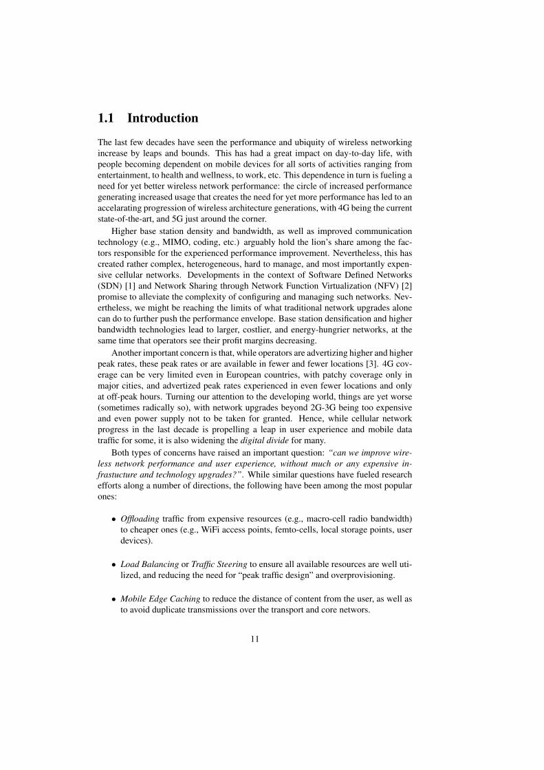
2.1 Notation . . . . . . . . . . . . . . . . . . . . . . . . . . . . . . . . . 412.2 Simulation parameters . . . . . . . . . . . . . . . . . . . . . . . . . 442.3 Taxi Trace & Limited buffer and bandwidth . . . . . . . . . . . . . . 442.4 ZebraNet Trace & Limited buffer and bandwidth . . . . . . . . . . . 44

3.1 Relative Step Delay Error REk: Averaged over All Steps and over 100Network Instances . . . . . . . . . . . . . . . . . . . . . . . . . . . 57

3.2 Rmin, Pmin: Monotonicity and Asymptotic Limits . . . . . . . . . . 653.3 Multicast Communication . . . . . . . . . . . . . . . . . . . . . . . 70

4.1 Optimal aggregation densities. The first number is the density, the sec-ond number is the relative performance increase (compared to DT).MF: Most Frequent, MR = Most recent. . . . . . . . . . . . . . . . . 77

4.2 Relative performance improvement compared to Direct Transmission.The first value for each entry corresponds to performance obtained withalgebraic connectivity, the second value to Q modularity. . . . . . . . 84

4.3 Clustering Coefficients and Average Path Lengths using different graphdensities. Missing values in cases where there is no giant component. 88

4.4 Number of communities and modularity (Q). . . . . . . . . . . . . . 884.5 Important notation for Section 4.8. . . . . . . . . . . . . . . . . . . . 924.6 Modeling replication with Eq. (4.8) . . . . . . . . . . . . . . . . . . 934.7 Important notation in Section 4.9. . . . . . . . . . . . . . . . . . . . 1054.8 Mobility trace characteristics. . . . . . . . . . . . . . . . . . . . . . . 1114.9 Absorption probabilities . . . . . . . . . . . . . . . . . . . . . . . . 1154.10 Minimum L to achieve expected delay in ETH with SimBet . . . . . . 119

5.1 Variables and Shorthand Notation. . . . . . . . . . . . . . . . . . . . 1255.2 Probability of reneging for pedestrian and vehicular scenarios. . . . . 1355.3 Optimal deterministic deadline times vs theory. . . . . . . . . . . . . 143

6.1 Notation . . . . . . . . . . . . . . . . . . . . . . . . . . . . . . . . . 1496.2 Simulation Parameters . . . . . . . . . . . . . . . . . . . . . . . . . 1666.3 Numerical values for Figure 6.3. . . . . . . . . . . . . . . . . . . . . 1686.4 Numerical values for Figure 6.4. . . . . . . . . . . . . . . . . . . . . 1696.5 Mean throughp. for handed-over users (in Mbps). . . . . . . . . . . . 171

5

6.6 UL/DL Split Vs. Joint-association Improvements . . . . . . . . . . . 1726.7 Comparison with existing work. . . . . . . . . . . . . . . . . . . . . 173

7.1 Notation. . . . . . . . . . . . . . . . . . . . . . . . . . . . . . . . . 1807.2 Parameters of the scenarios considered. . . . . . . . . . . . . . . . . 1837.3 Estimated offloading gains of rounded allocation vs. continuous relax-

ation for different cache sizes (in percentage of the catalogue size). . . 1967.4 Mobility statistics . . . . . . . . . . . . . . . . . . . . . . . . . . . . 1977.5 Important Notation . . . . . . . . . . . . . . . . . . . . . . . . . . . 2047.6 Information contained in datasets. . . . . . . . . . . . . . . . . . . . 2147.7 Dataset analysis. . . . . . . . . . . . . . . . . . . . . . . . . . . . . 2147.8 Parameters used in simulations: default scenario. . . . . . . . . . . . 2167.9 Utility matrix density for the MovieLens dataset for different umin

thresholds. . . . . . . . . . . . . . . . . . . . . . . . . . . . . . . . . 218

6

List of Figures

1.1 Interplay between user association and TDD configuration. . . . . . . 29

2.1 Delivery probability and delay for Epidemic Routing with differentscheduling and drop policies. . . . . . . . . . . . . . . . . . . . . . . 45

2.2 QoS Policy vs ORWAR . . . . . . . . . . . . . . . . . . . . . . . . . 492.3 QoS Policy vs CoSSD . . . . . . . . . . . . . . . . . . . . . . . . . 492.4 Overall policies comparison . . . . . . . . . . . . . . . . . . . . . . 49

3.1 Markov Chain for epidemic spreading over a homogeneous networkwith N nodes . . . . . . . . . . . . . . . . . . . . . . . . . . . . . . 55

3.2 Markov Chain for epidemic spreading over a heterogeneous networkwith 4 nodes . . . . . . . . . . . . . . . . . . . . . . . . . . . . . . . 55

3.3 Relative Step Error for the step (a) k = 0.2 ·N (i.e. message spreadingat 20% of the network) and (b) k = 0.7 ·N . Each boxplot correspondto a different network size N (with µλ = 1 and CVλ = 1.5). Box-plotsshow the distribution of the Relative Step Error REk for 100 differentnetwork instances of the same size. . . . . . . . . . . . . . . . . . . . 57

3.4 Box-plots of the message delivery delay under (a) epidemic, (b) 2-hoprouting, and (c) SnW (with L = 6 copies) routing. On each box, the cen-tral horizontal line is the median, the edges of the box are the 25th and75th percentiles, the whiskers extend to the most extreme data pointsnot considered outliers, and outliers are plotted individually as crosses.The thick (black) horizontal lines represent the theoretical values pre-dicted by our model. . . . . . . . . . . . . . . . . . . . . . . . . . . 58

3.5 Prediction accuracy for the CCDF of the epidemic delay on real networks 603.6 Mean delivery delay of 4 routing protocols, namely Direct Transmis-

sion, Spray and Wait (SnW), 2-hop, and SimBet, on the (a) Gowalla and(b) Strathclyde datasets. . . . . . . . . . . . . . . . . . . . . . . . . . 62

3.7 Message delay under Direct Transmission, Spray and Wait (L = 5),and Epidemic routing in scenarios with varying traffic heterogeneity;mobility parameters are µλ = 1 and (a) CVλ = 1 and (b) CVλ = 2. . 67

3.8 P(src.) of mobility-aware routing in (a) synthetic scenarios with vary-ing mobility (CVλ) and traffic heterogeneity (k), and (b) real networkswith homogeneous and heterogeneous traffic. . . . . . . . . . . . . . 68

7

3.9 Delay ratio R in two scenarios with varying traffic heterogeneity k.Relay-assisted routing is SimBet with (a) L = 5 and (b) L = 10 mes-sage copies. . . . . . . . . . . . . . . . . . . . . . . . . . . . . . . . 70

4.1 Converting a sequence of connectivity graph instances into a contactgraph. . . . . . . . . . . . . . . . . . . . . . . . . . . . . . . . . . . 74

4.2 Aggregated contacts for the ETH trace at different time instants. . . . 764.3 Delivered messages and delivery delay for SimBet/Bubble Rap vs. Di-

rect Transmission. . . . . . . . . . . . . . . . . . . . . . . . . . . . . 774.4 Aggregated contact graph for a scenario with 3 social communities

driving mobility (denoted with different colors), and three different ag-gregation densities. . . . . . . . . . . . . . . . . . . . . . . . . . . . 79

4.5 Number of links and similarity values as a function of time. . . . . . 804.6 Histogram of encountered similarity values at three different aggrega-

tion levels, with 2 clusters shown for each. . . . . . . . . . . . . . . . 814.7 SimBet and Bubble Rap performance with different aggregation func-

tions compared to direct transmission. . . . . . . . . . . . . . . . . . 844.8 Mobility traces characteristics. . . . . . . . . . . . . . . . . . . . . . 864.9 Contact Graph for DART trace. . . . . . . . . . . . . . . . . . . . . . 874.10 Community sizes. . . . . . . . . . . . . . . . . . . . . . . . . . . . . 894.11 CCDFs for normalize global and community degree in log-linear scale.

Insets show the same values with different x-axis range. . . . . . . . . 904.12 Example state transitions in two 6-node DTNs. . . . . . . . . . . . . 954.13 Summary of the necessary steps when building a DTN-Meteo model. . 974.14 Contact model for a toy network with N = 4 nodes and E = 4 out of

6 node pairs contacting each other. . . . . . . . . . . . . . . . . . . . 994.15 Results of the χ2 goodness-of-fit test for exponentiality . . . . . . . . 1134.16 Absorption probability validation for purely greedy content placement

and routing. . . . . . . . . . . . . . . . . . . . . . . . . . . . . . . . 1144.17 Expected delay validation for state-of-the-art routing schemes. . . . . 1144.18 Predictions and meas. for randomized content placement and routing 1164.19 Effect of (non-)exponentiality on relative errors of predicted delays . . 118

5.1 The WiFi network availability model modelled as an alternating re-newal process. During ON periods there is WiFi connectivity whileduring OFF periods, only cellular connectivity is available. . . . . . . 124

5.2 The 2D Markov chain for the WiFi queue in delayed offloading. . . . 1265.3 The reduced Markov chain for ρ→ 0. . . . . . . . . . . . . . . . . . 1315.4 Average delay for pedestrian user scenario. . . . . . . . . . . . . . . 1345.5 Average delay for vehicular user scenario. . . . . . . . . . . . . . . . 1345.6 The delay for BP ON-OFF periods vs. theory. . . . . . . . . . . . . . 1355.7 Low utilization delay approximation for AR = 0.75. . . . . . . . . . 1355.8 Low utilization pr approximation for AR = 0.75 . . . . . . . . . . . 1365.9 High utilization delay approximation for AR = 0.5. . . . . . . . . . . 1365.10 Variable WiFi rates with the same average as theory. . . . . . . . . . . 1375.11 Deterministic packets . . . . . . . . . . . . . . . . . . . . . . . . . . 137

8

5.12 The delay for deterministic deadlines vs. theory. . . . . . . . . . . . . 1375.13 The delay for BP packet sizes vs. theory. . . . . . . . . . . . . . . . . 1375.14 Offloading gains for delayed vs. on-the-spot offloading. . . . . . . . . 1385.15 The delay function for the optimization problem. . . . . . . . . . . . 1425.16 The delay vs. cost curve for high cellular rate. . . . . . . . . . . . . . 1425.17 The delay vs. cost curve for low cellular rate. . . . . . . . . . . . . . 142

6.1 Access network queuing systems for different flows. . . . . . . . . . 1506.2 Backhaul topology in future Hetnet. . . . . . . . . . . . . . . . . . . 1536.3 DL Optimal user-associations (Spectral efficiency vs. Load balancing

and best-effort vs. ded. traffic performance) . . . . . . . . . . . . . . 1676.4 Optimal user-associations (DL vs. UL traffic performance) . . . . . . 1686.5 DL optimal associations in different scenarios. . . . . . . . . . . . . . 1696.6 Mean throughputs overall all users in the network. . . . . . . . . . . . 1716.7 Downlink Network Efficiencies (normalized). . . . . . . . . . . . . . 172

7.1 Communication protocol. . . . . . . . . . . . . . . . . . . . . . . . . 1817.2 Optimal allocation in semi-log scale. . . . . . . . . . . . . . . . . . . 1827.3 Cost comparison according to TTL. . . . . . . . . . . . . . . . . . . 1847.4 Cost comparison according to buffer capacity. . . . . . . . . . . . . . 1847.5 Cost comparison according to number of vehicles. . . . . . . . . . . . 1847.6 Sequence of contacts with three caches (above), and amount of data in

end user buffer over time (below, in green). The red region indicateswhen data is downloaded from I. . . . . . . . . . . . . . . . . . . . . 189

7.7 Proposed queuing model for the playout buffer. The queue inside thesmall box corresponds to the low density regime model (Section 7.2.2),while the large box (containing both queues) to the high density regime(Section 7.2.3) . . . . . . . . . . . . . . . . . . . . . . . . . . . . . . 191

7.8 Data offloading gain as a function of cache number (a) and buffer size(b). . . . . . . . . . . . . . . . . . . . . . . . . . . . . . . . . . . . . 197

7.9 Offloading gain vs. file size. . . . . . . . . . . . . . . . . . . . . . . 1987.10 Offloading gain vs. file size. . . . . . . . . . . . . . . . . . . . . . . 1997.11 Data offloaded for vehicular cloud vs. femto-caching. . . . . . . . . . 2007.12 Mobile app example for Soft Cache Hits: (a) related content recom-

mendation (that the user might not accept) , and (b) related contentdelivery. . . . . . . . . . . . . . . . . . . . . . . . . . . . . . . . . . 202

7.13 Cache hit ratio for all datasets and caching schemes, for the defaultscenario. . . . . . . . . . . . . . . . . . . . . . . . . . . . . . . . . . 216

7.14 Cache hit ratio vs. cache size C. . . . . . . . . . . . . . . . . . . . . 2177.15 Cache hit ratio vs. number of SCs M . . . . . . . . . . . . . . . . . . 2187.16 Cache hit ratio for the MovieLens dataset for scenarios with different

umin thresholds; default scenario. . . . . . . . . . . . . . . . . . . . 2197.17 Relative increase in the cache hit ratio due to soft cache hits (y-axis).

Amazon scenarios with different variance of number of related contents(x-axis). . . . . . . . . . . . . . . . . . . . . . . . . . . . . . . . . . 220

7.18 Average delay in the network for uniform SNR . . . . . . . . . . . . 224

9

Chapter 1

Extended Summary

10

1.1 Introduction

The last few decades have seen the performance and ubiquity of wireless networkingincrease by leaps and bounds. This has had a great impact on day-to-day life, withpeople becoming dependent on mobile devices for all sorts of activities ranging fromentertainment, to health and wellness, to work, etc. This dependence in turn is fueling aneed for yet better wireless network performance: the circle of increased performancegenerating increased usage that creates the need for yet more performance has led to anaccelarating progression of wireless architecture generations, with 4G being the currentstate-of-the-art, and 5G just around the corner.

Higher base station density and bandwidth, as well as improved communicationtechnology (e.g., MIMO, coding, etc.) arguably hold the lion’s share among the fac-tors responsible for the experienced performance improvement. Nevertheless, this hascreated rather complex, heterogeneous, hard to manage, and most importantly expen-sive cellular networks. Developments in the context of Software Defined Networks(SDN) [1] and Network Sharing through Network Function Virtualization (NFV) [2]promise to alleviate the complexity of configuring and managing such networks. Nev-ertheless, we might be reaching the limits of what traditional network upgrades alonecan do to further push the performance envelope. Base station densification and higherbandwidth technologies lead to larger, costlier, and energy-hungrier networks, at thesame time that operators see their profit margins decreasing.

Another important concern is that, while operators are advertizing higher and higherpeak rates, these peak rates or are available in fewer and fewer locations [3]. 4G cov-erage can be very limited even in European countries, with patchy coverage only inmajor cities, and advertized peak rates experienced in even fewer locations and onlyat off-peak hours. Turning our attention to the developing world, things are yet worse(sometimes radically so), with network upgrades beyond 2G-3G being too expensiveand even power supply not to be taken for granted. Hence, while cellular networkprogress in the last decade is propelling a leap in user experience and mobile datatraffic for some, it is also widening the digital divide for many.

Both types of concerns have raised an important question: “can we improve wire-less network performance and user experience, without much or any expensive in-frastucture and technology upgrades?”. While similar questions have fueled researchefforts along a number of directions, the following have been among the most popularones:

• Offloading traffic from expensive resources (e.g., macro-cell radio bandwidth)to cheaper ones (e.g., WiFi access points, femto-cells, local storage points, userdevices).

• Load Balancing or Traffic Steering to ensure all available resources are well uti-lized, and reducing the need for “peak traffic design” and overprovisioning.

• Mobile Edge Caching to reduce the distance of content from the user, as well asto avoid duplicate transmissions over the transport and core networs.

11

1.1.1 Wireless Data Offloading

Data offloading has been explored in a variety of formats. Perhaps the most popularone nowadays is the use of WiFi instead of the cellular connection for data-itensive ap-plications (streaming of long videos, file backup services, etc.), as almost every modernmobile device supports both. A user can configure to allow some applications to onlyaccess the Internet through WiFi, and some operators may even enforce WiFi connec-tivity when it is available. It is reported that 60% percent of total mobile data traffic wasoffloaded onto the fixed network through Wi-Fi or femtocells in 2016. In total, 10.7exabytes of mobile data traffic were offloaded onto the fixed network each month [4].

Data traffic can also be offloaded within the same Radio Access Technology (RAT),by redirecting traffic from macro-cells to small(er) cells like micro-, pico-, and femto-cells. The higher power of macro-cells can be translated to higher nominal capacityper user, during off-peak hours. Nevertheless, this also leads to much higher coverageand too many users being connected concurrently during peak-hours or in “hotspot”locations. As user experience is not just affected by SINR but often more so by BSload, it is beneficial to “offload” as much of the macro-cell traffic to smaller BSs,serving fewer users, even if they offer lower SINRs [5]. In addition to relieving macro-cell load, small BSs (e.g., femto-nodes) might also have local break-out points to theInternet, thus also relieving the transport and core networks of an operator.

Taking the above idea a step further, it has been argued that data traffic should beoffloaded to user devices themselves, when possible. For example, if a user devicerequesting some content X is near another device already storing that content X, thetwo devices can establish a local communication link (either by themselves, or withthe help of the cellular network), to satisfy this request without involving any BSs.This is often referred to as Device-to-Device communication or D2D-survey. The factthat the majority of mobile data traffic is content-related, with many users being inter-ested in the same popular content (e.g., latest episode of a popular series, or trendingYouTube clips) increases the potential of such D2D approaches. An domain whereD2D is promising is when users are interested in location-related content.

1.1.2 Load Balancing and Traffic Steering

The main goal of load-balancing is to move traffic away from congested resources ofthe system (e.g., BSs, links, cloud servers) towards underutilized ones. No resourcesshould be oversubcribed and underperforming due to congestion, while other equiv-alent resources remain underutilized or idle. On the one hand, such load balancingimproves performance: delay is usually a convex function of load, so having one linkunderutilized and another congested leads to much higher delays than those same linkssplitting the total load. One the other hand, intelligent traffic steering also avoids theneed for peak traffic provisioning, which is common but rather costly when loads fluc-tuate. Unfortunately, such load fluctuation in both space and time is to be expectedwhen cell sizes grow smaller. The reason is that the laws of large numbers that isable to smooth out loads of macro-cells covering many user do not hold for smallercells covering just a few users. To avoid costly peak traffic design to hedge for largefluctuations, traffic steering is performed using intelligent algorithms that attemp to

12

treat distributed and often heterogeneous resources as a “pooled” set of resources to beshared among all, thus offering statistical multiplexing gains. These resources mightbe base stations, carriers, RATs, antennas and even storage and processing capacity.

User association is one example problem, where careful load-balancing is needed.The traditional coverage with carefully positioned macro-cells, combined with the factthat voice was the dominant application, made user-association in 2G or even 3G net-works simply a matter of which BS offers the strongest signal. The situation looksquite more complex now. The same coverage area might have overlapping layers ofBSs (e.g., macro-cell with a number of small cells in its range). What is more, smallcells themselves might have also partially overlapping coverage areas, especially in thecontext of envisioned UDNs (Ultra Dense Networks) [6]. Finally, each BS might alsohave multiple carriers, multiple antennas, different frequency reuse areas (to avoid in-terference at the edge). All this make user association in future wireless networks ahard case of lod-balancing optimization problem.

1.1.3 Mobile Edge CachingCaching can be seen both as a way to offload data away from (congested) parts of thenetwork, as well as a way to balance the load among links and nodes along the contentrequest path (i.e., from the user asking for a content, to the content provide centralserver(s)). For example, Information-Centric Networking (ICN) [7] suggest to cachecontent anywhere along that route, in order to both minimize access latency as well aslocalize traffic and micro-manage congestion along any part of the network. However,the necessity of complex hierarchical caching arising in ICN has been challenged [8].

Mobile edge caching has also been recently proposed, namely to store data directlyat small cells. The latter, increase the radio access capacity (due to their shorter distanceto the user) but are often equipped with low cost backhaul links (e.g., DSL, T1, orwireless), making this backhaul the new “bottleneck”. Caching popular content at theBS itself though can keep most traffic local to it, not burderning the underprovisionedbackhaul link(s).

The goal of this thesis has been to explore all these three often inter-connecteddirections, using an arsenal of:

(i) Modeling tools including markov processes, fluid approximations, queueing the-ory, and others, in order to derive analytically an appropriate performance ob-jective for these problems, and to quantify the impact of key variables on thisobjective.

(ii) Optimization tools, such as convex, discrete, and distributed optimization, markovchain monte carlo (MCMC) theory, and others, to identify optimal or at least ef-ficient algorithms for each of these problems.

While the various contributions in these areas could probably be grouped in differentways, we have chosen to present the various contributions in two main parts, the firstmore closely related to device-based traffic offloading and the second related to BS-based offloading and mobile edge caching. This serves both as a more coherent story,as well as better (albeit not always) capturing the timeline of work, since the author

13

of this thesis has started exploring these topics from the device side, in relatively chal-lenged networking environments, and has gradually moved to the infrastructure side inwireless networks.

The remainder of this chapter will briefly introduce each of the remaining chap-ters, providing some historic and related work context for each problem tackled, andsummarizing and positioning the various contributions.

1.2 Thesis Contributions

1.2.1 Resource Management and QoS Provision in Delay TolerantNetworks (Chapter 2)

Delay Tolerant Networks (DTNs) can be broadly described as networks where messagedelivery delays well over the range we are familiar with, e.g., from a few minutes tohours, can or must be tolerated. Research in this area was motivated initially by ex-treme environements such as deep space communication, sparse networks, tactical andunmanned (airborne or underwater) vehicles, etc. However, it was soon recognizedthat introducing some delay tolerance to device-to-device or device-to-infrastructurecommunication can facilitate data offloading. Applications such as bulk syncroniza-tion traffic, software updates, asyncronous communication such as email, etc., couldtolerate delays without the user noticing or at least with appropriate incentives [9].Furthermore, it was observed that delay-tolerant and opportunistic data exchange be-tween mobile devices could also greatly simiplify the heavy-duty network routing andtopology maintenance algorithms needed in ad-hoc networking, a popular research areaat the time time. Opportunistic message exchange between mobile devices wheneverthey are in range, and without explicit knowledge about the global network topology,could still achieve eventual (i.e., delay-tolerant) delivery of end-to-end messages orretrieval of requested content even in denser networks found in urban environments.

In the context of end-to-end message delivery in such networks, a number of routing(or, more correctly, forwarding) schemes had been proposed. The main goal of suchschemes is to decide if a node currently carrying a message for destination D, shouldhand over the message or a replica of it, to another encountered node. The proposedschemes would range from making this decision randomly [10], epidemically [11],based on some replica budget [12], or using predictive metrics (“utilities”) regardingthe probability of delivery of each node (for destination D). The implicit objective ofmost of these heuristics was to ensure each message is delivered with a high probabilityto its destination, usually with some desired deadline (TTL). At the same time, it is wasimportant to efficiently utilize the limited resources of these networks: the node buffercapacity, the communication bandwidth during a “contact” between two nodes, andoften the node battery.

Nevertheless, the majority of these proposal didn’t really tackle the resource man-agement problem at all. It was common to either assume infinite buffer capacity and/orcontact bandwidth, or to heuristically try to maintain a reasonable overhead as a sideobjective. For example, some proposals considered “ACK” type of messages to cleanup valuable buffer space occupied by flooded messages that had already been deliv-

14

ered [13]. In contrast, our popular early protocol Spray and Wait [12] limited before-hand the number of replicas per message to a relatively small number, in order to capthe number of relay nodes (or “custodians”) that have to carry each message, as wellas the number of transmissions (and related bandwidth) each new message consumes.At the name suggests, the first L − 1 nodes encountered would immediately receive acopy of the message, and then each of the would “wait” until it encounters the destina-tion. If L is the replication limit for a message of size S bits, then each message wouldconsume at most L · S total bits of buffer and transmission capacity. This choice waspartly motivated by the seminal works of [14, 15], as well as by the (intuitive at thetime) observation, that the added value of each extra replica was diminishing. As a re-sult, choosing L > 1 but L≪ N (the total number of nodes) would often result in gooddelivery ratios, without the congestion collapse associated with earlier epidemic-typeprotocols [11].

Nevertheless, this parameter L had to be chosen beforehand empirically, or usingsome foreknowledge about network characteristics. If this value was too conservative(e.g., network traffic was low at the moment), valuable resources could stay underuti-lized. If the value was too high, congestion would occur as in epidemic schemes. Whilea number of follow up works attempted to rise to this challenge, introducing some in-telligence in the spray phase or in the wait phase [16, 17, 18], these still constituted aheuristic manner of resource management. The seminal work of [19] for the first timeintroduced the allocation of buffer and bandwidth resources as a formal optimizationproblem. The key observations were the following:

(i) It is usually suboptimal to leave any buffer space or contact bandwidth unuti-lized; any such available resource could potentially improve the delivery proba-bility/delay of some live message, without hurting the performance of others;

(ii) Intelligent forwarding mechanisms need to kick in only when necessary (e.g., ifthe buffer of one of the involved nodes is full); otherwise, epidemic forwardingis optimal;

(iii) The key role of these mechanism(s) should be to prioritize each message, ac-cording to the added value of an extra copy for that message.

In other words, the key insight of this approach is that you don’t need to decide inadvance how many resources a message will consume. One can let messages occupy allavailable resources, and need only select between two messages if a node’s resourcesare exhausted. For example, if a new message arrives but the buffer is full, then thatnode will have to intelligently choose whether to drop an existing message (copy) orreject the newly arrived one. Similarly, if a node knows that the contact bandwidthduring an encounter might not suffice to copy all messages, it then has to choose toprioritize some of them.

The key challenge in this context is then how to evaluate the added value or marginalutility of each message (copy). Making some simplifying assumptions about node mo-bility, the authors of [19] showed that this boils down to knowing the number of alreadyexisting replicas of that message. This number was assumed to be known through somelow-bandwidth side channel (e.g., cellular network), which allowed each node to makeindependent, distributed decisions.

15

Chapter Contributions

It is at this point that our first contributions of this chapter, come into the picture. Thesecomprise the following papers [20, 21].

• A. Krifa, C. Barakat, T. Spyropoulos, “Optimal Buffer Management Policies forDelay Tolerant Networks”, in Proc. of IEEE SECON 2008. (best paper award)

• A. Krifa, C. Barakat, T. Spyropoulos, “Message Drop and Scheduling in DTNs:Theory and Practice”, IEEE Transactions on Mobile Computing. 11(9): 1470-1483, 2012.

Contribution 2.1 We improved the proposed utility function of [19] to properly ac-count for the probability that the message has already been delivered, based on thenumber of nodes encountered so far by the message source (which might differ fromthe nodes currently holding a replica).Contribution 2.2 We generalized the framework of [19] and showed how to derive permessage utilities for different performance metrics, with delivery delay and deliveryprobability as two specific examples.Contribution 2.3 A side channel or centralized mechanism to keep track of numberof replicas per message might not always be present. In that case, estimating the num-ber of copies per message in a distributed manner is an intrinsically hard task in thiscontext, given the disconnected, delay-ridden nature of these networks. To this end,we proposed an efficient history-based mechanism to achieve this with the followingdesirable features: (i) the utility estimates derived are unbiased statistics; (ii) the datacollection mechanism to derive these statistics is in-band and low overhead in termsof message storage and propagation; (iii) the estimates do not require any knowledgeabout the current message (which is hard to obtain), but rather on past knowledge aboutsimilar messages. Simulations suggest that this distributed, online version of the algo-rithm performs close to the oracle one in a number of scenarios.

These contributions seemed relatively conclusive about the buffer and bandwidthmanagement problem, at the time, at least in the context of simple epidemic schemes.A number of issues remained though, one of which being how to provide some sortof Quality of Service (QoS) and differentiate between different classes of messages.Somewhat surprisingly, this question was only addressed much later. One might ar-gue that this was perhaps due to DTNs being inherently unreliable and delay-tolerant,which makes QoS a contradicting concept in this context. Nevertheless, a number ofDTN setups, such as tactical or space networks still gave rise to a need for traffic dif-ferentiation in DTNs as well. For example, some messages might be tolerant to largerthan usual delays, but might still have to be delivered with high probability before adeadline, otherwise they are useless. On the other side of the fence, some messagesmight be more time-critical than others, but losing some of them is OK.

To this end, we have extended our resource management framework in this direc-tion in the following papers [22, 23].

• P. Matzakos, T. Spyropoulos, and C. Bonnet, “Buffer Management Policies forDTN Applications with Different QoS Requirements,” in Proc. of IEEE GLOBE-COM 2015.

16

• P. Matzakos, T. Spyropoulos, and C. Bonnet, “Joint Scheduling and Buffer Man-agement Policies for DTN Applications of Different Traffic Classes,” in IEEETransactions on Mobile Computing, 2018.

Contribution 2.4 In addition to “best effort” type of messages (the only class of mes-sages in previous work), we have introduced classes of messages with QoS guarantees.E.g., a class (“VIP”) might require a given minimum delivery probability for eachmessage. The objective in this case is to first ensure that all QoS classes achieve theirminimum required performance, and then to allocate remaining resources (if any) tomaximize mean performance for all messages.Contribution 2.5 We have (re-)formulated the problem of optimal resource allocation(buffer and bandwidth) among classes with different QoS requirements as a constrainedoptimization problem. We showed that this problem is convex, and extended the dis-tributed protocol based on per message utilities of [21] in a manner that can be shownto solve the aforementioned QoS-aware problem.Contribution 2.6 We have also generalized the mobility assumptions under which theproposed framework can be applied, including: (i) heterogeneous (but still exponential)inter-contact times, (ii) heavy-tailed inter-contact times (Pareto), which are common insome DTN networks.Contribution 2.7 Using extensive sets of simulation, based on synthetic and real traces,we have demonstrated that the proposed framework achieves the desired objectives, asoutlined by (d), and outperforms previous related work that attempted to heuristicallyintroduce QoS.

1.2.2 Performance Modeling for Heterogeneous Mobility and Traf-fic Patterns (Chapter 3)

The previous discussion revolves around one of the key directions in the early DTN(and Opportunistic Networking) research, namely that of forwarding algorithm design.The second important direction has been that of analytical performance modeling. Theformer attempts to find a good message forwarding algorithm under a given networksetup. The latter is given the algorithm and network setup, and atempts to derive an an-alytical, ideally closed form prediction of this algorithm’s performance. Nevertheless,the existence of multiple nodes (message sources, destinations, relays) interacting in astochastic manner, and the additional dependence on protocol details, makes this taskdaunting, even in relatively simple network setups.

To this end, the majority of early DTN works that attempted to characterize differ-ent routing algorithms almost exclusively made the following simplifying assumptions:

(i) The inter-contact time between different nodes is independent and follows anexponential distribution; this assumptions allows the message evolution to bemodelled by a Markov chain.

(ii) Pair-wise inter-contact times, in addition to independent, are also identically dis-tributed. In other words, the average meeting time between any pair of nodes isthe same; this assumption is key to make the Markov chain analysis tractable.

17

These two assumptions enabled to derive closed form expressions for popular (albeitoften quite primitive) forwarding such as epidemic forwarding, 2-hop routing, randomforwarding, and spray and wait schemes

While additional simplifying assumptions had to often be made (we will considersome subsequently), these two have been the main “bottleneck” of DTN performanceanalysis for a while. As device-to-device opportunistic networking became a popularresearch topic in the mid-2000s, a number of experimental studies emerged that actu-ally tested these two hypotheses. These studies generally studied the contact charac-teristics of mobile (or nomadic) nodes in different setups including conferences, cam-puses, public transportation, etc. Initial findings suggested that both assumptions arequite far off from observations. Inter-contact time distributions where shown to followa power law distribution instead of being exponential, as assumed in theory, and to alsohave largely heterogeneous behaviors [24]. These findings seemed to invalidate thevarious analytical findings [24] as well as the relative performance among well-knownschemes [25].

Although the debate about the exponentiality of inter-contact times stayed hot for acouple of years (and is still not fully settled), subsequent measurement and theoreticalanalyses emerged that provided some support for the exponential assumption. Thissupport came from a number of directions:

(i) When looking at the intercontact times of specific node pairs, rather than ag-gregating all inter-contacts of all pairs in one histogram (as was done in [24]),a number of pairs do show such an exponential behavior (while some others aheavier-tail one) [26];

(ii) Aggregating inter-contact times of different pairs which are exponential, but withdifferent means, can give rise to a heavy tail aggregate inter-contact distribution,like the ones observed in measured traces [27].

(iii) Inter-contact times can be modeled as stopping times of specific random walks(a lot of mobility models can be modelled as a generalized random walk), whoseprobability distribution has a power law body but an exponential tail [28].

These findings suggested that, while inter-contact times are clearly neither alwaysnor exactly exponential, this can be a reasonable approximation in a number of cases,resulting in reliable performance predicton. Nevertheless, the second problematic as-sumption remained. Measurement studies (and common sense) suggest that not allnode pairs meet each other equally frequently. In fact, some node pairs never meeteach other [24]. Other nodes, due to their higher mobility (e.g., vehicle vs. pedes-trian, smartphone vs. laptop) might meet more nodes during the same amount of timethan others. The question thus remained: Does the entire analysis break down if nodemeetings are heterogeneous? Could this analysis be generalized?

While we already mentioned some cases of such generalizations in the previoussubsection, these applied to specific forwarding primitives only, and not the generalcase of epidemic schemes.

18


Our contributions, detailed in Chapter 3, start at this point. The following paper makesthree contributions in this direction [29].

• P. Sermpezis, and T. Spyropoulos, “Delay analysis of epidemic schemes in sparseand dense heterogeneous contact environments”, IEEE Transactions on MobileComputing, 16(9): 2464-2477, 2017.

Contribution 2.1 We have kept the assumption of exponentiality but generalized theinter-contact process between nodes using a 2-layer model: the first layer is a randomgraph capturing which nodes communicate (at all) with each other; for each existinglink i, j on the graph, we draw a random weight λij from a common distributionF (λ) which corresponds to the meeting rate for that pair. In other words, the inter-contact times between nodes i and j are distributed as ˜expλij . By changing the under-lying random graph model or the function F (·), a large number of mobility models canbe captured.Contribution 2.2 We showed that, for an underlying Poisson contact graph, and F (·)with finite variance, the delay of each epidemic step asymptotically converges to aclosed form expression (asymptotically in the size of the network). The same holds forthe delivery delay of epidemic forwarding, which is the sum of such steps (as well asother schemes that can be expressed as a simple combination of epidemic steps).Contribution 2.3 We derived approximations for finite networks, as wells as for gener-alized underlying contact graphs, captured by the well known Configuration model [30].

The above model manages to capture both pairs of nodes that don’t meet (i.e.,sparse networks) as well as heterogeneous intercontact times. While quite generic, thismodel requires some structure: pairwise meeting rates, while different, are drawn IIDfrom the same probability distribution F (λ). The above model does not capture arbi-trary meeting rate combinations. Most importantly, it doesn’t well capture communitystructure, which is ubiquitous in real mobility traces. In realitly, there exist some tran-sitivity between meeting rates: if node i tends to meet often node j and node k, thenj and k probably meet often. This is also referred to as clustering [30], and cannot becaptured by the model in [29]. To this end, in the following work [31], we extendedour analytical results in this direction.

• A. Picu, T. Spyropoulos and T. Hossmann, “An Analysis of the InformationSpreading Delay in Heterogeneous Mobility DTNs,” in Proc. of IEEE WoW-MoM 2012. (best paper award)

Contribution 2.4 We formalized the weighted graph model for inter-contact rates be-tween pairs as a generic matrix, and showed how epidemic step delay can be capturedby properties of this matrix.Contribution 2.5 Based on this model, we derived upper bounds for both the meandelay and the delay distribution of epidemic routing that apply to generic mobilityscenarios, including community-based ones, and are validated against real traces.

As a final set of contributions in this chapter, we took a step beyond heterogeneityin terms of who contacts whom, and considered for the first time the equally important

19

question of traffic heterogeneity, namely who wants to send a message to whom. Infact, the majority of related work, both analytical and simulation-based, did not onlyassume IID mobility, an aspect that has been extensively revisited as explained above,but also assumed uniform traffic demand. Somewhat surprisingly, this latter assump-tion had received to that day almost no attention. We made the following contributionsto amend this, elaborated at the end of Chapter 3. The material is based on three arti-cles [32, 33, 34]:

• P. Sermpezis, and T. Spyropoulos, “Not all content is created equal: effectof popularity and availability for content-centric opportunistic networking,” inProc. of ACM MobiHoc 2014.

• P. Sermpezis, and T. Spyropoulos, “Modelling and analysis of communicationtraffic heterogeneity in opportunistic networks”, in IEEE Transactions on MobileComputing,” 14(11): 2316-2331, 2015.

• P. Sermpezis, and T. Spyropoulos, “Effects of content popularity in the per-formance of content-centric opportunistic networking: An analytical approachand applications,” IEEE/ACM Transactions on Networking, 24(6): 3354-3368,2016.

Contribution 2.6 We showed both analytically and using simulations that traffic het-erogeneity impacts performance only if its correlated with mobility heterogeneity. Inother words, if who sends more messages to whom is independent from who encoun-ters whom more frequently, then traffic heterogeneity does not impact performancebeyond the aggregate mean traffic demand.Contribution 2.7 We proposed a class of traffic-mobility correlation models and ex-tended our analytical framework accordingly. We used this framework to derive closedform performance results for a number of simple but well-known opportunistic networkrouting schemes, under both mobility and traffic heterogeneity. Using both theory andtrace-based simulations we showed how configuring well known protocols (e.g., sprayand wait) needs to be modified in light of such heterogeneity.Contribution 2.8 We extended our analysis beyond end-to-end communication tocontent-centric applications, making some links with device-side caching and D2D.(the topic of caching is more extensively considered in a later chapter).

1.2.3 Complex Network Analysis for Opportunistic Device-to-DeviceNetworking (Chapter 4)

The previous two research threads led to new insights, models, and algorithms, in termsof both resource allocation in DTNs, as well as more accurate analytical models thatwhere inline with recent mobility trace insights. Nevertheless, the majority of theseworks were still mostly based on simple “random” forwarding protocols like epidemicrouting, spray and wait, 2-hop routing, and variants. These protocols, which could bearguably referred to as “1st generation” DTN routing, where based on simple forward-ing decisions: when a node with a message copy encounters another node without acopy, it can: (i) create a new copy (epidemic), (ii) create one with some probability

20

(probabilistic routing), (iii) create one only if the copy budget is not depleted (sprayand wait), and other variabts. In other words, the decision to give a copy to a newlyencountered node did not really depend on properties of the relay or the destination(e.g., whether the two might meet soon). This justifies the term “random”, used earlier.

The natural progress in this direction was to amend these protocols to make “smarter”decisions that can assess the usefulness or utility of a given relay node. For example,

(i) the utility might capture the ability of that node to delivery messages to a givendestination (e.g., if the two nodes rely in the same “community” or location areaand tend to meet often)

(ii) a node might also have high utility for any destination (e.g., a node that tends toexplore larger areas of the network compared to average nodes).

Utility-based routing protocols for DTNs had already been explored early on. Prophetwas a popular early variant of epidemic forwarding. There, a node A encounteringanother node B would give the latter a copy of a message for destination X , only ifthe utility of B (related to X) was higher than that of A. This utility in turn was basedon a mechanism that considered the recency of encounter between the two nodes. Itcould also consider some transitivity in utilities, e.g., B could have a high utility forX , not because it saw X recently, but because it sees other nodes that see X recently.Similarly, the early “single-copy” study of [10] considered such simple utility metricsbut assuming a message is not copied, but rather forwarded. Single-copy DTN for-warding had the advantage of significantly limiting the overhead per message, but didnot benefit from the path diversity that multiple-copy schemes exploit [25].

Finally, utility metrics were used to improve specific aspects of existing protocols.For example, Spray and Focus [12] did not create any new copies after there was a totalof L in the network, in order to limit the amount of overhead per message (just as inSpray and Wait), but did allow each such copy to be handed over to a relay with higherutility for the destination, if one was encountered. Similarly, smart spraying methodswere proposed to not randomly handover the L copies, but to do so according to somemeeting-related utility metric [16, 17, 18].

Nevertheless, the majority of these utility-based methods were simple heuristics,that sometimes improved protocol performance but not always. More importantly, util-ities were pairwise metrics, based on the meetings characteristics between the relay inquestion and the destination. A breakthrough came by the seminar works of [35, 36].Motivated by the intricate structure between node contacts, revealed in the recentlystudied mobility traces, the authors suggested that contacts between mobile devices aresubject to the same social relations that the users carrying these devices are subject to.Hence, it is only reasonable to utilize the new science of Complex Networks or SocialNetwork Analysis to answer questions related to which node might be a better relay foranother (these terms, including the term Network Science are often used interchange-ably, to mean the same thing).

This gave rise to Social Network based opportunistic networking protocols. Themain idea behind these first schemes was simple:

• First, collect knowledge about past contacts into a graph structure called a socialor contact graph; a link in this graph could mean, for example, that the two

21

endpoints of the link have met recently, or have been observed to meet frequentlyenough in the past.

• Then, use appropriate social network tools or metrics to make forwarding deci-sions.

For example, BubbleRap [36] uses Community Detection algorithms to split thenetwork into communities. Then, epidemic routing was modified using communitiesand degree centrality [30]. The node with the highest degree centrality would be thenode that has met, for example, the largest number of other nodes within some timeinterval. If the message has not yet reached the destination community, a messagecopy in BubbleRap is given to an encountered node only if the latter has higher degreecentrality. When the message has reached a relay in the destination community, thenlocal degree centrality would be used instead (i.e., a node would become a new relayonly if it was better connected in that community).

SimBet [35] uses instead node betweeness (a different measure of node centrality)to traverse the network. It then “locks” to the destination using node similarity. Nodesimilarity captures the percentage of neighbors in common with the destination. Dueto the high clustering coefficient of social networks, if two nodes share many neighborsthen they belong to the same community with high probability. Hence, trying to find anode with high similarity with the destination in SimBet is equivalent to trying to finda node in the destination community (just as BubbleRap does, in the first phase).

As expected, these two protocols outperformed traditional random and utility-basedones, by intelligently exploiting not just pairwise structure in node contacts, but rathermacroscopic structure such as communities, betweeness, etc., that depend on the in-teractions of multiple nodes. Nevertheless, this new line of work also raised someimportant questions:

1. How should one optimally built the contact graph on which the social metricswill be calculated?

2. Do all opportunistic networks exhibit such “social” characteristics, and if so whatare the most prominent ones? Do state-of-the-art mobility models capture these?

3. Can one still hope to do useful performance analysis when forwarding protocolsbecome that complex and interdependent with the underlying mobility process?

The goal of this chapter is to present our contributions towards answering thesethree questions.


The begining of the chapter is concerned with the first question, which we attemptedto answer in the following two works [37, 38]:

• T. Hossmann, F. Legendre, and T. Spyropoulos, “From Contacts to Graphs:Pitfalls in Using Complex Network Analysis for DTN Routing,” in Proc. ofIEEE International Workshop on Network Science For Communication Net-works (NetSciCom 09), co-located with INFOCOM 2009.

22

• T. Hossmann, T. Spyropoulos, and F. Legendre, “Know Thy Neighbor: TowardsOptimal Mapping of Contacts to Social Graphs for DTN Routing,” in Proc. ofIEEE INFOCOM 2010.

Contribution 4.1 We studied different “aggregation methods”, i.e., methods to convertthe history of past contacts into a social graph, and showed that the performance ofSocial Network based protocols is very sensitive to the contact graph creation method;simple empirical tuning or rules of thumb will likely fail to unleash the potential ofsuch protocols.Contribution 4.2 We proposed a distributed and online algorithm, based on spectralgraph theory. It enables each node to estimate the correct social graph in practice, as-sessing the role of new nodes in the graph without any training, in a manner reminiscentof unsupervised learning. This algorithm is generic, and could be applied as the firststep of any opportunistic networking protocol that uses social network metrics.

Regarding the second question, some initial insights about community structurehad been observed in [36]. However, we embarked on a systematic study towardsanswering that question in [39, 40]:

• T. Hossmann, T. Spyropoulos and F. Legendre, “A Complex Network Analysisof Human Mobility,” in Proc. of IEEE NetSciCom 11, co-located with IEEEInfocom 2011.

• T. Hossmann, T. Spyropoulos, and F. Legendre, “Putting Contacts into Context:Mobility Modeling beyond Inter-Contact Times,” in Proc. of ACM MobiHoc2011. (best paper award runner-up)

Our contributions in these papers can be summarized as follows:Contribution 4.3 We performed a large study of contact traces coming from state-of-the-art mobility models, existing real traces, and traces collected by us (from geo-social networks). We convert each of them into a social graph, using some of the earliermethods from this chapter.Contribution 4.4 We investigated whether these graphs exhibit well-known propertiesof social networks: (i) high clustering and community structure, (ii) small-world con-nectivity, and (iii) power-law degree distributions. Indeed, we found that the majorityof mobility traces exhibit the first two, but not always the third property .Contribution 4.5 We showed that state-of-the-art synthetic mobility models, whileable to recreate some of these social properties well, are unable to model bridgingnodes, which seem to be common in real traces. To this end, we suggested a modi-fication of such models using multi-graphs, which can be applied as an “add-on” todifferent mobility models, without interfering with other desirable properties of thesemodels.

These developments were quite positive, corroborating the initial evidence aboutthe strength of social network analysis for opportunistic D2D networking, as well asdemonstrating how to properly tap into this potential. Nevertheless, the complexityof protocols based on social graph metrics came on top of the existing challenges ofperformance analysis for non-IID mobility models, mentioned earlier. The intricatedependence of forwarding decisions on past contacts between many different nodes

23

creates state history for the Markovian analysis model that is hard to keep track of.What is more, by that time, a large number of utility-based routing protocols had beenproposed, making it difficult to come up with a proprietary analytical model (e.g., aspecific Markov chain) for each different protocol. To this end, in the following twoworks, we proposed a unified analytical performance prediction model, coined DTN-Meteo [41, 42].

• A. Picu and T. Spyropoulos, “Forecasting DTN Performance under Heteroge-neous Mobility: The Case of Limited Replication,” in Proc. of IEEE SECON2012.

• A. Picu, and T. Spyropoulos, “DTN-Meteo: Forecasting the Performance of DTNProtocols Under Heterogeneous Mobility,” in IEEE/ACM Transactions on Net-working, 23(2): 587-602, 2015.

Our main contributions, can be summarized as follows:Contribution 4.6 We attempted to generalize the performance prediction models forheteregenous mobility of Chapter 3, in order to allow deriving perfomance metricsfor generic utility-based algorithms. Our framework combined the theory of MarkovChain Monte Carlo (MCMC) based optimization and the theory of Absorbing Markovchains as follows:

• Each state of a Markov chain corresponds to a possible configuration or state ofthe network (e.g., which nodes have which message(s)) at a time.

• The mobility process governs the possible transitions and the respective transi-tion rates between states.

• The algorithm (e.g., forwarding) governs the acceptance probabilities of a po-tential transition, a probability that may depend on the utility of the previous andthe potential new state.

• Absorbing states correspond to desired final states of the protocol (e.g. messagedelivered to its destination, or to all destination in case of multicast, etc.). Perfor-mance metrics can be expressed in terms of absorption times and probabilities.

Contribution 4.7 Using this framework, we managed to successfully model the state-of-the-art protocols mentioned earlier, namely SimBet and BubbleRap, running on topof generic, trace-based mobility models. We also showed that this framework appliesto various delivery semantics, beyond end-to-end message delivery, such as multicast,anycast, etc.

1.2.4 WiFi-based Offloading (Chapter 5)Offloading mobile data via WiFi has been common practice for network operators andusers alike. Operators might purchase WiFi infrastructure or lease a third-party one,to relieve their congested cellular infrastructure. User prefer to use WiFi at home,cafes, office, for bulk data transfers, video streaming, etc., as much as possible, toavoid depleting their cellular data plans, improve their rates, or sometimes to save their

24

battery life. As mentioned earlier, it is reported that 60% percent of total mobile datatraffic was offloaded onto the fixed network through Wi-Fi or femtocells in 2016 [4].

The ubiquity of WiFi access points, and the interest of network operators in theiruse, has motivated researchers to study a number of ways to use WiFi-based Internetaccess as an inexpensive complement to cellular access. One such proposal was to useWiFi access points (AP) while on the move, e.g., from a vehicle, accessing a sequenceof encountered WiFi APs to download Internet content [43]. WiFi was originally de-signed for “nomadic” users, i.e., users who come into the range of the AP and stayfor long periods of time, and not for moving users. A number of measurement studieswere thus performed to identify the amount of data one could download from such anAP, travelling at different speeds [44, 45]. While the measured amounts suggested thatreasonably sized files could already be downloaded even at high speeds, there were anumber of shortcomings related to mobile WiFi access:

• The association process with a WiFi AP takes a long time (due to authenticationprocedures, scanning, and other suboptimalities in the protocol design). Thiswastes a large amount of the limited time during which a mobile node mightbe within communication range with that AP (and thus wastes communicationcapacity).

• The rate adaptation mechanism of WiFi, which reduces the PHY encoding rate(and thus the transmission rate), as a function of the SINR of the receiving node,has dire side-effects when a number of nodes on the move would try to access thesame AP. In that case, there always exist at least some nodes at the edge of theAP coverage range, who receive the lowest possible transmission rate. However,it is well known that the way scheduling works in WiFi, the average performanceis highly impacted by the existence of edge users [46]. Connecting to WiFi onthe move greatly deteriorates the mean WiFi throughput for every node, even theones close to the AP, as at least some of the mobile nodes are at the edge of theAP, entering its range (or leaving it).

A number of works emerged to address both these issues. Some of the ideas in-cluded streamlining the WiFi association procedure [47], maintaining a history of APlocation and quality to improve the speed and efficiency of scanning [48], as well asmodifications to the scheduling mechanism of WiFi, ensuring that the capacity is allo-cated to mobile nodes during the time they are close to the AP, a form of opportunisticscheduling. While a lot of research activity was taking place in the context of protocolimprovements, system design, and experimentation, there was little ongoing in termsof the theoretical understanding for WiFi offloading methods.


This line of research made us interested in the following question: Assuming a stochas-tic traffic mix (i.e., both random traffic arrival, and random flow/session sizes), whatis the expected performance of WiFi offloading, as a function of AP deployment andcharacteristics, mobile node behavior, and traffix characteristics?. We have attemptedto answer it in the following works [49, 50]:

25

• F. Mehmeti, and T. Spyropoulos, “Performance Analysis of On-the-spot MobileData Offloading,” in Proceedings of IEEE GLOBECOM 2013.

• F. Mehmeti, and T. Spyropoulos, “Performance analysis of mobile data offload-ing in heterogeneous networks,” in IEEE Transactions on Mobile Computing,16(2): 482-497, 2017.

Our contributions can be summarized as follows:Contribution 5.1 We proposed a queueing-theoretic model, an M/G/1 with differentlevels of service rate. Assuming a user generating random download requests and acommon queue on top of the WiFi and cellular interfaces: when a WiFi AP is in range,these requests are always served through the WiFi interface (with one servicerate); ifthere is no WiFi in range, the requests are served by cellular interface (with a differentservice rate).Contribution 5.2 We analyzed the performance of this system for both First ComeFirst Serve (FCFS) and Processor Sharing (PS) queueing disciplines, and derived closedform expressions for the expected amount of offloaded data, as well as the mean down-load performance. These expressions are a function of user mobility, WiFi coverage,and WiFi/Cellular capacity characteristics.

A second research direction that emerged was that of Delayed WiFi Offloading.This was partly motivated by the study and exploitation of delay-tolerance (the appli-cation and/or the user might be tolerant to delays). As explained earlier, this delaytorelance might sometimes be natural, and sometimes requires some incentives. Tothis end, researchers suggested that some traffic does not need to be immediately trans-mitted over the cellular interface (as required in the previous scenario), if there is noWiFi connectivity. Instead, such delay-tolerant download (or upload) requests couldbe queued at the WiFi interface, until a WiFi AP is encountered. If such an AP is notencountered until a maximum wait timer expires, only then must the request be turnedover to the cellular interface [51, 52]. This more “aggressive” offload policy was shownto be able to offload even more data, at the expense of a delay increase for some traffic.

To this end, in the following works, we extended our performance analysis frame-work to investigate such delayed offloading policies as well [53, 54].

• F. Mehmeti, and T. Spyropoulos, “Is it worth to be patient? Analysis and opti-mization of delayed mobile data offloading,” in Proc. of IEEE INFOCOM 2014.

• F. Mehmeti, and T. Spyropoulos, “Performance modeling, analysis and opti-mization of delayed mobile data offloading under different service disciplines,”in ACM/IEEE Transactions on Networking, 25(1): 550-564, 2017.

Contribution 5.3 We used a queueing theoretic model with service interruptions andabandonments, to model the intermittent access to WiFi APs (the interruptions) and thepossibility that a request waiting in the WiFi queue might expire and move back to thecellular interface (the abandonments).Contribution 5.4 We derived closed form expressions for the amount of offloaded dataand mean per flow delay in this system, as a function of the mean delay-tolerance ofthe application mix considered, and other network parameters.

26

Contribution 5.5 In a scenario where it is the user that can decide this delay tolerance,we showed our analytical expressions and convex optimization theory to show how thewait threshold can be optimized to achieve different delay-vs-offloaded data or delay-vs-energy efficiency tradeoffs.

1.2.5 User Association in Heterogeneous Wireless Networks (Chap-ter 6)

In addition to using third-party WiFi or own WiFi platforms, operators are increasinglyconsidering denser, heterogeneous network (HetNet) cellular deployments. In a Het-Net, a large number of small cells (SC) are deployed along with macrocells to improvespatial reuse [55, 56, 57]. The higher the deployment density, the better the chancethat a user equipment (UE) can be associated with a nearby base station (BS) withhigh signal strength, and the more the options to balance the load. Additionally, theline between out-of-band WiFi “cells”, and in-band cellular small cells (femto, pico),is getting blurred, due to developments like LTE-unlicensed. The trend towards basestation (BS) densification will continue in 5G systems, towards Ultra-Dense Networks(UDN) where: (i) many different small cells (SCs) are in range of most users; (ii) asmall number of users will be active at each SC [58, 59, 6]. The resulting traffic vari-ability makes optimal user association a challenging problem in UDNs [58], as the goalhere is not to simply choose between WiFi or cellular as in the previous chapter, but tochoose between a large range of heterogeneous and overlapping cells.

As a result, a number of research works emerged that studied the problem of userassociation in heterogeneous networks, optimizing user rates [60, 61], balancing BSloads [62], or pursuing a weighted tradeoff of them [63]. Range-expansion techniques,where the SINR of lightly loaded BSs is biased to make them more attractive to theusers are also popular [56, 57]. The main goal of these works is to offload or “steer”traffic away from overloaded base stations, towards underloaded ones, while maintain-ing (or improving) user performance. Nevertheless, the majority of these works fo-cused on DL traffic and the radio access link only. Future user association algorithmsshould be sophisticated enough to consider a number of other factors.

• Uplink: While optimization of current networks revolves around the downlink(DL) performance, social networks, machine type communication (MTC), andother upload-intensive applications make uplink (UL) performance just as im-portant. Some SCs might see their UL resources congested, while others theirDL resources, depending on the type of user(s) associated with that SC. What ismore, the same SC might experience higher UL or DL traffic demand over time.

• Traffic Classes: Most existing studies of user association considered homoge-neous traffic profiles. For example, [63, 64, 65] assume that all flows generatedby a UE are “best-effort” (or “elastic”). Modern and future networks will haveto deal with high traffic differentiation, with certain flows being able to requirespecific, dedicated resources [66], [67, 68]. Such dedicated flows do not “share”BS resources like best-effort ones, are sensitive to additional QoS metrics, andaffect cell load differently.

27

• Backhaul Network: Ignoring the backhaul during user association is reasonablefor legacy cellular networks, given that the macrocell backhaul is often over-provisioned (e.g., fiber). However, the considerably higher number of smallcells, and related Capital Expenditure (CAPEX) and Operational Expenditure(OPEX) suggest that backhaul links will mostly be inexpensive wired or wireless(in licensed or unlicensed bands), and underprovisioned [69]. Multiple BS mightalso have to share the capacity of a single backhaul link due to, e.g, point-to-multipoint (PMP) or multi-hop mesh topologies to the aggregation node(s) [70].Hence, associating a user to a given BS might lead to backhaul congestion andlow end-to-end performance, even if that BS can provide a high radio access rateto the user.


In the following three works, we have addressed these exact questions, within a com-mon unifying framework [71, 72, 73].

• N. Sapountzis, T. Spyropoulos, N. Nikaein, and U. Salim, “An Analytical Frame-work for Optimal Downlink-Uplink User Association in HetNets with Traffic Dif-ferentiation,” in Proc. of IEEE GLOBECOM 2015.

• N. Sapountzis, T. Spyropoulos, N. Nikaein, U. Salim, “Optimal Downlink andUplink User Association in Backhaul-limited HetNets,” in Proc. of IEEE INFO-COM 2016.

• N. Sapountzis, T. Spyropoulos, N. Nikaein, U. Salim, User Association in Het-Nets: Impact of Traffic Differentiation and Backhaul Limitations,” in ACM/IEEETransactions on Networking, 25(6): 3396-3410, 2017.

The related contributions can be summarized as follows:Contribution 6.1 Using the flow-level performance framework of α-fair user asso-ciation [63] as our starting point, we extended it considerbaly to include (i) trafficdifferentiation: splitting scheduler resources between GBR and non-GBR traffic, andassuming a different scheduler for each class; (ii) UL traffic: considering both legacyscenarios where UL and DL traffic must go through the same BS, as well as the envi-sioned UL/DL split [74]; (iii) backhaul characteristics: considering underprovisionedbackhaul links as well as different network topologies (star or tree).Contribution 6.2 We derived optimal association rules for each combination of theabove scenarios that can be implemented efficiently in a distributed manner and provedconvergence to the global optimum (i.e., without any central element requiring globalknowledge of all network state).Contribution 6.3 We used extensive simulations to understand the impact of backhaultopology, and interplay of UL/DL traffic, and showed that our algorithm outperformedstate of the art algorithms at that time.

In addition to this work, presented in detail in Chapter 6, we have very recentlymade new contributions related to user association in heterogeneous, dense networks.In the interest of space, we will not elaborate on them further in the respective chapter,but only provide a short summary here.

28

Joint Optimization of User Association and Flexible TDD

.Conventional networks usually operate with the same amount of resources for UL

and DL (FDD or static TDD) [75]. Consider for example the standard FDD whichuses some fixed, separate bands for uplink and for downlink. Our results from [73]suggested that this can often be suboptimal. In TDD, it is possible to configure moreresources for DL than UL (or vice versa, although not common), but each macro-cellis usually configured with the same ratio to be used permanently. However, recentlyproposed Dynamic or Flexible TDD systems can better accommodate UL/DL trafficasymmetry, by varying the percentage of LTE subframes used for DL and UL trans-mission [76]. Hence, more UL resources can be allocated to SCs with UL intensiveusers, and vice versa. Nevertheless, dynamic TDD introduces new challenges.

First, there is a strong interplay between user association and dynamic TDD poli-cies. Consider the simple example of Fig. 1.1, where a UL intensive user (1) and aDL intensive user (2) are both in range of a SC A (which is close) and a SC B (whichis further away). Assume that each SC has initially the same amount of DL and ULresouces (50%). Both the DL and the UL user will connect to A, as it offers the bestSINR. Now, notice that any change in the TDD schedule of SC A will hurt one of thetwo users. However, assume that A increases its UL resources to 80%. There are now8/5 (i.e. 60%) more resources for the UL user, which could lead to 60% higher rate.Furthermore, assume that SC B increases its DL resources to 80%. Connecting the DLuser to B can increase the available resource blocks for her also by a factor of 8/5. Ifthe resulting SINR decrease has a smaller impact than this factor, then both users canwin by revisiting both the TDD schedules and the association decisions of the two basestations, in coordination.

Figure 1.1: Interplay between user association and TDD configuration.

The previous example, while oversimplified, helps illustrate some of the dependen-cies at hand. One important omission in the above example, is that we ignored theDL-to-UL cross interference that might arise if nearby BSs have different schedules(see Fig. 1.1). E.g. a macro-cell transmitting on the DL, can really hurt a nearby SCtransmitting on the UL [77]. Hence, excessive liberty in tuning UL and DL resourcesmight hurt rather than help.

29

To this end, our main goal in a recent paper was to use the above framework tojointly optimize user association and TDD allocation per BS in order to:

• Associate users with BSs to optimize a chosen user- or network- centric perfor-mance metric (e.g. spectral efficiency, load-balancing, etc.).

• Choose the TDD UL/DL configuration for each SC to best match the UL/DLtraffic demand for that metric.

• Consider the TDD UL/DL configuration of nearby SCs to avoid cross-interference.

The respective paper is [78]

• N. Sapountzis, T. Spyropoulos, N. Nikaein, and U. Salim, “Joint Optimizationof User Association and Dynamic TDD for Ultra-Dense Networks,” in Proc. ofIEEE INFOCOM 2018,

and the related contributions where the following:Contribution 6.4 We modified our analytical framework further, in order to includethe possibility to tune the DL/UL schedule per BS, as well as capture cross-interferencefrom nearby schedule discrepancies.Contribution 6.5 We showed that the joint problem is non-convex in general, andpropose a primal decomposition algorithm that reduces complexity and can be imple-mented in a distributed manner. We then prove that this algorithm converges to theoptimal solution of the joint problem.Contribution 6.6 Using simulations, we show our approach can concurrently improveUL and DL performance compared to the state of the art, showing more than 2× ag-gregate improvement, in the scenarios considered.

1.2.6 Mobile Edge Caching (Chapter 7)As already argued in the previous chapters, a promising and highly-investigated way ofdealing with the tremendous increase in traffic demand is via the deployment of manysmall cell base stations (e.g pico/femto-cells, or out-of-band WiFi APs) together withthe standard macro-cellular network. The bulk of current state of the art for small cellsolutions tackle mainly aspects of self-organizing radio resource management, inter-cell and interference coordination (ICIC), energy-efficiency and MIMO techniques, aswell as traffic steering techniques like the ones considered in the last two chapters. Acommon problem for a lot of work on small cell networks is the impact of the backhaulnetwork.

While the reduced distances to the user and better spatial reuse, offered by smallcells, can greatly increase the (radio) capacity in the last hop, in order to support highcell densification the capacity of the backhaul network needs to scale at unrealisticrates. As explained, small cells are expected to be mostly connected by inexpensivewired or wireless links, and thus will often be under-provisioned, according to theSmall Cell Forum [79]. This makes the backhaul network a potential new bottleneckthat can significantly reduce the envisioned gains by cell densification.

30

In the previous chapter, we investigated how to take such backhaul bottlenecks intoaccount, even when optimizing radio access functions like user association. Whilethis approach can redirect some traffic to different BSs, possibly connected with lesscongested transport links, some important issues remain: (a) this is not always pos-sible or it introduces considerable suboptimalities on the radio access (e.g., in termsof spectral efficiency); (b) inter-cell interference coordination (ICIC) techniques andNetwork MIMO coordination occurs over the backhaul and further taxes such lingks;(c) the transport network (backhaul/fronthaul) might simply not be able to support theaggregate radio traffic, for any routing path(s). To further alleviate the backhaul bot-tleneck, but also to reduce content access latency, the idea of edge caching has beenproposed [80, 81, 82, 83]

The increasing demand for Internet content, and the inherent overlap between userdata requests, suggests that storing popular content closer to the user could: (a) avoidcongesting the capacity-limited backhaul links by avoiding duplicate backhaul trans-missions, and (b) reduce the content access latency. Specifically, in [80], local contentcaching has been identified as one of the five most disruptive enablers for 5G networks,sparking a tremendous interest of academia and industry alike, as a cost-efficient wayof tackling the data tsunami. Using real measurement data, [84] has explored the poten-tial benefits of forward caching inside the core of a 3G network (e.g. in the SGSNs orGGSNs), suggesting that hit ratios up to 33% can be achieved for such caches. Similarbenefits based on real workloads have been also found for LTE networks [85]. Whilethese works already demonstrate the potential benefits of caching, a number of keyquestions remain open.

Edge cache size can be a major bottleneck: First, the above measurement-basedstudies have only considered caching in core nodes or backhaul aggregation points.Such nodes see a significant amount of the global network traffic and could also beequipped with large storage capacities (comparable to the size of regular CDN servers).It remains widely open whether similar benefits could be achieved with small, localcaches at each BS and small cell. Such caches would have a much smaller storagecapacity due to CAPEX/OPEX cost reasons: each core node considered as a potentialcaching location in the above studies would correspond to 100s or 1000s of small cellsin future ultra-dense networks. As a result, the storage space per local edge cache mustbe significantly smaller to keep costs reasonable. This suggests that only a tiny fractionof the constantly and exponentially increasing content catalog could realistically bestored at each edge cache. In most practical cases, a local edge cache would fit lessthan 0.1 − 0.01% of the entire Internet catalog. E.g., a typical torrent catalog is about1.5PB and the entire Netflix catalogue about 3PBs. More than 1TB storage wouldbe needed to just store 0.1% of either one [86]. Considering other VoD platforms,YouTube, etc., this number explodes. Even, with a skewed popularity distribution,local cache hit ratios would be rather low [87, 88, 89].

Convergence of cooperative caching and cooperatice communication: Second,a number of technological advances are envisioned for future 5G networks, such asCoordinated Multi-Point (CoMP) transmission, Coded Caching, and the CloudRANarchitecture. These technologies are considered as major drivers to improve the per-formance on the radio access network (RAN) in 5G, but also introduce novel compli-cations and challenges for caching algorithms. To cooperatively transmit a requested

31

content from multiple BSs, so as to improve radio access performance (e.g. throughdiversity gains), that content must be available in the caches of all BSs involved ina coordinated transmission. Otherwise, the effective rate of one or more of the linksmight be severed by a congested backhaul link. Yet, storing the same content in mul-tiple nearby BSs means not storing other contents there, thus leading to a considerabledecrease in cache hit rates and increased backhaul costs, if those contents are requestedinstead. This creates a novel tradeoff: how could a caching policy facilitate coopera-tive transmission opportunities (and radio access performance) while maximizing localcache hit rates (and backhaul performance)?

Application-dependent caching optimization Third, specific applications, espe-cially content streaming, are beginning to dominate the mobile data traffic (e.g., morethan 50% percent of the total traffic is consistently reported to be streamed video),and this is not expected to change in the future. Any means to reduce network trafficthrough caching should thus pay particular attention to this application. This raises thequestion: could application-driven optimizations targeting video traffic further improvethe performance of edge caching?


The goal of this last chapter is to highlight a subset of our recent contributions towardsanswering these questions. We would like to also note that the topic of this chapter,namely mobile edge caching, is one of the main directions of our ongoing and plannedresearch.

A first set of contributions is motivated partly by some shortcomings of HetNets,and partly by the delay-tolerance related work exposed in early chapters. Installinga large enough number of small cells with local storage (SCs), to ensure every userequipment (UE) has access to at least one such low range BS, still requires highCAPEX/OPEX costs (e.g. rental costs, maintenance, backhaul). Combined with thestagnating revenues per user, this maked operators reluctant to considerable densifi-cation. The more radical proposal to use UEs for storage and relaying (e.g., throughDevice-to-Device (D2D) communication) [90, 91] largely avoids these costs, but isstifled by device resource constraints (especially battery) and privacy concerns. As aresult, SC storage and/or D2D might offer small performance mprovements. E.g., auser requesting a content k might not have an SC in range, in which case k must befetched over an expensive macro-BS. Even if the user has some SCs (or other UEs) inrange, these might not in fact store content k (due to their relatively small size com-pared to the content catalog). Fetching content k will again be costly.

To improve this situation, one could exploit the mobility of UEs or even of BSs,to tradeoff access delay for cache hit ratio. This, in essense, is a natural follow-up ofthe ideas of Chapters 2 to 4, adapted for regular networks. The differences here are:(i) that the opportunistic (D2D) communication is only a single hop long; (ii) unlikemost of the work there, the D2D part is supported by regular infrastructure; (iii) theinfrastructure (operator) has control over (and knowledge of) the D2D part.

For example, if a user i requests a content k, which is not “locally” available, theoperator can ask the user to wait for some time (e.g. up to some TTL). During thattime, user i may encounter some other cache storing k (either because i moved, or

32

because the cache moved, as in the case of mobile relays [92]). E.g., consider a simpleexample where there are M total edge caches, and intermeeting time between a userand such a cache is IID with rate λ. Assume that in the baseline (“immediate access”)scenario, a user sees on average c of these M caches, where c < 1 in most cases(since SC coverage is limited). In the “delayed access” case, a user sees an additionalM · λ · TTL caches, on average. Hence, the effective cache size that the average usersees is approximately M · λ · TTL times larger, which may lead to more cache hits.

The challenge here is to optimally allocate this larger (effective) cache space amongall contents. E.g. if a node saw at most one cache (e.g. in the static scenario), it is wellknown that the optimal policy is to store the most popular contents (that fit) in everycache. However, it is easy to see that this is suboptimal in the delayed access case. Ifthe size of each cache is C contents, and node i encounters 2 caches during a TTL,storing contents 1 to C in one cache, and C + 1 to 2C in the other, would lead tomuch higher hit rates for that node than storing contents 1 to C in both. While thisexample provides some intuition how the cache policy could exploit mobility (and theadditional cache space it allows node to “see”), finding the optimal policy depends onthe mobility characteristics, content popularities, and TTL.

In the following works, we have addressed these issues in the context of both delay-tolerant content download but also non delay-tolerant streaming [92, 93, 94]:

• L. Vigneri, T. Spyropoulos, and C. Barakat, “Storage on wheels: Offloadingpopular contents through a vehicular cloud,” in Proc. of IEEE WoWMoM 2016.

• L. Vigneri, T. Spyropoulos, and C. Barakat, “Low Cost Video Streaming throughMobile Edge Caching: Modelling and Optimization,” in IEEE Trans. on MobileComputing, 2018.

• L. Vigneri, T. Spyropoulos, and C. Barakat, “Quality of Experience-Aware Mo-bile Edge Caching through a Vehicular Cloud,” to appear in IEEE Transactionson Mobile Computing, 2018.

The main contributions in these works are summarized below, and are described indetail at the beginning of the chapter:Contribution 7.1 We model the problem of maximizing the percentage of traffic of-floaded through the vehicular cloud when users are downloading an entire content (be-fore they can consume it). We do so, while controlling the user QoE (captured by amaximum delay or slowdown metric), and having two sets of control variables: (i) thenumber of replicas cached per content in vehicles; (ii) the deadline assigned to eachcontent. Note that the slowdown metric attempts to control the total download delayrelated to the file size (e.g., an extra delay of 3 minutes might be very annoying whendownloading a small file, but almost unnoticeable when the file download would any-way take some 10-20min).Contribution 7.2 We solve this problem presenting two variable deadline caching poli-cies: QoE-Aware Caching (QAC) introduces a tight approximation on the generic for-mulation; QoE-Aware Caching for Small Content (QAC-SC) provides better offloadinggains for content of small size but performs poorly as content size increases. Simula-tions with real traces for vehicle mobility and content popularity show that, in an urban

33

scenario, our system can achieve considerable offloading gains with modest technologypenetration ( < 1% of vehicles participating in the cloud) with reasonable deadlines.Contribution 7.3 Instead of downloading the entire content, we consider as scenariowhere users stream the content in small chunks. We exploit the fact that streaming ofstored video content offers some delay tolerance “for free”, in order to get some of theoffloading benefits of the previous approach, without any delay impact on the user. Wemodel the playout buffer dynamics, as new chunks are retrieved and old are played out,as a queueing system, and analyze the characteristics of its idle periods (during whichaccess to the cellular infrastructure is required).Contribution 7.4 Based on this model, we formulate the problem of optimal allocationof content in vehicles, in order to minimize the total load on the cellular infrastruc-ture. We provide closed-form expressions for the optimal allocation for two interestingregimes of vehicular traffic densities, assuming a relatively generic setting. We validateour theoretical results, and show that our up to 50% of streamed data can be offloadedeven in a realistic scenario, with modest technology penetration, without any delayimpact to the user.

A second research thread in the area of edge caching was to try to understandand exploit the impact of recommendation systems. In an Internet which is becomingincreasingly entertainment-oriented and recommendation-driven, moving away fromsatisfying a given user request towards satisfying the user could prove beneficial forcaching systems. For example, when a user requests a content not available in the localcache(s), a recommendation system could propose a set of highly related contents thatare locally available. If the user accepts one of these contents, an expensive remoteaccess could be avoided. We will use the term soft cache hit to describe such scenarios.

Although many users in today’s cellular ecosystem might be reluctant to acceptalternative contents, we believe there are a number of scenarios where soft cache hitscould benefit both the user and the operator. As one example, a cache-aware recom-mendation system could be a plugin to an existing application (e.g., the YouTube app).The operator can give incentives to users to accept the alternative contents when thereis congestion (e.g., zero-rating services [95, 96]) or letting the user know that access-ing content X from the core infrastructure would be slow and choppy, while contentsA,B,C, ... might have much better performance. The user can still reject the recom-mendation and demand the original content. In a second example the operator might“enforce” an alternative (but related) content, e.g.: (i) making very low rate plans (cur-rently offering little or no data) more interesting by allowing regular data access, exceptunder congestion, at which time only locally cached content can be served; (ii) in de-veloping areas [97] or when access to only a few Internet services is provided, e.g., theFacebook’s Internet.org (Free Basics) project [98, 99].

We believe such a system is quite timely, given the increased convergence of con-tent providers with sophisticated recommendation engines (e.g., NetFlix and YouTube)and Mobile Network Operators (MNO), in the context of RAN Sharing [100, 101].More importantly, the idea of soft cache hits is complementary and can be applied ontop of existing proposals for edge caching, like the ones described earlier. As an ex-ample, in [102] we have considered the idea of soft cache hits on top of a setup withdelayed access setup and mobile relays (like the one considered earlier). Although thetopic of caching-recommendation interplay is an ongoing research topic for the author,

34

in this chapter we will focus on the following work:

• T. Giannakas, P. Sermpezis, T. Spyropoulos, and L. Vigneri, Soft Cache Hits:Improving Performance through Recommendation and Delivery of Related Con-tent, to appear in IEEE JSAC special issue on Caching for Communication Sys-tems and Networks, 2018.

The main contributions of this work are:Contribution 7.5 We introduce the novel concept of soft cache hits. To our best knowl-edge, this is the first time that this idea has been applied to edge caching for cellularnetworks. We propose a generic model for mobile edge caching with soft cache hitsthat can capture a number of interesting content substitution scenarios and is versatileenough to apply on top of both non-cooperative (i.e. single cache) and cooperativecaching frameworks [81], as well as various networking assumptions.Contribution 7.6 We prove that the problem of optimal edge caching with SCH isNP-hard even when considering a single cache only. This is in stark contrast to thestandard case without SCH. We then prove that, despite the increased complexity, thegeneric problem of femto-caching with SCH still exhibits properties that can be takenadvantage of to derive efficient approximation algorithms with provable performance.Contribution 7.7 We corroborate our SCH proposal and analytical findings throughan extended evaluation on 5 real datasets containing information about related content,demonstrating that promising additional caching gains could be achieved in practice.

Finally, in the last part of this chapter, we move away from the application itselfand consider the radio access network when deciding what to cache. The commondenominators between most of the works considered thus far can be summarized asfollows:

(i) The main bottleneck is the backhaul link (in the femto-caching setup) or themacro-cell link (in the vehicular cloud setup), (ii) the transmission phase is ig-nored (assuming requests are asynchronous and non-interfering) or simplified,

(iii) caching gains are in terms of cache-hit ratio and amount of traffic offloaded awayfrom expensive links.

Nevertheless, when considering a wireless setup, content delivery over the radio ac-cess link becomes just as important as the placement problem. If multiple nearby basestations (BS) have the same content cached, they can coordinate in order to improveperformance on the radio access link. For example, several base stations can performJoint Transmission (JT) to simultaneously transmit the same file to a single user, e.g.for power and diversity gains, which is particularly useful to edge users. Alternatively,multiple user requests could be satisfied in parallel by forming a MU-MIMO channel,between the BSs and users involved. Such techniques are often referred to as Coordi-nated Multi-point (CoMP) transmission [103]. With the data cached locally on each BSinvolved, only channel state information (CSI) information needs to be exchanged overthe backhaul to coordinate the transmission, which is a much smaller burden, com-pared to exchanging whole video files. These ideas have led researchers to argue thatcaching and transmission algorithms at each involved BS must be jointly designed in

35

order to facilitate such CoMP opportunities, whether this is a distributed BS setup orcloudRAN scenario [104].

As a first step in this direction, we have focused on the JT technique for the radioaccess part. Every time the requested file is cached at several base stations in theuser’s range, the base stations can jointly transmit the file to the user. The transmissionrate of JT is higher than that of each separate base station. Hence, storing the same(popular) files is optimal with respect to radio access transmission. On the other hand,storing different files in these base stations might lead to fewer cache misses and thusaccesses to the backhaul network, which is important if the latter is the bottleneck. Ourpreliminary contribution in this direction is captured in:

• A. Tuholukova, G. Neglia, T. Spyropoulos, “Optimal cache allocation for femtohelpers with joint transmission capabilities,” in Proc. of IEEE ICC 2017.

Our main contribution is the following:Contribution 7.8 We prove that the femtocaching problem with joint transmission (JT)capabilities is NP-hard, but its objective is monotonic and submodular. Based on this,we propose a polynomial time allocation algorithm that has a provable approximationratio. Initial simulation results suggest that the optimal policy differs depending onwhether the radio access is the bottleneck (caching then tends to reduce diversity innearby caches, to facilitate JT) or the backhaul is the bottleneck (the cache allocationtends to store different content in overlapping base stations, to maximize the numberof cache hits and minimize the number of contents fetched over the backhaul).

36

Part I

Data Offloading ThroughOpportunistic Device-to-Device

Networking

37

Chapter 2

Resource Management and QoSProvision in Delay TolerantNetworks

38

2.1 Buffer Management for Best Effort Traffic

2.1.1 MotivationDespite a large amount of effort invested in the design of efficient routing algorithms forDTNs, there has not been a similar focus on queue management and message schedul-ing. Yet, the combination of long-term storage and the, often expensive, message repli-cation performed by many DTN routing protocols [11, 105] imposes a high bandwidthand storage overhead on wireless nodes [12]. As a result, it is expected that nodes’buffers, in this context, will often operate at full capacity. Similarly, the availablebandwidth during a contact could be insufficient to communicate all intended mes-sages. Consequently, regardless of the specific routing algorithm used, it is importantto have:

(i) efficient drop policies to decide which message(s) should be discarded when anode’s buffer is full;

(ii) efficient scheduling policies to decide which message(s) should be chosen toexchange with another encountered node when bandwidth is limited.

To this end, the goal of our work has been to model the problem of of buffer manage-ment and scheduling as an optimal resource allocation problem, and propose efficientyet practical algorithms.

2.1.2 Related WorkIn [13], Zhang et al. present an analysis of buffer constrained Epidemic routing, andevaluate some simple drop policies like drop-front and drop-tail. The authors concludethat drop-front, and a variant of it giving priority to source messages, outperform drop-tail in the DTN context. A somewhat more extensive set of combinations of heuristicbuffer management policies and routing protocols for DTNs is evaluated in [106], con-firming the performance of drop-front. In [107], Dohyung et al. present a drop policywhich discards a message with the largest expected number of copies first to minimizethe impact of message drop. However, all these policies are heuristic, i.e. not explic-itly designed for optimality in the DTN context. Also, these works do not addressscheduling.

RAPID was the first protocol to explicitly assume both bandwidth and (to a lesserextent) buffer constraints exist, and to handle the DTN routing problem as an optimalresource allocation problem. As such, it is the most related to our proposal, and wehave compared our scheme(s) directly against it. Despite the elegance of the approach,and performance benefits demonstrated compared to well-known routing protocols,RAPID suffers from the following drawbacks: (i) its policy is based on suboptimalmessage utilities (we elaborate on this sortly); (ii) in order to derive these utilities,RAPID requires the flooding of information about all the replicas of a given messagein the queues of all nodes in the network; yet, the information propagated across thenetwork might arrive stale to nodes (a problem that the authors also note) due to changein the number of replicas, change in the number of messages and nodes, or if the

39

message is delivered but acknowledgements have not yet propagated in the network;and (iii) RAPID does not address the issue of signalling overhead. Indeed, in [19],the authors showed that whenever the congested level of the network starts increasing,their meta-data channel consumes more bandwidth. This is rather undesirable, as meta-data exchange can start interfering with data transmissions amplifying the effects ofcongestion. Our contributions in this chapter can be summarized as follows:

1. We formulate the optimal resource allocation problem and derive an optimal anddistributed joint scheduling and drop policy, GBSD (Global knowledge BasedScheduling and Drop). While distributed, i.e. each node locally decides whichof its messages to keep or forward, this policy assumes knowledge about the totalnumber of copies per message, in order to derive the utility of each message inits buffer. It is thus not implementable in practice, and used as reference.

2. We propose a second policy, HBSD (History Based Scheduling and Drop) whichis also distributed but is based on unbiased estimates of per message utilitiesbased on collected statistics of network history.

3. We discuss how these statistics could be collected in practice, and the relatedoverhead for this collection.

4. We extend the basic policy to consider different classes of messages with QoSrequirements.

2.2 GBSDOur nework setup consists of L nodes, each able to store up to B messages in its buffer(we assume for simplicity equal message sizes). New messages are generated by eachnode randomly and all messages are unicast. Unless otherwise stated, we assume thatinter-contact times between nodes are IID with meeting rate λ and have an exponentialtail (we also discuss how this can be generalized). We summarize some useful notationin Table 2.1.

We first assume that our goal is to maximize the delivery rate of this network. Eachmessage has a lifetime TTLi, beyond which it is no longer useful to its destination andmust be discarded. Buffer management consists of the following two actions:

(Message Scheduling) When node i encounters a node j, nodes i and j must ex-change messages not in common (according to the epidemic routing protocol). As thecontact between nodes i and j are of limited (and unknown) duraton, i has to decidewhich messages to send first.

((Message Drop) If node j receives from i a new message, but its buffer is full, itneeds to pick a message to drop.

The next theorem shows that both scheduling and message drop can be performedoptimally, by deriving a marginal utility per message that a node can use to make localdecision.

Theorem 2.1. [GBSD Policy] Let K denote the total number of non-expired mes-sages in the network, and Ti the elapsed time for message i. Let further ni(Ti)

40

Table 2.1: Notation

Variable DescriptionL Number of nodes in the network

K(t) Number of distinct messages in the network at time t

TTLi Initial Time To Live for message i

Ri Remaining Time To Live for message i

Ti = TTLi - Ri Elapsed Time for message i. It measures the time since thismessage was generated by its source

ni(Ti) Number of copies of message i in the network after elapsedtime Ti

mi(Ti) Number of nodes (excluding source) that have seen message isince its creation until elapsed time Ti

λ Meeting rate between two nodes

B Buffer capacity per node

be the number of nodes who have a copy of the message at that time instant, andmi(Ti) those that have “seen” the message (excluding the source) since it’s creation1

(ni(Ti) 6 mi(Ti) + 1). To maximize the average delivery rate of all messages, eachnode should use the following utility per message i,

Ui(DR) = (1− mi(Ti)

L− 1)λRi exp(−λni(Ti)Ri). (2.1)

as follows: (i) transmit messages to an encountered node in decreasing order of utility;(ii) drop the lowest utility message when its buffer is full.

Proof. The proof can be found at the end of this chapter (Section 2.7).

This utility can be viewed as the marginal utility value for a copy of a message iwith respect to the total delivery rate.

Optimal (but different) per message utilities can also be similarly derived for thecase of minimizing the average per message delivery delay (note that in that case weassume that there is no TTL).

Theorem 2.2. To minimize the average delivery delay of all messages, a DTN nodeshould apply the GBSD policy using the following utility for each message i:

Ui(DD) =1

ni(Ti)2λ(1− mi(Ti)

L− 1). (2.2)

In other words, during each contact the nodes involved make a greedy decisionbased on marginal message utilities that locally optimize the expected delivery ratio(or expected delivery delay). Given the convexity of both problems, this can be seen asa distributed implementation of a gradient method for the centralized problem subjectto buffer constraints, where during a contact only a subset of the control variables (ni)

1We say that a node A has “seen” a message i, when A had received a copy of message i sometime in thepast, regardless of whether it still has the copy or has already removed it from the buffer.

41

are improved (these are the variables corresponding only to the messages in a node’sbuffer).

Nevertheless the value of these utilities is a function of the global state of the mes-sage (ni and mi) in the network. The current buffer state of remote nodes cannot beknown in practice, due to the DTN and disconnected nature of such networks. Hence,this method cannot be known in practice and the above quantities must be estimated.

2.3 HBSDFor the purpose of our analysis, let us suppose that the variables mi(T ) and ni(T ) atelapsed time T are instances of the random variables N(T ) and M(T ). We developour estimators

∧n (T ) and

∧m (T ) so that when plugged into the GBSD’s delivery rate

and delay per-message utilities calculated earlier we get new per-message utilities (i.e.estimates of the actual utilities) that can be used by a DTN node without any need forglobal information about messages. This results in a new scheduling and drop policy,called HBSD (History Based Scheduling and Drop), a deployable variant of GBSD.

When global information is unavailable, one can calculate the average delivery rateof a message over all possible values of M(T ) and N(T ), and then try to maximizeit. In the framework of the GBSD policy, this is equivalent to choosing the estimators∧n (T ) and

∧m (T ) so that the calculation of the average delivery rate is unbiased:

E[(1− M(T )

L− 1) ∗ (1− exp(−λN(T )Ri)) +

M(T )

L− 1] =

(1−∧m (T )

L− 1) ∗ (1− exp(−λ ∧

n (T )Ri)) +

∧m (T )

L− 1

Plugging any values for∧n (T ) and

∧m (T ) that verify this equality into the expres-

sion for the per-message utility of Eq.( 2.1), one can make sure that the obtained policymaximizes the average delivery rate. This is exactly our purpose. Suppose now that

the best estimator for∧m (T ) is its average, i.e.,

∧m (T ) =

−m (T ) = E[M(T )]. This

approximation is driven by the observation we made that the histogram of the randomvariable M(T ) can be approximated by a Gaussian distribution with good accuracy. Toconfirm this, we have applied the Lillie test [108], a robust version of the well knownKolmogorov-Smirnov goodness-of-fit test, to M(T ) for different elapsed times (T =25%,50% and 75% of the TTL). This test led to acceptance for a 5% significancelevel. Consequently, the average of M(T ) is at the same time the unbiased estimatorand the most frequent value among the vector M(T ). Then, solving for

∧n (T ) gives:

∧n (T ) = − 1

λRiln(

E[(1− M(T )L−1 ) exp(−λN(T )Ri)]

(1−−m(T )L−1 )

) (2.3)

Substituting this expression into Eq.(2.1) we obtain the following new per messageutility for our approximating HBSD policy:

42

λRiE[(1− M(T )

L− 1) exp(−λRiN(T ))] (2.4)

The expectation in this expression is calculated by summing over all known valuesof N(T ) and M(T ) for past messages at elapsed time T . Unlike Eq.(2.1), this newper-message utility is a function of past history of messages and can be calculated lo-cally. It maximizes the average message delivery rate calculated over a large number ofmessages. When the number of messages is large enough for the law of large numbersto work, our history based policy should give the same result as that of using the realglobal network information. Similar utility estimators can be derived for the case ofdelay minimization.

Finally, we note that L, the number of nodes in the network, could also be cal-culated from the statistics maintained by each node in the network. In this work, weassume it to be fixed and known, but one could estimate it similar to n and m, or usingdifferent estimation algorithms like the ones proposed in [109].

2.4 Simulation Results

2.4.1 Experimental SetupTo evaluate our policies, we have implemented a DTN framework into the NetworkSimulator NS-2 [110]. This implementation includes (i) the Epidemic routing protocolwith FIFO for scheduling messages queued during a contact and drop-tail for mes-sage drop, (ii) the RAPID routing protocol based on flooding (i.e. no side-channel)as described, to our best understanding, in [19], (iii) a new version of Epidemic rout-ing enhanced with our optimal joint scheduling and drop policy (GBSD), (iv) anotherversion using our statistical learning based distributed algorithm (HBSD), and (v) theVACCINE anti-packet mechanism described in [13]2.

In our simulations, each node uses the 802.11b protocol to communicate, with rate11Mbits/sec. The transmission range is 100 meters, to obtain network scenarios thatare neither fully connected (e.g. MANET) nor extremely sparse. Our simulations arebased on three mobility scenarios, a synthetic one, based on the Random Waypointmodel and two real-world mobility traces: the first trace was collected as part of theZebraNet wildlife tracking experiment in Kenya described in [111]. The second mo-bility trace tracks San Francisco’s Yellow Cab taxis. Many cab companies outfit theircabs with GPS to aid in rapidly dispatching cabs to their costumers. The Cabspottingsystem [112] talks to the Yellow Cab server and stores the data in a database. We haveused an API provided by the Cabspotting system in order to extract mobility traces3.

To each source node, we have associated a CBR (Constant Bit Rate) application,which chooses randomly from [0, TTL] the time to start generating messages of 5KB

2We have also performed simulations without any anti-packet mechanism, from which similar conclu-sions can be drawn.

3Note that this trace describes taxi’s positions according to the GPS cylindrical coordinates (Longitude,Latitude). In order to uses these traces as input for the NS-2 simulator, we have implemented a tool [110]based on the Mercator cylindrical map projection which permit us to convert traces to plane coordinates.

43

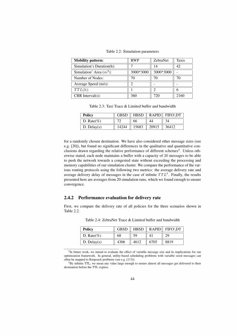
Table 2.2: Simulation parameters

Mobility pattern: RWP ZebraNet TaxisSimulation’s Duration(h): 7 14 42Simulation’ Area (m2): 3000*3000 3000*3000 -Number of Nodes: 70 70 70Average Speed (m/s): 2 - -TTL(h): 1 2 6CBR Interval(s): 360 720 2160

Table 2.3: Taxi Trace & Limited buffer and bandwidth

Policy GBSD HBSD RAPID FIFO\DTD. Rate(%) 72 66 44 34D. Delay(s) 14244 15683 20915 36412

for a randomly chosen destination. We have also considered other message sizes (seee.g. [20]), but found no significant differences in the qualitative and quantitative con-clusions drawn regarding the relative performance of different schemes4. Unless oth-erwise stated, each node maintains a buffer with a capacity of 20 messages to be ableto push the network towards a congested state without exceeding the processing andmemory capabilities of our simulation cluster. We compare the performance of the var-ious routing protocols using the following two metrics: the average delivery rate andaverage delivery delay of messages in the case of infinite TTL5. Finally, the resultspresented here are averages from 20 simulation runs, which we found enough to ensureconvergence.

2.4.2 Performance evaluation for delivery rate

First, we compare the delivery rate of all policies for the three scenarios shown inTable 2.2.

Table 2.4: ZebraNet Trace & Limited buffer and bandwidth

Policy GBSD HBSD RAPID FIFO\DT

D. Rate(%) 68 59 41 29

D. Delay(s) 4306 4612 6705 8819

4In future work, we intend to evaluate the effect of variable message size and its implications for ouroptimization framework. In general, utility-based scheduling problems with variable sized messages canoften be mapped to Knapsack problems (see e.g. [113]).

5By infinite TTL, we mean any value large enough to ensure almost all messages get delivered to theirdestination before the TTL expires.

44

0

0.2

0.4

0.6

0.8

1

1.2

10 20 30 40 50 60 70

Avera

ge D

elivery

Rate

Number of Sources

FIFO/Drop-TailHBSDRAPIDGBSD

(a) Delivery Probability

1000

2000

3000

4000

5000

6000

7000

8000

10 20 30 40 50 60 70

Avera

ge D

elivery

Dela

y(s

)

Number of Sources

FIFO/Drop-TailHBSDRAPIDGBSD

(b) Delivery Delay

Figure 2.1: Delivery probability and delay for Epidemic Routing with differentscheduling and drop policies.

Figure 2.1(a) shows the delivery rate based on the Random Waypoint model. Fromthis plot, it can be seen that: the GBSD policy plugged into Epidemic routing gives thebest performance for all numbers of sources. When congestion-level decreases, so doesthe difference between GBSD and other protocols, as expected. Moreover, the HBSDpolicy also outperforms existing protocols (RAPID and Epidemic based on FIFO/drop-tail) and performs very close to the optimal GBSD. Specifically, for 70 sources, HBSDoffers an almost 60% improvement in delivery rate compared to RAPID and is only14% worse than GBSD. Similar conclusions can be also drawn for the case of the realTaxi traces or ZebraNet traces and 70 sources. Results for these cases are respectivelysummarized in Table 2.3 and Table 2.4.

2.4.3 Performance evaluation for delivery delay

To study delays, we increase messages’ TTL (and simulation duration), to ensure al-most every message gets delivered, as follows. Random Waypoint: (duration 10.5h,TTL = 1.5h). ZebraNet: (simulation duration = 28h, TTL = 4h). Taxi trace: (simula-tion duration = 84h, TTL = 12h). Traffic rates are as in Section 2.4.2.

For the random waypoint mobility scenario, Figure 2.1(b) depicts the average deliv-ery delay for the case of both limited buffer and bandwidth. As in the case of deliveryrate, GBSD gives the best performance for all considered scenarios. Moreover, theHBSD policy outperforms the two routing protocols (Epidemic based on FIFO/drop-tail, and RAPID) and performs close to GBSD. Specifically, for 70 sources and bothlimited buffer and bandwidth, HBSD average delivery delay is 48% better than RAPID

45

and only 9% worse than GBSD.Table 2.3 and Table 2.4 show that similar conclusions can be drawn for the delay

under respectively the real Taxi(s) and ZebraNet traces.

2.5 Buffer Management for Traffic Classes with QoSRequirements

The proposed algorithms considered thus far assume all end-to-end sessions (and, thus,messages) to be of equal importance. In many envisioned scenarios, network nodesmight be running multiple applications in parallel. In this context, ensuring success-ful data delivery and/or minimizing the delivery delay may be more important for oneDTN application than for another. Consider the example of a military operation wherewe have two applications launched concurrently at the DTN nodes: one reporting po-sition information of friendly forces periodically and another one generating missiondebriefings less frequently. We can consider that the delivery delay requirement forthe first one is lower than the second one, since, after some time, a reported positionmay be stale. On the contrary, ensuring that a single mission debriefing message isdelivered successfully may be more important than losing some (out of many) positionupdates. It is thus reasonable to assume that different messages might have differentQoS requirements and resource allocation decisions should take these into account.

To model this setup we make some additional assumptions. We assume there areC different traffic classes different QoS requirements. E.g., focusing on the case ofdelivery ratio, class k is assumed to have a minimum acceptable delivery probabilityP

(k)QoS (a class k can also be “best effort”, i.e. P (k)

QoS = 0.). Similarly, we use superscript

(k) to refer to a specific quantify for class k (e.g. n(k)i ).

Within this context, our goal is to modify the previous optimization framework withthe following objectives:

Feasible Region: If there are enough resources in the network,

Obj. 1 To ensure that the achieved delivery probability for every class k is at least ashigh as P (k)

QoS .

Obj. 2 Provided that minimum delivery ratios are achieved, any remaining resouces areallocated towards improving the total delivery rate (across classes).

Infeasible Region: If there are not enough resouces to fulfill Obj. 1 then

Obj. 3 Allocate the resources, so as to satisfy the requirements of higher priority classes(without loss of generality we assume priority is decreasing with k)

Objective (1) above suggest that satisfying QoS requirement of each class is a hardconstraint. Objective (2) implies that beyond satisfying the QoS, extra resources shouldbe allocated to messages which can most benefit by these resources. Given the decreas-ing nature of message marginal utilities (with respect to the number of copies), shownearlier, this results as we shall see to a max-min allocation policy of remaining re-sources. Finally, Objective (3) says that, if there are not enough resources, then class

46

priorities are absolute and all resources should be greedily allocated to the highestpriority classes. The following formulates the above objectives into an optimizationproblem.

Definition 2.5.1 (Buffer Management with QoS Guarantees). Consider a networksnapshot at time t with K live messages, and Ri, Ti m

(k)i , being the remaining time,

elapsed time, and number of nodes that have seen message i after elapsed time Ti,respectively (superscript (k) denotes that a quantity refers to class k). If the followingoptimization problem has a feasible solution n

(k)i , then any optimal solution satisfies

Obj.1 and Obj.2.

maxn(k)i

K(t)∑i=1

(1− m

(k)i

L− 1

)· P (k)

i (Ti), (2.5)

gk

(n(k)i ,m

(k)i

)=

m(k)i

L− 1+

(1− m

(k)i

L− 1

)· P (k)

i (Ti) ≥ P(k)QoS ∀i ∈ class k, (2.6)

P(k)i (Ti) = 1− exp(−λn(k)

i (Ti) ·Ri). (2.7)

L ·B −C∑

k=1

Lk(t)∑i=1

n(k)i ≥ 0, (2.8)

L− n(k)i ≥ 0 ∀i, k, (2.9)

The key additonal constraint, compared to the original best effort problem is Eq.(2.6).It says that the delivery probability is 1 if message i has been delivered already (with

probability 1− m(k)i

(L−1) ) or P (k)i (t) if it hasn’t (this probability depends on the number of

allocated copies n(k)i ) if it hasn’t, and the sum of both should be at least as large as de-

sired QoS for this message’s class. This constraint is convex on n(k)i , so the centralized

problem remains convex.Eq.(2.7) is not a contraint per se (otherwise the problem would not be convex, since

this is not affine), but just defines notation P(k)i (t) for brevity. If one could centrally

and instantaneously choose all values for n(k)i , it is easy to see that Eq.(2.6) captures

Obj.1 and the objective captures Obj.2. Any interior-point method could solve thisproblem centrally. Nevertheless, as explained earlier, such a centralized policy cannotbe implemented in our DTN context. Our goal instead is to ensure every node takes adrop or scheduling decision independently, in a distributed manner. Additionally, theabove problem does not give any guarantees for when the problem is infeasible, andthus does not satisfy Obj.3.

Based on the above observations, we propose the following modified utilities, thatnodes can use for both scheduling and dropping messages (as in the case of best efforttraffic, considered earlier), towards achieving these objectives.

U(k)i (DR) = Ui(DR) ·

[1 + max

0, ck

(P

(k)QoS − gk

(n(k)i ,m

(k)i

))], (2.10)

47

where ck is a large constant and ck ≫ cl, ∀k > l.The above utility function achieves the following: (i) It first pushes the solution

back into the feasible domain for each QoS constraint (because the term inside themax is much higher than 1, when the constraint is violated). (ii) If there is a feasiblesolution (i.e. Eq.(2.6) can be satisfied for all messages of all classes), then it performsgradient ascent among feasible solutions (as in the problem without QoS constraints);this ensures Obj.1-2 above are satisfied eventualy. (iii) If there is no feasible solutionto the problem, the requirement on constants ck ensures that the available resourcesare allocated to highest priority class, till its constraint is satisfied, then remainingresources to 2nd highest priority class, and so forth.

This can be seen as a distributed implementation of the centralized problem ofDef. 2.5.1, where the constraints of Eq.(2.6) are introduced in the objective as penaltyfunctions. The types of penalty functions corresponding to the chosen utility are hardbarrier functions, as they are 0 when the constraint is not violated but take a very highvalue when the constraint is violated even a little. During a contact then the nodesinvolved update only a subset of the control variables (independently and possibly inparallel with other pairs), corresponding only to the messages inside the two buffers.

Note that it is often more common to assume “soft” penalty functions in distributedimplementations (gradually tightening the constraint), in order to ensure the algorithmdoes not get stuck on the border of the feasible region. However, the convexity of theproblem together with the randomized nature of coordinate ascent here (the controlvariables updated at each step are random, and depend on the nodes that meet eachother), a hard constraint like the above does not pose a problem. An implementationwith soft penalty functions would be perhaps interesting when quantities ni and mi arein fact noisy estimates obtained as explained in the next section. We defer this to futurework.

2.5.1 Performance EvaluationTo evaluate our policy we considered three priority classes, namely Expedited (high-est), Normal and Bulk (lowest) (based on the terminology of the bundle protocol speci-fication [114] regarding different QoS classes). The BDR results are presented for vari-ous values of total available buffer space in the network. We consider a setup where thenodes create bundles every 1/r seconds, they meet each with exponential inter-contacttimes with a common rate, and they exchange their non-common bundle copies (anddrop copies, if the buffer is full) according to the utilities of Eq.(2.10). We present somesample results, comparing the performance of our policy with two existing QoS-basedbuffer management policies, namely: ORWAR [115] and CoSSD [116]. More detailsabout the simulation setup and additional results (e.g. with real traces) can be foundin [23].

Based on Fig. 2.2, it is clear that our scheme outperforms ORWAR. For low buffervalues (i.e., < 500 buffer spaces), all three classes achieve higher BDR with ourscheme. ORWAR fails to capture even the required performance of the Expedited class,even when the resources are adequate to do so. For higher buffer availabilities, OR-WAR’s expedited class reaches to higher BDR than the required threshold. However,this is not desired based on the previous discussion, as it comes at the cost of the other

48

Figure 2.2: QoS Policy vs ORWAR Figure 2.3: QoS Policy vs CoSSD

Figure 2.4: Overall policies comparison

two classes, whose performance is much lower than it could be. The superiority of ourscheme is also captured by the overall network performance (Fig. 2.4, considering allclasses), which is up to 20% higher with our policy, comparing to ORWAR.

In Fig. 2.3, the results of the comparison with CoSSD policy are shown. Insidethe infeasible region (< 400) the lower classes, as well as the overall performance(Fig. 2.4), are improved comparing to our policy. However, this comes at the cost ofsignificant performance degradation for the Expedited class, which does not manageto reach its required performance threshold for the first values of Buffer sizes (< 400).This is obviously contrary to the intended behavior, which dictates that our primalgoal is to reach the desired performance for the expedited class. The relative behaviorbetween the two compared policies changes inside the feasible region (> 400). TheExpedited class’s BDR for CoSSD increases beyond its desired QoS threshold, withoutthe lower classes having reached this threshold. As highlighted for the comparisonwith ORWAR, this is opposite to the optimal behavior. The consequence is that ourpolicy outperforms CoSSD both in terms of lower classes, as well as overall networkperformance in this buffer availability region.

49

2.6 Implementation and ExtensionsIn addition to the above basic framework, we have also considered various extensions,generalizations, and implementation details. We summarize them here and refer theinterested reader to the respective publicatons.

2.6.1 Statistics CollectionAs explained earlier, the HBSD policy requires estimates for quantities ni and mi inorder to derive the (a local estimate of) the utility of each message in the local buffer.However, due to the DTN nature of the network, it is not possible for a node which hasa message k in its buffer, at some time t, to know how many other nodes currently havemessage k in their buffer as well at that time t. While one could try to use obsoleteinformation obtained from times t − T for some T > 0, such information might bequite old and noisy (since the number of copies for a message might be small).

Instead, we choose to estimate the expected value of variables n(t) and m(t), bycollecting data about the history of other, older messages after a similar elapsed timet. Nodes keep track of their buffer status (message ID, elapsed time T tuples) andexchange these with encountered nodes when they meet (updating their known copyestimate). Hence, estimates of these expectations can be built despite the slow natureof DTN propagation, and these estimates are more robust, as they are based on manymessages. More details about this statistics collection method and its overhead can befound in [21], which also contains some interesting insights on the behavior of theseutilities as a function of elapsed time, for high traffic (“congested”) and low trafficregimes.

2.6.2 Generalized Inter-ContactsThe proposed methodology can be applied also for generic, i.e., non exponential in-tercontact times. E.g., assuming the time until the next contact between two nodes iand j is distributed according to F (t) (F (t) = 1 − exp(λt) in the previous analy-sis). For example, the utility function of Theorem 2.1 could be modified by replacingexp(−λni(Ti)Ri) with

(F (Ri)

)(ni). We can even generalize to heterogeneous contactrates λij between nodes, in relatively large networks. We will discuss heterogeneouscontact rates in a more general setup in the next chapter. Details about heterogeneouscontact rates for the problem of buffer management specifically, can be found in [23].

2.6.3 Messages with Heterogeneous PopularitiesSo far, we have also been assuming that each message has a unique destination and itis equally important with all other messages. In [117], we have extended some of theideas in this chapter to a setup where each message might be of interest to multipledestinations. Our protocol, CEDO aims at maximizing the total delivery-rate of dis-tributed content in a setting where a range of contents of different popularity may berequested and stored, but nodes have limited resources. It achieves this by extendingthe delivery-rate utility per content to account for different content popularities as well.

50

2.7 Proof of Theorem 2.1

The probability that a copy of a message i will not be delivered by a specific node, whenmeeting times are exponential, is equal to exp(−λRi) (where Ri is the remaining timeuntil the TTL expires: Ri = TTL− Ti). Knowing that message i has ni(Ti) copies inthe network, and assuming that the message has not yet been delivered, we can derivethe probability that the message itself will not be delivered (i.e. none of the ni copiesgets delivered):

Pmessage i not delivered | not delivered yet =ni(Ti)∏i=1

exp(−λRi) = exp(−λni(Ti)Ri). (2.11)

Note that we have not taken into account that more copies of a given message i maybe created in the future through new node encounters, or a copy of message i could bedropped within Ri. Nevertheless, the same assumptions are applied for all messagesequally and thus can justify the relative comparison between the delivery probabilitiesfor different messages.

We also need to considern what has happened in the network since the messagegeneration, in the absence of an explicit delivery notification (this part is not consideredin RAPID [19], making the utility function derived there suboptimal). Given that allnodes including the destination have the same chance to see the message (due to IIDmobility), the probability that a message i has already been delivered is equal to:

Pmsg i already delivered = mi(Ti)/(L− 1). (2.12)

Combining the above two equations, the probability that a message i will get deliveredbefore its TTL expires is:

Pi = (1− mi(Ti)

L− 1) ∗ (1− exp(−λni(Ti)Ri)) +

mi(Ti)

L− 1.

So, if we take at instant t a snapshot of the network, the global delivery rate for theentire whole network will be:

DR =

K(t)∑i=1

[(1− mi(Ti)

L− 1) ∗ (1− exp(−λni(Ti)Ri)) +

mi(Ti)

L− 1

]

The above sum defines the expected additional contribution of the messages cur-rently not expired to the total delivery ratio (messages already delivered, will not con-tribute to tis ratio, hence the need for the first term in the parenthesis). In case of a fullbuffer or limited transfer opportunity, a DTN node should take respectively a drop orreplication decision that leads to the best gain in the global delivery rate DR. To definethis optimal decision, we differentiate DR with respect to ni(Ti), then we discretizeand replace dn by ∆n to obtain:

51

∆(DR) =

K(t)∑i=1

∂Pi

∂ni(Ti)∗ ni(Ti)

=

K(t)∑i=1

[(1− mi(Ti)

L− 1)λRi exp(−λni(Ti)Ri) ∗ ni(Ti)

]Our aim is to maximize ∆(DR). In the case of message drop, for example, we

know that: ∆ni(Ti) = −1 if we drop an already existing message i from the buffer,∆ni(Ti) = 0 if we don’t drop an already existing message i from the buffer, and∆ni(Ti) = +1 if we keep and store the newly-received message i. Based on this,GBSD ranks messages using the per message utility in Eq.(2.1), then schedules anddrops them accordingly.

52

Chapter 3

Performance Modeling forHeterogeneous Mobility andTraffic Patterns

53

3.1 Performance under Heterogeneous MobilityEpidemic spreading is probably one of the most popular bio-inspired principles thathave made their way into computer engineering. Epidemic algorithms and variants(e.g. gossip) have been used for communication in distributed systems, synchroniza-tion of distributed databases, content searching in peer-to-peer systems, etc. As pre-sented in the previous chapter, epidemic-based schemes have also been proposed forrouting and data dissemination in Opportunistic Networks [118] or Delay Tolerant Net-works (DTNs). In the previous chapter, we have considered how to modify epidemicalgorithms for DTN, in order to efficiently deal with limited buffer capacity and contactbandwidth. In this chapter, we are interested instead in understanding the theoreticalperformance of such epidemic schemes and variants.

Since the mobility process of nodes involved (e.g. humans or vehicles carrying thedevices) is, in most cases, not deterministic, the performance of epidemic algorithms(and variants) heavily depends on the underlying contact patterns between nodes. Tothis end, epidemic algorithms have been extensively studied through both simulationsand analytical models. While simulations with state-of-the-art synthetic models or realmobility traces can provide more reliable predictions for the specific scenario tested,analytical models can give quick, qualitative results and intuition, answer “what-if”questions, and help optimize protocols (e.g. choosing the number of copies in [12], orgossip probability [13]).

For the sake of tractability, state-of-the-art analytical models for epidemic spread-ing mainly rely on simple mobility assumptions (e.g. Random Walk, Random Way-point), where node mobility is stochastic and independent, identically distributed (IID)(see e.g. [119, 13, 120]). Nevertheless, numerous studies of real mobility traces [121,122, 26, 36] reveal a different picture. One key finding is that contact rates betweendifferent pairs of nodes can vary widely. Furthermore, many pairs of nodes may nevermeet. This puts in question the accuracy and utility of these models’ predictions. Yet,departures from these assumptions [123, 124, 125, 122] seem to quickly increase com-plexity and/or limit the applicability of results. This raises the question: can we deriveuseful and accurate closed form expressions for the performance of epidemic schemes,under more generic mobility assumptions? In the next sections, we consider increas-ingly complex mobility, or more specifically contact models, and derive analytical ex-pressions for the expected delay of epidemic routing in the respective (class of) net-works.

3.1.1 Heterogeneous Contact Rates over Random Connectivity Graphs

Definition 3.1.1 (Heterogeneous Full Contact Network). The sequence of the contactevents between each pair of nodes i, j is independent from other pairs, and given bya Poisson process with rate λij . The contact rates λij are independently drawn froman arbitrary distribution fλ(λ), λ ∈ A ⊆ (0,∞), with finite mean µλ and varianceσ2λ.

The above model is a generalization of the standard IID inter-contact model, usedalso in the previous chapter, which assumes λij = λ > 0 for all pairs. Different choices

54

Figure 3.1: Markov Chain for epidemic spreading over a homogeneous network withN nodes

Figure 3.2: Markov Chain for epidemic spreading over a heterogeneous network with4 nodes

of fλ(λ) can describe a significantly broader range of scenarios. For example, largeσ2λ values imply that the contact frequencies between different pairs are very hetero-

geneous, e.g. some pairs will rarely contact each other while others much more often.An fλ(λ) symmetric around µλ (e.g. uniform distribution) implies a balanced numberof high and low contact rates, while a right-skewed fλ(λ) (e.g. Pareto) describes anetwork with most pairs having large inter-contact times, but few contacting very fre-quently. Small µλ values could correspond to slow moving nodes, e.g. pedestrians,(or large geographical areas). Finally, multi-modal fλ(λ) functions might approximatescenarios with some hierarchical structure. Note that, conditional on fλ, we get a classof random matrices Λ = λij. Our goal is to analyze the expected performance ofepidemic spreading across the possible instances in this class.

To understand the complexity of the problem, let us first assume the simple case ofλij = λ > 0. We can model epidemic spreading with a pure-birth Markov chain, asdepicted in Fig. 3.1, where a state k denotes the number of “infected” nodes (i.e. nodeswith the message). In this homogeneous contact network, it is easy to show that the steptime Tk,k+1 (i.e. the time to move from state k to state k+1) is exponentially distributedwith rate k(N − k)λ (due to independent Poisson pair-wise meetings. Its expectedvalue is then given by E[Tk,k+1] =

1k(N−k)λ , and, therefore, one could straightwardly

calculate the expected spreading time (broadcast, anycast or unicast).

While we could still use a Markov chain for the heterogeneous contact network, inorder to find E[Tk,k+1], we now need to know which nodes exactly are included in the kinfected nodes. As an example, in Fig. 3.2, we present the Markov Chain of a messageepidemic spreading in a heterogeneous network with four nodes, A,B,C,D. ThisMarkov Chain is composed of 15 states, whereas the respective Markov Chain of anhomogeneous network with 4 nodes would be composed of only 4 states. Hence, itbecomes evident that the complexity increases quickly, even for this simple 4-nodenetwork. In a network with N there will be

(Nk

)different states for step k, each with a

potentially different probability.

55

Lemma 1. The expected delay for the transition from step k to step k + 1 is given by

E[Tk,k+1] =

(NK)∑m=1

1

Smk

· PCmk , (3.1)

where PCmk is the probability that Cm

k is the set of infected nodes at step k, and

Smk =

∑i∈Cm

k

∑j /∈Cm

k

λij (3.2)

While keeping track of the probabilities in the above lemma could be done recur-sively, the state space grows exponentially fast, so even numerical solutions [126] areinfeasible beyond very simple problems. Instead, we prove that, in the limit of large N(number of nodes), the majority of such starting states become statistically equivalentand the aproximation error from using the mean value for Sm

k goes to 0.This is captured by the following main result. The proof is technical and can be

found in [29]

Theorem 1.1. As the network size increases, the relative error REk between the ex-pected step delay E[Tk,k+1] and the quantity 1

k(N−k)µλconverges to zero in probabil-

ity:

limN→∞

REk = limN→∞

E[Tk,k+1]− 1k(N−k)µλ

E[Tk,k+1]= 0. (3.3)

In Table 3.1, we present the values for the relative error REk (Theorem 1.1) insynthetic simulation scenarios of different network sizes N and contact rates hetero-geneity CVλ =

(σλ

µλ

). The values in Table 3.1 correspond to the relative error REk

averaged over all the steps k of the epidemic process and over 100 different networkinstances Λ with equivalent characteristics (N , fλ). It can be seen that in networkswith higher heterogeneity (CVλ) the errors are larger, as our theory predicts. However,as the network size increases, the errors for all scenarios become very small.

The decrease of the relative errors can be observed also in Fig. 3.3, where wepresent the distribution (boxplots) of the values of REk in the different network in-stances. Here, the relative errors do not correspond to averaged (over different steps)values, but we present the REk at the steps that correspond at the 20% (e.g. in thescenario with N = 100, we present the relative errors in the step k = 20) and 70%of the spreading process, in Fig. 3.3(a) and Fig. 3.3(b), respectively. These plots showthat the error not only decreases on average, but it does so for almost all instances fromthat contact class.

While the above approximation becomes exact for large N , the error can be non-negligible for finite networks. For such networks we can derive a better, second orderapproximation using the Delta method known from statistics. Details can be foundin [29].

Lemma 2. For a heterogeneous contact network following Definition 3.1.1, the ex-pected step delay can be approximated by

E[Tk,k+1] =1

k(N − k)µλ·(1 +

σ2λ

k(N − k)

). (3.4)

56

Table 3.1: Relative Step Delay Error REk: Averaged over All Steps and over 100Network Instances

N = 50 N = 100 N = 200 N = 500CVλ = 0.5 2.8% 2.7% 2.6% 2.5%CVλ = 1 4.2% 3.1% 2.7% 2.6%CVλ = 1.5 8.2% 4.6% 3.2% 2.6%CVλ = 3 34.1% 15.3% 8.2% 3.8%

N: 20 50 100 200 5000

0.2

0.4

0.6

0.8

1

RE

k

(a) spreading step: 20%

N: 20 50 100 200 5000

0.2

0.4

0.6

0.8

1

RE

k

(b) spreading step: 70%

Figure 3.3: Relative Step Error for the step (a) k = 0.2 · N (i.e. message spreadingat 20% of the network) and (b) k = 0.7 · N . Each boxplot correspond to a differentnetwork size N (with µλ = 1 and CVλ = 1.5). Box-plots show the distribution of theRelative Step Error REk for 100 different network instances of the same size.

The above results can be further generalized for networks where some nodes nevermeet. Specifically, we can assume an underlying Poisson connectivity graph with pa-rameter ps, where a pecentage of randomly chosen pairs 1 − ps do not communicateat all (i.e. λij = 0)), and the non-zero contact rates are drawn again according toDef.3.1.1. Then, the following Corollary holds:

Corollary 1. Under a Heterogeneous Poisson Mixing Contact Network, where a con-tact pair either never meets (with probability 1 − ps), or meets regularly (with prob-ability ps) and according to Definition 3.1.1, all previous theoretical results hold, bysubstituting the moments of the contact rate distribution (µλ and σ2

λ) with the expres-sions

µλ(p) = ps · µλ, (3.5)

σ2λ(p) = ps ·

[σ2λ + µ2

λ · (1− ps)]

(3.6)

With these basic results in hand, we can derive or aproximate the performance ofepidemic routing as well as other DTN routing variants (e.g. Spray and Wait). Detailsand additional plots for synthetic scenarios can be found in [29], corroborating ourresults.

57

Figure 3.4: Box-plots of the message delivery delay under (a) epidemic, (b) 2-hoprouting, and (c) SnW (with L = 6 copies) routing. On each box, the central horizontalline is the median, the edges of the box are the 25th and 75th percentiles, the whiskersextend to the most extreme data points not considered outliers, and outliers are plottedindividually as crosses. The thick (black) horizontal lines represent the theoreticalvalues predicted by our model.

In Table, we just show the analytical expressions for these protocols, for reference.We also show sample performance results for real mobility traces and realistic mo-

bility models. Analytical results against synthetic contact scenarios conforming to theassumptions in our model show remarkable accuracy, even for modestly sized net-works, and are omitted here. The traces we consider are: (i) Cabspotting [127], whichcontains GPS coordinates from 536 taxi cabs collected over 30 days in San Francisco,and (ii) Infocom [128], which contains traces of Bluetooth sightings of 78 mobile nodesfrom the 4 days iMotes experiment during Infocom 2006. In addition to these realtraces, we generated mobility traces with two recent mobility models that have beenshown to capture well different aspects of real mobility traces, namely, TVCM [129]and SLAW[130]. In order to compare with analysis, we parse each trace and estimatethe mean contact rate for all pairs i, j. We then produce estimates for the 1st and2nd moments of these rates, µλ and σ2

λ, as well as the percentage of connected pairs pand use them in our analytical expressions.

Fig.3.4 compares the theoretical performance of three protocols, epidemic routing,2-hop routing, and spray and wait (SnW), according to our analytical expressions, tosimulation results. Source-destination pairs are chosen randomly in different runs andmessages are generated in random points of the trace. In the next chapter, we willconsider scenario where traffic demand is not random among pairs of nodes.

The first thing to observe is that delay values span a wide range of values for dif-ferent source-destination pairs. This implies a large amount of heterogeneity in the“reachability” of different nodes. Our analytical predictions are shown as thick darkhorizontal lines. As it can be seen, our result is in most cases close to the median andin almost all cases between the 25th and 75th percentile of the delay observed in boththe real traces and mobility models.

It is somewhat remarkable that our delay predictors are close to the actual results(qualitatively or even quantitatively in some cases) in a range of real or realistic sce-narios; studies of these scenarios reveal considerable differences to the much simplercontact classes for which our results are derived. We should also be careful not to jump

58

to generalizations about the accuracy of these results in all real scenarios, as we areaware of situations that could force our predictors to err significantly. Nevertheless,we believe these results are quite promising in the direction of finding simple, usableanalytical expressions even for complex, heterogeneous contact scenarios.

3.1.2 An Upper Bound for Generic Contact MatricesWhile the above results are applicable to many different contact matrices Λ the entriesof these matrices cannot be arbitrary, but are drawn from the same distribution. Thisis what allows us to invoke law of large number types of arguments when the networkinstances become large. However, these do not apply to arbitrary contact matrices,and thus arbitrary underlying mobility processes. In some real networks, the contactmatrix Λ tends to exhibit clear community structure, which cannot be well captured byrandom models, even heterogeneous ones, like the ones considered earlier.

To understand why the above results might not hold, consider a network with 2communities, which grow as N grows, but the number of links between community 1and 2 remain finite, say m. This suggests that at some step k, the number of ways wecan go from k to k+ 1 infected nodes will not grow with N , and we cannot invoke thelaw of large numbers, e.g. approximating the infection rate between the communitieswith m ·µλ (if m is small). It is easy to see that the “bottleneck” delay for this networkis for the infection to spread between the two communities, and the delay of that stepshould depend on the total contact rate across the cut between the communities. Thiscan be generalized by converting a given contact matrix Λ into an appropriate Markovchain and using transient analysis to derive the following result.

Theorem 1.2 (Delay Bound.). Let S denote a “cut” of an arbitrary contact graph Λ.Let further ϕ(S) denote the conductance of this cut1

ϕ(S) =∂(S)

|S| · |S|=

∂(S)

|S| · |S|= ϕ(S), , (3.7)

where |S| denotes the cardinality of the set S, and ∂(S) =∑

i∈S,j /∈S λij . Finally, letΦ be defined as Φ = minS∈Ω ϕ(S). Then, the expected delay of epidemic spreadingover contact network Λ can be upper bounded as follows:

E[DΛ] <2 ln(N − 1)

NΦ, . (3.8)

The above result is generic, and can be further elaborated to derive the distributionof the delay. More importantly, the conducance of a graph, which essentially corre-sponds to finding a balanced min cut, relates to the spectral properties of matrix Λ,namely the 2nd eigenvalue of the Laplacian through Cheeger’s inequality. The proofand more details can be found in [31].

Figs. 3.5(a)–3.5(d) show the empirical CCDFs for the spreading delays in compar-ison with our theoretical CCDFs, obtained from Eq. (3.8). We also depict a tighter

1This is one of several definitions of conductance to be found in the literature. We use it as it providesthe best bound.

59

(a) HCMM (b) Infocom (c) MIT (d) SLAW

Figure 3.5: Prediction accuracy for the CCDF of the epidemic delay on real networks

(but more complex to calculate) bound based on min cuts for each step k denoted as“a-bound” as well as the tail bound obtained by Shah in [131], the best known boundup to that time. The empirical results are well within all the predicted bounds. Notethat the tail bound is at least one order of magnitude larger than the bounds we obtainedhere.

A relatively loose bound, as in the case of MIT attests the presence of at leasttwo strong communities connected through a relatively small set of edges (i.e., smallconductance), as observed in [40]. On the other hand, for the community-free tracesInfocom and SLAW [40], as well as for the HCMM trace (which has built-in verysmall communities of 10 nodes each) the bounds are, as expected, (much) closer to theempirical results. We will revisit some of these traces, in terms of their contact graphproperties, in Ch. 4.

With the results of Section 3.1.1 and this section, we are now able to approximatethe performance of epidemic routing and variants in a very large class of contact net-works, and thus underlying moblity properties. The only remaining properties observedin real traces that are not explicitly captured, is potential dependence between pair-wisecontact properties and non-stationarity (e.g. periodicity). The latter could be capturedby identifying periods in the mobility model or trace, and apply different contact ma-trices Λ for each. Pair-wise dependence is significantly more complex to be capturedand lead to closed-form expression. Nevertheless, appropriate bounds could be soughtfor, if some knowledge about the type of dependence is known. Finally, the fact that Λis in principle a random matrix, and epidemic performance depends on the eigenvaluesof this matrix, random matrix theory could be a useful tool to further elaborate on theseresults [132].

3.2 Performance under Heterogeneous Traffic

3.2.1 Communication Traffic

In all previous analyses we have assumed that any source-destination pair is equallylikely to generate a message. We did this explicitly in simulations, and we also implic-itly assumed it in our theory (as we shall explain). Nevertheless, in addition to whocontacts whom and how often (i.e. mobility and the resulting contact process), anothermajor question that should be raised in opportunistic networks (but rarely is) is whowants to communicate with whom and how much traffic do they exchange?

60

Intuition suggests that every pair of nodes will not exchange the same amount oftraffic. To support intuition, studies from fields related to technological and socialnetworks [133, 134, 135] have demonstrated the existence of heterogeneous traffic pat-terns. The same studies further suggest that this heterogeneity depends on the spatialand social characteristics of these networks. Since location-based services [136] andsocial networking [137] are considered among the major applications supported by op-portunistic networks, such traffic dependencies on social and/or spatial factors are veryprobable to appear. What is more, mobility characteristics have also been found to de-pend on spatial and social characteristics [138, 139, 140]. This clearly seems to arguefor a non-homogeneous traffic model. Moreover, traffic and mobility in such networksare expected to exhibit some correlations [133, 134].

Before we proceed to choose a traffic model, one should consider the followingquestions: Would the mere heterogeneity of traffic suffice to affect performance? Is itnecessary to consider traffic and mobility correlations?

As stated earlier, information dissemination is determined by the sequence of con-tact events. Hence, if traffic characteristics are independent of node mobility, one mightexpect a limited impact on performance.

Towards examining the validity of the above argument, we decided to compare theperformance of some well-known opportunistic protocols (direct transmission [10],spray and wait [12], 2-hop routing [119], and SimBet [35]) through simulations on tworeal traces, for three traffic scenarios: (i) homogeneous traffic: every pair of nodes hasthe same chance of being chosen as the source-destination pair for the next message;(ii) heterogeneous traffic that is mobility independent: we assign randomly to eachpair a different end-to-end traffic demand (with the normalized message generationrate for a pair drawn uniformly in [1, 1000]); (iii) heterogeneous traffic that is mobilitydependent: end-to-end traffic between two nodes is proportional to their contact rate.We generated an equal (sufficiently large) number of messages for all scenarios.

Results for the mean message delivery delay are shown in Fig. 3.6. As is evidentfrom these results, when traffic heterogeneity is independent of mobility (middle bar),the average delay is practically the same to the homogeneous case (left bar), for allprotocols, and across all scenarios (including additional ones we have tried). In con-trast, when traffic is heterogeneous and correlated with the contact rates (rightmostbar), Fig. 3.6 shows a clear difference in average delay for all scenarios and protocols.These results provide an initial answer to the above questions. It is not traffic het-erogeneity itself that affects performance, but rather the joint effect of mobility andtraffic (heterogeneity).

In other words, unless differences in traffic demand correspond also to differencesin contact frequency (e.g. frequently meeting pairs tend to also consistently generatemore/less traffic for each other), end-to-end performance will not be affected. Thisstatement is also formally proven in [33].

The above observation, together with the initial insight coming from real datasets,motivates us to propose the following simple, yet quite generic, model for end-to-endtraffic.

Definition 3.2.1 (Heterogeneous Communication Traffic). The end-to-end traffic de-mand (per time unit) between a pair of nodes i, j, is a random variable τij , such that

61

Direct SnW 2−hop SimBet3

3.5

4

4.5

5

5.5

6x 105

Del

ay

Homogeneous trafficHeterogeneous traffic (mobility independent)Heterogeneous traffic(mobility correlated)

(a) Gowalla dataset

Direct SnW 2−hop SimBet

4

6

8

10

12

14x 105

Del

ay

Homogeneous trafficHeterogeneous traffic (mobility independent)Heterogeneous traffic(mobility correlated)

(b) Strathclyde dataset

Figure 3.6: Mean delivery delay of 4 routing protocols, namely Direct Transmission,Spray and Wait (SnW), 2-hop, and SimBet, on the (a) Gowalla and (b) Strathclydedatasets.

E[τij ] = τ(λij), where τ(·) is a continuous function from R+ to R+.

Hence, traffic demand between node pairs can differ and is on average correlatedwith the nodes’ contact rate. However, τij itself is still random, allowing some nodepairs to have little traffic demand even if they meet often (e.g. “familiar strangers”).Furthermore, through the function τ(·) one can introduce a number of different typesand amounts of (positive or negative) correlations between traffic and mobility. Whilereal traffic patterns are clearly expected to have a number of additional nuances anddetails, not captured by the model of Def. 3.2.1, it turns out that these abstractions arestill “rich” enough to allow us to draw useful conclusions.

3.2.2 Communication Traffic Heterogeneity: Model and Implica-tions

Let us assume a heterogeneous mobility/contact model as the one introduced earlierin Def. 3.1.1. If a message is equally likely to be generated between any pairs ofnodes, then the contact rate between the source and destination of this message in aheterogeneous contact setup should be distributed according to the contact rate fλ.However, if messages are more likely to come from a frequently meeting pair ratherthan an “average” pair (e.g. if communication rate is positively correlated with contactrate) then the source-destination contact rate (we refer to it as the effective contactrate) would be biased towards higher values. The following proposition captures thisformally. Its proof can be found in [33].

Proposition 1. The probability density function fτ of the contact rate between thesource and the destination s, d of a random message, in a network following Defini-

62

tions 3.1.1 and 3.2.1, converges as follows:

fτ (x)p→ 1

C· τ(x) · fλ(x) (3.9)

where fτ (x)dx = Pλsd ∈ [x, x + dx), p→ denotes convergence in probability, andC = E[τ(λ)] =

∫∞0

τ(x)fλ(x)dx is a normalizing constant.

An opportunistic routing protocol tries to deliver the end-to-end traffic demand τij ,and we would like to consider the effects of different contact patterns fλ and trafficpatterns τ(λ) on its performance. There exists a very large abundance of proposedschemes [141] and it would not be possible, nor would it provide any intuition, toanalyze the effect of heterogeneity on each and every one. Instead, we focus on twobasic forwarding mechanisms, underlying many DTN protocols, to gain intuition:

Direct Transmission (“DT”): This is the simplest imaginable method: nodes wish-ing to exchange data or information with each other, may do so, only when they arein direct contact, without involving any relays. For instance, DT is often assumed incontent-centric applications, where a node interested in some content will query di-rectly encountered nodes for content of interest, and retrieve it only if it is availablethere. DT has the minimum amount of overhead and worst amount of delay (in non-limited resource setups), and will serve as the baseline.

Relay-Assisted: To improve the performance of direct transmission, replication orRelay-Assisted schemes can be used. Extra copies can be handed over to encounterednodes, and the destination can receive the message from either the source or any of therelays, reducing thus the expected delivery delay. In its simplest form, schemes likespray and wait distribute a small number of additional copies to the first few relaysencountered, and any of these relays can deliver the message to the destination. Innetworks with homogeneous mobility and traffic, it is known that using just a few extracopies leads to significant performance gains. For example, in a network of 1000 nodes,simply distributing 10 extra copies to the first 10 nodes encountered provides an almost10-fold improvement in delay compared to direct transmission [12]. Although this alsocomes with a 10-fold increase in the amount of (storage and bandwidth) resourcesneeded, it presents a very useful tradeoff to DTN protocol designers, especially sincethis ratio actually decreases with network size and thus scales well [12].

However, when it comes to heterogeneous mobility and traffic, Proposition 1 sug-gests that, unlike the above example, the source is no longer equivalent with otherrandom relays, in terms of their probability of contacting an intended destination soon.It is thus of particular interest to examine whether the above trade-off still holds, if oneconsiders the joint effect of realistic mobility and communication traffic patterns.

To compare the performance of Relay-assisted routing and Direct Transmission, interms of delivery delay and delivery probability (the two main metrics considered inrelated work), we first define the following metrics:(a) Delay Ratio, R: the ratio of the expected delivery delay of Relay-Assisted routing,E[TR], over the expected delivery delay of Direct Transmission routing, E[TDT ], i.e.

R =E[TR]

E[TDT ]

63

(b) Source Delivery Probability, P(src.): the probability that a message is delivered tothe destination by the source node, rather than by any of the relays.

For instance, when R = 0.1 Relay-assisted routing delivers (on average) a message10 times faster than Direct Transmission, while a value R = 0.5 implies that Relay-assisted routing is only 2 times faster. Respectively, when P(src.) = 0.1 the probabilitythat the source node s meets the destination d, before any other relay node meets d, is10%, and P(src.) = 0.5 means that this probability is 50%. And in the limiting cases:when R,P(src.) → 1, it means the message is delivered to the destination by the sourcenode itself; when R,P(src.) → 0, delivery takes place (entirely) due to the relays.

In Result 1, we derive analytical expressions for these two metrics, R and P(src.).The proof can be found in [33].

Result 1. When Relay-assisted routing with L extra copies is considered, then

R =1

E[τ(λ)λ

] · ∫ ∞

0

∫ ∞

0

τ(x)

x+ y· fλ(x)dx · fR(y)dy

P(src.) =1

E[τ(λ)]·∫ ∞

0

∫ ∞

0

x · τ(x)x+ y

· fλ(x)dx · fR(y)dy

where the expectations are taken over fλ and fR = f(∗L)λ is the L-fold convolution of

fλ.

3.2.3 A Case StudyTo obtain additional insight, we consider the following setup as an example:

Mobility: We will assume the contact rates to be gamma distributed, i.e. fλ(x) ∼Γ(x;α, β) = βα

Γ(α)xα−1e−βx.

Our choice is initially motivated by the findings of Passarella et al. [138], whohave shown, through statistical analysis of pervasive social networks’ datasets, thatthe Gamma distribution matches well the observed contact rates. Additionally, byselecting appropriately the parameters α and β of a Gamma distribution, we can assignany desired value to the mean value µλ and the variance σ2

λ of the contact rates2. Thisallows us to describe (or fit up to the first two moments) a large range of scenarios withdifferent mobility heterogeneities captured by CVλ = σλ

µλ.

Traffic: We will describe the traffic using a polynomial function of the form τ(x) =c · xk, c > 0. By choosing different values of k, one can control both the amount ofcorrelation, as well as the shape (concave or convex).

Under these assumptions, the following closed form expression bounds can be de-rived for our two metrics of interest. The proof can be found in [34].

Result 2. In a Heterogeneous Contact Network where fλ ∼ Γ(α, β) with mean valueµλ and variance σ2

λ (coefficient of variation CVλ = σλ

µλ) and τ(x) = c · xk, it holds:

1 ≥ R ≥ Rmin =1 + (k − 1) · CV 2

λ

1 + k · CV 2λ + L

(3.10)

2The mean value and variance of a gamma distribution are given by µλ = αβ

and σ2λ = α

β2 , respectively.

64

Table 3.2: Rmin, Pmin: Monotonicity and Asymptotic Limits

Parameter Monotonicity as Limits forx parameter x increases x → minx x → maxx

mobilityheterogeneity:

CVλ ∈ [0,∞)

Rminincreases , if k > 1 + 1

Ldecreases , otherwise

Pminincreases , if k > 1

Ldecreases , otherwise

limCVλ→0

Rmin =1

1+L

limCVλ→0

Pmin =1

1+L

limCVλ→∞

Rmin = 1-1

k

limCVλ→∞

Pmin = 1-1

k+1

trafficheterogeneity:

k ∈ (kmin,∞)Rmin, Pmin increase lim

k→kminRmin, Pmin = 0 lim

k→∞Rmin, Pmin = 1

extra copies:L (L ≪ N)

Rmin, Pmin decrease -

for k > kmin = 1− 1CV 2

λ, and

1 ≥ P(src.) ≥ Pmin =1 + k · CV 2

λ

1 + (k + 1) · CV 2λ + L

(3.11)

for k > kmin = − 1CV 2

λ.

Practical Example: If the measured network characteristics are CVλ = 2 andk = 2, then from Result 2 we get R = 5

9+L . Therefore, to achieve delivery delay twotimes faster than Direct Transmission, one extra copy should be used (L = 1 → R =0.5), while to achieve 4 times faster delivery, L = 11 relay nodes are needed. In thelatter case, if traffic/mobility heterogeneity has not been taken into account [12], theprediction would be L = 3 and this would lead only to 2.5 (instead of 4) times fasterdelivery (i.e. R = 5

12 ).It is evident from the above example that traffic heterogeneity can have a major

impact on performance and thus protocol design. Table 3.2 formalizes this impact, byconsidering how Rmin and Pmin (Eq. (3.10) and Eq. (3.11)) behave.

Gain of Extra Copies

A strong positive correlation (large k) between traffic and mobility reduces the addedvalue of extra copies (i.e. Rmin, Pmin as k ). This indicates that, as corre-lation (k) increases, one needs to distribute message copies to more relays nodes inorder to achieve a certain performance improvement compared to the baseline, DirectTransmission.

In contrast, a negative (or weak positive) correlation renders each extra copy moreuseful (i.e. Rmin, Pmin → 0 as k → kmin

3). It becomes evident that it is crucial toidentify whether a traffic-mobility correlation exists in a given scenario, and what itsnature is, as this could decide whether the overhead of using few or more extra copiesis justified or would just waste a lot of valuable resources.

Routing for Unicast Applications

For high heterogeneity (traffic and mobility), our results imply that a unicast mes-sage is likely to arrive to its destination at the time the source and destination come

3The values of kmin are given in Result 2.

65

in contact (i.e. Rmin, Pmin → 1 as k,CVλ → ∞). This raises questions aboutthe usefulness of opportunistic networking for unicast applications in which end-to-end traffic is expected to be highly correlated with contact frequency (e.g. Facebookmessaging) [133, 134]. On the other hand, our results suggest that potential unicastapplications with an end-to-end traffic demand between nodes with non-frequent meet-ings, i.e. scenarios with small or negative k, (e.g. social peers residing in differentcommunities) could benefit a lot (more than normally assumed).

Although these observations might appear somewhat self-evident at first glance,the question of how to tune protocols and choose the right number of replicas stillsremains. To our best knowledge, our results are the first to provide closed form, quan-titative insights into the tradeoffs involved in real scenarios with both mobility andtraffic heterogeneity. Furthermore, although our analytical results are derived for thecase of random replication protocols, the above qualitative implications hold also formobility-aware protocols (e.g. EBR [17]), which exploit mobility heterogeneity in or-der to select better relays.

Content-Centric Communication

While our results are somewhat pessimistic when it comes to the usefulness of op-portunistic networking for unicast applications, the opposite holds when it comes tomodern, content-centric applications (e.g. file sharing, D2D-based offloading, servicecomposition). In such applications nodes are looking, for example, for some contentof interest [142] or service [143], which they can access directly from any encounterednode that offers it. If the interests of nodes are heterogeneous (which is known to bethe case [144]) and nodes with similar mobility patterns tend to have some similarityin their interests too (evidence for this does exist [145]), then our results suggest: (i)that there is a better chance to find a content or service “soon” from a directly encoun-tered node than one would expect in homogeneous scenarios, and (ii) coming up withcomplex, resource-costly mechanisms, e.g. multi-hop query-response, directories, etc.,might not be necessary. We plan to look into such content-centric scenarios in moredetail in future work.

In Fig. 3.7 we compare the message delay of (i) Direct Transmission (i.e. theprotocol with the highest delay), (ii) Relay-assisted routing (Spray and Wait, SnW, [12]with L = 5 copies) and (iii) Epidemic routing [11] (i.e. the protocol with the lowestdelay), in two scenarios, for varying traffic heterogeneity (k). Two main observations,with respect to the previous implications, can be made in Fig. 3.7.

We have extensively validated our results against both synthetic and real traces ina number of scenarios. More details can be found in [33]. In the following, we discussinstead some interesting extensions of the above basic framework.

3.2.4 Extensions

We have tried to present our results in the context of simple schemes (e.g. unicasttraffic, random relay selection), to keep analysis tractable and illustrate key principles.In this section, we discuss how our framework could be applied in some additional

66

0 1 2 3 40

0.2

0.4

0.6

0.8

1

k

Del

ay

direct transmissionspray and waitepidemic routing

(a) CVλ = 1

0 1 2 3 40

0.2

0.4

0.6

0.8

1

k

Del

ay

direct transmissionspray and waitepidemic routing

(b) CVλ = 2

Figure 3.7: Message delay under Direct Transmission, Spray and Wait (L = 5), andEpidemic routing in scenarios with varying traffic heterogeneity; mobility parametersare µλ = 1 and (a) CVλ = 1 and (b) CVλ = 2.

cases. Although far from complete, we believe this set of examples, further underlinesthe utility of our analysis.

Mobility-Aware Protocols

Mobility-aware schemes are often used to select good relays for the intended replicas,rather than picking random ones, e.g. [36, 146, 17, 35]. The selection of the relays isusually based on their social or mobility characteristics. For instance, in encounter-based routing (EBR) [17], the more frequently a node i encounters node d, the higherthe probability to become a relay of a message destined to d.

The relay-selection mechanism in a number of proposed mobility-aware protocolscan be described as following:

Definition 3.2.2. The probability pi a node i to be selected as a relay for a messagedestined to node d, is related to their contact rate λid and this relation is described bya function p(λid).

As an example, we present two protocols belonging to the above class and theirp(λ) functions: (a) a modified mobility-aware version of spray and wait [12] protocol(we refer to it as U1), and (b) a variation of the EBR [17] protocol (we refer to it asU2), where each relay can hold only one message copy.

U1: A node i, which would be selected as a relay by the spray and wait mechanism,under U1 becomes a relay with a probability pi that is proportional to its contactrate with the destination d, i.e. pi = p(λid) = c · λid, where c a normalizingfactor such as p(λ) ∈ [0, 1].

U2: For each message copy, the source node s selects the relay node i with a proba-bility pi that is computed according to the EBR mechanism, i.e. pi = p(λid) =

λid

λid+λsd.

67

CV =0.5 CV = 1 CV = 20

0.2

0.4

0.6

0.8

1

k = 0.5k = 1k = 2

(a) Synthetic scenarios

AU SF St0.7

0.75

0.8

0.85

0.9

0.95

1

Homogeneous TrafficHeterogeneous Traffic

(b) Real networks

Figure 3.8: P(src.) of mobility-aware routing in (a) synthetic scenarios with varyingmobility (CVλ) and traffic heterogeneity (k), and (b) real networks with homogeneousand heterogeneous traffic.

In the following corollary, we show how Results 1 and 2 can be simply modifiedto capture such mobility-aware protocols as well. The proof follows similar ideas, andcan be found in [33].

Corollary 2. Under a mobility-aware Relay-Assisted protocol conforming to Defini-tion 3.2.2, Results 1 and 2 are modified as:Result 1: fR is given by the L-fold convolution of fu(λ), where

fu(x) =1

E[p(λ)]· p(x) · fλ(x)

Result 2: The number of copies L is multiplied by cu, where

cu =E[λ · p(λ)]

E[λ] · E[p(λ)]

For instance, applying Corollary 2, the expression for the delay ratio R, becomes

1 ≥ R ≥ Rmin =1 + (k − 1) · CV 2

λ

1 + k · CV 2λ + cu · L

(3.12)

and for the U1 protocol presented above, cu is given by the expression4:

c(U1)u = 1 + CV 2

λ (3.13)

When mobility is highly heterogeneous (i.e. high CVλ), c(U1)u becomes large, and

thus Rmin and Pmin decrease compared to the random replication mechanism (e.g.

4An expression for cu in the case of the U2 protocol could also be derived, albeit with more complexity,due to the fact that the function p(λ) involves the source destination contact rate λsd as well.

68

random SnW). This confirms that the performance gain is larger when mobility-awareprotocols are used. However, even in this case, as traffic heterogeneity increases, theperformance gain diminishes, i.e. Rmin, Pmin → 1.

We further demonstrate some preliminary simulation results suggesting that ourconclusions hold also for mobility-aware routing. We use the U2 protocol presentedabove. In Fig. 3.8(a) we present simulation results for the delivery metric P(src.) onsynthetic scenarios with varying mobility (CVλ) and traffic (k) heterogeneity. Similarlyto the random replication case, for increasing heterogeneity (in mobility and/or traffic)the gain of the extra copies clearly decreases (i.e. P(src.) increases) under mobility-aware schemes. In Fig. 3.8(b) we compare the probability P(src.) of scenarios withand without traffic heterogeneity in real networks. As before, the results are consis-tent with our theory: the gain of extra copies decreases even for protocols using moresophisticated techniques for relay selection.

Routing based on Contact Graph Structure

A number of mobility-aware routing schemes, e.g. SimBet [35], BubbleRap [36], arebased on the structure of the contact graph (centrality, similarity, communities, etc.)rather than the pairwise contact rates. A direct mapping to a function p(λ) for theseprotocols requires a separate, and rather cumbersome analysis for each such protocol,in most cases not leading to a closed form expression (see, e.g. [42]). However, thecontact graphs used to make forwarding decisions by these more sophisticated proto-cols, still are built based on pair-wise contact rates [38]. We thus expect the utilityof such mobility-related information to be similarly affected by the amount of trafficheterogeneity and its relation to mobility patterns.

To test this further, we simulated, as an example, scenarios using the SimBet pro-tocol [35]5. In Fig. 3.9 we present the simulation results (continuous lines) for the ratioR = E[TSimBet]

E[TDT ] and the theoretical predictions Rmin of Eq. (3.12), for different valuesof the cu parameter (dashed lines). Two main observations that confirm our intuitionare: (i) simulated and theoretical curves increase in a similar manner, and (ii) one canfind (numerically) the value cu that more accurately predicts the performance.

Although this is clearly not conclusive for the applicability of our result to everymobility-aware scheme, we believe it helps to corroborate our findings for the interplaybetween mobility and traffic heterogeneity on protocol performance.

Multicast Communication

We have also been assuming unicast messages between a s, d pair. However, ourresults apply also to multicast [122] or anycast (e.g. content sharing or service compo-sition applications) [143] messages from s, with d being one of the destinations, sincesimilar mechanism are often used for their dissemination. To demonstrate this, in Ta-ble 3.3 we present simulation results for two multicast scenarios, with homogeneous

5For the contact graph we considered the 10% most frequently meeting pairs following the guidelinesof [38], we set the similarity and betweenness weights α = β = 0.5 [35], and we generated multiple copiesas in [147].

69

0 1 2 3 40

0.2

0.4

0.6

0.8

1

k

R

SimBetc

u = 0.25

cu = 0.5

cu = 0.75

cu = 1

(a) CVλ = 1

0 1 2 3 40

0.2

0.4

0.6

0.8

1

k

R

SimBetc

u = 0.25

cu = 0.5

cu = 0.75

cu = 1

(b) CVλ = 2

Figure 3.9: Delay ratio R in two scenarios with varying traffic heterogeneity k. Relay-assisted routing is SimBet with (a) L = 5 and (b) L = 10 message copies.

Table 3.3: Multicast Communication

CVλ 0.1 0.5 1 1.5 2HOM R 0.18 0.12 0.01 0 0

P(src.) 0.01 0.01 0.01 0.01 0.01HET R 0.18 0.26 0.39 0.52 0.61

P(src.) 0.01 0.03 0.12 0.26 0.41

(HOM) and heterogeneous (HET) traffic (τ(x) = c · x4), under varying mobility het-erogeneity. A source sends messages to 5 destinations (each selected with a probability∝ τij) either by Direct Transmission or by Relay-Assisted routing with L = 5 copies.As delivery delay, we consider the delay till all the destinations get the message. It isevident that R and P(src.) (i) increase significantly with mobility heterogeneity whentraffic is heterogeneous, and (ii) become much larger compared to the homogeneouscase (where R decreases and P(src.) is constant), which is in agreement with our re-sults.

Node Selfishness

Another interesting pair-wise property related to the performance of unicast routingprotocols is “selfishness”. Most efficient protocols for DTNs require some sort ofmulti-hop communication, where intermediate nodes that are neither the source nor thedestination for a message must act as relays. However, due to limited resources (bat-tery, bandwidth etc.) and privacy concerns, it might happen that nodes are reluctant tocooperate and forward messages of other nodes. For example, a selfish node could onlyforward and receive its own messages and never act as a relay in order to avoid wast-ing resources. To avoid such behaviors and isolate selfish nodes, many mechanismsproviding incentives for cooperation (e.g. reputation [148] or credit based [149, 150]mechanisms) have been proposed.

70

In many cases, nodes will be more willing to forward messages for nodes withwhom they have a strong social tie (e.g. friends or acquaintances), because they (i)trust them and (ii) have received similar services by them in the past (or it is probableto receive in the future). Additionally, studies from sociology [140], social media [135]and pervasive social networks [151] have shown that the strength of social ties can bepredicted by the contact rate and, specifically, the more frequent two nodes contact, thestronger their social tie probably is.

Hence, combining the previous observations, i.e. (a) the level of cooperation isrelated to social ties and (b) the strength of the ties is related to the contact rate, we canmodel the nodes’ selfishness in a probabilistic way, which allows us to predict its effecton the network performance.

Definition 3.2.3 (Social Selfishness). A pair of nodes i and j either can exchangemessages in every contact event with probability pij or can never exchange messageswith probability 1−pij . The probability pij depends on the meeting rate between thesenodes, i.e. λij , and is described by the relation:

pij = p(λij), pij ∈ [0, 1] (3.14)

The above definition is generic and can be used to describe also scenarios wherethe cooperation between nodes is not determined only by social factors. For instance,in [152] authors investigate how more efficient communication can be achieved: Theypropose a content sharing application where the decision for message exchanges de-pend on the contact rate of nodes and evaluate through simulations different contentsharing policies (i.e. different decision rules based on the contact rates).

When node willingness to act as a relay is correlated to the contact rate, similaranalytical steps as in the case of traffic heterogeneity can be applied to study the jointimpact of the two. We refer the interested reader to [153] for more details on the topic.

71

Chapter 4

Complex Network Analysis forOpportunistic Device-to-DeviceNetworking

72

4.1 Introduction

As we have seen already in previous chapters, many protocols forward in parallel mul-tiple replicas of the same content, to combat the inherent uncertainty of future contactopportunities, [11, 12]. We have also stressed the fact that contact patterns betweennodes are heterogeneous and we studied the impact of simple forwarding schemes un-der both homogeneous and heterogeneous patterns. However, it is not just that nodemobility and resulting contact opportunities are not heterogeneous, but more impor-tantly this mobility is not entirely random. Instead, weak or strong patterns are presentthat utility-based routing schemes attempt to take advantage of to differentiate nodesthat are more likely to deliver content or bring it closer to the destination [10]. E.g.,rather than handing over an extra message copy to a random encountered node, it makesmore sense to wait and hand over that copy to another node if one can predict that thelatter will encounter the destination soon, with high probability.

Among the numerous utility-based schemes proposed, even some early ones al-ready implicitly assessed the strength of “social” ties between nodes. For example[105] uses time of last encounter, and [154] uses contact frequency as a hint on the sim-ilarity of mobility patterns. [25, 16] use instead a metric much akin to degree centralityto identify nodes that are highly mobile/social1; the former scheme is reminiscent ofsearch in scale-free networks, while the latter uses centrality to choose which relays tospray a limited budget of message replicas to. However, these simple metrics may onlycapture one facet of the underlying mobility process, which might not suffice for goodcontact predictions.

More recently, complex network analysis [30] (CNA) was proposed as a moregeneric and powerful tool to formulate and solve the problem of future contact pre-diction in DTNs. The main idea behind this approach is the following: communicationdevices are most often carried by users, whose mobility pattern is governed by com-plex social relations with other users (as well as purpose, schedules, etc.); hence, thesepatterns should also give rise to social properties in the observed contacts between com-municating devices, that could be exploited for protocol design, if inferred correctly.To this end, past observed contacts between nodes are aggregated into a social graph,with graph edges representing (one or more) past meetings between the vertices. Anedge in this graph conveys the information that two nodes often encounter each othereither because they have a strong social tie (friends), or because they are frequently co-located without actually knowing each other (familiar strangers), as shown in Fig. 4.1.Thus, existence of an edge intends to have predictive capacity for future contacts.

Two recently proposed routing protocols, SimBet [35] and BubbleRap [36] , makeexplicit use of CNA metrics and algorithms in order to highlight a node’s positionin the aggregated social graph, and assess its utility to act as a relay for messagesdestined to other nodes. Although the detailed mechanisms of the two protocols dif-fer, they are both based on the same principles: they assume that nodes naturally re-side in mobility-related communities (e.g., class, work, home). Increasingly “central”or “well-connected” nodes in the graph are then chosen as carriers to relay content

1“Degree” is the number of neighbors a node has on a graph, and the node with the highest “degreecentrality” is the node with the largest number of neighbors.

73

Figure 4.1: Converting a sequence of connectivity graph instances into a contact graph.

over different communities, until a node that shares many neighbors with the destina-tion [35], (i.e., belongs to the destinations community [36]) is reached. These protocolshave been reported to often outperform well-known DTN routing schemes that are notexplicitly social.

Nevertheless, it is not well understood under what conditions these protocols andtheir individual components can achieve the suggested performance, nor is it why.What is more, it is actually not (just) the choice or sophistication of social metricsor algorithms that bears the most weight on performance, but rather the mapping fromthe mobility process generating contacts to the aggregated social graph. This map-ping presents a tradeoff, where some information about timing of contacts is lost. Asa simple example, one could create a link if at least one contact has occurred in thepast between the two nodes [35], but this would result in an overly dense graph after acertain network lifetime. Meaningful differentiation between nodes using complex net-work analysis will not be possible. The social graph created out of past contacts shouldbest reflect the underlying (mobility or social) structure generating these contacts, sothat nodes can be meaningfully differentiated and edges have predictive value.

Given that social-network based schemes are arguably the state-of-the-art in DTNrouting, in this chapter we focus on such protocols and make the following contribu-tions:

• We demonstrate that the performance of CNA-based DTN routing is in factrather sensitive to the “quality” of the inferred social graph: good performanceis achieved only for a relatively narrow range of parameters, while otherwiseperformance can be as bad as that of direct transmission.

• We investigate different methods to identify this optimal operating point “on thefly”. Specifically, we use clustering techniques [155] to identify desirable pat-terns in observed node similarities, and then use concepts from spectral graphtheory [156] to maximize the modularity of such clusters, and compare the be-

74

havior of various contact models under different aggregation methods.

• We propose a distributed online algorithm that can adjust its contact graph map-ping to achieve optimal performance, regardless of the mobility scenario or thespecific routing protocol used.

4.2 Contact Aggregation: Preliminaries

We will focus our study on the two popular protocols mentioned above, SimBet andBubbleRap.

SimBet [35] assesses similarity to detect nodes that are part of the same commu-nity, and betweenness centrality to identify bridging nodes, that could carry a messagefrom one community to another. Similarity is defined as the percentage of commonneighbors (e.g. two nodes A and B, who have one common neighbor C, and each onemore neighbor not in common, have a similarity of 0.5). Nodes in the same communitywill have high similarity. Betweeness centrality is related to the importance of a nodeto route traffic between other pairs. E.g. a node sitting between two communities willtend to have high degree centrality. The decision to forward a message depends on thesimilarity and centrality values of the newly encountered node, relative to the currentone: If the former node has a higher similarity with the destination, the message isforwarded to it; otherwise, the message stays with the most central node. The goal isto first use increasingly central nodes to carry the message between communities, andthen use similarity to “home in” to the destination’s community.

Bubble Rap [36] uses a similar approach. Again, betweenness centrality is used tofind bridging nodes until the content reaches the destination community. Communitieshere are explicitly identified by a community detection algorithm, instead of implicitlythrough similarity. Once in the right community, content is only forwarded to othernodes of that community: a local centrality metric is used to find increasingly betterrelay nodes within the community.

The original versions of these protocols used time-based aggregation methods. Anaive such approach is for example to add a link to the contact graph if there has been atleast one contact (or a given threshold of contacts) ever in the past. However, if nodesvisit different locations around the network, even rarely, this method would eventuallygive rise to an almost complete graph (every node is connected to every other node).Such a graph has maintained very little information about the underlying process, andit is clearly not possible to differentiate nodes based on it. To combat this, a slidingtime window approach can be applied. However, choosing the “right” time-window ishighly dependent on the mobility trace considered (as also mentioned by the authorsof [36]) as in some mobility scenarios (and respective traces), many nodes might haveencountered each other within some time window ∆T while in another almost none.Example contact graphs, resulting for different time windows for a small contact traceof 20 nodes collected at ETH, Zurich are shown in Fig. 4.2.

75

Figure 4.2: Aggregated contacts for the ETH trace at different time instants.

4.2.1 Density-based AggregationA more generic approach is instead to fix a (desired) graph density rather than a timewindow as follows. Since most real social graphs are relatively sparse, one could im-pose a weight on each edge and then keep the top d% of edges with the highest weight.We will refer to d(Gn) as the aggregation density of a given contact graph Gn: e.g. ifd(Gn) = 0.2 it will mean that only the top 20% of all possible node edges (a graph ofN nodes can have at most N(N − 1)/2 edges) will be included in the contact graph.Based on this contact graph the respective protocol will try to derive the needed graphmetrics (e.g. similarity, centrality, etc.), and use the to decide which nodes to forwarda message to. The ranking of edges is done in terms of weight, where we focus onsimplicity on two weight types:

• Most Recent Contacts (MR): the more recent a contact, the higher its weight.

• Most Frequent Contacts (MF): the larger the number of past contacts (possiblywithin some large time-window to account for non-stationarity), the higher theweight.

A number of more sophisticated mappings are possible, taking additional featuresinto account. E.g., in [40], we have using Principal Component Analysis (PCA) toderive a weight metric that depends on both recency and frequency. Our goal here isnot to derive an optimal aggregation function, but rather to demonstrate, that even withsimple aggregation functions, one can considerably influence the performance of DTNrouting schemes which utilize complex network analysis.

4.3 Performance Sensitivity to AggregationHaving discussed how to create a contact graph, out of a time-sequence of pair-wisecontacts, and the need for this graph to be useful for distinguishing good forwardingnodes, two interesting questions arise: (a) How sensitive is the usefulness of the contactgraph to the aggregation density we pick? and (b) How can we find the right density?

Towards answering the first one, we evaluate the performance of SimBet and Bub-bleRap as a function of aggregation density (as well as type of metric used), we have

76

Figure 4.3: Delivered messages and delivery delay for SimBet/Bubble Rap vs. DirectTransmission.

Protocol SW CAVE MIT ETH INFOSimBet MF .09/4.3 .09/3.3 .03/1.8 .43/1.6 .64/1.3SimBet MR .09/3.7 .12/3.5 .09/2.1 .02/1.5 .71/1.4Bubble MF .08/4.2 .09/4.5 .08/2.5 .44/1.5 .67/1.4SimBet MR .09/3.3 .09/3.9 .14/2.5 .33/1.4 .67/1.4

Table 4.1: Optimal aggregation densities. The first number is the density, the secondnumber is the relative performance increase (compared to DT). MF: Most Frequent,MR = Most recent.

considered two synthetic contact processes with explicit social properties: a smallworld process (SW) and a caveman process (CAVE), popular in social networks lit-erature. We have also considered three real traces, the MIT Reality Mining (MIT),the iMotes Infocom 2005 (INFO), and the ETH (ETH) traces. Details about thesescenarios can be found in [38].

In Fig. 4.3 we examine the performance of BubbleRap with SW and CAVE andSimBet with ETH and MIT contacts, respectively, as a function of aggregation density.We compare the respective performance of each protocol with respect to that of DirectTransmission, which has the worst possible performance and serves as a baseline.

The first thing to note is that, for aggregation densities close to 0 or 1 (i.e., the graphis either empty or complete), the performance factors are 1, that is, the performance isthe same as for direct transmission2.

For SW, CAVE and MIT, we observe clear performance peaks at small densities(around 0.1) and clear performance drops at densities of about 0.2 and higher. Forthe INFO trace (not shown in the figures) and for ETH, the performance peak is a bitless pointy and at a higher density of around 0.4 for ETH (around 0.65 for INFO). Wesuspect the reason for this is that both traces are smaller than MIT in terms of nodesand geographical extent.

Table 4.1 summarizes the results of all combinations of the two protocols withthe two mapping functions and with the five contact processes, in terms of density at

2Note that for the MIT contacts, the graph only reaches a density of about 0:4 during the trace duration.We believe that this is due to the large time granularity, which potentially does not capture many short randomco-locations.

77

which the peak performance occurs and height of the peak performance factor. Let’s anexample of how to read this table, for SimBet running over a Caveman (CAVE) contactgeneration model, and with contact graph construction based on the most recent (MR)links (row 2, column 3 on the table): the optimal aggregation density is 0.12 (i.e.the contact graph containts only 12% of all possible pair-wise links, namely the linkscorresponding to the 12% pairs that most recently met); the performance gains forthis scenario and this contact graph density is 3.5, compared to Direct Transmission.Considering that this is a single-copy scheme [10], this is an important improvement.

One important observation from this table is that the peak densities differ fromscenario to scenario, but are consistent within a scenario (e.g., peak densities for SWare all along the same value). This indicates that the optimal point of aggregation doesnot depend on the forwarding metric, but rather on the contact process. One exceptionis the ETH trace, where the peak density for SimBet with MR mapping is at a quitesmaller value. One might deduce from this that the few very recent contacts havemuch more predictive power than slightly older ones. Another possibility is due to therelatively more flat nature of the ETH plot (thus making the optimal point more noisy).

Finally, the performance peaks of SimBet and Bubble Rap are of similar heightwithin a scenario. However, the peak height differs from scenario to scenario. Thisindicates that different networks show different degrees of structure, which the routingprotocols can use to increase their performance compared to direct transmission.

4.4 Inferring The Optimal Aggregation Density Online

Assuming a node has collected enough information about past contacts3, it could usedensity-based aggregation to maintain a contact graph around the optimal density point,and apply its preferred forwarding metrics on this graph. However, the above analysisgives rise to an interesting question: How can each node decide an optimal aggregationdensity in real time, without any prior knowledge (e.g., mobility context), in order tooptimize its performance?

We conjecture that this optimal density lies at the point where the underlying (so-cial) structure governing mobility best correlates with the social structure that can beobserved on the aggregated contact graph. Consider for example a simple CAVEmodel: each node belong to exactly one community, and nodes have links to mostother nodes in their community (with equal or different weights); we refer to theselinks/neihgbors as regular; in terms of mobility each community is assigned to a sep-arate physical location (“cave”), and nodes either move towards a node in their com-munity (with higher probability), or perform a random “roaming” trip in the network(with lower probability). In this mobility model, as nodes move around, they mostlycome in contact with regular neighbors, but every now and then they might encountera node from another community (e.g. during a roaming trip). A link to such a nodecould be included in the contact graph (e.g. if the contact was recent enough, or the ag-gregation density is high enough). We will call such a node a random neighbor (on the

3given that there are no delay constraints on this collection process, it can be performed with relativelylow overhead as nodes meet and exchange info about their past contacts.

78

Figure 4.4: Aggregated contact graph for a scenario with 3 social communities drivingmobility (denoted with different colors), and three different aggregation densities.

contact graph). Hence, regular links imply future contacts while random links mightbe incidental, not necessarily implying future contacts.

For CNA-based forwarding to work, we argue that a strong “relationship” in thecontact process (e.g., a community/regular link the above model) should also be anobservable relationship (edge) in the aggregated graph. At the same time, the numberof additional graph edges (e.g., random links) should be as few as possible, as thesewill most probably be the result of incidental past meetings. There is solid evidencethat real life mobility is predominantly small-world, with salient features such as com-munities [157] and a high clustering coefficient [158]. Our detailed study of real tracesin [40, 39] confirms this.

The goal of this section is thus to devise an algorithm that observes the aggre-gated social graph online (i.e., as new contacts arrive), and tries to assess the densityat which this graph has a structure that best reflects the above intuition about connec-tivity/contact patterns. This is a difficult unsupervised learning problem. We first givehints on how to tackle this problem on a simple example, like the above. Then, we pro-pose two clustering-related methods for identifying distinguishable similarity patterns:one based on spectral graph theory [156] and the other based on established methodsof evaluating the quality of graph partitioning [159]. Both can be used at the core ofour algorithm.

4.4.1 Optimal community structure of the social graph

One way to distinguish regular neighbors from random neighbors is by their similarityvalues. Each node will see a set of nodes to which it is highly similar (i.e., many sharedregular neighbors in the graph) and another set of nodes to which it is less similar (i.e.,random neighbors). Fig. 4.4 shows such an example, for “low”, “good”, and “high”aggregation density. As can be seen there, if density is too low, very few of the regular(intra-community) links appear, and the similarity of most node pairs is 0. On theother hand, if density is too high, the graph is too dense giving the (wrong) impressionthat random neihgbors, belonging in different communities, have high similarity aswell (and thus leading to the wrong conclusion that these nodes belong to the samecommunity).

79

(a) # links vs. # contacts (b) similarity vs. # contacts

Figure 4.5: Number of links and similarity values as a function of time.

Based on the above observations, our problem could thus be cast as maximizingthe similarity to regular neighbors, while minimizing the similarity to random ones. Inorder to motivate this approach, we use the CAVE model without rewiring, to analyzethe expected number of regular neighbors and the expected number of random neigh-bors for a node in the aggregated graph. Due to the simplicity of this model, thesequantities can also be derived in closed form. From these, we get the expected valuesof similarity that would be observed online, as a function of time.

We omit the detailed analysis here, which can be found in [38], and we just plotthe expected number of regular, random and total links in Fig. 4.5(a), as a functionof contacts seen by a specific node (this is an implicit measure of time as well). Thisfigure shows that the point when all (or most) regular links are in the graph is reachedquickly (after a few 10s of contacts). In this scenario, this is the right point to stop theaggregation and fix the density. After that point, only random links are added to thegraph. These have little predictive value and erroneously increase nodes’ similarity.4

Ideally, assume that a node could measure the average similarity with its regularneighbors (e.g. nodes in the same community) at different aggregation densities d,denoted as simreg(d), and its average similarity with random neighbors, denoted assimrnd(d). Then, in order too maximize the predictive capacity of the aggregatedgraph, it could try to maximize simreg(d) − simrnd(d). As nodes do not have any apriori knowledge about community membership and size, or the total number of nodes,it is more sensible to use normalized similarities and divide similarities by the expectednode degree nreg(d)+nrnd(d), where nreg(d) and nrnd(d) are the number of observedregular and random neighbors, respectively. Consequently, in order for our algorithmto automatically adjust to the optimal aggregation density, it seems reasonable to solvethe following maximization problem.

4We stress here that, in some cases, nodes with little similarity can still share a strong social link withpredictive value, as e.g. in the case of two friends who belong each in different communities. This initial dis-cussion serves only as a motivation, based on a simple scenario. The algorithms we propose later, while stillpartly based on this idea, can be applied to complex setups where such clear distinctions between “random”and “regular” neighbors start getting blurred.

80

Figure 4.6: Histogram of encountered similarity values at three different aggregationlevels, with 2 clusters shown for each.

maximized

(simreg(d)− simrnd(d)

nreg(d) + nrnd(d)

).

Figure 4.5(b) depicts the normalized similarities and their difference. It is clearfrom this plot, that the difference is maximized around the point where enough contactsper node have occurred to fill in most regular links, but only few random links have beeninstantiated. We will show later that this maximum correlates well with the aggregationdensity at which the performance of SimBet and Bubble Rap is optimal.

Nevertheless, all the above discussion hinges on the assumption that a node knowswhich neighbors are regular and which random, in advance. In practice however, thereare no such pre-assigned labels on nodes. When a node encounters another, it onlyknows and logs down its similarity value to this node, and whether this similarity valueshould be counted for a random or regular node is not possible without knowing suchlabels. Consequently, in order to apply the above maximization, nodes need to first beable to distinguish between these two classes of links.

To solve this classification problem a node can create a histogram of similarity val-ues observed, out of the contacts observed over time. One way to assign “labels” toeach past contact (regular vs. random) is to perform clustering on the set of normalizedsimilarity values. If the aggregated density is appropriate, a 2-means algorithm shouldproduce two clusters of similarity values, one for similar regular nodes (with high simi-larity) and another for similar random nodes (low similarity). Note that at low (close to0) and high densities (close to 1) only one cluster appears since all nodes have similarsimilarities close to 0 (no similarity) and 1 (all nodes similar), respectively. Hence, theunsupervised problem of finding the right aggregation density then becomes equivalentto maximizing the distance between the two cluster centroids of low and high similar-ities. Fig. 4.6 shows an example that captures this intuition, for the CAVE scenario.Two clusters are clearly separable at a density of 0.1 (which is close to the “optimal”densities of Table 4.1).

4.5 Robust Clustering of Similarity ValuesAlthough the above discussion provides useful intuition, in practice, the structure guid-ing mobility (and thus contacts) cannot be captured in a straightforward way using the

81

2-means clustering approach based on normalized similarity. First, as explained earlier,there might not be 2 clear cluster centers at low and high densities. In this case, theresult returned by the simple 2-means approach is unreliable. Second, the real worldtraces, albeit sharing basic structure with the synthetic models, exhibit more hetero-geneity: nodes might belong to more than one community, degree distributions mightbe skewed, communities might be overlapping, and the line between regular and ran-dom contacts becomes blurred. As a result, the two classes of similarities might not beeasily distinguishable even around the “correct” aggregation point. Thus, the simpleclustering algorithm sketched above, based only on cluster center distance, might drawdeceiving conclusions.

To cope with the difficulty of identifying a contact as random or regular, we usetwo approaches to assess how distinguishable the two clusters returned by the cluster-ing algorithm are. One is spectral analysis of a pre-processed similarity matrix andthe study of the matrix algebraic connectivity [156]. The second is the Q function ofcluster modularity that has been found to correlate with cluster quality in many exam-ples [159].

4.5.1 Spectral AnalysisLet us assume that a node u has collected a set of n contacts ci(i = 1 · · ·n) duringa time period. Node u uses these contacts to build its view of the social graph. Eachcontact ci observed is assigned a real number si measuring the normalized similaritybetween u and the node encountered v:

si =|N(u) ∩N(v)|

min|N(u)|, |N(v)|, (si ∈ [0, 1]), (4.1)

where N(x) is the set of neighbors of node x in the aggregated social graph, and | · |denotes cardinality. In other words, each node has now a vector s of n real-valuedentries in [0, 1] representing the various similarity values observed thus far. Accordingto the previous discussion, when the right amount of contacts has been observed, thevalues in this vector should cluster around small and high values.

In order to formally measure this, spectral clustering [156] converts the vector sinto an n× n affinity matrix W.

W = wij, (4.2)

wij = exp

(−∥si − sj∥2

2σ2

), if i = j, and wii = 1, (4.3)

where σ ∈ [0, 1] (threshold value).Let us further define the symmetric normalized Laplacian of W as

L = I−D− 12WD− 1

2 , (4.4)

where I is the identity matrix and D is a diagonal matrix whose (i, i)-element dii =∑j wij (i.e., is the degree of vertex i on the matrix W). Spectral Graph Theory studies

the structural properties and invariants of the weighted graph defined by W, using

82

eigenvalue decomposition of the Laplacian L. Spectral clustering uses this theory toidentify k strongly connected components in W with few weak links between them, byprojecting the n points into the eigenspace of L consisting of L’s first k eigenvectors.In fact, spectral clustering methods solve a relaxation of the normalized cut problem (aknown NP-hard problem), which is a min cut problem under the constraint that the twocut-sets are balanced.

In the ideal case where W is block-diagonal, that is, it consists of k connectedcomponents with all weights 0 between blocks, the eigenvalues λi, i = 1 · · ·n of L are

λ1 = · · · = λk < λk+1 · · ·λn.

This means, it has exactly k eigenvalues equal to 0, and all other eigenvalues boundedaway from and larger than 0. In that case, spectral clustering algorithms are guaranteedto identify clusters correctly even when they form non-convex (nonlinearly separable)regions. In the non-ideal case, W is not block diagonal (i.e., is connected with lowerweights between clusters), and only the first eigenvalue of L is 0. Nevertheless, matrixperturbation theory [160] suggests that if the clusters are compact and modular (in otherwords, identifiable by a human), the eigenvalues corresponding to these clusters willstill be small.

This is the basis of our algorithm that seeks to locally minimize the second eigen-value λ2 of the Laplacian (known as the Algebraic Connecitivty) of the similarity vectors observed locally over time.

4.5.2 Modularity Function Q

A different approach often used for evaluating community structure in complex net-works is the use of an appropriate modularity function Q [159]:

Q(Pk) =k∑

c=1

[A(Vc, Vc)

A(V, V )−(A(Vc, V )

A(V, V )

)2], (4.5)

wherePk is a partition of the vertices into k groups andA(V ‘, V “) =∑

i∈V ‘,j∈V “ wij ,with wij defined as earlier. This function attempts to evaluate a particular graph par-titioning by measuring the ratios of intra-community links to inter-community links.The more the intra-community link occurrence diverges from what one would expectfor a random network, the more clearly separable the communities, and the higher thevalue of Q.

Although the modularity function approach and the spectral clustering approach arenot completely different (in fact, spectral methods can be used to maximize Q [161]),these have particular strengths and weaknesses (as we have also observed for ourdatasets), as well as differences in implementation overhead. For this reason, we aregoing to present results for both approaches and compare their performance in variousscenarios.

83

Figure 4.7: SimBet and Bubble Rap performance with different aggregation functionscompared to direct transmission.

Protocol SW CAVE MIT ETH INFOSimBet MF 4.1/3.3 3.0/3.0 1.8/1.7 1.5/1.5 1.2/1.2SimBet MR 3.6/3.2 2.8/2.5 2.1/2.0 1.4/1.5 1.3/1.2Bubble MF 2.9/2.7 3.6/3.8 2.1/1.7 1.5/1.5 1.3/1.2SimBet MR 3.2/3.3 3.4/3.2 1.8/1.3 1.4/1.4 1.1/1.2

Table 4.2: Relative performance improvement compared to Direct Transmission. Thefirst value for each entry corresponds to performance obtained with algebraic connec-tivity, the second value to Q modularity.

4.5.3 Online optimal density tracking algorithmThe idea is to find the density at which the Algebraic Connectivity of observed simi-larity values is minimal, or alternatively, the Q function is maximal. While collectingand logging n contacts5, we compute similarity values, using the aggregated graph atdifferent densities. After n contacts, we use these similarities to determine the gradi-ent of the Algebraic Connectivity (or Q Function) and adapt the density of operationaccordingly, towards the optimum. In order not to get stuck in local extrema, we useoccasional random lookaheads.

4.6 Performance EvaluationUsing this simple tracking algorithm, we evaluate in Fig. 4.7 how close we get to theoptimal performance (that we identified offline in Table 4.1. Fig. 4.7(a) shows the cu-mulative number of messages BubbleRap delivers, when we create messages betweenrandom senders and destinations throughout the simulation. We choose the densitywith the online algorithm using the Algebraic Connectivity metric, and compare it tothe original offline algorithm with the naive growing time window (where density in-creases over time), and to direct transmission. We observe that after a short initialperiod, the growing time window graph becomes too dense to be useful, and the per-formance degrades compared to that of direct transmission (i.e., the two lines are par-

5We set the update interval n empirically to 100 contacts, as a tradeoff between having enough similaritysamples, and reacting sufficiently fast to changes in the network.

84

allel). On the other hand, our online algorithm keeps the good performance throughoutthe simulation with both the most recent and most frequent mappings. Most frequentperforms a bit better in this case, as community links are more frequent than randomones in the CAVE model, by design.

A similar result is shown in Fig. 4.7(b), where we use SimBet and the ETH tracewith the same simulation setup. However, in this case the performance increase is abit smaller, since the trace is less structured, as reported earlier. Fig. 4.7(c) shows theevolution of the chosen density by our online algorithm in the course of trace time(MIT). Our algorithm moves around a density of 0.09, which indeed coincides with thebest performance benefit calculated offline. We note here that, in the case of the traces,we have also observed some small variance in the density value that achieves the bestperformance at different time slices of the trace, indicating some non-stationarity in theprocess. Nonetheless, our online algorithm seems to be capable, in most cases, to tracka close to optimal density value.

Table 4.2 summarizes the performance improvement factor for all combinationsof protocols, aggregation functions, and contact processes. Most values are close tothe ones shown earlier in Table. 4.1. In some cases, for instance SimBet with the MITtrace, we even reach the reported optimal values. Note also, that the performance of theAlgebraic Connectivity and the Q Function versions are very similar. In some cases,Algebraic Connectivity is slightly better. However, the computation of the Q values issignificantly less complex (i.e., less similarity pre-processing). The choice between thetwo is thus a tradeoff between complexity and a slightly better performance.

4.7 Complex Network Analysis of Human MobilityHaving established an efficient method to infer a contact graph out of a sequence ofpairwise contacts online, we then went ahead to analyze a number of mobility tracesto understand the extent and type of social properties appearing in such traces. Thesetraces range from actual contact traces (e.g. logs of Bluetooth associations) to WiFinetwork logs (showing which nodes are associated with which AP and when) and datafrom geosocial applications. We report here some results from this study. More detailscan be found in [39].

Dartmouth (DART) We use 17 weeks of the WLAN Access Point (AP) associ-ation trace [162], between Nov. 2nd 2003 and Feb. 28th 2004. We choose the 1044nodes which have activities at least 5 days a week on average i.e., the nodes haveassociations at least 5× 17 = 85days. The trace is pre-processed to remove short dis-connections (< 60s) which we attribute to interference and other non-mobility relatedeffects, as well as the well known ping-pong effect where devices jump back and forthbetween different APs in reach. We assume that two nodes are in contact when theyare associated to the same AP at the same time.

ETH Campus (ETH) Using the same methodology as for Dartmouth, we processa trace collected at the ETH campus [163] during almost 15 weeks between Oct. 25th2006 and Feb. 3rd 2006. Similarly, we choose 285 nodes which connect to the WLANAP network at least 5 days a week (i.e., 75 days).

Gowalla (GOW) Gowalla was a location-based service where users check-in to

85

Figure 4.8: Mobility traces characteristics.

close-by spots (e.g., restaurants, office buildings), thereby logging their position. Weuse the publicly available location data of 473 heavy-users who, during the 6 monthsfrom Apr. to Sept. 2010, check-in at least 5 days a week somewhere in the State ofTexas in the United States. Since users only check-in and do not check-out, we cannotinfer the stay duration at a spot. Therefore, we assume users are in contact when theycheck-in less than 1 hour apart at the same spot. As we do not know the duration of acontact, we assume all contacts have the same duration (1 hour).

MIT Reality Mining (MIT) The MIT trace [164] logs contacts between 92 campusstudents and staff, detected by Bluetooth scans with a scanning interval of 5 minutes.We take a 3 months long piece of the trace. It is the only trace we use where contactsare measured directly (and not inferred from location). However, supposedly, manyshort contacts are not registered due to the relatively long scanning interval.

Note that these traces differ vastly in their nature, and different traces capture differ-ent aspects of mobility. For instance the Gowalla trace, by the nature of the application,mainly captures the mobility of users while they go out and socialize. The DART tracecaptures students and staff at home and at the university, whereas the ETH trace cap-tures only work behavior, since there are no APs in residential buildings. MIT is thesmallest trace but captures work, home and leisure equally. We believe that due tothe variety of the traces, our results are general even though individual traces may bebiased. Details for these traces are summarized in the table of Fig. 4.8.

Fig. 4.9 shows as an example the DART contact graph (at an appropriately cho-sen density). We observe that there is strong non-random structure. To quantify thisstructure, we first measure some standard metrics such as average shortest path lengthsand clustering coefficients. With these properties we can examine the graphs for small-world characteristics. Small-world networks, according to [30], manifest short pathsbetween nodes (a typical property of random, Erdos-Renyi or Poisson graphs) and highclustering coefficient (tendency of relations to be transitive).

Table 4.3 shows the average clustering coefficients for different contact graph den-sities values of 1-4%. Note that for a random (“Poisson”) graph , the clustering co-efficient increases linearly with density from 0 to 1. Thus, in a graph where 10% ofthe node pairs are connected, the expected clustering coefficient is 0.1. The valuesshown in the table suggest that all scenarios are considerably more clustered than arandom graph would be: for example, in the DART trace for a density of 3%, the mea-sured clustering co-efficient is 0.57, which is an order of magnitude higher than thatof a Poisson graph with the same density. This finding strongly suggests non randomconnectivity. We observe that the clustering coefficient of DART, ETH and MIT arevery high and strikingly similar, whereas the GOW trace is a bit less clustered. We

86

Figure 4.9: Contact Graph for DART trace.

87

Clustering Coefficient Avg. Path Length1% 2% 3% 4% 1% 2% 3% 4%

DART 0.71 0.63 0.57 0.54 7.4 3.7 2.9 2.6ETH - 0.66 0.57 0.53 - 6.1 5.6 4.0GOW 0.28 0.27 0.27 0.26 4.5 3.4 3.0 2.8MIT - - 0.56 0.57 - - 4.6 3.8

Table 4.3: Clustering Coefficients and Average Path Lengths using different graphdensities. Missing values in cases where there is no giant component.

Trace/Model # Communities QDART 23 0.84ETH 21 0.81GOW 29 0.7MIT 6 0.52

Table 4.4: Number of communities and modularity (Q).

attribute this to the different nature of the traces: Transitivity of ties in work and homeenvironments is stronger than in social activities captured by Gowalla.

Looking at the average shortest path length, we see that paths are only few hopslong on average. Thus, we observe the small-world behavior, typical for social net-works, also in the network of physical encounters.

This latter finding is related to the report of short opportunistic paths by Chaintreauet. al. [165]. However, [165] measures path length in terms of number of relays usingepidemic dissemination (i.e., messages are copied at every encounter). Their resultmeans that short paths exist, when accounting for both, strong and weak ties (pairswhich meet often and ones that only meet randomly). The way we create contactgraphs out of mobility traces, we limit the edges to strong ties. Nevertheless, we findthat paths are still short. This is an important distinction for designing disseminationprotocols, where forwarding decisions must be made based on regular encounters andnot random, unpredictable ones, as for example [38].

Additionally to the described small-world characteristics, we were interested in theexistence of communities in the contact graph. Communities, informally defined assubsets of nodes with stronger connections between them than towards other nodes,are typical for the structure of social networks. To detect communities in the contactgraph, we apply the widely used Louvain community detection algorithm [166], andto measure how strongly modular the resulting partitioning is, we use Newman’s Qfunction, introduced earlier.

The number of identified communities and the respective Q values are reportedin Table 4.4. We observe that in all cases, we get high modularity values between0.52 and 0.84 (Q values of larger than 0.3 suggest strong community structure). Notethat high modularity values of the graph of aggregate contact durations have also beenreported in [36] (for smaller traces and different community detection algorithms),

88

Figure 4.10: Community sizes.

thus our findings are in agreement. Relating the modularities to clustering coefficients(see Table 4.3), we observe on one hand that for DART and ETH, where we measurehigh clustering coefficients, also modularities are strong. On the other hand, MIThaving similarly high clustering coefficient, has the lowest modularity, and GOW hasa high modularity despite having the lowest clustering coefficient among all traces.This confirms that clustering coefficient and modularity measure different aspects ofclusteredness: While the social nature of the GOW contacts makes them less transitivein terms of forming triangles, they are still grouped into larger communities.

To get an impression of the sizes of such communities, we show two examplesof community size histograms in Fig. 4.10. In both, ETH and GOW we observe thatthe majority of communities are small (≤ 10 nodes), yet, there are few very largecommunities. The same observation holds for DART, not shown here. MIT is, withonly 6 communities, too small to draw conclusions on the community size distribution.These large communities, some of which have 100 and more nodes, raise the questionabout the community internal structure: Are communities homogenous entities withinwhich all nodes have similarly strong connections to all other community members, ordo they manifest more complex internal structure?

To study this latter question, we evaluated the degree differences of nodes inside thesame community, as well as across communities. We refer the interested reader to [39]for the details of our methodology and findings. We just include here some exampleplots in Fig. 4.11. The (normalized) degree distributions are plotted both for nodesinside the same community (“Community”) and across all nodes (“Global”). Interest-ingly, these curves appear as almost straight lines in the log-linear scales shown, for alltraces considered (including ones not shown), suggesting an exponential degree distri-bution with much smaller skewdness than usually encountered in complex networks.This finding raises some questions as to the efficiency of intra- and inter-communityrouting schemes based on increasing degree centrality of the relay (see e.g. [36]), whichis known to be an efficient search strategy for networks with scale-free degrees.

89

Figure 4.11: CCDFs for normalize global and community degree in log-linear scale.Insets show the same values with different x-axis range.

4.7.1 Mobility ModelingAs a last direction in this complex network analysis of opportunistic networking, we re-visited some popular mobility models, namely TVCM [?], HCMM [167], and SLAW [130].These synthetic models had proven their merit against the well known findings re-garding pairwise contact processes [168]. These propertieds could be characterized as“micro-scopic” in the sense that they focus on specific node pairs and the timing ofcontacts. Our goal was to investigate whether these model further capture the “macro-scopic” properties observed in real mobility traces, that we have seen exhibit manysimilarities to social or complex networks.

While these models reproduce more or less realistic community structure - reflect-ing groups of nodes who work or live together - and were in agreement with our realtrace findings, they failed to correctly capturing what happens between such commu-nities: they are often connected by few bridging links between nodes who socializeoutside of the context and location of their home communities. To this end, we stud-ied this phenomenon in more detailed and proposed simple modifications that can beapplied on top of existing mobility models. The modified models correctly capture thebridging link behavior without violating any of the previously mentioned micro-scopicor macro-scopic properties. The details of this study can be found in [40].

90

4.8 DTN Meteo: A Generic Framework for PredictingDTN Protocol Performance

The previous approaches are able to provide good approximations or upper bounds forthe performance of epidemic routing, and simple variants. The common denominatorof all the protocol variants is that they are “random”, in the sense that none of them ex-plicitly differentiates among nodes, based on their characteristics (mobility, resourcesor other), when making a forwarding/dropping decision. In contrast, almost all newerDTN algorithms and protocols [35, 169, 170] base their decisions on nodes’ utilitieswith respect to the scheme’s end goal (position in the network, relationship to desti-nation etc). These node utilities are most often based on the observation that humanmobility has non-trivial structure, manifesting in mixing/meeting patterns which canbe extracted from real world experiments [171, 172].

We propose such a common analytical framework, which we entitle DTN-Meteo,and which is based on the following three common features of most DTN protocols.Firstly, the bulk of proposed algorithms, whether for routing, content dissemination,distributed caching etc, essentially solve a combinatorial optimization problem overthe state of every node in the network. Each algorithm defines a preference (utility)function over possible network states and aims at moving to better states. Secondly,candidate new states, in the DTN context, are presented according to the stochasticmobility of the nodes involved. As such, the traversal of the solution space of a problemis also stochastic. And thirdly, due to the difficulty (usually impossibility), in thiscontext, of updating nodes’ states globally, protocols resort to local search heuristics(with a deterministic or randomized search strategy) to choose between the current anda new possible state, involving state changes only in the two nodes in contact.

Using the above insight, DTN-Meteo maps a combinatorial optimization probleminto a Markov chain (MC), where each state is a potential solution (e.g. assignment ofcontent replicas to nodes), and transition probabilities are driven by two key factors: (i)node mobility, which makes available new potential solutions to the algorithm, over

time, based on the (heterogeneous) contact probability of each node pair, and (ii) thealgorithm, which orders the states using a utility function and accepts better ones eitherdeterministically (greedy algorithm) or probabilistically (randomized algorithm), toavoid getting stuck in local maxima6. This not only decouples the algorithm’s effectand the mobility’s effect from each other, but also enables deriving useful performancemetrics (convergence delay, delivery probability) using transient analysis of this MC.

LetN be our Opportunistic Network, with |N | = N nodes. N is a relatively sparsead hoc network, where node density is insufficient for establishing and maintaining(end-to-end) multi-hop paths, in the sense of [174]. Instead, data is stored and carriedby nodes, and forwarded through intermittent contacts established by node mobility. Acontact occurs between two nodes who are in range to setup a bi-directional wirelesslink to each other.

We assume an optimization problem over the N -node network N (e.g. multicastunder resource constraints) and a distributed algorithm for this problem, run by all

6In the spirit of solutions like Markov Chain Monte Carlo optimization and simulated annealing, fortraditional optimization problems [173].

91

nodes. Our long term aim is to understand the performance of the algorithm as a func-tion of the nodes’ behavior and attributes (mobility, collaboration, resource availabilityetc). Table 4.5 summarizes this section’s notation.

N and N the network (set of nodes), resp. its sizei, j, k nodes inNL maximum allowed replication (number of copies)S and Ω node, resp. network state spacex, y, z network states (elements of Ω)U(x), u(i) utility of a network state, resp. of a nodeδ(x,y) difference between network states x and yAxy acceptance probability for transition xypcij contact probability between nodes i and jP = pxy Markov transition probability matrix

T(ij)m , Tn starting times for (i, j) contacts , resp. any contacts

J(ij)m , Jn intercontact times for (i, j), resp. any contacts

K(ij)(t) residual intercontact times for (i, j)αij power law exponent of (i, j) intercontact timesβij rate parameter of (i, j) intercontact timesFij , Fij CDF, resp. CCDF of (i, j) intercontact times

Table 4.5: Important notation for Section 4.8.4.8.1 Solution SpaceWe consider a class of DTN problems for which a solution can be expressed in termsof nodes’ states. In this paper, we restrict ourselves to binary node states, to betterillustrate the key concepts; however, in a more realistic variant of DTN-Meteo, nodes’states could be chosen from a set of B-bit integers (e.g. to allow the modeling of somestorage constraint of C 6 B messages for each node, out of a maximum B contem-poraneous messages in the network). In all cases, the space of candidate solutions forsuch problems is a set of N -element vectors, possibly restricted by a number of con-straints. Finally, an algorithm for the problem defines a ranking over these solutions,captured by a utility function U(·). The goal is to maximize this utility (or minimize acost function). We define our class of problems as follows:

• node state space S = 0, 1 or S ⊂ N (4.6)

• network state space Ω ⊆ SN

Ω = x | x = (x1, x2, . . . , xN ), xi ∈ S, ∀i ∈ N (4.7)• a set of constraints fi(x1, . . . , xN ) 6 ρi (4.8)• a utility function U : Ω 7→ R (4.9)

This is, in fact, the combinatorial optimization class, which naturally encompassesseveral DTN problems, as they are dealing with indivisible entities (nodes, messages,channels etc) and have rules that define a finite number of allowable choices (choice ofrelays, assignment of channels etc). Below are some examples of DTN problems thatcan be thus modeled.

92

Content placement. The goal in content placement, is to make popular content(news, software update etc) easily reachable by interested nodes. As flooding the con-tent is unscalable, a small number L of replicas can be pushed from its source to Lstrategic relays, which will store it for as long as it is relevant, and from whom en-countered interested nodes retrieve it7. In its simplest form, the source of the contentdistributes the L replicas to L initial nodes (e.g. randomly, using binary or sourcespraying [175]). These initial relays then forward their copies only to nodes that im-prove the desired utility – which can be based on mobility properties, willingness tohelp, resources, etc. (see [170] for some examples).

Here, the binary state of a node i is interpreted as the node being (xi = 1) or notbeing (xi = 0) a provider for the content of interest8. There is a single constraint forany allowed solution, namely

∑Ni=1 xi 6 L, that is, in Eq. (4.8) ρi = ρ = L.

Routing. In routing, be it unicast, multicast, broadcast, or anycast, the binary stateof node i is interpreted as carrying or not carrying a message copy. For example, forunicast routing from source node s to destination node d, the initial network state isx0 = (0, 0, . . . , xs = 1, . . . , xd = 0, . . . , 0). The desired network state is anyx⋆, with xd = 1 and xi ∈ 0, 1, ∀i = d. This can easily be extended to groupcommunication, with multiple sources and/or multiple destinations.

Various replication strategies can be expressed using Eq. (4.8) constraints, as shownin Table 4.6. Different schemes in each category, essentially differ in the utility functionused to rank states and the action taken given a utility difference. In this paper, weanalyze the first two strategies in Table 4.6.

Replication Constraint

i) single-copy [15, 12, 35]∑N

i=1 xi = 1

ii) fixed budget L [175, 147]∑N

i=1 xi 6 L

iii) epidemic [11]∑N

i=1 xi 6 N

iv) utility-based9 [105, 176, 169]∑N

i=1 xi 6 N

Table 4.6: Modeling replication with Eq. (4.8)As a final note, replication-based schemes have an initial spreading phase, during

which the L copies are distributed to the initial relays. This phase can straightforwardlybe included in our model, by considering also all states with 1 to L − 1 copies in thenetwork. This, however, increases the complexity of the model, while offering littleadded value. Indeed, the delay of this initial phase is negligible in networks with largeN and L ≪ N , which is the case in scenarios of interest (see e.g. [175]). Hence,we will only consider the effect of this phase on the starting configuration (as shownin Section 4.9.1, Eq. (4.25)) of the algorithm and ignore its delay. Thus, our solution

7L must be derived to achieve a trade-off between desired performance and incurred costs, for exampleas in [175].

8A B-bit integer node state extends this to providing B pieces of content.9Replicating only to higher utility nodes limits copies implicitly, but in the worst case, there will still be

N copies.

93

space Ω, will only be composed of network states with exactly L copies at L differentnodes.

4.8.2 Exploring the Solution SpaceIn traditional optimization problems, local search methods define a neighborhood aroundthe current solution, evaluate all solutions in the neighborhood and “move” towards thebest one therein (purely greedy algorithms). Occasionally, they may also move to lowerutility states (using randomization) in order to overcome local maxima, as in random-ized local search algorithms (e.g. simulated annealing). This aspect is fundamentallydifferent in DTN optimization. The next candidate solution(s) cannot usually be cho-sen. Instead, the solution space Ω is explored via node mobility (contacts): a newpotential solution will only be offered, after some time, when two nodes come in con-tact. This has two major implications: (i) this new solution can differ (from the current)in the state of at most two nodes: the ones involved in the contact; (ii) which pair ofnodes meets next (a random event) will define which potential new state will becomeavailable, and how much better/worse the new state will be (whether the transition tothe new state occurs, is finally decided by the algorithm). As a result, the traversal ofthe solution space is inherently stochastic.

Consider implication (i) first (we treat (ii) when defining our network model, inSection 4.8.4). Every contact between a relay node/content provider i (xi = 1) andanother node j (xj = 0) offers the chance of moving to a new network state y ∈ Ω,with yi = 0 and yj = 1 (forwarding) or yi = 1 and yj = 1 (replication). If the replicais transferred from relay i to j, then the xy transition happens. Fig. 4.12 providesexamples of potential state transitions, along with contacts required for the transitionsto be possible.

Transition xz in Fig. 4.12 requires two contacts to start simultaneously, and is thusnot possible10. This means that only transitions between adjacent states are possible,where we define state adjacency as:

δ(x,y) =∑

16i6N

Ixi = yi 6 2, (4.10)

i.e., the two network states may only differ in one or two nodes (Ixi = yi are binaryindicator variables). An encounter of those two nodes is a necessary (but not sufficient)condition for transition xy to happen.

Summarizing, our solution space exploration goes as follows: When at a state x,the next contact between two nodes i, j presents a new potential solution y to thealgorithm with a (time-homogeneous) probability pcij , the contact probability of nodepair (i, j) (we look deeper into these contact probabilities and the assumptions behindthem in Section 4.8.4). The new solution y differs from x in positions i and j only. Forexample, in Fig. 4.12(a): when at state x = (0, 0, 0, 1, 1, 1) the algorithm could moveto a new solution y = (0, 1, 0, 0, 1, 1) in the next contact, with probability pc24.

10We emphasize that this is not a strict necessity for our networks of interest, but rather a technical as-sumption of our mobility model, for analytical convenience (see Section 4.8.4 for more details). However,given the relative sparsity of the networks in question, such events occur with low probability.

94

Contact:Contact:

Contact:Contact:

(a) Forwarding

Contact:Contact:

(b) Replication

Figure 4.12: Example state transitions in two 6-node DTNs.

4.8.3 Modeling a Local Optimization Algorithm

Node contacts merely propose new candidate solutions. Whether the relay i does infact hand over its message or content replica to j (or, more generally, whether a newallocation of objects between i and j is chosen), is decided by the algorithm. In purelygreedy (utility-ascent) schemes, a possible state transition occurs only if it improves theutility function U , specific to each problem. Then, for our DTN problems, a possibletransition xy occurs with binary acceptance probability:

Axy = IU(x) < U(y). (4.11)

More generally, the acceptance probability may be any function of the two utilities:Axy ∈ [0, 1]. This allows DTN-Meteo to model randomized local search algorithms(e.g. Markov Chain Monte Carlo methods, simulated annealing) as well.

It is important to make some remarks about utilities here. First, the (global) utilityvalues above may sometimes require knowning the state of remote nodes (in the worstcase, all nodes). This state may not be readily available locally at each node. Therefore,the algorithm must solve the added problem of collecting information and/or estimatingit – usually through an integrated sampling component [105, 176]. Most DTN protocolssuppose the existence of a mobility-related node utility u : N 7→ R (e.g. contactfrequency). Thus, if the mobility is stationary and the estimation designed correctly, theonline and offline utility rankings will coincide. However, estimating node propertiesand utilities is beyond the scope of this work.

Second, in any distributed algorithm, a node must be able to evaluate locally whethera given decision (e.g. to hand over its copy to an encountered node, for routing) willimprove the global utility. This is a challenge for the algorithm designer, often solvedby using additive global utilities (e.g. U(x) =

∑Ni=1 xi · u(i), where u : N 7→ R can

be applied to each node separately). Therefore, DTN-Meteo assumes any state utilityU and/or node utility u are readily available.

Finally, we note that some protocols use packet-based utilities [176], while inDTN-Meteo we assume node-based utilities. Furthermore, the types of packet utili-ties in [176] are time-dependent. While such time-dependent packet utilities cannotbe modelled by our framework (as explained immediately below), some types of static

95

packet-based utilities could be included in future work.

Summarizing from sections 4.8.1, 4.8.2, and 4.8.3, the transition probability be-tween adjacent network states x and y can be expressed in function of the contactprobability (to be discussed in Section 4.8.4) and the acceptance probability as fol-lows:

pxy = pcij ·Axy, (4.12)

where nodes i and j are the two nodes whose encounter could provoke the state tran-sition. pcij is the mobility component of the transition probability and Axy is the algo-rithmic component.

We must stress here that Eq. (4.12) assumes that both variables are time-invariant,such that the resulting Markov chain for the problem will be time-homogeneous. Specif-ically, this requirement on the algorithm component Axy implies time-invariant (orvery slowly varying) utilities, such as ones derived from social relationships amonghumans carrying the devices (nodes) which form our network. Additional types ofutilities that are time-invariant (or very slowly varying), that DTN-Meteo can support,include functions based on computational power, operating system, trust relationshipstied to social closeness, long-term traffic patterns etc.

The mobility component pcij (contact probability between i, j) is also assumed tobe time-homogeneous. This is not unreasonable, as the above probabilities refer tolong-term contact relations of humans, which tend to be stable. Some diurnal patternsmight be present, but these could be further handled as discussed in the Section 4.8.6.

Therefore, for any two states x and y, our algorithm is a discrete-time time-homogeneousMarkov chain (Xn)n∈N0

over the solution space Ω, described by the transition proba-bility matrix P = pxy, with:

pxy = P [Xn+1 = y |Xn = x] =

0, δ(x,y) > 2

pcij ·Axy, 0 < δ(x,y) 6 2

1−∑z =x

pxz, x = y.(4.13)

with i, j as before.This formulation allows us to transform any problem of our defined class into a sim-

ple Markov chain, which can be used for performance analysis and prediction. Fig. 4.13presents the necessary steps to apply DTN-Meteo.

4.8.4 Modeling Heterogeneous Node ContactsRecall our Opportunistic Network N , with |N | = N nodes and E 6

(N2

)node pairs

contacting each other. As data is exchanged only upon contacts inN , a mobility modelbased on contact patterns is sufficient for our analysis.

Definition 4.8.1 (Node pair processes). Every node pair’s contact process is an inde-pendent, stochastic, stationary, and ergodic renewal process

(T

(ij)m

)m∈Z

, where T(ij)m

denotes the starting time of a contact between nodes (i, j). The random variables

96

Applying the DTN-Meteo Framework in Practice

1. Mobility. Extract all pairwise contact rates βij > 0 from your mobilityscenario. To do this, use the assumption that pairwise intercontacts aredistributed as a power law with exponential cutoff, as in Eq. (4.14) anda parameter estimation method (e.g., Maximum Likelihood Estimation– MLE).

2. Problem. Identify your problem’s state space. Many problems canbe described with binary node states, which results in a problem statespace Ω formed of binary vectors of length N (size of the network). Forexample, in epidemic routing, Ω consists of all possible binary vectorsof size N .

• Add any constraints your problem may have, to help you reducethe state space size.

3. Optimization Algorithm.• Based on your state space Ω from Step (2) and the contact proba-

bilities from Step (1), create M, an |Ω| × |Ω| probability matrix,describing which contact(s) are needed for which state transition,as in Fig. 4.12.• Using the utility function of your protocol, calculate the utility of

each state of Ω. Based on these utility values, create A, another|Ω| × |Ω| matrix containing acceptance probabilities Axy (eitherbinary or in [0, 1]).

4. Markov chain. Take the element-wise (Hadamard) product of Mand A, to obtain the transition matrix of your Markov chain P = MA.

5. Analysis. Using standard Markov chain analysis, obtain performanceresults for your triple combination of: < mobility – problem –algorithm >.

Figure 4.13: Summary of the necessary steps when building a DTN-Meteo model.

97

J(ij)m = T

(ij)m − T

(ij)m−1 are the times between the initiations of two successive contacts

between nodes (i, j). The process being renewal implies that the times J(ij)m are IID

with a generic distribution.

The main implications of the above definition (stationarity and independence) arediscussed in detail in Section 4.8.6. We just stress here, that we do not claim all theseassumptions to hold in real scenarios (though they are more realistic than in previousmodels). They just represent our chosen tradeoff between the tractability and predictionaccuracy of our model, the latter being validated against real traces.

Corollary 3 (The network process). The entire networkN is described by the super-position of the E individual

(T

(ij)m

)m∈Z

processes (which are mutually independent),

forming a new stationary and ergodic marked point process (Mn)n∈Z = Tn, σn,with σn = (i, j). Therefore, the newly indexed time instants (Tn)n∈Z are epochs of asuperposition of E renewal processes. The new holding times are Jn = Tn − Tn−1.

Making the following two technical provisions, the model is summarized in Fig. 4.14for a small toy network of N = 4 nodes and E = 4 contacting pairs out of the 6 possi-ble:(a) Tn < Tn+1, ∀n ∈ Z – the probability of two contacts starting at exactly the same

time is negligible11, i.e. Jn > 0.(b) the duration of a contact is negligible compared to the time between two contacts,

but sufficient for all data transfers to take place.As made evident in Fig. 4.14, any holding time Jn = Tn − Tn−1 of the aggregate

process is, in fact, the minimum of (i) E − 1 residual times of the pairwise holdingtimes J (ij)

m , and (ii) one full pairwise holding time corresponding to the latest renewal.Since we are planning to define a Markov model on the network’s contact process, theprobability distribution of the superposition’s holding times Jn = Tn−Tn−1 is crucial.

Based on the above contact model, it is easier to see how our transition probabilitymatrix P, defined in Eq. (4.13) fits into the picture. We are essentially embedding adiscrete time process at points Tn, the epochs of the superposition process. Whetherthis embedded process is indeed Markovian and time-homogeneous will thus dependon the superposition process (Mn)n∈Z and its holding times Jn.

If the E individual contact processes(T

(ij)m

)m∈Z

are Poisson (i.e., pairwise inter-

contacts J(ij)m are exponential), an assumption commonly made in most related liter-

ature, then it is easy to see that their residuals are exponential as well. This meansthat the superposition epochs Tn define a Poisson process and the (embedded) Markovchain of Eq. (4.13) can be used to analyze performance, despite the heterogeneouscontact rates.

However, the assumption of purely exponential intercontact times has been chal-lenged by real collected contact traces [177]. Recently, a solid case has been made [178,28] for pairwise intercontact times J (ij)

m being distributed as a power law with an ex-ponential cutoff. Using this as a starting point, we will investigate in the following,

11Even in reality, this is highly improbable in our sparse networks.

98

Nod

e pa

irs

Wholenetwork

Residual of:

Figure 4.14: Contact model for a toy network with N = 4 nodes and E = 4 out of 6node pairs contacting each other.

whether the new pairwise residual times (which determine holding times Jn) allow usto maintain our Markov model and proceed with the analysis.

(Non-)Exponentiality of Intercontact Times.As shown in Fig. 4.14, the holding times Jn of our superposition process Mn =

Tn, σn are, in fact, minima of E− 1 residual times and one holding time of the orig-inal source processes

(T

(ij)m

)m∈Z

, representing pairwise intercontacts. Thus, in order

to say something about Jn, we must thoroughly understand the probability distributionsof J (ij)

m .

Cai et al. showed in [178] that, under relatively generic conditions, the pairwiseintercontact times have a probability distribution, which is a mixture between a power-law and an exponential (i.e., power-law head and exponential tail). This has also beenconfirmed in real-world traces by Karagiannis et al. [28], who analyzed the empiricalcomplementary cumulative distribution functions (CCDFs) of the intercontacts. As-suming such a distribution for the pairwise intercontacts J (ij)

m , we will show that theirresiduals converge to exponential distributions. Based on these findings, we can ap-proximate the random variables Jn as exponentials, which makes the contact process asuitable substrate for Markov models.

99

Definition 4.8.2 (Contact process). Let the CCDF of the random variables J (ij)m be:

Fij(x) =

Cij · x−αije−βijx, for x > t

(ij)0 ,

1, for 0 < x < t(ij)0 ,

(4.14)

where t(ij)0 is the minimum intercontact time for the (i, j) node pair and Cij =(t(ij)0

)αij

eβijt(ij)0

is a positive normalization constant. The above function is a combination of a Paretodistribution and an exponential distribution.

For each and every node pair (i, j), there uniquely corresponds to any fixed timeinstant t exactly one index m, such that T (ij)

m−1 6 t < T(ij)m . Then, the residual time

on (i, j)’s contact process is the time K(ij)(t) (random variable), from t to the nextrenewal epoch (next (i, j) contact):

K(ij)(t) = T (ij)m − t. (4.15)

Then, applying our earlier observation that aggregate intercontact times are, in fact,minima of E−1 residuals of the pairwise intercontact times and one intercontact time,the aggregate intercontacts from Fig. 4.14 can be expressed as:

Jn−3 = Tn−3 − Tn−4 = min(i,j)=(1,2)

(K(ij)

(T

(1,2)m−1

), J (1,2)

m

), (4.16)

Jn−2 = Tn−2 − Tn−3 = min(i,j)=(1,3)

(K(ij)

(T

(1,3)m−1

), J (1,3)

m

), (4.17)

and so on for the following ones. Note that, within the aggregate contact process(Mn)m∈Z, the residual times K(ij)(t) are correlated, as a result of the superposition.However, it has been shown [179] that approximating a superposition of independentrenewal processes as a renewal process yields accurate results. This amounts to approx-imating residual times K(ij)(t) as independent, and the aggregate intercontact timesabove as minima of independent random variables.

With Definition 4.8.2 as a starting point, we will show, in the following, that theresidual times K(ij)(t) converge to the exponential distribution of rate βij . A validationof this finding on our real and synthetic traces is also presented in Section 4.10.2, whenwe introduce and describe each trace.

The mean residual lifetime (MRL) of a non-negative random variable X with CDFdenoted F is defined as:

MRL(t) = E[X − t | X > t] =

∫∞t

F (x) dx

F (t). (4.18)

Meilijson showed in [180] that if MRL(t) converges to a constant A as t → ∞, thenthe conditional distribution of (X − t) given that X > t (which is none other than theresidual of X) converges to the exponential distribution of rate A−1.

Theorem 8.1 (Residual Convergence to Exp(βij)). The pairwise residual intercon-tact times K(ij)(t) for a superposition of heterogeneous pairwise contact processes

100

obeying Definition 4.8.2, converge to the exponential distribution of rate βij , as thepairwise contact processes approach equilibrium12 (t→∞).

Proof. In our case, the MRL is the expectation of the pairwise residual intercontacttimes K(ij)(t). Using Eq. (4.14) for x > t

(ij)0 , we obtain the following MRL for the

pairwise intercontact time variables J (ij)m :

MRL(t) = E[K(ij)(t)] =1

βij· Γ (1− αij , βijt)

(βijt)−αij e−βijt

. (4.19)

The second fraction in the above equation is known to converge to 1 as t→∞. There-fore,

limt→∞

MRL(t) =1

βij, (4.20)

which means that the residual time K(ij)(t) converges to the exponential distributionof rate βij , as the renewal process reaches equilibrium (t → ∞). This implies that,

if our pairwise mobility process(M

(ij)m

)m∈Z

has been going on for a very long time

(t → ∞) before we start observing it, the residual time of the (i, j) intercontacts willbe exponential with rate βij .

Considering Eqs. (4.16–4.17) and recalling that the minimum of independent ex-ponentials is itself exponential, we can approximate the distribution of aggregate inter-contact times (Jn)n∈Z by Exp(

∑βij).

4.8.5 A Markov Chain Model for Distributed OptimizationTherefore, the pairwise contact probabilities pijc , that we used in the definition of ourMarkov chain P = pxy from Eq. (4.13) can now be defined as:

pcij =βij∑

16i<j6N βij, (4.21)

and P = pxy defines indeed a discrete-time homogeneous Markov chain, as we haveinitially claimed.

To analyze this chain in the rest of the paper, we use Eq. (4.14) and maximum like-lihood estimation (MLE) to estimate the pairwise intercontact time parameters αij andβij for all (i, j) pairs. The resulting N×N contact probability matrix Pc = pcij en-tirely describes any given mobility scenario with heterogeneous node mobility. Notethat, since we are using the embedded Markov chain (Xn)N0

, all the time related quan-tities that we calculate will be expressed in event time (measured in number of contactevents or “contact ticks”) as opposed to standard time (wall-clock time). Because ourcontact process is stationary and ergodic, it is easy to revert from event time to walltime, using Wald’s equation [182].

12An equilibrium renewal process, in the sense of [181] (page 28), is an ordinary renewal process startedin the remote past at ts → −∞, with respect to to = 0, when the observation of the process starts.

101

4.8.6 DTN-Meteo’s Realism-Tractability Trade Off

DTN-Meteo, our analytical framework described in the above sections and summarizedin Fig. 4.13, relies on a set of assumptions about the characteristics of node encounters(tail exponentiality, independence, stationarity), aiming at a good trade off betweenrealism and tractability. Below we discuss whether/how each assumption could berelaxed or even lifted and how that would affect DTN-Meteo’s tractability.

Tail Exponentiality. As shown in Section 4.8.4, our framework requires that pair-wise intercontact times obey an exponentially-tailed distribution (that is, either fullyexponential or power law with exponential cutoff). While these two cases seem to wellcover many of the related trace studies and findings, some analyses suggest that a sub-set of pairwise intercontact times may have a heavier tail (most often Pareto). However,attempts at obtaining even just averages of DTN performance metrics in the presenceof heavy-tailed intercontact times have only yielded asymptotic results related to finitevs. infinite delay time (e.g. [183]).

Space/Time Heterogeneity. Realistic node mobility may feature spatial preference(nodes visiting some locations more than others) as well as time variations (e.g. nodesmeeting predominantly at certain times of day). Spatial preference translates, in thecontact process, to higher meeting rates among nodes sharing a preferred location; suchscenarios can already be captured by DTN-Meteo through its use of heterogeneous(arbitrary) contact rates.

Time-dependent meeting rates can be more challenging to account for. Such non-stationarity effects are often observed as time-of-day (e.g. diurnal) periodicity, andcould sometimes be captured, with a different contact matrix for each period or timewindow (as in [?], Section V.B). Depending on the time-scale of interest for the tar-geted algorithm, it might suffice to choose the appropriate contact matrix, accordingto the algorithm’s start time. Algorithm runtimes spanning multiple periods requiretime-dependent Markov Chains, increasing complexity beyond solution. We keep itfor future work to investigate if any useful approximations to such time-dependencyproblems are possible.

Correlation. Def. 4.8.1 implies that every node pair’s contacts are mutually in-dependent from the contacts of all other node pairs. This is a step forward from theusual assumption that every node moves independently from all other nodes. When allnodes move mutually independently, all contacts happen purely by chance. With ourapproximation, if nodes i and j come in contact, their two mobilities may be correlated(i.e. they may meet on purpose, as in [40]); however, their contact will happen inde-pendently of any other node pairs’ mobility, including node pairs involving one of i orj.

Further correlation in node mobility and/or node contacts may refer to a numberof aspects of the mobility/contact process: almost every paper on the subject of suchcorrelation has a different definition for it. For example:• [184] loosely defines correlation as the space/time heterogeneity discussed above.

This work does not perform any analytical work, but only proposes a protocol toexploit such correlation.• [185] uses a model of correlated node mobility, in which groups of nodes con-

fined to a disc area move together as a whole, with each group moving uniformly,

102

identically and independently of other groups. Based on this model, the authorsderive asymptotic scaling laws for delay and capacity in MANETs.

• [186] models epidemic spreading using a colouring process and only requiresindependence among the consecutive times for the epidemic to spread to oneadditional node. It is unclear what kind of correlation this allows at the level ofnode mobility or even at the level of (pairwise) contact processes. Moreover, theanalysis does not apply to DTN protocols that actually exploit correlation andheterogeneity, thus limiting its practical relevance.

• [187] expresses correlation in the contact process as the conditional intermeetingtime between two nodes, relative to meeting with a third node (note that higherorder correlations are likely to be present in reality). Similarly to the first ex-ample, this work does not propose any analytical evaluation, but only modifiesexisting DTN protocols to account for such correlations.

All in all, these examples show that: (i) while everyone agrees that there exist cor-relations in node mobility/contacts, the nature of these correlations is not yet clearlyunderstood and defined; (ii) almost all types of correlation severly limit the useful-ness of analytical derivations, by restricting them to simple protocols such as epidemicspreading and/or by only allowing for asymptotic results.

The current version of DTN-Meteo supports spatial heterogeneity and can be ex-tended to also support time heterogeneity, as discussed above. DTN-Meteo could alsobe extended to support, for instance, conditional intermeeting times, as in the last ex-ample. This would essentially imply introducing additional “memory” in our Markovchain (similarly to turning a normal Markov chain into an order-2 Markov Chain orhigher). Besides the relatively limited increase in realism, such a step explodes the statespace from N (number of nodes) for the original chain to N2 for the respective order-2chain. Hence, we would have a similar impact on the state space of our model, makingit prohibitive to provide a prediction for anything usefully large. We thus choose to notinclude this aspect in the model, and instead put our model’s prediction up against realtraces, where such effects might be present.

In conclusion, we believe DTN-Meteo strikes a good balance between realism andanalytical tractability. Improving the realism of analytical models without compromis-ing their usefulness is a central theme of our work. An analytical model that includesall possible human and vehicular features, in all contexts covered by existing traces,does not exist, and even if it did, it would probably be of little use. At the same time,we expect that DTN-Meteo might fail in some scenarios. In Section 4.10.4 we furtherinvestigate when and how a given setting could lead to prediction accuracies.

4.9 Analyzing DTN Optimization AlgorithmsIn this section, we show some examples of how to use the DTN-Meteo model to quan-tify the expected performance of an algorithm – Step (5) of the DTN-Meteo recipe fromFig. 4.13. DTN-Meteo can also be used to analyze worst-case performance and cor-rectness; we performed a detailed investigation of these properties using DTN-Meteoin [188], so we focus here on average performance. Specifically, we will: (i) describehow to calculate the expected performance of greedy algorithms for two DTN prob-

103

lems (routing and content placement), from standard Markov chain analysis; and (ii)present an example of randomized local search algorithm (based on a Markov ChainMonte Carlo (MCMC) method) applied to content placement and derive its expectedperformance. Table 4.7 summarizes this section’s notation.

To clarify, a “greedy” algorithm will always move to a better solution, if one isavailable. The majority of existing DTN utility-based forwarding algorithms are in factgreedy, always give a message replica to a “better” (according to the chosen utility) re-lay. As we will show, such protocols might get stuck into local maxima of the problemin hand, the existence of which depends on the interplay between the nodes’ mobilityproperties and the selected utility function. Such local maxima might materialize, ex-ample, as the message not getting delivered on time (for end-to-end message delivery),or a highly suboptimal choice of content storers (for content placement problems). Wewill start our analysis with such greedy algorithms, in the next section. However, tocircumvent the problem of such local maxima, we will show later how our frameworkcan be used to modify such algorithms using the correct amount of randomization toensure convergence to the optimal solution. We stress here that both the existence ofsuch local maxima (and related protocol troubles) as well as the methodology to copewith them is a a key contribution of our proposed DTN-Meteo framework.

4.9.1 DTN-Meteo for Greedy Algorithms

We will focus here on greedy algorithms for two key problems, routing and contentplacement. We use the theory of absorbing Markov chains [189], to obtain absorptionprobabilities and delays for all pairs: (transient state→ absorbing state). From these,we derive crucial performance metrics for our algorithms, such as delivery ratio anddelivery delay in routing and probability and delay in the context of optimally placingcontent.

For each of the described DTN problems, there exist(s) some state(s) correspondingto the best possible solution globally (e.g. best allocation of content replicas, or, forrouting: any state in which the destination holds a message copy). This state willhave maximum utility globally. By definition, a greedy algorithm only moves to betterstates. Hence, if and when the best state is reached, there will never be any othertransition in the respective Markov Chain for the problem (since there are no betterstates). Formally, we say that the chain gets absorbed.

In addition to states with maximum utility globally, there may also be networkstates of lower utility, but from which it is impossible to greedily advance to higherutility: as a very simple example, the mobility of nodes may be such, that the nodescurrently holding a content replica never directly meet the better nodes. This type oflower utility states might or might not exist, depending on the mobility scenario andutility function. When such a state is reached, then further transitions are, once again,no longer possible. Thus, these states are also absorbing states in P, and we call themlocal maxima. We use the following notation for the two sets of states:

GM = x⋆ ∈ Ω | U(x⋆) > U(y), ∀y ∈ Ω (global maxima),LM = x ∈ Ω \ GM | pxy = 0, ∀y ∈ Ω (local maxima).

104

N , N the network (set of nodes), resp. its sizeL maximum allowed replication (number of copies)Ω network state space (set of binary vectors x)x⋆ optimum network state(s) (element(s) of Ω)P Markov chain under analysis (transition matrix)p(0)x initial probability for state x

pd, Td convergence probability, resp. delaypd(x

⋆) prob. of convergence to one of several opt. states x⋆

Td(x⋆) delay of convergence to one of several opt. states x⋆

Q transient part of P (greedy algo’s)R1, R2 local/global opt. absorbing parts of P (greedy algo’s)N = nxy fundamental matrix of P (greedy algo’s)bxx⋆ , τxx⋆ prob., resp. delay of convergence from x to x⋆

Z = zxy fundamental matrix of P (randomized algo’s)π stationary distribution of P (randomized algo’s)mxy mean first passage time from x to y (rand. algo’s)

Table 4.7: Important notation in Section 4.9.

For example, in Spray and Wait routing, global maxima states x⋆ are the states in whichone of the L copies is at the destination node d. Local maxima states LM arise whenthe probabilities pxy for transitions leaving the LM state x is zero, either because:• δ(x,y) > 2 – the states are not adjacent, or because• pcij = 0 – the required nodes never meet, or because• U(y) < U(x) – neighboring states y have lower utilities.

Every other solution in Ω \ GM is a transient state. Denote by TR ⊂ Ω, the set oftransient states. Then, Ω = GM∪ LM∪ TR.

In order to derive absorption related quantities, we write the matrix P in canonicalform, where states are re-arranged such that transient states (TR) come first, followedby absorbing states corresponding to local maxima (LM), followed by maximum util-ity states GM:

TR LM GM

P =

Q R1 R2

0 I1 00 0 I2

TRLMGM

(4.22)

Let |GM| = r2, |LM| = r1 and |TR| = t. That is, there are r2 optimum states,r1 local maxima and t transient states. Then, I1 and I2 are, respectively, the r1 × r1and the r2× r2 identity matrices, Q is a t× t matrix, and R1 and R2 are, respectively,non-zero t× r1 and t× r2 matrices.

We can now define the fundamental matrix N for the absorbing Markov chain as

105

follows:N = (I−Q)−1 = I+Q+Q2 + · · · (4.23)

The last equality is easy to derive (see [189], page 45). N is a t × t matrix whoseentry nxy is the expected number of times the chain is in state y, starting from statex, before getting absorbed. Thus, the sum of all elements of line k of the fundamentalmatrix of an absorbing Markov chain is the expected number of steps until absorption,when starting from state k.

Finally, for the derivation of absorption quantities, we also need the initial proba-bility distribution, p(0)x , of the DTN-Meteo chain (Xn)n∈N0 . For illustrative purposes,let us assume that all N nodes are equally likely content/message sources. However,we cannot directly use this as the initial probability distribution of our chain, sincethe model does not include the algorithms’ replication phase (as explained in Sec-tion 4.8.1). Therefore, we derive the initial probability distribution for all states x ∈ Ω(with exactly L copies at L different nodes) as:

p(0)x =1

N

∑i | xi=1

P[X0 = x | source is i]. (4.24)

The conditional probability above may be hard to calculate depending on the initialreplication strategy. For the sake of tractability, we assume that simple source spray-ing [175] is used and that the spreading completes before the forwarding algorithmstarts. We defer the treatment of more sophisticated initial spreading conditions tofuture work. Then:

p(0)x =1

N

∑i | xi=1

∏Nj=1 xjp

cij∑

y | yi=1

(∏Nj=1 yjp

cij

) . (4.25)

From Absorption Analysis to Practical Metrics. Based on the fundamental matrixand the initial probability distribution, we can now easily derive the metrics of interestfor any algorithm of our class. In the following theorems, we show how to do this forour example problems: routing and content placement. However, the theorems applyto any other problem unchanged, as long as the state space and utility are defined.

Theorem 9.1 (Success Probability). Routing: The end-to-end delivery probability fora greedy routing algorithm modeled by chain P starting from any initial source(s) withequal probability, is

pd =∑

x⋆∈GMpd(x

⋆) =∑

x⋆∈GM

( ∑x∈TR

p(0)x bxx⋆

), (4.26)

where bxx⋆ is the probability of being absorbed at state x⋆, given we start at x andp(0)x is the probability of starting at x.

Content Placement: The success probability of greedy content placement findingthe best set of L relays, starting from any initial source(s) with equal probability obeysthe same relation.

106

Proof. Using first step analysis, it is relatively straightforward to obtain individual ab-sorption probabilities bxx⋆ in matrix form, as B⋆ = NR2, where B⋆ = bxx⋆ is at× r2 matrix. We refer the interested reader to [182], for a comprehensive proof of thistheorem.

In addition to knowing what chances a greedy algorithm has of finding an optimalsolution, we are also interested in how long it will take. In the following theorem,we derive the expected end-to-end delivery delay of routing and the convergence de-lay of content placement using the fundamental matrix N and the individual deliveryratios/success probabilities pd(x⋆) =

∑x∈TR p

(0)x bxx⋆ defined in Eq. (4.26) above.

Theorem 9.2 (Expected Delay). Routing: The expected end-to-end delivery delay fora greedy routing algorithm modeled by chain P, starting from any source with equalprobability, given that it does not get absorbed in any local maximum is:

E[Td] =∑

x⋆∈GM

pd(x⋆)

pdE[Td(x

⋆)] =∑

x⋆∈GM

pd(x⋆)

pd

( ∑x∈TR

p(0)x τxx⋆

), (4.27)

where τxx⋆ is the (discrete) delay of being absorbed at state x⋆, given we start at x,and p

(0)x is the probability of starting at x.

Content Placement: The expected convergence delay for greedy content placementto find the best set of L relays, starting from any initial source with equal probabilityobeys the same relation.

Proof. Assume we start in a transient state x of our chain Xn and compute all condi-tional transition probabilities, given that the process ends up in optimal state x⋆. Then,we obtain a new absorbing chain Yn with a single absorbing state x⋆. The transientstates are unchanged, except we have new transition probabilities. Then, the vector ofabsorption delays τx⋆ = τxx⋆ is obtained from the fundamental matrix of the newchain, as the matrix’ row sums.

This process must be repeated for all x⋆ ∈ GM. Then, using the initial probabil-ities p(0)x and the law of total expectation, Eq. (4.27) is obtained. We refer the readerto [182], for a comprehensive proof of this theorem.

4.9.2 DTN-Meteo for Randomized Local SearchSo far, we have only considered greedy algorithms, for which the acceptance probabil-ity Axy from Section 4.8.3 is always 0 or 1: a better solution is always chosen and aworse one is never chosen. This feature makes the Markov chain (Eq. (4.13)) for theproblem absorbing and may also create local maxima, where greedy algorithms mayget blocked.

To this end, randomized local search algorithms have been proposed. While a ran-domized local search still deterministically accepts a better (higher utility) solution, itmay also move to a lower utility solution with a probability Axy > 0. These probabili-ties (of moving to lower utility states) are calibrated so as to provably converge to the/anoptimal solution. One example of a class of such randomized local search algorithms

107

are Markov Chain Monte Carlo (MCMC) methods [173]. While MCMC methods areoften used to simulate and sample complex (and non-invertible) functions, they alsoprovide a powerful tool for stochastic optimization. The most commonly used MCMCoptimization algorithm and also our choice for this example is Metropolis-Hastings.

As transitions between two adjacent states are now possible in both directions, theDTN-Meteo Markov chain (Eq. (4.13)) for an MCMC algorithm is not absorbing.Moreover, since we have established in Section 4.8.4 that mobility is stationary andergodic, the DTN-Meteo chain is, as well, stationary and ergodic. It has a uniquestationary distribution, which depends on both the contact probabilities (mobility) andon the acceptance probabilities (algorithm). The latter can be chosen by the algorithmdesigner.

Since we are interested in finding a/the global maximum solution, we naturallyshould try to maximize the stationary probabilities of good (high utility) solutions.One example of such a distribution is the Gibbs distribution [173]:

π(x) =exp

(U(x) · T−1

)∑y∈Ω exp (U(y) · T−1)

, (4.28)

where T is an algorithm parameter, the temperature. When T is small, the distributionis concentrated around the large values of U(x) and thus, the algorithm converges to a“good” solution with high probability.

Using the Metropolis-Hastings acceptance probability formula [173] and the above-defined stationary distribution, we obtain the following:

Axy = min

(1,

π(y)

π(x)

)= min

(1, exp

(U(y)− U(x)

T

)). (4.29)

A Metropolis-Hastings algorithm using this acceptance probability has been proved toeventually converge to an/the optimum solution [173].

To sum up, assuming that node mobility creates a connected contact graph (i.e.for all nodes i, there exists at least one node j such that their meeting probabilitypcij > 0) and recalling that our mobility process is ergodic, the Markov chain of ourrandomized local search algorithm will be irreducible and aperiodic, with π(x) as itsunique stationary distribution. Since we have chosen π (see Eq. (4.28)) to be highlyconcentrated around the states x⋆ ∈ GM with the largest utility, the Markov chain,and hence, the algorithm, will eventually converge to those states with high probability(P[convergence]→ 1).

Remark: Sometimes, the temperature parameter T is varied during the algorithm’soperation, in order to speed up convergence. This is known as simulated annealing,when T starts relatively high and gradually “cools down”. However, it is beyond thescope of our paper, as we do not focus on “tweaking” the algorithm itself.Convergence Analysis for Randomized Local Search. Since the Markov chain isnow irreducible, hitting an optimal state does not guarantee that the algorithm staysthere forever. Convergence to one of the optimum states x⋆ ∈ GM now correspondsto the first hitting/passage time(s) to (one of) the respective state(s) x⋆ ∈ GM in anergodic Markov chain, starting from any other state y ∈ Ω \ GM.

108

The first passage time may still correspond exactly to a performance metric ofinterest, for example end-to-end delay in routing (the algorithm terminates as soon asthe destination node has been reached). However, in other cases, the first passage timewill be a lower bound, for example, for the delay of reaching the optimum contentstorers in content placement. If the algorithm is designed correctly (according to theremark above), this bound can become tight.

Several methods are available for the analysis of stationary and ergodic Markovchains, from first step analysis to the electric network analogy, and including spectralproperties. In the following, we will use an approach similar to the one in Section 4.9.1,based on an equivalent of the fundamental matrix for ergodic chains, derived from firststep analysis:

Z = (I−P+Π)−1, (4.30)

where Π is a matrix with each of its rows being the stationary probability vector π(Eq. (4.28)) for transition matrix P.

We will derive a lower bound for the expected convergence delay of randomizedcontent placement and the exact expected end-to-end delay of randomized routing, inan equivalent way to Theorem 9.2. We use the new fundamental matrix Z and theinitial probability vector derived in Eq. (4.25).

Recall from Section 4.9.1 that, for each DTN problem’s state space, there may bemore than one optimal (maximum utility) state x⋆. For example, in fixed-replicationrouting, all of the

(N−1L−1

)states in which one of the L copies is at the destination node d

are equally good and will form the set GM. This is less likely in our content placementexample, where all of the L relays defining a network state x count towards that state’sfinal utility U(x).

When several optimal states are present, each of their first passage times must becombined, in order to obtain the final performance metric of the randomized localsearch algorithm (e.g., end-to-end delivery delay in routing or convergence delay incontent placement). Below, we will first show how to derive the first passage time fora unique optimal state (Theorem 9.3) and then how to combine the results to obtain thefinal performance metrics (Corollary 4).

Theorem 9.3 (First Passage Time). Assuming a unique optimal state x⋆, a lowerbound for the expected convergence delay of a randomized algorithm modeled by ourMarkov chain P, starting from any source with equal probability is:

E[Td(x⋆)] >

∑y =x⋆

p(0)y

zx⋆x⋆ − zyx⋆

π(x⋆), (4.31)

where Z = zxy is the fundamental matrix for ergodic chains and |Ω| is the size ofthe solution space.

Proof. In [189] (p. 78), the authors prove that the matrix M, containing the meanfirst passage times from any state x ∈ Ω to any other state y ∈ Ω is given by: M =(I − Z + EZdg)D, where E is a square matrix with all entries 1, Zdg agrees withZ on the main diagonal and is 0 elsewhere, and D is a diagonal matrix with diagonalelements dyy = (π(y))

−1.

109

From a given state y to the unique optimal configuration x⋆, the mean first passageis element myx⋆ of M, which from above can be written as:

myx⋆ =zx⋆x⋆ − zyx⋆

π(x⋆). (4.32)

Using the initial probability distribution in Eq. (4.25), we calculate the weighted aver-age of Eq. (4.32) over all non-optimal states y to obtain the expected first passage timestarting from any source node with equal probability to the unique optimal state x⋆ asshown in Eq. (4.31).

To address the case when the several optimal states of equal utility values arepresent, we must also obtain the probabilities for each of those optimum states to bereached first (i.e., before any other optimum state), in addition to the first passagetimes. Then, using the first passage times calculated as above, we can derive, e.g., theexpected end-to-end delay of randomized routing.

The probability for an optimum state x⋆ to be reached before any other optimumstate can be easily calculated by setting all states x⋆ ∈ GM as absorbing in our Markovchain of the randomized local search algorithm and using Theorem 9.1 from Sec-tion 4.9.1 to calculate each pd(x

⋆). (Note that, in this case, it will not make senseto add up the probabilities, like in Theorem 9.1. They will simply sum to 1, as therewill be no other absorbing states in the chain.)

Corollary 4 (Expected Delay). The exact expected end-to-end delivery delay for arandomized routing algorithm modeled by chain P, starting from any source with equalprobability, is:

E[Td] =∑

x⋆∈GMpd(x

⋆)E[Td(x⋆)] (4.33)

where E[Td(x⋆)] is given in Eq. (4.31). A lower bound for the expected convergence

delay for randomized content placement to find the best set of L relays, starting fromany initial source with equal probability obeys the same relation.

Summarizing Section 4.9, we have shown detailed examples of how to use theDTN-Meteo model and Markovian analysis, to quantify the worst-case and expectedperformance of two types of algorithms (purely greedy and randomized local search),for two important DTN problems: routing and content placement. We have usedgeneric utility functions, only requiring that the functions be time-invariant and thatthey can be locally calculated at each node.

In Section 4.10, we validate the accuracy of the results provided by DTN-Meteoagainst simulation results from both real world traces and synthetic mobility models.We use state-of-the-art routing and content placement algorithms, whereof the utilityfunctions obey our requirements.

4.10 Applications to Communication AlgorithmsIn this section, we apply DTN-Meteo to the state-of-the-art routing algorithms – Sim-Bet [147] and BubbleRap [169], and to content placement, all of them using the first

110

two replication strategies in Table 4.6: single-copy and fixed budget L. None of theseutility-based algorithms can be modeled by existing tools. We also describe in moredetail the practical value of DTN-Meteo through various usage examples, as well asthrough comparison with simulations.

4.10.1 Utilities for Routing and Content PlacementFirst, we briefly describe the utility used by each algorithm. These utilities were chosenby the designer of the proposed algorithms for the respective problem, and are notnecessarily optimal (different utilities would define different algorithms).

In many recent protocols (including our case studies), a node’s utility is assessedusing the strength of its mobility ties to other nodes, e.g., based on contact frequencyand/or duration etc. These tie strengths are sometimes used as such. However, predom-inantly, they are aggregated in a single static (“social”) graph, on which node utility canbe mapped to metrics from social network analysis, such as centrality and communitymembership or similarity. This may be a weighted (W) or a binary (Wbin) graph.For our case studies, we use normalized pairwise meeting frequencies as weights wij .When necessary, we obtain Wbin from W by keeping only the highest weights up tothe optimal link density [38], as explained earlier in Chapter 4.

Content Placement

Recall the goal of content placement: to make popular content (news, software updateetc) easily reachable by interested nodes, by pushing L copies of it from its source toL “strategic” relays. The accessibility that a relay offers to the rest of the network isrelated to the expected meeting delay between the relay and any other node. This delayis minimized (and accessibility maximized) by relays who meet the highest numberof (unique) nodes per unit time [190]. Using the graph W, this number amounts toa node’s degree: di =

∑Nj=1 wij , with wii = 0 by convention. Thus, we define the

utility of a network state x as:

U(x) =∑N

i=1xi · di. (4.34)

MIT INFO ETH TVCM

Scale andcontext

92 campus stu-dents & staff

41 conference at-tendees

20 lab students &staff

24/104 nodes,2/4 disjointcommunities

Period 9 months 3 days 5 days 11 daysScanning In-terval

300s (Bluetooth) 120s (Bluetooth) 0.5s (Ad HocWiFi)

N/A

# Contacts to-tal

81 961 22 459 22 968 1 000 000

Table 4.8: Mobility trace characteristics.

111

SimBet

is a DTN routing algorithm based on social network analysis. It assesses similarity(number of neighbors in common) to detect nodes that are part of the same community,and (ego) betweenness centrality to identify bridging nodes, that could carry a messagefrom one community to another. We calculate these metrics on the binary graph Wbin.Thus, in SimBet the utility of node i, for a destination node d is13:

ud(i) = α · Simd(i) + β ·Bet(i) (4.35)

and the utility of a network state is, as above, the sum of individual relay utilities:Ud(x) =

∑Ni=1 xiud(i).

SimBet was first published as a single-copy utility-based protocol. It was laterenhanced [147] with the option of using a fixed number of copies L.

BubbleRap

uses an approach to routing similar to SimBet. Again, betweenness centrality is used tofind bridging nodes until the content reaches the destination community. Communitiesare explicitly identified by a community detection algorithm, instead of implicitly byusing similarity. Once in the right community, content is only forwarded to other nodesof that community: a local centrality metric is used to find increasingly better relayswithin the community. We use Wbin to obtain betweenness and apply the Louvainmethod [166] on the same graph to detect communities. Thus, in BubbleRap the utilityof node i, for a destination node d is:

ud(i) = Ii ∈ Cd · LBet(i) + Ii ∈ Cd ·GBet(i), (4.36)

where Ii ∈ Cd is an indicator variable for node i belonging to the destination’s com-munity, and LBet(i) and GBet(i) are the local and global centralities, respectively.The utility of a network state is: Ud(x) =

∑Ni=1 xiud(i).

Bubble Rap does not originally limit the number of copies, but this is easily accom-plished with only insignificant modification of the algorithm.

For all three problems, the respective Markov chain P from Eq. (4.13) is now en-tirely defined14 and we can apply the convergence analysis from Section 4.9 to boththe purely greedy and to the randomized local search versions of each of them. Whilecontent placement fundamentally differs from routing (in one problem, node charac-teristics are sought for, in the other the nodes themselves), our three example problemsare suddenly similar: same state space, just different utilities. This is, to a great extent,the merit of our unified framework DTN-Meteo, whose declared goal is to exploit thesimilarities of DTN problems and algorithms. On a practical level, applying the analy-sis step of DTN-Meteo to each problem still exhibits some particularities: (i) contentplacement, has a single utility function per network scenario – in routing, we mustevaluate a collection of utilities (one per destination d) for each network; (ii) content

13For parameters α and β, we use the original paper values: α = β = 0.5.14The state space Ω is formed by all L-node subsets of N , i.e., |Ω| =

(NL

), as we ignore the delay of the

initial replication phase.

112

eth info mit tvcm24 tvcm1040

20

40

60

80

100

%pa

irs

Traces

intercontactsresiduals

Failure to reject exponentiality by

(a) 25 bins, significance level 95%


20

40

60

80

100

%pa

irs

Traces

interc.resid.

Failure to reject exponentiality by

(b) 20 bins, significance level 99.9%

Figure 4.15: Results of the χ2 goodness-of-fit test for exponentiality

placement usually has a single optimal state – in routing, for each utility function ordestination d, there are

(N−1L−1

)optimal states (any subset of L nodes containing d);

(iii) local maxima (and thus an algorithm’s behavior) radically change with the utilityfunction, as shown in [182].

4.10.2 Traces and Mobility ModelsTo cover a broad range of scenarios, we use three real contact traces and two syntheticmobility trace for validation: (i) the Reality Mining trace (MIT) [164], (ii) the Infocom2005 trace (INFO) [191], (iii) the ETH trace [172], and (iv) two synthetic scenarioscreated with a recent mobility model (TVCM104, TVCM24) [?], which is theoreticallytractable and very well-understood.

Their characteristics are summarized in Table 4.8. In addition, we also validate onthese traces, the theoretical result we obtained in Section 4.8.4. In that section, weshowed that despite the fact that pairwise intercontact times may not always obey theexponential assumption, the pairwise residual intercontact times can still be exponen-tial, as long as the pairwise intercontact times have an exponential tail.

To validate this in the above traces, we used MATLAB’s χ2 goodness-of-fit testfor exponentiality of both pairwise intercontact times and their residuals15. Recall thatgoodness-of-fit tests measure the distance between the empirical CDF (i.e., the oneobserved in traces) and the CDF of the hypothesized distribution (exponential, in ourcase). The hypothesis is rejected if the distance is not small enough (this is determinedvia the significance level). We chose the χ2 test as: (i) it makes no strong assumptionsabout the samples, (ii) it applies even when the parameters of the hypothesized distri-bution are estimated from the samples, and (iii) it can test for any distribution (discreteor continuous), for which the CDF can be computed. However, the χ2 test does requirea large enough sample size in order to be valid, therefore we only tested pairs with at

15To sample residuals of a given node pair (i, j), we determine the times of its first and last contactsin the trace. Between these times, we randomly select geometrically-spaced contacts of any node pair (toensure Bernoulli arrivals) and measure the time from the selected contact to the next (i, j) contact. We aim atsampling about the same number of residuals as there are (i, j) contacts (i.e., about one residual per contact).

113

least 50 contacts (in all but the INFO trace, this represents more than 70% of all con-tacts). Finally, the test also requires binning, to be done such that no bin has less than5 samples. We found that, in most cases, a good number of bins is between 15 and25 (MATLAB attempts to merge bins with less than 5 values and issues a warning if itfails).


500

1000

1500

2000

2500

3000

3500

4000

Exp

ecte

d de

lays

Traces

Expected convergence delay

pred.meas.

(a) Absorption by optimum


500

1000

1500

2000

2500

3000

3500

4000

Exp

ecte

d de

lays

Traces

Expected convergence delay (local max.)

pred.meas.

(b) Absorption by local max.

Figure 4.16: Absorption probability validation for purely greedy content placementand routing.


500

1000

1500

2000

2500

3000

Exp

ecte

d de

lays

Traces

Expected end−to−end delay

pred.meas.

(a) SimBet


1000

2000

3000

4000

5000

6000

Exp

ecte

d de

lays

Traces

Expected end−to−end delay

pred.meas.

(b) BubbleRap

Figure 4.17: Expected delay validation for state-of-the-art routing schemes.

Under these settings, Fig. 4.15 shows that, in all traces, a large percentage of pair-wise residual times are exponential, despite the much smaller percentage of corre-sponding pairwise intercontact times. The results are similar under a variety of sig-nificance levels and numbers of bins. This serves to validate our theoretical analysisfrom Section 4.8.4 in the real world.

114

4.10.3 Measuring the Accuracy of DTN-Meteo

In simulations (trace replays), we measure absorption or convergence quantities – prob-abilities and average delays – as follows. For every node i in the network, we set i as asource of content/messages and do one simulation run. For the two routing algorithms,we do one run per source–destination node pair (using only a subset of randomly cho-sen destinations, in larger scenarios). In each run, the source node i generates pieces ofcontent/messages using a Poisson process. This ensures, via the PASTA property [192],that we do not introduce any sampling bias. The content/message generation processproduces a sample of at least 1 000 observations per source node/run for shorter tracesand up to 15 000 observations per source node/run for longer ones. For all measureddelays, we compute the 95th percentile using the normal distribution (too small to bevisible in most plots).

To obtain the source (and destination) independent metrics, we then average overall source (and destination) nodes.

LOptimum Best local max.

pred. meas. pred. meas.

ETH 5 1.00 1.00 N/A N/AINFO 3 0.34 0.36 0.18 0.20MIT 2 0.39 0.38 0.42 0.42TVCM24 4 0.10 0.10 0.38 0.38TVCM104 2 0.30 0.28 0.25 0.26

Table 4.9: Absorption probabilities

Tab. 4.9 shows the measured vs. predicted (Thm. 9.1) success probabilities ofgreedy content placement. The first two columns give the probability of absorptionby the global optimum, the second two – the probability of absorption by a local max-imum. In all cases, the prediction is reliably accurate, both with a single absorbingstate, the global maximum (in ETH) and when local maxima are present, resulting inmultiple absorbing states (in INFO, MIT, TVCM24, TVCM104). The delivery ratiosof the greedy routing algorithms show similar accuracy; we omit them due to spacelimitations.

The first two plots in Fig. 4.17 compare the measured and predicted (Thm. 9.2)values of the convergence delay of greedy content placement, averaged over all initialstates (L values as in Tab. 4.9). The theoretical results coincide once again surprisinglywell with the measured delays, both for absorption by the optimum state – Fig. 4.16(a),and for absorption by a local maximum – Fig. 4.16(b). In Fig. 4.16(b), the ETH tracedoes not have any local maxima with our utility.

Figs. 4.17(a) and 4.17(b) compare the measured and predicted (Thm. 9.2) values ofthe end-to-end delivery delay of greedy SimBet and BubbleRap routing, averaged overall initial states (L values as in Tab. 4.9). Again, the theoretical results of both algo-rithms coincide well with the measured delays, except for BubbleRap routing on the

115


2000

4000

6000

8000

10000

12000

Exp

ecte

d de

lays

Traces

Expected convergence delay (T = 1)

pred.meas.

(a) Rand. Content placement (L = 1)


0.5

1

1.5

2x 10

4

Exp

ecte

d de

lays

Traces

Expected end−to−end delay (T = 1)

pred.meas.

(b) Randomized SimBet (L = 2)

Figure 4.18: Predictions and meas. for randomized content placement and routing

MIT trace. We investigate the potential causes of such deviations in the Section 4.10.4.Finally, in Fig. 4.18, we explore the randomized versions of content placement and

SimBet routing. As explained in Section 4.9.2, randomization helps navigate aroundlocal maxima, at the cost of convergence time. Figs. 4.18(a) and 4.18(b) show the pre-dicted (Thm. 4) versus measured values for randomized content placement and respec-tively, randomized SimBet routing. The predictions generally show similar accuracyas their greedy counterparts, with the exception of randomized SimBet routing on theETH trace and the TVCM104 scenario. This is also examined in the following.

4.10.4 What Influences the Accuracy of DTN-Meteo?As seen above, in some cases, the prediction of DTN-Meteo may deviate from theresults obtained through simulation. In this section, we discuss the factors that lead tosuch discrepancies. These factors fall generally in two categories: First, the simulationresults may be statistically unreliable, usually because the underlying trace is not longenough. Second, DTN-Meteo’s operation may be disturbed by breaking one or moreof the three basic assumptions made in Section 4.8.4 (tail exponentiality, stationarity,independence).

Looking into the first category, simulation results on single trace instances can bedeceiving. If the algorithm’s expected time to completion is larger than the trace’slength, simulation results will gravely underestimate that algorithm’s delay: in routing,for example, the delay will be calculated over only the small subset of messages thatdo get delivered, producing a very biased statistic. This is readily noticeable in thecase of randomized algorithms. While these algorithms can provably “escape” localmaxima, they might take long to do so, as pointed out in Section 4.9.2. This problemhas been explored in detail and illustrated through an example in Fig. 9 from [182].In contrast, DTN-Meteo can produce a reliable estimate of the expected delay, quickly,even for the scenarios corresponding to such traces, provided there are enough samplesto estimate the pairwise contact rates. Furthermore, DTN-Meteo allows one to pick

116

the right simulation duration when using synthetic simulation models. We consideradditional applications of our framework in Section 4.10.5.

Significant departures from the assumptions made by our framework, can createfurther problems. At the same time, as discussed in Section 4.8.6, dropping one of ourthree basic assumptions (tail exponentiality, stationarity, independence) can quicklyrender an already complex framework intractable. Although it is usually hard to isolateeach of these factors, synthetic mobility models (e.g. TVCM [?]) have independentnode mobility by design and can be made to create stationary scenarios. We can there-fore isolate and test the effect of non-exponentiality. In the simplest case of TVCM,nodes exhibit some spatial preference (a common characteristic of human mobility, of-ten responsible for the observed “communities” in a contact graph) as follows: eachnode has a small, local “home” area and performs random trips inside this area, fol-lowed by some roaming trips around the whole network area, then back to doing hometrips, and so on, driven by a simple 2-state Markov chain.

Lemma 4.2 of [193] shows that, in order for pairwise intermeeting times in thissimple model to have an exponential tail, a first requirement is that the nodes’ transmis-sion range must be significantly smaller than the size of their preferred subarea (and,implicitly, than the whole network area, as well). To show the effect of the nodes’transmission range on DTN-Meteo’s prediction accuracy, we used a simple TVCMscenario with 20 nodes moving within an area of 200 × 200. Nodes are split in twogroups of 12 and, respectively 8 nodes, each with their own preferred subarea. The twosubareas are equally sized (84 × 84) and non-overlapping. The strength of the nodes’spatial preference is controlled by the home probability: the probability that the nexttrip is spent exclusively within the node’s preferred subarea, as opposed to “roaming”over the whole area. Varying the home probabilities and the nodes’ transmission range,Fig. 4.19(a) shows DTN-Meteo’s prediction error relative to simulation results for con-tent placement with L = 1 copy. The error drops significantly at all levels of spatialpreference, as the transmission range is reduced and the intercontact times becomemore exponential.

A second interesting observation is that the error increases as the home probabilityincreases (up to 0.9) and then falls again, when communities become disjoint (i.e. homeprobability is 1, making nodes move only locally). This is also predicted by Lemma 4.2in [193], which says that the 2-state chain driving local and roaming trips must haveconverged between two consecutives contacts of two nodes, for the intermeeting timeof these nodes to have an exponential tail. While this convergence is also affected bytransmission range (as clearly evident in Fig. 4.19(a)), it results from a more subtleinterplay of various spatial factors.

Summarizing, the above example allows us to conclude that: (i) departures fromexponentiality in the underlying mobility model are already known to lead to predictioninaccuracies, even for the analytical predictions of expected intercontact times (as canbe seen by the prediction errors of [?]); hence, this seems to be the main culprit forDTN-Meteo’s inaccuracies, at least in the case of TVCM; more importantly, DTN-Meteo itself does not lead to additional errors; (ii) in many cases, when it comes tosynthetic models, one can tune out such sources of error, or at least predict parametersthat would lead to non-conforming scenarios.

The above analysis already provides some hints as to potential problems in real

117

0 0.2 0.4 0.6 0.8 10

5

10

15

20

Rela

tive e

rror

(% o

f m

easure

ment)

Home probabilities (tvcm20 scenario)

Relative error in average convergence delay

tx=2

tx=5

tx=10

tx=20

tx=30

(a) Greedy content placement (L = 1)

info mit0

10

20

30

40

50

60

70

Rel

ativ

e er

ror

(% o

f mea

sure

men

t)

Traces

Relative error in average end−to−end delay

originalw/o rejected links (χ2: 20 bins, sig. 99.9%)w/o rejected links (χ2: 15 bins, sig. 95%)

(b) BubbleRap (L = 1)

Figure 4.19: Effect of (non-)exponentiality on relative errors of predicted delays

traces: community structure is particularly strong in the MIT trace16 (compared toETH and INFO), and it is very likely to originate, at least partially, from spatial pref-erence (even if more complex than described above). Further, there is also evidence ofnode mobility correlations [40], not present in the TVCM case. Although, traces arenot really amenable to a similar “sensitivity” analysis, it may still be possible to get anidea of the effect of (tail) non-exponentiality, by ignoring those links in simulation andanalysis, for which the χ2 test rejects the exponential hypothesis (see Section 4.10.2).Fig. 4.19(b) shows DTN-Meteo’s prediction error relative to simulation results for Bub-bleRap with L = 1, in three variants of the INFO and MIT traces17: the original trace,and the trace without links rejected by χ2 at significance levels 95%, and respectively99.9%. Decreasing the significance level makes it easier for the test to reject the expo-nential hypothesis (i.e., more links to ignore). Thus, Fig 4.19(b) shows that the morenon-exponential links we ignore, the better DTN-Meteo’s prediction. In other words,while DTN-Meteo can tolerate a number of non-exponential links, its prediction willslowly worsen, as this number increases.

4.10.5 The Practical Value of DTN-MeteoBeyond the theoretical aspects of our analysis, we show here how DTN-Meteo maybe useful to protocol or system designers. We believe this utility is along three maindirections.

Correctness Analysis: First, DTN-Meteo offers valuable insight into a protocol’sinner-workings, which simulations alone cannot provide: e.g., a small delivery ratiocan be directly linked to the presence of local maxima. This is a crucial issue forgreedy algorithms in DTNs. Our model can predict whether a given (greedy) algorithmwill work for a given mobility scenario; if it does not, some randomization may need

16As shown in Table 4.8, the MIT Reality experiment followed people along their daily routine on a largerscale and for a much longer time than the other two traces, making it more likely to observe such structure.

17ETH has less nodes, making it harder to perform such operations.

118

to be introduced (as discussed in Sec. 4.9.2). Moreover, DTN-Meteo allows to identifywhich properties of mobility or of the utility function are responsible for such conver-gence or lack thereof. For example, in [182], we treat this issue at large for the case ofgreedy content placement, and find that this algorithm is only correct under relativelystrong requirements on the mobility scenario: for L-copy greedy content placement,each node should have at least L higher utility neighbor nodes.

Protocol Tuning: DTN-Meteo can also be used for tuning key protocol parameters.For example, in Table 4.10 we show how to choose the right number of replicas forSimBet to achieve a desired performance on the ETH scenario. It can further help tuneparameters of a utility function (e.g. α and β in SimBet) or compare two functions, tohave as little local maxima as possible and good delays.

Desired Expected Delay < 475 285 190 135Minimum Required L 1 2 3 4

Table 4.10: Minimum L to achieve expected delay in ETH with SimBet

Simulation Speedup/Tuning: Finally, DTN-Meteo has a number of advantagesover simulations, when used for the (quantitative) performance evaluation of DTN al-gorithms. First, as mentioned above, trace-driven simulations often suffer from therather short time span of the data collection, which makes it hard to achieve statis-tical significance. This is especially true when evaluating algorithms with (average)completion/convergence times longer than the trace.

Second, even if the trace is long enough, simulations usually require considerablymore resources (time, computational power) to achieve the same level of statisticalsignificance as DTN-Meteo. As an example, consider the case of unicast routing. Toobtain the average delay from all source nodes to a certain destination d, DTN-Meteo’slargest task consists in inverting a matrix. Depending on the matrix’ size (determinedby the network size and number of copies allowed) and sparsity, this can require froma few milliseconds to an hour, on a regular laptop computer. In contrast, obtaining thesame results through simulations requires the trace to be replayed as many times asthere are source nodes, each time generating a large enough number of messages toachieve a good confidence level. In our experience, in function of the trace length, thenetwork size and the number of copies allowed, this may require a computer clusterand may take from half an hour to a day or even more.

119

Part II

Network Optimization inHeterogeneous Wireless

Networks

120

Chapter 5

WiFi Offloading

121

So far we have considered offloading mainly through Device-to-Device commu-nication, exploiting the storage resources of mobile nodes and the local bandwidthbetween nearby devices. Specifically, we have assumed that nodes opportunistically(i.e., when they themselves discover a nearby device, and not controlled by an opera-tor as in cellular D2D models) exploit an “out-of-band” channel (e.g., WiFi, 802.11p,Bluetooth) to exchange or relay end-to-end messages or content. Additionally, we haveassumed that participating nodes are tolerant to some delays, not requiring the desiredfiles to be delivered or retrieved immediately, but instead can wait (or sometimes mustwait) until this opportunistic D2D exchange achieves delivery. In this second part ofthe thesis, we will mostly move away from D2D communication and consider a het-erogeneous cellular infrastructure, where the goal is again to offload data traffic butthis time from expensive parts/links of the infrastructure (expensive in terms of cost orcongestion, etc.) towards cost-efficient ones. In this first chapter of Part II, we will stillmaintain that aspect of delay tolerance, but consider a HetNet with WiFi and Cellularconnectivity.

5.1 IntroductionA common cost-effective way to cope with the problem of highly congested mobilenetworks has been offload some traffic to WiFi networks. In 2016, 60% of the totalmobile data traffic was offloaded through WiFi or femto-nodes. Wireless operatorshave already deployed or bought a large number of WiFi access points (AP) [194].

There are two main types of WiFi offloading. The usual way of offloading is on-the-spot offloading: when there is WiFi available, all traffic is sent over the WiFi net-work; otherwise, all traffic is sent over the cellular interface. This is standard prac-tice in today’s industry. More recently, “delayed” offloading has been explored: ifthere is currently no WiFi availability, (some) traffic can be delayed instead of beingsent/received immediately over the cellular interface. In the simplest case, traffic isdelayed until WiFi connectivity becomes available. This is already the case with cur-rent smartphones, where the user can select to send synchronization or backup traffic(e.g. Dropbox, Google+) only over WiFi. A more interesting case is when the user(or the device on her behalf) can choose a deadline (e.g. per application, per file, etc.).If up to that point no AP is detected, the data are transmitted through the cellular net-work [195, 51].

As a first contribution on this topic, we analyzed the case of on-the-spot offloadingin [49, 50]. We model the transmission of traffic as a queue with multiple transmissionstates (corresponding to WiFi connectivity, cellular connectivity, or even multiple lay-ers of cellular infrastucture such as macro, pico, femto, etc.), and stochastic transitionsbetween these states that depend on user mobility and network topology. In this chapterwe will focus on the case of delay offloading. Delayed offloading offers additional flex-ibility and promises potential performance gains to both the operator and user. First,more traffic could be offloaded, further decongesting the cellular network. Second, ifa user defers the transmission of less delay-sensitive traffic, this could lead to energysavings [196]. Finally, with more operators moving away from flat rate plans towardsusage-based plans [197], users have incentives to delay “bulky” traffic to conserve their

122

plan quotas or to receive better prices [9].Despite it’s promise, at the time of our investigation, there was no real consensus as

to the added value of delayed offloading. Recent experimental studies largely divergein their conclusions about the gains of delayed offloading [195, 51]. Additionally, theexact amount of delay a flow can tolerate is expected to depend heavily on (a) theuser, and (b) the application type. For example, a study performed in [198] suggeststhat “more than 50% of the interviewed users would wait up to 10 minutes to streamYouTube videos and 3-5 hours for file downloads”. More importantly, the amount ofpatience will also depend on the potential gains for the user. As a result, two interestingquestions arise in the context of delayed offloading:

• If deadlines are externally defined (e.g. by the user or application), what kindof performance gains for the user/operator should one expect from delayed of-floading and what parameters do these depend on?

• If an algorithm can choose the deadline(s) to achieve different performance-costtrade offs, how should these deadlines be optimally chosen?

We will first consider the former question, propose a queueing analytic model fordelayed offloading, based on 2D Markov chains, and derive expressions for the averagedelay, and other performance metrics as a function of the deadlines, and key systemparameters. We will also give closed-form approximations for different regimes ofinterest (Section 5.2). Subsequently we will discuss how traffic should be “steered”between the two interfaces, towards achieving different cost-performance tradeoffs.

5.2 Analysis of Delayed OffloadingWe consider a mobile user that enters and leaves zones with WiFi coverage, with a ratethat depends on the user’s mobility (e.g. pedestrian, vehicular) and the environment(e.g. rural, urban). Without loss of generality, we assume that there is always cellularnetwork coverage. We also assume that the user generates flows over time (differentsizes, different applications, etc.) that need to be transmitted (uploaded or downloaded)over the network1. Whenever there is coverage by some WiFi AP, all traffic will betransmitted through WiFi, assuming for simplicity a First Come First Served (FCFS)queueing discipline. In [54] we show that our results can be applied to ProcessorSharing (PS) queueing as well, which often better approximates how a wireless link isshared between concurrent flows. When the WiFi connectivity is lost, we assume thatflows waiting in the queue and new flows arriving can be delayed until there is WiFicoverage again. However, each flow has a maximum delay it can wait for (a deadline),which might differ between flows and users [198]. If the deadline expires before theflow can be transmitted over some WiFi AP, then it is sent over the cellular network2.

1We will use the terms “flow”, “file”, and “packet” interchangeably throughout the paper, as the mostappropriate term often depends on the application and the level at which offloading is implemented.

2In practice the switch in connectivity might sometimes occur while some flow is running. Without lossof generality, we will assume that the transmission is resumed from the point it was interrupted when WiFiwas lost. It might continue over the cellular network (vertical handover) or paused until WiFi becomesavailable again or the deadline expires.

123

ON

OFFCellullarWiFi

TON TOFF

Figure 5.1: The WiFi network availability model modelled as an alternating renewalprocess. During ON periods there is WiFi connectivity while during OFF periods, onlycellular connectivity is available.

We model the WiFi network availability as an ON-OFF alternating renewal pro-cess [199]

(T

(i)ON , T

(i)OFF

), i ≥ 1, as shown in Fig. 5.1. The duration of each ON

period (WiFi connectivity), T (i)ON , is assumed to be an exponentially distributed ran-

dom variable with rate η, and independent of the duration of other ON or OFF periods.During such ON periods data can be transmitted over the WiFi network with a rateequal to µ. Similarly, all OFF periods (Cellular connectivity only) are assumed to beindependent and exponentially distributed with rate γ. We further assume that trafficarrives as a Poisson process with rate λ, and file sizes are exponentially distributed. Fi-nally, to capture the fact that each file or flow may have a different deadline assigned toit, we assume that deadlines are also random variables that are exponentially distributedwith a mean deadline of 1

ξ .

The above model is flexible enough to describe a large number of interesting set-tings: high vs. low WiFi availability (by manipulating γ

γ+η ), low vs. high speed users(low γ, η vs. high γ, η, respectively), low utilization vs. congested scenarios (via λand µ), etc. However, the assumptions of exponentiallity, while necessary to proceedwith any meaningful analysis (as it will be soon made evident), might “hide” the ef-fect of second order statistics (e.g. variability of ON/OFF periods, flow sizes, etc.).To address this, in Section 5.3 we relax most of these assumptions, and validate ourresults in scenarios with generic ON/OFF periods, generic flow size distributions, andnon-exponential deadlines.

Our goal is to analyze this system to answer the following questions: (i) if thedeadlines are given (e.g. defined “externally” by the user or application), what is theexpected performance as a function of network parameters like WiFi availability statis-tics, and user traffic load? (ii) if the deadlines are “flexible”, i.e. the user would liketo choose these deadlines in order to optimize his overall performance (e.g. trading offsome delay to wait for WiFi connectivity, to avoid the often higher energy and mone-tary cost of cellular transmission), how should they be chosen? Before proceeding, wesummarize in Table 5.1 some useful notation. The total time a file spends in the system(queueing+ service time) will be referred to as the system time or transmission delay.

124

Table 5.1: Variables and Shorthand Notation.

Variable Definition/DescriptionTON Duration of ON (WiFi) periodsTOFF Duration of periods (OFF) without WiFi connectivity

λ Average packet (file) arrival rate at the mobile userπi,c Stationary probability of finding i files in cellular stateπi,w Stationary probability of finding i files in WiFi stateπc Probability of finding the system under cellular coverage onlyπw Probability of finding the system under WiFi coveragepr Probability of renegingη The rate of leaving the WiFi stateγ The rate of leaving the cellular stateµ The service rate while in WiFi stateξ The reneging rate

E[S] The average service timeE[T ] The average system (transmission) timeTd The deadline time

ρ = λE[S] Average user utilization ratio

5.2.1 Performance of WiFi queueAll files arriving to the system are by default sent to the WiFi interface with a deadlineassigned (drawn from an exponential distribution). Files are queued if there is anotherfile already in service (i.e. being transmitted) or if there is no WiFi connectivity at themoment, until their deadline expires. If the deadline for a file expires (either whilequeued or while at the head of the queue, but waiting for WiFi), the file abandons theWiFi queue and is transmitted through the cellular network. These kind of systems areknown as queueing systems with impatient customers [200] or with reneging [201].Throughout our analysis, we’ll assume that files will abandon the queue only duringperiods without WiFi connectivity3.

Our main concern is the performance of the WiFi queue, for two reasons: First, thisis the place where files accumulate most of the delay. Second, the cellular interfaceis assumed to be the default option, which has enough capacity to serve all flows atreasonable speed (i.e. a utilization/load of less than 80 − 90%) but is expensive andneeds to be avoided (which is why all flows are initially sent to the WiFi interface).At the end of the chapter we briefly discuss situations where either interface can getcongested, and how traffic flows should be assigned between interfaces in that case.

Given the previously stated assumptions, the WiFi queue can be modeled with a 2DMarkov chain, as shown in Figure 5.2. States with WiFi connectivity are denoted withi, w, and states with only cellular connectivity i, c. i corresponds to the number

3In this manner, abandonments are plausibly associated with the accumulated “opportunity cost”, i.e. thetime spent waiting for WiFi connectivity (the “non-standard” option for transmission). Instead, if WiFi isavailable, but there are some files in front, it might make no sense to abandon, as queueing delays might alsooccur in the cellular interface.

125

0,c 1,c 2,c

0,w 1,w 2,w

i-1,c

i-1,w

i,c i+1,c

i,w i+1,w

ξ 2ξ iξ (i+1)ξ

µ µ µ µ

λ λ λ λ

γ γ γ γ γ

λ λ λ λ

η η η η η ηγ

Figure 5.2: The 2D Markov chain for the WiFi queue in delayed offloading.

of customers in the system (service+queue). During WiFi states, the system empties atrate µ (since files are transmitted 1-by-1) and during cellular states the system emptiesat rate i · ξ since any of the i queued packets can renege. The following theorem usesprobability generating functions (PGF) to derive the mean system time for this queue.The use of PGFs in 2D Markov chains is known for quite a long time [202], [203],[204].

Theorem 2.1. The mean system time for the WiFi queue when delayed mobile dataoffloading is performed is

E[T ] =1

λ

[(1 +

γ

η

)λ− µ( γ

η+γ − π0,w)

ξ+

(λ− µ) γη+γ + µπ0,w

η

], (5.1)

where π0,w is the probability of the system being idle during WiFi connectivity, and canbe obtained as explained subsequently.

Proof. Let πi,c and πi,w denote the stationary probability of finding i files when thereis only cellular network coverage, or WiFi coverage, respectively.

Writing the balance equations for the cellular and WiFi state gives

(λ+ γ)π0,c = ηπ0,w + ξπ1,c (5.2)(λ+ γ + iξ)πi,c = ηπi,w + (i+ 1)ξπi+1,c + λπi−1,c (5.3)

(λ+ η)π0,w = γπ0,c + µπ1,w (5.4)(λ+ η + µ)πi,w = γπi,c + µπi+1,w + λπi−1,w (5.5)

The long term probabilities of finding the system in cellular or WiFi state are πc =η

η+γ

and πw = γη+γ , respectively.

We define the PGFs for both the cellular and WiFi states as Gc(z) =∑∞

i=0 πi,czi,

and Gw(z) =∑∞

i=0 πi,wzi, |z| ≤ 1. After multiplying Eq.(5.3) with zi and adding to

Eq.(5.2), we obtain

(λ+ γ)Gc(z) + ξ(1− 1

z)

∞∑i=1

iπi,czi = ηGw(z) + λzGc(z). (5.6)

126

The summation in the above equation gives∑∞

i=1 iπi,czi = zG

′

c(z) Hence, after somerearrangements in Eq.(5.6) we obtain

ξ(1− z)G′

c(z) = (λ(1− z) + γ)Gc(z)− ηGw(z). (5.7)

Repeating the same procedure for Eq.(5.4)-(5.5) we get

(λ+ η)Gw(z) = γGc(z) + λzGw(z) + µ(1

z− 1)(Gw(z)− π0,w),

which after some rearrangements yields to

((λz − µ)(1− z) + ηz)Gw(z) = γzGc(z)− µ(1− z)π0,w.

Next, we make two replacements α(z) = λ(1−z)+γ, and β(z) = (λz−µ)(1−z)+ηz.Now, we have the system of equations

Gw(z) =γzGc(z)− µ(1− z)π0,w

β(z), (5.8)

G′

c(z)−α(z)β(z)− ηγz

ξ(1− z)β(z)Gc(z) =

ηµπ0,w

ξβ(z). (5.9)

The roots of β(z) are

z1,2 =λ+ µ+ η ∓

√(λ+ µ+ η)2 − 4λµ

2λ. (5.10)

It can be shown easily that these roots satisfy the relation 0 < z1 < 1 < z2. Weintroduce the function f(z) = −α(z)β(z)−ηγz

ξ(1−z)β(z) , as the multiplying factor of Gc(z) inthe differential equation of Eq.(5.9). Performing some simple calculus operations, theabove function transforms into

f(z) = −λ

ξ+

γ

ξ(1− z)

(ηz

β(z)− 1

). (5.11)

After some algebra and applying the partial fraction expansion the function f(z)becomes

f(z) = −λ

ξ+

γ

ξ

(M

z − z1+

N

z2 − z

). (5.12)

We determine the coefficients M and N in the standard way as M =µλ−z

z2−z |z=z1=µλ−z1z2−z1

= z1z2−z1z2−z1

> 0, and N =µλ−z

z−z1|z=z2=

µλ−z2z2−z1

< 0.

In order to solve the differential equation Eq.(5.9) we can multiply it by e∫f(z)dz .

Hence, we get

G′

c(z)e∫f(z)dz + f(z)Gc(z)e

∫f(z)dz =

ηµπ0,w

ξβ(z)e∫f(z)dz. (5.13)

We thus need to integrate the function in Eq.(5.15):

127

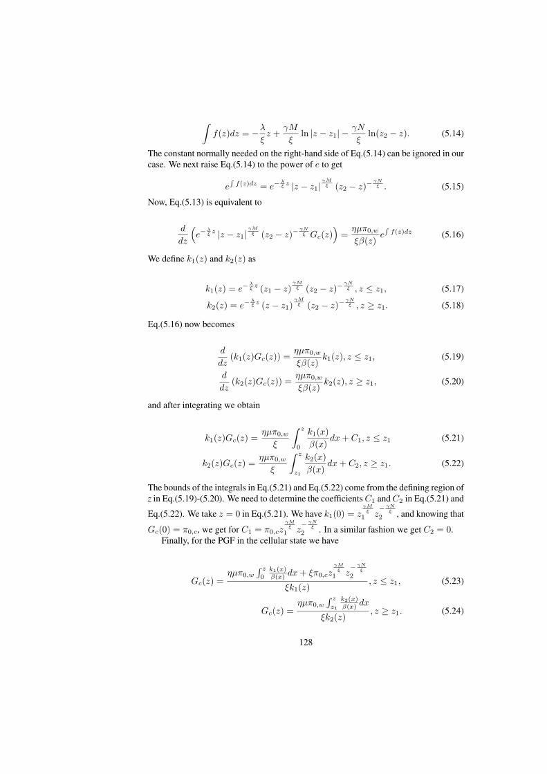
∫f(z)dz = −λ

ξz +

γM

ξln |z − z1| −

γN

ξln(z2 − z). (5.14)

The constant normally needed on the right-hand side of Eq.(5.14) can be ignored in ourcase. We next raise Eq.(5.14) to the power of e to get

e∫f(z)dz = e−

λξ z |z − z1|

γMξ (z2 − z)−

γNξ . (5.15)

Now, Eq.(5.13) is equivalent to

d

dz

(e−

λξ z |z − z1|

γMξ (z2 − z)−

γNξ Gc(z)

)=

ηµπ0,w

ξβ(z)e∫f(z)dz (5.16)

We define k1(z) and k2(z) as

k1(z) = e−λξ z (z1 − z)

γMξ (z2 − z)−

γNξ , z ≤ z1, (5.17)

k2(z) = e−λξ z (z − z1)

γMξ (z2 − z)−

γNξ , z ≥ z1. (5.18)

Eq.(5.16) now becomes

d

dz(k1(z)Gc(z)) =

ηµπ0,w

ξβ(z)k1(z), z ≤ z1, (5.19)

d

dz(k2(z)Gc(z)) =

ηµπ0,w

ξβ(z)k2(z), z ≥ z1, (5.20)

and after integrating we obtain

k1(z)Gc(z) =ηµπ0,w

ξ

∫ z

0

k1(x)

β(x)dx+ C1, z ≤ z1 (5.21)

k2(z)Gc(z) =ηµπ0,w

ξ

∫ z

z1

k2(x)

β(x)dx+ C2, z ≥ z1. (5.22)

The bounds of the integrals in Eq.(5.21) and Eq.(5.22) come from the defining region ofz in Eq.(5.19)-(5.20). We need to determine the coefficients C1 and C2 in Eq.(5.21) and

Eq.(5.22). We take z = 0 in Eq.(5.21). We have k1(0) = zγMξ

1 z− γN

ξ

2 , and knowing that

Gc(0) = π0,c, we get for C1 = π0,czγMξ

1 z− γN

ξ

2 . In a similar fashion we get C2 = 0.Finally, for the PGF in the cellular state we have

Gc(z) =ηµπ0,w

∫ z

0k1(x)β(x) dx+ ξπ0,cz

γMξ

1 z− γN

ξ

2

ξk1(z), z ≤ z1, (5.23)

Gc(z) =ηµπ0,w

∫ z

z1

k2(x)β(x) dx

ξk2(z), z ≥ z1. (5.24)

128

In the last equation, the ’zero probabilities’ π0,c and π0,w are unknown. We can find

them in the following way: We know that πc = ηη+γ = Gc(1) =

ηµπ0,w

∫ 1z1

k2(x)

β(x)dx

ξk2(1).

From this we have

ξk2(1)

η + γ= µπ0,w

∫ 1

z1

k2(x)

β(x)dx. (5.25)

Similarly, from the boundary conditions in Eq.(5.23) for z ≤ z1, we get

ηµπ0,w

∫ z1

0

k1(x)

β(x)dx+ ξπ0,cz

γMξ

1 z− γN

ξ

2 = 0. (5.26)

After solving the system of equations Eq.(5.25) and Eq.(5.26), for the ’zero probabili-ties’ we obtain

π0,w =ξk2(1)

(η + γ)µ

1∫ 1

z1

k2(x)β(x) dx

, and (5.27)

π0,c = −ηk2(1)

∫ z10

k1(x)β(x) dx

(η + γ)zγMξ

1 z− γN

ξ

2

∫ 1

z1

k2(x)β(x) dx

. (5.28)

The value of the integral∫ k1(x)

β(x) dx is always negative, hence π0,c is always positive.By using a vertical cut between any two-pairs of neighboring states in Fig. 5.2 and

writing balance equations we have

λπi,c + λπi,w = µπi+1,w + (i+ 1)ξπi+1,c. (5.29)

Summing over all i yields to

λ(πc + πw) = µ(πw − π0,w) + ξ∞∑i=0

(i+ 1)πi+1,c. (5.30)

The last equation, obviously reduces to

λ = µ(πw − π0,w) + ξE[Nc], (5.31)

where E[Nc] = G′

c(1), and E[Nw] = G′

w(1). Eq.(5.31) yields

E[Nc] =λ− µ(πw − π0,w)

ξ. (5.32)

So far, we have derived E[Nc] as the first derivative at z = 1 of Gc(z). In order to findthe average number of files in the system, we need E[Nw] as well. We can get it bydifferentiating Eq.(5.8):

129

G′

w(z) =β(z)

(γGc(z) + γzG

′

c(z) + µπ0,w

)β2(z)

− β′(z) (γzGc(z)− µ(1− z)π0,w)

β2(z), (5.33)

and setting z = 1. After some calculus we obtain

E[Nw] =(γE[Nc] + µπ0,c) η − γπc(µ− λ)

η2. (5.34)

Replacing Eq.(5.32) into Eq.(5.34) we get

E[Nw] =γ

η

λ− µ (πw − π0,w)

ξ+

µπ0,w

η− γπc(µ− λ)

η2. (5.35)

The average number of files in the system is

E[N ] = E[Nc] + E[Nw]. (5.36)

Finally, using the Little’s law E[N ] = λE[T ] [199], we obtain the average packetdelay in delayed offloading as in Eq.(5.1).

The above result gives the total expected delay that incoming flows experience inthe WiFi queue. For flows that do get transmitted over WiFi (i.e. whose deadline doesnot expire) this amounts to their total delay. Flows that end up reneging (deadlineexpires before transmission) must be transmitted through the cellular system and thusincur an additional delay ∆ (related to their transmission time over the cellular link,i.e. packet size

cellular rate , and possibly some queueing delay as well). The following Corollarygives the probability of reneging for each.

Corollary 5. The probability that an arbitrary flow arriving to the WiFi queue willrenege, i.e. its deadline will expire before it can be transmitted over a WiFi AP is

pr =λ− µ(πw − π0,w)

λ. (5.37)

In other words, the rate of flows sent back to the cellular network is given by λ · pr.This must be equal to ξ ·E[Nc], which is the average abandonment rate in Fig. 5.2, i.e.λpr = ξE[Nc]. Replacing E[Nc] from Eq.(5.32) gives us the above result. This alsogives us another important metric, the offloading efficiency of our system, namely thepercentage of flows that get offloaded over some WiFi network, as Eoff = 1− pr.

The above expressions can be used to predict the performance of a delayed offload-ing system, as a function of most parameters of interest, such as WiFi availability andperformance, user traffic load, etc. As we shall see later, it does so with remarkableaccuracy even in scenarios where many of the assumptions do not hold. However,Eq.(5.1) cannot easily be used to solve optimization problems related to the deadline

130

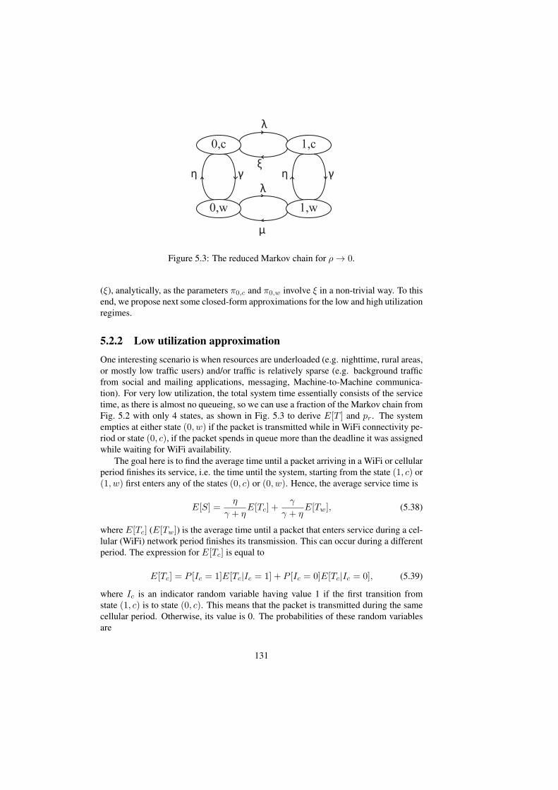
0,c 1,c

0,w 1,w

ξ

µ

λ

γ γ

λ

η η

Figure 5.3: The reduced Markov chain for ρ→ 0.

(ξ), analytically, as the parameters π0,c and π0,w involve ξ in a non-trivial way. To thisend, we propose next some closed-form approximations for the low and high utilizationregimes.

5.2.2 Low utilization approximationOne interesting scenario is when resources are underloaded (e.g. nighttime, rural areas,or mostly low traffic users) and/or traffic is relatively sparse (e.g. background trafficfrom social and mailing applications, messaging, Machine-to-Machine communica-tion). For very low utilization, the total system time essentially consists of the servicetime, as there is almost no queueing, so we can use a fraction of the Markov chain fromFig. 5.2 with only 4 states, as shown in Fig. 5.3 to derive E[T ] and pr. The systemempties at either state (0, w) if the packet is transmitted while in WiFi connectivity pe-riod or state (0, c), if the packet spends in queue more than the deadline it was assignedwhile waiting for WiFi availability.

The goal here is to find the average time until a packet arriving in a WiFi or cellularperiod finishes its service, i.e. the time until the system, starting from the state (1, c) or(1, w) first enters any of the states (0, c) or (0, w). Hence, the average service time is

E[S] =η

γ + ηE[Tc] +

γ

γ + ηE[Tw], (5.38)

where E[Tc] (E[Tw]) is the average time until a packet that enters service during a cel-lular (WiFi) network period finishes its transmission. This can occur during a differentperiod. The expression for E[Tc] is equal to

E[Tc] = P [Ic = 1]E[Tc|Ic = 1] + P [Ic = 0]E[Tc|Ic = 0], (5.39)

where Ic is an indicator random variable having value 1 if the first transition fromstate (1, c) is to state (0, c). This means that the packet is transmitted during the samecellular period. Otherwise, its value is 0. The probabilities of these random variablesare

131

P [Ic = 1] = ξξ+γ , and P [Ic = 0] = γ

ξ+γ , respectively. For the conditionalexpectations from Eq.(5.39), we have

E[Tc|Ic = 1] =1

ξ + γ, (5.40)

E[Tc|Ic = 0] =1

ξ + γ+ E[Tw]. (5.41)

Eq.(5.40) is actually the expected value of the minimum of two exponentially dis-tributed random varibles with rates ξ and γ. Replacing Eq.(5.40) and (5.41) intoEq.(5.39), we get

E[Tc]−γ

ξ + γE[Tw] =

1

ξ + γ. (5.42)

Following a similar procedure for E[Tw] we obtain

E[Tw]−η

µ+ ηE[Tc] =

1

µ+ η. (5.43)

After solving the system of equations Eq.(5.42)-(5.43), we have

E[Tw] =ξ + γ + η

ξµ+ ξη + µγ, (5.44)

E[Tc] =µ+ γ + η

ξµ+ ξη + µγ. (5.45)

Now, replacing Eq.(5.44)-(5.45) into Eq.(5.38), we have the average service time,and the low utilization approximation is (E[T ] ≈ E[S]):

E[T ] =(η + γ)2 + γξ + ηµ

(ξµ+ ξη + µγ)(γ + η). (5.46)

To find the probability of reneging, we need to know π0,c. We find it solving thelocal balance equations for Fig. 5.3. After solving the system we get

π0,c =η

η + γ

ξ(µ+ λ+ η) + µγ

ξ(µ+ λ+ η) + µγ + λ2 + λ(η + γ + µ). (5.47)

Replacing Eq.(5.47) and πc = ηη+γ into Eq.(5.37), we get the probability of reneging

for low utilization as

pr =θ1ξ

θ2ξ + θ3, (5.48)

where θ1 = η(λ+η+γ+µ)η+γ , θ2 = µ+ λ+ η, and θ3 = µγ + λ2 + λ(η + γ + µ).

Hence, we can write the results for the low utilization regime for both the averagedelay and probability of reneging as following:

Low utilization approximation: The expected system time in the WiFi queue andthe probability of reneging for sparse input traffic can be approximated by

132

E[T ] =(η + γ)2 + γξ + ηµ

(ξµ+ ξη + µγ)(γ + η), (5.49)

pr =θ1ξ

θ2ξ + θ3, (5.50)

where θ1 =η(λ+η+γ+µ)

η+γ, θ2 = µ+ λ+ η, and θ3 = µγ + λ2 + λ(η + γ + µ).

5.2.3 High utilization approximationAnother interesting regime is that of high utilization. As explained earlier, wirelessresources are often heavily loaded, especially in urban centers, due to the increasinguse of smart phones, tablets, and media-rich applications. Hence, it is of special interestto understand the average user performance in such scenarios. Here, we provide anapproximation that corresponds to the region of high utilization (ρ→ 1).

The expected system time in the WiFi queue for a user with heavy traffic can beapproximated by

E[T ] =1

λ

[(1 +

γ

η

)λ− µπw

η+

(λ− µ)πw

η

]. (5.51)

The approximation Eq.(5.51) comes from Eq.(5.1) by replacing π0,w = 0.To find the approximation for the probability of reneging in the high utilization

regime we proceed as follows. Since from Eq.(5.37) the only term that depends on ξis π0,w (we will need it later to solve optimization problems), we will not take it equalto 0. We will approximate it by a first order Taylor approximation at ξ = 1. For thatpurpose, we will denote π0,w as π0,w(ξ). So, we write

π0,w(ξ) = π0,w(1) + (ξ − 1)π′

0,w(1), (5.52)

where π0,w(1) =A(1)

(η+γ)µ∫ 1z1

A(x)β(x)

dx, and π

′

0,w(1) =A(1)

(η+γ)µ

ln (A(1)e)∫ 1z1

A(x)β(x)

dx−∫ 1z1

A(x) lnA(x)β(x)

dx(∫ 1z1

A(x)β(x)

dx)2 ,

where A(x) = (x−z1)γM

(z2−x)γN e−λx.Hence, the probability of reneging in the high utilization regime can be approxi-

mated by

pr =λ− µπw

λ+

µ

λπ0,w, (5.53)

where π0,w is given by Eq.(5.52).Now, we can write jointly the expressions for the average file delay and probability

of reneging in a delayed offloading system for high utilization.High utilization approximation: The expected system time in the WiFi queue and

the probability of reneging for a user with heavy traffic can be approximated by

E[T ] =1

λ

[(1 +

γ

η

)λ− µπw

η+

(λ− µ)πw

η

], (5.54)

pr =λ− µπw

λ+

µ

λπ0,w, (5.55)

where π0,w is the first order Taylor series approximation of Eq.(5.27).

133

0 0.5 1 1.50

50

100

150

200

250

300

350

Arrival rate

Transmission delay

Sims:Td1=60min

Theory:Td1=60min

Sims:Td2=120min

Theory:Td2=120min

Figure 5.4: Average delay for pedestrianuser scenario.

0 0.5 1 1.50

10

20

30

40

50

60

70

Arrival rate

Transmission delay

Sims:Td=30s

Theory:Td=30s

Sims:Td=60s

Theory:Td=60s

Figure 5.5: Average delay for vehicularuser scenario.

5.3 Performance evaluationIn this section we will validate our theory against simulations for a wide range oftraffic intensities, different values of file sizes, WiFi availability periods with differ-ent distributions, and different deadline times. We define the WiFi availability ratioas AR = E[TON ]

E[TON ]+E[TOFF ] = γη+γ . Unless otherwise stated the durations of WiFi

availability and unavailability periods will be drawn from independent exponential dis-tributions with rates η and γ, respectively. The deadlines are exponentially distributedwith rate ξ, although we will simulate scenarios with deterministic deadlines as well.We mainly focus on two scenarios, related to the user’s mobility. The first one consid-ers mostly pedestrian users with data taken from [195]. Measurements in [195] reportthat the average duration of WiFi availability period is 122 min, while the average du-ration with only cellular network coverage is 41 min (we use these values to tune η andγ), with AR=0.75. The second scenario corresponds to vehicular users, related to themeasurement study of [51]. An AR of 11 % has been reported in [51], although not allthe details are mentioned there. For more details about the measurements we refer theinterested reader to [195] and [51]. Finally, unless otherwise stated, file/flow sizes areexponentially distributed, and file arrival at the mobile user is a Poisson process withrate λ.

5.3.1 Validation of main delay resultWe first validate here our model and main delay result (Eq.(5.1)) against simulationsfor the two mobility scenarios mentioned (pedestrian and vehicular). The data rate forWiFi is assumed to be 1 Mbps. The mean packet size is assumed to be 7.5 MB for thepedestrian scenario and 125 kB for the vehicular scenario.

Fig. 5.4 shows the average file transmission delay (i.e. queueing + transmission)for the pedestrian scenario, for two different average deadline times of Td1 = 1 hour(ξ1 = 1/3600 s−1) and Td2 = 2 hours (ξ2 = 1/7200 s−1), respectively. The range ofarrival rates shown corresponds to a server utilization of 0-0.9. We can observe fromFig. 5.4 that there is a good match between theory and simulations. Furthermore, the

134

Table 5.2: Probability of reneging for pedestrian and vehicular scenarios.

Scenario Deadline λ = 0.1 λ = 0.5 λ = 1 λ = 1.5

Pedestrian(Theory) 1 hour 0.103 0.109 0.252 0.501Pedestrian(Simulation) 1 hour 0.1 0.117 0.239 0.508

Vehicular(Theory) 60 s 0.32 0.778 0.889 0.926Vehicular(Simulation) 60 s 0.32 0.776 0.891 0.925

0 0.2 0.4 0.6 0.8 1 1.2 1.4 1.60

10

20

30

40

50

60

70

80

90

100

110

Arrival rate

Transmission delay

Sims.BPTheory

Figure 5.6: The delay for BP ON-OFFperiods vs. theory.

0.02 0.04 0.06 0.08 0.10

0.5

1

1.5

2

2.5

3

Arrival rate

Transmission delay

ApproximationTheory

Figure 5.7: Low utilization delay ap-proximation for AR = 0.75.

average file transmission delay is increased by increasing the arrival rate, as expected,due to queueing effects. On the other hand, the average delay increases for higherdeadlines, since flows with lower deadlines leave the WiFi queue earlier, leading tosmaller queueing delays. Fig. 5.5 further illustrates the average file transmission delayfor the vehicular scenario with average deadline times Td1 = 30s (ξ1 = 1/30s−1) andTd2 = 60s (ξ2 = 1/60s−1). Despite the differences of the vehicular scenario, similarconclusions can be drawn. Finally, Table 5.2 depicts the respective probabilities ofreneging for the two scenarios. The percentage of flows that abandon the WiFi queueis higher in the vehicular scenario, since the availability ratio of the WiFi network isvery small (11%), and deadlines are rather small. These observations agree with [51].Nevertheless, our theory matches simulation values in all scenarios.

So far, we have assumed exponential distributions for ON and OFF periods, ac-cording to our model. While the actual distributions are subject to the user mobilitypattern, a topic of intense research recently, initial measurement studies ([195, 51])suggest these distributions to be ”heavy-tailed”. To this end, we consider a scenariowith ”heavy-tailed” ON/OFF distributions (Bounded Pareto). Due to space limitations,we focus on the vehicular scenario only. The shape parameters for the Bounded ParetoON and OFF periods are α = 0.59 and α = 0.64, respectively. The average deadlineis 100s. Fig. 5.6 compares the average file delay against our theoretical prediction.Interestingly, our theory still offers a reasonable prediction accuracy, despite the con-siderably higher variability of ON/OFF periods in this scenario. While we cannot claimthis to be a generic conclusion for any distribution and values, the results underline theutility of our model in practice.

135

0.02 0.04 0.06 0.08 0.10

0.1

0.2

0.3

0.4

0.5

0.6

0.7

0.8

0.9

1

Arrival rate

Probability of reneging

ApproximationTheory

Figure 5.8: Low utilization pr approx-imation for AR = 0.75

1 1.2 1.4 1.6 1.8 20

0.5

1

1.5

2

2.5

3

3.5

4

Arrival rate

Transmission delay

ApproximationTheory

Figure 5.9: High utilization delay ap-proximation for AR = 0.5.

5.3.2 Validation of approximationsWe next validate the approximations we have proposed in Section 5.2. We start withthe low utilization approximation of Section 5.2.2 with AR = 0.75 (similar accuracylevels have been obtained with other values) and with a deadline of 2min. Fig. 5.7shows the packet delay for low arrival rates in the range 0.01−0.11, which correspondto a maximum utilization of up to 0.2. As λ increases, the difference between theapproximated result and the actual value increases, since we have considered only theservice time for this approximation. The same conclusion holds for the probability ofreneging (Fig. 5.8).

Next, we consider the high utilization regime and respective approximation (Eq.(5.54)).We consider ρ around 0.8. Fig. 5.9 shows the delay for high values of λ (AR = 0.5).We can see that our approximation is very close to the actual delay and should becomeexact as ρ gets larger.

5.3.3 Variable WiFi rates and non-exponential parametersWhile in our model we consider a fixed transmission rate for all WiFi hotspots, this isnot realistic in practice. For this reason, we have also simulated scenarios where theWiFi rate varies uniformly in the range 0.4-1.6 Mbps. Fig. 5.10 shows the delay forthe vehicular scenario with a deadline of 10 minutes. Even in this case, our theory cangive solid predictions for the incurred delay.

In all of the above scenarios, we have assumed variable deadlines for each file(drawn from an exponential distribution). In some cases, the user might choose thesame deadline for many (or most) flows that can be delayed, which would be a measureof her patience. To this end, we simulate a scenario where the deadline is fixed for anarrival rate of 0.1. The other parameters are the same as for the vehicular scenario.In Fig. 5.12 we compare simulation results for this scenario against our theory (whichassumes exponentially distributed deadlines with the same average). It is evident thateven in this case, there is a reasonable match with our theory.

To conclude our validation, we finally drop the exponential packet assumption aswell, and test our theoretical result vs. generic file size results. Fig. 5.11 compares

136

0 0.2 0.4 0.6 0.8 1 1.2 1.4 1.60

100

200

300

400

500

600

Arrival rate

Transmission delay

VariableTheory

Figure 5.10: Variable WiFi rates withthe same average as theory.

0 0.2 0.4 0.6 0.8 1 1.2 1.4 1.66.5

7

7.5

8

8.5

9

9.5

10

10.5

11

Arrival rate

Transmission delay

SimulationsTheory

Figure 5.11: Deterministic packets

0.05 0.1 0.15 0.20

1

2

3

4

5

6

7

8

9

10

Reneging rate

Transmission delay

Det. deadlineTheory

Figure 5.12: The delay for determinis-tic deadlines vs. theory.

0.2 0.4 0.6 0.8 1 1.2 1.40

5

10

15

20

25

30

Arrival rate

Transmission delay

BP file sizeTheory

Figure 5.13: The delay for BP packetsizes vs. theory.

analytical and simulation results for deterministic, and Fig. 5.13 does it for BoundedPareto files sizes (shape parameter α = 1.2 and cv = 3). In both scenarios, the deadlineis Td = 20s. Mean file size is in both cases 125KB, AR is 0.5, and the rest of theparameters correspond to the vehicular scenario. Our theoretical prediction remainsreasonably close, despite higher size variability.

5.3.4 Delayed offloading gainsWe have so far established that our analytical model offers considerable accuracy forscenarios commonly encountered in practice. In this last part, we will thus use ourmodel to acquire some initial insight as to the actual offloading gains expected in differ-ent scenarios. The operator’s main gain is some relief from heavy traffic loads leadingto congestion. The gains for the users are the lower prices usually offered for traffic mi-grated to WiFi, as well as the potential higher data rates of WiFi connectivity. There arealso reported energy benefits associated [196], but we do not consider them here. In thislast part, we will investigate the actual gains from data offloading, in terms of offload-ing efficiency. Higher offloading efficiency means better performance for both clientand operator. We compare the offloading efficiencies for on-the-spot offloading [49] vs.

137

delayed offloading for different deadline times (Td1 = 2min, Td2 = 1min). Fig. 5.14illustrates the offloading efficiency vs. availability ratio for a moderate arrival rate ofλ = 0.2. For comparison purposes we also depict the line x = y (offloading efficiency= availability ratio). First, as expected, we can observe that offloading efficiency in-creases with AR. However, this increase is not linear. More interestingly, the actualoffloading efficiencies are always higher than the respective availability ratio. As ex-pected, the delayed offloading provides higher offloading efficiencies compared to on-the-spot offloading, with higher deadlines leading to higher offloading efficiencies. Forthe same AR doubling the deadline time, the offloading efficiency is increased by about10%. Also, although not shown here, the respective offloading efficiency increaseseven further as traffic loads decreases. Summarizing, these findings are particularly in-teresting to operators (and users), as they imply that high offloading efficiencies can beachieved for loaded regions, without necessarily providing almost full coverage withWiFi APs.

0.2 0.3 0.4 0.5 0.6 0.7 0.8 0.9 1

0.4

0.5

0.6

0.7

0.8

0.9

1

Availability ratio

Off

loa

din

g e

ffic

ien

cy

On−the−spotDeadline=1minDeadline=2min

Figure 5.14: Offloading gains for delayed vs. on-the-spot offloading.

5.4 Optimizing Delayed Offloading

The results considered so far allow us to predict the expected system delay when thedeadlines are defined externally (e.g. by the user or the application). However, the user(or the device on her behalf) could choose the deadline in order to solve an optimiza-tion problem among additional (often conflicting) goals, such as the monetary cost foraccessing the Internet and the energy consumption of the device. For example, the usermight want to minimize the delay subject to a maximum (energy or monetary) cost, orto minimize the cost subject to a maximum delay the user can tolerate.

To formulate and solve such optimization problems, we need analytical formulasfor the average delay and the incurred cost. We already have such formulas for the delayof files sent over WiFi, where we will use the two approximations of Sections 5.2.2and 5.2.3. Furthermore, we can assume that files transmitted over the cellular network

138

incur a fixed delay ∆, capturing both the service and queueing delays over the cellularinterface4. To proceed, we need to also assume simple models for energy and cost,in order to get some initial intuition about the tradeoffs involved. We are aware thatreality is more complex (for both energy and cost) and may differ based on technology(3G, LTE), provider, etc. We plan to extend our models in future work.

Assume a user has to download or upload a total amount of data equal to L. Onaverage pr · L data units will be transmitted through the cellular interface. Assumefurther that Dc and Dw denote the costs per transmitted data unit for a cellular andWiFi network, where Dw < Dc (often Dw = 0). Finally, let cc and cw denote thetransmission rates, and Ec and Ew energy spent per time unit during transmission overthe cellular and WiFi network, respectively. It is normally the case that cc < cw as wellas Ec ≈ Ew [205]. It follows then that the total monetary and energy costs, D, and E,could be approximated by

D = (Dc −Dw)pr +Dw and E =

(Ec

cc− Ew

cw

)pr +

Ew

cw. (5.56)

5.4.1 Optimization problems

Optimization problem 1: Eq.(5.56) suggests that both the average power consump-tion and cost depend linearly on the probability of reneging, pr, which we have alsoderived in Section 5.2, and which is a function of the system deadline 1

ξ . The systemdelay is also a function of ξ. We can thus formulate optimization problems of the fol-lowing form, for both the high and low utilization regimes, where ξ is the optimizationparameter

minξ

E[T ] + pr∆

s. t. pr ≤ Pmaxr ,

(5.57)

where E[T ] is given by Eq.(5.49), and pr by Eq.(5.50), for low utilization, and Eq.(5.54)and Eq.(5.55), for high utilization, respectively. Due to the linearity of Eq.(5.56), wecan express the constraint directly for pr, where Pmax

r depends on whether we con-sider monetary cost, energy or a weighted sum of both, and the respective parameters.Finally, we can also exchange the optimization function with the constrain, to minimizethe cost, subject to a maximum delay. This provides us with a large range of interestingoptimization problems we can solve.

If we express the inequality constraint in Eq.(5.57) through ξ, we have the equiv-alent constraint ξ ≤ θ3P

maxr

θ1−θ2Pmaxr

. The probability of reneging from Eq.(5.50) is an

increasing function of ξ, since p′

r(ξ) > 0. This implies that maximum pr correspondsto maximum ξ. We denote by f(ξ) the total average delay of Eq.(5.57) (delay functionfrom now on). Hence we have

4We could also try to model the cellular queue as an M/M/1 or G/M/1 system, but we are more interestedin the dynamics of the WiFi queue, since this is where the reneging decisions take place. To keep thingssimple, we defer this to future work.

139

f(ξ) =A1ξ +A2

B1ξ +B2+

θ1ξ

θ2ξ + θ3∆, (5.58)

where A1 = γ,A2 = (η + γ)2 + ηµ,B1 = (µ+ η)(γ + η), B2 = µγ(γ + η). In orderto solve the optimization problem given by Eq.(5.57), we need to know the behaviorof the delay function. For that purpose, we analyze the monotonicity and convexity ofEq.(5.58). To do that we need the first and second derivatives, which are

f′(ξ) =

A1B2 −A2B1

(B1ξ +B2)2+

θ1θ3∆

(θ2ξ + θ3)2, and

f′′(ξ) =

2(A2B1 −A1B2)

(B1ξ +B2)3− θ1θ2θ3∆

(θ2ξ + θ3)3.

It is worth noting that A1B2 < A2B1. This prevents delay function being alwaysconcave. The delay function is decreasing in the interval for which f

′(ξ) ≤ 0. This

happens when

ξ ≤ ξ0 =θ3

√A2B1−A1B2

θ1θ3∆−B2

B1 − θ2

√A2B1−A1B2

θ1θ3∆

.

Hence, the delay function is decreasing in the interval (0, ξ0), and increasing in therest, with ξ0 being a minimum. Further, the solution of f

′′(ξ) > 0 gives the interval

where the function is convex. This happens when

ξ ≤ ξ1 =θ3 3

√2A2B1−A1B2

θ1θ2θ3∆−B2

B1 − θ2 3

√2A2B1−A1B2

θ1θ2θ3∆

. (5.59)

It can be easily proven that ξ0 < ξ1.Such constrained-optimization problems are often solved with the Lagrangian method

and KKT conditions. However, the optimal solution for our problem can be found moreeasily. The delay function looks like in Fig. 5.15. The optimal deadline depends onthe maximum cost, that is proportional to the probability of reneging. So, we can de-termine the optimal deadline based on the value of Pmax

r . If this value of Pmaxr is

quite high, the corresponding reneging rate ξq1 (dashed line in Fig. 5.15) will be higherthan the global minimum ξ0. Consequently, the global minimum of Eq.(5.59) is alsothe optimal reneging rate. On the other hand, if the maximum cost is quite low (lowPmaxr ), the maximum reneging rate ξq,2 (dotted line in Fig. 5.15) is lower than the

global minimum. This implies that the minimum delay will be achieved for the max-imum reneging rate of ξq,2 =

θ3Pmaxr

θ1−θ2Pmaxr

. In other words, the average deadline timethat minimizes the delay for a given maximum cost is

Td,opt =1

ξopt=

1

min(ξ0,

θ3Pmaxr

θ1−θ2Pmaxr

) . (5.60)

140

Similar steps can be followed to solve the same optimization problem for highutilization, as well as other problems. These sometimes involve a quadratic constraintfunction.

Optimization problem 2: After minimizing the transmission delay subject to amaximum reneging rate (cost, energy), our next goal now is to minimize the renegingprobability subject to a maximum transmission delay, which can be for example due toQoS requirements. Hence, the optimization problem in this case would be

minξ

pr =θ1ξ

θ2ξ + θ3

s. t. E[T ] + pr∆ ≤ Tmax.

(5.61)

Just as in Optimization problem 1, we study the monotonicity and convexity of thedelay function, with the only difference that now it is the constrain function. For theprobability of reneging, we already now that it is an increasing function. Followinga similar procedure as in the previous problem, we get for the optimum value of thedeadline (from a quadratic constraint)

Td,opt =1

max

(0,

K2−√

K22−4K1K3

2K1

) , (5.62)

where K1 = A1θ2 + θ1∆B1 − TmaxB1θ2, K2 = TmaxB1θ3 + TmaxB2θ2 −A1θ3 −A2θ2 − θ1∆B2, K3 = A2θ3 − TmaxB2θ3, C1 = 1

λ

(1 + γ

η

)(λ− µπw).

In [54] we have also considered the respective optimization problems for high uti-lization regime, where the expressions for E[T ] and pr are given by Eq.(5.54) andEq.(5.55), respectively. The interested reader can find the details there.

5.4.2 Optimization evaluationWe will now validate the solutions of the previous optimization problem for two dif-ferent cases. In both of them the arrival rate is 0.1, and the maximum cost per dataunit one can afford is 2.8 monetary units. The transmission of a data unit through WiFicosts 1, and through cellular 5 units. The choice of these values is simply for bettervisualizing the results; different values yield similar conclusions. Fig. 5.16 shows thedelay vs. cost curve for cellular rate being 2× lower than WiFi rate. First thing thatwe can observe is that the minimum delay is achieved for the highest possible cost(2.8). The optimal average deadline is Td = 1s. This is in agreement with the optimalvalue predicted from Eq.(5.60), and shown with an asterisk in Fig. 5.16. We replaceEq.(5.50) into Eq.(5.56) to get the relationship between the cost and the renege rate.We have shown in Eq.(5.56) that the cost is directly proportional to pr, and the laterone is an increasing function of ξ. This implies that the maximum cost is in fact themaximum ξ (minimum deadline). This practically means that in Eq.(5.57), ∆ is smalland that the delay in the WiFi queue represents the largest component of the delay. Asa consequence of that, it is better to redirect the files through the cellular interface assoon as possible. Hence, in these cases (when cellular rate is comparable to the WiFi),

141

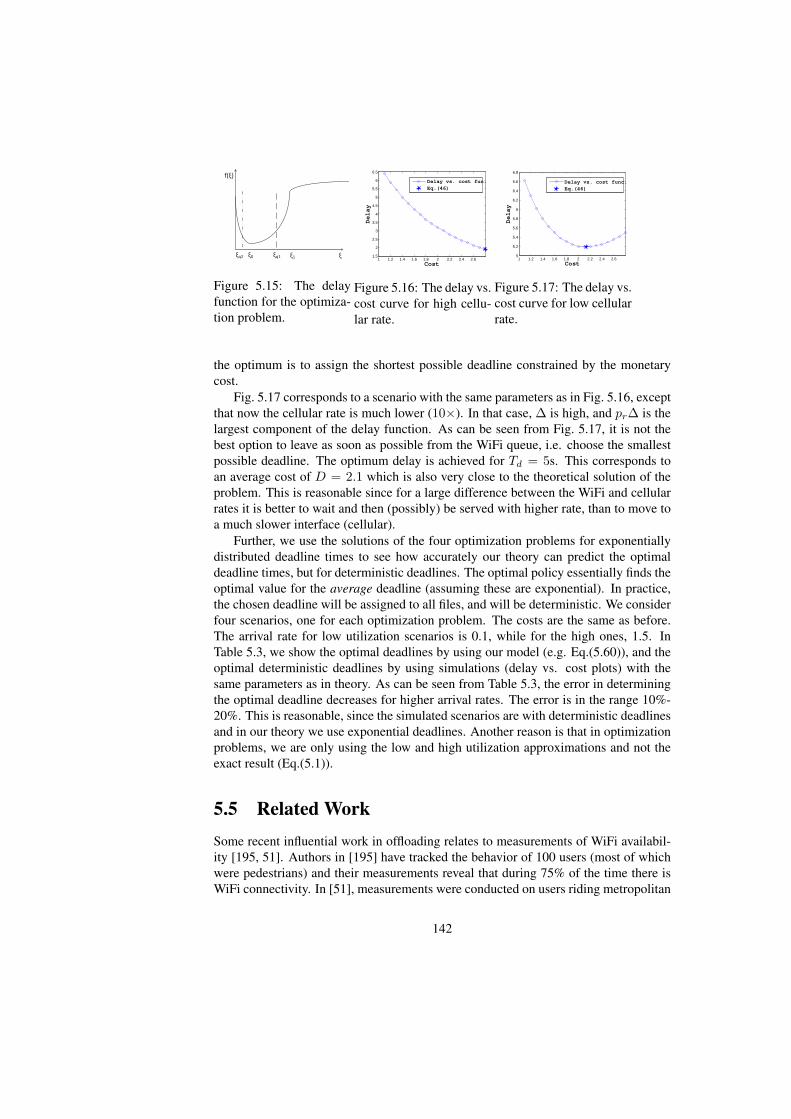
ξ

f(ξ)

ξ0 ξ1ξq1ξq2

Figure 5.15: The delayfunction for the optimiza-tion problem.

1 1.2 1.4 1.6 1.8 2 2.2 2.4 2.61.5

2

2.5

3

3.5

4

4.5

5

5.5

6

6.5

Cost

Delay

Delay vs. cost fun.Eq.(46)

Figure 5.16: The delay vs.cost curve for high cellu-lar rate.

1 1.2 1.4 1.6 1.8 2 2.2 2.4 2.65

5.2

5.4

5.6

5.8

6

6.2

6.4

6.6

6.8

Cost

Delay

Delay vs. cost func.Eq.(46)

Figure 5.17: The delay vs.cost curve for low cellularrate.

the optimum is to assign the shortest possible deadline constrained by the monetarycost.

Fig. 5.17 corresponds to a scenario with the same parameters as in Fig. 5.16, exceptthat now the cellular rate is much lower (10×). In that case, ∆ is high, and pr∆ is thelargest component of the delay function. As can be seen from Fig. 5.17, it is not thebest option to leave as soon as possible from the WiFi queue, i.e. choose the smallestpossible deadline. The optimum delay is achieved for Td = 5s. This corresponds toan average cost of D = 2.1 which is also very close to the theoretical solution of theproblem. This is reasonable since for a large difference between the WiFi and cellularrates it is better to wait and then (possibly) be served with higher rate, than to move toa much slower interface (cellular).

Further, we use the solutions of the four optimization problems for exponentiallydistributed deadline times to see how accurately our theory can predict the optimaldeadline times, but for deterministic deadlines. The optimal policy essentially finds theoptimal value for the average deadline (assuming these are exponential). In practice,the chosen deadline will be assigned to all files, and will be deterministic. We considerfour scenarios, one for each optimization problem. The costs are the same as before.The arrival rate for low utilization scenarios is 0.1, while for the high ones, 1.5. InTable 5.3, we show the optimal deadlines by using our model (e.g. Eq.(5.60)), and theoptimal deterministic deadlines by using simulations (delay vs. cost plots) with thesame parameters as in theory. As can be seen from Table 5.3, the error in determiningthe optimal deadline decreases for higher arrival rates. The error is in the range 10%-20%. This is reasonable, since the simulated scenarios are with deterministic deadlinesand in our theory we use exponential deadlines. Another reason is that in optimizationproblems, we are only using the low and high utilization approximations and not theexact result (Eq.(5.1)).

5.5 Related WorkSome recent influential work in offloading relates to measurements of WiFi availabil-ity [195, 51]. Authors in [195] have tracked the behavior of 100 users (most of whichwere pedestrians) and their measurements reveal that during 75% of the time there isWiFi connectivity. In [51], measurements were conducted on users riding metropolitan

142

Table 5.3: Optimal deterministic deadline times vs theory.

Sc. Constraint Td (theory) Td (deterministic) Relative error1 D ≤ 2.8 2.71 2.2 18%2 Tmax = 6.6 1.56 1.22 22%3 D ≤ 3.8 1.73 1.55 11%4 Tmax = 15 7.97 6.82 15%

area buses. In contrast to the previous study, the WiFi availability reported there isonly around 10%. The mean duration of WiFi availability and non-availability periodsis also different in the two studies, due to the difference in speeds between vehicularand pedestrian users. The most important difference between the two studies relates tothe reported offloading efficiency, with [51] reporting values in the range from 20%-33% for different deadlines, and [195] reporting that offloading does not exceed 3%.We believe this is due to the different deadlines assumed together with the differentavailabilities.

The authors in [206] define a utility function related to delayed offloading to quan-titatively describe the trade-offs between the user satisfaction in terms of the price thatshe has to pay and the experienced delay by waiting for WiFi connectivity. However,their analysis does not consider queueing effects. Such queueing effects may affect theperformance significantly, especially in loaded systems (which are of most interest) orwith long periods without WiFi. The work in [207] considers the traffic flow charac-teristics when deciding when to offload some data to the WiFi. However, there is nodelay-related performance analysis. Modeling the cost factors is the focus of [208],which also shows where the offloading APs should be installed. A WiFi offloadingsystem that takes into account a user’s throughput-delay tradeoffs and cellular budgetconstraints is proposed in [209]. However, only heuristic algorithms are proposed, andqueueing effects are ignored. Finally, in [210], an integrated architecture has been pro-posed based on opportunistic networking to switch the data traffic from the cellular toWiFi networks. Summarizing, in contrast to our work, these papers either perform noanalysis or use simple models that ignore key system effects such as queueing.

To our best knowledge, the closest work in spirit to ours is [52]. The results in[52] are the extension of the results in [195] containing the analysis for delayed of-floading. Authors there also use 2D Markov chains to model the state of the system.However, they use matrix-analytic methods to obtain a numerical solution for the of-floading efficiency. Such numerical solutions unfortunately do not provide insights onthe dependencies between different key parameters, and cannot be used to formulateand analytically solve optimization problems that include multiple metrics.

As a final note, in [49], we have proposed a queueing analytic model for on-the-spotmobile data offloading, and a closed form solution was derived for the average delay.While the model we propose here shares some similarities (ON/OFF availabilities, 2DMarkov chain approach) with the basic model in [49], it is in fact considerably moredifficult to solve.

143

5.6 ConclusionSummarizing, in this chapter we have proposed a queueing analytic model for the per-formance of delayed mobile data offloading, and have validated it against realistic WiFinetwork availability statistics. We have also considered a number of scenarios whereone or more of our model’s assumptions do not hold, and have observed acceptableaccuracy, in terms of predicting the system delay as a function of the user’s patience.Finally, we have also shown how to manipulate the maximum deadlines, in order tosolve various optimization problems involving the system delay, monetary costs, andenergy costs.

144

Chapter 6

User Association in HetNets

145

6.1 Introduction

In the previous chapter, we considered offloading through out-of-band communication,namely WiFi access points. Here we will generalize to a scenario consisting of varioustypes of base stations, with heterogeneous powers and coverage ranges, such as macro-cells, micro-cells, pico-cells, femto-cells, etc. These networks are offered referredto as HetNets (or sometimes Ultra-Dense Networks, UDN depending on the densityand topology of base stations. Note that WiFi can also be seen as a type of smallcell. However, we will here assume that all these cells are under the control of asingle operator, whose goal is to optimally utilize all its available BSs, balancing theirloads, while also ensuring good user QoS.1 Finally, we also remove in this chapter theassumption of delay-tolerance (Note that a user is still sensitive to delay, but the orderof delays experienced here is assumed smaller, and the source of delays is queueingand transmission delay, rather than the explicit and larger delays to encountered a WiFiAP, considered in the previous chapter).

In a HetNet, a large number of small cells (SC) are deployed along with macrocellsto improve spatial reuse [55, 56, 57]. The higher the deployment density, the better thechance that a user equipment (UE) can be associated with a nearby base station (BS)with high signal strength, and the more the options to balance the load. At the sametime, denser deployments experience high spatio-temporal load variations, and requiresophisticated user association algorithms. There are two key, often conflicting concernswhen assigning UEs to a BS: (i) maximizing the spectral efficiency, and (ii) ensuringthat the load across BSs is balanced to ensure efficient utilization of BSs, and preemptcongestion events (i.e., no BS is underutilized while neighboring ones are operatingclose or above their capacity). The former is usually achieved by associating the UE tothe BS with maximum SINR: this association rule was the norm up to LTE (Long-TermEvolution)-release 8. While this rule also maximizes the instantaneous rate of a user(i.e., the modulation and coding scheme - MCS - supported), it reflects user QoS onlywhen the BS is lightly loaded. However, user performance, in terms of per flow delay,may be severely affected if the BS offering the best SINR is congested [211, 212].

As a result, a number of research works have studied the problem of user as-sociation in heterogeneous networks, optimizing user rates [60, 61], balancing BSloads [62], or pursuing a weighted tradeoff of them [63]. For instance, a distributeduser-association algorithm is proposed in [213], where the global outage probabil-ity and the long term rate maximization are studied. The authors in [214] proposea framework that studies the interplay of user association and resource allocation in fu-ture HetNets, by formulating a non-convex optimization problem and deriving perfor-mance upper bounds. Range-expansion techniques, where the SINR of lightly loadedBSs is biased to make them more attractive to the users are also popular [56, 57]. Fi-nally, a framework that has received much attention is [63]. This framework jointlyconsiders a family of objective functions, each of which directs the optimal solutiontowards different goals (e.g. throughput optimal, delay-optimal, load balancing, etc.),using an iterative algorithm. [64, 215, 216] extend this framework to further include

1Note that energy-efficiency might be another concern of such an operator, sometimes having the oppositeintention to “unbalance” loads, so as to turn off underloaded BSs. We have considered such a scenario in [68].

146

energy management, e.g., by switching off under-loaded BSs.Nevertheless, the majority of these works are relatively simplified, not taking into

account key features of future networks. Firstly, most existing studies only considerhomogeneous traffic profiles. For example, [63, 64] assume that all flows generated bya UE are “best-effort” (i.e. elastic). However, modern and future networks will have todeal with high traffic differentiation, with certain flows being able to require specific,dedicated2 (i.e., non-elastic) resources [67]. Such dedicated flows do not share BSresources like best-effort ones, are subject to admission control, and sensitive to differ-ent performance metrics [68]. Secondly, the majority of related studies only considerdownlink (DL) traffic. Uplink (UL) traffic is becoming important, due to symmetric(e.g. social networking) applications, Machine-Type Communication (MTC), etc. Yet,due to the asymmetric transmit powers of UEs and BSs, leading to different physicaldata rates, the BS which is optimal for DL traffic might lead to severely degraded per-formance for UL traffic. Summarizing, a proper user-association scheme should con-sider all the above dimensions, and attempt to strike an appropriate tradeoff betweenthem.

On top of that, most related works focus on the radio access part (e.g., consideringthe user rate on the radio interface or BS load), ignoring the backhaul (BH) network.While this might be reasonable for legacy cellular networks, given that the macro-cell backhaul is often over-provisioned (e.g., fiber), this might be quite suboptimalfor future cellular networks. The considerably higher number of small cells, and re-lated Capital Expenditure (CAPEX) and Operational Expenditure (OPEX) suggest thatbackhaul links will mostly be inexpensive wired or wireless links (in licensed or unli-censed bands), and often underprovisioned [69]. Multiple BS might also have to sharethe capacity of a single backhaul link due to, e.g, point-to-multipoint (PMP) or multi-hop mesh topologies to the aggregation node(s) [70]. Finally, various BS-coordinatedschemes have been proposed in the literature as a promising way to better use theavailable spectrum and further improve system performance, e.g., enhanced Inter-CellInterference Coordination (eICIC) [217, 218] and Coordinated Multi-Point (CoMP)transmission [219] scenarios. Such schemes are expected to further stress the backhaulnetwork capacities. Hence, as the radio access technologies are constantly improving,it is argued that the backhaul network will emerge as a major performance bottleneck,and user association algorithms that ignore the backhaul load and topology can lead topoor performance [220].

As a result of this increasing focus on the backhaul, some recent works have ap-peared that attempt to jointly consider radio access and backhaul. These are mostlyconcerned with joint scheduling issues (for in-band or PMP backhaul links) [220, 221],signaling overhead and performance tradeoffs for cooperative multi-point communica-tion [222], and Software-Defined-Networking (SDN)-based implementation flexibil-ity [223].

The user rate maximization problem is studied in [224] under backhaul capacityconstraints, and in [225] jointly with backhaul resource allocation and flow control.Also, a distributed user association scheme was developed for maximizing the network-

2In terms of LTE systems, dedicated flows are differentiated by their QoS class (QCI) ranging from 1 to4, whereas best-effort from 5 to 9 [67].

147

wide spectrum efficiency in [226] using combinatorial optimization. Some backhaulaware association heuristics include: [227] where the sum of user rates is attempted tobe optimized in an energy-efficient manner, [228] where the ergodic capacity is maxi-mized under an iterative algorithm, and [229] where resource allocation is investigatedin conjunction with carrier aggregation. Other works in this context include investiga-tion of caching capabilities to overcome the backhaul capacity limitations and enhanceQoS [230, 81]. Finally, Chen et al. attempt to derive the total expected delay by con-sidering retransmission over the wireless backhaul links [231].

Nevertheless, to our best knowledge, none of these works formally addresses theproblem of optimal user association in traffic-differentiated and backhaul-limited Het-Nets. To this end, in this chapter we revisit the user association problem, jointly con-sidering the radio access and backhaul networks. Specifically, our main contributionscan be summarized as follows:

1. We use the popular framework of α-optimal user association [63] as our startingpoint, and introduce (i) traffic differentiation, (ii) UL traffic, and (iii) backhaultopology and capacity constraints.

2. We then analytically prove optimal association rules, depending on whether ULand DL traffic of the same UE can be “split” to different BSs or not [74]. We alsoshow how this optimal regime can be attained using an iterative and distributedalgorithm that does not require global network knowledge.

3. We use this framework to investigate the various tradeoffs arising in this com-plex association problem, and provide some initial insights and guidelines aboutthe impact of traffic differentiation and backhaul limitations in optimal user-association policies for future HetNets.

6.2 System Model and AssumptionsIn the following, we describe our traffic arrival model (Section 6.2.1), then discussour assumptions related to the access network (Section 6.2.2) and backhaul network(Section 6.2.3).

We use a similar problem setup as the one used in a number of related works [63,64, 232, 215], and extend it accordingly. To keep notation consistent, for all variablesconsidered, a first superscript “D” and “U” refers to downlink (DL) and uplink (UL)traffic, respectively. A second superscript “b” or “d” refers to best-effort and dedicatedtraffic, respectively. For brevity, in the following we present most notation and assump-tions in terms of downlink traffic only, assuming that the uplink case and notation issymmetric. Specific differences will be elaborated, where necessary. In Table 6.1, wesummarize some useful notation we use throughout the paper.

6.2.1 Traffic Model(A.1 - Traffic arrival rates) Traffic at location x ∈ L consists of file (or more gener-ally flow) requests arriving according to an inhomogeneous Poisson point process with

148

Table 6.1: Notation

Variable Best-Effort Flows Dedicated FlowsDownlink Uplink Downlink Uplink

Flow type superscript D,b U,b D,d U,dFlow type probability zD · zb zU · zb zD · zd zU · zd

Devoted amount of bandwidth for BS i wDi · ζD wU

i · ζU wDi · (1− ζD) wU

i · (1− ζU )

Traffic arrival rate at location x λD,b(x) λU,b(x) λD,d(x) λU,d(x)

Maximum rate | servers at location x for BS i cD,bi (x) cU,b

i (x) kDi (x) kUi (x)

Load density at location x for BS i ρD,b(x) ρU,b(x) ρD,d(x) ρU,d(x)

Alpha-fair parameter ∈ [0,∞) αD,b αU,b αD,d αU,d

Utilization (load) of BS i ρD,b ρU,b ρD,d ρU,d

Probability to route a flow from x to BS i pD,b(x) pU,b(x) pD,d(x) pU,d(x)

Mean flow size (bits) | flow duration (sec) at x 1µD,b(x)

1µU,b(x)

BD(x),1

µD,d(x)

BU (x),1

µU,d(x)

Capacity of BH link j CDh (j) CU

h (j) - -Congestion indicator at BH link j ID(j) IU (j) - -

arrival rate per unit area λ(x)3. This inhomogeneity facilitates the creation of “hotspot”areas. Each new arriving request is for a downlink (DL) flow, with probability zD, oruplink (UL) flow with probability zU = 1 − zD. Each DL (or UL) flow can furtherbe a best-effort flow (e.g., file download) with probability zb, or dedicated flow (e.g., aVoIP call), with probability zd = 1 − zb. zD and zb are input parameters that dependon the traffic mix.

Using a Poisson splitting argument [233], it follows that the above gives rise to 4independent, Poisson flow arrival processes with respective rates

λD,b(x) = zD · zb · λ(x), λD,d(x) = zD · zd · λ(x) (6.1)λU,b(x) = zU · zb · λ(x), λU,d(x) = zU · zd · λ(x), (6.2)

(λD,b(x) for downlink best-effort flows, λU,b(x) for uplink best-effort flows, etc.).(A.2 - Best effort flow characteristics) Each best-effort flow is associated with a

flow-size (in bits) drawn from a generic distribution with mean 1/µD,b(x). This canmodel heterogeneous flow characteristics across locations.

(A.3 - Dedicated flow characteristics) Each dedicated flow has a required data-rate (in bits per second) that is drawn from a generic distribution with mean BD(x).This rate must be guaranteed by the network throughout the flow’s duration. Thisduration (in seconds) is another, independent random variable with mean 1/µD,d(x).

6.2.2 Access Network(B.1 - Access network topology) We assume an area L ⊂ R2 served by a set ofbase stations B, that are either macro BSs (eNBs) or small cells (SCs). These togetherconstitute the access network.

(B.2 - DL resources) Each BS i ∈ B is associated with a transmit power Pi anda total downlink bandwidth wD

i . Out of the total bandwidth, ζDi · wDi is allocated to

3Without loss of generality, we do not distinguish between users at location x, as we assume that allusers/flows related to location x are treated similarly.

149

Figure 6.1: Access network queuing systems for different flows.

best-effort traffic and (1 − ζDi ) · wDi for dedicated traffic (0 ≤ ζDi ≤ 1). Throughout

this paper, we will assume that this allocation is static, at least for a given time windowof interest (based on long term traffic characteristics and operator policy).

Remark: Dynamically updating the ζDi parameters could further improve perfor-mance. This could, for example, be achieved through dynamic/flexible TDD, wherethe amount of downlink and uplink resources are jointly optimized with the associationparameters. We have recently extended our framework in this direction. We refer theinterested reader to [78].

(B.3 - DL physical data rate) BS i can deliver a maximum physical data transmis-sion rate of cD,b

i (x) to a user at location x, in absence of any other best-effort flowsserved, which is given by the Shannon capacity4

cD,bi (x) = ζDi · wD

i · log2(1 + SINRi(x)), (6.3)

where SINRi(x) = Gi(x)Pi∑j =i Gj(x)Pj+N0

.5 N0 is the noise power, and Gi(x) representsthe path loss and shadowing effects between the i-th BS and the UE located at x (as wellas antenna and coding gains, etc.)6. We assume that effects of fast fading are filteredout. Our model assumes that the total intercell interference at location x is static, and

4We use Shannon capacity for clarity of presentation. However, our approach could be easily adapted toinclude modulation and coding schemes (MCS). Furthermore, capacity improving technologies, e.g., the useof MIMO, and modifications to this capacity formula are othogonal to our framework.

5We have assumed that the interference caused to a BS, does not depend on the load of the (neighbor-ing) BSs that interfere with it. This is standard practice to avoid the “coupled queues” problem which isusually not tractable, e.g. see [211],[63]. For a study of random HetNet deployments with such load-basedinterference, we refer the reader to our recent work of [234].

6In the case of UL, we assume that the Tx power of each user is PUE , and slightly abuse notation

150

considered as another noise source, as is previously considered in most aforementionedworks [63, 64].

The next 4 points (B.4-B.7) describe the scheduling and performance model forbest effort traffic only. We return to dedicated traffic in (B.8-B.9).

(B.4 - Best effort load density) We introduce the load density for best effort flows,at different locations x,

ρD,bi (x) =

λD,b(x)

µD,b(x)cD,bi (x)

, (6.4)

which is the contribution of location x to the total load of a BS i, when location x isassociated to BS i.

(B.5 - Best effort load) Each location x is associated with routing probabilitiespD,bi (x) ∈ [0, 1], which are the probabilities that best effort DL flows generated for

users at location x get associated with (i.e., are served by) BS i. We can thus define thetotal best effort load ρD,b

i for BS i as

ρiD,b =

∫LpD,bi (x)ρD,b

i (x)dx. (6.5)

Similarly to [211, 63], we are interested in the flow-level dynamics of this system, andmodel the service of DL best-effort flows at each BS as a queueing system with loadρD,bi shown in Fig. 7.7. Finally, since we are interested in the aggregation of all flows at

BS level (i.e., all flows from all locations x assosicated to BS i), even if flow arrivals ateach location are not Poisson (as in A.1), the Palm-Khintchine theorem [233] suggeststhat the Poisson assumption could be a good approximation for the input traffic to aBS.

(B.6 - Best effort scheduling) Proportionally fair scheduling is often implementedin 3G/4G networks for best-effort flows, due to its good fairness and spectral efficiencyproperties [67]. This can be modeled as an M/G/1 multi-class processor sharing (PS)system (see, e.g., [211, 63, 64]). It is multi-class, because each flow might get differentrates for similarly allocated resources, due to different channel quality and MCS at x.Channel-based scheduling could also be included in the model and can be accountedfor using a multiplicative factor in the average service rate [235].

(B.7 - Performance for best effort flows) The stationary number of flows in BS i

is equal to E[Ni] =ρD,bi

1−ρD,bi

[233]. Hence, minimizing ρD,bi minimizes E[Ni], and by

Little’s law it also minimizes the per-flow delay for that base station [233]. Also, thethroughput for a flow at location x is cD,b

i (x)(1− ρD,bi ). This observation is important

to understand how the user’s physical data rate cD,bi (x) (related to users at location x

only) and the BS load ρD,bi (related to all users associated with BS i) affect the optimal

association rule.(B.8 - Dedicated traffic load density) Unlike best-effort flows which are elastic,

dedicated flows are subject to admission control, since they require some resources for

for SINR, G, etc., as these don’t play a major role in the remaining discussion. Note that since the uplinkpower of each UE is fixed, the aggregate uplink interference at a given point location x is independent of theactual uplink association of these UEs. The case of power-controlled uplinks would introduce all the controlvariables in the denominator of the SINR expression, significantly complicating the problem. One can seethe chosen setup as a pessimistic bound on the uplink intereference.

151

exclusive usage in order to be accepted in the system. Specifically, let ciD,d(x) denotethe maximum offered rate to users at location x corresponding to dedicated flows only(referred to (1 − ζi) - see B.3 above). If each flow at x demands, on average, a rateof BD(x) (see A.3), then at most kDi (x) = ci

D,d(x)B(x) dedicated flows from x could

be served in parallel by BS i (assuming again no other flows in the system), and anyadditional flows would be rejected7. Similarly to the best effort case (B.4), we candefine a system load density for dedicated traffic at x

ρiD,d(x) =

λD,d(x)

µD,d(x)kDi (x)=

λD,d(x) ·BD(x)

µD,d(x) · ciD,d(x). (6.6)

Hence, a different number of resources kDi (x) can be offered to different locations x,depending on the rate demand BD(x) as well as the channel quality (rate ci

D,d(x)) atlocation x.

(B.9 - Dedicated traffic performance) Given the above heterogeneous blockingmodel for dedicated flows, we can approximate the allocation of BS i dedicated re-sources with an M/G/k/k (or k-loss) system, where the total load ρD,d

i can be calcu-lated as in (B.5) and Eq. (6.5), using the density of Eq. (6.6) and corresponding routingprobability pD,d

i (x) for dedicated flows (see also Fig. 7.7). It is known that for M/G/k/ksystems, minimizing ρD,d

i is equivalent to minimizing the blocking probability for newflows [233]. This observation is important to understand that a similar tradeoff (as inB.7) exists between choosing a BS at x that maximizes kDi (x) (related only to flow andchannel characteristics at x) and choosing a BS whose total load ρD,d

i (related to allusers attached to BS i).

(B.10 - UL/DL association split) We investigate two scenarios, depending on thewhether a UE is allowed to be attached to different BSs for its DL and UL traffic [74]:

Split UL/DL: Each UE can be associated to different BSs for its DL and UL traffic.This allows one to optimize UL and DL performance independently [236].

Joint UL/DL: Each UE must be associated with the same BS for both UL and DLtraffic. This is the standard practice in current networks.

6.2.3 Backhaul Network(C.1 - Backhaul network topology) Each access network node (either eNB or SC)is connected to the core network through the eNB aggregation gateway via a certainnumber of backhaul links that constitute the backhaul network. This connection can beeither direct (“star” topology) or through one or more SC aggregation gateways (“tree”topology). Fig. 6.2 shows such a backhaul routing topology.

Without loss of generality, we assume that there is a fiber link from the eNB tothe core network, and focus on the set of capacity-limited backhaul links (wired orwireless) connecting SCs to the eNB, denoted as Bh. We denote as routing path Bh(i)the set of all backhaul links j ∈ Bh along which traffic is routed from BS i to an eNB

7In fact, since the rate requirement for each flow is a random variable, using its mean BD(x) in thedenominator yields a lower bound for kDi (x) (by Jensen’s inequality), which can be used as a conservativeestimate.

152

Figure 6.2: Backhaul topology in future Hetnet.

aggregation point. For example, in Fig. 6.2, Bh(1) = 1, and Bh(3) = 1, 2, 3. Wefurther denote as B(j) the set of all BS i ∈ B whose traffic is routed over backhaullink j. E.g., B(1) = 1, 2, 3, 4 and B(2) = 2, 3, 4 in Fig. 6.2. In the case ofa star topology, there is exactly one (unique) backhaul link used for each BS (i.e.,∥Bh(i)∥ = ∥B(j)∥ = 1, ∀i, j). Finally, we assume that the backhaul route for each BSis given, e.g., calculated in practice as a Layer 2 (L2) spanning tree, and is an input toour problem. In Section 7.3.9, we highlight some limitations of L2 backhaul routing.

(C.2 - Backhaul load) Each backhaul link j ∈ Bh is characterized by a DL andUL capacity, denoted as CD

h (j) and CUh (j) bps. The capacity on the UL and DL

might be the same or different (e.g., Frequency-Division Duplex (FDD). Additionally,dynamic Time-Division Duplex (TDD) systems [237]) could also be assumed for thebackhaul links as well, where the UL/DL resource split is yet another control variable(the interested reader can find more details here [238]. Backhaul links usually don’timplement any particular scheduling algorithm, and can be seen as a data “pipe”.

Without loss of generality, we focus on a scenario with only best-effort traffic, whenincluding backhaul constraints. This will allow us to better understand the impact ofbackhaul limitations on the wide system performance. Focusing on the DL, the loadon a backhaul link j ∈ Bh consists of the sum of downlink loads (corresponding tobest-effort traffic) of all BSs using that link:∑

i∈B(j)

ρD,bi cDi , (6.7)

where cDi is a parameter tuned by the operator. It corresponds to the total rate that BSi can support on the air (and thus has to also carry over the backhaul) when it is busy(i.e. for ρi percent of the time). Note that, while ρi gives the load of the BS, the actualrate for the same load might vary, and it depends on the MCS (Modulation and CodingScheme) of the users currently being served by it. For example, if the active users(creating the load ρi) are close to the BS and are being served with the maximum MCSthen the actual rate that needs to be carried on the backhaul is very close to the peaknominal rate and cDi shall be relatively high. However, if it is generated by a largernumber of users distributed around the entire coverage area of this BS the averageMCS (and thus rate) per user will be lower, and thus cDi shall be quite lower than theprevious scenario. To that end, depending on how conservative the operator wants to

153

be (or perhaps depending on past statistics) one could set ci close the peak rate, orclose to the average by being more aggressive (it is well known that a heavily loadedBS actually has a lower rate per user than a lightly loaded one [69])8.

(C.3 - Backhaul provisioning) We have derived the backhaul link load (∑

i∈B(j) ρD,bi cDi )

and defined the backhaul capacity limitation (CDh (j)) for each backhaul link j ∈

Bh (see C.2). Thus, each of these links is subject to and additional constraint toavoid exceeding its maximum capacity and backhaul congestion (

∑i∈B(j) ρ

Di cDi ≺

CDh (j) ∀j ∈ Bh).

Throughout this paper, we assume that the backhaul network is either under-provisionedif the capacity of at least one backhaul link is exceeded, or provisioned otherwise. Weinvestigate the user-association problem separately for each scenario in Sections 6.3and 6.4, by focusing on different tradeoffs.

6.3 User-Association for Provisioned Backhaul Networks

We start our discussion for optimal user-association by first assuming that the backhaulnetwork is provisioned. In other words the backhaul constraints are always satisfiedand can be safely ignored when deriving the optimal association rules. Our focuswill thus be on the radio access network performance: uplink/downlink and traffic-differentiation tradeoffs.

We remind to the reader that based on our system model, the association policy con-sists in finding appropriate values for the routing probabilities pl,ti (x), l ∈ D,U, t ∈b, d, for DL and UL, best-effort and dedicated traffic, respectively (defined earlier inassumption B.5 and B.9). That is, for each location x, we would like to optimallychoose to which BS i to route different flow types generated from (UL) or destined at(DL) users in x9. Our goal for this association problem is threefold: (i) ensure that thecapacity of no BS is exceeded; (ii) achieve a good tradeoff between spectral efficiency,user QoS and load balancing, (iii) investigate how UL/DL association split impacts theoptimal rule derivation and the overall performance benefits.

We define the feasible region for the aforementioned routing probabilities, by re-quiring that no BS capacity being exceeded.

Definition 6.3.1. (Feasible set): Let l ∈ U,D, t ∈ b, d, and let ϵ be an arbitrarily

8Note that, since the routing paths on the backhaul network are given (see C.1), if a small cell uses linksi and j to send its traffic to the macro cell, then all of its traffic will be send over both links.

9The use of a probabilistic association rule convexifies the problem at hand. As it will turn out, theoptimal values will turn out to be integer anyway.

154

small positive constant. The set f l,t of feasible BS loads ρl,t = (ρl,t1 , ρl,t2 , . . . , ρl,t∥B∥) is

f l,t =ρl,t | ρl,ti =

∫Lpl,ti (x)ρl,ti (x)dx,

0 ≤ ρl,ti ≤ 1− ϵ,∑i∈B

pl,ti (x) = 1,

0 ≤ pl,ti (x) ≤ 1, ∀i ∈ B,∀x ∈ L.

(6.8)

Lemma 3. The feasible sets fD,b, fD,d, fU,b, fU,d as well as the [fD,b; fD,d], [fU,b; fU,d],[fD,b; fU,b], [fD,b; fD,d; fU,b; fU,d], are convex.

Proof. The proof for the feasible set fD,b is presented in [63]. It can be easily adaptedfor the other cases, too (e.g., see [239]).

Following [63] we extend the proposed objective to also include the DL dedicatedtraffic (see B.8-B.9). We introduce the parameter θ ∈ [0, 1] that helps the operatorweigh the importance of DL best effort versus DL dedicated traffic performance. αD,b

(αD,d) ≥ 0 controls the amount of load balancing desired in the DL best-effort (dedi-cated) resources. Lets denote αD = [αD,b;αD,d] and ρD = [ρD,b; ρD,d].

Definition 6.3.2. (Objective function for DL) Our objective is

ϕαD (ρD) =∑i∈B

θ(1− ρD,b

i )1−αD,b

αD,b − 1+ (1− θ)

(1− ρD,di )1−αD,d

αD,d − 1, (6.9)

when αD,d, αD,b = 1. If αD,b (or, αD,d) is equal to 1, the respective fraction must bereplaced with log(1− ρD,b

i )−1 (or, log(1− ρD,di )−1).

As a final step, we want to further extend this objective to also capture the UL trafficperformance and thus we introduce τ ∈ [0, 1] to trade it off with DL. Lets assume thatα = [αD,b;αD,d;αU,b;αU,d] and ρ = [ρD,b; ρD,d; ρU,b; ρU,d].

Definition 6.3.3. (Objective function for DL and UL) The objective that jointly con-siders DL and UL performance follows

ϕα(ρ) = τ · ϕαD(ρD) + (1− τ) · ϕαU(ρU). (6.10)

Lemma 4. The objective function ϕα(ρ) is convex.

Proof. Since ϕα(ρ) is a weighted non-negative sum of convex functions [63], convex-ity is preserved [240].

Definition 6.3.4. (Optimization Problem) Our problem is

minρϕα(ρ)|ρ ∈ F. (6.11)

155

Lemma 5. This is a convex optimization problem.

Proof. This is a convex optimization problem since the objective is convex on the con-vex feasible set F .

While θ linearly weights the best effort versus dedicated flow performance (seeEq. 6.9), the impact of αb, αd is not obvious. We now discuss their impact on thesystem performance and refer to [63], [71] for the respective proofs.

• Optimizing Spectral Efficiency: αb = 0 maximizes the average physical rate forbest-effort flows (defined in B.3), whereas αd = 0 maximizes the number of ded-icated flows that can be served concurrently (defined in B.8). This is equivalentto maximizing the user SINR and thus the spectral efficiency.

• Optimizing flow-level QoS: if αb = 1 the corresponding optimal rule tends tomaximize the average user throughput. If αb = 2 the per-flow delay is min-imized since the objective for best effort flows corresponds to the delay of anM/G/1/PS system. If αd = 1 the corresponding optimal rule becomes equivalentto the average idle dedicated servers in a k-loss system, and the actual blockingprobability is minimized.

• Optimizing Load-Balancing: As αb → ∞, the maximum BS utilization is min-imized. Hence, load-balancing has the highest priority. Similarly for αd andbalancing the loads in terms of dedicated traffic.

As a final note, observe that the association rules optimize the objective with respectto best effort traffic (e.g., maximally balanced loads) will usually be different than theassociation that optimizes for dedicated traffic. Since both dedicated and best efforttraffic for each node must be served by the same BS, this creates a conflict that must beoptimally resolved.

6.3.1 Optimal Split UL/DL User AssociationIn the Split UL/DL, since UL and DL traffic can be split at location x, the problem ofoptimal DL and UL association decouples into two independent problems. Specifically,minρ ϕα(ρ) = minρD ϕαD(ρD) + minρU ϕαU(ρU).

Note that all DL best-effort and dedicated flows at x have to be downloaded fromthe same BS, i.e., pDi (x) = pD,b

i (x) = pD,di (x). Also, all UL best-effort and dedicated

should be offloaded to the same BS, so pUi (x) = pU,bi (x) = pU,d

i (x). Nevertheless,as explained in Split UL/DL scenarios pDi (x) and pUi (x) can take different values (seeB.10). In that case, the optimal user association rules follow. In the remainder of thissection, we focus on the downlink, and we omit the superscripts D,U to simplifynotation. (We return to the Joint UL/DL association problem in the next subsection.)

Theorem 3.1. If ρ∗ = (ρ∗1, ρ∗2, · · · , ρ∗||B||) denotes the optimal load vector, the optimal

association rule at x is

i(x) = argmaxi∈B

(1− ρ∗bi

)αb

·(1− ρ∗di

)αd

eb(x) ·(1− ρ∗di

)αd

+ ed(x) ·(1− ρ∗bi

)αb(6.12)

156

where eb(x) = θzDzb

µb(x)ci(x)and ed(x) = (1−θ)zDzd

µd(x)ki(x), can be seen as weight for the

corresponding individual rules, and together forming a (weighted) harmonic mean ofthese.

Proof. We prove that the above association rule (Eq. 6.12) indeed minimizes the ob-jective of Eq. (6.9). This is a convex optimization problem. Let ρ∗ = [ρ∗b; ρ∗d] bethe optimal solution of Problem (6.9). (We will relax this assumption in Section 6.3.3,as the optimal vector ρ∗ is not necessarily known.) Hence, the first order optimalitycondition is that

⟨∇ϕα(ρ∗), ρ− ρ∗⟩ ≥ 0 (6.13)

for any ρ ∈ f . Let p(x) and p∗(x) be the associated routing probability vectors forρ and ρ∗, respectively. Using the deterministic cell coverage generated by (6.12), theoptimal association rule is given by:

p∗i (x) = 1i = argmax

i∈B

(1− ρ∗bi

)αb

·(1− ρ∗di

)αd

eb(x) ·(1− ρ∗di

)αd

+ ed(x) ·(1− ρ∗bi

)αb

. (6.14)

Then the inner product in Eq. (6.13) can be written as:

⟨∇ϕα (ρ∗) ,∆ρ∗⟩ =∑

z=b,d

∂ϕα

∂ρz(ρ∗) (ρz − ρ∗z)

=∂ϕα

∂ρb(ρ∗)(ρb − ρ∗b) +

∂ϕα

∂ρd(ρ∗)(ρd − ρ∗d)

= θ∑i∈B

1

(1− ρbi )αb (ρ

bi − ρ∗bi ) + (1− θ)

∑i∈B

1

(1− ρdi )αd (ρ

di − ρd∗i )

=∑i∈B

θ∫Lρbi (x)(pi(x)− p∗i (x))dx

(1− ρbi )αb +

(1− θ)∫Lρdi (x)(pi(x)− p∗i (x))dx

(1− ρdi )αd

=

∫L

λ(x)∑i∈B

(pi(x)− p∗i (x))[eb(x)(1− ρ∗di )α

d

+ ed(x)(1− ρ∗bi )αb

(1− ρ∗bi )αb(1− ρ∗di )αd

]dx,

(6.15)

where eb(x) = θzDLzb

µb(x)ci(x)and ed(x) = (1−θ)zDzd

µd(x)ki(x). Note that,

∑i∈B

pi(x)eb(x)(1− ρ∗di )α

d


(1− ρ∗bi )αb(1− ρ∗di )αd ≥

∑i∈B

p∗i (x)eb(x)(1− ρ∗di )α

d


(1− ρ∗bi )αb(1− ρ∗di )αd

(6.16)

holds because p∗(x) in (6.14) is an indicator for the minimizer of eb(x)(1−ρ∗di )α

d+ed(x)(1−ρ∗b

i )αb

(1−ρ∗bi )αb (1−ρ∗d

i )αd .

Hence, (6.13) holds.

In the case of split UL/DL association, the above analysis can be applied separatelyon UL and DL traffic, and optimize UL and DL associations independently.

157

6.3.2 Optimal Joint UL/DL User AssociationCurrent cellular networks (e.g. 3G/4G) suggest that a UE should be connected to asingle BS for both UL and DL traffic [241], i.e. pDi (x) = pUi (x). In that case, the twoproblems are coupled and the (single) optimal association rule at x shall appropriatelyweigh DL and UL performance as it follows.

Theorem 3.2. If ρ∗ = (ρ∗1, ρ∗2, · · · , ρ∗||B||) denotes the optimal load vector, and given

the set of all flow-types Ω = (D, b), (D, d), (U, b), (U, d), the optimal rule at x is

i(x) = argmaxi∈B

∏c∈Ω

((1− ρ∗c)αc

)∑c∈Ω

ec(x)∏

l∈Ω =c

((1− ρ∗c)αc), (6.17)

where eD,b(x) = τ θDzDzb

µD,b(x)cDi (x), eD,d(x) = τ (1−θD)zDzd

µD,d(x)kDi (x)

, eU,b(x) = (1−τ) θUzUzb

µU,b(x)cUi (x)

and eU,d(x) = (1− τ) (1−θU )zUzd

µU,d(x)kUi (x)

are the corresponding weight factors.

Proof. We refer the interested reader to [239].

Remark 1. The above optimal rule derived in Eq. (6.17) suggests that in the JointUL/DL scenario associated with objectives that potentially conflict with each other(due to the different flow type performances), it is optimal to associate a user withthe BS that maximizes a weighted version of the harmonic mean of the individual as-sociation rules when considering each objective alone. To better understand this, wefocus on a simple scenario with only DL and UL best-effort traffic. And assume thefollowing BS options for a user: (BS A) offers 50Mbps DL and only 1Mbps UL; (BSB) 200Mbps DL and 0.5Mbps UL; (BS C) 20Mbps DL and 5Mbps UL. If we careabout UL and DL performance equally (i.e. τ = 0.5), one might assume that the BSthat maximizes the arithmetic mean (or arithmetic sum) of rates would be a fair choice(i.e. BS B). However, this would lead to rather poor UL performance. Maximizing theharmonic mean would lead to choosing (BS C) instead10. Additionally, note that in thecase of split UL/DL, covered in Section 6.3.1, where each user is free to be associatedwith two different BSs for the DL and UL traffic offloading, DL traffic would be as-sociated with (BS B), and UL traffic with (BS C) by maximizing the arithmetic mean(or, sum) of their throughputs 11. These simple examples intuitively explain how splitUL/DL impacts the user association policies, by allowing to independently optimizeeach objective. This also demonstrates why UL/DL split may perform considerablybetter than the joint association. We will further explore this in the simulation section.

Summarizing, we showed that our framework supports both best-effort and ded-icated (in both DL and UL direction) traffic demand and we analytically found thecorresponding optimal rules in different scenarios. Nevertheless, we highlight thatour derived formulas allow to add more dimensions in our setup and flexibly derive

10While this simple example captures the main principle, the actual rule is more complex, as it weighseach objective with the complex factor el(x).

11The usage of harmonic mean and arithmetic mean/sum appears in a number of physical examples, suchas in the calculation of the total resistance in circuits where all resistances are set in series or in parallel.

158

the optimal rules without any analytical calculations (e.g., by using the arithmetic orharmonic mean maximization). For instance, consider a more modern offloading tech-nique, where different downlink, or uplink, flow types are able to be offloaded to dif-ferent BSs (e.g., per flow/QCI offloading) with conflicting aims. Using our model wecan consider an additional respective α-function for each flow type, and analyticallyoptimize the complete objective as showed earlier.

6.3.3 Iterative Algorithm Achieves Optimality

The above derived association rules (see e.g., Eq. (6.12) or (6.17)) tell a UE at somelocation x, where to associate given the optimal BS load vector. However, the loadsmight not be optimal at that time (i.e. equal to ρ∗, e.g. see proof of Theorem 3.1). Inthe following, we show that starting within a feasible point ρ(0), iterative applicationof these rules, push the BS load vector to converge to the global optimal point. In suchan iterative framework two parts are involved: the mobile device and the BS. Later,in our summarizing Remark 2, we show that our framework (in both over and underprovisioned backhaul cases) (i) is applicable for distributed implementations, as wellas (ii) satisfies various important properties (e.g., scalability).

Mobile Device: At the beginning of the k period, each new flow request comingfrom a user at location x simply selects the BS i that maximizes the derived rule (seee.g., Eq. (6.12)), using device-centric information (e.g. data rate) and BS broadcastcontrol messages (e.g. current BS load).

Base Station: At each iteration k, each BS measures its utilization ρ(k) after somerequired amount of time (e.g., see Eq. (6.5)). Then, based on the previous BS loads ρ(k)

and the latest measurement ρ(k), the new BS vector ρ(k+1) needed for the broadcastmessage in the next iteration would be

ρ(k+1) = β(k) · ρ(k) + (1− β(k)) · ρ(k), (6.18)

where β(k) ∈ [0, 1) is an exponential-averaging parameter. Note that, in the SplitUL/DL scenario the UL and DL loads can be independently updated, whereas in theother cases the corresponding loads should be updated using the same β(k).

This iterative algorithm converges to the global optimum, by requiring a simplemodification of the proof found on the original algorithm [63]. The descent directionat x, improving the objective at the next k + 1 iteration i.e. satisfying

⟨∇ϕα(ρ(k)), ρ(k+1) − ρ(k)⟩ < 0, (6.19)

is now provided from Eq. (6.12) under joint DL dedicated/DL best-effort association.This formula appropriately projects the direction under the constraint pbi (x) = pdi (x);as shown in the proof of Theorem 3.1. Similarly for the Joint UL/DL association,where the optimization problem does not decouple.

159

6.4 User-Association for Under-Provisioned BackhaulNetworks

While the rules derived above, that try to reflect different performance tradeoffs, al-ways lead to BS loads that are supported from the access network, they perhaps willnot be supported from the backhaul link (or the corresponding backhaul link path) forthat BS, since they ignore potential backhaul limitations. To that end, in this sectionwe try to extensively consider the backhaul network and related limitations while ex-tracting the optimal association rules, and include to our goals (i) that no backhaul linkis congested, (ii) the impact of backhaul topology and capacity on key performancemetrics. In order to better elucidate this problem at hand and without loss of generality,we focus on a simple scenario with only best-effort traffic. So, in the remainder of thesection we drop the corresponding superscripts “b”, “d” to simplify notation.

One of the main challenges when attempting to consider these backhaul constraintsis to maintain the user association policy distributed, mainly for scalability reasons.To that end, we chose to consider the backhaul constraints in the objective functionas appropriate penalty functions [72]. First, this facilitates deriving a distributed im-plementation of the policy. Second, it allows us to treat the backhaul constraint as a“soft” constraint in general (that could gradually converge into a “hard” constraint anda strictly feasible solution, as we shall see).

6.4.1 Optimal Split UL/DL User AssociationWe follow the same presentation as the provisioned case, and start out discussion withthe Split UL/DL case. As the association problem can be decoupled, in that case, intotwo independent problems, we focus on the optimal DL association problem, and weomit the superscripts D,U. We return to the Joint UL/DL case in the next section.To better illustrate our approach, we first consider a simple BH star topology, and thengeneralize for tree topologies.

Optimal User Association for Star BH TopologyIn the following, since for star topologies there is exactly one backhaul link (j)

associated with each BS (i), it is i = j (see C.1). Let I(i) be an indicator variableshowing if the i-th BH link is congested (I(i)=1) or not (I(i)=0) (see C.2)

I(i) =

0, when ρici

Ch(i)< 1

1, otherwise.(6.20)

Furthermore, the objective shall be extended to include the penalty functions forthe backhaul constraints, as follows:

ϕα(ρ) =∑i∈B

(1− ρi)1−α

α− 1+ γ

∑i∈Bh

I(i)(

ρiciCh(i)

− 1

)2

. (6.21)

The first term is the standard α-fair function for each BS i, already analyzed in theprevious section. The second sum introduces a penalty for each backhaul link i whose

160

capacity is exceeded (I(i) = 1). γ could be chosen as a small constant, introduc-ing a “soft” constraint for the backhaul links (i.e., backhaul capacity could be slightlyexceeded, if this really improves access performance), or, preferably, be iterativelyadapted using increasing values, so as to converge to a “hard” constraint. This penaltyfunction is quadratic on the amount of excess load (quadratic penalty functions are of-ten considered in convex optimization literature [242]). The corresponding optimalbackhaul-aware rules follow.


association rule at location x is

argmaxi∈B

ci(x)(1− ρ∗i )

α

1 + 2γ · (1− ρ∗i )α · ci · I(i)

Ch(i)·(

ρ∗i ci

Ch(i)− 1) . (6.22)

Proof. We now prove that the above rule indeed minimizes the cost function of Eq. (6.21)within the penalty term γ. This is a convex optimization problem (quadratic penaltyfunctions are convex due to the composition property of convexity [240]). Let ρ∗ bethe optimal solution of this problem. Again, it is adequate to check if

⟨∇ϕα(ρ∗), ρ− ρ∗⟩ ≥ 0 (6.23)

for all ρ ∈ f . Let p(x) and p∗(x) be the associated routing probability vectors for ρ andρ∗, respectively. Using the deterministic cell coverage generated by (6.22), the optimalassociation rule is given by:

p∗i (x) = 1i = argmax

i∈B

ci(x)(1− ρ∗i )α

1 + 2γ · (1− ρ∗i )α · ci · I(i)

Ch(i)·(

ρ∗i ci

Ch(i)− 1). (6.24)

Before proceeding to the calculation of the inner product, we analytically calculatethe derivative of the corresponding cost function ϕα(ρ), described in Eq. (6.21). Thederivative is an i-th dimensional vector; the i-th element of which has value:

∇ϕα(ρi) =

(1− ρi)

−α, if ρiciCh(i)

≤ 1

(1− ρi)−α + γI(i) 2ρic

2i−2ciCh(i)Ch(i)2

, if ρiciCh(i)

≥ 1.(6.25)

When ρi =Ch(i)ci

, we work out explicitly from the definition to calculate the derivative.It is:

limρi→

Ch(i)

ci

+∇ϕα(ρi) = lim

ρi→Ch(i)

ci

−∇ϕα(ρi) = (1− ρi)

−α. (6.26)

Summarizing, The i-th element of the derivative of the considered function can bewritten:

∇ϕα(ρi) = (1− ρi)−α + γI(i)2ρic

2i − 2ciCh(i)

Ch(i)2. (6.27)

Thus, the inner product defined in Eq. (6.23), becomes:

161

⟨∇ϕα (ρ∗) ,∆ρ∗⟩ =∑i∈B

1

(1− ρ∗i )α+ γI(i)2ρ

∗i c

2i − 2ciCh(i)

Ch(i)2

(ρi − ρ∗i )

=∑i∈B

1 + 2γI(i)(1− ρ∗i )α (ρ∗

i c2i−ciCh(i))Ch(i)2

(1− ρ∗i )α

∫Lρi(x) (pi(x)− p∗i (x)) dx

=

∫L

λ(x)

µ(x)

∑i∈B

1 + 2γ(1− ρ∗i )αci

I(i)Ch(i)

(ρ∗i ci

Ch(i)− 1)


(pi(x)− p∗i (x)) dx.

Note that,

∑i∈B

pi(x)

1 + 2γ(1− ρ∗i )αci

I(i)Ch(i)

(ρ∗i ci

Ch(i)− 1)


≥

∑i∈B

p∗i (x)

1 + 2γ(1− ρ∗i )αci

I(i)Ch(i)

(ρ∗i ci

Ch(i)− 1)


holds because p∗i (x) in (6.24) is an indicator for the minimizer of1+2γ·(1−ρ∗

i )α·ci· I(i)

Ch(i)·(

ρ∗i ciCh(i)

−1

)ci(x)(1−ρ∗

i )α .

Hence (6.23) holds.

Regarding the optimal association rule of Eq. (6.22), we note that when the capac-ity constraint for the backhaul link i is not active (i.e., I(i) = 0, in provisioned BHnetworks), the above theorem states that the optimal association rule is the same asthe one found in [63], or the one defined in Eq. (6.12) when θ → 1. However, whenthe backhaul link of BS i gets congested, a second term is added in the denominatorthat penalizes that BS making it less preferable to UEs at location i, even if the offeredradio access rate ci(x) is high, or the radio interface of i is not itself congested.

Optimal User Association for Tree BH Topology)We now consider a more complex backhaul scenario, where a single backhaul link

might route traffic from multiple BSs, and the traffic of a single BS might be routedover multiple backhaul links (multi-hop path) towards the eNB. I(j) is now

I(j) =

0, when

∑i∈B(j) ρici

Ch(j)< 1

1, otherwise.(6.28)

Similarly, the backhaul constraint must be modified accordingly, and the cost func-tion becomes

ϕα(ρ) =∑i∈B

(1− ρi)1−α

α− 1+ γ

∑j∈Bh

I(j)

∑

i∈B(j)

ρici

Ch(j)− 1

2

. (6.29)

162


association rule at location x is

argmaxi∈B

ci(x)(1− ρ∗i )

α

1 + 2γ · (1− ρ∗i )α · ci

∑j∈Bh(i)

I(j)Ch(j)

·( ·

k∈B(j)

∑ρ∗k ck

Ch(j)− 1

)(6.30)

Proof. The steps of this proof are similar to the star case, so we present here directlythe corresponding inner product.

⟨∇ϕα (ρ∗) ,∆ρ∗⟩ =

=∑i∈B

1

(1− ρ∗i )α+ 2γ

∑j∈Bh(i)

I(j)[∑k∈B(j) ρ

∗k ck

Ch(j)2ci −

ciCh(j)

](ρi − ρ∗i )

·∫Lρi(x) (pi(x)− p∗i (x)) dx =

=

∫L

λ(x)

µ(x)

∑i∈B

1 + 2γ(1− ρ∗i )

αci∑

j∈Bh(i)

I(j)Ch(j)

·

( ∑k∈B(j)

ρ∗k ck

Ch(j)− 1

)ci(x)(1− ρ∗i )

α

·· (pi(x)− p∗i (x)) dx ≥ 0,

(6.31)due to the corresponding maximizer p∗i (x) derived from (6.30).

There are a number of interesting differences between the optimal association rulesof star and tree topology. First, the penalty term in the denominator of the rule (Eq. (6.30))now considers the whole backhaul path Bh(i) that traffic from BS i traverses, and addsa penalty for every link along that path that is congested (outer sum in the denomi-nator). This observation provides some support for the number of BH hops heuristicproposed in [243, 227]. However, our analysis also suggests that it can be suboptimal,as a path with few hops might still include one or more congested links, and providesthe optimal way to weigh in the amount of congestion on each link.

Second, the actual congestion on each backhaul link j is now not only dependenton the load of the candidate BS i, but also on other BSs whose load is routed overj. Hence, a BS i which would otherwise be a good candidate for traffic at location x,might still be penalized and not selected, even if it does not impose itself a large loadon a backhaul link j. This is because other BSs sharing the same backhaul link mightbe heavily loaded or congested.

In the case of split UL/DL traffic, the above analysis can be applied separatelyon UL and DL traffic, and optimize UL and DL associations independently. Finally,although we have provided separate solutions for star and tree topologies, to betterillustrate our approach, the optimal rule for the tree topology is generic, and includesstar topologies as well.

163

6.4.2 Optimal Joint UL/DL User AssociationIn the Joint UL/DL case, we remind the reader that each user at x shall be associatedwith one BS for both UL and DL traffic, i.e. pDi (x) = pUi (x) ∀i ∈ B , as discussedin Section 6.3.2. The penalty function should now consider both uplink and down-link capacity being exceeded on each backhaul link, and the objective function ϕα(ρ)becomes

τϕαD(ρD) + (1− τ)ϕαU(ρU) + γ∑

k∈D,U

∑j∈Bh

Ik(j)

∑

i∈B(j)

ρki cki

Ckh(j)

− 1

2

(6.32)Here, we present our results directly for the general case of tree backhaul topology,

and we remind the reader that this is applicable to star backhaul topologies as well.


user-association rule at location x is

i(x) = argmaxi∈B

(1− ρ∗Di

)αD

·(1− ρ∗Ui

)αU

eD(x) ·(1− ρ∗Ui

)αU

+ eU (x) ·(1− ρ∗Di

)αD , (6.33)

where if gD = τ, gU = 1− τ , then for l ∈ D,U:

el(x) =

zl

gl + 2γ(1− ρ∗li

)αl ∑j∈Bh(i)

Il(j)

Clh(j)

∑k∈B(j)

ρ∗lk clk

Clh(j)

− 1

µl(x)cli(x)

.

Proof. We refer the interested reader to [239].

The penalty function for the backhaul network is simply the sum of the respectivepenalty functions for UL and DL, described in Theorem 4.1. However, despite the sim-ilarities of the cost functions, as we can see, the resulting association policy in the JointUL/DL case is more complex.

6.4.3 Iterative Algorithm Achieves OptimalityOur proposed iterative framework stays similar in nature as the one described in Sec-tion (6.3.3).

We now focus on the penalty method and the emerging convergence to the globaloptimal point. Using the proposed (quadratic) penalty functions we now solve a se-quence of unconstrained problems (e.g. see Eq. (6.21)) with monotonically increasingvalues of γ at each iteration (chosen so that the solution to the next problem is “close”to the previous one; otherwise we risk getting stuck in steep valleys). Thus, let ρ(k) =ρ(0), ρ(1), ..., ρ(k) be a sequence generated within iterations, where ρ(l), 0 ≤ l ≤ k,is the global minimum of ϕ(ρ) with penalty constant γ(l) at the l iteration. Then any

164

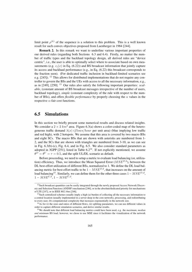
limit point ρ(k) of the sequence is a solution to this problem. This is a well knownresult for such convex objectives proposed from Luenberger in 1984 [244].

Remark 2. In this remark we want to underline various important properties ofour derived rules (regarding both Sections 6.3 and 6.4). Firstly, no matter the num-ber of traffic types and the backhaul topology design, all derived rules are “devicecentric”, i.e., the user is able to optimally select where to associate based on own mea-surements (e.g. ci(x) in Eq. (6.22)) and BS broadcast information that jointly captureits access and backhaul performance (e.g., in Eq. (6.22) this broadcast corresponds tothe fraction seen). (For dedicated traffic inclusion in backhaul-limited scenarios seee.g. [245]). 12 This allows for distributed implementations that do not require any con-troller to govern the BSs and the UEs with access to all the necessary information, e.g.,as in [249], [250]. 13 Our rules also satisfy the following important properties: scal-able, (constant amount of BS broadcast messages irrespective of the number of users,backhaul topology), simple (constant complexity of the rule with respect to the num-ber of BSs), and offers flexible performance by properly choosing the α values in therespective α-fair cost functions.

6.5 Simulations

In this section we briefly present some numerical results and discuss related insights.We consider a 2 × 2 km2 area. Figure 6.3(a) shows a color-coded map of the hetero-geneous traffic demand λ(x) (flows/hour per unit area) (blue implying low trafficand red high), with 2 hotspots. We assume that this area is covered by two macro BSsand eight SCs. The macro BSs that are shown with asterisks are numbered from 1-2, and the SCs that are shown with triangles are numbered from 3-10, as we can seein Fig. 6.3(b)-(c), Fig. 6.4, and in Fig. 6.5. We also consider standard parameters asadopted in 3GPP [251], listed in Table 6.214. If not explicitly mentioned, we assumeθD = θU = τ = 0.5, and the split UL/DL scenario as default.

Before proceeding, we need to setup a metric to evaluate load balancing (or, utiliza-tion) efficiency. Thus, we introduce the Mean Squared Error (MSED,b), between theDL best-effort utilization of different BSs, normalized to 1. We define the DL load bal-ancing metric for best-effort traffic to be 1−MSED,b, that increases on the amount ofload balancing15. Similarly, we can define them for the other three cases 1−MSED,d,1−MSEU,b, 1−MSEU,d.

12Such broadcast quantities can be easily integrated through the newly proposed Access Network Discov-ery and Selection Function (ANDSF) mechanism [246], or in the absolute/dedicated priority list mechanismsof LTE [247], or in IEEE 802.16m [248].

13Such centralized schemes usually imply a high (a) burden of collecting all the necessary information toa central location (usually implemented in a server deep in the core network), processing, and redistributingto every user, (b) computational complexity that increases exponentially in the network size.

14As for (i) the sizes and ratios of different flows, (ii) splitting parameters, we can use different values inorder to capture different simulation scenarios, and derive similar results.

15We should note that different load balancing metrics could have been used, e.g. the maximum, medianand minimum BS load; however, we chose to use MSE since it facilitates the visualization of the networkperformance.

165

Table 6.2: Simulation Parameters

Parameter Variable ValueTransm. Power of eNB/ SC/ UE PeNB/PSC/PUE 43/24/12 dBm

BS Bandwidth for DL, UL w/W 10/10 MHzNoise Power Density N0 -174 dBm/Hz

Splitting parameter for DL, UL ζDi , ζUi 0.5/0.5Average DL/UL flow sizes 1

µD,b /1

µU,b 100/20 KbytesAverage DL/UL flow demands BD(x)/BU (x) 512, 128 kbps

Different flow ratios zb, zD 0.3,0.6

6.5.1 Provisioned Backhaul

We now focus on the case of provisioned backhaul as considered in Section 6.3 andinvestigate the involved tradeoffs both qualitatively and quantitatively. We will presentthe impact of our proposed association rules via coverage snapshots to show how usersassociate in the considered network, while we will also provide values for related per-formance metrics that complete our study numerically.

Spectral efficiency vs. Load balancing. Figure 6.3(b) outlines the optimal DLuser-associations if αD,b = αD,d = 0, i.e., when spectral efficiency is maximized.Thus, each UE at x is attached to the BS that offers the highest DL SINR and promiseshigher DL physical rate for best effort flows cD,b

i (x), and more “dedicated” serverskDi (x); i.e. most of UEs are attached to macro BSs due to their high power trans-mission, and fewer to SCs, forming small circles around them. Consequently, macro-cells are overloaded and load imbalance within the cells is sharpened (decreased 1 −MSED,b, 1 −MSED,d; see line 1 of Table 6.3). However, in Fig. 6.3(c) we empha-size the load-balancing efficiency and set αD,b = αD,b = 10. Now, most SCs vastlyincrease their coverage area in order to offload the overloaded macro BSs (e.g., BSs 6,8, 10); “heavily” loaded (due to the hotspots) BSs, roughly maintain the same coverage(BS 4 and 7). Thus load balancing is improved, at the cost of E[cD,b], E[kD] (see line2 of Table 6.3). For further implications of α parameters we refer the reader to [63].

Best-effort versus dedicated traffic performance. Although in the previous sce-narios the best-effort- and dedicated- related traffic rules (represented from αD,b, αD,d)are aligned, one could ask how would two conflicting optimization objectives affect ournetwork? The answer lays in the usage of θD, that judges which objective carries moreimportance. E.g., an operator has two main goals: (i) to maximize the average numberof servers for “dedicated” traffic captured by E[kD] (set αD,d = 0), (ii) to better bal-ance the utilization of best-effort resources between BSs (set αD,b = 10). As shownin Fig. 6.3(d), if θ → 0 E[kD] is maximized, whereas as θ → 1, 1 −MSED,b (DLbest-effort load balancing) is optimized, and each objective comes at the price of theother.

DL vs. UL traffic performance is considered in Figure 6.3(b), 6.4(a)-6.4(b), withrespective numerical performance metrics in Table 6.4. The first two figures depict theDL and UL optimal associations, in case of split UL/DL, for each user at x. However,

166

(a) Traffic arrival rate.

0 500 1000 1500 2000

0

500

1000

1500

2000

BS1

BS3

BS4

BS10BS9

BS6

BS7

BS2BS8

BS5

(b) Spectral Efficiency OptimizationαD,b = αD,d = 0.

0 500 1000 1500 2000

0

500

1000

1500

2000

(c) Enhanced Load Balancing αD,b =αD,d = 10.

0 0.5 128

30

32

θ

E[k

D]

0 0.5 10.4

0.7

1

θDL

Util

iz. E

ff.Emphasize αD,d=0

Emphasize αD,b=10

(d) Ded. vs. Best-effort flows performance.

Figure 6.3: DL Optimal user-associations (Spectral efficiency vs. Load balancing andbest-effort vs. ded. traffic performance)

if split is not available from the operator point of view, we have to weight whether theDL or UL performance is more important while selecting a single BS for Joint UL/DLassociation, using parameter τ . To that end, Figure 6.3(b) (also) outlines the optimalassociations in the Joint UL/DL case if the whole emphasis is on the DL performance(τ = 1): this hurts the UL performance due to the asymmetric transmission powersof the UEs and BSs (see line 1 of Table 6.4). In Fig. 6.4(a) the emphasis is movedon the UL performance (τ = 0), and each UE is attached to the nearest BS, in orderto minimize the path loss [236] and enhance the UL performance; this hurts its DLperformance though (see line 3 of Table 6.4). Finally, Fig. 6.4(b) shows the optimalcoverage areas when one assigns equal importance to the UL and DL performance (i.e.τ = 0.5): this moderates both DL and UL performance (line 2 of Table 6.4). Thisalso corroborates the notion that split is able to simultaneously optimize UL and DLperformances, as already discussed in theory.

6.5.2 Under-provisioned BackhaulWe now continue with some backhaul-limited network scenarios. We remind to thereader that our focus is on the backhaul links between the macro cells and SCs (for

167

Table 6.3: Numerical values for Figure 6.3.

Rates and Servers Load BalancingE[cD,b] (Mbps) E[kD] 1-MSED,b 1-MSED,d

Fig. 6.3(b) 16.3 32 0.77 0.78Fig. 6.3(c) 14.3 27 0.96 0.995

0 500 1000 1500 2000

0

500

1000

1500

2000

(a) UL performance optimization τ = 0.

0 500 1000 1500 2000

0

500

1000

1500

2000

(b) Equal emphasis of DL vs. UL τ = 0.5.

Figure 6.4: Optimal user-associations (DL vs. UL traffic performance)

simplicity we assume provisioned links between the macro cells and core network). Asalready discussed in assumption C.1, we investigate two different backhaul topologyfamilies: (i) “star” topologies (single-hop paths), (ii) “tree” topologies (with multi-hop paths), along with two backhaul links types: wired and wireless16. Our aim isto evaluate the derived association rules described in Section 6.4 for different under-provisioned scenarios, by fixing the aforementioned trade-offs related to the trafficdifferentiation as it follows: θD = θU = 1 (we only focus on the best-effort flowsby dropping the superscripts “b” and “d”), and αD = αU = 1 (throughput optimalvalues). Also, we assume fixed backhaul routing paths, pre-established with tradi-tional Layer 2 routing, that the BH capacities on the DL and UL are the same (i.e.CD

h (j) = CUh (j) = Ch, ∀j ∈ Bh), and if not explicitly mentioned we assume them

to be equal to 400Mbps. We maintain this assumption to facilitate our discussion, al-though our framework works for heterogeneous backhaul links and UL/DL capacities(see C.2). We finally assumed that ci is the 80% of the maximum user capacity asso-ciated with BS i (we have also tried higher values for more “conservative” scenarios,and also lower for more “aggressive” with similar conclusions).

Before proceeding, we need to make an assumption about the backhaul link capac-ities. In case of wired backhaul links, we assume that the peak backhaul capacity Ch

is always guaranteed. For wireless backhaul links we adopt a simple model associatingpeak backhaul capacity to distance: if the length of the i-th link is ri, the peak capacity

16Note that copper and fiber access are the key technologies for wired backhaul links, and microWave andmillimeter-wave P2P or P2MP access are the counterpart for the wireless backhaul links [252].

168

Table 6.4: Numerical values for Figure 6.4.

DL performance UL performanceE[cD,b] (Mbps) E[kD] E[cU,b] (Mbps) E[kU ]

Fig. 6.3(b) 16.3 32 2.3 18Fig. 6.4(b) 14.7 28 3 24Fig. 6.4(a) 13.3 26 3.6 28

0 500 1000 1500 2000

0

500

1000

1500

2000

BS1

BS3

BS4 BS5

BS6

BS7

BS8BS9BS10 BS2

(a) BH: provisioned.

0 500 1000 1500 2000

0

500

1000

1500

2000

(b) BH: Wired-Star.

0 500 1000 1500 2000

0

500

1000

1500

2000

(c) BH: Wireless-Star.

0 500 1000 1500 2000

0

500

1000

1500

2000

(d) BH: Wireless-Tree.

Figure 6.5: DL optimal associations in different scenarios.

drops as:

d(ri) =

1, ri ≤ r0

( r0ri )n, otherwise,

(6.34)

where r0 is some threshold range within which the maximal rate is obtained (e.g.Line-of-Sight), and n is the attenuation factor. Hence, the available capacity dropsto d(ri)Ch(j) (≤ Ch(j)). For our simulations, we assumed that r0 = 200m, andn = 3. While the above model is perhaps oversimplifying, our main goal is to sim-ply include a generic model for the propagation related impact on wireless backhaul,compared to wired, without getting into the details of specific backhaul implementa-tions. For detailed path loss models for different backhaul technologies, we refer theinterested reader to [231].

Coverage Snapshots. In Fig. 6.5(a) we depict the optimal DL user-associationsfor provisioned backhaul network with respect to the traffic arrival rates shown in

169

Fig. 6.3(a). Compared to the associations showed in Figure 6.3(b) where αD = αU =0, we note that now some SCs have slightly increased coverage area, in order to im-prove the mean user throughput [63].

In the following, we focus on different under-provisioned backhaul scenarios, andstudy the DL associations (similar behavior in the UL; we refer the interested readerto [239] for them). In Fig. 6.5(b) we adopt a wired-star backhaul topology, where SCsshrink their coverage areas, by handing-over users to other BSs, in order to offload thecorresponding (under-provisioned) backhaul links; this phenomenon becomes moreintense in the “hot-spot” areas (e.g., BS7 have vastly decreased their coverage areas)due to the higher traffic demand. Similarly, in Fig. 6.5(c), we assume a wireless-starbackhaul topology, where SCs further decrease their coverage areas, due to the higherbackhaul capacity loss caused from the long wireless links (see Eq.(6.34)).

In Fig. 6.5(d) we adopt a wireless-tree topology, where some SCs are required tocarry also traffic of other SCs, and end up more congested. As a result, most SCsfurther decrease their coverage area, compared to the star-wireless topology. However,BS7 and BS10 enlarge their coverage areas, compared to the star case. This occursbecause these SCs are far from the eNB, and multi-hop topology allows them to routetheir traffic over shorter wireless links with smaller capacity losses, compared to thestar case (Fig. 6.5(c)). Hence, there are two main factors affecting the coverage areasin such wireless backhaul networks: (topology) each BS-load might traverse throughmulti-hop backhaul paths, by “wasting” resources from more than one backaul links(drawback for tree topologies); (location) the higher the η,r0 the worse the capacityloss “wastage” over a dedicated direct backhaul link (drawback for star topologies thatrequire longer links).

As backhaul networks become increasingly complex, e.g. “mesh” topologies, eachBS has multiple possible routing paths to follow, beyond what is shown in the figures(we remind the reader that the above shown topologies are simply the given spanningrouting trees). The above observations thus underline the shortcomings of predeter-mined, Layer 2 (L2) backhaul routing mechanisms, and call for a joint optimization ofuser-association on the radio access network along with dynamic, Layer 3 (L3) back-haul routing.

Under-provisioning impact on user performance. Figure 6.6(a), 6.6(b) depictthe average DL and UL user throughputs, as a function of the backhaul capacity con-straint Ch, on different scenarios. Generally, as Ch drops, the mean throughputs aredecreased, since users are handed over to (potentially far-away) macro BSs, causingperformance degradation. Interestingly, the slope of the dropping rate becomes moresteep for lower values of Ch, due to the logarithimic capacity formula chosen in as-sumption (B.2). Also, as Ch increases, the average throughputs “converge” to thevalue corresponding to a provisioned backhaul network. Note that the average ULthroughput convergences more quickly, compared to the DL. This happens due to theasymmetry between the DL and UL traffic demand on the radio access network: theUL one is much lower, mainly due to the asymmetry between the transmission powersof BSs and UEs, as well as different file sizes assumed in each direction. Beyond thispoint, the UL backhaul resources will be underutilized. This calls for a flexible TDDduplexing scheme, that will dynamically distribute the backhaul resources accordingly,for example by giving more backhaul resources to DL when the UL demand is already

170

50 300 5000

5

10

15

Ch (Mbps)

DL

Thr

ough

put (

Mbp

s)

Wired−StarWired−TreeWireless−TreeWireless−Star

(a) DL (global) user throughput.

50 300 5001.5

2

2.5

3

3.5

Ch (Mbps)

UL

Thr

ough

put (

Mbp

s)


(b) UL (global) user throughput.

Figure 6.6: Mean throughputs overall all users in the network.

satisfied (e.g. the eIMTA scheme [253]). Finally, in the wired case, star topology isalways slightly better than the tree, whereas in the wireless the opposite, as explainedearlier.

Table 6.5: Mean throughp. for handed-over users (in Mbps).

Topology Ch = 50 250 500 (Mbps)DL / UL thr.: Star-Wired 1.1 / 0.2 3.1 / 1.6 4.1 / XDL / UL thr.: Tree-Wired 0.6 / 0.1 2.4 / 0.7 3.2 / XDL / UL thr.: Tree-Wirel. 0.2 / 0.03 1.7 / 0.07 2.1 / 0.15DL / UL thr.: Star-Wirel. 0.1 / 0.001 1.4 / 0.05 1.7 / 0.02

One could notice that user throughputs drop slightly on the Ch constraint, e.g. in awired-star topology if Ch drops 500→ 50 Mbps (10 times), the mean user throughputonly drops 15 → 6 Mbps (∼ 3 times). This is due to the fact that, under-provisionedbackhaul links do not affect the whole network, but specific groups of users associatedwith the cells that suffer from low backhaul capacity. To better illustrate this, in Ta-ble 6.5 we show the average throughput of the handed-over users, as a function of Ch.Indeed, their performance is severely affected: for the same scenario, their DL through-put drops all the way to 1.1 Mbps (∼ 15 times). (In scenarios with no handovers, wemark the respective table entry with an X .)

Under-provisioning impact on Network Performance. Turning our attentionto network-related performance, Fig. 6.7(a) considers spectral efficiency (bit/s/Hz),normalized by the maximum corresponding value when the network is provisioned.Load-balancing (“utilization”) efficiency is further considered in Fig. 6.7(b) in termsof the MSE metric, described earlier. Both efficiencies converge to 1 as the networkgets provisioned. Low Ch values will push users to handover to far-away BSs, and thiswill potentially decrease their SINR (spectral efficiency decrease), and create steepdifferences between BSs loads, e.g. by congesting macro BSs and under-utilizing theSCs (load balancing decrease). Note that, the joint degradation of these performances

171

50 300 500

0.7

0.8

0.9

1

Ch (Mbps)

Spe

ctra

l Effi

cien

cy


(a) DL Spectral efficiency.

50 300 500

0.7

0.8

0.9

1

Ch (Mbps)

Util

iz. E

ffici

ency


(b) DL Load balancing (Utilization) Effi-ciency.

Figure 6.7: Downlink Network Efficiencies (normalized).

also impacts user performance negatively (e.g. user throughput), as explained in Sec-tion B.7.

Note that regarding spectral efficiency (for the wireless scenario), there is a crucialpoint that judges which topology is better than the other in different under-provisionedcases (that is actually the point where the two curves meet). Obviously, this point, thatis highly affected by the network topology and the given set of assumptions, can sig-nificantly vary between different performance metrics (e.g., in terms of load balancingand user throughput). Note that it is not possible to analytically derive this cross point,as this depends on the value of the objective function of the respective optimizationproblem. As a result, the actual cross point can only be found via sensitivity analysis.Nevertheless, we provide here the two main factors that affect this tradeoff between starand tree topology, to provide some qualitative insights. These factors are: (i) path losscharacteristics: the higher the path loss (e.g. higher η) the worse the capacity loss on along direct backhaul link required for a star topology, favoring multi-hop connectivity(i.e. a tree topology). (ii) the number of hops: the higher the number of backhaul hopsthe higher the total backhaul resources consumed “per BS” or “per bit of radio access”,which might disfavor a tree topology.

Table 6.6: UL/DL Split Vs. Joint-association Improvements

Performance τ = 0 τ = 0.5 τ = 1

DL / UL Throughput 6% / 32% 4% / 35% 0% / 37%DL / UL Spectr. Eff. 4% / 29% 3% / 31% 0% / 33%DL / UL Uiliz. Eff. 7% / 34% 4% / 38% 0% / 41%

Split UL/DL impact. As discussed earlier, while split is able to optimize the DLand UL performance, simultaneously, Joint UL/DL association is incapable of this par-allel optimization and using 0 ≤ τ ≤ 1 we can trade-off which dimension carries moreimportance. Table 6.6 illustrates the performance improvements that split promises

172

over the Joint UL/DL association, in terms of various metrics, for various τ whenbackhaul is underprovisioned. We underline that split enhances the UL performanceconsiderably, e.g. the average UL throughput is increased up to 37%. This is due tothe dependency that Joint UL/DL generates between the DL and UL associations in theaccess network, that often makes the DL the bottleneck in the backhaul (due to afore-mentioned asymmetry between the peak access rates). Thus, DL will often “preempt”the backhaul constraint, and potentially (i) leave some UL resources unused, (ii) causeUL performance degradation.

Comparison with existing work. We now compare our proposed algorithm with twoothers user-association schemes; specifically, we run them in our considered networktopology for the wired backhaul case (similar behavior for the wireless). In Table 6.7we depict the performance decrease compared to our scheme in terms of: Spectral Ef-ficiency (SE), User Performance (UP) (in terms of idle dedicated servers for dedicatedtraffic and throughput for best-effort) and Load Balancing (LB). We have assumedthat all BSs associated with a BH link that is congested decrease their SE and UPproportionally to the amount of congestion by illustrating the effective correspondingperformance.

Firstly, we investigate the algorithm proposed from Mesodiakaki et al. that focuseson dedicated traffic demand [227, 243]. This algorithm involves two stages, each ofwhich independently considers access and backhaul performance: in the first, a subsetof cells for each users’ association is selected as candidates separately for DL and ULbased on the radio access conditions (i.e., the DL data rate or the UL path loss withoutconsidering the BS load). Then, the best one among them is selected based on the BHconditions: the BS with the fewest backhaul hops to the core is selected as optimal.However, such a simplistic criterion can lead to rather suboptimal performance as ex-plained in Section 6.4.1. Specifically, in our case, in both DL and UL, we see thateffective SE and UP are decreased since the path with the fewest hops might includecongested backhaul links (obviously, this is more intense in the tree topology wheremultiple BSs share the resources of a single backhaul link). LB is also slightly hurt (byalso hurting UP) since the reference algorithm ignores the BS loads.

Table 6.7: Comparison with existing work.

DL performance UL performanceAlgorithm SE UP LB SE UP LB

[227, 243] Star-Wired 1.4 1.3 1.2 1.8 2.1 1.3[227, 243] Tree-Wired 1.5 1.4 1.2 2.2 3.2 1.4

[228] Star-Wired 5.3 5.6 2.1 3.9 5.1 1.1[228] Tree-Wired 5.7 5.9 2.4 4.1 5.4 1.2

Secondly, we consider the user-association algorithm proposed by Domenico et al.for DL best-effort flows [228]. There, the ergodic capacity is attempted to be maxi-mized through an iterative algorithm: at each step every user changes its associationif the corresponding gain in terms of ergodic capacity is positive. Nevertheless, suchan iterative algorithm, strongly dependent on the initial condition as well as the corre-

173

sponding step directions, does not necessarily converge to the best point by potentiallygetting stuck in subpar conditions. Also, this algorithm does not take into account het-erogeneous traffic demand, and thus BS loads. UL traffic and BH tree topology arenot considered, so we (i) assume that UL associations are identical as DL (as in JointUL/DL, see B.10), and (ii) extend the proposed resource allocation policy to evenlysplit the available backhaul resources of a link in tree topologies. Simulation resultsshow significant performance degradation since in the (suboptimal) converged point(i) some users end up being attached to far-away BSs, and (ii) some BSs are drivento congestion while attempting to improve ergodic capacity by affecting LB and SE,correspondingly. Joint degradation of them also impacts UP negatively, as explained in(B.7).

6.6 Conlusions and Future WorkIn this chapter we explored the problem of association in future HetNets and propose aframework which can be derived to find optimized association algorithms that take intoaccount factors like traffic type, traffic direction (UL/DL), and backhaul network con-nectivity and capacity. A couple of interesting issues arose from the simulation-basedevaluaton of these optimal policies. These have either been addressed in subsequentwork or are part of future work.

First, having the same amount of DL and UL resources in every BS is clearly sub-optimal. Same goes for the resource split in the backhaul network. To this end, in [78]we addressed the first issue, that of jointly optimizing the association variables in ourframework, together with the UL/DL resource allocation. This problem appears to benon-convex at first, but with some appropriate transformations it can be convexifiedand tackled with a distributed hierarchical algorithm, running at different time scales.A preliminary treatment of backhaul resource allocation has also been pursued in [238].

Second, as the backhaul network becomes more complex (e.g. a mesh network)routing should jointly be addressed with the user association problem, to further im-prove performance. As was evident in this chapter, the user association on the radioaccess might be limited by the available capacity on the backhaul path. In this chap-ter we assumed this routing path to be given (e.g., chosen before, or in a slower timescale than the user association variables, as is usually the case). However, re-visitingthe routing path together with the BS load-balancing problem is a promising direc-tion. We plan to explore whether the joint problem can be convexified and solved in adistributed/hierarchical manner as well.

Last but not least, we have made throughout this chapter the (strong) assumptionthat the traffic demand is known at each location x. In practice, this traffic mightnot only be unknown (at first) but also non-stationary. In our recent work of [254],we have considered data-driven framework to learn the mean traffic demand whileoptimizing the associations, in order to achieve robust association maps: to performwell on average, but deteriorate gracefully when the statistics diverge from their mean(e.g., flash crowds, special events, etc.).

174

Chapter 7

Mobile Edge Caching

175

As already argued in the previous chapters, a promising and highly-investigatedway of dealing with the tremendous increase in traffic demand is via the deploymentof many small cell base stations (e.g pico/femto-cells, or out-of-band WiFi APs) to-gether with the standard macro-cellular network. The bulk of current state of the artfor small cell solutions tackle mainly aspects of self-organizing radio resource man-agement, inter-cell and interference coordination (ICIC), energy-efficiency and MIMOtechniques, as well as traffic steering techniques like the ones considered in the last twochapters. A common problem for a lot of work on small cell networks is the impact ofthe backhaul network. While the reduced distances to the user and better spatial reusecan greatly increase the (radio) capacity in the last hop, in order to support high celldensification the capacity of the backhaul network needs to scale at unrealistic rates.As a result, small cells are expected to be mostly connected by inexpensive wired orwireless links, and thus will often be under-provisioned, according to the Small CellForum [79]. This makes the backhaul network a potential new bottleneck that cansignificantly reduce the envisioned gains by cell densification.

In the previous chapter, we investigated how to take such backhaul bottlenecks intoaccount, even when optimizing radio access functions like user association. While thisapproach can redirect some traffic to different BSs, possibly connected with less con-gested transport links, some important issues remain: (a) this is not always possible orit introduces considerable suboptimalities on the radio access (e.g., in terms of spectralefficiency); (b) the transport network (backhaul/fronthaul) might simply not be ableto support the aggregate radio traffic, for any routing path(s). To further alleviate thebackhaul bottleneck, but also to reduce content access latency, the idea of edge cachinghas been proposed [80, 81, 82, 83]

The increasing demand for Internet content, and the inherent overlap between userdata requests, suggests that storing popular content closer to the user could: (a) avoidcongesting the capacity-limited backhaul links by avoiding duplicate backhaul trans-missions, and (b) reduce the content access latency. Specifically, in [80], local contentcaching has been identified as one of the five most disruptive enablers for 5G networks,sparking a tremendous interest of academia and industry alike, as a cost-efficient wayof tackling the data tsunami. Using real measurement data, [84] has explored the poten-tial benefits of forward caching inside the core of a 3G network (e.g. in the SGSNs orGGSNs), suggesting that hit ratios up to 33% can be achieved for such caches. Similarbenefits based on real workloads have been also found for LTE networks [85]. Whilethese works already demonstrate the potential benefits of caching, a number of keyquestions remain open.

Edge cache size can be a major bottleneck: First, the above measurement-basedstudies have only considered caching in core nodes or backhaul aggregation points.Such nodes see a significant amount of the global network traffic and could also beequipped with large storage capacities (comparable to the size of regular CDN servers).It remains widely open whether similar benefits could be achieved with small, localcaches at each BS and small cell. Such caches would have a much smaller storagecapacity due to CAPEX/OPEX cost reasons: each core node considered as a potentialcaching location in the above studies would correspond to 100s or 1000s of small cellsin future ultra-dense networks. As a result, the storage space per local edge cache mustbe significantly smaller to keep costs reasonable. This suggests that only a tiny fraction

176

of the constantly and exponentially increasing content catalog could realistically bestored at each edge cache. In most practical cases, a local edge cache would fit lessthan 0.1 − 0.01% of the entire Internet catalog. E.g., a typical torrent catalog is about1.5PB and the entire Netflix catalogue about 3PBs. More than 1TB storage wouldbe needed to just store 0.1% of either one [86]. Considering other VoD platforms,YouTube, etc., this number explodes. Even, with a skewed popularity distribution,local cache hit ratios would be rather low [87, 88, 89].

Convergence of cooperative caching and cooperatice communication: Second,a number of technological advances are envisioned for future 5G networks, such asCoordinated Multi-Point (CoMP) transmission, Coded Caching, and the CloudRANarchitecture. These technologies are considered as major drivers to improve the per-formance on the radio access network (RAN) in 5G, but also introduce novel compli-cations and challenges for caching algorithms. To cooperatively transmit a requestedcontent from multiple BSs, so as to improve radio access performance (e.g. throughdiversity gains), that content must be available in the caches of all BSs involved ina coordinated transmission. Otherwise, the effective rate of one or more of the linksmight be severed by a congested backhaul link. Yet, storing the same content in mul-tiple nearby BSs means not storing other contents there, thus leading to a considerabledecrease in cache hit rates and increased backhaul costs, if those contents are requestedinstead. This creates a novel tradeoff: how could a caching policy facilitate coopera-tive transmission opportunities (and radio access performance) while maximizing localcache hit rates (and backhaul performance)?

Application-dependent caching optimization Third, specific applications, espe-cially content streaming, are beginning to dominate the mobile data traffic (e.g., morethan 50% percent of the total traffic is consistently reported to be streamed video),and this is not expected to change in the future. Any means to reduce network trafficthrough caching should thus pay particular attention to this application. This raises thequestion: could application-driven optimizations targeting video traffic further improvethe performance of edge caching?

In this chapter, we briefly present four main directions of ongoing and future plannedresearch to maximize the amount of traffic offloaded from, as well as to jointly optimizethe performance of, radio access and backhaul networks.

1. Using node mobility (UE or Relay) to trade-off content access delay (i.e. userQoE) for cache hit ratio. (Section 7.1)

2. Exploiting the properties of video streaming to offload more data through edgecaching without any QoE impact. (Section 7.2)

3. Using alternative content recommendation to improve caching performance through“soft cache hits”. (Section 7.3)

4. Coordinated caching and communication. (Section 7.4)

177

7.1 Delay-tolerant Edge Caching

Installing a large enough number of small cells with local storage (SCs), to ensure everyuser equipment (UE) has access to at least one such low range BS, still requires highCAPEX/OPEX costs (e.g. rental costs, maintenance, backhaul). Combined with thestagnating revenues per user, this maked operators reluctant to perform the necessarydensification. The more radical proposal to use UEs for storage and relaying (e.g.,through Device-to-Device (D2D) communication) [90, 91] largely avoids these costs,but is stifled by device resource constraints (especially battery) and privacy concerns.As a result, SC storage and/or D2D might offer small performance mprovements, inpractice. E.g., a user requesting a content k might not have an SC in range, in whichcase k must be fetched over an expensive macro-BS. Even if the user has some SCs(or other UEs) in range, these might not in fact store content k (due to their relativelysmall size compared to the content catalog). Fetching content k will again be costly,e.g. over an SC backhaul link which is usually wireless and capacity-limited.

To improve this situation, one could exploit the mobility of UEs or even of BSs,to tradeoff access delay for cache hit ratio. For example, if a user i requests a contentk, which is not “locally” available, the operator can ask the user to wait for some time(e.g. up to some TTL). During that time, user i may encounter some other cachestoring k (either because i moved, or because the cache moved, in the case of mobilerelays [92]). E.g., consider a simple example where there are M total edge caches, andintermeeting time between a user and such a cache is IID with rate λ. Assume that inthe baseline (“immediate access”) scenario, a user sees on average c of these M caches,where c < 1 in most cases (since SC coverage is limited). In the “delayed access” case,a user sees an additional M · λ · TTL caches, on average. Hence, the effective cachesize that the average user sees is approximately M · λ · TTL times larger, which maylead to more cache hits.

The challenge here is to optimally allocate this larger (effective) cache space amongall contents. E.g. if a node sees at most one cache, the optimal policy (putting aside thefurther considerations of Coded Caching [255]) is to store the most popular contentsin every cache, until it’s full. However, it is easy to see that this is suboptimal in thedelayed access case. If the size of each cache is C contents, and node i encounters 2caches during a TTL, storing contents 1 to C in one cache, and C + 1 to 2C in theother, would lead to much higher hit rates for that node than storing contents 1 to C inboth. While this example provides some intuition how the cache policy could exploitmobility (and the additional cache space it allows node to “see”), finding the optimalpolicy depends on the mobility characteristics, content popularities, and TTL.

7.1.1 Content Access Protocol

In this section, we state some assumptions about our system.A.1 - Network Setup. There are three types of nodes:

• Infrastructure Nodes (I), e.g., macrocells, that provide full coverage, and can serveany content request.

178

• (Mobile) Helper Nodes (H), e.g., cars, buses, taxis, where |H| = H . Each of thesenodes has a cache size of C bytes, and can serve only requests for content in itscache.

• End Users (U), e.g., smartphones, tablets, netbooks, that request different contents.

In the above, we are focusing on the case of mobile relays and storage points. Theseprovide many advantages, which are detailed in [92]. However, the theory is applicableto the case of storage at static helper nodes (e.g., small cells) or even other UEs (seee.g., [256]).

A.2 - Content Request Model. We assume the standard IRM request model,where each node independently asks for some content i out of a catalogue K of content(|K| = K), with probability ϕi [257, 258, 259]1. Without loss of generality, we assumecontent is sorted by decreasing popularity as ϕ1 ≥ ϕ2 ≥ · · · ≥ ϕK . We also assumethat content i has size si.

A.3 - Delayed Access. A user requesting content i will wait up to a maximum timeTTLi to find a (mobile) helper with that content. If it does, then it retrieves the contentlocally, imposing 0 cost on the infrastructure. If i is not found during that time, thenthe content is fetched from an (expensive) I node.

A.4 - Contact Model (U − H). Unless otherwise stated, pairwise inter-contacttimes between H and U are independent, drawn from a generic distribution FC(t) withmean rate λ. Contact durations are drawn from another generic distribution FD(t) withmean E[D]. We assume both distributions have bounded first and second moments.

A.5 - Cache Model. Let xij ∈ 0, 1, i ∈ K, j ∈ H be an indicator variabledenoting if helper node j stores content i. We assume H nodes store entire contents,and fractional storage is not allowed. Let further Ni denote the number of helper nodesstoring content i, that is

Ni =∑j∈H

xij . (7.1)

Ni will be a key control variable for our optimal cache allocation problem2.The goal of the operator is to optimally choose these number of copies Ni for each

content i that it should push into the helpers (called “seeding” phase, e.g. the nightbefore). The basic protocol is made up of three phases and is depicted in Fig. 7.1. Wesummarize some useful notation in Table 7.1.

7.1.2 Optimal Cache AllocationTo understand the basic ideas behind the cache allocation problem, let us consider asimple subcase of the above problem setup where TTLi = TTL (i.e., all contenthas the same delay-tolerance). Let us additionally assume that: (i) FC(t) = 1 − eλt,i.e. inter-contact times are exponential, and (ii) E[D] is much larger than the time to

1In practice, these quantities can be estimated as an expected request rate during some MNO-defined timewindow (e.g., a day [260, 83]). Several studies have shown that it is possible to predict the popularity withgood accuracy over relatively short periods (e.g., a few weeks for YouTube videos) [261].

2Note that given the assumption of IID mobility, it suffices to optimize the total number of copies Ni

without considering the per vehicle variables xij any more.

179

Table 7.1: Notation.

CONTROL VARIABLES

Ni Number of replicas stored for content i

TTLi Deadline for content i

CONTENT

K Number of content in the catalogue

ϕi Number of requests for content i

si Size of content i

MOBILITY

Tij Inter-meeting time between U andH nodes

λ Mean inter-meeting time with vehicles

Mi Number of contacts within yi

CHUNK DOWNLOAD

bij Bytes downloaded per contact

µ Mean of bij

σ2 Variance of bij

Bi Total bytes downloaded per content i

fBi(x) Probability density function of Bi

FBi(x) Cumulative density function of Bi

OTHER PARAMETERS

H Number of vehicles

C Buffer size per vehicle

ΩWeighted average of maximum slowdown(WAMS)

TTLmax Maximum deadline

180

Figure 7.1: Communication protocol.

download any of the contents (i.e., any content i can be downloaded in a single contactwith a helper storing i). In this setup, the optimization problem in hand is:

minimizeNi

∑i∈K ϕi · si · e−λ·Ni·TTL, (7.2)∑

i∈K Ni · si ≤ H · C, (7.3)0 ≤ Ni ≤ H, ∀i. (7.4)

The objective (7.2) corresponds to the total bytes that have to be downloaded afterthe TTL expires, and follows from basic properties of the exponential distribution.Constraint (7.3) is a knapsack type constraint related to the total storage capacity inH nodes, and constraint (7.4) simply says that the number of replicas must be non-negative and at most equal to the total number of helpers (there is no benefit fromstoring the same content twice in the same cache).

The above problem is a discrete optimization problem (as Ni must be integer)which could be mapped into a non-linear knapsack variant, and thus is hard in the-ory. However, if cache size C is larger than just a few contents (which is typically thecase), a very good approximation can be achieved by solving the continuous relaxationof the above problem, i.e. assuming Ni ∈ R (and then rounding appropriately). In thiscase the above problem is convex, and can in fact be solved analytically using KKTconditions. The following gives the optimal allocation:Result 1. The optimal number for the objective of (7.2) is given by:

N (i) =

0, if ϕi < L

1λ·TTL ln

(λ·TTL·ϕi

ρ

), if L ≤ ϕi ≤ U

H, if φ(i) > U

where L , 1+ρλ·TTL , U , (1+ρ)·eH·λ·TTL

λTTL , and ρ, µ(i), λ(i) and ρ are appropriate (non-negative) Lagrangian multipliers.

There are a couple of things to observe here. First, the number of copies is anincreasing (as expected) but concave function of the content popularity, suggestingdiminishing returns per extra copy (it is useful to compare this to the simple motivating

181

101

102

103

104

105

1060

20

40

60

80

100

120

Popularity

N(i) # of copies LOW

µ>0, λ=0MEDIUM

µ=0, λ=0HIGH

µ=0, λ>0

Figure 7.2: Optimal allocation in semi-log scale.

example discussed earlier). The number of copies is also a decreasing function ofthe TTL, since the larger the delay tolerance, the more caches a node sees during aTTL, and the higher the chance for a cache hit, even if fewer caches store i. Thecapacity constraint affects this allocation mainly through multiplier ρ, which acts asa scaling factor (the higher the capacity the smaller ρ is). Finally, in some scenariossome low popularity contents get 0 copies while very popular contents are replicatedin all helpers. An example of the above allocation (in log-linear scale) can be seen inFig. 7.2.

7.1.3 Performance Evaluation

We validate our model through MATLAB simulations. We simulate the load on theinfrastructure and we compare it with other caching systems. We consider the optimalallocation policy described earlier and we analyse the impact of different parameters inthe proposed cache system. Furthermore, we consider a square area of 5000m x 5000min the center of San Francisco. We use the Cabspotting3 trace to compute the averagemeeting rate λ: we randomly place the U nodes and, considering a communicationrange of 200m, we calculate the meeting rate with each H node. We find λ = 4contacts/day. According to the density of the city and to the number of vehicles percapita, we estimate to 100.000 the number of vehicles in the area considered. However,in order to be realistic about initial technology penetration we assume that only 1% ofthese vehicles is participating in the cloud. We assume that each car can store 100contents (0, 1% of the catalogue). We set TTL to 3 minutes.

In our analysis, we also consider the content popularity of YouTube videos, sincea large percentage of mobile data traffic is represented by video files. We down-load from [262] a database generated with YouStatAnalyzer that collects statistics for100.000 YouTube videos. The database includes static (title, description, author, du-ration, related videos, etc.) and dynamic information (daily and cumulative views,shares, comments, etc.). In our simulations, we only take into account the number of

3GPS coordinates from 536 taxis in San Francisco over 23 days [112].

182

views related to the last 360 days. However, these values are equal to the total numberof views per day in the world, then we scale them properly4.

Note that we have also created synthetic traces based on the work in [263]. Sim-ulations based on these synthetic traces confirm the observations made using the realtrace. We therefore focus on the former.

Unless otherwise stated, we will use the parameters summarized in Table 7.2.

DESCRIPTION PARAM VALUE

Number of vehicles H 1000 cars

Buffer size C 100 contents/car

Meeting rate λ 4 contacts/day

Time-To-Live TTL 3 minutes

Number of contents K 100.000 contents

Communication range 200m

Table 7.2: Parameters of the scenarios considered.

Finally, we compare our allocation policies with:

• No cache: no contents are stored in the vehicles; the probability of miss is equal to1, therefore the cost corresponds to the total demand: cost = ∆t

∑Ki=1 φ

(i);

• Random: contents are allocated randomly in the vehicles;

• Square root: this policy also has diminishing returns, similar to our optimal al-location, but it replaces the logarithm with the square root (after an appropriatenormalization to satisfy the storage constraint); such policies have been shown toperform well in P2P networks.

Fig. 7.3 shows the cost according to the value of TTL for the different policies. Itis very important to note that considerable gains can be achieved with very small TTLvalues (in the order of a few minutes) and small number of vehicles participating in thecloud (1%). This provides some evidence on the advantages of offloading based on avehicular cloud, compared to offloading using small cells or WiFi, as for example in[51] or [195]. E.g, [51] reports minor gains for similar small deadlines, while [195]requires a much longer TTL (order of 1-2 hours) to achieve similar gains. In addition,increasing the TTL further has diminishing returns. This implies that even users notwilling to wait too long could participate in such a system (benefiting themselves andthe operator).

Fig. 7.4 shows the cost according to the buffer size. From the plot we can observethat storing 100 contents/car (only 0,1% of the total number of contents) provides again of almost 60%. In a scenario with a larger catalogue (e.g., 100 millions), it seemsdoable to store 0,1% of the contents (e.g., 100.000 contents/car) needed to achieve goodsavings. What is more, due to the intrinsic characteristics of the popularity distribution,

4We scale them linearly taking into account the number of YouTube users and the population of SanFrancisco.

183

0 2 4 6 8 100

20

40

60

80

100

TTL (minutes)Cost (%)

No cacheRandomSquare rootOptimal

Figure 7.3: Cost comparison according to TTL.

0 0.2 0.4 0.6 0.8 10

20

40

60

Buffer [%]

Gai

n [%

]

Fixed TTLVar TTLFixed TTL [LR]Var TTL [LR]

Figure 7.4: Cost comparison according to buffer capacity.

100 200 300 400 5000

20

40

60

Number of vehicles

Gai

n [%

]

Fixed TTLVar TTLFixed TTL [LR]Var TTL [LR]

Figure 7.5: Cost comparison according to number of vehicles.

the system might require an even smaller number of storage in order to achieve similargains.

In an urban environment, the great availability of vehicles leads to large gains forthe proposed infrastructure. However, an operator will probably keep using our frame-work even if the number of vehicles available decreases: in Fig. 7.5 we depict the costsavings according to the number of (vehicular) helper nodes nodes participating in thecloud and the gain observed is not less than 50% when more than 250 vehicles are partof the cloud.

184

7.1.4 ExtensionsThe above framework and results provide some initial, yet important insights. In addi-tion, we have considered a number of extensions to the above basic framework.

Generic Inter-contact Times

A first possible extension is to generalize the inter-contact times. This can be done bereplacing e−λ·Ni·TTL in objective (7.2) with (1 − FC(TTL))

Ni . It is easy to see thatthe objective remains convex and optimal values for Ni can be found with standardmethods (albeit not always analytically, depending on FC(TTL)).

Limited Contact Duration

Although we have assumed unlimited contact duration (or equivalent, bandwidth), inpractice a content might not be downloaded in its entirety during a contact (e.g. thenode moves away before the download is finished). In this case, one could consider twopossible protocols: (Repeat) a node must restart the download of content i in the nextcontact (with some node storing i); (Resume) a node keeps the bytes it has downloadedso far, and continues with the remaining ones during a new contact. For the Repeatpolicy, let us denote with pi = 1 − FD( si

rH), the probability that content i of size si

is fully downloaded during a given contact during which the mean download rate isrH . This download is successful if the contact duration is at least equal to si

rH. Since

contact durations are assumed independent, one can use a Poisson thinning argument(in the case of exponential contacts) and replace λ in all the above equations with pi ·λ,to obtain the optimal allocation.

While analytically tractable, clearly the Repeat policy is not optimal (large con-tents, even if popular, will get very few copies, because there is very little chance onecan download them in one shot). Resume on the other hand is in some sense “workconserving” and can perform better. However, its analysis is more involved. In thecase of exponential inter-contact times, the total amount of bytes downloaded duringconsecutive successful contacts form a Compound Poisson Process whose distributionis a function of both FC(t) and FD(t). Nevertheless, one can approximate this with aGaussian distribution and derive an appropriate modification of (7.2) in closed form.Convexity is maintained (for the continuous relaxation of the problem) and the optimalsolution can be obtained. For more details, please see [92, 93].

Variable TTL

Although we have assumed an equal TTL for all contents so far, the above resultseasily generalize to different TTLi per content i. If different users further have dif-ferent delay tolerance for the same content, then the value TTLi could be seen as theaverage over all such users. However, objective (7.2) is only a first order approxi-mation in that case. Nevertheless, if one assumes that the TTL per user is a randomvariable from a known distribution, then one could replace the e−λ·Ni·TTLi (or even(1−FC(TTLi))

Ni , for generic inter-contacts) with ETTLi

(e−λ·Ni·TTLi

), where the

expectation is taken over the distribution of TTLi.

185

A more interesting case arises if we consider TTLi as a second set of controlvariables. The motivation for this is that the user perceives the enforced delay not inabsolute terms, but rather in relation to the total download time of the requested file.E.g., a user requesting a web page (which normally takes a few 10s of seconds todownload) would not be happy with an extra delay of 5 minutes. However, these extra5 minutes could more easily be “absorbed” if a user is downloading a large software orvideo, which anyway takes some 10s of minutes. Hence, an operator could allocate ahigher TTL to a large content, and lower TTL to small contents. This can be easilyformalized with the concept of slowdown, a metric that has recently attracted a lotof attention in queueing theory, and can be loosely defined as the total access delay(wait + download) divided by the download time. In its simplest case, the optimizationproblem then becomes:

minimizeNi,TTLi

∑i∈K ϕi · si · e−λ·Ni·TTLi , (7.5)∑

i∈K Ni · si ≤M · C, (7.6)∑ki=1 ϕi · TTLi·rH+si

si≤ S, (7.7)

0 ≤ Ni ≤M,∀i. (7.8)

We have just introduced TTLi as a control variable, and also added constraint (7.7)which normalizes the total TTL “budget” we have to allocate (for some constant S).This is a mixed integer program as some variables are integer (Ni) and others contin-uous (TTLi). We can again let Ni take real values to simplify the problem. However,note that the resulting problem is not convex in both variables anymore, even in thissimple setup. In fact it is “bi-convex”, as it is convex on either Ni or TTLi, but notboth. One can approach this problem with various solvers for bi-convex problem (e.g.iteratively optimizing for one set of variables, then the second, alternating the twosets till convergence). However, there are no strong guarantees of global convergence.Things get more compicated if one considers a Resume type of policy. Nevertheless,one can replace the respective objective with an approximate one (whose accuracy in-creases when there are plenty of contacts during a TTL), and which gives rise to aGeometric Program. The latter can be transformed into a convex one with appropri-ate manipulations and solved using standard methods. We refer the interested readerto [93].

Offloading through HetNets with SCs and UEs

As a final setup, in [256] we have considered a mixed setup, where a user can get thecontent both from small cells or from other UEs, storing the content. Additionally,we assume there that every UE that receives a given content k, can further act as alocal cache (with some probability, depending on incentives or other consideration).This setup is different compared to the previous one, as the number of storage pointshere increases over time, while in all previous scenarios the number of storage pointsis selected initially (when the optimal cache allocation is selected, e.g. at nighttime)and the number of caches remains unchanged during the delivery phase. While this

186

evolving number of storage points complicates the analysis, necessary to derive anobjective in closed form (that can be then optimized), we have used [256] mean fieldand fluid approximations for the problem, that were validated both against syntheticand trace-based simulations.

7.2 Low Cost Caching for Streamed Video Content

So far, we have been assuming that contents are downloaded in their entirety beforethey can be consumed. We then introduced an additional delay in the system, be-fore such a download starts, in order to allow a user to encounter low cost nodes (e.g.small cells or other UEs storing the content), and optimized the cache allocation in thissetup. In the simulation scenarios considered for such a system, we saw that interestingoffloading values can be achieved with delays ranging from 2-3 minutes to a few 10s.Such delay values could be acceptable in some scenarios, e.g. large files, delay-toleranttraffic (software updates, synchronization), developing regions and/or low cost plans.Nevertheless, if one considers standard urban environments, such deadlines might re-quire a significant monetary (or other plan-related) incentive by the operator, or mightbe unacceptable altogether.

In this second part, we focus on streamed (video) content specifically, and try to goone step further by exploiting the fact that streaming of stored video content offers somedelay tolerance “for free”. In other words, we would like to get some of the offloadingbenefits of the previous approach, without any delay impact on the user. Video contentis split into many chunks that are streamed into the user’s playout buffer one by one,and consumed at the playout speed. The user does not have to wait until the wholecontent is found in a local cache, but can start streaming right away, fetching chunksfrom the infrastructure or local/mobile caches, depending on availability of the latterand buffer status. For example, consider a user that start watching a 1h video, and achunk corresponding roughly to the middle of the video. This chunk does not have tobe downloaded until 30 minutes after the user starts streaming. During that time, theuser might encounter a mobile cache storing this chunk and fetch it inexpensively. Inthat case, traffic is offloaded from the main infrastructure (which would otherwise beused to download the chunk), but without any impact to user experience.

It is important to note that, while chunks are also “downloaded” in the streamingcase (as contents were downloaded before), the difference here is that no extra delayneeds to be imposed on the user (and thus deteriorate her QoE). Any chunk not avail-able in the playout buffer when its playout time arrives, can be streamed from the maininfrastructure. In this context, two interesting questions arise:

1. How many bytes of streamed video get offloaded through such mobile edge caching?

2. How can we optimize the edge cache allocation to maximize the amount of bytesthat get offloaded?

Our goal is to provide some initial answers to these questions assuming: (i) vehicularnodes acting as (mobile) SCs and local caches, and (ii) streamed video-on-demand

187

content as the main application5. Our main contributions are the following:

• We model the playout buffer dynamics of a user device in this setup as a queueingsystem, and analyze the expected amount of offloaded traffic (corresponding to theidle periods of this buffer) as a function of network characteristics (e.g., vehicledensity, file characteristics) and a given cache allocation.

• Based on this model, we formulate the problem of optimal allocation of content invehicles, that minimizes the total load on the cellular infrastructure. We formulatethe optimal allocation problem, show it is NP-hard, and propose appropriate approx-imations for two interesting regimes of vehicular traffic densities.

As a final remark, while we have performed our analysis within the context of vehicularmobile relays, the main framework and a number of our results could again be appliedto content streaming from fixed SCs or even UEs.

7.2.1 Problem SetupIn addition to the general network setup described in the previous section, we makehere the following additional assumptions6:

A.6 - Video Streaming Model. Each video is characterized by size si and consistsof a number of small chunks. New chunks are downloaded into a U node’s playoutbuffer in order, and consumed for playout as follows:

• Helper download. When a U node is in range of (at least) one H node that storesthe requested content, the next immediate chunks not yet in the playout buffer aredownloaded in order at mean rate rH . E.g., assume that a node is currently viewingchunk n, and its playout buffer already contains chunks n + 1, . . . , n + K; then,chunks starting from chunk n+K+1 will be downloaded until the connection withthat H node is lost. This opportunistic connection is represented by the green regionin Fig. 7.6 (e.g., between t1 and t2 the node will download from cache 1). What ismore, we do not allow for simultaneous connections, i.e., a U node can downloadfrom at most one H node at a time (we defer considering multi-connectivity to futurework). For this reason, in Fig. 7.6 the user will switch to cache 3 only at t4, i.e., afterit has finished downloading from cache 2.

• Infrastructure download. When a U node is not in range of an H node that stores therequested content and its playout buffer is empty, new chunks are downloaded fromthe infrastructure at a mean rate rI . This corresponds to the red region of Fig. 7.6.However, if the playout buffer is not empty, no chunks are downloaded from I untilthe buffer empties.

• Playout. Chunks in the playout buffer are consumed at a mean viewing (playout)rate rP .5Note that this scenario does not include live content streaming, which is not usually amenable to caching,

and is often optimized using multicast techniques.6Note that we convert all file sizes and cache storage spaces into bits (rather than bytes), as transmission

rates are also quoted in bits/sec, to avoid normalization

188

Figure 7.6: Sequence of contacts with three caches (above), and amount of data inend user buffer over time (below, in green). The red region indicates when data isdownloaded from I.

A.7 - Download Rates. We assume rI = rP + ϵ (ϵ > 0 small), in order to limit theaccess to the cellular infrastructure to the minimum required to ensure smooth playout(for simplicity, we assume that ϵ = 0). Furthermore, we assume that rH ≥ rI , onaverage (this is a reasonable assumption due to the reduced communication distance)7.

These assumptions are needed to adapt our architecture to facilitate stored (video)content streaming (A.6), and specifically to ensure that the expensive infrastructurenodes are used only when absolutely necessary (A.7). Based on this setup, the follow-ing defines the new objective for our system:

A.8 - Data Offloading. A request for content i will download a number of bitsfrom I nodes. This number is a random variable Xi that depends on Ni as well asthe sample path of the contact variable(s). We denote as E[Xi|Ni] the expected valueof this quantity, where the expectation depends on distributions fC(t) and fD(t). Ourgoal is to minimize it, since 1−E[Xi|Ni] is the traffic offloaded on average for requestsof content i. To keep notation simple, we will refer to this quantity as E[Xi].

The goal of the operator is to minimize the average number of bits downloadedper content, E[Xi], among all content i ∈ K, by appropriately choosing the controlvariables Ni (number of caches storing i). This is captured in the following:

Lemma 6. The optimal allocation Ni ∈ N, that minimizes the expected number of bitsdownloaded from the infrastructure is given by the solution of the following optimiza-tion problem:

minimizeNi

K∑i=1

ϕi ·E[Xi], (7.9)

subject to 0 ≤ Ni ≤ H, i ∈ K, (7.10)K∑i=1

si ·Ni ≤ C ·H, (7.11)

7Scenarios where rI (and/or rH ) are lower than the playout rate require initial buffering, which is knownto significantly degrade QoE [264], and are orthogonal issues to the problem addressed here. Nevertheless,our framework could be easily extended to include such initial buffering.

189

where E[Xi] is the expected number of bits downloaded from I for content i, when Ni

helper nodes store that content.

The objective function is subject to two constraints: (i) the number of replicas islimited by the number of vehicles participating in the cloud and cannot be negative(Eq. (7.10)); (ii) the allocation cannot exceed the aggregate buffer capacity C · Hof all vehicles. E[Xi] depends on the scenario parameters (content popularity, size,helper node density and mobility, etc.). Also, while in Eq. (7.9) we just consider theexpected cost, in the limit of many content requests during a time window, this resultbecomes asymptotically exact for a specific instance of requests (due to the law of largenumbers).

In this section, we approximate analytically E[Xi] for two regimes of mobile helperdensity, and we solve the respective optimization problem of Lemma 6 to find the op-timal content allocation. Specifically, in Section 7.2.2 we consider first a low densityscenario, which provides insights on how to solve the generic density scenario of Sec-tion 7.2.3. In addition to these results, in [94] we have also derived an analytical boundon the approximation error of E[Xi], that we omit here.

7.2.2 Low Density RegimeLet us assume first that contacts with vehicles are sparse, i.e., the probability of over-lapping contacts in time, with different vehicles both storing the same content, is small:

Definition 7.2.1 (Low Helper Density). We define a low helper density regime as ascenario where λ ·H · E[D]≪ 1 and rH

rP< (λ ·H · E[D])−1.

This is a reasonable assumption when the number of vehicles utilized in the cloudis small, and/or for medium/low popularity content that do not have replicas in everyvehicle. In this scenario, we model the playout buffer as a bulk GY /D/1 queue, wherenew bits arrive in bulks when a helper node with the requested content is encountered,and are consumed at a constant playout rate. This system is depicted inside the smallsquare of Fig. 7.7 (the queue on the left can be ignored for now). The following holdsfor the expected load on the infrastructure (see A.7):

Lemma 7. For a low density scenario the following expression is asymptotically tightas the content size si becomes large, that is:

limsi→∞

[E[Xi]− si ·

(1− λNi ·E[D] · rH

rP

)]= 0.

Proof. Consider a content i currently stored in Ni caches. The GY /D/1 queue modelfor the playout buffer has:

• Service Rate. Jobs (i.e., bits) in the buffer are served (i.e., viewed by the user) at theconstant playout rate rP .

• Bulk Size. A contact between a device and a helper node storing video i correspondsto a new (bulk) arrival in the playout buffer of the device. A new arrival brings arandom amount of new bits (with mean E[Y ] , E[D] · rH ) that depends on thecontact duration with that H node.

190

...

Figure 7.7: Proposed queuing model for the playout buffer. The queue inside the smallbox corresponds to the low density regime model (Section 7.2.2), while the large box(containing both queues) to the high density regime (Section 7.2.3)

• Arrival Rate. The total arrival rate into the playout queue is λPi , λNi since thereare Ni caches storing content i.

By Little’s law, the long term utilization of the playout queue is:

ρi = λPi ·E[Y ]/rP = λNi ·E[D] · rH/rP (7.12)

The necessary condition for this queue to be stable and ergodic is that ρi < 1, ∀i ∈ K.This condition is satisfied since λPi ≤ λNi and Definition 7.2.1 applies.

Let B(n)i (resp. I(n)i ) be the length of the nth busy (resp. idle) period of the playout

buffer for content i. When the queue is stable, (I(n)i , B(n)i ), n ≥ 1 forms an alternating

renewal process (as the queue regenerates at the end of each busy period). Let furtherI(n)i + B

(n)i define a cycle, and PI(t) the probability that the playout buffer is empty

at time t. Since E[I(n)i + B

(n)i ] < ∞ (by stability), and the distribution of I(n)i +

B(n)i is non-lattice, we can apply Theorem 3.4.4 of [199] to show that lim

t→∞PI(t) =

E[Ii]E[Ii]+E[Bi]

. However, by ergodicity it also holds that

1− ρi = limt→∞

PI(t) =E[Ii]

E[Bi] +E[Ii](7.13)

Let further associate to each cycle a reward equal to the bits downloaded from thecellular infrastructure during that cycle, i.e. the reward in cycle n is equal to I

(n)i · rP

(we remind the reader that the download rate from the infrastructure is assumed tobe equal to the playout rate rP , see A.4). Consider now a video of duration Ti andremember that variable Xi is equal to the number of total bits downloaded from theinfrastructure (see A.7). However, from the Renewal-Reward theorem (e.g. Theorem

191

3.6.1 in [199]) we have that

limTi→∞

E[Xi]

Ti=

E[Ii] · rPE[Bi] +E[Ii]

.

Combining Eq.(7.12) and Eq.(7.13) and the fact that the duration Ti =sirP

for largesi, we get that:

limsi→∞

[E[Xi]− si ·

(1− λNi ·E[D] · rH

rP

)]= 0.

The above results states that as si becomes large, we can easily express E[Xi] inclosed form. We will use this result, as an approximation for finite sized content, tointroduce the optimal cache allocation problem for the low helper density scenario. Asmentioned earlier, in [94] we formally elaborate on the approximation error introducedfor small files.

Lemma 8 (Low Density Optimization). For a low density scenario, the optimal contentallocation is the solution to the following integer linear programming (ILP):

maximizeNi

K∑i=1

ϕi · si ·Ni, (7.14)

subject to the constraints of Eqs. (7.10) and (7.11).

Proof. Our objective is to minimize the total number of bits downloaded from I. Basedon Lemma 7, this is equal to:

minimizeNi

K∑i=1

ϕi · si ·(1− λNi ·E[D] · rH

rP

),

which is equivalent to maximize the objective function of Eq. (7.14).

Theorem 2.1. The above optimization problem is NP-hard.

The above theorem states that the problem is hard, due to the integer nature ofvariables Ni (by reduction to a bounded knapsack problem). We therefore propose the“modified greedy” algorithm Algorithm 1 for this problem:

Lemma 9. Algorithm 1 guarantees a 12 -approximation for the above optimization

problem.

The proofs for Theorem 2.1 and Lemma 9 can be found in [94]. While Algorithm 1is 1

2 optimal, in realistic scenarios it provides much better performance (as cache sizesare large and can fit several content). Also, this algorithm stores the most popularcontent in every vehicle (except in some very corner scenarios, which is why we referto it as “modified”). This finding is interesting, because even if contacts do not overlap,

192

a node still sees multiple caches during the playout of a content. One would expect thatthese caches should store different content to maximize diversity. E.g., in the femto-caching setup, storing the most popular content in all caches is optimal only whencaches are isolated, but it is suboptimal when a node has access to multiple caches [81].We will see, that this most popular allocation is no longer efficient when vehicle densityincreases.

Algorithm 1 Caching Algorithm for Low Density.

Input: s, ϕ, C, H1: N← ∅; j ← 12: while

∑ji=1 si ≤ C do

3: Ni ← H4: j ← j + 15: end while6: if

∑j−1i=1 ϕi · si ·Ni ≤ ϕj · sj ·Nj then

7: N← ∅; Nj ← H8: end if9: return N

7.2.3 Generic Density Regime

We now consider a busy urban environment where contacts with different vehicles(with the same content) might overlap, i.e., λ · Ni · E[D] is not small. If a user isdownloading video i from node A, and the connection is lost (e.g., user or cache movesaway), the user could just keep downloading from another node B storing i, also inrange. Hence, as long as there is at least one cache with a copy within range (we denotethis time interval with Bi), the user will keep downloading content i at rate rH

8. Wecan then model these overlapping contacts with an extra G/G/∞ queue in front of theplayout queue (as shown in Fig. 7.7). New vehicles arrive in the G/G/∞ queue withrate λNi, each staying for a random service time (corresponding to a contact durationwith mean E[D]) and independently of other cars. The number of jobs in the G/G/∞queue is the number of cars concurrently within range of the user.

Hence, it is easy to see that: (a) the beginnings of busy periods of the queue on theleft correspond to new bulk arrivals in the playout buffer (queue on the right), and (b)the mean duration of such busy periods, multiplied by rH , corresponds to the (new)mean bulk size per arrival.

Lemma 10. For a generic density scenario, the bulk arrival statistics into the playout

8We ignore for now interruptions from switching between nodes. Such delays can be very small (e.g., inthe order of few ms if vehicles are operating as LTE relays [247]). We consider switching and associationdelays in the simulation scenarios.

193

buffer are:

λPi = λNi · e−λE[D]·Ni , (7.15)

E[Y ] =rHλNi

·(eλE[D]·Ni − 1

). (7.16)

Proof. Let ZCi(t), t > 0 be Ni identical and independent renewal processes corre-sponding to the inter-contact times with vehicles storing content i drawn from distri-bution fC(t) with rate λ (see A.5). Let further ZC(t), t > 0 be the superposition ofthese processes. According to the Palm-Kintchine theorem [265], ZC(t) approachesa Poisson process with rate λNi if Ni large and λ small. Thus, the G/G/∞ queue cap-turing overlapping meetings (Fig. 7.7 left) can be approximated by an M/G/∞ queuewith arrival rate λNi and mean service time E[D].

The probability that there are 0 jobs in the system (idle probability) is e−λE[D]·Ni

(this result is well known for M/M/∞ queue, but it also holds for generic contact dura-tions by the service process insensitivity of the M/G/∞ queue [233]). Furthermore, byergodicity, it holds that9:

E[Ii]

E[Bi] +E[Ii]= e−λE[D]·Ni .

Since E[Ii] = 1/λNi, solving for E[Bi] gives us the expected busy period of theM/G/∞ queue and multiplying by rH gives as the expected bulk size E[Y ] of Eq. (7.16).

Additionally, the beginnings of busy periods of the M/G/∞ queue correspond to(bulk) arrivals into the playout queue. The mean time between such arrivals is simplyE[Bi] +E[Ii]. Hence, the arrival rate of bulks into the playout buffer is:

λPi ,1

E[Bi] +E[Ii]=

1eλE[D]·Ni−1

λNi+ 1

λNi

= λNi · e−λE[D]·Ni .

Lemma 11. For a generic density scenario the following expression is asymptoticallytight as the content size si becomes large, when Ni <

1λE[D] · ln

(rH

rH−rP

):

limsi→∞

[E[Xi]− si ·

[1−

(1− e−λE[D]·Ni

)· rH/rP

]]= 0. (7.17)

Proof. The proof follows directly by replacing λPi and E[Y ] (from Lemma 10 above)into the proof of Lemma 7. The extra condition corresponds to the requirement of ρi <1 (for stationarity). Note that when this requirement is not satisfied, this essentiallyimplies that the mean delivery capacity of the helper system is higher than rP , and theinfrastructure is essentially not needed for large enough content.

We can now formulate the optimal cache allocation problem for the generic densityscenario:

9We slightly abuse notation for these idle and busy periods of the queue on the left, while in the proof ofLemma 7 we used them for the idle and busy period of the playout buffer (queue on the right).

194

Theorem 2.2 (Generic Density Optimization). For a generic density scenario, the opti-mal content allocation is the solution to the following integer non-linear programming:

minimizeNi

k∑i=1

ϕi · si · e−λE[D]·Ni , (7.18)

subject to the constraints of Eqs. (7.10) and (7.11).

Proof. Based on Lemma 11, the total number of bits downloaded from I is equal to

minimizeNi

K∑i=1

ϕi · si ·[1−

(1− e−λE[D]·Ni

)· rH/rP

],

which is equivalent to minimize the objective function of Eq. (7.18).

Corollary 6. The above optimization problem is NP-hard.

The optimization problem described in Theorem 2.2 corresponds to a nonlinearbounded knapsack problem, which is known to be NP-hard. Branch-and-bound algo-rithms have been developed for such problems, but they are not efficient when the sizeof the problem increases. Instead, we will consider here the continuous relaxation ofthe above problem, i.e., assuming that Ni ∈ [0,H] are real random variables. It iseasy to see that the continuous problem is convex, and we can solve it using standardLagrangian methods [266]. In addition to reduced complexity, this relaxation allowsus to also derive the optimal allocation in closed form thus offering additional insights(e.g., compared to discrete approximation algorithms).

Corollary 7 (Generic Density Allocation). For a generic density scenario with contin-uous allocation variables Ni ∈ [0,H], the optimal cache allocation is given by

N∗i =

0, if ϕi < L

1λE[D] · ln

(λE[D]·ϕi

mC

), if L ≤ ϕi ≤ U

H, if ϕi > U

where L , mC

λE[D] and U , mC

λE[D] · eminH,H

λE[D] , and mC is an appropriate Lagrangianmultiplier.

The proof is based on standard Lagrangian methodology and is omitted due tospace limitations. It can be found in [94]. We use randomized rounding [267] on thecontent allocation of Corollary 7 to go back to an integer Ni allocation, which is awidely used approach for designing and analyzing such approximation algorithms. Asargued earlier, the expected error is small when caches fit several content. To validatethis, in Table 7.3 we compare the objective value from our allocation to the one corre-sponding to the continuous solution of Corollary 7 (we report the percentage of trafficoffloaded). As the latter is a lower bound on the optimal solution of the discrete prob-lem of Theorem 2.2, the actual performance gap is upper bounded by the values shownin Table 7.3.

195

Table 7.3: Estimated offloading gains of rounded allocation vs. continuous relaxationfor different cache sizes (in percentage of the catalogue size).

Cache size 0, 02 0, 05 0, 10 0, 20

Rounded 33,148% 45,334% 54,959% 62,751%

Continuous 33,116% 45,323% 54,955% 62,750%

The above results are all based on the underlying assumption of queue stationarity.In simulation results, we can see that, in the scenario considered, this is valid for videoslonger than 30min, but is already accurate enough for 15min videos. In any case, in [94]we have derived analytically this stationarity error as a function of file size. One couldplug this into the objective as a correction factor and solve the resulting optimizationfor even better results. Nevertheless, for a realistic catalog of YouTube files, enoughoffloading gains can already be observed, as shown in the next section.

7.2.4 Performance EvaluationWe perform simulations based on real traces for vehicle mobility and content popu-larity to confirm the advantages of the vehicular cloud and to validate our theoreticalresults. To do so we extend our previous simulator to also model User Mobility.: Weuse synthetic traces based on SLAW mobility model [268]. Specifically, according tothe model, users move in a limited and defined area around popular places. The mo-bility is nomadic where users alternate between pauses (heavy-tailed distributed) andtravelling periods at constant (but random) speed.

Inline with the proposed protocols (e.g., 802.11p, LTE ProSe), we consider twomaximum communication ranges between U and H nodes: 100m (short range) or 200m(long range). As most wireless protocols implement some rate adaptation mechanism,our simulator also varies the communication rate according to the distance between theuser and the mobile helper she is downloading from (while we consider the averagedownload rate in the model). Given current wireless rates in the 802.* family and thatnear future vehicles will probably carry high speed mobile access points, we use a meanrH = 5Mbps. We also set rP = 1Mbps, that approximates the streaming of a 720pvideo. Additionally, we implement an association setup mechanism according to [247]that introduces a delay of 2s to synchronize a UE with a vehicle (i.e., the downloadfrom a cache starts 2s after the beginning of the contact). Finally, we set the cache sizeper node C in the range 0, 02%− 0, 5% of the total catalogue, which is an assumptionthat has also been used in [260, 83] (we use 0, 1% as default value). Unless otherwisestated, the mean video length is 1 hour (i.e., mean content size equal to 450MB).

7.2.5 Caching Strategy EvaluationWe compare the following allocation policies:

• Optimal. Caching policy for generic density (see Corollary 7).

196

Table 7.4: Mobility statistics

Range λ E[D]

Short range 0,964 day−1 31,23 s

Long range 2,83 day−1 50,25 s

100 200 300 400 5000

20

40

60

80

Number of caches H

Gai

n (

%)

OptimalLRUMost popularRandom

(a) Offloading gain vs. H (C = 0, 1% ·K).

0 0.1 0.2 0.3 0.4 0.50

20

40

60

80

Buffer size C (%)G

ain

(%

)


(b) Offloading gain vs. C (H = 531).

Figure 7.8: Data offloading gain as a function of cache number (a) and buffer size (b).

• Most popular (MP). Caching policy for low density regime (see Algorithm 1).

• Least Recently Used (LRU). Starting from a random initial allocation, it discards theleast recently used item when there is a cache miss. Unlike the above two policies,LRU keeps updating the cache content, and thus could incur higher traffic on thebackhaul (from I to H nodes).

• Random. Content is randomly allocated in H nodes.

Cache Density. Fig. 7.8 depicts the fraction of data offloaded by the vehicularcloud as a function of vehicle density, buffer capacity and video length, assuming longrange communication. Specifically, in Fig. 7.8(a) we vary the number of vehicles from100 to 500. While the number of envisioned connected vehicles in the centre of SanFrancisco is expected to be much larger, it is really interesting to verify that a subset ofthem can still provide non-negligible offloading gains (more than 30%), which is im-portant to promote the start up phase of the vehicular cloud. As proved in Section 7.2.2,the MP policy provides good performance in scenarios with low vehicle density: e.g.,for H = 100, the offloading gain is almost equal to the optimal. Conversely, for a largernumber of vehicles (that introduce contact overlaps), the gap between the two policiesbecomes higher than 10%. Finally, we observe that the LRU policy underperformsboth policies, in sparse scenarios, while it converges to the MP policy in dense ones.This is reasonable, as LRU approximates an LFU policy (least frequently used), i.e.,storing the most popular content when the popularity is stationary during the consid-ered window. While in some scenarios LRU is actually not far from the results of ourallocation strategy, it should be highlighted that we ignore the extra backhaul cost dueto the frequent cache updates for LRU (that optimal does not have). In fact, simulationshave shown that this “additional seeding” in LRU considerably degrades performance.

197

0 20 40 60 80 100 1200

20

40

60

80

Video length (min)

Gai

n (

%)


Figure 7.9: Offloading gain vs. file size.

Buffer Capacity. In Fig. 7.8(b) we vary the cache storage per vehicle between0,02% and 0,5% of the catalogue (where H = 531 and mean video length is 1h). In-terestingly, the smallest storage capacity still achieves considerable performance gains.E.g., if one considers an entire Torrent or Netflix catalogue (∼3PB), a mobile helpercapacity of about 500GB (0, 02%) already suffices to offload 30% of the total traffic.Moreover, for small C (< 0, 05%), optimal almost doubles the gain (from 18% to 30%)compared to the other policies. Finally, the random policy ignores the skewed Internetcontent popularity, and thus performs very poorly in all scenarios.

Video Length. Stationary regime analysis can be considered as a good approxi-mation when there is a reasonable number of busy + idle buffer playout periods, suchthat the transitory phase becomes negligible. In order to increase the number of theseperiods, the average content size needs to be large enough, given fixed mobility statis-tics. Fig. 7.10 shows the fraction of data offloaded by the vehicular cloud for set ofcontent of the same length. One can observe that the gain increases with video length.However, this increase is only marginal in the majority of the scenarios: in fact, evensmall content (15 minutes) provides a gain which is comparable to the asymptotic gain,validating the stationary regime analysis.

7.2.6 Mobile vs. Static HelpersIn this section, we verify the pertinence of the vehicular cloud, that is based on mobilehelpers, against the femtocaching framework described in [81], that is based on staticSCs equipped with storage. In this second network, SC helpers are distributed in theconsidered area proportionally to the popularity density, i.e., areas with a higher num-ber of requests have higher SC density (this is a common operator policy since SCsare deployed to alleviate traffic “hotspots”). Users move according to the previouslydescribed SLAW trace, and they can also download video chunks at low cost from anearby SC if it stores the requested video. Content is allocated using the algorithmdescribed in [81]. We consider two densities of SCs:

• Femtocaching (equal number of helpers). From the analysis of the Cabspotting trace,

198

0 20 40 60 80 100 1200

20

40

60

80

Video length (min)

Gai

n (

%)


Figure 7.10: Offloading gain vs. file size.

the average number of vehicles simultaneously inside the area considered is lowerthan 200. In order to have a fair comparison with the vehicular cloud, we set thenumber of SCs to 200.

• Low cost femto (equal cost). The CAPEX of a SC consists of base station equip-ment, professional services (planning, installation and commissioning), and back-haul transmission equipment. This cost may range from 1k euros for a femtocell to20-30k euros for a microcell [269]. In the proposed vehicular cloud, the equipmentmight be pre-installed, and a large part of the OPEX could also be avoided as ex-plained earlier. In fact, a first implementation of a similar vehicular cloud, wherevehicles act as proxies, has shown a 10-fold cost reduction compared to SCs [270].We therefore also consider a sparser deployment that equalizes the total cost wherewe set to 50 the number of SCs.

Fig. 7.11 compares vehicular cloud and femtocaching in terms of data offloaded. Wealso simulate a femtocaching scenario with the MP policy. As expected, gains providedby the vehicular cloud are considerably higher than femtocaching for both short and(mainly) long range communications. This result is even more interesting consideringthe cost: in fact, storing content in vehicles permits almost 2,5 times higher gains thanfemtocaching with equal cost.

7.3 Soft Cache Hits: Impact and Optimization of Re-lated Content Recommendation

7.3.1 IntroductionBackground and Motivation

In order to overcome the issue of limited cache size, additional caching gains have beensought by researchers, as already discussed, increasing the “effective” cache size vis-ible to each user. This could be achieved by: (a) Coverage overlaps, where each user

199

Vehicular cloud Femtocaching Femtocaching (MP) Low cost Femto0

10

20

30

40

50

Gai

n (

%)

Long rangeShort range

Figure 7.11: Data offloaded for vehicular cloud vs. femto-caching.

is in the range of multiple cells, thus having access to the aggregate storage capacityof these cells, as in the femto-caching framework [81, 271]. (b) Coded caching, wherecollocated users overhearing the same broadcast channel may benefit from cached con-tent in other users’ caches [255]. (c) Last but not least, delayed content access, wherea user might wait up to a TTL for her request, during which time more than one cache(fixed [272] or mobile [142, 273, 92, 274]) can be encountered, as detailed in the pre-vious sections. Nevertheless, each of these ideas still comes with limitations, e.g., dueto high enough cell density required for (a), sub-packetization complexity in (b), andimposed delays in (c).

To get around this seeming impasse, we propose to move away from trying to sat-isfy every possible user request, and instead try to satisfy the user. In an Internet whichis becoming increasingly entertainment-oriented, one can make the following observa-tions: (a) a user’s content requests are increasingly influenced by various recommen-dation systems (YouTube, Netflix, Spotify, or even Social Networks) [275]; (b) somerelated contents (e.g. two recent NBA games, two funny cat clips) might have similarutility for a user; in micro-economic terms, these are often called substitute goods; wewill use the terms alternative, related, and substitute content inter-changeably.

Soft Cache Hits: Idea and Implications

Based on these observations, we envision a system where “soft cache hits” can beleveraged to improve caching performance. As one example, consider the following,for the case of YouTube (or, any similar service). A user requests a content, e.g.,by typing on the YouTube search bar, and the content is not available in the localcache(s); Then, a local app proxy located near the cache and having knowledge of thecached contents (e.g. a YouTube recommender code running at a Multi-access EdgeComputing (MEC) server [276]), could recommend a set of related contents that arelocally available. If the user prefers or accepts (under some incentives; see below)one of these contents, instead of the one she initially typed/requested, a soft cache hit(SCH) occurs, and an expensive remote access is avoided. We will use the term softcache hit to describe such scenarios.

200

Of course, appropriate incentives would be needed to nudge a user towards sub-stitute content. While perhaps a somewhat radical concept in today’s ecosystem, webelieve there are a number of scenarios where soft cache hits are worth considering, asthey could benefit both the user and the operator. (i) A cache-aware recommendationplugin to an existing application could, for example, let a user know that accessing theoriginal content X is only possible at low quality and might be choppy, freeze, etc., dueto congestion, while related contents A,B,C, ... could be streamed at high resolution,as shown in Fig. 7.12(a). (ii) Alternatively, the operator could activate this system onlyduring predicted congestion periods, while giving some incentives to users to acceptthe alternative contents during that time (e.g., zero-rating services [95, 96]). (iii) Insome cases, the operator might even “enforce” an alternative (but related) content (seeFig. 7.12(b)), e.g., offering low rate plans with higher data quotas with the agreementthat, during congestion, only locally cached content can be served.

While, in the above cases, a potential unwillingness or utility loss needs to becounter-balanced with appropriate incentives, this is not always the case. Sometimessoft cache hits could be leveraged in a relatively seamless manner without the potentialpsychological impact on user quality of experience (QoE) due to conscient content re-placement10. For example, after a user watches a video X , the recommendation systemcould re-order its list of recommendations (among related contents of roughly equalsimilarity to X) to favor a cache hit in the next request, without the user being aware ofthis change or liking the recommended contents less. Such systems have already beenconsidered, and would be complementary to our proposal [278, 279]. A similar casecould be made for online radio type of apps (like last.fm, Pandora, Spotify, etc.). Whilea lot more can be said about each of the above preliminary incentive ideas, and plentymore thinking might be needed to go from these to concrete business cases, we believethese suffice to motivate an investigation of the potential impact of soft cache hits.

While soft cache hits could provide some benefits on top of an existing cachingpolicy, a first key observation is that the optimal caching policy might differ, some-times radically, when soft cache hits are allowed. As a simple example, consider asingle cache with a tiny content catalog with contents A, B, C of popularities 3, 2, 2,respectively (e.g. number of requests per minute). If the cache could fit only a singlecontent, traditional caching will choose to store the most popular content (A), leadingto a cache hit ratio of 3/(3 + 2 + 2), approx. 43%. However, assume we knew that1 out of 2 users requesting A, would be willing to watch content C instead (e.g. be-cause C is highly related to A, and available locally at HD). Same for users requestingcontent B. Then, caching content C would satisfy all requests for C (2), half the re-quests for B (0.5 · 2), and half the requests for A (0.5 · 3), leading to a cache hit ratioof 4.5/7, approximately 64% (an almost 50% improvement over the standard policy).This simple example motivates the significant potential of the approach, but also theneed for a fundamental reconsideration of caching policies, even in relatively simplenetworking setups. Finally, while this simple example might tempt the reader to thinkthat the new optimal policy is simply to (re-)rank contents based on total hit rate eachcan achieve (including SCHs), and then apply standard policies (e.g. picking the high-

10A user that has already chosen a content might over-value her original choice and feel unhappy to swapit to an objectively equally interesting content. This effect is somewhat akin to the well-known endowmenteffect from Behavioral Economics [277].

201

(a) (b)

Figure 7.12: Mobile app example for Soft Cache Hits: (a) related content recommen-dation (that the user might not accept) , and (b) related content delivery.

est ranked ones), in fact we will show that the optimal policy is a hard combinatorial(cover) problem.

Contributions

The main contributions of this work are summarized as follows.Soft Cache Hits (SCH) concept: We introduce the novel concept of soft cache hits.

To our best knowledge, this is the first time that this idea has been applied to edgecaching for cellular networks (besides our own preliminary work [280]).

Soft Cache Hits (SCH) model: We propose a generic model for mobile edge cachingwith soft cache hits that can capture a number of interesting content substitution sce-narios (e.g. both Fig. 7.12(a) and Fig. 7.12(b)) and is versatile enough to apply on topof both non-cooperative (i.e. single cache) and cooperative caching frameworks [81],as well as various networking assumptions.

Analytical Investigation: We prove that the problem of optimal edge caching withSCH is NP-hard even when considering a single cache only. This is in stark contrast tothe standard case without SCH. We then prove that, despite the increased complexity,the generic problem of femto-caching with SCH still exhibits properties that can betaken advantage of to derive efficient approximation algorithms with provable perfor-mance.

Trace-based Validation: We corroborate our SCH proposal and analytical findingsthrough an extended evaluation on 5 real datasets containing information about relatedcontent, demonstrating that promising additional caching gains could be achieved inpractice.

202

As a final remark, it is important to stress that we do not propose to modify the rec-ommendation systems themselves (unlike [278, 279], for example). Instead, our focusis on the caching policy side, using the output of a state-of-art recommendation systemfor the respective content type as input to our problem (this will be further clarifiedin Section 7.3.2). Of course, a content provider with a recommendation system canbenefit from our approach to optimize its caching policies, or even modify its recom-mendations to incorporate soft cache hits. For example, upon peak hours, a contentprovider can carefully “steer” recommendations to optimize the network performanceand user experience (e.g., from lower latency). Moreover, jointly optimizing both thecaching and the recommendation sides of the problem could offer additional benefits.We defer this to future work. Overall, we believe that such a convergence betweenrecommendation and caching systems is quite timely, given that dividing lines betweenMobile Network Operators (MNO) and content providers are becoming more blurry,due to architectural developments like Multi-access Edge Computing (MEC) [276] andRAN Sharing [100].

In the following section we introduce the problem setup and our soft cache hitsmodel corresponding to the example application of Fig. 7.12(a). In Section 7.3.4 weformulate and analyze the problem of edge caching with SCH for a single cache, andpropose efficient caching algorithms. Then, in Section 7.3.7, we generalize the prob-lem, analysis, and algorithms to the femto-caching case. In Section 7.3.8 we extendour model to capture scenarios as in the example application of Fig. 7.12(b), and showthat our analytic findings are applicable to these scenarios as well. The performanceevaluation is presented in Section 7.3.9. Finally, we discuss related work and futureresearch directions in Section 7.3.13.

7.3.2 Problem SetupNetwork and Caching Model

Network Model: Our network consists of a set of usersN (|N | = N) and a set of SCs(or, helpers)M (|M| = M). Users are mobile and the SCs with which they associatemight change over time. Since the caching decisions are taken in advance (e.g., thenight before, as in [81, 271], or once per few hours or several minutes), it is hard toknow the exact SC(s) each user will be associated at the time she requests a content. Tocapture user mobility, we propose a more generic model than the fixed bipartite graphof [81]:

qij.= Probuser i in range of SC j,

or, equivalently, qij is the percentage of time a user i spends in the coverage of SC j.Hence, deterministic qij (∈ 0, 1) captures the static setup of [81], while uniform qij(qij = q, ∀i, j) represents the other extreme (no advance knowledge).

Content Model: We assume each user requests a content from a catalogue K with|K| = K contents. A user i ∈ N requests content k ∈ K with probability pik.11 Wewill initially assume that all contents have the same size, and relax the assumption later.

11This generalizes the standard femto-caching model [81] which assumes same popularity per user. Wecan easily derive such a popularity pk from pik .

203

Cache Model (Baseline): We assume that each SC/helper is equipped with storagecapacity of C contents (all our proofs hold also for different cache sizes). We use theinteger variable xkj ∈ 0, 1 to denote if content k is stored in SC j. In the traditionalcaching model (baseline model), if a user i requests a content k which is stored in somenearby SC, then the content can be accessed directly from the local cache and a cachehit occurs. This type of access is considered “cheap”, while a cache miss leads to an“expensive” access (e.g., over the SC backhaul and core network).

For ease of reference, the notation is summarized in Table 7.5.

Table 7.5: Important Notation

N set of users (|N | = N )M set of SCs / helpers (|M| = M )C storage capacity of a SCqij probability user i in range of SC jK set of contents (|K| = K)pik probability user i to request content kxkj k is stored in SC j (xkj = 1) or not (xkj = 0)uikn utility of content n for a user i requesting content k

Fkn(x) distribution of utilities uikn, Fkn(x) = Pui

kn ≤ xukn avg. utility for content pair k, n (over all users)sk size of content k

7.3.3 Soft Cache HitsUp to this point the above model describes a baseline setup similar to the popularfemto-caching framework [81]. The main departure in this paper is the following.

Related Content Recommendation: When a user consumes a content (or initiallyrequests a content) that is not found in the local cache, we assume that an app proxy(e.g. YouTube, Netflix, Spotify), collocated or near this cache, looks at the list ofcontents its recommendation system deems related to the currently consumed content(or the initial request), checks which of them are available in the local cache, andrecommends them to the user (see the example in Fig. 7.12(a)). If a user selects toconsume next one of them, instead of the original content, a (soft) cache hit occurs,otherwise there is a cache miss and the network must fetch and deliver the originalcontent.

Below, we first propose a soft cache hit model that captures the scenario of Fig. 7.12(a).We will use this model throughout Sections 7.3.4 and 7.3.7, to develop most of our the-ory. However, in Section 7.3.8, we will modify our model to also analyze the scenarioof Fig. 7.12(b), which we will refer to as Related Content Delivery.

Definition 7.3.1. A user i that requests a content k that is not available, accepts arecommended content n with probability ui

kn, where 0 ≤ uikn ≤ 1, and ui

kk = 1,∀i, k.

These utilities/probabilities (in the remainder we use these terms interchangeably)define a content relation matrix Ui = ui

kn for each user. They could be estimatedfrom past statistics and/or user profiles, and are closely related to the output of therecommender for that user and that content app. For example, if a collaborative filtering

204

algorithm suggested that the cosine distance [281] between files k and n for user i is0.5, we could set ui

kn = 0.512.In some cases, the system might have a coarser view of these utilities (e.g., item-

item recommendation [282]). We develop our theory and results for the most genericcase of Definition 7.3.1, but we occasionally refer to the following two subcases, whichmight appear in practice:

Sub-case 1: The system does not know the exact utility uikn for each node i, but

only how they are distributed among all nodes, i.e., the distributions Fkn(x) ≡Pui

kn ≤ x.

Sub-case 2: The system knows only the average utility ukn per content pair k, n.

7.3.4 Single Cache with Soft Cache Hits

In order to better understand the impact of the related content matrices Ui on cachingperformance, we first consider a scenario where a user i is served by a single smallcell, i.e., each user is associated to exactly one SC, but we might still not know inadvance which. Such a scenario is in fact relevant in today’s networks, where thecellular network first chooses a single SC to associate a user to (e.g., based on signalstrength), and then the user makes its request [247]. In that case, we can optimize eachcache independently. We can also drop the second index for both the storage variablesxkj and connectivity variables qij , to simplify notation.

In the remainder, we select the cache hit ratio (CHR) as the basic performancemetric, similarly to the majority of the related work. However, the analysis for CHRmaximization can be generalized to utility maximization [283], where “utility” can bethe content access cost or delay, energy consumption, etc.

Soft Cache Hit Ratio

A request (from a user to a SC/helper) for a content k ∈ K would result in a (standard)cache hit only if the SC/helper stores the content k in its cache, i.e., if xk = 1. Hence,the (baseline) cache hit ratio for this request is simply

CHR(k) = xk

If we further allow for soft cache hits, the user might be also satisfied by receivinga different content n ∈ K. The probability of this event is, by Definition 7.3.1, equalto ui

kn. The following Lemma derives the total cache hit ratio in that case.

12Going from a content relation value to a value for the willingness of a user to accept that related contentarguably entails some degree of subjectivity, given that this also depends on the amount and type of incentivesoffered to the user. Nevertheless, it is clear that whatever the actual value of ui

kn, it will be some function ofand positively correlated to underlying content relevance, which can be readily available from the respectiverecommendation system.

205

Lemma 12 (Soft Cache Hit Ratio (SCHR)). Let SCHR denote the expected cache hitratio for a single cache (including regular and soft cache hits), among all users. Then,

SCHR =N∑i=1

K∑k=1

pik · qi ·

(1−

K∏n=1

(1− ui

kn · xn

)). (7.19)

Proof. The probability of satisfying a request for content k by user i with related con-tent n is Pn|k, i = ui

kn · xn, since uikn gives the probability of acceptance (by

definition), and xn denotes if content n is stored in the cache (if the content is notstored, then Pn|k, i = 0). Hence, it follows easily that the probability of a cachemiss, when content k is requested by user i, is given by13 ∏K

n=1(1 − uikn · xn). The

complementary probability, defined as the soft cache hit ratio (SCHR), is then

SCHR(i, k,U) = 1−K∏

n=1

(1− uikn · xn). (7.20)

Summing up over all users that might be associated with that BS (with probability qi)and all contents that might be requested (pik) gives us Eq.(7.19).

Lemma 12 can be easily modified for the sub-cases 1 and 2 of Definition 7.3.1presented in Section 7.3.3. We state the needed changes in Corollary 8.

Corollary 8. Lemma 12 holds for the the sub-cases 1 and 2 of Definition 7.3.1, bysubstituting in the expression of Eq. (7.19) the term ui

kn with

uikn → E[ui

kn] ≡∫

(1− Fkn(x)) dx (for sub-case 1) (7.21)

uikn → ukn (for sub-case 2) (7.22)

Proof. The proof can be found in [284]

7.3.5 Optimal SCH for Equal Content SizesThe (soft) cache hit ratio depends on the contents that are stored in a SC/helper. Thenetwork operator can choose the storage variables xk to maximize SCHR by solvingthe following optimization problem.

Optimization Problem 1. The optimal cache placement problem for a single cachewith soft cache hits and content relations described by the matrix Ui = ui

kn, ∀i ∈N , is

maximizeX=x1,...,xK

f(X) =

N∑i=1

K∑k=1

pik · qi ·

(1−

K∏n=1

(1− ui

kn · xn

))(7.23)

s.t.

K∑k=1

xk ≤ C. (7.24)

13To simplify our analysis, throughout our proofs we will assume that the user is informed about all cachedcontents n with non-zero relevance ui

kn to the original content k. In practice, only a limited number of themwould be recommended (e.g. the N most related among the cached ones, as in [279])). Our analysis alsoholds for this case, with limited modifications.

206

In the following, we prove that the above optimization problem is NP-hard (Lemma 13),and study the properties of the objective function Eq. (7.23) (Lemma 14) that allow usto design an efficient approximate algorithm (Algorithm 2) with provable performanceguarantees (Theorem 3.1).

Lemma 13. The Optimization Problem 1 is NP-hard.

Lemma 14. The objective function of Eq.(7.23) is submodular and monotone (non-decreasing).

The proofs for the previous two Lemmas can be found in Appendix 7.5.We propose Algorithm 2 as a greedy algorithm for Optimization Problem 1: to

select the contents to be stored in the cache, we start from an empty cache (line 1),and start filling it (one by one) with the content that increases the most the value of theobjective function (line 4), till the cache is full. The computation complexity of thealgorithm is O (C ·K), since the loop (lines 2-6) denotes C repetitions, and in eachrepetition the objective function is evaluated y times, where K ≥ y ≥ K − C + 1.An efficient implementation of the step in line 4 can be based on the method of lazyevaluations of the objective function; due to space limitations, we refer the interestedreader to [285].

The following theorem gives the performance bound for Algorithm 2.

Theorem 3.1. Let OPT be the optimal solution of the Optimization Problem 1, andS∗ the output of Algorithm 2. Then, it holds that

f(S∗) ≥(1− 1

e

)·OPT (7.25)

Proof. Lemma 14 shows that the Optimization Problem 1 belongs to the generic cate-gory of maximization of submodular and monotone functions (Eq. (7.23)) with a cardi-nality constraint (Eq. (7.24)). For such problems, it is known that the greedy algorithmachieves (in the worst case) a

(1− 1

e

)-approximation solution [286, 285].

While the above is a strict worst case bound, it is known that greedy algorithmsperform quite close to the optimal in most scenarios. In Sec. 7.3.9 we show that thissimple greedy algorithm can already provide interesting performance gains.

7.3.6 Optimal SCH for Different Content SizesTill now we have assumed that all contents have equal size. In practice, each contenthas a different size sk and the capacity C of each cache must be expressed in Bytes.Additionally, if a user requests a video of duration X and she should be recommendedan alternative one of similar duration Y (note that similar duration does not alwaysmean similar size). While the latter could still be taken care of by the recommendationsystem (our study of a real dataset in Sec. 7.3.9 suggests that contents of different sizesmight still be tagged as related), we need to revisit the optimal allocation problem:the capacity constraint of Eq.(7.24) is no longer valid, and Algorithm 2 can performarbitrarily bad [285].

207

Algorithm 2(1− 1

e

)-approximation Greedy Algorithm for Optimization Problem 1.

computation complexity: O (C ·K)

Input: utility uikn, content demand pik, mobility qi, ∀k, n ∈ K, i ∈ N

1: S0 ← ∅; t← 02: while t < C do3: t← t+ 14: n← argmax

ℓ∈K\St−1

f(St−1 ∪ ℓ)

5: St ← St−1 ∪ n,6: end while7: S∗ ← St

8: return S∗

Optimization Problem 2. The optimal cache placement problem for a single cachewith soft cache hits and variable content sizes, and content relations described by thematrix Ui = ui

kn, ∀i ∈ N , is

maximizeX=x1,...,xK

f(X) =N∑i=1

K∑k=1

pik · qi ·

(1−

K∏j=1

(1− ui

kn · xn

))(7.26)

s.t.K∑

k=1

skxk ≤ C. (7.27)

Remark: Note that the objective is still in terms of cache hit ratio, and does notdepend on content size. This could be relevant, e.g., when the operator is doing edgecaching to reduce access latency to contents (latency is becoming a core requirementin 5G).

The problem is a set cover problem variant with a knapsack type constraint. Wepropose the approximation Algorithm 3 for this problem, which is a “fast greedy”algorithm (based on a modified version of the greedy Algorithm 2) and has complexityO(K2).

Theorem 3.2.(1) The Optimization Problem 2 is NP-hard.(2) Let OPT be the optimal solution of the Optimization Problem 2, and S∗ the outputof Algorithm 3. Then, it holds that

f(S∗) ≥ 1

2

(1− 1

e

)·OPT (7.28)

Proof. A sketch of the proof can be found in [284].

In fact, a polynomial algorithm with better performance(1− 1

e

)-approximation

could be described, based on [287]. However, the improved performance guaranteescome with a significant increase in the required computations, O

(K5), which might

not be feasible in a practical scenario when the catalog size K is large. We thereforejust state its existence, and do not consider the algorithm further in this paper (thealgorithm can be found in [288]).

208

Algorithm 3 12 ·(1− 1

e

)-approximation Algorithm for Optimization Problem 2.

computation complexity: O(K2)

Input: utility uikn, content demand pik, content size sk, mobility qi, ∀k, n ∈

K, i ∈ N1: S(1) ←MODIFIEDGREEDY(∅,[s1, s2,...,sk])2: S(2) ←MODIFIEDGREEDY(∅,[1, 1,...,1])3: if f(S(1)) > f(S(2)) then4: S∗ ← S(1)

5: else6: S∗ ← S(2)

7: end if8: return S∗

9: function MODIFIEDGREEDY(S0,[w1, w2,...,wk])10: K(1) ← K; c← 0; t← 011: while K(1) = ∅ do12: t← t+ 113: n← argmax

ℓ∈K\St−1

f(St−1∪ℓ)wℓ

14: if c+ wn ≤ C then15: St ← St−1 ∪ n16: c← c+ wn

17: else18: St ← St−1

19: end if20: K(1) ← K(1)\n21: end while22: return← St

23: end function

7.3.7 Femtocaching with Related Content Recommendation

Building on the results and analytical methodology of the previous section for the op-timization of a single cache with soft cache hits, we now extend our setup to con-sider the complete problem with cache overlaps (referred to as “femtocaching” [81]).Note, however, that we do consider user mobility, through variables qij , unlike previ-ous works in this framework that often assume static users. Due to space limitations,we focus on the case of fixed content sizes.

In this scenario, a user i ∈ N might be covered by more than one SCs/helpersj ∈ M, i.e.

∑j qij ≥ 1,∀i. A user is satisfied, if she receives the requested content k

or any other related content (that she will accept), from any of the SCs/helpers withinrange. Hence, similarly to Eq. (7.20), the total cache hit ratio SCHR (that includesregular and soft cache hits) is written as

SCHR(i, k,U) = 1−M∏j=1

K∏n=1

(1− ui

kn · xnj · qij)

(7.29)

209

since for a cache hit a user i needs to be in the range of a SC j (term qij) that stores thecontent n (term xnj), and accept the recommended content (term ui

kn).Considering (i) the request probabilities pik, (ii) every user in the system, and (iii)

the capacity constraint, gives us the following optimization problem.

Optimization Problem 3. The optimal cache placement problem for the femtocachingscenario with soft cache hits and content relations described by Ui = ui

kn, ∀i ∈ N ,is

maximizeX=x11,...,xKM

f(X) =

=N∑i=1

K∑k=1

pik ·

(1−

M∏j=1

K∏n=1

(1− ui

kn · xnj · qij))

, (7.30)

s.t.

K∑k=1

xkj ≤ C, ∀j ∈M. (7.31)

The following lemma states the complexity of the above optimization problem, aswell as its characteristics that allow us to design an efficient approximation algorithm.

Lemma 15.(1) The Optimization Problem 3 is NP-hard,(2) with submodular and monotone (non-decreasing) objective function (Eq. (7.30))and a matroid constraint (Eq. (7.31)).

Proof. We prove Lemma 15 by extending the basic ideas of the single-cache case, andfollowing a similar methodology as in the proofs of Lemmas 13 and 14; the detailedproof is given in [288].

Lemma 15 states that the Optimization Problem 3 is a maximization problem witha submodular function and a matroid constraint. For this type of problems, a greedyalgorithm can guarantee an 1

2 -approximation of the optimal solution [285]. The greedyalgorithm is similar to Algorithm 2 and is of computational complexity O

(K2M2

);

i.e., instead of considering only contents in the allocation, now tuples content, helperneed to be greedily allocated until the caches of helpers are full (for a detailed pseu-docode of the algorithm, we refer the reader to [288]).

Theorem 3.3. Let OPT be the optimal solution of the Optimization Problem 3, andS∗ the output of the greedy algorithm. Then, it holds that

f(S∗) ≥ 1

2·OPT (7.32)

Submodular optimization problems have received considerable attention recently,and a number of sophisticated approximation algorithms have been considered (see,e.g., [285] for a survey). For example, a better

(1− 1

e

)-approximation (with increased

computation complexity though) can be found following the “multilinear extension”approach [289], based on a continuous relaxation and pipage rounding. A similar ap-proach has also been followed in the original femto-caching paper [81]. Other methods

210

also exist that can give an(1− 1

e

)-approximation [290]. Nevertheless, minimizing

algorithmic complexity or optimal approximation algorithms are beyond the scope ofthis paper. Our goal instead is to derive fast and efficient algorithms (like greedy) thatcan handle the large content catalogues and content related graphs U, and comparethe performance improvement offered by soft cache hits. The worst-case performanceguarantees offered by these algorithms are added value.

7.3.8 Femtocaching with Related Content DeliveryWe have so far considered a system corresponding to the example of Fig. 7.12(a), wherea cache-aware system recommends alternative contents to users (in case of a cachemiss), but users might not accept them. In this section, we consider a system closerto our second example of Fig. 7.12(b), where the system delivers some related contentthat is locally available instead of the original content, in case of a cache miss. Whilea more extreme scenario, we believe this might still have application in a number ofscenarios, as explained in Section 7.3.1 (e.g., for low rate plan users under congestion,or in limited access scenarios [98, 99]).

In the following, we model the related content delivery system, formulate the re-spective optimization problem, and show that it has the same properties with the prob-lems in the previous sections, which means that our results and algorithms apply to thiscontext as well. We present only the more generic femto-cache case of Sec. 7.3.7; theanalysis and results for the single cache cases of Sec. 7.3.4 follow similarly.

Since now original requests might not be served, the (soft) cache hit ratio metricdoes not describe sufficiently the performance of this system. To this end, we modifythe definition of content utility:

Definition 7.3.2. When a user i requests a content k that is not locally available andthe content provider delivers an alternative content n then the user satisfaction is givenby the utility ui

kn. uikn ∈ R is a real number, and does not denote a probability of

acceptance, but rather the happiness of user i when she receives n instead of k. Fur-thermore ui

kk = Umax,∀i.Note: we stress that the utilities ui

kn in Definition 7.3.2 do not represent the proba-bility a user i to accept a content n (as in Definition 7.3.1), but the satisfaction of user igiven that she accepted content n. User satisfaction can be estimated by past statistics,or user feedback, e.g., by asking user to rate the received alternative content.

Let us denote as Gi(t) ⊆ M the set of SCs with which the user i is associated attime t. Given Definition 7.3.2, when a user i requests at time t a content k that is notlocally available, we assume a system (as in Fig. 7.12(b)) that delivers to the user thecached content with the highest utility14, i.e., the content n where

n ≡ argmaxℓ∈K,j∈Gi(t)

uikℓ · xℓj

(7.33)

Hence, the satisfaction of a user i upon a request for content k is

maxn∈K,j∈Gi(t)

uikn · xnj

(7.34)

14Equivalently, the system can recommend all the stored contents to the user and then allow the user toselect the content that satisfies her more.

211

Using the above expression and proceeding similarly to Section 7.3.7, we formulatethe optimization problem that the network needs to solve to optimize the total usersatisfaction (among all users and all content requests), which we call soft cache hituser satisfaction (SCH-US).

Optimization Problem 4 (SCH-US). The optimal cache placement problem for thefemtocaching scenario with related content delivery and content relations described bythe matrix U = ui

kn is

maximizeX=x1,...,xK

f(X) =

=N∑i=1

K∑k=1

pik · EGi

[max

n∈K,j∈M

(uikn · xnj ·Qij

)], (7.35)

s.t.

K∑k=1

xkj ≤ C, ∀j ∈M. (7.36)

where Qij=

1 , if j ∈ Gi

0 , otherwise , and the expectation EGi [·] is taken over the proba-

bilities PGi =∏j∈Gi

qij ·∏j /∈Gi

(1− qij).

For the sub-cases 1 and 2 of Definition 7.3.1 presented in Sec. 7.3.3, the followingcorollary holds.

Corollary 9. The expression of Eq. (7.35) needs to be modified as

EGi

[max

n∈K,j∈M

(uikn · xnj ·Qij

)]→ EGi

[maxn∈S

(uikn

)]=

= EGi

[∫ (1−

∏n∈S

Fkn(x)

)dx

](7.37)

uikn → ukn (7.38)

where S = ℓ : ℓ ∈ K, m ∈M, xℓm ·Qim = 1, for the sub-cases 1 and 2 of Defi-nition 7.3.1, respectively.

Proof. The proof can be found in [288].

We can now derive the following Lemma, which shows that Theorem 3.3 appliesalso to the Optimization Problem 4, and thus it can be efficiently solved by the samegreedy algorithm (where the objective function of Eq. (7.35) is now used).

Lemma 16.(1) The Optimization Problem 4 is NP-hard,(2) with submodular and monotone objective function (Eq. (7.35)).

Proof. The proof is given in Appendix 7.5.3.

212

7.3.9 Performance Evaluation

In this section, we investigate the gains of employing soft cache hits and the perfor-mance of the proposed algorithms. We first analyze 5 real datasets collected from dif-ferent content-centric applications/sources, such as YouTube and Amazon-TV, as wellas other types of contents (e.g. Android applications) or data sources (like MovieLens)(Sec. 7.3.10). We have also tested our schemes with some data related to personalizedradio (lastFM) with similar conclusions. The datasets contain information about con-tent relations, based on which we build the utility matrices U. We use these realisticutility matrices U in our simulations to study the performance of caching with or with-out soft cache hits. In Sec. 7.3.11 we describe the simulation setup, and present anddiscuss the results in Sec. 7.3.12.

7.3.10 Datasets of Content Relations

YouTube dataset. We consider a dataset of YouTube videos from [291]15. The datasetcontains several information about the videos, such as their popularity, size, and a list ofrelated videos (as recommended by YouTube). We build the utility matrix U = unk,where unk = 1 if video n is in the list of related videos of k (or vice-versa), andotherwise unk = 0.

Amazon datasets. We also analyze 3 datasets of product reviews from Ama-zon [292] for Android applications (Amazon-App), Movies and TV (Amazon-TV), andVideogames (Amazon-VG). The datasets include for each item a list of contents that are“also bought”. 16 We consider for each dataset 10000 of its items, and build a utilitymatrix U = unk, where unk = 1 if item n is also bought with item k (or vice-versa),and otherwise unk = 0.

MovieLens dataset. We finally consider a movies-rating dataset from the Movie-Lens website [293], containing 69162 ratings (from 0.5 stars to 5) of 671 users for 9066movies. As these datasets contain only raw user ratings and not movie relations per se,to obtain content relation matrix U , in this case, we do an intermediate step and apply astandard concept from collaborative filtering [281]. Specifically, we calculate the sim-ilarity of each pair of contents based on their common ratings as their cosine-distancemetric:

sim(n, k) =

∑#usersi=1 ri(n) · ri(k)√∑#users

i=1 r2i (n) ·√∑#users

i=1 r2i (k)

where we normalized the ratings ri, by subtracting from each rating the average ratingof that item, so that we obtain similarity values ∈ [−1, 1]. Due to the sparsity of thedataset (few common ratings), we also apply an item-to-item collaborative filtering(using 10 similar items) in order to predict the missing user ratings per item, and thusthe missing similarity values. We build the utility matrix U = unk with unk =

15Data from 27-07-2008, and depth of search up to 3; see details in [291]16Our main motivation to use the game and app datasets was to also validate the robustness of our approach

to other types of data. Soft cache hits though might be more relevant for free apps or games, rather than paidproducts.

213

Table 7.6: Information contained in datasets.

content content content relations ukn

popularity size ∈ 0, 1 ∈ [0, 1]Amazon-* × × X ×MovieLens X × × XYouTube X X X ×

Table 7.7: Dataset analysis.

#contents content relations popularity

E[R](

std[R]E[R]

)E[p]

(std[p]E[p]

)Amazon-App 8229 16.0 (2.2) -Amazon-TV 2789 7.8 (1.0) -Amazon-VG 5614 22.0 (1.1) -MovieLens 4622 125.8 (0.5) 15 (1.6)YouTube 2098 5.3 (0.7) 500 (3.1)

max 0, sim(n, k), i.e, unk ∈ [0, 1]. Finally, we assign to each item a popularityvalue equal to the number of ratings for this item.

For ease of reference, Table 7.6 presents the information contained in each dataset.

Due to the sparsity of the YouTube dataset, we only consider contents belongingto the largest connected component (defining as adjacencies, the positive entries of theutility matrix). For consistency, we consider only the contents in the largest connectedcomponent for the other datasets as well. Moreover, since the Amazon and YouTubedatasets do not contain per-user information, and the per-user data in the MovieLensdataset is sparse, we consider the sub-case-2 of Definition 7.3.1, i.e., ui

kn = ukn for allusers i.

The number of remaining contents for each dataset are given in Table 7.7. Wealso calculate for each content the number of its related contents Rn =

∑k unk (or

the sum of its utilities for the MovieLens dataset where ukn ∈ [0, 1]), and present thecorresponding statistics in Table 7.7 along with the statistics for the content popularity.

7.3.11 Simulation SetupCellular network. We consider an area of 1 km2 that contains M SCs. SCs arerandomly placed in the area (following a Poisson point process), which is a commonassumption in related work [81, 83]. An SC can serve a request from a user, when theuser is inside its communication range, which we set to 200 meters. We also considerN mobile users.

We select as default parameters: N = 50 users, and M = 20 SCs with cachingcapacity C = 5 (contents). This creates a relatively dense network, where a randomuser is connected to 3 SCs on average.

Content demand. We consider a scenario of content demand for each dataset ofSec. 7.3.10, with the corresponding set of contents, content popularities and relations

214

(utility matrix). For datasets without information on content popularity (see Table 7.6),we generate a random sample of popularity values drawn from a Zipf distribution in[1, 400]17 with exponent α = 2. For each scenario we generate a set of 20 000 re-quests according to the content popularity, over which we average our results. Whensoft cache hits are allowed, we assume the related content recommendation model ofDefinition 7.3.1 (see also Fig. 7.12(a)).

Unless otherwise stated, the simulations use the default parameters summarized inTable 7.8.

Caching schemes / algorithms. We consider and compare the following schemesfor single-SC (single) and multi-SC (femto) to user association.

• Single: A single cache accessible per user (e.g., the closest one). Only normal cachehits allowed, and the most popular contents are stored in each cache, which is theoptimal policy in this simple setup. It will serve as the baseline for single cachescenarios.

• SingleSCH: Here soft cache hits are allowed. However, the caching policy is stillbased on popularity as before (i.e., is not explicitly optimized to exploit SCHs).

• SingleSCH*: This is our proposed policy. Here soft cache hits are allowed, andthe caching policy is optimized to fully exploit this (according to Algorithm 2 orAlgorithm 3).

• Femto: Femto-caching without soft cache hits. This is the baseline scheme for thisclass of scenarios, where the proposed algorithm from [81] is applied.

• FemtoSCH: Femto-caching based content placement (same as in Femto), but allow-ing soft cache hits on user requests (a posteriori).

• FemtoSCH*: Our proposed policy. Femto-caching is explicitly optimized for softcache hits, according the greedy algorithm (Sec. 7.3.7).

7.3.12 Results1. Overall performance

We simulate scenarios for all datasets / utility matrices with the default parame-ters (Table 7.8), both under single and multi user-SC association. Fig. 7.13 shows theachieved cache hit ratio CHR (or soft cache hit ratio, SCHR) under the baseline caching(Single/SingleSCH/Femto/FemtoSCH) and the SCHR under a content placement usingour algorithms (SingleSCH*/FemtoSCH*).

Key Message: Allowing soft cache hits can lead to a dramatic increase in the cachehit ratio.

Comparing the cache hit ratio (CHR) under the popularity-based caching (Sin-gle/Femto - red/pink bars) and the schemes we propose (SingleSCH*/FemtoSCH* -black/grey bars), shows that allowing soft cache hits brings a significant increase in theCHR for all datasets. The relative gain ranges from 60% in the Amazon-TV case, up to

17The max value is selected equal to the max number of requests per user, i.e., #requests#contents

.

215

AmazonApp AmazonTV AmazonVG MovieLens YouTube0

10

20

30

40

50

CacheHit

Ratio(%

)

Single

SingleSCH

SingleSCH*FemtoFemtoSCHFemtoSCH*

Figure 7.13: Cache hit ratio for all datasets and caching schemes, for the default sce-nario.

Table 7.8: Parameters used in simulations: default scenario.

Parameter Value Parameter ValueArea 1 x 1 km Cache size, C 5nb. of SCs, M 20 nb. of users N 50SC comm. range 200 m Zipf distr. ∈ [1, 400], α = 2

around 780% in the Amazon-App case, for the Single scenarios; the relative gains in theFemto scenarios are similarly impressing (from 70% up to 530%, respectively). Theseinitial results indicate that soft cache hits can be a promising solution for future mobilenetworks, by increasing the virtual capacity of mobile edge caching.

Key Message: While gains can sometimes already be achieved just by allowing softcache hits, to fully take advantage of soft cache hits, the caching policy should beredesigned to explicitly take these into account (through the utility matrix).

Fig. 7.13 demonstrates that gains could already be achieved by simply introducingsoft cache hits on top of existing (state-of-the-art) caching policy (SingleSCH/FemtoSCH- dark/light green bars), but these are scenario-dependent. For example, in the Amazonscenarios the increase in CHR by allowing soft cache hits is marginal (red vs. greenbars), while in the YouTube scenario it is 1.5× higher. In contrast, explicitly designingthe caching policy to exploit soft cache hits allows for important gains in all scenar-ios (black/grey bars). Specifically, in the Amazon scenarios the performance gainsare almost entirely due to the caching algorithm (just allowing soft cache hits, doesnot improve performance), while in the YouTube scenario our utility-aware algorithmsoutperform by around 40% popularity-based caching. These results show clearly thatexisting caching policies are not capable to exploit the full potential of soft cache hits.

2. Impact of network parametersWe proceed to study the effect of network parameters, on the performance of soft

cache hits schemes. We consider the YouTube dataset, for which the soft cache hits

216

2 4 6 8 10 12 140

20

40

60

80

Cache Size (in #contents)

CacheHit

Ratio(%

) FemtoSCH*SingleSCH*FemtoSingle

Figure 7.14: Cache hit ratio vs. cache size C.

schemes (SingleSCH*/FemtoSCH*) have a moderate gain (around 1.5 − 3×) over thebaseline schemes. We simulate scenarios where we vary the cache size C and the num-ber of SCs M ; the remaining parameters are set as in the default scenario (Table 7.8).

Key Message: (a) Soft cache hits improve performance irrespectively of the under-lying network parameters (even for a few SCs with small capacity); (b) Combiningfemto-caching and soft cache hits achieves significantly higher CHR that today’ssolutions.

Cache size impact: We first investigate the impact of cache size, assuming fixedcontent sizes. Fig. 7.14 depicts the total cache hit ratio, for different cache sizes C:we consider a cache size per SC between 2 and 15 contents. The simulations sug-gest that the SingleSCH*/FemtoSCH* scenarios consistently achieve more than 2.5×(single) and 1.2× (femto) higher CHR than Single/Femto. What is more, these gainsare applicable to both single- and femto- caching. The two methods (femto-cachingand soft cache hits) together offer a total of 3.3× to 7× improvement compared tothe baseline scenario Single. Finally, even with a cache size per SC of about 0.1% ofthe total catalog (C = 2), introducing soft cache hits offers 29% CHR (SingleSCH*),whereas today’s practices (popularity-based caching without SCH) would achieve only4% CHR.

SC density impact: In Fig. 7.15 we consider the impact of SC density. In sparsescenarios (e.g., M = 5), a user usually is in the range of at most one SC. For this reason,Femto and Single perform similarly. As the SC density increases, the basic Femto isable to improve performance, as expected, by exploiting cache cooperation. However,every 2× increase in density, which requires the operator doubling the infrastructurecost, offers roughly a relative improvement of 30−50%. Simply introducing soft cachehits instead, suffices to provide a 2× improvement.

Key Message: The extra cost to incentivize soft cache hits might be quite smallerthan the CAPEX/OPEX costs in infrastructure investment to achieve comparableperformance gains.

3. Impact of utility matrix

217

5 10 15 20 25 300

20

40

60

80

Number of SCs

CacheHit

Ratio(%

) FemtoSCH*SingleSCH*FemtoSingle

Figure 7.15: Cache hit ratio vs. number of SCs M .

We further investigate the impact of the content relations as captured by the matrixU (and its structure). To quantify the content relations, we use as a metric the sum ofthe utilities per content Rn =

∑k unk (see also Sec. 7.3.10 and Table 7.7).

Key Message: The CHR increases with the density (E[R]) of the utility matrix. Evenlow utility values ukn can significantly contribute towards a higher CHR.

The first important parameter to consider is the average value of Rn, i.e., the densityof the utility matrix U. We consider the MovieLens dataset, where the utilities ukn arereal numbers in the range [0, 1]. To investigate the impact of the density of U, weconsider scenarios where we vary the matrix U: for each scenario we set a thresholdumin and take into account only the relations between contents with utility higher thanumin, i.e.,

U′= u

′

kn =

ukn if ukn ≥ umin

0 if ukn < umin

Table 7.9 gives the density of the utility matrix for the different values of the thresholdumin, and Fig. 7.16 shows the cache hit ratio for these scenarios. When umin is setto a large value (i.e., only few relations are taken into account and the matrix U issparse), there is no (umin = 0.75) or negligible ( umin = 0.5) improvement from softcache hits. However, as the density of U increases (lower thresholds umin), the gainsin CHR significantly increase; note that these gains are from content relations with lowutility values (i.e., less than 0.5 or 0.25 for the two rightmost scenarios, respectively).Moreover, it is interesting that in the scenario with umin = 0.25, the gains are almostentirely due to the more efficient caching from our algorithms, i.e., popularity-basedcaching would not be efficient even if soft cache hits were allowed (green bars).

Table 7.9: Utility matrix density for the MovieLens dataset for different umin thresh-olds.

threshold umin 0.75 0.5 0.25 0E[R] 0.9 10.8 49.0 125.8

218

0.75 0.5 0.25 00

10

20

30

40

50

threshold (umin)

CacheHit

Ratio(%

) singlesingleSCHsingleSCH*femtofemtoSCHfemtoSCH*

Figure 7.16: Cache hit ratio for the MovieLens dataset for scenarios with differentumin thresholds; default scenario.

Key Message: Highly skewed distributions of #relations, Rn, can lead to more effi-cient caching (in analogy to heavy tailed popularity distributions).

Our simulation study demonstrates the effect of the variance of the number of re-lated contents, i.e., std[R]

E[R] . We consider the three Amazon scenarios of Fig. 7.13 thathave the same content popularity distribution and similar E[R] values (see Sec. 7.3.11).Fig. 7.17 shows the relative gain (of soft cache schemes over baseline schemes) in thesescenarios where the distribution of Rn has different variance (see Table 7.7). Whenthe variance is very high (Amazon-App, std[R]

E[R] = 2.2) the CHR under soft cache hitschemes is almost an order of magnitude larger than the baseline scenarios. Large vari-ance means that a few contents have very high Rn; thus storing these contents allowsto serve requests for a large number of other (non-cached) contents as well. Finally, aninteresting observation is that the variance of the distribution plays a more importantrole than the density of the utility matrix: although the utility matrix in the Amazon-VG scenario (E[R] = 22, std[R]

E[R] = 1.1) is denser than in the Amazon-App scenario

(E[R] = 16, std[R]E[R] = 2.2), the gain of the latter is higher due to the higher variance.

4. Performance of scheme extensions

Key Message: The gain of our algorithms is consistent for all the considered varia-tions of soft cache hits scenarios.

Finally, we evaluated scenarios with (a) contents of different size and (b) relatedcontent delivery model (Def. 7.3.2), and observed the following. In the former scenar-ios (from the YouTube dataset), the performance improves considerably for all cachesize values (e.g., similarly to the equal content sizes case). In the latter scenarios (fromthe MovieLens dataset; similar to scenarios of Fig. 7.16), the user satisfaction singifi-cantly increases with related content delivery (i.e., soft cache hits), and denser matrices(i.e., higher willingness of users to accept related contents) lead to better performance.

219

1 1.1 2.20

200

400

600

800

std[R]E[R]

Relative

gain

inCHR

(%)

SingleFemto

Figure 7.17: Relative increase in the cache hit ratio due to soft cache hits (y-axis).Amazon scenarios with different variance of number of related contents (x-axis).

7.3.13 Related Work

Mobile Edge Caching. Densification of cellular networks, overlaying the standardmacro-cell network with a large number of SCs (e.g., pico- or femto-cells), has been ex-tensively studied and is considered a promising solution to cope with data demand [294,295, 296]. As this densification puts a tremendous pressure on the backhaul network,researchers have suggested storing popular content at the “edge”, e.g., at SCs [81], userdevices [272, 142, 274], or vehicles [273, 92].

Our work is complementary to these approaches: it can utilize such mobile edgecaching systems and further optimize the cache allocation when there is a cache-awarerecommender systems in place. We have applied this approach in the context of mobile(ad-hoc) networks with delayed content delivery [102] as well, and applied it here forthe first time in the context of femto-caching [81]. Additional research directions havealso recently emerged, more closely considering the interplay between caching andthe physical layer such as Coded Caching [255] and caching for coordinated (CoMP)transmission [104, 297]. We believe the idea of soft cache hits could be applied in thesesettings as well, and we plan to explore this as future work.

Caching and Recommendation Interplay. There exist some recent works thathave jointly considered caching and recommendation for wireless systems [279], peer-to-peer networks [298], and CDNs [299, 278]. Specifically, [298] studies the interplaybetween a recommendation system and the performance of content distribution on apeer-to-peer network like BitTorrent (e.g., recommending contents based on the num-ber of “seeders”) towards improving performance.

[299] shows that users tend to follow YouTube’s suggestions, and despite the largecatalog of YouTube, the top-10 recommendations are usually common for differentusers in the same geographical region. Hence, CDNs can use the knowledge from therecommendation system to improve their content delivery. Finally, [278, 279] propose

220

approaches of recommended list reordering, which can achieve higher cache hit ratios(e.g., for YouTube servers/caches).

These works, except for [279] which is closer to our study, (i) focus on the recom-mendation side of the problem, ignoring or simplifying the optimal caching algorithm,and (ii) do not consider the wireless cooperative caching aspect of the problem. Nev-ertheless, the increasing dependence of user requests on the output of recommendersystems clearly suggests that there is an opportunity to further improve the perfor-mance of (mobile) edge caching by jointly optimizing both, with minimum impact onuser Quality of Experience.

A preliminary version of our work appears in [280]. However, there are a num-ber of key additions in this work: (i) we consider in detail the single-cache scenario(Sec. 7.3.4) and propose a more efficient algorithm (Alg. 2), as well as an algorithm forunequal content sizes (Alg. 3); (ii) we introduce the entirely new model of Sec. 7.3.8and the corresponding analysis; (iii) we collected and analyzed 4 extra real datasets ofcontent relations (Amazon and MovieLens datasets), in order to extend the evaluationand provide further insights on the gains of SCH (Sec. 7.3.9).

7.4 Coordinated Caching and Communication in 5G:Vision and Initial Results

The common denominators between most of the works considered thus far can be sum-marized as follows: (i) The main bottleneck is the backhaul link (in the femto-cachingsetup) or the macro-cell link (in the vehicular cloud setup), (ii) the transmission phaseis ignored (assuming requests are asynchronous and non-interfering) or simplified, (iii)caching gains are in terms of cache-hit ratio and amount of traffic offloaded away fromexpensive links.

Nevertheless, when considering a wireless setup, content delivery over the radio ac-cess link becomes just as important as the placement problem. If multiple nearby basestations (BS) have the same content cached, they can coordinate in order to improveperformance on the radio access link. For example, several base stations can performJoint Transmission (JT) to simultaneously transmit the same file to a single user, e.g.for power and diversity gains, which is particularly useful to edge users. Alternatively,multiple user requests could be satisfied in parallel by forming a MU-MIMO channel,between the BSs and users involved. Such techniques are often referred to as Coordi-nated Multi-point (CoMP) transmission [103]. With the data cached locally on each BSinvolved, only channel state information (CSI) information needs to be exchanged overthe backhaul to coordinate the transmission, which is a much smaller burden, com-pared to exchanging whole video files. These ideas have led researchers to argue thatcaching and transmission algorithms at each involved BS must be jointly designed inorder to facilitate such CoMP opportunities, whether this is a distributed BS setup orcloudRAN scenario [300].

Recent work by Maddah-Ali and Niesen [255] revealed quite interesting findingsabout the fundamental gains achievable by jointly considering caching and coded trans-missions in a broadcast channel. Finally, in the very recent work of [301], ideas from

221

coded caching are also used to derive fundamental performance bounds on the impactof caching for a simple K-user interference channel.

A dichotomy appears then in the existing literature: the femto-caching line of workaims to reduce backhaul traffic and then focuses on hit rates as main performance met-ric, the cache-aided communication line of work instead maximizes the transmissionrates achievable on the radio access channel, ignoring the effect of cache misses. Asa result, a clear understanding of the impact on end-to-end (or network-wide) perfor-mance is lacking. Our goal is to address the problem of cache placement that jointlyoptimizes both radio access and backhaul performance, in a setup where small cells(“femto-nodes”) can coordinate both in terms of what they cache and in how theytransmit.

As a first step in this direction, we have focused on the JT technique for the ra-dio access part. Every time the requested file is cached at several base stations in theuser’s range, the base stations can jointly transmit the file to the user. The transmissionrate of JT is higher than that of each separate base station. Hence, storing the same(popular) files is optimal with respect to radio access transmission. On the other hand,storing different files in these base stations might lead to fewer cache misses and thusaccesses to the backhaul network, which is important if the latter is the bottleneck. Arecent work looking at the radio access/backhaul tradeoff is [104], where two differ-ent CoMP techniques are studied, namely Maximum Ratio Transmission (MRT) andZero-Forcing BeamForming (ZFBF). The authors consider two caching heuristics: arandomized caching policy for MRT and a threshold policy for ZFBF. While they de-rive the optimal parameter setting of such heuristics, they are in general suboptimaland there is no theoretical performance guarantee in comparison to the optimal contentallocation. On the contrary, we prove and exploit submodularity properties of the ob-jective, and propose an allocation algorithm that has a provable approximation ratio.In the following, we briefly summarize our main theoretical results and provide someinitial performance-related insights.

Cooperative transmission

Let variable qiu denote again if user u can download from helper i (qiu = 1) or not(qiu = 0)18. When the download is possible giu denotes the corresponding downlinkSNR. For convenience, we also define giu = 0 when u cannot download from i.

Variables xif = 1 are still “placement” variables, implying that the file f is cachedon the helper i, and xif = 0 otherwise. The placement or caching matrix X is stillthe main control variable in our system but now our goal is to choose X optimally tominimize the average end-to-end delay per content download, taking into account bothbackhaul and radio access performance. We use variable k(u, f) to denote the numberof copies of the file f in the helpers of the user u under placement X:

k(u, f) =

H∑i=1

xifeiu.

18These are the same variables as in the SCH case, except there we allowed qij to take values smaller than1 allowing for location uncertainty (e.g. due to mobility). Without loss of generality, we focus here on thesimple case.

222

We assume base stations can cooperate using JT on the downlink, between thebase stations that already have the requested file cached and are in the user’s neighbor-hood 19.

Cache miss: Upon a miss, the content has to be fetched over a backhaul link to oneof the neihgboring base stations (when these have different SNRs, we assume the bestone is used), incurring a fixed backhaul delay Dbh and a transmission delay equal to

Dr,miss(u) = d0 ·[log2

(1 + max

i=1,...Hgiu

)]−1

, (7.39)

where d0 is just a normalizing constant that depends on file size, total bandwidth allo-cated to that connection, etc.

Cache hit: If user u requests file f , which is cached at least on one neighboringhelper, the backhaul delay is 0 and all the helpers will coordinate their transmissionsso that the SNRs sum at the mobile. The radio access delay is then:

Dr,hit(u, f) = d0

[log

(1 +

∑h=1..H

xifgiu

)]−1

.

Putting everything together, the goal is to select variables xif , in order to minimizethe expected delay over all users and all contents, captured in the following objective:

∑u,f

pf (1− Ik(u,f)>0) · (Dr,miss(u) +Dbh) + Ik(u,f)>0 ·Dr,hit(u, f). (7.40)

In a symmetric SNR scenario, i.e., giu = g, ∀giu > 0, the following main resulthas been proven

Lemma 17. When Dbh ≥ d0 [log (1 + g · xif )]−1, the objective of Eq.(7.40) is mono-

tone and submodular on the set of feasible allocation vectors X.

A similar result can also be proven for the more general case of asymmetric SNR.

Preliminary Performance Results

Based on the above lemma, and the fact that the capacity constraints remain the sameas in the original femto-caching problem, and thus are of matroid type, a greedy al-gorithm can be used to solve these problems guaranteeing a worst case approximationratio of 1

2 . This is a promising results as it means that the problem of optimal cacheallocation in a dense femto-caching setup that jointly optimizes radio access and back-haul delay (the latter being equivalent to the original cache hit rate) can be solved withthe same complexity and same accuracy as the simpler femto-caching problem with nocooperation on the radio access.

19Another possibility is to use also other base stations from the user’s neighborhood, that do not necessaryhave the requested file cached. However in this case the base stations, that do not have the requested filecached, have to download it from the backhaul. As this would multiply the backhaul load by a factor equalto the number of BSs cooperating, we do not consider it as an option here.

223

Figure 7.18: Average delay in the network for uniform SNR

We present here some initial results on the performance advantages of coordinatedcaching and communication. As a baseline, we consider the optimal caching allocationfound in a non-cooperative scenario [81]. In order to understand which part of theimprovement is simply due to JT, we also consider a third scenario, where contents areallocated according to [81], but then the base stations take advantage of any opportunityto jointly transmit the content. We refer to this third scenario as Femto+.

Unless otherwise said, the setting considered in our simulations is the following.We have a squared area with side equal to 300m, where 25 helpers located at the centersof an hexagonal grid, so that the minimum distance between two helpers is 75m. Thewireless channel has bandwidth W = 5 MHz, while the backhaul transmission rate is100 Mbps. The cache of each helper can store 3 files out of a catalogue of 20 files,with size M = 1 Gbit. Content popularities follow a Zipf distribution with parameters, i.e. pf ∝ 1/fs. 100 users are placed uniformly at random in the area. Each user canconnect to any helper less than R = 100 m away.

Figure 7.18 compares the average time to download a file in Femto, Femto+ andCoMP cases, for different values of the parameter s of the Zipf distribution (s = 0corresponds to the uniform distribution, the larger s the more skewed the distribution).First, we notice that Femto+ always outperforms Femto. This is expected becausecontent allocation is exactly the same in the two cases, but in Femto+ case the basestations are allowed to cooperate, if they store the same file. While in the Femto casethe user will always download from a single helper, in the Femto+ case he/she willdownload from the reachable helpers having a copy of the content.

Secondly, CoMP caching always outperforms femto-caching (both in the non-cooperativeand cooperative cases). This is also expected because this caching policy is designed tominimize delay, by taking into account all possibility of cooperative transmissions inadvance. What is more interesting is the relative performance of the three approachesas s varies. When contents have the same popularity (s ≈ 0), the improvement from

224

storing an additional copy of the same file on one of the helpers is always smaller thanthe improvement from storing the first copy of a new content. In this case, both femto-caching policies (with or without taking into account JT opportunities) in fact try tomake available the largest number possible of files to maximize the hit rate. As s in-creases, popularities start becoming different and CoMP caching starts showing signif-icant improvement comparing to femto-caching. For example, for moderately skeweddistribution with s = 0.6 femto-caching achieves a 4.84% improvement in compar-ison to the Femto+ case and 6.52% in comparison to the Femto case. For a moreskewed distribution with s = 1.5 the difference between the cachings is more signifi-cant: 22, 97% comparing to Femto+ case, 27, 2% comparing to Femto case. Note thatthe improvement cannot be simply explained through the possibility to exploit occa-sional opportunity for joint transmissions, otherwise the delay of CoMP and Femto+would be much closer. The figure suggests that the two problems produce a very dif-ferent content allocation.

We refer the reader to [302] for further details on our analysis as well as moresimulation scenarios.

7.5 Appendix

7.5.1 Proof of Lemma 13

We prove here the NP-hardness of the optimal cache allocation for a single cache withsoft cache hits. Let us consider an instance of Optimization Problem 1, where theutilities are equal among all users and can be either 1 or 0, i.e., ui

kn = ukn, ∀i ∈ Nand ukn ∈ 0, 1, ∀k, n ∈ K. We denote as Rk the set of contents related to contentk, i.e.

Rk = n ∈ K : n = k, ukn > 0 (related content set) (7.41)

Consider the content subsets Sk = k∪Rk. Assume that only content k is storedin the cache (xk = 1 and xn = 0, ∀n = k). All requests for contents in Sk will be satis-fied (i.e. “covered” by content k), and thus SCHR will be equal to

∑i∈N

∑n∈Sk

pin·qi.When more than one contents are stored in the cache, let S ′

denote the union of allcontents covered by the stored ones, i.e., S ′

=∪

k:xk=1 Sk. Then, the SCHR will beequal to

∑i∈N

∑n∈S′ pin ·qi. Hence, the Optimization Problem 1 becomes equivalent

to

maxS‘

∑n∈S′

pin · qi s.t. |k : xk = 1| ≤ C.

This corresponds to the the maximum coverage problem with weighted elements, where“elements” (to be “covered”) correspond to the contents i ∈ K, weights correspond tothe probability values pin · qi, the number of selected subsets k : xk = 1 must beless than C, and their union of covered elements is S ′

. This problem is known to bea NP-hard problem [303], and thus the more generic problem (with different ui

kn and0 ≤ ukn ≤ 1) is also NP-hard.

225

7.5.2 Proof of Lemma 14The objective function of Eq. (7.23) f(X) : 0, 1K → R is equivalent to a set functionf(S) : 2K → R, where K is the finite ground set of contents, and S = k ∈ K : xk =1. In other words,

f(S) ≡N∑i=1

K∑k=1

pik · qi ·

(1−

∏n∈S

(1− ui

kn

)). (7.42)

A set function is characterised as submodular if and only if for every A ⊆ B ⊂ Vand ℓ ∈ V \B it holds that

[f (A ∪ ℓ)− f (A)]− [f (B ∪ ℓ)− f (B)] ≥ 0 (7.43)

From Eq. (7.23), we first calculate

f (A ∪ ℓ)− f (A) =N∑i=1

K∑k=1

pikqi

1−∏

n∈A∪ℓ

(1− ui

kn

)−

N∑i=1

K∑k=1

pikqi

1−∏n∈A

(1− ui

kn

)=

N∑i=1

K∑k=1

pik · qi ·

∏n∈A

(1− ui

kn

)−

∏n∈A∪ℓ

(1− ui

kn

)=

N∑i=1

K∑k=1

pik · qi ·

uikℓ ·

∏n∈A

(1− ui

kn

) .

Then,

[f (A ∪ ℓ)− f (A)]− [f (B ∪ ℓ)− f (B)] =

=N∑i=1

K∑k=1

pikqi

uikℓ

∏n∈A

(1− ui

kn

)−

N∑i=1

K∑k=1

pikqi

uikℓ

∏n∈B

(1− ui

kn

)=

N∑i=1

K∑k=1

pikqi · uikℓ ·

∏n∈A

(1− ui

kn

)−

∏n∈B

(1− ui

kn

)=

N∑i=1

K∑k=1

pikqi · uikℓ ·

∏n∈A

(1− ui

kn

)·

1−∏

n∈B\A

(1− ui

kn

)The above expression is always ≥ 0, which proves the submodularity for function

f .Furthermore, the function f is characterised as monotone if and only if f(B) ≥

f(A) for every A ⊆ B ⊂ V . In our case, this property is shown as

226

f(B)− f(A) =

N∑i=1

K∑k=1

pikqi ·

1−∏n∈B

(1− ui

kn

)−

N∑i=1

K∑k=1

pikqi ·

1−∏n∈A

(1− ui

kn

)=

N∑i=1

K∑k=1

pikqi ·

∏n∈A

(1− ui

kn

)−

∏n∈B

(1− ui

kn

)=

N∑i=1

K∑k=1

pikqi ·∏n∈A

(1− ui

kn

)·

1−∏

n∈B\A

(1− ui

kn

) ≥ 0

7.5.3 Proof of Lemma 16Item (1): Optimization Problem 4 is of the exact same nature as Optimization Prob-lem 3, so it follows that it is NP-hard.Item (2): We proceed similarly to the proof of Lemma 14. The objective function ofEq. (7.35) f(X) : 0, 1K×M → R is equivalent to a set function f(S) : 2K×M → R,where K andM are the finite ground sets of contents and SCs, respectively, and S =k ∈ K, j ∈M : xkj = 1:

f(S) ≡N∑i=1

K∑k=1

pik · EGi

[max

(n,j)∈S

(uikn ·Qij

)](7.44)

For all sets A ⊆ B ⊂ V and content, SC tuples (ℓ,m) ∈ V \B, we get

f (A ∪ (ℓ,m))− f (A) =

=N∑i=1

K∑k=1

pik · EGi

[max

(n,j)∈A∪(ℓ,m)

(uiknQij

)]

−N∑i=1

K∑k=1

pik · EGi

[max

(n,j)∈A

(uiknQij

)]

=N∑i=1

K∑k=1

pik · EGi

[R

(uikℓ ·Qim − max

(n,j)∈A

(uiknQij

))]where in the last equation we use the ramp function defined as R(x) = x for x ≥ 0

and R(x) = 0 for x < 0. Subsequently,

[f (A ∪ (ℓ,m))− f (A)]− [f (B ∪ (ℓ,m))− f (B)] =

=N∑i=1

K∑k=1

pik · EGi

[R

(uikℓQim − max

(n,j)∈A

(uiknQij

))

−R

(uikℓQim − max

(n,j)∈B

(uiknQij

))]

227

The above equation is always≥ 0 (which proves that the objective function Eq. (7.35)is submodular), since the ramp function is monotonically increasing and comparingthe two arguments of the function R(x) in the above equation, gives

uikℓQim − max

(n,j)∈A

(uiknQij

)−(uikℓQim − max

(n,j)∈B

(uiknQij

))= max

(n,j)∈B

(uiknQij

)− max

(n,j)∈A

(uiknQij

)≥ 0

since B is a superset of A and therefore its maximum will be at least equal or greaterthan the maximum value in set A.

Similarly, since A ⊆ B it holds

f(B)− f(A) =

=N∑i=1

K∑k=1

pik · EGi

[(max

(n,j)∈B

(uiknQij

)− max

(n,j)∈A

(uiknQij

))]≥ 0

which proves that the Eq. (7.35) is monotone.

228

Bibliography

[1] D. Kreutz, F. M. V. Ramos, P. E. Verssimo, C. E. Rothenberg, S. Azodolmolky,and S. Uhlig, “Software-defined networking: A comprehensive survey,” Pro-ceedings of the IEEE, vol. 103, no. 1, pp. 14–76, Jan 2015.

[2] S. Vassilaras, L. Gkatzikis, N. Liakopoulos, I. N. Stiakogiannakis, M. Qi, L. Shi,L. Liu, M. Debbah, and G. S. Paschos, “The algorithmic aspects of networkslicing,” IEEE Communications Magazine, vol. 55, no. 8, pp. 112–119, 2017.

[3] “White paper for research beyond 5g,” 2015, http://networld2020.eu/wp-content/uploads/2015/11/B5G-Vision-for-Researchv-1.0-for-public-consultation.pdf.

[4] “Cisco visual networking index: Global mobile data traffic forecast update,2016-2021,” 2016, https://www.cisco.com/c/en/us/solutions/collateral/service-provider/visual-networking-index-vni/mobile-white-paper-c11-520862.html.

[5] A. Ghosh, N. Mangalvedhe, R. Ratasuk, B. Mondal, M. Cudak, E. Visotsky,T. A. Thomas, J. G. Andrews, P. Xia, H. S. Jo, H. S. Dhillon, and T. D. Novlan,“Heterogeneous cellular networks: From theory to practice,” IEEE Communica-tions Magazine, vol. 50, no. 6, pp. 54–64, June 2012.

[6] M. Kamel, W. Hamouda, and A. Youssef, “Ultra-dense networks: A survey,”IEEE Communication Surveys & Tutorials, 2016.

[7] I. Psaras, W. K. Chai, and G. Pavlou, “In-network cache management and re-source allocation for information-centric networks,” IEEE Transactions on Par-allel and Distributed Systems, vol. 25, no. 11, pp. 2920–2931, Nov 2014.

[8] S. K. Fayazbakhsh, Y. Lin, A. Tootoonchian, A. Ghodsi, T. Koponen,B. Maggs, K. Ng, V. Sekar, and S. Shenker, “Less pain, most of the gain:Incrementally deployable icn,” in Proceedings of the ACM SIGCOMM 2013Conference. New York, NY, USA: ACM, 2013, pp. 147–158. [Online].Available: http://doi.acm.org/10.1145/2486001.2486023

[9] S. Ha, S. Sen, C. Joe-Wong, Y. Im, and M. Chiang, “Tube: time-dependentpricing for mobile data,” in Proc. of ACM SIGCOMM, 2012.

229

[10] T. Spyropoulos, K. Psounis, and C. S. Raghavendra, “Efficient routing in in-termittently connected mobile networks: The single-copy case,” to appear inTransactions on Networking, 2007.

[11] A. Vahdat and D. Becker, “Epidemic routing for partially connected ad hoc net-works,” Duke University, Tech. Rep. CS-200006, 2000.

[12] T. Spyropoulos, K. Psounis, and C. S. Raghavendra, “Efficient routing in in-termittently connected mobile networks: The multiple-copy case,” IEEE/ACMTransactions on Networking, vol. 16, no. 1, pp. 77–90, 2008.

[13] X. Zhang, G. Neglia, J. Kurose, and D. Towsley, “Performance modeling ofepidemic routing,” Comput. Netw., vol. 51, no. 10, 2007.

[14] P. Gupta and P. Kumar, “Capacity of wireless networks,” Transactions on Infor-mation Theory, vol. 46, no. 2, 2000.

[15] M. Grossglauser and D. Tse, “Mobility increases the capacity of ad hoc wirelessnetworks,” IEEE/ACM Trans. Netw., vol. 10, no. 4, 2002.

[16] T. Spyropoulos, T. Turletti, and K. Obrazcka, “Routing in delay tolerant net-works comprising heterogeneous populations of nodes,” IEEE Transactions onMobile Computing, 2009.

[17] S. Nelson, M. Bakht, and R. Kravets, “Encounter-based routing in dtns,” in Proc.IEEE INFOCOM, 2009.

[18] V. Erramilli, M. Crovella, A. Chaintreau, and C. Diot, “Delegationforwarding,” in Proceedings of the 9th ACM International Symposiumon Mobile Ad Hoc Networking and Computing, ser. MobiHoc ’08.New York, NY, USA: ACM, 2008, pp. 251–260. [Online]. Available:http://doi.acm.org/10.1145/1374618.1374653

[19] A. Balasubramanian, B. Levine, and A. Venkataramani, “Dtn routing as a re-source allocation problem,” in Proceedings of ACM SIGCOMM, 2007.

[20] A. Krifa, C. Barakat, and T. Spyropoulos, “Optimal buffer management policiesfor delay tolerant networks,” in IEEE SECON, 2008.

[21] ——, “Message drop and scheduling in dtns: Theory and practice,” IEEE Trans-actions on Mobile Computing, vol. 11, no. 9, pp. 1470–1483, Sept 2012.

[22] P. Matzakos, T. Spyropoulos, and C. Bonnet, “Buffer management policies fordtn applications with different qos requirements,” in 2015 IEEE Global Com-munications Conference (GLOBECOM), Dec 2015, pp. 1–7.

[23] ——, “Joint scheduling and buffer management policies for dtn applicationsof different traffic classes,” IEEE Transactions on Mobile Computing, pp. 1–1,2018.

230

[24] A. Chaintreau, P. Hui, J. Crowcroft, C. Diot, R. Gass, and J. Scott, “Impactof human mobility on the design of opportunistic forwarding algorithms,” inProceedings of IEEE INFOCOM, 2006.

[25] V. Erramilli, A. Chaintreau, M. Crovella, and C. Diot, “Diversity of forwardingpaths in pocket switched networks,” in IMC, 2007.

[26] V. Conan, J. Leguay, and T. Friedman, “Characterizing pairwise inter-contactpatterns in delay tolerant networks,” in ACM Autonomics, October 2007.

[27] A. Passarella and M. Conti, “Analysis of individual pair and aggregate inter-contact times in heterogeneous opportunistic networks,” IEEE Trans. on MobileComputing,, vol. 12, no. 12, pp. 2483–2495, 2013.

[28] T. Karagiannis, J.-Y. Le Boudec, and M. Vojnovic, “Power Law and Exponen-tial Decay of Intercontact Times between Mobile Devices,” IEEE Trans. Mob.Comp., vol. 9, no. 10, 2010.

[29] P. Sermpezis and T. Spyropoulos, “Delay analysis of epidemic schemes in sparseand dense heterogeneous contact networks,” IEEE Transactions on Mobile Com-puting, vol. 16, no. 9, pp. 2464–2477, Sept 2017.

[30] M. Newman, Networks: An Introduction. New York, NY, USA: Oxford Uni-versity Press, Inc., 2010.

[31] A. Picu, T. Spyropoulos, and T. Hossmann, “An analysis of the informationspreading delay in heterogeneous mobility dtns,” in Proc. IEEE WoWMoM,2012.

[32] P. Sermpezis and T. Spyropoulos, “Not all content is created equal: Effectof popularity and availability for content-centric opportunistic networking,” inProceedings of the 15th ACM International Symposium on Mobile Ad HocNetworking and Computing, ser. MobiHoc ’14. New York, NY, USA: ACM,2014, pp. 103–112. [Online]. Available: http://doi.acm.org/10.1145/2632951.2632976

[33] ——, “Modeling and analysis of communication traffic heterogeneity in oppor-tunistic networks,” IEEE Transactions on Mobile Computing, vol. 14, no. 11,2015.

[34] ——, “Effects of content popularity on the performance of content-centric op-portunistic networking: An analytical approach and applications,” IEEE/ACMTransactions on Networking, vol. 24, no. 6, pp. 3354–3368, December 2016.

[35] E. M. Daly and M. Haahr, “Social network analysis for routing in disconnecteddelay-tolerant manets,” in Proc. ACM MobiHoc, 2007.

[36] P. Hui, J. Crowcroft, and E. Yoneki, “Bubble rap: Social-based forwarding indelay-tolerant networks,” IEEE Transactions on Mobile Computing, vol. 10, pp.1576–1589, 2011.

231

[37] T. Hossmann, F. Legendre, and T. Spyropoulos, “From contacts to graphs: Pit-falls in using complex network analysis for DTN routing,” in IEEE NetSciCom,2009.

[38] T. Hossmann, T. Spyropoulos, and F. Legendre, “Know thy neighbor: Towardsoptimal mapping of contacts to social graphs for DTN routing,” in IEEE Infocom2010, March 2010.

[39] ——, “A complex network analysis of human mobility,” in IEEE NetSciCom,2011.

[40] ——, “Putting contacts into context: Mobility modeling beyond inter-contacttimes,” in Proc. ACM MobiHoc, 2011.

[41] A. Picu and T. Spyropoulos, “Forecasting dtn performance under heterogeneousmobility: The case of limited replication,” in Proc. IEEE SECON, 2012.

[42] ——, “Dtn-meteo: Forecasting the performance of dtn protocols under hetero-geneous mobility,” IEEE/ACM Trans. on Networking, vol. PP, no. 99, 2014.

[43] J. Ott and D. Kutscher, “A disconnection-tolerant transport for drive-thru internetenvironments,” in Proceedings of INFOCOM, 2005.

[44] V. Bychkovsky, B. Hull, A. Miu, H. Balakrishnan, and S. Madden, “Ameasurement study of vehicular internet access using in situ wi-fi networks,” inProceedings of the 12th Annual International Conference on Mobile Computingand Networking, ser. MobiCom ’06. New York, NY, USA: ACM, 2006, pp.50–61. [Online]. Available: http://doi.acm.org/10.1145/1161089.1161097

[45] R. Mahajan, J. Zahorjan, and B. Zill, “Understanding wifi-based connectivityfrom moving vehicles,” in Proceedings of the 7th ACM SIGCOMM Conferenceon Internet Measurement, ser. IMC ’07. New York, NY, USA: ACM, 2007, pp.321–326. [Online]. Available: http://doi.acm.org/10.1145/1298306.1298351

[46] G. Arvanitakis, T. Spyropoulos, and F. Kaltenberger, “An analytical model forflow-level performance of large, randomly placed small cell networks,” in 2016IEEE Global Communications Conference (GLOBECOM), Dec 2016, pp. 1–7.

[47] J. Eriksson, H. Balakrishnan, and S. Madden, “Cabernet: Vehicularcontent delivery using wifi,” in Proceedings of the 14th ACM InternationalConference on Mobile Computing and Networking, ser. MobiCom ’08.New York, NY, USA: ACM, 2008, pp. 199–210. [Online]. Available:http://doi.acm.org/10.1145/1409944.1409968

[48] A. J. Nicholson and B. D. Noble, “Breadcrumbs: Forecasting mobileconnectivity,” in Proceedings of the 14th ACM International Conference onMobile Computing and Networking, ser. MobiCom ’08. New York, NY,USA: ACM, 2008, pp. 46–57. [Online]. Available: http://doi.acm.org/10.1145/1409944.1409952

232

[49] F. Mehmeti and T. Spyropoulos, “Performance analysis of on-the-spot mobiledata offloading,” in 2013 IEEE Global Communications Conference (GLOBE-COM), Dec 2013, pp. 1577–1583.

[50] ——, “Performance analysis of mobile data offloading in heterogeneous net-works,” IEEE Transactions on Mobile Computing, vol. 16, no. 2, pp. 482–497,Feb 2017.

[51] A. Balasubramanian, R. Mahajan, and A. Venkataramani, “Augmenting mobile3G using WiFi,” in Proc. of ACM MobiSys, 2010.

[52] K. Lee, J. Lee, Y. Yi, I. Rhee, and S. Chong, “Mobile data offloading: Howmuch can WiFi deliver,” IEEE/ACM Trans. Netw., 2013.

[53] F. Mehmeti and T. Spyropoulos, “Is it worth to be patient? analysis and opti-mization of delayed mobile data offloading,” in IEEE INFOCOM 2014 - IEEEConference on Computer Communications, April 2014, pp. 2364–2372.

[54] ——, “Performance modeling, analysis, and optimization of delayed mobiledata offloading for mobile users,” IEEE/ACM Trans. Netw., vol. 25, no. 1, pp.550–564, Feb. 2017. [Online]. Available: https://doi.org/10.1109/TNET.2016.2590320

[55] R. Madan, J. Borran, A. Sampath, N. Bhushan, A. Khandekar, and T. Ji, “Cellassociation and interference coordination in heterogeneous LTE-A cellular net-works,” IEEE Journal on Selected Areas in Communications (JSAC), 2010.

[56] A. Khandekar, N. Bhushan, J. Tingfang, and V. Vanghi, “LTE-Advanced: Het-erogeneous networks,” in Proc. European Wireless Conference, 2010.

[57] A. Damnjanovic, J. Montojo, Y. Wei, T. Ji, T. Luo, M. Vajapeyam, T. Yoo,O. Song, and D. Malladi, “A survey on 3GPP heterogeneous networks,” IEEEWireless Communications, 2011.

[58] D. Lopez-Perez, M. Ding, H. Claussen, and A. H. Jafari, “Towards 1 Gbps/UEin cellular systems: Understanding ultra-dense small cell deployments,” IEEECommunications Surveys & Tutorials, 2015.

[59] X. Ge, S. Tu, G. Mao, C. Wang, and T. Han, “5g ultra-dense cellular networks,”IEEE Wireless Communications, vol. 23, 2016.

[60] M. Andrews, K. Kumaran, K. Ramanan, A. Stolyar, P. Whiting, and R. Vi-jayakumar, “Providing Quality of Service over a shared wireless link,” IEEECommunications Magazine, 2001.

[61] A. Jalali, R. Padovani, and R. Pankaj, “Data throughput of CDMA-HDR a highefficiency-high data rate personal communication wireless system,” in Proc. Ve-hicular Technology Conference, 2000.

233

[62] P. Hande, S. Patil, and H. Myung, “Distributed load-balancing in a multi-carrierwireless system,” in Proc. IEEE Wireless Communications and Networking Con-ference (WCNC), 2009.

[63] H. Kim, G. de Veciana, X. Yang, and M. Venkatachalam, “Distributedalpha-optimal user association and cell load balancing in wireless networks,”IEEE/ACM Transactions on Networking, 2012.

[64] K. Son, H. Kim, Y. Yi, and B. Krishnamachari, “Base station operation and userassociation mechanisms for energy-delay tradeoffs in green cellular networks,”IEEE Journal on Selected Areas in Communications (JSAC), 2011.

[65] S. Liu and J. Virtamo, “Inter-cell coordination with inhomogeneous traffic dis-tribution,” in Proc. IEEE Next G. Int. Design and Eng., 2006.

[66] 3GPP, “Evolved Universal Terrestrial Radio Access (E-UTRA) and EvolvedUniversal Terrestrial Radio Access (E-UTRAN),” 2010.

[67] F. Capozzi, G. Piro, L. Grieco, G. Boggia, and P. Camarda, “Downlink packetscheduling in LTE cellular networks: Key design issues and a survey,” IEEECommunication Surveys and Tutorials, 2013.

[68] N. Sapountzis, S. Sarantidis, T. Spyropoulos, N. Nikaein, and U. Salim, “Reduc-ing the energy consumption of small cell networks subject to QoE constraints,”in Proc. IEEE Globecom, 2014.

[69] Backhaul technologies for small cells, Small Cell Forum, 2014.

[70] O. Tipmongkolsilp, S. Zaghloul, and A. Jukan, “The evolution of cellular back-haul technologies: Current issues and future trends,” in IEEE CommunicationsSurveys and Tutorials, 2011.

[71] N. Sapountzis, T. Spyropoulos, N. Nikaein, and U. Salim, “An analytical frame-work for optimal downlink-uplink user association in hetnets with traffic differ-entiation,” in Proc. IEEE Globecom, 2015.

[72] ——, “Optimal downlink and uplink user association in backhaul-limited het-nets,” in IEEE INFOCOM 2016 - The 35th Annual IEEE International Confer-ence on Computer Communications, April 2016, pp. 1–9.

[73] ——, “User association in hetnets: Impact of traffic differentiation and backhaullimitations,” IEEE/ACM Transactions on Networking, vol. 25, no. 6, pp. 3396–3410, Dec 2017.

[74] G. T. . v.12.0.0 Rel.12, Study on Small Cell enhancements for E-UTRA and E-UTRAN; Higher layer aspects. Academic press, 2013.

[75] V. Pauli and E. Seide, Dynamic TDD for LTE-A and 5G, 2015.

[76] 3GPP, “TS 36.300, Release 13 (version 13.2.0),” 2016.

234

[77] J. Kerttula, A. Marttinen, K. Ruttik, R. Jantti, and M. N. Alam, “Dynamic tdd inlte small cells,” EURASIP Journal on Wireless Communications and Network-ing, vol. 2016, no. 1, p. 194, Aug 2016.

[78] N. Sapountzis, T. Spyropoulos, N. Nikaein, and U. Salim, “Joint optimization ofuser association and dynamic tdd for ultra-dense networks,” in IEEE INFOCOM2016 - The 35th Annual IEEE International Conference on Computer Commu-nications, May 2018.

[79] Small Cell Forum, “Backhaul technologies for small cells: Use cases, require-ments and solutions,” 2013.

[80] F. Boccardi, R. W. Heath, A. Lozano, T. L. Marzetta, and P. Popovski, “Five dis-ruptive technology directions for 5g,” IEEE Communications Magazine, vol. 52,no. 2, pp. 74–80, February 2014.

[81] N. Golrezaei, K. Shanmugam, A. G. Dimakis, A. F. Molisch, and G. Caire,“Femtocaching: Wireless video content delivery through distributed cachinghelpers,” in Proc. IEEE INFOCOM, 2012.

[82] X. Wang, M. Chen, T. Taleb, A. Ksentini, and V. C. M. Leung, “Cache in theair: exploiting content caching and delivery techniques for 5g systems,” IEEEComm. Magazine, 2014.

[83] K. Poularakis, G. Iosifidis, A. Argyriou, and L. Tassiulas, “Video delivery overheterogeneous cellular networks: Optimizing cost and performance,” in IEEEINFOCOM, 2014.

[84] J. Erman, A. Gerber, M. Hajiaghayi, D. Pei, S. Sen, and O. Spatscheck, “Tocache or not to cache: The 3g case,” IEEE Internet Computing, vol. 15, no. 2,pp. 27–34, March 2011.

[85] S. Woo, E. Jeong, S. Park, J. Lee, S. Ihm, and K. Park, “Comparison ofcaching strategies in modern cellular backhaul networks,” in Proceeding of the11th Annual International Conference on Mobile Systems, Applications, andServices, ser. MobiSys ’13. New York, NY, USA: ACM, 2013, pp. 319–332.[Online]. Available: http://doi.acm.org/10.1145/2462456.2464442

[86] G. Paschos and P. Elia, “Caching for wireless networks,” in IEEE SigmetricsTutorials, 2016.

[87] G. S. Paschos, E. Bastug, I. Land, G. Caire, and M. Debbah,“Wireless caching: Technical misconceptions and business barriers,”http://arxiv.org/abs/1602.00173, 2016.

[88] M. Leconte, G. Paschos, L. Gkatzikis, M. Draief, S. Vassilaras, and S. Chouvar-das, “Placing dynamic content in caches with small population,” in Proc. IEEEInfocom, 2016.

235

[89] S.-E. Elayoubi and J. Roberts, “Performance and cost effectiveness of cachingin mobile access networks,” in Proceedings of the 2Nd ACM Conference onInformation-Centric Networking (ICN), 2015.

[90] X. Bao, Y. Lin, U. Lee, I. Rimac, and R. R. Choudhury, “Dataspotting: Ex-ploiting naturally clustered mobile devices to offload cellular traffic,” in Proc. ofIEEE INFOCOM, 2013.

[91] H. Cai, I. Koprulu, and N. B. Shroff, “Exploiting double opportunities for dead-line based content propagation in wireless networks,” in Proc. of IEEE INFO-COM, 2013.

[92] L. Vigneri, T. Spyropoulos, and C. Barakat, “Storage on Wheels: OffloadingPopular Contents Through a Vehicular Cloud,” in IEEE WoWMoM, 2016.[Online]. Available: https://hal.inria.fr/hal-01315370

[93] ——, “Low cost video streaming through mobile edge caching: Modelling andoptimization,” IEEE Transactions on Mobile Computing, pp. 1–1, 2018.

[94] ——, “Quality of experience-aware mobile edge caching through a vehicularcloud,” IEEE Transactions on Mobile Computing, 2018.

[95] “T-Mobile Music Freedom,” https://www.t-mobile.com/offer/free-music-streaming.html, 2017.

[96] Y. Yiakoumis, S. Katti, and N. McKeown, “Neutral net neutrality,” in Proc. ACMSIGCOMM, 2016, pp. 483–496.

[97] S. Guo, M. Derakhshani, M. Falaki, U. Ismail, R. Luk, E. Oliver, S. U. Rahman,A. Seth, M. Zaharia, and S. Keshav, “Design and implementation of the kiosknetsystem,” Computer Networks, vol. 55, no. 1, pp. 264–281, 2011.

[98] “Internet.org by Facebook,” https://info.internet.org/, 2017.

[99] “free basics by Facebook,” https://0.freebasics.com/desktop, 2017.

[100] C. Liang and F. R. Yu, “Wireless network virtualization: A survey, someresearch issues and challenges,” IEEE Communications Surveys & Tutorials,vol. 17, no. 1, pp. 358–380, 2015.

[101] R. Kokku, R. Mahindra, H. Zhang, and S. Rangarajan, “Cellslice: Cellular wire-less resource slicing for active ran sharing,” in COMSNETS, 2014, pp. 1–6.

[102] T. Spyropoulos and P. Sermpezis, “Soft cache hits and the impact of alternativecontent recommendations on mobile edge caching,” in Proc. ACM Workshop onChallenged Networks (CHANTS), 2016, pp. 51–56.

[103] D. Lee, H. Seo, B. Clerckx, E. Hardouin, D. Mazzarese, S. Nagata, andK. Sayana, “Coordinated multipoint transmission and reception in lte-advanced:deployment scenarios and operational challenges,” IEEE Communications Mag-azine, vol. 50, no. 2, pp. 148–155, 2012.

236

[104] W. C. Ao and K. Psounis, “Distributed caching and small cell cooperation forfast content delivery,” in Proc. ACM MobiHoc, 2015.

[105] A. Lindgren, A. Doria, and O. Schelen, “Probabilistic routing in intermittentlyconnected networks,” SIGMOBILE Mobile Computing and Communication Re-view, vol. 7, no. 3, 2003.

[106] A. Lindgren and K. S. Phanse, “Evaluation of queuing policies and forwardingstrategies for routing in intermittently connected networks,” in Proceedings ofIEEE COMSWARE, 2006.

[107] H. P. Dohyung Kim and I. Yeom, “Minimizing the impact of buffer overflow indtn,” in Proceedings International Conference on Future Internet Technologies(CFI), 2008.

[108] H. Lilliefors, “On the kolmogorov-smirnov test for normality with mean andvariance unknown,” Journal of the American Statistical Association, Vol. 62. pp.399-402, 1967.

[109] A. Guerrieri, A. Montresor, I. Carreras, F. D. Pellegrini, and D. Miorandi,“Distributed estimation of global parameters in delay-tolerant networks,” in inProccedings of Autonomic and Opportunistic Communication (AOC) Workshop(colocated with WOWMOM, 2009, pp. 1–7.

[110] DTN Architecture for NS-2. [Online]. Available: \urlhttp://www-sop.inria.fr/members/Amir.Krifa/DTN

[111] Y. Wang, P. Zhang, T. Liu, C. Sadler, and M. Martonosi, “Movementdata traces from princeton zebranet deployments,” CRAWDAD Database.http://crawdad.cs.dartmouth.edu/, 2007.

[112] Cabspotting Project. [Online]. Available: \urlhttp://cabspotting.org/

[113] C. Boldrini, M. Conti, and A. Passarella, “Contentplace: social-aware data dis-semination in opportunistic networks,” in Proceedings of ACM MSWiM, 2008.

[114] K. Scott and S. Burleigh, “Bundle protocol specification,” IRTF RFC 5050, Au-gust 2008.

[115] G. Sandulescu and S. Nadjm-Tehrani, “Opportunistic dtn routing with window-aware adaptive replication,” in Proc. of AINTEC ’08. ACM, 2008, pp.103–112. [Online]. Available: http://doi.acm.org/10.1145/1503370.1503397

[116] K. Shin, K. Kim, and S. Kim, “Traffic management strategy fordelay-tolerant networks,” Journal of Network and Computer Applications,vol. 35, no. 6, pp. 1762 – 1770, 2012. [Online]. Available: http://www.sciencedirect.com/science/article/pii/S1084804512001531

237

[117] F. N. dos Santos, B. Ertl, C. Barakat, T. Spyropoulos, and T. Turletti, “CEDO:content-centric dissemination algorithm for delay-tolerant networks,” in 16thACM International Conference on Modeling, Analysis and Simulation of Wire-less and Mobile Systems (MSWiM ’13), 2013.

[118] L. Pelusi, A. Passarella, and M. Conti, “Opportunistic networking: data for-warding in disconnected mobile ad hoc networks,” Comm. Mag., IEEE, vol. 44,no. 11, pp. 134–141, Nov. 2006.

[119] R. Groenevelt, P. Nain, and G. Koole, “The message delay in mobile ad hocnetworks,” Perform. Eval., vol. 62, no. 1-4, 2005.

[120] Z. J. Haas and T. Small, “A new networking model for biological applicationsof ad hoc sensor networks,” IEEE/ACM Trans. Netw., vol. 14, no. 1, 2006.

[121] W. Hsu and A. Helmy, “On nodal encounter patterns in wireless LAN traces,”IEEE Transactions on Mobile Computing, vol. 9, pp. 1563–1577, 2010.

[122] W. Gao, Q. Li, B. Zhao, and G. Cao, “Multicasting in delay tolerant networks:a social network perspective,” in Proc. ACM MobiHoc, 2009.

[123] T. Spyropoulos, T. Turletti, and K. Obraczka, “Routing in delay-tolerant net-works comprising heterogeneous node populations,” IEEE Transactions on Mo-bile Computing, vol. 8, pp. 1132–1147, 2009.

[124] C. Boldrini, M. Conti, and A. Passarella, “Less is more: Long paths do not helpthe convergence of social-oblivious forwarding in opportunistic networks,” inProc. ACM MobiOpp, 2012.

[125] C.-H. Lee and D. Y. Eun, “On the forwarding performance under heterogeneouscontact dynamics in mobile opportunistic networks,” IEEE Transactions on Mo-bile Computing, vol. 12, no. 6, 2013.

[126] Y. Kim, K. Lee, N. B. Shroff, and I. Rhee, “Providing probabilistic guarantees onthe time of information spread in opportunistic networks,” in IEEE INFOCOM,2013.

[127] M. Piorkowski, N. Sarafijanovic-Djukic, and M. Grossglauser, “CRAW-DAD data set epfl/mobility (v. 2009-02-24),” Downloaded fromhttp://crawdad.cs.dartmouth.edu/epfl/mobility.

[128] J. Scott, R. Gass, J. Crowcroft, P. Hui, C. Diot, and A. Chaintreau,“CRAWDAD data set cambridge/haggle (v. 2009-05-29),” Downloaded fromhttp://crawdad.cs.dartmouth.edu/cambridge/haggle, May 2009.

[129] W.-J. Hsu, T. Spyropoulos, K. Psounis, and A. Helmy, “Modeling spatialand temporal dependencies of user mobility in wireless mobile networks,”IEEE/ACM Trans. Netw., vol. 17, no. 5, 2009.

[130] K. Lee, S. Hong, S. J. Kim, I. Rhee, and S. Chong, “Slaw: A new mobilitymodel for human walks,” in IEEE INFOCOM, 2009.

238

[131] D. Shah, “Gossip Algorithms,” Foundations and Trends in Networking, vol. 3,no. 1, pp. 1–125, 2009.

[132] R. Couillet and M. Debbah, Random Matrix Methods for Wireless Communica-tions. New York, NY, USA: Cambridge University Press, 2011.

[133] T. Hossmann, G. Nomikos, T. Spyropoulos, and F. Legendre, “Collection andanalysis of multi-dimensional network data for opportunistic networking re-search,” Comput. Communications, vol. 35, no. 13, 2012.

[134] D. Wang, D. Pedreschi, C. Song, F. Giannotti, and A.-L. Barabasi, “Humanmobility, social ties, and link prediction,” in Proc. ACM KDD, 2011.

[135] E. Gilbert and K. Karahalios, “Predicting tie strength with social media,” inProc. CHI, 2009.

[136] J. Ott, E. Hyytia, P. Lassila, J. Kangasharju, and S. Santra, “Floating content forprobabilistic information sharing,” Pervasive Mob. Comput., vol. 7, no. 6, pp.671–689, Dec. 2011.

[137] A.-K. Pietilainen, E. Oliver, J. LeBrun, G. Varghese, and C. Diot, “Mobiclique:middleware for mobile social networking,” in ACM Proc. WOSN, 2009.

[138] A. Passarella, R. I. Dunbar, M. Conti, and F. Pezzoni, “Ego network models forfuture internet social networking environments,” Computer Communications,vol. 35, no. 18, pp. 2201–2217, 2012.

[139] N. Eagle and A. Pentland, “Inferring social network structure using mobilephone data,” in Proceedings of the National Academy of Sciences (PNAS), vol.Vol 106 (36), 2009, pp. 15 274–15 278.

[140] M. S. Granovetter, “The Strength of Weak Ties,” The American Journal of Soci-ology, vol. 78, no. 6, pp. 1360–1380, 1973.

[141] T. Spyropoulos, R. N. Rais, T. Turletti, K. Obraczka, and A. Vasilakos, “Routingfor disruption tolerant networks: taxonomy and design,” Wirel. Netw., vol. 16,no. 8, pp. 2349–2370, Nov. 2010.

[142] B. Han, P. Hui, V. Kumar, M. Marathe, J. Shao, and A. Srinivasan, “Mobiledata offloading through opportunistic communications and social participation,”IEEE Trans. on Mob. Comp.,, vol. 11, no. 5, 2012.

[143] M. Pitkanen, T. Karkkainen, and et al., “SCAMPI: service platform for socialaware mobile and pervasive computing,” ACM Comput. Commun. Rev., vol. 42,no. 4, pp. 503–508, Sep. 2012.

[144] L. Breslau, P. Cao, L. Fan, G. Phillips, and S. Shenker, “Web caching and zipf-like distributions: evidence and implications,” in Proc. IEEE INFOCOM, 1999.

239

[145] I. Trestian, S. Ranjan, A. Kuzmanovic, and A. Nucci, “Measuring serendipity:Connecting people, locations and interests in a mobile 3g network,” in Proc.ACM IMC, 2009.

[146] P. Hui and J. Crowcroft, “How small labels create big improvements,” in IEEEPerCom Workshops, 2007.

[147] E. Daly and M. Haahr, “Social network analysis for information flow in discon-nected delay-tolerant MANETs,” IEEE Trans. Mob. Comp., vol. 8, no. 5, 2009.

[148] A. Mei and J. Stefa, “Give2get: Forwarding in social mobile wireless networksof selfish individuals,” IEEE Trans. on Dependable and Secure Computing,,vol. 9, no. 4, pp. 569–582, july-aug. 2012.

[149] H. Zhu, X. Lin, R. Lu, Y. Fan, and X. Shen, “Smart: A secure multilayer credit-based incentive scheme for delay-tolerant networks,” IEEE Trans. on VehicularTechnology, vol. 58, no. 8, pp. 4628–4639, oct. 2009.

[150] B. B. Chen and M. C. Chan, “Mobicent: a credit-based incentive system fordisruption tolerant network,” in Proc. IEEE INFOCOM, 2010.

[151] A. Passarella, M. Conti, C. Boldrini, and R. I. Dunbar, “Modelling inter-contacttimes in social pervasive networks,” in Proc. ACM MSWiM’11.

[152] S. Ioannidis and A. Chaintreau, “On the Strength of Weak Ties in Mobile SocialNetworks,” in Proc. ACM SNS Workshop, 2009.

[153] P. Sermpezis and T. Spyropoulos, “Understanding the effects of social selfish-ness on the performance of heterogeneous opportunistic networks,” Eurecom,Tech. Rep. RR-13-283, 2013.

[154] J. Burgess, B. Gallagher, D. Jensen, and B. N. Levine, “MaxProp: Routing forVehicle-Based Disruption-Tolerant Networks,” in Proc. IEEE INFOCOM, 2006.

[155] C. M. Bishop, Pattern Recognition and Machine Learning (Information Scienceand Statistics). Berlin, Heidelberg: Springer-Verlag, 2006.

[156] P. V. Mieghem, Graph Spectra for Complex Networks. New York, NY, USA:Cambridge University Press, 2011.

[157] P. Hui, E. Yoneki, S. Y. Chan, and J. Crowcroft, “Distributed community detec-tion in delay tolerant networks,” in Proceedings of 2Nd ACM/IEEE InternationalWorkshop on Mobility in the Evolving Internet Architecture, ser. MobiArch ’07,2007.

[158] A. Scherrer, P. Borgnat, E. Fleury, J. L. Guillaume, and C. Robardet,“Description and simulation of dynamic mobility networks,” Comput.Netw., vol. 52, no. 15, pp. 2842–2858, Oct. 2008. [Online]. Available:http://dx.doi.org/10.1016/j.comnet.2008.06.007

240

[159] M. Newman and M. Girvan, “Finding and evaluating community structure innetworks,” 01 2004.

[160] A. Y. Ng, M. I. Jordan, and Y. Weiss, “On spectral clustering: Analysisand an algorithm,” in Proceedings of the 14th International Conference onNeural Information Processing Systems: Natural and Synthetic, ser. NIPS’01.Cambridge, MA, USA: MIT Press, 2001, pp. 849–856. [Online]. Available:http://dl.acm.org/citation.cfm?id=2980539.2980649

[161] S. White and P. Smyth, “A spectral clustering approach to finding communitiesin graphs,” in SDM, 2005.

[162] T. Henderson, D. Kotz, and I. Abyzov, “The changing usage of a mature campus-wide wireless network,” in Proceedings of ACM MOBICOM, 2004.

[163] C. Tuduce and T. Gross, “A mobility model based on wlan traces and its valida-tion,” in Proceedings of IEEE INFOCOM, 2005.

[164] N. Eagle and A. Pentland, “Reality mining: sensing complex social systems,”Personal and Ubiquitous Computing, May 2006.

[165] A. Chaintreau, A. Mtibaa, L. Massoulie, and C. Diot, “The diameter of oppor-tunistic mobile networks,” in Proceedings of ACM CoNEXT, 2007.

[166] V. Blondel, J.-L. Guillaume, R. Lambiotte, and E. Lefebvre, “Fast unfolding ofcommunities in large networks,” Journal of Stat. Mech.: Theory and Exp., vol.2008, no. 10, 2008.

[167] C. Boldrini, M. Conti, and A. Passarella, “Users mobility models for opportunis-tic networks: the role of physical locations,” in WRECOM, 2007.

[168] T. Karagiannis, J.-Y. Le Boudec, and M. Vojnovic, “Power law and exponentialdecay of inter contact times between mobile devices,” in Proceedings of ACMMobiCom ’07, 2007.

[169] P. Hui, J. Crowcroft, and E. Yoneki, “Bubble rap: social-based forwarding indelay tolerant networks,” IEEE Trans. Mob. Comp., vol. 10, no. 11, 2011.

[170] A. Picu and T. Spyropoulos, “Distributed stochastic optimization in Opportunis-tic Nets: The case of optimal relay selection,” in ACM CHANTS, 2010.

[171] N. Eagle and A. Pentland, “Reality mining: sensing complex social systems,”Pers. Ubiq. Comput., vol. 10, no. 4, 2006.

[172] V. Lenders, J. Wagner, and M. May, “Measurements from an 802.11b mobile adhoc network,” in IEEE WoWMoM, 2006.

[173] P. Bremaud, Markov chains : Gibbs fields, Monte Carlo simulation, and queues.Springer, 2001.

241

[174] K. Fall, “A delay-tolerant network architecture for challenged internets,” in ACMSIGCOMM, 2003.

[175] T. Spyropoulos, K. Psounis, and C. Raghavendra, “Spray and Wait: an efficientrouting scheme for intermittently connected mobile networks,” in ACM WDTN,2005.

[176] A. Balasubramanian, B. Levine, and A. Venkataramani, “Replication routing inDTNs: A resource allocation approach,” IEEE/ACM Trans. Netw., vol. 18, no. 2,2010.

[177] A. Chaintreau, P. Hui, J. Crowcroft, C. Diot, R. Gass, and J. Scott, “Impactof human mobility on opportunistic forwarding algorithms,” IEEE Trans. Mob.Comp., vol. 6, no. 6, 2007.

[178] H. Cai and D. Y. Eun, “Crossing Over the Bounded Domain: From Exponen-tial to Power-Law Intermeeting Time in Mobile Ad Hoc Networks,” IEEE/ACMTrans. Netw., vol. 17, no. 5, 2009.

[179] S. L. Albin, “Approximating a Point Process by a Renewal Process, II: Superpo-sition Arrival Processes to Queues,” Operations Research, vol. 32, no. 5, 1984.

[180] I. Meilijson, “Limiting properties of the mean residual lifetime function,” Ann.Math. Statist., vol. 43, no. 1, 1972.

[181] D. R. Cox, Renewal Theory, ser. Methuen’s monographs on applied probabilityand statistics. Methuen, 1962.

[182] A. Picu and T. Spyropoulos, “DTN-Meteo: Towards Forecasting the Perfor-mance of DTN Protocols under Heterogeneous Mobility,” ETHZ, Tech. Rep.348, 2012.

[183] C. Boldrini, M. Conti, and A. Passarella, “Performance modelling of opportunis-tic forwarding with imprecise knowledge,” in WiOpt, 2012.

[184] T. Spyropoulos, K. Psounis, and C. S. Raghavendra, “Spray and focus: Efficientmobility-assisted routing for heterogeneous and correlated mobility,” in IEEEPERCOMW, 2007.

[185] D. Ciullo, V. Martina, M. Garetto, and E. Leonardi, “Impact of correlated mobil-ity on delay-throughput performance in mobile ad hoc networks,” Networking,IEEE/ACM Transactions on, vol. 19, no. 6, 2011.

[186] M. Asplund and S. Nadjm-Tehrani, “Analysing delay-tolerant networks withcorrelated mobility,” in Ad-hoc, Mobile, and Wireless Networks, ser. LectureNotes in Computer Science, 2012, vol. 7363.

[187] E. Bulut, S. C. Geyik, and B. K. Szymanski, “Utilizing correlated node mobilityfor efficient DTN routing,” Pervasive and Mobile Computing, 2013.

242

[188] A. Picu and T. Spyropoulos, “Performance of Distributed Algorithms in DTNs:Towards an Analytical Framework for Heterogeneous Mobility,” in IEEEGLOBECOM, 2011.

[189] J. Kemeny and L. Snell, Finite Markov Chains. Springer, 1983.

[190] A. Picu and T. Spyropoulos, “Minimum Expected *-cast Time in DTNs,” inICST BIONETICS, 2009, pp. 103–116.

[191] P. Hui, A. Chaintreau, J. Scott, R. Gass, J. Crowcroft, and C. Diot, “Pocketswitched networks and human mobility in conference environments,” in ACMWDTN, 2005.

[192] R. Wolff, “Poisson Arrivals See Time Averages,” Operations Research, vol. 30,no. 2, 1982.

[193] T. Spyropoulos, K. Psounis, and C. S. Raghavendra, “Performance analysis ofmobility-assisted routing,” in ACM MobiHoc, 2006.

[194] “Mobile data offloading through WiFi,” 2010, proxim Wireless.

[195] K. Lee, I. Rhee, J. Lee, S. Chong, and Y. Yi, “Mobile data offloading: Howmuch can WiFi deliver,” in Proc. of ACM CoNEXT, 2010.

[196] N. Balasubramanian, A. Balasubramanian, and A. Venkataramani, “Energy con-sumption in mobile phones: A measurement study and implications for networkapplications,” in Proc. of ACM IMC, 2009.

[197] S. Sen, C. Joe-Wong, S. Ha, and M. Chiang, “Incentivizing time-shifting of data:a survey of time-dependent pricing for internet access,” IEEE CommunicationsMagazine, vol. 50, no. 11, 2012.

[198] C. Joe-Wong, S. Ha, and J. Bawa, “When the price is right: Enabling time-dependent pricing for mobile data,” ACM SIGCHI 2013.

[199] S. M. Ross, Stochastic Processes, 2nd ed. John Wiley & Sons, 1996.

[200] D.Y.Barrer, “Queuing with impatient customers and ordered service,” Opera-tions Research, 1957.

[201] R.E.Stanford, “Reneging phenomena in single channel queues,” Mathematics ofOperations Research, 1979.

[202] U. Yechiali and P. Naor, “Queueing problems with heterogeneous arrivals andservice,” Operations Research, 1971.

[203] N. Perel and U. Yechiali, “Queues with slow servers and impatient customers,”Europearn Journal of Operations Research, no. 201, 2010.

[204] E. Altman and U. Yechiali, “Analysis of customers’ impatience in queues withserver vacations,” Queueing Systems, vol. 52, 2006.

243

[205] A. Sharma, V. Navda, R. Ramjee, V. N. Padmanabhan, and E. M.Belding, “Cool-tether: Energy efficient on-the-fly WiFi hot-spots using mobile phones,” in Proc.of ACM CoNEXT, 2009.

[206] D. Zhang and C. K. Yeo, “Optimal handing-back point in mobile data offload-ing,” in Proc. of IEEE VNC, 2012.

[207] S. Wietholter, M. Emmelmann, R. Andersson, and A. Wolisz, “Performanceevaluation of selection schemes for offloading traffic to IEEE 802.11 hotspots,”in Proc. of IEEE ICC, 2012.

[208] K. Berg and M. Katsigiannis, “Optimal cost-based strategies in mobile networkoffloading,” in Proc. of ICST CROWNCOM, 2012.

[209] Y. Im, C. J. Wong, S. Ha, S. Sen, T. Kwon, and M. Chiang, “AMUSE: Empow-ering users for cost-aware offloading with throughput-delay tradeoffs,” in Proc.of IEEE Infocom Mini-conference, 2013.

[210] S. Dimatteo, P. Hui, B. Han, and V. Li, “Cellular traffic offloading through WiFinetworks,” in Proc. of IEEE MASS, 2011.

[211] T. Bonald and A. Proutiere, “Wireless downlink data channels: User perfor-mance and cell dimensioning,” in Proc. Mobile Computing and Networking(MobiCom), 2003.

[212] J. G. Andrews, S. Singh, Q. Ye, X. Lin, and H. S. Dhillon, “An overview of loadbalancing in HetNets: Old myths and open problems,” IEEE Wireless Commu-nications, 2014.

[213] H. Boostanimehr and V. Bhargava, “Unified and distributed QoS-driven cell as-sociation algorithms in heterogeneous networks,” IEEE Transactions on Wire-less Communications, 2015.

[214] D. Fooladivanda and C. Rosenberg, “Joint resource allocation and user associa-tion for heterogeneous wireless cellular networks,” IEEE Transactions on Wire-less Communications, 2013.

[215] T. Han and N. Ansari, “Smart grid enabled mobile networks: Jointly optimizingBS operation and power distribution,” in Proc. IEEE International Conferenceon Communications, 2014.

[216] J. Bartelt, A. Fehske, H. Klessig, G. Fettweis, and J. Voigt, “Joint bandwidthallocation and small cell switching in heterogeneous networks,” in Proc. IEEEVehicular Technology Conference, 2013.

[217] Y. Wang and K. Pedersen, “Performance analysis of enhanced inter-cell inter-ference coordination in LTE-Advanced heterogeneous networks,” in VehicularTechnology Conference (VTC Spring), 2012.

244

[218] S. Deb, P. Monogioudis, J. Miernik, and J. P. Seymour, “Algorithms for en-hanced inter-cell interference coordination (eICIC) in lte hetnets,” IEEE/ACMTransasctions on Networking, 2014.

[219] J. Lee, Y. Kim, H. Lee, B. L. Ng, D. Mazzarese, J. Liu, W. Xiao, and Y. Zhou,“Coordinated multipoint transmission and reception in LTE-advanced systems,”IEEE Communications Magazine, 2012.

[220] J. Ghimire and C. Rosenberg, “Revisiting scheduling in heterogeneous networkswhen the backhaul is limited,” IEEE Journal on Selected Areas in Communica-tions (JSAC), 2015.

[221] M. Shariat, E. Pateromichelakis, A. Quddus, and R. Tafazolli, “Joint TDD back-haul and access optimization in dense small cell networks,” IEEE Transactionson Vehicular Technology, 2013.

[222] O. Somekh, O. Simeone, A. Sanderovich, B. Zaidel, and S. Shamai, “On the im-pact of limited-capacity backhaul and inter-users links in cooperative multicellnetworks,” in Proc. Conference Information Sciences and System (CISS), 2008.

[223] P. Rost, C. Bernardos, A. Domenico, M. Girolamo, M. Lalam, A. Maeder,D. Sabella, and D. Wubben, “Cloud technologies for flexible 5G radio accessnetworks,” IEEE Communications Magazine, 2014.

[224] N. Wang, E. Hossain, and V. K. Bhargava, “Joint downlink cell association andbandwidth allocation for wireless backhauling in two-tier hetnets with large-scale antenna arrays,” IEEE Transactions on Wireless Communications, 2016.

[225] W. C. Liao, M. Hong, and Z. Q. Luo, “Max-min network flow and resourceallocation for backhaul constrained heterogeneous wireless networks,” in Proc.IEEE ICASSP, 2014.

[226] H. Beyranvand, W. Lim, M. Maier, C. Verikoukis, and J. A. Salehi, “Backhaul-aware user association in fiwi enhanced lte-a heterogeneous networks,” IEEETransactions on Wireless Communications, 2015.

[227] A. Mesodiakaki, F. Adelantado, L. Alonso, and C. Verikoukis, “Joint uplink anddownlink cell selection in cognitive small cell heterogeneous networks,” in Proc.IEEE Globecom, 2014.

[228] A. D. Domenico, V. Savin, and D. Ktenas, “A backhaul-aware cell selectionalgorithm for heterogeneous cellular networks,” in Proc. of IEEE PIMRC, 2013.

[229] Z. Cui and R. Adve, “Joint user association and resource allocation in small cellnetworks with backhaul constraints,” in Proc. IEEE CISS, 2014.

[230] F. Pantisano, M. Bennis, W. Saad, and M. Debbah, “Cache-aware user asso-ciation in backhaul-constrained small cell networks,” in in Proc. IEEE WiOpt,2014.

245

[231] D. Chen, T. Quek, and M. Kountouris, “Backhauling in heterogeneous cellularnetworks: Modeling and tradeoffs,” IEEE Transactions on Wireless Communi-cations, 2015.

[232] H. Kim, H. Y. Kim, Y. Cho, and S.-H. Lee, “Spectrum breathing and cell loadbalancing for self organizing wireless networks,” in Proc. IEEE Communica-tions Workshops, 2013.

[233] M. Harchol-Balter, Performance Modeling and Design of Computer Systems.Imperial college press, 2010.

[234] G. Arvanitakis, T. Spyropoulos, and F. Kaltenberger, “An analytical model forflow-level performance in heterogeneous wireless networks,” in IEEE Trans. onWireless Communications, vol. 3, no. 17, pp. 1488 – 1501, 2018.

[235] T. Bonald, S. Borst, N. Hegde, M. Jonckheere, and A. Proutiere, “Flow-levelperformance and capacity of wireless networks with user mobility,” 2009.

[236] H. Elshaer, F. Boccardi, M. Dohler, and R. Irmer, “Downlink and uplink de-coupling: A disruptive architectural design for 5G networks,” in Proc. IEEEGlobecom, 2014.

[237] “http://cbnl.com/solutions-mobile-backhaul.”

[238] N. Sapountzis, T. Spyropoulos, N. Nikaein, and U. Salim, “Hop: Hierarchizethen optimize: A distributed framework for user association and flexible tddallocation for access and backhaul networks.”

[239] N. Sapountzis, T. Spyropoulos, N. Nikaein, and U. Salim, “Under-provisionedbackhaul: How capacity and topology impacts user and network-wide perfor-mance,” Tech Report RR-16-311, Eurecom, 2016.

[240] S. Boyd and L. Vandenberghe, Convex Optimization. New York, NY, USA:Cambridge University Press, 2004.

[241] G. 36.300, “Evolved universal terrestrial radio access (E-UTRA); further en-hancements to LTE time division duplex (TDD) for downlink-uplink (DL-UL)interference management and traffic adaptation,” 2012.

[242] Z. G. Raphael T. Haftka, Elements of Structural Optimization. Springer Nether-lands, 1992.

[243] A. Mesodiakaki, F. Adelantado, L. Alonso, and C. Verikoukis, “Energy-efficientuser association in cognitive heterogeneous networks,” IEEE CommunicationsMagazine, 2014.

[244] D. G. Luenberger, Y. Ye et al., Linear and nonlinear programming. Springer,1984, vol. 2.

246

[245] N. Sapountzis, T. Spyropoulos, N. Nikaein, and U. Salim, “User association inover- and under- provisioned backhaul hetnets,” Tech Report RR-16-318, Eure-com, 2016.

[246] G. 24.312, “Access network discovery and selection function (andsf) manage-ment object (mo),” 2016.

[247] S. Sesia, I. Toufik, and B. M., LTE - The UMTS Long Term Evolution: FromTheory to Practice, 2nd Edition. Wiley, 2011.

[248] I. S. 802.16m, “IEEE p802.16m-2007 draft standards for local and metropolitanarea networks part 16: Air interface for fixed broadcast wireless access sys-tems,,” 2007.

[249] T. Bu, L. Li, and R. Ramjee, “Generalized proportional fair scheduling in thirdgeneration wireless data networks,” in Proc. IEEE Infocom, 2006.

[250] S. Das, H. Viswanathan, and G. Rittenhouse, “Dynamic load balancing throughcoordinated scheduling in packet data systems,” in Proc. IEEE Infocom, 2003.

[251] 3GPP, Technical Report LTE; Evolved Universal Terrestrial Radio Access (E-UTRA), TR 136 931, 2011.

[252] Alcatel-Lucet, “Mobile bakhaul architecture for hetnet, https://www.alcatel-lucent.com/solutions/mobile-backhaul,” 2015.

[253] G. 36.828, “Evolved universal terrestrial radio access (E-UTRA) and radio ac-cess network (E-UTRAN); overall descriptiom,” 2012.

[254] N. Liakopoulos, G. Paschos, and T. Spyropoulos, “Robust user association forultra dense networks,” in In Proc. of IEEE INFOCOM, 2018.

[255] M. A. Maddah-Ali and U. Niesen, “Fundamental limits of caching,” IEEE Trans-actions on Information Theory, vol. 60, no. 5, pp. 2856–2867, May 2014.

[256] P. Sermpezis and T. Spyropoulos, “Offloading on the edge: Performance andcost analysis of local data storage and offloading in HetNets,” in IEEE WONS2017, 2017.

[257] E. Leonardi and G. Luca, “Least recently used caches under the shot noisemodel,” in 2015 IEEE Conference on Computer Communications (INFOCOM),April 2015, pp. 2281–2289.

[258] N. C. Fofack, P. Nain, G. Neglia, and D. Towsley, “Analysis of ttl-based cachenetworks,” in 6th International ICST Conference on Performance EvaluationMethodologies and Tools, Oct 2012, pp. 1–10.

[259] E. G. Coffman and P. J. Denning, Operating systems theory. Prentice-HallEnglewood Cliffs, NJ, 1973, vol. 973.

247

[260] N. Golrezaei, A. F. Molisch, A. G. Dimakis, and G. Caire, “Femtocaching anddevice-to-device collaboration: A new architecture for wireless video distribu-tion,” IEEE Comm. Magazine, 2013.

[261] G. Szabo and B. A. Huberman, “Predicting the Popularity of Online Content,”ACM Comm., 2010.

[262] http://www.congas-project.eu/youstatanalyzer-database, 2013.

[263] R. Crane and D. Sornette, “Robust dynamic classes revealed by measuring theresponse function of a social system,” Proc. of the National Academy of Sci-ences, 2008.

[264] T. Hossfeld, S. Egger, R. Schatz, M. Fiedler, K. Masuch, and C. Lorentzen,“Initial delay vs. interruptions: Between the devil and the deep blue sea,” inQoMEX, 2012.

[265] S. Karlin and H. Taylor, A First Course in Stochastic Processes. Else-vier Science, 2012. [Online]. Available: https://books.google.fr/books?id=dSDxjX9nmmMC

[266] A. Antoniou and W.-S. Lu, Practical optimization - algorithms and engineeringapplications. Springer, 2007.

[267] P. Raghavan and C. D. Tompson, “Randomized rounding: A technique for prov-ably good algorithms and algorithmic proofs,” Combinatorica, vol. 7, no. 4, pp.365–374, 1987.

[268] K. Lee, S. Hong, S. J. Kim, I. Rhee, and S. Chong, “SLAW: A New MobilityModel for Human Walks,” in IEEE INFOCOM, 2009.

[269] Senza Fili Consulting, “The economics of small cells and wi-fi offload,” 2013.

[270] “Veniam,” https://veniam.com, 2015.

[271] K. Poularakis, G. Iosifidis, and L. Tassiulas, “Approximation algorithms for mo-bile data caching in small cell networks,” IEEE Transactions on Communica-tions, vol. 62, no. 10, pp. 3665–3677, Oct 2014.

[272] P. Sermpezis and T. Spyropoulos, “Not all content is created equal: Effectof popularity and availability for content-centric opportunistic networking,” inProc. of ACM MobiHoc, 2014.

[273] J. Whitbeck, M. Amorim, Y. Lopez, J. Leguay, and V. Conan, “Relieving thewireless infrastructure: When opportunistic networks meet guaranteed delays,”in Proc. IEEE WoWMoM, 2011.

[274] P. Sermpezis, L. Vigneri, and T. Spyropoulos, “Offloading on the edge:Analysis and optimization of local data storage and offloading in hetnets,”http://arxiv.org/abs/1503.00648, 2015.

248

[275] R. Zhou, S. Khemmarat, and L. Gao, “The impact of youtube recommendationsystem on video views,” in In Proc. of ACM IMC 2010.

[276] Y. C. Hu, M. Patel, D. Sabella, N. Sprecher, and V. Young, “Mobile edge com-puting a key technology towards 5g,” ETSI White Paper No. 11, 2016.

[277] D. Kahneman. New York: Farrar, Straus and Giroux, 2011.

[278] D. K. Krishnappa, M. Zink, C. Griwodz, and P. Halvorsen, “Cache-centric videorecommendation: an approach to improve the efficiency of youtube caches,”ACM Transactions on Multimedia Computing, Communications, and Applica-tions (TOMM), vol. 11, no. 4, p. 48, 2015.

[279] L. E. Chatzieleftheriou, M. Karaliopoulos, and I. Koutsopoulos, “Caching-awarerecommendations: Nudging user preferences towards better caching perfor-mance,” in Proc. IEEE INFOCOM, 2017.

[280] P. Sermpezis, T. Spyropoulos, L. Vigneri, and T. Giannakas, “Femto-cachingwith soft cache hits: Improving performance with related content recommenda-tion,” in Proc. IEEE GLOBECOM, 2017.

[281] X. Su and T. M. Khoshgoftaar, “A survey of collaborative filtering techniques,”Adv. in Artif. Intell., pp. 4:2–4:2, 2009.

[282] G. Linden, B. Smith, and J. York, “Amazon.com recommendations: Item-to-item collaborative filtering,” IEEE Internet computing, vol. 7, no. 1, pp. 76–80,2003.

[283] M. Dehghan, L. Massoulie, D. Towsley, D. Menasche, and Y. Tay, “A utility op-timization approach to network cache design,” in Proc. IEEE INFOCOM, 2016.

[284] P. Sermpezis, T. Giannakas, T. Spyropoulos, and L. Vigneri, “Soft cache hits:Improving performance through recommendation and delivery of related con-tent,” IEEE Journal on Selected Areas in Communications, 2018.

[285] A. Krause and D. Golovin, “Submodular function maximization,” Tractability:Practical Approaches to Hard Problems, vol. 3, no. 19, p. 8, 2012.

[286] G. L. Nemhauser and L. A. Wolsey, “Best algorithms for approximating themaximum of a submodular set function,” Mathematics of operations research,vol. 3, no. 3, pp. 177–188, 1978.

[287] M. Sviridenko, “A note on maximizing a submodular set function subject to aknapsack constraint,” Operations Research Letters, vol. 32, no. 1, pp. 41–43,2004.

[288] P. Sermpezis, T. Spyropoulos, L. Vigneri, and T. Giannakas, “Femto-cachingwith soft cache hits: Improving performance through recommendation and de-livery of related content,” available at https://arxiv.org/abs/1702.04943, 2017.

249

[289] G. Calinescu, C. Chekuri, M. Pal, and J. Vondrak, “Maximizing a monotone sub-modular function subject to a matroid constraint,” SIAM Journal on Computing,vol. 40, no. 6, pp. 1740–1766, 2011.

[290] Y. Filmus and J. Ward, “Monotone submodular maximization over a matroidvia non-oblivious local search,” SIAM Journal on Computing, vol. 43, no. 2, pp.514–542, 2014.

[291] http://netsg.cs.sfu.ca/youtubedata/, 2007.

[292] J. McAuley, C. Targett, Q. Shi, and A. Van Den Hengel, “Image-based recom-mendations on styles and substitutes,” in Proc. ACM SIGIR, 2015, pp. 43–52.

[293] F. M. Harper and J. A. Konstan, “The movielens datasets: History and context,”ACM Transactions on Interactive Intelligent Systems (TiiS), vol. 5, no. 4, p. 19,2016.

[294] A. Ghosh, N. Mangalvedhe, R. Ratasuk, B. Mondal, M. Cudak, E. Visotsky,T. A. Thomas, J. G. Andrews, P. Xia, H. S. Jo, H. S. Dhillon, and T. D. Novlan,“Heterogeneous cellular networks: From theory to practice,” IEEE Communica-tions Magazine, vol. 50, no. 6, pp. 54–64, 2012.

[295] J. G. Andrews, H. Claussen, M. Dohler, S. Rangan, and M. C. Reed, “Femto-cells: Past, present, and future,” IEEE Journal on Selected Areas in Communi-cations, vol. 30, no. 3, pp. 497–508, 2012.

[296] J. G. Andrews, “Seven ways that hetnets are a cellular paradigm shift,” IEEECommunications Magazine, vol. 51, no. 3, pp. 136–144, 2013.

[297] A. Liu and V. K. Lau, “Cache-enabled opportunistic cooperative mimo for videostreaming in wireless systems,” IEEE Trans. Signal Processing, 2015.

[298] D. Munaro, C. Delgado, and D. S. Menasche, “Content recommendation andservice costs in swarming systems,” in Proc. IEEE ICC, 2015, pp. 5878–5883.

[299] D. K. Krishnappa, M. Zink, and C. Griwodz, “What should you cache?: a globalanalysis on youtube related video caching,” in Procc. ACM NOSSDAV Work-shop, 2013, pp. 31–36.

[300] A. Liu and V. K. N. Lau, “Exploiting Base Station Caching in MIMO CellularNetworks: Opportunistic Cooperation for Video Streaming,” IEEE Transactionson Signal Processing, vol. 63, no. 1, pp. 57–69, Jan 2015.

[301] N. Naderializadeh, M. A. Maddah-Ali, and A. S. Avestimehr, “Cache-aided in-terference management in wireless cellular networks,” in 2017 IEEE Interna-tional Conference on Communications (ICC), May 2017.

[302] A. Tuholukova, G. Neglia, and T. Spyropoulos, “Optimal cache allocation forfemto helpers with joint transmission capabilities,” in 2017 IEEE InternationalConference on Communications (ICC), 2017.

250

[303] S. Khuller, A. Moss, and J. S. Naor, “The budgeted maximum coverage prob-lem,” Information Processing Letters, vol. 70, no. 1, pp. 39–45, 1999.

251

Data Offloading and Traffic Steering in Device-to ... - Eurecom

Documents

Transcript of Data Offloading and Traffic Steering in Device-to ... - Eurecom