
Authentication of Digital Images and Videos
228
Thèse de doctorat de l’UTT Gaël MAHFOUDI Authentication of Digital Images and Videos Champ disciplinaire : Sciences pour l’Ingénieur 2021TROY0043 Année 2021
-
Upload
khangminh22 -
Category
Documents
-
view
1 -
download
0
Transcript of Authentication of Digital Images and Videos

Thèse de doctorat
de l’UTT
Gaël MAHFOUDI
Authentication of Digital Images and Videos
Champ disciplinaire : Sciences pour l’Ingénieur
2021TROY0043 Année 2021

THESE
pour l’obtention du grade de
DOCTEUR
de l’UNIVERSITE DE TECHNOLOGIE DE TROYES
en SCIENCES POUR L’INGENIEUR
Spécialité : OPTIMISATION ET SURETE DES SYSTEMES
présentée et soutenue par
Gaël MAHFOUDI
le 14 décembre 2021
Authentication of Digital Images and Videos
JURY
Mme C. FERNANDEZ-MALOIGNE PROFESSEURE DES UNIVERSITES Présidente
M. P. BAS DIRECTEUR DE RECHERCHE CNRS Rapporteur
M. C. CHARRIER MAITRE DE CONFERENCES - HDR Rapporteur
M. B. EL HASSAN PROFESSEUR Examinateur
M. M. PIC DOCTEUR Examinateur
M. F. MORAIN-NICOLIER PROFESSEUR DES UNIVERSITES Directeur de thèse
M. F. RETRAINT PROFESSEUR DES UNIVERSITES Directeur de thèse

À ma grand-mère, mes parents, mon frère et ma soeur,
À Marie Marty, ma compagne,
Pour leur amour et leur soutien,
À la mémoire de Jean-Pierre Rigaud, mon grand-père,


AcknowlegmentThis thesis has been carried out in partnership with SURYS and the ComputerScience and Digital Society (LIST3N) laboratory at the University of Technologyof Troyes.
This work has been accomplished under the supervision of M. Florent RE-TRAINT, M. Frédéric MORAIN-NICOLIER and M. Marc Michel PIC. I wouldlike to express my gratitude to them for their precious advices, support but alsotheir kindness throughout my doctoral project. M. Marc Michel PIC and M. Flo-rent RETRAINT followed me since my master’s internship and encourage me topursue this thesis. I am grateful to M. Marc Michel PIC for the high confidence hehas given to me professionally. I would also like to thank M. Frédéric MORAIN-NICOLIER and M. Florent RETRAINT who made me discover and enjoy the fieldof image processing during my engineer’s degree.
I would like to thank M. Jean-Luc DUGELAY with whom I had the pleasureto work.
I would like to thank my coworkers at SURYS for the friendly environmentwhich they have offered me. I would like to express a particular thanks to AmineOUDDAN for his precious support and advice during those three years.
I would like to express my deepest gratitude to M. Patrick BAS and M.Christophe CHARRIER who agreed to review my thesis. I would also like tothank M. Bachar EL HASSAN and Mme. Christine FERNANDEZ-MALOIGNEwho accepted to examine this thesis.
i

AbstractDigital media are parts of our day-to-day lives. With years of photojournalism,we have been used to consider them as an objective testimony of the truth. Butimages and video retouching software are becoming increasingly more powerfuland easy to use and allow counterfeiters to produce highly realistic image forgery.Consequently, digital media authenticity should not be taken for granted any more.Recent Anti-Money Laundering (AML) regulation introduced the notion of KnowYour Customer (KYC) which enforced financial institutions to verify their cus-tomer identity. Many institutions prefer to perform this verification remotelyrelying on a Remote Identity Verification (RIV) system. Such a system reliesheavily on both digital images and videos. The authentication of those media isthen essential. This thesis focuses on the authentication of images and videos inthe context of a RIV system. After formally defining a RIV system, we studiedthe various attacks that a counterfeiter may perform against it. We attempt tounderstand the challenges of each of those threats to propose relevant solutions.Our approaches are based on both image processing methods and statistical tests.We also proposed new datasets to encourage research on challenges that are notyet well studied.
Keywords : digital forensic, image processing, statistical tests, imageforgery
ii

RésuméLes médias digitaux font partie de notre vie de tous les jours. Après des années dephotojournalisme, nous nous sommes habitués à considérer ces médias comme destémoignages objectifs de la réalité. Cependant les logiciels de retouches d’images etde vidéos deviennent de plus en plus puissants et de plus en plus simples à utiliser,ce qui permet aux contrefacteurs de produire des images falsifiées d’une grandequalité. L’authenticité de ces médias ne peut donc plus être prise pour acquise.Récemment, de nouvelles régulations visant à lutter contre le blanchiment d’argentont vu le jour. Ces régulations imposent notamment aux institutions financières devérifier l’identité de leurs clients. Cette vérification est souvent effectuée de manièredistantielle au travers d’un Système de Vérification d’Identité à Distance (SVID).Les médias digitaux sont centraux dans de tels systèmes, il est donc essentiel depouvoir vérifier leurs authenticités. Cette thèse se concentre sur l’authentificationdes images et vidéos au sein d’un SVID. Suite à la définition formelle d’un telsystème, les attaques probables à l’encontre de ceux-ci ont été identifiées. Nousnous sommes efforcés de comprendre les enjeux de ces différentes menaces afinde proposer des solutions adaptées. Nos approches sont basées sur des méthodesde traitement de l’image ou sur des modèles paramétriques. Nous avons aussiproposé de nouvelles bases de données afin d’encourager la recherche sur certainsdéfis spécifiques encore peu étudiés.
Mots clés : criminalistique, traitement d’images, test statistique,falsifications d’images
iii


Contents
1 General Introduction 1
1.1 Context . . . . . . . . . . . . . . . . . . . . . . . . . . 2
1.2 Outline . . . . . . . . . . . . . . . . . . . . . . . . . . 3
1.3 Communication. . . . . . . . . . . . . . . . . . . . . . . 4
2 Overview on Image forgery detection 7
2.1 Introduction . . . . . . . . . . . . . . . . . . . . . . . . 8
2.2 Remote Identity Verification systems . . . . . . . . . . . . . 9
2.2.1 General Overview . . . . . . . . . . . . . . . . . . . . 9
2.2.2 Controlled Acquisition Device . . . . . . . . . . . . . . . 10
2.2.3 Uncontrolled acquisition device . . . . . . . . . . . . . . 11
2.2.4 Remote Identity Verification Provider regulation (PVID) . . . . . 12
2.3 ID Documents Tampering . . . . . . . . . . . . . . . . . . 13
2.3.1 ID Documents Structure . . . . . . . . . . . . . . . . . 13
2.3.2 Security Features . . . . . . . . . . . . . . . . . . . . 14
2.3.3 Fraud Categories . . . . . . . . . . . . . . . . . . . . 15
2.3.4 Physical and digital tampering . . . . . . . . . . . . . . 16
2.4 Digital forgeries . . . . . . . . . . . . . . . . . . . . . . . 17
2.4.1 Image and Video Forgeries . . . . . . . . . . . . . . . . 17
2.4.2 Application in RIV system . . . . . . . . . . . . . . . . 22
v

CONTENTS
2.5 Overview on Image Forgery Detection . . . . . . . . . . . . . 25
2.5.1 Image Formation Pipeline . . . . . . . . . . . . . . . . 262.5.2 Forgery Detection Categories . . . . . . . . . . . . . . . 30
2.6 Image and Video Forgery Detection in RIV System . . . . . . . 33
2.6.1 Attacks against RIV systems . . . . . . . . . . . . . . . 342.6.2 Securing RIV Systems . . . . . . . . . . . . . . . . . . 35
2.7 Conclusion . . . . . . . . . . . . . . . . . . . . . . . . . 37
3 DEFACTO Dataset 39
3.1 Introduction . . . . . . . . . . . . . . . . . . . . . . . . 40
3.2 Related Work . . . . . . . . . . . . . . . . . . . . . . . . 41
3.3 Dataset Overview . . . . . . . . . . . . . . . . . . . . . . 42
3.3.1 Forgery categories . . . . . . . . . . . . . . . . . . . 423.3.2 Annotations . . . . . . . . . . . . . . . . . . . . . . 43
3.4 Automating forgery creation . . . . . . . . . . . . . . . . . 43
3.4.1 Segmenting meaningful objects . . . . . . . . . . . . . . 433.4.2 Refining segmentation . . . . . . . . . . . . . . . . . . 443.4.3 Object Removal . . . . . . . . . . . . . . . . . . . . 453.4.4 Copy-move . . . . . . . . . . . . . . . . . . . . . . 463.4.5 Splicing . . . . . . . . . . . . . . . . . . . . . . . 473.4.6 Face Morphing . . . . . . . . . . . . . . . . . . . . . 47
3.5 Conclusion . . . . . . . . . . . . . . . . . . . . . . . . . 49
4 Copy-Move detection on ID Documents 53
4.1 Introduction . . . . . . . . . . . . . . . . . . . . . . . . 54
4.2 Related work . . . . . . . . . . . . . . . . . . . . . . . . 55
4.3 Overview of the method . . . . . . . . . . . . . . . . . . . 57
4.4 SIFT Detection . . . . . . . . . . . . . . . . . . . . . . . 58
4.4.1 Keypoint extraction . . . . . . . . . . . . . . . . . . . 584.4.2 Matching . . . . . . . . . . . . . . . . . . . . . . . 58
vi

CONTENTS
4.4.3 Clustering . . . . . . . . . . . . . . . . . . . . . . . 59
4.5 Filtering with a local dissimilarity map . . . . . . . . . . . . . 60
4.5.1 Local Dissimilarity Map . . . . . . . . . . . . . . . . . 61
4.5.2 LDM for images with C channels . . . . . . . . . . . . . . 62
4.5.3 LDM Filtering . . . . . . . . . . . . . . . . . . . . . 64
4.6 Experimentation . . . . . . . . . . . . . . . . . . . . . . 64
4.7 CMID dataset . . . . . . . . . . . . . . . . . . . . . . . 65
4.8 Dataset overview . . . . . . . . . . . . . . . . . . . . . . 67
4.8.1 Dataset content . . . . . . . . . . . . . . . . . . . . 67
4.8.2 Automatic tampering process . . . . . . . . . . . . . . . 68
4.8.3 Tampering size . . . . . . . . . . . . . . . . . . . . . 69
4.9 Baseline results. . . . . . . . . . . . . . . . . . . . . . . 70
4.9.1 Algorithms . . . . . . . . . . . . . . . . . . . . . . 70
4.9.2 Metric . . . . . . . . . . . . . . . . . . . . . . . . 71
4.9.3 Results . . . . . . . . . . . . . . . . . . . . . . . . 72
4.10 Conclusion . . . . . . . . . . . . . . . . . . . . . . . . . 74
5 Object-removal forgery detection 77
5.1 Introduction . . . . . . . . . . . . . . . . . . . . . . . . 78
5.2 Object-removal forgery . . . . . . . . . . . . . . . . . . . 79
5.3 Related Works . . . . . . . . . . . . . . . . . . . . . . . 80
5.4 Proposed feature extraction . . . . . . . . . . . . . . . . . 81
5.4.1 Image reflectance estimates . . . . . . . . . . . . . . . 81
5.4.2 Local reflectance variability measure . . . . . . . . . . . . 82
5.5 Remarks . . . . . . . . . . . . . . . . . . . . . . . . . 83
5.5.1 Impact of texture scale . . . . . . . . . . . . . . . . . 83
5.5.2 Impact of sensor’s noise . . . . . . . . . . . . . . . . . 84
5.5.3 Impact of post-processing . . . . . . . . . . . . . . . . 84
vii

CONTENTS
5.6 Qualitative results. . . . . . . . . . . . . . . . . . . . . . 85
5.7 Conclusion . . . . . . . . . . . . . . . . . . . . . . . . . 87
6 Face morphing detection 93
6.1 Introduction . . . . . . . . . . . . . . . . . . . . . . . . 94
6.2 Problem Statement . . . . . . . . . . . . . . . . . . . . . 95
6.3 Face Morphing Attack . . . . . . . . . . . . . . . . . . . . 96
6.3.1 Automatic Face Morph creation . . . . . . . . . . . . . . 966.3.2 Dataset construction . . . . . . . . . . . . . . . . . . 98
6.4 Noise based Face Morphing Detector . . . . . . . . . . . . . 99
6.4.1 Homogeneous block detection. . . . . . . . . . . . . . . 996.4.2 Level-set variance estimation . . . . . . . . . . . . . . . 1006.4.3 Effect of Face Morphing on variance estimates . . . . . . . . 1006.4.4 Remarks . . . . . . . . . . . . . . . . . . . . . . . 1016.4.5 Noise based FMD Detection performance . . . . . . . . . . 1026.4.6 Iterative residual correction. . . . . . . . . . . . . . . . 1026.4.7 Detection Performance after Counter Forensic . . . . . . . . 104
6.5 Evaluation of no-reference Face Morphing Detectors . . . . . . 106
6.5.1 Implemented algorithms . . . . . . . . . . . . . . . . . 1066.5.2 Baseline results . . . . . . . . . . . . . . . . . . . . 1076.5.3 In-Database performance variation . . . . . . . . . . . . 1096.5.4 Mixed database performances . . . . . . . . . . . . . . 109
6.6 Conclusion . . . . . . . . . . . . . . . . . . . . . . . . . 110
7 H.264 Double Compression Detection 113
7.1 Introduction . . . . . . . . . . . . . . . . . . . . . . . . 114
7.1.1 Related works . . . . . . . . . . . . . . . . . . . . . 1157.1.2 Organisation of the Chapter . . . . . . . . . . . . . . . . 116
7.2 H.264 intra-frame compression. . . . . . . . . . . . . . . . 117
7.2.1 Prediction . . . . . . . . . . . . . . . . . . . . . . . 117
viii

CONTENTS
7.2.2 Transformation and Quantification . . . . . . . . . . . . . 1187.2.3 Rate Control . . . . . . . . . . . . . . . . . . . . . . 1197.2.4 Impact of a Double H.264 Compression . . . . . . . . . . . 1197.2.5 Sampling by Quantisation Parameter and Prediction Mode . . . 1207.2.6 Modelling of the Coefficient . . . . . . . . . . . . . . . . 120
7.3 Statistical Test Design . . . . . . . . . . . . . . . . . . . . 122
7.3.1 Likelihood ratio test for two simple hypotheses . . . . . . . . 1227.3.2 Generalised likelihood ratio test . . . . . . . . . . . . . . 126
7.4 Numerical experimentation . . . . . . . . . . . . . . . . . 128
7.4.1 Model validation . . . . . . . . . . . . . . . . . . . . 1287.4.2 Performances on simulated frames . . . . . . . . . . . . . 1307.4.3 Performances on Smartphone Videos . . . . . . . . . . . . 136
7.5 Comparaison to state-of-the-art methods . . . . . . . . . . . 138
7.6 Conclusion . . . . . . . . . . . . . . . . . . . . . . . . . 141
8 Conclusions and Perspectives 1458.1 Conclusions . . . . . . . . . . . . . . . . . . . . . . . . 146
8.2 Perspectives . . . . . . . . . . . . . . . . . . . . . . . . 148
A French Summary 151A.1 Introduction . . . . . . . . . . . . . . . . . . . . . . . . 152
A.2 Base de données DEFACTO . . . . . . . . . . . . . . . . . 153
A.2.1 Algorithme de falsification automatique . . . . . . . . . . . 154A.2.2 Résultats . . . . . . . . . . . . . . . . . . . . . . . 157
A.3 Détection du Copier-Coller . . . . . . . . . . . . . . . . . . 158
A.3.1 Principe de la méthode . . . . . . . . . . . . . . . . . 159A.3.2 Extraction des points clés . . . . . . . . . . . . . . . . 160A.3.3 Mise en correspondance . . . . . . . . . . . . . . . . . 160A.3.4 Partitionnement . . . . . . . . . . . . . . . . . . . . 160A.3.5 Filtrage avec la carte de dissimilarité locale . . . . . . . . . 162A.3.6 Résultats . . . . . . . . . . . . . . . . . . . . . . . 164
ix

CONTENTS
A.3.7 Base de données CMID . . . . . . . . . . . . . . . . . 166A.3.8 Résultats sur la base CMID . . . . . . . . . . . . . . . . 167
A.4 Détection de la suppression d’objet . . . . . . . . . . . . . . 168
A.4.1 Mesure de netteté basée sur la réflectance . . . . . . . . . . 168A.4.2 Application à la détection de falsification . . . . . . . . . . 170
A.5 Détection du Face Morphing . . . . . . . . . . . . . . . . . 170
A.5.1 Détection des Morphoses par analyse du bruit . . . . . . . . 172A.5.2 Résultats . . . . . . . . . . . . . . . . . . . . . . . 173
A.6 Détection de la double compression H.264. . . . . . . . . . . 175
A.6.1 Modélisation des coefficients DCT . . . . . . . . . . . . . 177A.6.2 Test d’hypothèse simple . . . . . . . . . . . . . . . . . 177A.6.3 Test d’hypothèse composé . . . . . . . . . . . . . . . . 179A.6.4 Résultats . . . . . . . . . . . . . . . . . . . . . . . 180
A.7 Conclusion . . . . . . . . . . . . . . . . . . . . . . . . . 181
B Appendix 183B.1 Maximum Likelihood Estimator for parameter b. . . . . . . . . 184
Bibliographie 185
x

List of Figures
2.1 Basic Remote Identity Verification System . . . . . . . . . . . . 9
2.2 Microprintings on the French driver licence . . . . . . . . . . . . 14
2.3 Hologramon theFrenchdriving licence from twodifferent viewpoints15
2.4 From left to right : Original image, splicing without colour adjust-ment, splicing with colour adjustment . . . . . . . . . . . . . . 18
2.5 From left to right : Original image, various tampering using Copy-Move . . . . . . . . . . . . . . . . . . . . . . . . . . . . 19
2.6 From left to right : Original image, Object-removal forgery . . . . . 21
2.7 From left to right : Original image, Complete replacement of thephoto, Face swapping . . . . . . . . . . . . . . . . . . . . . 23
2.8 From left to right : Original document, Document with first and lastname tampered . . . . . . . . . . . . . . . . . . . . . . . . 24
2.9 Image Formation Pipeline . . . . . . . . . . . . . . . . . . . 26
2.10 From left to right : Mosaiced red channel, Mosaiced green channel,Mosaiced blue channel, Demosaiced image. . . . . . . . . . . . 28
2.11 From left to right : Raw imagewith linear intensity, Gamma-correctedimage . . . . . . . . . . . . . . . . . . . . . . . . . . . . 29
2.12 All categories of image forgery detection techniques. . . . . . . . 30
xi

LIST OF FIGURES
3.1 MSCOCO mask refinement . . . . . . . . . . . . . . . . . . . 45
3.2 Example of inpainting . . . . . . . . . . . . . . . . . . . . . 47
3.3 Example of copy-move . . . . . . . . . . . . . . . . . . . . . 48
3.4 Example of splicing . . . . . . . . . . . . . . . . . . . . . . 48
3.5 Automatic Face Morphing creation. . . . . . . . . . . . . . . . 49
4.1 Images from COVERAGE dataset, LDMXY Z and examples of detec-tions . . . . . . . . . . . . . . . . . . . . . . . . . . . . . 56
4.2 Duplication of O and equivalence rules. . . . . . . . . . . . . . 61
4.3 Binary Local Dissimilarity Map . . . . . . . . . . . . . . . . . 62
4.4 Evolution of the false positives rate (FPR), true positives rate (TPR)and the F1 score with respect to δLDM on the COVERAGE dataset . . 66
4.5 From left to right : Genuine image, Binarisationof the letters, Bound-ing box of the letters, chosen letter pair . . . . . . . . . . . . . 68
4.6 From left to right : Tampered images, Ground truths, SIFT [71], SURF[71], BusterNet [109], FE-CMFD [99], SIFT-LDM [2] . . . . . . . . 71
5.1 Clone Stamp Tool Usage . . . . . . . . . . . . . . . . . . . . 80
5.2 From top to bottom : An image with two textures, the feature mapS, segmentation by applying Otsu’s method on S . . . . . . . . . 82
5.3 From top to bottom : Tampered image, Featuremapof the tamperedimage, Feature map S with synthetic noise added before tampering . 83
5.4 Impact of the sensor noise on the detection . . . . . . . . . . . 88
5.5 Impact of JPEG compression on the detection . . . . . . . . . . 89
5.6 Impact of resampling on the detection . . . . . . . . . . . . . . 90
5.7 Visible resampling in the feature map S . . . . . . . . . . . . . 91
xii

LIST OF FIGURES
5.8 From left column to right column : Original images, Tampered im-ages, Ground truths, Feature map S . . . . . . . . . . . . . . . 92
6.1 Automatic Face Morphing creation. . . . . . . . . . . . . . . . 96
6.2 σin,k and σout,k estimates . . . . . . . . . . . . . . . . . . . . 99
7.1 Empirical distribution of the DC coefficient for 20 videos fitted witha Laplacian distribution. . . . . . . . . . . . . . . . . . . . . 122
7.2 Distribution of b4,q1,1 for various QP for 40 video.. . . . . . . . . . . 123
7.3 From left to right : Theorical and empirical distribution underH0 andH1, theoretical and empirical power underH0 andH1 . . . . . . . 129
7.4 Theoretical and empirical distribution underH0 andH1. . . . . . . 130
7.5 Theoretical power with α0 = 0.05 for varying b0 and b1. . . . . . . . 131
7.6 Empirical AUC for the coefficient C1,1, C1,4 and C4,4 predicted withPred4 and recompressed with Pred4 with respect to |QP2 −QP1|. . . 133
7.7 Empirical AUC for the coefficient C1,1, C1,4 and C4,4 predicted withPred8 and recompressed with Pred8 with respect to |QP2 −QP1|. . . 134
7.8 Empirical AUC for the coefficient C1,1, C1,4 and C4,4 predicted withPred8 and recompressed with Pred4 with respect to |QP2 −QP1|. . . 134
7.9 Empirical AUC for the coefficient C1,1, C1,4 and C4,4 predicted withPred4 and recompressed with Pred8 with respect to |QP2 −QP1|. . . 135
7.10 Distribution of QP across the 45 videos. . . . . . . . . . . . . . 136
7.11 Empirical and theoretical power for the coefficientsC4,201,1 withQP2 =
15 . . . . . . . . . . . . . . . . . . . . . . . . . . . . . . 139
7.12 Empirical and theoretical power for the coefficientsC4,201,1 withQP2 =
20 . . . . . . . . . . . . . . . . . . . . . . . . . . . . . . 140
7.13 Empirical and theoretical power for the coefficientsC4,231,1 withQP2 =
25 . . . . . . . . . . . . . . . . . . . . . . . . . . . . . . 141
xiii

LIST OF FIGURES
A.1 Amélioration des annotations de MSCOCO . . . . . . . . . . . . 155
A.2 Exemple d’insertion . . . . . . . . . . . . . . . . . . . . . . 156
A.3 Exemple de Copier-Coller . . . . . . . . . . . . . . . . . . . 157
A.4 Exemple de suppression . . . . . . . . . . . . . . . . . . . . 157
A.5 Étape de création de morphose ou remplacement de visage . . . . 158
A.6 Duplication de O et règles d’équivalences . . . . . . . . . . . . 162
A.7 Images de COVERAGE, CDLXY Z et exemple de détection . . . . . 164
A.8 Étape de falsification du document . . . . . . . . . . . . . . . 166
A.9 Utilisation de la mesure de netteté S pour segmenter une image . . 169
A.10 De gauche à droite : Les images authentiques, les images falsifiées,les vérités terrain, la mesure de netteté S . . . . . . . . . . . . 171
A.11 Le systèmede reconnaissance facial authentifie les visagesdegaucheet de droite avec la morphose au centre pour un seuil de 0, 6. . . . . 172
A.12 σint,k et σext,k . . . . . . . . . . . . . . . . . . . . . . . . . 173
A.13 Distribution de b pour différente valeur de QP sur 40 vidéos. . . . . 178
xiv

List of Tables
3.1 Number of images per category in DEFACTO . . . . . . . . . . . 44
4.1 TPR, FPR, F1 (image level) on FAU [71] GRIP [94] and COVERAGE[73] and FP (pixel level) on GRIP . . . . . . . . . . . . . . . . 63
4.2 Dataset content . . . . . . . . . . . . . . . . . . . . . . . . 68
4.3 Datasets tampering size information . . . . . . . . . . . . . . . 70
4.4 Image-level scores . . . . . . . . . . . . . . . . . . . . . . 72
4.5 Pixel-level scores . . . . . . . . . . . . . . . . . . . . . . . 72
6.1 EERon thePUTmorph setwith varyingmorphed image JPEGqualityfactors and counter-forensic (CF) applied . . . . . . . . . . . . 101
6.2 EER on the FERET morph set with varying morphed image JPEGquality factors, counter-forensic (CF) and sharpening (SH) applied105
6.3 EER on the FERET morph set with varying Bona Fide JPEG quality,external Bona Fide and worst-case scenario . . . . . . . . . . . 108
7.1 AUC obtained on the smartphone dataset using the naive score fu-sion for various QP2 . . . . . . . . . . . . . . . . . . . . . . 138
7.2 Comparison to state-of-the-art methods . . . . . . . . . . . . . 142
xv
LIST OF TABLES
A.1 Contenu de la base DEFACTO . . . . . . . . . . . . . . . . . . 158
A.2 TPR, FPR, F1 (niveau image) sur FAU [71] GRIP [94] et COVERAGE[73] et FP (niveau pixel) sur GRIP . . . . . . . . . . . . . . . . 165
A.3 Contenu de la base CMID. . . . . . . . . . . . . . . . . . . . 166
A.4 Score niveau image . . . . . . . . . . . . . . . . . . . . . . 167
A.5 Score niveau pixel . . . . . . . . . . . . . . . . . . . . . . . 167
A.6 EER sur la base de données PUT en variant la qualité JPEG desmor-phoses de visage et en appliquant le Contre-Forensique (CF) . . . . 174
A.7 EER sur la base de données FERET en variant la qualité JPEG desimages authentiques . . . . . . . . . . . . . . . . . . . . . 174
A.8 Comparaison à l’état de l’art . . . . . . . . . . . . . . . . . . 180
xvi

CHAPTER 1General Introduction
1.1 Context . . . . . . . . . . . . . . . . . . . . . . 2
1.2 Outline . . . . . . . . . . . . . . . . . . . . . . 3
1.3 Communication . . . . . . . . . . . . . . . . . . 4
1

CHAPTER 1. GENERAL INTRODUCTION
1.1 Context
Images and videos are parts of our day-to-day lives. Whether we watch a docu-mentary, read a journal or share a memory on social networks we use images orvideos to share information. The use of photographs as an information media isnot new, in fact, photojournalism can be traced as far back as 1848 with a pho-tograph of the barricades of Paris during the June Days uprising in the Frenchjournal “L’illustration”. With years of photojournalism, we have been used to see-ing photographs as an objective testimony of the truth. As we say, a picture isworth a thousand words.
With the transition from analogue film photography to fully digital photogra-phy, those media gain even more attention as they became much easier to share.Most newspapers offer their articles digitally which are easily shared on social net-works. At the same time, digital image retouching technologies has come a longway. Nowadays retouching software such as Photoshop or Affinity Photo allowsone user to produce extremely realistic image forgery with great ease. The massiveuse of digital images, the advance of retouching software and the excessive con-fidence over media’s integrity inevitably led to an increased awareness regardingthe risk of digital tampering and the spread of fake news.
More recently, new Anti-Money Laundering (AML) regulations have emergedand introduced the notion of Know Your Customer (KYC). The idea behind KYCis to enforce banks to verify their client’s identity to prevent money laundering.When the client is a customer and not a company, KYC consist in the verificationof an identity document. Like many news media, banks and financial institutionsare also increasing their use of digital technologies. Electronic-KYC (eKYC) soonemerged and allows one customer to prove his identity remotely. The idea of eKYCis to let the user send pictures of his document remotely rather than having topresent those in person. This process is also known as remote onboarding.
If digital image tampering can help the spread of fake news, it can also haveserious implication in remote onboarding systems. One could perform identitytheft, create a bank account with fake IDs, etc. It is thus essential to verify theintegrity of all media used in a typical remote onboarding scenario.
2

1.2. OUTLINE
1.2 OutlineIn this thesis we explore various threats against remote onboarding systems andtry to propose countermeasures to fight against those.
In chapter 1, we introduce the general context and the motivation behind thisthesis. We also present the outline of the thesis and give a summary of all thescientific contributions made during the thesis.
In chapter 2, we go into deeper detail of the current state of the art of dig-ital forensic. We first introduce the complete image formation process and thenpresent the current-art forensic methods. Then we give a detail presentation ofa typical remote onboarding system and how a user is usually asked to acquireis ID document. We then present the classical structure of an ID document andthe typical frauds we expect. From this, we explain how those frauds relate tothe remote onboarding system and what forensic analysis can be performed andat which point.
In chapter 3, we introduce the DEFACTO dataset. We present the contextwhich led to the creation of this dataset and its various objectives. Finally, wepresent the automatic tampering process developed which allowed us to create theDEFACTO dataset.
In chapter 4, we present our work on Copy-Move detection. We first give abrief introduction to the challenge for copy-move forgery on ID documents. Thenwe present our method and the results obtained on state of the arts datasets.After, we explain why and how we created a new dataset for copy-move forgeryon ID documents. We evaluate several methods on this dataset and show howchallenging copy-move forgery detection is on ID documents. We then concludewith a few perspectives on copy-move forgery.
In chapter 5, we follow our work on copy-move forgery by addressing object-removal forgery. We explain briefly how copy-move and object-removal relate andwhat motivates the need for a method for object-removal. We then present themethod we developed and some qualitative results. Finally, we give perspectiveson future work to enhance this method.
In chapter 6, we introduce the face morphing attack. We will explain the twomain detection strategies. We then present a new method to detect such a forgery
3

CHAPTER 1. GENERAL INTRODUCTION
and present various results obtain on two datasets. From those results, we questionthe applicability of one detection strategy in some contexts.
In chapter 7, we extend our work to videos. We give our motivation for thestudy of videos rather than images. Then we present the video compression stan-dard H.264 which is widely used. After we present a novel method for double H.264compression detection and present various theoretical and experimental results.
Finally, in chapter 8, we conclude this thesis and present perspectives andopened challenges.
1.3 Communication
Conference papers1. G. Mahfoudi et al. “DEFACTO: Image and Face Manipulation Dataset”.
In: 2019 27th European Signal Processing Conference (EUSIPCO). 2019,pp. 1–5
2. G. Mahfoudi et al. “Copy and Move Forgery Detection Using SIFT andLocal Color Dissimilarity Maps”. In: 2019 IEEE Global Conference on Signaland Information Processing (GlobalSIP). 2019, pp. 1–5
3. M. Pic, G. Mahfoudi, and A. Trabelsi. “Remote KYC: Attacks andCounter-Measures”. In: 2019 European Intelligence and Security InformaticsConference (EISIC). IEEE. 2019, pp. 126–129
4. G. Mahfoudi et al. “Object-Removal Forgery Detection through ReflectanceAnalysis”. In: 2020 IEEE International Symposium on Signal Processing andInformation Technology (ISSPIT). IEEE. 2020, pp. 1–6
5. G. Mahfoudi et al. “CMID: A New Dataset for Copy-Move Forgeries on IDDocuments”. In: 2021 IEEE International Conference on Image Processing(ICIP). IEEE. 2021, pp. 3028–3032
4

1.3. COMMUNICATION
Book chapter1. M. Pic, G. Mahfoudi, T. Anis, et al. “Face Manipulation Detection in
Remote Operational Systems”. In: Handbook of Digital Face Manipulationand Detection. Ed. by R. Christian, T. Ruben, B. Christoph, et al. SpringerInternational Publishing, 2022,
Journal article1. G. Mahfoudi et al. “Statistical H.264 Double Compression Detection Method
Based on DCT Coefficients”. In: IEEE Access 10 (2022), pp. 4271–4283.doi: 10.1109/ACCESS.2022.3140588
Patents1. G. Mahfoudi et al. Method for processing a candidate image. French Patent
FR2000395. Jan. 2020
2. M. M. Pic, A. Ouddan, G. Mahfoudi, et al. Image processing method foran identity document. French Patent FR19004228. Feb. 2019,
3. G. Mahfoudi. Procédé de vérification d’une image numérique. FrenchPatent FR2012868. Oct. 2020
4. M. M. Pic, G. Mahfoudi, et al. Procédé d’authentification d’un élémentoptiquement variable. French Patent FR2006419. Feb. 2020,
5. G. Mahfoudi, M. M. Pic, and A. Trabelsi. Method for automaticallydetecting facial impersonation. French Patent FR3088457, World PatentWO2020099400. May 2020
6. G. Mahfoudi and A. Ouddan. Digital image processing method. FrenchPatent FR3091610B1. May 2020
5


CHAPTER 2Overview on Image forgery detection
2.1 Introduction . . . . . . . . . . . . . . . . . . . . 8
2.2 Remote Identity Verification systems . . . . . . . . 9
2.3 ID Documents Tampering . . . . . . . . . . . . . . 13
2.4 Digital forgeries . . . . . . . . . . . . . . . . . . 17
2.5 Overview on Image Forgery Detection . . . . . . . . 25
2.6 Image and Video Forgery Detection in RIV System . . 33
2.7 Conclusion . . . . . . . . . . . . . . . . . . . . 37
7

CHAPTER 2. IMAGE FORENSIC
2.1 IntroductionAs mentioned in chapter 1, this thesis focuses on the detection of image forgery.In particular, we are interested in the detection of forgeries in distant identityverification processes also called Remote Identity Verification (RIV) systems.
Because those systems rely heavily on digital media, it is essential to be ableto authenticate those. In fact, RIV systems are usually just a small part of a muchbigger system. Often they allow the user to create a digital identity which hewill use to authenticate himself and log into different services. Subsequent servicesecurity thus relies only on the robustness of the RIV systems.
We will start by introducing the basic architecture of a typical RIV system.From there, we will introduce two common scenarios for the acquisition of the userID documents and present how the recent French PVID regulation [14] will affectthe overall architecture of a RIV system.
After, we will take a closer look at the typical structure of an ID document. Wewill briefly introduce the classic physical tampering methods of such documentsbefore explaining how we expect digital tampering may be preferred over thosemethods. Then we will present the part of a document that will most likely betampered.
We will then give an overview of digital forgery in general. We will go througha formal definition of what we consider to be a forgery (as opposed to the enhance-ment) and present the main categories of forgeries. Then we will explain how eachof those forgeries relates to RIV systems and ID documents.
Then, we will give a brief overview of digital image forensic. Because eachchapter of this thesis address very different topics, we will give a more detailed stateof the art on a per chapter basis. This overview will introduce key concepts andgive a few examples for each. We will first present the image acquisition pipeline.From there we will differentiate passive and active image forgery detection. Thenwe will introduce the common passive image forgery detection approaches.
Finally, we will conclude by explaining the main objectives of this thesis andthe motivations behind those.
8

2.2. REMOTE IDENTITY VERIFICATION SYSTEMS
Figure 2.1 : Basic Remote Identity Verification System
2.2 Remote Identity Verification systemsIn the next sections, we will describe the typical architecture of RIV systems anddescribe the two main scenarios regarding the acquisition device. We will thenbriefly present the new PVID regulation and how it will affect the architecture ofRIV systems.
2.2.1 General OverviewIn its simplest form, a Remote Identity Verification system consists of two inputstreams and one verification system as seen in Fig. 2.1.
One of the inputs is an acquisition of the user ID documents. In most cases,RIV systems ask the user to present an official ID documents because they havebeen issued by a trusted entity and are equipped with known security featureswhich can be used to perform the authentication.
But ID documents on their own cannot be used to enrol a person. In fact, wehave no guarantee that the person who acquired the image of the document is therightful owner of this document. This is where the second input stream comes intoplay. The RIV system needs a proof that the distant user is the rightful owner ofthe document. To do so, the system will typically ask the user to send a biometricproof that will link the user to his document. The simplest solution that comes tomind is a picture or a video of the user face as this can be directly compared to theportrait photo on the document. But it is worth noticing that fingerprints or iriscould also be used as they are present in biometric passports. Unfortunately, that
9

CHAPTER 2. IMAGE FORENSIC
biometrics are stored in the passport chip which requires the user to have an NFCcapable smartphone and the RIV provider to have an Extended Access Control(EAC) [15]. Also, fingerprint and iris sensors are not widely used by smartphonemanufacturers and when they are present software editing companies often havealmost no control on those. A RIV system based on that biometrics would limittheir client base to people having NFC capable sensors and a biometric passport.For these reasons, the face is often preferred over other biometry as it requires asimple RGB camera and any ID documents. In the rest of the thesis, we will thusassume that face biometry is used.
Once those two streams are acquired, they are typically sent to a distant serverwho will perform a few verification. This server will mainly try to answer twoquestions. Is the document authentic ? And is the person the rightful owner ofthe document ? To answer the first question, the verification system will first needto determine what document has been presented. Is it a French ID card ? Isit a German passport ? The system will only then check various known securityfeatures for this specific document such as variables inks, holograms, microprinting,etc. Once the document is authenticated, the information (portrait, last name, firstname, date of birth ...) can be extracted and considered safe.
To answer the second question, the system must verify mainly two things. Isthe person really behind the camera ? And does the person match the portrait ofthe document ? The first interrogation is often referred to as Liveness detection.The objective is to verify if the user acquired a living person rather than a printedphotograph or screen for instance. Once the liveness detection is performed, a face-recognition software is used to compare the extracted portrait and the acquireduser face. If they are matched, the RIV is successful and the person is enrolledin the system. One of the pictures will then be stored to allow re-authenticationlater on.
2.2.2 Controlled Acquisition DeviceAs we explain, the RIV system acquires two streams. The person’s face acquisitionis always performed live as some liveness detection methods will be used. Becausethis requires to develop some user interface which performs this acquisition, RIV
10

2.2. REMOTE IDENTITY VERIFICATION SYSTEMS
providers often include the document acquisition in that interface. We will referto this use cases as the controlled acquisition device scenario.
In that case the RIV provider has some control over the acquisition device. Thisis convenient for many reasons. One of which is the ability of the RIV providerto give precise instruction to the user. This allows the RIV provider to avoidreceiving poor quality pictures. Initially, RIV providers implemented those usersguided acquisition processes to reduce the rejection rates of the documents. Theuser is typically asked to avoid blurry images, glares on the documents and so on.Having some control over the acquisition device also allows the RIV provider toinject some knowledge in the digital media. He can decide to apply a watermark,compute a cryptographic signature, choose a specific file format, etc.
We see that the control of the acquisition device can greatly help to authenti-cate the document in later stages. Even though the acquisition is controlled, wemust recall that this control can be limited. The device could be provided by theRIV provider himself in which case he has a full control over it and can have ahigh confidence in the acquired media. But the RIV provider may perform theacquisition through the user’s terminal. In that case, the RIV provider would re-quire the user to install an application on his device which would be responsible forperforming the acquisition. Even if we assume this application to be perfectly se-cure, we understand that it may not have complete control over the device sensors.Moreover, the device itself could be compromised in the first place.
With those facts in mind, we understand that we should not assume the mediacoming from the device cannot be considered authentic just because the said deviceis controlled. But this may allow the RIV provider to embed enough informationin the media to prevent Man in the Middle attacks between the device and theverification server.
2.2.3 Uncontrolled acquisition deviceEven though it is preferable to have control over the acquisition media, some RIVproviders used to allow the user to send a previously acquired media.
Earlier Identity Verification systems required the user to physically come to anadministration where an employee would perform the acquisition (generally a scan)
11

CHAPTER 2. IMAGE FORENSIC
for him. The authenticity of the digital acquisition was then implicitly assumedand the Identity Verification system would only look for physical tampering of thedocument.
Those Identity Checks were at first directly used remotely. At first, they wouldrequire the user to send a scanned version of his document and then allowedphotographs of the documents. A counterfeiter would then have all the time heneeds to perform a digital forgery. This makes the authentication process muchharder.
This solution was acceptable at first as it allows the RIV provider to check forphysical tampering if the quality of the picture is good enough. Unfortunately,it leaves too many opportunities for the counterfeiter to perform a good qualityforgery.
2.2.4 Remote Identity Verification Provider regula-tion (PVID)
With the COVID-19 pandemic, we saw an increasing use of RIV systems. Manycompanies started developing RIV services. Some reused older identity verificationsystem and implemented uncontrolled acquisition device scenarios whereas othersstarted implementing controlled acquisition device scenarios.
With the increasing number of RIV providers, all with very different architec-tures and procedures, the French National Cyber Security Agency (ANSSI) quicklysaw the need to define a set of security requirements to limit frauds against RIVsystems. This led to the writing of the PVID regulation [14] in late 2020. Thefirst applicable version was released on the 1st of March of 2021.
The PVID regulation first give formal definition of a RIV system which ismostly similar to the definition given in the section 2.2.1.
The most notable element of this regulation is that it acknowledges the risk ofdigital tampering of the document. A direct consequence of that is that it imposesRIV systems to operate in the controlled acquisition device scenario. This in factseems necessary to fight against digital frauds.
The PVID regulation also imposes both the acquisition of the ID document and
12

2.3. ID DOCUMENTS TAMPERING
the face to be videos and not images. Finally, the RIV system must authenticatethe ID document, perform the liveness detection and compare the document andwith the person. It is worth noticing that the first version of the PVID regulationrequires the RIV system to perform both a human and a machine verification.
2.3 ID Documents TamperingHere we will first introduce the overall structure of ID documents. Then we willpresent the common fraud categories on such documents. We will then give a briefoverview the common physical forgeries and then move on to digital tampering onwhich we will focus our attention in the rest of the thesis.
2.3.1 ID Documents StructureAn identity document is any document that is used to prove someone’s identity.There exist multiple types of identity documents such as passports, national iden-tity cards, driving licences. Those documents are issued by the states.
To facilitate the use of one ID documents across different states, the ISO/IEC7810 [16] and the ICAO Doc 9303 [17] formalise various aspects of ID documents.
In particular, we can distinguish three major zones present in every ID doc-uments which may be targeted by a counterfeiter. The first one is the identitypicture. This is a portrait of the document owner which is used to identify him.The portrait must follow a set of rules described by the International Civil Avia-tion Organization (ICAO) such as the inter-eye distance, face angle, exposure. Thesecond zone of interest is called the Variable Information Zone (VIZ). It containsall the information about the owner such as the first name, last name. Finally, wehave the Machine Readable Zone (MRZ). The MRZ is a summary of the informa-tion contained in the VIZ and is meant to be automatically read by a machine. Italso contains a checksum which allows confirming that it was read properly.
Various size or templates can be used for the documents. For example, theFrench ID card used to have the ID2 format with the photo, the VIZ and theMRZ on the front. But since the 15th of March 2021, it changed to the ID1 formatwith the photo and the VIZ on the front but with the MRZ on the back.
13

CHAPTER 2. IMAGE FORENSIC
Figure 2.2 : Microprintings on the French driver licence
2.3.2 Security FeaturesAt first, the document contains no information. We call it a blank document.A blank document usually already contains a lot of security features to preventfrauds.
Common security features on the blank documents are microprintings whichare very detailed elements printed on the documents. Microprintings are oftenused in the background of the document as seen in Fig. 2.2.
Another common security feature is the presence of variable inks. Those inkschange colours depending on the viewing angle.
Once the person information is acquired, they are printed onto the blank doc-ument. We call this the customisation of the document. Other security featuresare often added after the customisation.
One common example is the addition of a holographic laminate on top of thedocument. Much like the variable ink, a holographic laminate will look differentdepending on the viewing angle. An example of the varying nature of a hologramis given in Fig. 2.3.
14

2.3. ID DOCUMENTS TAMPERING
Figure 2.3 : Hologram on the French driving licence from two differentviewpoints
2.3.3 Fraud CategoriesThe basic issuing process of an ID document can be summarised as follows; Anindividual first request a new ID document. A blank document is thus customisedwith personal data and then secured with additional security features. Once thisprocess is done, the finished document is issued to the individual.
This process allows mainly three categories of document fraud [18]. The firstcategory is often called blank stolen documents. In that case, the counterfeiterwas able to steal blank documents prior to the customisation. Assuming thathe also knows the exact customisation process and that he is also able to addthe final security features, he would theoretically be able to produce a completelylegitimate fraudulent ID that would be undetectable. Nowadays, this kind of fraudcan reasonably be considered impossible.
Another approach is to try to completely recreate the ID document. Whichis called counterfeiting. Similarly to the blank stolen document fraud, the coun-terfeiter would need to have both the knowledge and the machinery to produce aconvincing fraudulent ID. This makes the production of a convincing counterfeitextremely hard. In general, counterfeiters will produce bad counterfeit and sold
15
CHAPTER 2. IMAGE FORENSIC
them to naive peoples.In this thesis we will be mostly interested in the last category of fraud, docu-
ment forgeries. A document forgery is the alteration of one or many parts of anID document. In that case the counterfeiter starts from an issued ID documentswhich contain every security elements and try to change one or many fields withoutdegrading the security features. In that case, less knowledge about the productionof the document is needed which make this kind of fraud more accessible.
2.3.4 Physical and digital tamperingIn the case of a RIV system, the document tampering can be performed in twodifferent ways.
The first approach is to tamper the document physically. In that case, thecounterfeiter will directly alter the document. Typically, he will try to alter thephoto or some information in the VIZ and the MRZ. For example, to perform anidentity theft, the counterfeiter would replace the photo of a stolen document butleave the information in the VIZ intact.
Such physical tampering can be extremely difficult to make and requires thecounterfeiter to be highly skilled. He must have excellent knowledge about thevarious security features present in the document and also be aware of specificproduction details such as the printing techniques used for the text, the photo. Awell-executed forgery can be extremely difficult to detect and specific equipmentmay be required to perform the detection. One would look for inconsistent useof printing techniques, visible degradation due to the detachment of the hologramlaminate, etc.
Because such tampering requires the help of a skilled counterfeiter, it usuallycost a lot. It thus makes more sense if the tampered document is intended to beused to cross the border or to be presented during a police control for instance.
To attack a RIV system, a simple and more accessible digital tampering mightbe preferred. Much like a physical tampering, a digitally altered document mightbe used to perform an identity theft or just to modify a few information (date ofbirth, end of validity, etc.).
Unlike the physical tampering, the counterfeiter does not need to be particu-
16

2.4. DIGITAL FORGERIES
larly skilled. Because of some possible acquisition pipeline (smartphone cameras,webcams) and the various compression applied to the media, it is unlikely thatthe verification system will be able to verify fine scaled details such as the printingtechniques small degradation.
One concern regarding digital tampering is the possibility of one counterfeiterto develop an automatic tampering software similarly to what happened with thedeepfakes. This could allow anyone to produce extremely realistic forgeries.
In this thesis we will focus only on the digital tampering of the ID documentswhich we think are one of the main threats against RIV systems.
2.4 Digital forgeriesWe gave a brief overview on RIV systems. We saw that a RIV system must be ableto authenticate digital media to ensure its reliability. For a RIV system, digitalimage and video forgeries are a dangerous threat.
In this section, we will give an overview of the various images and video forgerycategories. Then we will show how each of those relates to RIV systems.
2.4.1 Image and Video ForgeriesFirst we will define an image forgery as any local alteration that changes thesemantic of a given image. In opposition, we will call a global modification thatdoes not change the semantic an enhancement. For instance, a global adjustmentof the contrasts would be called an enhancement whereas a local colour changewill be considered as a forgery.
A video can be seen as a three-dimensional image where the third dimension isthe time. A video forgery consists of a local alteration that changes the semanticof the video either spatially (x and y dimension) or temporally (time dimension).We will thus talk about Spatial and Temporal video forgeries.
Spatial video forgeries can be seen as simple image forgeries applied to multipleframes. We will consider four main categories [19, 20, 21] of image and spatial videoforgeries which we will describe in the next sections.
17
CHAPTER 2. IMAGE FORENSIC
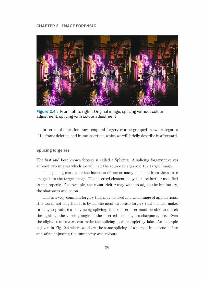
Figure 2.4 : From left to right : Original image, splicing without colouradjustment, splicing with colour adjustment
In terms of detection, any temporal forgery can be grouped in two categories[21]: frame deletion and frame insertion, which we will briefly describe in afterward.
Splicing forgeries
The first and best known forgery is called a Splicing. A splicing forgery involvesat least two images which we will call the source images and the target image.
The splicing consists of the insertion of one or many elements from the sourceimages into the target image. The inserted elements may then be further modifiedto fit properly. For example, the counterfeiter may want to adjust the luminosity,the sharpness and so on.
This is a very common forgery that may be used in a wide range of applications.It is worth noticing that it is by far the most elaborate forgery that one can make.In fact, to produce a convincing splicing, the counterfeiter must be able to matchthe lighting, the viewing angle of the inserted element, it’s sharpness, etc. Eventhe slightest mismatch can make the splicing looks completely fake. An exampleis given in Fig. 2.4 where we show the same splicing of a person in a scene beforeand after adjusting the luminosity and colours.
18

2.4. DIGITAL FORGERIES
Figure 2.5 : From left to right : Original image, various tampering usingCopy-Move
Because a splicing forgery requires many adjustments in order to look realistic,it usually leaves more traces which arguably makes it easier to detect than otherforgery types.
Copy-Move forgeries
As opposed to splicing forgeries, copy-move only involve one image.
In a copy-move forgery, one region (the source) is copied and paste onto anotherregion (the target). The duplicated element can be translated, rotated, scaled ortransformed. As for splicing, the duplicated element may be modified to fit betterin the scene.
A copy-move forgery is usually much easier to create than a splicing forgery.Even though it seems quite limited, it is actually quite versatile. One can use acopy-move to fool on a quantity, to hide an element, or to alter a text field. Suchforgeries can be seen in Fig. 2.5.
Because the duplicated element comes from the same image, it generally re-quires less modification to create a convincing forgery. Copy-move will thus usuallyproduce fewer detectable artefact than splicing.
19

CHAPTER 2. IMAGE FORENSIC
Object-Removal Forgeries
As for copy-move, object-removal only involves one image. Object-removal consistsof the suppression of one element from an image.
Such forgery can be performed using a copy-move but there exists other meth-ods to create this forgery. In particular, an object removal is often performedusing an inpainting algorithm. There are many types of inpainting techniques [22]such as exemplar-based inpainting, diffusion-based, deep learning based. All thosealgorithms are used to fill a given area in an image using only information presentin that image. Exemplar-based method for example progressively fill the area bycopying and pasting extremely small patches. Diffusion-based, on the other hand,propagate the information at the boundary of the area to fill.
An object-removal forgery is extremely simple to create. In particular withmodern photo retouching software such as Photoshop or Affinity photo. An ex-ample of object removal is given in Fig. 2.6 which required only click in affinityphoto.
When the object to remove is on a relatively simple background, the resultswill most likely be impressively realistic. As for copy-move, object removal oftenleaves fewer artefact than splicing forgeries.
Face Manipulations
A last forgery category that we will consider is face manipulations. It could beargued that those are just splicing forgeries applied to facial images. And in fact,some face manipulations are effectively simply splicing.
But because those are really specific to facial images, they allow the counter-feiter to use techniques that goes beyond a simple splicing so we argue that theyare a kind a forgery on their own.
The simplest and best known facial manipulation is called a face swap. A faceswap is a simple splicing of one face onto another. Earlier face swap would onlywork for static images. With the advance of deep neural networks, it is now possibleto produce very realistic face swapping even on videos effortlessly. Those dynamicsface swapping methods are often called DeepFakes. They generally perform theswapping by using a deep neural network to synthesise a fake face in place of the
20

2.4. DIGITAL FORGERIES
Figure 2.6 : From left to right : Original image, Object-removal forgery
genuine one hence the name DeepFakes.More recently another approach to perform a face swapping as gain a lot of
attention. Instead of replacing the face of a person A by the face of a person B ina video, it was proposed to use a video of the person B and modify it accordingto a video of the person A. Such forgery is called a face reenactment as the actingof the person A is applied to the video of B rather than superimposing the face ofB onto A.
Another facial forgery is called de-identification. The objective is to removeevery element of a facial image that would allow a Face Recognition Software(FRS) to operate properly.
A last common facial manipulation is called face morphing. Face morphingcan be seen as a generalisation of a simple face swapping. Having a person A anda person B, a Face Morphing consists in the mix of the two faces. This results ina synthetic face which shares the biometry of both A and B. In chapter 6 we willdescribe more deeply this kind of forgery.
21

CHAPTER 2. IMAGE FORENSIC
Frame Deletion
Frame deletion is specific to video forgeries. As the name implies, it consists ofthe suppression of one or many frames. The deleted part can be anywhere in thevideo.
It is typically use hide parts of a video. For example, a counterfeiter may wantto tamper a surveillance video in which he appears. He would thus remove everyframe in which he is visible.
Frame Insertion
Frame insertion, on the other hand, consists of the addition of new frames insidea video. Those new frame can come from the same video or another.
The primary use for such a forgery is to create a video composite of multiplesequence. It could also be used alongside a frame deletion forgery to fill theremoved portion of the video.
2.4.2 Application in RIV systemWe will now discuss how those attacks relates to a typical RIV system.
To begin with, a counterfeiter could have three main objectives while attackinga RIV. A first goal would be to perform an identity theft. When doing an identitytheft, the counterfeiter wants to use someone’s else personal information. Anotherobjective maybe to access some service anonymously. In such case, he may providea completely fake identity. Finally, he might simply want to alter a few informationon his ID.
Depending on his objectives, the counterfeiter will tamper specific parts of thedocument or target a specific part of the RIV process. Consequently, he will alsouse specific forgery categories.
During the RIV process, we except the forgeries to targets three specific things.It is likely that either the photo on the ID document or the live acquisition of theface will be tampered. And we also expect the information on the document tobe targeted. In the next sections, we will explain how specific forgery categorieswould be applied to tamper those various elements.
22

2.4. DIGITAL FORGERIES
Figure 2.7 : From left to right : Original image, Complete replacement of thephoto, Face swapping
Alteration of the ID Documents Photo
As we mentioned, the photo present on the ID document is a probable target forthe counterfeiter as it bears a lot of information about the user. And how weexplain, face biometry plays a central role in a RIV system.
Consequently, the photo on the ID document is a vector for many attacks onthe system. For example, to perform an identity theft, the counterfeiter will mostlikely steal an ID document. Because the RIV system makes a comparison of thephoto and the user, the counterfeiter must alter the ID document to pass thisverification. To perform such an attack, the easiest way would be to perform asimple splicing by replacing the complete photograph. Such forgeries can be seenon Fig. 2.7. A more elaborate forgery would consist of a face swap. In that case,only the inner part of the face is tampered which leaves fewer traces of forgery asin Fig. 2.7.
The photo may be tampered similarly to perform a de-identification [23, 24,25]. The counterfeiter may in fact share his real information but may not bewilling to share his biometry. In such case, the live acquisition would also have tobe tampered.
Another attack that will be explored more deeply in chapter 6 is called FaceMorphing. When performing a Face Morphing, the counterfeiter will replace theID document photo by a synthetic face. His goal will be to create a document thatcould be shared by two people. This would allow two people to access servicesusing the same digital identity.
23

CHAPTER 2. IMAGE FORENSIC
Figure 2.8 : From left to right : Original document, Document with first andlast name tampered
Alteration of the ID documents variable fields
The counterfeiter may not necessarily try to fake his biometry, in fact, he may usehis own document on which he would like to change only a few information.
The motivation for such forgery could be multiple such as hiding his name,faking his date of birth or use an expired document.
In those cases, he would not need to alter either the photo on the documentnor the acquisition of his face but would rather have to tamper the text fields (orvariable fields) of the document.
The most straightforward approach to perform such a forgery is to perform acopy-move. This is in fact the easiest and most realistic way to proceed. BecauseID documents use very specific fonts, it is usually much easier to reuse lettersalready present in the document to alter some fields. An example is given in Fig.2.8. It can be seen that those forgeries are barely visible if not invisible withouttelling where they are located.
Alongside a copy-move, an object-removal might be needed to erase previoustext fields.
While Copy-Move is the preferred choice, the counterfeiter may not find theneeded letters. In such case, he would splice the new text field instead.
Alteration of the Face Acquisition
Lastly, the face acquisition may be the target of several attacks. The objectiveswould then be very similar to the ID documents photo scenario but the approachwould be very different.
24

2.5. OVERVIEW ON IMAGE FORGERY DETECTION
Because the acquisition of the face will undergo a variety of liveness detectiontest and challenges, a simple static face swap will not be enough. A more dynamicapproach is needed and the counterfeiter might thus use more advance forgerymethods.
For such forgeries, realtime face reenactment methods are the most appro-priate. Those forgeries seemed hypothetical at first, because of the complexityof older face reenactment algorithms and also because of the resource needed torun such algorithms. But recent advances of deep learning based methods madeit possible for anyone to create a convincing realtime face reenactment forgery.Freely available tools are now accessible to anyone to create such forgeries even ona modest laptop. While complete solutions are not yet available on smartphones,there already exists tools that allow 3D face landmarks detection in a web browserthat works in realtime even on a smartphone [26, 27]. We thus can reasonablyexpect to see convincing 3D face swapping tools to be available on smartphonesin the next future.
2.5 Overview on Image Forgery DetectionIn this section we will give a general overview of digital image forgery detection.A more thorough state of the art will be presented on a per chapter basis as eachchapter addresses very different topics.
We will start by introducing the image formation pipeline by dividing it intothree main steps. We will first briefly introduce the hardware part of an acquisitiondevice and how it impacts the raw image formation. Then we will present thevarious post-processes which are included in the software of the acquisition device.Finally, we will talk about the compression stage which is necessary to reduce theinformation needed to store the digital media.
After, we introduce the common classification of image forgery detection algo-rithms. From this we will derive three categories which differ based on the studiedartefacts.
25
CHAPTER 2. IMAGE FORENSIC
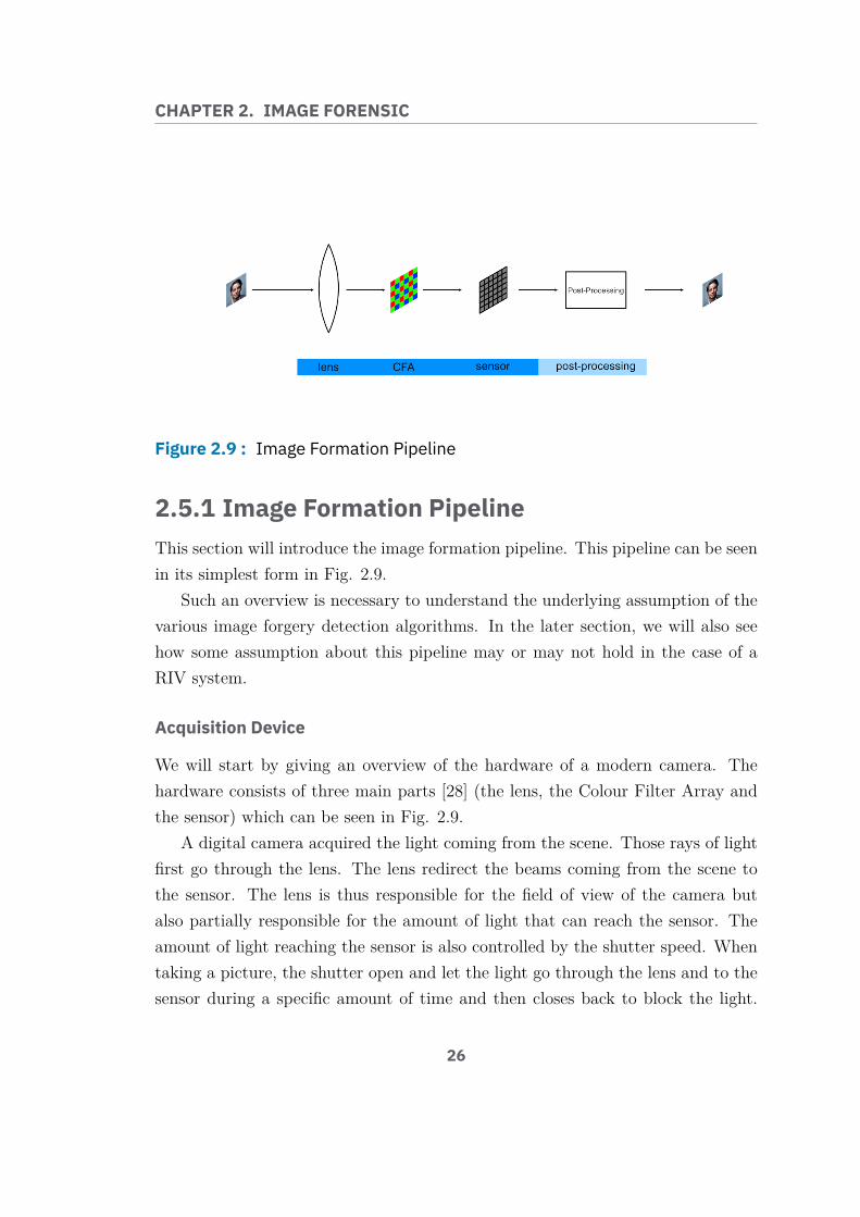
Figure 2.9 : Image Formation Pipeline
2.5.1 Image Formation PipelineThis section will introduce the image formation pipeline. This pipeline can be seenin its simplest form in Fig. 2.9.
Such an overview is necessary to understand the underlying assumption of thevarious image forgery detection algorithms. In the later section, we will also seehow some assumption about this pipeline may or may not hold in the case of aRIV system.
Acquisition Device
We will start by giving an overview of the hardware of a modern camera. Thehardware consists of three main parts [28] (the lens, the Colour Filter Array andthe sensor) which can be seen in Fig. 2.9.
A digital camera acquired the light coming from the scene. Those rays of lightfirst go through the lens. The lens redirect the beams coming from the scene tothe sensor. The lens is thus responsible for the field of view of the camera butalso partially responsible for the amount of light that can reach the sensor. Theamount of light reaching the sensor is also controlled by the shutter speed. Whentaking a picture, the shutter open and let the light go through the lens and to thesensor during a specific amount of time and then closes back to block the light.
26

2.5. OVERVIEW ON IMAGE FORGERY DETECTION
Once the light has gone through the lens, it is filtered by the Colour Filter Array(CFA). The CFA physically filter the red, green and blue light before being finallycaptured by the sensor.
The light received light by the sensor is subject to two perturbations. The firstone is inherent to the physic of light and is called the shot noise. The shot noise isdue to the fluctuation of the number of photons reaching each individual pixel ofthe sensor. Another perturbation is due to the CFA. Because the manufacturingof this filter cannot be perfect, small differences in pixel intensity may be observedfor nearby pixels. Those imperfections produce a fixed noise-like pattern calledthe Photo Response Non Uniformity (PRNU) which is unique for each camera.This pattern will be present for every image taken by the same device.
The sensor counts the number of photos reaching each individual pixel. Thisinformation is then electrically amplified to map a given photon count to a givenpixel intensity. The mapping is usually called the Camera Response Function(CRF) [29]. The CRF varies from one camera manufacturer to the other. Duringthis amplification two perturbations occur. The first one is called the dark currentnoise. Dark currents are small current fluctuation presents in every electronicdevice. In the case of a camera sensor, the dark current gets amplified with theremaining of the information. The other source of noise is called the readout noiseand is due to random errors while reading the pixel information from the sensor.
At the end of the acquisition of an image, the RAW pixel data is thus affectedby four different sources of noise. We will see later that those can be used toauthenticate a digital image.
Post-processes
Once the RAW image data has been acquired, it must go through a few post-processes in order to be shown as a regular RGB image on a screen.
First of all, the image must first be demosaiced. As we mentioned, the lightgoes through the CFA before reaching the sensor. The CFA is used to separatethe light into three distinct colours i.e. red, green and blue.
The CFA filter the light following a specific pattern (e.g. the Bayer pattern).The RAW image is thus a single image of size N ×M where each pixel record the
27

CHAPTER 2. IMAGE FORENSIC
Figure 2.10 : From left to right : Mosaiced red channel, Mosaiced greenchannel, Mosaiced blue channel, Demosaiced image
intensity of one of the three colours.A demosaicing algorithm is used to infer three colour channels of size N ×M
from this single RAW image. Basically, the demosaicing algorithm first extracteach individual colour information from the single-channel RAW image and theninterpolate the missing pixels to produce three N ×M images. On Fig. 2.10 wecan see the three channels extracted from the single-channel raw image. Thosechannels are interpolated and combined to produce the RGB image.
Once the image is demosaiced, it is usually white balanced. Depending onthe lighting condition, an unwanted colour-cast may be present in the image.White balancing is used to remove such colour casts. Typically, a white balancingalgorithm finds a set of pixels for which it assumes that their true colour is neutralgrey. Then it computes a scalar for each channel and correct those pixels to makethem neutral grey.
A last-processing step is called the gamma correction. The gamma correctionis a non-linear operation applied to all pixels. It is typically a simple power law :
Iout = Iγin. (2.1)
The human visual system is more sensitive to differences of darker shades thanbrighter shades. The gamma correction thus takes advantages of that to compressthe highlights in order to use more space to encode darker shades. The impact ofgamma correction can be seen on Fig. 2.11.
Image Compression
The resulting post-processed RAW images from the two previous steps usuallyresults in a relatively large file. In fact, at this point, a lot of unnecessary infor-
28

2.5. OVERVIEW ON IMAGE FORGERY DETECTION
Figure 2.11 : From left to right : Raw image with linear intensity,Gamma-corrected image
mation is encoded in the file. For instance, the RAW image has been corruptedby some perturbation noises that are barely visible to the human eye.
In order to reduce file sizes, image compression algorithms are often used. Infact, it is very unlikely that a digital media will never be compressed during itslife cycle. We thus consider the compression as part of the acquisition process.
On famous image compression algorithm is the JPEG compression. The JPEGcompression first convert the image into the YCbCr colour space. In this space,the image is separated into one luminance channel (Y) and two chroma channels(Chroma blue and Chroma red resp. Cb and Cr). Because the human eye is moresensitive to luminance variation, JPEG first highly reduce the size of the chromachannels which is sometimes called chroma subsampling.
Once the chroma subsampling is performed, the JPEG compression also re-duces the file size by removing high frequencies which are imperceptible.
To do so, the image is first sliced into non-overlapping blocks of size 8 × 8.Each block is then transformed using a Discrete Cosine Transform (DCT). Thoseblocks are then quantified to remove high frequencies. At the end of this process,the image contains many null pixels. This can be further compressed using losslessentropy coding such as the Huffman coding.
The JPEG compression algorithm is a fairly old algorithm, but it is still heavilyused. Nowadays many algorithms use principle introduced by the JPEG algorithm.
In this thesis we will study the H.264 video compression algorithm in chapter7 which has many similarities with JPEG. As for JPEG, H.264 also uses chroma
29

CHAPTER 2. IMAGE FORENSIC
Figure 2.12 : All categories of image forgery detection techniques
subsampling and also compress the luminance using the DCT on non-overlappingblocks.
2.5.2 Forgery Detection CategoriesThere exist many different categories of image forgery detection methods. Anoverview of all those categories can be seen in Fig. 2.12.
We can see two main image forgery detection families. The passive approachand the Active approach.
The active approach can be categorised into two main families. The approachbased and watermarking and the methods using cryptography. The idea of bothfamilies is to add an element to the media that cannot be tampered. This requiresto have access to the media and to be certain that the media is authentic at thattime. If the idea is similar, the methods used are not. Digital watermarks alter
30

2.5. OVERVIEW ON IMAGE FORGERY DETECTION
the pixel information to insert what is called a watermark. A watermark can bevisible such as clear text on top of the image or invisible. A watermark can befurther classified based on its robustness. For digital tampering detection, fragilewatermarks are often used. Such watermarks are destroyed even by the slightestalteration of the media. Cryptography based approaches, on the other hand, donot alter the pixel information. Instead, the media is either encrypted using acipher algorithm so it cannot be altered without knowing the encryption key. Orit can be digitally signed, so any alteration would be detected by a mismatchbetween the tampered media and the signature.
On the other hand, passive approaches are based on knowledge about theimage formation or assumption on the tampering process. We can differentiatefour passive detection categories which we will describe in the next sections.
Physic Based Methods
The first category is the physic-based methods. Those methods rely on physicalprinciples to detect forgeries. With some knowledge on what kind of scene hasbeen acquired, it is in fact possible to model some physical property that elementsin the scene should respect.
Many methods rely on the analysis of the lighting environment [30, 31, 32, 33,34, 35, 36].For example, for an outdoor image during a sunny day we can expectthe light direction to be consistent across the image because we can assume thelight from the sun to originate from an infinitely far point. Similarly, for an indoorimage with people on it, we could look for inconsistencies in the reflection in theeyes to see if a person has been added to the scene . For the detection of deepfakes,authors of [37] proposed to study the inconsistent face pose due to the imprecisionof the generation process.
Those methods are extremely specific as they model physical property for well-defined scenarios. One advantage of those approaches is that they are completelyindependent of the camera, the media type (image or video) and even the compres-sion used. They rely on mistakes made by the counterfeiter that can be extremelyhard to avoid (e.g. inconsistent lighting in a splicing).
31

CHAPTER 2. IMAGE FORENSIC
Camera-Based Methods
Camera-based methods focus on the acquisition device. They will either try tomodel the image formation pipeline as a whole or instead focus on very specificartefacts. They would model how an image would normally be formed and lookfor abnormality regarding this model.
For example, some methods [38, 39] modelled how the chromatic aberration dueto the lens should be oriented and exposed the forgery by looking for inconsistentorientation. Some approaches [40, 41, 42, 43] assumed that the estimated CRFmust be unique for every sub portion of an image and try to detect if there exist asignificantly different estimated CRF to expose traces of forgeries. Many methods[44, 45, 46, 47, 48, 49] try to infer the CFA grid and try to expose misaligned ormismatch area as traces of forgeries. Other uses multiple photos from one deviceto estimates the PRNU [50, 51, 52, 53, 54, 55] which allow them to authenticatelater images from the same device or to detect forgeries. Finally, many methods[56, 57, 55, 58, 59, 60] try to expose inconsistencies in the noise as evidence.
The performances of such methods varies greatly depending on the studiedartefact. In general, those methods work best when the image quality is sufficientenough. The advantage of those methods is that they provide great evidence offorgeries which are easily interpretable.
Pixel-Based Methods
Unlike the previous two categories, pixel-based methods makes no assumption onthe acquisition media nor the physical properties of the acquired object. Rather itmakes assumptions about the tampering process that the counterfeiter might use.
For example, Copy-Move detection methods assume that the duplicate partwon’t be altered much after being pasted. They thus look for abnormally similarelements in the image [61]. Some methods [62, 42] assume that the counterfeitermay blur the boundary of a splice object or even the whole object to seamlesslyblend it. They will thus look for traces of artificial blur. Similarly, some methods[63, 64] will look for inconsistent white balance assuming that the counterfeiterwill try to match the spliced object’s colours.
By definition those methods are generally specific to a certain forgery. Like
32

2.6. IMAGE AND VIDEO FORGERY DETECTION IN RIV SYSTEM
physic-based methods, they make no assumption on the device nor the compres-sion.
Format-Based Methods
Finally, the format-based methods focus on the compression applied to the media.They thus must assume that the media was authentic prior to the first compression.
Similarly to camera-based approach, they model either the whole compressionprocess or only a specific part. From there, they will look for inconsistencies insome JPEG artefacts [65], look for traces of double compression [66] or detectprevious traces of compression in uncompressed images [67].
In general, those methods are extremely effective. One major disadvantage ofsuch method is that they cannot detect forgeries which occurred prior to the firstcompression. Although, this can be convenient as those methods can be used in amore active manner by constraining the compression parameters to specific valuesand authenticate the media based on this knowledge.
2.6 ImageandVideoForgeryDetection inRIVSystem
In the previous sections, we presented the standard architecture of a RIV system.We showed that two scenarios could be considered. The acquisition device could beeither control or uncontrolled. As explained, having no control over the acquisitiondevice makes the authentication process much harder. This scenario must thenbe avoided if possible. We will thus only consider RIV system with controlledacquisition device.
We then gave an overview of digital forgery and how those forgeries could beused against a RIV system. From there, we presented the image formation processas a whole and presented the various approaches to detect image forgeries.
We already have an intuition of how and what the counterfeiter might tam-per and we introduced the various methods for forgery detection. To select themost appropriate detection approach, we have yet to consider at which point the
33
CHAPTER 2. IMAGE FORENSIC
counterfeiter will attack the RIV system.We will first look at where a RIV system using a controlled acquisition device
could be compromised. After, we will see how this influence the choice of oneforgery detection category to secure a RIV system.
Based on those observations, we will finally present the motivation behind eachchapter of this thesis.
2.6.1 Attacks against RIV systemsAs already mentioned we only consider RIV systems with controlled acquisitiondevice as we believe that uncontrolled device cannot allow the creation of a secureprocess.
As we mentioned, in a controlled acquisition device scenario the RIV providermay use the user’s terminal as the acquisition device. In such case, an applicationwould be installed on the user’s terminal. This application would be responsiblefor controlling the acquisition device. In this context, it is unwise to ignore thepossible for a counterfeiter to compromise the device itself. A more detail pipelineof the acquisition process in such a scenario is given in Fig.
We can see that the image is produced by the acquisition device. The RIVprovider’s app can control the acquisition device but as no control over the user’sterminal as a whole. Once the acquisition is performed, the media is handledby the application which later sends it to a distant authentication server. Onceagain, the application can control the sending process still can’t control the wholeterminal. Consequently we can expect the counterfeiter to attack the system atthree different points assuming that the distant server cannot be compromised.
The earliest attack can occur if the counterfeiter compromise the terminal it-self. In such case, the RIV provider’s application cannot even trust the incomingmedia stream. Similarly, the counterfeiter may compromise communication chan-nel between the user’s terminal and the distant server by performing a man in themiddle attack. In that case, the stream could be intercepted directly on the user’sterminal or through an independent system in between the user’s terminal and thedistant server. A last approach would consist of the alteration of the applicationitself. The application would thus directly send tampered media.
34

2.6. IMAGE AND VIDEO FORGERY DETECTION IN RIV SYSTEM
When the media finally reaches the authentication server, we do not knowwhich of those scenarios may have occurred. In the best-case scenario, the deviceis not compromised prior to the application and the application itself is not com-promised either. In that case only a man in the middle attack is possible to tamperthe digital media. We can thus use any type of forgery detection category. In aless optimistic scenario, the acquisition device is compromised. In that case, notall forgery detection methods may be appropriated. Camera-based methods andformat-based methods become less relevant because we cannot trust the streamin the first place. In fact, the counterfeiter may have been able to apply somecounterforensic methods to hide traces of forgery. We will see in chapter 6 howsuch counterforensics can completely fool camera-based approach. Camera-basedmethods can still be somewhat relevant as the counterfeiter may not be able tocompletely hide is traces. It is still interesting to use format-based method as wewill never know for sure if the tampering is applied after or before the applicationbut we must keep in mind that in the latter case such forgery detection approachwon’t do much.
In any case, physic-based and pixel-based method stay relevant as no assump-tion on the acquisition device is made. Because the acquisition device is controlled,the user can be asked to perform specific action that would facilitate physic-basedor pixel-based detection later on.
2.6.2 Securing RIV SystemsAs we saw, when considering a RIV system with a controlled acquisition device,pixel-based forgery detection methods seems more appropriate. Furthermore, wewill be more interested in methods that can be used to detect forgeries in a textor facial manipulations. Even though one of the main focuses of this thesis is tosecure RIV systems, we also took part in the ANR-16-DEFA-0002 project calledDEFALS which focuses on general image forensic. For those reasons we exploredvarious forgery detection methods during this thesis often with a strong focus onID documents forgeries but also more general approaches.
The security and reliability of a RIV system rely on effective image tamperingdetection methods. To assess the effectiveness of such methods, it is necessary to
35

CHAPTER 2. IMAGE FORENSIC
be able to evaluate those methods on representative data. As part of our workin the project DEFALS, we realised that very few datasets were available at thetime. The first work of this thesis was thus to propose a dataset for generalimage forensics. Because we are interested in RIV security, we also include FacialManipulation in this dataset. This dataset will be presented in chapter 3.
As we explain, we were then interested in forgery detection methods that focuson text and facial forgeries. When tampering a text, we showed that the easiestand yet most convincing approach was to use a Copy-Move forgery. In the contextof a RIV system, the copy-move would be applied to an ID document . In suchimages, many elements look really similar and are called Similar but GenuineObjects (SGO). Copy-Move detection methods were shown to be less effectivein the presence of SGO. We thus decided to address the challenge of SGO forcopy-move detection in chapter 4. We also proposed a new dataset of forged IDdocuments with Copy-Move to promote research in that field.
Before tampering a text, it is likely that the counterfeiter would first have toerase what was already written. He would then use an object-removal forgery. Westudy the possibility to expose object-removal forgery through the analysis of thereflectance of an image in chapter 5.
One well-known attack against ID document portrait is the Face Morphingattack. In Chapter 6, we study this attack by proposing a novel pixel-based ap-proach. One specificity of the Face Morphing forgery is that it might have beenused during the creation of the ID document. In such cases, the attack is notdigital. We studied how our method and other state-of-the-art approach react todigital counterforensic techniques and then questioned the applicability of thosemethods for general Face Morphing detection.
Finally, we wanted to evaluate how we could use a sequence of images toenhance the detection of forgeries. The acquisition of a sequence of images ratherthan a single image seems indeed intuitive in a RIV system as ID documentsand living peoples are not static elements. In fact, an ID document containsdynamic elements such as holograms and variable inks. With the publication ofthe first PVID regulation which imposed the use of video for RIV system, we finallyproposed a new method to detect a double H.264 video compression in chapter 7.Such a format-based method might not be ideal in the case of a RIV system but
36

2.7. CONCLUSION
is nonetheless interesting as a first approach to video authentication.
2.7 ConclusionThe main focus of this thesis is the use of image forgery detection in RemoteIdentity Verificaton system. We first gave a formal definition of a RIV system andthen presented the common architecture of such a system. We saw that a RIVsystem’s main goal was to authenticate a user against his ID document. To doso, two streams are acquired. One stream containing the ID document and onestream containing himself. The RIV system starts by verifying he ID documentand perform some liveness verification on the person. Only then is the personcompared against the document. In general the comparison is performed usingface biometry. We thus except the document or the person to be the target of anycounterfeiter.
After, we presented the structure of an ID document. We gave a brief overviewof the various security features and explains the different types of document frauds.We explained how the security features of the document makes a physical tam-pering difficult and how, on the other hand, a digital alteration was much simplerand accessible. This motivates the study of digital forgeries in the case of a RIVsystem.
We thus gave an overview of the common image forgery methods and howeach of these relates to the case of a document tampering. We then introduced thecomplete image formation pipeline and presented the main image forgery detectioncategories.
We then presented how a counterfeiter could attack a RIV system when theacquisition device is controlled. From there, we explain that some forgery detectioncategories may not be the most appropriate in the case of a RIV system. We finallypresented the motivation behind each chapter of this thesis. We explained thata lack of image forgery datasets motivated us to develop the DEFACTO datasetin chapter 3. Then to detect text forgeries on the ID documents we proposed tostudy copy-move forgeries in chapter 4 but also object-removal forgeries in chapter5. The other commonly attacked element of ID documents is the portrait. We
37

CHAPTER 2. IMAGE FORENSIC
thus decided to study Face Morphing forgeries in chapter 6. Finally, in chapter 7,we decided to study the double compression of H.264 video as a first step towardthe transition to video imposed by the PVID regulation.
38

CHAPTER 3DEFACTO Dataset
3.1 Introduction . . . . . . . . . . . . . . . . . . . . 40
3.2 Related Work . . . . . . . . . . . . . . . . . . . 41
3.3 Dataset Overview . . . . . . . . . . . . . . . . . 42
3.4 Automating forgery creation . . . . . . . . . . . . 43
3.5 Conclusion . . . . . . . . . . . . . . . . . . . . 49
39

CHAPTER 3. DEFACTO DATASET
3.1 IntroductionThis thesis focus on the detection of image forgery in the context of a RIV system.Even though the content of the studied image is specific, the detection methodmust stay general. In fact, in some RIV systems where the acquisition device iscontrolled camera-based or format-based method will arguably be more appropri-ate than method based on some knowledge about the image content.
For this reason, we actively participate in the project ANR-16-DEFA-000 calledDEFALS which stands for “Détection de FALSification dans des images”1. Thegoal of this project was to propose image forgery detection methods. We tookpart in this project as members of the DEFACTO team. The DEFACTO teamwas a partnership between the University of Technology of Troyes, EURECOM andSURYS. The University of Technology of Troyes would propose classical forgery de-tection methods whereas EURECOM would perform research deep learning basedapproach.
Deep learning methods requires a large number of representative data to beeffectively trained. At the time very few datasets for image forgery detection wereavailable and those would not represent well the images of the DEFALS challenge.We thus decided to construct a novel public dataset.
The objectives for this dataset were multiples. Firstly, it had to be large andproperly annotated in order to be able to train a deep learning method on it.Secondly, it had to be representative of the DEFALS challenge. This implies thata wide range of forgeries had to be proposed but also that those forgeries had tobe convincing.
The creation of a convincing and properly annotated forged image is extremelytime consuming. Even the simplest copy-move of a letter on an ID document couldtake about five minutes. Previous datasets were created by hand but only consistedof a maximum of about 2000 images. Because the DEFACTO dataset was meantto train deep learning methods, we targeted a minimum of 200000 forged images.By assuming the creation time of a single forgery to be five minutes, it would thentake more than 16000 hours for a single person to produce a total of 200000 forged
1English translation : Detection of forged images
40

3.2. RELATEDWORK
images. We thus quickly decided to develop an automatic tampering process.We will first give a brief overview of the dataset (forgery, categories, annota-
tions, etc.). Then we will describe in greater detail how we developed our automatictampering algorithm in order to produce meaningful forgeries in each category. Fi-nally, we will conclude on some perspectives on how to further develop this work.
3.2 Related WorkSeveral publicly available datasets exist, the first one was the Columbia GrayDataset [68]. It contains only splicing forgeries, no ground truth and images wereonly in grayscale. Two years later in 2006, they released a new version calledColumbia Colour Dataset [41] to extend the first one.
CASIA V1.0 and V2.0 [69] were introduced in 2009 to propose a larger (about6000 tampered images) datasets with more realistic tampering. It contains splicingand copy-move forgeries with post-processing (blurring along edges or in otherregions). They are still widely used as they contain a large number of forgedimages and their associated authentic images. Many datasets have been releasedlater which only propose copy-move forgeries (MICC [70], IMD [71], CoMoFoD[72], COVERAGE [73], GRIP [74], FAU [71]). The National Institute of Standardsand Technology (NIST) also released multiple datasets in the context of the MediaForensic Challenge 2019 [75]. It includes both image and video manipulations.While some parts are accessible upon a simple request, one needs to participate inthe challenge to get access to the most recent version of the data.
Previously cited datasets were all made manually by the authors. The WildWeb dataset [76] released in 2015 was the first to introduce the real world tamperedimages. This dataset contains about 10000 images for which they manually createdthe ground truth binary masks to locate the forgery. More recently, the PS-BattleDataset [77] was released. In this work, the author collected images from theactive Reddit thread Photoshop Battles. In this thread, people try to producethe best photo manipulation from a given image. They gathered more than 10000original images and 90000 tampered images. This dataset is meant to provide along-lasting benchmark dataset and will keep growing with the Reddit community.
41

CHAPTER 3. DEFACTO DATASET
In this chapter, we propose a novel dataset called DEFACTO meant for thestudy and training of image manipulation detection algorithms. We tried to pro-duce a large amount of semantically meaningful forgeries for each category wedefined in 3.3.1.
3.3 Dataset Overview
3.3.1 Forgery categoriesIn this dataset, we wanted to cover most of the common methods that one coulduse when creating a forgery. Hence, four major categories of forgeries have beenconsidered : copy-move, splicing, object-removal and morphing.
Copy-move forgeries consist in the duplication of an element within the image.For splicing, one portion of an image is copied and pasted onto another image.In object-removal, an object is removed from the image by the use of inpaint-ing algorithms. Finally, morphing consists in warping and blending two imagestogether. For each forgery, post-processing may be applied (rotation, scaling, con-trast ...). Those four categories can be seen as elemental forgery operations. Animage composite would most likely be a composition of those basic operations.As the methods to detect those categories can be quite different, we decided tofirst construct a dataset where each image as only been forged using one of thosecategories only. The whole dataset content is detailed in Table. 3.1. Generatingthose forgeries in a random manner is simple. This would allow us to produce alarge number of forged images but they would be semantically meaningless andeasy to detect by the human eyes. We wanted to create a dataset with meaningfulforgeries and challenging for the human eye by removing most of the traces thatan automatically generated forgery could contain. This goes from generating aproper segmentation of the object to select where to paste it in the final compositeimage. We believe that some mistakes (strong edges of the forged element) couldintroduce a bias in learning algorithms and wanted to address this issue.
42

3.4. AUTOMATING FORGERY CREATION
3.3.2 AnnotationsOne advantage of automatically generated forgeries is that we can provide pre-cise annotations for each image. In our dataset, each generated forged image isaccompanied by diverse annotations to give further information on the tamperingprocess.
General information
for each image, a detailed JSON file is provided. In this file, every operation madeon the ground truth images are listed. Parameters used by each operation aredetailed.
Localisation
every image is also accompanied by one or more ground truth binary masks.One binary mask serves to localise the forgery under the probe_mask directory.For splicing, copy-move, face morphing and swapping, a binary mask under thedonor_mask directory gives the localisation of the source. Object-removal hasa binary mask under the inpaint_mask directory which localise what has beenfilled by the inpainting algorithm.
3.4 Automating forgery creation
3.4.1 Segmenting meaningful objectsTo produce meaningful forgeries, we took advantages of MSCOCO dataset [78].They collected more than 300,000 non-iconic images from Flickr. Afterwards,they defined 91 object categories of objects and annotated all the images. Thoseannotations include the segmentation of the objects that we use as a base toproduce our forgeries. The raw segmentation annotation cannot be used directlyto generate a forgery as they are not precise enough (Fig. 3.1a). They need to beprocessed to obtain more suitable segmentation.
43

CHAPTER 3. DEFACTO DATASET
Table 3.1 : Number of images per category in DEFACTO
Forgeries Copy-Move Inpainting Splicing MorphingImages 19000 25000 105000 80000
3.4.2 Refining segmentationMSCOCO has over 2,000,000 object instances. Refining all annotations or even asmall part by hand was not possible. We employed an alpha matting technique torefine the masks. Alpha matting consists in finding the foreground of an image
I = Fα +B(1− α) (3.1)
where I is the image, F the foreground, B the background and α the alphamatte.This equation cannot be solved without any prior information. Thus, alpha mat-ting techniques rely on a user input to define areas that are known to be part ofthe foreground F and areas that are known to be part of the background B. Thoseinputs can go from simple lines to what is called a trimap.
Trimap defines three areas: the foreground, the background and an unknownarea (Fig. 3.1b).
Based on the given foreground and background areas, the alpha matting algo-rithm automatically affects a value to every unknown pixel to produce the finalalpha matte.
We used MSCOCO raw segmentation to construct the trimaps. First theforeground region is obtained by applying a morphological erosion to the rawMSCOCO mask to make sure that no background pixel is added to the foregroundregion. The unknown region is obtained by applying a morphological dilation tothe raw mask (Fig. 3.1b). We then use a modified version of [79] to produce thealpha matte. This alpha matte is finally used to produce a much more convincingsegmentation of the objects. This allows us to produce forgeries that are morepleasant (Fig. 3.1d).
Having a good segmentation of the objects is a first step toward the automaticgeneration of meaningful forgeries. Though it is not enough, removing or copying
44

3.4. AUTOMATING FORGERY CREATION
(a) Raw MSCOCOannotations
(b) Generated trimap (c) Copy-move withoutalpha matting
(d) Copy-move withalpha matting
Figure 3.1 : MSCOCO mask refinement
those objects in a random manner would most certainly produce bad results. Foreach category of forgery, a set of rules had to be applied to maximise the chancesof producing good results.
3.4.3 Object RemovalThere are six main categories of image inpainting [80][81][82][83] techniques. Tex-ture synthesis based inpainting, exemplar-based inpainting, Partial DifferentialEquation (PDE) based inpainting, hybrid-inpainting semi-automatic and fast in-painting and deep learning based inpainting.
Semi-automatic and fast inpainting methods were not usable in our case as theyrely on a strong user interaction. PDE based inpainting are not able to fill a largemissing region. Texture synthesis based methods are meant to fill the region withhomogeneous textures which is something we cannot ensure in our case. Hybridinpainting methods are a combination of PDE and texture synthesis and thus doesnot suit our needs. Deep learning based methods are efficient but depend on theperformances vary depending on the dataset used for training and the targeted
45

CHAPTER 3. DEFACTO DATASET
images to inpaint.
We thus used an exemplar-based inpainting method [84] as they have provedto be effective in various conditions and are still in common retouching software.
Inpainting methods are more efficient if the subject to remove is on a relativelysimple background (Fig. 3.2). To produce convincing forgeries, we excluded ob-jects for which the background was too complex. A border region is extracted bydilating the raw MSCOCO mask, and the standard deviation is computed withinthis region. Objects for which the standard deviation was below a fixed thresholdwere kept.
3.4.4 Copy-move
For copy-move, the raw MSCOCO annotations were first used to produce theforgeries. Resulting images were almost systematically unpleasing due to strongvisual artefacts on the object’s borders (Fig. 3.1c). For this reason we had touse alpha matting as described in 3.4.2 to obtain much better results in mostcases (Fig. 3.1d). At first, objects would be copied and paste randomly withinthe image. This would cause the creation of images that were often semanticallyincorrect (e.g. people walking in the sky ...). To reduce chances of producing thosekinds of images, we constrained the location of the forgery to be on the same axisas the source object (Fig. 3.3a and 3.3b). Decision to stay on the x or y axis isbased on the width and height of the object. If width > height then the object isduplicated on the x axis otherwise it is duplicated on the y axis. As for the objectremoval, we only kept objects on a fairly simple surroundings. This is to prevent tocopy-move an object that is too tightly coupled with its context. For instance, inthe MSCOCO dataset, a person and his backpack would be annotated separately,thus copying the person would not produce a good forgery as the backpack wouldbe missing. Those rules allowed us to produce convincing copy-move forgeries (Fig.3.3).
46

3.4. AUTOMATING FORGERY CREATION
(a) Ground truth image (b) Inpainted image
Figure 3.2 : Example of inpainting
3.4.5 SplicingSplicing is arguably the most complex forgery to generate automatically. Whencreating a splicing, an object from an image is pasted onto a new one. Whenmanually creating the splicing, we can make sure that the target image has asimilar point of view, lighting condition and so on. Those are essential to make arealistic splicing. Unfortunately, it is extremely difficult to assess all those elementsautomatically, thus it is extremely hard to produce good splicing forgeries. Toaddress this issue, we decided to limit the MSCOCO categories used to producesplicing forgeries. We kept categories for which the objects appearance does notvary or depend too much on the point of view and the context. For example, aperson could be standing, sitting, running ... and for each case, the appearancewould vary a lot depending on the point of view to make it almost impossible togenerate a convincing forged image. But if we take a sports ball, which is spherical,it will always look about the same and will be more easily spliced onto anotherimage. Or if we take a bird which is either standing or flying, cutting and pastingit onto an image already containing birds has reasonable chances of producing anacceptable result. Objects are either pasted on an object of the same categoryor randomly pasted in a relatively smooth area to avoid pasting an object ontoanother one (Fig. 3.4b).
3.4.6 Face MorphingImage morphing was originally used to produce smooth transitions between manyimages. One of the first notable appearances was in the Michael Jackson music
47

CHAPTER 3. DEFACTO DATASET
(a) Copy-move of thekite on the y axis
(b) Copy-move of thebird on the x axis
Figure 3.3 : Example of copy-move
(a) Ground truths (b) Tampered
Figure 3.4 : Example of splicing
video “Black or White” where the method described in [85] was used to morphpeoples together. Nowadays, face morphing as received particular attention amongthe forensic community [86]. As shown in [87], Automatic Border Control systemsare very vulnerable to face morphing attack. Thus we decided to include suchforgeries into our dataset.
We gathered public figure portraits on IMDB website and selected 200 frontfacing actors with a relatively neutral expression as a base to generate our facemorphing forgeries.
The complete face morphing process can be seen in Fig. 3.5. Given two facesA and B, we used Dlib [88] to extract a set of facial landmarks. Thanks to thoselandmarks, the two are first roughly align with respect to their eyes (Fig. 3.5c). A
48

3.5. CONCLUSION
(a) Face A (b) Face B (c) Roughalignment offaces A and B
(d) Precisealignment offaces A and B
(e) Withoutcolor balance
(f) With colorbalance
Figure 3.5 : Automatic Face Morphing creation
weighted average by a factor α ∈ [0, 1] of the two sets of landmarks is computed,and the two faces are warped [89] to this weighted average to precisely align them(Fig. 3.5d). Finally, the two faces are alpha blended using the same factor α. Alocal RGB scaling is performed to better take the skin tone into account. Thefactor α allows us to decide which face’s biometric traits are more visible. A α
value of one produces what is commonly called a face swapping.
3.5 ConclusionEarlier image forgery detection methods were mostly based on knowledge of theimage format, the camera properties, etc. Many researchers thus published theirmethods alongside with a handmade dataset representing their use case. As aconsequence, there were no large datasets that were publicly available.
To our knowledge, the first initiative to propose such a dataset was the Photo-
49

CHAPTER 3. DEFACTO DATASET
shopBattle dataset. They gathered real-world tampered images from the internetand managed to create a dataset of over 80000 images which is perfect to evaluateforensic algorithms.
More recently, researchers have started to develop image forgery detectionmethod based on deep learning approach. For those, a large dataset of repre-sentative example is needed. Apart from the PhotoshopBattle dataset, no otherlarge datasets existed. Unfortunately, even though the PhotoshopBattle datasetis excellent for evaluation purposes, it does not provide enough annotation neededto train a deep neural network.
As part of the project ANR-16-DEFA-000 we thus developed a dataset of over200000 images. We developed an automatic tampering algorithm which couldgenerate convincing forgeries with exact annotations. Since we released the DE-FACTO dataset, another large dataset (IMD2020) has been released. We thinkthat the DEFACTO dataset along with the IMD2020 and the PhotoshopBattledataset now allows for proper training and evaluation of deep-learning-based de-tection algorithms.
But future works are still needed. In particular, more work on the imageprovenance is needed. At the moment, both the IMD2020 and the DEFACTOdataset gathered the ground truth images on the web. What we thus consideras a ground truth is in fact already advance in the image acquisition pipeline.The demosaicing has been performed, some global adjustment may have beenperformed and a first compression may have been applied. Ideally, all forgedimages should be created from raw input.
Initially we wanted to develop the DEFACTO dataset using the raw RAISEimage dataset but without annotation we could only generate completely randomforgeries. One of the objectives was to develop an automatic algorithm that wouldstart from the raw image and apply post-processing such as resampling, globalenhancements, compression or local forgeries successively. This would allow us togenerate a precise history of the image or even playback the tampering processuntil a certain point and so on. Interestingly, the JSON files in the DEFACTOdataset are actually traces of prior works toward that direction.
Future work may focus on the development of such a tool rather than develop-ing more dataset. A flexible enough tool may allow researchers to design tampering
50

3.5. CONCLUSION
scenarios from start to finish and apply those scenarios on already existing rawimage dataset. This would be extremely beneficial for future research.
51


CHAPTER 4Copy-Move detection on ID Documents
4.1 Introduction . . . . . . . . . . . . . . . . . . . . 54
4.2 Related work . . . . . . . . . . . . . . . . . . . 55
4.3 Overview of the method . . . . . . . . . . . . . . 57
4.4 SIFT Detection. . . . . . . . . . . . . . . . . . . 58
4.5 Filtering with a local dissimilarity map . . . . . . . . 60
4.6 Experimentation . . . . . . . . . . . . . . . . . . 64
4.7 CMID dataset . . . . . . . . . . . . . . . . . . . 65
4.8 Dataset overview . . . . . . . . . . . . . . . . . 67
4.9 Baseline results . . . . . . . . . . . . . . . . . . 70
4.10 Conclusion . . . . . . . . . . . . . . . . . . . . 74
53

CHAPTER 4. COPY-MOVE DETECTION
4.1 IntroductionCopy-Move is one of the main image forgery categories. Even though this techniqueseems rather simple and quite limited, it is actually one of the more versatileand most used tampering techniques. In its simplest form, copy-move is used toduplicate some of the image content. To change some quantities (e.g. turn afew people into a crowd) or to alter some text for which we do not have accessto the original fonts. In more advanced composites, copy-move is typically usedas a way of removing something from an image by progressively hiding it behindsmall copied and pasted elements. For example, the widely used clone stamptool in software such as Photoshop, Affinity Photo or GIMP allows the user tosimply create a copy-move forgery and is often used to correct small elementssuch as freckles on a face, electrical wires in landscapes. Finally, many inpaintingalgorithms use some form of copy-move.
We thus understand how beneficial a copy-move detection method is for generalimage forensic analysis. It is even more interesting in the case of document frauddetection as copy-move is the way to go to tamper a document digitally. In fact,when tampering a document it is very likely that one will try to alter some of thevariable field. In such case, copy-move is both the simplest way to proceed butwill also produce the most realistic results. In our case it is thus essential to beable to detect such forgeries.
The task of Copy-Move Forgery Detection (CMFD) mainly consist in the de-tection of abnormally similar elements in an image. The main challenge of CMFDis thus defined in its own definition. What is considered to be abnormally similar? Even though this seems like an obvious statement, CMFD has been studied foryears without really considering this question. To the best of our knowledge, thefirst CMFD algorithm can be dated as far back as 2003 [90], it was then quicklyfollowed by [91] and later by many more methods [92, 93, 94, 95]. But it wasnot until 2016 that the main challenge of CMFD was first exposed in [73]. Theauthors of [73] in fact realised that CMFD aims at discovering abnormally similarobjects but none of the available datasets at that time proposed images containingnaturally similar objects. They introduced the term Similar but Genuine Objects(SGO) to refer to those. They thus proposed a dataset with many SGO and showed
54

4.2. RELATEDWORK
that many algorithms performed poorly on this dataset.Our main goal is to perform a forensic analysis of an ID document. We will
thus focus on images which contains a lot of SGO (i.e. the letters). The poorperformance of CMFD algorithms in the presence of SGO is then a strong limi-tation that makes state-of-the-art methods ill suited to our use case. It is thennecessary to find a way to reduce as much as possible CMFD false positives whilemaintaining good detection performances.
In this chapter we will address the problematic of SGO for CMFD algorithms inan attempt to propose a method well suited in the case of ID documents forensic.We will evaluate the impact of adding a block-based filtering steps based on thelocal dissimilarity map on top of a typical keypoint-based technique. We willshow that not only we can achieve better results than state-of-the-art CMFDalgorithms, but we do so with a much less elaborated keypoint-based scheme thatcurrent methods. This will show one inherent flaws of keypoint-based algorithmsthat must be addressed in order to properly handle the challenge of SGO.
Then we will introduce a new dataset containing only forged ID documents.Even though the COVERAGE dataset [73] focuses on SGO, the dataset is rathersmall (only 100 images) and the images are also quite small. In addition, webelieve that images from COVERAGE do not represent practical examples as theforgeries are large, which may simplify the detection of the forgery even in presenceof SGO. We will first give a brief overview of our dataset and its advantages overCOVERAGE and then evaluate our method and other state-of-the-art algorithmson this newly proposed dataset.
4.2 Related workCopy-move forgery detection algorithms can be divided in four major categories.Block-based detection, Keypoint-based detection, hybrid detection and deep learn-ing methods.
Block-based detection algorithms [96, 97, 94, 92] divide the image into regularor non-regular blocks which are then clustered according to some defined similaritymeasure. Keypoint-based detection algorithms [93, 98, 99, 100, 101, 102, 103, 104]
55

CHAPTER 4. COPY-MOVE DETECTION
(a) Original image (b) Tamperedimage
(c) Ground truthmask
(d) Detectionwithout LDMXY Z
(e) Detection withLDMXY Z
Figure 4.1 : Images from COVERAGE dataset, LDMXY Z and examples ofdetections
can be divided into two steps. First a set of keypoints is extracted from the imageand one or many descriptors are computed for each keypoint. Then those keypointsare matched and clustered. The clustering process aims at removing wronglymatched keypoints by discarding clusters which do not have correct properties(size, structure ...). Hybrid-based detection algorithms [105, 106] try to combinethe advantages of both the sides. Lastly, many deep learning based approacheshave emerged [107, 108, 109, 110, 111, 112]. Such methods train deep learningnetworks to detect and locate copy-move forgeries.
Whatever the method used, copy-move detection algorithms tend to producehigh false positive rates on images that have repeated or similar structures. Asmentioned earlier, authors of [73] proposed a dataset called COVERAGE meantfor studying how detection algorithms behave in the presence of highly similar but
56

4.3. OVERVIEW OF THE METHOD
genuine objects in images. Examples from the COVERAGE dataset can be seen inFig. 4.1a and Fig. 4.1b. The ground truth binary mask (Fig. 4.1c) indicates thatrightmost box of potato chips has been copied and moved onto the leftmost one. In[99] many state-of-the-art algorithms have been evaluated onto the COVERAGEdataset and have generated high false positive rates [99, Table II].
In this chapter, we propose a novel hybrid method. We evaluate the use of acolour local dissimilarity map as a way of reducing false positive rates of keypoint-based detection algorithms.
4.3 Overview of the methodAs presented in section 4.2, four main kinds of CMFD exist. The Keypoint-basedmethods, the block-based methods and the deep-learning-based methods. A lastcategory contains the so-called hybrid methods which combine multiple techniquesto take full advantage of each. Our target application is the detection of copy-moveforgeries in a remote onboarding system. In this application, processing time isof crucial importance as a lot of images must be processed in very little time.For this reason, we decided to focus our attention on keypoint-based methodswhich are much more efficient. Unfortunately, they are also extremely sensitiveto SGO. Keypoint-based methods are typically based on state of the arts interestpoint detection methods such as SIFT [113], SURF [114], ORB [115] . Suchmethods are in general designed to be invariant to rotation, translation, scaling,etc. This allows those methods to detect one object even with slight variationsof points of view, lighting condition, etc. This is perfect for object detection butwill inevitably cause troubles for CMFD in presence of SGO. To compensate forthis, Keypoint-based CMFD rely on the fact that the matched keypoints will havea remarkable structure. Various clustering methods are thus applied to try andfilter false positives. If this is in fact enough to filter obvious false positives recentstudies on the COVERAGE datasets [73, 99] indicates that this might not beenough to tackle the challenge of SGO.
We believe that clustering is not enough to differentiate a copy-move forgeryfrom a SGO. We thus decided to employ a hybrid approach. In general, hybrid
57

CHAPTER 4. COPY-MOVE DETECTION
approaches are mostly used to perform a more precise pixel wise detection. Inour case, we decided to use another block-based filtering steps to remove falselymatched keypoints instead of improving pixel wise detection. If this helps with inpresence of SGO, we will see that it has the drawbacks of reducing the localisationperformances.
Our method will thus follow a typical Keypoint-based CMFD pipeline. Firstkeypoints are extracted and matched, then a clustering step aims at removingobvious false positives. We then proposed to add a new filtering step based onthe local dissimilarity map to further verify the remaining matched keypoints. Inthe next section, we will present each step and then we will present some resultsobtain on three common datasets including COVERAGE.
4.4 SIFT Detection
4.4.1 Keypoint extractionKeypoint extraction is done using SIFT. In order to detect all kinds of copy-move forgeries, it is important to extract as much keypoints as possible. If theduplicated portions of the image are not sufficiently covered with keypoints, itwould be almost impossible to detect the forgery. To address this issue, keypointsare extracted using non-overlapping sliding windows. For each window the contrastthreshold is adjusted, so keypoints in portions of the image with lower gradientsare kept.
4.4.2 MatchingAuthors of [113] describe a method to match the SIFT descriptors using the secondnearest neighbour (2NN).
For a given descriptor, the two nearest neighbour with distances d1 and d2 arefound. To decide whether a match is a false positive, the following condition istested :
d1d2
< δ, δ ∈ [0, 1]. (4.1)
58

4.4. SIFT DETECTION
The match is considered to be a false positive if (4.1) is false. The recommendedvalue by [113] for δ is 0.6 which we used in all our experiments.
When using the 2NN test, only one match is considered per keypoint. The2NN test was designed to search for a single occurrence of a given object insidean image. In the case of copy-move forgery, there may be many instances of theobject in the image thus making the 2NN test not adapted for multiple copy-movedetection.
For this reason, the authors of [93] propose a generalised version g2NN thatcan handle multiple copy-move. In the g2NN test, the k nearest neighbours arefound with distances di, i ∈ [1, k]. For each pair (di, di+1), if di
di+1< δ then the ith
nearest neighbour is kept as a true positive match.
We used this generalised test which allows the detection of multiple copy-moveforgery.
4.4.3 Clustering
During the matching step, the threshold δ cannot be too low in order to detectcopy-move with post processing applied. A tradeoff has to be made in order tomaintain a low false positive rate and a high true positive rate. The matching stepis not sufficient enough to discard all false positives so a second filtering is needed.
One common way of filtering the remaining false positives is to take advantageof the properties that clusters of true positives match should have. In particular,when an object is duplicated with a simple transformation (i.e. an affine transfor-mation), we should observe large clusters of matched keypoints having a similarnorm and orientation (see Fig. 4.2).
We achieve the clustering using the method described in [116] which do theclustering according to a set of predefined rules.
Given an object O and OD its duplicate (Fig. 4.2). Given A and C twokeypoints inside O and the keypoints B and D inside OD. Given the match MAB
between A and B forming−→AB. Given the match MCD between C and D forming
−−→CD.
59

CHAPTER 4. COPY-MOVE DETECTION
The two matches MAB and MCD are considered equivalent if :
‖−→AB −
−−→CD‖ < δ1 (4.2)
‖AC‖ < δ2 and ‖BD‖ < δ2, (4.3)
‖AB‖ > δ3 and ‖CD‖ > δ3. (4.4)
The threshold δ1 constrains the difference in orientation between the two vec-tors−→AB and
−−→CD. If δ1 is set too low, the number of generated clusters will tend
to grow. A duplicated object that has been slightly transformed will be cut intosmaller clusters. If δ1 is too high, the number of generated clusters will tend todecrease and false positives match might be added into true positives clusters.This threshold does not depend on the image size. In our experimentation, δ1 hasbeen set to 10.
The maximum distance between A and C is bounded by the size of the objectO. If δ2 is too high, the number of generated clusters will tend to decrease andfalse positives match might be added into true positives clusters. But δ2 must notbe too small because of some regions where the density of the extracted keypointsmight be lower.
The distance between A and B cannot be lower than a given threshold δ3 andso does the distance between C and D. δ2 and δ3 thresholds mostly depends onthe image size and the SIFT keypoints density. δ2 and δ3 were experimentally setto 50.
The choice of values for δ1, δ2 and δ3 is not critical if the contrast threshold in4.4.1 is chosen arbitrarily small.
At the end of the clustering step, every cluster containing fewer than threematches are discarded as we expect large clusters on duplicated objects.
4.5 Filtering with a local dissimilarity mapThe SIFT descriptor is the histogram of oriented gradients around the keypoint.This descriptor does not contain enough information about the local structurearound the keypoint. In the case of copy-move forgery detection, many false
60

4.5. FILTERINGWITH A LOCAL DISSIMILARITY MAP
Figure 4.2 : Duplication of O and equivalence rules
positives can be produced when the image contains highly repetitive or similarstructure. The use of this information about the structure and colour around thekeypoint could help to discard obvious false positives. We propose to use the LocalDissimilarity Map described in [117] to filter those false positives.
4.5.1 Local Dissimilarity Map
The Local Dissimilarity Map (LDM) introduced in [117] allows the quantificationof local dissimilarities between binary images. For this, a modified version of theHausdroff distance is proposed. For two binary images A and B, the LDM isdefined from R2 × R2 to R2 by
LDMbin(A,B)(p) =| A(p)−B(p) | max(dA(p), dB(p)) (4.5)
with p = (x, y) and dX(p) the distance transform of X at p. In the distancetransform dX(p), every pixel p takes for value its distance to the closest zero-pixelin the image. An example of binary LDM is given on Fig. 4.3, darker pixels meanhigher similarity.
An extension of the LDM for the greyscale images is used [118]. Images arefirst cut into two sets of binary images. The greyscale LDM is then computed asthe sum of the LDM of each binary image pair. Given A and B two greyscaleimages, the LDM is thus defined from R2 × R2 to R2 by
LDM(A,B)(p) =1
N
N∑i=1
LDMbin(Ai,Bi)(p) (4.6)
61

CHAPTER 4. COPY-MOVE DETECTION
(a) Image A (b) Image B (c) LDMbetweenA andB
Figure 4.3 : Binary Local Dissimilarity Map
where N is the number of cuts, Ai (respectively Bi) is a binary version of A
(respectively B), obtained by a global thresholding of A > si. The thresholds si
are regularly spaced between 0 and the maximum m of each image. For example,for A : si =
iNmA, i ∈ [1..N ].
4.5.2 LDM for images with C channelsFor the copy-move, we propose a direct extension of the greyscale LDM for imageswith C channels. In our case, images are converted into the CIE XYZ colour spacewhich provides a colour representation that is closer to the human visual systemand was less sensitive to slight illumination and colour change. Given Ak the kth
channel of image A in CIE XYZ colour space. The LDMXYZ is defined as
LDMXYZ(A,B)(p) =1
3
∑k
LDM(Ak, Bk)(p). (4.7)
62
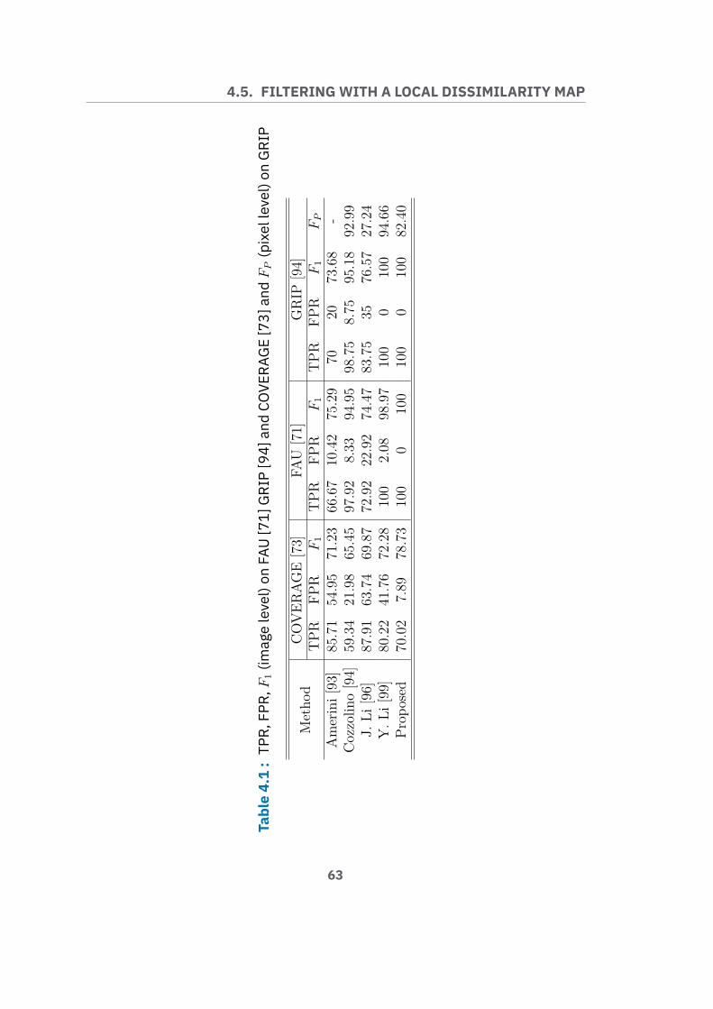
4.5. FILTERINGWITH A LOCAL DISSIMILARITY MAP
Table4.1:TPR,FPR,
F1(im
agelevel)on
FAU[71]GRIP[94]andCO
VERA
GE[73]andFP(pixellevel)on
GRIP
Met
hod
CO
VER
AG
E[7
3]FA
U[7
1]G
RIP
[94]
TPR
FPR
F1
TPR
FPR
F1
TPR
FPR
F1
FP
Am
erin
i[93
]85
.71
54.9
571
.23
66.6
710
.42
75.2
970
2073
.68
-C
ozzo
lino
[94]
59.3
421
.98
65.4
597
.92
8.33
94.9
598
.75
8.75
95.1
892
.99
J.Li
[96]
87.9
163
.74
69.8
772
.92
22.9
274
.47
83.7
535
76.5
727
.24
Y.L
i[99
]80
.22
41.7
672
.28
100
2.08
98.9
710
00
100
94.6
6Pr
opos
ed70
.02
7.89
78.7
310
00
100
100
010
082
.40
63

CHAPTER 4. COPY-MOVE DETECTION
4.5.3 LDM FilteringAt the end of the clustering step 4.4.3, most of the false positives from 4.4.2 areremoved.
On Fig. 4.1d, we can see the detection result without filtering with the LDM.Elements are still wrongly detected as copy-move. To remove those last false pos-itives, every remaining matching after 4.4.3 will be confirmed using the LDMXY Z .
For each pair of matched keypoints in a cluster, two windows W1 and W2 areextracted. The windows are centred on the keypoints. The sizes of the windowsare fixed by the sizes associated with the keypoints and the windows are rotatedaccording to the keypoints angles. The match is finally considered as a falsepositive if
‖LDMXYZ(W1,W2)‖2 > δLDM. (4.8)
As in 4.4.3, all the clusters containing fewer than three elements are consideredas false positives and thus removed. We can see the detection result after the LDMfiltering step on Fig. 4.1e.
4.6 ExperimentationExperiments were conducted on the FAU [71], GRIP [94] and the COVERAGE[73] dataset.
On FAU and GRIP datasets the threshold δLDM has been fixed to 7 while δ1,δ2 and δ3 were chosen to maximise the true positive rates. The true positive rate(TPR), false positive rate (FPR) and the F1 score is computed at image level oneach dataset. For the GRIP dataset, the F1 score has also been computed at pixellevel and is reported in Tab. 4.1 as FP . We can see in Tab. 4.1 that our detectorperforms without error at image level on the FAU and GRIP dataset. We furtherevaluate the performance at pixel level on GRIP. Even though the F1 score atpixel level is lower than state-of-the-art methods, it is worth noticing that the truepositive rate at pixel level is 74.92% and the false positive rate is only 00.16%.
For the COVERAGE δ1, δ2 and δ3 are fixed to maximise the true positive ratewithout LDM filtering and δLDM vary.
64

4.7. CMID DATASET
The detection algorithm is applied to each image. The TPR and FPR at imagelevel is evaluated with and without LDM filtering. On Fig. 4.4 the TPR, FPRand F1 scores are reported with the varying threshold δLDM.
Without filtering, the TPR is maximum but the FPR is extremely high (i.e.93%). Those initial performances are reported as horizontal dotted lines on Fig.4.4. We can see that the detector (without filtering) performs really poorly on theCOVERAGE images containing highly similar objects.
The benefit of the LDM filtering is evaluated by varying the threshold δLDM.For a strict threshold (i.e. 2), the LDM allow obtaining an FPR of 0%, but theTPR drops from 100% to only 30% and an F1 score of only 45%. With δLDM
increasing, the detector reach is best performance at δLDM = 7, with a TPR of70%, FPR of 7% and an F1 score of 78%. The TPR, FPR and F1 score then tendto the initial performance without filtering.
The impact on the processing time depends on the remaining clusters thatneed to be validated with the LDM at the end of 4.4.3 as well as the windowsize of every compared keypoints pair. On the COVERAGE dataset, the globalprocessing time is about 400 seconds. With the LDM filtering it reaches about815 seconds which is an average of 1 second of added processing time per image.
4.7 CMID datasetAs we saw in Table. 4.1 images containing SGO is a real challenge for CMFDalgorithms. When not designed with this problematic in mind, we will observethat they tend to produce many false positives making them impractical. Whendesign with this goal, we will see that it is possible to reduce the false positivesbut at the cost of a lower detection rate. In this section we propose a new publiclyavailable dataset called CMID1 to address a few novel challenges. The objective ofthis dataset is to provide challenging copy-move forgeries that also correspond toa real life problematic. We thus decided to produce digital ID document forgeries.
This specific type of content comes with many challenges for CMFD algorithms.The first one being the large number of SGO. Because the font in an ID is most
1https://cmiddataset.github.io/
65

CHAPTER 4. COPY-MOVE DETECTION
Figure 4.4 : Evolution of the false positives rate (FPR), true positives rate(TPR) and the F1 score with respect to δLDM on the COVERAGE dataset
of the time the same across the whole document, we will most likely observemany occurrences of the same letter at the same scale. To complicate the task,standard ID documents fonts are typically quite simple making it more difficult todistinguish two distinct letters in the first place (see Fig. 4.5).
Another challenge that arise from those kinds of forgeries is the size of thetampering. When producing a digital forgery of an ID document, the counterfeiterwill only duplicate a small surrounding of the letter and might apply a smoothtransition to seamlessly blend the tampering. Doing so we might be left with onlya few tampered pixels.
In this context the challenges for CMFD are multiples. First, they must be ableto detect the tampering at this small scale. We will see that this is not a trivialtask even in the absence of post-processing. Having detected the tampering, theCMFD must then be able to tell the difference between a SGO and an actual fake.This notion of scale is an addition in comparison with the COVERAGE datasetwhere the forgeries are actually quite large.
66

4.8. DATASET OVERVIEW
4.8 Dataset overviewIn this section we will give a brief overview of the dataset goals, content and thecreation process.
4.8.1 Dataset contentThe dataset only contains copy-move forgeries. Genuine images were acquired ona smartphone, cropped to mostly contain the ID document and saved to JPEGwith a quality factor of 95. All images from the dataset have the size 1342 by 943.
The dataset contains three folders named ref , gt, tampered. The ref foldercontains 304 images named :NAME_Ywith NAME the identifier of the document (e.g. Belgian passport) and Y ∈0, 1, ..., 18. The dataset contains a total of 16 different documents for which 19
images are provided.The tampered folder contains all the tampered images, we generated three
tampered images for each genuine image. For tampered images, the followingnaming convention is employed :X_NAME_YWith X ∈ 0, 1, 2, NAME the ID document name (matches the reference identifierin ref) and Y ∈ 0, 1, ...18 the reference image number.
The total numbers of pristine and tampered images can be seen in Table 4.2.Finally, the gt folder contains all the ground truths. Ground truth images will
have the same name as the tampered ones. Ground truth images will be presentedas coloured images to differentiate the source and the target of the tampering.Pure green pixels are the sources i.e. the region that is duplicated and pure redpixels are the target i.e. the region that has been duplicated.
For convenience, a program is provided with the dataset to compute the image-level scores and pixel-level scores. In particular the program will compute the TruePositives (TP), the False Positives (FP), the True Negatives (TN) and the FalseNegatives (FN) which can later be used to compute other desired metrics. Moreinformation on this program is available on the dataset page (link available in 4.7).
67

CHAPTER 4. COPY-MOVE DETECTION
Document types Pristine Tampered Image size16 304 893 1342× 943
Table 4.2 : Dataset content
Figure 4.5 : From left to right : Genuine image, Binarisation of the letters,Bounding box of the letters, chosen letter pair
4.8.2 Automatic tampering processTo generate the dataset, we developed an algorithm that automatically producethe document forgeries. The method can be decomposed into three basic steps.The letter binarisation, the bounding box detection and filtering and the pairselection.
In the first step, we try to remove most of the image content to isolate theletters. To do so, we first assume that a letter will always be thin strokes of a darkshade. Following this assumption, we apply a black top-hat with an arbitraryrectangle kernel of size 7× 7 to each of the RGB channels to highlight small darkregions in each channel. We then take the maximum value of the resulting filteredchannels and then binarise the result following Otsu’s method [119]. The resultcan be seen on Fig. 4.5. We then found the bounding boxes of every connectedcomponent of the binarised image. Those boxes are then filtered according to theirsize. Again the size is fixed experimentally to isolate letters (result visible on Fig.4.5). Finally, a pair of bounding boxes with approximately the same size is chosen(Fig. 4.5). One of these letters is then copy and paste onto the other one.
68

4.8. DATASET OVERVIEW
4.8.3 Tampering sizeAs stated in section 4.7, one challenge introduced in our dataset is the size ofthe tampering. Current public datasets propose copy-move forgeries with variouspost-processing such as rotation, scaling, JPEG compression and so on. Overall,state-of-the-art methods seem to manage such processing with ease except in someextreme cases. Those properties are indeed wanted. One challenge that has beenoverlooked is the ability to detect forgeries when both the source and the target ofthe copy-move are relatively small. Many problems arise in such situation whateverthe method type (i.e. block-based, keypoint-based, hybrid ...).
The first and obvious issue is the ability of the method to detect the tampering.For block-based method, the problem will have to do with computation time.Because of the size, if the blocks are too big, the tampering will most likely bemissed as the blocks would mostly consist of pristine pixels. By decreasing theblock size, the computation time will quickly rise as more and more comparison willhave to be performed. For Keypoint-based method, the problem slightly differ. Asfor block-based method, the computation will also increase but not as notably. Thechallenge mostly reside in the huge addition of probable false positives. To detectsmaller tampering, keypoints must be extracted from more scales and by beingless strict on the stability (e.g. lower contrast thresholds for SIFT/SURF). Thiscompromise has to be done in order to have a sufficient number of keypoints in boththe source and target location. This increases the chances of falsely match pristineareas and current methods often sacrifice detection performances at smaller scalefor better precision.
When the tampering is detected, another challenge arises because of the smallerforgery size. Whatever the method used, some kind of similarity measure is appliedto decide if the detection is a tampering. With less information due to the reducedforgery size, it becomes much harder to differentiate a SGO from a tamperedcomparison. Because our dataset contains only ID documents images, those newchallenges arise naturally as we duplicated small letters. In Table 4.3, a few metricsare given as a comparison between our dataset, COVERAGE [73], GRIP [94] andthe DEFACTO dataset [1]. All values represent the percentage of tampered pixels(including both source and target) in the whole image. For COVERAGE, we can
69

CHAPTER 4. COPY-MOVE DETECTION
Dataset Minimum Maximum AverageCOVERAGE [73] 0.02 0.56 0.23
GRIP [94] 0.0131 0.1371 0.047DEFACTO [1] 0.0006 1 0.0632
Our 0.0015 0.0154 0.0021
Table 4.3 : Datasets tampering size information
see how the forgeries are relatively big with an average of 23% percents of thepixel tampered. Even though the COVERAGE dataset contains many SGO, thesize of the tampered area allows CMFD algorithms to be more confident abouttheir detection. For the GRIP dataset, the forgeries are smaller but images do notcontain SGO, so CMFD algorithms are less likely to produce false positives. Asfor GRIP, the DEFACTO dataset contains smaller forgeries but does not containSGO. Our dataset contains both small forgeries (average of only 0.21%) and alsomany SGO. We will see in the next section how current state-of-the-art methodshandle this new challenge.
4.9 Baseline results
4.9.1 AlgorithmsTo assess the challenging aspect of our dataset, we evaluated 5 common state-of-the-art methods. We evaluate two simple keypoint-based algorithms from [71],we used the implementation provided by the authors with the default configura-tion. We also evaluated three modern methods. BusterNet [109] which is a DeepLearning based method, FE-CMFD [99, 120] which is a keypoint-based methodand SIFT-LDM [2] which is a hybrid method. For BusterNet, we used the imple-mentation and the pretrained network provided by the authors. We did not usethe source/target distinction of BusterNet but instead applied the method theyused to evaluate on the CoMoFod dataset (i.e. every pixel below 0.5 in the bluechannel is considered as pristine). For FE-CMFD we used the implementationgiven by the author as is. Finally, for SIFT-LDM, we used the default parameters
70

4.9. BASELINE RESULTS
Figure 4.6 : From left to right : Tampered images, Ground truths, SIFT [71],SURF [71], BusterNet [109], FE-CMFD [99], SIFT-LDM [2]
described in [2]. We cannot share the implementation of SIFT-LDM but we willprovide an executable upon request if needed to reproduce the results present inthis chapter.
4.9.2 MetricFor each algorithm, we studied the performances at two levels. At the image level,we evaluate how many images are considered as tampered. An image is marked astampered if at least one pixel in the detection map is labelled as tampered. In apractical situation, we would like to minimise as much as possible false detectionat an image level if the algorithm is meant to be automatic because even a fewfalse positives pixels would then possibly imply a manual verification. We alsoevaluate algorithms at a pixel level to assess the localisation performances.
Image level
For image-level evaluation, we used the True Positive Rate (TPR), the False Pos-itive Rate (FPR) and the Matthew Correlation Coefficient (MCC). Ideally, alldetectors should be able to maintain a high TPR and MCC while keeping theFPR low.
Pixel level
For pixel-level performances, we only computed the scores on tampered imagesbecause we are only interested in localisation performances when an image is tam-pered.
Because the tampered area is small in comparison to the size of the image, thenumber of true negatives is much higher than the true positives. We thus decided
71

CHAPTER 4. COPY-MOVE DETECTION
Method TPR FPR MCCSURF [71] 0.7919 0.7697 0.0236SIFT [71] 0.9676 0.9145 0.1104
BusterNet [109] 0.1601 0.1607 -0.0006FE-CMFD [99] 0.0246 0.0066 0.0561SIFT-LDM [2] 0.7917 0.0197 0.6847
Table 4.4 : Image-level scores
Method TPR FDR F1 MCCSURF [71] 0.2155 0.9792 0.0378 0.0606SIFT [71] 0.6004 0.9610 0.0731 0.1471
BusterNet [109] 0.0016 0.9979 0.0018 0FE-CMFD [99] 0.0341 0.3114 0.0650 0.1530SIFT-LDM [2] 0.2555 0.0541 0.4024 0.4912
Table 4.5 : Pixel-level scores
to evaluate the pixel-level performance in terms of True Positive Rate (TPR), FalseDiscovery Rate (FDR), F1 score and the Matthews Correlation Coefficient (MCC).
4.9.3 Results
Image-Level
Table 4.4 gives the results at image level. Of all the method, we can see that SIFT[71] has the highest TPR (at 0.96) which indicates the best detection performances.SURF [71] and SIFT-LDM [2] follow with an already much lower result (about0.16 below) meaning that both methods were either unable to detect many of thetampering or decided to reject them. Far behind, we can see that BusterNet [109]and FE-CMFD [99] seems to barely detect the tampered images or are stricterthan previous method.
The answer lies in the FPR results for every method. We can first notice thatfor SIFT, SURF and BusterNet the FPR is almost equal to the TPR. For SIFT andSURF we thus understand that they both struggle with SGO and tend to classifyevery image as tampered, which yield a high TPR and FPR. For BusterNet the
72

4.9. BASELINE RESULTS
result is different as the TPR and FPR are both quite low (about 0.16). Thisprobably indicates that BusterNet is unable to detect the forgeries at this smallscale, the detection is then more or less random. Even though BusterNet is unableto detect the forgeries, it manages not to trigger too many false alarms which isa good property. The result of BusterNet is overall not surprising as it has neverbeen trained with really small forgeries. FE-CMFD [99] maintain the lowest FPRof all methods but was not able to detect many forgeries. As for BusterNet, theissue most likely comes from the size of the tampering. Though it only detecteda few tampered images, it did almost no mistake which could make it practical ifa lower FPR is more important than detection performances. For example, in afully automatic pipeline where no human intervention is possible, one might preferto miss many tampered images to provide a better user experience. Finally, SIFT-LDM [2] achieve the best overall performances with a TPR of 0.79 and an FPR of0.02. Even though this result is far from perfect, it is encouraging as SIFT-LDMwas designed to tackle both challenges mentioned in 4.7 and seems able to achievesatisfactory results. With time we can expect to achieve even better results.
Pixel Level
For the pixel level evaluation, algorithms have been applied to all tampered images.Then the total number of true positives, false positives, true negatives and falsenegatives pixels are computed. We evaluate the pixel-level performance acrossall images as some scores might be undefined in certain conditions (e.g. FDR isundefined for TP + FP = 0). Because the images of our dataset contains manySGO and the tampered area are relatively small, we are interested in a particularresult. First we would like the true positive rate to be as high as possible whilemaintaining the lowest possible false discovery rate.
We can first see how both SIFT and SURF method seems able to locate mostof the forgeries (see TPR in Table 4.5) but generate a large amount of false positiveresulting in an extremely high FDR making both detectors completely impractical.This confirms the tendency observed in Table 4.4.
For BusterNet, we can see that the True Positive rate is almost 0 while theFDR approaches 1. This corresponds to the observed result in 4.4. Because of the
73

CHAPTER 4. COPY-MOVE DETECTION
small size of the tampered areas, BusterNet seems unable to detect the forgery inthe first place thus the TPR is extremely low. With only a few false detections, theFDR, on the other hand, quickly rises to 1. Those false detections could probablybe discarded with a stricter decision threshold (i.e. greater than 0.5).
For FE-CMFD, we observe a similar behaviour as BusterNet with a low truepositive rate. This might be due to the small size of the tampering. But unlikeBusterNet, FE-CMFD still manage to maintain a satisfactory FDR. In practice,this would mean that FE-CMFD does not rise to many false alarms which is adesired property. The F1 score obtained (0.0653) and the MCC (0.1571) stillremain quite low because of this strong tendency to reject true positives.
Finally, SIFT-LDM achieve the best performance of all methods with an F1
score of 0.4024 and an MCC of 0.4912. The better results are explained by theability to maintain a much lower FDR than all other (5 times lower than FE-CMFD) while discarding less true positives (7 time less than FE-CMFD).
For both FE-CMFD and SIFT-LDM, we see that the FRD is quite low, thisindicates that both methods highlight the true tampered area. This is importantto notice as the results in Table 4.4 could have been misleading. For instance, inFig 4.6 we can see that the detection does not necessarily correspond to the truetampered area. Which means that an algorithm could correctly labelled an imageas tampered even though it did not detect the forgery. The slightly higher FDR ofFE-CMFD is mostly due to the final post-processing on the detection maps whichtends to produce a region that is always slightly bigger than the ground truth.
4.10 ConclusionCopy-move has been well studied over the last decade. Thanks to that, manymethods and datasets have been publicly released. Unfortunately, we believedthat the challenge of similar but genuine objects has been and still is widely underconsidered. Consequently, many methods have been shown to be ineffective in thepresence of SGO.
In this chapter we wanted to develop a copy-move detection method applicableto ID document forgery. We faced the challenge of SGO and confirmed the dif-
74

4.10. CONCLUSION
ficulty for many state-of-the -art methods to handle such images. While currentmethods are able to detect large Copy-move with various transformations (rota-tion, scaling, lightning changes ...) with ease, they struggle to detect even thesimplest copy-move (no rotation, no scaling) when it is small and in the presenceof SGO.
We decided to evaluate the benefits of adding an extra filtering step based onthe local dissimilarity transform to the typical keypoint-based detection pipeline.We showed that we were able to achieve perfect results in common datasets with arather trivial keypoint-based detection scheme and that we were able to drasticallyreduce the false positive rate on the COVERAGE dataset which contains manySGO. This first results were really encouraging as they showed that it was possibleto handle SGO by redesigning common CMFD algorithms with those in mind.
To contribute to the research on copy-move detection in the presence of SGO,we decided to propose a new dataset. We focused on ID documents for two mainreasons. Firstly, the thesis is oriented towards the detection of forgery on IDdocuments. Secondly, we think that ID documents are both a realistic use case ofCopy-Move forgery but also an extremely challenging one. In fact, we saw that thestudied state-of-the-art methods were either producing a lot of false positives orcompletely unable to detect the forgeries. We also evaluated our method on thisdataset. We saw that it performed significantly better than other state-of-the-artmethods but there is still a great room for improvement.
It is important for future research to acknowledge the challenge of SGO andsmall copy-move. Nowadays researches are still often evaluated on datasets thatare not representative of a typical copy-move forgery. Most of those datasetscontains extremely large forgeries in images with no SGO. In practice, Copy-Moveis rarely used in such an obvious way. Most of the time it will be used as a way ofperforming an Object-Removal forgery or to tamper some text. In both scenariosthe forgery will most likely be rather small in images with potentially many SGO.Having more datasets containing SGO is also becoming crucial as many currentmethods achieve perfect results on many of the public datasets.
75


CHAPTER 5Object-removal forgery detection
5.1 Introduction . . . . . . . . . . . . . . . . . . . . 78
5.2 Object-removal forgery . . . . . . . . . . . . . . . 79
5.3 Related Works . . . . . . . . . . . . . . . . . . . 80
5.4 Proposed feature extraction . . . . . . . . . . . . 81
5.5 Remarks . . . . . . . . . . . . . . . . . . . . . 83
5.6 Qualitative results . . . . . . . . . . . . . . . . . 85
5.7 Conclusion . . . . . . . . . . . . . . . . . . . . 87
77

CHAPTER 5. OBJECT-REMOVAL FORGERY DETECTION
5.1 IntroductionWe began by studying Copy-Move forgery detection. As we stated, copy-move isa simple and widely use tampering technique and is particularly appropriate fortampering an ID document. As we briefly mentioned, copy-move is sometimesused to remove objects from an image. Those kinds of forgeries are called Object-Removal.
Object-Removal forgery is arguably one of the most used tampering techniques.In fact, it is often used alongside with other techniques. For example, you oftenneed to remove a few elements before inserting a new one.
There exist multiple methods to perform an object-removal forgery. As alreadymentioned, one can perform multiple copy-move forgeries to hide the unwanted el-ements. On a professional software such as Photoshop or Affinity Photo, one woulduse the clone stamp tool to perform such a forgery. Another common approach isto use an inpainting algorithm to fill the area we want to hide. One would use toolssuch as the healing brush tool or the content aware fill in Photoshop. Such tools aregenerally based on some examplar-based inpainting algorithms [121, 122]. Thosework much like the clone stamp tool but the selection of the patch to be duplicatedis fully automated. For this reason, they generally don’t handle very well sceneswith complex backgrounds. Recently, deep learning based approaches to performobject-removal have been more studied to tackle more complex backgrounds, butat the moment those have not yet been implemented in professional software. Thecounterfeiter will in practice choose the appropriate tool based on the circum-stances. For example, the inpainting-based algorithm will work extremely wellfor objects on simple backgrounds whereas for more complex background a moremanual approach using the clone stamp tool will be preferred.
Apart from deep learning based inpainting method, object-removal is essen-tially a kind of copy-move forgery. While it is true and some CMFD can detectobject-removals, there exist cases in which CMFD are inappropriate. In this chap-ter we are interested in the detection of object-removal forgeries. We would like tobe able to detect such forgery regardless of the technique used to perform it. Whenperforming an object-removal forgery, the counterfeiter is recreating some back-ground texture. To seamlessly blend it with the rest of the image, it is common to
78

5.2. OBJECT-REMOVAL FORGERY
use a smooth transition between the crafted texture and the original background.This blending acts like a smoothing operation around the forged area which mayserve as a clue for object-removal detection. In this chapter we will thus explorethe possibility of exposing those smooth areas to reveal possible traces of forgeries.We will show that other operation such as splicing or resampling can sometimesproduce similar artefacts and can be exposed using this method.
We will first briefly cover the various methods to perform an object-removalforgery and the implication of those. Then we will propose a novel method toreveal traces of object-removal forgery by exposing those smooth transitions. Wewill also show that in some cases our method can expose splicing forgeries byrevealing abnormally smooth or sharp region in an image and can also help toperform source-target identification for copy-move forgeries.
5.2 Object-removal forgeryWe will first give a few examples of the typical techniques used to perform anobject removal forgery.
As we mentioned, there exist two commonly used tools to perform an objectremoval forgery. The first well-known tool is the clone stamp which is present inalmost every image retouching software. In Fig. an example of the use of theclone stamp is given. When using the clone stamp, the digital artist first choosea reference point. He can then duplicate the pixel around this reference pointusing what is called a brush in most retouching software. A brush has two mainproperties, its size and its softness. In Fig. 5.1 the brush size is represented asthe red circle and the softness can be seen in the middle as the smooth transitionaround the duplicated region. The tampering process is quite similar when usingthe healing brush or the content aware fill. The main difference is that the artistdoes not have to choose the reference point. Rather, the user uses the brush todraw the area he wants to remove and the inpainting algorithm automatically fillsthat area.
In both cases, the artist often use a so-called brush during the tamperingprocess. The softness of the brush creates a smooth transition around the forged
79
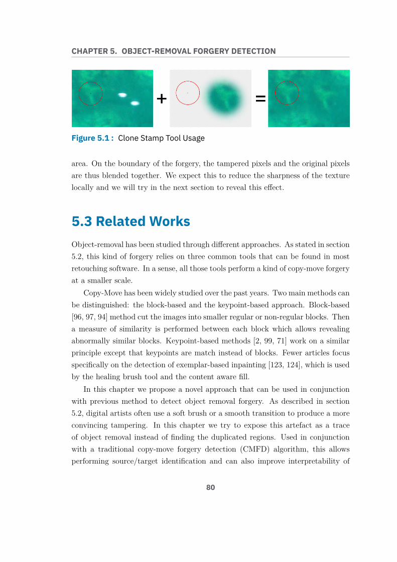
CHAPTER 5. OBJECT-REMOVAL FORGERY DETECTION
Figure 5.1 : Clone Stamp Tool Usage
area. On the boundary of the forgery, the tampered pixels and the original pixelsare thus blended together. We expect this to reduce the sharpness of the texturelocally and we will try in the next section to reveal this effect.
5.3 Related WorksObject-removal has been studied through different approaches. As stated in section5.2, this kind of forgery relies on three common tools that can be found in mostretouching software. In a sense, all those tools perform a kind of copy-move forgeryat a smaller scale.
Copy-Move has been widely studied over the past years. Two main methods canbe distinguished: the block-based and the keypoint-based approach. Block-based[96, 97, 94] method cut the images into smaller regular or non-regular blocks. Thena measure of similarity is performed between each block which allows revealingabnormally similar blocks. Keypoint-based methods [2, 99, 71] work on a similarprinciple except that keypoints are match instead of blocks. Fewer articles focusspecifically on the detection of exemplar-based inpainting [123, 124], which is usedby the healing brush tool and the content aware fill.
In this chapter we propose a novel approach that can be used in conjunctionwith previous method to detect object removal forgery. As described in section5.2, digital artists often use a soft brush or a smooth transition to produce a moreconvincing tampering. In this chapter we try to expose this artefact as a traceof object removal instead of finding the duplicated regions. Used in conjunctionwith a traditional copy-move forgery detection (CMFD) algorithm, this allowsperforming source/target identification and can also improve interpretability of
80

5.4. PROPOSED FEATURE EXTRACTION
CMFD results when duplicated regions are small and scattered. We will also showhow this method sometimes applied to other forgeries.
5.4 Proposed feature extractionIn the following section, we will describe the method used to measure the localsharpness of a texture relative to the rest of the image.
5.4.1 Image reflectance estimatesA simple model of image formation is the illumination-reflectance model. In thismodel, the image is modelled as the product of illumination and reflectance.
I(x, y) = L(x, y) ∗R(x, y) (5.1)
where L is the illumination, R the reflectance, I the image and (x, y) the pixelcoordinates. In this simplified model, the illumination L is the amount of lightcoming to the surface visible at (x, y). The reflectance R is the capacity of thesurface (x, y) to reflect the incoming light L.
In most contexts, L varies relatively slowly with respect to R hence it hasbeen proposed [125] to extract the reflectance R using a homomorphic filtering.By taking the logarithm of (5.1), we separate L and R with R lying in the highfrequencies.
ln(I(x, y)) = ln(L(x, y)) + ln(R(x, y)). (5.2)
Applying a high-pass filter in the Fourier domain thus isolate R from L.
r(u, v) = F(ln(I(x, y)))H(u, v) (5.3)
with H a high-pass filter in the Fourier domain.We get our final reflectance estimate R̂ by taking the exponential of the invert
81

CHAPTER 5. OBJECT-REMOVAL FORGERY DETECTION
(a) Texture image (b) Feature map S (c) Obtainedsegmentation
Figure 5.2 : From top to bottom : An image with two textures, the featuremap S, segmentation by applying Otsu’s method on S
Fourier transform :
R̂(x, y) = exp(F−1(r(u, v))). (5.4)
5.4.2 Local reflectance variability measure
The extracted reflectance R̂ gives us an idea of the surface roughness (x, y). Themore R̂ varies around a neighbour of (x, y) the rougher the texture is at thislocation. As a sharpness measure, we use the local standard deviation with aneighbour size n of the reflectance estimate. In all our experiments, n is fixed to11. From this we obtain an image σR̂ with the same size as I.
Once the standard deviation is computed. The image is cut into K non-overlapping segments sk depending on the dynamic range. For each pixel pk inthe segment sk, we compute the median absolute deviation of its local reflectancestandard deviation σR̂ within its segment sk to obtain our final local reflectancevariability measure S. The final result tells us how sharp a pixel is relative to therest of the image. Large positive values indicate the most variable pixels in theimage and large negative values indicate the less variable pixels in the image.
An example of application is given in Fig. 5.2. Given two textures on Fig.5.2a, the feature map S is computed and a median filter is applied to reduce noise(Fig. 5.2b). The feature map is the binarised following Otsu’s method [119] anda morphological closing is applied (Fig. 5.2c). We can see that the left textureis clearly marked as sharper. Also three areas of the right texture are marked as
82

5.5. REMARKS
(a) Tampered image (b) Feature map S (c) Feature map S withnoise added
Figure 5.3 : From top to bottom : Tampered image, Feature map of thetampered image, Feature map S with synthetic noise added before tampering
sharp which indeed correspond to sharper regions of the right texture.In case of a forgery, we expect to observe a notable drop in a relatively uniformly
textured area. An example is given in Fig. 5.3b, where we can observe a less sharpring that does not correspond to anything visible on Fig. 5.3a.
5.5 Remarks
5.5.1 Impact of texture scaleThe proposed feature measure the relative sharpness of one pixel relative to therest of the image. We expect to observe less sharp pixels at the boundary of theforged region if a smooth transition is applied as described in section 5.2. It isimportant to remark that this phenomenon can only be seen if the transition areais sufficiently greater than the scale of the surface details. An example is given inFig. 5.3a where the healing brush tool has been used on two textures (sand andgravel). We can see how the forged area is visible in the sand texture (left image),because the transition is much larger than the texture size. Whereas nothing isvisible for the gravel texture. Increasing the neighbour size n when computing thelocal standard deviation of R̂ can slightly increase the visibility of tampered regionfor large-scale texture. But this also largely degrades the detection performancefor lower scale texture which is overall not worth it.
83

CHAPTER 5. OBJECT-REMOVAL FORGERY DETECTION
5.5.2 Impact of sensor’s noiseWhile extracting the reflectance estimate R̂ we do include the image sensor noise.This is important to keep in mind as this noise can be seen as kind of a dominanttexture across the image. In the presence of a strong sensor noise, S will mostlymeasure this noise leading in a more uniform appearance whereas a week sensornoise will lead to a more variable S. This effect is to our advantage as the sensornoise is a small-scale texture and, as previously mentioned, tampered region willbe more visible in the area with a fine-grained texture. This positive effect can beseen in Fig. 5.3c where white Gaussian noise is added on top of the textures priorto tampering. We can now clearly see the tampering even in the gravel texturesas the noise becomes dominant.
To illustrate this effect, three photos of a pen where took (Fig. 5.4) with asmartphone with three different ISO settings. From left to right the ISO are 3200,800 and 100. We can see how the tampering is more visible with a higher ISOsetting. Also note how S becomes more uniform with higher ISO this is becausethe sensor noise become the predominant texture hence the sharpness measure ismostly defined by the sensor noise.
5.5.3 Impact of post-processingWe tested the impact of JPEG recompression and resampling on our methodwhich are two extremely simples and common post-processing. In both cases, thetampering is performed on the raw image and first saved to JPEG with a qualityfactor of 90.
In Fig. 5.5, we recompressed the tampered image using different quality factors(i.e. 80, 70, 50 and 20). We see that the tampering progressively disappear untilit becomes barely noticeable for a quality factor of 20. This behaviour is expectedas JPEG will tend to suppress more and more detail which leads to the sharpnessmeasure being almost null on the whole image. It is interesting to notice that ifthe detection was possible at the creation of the tampering, it will stay visible evenwith extremely low quality factors (i.e. 50) by nowadays standard.
We then tested the detection against resampling. In this case, the tampered
84

5.6. QUALITATIVE RESULTS
image in Fig. 5.6 is progressively downsampled to a factor of 0.1. Once again wecan see that the detection becomes less and less visible. As for JPEG recompres-sion, the detection still remains possible for low resampling factors (i.e. 0.5).
Those experiments show that the detection is quite resilient to common post-processing. In the next section, we tested our method of real-world examples toassess its applicability.
5.6 Qualitative resultsAs the method is quite specialised and mostly perceptual, we present here somequalitative results. We made the first example from a JPEG image that directlycomes from the camera. To assess the applicability of our method of real-worldimages, we also tested it on three images from the PhotoshopBattles reddit forumon which participants are asked to retouch a given image.
Because we compute the median absolute deviation of each pixel pk to producethe feature map S, we can observe strong positive deviation at edge location. Aswe are only interested in finding smoother regions of the image (i.e. large negativevalues in S), we can set every positive value to 0 in our feature map S. This willsignificantly reduce the noisy appearance of S and further enhance the tamperedregion. This step is applied to all the following examples (Fig. 5.8).
The first image has been taken in low light condition, as stated in 5.5.2 thiscauses our feature map S to mostly characterise the sensor noise leading to a moreuniform result and will make the tampering more visible even if the transition sizeis small. On Fig. 5.8d we can see a large darker region where the woman hasbeen removed. This matches the ground truth on Fig. 5.8c. This example wasmade using the clone-stamp tool in Affinity Photo and shows how the recreatedbackground appears less sharp in the forged area.
The other examples have been found on the PhotoshopBattles reddit. For eachexample we found the original image and recreate an approximate ground truth.
On the first example from reddit (Fig.5.8e-5.8h) the artist1 had to remove thecharacter from the original image to insert the kid. The feature map Fig. 5.8h
1Artist : kann_i, Link : https://www.reddit.com/r/photoshopbattles/comments/hb01hh/psbattle_a_girl_staring_at_her_neighbor_mowing/
85

CHAPTER 5. OBJECT-REMOVAL FORGERY DETECTION
reveal those two steps as we can see a region that is considerably smoother thanthe rest of the image just around the kid. Also, because the inserted kid comesfrom an image with a much lower quality, we can see how he also appears muchsmoother than the rest of the image.
In the second example, the artist2 removed the legs and added a hand. Onceagain large smooth region appears on Fig. 5.8l where the snow texture has beenreconstructed. One might notice some circular patterns appearing on the featuremap. Those are likely due to the correction of a lens distortion. In fact, looking atthe buildings on the original image (Fig. 5.8i), their curvy appearance indicatesthat the picture was taken with a wide-angle lens which causes what it is calleda barrel distortion. While correcting this distortion, a resampling is performedon some pixels which decrease the variance of the sensor noise and might be thesource of those circular pattern. To confirm this thought we apply this correctionon the photo of the pen with the highest ISO and observed similar patterns S (seeFig. 5.7).
The last example is here to illustrate how this method can sometimes be usedto detect a splicing forgery. In this example, the artist 3 inserted a woman andthe David head onto the well-known painting by Michelangelo. As for the firstexample, notice how the two inserted elements appear much smoother than therest of the image. Even though our method is not meant to perform splicingdetection, we can see that in some cases the computed feature map S can givea strong intuition on a probable tampering because the quality of the insertedelement might not match the quality of the target image, we can either observe anabnormally smooth element like in this example or an abnormally sharp elementin the image.
2Artist : KrombopulosJeff, Link : https://www.reddit.com/r/photoshopbattles/comments/gz9lsl/psbattle_man_sat_on_snowy_roof_overlooking/
3Artist : V_LochNessLobster_V, Link : https://www.reddit.com/r/photoshopbattles/comments/heqrwr/psbattle_this_woman_with_david/
86

5.7. CONCLUSION
5.7 ConclusionWhen creating a forgery, a digital artist might have to remove a subject from thescene. To do so, he will sometimes need to recreate parts of the background thatwere hidden by the subject. Artists will often use tools which are available inmost professional software such as the clone-stamp tool, the healing brush toolor the content aware fill. It is common to use a soft brush or apply a smoothtransition to enhance the resulting forgery. In this chapter, we suggest that thisoperation will lead to the apparition of less sharp areas in the image that mightgive an intuition for the presence of a tampering. To do so, we proposed a relativesharpness measure for a pixel within an image based on the reflectance of thatimage. We show that it is possible to expose forgeries using this feature undercertain circumstances. The image must have sufficient detail for our sharpnessmeasure to work. And the size of the transition area (for the soft brush or the softtransition) must be greater than the underlying texture scale. We show that formodern cameras with reasonable ISO settings those criteria are easily met. Thenwe observed that the detection is quite resilient to simple post-processing such asJPEG recompression and rescaling which is really important as images are oftenrecompressed or resampled when uploaded on social media. Finally, we assessedthe applicability of our method on real examples took on the PhotoshopBattlereddit. While not automated, our method can allow a human operator to get astrong intuition on the possible traces of a forgery. It also allows the operator tolocate and interpret what the tampering process was.
We showed that our method allows us to detect object removal forgeries whena soft transition is applied but can also be used in splicing detection. For splicings,our method can sometimes amplify a difference in sharpness (between the insertedelement and the rest of the image) or exposed a synthetic noise added to blendmore seamlessly an element.
Further works need to be done to enhance the results of our method in orderfor it to work in an automated manner. As is, it is a quick yet efficient tool formultimedia forensic, in particular if the image provenance if somewhat controlled(e.g. constraints on a minimum required quality).
87

CHAPTER 5. OBJECT-REMOVAL FORGERY DETECTION
(a) ISO 3200 (b) ISO 800 (c) ISO 100
(d) Tampered ISO 3200 (e) Tampered ISO 800 (f) Tampered ISO 100
(g) Feature map S ISO3200
(h) Feature map S ISO800
(i) Feature map S ISO100
Figure 5.4 : Impact of the sensor noise on the detection
88

5.7. CONCLUSION
(a) Tampered ISO 800 (b) Feature map S JPEG90
(c) Feature map S JPEG80
(d) Feature map S JPEG70
(e) Feature map S JPEG50
(f) Feature map S JPEG20
Figure 5.5 : Impact of JPEG compression on the detection
89

CHAPTER 5. OBJECT-REMOVAL FORGERY DETECTION
(a) Tampered ISO 800 (b) S after resampling bya factor 0.9
(c) S after resampling bya factor 0.7
(d) S after resampling bya factor 0.5
(e) S after resampling bya factor 0.3
(f) S after resampling bya factor 0.1
Figure 5.6 : Impact of resampling on the detection
90

5.7. CONCLUSION
(a) Lens correction applied (b) Circular patterns due to the lenscorrection
Figure 5.7 : Visible resampling in the feature map S
91

CHAPTER 5. OBJECT-REMOVAL FORGERY DETECTION
(a) Genuineimage
(b) Tamperedimage
(c) Ground truth (d) Feature map S
(e) Genuineimage
(f) Tamperedimage
(g) Ground truth (h) Feature map S
(i) Genuine image (j) Tamperedimage
(k) Ground truth (l) Feature map S
(m) Genuineimage
(n) Tamperedimage
(o) Ground truth (p) Feature map S
Figure 5.8 : From left column to right column : Original images, Tamperedimages, Ground truths, Feature map S
92

CHAPTER 6Face morphing detection
6.1 Introduction . . . . . . . . . . . . . . . . . . . . 94
6.2 Problem Statement . . . . . . . . . . . . . . . . 95
6.3 Face Morphing Attack . . . . . . . . . . . . . . . 96
6.4 Noise based Face Morphing Detector. . . . . . . . . 99
6.5 Evaluation of no-reference Face Morphing Detectors . 106
6.6 Conclusion . . . . . . . . . . . . . . . . . . . . 110
93

CHAPTER 6. FACE MORPHING DETECTION
6.1 IntroductionFace morphing has been proved to be a threat to face recognition software. In[126] the authors showed that two peoples could share a single ID document bysubmitting a morphed face images during an official ID onboarding procedure.This attack is plausible as [127] shown that humans are not good at detecting facemorphing thus making it possible to obtain a fraudulent ID (FID). Once the FIDhas been acquired, two peoples can use it and pass automated face recognitionsystem tests. The most obvious threat presented by [126] is the ability for twopeoples to pass automated border control (ABC) systems with a shared passport.With face biometry being used in many systems and with the rise of digital identity,the ability to detect face morphing is becoming crucial.
Two kinds of Face Morphing Detectors (FMD) can be differentiated. The no-reference FMD and the differential FMD.
For the differential FMD, the task is similar to Face Recognition (FR). Havinga Bona Fide image of a person A, we want to decide if a given photo of theperson A is a Face Morph (FM). Unlike FR, differential FMD does not have tobe able to recognise A in any complex scene (e.g. complex lightning condition).It can be assumed that both the Bona Fide photo and the suspect photo A willhave a sufficient quality and may be taken similarly (e.g. frontal with a neutralexpression). In [128], authors propose to demorph the picture on the FID thencheck if the face recognition system still match the two pictures. Authors of [129]propose to study the difference in the landmarks between the two photos and touse an SVM to decide if the difference is due to a pose and expression variationor due to a face morphing attack. Other approaches [130, 131, 132, 133, 134] usesdeep learning methods to detect the face morphing attack.
For the no-reference FMD, no Bona Fide is available. The detection is blind ina single image. The task becomes much harder as no history of the image can beassumed, the photo could have been printed and scanned for instance. No-referenceFMD would be used when submitting a photo to obtain an ID document to validatethe integrity of that photo before creating a document. Many methods exist [135,136, 137, 138, 139] and addresses very different artefacts. In [140] authors proposeto train an SVM on texture descriptors to detect the Face Morphing attack. In
94

6.2. PROBLEM STATEMENT
[141] authors propose to use the sensor pattern noise (SPN) to detect the facemorphing attack, they use a SVM trained on features extracted from the Fourierspectrum of the SPN to decide if the image is a morph. Authors of [142] proposedto use the photo response non-uniformity (PRNU) and analyse the difference ofvariance of the PRNU across the image to detect the face morphing attack.
In this chapter we present the Face Morphing creation process and how thisaffects the overall image. We show how this can be used to create a simple yetefficient no-reference FMD for common JPEG quality factor. We then analysehow this FMD can be fooled and show that many no-reference FMD suffer fromsimilar flaws. Finally, we propose to analyse FMD in various scenarios, and showthat performance can vary with Bona Fide image provenance and quality raisingthe question of the applicability of no-reference FMD for Blind Face MorphingDetection.
6.2 Problem StatementTwo main FMD exists. The no-reference and the differential detectors. For bothkinds of detectors, the same attack scenario is considered. In [143], authors pro-posed a formal document lifecyle modelling. They decomposed the life of a doc-ument into three steps. The image acquisition, the document issuing process andthe document usage. As they explained, Face Morphing attacks could occur duringtwo steps. The attacker could inject the morph at the document issuing processor could manipulate the document obtained with a genuine photo to produce aforged id. In those two cases, no-reference FMD cannot make precise assumptionsregarding the photo history. Whether the verification is performed before the doc-ument generation or at the usage. In this chapter we will consider this task asBlind Face Morphing Detection (BFMD) as opposed to Controlled Face MorphingDetection (CFMD) where the acquisition pipeline is controlled. For both BFMDand CFMD, cross-dataset performance and performance against simple counterforensic has been identified as an issue [144][143]. In this chapter, we will formallypresent the fully digital Face Morphing attack and introduce a simple method forCFMD that requires no training and performs well against various simple post-
95

CHAPTER 6. FACE MORPHING DETECTION
(a) Face A (b) Face B (c) Roughalignmentof faces Aand B
(d) Precisealignmentof faces Aand B
(e) Withoutcolourbalance
(f) Withcolourbalance
Figure 6.1 : Automatic Face Morphing creation
processing. We will show that, as other FMD algorithms, our method suffers fromtargeted counter-forensic method. We will then consider another potential pitfallfor FMD by looking at performance variation against varying Bona Fide prove-nance and quality. We will thus discuss on the applicability of no-reference FMDfor the BFMD task.
6.3 Face Morphing AttackWe will begin by introducing the basic steps to create a Face Morph. We willconsider two face images IA and IB where IA is inserted into IB.
6.3.1 Automatic Face Morph creation
Landmarks extraction and face alignment
The first step is to extract a set of facial landmarks LA = {la,0, la,1, ..., la,n} (re-spectively LB) for the two faces we want to morph. To extract the landmarks weuse the implementation of [145] in the Dlib [146] library. Once the two sets oflandmarks are extracted, we can proceed with the alignment of the two faces. Thetwo faces must first be roughly aligned. To do so, one of the faces is aligned withrespect to the eyes of the other with a similarity transformation to keep the facialgeometry untouched. When the two faces are aligned a weighted average of the
96

6.3. FACE MORPHING ATTACK
landmarks of LA and LB is computed to produce a set LW with
lw,i = αl,ila,i + (1−αl,i)lb,i,αl,i ∈ [0, 1] (6.1)
αl being the shape vector determining how much of each faces biometry is keptand would be set by the attackers to produce a Face Morph convincing enoughto fool a human inspector. In the rest of the chapter, αl is considered to be aconstant αl for all the detected landmarks.
The two faces are then warped to LW before performing any kind of blendingto avoid ghost artefacts.
During that first step of the Face Morphing creation process, the two imagesIA or IB will be interpolated many times. We can thus except that they will havea lower noise variance due to the multiple interpolations. From now on IA and IB
denotes the two face images after being warped.
Skin tone matching
Prior to the blending, a skin-tone matching step can be applied which allows toproduce much better morph in more cases.
We perform a local RGB scaling on IA to match IB colours. Rough estimatesof IA and IB expectation are first computed by applying a Gaussian blur, thisresults in the two images approximations AA and AB. Each pixel IA is scaled toobtain the skin tone matched image BA
BA = IA ◦ (AB � AA) (6.2)
where ◦ is the Hadamard product and � the Hadamard division.
Blending
Once the skin tone is matched, the two images can be blended. A simple alphablending is performed.
Given an alpha matte αb with αbi,j ∈ [0, 1],∀(i, j). The final morph imageMAB is given by
MAB = αb ◦BA + (1−αb) ◦ IB. (6.3)
97

CHAPTER 6. FACE MORPHING DETECTION
In the rest of the chapter, we assume that αb is a constant αb inside the facialarea. In practice, the exact alpha matte αb cannot be known. One could decide toonly blend important features such as the nose, eyes. It is worth noticing that thisdefinition of Face Morphing contains many other possible attacks. For instance,a simple face swap is performed by setting αl to preserve IA biometry and αb toonly keep IA texture. One might want to keep IB biometry but with IA texture.In [128], authors showed that αb have more impact on FR systems which suggestthat, as for us, FR systems tend to be more sensitive to the textural information.Further study has yet to be done when considering an alpha matte αb and a shapevector αl instead of constants. In fact, the attacker might not use automatic toolsto produce the face morph and would instead try to replicate those steps manuallyusing photo retouching software. In such cases, αl and αb would not be constant.Those cases are later called handmade morphs.
6.3.2 Dataset constructionFor the rest of the chapter, we constructed two datasets of face morphing attacksaccording to the process described previously. All the morphs are generated withαl = 0.5 and αb = 0.5.
PUT Morph Dataset
The PUT dataset [147] is composed of 100 subjects. Images of each subject hasbeen taken under various angles but with consistent illumination conditions. Foreach subject we selected the more frontal and neutral image as reference images.From those references 171 morphs have been generated. Each morph image is thencompressed at different JPEG quality factors (i.e. 100, 95, 90, 85, 80, 75).
FERET Morph Dataset
The FERET dataset is a well-known face recognition set composed of 14126 photosof 1199 individuals taken in 15 sessions between 1993 and 1996. At the time,photos were taken on a film camera and then digitalised. We took a subset ofthose photos to construct two face morphing sets (as in 6.3.2) for training and
98

6.4. NOISE BASED FACE MORPHING DETECTOR
0.35 0.4 0.45 0.5 0.55 0.6 0.65 0.73
3.2
3.4
3.6
3.8
410
-3
in,k
out,k
(a) σin,k and σout,k estimates on agenuine face
0.2 0.3 0.4 0.5 0.6 0.72.5
3
3.5
410
-3
in,k
out,k
(b) σin,k and σout,k estimates on amorph face
Figure 6.2 : σin,k and σout,k estimates
validation. Original and Morph images are compressed with various JPEG qualityfactors (i.e. 100, 95, 90, 85, 80, 75). The training set consist of 919 Bona Fideimages and 900 morphs. The validation set consist of 1361 Bona Fide imagesand 992 morphs. The training set and the validation set contains no overlappingidentity as recommended in [148].
6.4 Noise based Face Morphing DetectorTo detect the Face Morphing attack, we make the assumption that the processdescribed in 6.3.1 alters the noise residual of the resulting image. In this section wewill briefly describe how the noise residual is extracted, introduce some notationsused in the rest of the chapter, show the effect of 6.3.1 on the noise residual andpresent a simple yet reliable method to detect such an effect.
6.4.1 Homogeneous block detectionGiven an image I, the image approximation A is estimated using a wavelet de-noising method. The image residual is then computed as R = I −A. Having I, R
and A, it is proposed to use [149] to detect homogeneous blocks that can be usedto get a correct estimate of the noise variance.
99

CHAPTER 6. FACE MORPHING DETECTION
6.4.2 Level-set variance estimationOnce homogeneous blocks are detected, the image is partitioned into K non-overlapping segments Sk by dividing the dynamic range. For each segment Sk, pix-els belonging to segment Sk in the image I will be denoted as Ik,i with k ∈ 1, ..., K
the kth segment and i ∈ 1, ..., nk the ith pixel of the segment k with nk the cardi-nality of Sk.
For a segment Sk, the expectation µk is estimated from Ak and the varianceσk from Rk.
With a sufficiently large value of K, Rk,i become more probably identicallydistributed thus for nk large enough Rk,i follows a normal distribution.
We further separate pixels from inside and outside the facial area to get twovariance estimates for each segment Sk. In the rest of the chapter, the pixels ofa segment Sk of image I inside the facial area will be denoted as Iin,k,i and thoseoutside the facial area Iout,k,i. Similarly the inside variance estimate of segment Sk
will be denoted as σ2in,k and the outside variance estimate σ2
out,k.
6.4.3 Effect of Face Morphing on variance estimates
The Face Morphing process described in 6.3.1 can be seen as a kind of splicingforgery.
Unlike a typical splicing forgery, some knowledge can be use to our advantage.The first one being the location of the forgery which we exploit by comparing theinside from the outside area. The second being that both the inserted element andthe insertion location are interpolated prior to a final alpha-blending step.
From (6.3) we have that
MABin,k = αbB
Ain,k + (1− αb)I
Bin,k. (6.4)
Meaning thatRin,k = αbR
′in,k + (1− αb)Rout,k (6.5)
100

6.4. NOISE BASED FACE MORPHING DETECTOR
Table 6.1 : EER on the PUT morph set with varying morphed image JPEGquality factors and counter-forensic (CF) applied
EER at JPEG 100 95 90 85 80 75 CFLBP 11.20 37.98 59.98 77.82 85.67 73.26 22.86BSIF 26.86 5.86 1.19 5.86 11.21 13.87 41.63LPQ 4.26 54.01 33.07 37.05 58.17 53.06 27.43
Proposed method 0.59 0.37 2.35 4.73 8.48 21.08 35.86
with R′ being the residual of BA.As stated in 6.4.2 Rk,i (and R′
k,i) follows a normal distribution, this leads to
σ2in,k = (αbσ
′in,k)
2 + ((1− αb)σout,k)2. (6.6)
With αb ∈ [0, 1] we have ((1 − αb)σout,k)2 < σ2
out,k. Thus σ2in,k can only be
greater than σ2out,k if we have (αbσ
′in,k)
2 > σ2out,k − ((1 − αb)σout,k)
2. While this ispossible, it is unlikely as BA
in and IBin are interpolated pixels to begin with.On Fig. 6.2a we can see that both σin,k and σout,k estimates are similar. While
in the presence of a Face Morphing attack σin,k are significantly lower than σout,k.As a result, the mean of σin,k and σout,k estimates will vary greatly. We can thususe a two-sample t-test to get the p-value of observing σin,k and σout,k.
6.4.4 RemarksA few remarks must be made regarding this detection method. The first assump-tion made is that the noise variance should drop in the facial area during thewarping steps 6.3.1. This should be generally true, but the extent to which thevariance will drop cannot be known as it depends on the interpolation methodused and also the warping technic used. In particular, handmade morph mightnot be as warped as automatic ones as a digital artist can apply precise deforma-tion only to the critical areas (e.g. nose, mouth, eyes). The second assumption wemake is on the alpha matte αb. We assume it to be constant in the facial area.In practice it is not hard to vary αb to preserve the skin texture of one of the twopeople for example and only blend facial features like the nose, eyes or the mouth.Furthermore, for this method to work, a sufficient number of pixels per segment
101

CHAPTER 6. FACE MORPHING DETECTION
Sk must be available to compute a correct estimate of σin,k and σout,k. In the restof the chapter, we only compute σin,k and σout,k if we have at least 100 samples.
Finally, the assumption is made that images are taken with modern camerahardware which follows the generalised noise model in [149]. While this is a rea-sonable assumption, we will see that detection performances are affected when thisassumption does not hold (see 6.5.2).
6.4.5 Noise based FMD Detection performanceTo evaluate our approach, we constructed a dataset of Face Morphing attacks asdescribed in 6.3 and evaluated the performance against JPEG compression forvarious quality factors (100, 95, 90, 85, 80, 75).
As recommended in [148], we evaluate the detection performance in terms ofAttack Presentation Classification Error Rate (APCER) and Bona Fide Presen-tation Classification Error Rate (BPCER).
APCER being the proportion of attack presentations incorrectly classified asbona fide presentations in a specific scenario and BPCER being the proportion ofbona fide presentations incorrectly classified as presentation attacks in a specificscenario.
The Equal Error Rate (EER) where APCER=BPCER will be used in therest of the chapter as a performance metric.
Results for the Noise based FMD can be seen in Table. 6.1.
6.4.6 Iterative residual correctionIn 6.4, we showed that a Face Morphing attack can be reliably detected by com-paring the noise residual inside and outside the facial area.
This method suffers from a direct flaw. One could correct the noise discrepancyto hide the traces of a Face Morphing. In this section we will introduce a quickcounter-forensic method that greatly reduces our FMD performances.
As shown in [149], the noise variance is a non-linear function of the imageexpectation. To fool the detector proposed in 6.4, the noise variance must then becorrected per level of intensity.
102

6.4. NOISE BASED FACE MORPHING DETECTOR
Algorithm 1 Iterative residual correctionInput: IOutput: C
1: C ← I2: Get σout,k, σin,k from residual(C)3: pn ← ttest2(σout,k, σin,k)4: pn−1 ← pn5: while pn ≥ pn−1 do6: R← residual(C)7: for all segment Sk do8: Get σout,k, σin,k from R9: Compute mk using (6.7)
10: Update R according to (6.8)11: end for12: Get σout,k, σin,k from residual(C +R)13: if kstest2(σout,k, σin,k) ≥ pn then14: C ← C +R15: pn−1 ← pn16: pn ← ttest2(σout,k, σin,k)17: end if18: end while19: return C
The image residual is first extracted as in 6.4. Then for each segment Sk wewant to add enough noise to compensate for the morphing operation.
To do so, for a segment Sk, we compute mk as
mk =|σout,k − σin,k|
σin,k
. (6.7)
And update the noise residual as
Rin,k,i ← mkRin,k,i, i ∈ {1, ..., nk}. (6.8)
Those steps are repeated until the p-value obtain from 6.4.5 stops increasing.In practice the algorithm 1 converges from three to four iteration.
103

CHAPTER 6. FACE MORPHING DETECTION
6.4.7 Detection Performance after Counter ForensicTo evaluate the impact of the algorithm 1, we applied it on every image with aquality factor of 100 of the dataset 6.3.2 and to produce the results in Table. 6.1.
We can see in Table 6.1 that the Algorithm 1 greatly reduces the proposeddetection method performances.
104

6.4. NOISE BASED FACE MORPHING DETECTOR
Table6.2:EERon
theFERETmorph
setw
ithvaryingmorphed
imageJPEG
quality
factors,counter-forensic
(CF)andsharpening
(SH)applied
EE
Rat
JPEG
Raw
100
9590
8580
75C
FSH
LBP
9.74
1014
.90
14.5
713
.97
13.1
413
.22
41.4
957
.97
BSI
F5.
325.
786.
206.
096.
657.
297.
9613
.20
26.2
LPQ
5.30
5.24
6.05
8.37
9.80
11.7
914
.71
9.30
16.9
4Pr
opos
edm
etho
d6.
667.
128.
4613
.57
19.7
425
.46
31.4
135
.10
9.66
105

CHAPTER 6. FACE MORPHING DETECTION
6.5 Evaluation of no-reference Face Morph-ing Detectors
In this section, we have implemented three state-of-the-art methods and evaluatedthem against our simple FMD. We will first study the performances of all thealgorithms for various Face Morphed image quality. We will then vary the BonaFide image quality to assess the impact on detection performances. Finally, wewill evaluate all algorithms in a mixed dataset scenario.
6.5.1 Implemented algorithmsFor comparison, we implemented three common state of the arts algorithms. Twomethods from [144] and one method from [140]. which we will briefly introduce.For each method, the face is detected and cropped to only keep the facial area.Descriptors are then computed on the cropped face and the histogram of thosedescriptors are then used to train a cubic SVM.
LBP-Based detection
For the LBP-based FMD we used the non-rotational invariant descriptors in aneight-pixel neighbourhood [150].
BSIF-based detection
For the BSIF-based FMD we used learnt filters from [151].
LPQ-based detection
For the LPQ-based FMD, we used a 3 × 3 window size with decorellation and ashort-term Fourier transform with uniform window for local frequency estimation,see [152] for more information .
106

6.5. EVALUATION OF NO-REFERENCE FACE MORPHING DETECTORS
6.5.2 Baseline resultsThe first evaluation is the typical training/validation performance test. Algorithmsare trained on the FERET morphs training set and test on a disjoint test with nooverlapping identities as recommended by [148]. Results are summarised in Table6.2.
Without any counter forensic applied, it can be seen that all method reasonablyclassifies the Morphing attack with our method being slightly behind.
As stated in 6.4.4, we assume that photos are taken with modern cameras andfollow the noise model in [149] which is not true for the FERET images. Photoswere taken with a film camera and digitalise with an unknown process. Our fairlygood results thus support the assumption made in 6.4.3 as the variance drop issignificant enough to be distinguished even with unsure Bona Fide images. As forthe test on the PUT set, performances decrease with lower JPEG qualities as ittends to suppress the noise residual.
For the three state-of-the-art algorithm, performances also decrease with lowerJPEG quality with LBP being the most impacted.
When the iterative residual correction is applied, our method performancedrops significantly which is not surprising as it is a targeted attack. LBP Perfor-mances also drop significantly to about 4 times higher EER. The impact on boththe BSIF and the LPQ is less visible but it still drops the performances by a factorof two. For a naive sharpening (applied to the whole image). All performancesdrop with the less impacted method being ours.
Those baselines results indicate that while no-reference FMD seems feasible,it can suffer a lot from quick counter-forensic methods. It is worth noticing thatin a real case scenario, sharpening would probably be systematically applied bythe attacker. In such cases, none of the method could be used with satisfactoryresults.
107

CHAPTER 6. FACE MORPHING DETECTION
Table6.3:EERon
theFERETmorph
setw
ithvaryingBona
Fide
JPEG
quality,externalBonaFide
and
worst-casescenario
EE
Rfo
rJP
EGR
aw10
095
9085
8075
Exte
rnal
Wor
stca
seLB
P3.
933.
424.
878.
0711
.71
16.1
918
.42
9.43
62.8
3B
SIF
1.63
1.75
2.23
3.87
6.24
8.75
11.9
044
.39
63.0
4LP
Q2.
642.
782.
724.
805.
828.
068.
8611
.79
30.2
5Pr
opos
edm
etho
d7.
597.
797.
246.
596.
025.
455.
202.
8237
.10
108

6.5. EVALUATION OF NO-REFERENCE FACE MORPHING DETECTORS
6.5.3 In-Database performance variationIn 6.5.2 we showed that some simple counter forensic methods can have a sig-nificant impact on the detection performances of no-reference FMD. Even with-out considering cross-dataset performances yet. Systematic evaluations of suchcounter-forensic methods should be done in order to perceive FMD weakness.
Now we propose to look at the detection performances from another point ofview. Instead of varying the morphed image quality, we will vary the Bona Fideimage quality to assess the impact on the detection performance. Results aresummarised on Table. 6.3.
For our method we can see that performance increase while JPEG qualityfactors of the Bona Fide decreases. Once again, this is due to the fact that lowerJPEG quality tends to remove the noise residual, which leads to our detectorclassifying everything as Bona Fide.
For the three state-of-the-art approach, we can see that the detection perfor-mance decreases while the Bona Fide quality decrease. What should be noted isthe amplitude of this variation, from about 6% for the LPQ to as high as 14% forthe LBP detector. Our detector being more stable with an amplitude of about2%.
This show that performance detection can be dependent on the Bona Fideimages. We believe that this is a strong issue as no prior knowledge on the imagecan be done in the no-reference BFMD. The most naive Face Morphing attackcould then be confused with a whole range of Bona Fide images.
6.5.4 Mixed database performancesIn a real case scenario, FMD algorithms would be trained and tested on somedatasets then applied to unseen images. In particular, we cannot make any as-sumption regarding the quality of the Bona Fide images nor their provenance. Wesaw in 6.5.3 that the Bona Fide quality can noticeably affect the performance ofthe FMD and this while staying in the same controlled environment as the trainingstep.
We now propose to study the Bona Fide provenance impact on FMD perfor-
109

CHAPTER 6. FACE MORPHING DETECTION
mances. On Table. 6.3, the eighth column corresponds to the detection perfor-mance for morphs coming from the FERET morphs test set and Bona Fide comingfrom the PUT set.
In practice, we want to be able to set a threshold between morph images andBona Fide that holds whatever the dataset used. In other words, morph imagesfrom any dataset should have lower scores than Bona Fide from any datasets.
For our detector, we can see that the performance increases. This is due to thefact that PUT Bona Fide images do come from modern hardware (see 6.4.4).
For other methods, performances drop significantly. Meaning that for those no-reference FMD systematic dataset adjustment is required and cross/mixed datasetperformances cannot be guaranteed.
6.6 ConclusionIn most current research, no-reference FMD is applied to the Blind Face Morphingdetection (BFMD) task. As presented in [143], Face Morphing attacks constrainus to consider BFMD.
With this scenario in mind, two problems arise. The unknown origins of theFace Morphed images and the unknown origins of the Bona Fide images.
When considering the unknown origins of the Face Morphed images, we canimagine that no-reference FMD will have to deal with counter-forensic methods.But as shown in 6.5.2 current FMD might be easily fooled by some trivial post-processing. Some results in Table. 6.2 might not look alarming but one needs toremember that those results are presented for an in-database scenario where theconfidence level of Bona Fide images is extremely high. Which means that thosesimple counter-forensic methods lead to detectors being extremely confident thatmorphs images are indeed Bona Fide.
The second issue arise when considering the unknown origins of Bona Fideimages. We showed in 6.5.3 that even for an in-database scenario we can seenoticeable performance variation when varying Bona Fide qualities. In our case,we simply vary the JPEG quality factors of the Bona Fide images. Even moreextreme performance drops are seen when testing in a mixed-dataset scenario as
110

6.6. CONCLUSION
shown in 6.5.4 when confidence in Bona Fide images becomes lower. When dealingwith both problems simultaneously performances collapsed for all FMD (see lastrow Table. 6.3).
When considering the results from 6.5.3 and 6.5.4 we believe that no-referenceFMD is ill suited for BFMD as the combination of unknown Bona Fide sourcesand unknown Face Morphed images sources is an extremely difficult problem totackle. On top of those issues, something that it is not studied in this chapter is theimpact of non-constant αb and αl. For all the results, those parameters are set to0.5, some combination might lead to less visible impact on the final result. Havingαb set to 1 invalidate equation (6.6) leaving only interpolation traces. RecentlyNIST organised a Face Morphing detection competition1. Current results tend toconfirm the difficulty of the task of no-reference FMD. It is worth noticing thatin the NIST challenge, the worst performances are observed for handmade morphwhich indeed suggest that nonconstant αl and αb have an impact and should befurther studied.
For BFMD, we believe that differential FMD are the way to go as they donot have to deal with previously mentioned issues and would not require moreinfrastructure changes than no-reference FMD.
While no-reference FMD might not be a good option for BFMD. We still believethat they could be reliable for Controlled Face Morphing detection (CFMD) suchas Know Your Customer (KYC) remote onboarding where a priori knowledge canbe used (e.g. image format, sensor properties). For those cases, proper evaluationof FMD should be done to ensure robustness against varying Bona Fide provenanceand quality.
1https://pages.nist.gov/frvt/html/frvt_morph.html
111


CHAPTER 7H.264 Double Compression Detection
7.1 Introduction . . . . . . . . . . . . . . . . . . . . 114
7.2 H.264 intra-frame compression . . . . . . . . . . . 117
7.3 Statistical Test Design . . . . . . . . . . . . . . . 122
7.4 Numerical experimentation . . . . . . . . . . . . . 128
7.5 Comparaison to state-of-the-art methods . . . . . . 138
7.6 Conclusion . . . . . . . . . . . . . . . . . . . . 141
113

CHAPTER 7. DOUBLE H.264 COMPRESSION
7.1 IntroductionWith the 2019 Coronavirus pandemic, we have seen an increasing use of remotetechnologies such has remote identity verification. In a remote identity verificationsystem, a video acquisition of both the Identity Document and the person seemslike an obvious choice.
In fact, the person and the ID are not static by nature and thus require manyframes to be authenticated. Video has been commonly used for some time toperform liveness verification of an individual and is being used more and moreto authenticate security elements such as holograms or variable ink on identitydocuments. Another great advantage of video stream against simple images is theadded complexity for a counterfeiter to tamper such a stream.
In fact, with a video stream the counterfeit needs to develop complex tamperingalgorithms that work in real time. To tamper a text field, a simple copy-movewould be enough for an image. For video, the counterfeit would have to detectand precisely track the identity document by using methodology such as shape-from-template. We understand intuitively how challenging the tampering processbecome in comparison to a simple image tampering. Recently, those argumentswere acknowledged and lead to new regulations such as the French requirementrule set for remote identity verification service providers [14] enforcing the use ofvideo in the context of remote identity verification.
The challenging aspect of video tampering must not induce a blind confidencein such media. Remote identity verification is heavily based on face biometrywe thus expect attacks on either the live person acquisition or on the identitydocument picture. If the detection and tracking of the full document are notparticularly well study. Face detection and tracking, on the other hand, has beenextensively studied for quite some time now. The research in this field is in factso advanced that it is even possible to detect and track as much as 468 3D facelandmarks in realtime in a web browser using open-source frameworks [26, 27].Assuming that the counterfeit will not be able to tamper the video stream inrealtime or inject a prepared video is thus unreasonable.
We see that before any biometric matching between a person and the identitydocument, it is necessary to first authenticate the video media. While liveness
114

7.1. INTRODUCTION
detection methods are well studied and allow to reasonably reject the hypothesisof an injected stream when combined with random challenges such as eye blinking,smiling, etc. Those are not enough to authenticate the video, as it could betampered in realtime.
In this chapter, we suppose that a counterfeit will tamper a video in realtime.We assume that the acquisition device is controlled and safe, and that the coun-terfeit will intercept the stream before being sent to the server. In order to tamperthe video, the counterfeit must first decompress the stream then perform the tam-pering and finally recompress it before sending it back to the server. Detectingthe double compression of the video is thus a first step toward authenticating themedia. We will focus on the H.264 compression which is, along with VP8, the onlycodec imposed by the WebRTC RFC [153].
7.1.1 Related worksThe first H.264 encoder has been officially approved in 2003. It was proposed tohave an extension to the previous encoder i.e. H.263 and aimed at providing agood visual quality while lowering the bitrate as much as possible. This led to afew major differences from previous encoders. Even though H.264 has been aroundsince 2003, many research [154, 155, 156, 157] kept focusing on older versions. Thismade sense as older encoders were still extensively used at that time and H.264was still rapidly evolving. Nowadays, H.264 has become one of the most usedvideo encoders in particular for video content on the internet as it is one of thetwo mandatory video codecs used in the WebRTC protocol.
This extensive use soon encouraged researchers to move their attention to H.264instead of older encoders. In its core principles, H.264 is similar to the olderstandards. In particular, it is mainly composed of two stages. A first predictionstage aiming at reducing the amount of information and a second stage whichfurther compress that information using a DCT transformation and quantification.Unlike previous standards, H.264 introduced a new integer approximation of theDCT transform and also introduced a variable size prediction algorithm.
As most video encoding algorithms, H.264 takes advantage of the temporalredundancy in video to reduce the information needed to encode multiple frames.
115

CHAPTER 7. DOUBLE H.264 COMPRESSION
H.264 groups many frames into a Group Of Pictures (GOP) where an I-frameusually serves as a reference and the next frames (P or B-frames) are predictedbased on this I-frame and other B or P-frame of the same GOP. When a videois compressed twice, some I-frame might be recompressed as P or B-frame andvice versa. This is often called frame relocation. Many research focuses on framerelocation to detect double video compression. In [158, 159, 160], authors traineddeep neural networks on the frame residual to detect relocated frames. In [161],authors trained a One-Class classifier on the reconstructed frame residual to detectthe double compression. In [162], the authors directly study the bit size of eachencoded frame. They showed that relocated I-frame requires more bits than typicalP or B-frame and can thus be detected. This allows them to estimate the primaryGOP size in case of a double compression. Similarly [163, 164, 165, 166, 167,168, 169] also try to estimate the primary GOP size as an evidence of doubleH.264 compression. One advantage of those methods is that they are applicable toother video encoder as the principle of GOP is present in many video compressionalgorithms.
Other approaches such as [170, 171, 172] focus on recompression using thesame quantification parameters. They showed that for H.264 the frames convergeto a particular state when compressed multiple times using the same quantifica-tion parameters. This property can be exposed through an analysis of the DCTcoefficient or using the frame noise residual.
Finally, some methods [173, 174] try to expose the double H.264 by studyingthe DCT coefficient distribution. They trained different classifier on the DCTcoefficient to detect if a video is compressed twice.
7.1.2 Organisation of the ChapterThe chapter will be organised as follows. A brief overview of the main step ofthe H.264 compression will first be introduced. After, the motivation behind thechoice of the analysis of the DCT coefficient to expose a double compression will beexplained. Then we will present how those coefficients are sampled and modelledprior to the analysis.
We will then derive two hypothesis tests to detect a double video compression.
116

7.2. H.264 INTRA-FRAME COMPRESSION
First, a simple ratio test will be presented when all parameters are known inadvance. Then a generalised likelihood ratio test will be introduced to take intoaccount the lack of knowledge regarding some parameters.
Then, a few numerical experimentation will be performed. We will first validatethe theoretical model and evaluate the performances on a set of simulated frames.Then the method will be evaluated on a set of real video.
Finally, we will conclude with a few remarks and perspectives regarding thepresented method.
7.2 H.264 intra-frame compressionIn this section, we will give a brief overview of the main steps of the H.264 com-pression. We will skip through many aspects of the compression as they are notrelevant in our analysis. We encourage the reader to read [175] to get a morein-depth presentation of the complete H.264 encoding process.
We will only focus on the intra-frame compression and on the luma componentin the rest of the chapter. Intra-frames, and the luma component, of H.264 streamcontains the most of the information.
For those frame, the compression is mostly divided into two major steps. Theprediction step and the transformation and quantification step. We will first brieflyexplain the objective of the prediction step and then explain the transformationand quantification process. Finally, we will briefly introduce the mechanism of therate control which is a relevant part of the encoding process for our method.
7.2.1 PredictionAt the prediction stage the H.264 aim at producing an estimate of the frame usingthe least amount of information as possible. To do so, the frame is first split intoMacroblocks (MB) of size 16×16. Each MB is then predicted only by extrapolatinginformation from neighbouring MBs. For intra-frames the MB can be predictedat three different sizes i.e. 16 × 16, 8 × 8 and 4 × 4. In each case, the MBis subdivided into smaller sub-blocks that are predicted using information fromalready decoded sub-blocks or neighbouring MB. For each sub-block, the encoder
117

CHAPTER 7. DOUBLE H.264 COMPRESSION
find the best approximation (in terms of sum of absolute error) by choosing oneof the available prediction modes for a given sub-block size. In the rest of thechapter, we will use the notation PredX with X the size of the prediction used torefer to a MB subdivided into sub-blocks of size X. The prediction PredX dictateswhich transformation will be used in the following stage, so we will always treatMB with different prediction mode separately.
Once the prediction is made, it is subtracted to the current frame to obtain aresidual. This residual is mostly null and can thus be compressed efficiently.
7.2.2 Transformation and QuantificationThe residual is compressed using a process similar to JPEG. It first transformedinto the frequency domain using a DCT transform and then compressed by remov-ing higher frequencies.
The DCT transformation is an approximation of the integer DCT. In H.264there exist two main transformations. A 4 × 4 DCT transformation for MB pre-dicted with Pred4 and Pred16. And an 8×8 transformation for Pred8. It is worthnoticing that the 8 × 8 prediction and transformation are only available in theHigh compression profile of H.264. In theory, this profile is not mandatory in theWebRTC RFC [153]. In practice, this profile has been included in H.264 version3 in 2005 and is nowadays the most commonly used profile. Both transformationfollows the same principle. First the residual is transformed, then it is scaled andquantised:
C = b(DCT (R) ◦Q) · sc (7.1)
with ◦ the Hadamard product, R the residual sub-block, Q the quantificationmatrix and s a scaling scalar.
The quantification matrix Q and the scaling scalar s depends on the quantisa-tion parameter QP. This quantisation parameter can vary between MBs. In H.264QP can vary from 0 to 51 with 0 being almost lossless, 23 considered as visuallylossless and 51 the strongest compression.
When Pred16 is used, an additional transformation, called the DC transform,
118

7.2. H.264 INTRA-FRAME COMPRESSION
can be applied. This transformation is applied to every DC component just beforequantification. We decided to ignore MBs predicted with Pred16 for simplicity.For the rest of the chapter, we will only consider MBs predicted either with Pred8
or Pred4.
7.2.3 Rate ControlAs we mentioned the quantisation parameter QP can vary for each Macroblockswithin the same frame. This depends on the rate control used by the H.264encoder. There exists multiple modes that can be chosen for the rate control.There are mainly two objectives that one might want to achieve when compressingwith H.264. He will either want to archive the file or stream the file. For archiving,the typical rate controls used are the Constant QP which maintain a fixed QPfor each frame or the Constant Rate Factor (CRF) which will try to maintain aconstant visual quality given a target QP. When streaming, rate controls that tryto maintain a given bitrate is usually preferred such as the Average Bitrate modeor the Constant Bitrate mode.
Apart from the constant QP rate control, every mode allows the encoder to varythe QP per Macroblock. This implies that the choice of QP for each Macroblockcannot be controlled exactly unless one chooses the constant QP mode. Whileit is possible to implement a H.264 encoder for which we can control the QP atthe Macroblock level, we argue that it is not trivial and we will consider that thecounterfeit will use a standard encoder a will thus not have full control over theQP.
7.2.4 Impact of a Double H.264 CompressionWe briefly introduced the I-Frame compression in the earlier section. We showedthat a frame is first segmented into many Macroblocks of size 16 × 16. EveryMacroblock is then predicted in order to extract a residual. That residual isfinally transformed using an integer approximation of the DCT and quantised.One particularity of an H.264 encoder is that it can change the algorithm used toperform the prediction, the type of DCT and the quantisation parameter at the
119

CHAPTER 7. DOUBLE H.264 COMPRESSION
Macroblock level. All that information can be retrieved for each Macroblock whiledecoding the H.264 stream. But when compressing a video using a standard H.264encoder, those parameters cannot be predicted in advance. As a result, when for aMacroblock predicted using PredX and a quantisation parameter QP1 we expectto observe things in case of a double compression :
1. The MB will be predicted by PredY with Y 6= X
2. The MB will be quantised using QP2 6= QP1
Of course we could have Y = X,QP2 = QP1 in which case the recompressionwill have no impact on the MB. Nevertheless, it is reasonable to assume that a non-negligible number of MB will be recompressed with either Y 6= X or QP2 6= QP1
or both.We thus propose to study the distribution of the DCT coefficient to detect a
double compression. In particular, we will see that the coefficients of MB predictedusing PredX and a quantisation parameter QP1 have a characteristic distributionand that the recompression have an impact on that distribution.
7.2.5 Sampling by Quantisation Parameter and Pre-diction Mode
As previously exposed, the prediction and compression are performed at the levelof Macroblocks. While processing a video, it is thus proposed to first partitionedall Macroblocks according to their prediction mode i.e. Pred4 and Pred8. Thispartitioning is necessary as the prediction mode also dictates which transformationis applied before the quantification. Then the Macroblocks are further partitionedaccording to the quality factor QP used. With Bx,q denoting all the sub-blockspredicted with Predx and quantified at QP, we thus have a set of vectors denotedCx,q
i,j containing all coefficients at the location (i, j) of each sub-block Bx,q.
7.2.6 Modelling of the CoefficientIn this chapter, we propose to study the DCT coefficient. In particular, we pro-pose to study if the DCT coefficient at a specific quantification level can be char-
120

7.2. H.264 INTRA-FRAME COMPRESSION
acterised. The distribution of DCT coefficients for images has been extensivelystudied. Firstly, supposed to be normally distributed [176]. It was, then showedthat the Laplacian distribution [177] was a better modelling for AC coefficients.Since then, the Laplacian modelling has been a predominant choice because of itssimplicity and good overall accuracy. Another model has been proposed such hasCauchy [178], Gaussian mixture [179] etc. More recently the authors of [180] pro-posed a doubly stochastic model of AC coefficients and showed that it was moreaccurate than other models. For H.264, the Laplacian and Cauchy distributionremain the preferred choice [181].
We will consider that the DCT coefficients Cx,qi,j follow a Laplacian distribution
:
Cx,qi,j ∼ Laplace(0, bx,qi,j ). (7.2)
In Fig. 7.1 it can be seen that the Laplacian distribution is indeed a goodapproximation.
In Fig. 7.2 it can be seen that for a given QP the parameter bx,qi,j seems stableacross multiple videos. To the best of our knowledge, this stability was first pointedin [181]. We will thus consider a single scale parameter b for each tuple (x, q, i, j).
The probability density function for the coefficients Cx,qi,j is given by
f(x|b) = 1
2bexp(−|x|
b). (7.3)
As shown in [182], it is not possible to assume the coefficient of a DCT transfor-mation independent and identically distributed (i.i.d) when directly applied to theimage content. In H.264, the prediction tries to approximate each pixel value. Thisprediction can be seen as an estimator for each pixel mean. The DCT transforma-tion is finally applied on the residual of the initial frame to which the predictionis subtracted. This allows us to consider Cx,q
i,j i.i.d.In the following section, we will omit the tuple (x, q, i, j) to improve readability.
The coefficients Cx,qi,j for a given tuple (x, q, i, j) will simply be denoted as C =
{c1, c2, ..., cN} with N the number of coefficients. In the same manner, bx,qi,j will bedenoted as b. Finally, all the coefficients ci, i ∈ [1;N ] will be considered i.i.d.
121

CHAPTER 7. DOUBLE H.264 COMPRESSION
-20 -15 -10 -5 0 5 10 15 200
0.1
0.2
0.3
0.4
0.5
0.6
Empirical DCT distribution
Laplacian fit
Figure 7.1 : Empirical distribution of the DC coefficient for 20 videos fittedwith a Laplacian distribution.
7.3 Statistical Test DesignWe consider that C follows Laplacian distribution with zero mean and with scaleb. We expect b to be affected by the double compression process. In the followingsection, we will first introduce the first statistical test when every parameter isknown (i.e. the value of b for the first and second compression). Then we willderive a more practical test where only the first compression parameter is known.
7.3.1 Likelihood ratio test for twosimplehypothesesWe saw that for a given tuple (x, q, i, j), the scale parameter b seems to approacha fixed value. We will thus assume in the rest of the chapter that for a video
122

7.3. STATISTICAL TEST DESIGN
Figure 7.2 : Distribution of b4,q1,1 for various QP for 40 video.
compressed with H.264 once. The coefficients C follows a zero mean Laplaciandistribution of scale b0.
To verify if a video has been compressed twice we then propose to define thefollowing hypothesis test.
H0 : C ∼ Laplace(0, b0)
H1 : C ∼ Laplace(0, b1), b1 6= b0.(7.4)
If the video has gone through a single compression then it should follow aLaplacian distribution of scale b0. Else, it will follow a Laplacian distribution ofscale b1.
123

CHAPTER 7. DOUBLE H.264 COMPRESSION
We can define the likelihood ratio as
Λ(C) =L1(C)
L0(C). (7.5)
Because the coefficients ci, i = {1, 2, ..., N} are i.i.d, we can rewrite the likeli-hood ratio as
Λ(C) =N∏i=0
Λ(ci). (7.6)
The log-likelihood ratio is then obtained by combining (B.3) and (7.6)
Λ(C) = logN∏i=0
Λ(ci)
=N∑i=0
logΛ(ci)
= N log b0b1
+b1 − b0b0b1
N∑i=0
|ci|.
(7.7)
With N →∞ the Central Limit Theorem (CLT) gives us
1
N
N∑i=0
|ci| ∼ N (µ,σ√N), µ = E|C|, σ = Var|C|. (7.8)
Under the hypotheses Hh, h ∈ {0, 1} we have that |C| ∼ Exponentiel(b−1h )
which lead toN∑i=0
|ci| ∼ N (Nbh, |N |bh√N). (7.9)
By combining (7.7), (7.9) we have that under Hh, h ∈ {0, 1} :
Λh(C) ∼ N (µh, σh), (7.10)
withµh = N log b0
b1+Nbh
b1 − b0b0b1
(7.11)
124

7.3. STATISTICAL TEST DESIGN
σh = |N b1 − b0b0b1
| bh√N. (7.12)
Let define
Λ?(C) =Λh(C)− µ0
σ0
∼ N (µh − µ0
σ0
,σh
σ0
). (7.13)
The statistic Λ?(C) thus follows a standard normal distribution under H0.
In virtue of the Neyman-Pearson lemma, the most powerful test δ for theproblem (7.4) is the likelihood ratio test :
δ(C) =
H0 si L1(C)L0(C)
< τ
H1 si L1(C)L0(C)
≥ τ. (7.14)
We can define the test δ?
δ?(C) =
H0 si Λ?(C) < τ ?
H1 si Λ?(C) ≥ τ ?. (7.15)
Which is equivalent as the logarithm is monotonic and the transformation(7.13) is linear.
One advantage of hypothesis testing is to allow us to guaranty a prescribedfalse alarm rate α0. It is also possible to define the theoretical power of the testas a function of the false alarm rate.
The power β of a test δ is given by the probability α of rejecting the nullhypothesis H0 under H1:
β(δ) , PH1 [δ(C) = H1] = 1− α. (7.16)
For our test δ? the threshold τ ? with respect to the false alarm rate α0 can bededuced by solving
PH0 [Λ?(C) ≥ τ ?] = α0, (7.17)
125

CHAPTER 7. DOUBLE H.264 COMPRESSION
then, the power of the test is simply given by
β(δ?) = PH1 [Λ?(C) ≥ τ ?]. (7.18)
7.3.2 Generalised likelihood ratio test
For the test δ? define in (7.15), both the parameter b0 and b1 are supposed to beknown in advance.
If we assume b to mostly depend on the quantisation parameter QP, then b1
cannot be known in advance. In fact, even though all the coefficients of C comefrom macroblocks quantised using the same known quantisation parameter QP2.The value of the previous quality factor QP1 is unknown and may even vary foreach coefficient.
In practice, in case of a double compression the coefficients C will not exactlyfollow a Laplacian distribution as shown by the authors of [173]. We can thusexcept b1 to differ from the expected value of a quantisation parameter QP2.
In case of a simple compression, we expect C to follow a Laplacian distributionof scale b0. So to verify if a frame is double compressed, we propose to test ifthe coefficient C does follow a Laplacian distribution of scale b0 which depend onthe quantisation parameter QP2 or if it follows a Laplacian distribution of scaleb1 6= b0 and with b1 unknown.
This is equivalent to the test proposed in 7.4 but with the parameter b1 replacedby the maximum likelihood estimate (B.6).
We thus have the log-likelihood ratio given by
Λ(C) = N log(b0b̂) +
b̂− b0
b0b̂
N∑i=0
|ci|
=1
b0
N∑i=0
|ci| −N log( 1N
N∑i=0
|ci|) +N(log(b0)− b0)
=NCb0−N log(C) +N(log(b0)− b0)
(7.19)
126

7.3. STATISTICAL TEST DESIGN
with
C =1
N
N∑i=0
|ci|. (7.20)
Under Hh we have that
C ∼ N (bh,bh√N). (7.21)
LetC? =
C− bhbh
√N ∼ N (0, 1). (7.22)
We then have
Λ(C) =N
b0(bh√N
C? + bh
− b0 log(bh)− b0 log( 1√N
C? + 1))
+N(log(b0)− b0).
(7.23)
The Taylor expansion gives us that
log( 1√N
C? + 1) ' 1√N
C? − 1
2N(C?)2. (7.24)
Finally, by combining (7.23) and (7.24) we have that
Λ(C) =(C?)2
2+√Nbh − b0
b0C? +N
bh − b0 log(bh)b0
+N(log(b0)− b0)
=1
2(C? + dh)
2 + ah
(7.25)
with
dh =√Nbh − b0
b0(7.26)
127

CHAPTER 7. DOUBLE H.264 COMPRESSION
ah = N(log(b0)− b0) +Nbh − b0 log(bh)
b0− 1
2d2h. (7.27)
In particular, under H0 we will have d0 = 0 and
a0 = N(1− b0). (7.28)
FinallyΛ̂(C) = 2(Λ(C)− a0) ∼ χ2(1). (7.29)
In virtue of the Neyman-Pearson lemma, the most powerful test is the gener-alised likelihood ratio
δ̂(C) =
H0 si Λ̂(C) < τ̂
H1 si Λ̂(C) ≥ τ̂. (7.30)
As for the test δ, the threshold τ̂ can be deduced by solving
PH0 [Λ̂(C) ≥ τ̂ ] = α0. (7.31)
Finally, the power β(δ̂) is given by
β(δ̂) = PH1 [Λ̂(C) ≥ τ̂ ]. (7.32)
7.4 Numerical experimentation
7.4.1 Model validationTo verify the validity of the proposed test (7.15), we performed a Monte Carlosimulation. We generated 2000 random vectors C of 1000 elements c, those 2000
vectors were split in half with 1000 vectors following the hypotheses H0 and 1000
vectors following the hypotheses H1. We fixed the value of the parameters tob0 = 0.8 and b1 = 0.9.
In Fig. 7.3, a comparison between the theoretical and the empirical distribution
128

7.4. NUMERICAL EXPERIMENTATION
Figure 7.3 : From left to right : Theorical and empirical distribution underH0
andH1, theoretical and empirical power underH0 andH1
is given under H0 and H1. One can see how the empirical distributions match thetheoretical model given in (7.13).
In Fig. 7.3, the theoretical and the empirical power β(δ̂) of the test are shown.Once again the empirical simulation matches the theoretical model.
We performed the same simulation for the test (7.29). On Fig. 7.4 one can seethat the empirical distribution once again match with the theoretical model. Thisis also true for the theoretical and empirical power as one can see in Fig. 7.4.
The power of the two tests mostly depends on the difference between b0 and b1
i.e. |b0 − b1|. On Fig. 7.5 we evaluate the theoretical power of the test δ̂(C) for afixed false alarm rate α0 = 0.05 and with varying b0 and b1.
We can observe that when we increase |b0 − b1|, the power increase. This isnot surprising as we show in (7.8) that the maximum likelihood estimation of bbecomes normally distributed for a sufficient number of samples. Then naturallyif |b0− b1| is much greater than the variance of the maximum likelihood estimatorsthen (7.19) tends to become perfectly separable between H0 and H1.
It is also important to note that as b0 and b1 increase, the difference |b0 − b1|must increase to maintain the test power. This is also explained by the distributiongiven in (7.8). As b increase the variance of the maximum likelihood estimatorincrease and thus the distance |b0 − b1| must also increase to overcome this loss
129

CHAPTER 7. DOUBLE H.264 COMPRESSION
Figure 7.4 : Theoretical and empirical distribution underH0 andH1.
of precision. We will see that this phenomenon affects the performances when thequantisation parameter QP is high.
7.4.2 Performances on simulated framesThe test (7.30) is first evaluated on simulated H.264 frame. This allows us toprecisely control both the prediction mode and the quality factor use for eachmacroblock.
To do so, we randomly selected 500 images from the RAISE [183] dataset. Foreach image, only a central portion of size 504 × 504 is kept. Those images havethen been converted to grayscale, before being compressed. We reimplemented theH.264 compression as described in [184].
We first compressed every image with a prediction and transformation of size
130

7.4. NUMERICAL EXPERIMENTATION
Figure 7.5 : Theoretical power with α0 = 0.05 for varying b0 and b1.
4 at various QP1. We then repeat this process for a prediction and transformationof size 8.
Then each of these compressed images is recompressed with both predictionmode and various QP2. For a given image predicted with PredX and compressedwith a quality factor QP1 we thus have to scenarios of interest after the recom-pression
1. The frame is predicted with PredY and Y 6= X
2. The frame is compressed at QP2 6= QP1
We will first focus on the case where PredY = PredX to evaluate the impactof the quantisation parameter on the detection performances.
Then we will study the case where PredY 6= PredX and various QP to evaluatethe impact of the prediction mode on the prediction.
131

CHAPTER 7. DOUBLE H.264 COMPRESSION
In each case, the parameter b0 is estimated as the median of all the maximumlikelihood estimations b̂ observed for images simply compressed by a quantisationparameter QP2.
Recompression with the same prediction mode
The generalised log-likelihood ratio given in (7.29) is calculated for each imagecompressed at QP2 and images first compressed at QP1 and then recompressed atQP2.
The empirical Area Under the Curve (AUC) was computed in order to obtainan overview of the detection performance for various QP1 and QP2. The resultsare also given for different coefficient i.e. C1,1,C1,4 and C4,4 In Fig. 7.6 the firstand second predictions were made using Pred4.
Whatever the coefficient used, the first observation to be made is that forQP1 = QP2 the detection is completely random (i.e. an AUC of 0.5). This isexpected as a recompression at the same quantisation parameter in H.264 has noimpact.
It is also important to remark that the detection is not possible for QP2 > QP1.In Fig. 7.6, this corresponds to the upper-left part. With QP2 > QP1 the secondcompression is stronger than the first compression and thus erase any traces of thefirst compression.
The detection is possible only for QP2 < QP1. In particular, the performanceincrease with |QP2 −QP1|. We also notice that for every coefficient the detectionperformances are satisfactory for |QP2 −QP1| > 10.
Finally, the choice of the coefficient has a strong influence on the detectionperformance. We can see how the performances for lower values of QP2 are worstfor the DC coefficient C1,1 than for the other two. The performances also increasebetween C1,4 and C4,4.
To understand this phenomenon, it is important to recall two things. First,the value of b0 depends mostly on the quantisation parameter. And secondly, thecompression becomes increasingly stronger for coefficients further away from theDC coefficient. This implies that b0 decrease as QP2 increase. But also that for afixed value of QP2, b0 also decrease as the studied coefficient gets farther from the
132

7.4. NUMERICAL EXPERIMENTATION
Figure 7.6 : Empirical AUC for the coefficient C1,1, C1,4 and C4,4 predicted withPred4 and recompressed with Pred4 with respect to |QP2 −QP1|.
DC coefficient. As shown in Fig. 7.5, the performances increase when b0 and b1
are lower.For lower value of QP2, it is then natural to observe better performance for
coefficients farther away from the DC coefficient. But this is only true as long asthere exists a sufficiently large number of non-zero coefficients. In fact, one cannotice that for QP2 > 35 the detection becomes random for the coefficient C4,4
whereas for the DC coefficient we still observe an AUC of about 0.8.On Fig. 7.7, the same simulation has been performed but with a first and
second prediction using Pred8. It can be seen that the results are mostly similar.For the 8 × 8 transform, the results are slightly worse than the 4 × 4 transformwhen both QP1 and QP2 are lower.
Recompression with a different prediction mode
In the previous section, we evaluated the performances in the case where the firstand second predictions were the same. As we mentioned, it is also possible toobserve Macroblocks for which the first and second prediction will not be thesame.
On Fig. 7.8, we can see the result of a first prediction with Pred8 and a secondprediction with Pred4. In this case, b0 is estimated from simply compressed images
133

CHAPTER 7. DOUBLE H.264 COMPRESSION
Figure 7.7 : Empirical AUC for the coefficient C1,1, C1,4 and C4,4 predicted withPred8 and recompressed with Pred8 with respect to |QP2 −QP1|.
Figure 7.8 : Empirical AUC for the coefficient C1,1, C1,4 and C4,4 predicted withPred8 and recompressed with Pred4 with respect to |QP2 −QP1|.
with Pred4 and QP2. We can see that the performances are lower but overallsimilar. The double compression can only be detected for QP1 > QP2.
On Fig. 7.9, we observe similar result when the first prediction is Pred4 followedby Pred8. Interestingly, we can see that the detection is somewhat possible withQP1 � QP2 for the coefficient C1,1 but the performances are really low.
We can observe that the performance drop is more important in the case of
134

7.4. NUMERICAL EXPERIMENTATION
Figure 7.9 : Empirical AUC for the coefficient C1,1, C1,4 and C4,4 predicted withPred4 and recompressed with Pred8 with respect to |QP2 −QP1|.
Pred4 followed by Pred8. This can be explained by the fact that Pred8 is lessaccurate than Pred4, we will thus have a residual that might not be affected bythe first compression. In fact, we can see that unless the QP1 was extremely high(i.e. really strong compression), the detection is pretty much impossible.
For Pred8 followed by Pred4 the performances are slightly better. This timethe second prediction is more accurate than the first one. One block of size 8×8 isnow predicted using 4 blocks of size 4× 4. Because of the first compression, everylower right 4× 4 block will appear as if it was more compressed than every upperleft 4 × 4 block. This will create a discrepancy between the Pred4 block whichaffects the estimation of b̂.
Overall, the performances decrease in this scenario. As we explained, H.264apply the transformation to the residual. When the first and second predictionmatch, it is likely that the H.264 will choose the same prediction mode. This leadsto the same residual data compressed twice. When the prediction size mismatch,this does not hold. The block will be predicted on a different scale and thusthe residual will not be the same. The performances are better when the secondprediction is more accurate than the first one.
135

CHAPTER 7. DOUBLE H.264 COMPRESSION
Figure 7.10 : Distribution of QP across the 45 videos.
7.4.3 Performances on Smartphone VideosIn this section we evaluate the performances on a dataset of real videos. Thedataset contains 45 videos taken with 4 different smartphones. All videos are infull HD i.e. 1920× 1080 pixels. All videos were compressed by the various smart-phones H.264 encoders using the high profile. Each video thus contains both 4× 4
and 8× 8 macroblocks. The videos are then recompressed using the x264 encoder.We recompressed the video using the CRF rate control with different quality fac-tors. On Fig. 7.10, the distribution of the original quantisation parameters forevery video is given. The average QP across all videos is around 20. To recall, aquantisation parameter of 23 is considered as visually lossless. We can reasonablyconsider that the videos were originally compressed with a rate control aiming atmaintaining the QP around 23.
136

7.4. NUMERICAL EXPERIMENTATION
We will evaluate three different scenarios. In the first scenario we will setQP = 15, so that macroblocks will tend to be recompressed at lower qualityfactor than the original. In the second scenario, QP is set two 20 so that thesecond compression is close to the first one. Finally, we evaluate the performancesfor QP = 25 for which macroblocks will tend to be recompressed at a higherquantisation parameter.
Unlike the previous evaluation on simulated frames, we cannot predict theprimary prediction mode nor the primary quantisation parameter. We expect theperformance to be worst when the second compression is set to QP = 20 andQP = 25 as it is then less likely that a macroblock will be recompressed at a lowerquantisation parameter. In every scenario, b0 is estimated as the median of theobserved b̂ for the original video. For the theoretical results b1 is also estimated asthe median of the observed b̂ for the recompressed videos.
On Fig. 7.11, the results are given for the coefficients C4,201,1 . Both the empirical
power and the theoretical power are given. Firstly, we can see that the recompres-sion does affect the value b̂. The difference between b0 and b1 is big enough so thatthe theoretical power is almost perfect. In practice we can observe a significantloss in power. As observed in Fig. 7.2, even though the values b̂ seem to varyaround some b0. It is obvious that the assumption that C ∼ Laplace(0, b0) doesnot fully reflect the real world and that b0 is not only defined by the quantisa-tion parameter and the coefficient position. This variance around the hypotheticalvalue b0 translates into a loss of power in practice. Nonetheless, we observe gooddetection performances in that scenario which validate the approach to real-worldexamples.
On Fig. 7.12, the results are given for C4,201,1 . In that scenario, the second
compression approximately matches the first compression. As a result, it is morelikely that a macroblock will be recompressed at the same quantisation parameteror above as the distribution of QP overlaps. We indeed observe both lower theo-retical and empirical performances as b0 and b1 are closer. Once again we observea loss in power between the theoretical model and the empirical evaluation.
Finally, on Fig. 7.13 the results are given for C4,231,1 . This time the second com-
pression is set to QP = 25. In this scenario, it is more likely that a macroblockwill be recompressed at a higher quantisation parameter so we expect the perfor-
137

CHAPTER 7. DOUBLE H.264 COMPRESSION
Table 7.1 : AUC obtained on the smartphone dataset using the naive scorefusion for various QP2
QP2 15 20 25 30AUC 0.9995 0.9274 0.9723 0.9990
mances to be lower. We can see in Fig. 7.13 that the performances are indeedslightly lower than for the first scenario (i.e. 7.11) but are still reasonably good.
Those results are really encouraging as they show that even though it is notpossible to detect a double compression at the same or higher quantisation param-eter. The mechanism of rate control in H.264 introduce enough perturbation toobtain good detection performances. It is important to recall that in Fig. 7.11,7.12 and 7.13 only a single QP and a single DCT sub-band are used to performthe detection. In practice the test (7.30) can be performed for each QP and eachsub-band of a given video. We expect that lower values of QP will yield the betterperformances as they have more chances of being recompressed at a lower quantisa-tion parameter. In Table. 7.1, we performed a naive combination of the subbandsC4
1,1 and C81,1 by taking the average value of the test (7.30) for each QP present in
the video. We can see how this simple fusion greatly improves the performances.
7.5 Comparaison to state-of-the-art meth-ods
Finally, we evaluate our method against two state-of-the-art methods. For the firstmethod, we implemented the algorithm described in [173] which is based on theDCT coefficients like our approach. They propose to extract non zero coefficientsof every I-frame. They then extract all the coefficients in the range [−10; 10]excluding 0. Finally, they compute the empirical probability of a coefficient beingequal to −10,−9, ..., 9, 10 to create a feature vector of dimension 20. A SVMis then used to perform the classification. For the second method, we used theavailable implementation of [165]. They study the distribution of macroblockstypes to both estimate the GOP size of the first compression and to detect apossible double compression.
138

7.5. COMPARAISON TO STATE-OF-THE-ART METHODS
0 0.1 0.2 0.3 0.4 0.5 0.6 0.7 0.8 0.9 1
0
0
0.1
0.2
0.3
0.4
0.5
0.6
0.7
0.8
0.9
1(
0)
LRT theoretical power
GLRT
Figure 7.11 : Empirical and theoretical power for the coefficients C4,201,1 with
QP2 = 15
Because the method [173] requires a training dataset and the method [165]requires the first compression GOP size to be fixed, we constructed two datasets.A first dataset of 11 HD videos from [185] which we used to train the method [173]and also to get an estimate of the parameter b0 for each QP for our method. Anda second dataset of 31 CIF videos from [185].
For both dataset we compressed the video using ffmpeg and the x264 encoderwith the following compression parameters. We fixed the GOP size to 9 for the firstcompression and a GOP size of 25 for the second compression. We use the CRF forthe rate control mechanism with QP ∈ {18, 20, 23, 25, 30} for both compressions.Finally, we did not specify any parameters regarding the use of B-Frames.
In the previous section, we used a single DCT subband and a single QP toperform the detection. Here we perform a naive combination of the subbands C4
1,1
139

CHAPTER 7. DOUBLE H.264 COMPRESSION
0 0.1 0.2 0.3 0.4 0.5 0.6 0.7 0.8 0.9 1
0
0
0.1
0.2
0.3
0.4
0.5
0.6
0.7
0.8
0.9
1
(0)
LRT theoretical power
GLRT
Figure 7.12 : Empirical and theoretical power for the coefficients C4,201,1 with
QP2 = 20
and C81,1 by taking the average value of the test (7.30) for each QP present in the
video.
The detection results are given in terms of Area Under the Curve (AUC) inTable 7.2 for various QP1 and QP2. In the first part of the Table, we can seethe results for QP2 < QP1. In such case, we see that our method outperform thestate-of-the-art algorithms. In the second part of the Table, we show two exampleswhere QP2 > QP1. We know that for a fixed QP the detection is theoretically notpossible for our method based on the DCT coefficients. But for our dataset onsmartphone video we saw that the rate control introduced enough perturbation toperform the detection. Here we see that the perturbation does not overcome thislimitation which could be explained by the implementation of the H.264 encoder.If the variance around the targeted QP value is lower, then it is more likely that
140

7.6. CONCLUSION
0 0.1 0.2 0.3 0.4 0.5 0.6 0.7 0.8 0.9 1
0
0
0.1
0.2
0.3
0.4
0.5
0.6
0.7
0.8
0.9
1(
0)
LRT theoretical power
GLRT
Figure 7.13 : Empirical and theoretical power for the coefficients C4,231,1 with
QP2 = 25
we will have QP2 > QP1 for an individual macroblock. Similarly the method[173] fail in that scenario as it is based on the DCT coefficients. In contrary,G-VPF [165] suffer less in that scenario. The authors of [165] also notice thatthe performances eventually collapse when QP1 � QP2. Here we see that forQP1 = 25 and QP2 = 30, the AUC of G-VPF drops to 0.7432.
7.6 ConclusionIn this chapter we proposed a method to detect a double H.264 video compres-sion detection algorithm based on an analysis of the DCT coefficient. We showedthat the DCT coefficients can be roughly approximated by a zero mean Laplaciandistribution and that the scale parameter is dependent on the quantisation param-
141

CHAPTER 7. DOUBLE H.264 COMPRESSION
Table 7.2 : Comparison to state-of-the-art methods
Quantization parameter MethodQP1 QP2 Proposed SVM-DCT [173] G-VPF [165]25 18 1 0.9781 0.958025 20 1 0.7503 0.917025 23 0.9512 0.6629 0.892623 18 0.9990 0.8241 0.956123 20 0.9863 0.7575 0.911120 18 0.9570 0.5078 0.926823 25 0.4453 0.4724 0.893625 30 0.3028 0.3632 0.7432
eter. We thus proposed a statistical test to determine whether or not the observedcoefficients follow a Laplacian distribution with a scale parameter b0 based on theobserved QP.
We showed that the detection was only possible when the second quantisationparameter was lower than the first one. Even though this seems like a strong limi-tation, we showed on real example that in practice this might not be as problematicthanks to the rate control mechanism of H.264. Indeed, in H.264 a single framecan be encoded using many different quantisation parameters. Our experimentalevaluation showed that this behaviour introduces enough variation in the differ-ence between the first and second quantisation parameters to make the detectionpossible.
In future works, many points could be addressed to improve the results of theproposed method. In [182], it was shown that the DCT coefficients for JPEGimages could only be assumed i.i.d after suppressing the image content (i.e. theimage expectation). Unlike JPEG images, H.264 compression includes a predictionstage prior to the DCT transformation and quantification. In this chapter, weconsidered this prediction as a rough estimation of the image expectation and thusconsidered the DCT coefficients to be i.i.d and following a Laplacian distribution.But we can see in Fig. 7.2 that the estimated scale b has a non-negligible varianceand on Fig. 7.1 is not perfectly accurate in particular around zero. This suggeststhat the H.264 prediction may not be considered as a good approximation of theimage prediction. In fact, it is not designed to estimate the expectation but rather
142

7.6. CONCLUSION
to estimate the exact pixel values (noise included).A first perspective to improve the results of the proposed method would then
be to proceed as in [182] by first decoding the H.264 stream in order to computethe expectation and remove it prior to the estimation of the scale parameter.
Another perspective would be to propose a more elaborate model of the DCTcoefficients as in [180] by adding the impact of the prediction stage prior to thetransformation and quantification.
In this chapter, we proposed a statistical test for a single DCT coefficient atcertain quantisation parameters. In practice, it would be interesting to designa method using every coefficient at every QP to maximise the detection perfor-mance. A last perspective is to study the application of our method to othervideo compression algorithms. Here we focused on H.264 compression only butvideo compression algorithms are often quite similar. For instance, the successorof H.264 (namely H.265) mainly follows the same compression scheme. SimilarlyVP9 and its successor AV1 also uses a DCT transformation on residual blocks.Moreover, the two latest encoders (i.e. AV1 and H.265) can both be used to per-form image compression. This convergence of technologies is a great opportunityto develop forensic algorithms for both images and videos.
143


CHAPTER 8Conclusions and Perspectives
8.1 Conclusions . . . . . . . . . . . . . . . . . . . . 146
8.2 Perspectives. . . . . . . . . . . . . . . . . . . . 148
145

CHAPTER 8. CONCLUSIONS AND PERSPECTIVES
8.1 ConclusionsDigital images and videos are parts of our day-to-day lives. Because of their earlyadoption by news media, we have been used to trust those digital contents andrarely question their authenticity. Unfortunately, the increasing use of such mediaalso came with great advances in photo retouching software making it much easierto produce forged images.
Most recently, Remote Identity Verification systems have become more popu-lar partially due to the COVID-19 pandemic. Such systems rely heavily on digitalimages and videos to identify and authenticate an individual. Earlier RIV systemswould hardly question the authenticity of the digital media itself but rather ques-tion the authenticity of the physical document being acquired. Consequently, theywould mostly perform verification of the various security elements and their phys-ical properties. While such counterfeiting techniques exist, only a highly skilledcounterfeiter may be able to produce convincing results. On the other hand, photoretouching software makes it easier to produce highly realistic tampering even bya non-expert.
A counterfeiter will most likely tamper the photo of the ID document, the textfields or both. We thus focused our research on forgeries targeting such elements.To evaluate image forensic algorithms, representative dataset is needed. As partof the ANR project DEFALS, we decided to propose a novel dataset as no largeimage forensic datasets were available at the time. We developed an automatictampering algorithm which allowed us to generate over 200000 tampered images.In this dataset we included face manipulation forgery to encourage research in thatfield.
In chapter 4, we considered the attacks against ID documents text fields. Acounterfeiter will most likely use a Copy-Move forgery to alter the texts present inthe ID document. One of the biggest challenges for copy-move forgery detection isthe presence of Similar but Genuine Object (SGO). With SGO, copy-move forgerydetection algorithms were shown to generate high False Positive Rates (FPR). Weproposed a novel hybrid method to reduce the FPR of Keypoint-based detections inthe presence of SGO. Typical descriptors used by keypoint-based methods such asSIFT or SURF are designed to be robust to many transformations. While this is a
146

8.1. CONCLUSIONS
desired property for object detection in general. It tends to generate a high numberof False Positive in the presence of SGO. We thus added a novel filtering stagebased on the Local Dissimilarity Map (LDM). Each matched keypoints are filteredby computing the LDM between the two neighbourhoods of those keypoints. Wealso proposed a novel dataset containing forged ID documents. We showed thatour method outperform state of the arts methods on this novel dataset and alsocommon datasets.
A counterfeiter might first need to remove some text before using copy-moveto tamper it. In such case he would use an object removal forgery. In chapter5, we proposed to detect such forgeries. When performing an object removal,counterfeiters will often apply a smooth transition to seamlessly blend the recreatedtexture. This produces a softer texture around the tampered area. We proposeda novel local sharpness measure based on the reflectance of the image to exposethose artefacts. We showed that this method provides an easily interpretablefeature map which can reveal object removal forgeries. We also showed that insome cases this method can expose splicing forgeries.
In chapter 6 we studied the face morphing attack, a specific attack against theID document picture. This forgery represents a serious threat against RIV systemsas it can allow two peoples to share an ID document. Because a Face Morphingattack may be performed during the issuing process, many detection methods tryto detect digital attacks but also in a print and scan scenario. We proposed a fullydigital detection method based on the analysis of the noise. We showed that a FaceMorphing attack significantly decreases the variance of the noise in the face areadue to the warping and blending of the two faces. We showed that our method canbe fooled by a well-designed counterforensic. We also showed that state-of-the-artmethods can also be fooled similarly. We showed that the performances of manystate-of-the-art methods also drop significantly as the quality of the authenticimage decrease. From there we questioned the applicability of no-reference facemorphing detection methods for completely blind detection (i.e. possibly printand scan). In RIV system, no-reference face morphing detection methods are stillrelevant as it is likely that the face morphing attack will be performed digitally.
Finally, in chapter 7, we studied the detection of doubly compressed video us-ing H.264. A RIV system acquires one stream of the person faces and one stream
147

CHAPTER 8. CONCLUSIONS AND PERSPECTIVES
of an ID documents. Both the person and the ID documents are dynamic elementsit thus makes sense to acquire a video stream rather than simple images to authen-ticate those. In fact, the new PVID regulation recently enforced RIV providers toperform a video acquisition of those elements. We focused our attention on theH.264 compression algorithm as it is the most widely used and also mandatory inthe WebRTC protocol used to stream video content. To tamper an H.264 stream,the counterfeiter will first need to decode it. Then he will perform his tamperingand finally will recompress it using H.264 or another algorithm. The ability todetect double H.264 compression is thus a first step toward the detection of forgedvideo content. We studied the distribution of the DCT coefficients of an H.264video. We showed that they follow a zero mean Laplacian distribution. The pa-rameter b depends on the quality factor and also the transformation size (e.g. 4×4or 8 × 8). We proposed a Generalised Likelihood Ratio Test (GLRT) to detectthe double compression of H.264 videos. We showed that our method outperformscurrent state-of-the-art approaches.
8.2 PerspectivesIn this thesis we addressed the various attacks against a RIV system. Althoughthe proposed works are effective and have been applied to some real-world examplesuccessfully, many challenges have yet to be tackled.
In chapter 4, we proposed an approach to reduce FPR of keypoint-based copy-move detection methods.Even though it outperforms current state-of-the-art meth-ods on tampered ID documents, we saw that the results were not yet good enough.As is, the block-based filtering is applied on a per keypoint basis. Only after theclusters containing less than a fixed number of keypoints are considered as copy-move. This is a strong limitation for the detection of small forged region. In fact,small region will inevitably have fewer keypoints and thus have higher chances ofbeing discarded. One approach that could solve this problem would be to performthe filtering on a per cluster basis. For example, the objects corresponding to thecluster of keypoints could be segmented and compared to each other. Anotherapproach could be to compute an overall similarity score by combining the scores
148
8.2. PERSPECTIVES
obtain per keypoint.In chapter 5, the proposed method still requires a visual inspection. In RIV
systems this may not be an issue as a human supervisor could double check thoseresults but for a more general forensic application, the decision may need to beautomated. The method proposed in 5 reveal the boundary of the forged area.On approach to automate the detection would be to compare this feature mapwith the image and look for weak edges in the feature map that are absent fromthe original image. The local dissimilarity map could be used to perform such atask. Such an approach could be used to automate the detection of object-removalforgery but would not allow the automatic detection of splicing.
In chapter6, we proposed a new method for face morphing detection. For theface morphing attack, we fixed the parameters αb and αl to 0.5. In reality, it isvery unlikely that those parameters will be constant. More studies on the impactof those parameters have yet to be done. Ideally, future work should focus ondifferential face morphing detection which is applicable in most contexts. Also,because the face morphing attack could occur during the issuing process physicalseal or watermarks should be considered to secure the ID photo.
In chapter 7, we proposed an approach for the detection of doubly compressedvideo. The current modelling of the DCT coefficients does not take the block con-tent into account which is not completely accurate. A more accurate model shouldbe evaluated. Currently, no elaborate methods have been proposed to combine thescores obtained for various DCT subbands. Further works are needed to increasethe detection accuracy. At the moment, the method is not applicable when thesecond compression is stronger. Other approaches must be studied to cover thisscenario. As many video compression algorithms use the DCT transformation in-ternally, it would be interesting to evaluate the performance of our method forother compression algorithms.
Recently, the PVID regulation enforced the use of video to acquire both theface and the ID documents. Many methods in this thesis were designed to beapplied to images. Future works could also extend those methods to be applicableto videos. The use of videos would also allow us to use liveness verification andtake advantage of the dynamic nature of certain security elements such as theholograms or variable inks. A carefully designed user experience could be used to
149

CHAPTER 8. CONCLUSIONS AND PERSPECTIVES
design robust physical-based forgery detection on those security features. Newerapproaches could take advantage of possible temporal inconsistencies due to theadded difficulty for a counterfeiter to tamper a video. Finally, the latest videocompression algorithms can all be used for image compression. This may allowresearchers to develop newer method applicable to both images and video. Butalso to combine both images and video forgery detection. For example, the sameencoder could provide high quality images alongside a lower-quality video. Thiswould allow the use of precise camera-based approach on the images while stillexposing the temporal or physical inconsistencies in the video.
150

APPENDIX AFrench Summary
A.1 Introduction . . . . . . . . . . . . . . . . . . . . 152
A.2 Base de données DEFACTO . . . . . . . . . . . . . 153
A.3 Détection du Copier-Coller . . . . . . . . . . . . . 158
A.4 Détection de la suppression d’objet . . . . . . . . . 168
A.5 Détection du Face Morphing. . . . . . . . . . . . . 170
A.6 Détection de la double compression H.264 . . . . . . 175
A.7 Conclusion . . . . . . . . . . . . . . . . . . . . 181
151

APPENDIX A. FRENCH SUMMARY
A.1 IntroductionLes images et les vidéos font partie intégrante de notre quotidien. Que ce soitlorsque l’on visionne un documentaire, qu’on lise un journal ou encore que l’onpartage des souvenirs sur des réseaux sociaux. Nous utilisons des images et desvidéos pour illustrer nos idées et partager une information.
L’usage de la photographie dans le journalisme n’est pas nouveau. En réalité,on peut retracer l’histoire du photojournalisme jusqu’en 1848 ou le journal français«L’illustration» utilisa une photographie pour illustrer son article sur les barricadesde juin 1848 à Paris. Avec plus d’un siècle de photojournalisme, nous avons étéaccoutumés à l’utilisation de la photographie comme témoignage d’une réalité. Leproverbe «une image vaut mille mots» n’a jamais été plus juste qu’aujourd’hui.
Avec la transition du support photographique analogique vers les technologiesnumériques, ce type de médias a vu son utilisation croître de manière exponentielle.Cette forte croissance s’explique notamment par la simplicité de partage et d’accèsde ces médias sur internet. On constate aujourd’hui que la plupart des journauxproposent maintenant une version numérique de leurs articles ou même de courtesvidéos largement diffusées sur les réseaux sociaux. En parallèle, les technologies deretouche photographique ont largement évoluées. Si la retouche photographiqueétait un domaine de niche à l’ère de la photographie argentique, c’est maintenantune pratique commune et accessible au plus grand nombre.
Les outils de retouche tels que Photoshop, Affinity Photo ou encore Gimp per-mettent aujourd’hui de produire simplement des retouches photographiques d’unegrande qualité. L’utilisation massive des images et vidéos ainsi que l’évolutiondes logiciels de retouche ont progressivement fait grandir les craintes concernantla falsification d’image et la propagation des fausses informations.
Récemment, des régulations visant à lutter contre le blanchiment d’argent onfait leurs apparitions en Europe. De ces régulations est né le concept de «KnowYour Customer» (KYC) ou «Connaître ses Utilisateurs». L’idée du KYC est d’im-poser les institutions financières à mettre en place des mécanismes permettant devérifier l’identité de ses clients afin de limiter les risques de blanchiment d’argent.Quand le client est un individu, cela revient en la vérification d’une pièce d’identitéofficielle. Initialement ces vérifications se faisaient en présentiel, mais la crise du
152

A.2. BASE DE DONNÉES DEFACTO
COVID19 a favorisé le développement d’alternative distancielle à la fois plus sim-ple pour l’utilisateur et pour l’institution financière. Ce nouveau mode de KYC estcommunément appelé «Electronic-KYC» ou eKYC. Lors d’un eKYC, l’utilisateurest amené à envoyer une photo de son document d’identité ainsi qu’une photo delui-même. L’institution financière cherche alors à déterminer si le document estauthentique et si la personne en est le propriétaire.
Dans ce contexte, l’authentification des images et vidéos est essentielle puisquela sécurité du reste du système reposera intégralement sur cette vérification. Unsystème de vérification d’identité à distance peut être sujet à de multiples attaquestelles que le vol d’identité, la création de fausse identité, la modification de toutou partie de l’identité, etc.
Dans cette thèse, nous nous concentrons sur la sécurisation de tels systèmes devérification d’identité à distance. En particulier, nous étudierons les falsificationsnumériques qui peuvent être effectuées sur les images et vidéos et proposerons desméthodes permettant d’authentifier ces médias.
Dans un premier temps, nous présenterons la base de données DEFACTOqui a été développée afin de favoriser la recherche sur la détection de falsifica-tions numériques. Ensuite, nous étudierons les falsifications de type Copier-Collerqui permettent notamment de falsifier les textes d’un document d’identité. Nousaborderons ensuite la suppression d’objet qui est souvent nécessaire pour produireune falsification. Puis nous étudierons les attaques de type Face Morphing quiprésentent une menace particulière contre les systèmes de vérification d’identité àdistance. Enfin nous aborderons la détection de la double compression vidéo afinde sécuriser le flux vidéo après son acquisition.
A.2 Base de données DEFACTOAfin d’étudier et de comparer différentes méthodes de détection de falsificationd’images, des bases de données représentatives sont nécessaires. Cependant, lacréation manuelle de telles bases de données nécessite un travail conséquent etseule une petite quantité de données pourraient être produites dans un tempsraisonnable. Pendant de nombreuses années, seules des bases de relativement
153

APPENDIX A. FRENCH SUMMARY
petites tailles étaient disponibles. La plus grande d’entre elles, CASIA [69] ne con-tient par exemple qu’un peu plus de 3200 images. Pour des méthodes de détectiondîtes sans apprentissage ceci ne représentait pas un problème puisque l’intégralitédes 3200 images pouvaient être utilisée pour évaluer les algorithmes. Cependantles méthodes basées sur l’apprentissage ont commencé à devenir de plus en pluspopulaires et nécessitent quant à elle une base d’apprentissage et une base d’éval-uation distincte. En particulier, les méthodes basées sur l’apprentissage profondnécessitent des bases d’apprentissage extrêmement large pour réaliser l’apprentis-sage.
Dans le cadre du projet ANR-16-DEFA-0002, il était envisagé d’utiliser desméthodes basées sur l’apprentissage profond. Dès lors, il est apparu nécessairede constituer un corpus d’apprentissage conséquent. Les objectifs de ce corpusétaient multiples. La base devait tout d’abord contenir un nombre d’images falsifiéconséquent afin de permettre l’apprentissage d’un réseau de neurones profond.Tout type de falsification devait être présent dans ce corpus. Et finalement, lesfalsifications devaient être le plus réalistes possible.
Pour produire un nombre d’images conséquent, il n’était pas envisageable decréer les images manuellement. Nous avons donc mis au point un algorithme per-mettant de générer automatiquement des falsifications. Pour que les falsificationssoient le plus réalistes possible, nous nous sommes basés sur la base de donnéesMSCOCO [78] contenant de nombreuses images annotées. Ces annotations étaientnécessaires pour la production de falsifications réalistes. Dans la section suivante,nous allons détailler le fonctionnement de l’algorithme de falsification automatique.
A.2.1 Algorithme de falsification automatiqueUne falsification réaliste implique d’insérer, de dupliquer ou encore de supprimer unobjet significatif dans une image. En effet, la simple insertion ou duplication d’élé-ment aléatoire n’aurait pas de sens sémantique et serait simplement perceptible àl’oeil. Il est donc nécessaire d’avoir accès à des images annotées afin de produiredes falsifications réalistes. Cependant la création de telles annotations représenteun travail tout aussi conséquent que la création d’images falsifiées. Nous avonsdonc utilisé les images de la base MSCOCO [78] afin d’obtenir des annotations
154
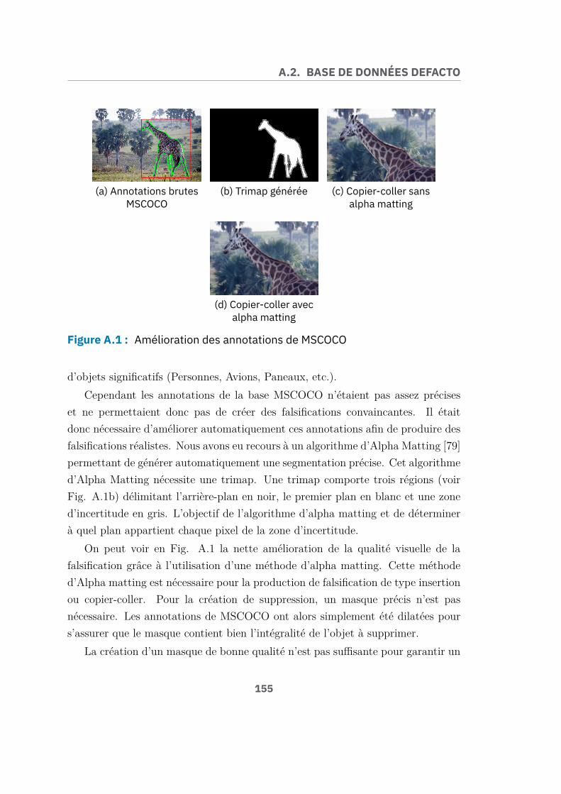
A.2. BASE DE DONNÉES DEFACTO
(a) Annotations brutesMSCOCO
(b) Trimap générée (c) Copier-coller sansalpha matting
(d) Copier-coller avecalpha matting
Figure A.1 : Amélioration des annotations de MSCOCO
d’objets significatifs (Personnes, Avions, Paneaux, etc.).Cependant les annotations de la base MSCOCO n’étaient pas assez précises
et ne permettaient donc pas de créer des falsifications convaincantes. Il étaitdonc nécessaire d’améliorer automatiquement ces annotations afin de produire desfalsifications réalistes. Nous avons eu recours à un algorithme d’Alpha Matting [79]permettant de générer automatiquement une segmentation précise. Cet algorithmed’Alpha Matting nécessite une trimap. Une trimap comporte trois régions (voirFig. A.1b) délimitant l’arrière-plan en noir, le premier plan en blanc et une zoned’incertitude en gris. L’objectif de l’algorithme d’alpha matting et de déterminerà quel plan appartient chaque pixel de la zone d’incertitude.
On peut voir en Fig. A.1 la nette amélioration de la qualité visuelle de lafalsification grâce à l’utilisation d’une méthode d’alpha matting. Cette méthoded’Alpha matting est nécessaire pour la production de falsification de type insertionou copier-coller. Pour la création de suppression, un masque précis n’est pasnécessaire. Les annotations de MSCOCO ont alors simplement été dilatées pours’assurer que le masque contient bien l’intégralité de l’objet à supprimer.
La création d’un masque de bonne qualité n’est pas suffisante pour garantir un
155

APPENDIX A. FRENCH SUMMARY
(a) Authentique (b) Falsifiée
Figure A.2 : Exemple d’insertion
résultat final convaincant. En effet, une des problématiques majeures est de placerl’élément dupliqué ou inséré à un endroit cohérent dans l’image finale. Dans lecas d’une falsification de type insertion, cette tache peut se révéler particulière-ment ardue, voire même impossible. Effectivement, si l’élément inséré n’a pas étéphotographié selon le même angle de vue que l’image cible, alors il peut être toutbonnement impossible d’obtenir un résultat réaliste. Pour relever ce défi, nousavons donc limité nos falsifications à un ensemble d’objets ne variant que peu enfonction de l’angle de vue. Par exemple, une balle de foot sphérique aura toujoursle même aspect, quel que soit notre point de vue. Il est alors aisé de l’insérer dansune autre image. Un exemple de ce type de falsification est donné en Fig. A.2.
De la même manière, lors de la réalisation d’un copier-coller, nous avons con-traint le placement de l’élément dupliqué. En plaçant celui-ci sur le même axeque l’objet initial, on s’assure que les perspectives sont respectées ce qui permetd’obtenir des résultats plus convaincants. Des exemples sont donnés en Fig. A.3.
Pour la suppression, les contraintes sont moins importantes et surtout liées àl’algorithme de suppression. Nous avons utilisé une méthode basée sur l’exemple[84] qui nécessite que l’objet à supprimer se trouve sur un fond relativement simple.Nous avons donc limité la suppression aux objets se trouvant sur un fond simple enappliquant un seuil sur la variance de l’image dans un voisinage proche de l’objet.Un exemple est donné en Fig. A.4
156

A.2. BASE DE DONNÉES DEFACTO
(a) Copier-Coller surl’axe y
(b) Copier-Coller surl’axe x
Figure A.3 : Exemple de Copier-Coller
(a) Authentique (b) Falsifiée
Figure A.4 : Exemple de suppression
Enfin, nous avons aussi généré deux types de falsification supplémentaire. Lesmorphoses et les remplacements de visage. La génération de ces falsifications peutêtre vue en Fig. A.5. Dans un premier temps les deux visages sont approximative-ment alignés. Puis le visage cible est déformé (ou non selon la falsification voulue).Enfin une étape de correction de couleur et de mélange permet de produire la fal-sification finale.
A.2.2 RésultatsGrâce à l’algorithme de falsification présenté précédemment, il a été possible degénérer une grande quantité d’images falsifiées. Ceci a permis de construire unebase de données conséquente et significative permettant d’entraîner des réseaux deneurones profonds.
Le contenu de la base de données est détaillé en Table. A.1.
157

APPENDIX A. FRENCH SUMMARY
(a) Visage A (b) Visage B (c)Alignementapproximatifdes visages A
et B
(d)Alignementprécis des
visages A et B
(e) sanscorrection des
couleurs
(f) Aveccorrection des
couleurs
Figure A.5 : Étape de création de morphose ou remplacement de visage
Table A.1 : Contenu de la base DEFACTO
Falsifications Copier-Coller Suppression Insertion MorphoseImages 19000 25000 105000 80000
A.3 Détection du Copier-CollerUne méthode très commune de falsification des images numériques est courammentappelée le copier-coller. Cette falsification élémentaire consiste en la duplicationd’une portion de l’image. L’élément dupliqué n’est pas contraint en taille et peutsubir une déformation affine avant d’être à nouveau collé dans l’image. Il estintéressant de pouvoir détecter un tel type de falsification puisque cette opérationbasique est couramment utilisée dans les photomontages.
158

A.3. DÉTECTION DU COPIER-COLLER
Cette méthode peut servir à la simple duplication d’un élément pour trompersur une quantité. Ou encore pour la suppression d’un élément sur une image en lecachant derrière un ou plusieurs éléments dupliqués.
Dans le cadre des systèmes de vérification d’identité à distance, le copier-collersera particulièrement efficace pour falsifier les textes du document. En effet, uncontrefacteur pourra simplement copier-coller certaines lettres déjà présentes afind’altérer un ou plusieurs champs de textes. La détection du copier-coller est unsujet déjà bien étudié. Ici nous effectuons la détection à l’aide des points clés SIFTet proposons l’utilisation d’une carte de dissimilarités locales [117] pour permettreune détection plus précise. Une telle amélioration est nécessaire, car les méthodesde détections de copier-coller sont très sensibles aux éléments similaires et tendentà produire de nombreux faux positifs en présence de ceux-ci. Or les lettres sontextrêmement similaires dans un document d’identité ce qui rend la plupart desapproches de l’état de l’art inutilisable dans un cadre pratique.
Dans un premier temps nous présenterons une nouvelle approche pour la dé-tection du copier-coller. Puis, nous montrerons qu’il est possible de grandementréduire le taux de faux positifs à l’aide de cartes de dissimilarités locales. Enfin,nous proposerons une nouvelle base de données contenant de nombreux documentsd’identité falsifiés afin d’encourager la recherche dans ce contexte difficile.
A.3.1 Principe de la méthodeLa méthode de détection peut être découpée en deux phases distinctes. Dansun premier temps, les falsifications sont détectées de manière grossière à l’aide depoints clés SIFT. Les points clés sont extraits de l’image et mis en correspondance.Ils sont ensuite partitionnés afin de grouper les points appartenant à un même objetde l’image, mais aussi de supprimer les faux positifs évidents. Cette premièredétection est efficace, mais très sensible à la présence d’objets similaires.
Une deuxième étape vise donc à supprimer les faux positifs issus de la mise encorrespondance et ayant résisté à l’étape de partitionnement. Dans cette étape, lespoints clés de chaque partition sont filtrés un à un à l’aide de carte de dissimilaritéslocales. À l’issue de cette étape, seules les partions contenant suffisamment depoints clés sont finalement considérés comme des zones falsifiées.
159

APPENDIX A. FRENCH SUMMARY
Dans les sections suivantes, nous présenterons chaque étape de la détectionplus en détail.
A.3.2 Extraction des points clésL’extraction des points clés est effectuée à l’aide du détecteur de la méthode SIFT[113]. Plutôt que d’effectuer une détection globale des points clés sur l’image, ladétection est faite au travers d’une fenêtre glissante non superposée. Les méthodesde détection du copier-coller basées sur les points clés nécessitent que les régionsdupliquées soient couvertes par un nombre suffisant de points clés. Pour pallierce problème, le seuil de rejet sur le contraste est ajusté pour extraire une quantitéde points clés SIFT suffisante pour chaque portion de l’image. Ceci permet deconserver les points clés sur les contours et dans les zones de gradient faible.
A.3.3 Mise en correspondanceLa mise en correspondance classique de descripteur SIFT décrit dans [113] est laméthode 2NN . Pour un descripteur donné, les deux voisins les plus proches avecdes distances d1 et d2 sont trouvés. On considère qu’une mise en correspondanceest positive si le rapport d1
d2est inférieur à un seuil δ.
Une seule mise en correspondance est considérée par le test 2NN . Dans lecadre de la détection du copier-coller, l’hypothèse qu’un élément ne sera dupliquéque de manière unique n’est pas raisonnable. Pour cette raison les auteurs de [93]proposent g2NN , une généralisation de 2NN . Le test 2NN est itéré pour les k
plus proches voisins d’un point clé donné. On teste alors les rapports didi+1
tant queceux-ci sont inférieurs à un seuil δ fixé. Nous avons utilisé ce test généralisé quipermet une détection du copier-coller multiple.
A.3.4 PartitionnementÀ l’étape de mise en correspondance, le seuil δ choisi ne peut être trop strict si l’onveut pouvoir détecter un copier-coller ayant subi un quelconque post-traitement(réechantillonage, ajustement des couleurs ou du contraste ...). Ce qui entraîne
160

A.3. DÉTECTION DU COPIER-COLLER
l’obtention de faux positifs à ce stade. Un deuxième filtrage est nécessaire poursupprimer un maximum de fausses alarmes.
Nous effectuons un partitionnement à l’aide de la méthode décrite dans [116]qui permet de grouper des éléments selon des règles d’équivalences. Soit un objetO de l’image, et OD sa copie (figure A.6). Soit A et C des points clés dans l’objetO et les points clés B et D dans OD. Soit la mise en correspondance MAB entreA et B formant le vecteur
−→AB et la mise en correspondance MCD entre C et D
formant le vecteur−−→CD. Les mises en correspondance MAB et MCD sont considérées
équivalentes et sont groupées si :
‖−→AB −
−−→CD‖ < δ1 (A.1)
‖AC‖ < δ2 et ‖BD‖ < δ2, (A.2)
et ‖AB‖ > δ3 et ‖CD‖ > δ3. (A.3)
Sur la figure A.6 l’objet O est dupliqué en OD avec une légère rotation. Dansle cas d’une duplication avec une déformation simple (rotation, échelle), toutes lesmises en correspondance ont une orientation et une norme similaire.
Le seuil δ1 permet de limiter l’écart entre deux vecteurs formés par deux pairesde points mis en correspondance. Ceci permet de grouper les mises en correspon-dance d’orientation proches. Un seuil δ1 faible tendra à augmenter le nombre departitions. Un objet dupliqué subissant une rotation sera décomposé en plusieurspartitions de plus petite taille. Un seuil δ1 important tendra à diminuer le nombrede partitions. De faux positifs risquent alors d’être inclus dans les partitions desobjets dupliqués. Ce seuil ne dépend pas de la taille de l’image analysée. Danstoutes nos expérimentations, δ1 est fixé à 10.
La distance entre A et C est limitée par la taille de l’objet O dupliqué. Leseuil δ2 fixe la taille maximale de l’objet dupliqué que l’on pourra détecter. Unseuil δ2 trop grand tendra à ajouter des faux positifs dans les partitions des objetsdupliqués. Celui-ci ne peut être trop faible non plus en raison de la densité parfoisplus faible de point SIFT extrait.
A et B sont nécessairement à une distance supérieure à un seuil donné , demême pour C et D, si l’on veut dupliquer O intégralement. Le seuil δ3 fixe ladistance minimale entre l’objet O et sa copie OD que l’on souhaite détecter. La
161

APPENDIX A. FRENCH SUMMARY
Figure A.6 : Duplication de O et règles d’équivalences
valeur de δ3 sera principalement choisie en fonction de la taille de l’image analysée.Dans nos expérimentations, les valeurs de δ2 et δ3 sont fixées à 50.
Le choix des valeurs δ1, δ2 et δ3 n’est pas critique si le seuil sur le contraste enA.3.2 est choisi arbitrairement bas.
À l’issue du partitionnement, les partitions comportant trop peu éléments(moins de trois paires de points mises en correspondance) sont écartées.
A.3.5 Filtrage avec la carte de dissimilarité localeLe descripteur SIFT est l’histogramme des gradients orientés autour du point clé.Ce descripteur ne contient que peu d’information concernant la structure de l’imageautour du point clé.
Dans le cadre de la détection du copier-coller, de nombreux faux positifs peu-vent être produits dans le cas d’une image avec des structures répétitives (façaded’un bâtiment, textes ...). L’utilisation des informations de couleurs et de struc-tures permettrait de rejeter de faux positifs évidents. Nous proposons d’utiliser lacarte de dissimilarité locale (CDL) afin de filtrer ces faux positifs.
La carte de dissimilarité locale [117] permet de mesurer les écarts locaux entredeux images binaires. Pour deux images binaires A et B, la CDL est définie deR2 × R2 dans R2 par
CDLbin(A,B)(p) =| A(p)−B(p) | max(dA(p), dB(p)) (A.4)
avec p = (x, y) et dX(p) la transformée en distance de X au point p.Une extension de la CDL aux images en niveau de gris est utilisée [118]. Les
images sont dans un premier temps découpées en un ensemble d’images binaires.
162

A.3. DÉTECTION DU COPIER-COLLER
La CDL en niveau de gris est alors l’accumulation des CDL entre chacune de cesimages binaires. Soient A et B deux images en niveau de gris, CDLN est alorsdéfinie de R2 × R2 dans R2 par
CDL(A,B)(p) =1
N
N∑i=1
CDLbin(Ai,Bi)(p) (A.5)
Où N est le nombre de coupes, Ai (resp. Bi) est une version binaire de A (resp. Bi),obtenue par seuillage global A > si. Les seuils si sont régulièrement espacés entre0 et le maximum m de chaque image. Par exemple, pour A : si = i
NmA, i ∈ [1..N ].
Pour le copier-coller, nous utilisons une extension directe de la CDL pour desimages avec C canaux. Dans notre cas les images sont converties dans l’espacecolorimétrique CIE XYZ, qui propose une répartition des couleurs se rapprochantde celle du système visuel humain. Soit Ak le canal k ∈ (X,Y,Z) de l’image A, laCDL est définie comme :
CDLXYZ(A,B)(p) =1
3
∑k
CDLN(Ak, Bk)(p). (A.6)
Pour supprimer les derniers faux positifs, les partitions issues du partition-nement (section A.3.4) vont être validées à l’aide des CDL. Pour chaque paire depoints clés mis en correspondances de la partition, deux fenêtres, F1 et F2, sontextraites pour chacun des points clés. Les fenêtres sont centrées sur les points cléset leurs tailles sont fixées par l’échelle des points clés associés. Le contenu des deuxfenêtres est aligné en fonction de l’angle des points clés associés. Finalement, lapaire de points est supprimée de la partition si
‖CDLXYZ(F1, F2)‖2 > δCDL. (A.7)
Comme pour A.3.4, la partition est finalement supprimée si elle contient moinsde trois paires de points clés. On peut voir le résultat de la détection après filtragedans la figure A.7e.
163

APPENDIX A. FRENCH SUMMARY
(a) Imageauthentique
(b) Image falsifiée (c) Vérité terrain (d) Détection sansCDLXY Z
(e) Detection avecCDLXY Z
Figure A.7 : Images de COVERAGE, CDLXY Z et exemple de détection
A.3.6 RésultatsLa méthode a été évaluée sur un ensemble de base de données et comparé à dif-férentes approches de l’état de l’art. Le seuil δCDL est fixé à 7 et les seuils δ1, δ2et δ3 sont fixés pour chacune des bases pour maximiser le taux de vrais positifs.
Les différents résultats sont présentés en Table. A.2. On peut voir que l’ajoutde la CDL permet de surpasser les méthodes de l’état en diminuant très signi-ficativement le taux de faux positifs tout en maintenant un taux de vrai positifsatisfaisant.
164

A.3. DÉTECTION DU COPIER-COLLER
TableA.2:TPR,FPR,
F1(niveauimage)surFAU
[71]GRIP[94]etCO
VERA
GE[73]et
FP(niveaupixel)sur
GRIP
Mét
hode
CO
VER
AG
E[7
3]FA
U[7
1]G
RIP
[94]
TPR
FPR
F1
TPR
FPR
F1
TPR
FPR
F1
FP
Am
erin
i[93
]85
.71
54.9
571
.23
66.6
710
.42
75.2
970
2073
.68
-C
ozzo
lino
[94]
59.3
421
.98
65.4
597
.92
8.33
94.9
598
.75
8.75
95.1
892
.99
J.Li
[96]
87.9
163
.74
69.8
772
.92
22.9
274
.47
83.7
535
76.5
727
.24
Y.L
i[99
]80
.22
41.7
672
.28
100
2.08
98.9
710
00
100
94.6
6Pr
opos
ed70
.02
7.89
78.7
310
00
100
100
010
082
.40
165

APPENDIX A. FRENCH SUMMARY
(a) Image d’undocument
(b) Binarisation deslettres
(c) Détection deslettres
(d) Falsification
Figure A.8 : Étape de falsification du document
Type de document Authentique Falsifié Taille des images16 304 893 1342× 943
Table A.3 : Contenu de la base CMID
A.3.7 Base de données CMIDOn a vu que la méthode permettait de faire diminuer significativement le taux defaux positif. Cependant les résultats ne sont toujours pas satisfaisants en présenced’objets hautement similaires. On peut voir dans la Table. A.2 que le meilleur tauxde vrais positifs atteint est d’environ 88% pour un taux de faux positif d’environ64%. Notre méthode permet d’atteindre le meilleur compromis avec un taux devrai positif d’environ 70% pour un taux de faux positif d’environ 8%. En pratiquece taux de vrai positif n’est pas satisfaisant. Malheureusement, COVERAGE estactuellement la seule base de données permettant d’évaluer les algorithmes dans cecontexte défavorable et ne contient que 100 images falsifiées. De plus, même si lesimages falsifiées contiennent des objets similaires et authentiques. Les falsificationssont relativement larges et ne représentent pas un usage réaliste du copier-coller.
Nous avons donc constitué une nouvelle base de données plus conséquente etreprésentant un cas d’usage pratique du copier-coller. La base CMID est constituéede document d’identité falsifié. Pour la constituer, nous avons mis au point unalgorithme permettant de détecter les lettres du document, puis de dupliquer l’uned’entre elles (voir Fig. A.8). Ainsi nous avons pu produire 893 images falsifiées.Le contenu exact de la base de données est donné en Table. A.3.
166

A.3. DÉTECTION DU COPIER-COLLER
Méthode TPR FPR MCCSURF [71] 0.7919 0.7697 0.0236SIFT [71] 0.9676 0.9145 0.1104
BusterNet [109] 0.1601 0.1607 -0.0006FE-CMFD [99] 0.0246 0.0066 0.0561SIFT-LDM [2] 0.7917 0.0197 0.6847
Table A.4 : Score niveau image
Méthode TPR FDR F1 MCCSURF [71] 0.2155 0.9792 0.0378 0.0606SIFT [71] 0.6004 0.9610 0.0731 0.1471
BusterNet [109] 0.0016 0.9979 0.0018 0FE-CMFD [99] 0.0341 0.3114 0.0650 0.1530SIFT-LDM [2] 0.2555 0.0541 0.4024 0.4912
Table A.5 : Score niveau pixel
A.3.8 Résultats sur la base CMID
Nous avons évalué plusieurs méthodes de l’état de l’art ainsi que notre approchesur cette nouvelle base de données. On peut voir les résultats au niveau imageen Table. A.4. On constate que les méthodes ont du mal à maintenir un taux devrais positifs élevé tout en maintenant un taux de faux positifs faible. De la mêmemanière, on peut voir en Table. A.5 que les résultats ne sont pas satisfaisants auniveau pixel.
On peut voir que notre approche qui a été conçue pour diminuer le taux de fauxpositif obtient les meilleurs résultats. Cependant ceux-ci ne sont pas encore suff-isants pour une utilisation pratique. La base de données CMID est publiquementaccessible afin de favoriser la recherche de méthode de détection plus robuste enprésence d’objets similaires. Les résultats de notre approche, bien qu’insuffisants,montrent que ce défi peut être relevé s’il est pris en compte.
167

APPENDIX A. FRENCH SUMMARY
A.4 Détection de la suppression d’objetUne manipulation d’image commune est la suppression d’objet. Un ou plusieurséléments de l’image sont alors effacés en reconstituant l’arrière-plan. Des algo-rithmes d’inpainting sont souvent utilisés dans ce type de falsification et les bordsde la falsification sont souvent floutés afin de rendre celle-ci visuellement imper-ceptible. En conséquence, la bordure de la texture reconstituée peut apparaîtremoins nette que le reste de la texture. Nous proposons une méthode de détectionde la suppression en mettant en évidence ce phénomène. Pour se faire, nous avonsdéveloppé une mesure de netteté relative d’un pixel par rapport au reste de l’im-age. Cette mesure permet de mettre en évidence des zones anormalement lisses del’image.
Dans les sections suivantes, nous introduirons la méthode de détection pro-posée.
A.4.1 Mesure de netteté basée sur la réflectance
On peut simplifier le processus de formation d’une image en utilisant le modèled’illumination-réflectance. La réflectance est la capacité d’une surface à réfléchir dela lumière tandis que l’illumination est la quantité de lumière parvenant sur cettesurface. Le modèle illumination-réflectance modélise donc chaque pixel (x, y) del’image comme étant le produire de l’illumination en (x, y et de la réflectance en(x, y). On a donc :
I(x, y) = L(x, y) ∗R(x, y) (A.8)
ou I(x, y) est l’intensité du pixel en (x, y), L(x, y) l’illumination et R(x, y) laréflectance. Les variations de L sont typiquement très lentes par rapport à R,il est donc possible d’extraire la réflectance en utilisant un filtrage homomorphe[125]. Tout d’abord on applique une transformation logarithmique à l’image afinde séparer l’illumination et la réflectance en une somme :
ln(I(x, y)) = ln(L(x, y)) + ln(R(x, y)). (A.9)
168

A.4. DÉTECTION DE LA SUPPRESSION D’OBJET
(a) Image de deuxtextures
(b) Mesure de nettetérelative S
(c) Segmentation de S
Figure A.9 : Utilisation de la mesure de netteté S pour segmenter une image
On peut ainsi isoler la réflectance en utilisant un filtre passe-haut :
r(u, v) = F(ln(I(x, y)))H(u, v) (A.10)
avec F la transformée de Fourier, H un filtre passe-haut dans le domaine fréquen-tiel et r(u, v) l’estimation de la réflectance dans le domaine fréquentielle.
On obtient l’approximation finale de la réflectance R̂ en prenant l’exponentiellede la transformée de Fourier inverse de r(u, v) :
R̂(x, y) = exp(F−1(r(u, v))). (A.11)
La réflectance estimée R̂ est une approximation grossière, mais suffit commemesure de netteté. En effet, plus une surface est rugueuse et plus l’estimation R̂
sera variable. Ainsi on peut dériver une mesure de netteté locale d’un pixel (x, y)comme étant la variance dans une fenêtre autour de ce pixel. Chaque pixel estdonc associé à une mesure de netteté locale σR̂ pour obtenir une mesure de nettetérelative au reste de l’image, les pixels de celle-ci sont partitionnés en fonction deleur intensité. Pour chaque pixel, sa netteté est calculée comme étant la déviationabsolue médiane de sa netteté locale σR̂ par rapport aux autres pixels de la mêmepartition. On obtient une carte de netteté relative S dans laquelle les grandesvaleurs positives représentent des zones perceptiblement plus nettes tandis que degrandes valeurs négatives indiquent des zones perceptiblement plus lisses. On peutvoir en Fig. A.9 un exemple de segmentation basé sur cette mesure S permettantde séparer une texture rugueuse d’une texture plus lisse.
169

APPENDIX A. FRENCH SUMMARY
A.4.2 Application à la détection de falsificationIl est commun pour un contrefacteur de flouter les bords de la falsification lorsd’une suppression. On espère donc que cet artefact pourra être mis en évidence àl’aide de la mesure de netteté proposée.
On peut voir sur la figure A.10d, une zone qui apparaît effectivement beaucoupplus lisse que le reste de l’image à l’endroit de la falsification. L’exemple donné enFig. A.10b a été créé spécifiquement pour évaluer notre approche. Afin de validercette méthode sur des cas concrets, nous l’avons appliquée sur des images falsifiées(Fig. A.10f et Fig. A.10j) provenant du forum internet «PhotoshopBattle» ou desutilisateurs réalisent des photomontages à partir d’une image donnée. On peut voirque la méthode permet effectivement de mettre en évidence les suppressions pources exemples. De plus, on peut voir sur la Fig. A.10h que l’insertion de l’enfantest aussi mise en évidence par notre méthode. Ceci est dû à la forte différencede qualité entre l’image originale et l’image insérée qui fait apparaître l’élémentinséré comme beaucoup plus flou que le reste de l’image. Le même phénomène estvisible pour la Fig. A.10p. On voit donc que notre méthode peut aussi mettre enévidence des falsifications de types insertion sous certaines conditions.
A.5 Détection du Face MorphingDans ce chapitre nous nous intéressons à la détection des attaques de type Mor-phose de visage. Une morphose de visage consiste en un mélange de deux visagesou plus. Les deux visages sont mélangés comme expliqué en Fig. A.5. L’intérêtd’une telle attaque est de créer un visage synthétique partageant la biométrie dedeux individus. Un système de reconnaissance facial est alors trompé par ce vis-age synthétique et authentifiera les deux personnes ayant servi à générer cettemorphose.
Sur la Fig. A.11, on peut voir au centre une morphose de visage entre le visagede gauche et de droite. Le système de reconnaissance faciale libre de la librairieDlib [88] authentifie alors les deux visages si l’on utilise le seul recommandé de0, 6.
Pour un système de vérification d’identité à distance les morphoses de visage
170

A.5. DÉTECTION DU FACE MORPHING
(a) Imageauthentique
(b) Imagefalsifiée
(c) Vérité terrain (d) Carte denetteté S
(e) Imageauthentique
(f) Image falsifiée (g) Vérité terrain (h) Carte denetteté S
(i) Imageauthentique
(j) Image falsifiée (k) Vérité terrain (l) Carte denetteté S
(m) Imageauthentique
(n) Imagefalsifiée
(o) Vérité terrain (p) Carte denetteté S
Figure A.10 : De gauche à droite : Les images authentiques, les imagesfalsifiées, les vérités terrain, la mesure de netteté S
sont une réelle menace puisqu’elles permettraient la création d’identité partagée.Deux contrefacteurs pourraient en effet la photo du document d’identité par unemorphose afin de pouvoir plus tard s’authentifier à l’aide d’un même document.
Dans ce chapitre nous proposons une méthode à l’aveugle et sans référence dedétection des attaques de types morphoses de visage par analyse du bruit. Notre
171

APPENDIX A. FRENCH SUMMARY
Figure A.11 : Le système de reconnaissance facial authentifie les visages degauche et de droite avec la morphose au centre pour un seuil de 0, 6.
méthode est à l’aveugle, car elle ne fait pas recourt à un marquage actif de l’image.Elle est sans référence, car la détection est faite uniquement à l’aide du visagesynthétique. Nous montrons ensuite qu’il est possible de tromper notre approcheà l’aide d’une attaque de contre forensique ciblée. Nous montrons que cette mêmeattaque permet de tromper d’autres méthodes de l’état de l’art à l’aveugle et sansréférences. Nous montrons ensuite les difficultés de certaines de ces méthodes vis-à-vis d’un changement de qualité des images authentiques. Ces difficultés ainsique la possibilité de créer des algorithmes de contre forensique efficace mettenten doute la possibilité d’utilisé des méthodes à l’aveugle et sans référence pourcertains scénarii d’usage des morphoses de visages.
A.5.1 Détection des Morphoses par analyse du bruitLa morphose d’un visage A et d’un visage B peut être formalisée de la manièresuivante. Étant donné un alpha matte αb avec αbi,j ∈ [0, 1],∀(i, j). L’image finale
172

A.5. DÉTECTION DU FACE MORPHING
0.35 0.4 0.45 0.5 0.55 0.6 0.65 0.73
3.2
3.4
3.6
3.8
410
-3
in,k
out,k
(a) σint,k et σext,k pour un visageauthentique
0.2 0.3 0.4 0.5 0.6 0.72.5
3
3.5
410
-3
in,k
out,k
(b) σint,k et σext,k pour unemorphose
Figure A.12 : σint,k et σext,k
MAB est donnée par
MAB = αb ◦BA + (1−αb) ◦ IB (A.12)
avec BA l’image du visage A déformé et dont les couleurs ont été corrigées et IB
l’image du visage B déformé.Dans l’image résultante MAB le comportement du bruit sera donc celui d’une
image naturelle en tout point ou αb = 0. Pour αb 6= 0, MAB est donc une moyennepondérée de deux images interpolées.
On peut montrer que pour des pixels appartenant à une partition k d’intensitéproche, la variance σ2
int,k des pixels de la partition k à l’intérieur du visage estdonnée par :
σ2int,k = (αbσ
′int,k)
2 + ((1− αb)σext,k)2. (A.13)
On s’attend donc à ce que la variance du bruit soit plus faible dans la région ouαb 6= 0.
On peut voir en Fig. A.12 la chute de variance des pixels à l’intérieur du visagepour une morphose.
A.5.2 RésultatsNous avons créé une première base de données contenant 100 visages authentiqueset 171 morphoses de visages à partir de la base de données PUT [147]. Nous avonsensuite évalué et comparé notre approche sur cette base de données. On peut voir
173

APPENDIX A. FRENCH SUMMARY
Table A.6 : EER sur la base de données PUT en variant la qualité JPEG desmorphoses de visage et en appliquant le Contre-Forensique (CF)
EER at JPEG 100 95 90 85 80 75 CFLBP 11.20 37.98 59.98 77.82 85.67 73.26 22.86BSIF 26.86 5.86 1.19 5.86 11.21 13.87 41.63LPQ 4.26 54.01 33.07 37.05 58.17 53.06 27.43
Méthode proposée 0.59 0.37 2.35 4.73 8.48 21.08 35.86
Table A.7 : EER sur la base de données FERET en variant la qualité JPEG desimages authentiques
EER pour JPEG Raw 100 95 90 85 80 75LBP 3.93 3.42 4.87 8.07 11.71 16.19 18.42BSIF 1.63 1.75 2.23 3.87 6.24 8.75 11.90LPQ 2.64 2.78 2.72 4.80 5.82 8.06 8.86
Méthode proposée 7.59 7.79 7.24 6.59 6.02 5.45 5.20
les résultats en Table. A.6.On voit que notre approche surpasse les méthodes de l’état de l’art pour des fac-
teurs de qualité standard. Cependant, on peut voir qu’il est possible de développerune approche de contre-forensique permettant de tromper.
Dans la Table. A.7, nous avons cette fois fait varier la qualité JPEG desimages authentiques et en prenant les morphoses de visage de meilleure qualité.Idéalement, on s’attend à ce que la détection soit aisée, quelle que soit la qualitédes images authentiques puisque les morphoses sont de bonne qualité et doncsimplement détectables. En réalité on observe que les performances des détecteursde l’état de l’art chutent lorsque la qualité des images authentique diminue. Cecimontre que ces détecteurs se comportent comme des détecteurs de qualité d’imagesplutôt que des détecteurs de morphose. À l’inverse, les performances de notredétecteur augmentent puisque le résidu des images fortement compressées tend àêtre nul. Notre détecteur ne parvient donc plus à faire de différence entre le résiduà l’intérieur et à l’extérieur du visage. Cette faiblesse n’est pas gênante puisqu’elleest explicable est qu’elle est valable quelle que soit l’image étudiée (authentiqueou falsifiée).
Ces résultats soulèvent des questionnements concernant l’utilisation pratique
174

A.6. DÉTECTION DE LA DOUBLE COMPRESSION H.264
des méthodes de détection à l’aveugle et sans référence dans certains scénarii. Eneffet, certaines méthodes visent à être utilisées dans des cas d’usage non contrôlé.L’image étudiée provient d’une source inconnue est pourrait ainsi avoir été im-primée et rescannée par exemple. Or nous avons montré les difficultés dont lesdétecteurs faisaient preuve en présence de variation de qualité des images authen-tiques ou falsifiées. De plus, nous avons montré qu’un algorithme de contre foren-sique conçu pour tromper notre méthode permettait aussi de tromper d’autresméthodes. Nous pensons que l’accumulation de ces défis ne permet pas la dé-tection des morphoses de visage par des méthodes à l’aveugle et sans référencesdans des contextes non contrôlés. Pour ces applications, des méthodes basées surune référence (c.-à-d. autre acquisition sûre de la personne) sont préférables. Lesméthodes à l’aveugle et sans références restent cependant intéressantes dans uncontexte contrôlé, mais une évaluation rigoureuse des performances face à unevariation de qualité des images est nécessaire.
A.6 Détectionde ladouble compressionH.264Dans un contexte de vérification d’identité à distance, l’acquisition du documentet de la personne sous forme d’une vidéo se présente comme une solution na-turelle. En effet, les personnes ou les éléments de sécurité standard tels que leshologrammes et encres variables sont par nature dynamiques et nécessitent de faitplus d’une image pour être pleinement caractérisés. Un autre argument en faveurde l’authentification via une vidéo plutôt qu’une image et la complexité ajoutéespour falsifier le document numériquement. Contrairement à la falsification d’uneimage, le contrefacteur fait en ici face à la contrainte du temps réel, mais aussidéveloppé des méthodes plus évoluées. Pour falsifier les champs de textes d’undocument sur une vidéo par copier-coller, l’algorithme devrait déjà être en mesurede détecter et suivre chaque champ du document. Une alternative serait l’usagede méthode de type «shape from template» afin de venir synthétiser l’intégralitédu document. Quelle que soit la méthode choisie, on perçoit aisément le challengepour le contrefacteur en comparaison d’une simple image. Ces raisons ont notam-ment privilégié le choix de la vidéo dans le cadre de la vérification d’identité pour
175

APPENDIX A. FRENCH SUMMARY
la certification de ces systèmes [14].
La complexité de telles falsifications ne devrait pas pour autant justifier uneconfiance aveugle dans les médias vidéos. En particulier dans le contexte de vérifi-cation qui nous intéresse. Une des attaques les plus pressenties dans le cadre d’uncontrôle d’identité est la vérification de la biométrie de la personne. En particulier,de la biométrie faciale. Si la détection et le suivi en temps réel d’un documentd’identité quelconque ne sont pas un sujet très étudié, il n’en va pas de mêmepour les visages. La détection et le suivi de ceux-ci sont des problématiques bienétudiées. Certaines technologies permettent même aujourd’hui la détection et l’ap-proximation d’un maillage en 3D du visage en temps réel dans un navigateur surun téléphone mobile [26, 27]. De même, exclure la possibilité pour le contrefacteurd’injecter un flux vidéo déjà falsifié au sein du système n’est pas raisonnable.
Il est donc nécessaire de justifier de l’intégrité du média vidéo en amont de lavérification de l’identité de la personne. De nombreuses recherches ont été menéesconcernant la détection du vivant. En pratique, les méthodes de détections duvivant combinées à l’utilisation de challenge aléatoire (clignement des yeux, sourire...) permettent d’écarter raisonnable l’hypothèse d’un flux vidéo préparé en avanceet injecté dans le système. Pour autant, ces systèmes ne suffisent pas à garantirl’intégrité du média final. Dans ce chapitre, on suppose donc que le flux est falsifiéen temps réel. En particulier, on suppose que l’appareil d’acquisition est contrôlé etsûr. Dans ce cas d’usage, le contrefacteur intercepte le flux et le falsifie avant l’envoisur le serveur. Si le flux est compressé, il est nécessaire pour le contrefacteur de ledécompresser puis de le recompresser après sa falsification. Une première approchepour vérifier l’intégrité du flux est alors de détecter la double compression. Ons’intéressera en particulier à la compression vidéo H.264 qui est, avec VP8, le seulcodec imposé par la norme WebRTC [153].
Dans ce chapitre une approche de détection basée sur la distribution des coef-ficients DCT sera présentée.
176

A.6. DÉTECTION DE LA DOUBLE COMPRESSION H.264
A.6.1 Modélisation des coefficients DCT
Dans ce chapitre, nous considérons les coefficients C distribués selon une loi deLaplace
C ∼ Laplace(0, b). (A.14)
En figure A.13 on peut constater que pour des vidéos simplement compressées,le paramètre b semble relativement stable d’une vidéo à l’autre.
La loi de Laplace est un choix populaire pour la modélisation des coefficientsDCT. Cette modélisation n’est pas tout à fait exacte [180] mais à l’avantage d’êtreune bonne approximation avec une forme analytique plus simple.
La densité de probabilité des coefficients C sera donc donnée par :
f(x|b) = 1
2bexp(−|x|
b). (A.15)
On suppose que b sera modifié par le processus de double compression. Onpropose donc deux tests d’hypothèse. Dans un premier temps, on suppose quela valeur théorique pour une simple compression b0 ainsi que la valeur b1 d’unedouble compression sont connues. Ensuite nous proposerons un test ou seule lavaleur b0 pour une simple compression est connue.
A.6.2 Test d’hypothèse simple
Pour vérifier si la vidéo est doublement compressée nous proposons donc le testsuivant : H0 : C ∼ Laplace(0, b0)
H1 : C ∼ Laplace(0, b1), b1 6= b0.(A.16)
Le rapport de vraisemblance est défini comme :
Λ(C) =L1(C)
L0(C). (A.17)
177

APPENDIX A. FRENCH SUMMARY
Figure A.13 : Distribution de b pour différente valeur de QP sur 40 vidéos.
On a donc le rapport de log-vraisemblance qui est donné par :
Λ(C) = N log b0b1
+b1 − b0b0b1
N∑i=0
|ci|. (A.18)
On peut montrer que sous Hh, h ∈ {0, 1} on a :
Λh(C) ∼ N (µh, σh), (A.19)
avec
µh = N log b0b1
+Nbhb1 − b0b0b1
, (A.20)
σh = |N b1 − b0b0b1
| bh√N. (A.21)
178

A.6. DÉTECTION DE LA DOUBLE COMPRESSION H.264
On pose finalement
Λ?(C) =Λh(C)− µ0
σ0
∼ N (µh − µ0
σ0
,σh
σ0
). (A.22)
Sous H0 on a donc Λ?(C) qui suit une loi normale centrée réduite.En vertu du Lemme de Neyman-Pearson, le test le plus puissant est le test du
rapport de vraisemblance. On définit donc le test :
δ?(C) =
H0 si Λ?(C) < τ ?
H1 si Λ?(C) ≥ τ ?. (A.23)
Pour ce test la puissance β est donnée par la probabilité α de rejeter l’hypothèsenulle sous H1 :
β(δ?) , PH1 [δ?(C) = H1] = 1− α. (A.24)
On peut définir un seuil τ ? permettant d’obtenir un taux de fausses alarmesα0 en résolvant :
PH0 [Λ?(C) ≥ τ ?] = α0. (A.25)
La puissance de notre test est finalement donnée par :
β(δ?) = PH1 [Λ?(C) ≥ τ ?]. (A.26)
A.6.3 Test d’hypothèse composéPour le test composé, seul le paramètre b0 est connu. Le paramètre b1 est quant àlui remplacé par le maximum de vraisemblance estimé à partir des données. On adonc le rapport de vraisemblance donné par
Λ(C) =NCb0−N log(C) +N(log(b0)− b0) (A.27)
avec
C =1
N
N∑i=0
|ci|. (A.28)
179

APPENDIX A. FRENCH SUMMARY
Table A.8 : Comparaison à l’état de l’art
Paramètre de quantification QP MéthodeQP1 QP2 Proposée SVM-DCT [173] G-VPF [165]25 18 1 0.9781 0.958025 20 1 0.7503 0.917025 23 0.9512 0.6629 0.892623 18 0.9990 0.8241 0.956123 20 0.9863 0.7575 0.911120 18 0.9570 0.5078 0.926823 25 0.4453 0.4724 0.893625 30 0.3028 0.3632 0.7432
On peut montrer que :
Λ̂(C) = 2(Λ(C)− a0) ∼ χ2(1) (A.29)
aveca0 = N(1− b0). (A.30)
A.6.4 RésultatsNous avons constitué une base de données de vidéos simplement et doublementcompressée afin d’évaluer notre approche et de la comparer à l’état de l’art. Lesrésultats sont donnés en Table. A.8.
On peut voir que notre approche surpasse les méthodes de l’état de l’art pourtout recomperssion ou QP1 > QP2. Cependant notre méthode n’est pas applicabledans le cas ou QP2 > QP1. En effet, une seconde compression plus forte que lacompression initiale tend à effacer toutes traces de celle-ci. Ainsi, le paramètre b
estimé correspond à la valeur attendue dans le cas d’une simple compression. Ilest intéressant de noter que la méthode SVM-DCT est aussi inapplicable dans cescénario. Ce résultat est attendu puisque la détection est basée sur les coefficientsDCT. À l’inverse, la méthode G-VPF est plus robuste que les approches baséessur les coefficients DCT. On voit cependant que les performances chutent lorsquel’écart entre QP2 et QP1 grandit.
180

A.7. CONCLUSION
A.7 ConclusionDans cette thèse nous avons abordé les problématiques d’authentifications desimages et vidéos. Ces médias font partie de notre vie de tous les jours et nousne questionnons que rarement leurs authenticités. Cependant, les technologiesde retouches photographiques et vidéos permettent aujourd’hui de produire desfalsifications d’une très grande qualité.
Avec la pandémie liée au COVID19, l’utilisation des systèmes de vérificationd’identité à distance s’est intensifiée. De tels systèmes reposent en grande partiesur des images et vidéos. Il est donc essentiel de pouvoir garantir l’intégrité de cesmédias afin de sécuriser ces systèmes.
Nous avons abordé différentes attaques qui pourraient être menées par un con-trefacteur tout en essayant de traiter des problématiques plus larges liées à cesattaques.
Dans un premier temps, nous avons constitué une base de données d’imagesfalsifiées en tout genre afin de permettre d’étudier les approches par réseaux deneurones profonds.
Ensuite, nous avons étudié la problématique du copier-coller. Le copier-collerest une technique de falsification très simple et très efficace pour modifier les textesd’un document d’identité. Nous avons vu que ces méthodes sont très sensibles àla présence d’objet hautement similaire. En effet, les méthodes de l’état de l’artn’abordent que très peu cette problématique en se concentrant majoritairementsur la détection de copier-coller ayant subi de multiples transformations. Nousavons montré que ceci rendait leur utilisation impossible dans un contexte dedétection de documents retouchés à cause des lettres fortement similaires. Nousavons donc proposé une première approche pour réduire le taux de faux positifsdans ce scénario ainsi qu’une nouvelle base de données de copier-coller sur desdocuments d’identité afin de favoriser la recherche dans cette direction.
Nous avons ensuite abordé la problématique de la suppression d’objet. Cetype de falsification est souvent utilisé en amont d’une autre attaque telle qu’uneinsertion ou un copier-coller. Nous avons montré que les contrefacteurs floutaientlégèrement les bords de leur falsification afin d’obtenir un résultat visuel plusconvaincant. Nous avons montré qu’il était possible de mettre en évidence cette
181

APPENDIX A. FRENCH SUMMARY
opération en étudiant la réflectance de l’image. En effet, cette opération tend àproduire des textures plus lisses qui se traduisent par une chute localisée de lavariance de la réflectance. Nous avons montré que ceci pouvait aussi mettre enévidence des falsifications de types insertions dans le cas ou la qualité de l’imageinsérée diffère largement de l’image cible.
Nous nous sommes ensuite intéressés à la problématique de la Morphose de vis-age qui peut permettre la création d’une biométrie partagée. Nous avons d’abordmontré que la morphose de visage induit une chute de la variance à l’intérieurdu visage retouché. Nous avons montré qu’il était possible de détecter ce typede falsification en étudiant la différence de niveau de variance à l’intérieur et àl’extérieur du visage. Nous avons aussi montré que les méthodes à l’aveugle etsans référence pouvaient être sensibles à la qualité des morphoses, mais aussi desimages authentiques. Il est donc nécessaire de bien définir le cadre d’applicationpour de telles méthodes.
Enfin, nous avons étudié la double compression vidéo. En particulier nous noussommes intéressés à l’algorithme H.264 qui est le plus répandu. En supposant queles coefficients sont distribués selon une loi de Laplace. Nous avons proposé deuxtests d’hypothèses permettant la détection de la double compression. Dans unpremier temps, nous avons proposé un test ou tous les paramètres sont connus.Puis nous avons proposé un test généralisé pour lequel l’un des paramètres estinconnu. Nous avons montré que ce test généralisé permet d’obtenir de meilleursrésultats de détection que les méthodes de l’état de l’art. Nous avons aussi montréque notre méthode n’est pas applicable dans le cas où la seconde compression estplus forte que la première.
182

APPENDIX BAppendix
B.1 Maximum Likelihood Estimator for parameter b. . . . 184
183

APPENDIX B. APPENDIX
B.1 Maximum Likelihood Estimator for pa-rameter b
We suppose that C ∼ Laplace(0, b). We can then define the likelihood function ofa given parameter b as :
Lb(ci) =1
2bexp(−|ci|
b). (B.1)
For C we then have
Lb(C) =N∏i=0
Lb(ci)
=1
(2b)Nexp(−
∑Ni=0|ci|b
).
(B.2)
The log-likelihood function for C is finally given by
`b(C) = log(Lb(C))
= −N log(2b) + −∑N
i=0|ci|b
.(B.3)
The maximum likelihood estimate is thus give for
∂`b(C)
∂b= 0, (B.4)
With∂`b(C)
∂b=−Nb
+
∑Ni=0|ci|b2
. (B.5)
We finally derive the maximum likelihood estimator b̂ as
b̂ =
∑Ni=0|ci|N
. (B.6)
184

Bibliographie
[1] G. Mahfoudi et al. “DEFACTO: Image and Face Manipulation Dataset”.In: 2019 27th European Signal Processing Conference (EUSIPCO). 2019,pp. 1–5.
[2] G. Mahfoudi et al. “Copy and Move Forgery Detection Using SIFT andLocal Color Dissimilarity Maps”. In: 2019 IEEE Global Conference on Signaland Information Processing (GlobalSIP). 2019, pp. 1–5.
[3] M. Pic, G. Mahfoudi, and A. Trabelsi. “Remote KYC: Attacks and Counter-Measures”. In: 2019 European Intelligence and Security Informatics Con-ference (EISIC). IEEE. 2019, pp. 126–129.
[4] G. Mahfoudi et al. “Object-Removal Forgery Detection through ReflectanceAnalysis”. In: 2020 IEEE International Symposium on Signal Processing andInformation Technology (ISSPIT). IEEE. 2020, pp. 1–6.
[5] G. Mahfoudi et al. “CMID: A New Dataset for Copy-Move Forgeries on IDDocuments”. In: 2021 IEEE International Conference on Image Processing(ICIP). IEEE. 2021, pp. 3028–3032.
[6] M. Pic et al. “Face Manipulation Detection in Remote Operational Sys-tems”. In: Handbook of Digital Face Manipulation and Detection. Ed. byR. Christian et al. Springer International Publishing, 2022.
[7] G. Mahfoudi et al. “Statistical H.264 Double Compression Detection MethodBased on DCT Coefficients”. In: IEEE Access 10 (2022), pp. 4271–4283. doi:10.1109/ACCESS.2022.3140588.
185

BIBLIOGRAPHIE
[8] G. Mahfoudi et al. Method for processing a candidate image. French PatentFR2000395. Jan. 2020.
[9] M. M. Pic et al. Image processing method for an identity document. FrenchPatent FR19004228. Feb. 2019.
[10] G. Mahfoudi. Procédé de vérification d’une image numérique. French PatentFR2012868. Oct. 2020.
[11] M. M. Pic et al. Procédé d’authentification d’un élément optiquement vari-able. French Patent FR2006419. Feb. 2020.
[12] G. Mahfoudi, M. M. Pic, and A. Trabelsi. Method for automatically detect-ing facial impersonation. French Patent FR3088457, World Patent WO2020099400.May 2020.
[13] G. Mahfoudi and A. Ouddan. Digital image processing method. FrenchPatent FR3091610B1. May 2020.
[14] ANSSI. Publication du référentiel d’exigences applicables aux Prestatairesde Vérification d’Identité à Distance (PVID). https://www.ssi.gouv.fr/uploads/2021/08/anssi-requirements_rule_set-pvid-v1.1.pdf.Accessed: 2020-09-27. Mar. 2021.
[15] G. S. Kc and P. A. Karger. Security and Privacy Issues in Machine ReadableTravel Documents (MRTDs). 2005.
[16] Identification cards — Physical characteristics. Standard. Geneva, Switzer-land: International Organization for Standardization, Dec. 2019.
[17] Machine Readable Travel Documents : Part 3 — Specifications Common toall MRTDs. Specification. Geneva, Switzerland: International Civil AviationOrganization, 2021.
[18] S. Baechler. “Document Fraud: Will Your Identity Be Secure in the Twenty-First Century?” In: European Journal on Criminal Policy and Research26.3 (Sept. 2020), pp. 379–398. issn: 0928-1371, 1572-9869. doi: 10.1007/s10610-020-09441-8. url: https://link.springer.com/10.1007/s10610-020-09441-8 (visited on 10/20/2021).
186

BIBLIOGRAPHIE
[19] L. Verdoliva. “Media Forensics and DeepFakes: An Overview”. In: IEEEJournal of Selected Topics in Signal Processing 14.5 (2020), pp. 910–932.doi: 10.1109/JSTSP.2020.3002101.
[20] L. Zheng, Y. Zhang, and V. L. L. Thing. “A Survey on Image Tamperingand Its Detection in Real-World Photos”. In: Journal of Visual Communi-cation and Image Representation 58 (2019), pp. 380–399. issn: 1047-3203.doi: 10.1016/j.jvcir.2018.12.022.
[21] N. A. Shelke and S. S. Kasana. “A Comprehensive Survey on Passive Tech-niques for Digital Video Forgery Detection”. In: Multimedia Tools and Ap-plications 80.4 (Feb. 2021), pp. 6247–6310. issn: 1380-7501, 1573-7721. doi:10.1007/s11042-020-09974-4. url: https://link.springer.com/10.1007/s11042-020-09974-4 (visited on 10/20/2021).
[22] P. Joshi and N. Shrivastav. “A Review Paper on Image Inpainting andTheir Different Techniques”. English. In: (2018), p. 4.
[23] E. M. Newton, L. Sweeney, and B. Malin. “Preserving Privacy by De-Identifying Face Images”. In: IEEE transactions on Knowledge and DataEngineering 17.2 (2005), pp. 232–243.
[24] R. Gross et al. “Integrating Utility into Face De-Identification”. In: In-ternational Workshop on Privacy Enhancing Technologies. Springer. 2005,pp. 227–242.
[25] O. Gafni, L. Wolf, and Y. Taigman. “Live Face De-Identification in Video”.In: Proceedings of the IEEE/CVF International Conference on ComputerVision. 2019, pp. 9378–9387.
[26] Y. Kartynnik et al. “Real-time facial surface geometry from monocularvideo on mobile GPUs”. In: arXiv preprint arXiv:1907.06724 (2019).
[27] Google. Face Mesh - MediaPipe. https://google.github.io/mediapipe/solutions/face_mesh.html. Accessed: 2020-09-27. 2020.
[28] J. Nakamura, ed. Image Sensors and Signal Processing for Digital StillCameras. Boca Raton, FL: Taylor & Francis, 2006. 336 pp. isbn: 978-0-8493-3545-7.
187

BIBLIOGRAPHIE
[29] C. Chen, S. Mccloskey, and J. Yu. “Analyzing Modern Camera ResponseFunctions”. In: 2019 IEEE Winter Conference on Applications of Com-puter Vision (WACV). 2019 IEEE Winter Conference on Applications ofComputer Vision (WACV). Waikoloa Village, HI, USA: IEEE, Jan. 2019,pp. 1961–1969. isbn: 978-1-72811-975-5. doi: 10.1109/WACV.2019.00213.url: https://ieeexplore.ieee.org/document/8658243/ (visited on10/20/2021).
[30] B. Peng et al. “Optimized 3D Lighting Environment Estimation for ImageForgery Detection”. In: IEEE Transactions on Information Forensics andSecurity 12.2 (Feb. 2017), pp. 479–494. issn: 1556-6021. doi: 10.1109/TIFS.2016.2623589.
[31] B. Peng et al. “Improved 3D Lighting Environment Estimation for ImageForgery Detection”. In: 2015 IEEE International Workshop on InformationForensics and Security (WIFS). Nov. 2015, pp. 1–6. doi: 10.1109/WIFS.2015.7368587.
[32] A. Mazumdar, J. Jacob, and P. K. Bora. “Forgery Detection in DigitalImages through Lighting Environment Inconsistencies”. In: 2018 TwentyFourth National Conference on Communications (NCC). Feb. 2018, pp. 1–6. doi: 10.1109/NCC.2018.8600175.
[33] A. Mazumdar and P. K. Bora. “Estimation of Lighting Environment forExposing Image Splicing Forgeries”. In: Multimedia Tools and Applica-tions 78.14 (July 2019), pp. 19839–19860. issn: 1573-7721. doi: 10.1007/s11042-018-7147-2.
[34] J.-B. Lee et al. “Detecting Digital Forgeries Using of a Lighting Direction”.In: 2007 Digest of Technical Papers International Conference on ConsumerElectronics. Jan. 2007, pp. 1–2. doi: 10.1109/ICCE.2007.341520.
[35] W. Fan et al. “3D Lighting-Based Image Forgery Detection Using Shape-from-Shading”. In: 2012 Proceedings of the 20th European Signal ProcessingConference (EUSIPCO). 2012, pp. 1777–1781.
[36] T. Carvalhoa, H. Faridb, and E. Keec. Exposing Photo Manipulation FromUser-Guided 3-D Lighting Analysis.
188

BIBLIOGRAPHIE
[37] X. Yang, Y. Li, and S. Lyu. “Exposing Deep Fakes Using Inconsistent HeadPoses”. In: ICASSP 2019 - 2019 IEEE International Conference on Acous-tics, Speech and Signal Processing (ICASSP). May 2019, pp. 8261–8265.doi: 10.1109/ICASSP.2019.8683164.
[38] O. Mayer and M. C. Stamm. “Accurate and Efficient Image Forgery De-tection Using Lateral Chromatic Aberration”. In: IEEE Transactions onInformation Forensics and Security 13.7 (July 2018), pp. 1762–1777. issn:1556-6021. doi: 10.1109/TIFS.2018.2799421.
[39] M. K. Johnson and H. Farid. “Exposing Digital Forgeries through Chro-matic Aberration”. In: Proceeding of the 8th Workshop on Multimedia andSecurity - MM&Sec ’06. Geneva, Switzerland: ACM Press, 2006, p. 48.isbn: 978-1-59593-493-2. doi: 10.1145/1161366.1161376.
[40] Y.-F. Hsu and S.-F. Chang. “Image Splicing Detection Using Camera Re-sponse Function Consistency and Automatic Segmentation”. In: 2007 IEEEInternational Conference on Multimedia and Expo. July 2007, pp. 28–31.doi: 10.1109/ICME.2007.4284578.
[41] Y.-f. Hsu and S.-f. Chang. “Detecting Image Splicing Using Geometry In-variants and Camera Characteristics Consistency”. English. In: 2006 IEEEInternational Conference on Multimedia and Expo. Toronto, ON, Canada:IEEE, July 2006, pp. 549–552. isbn: 978-1-4244-0367-7. doi: 10.1109/ICME.2006.262447.
[42] C. Chen, S. McCloskey, and J. Yu. “Image Splicing Detection via Cam-era Response Function Analysis”. In: 2017 IEEE Conference on ComputerVision and Pattern Recognition (CVPR). Honolulu, HI: IEEE, July 2017,pp. 1876–1885. isbn: 978-1-5386-0457-1. doi: 10.1109/CVPR.2017.203.
[43] Y.-F. Hsu and S.-F. Chang. “Camera Response Functions for Image Foren-sics: An Automatic Algorithm for Splicing Detection”. In: IEEE Transac-tions on Information Forensics and Security 5.4 (Dec. 2010), pp. 816–825.issn: 1556-6021. doi: 10.1109/TIFS.2010.2077628.
189
BIBLIOGRAPHIE
[44] P. Ferrara et al. “Image Forgery Localization via Fine-Grained Analysis ofCFA Artifacts”. English. In: IEEE Transactions on Information Forensicsand Security 7.5 (Oct. 2012), pp. 1566–1577. issn: 1556-6013, 1556-6021.doi: 10.1109/TIFS.2012.2202227.
[45] C.-H. Choi, H.-Y. Lee, and H.-K. Lee. “Estimation of Color Modificationin Digital Images by CFA Pattern Change”. In: Forensic Science Interna-tional 226.1 (Mar. 2013), pp. 94–105. issn: 0379-0738. doi: 10.1016/j.forsciint.2012.12.014.
[46] A. Singh, G. Singh, and K. Singh. “A Markov Based Image Forgery De-tection Approach by Analyzing CFA Artifacts”. In: Multimedia Tools andApplications 77.21 (Nov. 2018), pp. 28949–28968. issn: 1573-7721. doi:10.1007/s11042-018-6075-5.
[47] A. Popescu and H. Farid. “Exposing Digital Forgeries in Color Filter ArrayInterpolated Images”. In: IEEE Transactions on Signal Processing 53.10(Oct. 2005), pp. 3948–3959. issn: 1941-0476. doi: 10.1109/TSP.2005.855406.
[48] N. Le and F. Retraint. “An Improved Algorithm for Digital Image Au-thentication and Forgery Localization Using Demosaicing Artifacts”. In:IEEE Access 7 (2019), pp. 125038–125053. issn: 2169-3536. doi: 10.1109/ACCESS.2019.2938467.
[49] A. E. Dirik and N. Memon. “Image Tamper Detection Based on Demo-saicing Artifacts”. In: 2009 16th IEEE International Conference on ImageProcessing (ICIP). Nov. 2009, pp. 1497–1500. doi: 10.1109/ICIP.2009.5414611.
[50] F. Marra et al. “Blind PRNU-Based Image Clustering for Source Identifi-cation”. In: IEEE Transactions on Information Forensics and Security 12.9(Sept. 2017), pp. 2197–2211. issn: 1556-6021. doi: 10.1109/TIFS.2017.2701335.
[51] P. Korus and J. Huang. “Multi-Scale Analysis Strategies in PRNU-BasedTampering Localization”. In: IEEE Transactions on Information Forensics
190

BIBLIOGRAPHIE
and Security 12.4 (Apr. 2017), pp. 809–824. issn: 1556-6021. doi: 10.1109/TIFS.2016.2636089.
[52] A. J. Cooper. “Improved Photo Response Non-Uniformity (PRNU) BasedSource Camera Identification”. In: Forensic Science International 226.1(Mar. 2013), pp. 132–141. issn: 0379-0738. doi: 10.1016/j.forsciint.2012.12.018.
[53] G. Chierchia et al. “Guided Filtering for PRNU-Based Localization ofSmall-Size Image Forgeries”. In: 2014 IEEE International Conference onAcoustics, Speech and Signal Processing (ICASSP). May 2014, pp. 6231–6235. doi: 10.1109/ICASSP.2014.6854802.
[54] G. Chierchia et al. “A Bayesian-MRF Approach for PRNU-Based ImageForgery Detection”. In: IEEE Transactions on Information Forensics andSecurity 9.4 (Apr. 2014), pp. 554–567. issn: 1556-6021. doi: 10.1109/TIFS.2014.2302078.
[55] J. Lukas, J. Fridrich, and M. Goljan. “Digital Camera Identification fromSensor Pattern Noise”. In: IEEE Transactions on Information Forensicsand Security 1.2 (June 2006), pp. 205–214. issn: 1556-6021. doi: 10.1109/TIFS.2006.873602.
[56] X. Pan, X. Zhang, and S. Lyu. “Exposing Image Forgery with Blind NoiseEstimation”. In: Proceedings of the Thirteenth ACM Multimedia Work-shop on Multimedia and Security - MM&Sec ’11. Buffalo, New York, USA:ACM Press, 2011, p. 15. isbn: 978-1-4503-0806-9. doi: 10.1145/2037252.2037256.
[57] B. Mahdian and S. Saic. “Using Noise Inconsistencies for Blind ImageForensics”. English. In: Image and Vision Computing 27.10 (Sept. 2009),pp. 1497–1503. issn: 02628856. doi: 10.1016/j.imavis.2009.02.001.
[58] T. Julliand, V. Nozick, and H. Talbot. “Automated Image Splicing De-tection from Noise Estimation in Raw Images”. In: 6th International Con-ference on Imaging for Crime Prevention and Detection (ICDP-15). July2015, pp. 1–6. doi: 10.1049/ic.2015.0111.
191

BIBLIOGRAPHIE
[59] N. Le and F. Retraint. “Statistical Detector of Resampled TIFF Images”. In:2018 IEEE International Symposium on Signal Processing and InformationTechnology (ISSPIT). Dec. 2018, pp. 398–401. doi: 10 . 1109 / ISSPIT .2018.8642747.
[60] T. N. C. Doan, F. Retraint, and C. Zitzmann. “Image Tampering DetectionBased on a Statistical Model”. In: Multimedia Tools and Applications (Aug.2021). issn: 1573-7721. doi: 10.1007/s11042-021-11213-3.
[61] B. Soni, P. K. Das, and D. M. Thounaojam. “CMFD: A Detailed Reviewof Block Based and Key Feature Based Techniques in Image Copy-MoveForgery Detection”. In: IET Image Processing 12.2 (2018), pp. 167–178.
[62] G. Liu et al. “Detect Image Splicing with Artificial Blurred Boundary”. In:Mathematical and Computer Modelling 57.11-12 (2013), pp. 2647–2659.
[63] J. Stanton, K. Hirakawa, and S. McCloskey. “Detecting Image ForgeryBased on Color Phenomenology.” In: CVPR Workshops. 2019, pp. 138–145.
[64] P. Sun et al. “Exposing Splicing Forgery Based on Color Temperature Es-timation”. In: Forensic Science International 289 (Aug. 2018), pp. 1–11.issn: 03790738. doi: 10.1016/j.forsciint.2018.04.049. url: https://linkinghub.elsevier.com/retrieve/pii/S037907381830207X (vis-ited on 10/12/2021).
[65] S. Ye, Q. Sun, and E.-C. Chang. “Detecting Digital Image Forgeries byMeasuring Inconsistencies of Blocking Artifact”. In: 2007 IEEE Interna-tional Conference on Multimedia and Expo. Ieee. 2007, pp. 12–15.
[66] T. Bianchi and A. Piva. “Detection of Nonaligned Double JPEG Compres-sion Based on Integer Periodicity Maps”. In: IEEE transactions on Infor-mation Forensics and Security 7.2 (2011), pp. 842–848.
[67] C. Kumawat and V. Pankajakshan. “A JPEG Forensic Detector for ColorBitmap Images”. In: IEEE Open Journal of Signal Processing (2021).
[68] T.-T. Ng and S.-F. Chang. A Data Set of Authentic and Spliced ImageBlocks. Tech. rep. Columbia University, June 2004.
192

BIBLIOGRAPHIE
[69] J. Dong, W. Wang, and T. Tan. “CASIA Image Tampering Detection Eval-uation Database”. English. In: 2013 IEEE China Summit and InternationalConference on Signal and Information Processing. Beijing, China: IEEE,July 2013, pp. 422–426. isbn: 978-1-4799-1043-4. doi: 10.1109/ChinaSIP.2013.6625374.
[70] I. Amerini et al. “A SIFT-Based Forensic Method for Copy–Move AttackDetection and Transformation Recovery”. English. In: IEEE Transactionson Information Forensics and Security 6.3 (Sept. 2011), pp. 1099–1110.issn: 1556-6013, 1556-6021. doi: 10.1109/TIFS.2011.2129512.
[71] V. Christlein et al. “An Evaluation of Popular Copy-Move Forgery Detec-tion Approaches”. In: IEEE Transactions on Information Forensics andSecurity 7.6 (2012), pp. 1841–1854. doi: 10.1109/TIFS.2012.2218597.
[72] D. Tralic et al. “CoMoFoD - New Database for Copy-Move Forgery Detec-tion”. en. In: (), p. 7.
[73] B. Wen et al. “COVERAGE — A Novel Database for Copy-Move ForgeryDetection”. In: 2016 IEEE International Conference on Image Processing(ICIP). Sept. 2016, pp. 161–165. doi: 10.1109/ICIP.2016.7532339.
[74] D. Cozzolino, G. Poggi, and L. Verdoliva. “Copy-Move Forgery DetectionBased on PatchMatch”. In: 2014 IEEE International Conference on ImageProcessing (ICIP). Oct. 2014, pp. 5312–5316. doi: 10.1109/ICIP.2014.7026075.
[75] H. Guan et al. “MFC Datasets: Large-Scale Benchmark Datasets for Me-dia Forensic Challenge Evaluation”. In: 2019 IEEE Winter Applications ofComputer Vision Workshops (WACVW). IEEE, 2019, pp. 63–72.
[76] M. Zampoglou, S. Papadopoulos, and Y. Kompatsiaris. “Detecting ImageSplicing in the Wild (WEB)”. English. In: 2015 IEEE International Con-ference on Multimedia & Expo Workshops (ICMEW). Turin, Italy: IEEE,June 2015, pp. 1–6. isbn: 978-1-4799-7079-7. doi: 10.1109/ICMEW.2015.7169839.
193

BIBLIOGRAPHIE
[77] S. Heller, L. Rossetto, and H. Schuldt. “The PS-Battles Dataset - an ImageCollection for Image Manipulation Detection”. English. In: arXiv:1804.04866[cs] (Apr. 2018). arXiv: 1804.04866 [cs].
[78] T.-Y. Lin et al. “Microsoft COCO: Common Objects in Context”. English.In: arXiv:1405.0312 [cs] (May 2014). arXiv: 1405.0312 [cs].
[79] K. He et al. “A Global Sampling Method for Alpha Matting”. English. In:CVPR 2011. Colorado Springs, CO, USA: IEEE, June 2011, pp. 2049–2056.isbn: 978-1-4577-0394-2. doi: 10.1109/CVPR.2011.5995495.
[80] J. K. Chhabra and M. V. Birchha. “Detailed Survey on Exemplar BasedImage Inpainting Techniques”. English. In: 5 (2014), p. 5.
[81] K. s Mahajan. “Image in Painting Techniques: A Survey”. English. In: IOSRJournal of Computer Engineering 5.4 (2012), pp. 45–49. issn: 22788727,22780661. doi: 10.9790/0661-0514549.
[82] N. Pandya and B. Limbasiya. “A Survey on Image Inpainting Techniques”.English. In: International Journal of Current Engineering and Technology(2013), p. 4.
[83] R. Suthar and M. K. R. Patel. “A Survey on Various Image InpaintingTechniques to Restore Image”. English. In: 4.2 (2014), p. 4.
[84] M. Daisy et al. “A Smarter Exemplar-Based Inpainting Algorithm UsingLocal and Global Heuristics for More Geometric Coherence”. English. In:2014 IEEE International Conference on Image Processing (ICIP). Paris,France: IEEE, Oct. 2014. isbn: 978-1-4799-5751-4. doi: 10.1109/ICIP.2014.7025937.
[85] C. GraDhics. “Feature-Based Image Metamorphosis”. English. In: Com-puter Graphics (1992), p. 8.
[86] A. Makrushin and A. Wolf. “An Overview of Recent Advances in Assessingand Mitigating the Face Morphing Attack”. English. In: (2018), p. 5.
194

BIBLIOGRAPHIE
[87] M. Ferrara, A. Franco, and D. Maltoni. “The Magic Passport”. English. In:IEEE International Joint Conference on Biometrics. Clearwater, FL, USA:IEEE, Sept. 2014, pp. 1–7. isbn: 978-1-4799-3584-0. doi: 10.1109/BTAS.2014.6996240.
[88] D. E. King. “Dlib-Ml: A Machine Learning Toolkit”. In: Journal of MachineLearning Research 10 (2009), pp. 1755–1758.
[89] F. Bookstein. “Principal Warps: Thin-Plate Splines and the Decompositionof Deformations”. English. In: IEEE Transactions on Pattern Analysis andMachine Intelligence 11.6 (June 1989), pp. 567–585. issn: 01628828. doi:10.1109/34.24792.
[90] A. J. Fridrich, B. D. Soukal, and A. J. Lukáš. “Detection of Copy-MoveForgery in Digital Images”. In: In Proceedings of Digital Forensic ResearchWorkshop. Citeseer. 2003.
[91] A. C. Popescu and H. Farid. “Exposing Digital Forgeries by Detecting Du-plicated Image Regions”. In: (2004).
[92] B. Mahdian and S. Saic. “Detection of Copy–Move Forgery Using a MethodBased on Blur Moment Invariants”. In: Forensic Science International 171.2(2007), pp. 180–189. issn: 0379-0738. doi: 10.1016/j.forsciint.2006.11.002.
[93] I. Amerini et al. “A SIFT-Based Forensic Method for Copy–Move AttackDetection and Transformation Recovery”. In: IEEE Transactions on Infor-mation Forensics and Security 6.3 (2011), pp. 1099–1110.
[94] D. Cozzolino, G. Poggi, and L. Verdoliva. “Efficient Dense-Field Copy MoveForgery Detection”. In: IEEE Transactions on Information Forensics andSecurity 10.11 (Nov. 2015), pp. 2284–2297. issn: 1556-6013. doi: 10.1109/TIFS.2015.2455334.
[95] E. Ardizzone, A. Bruno, and G. Mazzola. “Copy–Move Forgery Detectionby Matching Triangles of Keypoints”. In: IEEE Transactions on InformationForensics and Security 10.10 (Oct. 2015), pp. 2084–2094. issn: 1556-6013.doi: 10.1109/TIFS.2015.2445742.
195

BIBLIOGRAPHIE
[96] J. Li et al. “Segmentation-Based Image Copy-Move Forgery Detection Scheme”.In: IEEE Transactions on Information Forensics and Security 10.3 (Mar.2015), pp. 507–518. issn: 1556-6013. doi: 10.1109/TIFS.2014.2381872.
[97] S. Bravo-Solorio and A. K. Nandi. “Exposing Duplicated Regions Affectedby Reflection, Rotation and Scaling”. In: 2011 IEEE International Confer-ence on Acoustics, Speech and Signal Processing (ICASSP). 2011, pp. 1880–1883. doi: 10.1109/ICASSP.2011.5946873.
[98] B. Soni, P. K. Das, and D. M. Thounaojam. “Keypoints Based EnhancedMultiple Copy-Move Forgeries Detection System Using Density-Based Spa-tial Clustering of Application with Noise Clustering Algorithm”. In: IETImage Processing 12.11 (2018), pp. 2092–2099. issn: 1751-9659. doi: 10.1049/iet-ipr.2018.5576.
[99] Y. Li and J. Zhou. “Fast and Effective Image Copy-Move Forgery Detec-tion via Hierarchical Feature Point Matching”. In: IEEE Transactions onInformation Forensics and Security 14.5 (2019), pp. 1307–1322.
[100] A. Shahroudnejad and M. Rahmati. “Copy-Move Forgery Detection in Dig-ital Images Using Affine-SIFT”. In: 2016 2nd International Conference ofSignal Processing and Intelligent Systems (ICSPIS). Dec. 2016, pp. 1–5.doi: 10.1109/ICSPIS.2016.7869896.
[101] Y. Fan, Y.-S. Zhu, and Z. Liu. “An Improved SIFT-Based Copy-MoveForgery Detection Method Using T-Linkage and Multi-Scale Analysis”. en.In: (2016), p. 10.
[102] T. Du, L. Tian, and C. Li. “Image Copy-Move Forgery Detection Basedon SIFT-BRISK”. en. In: 2018 International Conference on Control, Au-tomation and Information Sciences (ICCAIS). Hangzhou: IEEE, Oct. 2018,pp. 141–145. isbn: 978-1-5386-6020-1. doi: 10.1109/ICCAIS.2018.8570513.
[103] E. Baykal, B. Ustubioglu, and G. Ulutas. “Image Forgery Detection Basedon SIFT and K-Means++”. In: 2016 39th International Conference onTelecommunications and Signal Processing (TSP). June 2016, pp. 474–477.doi: 10.1109/TSP.2016.7760924.
196

BIBLIOGRAPHIE
[104] C. S. Prakash et al. “Detection of Copy-Move Forgery Using AKAZE andSIFT Keypoint Extraction”. In: Multimedia Tools and Applications 78.16(Aug. 2019), pp. 23535–23558. issn: 1380-7501, 1573-7721. doi: 10.1007/s11042 - 019 - 7629 - x. url: http : / / link . springer . com / 10 . 1007 /s11042-019-7629-x (visited on 10/12/2021).
[105] X. Bi, C.-M. Pun, and X.-C. Yuan. “Multi-Scale Feature Extraction andAdaptive Matching for Copy-Move Forgery Detection”. en. In: MultimediaTools and Applications 77.1 (Jan. 2018), pp. 363–385. issn: 1380-7501, 1573-7721. doi: 10.1007/s11042-016-4276-3.
[106] E. Silva et al. “Going Deeper into Copy-Move Forgery Detection: ExploringImage Telltales via Multi-Scale Analysis and Voting Processes”. In: Journalof Visual Communication and Image Representation 29 (2015), pp. 16–32.issn: 1047-3203. doi: 10.1016/j.jvcir.2015.01.016.
[107] A. Islam et al. “DOA-GAN: Dual-Order Attentive Generative AdversarialNetwork for Image Copy-Move Forgery Detection and Localization”. In:Proceedings of the IEEE/CVF Conference on Computer Vision and PatternRecognition. 2020, pp. 4676–4685.
[108] Y. Zhu et al. “AR-Net: Adaptive Attention and Residual Refinement Net-work for Copy-Move Forgery Detection”. In: IEEE Transactions on Indus-trial Informatics 16.10 (2020), pp. 6714–6723.
[109] R. Y. Wu, W. Abd-Almageed, and P. Natarajan. “BusterNet: DetectingCopy-Move Image Forgery with Source/Target Localization”. en. In: (2018),p. 17.
[110] E. Kafali et al. “RobusterNet: Improving Copy-Move Forgery Detectionwith Volterra-Based Convolutions”. In: 2020 25th International Confer-ence on Pattern Recognition (ICPR). 2021, pp. 1160–1165. doi: 10.1109/ICPR48806.2021.9412587.
[111] M. A. Elaskily et al. “A Novel Deep Learning Framework for Copy-MoveforgeryDetection in Images”. In: Multimedia Tools and Applications 79.27-28 (July2020), pp. 19167–19192. issn: 1380-7501, 1573-7721. doi: 10.1007/s11042-
197
BIBLIOGRAPHIE
020-08751-7. url: http://link.springer.com/10.1007/s11042-020-08751-7 (visited on 10/12/2021).
[112] Y. Wu, W. Abd-Almageed, and P. Natarajan. “Image Copy-Move ForgeryDetection via an End-to-End Deep Neural Network”. In: 2018 IEEE Win-ter Conference on Applications of Computer Vision (WACV). 2018 IEEEWinter Conference on Applications of Computer Vision (WACV). LakeTahoe, NV: IEEE, Mar. 2018, pp. 1907–1915. isbn: 978-1-5386-4886-5. doi:10.1109/WACV.2018.00211. url: https://ieeexplore.ieee.org/document/8354315/ (visited on 10/12/2021).
[113] D. G. Lowe. “Distinctive Image Features from Scale-Invariant Keypoints”.en. In: International Journal of Computer Vision 60.2 (Nov. 2004), pp. 91–110. issn: 0920-5691. doi: 10.1023/B:VISI.0000029664.99615.94.
[114] H. Bay et al. “Speeded-Up Robust Features (SURF)”. In: Computer Visionand Image Understanding 110.3 (June 2008), pp. 346–359. issn: 10773142.doi: 10 . 1016 / j . cviu . 2007 . 09 . 014. url: https : / / linkinghub .elsevier.com/retrieve/pii/S1077314207001555 (visited on 10/12/2021).
[115] E. Rublee et al. “ORB: An Efficient Alternative to SIFT or SURF”. In:2011 International Conference on Computer Vision. 2011, pp. 2564–2571.doi: 10.1109/ICCV.2011.6126544.
[116] B. A. Galler and M. J. Fisher. “An Improved Equivalence Algorithm”.en. In: Communications of the ACM 7.5 (May 1964), pp. 301–303. issn:00010782. doi: 10.1145/364099.364331.
[117] É. Baudrier et al. “Binary-Image Comparison with Local DissimilarityQuantification”. In: Pattern Recognition 41.5 (2008), pp. 1461–1478. issn:0031-3203. doi: 10.1016/j.patcog.2007.07.011.
[118] Y. Ech-Choudany et al. “Méthodes de Reconnaissance de Formes BaséesSur La Carte de Dissimilarité Locale Pour La Classification Des Images”.In: GRETSI (2017).
[119] N. Otsu. “A Threshold Selection Method from Gray-Level Histograms”. In:IEEE Transactions on Systems, Man, and Cybernetics 9.1 (1979), pp. 62–66.
198

BIBLIOGRAPHIE
[120] Y. Li and J. Zhou. “Image Copy-Move Forgery Detection Using Hierarchi-cal Feature Point Matching”. In: 2016 Asia-Pacific Signal and InformationProcessing Association Annual Summit and Conference (APSIPA). 2016,pp. 1–4.
[121] C. Barnes et al. “PatchMatch: A Randomized Correspondence Algorithmfor Structural Image Editing”. In: 28.3 (July 2009). issn: 0730-0301. doi:10.1145/1531326.1531330.
[122] A. Criminisi, P. Perez, and K. Toyama. “Object Removal by Exemplar-Based Inpainting”. In: 2003 IEEE Computer Society Conference on Com-puter Vision and Pattern Recognition, 2003. Proceedings. Vol. 2. 2003,pp. II–II.
[123] Z. Liang et al. “An Efficient Forgery Detection Algorithm for Object Re-moval by Exemplar-Based Image Inpainting”. In: Journal of Visual Com-munication and Image Representation 30 (2015), pp. 75–85.
[124] D. T. Trung, A. Beghdadi, and M. Larabi. “Blind Inpainting Forgery De-tection”. In: 2014 IEEE Global Conference on Signal and Information Pro-cessing (GlobalSIP). 2014, pp. 1019–1023.
[125] A. V. Oppenheim, R. W. Schafer, and T. G. Stockham. “Nonlinear Filteringof Multiplied and Convolved Signals”. In: Proceedings of the IEEE 56.8(1968), pp. 1264–1291.
[126] M. Ferrara, A. Franco, and D. Maltoni. “The Magic Passport”. In: IEEEInternational Joint Conference on Biometrics. Sept. 2014, pp. 1–7. doi:10.1109/BTAS.2014.6996240.
[127] D. J. Robertson et al. “Detecting Morphed Passport Photos: A Trainingand Individual Differences Approach”. In: Cognitive research: principles andimplications 3.1 (2018), pp. 1–11.
[128] M. Ferrara, A. Franco, and D. Maltoni. “Decoupling Texture Blending andShape Warping in Face Morphing”. In: 2019 International Conference ofthe Biometrics Special Interest Group (BIOSIG). 2019, pp. 1–5.
199

BIBLIOGRAPHIE
[129] N. Damer et al. “Detecting Face Morphing Attacks by Analyzing the Di-rected Distances of Facial Landmarks Shifts”. In: Pattern Recognition. Ed.by T. Brox, A. Bruhn, and M. Fritz. Cham: Springer International Pub-lishing, 2019, pp. 518–534. isbn: 978-3-030-12939-2.
[130] S. Banerjee and A. Ross. “Conditional Identity Disentanglement for Dif-ferential Face Morph Detection”. In: 2021 IEEE International Joint Con-ference on Biometrics (IJCB). 2021, pp. 1–8. doi: 10.1109/IJCB52358.2021.9484355.
[131] B. Chaudhary et al. “Differential Morph Face Detection Using Discrimina-tive Wavelet Sub-Bands”. In: Proceedings of the IEEE/CVF Conference onComputer Vision and Pattern Recognition (CVPR) Workshops. June 2021,pp. 1425–1434.
[132] S. Soleymani et al. “Mutual Information Maximization on DisentangledRepresentations for Differential Morph Detection”. In: Proceedings of theIEEE/CVF Winter Conference on Applications of Computer Vision (WACV).Jan. 2021, pp. 1731–1741.
[133] U. Scherhag et al. “Deep Face Representations for Differential MorphingAttack Detection”. In: IEEE Transactions on Information Forensics andSecurity 15 (2020), pp. 3625–3639. doi: 10.1109/TIFS.2020.2994750.
[134] G. Borghi et al. “A Double Siamese Framework for Differential MorphingAttack Detection”. In: Sensors 21.10 (2021). issn: 1424-8220. doi: 10.3390/s21103466. url: https://www.mdpi.com/1424-8220/21/10/3466.
[135] R. Raghavendra et al. “Transferable Deep-CNN Features for Detecting Digi-tal and Print-Scanned Morphed Face Images”. English. In: IEEE, July 2017,pp. 1822–1830. isbn: 978-1-5386-0733-6. doi: 10.1109/CVPRW.2017.228.
[136] R. Ramachandra et al. “Detecting Face Morphing Attacks with Collabora-tive Representation of Steerable Features”. In: Proceedings of 3rd Interna-tional Conference on Computer Vision and Image Processing. Ed. by B. B.Chaudhuri et al. Vol. 1022. Advances in Intelligent Systems and Comput-ing. Singapore: Springer Singapore, 2020, pp. 255–265. isbn: 978-981-329-087-7 978-981-329-088-4. doi: 10.1007/978-981-32-9088-4_22. url:
200

BIBLIOGRAPHIE
http://link.springer.com/10.1007/978-981-32-9088-4_22 (visitedon 10/14/2021).
[137] C. Seibold et al. Accurate and Robust Neural Networks for Security RelatedApplications Exampled by Face Morphing Attacks. 2018. arXiv: 1806.04265.
[138] C. Seibold, A. Hilsmann, and P. Eisert. “Reflection Analysis for Face Mor-phing Attack Detection”. In: 2018 26th European Signal Processing Con-ference (EUSIPCO). 2018, pp. 1022–1026. doi: 10.23919/EUSIPCO.2018.8553116.
[139] L. Wandzik, G. Kaeding, and R. V. Garcia. “Morphing Detection Using aGeneral- Purpose Face Recognition System”. In: 2018 26th European SignalProcessing Conference (EUSIPCO). 2018, pp. 1012–1016. doi: 10.23919/EUSIPCO.2018.8553375.
[140] R. Raghavendra, K. B. Raja, and C. Busch. “Detecting Morphed Face Im-ages”. English. In: 2016 IEEE 8th International Conference on BiometricsTheory, Applications and Systems (BTAS). Niagara Falls, NY, USA: IEEE,Sept. 2016, pp. 1–7. isbn: 978-1-4673-9733-9. doi: 10.1109/BTAS.2016.7791169.
[141] L. Zhang, F. Peng, and M. Long. “Face Morphing Detection Using FourierSpectrum of Sensor Pattern Noise”. In: 2018 IEEE International Conferenceon Multimedia and Expo (ICME). July 2018, pp. 1–6. doi: 10.1109/ICME.2018.8486607.
[142] L. Debiasi et al. “PRNU Variance Analysis for Morphed Face Image Detec-tion”. In: 2018 IEEE 9th International Conference on Biometrics Theory,Applications and Systems (BTAS). Oct. 2018, pp. 1–9. doi: 10.1109/BTAS.2018.8698576.
[143] C. Kraetzer et al. “Modeling Attacks on Photo-ID Documents and Ap-plying Media Forensics for the Detection of Facial Morphing”. English. In:Proceedings of the 5th ACM Workshop on Information Hiding and Multime-dia Security - IHMMSec ’17. Philadelphia, Pennsylvania, USA: ACM Press,2017, pp. 21–32. isbn: 978-1-4503-5061-7. doi: 10.1145/3082031.3083244.
201

BIBLIOGRAPHIE
[144] U. Scherhag, C. Rathgeb, and C. Busch. “Performance Variation of Mor-phed Face Image Detection Algorithms across Different Datasets”. In: 2018International Workshop on Biometrics and Forensics (IWBF). IEEE. 2018,pp. 1–6.
[145] V. Kazemi and J. Sullivan. “One Millisecond Face Alignment with an En-semble of Regression Trees”. English. In: 2014 IEEE Conference on Com-puter Vision and Pattern Recognition. Columbus, OH: IEEE, June 2014,pp. 1867–1874. isbn: 978-1-4799-5118-5. doi: 10.1109/CVPR.2014.241.
[146] D. E. King. “Dlib-Ml: A Machine Learning Toolkit”. English. In: (), p. 4.
[147] A. Kasinski, A. Florek, and A. Schmidt. “The PUT face database”. In:Image Processing and Communications 13.3-4 (2008), pp. 59–64.
[148] Information Technology—Biometric Presentation Attack Detection— Part3: Testing and Reporting. Standard ISO/IEC 30107-3:2017. Geneva, Switzer-land: ISO/IEC JTC1 SC37 Biometrics, International Organization for Stan-dardization, 2017.
[149] T. Hai Thai, F. Retraint, and R. Cogranne. “Generalized Signal-DependentNoise Model and Parameter Estimation for Natural Images”. English. In:Signal Processing 114 (Sept. 2015), pp. 164–170. issn: 01651684. doi: 10.1016/j.sigpro.2015.02.020.
[150] T. Ojala, M. Pietikainen, and T. Maenpaa. “Multiresolution Gray-Scaleand Rotation Invariant Texture Classification with Local Binary Patterns”.In: IEEE Transactions on pattern analysis and machine intelligence 24.7(2002), pp. 971–987.
[151] J. Kannala and E. Rahtu. “BSIF: Binarized Statistical Image Features”. In:Proceedings of the 21st International Conference on Pattern Recognition(ICPR2012). Nov. 2012, pp. 1363–1366.
[152] V. Ojansivu and J. Heikkilä. “Blur Insensitive Texture Classification Us-ing Local Phase Quantization”. In: International Conference on Image andSignal Processing. Springer. 2008, pp. 236–243.
202

BIBLIOGRAPHIE
[153] A. Roach. WebRTC Video Processing and Codec Requirements. RFC 7742.Mar. 2016. doi: 10.17487/RFC7742. url: https://rfc-editor.org/rfc/rfc7742.txt.
[154] W. Chen and Y. Q. Shi. “Detection of double MPEG compression based onfirst digit statistics”. In: International Workshop on Digital Watermarking.Springer. 2008, pp. 16–30.
[155] T. Sun, W. Wang, and X. Jiang. “Exposing video forgeries by detectingMPEG double compression”. In: 2012 IEEE International Conference onAcoustics, Speech and Signal Processing (ICASSP). IEEE. 2012, pp. 1389–1392.
[156] W. Wang and H. Farid. “Exposing digital forgeries in video by detectingdouble MPEG compression”. In: Proceedings of the 8th workshop on Multi-media and security. 2006, pp. 37–47.
[157] Y. Su and J. Xu. “Detection of double-compression in MPEG-2 videos”. In:2010 2nd International Workshop on Intelligent Systems and Applications.IEEE. 2010, pp. 1–4.
[158] P. He et al. “Frame-wise detection of relocated I-frames in double com-pressed H. 264 videos based on convolutional neural network”. In: Journalof Visual Communication and Image Representation 48 (2017), pp. 149–158.
[159] Q. Xu et al. “Relocated I-Frames Detection in H. 264 Double CompressedVideos Based on Genetic-CNN”. In: 2018 Asia-Pacific Signal and Infor-mation Processing Association Annual Summit and Conference (APSIPAASC). IEEE. 2018, pp. 710–716.
[160] S.-H. Nam et al. “Two-stream network for detecting double compression ofH. 264 videos”. In: 2019 IEEE International Conference on Image Process-ing (ICIP). IEEE. 2019, pp. 111–115.
[161] Q. Li et al. “One-Class Double Compression Detection of Advanced VideosBased on Simple Gaussian Distribution Model”. In: IEEE Transactions onCircuits and Systems for Video Technology (2021), pp. 1–1. doi: 10.1109/TCSVT.2021.3069254.
203

BIBLIOGRAPHIE
[162] H. Yao et al. “Detection of double-compressed H. 264/AVC video incor-porating the features of the string of data bits and skip macroblocks”. In:Symmetry 9.12 (2017), p. 313.
[163] H. Yao, R. Ni, and Y. Zhao. “Double compression detection for H. 264videos with adaptive GOP structure”. In: Multimedia Tools and Applications79.9 (2020), pp. 5789–5806.
[164] D. Vazquez-Padin et al. “Detection of video double encoding with GOPsize estimation”. In: 2012 IEEE International Workshop on InformationForensics and Security (WIFS). IEEE. 2012, pp. 151–156.
[165] D. Vázquez-Padín et al. “Video integrity verification and GOP size estima-tion via generalized variation of prediction footprint”. In: IEEE Transac-tions on Information Forensics and Security 15 (2019), pp. 1815–1830.
[166] S Chen et al. “Detecting double H. 264 compression based on analyzingprediction residual distribution”. In: International Workshop on Digital Wa-termarking. Springer. 2016, pp. 61–74.
[167] J. Zheng et al. “Double H. 264 compression detection scheme based onprediction residual of background regions”. In: International Conference onIntelligent Computing. Springer. 2017, pp. 471–482.
[168] P. Bestagini et al. “Codec and GOP identification in double compressedvideos”. In: IEEE Transactions on Image Processing 25.5 (2016), pp. 2298–2310.
[169] P. He et al. “Double compression detection based on local motion vectorfield analysis in static-background videos”. In: Journal of Visual Commu-nication and Image Representation 35 (2016), pp. 55–66.
[170] Z. Zhang et al. “Detecting multiple H. 264/AVC compressions with thesame quantisation parameters”. In: IET Information Security 11.3 (2016),pp. 152–158.
[171] X. Jiang et al. “Detection of double compression with the same codingparameters based on quality degradation mechanism analysis”. In: IEEETransactions on Information Forensics and Security 13.1 (2017), pp. 170–185.
204

BIBLIOGRAPHIE
[172] S. Ting, S. Tanfeng, and J. Xinghao. “Detection of Double Compressionwith the Same Quantization Parameter Based on Dual Encoding ParameterModel”. In: Journal of Shanghai Jiaotong University 53.3 (2019), p. 334.
[173] D. Liao et al. “Double H. 264/AVC compression detection using quantizednonzero AC coefficients”. In: Media Watermarking, Security, and Foren-sics III. Vol. 7880. International Society for Optics and Photonics. 2011,78800Q.
[174] X. Jiang et al. “Detection of double compression in MPEG-4 videos basedon Markov statistics”. In: IEEE Signal processing letters 20.5 (2013), pp. 447–450.
[175] I. E. Richardson. The H. 264 advanced video compression standard. JohnWiley & Sons, 2011.
[176] W. K. Pratt. “Digital image processing john wiley & sons”. In: Inc., NewYork (1991).
[177] R. Reininger and J. Gibson. “Distributions of the two-dimensional DCTcoefficients for images”. In: IEEE Transactions on Communications 31.6(1983), pp. 835–839.
[178] J. D. Eggerton and M. D. Srinath. “Statistical distributions of image DCTcoefficients”. In: Computers & electrical engineering 12.3-4 (1986), pp. 137–145.
[179] T. Eude et al. “On the distribution of the DCT coefficients”. In: Proceedingsof ICASSP’94. IEEE International Conference on Acoustics, Speech andSignal Processing. IEEE. 1994, pp. V–365.
[180] T. H. Thai, R. Cogranne, and F. Retraint. “Statistical model of quantizedDCT coefficients: Application in the steganalysis of Jsteg algorithm”. In:IEEE Transactions on Image Processing 23.5 (2014), pp. 1980–1993.
[181] Y. Altunbasak and N. Kamaci. “An analysis of the DCT coefficient distribu-tion with the H. 264 video coder”. In: 2004 IEEE International Conferenceon Acoustics, Speech, and Signal Processing. Vol. 3. IEEE. 2004, pp. iii–177.
205

BIBLIOGRAPHIE
[182] T. Qiao et al. “Steganalysis of JSteg algorithm using hypothesis testing the-ory”. In: EURASIP Journal on Information Security 2015.1 (2015), pp. 1–16.
[183] D.-T. Dang-Nguyen et al. “Raise: A raw images dataset for digital imageforensics”. In: Proceedings of the 6th ACM multimedia systems conference.2015, pp. 219–224.
[184] ISO. Information technology — Coding of audio-visual objects — Part 10:Advanced video coding. ISO 14496-10:2020. Geneva, Switzerland: Interna-tional Organization for Standardization, 2020.
[185] Derf’s collection. https://media.xiph.org/video/derf/. Accessed:2021-08-17.
206


Authentification des images et vidéos numériques Les médias digitaux font partie de notre vie de tous les jours. Après des années de photojournalisme, nous nous sommes habitués à considérer ces médias comme des témoignages objectifs de la réalité. Cependant les logiciels de retouches d'images et de vidéos deviennent de plus en plus puissants et de plus en plus simples à utiliser, ce qui permet aux contrefacteurs de produire des images falsifiées d'une grande qualité. L'authenticité de ces médias ne peut donc plus être prise pour acquise. Récemment, de nouvelles régulations visant à lutter contre le blanchiment d'argent ont vu le jour. Ces régulations imposent notamment aux institutions financières de vérifier l'identité de leurs clients. Cette vérification est souvent effectuée de manière distantielle au travers d'un Système de Vérification d'Identité à Distance (SVID). Les médias digitaux sont centraux dans de tels systèmes, il est donc essentiel de pouvoir vérifier leurs authenticités. Cette thèse se concentre sur l'authentification des images et vidéos au sein d'un SVID. Suite à la défini-tion formelle d'un tel système, les attaques pro-bables à l'encontre de ceux-ci ont été identifiées. Nous nous sommes efforcés de comprendre les enjeux de ces différentes menaces afin de proposer des solutions adaptées. Nos approches sont basées sur des méthodes de traitement de l'image ou sur des modèles paramétriques. Nous avons aussi pro-posé de nouvelles bases de données afin d'encoura-ger la recherche sur certains défis spécifiques en-core peu étudiés. Mots clés : criminalistique – traitement d'images – test d’hypothèses (statistique) – détection de falsifi-cations d'images – statistique mathématique.
Gaël MAHFOUDI Doctorat : Optimisation et Sûreté des Systèmes
Année 2021
Authentication of Digital Images and Videos Digital media are parts of our day-to-day lives. With years of photojournalism, we have been used to consider them as an objective testimony of the truth. But images and video retouching software are be-coming increasingly more powerful and easy to use and allow counterfeiters to produce highly realistic image forgery. Consequently, digital media authen-ticity should not be taken for granted any more. Recent Anti-Money Laundering (AML) relegation introduced the notion of Know Your Customer (KYC) which enforced financial institutions to verify their customer identity. Many institutions prefer to per-form this verification remotely relying on a Remote Identity Verification (RIV) system. Such a system relies heavily on both digital images and videos. The authentication of those media is then essential. This thesis focuses on the authentication of images and videos in the context of a RIV system. After formally defining a RIV system, we studied the various at-tacks that a counterfeiter may perform against it. We attempt to understand the challenges of each of those threats to propose relevant solutions. Our approaches are based on both image processing methods and statistical tests. We also proposed new datasets to encourage research on challenges that are not yet well studied. Keywords: forensic sciences – image processing – statistical hypothesis testing – image forgery detec-tion – mathematical statistics.
Ecole Doctorale "Sciences pour l’Ingénieur"
Thèse réalisée en partenariat entre :