Violence Detection in Videos - arXiv

Technical University Kaiserslautern

Master Thesis

Violence Detection in Videos

Author:

Praveen Tirupattur

Supervisors:

Prof. Dr. Andreas Dengel

Dr. Christian Schulze

A thesis submitted in fulfilment of the requirements

for the Masters Degree

in the

Department of Computer Science

January, 2016

arX

iv:2

109.

0894

1v1

[cs

.CV

] 1

8 Se

p 20

21

http://www.tu-kl.de

http://www3.dfki.uni-kl.de/agd/dengel/content/index_ger.html

http://www.dfki.uni-kl.de/~cschulze/

http://cs.uni-kl.de

Declaration of Authorship

I, Praveen Tirupattur, declare that this thesis titled, ‘Violence Detection in Videos’ and

the work presented in it are my own. I confirm that:

� This work was done mainly while in candidature for a masters degree at this

University.

� Where I have consulted the published work of others, this is always clearly at-

tributed.

� Where I have quoted from the work of others, the source is always given. With

the exception of such quotations, this thesis is entirely my own work.

� I have acknowledged all main sources of help.

Signature:

Date:

i

“Satisfaction lies in the effort, not in the attainment, full effort is full victory.”

Mahatma Gandhi

Abstract

In the recent years, there has been a tremendous increase in the amount of video content

uploaded to social networking and video sharing websites like Facebook and Youtube.

As of result of this, the risk of children getting exposed to adult and violent content

on the web also increased. To address this issue, an approach to automatically detect

violent content in videos is proposed in this work. Here, a novel attempt is made also

to detect the category of violence present in a video. A system which can automatically

detect violence from both Hollywood movies and videos from the web is extremely

useful not only in parental control but also for applications related to movie ratings,

video surveillance, genre classification and so on.

Here, both audio and visual features are used to detect violence. MFCC features are used

as audio cues. Blood, Motion, and SentiBank features are used as visual cues. Binary

SVM classifiers are trained on each of these features to detect violence. Late fusion using

a weighted sum of classification scores is performed to get final classification scores for

each of the violence class target by the system. To determine optimal weights for each

of the violence classes an approach based on grid search is employed. Publicly available

datasets, mainly Violent Scene Detection (VSD), are used for classifier training, weight

calculation, and testing. The performance of the system is evaluated on two classification

tasks, Multi-Class classification, and Binary Classification. The results obtained for

Binary Classification are better than the baseline results from MediaEval-2014.

Acknowledgements

• First of all, I would like to express my gratitude to my supervisor Dr. Christian

Schulze for his support.

• I would like to thank my professors Prof. Andreas Dengel for introducing me to

this topic.

• Furthermore, I would like to thank my loved ones, who have supported me through

out my journey.

• I will be grateful to you all, for all your care and support.

iv

Contents

Declaration of Authorship i

Abstract iii

Acknowledgements iv

Contents v

List of Figures vii

List of Tables viii

Abbreviations ix

1 Introduction 1

2 Related Work 4

2.1 Using Audio and Video . . . . . . . . . . . . . . . . . . . . . . . . . . . . 4

2.2 Using Audio or Video . . . . . . . . . . . . . . . . . . . . . . . . . . . . . 6

2.3 Using MediaEval VSD . . . . . . . . . . . . . . . . . . . . . . . . . . . . . 8

2.4 Summary . . . . . . . . . . . . . . . . . . . . . . . . . . . . . . . . . . . . 9

2.5 Contributions . . . . . . . . . . . . . . . . . . . . . . . . . . . . . . . . . . 9

3 Proposed Approach 10

3.1 Training . . . . . . . . . . . . . . . . . . . . . . . . . . . . . . . . . . . . . 10

3.1.1 Feature Extraction . . . . . . . . . . . . . . . . . . . . . . . . . . . 11

3.1.1.1 MFCC-Features . . . . . . . . . . . . . . . . . . . . . . . 11

3.1.1.2 Blood-Features . . . . . . . . . . . . . . . . . . . . . . . . 12

3.1.1.3 Motion-Features . . . . . . . . . . . . . . . . . . . . . . . 15

3.1.1.3.1 Using Codec . . . . . . . . . . . . . . . . . . . . 16

3.1.1.3.2 Using Optical Flow . . . . . . . . . . . . . . . . 16

3.1.1.4 SentiBank-Features . . . . . . . . . . . . . . . . . . . . . 17

3.1.2 Feature Classification . . . . . . . . . . . . . . . . . . . . . . . . . 18

3.1.3 Feature Fusion . . . . . . . . . . . . . . . . . . . . . . . . . . . . . 19

3.2 Testing . . . . . . . . . . . . . . . . . . . . . . . . . . . . . . . . . . . . . 19

v

Contents vi

3.3 Evaluation Metrics . . . . . . . . . . . . . . . . . . . . . . . . . . . . . . . 20

3.4 Summary . . . . . . . . . . . . . . . . . . . . . . . . . . . . . . . . . . . . 21

4 Experiments and Results 22

4.1 Datasets . . . . . . . . . . . . . . . . . . . . . . . . . . . . . . . . . . . . . 22

4.1.1 Violent Scene Dataset . . . . . . . . . . . . . . . . . . . . . . . . . 22

4.1.2 Fights Dataset . . . . . . . . . . . . . . . . . . . . . . . . . . . . . 25

4.1.3 Data from Web . . . . . . . . . . . . . . . . . . . . . . . . . . . . . 27

4.2 Setup . . . . . . . . . . . . . . . . . . . . . . . . . . . . . . . . . . . . . . 27

4.3 Experiments and Results . . . . . . . . . . . . . . . . . . . . . . . . . . . . 29

4.3.1 Multi-Class Classification . . . . . . . . . . . . . . . . . . . . . . . 29

4.3.2 Binary Classification . . . . . . . . . . . . . . . . . . . . . . . . . . 30

4.4 Discussion . . . . . . . . . . . . . . . . . . . . . . . . . . . . . . . . . . . . 31

4.4.1 Individual Classifiers . . . . . . . . . . . . . . . . . . . . . . . . . . 32

4.4.1.1 Motion . . . . . . . . . . . . . . . . . . . . . . . . . . . . 33

4.4.1.2 Blood . . . . . . . . . . . . . . . . . . . . . . . . . . . . . 34

4.4.1.3 Audio . . . . . . . . . . . . . . . . . . . . . . . . . . . . . 34

4.4.1.4 SentiBank . . . . . . . . . . . . . . . . . . . . . . . . . . 35

4.4.2 Fusion Weights . . . . . . . . . . . . . . . . . . . . . . . . . . . . . 36

4.4.3 Multi-Class Classification . . . . . . . . . . . . . . . . . . . . . . . 39

4.4.4 Binary Classification . . . . . . . . . . . . . . . . . . . . . . . . . . 39

4.5 Summary . . . . . . . . . . . . . . . . . . . . . . . . . . . . . . . . . . . . 40

5 Conclusions and Future Work 41

5.1 Conclusions . . . . . . . . . . . . . . . . . . . . . . . . . . . . . . . . . . . 41

5.2 Future Work . . . . . . . . . . . . . . . . . . . . . . . . . . . . . . . . . . 42

List of Figures

3.1 Figure showing the overview of the system. . . . . . . . . . . . . . . . . . 11

3.2 Figure showing sample cropped regions of size 20 × 20 containing blood. . 13

3.3 Figure showing sample images downloaded from Google to generate bloodand non-blood models. . . . . . . . . . . . . . . . . . . . . . . . . . . . . . 14

3.4 Performance of Blood model in detecting blood. . . . . . . . . . . . . . . . 15

3.5 Motion information from frames extracted using codec vs using opticalflow. . . . . . . . . . . . . . . . . . . . . . . . . . . . . . . . . . . . . . . . 17

4.1 Sample frames from the fight videos in the Hockey (top) and action movie(bottom) datasets. . . . . . . . . . . . . . . . . . . . . . . . . . . . . . . . 26

4.2 Performance of the system in the Multi-Class Classification task. . . . . . 30

4.3 Performance of the system in the Binary Classification task. . . . . . . . . 31

4.4 Performance of individual binary classifiers on the test set. . . . . . . . . . 32

4.5 Performance of the Motion feature classifiers on Hockey and Hollywood-Test Datasets. . . . . . . . . . . . . . . . . . . . . . . . . . . . . . . . . . . 33

4.6 Figure showing the performance of the blood detector on sample framesfrom the Hollywood dataset. . . . . . . . . . . . . . . . . . . . . . . . . . . 35

4.7 Graphs showing average scores of Top 50 SentiBank ANPs for framescontaining violence and no violence. . . . . . . . . . . . . . . . . . . . . . 37

4.8 Plutchik’s wheel of emotions and the number of ANPs per emotion in VSO. 38

vii

List of Tables

4.1 Statistics of the movies and videos in the VSD2014 subsets. . . . . . . . . 24

4.2 Classifier weights obtained for each violence class using Grid-Search Tech-nique . . . . . . . . . . . . . . . . . . . . . . . . . . . . . . . . . . . . . . . 30

4.3 Classification results obtained using the proposed approach. . . . . . . . . 31

4.4 Classification results obtained by the best performing teams from MediaEval-2014. . . . . . . . . . . . . . . . . . . . . . . . . . . . . . . . . . . . . . . . 31

viii

Abbreviations

ANP Adjective Noun Pair

AP Average Precision

BPM Blood Probability Map

EER Equal Error Rate

HSV Hue Saturation Value

MAP Mean Average Precision

MFCC Mel Frequency Cepstral Coefficients

MoSIFT Motion Scale Invariant Feature Transform

RBF Radial Basis Function

RGB Red Green Blue

ROC Receiver Operating Characteristic

SIFT Scale Invariant Feature Transform

STIP Space Time Interest Points

SVM Support Vector Machines

ViF Violent Flows

VSD Vioent Scene Dataset

VSO Visual Sentiment Ontology

XML EXtended Markup Language

ZCR Zero Cross Rate

ix

This thesis is dedicated to my father, for his love, support, andencouragement. . .

x

Chapter 1

Introduction

The amount of multimedia content uploaded to social networking websites and the ease

with which these can be accessed by children is posing a problem to parents who wish

to protect their children from getting exposed to violent and adult content on the web.

The number of video uploads to websites like YouTube and Facebook are on the rise.

There is an increase of 75% in the number of video posts on Facebook (Blog-FB [3])

in the last one year and more than 120,000 videos are uploaded to YouTube every day

(Wesch [56], Gill et al. [26]). It is estimated that 20% of the videos uploaded to these

websites contain violent or adult content (Sparks [54]). This makes it easy for children

to access or accidentally get exposed to these unsafe contents. The effects of watching

violent content on children are well studied in psychology (Tompkins [55], Sparks [54],

Bushman and Huesmann [6], and Huesmann and Taylor [32]) and the results of these

studies suggest that watching of violent content has a substantial effect on emotions of

the children. The major effects are increases in the likelihood of aggressive or fearful

behavior and becoming less sensitive to the pain and suffering of others. Huesmann and

Eron [31] conducted a study involving children from elementary school, who watched

many hours of violence on television. By observing these children into adulthood, they

found that the ones who did watch a lot of television violence when they were 8 years

old were more likely to be arrested and prosecuted for criminal acts as adults. Similar

studies by Flood [25] and Mitchell et al. [40] suggest that exposure to adult content also

has detrimental effects on children. This motivated research in the field of automatic

violent and adult content detection in videos.

Adult content detection (Chan et al. [8], Schulze et al. [52], Pogrebnyak et al. [47]) is

well studied and much progress has been made. Violence detection, on the other hand,

has been less studied and has gained interest only in the recent past. Few approaches

for violence detection were proposed in the past and each of these approaches tried to

1

Chapter 1. Introduction 2

detect violence using different visual and auditory features. For example, Nam et al. [41]

combined multiple audio-visual features to identify violent scenes. In their work, flames

and blood were detected using predefined color tables and various representative audio

effects (gunshots, explosions, etc.) were also exploited. Datta et al. [14] proposed an

accelerated motion vector based approach to detect human violence such as fist fighting,

kicking, etc. Cheng et al. [11] presented a hierarchical approach to locating gun play and

car racing scenes through detection of typical audio events (e.g. gunshots, explosions,

and car-braking).

More approaches proposed for violence detection are discussed in Chapter 2. All of these

approaches focused mainly only on detection of violence in Hollywood movies but not

in videos from video sharing and social media websites such as YouTube or Facebook.

Detection of violence in Hollywood movies is relatively easy as these movies follow some

moviemaking rules. For example, to exhibit exciting action scenes, the atmosphere of

fast-pace is created through high-speed visual movement and fast-paced sound. But the

videos from the video-sharing websites, like YouTube and Facebook, do not follow these

moviemaking rules and often have poor audio and video quality. These characteristics

of user-generated videos make it very hard to detect violence in them.

Before the approach to detect violence is discussed, it is important to provide a definition

for the term “Violence”. All of the previous approaches for violence detection have not

followed the same definition of violence and have used different features and different

datasets. This makes the comparison of different approaches very difficult. To overcome

this problem and to foster research in this area, a dataset named Violent Scene Detection

(VSD) was introduced by Demarty et al. [15] in 2011 and the recent version of this dataset

is the VSD2014. According to this latest dataset, “Violence” in a video is, “any scene one

would not let an 8 year old child watch because they contain physical violence”Schedl

et al. [51]. This definition is believed to be formulated based on the research findings

from psychology, which are mentioned above. From this definition, it can be observed

that violence is not a physical entity but a concept which is very generic, abstract and

also very subjective. Hence, violence detection is not a trivial task.

The aim of this work is to build a system which automatically detects violence not only

in Hollywood movies, but also in videos from the video-sharing websites like YouTube

and Facebook. In this work, an attempt is made to also detect the category of violence in

a video, which was not addressed by earlier approaches. The categories of violence which

are targeted in this work are the presence of blood, presence of cold arms, explosions,

fights, screams, presence of fire, firearms, and gunshots. These represent the subset of

concepts defined and used in the VSD2014 for annotating video segments. The categories

“gory scenes” and “car chase” from VSD2014 were not selected as there were not many

Chapter 1. Introduction 3

video segments in VSD2014 annotated with these concepts. Another such category is

the “Subjective Violence”. It is not selected as the scenes belonging to this category

do not have any visible violence and hence are very hard to detect. In this work, both

audio and visual features are used for violence detection as combining both audio and

visual information provides more reliable results in classification.

The advantages of developing a system like this, which can automatically detect violence

in multi-media content are many. It can be used to rate movies depending on the amount

of violence. This can be used by social networking sites to detect and block upload of

violent videos to their platforms. Also, it can be used for scene characterization and genre

classification which helps in searching and browsing movies. Recognition of violence in

video streams from real-time camera systems will be very helpful for video surveillance

in places such as airports, hospitals, shopping malls, public places, prisons, psychiatric

wards, school playgrounds etc. However, real time detection of violence is much more

difficult and in this work no attempt is made to deal with it.

An overview of related work, detailed description of the proposed approach and the

evaluation are presented next. The following chapters are organized as follows. In

Chapter 2 some of the previous works in the area of violence detection are explained

in detail. In Chapter 3, the details of the approach used for training and testing of

feature classifiers are presented. It also includes the details of feature extraction and the

classifier training. Chapter 4 describes the details of datasets used, experimental setup

and the results obtained from the experiments. Finally, in Chapter 5 conclusions are

provided followed by the possible future work.

Chapter 2

Related Work

Violence Detection is a sub-task of activity recognition where violent activities are to be

detected from a video. It can also be considered as a kind of multimedia event detection.

Some approaches have already been proposed to address this problem. These proposed

approaches can be classified into three categories: (i) Approaches in which only the

visual features are used. (ii) Approaches in which only the audio features are used.

(iii) Approaches in which both the audio and visual features are used. The category

of interest here is the third one, where both video and audio are used. This chapter

provides an overview of some of the previous approaches belonging to each of these

categories.

2.1 Using Audio and Video

The initial attempt to detect violence using both audio and visual cues is by Nam et al.

[41]. In their work, both the audio and visual features are exploited to detect violent

scenes and generate indexes so as to allow for content-based searching of videos. Here,

the spatio-temporal dynamic activity signature is extracted for each shot to categorize

it to be violent or non-violent. This spatio-temporal dynamic activity feature is based

on the amount of dynamic motion that is present in the shot.

The more the spatial motion between the frames in the shot, the more significant is the

feature. The reasoning behind this approach is that most of the action scenes involve a

rapid and significant amount of movement of people or objects. In order to calculate the

spatio-temporal activity feature for a shot, motion sequences from the shot are obtained

and are normalized by the length of the shot to make sure that only the shots with

shorter lengths and high spatial motion between the frames have higher value of the

activity feature.

4

Chapter 2. Related Work 5

Apart from this, to detect flames from gunshots or explosions, a sudden variation in

intensity values of the pixels between frames is examined. To eliminate false positives,

such as intensity variation because of camera flashlights, a pre-defined color table with

color values close to the flame colors such as yellow, orange and red are used. Similarly to

detect blood, which is common in most of the violent scenes, pixel colors within a frame

are matched with a pre-defined color table containing blood-like colors. These visual

features by itself are not enough to detect violence effectively. Hence, audio features are

also considered.

The sudden change in the energy level of the audio signal is used as an audio cue. The

energy entropy is calculated for each frame and the sudden change in this value is used

to identify violent events such as explosion or gunshots. The audio and visual clues are

time synchronized to obtain shots containing violence with higher accuracy. One of the

main contributions of this paper is to highlight the need of both audio and visual cues

to detect violence.

Gong et al. [27] also used both visual and audio cues to detect violence in movies. A

three-stage approach to detect violence is described. In the first stage, low-level visual

and auditory features are extracted for each shot in the video. These features are used

to train a classifier to detect candidate shots with potential violent content. In the next

stage, high-level audio effects are used to detect candidate shots. In this stage, to detect

high-level audio effects, SVM classifiers are trained for each category of the audio effect

by using low-level audio features such as power spectrum, pitch, MFCC (Mel-Frequency

Cepstral Coefficients) and harmonicity prominence (Cai et al. [7]). The output of each of

the SVMs can be interpreted as probability mapping to a sigmoid, which is a continuous

value between [0,1] (Platt et al. [46]). In the last stage, the probabilistic outputs of

first two stages are combined using boosting and the final violence score for a shot is

calculated as a weighted sum of the scores from the first two stages.

These weights are calculated using a validation dataset and are expected to maximize

the average precision. The work by Gong et al. [27] concentrates only on detecting

violence in movies where universal film-making rules are followed. For instance, the

fast-paced sound during action scenes. Violent content is identified by detecting fast-

paced scenes and audio events associated with violence such as explosions and gunshots.

The training and testing data used are from a collection of four Hollywood action movies

which contain many violent scenes. Even though this approach produced good results

it should be noted that it is optimized to detect violence only in movies which follow

some film-making rules and it will not work with the videos that are uploaded by the

users to the websites such as Facebook, Youtube, etc.


In the work by Lin and Wang [38], a video sequence is divided into shots and for each

shot both the audio and video features in it are classified to be violent or non-violent

and the outputs are combined using co-training. A modified pLSA algorithm (Hofmann

[30]) is used to detect violence from the audio segment. The audio segment is split into

audio clips of one second each and is represented by a feature vector containing low-

level features such as power spectrum, MFCC, pitch, Zero Cross Rate (ZCR) ratio and

harmonicity prominence (Cai et al. [7]). These vectors are clustered to get cluster centers

which denote an audio vocabulary. Then, each audio segment is represented using this

vocabulary as an audio document. The Expectation Maximization algorithm (Dempster

et al. [20]) is used to fit an audio model which is later used for classification of audio

segments. To detect violence in a video segment, the three common visual violent events:

motion, flame/explosions and blood are used. Motion intensity is used to detect areas

with fast motion and to extract motion features for each frame, which is then used to

classify a frame to be violent or non-violent. Color models and motion models are used to

detect flame and explosions in a frame and to classify them. Similarly, color model and

motion intensity are used to detect the region containing blood and if it is greater than

a pre-defined value for a frame, it is classified to be violent. The final violence score

for the video segment is obtained by the weighted sum of the three individual scores

mentioned above. The features used here are same as the ones used by Nam et al. [41].

For combining the classification scores from the video and the audio stream, co-training

is used. For training and testing, a dataset consisting of five Hollywood movies is used

and precision of around 0.85 and recall of around 0.90 are obtained in detecting violent

scenes. Even this work targets violence detection only in movies but not in the videos

available on the web. But the results suggest that the visual features such are motion

and blood are very crucial for violence detection.

2.2 Using Audio or Video

All the approaches mentioned so far use both audio and visual cues, but there are

others which used either video or audio to detect violence and some others which try to

detect only one a specific kind of violence such as fist fights. A brief overview of these

approaches is presented next.

One of the only works which used audio alone to detect semantic context in videos is

by Cheng et al. [11], where a hierarchical approach based on Gaussian mixture models

and Hidden Markov models is used to recognize gunshots, explosions, and car-braking.

Datta et al. [14] tried to detect person-on-person violence in videos which involve only

fist fighting, kicking, hitting with objects etc., by analyzing violence at object level rather


than at the scene level as most approaches do. Here, the moving objects in a scene are

detected and a person model is used to detect only the objects which represent persons.

From this, the motion trajectory and orientation information of a person’s limbs are

used to detect person-on-person fights.

Clarin et al. [12] developed an automated system named DOVE to detect violence in

motion pictures. Here, blood alone is used to detect violent scenes. The system extracts

key frames from each scene and passes them to a trained Self-Organizing Map for labeling

the pixels with the labels: skin, blood or nonskin/nonblood. Labeled pixels are then

grouped together through connected components and are observed for possible violence.

A scene is considered to be violent if there is a huge change in the pixel regions with skin

and blood components. One other work on fight detection is by Nievas et al. [42] in which

Bag-of-Words framework is used along with the action descriptors Space-Time Interest

Points (STIP - Laptev [37]) and Motion Scale-invariant feature transform (MoSIFT -

Chen and Hauptmann [10]). The authors introduced a new video dataset consisting of

1,000 videos, divided into two groups fights and non-fights. Each group has 500 videos

and each video has a duration of one second. Experimentation with this dataset has

produced a 90% accuracy on a dataset with fights from action movies.

Deniz et al. [21] proposed a novel method to detect violence in videos using extreme

acceleration patterns as the main feature. This method is 15 times faster than the state-

of-the-art action recognition systems and also have very high accuracy in detecting scenes

containing fights. This approach is very useful in real-time violence detection systems,

where not only accuracy but also speed matters. This approach compares the power

spectrum of two consecutive frames to detect sudden motion and depending on the

amount of motion, a scene is classified to be violent or non-violent. This method does

not use feature tracking to detect motion, which makes it immune to blurring. Hassner

et al. [28] introduced an approach for real-time detection of violence in crowded scenes.

This method considers the change of flow-vector magnitudes over time. These changes

for short frame sequences are called Violent Flows (ViF) descriptors. These descriptors

are then used to classify violent and non-violent scenes using a linear Support Vector

Machine (SVM). As this method uses only flow information between frames and forgo

high-level shape and motion analysis, it is capable of operating in real-time. For this

work, the authors created their own dataset by downloading videos containing violent

crowd behavior from Youtube.

All these works use different approaches to detect violence from videos and all of them

use their own datasets for training and testing. They all have their own definition of

violence. This demonstrates a major problem for violence detection, which is the lack of


independent baseline datasets and a common definition of violence, without which the

comparison between different approaches is meaningless.

To address this problem, Demarty et al. [16] presented a benchmark for automatic de-

tection of violence segments in movies as part of the multimedia benchmarking initiative

MediaEval-2011 1. This benchmark is very useful as it provides a consistent and substan-

tial dataset with a common definition of violence and evaluation protocols and metrics.

The details of the provided dataset are discussed in detail in Section 4.1. Recent works

on violence recognition in videos have used this dataset and details about some of them

are provided next.

2.3 Using MediaEval VSD

Acar et al. [1] proposed an approach that merges visual and audio features in a supervised

manner using one-class and two-class SVMs for violence detection in movies. Low-level

visual and audio features are extracted from video shots of the movies and then combined

in an early fusion manner to train SVMs. MFCC features are extracted to describe the

audio content and SIFT (Scale-Invariant Feature Transform - Lowe [39]) based Bag-of-

Words approach is used for visual content.

Jiang et al. [33] proposed a method to detect violence based on a set of features derived

from the appearance and motion of local patch trajectories(Jiang et al. [34]). Along

with these patch trajectories, other features such as SIFT, STIP, and MFCC features

are extracted and are used to train an SVM classifier to detect different categories of

violence. Score and feature smoothing are performed to increase the accuracy.

Lam et al. [36] evaluated the performance of low-level audio/visual features for the

violent scene detection task using the datasets and evaluation protocols provided by

MediaEval. In this work both the local and global visual features are used along with

motion and MFCC audio features. All these features are extracted for each keyframe in

a shot and are pooled to form a single feature vector for that shot. An SVM classifier

is trained to classify the shots to be violent or non-violent based on this feature vector.

Eyben et al. [23] applied large-scale segmental feature extraction along with audio-

visual classification for detecting violence. The audio feature extraction is done with the

open-source feature extraction toolkit openSmile(Eyben and Schuller [22]). Low-level

visual features such as Hue-Saturation-Value (HSV) histogram, optical flow analysis,

and Laplacian edge detection are computed and used for violence detection. Linear

SVM classifiers are used for classification and a simple score averaging is used for fusion.

1http://www.multimediaeval.org


2.4 Summary

In summary, almost all methods described above try to detect violence in movies using

different audio and visual features with an expectation of only a couple [Nievas et al.

[42], Hassner et al. [28]], which use video data from surveillance cameras or from other

real-time videos systems. It can also be observed that not all these works use the

same dataset and each have their own definition of violence. The introduction of the

MediaEval dataset for Violent Scene Detection (VSD) in 2011, has solved this problem.

The recent version of the dataset, VSD2014 also includes video content from Youtube

apart from the Hollywood movies and encourages researchers to test their approach on

user-generated video content.

2.5 Contributions

The proposed approach presented in Chapter 3 is motivated by the earlier works on

violence detection, discussed in Chapter 2. In the proposed approach, both audio and

visual cues are used to detect violence. MFCC features are used to describe audio

content and blood, motion and SentiBank features are used to describe video content.

SVM classifiers are used to classify each of these features and late fusion is applied to

fuse the classifier scores.

Even though this approach is based on earlier works on violence detection, the important

contributions of it are: (i) Detection of different classes of violence. Earlier works on

violence detection concentrated only on detecting the presence of violence in a video.

This proposed approach is one of the first to tackle this problem. (ii) Use of SentiBank

feature to describe visual content of a video. SentiBank is a visual feature which is

used to describe the sentiments in an image. This feature was earlier used to detect

adult content in videos (Schulze et al. [52]). In this work, it is used for the first time to

detect violent content. (iii) Use of 3-dimensional color model, generated using images

from the web, to detect pixels representing blood. This color model is very robust and

has shown very good results in detecting blood. (iv) Use of information embedded in

a video codec to generate motion features. This approach is very fast when compared

to the others, as the motion vectors for each pixel are precomputed and stored in the

video codec. A detailed explanation of this proposed approach is presented in the next

chapter, Chapter 3.

Chapter 3

Proposed Approach

This chapter provides a detailed description of the approach followed in this work. The

proposed approach consists of two main phases: Training and Testing. During the

training phase, the system learns to detect the category of violence present in a video by

training classifiers with visual and audio features extracted from the training dataset.

In the testing phase, the system is evaluated by calculating the accuracy of the system

in detecting violence for a given video. Each of these phases is explained in detail in the

following sections. Please refer to Figure 3.1 for the overview of the proposed approach.

Finally, a section describing the metrics used for evaluating the system is presented.

3.1 Training

In this section, the details of the steps involved in the training phase are discussed. The

proposed training approach has three main steps: Feature extraction, Feature Classifica-

tion, and Feature fusion. Each of these three steps is explained in detail in the following

sections. In the first two steps of this phase, audio and visual features from the video

segments containing violence and no violence are extracted and are used to train two-

class SVM classifiers. Then in the feature fusion step, feature weights are calculated

for each violence type targeted by the system. These feature weights are obtained by

performing a grid search on the possible combination of weights and finding the best

combination which optimizes the performance of the system on the validation set. The

optimization criteria here is the minimization of EER (Equal Error Rate) of the system.

To find these weights, a dataset disjoint from the training set is used, which contains

violent videos of all targeted categories. Please refer to Chapter 1 for details of targeted

categories.

10

Chapter 3. Proposed Approach 11

Input Video

Video Segments

Audio (MFCC) Blood Motion SentiBank

SVM Classifiers Late Fusion

Col

d A

rms

Exp

losi

ons

Figh

ts

Fire

Gun

Sho

ts

Scr

eam

s

Blo

od

Images from Web Hockey Fights Dataset VSD Dataset

No

Vio

lenc

e

Fire

arm

s

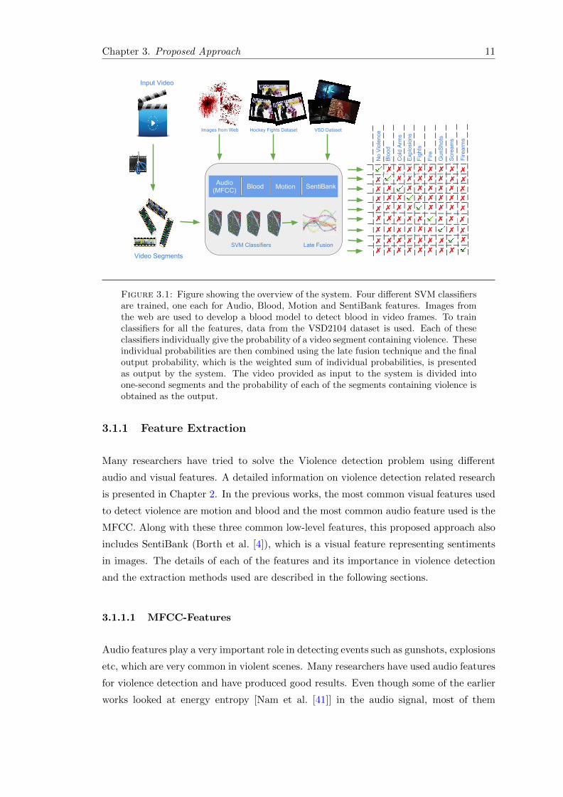
Figure 3.1: Figure showing the overview of the system. Four different SVM classifiersare trained, one each for Audio, Blood, Motion and SentiBank features. Images fromthe web are used to develop a blood model to detect blood in video frames. To trainclassifiers for all the features, data from the VSD2104 dataset is used. Each of theseclassifiers individually give the probability of a video segment containing violence. Theseindividual probabilities are then combined using the late fusion technique and the finaloutput probability, which is the weighted sum of individual probabilities, is presentedas output by the system. The video provided as input to the system is divided intoone-second segments and the probability of each of the segments containing violence isobtained as the output.

3.1.1 Feature Extraction

Many researchers have tried to solve the Violence detection problem using different

audio and visual features. A detailed information on violence detection related research

is presented in Chapter 2. In the previous works, the most common visual features used

to detect violence are motion and blood and the most common audio feature used is the

MFCC. Along with these three common low-level features, this proposed approach also

includes SentiBank (Borth et al. [4]), which is a visual feature representing sentiments

in images. The details of each of the features and its importance in violence detection

and the extraction methods used are described in the following sections.

3.1.1.1 MFCC-Features

Audio features play a very important role in detecting events such as gunshots, explosions

etc, which are very common in violent scenes. Many researchers have used audio features

for violence detection and have produced good results. Even though some of the earlier

works looked at energy entropy [Nam et al. [41]] in the audio signal, most of them


used MFCC features to describe audio content in the videos. These MFCC features are

commonly used in voice and audio recognition.

In this work, MFCC features provided in the VSD2014 dataset are used to train the

SVM classifier while developing the system. During the evaluation, MFCC features are

extracted from the audio stream of the input video, with window size set to the number

of audio samples per frame in the audio stream. This is calculated by dividing the audio

sampling rate with fps (frames per second) value of the video. For example, if the audio

sampling rate is 44,100 Hz and the video is encoded with 25 fps, then each window

has 1,764 audio samples. The window overlap region is set to zero and 22 MFCC are

computed for each window. With this setup, a 22-dimensional MFCC feature vector is

obtained for each video frame.

3.1.1.2 Blood-Features

Blood is the most common visible element in scenes with extreme violence. For example,

scenes containing beating, stabbing, gunfire, and explosions. In many earlier works on

violence detection, detection of pixels representing blood is used as it is an important

indicator of violence. To detect blood in a frame, a pre-defined color table is used

in most of the earlier works, for example, Nam et al. [41] and Lin and Wang [38].

Other approaches to detecting blood, such as the use of Kohonen’s Self-Organizing Map

(SOM)(Clarin et al. [12]), are also used in some of the earlier works.

In this work, a color model is used to detect pixels representing blood. It is represented

using a three-dimensional histogram with one dimension each for red, green and blue

values of the pixels. In each dimension, there are 32 bins with each bin having width

of 8 (32 × 8 = 256). This blood model is generated in two steps. In the first step,

the blood model is bootstrapped by using the RGB (Red, Green, Blue) values of the

pixels containing blood. The 3 dimensional binned histogram is populated with the

RGB values of these pixels containing blood. The value in the bin to which a blood

pixel belongs to is incremented by 1 each time a new blood pixel is added to the model.

Once a sufficient number of bloody pixels are used to fill the histogram, the values in

the bins are normalized by the sum of all the values. The values in each of the bins now

represent the probability of a pixel showing blood given its RGB values. To fill the blood

model, pixel containing blood are cropped from various images containing blood which

are downloaded from Google. Cropping of the regions containing only blood pixels is

done manually. Please refer to the image Figure 3.2 for samples of the cropped regions,

each of size 20 pixels × 20 pixels.


Figure 3.2: Figure showing sample cropped regions of size 20 × 20 containing blood.

Once the model is bootstrapped, it is used to detect blood in the images downloaded

from Google. Only pixels that have a high probability of representing blood are used

to further extend the bootstrapped model. Downloading the images and extending the

blood model is done automatically. To download images from Google which contain

blood, search words such as “bloody images”, “bloody scenes”, “bleeding”, “real blood

splatter”, “blood dripping” are used. Some of the samples of the downloaded images

can be seen in the Figure 3.3. Pixel values with high blood probability are added to the

blood model until it has, at least, a million pixel values.

This blood model alone is not sufficient to accurately detect blood. Along with this

blood model, there is a need for a non-blood model as well. To generate this, similar to

the earlier approach, images are downloaded from Google which do not contain blood

and the RGB pixel values from these images are used to build the non-blood model.

Some samples images used to generate this non-blood model are shown in Figure 3.3.

Now using these blood and non-blood models, the probability of a pixel representing

blood is calculated as follows

P (blood/pixel) = Pblood(pixel)/(Pblood(pixel) + Pnon−blood(pixel)) (3.1)

where P(blood/pixel) defines the probability of a pixel containing blood, Pblood(pixel)

refers to the probability of blood for a given pixel and Pnon−blood(pixel) corresponds to


Figure 3.3: Figure showing sample images downloaded from Google to generate bloodand non-blood models.

the probability of non-blood for a pixel.

Using this formula, for a given image, the probability of each pixel representing blood

is calculated and Blood Probability Map (BPM) is generated. This map has the same

size as that of the input image and contains the blood probability values for every pixel.

This BPM is binarized using a threshold value to generate the final binarized BPM.

The threshold used to binarize the BPM is estimated (Jones and Rehg [35]). From this

binarized BPM, a 1-dimensional feature vector of length 14 is generated which contains

the values such as the blood ratio, blood probability ratio, size of the biggest connected

component, mean, variance etc. This feature vector is extracted for each frame in the

video and is used for training the SVM classifier. A sample image along with its BPM

and binarized BPM are presented in Figure 3.4. It can be observed from this figure that

this approach has performed very well in detecting pixels containing blood.


Figure 3.4: Figure showing the performance of the generated blood model in detect-ing blood. The first column has the input images, the second column has the bloodprobability maps and the last column has the binarized blood probability maps.

3.1.1.3 Motion-Features

Motion is another widely used visual feature for violence detection. The work of Deniz

et al. [21], Nievas et al. [42] and Hassner et al. [28] are some of the examples in which

motion is used as the main feature for violence detection. Here, motion refers to the

amount of spatio-temporal variation between two consective frames in a video. Motion

is considered a good indicator of violence as substantial amount of violence is expected

in the scenes that contain violence. For example, in the scenes that contain person-on-

person fights, there is fast movement of human body parts like legs and hands, and in

scenes that contain explosions, there is a lot of movement from the parts that are flying

apart because of the explosion.

The idea of using motion information for activity detection stems from psychology.

Research on human perception has shown that the kinematic pattern of movement is

sufficient for the perception of actions (Blake and Shiffrar [2]). Research studies in

computer vision (Saerbeck and Bartneck [50], Clarke et al. [13], and Hidaka [29]) have

also shown that relatively simple dynamic features such as velocity and acceleration

correlate to emotions perceived by a human.

In this work, to calculate the amount of motion in a video segment, two different ap-

proaches are evaluated. The first approach is to use the motion information embedded


inside the video codec and the next approach is to use optical flow to detect motion.

These approahces are presented next.

3.1.1.3.1 Using Codec In this method, the motion information is extracted from

the video codec. The magnitude of motion at each pixel per frame called the motion

vector is retrieved from the codec. This motion vector is a two-dimensional vector and

has the same size as a frame from the video sequence. From this motion vector, a motion

feature which represents the amount of motion in the frame is generated. To generate

this motion feature, first the motion vector is divided into twelve sub-regions of equal

sizes by slicing it along the x and y-axis into three and four regions respectively. The

amount of motion along the x and y-axis at each pixel from each of these sub-regions

are aggregated and these sums are used to generate a two-dimensional motion histogram

for each frame. This histogram represents the motion vector for a frame. Refer to the

image on the left in Figure 3.5 to see the visualization of the aggregated motion vectors

for a frame from a sample video. In this visualization, the motion vectors are aggregated

for sub-regions of size 16 × 16 pixels. The magnitude and direction of motion in these

regions is represented using the length and orientation of the green dashed lines which

are overlaid on the image.

3.1.1.3.2 Using Optical Flow The next approach to detect motion uses Optical

flow (Wikipedia [57]). Here, the motion at each pixel in a frame is calculated using Dense

Optical Flow. For this, the implementation of Gunner Farneback’s algorithm (Farneback

[24]) provided by OpenCV (Bradski [5]) is used. The implementation is provided as a

function in OpenCV and for more details about the function and the parameters, please

refer to the documentation provided by OpenCV (OpticalFlow [43]). The values 0.5,

3, 15, 3, 5, 1.2 and 0 are passed to the function parameters pyr scale, levels, win-size,

iterations, poly n, poly sigma and flags respectively. Once the motion vectors at every

pixel are calculated using Optical flow, the motion feature from a frame is extracted

using the same process mentioned in the above Section 3.1.1.3.1. Refer to the image on

the rights in Figure 3.5 to get an impression of the aggregated motion vectors extracted

from a frame. The motion vectors are aggregated for sub-regions of size 16×16 pixels as

in the previous approach to provide a better comparison between the features extracted

by using Codec information and Optical flow.

After the evaluation of both these approaches to extract motion information from videos,

the following observations are made. First, extracting motion from Codecs is much faster

than using optical flow as the motion vectors are precalculated and stored in video codecs.

Second, motion extraction using optical flow is not very efficient when there are blurred


Figure 3.5: Motion information from frames extracted using codec vs using opticalflow.

regions in a frame. This blur is usually caused by sudden motions in a scene, which is

very common in scenes containing violence. Hence, the use of optical flow for extracting

motion information to detect violence is not a promising approach. Therefore, in this

work information stored in the video codecs is used to extract motion features. The

motion features are extracted from each frame in the video and are used to train an

SVM classifier.

3.1.1.4 SentiBank-Features

In addition to the aforementioned low-level features, the SentiBank feature introduced

by Borth et al. [4] is also applied. SentiBank is a mid-level representation of visual con-

tent based on the large-scale Visual Sentiment Ontology (VSO) 1. SentiBank consists

of 1,200 semantic concepts and corresponding automatic classifiers, each being defined

as an Adjective Noun Pair (ANP). Such ANPs combine strong emotional adjectives to

be linked with nouns, which correspond to objects or scenes (e.g. “beautiful sky”, “dis-

gusting bug”, or “cute baby”). Further, each ANP (1) reflects a strong sentiment, (2)

has a link to an emotion, (3) is frequently used on platforms such as Flickr or YouTube

and (4) has a reasonable detection accuracy. Additionally, the VSO is intended to be

comprehensive and diverse enough to cover a broad range of different concept classes

such as people, animals, objects, natural or man-made places and, therefore, provides

additional insights about the type of content being analyzed. Because SentiBank demon-

strated its superior performance as compared to low-level visual features on the analysis

1http://visual-sentiment-ontology.appspot.com


of sentiment Borth et al. [4], it is used now for the first time to detect complex emotion

such as violence from video frames.

SentiBank consists of 1,200 SVMs, each trained to detect one of the 1,200 semantic

concepts from an image. Each SVM is a binary classifier which gives a binary output

0/1 depending on whether or not the image contains a specific sentiment. For a given

frame in a video, a vector containing the output of all 1,200 SVMs is considered as the

SentiBank feature. To extract this feature, a python-based implementation is utilized.

For training the SVM classifier, the SentiBank features extracted from each frame in

the training videos are used. The SentiBank feature extraction takes few seconds as it

involves collecting output from 1,200 pre-trained SVMs. To reduce the time taken for

feature extraction, the SentiBank feature for each of the frame is extracted in parallel

using multiprocessing.

3.1.2 Feature Classification

The next step in the pipeline after feature extraction is feature classification and this

section provides the details of this step. The selection of classifier and the training

techniques used play a very important role in getting good classification results. In

this work, SVMs are used for classification. The main reason behind this choice is the

fact that the earlier works on violence detection have used SVMs to classify audio and

visual features and have produced good results. In almost all the works mentioned in

Chapter 2 SVMs are used for classification, even though they may differ in the kernel

functions used.

From all the videos available in the training set, audio and visual features are extracted

using the process described in the Section 3.1.1. These features are then divided into

two sets, one to train the classifier and the other to test the classification accuracy of the

trained classifier. As the classifiers used here are SVMs, a choice has to be made about

what kernel to use and what kernel parameters to set. To find the best kernel type and

kernel parameters, a grid search technique is used. In this grid search, Linear, RBF

(Radial Basis Function), and Chi-Square kernels along with a range of value for their

parameters are tested, to find the best combination which gives the best classification

results. Using this approach, four different classifiers are trained, one for each feature

type. These trained classifiers are then used in finding the feature weights in the next

step. In this work, the SVM implementation provided by scikit-learn (Pedregosa et al.

[45]) and LibSVM (Chang and Lin [9]) are used.


3.1.3 Feature Fusion

In the feature fusion step, the output probabilities from each of the feature classifiers

are fused to get the final score of the violence in a video segment along with the class

of violence present in it. This fusion is done by calculating the weighted sum of the

probabilities from each of the feature classifiers. To detect the class of violence to which

a video belongs, the procedure is as follows. First, the audio and visual features are

extracted from the videos belonging to each of the targeted violence classes. These

features are then passed to the trained binary SVM classifiers to get the probabilities of

each of the video containing violence. Now, these output probabilities from each of the

feature classifiers are fused by assigning each feature classifier a weight for each class of

violence and calculating the weighted sum. The weights assigned to each of the feature

classifiers represent the importance of a feature in detecting a specific class of violence.

These feature weights have to be adjusted appropriately for each violence class for the

system to detect the correct class of violence.

There are two approaches to finding the weights. The first approach is to manually

adjust weights of a feature classifier for each violence type. This approach needs a lot of

intuition about the importance of a feature in detecting a class of violence and is very

error prone. The other approach is to find the weights using a grid-search mechanism

where a set of weights is sampled from the range of possible weights. In this case, the

range of possible weights for each feature classifier is [0,1], subjected to the constraint

that the sum of weights of all the feature classifiers amounts to 1. In this work, the latter

approach is used and all the weight combinations which amount to 1 are enumerated.

Each of these weight combinations is used to calculate the weighted sum of classifier

probabilities for a class of violence and the weights from the weight combination which

produces the highest sum is assigned to each of the classifiers for the corresponding class

of violence. To calculate these weights, a dataset which is different from the training set

is used, in order to avoid over-fitting of weights to the training set. The dataset used

for weight calculation has videos from all the classes of violence targeted in this work.

It is important to note that, even though each of the trained SVM classifiers are binary

in nature, the output values from these classifiers can be combined using weighted sum

to find the specific class of violence to which a video belongs.

3.2 Testing

In this stage, for a given input video, each segment containing violence is detected along

with the class of violence present in it. For a given video, the following approach is used


to detect the segments that contain violence and the category of violence in it. First,

the visual and audio features are extracted from one frame every 1-second starting from

the first frame of the video, rather than extracting features from every frame. These

frames from which the features are extracted, represent a 1-second segment of the video.

The features from these 1-second video segments are then passed to the trained binary

SVM classifiers to get the scores for each video segment to be violent or non-violent.

Then, weighted sums of the output values from the individual classifiers are calculated

for each violence category using the corresponding weights found during fusion step.

Hence, for a given video of length ‘X’ seconds, the system outputs a vector of length ‘X’.

Each element in this vector is a dictionary which maps each violence class with a score

value. The reason for using this approach is two fold, first to detect time intervals in

which there is violence in the video and to increase the speed of the system in detecting

violence. The feature extraction, especially extracting the Sentibank feature, is time-

consuming and doing it for every frame will make the system slow. But this approach

has a negative effect on the accuracy of the system as it detects violence not for every

frame but for every second.

3.3 Evaluation Metrics

There are many metrics that can be used to measure the performance of a classification

systems. Some of the measures used for binary classification are Accuracy, Precision,

Recall (Sensitivity), Specificity, F-score, Equal Error Rate (EER), and Area Under the

Curve (AUC). Some other measures such as Average Precision (AP) and Mean Av-

erage Precision (MAP) are used for systems which return a ranked list as a result to

a query. Most of these measures that are increasingly used in Machine Learning and

Data Mining research are borrowed from other disciplines such as Information Retrieval

(Rijsbergen [49]) and Biometrics. For a detailed discussion on these measures, refer to

the works of Parker [44] and Sokolova and Lapalme [53]. The ROC (Receiver Operating

Characteristic) curve is another widely used method for evaluating or comparing binary

classification systems. Measures such as AUC and EER can be calculated from the ROC

curve.

In this work, ROC curves are used to: (i) Compare the performance of individual classi-

fiers. (ii) Compare the performance of the system in detecting different classes of violence

in the Multi-Class classification task. (iii) Compare the performance of the system on

Youtube and Hollywood-Test dataset in the Binary classification task. Other metrics

that are used here are, Precision, Recall and EER. These measures are used as these are


the most commonly used measures in the previous works on violence detection.In this

system, the parameters (fusion weights) are adjusted to minimize the EER.

3.4 Summary

In this chapter, a detailed description of the approach followed in this work to detect

violence is presented. The first section deals with the training phase and the second

section deals with the testing phase. In the first section, different steps involved in the

training phase are explained in detail. First the extraction of audio and visual features

is discussed and the details of what features are used and how they are extracted are

presented. Next, the classification techniques used to classify the extracted features are

discussed. Finally, the process used to calculate feature weights for feature fusion is

discussed. In the second section, the process used during the testing phase to extract

video segments containing violence and to detect the class of violence in these segments

is discussed.

To summarize, the steps followed in this approach are feature extraction, feature classi-

fication, feature fusion and testing. The first three steps constitute the training phase

and the final step is the testing phase. In the training phase, audio and visual features

are extracted from the video and they are used to train binary SVM classifiers one for

each feature. Then, a separate dataset is used to find the feature weights which min-

imize the EER of the system on the validataion dataset. In the final testing phase,

first the visual and audio features are extracted one per a 1-second video segment of

the input test video. Then, these features are passed to the trained SVM classifiers to

get the probabilities of these features representing violence. A weighted sum of these

output probabilities is calculated for each violence type using the weights obtained in

the feature fusion step. The violence type for which the weighted sum is maximum is

assigned as a label to the corresponding 1-second video segment. Using these labels the

segments containing violence and the class of violence contained in them is presented

as an output by the system. The experimental setup and evaluation of this system are

presented in the next chapter.

Chapter 4

Experiments and Results

In this chapter, details of the experiments conducted to evaluate the performance of the

system in detecting violent content in videos are presented. The first section deals with

the datasets used for this work, the next section describes the experimental setup and

finally in the last section, results of the experiments performed are presented.

4.1 Datasets

In this work, data from more than one source has been used to extract audio and visual

features, train the classifiers and to test the performance of the system. The two main

datasets used here are the Violent Scene Dataset (VSD) and the Hockey Fights dataset.

Apart from these two datasets, images from websites such as Google Images1 are also

used. Each of these datasets and their use in this work is described in detail in the

following sections.

4.1.1 Violent Scene Dataset

Violent Scene Dataset (VSD) is an annotated dataset for violent scene detection in Hol-

lywood movies and videos from the web. It is a publicly available dataset specifically

designed for the development of content-based detection techniques targeting physical

violence in movies and videos from the websites such as YouTube2. The VSD dataset

was initially introduced by Demarty et al. [15] in the framework of the MediaEval bench-

mark initiative, which serves as a validation framework for the dataset and establishes

a state of the art baseline for the violence detection task. The latest version of the

1http://www.images.google.com2http://www.youtube.com

22

Chapter 4. Experiments and Results 23

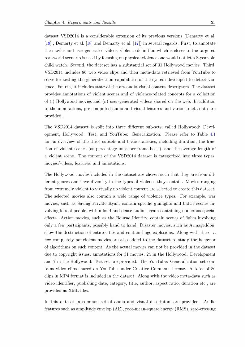
dataset VSD2014 is a considerable extension of its previous versions (Demarty et al.

[19] , Demarty et al. [18] and Demarty et al. [17]) in several regards. First, to annotate

the movies and user-generated videos, violence definition which is closer to the targeted

real-world scenario is used by focusing on physical violence one would not let a 8-year-old

child watch. Second, the dataset has a substantial set of 31 Hollywood movies. Third,

VSD2014 includes 86 web video clips and their meta-data retrieved from YouTube to

serve for testing the generalization capabilities of the system developed to detect vio-

lence. Fourth, it includes state-of-the-art audio-visual content descriptors. The dataset

provides annotations of violent scenes and of violence-related concepts for a collection

of (i) Hollywood movies and (ii) user-generated videos shared on the web. In addition

to the annotations, pre-computed audio and visual features and various meta-data are

provided.

The VSD2014 dataset is split into three different sub-sets, called Hollywood: Devel-

opment, Hollywood: Test, and YouTube: Generalization. Please refer to Table 4.1

for an overview of the three subsets and basic statistics, including duration, the frac-

tion of violent scenes (as percentage on a per-frame-basis), and the average length of

a violent scene. The content of the VSD2014 dataset is categorized into three types:

movies/videos, features, and annotations.

The Hollywood movies included in the dataset are chosen such that they are from dif-

ferent genres and have diversity in the types of violence they contain. Movies ranging

from extremely violent to virtually no violent content are selected to create this dataset.

The selected movies also contain a wide range of violence types. For example, war

movies, such as Saving Private Ryan, contain specific gunfights and battle scenes in-

volving lots of people, with a loud and dense audio stream containing numerous special

effects. Action movies, such as the Bourne Identity, contain scenes of fights involving

only a few participants, possibly hand to hand. Disaster movies, such as Armageddon,

show the destruction of entire cities and contain huge explosions. Along with these, a

few completely nonviolent movies are also added to the dataset to study the behavior

of algorithms on such content. As the actual movies can not be provided in the dataset

due to copyright issues, annotations for 31 movies, 24 in the Hollywood: Development

and 7 in the Hollywood: Test set are provided. The YouTube: Generalization set con-

tains video clips shared on YouTube under Creative Commons license. A total of 86

clips in MP4 format is included in the dataset. Along with the video meta-data such as

video identifier, publishing date, category, title, author, aspect ratio, duration etc., are

provided as XML files.

In this dataset, a common set of audio and visual descriptors are provided. Audio

features such as amplitude envelop (AE), root-mean-square energy (RMS), zero-crossing


Table 4.1: Statistics of the movies and videos in the VSD2014 subsets. All values aregiven in Seconds.

Name Duration Fraction of Violence(%)

Avg.Duration

Hollywood: Development

Armageddon 8,680.16 7.78 25.01Billy Elliot 6,349.44 2.46 8.68Dead Poets Society 7,413.20 0.58 14.44Eragon 5,985.44 13.26 39.69Fantastic Four 1 6,093.96 20.53 62.57Fargo 5,646.40 15.04 65.32Fight Club 8,004.50 15.83 32.51Forrest Gump 8,176.72 8.29 75.33Harry Potter 5 7,953.52 5.44 17.30I am Legend 5,779.92 15.64 75.36Independence Day 8,833.90 13.13 68.23Legally Blond 5,523.44 0.00 0.00Leon 6,344.56 16.36 41.52Midnight Express 6,961.04 7.12 24.80Pirates of the Caribbean 8,239.40 18.15 49.85Pulp Fiction 8,887.00 25.05 202.43Reservoir Dogs 5,712.96 30.41 115.82Saving Private Ryan 9,751.00 33.95 367.92The Bourne Identity 6,816.00 7.18 27.21The God Father 10,194.70 5.73 44.99The Pianist 8,567.04 15.44 69.64The Sixth Sense 6,178.04 2.00 12.40The Wicker Man 5,870.44 6.44 31.55The Wizard of Oz 5,859.20 1.02 8.56

Total 180,192.40 12.35

Hollywood: Test

8 Mile 6,355.60 4.70 37.40Braveheart 10,223.92 21.45 51.01Desperado 6,012.96 31.94 113.00Ghost in the Shell 4966.00 9.85 44.47Jumanji 5993.96 6.75 28.90Terminator 2 8831.40 24.89 53.62V for Vendetta 7625.88 14.27 25.91

Total 50,009.72 17.18

YouTube: Generalization

Average 109.76 31.69 26.62Std.dev 68.05 36.28 50.41

Total 9,439.39 31.69


rate (ZCR), band energy ratio (BER), spectral centroid (SC), frequency bandwidth

(BW), spectral flux (SF), and Mel-frequency cepstral coefficients (MFCC) are provided

on a per-video-frame-basis. As audio has a sampling rate of 44,100 Hz and the videos

are encoded with 25 fps, a window of size 1,764 audio samples in length is considered

to compute these features and 22 MFCCs are computed for each window while all other

features are 1-dimensional. Video features provided in the dataset include color naming

histograms (CNH), color moments (CM), local binary patterns (LBP), and histograms

of oriented gradients (HOG). Audio and visual features are provided in Matlab version

7.3 MAT files, which correspond to HDF5 format.

The VSD2014 dataset contains binary annotations of all violent scenes, where a scene

is identified by its start and end frames. These annotations for Hollywood movies and

YouTube videos are created by several human assessors and are subsequently reviewed

and merged to ensure a certain level of consistency. Each annotated violent segment

contains only one action, whenever this is possible. In cases where different actions

are overlapping, the segments are merged. This is indicated in the annotation files by

adding the tag “multiple action scene”. In addition to binary annotations of segments

containing physical violence, annotations also include high-level concepts for 17 movies in

the Hollywood: Development set. In particular, 7 visual concepts and 3 audio concepts

are annotated, employing a similar annotation protocol as used for violent/non-violent

annotations. The concepts are the presence of blood, fights, presence of fire, presence

of guns, presence of cold arms, car chases, and gory scenes, for the visual modality; the

presence of gunshots, explosions, and screams for the audio modality.

A more detailed description of this dataset is provided by Schedl et al. [51] and for the

details about each of the violence classes, please refer to Demarty et al. [19].

4.1.2 Fights Dataset

This dataset is introduced by Nievas et al. [42] and it is created specifically for evaluating

fight detection systems. This dataset consists of two parts, the first part (“Hockey”)

consists of 1,000 clips at a resolution of 720 × 576 pixels, divided into two groups, 500

fights, and 500 non-fights, extracted from hockey games of the National Hockey League

(NHL). Each clip is limited to 50 frames and resolution lowered to 320 × 240. The

second part (“Movies”) consists of 200 video clips, 100 fights, and 100 non-fights, in

which fights are extracted from action movies and the non-fight videos are extracted

from public action recognition datasets. Unlike the hockey dataset, which was relatively

uniform both in format and content, these videos depict a wider variety of scenes and


Figure 4.1: Sample frames from the fight videos in the Hockey (top) and action movie(bottom) datasets.


were captured at different resolutions. Refer to Figure 4.1 for some of the frames showing

fights from the videos in the two datasets. This dataset is available on-line for download3.

4.1.3 Data from Web

Images from Google are used in developing the color models (Section 3.1.1.2) for the

classes blood and non-blood, which are used in extracting blood feature descriptor for

each frame in a video. The images containing blood are downloaded from Google Images 1

using query words such as “bloody images”, “bloody scenes”, “bleeding”, “real blood

splatter” etc. Similarly, images containing no blood are downloaded using search words

such as “nature”,“spring”,“skin”,“cars” etc.

The utility to download images from Google, given a search word, was developed in

Python using the library Beautiful Soup (Richardson [48]). For each query, the response

contained about 100 images of which only the first 50 were selected for download and

saved in a local file directory. Around 1,000 images were downloaded in total, combining

both blood and non-blood classes. The average dimensions of the images downloaded

are 260× 193 pixels with a file size of around 10 Kilobytes. Refer to Figure 3.3 for some

of the sample images used in this work.

4.2 Setup

In this section, details of the experimental setup and the approaches used to evaluate

the performance of the system are presented. In the following paragraph, partitioning

of the dataset is discussed and the later paragraphs explain the evaluation techniques.

As mentioned in the earlier Section 4.1, data from multiple sources is used in this system.

The most important source is the VSD2014 dataset. It is the only publicly available

dataset which provides annotated video data with various categories of violence and it

is the main reason for using this dataset in developing this system. As explained in the

previous Section 4.1.1, this dataset contains three subsets, Hollywood: Development,

Hollywood: Test and YouTube: Generalization. In this work all the three subsets are

used. The Hollywood: Development subset is the only dataset which is annotated with

different violence classes. This subset consisting of 24 Hollywood movies is partitioned

into 3 parts. The first part consisting of 12 movies (Eragon, Fantastic Four 1, Fargo,

Fight Club, Harry Potter 5, I Am Legend, Independence Day, Legally Blond, Leon,

Midnight Express, Pirates Of The Caribbean, Reservoir Dogs) is used for training the

3http://visilab.etsii.uclm.es/personas/oscar/FightDetection/index.html


classifiers. The second part consisting of 7 movies (Saving Private Ryan, The Bourne

Identity, The God Father, The Pianist, The Sixth Sense, The Wicker Man, The Wizard

of Oz) is used for testing the trained classifiers and to calculate weights for each violence

type. The final part consisting of 3 movies (Armageddon, Billy Elliot, and Dead Poets

Society) is used for evaluation. The Hollywood: Test and the YouTube: Generalization

subsets are also used for evaluation, but for a different task. The following paragraphs

provide details of the evaluation approaches used.

To evaluate the performance of the system, two different classification tasks are defined.

In the first task, the system has to detect specific category of violence present in a video

segment. The second task is more generic where the system has to only detect the

presence of violence. For both these tasks, different datasets are used for evaluation. In

the first task which is a multi-class classification task, the validation set consisting of 3

Hollywood movies (Armageddon, Billy Elliot, and Dead Poets Society) is used. In this

subset, each frame interval containing violence is annotated with the class of violence

that is present. Hence, this dataset is used for this task. These 3 movies were neither

used for training, testing of classifiers nor for weight calculation so that the system can

be evaluated on a purely new data. The procedure illustrated in Figure 3.1 is used for

calculating the probability of a video segment to belong to a specific class of violence.

The output probabilities from the system and the ground truth information are used to

generate ROC (Receiver Operating Characteristic) curves and to assess the performance

of the system.

In the second task, which is a binary classification task, Hollywood: Test and the

YouTube: Generalization subsets of the VSD2104 dataset are used. The Hollywood:

Test subset consists of 8 Hollywood movies and the YouTube: Generalization subset

consists for 86 videos from YouTube. In both these subsets the frame intervals contain-

ing violence are provided as annotations and no information about the class of violence

is provided. Hence, these subsets are used for this task. In this task, similar to the pre-

vious one, the procedure illustrated in Figure 3.1 is used for calculating the probability

of a video segment to belong to a specific class of violence. For each video segment,

the maximum probability obtained for any of the violence class is considered to be the

probability of it being violent. Similar to above task, ROC curves are generated from

these probability values and the ground truth from the dataset.

In both these tasks, first all the features are extracted from the training and testing

datasets. Next, the training and testing datasets are randomly sampled to get an equal

amount of positive and negative samples. 2,000 feature samples are selected for training

and 3,000 are selected for testing. As mentioned above, disjoint training and testing sets

are used to avoid testing on training data. In both the tasks, SVM classifiers with Linear,


Radial Basis Function and Chi-Square kernels are trained for each feature type and the

classifiers with good classification scores on the test set are selected for the fusion step.

In the fusion step, the weights for each violence type are calculated by grid-searching

the possible combinations which maximize the performance of the classifier. The EER

(Equal Error Rate) measure is used as the performance measure.

4.3 Experiments and Results

In this section, the experiments and their results are presented. First, the results of

the multi-class classification task are presented, followed by the results of the binary

classification task.

4.3.1 Multi-Class Classification

In this task, the system has to detect the category of violence present in a video. The

violence categories targeted in this system are Blood, Cold arms, Explosions, Fights,

Fire, Firearms, Gunshots, Screams. As mentioned in the Chapter 1, these are the

subset of categories of violence that are defined in the VSD2014. Apart from these eight

categories, Car Chase, and Subjective Violence are also defined in VSD2014, which

are not used in this work as there were not enough video segments tagged with these

categories in the dataset. This task is very difficult as detection of sub-categories of

violence adds more complexity to the complicated problem of violence detection. The

attempt to detect fine-grained concepts of violence by this system is novel and there is

no existing system which does this task.

As mentioned in Chapter 3, this system uses weighted decision fusion approach to detect

multiple classes of violence where weights for each violence category are learned using a

grid-search technique. Please refer to Section 3.1.3 for more details about this approach.

In Table 4.2, the weights for each violence class which is found using this grid-search

technique are presented.

These weights are used to get the weighted sum of output values of binary feature

classifiers for each violence category. The category with the highest sum is then the

category of violence present in that video segment. If the output sum is less than

0.5 then the video segement is categorised as Non-Violent. The video segments in the

validation set are classified using this approach and the results are presented in the

Figure 4.2. In the figure, each curve represents the ROC curve for each of the violence

categories.


Table 4.2: Classifier weights obtained for each of the violence class using Grid-Searchtechnique. Here the criteria for selecting the weights for a violence class was to find theweights which minimize the EER for that violence class.

Violence Class Audio Blood Motion SentiBank

GunShots 0.50 0.45 0.00 0.05Fights 0.40 0.05 0.25 0.30Explosions 0.90 0.00 0.00 0.10Fire 0.05 0.05 0.05 0.85Cold arms 0.05 0.00 0.00 0.95Firearms 0.05 0.30 0.05 0.60Blood 0.00 0.05 0.00 0.95Screams 0.05 0.20 0.00 0.75

0.0 0.2 0.4 0.6 0.8 1.0

False Positive Rate

0.0

0.2

0.4

0.6

0.8

1.0

True

Posi

tive

Rat

e

ROCs for Multiclass classifier

bloodcoldarmsexplosionsfightsfirefirearmsgunshotsscreams

Figure 4.2: Performance of the system in the Multi-Class Classification task.

4.3.2 Binary Classification

In this binary classification task, the system is expected to detect the presence of violence

without having to find the category. Similar to the previous task, the output probabil-

ities of binary feature classifiers are combined using a weighted sum approach and the

output probabilities of the video segment to belong to each of the violence classes are

calculated. If the maximum probability for any of the class exceeds 0.5 then the video

segment is categorized as violence or else it is categorized as non-violence. As mentioned

in Section 4.2, this task is performed on YouTube-Generalization and Hollywood-Test

datasets. The Figure 4.3 provides the results of this task on both the datasets. Two


0.0 0.2 0.4 0.6 0.8 1.0

False Positive Rate

0.0

0.2

0.4

0.6

0.8

1.0

True

Posi

tive

Rat

e

Binary Classification Performance

YouTubeHollywood

Figure 4.3: Performance of the system in the Binary Classification task.

Table 4.3: Classification results obtained using the proposed approach.

Test Set Precision Recall Accuracy EER

YouTube-Gen 51.4% 61.3% 55.6% 45.0%Hollywood-Test 62.7% 85.1% 59.2% 44.0%

Table 4.4: Classification results obtained by the best performing teams fromMediaEval-2014 (Schedl et al. [51]).

Test Set Precision Recall MAP@100 MAP2014

YouTube-Gen 49.7% 85.8% 86.0% 66.4%Hollywood-Test 41.1% 72.1% 72.7% 63.0%

ROC curves one for each of the datasets are used to represent the performance of the

system. Using 0.5 as the threshold to make the decision of whether the video segment

contains violence or not, the precision, recall and accuracy values are calculated. Please

refer to Table 4.3 for the obtained results.

4.4 Discussion

In this section, the results presented in Section 4.3 are discussed. Before discussing

the results of the Multi-Class and Binary classification tasks, the performance of the


individual classifiers is discussed.

4.4.1 Individual Classifiers

In both the classification tasks discussed in Section 4.3, a fusion of classifier scores

is performed to get the final results. Hence, the performance of the system mainly

depends on the individual performance of each of the classifiers and partially on the

weights assigned to each of the classifiers. For the final classification results to be

good, it is important that each of the classifiers have good individual performance. To

get best performing classifiers, SVMs are trained using three different kernel functions

(Linear, RBF, and Chi-Square) and the classifier with optimal performance on the test

set are selected. Following this approach, best performing classifiers for each feature

type are selected. The performance of these selected classifiers on the test dataset in

presented in Figure 4.4. It can be observed that SentiBank and Audio are the two feature

classifiers that show reasonable performance on the test set. Motion feature classifier has

a performance which is a little better than chance and Blood has performance equivalent

to chance. A detailed discussion on the performance of each of these classifiers in the

increasing order of their performance are presented next.

0.0 0.2 0.4 0.6 0.8 1.0

False Positive Rate

0.0

0.2

0.4

0.6

0.8

1.0

True

Posi

tive

Rat

e

Individual Classifier Performance

AudioBloodMotionSentibank

Figure 4.4: Performance of individual binary classifiers on the test set.


0.0 0.2 0.4 0.6 0.8 1.0

False Positive Rate

0.0

0.2

0.4

0.6

0.8

1.0

True

Posi

tive

Rat

e

Performance of Motion Detectors on Hockey Dataset

Hockey (RBF)Hollywood-Dev (Linear)Hollywood-Dev (RBF)Hollywood-Dev (Chi-Square)

0.0 0.2 0.4 0.6 0.8 1.0

False Positive Rate

0.0

0.2

0.4

0.6

0.8

1.0

True

Posi

tive

Rat

e

Performance of Motion Detectors on Hollywood-Test Dataset

Hockey (RBF)Hollywood-Dev (Linear)Hollywood-Dev (RBF)Hollywood-Dev (Chi-Square)

Figure 4.5: Performance of the Motion feature classifiers on Hockey and Hollywood-Test Datasets. The red curve is for the classifier trained on the Hockey Dataset andthe remaining three are for the three classifiers trained on Hollywood-Dev dataset withLinear, RBF and Chi-Square kernels.

4.4.1.1 Motion

As it is evident from Figure 4.4, the performance of the motion feature classifier on the

test set is only a little better than chance. To understand the reason behind this, the

performance of all the motion feature classifiers, trained with different SVM kernels on

available datasets are compared. Refer to Figure 4.5 for the comparison. In the figure,

the left plot shows the performance of the classifiers on the test set from Hockey dataset

and the plot on the right shows the comparison on Hollywood-Test dataset. In both the

graphs, the red curve corresponds to the classifier trained on the Hockey dataset and the

remaining three curves correspond to classifiers trained on the Hollywood-Dev dataset.

From both these plots, it can be observed that the performance of the classifiers trained

and tested on the same dataset is reasonably good when compared to the classifiers which

are trained on one dataset and tested on another. In the plot on the left (TestSet: Hockey

Dataset), the classifier trained on Hockey Dataset has better performance. Similarly, in

the plot on the right (TestSet: Hollywood-Test), the performance of classifiers trained

on Hollywood-Dev dataset have better performance. From there observations, it can

be inferred that the motion feature representation learned from one dataset can not be

transferred to another dataset. The reason for this could be to the disparity in video

resolution and video format between the datasets. The videos from the Hockey dataset

and the Hollywood-Test dataset have different formats, and also, not all videos from

Hollywood-Development and Hollywood-Test have the same format. The video format

plays an important role as the procedure used to extract motion features (explained in

Section 3.1.1.3.1) use motion information from video codecs. Length and resolution of

a video will also have some effect, even though the procedure used here tries to reduce

this by normalizing the extracted features with the length of the video segment and by

aggregating the pixel motions over a pre-defined number of sub-regions of the frame.


Videos from Hockey dataset are very short segments of one second each and have small

frame size and low quality. Whereas, the video segments from the Hollywood dataset

are longer and have larger frame size with better quality. One solution for this problem

could be to convert all the videos to the same format, but even then there could be a

problem due to improper video encoding. The other solution could be to use an Optical

flow based approach to extract motion features (explained in Section 3.1.1.3.2). But as

explained earlier, this approach is tedious and may not work when there is blur due to

motion in a video.

4.4.1.2 Blood

The performance of blood feature classifier on the test set is just as good as a chance.

Refer to Figure 4.4 for the results. Here the problem is not with the feature extraction

as the blood detector used for blood feature extraction has shown very good results in

detecting regions containing blood in an image. Please refer to Figure 3.4 for the perfor-

mance of blood detector on images from the web and to Figure 4.6 for the performance

of it on sample frames from the Hollywood dataset. From this, it is clear that the blood

feature extractor is doing a pretty good job and it is not the problem with the feature

extraction. Hence, it can be concluded that the problem is with the classifier training

and it is due to the limited availability of training data.

In the VSD2014 dataset which is used for training, the video segments containing blood

are annotated with labels (“Unnoticeable”, “Low”, “Medium”, and “High”) representing

the amount of blood contained in these segments. There are very few segments in this

dataset which are annotated with the label “High”, as a result of which, the SVM

classifiers are unable to learn the feature representation of the frames containing blood

effectively. The performance of this feature classifier can be improved by training it

with a larger dataset with many instances of frames containing a high amount of blood.

Alternatively images from Google can also be used to train this classifier.

4.4.1.3 Audio

Audio feature classifier is the second best-performing classifier (refer to Figure 4.4) on

the test set and this shows the importance of audio in violence detection. Although

visual features are good indicators of violent content, there are some scenes in which

audio plays more important role. For example, scenes containing fights, gunshots, and

explosions. These scenes have characteristic sounds and audio features such as MFCCs

and Energy-entropy, can be used to detect sound patterns associated with these violent

scenes.


In this work, MFCC features are used to describe audio content (refer to Section 3.1.1.1)

as many previous works on violence detection (Acar et al. [1], Jiang et al. [33], Lam et al.

[36], etc.) have shown the effectiveness of MFCC features in detecting audio signatures

associated with violent scenes. Other audio features such as energy entropy, pitch and

power spectrum can also be used along with MFCC features to further improve the

performance of the feature classifier. But it is important to note that, audio alone is not

sufficient to detect violence and it only plays an important role in detecting few violence

classes such as Gunshots and Explosions which have unique audio signatures.

4.4.1.4 SentiBank

The SentiBank feature classifier has shown the best performance of all the feature clas-

sifiers (Refer to Figure 4.4) and has contributed strongly to the overall performance of

the system. This demonstrates the power of SentiBank, in detecting complex visual

sentiments such as violence. Figure 4.7 shows the average scores for top 50 ANPs for

frames containing violence and no violence. As it can be observed the list of ANPs with

(a) (b) (c)

(d) (e) (f)

Figure 4.6: Figure showing the performance of the blood detector on sample framesfrom the Hollywood dataset. The images in the first column (A and D) are the inputimages, the second column images (B and E) are the blood probability maps and the

images in the last column (C and F) are the binarized blood probability maps.


highest average scores for violence and no-violence class are very different and this is

the reason behind the very good performance of SentiBank in separating violence class

from no-violence class. Note that, not all the adjectives in the ANP list for violence

class describe violence. This could be due to many different reasons, one of which could

be the fact that, of the 1,200 ANPs used in SentiBank only a few describe the emotions

related to violence (like fear, terror, rage, anger etc.,). Please refer to Figure 4.8 which

shows the Plutchik’s Wheel of Emotions and the distribution of ANPs for each category

of emotion in VSO.

4.4.2 Fusion Weights

As mentioned earlier (Section 3.1.3), the final classification scores are calculated by late

fusion of individual classifier scores using weighted sum approach. The weights used here

are calculated using a grid-search approach with the goal to minimize the Equal Error

Rate (EER). So, weights play an important role in determining the overall classification

performance of the system. Note that all these weights are calculated on the test set.

In Table 4.2, the weights of the classifiers for each of the eight violence class, obtained

using the grid-search technique, are presented. From the weights obtained, the following

observations about weight distribution can be made, (i) For most of the violence classes,

the highest weight is assigned to SentiBank as it is the most discriminative feature. (ii)

Audio has received the highest weight for violence classes such as Gunshots, Explosions,

and Fights where audio plays a very important role. (iii) Blood has received high weights

for violence classes such as Screams, Gunshots, and Firearms. This is interesting as a

video segment belonging to any of these violence classes can also have blood in it. (iv)

Motion has received the least weight in most of the violence classes as it the least

performing feature. But, it can also be observed that it has a higher weight for the class

Fights where a lot of motion can be expected.

If the weights assigned to each of the violence classes are analyzed the following observa-

tions can be made, (i) For the class Gunshots, the highest distribution weights is between

Audio (0.5) and Blood (0.45). This is expected as audio features play an important role

in detecting gunshots and the scenes containing gunshots are also expected to have a

lot of blood. (ii) Audio (0.4), and visual features (Motion - 0.25 and SentiBank - 0.30)

have received an almost equal amount of weight for the class Fights. This is expected as

both audio and visual features are important in detecting scenes containing fights. (iii)

For the class Explosions, highest weights are assigned to Audio (0.9) which is expected,

as audio features are crucial in detecting explosions. (iv) Fire is a violence class where

visual features are expected to have high weights and as expected the best performing

visual feature, SentiBank (0.85), is assigned the highest weight. (v) Violence class Cold


peac

eful

win

ter

dark

nigh

tm

isty

trees

mis

tyva

lley

roug

hsk

etch

nice

clou

dscl

earw

ater

calm

wat

erst

unni

ngar

chite

ctur

eco

lorfu

lsky

evil

shad

owm

isty

sunr

ise

colo

rfulc

loud

sca

lmsk

yan

gry

men

mis

tyfie

ldst

orm

ycl

ouds

pret

tysk

yca

lmla

kebr

ight

moo

nin

cred

ible

suns

etda

rkw

all

calm

ocea

nst

unni

ngsu

nset

brig

htsu

nset

empt

yro

omge

ntle

wav

esflu

ffygr

ass

mis

tyhi

llsm

isty

lake

sere

nesk

ym

isty

road

clou

dym

oon

clou

dym

ount

ains

dark

room

scar

yst

orm

mis

tyw

inte

rcl

earn

ight

cold

dark

ness

pow

erfu

lriv

erem

pty

spac

eco

lorfu

lbui

ldin

gtin

ybo

atgo

lden

sunr

ise

love

lycl

ouds

amaz

ing

suns

etin

cred

ible

sky

fanc

yha

irsm

ooth

clou

dsm

isty

autu

mn

0.0

0.2

0.4

0.6

0.8

1.0

aver

age

scor

e

Top 50 average Sentibank scores for Violence class

sere

nesc

ene

gent

lew

aves

fam

ous

cast

lein

cred

ible

sunr

ise

incr

edib

lesk

yst

upid

sign

amaz

ing

sky

scen

icro

adcl

ears

kycl

eara

utum

nm

isty

autu

mn

wild

coas

tre

laxi

ngvi

ewco

lorfu

lclo

uds

mis

tysu

nris

etin

ysp

ider

empt

yba

thro

omca

lmau

tum

npo

wer

fulo

cean

fam

ous

mon

umen

tbr

ight

city

gold

ensu

nset

smoo

thw

ater

quie

triv

erni

cebe

ach

dark

nigh

tfu

nny

baby

grea

tsky

pow

erfu

lwat

erfa

llgo

lden

sunr

ise

tranq

uilr

iver

outd

oorm

arke

tdu

sty

sky

calm

lake

mag

ical

sky

incr

edib

lear

chite

ctur

equ

ietl

ake

tranq

uilm

orni

ngab

ando

ned

offic

ecl

earn

ight

pret

tyvi

ewpr

etty

sky

tranq

uill

ake

stun

ning

suns

etbr

ight

sea

brig

htsu

nset

wei

rdcl

ouds

clou

dyni

ght

dere

licts

hip

funn

yha

ir

0.0

0.2

0.4

0.6

0.8

1.0

aver

age

scor

e

Top 50 average Sentibank scores for No-Violence class

Figure 4.7: Graphs showing average scores of Top 50 SentiBank ANPs for framescontaining violence and no violence.


Figure 4.8: Plutchik’s wheel of emotions and the number of ANPs per emotion inVSO.

arms contain scenes which have the presence of any cold weapon (e.g., knives, swords,

arrows, halberds, etc.). For this class, visual features are expected to have high weights.

And as expected, SentiBank (0.95) has the highest weight for this class. (vi) “Firearms”

is the violence class in which the scenes contain guns and firearms. Similar to the above

class, visual features are expected to have high weights. For this class, SentiBank (0.6)

and Blood (0.3) have received the highest distribution of weights. The reason for Blood

being assigned a higher weight might be due to the fact that most of the scenes con-

taining guns will also contain bloodshed. (vii) For the class Blood, the feature Blood

is expected to have the highest weight. But feature Blood (0.05) received only a small

weight and SentiBank (0.95) gained the highest weight. This is not an expected result

and this could be due to the poor performance of the Blood feature classifier on the test

set. (viii) It is intuitive to expect Audio to have higher weights for class “Screams” as

audio features play an important role in detecting screams. But, the weights obtained

here are against this intuition. Audio has received very less weight whereas SentiBank

has received highest weight. Overall, the weights obtained from the grid-search are more

or less as expected for most of the classes. Better weight distribution could be obtained

if the performance of individual classifiers on the test is improved.


4.4.3 Multi-Class Classification

In this section, the results obtained in the multi-class classification task are discussed.

Please refer to Figure 4.2 for the results obtained in this task. From the figure, the

following observations can be drawn (i) The system shows good performance (EER of

around 30%) in detecting Gunshots. (ii) For the violence classes, Cold arms, Blood

and Explosions, the system shows moderate performance (EER of around 40%). (iii)

For the remaining violence classes (Fights, Screams, Fire, Firearms) the performance

is as good as a chance (EER of more than 45%). These results suggest that there is

huge scope for improvement, but, it is important to remember that violence detection is

not a trivial task and distinguishing between different classes of violence is, even more,

difficult. All the approaches proposed so far have only concentrated on detecting the

presence or absence of violence, but not on detecting the category of violence. The novel

approach proposed in this work is one of the first in this direction and there are no

baseline systems to compare the performance with. The results obtained from this work

will serve as a baseline for future works in this area.

In this system, the late fusion approach is followed which has shown good results in

a similar multimedia concept detection task of adult content detection (Schulze et al.

[52]). Hence, the poor performance of the system can not be attributed to the approach

followed. The performance of the system depends on the performance of individual

classifiers and the fusion weight assigned to them for each of the violence classes. As the

fusion weights are adjusted to minimize the EER using the Grid-Search technique, the

overall performance of the system solely depends on the performance of the individual

classifiers. So, to improve the performance of the system in this task, it is necessary to

improve the performance of individual classifiers in detecting violence.

4.4.4 Binary Classification

The results for the binary classification task are presented in Figure 4.3. This task is

an extension to the multi-class classification task. As explained earlier, in this task, a

video segment is categorized as “Violence” if the output probability for any one of the

violence classes is more than the threshold of 0.5. The performance of the system in

this task is evaluated on two datasets, Hollywood-Test, and YouTube-Generalization. It

can be observed that the performance of the system on these datasets is a little better

than chance. It can also be observed that the performance is better on Hollywood-Test

dataset than YouTube-Generalization dataset. This is expected as all the classifiers are

trained on data from Hollywood-Development dataset which have similar video content

to that of Hollywood-Test dataset. The precision, recall and accuracy values obtained


by the system for this task are presented in Table 4.3. The results obtained by the best

performing team in this task from MediaEval-2014 are given in Table 4.4.

These results can not be directly compared, even though the same dataset is used, as the

process used for evaluation is not the same. In MediaEval-2014, a system is expected to

output the start and end frame for the video segments which contain violence and, if the

overlap between the ground truth and the output frame intervals is more than 50% then

it is considered as a hit. Please refer to Schedl et al. [51] for more information on the

process followed in MediaEval-2014. In the proposed approach, the system categorizes

each 1-second segment of the input video to be of class “Violence” or “No Violence” and

the system performance is calculated by comparing this with the ground truth. This

evaluation criteria used here is much more stringent and more granular when compared

to the one used in MediaEval-2014. Here, as the classification is done for each 1-second

segment, there is no need for a strategy to penalize detection of shorter segments. MAP

metric is used for selecting the best performing system in MediaEval whereas, in the

proposed system, the EER of the system is optimized.

Even though the results obtained from this system can not be directly compared to the

MediaEval results, it can be observed that the performance of this system is comparable

to, if not better than, the best performing system from MediaEval-2014 even though

strict evaluation criteria are used. These results suggest that the system developed

using the proposed novel approach is better than the existing state-of-art systems in

this area of violence detection.

4.5 Summary

In this chapter, a detailed discussion on the evaluation of the developed system is pre-

sented. In the Section 4.1, details of the datasets used in this work are explained and

in the next section Section 4.2, the experimental setup is discussed. In Section 4.3 the

experiments and their results are presented, followed by a detailed discussion on the

obtained results in Section 4.4.

Chapter 5

Conclusions and Future Work

In this chapter, the conclusions and the directions in which the existing work can be

extended are discussed in the Section 5.1 and Section 5.2 respectively.

5.1 Conclusions

In this work, an attempt has been made to develop a system to detect violent content in

videos using both visual and audio features. Even though the approach used in this work

is motivated by the earlier works in this area, the following are the unique aspects of it:

(i) Detection of different classes of violence, (ii) the use of SentiBank feature to describe

visual content of a video, (iii) the Blood detector and the blood model developed using

images from the web, and (iv) using information from video codec to generate motion

features. Here is a brief overview of the process used to develop this system.

As violence is not a physical entity, the detection of it in a video is not a trivial task.

Violence is a visual concept and to detect it there is a need to use multiple features.

In this work, MFCC features were used to describe audio content and Blood, Motion

and SentiBank features are used to describe visual content. SVM classifiers were trained

for each of the selected features and the individual classifier scores were combined by

weighted sum to get the final classification scores for each of the violence classes. The

weights for each class are found using a grid-search approach with the optimizing criteria

to be the minimum EER. Different datasets are used in this work, but the most important

one is the VSD dataset, which is used for training the classifiers, calculating the classifier

weights and for testing the system.

The performance of the system is evaluated on two different classification tasks, Multi-

Class, and Binary classification. In Multi-Class classification task, the system has to

41

Bibliography 42

detect the class of violence present in a video segment. This is a much more difficult

task than just detecting the presence of violence and the system presented here is one of

the first to tackle this problem. The Binary classification task is where the system has to

just detect the presence of violence without having to find the class of violence. In this

task, if the final classification score from the Multi-Class classification task for any of the

violence class is more than 0.5, then the video segment is categorized as “Violence” else,

it is categorized as “No Violence”. The results from the Multi-Class classification task is

far from perfect and there is room for improvement, whereas, the results on the Binary

classification tasks are better than the existing benchmark results from MediaEval-2014.

However, these results are definitely encouraging. In Section 5.2, a detailed discussion

on the possible directions in which the current work can be extended are presented.

5.2 Future Work

There are many possible directions in which the current work can be extended. One

direction would be to improve the performance of the existing system. For that, the

performance of the individual classifiers has to be improved. Motion and Blood are the

two features whose classifier performance needs resonable improvement. As explained in

Section 4.4, the approach used to extract motion features has to be changed for improving

the performance of the motion classifier. For Blood, the problem is with the dataset

used for training the classifier but not the feature extractor. An appropriate dataset

with decent amount of frames containing blood should be used for training. Making

these improvements should be the first step towards building a better system. Another

direction for the future work would be to adapt this system and develop different tools

for different applications. For example, (i) a tool could be developed which could extract

the video segments containing violence from a given input video. This could be helpful

in video tagging. (ii) A similar tool could be developed for parental control where the

system could be used to rate a movie depending on the amount of violent content in

it. Another possible direction for future work is, to improve the speed of the system so

that it can be used in the real-time detection of violence from the video feed of security

cameras. The improvements needed for developing such a system will not be trivial.

Bibliography

[1] E. Acar, S. Spiegel, S. Albayrak, and D. Labor. Mediaeval 2011 affect task: Violent

scene detection combining audio and visual features with svm. In MediaEval, 2011.

[2] R. Blake and M. Shiffrar. Perception of human motion. Annu. Rev. Psychol., 58:

47–73, 2007.

[3] Blog-FB. Facebook statistics, 2015. URL http://media.fb.com/2015/01/07/

what-the-shift-to-video-means-for-creators/. Online: accessed 08-Jan-

2016.

[4] D. Borth, R. Ji, T. Chen, T. Breuel, and S.-F. Chang. Large-scale visual sentiment

ontology and detectors using adjective noun pairs. In Proceedings of the 21st ACM

international conference on Multimedia, pages 223–232. ACM, 2013.

[5] G. Bradski. Opencv. Dr. Dobb’s Journal of Software Tools, 2000.

[6] B. J. Bushman and L. R. Huesmann. Short-term and long-term effects of violent

media on aggression in children and adults. Archives of Pediatrics & Adolescent

Medicine, 160(4):348–352, 2006.

[7] L.-H. Cai, L. Lu, A. Hanjalic, H.-J. Zhang, and L.-H. Cai. A flexible framework

for key audio effects detection and auditory context inference. Audio, Speech, and

Language Processing, IEEE Transactions on, 14(3):1026–1039, 2006.

[8] Y. Chan, R. Harvey, and D. Smith. Building systems to block pornography. In Chal-

lenge of Image Retrieval, BCS Electronic Workshops in Computing series, pages

34–40, 1999.

[9] C.-C. Chang and C.-J. Lin. LIBSVM: A library for support vector machines. ACM

Transactions on Intelligent Systems and Technology, 2:27:1–27:27, 2011. Software

available at http://www.csie.ntu.edu.tw/~cjlin/libsvm.

[10] M.-y. Chen and A. Hauptmann. Mosift: Recognizing human actions in surveillance

videos. 2009.

43

http://media.fb.com/2015/01/07/what-the-shift-to-video-means-for-creators/

http://media.fb.com/2015/01/07/what-the-shift-to-video-means-for-creators/

http://www.csie.ntu.edu.tw/~cjlin/libsvm

Bibliography 44

[11] W.-H. Cheng, W.-T. Chu, and J.-L. Wu. Semantic context detection based on

hierarchical audio models. In Proceedings of the 5th ACM SIGMM international

workshop on Multimedia information retrieval, pages 109–115. ACM, 2003.

[12] C. Clarin, J. Dionisio, M. Echavez, and P. Naval. Dove: Detection of movie violence

using motion intensity analysis on skin and blood. PCSC, 6:150–156, 2005.

[13] T. J. Clarke, M. F. Bradshaw, D. T. Field, S. E. Hampson, D. Rose, et al. The

perception of emotion from body movement in point-light displays of interpersonal

dialogue. Perception-London, 34(10):1171–1180, 2005.

[14] A. Datta, M. Shah, and N. D. V. Lobo. Person-on-person violence detection in video

data. In Pattern Recognition, 2002. Proceedings. 16th International Conference on,

volume 1, pages 433–438. IEEE, 2002.

[15] C.-H. Demarty, C. Penet, G. Gravier, and M. Soleymani. The mediaeval 2011 affect

task. 2010.

[16] C.-H. Demarty, C. Penet, G. Gravier, and M. Soleymani. A benchmarking campaign

for the multimodal detection of violent scenes in movies. In Computer Vision–ECCV

2012. Workshops and Demonstrations, pages 416–425. Springer, 2012.

[17] C.-H. Demarty, B. Ionescu, Y.-G. Jiang, V. L. Quang, M. Schedl, and C. Penet.

Benchmarking violent scenes detection in movies. In Content-Based Multimedia

Indexing (CBMI), 2014 12th International Workshop on, pages 1–6. IEEE, 2014.

[18] C.-H. Demarty, C. Penet, B. Ionescu, G. Gravier, and M. Soleymani. Multimodal

violence detection in hollywood movies: State-of-the-art and benchmarking. In

Fusion in Computer Vision, pages 185–208. Springer, 2014.

[19] C.-H. Demarty, C. Penet, M. Soleymani, and G. Gravier. Vsd, a public dataset for

the detection of violent scenes in movies: design, annotation, analysis and evalua-

tion. Multimedia Tools and Applications, pages 1–26, 2014.

[20] A. P. Dempster, N. M. Laird, and D. B. Rubin. Maximum likelihood from incom-

plete data via the em algorithm. Journal of the royal statistical society. Series B

(methodological), pages 1–38, 1977.

[21] O. Deniz, I. Serrano, G. Bueno, and T. Kim. Fast violence detection in video.

In The 9th International Conference on Computer Vision Theory and Applications

(VISAPP), 2014.

[22] F. Eyben and B. Schuller. opensmile:): the munich open-source large-scale multi-

media feature extractor. ACM SIGMultimedia Records, 6(4):4–13, 2015.

Bibliography 45

[23] F. Eyben, F. Weninger, N. Lehment, B. Schuller, and G. Rigoll. Affective video

retrieval: Violence detection in hollywood movies by large-scale segmental feature

extraction. PloS one, 8(12):e78506, 2013.

[24] G. Farneback. Two-frame motion estimation based on polynomial expansion. In

Image Analysis, pages 363–370. Springer, 2003.

[25] M. Flood. The harms of pornography exposure among children and young people.

Child abuse review, 18(6):384–400, 2009.

[26] P. Gill, M. Arlitt, Z. Li, and A. Mahanti. Youtube traffic characterization: a view

from the edge. In Proceedings of the 7th ACM SIGCOMM conference on Internet

measurement, pages 15–28. ACM, 2007.

[27] Y. Gong, W. Wang, S. Jiang, Q. Huang, and W. Gao. Detecting violent scenes

in movies by auditory and visual cues. In Advances in Multimedia Information

Processing-PCM 2008, pages 317–326. Springer, 2008.

[28] T. Hassner, Y. Itcher, and O. Kliper-Gross. Violent flows: Real-time detection of

violent crowd behavior. In Computer Vision and Pattern Recognition Workshops

(CVPRW), 2012 IEEE Computer Society Conference on, pages 1–6. IEEE, 2012.

[29] S. Hidaka. Identifying kinematic cues for action style recognition. Cognitive Science

Society, 2012.

[30] T. Hofmann. Unsupervised learning by probabilistic latent semantic analysis. Ma-

chine learning, 42(1-2):177–196, 2001.

[31] L. R. Huesmann and L. D. Eron. Television and the aggressive child: A cross-

national comparison. Routledge, 2013.

[32] L. R. Huesmann and L. D. Taylor. The role of media violence in violent behavior.

Annu. Rev. Public Health, 27:393–415, 2006.

[33] Y.-G. Jiang, Q. Dai, C. C. Tan, X. Xue, and C.-W. Ngo. The shanghai-hongkong

team at mediaeval2012: Violent scene detection using trajectory-based features. In

MediaEval, 2012.

[34] Y.-G. Jiang, Q. Dai, X. Xue, W. Liu, and C.-W. Ngo. Trajectory-based modeling

of human actions with motion reference points. In Computer Vision–ECCV 2012,

pages 425–438. Springer, 2012.

[35] M. J. Jones and J. M. Rehg. Statistical color models with application to skin

detection. International Journal of Computer Vision, 46(1):81–96, 2002.

Bibliography 46

[36] V. Lam, D.-D. Le, S. Phan, S. Satoh, D. A. Duong, and T. D. Ngo. Evaluation

of low-level features for detecting violent scenes in videos. In Soft Computing and

Pattern Recognition (SoCPaR), 2013 International Conference of, pages 213–218.

IEEE, 2013.

[37] I. Laptev. On space-time interest points. International Journal of Computer Vision,

64(2-3):107–123, 2005.

[38] J. Lin and W. Wang. Weakly-supervised violence detection in movies with audio

and video based co-training. In Advances in Multimedia Information Processing-

PCM 2009, pages 930–935. Springer, 2009.

[39] D. G. Lowe. Distinctive image features from scale-invariant keypoints. International

journal of computer vision, 60(2):91–110, 2004.

[40] K. J. Mitchell, D. Finkelhor, and J. Wolak. The exposure of youth to unwanted

sexual material on the internet a national survey of risk, impact, and prevention.

Youth & Society, 34(3):330–358, 2003.

[41] J. Nam, M. Alghoniemy, and A. H. Tewfik. Audio-visual content-based violent

scene characterization. In Image Processing, 1998. ICIP 98. Proceedings. 1998

International Conference on, volume 1, pages 353–357. IEEE, 1998.

[42] E. B. Nievas, O. D. Suarez, G. B. Garcıa, and R. Sukthankar. Violence detection

in video using computer vision techniques. In Computer Analysis of Images and

Patterns, pages 332–339. Springer, 2011.

[43] D. OpticalFlow. Optical flow implementation, 2015. URL http:

//docs.opencv.org/modules/video/doc/motion_analysis_and_object_

tracking.html#calcopticalflowfarneback. Online: accessed 21-Oct-2015.

[44] C. Parker. An analysis of performance measures for binary classifiers. In Data Min-

ing (ICDM), 2011 IEEE 11th International Conference on, pages 517–526. IEEE,

2011.

[45] F. Pedregosa, G. Varoquaux, A. Gramfort, V. Michel, B. Thirion, O. Grisel,

M. Blondel, P. Prettenhofer, R. Weiss, V. Dubourg, J. Vanderplas, A. Passos,

D. Cournapeau, M. Brucher, M. Perrot, and E. Duchesnay. Scikit-learn: Machine

learning in Python. Journal of Machine Learning Research, 12:2825–2830, 2011.

[46] J. Platt et al. Probabilistic outputs for support vector machines and comparisons to

regularized likelihood methods. Advances in large margin classifiers, 10(3):61–74,

1999.

http://docs.opencv.org/modules/video/doc/motion_analysis_and_object_tracking.html#calcopticalflowfarneback



Bibliography 47

[47] M. Pogrebnyak, D. Timoshenko, I. Burcev, and A. Kulinkin. Adult-content detec-

tion in video with the use of nvidia gpu. 2015.

[48] L. Richardson. Beautiful soup. Crummy: The Site, 2013. URL http://www.

crummy.com/software/BeautifulSoup/.

[49] C. J. V. Rijsbergen. Information Retrieval. Butterworth-Heinemann, Newton, MA,

USA, 2nd edition, 1979. ISBN 0408709294.

[50] M. Saerbeck and C. Bartneck. Perception of affect elicited by robot motion. In

Proceedings of the 5th ACM/IEEE international conference on Human-robot inter-

action, pages 53–60. IEEE Press, 2010.

[51] M. Schedl, M. Sjoberg, I. Mironica, B. Ionescu, V. L. Quang, and Y.-G. Jiang.

Vsd2014: A dataset for violent scenes detection in hollywood movies and web videos.

Sixth Sense, 6(2.00):12–40.

[52] C. Schulze, D. Henter, D. Borth, and A. Dengel. Automatic detection of csa me-

dia by multi-modal feature fusion for law enforcement support. In Proceedings of

International Conference on Multimedia Retrieval, page 353. ACM, 2014.

[53] M. Sokolova and G. Lapalme. A systematic analysis of performance measures for

classification tasks. Information Processing & Management, 45(4):427–437, 2009.

[54] G. Sparks. Media effects research: A basic overview. Cengage Learning, 2015.

[55] A. Tompkins. The psychological effects of violent media on children. AllPsych

Journal, 14, 2003.

[56] M. Wesch. Youtube statistics, 2008. URL http://mediatedcultures.net/

thoughts/youtube-statistics/. Online: accessed 08-Jan-2016.

[57] Wikipedia. Optical flow, 2015. URL https://en.wikipedia.org/wiki/Optical_

flow. Online: accessed 21-Oct-2015.

http://www.crummy.com/software/BeautifulSoup/

http://www.crummy.com/software/BeautifulSoup/

http://mediatedcultures.net/thoughts/youtube-statistics/

http://mediatedcultures.net/thoughts/youtube-statistics/

https://en.wikipedia.org/wiki/Optical_flow

https://en.wikipedia.org/wiki/Optical_flow

Violence Detection in Videos - arXiv

Documents

Transcript of Violence Detection in Videos - arXiv