Lecture 18: Videos - Eecs Umich
91
Justin Johnson November 18, 2019 Lecture 18: Videos Lecture 18 - 1
-
Upload
khangminh22 -
Category
Documents
-
view
2 -
download
0
Transcript of Lecture 18: Videos - Eecs Umich

Justin Johnson November 18, 2019
Lecture 18:Videos
Lecture 18 - 1

Justin Johnson November 18, 2019
Computer Vision Tasks: 2D Recognition
Lecture 18 - 2
Classification SemanticSegmentation
Object Detection
Instance Segmentation
CAT GRASS, CAT, TREE, SKY
DOG, DOG, CAT DOG, DOG, CAT
No spatial extent Multiple ObjectsNo objects, just pixelsThis image is CC0 public domain

Justin Johnson November 18, 2019
Last Time: 3D Shapes
Lecture 18 - 3
Predicting 3D Shapes from single image
Processing 3D input data
Input Image 3D Shape 3D Shape
Chair

Justin Johnson November 18, 2019
Last Time: 3D Shape Representations
Lecture 18 - 4
∞∞2
22
2
Depth Map
Voxel Grid
Implicit Surface
Pointcloud Mesh
Justin Johnson November 18, 2019
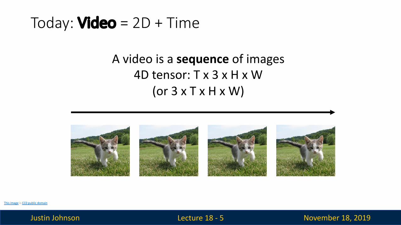
Today: Video = 2D + Time
Lecture 18 - 5
This image is CC0 public domain
A video is a sequence of images4D tensor: T x 3 x H x W
(or 3 x T x H x W)

Justin Johnson November 18, 2019
Example task: Video Classification
Lecture 18 - 6
Input video:T x 3 x H x W
Running video is in the public domain
SwimmingRunningJumpingEatingStanding

Justin Johnson November 18, 2019
Example task: Video Classification
Lecture 18 - 7
SwimmingRunningJumpingEatingStanding
DogCatFishTruck
Images: Recognize objects
Videos: Recognize actions
Running video is in the public domain

Justin Johnson November 18, 2019
Problem: Videos are big!
Lecture 18 - 8
Input video:T x 3 x H x W
Videos are ~30 frames per second (fps)
Size of uncompressed video (3 bytes per pixel):
SD (640 x 480): ~1.5 GB per minuteHD (1920 x 1080): ~10 GB per minute

Justin Johnson November 18, 2019
Problem: Videos are big!
Lecture 18 - 9
Input video:T x 3 x H x W
Videos are ~30 frames per second (fps)
Size of uncompressed video (3 bytes per pixel):
SD (640 x 480): ~1.5 GB per minuteHD (1920 x 1080): ~10 GB per minute
Solution: Train on short clips: low fps and low spatial resolutione.g. T = 16, H=W=112(3.2 seconds at 5 fps, 588 KB)

Justin Johnson November 18, 2019
Training on Clips
Lecture 18 - 10
Raw video: Long, high FPS

Justin Johnson November 18, 2019
Training on Clips
Lecture 18 - 11
Raw video: Long, high FPS
Training: Train model to classify short clips with low FPS

Justin Johnson November 18, 2019
Training on Clips
Lecture 18 - 12
Raw video: Long, high FPS
Training: Train model to classify short clips with low FPS
Testing: Run model on different clips, average predictions
Justin Johnson November 18, 2019
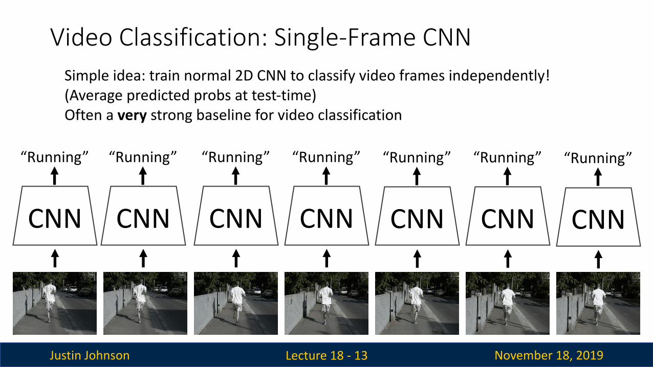
Video Classification: Single-Frame CNN
Lecture 18 - 13
CNN
“Running”
Simple idea: train normal 2D CNN to classify video frames independently! (Average predicted probs at test-time)Often a very strong baseline for video classification
CNN
“Running”
CNN
“Running”
CNN
“Running”
CNN
“Running”
CNN
“Running”
CNN
“Running”

Justin Johnson November 18, 2019
Video Classification: Late Fusion (with FC layers)
Lecture 18 - 14
CNNCNNCNN CNN CNN CNN
Input:T x 3 x H x W
2D CNN on each frame
Frame featuresT x D x H’ x W’
Flatten
MLP
Class scores: C
Karpathy et al, “Large-scale Video Classification with Convolutional Neural Networks”, CVPR 2014
Run 2D CNN on each frame, concatenate features and feed to MLP
Clip features: TDH’W’
Intuition: Get high-level appearance of each frame, and combine them

Justin Johnson November 18, 2019
Video Classification: Late Fusion (with pooling)
Lecture 18 - 15
CNNCNNCNN CNN CNN CNN
Input:T x 3 x H x W
2D CNN on each frame
Frame featuresT x D x H’ x W’
Average Pool over space and time
Clip features: DLinear
Class scores: C Run 2D CNN on each frame, pool features and feed to Linear
Intuition: Get high-level appearance of each frame, and combine them

Justin Johnson November 18, 2019
Video Classification: Late Fusion (with pooling)
Lecture 18 - 16
CNNCNNCNN CNN CNN CNN
Input:T x 3 x H x W
2D CNN on each frame
Frame featuresT x D x H’ x W’
Average Pool over space and time
Clip features: DLinear
Class scores: C Run 2D CNN on each frame, pool features and feed to Linear
Intuition: Get high-level appearance of each frame, and combine themProblem: Hard to compare low-level motion between frames

Justin Johnson November 18, 2019
Video Classification: Early Fusion
Lecture 18 - 17
2D CNN
Input:T x 3 x H x W
Reshape:3T x H x W
Class scores: C
Rest of the network is standard 2D CNN
Intuition: Compare frames with very first conv layer, after that normal 2D CNN
First 2D convolution collapses all temporal information:Input: 3T x H x WOutput: D x H x W
Karpathy et al, “Large-scale Video Classification with Convolutional Neural Networks”, CVPR 2014

Justin Johnson November 18, 2019
Video Classification: Early Fusion
Lecture 18 - 18
2D CNN
Input:T x 3 x H x W
Reshape:3T x H x W
Class scores: C
Rest of the network is standard 2D CNN
Intuition: Compare frames with very first conv layer, after that normal 2D CNNProblem: One layer of temporal processing may not be enough!
First 2D convolution collapses all temporal information:Input: 3T x H x WOutput: D x H x W
Karpathy et al, “Large-scale Video Classification with Convolutional Neural Networks”, CVPR 2014

Justin Johnson November 18, 2019
Video Classification: 3D CNN
Lecture 18 - 19
3D CNN
Input:3 x T x H x W
Class scores: C
Intuition: Use 3D versions of convolution and pooling to slowly fuse temporal information over the course of the network
Each layer in the network is a 4D tensor: D x T x H x WUse 3D conv and 3D poolingoperations
Ji et al, “3D Convolutional Neural Networks for Human Action Recognition”, TPAMI 2010 ; Karpathy et al, “Large-scale Video Classification with Convolutional Neural Networks”, CVPR 2014

Justin Johnson November 18, 2019
Early Fusion vs Late Fusion vs 3D CNN
Lecture 18 - 20
LayerSize (C x T x H x W)
Receptive Field (T x H x W)
Input 3 x 20 x 64 x 64Conv2D(3x3, 3->12) 12 x 20 x 64 x 64 1 x 3 x 3Pool2D(4x4) 12 x 20 x 16 x 16 1 x 6 x 6Conv2D(3x3, 12->24) 24 x 20 x 16 x 16 1 x 14 x 14GlobalAvgPool 24 x 1 x 1 x 1 20 x 64 x 64
Late Fusion

Justin Johnson November 18, 2019
Early Fusion vs Late Fusion vs 3D CNN
Lecture 18 - 21
LayerSize (C x T x H x W)
Receptive Field (T x H x W)
Input 3 x 20 x 64 x 64Conv2D(3x3, 3->12) 12 x 20 x 64 x 64 1 x 3 x 3Pool2D(4x4) 12 x 20 x 16 x 16 1 x 6 x 6Conv2D(3x3, 12->24) 24 x 20 x 16 x 16 1 x 14 x 14GlobalAvgPool 24 x 1 x 1 x 1 20 x 64 x 64
Late Fusion
Input
Conv(3x3)

Justin Johnson November 18, 2019
Early Fusion vs Late Fusion vs 3D CNN
Lecture 18 - 22
LayerSize (C x T x H x W)
Receptive Field (T x H x W)
Input 3 x 20 x 64 x 64Conv2D(3x3, 3->12) 12 x 20 x 64 x 64 1 x 3 x 3Pool2D(4x4) 12 x 20 x 16 x 16 1 x 6 x 6Conv2D(3x3, 12->24) 24 x 20 x 16 x 16 1 x 14 x 14GlobalAvgPool 24 x 1 x 1 x 1 20 x 64 x 64
Late Fusion
Input
Pool(4x4)
Conv(3x3)
Justin Johnson November 18, 2019
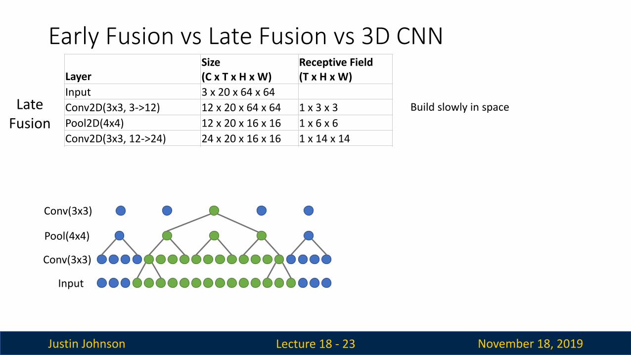
Early Fusion vs Late Fusion vs 3D CNN
Lecture 18 - 23
LayerSize (C x T x H x W)
Receptive Field (T x H x W)
Input 3 x 20 x 64 x 64Conv2D(3x3, 3->12) 12 x 20 x 64 x 64 1 x 3 x 3Pool2D(4x4) 12 x 20 x 16 x 16 1 x 6 x 6Conv2D(3x3, 12->24) 24 x 20 x 16 x 16 1 x 14 x 14GlobalAvgPool 24 x 1 x 1 x 1 20 x 64 x 64
Late Fusion
Input
Pool(4x4)
Conv(3x3)
Conv(3x3)
Build slowly in space
Justin Johnson November 18, 2019
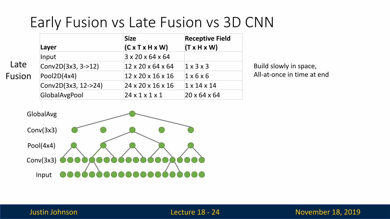
Early Fusion vs Late Fusion vs 3D CNN
Lecture 18 - 24
LayerSize (C x T x H x W)
Receptive Field (T x H x W)
Input 3 x 20 x 64 x 64Conv2D(3x3, 3->12) 12 x 20 x 64 x 64 1 x 3 x 3Pool2D(4x4) 12 x 20 x 16 x 16 1 x 6 x 6Conv2D(3x3, 12->24) 24 x 20 x 16 x 16 1 x 14 x 14GlobalAvgPool 24 x 1 x 1 x 1 20 x 64 x 64
Late Fusion
Input
Pool(4x4)
Conv(3x3)
Conv(3x3)
GlobalAvg
Build slowly in space,All-at-once in time at end
Justin Johnson November 18, 2019
Early Fusion vs Late Fusion vs 3D CNN
Lecture 18 - 25
LayerSize (C x T x H x W)
Receptive Field (T x H x W)
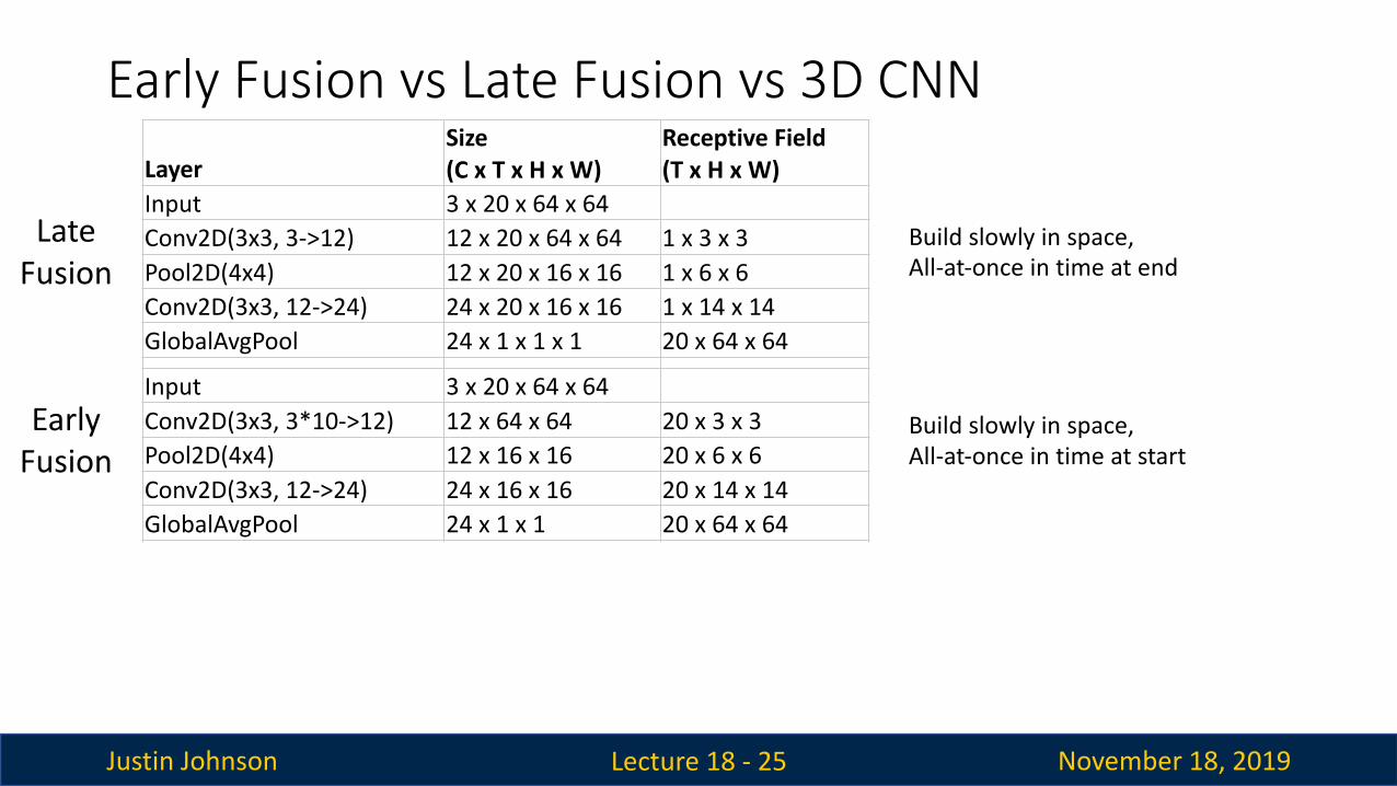
Input 3 x 20 x 64 x 64Conv2D(3x3, 3->12) 12 x 20 x 64 x 64 1 x 3 x 3Pool2D(4x4) 12 x 20 x 16 x 16 1 x 6 x 6Conv2D(3x3, 12->24) 24 x 20 x 16 x 16 1 x 14 x 14GlobalAvgPool 24 x 1 x 1 x 1 20 x 64 x 64
Input 3 x 20 x 64 x 64Conv2D(3x3, 3*10->12) 12 x 64 x 64 20 x 3 x 3Pool2D(4x4) 12 x 16 x 16 20 x 6 x 6Conv2D(3x3, 12->24) 24 x 16 x 16 20 x 14 x 14GlobalAvgPool 24 x 1 x 1 20 x 64 x 64
Input 3 x 20 x 64 x 64Conv3D(3x3x3, 3->12) 12 x 20 x 64 x 64 3 x 3 x 3Pool3D(4x4x4) 12 x 5 x 16 x 16 6 x 6 x 6Conv3D(3x3x3, 12->24) 24 x 5 x 16 x 16 14 x 14 x 14GlobalAvgPool 24 x 1 x 1 20 x 64 x 64
Late Fusion
Early Fusion
3D CNN
Build slowly in space,All-at-once in time at end
Build slowly in space,All-at-once in time at start

Justin Johnson November 18, 2019
Early Fusion vs Late Fusion vs 3D CNN
Lecture 18 - 26
LayerSize (C x T x H x W)
Receptive Field (T x H x W)
Input 3 x 20 x 64 x 64Conv2D(3x3, 3->12) 12 x 20 x 64 x 64 1 x 3 x 3Pool2D(4x4) 12 x 20 x 16 x 16 1 x 6 x 6Conv2D(3x3, 12->24) 24 x 20 x 16 x 16 1 x 14 x 14GlobalAvgPool 24 x 1 x 1 x 1 20 x 64 x 64
Input 3 x 20 x 64 x 64Conv2D(3x3, 3*10->12) 12 x 64 x 64 20 x 3 x 3Pool2D(4x4) 12 x 16 x 16 20 x 6 x 6Conv2D(3x3, 12->24) 24 x 16 x 16 20 x 14 x 14GlobalAvgPool 24 x 1 x 1 20 x 64 x 64
Input 3 x 20 x 64 x 64Conv3D(3x3x3, 3->12) 12 x 20 x 64 x 64 3 x 3 x 3Pool3D(4x4x4) 12 x 5 x 16 x 16 6 x 6 x 6Conv3D(3x3x3, 12->24) 24 x 5 x 16 x 16 14 x 14 x 14GlobalAvgPool 24 x 1 x 1 20 x 64 x 64
Late Fusion
Early Fusion
3D CNN
Build slowly in space,All-at-once in time at end
Build slowly in space,All-at-once in time at start
(Small example architectures, in practice much bigger)
Build slowly in space,Build slowly in time”Slow Fusion”

Justin Johnson November 18, 2019
Early Fusion vs Late Fusion vs 3D CNN
Lecture 18 - 27
LayerSize (C x T x H x W)
Receptive Field (T x H x W)
Input 3 x 20 x 64 x 64Conv2D(3x3, 3->12) 12 x 20 x 64 x 64 1 x 3 x 3Pool2D(4x4) 12 x 20 x 16 x 16 1 x 6 x 6Conv2D(3x3, 12->24) 24 x 20 x 16 x 16 1 x 14 x 14GlobalAvgPool 24 x 1 x 1 x 1 20 x 64 x 64
Input 3 x 20 x 64 x 64Conv2D(3x3, 3*10->12) 12 x 64 x 64 20 x 3 x 3Pool2D(4x4) 12 x 16 x 16 20 x 6 x 6Conv2D(3x3, 12->24) 24 x 16 x 16 20 x 14 x 14GlobalAvgPool 24 x 1 x 1 20 x 64 x 64
Input 3 x 20 x 64 x 64Conv3D(3x3x3, 3->12) 12 x 20 x 64 x 64 3 x 3 x 3Pool3D(4x4x4) 12 x 5 x 16 x 16 6 x 6 x 6Conv3D(3x3x3, 12->24) 24 x 5 x 16 x 16 14 x 14 x 14GlobalAvgPool 24 x 1 x 1 20 x 64 x 64
Late Fusion
Early Fusion
3D CNN
Build slowly in space,All-at-once in time at end
Build slowly in space,All-at-once in time at start
Build slowly in space,Build slowly in time”Slow Fusion”
What is the difference?

Justin Johnson November 18, 2019
2D Conv (Early Fusion) vs 3D Conv (3D CNN)
Lecture 18 - 28
Input: Cin x T x H x W(3D grid with Cin-dim feat at each point)
W = 224
H = 224
T = 16
Weight:Cout x Cin x T x 3 x 3Slide over x and y
T = 16
Cout different filters
Output: Cout x H x W2D grid with Cout –dim feat at each point
W = 224
H = 224

Justin Johnson November 18, 2019
2D Conv (Early Fusion) vs 3D Conv (3D CNN)
Lecture 18 - 29
Input: Cin x T x H x W(3D grid with Cin-dim feat at each point)
W = 224
H = 224
T = 16
Weight:Cout x Cin x T x 3 x 3Slide over x and y
Cout different filters
Output: Cout x H x W2D grid with Cout –dim feat at each point
W = 224
No temporal shift-invariance! Needs to learn separate filters for the same motion at different times in the clip

Justin Johnson November 18, 2019
2D Conv (Early Fusion) vs 3D Conv (3D CNN)
Lecture 18 - 30
Input: Cin x T x H x W(3D grid with Cin-dim feat at each point)
W = 224
H = 224
T = 16
Weight:Cout x Cin x 3 x 3 x 3Slide over x and y
T = 3
Cout different filters
Output: Cout x T x H x W3D grid with Cout–dim feat at each point
W = 224
H = 224

Justin Johnson November 18, 2019
2D Conv (Early Fusion) vs 3D Conv (3D CNN)
Lecture 18 - 31
Input: Cin x T x H x W(3D grid with Cin-dim feat at each point)
W = 224
H = 224
T = 16
Weight:Cout x Cin x 3 x 3 x 3Slide over x and y
T = 3
Cout different filters
Output: Cout x T x H x W3D grid with Cout–dim feat at each point
W = 224
H = 224
Temporal shift-invariant since each filter slides over time!

Justin Johnson November 18, 2019
2D Conv (Early Fusion) vs 3D Conv (3D CNN)
Lecture 18 - 32
Input: Cin x T x H x W(3D grid with Cin-dim feat at each point)
W = 224
H = 224
T = 16
Weight:Cout x Cin x 3 x 3 x 3Slide over x and y
T = 3
Cout different filters
Temporal shift-invariant since each filter slides over time!
First-layer filters have shape 3 (RGB) x 4 (frames) x 5 x 5 (space)Can visualize as video clips!
Karpathy et al, “Large-scale Video Classification with Convolutional Neural Networks”, CVPR 2014

Justin Johnson November 18, 2019
Example Video Dataset: Sports-1M
Lecture 18 - 33
1 million YouTube videos annotated with labels for 487 different types of sports
Karpathy et al, “Large-scale Video Classification with Convolutional Neural Networks”, CVPR 2014
Ground TruthCorrect predictionIncorrect prediction

Justin Johnson November 18, 2019Lecture 18 - 34
77.7 76.878.7
80.2
84.4
7274767880828486
SingleFrame
EarlyFusion
LateFusion
3D CNN C3D
Sports-1M Top-5 Accuracy
Karpathy et al, “Large-scale Video Classification with Convolutional Neural Networks”, CVPR 2014
Single Frame model works well – always try this first!
3D CNNs have improved a lot since 2014!
Early Fusion vs Late Fusion vs 3D CNN

Justin Johnson November 18, 2019
C3D: The VGG of 3D CNNs
Lecture 18 - 35
Layer SizeInput 3 x 16 x 112 x 112
Conv1 (3x3x3) 64 x 16 x 112 x 112Pool1 (1x2x2) 64 x 16 x 56 x 56Conv2 (3x3x3) 128 x 16 x 56 x 56Pool2 (2x2x2) 128 x 8 x 28 x 28
Conv3a (3x3x3) 256 x 8 x 28 x 28Conv3b (3x3x3) 256 x 8 x 28 x 28Pool3 (2x2x2) 256 x 4 x 14 x 14
Conv4a (3x3x3) 512 x 4 x 14 x 14Conv4b (3x3x3) 512 x 4 x 14 x 14Pool4 (2x2x2) 512 x 2 x 7 x 7
Conv5a (3x3x3) 512 x 2 x 7 x 7Conv5b (3x3x3) 512 x 2 x 7 x 7
Pool5 512 x 1 x 3 x 3FC6 4096FC7 4096FC8 C
3D CNN that uses all 3x3x3 conv and 2x2x2 pooling (except Pool1 which is 1x2x2)
Released model pretrained on Sports-1M: Many people used this as a video feature extractor
Tran et al, “Learning Spatiotemporal Features with 3D Convolutional Networks”, ICCV 2015

Justin Johnson November 18, 2019
C3D: The VGG of 3D CNNs
Lecture 18 - 36
Layer Size MFLOPsInput 3 x 16 x 112 x 112
Conv1 (3x3x3) 64 x 16 x 112 x 112 1.04Pool1 (1x2x2) 64 x 16 x 56 x 56Conv2 (3x3x3) 128 x 16 x 56 x 56 11.10Pool2 (2x2x2) 128 x 8 x 28 x 28
Conv3a (3x3x3) 256 x 8 x 28 x 28 5.55Conv3b (3x3x3) 256 x 8 x 28 x 28 11.10Pool3 (2x2x2) 256 x 4 x 14 x 14
Conv4a (3x3x3) 512 x 4 x 14 x 14 2.77Conv4b (3x3x3) 512 x 4 x 14 x 14 5.55Pool4 (2x2x2) 512 x 2 x 7 x 7
Conv5a (3x3x3) 512 x 2 x 7 x 7 0.69Conv5b (3x3x3) 512 x 2 x 7 x 7 0.69
Pool5 512 x 1 x 3 x 3FC6 4096 0.51FC7 4096 0.45FC8 C 0.05
3D CNN that uses all 3x3x3 conv and 2x2x2 pooling (except Pool1 which is 1x2x2)
Released model pretrained on Sports-1M: Many people used this as a video feature extractor
Problem: 3x3x3 conv is very expensive! AlexNet: 0.7 GFLOPVGG-16: 13.6 GFLOPC3D: 39.5 GFLOP (2.9x VGG!)
Tran et al, “Learning Spatiotemporal Features with 3D Convolutional Networks”, ICCV 2015

Justin Johnson November 18, 2019Lecture 18 - 37
77.7 76.878.7
80.2
84.4
7274767880828486
SingleFrame
EarlyFusion
LateFusion
3D CNN C3D
Sports-1M Top-5 Accuracy
Karpathy et al, “Large-scale Video Classification with Convolutional Neural Networks”, CVPR 2014Tran et al, “Learning Spatiotemporal Features with 3D Convolutional Networks”, ICCV 2015
Early Fusion vs Late Fusion vs 3D CNN
Justin Johnson November 18, 2019
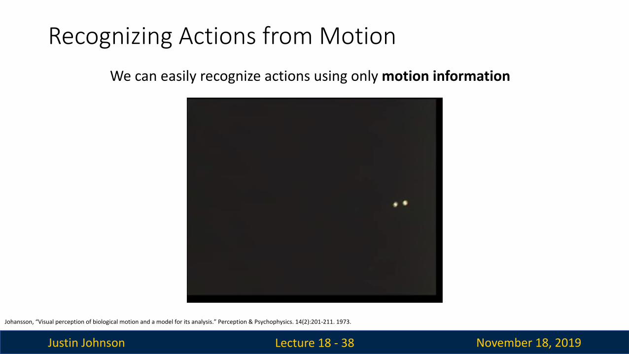
Recognizing Actions from Motion
Lecture 18 - 38
Johansson, “Visual perception of biological motion and a model for its analysis.” Perception & Psychophysics. 14(2):201-211. 1973.
We can easily recognize actions using only motion information

Justin Johnson November 18, 2019
Measuring Motion: Optical Flow
Lecture 18 - 39
Image at frame t
Image at frame t+1
Simonyan and Zisserman, “Two-stream convolutional networks for action recognition in videos”, NeurIPS 2014

Justin Johnson November 18, 2019
Measuring Motion: Optical Flow
Lecture 18 - 40
Image at frame t
Image at frame t+1
Optical flow gives a displacement field F between images It and It+1
Tells where each pixel will move in the next frame:F(x, y) = (dx, dy)It+1(x+dx, y+dy) = It(x, y)
Simonyan and Zisserman, “Two-stream convolutional networks for action recognition in videos”, NeurIPS 2014

Justin Johnson November 18, 2019
Measuring Motion: Optical Flow
Lecture 18 - 41
Image at frame t
Image at frame t+1
Optical flow gives a displacement field F between images It and It+1
Tells where each pixel will move in the next frame:F(x, y) = (dx, dy)It+1(x+dx, y+dy) = It(x, y)
Horizontal flow dx
Vertical Flow dySimonyan and Zisserman, “Two-stream convolutional networks for action recognition in videos”, NeurIPS 2014
Optical Flow highlights local motion

Justin Johnson November 18, 2019
Separating Motion and Appearance: Two-Stream Networks
Lecture 18 - 42
Simonyan and Zisserman, “Two-stream convolutional networks for action recognition in videos”, NeurIPS 2014
Input: Stack of optical flow:[2*(T-1)] x H x W
Early fusion: First 2D conv processes all flow images
Input: Single Image3 x H x W

Justin Johnson November 18, 2019Lecture 18 - 43
65.4
73
83.786.9 88
505560657075808590
3D CNN Spatial only Temporal only Two-stream(fuse by average)
Two-stream(fuse by SVM)
Accuracy on UCF-101
Separating Motion and Appearance: Two-Stream Networks
Simonyan and Zisserman, “Two-stream convolutional networks for action recognition in videos”, NeurIPS 2014

Justin Johnson November 18, 2019
Modeling long-term temporal structure
Lecture 18 - 44
First event Second event3D CNN
~5 seconds
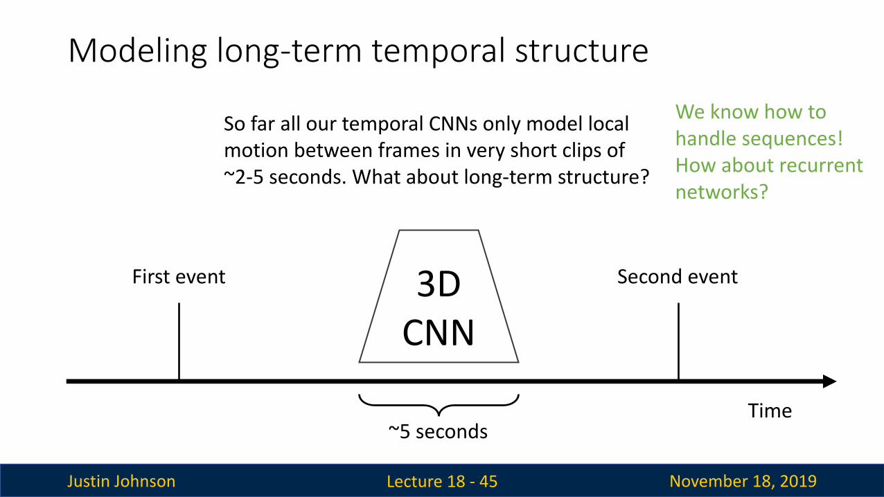
So far all our temporal CNNs only model localmotion between frames in very short clips of ~2-5 seconds. What about long-term structure?
Time
Justin Johnson November 18, 2019
Modeling long-term temporal structure
Lecture 18 - 45
First event Second event3D CNN
~5 seconds
So far all our temporal CNNs only model localmotion between frames in very short clips of ~2-5 seconds. What about long-term structure?
Time
We know how tohandle sequences!How about recurrent networks?

Justin Johnson November 18, 2019
Modeling long-term temporal structure
Lecture 18 - 46
CNN
Time
CNN CNN CNN CNN
Extract features
with CNN (2D or 3D)
Justin Johnson November 18, 2019
Modeling long-term temporal structure
Lecture 18 - 47
CNN
Time
CNN CNN CNN CNN
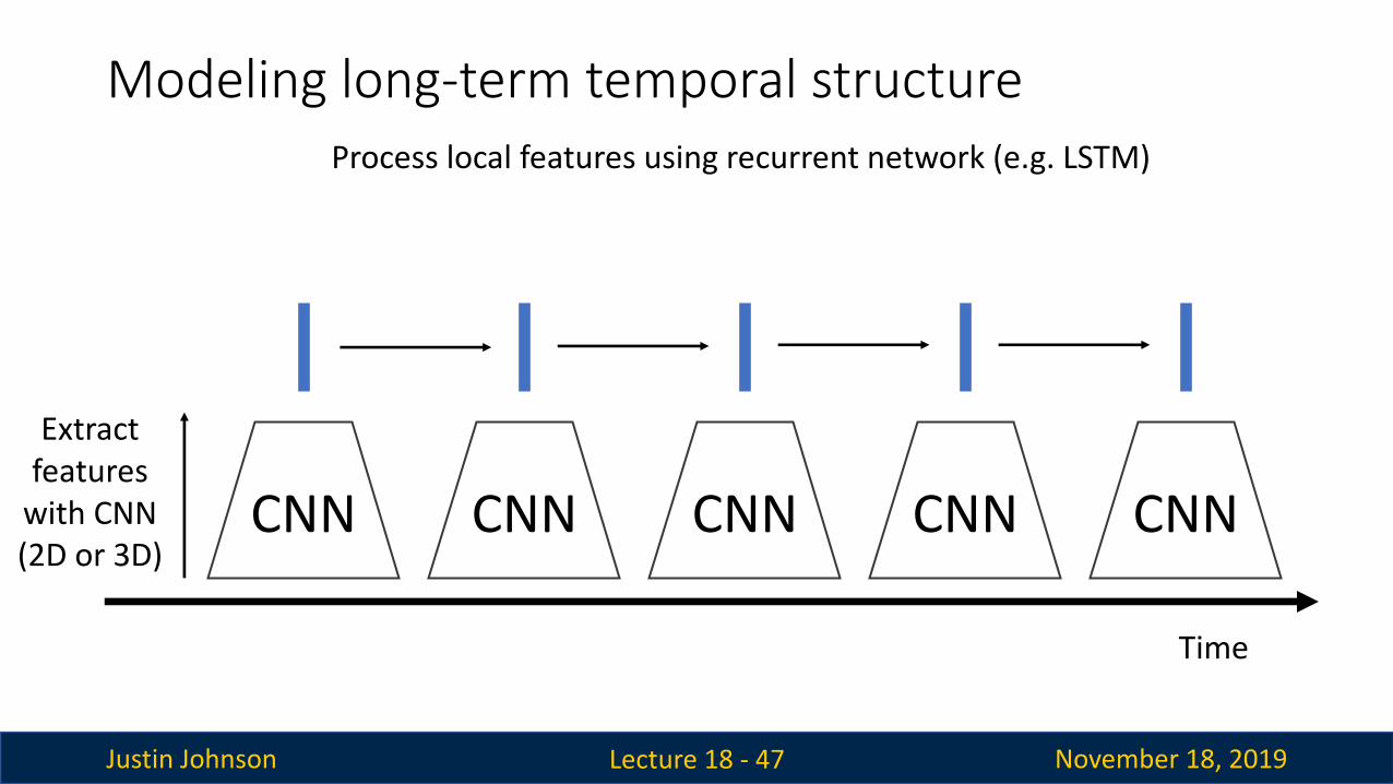
Extract features
with CNN (2D or 3D)
Process local features using recurrent network (e.g. LSTM)

Justin Johnson November 18, 2019
Modeling long-term temporal structure
Lecture 18 - 48
CNN
Time
CNN CNN CNN CNN
Extract features
with CNN (2D or 3D)
Process local features using recurrent network (e.g. LSTM)Many to one: One output at end of video

Justin Johnson November 18, 2019
Modeling long-term temporal structure
Lecture 18 - 49
CNN
Time
CNN CNN CNN CNN
Extract features
with CNN (2D or 3D)
Process local features using recurrent network (e.g. LSTM)Many to many: one output per video frame

Justin Johnson November 18, 2019
Modeling long-term temporal structure
Lecture 18 - 50
CNN
Time
CNN CNN CNN CNN
Extract features
with CNN (2D or 3D)
Process local features using recurrent network (e.g. LSTM)Many to many: one output per video frame
Baccouche et al, "Sequential Deep Learning for Human Action Recognition”, 2011
Used 3D CNNs and LSTMs in 2011! Way ahead of its time

Justin Johnson November 18, 2019
Modeling long-term temporal structure
Lecture 18 - 51
CNN
Time
CNN CNN CNN CNN
Extract features
with CNN (2D or 3D)
Process local features using recurrent network (e.g. LSTM)Many to many: one output per video frame
Baccouche et al, "Sequential Deep Learning for Human Action Recognition”, 2011
Used 3D CNNs and LSTMs in 2011! Way ahead of its time

Justin Johnson November 18, 2019
Modeling long-term temporal structure
Lecture 18 - 52
CNN
Time
CNN CNN CNN CNN
Extract features
with CNN (2D or 3D)
Process local features using recurrent network (e.g. LSTM)Many to many: one output per video frame
Baccouche et al, "Sequential Deep Learning for Human Action Recognition”, 2011Donahue et al, “Long-term recurrent convolutional networks for visual recognition and description”, CVPR 2015

Justin Johnson November 18, 2019
Modeling long-term temporal structure
Lecture 18 - 53
CNN
Time
CNN CNN CNN CNN
Extract features
with CNN (2D or 3D)
Sometimes don’t backprop to CNN to save memory; pretrain and use it as a feature extractor
Baccouche et al, "Sequential Deep Learning for Human Action Recognition”, 2011Donahue et al, “Long-term recurrent convolutional networks for visual recognition and description”, CVPR 2015

Justin Johnson November 18, 2019
Modeling long-term temporal structure
Lecture 18 - 54
CNN
Time
CNN CNN CNN CNN
Extract features
with CNN (2D or 3D)
Inside CNN: Each value a function of a fixed temporal window (local temporal structure)Inside RNN: Each vector is a function of all previous vectors (global temporal structure)
Can we merge both approaches?
Baccouche et al, "Sequential Deep Learning for Human Action Recognition”, 2011Donahue et al, “Long-term recurrent convolutional networks for visual recognition and description”, CVPR 2015

Justin Johnson November 18, 2019
Recall: Multi-layer RNN
Lecture 18 - 55
time
depth x0 x1 x2 x3 x4 x5 x6
h20 h2
1 h22 h2
3 h24 h2
5 h26
y0 y1 y2 y3 y4 y5 y6
h10 h1
1 h12 h1
3 h14 h1
5 h16
Three-layer RNN
h30 h3
1 h32 h3
3 h34 h3
5 h36
We can use a similar structure to process videos!

Justin Johnson November 18, 2019
Recurrent Convolutional Network
Lecture 18 - 56
2D conv 2D conv 2D conv 2D conv
Layer 2
Layer 1
Layer 3Entire network uses 2D feature maps: C x H x W
Each depends on two inputs:1. Same layer, previous timestep2. Prev layer, same timestep
Use different weights at each layer, share weights across time
Ballas et al, “Delving Deeper into Convolutional Networks for Learning Video Representations”, ICLR 2016

Justin Johnson November 18, 2019
Recurrent Convolutional Network
Lecture 18 - 57
Input features:C x H x W
Output features:C x H x W
2D Conv
Normal 2D CNN:

Justin Johnson November 18, 2019
Recurrent Convolutional Network
Lecture 18 - 58
Features for layer L, timestep t
Ballas et al, “Delving Deeper into Convolutional Networks for Learning Video Representations”, ICLR 2016
new state old state
some functionwith parameters W
Recall: Recurrent Network
RNN-like recurrence
Features from layer L-1, timestep t
Features from layer L, timestep t-1

Justin Johnson November 18, 2019
Recurrent Convolutional Network
Lecture 18 - 59
Features from layer L-1, timestep t
Features for layer L, timestep t
Features from layer L, timestep t-1
Ballas et al, “Delving Deeper into Convolutional Networks for Learning Video Representations”, ICLR 2016
Recall: Vanilla RNN
ℎ"#$ = tanh(𝑊,ℎ" +𝑊.𝑥)Replace all matrix multiply with 2D convolution!
2D Conv
2D Conv
𝑊,
𝑊.
+ tanh

Justin Johnson November 18, 2019
Recurrent Convolutional Network
Lecture 18 - 60
Features from layer L-1, timestep t
Features for layer L, timestep t
Features from layer L, timestep t-1
Ballas et al, “Delving Deeper into Convolutional Networks for Learning Video Representations”, ICLR 2016
Can do similar transform for other RNN variants (GRU, LSTM)
2D Conv
2D Conv
𝑊,
𝑊.
+ tanh
Recall: GRU

Justin Johnson November 18, 2019
Modeling long-term temporal structure
Lecture 18 - 61
CNN
Time
CNNRecurrent
CNNCNN: finite
temporal extent(convolutional)
Baccouche et al, "Sequential Deep Learning for Human Action Recognition”, 2011Donahue et al, “Long-term recurrent convolutional networks for visual recognition and description”, CVPR 2015
RecurrentCNN
RNN: Infinite temporal extent(fully-connected)
Time
Recurrent CNN: Infinite temporal extent(convolutional)
Ballas et al, “Delving Deeper into Convolutional Networks for Learning Video Representations”, ICLR 2016

Justin Johnson November 18, 2019
Modeling long-term temporal structure
Lecture 18 - 62
CNN
Time
CNNRecurrent
CNNCNN: finite
temporal extent(convolutional)
Baccouche et al, "Sequential Deep Learning for Human Action Recognition”, 2011Donahue et al, “Long-term recurrent convolutional networks for visual recognition and description”, CVPR 2015
RecurrentCNN
RNN: Infinite temporal extent(fully-connected)
Time
Recurrent CNN: Infinite temporal extent(convolutional)
Ballas et al, “Delving Deeper into Convolutional Networks for Learning Video Representations”, ICLR 2016
Problem: RNNs are slow for long sequences (can’t be parallelized)

Justin Johnson November 18, 2019
Recall: Different ways of processing sequences
Lecture 18 - 63
x1 x2 x3
y1 y2 y3
x4
y4
x1 x2 x3 x4
y1 y2 y3 y4
Recurrent Neural Network 1D Convolution
Works on Ordered Sequences(+) Good at long sequences: After one RNN layer, hT ”sees” the whole sequence(-) Not parallelizable: need to compute hidden states sequentiallyIn video: CNN+RNN, or recurrent CNN
Works on Multidimensional Grids(-) Bad at long sequences: Need to stack many conv layers for outputs to “see” the whole sequence(+) Highly parallel: Each output can be computed in parallelIn video: 3D convolution

Justin Johnson November 18, 2019
Recall: Different ways of processing sequences
Lecture 18 - 64
x1 x2 x3
y1 y2 y3
x4
y4
x1 x2 x3 x4
y1 y2 y3 y4
Q1 Q2 Q3
K3K2K1
E1,3E1,2E1,1
E2,3E2,2E2,1
E3,3E3,2E3,1
A1,3
A1,2
A1,1
A2,3
A2,2
A2,1
A3,3
A3,2
A3,1
V3
V2
V1
Product(→),Sum(↑)
Softmax(↑)
Y1 Y2 Y3
X1 X2 X3
Recurrent Neural Network 1D Convolution Self-Attention
Works on Ordered Sequences(+) Good at long sequences: After one RNN layer, hT ”sees” the whole sequence(-) Not parallelizable: need to compute hidden states sequentiallyIn video: CNN+RNN, or recurrent CNN
Works on Multidimensional Grids(-) Bad at long sequences: Need to stack many conv layers for outputs to “see” the whole sequence(+) Highly parallel: Each output can be computed in parallelIn video: 3D convolution
Works on Sets of Vectors(-) Good at long sequences: after one self-attention layer, each output “sees” all inputs!(+) Highly parallel: Each output can be computed in parallel(-) Very memory intensiveIn video: ????

Justin Johnson November 18, 2019
Recall: Self-Attention
Lecture 18 - 65
Q1 Q2 Q3
K3K2K1
E1,3E1,2E1,1
E2,3E2,2E2,1
E3,3E3,2E3,1
A1,3
A1,2
A1,1
A2,3
A2,2
A2,1
A3,3
A3,2
A3,1
V3
V2
V1
Product(→),Sum(↑)
Softmax(↑)
Y1 Y2 Y3
X1 X2 X3
Vaswani et al, “Attention is all you need”, NeurIPS 2017
Input: Set of vectors x1, ..., xN
Keys, Queries, Values: Project each x to a key, query, and value using linear layer
Affinity matrix: Compare each pair of x, (using scaled dot-product between keys and values) and normalize using softmax
Output: Weighted sum of values, with weights given by affinity matrix
Features in 3D CNN: C x T x H x WInterpret as a set of THW vectors of dim C
Justin Johnson November 18, 2019
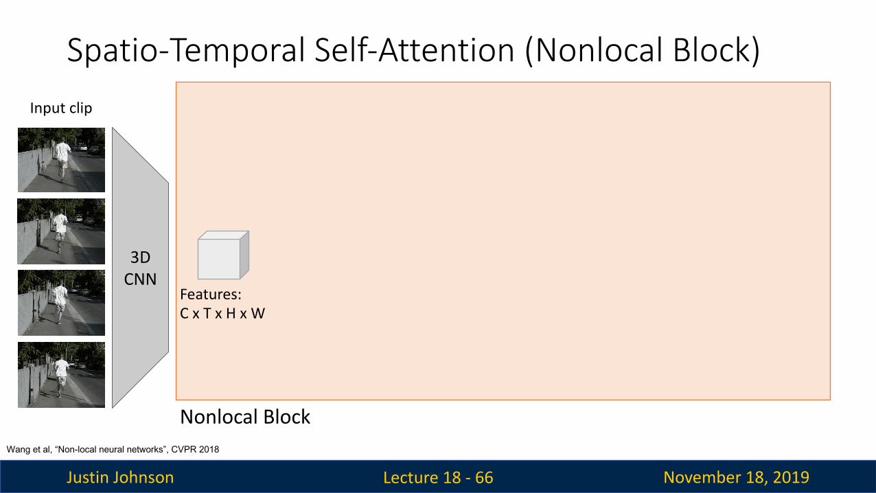
Spatio-Temporal Self-Attention (Nonlocal Block)
Lecture 18 - 66
3D CNN
Features: C x T x H x W
Wang et al, “Non-local neural networks”, CVPR 2018
Nonlocal Block
Input clip

Justin Johnson November 18, 2019
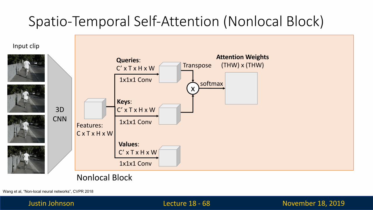
Spatio-Temporal Self-Attention (Nonlocal Block)
Lecture 18 - 67
3D CNN
Features: C x T x H x W
Queries:C’ x T x H x W
Keys:C’ x T x H x W
Values:C’ x T x H x W
1x1x1 Conv
1x1x1 Conv
1x1x1 Conv
Wang et al, “Non-local neural networks”, CVPR 2018
Nonlocal Block
Input clip
Justin Johnson November 18, 2019
Spatio-Temporal Self-Attention (Nonlocal Block)
Lecture 18 - 68
3D CNN
Features: C x T x H x W
Queries:C’ x T x H x W
Keys:C’ x T x H x W
Values:C’ x T x H x W
1x1x1 Conv
1x1x1 Conv
x
Transpose
softmax
Attention Weights(THW) x (THW)
1x1x1 Conv
Wang et al, “Non-local neural networks”, CVPR 2018
Nonlocal Block
Input clip

Justin Johnson November 18, 2019
Spatio-Temporal Self-Attention (Nonlocal Block)
Lecture 18 - 69
3D CNN
Features: C x T x H x W
Queries:C’ x T x H x W
Keys:C’ x T x H x W
Values:C’ x T x H x W
1x1x1 Conv
1x1x1 Conv
x
Transpose
softmax
Attention Weights(THW) x (THW)
x
C’ x T x H x W
1x1x1 Conv
Wang et al, “Non-local neural networks”, CVPR 2018
Nonlocal Block
Input clip

Justin Johnson November 18, 2019
Spatio-Temporal Self-Attention (Nonlocal Block)
Lecture 18 - 70
3D CNN
Features: C x T x H x W
Queries:C’ x T x H x W
Keys:C’ x T x H x W
Values:C’ x T x H x W
1x1x1 Conv
1x1x1 Conv
x
Transpose
softmax
Attention Weights(THW) x (THW)
x
C’ x T x H x W
1x1x1 Conv
C x T x H x W
1x1x1 Conv
Wang et al, “Non-local neural networks”, CVPR 2018
Nonlocal Block
Input clip

Justin Johnson November 18, 2019
Spatio-Temporal Self-Attention (Nonlocal Block)
Lecture 18 - 71
3D CNN
Features: C x T x H x W
Queries:C’ x T x H x W
Keys:C’ x T x H x W
Values:C’ x T x H x W
1x1x1 Conv
1x1x1 Conv
x
Transpose
softmax
Attention Weights(THW) x (THW)
x
C’ x T x H x W
1x1x1 Conv
+
C x T x H x W
Residual Connection
1x1x1 Conv
Wang et al, “Non-local neural networks”, CVPR 2018
Nonlocal Block
Input clip

Justin Johnson November 18, 2019
Spatio-Temporal Self-Attention (Nonlocal Block)
Lecture 18 - 72
3D CNN
Features: C x T x H x W
Queries:C’ x T x H x W
Keys:C’ x T x H x W
Values:C’ x T x H x W
1x1x1 Conv
1x1x1 Conv
x
Transpose
softmax
Attention Weights(THW) x (THW)
x
C’ x T x H x W
1x1x1 Conv
+
C x T x H x W
Nonlocal Block
Residual Connection
1x1x1 Conv
Wang et al, “Non-local neural networks”, CVPR 2018
Input clip

Justin Johnson November 18, 2019
Spatio-Temporal Self-Attention (Nonlocal Block)
Lecture 18 - 73
Input clip
3D CNN
Features: C x T x H x W
Queries:C’ x T x H x W
Keys:C’ x T x H x W
Values:C’ x T x H x W
1x1x1 Conv
1x1x1 Conv
x
Transpose
softmax
Attention Weights(THW) x (THW)
x
C’ x T x H x W
1x1x1 Conv
+
C x T x H x W
Residual Connection
1x1x1 Conv
Wang et al, “Non-local neural networks”, CVPR 2018
Trick: Initialize last conv to 0, then entire block computes identity. Can insert into existing 3D CNNs
Nonlocal Block In practice, actually insert BatchNorm layer after final conv, and initialize scale parameter of BN layer to 0 rather than setting conv weight to 0

Justin Johnson November 18, 2019
Spatio-Temporal Self-Attention (Nonlocal Block)
Lecture 18 - 74
Input clip
3D CNN
Wang et al, “Non-local neural networks”, CVPR 2018
Nonlocal Block
Features: C x T x H x W
Queries:C’ x T x H x W
Keys:C’ x T x H x W
Values:C’ x T x H x W
1x1x1 Conv
1x1x1 Conv
x
Transpose
softmax
Attention Weights(THW) x (THW)
x
C’ x T x H x W
1x1x1 Conv
+C x T x H x W
Residual Connection
1x1x1 Conv
3D CNN 3D CNNFeatures: C x T x H x W
Queries:C’ x T x H x W
Keys:C’ x T x H x W
Values:C’ x T x H x W
1x1x1 Conv
1x1x1 Conv
x
Transpose
softmax
Attention Weights(THW) x (THW)
x
C’ x T x H x W
1x1x1 Conv
+C x T x H x W
Residual Connection
1x1x1 Conv
Running
We can add nonlocal blocks into existing 3D CNN architectures.But what is the best 3D CNN architecture?
Nonlocal Block

Justin Johnson November 18, 2019
Inflating 2D Networks to 3D (I3D)
Lecture 18 - 75
There has been a lot of work on architectures for images. Can we reuse image architectures for video?
Carreira and Zisserman, “Quo Vadis, Action Recognition? A New Model and the Kinetics Dataset”, CVPR 2017
Idea: take a 2D CNN architecture.
Replace each 2D Kh x Kw conv/pool layer with a 3D Kt x Kh x Kw version

Justin Johnson November 18, 2019
Inflating 2D Networks to 3D (I3D)
Lecture 18 - 76
There has been a lot of work on architectures for images. Can we reuse image architectures for video?
Previous layer
3x3 Conv
1x1 Conv
3x3 MaxPool
Concatenate
1x1 Conv
1x1 Conv
5x5 Conv
1x1 Conv
Inception Block: Original
Carreira and Zisserman, “Quo Vadis, Action Recognition? A New Model and the Kinetics Dataset”, CVPR 2017
Idea: take a 2D CNN architecture.
Replace each 2D Kh x Kw conv/pool layer with a 3D Kt x Kh x Kw version

Justin Johnson November 18, 2019
Inflating 2D Networks to 3D (I3D)
Lecture 18 - 77
There has been a lot of work on architectures for images. Can we reuse image architectures for video?
Previous layer
3x3x3 Conv
1x1x1 Conv
3x3x3MaxPool
Concatenate
1x1x1 Conv
1x1x1 Conv
5x5x5 Conv
1x1x1 Conv
Inception Block: Inflated
Carreira and Zisserman, “Quo Vadis, Action Recognition? A New Model and the Kinetics Dataset”, CVPR 2017
Idea: take a 2D CNN architecture.
Replace each 2D Kh x Kw conv/pool layer with a 3D Kt x Kh x Kw version

Justin Johnson November 18, 2019
Inflating 2D Networks to 3D (I3D)
Lecture 18 - 78
There has been a lot of work on architectures for images. Can we reuse image architectures for video?
Idea: take a 2D CNN architecture.
Replace each 2D Kh x Kw conv/pool layer with a 3D Kt x Kh x Kw version
Can use weights of 2D conv to initialize 3D conv: copy Kt times in space and divide by KtThis gives the same result as 2Dconv given “constant” video input
2D conv kernel:Cin x Kh x Kw
3D conv kernel:Cin x Kt x Kh x Kw
Input:3 x H x W
Input:3 x Kt x H x W
Copy kernel Kt times, divide by Kt
Output:H x W
Output:1 x H x W
Duplicate input Kt times
Output is the same!
Carreira and Zisserman, “Quo Vadis, Action Recognition? A New Model and the Kinetics Dataset”, CVPR 2017

Justin Johnson November 18, 2019
Inflating 2D Networks to 3D (I3D)
Lecture 18 - 79
There has been a lot of work on architectures for images. Can we reuse image architectures for video?
Idea: take a 2D CNN architecture.
Replace each 2D Kh x Kw conv/pool layer with a 3D Kt x Kh x Kw version
Can use weights of 2D conv to initialize 3D conv: copy Kt times in space and divide by KtThis gives the same result as 2Dconv given “constant” video input
57.953.9
62.8
68.471.6
62.2 63.365.6
71.174.2
40
45
50
55
60
65
70
75
80
Per-frame CNN CNN+LSTM Two-streamCNN
Inflated CNN Two-streaminflated CNN
Top-1 Accuracy on Kinetics-400
Train from scratch Pretrain on ImageNetCarreira and Zisserman, “Quo Vadis, Action Recognition? A New Model and the Kinetics Dataset”, CVPR 2017 All using Inception CNN

Justin Johnson November 18, 2019
Visualizing Video Models
Lecture 18 - 80
Image
Flow
Forward: Compute class score
Backward: Compute gradient
”weightlifting” score
Figure credit: Simonyan and Zisserman, “Two-stream convolutional networks for action recognition in videos”, NeurIPS 2014Feichtenhofer et al, “What have we learned from deep representations for action recognition?”, CVPR 2018Feichtenhofer et al, “Deep insights into convolutional networks for video recognition?”, IJCV 2019.
Add a term to encourage spatially smooth flow; tune penalty to pick out “slow” vs “fast” motion

Justin Johnson November 18, 2019
Can you guess the action?
Lecture 18 - 81
Fast motion appearance
Appearance “Slow” motion “Fast” motion
Feichtenhofer et al, “What have we learned from deep representations for action recognition?”, CVPR 2018Feichtenhofer et al, “Deep insights into convolutional networks for video recognition?”, IJCV 2019. Slide credit: Christoph Feichtenhofers

Justin Johnson November 18, 2019
Can you guess the action? Weightlifting
Lecture 18 - 82
Fast motion appearance
Appearance “Slow” motion “Fast” motion
Feichtenhofer et al, “What have we learned from deep representations for action recognition?”, CVPR 2018Feichtenhofer et al, “Deep insights into convolutional networks for video recognition?”, IJCV 2019. Slide credit: Christoph Feichtenhofer
”Bar Shaking” “Push overhead”

Justin Johnson November 18, 2019
Can you guess the action?
Lecture 18 - 83
Fast motion appearance
Appearance “Slow” motion “Fast” motion
”Bar Shaking” “Push overhead”Fast motion appearance

Justin Johnson November 18, 2019
Can you guess the action? Apply Eye Makeup
Lecture 18 - 84
Fast motion appearance
Appearance “Slow” motion “Fast” motion
”Bar Shaking” “Push overhead”Fast motion appearance

Justin Johnson November 18, 2019
Treating time and space differently: SlowFast Networks
Lecture 18 - 85
Fast pathway
Slow pathwayTime
Channels
Space
prediction
CC
C
αTαT
αT βCβC
βC
TT
T
Slow
Fast
Lightweight (< 20% of compute)
Low framerate
High framerateLateral connections
β = 1/8e.g. α = 8
Feichtenhofer et al, “SlowFast Networks for Video Recognition”, ICCV 2019Slide credit: Christoph Feichtenhofer

Justin Johnson November 18, 2019Lecture 18 - 87
• Dimensions are• Strides are {temporal, spatial2} • The backbone is ResNet-50• Residual blocks are shown by brackets• Non-degenerate temporal filters are
underlined• Here the speed ratio is α = 8 and the
channel ratio is β = 1/8• Orange numbers mark fewer channels,
for the Fast pathway• Green numbers mark higher temporal
resolution of the Fast pathway• No temporal pooling is performed
throughout the hierarchy
Feichtenhofer et al, “SlowFast Networks for Video Recognition”, ICCV 2019Slide credit: Christoph Feichtenhofer
Treating time and space differently: SlowFast Networks
Justin Johnson November 18, 2019
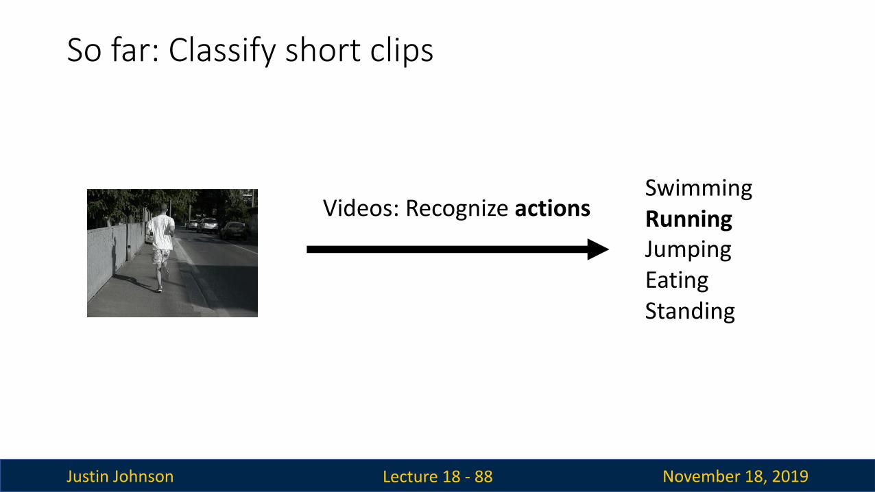
So far: Classify short clips
Lecture 18 - 88
SwimmingRunningJumpingEatingStanding
Videos: Recognize actions

Justin Johnson November 18, 2019
Temporal Action Localization
Lecture 18 - 89
Running Jumping
Given a long untrimmed video sequence, identify frames corresponding to different actions
Chao et al, ” Rethinking the Faster R-CNN Architecture for Temporal Action Localization”, CVPR 2018
Can use architecture similar to Faster R-CNN: first generate temporal proposals then classify

Justin Johnson November 18, 2019
Spatio-Temporal Detection
Lecture 18 - 90
Given a long untrimmed video, detect all the people in space and time and classify the activities they are performingSome examples from AVA Dataset:
Gu et al, “AVA: A Video Dataset of Spatio-temporally Localized Atomic Visual Actions”, CVPR 2018

Justin Johnson November 18, 2019
Recap: Video Models
Lecture 18 - 91
Many video models:Single-frame CNN (Try this first!)Late fusionEarly fusion3D CNN / C3DTwo-stream networksCNN + RNNConvolutional RNNSpatio-temporal self-attentionSlowFast networks (current SoTA)

Justin Johnson November 18, 2019
Next time:Generative Models, part 1
Generative Adversarial Networks
Lecture 18 - 92