Interpretable Visual Models for Human Perception-BasedObject Retrieval

Ahmed REBAIINRIA Rocquencourt78153 Le Chesnay

FranceAhmed.Rebai@inria.fr

Alexis JOLYINRIA Rocquencourt78153 Le Chesnay

FranceAlexis.Joly@inria.fr

Nozha BOUJEMAAINRIA Rocquencourt78153 Le Chesnay

FranceNozha.Boujemaa@inria.fr

ABSTRACTUnderstanding the results returned by automatic visual con-cept detectors is often a tricky task making users uncom-fortable with these technologies. In this paper we attemptto build humanly interpretable visual models, allowing theuser to visually understand the underlying semantic. Wetherefore propose a supervised multiple instance learningalgorithm that selects as few as possible discriminant localfeatures for a given object category. The method finds itsroots in the lasso theory where a L1-regularization term isintroduced in order to constraint the loss function, and sub-sequently produce sparser solutions. Efficient resolution ofthe lasso path is achieved through a boosting-like procedureinspired by BLasso algorithm. Quantitatively, our methodachieves similar performance as current state-of-the-art, andqualitatively, it allows users to construct their own modelfrom the original set of patches learned, thus allowing formore compound semantic queries.

Categories and Subject DescriptorsI.4.8 [IMAGE PROCESSING AND COMPUTER VI-SION]: Scene Analysis—Object recognition

General TermsAlgorithms

KeywordsObject retrieval, interpretability, feature selection, sparsity,human perception, interactivity.

1. INTRODUCTIONUnderstanding an image scene is definitely related to rec-

ognizing what it is composed of. Unfortunately, in practice,the results returned by state-of-the-art visual concept detec-tors are often difficult to interpret from a user point of view.The visual models produced are indeed highly depending on

Permission to make digital or hard copies of all or part of this work forpersonal or classroom use is granted without fee provided that copies arenot made or distributed for profit or commercial advantage and that copiesbear this notice and the full citation on the first page. To copy otherwise, torepublish, to post on servers or to redistribute to lists, requires prior specificpermission and/or a fee.ICMR ’11, April 17-20, Trento, ItalyCopyright c©2011 ACM 978-1-4503-0336-1/11/04 ...$10.00.

the used training data and might convey a different seman-tic than the words used to describe the originally targetedconcept. This often makes users uncomfortable with thesetechnologies since they do not get what they expected fromthe textual description of the trained concept. In this pa-per we rather attempt to build humanly interpretable visualmodels, allowing the user to visually understand the under-lying semantic.

Our basic idea is to build concise, effective and visuallyinterpretable models to allow for fast retrieval. Each objectmodel consists of a concise set of visual patches representingthe most discriminant image regions of a concept. Conse-quently, users can easily visualize the trained image regionsand query the system by only choosing the visual patchesthat most correspond to their needs. This involves adding,subtracting and attributing weights to the visual patchesdisplayed.

Composing a statistically and visually discriminant modelprovides a unique way for an interactive search. Now, thechallenging question to answer is how to train the most con-cise set of visual patches while preserving a good retrievaleffectiveness. The key to this question is provided by the im-age representation and the learning technique used. Usingstate-of-the-art bag-of-features technique is for instance notadapted because it discards the positions of the features be-ing learned. These visual words do not provide any guarantyon whether the underlying clusters pertain to tangible partsof the objects (i.e eye, tooth, finger, etc.) or if they are just astatistical combination of some of these parts. On the otherhand, using learning techniques based on such features witha SVM classifier is also not adequate for the matter sinceour objective is to locate a few representative image regionsrather than creating an optimal separation between the pos-itive and negative feature sets. It is worth mentioning thatthe method we propose is generic in the sense that it couldbe used with any local features or feature sets representingthe content of an image region. In this work, we simply usedSIFT features as the basic image primitives.

The main contribution of this paper is a novel multiple-instance learning method that allows for user interactivitywhen retrieving visual concepts. Applying the principle ofthe lasso technique to a discriminative approach for conceptretrieval constitutes our second contribution. The third con-tribution consists in adapting the BLasso algorithm to ourpurpose by using weighted training data and constrainingthe forward steps to be only positive steps. As a last contri-bution, we propose an efficient implementation for our learn-ing method to speed up the process of backward steps. The

next section briefly reviews state-of-the-art feature selectionmethods related to our work. Section 3 explains our learningstrategy in more detail. Then, we present our experimentsin section 4 and set out our conclusions in section 5.

2. FEATURE SELECTIONFeature selection has always been an overwhelming task.

The method we propose is based on a modified version ofthe BLasso algorithm. Our original idea is to train with aboosting-like procedure but with adding extra constraintsto the loss function in order to produce sparser solutions.Added to highlighting interest features, sparsity is indeedpreferable because it reduces the model complexity and sub-sequently enhances the interpretability of the produced mod-els as well as it reduces the prediction time.

Constraining the empirical loss dates back to 1996 whenTibshirani observed that the ordinary least squares mini-mization technique is not always satisfactory since the esti-mates often have a low bias but a large variance. He cameout with lasso [10] which shrinks or sets some coefficients tozero. Lasso stands for Least Absolute Shrinkage and Selec-tion Operator. The idea has two goals: first to gain moreinterpretation by focussing on relevant predictors and, sec-ondly to improve the prediction accuracy by reducing thevariance of the predicted values. Lasso minimizes the L2

loss function penalized by the L1 norm on the parameters.This is a quadratic programming problem with linear in-equality constraints and it is intractable when the vector ofparameters is very large.

In literature, some efficient methods have been proposedto solve the exact Lasso namely the least angle regressionby Efron et al. [1] and the homotopy method by Osborne etal. [6]. These methods were developed specifically to solvethe least squares problem (i.e. using L2 loss). They workwell where the number of predictors is small. However, theyare not adapted to nonparametric and classification tasks.To encounter these limitations, Zhao and Yu [12] proposedan algorithm with the name of BLasso (Boosted Lasso). Theadvantage of this algorithm lies in its ability to functionwith an infinite number of predictors and with various lossfunctions. These are some characteristics of the algorithmsbelonging to the boosting family.

The boosting mechanism was proposed by Schapire [8] in1990. Since then, many algorithms have emerged [2, 3, 5,9, 11] and boosting has become one of the most successfulmachine learning techniques. The underlying idea is to com-bine many weak classifiers (also called hypotheses) in orderto obtain one final “strong” classifier. Boosting is an ad-ditive model which builds up one hypothesis after anotherby re-weighting the data for the next iteration—increasingthe weights of misclassified images and decreasing those ofwell classified ones. This concept helps to generate differ-ent hypotheses, putting emphasis on misclassified examples,typically those located near the decision boundary in thefeature space. Although it is an intuitive algorithm, boost-ing may overfit the training data, particularly when it runsfor a large number of iterations T in high dimensional andnoisy data [4, 7]. That’s why, adding a regularization termis usually needed.

Unlike boosting, and in order to approximate lasso solu-tions, BLasso adds a backward step after each iteration ofboosting. Thus, one is able to build up solutions with a co-ordinate descent manner and then take a look back at the

consistency of these solutions regarding the model complex-ity. Added to that, BLasso does not suffer from the stopcondition like an ordinary boosting does. In fact, and for aboosting procedure, fixing a large value of T implies a possi-ble overfitting not to mention the long prediction time. Onthe other hand, setting T to a small value may lead to un-derfitting. Therefore, the model may be non-discriminant,inconsistent and might not cover the variability inside thecategory itself. A usual boosting algorithm can also be qual-ified as oblivious as it always functions in a forward manneraiming to minimize the empirical loss. Although the con-cept of re-weighting is interesting, at an iteration t + 1, wehave no idea whether the t previous generated hypothesesare good enough or not versus the model complexity.

3. LEARNING VISUAL PATCHES

3.1 Multiple-Instance Learning with BLasso

3.1.1 Training a Weak ClassifierBackground information sometimes plays a primordial role

in recognition. Thus, we propose to train our classifiers in acontext of weak learning. That is, a training image is labeledas a whole sample. It will take the label +1 if it contains theobject, −1 if not. This is also known as multiple instancelearning. It deals with uncertainty of instance labels. Animage is viewed as a bag of multiple features which are thelocal visual signatures. The bag will have only one labelaccording to whether or not it includes at least one positiveinstance. It follows that it is only certain for a negative bagthat there are no objects. Moreover, using a multi-instanceapproach has the luxury of unsupervised learning. It givesmore freedom to the algorithm to select background featureswhenever they turn out to be useful to characterize the cat-egory.

Visual patches are viewed as weak classifiers. A weak clas-sifier hk represents a coordinate of base learners. Its weightis strictly positive if it was chosen at least once during theboosting process and remains zero if not. In the context ofobject categorization, the weak hypothesis hk is a local im-age signature Fk with an optimal radius rk (Opelt et al. [5]).In other words, hk corresponds to a hypersphere centered ona local image feature Fk. For a test image x, hk will output+1 if the distance between x and Fk is less than rk and −1otherwise. Discriminant radii of weak classifiers are optimalin the sense that the classification error is as minimal aspossible. They are determined through a distance matrix.Each entry of the matrix represents a local feature with acorresponding ranked list of the training images. The dis-tance between any feature Fki belonging to the image Ii andany image Ij of the training set is defined by:

d(Fki, Ij) = min1≤k′≤Mj

d(Fki, Fk′j)

Let Si = (Ii, li) be the couple representing the trainingimage Ii labeled with li ∈ {−1, 1} and wi be the weightassociated to Ii. S = {S1, · · · , SN} represents the set of allthe training data. We denote by dk,η the distance separatingthe feature Fk from the image whose rank is η. The optimalradius rk is determined after two steps. First we computethe curve corresponding to the sums of the weighted image

labels and take the index where the maximum is achieved:

η = arg max1≤η≤N

η∑i=1

wi · li (1)

Then, rk is given by:

rk =dk,η + dk,η+1

2(2)

Training a weak classifier is a simple boosting iteration.At an iteration t, we compute the score sk corresponding tothe feature Fk based on the image weights

sk = maxm

m∑j=1

wj · lj (3)

Then, we select the feature which obtains the highest score.Note that Eq. (1) is in accordance with Eq. (3) in the sensethat Eq. (1) looks for the index at which the score curve ismaximum.

Using AdaBoost algorithm, Opelt et al. [5] considered aninfinity of base learners. At the iteration t, and after select-ing the best feature Fk, the base learner associated to Fk

is defined by the couple (Fk, rk) and is attributed a weightaccording to the training error. (rk is given by eq. 2.) Thisseems plausible because AdaBoost uses a steepest descentto converge.

In our work, and for the sake of interpretability, each fea-ture Fk represents only one base learner and should at mostbe selected once. It has to have its weight determined af-ter several boosting iterations (forward stagewise). How-ever, whenever selected, this base learner sees its radius rkchanges according to the weight updates, thus the final rkattributed is the average of all the computed radii.

3.1.2 The AlgorithmOur algorithm is viewed as a boosting method constrained

by a L1-regularization term. L1-regularization is equivalentto lasso [10]. Let β = (β1, · · · , βk, · · · )T be the vector of pa-rameters to estimate (the weights of the weak hypotheses).β is initially zero. The lasso loss function Γ can be writtenas:

Γ(β, λ) =N∑

n=1

L2(Sn, β) + λ · ||β||1 (4)

where ||β||1 =∑

j |βj | denotes the L1 norm of the vector βand λ ≥ 0 is the parameter controlling the amount of reg-ularization applied to the estimate. In order to get sparsesolutions with an efficient shrinkage tradeoff, λ usually takesa moderate value since a large value may set these coeffi-cients to exactly zero, leading to the null model. On theother hand, setting λ to zero reverses the lasso problem tominimizing the unregularized empirical loss. In our case, forclassification, we replace L2-loss function by the exponentialloss function.

Since the exact lasso minimization is not tractable, BLasso [12]tries to find the same solutions as lasso with more cautioussteps. Indeed it works with both forward and backwardsteps. Forward steps are used to minimize the empiricalloss. On the other hand, backward steps minimize the reg-ularization. In fact, at each iteration, a coordinate βj isselected and updated by a small step size ε > 0. It has beenshown that it is preferable to choose a very small step sizeso that BLasso can approximate the lasso path perfectly. In

practice, ε should always be less than 0.1. In the originalBLasso algorithm, forward steps can be either positive ornegative (update by ±ε). However, we chose not to. Ourforward steps are always positive. We justify this choice bythe fact that a selected classifier is a visual patch that con-tributes to build the object category model, thus it has tobe positive.

Algorithm 1 BLasso

1. Initialization: β = 0Make a forward step and initialize λ

2. Backward and forward steps:Find the backward step that leads to the minimalempirical loss.

if the step decreases the lasso loss then take it.else make a forward step and relax λ if necessary

3. Repeat step 2 until λ ≤ 0.

Algorithm 1 gives a general overview on the BLasso mech-anism. In our implementation, and in order to minimize theempirical loss, we used a weighting scheme as in AdaBoost.Adopting this strategy is appealing because it gives more at-tention to the misclassified observations by increasing theirrespective weights. Note that, at initialization, all weightsare equal to 1/N .

At the iteration t, a forward step can be summarized inthe next five points.

1. Update weights

w(t+1)n =

w(t)n · exp (− ε · ln · h(t)

κ I(n))

τ(5)

τ is a normalization constant s.t.∑N

n=1 w(t+1)n = 1

2. Train the classifier and get the best hypothesis h(t+1)κ

3. β(t+1) = β(t) + ε · 1κ

4.

λt+1 = min[λt,

1

ε

( N∑n=1

L(Sn, β(t)−

N∑n=1

L(Sn, β(t+1)−ξ

)]

(6)

5. I(t+1)A = I

(t)A ∪ {κ} where IA is the active index set.

Note that equation 5 is in accordance with the weight updatemechanism used in AdaBoost. In fact, we just replaced theestimated hypothesis weight by the forward step ε.

The variable ξ, used when updating λ, is a tolerance pa-rameter that is strictly positive. This parameter is addedto gain more stability and it should be set to a very smallvalue. Moreover, the initial value of λ can be obtained bythe same formula (eq. 6) but with omitting ξ (as if ξ = 0). ξis also used to decide whether to accept or reject a backwardstep. A backward step consists in finding the step that leadsto the minimal empirical loss. It is given by:

j = arg minj∈I

(t)A

N∑n=1

L(Sn, β(t) − ε · 1j) (7)

This step is taken if and only if it decreases the lasso loss.That is, if Γ(β(t) − ε · 1j , λt)− Γ(β(t), λt) ≤ −ξ then

β(t+1) = β(t) − ε · 1j ; λt+1 = λt

3.2 Efficient ImplementationThe inescapable processing burden for training is the com-

putation of the distance matrix. To accelerate the process,one solution consists in trading accuracy for time by relyingon approximate rather than exhaustive search. This couldbe achieved through range queries with an appropriate in-dex structure like LSH for example. However, extreme careshould be taken because it may drastically lower the qual-ity of weak classifiers. This paper doesn’t cover the gainsobtained with such optimization.

The next processing burden and greediest block duringtraining is computing the loss function. In fact, we need tocompute both of the empirical and lasso losses many timesduring each iteration. The complexity increases every timea new coordinate is chosen. Luckily, the lasso loss can bededuced from the empirical loss. It follows that, in order tocompute the current lasso loss and the backward lasso loss,we just need to compute their respective empirical losses.On the other hand, and at each iteration, only one coordi-nate is modified while all the other coordinates remain un-changed. Therefore, assuming that memory is cheaper thanprocessing time, the computation of the empirical loss canbe accelerated—at an iteration t—by preserving in memorythe classification values of the previous state for each coor-dinate βj and for each image In. Since our solutions aresparse, even when using a large number of training images,this method is still applicable. Each image In will have astorage vector ζn. To simplify the notation, we will considerthat the jth entry of the vector ζn (i.e. ζn(j)) refers to theclassification value of the variable βj

ζn(j) = βj · hj(In) 1 ≤ n ≤ N ; j ∈ IA (8)

Thus, when changing a hypothesis hk in the next iteration,we only need to update (if βk has already been selectedbefore) or create new (if the index k is selected for the firsttime) N classification values. That is, we have to computeζn(k) for all 1 ≤ n ≤ N

The storage of the classification values is more importantwhen searching for the backward step. The empirical loss isnot computed just once but at least card{IA} times wherecard{IA} is the cardinal of the index set (It is computedcard{IA}+ 1 times if the coordinate is selected for the firsttime.) Given an image In, for each coordinate j, we need tocompute the empirical loss based on the coordinates β−ε1j .Except for the coordinate βj , the other classification val-ues have already been computed and stored in ζn(k) withk �= j. Moreover, the absolute difference between ζn(j) (al-ready computed if the hypothesis is old) and the classifica-tion value δnj that we need to compute is ε

if

{ζn(j) < 0 ⇒ δnj = ζn(j) + εζn(j) > 0 ⇒ δnj = ζn(j) − ε

(9)

It follows that the classification value of the image In (i.e.∑k ζn(k)) will only change by an absolute difference of ε.

We denote by ζn(j) =∑

k �=j ζn(k) + δnj , that is:

ζn(j) =

{ ∑k ζn(k) + ε if ζn(j) < 0∑k ζn(k)− ε if ζn(j) > 0

(10)

This formulation helps to locate the backward step quickly.In fact, it only takes a linear time according to the numberof the selected hypotheses. After subtracting the value εfrom the coordinate βj , the empirical loss Ej is computed

as follows:

Ej =N∑

n=1

exp(−ln · ζn(j)) (11)

The backward step j is then defined by

j = argminj

Ej (12)

When the algorithm proceeds and selects a coordinate gat the iteration t, the stored values will be altered as follows.If g is selected for the first time, then

∀n ζn(g) =∑k �=g

ζn(k) ; ζn(g) = ε · hg(In) (13)

and

ζ(t)

n (j) = ζ(t−1)

n (j) + ε · hg(In) ∀j �= g (14)

Now, if g already belongs to the active index IA, then

ζ(t)n (g) = ζ(t−1)n (g) + sign(ζ(t−1)

n (g)) · ε (15)

In this case, equation (14) is valid for all j ∈ IA. Note thatwhen j = g, this equation automatically takes into accountthe backward step (i.e the term −ε · 1g) because it was notadded in the first place.

3.3 PredictionFor classification purpose, each image is predicted sepa-

rately by looping through all weak classifiers. However, tobe more efficient in retrieval, we predict by means of rangequeries. The final scores of all images are computed at thesame time. First, these scores are initialized to zero. Then,and for each weak classifier, we query the search engine toretrieve all the images that fall into its hypersphere. Conse-quently, these images will see their scores incremented eachby the weight of this weak classifier. On the other hand,images that are not returned by the system will have theirscores decremented by the same weight of this classifier. Af-ter looping through all weak classifiers, each image ends upwith a score judging its relevance to the concept.

The process described earlier can be relatively slow de-pending on the database size and the number of hypothesesconstituting the model. For applications that have a fixedimage database (not updated online), we can compute a pri-ori the distances separating each weak classifier from eachimage and load them when the search engine starts. Thiscould be achieved with no worries because the models usedare concise and so won’t consume too much computer mem-ory. Moreover, since distances are computed offline, the pro-cess can be done either exhaustively or using an index struc-ture. Unlike retrieval with range queries, to answer a givenquery, images are processed one by one. For each image,the distances to the model defined are obtained through alookup table then the score is computed by comparing thesedistances to the corresponding classifier radii.

4. EXPERIMENTS

4.1 Performance EvaluationOur experiments aims to prove that sparse models are still

able to achieve good retrieval results. We first evaluated theretrieval effectiveness on 10 object categories belonging to

the ImageNet database1. It consists on comparing the per-formance between BLasso and AdaBoost. The name of thecategories as well as the composition of the database usedfor training are given in table 1. Note that for each objectcategory, we built the counter-class (negative samples) byrandomly collecting images from the other categories whilekeeping the same number. We relied on SIFT descriptorsas the basic image primitives. Moreover, each image con-tained at most 500 features. The original image set was di-vided equally between training and test. Therefore, the testdatabase has the same composition shown in table 1 (a totalof 6830 images). For all our experiments, the parameters ofBLasso were tuned as follows

ξ = 10−6 and ε =1

80

This choice is made based on the experiments in [12]. ForAdaBoost, we fixed the number of iterations T = 100.

For evaluation, we used the average precision. It is a reli-able measure for retrieval and is computed as the area underthe precision-recall curve. Precision is defined as the ratioof the number of correct answers to the number of the docu-ments retrieved. Recall is defined as the ratio of the numberof correct answers to the number of all the relevant docu-ments in the database. Results are given in table 2.

camel

laptop

penguin

revolver

snail

sunflower

tennisracket

tomato

watch

zebra

714

694

656

652

731

700

649

616

681

737

Table 1: Composition of the training set.

# features Average precisionCategory

Original BL AB BL ABcamel 282576 66 100 0.2589 0.2568laptop 191445 69 100 0.4606 0.4467penguin 264364 84 100 0.3406 0.3257revolver 122472 2 30 0.2003 0.3134snail 214597 44 100 0.261 0.2784sunflower 264355 101 100 0.5589 0.5065tennis racket 173781 46 100 0.2287 0.3156tomato 210641 62 100 0.5424 0.5244watch 174818 51 100 0.413 0.4712zebra 304673 78 100 0.7146 0.7029Average 220372.2 60.3 93 0.3979 0.4142

Table 2: Performance evaluation of BLasso (BL) andAdaBoost (AB) in 10 categories of ImageNet.

BLasso outperformed AdaBoost in 6 categories (camel,laptop, penguin, sunflower, tomato and zebra). However,on average, AdaBoost was better approximately by 1.6%.This result is due to the clear domination of AdaBoost inthe categories revolver and tennis_racket where the per-formance was respectively higher by 11.3% and 8.7%. Onthe other hand, it is noticeable that the feature selectionperformed by BLasso is better. In fact, the number of thefeatures composing the model is fewer. Knowing that theprediction time is linear with the model size, the time needed

1http://www.image-net.org/

0.1

0.2

0.3

0.4

0.5

0.6

0.7

0.8

0.9

1

0 0.2 0.4 0.6 0.8 1

Pre

cisi

on

Recall

Average over the 10 categories

AdaBoostBLasso

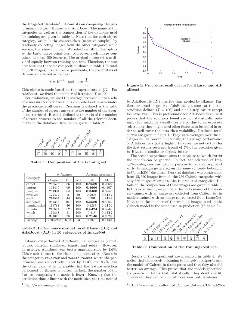
Figure 1: Precision-recall curves for BLasso and Ad-aBoost.

by AdaBoost is 1.5 times the time needed by BLasso. Fur-thermore, and in general, AdaBoost get stuck at the stopcondition defined (T = 100) and didn’t stop earlier exceptfor revolver. This is problematic for AdaBoost because itproves that the solutions found are not statistically opti-mal, they might be visually correlated due to an excessiveselection or they might need other features to be added in or-der to well cover the intra-class variability. Precision-recallcurves are given in figure 1. They were averaged over the 10categories. As proven numerically, the average performanceof AdaBoost is slightly higher. However, we notice that forthe first results returned (recall of 5%), the precision givenby BLasso is similar or slightly better.

The second experiment aims to measure to which extentthe models can be generic. In fact, the selection of Ima-geNet categories was done in purpose to be able to predictwith the models generated on the same concepts belongingto Caltech2562 database. Our test database was constructedfrom 15, 360 images from all the 256 Caltech categories withonly 586 images relevant to the 10 predicted categories. De-tails on the composition of these images are given in table 3.In this experiment, we compare the performance of the mod-els trained with an image set collected from Caltech to themodels trained with an image set collected from ImageNet.Note that the number of the training images used in theCaltech model is the same used in prediction (cf. table 3).

028.camel

127.laptop-101

158.penguin

172.revolver-101

189.snail

204.sunflower-101

218.tennisracket

221.tomato

240.watch-101

250.zebra

55

64

75

50

60

40

41

52

101

48

Table 3: Composition of the training/test set.

Results of this experiment are presented in table 4. Wenotice that the models belonging to ImageNet outperformedthe models of Caltech in 6 categories and that they also didbetter, on average. This proves that the models generatedare generic in terms that, statistically, they don’t overfit.Therefore, they can be applied to various test databases.

2http://www.vision.caltech.edu/Image Datasets/Caltech256/

Average precisionCategory

Caltech model Image-net model028.camel 0.0056 0.0132127.laptop-101 0.0388 0.0382158.penguin 0.01 0.0159172.revolver-101 0.0128 0.0096189.snail 0.0067 0.0178204.sunflower-101 0.567 0.759218.tennis-racket 0.0819 0.017221.tomato 0.0156 0.1018240.watch-101 0.0458 0.0792250.zebra 0.0933 0.0787Average 0.0878 0.113

Table 4: Illustration of prediction on a differentdatabase.

4.2 Interactive Retrieval

4.2.1 How It WorksInteractive search is based on the user specialization of

the models. Thanks to interpretability, the trained patchesallow users to retrieve images, with not just the object inside,but also within a specific context, or with a desired scaleor pose. For example, one may need to search for imagescontaining cars in sand roads or airplanes in airports, etc.

Figure 2 is a snapshot of the user interface we developed.It gives an idea about what our interactive retrieval lookslike. On the left side, users can choose a category from a listof predefined visual categories. The corresponding modelis then loaded. Consequently, users can browse the visualpatches displayed and start to form their own concept. Infigure 2, the model of the sunflower category is chosen. Inthe left panel, we can browse all the 101 patches selectedduring training (cf. table 2). Note that the patches are dis-played with their relative weights learned during training.However, when building their models, users have the possi-bility to change these confidence measures according to theirown perception. That is, the more relevant a feature is, thehigher the weight it will be assigned. Each visual patch cho-sen as well as its weight are displayed in the middle panel(11 patches in our snapshot). The visual query is now readyand the search engine can be interrogated. The retrievedimages are displayed in the right panel.

4.2.2 Interactively Building ConceptsIn this section, we will give visual illustrations on how

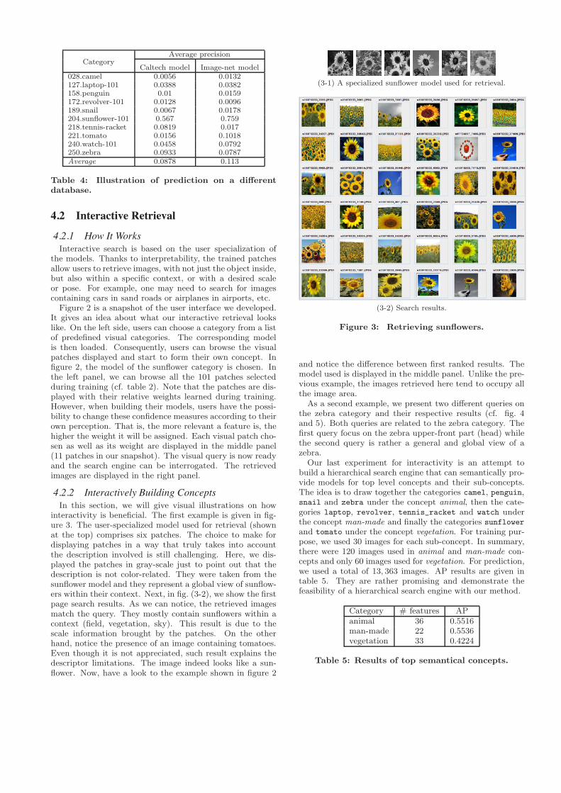
interactivity is beneficial. The first example is given in fig-ure 3. The user-specialized model used for retrieval (shownat the top) comprises six patches. The choice to make fordisplaying patches in a way that truly takes into accountthe description involved is still challenging. Here, we dis-played the patches in gray-scale just to point out that thedescription is not color-related. They were taken from thesunflower model and they represent a global view of sunflow-ers within their context. Next, in fig. (3-2), we show the firstpage search results. As we can notice, the retrieved imagesmatch the query. They mostly contain sunflowers within acontext (field, vegetation, sky). This result is due to thescale information brought by the patches. On the otherhand, notice the presence of an image containing tomatoes.Even though it is not appreciated, such result explains thedescriptor limitations. The image indeed looks like a sun-flower. Now, have a look to the example shown in figure 2

(3-1) A specialized sunflower model used for retrieval.

(3-2) Search results.

Figure 3: Retrieving sunflowers.

and notice the difference between first ranked results. Themodel used is displayed in the middle panel. Unlike the pre-vious example, the images retrieved here tend to occupy allthe image area.

As a second example, we present two different queries onthe zebra category and their respective results (cf. fig. 4and 5). Both queries are related to the zebra category. Thefirst query focus on the zebra upper-front part (head) whilethe second query is rather a general and global view of azebra.

Our last experiment for interactivity is an attempt tobuild a hierarchical search engine that can semantically pro-vide models for top level concepts and their sub-concepts.The idea is to draw together the categories camel, penguin,snail and zebra under the concept animal, then the cate-gories laptop, revolver, tennis_racket and watch underthe concept man-made and finally the categories sunflowerand tomato under the concept vegetation. For training pur-pose, we used 30 images for each sub-concept. In summary,there were 120 images used in animal and man-made con-cepts and only 60 images used for vegetation. For prediction,we used a total of 13, 363 images. AP results are given intable 5. They are rather promising and demonstrate thefeasibility of a hierarchical search engine with our method.

Category # features APanimal 36 0.5516man-made 22 0.5536vegetation 33 0.4224

Table 5: Results of top semantical concepts.

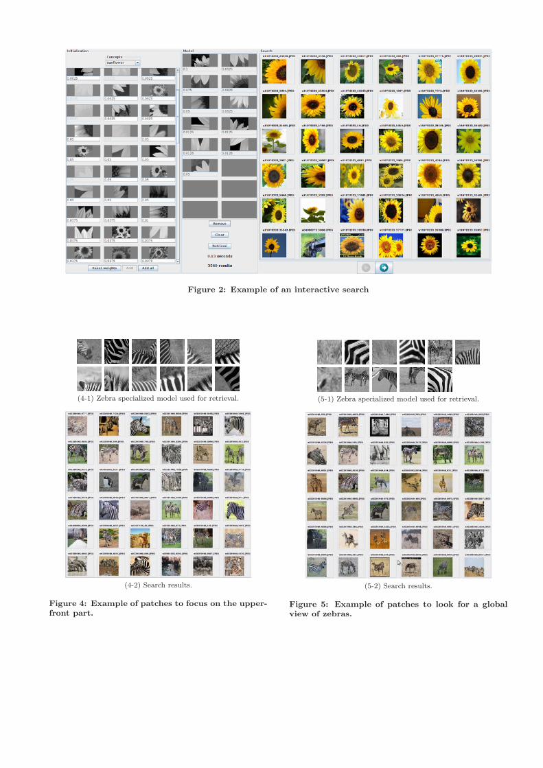
Figure 2: Example of an interactive search

(4-1) Zebra specialized model used for retrieval.

(4-2) Search results.

Figure 4: Example of patches to focus on the upper-front part.

(5-1) Zebra specialized model used for retrieval.

(5-2) Search results.

Figure 5: Example of patches to look for a globalview of zebras.

Full model.

0.1

0.2

0.3

0.4

0.5

0.6

0.7

0.8

0 0.2 0.4 0.6 0.8 1

Pre

cisi

on

Recall

Revolver category

1st patch2nd patchFull model

Figure 6: Performance of the revolver category.

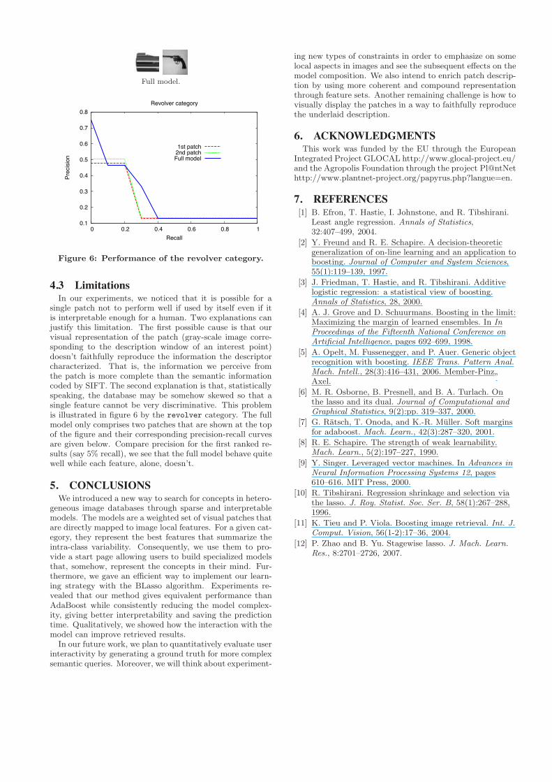
4.3 LimitationsIn our experiments, we noticed that it is possible for a

single patch not to perform well if used by itself even if itis interpretable enough for a human. Two explanations canjustify this limitation. The first possible cause is that ourvisual representation of the patch (gray-scale image corre-sponding to the description window of an interest point)doesn’t faithfully reproduce the information the descriptorcharacterized. That is, the information we perceive fromthe patch is more complete than the semantic informationcoded by SIFT. The second explanation is that, statisticallyspeaking, the database may be somehow skewed so that asingle feature cannot be very discriminative. This problemis illustrated in figure 6 by the revolver category. The fullmodel only comprises two patches that are shown at the topof the figure and their corresponding precision-recall curvesare given below. Compare precision for the first ranked re-sults (say 5% recall), we see that the full model behave quitewell while each feature, alone, doesn’t.

5. CONCLUSIONSWe introduced a new way to search for concepts in hetero-

geneous image databases through sparse and interpretablemodels. The models are a weighted set of visual patches thatare directly mapped to image local features. For a given cat-egory, they represent the best features that summarize theintra-class variability. Consequently, we use them to pro-vide a start page allowing users to build specialized modelsthat, somehow, represent the concepts in their mind. Fur-thermore, we gave an efficient way to implement our learn-ing strategy with the BLasso algorithm. Experiments re-vealed that our method gives equivalent performance thanAdaBoost while consistently reducing the model complex-ity, giving better interpretability and saving the predictiontime. Qualitatively, we showed how the interaction with themodel can improve retrieved results.

In our future work, we plan to quantitatively evaluate userinteractivity by generating a ground truth for more complexsemantic queries. Moreover, we will think about experiment-

ing new types of constraints in order to emphasize on somelocal aspects in images and see the subsequent effects on themodel composition. We also intend to enrich patch descrip-tion by using more coherent and compound representationthrough feature sets. Another remaining challenge is how tovisually display the patches in a way to faithfully reproducethe underlaid description.

6. ACKNOWLEDGMENTSThis work was funded by the EU through the European

Integrated Project GLOCAL http://www.glocal-project.eu/and the Agropolis Foundation through the project Pl@ntNethttp://www.plantnet-project.org/papyrus.php?langue=en.

7. REFERENCES[1] B. Efron, T. Hastie, I. Johnstone, and R. Tibshirani.

Least angle regression. Annals of Statistics,32:407–499, 2004.

[2] Y. Freund and R. E. Schapire. A decision-theoreticgeneralization of on-line learning and an application toboosting. Journal of Computer and System Sciences,55(1):119–139, 1997.

[3] J. Friedman, T. Hastie, and R. Tibshirani. Additivelogistic regression: a statistical view of boosting.Annals of Statistics, 28, 2000.

[4] A. J. Grove and D. Schuurmans. Boosting in the limit:Maximizing the margin of learned ensembles. In InProceedings of the Fifteenth National Conference onArtificial Intelligence, pages 692–699, 1998.

[5] A. Opelt, M. Fussenegger, and P. Auer. Generic objectrecognition with boosting. IEEE Trans. Pattern Anal.Mach. Intell., 28(3):416–431, 2006. Member-Pinz

”Axel.

[6] M. R. Osborne, B. Presnell, and B. A. Turlach. Onthe lasso and its dual. Journal of Computational andGraphical Statistics, 9(2):pp. 319–337, 2000.

[7] G. Ratsch, T. Onoda, and K.-R. Muller. Soft marginsfor adaboost. Mach. Learn., 42(3):287–320, 2001.

[8] R. E. Schapire. The strength of weak learnability.Mach. Learn., 5(2):197–227, 1990.

[9] Y. Singer. Leveraged vector machines. In Advances inNeural Information Processing Systems 12, pages610–616. MIT Press, 2000.

[10] R. Tibshirani. Regression shrinkage and selection viathe lasso. J. Roy. Statist. Soc. Ser. B, 58(1):267–288,1996.

[11] K. Tieu and P. Viola. Boosting image retrieval. Int. J.Comput. Vision, 56(1-2):17–36, 2004.

[12] P. Zhao and B. Yu. Stagewise lasso. J. Mach. Learn.Res., 8:2701–2726, 2007.