
Soft morphological filtering
32
Joumal of MathematicalImagingand Vision, 5, 231-262 (1995) @ 1995 KluwerAcademicPublishers, Boston. Manufacturedin The Netherlands. Soft Morphological Filtering PAULI KUOSMANEN AND JAAKKO ASTOLA Tampere University of Technology, Tampere, Finland Abstract. Stack filters are widely used nonlinear filters based on threshold decomposition and positive Boolean functions. They have shown to form a very large class of filters which includes rank-order operations as well as standard morphological operations. The stack filter representation of an order statistic filter provides an efficient tool for the theoretical analysis of the filter. Soft morphological filters form a large subclass of stack filters. They were introduced to improve the behavior of standard morphological filters in noisy conditions. In this paper, different properties of soft morphological filters are analysed and illustrated. Their connection to stack filters is established, and that connection is used in the statistical analysis of soft morphological filters. Soft morphological filters are less sensitive to additive noise than standard morphological, filters. The deterministic properties of soft morphological filters are also analysed and it is shown that soft morphological filters form a class of filters with many desirable properties. For example, they preserve well details of images. Keywords: 1 Introduction Linear filters have long been the primary tool for sig- nal and image processing. The reason for this is that they are easy to implement and analyze and, perhaps most importantly, the linear filter which minimizes the mean sum squared error criterion can usually be found in closed form. Furthermore, they are optimal among the class of all filtering operations when the noise being considered is additive Gaussian noise. Unfortunately, in many applications in which non- Gaussian noise arises, linear methods have proven to be inadequate for signal smoothing and noise reduc- tion. Also signal-dependent noise cause problems to linear filters. These kind of cases occur frequently, per- haps more frequently than not; therefore linear methods are not completely satisfactory when dealing with real signals and noise. Nonlinear filters have been developed for solving the difficulties of linear filters. There are many classes of nonlinear filters, and the task for choosing the right class for any application is a challenge itself. Morphological filters are a class of nonlinear fil- ters based on an algebraic theory of the geometrical structure of sets. Several types of morphological fil- ters have been defined and applications of morpho- logical filters in image processing are numerous, cf. e.g. [4] and [18]. Discrete flat morphological filters belong to a broad class of nonlinear filters called stack filters. In this paper, robustly behaving modifications of discrete flat morphological filters, soft morphological filters, are defined. Their deterministic properties are studied as well as their statistical properties by using the theory developed for stack filters. Soft morpholog- ical filters are less sensitive to additive noise and small variations of the object to be filtered than standard dis- crete flat morphological filters. In the following we define some basic concepts and notations used in this paper. A signal is a real function f: Z m -+ R~ where Z m is the set ofm-tuples of integers, m is a positive integer, the dimension of the signal, and IR is the set of real numbers. When m = 2, signals are often called images or gray level images. If a signal can only attain two values, it is often called a binary signal or a binary image. By the concept filter we mean a mapping of the set of signals to itself. In Boolean expression we use x + y for x AND y, x • y or xy for x OR y, and ~? for NOT x. In some formulas, where Boolean variables occur in exponents, they are to be understood as real l's and O's. The number of elements in the set A is denoted by IA[. 2 Soft Morphological Operations Soft morphological operations are nonlinear signal transforms which are related to discrete fiat
Transcript of Soft morphological filtering
Joumal of Mathematical Imaging and Vision, 5, 231-262 (1995) @ 1995 Kluwer Academic Publishers, Boston. Manufactured in The Netherlands.
Soft Morphological Filtering
PAULI KUOSMANEN AND JAAKKO ASTOLA Tampere University of Technology, Tampere, Finland
Abstract. Stack filters are widely used nonlinear filters based on threshold decomposition and positive Boolean functions. They have shown to form a very large class of filters which includes rank-order operations as well as standard morphological operations. The stack filter representation of an order statistic filter provides an efficient tool for the theoretical analysis of the filter.
Soft morphological filters form a large subclass of stack filters. They were introduced to improve the behavior of standard morphological filters in noisy conditions. In this paper, different properties of soft morphological filters are analysed and illustrated. Their connection to stack filters is established, and that connection is used in the statistical analysis of soft morphological filters. Soft morphological filters are less sensitive to additive noise than standard morphological, filters. The deterministic properties of soft morphological filters are also analysed and it is shown that soft morphological filters form a class of filters with many desirable properties. For example, they preserve well details of images.
Keywords:
1 Introduction
Linear filters have long been the primary tool for sig- nal and image processing. The reason for this is that they are easy to implement and analyze and, perhaps most importantly, the linear filter which minimizes the mean sum squared error criterion can usually be found in closed form. Furthermore, they are optimal among the class of all filtering operations when the noise being considered is additive Gaussian noise.
Unfortunately, in many applications in which non- Gaussian noise arises, linear methods have proven to be inadequate for signal smoothing and noise reduc- tion. Also signal-dependent noise cause problems to linear filters. These kind of cases occur frequently, per- haps more frequently than not; therefore linear methods are not completely satisfactory when dealing with real signals and noise.
Nonlinear filters have been developed for solving the difficulties of linear filters. There are many classes of nonlinear filters, and the task for choosing the right class for any application is a challenge itself.
Morphological filters are a class of nonlinear fil- ters based on an algebraic theory of the geometrical structure of sets. Several types of morphological fil- ters have been defined and applications of morpho- logical filters in image processing are numerous, cf. e.g. [4] and [18]. Discrete flat morphological filters belong to a broad class of nonlinear filters called stack filters.
In this paper, robustly behaving modifications of discrete flat morphological filters, soft morphological filters, are defined. Their deterministic properties are studied as well as their statistical properties by using the theory developed for stack filters. Soft morpholog- ical filters are less sensitive to additive noise and small variations of the object to be filtered than standard dis- crete flat morphological filters.
In the following we define some basic concepts and notations used in this paper. A signal is a real function f : Z m -+ R~ where Z m is the set ofm-tuples of integers, m is a positive integer, the dimension of the signal, and IR is the set of real numbers. When m = 2, signals are often called images or gray level images. If a signal can only attain two values, it is often called a binary signal or a binary image.
By the concept filter we mean a mapping of the set of signals to itself.
In Boolean expression we use x + y for x AND y, x • y or xy for x OR y, and ~? for NOT x. In some formulas, where Boolean variables occur in exponents, they are to be understood as real l ' s and O's.
The number of elements in the set A is denoted by IA[.
2 Soft Morphological Operations
Soft morphological operations are nonlinear signal transforms which are related to discrete fiat
232 Kuosmanen and Astola
morphological operations stemming from mathemat- ical morphology, which was introduced by Matheron [15] and Serra [18]. Indiscrete flat morphologicaloper- ations the geometrical features of a signal are modified by convolving the signal with a structuring set. The result of the modification depends on the shape and the size of the structuring set. Thus, discrete flat morpho- logical filters process signals by sets. Henceforwarth, we always mean by the term "standard morphological filter" a discrete flat morphological filter.
The deterministic properties of standard morpholo- gical operations have been extensively studied. Cer- tain statistical properties of standard morphological operations have been studied in [2], [6], [7], [19], and [20]. The restoration and representation proper- ties of noisy images when using morphological filters have been studied e.g. in [17]. Standard morpholog- ical operations have very good smoothing capabilities but at the same time they bias expectations heav- ily, [71.
Koskinen et al. [8], [9] and Kuosmanen et al. [10], [11] introduced soft morphological operations (filters) where the idea was to slightly relax the standard definitions in such a way that a degree of robustness is achieved, while most of the desirable properties of standard morphological operations are maintained. Standard morphological operations are based on lo- cal maximum and minimum operations while soft morphological operations are based on more general weighted order statistics. The main difference between soft and standard morphological filters is that soft mor- phological filters are less sensitive to additive noise and small variations in the shapes of the object to be filtered. Some filters which belong to the class of soft morphological filters have also much in common with weighted median filters.
Soft morphological operations are most naturally de- fined in the framework of weighted order statistics. The two basic soft morphological operations are soft ero- sion and soft dilation. Based on these operations, two important compound operations, soft closing and soft opening are defined. Before the definitions of the op- erations we define some other concepts to be used in this paper.
DEFINITION 2.1. The structuring system [B, A, r] consists of three parameters, finite sets A and B, A C B, of Z m and a natural number r satisfying 1 < r < I B I. The set B is called the structuring set, A its (hard) centre, B \ A its (soft) boundary and r the order index of its centre or the repetition parameter.
There are no analytical criteria for choosing the structuring set and its centre. Usually the choice of the structuring set and its centre is based on some geometrical properties. In [10] an adaptive scheme for choosing them is introduced.
DEFINITION 2.2. The translated set Tx, where the set T is translated by x 6 Z m, is defined by
Tx = {x + s: s E T}. (2.1)
DEFINITION 2.3. The symmetric set of T is the set
T ~ = {- t : t E T}. (2.2)
We denote the repetition operation of any object, in our case real numbers, by ~, that is
r t imes
r <~ x = x . . . . . x . (2.3)
DEFINITION 2.4. A multiset is a collection of objects, where the repetition of objects is allowed.
For example, {1, 1, 1,2,3,3} = {3<~ 1, 2, 2<>3} is a multiset.
2.1 Basic Soft Morphological Operations
Soft morphological operations transform a signal f : Z m --)" ]~ to another signal by the following rules.
DEFINITION 2.5. Soft erosion of f by the structuring system [B, A, r] is denoted by f G [B, A, r] and is defined by
f • [B, A, r](x) = the rth smallest value of the
multiset
{ r © f ( a ) : a E a x } U { f ( b ) : b ~ ( B k a ) x } (2.4)
for all x E Z m.
DEFINITION 2.6. Soft dilation of f by the structuring system [B, A, r] is denoted by f ~ [B, A, r], and is defined by
f ~ [B, A, r](x) = the rth largest value of the
multiset
{r© f(a): a E a x } U { f ( b ) : b £ ( B k a ) x } (2.5)
for all x ~ Z m.
Soft Morphological Filtering 233
As an extreme case, soft morphological operations by th e structuring system [B, A, r] reduce to standard morphological operations by the structuring set B, if r = 1 or alternatively A = B. I f r > [B\A[, soft morphological operations by the structuring system [B, A, r] reduce to standard morphological operations by the structuring set A.
EXAMPLE 2.1. Let the structuring set and its centre be
B = {(-I , 0), (0, 1), (0, 0), (0, -1) , (1, 0)1, a ----- {(0, 0)}. (2.6)
Then the soft erosion by the structuring system [B, A, 4] is defined by
f e [B, A, 4](x)
= the 4th smallest value of the multiset
{f(x1 - - 1, x2), f (xs , x2 + 1), f ( x l , x2),
f ( x l , x2), f ( x t , x2), f ( x l , x2), (2.7)
f ( x l , x2 - 1), f ( x l + 1, x2)}.
The output of this filter at point x = (xl, x2) is f ( x ) unless all the values of the set {f(b): b ~ (B - A)x}
are smaller than f (x) , in which case the output is the largest value of set {f(b): b ~ (B - A)x}.
Thus, the soft erosion (dilation) of f by the struc- turing system [B, A, r] at any point x is obtained by shifting the sets B and A to the location x and form- ing the multiset from the values of f inside the shifted sets, where the values of f inside the hard centre, are repeated r times, and then by taking the rth smallest (largest) value of the multiset.
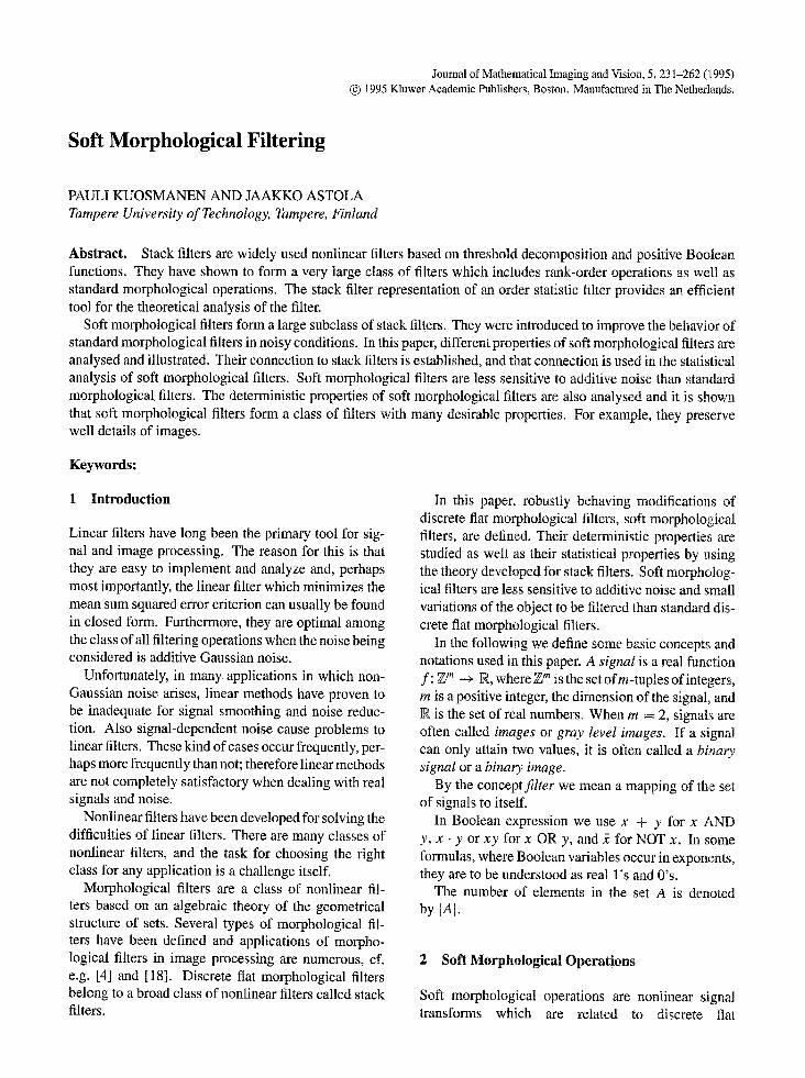
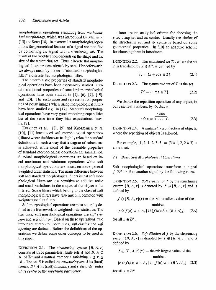
Geometrically, soft dilations (erosions) can be viewed as operations which expand (shrink) the origi- nal image. The way in which soft dilations (erosions) expand (shrink) the original image depends on the fol- lowing things: the size and the shape of the structuring set B, the size and the shape of the hard centre A, the situation of the origin, and the order index r. In gen- eral, the smaller the parameter r is the more the original image is expanded (shrunk). See Figs. 1 and 2.
2.2 Compound Soft Morphological Operations
In general, soft dilation is not the inverse operation of soft erosion. This means that soft erosion by the
• o a) b) o o • • c) oo o o
• o @ oooo 00oo
oOO @oo • • ooo o o @ o®oo o0oo
d) 0 0 0 oo 0 o e) O0 o 0 0 @o 0 0
0 0 0 O000 O@@O @@@@
OOO 0 0 o@o 0 0 @o@ o o OOO0 o@@O O@@O
Fig. 1. Soft erosions of a binary image: a) the structuring set B and its centre A (O -= an element of the structuring set which marks the origin of Z 2 and the hard centre A, • = an element of the structuring set B ), b) the original image (O = an image point ), c) f (3 [B, A, 1], d) f G [B, A, 2], e) f G [B, A, 3], f) f O [B, A, 4] (O = a point, which belongs to the original image but not to the erosion).
Q @ ® 0 0 @ 0
a) b) o o @ • c) Q O o o O @ @ O g Q O O Q Q @ O
• @ O O 0 @ O O O O Q O Q O O @ @@O • @ O O O O Q O O Q O O
• @@@@ O @ O O O Q 0 OOQQ
d) Q@O • • O e o O O @ e) OO OO@ ~ @ 0 ®O@ OO 0 0 0 • •
o I O O O O @ O O O ® 6 @ @ Q @ O O O O O O O @ O O O O • @ @ l @ ® O Q O O O O @ o O O @ O o @
Fig. 2. Soft dilations of a binary image: a) the structuring set B and its centre A (O -- an element of the structuring set which marks the origin of Z 2 and the hard centre A, • = an element of the structuring set B ), b) the original image (e = an image point ), c) f G [B, A, 1], d) f @ [B, A, 2], e) f (9 [B, A, 3], f) f ~ [B, A, 4] (O = a point, which belongs to the dilation but not to the original image).
234 Kuosmanen and Astola
structuring system [B, A, r] followed by soft dilation by the same structuring system does not necessarily yield the original image. Similarly, soft erosion is not in general the inverse operation of soft dilation. So, we achieve different results depending on whether soft dilation by the structuring system [B, A, r] is fol- lowed by soft erosion or vice versa. This fact sug- gests the use of compound operations. Soft opening by the structuring system [B, A, r] is defined as soft erosion by the structuring system [B, A, r] followed by the soft dilation by the structuring system [B s, A ~, r], and soft closing by the structuring system [B, A, r] is defined as soft dilation by the structuring system [B, A, r] followed by soft erosion by the structuring system [B s, A s, r].
DEFINITION 2.7. Soft opening of f by [B, A, r] is denoted by f[B,A,rl and is defined by
f[B,A,r](X) ~-- ( f 63 [B, A, r]) $ [B', A s, r](x) (2.8)
for all x 6 •m.
DEFINITION 2.8. Soft closing of f by [B, A, r] is de- noted by f[B,A,r] and is defined by
f [B 'A ' r ] (x ) ---- ( f ~ [B, A, r]) • [B s, A s, rl(x) (2.9)
for all x e Z m .
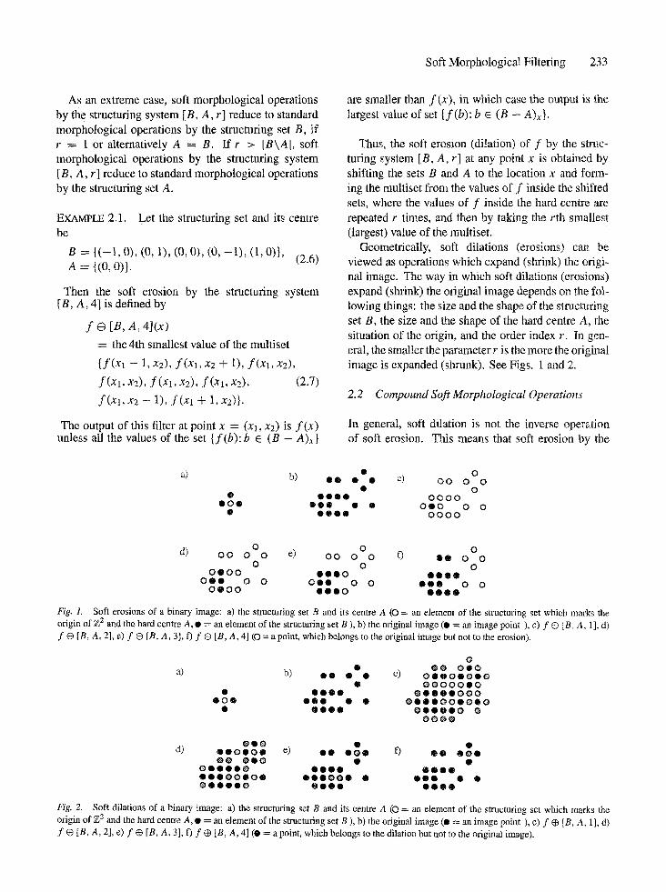
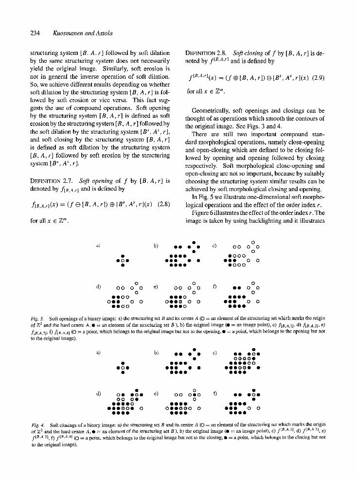
Geometrically, soft openings and closings can be thought of as operations which smooth the contours of the original image. See Figs. 3 and 4.
There are still two important compound stan- dard morphological operations, namely close-opening and open-closing which are defined to be closing fol- lowed by opening and opening followed by closing respectively. Soft morphological close-opening and open-closing are not so important, because by suitably choosing the structuring system similar results can be achieved by soft morphological closing and opening.
In Fig. 5 we illustrate one-dimensional soft morpho- logical operations and the effect of the order index r.
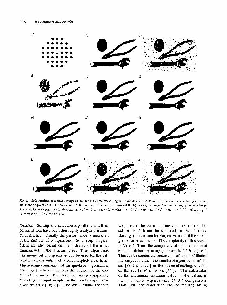
Figure 6 illustrates the effect of the order index r. The image is taken by using backlighting and it illustrates
• o a) b) • • • • c) o• o o
• o • O O O 0 go00
OOO gig • • OOO 0 0 • OOO0 O000
d) 0 o 0
o• o o e) o• o 0 0 o • o 0 0 o o
0000 0000 0000 000 0 0 000® o 0 000 o 0 000o 000o 0000
Fig. 3. Soft openings of a binary image: a) the structuring set B and its centre A (O = an element of the structuring set which marks the origin of Z 2 and the hard centre A, • = an element of the structuring set B ), b) the original image (O = an image point), c) f[n,a,t], d) f[8,A,21, e) f[B,A,3], f) f[B,a,4] (O = a point, which belongs to the original image but not to the opening, • = a point, which belongs to the opening but not
to the original image).
a) b) g o • • c) o • o o o • Q O 0 © O
• 0 0 0 0 0 0 0 0 © 0 0 0 0 g i g • • O O O O Q O •
• 0 0 0 0 0 0 0 0
d) • o • o • o o o e) o • o 0 o ~ 0 0 o o o O Q o o o •
o o o o 0 O O O o 0 0 0 0 o O O O O o 0 OOO®O0 0 0 0 0 0 0
0 0 0 0 0 0 0 0 0 0 0 0
Fig. 4. Soft closings of a binary image: a) the structuring set B and its centre A (O = an element of the structuring set which marks the origin of Z 2 and the hard centre A, • = an element of the structuring set B ), b) the original image ( • = an image point), c) fiB,a,1], d) fiB.a.2], e) fiB,a,31, f) f[B.A,4] (O = a point, which belongs to the original image but not to the closing, • ---- a point, which belongs to the closing but not
to the original image).
Soft Morphological Filtering 235
a)
b)
c)
I I I
lb 15 io 23 30 3; 40 4; 50
; lb 15 io 23 3'0 35 40 g5 50 i
o . • . j - _ , . J
1'0 15 2'0 25 3'0 35-- 40 45 50
d) 5
I I
5 10 15 20 25 30 35 40 45 50
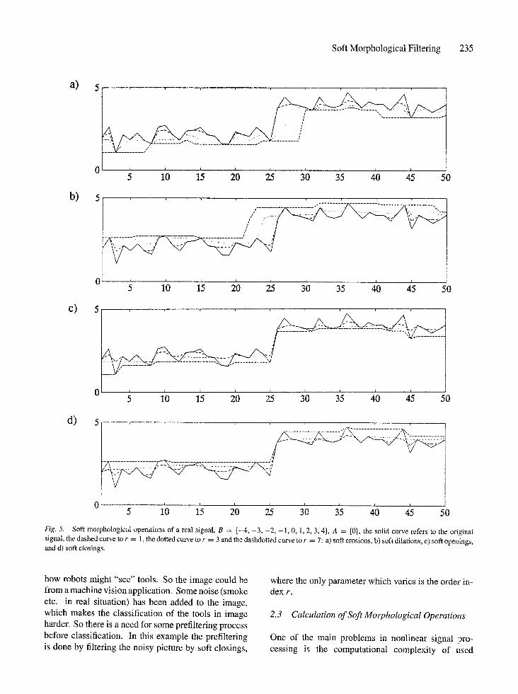
Fig. 5. Soft morphological operations of a real signal, B = {-4, -3, -2, -1, 0, l, 2, 3, 4}, A = {0}, the solid curve refers to the original signal, the dashed curve to r = 1, the dotted curve to r = 3 and the dashdotted curve to r = 7: a) soft erosions, b) soft dilations, c) soft openings, and d) soft closings.
how robots might "see" tools. So the image could be from a machine vision application. Some noise (smoke etc. in real situation) has been added to the image, which makes the classification of the tools in image harder. So there is a need for some prefiltering process before classification. In this example the prefiltering is done by filtering the noisy picture by soft closings,
where the only parameter which varies is the order in- dex r.
2.3 Calculation of Soft Morphological Operations
One of the main problems in nonlinear signal pro- cessing is the computational complexity of used
236 Kuosmanen and Astola
a) O O 0
O O O O 0 O O O O 0 0 0
O 0 0 0 0 0 0 O O O O O O 0
O O O 0 0 O O 0
b) c)
, • : : ' : " i" "''~'"'" "~ "'::"' ""* :""
• i~-~:.. :,..-"-; .' .,'
d) e) f)
g) h) i)
J) k) 1) • , . . ; , , ; • . • ~ . . . . .~ !..- , :, .. .. ." ~ -... ,.. "!...-"
ii!! ~ I ' : : ' ~ : i i ~ " . . . . j .~ .,::'., . ..- .." i . " " i " . , ' ." . . , " . , " . , "¢ ' " ." "
: : . : . ;
" ~ , : : . : .
. . . . . . . • . :. ,.;:':;.. : . , . . :
Fig. 6. Soft openings of a binary image called "tools": a) the structuring set B and its centre A (O = an element of the structuring set which marks the origin of Z 2 and the hard centre A, • = an element of the structuring set B ), b) the original image f without noise, c) the noisy image f + n, d) ( f + n)[B,a,.l], e) ( f + n)[B,A,SI, f) ( f + n)[B,A,IOI, g) ( f + n)[B,a,15], h) ( f + n)[B,A,20], i) ( f -}- n)[B,a,25] j) ( f + n)[B,A,30I, k) ( f + n)[B,a,351, 1) ( f + n)[B,a,36],
routines. Sorting and selection algorithms and their performances have been thoroughly analyzed in com- puter science. Usually the performance is measured in the number of comparisons. Soft morphological filters are also based on the ordering of the input samples within the structuring set. Thus, algorithms like mergesort and quicksort can be used for the cal- culation of the output of a soft morphological filter. The average complexity of the quicksort algorithm is O (n log n), where n denotes the number of the ele- ments to be sorted. Therefore, the average complexity of sorting the input samples in the structuring set B is given by O(IBllog tBI). The sorted values are then
weighted to the corresponding value (r or l) and in soft erosion/dilation the weighted sum is calculated starting from the smallest/largest value until the sum is greater or equal than r. The complexity of this search is O(IBI). Thus, the complexity of the calculation of erosion/dilation by using quicksort is O (I B I log [B I). This can be decreased, because in soft erosion/dilation the output is either the smallest/largest value of the set {f(a): a 6 Ax} or the rth smallest/largest value of the set {f(b):b ~ (B\A)x}. The calculation of the minimum/maximum value of the values in the hard centre requires only O(IAI) comparisons• Thus, soft erosion/dilation can be realized by an
Soft Morphological Filtering 237
algorithm with O(max([AI, IB\Ailog IB\AI)) com- parisons. The SELECT-algorithm, [16], has the av- erage theoretical complexity O(n) for the calculation of the rth order statistic of the set with n members. This reduces the theoretical complexity of the calculation of soft erosion/dilation to O (I B I).
Also running algorithms, i.e. algorithms using in- formation of the ordering of the previous position of the structuring system, have been developed for sort- ing and max/rain selection. A brief overview of these algorithms is presented e.g. in [16]. For complicated window structures these methods do not give much in- crease of execution speed.
As soft closings and openings compound operations (or more precisely: two successive operations) of soft erosions and dilations their complexities can be di- rectly found from the complexities of soft erosions and dilations.
3 The Connection between Soft Morphological Operations and Stack Filtering
In this chapter we consider the relation of soft morpho- logical filters to stack and generalized stack filters. We show that soft morphological filters are in fact stack filters. We give also the explicit formulas for the stack filter expressions of soft morphological filters using positive Boolean functions indexed by sets. This stack filter representation has proven useful because it allows morphological filters to be analyzed in the framework of positive Boolean functions.
We then provide sufficient conditions under which Boolean functions can form a stacking set in general- ized stack filters. In addition, we present a method to use soft morphological operations in generalized stack filters based on these conditions. An example demonstrating the usefulness of the presented method is provided.
3.1 Stack Filters
Stack filters are a class of nonlinear filters, first intro- duced by Wendt et al. [21]. Stack filters perform well in many situations where linear filters fail. Thus, stack filters have been used in many applications cf. e.g. [16].
DEFINITION 3.1. The real unit step function, denoted by u(.), is defined by
1, if or > 0 u(~) = 0, otherwise,
(3.1)
and the thresholding function at level fl, denoted by T~ (.), is defined by
1, if or > fi (3.2) T~(a) = 0, otherwise.
Stack filters exhibit the properties of threshold de- composition and the stacking property. The class of stack filters is relatively large and includes all ranked- order operators. The key to the analysis of stack filters comes from their definition by threshold decompo- sition which we now take under consideration, [21] and [22].
Consider a vector x = (X1, X2 . . . . XN), where Xi E {0, 1 . . . . . M - 1}. The threshold decomposi- tion of x amounts to decomposing it to M - 1 binary vectors x 1, x 2 . . . . . x m-1 defined by
m Tm(Xn) = { 1 i f X , > m x, = 0 otherwise.
(3.3)
Thus, each binary vector x m is obtained by threshold- ing the input vector at the levels m, for 1 < m __< M - 1, The kth level element x~ of a binary vector takes on the value 1 whenever the element of the input vector X, is greater than or equal to the level k.
It is important to note that this thresholding process can also be applied to all vectors that are quanfized to a finite number of arbitrary levels.
The original multi-valued vector can be recon- structed from its binary vectors
M-1
X = Z Xm (3.4) m=l
or equally
M-1
Xn= m=l
(3.5)
f (x ) > f (y ) , whenever x > y. (3.6)
The stacking property is an ordering property and is closely related to partial ordering. The relation > of binary vectors x = (xl, x2 . . . . . xu) and y = (Y~, Y2 . . . . . YN) is defined as x > y if and only if xi >_ Yi for all i c {1, 2 . . . . . N}. As this relation is reflexive, antisymmetric, and transitive it defines a partial ordering on the set of binary vectors. This order property is known as the stacking property and it is said that x and y stack, or y stacks on x, if and only i fx _>_ y. A Boolean function f is said to possess the stacking property if and only if
238 Kuosmanen and Astola
INPUT OUTPUT
..00314132041400.. ~ - ~ ~ ~ - ~ ..013132221410..
Threshold Binary decomposition addition
x4 .00001000010100., " ~ 1 Bin" ged' Filter g(" )l ~ ..000000000100.. x3 . . 0 0 1 0 1 0 1 0 0 1 0 1 0 0 . . - - ~ [ Bin. Med. Filter g(. )] - - - -~. .001010000100. . x a , , 0 0 1 0 1 0 1 1 0 1 0 1 0 0 . . ~ 1 Bin' ged' Filter ~( )l ~ . . 0 0 1 0 1 1 1 1 0 1 0 0 . . xl . ,00111111011100.. ~ l Bin' Med' Filter g(" )l ~ " 0 1 1 1 1 1 1 II110..
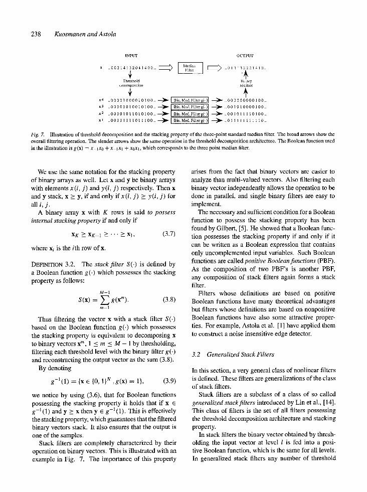
Fig, 7. Illustration of threshold decomposition and the stacking property of the three-point standard median filter. The broad arrows show the overall filtering operation. The slender arrows show the same operation in the threshold decomposition architecture. The Boolean function used in the illustration is g(x) = x- lxo + x-ix1 + xoxl, which corresponds to the three point median filter.
We use the same notation for the stacking property of binary arrays as well. Let x and y be binary arrays with elements x(i, j ) and y(i, j ) respectively. Then x and y stack, x > y, if and only if x(i, j ) >_ y(i, j ) for all/, j .
A binary array x with K rows is said to possess internal stacking property if and only if
X K > X K - 1 > . . . > X1, (3.7)
where xi is the ith row of x.
DEFINITION 3.2. The stack filter S(.) is defined by a Boolean function g(.) which possesses the stacking property as follows:
M-1
S ( x ) = E g(xm)" (3 .8) m=l
Thus filtering the vector x with a stack filter S(.) based on the Boolean function g(.) which possesses the stacking property is equivalent to decomposing x to binary vectors x m, 1 _< m _< M - 1 by thresholding, filtering each threshold level with the binary filter g (.) and reconstructing the output vector as the sum (3.8).
By denoting
g- l (1) = {x 6 {0, 1}N [g(x) = 1}, (3.9)
we notice by using (3.6), that for Boolean functions possessing the stacking property it holds that if x g- l (1) and y > x then y ~ g-1(1). This is effectively the stacking property, which guarantees that the filtered binary vectors stack. It also ensures that the output is one of the samples.
Stack filters are completely characterized by their operation on binary vectors. This is illustrated with an example in Fig. 7. The importance of this property
arises from the fact that binary vectors are easier to analyze than multi-valued vectors. Also filtering each binary vector independently allows the operation to be done in parallel, and single binary filters are easy to implement.
The necessary and sufficient condition for a Boolean function to possess the stacking property has been found by Gilbert, [5]. He showed that a Boolean func- tion possesses the stacking property if and only if it can be written as a Boolean expression that contains only uncomplemented input variables. Such Boolean functions are called positive Boolean functions (PBF). As the composition of two PBF's is another PBF, any composition of stack filters again forms a stack filter.
Filters whose definitions are based on positive Boolean functions have many theoretical advantages but filters whose definitions are based on nonpositive Boolean functions have also some attractive proper- ties. For example, Astola et al. [1] have applied them to construct a noise insensitive edge detector.
3.2 Generalized Stack Filters
In this section, a very general class of nonlinear filters is defined. These filters are generalizations of the class of stack filters.
Stack filters are a subclass of a class of so called generalized stack filters introduced by Lin et al., [14]. This class of filters is the set of all filters possessing the threshold decomposition architecture and stacking property.
In stack filters the binary vector obtained by thresh- olding the input vector at level l is fed into a posi- tive Boolean function, which is the same for all levels. In generalized stack filters any number of threshold
Soft Morphological Filtering 239
b) @ c)
100 010 00I \ [ /
000 000 000
Y;, It0 10l 011
00l 1000 0100 0010 0001 \ I Z-
0000
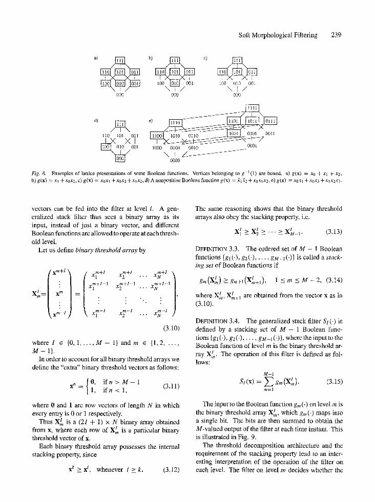
Fig. 8. Examples of lattice presentations of some Boolean functions. Vertices belonging to g-l(1) are boxed, a) g(x) = xo + Xl -~- x2, b) g(x) = X l + xox2, c) g (x) = XOXl + xox2 + X lX2, d) A nonpositive Boolean function g (x) = 21-72 + XOXlX2, e) g(x) = xoxl + xox3 + X lX2X3.
vectors can be fed into the filter at level I. A gen- eralized stack filter thus sees a binary array as its input, instead of just a binary vector, and different Boolean functions are allowed to operate at each thresh- old level.
Let us define binary threshold array by
( xrn+]5 ] { X ? +, X7 -1-1
Ix?+,-1 x7 +'-t "" / . X~g +1-1
rn-I X N
(3.1o)
where I 6 {0,1 . . . . . M - 1 } a n d m 6 {1,2 . . . . . M - l } .
In order to account for all binary threshold arrays we define the "extra" binary threshold vectors as follows:
x n = /O ' i f n > M - 1 (3.11) 1, i fn < 1, /
where 0 and 1 are row vectors of length N in which every entry is 0 or 1 respectively.
Thus X / is a (21 + 1) x N binary array obtained from x, where each row of Xlm is a particular binary threshold vector of x.
Each binary threshold array possesses the internal stacking property, since
x k > x t, whenever l > k. (3.12)
The same reasoning shows that the binary threshold arrays also obey the stacking property, i.e.
X~ >__ X~ > - . . > X~t_ 1. (3.13)
DEFINITION 3.3. The ordered set of M - 1 Boolean functions {gl ('), g2 (') . . . . . gM-t( ' ) } is called a stack- ing set of Boolean functions if
I grn(X I ) >_ gm+l(Xm+l), 1 < rn < M - 2, (3.14)
where XZm i , Xrn+l are obtained from the vector x as in (3.1o).
DEFINITION 3.4. The generalized stack filter S 1 (') is defined by a stacking set of M - 1 Boolean func- tions {ga ('), g2(') . . . . . gM-I (')}, where the input to the Boolean function of level m is the binary threshold ar- ray Xlm . The operation of this filter is defined as fol- lows:
M-1
SI(X) : E g m ( X l ) " m=l
(3.15)
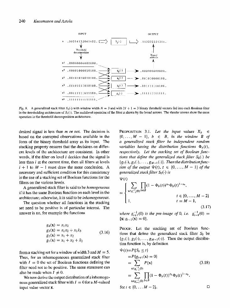
The input to the Boolean function gm (') on level m is the binary threshold array Xlm, which gm (') maps into a single bit. The bits are then summed to obtain the M-valued output of the filter at each time instant. This is illustrated in Fig. 9.
The threshold decomposition architecture and the requirement of the stacking property lead to an inter- esting interpretation of the operation of the filter on each level. The filter on level m decides whether the
240 Kuosmanen and Astola
INPUT OUTPUT
x ..00314132041400.. ~ ~ ~ ..113232221311..
Thr~hold d~om~sition
Bin~y ~dition
x5 ..00000000000000..,. . . . l
...... ~ ~ ] ~ . . . 000000000000 . . x 4 . . 0 0 0 0 1 0 0 0 0 1 0 1 0 0 . . - - .
x 3 ..00101010010100.. ~ . . 0 0 1 0 1 0 0 0 0 1 0 0 _
x2 ..00101011010100.. ~ ) - - ] ~ ..001111110100..
xO ..11111111111111.. - ' '° ' ' '
Fig. 9. A generalized stack filter S 1 (-) with window width N = 3 and with 21 + 1 = 3 binary threshold vectors fed into each Boolean filter in the thresholding architecture of SI (.). The multilevel operation of the filter is shown by the broad arrows. The slender arrows show the same operation in the threshold decomposition architecture.
desired signal is less than m or not. The decision is based on the corrupted observations available in the form of the binary threshold array as its input. The stacking property ensures that the decisions on differ- ent levels of the architecture are consistent. In other words, if the filter on level i decides that the signal is less than i at the current time, then all filters at levels i + 1 to M - 1 must draw the same conclusion. A necessary and sufficient condition for this consistency is the use of a stacking set of Boolean functions for the filters on the various levels.
A generalized stack filter is said to be homogeneous if it has the same Boolean function on each level in the architecture; otherwise, it is said to be inhomogeneous.
The question whether all functions in the stacking set need to be positive is of particular interest. The answer is no, for example the functions
g4(x) =XlX2 g3(x) = X l X z + X l X 3 g2(x) = X l + X 2 g l ( X ) = X l + X 2 + X 3
(3.16)
form a stacking set for a window of width 3 and M = 5. Thus, for an inhomogeneous generalized stack filter with I = 0 the set of Boolean functions defining the filter need not to be positive. The same statement can also be made when I # 0.
We now derive the output distribution of a inhomoge- nous generalized stack filter with I = 0 for a M-valued input value vector x.
PROPOSITION 3.1. Let the input values X b E {0 . . . . . M - 1}, b ~ B, in the window B of a generalized stack f l ter be independent random variables having the distribution functions dPb(t), respectively. Let the stacking set of Boolean func- tions that define the generalized stack filter So(.) be {gl ('), g2(') . . . . . gM-a (')}. Then the distribution func- tion of the output eg(t), t ~ {0 . . . . . M - 1} of the generalized stack filter So (.) is
~ ( t )
E I - I (1 - dPb(t))Xb~b(t)l--xb' xEgt~ll (0) bEB
t ~ {0 . . . . . M - 2 } 1, t = M - 1 ,
(3.17)
where g711(0) is the pre-image of O, i.e. g~+ll(0 ) = {x: gt+l(x) = 0}.
PROOF. Let the stacking set of Boolean func- tions that define the generalized stack filter So be {gl('), g2(') . . . . . gM-t( ')}. Then the output distribu- tion function is, by definition
qJ(t)=P{So < t}
=P{gt+l(X) = O}
P{x} (3.18) x~gT+11 (0)
= ~ H ( 1 - ~b(t))Xb~b(t)l-xb ' x~g~l+l (0) bEB
fo r t ~ {0 . . . . M - 2 } . []
Soft Morphological Filtering 241
In the case of independent and identically distributed (i.i.d.) input values we get the following corollary.
COROLLARY 3.1. Let the input values Xb, b ~ B in the window B of a generalized stack filter be independent random variables having a common dis- tribution function • ( t ). Let the positive Boolean func- tions that define the generalized stack filter So(.) be {gl ( ' ) , g 2 ( ' ) . . . . . gin-1 (')}. Then the distribution func- tion of the output ~( t ) , t ~ {0 . . . . . M - 1} of the generalized stack filter So(.) is
qJ(t) =
IBI E A i (1 - • (t)) i • (t) IBI-i, i=0
t E {0 . . . . . m - 2} 1, t = M - 1 ,
(3.19) where the numbers Ai are defined by
Ai -= !{x: gt+l(X) = 0, wn(x) = i}l (3.20)
and wH denotes the number of 1 's in x, that is, its Hamming weight.
3.3 Continuous Stack Filters
In the following we define the concept of a Boolean function indexed a by set, [6]. By this definition we link the geometrical concepts of sets to Boolean functions.
DEFINITION 3.5. Let A be a finite subset of Z m.
Then the Boolean function g(.) indexed by a set A is a Boolean expression of variables xa, a 6 A, de- noted by
g(x) = g(Xa: a C A). (3.21)
EXAMPLE 3.1. Let A C Z 3, A = {(0, 0, 0), (0, 0, 1), (0, 1, 0), (1, 0, 0)}. A Boolean function g(.) indexed by the set A is
g (X(o,o,o), x{o,o, 1), X(o, ~,o), Xo,o,o))
= X(o,o,1)x(o,l,o)x(1,o,o) + x(o,o,o). (3.22)
We use Boolean functions with their variables in- dexed by sets to define the corresponding continuous stack filters in the following way, [6].
DEFINITION 3.6. Let A be a finite subset o r e m, g(.) a positive Boolean function indexed by A, and f : Z m --+
IRa real signal. Then the continuous stack filter S(.) corresponding to g(.) is defined by
S(n) = max{3 6 R : g ( u ( f ( n + a ) - f l ) : a ~ A) = 1}. (3.23)
The moving window corresponds to the index set A of the defining positive Boolean function. In the def- inition of the continuous stack filter, the positivity of the Boolean function is related to the stacking prop- erty and the unit step function is related to the thresh- old decomposition. In fact, u ( f ( x ) - fl) is obtained by thresholding f ( x ) at level 13, i.e. u ( f ( x ) - 3) = Te(f(x)) .
The following proposition yields an important iso- morfism between the continuous stack filter S(.) cor- responding to a positive Boolean function g(.). This isomorfism is a slight modification of the isomorfism given in [22] for integer valued inputs.
PROPOSITION 3.2. Let the input vector to a continuous stack filter S(.) be x = (X1, X2 . . . . . XN) and g(.) be the corresponding positive Boolean function indexed by the set {1, 2 . . . . . N}. Then
K
g(x) = E 1-I x j, i=1 jEP~
(3.24)
where Pi are subsets of{l, 2 . . . . . N}, if and only if the continuous stack filter S(.) corresponding to g(x) is
max{min{Xi:i ~ P~}, min{Xi:i ~ P2} . . . . .
min{Xi:i ~ Px}} (3.25)
PROOF. By using Definition 3.6 we get the following equations
K
S = max{fi 6 IR: E [-[ u(Zj - fl) = I} i=1 jEPi
= max{min{Xi:i ~ P1}, min{Xi:i E P2} . . . . .
min{Xi:i E PK}}, (3.26)
from which Proposition 3.2 follows. []
EXAMPLE 3.2. Let f : 2 2 --+ ]l~ be an image and sup- pose that f is filtered by a two-dimensional continuous stack filter corresponding to the positive Boolean func- tion f (x ) = x(-1,o)x(o,o) + x(-1,o)X(o,o) + x(o,o)x(o,1) indexed by the set A = {(-1, 0), (0, 0), (0, 1)}. Then
242 Kuosmanen and Astola
the equivalent stack filter is
S(a, b) = max{fl 6 ]t~:
(u(f((a, b) + ( -1 , 0)) - fl)
• u( f ( (a , b) + (0, 0)) - fl))
+ (u(f((a, b) + ( -1 , 0)) - fl)
• u ( f ( ( a , b) + (0, 1)) - fl))
+ (u(f((a, b) + (0, 0)) - fl) • u ( f ( (a ,b ) +(0 , 1)) - f l ) ) = 1}. (3.27)
This filter corresponds to the two-dimensional three point median filter with filter window A.
An attractive property of continuous stack filters is the possibility of deriving analytical results for their statistical properties. For example, the output distribu- tion of a continuous stack filter can be expressed using the following proposition, [22].
PROPOSITION 3.3. Let the input values Xb, b E B, in the window B of a stack filter S(.) be indepen- dent random variables having the distribution func- tions • b(t ), respectively. Then the output distribution function • (t) of a stack filter S(.) defined by a positive Boolean function g (.) is
tP(t) = y ~ I--I(1 - dPb(t))xbCbb(t) l-xb (3.28) xEg -1 (0) bEB
where g-l(0) is the pre-image of 0, i.e. g-l(0) = {x: g ( x ) = 0}.
PROOF. Let g (x) be the positive Boolean function that defines S. Then the output distribution function is, by definition,
ko(t) = P{S < t}
=P{g(U(Xb -- t ) :b 6 B) = 0}
=P{(u(Xb -- t): b 6 B) ~ g-l(0)} (3.29)
= ~ P { ( u ( X b - t ) :b E B) = x} x E g -1 (0)
= y ~ I I ( 1 - - ¢~b(t))xbf~b(t) 1-xb.
x E g - l ( 0 ) bEB
[]
In the case of independent and identically distributed input values we get the following corollary.
COROLLARY 3.2. Let the input values Xb, b E B in the window B of a stack filter S (.) be independent, iden- tically distributed random variables having a common distribution function el) (t). Let the positive Boolean
function that defines the stack filter S(.) be g(.). Then the distribution function of the output • ( t ) of the stack filter S(.) is
IBI
• (t) = ~ A i ( 1 - cO(t))ic~(t) IBI-i, (3.30) i = 0
where the numbers A i are defined by
ai = I{x: g(x) ---- 0, w/i(x) = i}1. (3.31)
EXAMPLE 3.3. Consider filtering by a three point stack filter defined by g(x) = Xl + xox2 (See Fig. B.2 c)), where the input values in the moving window are independent random variables and two (X0, X1) of the input values in the moving window have distribution function ~1 (t) and one (X2) of the input values has dis- tribution function ~2(t). Then the output distribution function ko(t) of the stack filter is, by Proposition 3.3,
• (t) = (:I)l ( t ) 2 ( : I ) 2 ( t ) + (1 - Cl)l(t))di)l(t)di)2(t )
+ (I)l (t)2(1 - qbz(t)). (3.32)
EXAMPLE 3.4. Consider filtering by a three point stack filter defined by g(x) = xl q- XoX2, where the input values in the moving window are independent, identically distributed random variables having a com- mon distribution function • (t). Then the output distri- bution function • (t) of the stack filter is, by Corollary 3.2,
qt(t) = qb(t) 3 +2dP(t)2(1 -- (P(t)) = 2qb(t) 2 -- (I)(t) 3. (3.33)
DEFINITION 3.7. The dual go (z) of a Boolean func- tion g (z) is defined by the relation
go (z) -- g(~). (3.34)
Stack filters which have been defined by dual filters have the following useful statistical symmetry proper- ties, [7].
PROPOSITION 3.4. Let g (.) be apositive Boolean func- tion, gD(') the dual of g(.), S(.) the stack filter defined by g (.), and So (.) the stack filter defined by gD ('). Let the input values Xb, b E B, in the window B, I B I = n, of a stack filter S(.) be independent random variables having the distribution functions dPb(t), respectively. If the output distribution function • (t ) of the stack fil- ter S(.) is G (dPl(t), qbz(t) . . . . . ¢bn(t)) then the output
Soft Morphological Filtering 243
distribution function of the stack flter So (') is
GD(~I(t), dP2(t) . . . . . ~,(t))
= 1 -- G((1 - qbl(t)), (1 - qb2(t)) . . . . .
x (1 - ~,,(t))). (3.35)
PROPOSITION 3.5. Letg(.)beapositiveBooleanfunc- tion, go (') the dual of g(,), S(.) the stack filter defined by g(.), and So(.) the stack filter defined by gn('). Let the input values Xb, b E B, in the window B, I B I = n, of a stack filter S(.) be independent, identically and symmetrically distributed random variables having a common distribution function • ( t ) and the expectation t*. If the expectation of the output of the stack filter S is E{S} = # + ~, then the expectation of the output of the stack filter So is E{SM = # - X. Moreover, the output variances of S(.) and So(,) are equal.
3.4 Stack Filter Expressions of Soft Morphological Filters
The concept of a positive Boolean function indexed by a set plays a key role when we study the connection be- tween stack and soft morphological filters. The index set is the link between the moving window of a stack fil- ter and the structuring set of a soft morphological filter.
In this section we first prove that the soft erosion and dilation by the structuring system [B, A, r] corre- spond to certain continuous stack filters whose defin- ing positive Boolean functions are indexed by B, [13]. Furthermore, cascaded operations of soft erosions and dilations correspond to a single stack filter because all compositions of positive Boolean functions can be ex- pressed as a single positive Boolean function.
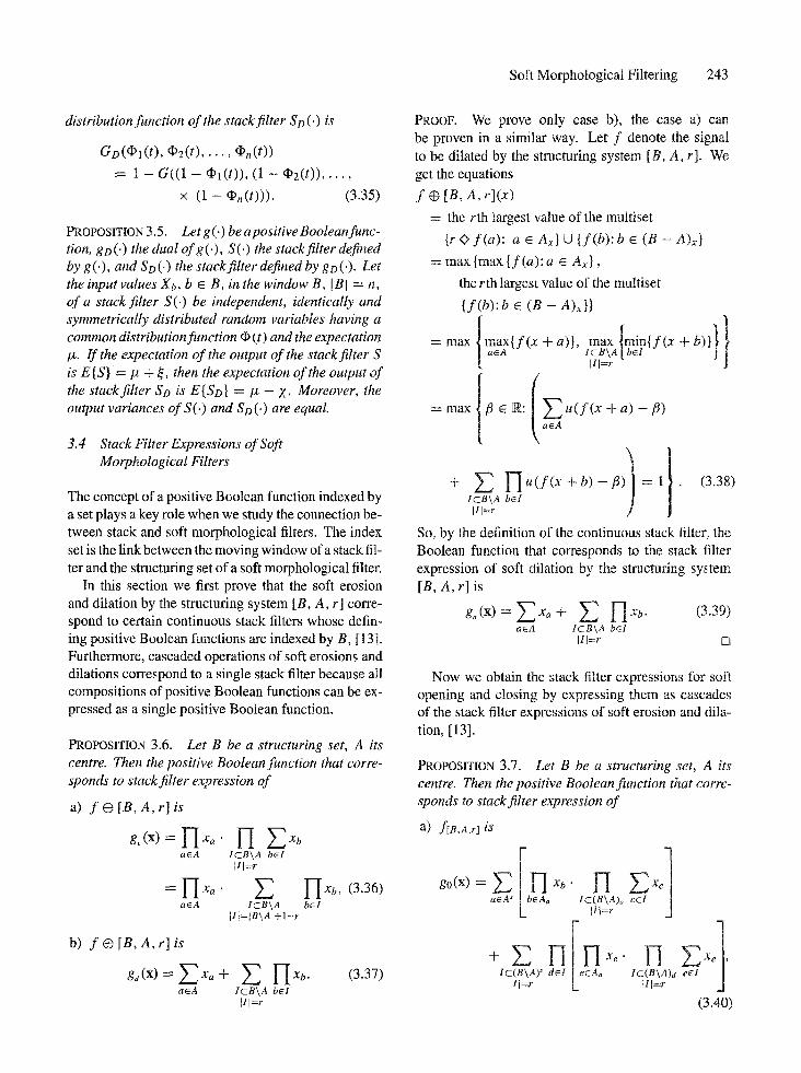
PROPOSITION 3.6. Let B be a structuring set, A its centre. Then the positive Boolean function that corre- sponds to stack filter expression of
a )
b)
f G [B, A, r] is
ge (x) = 1-1 xa • a~A
-~- I - I xa •
a~A
f @[B,A,r] is
ge (x) = ~ Xa + a6A
IcBkA bE1 I/l=r
I-Ix , (3.36) IcB\A bEl
II[=tB\AI+I-r
I-I xb" IcB\A bcl I/l=r
(3.37)
PROOF. We prove only case b), the case a) can be proven in a similar way. Let f denote the signal to be dilated by the structuring system [B, A, r]. We get the equations
f q) [B, A, r](x)
= the rth largest value of the multiset
{r© f(a): a ~ Ax} U {f(b):b ~ (B - A)x}
= max{max{f(a):a ~ Ax},
the rth largest value of the multiset
{f(b):b ~ (B - A)x}}
= m a x { m a x { f ( x + a ) } , icB\A[bcImaxlmin{f(x+b)}}}[i] =r
/
= max ]f i 6 R: 1 2 u ( f ( x +a) - fi)
/ I ~k a6A
+ 21CS\Al/l=r I - - I u ( f ( x + b ) - f i ) ) = b ~ l 1 ] . (3.38)
So, by the definition of the continuous stack filter, the Boolean function that corresponds to the stack filter expression of soft dilation by the structuring system [B, A, r] is
a~A 1cB\A bEl II]=r []
Now we obtain the stack filter expressions for soft opening and closing by expressing them as cascades of the stack filter expressions of soft erosion and dila- tion, [13].
PROPOSITION 3.7. Let B be a structuring set, A its centre. Then the positive Boolean function that corre- sponds to stack filter expression of
a) f[B,A,r] is
a~A ~ Ic(B\A)a c~l ] tll=r J
Ic(B\N) s dEI Ic(B\A)d Le~A,~ e~l J [ll=r II]=r
(3.40)
244 Kuosmanen and Astola
b) f[B,A,r] is
+ 1 aEAs b E A a Ic(B\A)a c~l Ill=r
1c(B\A) s dEl Ic(B\A)d eel Ill=r Ill=r
(3.41)
The following example shows how soft dilations can be expressed as stack filters.
EXAMPLE 3.5. Let f ( i , j ) be a real image. Consider soft morphological filtering of f by the structuring set and its centre
B = {(0, 0), (0, 1), (1, 0), (1, 1)}, A = {(0, 0)}. (3.42)
Then by Proposition 3.6 the stack filter expressions of f ~ [B, A, 1], which equals the standard morpholog- ical dilation by B corresponds to the positive Boolean function
g(x) = x(o,o) + x(o,~) + x(1,o) -}- x(1,1), (3.43)
and the stack filter expressions of f ~ [B, A, 2] corre- sponds to the positive Boolean function
g(x) = x(o,o) + X(o,1)X(1,O) q- X(O, 1)X(1,1) -~- X(I,O)X(1,1). (3.44)
Now Proposition 3.2 implies that the output of the continuous stack filter corresponding to f ~ [B, A, 1] is
S = max {X(o,o), X(0,l), X(1,o), X(1,1)}, (3.45)
and corresponding to f @ [B, A, 2] is
S = max {X(o,o), min{X(o,l), X(1,o)},
min{X(o,1)X(t,t)}, min{X(1,o)X(a,1)}} • (3.46)
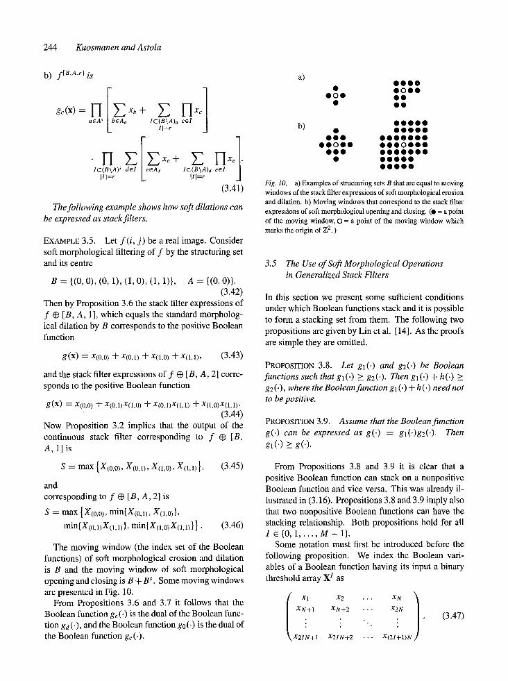
The moving window (the index set of the Boolean functions) of soft morphological erosion and dilation is B and the moving window of soft morphological opening and closing is B + B'. Some moving windows are presented in Fig. 10.
From Propositions 3.6 and 3.7 it follows that the Boolean function ge( ' ) is the dual of the Boolean func- tion gd ('), and the Boolean function go(') is the dual of the Boolean function gc (').
a) 0 0 0 0
• 0 0 0 0 0 0 0 O 0
• O 0
b) 0 0 0 0 0 • 0 0 0 0 0
0 0 0 0 0 0 9 0 0 0 0 0 0 0 0 0 0 0 0 0 0 0
0 0 0 0 0 0 0 0 0 0 • 0 0 0 0 0
0 0 0 0 0
Fig. 10. a) Examples of structuring sets B that are equal to moving windows of the stack filter expressions of soft morphological erosion and dilation, b) Moving windows that correspond to the stack filter expressions of soft morphological opening and closing. (e = a point of the moving window, O = a point of the moving window which marks the origin of Z 2. )
3.5 The Use of Soft Morphological Operations in Generalized Stack Filters
In this section we present some sufficient conditions under which Boolean functions stack and it is possible to form a stacking set from them. The following two propositions are given by Lin et al. [14]. As the proofs are simple they are omitted.
PROPOSITION 3.8. Let ga(') and g2(') be Boolean functions such that gl(') > g2('). Then gl(') + h(-) _> g 2 ( ' ) , where the Boolean function gl (') + h(.) need not to be positive.
PROPOSITION 3.9. Assume that the Boolean function g(.) can be expressed as g(.) = gl(')g2('). Then
gl(') > g(').
From Propositions 3.8 and 3.9 it is clear that a positive Boolean function can stack on a nonpositive Boolean function and vice versa. This was already il- lustrated in (3.16). Propositions 3.8 and 3.9 imply also that two nonpositive Boolean functions can have the stacking relationship• Both propositions hold for all I ~[0 ,1 . . . . . M - I } .
Some notation must first be introduced before the following proposition. We index the Boolean vari- ables of a Boolean function having its input a binary threshold array X I as
I x1 x2 • • • XN \
I XN+I XN+2 • . . X2N
• . o .
\ X21N+ 1 X21N+2 . . . X(2I+I)N I
(3 •47)
Soft Morphological Filtering 245
PROPOSITION 3.10. Let Pi, Qy be subsets of {1, 2 . . . . . (21 + 1)N} and let Boolean functions gm ('), gm+ l (') be in the minimum sum of products f o rm
g~(X') = E I 7 xk (3.48) i~I k~Pi
and
gm+l ( x I ) ----" E I - ' I xl" (3.49) jcJ IEQ)
I Then g m ( X / ) > gm+l(Xm+l), i f for all j ~ J there exist i ~ I, such that Pi c_ Q j.
I PROOF. Assume that gm+l(Xrn+l ) = 1. Then there is j 6 L such that I-IteQj xl = 1. As binary threshold
1 l arrays obey the stacking property, i.e. Xm+ 1 > X m, the equation 1-IteQj xz = 1 for the input X~+ t im-
plies equation l-IteQj xl = 1 for the input X~. Now
if there exists Pi c_ Qj then also l-Ik~eixl = 1
for the input X~. Thus, gm(Xlm) = 1 and therefore
gin(X/m) > g m + l ( X / + l ).
Proposition 3.10 together with the Boolean function expressions of soft morphological erosion and dilation given in Proposition 3.6 imply the following proposi- tion.
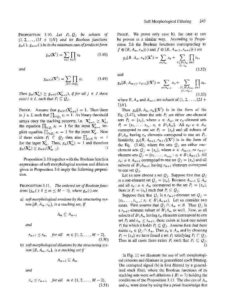
PROPOSITION 3.11. The ordered set of Boolean func- tions {gin('): 1 < m < M - 1}, wheregm(.) are
a) soft morphological erosions by the structuring sys- tem [B, Am, rm], is a stacking set, if
Am ~ Am+l
and
rm+l <_rm, for all m r { l , 2 . . . . . M - 2 } , (3.50)
b) soft morphological dilations by the structuring sys- tem [B, Am, r~], is a stacking set if
Am+l C_ A~
and
rm << rm+l, foral l m ~ {1, 2 . . . . . M - - 2}, (3.51)
PROOF. We prove only case b), the case a) can be proven in a similar way. According to Propo- sition 3.6 the Boolean functions corresponding to f ~ [B, Am, rml(') and f q3 [B, Am+l, rm+ll( ') are
gd[B 'Am'rm](XI)= E xa + E l--I xb' aEAm IcB\A~ b~I
Ill=r~ (3.52)
and
gd[B, Am+l, r,~+!l(X t) = aEArn+l JcB\Am+I bEJ
]Jl=rm+l (3.53)
where B, Am and Am+l are subsets of {1,2 . . . . . (2I + 1)N},
Thus gd[B, Am, rm](X l) is in the form of the Eq. (3.47), where the sets Pi are either one-element sets Pi = {xa}, where a ~ Am, or rm-element sets Pi = {xl . . . . . Xr~ : xi ~ B\A,,}. All xa: a ~ Am correspond to one set Pi = {x~} and all subsets of B\Am having rm elements correspond to one set Pi. Similarly, gd[B, Am+l, rm+l](X 1) is in the form of the Eq. (3.48), where the sets Qj are either one- element sets Qj = {xa}, where a E Am+l, or rm+l- element sets Qj = {Xl . . . . . Xrm+~ : Xi E B\Am+i}. All x~: a ~ Am+l correspond to one set Qj = {x~} and all subsets of B\Am+I having rm+l elements correspond to one set Qj.
Let us now choose a set Qj. Suppose first that Qj is a one-element set Q j = {Xa}. Because Am+l C Am and all x~ : a ~ A m correspond to the set Pi = {xa }, there is Pi = {Xa} such that Pi - Qj.
Suppose then that Qj is a rm+~-element set Qj = {xl . . . . . Xrm+l: Xi E B\Am+I}. Let us consider two cases. First assume that Qj • A,, = t3. Thus Qj is a rm+l-element subset of B\Am as well. Now, as all subsets of B\Am having rm elements correspond to one set Pi and rm < rm+l, there exists at least one subset Pi for which it holds Pi c_ Qj. Assume then that there exists xa ~ Qj (3 Am. Thus x~ ~ Am and by choosing Pi = {xa } we have found a set Pi satisfying P/ c_ Qj. Thus in all cases there exists Pi such that Pi c Q.i.
[]
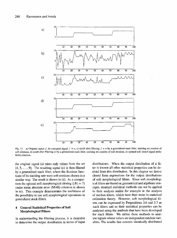
In Fig. 11 we illustrate the use of soft morphologi- cal erosions and dilations in generalized stack filtering. The corrupted signal (b) is first filtered by a general- ized stack filter, where the Boolean functions of its stacking sets were soft dilations ([ B] = 7) holding the conditions of the Proposition 3.11. The choices of Am and r,~ were done by using the a priori knowledge that
246 Kuosmanen and AstoIa
a)
b)
c)
d)
e)
° I I
I0 20 30 4~3 50 60 70 80 90 100
I 0 . . . . . . . . . .
I0 20 30 40 50 60 70 80 90 100
/ A.A__/'VLA_
11 10 20 30 40 50 60 70 80 90 1(30
\
I'0 ~ 30 4o 50 ~ 70 ~ ~ too
10 f---k__
r? / 5[
10 2'0 30 40 5~0 60 70 80 90 100
Fig. 11. a) Original signal f , b) corrupted signal f + n, c) result after filtering f + n by a generalized stack filter, stacking set consists of soft dilations, d) result after filtering c) by a generalized stack filter, stacking set consists of soft erosions, e) optimal soft closed signal under MAE criterion.
the original signal (a) takes only values from the set {4, 5 . . . . . 9}. The resulting signal (c) is then filtered by a generalized stack filter, where the Boolean func- tions of its stacking sets were soft erosions chosen in a similar way. The result is shown in (d). As a compar- ison the optimal soft morphological closing (I B I = 7) under mean absolute error (MAE) criterion is shown in (e). This example demonstrates the usefulness of the possibility to use soft morphological operations in generalized stack filters.
4 General Statistical Properties of Soft Morphological Filters
In understanding the filtering process, it is desirable to determine the output distribution in terms of input
distributions. When the output distribution of a fil- ter is known all other statistical properties can be de- rived from this distribution. In this chapter we derive closed form expressions for the output distributions of soft morphological filters. Since soft morpholog- ical filters are based on geometrical and algebraic con- cepts, standard statistical methods can not be applied to their analysis unlike for example in the analysis of median filters, which have their roots in statistical estimation theory. However, soft morphological fil- ters can be expressed by Propositions 3.6 and 3.7 as stack filters and so their statistical properties can be analysed using the methods that have been developed for stack filters. We utilize these methods to anal- yse signals whose values are independent random vari- ables. The results that concern identically distributed
Soft Morphological Filtering 247
inputs apply on the constant parts of images and they give an idea of the noise suppression capability and the biasing effects of the filter. We illustrate also the improved behavior of soft morphological filters compared to standard morphological filters in the pres- ence of an edge i.e. when inputs are nonidentically distributed.
4.1 Expressions for Output Distributions of Soft Morphological Filters
Propositions 4.1 and 4.2 are direct consequences of Propositions 3.3, 3.6 and 3.7. They give expressions for the output distributions of soft morphological filters in the case Of independent inputs.
PROPOSITION 4.1. Consider a signal f and the soft morphological dilation of f by a structuring system [ B, A, r] at point xo. Let the values f (xo + b), b E B be independent random variables having the distribu- tion functions qbb(t), respectively. Then the distribu- tion function tPd(t) of the value f E3 [B, A, r] of the soft dilated signal is
1-I E 1-I bEA X:xb=O,k/b~A cE(B\A)
w(X)<r
× (1 - ~c(t))x~dPc(t) 1-x~. (4.1)
PROOF. Let g(.) be the positive Boolean function corresponding to the soft morphological dilation f @ [B, A, r] given by Proposition 3.6. Then according to the Proposition 3.3 the output distribution function of f E) [B, A, r] is
• (t) = Z I-l(1 - ~b(t))xb~b(t)l-xb (4.2) XEg-1 (0) bEB
Now, g(x) = 0, if and only if for all xa E A, x, = 0, and Ixb: Xb E (B\A),Xb = 1[ < r. Thus (4.1) follows. []
COROLLARY 4.1. Let f : Z k --+ I~ be a signal whose values are independent random variables having a common distribution function d)(t). Then the output distribution kPd(t) of the values of the dilated signal f E ) [ B , a , r ] i s
~d(t) = ~ IB AI (1 - o~(t))i~(t) 181-i. (4.3) i=0
From the output distribution formula for soft dila- tion we obtain the output distribution formula for soft
erosion by using the statistical symmetry property (Proposition 3.4) of the output distribution of dual filters.
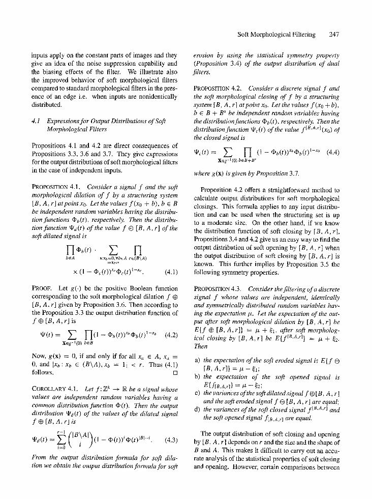
PROPOSITION 4.2. Consider a discrete signal f and the soft morphological closing of f by a structuring system [ B, A, r] at point Xo. Let the values f (xo + b), b E B + B s be independent random variables having the distribution functions ~b(t), respectively. Then the distribution function ~c(t) of the value f[B'A'r](x9) of the closed signal is
*c(t)= ~ 1--[ (1-- ~b(t))xbCFb(t)l--xb (4.4) XEg -1 (0) bEB+B s
where g(x) is given by Proposition 3.7.
Proposition 4.2 offers a straightforward method to calculate output distributions for soft morphological closings. This formula applies to any input distribu- tion and can be used when the structuring set is up to a moderate size. On the other hand, if we know the distribution function of soft closing by [B, A, r], Propositions 3.4 and 4.2 give us an easy way to find the output distribution of soft opening by [B, A, r] when the output distribution of soft closing by [B, A, r] is known. This further implies by Proposition 3.5 the following symmetry properties.
PROPOSITION 4.3. Consider the filtering of a discrete signal f whose values are independent, identically and symmetrically distributed random variables hav- ing the expectation IZ. Let the expectation of the out- put after soft morphological dilation by [B, A, r] be E { f ~ [B, A, r]} = /~ + ~1, after soft morpholog- ical closing by [B, A, r] be E { f [B'a'r]} ---- # + ~2.
Then
a) the expectation of the soft eroded signal is E { f G [B, A, r]} = / z - ~1;
b) the expectation of the soft opened signal is E{f[B,a,r]} = lZ -- ~2;
C) the variances of the soft dilated signal f @ [ B , A, r ] and the soft eroded signal f G [ B, A, r] are equal;
d) the variances of the soft closed signal f[B.A,r] and the soft opened signal f[8,a,r] are equal.
The output distribution of soft closing and opening by [B, A, r] depends on r and the size and the shape of B and A. This makes it difficult to carry out an accu- rate analysis of the statistical properties of soft closing and opening. However, certain comparisons between
soft and standard filters can be made and asymptotic analysis can be performed.
Experiments have shown that the statistical behav- ior of soft morphological filters is more consistent than the behavior of standard morphological filters. For in- stance the tendency to bias the gray-level of smooth noisy regions is less pronounced in the case of soft morphological filters. Koskinen et al. [9] showed an- alytically that this property holds for symmetric one- dimensional filters.
PROPOSITION 4.4. Consider the structuring system [B, A,r], where B = { - n , - n + 1 . . . . . n - 1,n}, A = { - k , - k + 1 . . . . . k - l , k } . L e t f : Z - - + ~ b e a signal whose values are independent random vari- ables with a finite expectation. Then the expectations satisfy
E{fB} < E{f[B,a,r]} ~ E{ f } ~ E{f[B'A'r]}<E{fB} (4.5)
where f 8 and f~ stand for standard closing and open- ing by 8.
Astola et al. [3] have shown that standard mor- phological filters are asymptotically unstable. This means that whenever the inputs are independent and identically distributed random variables which can get arbitrarily large values (e.g, Gaussian noise), the ex- pectation of closing (opening) tends to infinity as the size of the structuring set increases. The follow- ing proposition shows that a large class of soft clos- ings (openings) consists of asymptotically stable filters, [9].
PROPOSITION 4.5. Consider the sequence {[Bn, An, r(n)]: n -- 0, 1, 2 . . . . } of structuring systems where Bn C Z k, ]Bn I is strictly increasing, the origin be- longs to An for all n, and there exists an integer M such that IAnl < M for all n. Let f : Z k --+ ]~ be a signal whose values are independent and identi- cally disributed random variables which have a strictly monotonous distribution function ~(t) . Let r(n) and I Bn [ satisfy
r(n) l i m i n f n ~ - - > 0 (4.6)
In, I
and
0 1 2 3
-4
l i m s u p , ~ E { f [B"'A"'r~n)]} < ~ (4.7)
liminf,--.o~E{f[B,,A,,r(,)]} > --oo. (4.8)
4.2 Numerical Computations
In this section, we utilize the results achieved in preceding sections to numerically compute output dis- tributions and other statistical properties of some soft morphological filters.
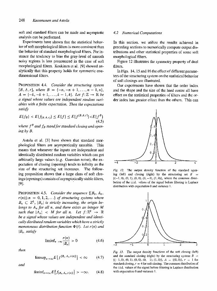
Figure 12 illustrates the symmetry property of dual filters.
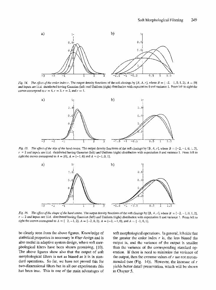
In Figs. 14, 15 and 16 the effect of different parame- ters of the structuring system on the statistical behavior of soft closings are illustrated.
Our experiments have shown that the order index and the shape and the size of the hard centre all have effect on the statistical properties of filters and the or- der index has greater effect than the others. This can
2
.8
0.6
-2
248 Kuosmanen and Astola
Fig. 12. The output density function of the standard open- ing (left) and closing (right) by the structuring set B = {(-1, 0), (0, 1), (0, 0), (0, - 1 ) , (1,0)}, where the common distri- bution of the i.i.d, values of the signal before filtering is Laplace distribution with expectation 0 and variance 1.
1
O.
O.
-2 -i
then Fig. 13. The output density functions of the soft closing (left) and the standard closing (right) by the structuring system B = { ( - 1 , 0 ) , ( 0 , 1 ) , ( 0 , 0 ) , ( 0 , - 1 ) , ( 1 , 0 ) } , A = {(0,0)}, r = 1 for standard closing, r = 4 for soft closing. The common distribution of the i.i.d, values of the signal before filtering is Laplace distribution with expectation 0 and variance 1.
Soft Morphological Filtering 249
a)
23
i
0.8
° S z 2 z I
b)
0.
1 2 3 -1.5 -i -0.5 0.5 1 1.5
Fig. 14. The effect of the order index r. The output density functions of the soft closings by [B, A, r], where B = { -2 , -- 1, 0, 1, 2}, A := {0} and inputs are i.i.d, distributed having Ganssian (left) and Uniform (right) distribution with expectation 0 and variance 1. From left to right the curves correspond to r = 4, r = 3, r = 2, and r = 1.
a) 1 b) 1
0.8 0.8
• 0.6
-:3 -:2 -I 1 2 ~ -i. 5 -i -0.5 0.5 1 1.5
Fig. 15. The effect of the size of the hard centre. The output density functions of the soft closings by [B, A, r], where B = { - 2 , - 1, 0, 1, 2}, r = 2 and inputs are i.i.d, distributed having Gaussian (left) and Uniform (right) distribution with expectation 0 and variance 1. From left to right the curves correspond to A = {0}, A = { - 1 , 0] and A = { - 1 , 0 , 1}.
a :j ol o o]
- '3 - '2 - 1
b) 1
0 . 8
1 2 3- -1.5 -I -0.5 0.5 ! 1.5
Fig. 16. The effect of the shape of the hard centre. The output density functions of the soft closings by [B, A, r], where B = { -2 , - I, 0, l, 2}, r = 2 and inputs are i.i.d, distributed having Gaussian (left) and Uniform (right) distribution with expectation 0 and variance 1. From left to right the curves correspond to A = { - 2 , - 1 , 2}, A = { -2 , 0, 2}, A = { -2 , - 1 , 0/, and A = { -1 , 0, 1}.
be clearly seen from the above figures. Knowledge of statistical properties is necessary in filter design and is also useful in adaptive system design, where soft mor- phological filters have been shown promising, [10]. The above figures show also that the output of soft morphological filters is not as biased as it is in stan- dard operations. So far, we have not proved this for two-dimensional filters but in all our experiments this has been true. This is one of the main advantages of
soft morphological operations. In general, it holds that the greater the order index r is, the less biased the output is, and the variance of the output is smaller than the variance of the corresponding standard op- eration. If there is need to minimize the variance of the output, then the extreme values of r are not recom- mended (see (Fig. 14)). However, the increase of r yields better detail preservation, which will be shown in Chapter 5.
250 Kuosmanen and Astola
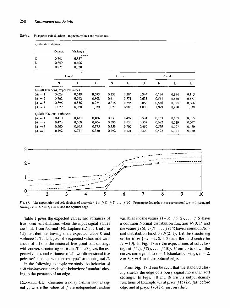
Table 1. Five point soft dilations: expected values and variances.
a) Standard dilation
Expect. Variance
N 0,746 0,357 L 0,649 0,406 U 0,825 0,320
r = 2 r = 3 r = 4
N L U N L U N L U
b) Soft Dilations, expected values [AI = 1 0,629 0,549 0,693 0,332 0,306 0,346 0,134 0,144 0,115 IAI = 2 0,762 0,692 0,808 0,614 0,571 0,635 0,564 0,530 0,577 IAI = 3 0,896 0,836 0,924 0,846 0,795 0,866 0,846 0,795 0,866 IA[ = 4 1,029 0,980 1,039 1,029 0,980 1,039 1,029 0,980 1,039
c) Soft dilations, variances IAI = 1 0,410 0,431 0,406 0,533 0,494 0,594 0,733 0,663 0,815 IAI = 2 0,473 0,569 0,404 0,596 0,650 0,568 0,682 0,719 0,667 IAI = 3 0,500 0,665 0,375 0,559 0,707 0,450 0,559 0,707 0,450 IAI = 4 0,492 0,721 0,320 0,492 0,721 0,320 0,492 0,721 0,320
2-- . p
ii:ii:iiii:iiiiiiiiiiiiii ;i .... 1 2 3 4 5 6 7 8 9 10
Fig. 17. The expectations of soft closings of Example 4.1 at f (1), f (2) . . . . . f (10). From up to down the curves correspond to r = 1 (standard closing), r = 2, r = 3, r = 4, and the optimal edge.
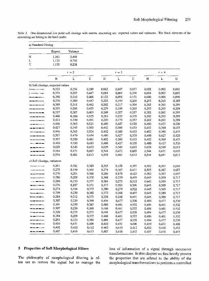
Table 1 gives the expected values and variances of five point soft dilations when the input signal values are i.i.d, from Normal (N), Laplace (L) and Uniform (U) distributions having their expected value 0 and variance 1. Table 2 gives the expected values and vari- ances of all one-dimensional five point soft closings with convex structuring set B and Table 3 gives the ex- pected values and variances of all two-dimensional five point soft closings with "cross-type" structuring set B.
In the following example we study the behavior of soft closings compared to the behavior of standard clos- ing in the presence of an edge.
EXAMPLE 4.1. Consider a noisy 1-dimensional sig- nal f , where the values of f are independent random
variables and the values f ( - 3 ) , f ( - 2 ) . . . . . f (5) have a common Normal distribution function N(0, 1) and the values f ( 6 ) , f ( 7 ) . . . . . f ( 1 4 ) have a common Nor- mal distribution function N(2, 1). Let the structuring set be B = { -2 , - 1 , 0, 1, 2} and the hard centre be A = {0}. In Fig. 17 are the expectations of soft clos- ings at f ( 1 ) , f ( 2 ) . . . . . f ( 10 ) . From up to down the curves correspond to r = 1 (standard closing), r = 2, r = 3, r = 4, and the optimal edge.
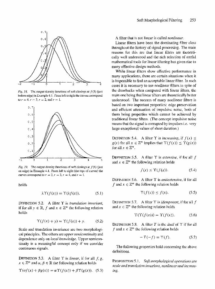
From Fig. 17 it can be seen that the standard clos- ing smears the edge of a noisy signal more than soft closings. In Figs. 18 and 19 are the output density functions of Example 4.1 at place f (5) i.e. just before edge and at place f ( 6 ) i.e. just on edge.
Soft Morphological Filtering 251
Table 2. One-dimensional five point soft closings with convex structuring set: expected values and variances. The black elements of the structuring set belong to the hard centre.
a) Standard Closing
Expect. Variance
N 1,163 0,448 L 1,123 0,735 U 1,155 0,238
r = 2 r : 3 r = 4
N L U N L U N L U
b) Soft closings, expected values I 0,323 0,254 0,389 0,062 0,047 0,077 0,902 0,002 0,063 ~ = ~ 0,374 0,297 0,447 0,084 0,064 0,104 0,004 0,003 0,095
. . . . . 0,390 0,310 0,466 0,123 0,094 0,151 0,000 0,00[3 0,000 0,376 0,300 0,447 0,232 0,190 0,269 0,282 0,265 0,289
. . . . =. 0,389 0,311 0,462 0,262 0,217 0,304 0,282 0,265 0,289 0,359 0,285 0,429 0,229 0,188 0,265 0,282 0,265 0,289 0,337 0,267 0,403 0,249 0,207 0,287 0,282 0,265 0,289 0,446 0,360 0,525 0,283 0;232 0,329 0,282 0,265 0,289
, 0,413 0,330 0,491 0,220 0,t79 0,257 0,282 0,265 0,289 0,446 0,363 0,524 0,480 0,427 0,520 0,480 0,427 0,520 0,427 0,345 0,503 0,402 0,360 0,433 0,402 0,360 0,433 0,446 0,363 0,524 0,402 0,360 0,433 0,402 0,360 0,433
. . . . 0,567 0,470 0,654 0,480 0,427 0,520 0,480 0,427 0,520 ~ = ~ 0,387 0,310 0,461 0,402 0,360 0,433 0,402 0,360 0,433
0,410 0,330 0.485 0,480 0,427 0,520 0,480 0,427 0,520 . . . . . 0,629 0,549 0,693 0,629 0,549 0,693 0,629 0,549 0,693
0,544 0,471 0,603 0,544 0,471 0,603 0,544 0,471 0,603 0,554 0,481 0,613 0,554 0,481 0,613 0,544 0,481 0,613
c) Soft closings, variances
0,261 0,181 0,360 0,263 0,158 0,397 0,502 0,367 0,656 0,275 0,199 0,369 0,274 0,167 0,411 0,503 0,367 0,657
. . . . . 0,276 0,201 0,368 0,286 0,178 0,429 0,503 0,367 0,657
. . . . . 0,286 0,209 0,378 0,368 0,259 0,499 0,645 0,589 0,717
. . . . . 0,286 0,210 0,377 0,384 0,275 0,512 0,645 9,589 09717 0,276 0,197 0,371 0,373 0,263 0,506 0,645 9,589 0,717 0.274 0,194 0,372 0,390 0,279 0,522 0,645 9,589 0,717 0,299 0,230 0,380 0,373 0,268 0,497 0,645 0,589 0,717
e= . . . . 0,284 0,212 0,372 0,358 0,248 0,491 0,645 0,589 0,717 . . . . . 0,307 0,239 0,388 9,494 0,477 0,530 0,494 0,477 0,530 . . . . . 0,301 0,230 0,385 0,486 0,461 0,532 0,486 0,461 0,532
0,307 0,239 0,388 0,486 0,461 0,532 0,486 0,461 0,532 ~=--m--= 0,320 0,273 0,373 0,494 0,477 9,530 0,494 0,477 0,530
0,284 0,209 0,375 0,486 0,461 9,532 0,486 0,461 0,532 . . . . . 0,293 0,220 0,380 0,494 0,477 0,530 0,494 0,477 0,530 . . . . == 0,410 0,431 0,406 0,410 0,431 0,406 0,410 0,431 0,406 . . . . . 0,402 0,410 0,412 0,402 0,410 0,412 0,402 0,410 0,412
0,407 0,416 0,415 0,407 0,416 0,415 0,407 0,416 0,415
5 Properties of Soft Morphological Filters
The philosophy of morphological filtering is of- ten not to restore the signal but to manage the
loss of information of a signal through successive transformations. In this chapter we first briefly present
the properties that are related to the ability of the morphological transformations to perform a controlled
252 Kuosmanen and Astola
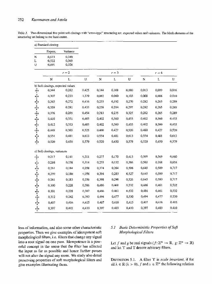
Table 3. Two-dimensional five point soft closings with "cross-type" structuring set: expected values and variances. The black elements of the structuring set belong to the hard centre.
a) Standard closing
Expect. Variance
N 0,613 0,340 L 0,522 0,369 U 0,691 0,328
r = 2 r = 3 r = 4
N L U N L U N L U
b) Soft closings, expected values 0,% 0,344 0,262 0,425 0,144 0,108 0,180 0,013 0,009 0,016
0
,o% 0,307 0,233 0,379 0,082 0,060 0,103 0,008 0,006 0,010 O
oo% 0,345 0,272 fl,416 0,233 0,192 0,270 0,282 0,265 0,289 0
o~o 0,359 0,281 0,433 0,258 0,214 0,297 0,282 0,265 0,289 O
0*% 0,376 0,295 0,454 0,283 0,235 0,325 0,282 0,265 0,289 O
,~, 0,410 0,331 0,483 0,402 0,360 0,433 0,402 0,360 0,433 0
**% 0,412 0,333 0,485 0,402 0,360 0,433 0,402 0,360 0,433 0
0*% 0,449 0,365 0,525 0,480 0,427 0,520 0,480 0,427 0,520 0
o~, 0,554 0,481 0,613 0,554 0,481 0,613 0,554 0,481 0,613 O
**** 0,520 0,450 0,579 0,520 0,450 0,579 0,520 0,450 0,579 O
c) Soft closings, variances
0.% 0,217 0,141 0,311 0,277 0,170 0,413 0,505 0,369 0,660 O
.o°o 0,216 0,138 0,314 0,255 0,152 0,386 0,503 0,368 0,658 0
,% 0,261 0,184 0,358 0,374 0,264 0,506 0,645 0,589 0,717 0
oo*o 0,259 0,180 !),356 0,394 0,283 0,527 0,645 0,589 0,717
0*% 0,261 0,183 0,356 0,398 0,290 0,526 0,645 0,589 0,717 O
.g* 0,300 0,228 0,386 0,486 0,461 0,532 0,486 0,461 0,532 o
***o 0,301 0,228 0,387 0,486 0,461 0,532 0,486 0,461 0,532 0
o~o 0,312 0,242 0,393 0,494 0,477 0,530 0,494 0,477 0,530 0
**o, 0,407 0,416 0,415 0,407 0,416 0,415 0,407 0,416 0,415 o
,~, 0,397 0,403 0,410 0,397 0,403 0,410 0,397 0,403 0,410 O
loss of information, and also some other characteristic properties. Then we give examples of idempotent soft morphological filters, i.e. filters that change any signal into a root signal on one pass. Idempotence is a pow- erful concept in the sense that the filter has affected the input as far as possible and hence further passes will not alter the signal any more. We study also detail preserving properties of soft morphological filters and give examples illustrating them.
5.1 Basic Deterministic Properties of Soft Morphological Filters
Let f and g be real signals ( f : Z m ~ N, g: •m ._~ ~ ) and let T and T denote arbitrary filters.
DEFINITION 5.1. A filter T is scale invariant, if for all Z 6 ~ (~ > 0), f and x 6 Z m the following relation
0 . 7
1 2 3 -2 - 1
0 . 7
0.6
0.
. 4
0.
0
Fig. l& The output density functions of soft closings at f (5) Oust before edge) in Example 4.1. From left to right the curves correspond tor =4, r = 3 , r = 2 , andr= 1.
- 1 1 2 3 4 5
0.6
0.5
0.4
0.3
0.2
0.i
0
Soft Morphological Filtering 253
Fig. 19. The output density functions of soft closings at f(6) Oust on edge) in Example 4.1. From left to right (the tops of curves) the curves correspond to r = 2, r = 3, r = 4, and r = 1.
holds
)vT( f (x ) ) = T(~.f(x)) . (5.1)
DEFINITION 5.2. A filter T is translation invariant, if for all y e R, f and x 6 Z m the following relation holds
T ( f ( x ) + y) = T ( f ( x ) ) + y. (5.2)
Scale and translation invariance are two morphologi- cal principles. The others are uppersemicontinuity and dependence only on local knowledge. Upper semicon- tinuity is a meaningful concept only if we consider continuous signals.
DEFINITION 5.3. A filter T is linear, if for all f , g, x e Z m and or, f i e R the following relation holds
T(c~f(x) + fig(x)) = ~ T ( f ( x ) ) + f iT(g(x)) . (5.3)
A filter that is not linear is called nonlinear. Linear filters have been the dominating filter class
throughout the history of signal processing. The main reasons for this are that linear filters are theoreti- cally well understood and the rich selection of useful mathematical tools for linear filtering has given rise to many effective design methods.
While linear filters show effective performance in many applications, there are certain situations when it is impossible to find an acceptable linear filter. In such cases it is necessary to use nonlinear filters in spite of the drawbacks when compared with linear filters, the main one being that linear filters are theoretically better understood. The success of many nonlinear filters is based on two important properties: edge preserva'fion and efficient attenuation of impulsive noise, both of them being properties which cannot be achieved by traditional linear filters. (The concept impulsive noise means that the signal is corrupted by impulses i.e. very large exceptional values of short duration.)
DEFINITION 5.4. A filter T is increasing, if f ( x ) <_ g(x) for all x E Z m implies that T ( f ( x ) ) < T(g(x) ) for all x E Z m.
DEFINITION 5.5. A filter T is extensive, if for all f and x 6 Z m the following relation holds
f ( x ) < T ( f ( x ) ) . (:5.4)
DEFINITION 5.6. A filter T is antiextensive, if for all f and x 6 Z m the following relation holds
T ( f ( x ) ) _< f ( x ) . (:5.5)
DEFINITION 5.7. A filter T is idempotent, if for all f and x e Z m the following relation holds
T ( T ( f ( x ) ) ) -- T ( f ( x ) ) . (5.6)
DEFINITION 5.8. A filter T is the dual of T if for all f and x e •m the following relation holds
- T ( - f ) = T ( f ) . (5.7)
The following properties hold concerning the above definitions.
PROPOSITION 5.1. Soft morphological operations are scale and translation invariant, nonlinear and increas- ing.
254 Kuosmanen and Astola
PROOF. Weighted order statistic operations are scale and translation invariant, nonadditive, and increasing. Since soft morphological operations are defined to be compositions of weighted order statistic operations, they also are scale and translation invariant, nonad- ditive, and increasing. []
PROPOSITION 5.2.
a) Soft erosion by [B, A, r] is the dual of soft dilation by [B, A, r].
b) Soft opening by [B, A, r] is the dual of soft closing by [B, A, r].
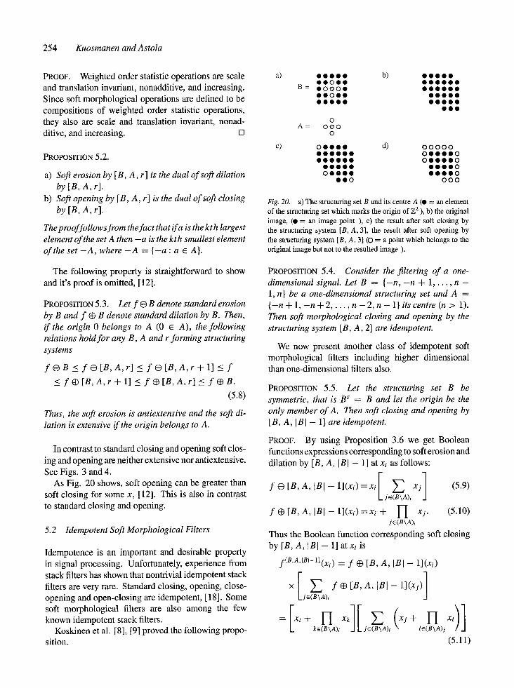
The proof follows from the fact that if a is the kt h largest element of the set A then - a is the kth smallest element of the set - A, where - A = {-a : a E A }.
The following property is straightforward to show and it's proof is omitted, [12].
PROPOSITION 5.3. Let f G B denote standard erosion by B and f ~ B denote standard dilation by B. Then, if the origin 0 belongs to A (0 ~ A), the following relations hold for any B, A and r forming structuring systems
f O B < f G [ B , A , r ] < f G [ B , A , r + I ] < f
< f ~ [ B , A , r + I ] < f ~ [ B , A , r ] < fEDB.
(5.8)
Thus, the soft erosion is antiextensive and the soft di- lation is extensive if the origin belongs to A.
In contrast to standard closing and opening soft clos- ing and opening are neither extensive nor antiextensive. See Figs. 3 and 4.
As Fig. 20 shows, soft opening can be greater than soft closing for some x, [12]. This is also in contrast to standard closing and opening.
5.2 Idempotent Soft Morphological Filters
Idempotence is an important and desirable property in signal processing. Unfortunately, experience from stack filters has shown that nontrivial idempotent stack filters are very rare. Standard closing, opening, close- opening and open-closing are idempotent, [18]. Some soft morphological filters are also among the few known idempotent stack filters.
Koskinen et al. [8], [9] proved the following propo- sition.
a) o o o o o b) O O O O O o o o o o o o o o o o
B = O O O O O O O O O O O O O O O O O O O O O O O O O O O O O O O
O Q O
A = 0
0 0 0 0
c) O O O 0 0 d) 0 0 0 0 0 0 0 g Q 0 0 O O Q O 0 0 0 0 0 0 0 0 0 0 0 0 0 0
0 0 0 0 0 0 0 0 0 0 0 0 0 0 0 0 0 0 0 0
0 0 0 0 0 0
Fig. 20. a) The structuring set B and its centre A (O = an element of the structuring set which marks the origin of 7Z z ), b) the original image, (e = an image point ), c) the result after soft closing by the structuring system [B, A, 3], the result after soft opening by the structuring system [B, A, 3] (O = a point which belongs to the original image but not to the resulted image ).
PROPOSITION 5.4. Consider the filtering of a one- dimensional signal. Let B = {-n, - n + 1 . . . . . n - 1, n} be a one-dimensional structuring set and A = { - n + 1, - n + 2 . . . . . n - 2 , n - 1} itscentre (n > 1). Then soft morphological closing and opening by the structuring system [ B, A, 2] are idempotent.
We now present another class of idempotent soft morphological filters including higher dimensional than one-dimensional filters also.
PROPOSITION 5.5. Let the structuring set B be symmetric, that is B s = B and let the origin be the only member of A. Then soft closing and opening by [n, A, Inl - 1] are idempotent.
PROOF. By using Proposition 3.6 we get Boolean functions expressions corresponding to soft erosion and dilation by [B, A, I B I - 1] at xi as follows:
f ~3[B ,A , [B l -1] (x i )=x i [ jE(B\A)i y~ xjJ (5.9)
f ~ [B, A, [B[ - 1](xi)=xi + 1-I xj. (5.10) jE(B\A)I
Thus the Boolean function corresponding soft closing by [B, A, ]B[ - 1] atxi is
f[B'A'IBI-1](Xi) ---- f ~ [B, A, [B[ - 1](xi)
x [ (~B~a f ~ [ B ' A ' L B l - 1 ] ( x j ) l j e )i
:[Xi'37kr(1--IB\A)iXkI[jE(B\~A)i(XJ-l-IE(I-IB\A)jXl)I (5.11)
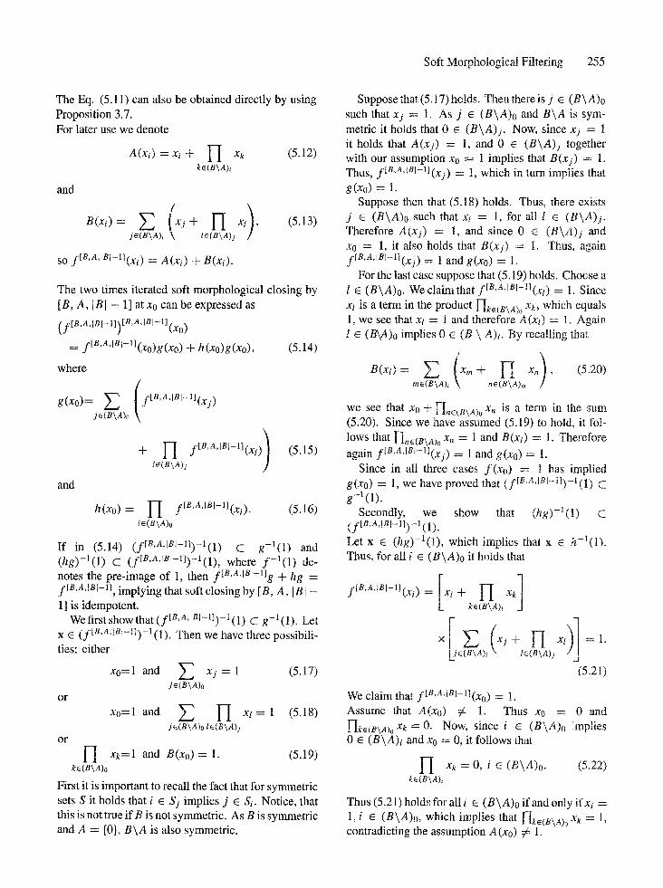
Soft Morphological Filtering 255
The Eq. (5.11) can also be obtained directly by using Proposition 3.7. For later use we denote
~" Xi @ 17 Xk (5.12) A(xi) kE(B\A)I
and
B(xi) = 2 (xj -t- I-'I xl), (5.13) jE(B\A)I I~(B\A)j
SO f[B'A'IBI-1](Xi) -~- A(xi) + B(xi).
The two times iterated soft morphological closing by [B, A, IBI - 1] at xo can be expressed as
( f[B,A,IBI-I])[B'AdBI--1] (XO)
= ftB'A'IBHI(XO)g(XO) + h(xo)g(xo), (5.14)
where
g(x0)= jE(B\A)o
and
h(xo) =
f[B,A,IBI-1](Xj)
-~- IE(B\A)jI-I f[B'A'IBI-1I(xl))
x o = l and
or
(5.15)
H f[B,A, Bl-t](xi)" (5.16) i~(B\A)o
If in (5.14) (f[B'A'IBI-1])-I(1) C g - l ( 1 ) and (hg) - l (1 ) C (f[B'A'IBI--1])-I(1), where f - l ( 1 ) de- notes the pre-image of 1, then f[B,A,IBI-1]g + hg = f[B,A,IBI-11, implying that soft closing by [B, A, I B [ - 1] is idempotent.
We first show that (f[B,A,IBI--1])-I (1) C g -1 (1). Let x E (f[B'A'IBt-ll)-~(1). Then we have three possibili- ties: either
Z xj = 1 (5.17) j~(B\A)o
2.., H x, = 1 (5.18) Xo--~- 1 and jE(B\A)o IE(B\A)]
or U x k = l and B(xo) = 1. (5.19)
kE(B\A)o First it is important to recall the fact that for symmetric sets S it holds that i ~ Sj implies j E 5"/. Notice, that this is not true if B is not symmetric. As B is symmetric and A = {0}, B\A is also symmetric.
Suppose that (5.17) holds. Then there is j E (B \ A)0 such that xj = 1. As j E (B\A)o and B \ A is sym- metric it holds that 0 6 (B \A) j . Now, since xj = 1 it holds that A(xj) = 1, and 0 6 (B \A) j together with our assumption xo = 1 implies that B(x j ) = l. Thus, f[B'A'IBI-1](Xj) = 1 , which in turn implies that g(xo) = 1.
Suppose then that (5.18) holds. Thus, there exists j E (B\A)o such that xl = 1, for all l E (B\A) j . Therefore A(xj) = 1, and since 0 6 ( B \ A ) j and x0 = 1, it also holds that B(x j ) = 1. Thus, again f[B'A'IBI-I](xj) = 1 and g(xo) = 1.
For the last case suppose that (5.19) holds. Choose a l ~ (B\A)o. We claimthat f[B'A'IBI-I](Xl) = 1. Since xl is a term in the product I-Le(B\a)0 xk, which equals 1, we see that xt = 1 and therefore A(xl) = 1. Again 1 6 ( B ~ ) o implies 0 6 (B \ A)l. By recalling that
ms(B\A)I ne(B\A),~
we see that xo + 1--[ne(B\A)o Xn is a term in the sum (5.20). Since we have assumed (5.19) to hold, it fol- lows that [Ine(8\a)0 xn = 1 and B(xl) = 1. Therefore again f[B'A'IBI-1I(xj) = 1 and g(xo) = 1.
Since in all three cases f (xo) = 1 has implied g(xo) = 1, we have proved that (f[n,A,l~l-ll)-I (1) C g-1(1 ) .
Secondly, we show that (hg) -1 (1) C (f[B,A,IBI-1])-I (1). Let x E (hg) - l (1 ) , which implies that x E h - l (1 ) . Thus, for all i E (B\A)o it holds that
e(B\A)i le(B\A)j (5.21)
We claim that f[B'A'iBI-1](Xo) = 1. Assume that A(xo) 7 ~ 1. Thus x0 = 0 and l--lk~(B\A)o Xk-----0. NOW, since i c (B\A)o implies 0 ~ (B\A)i and x0 = 0, it follows that
17 Xk ----O, i E (B\A)o. (5.22) kE(B\A)i
Thus (5.21) holds for all i ~ (B\A)o if and only ifxi = I, i ~ (B\A)o, which implies that HkE(B\A)o Xk ~- 1, contradicting the assumption A(xo) # 1.
256 Kuosmanen and Astola
Assume then that B(xo) ~ 1. Thus the following equa- tions hold:
x j = 0 a n d ~ 1--I x l = 0 . (5.23) jE(B\A)o jE(B\A)o IE(B\A)j
From the first equation of (5.23) we see that xj = O, j ~ (B\A)o. Thus for the (5.21) to hold it is re- quired that
1-I xk = 1, i E (B\A)o (5.24) kE(B\A)i
and therefore
1-I xk---- 1. (5.25) iE(B\A)o kE(B\A)j
This contradicts the assumption B(xo) ~ 1. Thus we have proved that A(xo) = 1 and B(xo) =
1 and t h u s f[B'A'IBI-1](Xo) = 1. This implies that x E (f[B'A'IBI-1])-I(1) and therefore (hg)-l(1) C (f[8,A,IBI-1])-I (1).
Since (f[B'A'IBI-1])-I(1) ( g - I ( 1 ) and (hg)-](1) C (f[B'A'IBI-1])-I(1), soft closing by the structuring system [B, A, I B [ - 1 ] is idempotent and by the duality also the soft opening by the same structuring system is idempotent. []
5.3 Detail Preservation Properties of Soft Morphological Filters
Soft morphological filters have a good ability of pre- serving shapes and details of the original image. In the following we show how soft morphological filters remove impulsive noise and how certain details are pre- served.
Let us call a function Ic: Z 2 --~ /I~ a positive C- impulse (C C Z 2) if
1, i f ( x , y ) ~ C Ic(x, y) = 0, otherwise. (5.26)
The function - I ¢ is called a negative C-impulse and if, especially, C --- {(0, 0)} lc is called an origin im- pulse and denoted by I. One-dimensional impulses are defined in a similar way and they are often called pulses.
Proposition 5.6 ([12]) implies that soft closing (opening) removes impulsive noise better than stan- dard closing (opening), Which can only remove nega- tive (positive) impulses (see Fig. 21).
PROPOSITION 5.6. Consider soft closing (opening) by the structuring system [B, A, r], where A is symmetric.
Let C C Z k (k E {1,2}) be such that ICI < r and Inl - I f + AI ~ r. Then sofi closing (opening) by [B, A, r] removes both positive and negative C impulses, that is, for all x c Z ~ (k ~ {1, 2}) it holds
Ic[B'A'rI(x) = (--Ic)[B'A'rl(x) = Ic [B,A,r](X)
= (--Ic)[B,A,rl(X). (5.27)
PROOF. As [BI - ICl >__ IBI - I f + AI >__ r, the negative C-impulse after soft dilation by [B, A, r] is a constant function, which will not be changed by soft erosion. Thus, soft closing removes the negative C-impulse. As ICI < r, the positive C-impulse af- ter soft dilation by [B, A, r] is the positive (C + A)- impulse. This impulse will be removed by soft erosion by [ B ' , A ' , r ] since I B I - I C q - A I > r. Thus, soft closing removes the positive C-impulse. By duality soft opening by [B, A, r] also removes negative and positive C-impulses. []
COROLLARY 5.1. Soft closing and opening by [B, A, r] remove arbitrary shaped positive and neg- ative C-impulse, if
ICl < min { IB[ - r } - IAI ' r - 1 . (5.28)
PROOF. AsIC+AI _< ICIIAl, i tholds[Bl- lCWAi >_ r whenever [BI - ICIIAI _ r, where the latter in-
IBI-r equality is equivalent to ICI _< i--TV" This combined together with the inequality I CI < r proves Corol- lary 5.1. []
COROLLARY 5.2. Soft closing and opening by [B, A, r] (1 < r < [B\A[) remove both positive and negative origin impulses.
PROOF. As we suppose that IB\AI > r, [B] - [C + AI = IBI - IAi = IB\AI >_ r. It also holds that ICI = 1 < r and so Corollary 5.2 follows. []
In the following we concentrate on two-dimensional signals and how their details are preserved in soft mor- phological filtering.
Let us call a function E: Z 2 --+ I~ an infinite straight edge if it can be written as
1, i f a x + b y < c E(x, y) = 0, otherwise, (5.29)
The line ax + by = c is called the edge-line and is denoted by e. We denote the set of the points belonging to the edge by E, that is, E = {(x, y): E(x, y) = 1}.
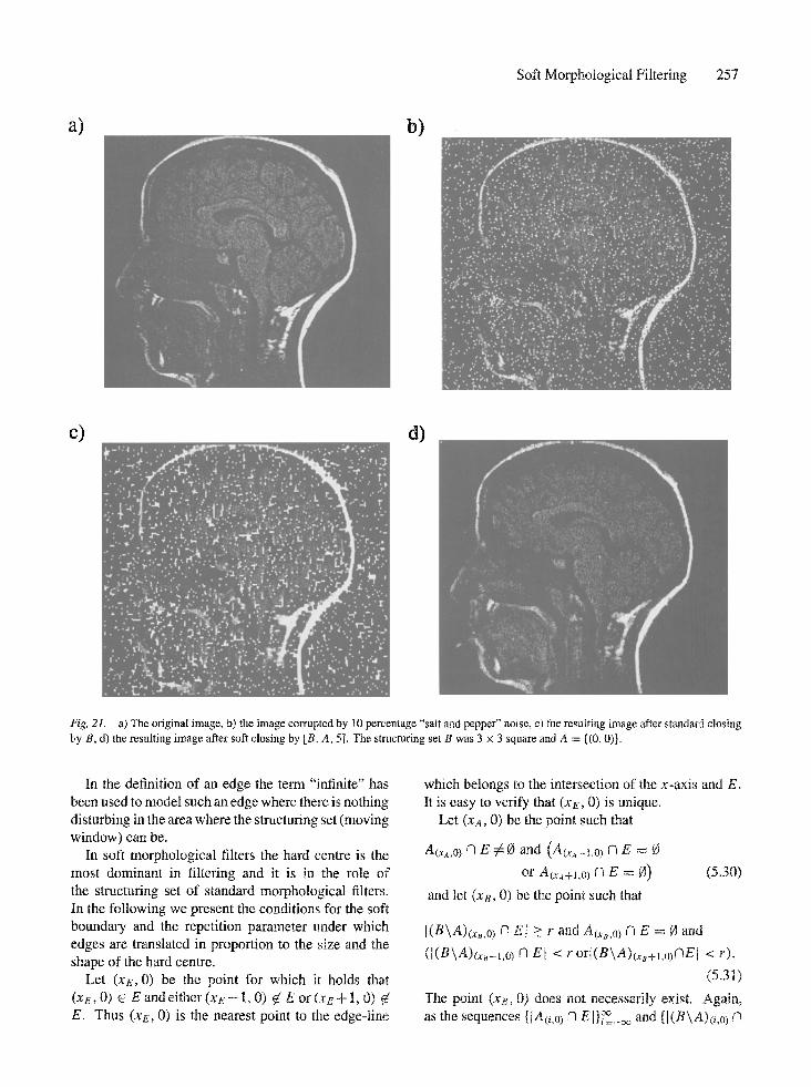
Soft Morphological Filtering 257
a) . . . . . b )
c) d)
. : ~" ~ , . . . . . . . . . f ' : ' ~ " . " " :. , . : . :
Fig. 21. a) The original image, b) the image corrupted by 10 percentage "salt and pepper" noise, c) the resulting image after standard closing by B, d) the resulting image after soft closing by [B, A, 5]. The structuring set B was 3 × 3 square and A = {(0, 0)}.
In the definition of an edge the term "infinite" has been used to model such an edge where there is nothing disturbing in the area where the structuring set (moving window) can be.
In soft morphological filters the hard centre is the most dominant in filtering and it is in the role of the structuring set of standard morphological filters. In the following we present the conditions for the soft boundary and the repetition parameter under which edges are translated in proportion to the size and the shape of the hard centre.
Let (xE, 0) be the point for which it holds that (xe, 0) 6 E and either (xe - 1, 0) ¢~ E or (xE + 1, 0) E. Thus (xe, 0) is the nearest point to the edge-line
which belongs to the intersection of the x-axis and E, It is easy to verify that (XE, 0) is unique•
Let (XA, 0) be the point such that
A(xa,O) N E 7 & 13 and (A(xa-i,0) A E = 13
or A(xa+l,o) (q E = 13) (5•30)
and let (x~, 0) be the point such that
[(B\A)(x~,O) N E[ > r and A(xs,O) A E = 13 and
(I(B\A)(xB-1,0) f3 El < r or](B\A)(x~+l.o)r3EI < r).
(5.31)
The point (xe, 0) does not necessarily exist. Again, as the sequences {IA(i,0) (h E[}~°=_oo and {[(B\A)(i ,o) ('1
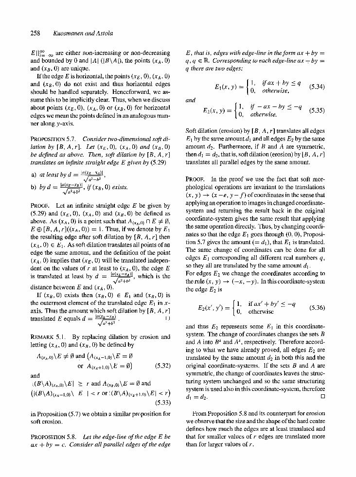
258 Kuosmanen and Astola
o o E I}i=_~ are either non-increasing or non-decreasing and bounded by 0 and IAI (IB\AJ), the points (XA, O) and (xB, 0) are unique.
If the edge E is horizontal, the points (xe, 0), (XA, O) and (x~, 0) do not exist and thus horizontal edges should be handled separately. Henceforward, we as- sume this to be implicitly clear. Thus, when we discuss about points (xe, 0), (XA, 0) or (x~, 0) for horizontal edges we mean the points defined in an analogous man- ner along y-axis.
PROPOSITION 5.7. Consider two-dimensional soft di- lation by [B, A, r]. Let (xe, 0), (XA, O) and (XB, O) be defined as above. Then, soft dilation by [B, A, r] translates an infinite straight edge E given by (5.29)
a) at least by d = Iq(xE--XA)I :,/;rga '
b) by d = la(xe-xs)t , if (XB, O) exists.
PROOF. Let an infinite straight edge E be given by (5.29) and (xE, 0), (xa, 0) and (xB, 0) be defined as above. As (XA, 0) is a point such that A(xA,0) fq E # 0, E ~ [B, A, r]((XA, 0)) = 1. Thus, if we denote by E1 the resulting edge after soft dilation by [B, A, r] then (XA, O) ~ El. As soft dilation translates all points of an edge the same amount, and the definition of the point (xa, 0) implies that (XE, 0) will be translated indepen- dent on the values of r at least to (XA, 0), the edge E is translated at least by d - la(xE--xa)l which is the
a 47;7 ' distance between E and (XA, 0).
If (xB, 0) exists then (XB, 0) ~ El and (xB, 0) is the outermost element of the translated edge El in x- axis. Thus the amount which soft dilation by [B, A, r] translated E equals d -- la(xE-xB)l []
: , / 7 ; 7
REMARK 5.1. By replacing dilation by erosion and letting (XA, 0) and (xB, 0) be defined by
A(XA,O)\E # 0 and (A(xa_l,0)\E = 0
or A(xA+I,O)\E = O)
and I(B\A)(~,,o)\EJ
O(B\A)(x.-1,o)\
(5.32)
> r and A(xB,o)\E = 0 and
E I < r or I(B\A)(xB+I,o)\EI < r)
(5.33)
in Proposition (5.7) we obtain a similar proposition for soft erosion.
PROPOSITION 5.8. Let the edge-line of the edge E be ax + by = c. Consider all parallel edges of the edge
E, that is, edges with edge-line in the form ax + by = q, q ~ IR. Corresponding to each edge-line ax + by = q there are two edges:
and
1, if ax + b y < q (5.34) E l (x ,y ) = 0, otherwise,
1, if - ax - by < - q E2(x, y) = O, otherwise. (5.35)
Soft dilation (erosion) by [B, A, r] translates all edges E1 by the same amount dl and all edges E2 by the same amount d2. Furthermore, if B and A are symmetric, thendl = d2, thatis, soft dilation (erosion)by [B, A, r] translates all parallel edges by the same amount.
PROOF. In the proof we use the fact that soft mor- phological operations are invariant to the translations (x, y) --+ (x - e , y - f ) of coordinates in the sense that applying an operation to images in changed coordinate- system and returning the result back in the original coordinate-system gives the same result that applying the same operation directly. Thus, by changing coordi- nates so that the edge E1 goes through (0, 0), Proposi- tion 5.7 gives the amount (= dr), that El is translated. The same change of coordinates can be done for all edges E1 corresponding all different real numbers q, so they all are translated by the same amount &. For edges E2 we change the coordinates according to the rule (x, y) --+ ( - x , - y ) . In this coordinate-system the edge E2 is
, , [ 1 , i f a x ' + b y ' < _ - q E2(x , y ) = I O, otherwise (5.36)
and thus E2 represents some E1 in this coordinate- system. The change of coordinates changes the sets B and A into B s and A s, respectively. Therefore accord- ing to what we have already proved, all edges E2 are translated by the same amount d2 in both this and the original coordinate-systems. If the sets B and A are symmetric, the change of coordinates leaves the struc- turing system unchanged and so the same structuring system is used also in this coordinate-system, therefore dl = d2. []
From Proposition 5.8 and its counterpart for erosion we observe that the size and the shape of the hard centre defines how much the edges are at least translated and that for smaller values of r edges are translated more than for larger values of r.
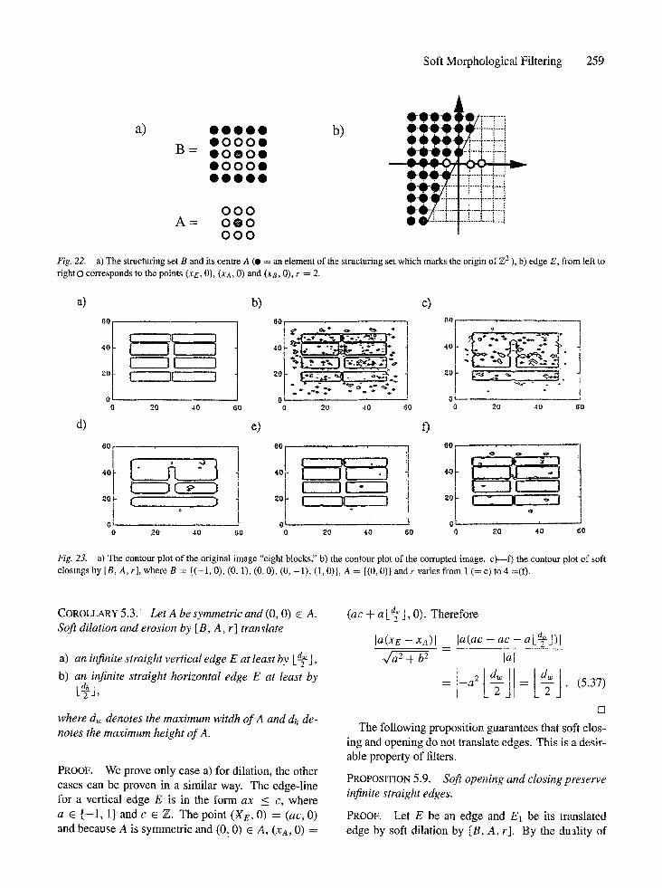
Soft Morphological Filtering 259
a) o o o o o b) O 0 0 0 O
B = O 0 0 0 0
O 0 0 0 0 O O O O 0
A = 0 0 0 0 0 0 0 0 0
,OOOO-6OTF---.~---~ o-eoooq~--i----~---i eeeo~/.,--~--i---i
o ~ - - H
Fig. 22. a) The structuring set B and its centre A (O = an element of the structuring set which marks the origin of Z z ), b) edge E, from teR to rightO corresponds to the points (xE, 0), (Xa, 0) and (xB, 0), r = 2.
a) b) c)
d)
60
40
20
0
60
40
20
0
I I E--i I II J
0 i 20 40 60 0 20 40
[. ( )
e)
20 40 GO 60
6 0 ,
l I - } - I ,o LV__~I -1
I - ° I 20 I I1
0 n ,' 0 20 40
B0
f)
°°! °
40 : ",~ K . - -
0 0 ~0 40 60
60
40
20
0
o
20 40 60
Fig. 23. a) The contour plot of the original image "eight blocks," b) the contour plot of the corrupted image, c)--f) the contour plot of soft closings by [B, A, r], where B = {(-1, 0), (0, 1), (0, 0), (0, -1), (1, 0)}, A = {(0, 0)} and r varies from 1 (= c) to 4 =(f).
COROLLARY 5.3. Let A be symmetric and (0, O) 6 A. Soft dilation and erosion by [B, A, r] translate
a) an infinite straight vertical edge E at least by k-~J,
b) an infinite straight horizontal edge E at least by
k~J,
where dw denotes the maximum witdh o f A and dh de- notes the maximum height o f A.
PROOF. We prove only case a) for dilation, the other cases can be proven in a similar way. The edge-line for a vertical edge E is in the form ax < c, where
a 6 { - 1 , 1} and c E Z. The point (Xe , O) = (ac, O) and because A is symmetric and (0, 0) 6 A, (XA, 0) =
(ac + a L~J, 0). Therefore
la(xe - XA)I Ja(ac -- ac -- a k-~J)l
q- b 2 Lal
D
The following proposit ion guarantees that soft clos- ing and opening do not translate edges. This is a desir- able property of filters.
PROPOSITION 5.9. Soft opening and closing preserve infinite straight edges.
PROOF. Let E be an edge and E1 be its translated edge by soft dilation by [B, A, r]. By the duality of
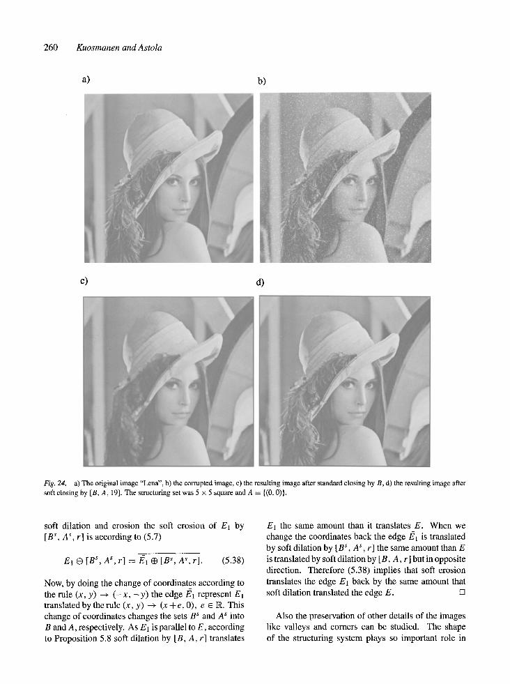
260 Kuosmanen and Astola
a) b)
c) d)
Fig. 24. a) The original image "Lena", b) the corrupted image, c) the resulting image after standard closing by B, d) the resulting image after soft closing by [B, A, 19]. The structuring set was 5 x 5 square and A = {(0, 0)}.
soft dilation and erosion the soft erosion of E1 by [ B s, A s, r] is according to (5.7)
E1 G [B s, A s ,r] = ff~l • [ Bs, As, r]. (5.38)
Now, by doing the change of coordinates according to the rule (x, y) ~ ( - x , - y ) the edge/~1 represent E1 translated by the rule (x, y) ~ (x + e, 0), e 6 R. This change of coordinates changes the sets B s and A s into B and A, respectively. As Et is parallel to E, according to Proposition 5.8 soft dilation by [B, A, r] translates
E1 the same amount than it translates E. When we change the coordinates back the edge/~1 is translated by soft dilation by [B s, A s, r] the same amount than E is translated by soft dilation by [B, A, r] but in opposite direction. Therefore (5.38) implies that soft erosion translates the edge E1 back by the same amount that soft dilation translated the edge E. []
Also the preservation of other details of the images like valleys and corners can be studied. The shape of the structuring system plays so important role in
Soft Morphological Fi l ter ing 261
preservat ion of these details that it is practically impos-
sible to give exact properties for how soft operations
work. Still it is possible to say that in general the
increase of the order index r yields better detail preser- vation. This is i l lustrated in the Fig. 23, where the widths of the valleys be tween blocks in one co lumn varies f rom 1 to 3. Soft c losing by [B, A, 1] (standard
closing) filled valleys of width 1 and 2, soft closing by
[B, A, 2] filled valleys of width 1 and rounded comers. The abil i ty of soft morphological filters to remove im-
pulsive noise is also clearly p ronounced in Fig. 23.
Figure 24 illustrates the better abil i ty of soft morpho- logical closing to preserve small details of the image
compared to standard closing. For example, the soft closing did not distort the hairs of the girl as badly as standard closing did.
References
1. J. Astola, L. Koskinen, O. Yli-Harja, and Y. Neuvo, "Digital fil- ters based on threshold decomposition and Boolean functions," in Proc. SPIE Symp., Visual Comm., Image Proc., Philadelphia, USA, pp. 461-470, November 1989.
2. J. Astola, L. Koskinen, and Y. Neuvo, "StatisticaI properties of discrete morphological filters," in E. Dougherty (Ed.) Mathe- matical Morphology in Image Processing, New York: Marcel Dekker, pp. 93-120, 1992.
3. J. Astola and Y. Neuvo, "An efficient tool for analysing weighted median and stack filters," submitted to IEEE Transactions on Circuits and Systems, 1992.
4. E. Dougherty and C. Ciardiana, Morphological Methods in im- age and Signal Processing, Englewood Cliffs, NJ: Prentice- Hall, 1988.
5. E.N. Gilbert, "Lattice theoretic properties of frontal switching functions," Journal of Mathematical Physics, Vol. 33, pp. 57-67, 1954.
6. L. Koskinen, J. Astola, and Y. Neuvo, "Statistical properties of discrete morphological filters," in Proceedings oflEEE Interna- tional Symposium on Circuits and Systems, New Orleans, USA, pp. 1219-1222, May 1990.
7. L. Koskinen, J. Astola, and Y. Neuvo, "Analysis of noise atten- uation in morphological image processing," in Proceedings of SPIE Symposium on Nonlinear Image Processing II, San Jose, USA, pp. 102-113, February 1991.
8. L. Koskinen, J. Astola, and Y. Neuvo, "Soft morphological fil- ters," in Proceedings of SPIE Symp. on Image Algebra and Mor- phological Image Processing II, San Diego, USA, pp. 262-270, July 1992.
9. L. Koskinen and J. Astola, "Soft morphological filters: A ro- bust morphological filtering method," submitted to Journal of Electronic Imaging.
10. E Kuosmanen, L. Koskinen, and J. Astola, "An adaptive mor- phological filtering method," in Proc. EUSIPCO -92, Brussels, Belgium, pp. 1089-1092, August 1992.
11. E Kuosmanen, L. Koskinen, and J. Astola, "Detail preserv- ing morphological filtering," in Proc. l lth IAPR International
Conference On Pattern Recognition, Volume HI, The Hague, The Netherlands, pp. 236-239, September t992.
t2. R Kuosmanen, L. Koskinen, and J. Astola, "Analysis and exten- sions of soft morphological filters," in Proc. SPIE/1S&T Symp. onElectroniclmaging: Scienee and Technology, San Jose, USA, January 1993.
13. E Kuosmanen, L. Koskinen, and J. Astota, "The connection between generalized soft morphological filters and stack Filters," in Proc. IEEE Winter Workshop on Nonlinear Digital Signal Processing, Tampere, Finland, January 1993.
14. J.H. Lin and E.J. Coyle, "Generalized stack filters and mean ab- solute error nonlinear filtering," IEEE Trans. on A coust., Speech, and Signal Processing, Vol. ASSP-38, No. 6, pp. 938-954,1990.
15. E Matheron, Random Sets and Integral Geomet~, New York: Wiley 1975.
16. I. Pitas and A. Venetsanopoulos, Nonlinear Digital Filters, Boston: Kluwer Academic Publisher, 1990.
17. D. Schonfeld and L Goutsias, "Optimal morphological pattern restoration from noisy binary images," IEEE Transaction on Pattern Analysis and Machine Intelligence, Vol. 13, pp. 14-29, 199L
18. S. Serra, Image Analysis and Mathematical Morphology, London: Academic Press, 1988.
19. S. Sternberg, "Grayscale morphology," Computer Vision, Graphic, andlmage Processing, VoL 35, pp. 333-355, 1986.
20. S. Stevenson and G. Arce, "Morphological filters: Statistk:s and further syntactic properties," IEEE Transaction on Circu#s and Systems, Vol. 34, pp. 1292-1305, 1987.
21. E Wendt, E. Coyle, and N. Gallagher~ "Stack filters," IEEE Transaction on Acoustics, Speech, and Signal Processing, VoL 34, pp. 898-911, 1986.
22. O. Yti-Harja, J. Astola, and Y. Neuvo, "Analysis of the proper- ties of median and weighted median filters using threshold logic and stack filter representation," IEEE Transaction on Signal Pro- cessing, Vol. 39, pp. 395-410, 1991.
Pauli Kuosmanen received the M.Sc. and licentiate degrees in math- ematics from Tampere University, Finland, in 1991 and 1993, re- spectively. He received the Ph.D. degree in signal processing from Tampere University of Technology in 1994. Currently he is working in Signal Processing Laboratory, Tampere University of Technology as a senior researcher. His main research interests include signal and image processing with emphasis on nonlinear image processing.
262 Kuosmanen and Astola
Jaakkto Astola received the B.Sc., M.Sc., Licentiate and Ph.D. de- grees in mathematics from Turku University, Finland, in 1972, 1973, 1975, and 1978 respectively. From 1976 to 1977 he was a research assistant at the Reasearch Institute for Mathematical Sciences of Ky- oto University, Kyoto, Japan. Between 1979 and 1987 he was with the Department of Information Technology, Lappeenranta Univer- sity of Technology, Lappeenranta, Finland holding various teaching position in mathematics, applied mathematics and computer science. From 1988 and 1993 he was an Associate Professor in Applie Math- ematics at Tampere University, Tampere, Finland. Currently he is Professor of digital signal processing at Tampere University of Tech- nology. His research interests include image and signal processing, coding theory, and statistics.