IEEE TRANSACTIONS ON SIGNAL PROCESSING, VOL. 48, NO. 8, AUGUST 2000 2343

Space/Spatial-Frequency Analysis Based FilteringLJubisa Stankovic´, Senior Member, IEEE, Srdjan Stankovic´, Member, IEEE, and Igor Djurovic, Student Member, IEEE

Abstract—Space-invariant filtering of signals that overlap withnoise in both space and frequency can be inefficient. However, thesignal and noise may be well separated in the joint space/spatial-frequency domain. Then, it is possible to benefit from the appli-cation of space/spatial frequency approaches. Processing based onthese approaches can outperform space or frequency invariant-based methods. To this aim the concept of nonstationary space-varying filtering is introduced in this paper as an extension of thetime-varying filtering concept. The filtering definitions are basedon statistical averages, although the filtering should commonly beapplied knowing only a single noisy signal realization. The pro-cedures that can produce good estimates of quantities crucial forefficient filtering, based on a single noisy signal realization, areconsidered. Special attention has been paid to the region of sup-port estimation and cross-term effects removal. The efficiency ofthe proposed space/spatial-frequency filtering concept is tested onthe signal forms inspired by the interferograms in optics, includingreal images as disturbances. Examples demonstrate the superiorityof the proposed filtering over the space-invariant one for the con-sidered type of signals and noise.

Index Terms—Estimation, filtering, noisy signals, space varyingfiltering, time–frequency analysis, Wigner distribution.

I. INTRODUCTION

WHEN a two-dimensional (2-D) signal and noise do notoccupy the same frequency range, then efficient filtering

can be performed using space-invariant filters. However, inthe cases when the signal and noise overlap in a significantpart of the space and frequency domain, then the stationaryfiltering may be difficult and inefficient. We will consider noisysignals that occupy the same space and frequency range whentheir separation may be done in the joint space/spatial-fre-quency domain. For these kinds of noisy signals, a conceptof space-varying filters is presented. It is an extension of theone-dimensional (1-D) time–varying filtering approach, [4],[22], [23], [25], [29], [33] to the 2-D problems. Since the con-cept of time-varying filtering is based on the time–frequencydistributions, we will use joint space/spatial-frequency distri-butions [7], [8], [16], [17], [27], [37], [39], [42]–[44] in order todefine and implement space-varying filtering. The 2-D Wignerdistribution, along with the 2-D extension of the Weyl operator[18], [23], [25], [28], is used as a basic distribution. In order toproduce undistorted version of the frequency modulated signalpassing through the filter whose region of support is ideally

Manuscript received February 26, 1999; revised March 27, 2000. The workof LJ. Stankovic´ and S. Stankovic´ was supported by the Alexander von Hum-boldt Foundation. The associate editor coordinating the review of this paper andapproving it for publication was Prof. Gregori Vazquez.

LJ. Stankovic´ and I. Djurovic are with the Elektrotehnicki Fakultet,University of Montenegro, Podgorica, Montenegro, Yugoslavia (e-mail:l.stankovic@ieee.org).

S. Stankovic´ is with the Institute of Communications Technology, DarmstadtUniversity of Technology, Germany, on leave from the Elektrotehnicki Fakultet,University of Montenegro, Podgorica, Montenegro, Yugoslavia.

Publisher Item Identifier S 1053-587X(00)05975-4.

concentrated along the local frequency (or group shift), a slightmodification of the existing time–frequency filtering relationis proposed and justified.The implementation is performedusing a single noisy signal realization.The algorithm for theWigner distribution estimation by using only one noisy signalobservation that would be close to the optimal one, with respectto the bias and variance, is presented [11], [20], [35], [36]. Thisis important since the Wigner distribution plays a crucial role inthe region of support estimation and, consequently, determinesfiltering efficiency. In order to extend the presented forms forthe application on multicomponent signals, the multidimen-sional S-method is used [30], [37]. The results presented in thispaper are applied to the space-varying filtering of signals witha high amount of noise, including real image as a disturbance.

The paper is organized as follows. The concept of space-varying filtering is presented in Section II. A slight modificationwith respect to the common time-varying form is introduced andjustified in the Appendix. The pseudo and discrete forms of thefiltering relations are given. Efficient region of support estima-tion, as a crucial part of good filtering, is considered in detailin Section III. Since the Wigner distribution turns out to be thebasic form for the region of support estimation, its variance andbias are considered. Based on a specific statistical approach ofcomparing the bias and the variance, an algorithm for the op-timal Wigner distribution estimation, i.e., the filtering regionof support estimation with minimal mean square error, is pre-sented in this section. Efficiency of the proposed space-varyingfiltering is demonstrated in Section IV by examples.

II. THEORY

Consider a 2-D noisy signal

(1)

where is the signal, whereas denotes the noise.The above relation may be written in a vector notation as

where (2)

The nonstationary 2-D filter relation will be defined in analogywith the 1-D time-varying filtering [4], [22], [23], [25], [33],[40]

(3)

where is an impulse response of the space-varying 2-Dfilter.

This definition is slightly modified with respect to the existing1-D definitions [4], [22], [23], [25], [40]. The modification hasbeen introduced in order to provide that for ,we get if the filter in space/spatial-frequency

1053–587X/00$10.00 © 2000 IEEE

2344 IEEE TRANSACTIONS ON SIGNAL PROCESSING, VOL. 48, NO. 8, AUGUST 2000

domain is defined as a delta function along thelocal frequency for signals that satisfy stationary phasemethod conditions [2], [6], [26] (see the Appendix).

The optimal transfer function derivation will be done byanalogy with the Wiener filter derivation in the stationarysignal cases [22], [26], [40]. The error isorthogonal to the data when the mean square error

reaches its minimum [26], [40]

(4)

Denote the expected value of the ambiguity function, [15], [24] as

(5)

and the Fourier transform of over by

(6)

From (4), it then follows that

(7)

for the processes that are mainly concentrated around the am-biguity domain origin (being different from zero only for small

) when . In the 1-D case,these processes are referred to as theunderspread processes[15], [22], [24].

1) Note: Relation (7) directly follows from (4) without anyadditional assumption if the considered processes are quasista-tionary [26], [33], [40], i.e., if

, and. It provides an additional physical

motivation for modification (3).The 2-D Fourier transform of (7) results in

(8)

where is the Wigner spectrum (the expected valueof the Wigner distribution [9]) of signal

and is defined by

(9)

If the signal and noise are not correlated, then

(10)

2) Note: For the stationary processes, with, , and

, (3), (9), and (10) reduce to the well-known sta-tionary Wiener filter forms [26], [40].

When the Wigner spectrum of signal lies inside aspace/spatial-frequency region denoted by, while the noiseis dominantly spread outside this region, then a simple solutionsatisfying (10) is given by

for

for(11)

where is the region where . This is true,for example, for a wide class of frequency modulated (highlyconcentrated in the space/spatial-frequency plane) signals

corrupted with a white noise widely spread in thespace/spatial-frequency plane.

3) Note: Relation (11) could also be obtained in a semi-in-tuitive way, as in [23]. Then, some restrictions imposed in itsderivation, like the one about underspreadness, would not benecessary either. More details about this derivation, in the 1-Dcase, may be found in [23].

In the numerical implementations, the pseudo (space limited)forms of the filter relations should be introduced. The pseudoform of operator (3) will be defined as

(12)

This relation enables one to use the space limited intervals. Itmay be shown that for the signals ideally concentrated along thelocal frequency in the space/spatial-frequency domain, the fol-lowing important conclusion holds: The window does notinfluence the filter output (12) as far as (see the Ap-pendix). Using the Parseval’s theorem, (12) assumes the form

(13)

where is the “short space” Fourier transform de-fined by

(14)

Discrete form of (13), as it used in the implementation, is

(15)

where assumes unity values where the Wigner distri-bution of signal is different from zero. Therefore, in order to per-form a 2-D space-varying filtering, we should know theand . Computation of the is simple, but the problemof determination still remains. Obviously, a precise deter-mination of is directly related to precise determination,which further leads tothe estimation of the Wigner distributionof signal without noise using only one noisy signal observationwith the mean square error as small as possible.

STANKOVIC et al.: SPACE/SPATIAL-FREQUENCY ANALYSIS-BASED FILTERING 2345

Note that the support region determination based on thesquared modulus of , i.e., multidimensionalspectrogram, would be appropriate only in the case whenthelocal frequency does not change over space or changes veryslowly so that it may be considered as a constant within thewindow . Otherwise, when the local frequency variationswithin the considered domain are significant, for low and highfrequencies, then its estimation based on either spectrogramor scalogram is not reliable. In addition, the region of supportdetermined by using these distributions would be very spreadout and would result in inefficient filtering.

III. SINGLE REALIZATION -BASED ESTIMATION OF THE FILTER

REGION OFSUPPORT

A. Optimal Window Width in the Wigner Distribution

The analysis in this paper is focused on the one realizationbased filtering of noisy signals. Accurate determination of thefiltering region of support, i.e., the Wigner distribution of thesignal, is crucially important for the efficient filtering. Two pa-rameters that determine the mean square error of the Wigner dis-tribution estimation are the bias and variance. They will be an-alyzed for the pseudo Wigner distribution of discrete unknowndeterministic noisy signal

(16)

where , withdenoting signal and additive Gaussian white noise

with independent real and imaginary parts and total variance. This form corresponds to the practical cases when only a

single realization of the image is known. Therefore, we maytreat the signal as deterministic. The noise autocorrelation func-tion is .

The pseudo Wigner distribution mean value is [34]

(17)

where is the Fourier transform of the 2-D window, whereas is a 2-D convolution along and

. Since the term is con-stant pedestal and does not depend on the window shape and thesignal form, it will not be considered further. The first term canbe written as

. The bias can be approximated by

(18)

where .

The variance is defined by

(19)

Using (19) we get, as in the 1-D case [1], [34], that

(20)

where a real and even window function is assumed.For a signal with slow-varying amplitude, we get

(21)

where is the signal’s amplitude, and isthe window energy. For the 2-D separable window

, where is the Hanningwindow, the energy is , and is the windowwidth. Similar results could be obtained for any other windowshape. For example, for the separable Hamming window, theenergy is and for the rectangular window,it is .

The mean square error is defined by. According to (18) and (21), it may be

written as

(22)

where

(23)

(24)

It is important to note that the variance is proportional tothe square of the window width, whereas the bias decreaseswith the same rate. Optimal window width follows from

. From (22), we get

(25)

Note that the optimal window width is space and frequencyvarying since it depends on From (22), we canconclude that for the optimal width , the ratio of the biasand standard deviation

(26)

is constant and depends neither on the problem parameters noron the signal. The optimal window width is given by (25). How-ever, it is not applicable to practical problems since it requiresthe knowledge of bias parameter , that is, a functionof the distribution derivatives, and is therefore unknown in ad-vance. An algorithm for the optimal window width determina-tion without using the bias parameter is describednext.

2346 IEEE TRANSACTIONS ON SIGNAL PROCESSING, VOL. 48, NO. 8, AUGUST 2000

B. Algorithm

In order to estimate the Wigner distribution of signaland its region of support using the optimal window widthfor each space and frequency point, we will use a statistical ap-proach [11], [20], [21], [29], [36]. It is based on the fact that thevalue of the pseudo Wigner distribution of anoisy signal is a scalar random variable. It is spread around theexact Wigner distribution with the bias de-noted by (including constant pedestal ) andthe variance . As for any biased random variable, wemay write the following inequality:

(27)

This inequality holds with probability . For large , wehave that (27) is satisfied with for any distributionlaw of random variable . For example, with

(“three sigma rule”) for normal distribution of the randomvariable, .

For the cases of when the bias is small, i.e.,, the above inequality may

be written as

(28)According to (28), we may write the expressions for the lowerand upper confidence interval limitwithin which the value of the pseudo Wigner distribution

is located with probability

(29)

Index denotes an arbitrary window length .Consider now the successive values of the window lengths

such that . Consider two casesfor : a) small bias cases and b) small variance and largebias cases. Confidence intervals calculated with,intersect in the case of small bias since, according to (28),the true value of the Wigner distribution belongs to both ofthese intervals [with probability ]. In the cases of verylarge bias and small variance, the confidence intervals do notintersect . Values for ,as well as interval for possible, will be determined fromthe condition that all confidence intervals for small bias suchthat intersect, whereas allconfidence intervals fordo not intersect. In this way, the examination of the inter-section of two confidence intervals will be an indicator forthe bias to standard deviation ratio. When critical value

is reached, that means thatwe have the optimal window width for this space and frequencypoint (26).

To that aim, assume that the window widths have a dyadicscheme

(30)

with , and is unknown op-timal width. It has been assumed that the optimal window widthbelonged to this set.1 With (22) and (30), the relations for thebias and standard deviation for an arbitrary window widthmay be written as functions of the bias and standard deviationfor optimal width

(31)

Consider now three regions and impose, accordingto the previous discussion, the condition that the regionsand

intersect and that the regions and do not intersect.Due to monotonicity of the bias and variance if and inter-sect, then all and for will intersect. This meansthat the region is defined by the optimal window width. As-suming, without loss of generality, that the bias is positive, thiscondition may be written in the following way:

(32)

where, for example, is the minimal possible value ofthe upper bound for . Based on (27), it follows that forthe window of the width , the Wigner distribution of iswithin the interval

(33)

The lower and upper bounds of the confidence interval, for agiven window width, according to (29), takes the values within

(34)

Substituting (34) and (31) into (32), we get

(35)

This means for . For example, for, we have . The value of de-

termines the probability that (28) is satisfied. In that sense,it is desirable to take as large value ofas possible from the de-rived interval. For example, with , we get .A further increase of does not make sense since the proba-bility is already close to 1 and other factors, like, for example,effects of discretization, become dominant. In this way, we havedefined and as the key factors for the algorithm.

The above procedure may be significantly simplified usingonly two window widths in calculations [29]. Denote these two

1If N does not belong to the setNNN , then the algorithm will produce thenearest value to this one. Since the MSE changes slowly around the stationarypoint, it will not significantly degrade performance.

STANKOVIC et al.: SPACE/SPATIAL-FREQUENCY ANALYSIS-BASED FILTERING 2347

window widths by and , where .Window produces small variance, whereas hassmall bias. Therefore, when the confidence intervals for thesetwo windows intersect, then it means that the bias is small, andwe use in order to reduce the variance. Otherwise, thebias is large, and we use in order to reduce it. Theresulting adaptive Wigner distribution is

true

elsewhere(36)

where for , it holds that

(37)

In this way, using only two window widths, we may expect sig-nificant improvements since the Wigner distribution is eitherslow-varying (bias very small) or highly concentrated along thelocal frequency (bias very large). If we used a multiwindow ap-proach with many windows between and , thenthe algorithm applied to the Wigner distribution would selectone of these two extreme window widths almost everywhere.

Relation (36) reduces to the calculation of the Wigner dis-tribution and its variance for two-window widths. One possiblerelation for the variance estimation is

(38)

It holds for the low signal-to-noise ratio. For cases of smallnoise, the variance estimation procedure is given in [21]. From(38), it follows that . Thus, we havedefined the algorithm and all parameters for the Wigner distri-bution calculation, which is then used for the region of support

determination and space varying filtering.

C. Multicomponent Signal Case

For multicomponent signal , the Wignerdistribution contains -signal terms (auto-terms) and

interference terms (cross-terms) with amplitude that couldcover the signal terms

(39)

This is the reason why the RID class of distributions [19] hasbeen introduced

(40)

where [5] is the kernel in the space/spatial-frequencyplane, whose Fourier transform

(kernel in ambiguity plane) is a lowpass filter function. Formulticomponent signals, we will use the S-method (SM) [30],[37]

(41)

where is rectangular window with width in eachdirection. The SM belongs to general Cohen class of distribu-tions [5]. When the components of a multicomponent signal donot overlap in the joint space/spatial-frequency plane, it is pos-sible to determine the width of the frequency window sothat the SM is equal to a sum of the Wigner distributions of eachsignal component individually [30]

(42)

This interesting property has attracted the attention of someother researches to use the SM in their work [3], [10], [12].Noise influence on the SM was considered in [31]. The vari-ance for nonoverlapped multicomponent signals can here be ex-pressed as (21)

for

for

(43)Estimation of the autoterms in the Wigner distribution, based onthe SM, could be done as

true

elsewhere(44)

where for , it holds that

(45)

Note that for , the spectrogram (square magnitude of theSTFT) is obtained as a special case of the SM. Region of signal’ssupport could be obtained from as

(46)

where is a given reference level. We used.

The procedures and theory presented in the paper will be nowsummarized in the

2348 IEEE TRANSACTIONS ON SIGNAL PROCESSING, VOL. 48, NO. 8, AUGUST 2000

(a) (b)

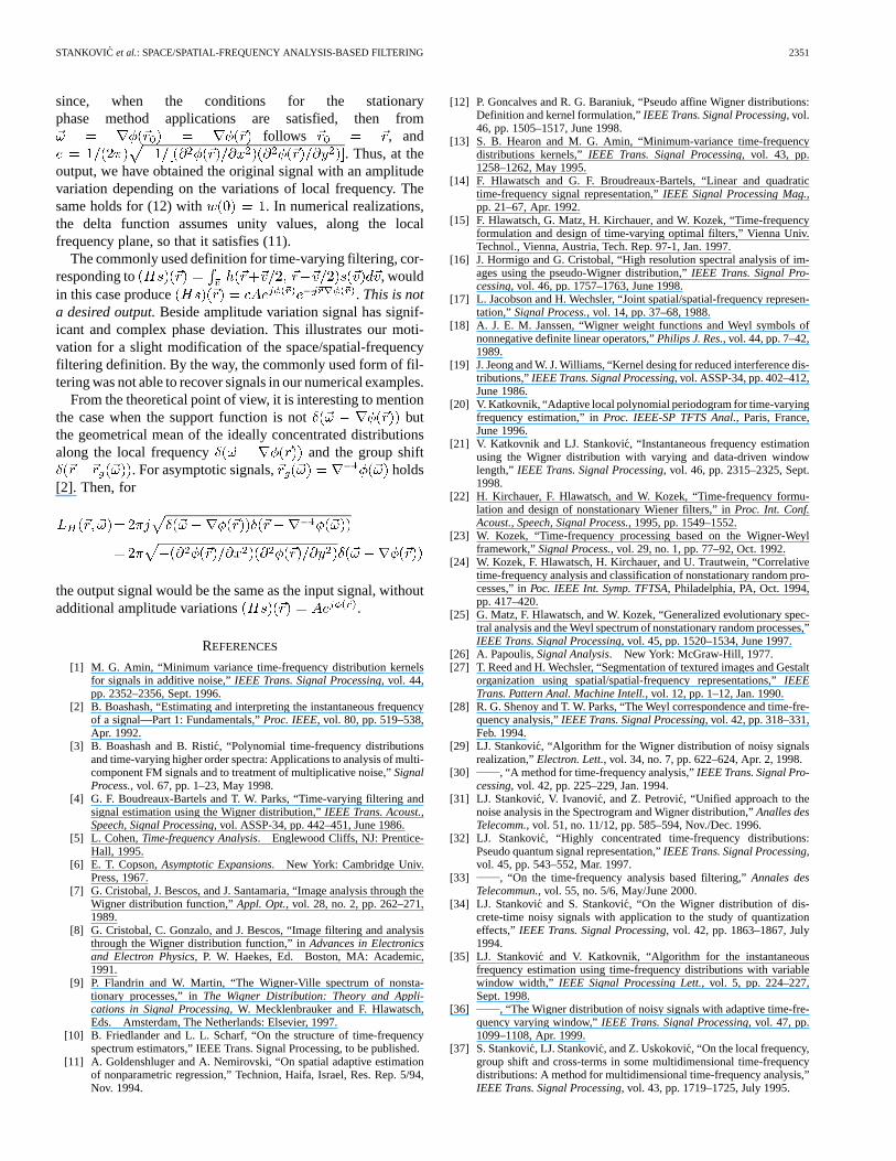
Fig. 1. Determination of the region of supportR for the space-varying filter at the point(x; y) = (0:5; 0:5). (a) Wigner distribution of noisy signal calculatedusing the windowN �N = 128� 128. (b) Wigner distribution of the noisy signal calculated using the proposed algorithm. Distribution from (b) is used forR determination at the point(x; y) = (0:5; 0:5).

Algorithm for Numerical Implementation:

1) Calculate for a given noisy signal. In highlynonstationary cases, application of narrower windows ispreferred.

2) Calculate the Wigner distribution either by definition (16)or by using (41), with two window widths and values of

. Details about (41), which has been used in numericalexamples, including its realization without interpolationand oversampling, may be found in [37].

3) Find the “optimal” distribution, for each point, accordingto (44).

4) Determine the filter region of support by using (46).For one-component signals, determination ofmay be simplified just by taking at thepoint where the maximum ofor is detected for a given . The sameprocedure may be used for multicomponent signals witha known number of components [33]. Otherwise, thegeneral form (46) must be used.

5) Compute the filtered signal according to (15).

IV. NUMERICAL EXAMPLES

Example 1: The presented theory will be illustrated on thenumerical example with the signal

(47)

corrupted with a high amount of additive noise with variance, meaning that [dB]. The signal

form (47) is inspired with the interferograms in optics.Fig. 1 demonstrates the algorithm for the regiondetermi-

nation at the point . The Wigner distributioncalculated using the window widthis shown in Fig. 1(a). Fig. 1(b) presents the Wigner distribu-tion calculated using the two-window algorithm presented inSection IV with and

. The algorithm used the lower variance distributioncalculated with everywhere, exceptat the point where the signal energy is concentrated when thelower bias window is used.

Noisy signal (47) is considered within the interval. Signal frequency changes along both axis

from 0 to , where is the maximal frequency fora given sampling interval. In (37), we assumed .

The original signal without noise is shown in Fig. 2(a),whereas the noisy signal is given in Fig. 2(b). Signal filteredusing stationary filters with the cutoff frequency in bothdirections is given in Fig. 2(c). Filtering withlower cutoff frequencies reduces the noise but also degrades thesignal in Fig. 2(d) and (e) with and ,respectively. Signal obtained from the noisy signal in Fig. 2(b)using the space-varying filtering presented in this paper, by (3),(13), and the algorithm in Section III, is shown in Fig. 2(f).The advantage of the proposed concept with respect to thestationary filtering is evident.

Example 2: For the multicomponent case we will, as an ex-ample, consider the signal

(48)

corrupted with a high amount of additive noise with variance. In the spectrogram calculation, the Hanning window

with is used, whereas for the SMcalculation, the Hanning window withand are taken. The original signal is shown in Fig. 3(a).The noisy signal is given in Fig. 3(b). The signal filtered withthe proposed algorithm is presented in Fig. 3(c).

Example 3: Finally, we will consider a separation of linearfrequency modulated signals from real image. This would cor-respond to a generalization of the notch filtering in the sta-tionary cases. Here, the local frequency is varying, and the po-sition of the notch frequency changes for each point. Its de-tection based on the spectrogram would not be precise whatwould cause an imprecise and wide support region, resultingin unsatisfactory separation. The spectrogram-based region ofsupport determination would be efficient only in the cases ofconstant (or slow-varying) local frequency. The Wigner distri-bution approach gives very precise determination of the localfrequency when it changes over the image. It results in an effi-cient separation using the proposed procedure, as demonstrated

STANKOVIC et al.: SPACE/SPATIAL-FREQUENCY ANALYSIS-BASED FILTERING 2349

(a) (b) (c)

(d) (e) (f)

Fig. 2. Filtering of a 2-D signal. (a) Original signal without noise. (b) Noisy signal. (c) Noisy signal filtered using the stationary filter with a cutoff frequencyequal to the maximal signal frequency. (d) Noisy signal filtered using the stationary filter with a cutoff frequency equal to a half of the maximal frequency. (e) Noisysignal filtered using the stationary filter with a cutoff frequency equal to a fourth of the maximal frequency. (f) Noisy signal filtered using the space-varying filter.

(a) (b) (c)

Fig. 3. (a) Two-dimensional multicomponent signal without noise. (b) Noisy 2-D multicomponent signal. (c) Filtered noisy signal.

in Fig. 4. Fig. 4(a) shows original image. A part of the fre-quency-modulated signal added to the image Fig. 4(a) is shownin Fig. 4(b). The image corrupted with the frequency modulatedsignal is shown in Fig. 4(c), whereas the frequency-modulatedsignal extracted from Fig. 4(c), by using the proposed proce-dure, is shown in Fig. 4(d). The reconstruction is very good,although the ratio of the original image maximal value to thefrequency-modulated signal maximal value was extremely high

where is the image, and denotes frequency-modulatedsignal added to image.

V. CONCLUSION

The concept of space-varying filtering of multidimensionalsignals is presented. It has been shown that it can outperform thespace invariant approaches when the signal and noise overlapin both space and frequency domains separately but not in thejoint space/spatial-frequency domain. Special attention has beenpaid to the realization of space/spatial-frequency-based filteringusing only a single noisy signal realization. In order to produceaccurate region of support estimation, the optimization of theWigner distribution parameters is considered. This optimizationproduces space/spatial-frequency varying parameters based on aspecific statistical approach of comparing the bias and varianceof distribution. Further modifications are done in order to applythe algorithm on the multicomponent signals. Efficiency of

2350 IEEE TRANSACTIONS ON SIGNAL PROCESSING, VOL. 48, NO. 8, AUGUST 2000

Fig. 4. (a) Original image. (b) Part of the linear frequency-modulated signal added to the image. (c) Sum of the previous two signals. (d) Reconstructed linearfrequency modulated signal from (c).

the proposed filtering, and the algorithm for its support deter-mination, has been illustrated on noisy signals whose form isinspired by the interferograms in optics, as well as on the signalcorrupted with a real image. The second example is inspired bythe watermarking in the space/spatial-frequency domain. Fromthe presented theory and examples, we may conclude that in thecases when the signal and noise do not significantly overlap inthe joint space/spatial-frequency domain, the proposed filteringmay produce better results than the space or frequency-invariantone. Beside the application in filtering of images, this paperoffers an interesting application possibility in watermarking inthe space/spatial-frequency domain. This is a topic of currentresearch [38].

APPENDIX

ON THE MODIFICATION (3)

The property of the space/spatial frequency distributions thatthey are well concentrated around the local frequency

isoneof thebasicpoints for their introductionandapplica-tion.TheWignerdistributioncanachievecompleteconcentrationfor the signals whose local frequency variations could be consid-ered as linear within the considered domains, while, in order toimprove concentration for nonlinear local frequency forms, var-ious modifications have been defined [2], [3], [5], [20], [32].

Let us consider a 2-D FM signal . Assumethat the signal satisfies the condition that its Fourier transformmay be obtained by using a 2-D form of the stationary phase

method [2], [6], [26], which is given as

where is the point where . Assume that we haveachieved ideally concentrated space/spatial-frequency represen-tation, which is given by , for . When thereis no input noise , one expects from a filtering rela-tion that it can produce undistorted signal at the output, at leastin this ideal case.

According to Parseval’s theorem, from (3), we get

STANKOVIC et al.: SPACE/SPATIAL-FREQUENCY ANALYSIS-BASED FILTERING 2351

since, when the conditions for the stationaryphase method applications are satisfied, then from

follows , and. Thus, at the

output, we have obtained the original signal with an amplitudevariation depending on the variations of local frequency. Thesame holds for (12) with . In numerical realizations,the delta function assumes unity values, along the localfrequency plane, so that it satisfies (11).

The commonly used definition for time-varying filtering, cor-responding to , wouldin this case produce . This is nota desired output.Beside amplitude variation signal has signif-icant and complex phase deviation. This illustrates our moti-vation for a slight modification of the space/spatial-frequencyfiltering definition. By the way, the commonly used form of fil-tering was not able to recover signals in our numerical examples.

From the theoretical point of view, it is interesting to mentionthe case when the support function is not butthe geometrical mean of the ideally concentrated distributionsalong the local frequency and the group shift

. For asymptotic signals, holds[2]. Then, for

the output signal would be the same as the input signal, withoutadditional amplitude variations .

REFERENCES

[1] M. G. Amin, “Minimum variance time-frequency distribution kernelsfor signals in additive noise,”IEEE Trans. Signal Processing, vol. 44,pp. 2352–2356, Sept. 1996.

[2] B. Boashash, “Estimating and interpreting the instantaneous frequencyof a signal—Part 1: Fundamentals,”Proc. IEEE, vol. 80, pp. 519–538,Apr. 1992.

[3] B. Boashash and B. Ristic´, “Polynomial time-frequency distributionsand time-varying higher order spectra: Applications to analysis of multi-component FM signals and to treatment of multiplicative noise,”SignalProcess., vol. 67, pp. 1–23, May 1998.

[4] G. F. Boudreaux-Bartels and T. W. Parks, “Time-varying filtering andsignal estimation using the Wigner distribution,”IEEE Trans. Acoust.,Speech, Signal Processing, vol. ASSP-34, pp. 442–451, June 1986.

[5] L. Cohen,Time-frequency Analysis. Englewood Cliffs, NJ: Prentice-Hall, 1995.

[6] E. T. Copson,Asymptotic Expansions. New York: Cambridge Univ.Press, 1967.

[7] G. Cristobal, J. Bescos, and J. Santamaria, “Image analysis through theWigner distribution function,”Appl. Opt., vol. 28, no. 2, pp. 262–271,1989.

[8] G. Cristobal, C. Gonzalo, and J. Bescos, “Image filtering and analysisthrough the Wigner distribution function,” inAdvances in Electronicsand Electron Physics, P. W. Haekes, Ed. Boston, MA: Academic,1991.

[9] P. Flandrin and W. Martin, “The Wigner-Ville spectrum of nonsta-tionary processes,” inThe Wigner Distribution: Theory and Appli-cations in Signal Processing, W. Mecklenbrauker and F. Hlawatsch,Eds. Amsterdam, The Netherlands: Elsevier, 1997.

[10] B. Friedlander and L. L. Scharf, “On the structure of time-frequencyspectrum estimators,” IEEE Trans. Signal Processing, to be published.

[11] A. Goldenshluger and A. Nemirovski, “On spatial adaptive estimationof nonparametric regression,” Technion, Haifa, Israel, Res. Rep. 5/94,Nov. 1994.

[12] P. Goncalves and R. G. Baraniuk, “Pseudo affine Wigner distributions:Definition and kernel formulation,”IEEE Trans. Signal Processing, vol.46, pp. 1505–1517, June 1998.

[13] S. B. Hearon and M. G. Amin, “Minimum-variance time-frequencydistributions kernels,”IEEE Trans. Signal Processing, vol. 43, pp.1258–1262, May 1995.

[14] F. Hlawatsch and G. F. Broudreaux-Bartels, “Linear and quadratictime-frequency signal representation,”IEEE Signal Processing Mag.,pp. 21–67, Apr. 1992.

[15] F. Hlawatsch, G. Matz, H. Kirchauer, and W. Kozek, “Time-frequencyformulation and design of time-varying optimal filters,” Vienna Univ.Technol., Vienna, Austria, Tech. Rep. 97-1, Jan. 1997.

[16] J. Hormigo and G. Cristobal, “High resolution spectral analysis of im-ages using the pseudo-Wigner distribution,”IEEE Trans. Signal Pro-cessing, vol. 46, pp. 1757–1763, June 1998.

[17] L. Jacobson and H. Wechsler, “Joint spatial/spatial-frequency represen-tation,” Signal Process., vol. 14, pp. 37–68, 1988.

[18] A. J. E. M. Janssen, “Wigner weight functions and Weyl symbols ofnonnegative definite linear operators,”Philips J. Res., vol. 44, pp. 7–42,1989.

[19] J. Jeong and W. J. Williams, “Kernel desing for reduced interference dis-tributions,”IEEE Trans. Signal Processing, vol. ASSP-34, pp. 402–412,June 1986.

[20] V. Katkovnik, “Adaptive local polynomial periodogram for time-varyingfrequency estimation,” inProc. IEEE-SP TFTS Anal., Paris, France,June 1996.

[21] V. Katkovnik and LJ. Stankovic´, “Instantaneous frequency estimationusing the Wigner distribution with varying and data-driven windowlength,” IEEE Trans. Signal Processing, vol. 46, pp. 2315–2325, Sept.1998.

[22] H. Kirchauer, F. Hlawatsch, and W. Kozek, “Time-frequency formu-lation and design of nonstationary Wiener filters,” inProc. Int. Conf.Acoust., Speech, Signal Process., 1995, pp. 1549–1552.

[23] W. Kozek, “Time-frequency processing based on the Wigner-Weylframework,”Signal Process., vol. 29, no. 1, pp. 77–92, Oct. 1992.

[24] W. Kozek, F. Hlawatsch, H. Kirchauer, and U. Trautwein, “Correlativetime-frequency analysis and classification of nonstationary random pro-cesses,” inPoc. IEEE Int. Symp. TFTSA, Philadelphia, PA, Oct. 1994,pp. 417–420.

[25] G. Matz, F. Hlawatsch, and W. Kozek, “Generalized evolutionary spec-tral analysis and the Weyl spectrum of nonstationary random processes,”IEEE Trans. Signal Processing, vol. 45, pp. 1520–1534, June 1997.

[26] A. Papoulis,Signal Analysis. New York: McGraw-Hill, 1977.[27] T. Reed and H. Wechsler, “Segmentation of textured images and Gestalt

organization using spatial/spatial-frequency representations,”IEEETrans. Pattern Anal. Machine Intell., vol. 12, pp. 1–12, Jan. 1990.

[28] R. G. Shenoy and T. W. Parks, “The Weyl correspondence and time-fre-quency analysis,”IEEE Trans. Signal Processing, vol. 42, pp. 318–331,Feb. 1994.

[29] LJ. Stankovic´, “Algorithm for the Wigner distribution of noisy signalsrealization,”Electron. Lett., vol. 34, no. 7, pp. 622–624, Apr. 2, 1998.

[30] , “A method for time-frequency analysis,”IEEE Trans. Signal Pro-cessing, vol. 42, pp. 225–229, Jan. 1994.

[31] LJ. Stankovic´, V. Ivanovic, and Z. Petrovic´, “Unified approach to thenoise analysis in the Spectrogram and Wigner distribution,”Analles desTelecomm., vol. 51, no. 11/12, pp. 585–594, Nov./Dec. 1996.

[32] LJ. Stankovic´, “Highly concentrated time-frequency distributions:Pseudo quantum signal representation,”IEEE Trans. Signal Processing,vol. 45, pp. 543–552, Mar. 1997.

[33] , “On the time-frequency analysis based filtering,”Annales desTelecommun., vol. 55, no. 5/6, May/June 2000.

[34] LJ. Stankovic´ and S. Stankovic´, “On the Wigner distribution of dis-crete-time noisy signals with application to the study of quantizationeffects,” IEEE Trans. Signal Processing, vol. 42, pp. 1863–1867, July1994.

[35] LJ. Stankovic´ and V. Katkovnik, “Algorithm for the instantaneousfrequency estimation using time-frequency distributions with variablewindow width,” IEEE Signal Processing Lett., vol. 5, pp. 224–227,Sept. 1998.

[36] , “The Wigner distribution of noisy signals with adaptive time-fre-quency varying window,”IEEE Trans. Signal Processing, vol. 47, pp.1099–1108, Apr. 1999.

[37] S. Stankovic´, LJ. Stankovic´, and Z. Uskokovic´, “On the local frequency,group shift and cross-terms in some multidimensional time-frequencydistributions: A method for multidimensional time-frequency analysis,”IEEE Trans. Signal Processing, vol. 43, pp. 1719–1725, July 1995.

2352 IEEE TRANSACTIONS ON SIGNAL PROCESSING, VOL. 48, NO. 8, AUGUST 2000

[38] S. Stankovic´, I. Djurovic, and I. Pitas, “Watermarking in the space/spa-tial-frequency domain using two-dimensional Radon-Wigner distribu-tion,” IEEE Trans. Signal Processing, to be published.

[39] H. Suzuki and F. Kobayashi, “A method of two-dimensional spectralanalysis using the Wigner distribution,”Electron. Commun. Jpn., vol.75, no. 1, pp. 1006–1013, 1992.

[40] H. L. Van Trees,Detection, Estimation, and Modulation Theory. NewYork: Wiley, 1968.

[41] D. Wu and J. M. Morris, “Discrete Cohen’s class of distributions,” inProc. IEEE-SP TFTS Anal., Philadelphia, PA, Oct. 1994, pp. 532–535.

[42] Y. M. Zhu, F. Peyrin, and R. Goutte, “Transformation de Wigner Ville:Description d’un nouvel outil de traitment du signal et des images,”Ann.Telecommun., vol. 42, no. 3–4, pp. 105–117, 1987.

[43] Y. M. Zhu, R. Goutte, and F. Peyrin, “The use of a two-dimensionalWigner-Ville distribution for texture segmentation,”Signal Process.,vol. 19, no. 3, pp. 205–222, 1990.

[44] Y. M. Zhu, R. Goutte, and M. Amiel, “On the use of a two-dimensionalWigner-Ville distribution for texture segmentation,”Signal Process.,vol. 30, pp. 329–354, 1993.

LJubi sa Stankovic (M’91–SM’96) was born inMontenegro, Yugoslavia, on June 1, 1960. Hereceived the B.S. degree in electrical engineringfrom the University of Montenegro, Podgorica,Yugoslavia, in 1982 with the honor of “the beststudent at the University,” the M.S. degree in elec-trical enginering from the University of Belgrade,Belgrade, Yugoslavia, in 1984, and the Ph.D. degreein electrical enginering from the University ofMontenegro in 1988.

As a Fulbright grantee, he spent 1984 to 1985 atthe Worcester Polytechnic Institute, Worcester, MA. He was also active in poli-tics, as a Vice President of the Republic of Montenegro from 1989 to 1991 andthen the leader of democratic (anti-war) opposition in Montenegro from 1991 to1993. Since 1982, he has been on the Faculty of the University of Montenegro,where he presently holds the position of a Full Professor. From 1997 to 1999, hewas on leave at the Ruhr University Bochum, Bochum, Germany, with SignalTheory Group, which was supported by the Alexander von Humboldt founda-tion. His current interests are in the signal processing and electromagnetic fieldtheory. He has published about 200 technical papers, 47 of them in the leadinginternational journals, mainly IEEE editions. He has published several textbookson signal processing (in Serbo-Croatian) and the monographTime–FrequencySignal Analysis(in English).

Dr. Stankovicwas awarded the highest state award of the Republic of Mon-tenegro for scientific achievements in 1997. He is a member of the NationalAcademy of Science and Art of Montenegro (CANU).

Srdjan Stankovic (M’94) was born in Montenegro,Yugoslavia, on May 9, 1964. He received the B.S.degree in electrical engineering (with honors) in1988 from the University of Montenegro, Podgorica,Yugoslavia, the M.S. degree in electrical engineeringfrom the University of Zagreb, Zagreb, Croatia, in1991, and the Ph.D. in electrical engineering fromthe University of Montenegro in 1993.

From 1988 to 1992, he was with the AluminumPlant of Podgorica, as a Research Assistant. In 1992,he joined the faculty of the Electrical Engineering

Department, University of Montenegro, where he is currently an Associate Pro-fessor. His interests are in signal processing and digital electronics. Severalof his papers have appeared in leading journals. He published a textbook onelectronic devices in Serbo-Croatian and coauthored a monograph on time–fre-quency signal analysis. He is now on leave at the Institute of CommunicationsTechnology, Darmstadt University of Technology, Darmstadt, Germany.

Prof. Stankovic´ was awarded the biannual young researcher prize for 1995by the Montenegrin Academy of Science and Art.

Igor Djurovic (S’99) was born in Montenegroin 1971. He received the B.S. and M.S. degrees,both in electrical engineering, from the Universityof Montenegro, Podgorica, Yugoslavia, in 1994and 1996, respectively. Currently, he is a TeachingAssistant and is pursuing the Ph.D. degree inelectrical engineering in the area of time–frequencysignal analysis.

His current research interests include appli-cation of virtual instruments, time–frequencyanalysis-based methods for signal estimation and

filtering, fractional Fourier transform applications, image processing, anddigital watermarking.