.

SVD filtering applied to ground-roll attenuation

Milton J. Porsani+

Michelangelo G. Silva+

Paulo E. M. Melo+

and Bjorn Ursin∗

+ Centro de Pesquisa em Geofısica e Geologia (UFBA) and National

Institute of Science and Technology of Petroleum Geophysics (CNPQ)

Instituto de Geociencias, Universidade Federal da Bahia.

Campus Universitario da Federacao

Salvador, Bahia, Brasil.

Email: porsani@cpgg.ufba.br

∗ Norwegian University of Science and Technology (NTNU),

Department of Petroleum Engineering and Applied Geophysics,

S.P. Andersenvei 15A, NO-7491 Trondheim, Norway

Email: bjorn.ursin@ntnu.no

1

Abstract

We present a singular value decomposition (SVD) filtering method for atten-

uation of the ground roll. Before the SVD computation, normal move-out

(NMO) correction is applied to the seismograms, with the purpose of flatten-

ing the reflections. SVD is performed on a small number of traces in a sliding

window. The output trace is the central trace of the first few eigenimages.

These contains mostly horizontally aligned signals, and other noise in the data

will be suppressed. By performing this action with the sliding window moving

in steps of one trace, the number of output traces is equal to the number of

input traces. The new method preserves the character and frequency content

of the horizontal reflections and attenuates all other type of events. We il-

lustrate the method using land seismic data of the Tacutu basin, located in

the north-east part of Brazil. The results show that the proposed method is

effective and is able to reveal reflections masked by the ground-roll. The new

SVD filtering approach provides results of better quality, when compared with

results obtained from the conventional f-k filtering method.

2

Introduction

Ground roll is a particular type of Rayleigh wave and has high amplitude,

low frequency, and low velocity, being the main type of coherent noise in land

seismic surveys. Ground roll is also dispersive and normally overwhelms the

desired reflected signal. Because of its dispersive nature, ground-roll masks at

short offsets the shallow reflections, and at long offsets the deeper reflections

(Claerbout, 1983; Saatcilar and Canitez, 1988; Henley, 2003). Many authors

have shown that the ground roll can be attenuated by proper acquisition design

and filtering (Harlan et al., 1984; Anstey, 1986; Shieh and Herrmann, 1990;

Pritchett, 1991; Brown and Clapp, 2000). Such a strategy may either have

logistical limitations or may not be applicable to data already acquired.

One of the most simple filtering approaches used in the ground roll attenuation

problem is f-k filtering, which is applied in the frequency × spatial wave-

number domain. The f-k method uses 2-D Fourier transform (Embree et al.,

1963; Wiggins, 1966) and the ground-roll, represented by linear events with low

velocities, is mapped as lines in the f-k domain. It can consequently be filtered

using a 2D band-pass filter. This has the disadvantage that it also eliminates

reflected energy which contributes to the character of reflected events.

Various methods to filter ground roll have been proposed in recent years.

Deighan and Watts (1997) proposed the use of wavelets which does not assume

that the signal is stationary. Liu (1999) and Montagne and Vasconcelos (2006)

proposed the use of the Karhunen-Loeve transform to estimate and subtract

the ground roll from the common-shot gathers. SVD is a coherency-based

technique that provides both signal enhancement and noise suppression. It

has been implemented in a variety of seismic applications (Freire and Ulrych,

1988, Bekara and van der Baan, 2006). Kendall et al. (2005) proposed a

SVD-polarization filter for ground roll attenuation on multicomponent data.

Tyapkin et al. (2003) proposed to use the data alignment method of Liu

3

(1999) to make the coherent noise horizontally aligned in one or more time

sections of a common shot gather. In each of the time sections the noise is

represented by the first eigenimages (with a given fraction of the total energy).

The remaining eigenimages represent the signal, and this part is transformed

back to the original time-space domain. Chiu and Howell (2008) proposed a

method that uses SVD to compute eigenimages that represent coherent noise in

a localized time-space windows. The data in the local windows is transformed

into analytic signal and followed by a complex SVD to decompose the analytic

signal into eigenimages that represent the coherent noise model. Yarham et

al. (2006) proposed a two stage method of identifying and removing ground

roll using the curvelet transform. Karsli and Bayrak (2008) proposed to use

a Wiener filter in the estimation of ground roll via a reference noise such as

a linear or nonlinear sweep signal. Melo et al. (2009) presented a filtering

method for ground-roll attenuation that uses a 2-D time-derivative filter.

Bekara and van der Baan (2006) proposed a local SVD approach to noise

removal. In each data window the signal is horizontally aligned in time, and

after SVD only the first eigenimage is retained. Then the procedure is repeated

in the next data window using sliding windows with 50% overlap. Here we

proposed a new approach to local SVD noise removal. In each data window

(consisting of an odd number of traces) the signal is aligned in time. After SVD

only the middle trace of the first one or two eigenimages is retained. Then the

data window is moved one trace position and the procedure is repeated. This

preserves the amplitude and character of horizontal events and attenuates all

other events.

We illustrate the method using land seismic data from the Tacutu basin (lo-

cated in the north-est part of Brazil) acquired by PETROBRAS in 1981 (Eiras

and Kinoshita, 1990). The results are compared with f-k filtering.

4

SVD Filtering

We consider a seismic data set d(t, xn), t = 1, . . . , Nt , n = 1, . . . , Nx where

the primary reflections have been corrected for NMO so that they are hor-

izontally aligned in the x-direction. A windowed data set of 2M + 1 traces

centered at xn is given by the matrix Dn with components Dntj = d(t, xn+j), t =

1, . . . , Nt, j = −M, . . . , 0, . . . ,M . It can be represented by the reduced

SVD (Golub & van Loan, 1996):

Dn =2M+1∑k=1

σkukvTk (1)

where the left singular vectors uk are orthogonal and the right singular vector

vk also are orthogonal. The singular values are sorted such that σ1 ≥ σ2 ≥. . . ≥ σ2M+1 ≥ 0. In component form the SVD is

Dntj = d(t, xn+j) =

2M+1∑k=1

σkuk(t)vk(j) (2)

with t = 1, . . . , Nt and j = −M, . . . ,M .

In the filtered output data set only the first K eigenimages or the center trace

is being used. That is, the output is

d(t, xn) =K∑

k=1

σkuk(t)vk(0) (3)

The procedure is started at n = M + 1 where the filtered output is the K

eigenimages of the first M + 1 traces:

5

d(t, xM+1+j) =K∑

k=1

σkuk(t)vk(j) , j = −M, . . . , 0. (4)

Them n is increase by one and equation (3) is used until n = Nx −M where

the output data are given by the K first eigenimages of the last M + 1 traces.

That is

d(t, xNx−M+j) =K∑

k=1

σkuk(t)vk(j), j = 0, . . . ,M (5)

The sliding window scheme is shown in Figure 1 for a window of 5 traces

(M = 2).

The result is a filtered data set d(t, xn) of the same dimension as the input data

set where energy which is not coherent in the x-direction has been attenuated.

Both the character and amplitude of the horizontal events are well preserved

as they are represented by the first eigenimages which have the largest energy.

Data Results

The proposed method of SVD filtering was tested on the RL-5090 land seismic

line. It contains 179 shots recorded at 4 ms sampling interval. There are 96

channels per shot in a split-spread geometry with offsets 2.500-150-0-150-2.500

m and 50 m between the geophones. The distance between the shots is 200 m

giving a low CMP coverage of 12 fold.

The data processing was very basic. First a standard processing sequence was

applied: geometry, edit, preliminary spherical divergence correction, standard

velocity analysis and NMO correction. Due to the limited CMP coverage, the

6

data were then resorted into shot gathers before the SVD filtering was applied.

In the filtering process we used a 5-trace window (M=2 in equation (1)) for the

SVD analysis, and we kept the two most significant central eigentraces (K=2

in equation (3)). The results were compared to a classical f-k filter method

where all non-horizontal events were filtered out.

Fig. 2a shows a shot gather after NMO-correction. The results after f-k

filtering and SVD filtering are shown in Fig. 2b and 2c, respectively. The

ground roll is very well filtered in both cases, and the horizontal events which

are associated with the reflections of interest are preserved. However, the SVD

filtered data exhibit less smear and have more lateral character than the f-k

filtered data.

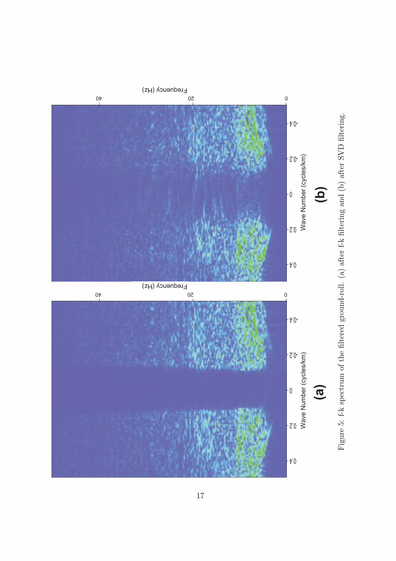
In order to compare f-k spectra of the three shot gathers, they were muted,

as shown in Fig. 3. The corresponding f-k spectra in Fig. 4 show the severe

cut-off characteristic of the f-k filter. The spectra of the f-k filtered ground

roll are shown in Fig. 5. From the two last figures one can see that the

f-k filter separates the input data in two separate regions of the f-k domain

(as expected). The SVD filter has a less dramatic effect, leaving estimated

signal in the larger wave-number domain, and it reduces noise also in the low

wave-number domain.

The three shot-point gathers in Fig. 2 are shown in Fig. 6 after the removal

of NMO correction. The effect of f-k filtering and SVD filtering are similar as

seen in the NMO corrected gathers. The SVD filter seems to have removed

noise in a better way than the f-k filter, preserving the character of the data.

The two filtering procedures were applied to the complete NMO corrected

data set before stacking. Details from the resulting stacked sections are shown

in Fig. 7. Both f-k filtering and SVD filtering have reduced the noise. And

again, the SVD filtered section has less smear and more character than the f-k

filtered section.

7

Conclusions

We have developed a new and efficient SVD filter method which enhances

horizontal events on seismic sections. The SVD filter process preserves the

character and frequency content of the horizontal reflections and attenuate all

other types of events. The method was successfully applied to ground roll

attenuation on a land seismic data set. In particular, ground roll was virtually

absent from the filtered pre-stack gathers. f-k filtering of the same data set

also removed the ground roll, but it resulted in loss of lateral variation in the

data.

Acknowledgements

The authors wish to express their gratitude to FINEP, FAPESB and CNPq,

Brazil, for financial support. We also thanks PARADIGM, LANDMARK,

SEISMIC-MICRO TECHNOLOGY and Schulumberger for the licenses granted

to CPGG-UFBA. Bjorn Ursin has received financial support from the VISTA

project and from the Norwegian Research Council through the ROSE project.

8

References

Anstey, N. 1986. Whatever happened to ground-roll?. The Leading Edge, 5,

40-46.

Bekara, M. and Baan, M. V, 2007, Local singular value decomposition for signal

enhancement of seismic data: Geophysics, 72, V59-V65.

Brown, M., and R. G. Clapp, 2000, (T-x) domain, pattern-based ground-roll re-

moval: 70th Ann. Internat. Mtg., Soc. Expl. Geophys., Expanded Abstracts,

2103-2106.

Chiu, S. K. and Howell, J. E., 2008, Attenuation of coherent noise using localized-

adaptive eigenimage filter: 78th Ann. Internat. Mtg., Soc. Expl. Geophys.,

Expanded Abstracts, 2541-2545.

Claerbout, J. F. 1983. Ground roll and radial traces: Stanford Exploration

Project Report, SEP-35, 43-53.

Eiras, J. F. and Kinoshita, E. M., 1990, Geologia e perspectivas petrolıferas da

Bacia do Tacutu, Origem e Evolucao das Bacias Sedimentares: PETROBRAS,

Anais, 197-220.

Embree, P., Burg, J. P. e Backus, M. M., 1963, Wide-band velocity filtering -

the pie-slice process: Geophysics, 28, 948-974.

Deighan, A. J. and Watts, D. R., 1997, Ground-roll suppression using the wavelet

transform: Geophysics 62, 1896-1903.

Freire, S. L. M., and T. J. Ulrych, 1988, Application of singular value decompo-

sition to vertical seismic profiling: Geophysics, 53, 778-785.

Golub, G. H., and C. F. V. Loan, 1996, Matrix computations: Johns Hopkins

University Press.

9

Harlan, W. S., Claerbout J. F. and Rocca F., 1984, Signal/noise separation and

velocity estimation: Geophysics, 49, 1869-1880.

Henley, D. C., 2003, Coherent noise attenuation in the radial trace domain:

Geophysics, 68, 1408-1416.

Karsli, H. and Bayrak, Y., 2008, Ground-roll attenuation based on Wiener filter-

ing and benefits of time-frequency imaging: The Leading Edge, 27, 206-209.

Kendall R., Jin, S., Ronen, S., 2005, An SVD-polarization filter for ground roll

attenuation on multicomponent data: 77th Ann. Internat. Mtg., Soc. Expl.

Geophys., Expanded Abstracts, 928-932.

Liu, X, 1999, Ground roll suppression using the Karhunen-Loeve transform:

Geophysics 64, 564-566.

Melo, P. E. M., Porsani, M. J. and Silva, M. G, 2009, Ground roll attenuation

using a 2D time derivative filter: Geophysical Prospecting. Received May

2007, revision accepted July 2008.

Montagne, R., and Vasconcelos, G. L., 2006, Optimized suppression of coherent

noise from seismic data using the karhunen-Loeve transform: Physical Review

E., 74, 1-9.

Pritchett, W., 1991, System design for better seismic data: The Leading Edge,

11, 30-35.

Saatcilar, R. and Canitez, N., 1988, A method of ground-roll elimination: Geo-

physics 53, 894-902.

Shieh, C. and Herrmann, R. B., 1990, Ground roll: Rejection using polarization

filters: Geophysics, 55, 1216-1222.

Tyapkin, Y. K., Marmalyevskyy, N. Y. and Gornyak, Z. V., 2003, Source-

generated noise attenuation using the singular value decomposition: 75th Ann.

10

Internat. Mtg. Soc. Expl. Geophys., Expanded Abstracts.

Wiggins, R. A., 1966, W-K Filter design: Geophysical Prospecting, 14, 427-440.

Yarham, C., Boeniger, U. and Herrmann, F., 2006, Curvelet-based ground roll

removal: 76th Ann. Internat. Mtg., Soc. Expl. Geophys., Expanded Ab-

stracts, 2777-2780.

11

Figures

FIG. 1. Sliding window SVD filtering scheme.

FIG. 2. Comparison of SVD filtering with f-k filtering. (a) input data, (b)

output after f-k filtering, (c) output after SVD filtering.

FIG. 3. Muted seismograms preserving the ground-roll area. (a) muted input

data, (b) after f-k filtering, (c) after SVD filtering.

FIG. 4. f-k spectrum of the muted original and filtered seismograms shown

in Fig. 3. (a) input data, (b) f-k filtering, (c) SVD filtering.

FIG. 5. f-k spectrum of the filtered ground-roll. (a) after f-k filtering and (b)

after SVD filtering.

FIG. 6. Comparison of SVD filtering with f-k filtering after inverse NMO

correction. (a) input data, (b) output after f-k filtering, (c) output after SVD

filtering.

FIG. 7. Details from the stacked sections: (a) original data (b) f-k filtered

data, (c) SVD filtered data.

12

Figure 1: Sliding window SVD filtering scheme.

13

0

0.5

1.0

1.5

2.0

2.5

3.0

3.5

4.0

Time(s)

2040

6080

Tra

ces

(a)

0

0.5

1.0

1.5

2.0

2.5

3.0

3.5

4.0

2040

6080

Tra

ces

(b)

0

0.5

1.0

1.5

2.0

2.5

3.0

3.5

4.0

2040

6080

Tra

ces

(c)

Fig

ure

2:C

ompar

ison

ofSV

Dfilt

erin

gw

ith

f-k

filt

erin

g.(a

)in

put

dat

a,(b

)ou

tput

afte

rf-

kfilt

erin

g,(c

)ou

tput

afte

rSV

Dfilt

erin

g.

14

0

0.5

1.0

1.5

2.0

2.5

3.0

3.5

4.0

Time(s)

2040

6080

Tra

ces

(a)

0

0.5

1.0

1.5

2.0

2.5

3.0

3.5

4.0

2040

6080

Tra

ces

(b)

0

0.5

1.0

1.5

2.0

2.5

3.0

3.5

4.0

2040

6080

Tra

ces

(c)

Fig

ure

3:M

ute

dse

ism

ogra

ms

pre

serv

ing

the

grou

nd-r

oll

area

.(a

)m

ute

din

put

dat

a,(b

)af

ter

f-k

filt

erin

g,(c

)af

ter

SV

Dfilt

erin

g.

15

Fig

ure

4:f-

ksp

ectr

um

ofth

em

ute

dor

igin

alan

dfilt

ered

seis

mog

ram

ssh

own

inF

ig.

3.(a

)in

put

dat

a,(b

)f-

kfilt

erin

g,(c

)SV

Dfilt

erin

g.

16

Fig

ure

5:f-

ksp

ectr

um

ofth

efilt

ered

grou

nd-r

oll.

(a)

afte

rf-

kfilt

erin

gan

d(b

)af

ter

SV

Dfilt

erin

g.

17

0

0.5

1.0

1.5

2.0

2.5

3.0

3.5

4.0

Time(s)

2040

6080

Tra

ces

(a)

0

0.5

1.0

1.5

2.0

2.5

3.0

3.5

4.0

2040

6080

Tra

ces

(b)

0

0.5

1.0

1.5

2.0

2.5

3.0

3.5

4.0

2040

6080

Tra

ces

(c)

Fig

ure

6:C

ompar

ison

ofSV

Dfilt

erin

gw

ith

f-k

filt

erin

gaf

ter

inve

rse

NM

Oco

rrec

tion

.(a

)in

put

dat

a,(b

)ou

tput

afte

rf-

kfilt

erin

g,(c

)ou

tput

afte

rSV

Dfilt

erin

g.

18

1.5

1.8

2.0

2.2

2.5

2.8

3.0

Tim

e(s)

20 21 22 23 24 25Distance (Km)

(a)

1.5

1.8

2.0

2.2

2.5

2.8

3.0

Tim

e(s)

20 21 22 23 24 25Distance (Km)

(b)

1.5

1.8

2.0

2.2

2.5

2.8

3.0

Tim

e(s)

20 21 22 23 24 25Distance (Km)

(c)

Figure 7: Details from the stacked sections: (a) original data (b) f-k filtereddata, (c) SVD filtered data.

19