ADAPTIVE FILTERING ALGORITHMS FOR ACOUSTIC ECHO ...

KU LEUVEN

FACULTEIT INGENIEURSWETENSCHAPPEN

DEPARTEMENT ELEKTROTECHNIEK

AFDELING ESAT-STADIUS

Kasteelpark Arenberg 10 – B-3001 Leuven

ADAPTIVE FILTERING ALGORITHMS FOR

ACOUSTIC ECHO CANCELLATION AND

ACOUSTIC FEEDBACK CONTROL IN

SPEECH COMMUNICATION APPLICATIONS

Promotoren:

Prof. dr. ir. M. Moonen

Prof. dr. ir. T. van Waterschoot

Prof. dr. ir. S. H. Jensen

Proefschrift voorgedragen

tot het behalen van de

graad van Doctor in de

Ingenieurswetenschappen

door

Jose Manuel GIL-CACHO

December 2013

KU LEUVEN

FACULTEIT INGENIEURSWETENSCHAPPEN

DEPARTEMENT ELEKTROTECHNIEK

AFDELING ESAT-STADIUS

Kasteelpark Arenberg 10, B-3001 Heverlee

ADAPTIVE FILTERING ALGORITHMS FOR

ACOUSTIC ECHO CANCELLATION AND

ACOUSTIC FEEDBACK CONTROL IN

SPEECH COMMUNICATION APPLICATIONS

Jury:

Prof. dr. A. Bultheel, chairman

Prof. dr. ir. M. Moonen, promotor

Prof. dr. ir. T. van Waterschoot, co-promotor

Prof. dr. ir. S. H. Jensen, promotor

(Aalborg University, Denmark)

Prof. dr. ir. J. Swevers, assessor

Prof. dr. ir. J. Wouters, assessor

Prof. dr. ir. S. Gannot

(Bar Ilan University, Israel)

Prof. dr. ir. P. C. W. Sommen

(Eindhoven University of Technology, The

Netherlands)

Proefschrift voorgedragen

tot het behalen van de

graad van Doctor in de

Ingenieurswetenschappen

door

Jose Manuel GIL-CACHO

December 2013

c©2013 KU LEUVEN, Groep Wetenschap & Technologie,Arenberg Doctoraatsschool, W. de Croylaan 6, 3001 Heverlee, Belgie

Alle rechten voorbehouden. Niets uit deze uitgave mag vermenigvuldigd en/ofopenbaar gemaakt worden door middel van druk, fotokopie, microfilm, elektro-nisch of op welke andere wijze ook zonder voorafgaande schriftelijke toestem-ming van de uitgever.

All rights reserved. No part of the publication may be reproduced in any formby print, photoprint, microfilm, electronic or any other means without writtenpermission from the publisher.

ISBN 978-94-6018-758-2

D/2013/7515/143

Voorwoord

A five-year journey has come to an end and I am finally ready to write thepreface for my PhD thesis. At this moment, I just want to express my gratitudeand countless thanks to all of those who have helped me during my PhD.

I would like to thank Prof. Marc Moonen for giving me the opportunity tojoin his research group, for his guidance and good ideas. I remember our firstmeeting when I was asking for this opportunity. Although I sometimes thoughtthat he regretted his decision, he gave me freedom to choose my own way andalways showed respect for my own ideas. I learned lots of things from him,some of them worth keeping my entire life.

In that difficult task of finding my own way, Prof. Toon van Waterschoot hasbeen essential all these years. I remember my first ever conference paper, whichhe encouraged me to write. The fact that he was interested in the idea wassomething truly motivating. After that conference paper, everything startedto be easier. We had very interesting discussions and more ideas came afterthat. I deeply thank him for all those evening he spent proofreading my messypapers and for becoming a friend. The support and feedback from Prof. SørenHoldt Jensen has without any doubt been very helpful. His suggestions forimprovement on my papers were always very much appreciated. My deepestgratitude to the jury members: Prof. Adhemar Bultheel, Prof. Jan van Wou-ters, Prof. Jan Swevers, Prof. Sharon Gannot and Prof. Piet C. W. Sommenfor their time, effort, and valuable comments and suggestions to improve mythesis.

I would like to thank Prof. Johan Shoukens for the time I spent in the ELECdepartment of the Vrije Universiteit Brussels. He introduced me to the excitingworld of nonlinear system identification and honestly I could not imagine thisthesis without his initial guidance. I would like to thanks Prof. Johan Suykensfor bringing the idea of kernel adaptive filtering and to Dr. Marco Signorettofor collaborating with me on this idea. Thanks to them, an important part ofthis thesis (and my first ever published journal) has been possible.

i

To the research group at the KU Leuven and to the people in the SIGNALproject, thank you all for the many travels, the courses we had together andfor the inspiring discussions. Thanks to Dr. Alexander Bertrand (Belly) forbeing my guarding angel all these years. For reminding me all bank holidays,how to ask for a refund, how to book a room, how to re-enroll (every year)and a long etc. I am afraid that without him I was still trying to loggingto the intranet. Thanks to almost-Dr. Joseph Szurley (Joe) for being mybrocito in a period of my life when I really needed it. The middle-life middle-PhD crisis came together at once, however making fun of the same things andsharing great moments with Joe was indeed healing. Thanks to Bruno for beingmy Dutch translator, to Amin, Giuliano, Giacomo, Niccolo, Rodolfo, Marijn,Aldona, Paschalis, Rodrigo, Kim and Javi. Thanks a lot to Ida for doing allthose things that I forgot to do in the most inconvenient moment, without herI would not be here. Thanks of course to all the administrative staff.

I would like to thanks my mother for telling me since I was a kid ’you can doit’, to my father for teaching me to stay alert from myself and to my sister formaking me feel special. Thanks to my boyfriend for reminding me how funlife can be, to my friends for making things easier and full of joy and relativesto encourage me to continue. Thanks to my wife Ines for her endless love andpatience, for always being my best friend, for understanding when I had to workduring the weekends, for cheering me up when life was difficult, for sharing thefun of big moments, for always having a moment for me and for showing methat nothing can go wrong if we are together. Thank you also for having ourson Jose, the most beautiful thing on earth (after this thesis).

Jose, every day you make me understand the actual meaning of infinity.

Jose Manuel Gil-Cacho Leuven, December 2013

ii

Abstract

Multimedia consumer electronics are nowadays everywhere from teleconferenc-ing, hands-free communications, in-car communications to smart TV applica-tions and more. We are living in a world of telecommunication where idealscenarios for implementing these applications are hard to find. Instead, practi-cal implementations typically bring many problems associated to each real-lifescenario. This thesis mainly focuses on two of these problems, namely, acousticecho and acoustic feedback. On the one hand, acoustic echo cancellation (AEC)is widely used in mobile and hands-free telephony where the existence of echoesdegrades the intelligibility and listening comfort. On the other hand, acousticfeedback limits the maximum amplification that can be applied in, e.g., in-carcommunications or in conferencing systems, before howling due to instability,appears. Even though AEC and acoustic feedback cancellation (AFC) are func-tional in many applications, there are still open issues. This means that manyof the issues associated to practical AEC and AFC are overlooked. In thisthesis, we contribute to the development of a number of algorithms to tacklethe main issues associated to AEC and AFC namely, (1) that very long roomimpulse responses (RIRs) make standard adaptive filters converge slowly andlead to a high computational complexity, (2) that double-talk (DT) situationsin AEC and model mismatch in AFC distort the near-end signal , and (3) thatthe nonlinear response of some of the elements forming part of the audio chainmakes linear adaptive filters fail.

In the view of computational complexity reduction, we consider introducingthe concept of common-acoustical-pole room modeling into AEC. To this end,we perform room transfer function (RTF) equalization by compensating for themain acoustic resonances common to multiple RTFs in the room. We discussthe utilization of different norms (i.e., 2-norm and 1-norm) and models (i.e.,all-pole and pole-zero) for RTF modeling and equalization. A computation-ally cheap extension from single-microphone AEC to multi-microphone AEC isthen presented for the case of a single loudspeaker. The RTF models used formulti-microphone AEC share a fixed common denominator polynomial, whichis calculated off-line by means of a multi-channel warped linear prediction.This allows high computational savings. In the context of acoustic feedback

iii

control, we develop a method for acoustic howling suppression based on adap-tive notch filters (ANF) with regularization (RANF). This method achievesfrequency tracking, howling suppression and improved howling detection in aone-stage scheme. The RANF approach to howling suppression introduces min-imal processing delay and minimal complexity, in contrast to non-parametricblock-based methods that feature a non-parametric frequency analysis in atwo-stage scheme.

To tackle the issue of robustness to double-talk (DT) in AEC and robustnessto model mismatch in AFC, a new adaptive filtering framework is proposed.It is based on the frequency-domain adaptive filtering (FDAF) implementationof the so-called PEM-AFROW (FDAF-PEM-AFROW) algorithm. We showthat FDAF-PEM-AFROW is related to the best, i.e., minimum-variance, lin-ear unbiased estimate (BLUE) of the echo path. We derive and define theinstantaneous pseudo-correlation (IPC) measure between the near-end signaland the loudspeaker signal. The IPC measure serves as an indication of theeffect of a DT situation occurring during adaptation due to the correlationbetween these two signals. Based on the good results obtained using FDAF-PEM-AFROW, we derive a practical and computationally efficient algorithmfor DT-robust AEC and for AFC. The proposed algorithm features two modifi-cations in the FDAF-PEM-AFROW: (a) the WIener variable Step sizE (WISE),and (b) the GRAdient Spectral variance Smoothing (GRASS), leading to theWISE-GRASS-FDAF-PEM-AFROW. The WISE modification is implementedas a single-channel noise reduction Wiener filter where the Wiener filter gainis used as a variable step size in the adaptive filter. On the other hand, theGRASS modification aims at reducing the variance in the noisy gradient esti-mates based on time-recursive averaging of instantaneous gradients.

In the last part of this thesis, the nonlinear response of (active) loudspeak-ers forming part of the audio chain is studied. We consider the descriptionof odd and even nonlinearities in (active) loudspeakers by means of periodicrandom-phase multisine signals. The fact that the odd nonlinear contributionsare more predominant than the even ones implies that at least a 3rd-ordernonlinear model of the loudspeaker should be used. Therefore, we consider theidentification and validation of a model of the loudspeaker using several linear-in-the-parameters nonlinear adaptive filters, namely, Hammerstein and Leg-endre polynomial filters of various orders, and a simplified 3rd-order Volterrafilter of various lengths. In our measurement set-up, the obtained results implyhowever, that a 3rd-order nonlinear filter fails to capture all the nonlinearities,meaning that odd and even nonlinear contributions are produced by higher-order nonlinearities. High-order Volterra filters are impractical in AEC andAFC due to their large computational complexity together with inherentlyslow convergence. On the other hand, the kernel affine projection algorithm(KAPA) has been successfully applied to many areas in signal processing butnot yet to nonlinear AEC (NLAEC). In KAPA, and kernel methods in general,

iv

the kernel trick is applied to work implicitly in a high-dimensional (possiblyinfinite-dimensional) space without having to transform the input data intothis space. This is one of the most appealing characteristics of kernel methods,as opposed to nonlinear adaptive filters requiring explicit nonlinear expansionsof the input data as, for instance, Volterra filters. In fact, all computationscan be done by evaluating the kernel function in the input space. This factprovides powerful modeling capabilities to kernel adaptive algorithms wherethe computational complexity will be determined by the input dimension, in-dependent of the order of the nonlinearity. Our contributions in this contextare to apply KAPA to the NLAEC problem, to develop a sliding-window leakyKAPA (SWL-KAPA) that is well suited for NLAEC applications, and to pro-pose a suitable kernel function, consisting of a weighted sum of a linear and aGaussian kernel.

v

Korte Inhoud

Multimedia-consumentenelektronica is dezer dagen overal te vinden, voor toe-passingen zoals teleconferentie, handenvrije communicatie, voertuigcommuni-catie, en intelligente TV. We leven in een wereld van telecommunicatie, waarideale scenario’s om deze toepassingen te implementeren zelden voorkomen.Praktische implementaties daarentegen brengen typisch vele problemen mee,gekoppeld aan het realistische scenario waarin men zich bevindt. Dit docto-raatsproefschrift richt zich voornamelijk op twee van deze problemen, namelijk,akoestische echo en akoestische feedback. Aan de ene kant wordt akoestische-echo-onderdrukking (AEC) op grote schaal aangewend in mobiele en handen-vrije telefonie, waar de aanwezigheid van echo’s de verstaanbaarheid en hetluistercomfort aantast. Aan de andere kant begrenst akoestische feedback demaximale versterking die kan worden toegepast in bv. voertuigcommunicatie ofin teleconferentie, vooraleer fluittonen optreden door instabiliteit. Hoewel AECen akoestische-feedback-onderdrukking (AFC) functioneel zijn in vele toepas-singen, bestaan er nog een aantal open problemen. Dit betekent dat vele vande problemen gekoppeld aan praktische AEC- en AFC-systemen tot nog toeover het hoofd worden gezien. Dit doctoraatsproefschrift draagt bij tot de ont-wikkeling van een aantal algoritmen die de belangrijkste problemen gekoppeldaan AEC en AFC aanpakken, namelijk, (1) dat zeer lange kamerimpulsres-ponsies (RIRs) de standaard adaptieve filters trager doen convergeren en toteen hoge rekencomplexiteit leiden, (2) dat situaties met dubbelspraak (DT) inAEC en modelafwijkingen in AFC het microfoonsignaal vervormen en (3) datde niet-lineaire responsie van sommige elementen in de audio-keten de werkingvan lineaire adaptieve filters doet mislukken.

Met het oog op een reductie van de rekencomplexiteit, introduceren we het con-cept van kamermodellering via gemeenschappelijke-akoestische-polen in AEC.Hiertoe voeren we een egalisatie van de kamerakoestische overdrachtsfunctie(RTF) uit door de belangrijkste akoetische resonanties te compenseren die ge-meenschappelijk zijn voor meerdere RTFs binnen de kamer. We bespreken hetgebruik van verschillende normen (nl. 2-norm en 1-norm) en modellen (nl.enkel-polen en pool-nulpunt) voor de modellering en egalisatie van RTFs. Ver-volgens wordt een uitbreiding met lage rekencomplexiteit voorgesteld van AEC

vii

met n microfoon naar AEC met meerdere microfoons voor het geval van eenenkele luidspreker. De RTF-modellen gebruikt voor AEC met meerdere micro-foons delen een vaste gemeenschappelijke noemerveelterm, die off-line berekendwordt via een meerkanaals verdraaide lineaire predictie. Dit laat aanzienlijkebesparingen in rekencomplexiteit toe. In de context van akoestische-feedback-beheersing, ontwikkelen we een methode voor akoestische fluittoononderdruk-king gebaseerd op adaptieve inkepingsfilters (ANF) met regularisatie (RANF).Deze methode bewerkstelligt frequentietracking, fluittoononderdrukking en eenverbeterde fluittoondetectie in een n-staps-schema. De RANF-aanpak voorfluittoononderdrukking introduceert een minimale vertraging en heeft een mi-nimale rekencomplexiteit, in tegenstelling tot niet-parametrische venstergeba-seerde methodes, die een niet-parametrische frequentieanalyse uitvoeren in eentwee-staps-schema.

Om het probleem van situaties met dubbelspraak (DT) in AEC en het probleemvan robuustheid tegen modelafwijkingen in AFC op te lossen, wordt een nieuwadaptief-filter-raamwerk voorgesteld. Het is gebaseerd op de adaptieve filteringfrequentiedomeinimplementatie (FDAF) van het zogenaamde PEM-AFROW(FDAF-PEM-AFROW) algoritme. We tonen aan dat FDAF-PEM-AFROWgerelateerd is met de beste, d.i. de minimale-variantie, lineaire zuivere schat-ting (BLUE) van het echo-pad. We definiren de instantane pseudo-correlatie(IPC) tussen het microfoonsignaal en het luidsprekersignaal. De IPC-maatgeeft een indicatie van het effect van een DT-situatie die tijdens de adap-tatie voorkomt door de correlatie tussen deze twee signalen. Op basis vande goede resultaten verkregen met FDAF-PEM-AFROW, leiden we een prak-tisch en efficint algoritme af voor DT-robuuste AEC en voor AFC. Het voorge-stelde algoritme bevat twee wijzigingen ten opzichte van FDAF-PEM-AFROW:(a) de Wiener variabele stapgrootte (WISE), en (b) de gradint spectrale va-riantie smoothing (GRASS), die samen leiden tot het WISE-GRASS-FDAF-PEM-AFROW-algoritme. De WISE-wijziging is gemplementeerd als een nka-naals Wiener-ruisonderdrukkingsfilter, waarbij de Wiener-filterversterking aan-gewend wordt als variabele stapgrootte in het adaptieve filter. Anderzijds heeftde GRASS-wijziging als doel om de variantie in de ruizige gradintschattingente verkleinen door middel van een tijdsrecursieve uitmiddeling van instantanegradinten.

In het laatste deel van dit doctoraatsproefschrift wordt de niet-lineaire res-ponsie bestudeerd van (actieve) luidsprekers die deel uitmaken van de audio-keten. We beschouwen de beschrijving van oneven en even niet-lineariteitenin (actieve) luidsprekers door middel van periodische multisine-signalen metwillekeurige fase. Het feit dat de oneven niet-lineaire bijdragen de even niet-lineaire bijdragen overheersen, impliceert dat een niet-lineair luidsprekermo-del van minstens derde orde moet gebruikt worden. Daarom beschouwen wede identificatie en validatie van een luidsprekermodel via verschillende niet-lineaire adaptieve filters die lineair zijn in de parameters, nl. Hammerstein

viii

en Legendre veelterm-filters van verschillende ordes, alsook een vereenvoudigdVolterra-filter van derde orde met verschillende lengtes. Resultaten verkregenvia onze meetopstelling impliceren evenwel dat een niet-lineair filter van derdeorde er niet in slaagt alle niet-lineariteiten te vatten, wat betekent dat one-ven en even niet-lineaire bijdragen geproduceerd worden door niet-lineariteitenvan hogere ordes. Volterra filters van hogere ordes zijn niet praktisch voorAEC en AFC omwille van hun hoge rekencomplexiteit en hun inherent trageconvergentie. Anderzijds is het kernel-affiene-projectie-algoritme (KAPA) metsucces toegepast in verscheidene signaalverwerkingsdomeinen, maar nog niet inniet-lineaire AEC (NLAEC). Bij KAPA, en kernel-methodes in het algemeen,wordt de kernel-truc toegepast om impliciet in een hoog-dimensionale (moge-lijk oneindig-dimensionale) ruimte te werken, zonder daarom de ingangsdatanaar deze ruimte te moeten transformeren. Dit is n van de meest aantrekkelijkekenmerken van kernel-methodes, in tegenstelling tot niet-lineaire adaptieve fil-ters, die een expliciete niet-lineaire expansie van de ingangsdata vereisen, zoalsbijv. Volterra-filters. Dit bezorgt kernel-adaptieve algoritmes krachtige mo-delleringsmogelijkheden, aangezien de rekencomplexiteit bepaald wordt doorde ingangsdimensie, onafhankelijk van de orde van de niet-lineariteit. In dezecontext bestaat onze bijdrage uit het toepassen van KAPA op het NLAEC-probleem, uit het ontwikkelen van een glijdend-venster lekke KAPA (SWL-KAPA), die geschikt is voor NLAEC-toepassingen, en uit het voorstellen vaneen gepaste kernel-functie, die bestaat uit een gewogen som van een lineaire eneen Gaussiaanse kernel.

ix

Glossary

Acronyms and Abbreviations

(K)APA (Kernel) Affine Projection Algorithm(N)LMS (Normalized) Least Mean Squares(NL)AEC (Nonlinear) Acoustic Echo Cancellation(R)LS (Recursive) Least SquaresA/D Analog-to-DigitalAFC Acoustic Feedback CancellationAFROW AFC using Row OperationsANF Adaptive Notch FilterANSI American National Standards InstituteAR Auto RegressiveAttmax Maximum AttenuationAttmean Mean AttenuationBLUE Best Linear Unbiased EstimatorCAP Common Acoustical PolesCPSD Cross power spectral densityCPZLP Constrained Pole-Zero Linear PredictionCVX Disciplined Convex ProgrammingD/A Digital-to-AnalogdB DecibelDFT Discrete Fourier TransformDT Double TalkDTD Double Talk DetectorERB Equivalent Rectangular BandwidthERLE Echo Return Loss EnhancementFDAF Frequency-Domain Adaptive FilterFFT Fast Fourier TransformFIR Finite Impulse ResponseFLOPS Floating-point Operations Per SecondFRF Frequency Response FunctionGLS Generalized Least SquaresGRASS Gradient Spectral Variance Smoothing

xi

HA Hearing aidsHz HertzIDFT Inverse DFTIFFT Inverse FFTIIR Infinite Impulse ResponseIPC Instantaneous pseudo-correlationkHz KilohertzLEM Loudspeaker-Enclosure-MicrophoneLNLR Linear-to-Nonlinear RatioLP Linear PredictionLPC Linear Prediction CodingMA Moving AverageMAE Mean Absolute ErrorMSD MisadjustmentMSG Maximum Stable GainNHS Notch-Filter-Based Howling SuppressionNPVSS Non-Parametric VSSPA Public addressPCVSS Projection-Correlation VSSPE Prediction ErrorPEM Prediction Error MethodPSD Power Spectral DensityPVSS Practical VSSRANF Regularized Adaptive Notch FilterRHS Right Hand SideRIR Room Impulse ResponseRTF Room Transfer FunctionROW Row OperationsSD Sparseness DegreeSDmax Maximum Frequency-Weighted

Log-Spectral Signal DistortionSDmean Mean Frequency-Weighted

Log-Spectral Signal DistortionSER Signal-to-Echo RatioSF Spectral FlatnessSNR Signal-to-Noise RatioSW Sliding WindowTD-NLMS Transform-Domain NLMSVoIP Voice over IPVR Variable RegularizationVSS Variable Step SizeWGN White Gaussian NoiseWISE Wiener Variable Step SizeWLP Warped Linear PredictionWLS Weighted Least Squares

xii

e.g. exempli gratia: for examplei.e. id est : that isw.r.t with respect to

Mathematical notation

Common notation

Scalars: small italic letters, α, d(i)Vectors: small bold letters, w, ω, c(i)Vectors: small letters with explicit index,

ek(i), k = 1, .., PMatrices: capital BOLD letters, U(i), Φ(i)Matrices: capital letters with explicit indexes,

G(P−k+1,P−j+1)(i), k, j = 1, .., PTime dependency: Indexes in parentheses, u(i), d(i)Vector entry: Subscript indexes, aj(i− 1), ek(i)Linear Spaces: Capital LATEX ’mathbb’ letters, F, HScalar constants: Capital ITALIC letters, L, Nq−1 time shift operator‖·‖p p-norm

◦ element-wise multiplicationRL L-dimensional real spaceO(·) of the order of a numberJ(·) cost functionI identity matrixF{·} FFT operatorF−1{·} inverse FFT operatorE{·} expectation operator(·)T transpose operation(·)H conjugate and transpose operationA−1 inverse of matrix A[·]a:b range from a to b elements in a vector

Chapter 2

p(k) kth common polezi(k, t) kth distinct ith zero at time ta(k) kth common AR coefficientbi(k, t) kth distinct ith MA coefficient at time tHi(q, t) ith RTF at time tQ order of numerator (zeros)P order of denominator (poles)

xiii

v matrix of RIRW compound matrixWi Toeplitz matrix made with ith RIRx coefficient vectorp order of the normhi ith measured RIRa AR coeffients from measured RIRbi MA coefficients from measured RIRD selective matrixA(q) filter polynomial in q

Bi(q) residual RTF

A(q) approximately A−1(q)R(n) residual RIRP (f) magnitude of fth frequencyN DFT sizeT threshold

Chapter 3

x(t) input/loudspeaker signalyi(t) ith echo signald(t) desired/microphone signale(t) error signalyi(t) ith estimated echo signalHi(q) ith RTFBi(q) model numerator polynomial in qAc(q) model common denominator polynomial in qpc(k) kth common poleac(k) kth common AR coefficientD(q, λ) first-order all-pass filterλ warping parameterHwi (q) ith warped RTF

hwi (t) ith all-pole-estimated warped impulse responseawc (k) kth warped common AR coefficientM number of AECs (channels)a vector of warped common AR coefficientW matrix of Toeplitz matrices

from measured and warped RIRv matrix of measured and warped RIRhwi measured and warped RIRHi Toeplitz matrix of measured and warped RIR

bi(t), Bi(q, t) ith channel’s adaptive filter coefficientsN RIR length

xiv

n ERLE time indexi channel index

Chapter 4

w0 radial notch frequencyf0 notch frequencyfs sampling frequencyr pole radiusH(q) notch filter transfer functiona(n) instant frequency updating parameteru(n) filter statet(n) filter statex(n) input signal to RANFy(n) output signal from RANF∆a(n) gradient (search direction)i index of RANFλ regularization parameter∇f frequency differenceT thresholdSy(f) spectrum of y(n)Sx(f) spectrum of x(n)L buffer size in decision rule

Chapter 5

f(t), F (q, t) estimated echo path

F(k) DFT estimated echo path

f(t) echo path due to DT

F(k) DFT echo path due to DTu(t) input/loudspeaker signalu(t) input/loudspeaker signal vectorx(t) estimated echo signalx(t) echo signalv(t) near-end signale(t) error signaly(t) microphone signal

ya[t, h(t)] prefiltered microphone signal using h(t)

ua[t, h(t)] prefiltered loudspeaker signal using h(t)

ea[t, h(t), f(t− 1)] prefiltered error signal using h(t)

e[t, f(t)] error signal calculated with f(t)

xv

e(t) error signal vectorea(t) prefiltered error signal vectorya prefiltered microphone signal vector

x[t, f(t)] estimated echo signal calculated with f(t)f (true) echo path model parametersy vector of microphone signal samplesv vector of near-end signal samplesX Toeplitz matrix of loudspeaker samples

fGLS estimated echo path coefficientsminimizing a GLS criterion

fBLUE estimated echo path coefficientsminimizing a BLUE criterion

FBLUE DFT estimated echo path coefficientsminimizing a BLUE criterion

fLS estimated echo path coefficientsminimizing a LS criterion

M weighting matrix in GLSMPEM weighting matrix in BLUE in PEMRv near-end signal autocorrelation matrixw(t) near-end excitation signal (white noise)H(q, t) near-end signal model parameterA(q, t) inverse near-end signal model parameter

A(q, t) estimated inverse near-end signal prefilterH(q) matrix of near-end signal model parameters

at different time instantsw vector of near-end signal excitation

at different time instantsak(t) kth autoregressive model parametera(t) estimated AR model parameter vectornA near-end signal model and prefilter orderk matrix indexWPEM near-end excit. signal variance diag. matrixσw(t) near-end excitation signal varianceσw(t) estimated near-end excitation signal varianceUa input DFT vectorEa prefiltered error DFT vectorz(t) IPC measure signalr(k) concatenated error signal vectorsG normalization factorSUa

input PSD estimateSEa

prefilter error PSD estimateΘ DFT grad. estimateP window size to calculate AR coefficientsK APA order

xvi

N filter lengthM DFT sizeeo(t) ‘ideal’ error signale(t) error signal due to DTα regularization parameterαVR variable regularizationµPVSS VSS in PVSSµPCVSS VSS in PCVSSµ0 fixed (maximum) step sizeµ′ VSS aux. variable in PCVSSλ0 PSD forgetting factorβ0 Corr. forgetting factorC correlation vector in PCVSS

Chapter 6

f(t), F (q, t) estimated echo pathu(t) input/loudspeaker signalx(t) estimated echo signalx(t) echo signalv(t) near-end signale(t) error signal

ya[t, h(t)] prefilter microphone signal using h(t)

ua[t, h(t)] prefilter loudspeaker signal using h(t)

ea[t, h(t), f(t− 1)] prefilter error signal using h(t)

e[t, f(t)] error signal calculated with f(t)n(t) near-end noise signalw(t) near-end model excitation signalH(q, t) near-end modelA(q, t) inverse near-end auto-regressive modelnA order near-end modelϑ(t) model system

ϑ(t) estimated model parametersf(t) acoustic path model parametersa(t) near-end signal model systema(t) near-end signal estimated coefficientsnF order acoustic path modelnF order acoustic path model estimatesσ2w(t) estimate of the near-end signal excitation variance

v(t) time-domain (TD) near-end signal vectoru(t) TD input signal vectorn(t) TD near-end noise signal vectory(t) TD microphone signal vector

xvii

N estimated RIR lengthM size of FFT or FD filter lengthk block-time indexL total length of the signalsP block length to estimate A(q, t)Ea(m, k) scalar frequency-domain prefiltered error signalm time/frequency index in length-M vectorK forward path gainEa(m, k) length-M FD prefiltered error signalea(k) length-M TD error signal after prefilteringva(k) length-M TD prefiltered near-end signalna(k) length-M TD prefiltered near-end noise signalya(k) length-M TD prefiltered microphone signalU(k) length-M FD input signal

F(k) length-M FD adaptive filter coeff.Θ(k) GRASSθ(m, k) length-M FD (noisy) gradient estimateθ0(k) length-M FD true gradientθ(k) length-M FD gradient noiseφ(k) TD aux. gradient variableµ(k) length-M normalization factor in FDAFW(k) WISE coefficientsµmax maximum allowed step-sizeENR(t) echo noise ratio variableσ2n(t) near-end noise signal varianceσ2x(t) echo signal varianceσ2v(t) near-end speech signal varianceY (m, k) FD microphone signalX(m, k) FD echo signalV (m, k) FD near-end speech signalD(m, k) FD disturbance signalW0(m, k) FD noise-reduction Wiener filterPXY (m, k) CPSD of X(m, k) and Y(m,k)PY (m, k) power spectral density of and Y (m, k)PX(m, k) power spectral density of and X(m, k)PD(m, k) power spectral density of and D(m, k)∇(m, k) recursive gradient power estimateα(m, k) gradient estimate phase

PUa(m, k) recursive PSD estimate of and Ua(m, k)

PXa(m, k) recursive PSD estimate of and Xa(m, k)

PDa(m, k) recursive PSD estimate of and Da(m, k)

ˆENR(m, k) estimated frequency-domain ENR

Pθ0(m, k) estimate of the true gradient PSD

λ1 forgetting factor WISE: desired signal

xviii

λ2 forgetting factor WISE: noise signalλ3 forgetting factor GRASSQ APA ordern one realization of a WGN processδ small number to avoid division by zerof1 original RIR coefficientsf2 synthesized RIR coefficientsΦ(k) WISE-GRASS time-domain gradient constraint

Chapter 7

u(t) input signalf [u(t)] nonlinear function of the input signaly(t) echo signal: output of a nonlinear systemy(t) estimated echo signald(t) microphone signaln(t) noise signale(t) error signalH(q, t) linear acoustic echo path model

H(q, t) estimated echo path modelbk time-domain deterministic amplitude

of the kth harmonicak frequency-domain deterministic amplitude

of the kth harmonicF number of harmonicsω0 fundamental radial frequencyf0 fundamental frequencyk harmonic indexik harmonic valuesφk realization of independent uniformly distributed

random processes on [0,2π]U(jωk) frequency-domain input signal of a

nonlinear systemY (jωk) frequency-domain output signal of a

nonlinear systemG(jωk) measured FRF of nonlinear system

G(jwk) =Y (jwk)

U(jwk)G0(jωk) true underlying linear systemGB(jωk) systematic nonlinear contributionGS(jωk) stochastic nonlinear contributionGBLA(jωk) best linear approximation (BLA) of the

nonlinear system

xix

GBLA(jωk) estimated BLA

G[q](jωk) FRF data averaged over P periodsσ2G[q]

(jwk) sample variance averaged over P periods

σ2GBLA

(jwk) total variance

σ2GBLA,n

(jwk) noise variance

var [GS(jwk)] stochastic nonlinear contribution varianceP number of periodsQ number of phase realizations

Y (jωk) averaged output spectrumK harmonic grid parameteryf linear-in-the-parameters nonlinear

filter outputhF linear-in-the-parameters nonlinear

filter modeluF linear-in-the-parameters nonlinear

filter inputhr linear-in-the-parameters nonlinear

filter model sub-vectorur linear-in-the-parameters nonlinear

filter input sub-vector

hF estimated linear-in-the-parametersnonlinear filter model coefficients

L nonlinear filter lengthM order of nonlinearityε small regularization termh(n) linear filter coefficientsgm amplitude of nonlinear terms

Hammerstein and LegendreLm [u(t)] mth-order Legendre nonlinear expansionLH Hammerstein filter total lengthLL Legendre polynomial filter total lengthLSV simplified Volterra filter total lengthh1(n1) linear filter coefficients in Volterra filterhm(n1, ..., nm) mth Volterra kernel coefficientsLV Volterra filter total lengthV2K simplified 2nd-order Volterra kernelV3K simplified 3rd-order Volterra kernelNd simplified Volterra kernel size parameters

Chapter 8

< ·, · > inner productP APA projection order

xx

‖·‖2 2-norm of a vectorL Input dimension in tapsF dimension in the feature spaceu(i) input (loudspeaker) signal vectorU(i) input (loudspeaker) signal matrixd(i) desired (microphone) signald(i) desired signal vectorh room impulse response (true filter weights)

h(i) weight vector estimate in an Euclidean spaceat iteration i

D storage memory (dictionary size)a(i) expansion coefficients vectorX(i) set of input vectors (dictionary)ϕ(·) a mapping induced by a reproducing kernelϕ(i) transformed input (vector in a feature space)Φ(i) transformed input APA matrixκ(i, j) kernel evaluationG(i) Gram matrixF feature space induced by the kernel mappingω(i) filter weights estimate in a feature space

at iteration iκΣ weighted sum of kernelsκL linear kernelκG Gaussian kernelα weight of κL in κΣ

β weight of κG in κΣ

µ step-size KAPAλ regularization factorδ forgetting factor LSRuu sample covariance matrixrud sample cross-covariance vector

Ruu approximate covariance matrixrud approximate cross-covariance vectorz auxiliary vector

xxi

Contents

Voorwoord i

Abstract iii

Korte Inhoud vii

Glossary xi

Contents xxiii

I Introduction

1 Introduction and Overview 3

1.1 Fundamentals of adaptive filtering . . . . . . . . . . . . . . . . 4

1.1.1 Objective function . . . . . . . . . . . . . . . . . . . . . 4

1.1.2 Adaptive transversal filters . . . . . . . . . . . . . . . . 4

1.1.3 Minimum MSE . . . . . . . . . . . . . . . . . . . . . . . 5

1.2 Adaptive algorithms . . . . . . . . . . . . . . . . . . . . . . . . 7

1.2.1 (Normalized) Least mean squares algorithm . . . . . . . 7

1.2.2 Recursive least squares algorithm . . . . . . . . . . . . . 8

1.2.3 Spectral dynamic range and misadjustment . . . . . . . 9

xxiii

1.3 Frequency-domain and transform-domainadaptive filters . . . . . . . . . . . . . . . . . . . . . . . . . . . 11

1.3.1 Frequency-domain adaptive filters . . . . . . . . . . . . 11

1.3.2 Transform-domain adaptive filters . . . . . . . . . . . . 13

1.4 Problem statement . . . . . . . . . . . . . . . . . . . . . . . . . 15

1.4.1 Acoustic Echo Cancellation . . . . . . . . . . . . . . . . 15

1.4.2 Acoustic Feedback Control . . . . . . . . . . . . . . . . 17

1.5 Outline of the thesis . . . . . . . . . . . . . . . . . . . . . . . . 19

Bibliography . . . . . . . . . . . . . . . . . . . . . . . . . . . . . . . 24

II Room Acoustics Modeling

2 Estimation of acoustic resonances for room transfer functionequalization 29

2.1 Introduction . . . . . . . . . . . . . . . . . . . . . . . . . . . . . 31

2.2 Pole estimation using different norms . . . . . . . . . . . . . . . 33

2.3 Results from measured impulse responses . . . . . . . . . . . . 35

2.4 Conclusions . . . . . . . . . . . . . . . . . . . . . . . . . . . . . 40

Bibliography . . . . . . . . . . . . . . . . . . . . . . . . . . . . . . . 40

3 Multi-Microphone acoustic echo cancellation using warped multi-channel linear prediction of common acoustical poles 43

3.1 Introduction . . . . . . . . . . . . . . . . . . . . . . . . . . . . . 45

3.2 Proposed Model . . . . . . . . . . . . . . . . . . . . . . . . . . 46

3.2.1 Common-acoustical-pole and zero model . . . . . . . . . 46

3.2.2 Warped linear prediction . . . . . . . . . . . . . . . . . 47

3.2.3 Warped multi-channel linear prediction of common acous-tical poles . . . . . . . . . . . . . . . . . . . . . . . . . . 49

3.3 Adaptive Algorithm . . . . . . . . . . . . . . . . . . . . . . . . 51

xxiv

3.4 Simulation Results . . . . . . . . . . . . . . . . . . . . . . . . . 52

3.4.1 Comparison of ERLE with and without warping . . . . 52

3.4.2 Prefilter in the adaptive signal path . . . . . . . . . . . 53

3.4.3 Prefilter in the loudspeaker signal path . . . . . . . . . 54

3.5 Conclusion . . . . . . . . . . . . . . . . . . . . . . . . . . . . . 56

Bibliography . . . . . . . . . . . . . . . . . . . . . . . . . . . . . . . 57

III Linear Adaptive Filtering

4 Regularized adaptive notch filters for acoustic howling sup-pression 61

4.1 Introduction . . . . . . . . . . . . . . . . . . . . . . . . . . . . . 63

4.2 Notch-filter-based howling suppression . . . . . . . . . . . . . . 64

4.2.1 Non-parametric frequency estimation . . . . . . . . . . . 64

4.2.2 Adaptive Notch filters . . . . . . . . . . . . . . . . . . . 65

4.3 Regularized Adaptive Notch Filters . . . . . . . . . . . . . . . . 66

4.4 Results . . . . . . . . . . . . . . . . . . . . . . . . . . . . . . . . 69

4.4.1 Speech signal . . . . . . . . . . . . . . . . . . . . . . . . 70

4.4.2 Music signal . . . . . . . . . . . . . . . . . . . . . . . . . 70

4.5 Conclusion . . . . . . . . . . . . . . . . . . . . . . . . . . . . . 75

4.A RANF regularization parameter λ . . . . . . . . . . . . . . . . 76

Bibliography . . . . . . . . . . . . . . . . . . . . . . . . . . . . . . . 78

5 A frequency-domain adaptive filter (FDAF) prediction errormethod (PEM) framework for double-talk-robust acoustic echocancellation 79

5.1 Introduction . . . . . . . . . . . . . . . . . . . . . . . . . . . . . 81

5.2 Best linear unbiased estimate . . . . . . . . . . . . . . . . . . . 85

5.2.1 Linear unbiased estimator . . . . . . . . . . . . . . . . . 85

xxv

5.2.2 Generalized least squares and BLUE . . . . . . . . . . . 86

5.3 The BLUE in adaptive filtering algorithms . . . . . . . . . . . . 86

5.3.1 PEM-based BLUE . . . . . . . . . . . . . . . . . . . . . 87

5.3.2 FDAF-based BLUE . . . . . . . . . . . . . . . . . . . . 88

5.4 Instantaneous pseudo-correlation measure . . . . . . . . . . . . 89

5.5 The FDAF-PEM-AFROW algorithm . . . . . . . . . . . . . . . 92

5.6 Simulation results . . . . . . . . . . . . . . . . . . . . . . . . . 94

5.6.1 Choice of the FDAF-PEM-AFROW algorithm . . . . . 94

5.6.2 Results from VSS algorithms . . . . . . . . . . . . . . . 97

5.6.3 Complexity analysis . . . . . . . . . . . . . . . . . . . . 100

5.7 Conclusion . . . . . . . . . . . . . . . . . . . . . . . . . . . . . 100

5.A Instantaneous pseudo-correlation calculation . . . . . . . . . . . 105

Bibliography . . . . . . . . . . . . . . . . . . . . . . . . . . . . . . . 107

6 Wiener variable step size and gradient spectral variance smooth-ing for double-talk-robust acoustic echo cancellation and acous-tic feedback cancellation 111

6.1 Introduction . . . . . . . . . . . . . . . . . . . . . . . . . . . . . 113

6.1.1 The problem of double-talk in acoustic echo cancellation 114

6.1.2 The problem of correlation in acoustic feedback cancellation116

6.1.3 Contributions and outline . . . . . . . . . . . . . . . . . 117

6.2 Prediction error method . . . . . . . . . . . . . . . . . . . . . . 118

6.3 Proposed WISE-GRASS Modifications in FDAF-PEM-AFROWfor AEC/AFC . . . . . . . . . . . . . . . . . . . . . . . . . . . . 121

6.3.1 WIener variable Step sizE . . . . . . . . . . . . . . . . . 121

6.3.2 GRAdient Spectral variance Smoothing . . . . . . . . . 125

6.4 Evaluation . . . . . . . . . . . . . . . . . . . . . . . . . . . . . . 126

6.4.1 Competing algorithms and tuning parameters . . . . . . 128

xxvi

6.4.2 Performance measures . . . . . . . . . . . . . . . . . . . 130

6.4.3 Simulation results for DT-robust AEC . . . . . . . . . . 130

6.4.4 Simulation results for AFC . . . . . . . . . . . . . . . . 137

6.5 Conclusion . . . . . . . . . . . . . . . . . . . . . . . . . . . . . 138

Bibliography . . . . . . . . . . . . . . . . . . . . . . . . . . . . . . . 143

IV Nonlinear Adaptive Filters

7 Linear-in-the-parameters nonlinear adaptive filters for acousticecho cancellation 149

7.1 Introduction . . . . . . . . . . . . . . . . . . . . . . . . . . . . . 151

7.2 Excitation signal and response of nonlinear systems . . . . . . . 154

7.3 Detection of nonlinear distortions . . . . . . . . . . . . . . . . . 156

7.4 Estimating the level of the nonlinear noise source . . . . . . . . 157

7.4.1 Analysis method . . . . . . . . . . . . . . . . . . . . . . 158

7.4.2 Results and discussion . . . . . . . . . . . . . . . . . . . 159

7.5 Classification of nonlinearities . . . . . . . . . . . . . . . . . . . 161

7.5.1 Analysis method . . . . . . . . . . . . . . . . . . . . . . 161

7.5.2 Results and discussion . . . . . . . . . . . . . . . . . . . 162

7.6 Linear-in-the-parameters nonlinear adaptive filters . . . . . . . 163

7.6.1 Adaptive algorithm . . . . . . . . . . . . . . . . . . . . . 164

7.7 Nonlinear filters without cross terms . . . . . . . . . . . . . . . 164

7.7.1 Hammerstein filters . . . . . . . . . . . . . . . . . . . . 164

7.7.2 Filters based on orthogonal polynomials . . . . . . . . . 165

7.8 Nonlinear filters with cross terms . . . . . . . . . . . . . . . . . 166

7.8.1 Volterra filters . . . . . . . . . . . . . . . . . . . . . . . 166

7.8.2 Simplified 3rd-order Volterra kernel . . . . . . . . . . . 167

xxvii

7.9 Simulated Hammerstein system identification . . . . . . . . . . 168

7.10 Loudspeaker identification . . . . . . . . . . . . . . . . . . . . . 170

7.11 Conclusions . . . . . . . . . . . . . . . . . . . . . . . . . . . . . 174

Bibliography . . . . . . . . . . . . . . . . . . . . . . . . . . . . . . . 177

8 Nonlinear Acoustic Echo Cancellation based on a Sliding-WindowLeaky Kernel Affine Projection Algorithm 181

8.1 Introduction . . . . . . . . . . . . . . . . . . . . . . . . . . . . . 183

8.2 Linear and Kernel APA . . . . . . . . . . . . . . . . . . . . . . 186

8.2.1 Linear APA . . . . . . . . . . . . . . . . . . . . . . . . . 186

8.2.2 Kernel Methods . . . . . . . . . . . . . . . . . . . . . . 189

8.2.3 Leaky APA in the Feature Space . . . . . . . . . . . . . 190

8.2.4 Leaky KAPA . . . . . . . . . . . . . . . . . . . . . . . . 191

8.3 Sliding-Window Leaky KAPA for Nonlinear AEC . . . . . . . . 192

8.3.1 Pruning by Use of a Sliding Window . . . . . . . . . . . 192

8.3.2 Weighted Sum of Kernels . . . . . . . . . . . . . . . . . 194

8.3.3 Sliding-Window Leaky KAPA . . . . . . . . . . . . . . . 195

8.4 Evaluation . . . . . . . . . . . . . . . . . . . . . . . . . . . . . . 195

8.4.1 Simulated Nonlinear System . . . . . . . . . . . . . . . . 195

8.4.2 Competing Filters: Hammerstein and Volterra . . . . . 197

8.4.3 Simulation Results . . . . . . . . . . . . . . . . . . . . . 198

8.4.4 Computational Complexity . . . . . . . . . . . . . . . . 203

8.5 Conclusions . . . . . . . . . . . . . . . . . . . . . . . . . . . . . 204

8.A Derivation of leaky KAPA . . . . . . . . . . . . . . . . . . . . . 205

Bibliography . . . . . . . . . . . . . . . . . . . . . . . . . . . . . . . 209

xxviii

V Conclusions

9 Conclusions and Suggestions for Future Research 217

9.1 Conclusions . . . . . . . . . . . . . . . . . . . . . . . . . . . . . 217

9.2 Future research . . . . . . . . . . . . . . . . . . . . . . . . . . . 222

Publication List 223

xxix

Part I

Introduction

Chapter 1

Introduction and Overview

THIS chapter introduces the fundamental principles of adaptive filtering.The commonly used adaptive filter structures and algorithms, as well as

practical applications employing adaptive filters are described. All problemsand difficulties encountered in time-domain adaptive filters are extensively dis-cussed. In this thesis, only discrete-time implementations of adaptive filters aretaken into account. It is, therefore, assumed that continuous-time signals, takenfrom the real world, are properly sampled, i.e., at least at twice their highest fre-quency, so that the Nyquist or sampling theorem is satisfied [1], [2], [4], [5], [19].The reader can find extensive discussions on general adaptive signal process-ing in many reference textbooks [4], [5], [13], [16]. Nowadays, adaptive filteringfinds practical applications in several fields such as communications, biomedicalengineering, control, radar, sonar, navigation, seismology, etc. In this chapter,we consider two of the state-of-the-art applications where adaptive filters arewidely used, namely acoustic echo cancellation and acoustic feedback controlapplications. The main characteristics of these applications are outlined interms of issues that a typical adaptive filter implementation would encounter.This chapter also gives a brief introduction to frequency-domain adaptive fil-ters that are computationally more efficient for applications that need longerfilter lengths, and are more effective when there is a high correlation in theinput signal. For instance, to cancel the acoustic echo in hands-free telephony,high-order adaptive filters are needed. However, high-order adaptive filters, to-gether with a highly correlated input signal, weakens the performance of mosttime-domain adaptive filters [6], [14], [16], [18].

3

1.1 Fundamentals of adaptive filtering

A filter, in general, may be seen as a system that extracts or enhances desiredinformation contained in a signal. If we want to process information in anunknown and changing environment, an adaptive filter is needed [13]. Typi-cally, an adaptive filter has an associated adaptive algorithm for updating filtercoefficients.

An adaptive algorithm adjusts the filter coefficients (or tap weights) in relationto the signal conditions and performance criterion (or quality assessment). Atypical performance criterion is based on the error signal e(n), which is thedifference between the filter output signal and the reference (or desired) signal[5], [16].

1.1.1 Objective function

The complexity and performance of the adaptive algorithm is affected by thedefinition of the objective function. We may list the following forms of objectivefunctions which are widely used in the derivation of adaptive algorithms:

• Mean Squared Error (MSE): J [e(n)] = E{e2(n)}.• Mean Absolute Error (MAE): J [e(n)] = E{|e(n)|}.• Sum of Squared Errors (SSE): J [e(n)] =

∑ni=1 e

2(i).• Weighted Sum Squared Error (WSSE): J [e(n)] =

∑ni=1 λ

n−ie2(i), with0 << λ < 1.

• Instantaneous Squared Error (ISE): J [e(n)] = e2(n).

where E{·} is the expectation operator. In a strict sense, the MSE functionis only of theoretical value, due to the infinite amount of information thatis required to be measured. This ideal objective function, in practice, canbe approximated by the SSE, WSSE, or ISE functions. These functions leadto filters that differ in the computational complexity and in the convergencecharacteristics. Generally, the ISE function is cheaper to implement but itexhibits noisy convergence properties [5], [16]. The SSE function is favorableto be used in stationary environments, whereas in slowly varying environments,the WSSE is much better suited.

1.1.2 Adaptive transversal filters

An adaptive filter is a self-designing and time-varying system, which employs arecursive algorithm, in order to adjust its tap weights in an unknown environ-ment. Figure 1.1 illustrates a typical structure of an adaptive filter, consistingof two basic blocks: (1) a digital filter to perform the desired filtering and (2)an adaptive algorithm to adjust the tap weights of the filter [5], [16]. An adap-

4

z−1 z−1 z−1

w0(n) w1(n) w2(n) wM−2(n)

u(n) u(n− 1) u(n− 2) u(n−M + 1)

y(n)

wM−1(n)

Figure 1.1: Transversal FIR adaptive filter.

tive filter computes the output signal y(n) in response to the input signal u(n).The error signal e(n) is then generated by comparing y(n) with the desired re-sponse d(n). An adaptive algorithm adjusts the tap weights based on the errorsignal e(n) (also called the performance feedback signal). In this section, weonly consider real-valued signals and real-valued tap weights. Many differentstructures can be used to realize the digital filter, e.g., lattice, infinite impulseresponse (IIR), finite impulse response (FIR). Figure 1.1 shows the commonlyused transversal FIR filter.

The adjustable tap weights, wm(n), m = 0, 1, ...,M − 1 (indicated by circleswith arrows through them) are the filter tap weights at time n and M is thefilter length. These time-varying tap weights form an M × 1 weight vectorexpressed as

w(n) = [w0(n), w1(n), ..., wM−1(n)]T (1.1)

where the superscript (·)T denotes the transpose operation. Similarly, the inputsignal samples, u(n−m), m = 0, 1, ...,M − 1, form an M × 1 input vector

u(n) = [u(n), u(n− 1), ..., u(n−M + 1)]T . (1.2)

The output signal y(n) of the adaptive FIR filter, with these vectors, can becomputed as the inner product of w(n) and u(n) given as

y(n) =

M−1∑m=0

wm(n)u(n−m) = wT (n)u(n). (1.3)

1.1.3 Minimum MSE

The difference between the desired signal d(n) and the filter output signal y(n),expressed as

e(n) = d(n)−wT (n)u(n) (1.4)

5

01

23

4−4

−3−2

−10

0

5

10

15

20

w1w

0

Figure 1.2: Error surface.

is the error signal e(n). The weight vector w(n) is updated recursively suchthat the error signal e(n) is minimized. The minimization of the MSE functionis regularly used as a performance criterion (or cost function), which is givenas

JMSE = E{e2(n)} (1.5)

For a given weight vector w = [w0, w1, ..., wM−1]T with stationary input signalu(n) and desired response d(n), the MSE can be calculated from (1.4) and (1.5)as

JMSE = E{d2(n)} − 2pTw + wTRw, (1.6)

where R ≡ E{u(n)uT (n)} is the input autocorrelation matrix andp ≡ E{d(n)u(n)} is the cross-correlation vector between the desired signal andthe input vector. The MSE is treated as a stationary function, hence the timeindex n has been dropped from the vector w(n) in (1.6). The MSE in (1.6)is a quadratic function of the tap weights [w0, w1, ..., wM−1] since they onlyappear in first and second degrees. Figure 1.2 shows a typical performance (orerror) surface for a two-tap transversal filter. A single global minimum MSEcorresponding to the optimum vector wo is therefore guaranteed to exist in aquadratic performance surface when considering a transversal FIR filter. Wecan obtain the optimum solution by taking the first derivative of (1.6) withrespect to w and setting the derivative to zero. This leads to the well-knownWiener-Hopf equations [5]

Rwo = p. (1.7)

6

If we assume R is invertible, the optimum weight vector is given as

wo = R−1p. (1.8)

By substituting (1.8) into (1.6), the minimum MSE corresponding to the opti-mum weight vector is obtained as

Jmin = E{d2(n)} − pTwo. (1.9)

1.2 Adaptive algorithms

An adaptive algorithm is a set of recursive equations that automatically adjustthe weight vector w(n) in order to minimize the objective function. Ideally,the weight vector converges to the optimum solution wo corresponding to thebottom of the performance surface, i.e. the minimum MSE Jmin.

1.2.1 (Normalized) Least mean squares algorithm

The most widely used adaptive algorithm is the least mean squares (LMS) al-gorithm [19] because of its robustness and simplicity [4]. Based on the steepest-descent method, using the negative gradient of the ISE function, i.e. J ≈ e2(n),the LMS algorithm weight update equation is written as

w(n+ 1) = w(n) + µu(n)e(n) (1.10)

with µ the convergence factor (or step size), that determines the stability andthe convergence rate of the algorithm.

The LMS algorithm uses, as shown in (1.10), a recursive approach for adjustingthe tap weights in the direction of the optimum Wiener-Hopf solution given in(1.7). The step size is chosen in the range

0 < µ <2

λmax(1.11)

to guarantee the stability of the algorithm, where λmax is the largest eigenvalueof the input autocorrelation matrix R. The sum of the eigenvalues (i.e., thetrace of R) is used instead of λmax. Accordingly, the step size is in the range of

0 < µ <2

trace(R). Taking into account that trace(R) = MPu is related to the

average power Pu of the input signal u(n), a common step size bound [5], [16]is obtained as

0 < µ <2

MPu. (1.12)

Convergence of the MSE for Gaussian input signals typically requires 0 < µ <2/3MPu [5]. Moreover, as shown in (1.12), for a larger filter length M a smaller

7

step size µ is used to prevent instability. We may also highlight that the stepsize is inversely proportional to the input signal power Pu. Consequently, asignal with high Pu must use a smaller step size, while a low-power signal canuse a larger step size. We may incorporate this relationship into the LMSalgorithm just by normalizing the step size with respect to the input signalpower. This type of normalization of the step size leads to a useful and widelyused variant of the LMS algorithm, the well-known normalized LMS (NLMS)algorithm [5].

The NLMS algorithm includes an additional normalization term uT (n)u(n) as

w(n+ 1) = w(n) + µu(n)

uT (n)u(n) + εe(n), (1.13)

where the step size is now bounded in the range 0 < µ < 2 and ε is a small reg-ularization term to prevent division by zero. It is worth noting that the NLMSalgorithm may also be derived as the solution to a constrained optimizationproblem formulating the principle of minimum disturbance [5], or as a memberof the underdetermined-order recursive least squares (URLS) family [28]. Whennormalizing the input vector u(n) the convergence rate becomes independentof the signal power. There is no significant difference between the convergenceperformance of the LMS and NLMS algorithms for stationary signals providedthat the step size of the LMS algorithm is properly chosen. The benefit ofthe NLMS algorithm only becomes clear for nonstationary signals like speech,where significantly faster convergence for the same level of steady-state MSEcan be achieved [4], [13], [16].

Assuming all the signals and tap weights are real-valued, the transversal FIRfilter requires M multiplications to produce the output y(n) and the updateequation (1.10) requires (M + 1) multiplications. Therefore, the adaptive FIRfilter with the LMS algorithm requires a total of (2M + 1) multiplicationsper iteration. On the other hand, the NLMS algorithm requires an additional(M + 1) multiplications for the normalization term, giving a total of (3M + 2)multiplications per iteration. The computational complexity of the LMS andNLMS algorithms is hence proportional to M , which is expressed as O(M).

1.2.2 Recursive least squares algorithm

Contrary to the (N)LMS algorithm, the recursive least squares (RLS) algorithm[5] is derived from the minimization of the WSSE

JLS(n) =

n∑i=1

λn−ie2(i), (1.14)

where 0 << λ < 1 is the forgetting factor. Indeed, in nonstationary envi-ronments, the forgetting factor weights the current error more than the past

8

error values. In this sense, the LS weight vector w(n) is optimized based onthe observation starting from the first iteration (i = 1) to the current iteration(i = n). It should be noted that the LS solution can be expressed as a specialcase of the Wiener-Hopf solution defined in (1.7), i.e,

w = R−1(n)p(n) (1.15)

where the autocorrelation matrix and cross-correlation vector are defined re-spectively as

R ≈ R(n) =

n∑i=1

λn−iu(i)uT (i) (1.16)

and

p ≈ p(n) =

n∑i=1

λn−id(i)u(i). (1.17)

By using the matrix inversion lemma, the RLS algorithm can be written as

w(n+ 1) = w(n) + g(n)e(n) (1.18)

where the updating gain vector is defined as

g(n) =r(n)

1 + uT (n)r(n)(1.19)

andr(n) = λ−1P(n− 1)u(n). (1.20)

The inverse input autocorrelation matrix, P(n) ≡ R−1(n), can also be com-puted recursively as

P(n) = λ−1P(n− 1)− g(n)rT (n). (1.21)

Due to the fact that both the NLMS and RLS algorithms converge to the sameoptimum weight vector (under stationarity and ergodicity conditions), thereis a strong link between them [7]. The computational complexity of the RLSalgorithm is O(M2), hence it is more expensive to implement than NLMS.On the other hand, the RLS algorithm typically converges much faster thanNLMS. There are diverse efficient versions of the RLS algorithm, including thefast transversal filter with reduced complexity O(M), but unfortunately thesefast algorithms suffer from instability issues [16].

1.2.3 Spectral dynamic range and misadjustment

The convergence behavior of the LMS algorithm is associated with the eigen-value spread of the autocorrelation matrix R which is defined by the charac-teristics of the input signal u(n). The eigenvalue spread is measured by the

9

condition number defined as κ (R) = λmax/λmin, where λmax and λmin arethe maximum and minimum eigenvalues, respectively. In addition, the condi-tion number depends on the spectral distribution of the input signal [13] and isbounded by the spectral dynamic range of the input power spectrum Puu

(ejω)

as

κ (R) ≤ maxω Puu(ejω)

minω Puu (eω)(1.22)

where maxω Puu(ejω)

and minω Puu(ejω)

are the maximum and minimumvalues of the input power spectrum, respectively. For white input signals, theideal condition number κ (R) = 1 is obtained. The convergence speed of theLMS algorithm decreases for increasing spectral dynamic range [4]. Frequency-domain and transform-domain adaptive filters will be introduced in Section 1.3as to improve the convergence rate when the input signal has a high spectraldynamic range (i.e., is highly correlated).

A time constant that defines the convergence rate of the MSE [4] may be writtenas

τm =1

2µλm, m = 0, 1, ...,M − 1. (1.23)

where λm is the mth eigenvalue. Therefore, the smallest eigenvalue λmin de-termines the slowest convergence. Despite the fact that a large step size canresult in faster convergence, it must be upper bounded by (1.10).

In practice, due to the use of the instantaneous squared error by the LMSalgorithm, the weight vector w(n) deviates from the optimum weight vector wo

in the steady state. As a result, after the algorithm has converged, the MSEin the steady state is greater than the minimum MSE Jmin. The differencebetween the steady-state MSE J(∞) and Jmin is called the excess MSE, and itis expressed as Jex = J(∞)− Jmin. We may also define the misadjustment as

M =JexJmin

=µ

2MPu (1.24)

The misadjustment is proportional to the step size, which in turn translates ina tradeoff between the misadjustment and the convergence rate given in (1.23).The misadjustment is normally defined as a percentage and has a typical valueof 10% for most applications. A small step size results in a slow convergence,but has the advantage of smaller misadjustment, and vice versa. Under theassumption that all the eigenvalues are equal, (1.23) and (1.24) are related bythe following simple expression

M =M

4τm(1.25)

Consequently, for achieving a small value of misadjustment, a long filter requiresa long time τm.

10

The transversal FIR filter shown in Figure 1.1 is the most commonly usedadaptive structure. This structure operates in the time domain and can be im-plemented in either the sample or the block processing mode [15], [16]. However,the time-domain LMS-type adaptive algorithms, associated with the FIR filter,suffers from high computational cost, when applications (such as acoustic echocancellation) demand a high-order filter and slow convergence when the inputsignal is highly correlated.

1.3 Frequency-domain and transform-domainadaptive filters

In this section, we describe the frequency-domain and transform-domain adap-tive filters [6], [8], [12], [16]. The advantages of these adaptive filters are fastconvergence and low computational complexity. We highlight as well the dif-ferences between frequency-domain and transform-domain adaptive filters andthe relation between these filters.

1.3.1 Frequency-domain adaptive filters

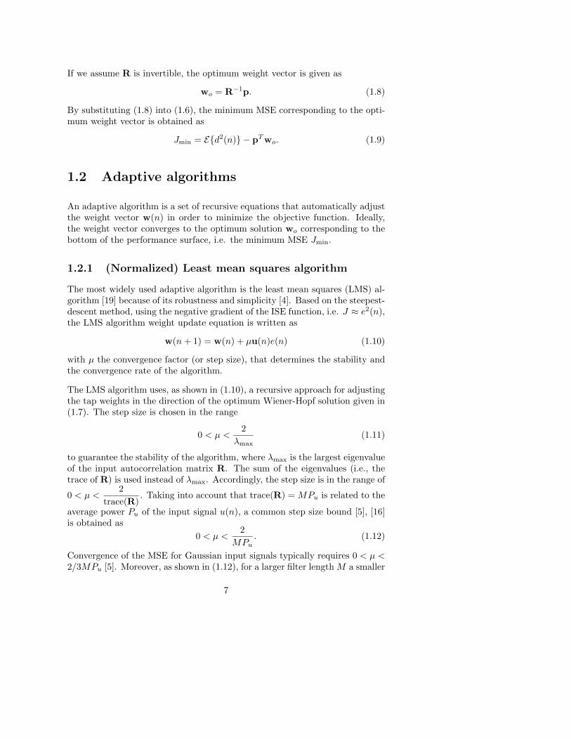
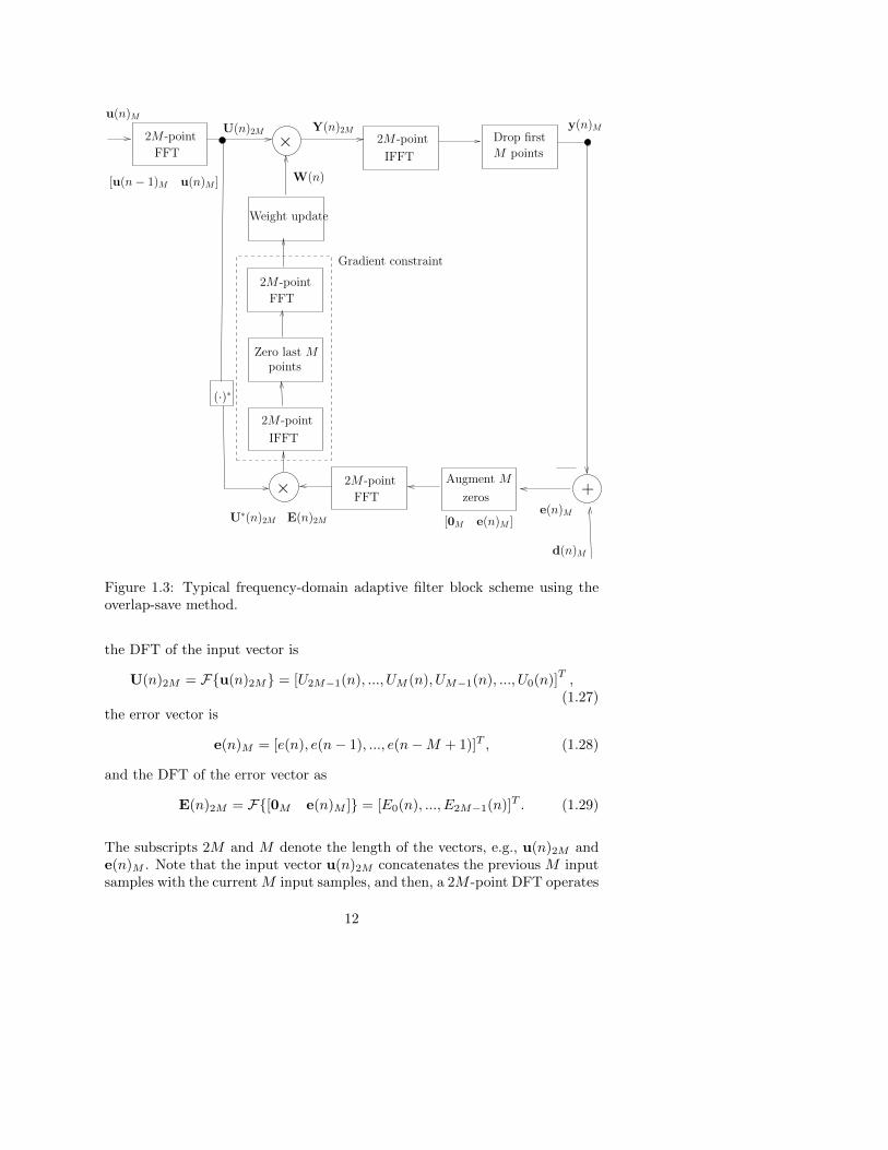
In a frequency-domain adaptive filter (FDAF) [8], [12] the desired signal d(n)and the input signal u(n) are transformed to the discrete frequency domain us-ing the discrete Fourier transform (DFT). FDAF performs frequency-domainfiltering and adaptation based on these transformed signals. As discussed inSections 1.1 and 1.1.2, the time-domain adaptive filter performs a linear con-volution (filtering) and linear correlation (weight updating) on a sample-by-sample basis. The FDAF performs a convolution and correlation on a block-by-block basis. In this way, substantial computational savings, especially forapplications that use high-order filters can be achieved. Unfortunately, thefrequency-domain operations result in circular convolution and circular correla-tion. Therefore, to overcome the error introduced by these circular operations,more complicated overlap-add or overlap-save methods [8], [12] are typicallyimplemented. These methods allow to obtain the correct linear convolutionand correlation results.

The block diagram of the FDAF using the fast LMS algorithm [8], [12] is shownin Figure 1.3. This algorithm uses the overlap-save method with 50% overlapand needs five 2M -point DFT/IDFT operations. This type of processing isknown as block processing, where the input vector is

u(n)2M = [u(n− 2M + 1), ..., u(n−M), u(n−M + 1), ..., u(n)]T , (1.26)

11

Zero last Mpoints

Weight update

2M -point

IFFT

2M -point

FFT

Augment M

zeros

Drop first

M points

2M -point

FFT

2M -point

IFFT

2M -point

FFT

(·)∗

×

+×

W(n)

Gradient constraint

U∗(n)2M E(n)2M

U(n)2M Y(n)2M y(n)M

e(n)M

d(n)M

u(n)M

[u(n− 1)M u(n)M ]

[0M e(n)M ]

Figure 1.3: Typical frequency-domain adaptive filter block scheme using theoverlap-save method.

the DFT of the input vector is

U(n)2M = F{u(n)2M} = [U2M−1(n), ..., UM (n), UM−1(n), ..., U0(n)]T,

(1.27)the error vector is

e(n)M = [e(n), e(n− 1), ..., e(n−M + 1)]T , (1.28)

and the DFT of the error vector as

E(n)2M = F{[0M e(n)M ]} = [E0(n), ..., E2M−1(n)]T . (1.29)

The subscripts 2M and M denote the length of the vectors, e.g., u(n)2M ande(n)M . Note that the input vector u(n)2M concatenates the previous M inputsamples with the current M input samples, and then, a 2M -point DFT operates

12

on this input vector resulting in the frequency-domain vector U(n)2M (i.e., a2M -point complex vector). The subscripts in the elements of a vector, e.g.,E0(n) and E2M−1(n), denote the entry number of the vector at time n. Wecan compute the output signal vector from the adaptive filter by taking theelement-wise multiplication between the input vector and the 2M -point weightvector as

Y(n) = W(n) ◦U(n), (1.30)

where ‘◦’ is the element-wise multiplication operator and

W(n) = [W0(n),W1(n), ...,W2M−1(n)]T (1.31)

is the complex-valued weight vector at time n.

In order to obtain the correct result using circular convolution, the frequency-domain output vector, Y(n) = [Y0(n), Y1(n), ..., Y2M−1(n)]T , is transformedback to the time domain using the inverse DFT (IDFT) and the firstM points ofthe 2M -point IDFT outputs are discarded to obtain the output vector y(n)M =[y(n), y(n − 1), ..., y(n −M + 1)]T . The output vector is subtracted from thedesired vector d(n) = [d(n), d(n − 1), ..., d(n −M + 1)]T to produce the errorsignal vector e(n)M . As shown in Figure 1.3, the error vector e(n) is thenaugmented with M zeros and transformed to the frequency-domain vector E(n)using the DFT.

We can express the complex weight update equation as

Wk(n+M) = Wk(n) + µ∇[U∗k (n)Ek(n)], k = 0, 1, ..., 2M − 1, (1.32)

where U∗k (n) is the complex conjugate of the frequency-domain signal Uk(n),and ∇[·] represents the operation of gradient constraint, which is explained asfollows. As shown in the ‘gradient constraint box’ in Figure 1.3, the weight-updating term [U∗k (n)Ek(n)] is inverse transformed, and the last M points areset to zero before taking the 2M -point DFT for the weight update equation.The so-called unconstrained FDAF [8] is an alternative where the gradientconstraint block is removed, thus producing a simpler implementation thatinvolves only three DFT operations [8], [12]. Unfortunately, this simplifiedalgorithm no longer produces a linear correlation between the transformed errorand input vectors, which results in poorer performance compared to the FDAFwith gradient constraints. The weight vector is not updated sample by sampleas in the time-domain LMS algorithm, but updated once for each block of Msamples. The FDAF typically features an input power normalization factor,similar to the NLMS, to ensure (approximately) equal convergence rate to allfrequency bins, hence the name FDAF-NLMS.

1.3.2 Transform-domain adaptive filters

As explained in Section 1.2, the eigenvalue spread of the input signal autocor-relation matrix plays an important role in determining the convergence speed

13

z−1 z−1 z−1u(n) u(n− 1) u(n− 2) u(n−M + 1)

y(n)

DFT/DCT with power normalization

W0(n) W1(n) W2(n) WM−2(n) WM−1(n)

Figure 1.4: Transform-domain adaptive filter using DFT/DCT with powernormalization.

of time-domain adaptive filters. Indeed, the convergence of the LMS algorithmis very slow when the input signal is highly correlated. In the literature, severalmethods have been developed to solve the problem of slow convergence due tohighly correlated input signals. One method is to use the RLS algorithm (seeSection 1.2). The RLS algorithm may be seen to extract past information fordecorrelating the present input signal. This approach suffers from high com-putational cost, poor robustness, and slow tracking ability in nonstationaryenvironments. Another method to improve convergence in the LMS algorithmis to decorrelate the input signal using a unitary transform such as the discreteFourier transform (DFT) or discrete cosine transform (DCT) [6], [15], [16]. Thetransform-domain NLMS (TD-NLMS) is also known as the self-orthogonalizingadaptive filter. Compared with the RLS approach, the self-orthogonalizingadaptive filter saves computational cost since it is independent of the charac-teristics of the input signal.

The TD-NLMS adaptive filter, shown in Figure 1.4, has a similar structureto the M−tap adaptive transversal filter shown in Figure 1.1, but with pre-processing (transform and normalization) on the input signal using the DFTor DCT, and thus named DFT-NLMS and DCT-NLMS. The transformationis performed on a sample-by-sample basis. The transformed signals Uk(n) arenormalized by the square root of its respective power in the transform domainas

U ′k(n) =Uk(n)√Pk(n) + ε

, k = 0, 1, ...,M − 1, (1.33)

14

where ε is a small regularization term to prevent division by zero, and Pk(n) isthe input power that can be estimated recursively as

Pk(n) = (1− λ)Pk(n− 1) + λU2k (n) (1.34)

Note that the power Pk(n) is updated recursively for every new input sampleand λ is a forgetting factor that is usually chosen as 1/M .

1.4 Problem statement

In this section, we consider two important and timely applications in whichadaptive filters have been widely used. The main characteristics of these ap-plications are outlined in terms of issues that a typical adaptive filter imple-mentation would encounter. From this perspective, we review the commonassumptions applying to each case.

1.4.1 Acoustic Echo Cancellation

The typical set-up for an acoustic echo canceler is depicted in Figure 1.5. A far-end speech signal u(n) is played back in an enclosure (i.e., the room) througha loudspeaker. In the room there is a microphone to record a near-end speechsignal which is to be transmitted to the far-end side. An acoustic echo pathbetween the loudspeaker and the microphone exists so that the microphonesignal y(n) = x(n)+v(n)+n(n) contains an undesired echo signal x(n) plus thenear-end speech signal v(n), generating a so-called double-talk (DT) situation,and the near-end noise signal n(n).

+-

+

path pathacoustic

From far-end

To far-end

cancellation

W

n(n)

e(n)

u(n)

v(n)

x(n)x(n)

y(n)

W

Figure 1.5: Typical set-up for AEC.

15

The echo signal x(n) can be considered as the loudspeaker signal u(n) filteredby the echo path. An acoustic echo canceler seeks to cancel the echo signalcomponent x(n) in the microphone signal y(n), ideally leading to an echo-freeerror signal e(n), which is then transmitted to the far-end side. This is done bysubtracting an estimate of the echo signal x(n) from the microphone signal, i.e.,e(n) = y(n)− x(n). Standard approaches to AEC rely on the assumption thatthe echo path can be modeled by a linear FIR filter [3], [14]. The coefficients ofthe echo path are collected in the parameter vector w = [w0, w1, , ..., wM−1]T

∈ RM such that x(n) = wTu(n) with u(n) = [u(n), u(n−1), . . . , u(n−M+1)]T .An adaptive filter of sufficient order is used to provide an estimate w(n) ∈ RMof w, such that the echo signal estimate is x(n) = wT (n)u(n).

The AEC task [3], [14] can be seen as a system identification task, thus, themain objective of an echo canceler is to identify a model that represents a bestfit to the echo path. Typically, ‘best’ in the LS sense is considered. Therefore,by (1.15) the echo path model estimate can be written as

w(n) = R−1(n)p(n) (1.35)

where

R(n) =

n∑i=1

λn−iu(n)uT (n) (1.36)

p(n) =

n∑i=1

λn−iy(n)u(n)

=

n∑i=1

λn−ix(n)u(n) +

n∑i=1

λn−i[v(n) + n(n)]u(n) (1.37)

One particular assumption in most AEC applications, is that the noise signaln(n) and the near-end signal v(n) are uncorrelated with the loudspeaker signalu(n). Consequently, the second term of the cross-correlation vector (1.37) tendsto zero and, then, w is an unbiased estimator minimizing the LS criterion.

There are many issues associated to practical AEC. In particular, long impulseresponses make (time-domain) adaptive filters converge slowly and increase theoverall computational complexity. The issue of regularization is also a matterof ongoing research [18]. Robustness to double-talk is obviously of vital impor-tance since it occurs 20% of the time in a normal conversation [29]. A recenttrend in consumer electronics is to utilize low-cost and small-sized analog com-ponents such as loudspeakers. These components usually have nonlinearities, sothe hope is to rely on signal processing algorithms to mitigate the nonlinear ef-fects. Nonlinearities can be roughly divided into two types: nonlinearities withand without memory. Nonlinearities with memory (or dynamic) usually occurin high-quality audio equipment where the time constant of the loudspeaker’selectro-mechanical system is large compared to the sampling rate [21]. Memo-ryless (or static) nonlinearities typically occur in low-cost power amplifiers and

16

loudspeakers [24]. The level of the nonlinearities depends on the quality of the(active) loudspeaker, although eventually any (active) loudspeaker suffers fromsignificant nonlinear distortion [17]. In AEC applications, nonlinear distor-tions are of great importance if the levels are high. As opposed to the situationwhen only background noise is present (i.e. where increasing the level of theloudspeaker signal will increase the SNR of the echo signal; hence improve theperformance of the AEC), if loudspeaker nonlinearities are present, increasingthe level of the input signal will also increase the level of the nonlinear echocomponent, which can be considered as an additional noise source. Thereforenonlinear adaptive filters are needed in AEC applications to account for nonlin-ear distortions. In the literature, second-order Volterra filters with memory aregenerally used [27]; however they can model only second-order nonlinearities.The use of third-order adaptive Volterra filters could become prohibitive inAEC applications [22], [23]. However it has been shown that some loudspeakernonlinearities can be modeled as static (memoryless) functions of the voice coilposition. Hence, the application of memoryless adaptive filters [24] featuringa block structure (i.e. static nonlinearities and linear dynamic blocks com-bined), would reduce the number of parameters to be estimated. All the abovepractical AEC issues will be tackled in the different chapters of this thesis.

1.4.2 Acoustic Feedback Control

Acoustic howling is well known to appear as a result of an acoustic feedbackpath, i.e., an acoustic coupling between a loudspeaker and a microphone. Dueto this coupling, the signal from the loudspeaker is captured by the microphone,and then this signal is fed back to the loudspeaker after amplification. Thisphenomenon is also referred to as acoustic feedback. From a closed-loop systempoint of view, howling will occur if certain instability conditions are met. Theanalysis is based on the Nyquist stability criterion [25] which can be derivedfrom the closed-loop frequency response of the system depicted in Figure 1.6,i.e

GCL(f) =W (f)

1−G(f)W (f)(1.38)

The second term in the denominator is called the loop response and is given as

GL(f) = G(f)W (f) (1.39)

The feedback path response W (f) is actually a combination of acoustic, me-chanical and electromagnetic feedback, while G(f) is a combination of A/Dand D/A-converters, amplification and signal processing. The Nyquist stabil-ity criterion says that, if there exists a frequency f such that{

|W (f)G(f)| ≥ 1∠W (f)G(f) = n2π, n = ...− 2,−1, 0, 1, 2...

17

Gforwardpath

path

acoustic

u(n)

x(n)y(n)

n(n)

v(n)

W feedback

Figure 1.6: Closed-loop system resulting from acoustic feedback in a scenariowith one loudspeaker and one microphone

then the closed-loop system is unstable. If the system is moreover excited withan input signal containing the critical frequency f , then an oscillation producingacoustic howling will occur. Howling is perceived as a very narrowband orsinusoidal signal at this critical frequency f .

Acoustic feedback limits the achievable amplification, which is critical in hear-ing aids (HA) and public address (PA) systems [9], [11]. It is noted that thetwo systems mentioned here (HA and PA) are quite different in nature. Forinstance, in HA systems usually one loudspeaker and one or two microphonesare used, whereas in PA systems multichannel configurations are used. Yet,not only the number of channels but also the acoustic scenario inherent tothese systems determines the preferred acoustic feedback control method. InHA systems, for instance, the feedback path impulse response is much shorterthan in PA systems while, on the other hand, the computational power is muchsmaller than in PA systems. Therefore, it seems natural that different acous-tic feedback control methods have been developed for these different systems.The state-of-the-art methods for acoustic feedback control in HA are based onacoustic feedback cancellation (AFC) [26], while for PA systems notch-filter-based howling suppression (NHS) methods are often preferred [11]. The typicalset-up of an AFC is depicted in Figure 1.7. The AFC approach is similar toAEC in the sense that a model of the feedback path is estimated to predictthe feedback signal component in the microphone signal. Like for AEC, longRIRs and nonlinearities are an issue for AFC. However, the main issue in AFCis the correlation that exists between the near-end speech component in themicrophone signal and the loudspeaker signal itself. The correlation between

18

+-

+

cancellationpathG

forwardpath path

acoustic

u(n)

x(n) x(n)

y(n)

n(n)

v(n)

W W

e(n)

Figure 1.7: Continuous adaptation in AFC.

these two signals makes the second term in (1.37) non-zero. This correlationissue, which is caused by the closed loop, makes standard adaptive filteringalgorithms to converge to a biased solution [9], [11]. This means that theadaptive filter does not only predict and cancel the feedback component inthe microphone signal, but also part of the near-end speech. One approachto reduce the bias in the feedback path model identification is to prefilter theloudspeaker and microphone signal with the inverse near-end speech model,which is estimated jointly with the adaptive filter [9], [11] using the predictionerror method (PEM) [10].

1.5 Outline of the thesis

A general overview of the thesis and its major contributions are now given:

Part II: Room Acoustic Modeling

Chapter 2. Estimation of acoustic resonances for room transfer func-tion equalization: In this chapter, the utilization of different norms (i.e.,2-norm and 1-norm) and models (i.e., all-pole and pole-zero) for room trans-fer function (RTF) modeling and equalization is discussed. It is known thatstrong acoustic resonances create long room impulse responses (RIRs) whichmay harm the speech transmission in an acoustic space and, hence, reducespeech intelligibility. Equalization is, therefore, performed by compensatingfor the main acoustic resonances common to multiple room transfer functions

19

(RTFs) measured in the same room. These acoustic resonances may be modeledby means of the common poles of the RTFs. In the literature, however, thereis no consensus about which model (i.e., all-pole or pole-zero) generates poleestimates that perform better in RTF equalization. Furthermore, MSE (i.e.,2-norm) minimization is typically employed for the estimation of the poles.In this chapter, an MAE (i.e., 1-norm) minimization is further proposed forpole estimation. A comparative evaluation of these different norms and mod-els in terms of their residual RTF and residual RIR (i.e., the residuals afterequalization) is provided.

Chapter 2 is based on:

• Gil-Cacho J. M., van Waterschoot T., Moonen M. and Holdt JensenS., “Estimation of acoustic resonances for room transfer function equal-ization”, in Proc. of the International Workshop on Acoustic Echo andNoise Control (IWAENC’10), Tel Aviv, Israel, Aug. 2010.

Chapter 3. Multi-Microphone acoustic echo cancellation using war-ped multi-channel linear prediction of common acoustical poles: Inthis chapter, a computationally cheap extension from single-microphone AECto multi-microphone AEC is presented for the case of a single loudspeaker.It employs the idea of common-acoustical-pole and zero RTF modeling. TheRTF models used for multi-microphone AEC share a fixed common denomina-tor polynomial, which is calculated off-line by means of a multi-channel warpedlinear prediction. By using the common denominator polynomial as a prefilter,only the numerator polynomial has to be estimated recursively for each mi-crophone, hence adapting to changes in the room. This approach allows thenumber of numerator coefficients to decrease by one order of magnitude foreach microphone compared with all-zero modeling. In a first configuration, theprefiltering is done on the adaptive filter signal, hence achieving a pole-zeromodel of the RTF in the AEC. In a second configuration, the prefiltering isdone on the loudspeaker signal, hence achieving a dereverberation effect, inaddition to AEC, on the microphone signals.


• Gil-Cacho J. M., van Waterschoot T., Moonen M. and Holdt Jensen S.,“Multi-Microphone acoustic echo cancellation using warped multi-channellinear prediction of common acoustical poles”, in Proc. 18th European Sig-nal Processing Conference 2010 (EUSIPCO’10), Aalborg, Denmark, Aug.2010.

Part III: Linear Adaptive Filters

Chapter 4. Regularized adaptive notch filters for acoustic howlingsuppression: In this chapter, a method for the suppression of acoustic howl-

20

ing is developed, based on adaptive notch filters (ANF) with regularization(RANF). The method features three RANFs working in parallel to achievefrequency tracking, howling detection and suppression. The ANF-based ap-proach to howling suppression introduces minimal processing delay and mini-mal complexity, in contrast to non-parametric block-based methods featuring anon-parametric frequency analysis. Compared to existing ANF-based howlingsuppression methods, the proposed method allows for a more advanced howl-ing detection such that tonal components in the source signal are not affected.The RANFs proposed in this chapter are implemented in direct form and areupdated using a gradient-descent-type algorithm. Results show that, undercertain conditions, the level of suppression and sound quality are similar towhat is obtained with block-based methods.


• Gil-Cacho J. M., van Waterschoot T., Moonen M. and Holdt Jensen S.,“Regularized adaptive notch filters for acoustic howling suppression”, inProc. 17th European Signal Processing Conference 2009 (EUSIPCO’09),Glasgow, UK, Aug. 2009.

Chapter 5. A frequency-domain adaptive filter (FDAF) predictionerror method (PEM) framework for double-talk-robust acoustic echocancellation: In this chapter, we propose a new framework to tackle thedouble-talk (DT) problem in acoustic echo cancellation (AEC). It is basedon a frequency-domain adaptive filter (FDAF) implementation of the so-calledPEM-AFROW algorithm (FDAF-PEM-AFROW). We show that FDAF-PEM-AFROW is by construction related to the best linear unbiased estimate (BLUE)of the echo path. We depart from this framework to show an improvementin performance with respect to other adaptive filters minimizing the BLUEcriterion, namely the PEM-AFROW and the FDAF-NLMS with near-end sig-nal normalization. One of the contributions is to propose the instantaneouspseudo-correlation (IPC) measure between the near-end signal and the loud-speaker signal. The IPC measure serves as an indication of the effect of aDT situation occurring during adaptation. We motivate the choice of FDAF-PEM-AFROW over PEM-AFROW and FDAF-NLMS with near-end signalnormalization, based on performance, computational complexity and relatedIPC measure values. Moreover, we use the FDAF-PEM-AFROW frameworkto improve several state-of-the-art variable step-size (VSS) and variable reg-ularization (VR) algorithms. The FDAF-PEM-AFROW versions significantlyoutperform the original versions in every simulation by at least 6 dB duringDT. In terms of computational complexity the FDAF-PEM-AFROW versionsare themselves 10 times cheaper than the original versions.


• Gil-Cacho J. M., van Waterschoot T., Moonen M. and Holdt Jensen

21

S., “A frequency-domain adaptive filter (FDAF) prediction error method(PEM) framework for double-talk-robust acoustic echo cancellation”, Sub-mitted to IEEE Transaction Audio Speech Language Processing, Sept.2013.

Chapter 6. Wiener variable step size and gradient spectral vari-ance smoothing for double-talk-robust acoustic echo cancellation andacoustic feedback cancellation: In this chapter, we derive a robust and com-putationally efficient algorithm based on the frequency-domain adaptive filterprediction error method using row operations (FDAF-PEM-AFROW) for DT-robust AEC and for AFC. The proposed algorithm features two main modifica-tions: (a) the WIener variable Step sizE (WISE), and (b) the GRAdient Spec-tral variance Smoothing (GRASS). In AEC simulations, the WISE-GRASS-FDAF-PEM-AFROW algorithm obtains improved robustness and smooth adap-tation in highly adverse scenarios such as in bursting DT at high levels, and ina change of acoustic path during continuous DT. Similarly, in AFC simulations,the algorithm outperforms state-of-the-art algorithms when using a low-ordernear-end speech model and in colored non-stationary noise.


• Gil-Cacho J. M., van Waterschoot T., Moonen M. and Holdt JensenS., “Wiener variable step size and gradient spectral variance smoothingfor double-talk-robust acoustic echo cancellation and acoustic feedbackcancellation”, submitted to Elsevier Signal Processing, May 2013.

Part IV: Nonlinear Adaptive Filters

Chapter 7. Linear-in-the-parameters nonlinear adaptive filters foracoustic echo cancellation: In this chapter, we consider the descriptionof odd and even nonlinearities in electrodynamic loudspeakers by means ofperiodic random-phase multisine signals. It is shown that the odd nonlinearcontributions are more predominant than the even ones. This fact impliesthat at least a 3rd-order nonlinear model of the loudspeaker should be used,which is in clear conflict with the extensive, almost unique, use of second-order(quadratic) Volterra filters. We, therefore, consider the identification and vali-dation of a model of the loudspeaker using several linear-in-the-parameters non-linear adaptive filters, namely, Hammerstein and Legendre polynomial filters ofvarious orders, and a simplified 3rd-order Volterra filter of various lengths. Inour measurement set-up, the obtained results imply however, that a 3rd-ordernonlinear filter can not capture all the nonlinearities, meaning that odd andeven nonlinear contributions are produced by higher-order nonlinearities. Leg-endre polynomial filters are shown to improve performance monotonically withincreasing order whereas Hammerstein filters do not. In the simplified 3rd-order Volterra filter case, the performance is remarkably poorer than in theLegendre polynomial case for the same filter length. The differences between

22

identification and validation appear to be very small in the Legendre polyno-mial filter case. However, the simplified 3rd-order Volterra filter presents clearsigns of overfitting.


• Gil-Cacho J. M., van Waterschoot T., Moonen M. and Holdt JensenS., “Study and characterization of odd and even nonlinearities in elec-trodynamic loudspeakers by means of periodic random-phase multisine”,in Proc. of the 127th Audio Engineering Society (AES) convention, NY,USA, Oct. 2009.

• Gil-Cacho J. M., van Waterschoot T., Moonen M. and Holdt JensenS., “Linear-in-the-parameters nonlinear adaptive filters for acoustic echocancellation.”, submitted to Journal of the Audio Engineering Society(JAES), July 2013.

Chapter 8. Nonlinear acoustic echo cancellation based on a sliding-window leaky kernel affine projection algorithm: In this chapter, wepropose an algorithm based on the kernel affine projection algorithm (KAPA).KAPA has been successfully applied to many areas in signal processing but notyet to nonlinear AEC (NLAEC). The contribution of this chapter is three-fold:(1) to apply KAPA to NLAEC applications, (2) to develop a sliding-windowleaky KAPA (SWL-KAPA) that is well suited for NLAEC applications, and(3) to propose a kernel function, consisting of a weighted sum of a linear anda Gaussian kernel. In our experiment set-up, the proposed SWL-KAPA forNLAEC consistently outperforms the linear APA, resulting in up to 12 dBof improvement in echo return loss enhancement (ERLE) at a computationalcost that is only 4.6 times higher. Moreover, it is shown that the SWL-KAPAoutperforms, by 4 − 6 dB, a Volterra-based NLAEC, which itself has a muchhigher computational cost than the linear APA.


• Gil-Cacho J. M., Signoretto M., van Waterschoot T., Moonen M.and Holdt Jensen S., “Nonlinear Acoustic Echo Cancellation based ona Sliding-Window Leaky Kernel Affine Projection Algorithm”, IEEETransactions on Audio, Speech, and Language Processing, vol. 21, no.9, pp. 1867-1878, Sept. 2013.

23

Bibliography

[1] A. Papoulis, Signal Analysis. New York, NY: McGraw Hill, 1977.

[2] A. V. Oppenheim, A. S. Willsky, S. H. Nawab, Signals and Systems. En-glewood Cliffs, New Jersey: Prentice Hall, 1997.

[3] E. Hansler, G. Schmidt, Acoustic Echo and Noise Control: A PracticalApproach. New York: John Wiley & Sons, Inc., 2004.

[4] B. Widrow, S. D. Stearns, Adaptive Signal Processing. Upper SaddleRiver, New Jersey: Prentice Hall, 1985.

[5] S. Haykin, B. Widrow, Least-Mean-Square Adaptive Filters. New York:John Wiley & Sons, Inc., 2003.

[6] K-A. Lee, W-S. Gan, S. M. Kuo, Subband adaptive filtering : Theory andimplementation. Chichester, West Sussex: John Wiley & Sons, Ltd, 2009.

[7] M. Montazeri and P. Duhamel, “A set of algorithms linking NLMS andblock RLS algorithms”, IEEE Trans. Signal Process. 43, no. 2, February1995, 444-453.

[8] D. Mansour, A. H. Gray, “Unconstrained frequency-domain adaptive fil-ters”, IEEE Trans. Acoust. Speech Signal Process., 30(3), October 1982,726-734.

[9] A. Spriet, I. Proudler, M. Moonen, J. Wouters, “Adaptive feedback can-cellation in hearing aids with linear prediction of the desired signal”, IEEETrans. Signal Process. 53, no. 10 (2005) 3749–3763.

[10] L. Ljung, System Identification: Theory for the user. Englewood Cliffs,New Jersey: Prentice Hall, 1987.

[11] T. van Waterschoot, M. Moonen, “Fifty years of acoustic feedback control:state of the art and future challenges”, Proc. IEEE 99, no. 2 (2011) 288–327.

[12] J. J. Shynk, “Frequency-domain and multirate adaptive filtering”, IEEESignal Process. Mag. 9, no. 1 (1992) 14–37.

[13] B. Farhang-Boroujeny,Adaptive filters: Theory and applications. Chich-ster, UK: Wiley, 1998.

[14] J. Benesty, T. Gansler, D. R. Morgan, M. M. Sondhi, and S. L. Gay,Advances in Network and Acoustic Echo Cancellation. Berlin: Springer-Verlag, 2001.

[15] S. Haykin, Adaptive Filter Theory. Upper Saddle River, NY: PrenticeHall, 2002.

24

[16] P. S. R. Diniz, Adaptive filtering: Algorithms and Practical Implementa-tions. Boston, MA: Springer, 2008.

[17] P. Gil-Cacho, T. van Waterschoot, M. Moonen, and S. H. Jensen, “Studyand characterization of odd and even nonlinearities in electrodynamicloudspeakers by means of periodic random-phase multisine,” in PreprintsAES 127th convention, New York, USA, Oct. Oct. 2009, Preprint 7841.

[18] T. van Waterschoot, G. Rombouts, and M. Moonen, “Optimally regular-ized adaptive filtering algorithms for room acoustic signal enhancement,”Signal Process., vol. 88, no. 3, pp. 594–611, Mar. 2008.

[19] B. Widrow and M. Hoff, “Adaptive switching circuits,” in Proc. WESCONConv. Rec., vol. 4, 1960, pp. 96–140.

[20] K. Ozeki and T. Umeda, “An adaptive filtering algorithm using an orthog-onal projection to an affine subspace and its properties,” Electronics andCommunication in Japan, vol. 67, no. 5, pp. 19–27, Aug. 1984.

[21] A. J. M. Kaizer, “Modeling of the nonlinear response of an electrodynamicloudspeaker by a Volterra series expansion,” J. Audio Eng. Soc., vol. 35,no. 6, pp. 421–432, June 1987.

[22] V. J. Mathews and G. L. Sicuranza, Polynomial Signal Processing. NewYork: Wiley, 2000.

[23] G. L. Sicuranza and A. Carini, “On the accuracy of generalized hammer-stein models for nonlinear active noise control,” in Proc. 2006 IEEE Inst.Meas. Tech. Conf., Sorrento, Italy, Apr. 2006, pp. 24–27.

[24] F. T. Agerkvist,“Modelling loudspeaker non-linearities”, in Proc. 32nd

AES Conference, Hillerød Denmark, Sep. 2007.

[25] H. Nyquist, “Regeneration theory,” Bell Syst. Tech. J., vol. 11, pp. 126–147, 1932.

[26] A. Spriet, S. Doclo, M. Moonen, , and J. Wouters, Feedback control inhearing aids. Springer, Germany, ch. 6 in “Part H. Speech Enhancement ofthe Springer Handbook of Speech Processing and Speech Communication(Benesty J., Huang Y. A., Sondhi M., eds.)”.

[27] A. Stenger and R. Rabenstein, “Adaptive Volterra filters for acoustic echocancellation,” in Proc. 1999 IEEE-EURASIP Workshop Nonlinear Signaland Image Process., (NSIP’99), Antalya, Turkey, June 1999.

[28] B. Baykal and A. Constantinides, “Underdetermined-order recursive least-squares adaptive filtering: the concept and algorithms,” IEEE Trans. Sig-nal Process., vol. 45, no. 2, pp. 346–362, Feb. 2008.

25

[29] M. M. Sondhi and D. A. Berkley, “Silencing echoes on the telephone net-work,” Proc. IEEE, vol. 68, pp. 948963, Aug. 1980.

.

26

Part II

Room Acoustics Modeling

Chapter 2

Estimation of acousticresonances for roomtransfer functionequalization

Estimation of acoustic resonances for room

transfer function equalization

Jose M. Gil-Cacho, Toon van Waterschoot, Marc Moonen andSøren Holdt Jensen

Published in Proc. of the International Workshop on AcousticEcho and Noise Control (IWAENC’10), Tel Aviv, Israel, Aug.

2010.

29

Contributions of first author

• literature study• design of simulation scenarios• software implementation and computer simulations• co-interpretation of simulation results• text redaction and editing

30

Abstract

In this chapter, the utilization of different norms (i.e., 2-norm and 1-norm) andmodels (i.e., all-pole and pole-zero) for room transfer function (RTF) modelingand equalization is discussed. It is known that strong acoustic resonances createlong room impulse responses (RIRs) which may harm the speech transmissionin an acoustic space and, hence, reduce speech intelligibility. Equalization is,therefore, performed by compensating for the main acoustic resonances com-mon to multiple room transfer functions (RTFs) measured in the same room.These acoustic resonances may be modeled by means of the common poles ofthe RTFs. In the literature, however, there is no consensus about which model(i.e., all-pole or pole-zero) generates pole estimates that perform better in RTFequalization. Furthermore, MSE (i.e., 2-norm) minimization is typically em-ployed for the estimation of the poles. In this chapter, an MAE (i.e., 1-norm)minimization is further proposed for pole estimation. A comparative evalua-tion of these different norms and models in terms of their residual RTF andresidual RIR (i.e., the residuals after equalization) is provided.

2.1 Introduction

THE sound transmission characteristics between a loudspeaker and a mi-crophone are described in the frequency domain by the room transfer

function (RTF) or in the time domain by the room impulse response (RIR)which depends on the loudspeaker-microphone position. In some audio ap-plications (e.g., sound reproduction systems in train stations or other largespaces) where speech intelligibility is an issue, an equalization filter is com-monly used to compensate for the frequency response of the room. Such afilter may remove, by inverse filtering, acoustical artifacts present in spaceswith long RIR originating from strong acoustic resonances. The equalizationperformance then depends on the model from which the inverse filter is derived.The most common model for the RTF is an all-zero model [1]. It representsthe physics of room acoustics where a microphone signal is a weighted sum ofdiscrete reflections of the loudspeaker signal. Its drawback is that any changein the loudspeaker-microphone or obstacle position inside the room will changeall the coefficients of the model. The equalization filter is then a single pointinverse filter which is only valid for a single point in the room and therefore arecalculation of every coefficient will be needed at each and every other pointin the room [6].

One of the alternatives is to use a pole-zero model for the RTF [1]. This modelrepresents the physics of room acoustics by also including the modeling of theacoustic resonances by means of the poles of the transfer function. Poles canrepresent long impulse responses caused by resonances, while zeros represent

31

time delays and anti-resonances [7]. Yet another alternative model is the all-pole model, which represents only the acoustic resonances in an effort to modelthe RTF spectral envelope [1]. This provides an appropriate strategy to cancelonly the main resonances discarding the cancellation of the zeros. Moreover,the concept of common acoustical poles, first introduced in [7], can be appliedto these two alternative models. The underlying idea is that the acousticresonances in a room depend on the dimensions and shape of the enclosure andnot on the loudspeaker-microphone position. Each RTF in the room may thenbe expressed using a common set of poles and different zeros. Hence an inversefilter that cancels the common acoustical poles can be created that equalizes thephysically common main resonances in multiple points in the room [6]. Findingthe poles of the transfer function may be seen as an optimization problemin which the set of poles that minimizes the error between the model andthe measurements (i.e., the actual impulse response) is sought for. Differentmodels and error criteria will obviously render different pole estimates andconsequently different equalization filters and residual RTFs. Typically a leastsquares error criterion (2-norm minimization) is employed. In the literature,however, it is not clear which of these models generate pole estimates thatperform better in the RTF equalization contest.

In this chapter, the use of a least absolute error criterion (1-norm minimization)for RTF pole estimation is proposed. In [2], sparse linear prediction of speechsignals is used to obtain sparse residuals with minimum number on non-zeroselements. With this idea in mind, 1-norm minimization is proposed here tocalculate the poles of an all-pole model, so that the inverse filtering will rendera residual impulse response having discrete separated reflection rather than adense impulse response. On the other hand, it is found that the poles calcu-lated from a pole-zero model using 1-norm minimization gives results similarto the 2-norm pole-zero approach and therefore this will not be considered anyfurther. The aim of this chapter is hence to make a comparative evaluationinvolving 2-norm minimization using an all-pole and a pole-zero model and1-norm minimization using an all-pole model. The comparative evaluation willbe presented both in time and frequency domain. Several questions on how thechoice of a model and norm affects the residual RTF and RIR will be addressed.

The chapter is organized as follows. In Section 2.2, the mathematical formula-tion is presented for each model. In Section 2.3, equalization results using thepresented techniques on real measured room impulse responses are presented.Finally, Section 2.4 concludes the chapter.

32

2.2 Pole estimation using different norms

Although the RTFs are different for each loudspeaker-microphone position, allRTFs in a room share the same resonance frequencies. These resonance fre-quencies may be visible as spectral peaks in the RTFs [1]. If only the zeros causeRTF variation then the RTFs can be expressed using a common denominatorfor all and a different numerator for each of them. This can be represented byeither common poles, p(k), and distinct zeros, zi(k, t), or in polynomial formusing common autoregressive (AR), a(k), and distinct moving average (MA),bi(k, t), coefficients [7],

Hi(q, t) =

∏Qk=1 (1− zi(k, t)q−1)∏Pk=1 (1− p(k)q−1)

=

∑Qk=1 bi(k, t)q

−k

1−∑Pk=1 a(k)q−k

(2.1)

where Q and P are the order of numerator and denominator respectively, i =1, ...,M the number of RTFs and where q denotes the time shift operator, i.e.,q−ku(t) = u(t− k).

Mathematically, the class of problems considered in this chapter can be cast intoone general optimization problem associated with finding the filter coefficientvector x from a set of measured impulse responses cast in v and W1, so thatthe error e = v−Wx is minimized as

minx‖v−Wx‖pp (2.2)

where ‖·‖p is the p-norm defined for p > 1 as ‖x‖p =(∑N

t=1 |x(t)|p)1/p

. Matrix

W and vector v involved in the minimization problem (2.2) depend on whetherthe model for pole estimation is all-pole or pole-zero and whether commonacoustical poles are considered. In the pole-zero model with common acousticalpoles case, matrix W and vector v are formed as

v = [h1,h2, ...,hM ]T (2.3)

hi = [hi(0), hi(1), ..., hi(N − 1), 0, 0, 0]T (2.4)

x = [a,b1, ...,bM ]T (2.5)

a = [a(1), a(2), ..., a(P )]T (2.6)

bi = [bi(0), bi(1), ..., bi(Q)]T (2.7)

W =

W1 D 0 0 0W2 0 D 0 0

... · · · 0. . . 0

WM · · · · · · · · · D

(2.8)

1Note the notation is different from the Introduction chapter

33

⇒ size [M(N + P − 1)× (P +M(Q+ 1))]

D =

11 0·

0 10 0· ·· ·0 · · 0

(2.9)

⇒ size [M(N + P − 1)× (P +M(Q+ 1))]

Wi =

0 0 · · · 0hi(0) 0 · · · 0hi(1) hi(0) · · · 0

......

......

......

... hi(0)

hi(N − 1) 0 · · ·...

0 hi(N − 1) · · ·...

...... · · ·

...0 0 · · · hi(N − 1)

(2.10)

⇒ size [(N + P − 1)× P ]

where hi is the ith length-N measured impulse response. If an all-pole modelis considered, matrix D and vectors bj are just set to zero and vector x willonly consist of AR coefficients (i.e., x = a). Conversely, when a pole-zeromodel is considered, vector x will consist of both AR and MA coefficients (i.e.,x = [a,b1, ...,bM ]T ). The set of a coefficients is estimated using either 2-normor 1-norm minimization and forms the filter polynomial A(q) = 1− a(1)q−1 −... − a(P )q−P . The residual Bi(q) is the result of multiplying the actual RTFwith the inverse filter A(q) as

A(q)Hi(q, t) = A(q)Bi(q)

A(q)= Bi(q) (2.11)

where A(q) ∼= A(q)−1. The description of Bi(q) in both time and frequencydomain (i.e., residual RIR and residual RTF respectively) is directly affectedby how A(q) is calculated. In 2-norm (i.e., least squares error) minimizationthe optimal filter coefficient vector may be given in closed-form as

x =(WTW

)−1

WTv (2.12)

34

However, in 1-norm (i.e., least absolute error) minimization there exists noclosed-form solution and therefore the filter coefficient vector is calculated asa solution to a convex optimization problem, which can be solved efficiently,e.g. using CVX [8]. It is found, experimentally, that similar ARMA coefficientsestimates are extracted from a pole-zero model using 1-norm or 2-norm mini-mization, so only 2-norm pole-zero model will be considered in the sequel.

2.3 Results from measured impulse responses

In this section, results obtained from two measured room impulse responses arepresented. The three methods (i.e., 1-norm all-pole and 2-norm all-pole andpole-zero) are compared by inspecting both the residual RTF and the residualRIR. Matlab computer simulations are performed at fs = 16 kHz. The impulseresponses, shown in Figure 2.1, (h1 and h2) of length N = 2001 samples aremeasured in a rectangular room of about 5 × 3 × 3 m. The order is chosenas P = 500 and in the ARMA case also Q = 500. This order is found to besufficient to accurately model the measured impulse response in the ARMAcase and thus serve as a quality reference. It is noted that parameters P = 500and Q = 500 are suitable for these two impulse responses but other values forP and Q may be needed for other lengths or type of Impulse responses.

Two objective measures are employed:

• Spectral Flatness (SF )

The spectral flatness is calculated by dividing the geometric mean of the powerspectrum by the arithmetic mean of the power spectrum, i.e.

SF =

N

√∏N−1f=0 P (f)∑N−1

f=0 P (f)

N

(2.13)

where P (f) represents the magnitude of the f th frequency bin, with N = 512.

• Sparseness Degree (SD)

The sparseness degree is the number of elements in the residual RIR that havean absolute value smaller than some threshold T close to zero, i.e.

SD = {R(n) : |R(n)| < T} (2.14)

where R(n) represents the residual RIR and T = 2 · 10−6.

Two different cases for each method are presented. In the first case, thecoefficients of the inverse filter are calculated from one single impulse response,

35

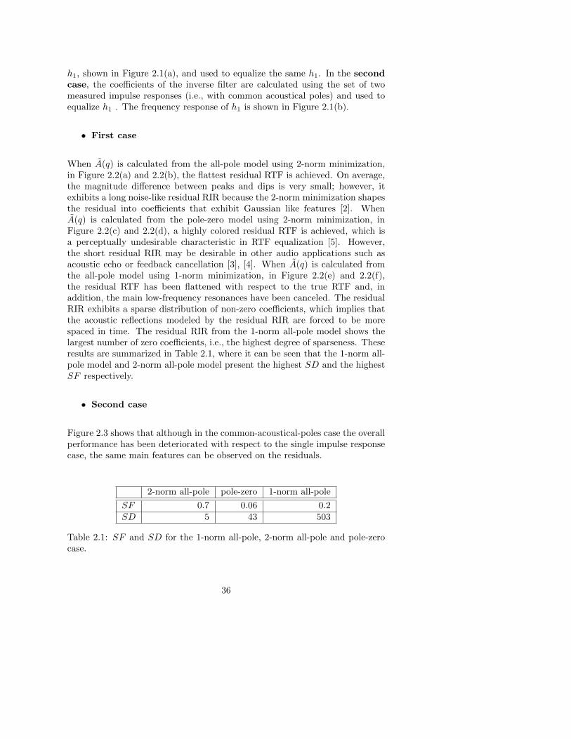
h1, shown in Figure 2.1(a), and used to equalize the same h1. In the secondcase, the coefficients of the inverse filter are calculated using the set of twomeasured impulse responses (i.e., with common acoustical poles) and used toequalize h1 . The frequency response of h1 is shown in Figure 2.1(b).

• First case

When A(q) is calculated from the all-pole model using 2-norm minimization,in Figure 2.2(a) and 2.2(b), the flattest residual RTF is achieved. On average,the magnitude difference between peaks and dips is very small; however, itexhibits a long noise-like residual RIR because the 2-norm minimization shapesthe residual into coefficients that exhibit Gaussian like features [2]. WhenA(q) is calculated from the pole-zero model using 2-norm minimization, inFigure 2.2(c) and 2.2(d), a highly colored residual RTF is achieved, which isa perceptually undesirable characteristic in RTF equalization [5]. However,the short residual RIR may be desirable in other audio applications such asacoustic echo or feedback cancellation [3], [4]. When A(q) is calculated fromthe all-pole model using 1-norm minimization, in Figure 2.2(e) and 2.2(f),the residual RTF has been flattened with respect to the true RTF and, inaddition, the main low-frequency resonances have been canceled. The residualRIR exhibits a sparse distribution of non-zero coefficients, which implies thatthe acoustic reflections modeled by the residual RIR are forced to be morespaced in time. The residual RIR from the 1-norm all-pole model shows thelargest number of zero coefficients, i.e., the highest degree of sparseness. Theseresults are summarized in Table 2.1, where it can be seen that the 1-norm all-pole model and 2-norm all-pole model present the highest SD and the highestSF respectively.

• Second case

Figure 2.3 shows that although in the common-acoustical-poles case the overallperformance has been deteriorated with respect to the single impulse responsecase, the same main features can be observed on the residuals.

2-norm all-pole pole-zero 1-norm all-pole

SF 0.7 0.06 0.2SD 5 43 503

Table 2.1: SF and SD for the 1-norm all-pole, 2-norm all-pole and pole-zerocase.

36

(a) Time evolution of h1 and h2

(b) Spectrum of h1 and h2 (RTF1 and RTF2)

Figure 2.1: Frequency response function and time evolution of h1 and h2.Normalized frequency π represents fs/2.

37

(a) 2-norm all-pole model (b) 2-norm all-pole model

(c) pole-zero model (d) pole-zero model

(e) 1-norm all-pole model (f) 1-norm all-pole model

Figure 2.2: Equalization prefilter obtained from h1. (a),(c),(e) h1 residualRIRs. (b),(d),(f) h1 residual RTFs. Normalized frequency π represents fs/2.

38

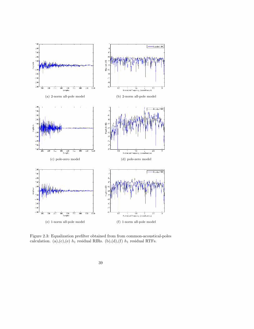
(a) 2-norm all-pole model (b) 2-norm all-pole model

(c) pole-zero model (d) pole-zero model

(e) 1-norm all-pole model (f) 1-norm all-pole model

Figure 2.3: Equalization prefilter obtained from from common-acoustical-polescalculation. (a),(c),(e) h1 residual RIRs. (b),(d),(f) h1 residual RTFs.

39

2.4 Conclusions

In this chapter, results from RTF equalization have been presented. Equal-ization is achieved by canceling the poles associated with the main resonancescommon to multiple RTFs in a room. Poles were estimated by means of threedifferent methods. Poles estimated using 2-norm minimization and an all-polemodel offered a residual RTF having the flattest response. Poles estimated us-ing 2-norm minimization and a pole-zero model offered a large reduction in themain low-frequency acoustic resonances. However the residual RTF exhibiteda highly colored response, while the residual RIR was shorter in time. Finally,poles estimated using 1-norm minimization and an all-pole model offered a flatresidual RTF with its main resonances canceled and a sparse residual RIR.This means that the residual RIR will represent sparsely distributed discretereflections. This feature may be desirable in speech applications although adeeper study taking into account perceptual considerations would be needed.

Bibliography

[1] J. Mourjopoulos and M. A. Paraskevas, “Pole and zero modeling of roomtransfer functions”, J. Sound and Vibration, vol. 146, no. 2, pp. 281-302,April 1991.

[2] J. A. Cadzow, “Minimum l1, l2, and l∞ Norm Approximate Solutions toan Overdetermined System of Linear Equations”, Dig. Sig. Proc., vol. 12,no. 4, pp. 524-560, Oct. 2002.

[3] T. van Waterschoot and M. Moonen, “Adaptive feedback cancellation foraudio applications,” Signal Processing, vol. 89, no. 11, pp. 2185-2201, Nov.2009.

[4] P. S. R. Diniz, Adaptive Filtering: Algorithms and Practical Implementa-tions. Springer, Boston, MA., 2008.

[5] D. M. Howard and J. A. S. Angus, Acoustics and Psychoacoustics. FocalPress, Elsevier, 2006.

[6] Y. Haneda, S. Makino and Y. Kaneda, “Multiple-Point Equalization ofRoom Transfer Functions by Using Common Acoustical Poles,” IEEETrans. Speech Audio Process., vol. 5, no. 4, pp. 325-333, July 1997.

[7] Y. Haneda, S. Makino and Y. Kaneda, “Common Acoustical Pole andZero Modeling of Room Transfer Function,” IEEE Trans. Speech AudioProcess., vol. 2, no. 2, pp. 320-328, Apr. 1994.

40

[8] M. Grant and S. Boyd, CVX: Matlab software for disciplined convex pro-gramming (web page and software). http://cvxr.com/cvx, April, 2010.

41

Chapter 3

Multi-Microphone acousticecho cancellation usingwarped multi-channellinear prediction ofcommon acoustical poles

Multi-Microphone acoustic echo cancellation

using warped multi-channel linear prediction of

common acoustical poles

Jose M. Gil-Cacho, Toon van Waterschoot, Marc Moonen andSøren Holdt Jensen

Published in Proc. 18th European Signal Processing Conference2010 (EUSIPCO’10), Aalborg, Denmark, Aug. 2010.

43


• literature study• design of simulation scenarios• software implementation and computer simulations• co-interpretation of simulation results• text redaction and editing

44

Abstract

In this chapter, a computationally cheap extension from single-microphoneAEC to multi-microphone AEC is presented for the case of a single loudspeaker.It employs the idea of common-acoustical-pole and zero RTF modeling. TheRTF models used for multi-microphone AEC share a fixed common denomina-tor polynomial, which is calculated off-line by means of a multi-channel warpedlinear prediction. By using the common denominator polynomial as a prefilter,only the numerator polynomial has to be estimated recursively for each mi-crophone, hence adapting to changes in the room. This approach allows thenumber of numerator coefficients to decrease by one order of magnitude foreach microphone compared with all-zero modeling. In a first configuration, theprefiltering is done on the adaptive filter signal, hence achieving a pole-zeromodel of the RTF in the AEC. In a second configuration, the prefiltering isdone on the loudspeaker signal, hence achieving a dereverberation effect, inaddition to AEC, on the microphone signals.

3.1 Introduction

ACOUSTIC echo cancellation (AEC) is used in speech communication ap-plications where the existence of echoes degrades the intelligibility and

listening comfort, such as in mobile and hands-free telephony and in telecon-ferencing. An acoustic echo canceler seeks to cancel the echo signal componenty(t) in the microphone signal, ideally leading to an echo-free error signal e(t).This is done by subtracting an estimate of the echo signal y(t) from the micro-phone signal as in Figure 3.1. Therefore, an adaptive filter is used to provide amodel that represents the best fit to the echo path H or room impulse response(RIR) [6]. This model is used to filter the input signal x(t) to obtain the es-timated echo signal. The most common model for the RIR is the FIR filtercorresponding with an all-zero model of the room transfer function (RTF). Thisis due to well-known behavior and ensured stability [5]. It is connected to thephysics of room acoustics as being a weighted sum of previous input samplesor, in other words, discrete reflections of the loudspeaker signal. Its drawbackis that the number of filter coefficients required to model a RIR increases dra-matically if the RIR is long which is typical in room acoustics applications.Besides, any change of loudspeaker-microphone or obstacle position inside theroom will change the coefficients of the model and therefore a recalculation ofevery coefficient will be needed.

One of the alternatives is to use an IIR filter which corresponds to a pole-zeromodel of the RTF. This model reduces the number of parameters to be esti-mated for the same modeling capabilities [5]. Moreover, this model representsthe physics of room acoustics including the modeling of the acoustic resonances

45

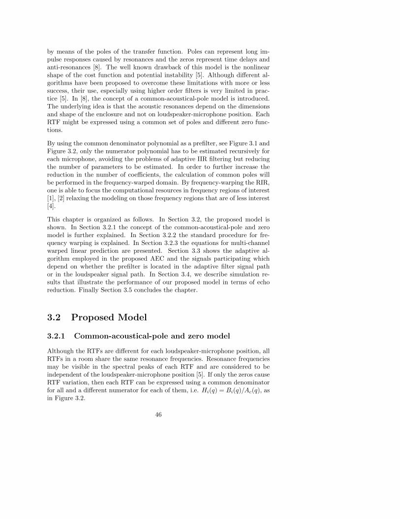
by means of the poles of the transfer function. Poles can represent long im-pulse responses caused by resonances and the zeros represent time delays andanti-resonances [8]. The well known drawback of this model is the nonlinearshape of the cost function and potential instability [5]. Although different al-gorithms have been proposed to overcome these limitations with more or lesssuccess, their use, especially using higher order filters is very limited in prac-tice [5]. In [8], the concept of a common-acoustical-pole model is introduced.The underlying idea is that the acoustic resonances depend on the dimensionsand shape of the enclosure and not on loudspeaker-microphone position. EachRTF might be expressed using a common set of poles and different zero func-tions.

By using the common denominator polynomial as a prefilter, see Figure 3.1 andFigure 3.2, only the numerator polynomial has to be estimated recursively foreach microphone, avoiding the problems of adaptive IIR filtering but reducingthe number of parameters to be estimated. In order to further increase thereduction in the number of coefficients, the calculation of common poles willbe performed in the frequency-warped domain. By frequency-warping the RIR,one is able to focus the computational resources in frequency regions of interest[1], [2] relaxing the modeling on those frequency regions that are of less interest[4].

This chapter is organized as follows. In Section 3.2, the proposed model isshown. In Section 3.2.1 the concept of the common-acoustical-pole and zeromodel is further explained. In Section 3.2.2 the standard procedure for fre-quency warping is explained. In Section 3.2.3 the equations for multi-channelwarped linear prediction are presented. Section 3.3 shows the adaptive al-gorithm employed in the proposed AEC and the signals participating whichdepend on whether the prefilter is located in the adaptive filter signal pathor in the loudspeaker signal path. In Section 3.4, we describe simulation re-sults that illustrate the performance of our proposed model in terms of echoreduction. Finally Section 3.5 concludes the chapter.

3.2 Proposed Model

3.2.1 Common-acoustical-pole and zero model

Although the RTFs are different for each loudspeaker-microphone position, allRTFs in a room share the same resonance frequencies. Resonance frequenciesmay be visible in the spectral peaks of each RTF and are considered to beindependent of the loudspeaker-microphone position [5]. If only the zeros causeRTF variation, then each RTF can be expressed using a common denominatorfor all and a different numerator for each of them, i.e. Hi(q) = Bi(q)/Ac(q), asin Figure 3.2.

46

A−1c (q)

Ac(q)

H1 H2 HM

B1(q, t)B2(q, t)BM(q, t)

+

+

+

−

−

−

y1(t)

y2(t)

yM(t)

y1(t)y2(t)yM(t)

e1(t)e2(t)

eM(t)

(a)

(b)

x(t)

Figure 3.1: Multi-microphone acoustic echo canceler set-up.

This can be represented by either common poles pc(k) and distinct zeros zi(k, t),or in polynomial form using common autoregressive (AR) ac(k) and distinctmoving average (MA) bi(k, t) coefficients [8],

Hi(q, t) =

∏Qk=1 (1− zi(k, t)q−1)∏Pk=1 (1− pc(k)q−1)

=

∑Qk=1 bi(k, t)q

−k

1−∑Pk=1 ac(k)q−k

(3.1)

where Q and P are the order of numerator and denominator respectively, i =1, ...,M , M the number of microphones and q denotes the time shift operator,i.e., q−ku(t) = u(t− k).

3.2.2 Warped linear prediction

In order to get the AR coefficients of an impulse response, a set of simultane-ous equations must be solved. This set of simultaneous equations are in ourcase of the same mathematical form comparing Wiener-Hopf equations for lin-

47

ear prediction, Yule-Walker equation for an autoregressive model [6] and theequation error between a measured impulse response and the estimated all-poleimpulse response [7]. In this chapter, it is used the term warped linear predic-tion (WLP) as in [3]. The standard procedure in producing frequency-warpedimpulse responses involves replacing the unit delay operator, q−1 of the originalRTF, Hi(q) =

∑Nt=0 hi(t)q

−t, by first-order all-pass filter [1] D(q, λ), i.e.,

Hwi (q) =

N∑t=0

hi(t)Dt(q, λ) (3.2)

with the warping parameter λ ∈ (−1, 1), N denotes the impulse response lengthand

D(q, λ) =q−1 − λ1− λq−1

, (3.3)

and where the superscript w means that the impulse response or RTF is trans-formed to the warped domain.

The inverse mapping or dewarping (i.e., from warped domain to original do-main) follows directly by applying again the same mapping with the sign of λ

H1(q, t) = B1(q, t)/Ac(q)

H2(q, t) = B2(q, t)/Ac(q)

HM(q, t) = BM(q, t)/Ac(q)

y1(t)y2(t)yM(t)

Figure 3.2: Different RTFs in a room. They have the same denominator basedon their common acoustical poles.

48

0 1000 2000 3000 4000 5000 6000 7000 8000−40

−20

0

20

40

60

Frequency (Hz)

Mag

nitu

de (

dB)

Room TF λ=0.95 λ=0.5 λ=0

0 200 400 600 800 1000 1200 1400 1600 1800 2000−40

−20

0

20

40

60

Frequency (Hz)

Mag

nitu

de (

dB)

Figure 3.3: Room transfer function (upper line) and frequency response func-tion of warped AR coefficients using different warping parameter λ = 0.95,λ = 0.5, λ = 0.

changed [1] as,

Hi(q) =

N∑t=0

hwi (t)Dt(q,−λ). (3.4)

Figure 3.3 shows the RTF of a measured room impulse response of 2001 sampleslength (fs = 16 kHz) together with the AR coefficients spectra calculated withorder P = 200 and warping the impulse response with λ = 0, λ = 0.5 andλ = 0.9 respectively. With λ = 0 the AR coefficients model uniformly overthe frequency axis. With λ = 0.5 the modeling effort is put in low frequencyregions and λ = 0.9 even in lower regions. As it can be seen, the low frequencyregion contains the main resonant peaks. Therefore it seems obvious to employthe limited computational resources in that area.

3.2.3 Warped multi-channel linear prediction of commonacoustical poles

From the set of warped impulse responses a set of common AR coefficients arefirst calculated and then transformed back to the original domain. This setof AR coefficients corresponds to the main resonances of the room. Assumingthat hwi (t) is the time-domain version of the warped RTF Hw

i (q), the estimated

49

warped all-pole version of the impulse response is [1]

hwi (t) =

P∑k=1

awc (k)hwi (t− k) (3.5)

The warped common AR coefficients can be calculated as those that minimizethe cost function

minawc (k)

M∑i=1

∞∑t=0

e2i (t) (3.6)

with

ei(t) = hwi (t)− hwi (t)

= hwi (t)−P∑k=1

awc (k)hwi (t− k).(3.7)

The warped multi-channel linear prediction of the common AR coeffients, i.e.,awc (k), that minimize (3.6) is calculated by solving the normal equations [7] as

a =(WTW

)−1

WTv (3.8)

where

a = [awc (1), awc (2), ..., awc (P )]T (3.9a)

W = [HT1 ,H

T2 , ...,H

TM ]T (3.9b)

v = [hwT1 ,hwT2 , ...,hwTM ]T (3.9c)

hwi = [hwi (1), hwi (2), .., hwi (N − 1), 0, 0, .., 0]T (3.9d)

Hi =

hwi (0) 0 · · · 0hwi (1) hwi (0) · · · 0

......

......

......

... hwi (0)

hwi (N − 1) 0 · · ·...

0 hwi (N − 1) · · ·...

...... · · ·

...0 0 · · · hwi (N − 1)

(3.9e)

⇒ size [(N + P − 1)× P ]

50

3.3 Adaptive Algorithm

Vector a (3.9a) contains the warped common AR coefficients that are mappedback to the original domain to use them as the prefilter’s fixed polynomial(3.10) as

Ac(q) = 1− ac(1)q−1 − ...− ac(P )q−P (3.10a)

or Ac(q) = aTc q in vector notation (3.10b)

The prefiltering is done on either the adaptive filter signal or the loudspeakersignal, as Figure 3.1 shows. For every microphone the numerator coefficients(3.11) are adapted using the well-known normalized least mean squares (NLMS)algorithm [6] as

Bi(q, t) = bi(0, t) + bi(1, t)q−1 + ...+ bi(Q, t)q

−Q (3.11a)

or Bi(q, t) = bTi (t)q in vector notation (3.11b)

NLMS is a gradient-based algorithm whose basic equations are given by

ei(t) = yi(t)− yi(t) (3.12a)

= yi(t)− bi(t)uT (t) (3.12b)

bTi (t+ 1) = bTi (t) + µ1

u(t)uT (t)u(t)T ei(t) (3.12c)

where i = 1, ...,M , the vector u(t) = [u(t), u(t− 1), ..., u(t−Q)] is the input tothe adaptive filter, yi(t) are the microphone signals, ei(t) are the error signals,yi(t) are the estimated echo signals and µ is the step size. In the filter coeffi-

cients update formula (3.12c) and in (3.12b), the vectors bTi (t) are the adaptivefilter coefficients of each channel. Signals u(t) and yi(t) will depend on whetherthe prefilter is in the adaptive filter signal path or in the loudspeaker signalpath as follows.

• Prefilter in the adaptive filter signal path

u(t) =1

Ac(q)x(t) (3.13)

= x(t)− ac(1)u(t− 1)− ...− ac(P )u(t− P ) (3.14)

yi(t) = Hi(q, t)x(t) (3.15)

• Prefilter in the loudspeaker signal path

u(t) = x(t) (3.16)

yi(t) = Ac(q)Hi(q, t)x(t) (3.17)

≈ Ac(q)Bi(q, t)

Ai(q)x(t) ≈ Bi(q, t)x(t) (3.18)

51

λ = 0.0 16.6λ = 0.7 28.0

Table 3.1: Attenuation (dB) of AEC1. Change of warping parameter λ.

3.4 Simulation Results

Matlab computer simulations are performed at fs = 16 kHz. Five room impulseresponses, (hi with i = 1, ..., 5) of length N = 2000 samples are measured ina rectangular room of about 5 × 3 × 3 m. In every simulation, µ = 1 as itoffered the best results. The input signal is speech (i.e. female voice) recordedat fs = .6 kHz of 6.7 s of duration (i.e., length L = 1340876 samples). Thewarping parameter λ = 0.7 is found to be optimal. The performance measuresare: Attenuation,

Attenuationi = 10 log10

∑Lt=0 y

2i (t)∑L

t=0 e2i (t)

(dB) (3.19)

which is a scalar that measures the difference in dB between the power ofthe L samples length error and microphone signals; and Echo Return LossEnhancement (ERLE),

ERLEi(n) = 10 log10

∑pk=1 y

2i

((n− 1)p+ k

)∑pk=1 e

2i

((n− 1)p+ k

) (dB) (3.20)

for n = 1, ..., Lp , which is (3.19) averaged over time frames of length p. Theorder of numerator Q and denominator P are the same in every simulation.

We define an echo canceler as AECi with i = 1, ..., 5. The performance in termsof Attenuationi and ERLEi of different acoustic echo cancelers is calculated intwo different scenarios. In the first scenario, the AR coefficients of the prefilterare calculated from a single impulse response. In the second scenario, theAR coefficients of the prefilter are calculated using the whole set of impulseresponses, thus defining the common acoustical poles of the system.

3.4.1 Comparison of ERLE with and without warping

The effect of warping an impulse response previous to calculating the AR co-efficients is shown in this section. Figure 3.4 shows the differences in the AECperformance when using different values of warping parameter λ. The optimalvalue λ = 0.7 was applied and compared with λ = 0 which means that no warp-ing is done to the impulse response previous to calculating the AR coefficients.The WLP (AR) order is P = 200 and the prefilter was then applied in theadaptive filter signal path. In such case, a pole-zero model of the RTF, with

52

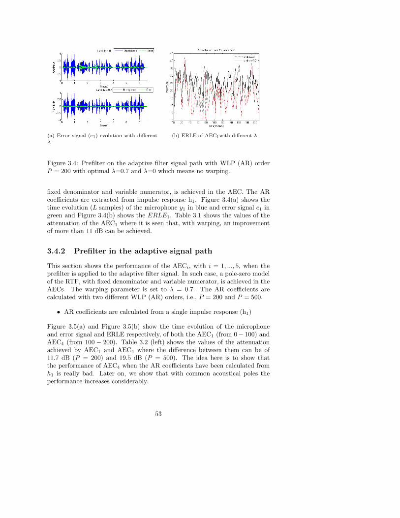
(a) Error signal (e1) evolution with differentλ

(b) ERLE of AEC1with different λ

Figure 3.4: Prefilter on the adaptive filter signal path with WLP (AR) orderP = 200 with optimal λ=0.7 and λ=0 which means no warping.

fixed denominator and variable numerator, is achieved in the AEC. The ARcoefficients are extracted from impulse response h1. Figure 3.4(a) shows thetime evolution (L samples) of the microphone y1 in blue and error signal e1 ingreen and Figure 3.4(b) shows the ERLE1. Table 3.1 shows the values of theattenuation of the AEC1 where it is seen that, with warping, an improvementof more than 11 dB can be achieved.

3.4.2 Prefilter in the adaptive signal path

This section shows the performance of the AECi, with i = 1, ..., 5, when theprefilter is applied to the adaptive filter signal. In such case, a pole-zero modelof the RTF, with fixed denominator and variable numerator, is achieved in theAECs. The warping parameter is set to λ = 0.7. The AR coefficients arecalculated with two different WLP (AR) orders, i.e., P = 200 and P = 500.

• AR coefficients are calculated from a single impulse response (h1)

Figure 3.5(a) and Figure 3.5(b) show the time evolution of the microphoneand error signal and ERLE respectively, of both the AEC1 (from 0− 100) andAEC4 (from 100 − 200). Table 3.2 (left) shows the values of the attenuationachieved by AEC1 and AEC4 where the difference between them can be of11.7 dB (P = 200) and 19.5 dB (P = 500). The idea here is to show thatthe performance of AEC4 when the AR coefficients have been calculated fromh1 is really bad. Later on, we show that with common acoustical poles theperformance increases considerably.

53

(a) Error signal evolution with different WLP(AR) orders

(b) ERLE with different WLP (AR) orders

Figure 3.5: Prefilter in the adaptive filter signal path. AR coefficients arecalculated from impulse response h1 with optimal λ=0.7 and P = 200 andP = 500. Performance of AEC1 and AEC4 are shown consecutively i.e., from0− 100 corresponds to AEC1 and from 100− 200 to AEC4.

• Common-acoustical-pole AR coefficients

In this case, the fixed filter coefficients are calculated from the whole set ofimpulse responses using (3.8). Figure 3.6(a) and Figure 3.6(b) show the timeevolution of the microphone and error signal and the ERLE respectively, ofevery AECi, with i = 1, ..5. Table 3.3 (top) shows that the difference amongthe Attenuation values with respect to Figure 3.5 is highly reduced with sat-isfactory individual results, i.e., average Attenuation = 21.6 and 25.2 dB withP = 200 and 500, respectively.

3.4.3 Prefilter in the loudspeaker signal path

This section shows the performance of the AECi, with i = 1, ..., 5, when the pre-filter is applied in the loudspeaker signal path. In such case, a dereverberatingeffect is achieved by canceling the main resonances. The warping parameter isset to λ = 0.7. The AR coefficients are calculated with two WLP (AR) orders,

LPC (h1) LPC (h1)(Adap. sig.) AEC1 AEC4 (Loud. sig.) AEC1 AEC4

P = 200 28.0 16.3 P = 200 19.4 14.0P = 500 37.8 18.3 P = 500 29.9 14.2

Table 3.2: Attenuation (dB). AR Coefficients obtained from h1. (Left) Prefilterin the adaptive filter signal path. (Right) Prefilter in loudspeaker signal path.

54



Figure 3.6: Prefilter in the adaptive filter signal path. AR coefficients arecalculated from common acoustical poles with optimal λ=0.7 and P = 200 andP = 500. Performance of every AECi are shown consecutively.

LPCcommon(Adap. sig.) AEC1 AEC2 AEC3 AEC4 AEC5

P = 200 24.8 20.3 19.4 24.2 19.4P = 500 27.9 24.3 24.4 26.0 22.5LPCcommon(Loud. sig.)

P = 200 15.4 15.7 13.8 15.2 13.4P = 500 24.0 19.9 19.7 22.5 18.3All-zero(No prefilter)Q = 2000 36.4 31.6 33.3 28.7 32.1

Table 3.3: Attenuation(dB). AR coefficients obtained from common acousticalpoles. Top) Prefilter in the Adaptive filter signal path. Middle) Prefilter in theloudspeaker signal path. Bottom) No prefilter.

i.e., P = 200 and P = 500.

• AR coefficients calculated from one impulse response h1

Figure 3.7(a) and Figure 3.7(b) show the time evolution of the microphoneand error signal and ERLE respectively, of both the AEC1 and AEC4. Table3.2.(Right) shows the values of the attenuation achieved by AEC1 and AEC4

where the difference between them can be of 5.4 dB (P = 200) and 15.7 dB(P = 500).

55

(a) Error signal evolution with different WLP(AR) orders (200 Top, 500 Bottom)


Figure 3.7: Prefilter in the loudspeaker signal path. AR coeffients are calculatedfrom impulse response h1 with optimal λ=0.7 and P = 200 and P = 500.Performance of AEC1 and AEC4 are shown consecutively.

• Common-acoustical-pole AR coefficients

In this case, the fixed filter coefficients are calculated from the whole set ofimpulse responses using (3.8). Figure 3.8(a) and Figure 3.8(b) show the timeevolution of the microphone and error signal and the ERLE respectively, ofevery AECi, with i = 1, ..5. Table 3.3.Middle) shows that the difference amongthe Attenuation values is reduced with satisfactory individual results only withP = 500, i.e., average Attenuation = 14.2 and 19.9 dB with P = 200 and500 respectively. Table 3.3 (bottom) shows the values of the Attenuation inthe case no prefilter is done (i.e., all-zero case) and order Q = 2000 whichis the total length of the impulse response. It can be seen that although theachieved attenuation is higher compared with our proposed model, the numberof coefficients increases dramatically. Assuming that NLMS requires 2Q +P multiply-add operations for each update (3.12a)-(3.12c) [5], the number ofparameters in the all-zero case is M · 2Q = 5· 4000 = 20000 operations whereaswith fixed prefiltering, M · 2Q+ P = 5· 400 + 200 = 2200 (i.e., 91% operationssaving) or M · 2Q + P = 5· 1000 + 500 = 5500 (i.e., 36% operations saving)multiply-add operations only.

3.5 Conclusion

In this chapter, we have proposed a model for multi-microphone AEC whichemploys the idea of common-acoustical-poles and zero modeling of RTFs usingwarped linear prediction of the impulse responses. Common acoustical poles

56



Figure 3.8: Prefilter in the loudspeaker signal path. The AR coeffients arecalculated from common acoustical poles with optimal λ=0.7 and P = 200 andP = 500. Performance of every AECi are shown consecutively.

are calculated off-line from a set of measured impulse responses. By frequency-warping the measured impulse responses one is able to focus the computationalresources in a frequency region of interest. In RTFs the predominant spectralpeaks are located in the low frequency region. Warping allows us to use themodeling effort in that frequency region to obtain better modeling results. Thisleads to a higher echo reduction for the same number of filter coefficients. More-over these predominant spectral peaks are common to every RTF which allowsus to have a fixed common denominator polynomial for every channel. Henceonly the numerator polynomial has to be estimated recursively for adaptingto changes in the room. This approach allows the number of numerator co-efficients to decrease by up to one order of magnitude for each microphonecompared with all-zero modeling to get satisfactory results (about 22 dB ofecho attenuation). Better results are obtained in the case of prefiltering in theadaptive filter signal path. This is due to the IIR nature of this configurationwhich leads to a better modeling capability.

Bibliography

[1] A. Harma, M. Karjalainen, L. Savioja, V. Valimaki, U. K. Laine, and J.Huopaniemi, “Frequency-warped signal processing for audio applications”,J. Audio Eng. Soc., vol. 48, no. 11, pp. 1011-1031, 2000.

[2] T. Paatero and M. Karjalainen, “Kautz Filters and Generalized Frequency

57

Resolution - Theory and Audio Applications”, J. Audio Eng. Soc.,vol. 51,no. 1/2, pp. 27-44, January/February 2003.

[3] H. W. Strube, “Linear prediction on a warped frequency scale”, J. Acoust.Soc. Amer., vol. 68, no. 4, pp. 1071-1076, Oct. 1980.

[4] T. van Waterschoot and M. Moonen, “Adaptive feedback cancellation foraudio signals using a warped all-pole near-end model,” in Proc. IEEE Int.Conf. on Acoust. Speech Signal Process. (ICASSP ’08), Las Vegas, Nevada,USA, Apr. 2008, pp. 269-272.

[5] P. S. R. Diniz, Adaptive Filtering: Algorithms and Practical Implementa-tions. Springer, Boston, MA., 2008.

[6] S. Haykin, Adaptive Filter Theory. Prentice Hall, 2001.

[7] Y. Haneda, S. Makino and Y. Kaneda, “Multiple-Point Equalization ofRoom Transfer Functions by Using Common Acoustical Poles,” IEEETrans. Speech Audio Process., vol. 5, no. 4, pp. 325-333, July 1997.

[8] Y. Haneda, S. Makino and Y. Kaneda, “Common Acoustical Pole andZero Modeling of Room Transfer Function,” IEEE Trans. Speech AudioProcess., vol. 2, no. 2, pp. 320-328, Apr. 1994.

58

Part III

Linear Adaptive Filtering

Chapter 4

Regularized adaptive notchfilters for acoustic howlingsuppression

Regularized adaptive notch filters for acoustic

howling suppression

Jose Manuel Gil-Cacho, Toon van Waterschoot, Marc Moonenand Søren Holdt Jensen

Published in Proc. 17th European Signal Processing Conference2009 (EUSIPCO’09), Glasgow, UK, Aug. 2009.

61


• literature study• co-development of the RANF algorithm• design of simulation scenarios• software implementation and computer simulations• co-interpretation of simulation results• text redaction and editing

62

Abstract

In this chapter, a method for the suppression of acoustic howling is devel-oped, based on adaptive notch filters (ANF) with regularization (RANF). Themethod features three RANFs working in parallel to achieve frequency track-ing, howling detection and suppression. The ANF-based approach to howlingsuppression introduces minimal processing delay and minimal complexity, incontrast to non-parametric block-based methods featuring a non-parametricfrequency analysis. Compared to existing ANF-based howling suppressionmethods, the proposed method allows for a more advanced howling detectionsuch that tonal components in the source signal are not affected. The RANFsproposed in this chapter are implemented in direct form and are updated usinga gradient-descent-type algorithm. Results show that, under certain conditions,the level of suppression and sound quality are similar to what is obtained withblock-based methods.

4.1 Introduction

In some applications, such as for public address (PA) systems, notch-filter-based howling suppression (NHS) methods are widely utilized [3]. The NHSmethod relies in the use of notch filters in the forward path so as to suppressfrequency components that produce acoustic howling [3]. In this chapter, wewill focus on the NHS method. NHS methods perform a frequency analysis,howling detection and howling suppression. We may tackle these actions usingeither block-based techniques, i.e., using the Fast Fourier Transform (FFT) oradaptive notch filters (ANF). Howling detection is very difficult in ANF-basedmethods since no power spectrum information is available [4], [5]. Block-basedmethods, on the other hand, accomplish howling detection based on powerspectra amplitude information. However, due to the FFT operations involved,block-based methods are more complex and require more processing delay thanANF-based methods. The method proposed in this chapter combines the ad-vantages of keeping the complexity small while having an improved howlingdetection mechanism, by including regularization and multiple parallel ANFs.

The chapter is organized as follows. Section 4.2 reviews with notch-filter-basedsuppression methods. The main structure of both block-based and ANF-basedmethods is shown. Moreover, the equations of the direct-form ANF algorithmare given. Section 4.3 presents the proposed method, showing its operationand its block structure. Simulation results are presented in Section 4.4 andconclusions are drawn in Section 4.5.

63

4.2 Notch-filter-based howling suppression

To eliminate narrowband or sinusoidal signals from a broadband signal (e.g. anoise, audio or speech signal) notch filters are often used. There exist differenttypes of notch filters, e.g. FIR or IIR filters. We will focus on second-order IIRfilters with constrained poles and zeros [6]. The constraint is that the zeros lieon the unit circle and the poles will lie in the same radial direction but witha pole radius within 0 << r < 1. The transfer function of such a notch filter,centered at a radial notch frequency ω0 = 2π (f0/fs), with fs the samplingfrequency, is given by.

H (z) =1− 2 cos(w0)z−1 + z−2

1− 2r cos(w0)z−1 + r2z−2(4.1)

When using notch filters for howling suppression, one aims to have maximumattenuation at the howling frequency but a minimal effect on surrounding fre-quencies so as to avoid distortion of the acoustic input signal. This can beachieved by employing a very narrow bandwidth, i.e., a pole radius close tounity. Therefore, the notch filter performance strongly depends on the esti-mation of the howling frequency in the sense that, if very narrowband filtersare to be used then very accurate frequency estimates are needed. Otherwise,there is a high risk of suppressing a signal component in the close vicinity of,but not exactly at the actual howling frequency. If the frequency estimationis known to have poor accuracy, a larger bandwidth must be used in order toensure that the howling frequency is sufficiently attenuated. Suppressing thesignal in a wider frequency band, on the other hand, leads to more distortion.

4.2.1 Non-parametric frequency estimation

Non-parametric frequency estimation methods, in which a block-based estima-tion is performed using the FFT [3], can yield accurate frequency estimates onlywhen long signal blocks are used. This in turn implies that a large processingdelay and a high computing power are required. The choice of the block sizeis hence a trade-off between processing delay and computational complexityon the one hand, and frequency estimation accuracy on the other hand. An-other issue with block-based methods is that for rapid changes in the howlingfrequency, proper frequency tracking is insufficient if the block is too long [7].

NHS methods based on non-parametric frequency estimation are two-stagemethods, where howling estimation/detection and suppression are performedseparately, see Figure 4.1. As explained before, the suppression block consistsof a notch filter, as in (4.1), or of a bank of notch filters in which several notchfilters are cascaded. Each of those notch filters can be tuned to a different howl-ing frequency previously estimated in the estimation/detection block. There

64

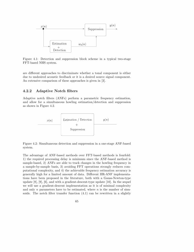
x(n) y(n)

w0(n)Estimation

Detection

Suppression

+

Figure 4.1: Detection and suppression block scheme in a typical two-stageFFT-based NHS system.

are different approaches to discriminate whether a tonal component is eitherdue to undesired acoustic feedback or it is a desired source signal component.An extensive comparison of these approaches is given in [3].

4.2.2 Adaptive Notch filters

Adaptive notch filters (ANFs) perform a parametric frequency estimation,and allow for a simultaneous howling estimation/detection and suppressionas shown in Figure 4.2.

Figure 4.2: Simultaneous detection and suppression in a one-stage ANF-basedsystem.

The advantage of ANF-based methods over FFT-based methods is fourfold:1) the required processing delay is minimum since the ANF-based method issample-based, 2) ANFs are able to track changes in the howling frequency ina sample-by-sample basis, 3) avoiding FFT operations strongly reduces com-putational complexity, and 4) the achievable frequency estimation accuracy isgenerally high for a limited amount of data. Different IIR-ANF implementa-tions have been proposed in the literature, both with a Gauss-Newton-typeupdate [8], [9], [6], and with a gradient-descent-type update [10]. In the sequelwe will use a gradient-descent implementation as it is of minimal complexityand only n parameters have to be estimated, where n is the number of sinu-soids. The notch filter transfer function (4.1) can be rewritten in a slightly

65

different form which is more suitable for coefficient updating, i.e.

H (q) =1− a(n)q−1 + q−2

1− a(n)rq−1 + r2q−2(4.2)

where q denotes the discrete time shift operator, i.e., q−ku(n) = u(n− k). Theparameter a(n) defines the instantaneous frequency w0(n), i.e.

w0(n) = arccos

[a(n)

2

](4.3)

The parameter a(n) is allowed to take values bounded by −2 < a(n) < 2. Thebasic idea underlying ANF-based frequency estimation and howling suppressionconsists in feeding the signal into the ANF and perform a minimization w.r.t.a(n), of the mean square error (MSE) of the notch filter output signal y(n)

mina(n)

E[y(n)2] (4.4)

This will cause the notch to be centered at the frequency corresponding to thesignal’s narrowband or sinusoidal component. The gradient descent algorithmwill adjust the coefficient a(n) in the negative gradient direction ∇a(n), until alocal minimum in the cost function is attained. The gradient descent algorithmfor the direct-form ANF is given by equations (4.5)-(4.9) [10]. Here the ANFinput and output signals are denoted by x(n) and y(n) respectively, and thefilter states are denoted by u(n), u(n − 1), t(n), t(n − 1). The step-size of thegradient descent algorithm is denoted by µ.

t(n+ 1) = u(n)− ra(n)t(n)− r2t(n− 1) (4.5)

∇a(n) = t(n+ 1)− rt(n− 1) (4.6)

u(n+ 1) = x(n)− ra(n)u(n)− r2u(n− 1) (4.7)

y(n) = u(n+ 1) + a(n)u(n) + u(n− 1) (4.8)

a(n+ 1) = a(n)− µy(n)∇a(n) (4.9)

4.3 Regularized Adaptive Notch Filters

The proposed NHS method employs three regularized ANFs (RANF) that runin parallel and share one decision block, see Figure 4.4. Each RANF is regu-larized with a term λi, which is chosen to have a different value for i = 1, 2, 3 .The regularized ANF cost function is given as

minai(n)

E[y2i (n)] + λiai(n)2 i = 1, 2, 3. (4.10)

66

This results in a modified gradient descent coefficient update, corresponding toa so-called Leaky LMS [11]:

ai(n+ 1) = ai(n)− µ {yi(n)∇ai(n) + λiai(n)} (4.11)

The effect of the regularization term is negligible when howling is present in thesignal. This is so because the term in (4.11) with the gradient search direction∇ai(n), i.e. yi(n)∇ai(n), is significantly larger than the term λiai(n). Con-versely, when howling is not present, the gradient search direction ∇ai(n) tendsto zero and so the coefficient update formula approximately equals ai(n+ 1) =ai(n)− µλiai(n) = (1− µλi)ai(n). The effect of this is that the regularizationterm is in fact penalizing the estimates ai(n). Moreover, depending on thesign of λi, the regularization term will introduce a leakage or an accumulationeffect on the coefficient estimate. Conventionally regularized algorithms ,i.e.,with a positive λi, produce estimates that are biased towards zero. By hav-ing negative λi, the proposed RANF algorithm also produces estimates thatare “biased towards infinity”. This is indeed what we observe in Figure 4.3:Whenever howling does not occur the RANF coefficients diverge either to theirupper bound if λi is negative or to zero if λi is positive.

Figure 4.3: Upper: representation of the time-domain input signal x(n) (upper)where the framed signal fragments correspond to howling segment. Lower: theRANF frequency estimates fi, with i = 1, 2, 3.

67

Figure 4.3 shows an example of the evolution of the frequency tracking asa function of time with the proposed method. When howling appears in thesignal, the three coefficients ai(n) converge to the same value. The boxes framethe part of the signal where howling is present. When howling disappears, thethree coefficients ai(n) move away from each other as a result of having differentregularization parameters λi.

RANF1

RANF2

RANF3y3(n)

x(n)

y1(n)

y2(n)

y(n)

L SamplesBuffer

L Samples

L Samples

Buffer

Buffer

Mean

Mean

Mean

and

andVariance

Variance

Varianceand

m1,v1

m2,v2

m3,v3

Decision Rule

Com

pareandSelect

Figure 4.4: Block diagram of the proposed RANF-based NHS method.

Figure 4.4 shows a block diagram of the proposed RANF-based NHS method.The signal x(n) is input into the three RANF blocks which will track a tonalcomponent in the signal. The Decision Rule block monitors the coefficientsai(n) of the three RANF blocks. After L samples are buffered, where L is asmall number so as to have minimum decision delay the mean and the varianceof a block of L samples is calculated and compared for the three RANF blocks.If the difference between two mean values is less than a fixed threshold T , inHz, then howling is assumed to be present. Essentially, this means that howlingis detected when at least two RANF coefficients have converged to the samefrequency. In this case, the output signal y(n) is assigned to be one of the threeRANF block output signals y(n)1,2,3, depending on the frequency estimationvariance. The smaller the variance the more reliable the result is assumed tobe. Similarly, if the differences in mean value for the three RANF blocks arelarger than the fixed threshold, then no howling is assumed in the signal andthe output is generated directly from the input.

The values of λi are chosen such that the difference ∆f (Hz), in a time pe-

68

riod of M samples, between two coefficients ai(n) corresponds to a given fixedthreshold (Hz). We will set λ1 = λ, λ2 = 0 and λ3 = −λ, where

λ =1

µ

[L

√1

cos(∆w)− 1

](4.12)

We have derived (4.12) based on the “small-angle approximation” (see Ap-pendix 4.A) , i.e., ∆f should be small compared to the sampling frequency fs,a trigonometric relationship between the regularization parameter λi, and thedesired divergence rate after a howling occurrence.

4.4 Results

In this section, the performance of the proposed method is evaluated for twotypes of signals. These signals, were generated in Matlab from clean speechand music signals. The feedback paths were synthetically generated, using anexponentially damped tone at a particular frequency, as a synthetic feedbackpath impulse response. The frequency and duration of the feedback path weredrawn from pre-defined distributions in order to simulate changing feedbackconditions (i.e., dynamic feedback path). A pre-specified loop gain was ob-tained by changing the forward gain appropriately. The frequency range andmaximum loop gain were chosen for two test scenarios (i.e., scenarios ’a’ and’b’) in order to change, besides the howling frequency, the speed at which thehowling appears, the exponential slope of the increasing howling amplitude, thehowling duration and how frequently howling appears in the signal, see Figure4.5(a), 4.6(a) and Figure 4.7(a), 4.8(a) . Therefore, for each clean signal twotypes of howling signals were generated, namely Speecha, Speechb, Musicaand Musicb.

The original signals were a speech signal (i.e., an English-speaking female voice)and a music signal (i.e. a fragment of a song) both sampled at 20 kHz. Thesystem parameters were set to λ1 = +2.6820e− 004, λ2 = 0, λ3 = −2.6820e−004, µ = 0.023, r = 0.85, T = 5 Hz, L = 50 samples.

Four objective performance measures will be used in this section, namely max-imum and minimum attenuation in dB ( Attmax and Attmin respectively) andmaximum and mean frequency-weighted log-spectral signal distortion (SDmax

and SDmean respectively). The Att (4.13) is calculated comparing the powerspectrum of the original signal without howling with the signal after howlingsuppression, i.e.

Att(f) = 10 log10

Sy(f)

Sx(f)(4.13)

69

where Sy(f) and Sx(f) denote the short-term power spectra of the signal aftersuppression and the original signal around the howling frequency f , respec-tively. Attmax is the difference in dB between the frequency component withthe smallest power in the signal after suppression and the original signal andso, Attmin is the difference with respect to the highest frequency component.Ideally, Attmax should be zero dB which means that perfect, distortion-free,howling suppression is achieved.

The SD is a measure of sound quality and objectively measures the distor-tion produced not only by applying notch filters to the signal but also due tohowling. It was proposed in [2] and is given as

SD(t) =

√∫ fs/2

0

wERB(f)

(10 log10

Sy(f)

Sx(f)

)2

df (4.14)

where wERB(f) is a weighting function that gives weights to each auditorycritical band within the Nyquist interval, following Table II of the ANSI S3.5-1997 standard. The integration in (4.14) is approximated by a summation overthe critical frequency bands. Both the mean and maximum values SDmean

SDmax, will be used.

4.4.1 Speech signal

Figure 4.5 and 4.6 show the spectrogram of the speech signal before and af-ter howling suppression by means of the proposed method. In Figure 4.5(a)and Figure 4.6(a), the howling speech signal is presented to show the howlingfrequency range and time evolution. From Figure 4.5(b) it is clearly observedthat suppression is performed equally well over time and frequency. However,in Figure 4.6(b) we can see that in the frequency range below 1.5 kHz, nosuppression is accomplished.

4.4.2 Music signal

The same procedure is followed in this case for a music signal. Figure 4.7and 4.8 show the spectrograms of the music signal before and after howlingsuppression. The same observation as in the speech simulation can be made inthis case.

In Table 4.1, the corresponding performance measures are shown. It can againbe observed that scenario ‘b’ is more problematic in terms of both maximumand minimum attenuation (i.e., howling suppression) and spectral distortion.For frequencies below 1500 Hz, the method not only is unable to suppress thehowling but also is further distorting the signal in a wider frequency range dueto false howling detection. This fact has been noted in [10] where it is pointedout that direct-form adaptive notch filters are not necessarily stable when the

70

Signal before howling suppression

Time(s)

Fre

quen

cy(H

z)

0 2 4 6 8 10 12 14 16 18

0

1000

2000

3000

4000

5000

6000

7000

8000

(a) Speecha before suppression

Signal after howling suppression

Time(s)

Fre

quen

cy(H

z)

0 2 4 6 8 10 12 14 16 18

0

1000

2000

3000

4000

5000

6000

7000

8000

(b) Speecha after suppression

Figure 4.5: Speecha signal before and after howling suppression. The frequencyrange, gain and time evolution of howling is generated differently in ’a’ and ’b’scenarios.

Signal SDmean SDmax Attmax dB Attmin dB

Speecha 1.66 14.78 5 6Speechb 4.32 28.83 5 40Musica 1.05 13.24 3 6Musicb 3.61 17.83 1 40

Table 4.1: System performance for given howling signals.

notch frequency approaches its extreme values, 0 and fs/2. Therefore, when thesignal contains howling in the neighborhood of these frequencies, the methodcannot be used to suppress it.

71


Time(s)

Fre

quen

cy(H

z)

0 2 4 6 8 10 12 14 16 18

0

1000

2000

3000

4000

5000

6000

7000

8000

(a) Speechb before suppression


Time(s)

Fre

quen

cy(H

z)

0 2 4 6 8 10 12 14 16 18

0

1000

2000

3000

4000

5000

6000

7000

8000

(b) Speechb after suppression

Figure 4.6: Speechb signal before and after howling suppression. The frequencyrange, gain and time evolution of howling is generated differently in ’a’ and ’b’scenarios.

72


Time(s)

Fre

quen

cy(H

z)

0 2 4 6 8 10 12 14 16 18

0

1000

2000

3000

4000

5000

6000

7000

8000

(a) Musicabefore suppression


Time(s)

Fre

quen

cy(H

z)

0 2 4 6 8 10 12 14 16 18

0

1000

2000

3000

4000

5000

6000

7000

8000

(b) Musica after suppression

Figure 4.7: Musica signal before and after howling suppression. The frequencyrange, gain and time evolution of howling is generated differently in ‘a’ and ‘b’scenarios.

73


Time(s)

Fre

quen

cy(H

z)

0 2 4 6 8 10 12 14 16 18

0

1000

2000

3000

4000

5000

6000

7000

8000

(a) Musicb before suppression


Time(s)

Fre

quen

cy(H

z)

0 2 4 6 8 10 12 14 16 18

0

1000

2000

3000

4000

5000

6000

7000

8000

(b) Musicb after suppression

Figure 4.8: Musicb signal before and after howling suppression. The frequencyrange, gain and time evolution of howling is generated differently in ‘a’ and ‘b’scenarios.

74

4.5 Conclusion

In this chapter, a new method for acoustic howling suppression has been pre-sented. It is based on adaptive notch filters that include a regularization term(RANF). The proposed method has the advantage over non-parametric block-based methods, e.g., FFT-based methods, that it requires a minimum process-ing delay and has a small computational complexity. Simulations show that themethod is able to suppress and track howling frequencies in situations where thehowling frequency is confined to mid-range frequencies. Compared to existingANF-based methods, a more accurate howling detection can be achieved.

75

Appendix

4.A RANF regularization parameter λ

We start from the fact that

a(n+ 1) = (1 + µλ)a(n) (4.15)

a(n+ L) = (1 + µλ)La(n) (4.16)

and define

∆f = f(n+ L)− f(n) (4.17)

∆w = w(n+ L)− w(n) (4.18)

∆w =2π∆f

fs. (4.19)

A

B

B′

C ′

C

w0(n) w0(n + L)

∆w

Figure 4.9: Small-angle approximation of ∆w.

From (4.3) we obtain a(n) = −2 cos(w(n)). Next, we define the ratio R of theadaptive coefficients at different time instants as

R =a(n+ L)

a(n)=

2 cos (w[n+ L])

2 cos (w[n])(4.20)

=A/C

A/C ′≈ C ′

C(4.21)

76

≈ 1

cos(∆w)(4.22)

where in (4.21) and (4.22) the small-angle approximation is applied. From Rwe easily get the value of λ

λ =1

µ

[L√R− 1

](4.23)

77

Bibliography

[1] H. Nyquist, “Regeneration theory,” Bell Syst. Tech. J., vol. 11, pp. 126–147, 1932.

[2] A. Spriet, S. Doclo, M. Moonen, , and J. Wouters, Feedback control inhearing aids. Springer, Germany, ch. 6 in “Part H. Speech Enhancement ofthe Springer Handbook of Speech Processing and Speech Communication(Benesty J., Huang Y. A., Sondhi M., eds.)”.

[3] T. van Waterschoot and M. Moonen, “Fifty years of acoustic feedbackcontrol: state-of-the-art and future challenges,” Proc. IEEE, vol. 99, no.2, Feb. 2011, pp. 288327., vol. 99, no. 2, pp. 288–327, Feb. 2011.

[4] J. B. Foley, “Adaptive periodic noise cancellation for the control of acoustichowling,” in Proc. IEEE Colloq. Adapt. Filt., London, UK, Mar 1989, pp.1–4.

[5] S. M. Kuo and J. Chen, “New adaptive IIR notch filter and its applicationto howling control in speakerphone system,” IEEE Electr. Lett., vol. 28,no. 8, pp. 764–766, Apr 1992.

[6] A. Nehorai, “A minimal parameter adaptive notchfilter with constrainedpoles and zeros,” IEEE Trans. Acoust. Speech, Signal Process., vol. 33,no. 4, pp. 983–996, Aug. 1985.

[7] S. Jiao and M.H.Nagrial, “Modeling and simulation of a real time adaptivenotch filter for sinusoidal frequency tracking,” Int. Conf. Power Electr.Drives Energy Syst. Indust. Growth, vol. 2, no. 1, pp. 948–952, Dec. 1998.

[8] J. M. Travassos-Romano and M. G. Bellanger, “Fast least-squares adaptivenotch filtering,” IEEE Trans. Acoust. Speech, Signal Process, vol. 36, no. 9,pp. 1536–1540, Sept. 1984.

[9] D. V. Bhaskar and S. Kung, “Adaptive notch filtering for the retrieval ofsinusoids in noise,” IEEE Trans. Acoust. Speech Signal Process, vol. 32,no. 4, pp. 791–802, Aug. 1984.

[10] P. Regalia, Adaptive IIR Filtering in Signal Processing and Control. 270Madison Avenue, NY: Marcel Dekker, 1995.

[11] K. Mayyas and T. Aboulnasr, “Leaky LMS algorithm: MSE analysis forgaussian data,” IEEE Trans. Signal Process., vol. 45, no. 4, pp. 927–934,Apr. 1997.

78

Chapter 5

A frequency-domainadaptive filter (FDAF)prediction error method(PEM) framework fordouble-talk-robust acousticecho cancellation

A frequency-domain adaptive filter (FDAF)

prediction error method (PEM) framework for

double-talk-robust acoustic echo cancellation

Jose Manuel Gil-Cacho, Toon van Waterschoot, Marc Moonenand Søren Holdt Jensen,

Submitted to IEEE Transaction Audio Speech and LanguageProcessing, Aug. 2013

79


• literature study• co-development of the FDAF-PEM-AFROW algorithm• design of simulation scenarios• software implementation and computer simulations• co-interpretation of simulation results• text redaction and editing

80

Abstract

In this chapter, we propose a new framework to tackle the double-talk (DT)problem in acoustic echo cancellation (AEC). It is based on a frequency-domainadaptive filter (FDAF) implementation of the so-called PEM-AFROW algo-rithm (FDAF-PEM-AFROW). We show that FDAF-PEM-AFROW is by con-struction related to the best linear unbiased estimate (BLUE) of the echo path.We depart from this framework to show an improvement in performance withrespect to other adaptive filters minimizing the BLUE criterion, namely thePEM-AFROW and the FDAF-NLMS with near-end signal normalization. Oneof the contributions is to propose the instantaneous pseudo-correlation (IPC)measure between the near-end signal and the loudspeaker signal. The IPCmeasure serves as an indication of the effect of a DT situation occurring dur-ing adaptation. We motivate the choice of FDAF-PEM-AFROW over PEM-AFROW and FDAF-NLMS with near-end signal normalization, based on per-formance, computational complexity and related IPC measure values. More-over, we use the FDAF-PEM-AFROW framework to improve several state-of-the-art variable step-size (VSS) and variable regularization (VR) algorithms.The FDAF-PEM-AFROW versions significantly outperform the original ver-sions in every simulation by at least 6 dB during DT. In terms of computationalcomplexity, the FDAF-PEM-AFROW versions are themselves 10 times cheaperthan the original versions.

5.1 Introduction

ACOUSTIC echo cancellation (AEC) is used in many speech communi-cation applications where the existence of echoes degrades the speech

intelligibility and listening comfort [1], [2]. These applications range from mo-bile and hands-free telephony to teleconferencing and voice over IP (VoIP),and are often integrated in smartphones, tablets, notebooks, laptops, etc. Thetypical set-up for an acoustic echo canceler is depicted in Figure 5.1.

81

+-

+

path pathacoustic

From far-end

To far-end

cancellation

u(t)

y(t)e(t)

v(t)x(t)x(t)

F F


A far-end speech signal u(t) is played back in an enclosure (i.e., the room)through a loudspeaker. In the room there is a microphone to record a near-end speech signal which is to be transmitted to the far-end side. An acousticecho path between the loudspeaker and the microphone exists so that the mi-crophone signal y(t) contains an undesired echo signal x(t) plus the near-endsignal v(t), i.e., y(t) = x(t)+v(t). The echo signal x(t) can be considered as thefar-end speech or loudspeaker signal u(t) filtered by the echo path. An acousticecho canceler seeks to cancel the echo signal component x(t) in the microphonesignal y(t), ideally leading to an echo-free error signal e(t), which is then trans-mitted to the far-end side. This is done by subtracting an estimate of the echosignal x(t) from the microphone signal, i.e., e(t) = y(t) − x(t). Standard ap-proaches to AEC rely on the assumption that the echo path can be modeledby a linear FIR filter [3]- [5]. The coefficients of the echo path are collectedin the parameter vector f(t) = [f0(t), f1(t), , ..., fN−1(t)]T ∈ RN such thatx(t) = fT (t)u(t) = F (q, t)u(t) where u(t) = [u(t), u(t − 1), . . . , u(t −N + 1)]T

and F (q, t) = f0(t) + f1(t)q−1 + ... + fN−1(t)qN−1 with q−1 the unit de-lay operator, i.e., q−1u(t) = u(t − 1). An adaptive filter of sufficient or-

der is used to provide an estimate f(t) = [f0(t), f1(t), ..., fN−1(t)]T ∈ RN of

f , such that the echo signal estimate is x(t) = fT (t)u(t) = F (q, t)u(t) with

F (q, t) = f0(t) + f1(t)q−1 + ...+ fN−1(t)qN−1.

Practical AEC implementations often rely on computationally simple time-domain stochastic gradient algorithms, such as the least mean squares (LMS)algorithm [34], the normalized LMS (NLMS) algorithm [4], or affine projectionalgorithm (APA) [12], which are very sensitive to the presence of a near-endsignal [3]. In general, the presence of a near-end signal, in a so-called double-talk (DT) scenario, makes the AEC adaptive filter converge slowly or evendiverge. There are several approaches to tackle the problem of DT in AEC.We give here a brief explanation of five different approaches: two that are based

82

on a variable step size (VSS), one based on a variable regularization (VR) andtwo based on a best linear unbiased estimate (BLUE) of the echo path.

The first approach is based on the so-called gradient-based VSS algorithms[6]- [11]. From this class of algorithms, the only one specifically designed forDT-robust AEC is the projection-correlation VSS (PCVSS) which has beenproposed in [11]. PCVSS is based on the APA, and so will be referred to asPCVSS-APA. In PCVSS-APA, the adaptation rate is controlled by a measureof the correlation between instantaneous and long-term averages of the so-calledprojection vectors, i.e., gradient vectors in APA.

The second approach is based on the non-parametric VSS (NPVSS) algorithmproposed in [13]. Different NPVSS-based algorithms have been developed andapplied for DT-robust AEC when updated with the NLMS algorithm, e.g., [14]and [15]. Their convergence, however, has been found to be slow in practice.Hence, also an APA version of these algorithms has been proposed to increasethe convergence speed, resulting in the practical VSS affine projection algo-rithm (PVSS-APA) [16].

The third approach is based on equipping the adaptive filter with a VR. SeveralVR algorithms have been proposed in the literature based on the derivation ofan optimal regularization parameter, which sometimes need quantities or mod-els that are difficult to obtain in practice [17], [18]. Practical implementationsof these algorithms have also been proposed that employ more easily measur-able quantities. One example is the APA-based VR (VR-APA) algorithm thathas been proposed in [19], which incorporates the statistics of the noise intothe design of the VR.

The fourth approach is based on a minimum-variance echo path estimate, i.e.,the BLUE [20]. This estimate depends on the near-end signal characteristics,which are in practice unknown and time-varying [3], [21]. One approach toachieve the BLUE is based on the prediction error method (PEM) [22] forjointly estimate the echo path model and an auto-regressive (AR) model ofthe near-end signal [31]. The algorithms in [3], [21] and [31] aim to whiten thenear-end signal component in the microphone signal by using adaptive decorre-lation prefilters that are estimated concurrently with the echo path. Among thePEM-based algorithms, the PEM-based adaptive filtering using row operations(PEM-AFROW) [23] is particularly interesting and it will be explained furtheron. Other algorithms, although not applied to DT-robust AEC, have beenproposed for recursively minimizing the BLUE criterion. In fact, in [24], [25],a frequency-domain adaptive filtering (FDAF) algorithm has been obtained byfirst minimizing the BLUE criterion using a time-domain block stochastic gra-dient algorithm and then switching to the frequency domain to reduce the com-putational complexity. One advantage of frequency-domain adaptive filteringcompared to time-domain adaptive filtering is that the step size can be nor-malized independently for each frequency bin. Including such a normalization

83

in the adaptive filter update equation results in a more uniform convergenceover the entire frequency range. In the sequel, the standard frequency-domainadaptive filtering [36] is referred to as FDAF-NLMS, i.e., an FDAF with aloudspeaker signal normalization factor. The algorithm proposed in [24] istherefore referred to as FDAF-NLMS with near-end signal normalization. ThePEM-based and FDAF-based approach to achieve the BLUE will be explainedfurther on.

One particular assumption in all these algorithms, and in most AEC appli-cations in general, is that the near-end signal is uncorrelated with the loud-speaker signal. This assumption can truly be exploited only for infinitely longobservations of ergodic and stationary processes [4]. In real AEC applications,however, the near-end signal as well as the loudspeaker signal is a speech signalthat is highly colored and non-stationary. Even when the near-end signal andthe loudspeaker signal are assumed to be uncorrelated, this however does notimply that the correlation between these two signals is zero within a short-timeobservation window [30]. Hence, one of the contributions of this chapter is toderive and define the instantaneous pseudo-correlation (IPC) measure betweenthe near-end signal v(t) and the loudspeaker signal u(t). The IPC measureserves as an indication of the effect of a DT situation occurring during adap-tation, as it will be explained.

The aim of this chapter is to introduce a new framework for DT-robust AECwhich is based on an FDAF implementation of the PEM-AFROW (FDAF-PEM-AFROW). We depart from this framework to show an improvement inperformance with respect to PEM-AFROW and FDAF with near-end signalnormalization. Although these three algorithms are related to the BLUE, weshow that FDAF-PEM-AFROW is the preferred choice for DT-robust AEC. Wemotivate the choice of FDAF-PEM-AFROW over PEM-AFROW and FDAF-NLMS with near-end signal normalization, based on performance improvement,computational complexity reduction and lower IPC measure values. More-over, we use the FDAF-PEM-AFROW framework to improve the previouslyintroduced VR-APA, PVSS-APA and PCVSS-APA algorithm leading to theVR-FDAF-PEM-AFROW, PCVSS-FDAF-PEM-AFROW and PCVSS-FDAF-PEM-AFROW respectively. The FDAF-PEM-AFROW versions significantlyreduce the computationally complexity and improve the performance of theoriginal versions in every simulation .

The chapter is organized as follows. In Section 5.2, the BLUE is explainedin two subsections: in Section 5.2.1, the basic linear regression model is re-viewed, including unbiasedness constraints that are assumed in the derivationof typical algorithms for AEC. In Section 5.2.2, the generalized least squaresmodel is reviewed, which provides a framework to explain other related esti-mators. In Section 5.3.1, the BLUE achieved using the PEM is consideredand in Section 5.3.2, the BLUE achieved using the FDAF-NLMS with near-end signal normalization is considered. In Section 5.4, the IPC measure is

84

derived and defined, and several simulation results are shown evaluating theIPC measure in the NLMS and the FDAF-NLMS. The recursions that are usedto compute the IPC measure are given in Appendix 5.A. In Section 5.5, theproposed FDAF-PEM-AFROW is derived. In Section 5.6, computer simula-tions are provided. In Section 5.6.1, we motivate the choice of the FDAF-PEM-AFROW algorithm over PEM-AFROW and FDAF-NLMS with near-end signal normalization, based on performance improvement, computationalcomplexity reduction and lower IPC measure values. In Section 5.6.2 moredetail is provided about the selected state-of-the-art VSS and VR algorithmsas well as an explanation of their FDAF-PEM-AFROW versions. Simulationresults are provided with a complexity analysis comparing the following al-gorithms: PVSS-APA, PCVSS-APA, VR-APA, PVSS-FDAF-PEM-AFROW,PCVSS-FDAF-PEM-AFROW and VR-FDAF-PEM-AFROW. Finally, Section5.7 concludes the chapter.

5.2 Best linear unbiased estimate

5.2.1 Linear unbiased estimator

We first assume that the echo path is time-invariant, f(t) = f ,∀t over theobservation window t = 1, 2, . . . , L with L >> N . A regression data modelmay be constructed as

y = Xf + v (5.1)

where

y = [y(1), y(2), ..., y(L))]T (5.2)

v = [v(1), v(2), ..., v(L))]T (5.3)

X = [u(1),u(2), ...,u(L)]T , (5.4)

with (·)T the transpose operator. The near-end signal and the loudspeakersignal are usually assumed to be uncorrelated so that E{XTv} = 0N×1, whereE{·} is the expected value operator. Any linear estimate of parameter vectorf can be written as a linear function of the data vector y, i.e.,

f = DTy. (5.5)

For this estimate to be unbiased, the L ×N matrix D should be subjected totwo constraints,

DTX = IN (5.6)

E{DTv} = 0N×1 (5.7)

These constraints are often implicitly assumed to hold in most of the existingAEC algorithms.

85

5.2.2 Generalized least squares and BLUE

Let us now consider a generalized least squares (GLS) estimator given as

fGLS =[XTM−1X

]−1XTM−1y (5.8)

This estimator is quite general since the structure of the weighting matrixM can result in different types of estimators [27], i.e., biased or unbiased,minimum-variance or not. As we are interested in an M that makes (5.8) theBLUE [3], we consider

MBLUE = Rv = E{vvT }, (5.9)

where Rv is the near-end signal autocorrelation matrix with symmetric Toeplitzstructure, such that

fBLUE =[XTR−1

v X]−1

XTR−1v y. (5.10)

Note that, when the near-end signal is a white noise with variance σ2v , the

weighting matrix Rv = σ2vIL, where IL is the L×L identity matrix. If we sub-

stitute this into (5.10) the ordinary least squares (OLS) estimator is obtained,i.e.,

fLS =[XTX

]−1XTy (5.11)

This means that the OLS estimator achieves the BLUE only if the near-endsignal is a white noise signal, otherwise the OLS estimate is suboptimal. Most ofthe existing AEC algorithms are based on the OLS estimator which is assumedto be unbiased following (5.6) and (5.7), but which is not necessarily minimum-variance.

5.3 The BLUE in adaptive filtering algorithms

It has been shown [21] that the BLUE can be considered an optimal acousticecho path estimate during DT. However, calculating the BLUE in an AECframework is problematic due to its dependence on the near-end signal covari-ance matrix Rv. Therefore, we will seek a signal transformation that diag-onalizes Rv and include an estimation of the resulting diagonal elements inthe proposed adaptive filtering algorithm. PEM-based algorithms, which havebeen proposed in [3], [21], provide a signal-dependent way of diagonalizing Rv,which requires the estimation of a near-end signal model. On the other hand,FDAF-based algorithms which have been proposed in [24], [25] are capable ofdiagonalizing Rv in a signal-independent way, after some matrix manipulation,and thus provide an attractive alternative to the PEM-based algorithms.

86

5.3.1 PEM-based BLUE

Note that the BLUE as in (5.10) usually cannot be calculated as such, becausethe autocorrelation matrix Rv is generally unknown. Therefore, Rv will beconveniently transformed. Let us first assume that the near-end signal is gen-erated as v(t) = H(q, t)w(t) where w(t) is a white noise excitation signal withvariance σw(t), i.e., E{w(t)w(t− i)} = δ(i)σ2

w(t), and

H(q, t) =1

A(q, t)=

1

1 + a1(t)q−1 + ...+ anA(t)q−nA

(5.12)

is the near-end signal auto-regressive (AR) model, expressed as an order-nAtime-varying linear filter. The near-end signal autocorrelation matrix may thenbe written as

MPEM = E{H(q)wwTHT (q)} (5.13)

where w = [w(1), ..., w(L)]T and the diagonal operator H(q) has the filtersH(q, t), t = 1, ..., L on the main diagonal. In [3], [21] it has been shown thatthe BLUE can then be realized as

fBLUE =[(

H−1(q)X)T

W−1PEM

(H−1(q)X

)]−1 (H−1(q)X

)TW−1

PEM

(H−1(q)y

)(5.14)

with

WPEM =

σ2w(1) . . . 0...

. . ....

0 . . . σ2w(L)

, (5.15)

which corresponds to a prefiltering and weighting of the tth row, t = 1, ..., Lof X and y with the inverse near-end signal model H−1(q, t) = A(q, t) and theinverse excitation signal variance σ−1

w (t). In practice, the AR model parametersin A(q, t) and σw(t) have to be estimated concurrently with the echo path modelat each time instant t = 1, ..., L. The use of the PEM [22] has been proposed

to achieve this, jointly providing estimates f(t), A(q, t) and σw(t) [31].

The PEM-based approach achieving the BLUE leads to very simple time-domain stochastic gradient algorithms that feature two components (as shownin Figure 5.2): (1) a whitening of the near-end signal component in the mi-crophone signal by using estimated decorrelation prefilters A(q, t), (2) a singleweighting scalar in the denominator of the adaptive filter update equation usingthe estimated excitation signal variance σw(t) [3], [21].

In [21], it has been shown that PEM-based algorithms that achieve the BLUE,are possible if three conditions are fulfilled, (1) the near-end signal v(t) can ateach time instant be modeled as an AR process of order nA, (2) the prefilterA(q, t) contains at each time instant the true AR coefficients, i.e., A(q, t) =A(q, t), and (3) the weighting scalar in the denominator of the adaptive filterupdate equation σw(t) is at each time instant equal to the true variance of the

87

+-

+

+-

+

F

F

cancellationpath

v(t)

u(t)

x(t)

y(t)

pathacoustic

H−1

H−1

H

decorrelatingprefilter

speechmodel

copyw(t)

ea[t, h(t), f(t− 1)]

e[t, f(t)]

ua[t, h(t)]

ya[t, h(t)]

f(t)

x[t, f(t)]

F0

From far-end

To far-end

Figure 5.2: Typical set-up for AEC using a decorrelation prefilter.

near-end excitation signal w(t), i.e., σw(t) = σw(t). However, it seems thatsome of the previous conditions are difficult to fulfill in practice. In this case,the complete whitening of the near-end signal will not be achieved (i.e., WPEM

will not be diagonal) and, therefore, the use of a single weighting scalar σw(t)in the denominator of the adaptive filter update equation will not be possible.Even if the near-end signal autocorrelation matrix Rv could be estimated assuch, its direct inversion, as needed in a typical time-domain stochastic gradientalgorithm, would be prohibitive in terms of computational complexity.

5.3.2 FDAF-based BLUE

In this section, we explain how in [24] an FDAF-based algorithm has beenobtained by first minimizing the BLUE criterion using a time-domain blockstochastic gradient algorithm and then switching to the frequency domain toreduce the computational complexity. To this end, consider the cost function

JBLUE(f) = (Xf − y)T

R−1v (Xf − y) , (5.16)

from which the BLUE in (5.10) is actually obtained. Following [24] and [25],a time-domain block stochastic gradient algorithm minimizing (5.16) can bederived. In [24]- [26] and [29] it has been shown how FDAF-based algorithmscan then be derived by rewriting a time-domain block stochastic gradient algo-rithm in a way that Toeplitz and circulant matrices are explicitly shown. It is

88

important to recognize that the Toeplitz property of Rv is a direct consequenceof the assumtion that the vector v is wide-sense stationary [4].

Similar to [26], [29], in [24], [25] a Toeplitz matrix is diagonalized in two steps:(1) a Toeplitz matrix is transformed into a circulant matrix and (2) a circulantmatrix is transformed into a diagonal matrix using the DFT. In the resultingdiagonal matrix, the different diagonal elements, correspond to the near-endsignal variance in different frequency bins. In FDAF-based algorithms, thenear-end signal variance in each frequency bin can be straightforwardly incorpo-rated as a normalization factor in the adaptive filter update equation. Indeed,in [24], and [25], it has been shown that such a normalization can significantlyimprove the performance of an FDAF-NLMS. The algorithm proposed in [24]is therefore referred to as FDAF-NLMS with near-end signal normalization.In [24] and [25], only a stationary colored near-end noise signal is consideredand the near-end noise signal variance in each frequency bin is then directlyestimated from the error signal e(t).

5.4 Instantaneous pseudo-correlation measure

The unbiasedness constraints in (5.6), (5.7) must be satisfied in both the PEM-based and FDAF-based BLUE. Since D in (5.7) is a function of the loudspeakersignal matrix X, the constraint reduces to E{XTv} = 0N×1. This meansthat the near-end signal should be uncorrelated with the loudspeaker signal.This assumption can truly be exploited only for infinitely long observations ofergodic and stationary processes [4]. In real AEC applications, however, thenear-end signal as well as the loudspeaker signal is a speech signal that is highlycolored and non-stationary. Even when the near-end signal and the loudspeakersignal are assumed to be uncorrelated, this however does not imply that thecorrelation between these two signals is zero within a short-time observationwindow [30]. It is known [31], [33] that the correlation between these twosignals causes standard adaptive filtering algorithms to converge to a biasedsolution. This means that the adaptive filter does not only predict and cancelthe echo signal component in the microphone signal, but also part of the near-end signal. To analyze this, we derive and define the instantaneous pseudo-correlation (IPC) measure between the near-end signal v(t) and the loudspeakersignal u(t). It should be clear that the IPC measure is a performance measureused in simulations hence the individual and clean signals are needed.

To this end, we first consider the time-domain LMS algorithm update equationgiven as

e(t) = y(t)− fT (t− 1)u(t) (5.17)

f(t) = f(t− 1) + µe(t)u(t). (5.18)

89

By repeated application of (5.18), and assuming f(0) = 0, it is straightfor-wardly shown that

f(t− 1) = µ

t−1∑i=1

e(i)u(i) (5.19)

so that

e(t) = y(t)− µt−1∑i=1

e(i)(uT (i)u(t)

)(5.20)

where y(t) = x(t) + v(t).

Let us now consider a second scenario where the near-end signal is absent, i.e.v(i) = 0, i = 1, ..., t, and so the microphone signal is equal to the echo signaly(i) = x(i), i = 1, ..., t. Applying the LMS algorithm to this scenario (denotedby means of a subscript ‘x’) then leads to

ex(t) = x(t)− µt−1∑i=1

ex(i)(uT (i)u(t)

)(5.21)

Here, the ex(t) corresponds to the residual echo, when an ‘ideal’ filter adaptionis run, i.e. in the absence of a near-end signal. In a DT scenario, the e(t) canthen be identified as the sum of ex(t) and an extra ev(t), which is due to theDT. From (5.20) and (5.21) it follows that

ev(t) = e(t)− ex(t)

= y(t)− x(t)− µt−1∑i=1

(e(i)− ex(i)

)(uT (i)u(t)

)= v(t)− µ

t−1∑i=1

ev(i)(uT (i)u(t)

)(5.22)

which effectively corresponds to applying the LMS algorithm to a scenario withonly the near-end signal v(t) and no echo signal, i.e., x(i) = 0 i = 1, ..., t.

The aim of AEC is to have the best possible echo cancellation, i.e. the smallestpossible eo(t), next to preserving the near-end signal v(t). Hence, ideally ev(t)should be equal to v(t). From (5.22) it follows that this implies that ideally

µ

t−1∑i=1

ev(i)(uT (i)u(t)

)= 0 (5.23)

Based on (5.23), we define a signal

z(t) =µ

N

t−1∑i=1

ev(i)(uT (i)u(t)

)(5.24)

90

=µ

NfT (t− 1)u(t) (5.25)

which resembles a correlation function, hence the name IPC. The signal z(t)contains the factor 1/N in (5.24) to normalize the inner product with respect tothe filter length. Consequently, we want z(t) to be as small as possible, ideallyz(t) = 0 as (5.23). Although, unfortunately, this is not the case in practice weshow that several algorithms can help to reduce the signal z(t).

We consider the recursions given in Appendix 5.A where it is shown how thesignal z(t) is computed in the NLMS and the FDAF-NLMS based on a deriva-tion similar to the above derivation for LMS. As an IPC measure within anadaptation loop, we consider

IPC measure = 10 log10

L∑t=1

z(t)2

L∑t=1

v(t)2

dB, (5.26)

i.e., the estimated variance of the signal z(t) normalized w.r.t. the estimatedvariance of the near-end signal with L the total length of the signals. Thenormalization makes the IPC measure independent of the level of the near-endsignal. In what follows, we show that within their adaptation loops the NLMS,and the FDAF-NLMS show different values of the IPC measure.

N = 80 White noise Colored noise SpeechNLMS −15.3 dB −14 dB −12.1 dB

FDAF-NLMS −34.5 dB −33.2 dB −31.7 dB

Table 5.1: IPC measure for the NLMS and the FDAF-NLMS. The loudspeakersignal is a female speech signal and the near-end signal is a white noise signal,a colored noise signal or male speech signal.

Table 5.1 shows the values of the IPC measure for the NLMS and the FDAF-NLMS. Here, the loudspeaker signal is a female speech signal and the near-endsignal is either a white noise signal, a colored noise signal or male speech signal,and N = 80 equal to the length of the impulse response of the system understudy. The smallest IPC measure is obtained using the FDAF-NLMS in eachscenario. As expected, it can also be observed that the largest IPC measure isobtained with a near-end signal. In addition, the values of the IPC measure fordifferent filter lengths are shown in Figure 5.3. It is shown that by increasingthe filter length, the IPC measure in NLMS and FDAF-NLMS is reduced. Thisreduction is clearly higher in the FDAF-NLMS.

91

0 1000 2000 3000 4000 5000 6000 7000 8000 9000 10000−55

−50

−45

−40

−35

−30

−25

−20

−15

−10

−5

Filter length (taps)

IPC

measure

(dB)

speechcolored noisewhite noise

FDAF-NLMS

NLMS

Figure 5.3: IPC measure for the NLMS and the FDAF-NLMS. The loudspeakersignal is a female speech signal and the near-end signal is a white noise signal,a colored noise signal or male speech signal.

5.5 The FDAF-PEM-AFROW algorithm

Among the PEM-based algorithms proposed for DT-robust AEC in [3] and [21],the PEM-based adaptive filtering using row operations (PEM-AFROW) [23] isparticularly interesting. When the near-end signal v(t) is a speech signal whichis considered to be short-term stationary, the near-end signal model A(q, t)does not need to be re-estimated at each time instant t. That is, instead ofidentifying the near-end signal model recursively, this can also be identifiednon-recursively on a block of loudspeaker and microphone samples. This isthe idea behind the PEM-AFROW, which estimates A(q, t) in a block-basedmanner, using a block length that approximates the stationarity interval ofthe near-end signal. The coefficients of the prefilter a(t) = [a1(t), ..., anA

]T

(5.12) and σw(t) are efficiently computed using the Levinson-Durbin recursion.The algorithm proposed in this chapter extends the PEM-AFROW using thewell-known FDAF with gradient constraint, based on the overlap-save methodwhere the size of each input block is N and so the DFT size is M = 2N . For acomplete description of the PEM-AFROW and the FDAF the reader is referredto [23] and [36], respectively. A complete description of the algorithm proposedhere, which is refereed to as FDAF-PEM-AFROW, is provided as Algorithm 1,where F(F−1) represents a DFT(IDFT) operation, ‘◦’ represents an element-

92

Algorithm 1 FDAF-PEM-AFROW

1: Initialize: M = 2N , F(0) = eT (0) = SUa(0) = 0M×1.

2: Vectors u(k), y(k), and hence ua(k) and ya(k), are length-M vectors satis-fying the overlap-save condition in FDAF, u(k) = [u(kN−N+1), ...u(kN+N)]T , y(k) = [y(kN−N+1), ...y(kN+N)]T , ua(k) = [ua(0), ...ua(M−1)]T

and ya(k) = [ya(0), ...ya(M − 1)]T .3: for k = 1, 2, ... do

4: e(k) =[y(k)−F−1

{F {u(k)} ◦ F(k − 1)

}]N+1:M

5: r(k) = [eT (k), eT (k − 1)]T

6: [a(k) σw(k)] = Levison-Durbin {[r(k)]1:P , nA}7: for m = 0, ...,M − 1 do (Decorrelation prefilter)8: ua(m, k) = [u(kN + 1 +m), ..., u(kN + 1 +m− nA)]a(k)9: ya(m, k) = [y(kN + 1 +m), ..., y(kN + 1 +m− nA)]a(k)

10: end for11: Ua(k) = F {ua(k)}12: ea(k) =

[ya(k)−F−1

{Ua(k) ◦ F(k − 1)

}]N+1:M

(Prediction-error

signal)

13: Ea(k) = F{[0N eTa (k)

]T }14: for m = 0, 1, ...,M − 1 do15: SUa

(m, k) = λ0SUa(m, k−1)+(1−λ0)|Ua(m, k)|2 (Recursive power

estimate of loudspeaker signal)

16: G(m, k) = (SUa(m, k) + σw(k) + α)−1

(Normalization factor)17: end for

18: F(k) = F(k− 1) +µ0F{[(F−1 {G(k) ◦Ua

∗(k) ◦Ea(k)})T

1:N0N

]T}19: end for

wise multiplication, [·]a:b represents a range of samples within a vector, k isthe block index, capital letters represent frequency-domain variables, lower-case letters represent time-domain variables, boldface letters represent vectorvariables and non-boldface letters represent scalar variables.

In line 5, two length-N error vectors are concatenated in r(k) to calculateboth the AR coefficients and the near-end excitation signal variance using theLevison-Durbin algorithm, where P is the block length used to estimate A(q, t)withN ≤ P ≤ 2N . The order-nA AR model coefficients are used to prefilter theloudspeaker signal u(t) and the microphone signal y(t) to obtain the length-2Nvectors ua and ya. With these prefiltered signals, a standard FDAF algorithmwith gradient constraint is then performed in line 11 to line 19.

It is worth noticing that the normalization factor in line 16 contains three terms:(1) the frequency-dependent loudspeaker signal power estimate SUa(m, k), (2)the non-frequency-dependent near-end excitation signal variance estimated in

93

line 6 and (3) a small regularization term α to avoid division by zero. The latterterm introduces some bias which, however, is assumed to be very small. It isnoted that in FDAF-based algorithms, the near-end signal variance estimate ineach frequency bin can be straightforwardly incorporated in the normalizationfactor of the adaptive filter update equation. In [24] and [25], the near-end noisesignal variance in each frequency bin is directly estimated in the frequency do-main from the error signal e(t). On the other hand, the FDAF-PEM-AFROWuses the same near-end signal variance estimate in each frequency bin, i.e., thenear-end excitation signal variance which is readily available from the Levison-Durbin algorithm. This is because PEM-AFROW-based algorithms feature awhitening of the near-end signal by applying the prefilters A(q, t) (as shown inFigure 5.2). In the next section, the superior performance of the FDAF-PEM-AFROW compared to PEM-AFROW and FDAF-NLMS with near-end signalnormalization is demonstrated.

5.6 Simulation results

Simulations are performed using speech signals. The sampling frequency inevery simulation is 8 kHz, the far-end signal is a female speech signal andthe near-end signal is a male speech signal. The microphone signal consistsof three concatenated segments of speech: the first and third 12.5-s segmentsconsist of echo only, the second segment is the sum of echo and near-end signalgenerating a DT situation of 13 s. Notice that throughout the chapter, weassume a sufficient-order condition for the acoustic path model, i.e., N = 80.The tuning parameters of every algorithm are chosen to have a similar initialconvergence that also leads to acceptable DT robustness. Their specific valuesare shown only for the FDAF-PEM-AFROW versions. The Matlab functions,and scripts with tuning parameters, that are used to generate the figures inthis section are available online 1.

The Misadjustment (MSD) is used as performance measure to evaluate the

different algorithms. The MSD between the estimated echo path f(t) and thetrue echo path f represents the accuracy of the echo path estimation and isdefined as,

MSD(t) = 10 log10

∥∥∥f(t)− f∥∥∥2

2

‖f‖22, dB (5.27)

5.6.1 Choice of the FDAF-PEM-AFROW algorithm

1http : //homes.esat.kuleuven.be/ ∼ dspuser/abstract13 − 13 2.html

94

Algorithm Computation Total

PEM-AFROW

(8 +

4P + 2nA + 1

P

)N +

1

Pn2A+(

4 +4P + 2

P

)nA +

P − 1

P+ 10 980

FDAF-NLMS 1/N(18M log2M + 18M+near-end sig. norm. 3M) 307

FDAF- 1/N(18M log2M + 18M)+PEM-AFROW 1/N(n2

A + nA(4 + 4M)) 334

Table 5.2: Complexity comparison by the number of FLOPS per recursion.One FFT/IFFT is a 3M log2M complexity operation. N = 80, nA = 1 andP = 160.

In this section, we compare the FDAF-PEM-AFROW to the FDAF-NLMS withnear-end signal normalization [24] and to the PEM-AFROW [23]. The com-parison is done based on both performance and complexity and it is structuredto investigate whether or not PEM-AFROW and FDAF-NLMS with near-endsignal normalization, could be a better option for DT-robust AEC than the pro-posed FDAF-PEM-AFROW algorithm. It is noted that these three algorithmsare constructed from the BLUE framework.

• Performance

Figure 5.4 shows the MSD performance comparison between the PEM-AFROW,the FDAF-NLMS with near-end signal normalization and the FDAF-PEM-AFROW, where the upper part shows the full-length simulation and the bottompart shows a zoom-in coinciding with the DT situation. FDAF-PEM-AFROWobtains the lowest MSD values of all the other at each time instant both in singletalk and in DT. In the bottom part of Figure 5.4, it is clearly seen that FDAF-PEM-AFROW generally outperforms, by 4−6 dB, the FDAF-NLMS with near-end signal normalization. Compared to PEM-AFROW, FDAF-PEM-AFROWachieves a 7− 9 dB improvement. FDAF-NLMS with near-end signal normal-ization appears to outperform the PEM-AFROW.

• Computational complexity

Table 5.2 shows the complexity analysis of the three algorithms. It is shownthat, for a typical choice of the algorithm parameters, FDAF-PEM-AFROWhas a similar complexity as FDAF-NLMS with near-end signal normalization,for a significant performance improvement. Moreover, FDAF-PEM-AFROW is3.2 times cheaper than PEM-AFROW, for an even more significant performanceimprovement.

• IPC measure in PEM-AFROW-based algorithms

95

0 5 10 15 20 25 30 35−50

−40

−30

−20

−10

0AEC performance

10 15 20 25−45

−40

−35

−30

−25

−20

t (s)

Misadjustment(dB)

PEM-AFROWFDAF-NLMS near-end sig. norm.FDAF-PEM-AFROW

Figure 5.4: AEC performance using speech signals (far-end and near-end) be-tween 12.5 and 25 s. Bursting DT occurs at −10 dB SER and white near-endnoise at 30 dB SNR, N = 80, M = 160, nA = 1, P = 160. The value ofSNR is typical in AEC applications and the value of SER results in a moderatelevel. The upper part shows the full-length simulation and the bottom partshows a zoom-in coinciding with the DT. Comparison among three algorithmsconstructed from the BLUE framework: PEM-AFROW, FDAF-NLMS withnear-end signal normalization, and FDAF-PEM-AFROW.

Table 5.3 shows the values of the IPC measure (5.26) for the PEM-AFROWand the proposed FDAF-PEM-AFROW. This is to show the impact that eitherthe prefilter or the type of adaptation (i.e., time-domain or frequency-domain)has on the resulting IPC measure. The IPC measure is calculated without usingthe near-end signal variance estimate. Calculations are performed in the samescenario as before with N = 80 and two different AR model orders, nA = 1and nA = 12. The recursions for computing z(t) in PEM-based algorithms aregiven in Appendix 5.A.

The results when the near-end signal is a white noise signal are similar whenusing nA = 1 and nA = 12. On the other hand, in the colored noise signalcase and in the speech signal case the improvement is much higher. Increasingthe near-end signal model order, from nA = 1 to nA = 12 also reduces theIPC measure in the speech signal case. The fact that a prefilter is includedin the recursions seems to significantly reduce the IPC measure in the colorednoise signal case and in the speech signal case. Interestingly enough, the IPC

96

N = 80 and nA = 1 White noise Colored noise Speech

PEM-AFROW −23.8 dB −26.1 dB −28 dBFDAF-PEM-AFROW −34.4 dB −41.1 dB −42.4 dB

N = 80 and nA = 12 White noise Colored noise Speech

PEM-AFROW −23.7 dB −27.9 dB −27.9 dBFDAF-PEM-AFROW −33.9 dB −40 dB −44 dB

Table 5.3: IPC measure for PEM-based algorithms. The loudspeaker signal isa female speech signal and the near-end signal is a white noise signal, a colorednoise signal or male speech signal. N = 80, nA = 1 and nA = 12.

measure in the white noise signal case is similar for FDAF-NLMS in Table 5.1and for the FDAF-PEM-AFROW in Table 5.3.

To conclude, comparing Table 5.1 to Table 5.3 it seems that the IPC mea-sure in the time-domain NLMS is higher than that of the time-domain PEM-AFROW. The reason appears to be that PEM-AFROW includes a prefilteringoperation. However, the IPC measure in PEM-AFROW is higher than thatof FDAF-NLMS. The reason is that FDAF-NLMS is implemented in the fre-quency domain which seems to reduce the IPC measure as seen in Figure 5.3.Finally and gathering both a prefilter and a frequency-domain implementa-tion, the FDAF-PEM-AFROW has the lowest IPC measure of all. Althoughthe three algorithms are constructed from the BLUE framework and shouldtherefore obtain the minimum variance echo path estimate during DT, it turnsout that the differences between them are clear (as shown in Figure 5.4). Inthe PEM-AFROW, it is clear that fulfilling the three conditions to achieve theBLUE in practice is very difficult. This fact seems to affect the time-domainPEM-AFROW much more than the FDAF-PEM-AFROW. The FDAF-NLMSwith near-end signal normalization performs better than PEM-AFROW as theconditions to achieve the BLUE seem to be less restricting. It seems howeverthat the assumption of the near-end signal being wide-sense stationary andobtaining the near-end signal variance estimate per frequency bin are also dif-ficult to fulfill in practice. FDAF-NLMS with near-end signal normalization isclearly outperformed by FDAF-PEM-AFROW which has the benefits of beingimplemented in the frequency-domain, featuring a prefilter and including thenon-frequency-dependent near-end signal variance estimate.

5.6.2 Results from VSS algorithms

In this section, we explain the proposed FDAF-PEM-AFROW versions of threestate-of-the-art algorithms: variable regularization (VR-APA) [19], practicalvariable step size (PVSS-APA) [16], projection-correlation variable step size(PCVSS-APA) [11]. It is important to notice that the FDAF-PEM-AFROW

97

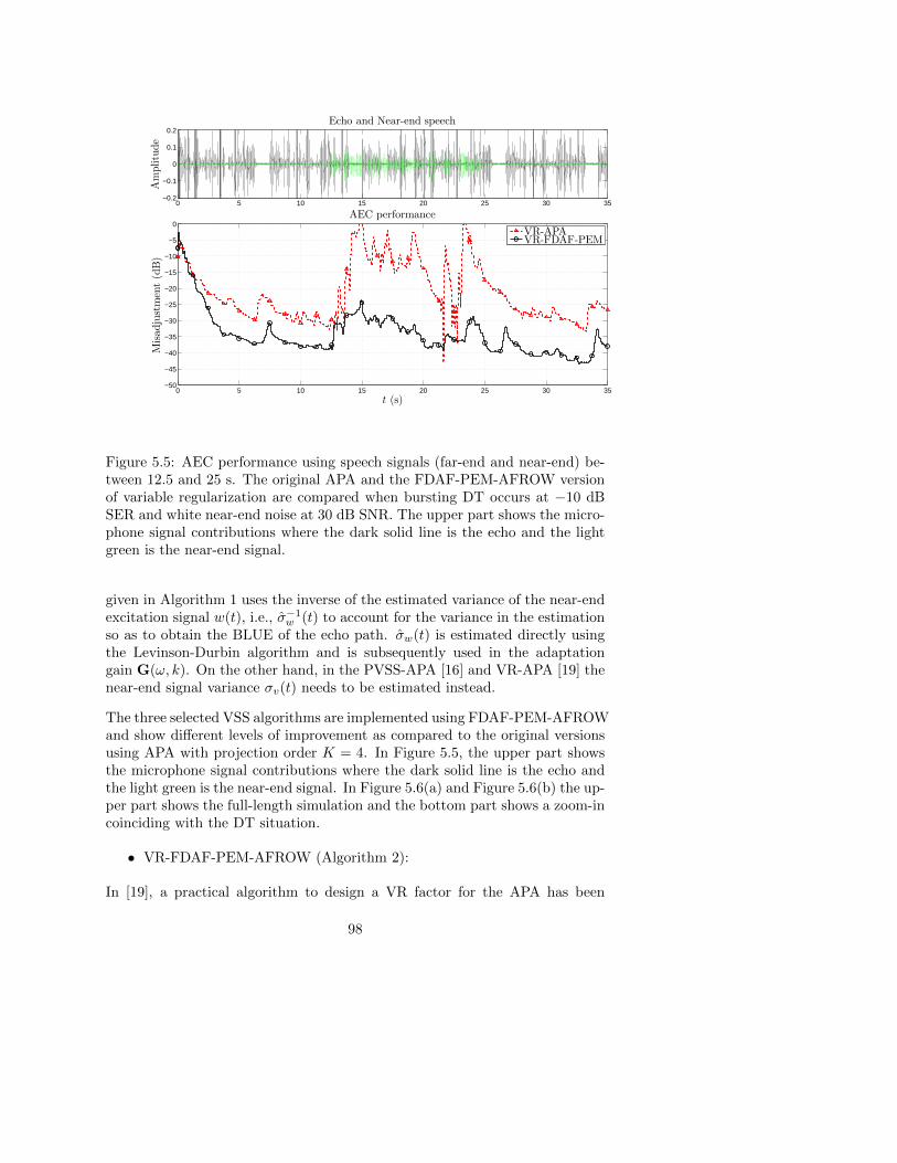
0 5 10 15 20 25 30 35−0.2

−0.1

0

0.1

0.2

Amplitude

Echo and Near-end speech

0 5 10 15 20 25 30 35−50

−45

−40

−35

−30

−25

−20

−15

−10

−5

0

t (s)

Misadjustment(dB)

AEC performance

VR-APAVR-FDAF-PEM

Figure 5.5: AEC performance using speech signals (far-end and near-end) be-tween 12.5 and 25 s. The original APA and the FDAF-PEM-AFROW versionof variable regularization are compared when bursting DT occurs at −10 dBSER and white near-end noise at 30 dB SNR. The upper part shows the micro-phone signal contributions where the dark solid line is the echo and the lightgreen is the near-end signal.

given in Algorithm 1 uses the inverse of the estimated variance of the near-endexcitation signal w(t), i.e., σ−1

w (t) to account for the variance in the estimationso as to obtain the BLUE of the echo path. σw(t) is estimated directly usingthe Levinson-Durbin algorithm and is subsequently used in the adaptationgain G(ω, k). On the other hand, in the PVSS-APA [16] and VR-APA [19] thenear-end signal variance σv(t) needs to be estimated instead.

The three selected VSS algorithms are implemented using FDAF-PEM-AFROWand show different levels of improvement as compared to the original versionsusing APA with projection order K = 4. In Figure 5.5, the upper part showsthe microphone signal contributions where the dark solid line is the echo andthe light green is the near-end signal. In Figure 5.6(a) and Figure 5.6(b) the up-per part shows the full-length simulation and the bottom part shows a zoom-incoinciding with the DT situation.

• VR-FDAF-PEM-AFROW (Algorithm 2):

In [19], a practical algorithm to design a VR factor for the APA has been

98

proposed. The condition to derive the VR-APA is to minimize the differencebetween the estimated and true filter coefficients. For this, it is assumed thatthe l2 norm of the a posteriori error is equal to the near-end noise signal vari-ance, similar to the condition imposed in [13], [16]. The VR-APA performancehas been compared to the performance of existing techniques [17], [18] [37],demonstrating the effectiveness of VR-APA. The implementation of the VR-FDAF-PEM-AFROW is straightforward since the estimate of the near-end ex-citation signal variance is calculated using the Levinson-Durbin algorithm. TheVR parameter is obtained in line 8 and included in the normalization factor inline 9 as shown in Algorithm 2.

In this particular case, the performance of VR-APA, shown in Figure 5.5, is verypoor. The algorithm is difficult to tune such that it has a comparable initialconvergence curve as the VR-FDAF-PEM-AFROW. On the other hand, itis obvious that VR-FDAF-PEM-AFROW significantly outperforms VR-APA,turning the latter into an algorithm suitable for DT situations as well.

• PVSS-FDAF-PEM-AFROW (Algorithm 3):

In PVSS-APA [16], the condition that is imposed to preserve the near-end com-ponent in the echo-compensated signal is to set the a posteriori error equal tothe near-end signal. As satisfying this condition is not possible in practice,an estimate of the near-end signal variance is calculated and compared to anestimate of the variance of the error signal [13], [16]. The PVSS-FDAF-PEM-AFROW version of the original algorithm is given in Algorithm 3. The mainsteps of this algorithm are: (1) the near-end signal variance estimation whichin PVSS-FDAF-PEM-AFROW is calculated using the Levinson-Durbin algo-rithm, and (2) the VSS calculation in line 7 which is frequency-dependent inPVSS-FDAF-PEM-AFROW.

The convergence of PVSS-FDAF-PEM-AFROW, shown in Figure 5.6(a), issimilar to the convergence for the PVSS-APA. During DT PVSS-FDAF-PEM-AFROW generally outperforms PVSS-APA by 5−7 dB. Moreover, it seems thatPVSS-FDAF-PEM-AFROW sets a lower bound in the MSD, i.e., consistentlyoutperforms PVSS-APA.

• PCVSS-FDAF-PEM-AFROW (Algorithm 4):

PCVSS-APA [11] belongs to the gradient-based VSS algorithms. It appearsthat PCVSS outperforms the algorithms given in [6] and [38] in DT situationsand moreover it does not rely on any signal or system model so it is claimed tobe easy to control in practice. The adaptation rate is controlled by a measureof the correlation between instantaneous and long-term averages of the so-called projection vectors, i.e., gradient vectors in APA. The three main featuresof PCVSS-FDAF-PEM-AFROW (Algorithm 4) are represented in (1) line 7where the correlation of the current and past gradient estimates is calculated,

99

(2) line 8 where the current step size is generated and (3) line 9 where thecontrol logic to bound its value is applied.The two algorithms, shown in Figure5.6(b), have a similarly fast initial convergence. During DT, the improvement ofPCVSS-FDAF-PEM-AFROW w.r.t. PCVSS-APA becomes apparent. PCVSS-FDAF-PEM-AFROW outperforms PCVSS-APA by 6−8 dB and it also showsa more stable curve.

5.6.3 Complexity analysis

The complexity analysis in Table 5.2 shows that, for a typical choice of the al-gorithm parameters, the FDAF-PEM-AFROW algorithms are about 10 timescheaper than the corresponding original algorithms. Hence, it is concludedthat the PVSS-FDAF-PEM-AFROW, PCVSS-FDAF-PEM-AFROW and VR-FDAF-PEM-AFROW algorithm are to be preferred over the original algorithmsduring DT situations. Based on FDAF-PEM-AFROW, a highly robust algo-rithm has been proposed in [39] using a Wiener variable step size (WISE) anda gradient spectral variance smoothing (GRASS) for DT-robust AEC and foracoustic feedback cancellation (AFC).

5.7 Conclusion

In this chapter, we have proposed a new framework to tackle the problemof double-talk (DT) in acoustic echo cancellation (AEC). It is based on afrequency domain adaptive filtering (FDAF) implementation of the so-calledPEM-AFROW algorithm (FDAF-PEM-AFROW). It has been shown that theFDAF-PEM-AFROW minimizes the BLUE criterion and so provides an op-timal acoustic echo path estimate during DT. The FDAF-PEM-AFROW al-gorithm shows an improved performance with respect to the PEM-AFROWand FDAF-NLMS with near-end signal normalization. Although these threealgorithms are constructed from the BLUE framework and should thereforeobtain the minimum variance echo path estimate during DT, in practice cleardifferences between them are observed. In PEM-AFROW, it is clear that fulfill-ing the three conditions to achieve the BLUE in practice is very difficult. Thisfact affects the PEM-AFROW much more than the FDAF-PEM-AFROW. TheFDAF-NLMS with near-end signal normalization performs better than PEM-AFROW as the conditions to achieve the BLUE seem to be less restricting.However, the FDAF-NLMS with near-end signal normalization is still outper-formed by FDAF-PEM-AFROW which has the benefits of being implementedin the frequency-domain, featuring a prefilter and including the non-frequency-dependent near-end excitation signal variance estimate. We have shown thatthe instantaneous pseudo-correlation (IPC) measure between the near-end sig-nal and the loudspeaker signal is significantly reduced when using the combi-

100

Algorithm 2 Variable regularization [19], using FDAF-PEM-AFROW (VR-FDAF-PEM-AFROW)

1: Initialize: SUa= SEa

= 0M×1.2: for k = 1, 2, ... do3: Perform lines 4− 14 from Algorithm 14: Φ(k) = Ua

∗(k) ◦Ea(k)5: for m = 0, 1, ...,M − 1 do6: SUa

(m, k) = λ0SUa(m, k − 1) + (1− λ0)|Ua(m, k)|2

7: SEa(m, k) = λ1SEa(m, k) + (1− λ1) |Ea(m, k)|2

8: α(m, k) = SUa(m, k)

√σw(k)√

SEa(m, k)−√σw(k)

9: G(m, k) = (SUa(m, k) + α(m, k))

−1

10: end for

11: F(k) = F(k − 1) + µ0F{[[F−1 {G(k) ◦Φ(k)}

]T1:N

0N

]T}12: end for13: In our simulation we used the following set of parameters: P = 160, N =

80, nA = 1, µ0 = 0.0325, λ0 = 0.95, λ1 = 0.9.

nation of FDAF and PEM, as done in FDAF-PEM-AFROW.

Finally, we have used the FDAF-PEM-AFROW framework to improve severalstate-of-the-art variable step-size (VSS) and variable regularization (VR) al-gorithms, in particular, the APA-based projection-correlation VSS (PCVSS-APA), the practical VSS affine projection algorithm (PVSS-APA) and theAPA-based VR (VR-APA). It has been shown that the FDAF-PEM-AFROWalgorithms significantly outperform the corresponding original algorithms inevery simulation by at least 6 dB during DT. In terms of computational com-plexity the FDAF-PEM-AFROW versions are themselves 10 times cheaper thanthe original versions.

101

Algorithm 3 Practical VSS [16] using FDAF-PEM-AFROW (PVSS-FDAF-PEM-AFROW)

1: Initialize: SUa= SEa

= 0M×1.2: for k = 1, 2, ... do3: Perform lines 4− 14 from Algorithm 14: for m = 0, 1, ...,M − 1 do5: SEa

(m, k) = λ0SEa(m, k − 1) + (1− λ0)|Ea(m, k)|2

6: SUa(m, k) = λ0SUa

(m, k − 1) + (1− λ0)|Ua(m, k)|2

7: µPVSS(m, k) = µ0

∣∣∣∣∣1−√σw(k)√

SEa(m, k) + α

∣∣∣∣∣8: G(m, k) = (SUa

(m, k) + α)−1

9: end for10: F(k) = F(k − 1)+

11: F{[[F−1 {µPVSS(k) ◦G(k) ◦Ua

∗(k) ◦Ea(k)}]T1:N

0N

]T}12: end for13: In our simulations we used the following set of parameters: P = 160,

N = 80, nA = 1, λ0 = 0.99, α = 2e−2, µ0 = 0.025, α = 10−8.

Algorithm 4 Projection-correlation VSS [11] using FDAF-PEM-AFROW(PCVSS-FDAF-PEM-AFROW)

1: Initialize: µPCVSS(0) = IM×1, SUa = Φ = C = 0M×1.2: for k = 1, 2, ... do3: Perform lines 4− 14 from Algorithm 14: Φ(k) = Ua

∗(k) ◦Ea(k)5: for m = 0, 1, ...,M − 1 do6: SUa(m, k) = λ0SUa(m, k − 1) + (1− λ0)|Ua(m, k)|27: C(m, k) = C(m, k − 1) + Φ(m, k)− Φ(m, k −B)8: µ′(m, k) = λ1 µPCVSS(m, k − 1) + β0 |C(m, k)|

9: µPCVSS(m, k) =

0, µ′(m, k) < 0µ0, µ′(m, k) > µ0

µ′(m, k), otherwise

10: G(m, k) = (SUa(m, k) + α)

−1

11: end for12: F(k) = F(k − 1)+

13: F{[[F−1 {µPCVSS(k) ◦G(k) ◦Ua

∗(k) ◦Ea(k)}]T1:N

0N

]T}14: end for15: In our simulation we used the following set of parameters: P = 160, N =

80, nA = 1, λ0 = 0.95, B = 50, β = λ1 = 0.9, α = 1e−3, µ0 = 0.03.

102

0 5 10 15 20 25 30 35−50

−40

−30

−20

−10

0AEC performance

10 15 20 25−50

−45

−40

−35

−30

−25

−20

t (s)

Misadjustment(dB)

PVSS-APAPVSS-FDAF-PEM-AFROW

(a)

0 5 10 15 20 25 30 35−50

−40

−30

−20

−10

0AEC performance

10 15 20 25−50

−45

−40

−35

−30

−25

−20

t (s)

Misadjustment(dB)

PCVSS-APAPCVSS-FDAF-PEM-AFROW

(b)

Figure 5.6: AEC performance using speech signals (far-end and near-end) be-tween 12.5 and 25 s. The original APA and the FDAF-PEM-AFROW versionsare compared when bursting DT occurs at −10 dB SER and white near-endnoise at 30 dB SNR. In (a) and (b) The upper part shows the full-length simula-tion and the bottom part shows a zoom-in coinciding with the DT. (a) PracticalVSS. (b) Projection-correlation VSS. 103


PVSS-APA 2K2N + 4KN + 15K + 8 3908

PVSS-FDAF- (FDAF)21M log2M + 34M

N+

PEM-AFROW (PEM) +6M log2M + 2M + n2

A + (4 + 4M)nAN

475

PCVSS-APA 2K2N + 4KN + 4K + 4N + 12 4188

PCVSS-FDAF- (FDAF)15M log2M + 19M +BM

N+


A + (4 + 4M)nAN

367

VR-APA 2K2N + 4KN + 4K 3878

VR-FDAF- (FDAF)15M log2M + 31M

N+


A + (4 + 4M)nAN

381

Table 5.4: Complexity comparison by the number of FLOPS per recursion.One FFT/IFFT is 3M log2M FLOPS, one

√· is M FLOPS and K = 4.

104

Appendix

5.A Instantaneous pseudo-correlation calculation

The following recursions show how the signal z(t) for the IPC measure iscalculated in different adaptive filtering algorithms, namely, in NLMS, PEM-AFROW, FDAF-NLMS and FDAF-PEM-AFROW.

We first consider the NLMS update equation given as

e(t) = y(t)− f(t− 1)u(t) (5.28)

f(t) = f(t− 1) + µe(t)

α+ uT (t)u(t)u(t). (5.29)

A derivation similar to (5.22) and (5.24) then leads to

ev(t) = e(t)− ex(t)

= v(t)− µt−1∑i=1

ev(i)

α+ uT (i)u(i)

(uT (i)u(t)

)(5.30)

and

z(t) =µ

N

t−1∑i=1

ev(i)

α+ uT (i)u(i)

(uT (i)u(t)

)(5.31)

=1

NfT (t− 1)u(t) (5.32)

with α = 10. The recursion to compute z(t) in PEM-AFROW can be derivedsimilarly where the NLMS is then a special case with a = [1 0nA

] ∀t

a = Levison-Durbin {v(t), nA} Computed every P samples. (5.33)

va(t) = aT v(t) (5.34)

ua(t) = aT u(t) (5.35)

eva(t) = va(t)− fT (t− 1)ua(t) (5.36)

g(t) =1

uTa (t)ua(t) + α(5.37)

f(t) = f(t− 1) + g(t)ua(t)eva(t) (5.38)

z(t) =1

NfT (t− 1)ua(t), (5.39)

where, in this case v(t) = [v(t), ..., v(t−P+1)]T , v(t) = [v(t), ..., v(t−nA+1)]T ,u(t) = [u(t), ..., u(t− nA + 1)]T and ua(t) = [ua(t), ..., ua(t−N + 1)].

105

The recursion to compute z(t) in FDAF-PEM-AFROW can be derived similarlywhere the FDAF-NLMS is then a special case with a = [1 0nA

] ∀t withλ = 0.99 is written as,

a(k) = Levison-Durbin {[v(k)]1:P , nA} (5.40)

ua(m, k) = [u(kN + 1 +m), ..., u(kN + 1 +m− nA)]a(k) m = 1, ...,M(5.41)

va(m, k) = [v(kN + 1 +m), ..., v(kN + 1 +m− nA)]a(k) m = 1, ...,M(5.42)

Ua(k) =1√MF{uTa (k)

}(5.43)

ea(k) =[va(k)−F−1

{F(k − 1) ◦Ua(k)

}√M]N+1:M

(5.44)

eva(k) =1√MF {[0N ea(k)]} (5.45)

SUa(m, k) = λSUa

(m, k − 1) + (1− λ)|Ua(m, k)|2 m = 1, ...,M (5.46)

G(m, k) = (SUa(m, k) + α)−1

m = 1, ...,M (5.47)

F(k) = Fa(k − 1) (5.48)

+1√MF{

[IN 0N ]T F−1

{G(k) ◦ Ea(k) ◦U∗a(k)

}√M}

(5.49)

z(k) =1

N

[F−1

{F(k − 1) ◦Ua(k)

}√M]N+1:M

(5.50)

Here (·)∗ represents a complex conjugation operation and v(k) = [v(kN −N +1), ..., v(kN + N)]T . It should be noted that the IPC measure is calculatedusing the signal va(t) instead of v(t), as given in (5.26).

106

Bibliography


[2] P. Gil-Cacho, T. van Waterschoot, M. Moonen, and S. H. Jensen, “Multi-microphone acoustic echo cancellation using multi-channel warped linearprediction of common acoustical poles,” in Proc. 18th European SignalProcess. Conf. (EUSIPCO’10), Aalborg, Denmark, Aug. 2010, pp. 2121–2125.

[3] T. van Waterschoot, G. Rombouts, P. Verhoeve, and M. Moonen, “Double-talk-robust prediction error identification algorithms for acoustic echo can-cellation,” IEEE Trans. Signal Process., vol. 55, no. 3, pp. 846–858, Mar.2007.



[6] V. J. Mathews and Z. Xie, “A stochastic gradient adaptive filter withgradient adaptive step size,” IEEE Trans. Signal Process., vol. 41, no. 6,pp. 2075–2087, June 1993.

[7] Y. Zhang, J. A. Chambers, W. Wang, P. Kendrick, and T. J. Cox, “Anew variable step-size LMS algorithm with robustness to nonstationarynoise,” in Proc. 2007 IEEE Int. Conf. Acoust. Speech Signal Process.(ICASSP’07), vol. 3, Honolulu, Hawaii, USA, Apr. 2007, pp. 1349–1352.

[8] W.-P. Ang and B. Farhang-Boroujeny, “A new class of gradient adaptivestep-size LMS algorithms,” IEEE Trans. Signal Process., vol. 49, no. 4,pp. 805–810, Apr. 2001.

[9] H.-C. Shin, A. H. Sayed, and W.-J. Song, “Variable step-size NLMS andaffine projection algorithms,” IEEE Signal Process. Lett., vol. 11, no. 2,pp. 132–135, Feb. 2004.

[10] Y. Zhang, N. Li, J. A. Chambers, and Y. Hao, “New gradient-based vari-able step size LMS algorithms,” EURASIP J. Advances Signal Process.,vol. 2008, no. 105, Jan. 2008.

[11] T. Creasy and T. Aboulnasr, “A projection-correlation algorithm foracoustic echo cancellation in the presence of double talk,” in Proc. 2000IEEE Int. Conf. Acoust. Speech Signal Process. (ICASSP’00), vol. 1, Is-tanbul, Turkey, June 2000, pp. 436–439.

107

[12] K. Ozeki and T. Umeda, “An adaptive filtering algorithm using an orthog-onal projection to an affine subspace and its properties,” Electronics andCommunication in Japan, vol. 67, no. 5, pp. 19–27, Aug. 1984.

[13] J. Benesty, H. Rey, L. R. Vega, and S. Tressens, “A nonparametric VSSNLMS algorithm,” IEEE Signal Process. Lett., vol. 13, no. 10, pp. 581–584,Oct. 2006.

[14] C. Paleologu, S. Ciochina, and J. Benesty, “Double-talk robust VSS-NLMSalgorithm for under-modeling acoustic echo cancellation,” in Proc. 2008IEEE Int. Conf. Acoust. Speech Signal Process. (ICASSP’08), Las Vegas,USA, Mar. 2008.

[15] M. A. Iqbal and S. L. Grant, “Novel variable step size NLMS algorithms forecho cancellation,” in Proc. 2008 IEEE Int. Conf. Acoust. Speech SignalProcess. (ICASSP’08), Las Vegas, USA, Mar. 2008, pp. 241 – 244.

[16] C. Paleologu, J. Benesty, and S. Ciochina, “A variable step-size affineprojection algorithm designed for acoustic echo cancellation,” IEEE Trans.Audio Speech Lang. Process., vol. 16, no. 8, pp. 1466 – 1478, Nov. 2008.

[17] H. Rey, L. R. Vega, S. Tressens, and J. Benesty, “Variable explicit reg-ularization in affine projection algorithm: Robustness issues and optimalchoice,” IEEE Trans. Signal Process., vol. 55, no. 5, pp. 2096 – 2108, May2007.

[18] Y.-S. Choi, H.-C. Shin, and W.-J. Song, “Adaptive regularization matrixfor affine projection algorithm,” IEEE Trans. Circuits Syst. II, Exp. Briefs,vol. 54, no. 12, pp. 1087–1091, Dec. 2007.

[19] W. Yin and A. S. Mehr, “A variable regularization method for affine pro-jection algorithm,” IEEE Trans. Circuits Syst. II, Exp. Briefs, vol. 57, no.6, pp. 476 – 480, June 2010.

[20] S. M. Kay, Fundamentals of statistical signal processing: Estimation the-ory. Upper Saddle River, New Jersey: Prentice Hall, 1993.

[21] T. van Waterschoot and M. Moonen, “Double-talk robust acoustic echocancellation with continuous near-end activity,” in Proc. 13th EuropeanSignal Process. Conf. (EUSIPCO ’05), Antalya, Turkey, Sep. 2005.

[22] L. Ljung, System Identification: Theory for the user. Englewood Cliffs,New Jersey: Prentice Hall, 1987.

[23] G. Rombouts, T. van Waterschoot, K. Struyve, and M. Moonen, “Acousticfeedback cancellation for long acoustic paths using a nonstationary sourcemodel,” IEEE Trans. Signal Process., vol. 54, no. 9, pp. 3426–3434, Sep.2006.

108

[24] T. Trump, “A frequency domain adaptive algorithm for colored measure-ment noise environment,” in Proc. 1998 IEEE Int. Conf. Acoust. SpeechSignal Process. (ICASSP’98), vol. 3, Seattle, Washington, USA, May 1998,pp. 1705 – 1708.

[25] ——, “Accounting for measurement noise color in frequency domain adap-tive algorithms,” in Proc. Thirty-Second Asilomar Conf. Signals Syst.Comp., vol. 1, Pacific Grove, CA, USA, May 1998, pp. 508 – 512.

[26] G. A. Clark, S. R. Parker and S. K. Mitra, “A Unified Approach to Time-and Frequency-Domain Realization of FIR Adaptive Digital Filters,” IEEETrans. Acoust. Speech Signal Process., Vol. 31, pp.1073-1083, Oct. 1983.

[27] T. Kariya, H. Kurata, Generalised Least Squares. John Wiley & Sons,2004.

[28] T. Soderstrom and P. Stoica System identification, Prentice Hall, 1988.

[29] H. Buchner, J. Benesty and W. Kellermann, “Generalized multichannelfrequency-domain adaptive filtering: efficient realization and applicationto hands-free speech communication,” Signal Process., vol. 85, pp. 549-570,Sep. 2005.

[30] P. Loizou, Speech Enhancement: Theory and Practice. Boca Raton,Florida: Taylor and Francis, 2007.

[31] A. Spriet, I. Proudler, M. Moonen and J. Wouters, “Adaptive feedbackcancellation in hearing aids with linear prediction of the desired signal,”IEEE Trans. Signal Process., vol. 53, no. 10, pp. 3749–3763, Oct. 2005.

[32] R. M. Gray, “On the Asymptotic Eigenvalue Distribution of Toeplitz Ma-trices,” IEEE Trans. on Information Theory, vol.18, no.6, pp. 725-730,Nov. 1972.

[33] T. van Waterschoot and M. Moonen, “Fifty years of acoustic feedbackcontrol: state of the art and future challenges,” Proc. IEEE, vol. 99, no.2, pp. 288–327, Feb. 2011.


[35] J. M. Gil-Cacho, T. van Waterschoot, M. Moonen, and S. H. Jensen,“Transform domain prediction error method for improved acoustic echoand feedback cancellation,” in Proc. 20th European Signal Process. Int.Conf. (EUSIPCO’12), Bucharest, Rumania, Aug. 2012, pp. 2422–2426.

[36] J. J. Shynk, “Frequency-domain and multirate adaptive filtering,” IEEESignal Process. Mag., vol. 9, no. 1, pp. 14–37, Jan. 1992.

109

[37] V. Myllyla and G. Schmidt, “Pseudo-optimal regularization for affine pro-jection algorithms,” in Proc. 2002 IEEE Int. Conf. Acoust. Speech SignalProcess. (ICASSP’02), vol. 2, Orlando, Florida, May 2002, pp. 1917–1920.

[38] C. Rohrs and R. Younce, “Double talk detector for echo canceler andmethod,” US Patent US 4 918 727, 04 17, 1990. [Online]. Available:http://www.patentlens.net/patentlens/patent/US4918727/

[39] J. M. Gil-Cacho, T. van Waterschoot, M. Moonen, and S. H. Jensen,“Wiener variable step size and gradient spectral variance smoothing fordouble-talk-robust acoustic echo cancellation and acoustic feedback can-cellation,” Submitted to Elsevier Signal Process., June 7, 2013. pp. 1–30.

110

Chapter 6

Wiener variable step sizeand gradient spectralvariance smoothing fordouble-talk-robust acousticecho cancellation andacoustic feedbackcancellation

Wiener variable step size and gradient spectral variancesmoothing for double-talk-robust acoustic echo cancellation and

acoustic feedback cancellation


Submitted to Elsevier Signal Processing, May. 2013.

111


• literature study• co-development of the WISE-GRASS-FDAF-PEM-AFROW algorithm• design of simulation scenarios• software implementation and computer simulations• co-interpretation of simulation results• text redaction and editing

112

Abstract

In this chapter, we derive a robust and computationally efficient algorithmbased on the frequency-domain adaptive filter prediction error method usingrow operations (FDAF-PEM-AFROW) for DT-robust AEC and for AFC. Theproposed algorithm features two main modifications: (a) the WIener vari-able Step sizE (WISE), and (b) the GRAdient Spectral variance Smoothing(GRASS). In AEC simulations, the WISE-GRASS-FDAF-PEM-AFROW al-gorithm obtains improved robustness and smooth adaptation in highly adversescenarios such as in bursting DT at high levels, and in a change of acousticpath during continuous DT. Similarly, in AFC simulations, the algorithm out-performs state-of-the-art algorithms when using a low-order near-end speechsignal model and in colored non-stationary noise.

6.1 Introduction

ACOUSTIC echo and acoustic feedback are two well-known problems ap-pearing in speech communication systems, which are caused by the acous-

tic coupling between a loudspeaker and a microphone. On the one hand,acoustic echo cancellation (AEC) is widely used in mobile and hands-free tele-phony [1] where the existence of echoes degrades the intelligibility and listeningcomfort. On the other hand, acoustic feedback limits the maximum amplifica-tion that can be applied, e.g., in a hearing aid, before howling due to instability,appears [2], [3]. This maximum amplification may be too small to compensatefor the hearing loss, which makes acoustic feedback cancellation (AFC) an im-portant component in hearing aids. Figure 6.1 shows the typical set-up forAEC and AFC.

The goal of AEC and AFC is essentially to identify a model for the echo orfeedback path, i.e., the room impulse response (RIR), and to estimate the echoor feedback signal which is then subtracted from the microphone signal. Themicrophone signal is given by y(t) = x(t)+v(t)+n(t) = F (q, t)u(t)+v(t)+n(t)where q denotes the time shift operator, e.g., q−ku(t) = u(t − k), t is thediscrete time variable, x(t) is the echo or feedback signal, u(t) is the loudspeakersignal, v(t) is the near-end speech signal and n(t) is the near-end noise signal.In the sequel, we will use the term near-end signal to refer to v(t) and/orn(t) if, according to the context, there is no need to point out a difference.F (q, t) = f0(t) + f1(t)q−1 + ... + fnF

(t)q−nF represents a linear time-varyingmodel of the RIR between the loudspeaker and the microphone, where nF isthe RIR model order. Therefore, the aim of AEC or AFC is to obtain anestimate F (q, t) of the RIR model F (q, t) by means of an adaptive filter, which

is steered by the error signal e(t) =[F (q, t)− F (q, t)

]u(t) + v(t) + n(t).

113

+-

+

cancellationpath F

v(t)

G

u(t)

x(t)

F

y(t)

n(t)

forwardpath path

acoustic

x(t)

e(t)

Figure 6.1: Typical set-ups for AEC/AFC. The left part (forward path) onlyrelates to AFC. The right part relates to both AEC and AFC.

In AEC applications the loudspeaker signal u(t) is considered to be the signalcoming from the far-end side, i.e., the far-end signal. The echo-compensatederror signal e(t) is then transmitted to the far-end side. In AFC applications, onthe other hand, the forward path G(q, t) maps the feedback-compensated errorsignal e(t) to the loudspeaker signal, i.e., u(t) = G(q, t)e(t). Typically, G(q, t)consists of an amplifier with a (possibly time-varying) gainK(t) cascaded with alinear equalization filter J(q, t) such that G(q, t) = J(q, t)K(t). AEC and AFCin principle look the same and share many common characteristics, howeverdifferent essential problems can be distinguished:

6.1.1 The problem of double-talk in acoustic echo cancel-lation

Practical AEC implementations rely on computationally simple stochastic gra-dient algorithms, such as the normalized least mean squares (NLMS) algo-rithms, which may be very sensitive to the presence of a near-end signal [4].Especially near-end speech, in a so-called double-talk (DT) scenario, will af-fect the adaptation in the AEC context by making the adaptive filter convergeslowly or even diverge.

To tackle the DT problem, adaptive filters have been equipped with DT detec-tors (DTDs) to switch off during DT periods. Since the Geigel algorithm [5]was proposed, several other DTD algorithms have been specifically designed forAEC applications, e.g., [6]. However, in general, DTDs take some time until anonset of a DT period is detected. Moreover, in some AEC scenarios the near-

114

end signal will be continuously present and then the use of a DTD becomesfutile. This may be the case for example in a noisy teleconferencing or AFCapplication. Therefore DT-robust algorithms without the need for a DTD arecalled for. DT-robustness may be achieved based on three approaches namely:(1) by using a postfilter to suppress or enhance residual echo, (2) by using avariable step size (VSS) to slow down adaption during DT, (3) by prefilteringthe loudspeaker and microphone signal with a decorrelation filter to achieve aminimum-variance RIR estimate.

The first approach consists in the use of a postfilter which interplays with theAEC to suppress residual echo (and also to reduce near-end signals) basedon signal enhancement techniques [7]- [9]. On the other hand, in [10], [11],the idea behind the postfilter design is the opposite, i.e., to the enhance theresidual echo in the adaptive filter loop. The postfilter design, in any case,is typically based on single-channel noise reduction techniques, which carry atrade-off between residual echo/noise reduction and signal distortion.

The second approach to DT-robust AEC is to equip the (stochastic gradient)adaptive filter with a VSS which may be derived using information about thegradient vector or information about the near-end signal power. The first typeof VSS algorithms rely on two properties of the gradient vector to control thestep size [12]- [16]: (1) the property that the norm of the gradient vector willbe large initially and converge to a small value, ideally zero, at steady state, (2)the property that the gradient vector direction will generally show a coherenttrend during initial convergence in contrast to a random trend around theoptimal value during DT and at steady state. From this class of algorithms, theonly one specifically designed for DT-robust AEC is the projection-correlationVSS (PC-VSS) which has been proposed in [17]. PC-VSS is a VSS algorithmbased on the affine projection algorithm (AP) [18] where the adaptation rateis controlled by a measure of the correlation between instantaneous and long-term averages of the so-called projection vectors, i.e., gradient vectors in APA,which allows to achieve robustness and to distinguish between an RIR changeand DT. PC-VSS is chosen as one of the competing algorithms in this chapterand hence further explanation will be given in Section 6.4.1.

Recently, more effort has been spent to steer VSS algorithm design towards DT-robust AEC. Some of these recent algorithms are based on the non-parametricVSS (NPVSS) algorithm proposed in [19]. The NPVSS algorithm was devel-oped in a system identification context, aiming to recover the system noise (i.e.,near-end noise) from the error signal of the adaptive filter when updated withthe NLMS algorithm. Inspired by this idea, several approaches have focusedon applying the NPVSS algorithm to real AEC applications where the micro-phone signal also contains a near-end speech signal. Consequently, differentVSS-NLMS algorithms have been successfully developed for DT-robust AEC,e.g., [20], [21]. Their convergence, however, is slow in practice and hence, anAPA version of the VSS-NLMS algorithm in [21] has been proposed in [22] to

115

increase the convergence speed. The resulting practical VSS affine projectionalgorithm (PVSS) [22] is chosen as one of the competing algorithms in thischapter and will be further explained also in Section 6.4.1.

The third approach is to search for the optimal AEC solution in a minimum-variance linear estimation framework, rather than in a traditional least squares(LS) framework. The minimum-variance RIR estimate, which is also known asthe best linear unbiased estimate (BLUE) [23], depends on the near-end signalcharacteristics, which are in practice unknown and time-varying [4], [24]. Thealgorithms in [4], [24] aim to whiten the near-end speech signal component inthe microphone signal by using adaptive decorrelation filters that are estimatedconcurrently with the RIR. In order to achieve the BLUE, it is also necessary toadd a scaled version of the near-end speech excitation signal variance to the de-nominator of the stochastic gradient update equation. The use of the predictionerror method (PEM) approach [25] was proposed to jointly estimate the RIRand an autoregressive (AR) model of the near-end speech signal. Among thePEM-based algorithms proposed in [4], [24], the PEM-based adaptive filteringusing row operations (PEM-AFROW) [26] is particularly interesting becauseit efficiently uses the Levison-Durbin algorithm to estimate both the near-endspeech signal AR model coefficients and the near-end speech excitation signalvariance. Thus the algorithms in [4], [24] can be seen as belonging to a newfamily aiming at both reducing the correlation between the near-end speechsignal and loudspeaker signal, and minimizing the RIR estimation variance.

6.1.2 The problem of correlation in acoustic feedback can-cellation

In the AFC set-up, the near-end speech signal will be continuously present sousing a DTD is pointless. However the main problem in AFC is the correlationthat exists between the near-end speech signal component in the microphonesignal and the loudspeaker signal itself. This correlation problem, which iscaused by the closed loop, makes standard adaptive filtering algorithms to con-verge to a biased solution [2], [27]. This means that the adaptive filter doesnot only predict and cancel the feedback component in the microphone sig-nal, but also part of the near-end speech signal. This generally results in adistorted feedback-compensated error signal. One approach to reduce the biasin the feedback path model identification is to prefilter the loudspeaker andmicrophone signal with the inverse near-end speech signal model, which is es-timated jointly with the adaptive filter [2], [27] using the PEM [25]. For anear-end speech signal, an AR model is commonly used [2] as this yields asimple finite impulse response (FIR) prefilter. However, the AR model fails toremove the speech periodicity, which causes the prefiltered loudspeaker signalstill to be correlated with the prefiltered near-end speech signal during voicedspeech segments. More advanced models using different cascaded near-end

116

speech signal models have been proposed to remove the coloring and periodic-ity in voiced as well as unvoiced speech segments. The constrained pole-zerolinear prediction (CPZLP) model [28], the pitch prediction model [3], and thesinusoidal model [29] are examples of alternative models used in recently pro-posed algorithms. However the overall algorithm complexity typically increasessignificantly when using cascaded near-end speech signal models [30]. In [31],a Transform-Domain PEM-AFROW (TD-PEM-AFROW) algorithm has beenproposed to improve the performance of an AFC without the need for cascadedand computationally intensive near-end signal models. Significant improvementwas achieved w.r.t. standard PEM-AFROW even using low-order AR models.PEM-AFROW and TD-PEM-AFROW are chosen as competing algorithmsfor AFC. TD-PEM-AFROW was also successfully applied to DT-robust AECin [31] and it is, therefore, also chosen as a competing algorithm for AEC.

6.1.3 Contributions and outline

In [32], we have proposed the use of the FDAF-PEM-AFROW framework toimprove several VSS and variable regularization (VR) algorithms. The im-provement is basically due to two aspects, (1) instantaneous pseudo-correlation(IPC) between the near-end signal and the far-end signal is heavily reducedwhen using FDAF-PEM-AFROW compared to stochastic gradient and (time-domain) PEM-AFROW algorithms [32] and (2) FDAF itself may be seen tominimize a BLUE criterion if a proper normalization factor is used duringadaptation [33]. In this chapter, we propose two modifications of the FDAF-PEM-AFROW algorithm for robust and smooth adaptation both in AFC andin AEC in continuous DT and bursting DT without the need of a DTD. Inparticular, we propose the WIener variable Step sizE (WISE) and the GRA-dient Spectral variance Smoothing (GRASS) to be performed in FDAF-PEM-AFROW leading to the WISE-GRASS-FDAF-PEM-AFROW algorithm. TheWISE modification is implemented as a single-channel noise reduction Wienerfilter applied to the (prefiltered) microphone signal. The Wiener filter gain [9]is used as a VSS in the adaptive filter, rather than as a signal enhancementparameter. On the other hand, the GRASS modification aims at reducing thevariance in the noisy gradient estimates based on time-recursive averaging of in-stantaneous gradients. The combination of the WISE and the GRASS into theFDAF-PEM-AFROW algorithm consequently gathers the best characteristicswe are seeking for in an algorithm both for AEC and AFC, namely, decorre-lation properties (PEM, FDAF), minimum variance (GRASS, FDAF, PEM),variable step size (WISE), and computational efficiency (FDAF).

The outline of the chapter is as follows. In Section 6.2, we briefly presentthe PEM, we provide a simple algorithm description and explain the choiceof the near-end speech signal model. In Section 6.3, the proposed algorithmis presented with in-depth explanations about the novel algorithm modifica-tions. The motivation for including these modifications is also justified for

117

DT-robust AEC and AFC. In Section 6.4, computer simulation results are pro-vided to verify the performance of the proposed algorithm compared to threecompeting algorithms, in particular, the PC-VSS [17], the PVSS [22] and theTD-PEM-AFROW [31] algorithm. A description of the competing algorithmsis provided together with a computational complexity analysis. The Matlabfiles implementing all the algorithms and those generating the figures in Sec-tion 6.3-6.4 can be found online 1. Finally, Section 6.5 concludes the chapter.

6.2 Prediction error method

The PEM-based AEC/AFC is shown in Figure 6.2. It relies on a linear modelfor the near-end speech signal v(t), which in Figure 6.2 is specified as

v(t) = H(q, t)w(t) (6.1)

where H(q, t) contains the filter coefficients of the linear model and w(t) rep-resents the excitation signal which is assumed to be a white noise signal withtime-dependent variance σ2

w(t) i.e.,

E{w(t)w(t− k)} = σ2w(t)δ(k) (6.2)

where E{·} is the expected value operator. The near-end noise n(t) is alsoassumed to be a white noise signal for the time being. As outlined before, aminimum-variance RIR model (in AEC) or an unbiased feedback path model (inAFC) can be identified by first prefiltering the loudspeaker signal u(t) and themicrophone signal y(t) with the inverse near-end speech signal model H−1(q, t)before feeding these signals to the adaptive filtering algorithm. As H−1(q, t) isobviously unknown, the near-end speech signal model and the echo/feedbackpath model have to be jointly identified using the PEM [25]. A common ap-proach in PEM-based AEC/AFC is to model the near-end speech signal withan AR model i.e.,

y(t) = x(t) + v(t) + n(t) (6.3)

= F (q, t)u(t) +1

A(q, t)w(t) + n(t) (6.4)

with F (q, t) defined previously and A(q, t) given as

A(q, t) = 1 + a1(t)q−1 + ...+ anA(t)q−nA (6.5)

where nA is the AR model order.

1http : //homes.esat.kuleuven.be/ ∼ dspuser/abstract12 − 214 2.html

118

+-

+

+-

+

F

F

cancellationpath F

v(t)

G

u(t)

x(t)

y(t)

n(t)

forwardpath path

acousticH−1

H−1

H

decorrelatingprefilter

speechmodel

copyw(t)

ea[t, h(t), f(t− 1)]

e[t, f(t)]

ua[t, h(t)]

ya[t, h(t)]

f(t)

x[t, f(t)]

Figure 6.2: AEC/AFC with prefiltering of the loudspeaker and microphonesignal using the inverse [H−1(q, t)] of the near-end speech signal model [H(q, t)].

The PEM gives an estimate of the models F (q, t) and A(q, t) by minimizationof the prediction error criterion

ϑ(t) = arg minϑ(t)

t∑i=1

e2a [i,ϑ(t)] (6.6)

where the prediction error is defined as

ea [i,ϑ(t)] = A(q, t) [y(i)− F (q, t)u(i)] (6.7)

and the parameter vector ϑ(t) =[fT (t),aT (t)

]Tcontains the parameters of

the echo or feedback path model and the near-end speech signal model i.e.,

f(t) = [f0(t), f1(t), ..., fnF(t)]T , (6.8)

a(t) = [1, a1(t), ..., anA(t)]T , (6.9)

Note that throughout the chapter we assume a sufficient-order condition forthe acoustic path model (i.e., nF = nF ). An additional assumption is thatthe near-end speech signal v(t) is short-term stationary, which implies that thenear-end speech signal model A(q, t) does not need to be re-estimated at eachtime instant t. That is, instead of identifying the near-end speech signal modelrecursively, it can also be identified non-recursively on a batch of loudspeaker

119

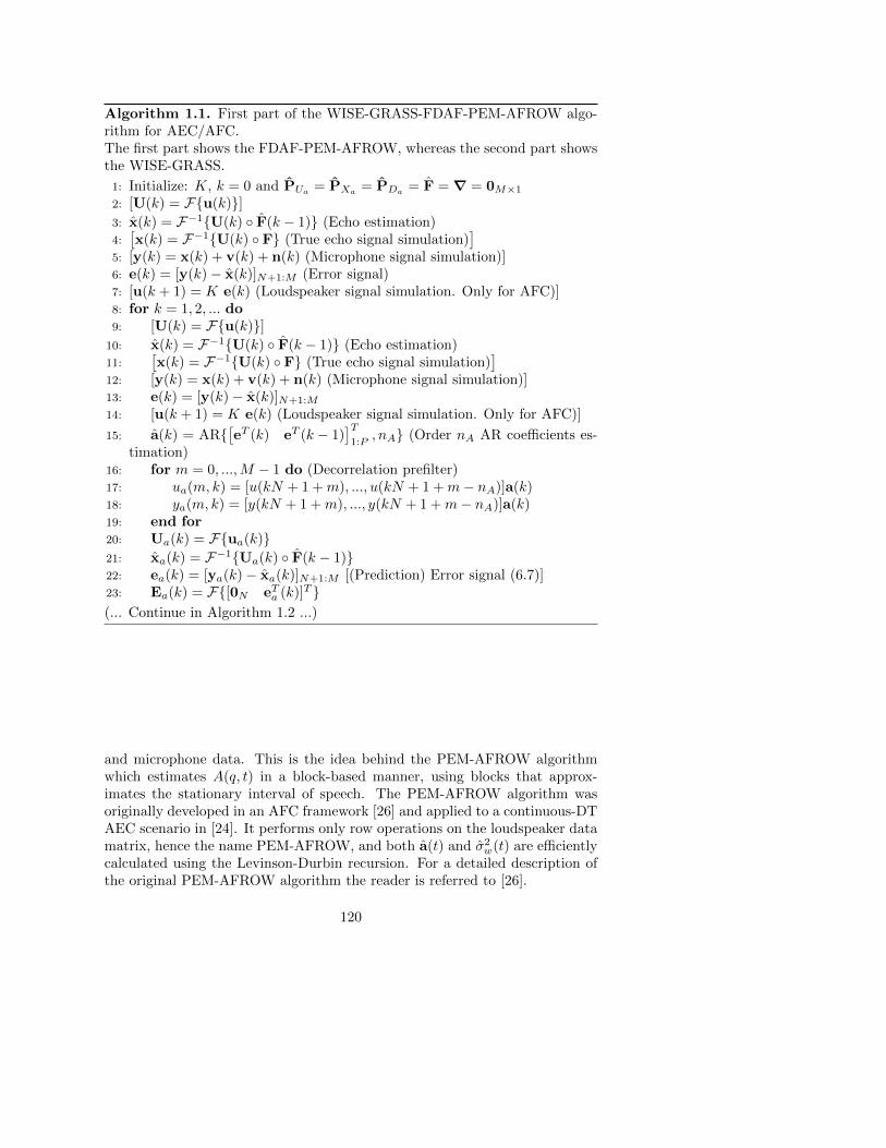
Algorithm 1.1. First part of the WISE-GRASS-FDAF-PEM-AFROW algo-rithm for AEC/AFC.The first part shows the FDAF-PEM-AFROW, whereas the second part showsthe WISE-GRASS.

1: Initialize: K, k = 0 and PUa= PXa

= PDa= F = ∇ = 0M×1

2: [U(k) = F{u(k)}]3: x(k) = F−1{U(k) ◦ F(k − 1)} (Echo estimation)4:[x(k) = F−1{U(k) ◦ F} (True echo signal simulation)

]5: [y(k) = x(k) + v(k) + n(k) (Microphone signal simulation)]6: e(k) = [y(k)− x(k)]N+1:M (Error signal)7: [u(k + 1) = K e(k) (Loudspeaker signal simulation. Only for AFC)]8: for k = 1, 2, ... do9: [U(k) = F{u(k)}]

10: x(k) = F−1{U(k) ◦ F(k − 1)} (Echo estimation)11:

[x(k) = F−1{U(k) ◦ F} (True echo signal simulation)

]12: [y(k) = x(k) + v(k) + n(k) (Microphone signal simulation)]13: e(k) = [y(k)− x(k)]N+1:M

14: [u(k + 1) = K e(k) (Loudspeaker signal simulation. Only for AFC)]

15: a(k) = AR{[eT (k) eT (k − 1)

]T1:P

, nA} (Order nA AR coefficients es-timation)

16: for m = 0, ...,M − 1 do (Decorrelation prefilter)17: ua(m, k) = [u(kN + 1 +m), ..., u(kN + 1 +m− nA)]a(k)18: ya(m, k) = [y(kN + 1 +m), ..., y(kN + 1 +m− nA)]a(k)19: end for20: Ua(k) = F{ua(k)}21: xa(k) = F−1{Ua(k) ◦ F(k − 1)}22: ea(k) = [ya(k)− xa(k)]N+1:M [(Prediction) Error signal (6.7)]23: Ea(k) = F{[0N eTa (k)]T }(... Continue in Algorithm 1.2 ...)

and microphone data. This is the idea behind the PEM-AFROW algorithmwhich estimates A(q, t) in a block-based manner, using blocks that approx-imates the stationary interval of speech. The PEM-AFROW algorithm wasoriginally developed in an AFC framework [26] and applied to a continuous-DTAEC scenario in [24]. It performs only row operations on the loudspeaker datamatrix, hence the name PEM-AFROW, and both a(t) and σ2

w(t) are efficientlycalculated using the Levinson-Durbin recursion. For a detailed description ofthe original PEM-AFROW algorithm the reader is referred to [26].

120

6.3 Proposed WISE-GRASS Modifications inFDAF-PEM-AFROW for AEC/AFC

The WISE-GRASS-FDAF-PEM-AFROW for AEC/AFC is given in Algorithm1 (parts 1.1 and 1.2). The FDAF implementation corresponds to the overlap-save FDAF with gradient constraint and power normalization [34], where u(k),v(k) and n(k) are length-M vectors, with M = 2N and N = nF + 1, satisfyingthe overlap-save condition in FDAF, e.g., u(k) = [u(kN−N+1), ...u(kN+N)]T ,where k = 0, 1, ....L−NN is the block-time index, L is the total length of thesignals, ◦ represents the element-wise multiplication operator, and finally, P isthe block length used to estimate A(q, t) with N ≤ P ≤ 2N . The upper asterisk(·)∗ denotes complex conjugation and [·]a:b represents a range of samples withina vector. The index m in frequency-domain variables, e.g., Ea(m, k), refersto a signal in the mth frequency bin of a block, m = 0, ...,M − 1. On theother hand, a capital bold-face variable, e.g., Ea(k) denotes an M -dimensionalvector of frequency components. The subscript a, e.g., Ea(m, k), denotes asignal output from the decorrelating prefilter, as shown in Figure 6.2. Lines2, 4, 5, 7 and 9, 11, 12, 14 correspond to the data generation and are bracketedto enphasyzed that these are not truly part of the algorithm. The specificWISE-GRASS modifications within the FDAF-PEM-AFROW algorithm areshown in Algorithm 1.2. The proposed WISE-GRASS-FDAF-PEM-AFROWweight update equation is given by

φ(k) =[F−1{µ(k) ◦W(k) ◦Θ(k)}

]1:N

(6.10)

F(k) = F(k − 1) + µmaxF{[φT (k) 0N ]T } (6.11)

where F{·} and F−1{·} denote the M -point discrete Fourier transform (DFT)and inverse DFT (IDFT) respectively, µ(k) corresponds to the power normal-ization step typically included in an FDAF update, µmax sets the maximumallowed value of the step size, and W(k) together with Θ(k) form the WISE-GRASS modifications which will be explained in detail in the following sections.

6.3.1 WIener variable Step sizE

The WIener variable Step sizE (WISE) modification into the FDAF-PEM-AFROW algorithm introduces a frequency-domain variable step size. Basically,the goal is to slow down the adaptation in frequency bins where the Echo-to-Near-End-Signal Ratio (ENR) is low and increase it in those frequency binswhere the ENR is high. If we recall that the near-end signal consists of the near-end speech signal and near-end noise signal, then we can calculate ENR(t) =

σ2x(t)

σ2v(t) + σ2

n(t), where σ2

x(t), σ2v(t) and σ2

n(t) are the variance of the echo, the

near-end speech signal and the near-end noise signal respectively. In the near-end-signal-free case, i.e. v(t) = n(t) = 0, the microphone signal consists only

121

Algorithm 1.2. Second part of the WISE-GRASS-FDAF-PEM-AFROW al-gorithm for AEC/AFC.The second part explains the WISE-GRASS.

24: for m = 0, ...,M − 1 do25: PUa

(m, k) = λ0PUa(m, k−1)+(1−λ0)|Ua(m, k)|2 (Recursive power

estimation)

26: µ(m, k) =[PUa(m, k) + δ

]−1

(Power normalization)

27: θ(m, k) = Ea(m, k)Ua∗(m, k) (Gradient estimation)

28: ∇(m, k) = λ3∇(m, k − 1) + (1− λ3)|θ(m, k)|229: α(m, k) = ∠θ(m, k) (Phase estimation)30: Θ(m, k) =

√∇(m, k)e[jα(m,k)] (GRASS)

31: PXa(m, k) = λ1PXa(m, k − 1) + (1− λ1)|Xa(m, k)|232: PDa

(m, k) = λ2PDa(m, k − 1) + (1− λ2)|Ea(m, k)|2

33: W (m, k) =

√PXa

(m, k)√PXa

(m, k) + PDa(m, k)

(WISE)

34: end for35: φ(k) =

[F−1{µ(k) ◦W(k) ◦Θ(k)}

]1:N

36: F(k) = F(k − 1) + µmaxF{[φT (k) 0N ]T }37: end for

of the echo so one could apply the maximum step size in each frequency bin.Once a near-end signal is present in the microphone signal, and especially so ifit is colored and non-stationary, the step sizes in the different frequency binsshould be reduced accordingly.

The concept for deriving the WISE is that of applying a single-channel frequency-domain noise reduction Wiener filter to the microphone signal y(t). This mayalso be seen as an echo-enhancement filter, however, we do not explicitly usethe output of the filter itself, but we use the Wiener filter gain as a variablestep size in the adaptive filer. The step size in each frequency bin is then variedby the gain of the Wiener filter at the frequency bin.

We assume that the signals are wide-sense stationary, that we have access tothe full record of samples and that disjoint frequency bins can be considereduncorrelated [35]. So, without loss of generality, we may consider a singlefrequency bin and work with the m-dependency. The frequency-domain micro-phone signal (6.3) is

Y (m, k) = X(m, k) + V (m, k) +N(m, k)

= X(m, k) +D(m, k)

where X(m, k) is the desired signal and D(m, k) is the noise signal which is tobe removed from the microphone signal. An estimate of the desired signal may

122

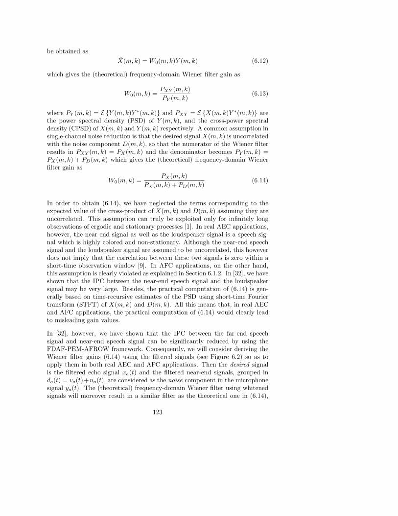
be obtained as

X(m, k) = W0(m, k)Y (m, k) (6.12)

which gives the (theoretical) frequency-domain Wiener filter gain as

W0(m, k) =PXY (m, k)

PY (m, k)(6.13)

where PY (m, k) = E {Y (m, k)Y ∗(m, k)} and PXY = E {X(m, k)Y ∗(m, k)} arethe power spectral density (PSD) of Y (m, k), and the cross-power spectraldensity (CPSD) of X(m, k) and Y (m, k) respectively. A common assumption insingle-channel noise reduction is that the desired signal X(m, k) is uncorrelatedwith the noise component D(m, k), so that the numerator of the Wiener filterresults in PXY (m, k) = PX(m, k) and the denominator becomes PY (m, k) =PX(m, k) + PD(m, k) which gives the (theoretical) frequency-domain Wienerfilter gain as

W0(m, k) =PX(m, k)

PX(m, k) + PD(m, k). (6.14)

In order to obtain (6.14), we have neglected the terms corresponding to theexpected value of the cross-product of X(m, k) and D(m, k) assuming they areuncorrelated. This assumption can truly be exploited only for infinitely longobservations of ergodic and stationary processes [1]. In real AEC applications,however, the near-end signal as well as the loudspeaker signal is a speech sig-nal which is highly colored and non-stationary. Although the near-end speechsignal and the loudspeaker signal are assumed to be uncorrelated, this howeverdoes not imply that the correlation between these two signals is zero within ashort-time observation window [9]. In AFC applications, on the other hand,this assumption is clearly violated as explained in Section 6.1.2. In [32], we haveshown that the IPC between the near-end speech signal and the loudspeakersignal may be very large. Besides, the practical computation of (6.14) is gen-erally based on time-recursive estimates of the PSD using short-time Fouriertransform (STFT) of X(m, k) and D(m, k). All this means that, in real AECand AFC applications, the practical computation of (6.14) would clearly leadto misleading gain values.

In [32], however, we have shown that the IPC between the far-end speechsignal and near-end speech signal can be significantly reduced by using theFDAF-PEM-AFROW framework. Consequently, we will consider deriving theWiener filter gains (6.14) using the filtered signals (see Figure 6.2) so as toapply them in both real AEC and AFC applications. Then the desired signalis the filtered echo signal xa(t) and the filtered near-end signals, grouped inda(t) = va(t)+na(t), are considered as the noise component in the microphonesignal ya(t). The (theoretical) frequency-domain Wiener filter using whitenedsignals will moreover result in a similar filter as the theoretical one in (6.14),

123

since

PXaYa(m, k) = E{A(m, k)X(m, k)Y ∗(m, k)A∗(m, k)} = |A(m, k)|2 PXY

(6.15)

PYa(m, k) = E{A(m, k)Y (m, k)Y ∗(m, k)A∗(m, k)} = |A(m, k)|2 PY , (6.16)

so that

W0(m, k) =PXaYa

(m, k)

PYa(m, k)

=PXa

(m, k)

PXa(m, k) + PDa

(m, k). (6.17)

We will compute time-recursive estimates of the PSDs instead and use availableestimates of the desired signal, i.e., Xa(m, k), and of the noise component in themicrophone signal, i.e., Ea(m, k). The Wiener filter gains are thus efficientlyestimated as follows

m = 0, ...,M − 1

PXa(m, k) = λ1PXa

(m, k − 1) + (1− λ1)|Xa(m, k)|2 (6.18)

PDa(m, k) = λ2PDa

(m, k − 1) + (1− λ2)|Ea(m, k)|2 (6.19)

Finally, using (6.18)-(6.19), we can write

W (m, k) =PXa(m, k)

PXa(m, k) + PDa

(m, k)(6.20)

where PXa(m, k) is an estimate of the PSD of Xa(m, k) which is calculated in

(6.18) using the output of the adaptive filter Xa(m, k) = Ua(m, k)F (m, k− 1),and where PDa(m, k) is an estimate of the PSD of Da(m, k) which is calculatedin (6.19) using the prediction-error signal Ea(m, k).

An interpretation of the Wiener filter gain W (m, k) in terms of the ÊNR(m, k)can be given by writing (6.20) as

W (m, k) =ÊNR(m, k)

ÊNR(m, k) + 1(6.21)

where

ÊNR(m, k) =PXa(m, k)

PDa(m, k)

(6.22)

=PXa(m, k)

PVa(m, k) + PNa

(m, k). (6.23)

The Wiener filter gain is a real positive number in the range 0 ≤W (m, k) ≤ 1which is used as a variable step size in (6.10). A maximum value for thestep size is also adopted, so that the effective step size is µmaxW (m, k). Let

124

us now consider the two limiting cases of (1) an ’echo-only’ microphone sig-nal, i.e., ˆENR(m, k) = ∞ and (2) a ’near-end-only’ microphone signal, i.e.,

ˆENR(m, k) = 0. In the first case the Wiener filter gain W (m, k) = 1, so thefilter would apply the maximum step size in the mth frequency bin. In the sec-ond case, the Wiener filter gain W (m, k) = 0 so the adaptation is suspended inthe mth frequency bin. In between these two extreme cases, the Wiener filtergain reduces the step size in proportion to an estimate of the ENR in eachfrequency bin.

6.3.2 GRAdient Spectral variance Smoothing

The GRAdient Spectral variance Smoothing (GRASS) is included to reducethe variance in the gradient estimation, in particular, the effect on the gradientestimation of sudden high-amplitude near-end signal samples. Although thestep size control has been considered in Section 6.3.1, it may not be sufficientlyfast to react in certain occasions, e.g., in DT bursts. In FDAF(-PEM-AFROW),an estimate of the gradient θ(m, k) = Ea(m, k)Ua

∗(m, k) is calculated for everyblock of samples. This noisy estimate may be separated into two componentsas

θ(m, k) = θ0(m, k) + θDa(m, k) (6.24)

where θ0(m, k) =[X(m, k)− X(m, k)

]Ua∗(m, k) is the true gradient and

θDa(m, k) = Da(m, k)Ua∗(m, k) is the gradient noise.

The concept for deriving the GRASS is that of applying averaged periodograms,which are typically used for estimating the PSD of a signal [36]. The peri-odogram is defined here as the squared magnitude of the gradient. An estimateof the true gradient PSD, at a given frequency m, is obtained as

Pθ0(m, k) =1

K

K−1∑j=0

|θ(m, k − j)|2. (6.25)

It is shown in [36] that the variance of (6.25) is

var{Pθ0(m, k)

}≈ 1

K|θ0(m, k)|2 (6.26)

so that it is proportional to the square of the true gradient’s PSD dividedby K and hence, as K → ∞, (6.26) approaches zero. This concept would besufficiently justified if the RIR does not change and the algorithm has convergedto an optimum, therefore θ0(m, k) = 0 by definition. In practice, of course, thetrue gradient θ0(m, k) is time-varying. Therefore the concept of averagingstarts to lose its sense. However we will assume that the true gradient variesslowly, therefore, a low-pass filter (LPF) with a low cut-off frequency would bemore beneficial than (6.25).

125

The realization of the GRASS is based on a time-recursive averaging of thegradient estimate (6.27)-(6.28). This is another way to obtain a first orderinfinite impulse response (IIR) filtering where λ3 is the pole of the low-passIIR filter, and it is given as

θ(m, k) = Ea(m, k)Ua∗(m, k) (6.27)

∇(m, k) = λ3∇(m, k − 1) + (1− λ3)|θ(m, k)|2 (6.28)

In fact, a LPF with a low cut-off frequency, will effectively filter out the gradientnoise and reduce the variance in the gradient estimation. Note that (6.25), is a

special case of a low-pass FIR filter, i.e., Pθ0(m, k) =K−1∑j=0

bk|θ(m, k − j)|2 with

weights bj = 1/K,∀j.

Finally, the phase α(m, k), that is obtained from the gradient estimate in (6.29),is applied in (6.30) to form the GRASS, i.e., Θ(m, k), as

α(m, k) = ∠θ(m, k) (6.29)

Θ(m, k) =√∇(m, k)e[jα(m,k)] (6.30)

A practical simulation of the GRASS for m = 15, i.e., the 15-th frequency bin,with k = 1, ..., 200 and λ3 = 0.95 is shown in Figure 6.3. For this simulationwe have used two speech signals, u(t) and v(t), and a noise signal n(t) sampledat 8 kHz. The AR coefficients of the near-end signal model are estimated usingd(t) = v(t) + n(t) and nA = 55. The signals, u(t) and d(t) are then filtered,as in Algorithm 1.1 lines 16 − 20, before feeding them to the overlap-save-type recursion. The gradient-constraint-type of calculations are performed,as in Algorithm 1.2 lines 34 − 35, to obtain both the noisy gradient and theGRASS gradient. We have assumed that the true gradient has converged to anoptimum, and thus it is, by definition, equal to zero. In Figure 6.3(a) a time-domain representation is shown where the upper and lower figures correspondto the real part of θ(m, k) and Θ(m, k), respectively. Besides, in Figure 6.3(b)a complex representation is shown where the circles (◦) represent the complexvalue of θ(m, k) and the crosses (×) represent the complex value of Θ(m, k). Inboth representations, the variance in the estimation is shown to be reduced by7 dB, the mean value is closer to zero, and high-amplitude samples are clearlysmoothed.

6.4 Evaluation

Simulations are performed using speech signals sampled at 8 kHz. Two types ofnear-end noise n(t) are used in the simulations namely, a white Gaussian noise

126

0 20 40 60 80 100 120 140 160 180 200−2

0

2

4

Time (blocks)Amplitude

Gradient Estimate 15th frequency bin

Gradient (variance: -7 dB)Mean: 0.058897

0 20 40 60 80 100 120 140 160 180 200−2

0

2

4

Time (blocks)

Amplitude

GRASS (variance: -14 dB)Mean: 0.01009

(a)

−2 −1 0 1 2 3 4

−2

−1

0

1

2

3

Real part

Imaginary

part

Gradient Estimate 15th frequency bin

GradientGRASS

(b)

Figure 6.3: Instantaneous gradient and GRASS estimates with m = 15 andk = 1, ..., 200. (a) Time representation: Upper and lower figures correspond tothe real part of θ(m, k) and Θ(m, k), respectively. The solid line (−) representsthe gradient estimate and the dotted line (· · · ) represents its mean value. (b)Complex representation: the circles (◦) represent the complex value of θ(m, k)and the crosses (×) represent the complex value of Θ(m, k).

(WGN) and a speech babble noise which is one of the most challenging noisetypes [37] in signal enhancement applications. We define two measures whichdetermine the relative signal levels in the simulations: the Signal-to-Echo Ratio

(SER)= 10 log10

σ2x

σ2v

and the Signal-to-Noise Ratio (SNR)= 10 log10

σ2x

σ2n

, where

σ2x, σ2

v and σ2n are the variances of the echo signal, the near-end speech signal

and near-end noise signal.

127

In the AEC simulations, the far-end (or loudspeaker) signal u(t) is a femalespeech signal and the near-end speech is a male speech signal. The microphonesignal consists of three concatenated segments of speech: the first and third 12s segment correspond to a single-talk situation, i.e., y(t) = x(t)+n(t), while thesecond 13 s segment corresponds to a DT situation, i.e, y(t) = x(t)+n(t)+v(t).The AR model order in the AEC is nA = 12, following the indications givenin [32], and the APA order is Q = 4. There are two RIRs used in the AECsimulations: an 80-taps impulse response f1 measured from a real mobile phone,and an artificial RIR f2 = f1 + n◦ f1 simulating an abrupt RIR change where nis one realization of a Gaussian random process. In the AEC simulations, theWGN and speech babble noise types are set at different SNRs: 30 and 20 dBrespectively. Several SER values are used for the simulations: from mild (15dB) to highly adverse (−5 dB) DT conditions.

In the AFC simulations, the near-end speech is the same female speech signalas in the AEC simulations. Two different AR model orders are chosen asin [4], [31]: nA = 12 which is common in speech coding for formant predictionand nA = 55 which is high enough to capture all near-end signal dynamics.The forward path gain K(t) is set 3 dB below the maxinum stable gain (MSG)without feedback cancellation i.e., see (6.32) in Section 6.4.2. A measured 100-tap acoustic impulse response was obtained from a real hearing aid and usedto simulate the feedback path. In both AEC and AFC, the window length Pwas chosen to be 20 ms (160 samples), which corresponds to the average timeinterval in which speech is considered stationary.

6.4.1 Competing algorithms and tuning parameters

AEC simulations are performed comparing four algorithms namely: the Pro-jection Correlation VSS (PC-VSS) algorithm [17], the Practical VSS affineprojection algorithm (PVSS) [22], the Transform-Domain PEM-AFROW (TD-PEM-AFROW) algorithm [31] and the proposed WISE-GRASS-FDAF-PEM-AFROW algorithm. PC-VSS belongs to the gradient-based VSS algorithmsand it is claimed to feature the appealing characteristics of being able to dis-tinguish between RIR changes and DT. PC-VSS is the result of improvingthe algorithm given in [12] to be specifically suited for AEC in DT situations.In PC-VSS, the adaptation rate is controlled by a measure of the correla-tion between instantaneous and long-term averages of the so-called projectionvectors, i.e., gradient vectors in APA. It appears that PC-VSS outperformsthe algorithms given in [12] and [38] in DT situations. Moreover, it does notrely on any signal or system model so it is easy to control in practice. Thesecond competing algorithm is the practical VSS affine projection algorithm(PVSS) [22] which stems from the so-called NPVSS proposed in [19]. PVSStakes into account the near-end signal power variations, it is effectively usedin DT situations and, it is claimed to be easy to control in practice. PVSShas been shown to outperform the algorithms proposed in [21], [39], and [40].

128


PC-VSS 2NQ+ 7Q2 + 4N + 12 1084PVSS 2NQ+ 7Q2 + 3Q+ 6 +Q+ 4Q+ 2 792

PEM-AFROW

(8 +

4P + 2nA + 1

P

)N +

1

Pn2A+(

4 +4P + 2

P

)nA +

P − 1

P+ 10 980

TD-PEM-AFROW Same as PEM-AFROW = 980+6N log2N 4015

WISE-GRASS 1/N(18M log2M + 25M + 3N)FDAF-PEM-AFROW +1/N(n2

A + 4MnA + 4 +M) 416

Table 6.1: Complexity comparison by the number of FLOPS per recursion.One FFT/IFFT is 3M log2M and the phase calculation is an M complexityoperation.

The third competing algorithms, TD-PEM-AFROW, has been investigated interms of DT robustness in AEC and general improvement in AFC. It has beenshown that the combination of a prewhitening of the input and microphone sig-nal together with transform-domain filter adaptation, successfully leads to analgorithm that solves the problem of decorrelation in a very efficient manner.TD-PEM-AFROW is very robust in DT situations and boosts the performanceof the simplest AFC (i.e., using only an AR model for the near-end signal).

All the algorithms presented in this chapter can be downloaded 2 along with thescripts generating every figure in this section. The tuning parameters in bothPVSS and PC-VSS are chosen according to the specifications given in [22]and [17] respectively. The parameters of TD-PEM-AFROW are chosen tohave similar initial convergence curves as PVSS and PC-VSS. In the proposedWISE-GRASS-FDAF-PEM-AFROW algorithm, the following parameters arechosen to have similar initial convergence properties as the other algorithms:µmax = 0.03, δ = 2.5e−6 , λ0 = 0.99, λ1 = 0.1, λ2 = 0.9. The different valuesof λ1 and λ2 in the time-recursive averaging for power estimation, basicallyaim for having a longer averaging window for the near-end signal and a shorteraveraging window for the echo signal. Note that for higher robustness to near-end signals a higher value of λ2 may be chosen; however, convergence would beslower.

AFC simulations are, on the other hand, performed comparing the originalPEM-AFROW [26], TD-PEM-AFROW [31] and the proposed WISE-GRASS-FDAF-PEM-AFROW. The parameters are tuned to have similar initial per-formance curves. In all three algorithms the following common values areapplied: the forward path G(q, t) consist of a delay of 80 samples and a fixed

2http : //homes.esat.kuleuven.be/ ∼ dspuser/abstract12 214 2.html

129

gain K(t) = K, ∀t, resulting in a 3 dB MSG without AFC, and a window ofP = 160 samples is used for estimating the AR model. For WISE-GRASS-FDAF-PEM-AFROW, λ0 = λ2 = 0.99, λ1 = 0.1, and µmax = 0.025.

The computational complexity of the different algorithms used in the AECsimulations is given in Table 6.1 using N = 80 and APA order Q = 4. Thecomputational complexity of WISE-GRASS-FDAF-PEM-AFROW is the low-est and that of TD-PEM-AFROWis the highest. The drawback of most ofthe FDAF-based algorithms is, however, their inherent delay of N samples. InAFC applications, this delay, or part of it, may be ‘absorbed’ by the forwardpath.

6.4.2 Performance measures

The performance measure for AEC simulations is the misadjustment (MSD).

The MSD between the estimated RIR f(t) and the true RIR f1 or f2 representsthe accuracy of the estimation and is defined as,

MSD(t) = 10 log10

∥∥∥f(t)− f1,2

∥∥∥2

2

‖f1,2‖22(6.31)

where f1,2 is either f1 or f2. The performance measure for AFC is the maximumstable gain (MSG). The achievable amplification before instability occurs ismeasured by the MSG, which is derived from the Nyquist stability criterion [27]and it is defined as

MSG(t) = −20 log10[maxω∈φ|J(ω, t)[F (ω)− F (ω, t)]|] (6.32)

where φ denotes the set of frequencies at which the loop phase is a multipleof 2π (i.e., the feedback signal x(t) is in phase with the near-end speech signalv(t)) and J(ω, t) denotes the forward path processing before the amplifier, i.e.,G(ω, t) = J(ω, t)K(t).

6.4.3 Simulation results for DT-robust AEC

In the first set of simulations, the noise n(t) is a WGN at 30 dB SNR. PVSS andPC-VSS are first tuned, as [22] and [17] respectively suggested, to obtain thebest performance both in terms of convergence rate and final MSD. TD-PEM-AFROW and WISE-GRASS-FDAF-PEM-AFROW are tuned to have similarinitial convergence rate as PVSS and PC-VSS. This set of parameters remainsunchanged throughout the simulations. All figures in this section consist ofan upper part showing the microphone signals and a bottom part showing theAEC performance. The upper part shows the echo (dark blue) and near-end(light green) signals, and the bottom part shows the MSD on the same time

130

scale. When a change of RIR occurs, the first part of the echo signal (generatedby f1) will be in a lighter color than the second part (generated by f2). Plottingthe time domain representation of these signals allows us to distinguish betweenthe amplitude and start/end points of both the echo and near-end signals.

Results for bursting DT

Figures 6.4 and 6.5 show the AEC performance when a bursting DT (from12.5 s during 12.5 s) occurs at two different SERs (15 dB and 5 dB) immersedin WGN at 30 dB SNR (Figure 6.4) and immersed in speech babble noise at20 dB SNR (Figure 6.5). More specifically, in Figure 6.4(a) and 6.4(b) a DTburst is shown at 15 and 5 dB SER respectively both immersed in WGN at30 dB SNR. It can be seen that in WGN, PC-VSS and PVSS achieve 5 dBimprovement in final MSD compared to the other two algorithms during singletalk, i.e., −45 to −40 dB respectively. However, during DT, WISE-GRASS-FDAF-PEM-AFROW outperforms the other three algorithms: in Figure 6.4(a)by 5 dB in the case of PVSS and TD-PEM-AFROW, and by around 10 dB inthe PC-VSS case; in Figure 6.4(b) these differences are increased since WISE-GRASS-FDAF-PEM-AFROW outperforms TD-PEM-AFROW by 8 − 10 dB,PVSS by 5− 8 dB and PC-VSS by 10− 20 dB.

Figure 6.5(a) and 6.5(b) show two scenarios where the near-end noise is speechbabble noise at 20 dB SNR and two DT bursts at 15 and 5 dB SER occur after12.5 s In these adverse scenarios, the improved performance of WISE-GRASS-FDAF-PEM-AFROW compared to the other three algorithms is demonstrated.The convergence of PVSS is seriously damaged in this scenario. As for thePC-VSS convergence, although it is the same as with WGN during the firstsecond, the MSD during single-talk is much higher than with WGN. On theother hand, TD-PEM-AFROW and WISE-GRASS-FDAF-PEM-AFROW ob-tain a smoother and faster convergence. During DT, the MSD of WISE-GRASS-FDAF-PEM-AFROW remains at−40 dB, insensitive to DT. The otherthree algorithms perform as in the WGN case during DT, which evidences thegreat difference with respect to the WISE-GRASS-FDAF-PEM-AFROW per-formance. These differences are clearly visible in the case of DT at 5 dBSER. After DT, WISE-GRASS-FDAF-PEM-AFROW restores the low MSDvalue (−40 dB) although it is outperformed by TD-PEM-AFROW followed byPVSS. PC-VSS seems to have serious problems in speech babble noise since itsMSD is almost 10 dB larger than for the other algorithms.

Results of RIR change during bursting DT

Figure 6.6 shows a scenario with an abrupt change of the RIR when the near-end noise is speech babble noise at 20 dB SNR. More specifically, in Figure ??the AEC performance is shown where the change of RIR occurs during DT at15 dB SER and in Figure 6.6(b) the SER is 5 dB. The poorest performance of

131

0 5 10 15 20 25 30 35−0.2

−0.1

0

0.1

0.2

Amplitude


0 5 10 15 20 25 30 35−50

−45

−40

−35

−30

−25

−20

−15

−10

−5

0

t (s)

Misad

justment(dB)

AEC performance

PVSSPC-VSSTD-PEMWISE-GRASS

(a)

0 5 10 15 20 25 30 35−0.2

−0.1

0

0.1

0.2

Amplitude


0 5 10 15 20 25 30 35−50

−45

−40

−35

−30

−25

−20

−15

−10

−5

0

t (s)

Misad

justment(dB)

AEC performance


(b)

Figure 6.4: AEC performance in WGN at 30 dB SNR. Bursting DT occurs atdifferent SER: (a) DT at 15 dB SER. (b) DT at 5 dB SER.

132

0 5 10 15 20 25 30 35−0.2

−0.1

0

0.1

0.2

Amplitude


0 5 10 15 20 25 30 35−50

−45

−40

−35

−30

−25

−20

−15

−10

−5

0

t (s)

Misad

justment(dB)

AEC performance


(a)

0 5 10 15 20 25 30 35−0.2

−0.1

0

0.1

0.2

Amplitude


0 5 10 15 20 25 30 35−50

−45

−40

−35

−30

−25

−20

−15

−10

−5

0

t (s)

Misad

justment(dB)

AEC performance


(b)

Figure 6.5: AEC performance in speech babble noise at 20 dB SNR. BurstingDT occurs at different SER: (a) DT at 15 dB SER. (b) DT at 5 dB SER.

133

(a)

0 5 10 15 20 25 30 35−0.2

−0.1

0

0.1

0.2Amplitude


0 5 10 15 20 25 30 35−50

−45

−40

−35

−30

−25

−20

−15

−10

−5

0

t (s)

Misad

justment(dB)

AEC performance


(b)

Figure 6.6: AEC performance in terms of MSD(t) in speech babble noise at 20dB SNR and an abrupt change of RIR after 17 s occurs during bursting DT(a) DT at 15 dB SER. (b) DT at 5 dB SER.

PC-VSS becomes apparent now since the DT contaminates its convergence andhence the MSD is still 15 dB. On the other hand, PVSS and TD-PEM-AFROW,although quite affected by DT, still show a descending trend in their MSDcurve which implies that they are converging during DT. In both Figure ??and 6.6(b), it is observed that the performance of WISE-GRASS-FDAF-PEM-AFROW is surprisingly almost constant. This fact highlights the robustnessof WISE-GRASS-FDAF-PEM-AFROW in an adverse scenario. In fact, itsperformance is barely degraded which demonstrates the robustness of WISE-GRASS-FDAF-PEM-AFROW as compared to the other three algorithms.

WISE evolution

Figure 6.7 shows the WISE evolution, i.e., W (m, k) for m = 0, ..., 79 and k =1, ..., L−NN , in two different scenarios: (1) in Figure 6.7(a) speech babble noise at40 dB SNR and bursting DT at 5 dB SER is used, and (2) in Figure 6.7(b) boththe loudspeaker signal and the near-end noise are WGN at 20 dB SNR, andan abrupt change of the RIR (f2 = 0.5f1) occurs at the 17.5 s mark. Figure6.7(a) displays the (dense) echo signal spectrogram and the near-end signal

134

(a)

(b)

Figure 6.7: WISE evolution in different scenarios together with the spectrogramof the echo signal and the near-end signals: (a) speech babble noise at 40 dBSNR and bursting DT at 5 dB SER. (b) Both the the near-end noise andthe loudspeaker signal are WGN at 20 dB SNR and abrupt change of RIR(f2 = 1/2f1) occurs at the 17.5 s mark.

spectrogram which clearly shows the near-end activity between 12.5 and 25 s.

135

In the bottom figure, the WISE evolution shows a drastic step size reductionduring DT. At t = 20 s where the PSD of the near-end signal is low in everyfrequency bin, the step size is increased in those frequency bins where the SERand SNR is appropriate: step sizes in frequency bins 0 − 10 are not increasedbecause the echo PSD is also low in the frequency bins and, thus, the Wienerfilter gain should be low. The step sizes in frequency bins from 75 and on, arealso smaller due to the fact that the echo PSD is lower. In Figure 6.7(b) it isshown how the step size follows the echo spectrum ‘weighted’ by the near-endsignal PSD.

Results in highly adverse scenarios

The performance of the algorithms is challenged in Figure 6.8 where two highlyadverse scenarios are proposed: In this DT situation WISE-GRASS-FDAF-PEM-AFROW significantly outperforms PC-VSS which appears to be stronglyaffected by DT, and moreover shows a significant improvement with respect toPVSS which itself outperforms TD-PEM-AFROW. In Figure 6.8(a) a change ofthe RIR occurs which decreases the PVSS performance, while WISE-GRASS-FDAF-PEM-AFROW performance is only decreased with respect to Figure6.6(b). WISE-GRASS-FDAF-PEM-AFROW shows a robust convergence afterthe RIR change even in a highly adverse DT level obtaining more than 8 dB im-provement compared to PVSS after the RIR change. On the other hand Figure6.8(b) shows another highly adverse situation where a continuous DT occurs.The simulation is done using four equal-length segments of speech babble noiseat four different SERs (20, 10, 5, 30 dB). It shows that, in these noise levels, theconvergence of PVSS decreases considerably and PC-VSS diverges as the SERincreases. After convergence, WISE-GRASS-FDAF-PEM-AFROW shows thelowest MSD, followed by that of TD-PEM-AFROW (3−5 dB above) and thenPVSS (6 − 7 dB above). Finally, Figure 6.8(b) shows that, after a change ofthe RIR in continuous DT, the only two algorithms that are able to convergeare TD-PEM-AFROW and WISE-GRASS-FDAF-PEM-AFROW.

Results of WISE-only, GRASS-only and WISE-GRASS in FDAF-PEM-AFROW

Figure 6.9 can shed some light on why WISE-GRASS-FDAF-PEM-AFROWis so robust and yet performs so well. A simulation of FDAF-PEM-AFROWusing WISE-only, GRASS-only and the proposed combination WISE-GRASSis shown in two adverse scenarios: speech babble noise at 10 dB and 20 dB SNRboth with DT at −5 dB SER and with an abrupt change of the RIR in Figure6.9(a) and 6.9(b) respectively. In FDAF and stochastic gradient algorithms ingeneral, the excess MSE depends on the step size and noise variance [1], [41].GRASS-only FDAF-PEM-AFROW, although robust and smooth, has a fixedstep size and thus, the final MSD is much higher. However, it is shown how

136

WISE-GRASS-FDAF-PEM-AFROW always obtains the best result comparedto WISE-only and GRASS-only. It is interesting to note how WISE-GRASS-FDAF-PEM-AFROW takes over GRASS-only FDAF-PEM-AFROW to WISE-only FDAF-PEM-AFROW at around 3 s in Figure 6.9(a) and around 5 s inFigure 6.9(b).

6.4.4 Simulation results for AFC

Three AFC scenarios are shown to compare the performance of PEM-AFROW,TD-PEM-AFROW and WISE-GRASS-FDAF-PEM-AFROW. The performanceis given in terms of the MSG. The value of W (m, k) = 1 for k = 1, ..., 20 be-cause at start-up the estimated PXa

(m, k), and therefore W (m, k), are verylow. WISE-GRASS-FDAF-PEM-AFROW needs some initial iterations until asignificant feedback signal PSD is estimated. In Figure 6.10 the circles repre-sent points of PEM-AFROW, stars represent points of TD-PEM-AFROW andsquares represent points of WISE-GRASS-FDAF-PEM-AFROW. More specif-ically, in Figure 6.10(a) the MSG is shown when using a near-end signal modelof nA = 55 and WGN at 40 dB SNR. It can be seen that the PEM-AFROWachieves 5− 7.5 dB MSG improvement and TD-PEM-AFROW achieves 3− 5dB MSG improvement w.r.t to PEM-AFROW. On the other hand, WISE-GRASS-FDAF-PEM-AFROW outperforms the other two algorithms by 8−10and 5− 3 dB respectively. The superior performance of WISE-GRASS-FDAF-PEM-AFROW appears more clearly in the case of a near-end signal modelof nA = 12 and WGN at 40 dB SNR shown in Figure 6.10(b). It can beseen that PEM-AFROW goes into the instability region and that TD-PEM-AFROW outperforms PEM-AFROW by 6 − 7 dB when using low nA orders.WISE-GRASS-FDAF-PEM-AFROW outperforms by far the other two algo-rithms, e.g., 10 − 15-dB improvement compared to PEM-AFROW. Moreover,it obtains almost the same performance as in the nA = 55 case. In Figure 6.11,a nA = 55 AR model order is used but, in this case, a speech babble noise at20 dB SNR is chosen. In this case both PEM-AFROW and TD-PEM-AFROWremain at around 5 dB above the instability region. On the other hand, WISE-GRASS-FDAF-PEM-AFROW maintains its superior performance of 6− 9 dBwith respect to the other two algorithms. In this last scenario, Figure 6.12shows the WISE evolution in terms of its instantaneous values (in each fre-quency bin) as time evolves. It is clearly seen that some frequency bins usuallyhave a smaller step size (e.g., frequency bin 5 − 35 and 85 − 100) than others(e.g., 35−60 and from 70−85). It is also interesting to notice that, during thefirst 7 s, frequency bins 5− 30 have smaller step sizes than after 7 s.

137

6.5 Conclusion

In this chapter, we have derived a practical yet highly robust algorithm basedon the frequency-domain adaptive filter prediction error method using row op-erations (FDAF-PEM-AFROW) for DT-robust AEC and AFC. The proposedalgorithm contains two modifications, namely (a) the WIener variable StepsizE (WISE) and (b) the GRAdient Spectral variance Smoothing (GRASS) tobe performed in FDAF-PEM-AFROW, leading to the WISE-GRASS-FDAF-PEM-AFROW algorithm. The WISE is implemented as a single-channel noisereduction Wiener filter applied to the (prefiltered) microphone signal, wherethe Wiener filter gain is used as a VSS in the adaptive filter. On the otherhand, the GRASS aims at reducing the variance in the noisy gradient esti-mates based on time-recursive averaging of gradient estimates. WISE-GRASS-FDAF-PEM-AFROW obtains improved robustness and smooth adaptation inhighly adverse scenarios such as in bursting DT at high levels, and with achange of the acoustic path during continuous DT. Simulations show thatWISE-GRASS-FDAF-PEM-AFROW outperforms other competing algorithmsin adverse scenarios both in AEC and AFC applications when the near-endsignals (i.e., speech and/or background noise) strongly affect the microphonesignal. WISE-GRASS-FDAF-PEM-AFROW combines the best characteris-tics of robust adaptation both in continuous DT and bursting DT withoutthe need for a DTD. WISE-GRASS-FDAF-PEM-AFROW consequently gath-ers all the characteristic we are seeking for namely, decorrelation properties(PEM, FDAF), minimum variance (GRASS, FDAF, PEM), variable step size(WISE), and computational efficiency (FDAF).

138

0 5 10 15 20 25 30 35−0.2

−0.1

0

0.1

0.2

Amplitude


0 5 10 15 20 25 30 35−50

−45

−40

−35

−30

−25

−20

−15

−10

−5

0

t (s)

Misad

justment(dB)

AEC performance


(a)

0 5 10 15 20 25 30 35−0.2

−0.1

0

0.1

0.2

Amplitude


0 5 10 15 20 25 30 35−50

−45

−40

−35

−30

−25

−20

−15

−10

−5

0

t (s)

Misad

justment(dB)

AEC performance


(b)

Figure 6.8: AEC performance comparison in highly adverse scenarios: (a)speech babble noise at 20 dB SNR and a change of the RIR after 17 s dur-ing bursting DT at −5 dB SER. (b) speech babble noise (continuous DT) at20, 10, 5, 30 dB SNR and change of RIR after 17 s.

139

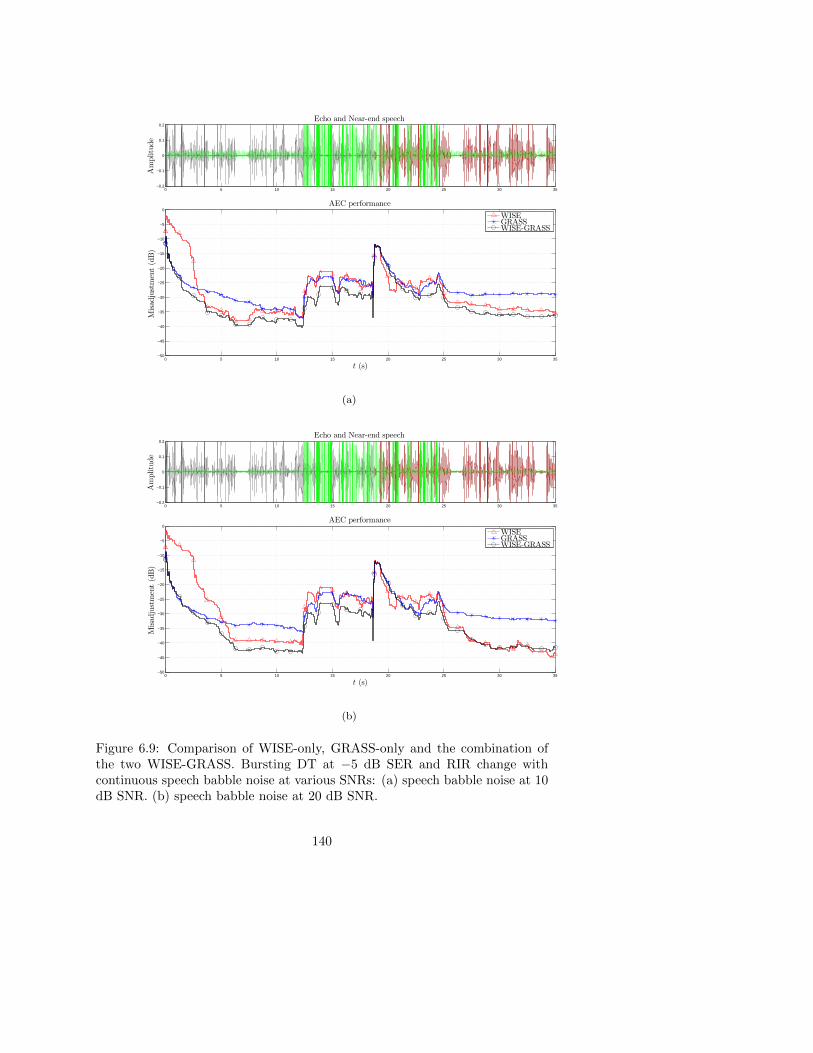
0 5 10 15 20 25 30 35−0.2

−0.1

0

0.1

0.2

Amplitude


0 5 10 15 20 25 30 35−50

−45

−40

−35

−30

−25

−20

−15

−10

−5

0

t (s)

Misad

justment(dB)

AEC performance

WISEGRASSWISE-GRASS

(a)

0 5 10 15 20 25 30 35−0.2

−0.1

0

0.1

0.2

Amplitude


0 5 10 15 20 25 30 35−50

−45

−40

−35

−30

−25

−20

−15

−10

−5

0

t (s)

Misad

justment(dB)

AEC performance

WISEGRASSWISE-GRASS

(b)

Figure 6.9: Comparison of WISE-only, GRASS-only and the combination ofthe two WISE-GRASS. Bursting DT at −5 dB SER and RIR change withcontinuous speech babble noise at various SNRs: (a) speech babble noise at 10dB SNR. (b) speech babble noise at 20 dB SNR.

140

0 5 10 15 20 25 30 35 4015

20

25

30

35

40

t (s)

MSG

(dB)

AFC performance

20 log10KMSG F (ω)WISE-GRASSTD-PEMPEM

(a)

0 5 10 15 20 25 30 35 4015

20

25

30

35

40

t (s)

MSG

(dB)

AFC performance


(b)

Figure 6.10: AFC performance in terms of MSG(t) of the three algorithms:PEM-AFROW, TD-PEM-AFROW and WISE-GRASS-FDAF-PEM-AFROW:(a) nA = 55 and WGN at 40 dB SNR. (b) nA = 12 and WGN at 40 dB SNR.

141

0 5 10 15 20 25 30 35 4015

20

25

30

35

40

t (s)

MSG

(dB)

AFC performance


Figure 6.11: AFC performance in terms of MSG(t) of the three algorithms:PEM-AFROW, TD-PEM-AFROW and WISE-GRASS-FDAF-PEM-AFROW:nA = 55 and speech babble noise at 20 dB SNR.

Figure 6.12: AFC WISE evolution in WISE-GRASS-FDAF-PEM-AFROWwith nA = 55 and speech babble noise at 20 dB SNR.

142

Bibliography

[1] S. Haykin, Adaptive Filter Theory, Upper Saddle River, New Jersey: Pren-tice Hall, 2002.

[2] A. Spriet, I. Proudler, M. Moonen, J. Wouters, Adaptive feedback cancel-lation in hearing aids with linear prediction of the desired signal, IEEETrans. Signal Process. 53, no. 10 (2005) 3749–3763.

[3] K. Ngo, T. van Waterschoot, M. G. Christensen, S. H. J. M. Moonen,J. Wouters, Prediction-error-method-based adaptive feedback cancellationin hearing aids using pitch estimation, in: Proc. 18th European SignalProcess. Conf. (EUSIPCO’10), Aalborg, Denmark, 2010.

[4] T. van Waterschoot, G. Rombouts, P. Verhoeve, M. Moonen, Double-talk-robust prediction error identification algorithms for acoustic echo cancel-lation, IEEE Trans. Signal Process. 55, no. 3 (2007) 846–858.

[5] D. L. Duttweiler, A twelve-channel digital echo canceler, IEEE Trans.Commun. 26, no. 5 (1978) 647–653.

[6] H. K. Jung, N. S. Kim, T. Kim, A new double-talk detector using echopath estimation, Speech Commun. 45, no. 1 (2005) 41–48.

[7] G. Enzner, P. Vary, Frequency-domain adaptive Kalman filter for acousticecho control in hands-free telephones, Signal Process. 86, no. 6 (2006)1140–1156.

[8] S. Gustafsson, F. Schwarz, A postfilter for improved stereo acousticecho cancellation, in: 1999 Int. Workshop Acoustic Echo Noise Control(IWAENC’99), Pocono Manor,Pennsylvania, Sep. 1999, pp. 32–35.

[9] P. Loizou, Speech Enhancement: Theory and Practice, Boca Raton,Florida: Taylor and Francis., 2007.

[10] T. S. Wada, B.-H. Juang, Towards robust acoustic echo cancellation dur-ing double-talk and near-end background noise via enhancement of resid-ual echo, in: Proc. 2008 IEEE Int. Conf. Acoust. Speech Signal Process.(ICASSP’08), Las Vegas, USA, Mar. 2008, pp. 253–256.

[11] T. S. Wada, B.-H. Juang, Enhancement of residual echo cancellation forimproved acoustic echo cancellation, in: Proc. 15th European Signal Pro-cess. Int. Conf. (EUSIPCO’07), Poznan, Poland, Sep. 2007, pp. 1620–1624.

[12] V. J. Mathews, Z. Xie, A stochastic gradient adaptive filter with gradientadaptive step size, IEEE Trans. Signal Process. 41, no. 6 (1993) 2075–2087.

143

[13] Y. Zhang, J. A. Chambers, W. Wang, P. Kendrick, T. J. Cox, A newvariable step-size lms algorithm with robustness to nonstationary noise, in:Proc. 2007 IEEE Int. Conf. Acoust. Speech Signal Process. (ICASSP’07),Vol. 3, Honolulu, Hawaii, USA, Apr. 2007, pp. 1349–1352.

[14] W.-P. Ang, B. Farhang-Boroujeny, A new class of gradient adaptive step-size LMS algorithms, IEEE Trans. Signal Process. 49, no. 4 (2001) 805–810.

[15] H.-C. Shin, A. H. Sayed, W.-J. Song, Variable step-size NLMS and affineprojection algorithms, IEEE Signal Process. Lett. 11, no. 2 (2004) 132–135.

[16] Y. Zhang, N. Li, J. A. Chambers, Y. Hao, New gradient-based variablestep size lms algorithms, EURASIP J. Advances Signal Process. 2008, no.105.

[17] T. Creasy, T. Aboulnasr, A projection-correlation algorithm for acousticecho cancellation in the presence of double talk, in: Proc. 2000 IEEEInt. Conf. Acoust. Speech Signal Process. (ICASSP’00), Vol. 1, Istanbul,Turkey, June 2008, pp. 436–439.

[18] K. Ozeki, T. Umeda, An adaptive filtering algorithm using an orthogo-nal projection to an affine subspace and its properties, Electronics andCommunication in Japan 67, no. 5 (1984) 19–27.

[19] J. Benesty, H. Rey, L. R. Vega, S. Tressens, A nonparametric VSS NLMSalgorithm, IEEE Signal Process. Lett. 13, no. 10 (2006) 581–584.

[20] M. A. Iqbal, S. L. Grant, Novel variable step size NLMS algorithms forecho cancellation, in: Proc. 2008 IEEE Int. Conf. Acoust. Speech SignalProcess. (ICASSP’08), Las Vegas, USA, Mar. 2008, pp. 241 – 244.

[21] C. Paleologu, S. Ciochina, J. Benesty, Double-talk robust VSS-NLMS algo-rithm for under-modeling acoustic echo cancellation, in: Proc. 2008 IEEEInt. Conf. Acoust. Speech Signal Process. (ICASSP’08), Las Vegas, USA,Mar. 2008.

[22] C. Paleologu, J. Benesty, S. Ciochina, A variable step-size affine projec-tion algorithm designed for acoustic echo cancellation, IEEE Trans. AudioSpeech Lang. Process. 16, no. 8 (2008) 1466 – 1478.

[23] S. M. Kay, Fundamentals of statistical signal processing: estimation the-ory, Upper Saddle River, New Jersey: Prentice Hall, 1993.

[24] T. van Waterschoot, M. Moonen, Double-talk robust acoustic echo cancel-lation with continuous near-end activity, in: Proc. 13th European SignalProcess. Conf. (EUSIPCO’05), Antalya, Turkey, 2005.

[25] L. Ljung, System Identification: Theory for the user, Englewood Cliffs,New Jersey: Prentice Hall, 1987.

144

[26] G. Rombouts, T. van Waterschoot, K. Struyve, M. Moonen, Acousticfeedback cancellation for long acoustic paths using a nonstationary sourcemodel, IEEE Trans. Signal Process. 54, no. 9 (2006) 3426–3434.

[27] T. van Waterschoot, M. Moonen, Fifty years of acoustic feedback control:state of the art and future challenges, Proc. IEEE 99, no. 2 (2011) 288–327.

[28] T. van Waterschoot, M. Moonen, Adaptive feedback cancellation for audioapplications, Signal Process. 89, no. 11 (2009) 2185–2201.

[29] K. Ngo, T. van Waterschoot, M. G. Christensen, M. Moonen, S. H. Jensen,J. Wouters, Adaptive feedback cancellation in hearing aids using a sinu-soidal near-end signal model, in: Proc. 2010 IEEE Int. Conf. Acoust.Speech Signal Process. (ICASSP’10), Dallas, USA, 2010.

[30] K. Ngo, T. van Waterschoot, M. G. Christensen, M. Moonen, S. H. Jensen,Improved prediction error filters for adaptive feedback cancellation in hear-ing aids, Elsevier Signal Processing.

[31] J. M. Gil-Cacho, T. van Waterschoot, M. Moonen, S. H. Jensen, Transformdomain prediction error method for improved acoustic echo and feedbackcancellation, in: Proc. 20th European Signal Process. Int. Conf. (EU-SIPCO’12), Bucharest, Rumania, Aug. 2012, pp. 2422–2426.

[32] J. M. Gil-Cacho, T. van Waterschoot, M. Moonen, S. H. Jensen, Afrequency-domain adaptive filtering (FDAF) prediction error method(PEM) for double-talk-robust acoustic echo cancellation, in: Tech-nical Report KULuven, ESAT-SCD, Aug. 2013, (online http ://homes.esat.kuleuven.be/ dspuser/abstract13− 132.html).

[33] T. Trump, A frequency domain adaptive algorithm for colored measure-ment noise environment, in: Proc. 1998 IEEE Int. Conf. Acoust. SpeechSignal Process. (ICASSP’98), Seattle, USA, Mar. 1998, pp. 1705–1708.

[34] J. J. Shynk, Frequency-domain and multirate adaptive filtering, IEEESignal Process. Mag. 9, no. 1 (1992) 14–37.

[35] N. J. Bershad, P. L. Feintuch, Analysis of the frequency domain adaptivefilter, Proc. IEEE 67, no. 12 (1979) 1658–1659.

[36] M. H. Hayes, Statistical Digital Signal Processing and Modeling, NewYork, NY: John Wiley & Sons, Inc., 1996.

[37] N. Krishnamurthy, J. H. L. Hansen, Babble noise: Modeling, analysis, andapplications, IEEE Trans. Audio Speech Lang. Process. 17, no. 7 (2009)1394–1407.

[38] C. Rohrs, R. Younce, Double talk detector for echo canceler and method(04 1990).URL http://www.patentlens.net/patentlens/patent/US4918727/

145

[39] T. Gansler, S. L. Gay, M. M. Sondhi, J. Benesty, Double-talk robust fastconverging algorithms for network echo cancellation, IEEE Trans. SpeechAudio Process. 8, no. 6 (2000) 656–663.

[40] H. Rey, L. R. Vega, S. Tressens, J. Benesty, Variable explicit regularizationin affine projection algorithm: Robustness issues and optimal choice, IEEETrans. Signal Process. 55, no. 5 (2007) 2096–2108.

[41] B. Farhang-Boroujeny, Adaptive filters: Theory and applications, Chich-ster, UK: Wiley, 1998.

146

Part IV

Nonlinear Adaptive Filters

Chapter 7

Linear-in-the-parametersnonlinear adaptive filtersfor acoustic echocancellation

Study and characterization of odd and even nonlinearities inelectrodynamic loudspeakers by means of periodic random-phase

multisinePublished in Proc. of the 127th Audio Engineering Society (AES)

convention, NY, USA, Oct. 2009.

Linear-in-the-parameters nonlinear adaptive filters for acousticecho cancellation

Accepted with major revision in Journal of the Audio EngineeringSociety (JAES), July 2013.


149


• literature study• co-development of the nonlinear algorithms• design of simulation scenarios• software implementation and computer simulations• co-interpretation of simulation results• text redaction and editing

150

Abstract

In this chapter, we consider the description of odd and even nonlinearities inelectrodynamic loudspeakers by means of periodic random-phase multisine sig-nals. It is shown that the odd nonlinear contributions are more predominantthan the even ones. This fact implies that at least a 3rd-order nonlinear modelof the loudspeaker should be used, which is in clear conflict with the extensive,almost unique, use of second-order (quadratic) Volterra filters. We, there-fore, consider the identification and validation of a model of the loudspeakerusing several linear-in-the-parameters nonlinear adaptive filters, namely, Ham-merstein and Legendre polynomial filters of various orders, and a simplified3rd-order Volterra filter of various lengths. In our measurement set-up, theobtained results imply however, that a 3rd-order nonlinear filter can not cap-ture all the nonlinearities, meaning that odd and even nonlinear contributionsare produced by higher-order nonlinearities. Legendre polynomial filters areshown to improve performance monotonically with increasing order whereasHammerstein filters do not. In the simplified 3rd-order Volterra filter case, theperformance is remarkably poorer than in the Legendre polynomial case forthe same filter length. The differences between identification and validationappear to be very small in the Legendre polynomial filter case. However, thesimplified 3rd-order Volterra filter presents clear signs of overfitting.

7.1 Introduction

ACOUSTIC echo cancellation (AEC) is used in many speech communi-cation systems where the existence of echoes degrades the speech in-

telligibility and listening comfort [1], [2]. Applications range from mobile orhands-free telephony to teleconferencing or voice over IP (VoIP) services, whichare often integrated in smartphones, tablets, notebooks, laptops, etc. Whilemobile devices are becoming smaller, the demand for quality, performance, andspecial features in audio products is increasing. Moreover, the need for highersound pressure levels, provided by smaller devices, presents a huge challengeto engineers who have to deal with (usually cheap) loudspeakers working closeto saturation.

The general set-up for an AEC is depicted in Figure 7.1. A far-end speech signalu(t) is played back into an enclosure (i.e., the room) through a loudspeaker.In the room, there is a microphone to record a near-end speech signal, whichis to be transmitted to the far-end side. An acoustic echo path H between theloudspeaker and the microphone exists, so that the microphone (i.e., desired)signal d(t) = y(t) + n(t) contains an undesired echo y(t) plus the backgroundnoise n(t). The echo signal y(t) can be considered as the far-end signal u(t)filtered by the loudspeaker-enclosure-microphone (LEM) system’s response. An

151

acoustic echo canceler seeks to cancel the echo signal component y(t) in themicrophone signal d(t), ideally leading to an echo-free error (or residual) signale(t), which is then transmitted to the far-end side. This is done by subtractingan estimate of the echo signal y(t) from the microphone signal, i.e., e(t) =d(t) − y(t) = y(t) − y(t) + n(t). Thus, the main objective of an echo canceleris to identify a model that represents a best fit to the LEM system.

+-

+

path pathacoustic

From far-end

To far-end

cancellationHH

LEM

u(t)

y(t)

n(t)

e(t) d(t)

y(t)

f [u(t)]

Figure 7.1: Typical set-up for an AEC.

Typically, a linear finite-impulse-response (FIR) filter is assumed to provide asufficiently accurate model for the LEM system, leading to a class of linear-adaptive-filter-based AEC systems. This assumption may be valid for somecomponents in the LEM system. In fact, even in nonlinear AEC (NLAEC),the acoustic path and microphone response may be modeled as a linear system.However, loudspeakers, as well as amplifiers, DACs, coders, etc., included in theLEM system introduce nonlinear distortion and must be modeled as a nonlinearsystem [3]. If the output f [u(t)], in Figure 7.1, is a highly nonlinear function ofu(t), poor performance may be expected from any linear-adaptive-filter-basedAEC system [4]. The error signal is contaminated by the nonlinear contributionthat is not modeled by the linear adaptive filter making the adaptive filter toconverge slowly or even diverge [5]. It is known that the nonlinearity alsochanges with time [6]- [8]. Therefore, a nonlinear adaptive filter is needed.Several nonlinear adaptive filters, intended to overcome the limitations of linearfilters, have been used for NLAEC with more or less success.

Linear-in-the-parameters nonlinear adaptive filters, which require nonlinear ex-pansions of the input vector, are appealing from an adaptive filtering per-spective since standard linear adaptive filtering techniques can be applied andglobal optimality can be guaranteed [9]- [11]. The main problem, however, isthat many more filter coefficients are needed than in the linear case, result-ing in a large computational complexity together with inherently slow con-

152

vergence [12]- [15]. Volterra [16]- [18] and simplified Volterra [9] filters arecommonly used linear-in-the-parameters nonlinear adaptive filters, althoughtypically only very low nonlinear orders are considered due to computationalcomplexity constraints.

The answer to ‘what model represents a best fit to the LEM system?’ is noteasily given. Indeed, a nonlinear model may exhibit an excellent performancefor one particular system but may be useless for a second one. A numberof contributions found in literature appear to select a nonlinear model basedon faith more than on a true examination of the LEM system. For instance,2nd-order Volterra filter are widely used where most of the times only a singlereference [13] is used to justify this choice. This nonlinear model assumptionmay be accurate in some cases, of course, but in other cases without previousstudy of the system it seems reasonably doubtful. Another problem foundin the NLAEC literature is that only the attenuation of the residual echo isconsidered without taking any prevention for overfitting. This clearly leads tosome misinterpretation of the obtained results and a lack of robustness of theadaptive filter.

The contribution of this chapter is twofold, namely, (1) to propose a methodfor analyzing and describing the nonlinear response of LEM systems, and (2)to compare and analyze several models adopted in linear-in-the-parametersnonlinear adaptive filters that are typically used in NLAEC.

The outline of the chapter is as follows. In Section 7.2, we present the type ofexcitation signal used in the considered analysis method, and explain the non-linear response of a nonlinear system based on this type of signal. In Section7.5, the analysis method for classification of nonlinearities is presented and oneexample is provided based on a simulated Hammerstein system. In Section 7.6,the structure of the class of linear-in-the-parameters nonlinear adaptive filtersis explained and a brief review of the normalized least mean squares (NLMS)algorithm [19] is also provided. The more specific sub-class of nonlinear fil-ters without cross terms is explained in Section 7.7, where Hammerstein filtersand Legendre polynomial filters are elaborated on. Volterra filters and simpli-fied Volterra filters which are a sub-class of nonlinear filters with cross termsare elaborated on in Section 7.8. In Section 7.9, the identification and modelvalidation of a simulated 5th-order Hammerstein system using both a Ham-merstein filter and a Legendre polynomial filter is performed. In Section 7.10,the identification and model validation of a real loudspeaker is performed usingHammerstein filters of different orders, Legendre polynomial filter of differentorders, and a simplified 3rd-order Volterra of different sizes. Finally, Section7.11 concludes the chapter.

153

7.2 Excitation signal and response of nonlinearsystems

A signal u(t) is a random-phase multisine [20] excitation when

u(t) =

F∑k=1

bk cos(ikω0t+ φk

)(7.1)

where ω0 = 2πf0, and f0 is the frequency of the first harmonic, i.e., the fun-damental frequency. The harmonics are classified as odd harmonics and evenharmonics which refer to odd multiples or even multiples of the fundamentalfrequency, respectively. F is the number of harmonics, bk is the deterministicamplitude of the kth harmonic and ik ∈ R. If ik ∈ {k | k = 1, 2, ..., F}, thenall odd and even harmonics are considered. The phases φk are a realizationof independent uniformly distributed random processes on [0,2π) such thatE{ejφk

}= 0 where E{·} represents the expected value operation. Periodic

random-phase multisine signals combine the advantage of broad-band signalsand periodicity (i.e., discrete spectrum), while providing total control over theamplitude of each harmonic. In the frequency domain, the signal in (7.1) isgiven as

U(jω) =

F∑k=−F

akδ(ω − ikω0)ejφk (7.2)

where a−k = ak = bk/2, i−k = −ik, φk = −φk and δ(·) represents the Diracdelta function defined as

δ(ω − ikω0)

{= 0 ω − ikω0 6= 0= 1 ω − ikω0 = 0.

(7.3)

In order to understand the effect of nonlinearities on the output spectrum, letus consider the output signal from a static nonlinearity y3(t) = f [u(t)] = u3(t),where u(t) is a random-phase multisine. The operation of the nonlinearitycorresponds to a time-domain multiplication of the input samples and, hence,a convolution in the frequency domain, so that

Y3(jω) =

F∑p=−F

F∑m=−F

F∑k=−F

apamakδ(ω − [ip + im + ik]ω0)ej(φp+φm+φk). (7.4)

154

In general, the output from a nonlinearity of order n consists on (2F )n con-tributions, i.e., of all possible combinations, with permutations, of n inputharmonics. It is then clear that a 3rd-order nonlinearity generates harmonicsat frequencies that are sums and differences of the frequency of three excitedinput harmonics. To clarify the effect of static nonlinearities we may considertwo types of contributions, namely, harmonic contributions and interharmoniccontributions.

• Harmonic contributions:

These contributions are generated by pairs of equal positive and negative har-monics, and also by one harmonic combined with pairs of equal positive andnegative harmonics. For example, for a 2nd-order nonlinearity, a combinationsuch as (+3ω0 − 3ω0) results in a harmonic contribution at 0ω0 (i.e., the so-called direct current (DC) term). For a 3rd-order nonlinearity, combinationssuch as (+3ω0 + 3ω0 − 3ω0 ) and ( +3ω0 + ω0 − ω0) results in harmonic con-tributions at +3ω0. The phase of the harmonic contribution equals the phaseof the corresponding input harmonic.

• Interharmonic contributions:

These contributions are generated by combinations of harmonics that follow adifferent pattern. For example, for a 2nd-order nonlinearity, the harmonic com-bination (+3ω0 − 2ω0) results in an interharmonic contribution at ω0, and, fora 3rd-order nonlinearity, the frequency combination (+3ω0 +ω0 +ω0) generatesan interharmonic contribution at +5ω0. The phases of these contributions varydepending on the phases of the specific input harmonics giving rise to them,i.e., (+3ω0 + 3ω0 − ω0) gives rise to +5ω0 but with different phase comparedto the contribution generated by (+3ω0 + ω0 + ω0).

The specific influence of these two types of contributions will depend on theorder of the nonlinearity, namely, odd-order nonlinearities and even-order non-linearities. This is explained as follows.

• Odd-order nonlinearities:

The harmonic contributions coincide with the excited input harmonics.They always have the same phase as their coinciding excited input harmonicsince they are generated by the combination of this input harmonic with pairsof equal positive and negative harmonics, where the phases cancel out. How-ever, it should be noted that, although the phases cancel out, this is not truefor the amplitudes which are multiplied together, and hence the resulting am-plitudes depend on the specific frequency combinations. Moreover, if the inputsignal contains only odd harmonics then the interharmonic contributionsoccur only at odd harmonic frequencies.

155

• Even-order nonlinearities:

The harmonic contributions all occur at DC in this case, since they aregenerated by pairs of equal positive and negative frequencies. If the inputsignal contains only odd harmonics, then the interharmonic contributionsoccur at even harmonic frequencies.

Harmonic contentOdd Even

NonlinearityOdd Odd EvenEven Even Even

Table 7.1: Odd / Even responses

In other words, as it is summarized in Table 7.1, a combination of odd harmon-ics generates odd harmonics only when input to an odd nonlinearity (i.e., anodd combination of odd harmonics generates odd harmonics only); however, acombination of odd harmonics generates even harmonics only when input to aneven nonlinearity (i.e., an even combination of odd harmonics generates evenharmonics only). On the other hand, a combination of even harmonics onlygenerates even harmonics at the output of both an even and odd nonlinearity(i.e., there is no even combination of even harmonics that generates an oddharmonic).

7.3 Detection of nonlinear distortions

In [21], it is shown that, for random excitations, a nonlinear system can berepresented by a linear system followed by an additive noise source (see Figure7.2). For the considered class of excitation signals, the linear system providesthe best linear approximation (BLA) of the output signal. The noise sourcerepresents the nonlinear distortions not represented by the linear system.

The measured frequency response function (FRF) G(jwk) =Y (jwk)

U(jwk)of the

nonlinear system may be written as

G(jwk) = GBLA(jwk) +GS(jwk)

= G0(jwk) +GB(jwk) +GS(jwk) (7.5)

156

Linear system

Noise source

Nonlinear system y(t)

u(t) y(t)

u(t)

ys(t)

yBLA(t)

U(jwk) Y (jwk)

Y (jwk)U(jwk)

Ys(jwk)

YBLA(jwk)GBLA(jwk)

G(jwk)

Figure 7.2: Representation of a nonlinear system as the combination of a linearsystem plus a noise source

Each term in expression (7.3) contributes to the echo path in different ways:

• G0(jwk) is the true underlying linear system and it forms together withGB(jw) the BLA.

• GB(jwk) is the systematic nonlinear contribution and it acts as a biasterm on the estimated model. Only odd nonlinearities contribute to thisterm.

• GS(jwk) is the stochastic nonlinear contribution and it acts as a noisesource (as represented in Figure 7.2 where YS(jwk) = GS(jwk)U(jwk)).Odd and even nonlinearities contribute to this term.

In the next two sections, a method is reviewed that has been developed in [20] inthe context of characterizing operational amplifiers, and which will be the basisfor our analysis. This method is suitable for nonlinear (dynamic) systems thatcan be approximated arbitrarily well (in a least-squares sense) by a Volterraseries. The method allows for a description of nonlinearities such as saturation(i.e., amplifiers, loudspeakers) and discontinuities (i.e., relays, quantizers), butexcludes chaotic systems and systems producing subharmonics [20].

7.4 Estimating the level of the nonlinear noisesource

The use of this class of signals allows for separating the nonlinear distortionand the disturbing noise levels. This is done by analyzing the variations overconsecutive periods and over different realizations of the input, as will be ex-plained.

157

7.4.1 Analysis method

To estimate the level of the noise source GS(jwk) several phase realizations ofa full multisine are used. A full multisine is a signal as in (2) where harmonicski ∈ {k | k = 1, 2, ..., F} (i.e. even and odd harmonics) are excited. This willallow to have the odd and even responses together, and will provide a completepicture of the total level of the stochastic nonlinear distortions. The method

starts from measured FRF data G(jwk) =Y (jwk)

U(jwk). The level of the stochastic

nonlinear distortion is obtained through averaging over different random phaserealizations of the multisine excitation as shown in Figure 7.3.

Transients

P periods

Qphaserealizations

[1, 1] [1, 2] [1, P ]

[2, 1] [2, 2] [2, P ]

[Q, 1] [Q, 2] [Q,P ]

Figure 7.3: Measurement scheme where P periods of the steady state responseto a random phase multisine is measured and repeated for Q different randomphase realization

The nonparametric estimation of the BLA, the variance of the stochastic non-linear distortions and the output noise variance, is based on the analysis of thesample mean and sample variance of the FRF over different multisine periodsand phase realizations as shown in Figure 7.3. Since Ny(jwk) is a stochasticprocess and YS(jwk) is a periodic signal depending on the phase realization ofthe input signal, the FRF of the qth phase realization and pth period is relatedto the BLA, the stochastic nonlinear distortions and the output noise as

G[q,p](jwk) =Y [q,p]

U [q]

= GBLA(jwk) +Y

[q]S

U [q]+N

[q,p]Y

U [q](7.6)

This shows that the sample variance over the P periods only depends on the

158

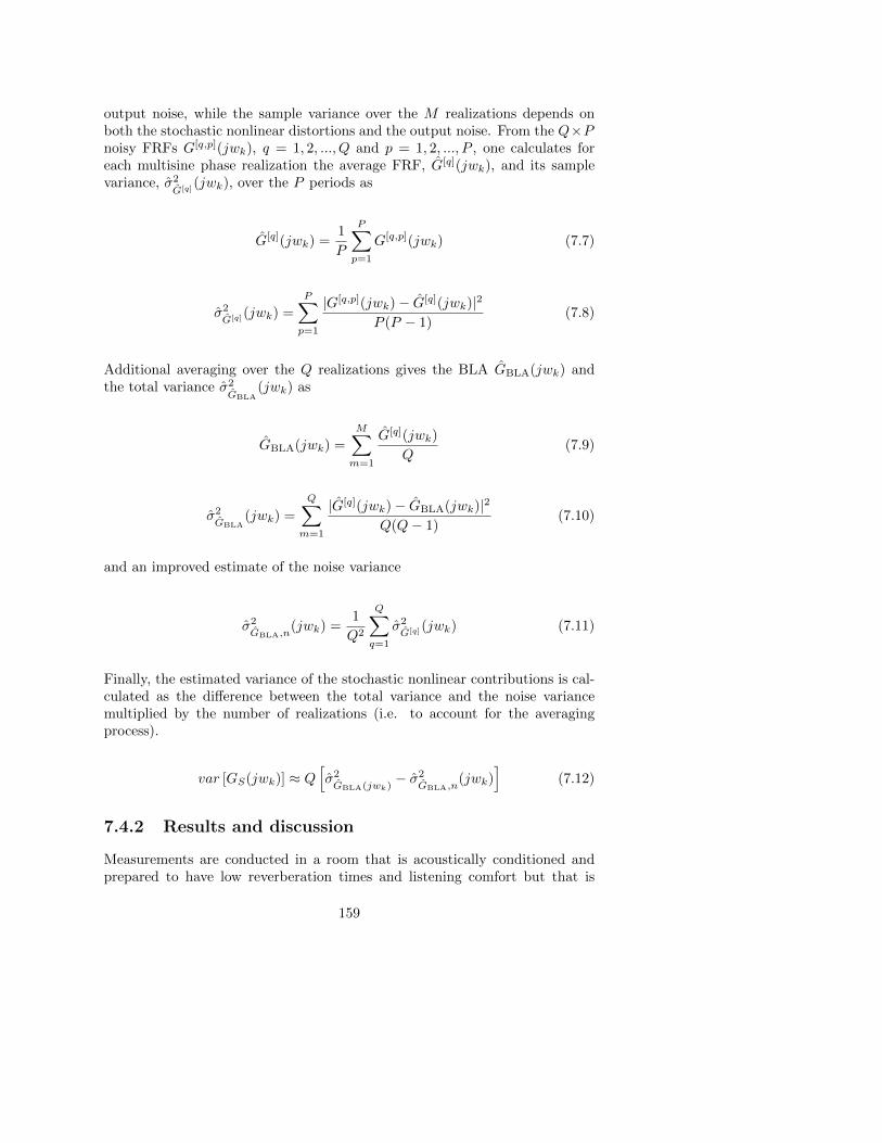
output noise, while the sample variance over the M realizations depends onboth the stochastic nonlinear distortions and the output noise. From the Q×Pnoisy FRFs G[q,p](jwk), q = 1, 2, ..., Q and p = 1, 2, ..., P , one calculates foreach multisine phase realization the average FRF, G[q](jwk), and its samplevariance, σ2

G[q](jwk), over the P periods as

G[q](jwk) =1

P

P∑p=1

G[q,p](jwk) (7.7)

σ2G[q](jwk) =

P∑p=1

|G[q,p](jwk)− G[q](jwk)|2P (P − 1)

(7.8)

Additional averaging over the Q realizations gives the BLA GBLA(jwk) andthe total variance σ2

GBLA(jwk) as

GBLA(jwk) =

M∑m=1

G[q](jwk)

Q(7.9)

σ2GBLA

(jwk) =

Q∑m=1

|G[q](jwk)− GBLA(jwk)|2Q(Q− 1)

(7.10)

and an improved estimate of the noise variance

σ2GBLA,n

(jwk) =1

Q2

Q∑q=1

σ2G[q](jwk) (7.11)

Finally, the estimated variance of the stochastic nonlinear contributions is cal-culated as the difference between the total variance and the noise variancemultiplied by the number of realizations (i.e. to account for the averagingprocess).

var [GS(jwk)] ≈ Q[σ2GBLA(jwk)

− σ2GBLA,n

(jwk)]

(7.12)

7.4.2 Results and discussion

Measurements are conducted in a room that is acoustically conditioned andprepared to have low reverberation times and listening comfort but that is

159

(a) (b)

Figure 7.4: BLA, nonlinear distortion and noise level of the multimedia loud-speaker at RMS input signals: (a) 0.02 (b) 0.16.

(a) (b)

Figure 7.5: BLA, nonlinear distortion and noise level of the teleconferencingmonitor at RMS input signals: (a) 0.02 (b) 0.16.

not anechoic. Hence, it is expected that some (linear) dynamics are added tothe measured frequency response. The microphone is a condenser microphone,AKG CK97-C with an AKG SE300-B pre-amplifier, connected to a PC runningCool Edit pro 2.0 through a RME Multiface II sound card. It is expected thatnone of these elements will cause any significant harmonic distortion. Threedifferent active loudspeakers are measured following the scheme of Figure 7.3,namely, a low-quality multimedia loudspeaker, a medium-quality Boss MA-12 monitor typically used in small teleconferencing rooms, and a high-qualitySoundcraft Spirit Absolute 4P recording studio monitor. The quality of theloudspeakers and their uses differ greatly. The input signal relative input powerRMS = 0.02 and 0.16. The low RMS value is set so that a non disturbingbackground noise is perceived and the high RMS value is set 18 dB higher.The first frequency with non-zero amplitude is fmin = 40 Hz, and the maximumexcited frequency fmax = 8 kHz

160

(a) (b)

Figure 7.6: BLA, nonlinear distortion and noise level of the studio monitor atRMS input signals:: (a) 0.02 (b) 0.16.

The level of the stochastic nonlinear contribution var [GS(jwk)] is calculatedfor different RMS values of a full multisine as explained in Section 7.4 withP = 2 and Q = 7. In the following figures the upper line (−.−) representthe GBLA, stars (?) represent the stochastic nonlinear contribution and dots(.) represent the output noise variance. It can be seen from Figure 7.4 and 7.5that for the multimedia loudspeaker and the teleconferencing monitor the levelof the stochastic nonlinear contribution increases steadily reaching significantlevels quite easy. On the other hand, the nonlinear distortion in the studiomonitor remains at low levels ( 50 dB below GBLA) for every input RMS value(see Figure 7.6). Active loudspeakers typically have a protection device (i.e.saturation curve) in the amplifier to avoid diaphragm damage at too high inputsignals. This saturation curve may also be a cause of nonlinear distortion athigh amplitudes. It is clear from this section that nonlinearities are present inlow quality loudspeaker and eventually in high quality loudspeakers as well.

7.5 Classification of nonlinearities

7.5.1 Analysis method

An odd multisine is a signal as in (7.1), where only odd harmonics are excited,i.e., ik ∈ {(2k − 1) | k = 1, 2, ..., F} . In the analysis that follows, a particulartype of odd multisine will be used as excitation signal, which is referred toas an odd-random multisine. An odd-random multisine is an odd multisinewhere in every set of K consecutive odd harmonics one randomly-chosen oddharmonic is not excited. The complete set of non-excited odd harmonics iscalled the harmonic grid. The non-excited odd harmonics together with theeven harmonics are called the detection lines.

161

(a) (b)

Figure 7.7: Output spectrum of the multimedia loudspeaker where (−.−) isthe output level at the excited lines, circles (o) represent the output level atnon-excited odd harmonics and stars (?) represent the level at non-excited evenharmonics. RMS input signals: (a) 0.02 (b) 0.16.

As the input detection lines have zero magnitude, the presence of signal energyat the corresponding output detection lines is due to the nonlinear distortionof the system plus, probably, some measurement noise. The information aboutthe nonlinear contribution (excluding the harmonic contribution generated byan odd-order nonlinearity) is obtained from the output DFT spectrum. The av-erage output spectrum is calculated at all frequencies (excited and non-excitedharmonics) [21], based on

Y (jωk) =1

P

P∑p=1

Y [p](jωk) k = 1, ..., F (7.13)

where ωk = ikω0, and Y [p](jωk) is the DFT spectrum of one period p of theoutput signal. It follows the measurement scheme illustrated in Figure 7.3 onlywith one phase realization, i.e., Q = 1.

7.5.2 Results and discussion

The frequency range is the same as previously, but now only odd harmonicsare excited with K = 6, Q = 1, and P = 40. The response of the high-qualitystudio monitor has not been considered here since the previous analysis showsa linear behavior. By inspecting the odd and even detection lines in the outputDFT spectrum we can see the loudspeaker odd and even nonlinear response.

From Figure 7.7 and 7.8, it can be seen that at relatively high input signallevels, nonlinear distortions should be taken into account. In this case, oddnonlinearities are significantly more predominant that even nonlinearities in

162

(a) (b)

Figure 7.8: Output spectrum of the teleconferencing monitor where (−.−) isthe output level at the excited lines, circles (o) represent the output level atnon-excited odd harmonics and stars (?) represent the level at non-excited evenharmonics. RMS input signals: (a) 0.02 (b) 0.16.

the full frequency range. This implies that the dominant nonlinearity must bemodeled at least as a 3rd-order system.

7.6 Linear-in-the-parameters nonlinear adaptivefilters

In this section, so-called linear-in-the-parameters nonlinear filters are reviewed,which are characterized by a linear dependence of the filter output on the filtercoefficients. These filters are particulary suited to AEC, where adaptive filtersare typically used to adapt to changes in the acoustic echo path, now includingalso the nonlinearities. Linear-in-the-parameters nonlinear adaptive filters thenhave derisable characteristics, namely, that they are inherently stable, and thatthey can converge to a globally minimum solution (in contrast to other types ofnonlinear filters whose cost function may exhibit many local minima) avoidingthe undesired possibility of getting stuck in a local minimum during adaptation.

In the general case, a linear-in-the-parameters nonlinear filter is described bythe input-output relationship

yF (t) = hTFuF (t) (7.14)

where hF is a vector containing L filter coefficients and uF (t) is the correspond-ing vector whose L elements are nonlinear combinations and/or expansions of

the input samples in u(t) = [u(t), u(t− 1), · · · , u(t−N + 1)]T

. In fact, (7.14)can be interpreted as an FIR filter with L coefficients in which uF (t) is usedinstead of the usual u(t). If uF (t) is chosen equal to u(t), the filter is truly a

163

linear FIR filter with L = N coefficients. In the nonlinear case, we may defineuF (t) and hF as a set of sub-vectors ur(t) and hr, with r = 1, . . . ,M . Thus,we may define the input vector as

uF (t) =[uT1 (t) uT2 (t) · · · uTM (t)

]T, (7.15)

and then the output is given as

yF (t) = hT1 u1(t) + hT2 u2(t) + · · ·+ hTMuM (t) (7.16)

where the vector hF has been divided in sub-vectors of matching lengths.

The next sections present a collection of linear-in-the-parameters nonlinear fil-ters that have been successfully applied in NLAEC [9]- [13]. A complete reviewof linear-in-the-parameters nonlinear filters with and without cross terms canbe found in [22].

7.6.1 Adaptive algorithm

Adaptive filter algorithms developed for the identification and tracking of linearFIR systems can also be applied to the nonlinear filter structure of (7.14). Thepopular NLMS algorithm [19], for instance, can be adopted, of which the updateequations are given as

e(t) = d(t)− hTF (t)uF (t) (7.17)

hF (t+ 1) = hF (t) + µuF (t)e(t)

uTF (t)uF (t) + ε(7.18)

where ε is a small positive constant to avoid overflow.

7.7 Nonlinear filters without cross terms

This section introduces linear-in-the-parameters nonlinear filters involving onlyinstantaneous nonlinear expansions of the input samples. This sub-class offilters includes Hammerstein filters [23] as well as filters involving nonlinearexpansions based on orthogonal polynomials [22], [23].

7.7.1 Hammerstein filters

A Hammerstein filter is formed by a static nonlinearity followed by a linearfilter h(n). Since the nonlinearity is usually expressed as a polynomial functionand the linear filter has a finite impulse response of N samples, it is considered

164

as a simple example of a truncated Volterra filter. Thus, for the Hammersteinfilter, the input-output relation is given as

yF (t) =

N−1∑n=0

h(n)

M∑m=1

gmum(t− n) (7.19)

including a linear term, and higher-order polynomial terms up to order M .This model, which is linear-in-the-parameters h(n)gm, has been studied andused for many applications including NLAEC [12], [22]. The vector uF (t) isa collection of instantaneous nonlinear expansions, using powers, of the inputsamples, as shown in the following expression

uF (t) = [u(t), u(t− 1), · · · , u(t−N + 1)

u2(t), u2(t− 1), · · · , u2(t−N + 1) (7.20)

...

uM (t), uM (t− 1), · · · , uM (t−N + 1)].

It is worth noting that Hammerstein filters have been called “power filters”in [12]. As observed, the terms in (7.20) are not mutually orthogonal. In [12] aGram-Schmidt orthogonalization of the input data matrix has been proposedfor improved convergence. However the computational load of the orthogonal-ization is very high even when considering a low-order filter.

7.7.2 Filters based on orthogonal polynomials

Filters using nonlinear expansions within the family of orthogonal polynomialshave been mentioned in [24]. While Hammerstein filters are based on a power-series expansion of the input signal, a better approximation can be achievedwith signal-independent polynomials such as orthogonal polynomials in theinterval [−1, 1], as for example Legendre, Chebyshev, and Hermite polynomials.

In Legendre polynomial filters, the sub-vectors are formed with

L1[u(t)] = u(t) (7.21)

L2[u(t)] = u2(t) (7.22)

Lm+1[u(t)] =1

m+ 1

[Lm[u(t)](2m+ 1)u(t)−mLm−1[u(t)]

]m = 3, ...,M (7.23)

Thus, a Legendre polynomial filter is described by the following input-outputrelationship

yF (t) =

N−1∑n=0

h(n)

M∑m=1

gmLm [u(t− n)] (7.24)

165

including a linear term, and higher-order polynomial terms up to order M .This model is again linear-in-the-parameters h(n)gm. The vector uF (t) is acollection of instantaneous nonlinear expansions, using Legendre polynomials,as shown in the following expression

uF (t) =[L1[u(t)], L1[u(t− 1)], · · · , L1[u(t−N + 1)]

L2[u(t)], L2[u(t− 1)], · · · , L2[u(t−N + 1)] (7.25)

......

LM [u(t)], LM [u(t− 1)], · · · , LM [u(t−N + 1)]]

The number of filter parameters in the Hammerstein filters as well as in theLegendre filters is LH = LL = MN .

7.8 Nonlinear filters with cross terms

The class of filters described by (7.14) includes also more general nonlinearfilters involving cross terms, i.e., products of input samples with different timeshifts, such as truncated Volterra filters [23] and simplified Volterra filters [9].

7.8.1 Volterra filters

Volterra filters are described by input-output relationships that result from twotruncations of the discrete Volterra series [23], namely, a memory truncation(N − 1) of the Volterra kernel orders, and a nonlinearity order truncation (M)to limit the number of Volterra kernels. The Volterra kernels can be assumedto be symmetric and, thus, the Volterra filter input/output relationship can becast in the compact triangular form as

y(t) =

N−1∑n1=0

h1(n1)u(t− n1)

+

N−1∑n1=0

N−1∑n2=n1

h2(n1, n2)u(t− n1)u(t− n2) + · · ·

+

N−1∑n1=0

· · ·N−1∑

nM=nM−1

hM (n1...nM )u(t− n1)...u(t− nM ) (7.26)

The model in (7.26) includes an FIR filter h1(n1) and higher-order kernelshm(n1, · · · , nm) with m = 2, . . . ,M . For instance, a 3rd-order Volterra fil-ter, which includes a 2nd-order and a 3rd-order kernel, involves the followingnonlinear expansions

166

u2(t) = [u2(t), u(t)u(t− 1), ..., u2(t− 1),

u(t− 1)u(t− 2), ..., u2(t−N + 1)]T

with dimension N(N + 1)/2 and

u3(t) = [u3(t), u(t)u(t)u(t− 1), ..., u(t)u(t− 1)u(t− 2),

..., u3(t−N + 1)]T

with dimension N(N+1)(N+2)/6. Thus, the total number of filter coefficientsis LV = N +N(N + 1)/2 +N(N + 1)(N + 2)/6.

7.8.2 Simplified 3rd-order Volterra kernel

Based on the simplified 2nd-order Volterra kernel presented in [9], we propose asimplified 3rd-order Volterra kernel. In [9], a simplification is made where onlya reduced number of terms is considered depending on the desired complexity.By analyzing the 2nd-order Volterra kernel obtained from a loudspeaker, it hasbeen observed that the coefficients with the most significant amplitude corre-spond to small values of Nd = n2 − n1. For this reason, a good approximationof a 2nd-order Volterra filter may be achieved when coefficients correspondingto large values of n2 − n1 are not selected, i.e.,

V2K(t) =

N−1∑n1=n2=0

h2(n1, n2)u(t− n1)u(t− n2) (7.27)

+

N−2∑n1=0

min(n1+Nd,N−1)∑n2=n1+1

h2(n1, n2)u(t− n1)u(t− n2). (7.28)

In the 3rd-order case, there is no evidence a similar approximation is justified.However, with the idea of reducing computation, we propose the followingsimplification for the 3rd-order Volterra kernel,

V3K(t) =

N−1∑n1=n2=n3=0

h3(n1, n2, n3)u(t− n1)u(t− n2)u(t− n3) (7.29)

+

N−2∑n1=0



h3(n1, n2, n3)u(t− n1)u(t− n2)u(t− n3) (7.30)

The vector u2(t) is then a collection of 2nd-order combinations of input sampleswith different time shifts, i.e.,

167

u2(t) = [u2(t), u2(t− 1), ..., u2(t−N + 1)

u(t)u(t− 1), ..., u(t−N)u(t−N + 1) (7.31)

. . .

u(t)u(t−N + 1)]T

with dimension N(N + 1)/2. Similary, the vector u3(t) is a collection of 3rd-order combinations of input samples with different time shifts, i.e.,

u3(t) = [u3(t), u3(t− 1), ..., u3(t−N + 1)

u(t)u(t− 1)u(t− 2), ..., u(t−N − 1)u(t−N)u(t−N + 1)

. . .

u(t)u(t−N)u(t−N + 1)]T

with dimension N(Nd + 1)(Nd + 2)/6. Thus, the total number of filter coeffi-cients is LSV = L+N(Nd + 1)/2 +N(Nd + 1)(Nd + 2)/6.

7.9 Simulated Hammerstein system identifica-tion

We consider the Hammerstein system illustrated in Figure 7.9, where a 5th-order power-series nonlinearity, i.e., f [u(t)] = u(t) +αu2(t) +βu3(t) +γu4(t) +δu5(t) is used. The linear filter is a 16-coefficient finite impulse response (FIR)low-pass filter (LPF) with cut-off frequency 1/4 of the sampling frequency.Figure 7.10 shows the simulated Hammerstein system input and output signals.The input signal is an odd-random multisine, the harmonic grid parameterK = 6, and the analysis method is based on (7.13). Figure 7.10(a) shows thespectrum of the input odd-random multisine after conversion to a 16-bit pulsecode modulation (PCM) representation. The round-off noise appears as a low-level (−60 dB) odd and even harmonics contribution. Figure 7.10(b) showsthe spectrum of the Hammerstein system output signal. The spectrum of thenonlinear contribution of f [u(t)] is clearly shown, where α, β, γ, and δ arechosen such that the nonlinear contributions are scaled to −20 dB comparedto the linear contribution.

u(t) y(t)f [u(t)]

Figure 7.9: Hammerstein system: Static nonlinearity followed by a linear filter.

168

0 2000 4000 6000 8000−100

−80

−60

−40

−20

0

20

40

Frequency (Hz)

Mag

nitu

de (

dB)

Spectrum

Excited harm 34.8559Odd non excited −60.9028Even harm −60.9546

(a)

0 2000 4000 6000 8000−100

−80

−60

−40

−20

0

20

40

Frequency (Hz)

Mag

nitu

de (

dB)

Spectrum

Excited harm 35.3812Odd non excited 14.5982Even harm 17.0654

(b)

Figure 7.10: Hammerstein system analysis using odd-random multisine. Spec-trum estimated using (7.13). (a) Input spectrum (16-bit precision PCM repre-senation). (b) Output spectrum.

The identification of this simulated Hammerstein system is performed usingNLMS and two different nonlinear filters, a 5th-order Hammerstein filter, anda 5th-order Legendre polynomial filter. The input signal is an odd-randommultisine, the fundamental frequency is 2 Hz, the first frequency with non-zero amplitude is fmin = 40 Hz, the maximum excited frequency fmax = 8kHz, the sampling frequency is 32 kHz and the harmonic grid parameter isK = 6. From the total number of periods, i.e., P = 40, we use the first 35periods for identification and the last 5 periods for validation. In identification,the analysis method is applied to the residual signal after the adaptive filtershave sufficiently converged. In validation, we fix the filter parameters obtainedpreviously in the identification and analyze the residual signal. A very usefulfeature of the analysis method is that one can easily calculate the power ofthe different contributions independently. The values we show correspond tothe averaged power of the excited odd, non-excited odd and even harmonicsindependently.

Figure 7.11 shows that the Legendre polynomial filter achieves significantlybetter performance than the Hammerstein filter. Interestingly, the Legendrepolynomial filter achieves −59 dB in the non-excited odd harmonics and −57dB in the even harmonics. These values are nearly the same as the level ofthe nonlinear distortion due to 16-bit format, see Figure 7.10(b). These twofacts, shed some light on the benefits of using orthogonal polynomial expansions(e.g., Legendre) if high orders are considered. It is known that non-orthogonalpolynomials (e.g., power series) are not well behaved when using high orders.Indeed, even when the underlying nonlinear and linear systems are exactlyknown, the (high order) Hammerstein filter does not provide a good approxi-mation.

169

0 2000 4000 6000 8000−100

−80

−60

−40

−20

0

20

40

Frequency (Hz)

Mag

nitu

de (

dB)

Spectrum

Excited harm −25.3898Odd non excited −26.3082Even harm −38.3644

(a)

0 2000 4000 6000 8000−100

−80

−60

−40

−20

0

20

40

Frequency (Hz)

Mag

nitu

de (

dB)

Spectrum


(b)

Figure 7.11: Results of simulated Hammerstein system identification usingNLMS adaptation and where the nonlinearity is a 5th-order power-series ex-pansion. (a) Validation of the 5th-order Hammerstein filter. (b) Validationof the 5th-order Legendre polynomial filter

7.10 Loudspeaker identification

The loudspeaker is a Boss MA-12 active monitor, which is measured using thesame input signal as in the previous section, shown in Figure 7.10(a). Thelower level is set so that a non disturbing background noise is perceived andthe high level is set 10 dB higher.

Figure 7.12(a) shows the spectrum of the output signal of the loudspeaker atlow input level where the non-excited odd and even harmonics levels are −24dB and −22 dB respectively. Figure 7.12(b) shows the output spectrum ofthe loudspeaker at high input level (+10 dB) where the even harmonics layat −9 dB and the non-excited odd harmonics are at much higher level +8dB. The loudspeaker clearly presents an odd-order nonlinearity that is morepredominant than the even-order nonlinearity, which means that at least a3rd-order nonlinear model must be considered for identification.

Figure 7.12(c) shows the estimated impulse response using a linear least-squares(LS) estimate based on the low level signal. Similarly, Figure 7.12(d) showsthe estimated impulse response based on the high level signal. The estimatedimpulse response is clearly less noisy in the low level case, as the nonlineardistortion is around 47 dB lower compared to the high level case, as shown inFigures 7.12(a) and 7.12(b). From the estimated impulse response we definethe length of the linear filter, i.e., 360 coefficients.

We now proceed with the identification of the loudspeaker and validation of themodel when using a Hammerstein filter and a Legendre polynomial filter, withnonlinear orders 3 ,7, 15, 31, 47, 55, and 67. We also identify and validate themodel when using a simplified 3rd-order Volterra filter with Nd = N/32 and

170

0 1000 2000 3000 4000 5000 6000 7000 8000−80

−60

−40

−20

0

20

40

Frequency (Hz)

Mag

nitu

de (

dB)

Spectrum


(a)

0 1000 2000 3000 4000 5000 6000 7000 8000−80

−60

−40

−20

0

20

40

Frequency (Hz)

Mag

nitu

de (

dB)

Spectrum

Excited harm 34.8127Odd non excited 8.0908Even harm −9.3333

(b)

0 50 100 150 200 250 300 350−0.5

0

0.5

1

Filter taps

Am

plitu

de

IR estimation using LS

(c)

0 50 100 150 200 250 300 350−0.5

0

0.5

1

Filter taps

Am

plitu

de

IR estimation using LS

(d)

Figure 7.12: Loudspeaker measurements. (a)-(b) Output spectrum measuredusing two input levels with 10 dB difference. (c)-(d) Normalized impulse re-sponse estimates with least-squares using two input levels with 10 dB difference.

Nd = N/16 in both the 2nd and 3rd-order Volterra kernel. The reason for thischoice is to keep the size of the filter reasonably small and comparable withthe length of the other filters without cross terms. The value of the differentaveraged power spectra is shown in Table 7.2, 7.3, 7.4, where Id. stands for“in identification” and Val. for “in validation”. In Figures 7.13 and 7.14,the spectrum obtained with the 3rd-order and 67th-order Hammerstein andLegendre polynomial filter is shown, and in Figure 7.15, the spectrum obtainedwith the simplified 3rd-order Volterra using Nd = N/32 and Nd = N/16 isshown.

In the 3rd-order case, the Hammerstein, Legendre, and simplified Volterra(both with Nd = N/32 and Nd = N/16) filter obtain similar values in identifi-cation and validation of the excited odd harmonics (around 5.5 dB Id. and 6.5dB Val. respectively) and non-excited odd harmonics (around 4 dB Id. and2.6 dB Val. respectively). For the even harmonics, the simplified Volterra fil-ter achieves 2 dB performance improvement compared to the Hammerstein andLegendre polynomial filter, but this is only in the identification step. In the val-idation step, the Hammerstein and Legendre polynomial filter achieve a muchbetter performance, −8.8 dB and −9.5 dB respectively, w.r.t. the simplified

171

Simp. Volt.Size Nd = N/32 Nd = N/16

ExcitedId. 5.6 5.5Val. 6.4 5.8

OddId. 4 4.3Val. 2.6 2.7

EvenId. -14.9 -16Val. -4.3 -2.9

Table 7.2: Loudspeaker identification using a simplified 3rd-order Volterra fil-ter. The values correspond to the averaged power of the excited odd, non-excited odd and even harmonics independently.

HammersteinOrder 3 7 15 31 47 55 67

ExcitedId. 5.3 3.8 3.8 3.8 3.8 3.8 3.8Val. 6.9 5.7 5.7 5.7 5.7 5.7 5.7

OddId. 3.8 1.2 1.1 1.1 1.1 1.1 1.1Val. 2.6 -0.7 -0.8 -0.8 -0.8 -0.8 -0.8

EvenId. -12.7 -13.5 -13.7 -13.7 -13.7 -13.7 -13.7Val. -8.8 -10.2 -10.4 -10.4 -10.4 -10.4 -10.4

Table 7.3: Loudspeaker identification using Hammerstein filter. The valuescorrespond to the averaged power of the excited odd, non-excited odd andeven harmonics independently.

Volterra filter using Nd = N/32 and Nd = N/16, which only achieves −4.3 dBand −2.9 dB respectively. Moreover, in the simplified 3rd-order Volterra filtercase, the performance improvement between the Nd = N/32 and Nd = N/16is nearly negligible.

The Legendre polynomial filter achieves a better performance than the Ham-merstein filter during identification and validation. Interestingly, the Hammer-stein filter performance does not improve with increasing order. Indeed, beyond7th order there is no improvement whatsoever in identification or validation.On the other hand, the Legendre polynomial filter performance improves withincreasing order in identification and, most importantly, in validation. Forinstance, using order 7, in the validation step the Legendre polynomial filterachieves Excited= 4.1 dB, Odd= −3.1 dB, and Even= −9.5 dB, whereas us-ing order 67, in the validation step the Legendre polynomial filter achievesExcited= −1.9 dB, Odd= −4.3 dB, and Even= −13.2 dB. The 7th-order Leg-endre polynomial filter achieves a remarkable performance improvement over

172

LegendreOrder 3 7 15 31 47 55 67

ExcitedId. 5.3 2.9 2.3 1.1 0 -0.6 -1.7Val. 6.9 4.1 3 1.4 0.1 -0.7 -1.9

OddId. 3.8 -0.2 -1 -1.4 -1.9 -2.3 -3.2Val. 2.6 -3.1 -3.4 -3.1 -3.3 -3.5 -4.3

EvenId. -12.5 -14 -14.6 -15.5 -16.2 -16.5 -16.6Val. -9.5 -9.5 -9.6 -11.5 -12.3 -12.7 -13.2

Table 7.4: Loudspeaker identification using Legendre polynomial filter. Thevalues correspond to the averaged power of the excited odd, non-excited oddand even harmonics independently.

the simplified Volterra filter, which in the validation step, achieves Excited= 5.8dB, Odd= 2.7 dB, and Even= −2.9 dB only.

The differences between identification and validation, comparing the simplified3rd-order Volterra filter with Nd = N/16 and the 67th-order Legendre polyno-mial filter, appear to be similar for the excited odd harmonics (0.3 dB and 0.2dB respectively) and non-excited odd harmonics (1.6 dB and 0.9 dB respec-tively). However, for the even harmonics, the difference between identificationand validation is remarkably high for the simplified 3rd-order Volterra filterwith Nd = N/16 (13.1 dB) compared to the 31st-order Legendre filter case (3.4dB). This is a clear sign of overfitting.

A general trend for the Hammerstein and Legendre filters is that the differencesbetween identification and validation decrease with increasing order. This im-plies that the identified model is a better model for the actual system. However,for the simplified 3rd-order Volterra filter, the differences between identificationand validation tend to increase with increasing Nd. In particular, for the evenharmonics, these differences are quite high (10.6 dB and 13.1 dB respectively).The reason is that in the 3rd-order simplified Volterra filter, the order of thefilter is constant, i.e., 3, but the length of the filter is increasing. The risk ofoverfitting in this case is clear, since keeping the order but increasing the filterlength makes identification and validation differ considerably.

In [25] and [26], it is shown that a physical model based on a nonlinear versionof the well known lumped parameter model of the loudspeaker can achieve agood representation of the odd harmonics when comparing simulations withmeasurements. This modeling approach is based on the dependence of thelumped parameters with the voice coil position. It is generally accepted thatthe variations of the magnetic force factor, the voice coil inductance and com-pliance of the suspension, are the main causes of nonlinear distortion. Theseare modeled as functions of cone displacement and therefore they are static

173

1000 2000 3000 4000 5000 6000 7000 8000−40

−20

0

20

40

Frequency (Hz)

Mag

nitu

de (

dB)

Spectrum


(a)

1000 2000 3000 4000 5000 6000 7000 8000−40

−20

0

20

40

Frequency (Hz)

Mag

nitu

de (

dB)

Spectrum


(b)

1000 2000 3000 4000 5000 6000 7000 8000−40

−20

0

20

40

Frequency (Hz)

Mag

nitu

de (

dB)

Spectrum


(c)

1000 2000 3000 4000 5000 6000 7000 8000−40

−20

0

20

40

Frequency (Hz)

Mag

nitu

de (

dB)

Spectrum


(d)

Figure 7.13: Loudspeaker identification and validation using a Hammer-stein filter and NLMS. (a) Identification and (b) Validation using a 3rd-orderfilter. (c) Identification and (d) Validation using 67th-order filter.

elements in the model. This implies that the odd nonlinear distortions may besuccessfully modeled as produced by a static nonlinear system.

7.11 Conclusions

In this chapter, we have presented a method to analyze the nonlinear response,in terms of odd and even nonlinearities, of an electrodynamic loudspeaker bymeans of periodic random-phase multisine experiments. Moreover, we haveconsidered the identification of a loudspeaker model by means of linear-in-the-parameters nonlinear adaptive filters. First of all, we have seen that thenonlinear odd contribution is much more predominant than the nonlinear evencontribution. This mean that at least a 3rd-order nonlinear filter must beconsidered. By analyzing the residual signal after the adaptive filter has con-verged, we have shown, however, that a 3rd-order nonlinear filter is not suf-ficient to capture all the nonlinearities. This means that the odd and evennonlinear contributions are produced by higher-order nonlinearities. Second,

174

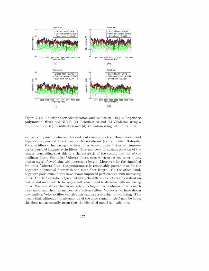
1000 2000 3000 4000 5000 6000 7000 8000−40

−20

0

20

40

Frequency (Hz)

Mag

nitu

de (

dB)

Spectrum


(a)

1000 2000 3000 4000 5000 6000 7000 8000−40

−20

0

20

40

Frequency (Hz)

Mag

nitu

de (

dB)

Spectrum


(b)

1000 2000 3000 4000 5000 6000 7000 8000−40

−20

0

20

40

Frequency (Hz)

Mag

nitu

de (

dB)

Spectrum


(c)

1000 2000 3000 4000 5000 6000 7000 8000−40

−20

0

20

40

Frequency (Hz)

Mag

nitu

de (

dB)

Spectrum


(d)

Figure 7.14: Loudspeaker identification and validation using a Legendrepolynomial filter and NLMS. (a) Identification and (b) Validation using a3rd-order filter. (c) Identification and (d) Validation using 67th-order filter.

we have compared nonlinear filters without cross-terms (i.e., Hammerstein andLegendre polynomial filters) and with cross-terms (i.e., simplified 3rd-orderVolterra filters). Increasing the filter order beyond order 7 does not improveperformance of Hammerstein filters. This may lead to misinterpreation of theresults, concluding that this is a characteristic of the system and not of thenonlinear filter. Simplified Volterra filters, even when using low-order filters,present signs of overfitting with increasing length. Moreover, for the simplified3rd-order Volterra filter, the performance is remarkably poorer than for theLegendre polynomial filter with the same filter length. On the other hand,Legendre polynomial filters have shown improved performance with increasingorder. For the Legendre polynomial filter, the differences between identificationand validation appear to be very small, which tend to decrease with increasingorder. We have shown that in our set-up, a high-order nonlinear filter is muchmore important than the memory of a Volterra filter. Moreover, we have shownhow easily a Volterra filter can give misleading results due to overfitting. Thismeans that, although the attenuation of the error signal in AEC may be large,this does not necessarily mean that the identified model is a valid one.

175

1000 2000 3000 4000 5000 6000 7000 8000−40

−20

0

20

40

Frequency (Hz)

Mag

nitu

de (

dB)

Spectrum


(a)

1000 2000 3000 4000 5000 6000 7000 8000−40

−20

0

20

40

Frequency (Hz)

Mag

nitu

de (

dB)

Spectrum


(b)

1000 2000 3000 4000 5000 6000 7000 8000−40

−20

0

20

40

Frequency (Hz)

Mag

nitu

de (

dB)

Spectrum


(c)

1000 2000 3000 4000 5000 6000 7000 8000−40

−20

0

20

40

Frequency (Hz)

Mag

nitu

de (

dB)

Spectrum


(d)

Figure 7.15: Loudspeaker identification and validation with a simplified3rd-order Volterra filter and NLMS. (a) Identification and (b) Validationusing Nd = N/32. (c) Identification and (d) Validation using Nd = N/16.

176

Bibliography


[2] P. Gil-Cacho, T. van Waterschoot, M. Moonen, and S. H. Jensen, “Multi-microphone acoustic echo cancellation using multi-channel warped linearprediction of common acoustical poles,” in Proc. 18th European SignalProcess. Conf., (EUSIPCO’10), Aalborg, Denmark, Aug. 2010, pp. 2121–2125.

[3] ——, “Study and characterization of odd and even nonlinearities in elec-trodynamic loudspeakers by means of periodic random-phase multisine,”in Preprints AES 127th convention, New York, USA, Oct. Oct. 2009,Preprint 7841.

[4] M. I. Mossi, C. Yemdji, N. Evans, C. Beaugeant, and P. Degry, “An assess-ment of linear adaptive filter performance with nonlinear distortions,” inProc. 2011 IEEE Int. Conf. Acoust. Speech Signal Process., (ICASSP’11),Dallas, TX, USA, Mar. 2011, pp. 313 – 316.


[6] R. Ravaud, G. Lemarquand, and T. Roussel, “Time-varying non linearmodeling of electrodynamic loudspeakers,” Applied Acoust., vol. 70, no. 3,pp. 450 – 458, Mar. 2009.

[7] C. A. Henricksen, “Heat-transfer mechanisms in loudspeakers: Analysis,measurement, and design,” J. Audio Eng. Soc., vol. 35, p. 778 791, Oct.1987.

[8] C. Zuccatti, “Thermal parameters and power ratings of loudspeakers,” J.Audio Eng. Soc., vol. 38, pp. 34 –39, Feb. 1990.

[9] A. Fermo, A. Carini, and G. L. Sicuranza, “Simplified Volterra filtersfor acoustic echo cancellation in GSM receivers,” in Proc. 10th EuropeanSignal Process. Conf., (EUSIPCO’00), Tampere, Finland, Sept. 2000, pp.2413–2416.

[10] G. L. Sicuranza, A. Carini, and A. Fermo, “Nonlinear adaptive filters foracoustic echo cancellation in mobile terminals,” in Nonlinear Signal andImage Processing: Theory, Methods, and Applications, ser. The ElectricalEngineering and Applied Signal Processing Series, K. E. Barner and G. R.Arce, Eds. Florida: CRC Press LLC, 2004, ch. 7, pp. 223–255.

177

[11] J. M. Gil-Cacho, M. Signoretto, T. van Waterschoot, M. Moonen, and S. H.Jensen, “Nonlinear acoustic echo cancellation based on a sliding-windowleaky kernel affine projection algorithm,” IEEE Trans. Audio Speech Lang.Process., vol. 99, p. Early Access Articles, Apr. 2013.

[12] F. Kuech and W. Kellerman, “Orthogonalized power filters for nonlinearacoustic echo cancellation,” Signal Process., vol. 86, pp. 1168–1181, Nov.2006.


[14] J. P. Costa, A. Lagrange, and A. Arliaud, “Acoustic echo cancellationusing nonlinear cascade filters,” in Proc. 2003 IEEE Int. Conf. Acoust.Speech Signal Process., (ICASSP’03), Hong Kong, China, Apr. 2003, pp.389–392.

[15] F. Kuech and W. Kellerman, “A novel multidelay adaptive algorithm forVolterra filters in diagonal coordinates,” in Proc. 2004 IEEE Int. Conf.Acoust. Speech Signal Process., (ICASSP’04), Montreal, Quebec, Canada,May 2004, pp. 869–872.

[16] F. Kuch, “Adaptive polynomial filters and their application to nonlin-ear acoustic echo cancellation,” Ph.D. dissertation, Friedrich–Alexander–Universitat Erlangen–Nurnberg, 2005.

[17] A. Guerin, G. Faucon, and R. L. Bouquin-Jeannes, “Nonlinear acousticecho cancellation based on Volterra filters,” IEEE Trans. Speech AudioProcess., vol. 11, no. 6, pp. 672–683, Nov. 2003.

[18] L. A. Azpicueta-Ruiz, M. Zeller, J. Arenas-Garcıa, and W. Kellermann,“Novel schemes for nonlinear acoustic echo cancellation based on filtercombinations,” in Proc. 2010 IEEE Int. Conf. Acoust. Speech Signal Pro-cess., (ICASSP’10), Taipei, Taiwan, Apr. 2010, pp. 193–196.


[20] R. Pintelon, G. Vandersteen, L. D. Locht, Y. Rolain, and J. Schoukens,“Experimental characterization of operational amplifiers: a system identi-fication approach - part i: theory and simulations,” IEEE Trans. Instrum.Meas., vol. 53, no. 3, pp. 854 – 862, 2004.

[21] R. Pintelon and J. Schoukens, System Identification: A frequency domainapproach. IEEE Press and John Wiley, 2001.

178

[22] G. L. Sicuranza and A. Carini, “On a class of nonlinear filters,” inFestschrift in Honor of Jaakko Astola on the Occasion of his 60th Birth-day, K. E. I. Tabus and M.Gabbouj, Eds. TICSP series, no. 47, Tampere,2009, pp. 115 – 144.


[24] G. L. Sicuranza and A. Carini, “On the accuracy of generalized hammer-stein models for nonlinear active noise control,” in Proc. 2006 IEEE Inst.Meas. Tech. Conf., Sorrento, Italy, Apr. 2006, pp. 24–27.

[25] F. T. Agerkvist,“Modelling loudspeaker non-linearities”, in Proc. 32nd

AES Conference, Hillerød Denmark, Sep. 2007.

[26] B. R. Pedersen, Error correction of loudspeakers. PhD thesis. AalborgUniversity, Denmark, May 2001.

179

Chapter 8

Nonlinear Acoustic EchoCancellation based on aSliding-Window LeakyKernel Affine ProjectionAlgorithm

Nonlinear Acoustic Echo Cancellation based on a Sliding-WindowLeaky Kernel Affine Projection Algorithm

Jose M. Gil-Cacho, Marco Signoretto, Toon van Waterschoot, Marc Moonenand Søren Holdt Jensen

Published in IEEE Transactions on Audio Speech and LanguageProcessing, vol. 21, no. 9, pp. 1867-1878, Sept. 2013.

c©2013 IEEE. Personal use of this material is permitted. However, permissionto reprint/republish this material for advertising or promotional purposes orfor creating new collective works for resale or redistribution to servers or lists,or to reuse any copyrighted component of this work in other works must beobtained from the IEEE.

181


• literature study• co-development of the SWLKAPA algorithm• design of simulation scenarios• software implementation and computer simulations• co-interpretation of simulation results• text redaction and editing

182

Abstract

In this chapter, we propose an algorithm based on the kernel affine projectionalgorithm (KAPA). KAPA has been successfully applied to many areas in signalprocessing but not yet to nonlinear AEC (NLAEC). The contribution of thischapter is three-fold: (1) to apply KAPA to the NLAEC problem, (2) to developa sliding-window leaky KAPA (SWL-KAPA) that is well suited for NLAECapplications, and (3) to propose a kernel function, consisting of a weightedsum of a linear and a Gaussian kernel. In our experiment set-up, the proposedSWL-KAPA for NLAEC consistently outperforms the linear APA, resulting inup to 12 dB of improvement in echo return loss enhancement (ERLE) at acomputational cost that is only 4.6 times higher. Moreover, it is shown thatthe SWL-KAPA outperforms, by 4 − 6 dB, a Volterra-based NLAEC, whichitself has a much higher computational cost than the linear APA.

8.1 Introduction

ACOUSTIC echo cancellation (AEC) is used in many speech communica-tion systems where the existence of echoes degrades the speech intelligi-

bility and listening comfort [1], [2]. These applications range from mobile orhands-free telephony to teleconferencing or voice over IP (VoIP) services, whichare often integrated in smartphones, tablets, notebooks, laptops, etc., whichare becoming standard devices in our every-day life. While mobile devices arebecoming smaller, the demand for quality, performance, and special featuresin audio products is increasing. Moreover, the need for higher sound pressurelevels, provided by smaller devices, presents a huge challenge to engineers whohave to deal with (usually cheap) loudspeakers working close to saturation.

+-

+

path pathacoustic

From far-end

To far-end

cancellationHH

LEM

e(i) d(i)

y(i)

v(i)

n(i)

y(i)

f [u(i)]

u(i)


183

The general set-up for an AEC is depicted in Figure 8.1. A far-end speech sig-nal u(i) is played back into an enclosure (i.e., the room) through a loudspeaker.In the room, there is a microphone to record a near-end speech signal, whichis to be transmitted back to the far-end side. An acoustic echo path H be-tween the loudspeaker and the microphone exists, so that the microphone (i.e.,desired) signal d(i) = y(i) + v(i) + n(i) contains an undesired echo y(i) plusthe near-end speech v(i) and the background noise n(i). The echo signal y(i)can be considered as the far-end signal u(i) filtered by the echo path, i.e., theloudspeaker-enclosure-microphone (LEM) response. An acoustic echo cancelerseeks to cancel the echo signal component y(i) in the microphone signal d(i),ideally leading to an echo-free error (or residual) signal e(i), which is then trans-mitted to the far-end side. This is done by subtracting an estimate of the echosignal y(i) from the microphone signal, i.e., e(i) = d(i)−y(i) = y(i)−y(i)+n(i),where a perfect double-talk detector (DTD) is assumed to be available so thatperiods when only the far-end speaker is active, i.e., v(i) = 0,∀i, can be con-sidered. Thus, the main objective of an echo canceler is to identify a modelthat represents a best fit to the echo path (i.e., similar to a system identifi-cation problem) or, in other words, a function f(·) that models the underly-ing mapping y(i) = f [u(i)], where u(i) is the input signal vector defined asu(i) = [u(i), u(i− 1), ..., u(i− L+ 1)]T ∈ RL.

Typically, a linear finite-impulse-response (FIR) filter is assumed to provide agood model for the echo path, leading to a class of linear-adaptive-filter-basedAEC systems. This assumption may be valid for some components in the LEMsystem. In fact, even in nonlinear AEC (NLAEC), the room (enclosure) andmicrophone responses may be modeled as linear systems. However, loudspeak-ers, as well as amplifiers, DACs, coders, etc., included in the LEM introducenonlinear distortion and must be modeled as nonlinear systems [3]. In thischapter, we will show simulation results obtained from a simulated nonlinearsystem in a controlled scenario, so as to avoid other problems related to realAEC applications (e.g., insufficient-order adaptive filters, or scenarios compris-ing non-stationary and colored background noise). If the mapping betweenu(i) and y(i) is highly nonlinear, poor performance may be expected from anylinear-adaptive-filter-based AEC. Several nonlinear models, intended to over-come the limitations of linear filters, have been used for NLAEC with more orless success.

Neural networks have been used for NLAEC [4], [5], but in that case the adap-tation consists of solving a non-convex optimization problem with many localminima, potentially leading to suboptimal solutions. A proper initialization isthen required to avoid local minima, which is already a big challenge in itself.Structured and block-oriented nonlinear models [6], [7] have also been stud-ied but, besides the need for proper initialization, the modeling capabilitiesare then limited to the specified nonlinear structure. Linear-in-the-parametersmodels that require nonlinear expansions of the input vector are appealing from

184

an adaptive filtering perspective since standard linear adaptive filtering tech-niques can be applied and global optimality can be guaranteed [8], [9]. The mainproblem however is that many more filter coefficients are needed than in thelinear case, resulting in a large computational complexity together with inher-ently slow convergence [10]- [13]. Volterra [14]- [16] and simplified Volterra [8]filters are common solutions belonging to the linear-in-the-parameters family,although typically only very low nonlinear orders are considered due to com-putational complexity constraints.

On the other hand, kernel adaptive algorithms [17]- [20] and on-line learningalgorithms [21], [22] have been subjects of great attention due to their good per-formance in nonlinear signal processing applications. Kernel methods are de-veloped based on the theory of reproducing kernel Hilbert spaces (RKHS) [23];a nonlinear model is obtained via a reproducing kernel by implicitly mappingdata into a high-dimensional feature space. If the adaptive filtering operationscan be expressed by particular vector inner products, then it is possible to applythe so-called kernel trick. The power of this idea is that the model parametersof the underlying nonlinear mapping y(i) = f [u(i)] are calculated by applyingnonlinear methods on the input data, corresponding to linear operations in thefeature space. This enables formulations where convergence to a global opti-mum may be guaranteed. In particular, the kernel affine projection algorithm(KAPA) [17] has been successfully applied to nonlinear equalization, nonlinearsystem identification, and nonlinear noise cancellation, as well as to the pre-diction of nonlinear time series. Although in [24] we have already introducedthe use of KAPA for NLAEC, its formal application is lacking so far.

The contribution of this chapter is therefore three-fold: (1) to formally applyKAPA to the NLAEC problem for the first time and confirm its potential forthis application, (2) to develop a sliding-window leaky KAPA (SWL-KAPA)that is best suited for NLAEC applications, and (3) to propose a kernel func-tion, that is a weighted sum of a linear and a Gaussian kernel, which is efficientfor acoustic applications. The motivation in designing this kernel is basically toseparate the problem into linear and nonlinear sub-problems. The weights inthe kernel also impose different forgetting mechanisms in the sliding window,which in turn translates to more flexible regularization.

The outline of the chapter is as follows. In Section 8.2, we present a reviewof the literature, which is instrumental for our purposes, namely, the affineprojection algorithm (APA), kernel methods, and the kernel APA (KAPA). InSection 8.3, the SWL-KAPA and the proposed kernel is described with explana-tion and justification of the choices made for NLAEC. In Section 8.4, computersimulation results are provided to verify the performance of the proposed al-gorithm, an overview of existing results in the NLAEC literature is given, anda computational complexity analysis of the competing algorithms is shown, inparticular, the linear APA and the 3rd-order Hammerstein and Volterra filters.Finally, Section 8.5 concludes the chapter.

185

8.2 Linear and Kernel APA

8.2.1 Linear APA

Standard approaches to AEC rely on the assumption that the echo path can bemodeled by a linear FIR filter [1], [2], [25]- [27], in which the coefficients of theecho path are collected in the parameter vector h = [h0, h1, ..., hL−1]T ∈ RLwith model order L−1. An adaptive filter is used to provide an estimate h ∈ RLof h with sufficient order, such that the echo signal estimate at the microphoneposition is y(i) = hT (i)u(i) with u(i) = [u(i), u(i − 1), . . . , u(i − L + 1)]T .Notice that, for now, we have also assumed that the echo path is time-invariant,hT (i) = hT ,∀i over the estimation time window [1, 2, . . . , i] with i� L; we willconsider time-varying echo paths further on. A least-squares regression datamodel may be constructed as

dLS(i) = ULS(i)h + eLS(i) (8.1)

where

dLS(i) = [d(i), d(i− 1), ..., d(1)]T (8.2)

eLS(i) = [e(i), e(i− 1), ..., e(1)]T (8.3)

ULS(i) = [u(i),u(i− 1), ...,u(1)]T . (8.4)

The error in (8.1) is minimized in a least-squares sense, giving

h(i) = arg minh(i)

i∑j=1

∣∣∣d(j)− hT (j)u(j)∣∣∣2 (8.5)

=[UT

LS(i)ULS(i)]−1

UTLS(i)dLS(i) (8.6)

where Ruu(i) =1

iUT

LS(i)ULS(i) and rdu(i) =1

iUT

LS(i)dLS(i) is the sample auto-

correlation matrix and the sample cross-correlation vector, respectively. Nearlyall linear adaptive filtering algorithms are related to the LS estimate, which isunique if the autocorrelation matrix is nonsingular. This condition is, however,not always met. Indeed a common problem in AEC applications is that thematrix Ruu(i) is ill-conditioned or even singular due to poor excitation [28].

This situation will generate large variance in the estimation of h(i). Therefore,to improve data generalization (i.e., to prevent small changes in the data from

producing large changes in the solution), the l2-norm of the vector h(i) is oftenused as a penalty term. This type of regression, commonly known as ridgeregression, was introduced by Tikhonov and Arsenin [29] (and formulated asa linear algebra problem in [30]) as a remedy for ill-posedness. Essentially, itestablishes a trade-off between fitting the data and reducing the norm of thesolution, i.e., the smoothness of the solution. Thus, the modified so called

186

regularized LS criterion is formulated as

h(i) = arg minh(i)

i∑j=1

∣∣∣d(j)− hT (i)u(j)∣∣∣2 + λ

∥∥∥h(i)∥∥∥2

2(8.7)

=[UT

LS(i)ULS(i) + λIL]−1

UTLS(i)dLS(i) (8.8)

where IL is the L×L identity matrix and λ is a regularization parameter thatcontrols the smoothness of the solution. This regularized LS solution basicallyturns an ill-posed problem into a well-posed problem by adding a scaled identitymatrix to Ruu(i).

Since the echo path may be time-varying due to changes in the room (e.g., peo-ple moving around, or changes in microphone or loudspeaker position) and/orthe loudspeaker characteristics (e.g., temperature or acoustic load changes),the system must be equipped with a mechanism that adapts to changes inthe echo path. Therefore, a recursive least-squares (RLS) algorithm may be

derived from the LS estimate of the filter h(i) [26]. Essentially the RLS al-gorithm updates the LS estimate every time a new pair of data {u(i), d(i)} isavailable [26]. The RLS algorithm includes an exponential weighting factor δthat “forgets” older data in order to improve its ability for tracking changesin the echo path. The Tikhonov regularized RLS, featuring both exponentialweighting and regularization, was proposed in [31]. It was called the leaky RLSalgorithm because of its similarity with the leaky least mean squares (LMS)algorithm [32], [33].

In general, RLS is computationally too expensive for AEC applications [1];hence, computationally cheaper algorithms are called for. The most popularand extensively used algorithm is the normalized (NLMS) version of Widrow’sLMS algorithm [34], which works with instantaneous estimates of the autocorre-lation matrix and hence typically has slow convergence. On the other hand, theso-called affine projection algorithm (APA), originally proposed in [35], com-putes an estimate of Ruu(i) from the current and P−1 past input vectors u(j).APA obtains faster convergence rates compared to NLMS and better trackingcapabilities compared to RLS, so it may be seen as a good compromise betweenNLMS and RLS in both performance and complexity. APA is, therefore, alsoadopted in AEC applications when faster convergence is necessary [36], [37].

In [38], APA is derived formally from the underdetermined RLS (URLS) family(whereas RLS is an overdetermined algorithm). The derivation in [38] adoptsa deterministic framework, in contrast to the classical stochastic derivation[26], [27], [35]. In [28], optimally-regularized APA and NLMS algorithms arederived as part of the URLS family. We use this framework to be consistentwith the notation and derivations in this chapter. The APA (and also NLMS)

187

weight-update equation can be written as [39],

h(i) = h(i− 1) + µ[Ruu(i) + λI

]−1 [rdu − Ruu(i)h(i− 1)

](8.9)

where µ is a fixed step size that is included as a relaxation mechanism to protectthe recursion from divergence due to the use of noisy estimates Ruu(i) andrdu(i), and λ is a fixed regularization parameter. In contrast to NLMS, whichupdates the weight vector based only on the current input data {u(i), d(i)}(i.e., P = 1), APA updates the weight vector based on {u(i) . . .u(i − P +1), d(i) . . . d(i− P + 1)} (i.e., P > 1). Using moving-average estimates

Ruu(i) =1

PUT (i)U(i), (8.10)

and

rdu(i) =1

PUT (i)d(i) (8.11)

where U(i) = [u(i),u(i− 1), ...,u(i− P + 1)]T ∈ RP×L, u(i) = [u(i), . . . , u(i−L + 1)]T ∈ RL, and d(i) = [d(i), d(i − 1), ..., d(i − P + 1)]T ∈ RP , the weight-update (8.9) becomes

h(i) = h(i− 1) + µ[UT (i)U(i) + λI

]−1UT (i)

[d(i)−U(i)h(i− 1)

](8.12)

By using the matrix inversion lemma[UT (i)U(i) + λIL

]−1UT (i) = UT (i)

[U(i)UT (i) + λIP

]−1(8.13)

the basic APA recursion is finally given as

e(i) = d(i)−U(i)h(i− 1) (8.14)

h(i) = h(i− 1) + µUT (i)[U(i)UT (i) + λI

]−1e(i). (8.15)

The Tikhonov regularized, or leaky, APA is the underdetermined version ofleaky RLS and is written as

e(i) = d(i)−U(i)h(i− 1) (8.16)

h(i) = (1− λµ)h(i− 1) + µUT (i)[U(i)UT (i) + λI

]−1e(i). (8.17)

The presence of the leakage term in (8.17) is known to introduce filter coeffi-cient bias, which degrades mean-squared error performance [26], [33]. However,in some applications, its use proves to be beneficial, in particular when usingnon-stationary, non-white signals like speech [40]- [42]. This is due to the poorexcitation properties of this type of signal and the subsequent need for reg-ularization [28], as explained in the introduction. Here, the leaky APA willbe the basis for developing a regularized kernel adaptive algorithm that more-over permits the use of a sliding-window, as will be explained in the followingsections.

188

8.2.2 Kernel Methods

A kernel [23] is a continuous, symmetric, and positive-definite function κ :U × U → R where U is the input space. A feature mapping from the inputspace to the feature space, ϕ : U → F, can be constructed such that for x, y∈ U

κ(x,y) = ϕT (x)ϕ(y), (8.18)

where F is referred to as the feature space and ϕ(x) is referred to as the featurevector. Conveniently, based on the theory of RKHS [23] and making use of theMercer’s condition [43], several algorithms may be constructed that apply theso-called kernel trick based on (8.18), which was originally proposed in [44].We give an example using a simple kernel for which explicit computations ofthe mapping ϕ can be shown.

The polynomial kernel is defined as κ(x,y) =(xTy + c

)dfor x,y ∈ RL and

c, d ∈ R. For example, if d = 2, x = [x1, . . . , xL]T and y = [y1, . . . , yL]T , then

κ(x,y) =

(∑i

xiyi + c

)2

(8.19)

=∑i

∑j

xixjyiyj +∑i

(√2cxi

)(√2cyi

)+ c2. (8.20)

From (8.19), we see that κ(x,y) represents the inner product in F, i.e., κ(x,y) =(xTy + c

)2= ϕT (x)ϕ(y), implicitly constructed by the mapping ϕ defined as

ϕ(x) =[x1x1, ..., x1xL, ..., xLxL,

√2cx1, ...,

√2cxL, c

]T(8.21)

ϕ(y) =[y1y1, ..., y1yL, ..., yLyL,

√2cy1, ...,

√2cyL, c

]T. (8.22)

The feature mapping, in this simple example, takes the form

ϕ : RL → RL2+L+1 (8.23)

The kernel trick is applied here to work implicitly in an (L2+L+1)-dimensionalspace without having to transform the input data into this space. In fact, themapping does not necessarily have to be known, since all computations can bedone by evaluating the kernel function in the input space. This also holds forany other polynomial order (i.e, d > 2) or for any other kernel function, e.g.,

the Gaussian kernel κ(x,y) = e−ρ‖x−y‖22 . By using the Taylor’s expansion of

ex =∑∞k=0

xk

k! , we see that the Gaussian kernel has an infinite set of polynomialterms, each corresponding to a feature i.e., ϕ : RL → R∞. This in particularprovides powerful modeling capabilities to kernel adaptive algorithms whendealing with nonlinear mappings; the only requirement for using the kerneltrick is that the algorithm in the feature space can be expressed in terms of

189

inner products, which are then replaced by kernel operations in the input space.Furthermore, it is clear that the estimation complexity will be determined bythe input dimension, independent of the order of the nonlinearity [45]. Thisis one of the most appealing characteristics of kernel methods, as opposed tononlinear adaptive filters requiring explicit nonlinear expansions of the inputdata as, for instance, Volterra filters [46].

8.2.3 Leaky APA in the Feature Space

To apply the kernel trick, the input signal vector u(i) ∈ RL is transformedby means of the feature mapping ϕ, into a high-dimensional (possibly infinite-dimensional) feature vector ϕ [u(i)] ∈ RF . The LS problem is defined in thefeature space as,

ω(i) = arg minω(i)

i∑j=1

∣∣d(j)− ωT (i)ϕ [u(j)]∣∣2 . (8.24)

Note that ω ∈ RF is a vector of estimated filter coefficients in the feature spaceF and therefore has the same dimension as ϕ [u(i)]. In the sequel, the simplifiednotation

ϕ(i) = ϕ [u(i)] and κ(i, j) = κ [u(i),u(j)] (8.25)

is introduced for compactness. The use of a high-dimensional feature spaceF provides kernel methods with a very high degree of flexibility in solvingminimization problems [18]. However, this appealing characteristic may causethe solution to perfectly fit any given data set while not generalizing well tonew incoming data. This so-called overfitting problem particularly occurs ifthe Gaussian kernel is used and no precautions are taken. In order to preventoverfitting, the minimization problem should be regularized, which is againachieved by using the l2-norm of the solution as a penalty term [17], [18], [21].By introducing a regularization term, the solution is indeed found to generalizebetter to new data points [22], [47], [48]. The regularized LS problem on thedata {d(1), d(2), ...} and {ϕ(1),ϕ(2), ...} can be formulated in the feature spaceas

ω(i) = arg minω(i)

i∑j=1

∣∣d(j)− ωT (i)ϕ(j)∣∣2 + λ ‖ω(i)‖22 (8.26)

where λ is the regularization parameter. Following the same reasoning as inthe previous section, the leaky APA (8.17) can be formulated in the featurespace to compute ω using the primal model representation as

e(i) = d(i)−Φ(i)ω(i− 1) (8.27)

ω(i) = (1− λµ)ω(i− 1) + µΦT (i)G−1(i)e(i) (8.28)

where d(i) = [d(i), d(i− 1), . . . , d(i− P + 1)]T , e(i) = [e1(i), e2(i), . . . , eP (i)]T ,Φ(i) = [ϕ(i),ϕ(i− 1), . . . ,ϕ(i− P + 1)]T , G(i) =

[Φ(i)ΦT (i) + λI

]∈ RP×P .

190

As discussed before, ϕT (i)ω(i) ∈ R is a much more powerful model than the

usual uT (i)h(i) ∈ R because of the transformation from u(i) to ϕ(i). However,in practice, ω(i) will never be computed explicitly. Instead, the dual modelrepresentation will be derived based on the Representer Theorem [49], wherethe filter coefficient vector ω(i) is expressed as an expansion of all transformedinput data up to time i, which then permits application of the kernel trick asshown in the next section.

8.2.4 Leaky KAPA

It is straightforwardly shown, by repeated application of (8.28), that

ω(i) =

i∑j=1

aj(i)ϕ(j) (8.29)

=

i−1∑j=1

aj(i− 1)ϕ(j) + µ

P∑k=1

ϕ(i− k + 1)ek(i) (8.30)

where the expansion coefficients aj(i) are computed recursively as

aj(i) =

µei−j+1(i), j = i(1− λµ)aj(i− 1) + µei−j+1(i), j = i− 1, ..., i− P + 1(1− λµ)aj(i− 1), j > P

(8.31)

and where ei−j+1(i) is the prediction error normalized by the P × P Grammatrix G(i) as,

ei−j+1(i) =

P∑k=1

G−1i−j+1,k(i)ek(i) (8.32)

with G−1j,k(i) defined as the matrix element lying on the jth row and kth column

of the inverse Gram matrix at time i, and with

ek(i) = d(i− k + 1)−ϕT (i− k + 1)ω(i− 1). (8.33)

The leaky KAPA [17], whose derivation is extended in Appendix 8.A, willinclude the expansion coefficients updating (8.31), but will never construct ω(i)explicitly. However, although (8.29) is never explicitly computed, it allows oneto rearrange (8.27) and (8.28) based on the kernel trick, leading to the leakyKAPA. First, the output vector y(i) = Φ(i)ω(i−1) in (8.27) can be computedin terms of kernel evaluations as

y(i) = Φ(i)

i−1∑j=1

aj(i− 1)ϕ(j) (8.34)

191

=

i−1∑j=1

aj(i− 1) [κ(i, j), κ(i− 1, j), ..., κ(i− P + 1, j) ]T. (8.35)

Next, the error vector in (8.27), i.e., with elements given in (8.33), can bedirectly computed as

ek(i) = d(i− k + 1)−i−1∑j=1

aj(i− 1)κ(i− k + 1, j). (8.36)

The matrix G(i) can be computed based on

Φ(i)ΦT (i) = [ϕ(i), ...,ϕ(i− P + 1)]T [ϕ(i), ...,ϕ(i− P + 1)] (8.37)

=

κ(i, i) κ(i, i− 1) κ(i, i− P + 1)κ(i− i, i) κ(i− 1, i− 1) κ(i− 1, i− P + 1)...

. . ....

κ(i− P + 1, i) . . . κ(i− P + 1, i− P + 1)

. (8.38)

In [17] and [19], it has been shown that, since KAPA is just APA in RKHS,the important properties of APA (convergence in mean, misadjustment, etc.)also hold for KAPA.

8.3 Sliding-Window Leaky KAPA for Nonlin-ear AEC

8.3.1 Pruning by Use of a Sliding Window

From a practical implementation point of view, leaky KAPA has to have twomemory buffers, one for the set of input vectors (usually called the dictionary),UD(i) = [u(1), ...,u(i)], needed to evaluate the kernel functions in (8.36) and(8.38), and another for the corresponding vector of expansion coefficients a(i) in(8.31). The equations defining leaky KAPA (8.31)-(8.38) start from an emptyset UD(0) and gradually add new input vectors u(i) (usually called the centers)to this set. The size of the dictionary and the corresponding expansion coef-ficient vector grow linearly with time i. This results in an increasing memoryand computational complexity requirement as time evolves. In the literature,there exist several strategies to cope with this problem, based on essentiallytwo criteria: a sparse dictionary criterion and a pruning criterion.

The first criterion is to optimally construct a sparse dictionary, i.e., whenevernew input data is considered, a decision is made whether or not to add thenew center u(i) to the dictionary. The well known novelty criterion for on-linesparsification, which was originally proposed for resource-allocation networks

192

(RAN) in [50], is based on the Euclidean distance between the new centerand the dictionary [17]. Approximate linear dependency (ALD) [51] is anothercriterion, which constructs the dictionary based on the linear dependency ofthe new input data and the dictionary. In [52], the concept of surprise has beenproposed, which measures the information a new center can contribute to thelearning system, based on Gaussian process theory. Also, in [53], sparseness hasbeen achieved in an off-line configuration based on the solution vector of a least-squares support vector machine (LS-SVM). Coherence-based sparsification hasbeen proposed in [54] and employed in [55] using multikernels. Also in [55], theso-called block soft-thresholding is employed in on-line sparsification. However,these strategies are not readily applicable to our problem; either because theyare restricted to off-line applications or because, as in on-line sparsification, thesparse memory buffers are in fact not bounded and therefore still grow withoutmemory limitation. This is specially so, if using non-stationary data [55].

A number of pruning criteria have also been developed that discard eitherredundant or least-significant information from the memory buffers. In [56],[57] a number of different criteria are presented to prune LS-SVMs. In [58] acriterion presented in [57] has been used to prune the kernel autocorrelationmatrix in Kernel RLS (KRLS) based on selecting the data that incurs the leasterror after it is omitted. The calculation of the error and further data selectionappears to be computationally expensive. A simpler strategy has been adoptedfor KRLS in [59] where a sliding window considers only the last pairs of data toform the kernel autocorrelation matrix. The problem with these strategies, inrelation to KAPA, is that they involve operations on the kernel autocorrelationmatrix, which carries much more information than our P×P matrix G(i). Theuse of these pruning strategies would therefore result in significant errors andpoor performance when applied to KAPA.

On the other hand, in the NORMA algorithm [21], which is equivalent to a ker-nel version of leaky LMS, the problem is solved by pruning the kernel expansioncoefficients. The idea is that, since at each time instant i the expansion coeffi-cients are scaled by the leakage term (1− λµ), which is less than 1, the oldestterm can be dropped without incurring significant error. This pruning criterionessentially converts NORMA into a sliding-window kernel LMS (SW-KLMS)algorithm. Following the spirit of NORMA, the leaky KAPA is converted hereinto a sliding-window leaky KAPA (SWL-KAPA). Thus, SWL-KAPA exploitsthe benefits of the leaky KAPA both in terms of regularization and in that thepruning criterion can be used. The implementation of the leaky KAPA usedhere differs from that of [17] in that the error signal in NLAEC applications isindeed computed explicitly, as this is the signal sent back to the far-end side.

193

8.3.2 Weighted Sum of Kernels

The choice of the kernel implicitly defines a RKHS with an appropriate innerproduct [19], [60]. Furthermore, the choice of the kernel also defines the type ofnonlinearity that underlies the model used. The choice of the kernel is thereforevital in the development of different algorithms, and the rationale behind thechoice may be multiple. For instance, one of the most commonly used kernelsis the Gaussian kernel since its performance is superior to that of other kernels,like polynomial kernels. However in [45], polynomial kernels are the preferredchoice since the obtained solutions can be directly transformed into their cor-responding Wiener or Volterra representation. In NLAEC applications, theenclosure impulse response is usually of very high order, e.g., hundreds of tapsin mobile communication systems and even thousands of taps in room acousticapplications. This in particular makes the single application of most of thekernels, e.g., Gaussian kernels, inefficient for real-time applications.

Kernels verifying Mercer’s condition [48], which guarantees the existence of aHilbert space and an inner product associated with the kernel considered, are ofparticular interest in on-line learning. Essentially, convergence of the trainingalgorithm to a unique optimum is ensured. This type of kernel can be usedto construct other families of kernels that also meet these conditions [22], [47].Several techniques have been applied to finding the best-suited kernel for agiven application. Most of the techniques are based on convex optimization ofthe kernel designing problem, so they are only suitable for off-line applications,e.g., [61]. On the other hand, in [55], a multikernel approach has been proposedto choose the best kernel parameters in an adaptive fashion. However, only onetype of kernel (i.e., Gaussian), with different parameters, is used.

Here, a kernel that consists of a weighted sum of linear and Gaussian kernelsis proposed for the NLAEC applications. The motivation for this kernel is toseparate the problem into linear and nonlinear subproblems. The proposedkernel is defined as

κΣ(i, j) = ακL(i, j) + βκG(i, j) (8.39)

= αuT (i)u(j) + β exp(−ρ ‖u(i)− u(j)‖22) (8.40)

where 0 ≤ α ≤ 1, β = (1−α), and ρ is the Gaussian kernel parameter control-ling its bandwidth. The kernel κΣ is positive definite and thus a reproducingkernel in RKHS, which immediately follows from the property that if α, β ≥ 0,then κΣ = ακL + βκG is positive definite provided that κL, κG are two arbi-trary positive definite kernels [62]. Moreover, this kernel elegantly fits into theSWL-KAPA since the parameters α and β give yet another degree of flexibilityin the regularization strategy by expanding the regularization term in (8.26)

194

on the last D observations as

λ ‖ω‖2 = λωT ω = λ

(D∑i=1

ai(D)ϕ [u(i)]

)T D∑j=1

aj(D)ϕ [u(j)]

(8.41)

= λ

D∑i=1

D∑j=1

aiajϕ(i)Tϕ(j) = λ

D∑i=1

D∑j=1

aiajκΣ(i, j) (8.42)

= λ

D∑i=1

D∑j=1

aiaj [ακL(i, j) + βκG(i, j)] (8.43)

= λL

D∑i=1

D∑j=1

aiajκL(i, j) + λG

D∑i=1

D∑j=1

aiajκG(i, j). (8.44)

The regularization can now be more favored in one kernel than in the other byvarying the weights λL = λα and λG = λβ.

8.3.3 Sliding-Window Leaky KAPA

A complete SWL-KAPA description is provided in Algorithm 16. The follow-ing variables are adopted: P is the APA projection order, D is the length ofthe memory buffers, i.e., the sliding-window length, µ is the step size, λ isthe regularization parameter, u(i) = [u(i), u(i − 1), ..., u(i − L + 1)]T is theL × 1 input (far-end) signal vector, d(i) is the desired (microphone) signal,y(i) = [y1(i), ..., yP (i)]T is a P × 1 output vector, a(i) is the D × 1 expan-sion coefficients vector, the dictionary UD is a L × D matrix, eAEC(i) is theNLAEC error (residual) signal that is sent to the far-end side, z is a P × 1auxiliary vector, G(i) = [Φ(i)ΦT (i) + λI] is the matrix defined in (8.38), ande(i) = [e1(i), ..., eP (i)]T is the P × 1 error vector. Note that although thekernel function was previously defined for only two vectors, the kernel κΣ inAlgorithm 16, line 4, takes inputs comprising an L × 1 vector u(i), and anL × D matrix UD(i − 1). The outcome of this operation is simply a D × 1vector whose elements are the kernel evaluations of the current input vectorwith the D previous input vectors that constitute the dictionary.

8.4 Evaluation

8.4.1 Simulated Nonlinear System

The simulated nonlinear system is a Hammerstein-like system implementedusing a 3rd-order Volterra nonlinearity (instead of a memoryless nonlinearity

195

Algorithm 5 Sliding-Window Leaky KAPA

1: initialization D, P , µ, λ, a1(1) = µe1(1) = µd(1), z = 0, UD(1) = u(1)2: while {u(i), d(i)} available do3: for i = 2→ end do4: for k = 1→ P do5: yk(i) = aT (i− 1)κΣ [u(i− k + 1),UD(i− 1)]6: end for7: eAEC(i) = e1(i)

8: z =

[aend−P+2:end(i− 1)

0

]+ µG−1(i)e(i)

9: a(i) =

[(1− λµ) [a(i− 1) + z1:P−1]

zP

]10: UD(i) = [UD(i− 1) u(i)]11: if lengtha(i) > D then12: a1(i)← ∅ (Delete first element)13: UD,1(i)← ∅ (Delete first column vector)14: end if15: end for16: end while

as commonly comprises a Hammerstein system):

ylin(i) =

L∑j=0

hju(i− j) (8.45)

yvolt(i) =

Lv∑j=0

Lv∑k=j

h2,(j,k)u(i− j)u(i− k) (8.46)

+

Lv∑j=0

Lv∑k=j

Lv∑l=k

h3,(j,k,l)u(i− j)u(i− k)u(i− l) (8.47)

ynl(i) =

L∑j=0

hjyvolt(i− j) (8.48)

d(i) = ylin(i) + σ ynl(i) + n(i) = f [u(i)] + n(i) (8.49)

where u(i) is the far-end signal, d(i) is the microphone signal, n(i) is the near-end noise signal, ylin(i) is the linear echo, ynl(i) is the nonlinear echo, yvolt(i)is the output of a 3rd-order Volterra filter, h = [h0, . . . , hL−1]T is a 400-tapsmeasured acoustic room impulse response (RIR), and σ controls the linear-to-

nonlinear ratio (LNLR), i.e., LNLR = 10 log10

∑Nj=1 y

2lin(j)∑N

j=1 y2nl(j)

with N the total

length of the signals. The order (i.e., memory) of the linear adaptive filteris L − 1 = 399, while the memory for the Volterra kernels is Lv − 1 = 79.

196

Kernel in this case refers to the nested summation of each nonlinearity. Thesimulated nonlinear system has a physical meaning since the nonlinearities areconcentrated locally on the amplifier and loudspeaker, which are then filteredby the RIR. The coefficients in the 3rd-order Volterra kernels (i.e., h2 and h3)were obtained from an i.i.d. Gaussian random process. This choice makesthe Volterra kernels fully populated which may generalize well for any type ofloudspeaker [3], [63], [64]. Moreover, the 3rd-order nonlinearity demonstratesthe validity of the SWL-KAPA using the kernel κΣ in dealing with high-ordernonlinearities, without having to specify the order of the nonlinearity. Bycontrast, in adaptive Volterra filters, the order of the nonlinearity has to beexplicitly set in advance and besides has a direct impact on the computationalcomplexity.

8.4.2 Competing Filters: Hammerstein and Volterra

The two nonlinear adaptive filters that will be compared to SWL-KAPA aredefined by the input-output relationship

yF(i) = hTFuF(i) (8.50)

where hF is a vector containing LF filter coefficients and uF(i) is the corre-sponding vector whose LF entries are formed with a nonlinear expansion of theinput samples in u(i). This expression can be interpreted as an FIR filter withLF coefficients in which the entries of uF(i) are used in place of the samplesu(i). If uF(i) is chosen equal to u(i), this corresponds to a linear FIR filterwith LF = L coefficients. It will be convenient to subdivide uF(i) and hF(i)into appropriate sub-vectors as

uF(i) =[uT (i), uT2 (i), uT3 (i)

]T, (8.51)

hF(i) =[hT (i), hT2 (i), hT3 (i)

]T, (8.52)

so thatyF(i) = hTu(i) + hT2 u2(i) + hT3 u3(i). (8.53)

It is clear that the linear APA recursion in (8.14) and (8.15) can be applieddirectly using (8.50) and (8.51), when the dimensions are adjusted accordingly.

• Hammerstein filter

Due to its intrinsic simplicity, the Hammerstein filter has been studied andused for many applications including NLAEC [10]. The Hammerstein filter isformed with a memoryless nonlinearity followed by a linear filter. Since thenonlinearity is usually expressed as a polynomial function and the linear filterhas a finite impulse response of L samples, it is considered as a simple memberof the class of Volterra filters. The sub-vectors of uF(i) in (8.51) are defined by

u2(i) = [u2(i), u2(i− 1), · · · , u2(i− L+ 1)]T , (8.54)

197

u3(i) = [u3(i), u3(i− 1), · · · , u3(i− L+ 1)]T . (8.55)

The total number of filter coefficients is therefore LH = 3L.

• Volterra filter

Volterra filters are characterized by input-output relationships that result fromtwo truncations of the discrete Volterra series [46], namely a memory truncationof the Volterra kernel orders (L2−1 and L3−1 in this case), and a nonlinearityorder truncation (3 in this case) to limit the number of Volterra kernels. TheVolterra kernels can be assumed to be symmetric and thus can be recast in themore compact triangular form

u2(i) = [u2(i), u(i)u(i− 1), ..., u2(i− 1), (8.56)

u(i− 1)u(i− 2), ..., u2(i− L2 + 1)]T (8.57)

with dimension L2(L2 + 1)/2× 1 and

u3(i) = [u3(i), u(i)u(i)u(i− 1), ..., u(i)u(i− 1)u(i− 2), (8.58)

..., u3(i− L3 + 1)]T (8.59)

with dimension L3(L3 + 1)(L3 + 2)/6 × 1. Thus, the total number of filtercoefficients is LV = L+ L2(L2 + 1)/2 + L3(L3 + 1)(L3 + 2)/6

8.4.3 Simulation Results

The performance measure is the echo return loss enhancement (ERLE), whichis given as

ERLE(m) = 10 log10

∑qj=1 d

2[(m− 1)q + j]∑qj=1 e

2[(m− 1)q + j]m = 1, ... (8.60)

and which can be seen as the achieved echo attenuation averaged over timeframes of length q. Simulations are performed using speech signals (femalespeech sampled at 8 kHz) and i.i.d. background noise n(i) with a SNR of 20 dB.Results are provided for two LNLR values 6 dB and 12 dB. Some parametersin every algorithm are the same, in order to make the comparison as fair aspossible: µ = 1, P = 24, ρ = 1, D = 1000, λ = 10−2. The input dimensionof the Gaussian and linear kernel is L = 400 and the linear APA filter orderis L − 1 = 399. The linear (dark-solid) and nonlinear (light-solid) part of theecho are shown in the bottom of each figure as a reference for the instantaneousLNLR. In each scenario, the ERLE of four algorithms is compared over time.The algorithms are the SWL-KAPA, the 3rd-order Volterra and Hammersteinfilters updated using APA, and the linear APA. The 3rd-order Volterra filter iscomputed using lower projection and memory orders, i.e., P = 3, L2− 1 = 349

198

0 0.1 0.2 0.3 0.4 0.5 0.6 0.7 0.8 0.9 1−10

−5

0

5

10

15

20

25

t (s)

ERLE(dB)

LNLR: 6 dB

Volt Ham Lin Kernel

(a)

0 0.1 0.2 0.3 0.4 0.5 0.6 0.7 0.8 0.9 1−10

−5

0

5

10

15

20

25

t (s)

ERLE(dB)

LNLR: 12 dB

Volt Ham Lin Kernel

(b)

Figure 8.2: ERLE comparison of four algorithms: Volterra (solid), Hammer-stein (triangle-dashed), linear APA (square-dotted) and SWL-KAPA (circle-solid). (a) 6-dB LNLR. (b) 12-dB LNLR.

and L3−1 = 349. The reason for this adjustment in the Volterra filter is simplythat it is too expensive to compute the 3rd-order Volterra using the same APAupdating as in the other three algorithms; even a low APA projection order,P = 3, results in excessive memory usage and computation times.

Figure 8.2 shows the ERLE of the four algorithms at different LNLR. As ex-pected, in the presence of non-negligible nonlinear echo, the linear APA pro-vides the worst performance, followed by the Hammerstein and Volterra filters.The Volterra filter either obtains the same results as the Hammerstein filter orit performs 5 − 6 dB better. These differences become more clear in the casewith 12 dB LNLR. Interestingly, SWL-KAPA generally outperforms any other

199

0 0.1 0.2 0.3 0.4 0.5 0.6 0.7 0.8 0.9 1−10

−5

0

5

10

15

20

25

t (s)

ERLE(dB)

LNLR: 6 dB

α =0.15 α =0.5 α =0.85

(a)

0 0.1 0.2 0.3 0.4 0.5 0.6 0.7 0.8 0.9 1−10

−5

0

5

10

15

20

25

t (s)

ERLE(dB)

LNLR: 12 dB

α =0.15 α =0.5 α =0.85

(b)

Figure 8.3: ERLE comparison of SWL-KAPA using different kernel weights:α = 0.15 (solid), α = 0.5 (triangle-dashed) and α = 0.85 (square-dotted). (a)6-dB LNLR. (b) 12-dB LNLR.

algorithm for both 6 and 12-dB LNLR, obtaining an almost constant improve-ment over the other three algorithms. The improvement with respect to thelinear APA is at some time instants 10 to 11 dB in the 12-dB LNLR case. Inthis comparison, the kernel weights are equal, α = β = 0.5, and thus the free-dom to choose different values is not exploited. To this end, Figure 8.3 showsthe ERLE obtained using SWL-KAPA for three different pairs of values forthe kernel weights, {α, β} = {0.15, 0.85}, {0.5, 0.5}, {0.85, 0.15}. It is clear thatlarge ERLE improvements can be achieved by choosing different kernel weightvalues at different times, essentially depending on the instantaneous LNLR.

Figure 8.4 is similar to Figure 8.2, but in this case the weights are variables,

200

choosing the best option among the three at each time instant. It is clear that,again, SWL-KAPA generally outperforms any other algorithm, now with a gen-eral ERLE improvement with respect to Figure 8.2. Particularly, around 0.35s, SWL-KAPA goes from being outperformed by the Volterra filter, in Figure8.2, to reaching the same ERLE in Figure 8.4. These observations show thata dynamic choice of the kernel weights can further improve the performanceof SWL-KAPA. The proposed SWL-KAPA consistently outperforms the linearAPA, resulting in 12-dB maximum improvement in ERLE at a computationalcost that is only 4.6 times higher. Moreover, it is shown that the SWL-KAPAoutperforms, by 4 to 6 dB, the Volterra-based NLAEC, which itself is 413 timesmore expensive than the linear APA. Moreover, the Volterra filter performanceduring high instantaneous LNLR (e.g., between 0.5 s and 0.8 s in both cases) de-creases considerably with respect to low LNLR, which is a known fact [16]; thelinear APA performance obviously increases during instantaneous high LNLR.In contrast, SWL-KAPA maintains its superior performance constantly in bothcases, during high or low instantaneous LNLR. This fact indeed constitutes an-other appealing characteristic of SWL-KAPA.

Although, comparing different methods appears to be cumbersome due to thefact that no simulation using a standard set of signals, echo paths, and, mostimportantly, nonlinear echo models, is found, we will now relate our results tothose given in the NLAEC literature. In [11], a 2nd-order Volterra filter hasbeen found to result in 4 to 5 dB improvement when using Gaussian noise asan input signal. In [12], a comparison has been presented among several non-linear cascaded filters, namely Hammerstein, Wiener, Wiener-Hammerstein,and Bilinear. In a simulated echo path with Gaussian noise as input signal,up to 8.5 dB of improvement has been achieved. Compared to those results,SWL-KAPA achieves better ERLE performance, even with speech as the inputsignal. For speech input signals, up to 8 dB of ERLE improvement has beenreported in [7] by using a memoryless (i.e., Hammerstein-like) preprocessor,however, this improvement has only been observed at specific time instantsand in the almost noise-free case. In [10] an orthogonalized version of thepolynomial Hammerstein filter (called “power filter”) has been suggested toimprove convergence. An improvement of 5 to 6 dB has been reported com-pared with a linear filter. SWL-KAPA still outperforms these latter exampleseven when they show a simpler model than a 3rd-order Volterra, and in thefirst case an almost noise-free environment. In [8], an improvement of 5 dBhas been achieved using 2nd-order Volterra filters. In [13], a comparison hasbeen presented among a linear filter, a time-domain Volterra filter, and theso-called multidelay filter (MDF), which applies partitioned block methods forfast convolution in the DFT domain. Results have shown around 5 dB of av-erage ERLE improvement and up to 8 dB at specific times using the MDF ascompared with the linear filter. Even though SWL-KAPA outperforms thesecomputationally cheaper 2nd-order Volterra filters, by 4 dB in the latter case, itis necessary to stress the fact that SWL-KAPA can easily deal with 3rd-order

201

0 0.1 0.2 0.3 0.4 0.5 0.6 0.7 0.8 0.9 1−10

−5

0

5

10

15

20

25

t (s)

ERLE(dB)

LNLR: 6 dB

Volt Ham Lin Kernel

(a)

0 0.1 0.2 0.3 0.4 0.5 0.6 0.7 0.8 0.9 1−10

−5

0

5

10

15

20

25

t (s)

ERLE(dB)

LNLR: 12 dB

Volt Ham Lin Kernel

(b)

Figure 8.4: ERLE comparison of four algorithms: Volterra (solid), Hammer-stein (triangle-dashed), linear APA (square-dotted) and SWL-KAPA (circle-solid). (a) Best weights (0.15− 0.5− 0.85) with 6-dB LNLR. (b) Best weights(0.15− 0.5− 0.85) with 12-dB LNLR.

Volterra nonlinearities. The only 3rd-order Volterra-based NLAEC is foundin [15], where two models have been proposed, showing improvements of 5 and2 dB, respectively. It is clear that SWL-KAPA outperforms these latter resultsand moreover at a much cheaper computational complexity. In [16], an inter-esting approach has been proposed with a convex combination of filters. Thecombination of linear and nonlinear filters achieves the best possible results,depending on the LNLR. Results have been given for a simulated 2nd-orderVolterra nonlinear path with speech as input signal and in the noise-free case.By varying the ratio between the linear and nonlinear contribution in the echopath, the performance of their proposed algorithm (which is a convex combi-

202

nation of a linear and a 2nd-order Volterra filter) and the standard adaptive2nd-order Volterra filter is compared. Improvements of 4 dB and 13 dB arereported for medium and high LNLR compared to the linear filter. This is theonly reported algorithm that achieves better performance, however it should bestressed that in [16] the explicit calculation of the 2nd-order Volterra kernel isnecessary, hence increasing its computational complexity. Moreover, a simplermodel for the nonlinear echo (i.e., a smaller quadratic Volterra kernel, withoutfiltering by the RIR) is considered in a noise-free case.

8.4.4 Computational Complexity

The computational complexity, i.e., the number of operations per sample up-date, of the linear APA is (P 2 + 2P )L + P 3 + P 2. SWL-KAPA has the samematrix inversion with G(i), but on the other hand does not have the explicitcalculations with the filter coefficient vector. Instead SWL-KAPA calculatesthe error signal based on kernel evaluations. The linear kernel evaluation re-quires L operations and the Gaussian kernel requires roughly 2L operationsplus the exponential calculation. These operations are repeated D times persample update. To calculate the echo estimate, SWL-KAPA dot-multiplies thekernel output with the vector of expansion coefficients for each output sample,summing up to PD operations altogether. Overall, the SWL-KAPA computa-tional complexity is (L+ 2L)D + PD + P 3.

We now calculate the resulting filter vector lengths to obtain the overall com-putational complexity when using an APA update. The filter coefficient vectorfor linear APA and the input dimension for SWL-KAPA is L = 400. TheHammerstein filter vector has LH = 3L = 1200 coefficients and the Volterrafilter vector has LV = L + L2(L2 + 1)/2 + L3(L3 + 1)(L3 + 2)/6 = 7269025coefficients, where the memory of the Volterra kernels is L2−1 = L3−1 = 349.The projection order is P = 24 except for the Volterra filter, which has PV = 3.Table 8.1 shows the overall complexity of the four algorithms. SWL-KAPA isonly 4.6 times more computationally expensive than the linear APA and 1.6times that of the 3rd-order Hammerstein filter. On the other hand, the 3rd-order Volterra with PV = 3 is 88 times more expensive than the SWL-KAPAand 413 times more than the linear APA.

Table 8.1: Computational complexity L = 400, LH = 1200 P = 24, LV =7269025, PV = 3 and D = 1000.

APA update Computation Operations

Linear (P 2 + 2P )L+ P 3 + P 2 264000Hammerstein 3rd (P 2 + 2P )LH + P 3 + P 2 763200

Volterra 3rd (P 2V + 2PV)LV + P 3

V + P 2V 109035411

SWL-KAPA (L+ 2L)D + PD + P 3 1237824

203

One can argue that the employed Volterra filter is merely the direct symmetricimplementation [46], which indeed is not as cheap as the simplified Volterrafilters of [8]. One can also argue that better convergence rates can be obtainedusing orthogonalized versions [10] or frequency-domain versions [14]. However,the complexity of the SWL-KAPA can also be reduced by implementing asliding Gram matrix or error reuse [17]. So the aim here is not to make an ex-haustive comparison of the different methods but to demonstrate the potentialof an alternative approach to NLAEC based on kernel adaptive methods. Muchmore work has to be done in this context, particularly in view of complexityreduction, optimization of the sliding window with respect to the leakage term,the use of other kernels, the “kernelization” of other adaptive filters used inAEC, the dynamic selection of the kernel weights, etc.

8.5 Conclusions

The sliding-window leaky KAPA (SWL-KAPA) has been introduced and itsvalidity and potential in tackling the NLAEC problem has been demonstrated.SWL-KAPA uses a kernel function that consists of a weighted sum of linearand Gaussian kernels. The motivation for using this kernel is to separate theproblem into linear and nonlinear subproblems, where weighting the kernelsalso imposes different forgetting mechanisms in the sliding window, which inturn translates to more flexible regularization. The result of this is that largeperformance improvements can be achieved by choosing different kernel weightvalues at different times, depending on the instantaneous LNLR. The combi-nation of SWL-KAPA with the proposed kernel function results in excellentERLE performance compared to that of a linear APA, 3rd-order Hammer-stein, and Volterra filters. In our experiment set-up, the proposed SWL-KAPAconsistently outperforms the linear APA, resulting in 12-dB maximum ERLEimprovement at a computational cost that is only 4.6 times higher. Moreover,it is shown that the SWL-KAPA outperforms, by 4 to 6 dB, the Volterra-basedNLAEC, which itself is 413 times more expensive than the linear APA.

204

Appendix

8.A Derivation of leaky KAPA

The derivation starts from (8.28) by repeated application of the weight-updateequation, but first it is worth noting that the error e(i) ∈ RP is

e1(i)...

eP (i)

=

d(i)...

d(i− P + 1)

− ϕT (i)

...ϕT (i− P + 1)

ω(i− 1)

[P × 1] = [P × 1]− [P × F ][F × 1]

or in a more compact way:

ek(i) = d(i− k + 1)−ϕT (i− k + 1)ω(i− 1), k = 1, ..., P (8.61)

Now let us derive step by step the expansion of ω assuming P > 2 of (8.28).For the sake of compactness, the normalization matrix G(i)−1 ∈ RP×P will bedropped out in the derivation by considering a normalized error

e(i) = G(i)−1e(i) ∈ RP (8.62)

to relax the notation. It will be included later on, when the kernel trick isapplied to the whole recursion.

ω(0) = 0

ω(1) = (1− λµ)ω(0) + µΦT (1)G−1(1)e(1) = µϕ(1)e1(1)

ω(2) = (1− λµ)ω(1) + µΦT (2)G−1(2)e(2)

= (1− λµ)ϕ(1)e1(1) + µϕ(2)e1(2) + µϕ(1)e2(2)

...

ω(P ) = (1− λµ)ω(P − 1) + µ

P∑k=1

ϕ(P − k + 1)ek(P )

...

ω(i) = (1− λµ)ω(i− 1) + µ

P∑k=1

ϕ(i− k + 1)ek(i) (8.63)

205

Let us look at the summation term in the right-hand side of the weight-updateequation (8.63). At different iterations it spans as

i⇒ ϕ(i)e1(i) +ϕ(i− 1)e2(i) + ...+ϕ(i− P + 1)eP (i)

i− 1⇒ ϕ(i− 1)e1(i− 1) +ϕ(i− 2)e2(i− 1) + ...

+ϕ(i− P )eP (i− 1)

...

i− P + 1⇒ ϕ(i− P + 1)e1(i− P + 1) + ...

+ϕ(i− 2P + 1)eP (i− P + 1)

i− P ⇒ ϕ(i− P )e1(i− P ) + ...+ϕ(i− 2P )eP (i− P )

...

If we look at it from the point of view of the basis defined by the transformedinput vectors ϕ(·), we may group together the ones with the same iterationindex between brackets. This is done by grouping terms across different itera-tion index. This makes sens because the expression for ω(i) also contains theprevious ω(i− 1), ω(i− 2), ... scaled by a factor (1− λµ), (1− λµ)2, ....

i⇒ ϕ(i)[e1(i)]

i− 1⇒ ϕ(i− 1)[e1(i− 1) + e2(i)]

...

i− P + 1⇒ ϕ(i− P + 1)[e1(i− P + 1) + e2(i− P ) + ...+ eP (i)]

i− P ⇒ ϕ(i− P )[e1(i− P ) + e2(i− P − 1) + ...+ eP (i− 1)]

... (8.64)

Now it has the look of what we actually want, namely the dual model rep-resentation, in which the weight vector is given as a linear combination oftransformed input vectors expanded by some coefficients. Let us now definethe vector of expansion coefficients a at iteration i i.e., a(i) = aj(i), j = 1, ..., i,based on the elements of (8.64) as

206

a(i) =

e1(i)e1(i− 1) + e2(i)

...e1(i− P + 1) + e2(i− P + 2) + ...+ eP (i)e1(i− P ) + e2(i− P + 1) + ...+ eP (i− 1)

...

(8.65)

and similarly for a(i− 1) = aj(i− 1), j = 1, ..., i− 1,

a(i− 1) =

e1(i− 1)e1(i− 2) + e2(i− 1)

...e1(i− P ) + e2(i− P + 1) + ...+ eP (i− 1)e1(i− P − 1) + e2(i− P ) + ...+ eP (i− 2)

...

(8.66)

This shows that at iteration i the expansion coefficient vector a(i) is formedwith the errors computed at time i. This is done by storing a new (cur-rent) error sample e1(i) and updating P − 1 previous coefficients by summingek(i), k = 2, .., P , i.e., [e2(i), ..., eP (i)]. All the other expansion coefficientsremain unchanged as seen from the last line of (8.65) on. Now, (8.63) can beexpressed by (8.64) and (8.65) as

ω(i) =

i∑j=1

(1− λµ)i−j aj(i)ϕ(j) (8.67)

=

i−1∑j=1

(1− λµ)i−j aj(i− 1)ϕ(j) + µ

P∑k=1

ϕ(i− k + 1)ek(i). (8.68)

This shows that the weight vector at time i − 1 is a linear combination of allprevious transformed input vectors with the expansion coefficients in a(i− 1),defined in (8.66), weighted by increasing powers of the leakage term (1− λµ).Denoting a(i) by its elements aj(i) = (1 − λµ)i−j aj(i) j = 1, ..., i. It followsthat (8.67) and (8.68) become

ω(i) =

i∑j=1

aj(i)ϕ(j) (8.69)

=

i−1∑j=1

aj(i− 1)ϕ(j) + µ

P∑k=1

ϕ(i− k + 1)ek(i) (8.70)

207

Finally, by (8.65) and (8.70) the updating of the weight vector reduces to theupdating on the expansion coefficients a(i) as

a(i) =

µek(i) if k = 1(1− λµ)a(i− 1) + µek(i) if k = 2, ..., P(1− λµ)a(i− 1), if k > P

(8.71)

where ek(i), as defined in (8.62), is the prediction error normalized by the P×PGram matrix G(i). It is now when the kernel trick can be exploited: Givenω(i − 1) and the transformed input matrix Φ(i) in the primal representation,the output vector y(i) = Φ(i)ω(i − 1) in (8.27) can be computed, using thedual model representation, in terms of kernel evaluations as

y(i) = Φ(i)ω(i− 1) = Φ(i)

i−1∑j=1

aj(i− 1)ϕ(j)

=

i−1∑j=1

aj(i− 1) [Φ(i)ϕ(j)]

=

i−1∑j=1

aj(i− 1) [κ(i, j), κ(i− 1, j), ..., κ(i− P + 1, j) ]T

(8.72)

Consequently, the error signal in (8.61) can be computed by (8.72) with k =1, ..., P , now in terms of kernel evaluations only as

e(i) = d(i)− y(i)

ek(i) = d(i− k + 1)−ϕT (i− k + 1)ω(i− 1)

= d(i− k + 1)− yk(i)

= d(i− k + 1)−i−1∑j=1

aj(i− 1)κ(i− k + 1, j) (8.73)

(8.74)

208

Bibliography


[2] P. Gil-Cacho, T. van Waterschoot, M. Moonen, and S. H. Jensen, “Multi-microphone acoustic echo cancellation using multi-channel warped linearprediction of common acoustical poles,” in Proc. 18th European SignalProcess. Conf., (EUSIPCO’10), Aalborg, Denmark, Aug. 2010, pp. 2121–2125.

[3] ——, “Study and characterization of odd and even nonlinearities in elec-trodynamic loudspeakers by means of periodic random-phase multisine,”in Preprints AES 127th convention, Oct. 2009, Preprint 7841.

[4] A. N. Birkett and R. A. Goubran, “Nonlinear echo cancellation for hands-free telephony using neural networks,” in Proc. 1994 IEEE Workshop Neu-ral Netw. Signal Process., (NNSP’94), Ermioni , Greece, Sept. 1994, vol.1, pp. 249 – 258.

[5] A. B. Rabaa and R. Tourki, “Nonlinear echo cancellation for hands-freetelephony,” in Proc. 10th European Signal Process. Conf., (EUSIPCO’00),Tampere, Finland, Sept. 2000, pp. 1875–1878.

[6] B. S. Nollett and D. L. Jones, “Nonlinear echo cancellation for hands-free speakerphones,” in Proc. 1997 IEEE Workshop Nonlinear Signal andImage Process., (NSIP’97), London, UK, May 1997, vol. 1, Paper number521.

[7] A. Stenger and W. Kellermann, “Adaptation of a memoryless preprocessorfor nonlinear acoustic echo cancelling,” IEEE Trans. Signal Process., vol.80, no. 9, pp. 1747–1760, Sept. 2000.

[8] A. Fermo, A. Carini, and G. L. Sicuranza, “Simplified Volterra filtersfor acoustic echo cancellation in GSM receivers,” in Proc. 10th EuropeanSignal Process. Conf., (EUSIPCO’00), Tampere, Finland, Sept. 2000, pp.2413–2416.

[9] G. L. Sicuranza, A. Carini, and A. Fermo, “Nonlinear adaptive filters foracoustic echo cancellation in mobile terminals,” in Nonlinear Signal andImage Processing: Theory, Methods, and Applications, ser. The ElectricalEngineering and Applied Signal Processing Series, K. E. Barner and G. R.Arce, Eds. Florida: CRC Press LLC, 2004, ch. 7, pp. 223–255.

[10] F. Kuech and W. Kellerman, “Orthogonalized power filters for nonlinearacoustic echo cancellation,” Signal Process., vol. 86, pp. 1168–1181, Nov.2006.

209


[12] J. P. Costa, A. Lagrange, and A. Arliaud, “Acoustic echo cancellationusing nonlinear cascade filters,” in Proc. 2003 IEEE Int. Conf. Acoust.Speech Signal Process., (ICASSP’03), Hong Kong, China, Apr. 2003, pp.389–392.

[13] F. Kuech and W. Kellerman, “A novel multidelay adaptive algorithm forVolterra filters in diagonal coordinates,” in Proc. 2004 IEEE Int. Conf.Acoust. Speech Signal Process., (ICASSP’04), Montreal, Quebec, Canada,May 2004, pp. 869–872.

[14] F. Kuch, “Adaptive polynomial filters and their application to nonlin-ear acoustic echo cancellation,” Ph.D. dissertation, Friedrich–Alexander–Universitat Erlangen–Nurnberg, 2005.

[15] A. Guerin, G. Faucon, and R. L. Bouquin-Jeannes, “Nonlinear acousticecho cancellation based on Volterra filters,” IEEE Trans. Speech AudioProcess., vol. 11, no. 6, pp. 672–683, Nov. 2003.

[16] L. A. Azpicueta-Ruiz, M. Zeller, J. Arenas-Garcıa, and W. Kellermann,“Novel schemes for nonlinear acoustic echo cancellation based on filtercombinations,” in Proc. 2010 IEEE Int. Conf. Acoust. Speech Signal Pro-cess., (ICASSP’10), Taipei, Taiwan, Apr. 2010, pp. 193–196.

[17] W. Liu, J. C. Prıncipe, and S. Haykin, Kernel Adaptive Filtering: A Com-prehensive Introduction. Hoboken, NY: Wiley, 2010.

[18] S. V. Vaerenbergh, “Kernel methods for nonlinear identification, equal-ization and separation of signals,” Ph.D. dissertation, Universidad deCantabria, 2010.

[19] P. Bouboulis and S. Theodoridis, “The complex Gaussian kernel LMSalgortihm,” in Proc. 20th Int. Conf. Artificial Neural Netw., (ICANN’10),Thessaloniki, Greece, Aug. 2010, pp. 11–20.

[20] S. Theodoridis, K. Slavakis, and I. Yamada, “Adaptive learning in a worldof projections: a unifying framework for linear and nonlinear classificationand regression tasks,” IEEE Signal Process. Mag., vol. 28, no. 1, pp. 97–123, Jan. 2011.

[21] J. Kivinen, A. J. Smola, and R. C. Williamson, “Online learning withkernels,” IEEE Trans. Signal Process., vol. 52, no. 8, pp. 165–176, Aug.2004.

[22] B. Scholkopf and A. J. Smola, Learning with kernels. Cambridge, MA:MIT Press, 2002.

210

[23] N. Aronszajn, “Theory of reproducing kernels,” Trans. Amer. Math. Soc.,vol. 68, pp. 337–404, Jan. 1950.

[24] J. M. Gil-Cacho, T. van Waterschoot, M. Moonen, and S. H. Jensen,“Nonlinear acoustic echo cancellation based on a parallel-cascade kernelaffine projection algorithm,” in Proc. 2012 IEEE Int. Conf. Acoust. SpeechSignal Process., (ICASSP’12), Kyoto, Japan, Mar. 2012, pp. 33–36.




[28] T. van Waterschoot, G. Rombouts, and M. Moonen, “Optimally regular-ized adaptive filtering algorithms for room acoustic signal enhancement,”Signal Process., vol. 88, no. 3, pp. 594–611, Mar. 2008.

[29] A. Tikhonov and V. Arsenin, Solutions of Ill-Posed Problems. New York:Wiley, 1977.

[30] A. Neumaier, “Solving ill-conditioned and singular linear systems: A tu-torial on regularization,” SIAM Rev., vol. 40, no. 3, pp. 636–666, 1998.

[31] E. Horita, K. Sumiya, H. Urakami, and S. Mitsuishi, “A leaky RLS algo-rithm: its optimality and implementation,” IEEE Trans. Signal Process.,vol. 52, no. 10, pp. 2924–2936, Oct. 2004.

[32] R. D. Gitlin, H. C. Meadors, and S. B. Weinstein, “The tap-leakage algo-rithm: An algorithm for the stable operation of a digitally-implementedfractionally-spaced equalizer,” Bell Sys. Tech. J., vol. 61, no. 10, pp. 1817–9840, Oct. 1982.

[33] K. Mayyas and T. Aboulnasr, “Leaky LMS algorithm: MSE analysis forGaussian data,” IEEE Trans. Signal Process., vol. 45, no. 4, pp. 927–934,Apr. 1997.


[35] K. Ozeki and T. Umeda, “An adaptive filtering algorithm using an orthog-onal projection to an affine subspace and its properties,” Electronics andCommunication in Japan, vol. 67, no. 5, pp. 19-27, Aug. 1984.

211

[36] S. S. Oh, M. Ali, and D. Linebarger, “Adaptive filtering method and ap-paratus employing modified fast affine projection algorithm,” US PatentNo: 6 137 881, Oct. 24, 2000.

[37] G. Q. Jin, “Modified affine projection algorithm for non-stationary signal,”US Patent No: 7 280 654, Oct. 09, 2007.

[38] B. Baykal and A. Constantinides, “Underdetermined-order recursive least-squares adaptive filtering: the concept and algorithms,” IEEE Trans. Sig-nal Process., vol. 45, no. 2, pp. 346-362, Feb. 2008.

[39] D. R. Morgan and S. G. Kratzer, “On a class of computationally efficient,rapidly converging, generalized NLMS algorithms,” IEEE Signal Process.Lett., vol. 3, pp. 245 – 247, Aug. 1996.

[40] P. Gil-Cacho, T. van Waterschoot, M. Moonen, and S. H. Jensen, “Reg-ularized adaptive notch filters for acoustic howling suppression,” in Proc.17th European Signal Process. Conf., (EUSIPCO’09), Glasgow, Scotland,UK, Aug. 2009, pp. 2574–2578.

[41] B. D. Rigling, “Subspace leaky LMS,” IEEE Signal Process. Lett., vol. 11,no. 2, pp. 136 – 139, Feb. 2004.

[42] G. B. Chandra and A. Mitra, “A fast adaptive echo canceler with leakyproportionate NLMS algorithm,” in Proc. IET-UK Int. Conf. Inf. Com-mun. Technol. Elect. Sc., (ICTES’07), Tamil Nadu, India, Dec. 2007, pp.611–15.

[43] J. Mercer, “Functions of positive and negative type and their connectionwith the theory of integral equations,” Philos. T. Roy. Soc. A, vol. 209,pp. 415-446, 1909.

[44] M. Aizerman, E. Braverman, and L. Rozonoer, “Theoretical foundations ofthe potential function method in pattern recognition learning,” Automat.Rem. Cont., vol. 25, pp. 821-837, 1964.

[45] M. O. Franz and B. Scholkopf, “A unifying view of Wiener and Volterratheory and polynomial kernel regression,” Neural Computation, vol. 18,no. 12, pp. 3097–3118, 2006.


[47] C. E. Rasmussen and C. Williams, Gaussian Processes for Machine Learn-ing. Cambridge, MA: MIT Press, 2006.

[48] V. N. Vapnik, The Nature of Statistical Learning Theory. New York:Springer-Verlag, 1995.

212

[49] B. Scholkopf, R. Herbrich, and A. J. Smola, “A generalized representertheorem,” in Proc. 14th Ann. Conf. Comput. Learning Theory, (COLT’01),Amsterdam, The Netherlands, 2001, pp. 416–426.

[50] J. Platt, “A resource-allocating network for function interpolation,” NeuralComputation, vol. 3, no. 2, pp. 213–225, June 1991.

[51] Y. Engel, S. Mannor, and R. Meir, “The kernel recursive least-squaresalgorithm,” IEEE Trans. Signal Process., vol. 52, no. 8, pp. 275–285, Aug.2004.

[52] W. Liu, I. Park, and J. C. Prıncipe, “An information theoretic approach ofdesigning sparse kernel adaptive filters,” IEEE Trans. Neural Netw., vol.20, no. 12, pp. 950–961, Dec. 2004.

[53] J. A. K. Suykens, L. Lukas, and J. Vandewalle, “Sparse approximationusing least squares support vector machines,” in Proc. 2000 IEEE Int.Symp. Circuits Syst., (ISCAS’00), Geneva, Switzerland, May 2000, vol. 2,pp. 757–760.

[54] C. Richard, J. C. M. Bermudez, and P. Honeine, “Online prediction oftime series data with kernels,” IEEE Trans. Signal Process., vol. 57, no.3, pp. 1058 – 1067, Mar. 2009.

[55] M. Yukawa, “Multikernel adaptive filtering,” IEEE Trans. Signal Process.,vol. 60, no. 9, pp. 4672 – 4682, Sept. 2012.

[56] L. Hoegaerts, J. A. K. Suykens, J. Vandewalle, and B. D. Moor, “A com-parison of pruning algorithms for sparse least squares support vector ma-chines,” Lect. Notes Comp. Sc., vol. 1, pp. 247–253, 2004.

[57] B. J. de Kruif and T. J. A. de Vries, “Pruning error minimization in leastsquares support vector machines,” IEEE Trans. Neural Netw., vol. 14, no.3, pp. 696–702, May 2003.

[58] S. V. Vaerenbergh, I. Santamarıa, W. Liu, and J. C. Prıncipe, “Fixed-budget kernel recursive least-squares,” in Proc. 2010 IEEE Int. Conf.Acoust. Speech Signal Process., (ICASSP’10), Dallas, TX, USA, Mar. 2010,pp. 882–885.

[59] S. V. Vaerenbergh, J. Vıa, and I. Santamarıa, “Nonlinear system identi-fication using a new sliding-window kernel RLS algorithm,” J. Commun.,vol. 2 no. 3, pp. 1–8, May 2007.

[60] G. Wahba, Spline models for observational data. Philadelphia, PA: SIAM,1990.

[61] G. Lanckriet, N. Cristianini, P. Bartlett, L. E. Ghaoui, and M. I. Jordan,“Learning the kernel matrix with semi-definite programming,” J. Mach.Learn. Res., vol. 5, pp. 27-72, Sept. 2004.

213

[62] C. Berg, J. Peter, R. Christensen, and P. Ressel, Harmonic Analysis onSemigroups. New York: Springer-Verlag, 1984.

[63] A. J. M. Kaizer, “Modeling of the nonlinear response of an electrodynamicloudspeaker by a Volterra series expansion,” J. Audio Eng. Soc., vol. 35,no. 6, pp. 421-432, June 1987.

[64] M. J. Reed and M. O. J. Hawksford, “Identification of discrete Volterraseries using maximum length sequences,” IEE Proc.-Circuits Devices Syst.,vol. 143, no. 5, pp. 241 – 248, Oct. 1996.

214

Part V

Conclusions

Chapter 9

Conclusions andSuggestions for FutureResearch

9.1 Conclusions

In this thesis, we have proposed a number of novel room acoustic signal en-hancement algorithms. These algorithms have been designed and evaluated foracoustic echo cancellation and acoustic feedback control applications. Thesetwo applications share many common challenges, namely, complexity reduc-tion, robustness to near-end signals, robustness to nonlinearities in the audiochain and algorithmic efficiency. These issues have been tackled, first by under-standing the systems under evaluation in the view of room acoustics modelingand nonlinear systems, second by improving existing techniques with significantcomputational reduction.

The first part of the thesis has focused on room acoustics modeling for roomtransfer function (RTF) equalization. The equalization performance then de-pends on the model from which an inverse filter is derived. The utilization ofdifferent norms (i.e., 2-norm and 1-norm) and models (i.e., all-pole and pole-zero) for RTF modeling and equalization has been studied. The most commonmodel for the RTF is an all-zero model but the equalization filter is then asingle-point inverse filter. One of the alternatives has been to use a pole-zeromodel for the RTF. Poles can represent long impulse responses caused by res-onances, while zeros represent time delays and anti-resonances. Yet anotheralternative model has been the all-pole model, which represents only the acous-

217

tic resonances in an effort to model the RTF spectral envelope. The conceptof common acoustical poles has been applied to these two alternative mod-els. Equalization has then been achieved by canceling the poles associatedwith the main resonances common to multiple RTFs in a room. Therefore,the poles have been estimated by means of three different methods. Poles esti-mated using 2-norm minimization and an all-pole model have offered a residualRTF having the flattest response. Poles estimated using 2-norm minimizationand a pole-zero model have offered a large reduction in the main low-frequencyacoustic resonances. However the residual RTF have exhibited a highly coloredresponse, while the residual RIR was shorter in time. Finally, poles estimatedusing 1-norm minimization and an all-pole model have offered a flat residualRTF with its main resonances canceled and a sparse residual RIR. This meansthat the residual RIR represents sparsely distributed discrete reflections.

We have applied this type of equalization in a prefiltering stage for multi-microphone acoustic echo cancellation (AEC), employing the idea of common-acoustical-pole and zero RTF modeling. Moreover, we have proposed thewarped linear prediction of the impulse responses to calculate the poles. Byfrequency-warping the measured impulse responses, we have been able to focusthe computational resources to the low frequency region where the predomi-nant spectral peaks are located. The use of frequency warping has led to ahigher echo reduction for the same number of filter coefficients. Moreover,these predominant spectral peaks are common to every RTF which has allowedus to have a fixed common denominator polynomial for every channel. Henceonly the numerator polynomial has had to be estimated recursively to adaptto changes in the room. In a first configuration, the prefiltering has been doneon the adaptive filter signal, hence achieving a pole-zero model of the RTF inthe AEC. In a second configuration, the prefiltering has been done on the loud-speaker signal, hence achieving a dereverberation effect, in addition to AEC,on the microphone signals. Compared with all-zero modeling, this approachhas allowed the number of numerator coefficients to be decreased by up toone order of magnitude for each microphone, still obtaining satisfactory results(about 22 dB of echo attenuation). We have obtained better results in the caseof prefiltering in the adaptive filter signal path. This is due to the IIR nature ofthis configuration which resulted in a better modeling capability. i The secondpart of the thesis has mainly focused on linear methods for signal enhancement.The algorithms treated in this part have been designed and evaluated to tacklethe issue of robustness to double-talk (DT) in AEC and robustness to modelmismatch in acoustic feedback cancellation (AFC). Moreover, from an acousticfeedback control point of view, an algorithm for acoustic howling suppressionbased on adaptive notch filters with regularization has been proposed.

We have proposed a new framework to tackle the problem of DT in AECwhich is based on a frequency-domain adaptive filtering (FDAF) implemen-tation of the so-called PEM-AFROW algorithm (FDAF-PEM-AFROW). It

218

has been shown that the FDAF-PEM-AFROW minimizes the BLUE criterionwhich can be considered an optimal acoustic echo path estimate during DT.We have departed from the FDAF-PEM-AFROW algorithm to show an im-provement in performance with respect to two other adaptive algorithms min-imizing a BLUE criterion, namely, the PEM-AFROW and the FDAF-NLMSwith near-end signal normalization. Although the three algorithm are con-structed from the BLUE framework and should therefore obtain the minimumvariance echo path estimate during DT, we have shown that the differencesbetween them are clear. The FDAF-NLMS with near-end signal normaliza-tion have performed better than PEM-AFROW as the conditions to achievethe BLUE seem to be less restricting. FDAF-NLMS with near-end signal nor-malization has been clearly outperformed by FDAF-PEM-AFROW which hasthe benefits of being implemented in the frequency-domain, featuring a decor-relation prefilter and including the non-frequency-dependent near-end signalvariance estimate. We, moreover, have proposed the instantaneous pseudo-correlation (IPC) measure between the near-end speech signal and the loud-speaker signal. The IPC measure has been shown to be a clear indicationof the effect of a DT situation occurring during adaptation. We have shownthat the IPC measure is significantly reduced using the combination of FDAFand PEM, as in FDAF-PEM-AFROW. We, moreover, have used the FDAF-PEM-AFROW framework to improve several state-of-the-art variable step-size(VSS) and variable regularization (VR) algorithms. In particular, the affineprojection algorithm (APA)-based projection-correlation VSS (PCVSS-APA),the practical VSS-APA (PVSS-APA) and the APA-based VR (VR-APA). It hasbeen showed that the FDAF-PEM-AFROW versions significantly outperformthe original versions in every simulation by at least 6 dB during DT. In termsof computational complexity the FDAF-PEM-AFROW versions are themselves10 times cheaper than the original versions.

Based on the FDAF-PEM-AFROW framework, we have derived a practical yethighly robust algorithm for DT-robust AEC and AFC. The proposed algorithmcontains two modifications to the FDAF-PEM-AFROW algorithm, namely (a)the WIener variable Step sizE (WISE) and (b) the GRAdient Spectral varianceSmoothing (GRASS), leading to the WISE-GRASS-FDAF-PEM-AFROW al-gorithm. The WISE has been implemented as a single-channel noise reductionWiener filter applied to the microphone signal after the decorrelation prefilter,where the Wiener filter gain is used as a VSS in the adaptive filter. On theother hand, the GRASS aims at reducing the variance in the noisy gradi-ent estimates and is based on time-recursive averaging of gradient estimates.WISE-GRASS-FDAF-PEM-AFROW has been shown to obtain improved ro-bustness and smooth adaptation in highly adverse scenarios such as in burst-ing DT at high levels, and with a change of the acoustic path during contin-uous DT. Simulations have shown that WISE-GRASS-FDAF-PEM-AFROWoutperforms other competing algorithms in adverse scenarios both in AECand AFC applications when the near-end signals (i.e., speech and/or back-

219

ground noise) strongly affect the microphone signal. WISE-GRASS-FDAF-PEM-AFROW combines the best characteristics of robust adaptation both incontinuous DT and bursting DT without the need for a DTD. WISE-GRASS-FDAF-PEM-AFROW consequently gathers all the characteristic we have beenseeking for namely, decorrelation properties (PEM, FDAF), minimum vari-ance (GRASS, FDAF, PEM), variable step size (WISE), and computationalefficiency (FDAF).

From an acoustic feedback control point of view, a new method for notch-filter-based howling suppression (NHS) has been proposed. NHS methods typ-ically perform a frequency analysis, howling detection and howling suppression.We have chosen a method based on adaptive notch filters (ANF) over thosebased on fast Fourier transform (FFT). Adaptive notch filters (ANFs) performparametric frequency estimation, and allow for a simultaneous howling estima-tion/detection and suppression. We have shown the advantage of ANF-basedmethods over FFT-based methods: 1) the required processing delay is minimalsince the ANF-based method works on a sample-by-sample basis, 2) ANFs areable to track changes in the howling frequency on a sample-by-sample basis,3) avoiding FFT operations strongly reduces computational complexity, and4) the achievable frequency estimation accuracy is generally high for a limitedamount of data. Howling detection is, however, difficult in ANF-based methodssince no power spectrum information is available. We have therefore proposeda novel and accurate howling detection method to overcome the limitationsof ANF-based NHS. The proposed method has been based on adaptive notchfilters (ANF) that include a regularization term (RANF). Simulations haveshown that the method is able to suppress and track howling frequencies insituations where the howling frequency is confined to mid-range frequencies.

Finally, the third part of the thesis has dealt with the problem of nonlinearitiesin the acoustic path. We, firstly, have performed a thorough analysis of threecommon types of active loudspeakers found in practical applications whereAEC and AFC are required. Moreover we have proposed a novel sliding-windowleaky kernel affine projection algorithm for nonlinear acoustic echo cancellation(NLAEC).

We have observed that the level of nonlinearities in all measured (active) loud-speakers is significant. The level of the nonlinearities depends on the quality ofthe (active) loudspeaker, although eventually any (active) loudspeaker suffersfrom nonlinear distortion. Therefore, we have considered the characterizationof the nonlinear response, in terms of odd and even nonlinearities, in activeloudspeakers by means of periodic random-phase multisine signals. First of all,we have seen that the nonlinear odd contributions are much more predominantthan the even ones. This means that at least a 3rd-order nonlinear filter hasto be considered. We have shown, however, that a 3rd-order nonlinear filteris not enough to capture all the nonlinearities, meaning that odd and evennonlinear contributions are produced by higher-order nonlinearities. More-

220

over, we have considered the identification of a loudspeaker model by meansof linear-in-the-parameters nonlinear adaptive filters. We have compared non-linear filters without memory (Hammerstein and Legendre polynomial filters)and with memory (simplified 3rd-order Volterra filter). The results have shownthat Legendre polynomial filters improve performance monotonically with in-creasing order. In the simplified 3rd-order Volterra filter case, the performanceis remarkably poorer than in the Legendre polynomial filter case for the samefilter length. The differences between identification and validation appear to bevery small in the Legendre polynomial filter case. Moreover, these differencestend to decrease with increasing order. In the simplified 3rd-order Volterrafilter case, the differences between identification and validation in the evenharmonics case are much higher than in the Legendre polynomial filter case.Moreover, these differences tend to increase with increasing order which is asign of overfitting. In Hammerstein filter identification after order 7, increasingthe filter order does not improve performance. Therefore, misleading resultsabout considering nonlinearities with or without cross terms may occur if onlya Hammerstein filter or a 3rd-order Volterra filter is considered for identifica-tion. We have shown that in our set-up the use of a high-order filter is muchmore important than the memory of a Volterra filter. If the nonlinear systemappears to have some memory it is clear that the use of high-order adaptiveVolterra filters becomes prohibitive in AEC applications.

Our main contribution to NLAEC is to propose a sliding-window leaky kernelaffine projection algorithm (SWL-KAPA). The SWL-KAPA has been intro-duced and its validity and potential in tackling the NLAEC problem has beendemonstrated. SWL-KAPA uses a kernel function that consists of a weightedsum of linear and Gaussian kernels. The motivation for using this kernel is toseparate the problem into linear and nonlinear subproblems, where weightingthe kernels also imposes different forgetting mechanisms in the sliding window,which in turn translates to more flexible regularization. The result of this isthat large performance improvements can be achieved by choosing differentkernel weight values at different time instants, depending on the instantaneouslinear-to-nonlinear ratio. The combination of SWL-KAPA with the proposedkernel function results in excellent echo return loss enhancement performancecompared to that of a linear APA, 3rd-order Hammerstein, and Volterra filters.In our experiment set-up, the proposed SWL-KAPA consistently outperformsthe linear APA, resulting in 12-dB maximum ERLE improvement at a com-putational cost that is only 4.6 times higher. Moreover, it is shown that theSWL-KAPA outperforms, by 4 to 6 dB, the Volterra-based NLAEC, whichitself is 413 times more expensive than the linear APA.

To conclude, throughout this thesis several novel algorithms have been pro-posed for acoustic echo cancellation and acoustic feedback control. We havesuccessfully approached some of the challenges typically found in practical ap-plications, namely, complexity reduction and efficiency, robustness to near-end

221

signals and nonlinearities. The main contribution of this thesis is thereforea step towards bridging the gap between fundamental research and practicalapplications. The next section gives suggestions for future research followingthe spirit of this thesis.

9.2 Future research

In the first part of the thesis, a recurrent estimation of poles in a batch fashionmay be beneficial for AEC/AFC applications. One can use measured impulseresponses calculated at system start-up or in subsequent time windows. Thestudy of different adaptive filters for the different types of equalized RTF modelhas not yet been performed. Presumably the pole-zero model with the shorterresidual RIR can be very beneficial in terms of computation reduction. Thesparse residual RIR obtained from 1-norm minimization can be exploited insparse adaptive filtering algorithms.

In the context of acoustic feedback control, it would be worth investigatingthe use of multiple RANFs for cancelling multiple howling components, andstudying its behavior in terms of howling detection. Moreover, including theRANF into an AFC should be investigated as a mechanism to avoid suddenhowling frequencies. Finally, the performance of the RANF would be increasedby featuring time-variable parameters, such as the pole of the notch filter, theregularization parameters and the step size.

In the WISE, the underlying cost function to derive the step size is a quadraticfunction of the error. We can look at different cost functions such as the Huberfunction, the median cost function or the least-absolute value function, whichhave all been related to robust adaptive filtering. In the GRASS, we can choosedifferent pole filters for each frequency bin or a variable pole depending on thevariance in the frequency bins. This in fact relates to the variable momentumLMS, in which the momentum term is variable.

Finally, the SWL-KAPA has been studied only for a simulated nonlinear sys-tem and controlled scenario, thus avoiding other problems related to real AECapplications such as insufficient order condition or double-talk situation. There-fore, the application of SWL-KAPA to real AEC applications would be worthinvestigating. Further research in this context would be beneficial, particularlyin view of complexity reduction, optimization of the sliding window with re-spect to the leakage term, the use of other kernels, the “kernelization” of otheradaptive filters used in AEC and the dynamic selection of the kernel weights.

222

Publication List1

International Journal Papers

1. Gil-Cacho J. M., Signoretto M., van Waterschoot T., Moonen M. andHoldt Jensen S., “Nonlinear Acoustic Echo Cancellation based on aSliding-Window Leaky Kernel Affine Projection Algorithm”, in IEEETransactions on Audio Speech and Language Processing, vol. 21, no. 9,pp. 1867-1878, Sept. 2013.

2. Gil-Cacho J. M., van Waterschoot T., Moonen M. and Holdt Jensen S.,“Wiener Variable Step Size and Gradient Spectral Variance Smoothingfor Double-Talk-Robust Acoustic Echo cancellation and Acoustic Feed-back Cancellation”, submitted to Elsevier Signal Processing, May. 2013.

3. Gil-Cacho J. M., van Waterschoot T., Moonen M. and Holdt Jensen S.,“A frequency-domain adaptive filter (FDAF) prediction error method(PEM) framework for double-talk-robust acoustic echo cancellation”,submitted to IEEE Transactions on Audio Speech and Language Pro-cessing.

4. Gil-Cacho J. M., van Waterschoot T., Moonen M. and Holdt JensenS., “Linear-in-the-parameter nonlinear adaptive filters for acoustic echocancellation.”, accepted with major revision in Journal Audio Engineer-ing Society (JAES), June 2013.

International Conference Papers

1. Gil-Cacho J. M., van Waterschoot T., Moonen M. and Holdt Jensen S.,“Transform domain prediction error method for improved acoustic echoand feedback cancellation”, in Proc. 20th European Signal ProcessingConference 2012 (EUSIPCO’12),Bucharest, Romania, Aug. 2012.

1An up-to-date publication list can be accessed online viahttp://homes.esat.kuleuven.be/~dspuser, where the full-text of most publications,as well as additional material (such as presentation slides, and Matlab software code) isavailable for download.

223

2. Gil-Cacho J. M., van Waterschoot T., Moonen M. and Holdt Jensen S.,“Nonlinear acoustic echo cancellation based on a parallel-cascade kernelaffine projection algorithm”,in Proc. of the 37th IEEE InternationalConference on Acoustics, Speech and Signal Processing (ICASSP’12),Kyoto, Japan, Mar. 2012.

3. Gil-Cacho J. M., van Waterschoot T., Moonen M. and Holdt JensenS., “Estimation of acoustic resonances for room transfer function equal-ization”, in Proc. of the International Workshop in Acoustic Echo andNoise Control (IWAENC’10), Tel Aviv, Israel, Aug. 2010.

4. Gil-Cacho J. M., van Waterschoot T., Moonen M. and Holdt Jensen S.,“Multi-Microphone Acoustic Echo Cancellation using Warped Multi-Channel Linear Prediction of Common Acoustical Poles”, in Proc. 18thEuropean Signal Processing Conference 2010 (EUSIPCO’10), Aalborg,Denmark, Aug. 2010.

5. Gil-Cacho J. M., van Waterschoot T., Moonen M. and Holdt Jensen S.,“Study and characterization of odd and even nonlinearities in electrody-namic loudspeakers by means of periodic random-phase multisine”, inProc. of the 127th Audio Engineering Society (AES) convention, NY,USA, Oct. 2009.

6. Gil-Cacho J. M., van Waterschoot T., Moonen M. and Holdt JensenS., “Regularized Adaptive Notch Filters for Acoustic Howling Suppres-sion”, in Proc. 17th European Signal Processing Conference 2009 (EU-SIPCO’09), Glasgow, UK, Aug. 2009

224

ADAPTIVE FILTERING ALGORITHMS FOR ACOUSTIC ECHO ...

Documents

Transcript of ADAPTIVE FILTERING ALGORITHMS FOR ACOUSTIC ECHO ...