Article

Volume 11, Number 8

20 August 2010

Q08017, doi:10.1029/2010GC003164

ISSN: 1525‐2027

Midperiod Rayleigh wave attenuation model for Asia

Anatoli L. LevshinDepartment of Physics, University of Colorado at Boulder, Boulder, Colorado 80309, USA(levshin@colorado.edu)

Xiaoning YangLos Alamos National Laboratory, Los Alamos, New Mexico 87545, USA

Mikhail P. Barmin and Michael H. RitzwollerDepartment of Physics, University of Colorado at Boulder, Boulder, Colorado 80309, USA

[1] We present an attenuation model for midperiod Rayleigh waves in Central Asia and surrounding regions.This model is defined bymaps of attenuation coefficient across the region of study in the period band 14–24 s.The model is constructed to characterize the regional variations in attenuation of seismic waves in the crust,which are related to the tectonic history of the studied territory, to calibrate the regional surface‐wavemagnitude scale, and to extend the teleseismic ’surface‐wave magnitude – body wave magnitude’(Ms‐mb) discriminant to regional distances. The construction of the model proceeds in three stages. Thefirst stage in model construction is the measurement of Rayleigh wave spectral amplitudes. We collectedand processed waveform data for 200 earthquakes occurring from 2003 to 2006 inside and around Eurasia,and used records of about 135 broadband permanent and temporary stations. This data set provided a suf-ficient number of spectral amplitude measurements between 14 and 24 s periods for the construction oftwo–dimensional tomographic maps of attenuation coefficients. At the second stage of the work, the inte-gral of attenuation coefficients along given paths is estimated using both inter‐station measurements andsingle‐station measurements corrected for source and receiver terms. The third stage includes the refiningof source parameters, recalculation of attenuation coefficient integrals after this refinement, grooming ofresulting coefficients, and multistage tomographic inversion of the data. Tomographic maps for the setof periods from 14 to 24 s, which exhibit clear correlation with geology and tectonics of the territory understudy, were obtained. Validation of these maps using the inter‐station measurements confirms their accu-racy in predicting the observations.

Components: 5900 words, 11 figures.

Keywords: attenuation; Rayleigh waves; Asia.

Index Terms: 7255 Seismology: Surface waves and free oscillations (1219); 7205 Seismology: Continental crust (1219);7270 Seismology: Tomography (6982).

Received 6 April 2010; Revised 15 June 2010; Accepted 1 July 2010; Published 20 August 2010.

Levshin, A. L., X. Yang, M. P. Barmin, and M. H. Ritzwoller (2010), Midperiod Rayleigh wave attenuation model for Asia,Geochem. Geophys. Geosyst., 11, Q08017, doi:10.1029/2010GC003164.

Copyright 2010 by the American Geophysical Union 1 of 15

1. Introduction

[2] Knowledge of the losses of seismic energy dur-ing the propagation of a wave from the source to thereceivers is essential for understanding the tectonichistory of a region under study and for estimation ofthe surface‐wave magnitude Ms and the seismicmoment of the source. This is especially importantfor monitoring of underground nuclear explosions,in which the estimation ofMs is used as a part of themost robust seismic discriminant, the Ms‐mb dis-criminant [e.g., Keilis‐Borok, 1960; Marshall andBasham, 1972]. In order to apply this discriminantto regional‐distance monitoring, a modified Msformula using shorter‐period (<20 s) surface waveamplitudes is required [Bonner et al., 2006; Russell,2006]. At shorter periods, the lateral variation of thesurface‐wave attenuation becomes an even moreimportant factor in causing station magnitude scatter.The two‐dimensional (2‐D), midperiod (14–24 s)surface‐wave attenuationmodel that we developed inthis study not only improves our knowledge of thetectonic history of the region, but also can be used toimplement 2‐D path corrections in calculatingregional short‐periodMs to reduce station‐magnitudescatter.

[3] The first stage in the model construction was themeasurement of Rayleigh wave spectral amplitudes.To overcome difficulties inherent to multipathingand scattering of short‐period surface waves, weapplied the Surface Wave Amplitude MeasurementTool (SWAMTOOL) designed at the Los AlamosNational Laboratory [Yang et al., 2005]. Weenhanced SWAMTOOL by providing differentoptions for phase‐matched filtering of surface wavesignals [Levshin et al., 2006]. Waveform data for200 earthquakes occurring throughout the period2003 to 2006, inside and around Eurasia, from about135 broadband permanent and temporary stationswere collected and processed. This data set provideda sufficient number of spectral amplitude mea-surements between 14 and 24 s periods for theconstruction of the 2‐D tomographic maps ofattenuation coefficients.

[4] At the second stage of the work, the integrals ofattenuation coefficients along source‐station pathsor between two stations were estimated using bothsingle‐station and inter‐station measurements cor-rected for the source and receiver terms. The cor-rections were based on the three‐dimensional (3‐D)global model of the crust and upper mantle(CUB2.0) of Shapiro and Ritzwoller [2002]. Infor-mation about source mechanisms of selected events

is taken from the CMT catalog [Dziewonski et al.,1981], and the hypocenter information is from theEHB catalog [Engdahl et al., 1998].

[5] The third stage included refining of sourceparameters (especially the depth and scalar mo-ments), recalculation of the attenuation‐coefficientintegrals after this refinement, grooming of resultingcoefficients, and multistage tomographic inversionof the data. As a result, tomographic maps ofattenuation coefficients for the set of periods from14 to 24 s were obtained. This work complementsnumerous studies of surface wave attenuation inAsia carried out by Patton [1980], Cong andMitchell [1998a, 1998b], Jemberie and Mitchell[2004, 2005], Stevens et al. [2001, 2007], Tayloret al. [2003], Yang et al. [2004], Mitchell et al.[2008], and others.

[6] This work provides the most detailed attenuationmaps characterizing the absorption and scattering ofsurface waves in the crust of the Asian continent.The main features of these maps are closely corre-lated with the geology and the tectonics of thestudied territory. These maps can be used for con-struction of 3‐D models of attenuation parametersof the Asian crust related to its tectonic history[Mitchell et al., 2008]. Another important appli-cation of these maps is in monitoring of regionalseismic events: calibration of the regional surface‐wave magnitude scale and extension of the tele-seismic (Ms‐mb) discriminant to regional distances.

2. Surface‐Wave Attenuation inLaterally Inhomogeneous Media:Elements of Theory

[7] We assume that the Rayleigh wave propagatesin a laterally and radially inhomogeneous medium,in which elastic and anelastic parameters changesmoothly along the Earth’s surface. The term“smoothly” means that the changes of these param-eters (wave speed, density, thickness of layers, Qs)along the distance of a wavelength are relativelysmall. Surface waves are generated by a point sourcewith amoment tensorM. The tensor and coordinatesof the source including depth h are presumed tobe known. Following the asymptotic ray theoryof surface wave propagation in a 3‐D medium[Woodhouse, 1974; Levshin, 1985; Levshin et al.,1989], we define the spectral amplitude A(w) for agiven event‐station pair as

Að!;D;8Þ ¼ Sð!; h;8ÞPð!;DÞBð!Þ ð1Þ

GeochemistryGeophysicsGeosystems G3G3 LEVSHIN ET AL.: RAYLEIGH WAVE ATTENUATION IN ASIA 10.1029/2010GC003164

2 of 15

Here w is the circular frequency in rad/s, 8 is theazimuth from epicenter to station, and D is theepicentral distance in degrees. The source term S(w,h, 8) may be presented as

Sð!; h;8Þ ¼ M0jMijEijð!; h;8Þj; i; j ¼ 1; 2; 3 ð2Þ

M0 is the scalar moment, Mij are the components ofthe normalized moment tensor, and Eij(w, h, 8) arecomponents of the strain tensor for the Rayleighwave at the given frequency and depth, whichdepends on the one‐dimensional (1‐D) structurearound the epicenter. The propagation term P isdefined by the elastic and anelastic structurebetween the source and receiver. Assuming that thewave propagates along the great circle L between thesource and the receiver, we have

P !;Dð Þ ¼exp �!

RL

dl

2UR !; lð ÞQR !; lð Þ� �

ffiffiffiffiffiffiffiffiffiffiffiffiffiffiffiro sinD

p

¼exp � R

L�R !; lð Þdl

� �ffiffiffiffiffiffiffiffiffiffiffiffiffiffiffiro sinD

p ð3Þ

where r0 is the Earth’s radius. Integrals I=RLgR (w, l)dl

andD =RLdl are taken along the great circle through

the source and receiver. FactorsUR,QR, gR are groupvelocity, quality factor Q, and attenuation coeffi-cient of Rayleigh wave, respectively. The attenua-tion coefficient gR has a dimension km−1 andcharacterizes the loss of the Rayleigh wave energyalong the length’s unit (km) as a result of propaga-tion through anelastic and scattering medium.

[8] Its frequency dependence is a combination oftwo factors: (1) Intrinsic attenuation coefficients gPand gS of the rock material are frequency dependent[e.g., Knopoff, 1964; Aki and Richards, 1980], and(2) Rayleigh waves of different frequency penetrateat different depths and propagate through the rockswith different anelastic and scattering properties.The sensitivity of a dimensionless attenuationparameter QR = 0.5w/(URgR) to intrinsic qualityfactor QS at different periods T = 2p/w is shown inFigure 1 for a typical continental crustal model.From Figure 1, it is apparent that at the period 5 s,surface wave attenuation is sensitive to the proper-

Figure 1. The sensitivity of the factor QR at periods from 5 to 20 s to the intrinsic factor QS at different depths in atypical continental crustal model.

GeochemistryGeophysicsGeosystems G3G3 LEVSHIN ET AL.: RAYLEIGH WAVE ATTENUATION IN ASIA 10.1029/2010GC003164

3 of 15

ties of the upper crust, and at the period 20 s it isinfluenced by the whole crust.

[9] All factors in (3) depend on frequency w andcorrespond to 1‐D radially inhomogeneous localstructure at the point l on the great circle. Thisstructure is described by functions a(r), b(r), r(r),QP (r),QS (r), where a and b are velocities of P and Swaves, r is density, and QP ,QS are intrinsic Q fac-tors for P and S waves, all of which depend on thedistance r from the Earth’s center. The receiver termB(w) depends on the structure near the receiver:

B !ð Þ ¼ I0R !ð ÞUR !ð ÞkR !ð Þð Þ�1=2 ð4Þ

Here I0R(w) is the normalized kinetic energy, andkR(w) and UR(w) are the wave number and groupvelocity of the Rayleigh wave at the given frequencyw for the 1‐D local model under the station. Similarexpressions are also valid for Love waves.

[10] Our goal was to predict the value of the integralI(w) between any two points inside the region understudy for the prescribed range of periods T = 2p/w.This was done by comparing the observed amplitudespectrum Aobs(w) for each event‐station pair with thepredicted spectrum from an elastic model for thispair:

Apred !ð Þ ¼ S !; h;8ð Þ 1ffiffiffiffiffiffiffiffiffiffiffiffiffiffiffir0 sinD

p B !ð Þ ð5Þ

The ratio of predicted and observed amplitudespectra is used to find the integral I:

I ¼ ln½Apred=Aobs� ð6Þ

In the case when we have two stations that are atapproximately the same azimuth 8 from the source,it is possible to use the ratio of the two observedspectra Aobs1(w) and Aobs2(w) to find the integral I12:

I12 ¼ZL12

�R !; lð Þdl ¼ lnAobs1B2

ffiffiffiffiffiffiffiffiffiffiffiffiffisinD1

p

Aobs2B1ffiffiffiffiffiffiffiffiffiffiffiffiffisinD2

p� �

ð7Þ

between the two stations. Here L12 is the path alongthe great circle between the two stations.

2.1. Interpreting Amplitude SpectraMeasurements

[11] The transition from amplitude spectra to atten-uation coefficients for the source to receiver paths isbased on information about the source mechanismand depth, which is originally taken from the CMTcatalog [Dziewonski et al., 1981]. Uncertainties inCMT solutions for the best double couple orienta-tion and source depth have a strong influence on theattenuation coefficients. We illustrated this by sim-ulating the effects of uncertainties in source mech-anism, when strike, dip, and slip of the best coupleare varied by +/−5 degrees (Figure 2, left). The

Figure 2. Effects of uncertainties in source parameters for an earthquake in Turkey. (left) The red stripe corresponds tothe possible range of spectral amplitudes, when strike, dip, and slip determining the best couple vary by ±5°. Parametersof the source are depth = 10 km, dip = 67 ± 5°, and rake = − 171 ± 5°; the difference between strike and the station azi-muth is 18 ± 5° . (right) The source depth varies from 5 to 25 km; source parameters are dip = 70° and rake = −15°; thedifference between strike and the station azimuth is 144°.

GeochemistryGeophysicsGeosystems G3G3 LEVSHIN ET AL.: RAYLEIGH WAVE ATTENUATION IN ASIA 10.1029/2010GC003164

4 of 15

simulation was performed for a realistic crustalmodel and source parameters, and variations in theamplitude spectrum are on the order of 10%. Moredramatic effects are produced by the uncertainty inthe source depth (Figure 2, right). The maximumuncertainty in the spectrum occurs when the sourceexcitation function experiences a minimum at ornear the source depth.

[12] Although the details depend on source mecha-nism and local structure, this simulation shows that a5 km error in source may produce up to a 50% errorin the spectral measurements at periods between 10 sand 20 s. If the event depth is known to lie between15 and 25 km, the amplitude spectra are expected tobe similar between the 10‐ and 20‐ s period. Whilespectra in this period range are very sensitive to thedepth of shallower events, inter‐station measure-ments are significantly less sensitive to these factors,but the number of these measurements is muchlower than the number of source/receiver measure-ments (Figure 5).

2.2. Effects of Lateral Inhomogeneities

[13] Uncertainties in knowledge of the local struc-ture of the crust near the source and receiver mayalso distort the estimated attenuation coefficients.This could occur due to significant differences in thecrustal structure near the source and receiver loca-tions (single‐station case) or near the location of thereceivers (inter‐station case).

[14] A simulated example was shown in Figure 3 fordramatically different crustal structures at the sourceand receiver. This effect is not as severe as the effectof uncertainty in source depth. Furthermore, thiseffect can be ameliorated in the transition fromamplitude spectra to attenuation coefficients byusing a realistic 3‐D model of the Eurasian crust[e.g., Shapiro and Ritzwoller, 2002]. Effects offocusing and defocusing of the surface wave in alaterally inhomogeneous crust unaccounted for in(5) and (7) may significantly contribute to datascatter.

3. Data Acquisition and Processing

3.1. Surface Wave Data Acquisition

[15] During the considered time interval, severalglobal and regional broadband networks haveexisted in Eurasia including Global SeismographicNetwork (GSN), International Monitoring System(IMS), GEOSCOPE, GEOFON, MediterraneanSeismic Network (MEDNET), China Digital Seis-mological Network (CDSN), Kyrgyz Seismic Net-work (KNET), and Kazakhstan Seismic Network(KAZNET). The list of 135 stations used in thisstudy and their coordinates is provided in Table S2.1

We collected surface‐wave waveform data for200 events that occurred in and around Eurasia from

Figure 3. The differences in synthetic amplitude spectra for the path from Tibet to station KMI and a realistic sourcemechanism. (left) Crustal models under the source (TIBET) and receiver (KMI). (right) Synthetic amplitude spectra forthree different simulations. The TIBET curve is for the TIBET model at both event and station locations; the KMI curveis for the KMI model at both locations; the TIBET‐KMI curve is for the TIBET model near the source and the KMImodel under the station.

1Auxiliary materials are available in the HTML. doi:10.1029/2010GC003164.

GeochemistryGeophysicsGeosystems G3G3 LEVSHIN ET AL.: RAYLEIGH WAVE ATTENUATION IN ASIA 10.1029/2010GC003164

5 of 15

2003 through 2006 (Table S1); selected events arecharacterized by magnitudes Ms between 5 and 6,and source depths of less than 70 km.

[16] Maps with the station and event distribution areshown in Figure 4. The original seismogram recordswere requested and provided by the Data Manage-ment Center (DMC) of Incorporated ResearchInstitutions for Seismology (IRIS). The criteria forselecting station pairs were (1) the difference inazimuths from the epicenter to the stations was lessthan 1°, and (2) the distance between stations wasbetween 300 and 5000 km. Figure 5 shows thenumber of obtained single‐station and inter‐stationmeasurements as a function of period. Altogether,more than 9000 records from 135 seismic stationswere selected for measurements. The moment‐

tensor solutions of selected events are taken fromthe CMT catalog [Dziewonski et al., 1981], and thehypocenter information is from the catalog EHB byEngdahl et al. [1998].

3.2. Measurements of Amplitude Spectra

[17] Following standard data‐preprocessing proce-dure, all records were corrected for the instrumentresponse and converted to ground displacementusing the Seismic Analysis Code (SAC). Inherentdifficulties in the measurement of surface waveamplitude spectra result from multipathing andscattering of short‐period surface waves crossingstrong lateral inhomogeneities in the crust. To over-come these difficulties, we applied SWAMTOOL,which incorporates dispersion analysis, phase‐

Figure 4. Stations and events selected for surface‐wave data analysis.

Figure 5. Number of paths for which the spectral amplitudes have been measured: 1, number of raw epicenter‐stationmeasurements; 2, number of epicenter‐station paths selected for tomographic inversion; 3, number of raw inter‐stationmeasurements; 4, number of inter‐station paths selected for validation of tomographic maps.

GeochemistryGeophysicsGeosystems G3G3 LEVSHIN ET AL.: RAYLEIGH WAVE ATTENUATION IN ASIA 10.1029/2010GC003164

6 of 15

matched filtering [e.g., Russell et al., 1988], andadditional means to reduce the contamination ofsurface‐wave amplitudes by various noise sourcesand to estimate the quality and reliability of mea-surements. We enhanced SWAMTOOL by provid-ing improved options for phase‐matched filteringof the surface‐wave signals [Levshin et al., 2006].As output, we obtained raw spectral amplitudes ofRayleigh waves in the period range dictated by themagnitude of an earthquake, the epicentral distance,and the level of the background noise. We comparedamplitude spectra obtained by SWAMTOOL withindependent measurements of the same records bymeans of the Frequency‐Time Analysis (FTAN)[Levshin et al., 1972, 1989; Ritzwoller and Levshin,1998]. The similarity of results obtained fromSWAMTOOL and FTAN, as well as numerousrepeatability tests for clustered events and closeinter‐station paths, confirms the validity of themeasurements.

3.3. Data Selection

[18] The spectral amplitudes at designated periodswere corrected according to equations (5) and (7)above. The correction, based on CUB2.0, is con-

structed on a 2° × 2° grid. To find factors S(w, h, 8)for given moment tensor M0M and depth h, wecalculated the strain E(w, h, 8) for the 1‐D structureat the grid node nearest the epicenter. To avoideffects caused by the near‐nodal radiation, weexcluded records for which the theoretical value of∣MijE

ij∣ for a given azimuth 8 is less than 0.1 of itsmaximum value. To calculate factor B(w) accordingto equation (4), we used the 1‐D structure at the gridnode nearest to the station. The local values of B(w)differ from the average across the region in the rangeof ±10%, except for deep seas and oceans.

[19] Spectral attenuation coefficients were estimatedusing both single‐station measurements correctedfor the source and receiver terms and inter‐stationmeasurements, The corrected amplitudes Acorr =Apred/Aobs for 18 s period are plotted as a function ofdistance in Figure 6 together with the regression line.The slope of this line determines the average atten-uation coefficient for the region. Figure 6 shows thatthere are indications of a possible bias in sourceparameters, which results in nonzero crossing by theleast squares line at the zero distance. Moreover,many calculated average attenuation coefficients arenegative, especially at epicentral distances less than

Figure 6. Corrected epicenter‐station spectral amplitudesAcorr = Apred /Aobs as a function of epicentral distance for 18 speriod. Regression line is also shown.

GeochemistryGeophysicsGeosystems G3G3 LEVSHIN ET AL.: RAYLEIGH WAVE ATTENUATION IN ASIA 10.1029/2010GC003164

7 of 15

5000 km, in contradiction to the physical natureof attenuation. Possible explanations for this phe-nomenon include:

[20] (1) errors in stations’ amplitude responses;

[21] (2) contamination of themeasured spectra of thefundamental‐mode Rayleigh wave by higher modesand multiple arrivals;

[22] (3) errors in source parameters (source depth,moment tensor, scalar moment); and

[23] (4) inadequate description of wave propagationby the ray theory (e.g., neglecting off‐path propa-gation, scattering).

[24] The maximum number of negative averageattenuation coefficients in raw data occurs at shortdistances (10–12% of all measurements). Thispercentage decreases by at least twice at greater epi-central distances. To overcome this effect, we intro-duced procedures for declustering and weighting ofdata depending on the epicentral distance. Ourdeclustering procedure selects data belonging to sim-ilar paths, finds the average amplitude for the cluster,and rejects data whose deviation from the averagevalue is more than the Rms value of deviations.

[25] Further grooming of the data was done afterobtaining preliminary tomographic maps of gR(w)by excluding paths to six stations which generatedanomalously large residuals. Such stations aremainlydeployed on islands or very close to the ocean’s coast,and they are very sensitive to station‐epicenter azi-muths. The numbers of paths before and after thisprocedure for both epicenter‐station and inter‐stationmeasurements are shown in Figure 5. The resultingpath density of the data used in the tomographicinversion is shown in Figure 7; it is defined as thenumber of paths crossing a 2° × 2° equatorial cell.

4. Attenuation‐Coefficient Tomography

[26] To invert selected measurements for tomo-graphic maps, we applied the inversion algorithmdescribed by Barmin et al. [2001], with somemodification. As was shown by Yang et al. [2004]and Levshin et al. [2006], CMT moment tensorsolutions may be biased with a tendency to exag-gerate the scalar momentMo for Asian earthquakes,and such a bias may distort measurements of atten-uation coefficients. To avoid these distortions, wemodified our algorithm of inversion by introducingan additional unknown dM0j in the functional F(T)designed for the minimization of the differencebetween predicted and observed decay of surface‐

wave amplitudes along selected paths, as describedbelow.

[27] Consider residual dij of the measurement atgiven period T along the ij‐th path from the j‐thepicenter to the i‐th station as

dij ¼ qobsij � qoij ¼Zij

m rð Þdsþ ln �M0j

� � ð8Þ

Here qijobs is the value of the integral Iij found from

observations for the ij‐path and qijo is the value of the

same integral predicted by the map to be inverted.Function m(r) is the perturbation of the model fromthe reference model m0(r). The functional for min-imization is defined as

F Tð Þ ¼ 1

N

Xij

!ijdij� �2 ð9Þ

We assume that

m0 rð Þ ¼ const ¼ 1

N

Xi; j

qobsij

Dijð10Þ

where N is the total number of paths and Dij is thelength of the ij‐path. The weighting in (9) is done byapplying

wij ¼0:5 Dij þDmax

� ��Dmin

Dmax �Dminð11Þ

Here wij is the weight applied to corrected ampli-tudes, and Dmax and Dmin are maximum and mini-mum epicentral distances of the data at given period,respectively.

[28] The tomographic inversion proceeds in twosteps. In the first step, the initial modelm0(r) is takento be a spatially homogeneous model obtained byaveraging observed values qij

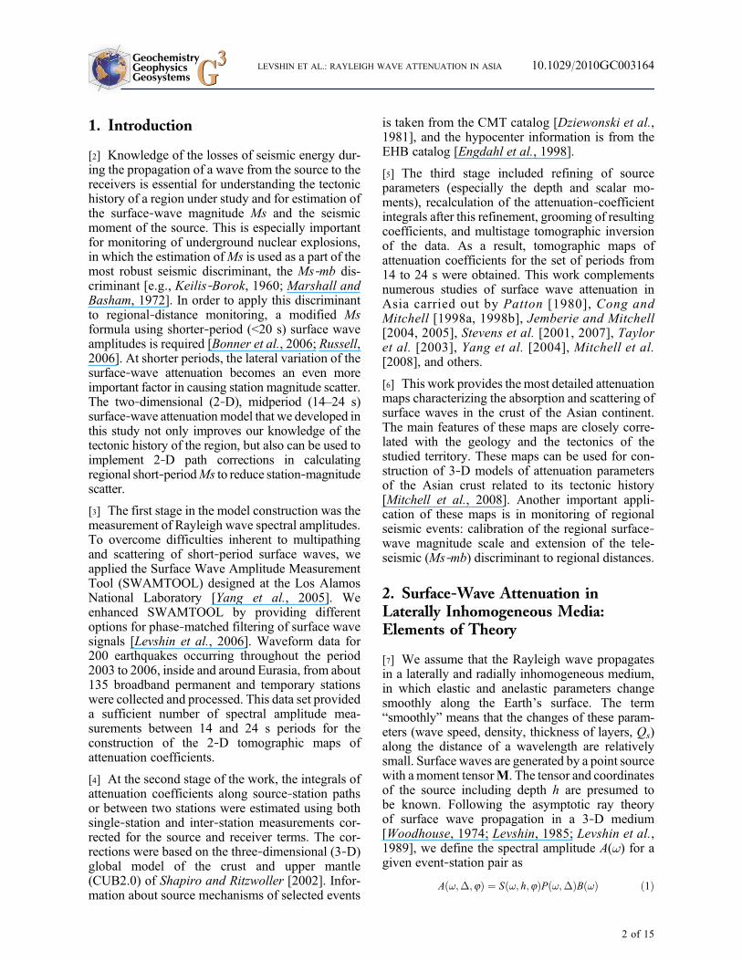
obs for a given period.We minimize F(T) using several damping para-meters described by Barmin et al. [2001], with anadditional damping parameter for the scalar‐moment correction. Numerous experiments withdifferent values of damping parameters provided theoptimal procedure for inversion. This procedure wasapplied to data for a set of periods between 14 and24 s. How much the corrected scalar momentsdiffer from CMT moments is shown in Figure 8.The tendency for M0 to decrease by 2–5% for allperiods in order to fit the data can be seen. Thesame tendency was noticed by Yang et al. [2004].

[29] For the second step of tomographic inversion,we selected period T = 18 s as representative forestimation of M0j and used source corrections ob-tained for 18‐s data to calculate predicted ampli-

GeochemistryGeophysicsGeosystems G3G3 LEVSHIN ET AL.: RAYLEIGH WAVE ATTENUATION IN ASIA 10.1029/2010GC003164

8 of 15

tudes at all periods before inversion. The startingmodels were still the spatially homogeneous modelsfound by a new averaging of corrected qij

obs.

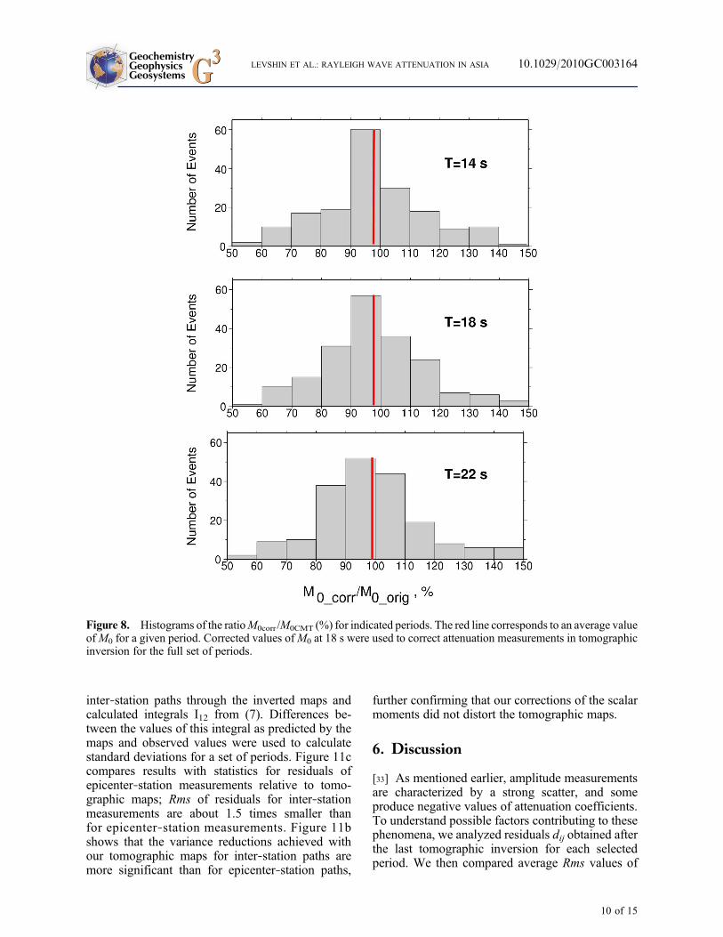
[30] Figure 9 shows resulting tomographic maps ofattenuation coefficients gR for Asia and surroundingregions, while the quality factor QR maps are shownin Figure 10.

5. Evaluating the Attenuation Models

[31] We estimated the variance reduction which wasachieved with our tomographic maps by comparing

their residual statistics with those found for spatiallyhomogeneous models. For periods between 14 and24 s, variance reduction was between 30 and 40%(Figure 11a). Fixing the scalar moment for the entireset of periods using the results for 18 s did not sig-nificantly degrade the data fit. Tomographic mapsobtained from inversions with the scalar‐momentcorrection included as an unknown are very similarto the maps shown in Figure 9.

[32] We also used inter‐station amplitude measure-ments, which are less subject to uncertainty in sourceparameters, to validate the inverted maps. We traced

Figure 7. Path density for selected epicenter‐station paths at indicated periods.

GeochemistryGeophysicsGeosystems G3G3 LEVSHIN ET AL.: RAYLEIGH WAVE ATTENUATION IN ASIA 10.1029/2010GC003164

9 of 15

inter‐station paths through the inverted maps andcalculated integrals I12 from (7). Differences be-tween the values of this integral as predicted by themaps and observed values were used to calculatestandard deviations for a set of periods. Figure 11ccompares results with statistics for residuals ofepicenter‐station measurements relative to tomo-graphic maps; Rms of residuals for inter‐stationmeasurements are about 1.5 times smaller thanfor epicenter‐station measurements. Figure 11bshows that the variance reductions achieved withour tomographic maps for inter‐station paths aremore significant than for epicenter‐station paths,

further confirming that our corrections of the scalarmoments did not distort the tomographic maps.

6. Discussion

[33] As mentioned earlier, amplitude measurementsare characterized by a strong scatter, and someproduce negative values of attenuation coefficients.To understand possible factors contributing to thesephenomena, we analyzed residuals dij obtained afterthe last tomographic inversion for each selectedperiod. We then compared average Rms values of

Figure 8. Histograms of the ratioM0corr /M0CMT (%) for indicated periods. The red line corresponds to an average valueofM0 for a given period. Corrected values ofM0 at 18 s were used to correct attenuation measurements in tomographicinversion for the full set of periods.

GeochemistryGeophysicsGeosystems G3G3 LEVSHIN ET AL.: RAYLEIGH WAVE ATTENUATION IN ASIA 10.1029/2010GC003164

10 of 15

residuals for all paths and subsets of selected paths;findings were

[34] (1) For paths ending at a given station: Weobserved significant increase in Rms relative toaverage values only for paths to a few stationssituated near the ocean and deep‐sea coasts (e.g.,station DVA in Philippines and station SANT on the

Santorin island in Mediterranean). Such paths wereexcluded from the final tomographic inversion.

[35] (2) For paths starting from the epicenters atsome geographical regions: We noticed only oneregion—namely the Aegean Sea—which is charac-terized by significant increase in Rms relative toaverage values. This could be explained by incon-

Figure 9. Tomographic maps of attenuation coefficients across Asia and surrounding regions. Grey color correspondsto areas where the path density is less than 20 paths across a 2° by 2° equatorial cell.

GeochemistryGeophysicsGeosystems G3G3 LEVSHIN ET AL.: RAYLEIGH WAVE ATTENUATION IN ASIA 10.1029/2010GC003164

11 of 15

sistent data on source depth and source mechanismspecific for this region, which has a complicatedlithospheric structure.

[36] (3) For paths of different lengths: Shorter paths(less than 1000 km) and very long paths (greaterthan 8000 km) are characterized on average byslightly larger values of Rms, but the difference isnot very significant.

[37] (4) For paths inside some geographical cell:Paths crossing predominantly platforms and shieldsare characterized by Rms values that are lower thanthose values for paths crossing tectonic regions by a

factor of 2 (Figure 11d). This can be explained (atleast in part) by inadequacy of our version of raytheory, which does not take into account the effectsof focusing and defocusing of wave energy, of scat-tering effects of mountain ranges, and of not com-pletely eliminating multipathing. We are inclinedto assume that at the existing level of knowledge ofthe detailed crustal velocity structure in tectonicregions, it is impractical to improve measurementsof short and midperiod surface wave attenuation byintroducing more sophisticated theory that may takeinto account ray bending or frequency‐dependentdiffraction effects.

Figure 10. Tomographic maps of QR across Asia and surrounding regions at indicated periods.

GeochemistryGeophysicsGeosystems G3G3 LEVSHIN ET AL.: RAYLEIGH WAVE ATTENUATION IN ASIA 10.1029/2010GC003164

12 of 15

[38] The resulting tomographic maps of Figures 9and 10 display many features that correlate wellwith the geology and tectonics of the studied region.Low attenuation is typical in stable regions such asEast Europe and the Siberian Platforms, the IndianShield, the Arabian platform, the Yangtze craton,and others. High attenuation is observed in tecto-nically active regions, such as the Himalayas, theTien‐Shan, the Pamir, and the Zagro. Within theperiod range from 14 to 24 s, the overall attenuationdecreases as the period increases. However, valuesof QR which are less sensitive to the value of periodare still quite low at periods 16 – 20 s in activetectonic regions as comparison with stable regions

shows (Figure 10). This may indicate partial meltingin the middle crust, especially at high orogenicplateaus such as Tibet and Pamir.

[39] We estimated the spatial resolution of our datausing the technique described by Barmin et al.[2001]. According to resolution maps obtained(not included here), the spatial resolution variesacross the continental parts of maps from 180 to400 km. The resolution decreases at oceanic parts ofour maps, in the Indian Ocean in particular, due tothe low density of observation paths (Figure 7).Therefore values of gR and QR in these parts of themap are less reliable.

Figure 11. (a) Variance reduction resulting from the tomographic inversion with “free” scalar moment corrections andfrom the inversion with fixed corrections according to the results of T = 18s inversion. (b) Validation of the tomographicmaps using inter‐station measurements. (c) Average Rms values of residuals dij for the Epicenter‐Station and Inter‐Station paths. (d) Difference in average Rms values of residuals dij for paths crossing platforms and shields (betweenlatitudes 35–70°N) and tectonic regions (between latitudes 0–35° N).

GeochemistryGeophysicsGeosystems G3G3 LEVSHIN ET AL.: RAYLEIGH WAVE ATTENUATION IN ASIA 10.1029/2010GC003164

13 of 15

[40] In general, there is good agreement betweenour 20‐s map (Figure 9) and the 20‐s map of Yanget al. [2004], which was based on a different set ofinput data. The maps of QR for periods 16 – 20 s(Figure 10) are in qualitative agreement with themap of Q0 given by Mitchell et al. [2008], which isbased on analysis of Lg coda. This is to be expectedas both types of waves are sensitive to the attenua-tion properties of the whole crust.

7. Conclusions

[41] Our modified SWAMTOOL technique permitsreliable measurement of surface‐wave amplitudespectra and the evaluation of the quality of themeasurements. We found that the existing networksand the pattern of seismicity provide a significantamount of spectral amplitudes for periods in therange of 14–24 s, appropriate for 2‐D tomographicinversions for attenuation coefficients. Notwith-standing the strong scatter, the resulting maps ofattenuation coefficients gR and factor QR providereliable and detailed new information concerninglosses of Rayleigh wave energy across the Asiancontinent. These maps can be used for constructionof 3‐Dmodel of attenuation parameters of the Asiancrust as related to its tectonic history. Anotherimportant application of these maps is in monitoringof regional seismic events: the calibration of theregional surface‐wave magnitude scale and exten-sion of the teleseismic ‘surface‐wave magnitude –body wave magnitude’ discriminant to regionaldistances.

Acknowledgments

[42] The authors greatly appreciate the opportunity to receivedigital records from IRIS DMC, GEOSCOPE, and GEOFON.Figures 4, 7, 9, and 10 were plotted using the Generic Map-ping Tool (GMT) [Wessel and Smith, 1995]. This work wassupported by the U.S. Department of Energy’s National NuclearSecurity Administration, contracts DE‐FC52‐05NA266081 andDE‐AC52‐06NA253962. We are also deeply grateful to theAssociated Editor S. Lebedev and B. Mitchell for their veryuseful comments.

References

Aki, K., and P. G. Richards (1980), Quantitative Seismology,vol. 1, W. H. Freeman, San Francisco, Calif.

Barmin, M. P., M. H. Ritzwoller, and A. L. Levshin (2001), Afast and reliable method for surface wave tomography, PureAppl. Geophys., 158, 1351–1375, doi:10.1007/PL00001225.

Bonner, J. L., D. R. Russel, D. G. Harkrider, D. T. Reiter,and R. B. Herrmann (2006), Development of a time‐domain,

variable‐period surface wave magnitude measurement proce-dure for application at regional and teleseismic distances,Bull. Seismol. Soc. Am., 96 , 678–696, doi:10.1785/0120050056.

Cong, L., and B. J. Mitchell (1998a), Lateral variations ofLg coda Q in the Middle East, Pure Appl. Geophys., 153,563–585, doi:10.1007/s000240050208.

Cong, L., and B. J. Mitchell (1998b), Seismic velocity andQ structure of the Middle Eastern crust and upper mantlefrom surface‐wave dispersion and attenuation, Pure Appl.Geophys., 153, 503–538, doi:10.1007/s000240050206.

Dziewonski, A., T.‐A. Chou, and J. H. Woodhouse (1981),Determination of earthquake source parameters fromwaveform data for studies of global and regional seismicity,J . Geophys . Res . , 86 , 2825–2852 , do i :10 .1029/JB086iB04p02825.

Engdahl, E. R., R. van der Hilst, and R. Buland (1998), Globalteleseismic earthquake relocation with improved travel timesand procedures for depth determination, Bull. Seismol. Soc.Am., 88, 722–743.

Jemberie, A. L., and B. J. Mitchell (2004), Shear wave Qstructure and its lateral variation in the crust of China andsurrounding regions, Geophys. J. Int., 157(1), 363–380,doi:10.1111/j.1365-246X.2004.02196.x.

Jemberie, A. L., and B. J. Mitchell (2005), Frequency‐dependent shear‐wave Q models for the crust of China andsurrounding regions, Pure Appl. Geophys., 162, 21–36,doi:10.1007/s00024-004-2577-3.

Keilis‐Borok, V. I. (1960), Difference of surface wavesspectrum for earthquakes and underground explosions(in Russian), Proc. Inst. Phys. Earth Acad. Sci. USSR,15(182), 88–100.

Knopoff, L. (1964), Q, Rev. Geophys. , 2 , 625–660,doi:10.1029/RG002i004p00625.

Levshin, A. L. (1985), Effects of lateral inhomogeneities onsurface wave amplitude measurements, Ann. Geophys., 3,511–518.

Levshin, A. L., V. F. Pisarenko, and G. A. Pogrebinsky(1972), On a frequency‐time analysis of oscillations, Ann.Geophys., 28, 211–218.

Levshin, A. L., T. B. Yanovskaya, A. V. Lander, B. G. Bukchin,M. P. Barmin, L. I. Ratnikova, and E. N. Its (1989), SeismicSurface Waves in Laterally Inhomogeneous Earth, edited byV. I. Keilis‐Borok, chap. 5, pp. 133–163, Kluwer, Dordrecht,Netherlands.

Levshin, A. L., X. Yang, M. H. Ritzwoller, M. P. Barmin, andA. R. Lowry (2006). Toward a Rayleigh wave attenuationmodel for Central Asia, in Proceedings of the 28th SeismicResearch Review: Ground‐Based Nuclear Explosion Moni-toring Technologies, pp. 1–10, Natl. Nucl. Security Admin.,Washington, D. C. (Available at https://na22.nnsa.doe.gov/cgi‐bin/prod/researchreview/index.cgi)

Marshall, P. D., and P. W. Basham (1972), Discriminationbetween earthquakes and underground explosions employ-ing an improved Ms scale, Geophys. J. R. Astron. Soc., 28,431–458.

Mitchell, B. J., L. Cong, and G. Ekström (2008), A continent‐wide map of 1‐Hz Lg coda Q variation across Eurasia and itsrelation to lithospheric evolution, J. Geophys. Res., 113,B04303, doi:10.1029/2007JB005065.

Patton, H. J. (1980), Crust and upper mantle structure of theEurasian continent from the phase velocity and Q of surfacewaves, Rev. Geophys., 18(3), 605–625, doi:10.1029/RG018i003p00605.

GeochemistryGeophysicsGeosystems G3G3 LEVSHIN ET AL.: RAYLEIGH WAVE ATTENUATION IN ASIA 10.1029/2010GC003164

14 of 15

Ritzwoller, M. H., and A. L. Levshin (1998), Eurasian surfacewave tomography: Group velocities, J. Geophys. Res., 103,4839–4878, doi:10.1029/97JB02622.

Russell, D. R. (2006), Development of a time‐domain, variable‐period surface wave magnitude measurement procedure forapplication at regional and teleseismic distances, part I:Theory, Bull. Seismol. Soc. Am., 96, 665–677, doi:10.1785/0120050055.

Russell, D., R. B. Herrman, and H. Hwang (1988), Applicationof frequency‐variable filters to surface wave amplitude anal-ysis, Bull. Seismol. Soc. Am., 78, 339–354.

Shapiro, N. M., and M. H. Ritzwoller (2002), Monte‐Carloinversion for a global shear‐velocity model of the crust andupper mantle, Geophys. J. Int., 151, 88–105, doi:10.1046/j.1365-246X.2002.01742.x.

Stevens, J. L., D. A. Adams, and G. E. Baker (2001).Improved surface wave detection and measurement usingphase‐matched filtering with a global one‐degree dispersionmodel, in Proceedings of the 23rd Seismic ResearchReview: Worldwide Monitoring of Nuclear Explosions,vol. 1, pp. 420–430, Natl. Nucl. Security Admin., Washington,D. C. (Available at https://na22.nnsa.doe.gov/cgi‐bin/prod/researchreview/index.cgi)

Stevens, J., J. Given, H. Xu, and G. Baker (2007). Develop-ment of surface wave dispersion and attenuation maps andimproved methods for measuring surface waves, in Proceed-

ings of the 29th Monitoring Research Review: Ground‐Based Nuclear Explosion Monitoring Technologies, vol. 1,pp. 285–291, Natl. Nucl. Security Admin., Washington,D. C. (Available at https://na22.nnsa.doe.gov/cgi‐bin/prod/researchreview/index.cgi)

Taylor, S. R., X. Yang, and W. S. Phillips (2003), Bayesian Lgattenuation tomography in central Asia, Bull. Seismol. Soc.Am., 93, 795–803, doi:10.1785/0120020010.

Wessel, P. A., and W. H. Smith (1995). New version of thegeneric mapping tools released, Eos Trans. AGU, 76, 329.

Woodhouse, J. H. (1974), Surface waves in a laterally varyinglayered structure, Geophys. J. R. Astron. Soc., 37, 461–490.

Yang, X., S. R. Taylor, and H. J. Patton (2004), The 20‐sRayleigh wave attenuation tomography for central andsoutheastern Asia, J. Geophys. Res. , 109 , B12304,doi:10.1029/2004JB003193.

Yang, X., A. R. Lowry, A. L. Levshin, and M. H. Ritzwoller(2005). Toward a Rayleigh wave attenuation model forEurasia and calibrating a new Ms formula, in Proceedingsof the 27th Seismic Research Review: Ground‐BasedNuclear Explosion Monitoring Technologies, pp. 259–265,Natl. Nucl. Security Admin., Washington, D. C. (Availableat https://na22.nnsa.doe.gov/cgi‐bin/prod/researchreview/index.cgi)

GeochemistryGeophysicsGeosystems G3G3 LEVSHIN ET AL.: RAYLEIGH WAVE ATTENUATION IN ASIA 10.1029/2010GC003164

15 of 15