Originally published as: 

 

 

 

Yang, Y., Zheng, Y., Chen, J., Zhou, S., Celyan, S., Sandvol, E., Tilmann, F., Priestley, K., Hearn, T. M., Ni, 

J. F., Broewn, L. D., Ritzwoller, M. H. (2010): Rayleigh wave phase velocity maps of Tibet and the 

surrounding regions from ambient seismic noise tomography. ‐ Geochemistry Geophysics 

Geosystems (G3), 11, Q08010  

DOI: 10.1029/2010GC003119 

Article

Volume 11, Number 8

6 August 2010

Q08010, doi:10.1029/2010GC003119

ISSN: 1525‐2027

Rayleigh wave phase velocity maps of Tibetand the surrounding regions from ambientseismic noise tomography

Yingjie YangCenter for Imaging the Earth’s Interior, Department of Physics, University of Colorado at Boulder,Boulder, Colorado 80309‐0390, USA

Key Laboratory of Dynamic Geodesy, Institute of Geodesy and Geophysics, Chinese Academy of Sciences,Wuhan 430077, China (yingjie.yang@colorado.edu)

Yong ZhengKey Laboratory of Dynamic Geodesy, Institute of Geodesy and Geophysics, Chinese Academy of Sciences,Wuhan 430077, China

John Chen and Shiyong ZhouInstitute of Theoretical and Applied Geophysics, School of Earth and Space Sciences, Peking University,Beijing 100871, China

Savas Celyan and Eric SandvolDepartment of Geological Sciences, University of Missouri, Columbia, Missouri 65211, USA

Frederik TilmannDepartment of Earth Sciences, University of Cambridge, Cambridge CB3 0EZ, UK

Helmholtz‐Zentrum Potsdam, Deutsches GeoForschungsZentrum, D‐14473 Potsdam, Germany

Keith PriestleyDepartment of Earth Sciences, University of Cambridge, Cambridge CB3 0EZ, UK

Thomas M. Hearn and James F. NiDepartment of Physics, New Mexico State University, Las Cruces, New Mexico 88003, USA

Larry D. BrownEarth and Atmospheric Sciences, Cornell University, Ithaca, New York 14853, USA

Michael H. RitzwollerCenter for Imaging the Earth’s Interior, Department of Physics, University of Colorado at Boulder,Boulder, Colorado 80309‐0390, USA

[1] Ambient noise tomography is applied to the significant data resources now available across Tibet and sur-rounding regions to produce Rayleigh wave phase speed maps at periods between 6 and 50 s. Data resourcesinclude the permanent Federation of Digital Seismographic Networks, five temporary U.S. Program for ArraySeismic Studies of the Continental Lithosphere (PASSCAL) experiments in and around Tibet, and Chineseprovincial networks surrounding Tibet from 2003 to 2009, totaling ∼600 stations and ∼150,000 interstation

Copyright 2010 by the American Geophysical Union 1 of 18

paths. With such a heterogeneous data set, data quality control is of utmost importance. We apply conserva-tive data quality control criteria to accept between ∼5000 and ∼45,000 measurements as a function of period,which produce a lateral resolution between 100 and 200 km across most of the Tibetan Plateau and adjacentregions to the east. Misfits to the accepted measurements among PASSCAL stations and among Chinese sta-tions are similar, with a standard deviation of ∼1.7 s, which indicates that the final dispersion measurementsfrom Chinese and PASSCAL stations are of similar quality. Phase velocities across the Tibetan Plateau arelower, on average, than those in the surrounding nonbasin regions. Phase velocities in northern Tibet arelower than those in southern Tibet, perhaps implying different spatial and temporal variations in the waythe high elevations of the plateau are created and maintained. At short periods (<20 s), very low phase veloc-ities are imaged in the major basins, including the Tarim, Qaidam, Junggar, and Sichuan basins, and in theOrdos Block. At intermediate and long periods (>20 s), very high velocities are imaged in the Tarim Basin,the Ordos Block, and the Sichuan Basin. These phase velocity dispersionmaps provide information needed toconstruct a 3‐D shear velocity model of the crust across the Tibetan Plateau and surrounding regions.

Components: 8600 words, 14 figures, 1 table.

Keywords: ambient noise; Rayleigh wave; tomography; Tibet.

Index Terms: 7255 Seismology: Surface waves and free oscillations (6982); 7270 Seismology: Tomography (6982); 7205Seismology: Continental crust (1219).

Received 4 March 2010; Revised 23 April 2010; Accepted 30 April 2010; Published 6 August 2010.

Yang, Y., et al. (2010), Rayleigh wave phase velocity maps of Tibet and the surrounding regions from ambient seismic noisetomography, Geochem. Geophys. Geosyst., 11, Q08010, doi:10.1029/2010GC003119.

1. Introduction

[2] Ambient noise tomography based on cross cor-relations of long recordings of seismic noise dataobserved between pairs of stations has proven to be apowerful method to construct surface wave disper-sion maps at short and intermediate periods. Thesesurface wave maps provide constraints on crustalstructure, which were difficult to obtain from tradi-tional earthquake surface wave tomography due tothe strong attenuation and scattering at short periodsat teleseismic distances.

[3] Since the first ambient noise tomographic ima-ges of Rayleigh wave group speeds in the micro-seismic band from 5 to 20 s appeared in 2004 [Sabraet al., 2005; Shapiro et al., 2005] for southernCalifornia based on the earliest data from theEarthScope Transportable Array (TA), this methodhas become increasingly widespread because of itsunique ability to constrain crustal structure inde-pendent of earthquakes or human‐made explosions.Ambient noise tomography has now been appliedaround the world to image crustal structures,including at regional scales in New Zealand [Linet al., 2007], Southern Africa [Yang et al., 2008a],Spain [Villaseñor et al., 2007], Korea [Cho et al.,2007], Japan [Nishida et al., 2008], and the west-

ern U.S. [Moschetti et al., 2007; Lin et al., 2008;Yang et al., 2008b] and at continental scales acrossEurope [Yang et al., 2007], China [Zheng et al.,2008], the USA [Bensen et al., 2008, 2009],Australia [Saygin and Kennett, 2010] as well asother places.

[4] Across Tibet and the surrounding regions,numerous global‐scale teleseismic earthquakestudies of surface wave dispersion have been per-formed [e.g., Levshin et al., 1994; Ritzwoller andLevshin, 1998; Ritzwoller et al., 1998; Villaseñoret al., 2001; Friederich, 2003; Huang et al., 2003;Shapiro et al., 2004; Levshin et al., 2005b; Priestleyet al., 2006]. In addition, several regional‐scalestudies based on ambient noise tomography havealready been carried out in southeastern Tibet [Yaoet al., 2006, 2008], southern Tibet [Guo et al.,2009], and in western Sichuan and eastern Tibet[Li et al., 2009]. The regional studies have all gen-erated high‐resolution crustal models at regionalscales. One velocity feature that has been inferredby several researchers in southern Tibet is a low‐velocity zone (LVZ) in the middle crust [Cotte et al.,1999; Rapine et al., 2003; Caldwell et al., 2009],which appears to support the crustal flow modelproposed by Royden et al. [1997] and Nelson et al.[1996] that predicts decoupling of the upper crustal

GeochemistryGeophysicsGeosystems G3G3 YANG ET AL.: RAYLEIGH WAVE PHASE VELOCITIES IN TIBET 10.1029/2010GC003119

2 of 18

deformation from the motion of the underlyingmantle. However, as shown by H. Yao et al.(Heterogeneity and anisotropy of the lithosphere ofSE Tibet from ambient noise and surface wavearray analysis, submitted to Journal of GeophysicalResearch, 2010), LVZs in the middle and lowercrust beneath southeastern Tibet appear to formcomplex 3‐D structures with substantial lateral var-iations in depth, thickness, and strength of velocityanomalies. The lateral and vertical variations ofLVZs raise questions, such as, whether the low‐velocity zones are present ubiquitously across all ofTibet and if they interconnect to form flowablechannels or are isolated and concentrated only incertain areas of Tibet.

[5] To address questions associated with middle andlower crustal flow and interpret crustal structures inthe context of larger‐scale structures, an integratedcrustal velocity model is needed. Recently, usingdata from 47 stations of the China National SeismicNetwork and 12 other global stations in adjacentregions, large‐scale group velocity maps at periodsfrom 8 to 60 s have been generated by Zheng et al.[2008] across all of China. However, due to thelimitations imposed by station number and distri-bution, most of raypaths lie in eastern China andresolution in Tibet is not high enough to detectdetailed lateral variations within the crust.

[6] In the past few years, several Program for ArraySeismic Studies of the Continental Lithosphere(PASSCAL) experiments have been carried out inTibet. Meanwhile, numerous Chinese provincialnetworks in Tibet and surrounding areas have beenupdated to intermediate‐band stations and seismicwaveforms from these networks have been archivedcontinuously. In this study, we assemble all stationsfrom the PASSCAL experiments operated betweenyears 2003 and 2009 as well as stations from theChinese Provincial Networks from August 2007 toJuly 2009, with the number of stations totalingapproximately 600. The details of these networks aredescribed in section 2. The large number of stationsprovides unprecedented coverage over the TibetanPlateau and also extends east of the plateau. Basedon cross correlations of the continuous data fromthese stations, we obtain Rayleigh phase velocitydispersion measurements at periods from 6 to 50 swhich are then used to generate phase velocity mapswith resolution on the order of 100–200 km. Thefocus of this paper is on the acquisition and qualitycontrol of the data set itself, on the ambient noisecross correlations and dispersionmeasurements, andthe production of the Rayleigh wave phase velocitymaps. Love wave maps, assimilation of teleseismic

data, and inversion for 3‐D isotropic and anisotropicstructures will be subjects of later contributions.

2. Data Acquisition and Quality Control

[7] The data used in this study are continuousseismic waveforms recorded at broadband stationsthat exist in and around Tibet from years 2003–2005 and 2007–2009 from the following networks:(1) five PASSCAL experiments (Namche Barwa,HI‐CLIMB, MIT‐CHINA, INDEPTH IV, westernTibet), (2) Chinese Provincial Networks in andaround Tibet, and (3) Federation of Digital Seis-mographic Networks (FDSN) stations (e.g., GSN,GEOSCOPE, GEOFON) and regional networks(KZ and KN) within and around the region of study.Figure 1 and Table 1 summarize these data sets. Intotal, we process data from approximately 600 sta-tions of which about 250 are from the ChineseProvincial Networks. The operating times of the fivePASSCAL experiments are listed in Table 1 alongwith the Chinese Provincial stations. In Table 1, theoverlap in time of two experiments, which is anecessary requirement for cross correlation ofambient noise, is marked with a cross. Blanks inTable 1 indicate no temporal overlap between a pairof experiments. For example, the three PASSCALexperiments that operated in the period of 2003–2005 overlap each other. The INDEPTH IV andwestern Tibet experiments in 2007–2009 alsooverlap each other and the entire Chinese ProvincialNetworks. These overlaps guarantee that dense raycoverage is generated in this study. Cross correla-tions with longer time series result in higher SNRsurface waves. Previous studies in Europe [Yanget al., 2007] and the US [Bensen et al., 2008]found that several months of continuous seismicdata are required to obtain high SNR cross correla-tions. The time spans of overlap between differentnetworks in this study are typically longer than1 year, which allows the high SNR cross correlationsbetween different networks to be obtained.

[8] Because the stations used in this study havedifferent types of seismometers, especially amongthe Chinese stations, significant effort must bedevoted to data quality control. The most criticalaspect in ambient noise tomography is consistencyand accuracy of timing between different networks.Because data from Chinese stations are recorded inBeijing Time, we first correct all the recording timesto Greenwich Mean Time (GMT). We then removeinstrument responses from all continuous wave-forms, which is necessary to unify the frequency‐dependent timings recorded at different types of

GeochemistryGeophysicsGeosystems G3G3 YANG ET AL.: RAYLEIGH WAVE PHASE VELOCITIES IN TIBET 10.1029/2010GC003119

3 of 18

seismometers. However, we found a difference inthe format of the response files between the PASS-CAL stations and the Chinese stations. In theresponse files of the PASSCAL stations, one addi-tional pole was added to the original response files,which was intended to convert velocity data to dis-placement data. On the other hand, in the responsefiles of the Chinese stations, the original responsefiles of the seismometers are kept, which means thewaveforms of Chinese stations after instrumentresponse removal have units of velocity. To ensurethe consistency of the data, we added an additionalpole to individual response files of the Chinese sta-tions, which converted all data to displacement.

[9] Figure 2 illustrates the problem of inconsis-tent response files by showing the cross correla-tion between PASSCAL station GS02 (from theINDEPTH IV experiment) and Chinese station SNT,which have an interstation distance of 637 km.When applying the original uncorrected responsefiles for the Chinese station, the negative componentof the cross correlation (red traces) and the positivecomponent (black traces) are inverted in sign rela-tive to each other in the time windows of the surfacewave signals (Figure 2b). This results from the p/2phase difference between velocity and displace-ment, which produces a phase difference of pbetween the positive and negative lags of cross

Table 1. Broadband Seismic Networks Installed During 2003–2009 in and Around Tibet

Network (Network Code)Approximate

Operation TimeSymbol

in Figure 1

Network Codea

XE(71)

YA(25)

XF(200)

X4(97)

Y2(9)

CPN(∼250)

FDSN(33)

Namche Barwa (XE) Jul 2003 to Oct 2004 red diamond X X X XMIT‐China (YA) Sep 2003 to Sep 2004 red circle X X XHi‐CLIMB (XF) Sep 2002 to Aug 2005 red square X XINDEPTH IV (X4) May 2007 to May 2009 red star X X X XWestern Tibet (Y2) Jul 2007 to Aug 2008 red triangle X X XChinese Provincial Network (CPN) May 2007 to May 2009 blue triangle X XFDSN and regional(G, PS, IC, II, IU, KZ, and KN)

yellow triangle X

aThe number of stations of each PASSCAL experiment is indicated in parentheses following the relevant network code. The crosses indicate stationsdeployed concurrently.

Figure 1. Station coverage in and around Tibet between 2003 and 2009. Symbols are defined in Table 1. Red symbolsrepresent PASSCAL stations, blue triangles represent Chinese Provincial stations, and yellow triangles are FDSN andother regional networks. Concurrent installations are indicated by crosses in Table 1.

GeochemistryGeophysicsGeosystems G3G3 YANG ET AL.: RAYLEIGH WAVE PHASE VELOCITIES IN TIBET 10.1029/2010GC003119

4 of 18

correlations. Upon adding one additional pole in theresponse files of the Chinese stations, equivalent toconverting all waveforms to displacement, the sur-face wave signals on the two components are nearlyidentical (Figure 2c). This is as expected because thetwo components represent surface waves propagat-ing in opposite directions but sensing the samemedium between the two stations.

[10] After removing instrument responses from thewaveforms using consistent response files, we thencheck the vertical polarities of all stations by com-paring the waveforms of first P arrivals from large

teleseismic events. We find all PASSCAL stationsand Chinese stations in this study have verticalpolarizations consistent with the FDSN stations.Furthermore, we check for possible timing errors foreach station using two methods. First, we comparethe two‐sided arrivals of interstation cross correla-tion, as shown in Figure 2. If one station has a timingerror, the resulting difference of arrival times ofsurface wave signals between the positive and neg-ative components will be twice the error; otherwise itwill be nearly zero. This method was used to detectstation timing errors in California by Stehly et al.[2007]. However, because strong noise energyusually comes from coastlines and noise energyattenuates when propagating inland [e.g., Yang andRitzwoller, 2008], surface wave signals from a crosscorrelation are typically not symmetric. In somecases only one component has a high signal‐to‐noiseratio (SNR), which renders this method invalid. Thesecond method to check for timing errors is per-formed during tomography. First, we create asomewhat overly smoothed tomographic map toavoid generating local phase velocity anomaliesintroduced by timing errors at a station. After thetomography, we calculate average misfit of traveltimes for each station. Because each station hasnumerous interstation phase velocity measurementswith other stations and the bearings of thecorresponding interstation paths align in variousazimuthal directions, the average misfit should bevery close to zero. We discard stations with averagemisfits larger than 5 s. The number of stations dis-carded in this step is only 15, small compared to thetotal number of stations (∼600). All of those stationsare Chinese stations except for one station from theINDEPTH IV experiment, C11, with a dysfunc-tional GPS clock.

3. Data Processing and Selection

[11] The data processing procedures we adopt herefollow those of Bensen et al. [2007] except in onestep: temporal normalization. In the work by Bensenet al. [2007], a running absolute mean normalizationis applied to seismic waveforms to suppress theeffects of earthquakes, instrumental irregularities andnonstationary noise sources near to stations on crosscorrelations, while still retaining some aspects of theamplitude information of the noise. This methodcomputes the running average of the absolute valuesof waveforms in a normalization time window offixed length and weights waveforms by the inverseof these averages. We apply this same temporalnormalization to data from PASSCAL stations and

Figure 2. (a) A cross correlation between PASSCALstationGS02 andChinese station SNTwith an interstationdistance of 637 km. The red trace is the negative lag com-ponent, and the black trace is the positive lag component.(b and c) Comparison between positive and negative com-ponents before and after correcting the instrumentresponse file of the Chinese station SNT. Note that thetwo components are inverted before the correction, whichconverts the Chinese waveform to displacement.

GeochemistryGeophysicsGeosystems G3G3 YANG ET AL.: RAYLEIGH WAVE PHASE VELOCITIES IN TIBET 10.1029/2010GC003119

5 of 18

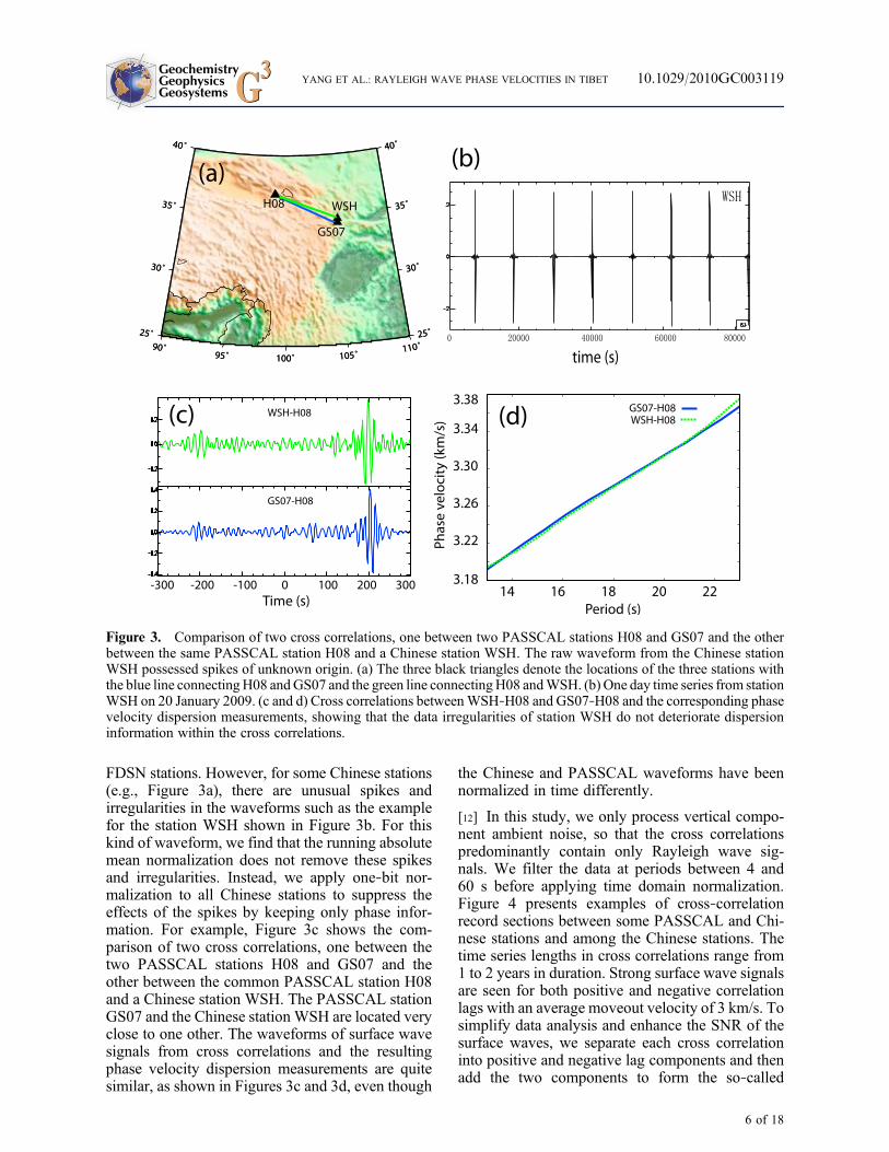
FDSN stations. However, for some Chinese stations(e.g., Figure 3a), there are unusual spikes andirregularities in the waveforms such as the examplefor the station WSH shown in Figure 3b. For thiskind of waveform, we find that the running absolutemean normalization does not remove these spikesand irregularities. Instead, we apply one‐bit nor-malization to all Chinese stations to suppress theeffects of the spikes by keeping only phase infor-mation. For example, Figure 3c shows the com-parison of two cross correlations, one between thetwo PASSCAL stations H08 and GS07 and theother between the common PASSCAL station H08and a Chinese station WSH. The PASSCAL stationGS07 and the Chinese station WSH are located veryclose to one other. The waveforms of surface wavesignals from cross correlations and the resultingphase velocity dispersion measurements are quitesimilar, as shown in Figures 3c and 3d, even though

the Chinese and PASSCAL waveforms have beennormalized in time differently.

[12] In this study, we only process vertical compo-nent ambient noise, so that the cross correlationspredominantly contain only Rayleigh wave sig-nals. We filter the data at periods between 4 and60 s before applying time domain normalization.Figure 4 presents examples of cross‐correlationrecord sections between some PASSCAL and Chi-nese stations and among the Chinese stations. Thetime series lengths in cross correlations range from1 to 2 years in duration. Strong surface wave signalsare seen for both positive and negative correlationlags with an average moveout velocity of 3 km/s. Tosimplify data analysis and enhance the SNR of thesurface waves, we separate each cross correlationinto positive and negative lag components and thenadd the two components to form the so‐called

Figure 3. Comparison of two cross correlations, one between two PASSCAL stations H08 and GS07 and the otherbetween the same PASSCAL station H08 and a Chinese station WSH. The raw waveform from the Chinese stationWSH possessed spikes of unknown origin. (a) The three black triangles denote the locations of the three stations withthe blue line connectingH08 andGS07 and the green line connectingH08 andWSH. (b) One day time series from stationWSH on 20 January 2009. (c and d) Cross correlations betweenWSH‐H08 and GS07‐H08 and the corresponding phasevelocity dispersion measurements, showing that the data irregularities of station WSH do not deteriorate dispersioninformation within the cross correlations.

GeochemistryGeophysicsGeosystems G3G3 YANG ET AL.: RAYLEIGH WAVE PHASE VELOCITIES IN TIBET 10.1029/2010GC003119

6 of 18

“symmetric component.” All subsequent analysis isperformed on the symmetric components.

[13] After obtaining all interstation cross correla-tions, we calculate the period‐dependent signal‐to‐noise (SNR) from the symmetric components. SNRis defined as the ratio of the peak amplitude within atime window containing the surface wave signals tothe root‐mean‐square of the noise trailing the signalarrival window. Figure 5 presents the average SNRas a function of period for cross correlations amongPASSCAL stations (red lines), among Chinese sta-tions (blue lines), and between PASSCAL stationsand Chinese stations (black lines), segregated intothree interstation distance ranges: three wavelengthsto 500 km, 500–1000 km, and 1000–1500 km. SNRis higher for cross correlations between PASSCALstations than between Chinese stations at all periodsand distance ranges, and is similar for cross corre-lations between Chinese stations and between Chi-nese and PASSCAL stations. Data quality fromChinese stations, therefore, is lower than that fromPASSCAL stations, consistent with the observationsof the unusual spikes and irregularities that affectsome of the Chinese network. The patterns of SNRas a function of period are similar for measurementsfrom both PASSCAL and Chinese stations. SNR ishighest at the microseism band (5–20 s). The peakSNR is around 15 s, at the center of the primarymicroseism band (10–20 s), which is consistent withambient noise studies in the USA [e.g.,Bensen et al.,2008]. SNR decreases with interstation distance

(Figures 5a–5c) due to scattering and attenuation.The SNR difference between the PASSCAL andChinese stations is relatively greatest at the longerperiods because the instrument response for many ofthe Chinese stations rolls off more rapidly above∼25 s period.

[14] After obtaining all cross correlations and cal-culating SNR, three selection criteria are appliedprior to tomography. The number of measurementsremaining after each selection step is plotted inFigure 6, segregated by measurements amongPASSCAL stations (Figure 6a) and among Chinesestations (Figure 6b). First, we accept measurementsonly when the distance between the two stations isgreater than three wavelengths. The total number ofmeasurements rejected by this criterion is ∼10% atshort periods, but increases to ∼20% at long periods.For example, the wavelength of Rayleigh wave at50 s period is ∼160 km, which requires interstationdistances longer than 480 km. Second, we use SNRto select acceptable measurements. At individualperiods, only those measurements with SNR higherthan 15 are accepted. This criterion rejects more thanhalf of all measurements. In particular, more than90% of the measurements from Chinese stations atperiods longer than 30 s are rejected, because theChinese seismometers have a corner period of 30 sat the long‐period end. Third, we require that thedispersion measurements agree with one anotheracross the data set; that is, most of the measurementsshould be able to be fit well during tomography. This

Figure 4. Record sections of cross correlations obtained from about 1 year of waveform data (a) between Chinese pro-vincial network stations and (b) between the Chinese stations and PASSCAL stations. The gray dash lines display amoveout of 3 km/s.

GeochemistryGeophysicsGeosystems G3G3 YANG ET AL.: RAYLEIGH WAVE PHASE VELOCITIES IN TIBET 10.1029/2010GC003119

7 of 18

condition is applied during tomography. This laststep rejects a small portion of data, typically less than5% of the number remaining after the second step.We finally obtain between ∼5000 and ∼45000 phasespeed measurements as a function of period from6 to 50 s (Figure 7). The number of measurementsreaches a maximum between periods of 10 and 20 s,i.e., in the primary microseismic band, and thendecreases with period so that at 50 s there are onlyabout 5000 measurements.

[15] The azimuthal distributions of SNR (Figures 8a–8c) and number of paths (Figures 8d–8f) of theselected measurements at 16 s period are plotted inFigure 8, segregated into station groups: PASSCALstations, Chinese stations, and all stations. The azi-muthal distribution at other periods is similar to the16 s period. In Figures 8a–8c, each red line representseither a positive or a negative component of a crosscorrelation and points in the direction fromwhich the

Figure 6. Number of data remaining after each step ofdata section, segregated by measurements (a) amongPASSCAL stations, (b) among Chinese stations, and(c) among all stations. Following the same order of thethree selection criteria, red lines represent the number ofall measurements, blue lines represent the numberremaining with interstation distances longer than threewavelengths, green lines represent the remaining numberof measurements with SNR > 15, and black lines repre-sent the remaining number of measurements that are fitto better than 7 s during tomography.

Figure 5. Average SNR as a function of period for crosscorrelations among PASSCAL stations (red lines), amongChinese stations (blue lines), and between PASSCAL sta-tions and Chinese stations (black lines), segregated byinterstation distance: (a) three wavelengths to 500 km,(b) 500–1000 km, and (c) 1000–1500 km.

GeochemistryGeophysicsGeosystems G3G3 YANG ET AL.: RAYLEIGH WAVE PHASE VELOCITIES IN TIBET 10.1029/2010GC003119

8 of 18

energy arrives (i.e., it points to the source location).Each line’s length is proportional to the SNR. TheSNR of lines pointing toward the southern quadrant ishighest, which means that strong ambient noise

comes from the directions of the IndianOcean and thewestern Pacific Ocean. The lowest SNR is observedtoward the west, implying that the amplitude ofambient noise from the interior of the Eurasian plate

Figure 7. Number of selected final phase velocity measurements as a function of period.

Figure 8. (a–c) Azimuthal distributions of SNR and (d–f) number of selected measurements at 16 s period, segregatedamong PASSCAL stations (Figures 8a and 8d), Chinese stations (Figures 8b and 8e), and all stations (Figures 8c and 8f).In Figures 8a–8c, each line represents either a positive or a negative component of a cross correlation and points in thedirection from which the energy arrives (i.e., it points to the source location). Each line’s length is proportional to theSNR, which is indicated by the concentric circles with the scale shown in the bottom right corner of each diagram. InFigures 8d–8f, each bar represents the number of selected paths calculated within each 10° azimuthal bin, and its numberis indicated by the concentric circles with the scale shown in the bottom right corner of each diagram. Both azimuth andback azimuth are plotted in these diagrams.

GeochemistryGeophysicsGeosystems G3G3 YANG ET AL.: RAYLEIGH WAVE PHASE VELOCITIES IN TIBET 10.1029/2010GC003119

9 of 18

is quite low. These observations are consistent withthe argument by Yang and Ritzwoller [2008] thatambient noise comes dominantly from the directionsof relatively nearby coastlines. In Figures 8d–8f, eachbar’s length represents the number of paths withineach 10° azimuth bin. Both azimuth and back azi-muth of each interstation path are included inFigure 8. For cross correlations exclusively amongPASSCAL or Chinese stations, there are preferentialdirections for paths. A large number of paths amongPASSCAL stations align in the NW–SE direction(Figure 8d) and a large number of paths amongChinese stations align in the NE–SW direction(Figure 8e). The variations of the number of pathswith azimuth are mainly due to the spatial distribu-tions of stations but are not due to azimuthal varia-tions of the strength of ambient noise. For example,most of the Chinese stations are located along theNE–SW strike in the eastern part of our study region(Figure 1), which results in the observed large num-ber of paths in this direction (Figure 8e). For mea-surements among all the stations (i.e., the totalmeasurements used in the final surface wavetomography), the azimuthal distribution of paths isquite homogeneous and uniform (Figure 8f), which isgood for resolution in surface wave tomography,particularly for extracting information about azi-muthal anisotropy that will be pursued in a futurestudy. These observations also highlight the advan-tage of ambient noise in providing homogenous raycoverage for surface wave tomography.

4. Phase Velocity Measurementsand Surface Wave Tomography

[16] We measure phase velocity dispersion curvesby automatic frequency‐time analysis (FTAN). Asillustrated by Bensen et al. [2007] and Lin et al.[2007], phase velocity measurements are muchmore accurate than group velocity measurements.Phase velocity is measured from instantaneousphase by reconciling the phase ambiguity. We fol-low Lin et al. [2007] to resolve the phase ambiguityby tracing phase velocity dispersion curves fromlong periods to short periods, because referencedispersion curves are more reliable at longer periods[e.g., Shapiro and Ritzwoller, 2002]. Some crosscorrelations, however, contain surface wave signalsonly at periods shorter than 40 s. To resolve thisproblem, we first perform a smoothed tomographyusing phase velocity dispersion measurements onlyfrom those cross correlations that have the longestperiod of surface wave signals greater than 40 s.With these dispersion measurements, we are able to

construct smoothed phase velocity maps in a periodrange from 6 to 50 s. Using the resulting smoothedphase velocity maps as a new reference, we performthe FTAN on the remaining cross correlations con-taining only surface wave signals at periods shorterthan 40 s to obtain the resulting dispersion curves.

[17] Figure 9 shows two examples of cross correla-tions and the corresponding phase velocity disper-sion curves. The path between stations GS09 andEMS (red) lies mostly within the Sichuan Basin, andthe path between stations D25 and MNI (blue) iswithin southeastern Tibet. Phase velocities at shortperiods (<12 s) in the Sichuan Basin are significantlylower than in southeastern Tibet because of thesediments in the Sichuan Basin. However, at periodslonger than 12 s, phase velocities in the SichuanBasin are much higher than in southeastern Tibet,indicating colder and stronger crust beneath theSichuan Basin.

[18] Rayleigh wave phase velocity dispersion mea-surements are used to invert for phase velocity mapson a 1° × 1° spatial grid using the tomographicmethod of Barmin et al. [2001]. This method is basedon minimizing a penalty functional composed of alinear combination of data misfit, model smoothness,and the perturbation to a referencemodel for isotropicwave velocity. The choice of the damping para-meters is subjective, but we perform a number oftests using different combinations of parameters todetermine reasonable values by considering datamisfit, model resolution, and model smoothness.

[19] During tomography, resolution is also simulta-neously estimated by using the method described byBarmin et al. [2001] with modifications presentedby Levshin et al. [2005a]. Each row of the resolutionmatrix is a resolution surface (or kernel) for a spe-cific grid node. We summarize the information ofthe resolution surface at each spatial node by fitting a2‐D symmetric spatial Gaussian function to the

resolution surface at each node: Aexp � rj j22�2

� �. The

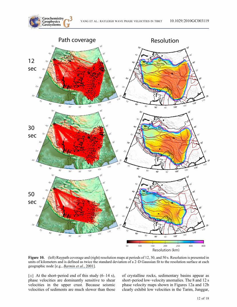
spatial resolution at each node is defined as twice thestandard deviation of this Gaussian function: g.Examples of resolution maps and associated pathcoverage are plotted in Figure 10 for the 12 s, 30 sand 50 s period measurements. Resolution is esti-mated to be about 1° (∼100 km) in the region to theeast of 90.0°E where station coverage is very denseand 2–3° (∼200–300 km) to the west of 90.0°Ewhere stations are sparse. At long periods, the areawith good path coverage shrinks and resolutionreduces gradually due to the decrease in the numberof measurements (Figure 7).

GeochemistryGeophysicsGeosystems G3G3 YANG ET AL.: RAYLEIGH WAVE PHASE VELOCITIES IN TIBET 10.1029/2010GC003119

10 of 18

[20] Histograms of data misfits from the tomographyat the three periods of 12, 25 and 40 s are plotted inFigure 11, segregated for measurements amongPASSCAL stations, among Chinese stations, andamong all stations. Misfits of measurements amongPASSCAL stations and among Chinese stations aresimilar with nearly identical standard deviationsof ∼1.7 s. This means that the measurements thatpass our selection criteria, particularly SNR > 15,obtained from the Chinese stations are probably asgood as those from PASSCAL stations.

5. Phase Velocity Maps and Discussion

[21] Sample phase velocity maps at periods of 8, 12,18, 25, 35 and 50 s are plotted in Figure 12 as per-

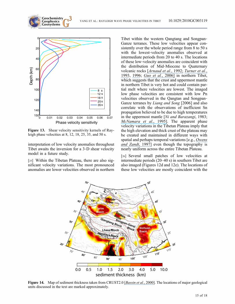
turbations relative to the average values at eachindividual period: 3.06 km/s, 3.11 km/s, 3.22 km/s,3.35 km/s, 3.53 km/s, and 3.77 km/s, respectively.The features of the phase velocity maps vary grad-ually with period due to the overlap of the Rayleighwave depth sensitivity kernels. The depth of maxi-mum phase velocity sensitivity of Rayleigh waves toshear velocity is about one third of its wavelength.To guide qualitative interpretation, shear velocitysensitivity kernels of Rayleigh phase velocities areplotted in Figure 13. The 1‐D Vs model used toconstruct the kernels is taken at (92.0°E, 32.0°N) fromthe 3‐D model of Shapiro and Ritzwoller [2002].Figure 14 presents the locations of some of themajor geological and tectonic features observed inthe Rayleigh phase velocity maps as well as amodel of sediment thickness.

Figure 9. (a) Raypaths between stations EMS andGS09 (red) and between stationsD25 andMNI (blue). (b) The 5–50 sband‐pass filtered symmetric component cross correlations for the station pairs EMS‐GS09 and D25–MNI. (c) Themeasured Rayleigh wave phase velocity dispersion curves based on the cross correlations shown in Figure 9b. Thered curve is for the station pair EMS‐GS09, and the blue curve for the station pair D25–MNI.

GeochemistryGeophysicsGeosystems G3G3 YANG ET AL.: RAYLEIGH WAVE PHASE VELOCITIES IN TIBET 10.1029/2010GC003119

11 of 18

[22] At the short‐period end of this study (6–14 s),phase velocities are dominantly sensitive to shearvelocities in the upper crust. Because seismicvelocities of sediments are much slower than those

of crystalline rocks, sedimentary basins appear asshort‐period low‐velocity anomalies. The 8 and 12 sphase velocity maps shown in Figures 12a and 12bclearly exhibit low velocities in the Tarim, Junggar,

Figure 10. (left) Raypath coverage and (right) resolutionmaps at periods of 12, 30, and 50 s. Resolution is presented inunits of kilometers and is defined as twice the standard deviation of a 2‐D Gaussian fit to the resolution surface at eachgeographic node [e.g., Barmin et al., 2001].

GeochemistryGeophysicsGeosystems G3G3 YANG ET AL.: RAYLEIGH WAVE PHASE VELOCITIES IN TIBET 10.1029/2010GC003119

12 of 18

Qadaim and Sichuan basins and also in the OrdosBlock where sediments are present (Figure 14). At18 s period, velocities in the Sichuan Basin and theOrdos Block become higher, while low velocitiespersist in the basins of Tarim, Junggar and Qadaim.This implies that sediment layers in the basins ofTarim, Junggar, Qadaim are thicker and/or sedimentshear wave speeds are slower than those in theSichuan Basin and the Ordos Block.

[23] At periods shorter than 20 s, velocities in theTibetan Plateau appear lower than the surroundingnonbasin regions, indicating the upper crust in theTibetan Plateau is warmer and weaker. Lowervelocities in the Tibetan Plateau are also consistently

observed at the intermediate and long periods(>25 s), which is in part due to the very thick crust ofthe Tibetan Plateau (>65 km).

[24] At long periods (>30 s), Rayleigh wavesbecome primarily sensitive to crustal thickness andthe shear velocities in the lower crust and uppermostmantle (Figure 13). The phase velocity maps atperiods from 25 to 50 s are inversely correlated withcrustal thickness, with high velocities in regionswith thin crust and low velocities in regionswith thick crust (Figures 12c–12e). Very highvelocity anomalies at 25–50 s periods are centeredin the Tarim Basin, the Ordos Block and theSichuan Basin, especially pronounced at 35 s period

Figure 11. Histograms of data misfits at the three periods of (top) 12 s, (middle) 25 s, and (bottom) 40 s, segregated formeasurements among (left) PASSCAL stations, (middle) Chinese stations, and (right) all stations. The correspondingstandard deviation for each case is shown in each diagram.

GeochemistryGeophysicsGeosystems G3G3 YANG ET AL.: RAYLEIGH WAVE PHASE VELOCITIES IN TIBET 10.1029/2010GC003119

13 of 18

(Figure 12e). Low velocities observed in easternTibet appear to bifurcate west of the Sichuan Basin,similar to the study of Li et al. [2009]. The low phasevelocities across the Tibetan Plateau at 25–50 speriods alone cannot be interpreted directly as a low‐velocity layer in the middle or lower crust because

low phase velocities in northern Tibet could be theresult of the uniformly thickened crust in northernTibet. Low shear wave velocities in the middlecrust were previously confirmed to exist only insouthern Tibet, west of 92°E [Cotte et al., 1999;Rapine et al., 2003;Caldwell et al., 2009]. Systematic

Figure 12. Phase velocity maps at periods of (a) 8, (b) 12, (c) 18, (d) 25, (e) 35, and (f) 50 s. Phase velocities are plottedas perturbations relative to the average value at each period. The maps truncate (reduce to gray shades) in regions wherethe resolution is worse than 400 km.

GeochemistryGeophysicsGeosystems G3G3 YANG ET AL.: RAYLEIGH WAVE PHASE VELOCITIES IN TIBET 10.1029/2010GC003119

14 of 18

interpretation of low velocity anomalies throughoutTibet awaits the inversion for a 3‐D shear velocitymodel in a future study.

[25] Within the Tibetan Plateau, there are also sig-nificant velocity variations. The most pronouncedanomalies are lower velocities observed in northern

Tibet within the western Qangtang and Songpan‐Ganze terranes. These low velocities appear con-sistently over the whole period range from 8 to 50 swith the lowest‐velocity anomalies observed atintermediate periods from 20 to 40 s. The locationsof these low‐velocity anomalies are coincident withthe distribution of Mid‐Miocene to Quaternaryvolcanic rocks [Arnaud et al., 1992; Turner et al.,1993, 1996; Guo et al., 2006] in northern Tibet,which suggests that the crust and uppermost mantlein northern Tibet is very hot and could contain par-tial melt where velocities are lowest. The imagedlow phase velocities are consistent with low Pnvelocities observed in the Qangtan and Songpan‐Ganze terranes by Liang and Song [2006] and alsocorrelate with the observations of inefficient Snpropagation believed to be due to high temperaturesin the uppermost mantle [Ni and Barazangi, 1983;McNamara et al., 1995]. The apparent phasevelocity variations in the Tibetan Plateau imply thatthe high elevation and thick crust of the plateau maybe created and maintained in different ways withspatial and perhaps temporal variations [e.g.,Owensand Zandt, 1997] even though the topography isnearly uniform across the entire Tibetan Plateau.

[26] Several small patches of low velocities atintermediate periods (20–40 s) in southern Tibet arealso imaged (Figures 12d and 12e). The locations ofthese low velocities are mostly coincident with the

Figure 13. Shear velocity sensitivity kernels of Ray-leigh phase velocities at 8, 12, 18, 25, 35, and 50 s.

Figure 14. Map of sediment thickness taken from CRUST2.0 [Bassin et al., 2000]. The locations of major geologicalunits discussed in the text are marked approximately.

GeochemistryGeophysicsGeosystems G3G3 YANG ET AL.: RAYLEIGH WAVE PHASE VELOCITIES IN TIBET 10.1029/2010GC003119

15 of 18

rift zones in southern Tibet, implying that riftsobserved at the surface may be related to lowvelocities in the middle to upper lower crust andhave a deep‐seated origin. This is consistent with theobservations from seismic refraction surveys [Coganet al., 1998]. Based on magnetotelluric data from theTibetan–Himalayan orogen, Unsworth et al. [2005]find very low resistivity present in the middle crustin the southern margin of the Tibetan plateau.Because electrical resistivity is sensitive to thepresence of interconnected fluids in the host rockmatrix, they interpret the low‐resistivity zone as apartially molten layer. Our observed low velocitiesat intermediate periods in southern Tibet may alsoreflect a partially molten layer.

[27] A small patch of high velocities appears innorthwestern Tibet at 12–50 s periods. This high‐velocity anomaly is aligned in the NW–SE direction,which is also the bearing direction of the majority ofraypaths (Figure 10). This high‐velocity feature maybe due to smearing of high velocities from the TarimBasin and/or in the western Tian Shan towardnorthwestern Tibet.

6. Summary

[28] We apply ambient noise tomography to signif-icant data resources available across Tibet and thesurrounding regions, including seismic stations fromthe permanent Federation of Digital SeismographicNetworks (FDSN), several temporaryU.S. PASSCALinstallations in and around Tibet, and the Chineseprovincial networks surrounding Tibet. These net-works comprise about 600 stations, which yieldbetween 5000 and 45000 high‐quality dispersionmeasurements depending on period and provideunprecedented path coverage across the entireTibetan Plateau. We devote considerable effort todata quality control by checking instrumentresponses, comparing the two‐sided arrivals in thecross correlations, comparing SNR and analyzingdata coherence during tomography. Data qualityfrom Chinese stations is overall lower than thatfrom PASSCAL stations because PASSCAL sta-tions are equipped with true broadband sensors.However, dispersion measurements that pass thethree selection criteria (interstation distance, SNR,and data coherence) obtained from the Chinesestations are as good as those from PASSCAL sta-tions. Ambient noise cross correlations are per-formed on these networks from 2003 to 2009.Interstation Rayleigh wave phase dispersion curvesat periods from 6 to 50 s are measured from cross

correlations of vertical components and then usedto invert for Rayleigh phase velocity maps.

[29] The resulting phase velocity maps have reso-lutions between 100 and 200 km across most ofthe Tibetan Plateau and reveal a wealth of veloc-ity features associated with tectonic structures.Rayleigh phase velocity maps at short periodsshow strong low‐velocity anomalies correlated withthe major sedimentary basins of Tarim, Junggar,Qaidam and Sichuan and the Ordos Block. Atintermediate and long periods (>25 s), high‐velocityanomalies are observed in the Tarim Basin, theOrdos Block and the Sichuan Basin. Phase velocitiesin the Tibetan Plateau are lower than in the sur-rounding regions. Phase velocities in northern Tibetare lower than in southern Tibet.

Acknowledgments

[30] The facilities of the IRIS Data Management System, andspecifically the IRIS Data Management Center, were used foraccess to waveforms and metadata of all the PASSCAL andFDSN stations required in this study. We thank all the PIs andteam members of the PASSCAL experiments and staff fromthe PASSCAL Instrument Center for collecting valuable datain Tibet. We thank the Network Center of Chinese EarthquakeAdministration for providing us with the Chinese data. We alsothank Hongyi Li and another anonymous reviewer for theirconstructive comments. This work is supported by NSF‐EARaward 0944022 and a subaward from NSF‐OISE 0730154.Yong Zheng is supported by a Chinese National ScienceFoundation award, 40974034, and a Chinese Academy ofSciences grant, CAS Y009021002. The INDEPTH‐IV passivesource team was supported by both China (grants 4052012222and 480821062) and the U.S. National Science Foundationunder grants EAR‐0634903 and EAR‐0409589.

References

Arnaud, N. O., P. Vidal, P. Tapponnier, P. Matte, and W. M.Deng (1992), The High K2O volcanism of northwesternTibet—Geochemistry and tectonic implications, EarthPlanet. Sci. Lett., 111, 351–367, doi:10.1016/0012-821X(92)90189-3.

Barmin, M. P., M. H. Ritzwoller, and A. L. Levshin (2001), Afast and reliable method for surface wave tomography, PureAppl. Geophys., 158, 1351–1375, doi:10.1007/PL00001225.

Bassin, C., G. Laske, and G. Masters (2000), The current limitsof resolution for surface wave tomography in North America,Eos Trans AGU, 81(48), FallMeet. Suppl., Abstract S12A‐03.

Bensen, G. D., M. H. Ritzwoller, M. P. Barmin, A. L. Levshin,F. Lin, M. P. Moschetti, N. M. Shapiro, and Y. Yang (2007),Processing seismic ambient noise data to obtain reliablebroad‐band surface wave dispersion measurements,Geophys. J. Int., 169, 1239–1260.

Bensen, G. D., M. H. Ritzwoller, and N. M. Shapiro (2008),Broadband ambient noise surface wave tomography across

GeochemistryGeophysicsGeosystems G3G3 YANG ET AL.: RAYLEIGH WAVE PHASE VELOCITIES IN TIBET 10.1029/2010GC003119

16 of 18

the United States, J. Geophys. Res. , 113 , B05306,doi:10.1029/2007JB005248.

Bensen, G. D., M. H. Ritzwoller, and Y. Yang (2009), A 3‐Dshear velocity model of the crust and uppermost mantlebeneath the United States from ambient seismic noise,Geophys. J. Int., 177, 1177–1196, doi:10.1111/j.1365-246X.2009.04125.x.

Caldwell, W. B., S. L. Klemperer, S. S. Rai, and J. F. Lawrence(2009), Partial melt in the upper‐middle crust of the northwestHimalayas revealed by Rayleigh wave dispersion, Tectono-physics, 477, 58–65, doi:10.1016/j.tecto.2009.01.013.

Cho, K. H., R. B. Herrmann, C. J. Ammon, and K. Lee (2007),Imaging the upper crust of the Korean Peninsula by surface‐wave tomography, Bull. Seismol. Soc. Am., 97, 198–207,doi:10.1785/0120060096.

Cogan, M. J., K. D. Nelson, W. S. F. Kidd, C. Wu, and theProject Indepth Team (1998), Shallow structure of theYadong‐Gulu rift, southern Tibet, from refraction analysisof Project INDEPTH common midpoint data, Tectonics,17, 46–61, doi:10.1029/97TC03025.

Cotte, N., H. Pedersen, M. Campillo, J. Mars, J. F. Ni, R. Kind,E. Sandvol, and W. Zhao (1999), Determination of the crustalstructure in southern Tibet by dispersion and amplitude anal-ysis of Rayleigh waves, Geophys. J. Int., 138(3), 809–819.

Friederich, W. (2003), The S‐velocity structure of the EastAsian mantle from inversion of shear and surface wave-forms, Geophys. J. Int., 153, 88–102, doi:10.1046/j.1365-246X.2003.01869.x.

Guo, Z., M. Wilson, J. Liu, and Q. Mao (2006), Post‐collisional, potassic and ultrapotassic magmatism of theNorthern Tibetan Plateau: Constraints on characteristics ofthe mantle source, geodynamic setting and uplift mechan-isms, J. Petrol., 47, 1177–1220, doi:10.1093/petrology/egl007.

Guo, Z., X. Gao, H. Yao, J. Li, and W. Wang (2009), Midcrus-tal low‐velocity layer beneath the central Himalaya andsouthern Tibet revealed by ambient noise array tomography,Geochem. Geophys. Geosyst., 10, Q05007, doi:10.1029/2009GC002458.

Huang, Z. X., W. Su, Y. J. Peng, Y. J. Zheng, and H. Y. Li(2003), Rayleigh wave tomography of China and adjacentregions, J. Geophys. Res., 108(B2), 2073, doi:10.1029/2001JB001696.

Levshin, A. L., M. H. Ritzwoller, and L. I. Ratnikova (1994),The nature and cause of polarization anomalies of surface‐wave crossing northern and central Eurasia, Geophys. J. Int.,117, 577–590, doi:10.1111/j.1365-246X.1994.tb02455.x.

Levshin, A. L., M. P. Barmin, M. H. Ritzwoller, and J. Trampert(2005a), Minor‐arc and major‐arc global surface wave dif-fraction tomography, Phys. Earth Planet. Inter., 149, 205–223, doi:10.1016/j.pepi.2004.10.006.

Levshin, A. L., M. H. Ritzwoller, and N. M. Shapiro (2005b),The use of crustal higher modes to constrain crustal structureacross central Asia, Geophys. J. Int., 160, 961–972,doi:10.1111/j.1365-246X.2005.02535.x.

Li, H. Y.,W. Su, C. Y.Wang, and Z. X. Huang (2009), Ambientnoise Rayleigh wave tomography in western Sichuan andeastern Tibet, Earth Planet. Sci. Lett., 282, 201–211,doi:10.1016/j.epsl.2009.03.021.

Liang, C. T., and X. D. Song (2006), A low velocity beltbeneath northern and eastern Tibetan Plateau from Pntomography, Geophys. Res. Lett., 33, L22306, doi:10.1029/2006GL027926.

Lin, F. C., M. H. Ritzwollerl, J. Townend, S. Bannister, andM. K. Savage (2007), Ambient noise Rayleigh wave tomog-

raphy of New Zealand, Geophys. J. Int., 170, 649–666,doi:10.1111/j.1365-246X.2007.03414.x.

Lin, F. C., M. P. Moschetti, and M. H. Ritzwoller (2008), Sur-face wave tomography of the western United States fromambient seismic noise: Rayleigh and Love wave phasevelocity maps, Geophys. J. Int., 173, 281–298, doi:10.1111/j.1365-246X.2008.03720.x.

McNamara, D. E., T. J. Owens, and W. R. Walter (1995),Observations of regional phase propagation across theTibetan Plateau, J. Geophys. Res., 100, 22,215–22,229,doi:10.1029/95JB01863.

Moschetti, M. P., M. H. Ritzwoller, and N. M. Shapiro (2007),Surface wave tomography of the western United States fromambient seismic noise: Rayleigh wave group velocity maps,Geochem. Geophys. Geosyst., 8, Q08010, doi:10.1029/2007GC001655.

Nelson, K. D., et al. (1996), Partially molten middle crustbeneath southern Tibet: Synthesis of Project INDEPTHresults, Science, 274, 1684–1688.

Ni, J., and M. Barazangi (1983), Velocities and propagationcharacteristics of Pn, Pg, Sn, and Lg seismic waves beneaththe Indian Shield, Himalayan Arc, Tibetan Plateau, andsurrounding regions: High uppermost mantle velocities andefficient Sn propagation beneath Tibet, Geophys. J. R.Astron. Soc., 72, 665–689.

Nishida, K., H. Kawakatsu, and K. Obara (2008), Three‐dimensional crustal S wave velocity structure in Japan usingmicroseismic data recorded by Hi‐net tiltmeters, J. Geophys.Res., 113, B10302, doi:10.1029/2007JB005395.

Owens, T. J., and G. Zandt (1997), Implications of crustalproperty variations for models of Tibetan plateau evolution,Nature, 387, 37–43, doi:10.1038/387037a0.

Priestley, K., E. Debayle, D. McKenzie, and S. Pilidou (2006),Upper mantle structure of eastern Asia from multimode sur-face waveform tomography, J. Geophys. Res., 111, B10304,doi:10.1029/2005JB004082.

Rapine, R., F. Tilmann, M. West, J. Ni, and A. Rogers (2003),Crustal structure of northern and southern Tibet from surfacewave dispersion analysis, J. Geophys. Res., 108(B2), 2120,doi:10.1029/2001JB000445.

Ritzwoller, M. H., and A. L. Levshin (1998), Eurasian surfacewave tomography: Group velocities, J. Geophys. Res., 103,4839–4878, doi:10.1029/97JB02622.

Ritzwoller, M. H., A. L. Levshin, L. I. Ratnikova, and A. A.Egorkin (1998), Intermediate‐period group‐velocity mapsacross central Asia, western China and parts of the MiddleEast, Geophys. J. Int., 134, 315–328.

Royden, L. H., B. C. Burchfiel, R. W. King, E. Wang, Z. L.Chen, F. Shen, and Y. P. Liu (1997), Surface deformationand lower crustal flow in eastern Tibet, Science, 276, 788–790, doi:10.1126/science.276.5313.788.

Sabra, K. G., P. Gerstoft, P. Roux, W. A. Kuperman, andM. C. Fehler (2005), Surface wave tomography from micro-seisms in Southern California, Geophys. Res. Lett., 32,L14311, doi:10.1029/2005GL023155.

Saygin, E., and B. L. N. Kennett (2010), Ambient seismicnoise tomography of Australian continent, Tectonophysics,481, 116–125, doi:10.1016/j.tecto.2008.11.013.

Shapiro, N. M., and M. H. Ritzwoller (2002), Monte‐Carloinversion for a global shear‐velocity model of the crustand upper mantle, Geophys. J. Int . , 151 , 88–105,doi:10.1046/j.1365-246X.2002.01742.x.

Shapiro, N. M., M. H. Ritzwoller, P. Molnar, and V. Levin(2004), Thinning and flow of Tibetan crust constrained by

GeochemistryGeophysicsGeosystems G3G3 YANG ET AL.: RAYLEIGH WAVE PHASE VELOCITIES IN TIBET 10.1029/2010GC003119

17 of 18

seismic anisotropy, Science, 305, 233–236, doi:10.1126/science.1098276.

Shapiro, N. M., M. Campillo, L. Stehly, and M. H. Ritzwoller(2005), High‐resolution surface‐wave tomography fromambient seismic noise, Science, 307, 1615–1618, doi:10.1126/science.1108339.

Stehly, L., M. Campillo, and N. M. Shapiro (2007), Traveltimemeasurements from noise correlation: Stability and detectionof instrumental time‐shifts, Geophys. J. Int., 171, 223–230,doi:10.1111/j.1365-246X.2007.03492.x.

Turner, S., C. Hawkesworth, J. Q. Liu, N. Rogers, S. Kelley,and P. Vancalsteren (1993), Timing of Tibetan uplift con-strained by analysis of volcanic rocks, Nature, 364, 50–54,doi:10.1038/364050a0.

Turner, S., N. Arnaud, J. Liu, N. Rogers, C. Hawkesworth,N. Harris, S. Kelley, P. Van Calsteren, and W. Deng (1996),Post‐collision, shoshonitic volcanism on the Tibetan plateau:Implications for convective thinning of the lithosphere and thesource of ocean island basalts, J. Petrol., 37, 45–71,doi:10.1093/petrology/37.1.45.

Unsworth, M. J., et al. (2005), Crustal rheology of the Hima-laya and Southern Tibet inferred from magnetotelluric data,Nature, 438, 78–81, doi:10.1038/nature04154.

Villaseñor, A., M. H. Ritzwoller, A. L. Levshin, M. P. Barmin,E. R. Engdahl, W. Spakman, and J. Trampert (2001), Shearvelocity structure of central Eurasia from inversion ofsurface wave velocities, Phys. Earth Planet. Inter., 123,169–184, doi:10.1016/S0031-9201(00)00208-9.

Villaseñor, A., Y. Yang, M. H. Ritzwoller, and J. Gallart(2007), Ambient noise surface wave tomography of theIberian Peninsula: Implications for shallow seismic structure,Geophys. Res. Lett., 34, L11304, doi:10.1029/2007GL030164.

Yang, Y. J., and M. H. Ritzwoller (2008), Characteristics ofambient seismic noise as a source for surface wave tomogra-phy, Geochem. Geophys. Geosyst., 9, Q02008, doi:10.1029/2007GC001814.

Yang, Y., M. Ritzwoller, A. Levshin, and N. Shapiro (2007),Ambient noise Rayleigh wave tomography across Europe,Geophys. J. Int., 168, 259–274, doi:10.1111/j.1365-246X.2006.03203.x.

Yang, Y. J., A. B. Li, and M. H. Ritzwoller (2008a), Crustaland uppermost mantle structure in southern Africa revealedfrom ambient noise and teleseismic tomography, Geophys.J. Int., 174, 235–248, doi:10.1111/j.1365-246X.2008.03779.x.

Yang, Y. J., M. H. Ritzwoller, F. C. Lin, M. P. Moschetti, andN. M. Shapiro (2008b), Structure of the crust and uppermostmantle beneath the western United States revealed by ambi-ent noise and earthquake tomography, J. Geophys. Res., 113,B12310, doi:10.1029/2008JB005833.

Yao, H. J., R. D. van der Hilst, and M. V. de Hoop (2006),Surface‐wave array tomography in SE Tibet from ambientseismic noise and two‐station analysis—I. Phase velocitymaps, Geophys. J. Int., 166, 732–744, doi:10.1111/j.1365-246X.2006.03028.x.

Yao, H., C. Beghein, and R. D. Van der Hilst (2008), Surface‐wave array tomography in SE Tibet from ambient seismicnoise and two‐station analysis: II—Crustal and upper mantlestructure, Geophys. J. Int., 173(1), 205–219, doi:10.1111/j.1365-246X.2007.03696.x.

Zheng, S. H., X. L. Sun, X. D. Song, Y. J. Yang, and M. H.Ritzwoller (2008), Surface wave tomography of Chinafrom ambient seismic noise correlation, Geochem. Geophys.Geosyst., 9, Q05020, doi:10.1029/2008GC001981.

GeochemistryGeophysicsGeosystems G3G3 YANG ET AL.: RAYLEIGH WAVE PHASE VELOCITIES IN TIBET 10.1029/2010GC003119

18 of 18