Predicting Atmospheric Attenuation Under Pristine Conditions ...

Received August 31, 2016, accepted October 25, 2016, date of publication November 7, 2016, date of current version January 27, 2017.

Digital Object Identifier 10.1109/ACCESS.2016.2626200

Predicting Atmospheric Attenuation UnderPristine Conditions Between 0.1 and 100 THzJINGYE SUN, (Student Member, IEEE), FANGJING HU, (Member, IEEE),AND STEPAN LUCYSZYN, (Fellow, IEEE)Centre for Terahertz Science and Engineering, Department of Electrical and Electronic Engineering, Imperial College London, London, SW7 2AZ, U.K.

Corresponding author: S. Lucyszyn ([email protected])

This work was supported in part by Imperial College MRC Confidence in Concept (ICiC) fund and NIHR Imperial BRC funding 2015/16.

ABSTRACT This multidisciplinary paper reports on a research application-led study for predicting atmo-spheric attenuation, and tries to bridge the knowledge gap between applied engineering and atmosphericsciences. As a useful comparative baseline, this paper focuses specifically on atmospheric attenuation underpristine conditions, over the extended terahertz spectrum. Three well-known simulation software packages(‘HITRAN on theWeb’, MODTRAN R©4, and LBLRTM) are compared and contrasted. Techniques used formodeling atmospheric attenuation have been applied to investigate the resilience of (ultra-)wide fractionalbandwidth applications to the effects of molecular absorption. Two extreme modeling scenarios are inves-tigated: horizontal path links at sea level and Earth-space path links. It is shown by example that a basicsoftware package (‘HITRAN on the Web’) can give good predictions with the former, whereas sophisticatedsimulation software (LBLRTM) is required for the latter. Finally, with molecular emission included, carrier-to-noise ratio fade margins can be calculated for the effects of line broadening due to changes in macroscopicatmospheric conditions with sub-1-THz ultra-narrow fractional bandwidth applications. Outdoors can be farfrom pristine, with additional atmospheric contributions only briefly introduced here; further discussion isbeyond the scope of this paper, but relevant references have been cited.

INDEX TERMS THz, thermal infrared, atmospheric attenuation, transmittance, carrier-to-noise, molecularabsorption, molecular emission, HITRAN, MODTRAN R©, LBLRTM, THz Torch.

I. INTRODUCTIONIndoor terahertz (THz) laboratories routinely conduct experi-ments on optical benches within an atmosphere under pristineconditions. For example, in an air-conditioned environment,sometime even without humidity control; or without the rec-ommended vacuum or inert gas. Alternatively, compresseddry air can be employed to avoid the risk of asphyxiation(a possible danger when using an inert gas like nitrogen orargon), although oxygen absorption lines will remain. Mea-surement discrepancies due to adverse effects from atmo-spheric attenuation may not always be properly taken intoaccount.

With another scenario, the relentless drive to pushfuture (ultra-)broadband systems up into the THz spectrumrequire ever-more sophisticated channel modeling (takinginto account additional aspects; for example, non-line-of-sight paths and multipath fading). Once again, atmosphericattenuation is important; in this case it represents a critical

contribution to the free-space power link budget analysisused to predict the system’s end-to-end carrier-to-noise ratio.Therefore, an understanding of atmospheric attenuation, howit can be predicted and its quantifiable effects on systems levelperformance is important. This multidisciplinary paper triesto bridge the knowledge gap between applied engineering andatmospheric sciences; and is intended for non-atmosphericresearchers interested in predicting atmospheric attenuation.

As a useful comparative baseline, this paper focuses specif-ically on atmospheric attenuation under pristine conditions(found indoors and some global location outdoors), within theextended terahertz spectrum. From the outset, an exhaustivereview of simulation software and their associated theoret-ical background and validation is beyond the scope of thisstudy. More realistic modeling scenarios would require amuch broader and deeper treatment of atmospheric sciences,including a very detailed be-spoke (time-variant) atmosphericmodel across the geographical path link under investigation.

VOLUME 4, 20162169-3536 2016 IEEE. Translations and content mining are permitted for academic research only.

Personal use is also permitted, but republication/redistribution requires IEEE permission.See http://www.ieee.org/publications_standards/publications/rights/index.html for more information.

9377

J. Sun et al.: Predicting Atmospheric Attenuation Under Pristine Conditions Between 0.1 and 100 THz

Nevertheless, our idealized treatment reveals many importantfacets associated with this multidisciplinary subject.

When referring to ‘terahertz’ it is useful to first define asso-ciated frequency bands. Often, ‘terahertz’ is loosely definedby the broad frequency range from 0.1 to 10 THz. This regionis sometimes referred to as the "THz Gap", where the per-formance of conventional electronic(photonic) devices falloff with increasing frequency(wavelength). Over time, thistechnology gap continues to shrink; leading to the Interna-tional Telecommunications Union (ITU)-designated spectralrange from 0.3 to 3 THz (also known as the submillimeter-wave band). With reference to heterodyne receivers, frequen-cies >3 THz are sometimes referred to as ‘‘super-THz’’ [1].For optics and photonics, the International Organization forStandardization quote the far infrared (FIR) as being from0.3 to 6 THz and mid-infrared (MIR) from 6 to 100 THz [2].When dealing with Earth systems, Harries et al. [3] definesthe FIR as THz frequencies below 20 THz; while in spec-troscopy, the FIR extends from 0.3 to 30 THz and MIRfrom 30 to 120 THz [4]. Here, the spectroscopic defini-tions for the infrared are adopted and the ‘over the THzhorizon’ thermal infrared from 10 to 100 THz is consid-ered as an extension of the THz spectrum. To illustrate thespectral locations for various key bands, Planck’s law forspectral radiance of a blackbody radiator at room temperature(e.g., 296K or 23◦C) as a function of frequency is plotted overthe extended THz spectrum from 0.1 to 100 THz, shown inFig. 1.

FIGURE 1. Calculated Planckian spectrum for a blackbody radiator at296 K as a function of frequency. (Spectral bands defined here areoverlaid in red).

For a blackbody radiator, the theoretical peak in spectralradiance is given by Wien’s displacement law; for example,at 296 K the emitted spectral radiance as a function of fre-quency peaks at 17.4 THz. However, the Planckian spectraltail theoretically extends down in frequency towards dc. Thisexplains why thermal detectors can still operate at microwavefrequencies.

One of the inherent limiting factors for practical free-spaceTHz applications (such as spectroscopy, sensing, imaging,communications and wireless power transfer) is atmosphericattenuation. This has a strong influence on the power linkbudget of complete end-to-end systems and ultimately lim-

its dynamic range and maximum path length. As a result,accurately predicting atmospheric attenuation is of criticalimportance for experimentalists and systems designers.

Three well-known simulation software packages(‘HITRAN on the Web’, MODTRAN R©4 and LBLRTM) arecompared and contrasted for predicting atmospheric attenua-tion from 0.75 to 100 THz. It will be shown that atmosphericattenuation is relatively very low if path lengths are of theorder of centimeters, or tens of meters within certain bands.This offers many new opportunities for potentially ubiquitousfree-space applications in spectroscopy (e.g., non-destructivetesting), sensing (e.g., motion detection, radiometry, radar),imaging, communications (e.g., key fobs, smart RFID, highdata rate terrestrial, drone and satellite links) and radiativewireless power transfer (R-WPT).

Section II gives a background to the characteriza-tion of atmospheric attenuation within the far and mid-infrared parts of the electromagnetic spectrum. The paperthen investigates, by examples, two very different ideal-ized scenarios (i.e., under pristine atmospheric conditions,which ignores aerosols and mist/fog/cloud/precipitation).In Sections III and IV, horizontal path links at sea level(i.e., 1 atm or 101.325 kPa) are investigated, using the threewell-known simulation software packages. In Section V,Earth-space path links are investigated using the gold stan-dard reference benchmark software (LBLRTM). Finally,Section VI investigates sub-1THz scenarios.

II. BACKGROUNDAtmospheric attenuation includes contributions from threegeneric categories: (i) gases; (ii) aerosols; and (iii) mist/fog/cloud/precipitation. These are represented respectively byeither molecules, particles or liquid droplets; all of whichmay absorb and scatter radiation with a frequency depen-dence that is a function of their size, shape and composition.A knowledge of atomic and molecular physics can explainand quantify how various gaseous molecules absorb radiationat specific frequencies, as well as the formation of ‘transmis-sion windows’.

Natural aerosols include forest exudates, pollen, min-eral dust and wildfire smoke; while anthropogenic aerosolsinclude industrial haze, dust, as well as smoke, and particulateair pollutants.

In addition to absorption, specular (mirror-type) anddiffuse (random) reflections can occur. An example of theformer is tropospheric scattering found at low gigahertz fre-quencies, and longer wavelengths, and thus below our spec-tral range of interest. With the latter, the amount of scatteringdepends on the levels of concentration, size, shape and com-position (represented by its refractive index) of the scatterer.

All scattering effects are ultimately governed byMaxwell’sequations and dependent on the size parameter x (equal tothe ratio of physical peripheral size of scatterer to excitationwavelength). As can be seen in Fig. 2, there are four scatteringregimes: (i) no scattering with x < 0.002; (ii) Rayleigh(or molecular) scattering with 0.002 < x < 0.2; (iii) Mie

9378 VOLUME 4, 2016


FIGURE 2. Scattering regimes that influence diffuse reflections.

scattering with 0.2 < x < 2000; and (iv) geometric opticswith x > 2000 [5]. This idealized treatment makes theimplicit assumption that the particles or liquid droplets arespherical, which is a generalized approximation.

Within our spectral range of interest, a combination ofRayleigh scattering, Mie scattering and geometric optics canoccur from aerosols and mist/fog/cloud/precipitation, as thesize of the particles or liquid droplets increases.

FIGURE 3. Early (1972) piecemeal modeling approach representation ofatmospheric attenuation for horizontal path links at sea level for differentweather conditions, reproduced in [6].

Atmospheric attenuation from microwave to visible fre-quencies is represented in Fig. 3, for different weather condi-tions [6]. It can be seen that the effects of gaseous water vapordominates atmospheric attenuation from ca. 0.6 to 10 THz,while rain can have an influence at all frequencies. As withaerosols, fog causes little attenuation at low THz frequencies,when compared at shorter wavelengths. The level of atmo-spheric attenuation by precipitation depends on rainfall rate,and the size and distribution of droplets.

It is interesting to note that Fig. 3 was re-published withinthe past decade [6], but a search for the original artworkrevealed numerous variations [7]. For gaseous attenuation,they state that results below 1 THz were published byRosenblum in 1961 [8] and above 10 THz byLukes in 1968 [9]. However, between 1 and 10 THz, theseauthors conceded that this region was drawn-in by hand [6].

The results for fog between 0.01 to 1,000 THz are fromMondre in 1970 [10]. Finally, data for atmospheric atten-uation due to rain, below 0.6 THz, was from Zuffereyin 1972 [11] and above 0.6 THz from Lukes [9]. While theresults shown in Fig. 3 give qualitative spectral information, itshould not be used to extract accurate quantitative data values;not least because the results only serve for specific scenarios(temperature, pressure, rainfall rate, etc.).

FIGURE 4. Atmospheric attenuation for horizontal path links at sea levelfor different weather conditions [6].

In the highly cited papers by Appleby and Wallace [6] andRosker andWallace [12] atmospheric attenuation is simulatedbetween 0.01 and 1,000 THz, shown in Fig. 4, using threeatmospheric radiative transfer codes – from 0.01 to 1 THzwith MPM89 [13]; 1 to 10 THz with FASCODE [14] andLBLRTM [15]; and 10 to 1,000 THz with MODTRAN R©4(released in 1999) [16], [17] – for a horizontal path linkat sea level, given various weather conditions. It can beseen in Fig. 4 that the relative coverage, spectral resolutionand agreement at the overlap points indicate the improvedability to model atmospheric attenuation across this spectralrange. Nevertheless, because of poor print quality, it is stillgenerally not possible to directly extract data from plots inpublished papers from 1 to 10 THz. In practice, atmosphericattenuation should be predicted using simulation softwarehaving a be-spoke model for the specific link scenario underinvestigation.

For example, a typical modeling scenario for radio astron-omy requires the prediction of transmittance through theEarth’s atmosphere at zenith. In 2013, Shaw and Nugent [18]reported results above 14 THz, from sea level to the topof atmosphere (i.e., vertical path through the atmosphere),using the MODTRAN R©5 Rural aerosol model with 23 kmvisibility; the result is shown in Fig. 5.

It is important to note that, within today’s atmosphericscience communities, atmospheric attenuation modeling is avery advanced and highly specialized discipline. For exam-ple, extensive theoretical and experimental work has beenundertaken to characterize the effect of gaseous water vaporon atmospheric attenuation within the 0.1 to 10 THz region[19]–[24] and above 10 THz [25]–[27].

VOLUME 4, 2016 9379


FIGURE 5. Atmospheric transmittance for Earth-space path links at zenithusing the U.S. standard 1976 model with MODTRAN R©5 [18].

Atmospheric attenuation measurements conducted withina controlled atmosphere was reported by Liu et al. [23],covering the 0.1 to 3 THz frequency range, at a temperatureof 296 K and relative humidity of 26%. It was found that thereare 9 transmission windows within this spectral range andthat, as expected, transmittance decreases with an increase inrelative humidity; while transmission windows shrink as pathlengths increase.

Recently, Slocum et al. [24] reported the transmittancebetween 0.3 to 1.5 THz for multiple humidity levels andpath lengths, using Fourier transform spectroscopy. Theycompared the modeled absorption lines of gaseous watervapor with experimental data from a controlled environment.A discrepancy was observed due to water vapor continuumabsorption and the air-broadening continuum parameter wasdetermined. This mechanism will be discussed further inSection III.

In 2008, an international collaborative study (by ImperialCollege London, CNR, Universities of Bologna and Basil-icata and NASA Langley Research Centre) modeled atmo-spheric attenuation from dc to 30 THz [3]. More recently,within the pure rotation band, between 2.5 and 12.5 THz,measurements were taken using the Imperial CollegeLondon Tropospheric Airborne Fourier TransformSpectrometer (TAFTS) instrument on-board the Facilityfor Airborne Atmospheric Measurement (FAAM) BAe-146research aircraft [28].

Accurately predicting atmospheric attenuation should bepossible for any arbitrarily defined geographical path linkand at any frequency. However, developing generic in-housesoftware for this purpose is challenging, because of theever-expanding database of spectral features and choice ofparameters used in subsequent calculations. For this reason,well-established benchmark simulation software has beendeveloped for the scientific and engineering communities.These codes are constantly being updated to take into accountrecent advances in experimental atmospheric spectroscopy.

Using such software, Schneider et al. [29] investigatedthe influences of different weather conditions (including fog,cloud and rain) on propagation from 1 GHz to 1 THz.Here, atmospheric attenuation was predicted using threeITU-Recommendations [30]–[32] and the am simulation

software package [33]. The ITU-R P.676 models havebeen adopted as an industry standard for predicting atmo-spheric attenuation (due to oxygen and water vapor molec-ular absorption) between 1 GHz and 1 THz, with valuesthat can even be extracted directly from plots. Developedby the Harvard-Smithsonian Center for Astrophysics, amperforms radiative transfer calculations from microwave tosubmillimeter-wave frequencies. Five transmission windowswere identified, shown in Table 1, for data transmissionover a fixed free-space path length of 1 km, between0.3 and 0.9 THz; under pristine conditions, 50 m visibilityfog and worst-case rainfall rates of 50 mm/h.

TABLE 1. Sub-1 THz free-space transmission windows for horizontal pathlinks at sea level.

A path loss analysis (which combines both atmo-spheric attenuation and spreading loss) for channelmodeling between 0.1 and 10 THz was reported byJornet and Akyildiz [34]. Analysis is based on radiativetransfer theory [35] and data from the HITRAN database [36]above 1 THz in their calculations of atmospheric attenuationdue to molecular absorption. The total loss for path lengthsfrom 10 µm to 10 m have been calculated for gaseouswater vapor fractional volumes of 0.1% and 10%. They thenreported total path losses under pristine conditions for 1, 10and 100 m path lengths [37]. From their recent study, theyindependently proposed four transmission windows between0.1 and 1 THz, shown in Table 1.

In their recently published paper [38], the same groupinvestigated the relationship between the distance and thetotal usable bandwidth for wireless systems, within the spec-tral range from 0.06 to 1 THz for line-of-sight (LOS) andmultipath (MP) propagation models. With the former, and theuse of highly directional pencil-beam antennas, the range ofcommunications is limited to 70 m with a 120 dB thresholdpath loss; the usable bandwidth shrinks from 0.94 to 0.26 THzwhen path length increases from 1 to 70 m. With the latter,path links are limited to 8 m with a lower threshold path lossof 80 dB; the usable bandwidth is now 0.29 THz at a pathlength of 1 m.

III. COMPARISON OF SELECTED SIMULATION SOFTWAREThere are two important differences between the resultsshown in Figs. 4 and 5. The first is that attenuation is replacedby transmittance; with the latter being a more useful wayof viewing atmospheric absorption/emission lines and bands.

9380 VOLUME 4, 2016


At a single frequency point, attenuation has a linear scal-ing law with path length; while transmittance has a powerlaw. However, over a band of frequencies, the mean bandattenuation(transmittance) can only exhibit a linear(power)scaling law relationship if its values are effectively constantacross the band. In practice, this scenario is only likely to existover narrow bandwidths. Secondly, results for the horizontalpath link at sea level will be different to that for the Earth-space path link at zenith, given the same path length of∼100 km, due to the variation in absorber (gases, aerosolsand mist/fog/cloud/precipitation) concentration levels andmacroscopic atmospheric conditions (e.g., temperature andpressure) with altitude. Gaseous water vapor variation is par-ticularly important, as it plays the dominant role between ca.0.1 and 10 THz.

In this section, three well-known simulation software pack-ages will be compared and contrasted. Before doing this,some of the most relevant output parameters are first definedfrom first principles.

When an electromagnetic wave is incident upon a non-opaque medium (solid, liquid or gas), some of this power Piis reflected back Pr , a proportion may be absorbed Pa andthe remaining transmitted through Pt ; such that the princi-ple of conservation of energy is observed at each frequency(i.e., Pi = Pr + Pa + Pt ) [39]. In terms of absolute powervalues, benchmark simulation software can generate resultsfor: (i) reflection or reflectance, R = Pr/Pi; (ii) absorptivity,absorption or absorptance, A = Pa/Pi; and (iii) transmissionor transmittance, T = Pt/Pi = e−τ , where e+τ is theatmospheric loss factor, τ = γL is the opacity, γ = (b+ kα)is the extinction coefficient, b is the scattering coefficient,kα is the attenuation or absorption coefficient and L is pathlength. Apart from path length, all other variables are implic-itly frequency dependent.

The gradient of attenuation with path length canbe expressed (in dB/km) as specific attenuation =−10log10 {T } = −10log10 {1− R− A}, where R, T, Ahave been calculated for a specific reference path length(e.g., LREF = 1 km); an example of this is shown inFig. 4. Therefore, at a single frequency point, attenuation (dB)over an arbitrary path length L (km) within a homogeneousatmosphere can be calculated from −L · 10log10 {T } =−L · 10log10 {1− R− A}, which exhibits a linear scalinglaw. Similarly, transmittance (%) over L can be calculatedfrom T L/LREF · 100%; exhibiting a power law. Both of theserelationships are only true if the atmosphere is homogeneous(such that γ 6= f (l), where l is the location along the path).

To represent realistic vertical atmospheric profiles, radia-tive transfer codes typically split the atmosphere into a num-ber of sub-layers. Given N homogeneous sub-layers, eachhaving different gaseous concentrations and macroscopicatmospheric conditions, the monochromatic transmittance ofthe whole atmosphere will be T =

∏Ni=1 e

−γiLi ; hence neitherlinear nor power scaling laws are valid.

As a useful comparative baseline, only pristine conditionsare considered further. Here, molecular scattering from gas

species is only significant at visible frequencies (outside ourspectral range of interest) and so scattering and, therefore,diffuse reflections can be ignored.

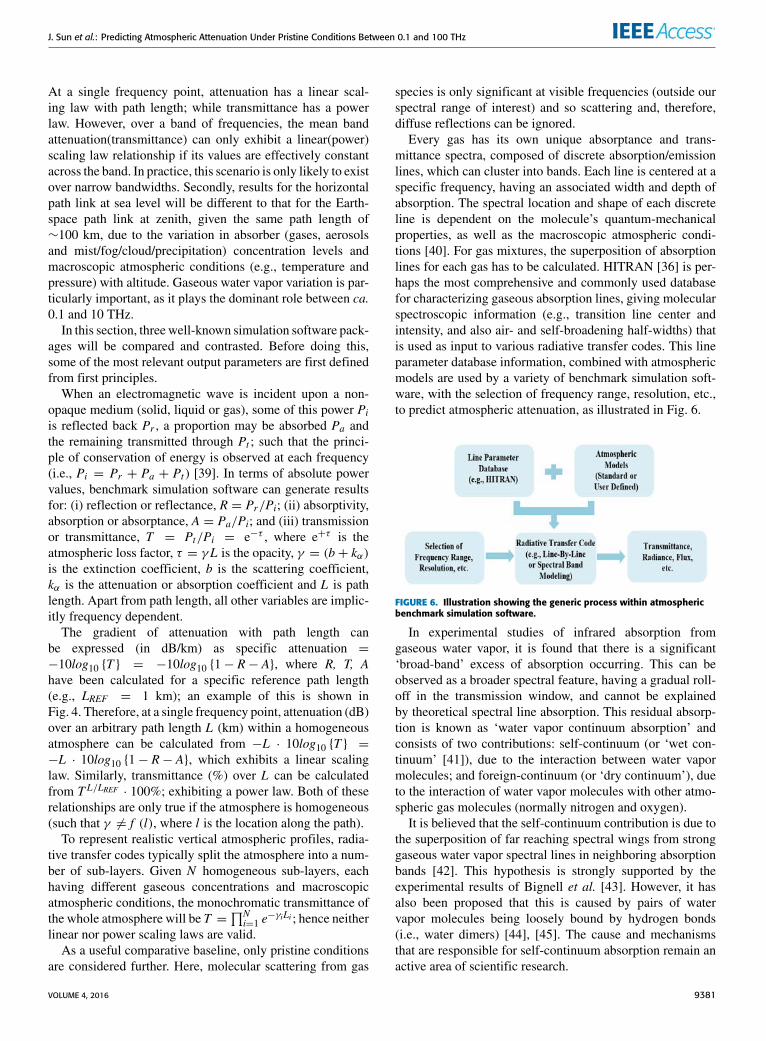
Every gas has its own unique absorptance and trans-mittance spectra, composed of discrete absorption/emissionlines, which can cluster into bands. Each line is centered at aspecific frequency, having an associated width and depth ofabsorption. The spectral location and shape of each discreteline is dependent on the molecule’s quantum-mechanicalproperties, as well as the macroscopic atmospheric condi-tions [40]. For gas mixtures, the superposition of absorptionlines for each gas has to be calculated. HITRAN [36] is per-haps the most comprehensive and commonly used databasefor characterizing gaseous absorption lines, giving molecularspectroscopic information (e.g., transition line center andintensity, and also air- and self-broadening half-widths) thatis used as input to various radiative transfer codes. This lineparameter database information, combined with atmosphericmodels are used by a variety of benchmark simulation soft-ware, with the selection of frequency range, resolution, etc.,to predict atmospheric attenuation, as illustrated in Fig. 6.

FIGURE 6. Illustration showing the generic process within atmosphericbenchmark simulation software.

In experimental studies of infrared absorption fromgaseous water vapor, it is found that there is a significant‘broad-band’ excess of absorption occurring. This can beobserved as a broader spectral feature, having a gradual roll-off in the transmission window, and cannot be explainedby theoretical spectral line absorption. This residual absorp-tion is known as ‘water vapor continuum absorption’ andconsists of two contributions: self-continuum (or ‘wet con-tinuum’ [41]), due to the interaction between water vapormolecules; and foreign-continuum (or ‘dry continuum’), dueto the interaction of water vapor molecules with other atmo-spheric gas molecules (normally nitrogen and oxygen).

It is believed that the self-continuum contribution is due tothe superposition of far reaching spectral wings from stronggaseous water vapor spectral lines in neighboring absorptionbands [42]. This hypothesis is strongly supported by theexperimental results of Bignell et al. [43]. However, it hasalso been proposed that this is caused by pairs of watervapor molecules being loosely bound by hydrogen bonds(i.e., water dimers) [44], [45]. The cause and mechanismsthat are responsible for self-continuum absorption remain anactive area of scientific research.

VOLUME 4, 2016 9381


Absorption due to foreign-continuum is much weakerthan self-continuum absorption between 25 and 37.5 THz(12 and 8 µm). Therefore, it is difficult to take accurateabsorption measurements within this spectral region. Asa result, the contribution of foreign-continuum absorptionis either considered to be negligible [25], [46] or under-estimated in radiative transfer calculations. Fortunately,the water vapor self-continuum and foreign-continuumabsorption phenomena have been modeled using a semi-empirical approach; namely the Mlawer-Tobin-Clough-Kneizys-Davies (MT_CKD) model [47], which is generallyused by most radiative transfer codes in climate modeling,numerical weather prediction and remote sensing of theEarth. Even below 1 THz, water vapor continuum absorptionhas been characterized [48], [49].

With a real atmosphere, an absorption/emission line willhave some finite width, due to line-broadening effects thatresult from collisions betweenmolecules (pressure or Lorentzbroadening) and the velocity of the molecules (Doppler orGaussian broadening). At higher pressures (e.g., above 0.1atm or 10 kPa) the Lorentz line shape dominates; while theGaussian line shape dominates at lower pressures (e.g., below0.01 atm or 1 kPa). The Voigt line shape is the convolutionof the Lorentz and Gaussian broadening mechanisms, and ismost commonly used because it gives a reasonable fit to theobserved behavior over the full range of atmospheric condi-tions.

The broadening of lines means that some choice has tobe made as to the spectral range to be considered whenmodeling the extent of their wings (sometimes expressed interms of the number of line half-widths to include). Thischoice of spectral line wing length is also important becausethe spectral range of interest may have strong contributionsfrom absorption lines that lie outside this region, which needto be accounted for. For this reason, wing length is set here tothe highest possible value, at the expense of increased com-putation time. Finally, the apparatus function emulates themeasurement system’s frequency-domain sampling aperture.Formaximum spectral resolution, ‘no influence of the device’should be selected.

There are more than 30 different radiative transfer codesavailable; three popular molecular absorption databases arealso available (HITRAN, JPL and GEISA) [50], [51]. Thefollowing subsections will compare and contrast three well-known simulation software packages – ‘HITRAN on theWeb’ [52], MODTRAN R© and LBLRTM – for transmit-tance under the same conditions of: (i) horizontal pathlinks at sea level with path lengths of 1 mm (reactivenear field probing scale), 1 m (standoff detection distance)and 1 km (communications range); (ii) HITRAN database;(iii) macroscopic atmospheric conditions (i.e., 296 K and101.325 kPa); and (iv) NASA’s U.S. standard 1976 model[53] for mid-latitude, to represent a homogeneous atmo-sphere (given in Table 2), modified from its original tem-perature of 288.15 K (15◦C) and gas species fractionalvolumes.

TABLE 2. NASA’s U.S. standard 1976 model at sea level [53] modified forgas species and temperature of 296 K.

Anumber of atmospheric trace gases and inert gases are notfully included in Table 2. This includes anthropogenic sourcecontributions of pollutant gases, such as carbon monox-ide (CO), nitrogen dioxide (NO2), sulfur dioxide (SO2) andammonia (NH3). Indeed, from vehicular emissions, carbonmonoxide reacts with other pollutants in the air to increaselevels of tropospheric greenhouse gases such as ozone (O3),carbon dioxide (CO2) and methane (CH4). The Russian stan-dard uses its Institute of Atmospheric Optics model, whichincludes small traces of SO2 and NH3; not significant withinour spectral range of interest. The inert gases are radia-tively inactive, since they do not possess either an electricor magnetic dipole moment, and so do not absorb infraredradiation. Nitrogen is not truly inert, and so included here, asit exhibits vibrational transitions and continuum absorptionin the extended THz spectrum at ∼71 THz.

Some software (e.g., ‘HITRAN on the Web’) assumes ahomogeneous atmosphere, and thus ignores specular reflec-tions, while others (e.g., MODTRAN R© and LBLRTM) cansplit-up the atmosphere into discrete homogeneous sub-layers. Moreover, with software that only considers pristineconditions and ignores molecular scattering (e.g., ‘HITRANon the Web’), diffuse reflections are ignored. Therefore,when no reflectance data is generated, attenuation resultsare deflated, as they are calculated directly from either A orT = 1− A (with both A and T being inflated).

The research-led motivation for our work is the needto accurately predict atmospheric attenuation for incoherentthermal infrared channels; more specifically, the mean chan-nel transmittance against path length for thermal infrared‘THz Torch’ applications [54]–[60]. To this end, the followingsoftware simulation tools were investigated.

A. HITRAN ON THE WEB (HotW)The HITRAN (HIgh-resolution TRANsmission) database[36], [61] was created by the U.S. Air Force CambridgeResearch Laboratories (AFCRL) in the early 1970s andlater the Atomic and Molecular Physics Division, Harvard-Smithsonian Centre for Astrophysics, contributed by updat-ing its database. Its spectroscopic parameters are oftenrevised by improved experimental techniques, measurements

9382 VOLUME 4, 2016


FIGURE 7. Predicted transmittance against frequency for horizontal path links at sea level using the modified U.S. standard 1976 model (at 296 K) formid-latitude with different path lengths: ‘HITRAN on the Web’ for (a) 1 mm; (b) 1 m; and (c) 1 km; MODTRAN R©4 for (d) 1 mm; (e) 1 m; and (f) 1 km; andLBLRTM for (g) 1 mm; (h) 1 m; and (i) 1 km. (Channel allocations for thermal infrared ‘THz Torch’ proof-of-concept demonstrators are overlaid).

and analysis; with a maximum spectral resolution of 30 kHz(wavenumber of 0.000001 cm−1).‘HITRAN on theWeb’ [52] is jointly supported by the U.S.

Civic Research and Development Foundation (CRDF) andthe Russian Foundation for Basic Research (RFBR). It useshigh resolution spectral line-by-line methods, based on theBeer-Lambert law to calculate the spectral radiance (or inten-sity) ratio of incident level received to radiated level emitted(equivalent to transmittance). The software is designed toprovide information about spectral line parameters for naturaland pollutant gases. ‘HITRAN on the Web’ has the impor-tant advantages of unrestricted access, a very simple user-interface, and is free to use. Different gas mixture models canbe selected; a be-spoke atmosphericmodel can also be createdfor registered users. Additional user settings are listed inTable 3, along with parameter values used in our simulations.

‘HITRAN on the Web’ can display molecular absorp-tion lines (e.g., through absorption coefficient, absorptionand transmittance spectra). In addition, radiances originatingfrom molecular emission at a given temperature can alsobe calculated and displayed. Planck’s law for spectral radi-ance as a function of wavenumber IBB is weighted by the

TABLE 3. ‘HITRAN on the Web’ user settings and parameter values.

emissivity ε at each wavenumber, such that the emitted spec-tral radiance is I = ε·IBB. Under thermodynamic equilibrium,ε = A. Hence, since absorptivity is a function of physicalparameters (e.g., path length, temperature and pressure) andIBB is a function of wavenumber and temperature, the emittedspectral radiance is also dependent on these parameters.

Figure 7(a)-(c) shows predicted transmittances from0.1 to 100 THz, with a spectral resolution of 0.3 GHz

VOLUME 4, 2016 9383


(corresponding to WNstep = 0.01 cm−1). The atmosphericcontribution of gaseous water vapor can be seen in Fig.7(a)-(c) over short and long path lengths, at frequencies lessthan 20 THz (due to pure molecular rotations) and withinthe mid-infrared from 42 to 57 THz. A partially transparentwindow, in the 12 to 18 THz region, is due to the lowerintensity levels of the gaseous water vapor transitions. Theeffect of carbon dioxide can be seen from 18 to 21.6 THz(due to molecular vibrations) and at ∼70 THz; becomingmore pronounced as path length increases. The results areconsistent with those reported by Brindley and Harries [62].In the 25 to 37.5 THz region, the extinction coefficient of CO2is only ∼0.02 km−1, which is small when compared to thetotal value of 0.15 km−1 [25]. Hence, in this region, watervapour is more dominant than CO2. The influence of ozone at∼31 THz is relatively insignificant with the horizontalpath link at sea level, but methane and gaseous watervapor have some effects over longer path lengths between90 and 100 THz. The contributions from other molecularspecies (due to pure rotational transitions or low-energyvibrational transitions) in this region are insignificant whencompared to those from gaseous water vapor and carbondioxide.

It should be noted that gaseous water vapor and car-bon dioxide continuum absorptions are not considered by‘HITRAN on theWeb’. Nevertheless, ‘HITRAN on theWeb’is a useful tool for investigating spectral lines. Since it doesnot include continuum absorption for predicting atmosphericattenuation it can only qualitatively show the broader spectralfeatures of the transmission window. For horizontal pathlinks, ‘HITRAN on the Web’ can still be used to goodeffect for predicting mean band transmittance for (ultra-)widefractional bandwidth applications (seen in Section IV) anddemonstrating line broadening (seen in Section VI).

B. MODTRAN R©4MODTRAN R© (MODerate resolution atmosphericTRANsmission) [63] is an atmospheric radiative transfercode, developed since 1987 by Spectral Sciences Inc. andthe U.S. Air Force Research Laboratory. This software hasa more sophisticated process than ‘HITRAN on the Web’.

It can incorporate the effects of gases, aerosols andmist/fog/cloud/precipitation absorption and emission, as wellas scattering, while its spectral range extends from the far-infrared to the ultraviolet. However, even the latest version,MODTRAN R©6 [64], has a maximum spectral bin resolutionof 3 GHz (0.1 cm−1). In essence, MODTRAN R© employsa spectral band approach that implicitly makes approxima-tions for mean band transmittance based on the underlyingspectroscopy. With this new version, released in 2016, thealgorithm solves the line-by-line radiative transfer equationsat arbitrarily fine spectral resolution within the 0.1 cm−1

spectral bins.While not considered here, this software has a number

of different aerosol models, which include rural, urban and

maritime [65]. The rural model has 70% water-soluble mate-rial (e.g., ammonium, calcium sulphate and organic com-pounds) and 30% dust-like aerosols. The urban model has80% of the rural aerosols, mixed with 20% carbonaceousaerosols (to represent anthropogenic contributions). The mar-itime model has a sea-salt component and a continentalcomponent (rural model that excludes the larger dust-likeparticles).

Significant differences between simulation results obtainedfrom ‘HITRAN on the Web’ and MODTRAN R© are to beexpected, due to the available spectral resolution and watervapor continuum absorption. For our work, MODTRAN R©4was used [16], [17]. Figure 7(d)-(f) shows predicted trans-mittances from 0.75 to 100 THz, with its maximum spectralresolution of 30 GHz (1 cm−1).Due to the representation of continuum absorption, the

mathematical formulation used in MODTRAN R©4 shouldonly scan a range of ±0.75 THz (±25 cm−1) for either sideof a given line or band. Hence, the lowest recommendedfrequency thatMODTRAN R© should go down to is 0.75 THz.

When compared to Fig. 7(c), it can be seen between 25and 37.5 THz in Fig. 7(f) that the transmission window roll-off is due to water vapor continuum absorption. Therefore,‘HITRAN on the Web’ has better spectral resolution, whileMODTRAN R© is more accurate at showing broader spectralfeatures.

C. LBLRTMLBLRTM (Line-By-Line Radiative TransferModel) emergedin the 1980s from the Fast Atmospheric Signature Code(FASCODE) program. LBLRTM was originally developedby the U.S. Air Force Research Laboratory and now bythe Atmospheric and Environmental Research’s RadiativeTransfer Working Group. Its spectral range extends fromthe submillimeter wave frequency range to the ultravi-olet. The main features of LBLRTM are described byClough et al. [66].

LBLRTM combines the spectral resolution advantage of‘HITRAN on the Web’ with the accurate broader spec-tral features associated with MODTRAN R©. LBLRTM has:(i) arbitrarily fine spectral resolution; (ii) incorporates bothself- and foreign-broadened water vapor continuum absorp-tion models; (iii) additional continua for carbon dioxide,oxygen, nitrogen, ozone; and (iv) extinction due to Rayleighscattering.

This software extracts gaseous absorption line parame-ters from the HITRAN database (e.g., half-width tempera-ture dependence, pressure shift coefficient and coefficientfor the self-broadening of gaseous water vapor), as well asfrom other databases. Similar to ‘HITRAN on the Web’,the Voigt line shape is used with an algorithm that linearlycombines line approximation functions. In general, limitingerrors are due to those associated with the line parametersand shapes (given in the line parameter database), since errorsassociated with computations are five orders of magnitude

9384 VOLUME 4, 2016


less than those associated with the line parameters [67]. Forthese reasons, LBLRTM is considered by some as the goldstandard reference benchmark atmospheric modeling soft-ware, used in radiative transfer applications (such as retriev-ing information on temperature, water vapor and trace gasconcentrations) [67], [68].

As with MODTRAN R©4, mathematical formulation limitsthe lowest recommended frequency of LBLRTM to 0.75 THz.Figure 7(g)-(i) shows predicted transmittances from 0.75 to100 THz, with a spectral resolution of 0.3 GHz (0.01 cm−1).As seen with shorter path lengths, the lower transmittancepredicted is due to the two orders of magnitude improvementin resolution when compared with MODTRAN R©4. Withlonger path lengths, as with MODTRAN R©4, the noticeablelow-frequency roll-off in transmittance below 37.5 THz is dueto water vapor continuum absorption.

IV. MEAN BAND TRANSMITTANCE FOR EXTENDEDTERAHERTZ SPECTRUM APPLICATIONSThe extended terahertz spectrum from 0.1 to 100 THzcan find many scientific, military and commercial free-space applications. Examples include THz time-domain spec-troscopy (THz-TDS) [69]–[71], infrared spectroscopy (timeand frequency domains) [72], radiometry and limb sounding[73]–[75], thermography [76], communications [54]–[57],[60] with ∼30 THz R-WPT [77], to mention just a few.An example of broadband THz-TDS has been developed bythe Japanese National Institute of Information and Commu-nications Technology (NICT), having a spectral coveragefrom 0.1 to 15 THz [71]. The atmospheric THz-TDS mea-surements at NICT were performed within a vacuum-tightenclosure at room temperature, having an atmospheric pathlength of 80 cm [71]. The chamber was first purged withnitrogen gas, to act as a reference; this was followed bymeasuring the transmission spectrum for air. The system isbased on NICT’s photoconductive antennas that can operateover this ultra-wide spectral range [78]–[81].

The thermal infrared ‘THz Torch’ concept was first intro-duced by Lucyszyn et al. in 2011, for short-range securecommunications over a single (25 to 50 THz) channel [55].It fundamentally exploits engineered blackbody radiation,by partitioning thermally-generated spectral power into pre-defined frequency channels; the incoherent signal powerwithin each channel is then independently pulsed modulated.More recently, advances in the foundations [56], [58], [60],subsystems level analysis [54], and multichannel communi-cations [57] and spectroscopy [59] applications have beenreported; incorporating frequency band multiplexing tech-niques across the 15 to 89 THz range. The single-channel(defined by the 70% transmittance cut-off frequencies) andmultichannel (with Channels A, B, C and D defined by the50% transmittance cut-off frequencies) ‘THz Torch’ demon-strator frequency ranges are given in Table 4.

In general, applications may have frequency channelswith ultra-narrow (.0.1%) or narrow (.10%) fractionalbandwidths located between discrete absorption/emission

TABLE 4. Mean channel transmittance for horizontal path links at sealevel (at 296 K) over a 1 cm path length

lines; while others may spread across wide (&20%) orultra-wide (&50%) fractional bandwidths, ‘seeing’ manydiscrete lines and/or strong bands. With (ultra-)widebandsystems, it is important to be able to accurately calculatethe mean band transmittance. This will determine the levelof resilience of free-space systems to atmospheric absorp-tion/emission; particularly with ultra-broad band coherentapplications such as THz-TDS and incoherent applicationsthat include radiometry-based remote sensing and thermalinfrared ‘THz Torch’ systems. This latter application is con-sidered further. Multichannel ‘THz Torch’ communicationsacts as a suitable exemplar for the quantitative prediction ofmean channel transmittance under pristine conditions with ahorizontal path link at sea level, at an ambient temperatureof 296 K.

There are two different approaches for calculating meanchannel transmittance. The first simply uses the statisticalmean; while the second takes the ratio of incident radiance atthe input of a receiver to radiated radiance from a blackbodyemitter. A detailed discussion on themerits for both is given inAppendix A.While the latter is more accurate (adopted here),it will be seen in Appendix A that the simpler approach canstill be used in certain circumstances.

FIGURE 8. Predicted transmittance against frequency using LBLRTM forhorizontal path links at sea level using the modified U.S. standard1976 model (at 296 K) over a 1 cm path length. (Channel frequencies for‘THz Torch’ proof-of-concept demonstrators are overlaid).

The channel frequencies used in early thermal infrared‘THz Torch’ proof-of-concept demonstrators, having a 1 cm

VOLUME 4, 2016 9385


path length, are overlaid onto the LBLRTM predicted trans-mittance results shown in Fig. 8. The mean channel trans-mittance for Channel B ‘sees’ the effects of gaseous watervapor, while part of Channel C ‘sees’ the effects of carbondioxide. The quantitative mean channel transmittance (%)and corresponding attenuation (dB) for all the channels aregiven in Table 4. As expected, Channel B has the lowest meanchannel transmittance, although still >99%. This quantita-tively proves that atmospheric attenuation is not a fundamen-tal limitation within this spectral range for very short-range(ultra-)broad bandwidth applications. Table 4 also includesthe comparative results from using ‘HITRAN on the Web’and MODTRAN R©4, indicating no significant variation inresults between software packages over such a short pathlength.

FIGURE 9. Calculated mean channel transmittance against horizontalpath length (at sea level) for different ‘THz Torch’ channels, usingpredictions from ‘HITRAN on the Web’ (dashed), MODTRAN R©4 (dotted)and LBLRTM (solid) at 296 K and 101.325 kPa.

The mean channel transmittance against path length forhorizontal paths links at sea level is shown in Fig. 9,using the three different software packages. With Chan-nels A and B, ‘HITRAN on the Web’ predicts larger valuesthan MODTRAN R©4 and LBLRTM, because water vaporcontinuum absorption is not taken into account. The influenceof gaseous water vapor on Channel B with path length isevident; mean channel transmittance is only 0.2% at 1 km(i.e., 27 dB/km). Channel C shows sensitivity to carbon diox-ide. Channel D has the highest mean channel transmittance,because its passband matches that of a transmission win-dow; being ∼93% at 1 km (i.e., 0.3 dB/km). For a worst-case mean channel transmittance of 50%, it can be seenthat the multichannel thermal infrared ‘THz Torch’ systemscan potentially operate up to a path length of 10 m; whileincreasing the Channel B transmit power (as compensationfor its greater atmospheric attenuation) can extend this rangeeven further. Alternatively, if only Channel D is used thenthe single-channel system can operate up to and beyond1 km; opening up the technology for new medium rangeapplications – for example, noise radio [82], noise radar[83], [84], thermal infrared camouflage and identification,friend or foe (IFF) [85].

FIGURE 10. Deviation in calculated transmittance data from LBLRTM with‘HITRAN on the Web’ (dashed) and MODTRAN R©4 (dotted) seen in Fig. 9.

Fig. 10 shows the deviation in transmittance for ‘HITRANon the Web’ and MODTRAN R©4, using LBLRTM as ourgold standard reference benchmark software. While bothMODTRAN R©4 and LBLRTM take into account water vaporcontinuum absorption, the different spectral resolutions resultin greater differences when compared with ‘HITRAN on theWeb’ and LBLRTM. The latter pair of simulation softwarehave the same spectral resolution and use line-by-line meth-ods. Fig. 10 shows the water vapor continuum absorptioninfluence is less significant than the difference in spectralresolution; this is particularly evident with Channels A and B.It can be concluded that the free and easy to use (even by anon-atmospheric scientists) ‘HITRAN on the Web’ softwarecan give good predictions of mean channel transmittance for(ultra-)wide fractional bandwidth applications.

The relationship between mean band transmittance, fre-quency and fractional bandwidth for any horizontal pathlink at sea level, under pristine conditions, between0.75 and 100 THz is shown in Fig. 11, calculated usingpredictions from LBLRTM for a 1 km path length. This colormap can act as a useful tool for channel spectral allocation.

FIGURE 11. Calculated color map of mean band transmittance againstfrequency and fractional bandwidth for horizontal path links at sea level,using predictions from LBLRTM at 296 K over a 1 km path length.

As an example, the thermal infrared ‘THz Torch’ channelcharacteristics are superimposed onto Fig. 11. For each chan-nel, the color representation of mean channel transmittanceat the center of the white circle corresponds to the value

9386 VOLUME 4, 2016


in Fig. 9 for the 1 km path length. Given a fixed centerfrequency, the performance of Channel B can be improvedby increasing its fractional bandwidth. Alternatively, for afixed fractional bandwidth, improvement can be achievedby translating its original ∼50 THz center frequency eithertowards 40 or 60 THz.

V. EARTH-SPACE PATH LINK SIMULATIONSIn this Section, the effects of atmospheric attenuation onEarth-space path links will be investigated, using LBLRTMfor pristine atmospheric conditions, from 0.75 to 100 THz.Thru-atmosphere transmittance is calculated for both(ultra-)wide (with incoherent source radiation) and ultra-narrow (with coherent source radiation) fractional bandwidthapplications.

The top of atmosphere (TOA) is considered to be∼100 km (the Karman line defines this geometric altitudefor the boundary between the Earth’s atmosphere and outerspace). In terms of the Earth’s geometric altitude, the low-est three atmospheric layers are the troposphere (0-10 km),stratosphere (10-50 km) and mesosphere (50-86 km).

In addition, Earth-space path links include propaga-tion through the ionosphere (50-1,000 km), which experi-ences attenuation (from absorption and diffusion), refrac-tion, depolarization (Faraday rotation) and propagationdelay variations [86]. However, since ionization (causedby solar radiation) has an associated plasma frequency of∼9√electron density ≤ 9 MHz for a typical maximum elec-

tron density of 1012 electrons/m3 within the ionospheric ‘F2’region (at an altitude of ∼280 km), ionospheric effects areinsignificant above 2 GHz [86] and so not considered further.

A. RADIO ASTRONOMYIn the case of radio astronomy (operating over the extendedTHz spectrum), where telescopes are located in regions hav-ing low levels of natural and anthropogenic aerosols, atmo-spheric attenuation is dependent exclusively on atmosphericprecipitable water vapor (PWV). This represents the totalwater content in a column of the atmosphere, from sea levelto the TOA, represented by liquid water [87]. The influenceof gaseous water vapor can be mitigated by locating groundstations in regions having drier climates.

Recent work by Suen et al. [87], analyzed the globalPWV distributions over the entire Earth’s surface usinghigh-resolution data from two NASA Earth Observing Sys-tem (EOS) satellites: Aqua and Terra. Using MODTRAN R©5they produced transmittance spectra for Earth-space pathlinks at zenith from dc to 1.6 THz, for values of PWVfrom 0 to 20 mm [87]. They also then compared theirMODTRAN R©5 transmittance spectra with results from am.It was found that MODTRAN R©5 and am give almostidentical results with values of PWV = 0.5 mm. How-ever, with PWV = 0, am predicts a near linear drop-off in transmittance with frequency, not seen in theMODTRAN R©5 spectrum. The authors suggested that this is

TABLE 5. Transmission windows for terabit-per-second satellite links [89].

because dry air collision-induced absorption is not modeledin MODTRAN R©5.The same researchers identified several dry locations, such

as Chile (where the international Atacama Large Millime-ter/Submillimeter Array (ALMA) is located, having Band10 operating from 0.787 to 0.950 THz [88]), Antarctica,Greenland Ice Sheet, Tibetan Plateau and high peaks in theWestern United States [87]. A more extreme solution wouldbe to locate infrared radiometers in space (with the HerschelSpace Observatory, operating from 0.48 to 5.3 THz, being agood example).

B. SATELLITE COMMUNICATIONSThe same research group, from the University of Califor-nia, Santa Barbara, modeled ground-to-geostationary satellitelinks at frequencies from 0.066 to 1.1 THz. The THz spectrumis segmented into 6 bands, shown in Table 5. It has beensuggested that, even with severe atmospheric attenuation,Tbit/s Earth-space links are possible [89], since the satellitelink only experiences atmospheric attenuation from an equiv-alent path length of several kilometers from a dry locationat sea level. As an example, with 45◦ elevation, for a lowEarth orbit (LEO) link (780 km altitude) and a geostation-ary equatorial orbit (GEO) link (35,768 km altitude), theequivalent ground path length is less than 10 km in the THzwindows [90].

C. GROUND-BASED RECEIVER LOCATED AT GIZAGiza (30.0◦ N, 31.1◦ E, in Egypt) was chosen as an arbitrarylocation at sea level, having very low levels of gaseous watervapor. As illustrated in Fig. 12, an ambient temperature TAS =296 K (at sea level) and zenith angle of 33◦ are considered.The following analysis will show the importance of modelingthe Earth’s atmosphere when calculating transmittance andcarrier-to-noise ratio at the input to a ground-based receiver.

A 2012 annual mean dataset was taken from the near-est location to Giza (at 30.0◦ N, 31.5◦ E), based on anatmospheric reanalysis dataset (a combination of measure-ment observations and modeling), considered as the currentstate of the art [91]. This provides realistic vertical profilesfor gaseous water vapor and ozone, as well as many otherparameters.

For Giza, our assumption of pristine conditions canin theory represent a reasonable approximation. At this

VOLUME 4, 2016 9387


FIGURE 12. (a) Ground-based receiver located at Giza (30.0◦ N, 31.1◦ E)with 33◦ zenith angle. (b) Simplified equivalent noise model for ahomogeneous atmosphere.

location, with some of the minor gases (e.g., CO2, CH4 andN2O), fractional volumes for the (near-)vertical path linksare different to those given in Table 2. In addition, relevantchlorofluorocarbons (CFCs) have also been included; notconsidered with the U.S. standard 1976 model used with theprevious horizontal path links at sea level. In practice, Gizais at times affected by the presence of aerosols (in the formof large mineral dust particles), which typically absorb andscatter within the thermal infrared [92].

For predicting atmospheric attenuation, a realistic baro-metric pressure against atmospheric temperature profile wascreated from the reanalysis dataset (the barometric pressureis then divided into 46 sub-layers). The geopotential altitudeagainst atmospheric temperature profile can then be cal-culated (with atmospheric temperature having a near-linearrelationship within each of the 46 sub-layers of geopotentialaltitude). More details are given in Appendix B.

FIGURE 13. Atmospheric temperature profile against geopotentialaltitude (black) and barometric pressure (blue) for our (near-)verticalLBLRTM simulations within the troposphere and stratosphere for asea-level temperature of 296 K.

FIGURE 14. Predicted Earth-space path link transmittance for theground-based receiver located at Giza with 33◦ zenith angle usingLBLRTM (black) and calculated Planckian spectrum for a blackbodyradiator at 296 K as a function of wavelength (blue).

The results for both barometric pressure and geopoten-tial altitude against atmospheric temperature are shown inFig. 13. These plots only extend to a barometric pressure of0.1 kPa (found at a geopotential altitude of 47.64 km′), as itonly has 0.11% of the standard sea-level atmospheric gas den-sity [53]. Therefore, since the concentration of air moleculesis so low, their effects at higher geopotential altitudes becomeinsignificant (even though the TOA is at∼100 km). It can beseen from Fig. 13 that barometric pressure is logarithmicallyrelated to geopotential altitude. More importantly, while thelocalized sea-level temperature is fixed at 296 K, microscopicatmospheric conditions (temperature and pressure) varies sig-nificantly with geopotential altitude.

For high accuracy, a spectral resolution of 0.3 GHz wasused by LBLRTM to predict the Earth-space path link trans-mittance, using the barometric pressure against atmospherictemperature profile shown in Fig. 13 at a zenith angle of 33◦,with predictions given in Fig. 14. The Planckian spectrum fora blackbody radiator at 296 K as a function of wavelength(plotted against frequency) is also shown in Fig. 14. FromWien’s displacement law, the emitted spectral radiance as afunction of wavelength has a peak at 9.8 µm (30.6 THz).

From Fig. 14, it can be seen that there are three main trans-mission windows through the Earth’s atmosphere, between0.75 and 100 THz – with thru-atmosphere 50% transmittancecut-off frequencies of 22.6 & 38.2 THz, 59.1 & 65.9 THz and72.4 & 90.0 THz. The effect of absorption by the ozone layer(having a maximum concentration within the stratosphereat around 25 km) is found at ∼31 THz and not evident inhorizontal path links at sea level.

It is interesting to compare the results from this locationand macroscopic atmospheric conditions with those fromHarries et al. [3]; demonstrating the benefits of operatingunder pristine conditions at zenith with a subarctic win-ter standard and from a geometric altitude of 8 km. Withthis extremely dry, cold and elevated altitude, transmittancebetween 24 to 29 THz is approximately 100%, compared to<88% shown in Fig. 14. This extreme condition can also beexploited by long-haul aircraft, for establishing terabit persecond satellite links, while maintaining a cruising altitude

9388 VOLUME 4, 2016


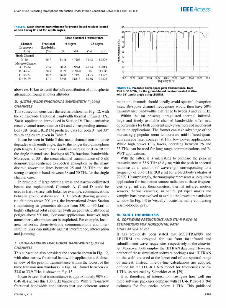
TABLE 6. Mean channel transmittance for ground-based receiver locatedat Giza having 0◦ and 33◦ zenith angles.

above ca. 10 km to avoid the bulk contribution of atmosphericattenuation found at lower altitudes.

D. (ULTRA-)WIDE FRACTIONAL BANDWIDTH (&20%)CHANNELSThis subsection considers the scenario shown in Fig. 12, withthe (ultra-)wide fractional bandwidth thermal infrared ‘THzTorch’ application, introduced in Section IV. The quantitativemean channel transmittance (%) and corresponding attenua-tion (dB) from LBLRTM predicted data for both 0◦ and 33◦

zenith angles are given in Table 5.It can be seen in Table 5 that mean channel transmittance

degrades with zenith angle, due to the longer thru-atmospherepath length. However, this is only an increase of 0.24 dB forthe single channel case, having a 66.7% fractional bandwidth.Moreover, at 33◦, the mean channel transmittance of 5 dBdemonstrates resilience to spectral absorption by the manydiscrete absorption lines between 25 and 38 THz and thestrong absorption band between 38 and 50 THz for the singlechannel case.

In principle, if large emitting areas and narrow collimatedbeams are implemented, Channels A, C and D could beused in Earth-space path links; for example, communicationsbetween ground stations and 1U CubeSats (having geomet-ric altitudes above 200 km), the International Space Station(maintaining an geometric altitude from 330 to 435 km) orhighly elliptical orbit satellites (with an geometric altitude atperigee above 500 km). For some applications, however, highatmospheric absorption can be exploited. For example, local-area networks, drone-to-drone communications and inter-satellite links can mitigate against interference, interceptionand jamming.

E. ULTRA-NARROW FRACTIONAL BANDWIDTH (.0.1%)CHANNELSThis subsection also considers the scenario shown in Fig. 12,with ultra-narrow fractional bandwidth applications. A close-in view of the peak in transmittance within the lowest of thethree transmission windows (in Fig. 14), found between ca.33.8 to 33.9 THz, is shown in Fig. 15.

It can be seen that transmittance is approximately 90% (or0.46 dB) across this 100 GHz bandwidth. With ultra-narrowfractional bandwidth applications that use coherent source

FIGURE 15. Predicted Earth-space path transmittance, from33.8 to 33.9 THz, for the ground-based receiver located at Gizawith 33◦ zenith angle using LBLRTM.

radiation, channels should ideally avoid spectral absorptionlines. Be-spoke channel frequencies would then have 50%transmittance bandwidths that range between 3 and 22 GHz.

Within the (at present) unregulated thermal infrared,large and freely available channel bandwidths offer newopportunities for both coherent and (evenmore so) incoherentradiation applications. The former can take advantage of theincreasingly popular room temperature mid-infrared quan-tum cascade laser sources [93] for low power applications.While high power CO2 lasers, operating between 26 and33 THz, can be used for long range communications and R-WPT applications.

With the latter, it is interesting to compare the peak intransmittance at 33.9 THz (8.8 µm) with the peak in spectralradiance as a function of wavelength corresponding to afrequency of 30.6 THz (9.8 µm) for a blackbody radiator at296 K. Unsurprisingly, thermography represents a ubiquitousapplication for incoherent source radiation at these frequen-cies (e.g., infrared thermometers, thermal infrared motionsensors, thermal cameras); in nature, pit viper snakes andvampire bats have evolved to exploit the lowest transmissionwindow (in Fig. 14) to ‘visually’ locate thermally-contrastingwarm-blooded pray.

VI. SUB-1 THz ANALYSISA. SOFTWARE PREDICTIONS AND ITU-R P.676-10ESTIMATIONS FOR HORIZONTAL PATHLINKS AT SEA LEVELIt has previously been stated that MODTRAN R© andLBLTRM are designed for use from far-infrared andsubmillimeter-wave frequencies, respectively, to the ultravio-let. Moreover, both employ the HITRAN database. However,neither of these simulation software packages nor ‘HITRANon the web’ are used at the lower end of our spectral rangeof interest. Instead, line-by-line calculations are adopted,defined by the ITU-R P.676 model for frequencies below1 THz, as reported by Schneider et al. [29].

It is, therefore, of interest to investigate how well ourthree software packages compare with ITU-R P.676-10 [94]estimates for frequencies below 1 THz. This published

VOLUME 4, 2016 9389


FIGURE 16. Predicted specific attenuation for horizontal path links at sealevel using simulation software packages and calculated estimates fromITU-R P.676-10 at 288.15 K.

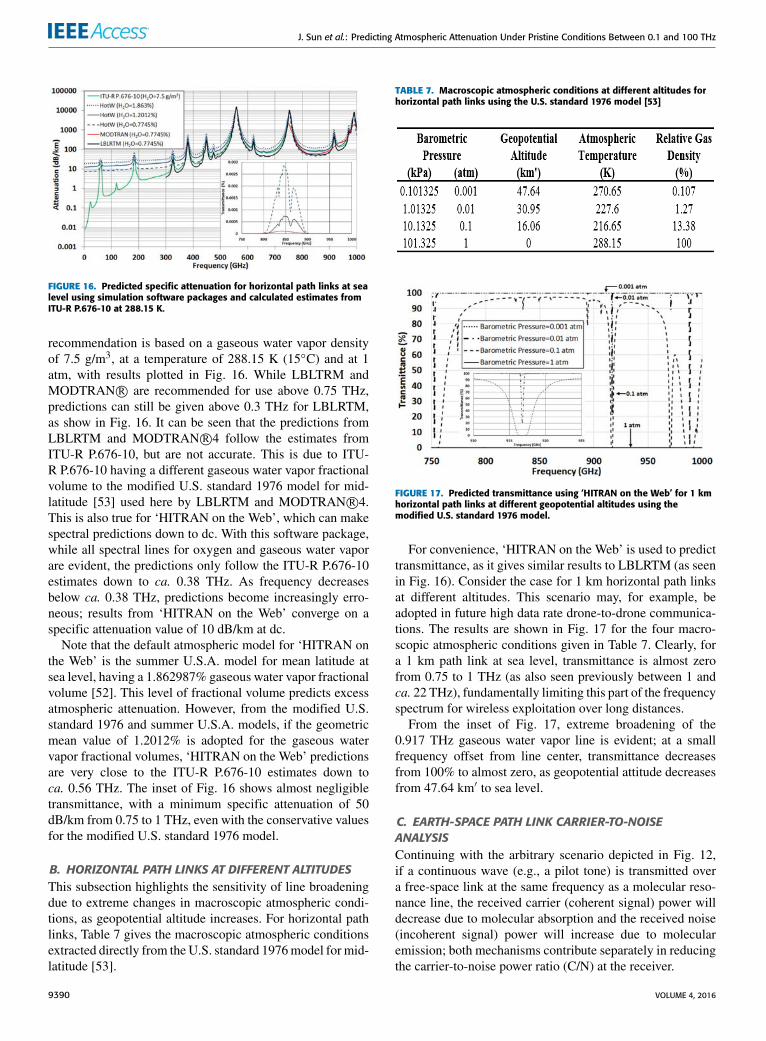
recommendation is based on a gaseous water vapor densityof 7.5 g/m3, at a temperature of 288.15 K (15◦C) and at 1atm, with results plotted in Fig. 16. While LBLTRM andMODTRAN R© are recommended for use above 0.75 THz,predictions can still be given above 0.3 THz for LBLRTM,as show in Fig. 16. It can be seen that the predictions fromLBLRTM and MODTRAN R©4 follow the estimates fromITU-R P.676-10, but are not accurate. This is due to ITU-R P.676-10 having a different gaseous water vapor fractionalvolume to the modified U.S. standard 1976 model for mid-latitude [53] used here by LBLRTM and MODTRAN R©4.This is also true for ‘HITRAN on the Web’, which can makespectral predictions down to dc. With this software package,while all spectral lines for oxygen and gaseous water vaporare evident, the predictions only follow the ITU-R P.676-10estimates down to ca. 0.38 THz. As frequency decreasesbelow ca. 0.38 THz, predictions become increasingly erro-neous; results from ‘HITRAN on the Web’ converge on aspecific attenuation value of 10 dB/km at dc.

Note that the default atmospheric model for ‘HITRAN onthe Web’ is the summer U.S.A. model for mean latitude atsea level, having a 1.862987% gaseous water vapor fractionalvolume [52]. This level of fractional volume predicts excessatmospheric attenuation. However, from the modified U.S.standard 1976 and summer U.S.A. models, if the geometricmean value of 1.2012% is adopted for the gaseous watervapor fractional volumes, ‘HITRAN on the Web’ predictionsare very close to the ITU-R P.676-10 estimates down toca. 0.56 THz. The inset of Fig. 16 shows almost negligibletransmittance, with a minimum specific attenuation of 50dB/km from 0.75 to 1 THz, even with the conservative valuesfor the modified U.S. standard 1976 model.

B. HORIZONTAL PATH LINKS AT DIFFERENT ALTITUDESThis subsection highlights the sensitivity of line broadeningdue to extreme changes in macroscopic atmospheric condi-tions, as geopotential altitude increases. For horizontal pathlinks, Table 7 gives the macroscopic atmospheric conditionsextracted directly from the U.S. standard 1976model for mid-latitude [53].

TABLE 7. Macroscopic atmospheric conditions at different altitudes forhorizontal path links using the U.S. standard 1976 model [53]

FIGURE 17. Predicted transmittance using ‘HITRAN on the Web’ for 1 kmhorizontal path links at different geopotential altitudes using themodified U.S. standard 1976 model.

For convenience, ‘HITRAN on the Web’ is used to predicttransmittance, as it gives similar results to LBLRTM (as seenin Fig. 16). Consider the case for 1 km horizontal path linksat different altitudes. This scenario may, for example, beadopted in future high data rate drone-to-drone communica-tions. The results are shown in Fig. 17 for the four macro-scopic atmospheric conditions given in Table 7. Clearly, fora 1 km path link at sea level, transmittance is almost zerofrom 0.75 to 1 THz (as also seen previously between 1 andca. 22 THz), fundamentally limiting this part of the frequencyspectrum for wireless exploitation over long distances.

From the inset of Fig. 17, extreme broadening of the0.917 THz gaseous water vapor line is evident; at a smallfrequency offset from line center, transmittance decreasesfrom 100% to almost zero, as geopotential attitude decreasesfrom 47.64 km′ to sea level.

C. EARTH-SPACE PATH LINK CARRIER-TO-NOISEANALYSISContinuing with the arbitrary scenario depicted in Fig. 12,if a continuous wave (e.g., a pilot tone) is transmitted overa free-space link at the same frequency as a molecular reso-nance line, the received carrier (coherent signal) power willdecrease due to molecular absorption and the received noise(incoherent signal) power will increase due to molecularemission; both mechanisms contribute separately in reducingthe carrier-to-noise power ratio (C/N) at the receiver.

9390 VOLUME 4, 2016


To investigate this further, a number of simplifyingassumptions will be made: (i) unless otherwise stated, thereceiver is ‘noiseless’ and represents a complete idealizedground station (i.e., the receiver, antenna and associated inter-connect feed line are all ideal); (ii) the antenna has a highlydirectional pencil-beam radiation pattern; (iii) Earth’s atmo-sphere is represented by a single homogenous layer in ther-modynamic equilibrium; (iv) a ‘plane atmosphere’ approx-imation is adopted (which is usually acceptable for zenithangles below 65◦) [95], whereby the Earth is assumed flatwith a horizontally stratified time-invariant atmosphere [96];(v) molecular scattering is neglected with pristine conditions;(vi) Rayleigh-Jeans law can be used to approximate Planck’slaws for calculating spectral radiance; and (vii) the totalopacity of the atmosphere is assumed to be frequency inde-pendent. A justification of these assumptions can be found inAppendix C.

With reference to Fig. 12(b), the sky brightness tempera-ture TINθ (f ) for all sourcecontributions (representing the effective input noisetemperature to a receiver), due to molecular absorp-tion/emission at zenith angle θ , is dependent on frequencyf and given by:

TINθ (f ) ≈ TCMB · e−τθ (f ) + TMAT ·(1− e−τθ (f )

)(1)

Since reflectance is neglected, transmittance is e−τθ (f ) andabsorptance is

(1− e−τθ (f )

), which is equal to the emissivity

of the atmosphere in thermodynamic equilibrium. At zenithangle θ , total opacity (sometimes referred to as ‘total opticalpath’ or ‘total optical thickness’) τθ (f ) = τ0(f ) sec θ , whereτ0(f ) is the total zenith opacity or ‘total optical depth’ andsec θ is referred to as the number of air masses. TCMB =2.725 K is the cosmic microwave background (CMB) noisetemperature and an estimate of the physical mean atmo-spheric temperature (known as the ‘sky emission tempera-ture’ [95]) is given by TMAT = 0.95TAS .At this point it is worth mentioning that with high zenith

angles, opacity τθ (f )→ kα(f )L. However, with such low ele-vation path links, the effects of kα(f ) are effectively maskedby the much greater path lengths through the Earth’s atmo-sphere (with L being of the order of 8 times the 50 km′

geopotential altitude). As a result, e−τθ (f )→ 0 and, therefore,TINθ (f ) ∼ TMAT (f ). In other words, path length, transmit-tance and CMB do not need to be considered when calculat-ing the sky brightness temperature for (near-)horizontal pathlinks.

Often, τθ (f ) is simply assumed to be frequency indepen-dent, which is reasonable over sufficiently narrow fractionalbandwidths. Therefore, when considering the noise contribu-tion from the Earth’s atmosphere, the effective input thermalnoise power to the noiseless receiver can be simply calculatedfrom the commonly used textbook expression:

PIN ≈ kTINθB (2)

where k is Boltzmann’s constant and B is channel bandwidth.It should be noted that (2) is only valid for frequencies up

to ca. 1 THz at an ambient temperature of 296 K for a 2%error. This frequency limit, the derivation of (2) and a moreaccurate approach for determining the input thermal noisepower are discussed in Appendix C.

The carrier and noise power levels at the input to a noisyreceiver Cθ and Nθ , respectively, can be expressed as:

Cθ = e−τθCθV (3)

Nθ ≈ k (TINθ + TRX )B (4)

where CθV is the received carrier power within a vac-uum atmosphere (i.e., without considering any molecularabsorption), TRX is the intrinsic noise temperature for anoisy receiver due to intrinsic noise contributions (e.g., fromreceiver, antenna and associated interconnect feed line). Sincee−τθ → 1, the received noise power within a vacuum atmo-sphere NθV (i.e., without considering any molecular emis-sion) is given by:

NθV ≈ k (TCMB+ TRX )B ∼ kTRXB with TCMB � TRX (5)

Therefore, the respective carrier-to-noise power ratios at theinput to a receiver within a vacuum atmosphereCθV /NθV andconsidering both molecular absorption and emission withinthe Earth’s atmosphere Cθ/Nθ are:

CθVNθV≈

CθVk (TCMB + TRX )B

(6)

and

CθNθ≈

e−τθCθVk[TCMB · e−τθ + TMAT ·

(1− e−τθ

)+ TRX

]B

(7)

Note that the spreading loss factor only affects carrier powerand not the noise power. Moreover, the reduction in thereceiver’s input carrier power with increasing path length(having an inverse square law) is the same in vacuum asit is with a terrestrial atmosphere. Therefore, the effects ofspreading loss can be ignored in this analysis. The calculatedreduction in C/N at the receiver when both molecular absorp-tion and emission are included is given by:

CθV /NθVCθ/N θ

(dB)

≈ 10log10

{(TCMB − TMAT )+ (TMAT + TRX ) · e+τθ

(TCMB + TRX )

}(8)

This is represented by Fig. 18 for different intrinsic receivernoise temperatures and atmospheric transmittance varyingfrom 0.1 to 100% (a transmittance of zero will result in aninfinite reduction in C/N for all values of TRX , which cannotbe displayed).

Transmittance can change significantly due to mod-eling errors and/or line broadening, discussed in sub-Sections A and B, respectively. With the latter, considertwo channels having ultra-narrow fractional bandwidths; thefirst channel is located midway between two deep spectralabsorption/emission lines (exhibiting high transmittance) and

VOLUME 4, 2016 9391


FIGURE 18. Calculated reduction in input C/N at a noisy receiver withboth molecular absorption and emission considered.

the second channel is close to a spectral line (still exhibit-ing high transmittance). Because significant line broadeningcan result from changes in macroscopic atmospheric condi-tions, the second channel only may experience a dramaticreduction in transmittance. Therefore, this analysis can beuseful for calculating the fade margins in the carrier-to-noiseratio with coherent source radiation applications below ca.1 THz. For example, if the second channel experiences adrop in transmittance from 90% to 50%, with a low noisereceiver having TRX = 50 K, the fade margin (i.e., differencein the calculated reduction in C/N at the receiver) will be(8.6 – 2.3) dB= 6.3 dB; this represents a very significant pro-portion of the overall allocated fade margin (typically 10 dB)within a power link budget for communications applications.

It may be the case that C/N is calculated (erroneously)without considering the increase in received noise power dueto molecular emission. The resulting error in Cθ/Nθ (dB) canbe expressed by:

NθNθV

(dB)

≈ 10log10

{TCMB · e−τθ + TMAT ·

(1− e−τθ

)+ TRX

TCMB + TRX

}(9)

The calculated error in Cθ/Nθ (dB) is shown in Fig. 19.For the limiting case of having no absorption line givesτθ → 0 and e−τθ → 1 and Nθ/NθV → 0 dB. How-

FIGURE 19. Calculated error in input C/N (dB) at a noisy receiver withonly molecular absorption considered.

ever, as expected, errors are at a maximum for the oppositelimiting case when both transmittance and intrinsic receivernoise temperatures values are zero. For a low noise receiver,having TRX = 50 K, the limiting case of a strong absorp-tion line gives τθ → ∞, e−τθ → 0, Cθ → 0, Nθ →k (TMAT + TRX )B, Cθ/Nθ (dB) → −∞ and Nθ/NθV →(TMAT + TRX ) / (TCMB + TRX ) → 8 dB (or TMAT /TCMB →20 dB with TRX → 0).

VII. CONCLUSIONThis article tries to bridge the knowledge gap between appliedengineering and atmospheric sciences, focusing specificallyon atmospheric attenuation between 0.1 and 100 THz underpristine conditions (found indoors and some global locationoutdoors); representing a useful comparative baseline. Anexhaustive review ofmodeling atmospheric attenuation for alloutdoor weather conditions is beyond the scope of this paper,as this would require a very detailed be-spoke (time-variantor statistical) atmospheric model across every geographicalpath link under investigation. Nevertheless, our idealizedtreatment reveals many important facets associated with thismultidisciplinary subject.

In practice, developing generic in-house simulation soft-ware to produce accurate predictions is challenging becauseof the ever-expanding spectroscopic line parameter databaseand improvements in radiative transfer codes. Instead, threewell-known simulation software packages were employed.

The techniques used for modeling atmospheric attenuationunder pristine conditions have been applied to investigate theresilience of (ultra-)wide fractional bandwidth applications tothe effects of molecular absorption. Two extreme modelingscenarios were investigated: horizontal path links at sea leveland Earth-space path links. It is shown by example that‘HITRAN on the Web’ can give good predictions with theformer (without having extensive knowledge of atmosphericscience); whereas LBLRTM is recommended for the latter(requiring specialist knowledge of atmospheric science).

A 1 to 10 THz atmospheric ‘band-stop’ transmission char-acteristic is evident, even under pristine conditions, when pathlength extends beyond approximately 20 to 50 m at sea level.In contrast, the three transmission windows within the ‘overthe THz horizon’ thermal infrared represents new opportuni-ties for exploiting this unregulated part of the electromagneticspectrum. The recently introduced ‘THz Torch’ technologyrepresents a good candidate for investigating its resilience tomolecular absorption. It is predicted that 1 km horizontal pathlinks at sea level exhibit 90% transmittance (with Channel D).

Furthermore, in principle, if large emitting areas and nar-row collimated beams are implemented, Earth-space pathlinks can be supported, as theoretically investigated witha ground-based receiver located at Giza. However, manylocations around the world can also be considered; globalatmospheric reanalysis data has been compiled and used withLBLRTM to predict THz transmittance statistics. To this end,NASA’s Modern Era Retrospective-analysis for Researchand Applications (MERRA) dataset represents a 30 year

9392 VOLUME 4, 2016


(1979-2007) global reanalysis, using the Goddard EarthObserving System Data Assimilation System [97].

Also, from first principles, it was shown that the Rayleigh-Jeans law approximation, widely used to calculate thermalnoise power, is only valid up to ca. 1 THz. Moreover,‘HITRAN on the Web’ predictions can be very close toestimates from the commonly used ITU-R P.676-10 model,down to ca. 0.56 THz. Finally, carrier-to-noise ratio fademargins have been investigated, which can take into accountthe effects of line broadening due to changes in molecularmacroscopic atmospheric conditions for sub-1 THz ultra-narrow fractional bandwidth applications.

APPENDIX AIn this appendix, two different approaches for calculatingmean channel transmittance are compared, both taking theassumption that the channel filters have a spectrally flat in-band transmittance. The first, more intuitive, definition sim-ply uses the statistical mean:

TChannel =1M

∑M

i=1Ti (10)

whereM is the total number of spectral data sampling pointsand Ti is channel transmittance for the ith frequency withineither the 70% or 50% transmittance channel bandwidth.This definition of mean channel transmittance is only validif the incident power spectral density is also considered flatacross the channel bandwidth.

The exact expression (adopted in this paper) for calculatingmean channel transmittance takes the ratio of incident radi-ance at the input of a receiver to radiated radiance from ablackbody emitter and is given by:

TChannel =

∫ f2f1[IBB (f ,TBB)T (f )] · df∫ f2f1IBB (f ,TBB) · df

(11)

where f1 and f2 are the lower and upper channel cut-offfrequencies, respectively; IBB (f ,TBB) is the exact spectralradiance radiated from a blackbody, which is dependent onboth frequency and blackbody temperature TBB (878 K in ourcalculations, representing the nominal operating temperaturefor commercial thermal infrared emitters used as sources in‘THz Torch’ applications); and T (f ) is the frequency depen-dent channel transmittance.

The mean channel transmittances for each channel iden-tified within the paper, against horizontal path length atsea level, for the two approaches (using T (f ) data fromLBLRTM with an atmospheric temperature and pressure of296 K and 101.325 kPa, respectively) are shown in Fig. 20.For simplicity, it is assumed that the atmosphere is homoge-nous at sea level.

It can be seen from Fig. 20 that the discrepancies in theresults for both Channels B and D are insignificant. Thisis because channel transmittance is spectrally flat over theirrespective channel bandwidths; T (f ) can be moved out ofthe integral and, therefore, (11) equates to (10). With Chan-nels A, C and the single channel case, transmittance is not

FIGURE 20. Calculated mean channel transmittance against horizontalpath length at sea level for different ‘THz Torch’ channels, usingpredictions from LBLRTM at 296 K and 101.325 kPa, (black: statisticalmean; blue: exact) for TBB = 878 K.

FIGURE 21. Statistical mean band transmittance against frequency andfractional bandwidth using predictions from LBLRTM for a 1 km pathlength.

FIGURE 22. Exact mean band transmittance against frequency andfractional bandwidth using predictions from LBLRTM for a 1 km pathlength.

spectrally flat across their respective bandwidths. As a result,discrepancies can be seen between the statistical mean andexact expressions.

Between 0.75 and 100 THz, for a 1 km path length, therelationship between mean band transmittance, frequencyand fractional bandwidth have been calculated using bothdefinitions and the results are shown in Figs. 21 and 22,respectively. The difference in calculated mean band trans-mittance is shown in Fig. 23. It can be seen that this differenceis less than 9% for Channel A (worst-case scenario) andmuch

VOLUME 4, 2016 9393


FIGURE 23. Difference between statistical and exact mean bandtransmittances against frequency and fractional bandwidth usingpredictions from LBLRTM for a 1 km path length.

lower for the other channels. Therefore, the simpler statisticalmean approach can be used for some channels [54].

APPENDIX BThe linear gradient of atmospheric temperature with geopo-tential altitude H is referred to as the ‘lapse rate’.Two equations are used for calculating barometric pressurePwithin the troposphere, stratosphere and mesosphere layers(up to a geopotential altitude of 84.852 km’ or geometricaltitude ∼86 km) [53]:

P = Pb ·

[Tb

Tb + Lb · (H − Hb)

] g′0M0RLb

for Lb 6= 0

e−

g′0M0 · (H − Hb)

RTb

for Lb = 0

(12)

where subscript b ranges from 0 to 6 (or 4 in our case; con-sidering only the troposphere and stratosphere) in accordancewith the general case of having 7 atmospheric boundaries; Pband Tb are the barometric pressure and atmospheric temper-ature, respectively, corresponding to geopotential altitude Hbfor the bth boundary; Lb is the lapse rate of the layer above thebth boundary, with our values of -6.5, 0.0, 1.0 and 2.8 K/km′,corresponding to our layers one to four having geopotentialaltitudes of 11, 20, 32 and 47 km′, respectively; g′0 = 9.80665is the dimensional constant relating the standard geopotentialmeter to geometric height [53] and is numerically equal tothe acceleration of gravity g0(m/s2) at sea level; M0 =

28.9644 kg/kmol is the mean molecular weight of air at sealevel; R = 8.31432×103 N ·m/(kmol ·K) is the gas constant.The respective reference-level values for T0 and P0 are 296 Kand 101.325 kPa, respectively. Here, Tb with b ∈ [1..4] iscalculated from Tb = Tb−1 + Lb−1 · (Hb − Hb−1) and Pb isobtained from (12).

APPENDIX CIn this Appendix the input thermal noise power to a noiselessreceiver is derived and the condition is shown for whencommonly used textbook approximations become invalid atterahertz frequencies. It is assumed throughout that ‘noise-less receiver’ refers to a complete idealized ground station

(i.e., the receiver, antenna and associated interconnect feedline are all ideal) for Earth-space path links (as depicted inFig. 12).Downward spectral radiance, incident at any point on the

ground, consists of contributions from: (i) CMB radiance;(ii) radiance scattered into the direction of view; and(iii) emission from the overlying bulk atmosphere. Thesecontributions are transmitted directly into the main lobe(s)and any side lobes of the receiving antenna. Under pristineconditions, the contribution of molecular scattering can beneglected. Therefore, only atmospheric absorption and emis-sion are considered further.

A. MULTI-LAYER ATMOSPHERE ANALYSISFrom the Beer-Lambert law, the spectral radiance absorbedby an atmospheric layer of thickness dz, dIa(f ) is:

dIa (f ) = −It (f ) µ (f ) ρ sec θdz (13)

where It (f ) is the combined spectral radiance incident at thetop of the atmospheric layer and is a function of frequency,µ(f ) is the mass absorption coefficient (since no scattering isassumed), ρ is the mass density of the atmospheric layer andθ is the zenith angle (from vertical to the antenna’s main lobe,as shown in Fig. 12).

The amount of spectral radiance emitted by the atmo-spheric layer in the same direction, dIE (f ) is:

dIE (f ) = Iatm (f ) µ (f ) ρ sec θdz (14)

where Iatm (f ) is the atmospheric source term. If the atmo-spheric layer is in thermodynamic equilibrium, Iatm (f ) isdefined by Planck’s law as IBB (f ,T (z)); the blackbody spec-tral radiance of the atmospheric layer is a function of fre-quency and its physical temperature T (z), with T (z) itselfbeing a function of altitude z (from the top of our definedatmosphere, as shown in Fig. 12).

In the absence of any scattering, the rate of net change inspectral radiance as a function of altitude is thus:

dI (f ) = − [It (f )− IBB (f ,T (z))] dτθ (f ) (15)

where dτθ (f ) = dτo (f ) sec θ and dτo (f ) = µ (f ) ρ dz arethe optical path at θ and optical depth at zenith, respectively,over geometrical thickness dz. At θ , the total opacity of theatmosphere is τθ (f ) = τo (f ) sec θ , where τ0(f ) is thetotal zenith opacity or ‘total optical depth’, sec θ is referredto as the number of air masses [98], for θ - 65◦ [95].From (15), using e−τθ (f ) as an integrating factor over height,Schwarzchild’s equation is obtained for the total spectralradiance I (f ,T ,Z ); describing radiative transfer in a non-scattering medium (suitable over the extended THz spec-trum) as:

I (f ,T ,Z ) = ITOA (f ,TCMB) · e−τθ (f )

+

∫ τθ (f )

0IBB (f ,T (z))

·

(e[τ′θ (f ,z)−τθ (f )]

)dτ ′θ (f , z) (16)

9394 VOLUME 4, 2016


where Z is the surface altitude of the receiver (at sea level inour case) and e−τθ (f ) is the atmospheric transmittance at θ ,(alternatively, e+τ θ (f ) is sometimes used and referred to asthe atmospheric loss factor [96], [98], as shown in Fig. 12).Total opacity τθ (f ) [Np] is sometimes referred to as thetotal optical path or thickness; τ ′θ (f , z) is the opacity fromthe TOA down to altitude z. Physically, (16) shows that thedownwelling spectral radiance at the receiver is comprisedof the CMB radiation transmitted from the TOA plus theemission from each atmospheric layer that makes it to thesurface. The CMB spectral radiance incident at the top ofatmosphere ITOA(f ,TCMB) is a function of frequency andCMB noise temperature TCMB.The input thermal noise power to a noiseless receiver

can be most accurately expressed in terms of total spectralradiance:

PIN = Ar

∫∫I (f ,T ) df d� (17)

where Ar is the effective radiating area for a generic radiatorand assumed here to be equivalent in value for all contribu-tions in (17).

B. SINGLE LAYER ATMOSPHERE APPROXIMATIONIn order to perform basic calculations, it is often assumed thatthe atmosphere is represented by a single homogenous layerin thermodynamic equilibrium [95], [98]. Therefore, in (16),T (z) is approximated by a single physical mean atmospherictemperature TMAT = 0.95 TAS (known as the ‘sky emissiontemperature’ [95]); dependent on frequency and macroscopicatmospheric conditions and can be represented with betteraccuracy by more sophisticated atmospheric models [99].With this single layer assumption, the approximate total spec-tral radiance at the input of a noiseless receiver is:

I (f ,T ) ∼= Itop (f ,TCMB) · e−τθ (f )

+ IBB(f ,TMAT ) ·(1− e−τθ (f )

)(18)

The first term on the right-hand side of (18) is the extrater-restrial contribution to the noiseless receiver, due to CMBradiation having a mean blackbody noise temperature ofTCMB = 2.725 K [98], [100], [101] (or more precisely2.7255 ± 0.0009 K when measured over the spectral rangefrom 60 to 625 GHz [102]). The second term is the terrestrialcontribution, where (1 − e−τθ (f )) is the frequency dependentemissivity of the bulk atmospheric layer. Since reflectance isneglected, absorptance is equal to the emissivity of the bulkatmospheric layer in thermodynamic equilibrium.

The approximated thermal noise power input to a noiselessreceiver can now be expressed using (17), giving:

PIN ∼= Ar1

∫∫Itop (f ,TCMB) · e−τθ (f )dfd�

+Ar2

∫∫IBB (f ,TMAT ) ·

(1− e−τθ (f )

)dfd�

(19)

where Ar1 and Ar2 are effective radiating areas associatedwith CMB radiation and bulk atmosphere, respectively. How-ever, in practice, it can be difficult to calculate the input ther-mal noise power using (19), since Ar1 and Ar2 are unknown.The exact spectral radiance from a blackbody IBB (f ,T )

describes the amount of energy it emits as a function of bothfrequency and physical temperature T , given by Planck’s law:

IBB (f ,T ) =2hf 3

c21

ehf /kT − 1(20)

where h is Planck’s constant, c is the speed of light in vac-uum and k is Boltzmann’s constant. In the limits of hightemperatures and/or low frequencies, the exponent in theexponential term becomes small and so the Taylor’s first-order polynomial approximation can be used:

ehf /kT ≈ 1+hfkT

(21)

Substituting (21) into (20) gives the Rayleigh-Jeans law:

IBB (f ,T ) ≈2f 2kTc2

(22)

Using (22), the spectral radiance of any emitter I (f ,T ) =ε(f ,T ) · IBB (f ,T ) can be expressed as:

I (f ,T ) ≈2f 2kTb (f )

c2= ε(f ,T ) ·

2f 2kTc2

(23)

where the brightness temperature of the emitter Tb (f ) =ε(f ,T ) ·T is directly related to the physical temperature T ofa blackbody in thermodynamic equilibrium by its emissivityε(f ,T ). Therefore, Rayleigh-Jeans law allows (18) to begreatly simplified, such that the total spectral radiance at theinput of a noiseless receiver is given by:

2f 2kT INθ (f )c2

≈2f 2kTCMB

c2· e−τθ (f ) +

2f 2kTMATc2

·

(1− e−τθ (f )

)(24)

where TINθ (f ) is the sky brightness temperature for all sourcecontributions [101], [103] (representing the effective inputnoise temperature for a noiseless receiver) due to molecularabsorption/emission. Note that, in this case, ‘effective’ tem-perature corresponds to the temperature for a single black-body that emits the same total amount of radiation from allsource contributions. It is then a trivial matter to replace (24)by the commonly used expression [95], [99], [101], [104]:

TINθ (f ) ≈ TCMB · e−τθ (f ) + TMAT ·(1− e−τθ (f )

)(25)

In some textbooks, TINθ (f ) is also referred to as the ‘skynoise temperature’ [86], [98], [100], (which should not beconfused with ‘sky emission temperature’). The more genericterm of ‘antenna noise temperature’ [86], [100], [103], rep-resents the convolution of the antenna’s radiation pattern(with contributions from main and side lobes) and brightnesstemperature from all incoming sources (e.g., sky, objects andground) [103]. With highly directional pencil-beam antennas

VOLUME 4, 2016 9395


(e.g., high efficiency horn and parabolic reflectors) tradi-tionally used in high-end applications (e.g., telecommunica-tions, radar and radio astronomy), antenna noise temperatureequates to the sky brightness temperature encompassed by themain lobe [102].

Both [86] and [103] generally ignore the first term in (25),and other extraterrestrial sources, as the contribution fromCMB radiation is considered insignificant for many applica-tions (such as low elevation path links).

The frequency dependency in (25) can be removed byaveraging over the channel bandwidth B = (f2 − f1), to givethe effective input noise temperature for a noiseless receiver:

TINθ =1B

∫ f2

f1TINθ (f ) df = TCMB + TATM (26)

where f1 and f2 are the lower and upper channel cut-

off frequencies, respectively, TCMB =TCMBB

∫ f2f1e−τ θ (f )df

is the channel’s effective CMB noise temperature andTATM =

TMATB

∫ f2f1(1− e−τ θ (f ))df is the channel’s effective

atmospheric noise temperature.Often, τθ (f ) is simply assumed to be frequency indepen-

dent, which is reasonable over sufficiently narrow fractionalbandwidths. In this case, (25) is simplified to give the fol-lowing textbook representation (using a frequency invariantvalue for total opacity) [96], [99], [100]:

TINθ ≈ TCMB · e−τθ + TMAT ·(1− e−τθ

)(27)

As an example, withmicrowave Earth-space path links, atmo-spheric transmittance is typically ∼90% and, therefore, thesky brightness temperature TINθ is ∼31 K [86]; with CMBradiation contributing only 8%.

The effective thermal noise power input to a noiselessreceiver can now be easily calculated from the commonlyused textbook expression [86], [105], [106]:

PIN ≈ kTINθB (28)

In practice, treating total opacity as being frequency inde-pendent can be a poor assumption and so (27) should beavoided with (ultra-)wide fractional bandwidth applications.Moreover, (21) to (28) are derived for the condition(s) thatthe temperature of a radiator is high and/or frequency is low(Rayleigh-Jeans law). It will be seen that significant errorswill be introduced above ca. 1 THz for a range of meanatmospheric temperatures. This is illustrated by example,where the error between the left- and right-hand sides of (21)are calculated; the results are shown in Figs. 24 and 25.It can be seen that, for a 2% error, the maximum acceptablefrequency is 1.3 THz at TMAT = 296 K. Therefore, above ca.1 THz, the approximate method for calculating the effectivethermal noise power input to a noiseless receiver, using (28),should be replaced by (19) with a single layer atmosphereapproximation.

A recent study by Jornet and Akyildiz [34] used radiativetransfer theory for calculating a receiver’s equivalent input

FIGURE 24. Percentage error for the Rayleigh-Jeans law approximation.

FIGURE 25. Upper frequency limits for the Rayleigh-Jeans lawapproximation for different levels of acceptable percentage error.

noise temperature (which includes the atmospheric contribu-tion from molecular emission), with horizontal path lengthsof up to 10 m at sea level and TMAT = 296 K. They thenused the integral form of (28) to calculate the correspondingnoise power, reported simulation results up to 10 THz. UsingFig. 24, it is evident that this would result in a worst-case errorof 48%.

In general, however, the commonly made assumption thatthe atmosphere can be represented by a single homogenouslayer in thermodynamic equilibrium is over-simplified.Whileoverall transmittance e−τθ is the net contribution from manysimulated layers, the associated temperature for each layer isfixed to just a single value of TMAT within the single layerapproximation. In contrast, by observing a realistic variationof atmospheric temperature, atmospheric temperature canvary significantly (from 203 to 296 K, seen in Fig. 13).For this reason, only (17) can truly determine the accurateeffective thermal noise power input to a noiseless receiver.

ACKNOWLEDGMENTSThe authors wish to thank Dr. Helen E. Brindley (Space andAtmospheric Physics Group, Department of Physics, Impe-rial College London) for generating the MODTRAN R©4 andLBLRTM data and useful discussions.

REFERENCES[1] D. J. Hayton et al., ‘‘A 4.7 THz heterodyne receiver for a balloon borne

telescope,’’ Proc. SPIE, vol. 9153, pp. 91531R-1–91531R-7, Jul. 2014.[2] Optics and Photonics—Spectral Bands, Standard ISO 20473:2007,

International Organization for Standardization, 2015.[3] J. Harries et al., ‘‘The far-infrared earth,’’ Rev. Geophys., vol. 46, no. 4,

pp. 1–34, Dec. 2008.

9396 VOLUME 4, 2016


[4] A. Mehta, Introduction to the Electromagnetic Spectrum and Spec-troscopy (Analytical Chemistry), Pharmaxchange, Aug. 2011.[Online].Available: http://pharmaxchange.info/press/2011/08/introduction-to-the-electromagnetic-spectrum-and-spectroscopy/

[5] G. W. Petty, A First Course in Atmospheric Radiation. Madison, WI,USA: Sundog Publishing, Mar. 2006.

[6] R. Appleby and H. B. Wallace, ‘‘Standoff detection of weapons andcontraband in the 100 GHz to 1 THz region,’’ IEEE Trans. AntennasPropag., vol. 55, no. 11, pp. 2944–2956, Nov. 2007.

[7] H. B. Wallace, ‘‘Millimeter waves: Myths and reality,’’ presented at theSPIE Defense Secur. Symp., Orlando, FL, USA, Apr. 2006.

[8] E. S. Rosenblum, ‘‘Atmospheric absorption of 10-400KMCPS radiations:Summary and bibliography to 1961,’’ Microw. J., vol. 4, pp.‘91–96,Mar. 1961.

[9] G. D. Lukes, ‘‘Penetrability of haze, fog, clouds and precipitationby radiant energy over the spectral range 0.1 micron to 10 centime-ters,’’ Center Naval Anal., Univ. Rochester, Arlington, TX, USA, Tech.Rep. AD847658, 1968.

[10] E. Mondre, ‘‘Atmospheric effects on millimeter wave communicationchannels,’’ NASA, Washington, DC, USA, Tech. Rep. N70-34446,Mar. 1970.

[11] C. H. Zufferey, ‘‘A study of rain effects on electromagnetic waves in the1-600 GHz ranges,’’ M.S. thesis, Dept. Elect. Eng., Univ. Colorado,Boulder, CO, USA, 1972.

[12] M. J. Rosker and H. B. Wallace, ‘‘Imaging through the atmosphere at ter-ahertz frequencies,’’ in IEEE/MTT-S Int. Microw. Symp. Dig., Jun. 2007,pp. 773–776.

[13] H. Liebe, ‘‘MPM89—An atmospheric mm-wave propagation model,’’Int. J. Infr. Millim. Waves, vol. 10, no. 6, pp. 631–650, Jun. 1989.

[14] H. J. P. Smith, D. J. Dube,M. E. Gardner, S. A. Clough, F. X. Kneizys, andL. S. Rothman, ‘‘FASCODE—Fast atmospheric signature code (spectraltransmittance and radiance),’’ Air Force Geophys. Lab., Hanscom AFB,MA, USA, Tech. Rep. AFGL-TR-78-0081, Jan. 1978.

[15] LBLRTM. accessed on Nov. 2016. [Online]. Available:http://rtweb.aer.com/lblrtm.html

[16] MODTRAN4User’sManual. accessed onNov. 2016. [Online]. Available:ftp://ftp.pmodwrc.ch/pub/Vorlesung

[17] A. Berk et al., ‘‘MODTRAN4 radiative transfer modeling for atmosphericcorrection,’’ Proc. SPIE, vol. 3756, pp. 348–353, Oct. 1999.

[18] J. A. Shaw and P. W. Nugent, ‘‘Physics principles in radiometric infraredimaging of clouds in the atmosphere,’’ Eur. J. Phys., vol. 34, no. 6,pp. S111–S121, Nov. 2013.

[19] S. Wohnsiedler et al., ‘‘Simulation and experiment of terahertz stand-offdetection,’’ Proc. SPIE, vol. 7215, p. 72150H, Feb. 2009.

[20] Y. Yang, A. Shutler, and D. Grischkowsky, ‘‘Measurement of the trans-mission of the atmosphere from 0.2 to 2 THz,’’ Opt. Exp., vol. 19, no. 9,pp. 8830–8838, Apr. 2011.

[21] T. Yuan, H. Liu, J. Xu, F. Al-Douseri, Y. Hu, and X. Zhang, ‘‘Terahertztime-domain spectroscopy of atmosphere with different humidity,’’ Proc.SPIE, vol. 5070, pp. 28–37, Aug. 2003.

[22] M. J. Weber, B. B. Yang, M. S. Kulie, R. Bennartz, and J. H. Booske,‘‘Atmospheric attenuation of 400 GHz radiation due to water vapor,’’IEEE Trans. THz Sci. Technol., vol. 2, no. 3, pp. 355–360, May 2012.

[23] H.-B. Liu, H. Zhong, N. Karpowicz, Y. Chen, and X.-C. Zhang, ‘‘Tera-hertz spectroscopy and imaging for defense and security applications,’’Proc. IEEE, vol. 95, no. 8, pp. 1514–1527, Aug. 2007.

[24] D. M. Slocum, E. J. Slingerland, R. H. Giles, and T. M. Goyette,‘‘Atmospheric absorption of terahertz radiation and water vapor contin-uum effects,’’ J. Quant. Spectrosc. Radiat. Transf., vol. 127, pp. 49–63,Sep. 2013.

[25] R. E. Roberts, J. E. A. Selby, and L. M. Biberman, ‘‘Infrared continuumabsorption by atmospheric water vapor in the 8–12-µm window,’’ Appl.Opt., vol. 15, no. 9, pp. 2085–2090, Sep. 1976.

[26] I. V. Ptashnik, T.M. Petrova, Y. N. Ponomarev, K. P. Shine, A. A. Solodov,and A. M. Solodov, ‘‘Near-infrared water vapour self-continuum at closeto room temperature,’’ J. Quant. Spectrosc. Radiat. Transf., vol. 120,pp. 23–35, May 2013.

[27] M. E. Thomas, ‘‘Infrared- and millimeter-wavelength continuum absorp-tion in the atmospheric windows:Measurements andmodels,’’ Infr. Phys.,vol. 30, no. 2, pp. 161–174, Dec. 1990.

[28] P. D. Green, S. M. Newman, R. J. Beeby, J. E. Murray, J. C. Pickering,and J. E. Harries, ‘‘Recent advances in measurement of the water vapourcontinuum in the far-infrared spectral region,’’Philos. Trans. A, Roy. Soc.,vol. 370, pp. 2637–2655, Apr. 2012.

[29] T. Schneider, A. Wiatrek, S. Preußler, M. Grigat, and R.-P. Braun, ‘‘Linkbudget analysis for terahertz fixed wireless links,’’ IEEE Trans. THz Sci.Technol., vol. 2, no. 2, pp. 250–256, Mar. 2012.

[30] Attenuation by Atmospheric Gases, document ITU-R P.676-8, Interna-tional Telecommunications Union Recommendation, Sep. 2009.

[31] Attenuation Due to Clouds and Fog, document ITU-R P.840-4, Interna-tional Telecommunications Union Recommendation, Oct. 2009.

[32] Specific Attenuation Model for Rain for Use in Prediction Methods,document ITU-R P.838-3, International Telecommunications Union Rec-ommendation, Sep. 2005.

[33] ‘‘The am atmospheric model, submillimeter array,’’ Harvard-SmithsonianCenter for Astrophysics, Cambridge, MA, USA, Tech. Rep. #152.[Online]. Available: https://www.cfa.harvard.edu/ spaine/am/

[34] J. M. Jornet and I. F. Akyildiz, ‘‘Channel modeling and capacity analysisfor electromagnetic wireless nanonetworks in the terahertz band,’’ IEEETrans. Wireless Commun., vol. 10, no. 10, pp. 3211–3221, Oct. 2011.

[35] R. M. Goody and Y. L. Yung, Atmospheric Radiation: Theoretical Basis,2nd ed. London, U.K.: Oxford Univ. Press, 1989.

[36] L. S. Rothman et al., ‘‘The HITRAN2012 molecular spectroscopicdatabase,’’ J. Quant. Spectrosc. Radiat. Transf., vol. 130, pp. 4–50,Nov. 2013.

[37] I. F. Akyildiz, J. M. Jornet, and C. Han, ‘‘Terahertz band: Next frontierfor wireless communications,’’ Phys. Commun. J., vol. 12, pp. 16–32,Sep. 2014.

[38] C. Han and I. F. Akyildiz, ‘‘Distance-aware bandwidth-adaptive resourceallocation for wireless systems in the terahertz band,’’ IEEE Trans. THzSci. Technol., vol. 6, no. 4, pp. 541–553, Jul. 2016.

[39] S. Lucyszyn and Y. Zhou, ‘‘Characterising room temperature THz metalshielding using the engineering approach,’’ Prog. Electromagn. Res. J.,vol. 103, pp. 17–31, 2010.

[40] Calculation of Molecular Spectra With the SpectralCalculator. accessed on Nov. 2016. [Online]. Available:http://www.spectralcalc.com/info/CalculatingSpectra.pdf

[41] J. G. Cormier, J. T. Hodges, and J. R. Drummond, ‘‘Infrared water vaporcontinuum absorption at atmospheric temperatures,’’ J. Chem. Phys.,vol. 122, no. 11, p. 114309, Mar. 2005.

[42] W. M. Elsasser, ‘‘Mean absorption and equivalent absorption coefficientof a band spectrum,’’ Phys. Rev., vol. 54, no. 2, pp. 126–129, Jul. 1938.

[43] K. Bignell, F. Saiedy, and P. A. Sheppard, ‘‘On the atmospheric infraredcontinuum,’’ J. Opt. Soc. Amer., vol. 53, no. 4, pp. 466–479, Apr. 1963.

[44] S. S. Penner and P. Varanasi, ‘‘Spectral absorption coefficients in the purerotation spectrum of water vapor,’’ J. Quant. Spectrosc. Radiat. Transf.,vol. 7, no. 4, pp. 687–690, Jul./Aug. 1967.

[45] P. Varanasi, S. Chou, and S. S. Penner, ‘‘Absorption coefficients for watervapor in the 600–1000 cm−1 region,’’ J. Quant. Spectrosc. Radiat. Transf.,vol. 8, no. 8, pp. 1537–1541, Aug. 1968.

[46] S. A. Clough, F. X. Kneizys, and R.W. Davies, ‘‘Line shape and the watervapor continuum,’’Atmos. Res., vol. 23, nos. 3–4, pp. 229–241, Oct. 1989.

[47] E. J. Mlawer, V. H. Payne, J.-L. Moncet, J. S. Delamere, M. J. Alvarado,and D. C. Tobin, ‘‘Development and recent evaluation of the MT_CKDmodel of continuum absorption,’’ Philos. Trans. Roy. Soc. A, vol. 370,pp. 2520–2556, Apr. 2012.

[48] T. Kuhn, A. Bauer, M. Godon, S. Bühler, and K. Künzi, ‘‘Water vaporcontinuum: Absorption measurements at 350 GHz and model calcula-tions,’’ J. Quant. Spectrosc. Radiat. Transf., vol. 74, no. 5, pp. 545–562,Sep. 2002.

[49] Q.Ma and R. H. Tipping, ‘‘Water vapor continuum in the millimeter spec-tral region,’’ J. Chem. Phys., vol. 93, no. 9, pp. 6127–6139, Nov. 1990.

[50] Atmospheric Radiative Transfer Codes. accessed on Nov. 2016.[Online]. Available: https://en.wikipedia.org/wiki/Atmospheric_radiative_transfer_codes

[51] J. R. Pardo, J. Cernicharo, and E. Serabyn, ‘‘Atmospheric transmissionat microwaves (ATM): An improved model for millimeter/submillimeterapplications,’’ IEEE Trans. Antennas Propag., vol. 49, no. 12,pp. 1683–1694, Dec. 2001.

[52] HITRAN on the Web. accessed on Nov. 2016. [Online]. Available:http://hitran.iao.ru/

[53] U.S. Standard Atmosphere 1976. accessed on Nov. 2016. [Online].Available: http://ntrs.nasa.gov/archive/nasa/casi.ntrs.nasa.gov/19770009539.pdf

[54] F. Hu, J. Sun, H. E. Brindley, X. Liang, and S. Lucyszyn, ‘‘Systemsanalysis for thermal infrared ‘THz torch’ applications,’’ J. Infr., Millim.,Terahertz Waves, vol. 36, no. 5, pp. 474–495, May 2015.

VOLUME 4, 2016 9397


[55] S. Lucyszyn, H. Lu, and F. Hu, ‘‘Ultra-low cost THz short-range wirelesslink,’’ in Proc. IEEE Int. Microw. Workshop Ser. Millim. Wave Integr.Technol., Sitges, Spain, Sep. 2011, pp. 49–52.

[56] F. Hu and S. Lucyszyn, ‘‘Emerging thermal infrared ‘THz torch’ tech-nology for low-cost security and defence applications,’’ in THz andSecurity Applications: Detectors, Sources and Associated Electronics forTHz Applications, C. Corsi and F. Sizov, Eds. Delft, The Netherlands:Springer, Apr. 2014, ch. 13, pp. 239–275.

[57] X. Liang, F. Hu, Y. Yan, and S. Lucyszyn, ‘‘Secure thermal infraredcommunications using engineered blackbody radiation,’’ Sci. Rep., vol. 4,p. 5245, Jun. 2014.

[58] F. Hu and S. Lucyszyn, ‘‘Modelling miniature incandescent light bulbsfor thermal infrared ‘THz torch’ applications,’’ J. Infr., Millim., TerahertzWaves, vol. 36, no. 4, pp. 350–367, Apr. 2015.

[59] J. Sun, F. Hu, Z. Wang, and S. Lucyszyn, ‘‘Banknote characterizationusing a thermal infrared ‘THz torch’ spectrometer,’’ in Proc. Asia–PacificMicrow. Conf., Nanjing, China, Dec. 2015, pp. 1–3.

[60] F. Hu and S. Lucyszyn, ‘‘Advances in front-end enabling technologies forthermal infrared ‘THz torch’ wireless communications,’’ J. Infr., Millim.,Terahertz Waves, vol. 37, no. 9, pp. 881–893, Sep. 2016.

[61] The HITRAN Database. accessed on Nov. 2016. [Online]. Available:http://www.cfa.harvard.edu/hitran/

[62] H. E. Brindley and J. E. Harries, ‘‘The impact of far I.R. absorp-tion on clear sky greenhouse forcing: Sensitivity studies at high spec-tral resolution,’’ J. Quant. Spectrosc. Radiat. Transf., vol. 60, no. 2,pp. 151–180, Aug. 1998.

[63] Software: MODTRANő Atmospheric Radiation TransportModel. accessed on Nov. 2016. [Online]. Available:http://www.spectral.com/MODTRAN.shtml

[64] A. Berk, P. Conforti, R. Kennett, T. Perkins, F. Hawes, andJ. van den Bosch, ‘‘MODTRAN6: A major upgrade of the MODTRANradiative transfer code,’’ Proc. SPIE, vol. 9088, pp. 90880H-1–90880H-7,Jun. 2014.

[65] S. B. Carr, ‘‘The aerosol models in MODTRAN?: Incorporating selectedmeasurements from Northern Australia,’’ Defence Sci. Technol. Organi-zation Edinburgh (Australia), Intell. Surveillance Reconnaissance Divi-sion, Edinburgh, Australia, Tech. Rep. DSTO-TR-1803, Dec. 2005.

[66] S. A. Clough et al., ‘‘Atmospheric radiative transfer modeling: A sum-mary of the AER codes,’’ J. Quant. Spectrosc. Radiat. Transf., vol. 91,no. 2, pp. 233–244, Mar. 2005.

[67] M. J. Alvarado et al., ‘‘Performance of the line-by-line radiative transfermodel (LBLRTM) for temperature, water vapor, and trace gas retrievals:Recent updates evaluated with IASI case studies,’’ Atmos. Chem. Phys.,vol. 13, pp. 6687–6711, Jul. 2013.

[68] M. W. Shephard, S. A. Clough, V. H. Payne, W. L. Smith, S. Kireev, andK. E. Cady-Pereira, ‘‘Performance of the line-by-line radiative transfermodel (LBLRTM) for temperature and species retrievals: IASI case stud-ies from JAIVEx,’’Atmos. Chem. Phys., vol. 9, pp. 7397–7417, Oct. 2009.

[69] A. G. Davies, A. D. Burnett, W. Fan, E. H. Linfield, and J. E. Cunning-ham, ‘‘Terahertz spectroscopy of explosives and drugs,’’ Mater. Today,vol. 11, no. 3, pp. 18–26, Mar. 2008.

[70] M. R. Leahy-Hoppa, M. J. Fitch, X. Zheng, L. M. Hayden, andR. Osiander, ‘‘Wideband terahertz spectroscopy of explosives,’’ Chem.Phys. Lett., vol. 434, nos. 4–6, pp. 227–230, Feb. 2007.

[71] I. Hosako et al., ‘‘At the dawn of a new era in terahertz technology,’’ Proc.IEEE, vol. 95, no. 8, pp. 1611–1623, Aug. 2007.

[72] B. Stuart, ‘‘Instrumentation,’’ in Modern Infrared Spectroscopy.West Sussex, U.K.: Wiley, 1996, pp. 19–31.

[73] P. H. Siegel, ‘‘THz Instruments for Space,’’ IEEE Trans. AntennasPropag., vol. 55, no. 11, pp. 2957–2965, Nov. 2007.

[74] J. W.Waters et al., ‘‘The earth observing systemmicrowave limb sounder(EOS MLS) on the aura satellite,’’ IEEE Trans. Geosci. Remote Sens.,vol. 44, no. 5, pp. 1075–1092, May 2006.

[75] P. H. Siegel et al., ‘‘Heterodyne radiometer development for the earthobserving system microwave limb sounder,’’ Proc. SPIE, vol. 1874,pp. 124–137, Jul. 1993.

[76] B. B. Lahiri, S. Bagavathiappan, T. Jayakumar, and J. Philip, ‘‘Medicalapplications of infrared thermography: A review,’’ Infr. Phys. Technol.,vol. 55, no. 4, pp. 221–235, Jul. 2012.

[77] R. Corkish, M. A. Green, and T. Puzzer, ‘‘Solar energy collection byantennas,’’ Solar Energy, vol. 73, no. 6, pp. 395–401, Dec. 2002.

[78] S. Kono, M. Tani, P. Gu, and K. Sakai, ‘‘Detection of up to 20 THz with alow-temperature-grown GaAs photoconductive antenna gated with 15 fslight pulses,’’Appl. Phys. Lett., vol. 77, no. 25, pp. 4104–4106, Dec. 2000.

[79] S. Kono, M. Tani, and K. Sakai, ‘‘Ultrabroadband photoconductive detec-tion: Comparison with free-space electro-optic sampling,’’ Appl. Phys.Lett., vol. 79, no. 7, pp. 898–900, Oct. 2001.

[80] S. Kono, M. Tani, and K. Sakai, ‘‘Coherent detection of mid-infrared radiation up to 60 THz with an LT-GaAs photoconductiveantenna,’’ IEE Proc.-Optoelectron., vol. 149, no. 3, pp. 105–109,Jun. 2002.

[81] H. Shimosato, S. Saito, M. Ashida, T. Itoh, and K. Sakai, ‘‘Ultrabroad-band detection of terahertz radiation from 0.1 to 100 THz with photo-conductive antenna,’’ in Ultrafast Optics V (Springer Series in OpticalSciences). New York, NY, USA: Springer, Jul. 2007, pp. 317–323.

[82] J. C. Haartsen, A. Meijerink, A. Bekkaoui, A. Taban, and J. L. Tauritz,‘‘Novel wireless modulation technique based on noise,’’ in Proc. IEEESymp. Commun. Veh. Technol. (SCVT), Nov. 2004, p. 8.

[83] T. Thayaparan and C. Wernik, ‘‘Noise radar technology basics,’’ DefenceRes. Develop. Canada, Ottawa, ON, Canada, Tech. Rep. TM 2006-266,Dec. 2006.

[84] S. C. Surender and R. M. Narayanan, ‘‘UWB noise-OFDM netted radar:Physical layer design and analysis,’’ IEEE Trans. Aerosp. Electron. Syst.,vol. 47, no. 2, pp. 1380–1400, Apr. 2011.

[85] ADAPTIV-a Unique Camouflage System. accessed on Nov. 2016.[Online]. Available: http://www.baesystems.com/en-uk/feature/adativ-cloak-of-invisibility

[86] G. Maral and M. Bousquet, ‘‘Comminication techniques,’’ in SatelliteCommunications Systems. Great Britain, U.K.: Wiley, 1987, pp. 51–57.

[87] J. Y. Suen, M. T. Fang, and P. M. Lubin, ‘‘Global distribution of watervapor and cloud cover—Sites for high-performance THz applications,’’IEEE Trans. THz Sci. Technol., vol. 4, no. 1, pp. 86–100, Jan. 2014.

[88] G. A. Ediss et al., ‘‘ALMA North American integration center front-end test system,’’ J. Infr., Millim., Terahertz Waves, vol. 31, no. 10,pp. 1182–1204, Oct. 2010.

[89] J. Y. Suen, M. T. Fang, S. P. Denny, and P. M. Lubin, ‘‘Modeling of terabitgeostationary terahertz satellite links from globally dry locations,’’ IEEETrans. THz Sci. Technol., vol. 5, no. 2, pp. 299–313, Mar. 2015.

[90] J. Y. Suen, ‘‘Terabit-per-second satellite links: A path toward ubiquitousterahertz communication,’’ J. Infr., Millim., Terahertz Waves, vol. 37,no. 7, pp. 615–639, Jul. 2016.

[91] D. P. Dee et al., ‘‘The ERA-Interim reanalysis: Configuration and per-formance of the data assimilation system,’’ Quart. J. Roy. Meteorol. Soc.,vol. 137, no. 656, pp. 553–597, Apr. 2011.

[92] H. E. Brindley and J. E. Russell, ‘‘The direct cloud-free longwaveradiative effect of Saharan dust as observed by the geostationary earthradiation budget (GERB) experiment, international radiation sympo-sium (IRC/IAMAS),’’ Amer. Inst. Phys., vol. 1100, no. 1, pp. 521–524,Mar. 2009.

[93] Y. Yao, A. J. Hoffman, and C. F. Gmachl, ‘‘Mid-infrared quantum cascadelasers,’’ Nature Pub. Group, vol. 6, no. 7, pp. 432–439, Jun. 2012.

[94] Attenuation by Atmospheric Gases, document ITU-R P.676-10, Interna-tional Telecommunications Union Recommendation, Sep. 2013.

[95] A. M. Melo et al., ‘‘Determination of submillimeter atmospheric opacityat El Leoncito, Argentina Andes,’’ Bull. Astronomical Soc. Brazil, vol. 23,no. 1, pp. 202–203, Aug. 2003.

[96] S. D. Slobin, M. M. Franco, and C. T. Steizried, ‘‘The 20.7- and31.4-GHz atmospheric noise temperature measurements,’’ Jet Propuls.Lab., Pasadena, CA, USA, Tech. Rep. 42-64, May/Jun. 1981,pp. 132–139.

[97] S. W. Berrick, D. Ostrenga, and S. Shen, ‘‘Modern era retrospective-analysis for research and applications (MERRA) data and services atthe GES DISC,’’ Amer. Geophys. Union, Washington, DC, USA, Tech.Rep. 5848, Dec. 2008.

[98] S. D. Slobin. (Sep. 2009). Atmospheric and Environmental Effects,DSN Telecommunications Link Design Handbook. [Online]. Available:http://deepspace.jpl.nasa.gov/dsndocs/810-005/105/105D.pdf

[99] J. W. Lamb, ‘‘SSB vs. DSB for submillimeter receivers,’’ALMA Memo, vol. 301, pp. 1–6, Apr. 2000. [Online]. Available:http://legacy.nrao.edu/alma/memos/html-emos/alma301/memo301.pdf

[100] N. K. Nikolova, ‘‘Lecture 7: Antenna noise temperature and systemsignal-to-noise ratio,’’ Dept. Elect. Comput. Eng., McMaster Univ.,Hamilton, ON, Canada, Tech. Rep. [Online]. Available: http://www.ece.mcmaster.ca/faculty/nikolova/antenna_dload/current_lectures/L07_Noise.pdf

9398 VOLUME 4, 2016


[101] S. Shambayati, ‘‘Atmosphere attenuation and noise temperatureat microwave frequencies,’’ in Low-Noise Systems in the DeepSpace Network, M. S. Reid, Ed. New York, NY, USA: Wiley,2008, ch. 6, pp. 255–281. [Online]. Available: http://descanso.jpl.nasa.gov/monograph/series10/06_Reid_chapt+6.pdf

[102] D. J. Fixsen, E. S. Cheng, J. M. Gales, J. C. Mather, R. A. Shafer, andE. L. Wright, ‘‘The cosmic microwave background spectrum from thefull COBE FIRAS data set,’’ Astrophys. J., vol. 473, no. 2, pp. 576–587,Dec. 1996.

[103] Radio Noise, document ITU-R P.372-10, International Telecommunica-tions Union Recommendation, Oct. 2009.

[104] S. D. Slobin, ‘‘Microwave noise temperature and attenuation of clouds:Statistics of these effects at various sites in the United States, Alaska, andHawaii,’’ Radio Sci., vol. 17, no. 6, pp. 1443–1454, Nov./Dec. 1982.

[105] K. L. Blackard, T. S. Rappaport, and C. W. Bostian, ‘‘Measurements andmodels of radio frequency impulsive noise for indoor wireless commu-nications,’’ IEEE J. Sel. Areas Commun., vol. 11, no. 7, pp. 991–1001,Sep. 1993.

[106] R. M. Gagliardi, ‘‘The satellite channel,’’ in Satellite Communications.The Netherlands, Springer, 2012, ch. 3, pp. 115–116.

JINGYE SUN was born in Changchun, China,in 1989. She received the B.Eng. degree in elec-tronic and electrical engineering from UniversityCollege London, London, U.K., in 2012, and theM.Sc. degree in electrical and electronic engineer-ing from Imperial College London, London, U.K.,in 2013.

She is currently pursuing the Ph.D. degreewith Imperial College London. Her main researchinterests are in modeling atmospheric attenuation

across the extended terahertz spectrum, thermal infrared THz Torch spec-troscopy and its applications.

FANGJING HU received the B.Sc. and M.Sc.degrees from the University of Electronic Sci-ence and Technology of China in 2007 and 2010,respectively, and the Ph.D. degree from ImperialCollege London, U.K., in 2015, all in electronicengineering.

He is currently the Lead Researcher for the ther-mal infrared ’THz Torch’ technology. His researchinterests include terahertz technologies and engi-neering, infrared systems, and computational elec-

tromagnetics. In 2016, he received the Eryl Cadwaladr Davies Prize forthe best doctoral thesis in 2015, within the Department of Electrical andElectronic Engineering, Imperial College London.

STEPAN LUCYSZYN (M’91–SM’04–F’14)received the Ph.D. degree in electronic engineeringfrom King’s College London (University of Lon-don), London, U.K., in 1992, and theD.Sc. (Hons.)degree in millimeter-wave and terahertz electron-ics from Imperial College London, London, U.K.,in 2010.

He was with Vega Space Systems EngineeringLtd., U.K., as a Satellite Systems Engineer formaritime and military communications where he

was involvedwithmicrowave power link budget analysis for the INMARSATsatellite network.

He is a Professor of Millimeter-wave Systems and Director of the Centerfor Terahertz Science and Engineering, Imperial College London. He hasco-authored approximately 200 papers and 12 book chapters in appliedphysics and electronic engineering. He serves as a Founding Member ofthe Steering Group for the U.K.’s EPSRC Terahertz Network. He is amember of the IEEE Technical Committee for Terahertz Technology andApplications (MTT-4).

In 2005, he became a fellow of the Institution of Electrical Engineers,U.K., and the Institute of Physics, U.K. In 2008, he became a fellow ofthe Electromagnetics Academy, U.S.A. He was an IEEE DistinguishedMicrowave Lecturer from 2010 to 2013. He is currently a EuropeanMicrowave Lecturer for the European Microwave Association. He co-founded the Imperial College London spin-out company Drayson WirelessLtd., in 2014.

VOLUME 4, 2016 9399

Predicting Atmospheric Attenuation Under Pristine Conditions ...

Documents

Transcript of Predicting Atmospheric Attenuation Under Pristine Conditions ...