DISSERTATION

PREDICTING DUCTILE FRACTURE IN STEEL CONNECTIONS

Submitted by

Huajie Wen

Department of Civil and Environmental Engineering

In partial fulfillment of the requirements

For the Degree of Doctor of Philosophy

Colorado State University

Fort Collins, Colorado

Summer 2016

Doctoral Committee:

Advisor: Hussam N. Mahmoud

Rebecca A. Atadero Suren Chen Bruce R. Ellingwood Christian M. Puttlitz

Copyright by Huajie Wen 2016

All Rights Reserved

ABSTRACT

PREDICTING DUCTILE FRACTURE IN STEEL CONNECTIONS

Separation of material, known as fracture, is one of the ultimate failure phenomena in steel elements.

Preventing or delaying fracture is therefore essential for ensuring structural robustness under extreme

demands. Despite the importance of fracture as the final stage during inelastic response of elements, the

underlying mechanisms and the factors influencing the onset and progression of fracture have not been

fully investigated. This is particularly the case for ductile fracture where significant pre-crack

deformations are present. Existing approaches geared at predicting brittle fracture, marked by little to no

plastic deformation, have been proven inadequate for capturing ductile fracture. Ductile fracture is

dependent on two stress state parameters, the stress triaxiality and Lode parameter, which correspond,

respectively, to two kinds of work hardening damage – that is hydrostatic and deviatoric stress

components. The role of stress triaxiality on ductile fracture has been well defined and implemented in

various models over the past several decades. Only until recently, however, has the role of Lode

parameter been identified as an important factor for accurate prediction of ductile fracture. In general, no

reliable fracture prediction methods are present that are consistent throughout the whole range of stress

states, where the stresses are dominated by either tension loading, shear loading, or a combination of both.

In this study, a new ductile fracture criterion based on monotonic loading conditions is first developed

based on analysis and definitions of the two stress state parameters and subsequently extended to the

reverse/cyclic loading conditions. The extension from monotonic to cyclic loading is based fundamentally

on the fact that as long as large pre-crack plastic strain fields exist, the inherent mechanism in both

loading cases can be viewed to be the same. Although the inherent mechanism is the same for both

loading cases, extending the model to the reverse loading conditions required the inclusion of the effects

of nonlinearity of the damage evolution rule as well as the loading history. The two criteria, monotonic

and cyclic, are then validated on the coupon specimen level through comparisons between predicted

2

fracture strains and their experimental equivalents for various metal types and steel grades that are

available in the literature. The newly developed models offer improvements to existing known ductile

fracture criteria in terms of both accuracy and practicality.

Following the validation of the fracture model on the coupon specimen level, the model is employed

on the connection level, up to and including failure, to evaluate block shear failure for gusset plate and

coped beam connections under monotonic loading and shear links under cyclic loading. The chosen

connection types are dependent on stress triaxiality (tension) and Lode parameter (shear) and are therefore

appropriate for the validation of the ductile fracture model. For the block shear failure, prediction

accuracy is verified through comparisons with results from corresponding laboratory tests, in the

perspective of load versus displacement curves, fracture profiles, and fracture sequences. Some

underlying mechanism of block shear is also explored and explained for the first time. Following the

same modeling procedure, parametric studies on geometric effects on block shear failure is conducted.

Three different block-shear failure modes and one bolt hole tear out mode are captured in the simulations

and suggestions on design code changes are provided. For the shear links, which are typically employed

in Eccentric Braced Frames, simulation of fracture under reverse/cyclic loading is also conducted and

verifications are performed through comparisons with their previous experimental results. The fracture-

associated variables are included in the cyclic loading analysis through deriving an implicit integration

algorithm for the material constitutive equations with combined hardening, which was integrated in the

simulation using a user-defined material subroutine VUMAT.

3

ACKNOWLEDGEMENTS

I would like to firstly express my sincere gratitude to my advisor Dr. Hussam Mahmoud for his

guidance, support, patience and encouragement throughout my Ph.D. studies at CSU. Without his vision,

thoughtfulness and brilliance, this dissertation would have not been possible. I feel I am very fortunate to

work with such excellent advisor one could possibly hope for. His devotion to work is the model for my

entire career.

I also would like to thank Dr. Bruce Ellingwood, Dr. Suren Chen, Dr. Rebecca Atadero and Dr.

Christian Puttlitz, for their willingness to participate in my Ph.D. dissertation committee and provide

valuable feedback.

I am indebted to the courses I have taken at CSU, and my appreciation goes to these course professors.

I would also like to thank my colleagues and friends at CSU, who are Chao Qin, Guo Chen, Akshat

Chulahwat, Xiaoxiang Ma --the list goes on, and I thank each one of them.

This dissertation is dedicated to my family, for their unconditional love and endless support. It is

difficult to use words to describe how much my parents have given to my life, both personally and

academically, thank you, for everything. I would like to express my most gratitude to my wife, Yufen, for

her love, kindness, support and incentives in every step of this work. Special thanks to my two beautiful

daughters, Alivia and Alaina, and their smiles are always my inspiration and encouragement. I would also

to thank my parents in law and my sister, for their constant help to me and my family. To all of you, I

dedicate this work.

4

DEDICATION

To my family

for their unconditional love and endless support

5

TABLE OF CONTENTS

ABSTRACT .................................................................................................................................................. ii

ACKNOWLEDGEMENTS ......................................................................................................................... iv

DEDICATION .............................................................................................................................................. v

TABLE OF CONTENTS ............................................................................................................................. vi

LIST OF TABLES ........................................................................................................................................ x

LIST OF FIGURES ...................................................................................................................................... xi

CHAPTER 1 Introduction ....................................................................................................................... 1

1.1 Motivation of the study ................................................................................................................. 1

1.2 Objectives and scope of the study ................................................................................................. 2

1.3 Organization and outline ............................................................................................................... 4

CHAPTER 2 Background and Current State of Research in Fracture Criteria ........................................ 8

2.1 The fracture mechanisms for metals .............................................................................................. 9

Microvoid growth to coalescence .......................................................................................... 9

Cleavage fracture ................................................................................................................ 14

The ductile-brittle transition ................................................................................................ 15

Intergranular fracture........................................................................................................... 15

2.2 Traditional fracture mechanics .................................................................................................... 15

Elastic plastic fracture mechanics ........................................................................................ 18

Concluding remarks ............................................................................................................ 19

2.3 Traditional fatigue ....................................................................................................................... 21

Mechanisms of fatigue failure and the fatigue crack propagation approach ......................... 22

Cumulative fatigue damage approach.................................................................................. 26

2.4 Ultra-low cycle fatigue models .................................................................................................... 28

Extensions from traditional fatigue model ........................................................................... 28

Extension from ductile fracture models ............................................................................... 30

Other phenomenological models ......................................................................................... 33

2.5 Ductile fracture models ............................................................................................................... 33

Physical-based ductile fracture model ................................................................................. 34

Experiment-based ductile fracture model ............................................................................ 38

Discussion on ductile fracture criteria ................................................................................. 38 2.6 Discussion on fatigue and fracture predictions ............................................................................. 39

6

CHAPTER 3 New Model to Predict Fracture of Metals under Monotonic Loading ............................... 41

3.1 Introduction ................................................................................................................................. 41

3.2 Description of the stress state ....................................................................................................... 44

3.3 New ductile fracture criterion ...................................................................................................... 46

Stress triaxiality dependency ................................................................................................ 46

Lode angle parameter dependency ....................................................................................... 48

Interaction of stress state parameters and new ductile fracture criterion ............................... 49

Study on bounds of the fracture strain and criterion refinement ........................................... 51

Damage evolution rule ......................................................................................................... 53

Effect of equation parameters (c7, c8, c9 and c12) .................................................................. 54

3.4 Ductile fracture model verification analysis and parameter calibration under monotonic loading conditions ................................................................................................................................................ 58

Application to predict the fracture locus of aluminum alloys ............................................... 61

Application to predict the fracture locus of various steel grades .......................................... 66

3.5 Discussion on and comparison with several existing models ....................................................... 74

3.6 Summary and conclusion ............................................................................................................. 78

CHAPTER 4 Validation and Implementation of the New Fracture Model to Structural Details under Monotonic Loadings .................................................................................................................................... 81

4.1 Introduction ................................................................................................................................. 81

4.2 Validation analysis of the numerical simulation methodology ..................................................... 83

Case 1: Rectangular gusset plate connections ...................................................................... 83

Case 2: Coped beam connection .......................................................................................... 89

4.3 Discussion on block shear mechanism ....................................................................................... 103

Fracture initiation location on the shear plane .................................................................... 103

Effect of loading conditions on the connections ................................................................. 107

Summary ........................................................................................................................... 110

4.4 Parametric study on geometry configurations ............................................................................ 111

Influence of hole spacing on the tensile plane .................................................................... 112

Failure modes transition ..................................................................................................... 117

Discussion on fracture modes ............................................................................................ 123

Influence of hole spacing on the shear plane ...................................................................... 125

Influence of edge/end distance ........................................................................................... 127

Summary ........................................................................................................................... 128 4.5 Concluding remarks .................................................................................................................. 129

7

CHAPTER 5 New Models to Predict Fracture of Metals under Reverse Loading ................................ 131

5.1 Introduction ............................................................................................................................... 131

5.2 Description of the Stress State ................................................................................................... 134

5.3 Discussion on the existence of a cut-off region .......................................................................... 134

5.4 Extension of the fracture criterion from monotonic loading to reverse loading ........................... 138

Nonlinear damage evolution rule ....................................................................................... 139

History-based damage evolution ....................................................................................... 141

Damage evolution under the combined effects of nonlinearity and loading histories ............ 144

5.5 Verification analysis and calibration of the proposed criterion .................................................. 144

Specimens under compression-tension loading ................................................................. 145

Specimens under loading with multiple tension-compression cycles ................................. 150

Summary and comparative study ...................................................................................... 155

5.6 Concluding remarks .................................................................................................................. 156

CHAPTER 6 Validation and Implementation of the New Fracture Model to Structural Details under Cyclic Loadings 159

6.1 Introduction ............................................................................................................................... 159

6.2 Constitutive equations for metal under cyclic loading ............................................................... 159

Constitutive equations of von Mises material .................................................................... 159

The integration of von Mises plasticity ............................................................................. 167

Implementation of the constitutive and damage equations into user- defined material subroutine .......................................................................................................................................... 172

6.3 Introduction to the selected experimental specimens ................................................................. 175

6.4 Numerical modeling of the selected specimens ......................................................................... 181

Modeling approach ............................................................................................................ 181

Residual stresses from welding process ............................................................................. 184

The heat affected zones (HAZ) .............................................................................................. 189

6.5 Simulation results and analysis .................................................................................................. 192

The load-displacement behavior ........................................................................................ 192

Fracture initiation and propagation .................................................................................... 195

Discussion of results .......................................................................................................... 196

6.6 Summary ................................................................................................................................... 198

CHAPTER 7 Conclusion and Future Work ......................................................................................... 200

7.1 Summary of main contributions ................................................................................................ 200

8

7.2 Suggestions for future studies .................................................................................................... 203

References ................................................................................................................................................. 205

Appendix I Popular Ductile Fracture Models ............................................................................................ 219

9

LIST OF TABLES

Table 3.1 Summary of the experimental data set for Al 2024-T351. (Test 1~15 are from Bao (2003) and

Bai and Wierzbicki, 2010; test 16~23 are from Seidt (2010)) ..................................................................... 64

Table 3.2 Summary of relative error of fracture strain predictions using the new criterion in Equation 3.18,

the three bounds criterion, and the MMC criterion...................................................................................... 78

Table 4.1 Geometries for all the specimens ................................................................................................ 91

Table 4.2 Comparisons of forces and beam end rotations for connections at ultimate load (Experimental

data from Franchuk et al. (2002)) .............................................................................................................. 102

Table 4.3 Rotations and fracture initiations of different load cases ........................................................... 108

Table 4.4 Gusset plate connection dimensions .......................................................................................... 113

Table 5.1 Summary of the data set under monotonic loading conditions on ASTM A572 steel

(experimental data after and calculated from Kanvinde and Deierlein (2007)) ......................................... 151

Table 55.2 Summary of experimental data and simulations of cyclic notched bar (Experimental data after

Kanvinde and Deierlein (2007)) ................................................................................................................ 152

Table 5.3 Comparison of the three approaches for different metals .......................................................... 156

Table 6.1 Severe Loading Protocol (SLP) used in specimen 2 .................................................................. 179

Table 6.2 Revised loading protocol (SLP) used in specimen 1 ................................................................. 179

1

LIST OF FIGURES

Figure 2.1 Ductile fracture propagation by void growth to coalescence in an initially dense steel ................ 10

Figure 2.2 Microvoids coalescence mechanisms: (a) Pictorial view of void impingement, (b) SEM photo

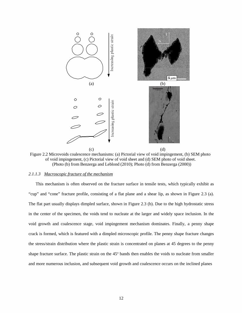
of void impingement, (c) Pictorial view of void sheet and (d) SEM photo of void sheet ............................. 12

Figure 2.3 Macroscopic fracture profiles of ductile fracture: (a) Cup and cone fracture profile, (b)

Dimpled fracture surface, (c) tensile fracture under atmospheric pressure and (d) tensile fracture under

1120 MPa hydrostatic pressure. (Photo (a) from Kabir and Islam (2014); Photo (b) from Benzerga et al.,

2004; Photo (c) and (d) from Kao et al. (1990)) .......................................................................................... 13

Figure 2.4 Sharp crack in infinite elastic plate in LEFM calculation ........................................................... 17

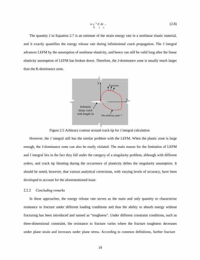
Figure 2.5 Arbitrary contour around crack tip for J integral calculation ...................................................... 19

Figure 2.6 Stage and mechanisms of fatigue crack growth .......................................................................... 24

Figure 2.7 Fatigue life predictions versus real fatigue life ........................................................................... 30

Figure 2.8 Relationship between the accumulated damage, DMiner, and the maximum strain range ∆εmax . 30

Figure 2.9 Fractograph of fracture surfaces for AW50 steel: (a) Fracture under monotonic loading with

deep dimples, and (b) Fracture after five loading cycles with shallower dimples ........................................ 32

Figure 2.10 Damage evolution at the center of a notched bar during a cyclic loading history ...................... 32

Figure 3.1 Bounding curves sketch of new criterion.................................................................................... 52

Figure 3.2 Effect of model parameters on fracture locus: (a) Effect of c7 on the new criterion, (b) Effect of

c8 on the new criterion and (c) Effect of c9 on the new criterion ................................................................. 57 Figure 3.3 Cutoff regions of fracture locus .................................................................................................. 58

Figure 3.4 The stress triaxiality variations during the loadings of various plates ......................................... 60

Figure 3.5 The damage rate variations and the average damage rate of various plates ................................. 60

Figure 3.6 The stress state and damage rate evolution and the average parameters of a circumferentially

double notched tube specimen .......................................................................................................................... 60

Figure 3.7 The fracture locus constructed with the new criterion for Al 2124-T351: (a) The new fracture

locus for 2024-T351 aluminum alloy on the plane ofεf and η (Calibrated from Seidt’s data set), (b) The

new fracture locus for 2024-T351 aluminum alloy on the plane ofεf and η (Calibrated from both data

sets), and (c) 3D representation of the new fracture criterion for 2024-T351 aluminum alloy (Calibrated

from both data sets) ..................................................................................................................................... 66

Figure 3.8 The fracture locus constructed with the new model for Al 5083 ................................................. 66

Figure 3.9 The fracture locus constructed with the new criterion for Weldox steel: (a) The new fracture

locus for Weldox 420 steel on the plane of ε f and η , (b) 3D representation of the new fracture criterion

1

for Weldox 420 steel, (c) The new fracture locus for Weldox 960 steel on the plane of ε f and η , and (d)

3D representation of the new fracture criterion for Weldox 960 steel ................................................................. 69

Figure 3.10 The fracture locus constructed with the new criterion for A710 steel: (a) The new fracture

locus for A710 steel on the plane of ε f and η , and (b) 3D representation of the new fracture criterion for

A710 steel ........................................................................................................................................................... 71

Figure 3.11 Comparison of fracture locus between 1045 and DH36 steel ................................................... 71

Figure 3.12 The fracture locus constructed with the new criterion for 1045 steel: (a) The new fracture

locus for 1045 steel on the plane of ε f and η , and (b) 3D representation of the new fracture criterion for

1045 steel .................................................................................................................................................... 73

Figure 3.13 The fracture locus constructed with the new criterion for TRIP780 steel: (a) The new fracture

locus for TRIP780 steel on the plane of ε f and η , and (b) 3D representation of the new fracture criterion

for TRIP780 steel ................................................................................................................................................ 74

Figure 3.14 Comparison of prediction from various criteria for the test results listed in Table 3.1 ................ 76

Figure 4.1 Tests set up for gusset plate connections: (a) Specimen T1, and (2) Specimen T2, after Huns et

al., 2002 ...................................................................................................................................................... 84

Figure 4.2 Numerical model for gusset plate connection T2 ....................................................................... 86

Figure 4.3 Comparison between the experimental and numerical fracture profiles of T1 connection ............ 87

Figure 4.4 Comparison between the experimental and numerical fracture profiles of T2 connection ............ 87

Figure 4.5 Fracture sequence of the connection T2 ..................................................................................... 88

Figure 4.6 Numerical and experimental load versus displacement curve of connection T1 .......................... 88

Figure 4.7 Numerical and experimental load versus displacement curves of connection T2 ........................ 89

Figure 4.8 (a) Representative beam geometry and set up, (b) representative geometry of connections

subjected to end rotation, and c) Geometry of connection of specimen D2 subjected to zero end rotation

(i.e. pure shear) ............................................................................................................................................ 90

Figure 4.9 Representative numerical model for coped beam connection ..................................................... 92

Figure 4.10 Spring system layout for vertical spring ................................................................................... 94

Figure 4.11 The two-fixed end beam system for the angles’ bending action (A-A section of Figure 4.8 (a))

.................................................................................................................................................................... 96

Figure 4.12 Layout of the calibration on global systems through zero rotations .......................................... 96

Figure 4.13 The sketch of the horizontal spring system ............................................................................... 97

Figure 4.14 Representative comparisons between the numerical and experimental load versus

displacement curves for (a) specimen B2, (b) specimen C1, (c) specimen D1, (d) specimen D2, (e)

specimen E2, and (f) specimen H2 ............................................................................................................ 100

12

Figure 4.15 Experimental and numerical fracture profiles for (a) specimen B2, (b) specimen C1, (c)

specimen D1, (d) specimen D2, (e) specimen E2, and (f) specimen H2 .................................................... 102

Figure 4.16 Contour of stress state paramters for specimen T2: (a) Stress triaxiality and (b) Lode angle

parameter ................................................................................................................................................... 104

Figure 4.17 (a) Damage contour for connection T2 directly before cracking occurs and (b) sequence of

fracture initiations on bolt holes ................................................................................................................ 106

Figure 4.18 Definition of the location angle in bolt hole............................................................................ 106

Figure 4.19 Depiction damage distribution around bolt holes for (a) Bolt hole 1, (b) Bolt hole 2, (c) Bolt

hole 3, and (d) Bolt hole 4 ......................................................................................................................... 107

Figure 4.20 Fracture strain contour of T2 .................................................................................................. 107

Figure 4.21 Comparisons of fracture profiles under different beam end rotation levels .............................. 109

Figure 4.22 Comparisons of load versus displacement curves under different beam end rotation levels 110

Figure 4.23 Comparisons on the bolt-hole interaction forces for top and bottom bolts under different beam

end rotations .............................................................................................................................................. 110

Figure 4.24 (a) Geometrical configuration of the model and (b) depiction of a typical numerical model

used ........................................................................................................................................................... 113

Figure 4.25 Strength ratio versus relative spacing on the tensile plane for group 1 and 2 and the

classification of failure modes ................................................................................................................... 116

Figure 4.26 Strength ratio versus relative spacing on the tensile plane and failure modes classification for

group 3 ...................................................................................................................................................... 116

Figure 4.27 Strength ratio versus relative spacing on the tensile plane and failure modes classification for

group 4 ...................................................................................................................................................... 117

Figure 4.28 Envelope of the fracture modes .............................................................................................. 117

Figure 4.29 Fracture profiles for the failure mode: Tensile fracture + shear yielding (a) tensile fracture and

(b) full fracture .......................................................................................................................................... 118

Figure 4.30 Load versus displacement curves for group 1 ......................................................................... 119

Figure 4.31 Fracture initiation for the failure mode: Tensile fracture + shear fracture ................................ 120

Figure 4.32 Load versus displacement curves for cases in group 2 with the failure mode: Tensile fracture

+ shear fracture .......................................................................................................................................... 120

Figure 4.33 Fracture profiles for the failure mode: Tensile yielding + shear fracture (a) fracture initiation

and (b) final fracture .................................................................................................................................. 121

Figure 4.34 Load versus displacement curves for cases in group 2 with the failure mode: Tensile yielding

+ shear fracture .......................................................................................................................................... 122

Figure 4.35 The fracture profiles for the failure mode: hole tearout ........................................................... 123

13

Figure 4.36 (a) Representative geometry detail of the double coped connection and (b) example of the

finite element model used ......................................................................................................................... 126

Figure 4.37 Strength ratio versus relative spacing in the shear plane for the pure shear cases .................. 126

Figure 4.38 Representative geometry details of the coped beam connections ........................................... 127

Figure 4.39 Strength ratios for different edge distances ............................................................................ 128

Figure 5.1 Cutoff regions of fracture locus ............................................................................................... 137

Figure 5.2 Comparison of linear and nonlinear damage evolution rule ..................................................... 141

Figure 5.3 Schematic representation of history effects based damage evolution ....................................... 142

Figure 5.4 Comparison of the three approaches (Specimen 7 in Table 5.2) .............................................. 144

Figure 5.5 Fracture locus constructed with the new criterion for 1045 steel under monotonic loading ... 146

Figure 5.6 Comparison of load-displacement curves and predicted fracture displacements for 1045 steel

.................................................................................................................................................................. 146

Figure 5.7 Comparison of the two correction approaches on 1045 steel ................................................... 147

Figure 5.8 Comparison of load-displacement curves and predicted fracture displacements for Al2024T351:

(a) Type A specimens, (b) Type B specimens, and (c) Type C specimens ................................................ 150

Figure 5.9 Experimental versus predicted accumulated equivalent plastic strain for Al 2024T351 .......... 150

Figure 5.10 Load-displacement curves for selected tests .......................................................................... 152

Figure 5.11 Fracture locus constructed with the new criterion for A572 steel under monotonic loading 154

Figure 5.12 Comparison of the three correction approaches on ASTM A572 steel .................................. 154

Figure 5.13 Damage evolution along with ε for test with number 6 (CTF) ...................................................... 155

Figure 5.14 Damage evolution along with ε for test with number 8 (C-PTF) .................................................. 155

Figure 6.1 Sketch of isotropic hardening ................................................................................................... 163

Figure 6.2 Sketch of kinematic hardening ................................................................................................. 165

Figure 6.3 Schematic representation of implicit integration using radial return method of von Mises

plasticity equations .................................................................................................................................... 168

Figure 6.4 Flow chart of the VUMAT subroutine ..................................................................................... 173

Figure 6.5 Comparison of load versus displacement curve between VUMAT and corresponding

ABAQUA embedded combined hardening material model ...................................................................... 174

Figure 6.6 Details and dimensions of the test setup of the experimental program in Galvez (2004),

Okazaki (2004) and Okazaki et al., (2005) ................................................................................................ 177

Figure 6.7 Geometry configurations and welding details for specimen 1 (corresponding to the specimen 5

and 8 in Galvez (2004)) ............................................................................................................................. 178

Figure 6.8 Geometry configurations and welding details for specimen 2 (corresponding to the specimen 1,

2 and 3 in Galvez (2004)) .......................................................................................................................... 178

14

Figure 6.9 Loading protocols and failure initiation locations: (a) Severe Loading Protocol (SLP); and (b)

Revised Loading Protocol (RLP) by Richards and Uang (2003) ............................................................... 180

Figure 6.10 Depiction of a typical numerical model used for EBF link (Specimen 1) ................................ 183

Figure 6.11 Typical distribution of the longitudinal and transverse residual stress within a welded joint186

Figure 6.12 Residual stress distribution of stiffened plate: (a) Typical stiffened plate, (b) idealized stress

distribution and (c) Faulkner stress distribution ......................................................................................... 187

Figure 6.13 Comparisons between the applied and Faulkner residual stress distribution ............................ 188

Figure 6.14 Classification of HAZ: (a) Single pass weld, and (b) Multi-pass weld .................................... 191

Figure 6.15 Comparisons on link shear force versus total rotation curves in numerical simulations and

laboratory tests: (a) Specimen 1, and (b) Specimen 2 ................................................................................ 194

Figure 6.16 Comparisons on link shear force versus plastic rotation curves in numerical simulations and

laboratory tests: (a) Specimen 1, and (c) Specimen 2 ................................................................................ 195

Figure 6.17 Comparisons on shear link fracture initiation between numerical simulations and laboratory

tests: (a) Simulation of specimen 1, (b) experiment of specimen 1, (c) simulation of specimen 2, and (c)

experiment of specimen 2 .......................................................................................................................... 197

Figure 6.18 Comparisons on shear link fracture propagation between numerical simulations and

laboratory tests: (a) Horizontal crack after completing the second cycle of load step 9, and (b) final

fracture ...................................................................................................................................................... 198

15

CHAPTER 1 Introduction

1.1 Motivation of the study

Fracture of steel components after extensive plasticity and cyclic inelastic deformations is common

under many extreme events. The failure usually occurs after very limited number of stress/strain cycles

and is often categorized as Ultra-Low Cycle Fatigue (ULCF), or Extreme-Low Cycle Fatigue (ELCF).

Large inelastic strains under extreme events are often desirable as a source of significant energy

absorption with sufficient level of ductility. While steel as a material is known to be very ductile with

ductility ratios as large as 50 to 100 (ductility ratio is the ratio of ultimate deformation to yield

deformation), overreliance on ductility can lead to catastrophic consequence. For example, in the 1994

Northridge earthquake, many moment connections fractured in a brittle manner as a result of various

design and fabrication defects.

Although numerous studies following the Northridge earthquake have been conducted in order to

improve the resistance of steel structures to large cyclic loadings, research on predicting fracture

resistance of components and details are scarce. Although a number of criteria have been proposed for

predicting fatigue and fracture in metal components under large loading demand, the studies have only

been geared exclusively towards cases with specific restraint conditions. In addition, attempts to extend

existing low cycle fatigue criteria to the ULCF have proven to be neither accurate nor applicable.

Furthermore, directly applying traditional fracture mechanics such as the J-integral and Crack Tip

Opening Displacement (CTOD) to cases of large inelastic strain reversals are also questionable. This is

because the conventional fracture mechanics approaches is based on assuming the presence of an initial

flaws with highly constraint crack tip, limited plastic strain crack regions, and nonlinear elastic behavior.

Fracture under monotonic loading with large pre-crack plastic strains, which is often named as ductile

fracture, can be viewed as a special case of “cyclic loading” with failure after a quarter cycle. The

asymmetric stress state in the case of monotonic loading, in terms of the hydrostatic and deviatoric stress

1

components, is the main contributor of the asymmetric damage in connections. However, existing fracture

criteria employing hydrostatic and deviatoric stresses are either inapplicable to all stress state ranges or

uneconomical in calibration and application to practical structural details. It is also arguable that since

monotonic loading is a “special” case of cyclic loading, appropriate ULCF criteria should capture ductile

fracture under monotonic loading.

The mechanisms of ULCF and monotonic ductile fracture are known to exhibit intrinsic similarities

through numerous analyses on crack topology using fractographic analysis (Kanvinde and Deierlein,

2007). Therefore, ULCF can be viewed as series of combination of monotonic ductile fracture and their

reversals. Thus, it is not too farfetched to presume that they also share similar crack formation, and the

extension of ductile fracture criteria to the all-around counterparts also consider the case of reverse

loading or ULCF merits extensive consideration.

Numerical simulations of structural components or systems through their full range of response,

including failure, under complex stress states are scarce. For instance, gusset plates and coped beam are

one of the most popular and widely used connection components in steel structures and, are designed to

transfer both tension and compression forces or tension and shear force, respectively. One of the

predominant failure modes in these connections is block shear, which is due to tensile and shear stress

states. The presence of both tension and shear stresses imposes challenges in numerical simulations of

such failure, which is evident in the lack of agreement between existing numerical studies and

experimental results. Therefore, the development of new and accurate fracture models and their

applications to predicting the response of structural components and systems can yield significant

dividends for understanding the failure mechanisms and the corresponding structural response.

1.2 Objectives and scope of the study

The main overarching objective in this study is to first develop new, accurate, and easy-use ductile

fracture model. The model is to be developed for monotonic loading and be extended to reverse loading

2

cases. Once validated on the material level, these models can then be implemented at the structural

detail/connection level, in order to solve practical structures problems under large loading demands.

The specific objectives of this study can be categorized as follows:

• Developing a new ductile fracture criterion under monotonic loading conditions that is

dependent on stress triaxiality and Lode parameters.

• Validating the monotonic fracture model against experimental coupon data for various alloys.

• Conducting numerical simulation on gusset plate and coped beam connections, under specific

monotonic loading conditions.

• Conducting parametric studies on gusset plate and coped beam connections to highlight the

usefulness on the model in determining the influence of detailing parameters on connection

performance

• Extending the monotonic loading ductile fracture criterion to ULCF cases through

introducing nonlinear damage evolution rule and loading history effects.

• Validating the cyclic fracture model against experimental coupon data for various alloys.

• Conducting numerical simulation on shear links that are typically employed in eccentrically

braced frames, under specific cyclic loading conditions.

• Conducting parametric studies on shear links that are typically employed in eccentrically

braced frames, to highlight the usefulness of the model in determining the influence of

loading scenario.

There have been many studies pertaining to simulating the full response of steel structures under large

inelastic demands with focus on the pre-cracking stage. However, studies focusing on simulating the

response at the onset of cracking and including the cracking stage are relatively scarce. The cracking or

failure stage is usually accounted for through providing limits on connection rotation that related to

connection fracture. In many fracture failure scenarios, the ultimate strength of a structural component

occurs at the onset of fracture initiation, so is the ultimate ductility. Although it is recognized that failure

3

in steel structures could be manifested through different limit states, including for example local or global

instability, the progression of failure, following instability, is usually directly associated with fracture

propagation (i.e. separation of material and/or components). In the present study, the full response of

connections including stiffness, ultimate strength, and ductility are investigated through assessing fracture

that entire load-displacement or moment-rotation curves of connections that accounts for crack initiation

and propagation.

There are many mechanisms responsible for fracture of metal under large inelastic deformations, and

the prevalent mechanisms are believed to be micro-void nucleation, growth and coalescence. Some other

mechanisms may play some marginal roles, depending on material properties, loading procedure, and

constraint conditions. Micro-void nucleation usually only accounts for a very limited portion of the entire

fracture process, while microvoid growth and coalescence usually dominate. In the present study, the

investigation will focus on micro-void growth and coalescence, while other mechanisms will be briefly

discussed but not in detail.

The current state of design and fracture resistance of structures still somehow relies on simplified

analytical models, which is mainly developed from empirical approaches, since the fracture process is

generally not well modelled. In this study, fracture is modelled based on the fundamentals of micro

mechanisms and can be easily implemented into structural fracture analysis in support of performance-

based design. Therefore, this study provides a step towards shifting the fracture process for structural

design from an empirical prescriptive to a more fundamental one.

1.3 Organization and outline

In chapter 2, important background for the present study is provided, through summarizing state-of-

the-art and through discussing current existing fracture models, methods and approaches for predicting

fractures in metal structures. The chapter begins with introduction of traditional fracture mechanics,

which includes current approaches used to quantify fracture with pre-existing defects, such as the stress

intensity factor and J-integral. In addition, existing methods used to predict high cycle and traditional low

4

cycle fatigue fracture such as the Miner’s Law for damage accumulation and ∆K for fracture propagation,

are presented. Existing ULCF models, derived either from extension of traditional fatigue models, or

fitting of experimental data, are later introduced and analyzed. Finally, the existing ductile fracture

models, such as the analytical micro-mechanical based Gurson-Tvergaard-Needleman (GTN) model and

the experimental based Johnson-Cook (J-C) model, are introduced and compared. The later discussion

provides clear distinctions between each model, while the assumptions on which each model was

developed are clearly outlined, so are their application range. It also indicated, conceptually, why some

existing models, especially those founded on traditional fracture mechanics and fatigue approaches work

in some cases, but would not be suitable for the present study.

In chapter 3, the main focus is on the development of the ductile fracture criterion with consideration

of the two stress state parameters, the stress triaxiality and Lode parameter. The chapter begins with

discussion of the two stress state parameter dependencies and their analytical expressions, with

comparison to other popular models. In addition, the interaction of the two parameters is discussed and

proposed in terms of the new ductile fracture model. Later the bounding curves of the fracture strain locus

calculated from ductile fracture model is discussed in detail, and comparisons are made between the

proposed model and other models. Based on the study on bounds, the proposed ductile fracture model is

further refined by including asymmetric bounds. A damage evolution rule for non-proportional loading

cases is later proposed. Moreover, the effects of the constants in the proposed ductile fracture criterion is

shown and discussed. Verification analysis is conducted through comparisons between the predicted

fracture strains and their experimental equivalents, which comprise of many experimental data extracted

from the literature for various metals. Finally, the proposed model is compared to four representative

existing fracture models in their prevailing ranges, including the Cockcroft-Latham-Oh (CLO) criterion

(Oh et al., 1979), the Modified Mohr-Coulomb (MMC) model (Bai and Wierzbicki, 2010), the Rice-

Tracy based models (Rice and Tracy, 1969), and the Bai-Wierzbicki model (Bai and Wierzbicki, 2008).

In chapter 4, the new ductile fracture model, proposed in chapter 3, is first implemented on structural

details, through the simulation of the block shear failure in gusset plate and coped beam connections. In

5

addition, parametric study on the effect of connection geometry and loading conditions on the response

characteristics are conducted. The numerical simulations are compared to experimental test data available

in the literature in terms of load versus displacement curves, fracture profiles, and the fracture sequences.

Discussion on the intrinsic mechanisms of this kind of failure type, such as fracture location and damage

around bolt hole is provided. Additional parametric study is conducted with focus on geometrical

variables, including bolt spacing on the tensile and shear planes, as well as bolt edge/end distances. Four

different fracture modes are identified and analyzed for the first time. In addition, numerous comparisons

are conducted between the strength obtained from previous tests and the predictions using the numerical

simulations. Recommendations on the geometrical configuration requirements such as bolt hole spacing

and edge distance are also provided, since they are shown to have an impact on the fracture mode and

undesirable fracture modes may occur due to inappropriate configurations.

In chapter 5, the main focus is on the extension of the fracture model provided in Chapter 3 from

monotonic ductile fracture to the cyclic cases. This chapter starts with discussion on and definition of the

cut-off region where damage will not develop. This region is located at the negative-stress triaxiality

range, whose limit is determined by both stress triaxiality and Lode angle parameter. Thereafter the

nonlinearity and history effects on damage evolution, due to reverse loading, are discussed and defined.

The proposed cyclic model is validated through comparisons between the predicted fracture strains and

their experimental equivalents, and the experimental data, extracted from literature, correspond to various

metal alloys.

In chapter 6, the newly proposed ductile fracture criterion for reverse loading cases, presented in

Chapter 5, is first implemented into structural details, through the simulation of eccentric shear links and

comparisons between the simulation results and experimental data are provided. This chapter starts by

developing an algorithm for integrating the von Mises plasticity with the combined hardening to be used

in simulating the shear links. This is because the material model embedded in ABAQUS does not allow

damage in the proposed fracture model to be determined. To that end, the user-subroutine VUMAT is

programmed according to the developed algorithm, with the damage variable included. The subroutine is

6

then verified through comparison between the response of the numerical models employing VUMAT and

those employing a typical embedded material model in ABAQUS. Since the shear link includes some

welded regions and there are associated heat affected zones (HAZ), the effect of residual stresses is

discussed. The residual stress seems to be insignificant to ductile fracture, while the fracture resistance in

HAZ is greatly reduced by welding heat input. Numerical simulations on bolted welded and un-welded

links were conducted, and good agreements with experimental equivalents were achieved.

In chapter 7, important conclusions of the study and recommendations for future research are

presented.

7

CHAPTER 2 Background and Current State of Research in Fracture Criteria

Fracture can be broadly categorized as brittle or ductile, corresponding to the cases with very limited

and large pre-crack deformations, respectively. This classification is too vague, since there is no clear

demarcation point for the two fracture types, and under different geometry and loading configurations,

entirely different fracture modes could be observed on the same material, from extensive ductile tearing to

highly brittle sudden cracking cases to somewhere in between (ductile-brittle transition). Therefore, it is

important to identify the mechanisms governing the fractures, the controlling factors for each fracture

type, and the appropriate fracture prediction criterion. Fracture criteria are generally categorized under

either traditional fracture mechanics or non-traditional micromechanics approaches. The traditional

approaches are mostly based on the principles of traditional fracture mechanics and are phenomenological

in nature. Traditional approaches have been popular since they are computationally efficient and do not

require extensive computational tools, which was a limiting factor prior to the substantial leaps in the

computer industry in mid to late 90s. With the increase in computing power, the non-traditional, physics-

based, approaches started to gain more attention and required the use of Finite Element Methods (FEMs).

In this chapter, the main mechanisms for fracture in structural steel materials, including void growth,

cleavage and intergranular fracture, are first introduced. This is then followed by description of traditional

fracture mechanics since it is the basis for most traditional approaches. In addition, the chapter outlines

fatigue issues in metals in relation to the mechanisms of different stages of fatigue and the modelling

methods. Thereafter, existing micro-mechanical models are introduced, which are mainly for ductile

fracture, and focus is placed on some key widely-accepted models. Later in the chapter several existing

ultra-low cycle fatigue criteria are introduced critical needs and key areas for improvements are

highlighted, which sets the tone for the work conducted in this thesis.

8

2.1 The fracture mechanisms for metals

Metal fracture can occur in a variety of modes, ranging from stable ductile tearing to abrupt unstable

cracking, depending on the material microstructure and composition, stress states as well as the

environmental conditions. These varying fracture modes are essentially due to the difference in the

corresponding responsible mechanisms. Therefore, it is essential to identify and understand the correct

mechanism prior to the development of appropriate fracture criterion. In the present study, the agreed-

upon ductile fracture mechanism, namely microvoid nucleation, growth, and coalescence, is considered.

Some other mechanisms, including cleavage fracture, transition modes, and intergranular fracture is also

reviewed for the purpose of completeness and comparison in addition to the fact that they are oftentimes

partially present and cannot be avoided. The mechanisms are summarized below and more comprehensive

information can be found in Anderson (1995). Moreover, traditional fracture mechanics and traditional

fatigue approaches are summarized so that a complete picture of the difference between traditional

approaches, which are typically utilized, and the nontraditional approach used in this study is provided.

This is intended to set the tone for the work being conducted in this study by describing traditional

methods and defining the bounds beyond which their use would be questionable.

Microvoid growth to coalescence

In ductile fracture, fracture occurs with large pre-crack inelastic deformation and the strain can

usually reach 50~100% or more. Ductile fracture is a mode of material failure in which microvoids, either

pre-existing or newly nucleated in the material, grow until the coalescence is triggered and a continuous

fracture surface is formed. This mechanism is usually called microvoid growth and coalescence. The

stages of this fracture type are expressed in the following sections and are outlined in Figure 2.1.

2.1.1.1 Microvoid nucleation

Most metals contain secondary particles or inclusions, such as carbides in the steel matrix. When

sufficient stress/strain/temperature fields are applied, void nucleation can occur by decohesion of the

particle-matrix interface, or by fracture of the particles, and in the cases of creep (elevated temperature),

9

voids can even nucleate at the grain boundaries of the matrix. Void nucleation occurs in a gradual manner,

which means voids will not initiate simultaneously, especially for material that contains more than one

type of secondary particle. Typically, voids first nucleate at larger particles, and as the process continues,

voids may initiate at the smaller particles, while it is possible that some of these particles will never

initiate voids at all. The shapes of the voids are influenced by the particle shapes. For example, in HSLA-

100 steel voids nucleated with equiaxed shape because of the spherical inclusions due to the addition of

calcium, Ca, for inclusion shape control (Chae and Koss, 2004), while in HY-100 steel elongated voids

are nucleated because of the elongated lath-shaped Manganese(II) sulfide, MnS, inclusions (Jablokov et

al., 2001). Various models have been proposed for void nucleation described by stress/strain fields, in

terms of calculating the nucleation-induced porosity, fn . More details and discussion on the mechanisms

of nucleation can be found in Argon (1975), Goods et al. (1979) and Benzerga and Leblond (2010).

Figure 2.1 Ductile fracture propagation by void growth to coalescence in an initially dense steel (Photo from Benzerga and Leblond, 2010)

2.1.1.2 Microvoid growth and coalescence

Once a void has been nucleated, it will start to grow at a certain rate and along specific directions,

which are determined by the material microstructures and applied stress/strain/temperature fields. There

are a variety of models for void growth, which will be introduced in the following sections. At the last

stage of void growth after the voids have grown to a certain level, interaction between adjacent voids

starts and the voids start to coalesce. Coalescence of voids is the last stage of ductile fracture at the

10

microstructure level and the beginning of fracture on the macroscopic level. At this stage, material inside

the inter-void ligament between neighboring voids have large localized plastic deformations and usually

localization planes are formed. In other parts of the element, the material is undergoing elastic unloading.

The localization can occur at any orientation relative to the ligament between two coalescing voids,

depending on the orientation of the principal-straining axis. Void coalescence usually occurs in two

modes, described as follows:

• Void impingement: This mechanism is also known as tensile void coalescence mechanism,

which implies an internal necking down of the ligaments between the two coalescing voids

that have enlarged their dimensions significantly until impinging on each other. The pictorial

view of the mechanism is shown in Figure 2.2 (a) and the corresponding scanning electron

micrograph (SEM) photo is shown in Figure 2.2 (b).

• Void sheet: This mechanism is also called shear coalescence, which is favored by low stress

triaxiality. In this mechanism, the localization occurs between two coalescing voids along the

maximum shear plane and is usually dimensionally narrow as a sheet. It is similar to shear

banding but in a microvoid scale. The mechanism is shown in the pictorial view in Figure 2.2

(c) and in SEM photo at Figure 2.2 (d).

11

(a) (b)

(c) (d) Figure 2.2 Microvoids coalescence mechanisms: (a) Pictorial view of void impingement, (b) SEM photo

of void impingement, (c) Pictorial view of void sheet and (d) SEM photo of void sheet. (Photo (b) from Benzerga and Leblond (2010); Photo (d) from Benzerga (2000))

2.1.1.3 Macroscopic fracture of the mechanism

This mechanism is often observed on the fracture surface in tensile tests, which typically exhibit as

“cup” and “cone” fracture profile, consisting of a flat plane and a shear lip, as shown in Figure 2.3 (a).

The flat part usually displays dimpled surface, shown in Figure 2.3 (b). Due to the high hydrostatic stress

in the center of the specimen, the voids tend to nucleate at the larger and widely space inclusion. In the

void growth and coalescence stage, void impingement mechanism dominates. Finally, a penny shape

crack is formed, which is featured with a dimpled microscopic profile. The penny shape fracture changes

the stress/strain distribution where the plastic strain is concentrated on planes at 45 degrees to the penny

shape fracture surface. The plastic strain on the 45o bands then enables the voids to nucleate from smaller

and more numerous inclusion, and subsequent void growth and coalescence occurs on the inclined planes

12

marked by the void sheet coalescence mechanism. This results in a much smoother fracture surface, often

termed “shear lips”, on the 45° bands as shown in Figure 2.3 (b).

(a) (b)

(c) (d) Figure 2.3 Macroscopic fracture profiles of ductile fracture: (a) Cup and cone fracture profile, (b)

Dimpled fracture surface, (c) tensile fracture under atmospheric pressure and (d) tensile fracture under 1120 MPa hydrostatic pressure. (Photo (a) from Kabir and Islam (2014); Photo (b) from Benzerga et al.,

2004; Photo (c) and (d) from Kao et al. (1990))

The effect of the level of the hydrostatic pressure on the fracture profile was demonstrated through

laboratory tests conducted by Kao et al. (1990). In these set of tests, specimens with different hydrostatic

stresses were pulled to failure and the fracture profiles examined as shown selectively in Figure 2.3 (c)

and (d). It was shown in the tests that portion of the flat plane, in a typical specimen, decreases as the

level of hydrostatic pressure decreases. In other words, the lower the hydrostatic pressure, the more the

tendency of the fracture to be ductile as oppose to brittle. Clearly, the normalized hydrostatic stress, the

13

stress triaxiality η, therefore plays significant role in the fracture type, brittle versus ductile, and hence has

been employed in various fracture criteria, which will be discussed in the following sections.

Cleavage fracture

Cleavage fracture occurs in the form of abrupt material separation along crystallographic planes

because of the stresses acting normal to the plane and low bonding. The fracture is typically very brittle

but often preceded by ductile fracture. This kind of fracture occurs in the form of breaking bonds, which

requires the local stress to exceed the theoretical strength (cohesive strength) of the material. In order to

achieve the extreme large stress field, a local discontinuity, such as the sharp micro-cracks ahead of the

macro-crack tip, has to exist to serve as stress raiser. Once crack initiates, there are two possible scenarios:

if the crack remains sharp, the crack will propagate in a fast manner until failure; the other option is that

the crack would be arrested by a grain boundary because of the insufficient external applied stress field or

the absence of a stress raiser.

Cleavage fracture occurs along the plane with fewest bonds, or lowest packing density. Therefore, in

the process, for body centered cubic material, the {100} planes are the favorable planes and in

polycrystalline materials, the fracture is transgranular. Since fracture will go through different grains, in

which the cleavage plane orientations are usually different, if the fracture propagates, the crack front has

to rotate as it moves forward, which leaves facets at each rotation. Therefore, the final fracture surface

usually exhibits a shiny faceted profile.

Compared to the cup cone fracture profile in the ductile fracture mechanisms, cleavage fracture

surface is smooth and shiny. As stated, it is usually featured with shiny, faceted appearance of the fracture

surface, which is also the identifying characteristic of a cleavage fracture. This kind of fracture is unstable

and can be self-propelled, with the rate of strain energy released by the crack propagation exceeding the

strain energy rate required to rupture the material.

14

The ductile-brittle transition

The mechanism of the ductile fracture, microvoid growth and coalescence, and the mechanism of

brittle cleavage fracture are very different and seem independent from each other, however, during the

fracture propagation process, one mechanism can suddenly transit to the other one. As stated in the

cleavage fracture section, cleavage brittle fracture is usually preceded by ductile fracture propagation. On

the other side, the ductile-to-brittle transition is quite straightforward in the perspective of mechanism in

which the crack initially propagates by ductile tearing and as it travels eventually a critical particle is

reached and then cleavage fracture occurs. The evidence for the transition is seen in the fracture profiles

with both cup cone and brittle shinny surface. This process is highly statistical in nature since the distance

between the nearest critical particle and the fracture front is random (Heerens and Read, 1988).

Intergranular fracture

In the fracture types discussed, the material usually does not fail along the grain boundary, but there

are situations that fracture initiates and propagates along the grain boundaries, and this kind of fracture is

termed intergranular fracture. There are some situations where the grain boundaries can be weakened,

including environmental-assisted reasons, intergranular corrosion and hydrogen embrittlement. Some

other metallurgical process can also trigger this fracture type.

2.2 Traditional fracture mechanics

Traditional fracture mechanics is based on the concept of the energy release rate, which is usually a

function of a single parameter (e.g., stress intensity factor (K), J-integral, or Crack Tip Opening

Displacement (CTOD)), and thus used as a one-parameter fracture criterion under specific conditions.

The basic concept is that cracks in solids will propagate when the strain energy released by the crack

extension exceeds the energy required for creating a new crack surface. By the difference in the

assumption made regarding the yield zone surrounding the crack tip, traditional fracture mechanics can be

categorized into Linear Elastic Fracture Mechanics (LEFM) with limited yield zone and Elastic- Plastic

15

K

Fracture Mechanics with noticeable yield zone, as further discussed in the following sections. Some of the

basic concepts are summarized from Anderson (1995).Linear elastic fracture mechanics.

Most traditional fracture mechanics approaches were developed through the singularity problems.

Linear elastic fracture mechanics (LEFM) is based on the assumption of linear elastic material behavior

during the fracture process. The main analysis variable in LEFM is the stress intensity factor, K, which is

function of the geometry, crack size and location, as well as loading conditions. Based on the linear

elastic assumption, the stress conditions around a crack tip can be determined. In traditional fracture

mechanics, the fracture is broadly categorized as three types: Mode I (in-plane opening or tensile), Mode

II (in-plane sliding or shear) and Mode III (out-of-plane tearing or shear) fracture. A pictorial view of a

typical Mode I is shown in Figure 2.4. In Figure 2.4, an infinite plate with a crack length of 2a is

subjected to a far field axial stress σ normal to the crack. The stress intensity factor KI for this mode can

be determined by Equation 2.1 as follows:

K I = σ πa , (2.1)

The stress components, σij, near the crack tip can be determined in the polar coordinates (r, θ) as follows

σ ij = KI

2πr fij (θ ) + higherorder terms , (2.2)

in which fij is a dimensionless quantity that varies with load and geometry and scales the singularity for

the stress component under consideration. For example, f22 can be described as

f22 = cos θ θ

1 + sin 2 2

sin 3θ

, (2.3) 2

As stated, the main momentum for the fracture is the measure of strain energy released, and for LEFM the

energy release rate G can be uniquely determined by the stress intensity factor, as follows

2 2

G = (1− v )KI

E for planestrain, (2.4)

2

G = I E

for planestress. (2.5)

16

K σ 2

Figure 2.4 Sharp crack in infinite elastic plate in LEFM calculation

As shown in Equation 2.2, in the vicinity of the crack tip, as r reaches 0, the stress should approach

infinite, which is a singularity problem. Undoubtedly, the real stress cannot exceed the yield stress for

elastic perfect plastic material. Therefore, there should be a region in which r≤rp, where the material

deforms plastically, and rp can be determined using the following equation:

rp = 2 C , (2.6) y

in which KC is the critical stress intensity factor for fracture. According to ASTM standard, LEFM is

valid only if the specimen’s least dimension is no less than 2.5rp. In LEFM, it is assumed that the material

is linear elastic, which holds true for most of the brittle fracture cases where inelastic deformations are

very limited. However, LEFM is found to be hold reasonable accuracy when larger inelasticity is present

but only if the corresponding yielding zone is “well-contained” around the crack tip. Anderson (1995)

indicates that typically the specimen dimensions should be over 50 times of the plastic zone length. In

Equation 2.2, the stress is determined regardless of specimen geometry, and therefore calculation only

holds accuracy in a certain region around the crack tip, which usually is referred to as K-dominance zone.

As stated, the plasticity region is very limited, and will not influence the influence the K-dominance zone.

17

However, it is virtually impossible for LEFM to describe the fracture behavior in cases where

plasticity is not confined to a small region, which may easily extend outside the boundary of K-

dominance zone, and under these situations the K-dominance zone actually does not exist anymore.

Therefore, the application of LEFM could be quite restrictive for many types of fracture with non-

negligible pre-crack plastic strains.

Elastic plastic fracture mechanics

Since the LEFM assumption is invalid under large plastic behavior, several approaches with increased

dominance zones have been developed, which are referred to as “Elastic-Plastic Fracture Mechanics”.

The most popular of such is the “J-integral” approach, proposed by Rice (1968). The J-dominance zone is

generally much larger than the K-dominance zone, and hence the J-integral approach is more applicable

than LEFM in many situations involving large-scale yielding. Another approach, known as the crack tip

opening displacement approach (CTOD) was widely explored even before the development of J-integral

by Rice (1968) mainly in the UK, and later identified to be in fact analogous to the J-integral (Anderson,

1995).

In the J-integral approach, a path independent contour integral, often named as J-integral, is employed

to estimate the amount of energy release rate in a nonlinear elastic material with a flaw. The pictorial

view of the problem is shown in Figure 2.5 within the 2D Cartesian coordinate system, and the contour

integral is calculated by assuming that a contour can follow an arbitrary path, which begins on the bottom

surface of the crack and travel counterclockwise around the crack tip until the top crack surface is reached.

The mathematical definition of the J-integral is shown in Equation 2.7 as follows:

J = wdy − T ∂ui ds , (2.7) ∫Γ

i ∂x

where Γ is an arbitrary path anticlockwise around the crack tip, Ti are the components of traction vectors,

ui are the displacement vector components, ds is the incremental length of the path Γ, and w is the density

of strain energy, defined as follows

18

w = εij σ dε . (2.8) ∫0 ij ij

The quantity J in Equation 2.7 is an estimate of the strain energy rate in a nonlinear elastic material,

and it exactly quantifies the energy release rate during infinitesimal crack propagation. The J integral

advances LEFM by the assumption of nonlinear elasticity, and hence can still be valid long after the linear

elasticity assumption of LEFM has broken down. Therefore, the J-dominance zone is usually much larger

than the K-dominance zone.

y Tractions

x

Infinitely sharp crack

with length 2a

The arbitrary path Γ

Figure 2.5 Arbitrary contour around crack tip for J integral calculation

However, the J integral still has the similar problem with the LEFM. When the plastic zone is large

enough, the J-dominance zone can also be easily violated. The main reason for the limitation of LEFM

and J integral lies in the fact they fall under the category of a singularity problem, although with different

orders, and crack tip blunting during the occurrence of plasticity defies the singularity assumption. It

should be noted, however, that various analytical corrections, with varying levels of accuracy, have been

developed to account for the aforementioned issue.

Concluding remarks

In these approaches, the energy release rate serves as the main and only quantity to characterize

resistance to fracture under different loading conditions and thus the ability to absorb energy without

fracturing has been introduced and named as “toughness”. Under different constraint conditions, such as

three-dimensional constraint, the resistance to fracture varies where the fracture toughness decreases

under plane strain and increases under plane stress. According to common definitions, further fracture

19

will occur when the energy release rate exceeds the toughness of the material. However, in reality the

stress state governs the potential for fracture. Consequently, a one-to-one correspondence between the

energy release rate and toughness is acceptable for traditional fracture mechanics under specific constraint

conditions. However, such approach is invalid in the presence of excessive pre-crack plasticity, in which

toughness actually depends on the size and geometry of the specimens and may significantly vary

throughout a loading history.

Another issue regarding the use of traditional fracture mechanics, in cases with excessive yielding at

the crack tip, is the validity of the singularity assumption, which is challenged by the presence of crack tip

blunting that, occurs due to large plasticization. The postulation of nonlinear elastic behavior in the J-

integral leads to another issue. That is when the crack grows, a plastic “wake” developed ahead of the

crack as the crack moves forward. The wake area represents a region where the material has been

plastically loaded and then elastically unloaded with residual plastic deformation, and hence the nonlinear

elastic assumption violates such true material behavior.

If the plasticity remains confined to a relatively small region and the constraints are not low, the

traditional fracture mechanic approaches are still the most popular and widely used ones, because of their

successful application in many practical situations over the years. However, if the plasticization grows

larger, or there exists low level and more complex constraint conditions, the use of these traditional

approaches is rather questionable.

Another issue regarding the use of traditional fracture mechanics approaches lies in their two

dimensional definition. It has been observed that thicker geometries are more prone to fracture, since

there are larger constraints, and this effect cannot be considered by these approaches. Although there are

approaches that attempt to add the additional stress constraints, such as the J-Q theory proposed by

O’Dowd and Shih (1991), they are either difficult to apply or calibrate.

20

2.3 Traditional fatigue

Fatigue failure can be defined as a series of fracture propagation when the material is subjected to

cyclic loading. Depending on the number of cycles to failure, fatigue can be phenomenologically

categorized as high cycle fatigue and low cycle fatigue. Repeated loadings are found to be very

detrimental to materials with respect to stiffness and strength, even when the levels of stresses from the

applied loads are far below the yield stress or ultimate strength. Paris et al. (1961) first employed fracture

mechanics to predict regions of stable fatigue crack growth under high-cycle fatigue. Since then, the

“Paris Law”, which is Equation 2.11, has become the main approach for assessing crack growth under

low magnitude stress range.

Fatigue cracks usually initiate at the component surfaces, as shear cracks on crystallographic slip

planes; after a transient period, further crack propagation takes place in directions normal to the applied

stresses; and finally, when the crack grows to a critical length and becomes unstable, final fracture occurs.

A more detailed categorization of the various fatigue crack stages include: (1) crack nucleation (a <am) ;

(2) microstructurally short crack propagation (am < a < a p ) ; (3) mechanically short crack propagation

(a p < a < al ) ; (4) long crack propagation (al < a < ac ) ; and (5) final fractures (Cui, 2002, Anderson,

1995). Where a is the characteristic dimension of an equivalent crack in certain component, am is the

smallest crack dimension detectable by current technology or on the order of the grain size (around 0.1

µm), a p is the smallest crack dimension for mechanically short cracks (about 100 µm), al is the smallest

crack length of long cracks (around 1 mm), and ac is the critical crack length where crack goes unstable

and then final fracture occurs. These classifications are subjective, and some of the early stages maybe

skipped due to the existence of initial defects in some metal components.

The key question regarding fatigue strength is whether or not a crack will grow over a certain number

of cycles. For some materials, when the cyclic stress range is below a certain value, the fatigue failure

will not occur, and this value is usually called fatigue limit, endurance limit, or fatigue strength; but for

21

some other material such threshold amplitude does not exist (Pyttel, et al., 2011). In the fracture

mechanics framework, the limit is identified as the fatigue threshold, ∆Kth , below which the fatigue crack

will not grow further ( ∆Kth is the change in stress-intensity factor threshold). When the stress range

amplitude near the crack tip, in terms change in stress intensity factor ∆K increases, the fatigue life

decreases.

Currently there are two types of modelling methodology considered for simulating the relation

between fatigue life and stress range amplitude during cyclic loading. The first approach is based on

fatigue crack propagation in terms of ∆K, and the other is based on cumulative fatigue damage as a

function of the amplitude of stresses and strains. The cumulative fatigue approaches are mostly

phenomenological, while the crack propagation theories are more dependent on physical mechanisms.

Mechanisms of fatigue failure and the fatigue crack propagation approach

The basic concept for the crack propagation approach is that the crack growth increment at each cycle

is calculated using a specific criterion, and once the crack grows to a critical length the material is

considered to have failed. The crack propagation rate is usually described as da dN, where N is number of

cycles, and such rate is shown schematically in Figure 2.6, which comprises of three stages. The fatigue

mechanisms and corresponding representative crack growth criterion in each stage are described in detail

in the following sections.

2.3.1.1 Stage I fatigue

The fatigue mechanism near the threshold, stage I in Figure 2.6, is dominated by short crack

propagation theories. The propagation behavior of short cracks is often very different from that of long

cracks. Although the definition of short cracks is very subjective and not precise, generally a crack where

a<al is considered to be short. It is well established that in high cycle fatigue most fatigue cracks spend

the vast majorities of their lives (up to 90%) as short cracks.

22

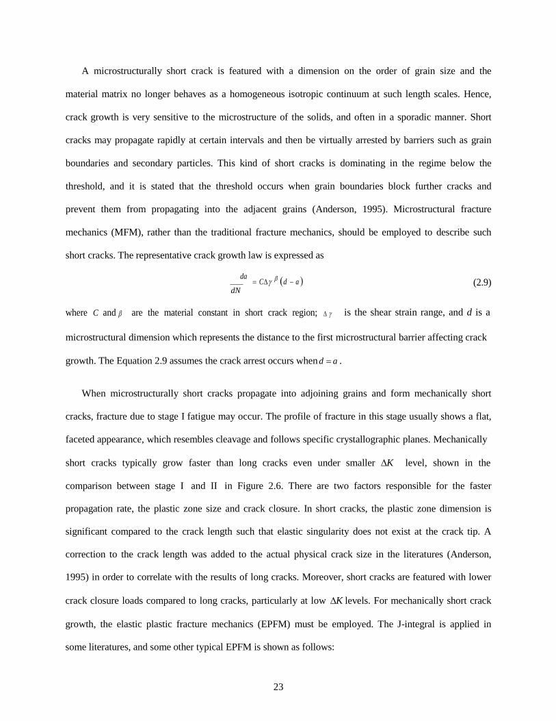
A microstructurally short crack is featured with a dimension on the order of grain size and the

material matrix no longer behaves as a homogeneous isotropic continuum at such length scales. Hence,

crack growth is very sensitive to the microstructure of the solids, and often in a sporadic manner. Short

cracks may propagate rapidly at certain intervals and then be virtually arrested by barriers such as grain

boundaries and secondary particles. This kind of short cracks is dominating in the regime below the

threshold, and it is stated that the threshold occurs when grain boundaries block further cracks and

prevent them from propagating into the adjacent grains (Anderson, 1995). Microstructural fracture

mechanics (MFM), rather than the traditional fracture mechanics, should be employed to describe such

short cracks. The representative crack growth law is expressed as

da = C∆γ β (d − a )

dN (2.9)

where C and β are the material constant in short crack region; ∆ γ is the shear strain range, and d is a

microstructural dimension which represents the distance to the first microstructural barrier affecting crack

growth. The Equation 2.9 assumes the crack arrest occurs when d = a .

When microstructurally short cracks propagate into adjoining grains and form mechanically short

cracks, fracture due to stage I fatigue may occur. The profile of fracture in this stage usually shows a flat,

faceted appearance, which resembles cleavage and follows specific crystallographic planes. Mechanically

short cracks typically grow faster than long cracks even under smaller ∆K level, shown in the

comparison between stage I and II in Figure 2.6. There are two factors responsible for the faster

propagation rate, the plastic zone size and crack closure. In short cracks, the plastic zone dimension is

significant compared to the crack length such that elastic singularity does not exist at the crack tip. A

correction to the crack length was added to the actual physical crack size in the literatures (Anderson,

1995) in order to correlate with the results of long cracks. Moreover, short cracks are featured with lower

crack closure loads compared to long cracks, particularly at low ∆K levels. For mechanically short crack

growth, the elastic plastic fracture mechanics (EPFM) must be employed. The J-integral is applied in

some literatures, and some other typical EPFM is shown as follows:

23

p da

= B (∆ε dN

πa )m − Ξ (2.10)

where B and m are material constant, and Ξ is the threshold condition in this crack regime.

log da dN

∆Kth log ∆K

Figure 2.6 Stage and mechanisms of fatigue crack growth

2.3.1.2 Stage II fatigue

In stage II, long crack growth is the governing propagation type and LEFM is valid and typically

employed in this regime. The crack growth rate increases proportionally with the stress intensity

amplitude on the log-log scale, and this stage is known as the Paris regime, described by the following

equations:

da = A(∆K )n

dN

(2.11)

where A and n are material constants, and ∆K = Y∆σ πa , here Y is a correction factor that depends

on loading and configuration of the cracked body. Various experimental studies have been conducted to

assess fatigue crack growth in Stage II (Dexter et al., 2003; Mahmoud and Dexter, 2005; Dexter et al.,

2005; and many others). At this stage, the crack growth rate is not strongly dependent on the

24

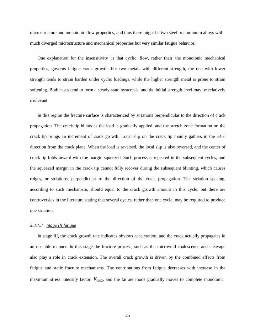
microstructure and monotonic flow properties, and thus there might be two steel or aluminum alloys with

much diverged microstructure and mechanical properties but very similar fatigue behavior.

One explanation for the insensitivity is that cyclic flow, rather than the monotonic mechanical

properties, governs fatigue crack growth. For two metals with different strength, the one with lower

strength tends to strain harden under cyclic loadings, while the higher strength metal is prone to strain

softening. Both cases tend to form a steady-state hysteresis, and the initial strength level may be relatively

irrelevant.

In this region the fracture surface is characterized by striations perpendicular to the direction of crack

propagation. The crack tip blunts as the load is gradually applied, and the stretch zone formation on the

crack tip brings an increment of crack growth. Local slip on the crack tip mainly gathers in the ±45°

direction from the crack plane. When the load is reversed, the local slip is also reversed, and the center of

crack tip folds inward with the margin squeezed. Such process is repeated in the subsequent cycles, and

the squeezed margin in the crack tip cannot fully recover during the subsequent blunting, which causes

ridges, or striations, perpendicular to the direction of the crack propagation. The striation spacing,

according to such mechanism, should equal to the crack growth amount in this cycle, but there are

controversies in the literature stating that several cycles, rather than one cycle, may be required to produce

one striation.

2.3.1.3 Stage III fatigue

In stage III, the crack growth rate indicates obvious acceleration, and the crack actually propagates in

an unstable manner. In this stage the fracture process, such as the microvoid coalescence and cleavage

also play a role in crack extension. The overall crack growth is driven by the combined effects from

fatigue and static fracture mechanisms. The contributions from fatigue decreases with increase in the

maximum stress intensity factor, Kmax, and the failure mode gradually moves to complete monotonic

25

fracture. Fracture under monotonic loadings, as microvoid coalescence, cleavage, or both, are very

sensitive to material properties, and hence such dependency is also high for stage III fatigue.

The main difference between fatigue failure and fracture under monotonic loadings lies in their

different driving forces. In fatigue, a crack will grow in each eligible cycle with stress amplitude above

the endurance limit. Meanwhile, under the same stress levels but without repeated loadings, fracture will

not progress further. Hence, the loading cycles is one of the additional driving forces for fatigue compared

to monotonic fracture and such extra driving force arise from the sharpening process of the crack tip in

the reversed half cycles. At the same time, when the stress/strain fields during cyclic loadings are so large,

even if the cyclicity halts crack growth still occurs.

For traditional fatigue failure, stage III does not play an important role since it takes a long time for

crack to grow from a small initial flaw to a critical size, and in such cases stage III probably only accounts

for less than 1 % of the total fatigue life. Studies on crack growth in region III is also scarce. For ULCF,

stage III is the dominating phase, and typical fatigue theories do not apply. Under large loading demand,

ULCF is the common failure modes and therefore modeling of this fatigue stages should be explored.

Cumulative fatigue damage approach

Fatigue damage develops with applied load cycles in an accumulative manner, and thus the

cumulative fatigue damage theory has been the traditional approach for fatigue life assessment. The most

common approach is the “linear damage rule” (LDR), which assumes fatigue damage accumulates in a

linear way, and is also known as the Miner’s rule (Miner, 1957), expressed as

D = ∑ ni

(2.12)

i Ni

where ni and Ni are the number of cycles and fatigue life, respectively, for the i th strain/stress range

amplitude. Although many nonlinear rules have been developed to address the shortcomings of LDR,

26

'

f

through more extensive considerations of the stress/strain amplitudes, such as load sequence and

deformation history effects, LDR remains the simplest and most frequently used cumulative rule.

Fatigue damage is fundamentally the result of microstructural changes in the materials. Such changes

on the microstructural level are assumed to have inherent relationships with macroscopic quantities, such

as the stress and strain. By employing different macroscopic quantities, various criterion have been

derived in order to describe the cumulative fatigue damage evolution in the framework of LDR. The

commonly used quantities, stress and strain, are briefly introduced in some representative models in the

following sections. A comprehensive review on the use of other quantities, such as energy and continuum

damage mechanics based approaches, can be found in the Fatemi and Yang (1998).

2.3.2.1 Stress-based approach (S-N curve)

The stress-based approach is the earliest, but still dominantly used approach in fatigue life prediction

of crack imitation especially in the cases of high cycle fatigue. The fatigue life (number of cycles N to

initiation) is assumed to be a function of stress amplitude ( σ a ), and expressed in the Basquin form

(Basquin, 1910) as

σa = σ f (2N)b

(2.13)

where σ ' is the fatigue strength coefficient, and b is the fatigue strength exponent, which is always

featured with a negative value. Since Equation 2.13 describes a curve with stress amplitude versus

number of cycles to failure, the approach is also named as S-N curve.

There are generally two types of stress concentration in practical structures and their components

arising from geometrical changes or discontinuities and welding profiles. Depending on how the stress

concentration is taken into account, the stress-based approaches are classified as three sub-approaches,

listed in order of their increasing accuracy and work effort as follows: the nominal stress approach, the

27

p f

hot-spot stress approach, and the effective notch stress approach. The nominal stress method is a global

method, while the other two are local approaches.

2.3.2.2 Strain-based approach

When plasticity occurs at the concerning regions of components, the problem will switch to strain-

controlled and the stress-based approach loses its primacy. In these cases, fatigue is usually attributed to

the low cycle fatigue domain and described by strain-based approach. The Manson-Coffin model

(Manson, 1965, and Coffin, 1954) is the most commonly used method, shown as

∆ ε p = ε ' (2 N )c

(2.14) 2 f

where ∆ε is the plastic strain range, ε' is the fatigue ductility coefficient, and c is the fatigue ductility

exponent, which is also negative all the time.

2.4 Ultra-low cycle fatigue models

Studies on fracture predictions of stage III fatigue are relatively scarce. Fatigue at this stage is always

featured with large plastic strain reversal, and thus the traditional stress-based fatigue approaches are not

applicable to this stage. The number of cycles up to failure is usually less than 10 to 15 cycles since local

strains are so large. In such case, crack propagation is more prone to fracture rather than fatigue. This

kind of fatigue is consequently named as Ultra-low cycle fatigue (ULCF), or Extremely-low cycle fatigue

(ELCF).

Extensions from traditional fatigue model

Traditional low cycle fatigue criteria, such as the strain-based approaches, only account for the

fatigue part, and inevitably gradually lose the accuracy with reduction in fatigue life. The predictions by

applying the Manson-Coffin criterion coupled with Miner’s rule to ULCF have been proven inaccurate

(Kuroda, 2001; Tateishi, et al., 2007). As is shown in Figure 2.7, as the plastic range ∆εp decreases,

predictions by the Manson-Coffin criterion gradually start to overestimate the fatigue life and the fracture

also transfers from the surface fracture mode (fatigue) to the internal fracture mode (ductile fracture). In

28

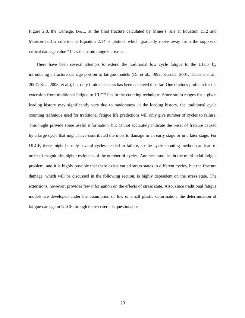
Figure 2.8, the Damage, DMiner, at the final fracture calculated by Miner’s rule at Equation 2.12 and

Manson-Coffin criterion at Equation 2.14 is plotted, which gradually move away from the supposed

critical damage value “1” as the strain range increases.

There have been several attempts to extend the traditional low cycle fatigue to the ULCF by

introducing a fracture damage portion to fatigue models (Du et al., 1992; Kuroda, 2001; Tateishi et al.,

2007; Xue, 2008; et al.), but only limited success has been achieved thus far. One obvious problem for the

extension from traditional fatigue to ULCF lies in the counting technique. Since strain ranges for a given

loading history may significantly vary due to randomness in the loading history, the traditional cycle

counting technique used for traditional fatigue life predictions will only give number of cycles to failure.

This might provide some useful information, but cannot accurately indicate the onset of fracture caused

by a large cycle that might have contributed the most to damage in an early stage or in a later stage. For

ULCF, there might be only several cycles needed to failure, so the cycle counting method can lead to

order of magnitudes higher estimates of the number of cycles. Another issue lies in the multi-axial fatigue

problem, and it is highly possible that there exists varied stress states in different cycles, but the fracture

damage, which will be discussed in the following section, is highly dependent on the stress state. The

extensions, however, provides few information on the effects of stress state. Also, since traditional fatigue

models are developed under the assumption of few or small plastic deformation, the determination of

fatigue damage in ULCF through these criteria is questionable.

29

Figure 2.7 Fatigue life predictions versus real fatigue life (Kuroda, 2002)

Figure 2.8 Relationship between the accumulated damage, DMiner, and the maximum strain range ∆εmax

(Data from Tateishi et al., 2007)

Extension from ductile fracture models

As previously stated, in the ULCF phenomenon, the fracture damage components gradually play the

key role instead of the fatigue damage part as has been previous indicated by Kuwamura and Yamamoto

(1997). The fractographs of fracture surface in Kanvinde and Deierlein (2001), shown in Figure 2.9,

indicates that both fracture surfaces of monotonic ductile fracture and ULCF are featured with dimpled

profiles, which suggests that the underlying mechanism of ULCF is at least partially microvoid nucleation,

growth and coalescence. Therefore, it is logical to model ULCF starting from the pure ductile damage

criterion that correspond to monotonic loading. Actually, fracture under monotonic loading corresponds

30

R

P

to a special case of ULCF, N ranges from 1/4 to 1/2, and in this case, the fatigue portion can be viewed as

none.

Inspired by the significant fracture contribution, Kanvinde and Deierlein (2007) extended Rice-Tracy

ductile fracture model to cases with ULCF. The original Rice-Tracey model can be defined as follows:

dR Rdε

= 0.283exp(1.5η ) , (2.15)

where R is the average microvoid radii, η is the stress triaxiality defined in Chapter 3. After mathematical

transformation, is given by

R VGImonotonic = ln C = ∫ε P exp(1.5η )dε P , (2.16)

0 0

in which VGI is an abbreviation for Void Growth Indicator, VGImonotonic is the VGI for monotonic

loading conditions, and R0 is the microvoid radius when plastic strain is zero. When VGImonotonic reaches a

critical value, the fracture is assumed to occur. It is so-called Void Growth Model, or VGM, and material

constant C is introduced in order to provide flexibility. Kanvinde and Deierlein (2007) extended the VGM

into a cyclic version Cyclic Void Growth Model (CVGM), through the assumption that the negative stress

triaxiality will heal the VGI, and the critical VGI will be degraded by the plastic strain excursion with

sudden drop manner as the loading direction change. The CVGM is shown as follows

VGI

cyclic =

∑ ∫ exp(1.5η )dε P − ∑

C2 ∫ exp(1.5η )dε , (2.17)

tensile cycles compressive cycles C1

( accumulated ) VGI cyclic = VGI monotonic exp − λε p , (2.18)

where C1 and C2 are material constants for VGM under tensile and compressive loading conditions, λ is

the material constants for VGI degradation, and εpaccumulated is the cumulative equivalent plastic strain

excursion. The representative VGI evolution is shown in Figure 2.10 for the center of notched bar under

cyclic loading.

31

(a) (b) Figure 2.9 Fractograph of fracture surfaces for AW50 steel: (a) Fracture under monotonic loading with

deep dimples, and (b) Fracture after five loading cycles with shallower dimples (Photos from Kanvinde and Deierlein, 2007)

Figure 2.10 Damage evolution at the center of a notched bar during a cyclic loading history (Redrawn from Kanvinde and Deierlein, 2007)

The work by Kanvinde and Deierlein on extending ductile fracture to predict ULCF is indeed a

creative idea. Some limitations, however, are worth noting to allow for proper extension of the model or

the development of new models. First, VGI serves as the quasi-damage variable, but it is not an ever-

32

increasing quantity, which is in contradiction with many mainstream experiments and theories. Actually,

generally the damage variable, except for some special metals and under extreme large compressive

loading, will not decrease. The VGI may be only viewed as measure of porosity evolution, but the

porosity itself is unable to reflect material conditions, since the void volume is not the only influencing

factor of fracture. Therefore, popular damage variables, such as the ductility measure, might be more

suitable to predict fracture. In addition, only the stress triaxiality dependency in the ductile fracture model

has been considered with some oversimplification in utilizing triaxiality, which lies in the fixed index 1.5

in Equation 2.6, which should be determined depending on many influencing factors, such as metal type

and stress state. Another issue lies in the cyclic degradation, which physically should be viewed as

gradual process rather than a sudden phenomenon. Despite these shortcomings, if the model is only

applied to mode I type loading in stage III fatigue, and if the stress triaxiality always lies in the

intermediate to the high range, which mainly represents components under pure tensile and compressive

cycles, acceptable results may be achieved.

Other phenomenological models

There have been many other phenomenological ULCF models. Some of the models of this type are

derived from the strain energy related process. In these models energy is used as damage variable to

predict failure in a member or component undergoing inelastic action under specific loading history.

Damage is typically defined as the ratio of the energy dissipation in N cycles to the total energy

dissipation until failure. Since phenomenological models are not directly related to this study, discussion

on their advantages and disadvantages will not be provided.

2.5 Ductile fracture models

There have been many attempts to model ductile fracture using either physical-based or empirical-

based approaches. In this section, some widely used models are discussed.

33

Physical-based ductile fracture model

Inspired by the physical evolution of ductile fracture, the mechanism of voids nucleation, growth and

coalescence, numerous physical-based fracture models have been proposed. Although the mechanism for

ductile fracture is microvoid nucleation, growth and coalescence, most popular approaches only consider

the void growth as main cause of fracture, since void nucleation only occupies a small portion of the total

damage and the coalescence is an unstable process. However, nucleation of microvoids still has been

investigated and modeled in Argon et al. (1975), Gurson (1977), Chu and Needleman (1980), Beremin

(1981), Lee and Mear (1999), Benzerga and Leblond (2010), among others. Voids coalescence has also

been investigated and modeled by Thomason (1968) and Tvergaard and Needleman (1984), among others.

In this section, only studies on void growth are introduced and discussed since void growth controls the

main portion of ductile fracture.

In many physical-based models, the porosity, f , is usually the only microstructural variable and often

viewed as a damage indicator, and hence the objective of the modelling is to obtain the evolution of the

porosity when subjected to strain and stress fields.

McClintock was a pioneer in modeling ductile fracture through void growth and his work on growth

of long cylindrical voids under a prescribed history of applied principal components of stress and strain

showed void growth to be strongly dependent on hydrostatic stress (McClintock, 1965). Thereafter, Rice

and Tracey (1969) indicated that fracture of ductile metals is strongly dependent on triaxiality of stress

state by studying growth of spherical voids in an incompressible, rigid-perfectly plastic solid for high tri-

axial loading cases, and the well-known Rice Tracy equation had been proposed to describe void growth

rate as shown in Equation 2.19 as follows

d ln f dε

= 0.849 exp(1.5η)

(2.19)

where η is the stress triaxiality and is defined in Chapter 3, and ε is the equivalent plastic strain.

34

σ

σ 2

=

y 2 σ

σ

1 2

Gurson (1975, 1977) developed a porous ductile material model and various modifications to this

model have been proposed by many researchers over the years. Gurson model was derived through

modelling a single spherical void in a unit cell where a perfect plastic von Mises homogeneous material

was assumed. The Gurson yield function is in a format of yield surface that takes into account the

porosity, f , and is shown as follows:

σ 2 φ = eq + 2 f cosh 3 σ m − (1 + f 2 )= 0 . (2.20)

2 y

where σeq is the von Mises equivalent stress, σm is the mean stress, and σy is the yield stress. The most

widely used void growth model was proposed by Tvergaard (1982) and Needleman (1984) through

extending the Gurson model in Equation 2.20, and usually named as the Gurson-Tvergaard-Needleman

(GTN) model. An equivalent porosity, f * , and two more factors (q1 and q2) were added to the original

Gurson model. The yield function GTN model is represented by

σ 2 φ = eq + 2q f * cosh 3 q σ m − (1 + q2 f *2 )= 0 , (2.21)

2 1 2 1 y y

where q1=1.5 and q2=1 as recommended, which leads to better results than the Gurson model, and the

equivalent porosity, f * , is defined as follows,

f ,

* f

1 q1 − fC

for f ≤ fC , (2.22)

fC + f f − fC

( f − fC ) for f > fC

in which f f is the porosity at final fracture, and fC is the critical porosity at which coalescence occurs.

As shown in Equation 2.22, once the coalescence starts, the evolution of the porosity is accelerated.

The growth rate of the porosity can be determined from the yield function, and is shown as follows:

d ln f * = 1.5q sinh(1.5q η) . (2.23)

dε

35

*

σ

where the porosity evolution rule of Equation 2.23 agrees well with the Rice-Tracy model in the trend of

exponential effect of the stress triaxiality on void growth rate. The porosity evolution can also include the

void nucleation effects, which is described in detail in Benzerga and Leblond (2010).

There have been many models modified from the Gurson model by introducing influencing factors,

such as the (initial) void shape and anisotropy. Another well-known extension was conducted by

Gologanu et al. (1993, 1994, and 1995), through introducing the void shape change effect into the

porosity evolution, and the model is usually called as the Gologanu-Leblond-Devaus (GLD) model.

These porosity-based models, known as the Gurson-like models, are only sensitive to stress triaxiality η.

This means that the equivalent fracture strain is only dependent on the ratio of the first invariant of the

stress tensor and the second invariant of the deviatoric stress tensor.

Gurson-like models have gained good reputations for describing predominant tensile fracture with

moderate and high stress triaxiality. However, the models generally fail to predict fracture in the low and

negative stress triaxiality domains, where shear fracture is believed to dominate. Various experimental

data has confirmed that the shear effect, often expressed in terms of Lode parameters or the third invariant

of the deviatoric stress tensor, also plays essential role in fracture formation and progression. Therefore,

extensions of ductile fracture models to include the shear effect have been proposed in the most recent

decade. Among the proposed extensions, the most representative is the one proposed by Nahshon and

Hutchinson (2008) who introduced a phenomenological term in the GTN model, to model void

deformation and reorientation in shear dominant stress state through an “effective void volume fracture”

or an “effective porosity”, which is expressed in Equation 2.24. It should be noted that currently there is

no well-accepted definition on how shear affects ductile fracture, and studies on this topic are still

ongoing.

df * = 1.5q sinh(1.5q η)dε + k w(σ) f s dε p , (2.24)

1 2 w ij ij e

in which the invariant measure w(σ) is defined as follows

36

ij

2 w(σ ) = 1 − 27J 3 . 2σ 3

e

where f* is the effective porosity, sij is the deviatoric stress components, εijp is the plastic strain

components (i, j=1, 2, 3), kw is a constant that sets the magnitude of the damage evolution rate in pure

shear stress states. There are two main concerns regarding Gurson-like models for the application to

ductile fracture prediction. The first issue lies in the fact that the effective/equivalent porosity serves as

the damage variable, which is usually very small and unstable (highly local microstructure dependent),

and such that it is hard to apply to real structure components. In addition, Gurson-like models usually

define the yield function, which is perfect plastic and difficult to calibrate, and sometimes do not

necessarily fit real metals. There are some well-accepted constitutive equations for most engineering

metals, and there is no need to calibrate the Gurson-like constitutive equations. Therefore, the best

approach is to propose another type of ductile fracture model, which also shares the features of Gurson-

like models.

From the discussed micromechanical ductile fracture models, it is easy to conclude that the stress

triaxiality is exponentially related to the damage variable. Taking the generalized Rice-Tracey criterion

for example, and assuming the DC as the damage variable value at fracture, the criterion can be rewritten

as

ε f

∫ c1 exp(c2η)dε = Dc ⇒ ε f = c1 exp(c2η) , (2.25) 0

where ε f is the equivalent plastic strain at fracture, named as fracture strain, and c1 and c2 are material

constants. The above transformation is conducted under the assumption that the stress triaxiality remains

constant during the loading process, which have been verified in Wen and Mahmoud (2015a) for

monotonic loading cases. Therefore, the fracture prediction can be measured in terms of the equivalent

strain, which are very convenient in the practical use. Actually, most of the leading ductile fracture

criteria are constructed somehow in terms of the concept of the fracture strain.

37

Experiment-based ductile fracture model

There have been extensive experimental programs on ductile fracture in bulk materials and sheets

(Cockcroft and Latham, 1968; Brozzo et al., 1969; Oh et al., 1972; Oyane et al., 1980; Wilkins et al.,

1980; Johnson and Cook, 1985; Clift et al., 1990; Ko et al., 2007; et al.). In the previously mentioned

models, the effect of stress triaxiality is intrinsically considered since the data sets fall predominantly in

the high stress triaxiality range. The loading cases with low and negative stress triaxialities were not

comprehensively studied until the implementation of a series of experiments involving smooth and

notched bars under complex tension and compression loading histories. The results of these tests are in

Bao (2003), Bao and Wierzbicki (2004), Wierzbicki et al. (2005b), and Bai (2008). The experimental

results from these tests, the recent experiments performed by Barsoum and Faleskog (2007), and the

analytical model developed by Bai and Wierzbicki (2010) have all shown that the Lode parameter as well

as the stress triaxiality plays an essential role in the prediction of strain and locus corresponding to ductile

fracture.

Many empirical ductile fracture criteria have also been proposed based on experimental results, and

one of the most widely-used empirical ductile fracture model is the Johnson-Cook criterion (Johnson and

Cook, 1985), shown as follows

ε f = c4 + c5 exp(c6η) , (2.26)

in which c4, c5 and c6 are material constants, and the exponential form agrees well with the physical-based

models. Actually, many empirical criteria are phenomenological at the same time, since in the proposing

process the fracture is assumed to be dependent on specific stress/strain variables, and the experiments

serve as the verification as well as the calibration source. Many phenomenological criteria are shown in

Appendix A.

Discussion on ductile fracture criteria

In order to predict the ductile fracture failure, there have been many criteria proposed analytically and

experimentally. The damage evolution for ductile fracture is found to be dependent on two stress state

38

parameters, the stress triaxiality and Lode parameters (shear effect). The stress triaxiality dependency has

been extensively investigated theoretically and experimentally in the last half century, and it is found that

there is an exponential relationship between the stress triaxiality and the damage evolution rate, which has

been modelled in the prevailing criteria. However, the effect of the deviatoric stress components, usually

in terms of the Lode parameters, has only been identified in the most recent decade, and has not been

fully studied and understood. Criteria with only the stress triaxiality dependencies are found to provide

reasonable predictions in the high stress triaxiality range but not in the low and negative stress triaxiality

range, which is assumed to be the reason for ignoring the Lode parameter dependencies, particularly for

problems that are dominated by medium to high triaxiality. Thus, it seems that the Lode parameter

dependency should not be neglected at least in the low stress triaxiality range. There is currently no well-

accepted criterion with both of the dependencies, and hence there is great need to identify and model

these two effects together. The two stress state dependencies and their application ranges will be further

discussed and defined in Chapter 3, and so is the new criterion with the effect of the two stress state

parameters.

In many porosity-based models, mostly the Gurson-like models, the porosity, or its variants, serves as

the main damage variable. At the same time, the fracture strain concept, adopted in many

phenomenological ductile fracture models, are not only convenient but also straightforward to use,

especially for practical applications. Luckily, porosity-based criteria can be easily transformed to the

fracture strain format, and hence the concept of utilizing fracture strain is recommended.

2.6 Discussion on fatigue and fracture predictions

Classical fracture mechanics, in which the stress intensity factor, the J-integral, or the energy release

rate is employed, provides reasonable solutions to stress-singularity problems when failure is

characterized by brittle fracture. The Paris law is a typical example of the application of this kind of

approach to the reverse/cyclic loading cases. However, the application of such criteria requires the

39

existence of real or assumed initial flaws and highly constrained crack tips, as well as limited plastic

strain crack regions, which are absent in many practical structural details.

Approaches in the framework of cumulative fatigue damage by means of direct stress and strain fields

have also been proposed and applied to the prediction of fracture in brittle manners under reverse loading.

The most well-known examples of such are the stress-based S-N curves developed for high cycle fatigue

and the strain-based Manson-Coffin for low cycle fatigue. However, the use of such approach is limited to

material that has been subjected to a considerable number of cycles of reverse loading with limited pre-

crack plastic strain. Attempts to apply the Manson-Coffin criterion to predict ULCF life have been proven

inaccurate, and existing extension from ductile fracture cannot accommodate all ULCF situations.

Ductile fracture is only widely assessed in detailed study under monotonic and proportional loading

cases; however, there is a lack of considerations of all influencing parameters in existing models.

Moreover, the development of ductile fracture models under non-proportional loading, especially reverse

loading, are limited although failure of structural components under such loading is common. The

mechanistic and physical differences between traditional LCF and ULCF also highlight the challenges for

using LCF models for predicting ULCF life of components. Indeed, the extension from ductile fracture

model to the ULCF cases is the most promising solution.

40

CHAPTER 3 New Model to Predict Fracture of Metals under Monotonic Loading

3.1 Introduction

Inspired by the physical evolution of ductile fracture, the mechanism of voids nucleation, growth and

coalescence, numerous physical-based fracture models have been proposed under monotonic loading.

Argon et al. (1975), Gurson (1977), Chu and Needleman (1980), Beremin (1981), Lee and Mear (1999),

Benzerga and Leblond (2010) investigated and modeled the nucleation of voids; the foremost framework

on voids growth was achieved by McClintock (1968), Rice and Tracey (1969), Gurson (1977), Tvergaard

and Needleman (1984); and the main findings on voids coalescence were introduced by Thomason (1968)

and Tvergaard and Needleman (1984). In these physical-based models, the porosity is usually the only

microstructural variable and often viewed as a damage indicator and the most widely used model,

utilizing porosity as a damage indicator is the Gurson-Tvergaard-Needleman (GTN) model. Gologanu et

al. (1993, 1994, and 1995) also introduced the void-shape change effect into porosity evolution and

proposed the Gologanu-Leblond-Devaus (GLD) model. These porosity-based models, known as the

Gurson-like models, are only sensitive to stress triaxiality. This means that the equivalent plastic strain to

fracture is only dependent on the ratio of the first invariant of the stress tensor and the second invariant of

the deviatoric stress tensor. Gurson-like models have gained good reputation for describing predominant

tensile fracture with moderate and high stress triaxiality. However, the models generally fail to predict

fracture in the low and negative stress triaxiality domains, where shear fracture is believed to dominate.

Various experimental data has confirmed that the shear effect, often expressed in terms of Lode

parameters or the third invariant of the deviatoric stress tensor, also plays essential role in fracture

formation and progression (Barsoum and Faleskog, 2007; Xue and Wierzbicki, 2008, Kiran and

Khandelwal, 2014).

In parallel with these “physical-based” criteria, empirical ductile fracture models have also been

proposed based on extensive experimental programs on bulk materials and sheets (Cockcroft and Latham,

41

1968; Brozzo et al., 1969; Oh et al., 1972; Oyane et al., 1980; Wilkins et al., 1980; Johnson and Cook,

1985; Clift et al., 1990; Ko et al., 2007; et al.). In the previously mentioned models, the effect of stress

triaxiality is intrinsically considered since the data sets fall predominantly in the high stress triaxiality

range. The loading cases with low and negative stress triaxialities were not comprehensively studied until

the implementation of a series of experiments involving smooth and notched bars under complex tension

and compression loading histories. The results of these tests are in Bao (2003), Bao and Wierzbicki

(2004), Wierzbicki et al. (2005b), and Bai (2008). The experimental results from these tests, the recent

experiments performed by Barsoum and Faleskog (2007), and the analytical model developed by Bai and

Wierzbicki (2010) have all shown that the Lode parameter as well as the stress triaxiality play an essential

role in the prediction of strain and locus corresponding to ductile fracture.

The approach used for developing ductile fracture criterion can also be categorized into two groups,

namely coupled and uncoupled approaches. In the coupled approach, the fracture criterion is coupled with

a plasticity model and fracture is regarded as an accumulation process, which requires the inclusion of a

damage evolution model. In the uncoupled approach, fracture is considered as an abrupt phenomena and

fracture suddenly occurs when the damage indicator, which is independent of the constitutive equations of

material, reaches a critical limit. The most representative of the coupled criteria are the Gurson-like model

and Lemaitre continuum damage model (Lemaitre, 1985). On the other hand, most empirical ductile

fracture criteria can be viewed as uncoupled. Although some phenomenon prior to fracture, such as work

softening, corresponds to the coupled criteria, most of fracture in structural components occurs in an

abrupt manner, which is manifested by a sudden drop in the stress-versus-strain or load-versus-

displacement curves. Noteworthy, the coupled constitutive and damage equations inevitably lead to

extensive modeling and computational requirements, while the existing uncoupled constitutive equations

have been already proven to be able to simulate material behavior with acceptable engineering accuracy.

Hence, the uncoupled approach is adopted in the present study.

It is also worth noting that the previously highlighted studies mostly accommodated a specific range

of stress states and attempts to predict fracture using a unified equation is scarce. Therefore, developing a

42

criterion which can be used in a wide range of stress state merits extensive study. Moreover, models for

fracture with large pre-crack yielding under non-proportional loading, especially reverse loading, are

limited, contrary to proportional loading in which the direction of the principal stresses remains constant

and the ratios of their values are unchanged. Therefore, the development of such models is needed since

failure is common in members or elements subjected to large strain cycles. For example, failure of

structural components under seismic loads is usually due to the concentration of large plastic stress/strain

reversals for a short duration (i.e. ULCF). Since there are intrinsic similarities in crack topology formed

under ULCF and monotonic loadings (i.e., uneven, dimple dominated surfaces exhibiting cup-and-cone

profiles), the two fracture phenomena are believed to share similar crack formation characteristics

including void nucleation, growth, and coalescence. Therefore, extending monotonic fracture models to

the case of reverse loading or ULCF appears to be a logical next step, which is investigated in chapter 5

of this study.

In this chapter, the focus is on the development of an easy-to-calibrate and easy-to-use monotonic

fracture criterion. The study first highlights the dependency of fracture on both stress triaxiality and Lode

angle, after which the proposed three/four-parameter ductile fracture model is introduced. Once the model

is introduced, an evaluation of the fracture strain bounds is conducted with further refinement of the

proposed criterion. This is followed by the inclusion of a damage evolution rule and with an assessment

of the effect of the model parameters on the fracture cut-off region and the fracture locus. The ductile

fracture model is then verified and calibrated against monotonic loading test data collected from the

literature. This includes fracture predictions against data pertaining to various aluminum and steel grades.

Finally, the proposed model is compared to four representative existing fracture models in their prevailing

ranges, including the Cockcroft-Latham-Oh (CLO) criterion (Oh et al., 1979), the Modified Mohr-

Coulomb (MMC) model (Bai and Wierzbicki, 2010), the Rice-Tracy based models (Rice and Tracy,

1969), and the Bai-Wierzbicki model (Bai and Wierzbicki, 2008). Accurate correlations between the

proposed model and experimental results are achieved in the entire range of stress states. The proposed

model also shows superiority in calibration and application when compared to other models.

43

3

1

3

3.2 Description of the stress state

Ductile fracture models are usually expressed in terms of the stress invariants of the Cauchy stress

tensor. Consider an arbitrary Cauchy stress tensor σwith principal stress denoted as σ , σ andσ , in the I II III

order of σI ≥ σII ≥ σIII . The three stress invariants of the stress tensor are defined respectively by

I1 = σI +σII +σIII , (3.1)

J = 1 σ : σ =

1 [(σ − σ )2 + (σ − σ )2 + (σ − σ )2 ] , (3.2) 2 2 6 I II

IIIII III I

J 3 = S ⋅ S : S = det(S) = (σ I − σ m )(σ II − σ m )(σ III − σ m ) 3

, (3.3)

where S is the deviatoric stress tensor and σ m is the mean stress. The deviatoric stress is defined as

S = σ + pI , where I is the unit tensor and p is the hydrostatic pressure. The deviatoric principal stress

therefore has the order SI ≥ SII ≥ SIII . The mean stress, σ m , and equivalent stress or von Mises stress, σ ,

are defined as function of the invariants as:

m = I1

3 and σ =

3J 2 (3.4)

The third deviatoric stress invariant J 3 can be normalized as

ξ = 27 J 3 =

3 3 J 3 (3.5) 2 σ 2 J 2

2

with −1 ≤ ξ ≤ 1, which characterizes the relationship between the intermediate principal stress, σ II , and

the major and minor principal stress, σ I and σIII . For any axisymmetric stress state, ξ equals to -1 or 1

for σ I = σ II ≥ σ III and σ I ≥ σ II = σ III , respectively, and have a zero value when σ II = (σ I + σ III )/ 2 .

In the present study, it is hypothesized that an accurate ductile fracture model should include the

hydrostatic pressure ( p), the stress triaxiality (η ), and the Lode angle (θ ), which can be expressed as:

p = −σ m = − 1 (σ

3 I + σ II

+ σ III

) = − I1 3 (3.6)

44

co π − θ σ

η = σ m = −

p =

I1 σ σ 3σ (3.7)

θ = 1 arccosξ

3

(3.8)

The normalized Lode angle, named as Lode angle parameter, is written as follows

θ = 1 − 6θ

π

= 1 − 2 arccosξ π

(3.9)

where − 1 ≤ θ ≤ 1 . The Lode angle parameter, θ , as well as the stress triaxiality, η , characterizes the

loading condition. Note that θ = −1 corresponds to axisymmetric compression (η = −1 3 ) or equi-biaxial

tension (η = 2 3 ), and θ = 0 represents the generalized shear (η = 0 ) and plastic plane strain (η = ± 3 3 ),

while θ = 1 is for axisymmetric tension (η = 1 3 ) and equi-biaxial compression (Wierzbicki and Xue, 2005;

Bai and Wierzbicki, 2008).

The traditional Cartesian coordinate system, described by three dimensional principal stresses ( σ I ,

σ II , σ III ), can be transformed into a system represented by stress invariants ( I1 , J 2 , J 3 ), which can also

be transformed to the spherical coordinate system (η, σ , θ), since η, σ , and θ are orthogonal. The

coordinate transformation between ( σ I , σ II , σ III ) and (η, σ , θ) has been described in Bai and Wierzbicki

(2010) and is shown in Equation 3.10.

2 σ I = η + cosθ σ

3 2 2 σ II = η + cos π − θ σ (3.10)

⌠ III

3 2

= η + 3

3 4

s σ 3

It should be noted that in Equation 3.10, σ I + σ II + σ III = 3σ m = I1 , which verifies the validity of the

transformation formulas. There is a unique relation between the parameter η and θ or ξ under the plane

stress condition, introduced by Wierzbicki and Xue (2005), expressed as

45

1 2

1 2 2

π 27 2 1 ξ = cos(3θ ) = cos 2

(1 − θ ) = − ηη − 2 3

(3.11)

3.3 New ductile fracture criterion

Stress triaxiality dependency

The stress triaxiality fracture dependency of ductile metals was first introduced by McClintock (1968)

who studied the growth of long cylindrical voids under a prescribed history of applied principal

components of stress and strain. Rice and Tracey (1969) proposed a similar exponential trend by

evaluating the behavior of spherical voids in an incompressible, rigid-perfectly plastic solid for high

triaxiality loading cases. The exponential function describing the effect of stress triaxiality on damage

evolution of ductile fracture is shown in Equation 3.12 in terms of void growth rate

d ln f = c exp(c η) (3.12) d ε

where f is the porosity, ε is the equivalent plastic strain, c1 and c2 are material constants with c1 = 0.850

and c2 =1.5in the original work of Rice and Tracey (1969). The same exponential trend was confirmed by

Gurson (1977), Tvergaard (1982), and Needleman (1984) with their well-known Gurson-Tvergaard-

Needleman (GTN) model, expressed as

d ln f

= 1.5q q sinh(1.5q η)

(3.13) dε

where the suggested values in Tvergaard and Needleman (1984) for constants q1 and q2 are 1.5 and 1 for

general elastic-perfectly-plastic materials, respectively. Under high stress triaxialities, Equation 3.13 will

reduce to Equation 3.12. Various studies have been conducted on the parameter c1 , c2 , q1 and q2 , good

correlations for spherical voids growth in perfectly plastic material under high triaxiality range were

achieved using these exponential type criteria.

Johnson and Cook (1985) proposed an empirical and monotonic relation between the critical

equivalent fracture strain and the stress triaxiality (for constant strain rate and temperature), expressed as

46

1 2

ε f = c4 + c5 exp(c6η) (3.14)

where c 4 to c6 are material constants and c6 is postulated to be negative. When the stress triaxiality

approaches positive infinity, the critical equivalent fracture strain tends to c4. In such case, the critical

fracture strain is believed to be very small and can be assumed to equal zero. If the ln f term in Equation

3.12 is treated as damage indicator with limit state value Dc = 1, the Rice-Tracy criterion can be

transformed into Johnson-Cook criterion in Equation 3.14 under proportional loading condition using the

mathematical operation in Equation 3.15, with c = c−1 , c = −c . Hence, the Johnson-Cook (J-C) and 1 5 2 6

Rice-Tracy (R-T) criterion are actually identical to each other under proportional loading.

d ln f = c exp(c η) ⇒ ε = c −1 exp(−c η) ⇒ ε = c exp(c η) (3.15)

dε f 1

2 f 5 6

If c6 is assumed constant with a value of -1.5 and η is set as a transient parameter, then Equation

3.15 reduces to the Stress Modified Critical Strain (SMCS) model. The Johnson-Cook model has gained

its reputation in predicting tensile ductile fracture and has been widely embedded into commercial codes.

However, it has been gradually losing its primacy in the literature for predicting ductile fracture since it is

only a monotonic function of η and does not include the Lode angle effect.

From a mechanistic perspective, there are two main components that drive the void nucleation-

growth-coalescence process; that is void dilation and shape/rotation. Under high triaxiality, exponential

relationships can capture spherically symmetric volume-changes, the void dilation, because the dilation is

driven by the hydrostatic stress components, which overwhelms the other shape-changing/rotation

phenomenon caused by the deviatoric stress components. However, in cases with moderate or low stress

triaxiality that will not introduce much dilation, the void shape-changing/rotation or other effects cannot

be neglected and thus stress triaxiality is no longer sufficient to predict the fracture locus. In the proposed

model, it is assumed that the stress triaxiality dependency for the ductile fracture is described by the

exponential formula in the Rice-Tracey and Johnson-Cook models.

47

Lode angle parameter dependency

The Lode parameter effect on ductile fracture is relatively unexplored and the physical mechanisms

are not as clear as those associated with stress triaxiality. This kind of dependency may be due to changes

in void shape or variation in growth direction. The importance of Lode parameter was first

comprehensively evaluated experimentally by a series of tests (Bao, 2003; Bao and Wierzbicki, 2004;

Wierzbicki et al., 2005b; Bai, 2008), Wilkins et al. (1980) and subsequently confirmed by Barsoum and

Faleskog (2007), especially in the low and negative stress triaxiality range.

In the present study, damage owing to deviatoric stress, in terms of Lode parameter effect, is

considered to constantly exist regardless of the stress triaxiality magnitude. In the high triaxiality range, it

is relatively small compared to the damage from the hydrostatic stress, where tensile fracture dominates.

In the negative stress triaxiality range, the roles of Lode parameter and stress triaxiality are opposite and

shear fracture prevails. In the low stress triaxiality range, the two effects compete and neglecting either of

them can lead to inaccurate estimate of damage and fracture strain. The effect of Lode parameter was

considered to intermittently exist even in negative stress triaxiality range in some studies (Xue, 2008;

Nahshon and Hutchinson, 2008), which is different than what is assumed in this present study.

The Lode parameter dependency also received attention in the sheet metal forming industry where the

main strain paths occur in the negative and low stress triaxiality ranges. Various criteria were proposed

including the maximum shear model, the modified Mohr-Coulomb fracture criterion (Bai and Wierzbicki,

2010), and many others. Wierzbicki et al. (2005a) evaluated the applicability of seven fracture models

based on experimental results of 2024-T351 aluminum alloy, and surprisingly the maximum shear (MS)

stress fracture model correlated well with the tests in low and negative triaxiality cases. However, the MS

stress model failed to predict fracture in the high stress triaxiality range since the MS model does not

include any stress triaxiality-related parameter. The MS criterion has been successfully used in the sheet

forming process, which only involved low and negative stress triaxiality range (Stoughton and Yoon,

2009).

48

θ

Compared to the various models developed on ductile fractures in recent decades, the well-

established MS criterion is found to be among the most excellent predictors of ductile fracture in negative

and low stress triaxiality ranges. Not only does it closely follow the trend of shear ductile fracture

initiation and location, it also comprises of stable and generic damage parameters that allow its use for

predicting failure of specimen with different geometry and similar forming conditions (Li, et al. 2011).

From a mechanism perspective, the maximum shear stress is responsible for void shape change in the

corresponding stage. In the final stage, two mechanisms were reported by Weck and Wilkinson (2008)

and included necking of ligaments between voids and shear-linking of voids. The former usually occurs

under high stress triaxiality and is due to maximum principal stress while the latter mostly occurs in the

low stress triaxiality range and owes to the maximum shear stress. Generally, the MS criterion may not

necessarily out-perform other models in terms of accuracy, but it is overwhelmingly more economical and

does not lag behind any of the other models. Therefore, the MS model is utilized to represent the Lode

angle parameter in the proposed model.

Interaction of stress state parameters and new ductile fracture criterion

The weighted sum method has been extensively applied to ductile fracture modeling involving multi-

factors, such as the modified Gurson model in Nahshon and Hutchinson (2008). Similarly, the weighted

product method has been utilized, for example, in the Johnson-Cook model (Johnson and Cook, 1985),

the X-W model (Xue and Wierzbicki, 2008), and the ductile fracture criteria in Lou et al. (2012).

Noteworthy, these two methods are transformable and equivalent by performing logarithm arithmetic on

both sides of the weighted product equation. In this Chapter, the new criterion is derived using the

weighted product approach.

The normalized MS criterion can be transformed into a function of θ according to Equation 3.10,

expressed as

σ I σ σ

III = cos π

6 (3.16)

49

9

s θ

c9

9

10 11

Since the equivalent fracture strain is highly dependent on both stress triaxiality and Lode angle

parameter, and η and θ are orthogonal to each other, therefore the effects of the two variables are

included in the unified fracture model but in a separable form in the present study. While the J-C/R-C

and MS criteria are monotonic functions of η and θ respectively, and are both well verified, it is

reasonable to develop a fracture criterion for the whole stress triaxiality range that is based on both

models. The new model can be written as

σ I − σ III ε f = c7 exp(c8η)

σ (3.17)

where c7 to c9 are material constants. Equation 3.17 can be transformed into the space of (η , σ , θ ), shown

as

c π

ε f = c7 exp(c8η)cos θ (3.18) 6

By taking the natural log of both sides of Equation 3.18, it becomes

ln ε = ln c + c η + c π ln cos θ

(3.19) f 7 8

9 6

This is expressed in the form of a weighted sum, which is easy to calibrate and fit to experimental

data.

Applying the inverse operation of Equation 3.15 on Equation 3.18 to Equation 3.12, a modified

format of the Rice-Tracy criterion is obtained and can be expressed as

d ln f = c − c

exp(c η)co π (3.20)

dε

6

This implies that the void growth rate is both stress triaxiality and Lode parameter dependent and that

the deviatoric stress accelerates or reduces the void growth.

50

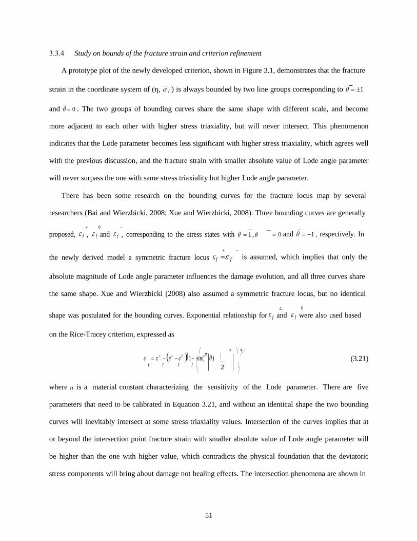
2

Study on bounds of the fracture strain and criterion refinement

A prototype plot of the newly developed criterion, shown in Figure 3.1, demonstrates that the fracture

strain in the coordinate system of (η, σ f ) is always bounded by two line groups corresponding to θ = ±1

and θ = 0 . The two groups of bounding curves share the same shape with different scale, and become

more adjacent to each other with higher stress triaxiality, but will never intersect. This phenomenon

indicates that the Lode parameter becomes less significant with higher stress triaxiality, which agrees well

with the previous discussion, and the fracture strain with smaller absolute value of Lode angle parameter

will never surpass the one with same stress triaxiality but higher Lode angle parameter.

There has been some research on the bounding curves for the fracture locus map by several

researchers (Bai and Wierzbicki, 2008; Xue and Wierzbicki, 2008). Three bounding curves are generally

+ 0 −

proposed, ε f , ε f and ε f , corresponding to the stress states with θ = 1 , θ = 0 and θ = −1 , respectively. In

+ −

the newly derived model a symmetric fracture locus ε f =ε f is assumed, which implies that only the

absolute magnitude of Lode angle parameter influences the damage evolution, and all three curves share

the same shape. Xue and Wierzbicki (2008) also assumed a symmetric fracture locus, but no identical

± 0

shape was postulated for the bounding curves. Exponential relationship for ε f and ε f were also used based

on the Rice-Tracey criterion, expressed as

1 n n

ε = ε ± − (ε ± − ε 0 )1 − sin(π θ ) (3.21) f f f f

where n is a material constant characterizing the sensitivity of the Lode parameter. There are five

parameters that need to be calibrated in Equation 3.21, and without an identical shape the two bounding

curves will inevitably intersect at some stress triaxiality values. Intersection of the curves implies that at

or beyond the intersection point fracture strain with smaller absolute value of Lode angle parameter will

be higher than the one with higher value, which contradicts the physical foundation that the deviatoric

stress components will bring about damage not healing effects. The intersection phenomena are shown in

51

Figure 3.1 with the fitting parameter based on the experimental data in Bai and Wierzbicki (2008). The

+ −

modified GTN model by Nahshon and Hutchinson (2008) and Xue (2008) also both hold the ε f =ε f

assumption by introducing bounded shear damage terms.

Bai and Wierzbicki (2008) also proposed a fracture criterion but with an asymmetric fracture locus

+ −

assumption ε f ≠ε f , based on parabolic behavior in the Lode angle parameter direction, and all bounding

curves were in the same format as the Rice-Tracy criterion but not the same shape. This model is shown

in Equation 3.41 in the appendix, and also encounters the intersection problem. Another priority of the

newly proposed model in Equation 3.18 lies in the description of the behavior in the Lode angle

parameter direction, which in other bounds-based models, such as Xue and Wierzbicki (2008) and Bai

and Wierzbicki (2008), are developed without physical foundation, while in the new model it is based on

the maximum shear criterion.

Figure 3.1 Bounding curves sketch of new criterion

The three fracture-strain bounding curves with distinct shapes will inevitably bring more intersection

phenomena, which might not influence the accuracy in the calibration zone, but will undoubtedly impact

some other prediction ranges. The asymmetric fracture locus may be more accurate when the sign of the

Lode angle parameter cannot be neglected. By assuming the bounding curves to share the same shape, a

52

s θ

co θ

0

0

9

linear modification term is introduced into Equation 3.18 to account for the asymmetric bounds, and the

integrated criterion is express as

ε = c exp(c η)co π c [1 + c (χ − 0.5)] (3.22)

f 7 8

12 6

where χ is the relative ratio of the principal deviatoric stresses, defined as

χ = S II − S III

sinπ

= 6 (1 − θ )

(3.23) S I − S III π s

6

+ − + − + −

and c12 is material constant, such that ε f < ε f when c12 > 0 , ε f > ε f when c12 < 0 , and ε f = ε f when

c12 = 0 . The absolute value of c12 is usually very small, which is shown in the calibration analysis in the

following model verification analysis and calibration section, and indicates that the discrepancy between

+ −

ε f and ε f is insignificant for most ductile materials and can usually be neglected. In this study, only for

data set with very negative Lode angle parameter, Equation 3.22 will be used for calibration instead of

Equation 3.18.

Damage evolution rule

Beside the previously discussed fracture locus as it relates to proportional and quasi-proportional

loading conditions, the rule of damage evolution is critical for non-proportional loading cases. The

damage evolution law is usually expressed in the format of an integral function of stress state, shown as

D = ∫ε p f (η,θ )d ε p (3.24)

in which the stress state parameters, η(ε p ) , andθ(ε p ) , are unique functions of the equivalent plastic strain.

Since the ductile fracture criterion is described in terms of fracture strain, it is reasonable to define the

relative loss of ductility of the material as the damage indicator, and Equation 3. 24 can be transformed

into

D = ∫ε p

1 d ε p , (3.25)

ε f (η,θ )

53

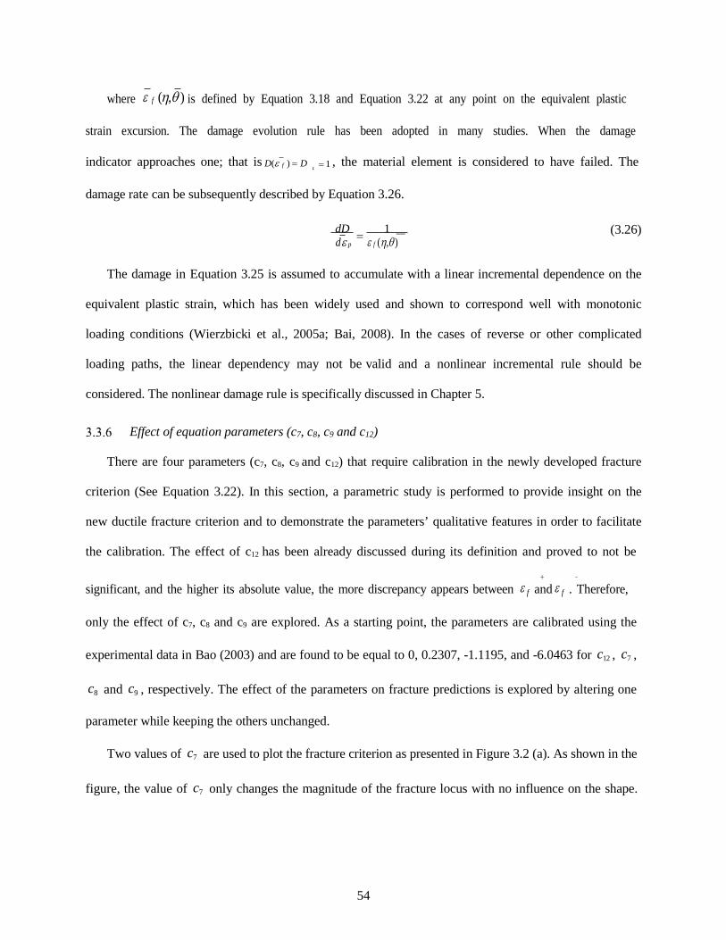
c

where ε f (η,θ ) is defined by Equation 3.18 and Equation 3.22 at any point on the equivalent plastic

strain excursion. The damage evolution rule has been adopted in many studies. When the damage

indicator approaches one; that is D(ε f ) = D = 1 , the material element is considered to have failed. The

damage rate can be subsequently described by Equation 3.26.

dD = 1 (3.26) dε p ε f (η,θ )

The damage in Equation 3.25 is assumed to accumulate with a linear incremental dependence on the

equivalent plastic strain, which has been widely used and shown to correspond well with monotonic

loading conditions (Wierzbicki et al., 2005a; Bai, 2008). In the cases of reverse or other complicated

loading paths, the linear dependency may not be valid and a nonlinear incremental rule should be

considered. The nonlinear damage rule is specifically discussed in Chapter 5.

Effect of equation parameters (c7, c8, c9 and c12)

There are four parameters (c7, c8, c9 and c12) that require calibration in the newly developed fracture

criterion (See Equation 3.22). In this section, a parametric study is performed to provide insight on the

new ductile fracture criterion and to demonstrate the parameters’ qualitative features in order to facilitate

the calibration. The effect of c12 has been already discussed during its definition and proved to not be

+ −

significant, and the higher its absolute value, the more discrepancy appears between ε f and ε f . Therefore,

only the effect of c7, c8 and c9 are explored. As a starting point, the parameters are calibrated using the

experimental data in Bao (2003) and are found to be equal to 0, 0.2307, -1.1195, and -6.0463 for c12 , c7 ,

c8 and c9 , respectively. The effect of the parameters on fracture predictions is explored by altering one

parameter while keeping the others unchanged.

Two values of c7 are used to plot the fracture criterion as presented in Figure 3.2 (a). As shown in the

figure, the value of c7 only changes the magnitude of the fracture locus with no influence on the shape.

54

9

The parameter c7 serves as a positive scalar, and larger c7 values scale up the whole fracture locus. The

parameter c7 is directly related to material ductility.

The parameter c8 always has a non-positive value since ductility decreases with increase in stress

triaxiality. It represents the stress triaxiality effect on the fracture locus and corresponds to the parameter

1.5q2 in the GTN model in Equation 3.11. A comparison of the fracture locus for three values of c8 ( c8 =-

0.1195, -1.1195, and -2.1195) is shown in Figure 3.2 (b). It is clearly demonstrated that the larger the

absolute value of c8 , the more the dependency of the fracture locus on stress triaxiality; the Lode angle

effect is uninfluenced by c8 . The criterion reduces to MS criterion when c8 reaches its limit zero, which

featured with two parallel straight-line bounds. A larger absolute value of c8 scales up the fracture locus

under negative stress triaxiality, while the fracture locus is scaled down in the positive stress triaxiality

range with increasing c8 .

Three values of the parameter c9 are used to explore its effect on the fracture locus as shown in

Figure 3.2 (c). Parameter c9 is also a non-positive value since smaller Lode angle parameter implies more

shear damage accompanied by unaffected tensile damage; hence lower fracture strain. One obvious

feature is that the lower bounding curve remains constant with variation in c9 , which is self-explanatory

since the lower bounds corresponds to θ = 0 and cos(π 6θ)c9 =1. Parameter c represents the Lode angle

effect on the fracture locus. It is observed that increasing the absolute value of c9 raises the upper

bounding curves while decreasing c9 increases the dependency of the fracture locus on Lode angle

parameter. This point has been confirmed by the calibration outputs based on the observed sensitivity of

Al2024 and 1045 steel and the insensitivity of Al5083 and DH36 steel to Lode parameter as discussed in

the following model verification analysis and calibration section. A value of zero for c9 transforms the

criterion into the traditional Rice-Tracey and J-C model, with the bounds ε± = ε 0 . f f

55

(a)

(b)

56

s

(c)

Figure 3.2 Effect of model parameters on fracture locus: (a) Effect of c7 on the new criterion, (b) Effect of c8 on the new criterion and (c) Effect of c9 on the new criterion.

3.3.6 Discussion on the existence of a cut-off region

The existence of a cut-off region in the negative stress triaxiality range of fracture locus map, in

which damage cannot develop and therefore fracture cannot occur, has been initially recognized by Bao

and Wierzbicki (2005) who proposed a uniform cut-off line withηcutoff = −1 3. In the present study, the cut-

off region is studied extensively in Chapter 5 and is defined in Equation 3.27. Figure 3.3 shows

representative cut-off regions including the curve represented by Equation 3.27.

η + 2

co π π

θ − ≤ 0 . (3.27) 3 6 6

57

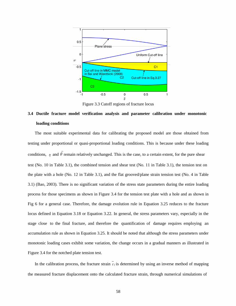
Figure 3.3 Cutoff regions of fracture locus

3.4 Ductile fracture model verification analysis and parameter calibration under monotonic

loading conditions

The most suitable experimental data for calibrating the proposed model are those obtained from

testing under proportional or quasi-proportional loading conditions. This is because under these loading

conditions, η and θ remain relatively unchanged. This is the case, to a certain extent, for the pure shear

test (No. 10 in Table 3.1), the combined tension and shear test (No. 11 in Table 3.1), the tension test on

the plate with a hole (No. 12 in Table 3.1), and the flat grooved/plane strain tension test (No. 4 in Table

3.1) (Bao, 2003). There is no significant variation of the stress state parameters during the entire loading

process for those specimens as shown in Figure 3.4 for the tension test plate with a hole and as shown in

Fig 6 for a general case. Therefore, the damage evolution rule in Equation 3.25 reduces to the fracture

locus defined in Equation 3.18 or Equation 3.22. In general, the stress parameters vary, especially in the

stage close to the final fracture, and therefore the quantification of damage requires employing an

accumulation rule as shown in Equation 3.25. It should be noted that although the stress parameters under

monotonic loading cases exhibit some variation, the change occurs in a gradual manners as illustrated in

Figure 3.4 for the notched plate tension test.

In the calibration process, the fracture strain ε f is determined by using an inverse method of mapping

the measured fracture displacement onto the calculated fracture strain, through numerical simulations of

58

ε 0 ε 0

the tested specimens. The functions of η(ε p ) and θ(ε p ) are also known from the simulations. The

variations of the stress state parameters can be combined and demonstrated in the fluctuation of the

damage rate defined in Equation 3.26, and representatively shown in Figure 3.5 for plates and in Figure

3.6 for general case. The nature of the calibration is to result in a total damage that is as close as possible

to a value of one, where the total damage is calculated through the definite integral of the damage rate

over ε p . Undoubtedly, the variation in the stress state parameters leads to variation in the damage rate

and subsequent difficulties in the calibration process. Therefore, in order to simplify the calibration

process, a numerical integration method is proposed where an averaged damage rate is calculated using

Equation 3.26 while employing average stress state parameters as defined in Equation 3.28. The accuracy

in the estimation method has been examined through the four loading cases shown in Figs. 4 and 5, in

which the Hole means tension test on a plate with a hole, and N6.67, N10, N20 represent tension on plates

with notches with 6.67, 10 and 20 mm radii, which are conducted by Dunand and Mohr (2011), and

another more general case in the format of a circumferentially double notched tube specimen conducted

by Barsoum and Faleskog (2007). The ratios of damage calculated from variable damage rate to the one

from average damage are 0.97, 1.04, 1.03 and 1.05 for the plates and 1.00 for the tube, which indicate

good accuracy of the “average” method. As long as stress state parameters fluctuate gradually and without

sign change in Lode parameters, the integration method should get acceptable accuracy. The averaged

stress state parameters also facilitate the construction of the fracture locus map. Furthermore, the

“averaged” stress state parameter concept has been successfully employed in many studies attempting to

obtain the fracture locus map (Bao and Wierzbicki, 2004; Bai and Wierzbicki, 2010).

ηav = 1

ε

∫ f ηd ε p f

1 ε

and θ av = ∫ f θd ε p . (3.28) f

59

Figure 3.4 The stress triaxiality variations during the loadings of various plates

(Data after Dunand and Mohr, 2011)

Figure 3.5 The damage rate variations and the average damage rate of various plates

Figure 3.6 The stress state and damage rate evolution and the average parameters of a circumferentially

double notched tube specimen (data after Barsoum and Faleskog (2007))

60

The fracture criterion defined in Equation 3.22 comprises of four variables that are yet to be

determined, therefore at least four different tests should be utilized for calibration. Substituting the

experimental data (ηav , θ av , ε f ) to Equation 3.22, a set of at least four nonlinear algebraic equations for c7,

c8, c9 and c12 are obtained. The parameter c12 describes the asymmetry of the fracture strain, and the

calibration for this parameter requires two of the Lode angle parameters to be different in signs.

Calibration of parameter c8 requires two of the triaxiality values to be different in signs. Calibration of c9

requires two distinct absolute values of the Lode angle parameter. There are many groups of test results

for different materials in the literature, mainly for aluminum and steel alloys, and they are used to

calibrate and evaluate the newly developed model. In addition, a comparative study among different

models is performed to evaluate the effectiveness of the proposed model against their existing

counterparts. Since data is scarce for negative Lode angle parameters, Equation 3.18, instead of Equation

3.22, is used unless otherwise specified. If the number of data points is over four, a MATLAB (Matlab

Users Guide, 2011) code is written to obtain the best fitting. Moreover, an optimization function is used

to minimize the relative error function, which is expressed as

Re l.Error (c , c , c , c ) =

1 ∑ (ε f _ Pr edicted − ε f Experiment al )/ ε f Experiment al (3.29) 7 8 9 12 N N

where N is the number of tests analyzed, and N>4.

Application to predict the fracture locus of aluminum alloys

Bao (2003) designed and performed a series of tests on 2024-T351 aluminum for fracture locus

calibration, covering a wide range of stress triaxialities ranging from -0.3 to 1.0. This set of data has been

widely used to provide indications as to the effect of the stress states on the equivalent plastic strain to

fracture in various studies (Lou et al, 2012; Wierzbicki et al, 2005; Bai and Wierzbicki, 2010). The

average stress triaxiality and Lode angle parameter are calculated by Bai and Wierzbicki (2010) and

presented with the corresponding equivalent fracture plastic strain in Table 3.1. Seidt (2010) also

performed a series of tests on 2024-T351 aluminum alloy, also presented in Table 3.1 with the same

format with Bao’s data set. The Seidt’s data set is first used for calibration, and then Bao’s set is

61

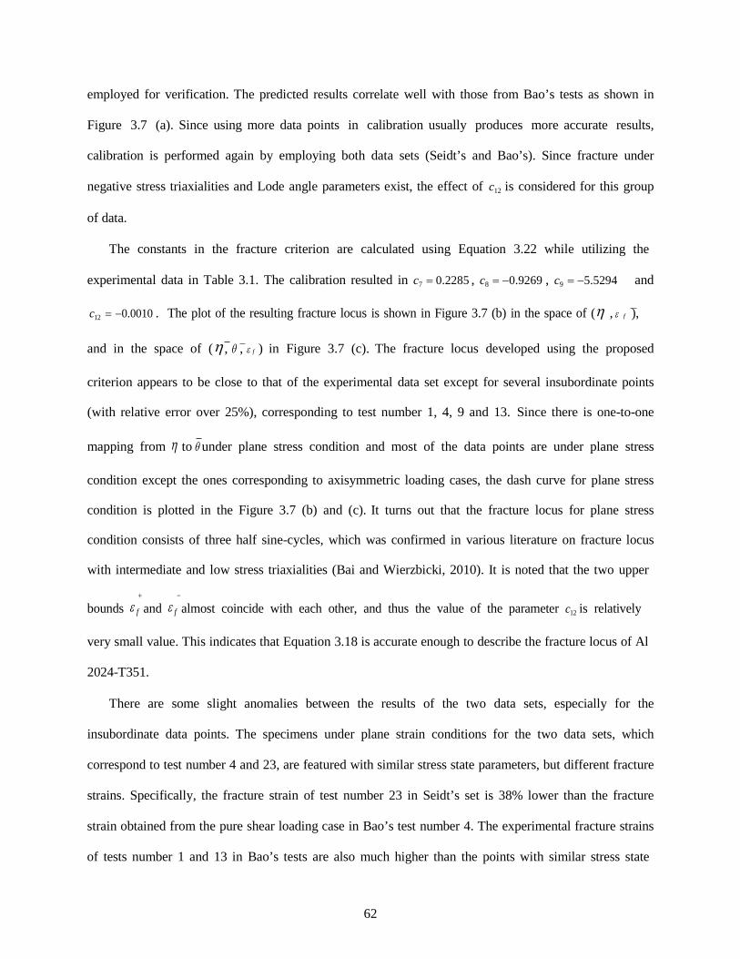
employed for verification. The predicted results correlate well with those from Bao’s tests as shown in

Figure 3.7 (a). Since using more data points in calibration usually produces more accurate results,

calibration is performed again by employing both data sets (Seidt’s and Bao’s). Since fracture under

negative stress triaxialities and Lode angle parameters exist, the effect of c12 is considered for this group

of data.

The constants in the fracture criterion are calculated using Equation 3.22 while utilizing the

experimental data in Table 3.1. The calibration resulted in c7 = 0.2285 , c8 = −0.9269 , c9 = −5.5294 and

c12 = −0.0010 . The plot of the resulting fracture locus is shown in Figure 3.7 (b) in the space of (η , ε f ),

and in the space of (η , θ , ε f ) in Figure 3.7 (c). The fracture locus developed using the proposed

criterion appears to be close to that of the experimental data set except for several insubordinate points

(with relative error over 25%), corresponding to test number 1, 4, 9 and 13. Since there is one-to-one

mapping from η to θ under plane stress condition and most of the data points are under plane stress

condition except the ones corresponding to axisymmetric loading cases, the dash curve for plane stress

condition is plotted in the Figure 3.7 (b) and (c). It turns out that the fracture locus for plane stress

condition consists of three half sine-cycles, which was confirmed in various literature on fracture locus

with intermediate and low stress triaxialities (Bai and Wierzbicki, 2010). It is noted that the two upper

+ −

bounds ε f and ε f almost coincide with each other, and thus the value of the parameter c12 is relatively

very small value. This indicates that Equation 3.18 is accurate enough to describe the fracture locus of Al

2024-T351.

There are some slight anomalies between the results of the two data sets, especially for the

insubordinate data points. The specimens under plane strain conditions for the two data sets, which

correspond to test number 4 and 23, are featured with similar stress state parameters, but different fracture

strains. Specifically, the fracture strain of test number 23 in Seidt’s set is 38% lower than the fracture

strain obtained from the pure shear loading case in Bao’s test number 4. The experimental fracture strains

of tests number 1 and 13 in Bao’s tests are also much higher than the points with similar stress state

62

parameters in the Seidt’s data set, and this unconformity sometimes may result in large variation in the

calibration.

Overall, it is found that when properly calibrated, the new criterion predicts the trends of the

experimental results very well. On the other hand, the best fit for the Rice-Tracey fracture model (Rice

and Tracey, 1969), expressed in Equation 3.30 and depicted in Figure 3.7 (a) and (b), fails to provide

reasonable prediction for this data set.

ε f = 0 .3574 exp( − 0 .5063 η ) (3.30)

Gao et al. (2009) carried out a series of tests on aluminum 5083 alloy covering a wide range of stress

triaxialities for the cases of θ = 0 and θ = 1 . The optimized bounding curves and predicted fracture strains

based on the new model are plotted in Figure 3.8, and show excellent agreement with test results. Unlike

Al 2124-T351, only minor Lode angle parameter dependency is observed for aluminum 5083 alloy while

stronger stress triaxiality dependency is identified in comparison with Al 2124-T351. Therefore, it can be

concluded that the dependency of ductility on Lode angle parameter and stress triaxiality vary with the

type of aluminum alloy being investigated. Although a slightly worse fitting is observed when the Rice-

Tracey model is used, the R-C model still provides satisfactorily prediction of the trends of the facture for

all the data points. This confirms that the Rice-Tracey criterion can provide acceptable predictions for

materials that are insensitive to the Lode parameter.

63

Specimen description ηav θ av ε f

Smooth round bar, tension 0.4014 0.9992 0.4687

Round large notched bar, tension 0.6264 0.9992 0.2830

Round small notched bar, tension 0.9274 0.9984 0.1665

Flat grooved/plane strain, tension 0.6030 0.0754 0.2100

Cylinder(d0/h0=0.5), compression -0.2780 -0.8215 0.4505

Cylinder(d0/h0=0.8), compression -0.2339 -0.6809 0.3800

Cylinder(d0/h0=1.0), compression -0.2326 -0.6794 0.3563

Cylinder(d0/h0=1.5), compression -0.2235 -0.6521 0.3410

Round notched, compression -0.2476 -0.7141 0.6217

Simple/pure shear 0.0124 0.0355 0.2107

Shear & tension 0.1173 0.3381 0.2613

Plate with a circular hole, tension 0.3431 0.9661 0.3099

Dog-bone specimen, tension 0.3570 0.9182 0.4798

Pipe, tension 0.3557 0.9286 0.3255

Solid square bar, tension 0.3687 0.9992 0.3551

Round notched bar (Radius: 3.04mm), tension

0.8551 1 0.2029

Round notched bar (Radius: 4.47mm), tension

0.7631 1 0.2447

Round notched bar (Radius: 6.10mm), tension

0.6760 1 0.2736

Round notched bar (Radius: 9.14mm), tension

0.6076 1 0.2904

Round notched bar (Radius: 14.5mm), tension

0.5243 1 0.3074

Smooth round bar, tension 0.3481 1 0.3223

Flat grooved/plane strain, tension 0.5797 0 0.1037

Simple/pure shear 0 0 0.1680

Table 3.1 Summary of the experimental data set for Al 2024-T351. (Test 1~15 are from Bao (2003) and Bai and Wierzbicki, 2010; test 16~23 are from Seidt (2010))

Test

No. ε f _ Pr edicted

1 0.3486

2 0.2830

3 0.2138

4 0.1312

5 0.5011

6 0.4023

7 0.4051

8 0.3904

9 0.4269

10 0.2261

11 0.2236

12 0.3485

13 0.3193

14 0.3248

15 0.3593

16 0.2292

17 0.2496

18 0.2706

19 0.2883

20 0.3114

21 0.3667

22 0.1335

23 0.2285

64

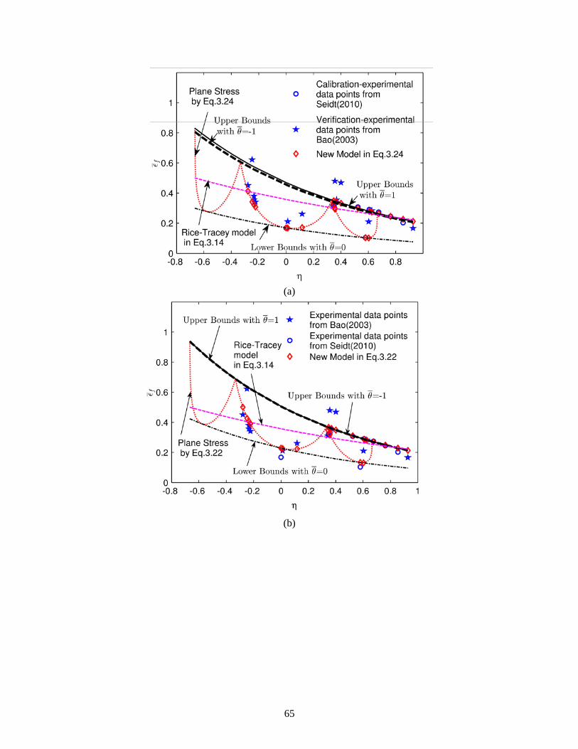
(a)

(b)

65

(c)

Figure 3.7 The fracture locus constructed with the new criterion for Al 2124-T351: (a) The new fracture locus for 2024-T351 aluminum alloy on the plane ofεf and η (Calibrated from Seidt’s data set), (b) The new fracture locus for 2024-T351 aluminum alloy on the plane ofεf and η (Calibrated from both data

sets), and (c) 3D representation of the new fracture criterion for 2024-T351 aluminum alloy (Calibrated from both data sets).

Figure 3.8 The fracture locus constructed with the new model for Al 5083

(Experimental data from Gao et al. (2009))

Application to predict the fracture locus of various steel grades

Barsoum and Faleskog (2007) designed and performed a series of bi-axial tension/torsion loading

tests up to fracture on circumferentially double notched tube specimens made of Weldox 420 and 960

66

steel. The predicted fracture strains based on the new model and their experimental equivalents are plotted

in the space of (η , ε f ) in Figure 3.9 (a) and (c), respectively, and the 3D plots are shown in Figure 3.9 (b)

and 9(d) in the space of (η,θ , ε f ), respectively. Although not statistically perfectly fitted, the fracture

trends are still well-fitted for the two data groups. As shown in the figures, the Rice-Tracey fracture

model again failed to provide even a rough prediction as a result of the fracture being highly dependent on

Lode parameter. Calibration of the constants in Equation 3.18 resulted in c7 = 0.9334 , c8 = −0.2403 , and

c9 = −3.4631 for Weldox 420 steel and c7 = 1.0901 , c8 = −1.3746 and c9 = −6.6868 for Weldox 960 steel.

The parameters for the Rice-Tracey criterion are c5 = 0.9593 and c6 = −0.1322 for Weldox 420 steel and

c5 = 0.8452 , c6 = −0.6822 for Weldox 960 steel.

It should be noted that the two types of steel from the same manufactures shows distinct stress

triaxiality dependency. The fracture strain for Weldox 420 steel generally does not depend on stress

triaxiality, with c8 = −0.2403 whereas Weldox 960 is very sensitive to stress triaxiality, with c8 = −1.3746 ,

which confirm the findings in the parametric study on c8 . The fracture locus maps for both types of the

steel are, however, very sensitive to the Lode angle parameter as observed by the large negative value for

c9 of -3.4631 and -6.6868 for Weldox 420 and 960 steel, respectively.

(a)

67

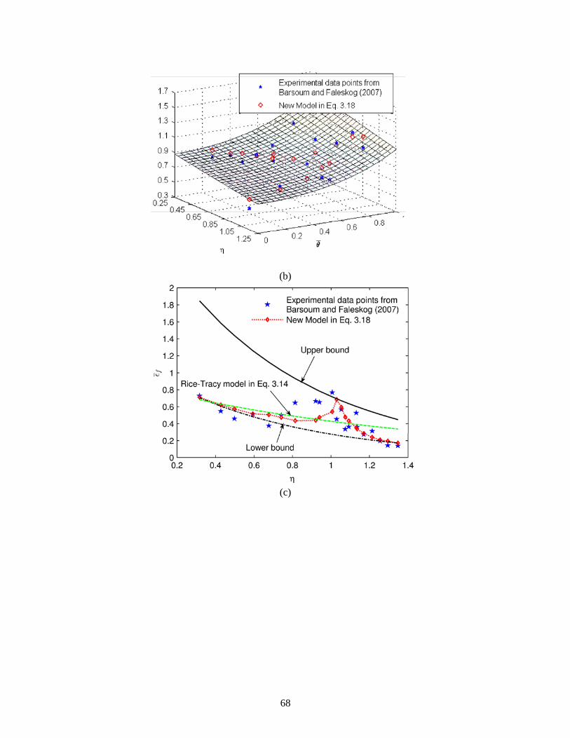
(b)

(c)

68

(d)

Figure 3.9 The fracture locus constructed with the new criterion for Weldox steel: (a) The new fracture locus for Weldox 420 steel on the plane of ε f and η , (b) 3D representation of the new fracture criterion for Weldox 420 steel, (c) The new fracture locus for Weldox 960 steel on the plane of ε f and η , and (d)

3D representation of the new fracture criterion for Weldox 960 steel

Wierzbicki et al. (2005b) designed and performed a series of tests on butterfly-shaped specimens

made of A710 steel, including eight loading cases with a wide range of stress triaxiality and Lode angle

parameter range. Since data for several specimens tested under negative Lode angle parameter exists, the

effect of c12 is considered for this group of data. The predicted and experimental fracture locus is plotted

in the space of (η , ε f ) as shown in Figure 3.10 (a). The 3D fracture locus in the space of (η ,θ , ε f ) is

shown in Figure 3.10 (b). Calibration of the model parameters resulted in c7 = 2.4564 , c8 = −0.4600 ,

c9 = −2.3441 , and c12 = −0.0360 . The prediction agrees well with the experimental results except for two

insubordinate points as shown in Figure 3.10 (a). The parameter c12 is still found to be insignificant, as is

the difference between the two upper fracture bounding curves. Therefore, it can be noted that Equation

3.22 does not outperform Equation 3.18 in a notable manner when applied to 710 steel for predicting

fracture.

69

The variation in the ductility-dependence of different material on stress triaxiality and Lode angle

parameter is confirmed by the experimental results in Bai et al. (2009). The 1045 and DH36 steel were

examined through evaluating the failure strain in axisymmetric specimens with different notch radii and

grooved specimens with different groove radii. The experimental as well as the predicted fracture locus

and bounding curves are plotted in Figure 3.11. It is clearly shown that the influence of Lode angle

parameter on ductility is more significant for 1045 steel and there is almost no Lode angle effect on DH36

since the bounding curves are close to each other and even reversely located: the lower bound shows

higher strains. It is observed that DH36 steel exhibits higher ductility, corresponding to a larger

c7 = 6.7509 compared to 1045 steel with c7 = 1.0517 , which correlates with the discussion on the effect of

c7 .

(a)

70

(b)

Figure 3.10 The fracture locus constructed with the new criterion for A710 steel: (a) The new fracture locus for A710 steel on the plane of ε f and η , and (b) 3D representation of the new fracture criterion for

A710 steel

Figure 3.11 Comparison of fracture locus between 1045 and DH36 steel (Experimental data from Bai et al. (2009))

The experimental results for 1045 steel in Bai et al. (2009), shown in Figure 3.11, are based on testing

classical specimens, including notched and smooth bars, grooved plates, and Tubular specimens. Another

group of experimental data for 1045 steel is also available in Bai (2008), which is obtained from testing

71

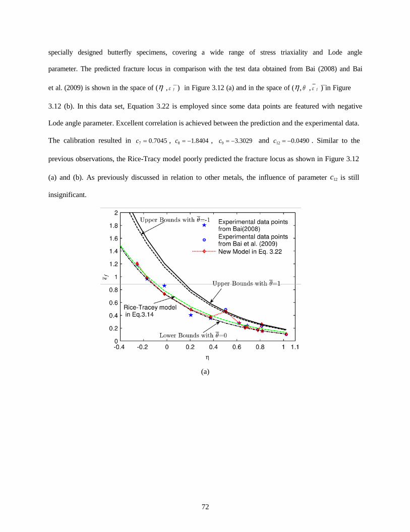
specially designed butterfly specimens, covering a wide range of stress triaxiality and Lode angle

parameter. The predicted fracture locus in comparison with the test data obtained from Bai (2008) and Bai

et al. (2009) is shown in the space of (η , ε f ) in Figure 3.12 (a) and in the space of (η, θ , ε f ) in Figure

3.12 (b). In this data set, Equation 3.22 is employed since some data points are featured with negative

Lode angle parameter. Excellent correlation is achieved between the prediction and the experimental data.

The calibration resulted in c7 = 0.7045 , c8 = −1.8404 , c9 = −3.3029 and c12 = −0.0490 . Similar to the

previous observations, the Rice-Tracy model poorly predicted the fracture locus as shown in Figure 3.12

(a) and (b). As previously discussed in relation to other metals, the influence of parameter c12 is still

insignificant.

(a)

72

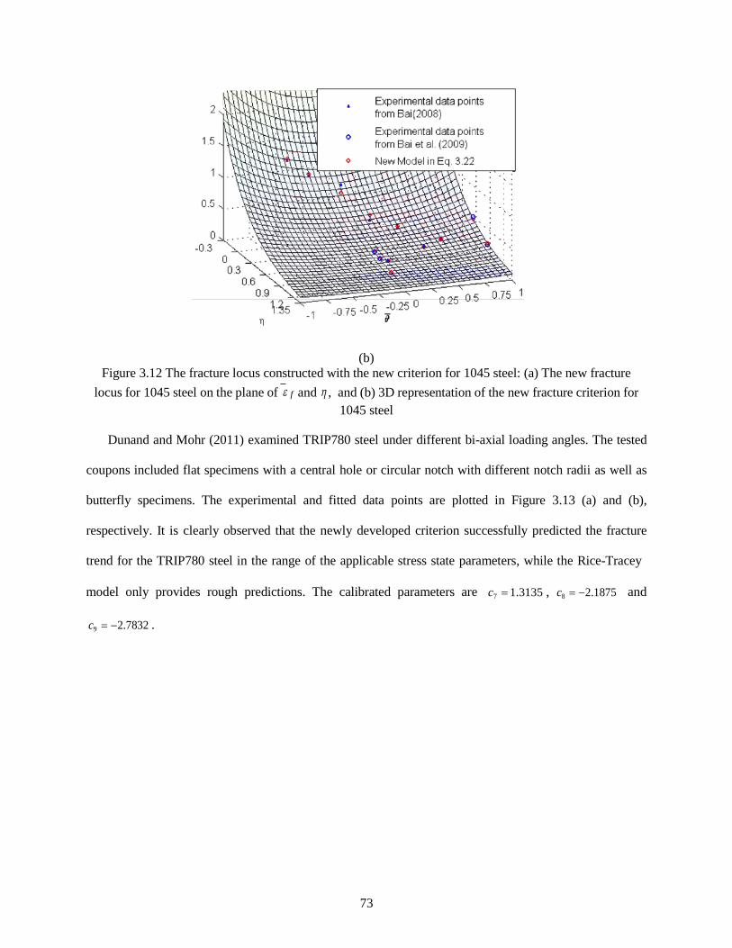
(b) Figure 3.12 The fracture locus constructed with the new criterion for 1045 steel: (a) The new fracture

locus for 1045 steel on the plane of ε f and η , and (b) 3D representation of the new fracture criterion for 1045 steel

Dunand and Mohr (2011) examined TRIP780 steel under different bi-axial loading angles. The tested

coupons included flat specimens with a central hole or circular notch with different notch radii as well as

butterfly specimens. The experimental and fitted data points are plotted in Figure 3.13 (a) and (b),

respectively. It is clearly observed that the newly developed criterion successfully predicted the fracture

trend for the TRIP780 steel in the range of the applicable stress state parameters, while the Rice-Tracey

model only provides rough predictions. The calibrated parameters are c7 = 1.3135 , c8 = −2.1875 and

c9 = −2.7832 .

73

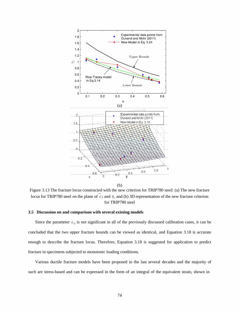
(a)

(b)

Figure 3.13 The fracture locus constructed with the new criterion for TRIP780 steel: (a) The new fracture locus for TRIP780 steel on the plane of ε f and η , and (b) 3D representation of the new fracture criterion

for TRIP780 steel

3.5 Discussion on and comparison with several existing models

Since the parameter c12 is not significant in all of the previously discussed calibration cases, it can be

concluded that the two upper fracture bounds can be viewed as identical, and Equation 3.18 is accurate

enough to describe the fracture locus. Therefore, Equation 3.18 is suggested for application to predict

fracture in specimens subjected to monotonic loading conditions.

Various ductile fracture models have been proposed in the last several decades and the majority of

such are stress-based and can be expressed in the form of an integral of the equivalent strain, shown in

74

Appendix A. Bao and Wierzbicki (2004) indicated and proved that the Cockcroft-Latham criterion and its

normalized version (i.e. the Oh criterion (CLO)), characterized by the maximum principal stress, provide

good predictions in negative and very low stress triaxiality ranges, but not for most positive stress

triaxiality cases. The MS criterion, as previously discussed, is quite accurate in low and negative stress

triaxiality ranges. Criteria only considering the maximum principal and shear stress with the use of

appropriate weighting function may provide good results in the negative, low, and intermediate stress

range, but not in the high stress triaxiality regions. This includes for example the Mohr-Coulomb criterion

and its modified version (Modified Mohr-Coulomb (MMC) criterion in Bai and Wierzbicki (2010)). The

Rice-Tracey and Johnson-Cook criteria have been so far the most utilized in fracture predictions under

high stress triaxiality and many variations on the same theme been proposed and shown to provide

accurate predictions in their applicable ranges, including for example the void growth model (VGM)

model by Kanvinde and Deierlein (2007).

In this study, predictions obtained using the newly developed criterion are compared with those

obtained using the Cockcroft-Latham-Oh (CLO) criterion in the negative stress triaxiality range, the

MMC model under low and negative stress triaxiality, and the Rice Tracey/Johnson-Cook/VGM

(RT/JC/VGM) model in the high stress triaxiality regions. The fracture data for Al 2024-T351 in Bao

(2003) and Seidt (2011), shown in Table 3.1, was taken as the sample in these comparisons because of its

wide stress triaxiality and Lode angle parameter range.

The RT/JC criterion is calibrated from axisymmetric specimens and the CLO model is calibrated

from specimens with negative stress triaxialities. The MMC criterion is featured with three or four

parameters only when non-quadratic yield function is employed and the number of parameters reduces to

only two when the von Mises yield surface is applied as shown in Equation 3.40 in the appendix. In this

comparison the four-parameter version is adopted for the sake of accuracy. The newly developed Bai-

Wierzbicki model in Bai and Wierzbicki (2008), featured with three unequal shaped bounds and six

parameters, is among the most popular and accurate fracture criteria and is also adopted in the comparison.

75

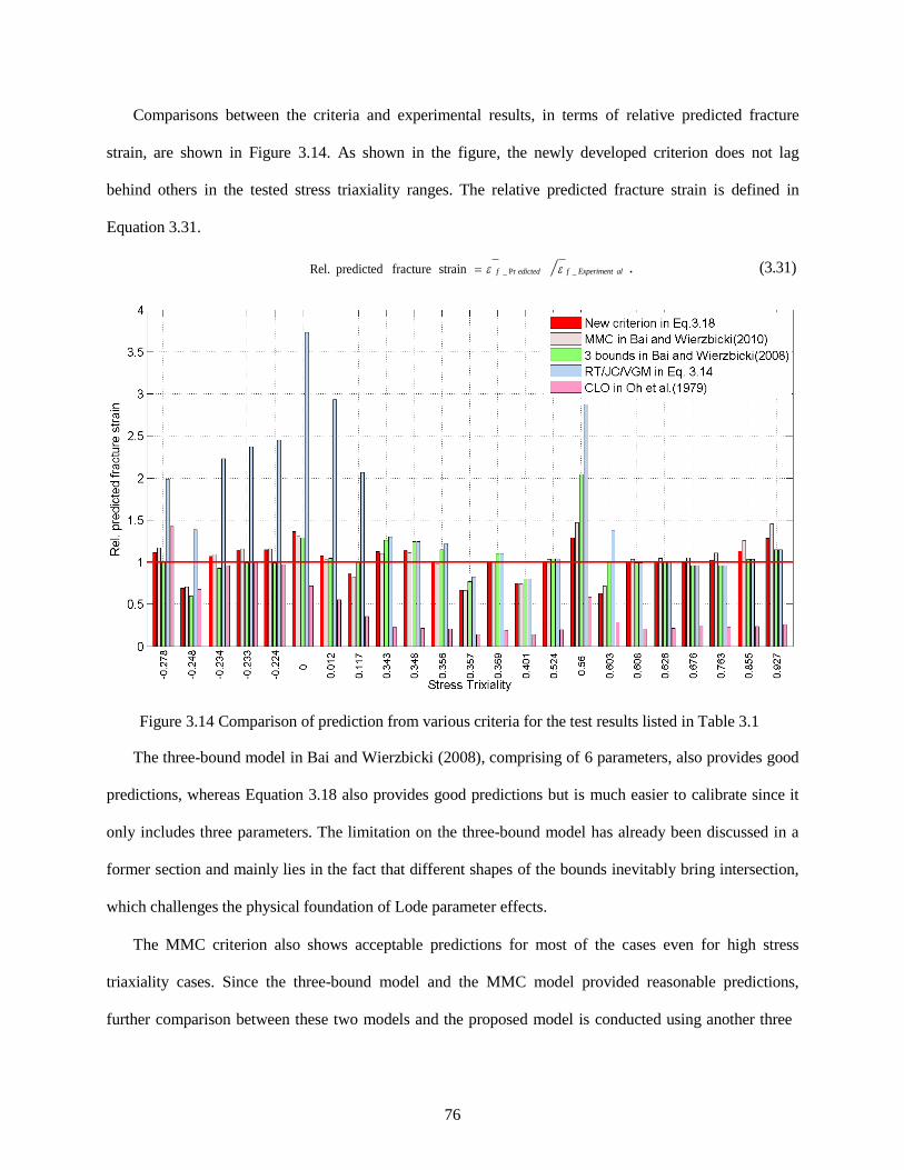
Comparisons between the criteria and experimental results, in terms of relative predicted fracture

strain, are shown in Figure 3.14. As shown in the figure, the newly developed criterion does not lag

behind others in the tested stress triaxiality ranges. The relative predicted fracture strain is defined in

Equation 3.31.

Rel. predicted fracture strain = ε f _ Pr edicted ε f _ Experiment al . (3.31)

Figure 3.14 Comparison of prediction from various criteria for the test results listed in Table 3.1

The three-bound model in Bai and Wierzbicki (2008), comprising of 6 parameters, also provides good

predictions, whereas Equation 3.18 also provides good predictions but is much easier to calibrate since it

only includes three parameters. The limitation on the three-bound model has already been discussed in a

former section and mainly lies in the fact that different shapes of the bounds inevitably bring intersection,

which challenges the physical foundation of Lode parameter effects.

The MMC criterion also shows acceptable predictions for most of the cases even for high stress

triaxiality cases. Since the three-bound model and the MMC model provided reasonable predictions,

further comparison between these two models and the proposed model is conducted using another three

76

groups of data. In the following comparative analysis, the von Mises version of the MMC criterion in

Equation 3.40 is adopted since the other two criteria utilize quadratic constitutive equations.

The three groups of data used for comparison are Al 5083 from Gao et al. (2009), Weldox 960 steel

from Barsoum and Faleskog (2007), and 1045 steel from Bai (2008) and Bai et al. (2009), which were all

analyzed in a former section. The relative error defined in Equation 3.29 is used as the main indicator of

the prediction accuracy and is listed in Table 3.2 for all three models. It is clearly shown that the MMC

criterion lags behind in terms of predictions for all metal grades, while the other two criteria provide

predictions at the same accuracy level. For Al 2024 T351 and Weldox 960 steel, the MMC criterion offers

reasonable predictions, while for Al 5083 and 1045 steel the MCC predictions are substantially erroneous.

The causes of such errors lie in the fact that the Lode angle parameter effect dominates in the MMC

model. If the metal is Lode parameter sensitive, the MMC model may provide acceptable predictions.

However, for metals with less Lode parameter dependency the minor stress triaxiality effect in the model

cannot track the fracture locus trends accurately. It can also be confirmed from the value of parameter c9 ,

listed in Table 3.2, that the large absolute value of c9 represents more Lode parameter dependency as

previously discussed.

The verification analysis discussed above includes various types of steel and aluminum alloy. It is

noted that even for the same metal type conducted by the same researcher in different group, the

experimental results still show some discreteness, and the divergence is more inevitable for specimens of

different researchers. For some metals, the average relative error is not insignificant, but still sufficient to

show the predicting trend. The resulting error may be due to various reasons, such as unexpected

machinery damage, discrepancy from manufacture and testing instrument, and possible different test

procedure. However, generally good correlations are achieved for all the materials, which strongly

demonstrate the validity of the newly developed criteria under monotonic loading conditions. It also

indicates the urgent demand on the fracture properties for the calibration of widely used metals including

structural steel.

77

New criterion

Metal grades in Equation

Table 3.2 Summary of relative error of fracture strain predictions using the new criterion in Equation 3.18, the three bounds criterion, and the MMC criterion

Three-bound

MMC criterion criterion c7 c8 c9

3.18

Al 2024 T351 14.56% 14.74% 17.22% 0.2285 -0.9269 -5.5294

Al 5083 4.95% 4.83% 33.48% 0.5454 -1.4082 -0.8766

Weldox 960

steel

21.71%

22.36%

32.67%

0.8452

-1.3746

-6.6868

1045 steel 4.9% 6.76% 44.8% 0.7045 -1.8404 -3.3029

3.6 Summary and conclusion

In this chapter, a new ductile fracture model under monotonic loading is proposed and the role of

stress triaxiality and Lode angle parameter in characterizing metal fracture locus map are assessed. It

turns out that the two kinds of damage owing to hydrostatic stress and deviatoric stress, respectively, in

terms of stress triaxiality and Lode parameter, are regarded to constantly exist regardless of the stress

state amplitudes. However, their relative magnitudes vary with the fluctuation of the stress states. The

damage due to the deviatoric stress components is relatively small in comparison with the one from the

hydrostatic stress in the high triaxiality range where tensile fracture usually occurs. In the negative stress

triaxiality range, the role of Lode parameter and stress triaxiality is opposite and shear-type fracture

prevails. On the other hand, in the low stress triaxiality domain the two effects compete and neither of

them can be neglected. Founded on the concepts discussed above, the three/four parameter ductile

fracture model is developed, with the consideration of the effects of both the hydrostatic and deviatoric

stress components. The corresponding fracture strain locus map is shown to exhibit a decreasing

exponential function of the stress triaxiality coupled with an asymmetric cosine function of the Lode

angle parameter. A detailed verification and parametric study is performed on the newly proposed

fracture model and the results are summarized as follows.

78

• The asymmetry of the Lode angle parameter is insignificant and parameter c12 always exhibits

very small value for all the correlated experimental data sets. Thus, the four parameter fracture

criterion in Equation 3.22 can be reduced to the three parameter model in Equation 3.18 without

noticeable loss of accuracy.

• Increasing parameter c7 shifts the fracture strain locus map without changing its map, which

indicates that the parameter is only directly related to the ductility of material.

• Parameter c8 is designed to describe the stress triaxiality dependency and increasing the absolute

value of c8 will increase the effect of the stress triaxiality or the hydrostatic stress in general.

• The dependency of the Lode angle parameter, or the deviatoric stress, is represented by parameter

c9 and the increase in the absolute value of c9 raises the upper bounding curves and enlarges the

influence the Lode angle parameter.

• The cutoff region of the fracture locus map exists in the negative stress triaxiality range, shown in

Equation 3.30, where damage will not accumulate and hence fracture will not occur.

• The exit bounds on the fracture strain locus map and the bounding curves may share the same

shape but should not intersect with each other.

The verification analysis of the proposed model includes comparison with experimental data obtained

for various types of aluminum alloys and steel grades. For all types of metals evaluated, satisfactory

correlations are achieved. Hence, it can be concluded that the proposed model is valid and can be applied

for metal fracture predictions. The fracture model parameters for the cited metal types are calibrated and

further calibration should be conducted for verification of other conventional structural metal types. The

dependency of the fracture strain locus map on the stress triaxiality and Lode angle parameter varies for

different type of metal alloys and both of Al 5083 and 1045 steel are insensitive to the effect of Lode

angle parameter. The DH36 steel, on the other hand, shows relatively minor stress triaxiality dependency

compared to others.

79

A comparative study is performed among the most popular ductile fracture criteria and, even in each

model’s prevailing ranges, the newly proposed criterion does not lag behind others. This model with

focus on the monotonic loading conditions has been extended to reverse loading in Chapter 5. With the

above-mentioned merits, the newly proposed model has great potential for many practical engineering

applications.

80

CHAPTER 4 Validation and Implementation of the New Fracture Model to Structural

Details under Monotonic Loadings

4.1 Introduction

Block shear is one of the governing failure modes for bolted connections. In a block shear failure, a

block of material is partially or entirely torn out from the parent component. The most significant feature

of block shear is the presence of varying stress state conditions, that cause the fracture to propagate on a

tension and shear plane and in some cases with additional inclined planes. The presence of these different

failure paths undoubtedly will have an impact on the resulting connection strength and ductility.

Therefore, the ability to model such failure can provide very useful information on the true behavior of

the connection. It is important to note that simulations conducted in previous studies, due to limitations in

modeling capabilities, were unable to capture failure of the connection (i.e., no crack initiation or

propagation). This is because capturing such failure requires the utilization of a fracture model that can

allow for the development of tension and shear failures in the connection. In other words, a unified ductile

fracture models that is applicable to a wide range of stress triaxiality and Lode parameter is required for

proper predictions.

The most representative block shear fractures are usually associated with gusset plate and coped beam

connections. In gusset plate connections, the development of block shear is due to direct tension loading

on a member connected to the gusset plate. There have been many laboratory tests on gusset plate

connections and accurate and reliable data have been obtained from these tests (Whitmore, 1952; Hardash

and Bjorhovde, 1984; Bjorhovde and Chakrabarti, 1985; Nast et al., 1999; Huns et al., 2002; and many

others). However, tests that included the entire fracture process up to and including failure, with focus on

the fracture mechanism are relatively limited. In coped beam connections, the development of block shear

is a result of pure shear loading at the connection that could be coupled with the second moment carried

by the connection because of beam rotation. Compared to gusset plate connections, bolted coped beams

81

are featured with asymmetric stress distribution resulting from the complex loading conditions. As a

result, the failure path is also often time asymmetrical and thus existing gusset plate failure tests cannot

directly be extended to the bolted coped beam connections. Block shear failure in coped beams was first

identified by Birkemoe and Gilmor (1978) through a comparative testing that included one coped and the

another un-coped beam, and subsequently confirmed through testing conducted by Yura et al. (1982),

Ricles and Yura (1983), and Aalberg and Larsen (2000). Franchuk et al. (2002) conducted seventeen full-

scale tests on coped beams with bolted double angle connections in order to evaluate the influence of

multiple variables related to geometry and loading conditions on failure. Fang et al. (2013) and Lam et al.

(2015) also conducted several groups of tests in order to investigate the effect of single angle bolted and

double bolt-line on the behavior and failure of the connections.

Due to the high cost and limitations associated with full-scale tests, numerical simulation can serve as

a substitute or supplement to testing and can provide meaningful insight on complex phenomena.

Numerical simulation on connections, pertaining to block shear, evolved from the two-dimensional linear

elastic and nonlinear finite element models (Ricles and Yura, 1983; Huns et al., 2002; Franchuk et al.,

2002; Wen and Mahmoud, 2015a ) to three-dimensional solid element nonlinear models (Yam et al., 2007;

Wei et al., 2010; Yam et al., 2011; Fang et al., 2013). The previous studies provided viable predictions of

connection strength in some cases but not in other cases. In addition, limitations in modeling capabilities

did not allow for the development and propagation of cracks, which are essential to include for reliable

predictions of connection capacity and ductility.

In this chapter, numerical simulations on block shear in gusset plate and coped beam connections are

conducted up to and including total failure, through the application of a newly developed ductile fracture

criterion with consideration of both the stress triaxiality and Lode angle parameter. The laboratory test

results from Huns et al. (2002) and Franchuk et al (2002) are utilized for validation of the numerical

modeling approach and for comparing the outcome of the numerical study to real experimental data and

observations. The comparisons include load verses displacement curves, fracture sequence, and fracture

profile. Through the numerical simulations, the inherent mechanisms of block shear in gusset plate and

82

coped beam connections are thoroughly discussed including the effect of various levels of beam end

rotations on connection behavior. Thereafter, a parametric study is conducted with focus on geometrical

variables, including bolt spacing in the tensile and shear planes, and bolt edge/end distances. Through the

parametric study, four different fracture modes are identified and analyzed for the first time, and

contradictions between the numerically obtained predictions and those predicted using the design

equations are found and shown, which indicates the needs for further design code modification.

4.2 Validation analysis of the numerical simulation methodology

The most common structural members prone to block shear failure are gusset plate and coped beam

connections, which have been widely tested in laboratories. Therefore, validating the numerical

simulation methodology using these two connection types is a logical choice. In this section, the

numerical simulation approach using the developed ductile fracture criterion is validated for an ensemble

of gusset plate and coped beam connections through comparison between the numerical simulation results

and the corresponding experimental equivalents. These comparisons include load versus displacement

curves, fracture sequence, and final fracture profiles.

Case 1: Rectangular gusset plate connections

4.2.1.1 Brief description of laboratory tests

There are many experimental programs on gusset plate connections with the majority of which

terminated soon after fracture initiation; hence lacking information on fracture propagation. Laboratory

tests on gusset plate connections up to and including failure however were conducted by Huns et al.

(2002), and therefore are ideal candidates for validating the numerical models. Two configurations,

named as T1 and T2, which were loaded up to total failure in tension are chosen for the validation. A

simple sketch of the two test setups is shown in Figure 4.1. The displacement, ∆, in Figure 4.1 was

monitored along the centerlines of the connections, which together with the loading force, F, were used to

generate the load-displacement curve of the connection. More details of the experimental set up can be

found in Huns et al. (2002), including photos of the fracture profiles and specimen configurations.

83

Mon

itore

d Di

spla

cem

ent

∆

Mon

itore

d Di

spla

cem

ent

∆

Connection T1

F Connection T2

F

Top load transfer plate

Top splice plate

Gusset plate

Modeled zone

Bottom splice plate

Bolts in load transfer zone

Bolts in potential fracture zone

Bottom load transfer plate

F F (a) (b)

Figure 4.1 Tests set up for gusset plate connections: (a) Specimen T1, and (2) Specimen T2, after Huns et al., 2002

84

4.2.1.2 Description of numerical modeling

The general finite element (FE) program ABAQUS/Explicit (Simulia, 2012) was employed in the

present numerical simulations. Since both gusset plate connections, against which the simulations will be

compared, showed minute to no out-of-plane deformations during the entire test, two dimensional plane

stress elements CPS4R were employed in the simulations. A refined mesh size with 1×1 mm resolution

was used at and around the fracture zones. Taking advantage of symmetry, only half of the specimen was

modeled to reduce the computational time as marked by the “modeled zone” with a large dashed box in

Figure 4.1. Nonlinear material behavior was introduced through the isotropic hardening model embedded

in ABAQUS, and the material parameters are adopted based on the corresponding coupon tests in Huns et

al. (2002). Since the experimental program was designed for investigating fracture in the gusset plate, the

bolts were designed with large safety factors where only minor deformation would occur in all bots.

Therefore, the bolts in this study were modeled as rigid bodies. The load in the analysis was simulated

though displacements of the bolts. A friction coefficient of 0.3, representing Class C slip factor for

untreated hot rolled steel per the 2010 AISC Specifications (AISC LRFD, 2010), was used primarily to

introduce the bolt-plate interaction. The upper boundary conditions were modeled as fixed, where there

are only insignificant stress/strain fields. A typical numerical model of a gusset plate is shown in Figure

4.2 for specimen T2.

85

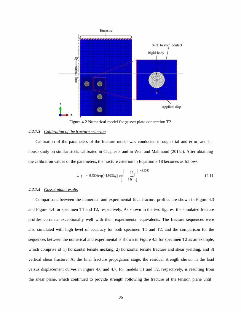
Figure 4.2 Numerical model for gusset plate connection T2

4.2.1.3 Calibration of the fracture criterion

Calibration of the parameters of the fracture model was conducted through trial and error, and in-

house study on similar steels calibrated in Chapter 3 and in Wen and Mahmoud (2015a). After obtaining

the calibration values of the parameters, the fracture criterion in Equation 3.18 becomes as follows,

π −3.3546 ε f = 0.7506exp(−1.9232η )cos θ (4.1)

4.2.1.4 Gusset plate results

6

Comparisons between the numerical and experimental final fracture profiles are shown in Figure 4.3

and Figure 4.4 for specimen T1 and T2, respectively. As shown in the two figures, the simulated fracture

profiles correlate exceptionally well with their experimental equivalents. The fracture sequences were

also simulated with high level of accuracy for both specimen T1 and T2, and the comparison for the

sequences between the numerical and experimental is shown in Figure 4.5 for specimen T2 as an example,

which comprise of 1) horizontal tensile necking, 2) horizontal tensile fracture and shear yielding, and 3)

vertical shear fracture. At the final fracture propagation stage, the residual strength shown in the load

versus displacement curves in Figure 4.6 and 4.7, for models T1 and T2, respectively, is resulting from

the shear plane, which continued to provide strength following the fracture of the tension plane until

86

complete fracture. Very strong correlation is also observed between the experimental and numerical load

versus displacement curves as shown in Figure 4.6 and 4.7 for connection T1 and T2, respectively, which

can be attributed to the high level of accuracy in simulating the fracture sequence. It is important to note

that fracture was introduced in the models through element deletion once the damage in Equation 3.25

reaches the critical value 1.

Figure 4.3 Comparison between the experimental and numerical fracture profiles of T1 connection

Figure 4.4 Comparison between the experimental and numerical fracture profiles of T2 connection

87

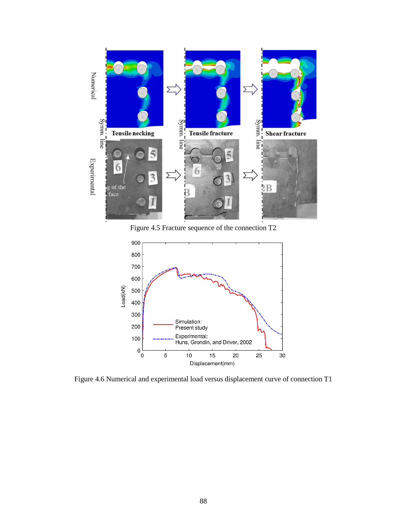
Figure 4.5 Fracture sequence of the connection T2

Figure 4.6 Numerical and experimental load versus displacement curve of connection T1

88

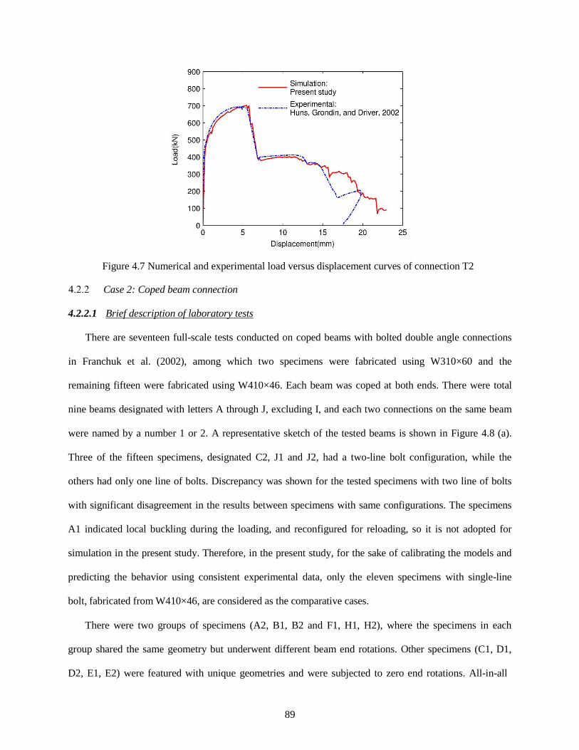
Figure 4.7 Numerical and experimental load versus displacement curves of connection T2

Case 2: Coped beam connection

4.2.2.1 Brief description of laboratory tests

There are seventeen full-scale tests conducted on coped beams with bolted double angle connections

in Franchuk et al. (2002), among which two specimens were fabricated using W310×60 and the

remaining fifteen were fabricated using W410×46. Each beam was coped at both ends. There were total

nine beams designated with letters A through J, excluding I, and each two connections on the same beam

were named by a number 1 or 2. A representative sketch of the tested beams is shown in Figure 4.8 (a).

Three of the fifteen specimens, designated C2, J1 and J2, had a two-line bolt configuration, while the

others had only one line of bolts. Discrepancy was shown for the tested specimens with two line of bolts

with significant disagreement in the results between specimens with same configurations. The specimens

A1 indicated local buckling during the loading, and reconfigured for reloading, so it is not adopted for

simulation in the present study. Therefore, in the present study, for the sake of calibrating the models and

predicting the behavior using consistent experimental data, only the eleven specimens with single-line

bolt, fabricated from W410×46, are considered as the comparative cases.

There were two groups of specimens (A2, B1, B2 and F1, H1, H2), where the specimens in each

group shared the same geometry but underwent different beam end rotations. Other specimens (C1, D1,

D2, E1, E2) were featured with unique geometries and were subjected to zero end rotations. All-in-all

89

End

dista

nce

S S

S

25

25

75

75

75

there were seven different connection geometries, and three levels of end rotations for all beams involved,

categorized in Table 3.1 and illustrated in Figure 4.8 (b) and (c). The different levels of end rotations were

achieved by controlling the displacement, ∆3, with linear increment, while imposing load stroke ∆4. For

maintaining zero end rotations, ∆2 was kept at zero. More details regarding the experimental set up and

procedures can be found in Franchuk et al. (2002).

Load cell A ∆4

∆1

F = Connection

Reaction Force

∆2 ∆3 A Load cell

(a)

Edge 50 distance

50 50

Beam flange Beam flange

Beam web Beam web

(b) (c) Figure 4.8 (a) Representative beam geometry and set up, (b) representative geometry of connections

subjected to end rotation, and c) Geometry of connection of specimen D2 subjected to zero end rotation (i.e. pure shear)

The block shear deformation, ∆, which equals the difference between ∆1 and ∆2 on the beam in Figure

4.8 (a), was taken as the displacement indicator in the load versus displacement behavior, and the

calculated connection reaction force, F in Figure 4.8 (a), was used as the load indicator.

90

Table 4.1 Geometries for all the specimens Connection designation

Edge distance (mm)

End distance (mm)

Spacing (S) (mm)

Rotation

(degrees) Number of bolts A1 0 A2 25 B1 B2

25 75 3.5 2 0

4

C1 25 25 102 0 3 D1 32 32 103 0 3 E1 50 25 75 0 4 E2 25 50 75 0 4 F1 H1 25

25

75

0 2

3

H2 3.5 Note: Since the pure shear specimen D2 is featured with distinct geometry, it is shown in Figure 4.8 (c) separately instead of in Table 4.1.

4.2.2.2 Description of numerical modeling

Similar to the gusset plate models, the general finite element platform ABAQUS/Explicit was also

employed in the simulations. Out-of-plane deformations were not observed for almost all beams during

the entire phase of testing, and consequently no buckling failure modes were identified. Therefore, the

two dimensional plane stress elements, CPS4R, were utilized in the simulations for the sake of

computational efficiency. Finite element models for selected beams were first developed then validated

through extensive comparisons with the corresponding experimental results. The comparisons included

load versus displacement curves as well as fracture profiles. The mesh size employed in the coped beam

simulations was 3mm×3mm, at and around the fracture region, and is outlined with the dash line and the

corresponding zoom in as shown in Figure 4.9.

91

Figure 4.9 Representative numerical model for coped beam connection

An isotropic hardening material model embedded in ABAQUS was adopted in the numerical analysis,

with the data extracted from coupons taken from the webs of the respective beams. A friction coefficient

of 0.3, representing Class C slip factor for untreated hot roll steel per the 2010 AISC Specifications

(AISC 360-10), was used primarily to introduce the bolt-hole interaction. Because the experimental

program was designed to investigate the fracture of the beam, the bolts were designed with large safety

factors. Since no obvious deformations were observed from bolts and column, the bolts were modeled as

rigid bodies, and their ignored stiffness was small and can be offset through boundary conditions that

incorporate springs with appropriate coefficients as will be discussed later in Section 4.2.2.3. Bolt preload

was not considered in the FE simulations since the bolts were only snug-tightened in the corresponding

laboratory programs.

Boundary conditions, representing load and support conditions, in the corresponding laboratory tests

were considerately modelled in order to mimic the testing protocol. In the laboratory tests, the beam was

loaded slowly under displacement control. Most of the tests were designed without applied end rotations,

and the supporting jack (∆3 in Figure 4.8 (a)) was adjusted but in very small increments (±0.25 mm), so it

can be viewed as pin in these cases. For the tests with end rotations, the jack was lowered at each load

92

increment to achieve the desired rotations, which is in a linear relationship with the vertical reaction, and

calculated through the predicted ultimate strength and desired ultimate rotation. The numerical models

developed in this study follow exactly the experimental procedures for the application of the load and

modification of the support conditions. The displacement was incremented through a specified

displacement of the node in the top flange corresponding to ∆4 and the corresponding force measured.

The displacement, ∆3, was also specified at a node on the bottom flange.

Two sets of vertical and horizontal spring elements were applied to simulate the vertical and

horizontal constraints from the bolts between the double angles and columns. The corresponding stiffness,

modeled through spring elements as discussed in Section 4.2.2.3, from the constraints consists in reality

of several resistances including resistance to slippage between the angles and columns, local bearing

deformation of every bolt hole, as well as local deformation of the bolts. In addition, a set of dampers

were also applied along with these spring elements in order to dissipate the dynamic response from the

fracture phenomena. The forces from the dampers are minute compared to those induced by the springs

and therefore are neglected during calibration. A representative set up for the spring system and dampers

is shown in Figure 4.8 (a) and details of the methodology by which the spring coefficients are calculated

is introduced in the following section. As in the case of the gusset plate models, the fracture behavior in

the FE model was captured through the implementation of the fracture criterion in chapter 3 and achieved

through element deletion.

4.2.2.3 Calibration of the FE model

The series of vertical and horizontal springs served as substitution of the constraints between the

double angles and columns. There are many factors influencing the vertical and horizontal stiffness of the

connection system. This includes for example bearing on bolt hole both the vertical and horizontal

directions, bolts’ bending and elongating, angles’ bending away from column (horizontal bending) and

vertical bending, slippage in every bolt in each direction and many other localized deformations. Most of

these nonlinear and complex features are hard to precisely measure and account for even if full details of

the connections modeled are available. Therefore, some simplifications are applied.

93

l l

1 K

In the present study, the vertical stiffness system is decomposed into two parts, the global stiffness Kg,

representing the mean stiffness components of the entire bolt line, and the local stiffness Kl, representing

the stiffness components unique to each individual bolt. The stiffness contributions from the behavior of

friction between the column flange and double angles, angles’ bending action, and some other local

deformations from the columns and angles are assumed to affect only the global stiffness performance.

The local stiffness, on the other hand, is assumed to be only influenced by bolts bearing on the angles and

column holes (angles to column flange connections), since the stiffness from bolts bending is relatively

small. The local springs are all connected in parallel and are in series with the global springs. A prototype

spring system layout is shown in Figure 4.10 and the overall stiffness K, combining the local and global

springs, can be determined through Equation 4.2.

Others

Angles bending

Bolts bending

Bolt holes bearing

Friction

Figure 4.10 Spring system layout for vertical spring

K = 1 Kg

1 + 1 (3K )

or K = 1 K g

1 + 1 (4K )

(4.2)

The stiffness of bolt bearing on plates, Kl in the present study, can be determined by Equation 4.3 as

outlined in Rex and Easterling (2003), as follows

Kl = br

1 + 1 Kb

+ 1 Kv

, (4.3)

where Kbr = bearing stiffness, Kb = bending stiffness, and K v = shearing stiffness. The three sub-

stiffness are calculated by Equation 4.4 to 4.6 (Rex and Easterling, 2003), expressed respectively as

K =120t F (d 25.4)0.8 , (4.4)

br p y b

K = 32Et (L d −1 2)3 , (4.5)

b p e b

K v = 6.67Gt p ( Le d b − 1 2) , (4.6)

94

where tp is the plate thickness, db is the bolt diameter, Fy is the yield stress, E is the modulus of elasticity,

G is the shear modulus of elasticity, and Le is the end distance, which represents the length between the

center of bolt and nearest end edge in the anticipated direction of loading.

The global stiffness can be determined through Equation 4.7. The angles’ bending action can be

simplified to a two-end fixed beam with concentrated force in the mid-span as shown in Figure 4.11, and

the corresponding stiffness KAngleBending can be determined in Equation 4.8. The other two components in

Equation are treated together as one term, and usually assumed to be featured with infinite starting value

in the following trial and error.

Kg = 1 K

AngleBendni g

1 +1 K

friction

+1 Kothers

(4.7)

Kab =192EI / L3

(4.8)

The eleven tested specimens of interest are featured with seven different geometries, and for each of

the seven geometries a test with zero end rotation was conducted. The presence of zero rotation provides a

convenient way to measure the entire stiffness of the connection in the vertical direction. As shown in

Figure 4.12, when the ultimate load is achieved, the beam end rotation is approximately zero, which

implies that the connection in the beam end has shifted downwards and that the horizontal stiffness of the

system has no influence on the load versus displacement curve. A trial and error method was employed to

calibrate the global stiffness, Kg, by correlating the beam end rotation to the load versus displacement

curves, with Kg in Equation 4.7 serving as a starting point. The adjustment to Kg is rather insignificant for

all beams, implying that the starting point in Equation 4.7 is quite adequate.

95

∆

∆

L Lg1 Lg2

Left angle

F

= Right angle L

F Beam Web

Figure 4.11 The two-fixed end beam system for the angles’ bending action (A-A section of Figure 4.8 (a))

Load

∆3=0

Vertical spring

Load

Rotation = 0

Figure 4.12 Layout of the calibration on global systems through zero rotations

In cases where the beam end rotation exits, the stiffness in the horizontal direction should be

considered as shown in Figure 4.13. Unlike the bolts performance in the vertical direction, the

orientations of bolt bearing on the angles are not the same, and there is no obvious global stiffness Kg,

which leads to the local stiffness Kl dominating the overall stiffness. The end rotations cause the upper

bolts to move away from the column while the bottom bolts are pushed towards the column. For the

96

bottom bolts, only Kbr is present in Equation 4.7 since the angles are tied with the column because of the

compression. Except the stiffness contribution from the bolt bearings on the angles, the actions of angles’

bending away also influences the behavior of upper bolts. In the laboratory tests, a 12.7 mm thick cover

plate was attached to reduce the bending of the angles away from the column and no information was

provided to describe the cover plate detail; hence it is not possible to account for the cover plate effect.

Therefore, the lateral stiffness of the bolts was primarily determined by the bolt bearing stiffness model,

expressed in Equation 4.6. In addition, reduction in the stiffness, determined from trial and error, was

applied to the stiffness of upper bolts, which accounts for the effects from angles’ bending away

(horizontal bending) and other possible local actions in the systems. During calibration of the models, the

initial location of bolts inside the bolt hole showed noticeable but not significant influence on the initial

stiffness of the load versus displacement curves and fracture profiles, which will be discussed in the

following sections.

Rotation

Figure 4.13 The sketch of the horizontal spring system

4.2.2.4 Calibration of the fracture criterion

There are three parameters that require calibration in Equation 3.18, and each of them holds unique

influence on the fracture locus map. As explained in Chapter 4, the parameter c7, as a positive value, only

proportionally varies the magnitude of the fracture strain. The parameter c8 relates to the dependency of

stress triaxiality, and c9 pertains to the Lode angle parameter sensitivity to the criterion. The unique role

97

of each of three parameters greatly reduces the effort required for calibration. In the original experimental

tests of the coped beams, the fracture strains were not measured since they were not of interest.

Fortunately, previous in-house study on a coupon level has narrowed the value of c8 to approximately -

1.9.One of the seven geometries previously mentioned connection D2 in Figure 4.8 (c) was designed to be

fractured under pure shear stress state (η = θ = 0 ) and was used to determine c7. Very good agreements

between the simulation and the experiment is achieved under c8= 0.5, in the perspective of load versus

displacement behavior and fracture profile. The remaining parameter c9 was obtained through trial and

error on specimen B2 so that the best correlation between the experimental and numerical results for the

load versus displacement curve and fracture profile is obtained. The resulting three fracture parameters in

Equation 3.18 for this steel type, for the fifteen tested beams, are c7=0.5, c8=-1.9, and c9=-6.2. Once the

three parameters were obtained, they were utilized for predicting the response of all remaining specimens.

4.2.2.5 Coped beams results

The numerical simulation procedure is verified by comparisons between the numerical and

experimental results, specifically in terms of the load versus displacement behavior, fracture profiles. The

loads and displacements were calculated from the numerical models using the same procedure as that of

the experimental study. The displacements are the difference between the top displacement ∆1 and bottom

displacement ∆2, along the bolt lines, and the loads are the supporting forces from the columns, which is

designated as the reaction force F in Figure 4.8 (a). The load versus displacement curves for specimens

with zero rotations are reviewed, and the representative ones are plotted in Figure 4.14 (a) through (e).

Very good correlation is observed for all the beams with zero rotations, not only before cracking occurred

but also after fracture has initiated. For the cases with large beam end rotations, such as H2, in the fracture

progression stage, the agreements between the analytical and experimental curves are questionable,

although the trends are still well predicted as shown in Figure 4.14 (f). The reason for the lack of accurate

predictions beyond the capacity point is due to the large rotation that causes a very complex stress

distribution, which results in a multifaceted failure path as discussed later. For beam D2 in Figure 4.14 (d),

98

the plateau in the early increase stage may due the slip of the bolts, and the numerical simulation

successful simulated this phenomena by including the bolts slippage.

The final fracture profiles are shown in Figure 4.15 for the representative analysis cases as well as

their experimental equivalents. It is shown that all the fracture profiles produced numerically correlate

very well with the corresponding ones obtained from the tests. The tensile fracture on the horizontal plane

and shear fracture on the vertical plane work together to form the entire tear-out, which is a key feature of

block shear failure. It is noted that most of the cases present a clear block shear fracture, but for the ones

with large beam end rotations, such as H2, the fracture profile on the shear plane shows tearing along a

complex path that started away from the bottom bolt hole. No information on the fracture sequence is

available in Franchuk et al. (2002). The fracture sequence, obtained numerically, for the loading cases

without beam end rotations, the fracture mostly initiates as tensile fracture, at the outer horizontal plane of

the bottom bolt. The cases with rotations, however, the fracture initiation transfers to the bottom bolt in

the vertical direction as shear fracture.

For specimens with end rotations, the specimens were designed to experimentally undergo three

levels of rotations: 0°, 2°, and 3.5°. Due to the complexity in measuring these rotations, the actual

experimentally achieved end rotations were different as shown in Table 4.2. Comparisons of the forces

and end rotations at ultimate load between the numerical and experimental results are listed at Table 4.2.

As shown in the table very good correlation is observed.

99

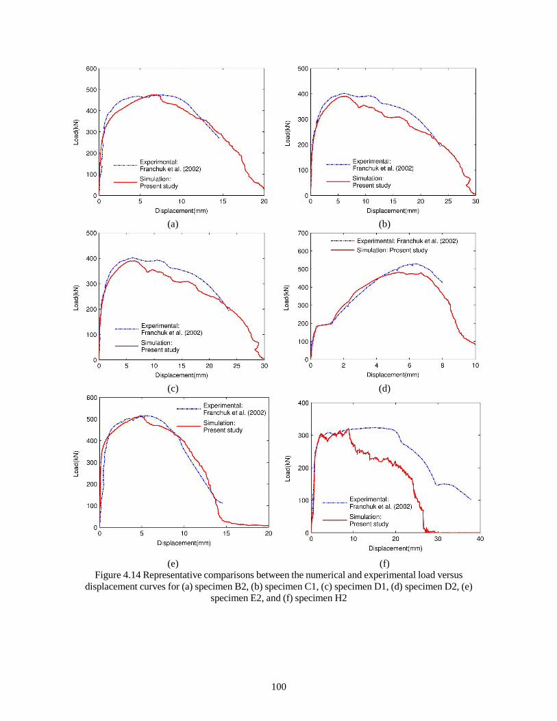
(a) (b)

(c) (d)

(e) (f) Figure 4.14 Representative comparisons between the numerical and experimental load versus

displacement curves for (a) specimen B2, (b) specimen C1, (c) specimen D1, (d) specimen D2, (e) specimen E2, and (f) specimen H2

100

(a) (b)

(c) (d)

101

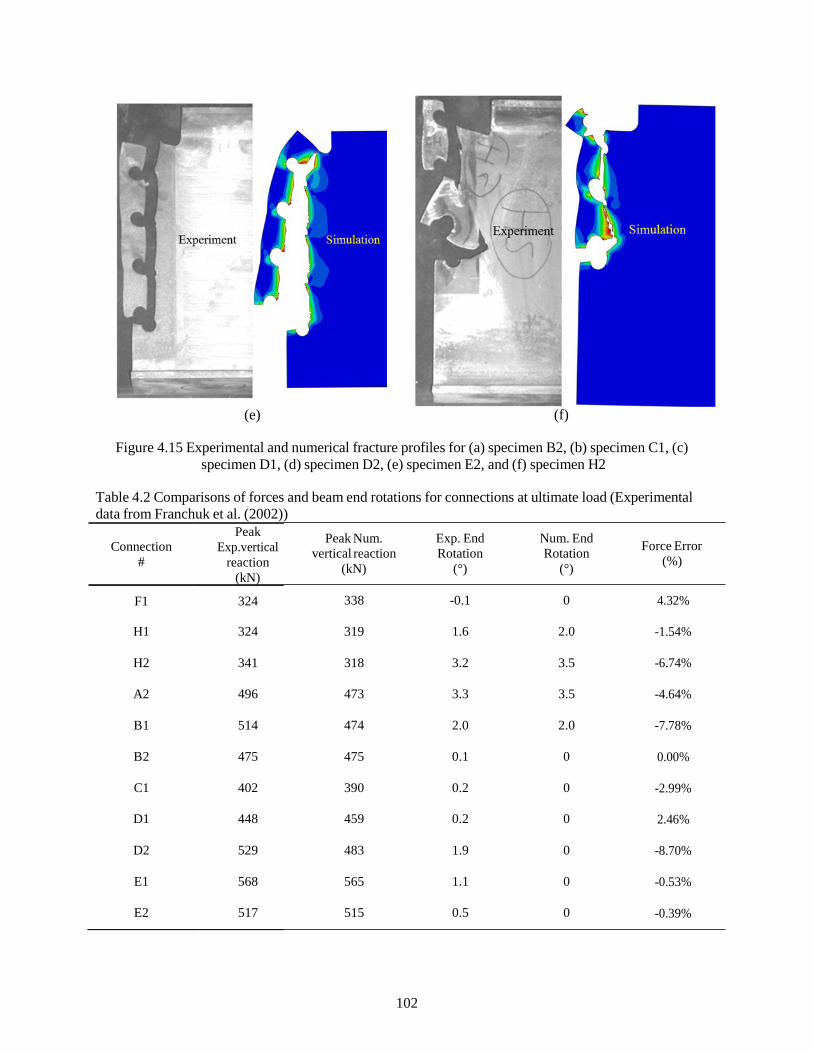
Connection

#

Peak Exp.vertical

reaction (kN)

F1 324

H1 324

H2 341

A2 496

B1 514

B2 475

C1 402

D1 448

D2 529

E1 568

E2 517

Peak Num. vertical reaction

(kN)

338

Exp. End Rotation

(°)

-0.1

Num. End Rotation

(°)

0

319 1.6 2.0

318 3.2 3.5

473 3.3 3.5

474 2.0 2.0

475 0.1 0

390 0.2 0

459 0.2 0

483 1.9 0

565 1.1 0

515 0.5 0

(e) (f)

Figure 4.15 Experimental and numerical fracture profiles for (a) specimen B2, (b) specimen C1, (c)

specimen D1, (d) specimen D2, (e) specimen E2, and (f) specimen H2

Table 4.2 Comparisons of forces and beam end rotations for connections at ultimate load (Experimental data from Franchuk et al. (2002))

Force Error (%)

4.32%

-1.54%

-6.74%

-4.64%

-7.78%

0.00%

-2.99%

2.46%

-8.70%

-0.53%

-0.39%

102

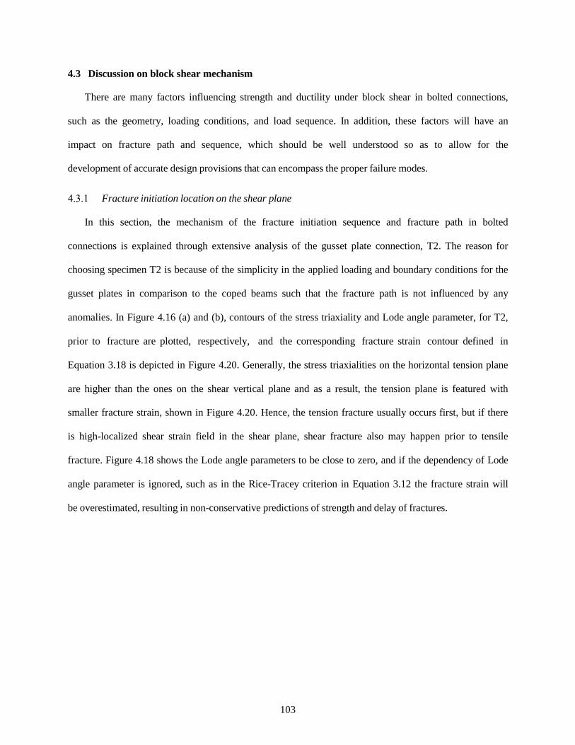
4.3 Discussion on block shear mechanism

There are many factors influencing strength and ductility under block shear in bolted connections,

such as the geometry, loading conditions, and load sequence. In addition, these factors will have an

impact on fracture path and sequence, which should be well understood so as to allow for the

development of accurate design provisions that can encompass the proper failure modes.

Fracture initiation location on the shear plane

In this section, the mechanism of the fracture initiation sequence and fracture path in bolted

connections is explained through extensive analysis of the gusset plate connection, T2. The reason for

choosing specimen T2 is because of the simplicity in the applied loading and boundary conditions for the

gusset plates in comparison to the coped beams such that the fracture path is not influenced by any

anomalies. In Figure 4.16 (a) and (b), contours of the stress triaxiality and Lode angle parameter, for T2,

prior to fracture are plotted, respectively, and the corresponding fracture strain contour defined in

Equation 3.18 is depicted in Figure 4.20. Generally, the stress triaxialities on the horizontal tension plane

are higher than the ones on the shear vertical plane and as a result, the tension plane is featured with

smaller fracture strain, shown in Figure 4.20. Hence, the tension fracture usually occurs first, but if there

is high-localized shear strain field in the shear plane, shear fracture also may happen prior to tensile

fracture. Figure 4.18 shows the Lode angle parameters to be close to zero, and if the dependency of Lode

angle parameter is ignored, such as in the Rice-Tracey criterion in Equation 3.12 the fracture strain will

be overestimated, resulting in non-conservative predictions of strength and delay of fractures.

103

(a) (b)

Figure 4.16 Contour of stress state paramters for specimen T2: (a) Stress triaxiality and (b) Lode angle

parameter

The damage contour directly prior to cracking is depicted in Figure 4.17 (a), and all four bolts are

numbered. As discussed before, for specimen T2, the damage is more significant on the tensile plane

while on the shear plane some moderate damage has accumulated, implying yielding on the shear plane.

The damage evolution before cracking corresponds well with the design equations in 2010 AISC

Specification (AISC 360-10) in that, the total capacity of the connection equals the sum of the ultimate

strength of the tensile plane and the yield strength of the shear plane. The load versus displacement curve

is shown in Figure 4.17 (b) and is marked with numbers at different points along the curve. The

designation, n1, refers to the first crack on bolt hole n while n2 refers to the second crack on the same bolt

hole. The fracture sequence can be defined on the load versus displacement curve where crack 11 occurs

first on the inner side of the hole, then immediately crack 12 starts on the outer side of the hole and soon

propagate to bolt hole 2, crack 21. After the entire tensile fracture is formed, the first shear crack forms is

41 then 42 forms. Thereafter, crack 22 develops and the last cracks are 31 and 32.

Another parameter that can shed light on the fracture path is the damage distributions on the edge of

each bolt hole, where specific points along the bolt hole edge can be defined by the angle from the

horizontal axis as depicted in Figure 4.18. The damage is plotted along the bolt hole edge for bolt 1 to 4

104

as shown in Figure 4.19 (a) to (d), respectively. As shown in figure 4.19 (a), damage on bolt hole 1

reaches a value of 1 at approximately 0° and 180°, which implies failure on the net tension area as

expected. The second hole, participating on the tension and shear planes, shows a damage value of 1 at

approximately 180° on the tension plane and at 67.5°, not on the net section at 90°, for the shear plane.

For holes 3 and 4 on the shear plane, the damage reaches a value of one at approximately 270° (center of

bottom edge of the hole), which together with a damage value of one at 67.5° at the top edge of the hole

form slanted cracks on the shear plane. The slanted fracture lines can also be observed in the laboratory

tests, as shown in Figure 4.4.

The observation made above for the shear fracture not being along the centerline of the bolt holes,

which has the least area, but rather at some locations between the gross and net sections has been made by

others. This phenomenon has been loosely accounted for in some codes (AISC, 1999; CSA-S16-09)

where the shear strength is calculated using the gross plane rather the net plane. There is no clear

explanation in the literature on the reason for the fracture shift on the shear plane. In this study, this

phenomenon can be explained using the ductile fracture model in Equation 3.18. Specifically, due to the

interactive compressive action between the bolt and bolt holes, negative stress triaxialities exist on the

plate adjacent to compressed bolt hole, shown in Figure 4.16 (a), which may result in very high fracture

strain, even higher than that of the cut-off region, which is clearly shown in Figure 4.20. The damage can

barely accumulate in these locations, which is clearly shown in Figure 4.20 for the bolt hole edges at

around 90°. Thus, fracture cannot occur along the centerlines of the bolt holes, and usually detours to take

place between the net and gross shear areas. On the other hands, there is no compressive action on the

lower side of the bolt hole, such that the fracture usually tends to go back to the centerlines of the holes,

seeking least resistance through least area, resulting in a slightly slanted fracture profile on the shear plane.

105

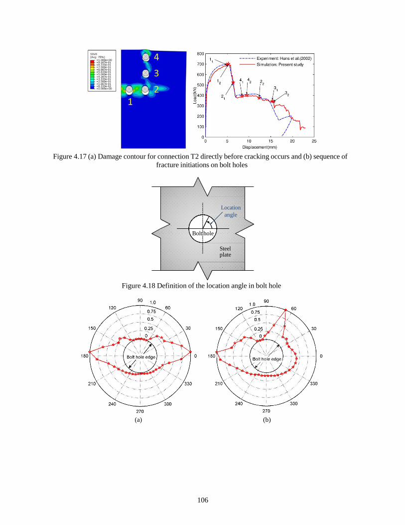
Figure 4.17 (a) Damage contour for connection T2 directly before cracking occurs and (b) sequence of

fracture initiations on bolt holes

Location angle

Bolt hole

Steel plate

Figure 4.18 Definition of the location angle in bolt hole

(a) (b)

106

(c) (d)

Figure 4.19 Depiction damage distribution around bolt holes for (a) Bolt hole 1, (b) Bolt hole 2, (c) Bolt

hole 3, and (d) Bolt hole 4.

Figure 4.20 Fracture strain contour of T2

Effect of loading conditions on the connections

Research regarding the effect of loading conditions, specifically the moments/rotations, on coped

beams is scarce. Through the experimental results, Franchuk et al. (2002) concluded that

moments/rotations did not hold adverse influences on the ultimate strength, but the failure modes might

be transferred from normal block shear, such as F1, to partial block shear, such as the H1. However, no

attempts were made towards understanding the intrinsic mechanism of failure resulting from end

107

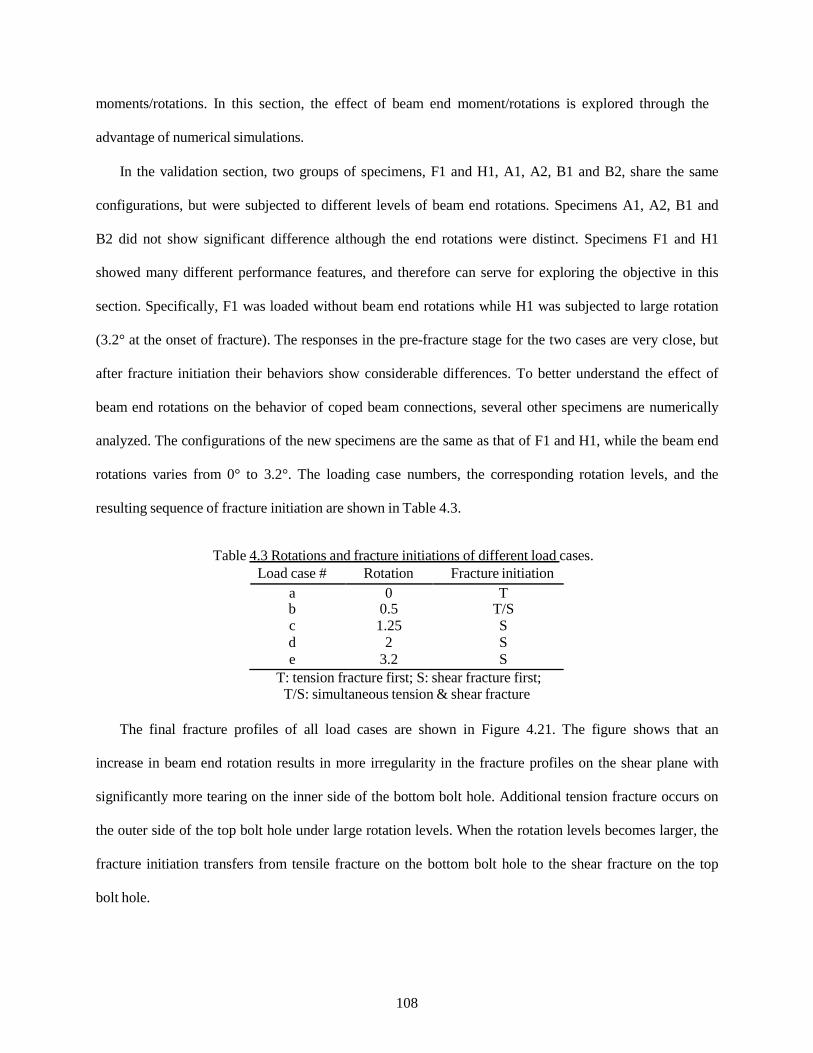
moments/rotations. In this section, the effect of beam end moment/rotations is explored through the

advantage of numerical simulations.

In the validation section, two groups of specimens, F1 and H1, A1, A2, B1 and B2, share the same

configurations, but were subjected to different levels of beam end rotations. Specimens A1, A2, B1 and

B2 did not show significant difference although the end rotations were distinct. Specimens F1 and H1

showed many different performance features, and therefore can serve for exploring the objective in this

section. Specifically, F1 was loaded without beam end rotations while H1 was subjected to large rotation

(3.2° at the onset of fracture). The responses in the pre-fracture stage for the two cases are very close, but

after fracture initiation their behaviors show considerable differences. To better understand the effect of

beam end rotations on the behavior of coped beam connections, several other specimens are numerically

analyzed. The configurations of the new specimens are the same as that of F1 and H1, while the beam end

rotations varies from 0° to 3.2°. The loading case numbers, the corresponding rotation levels, and the

resulting sequence of fracture initiation are shown in Table 4.3.

Table 4.3 Rotations and fracture initiations of different load cases.

Load case # Rotation Fracture initiation a 0 T b 0.5 T/S c 1.25 S d 2 S e 3.2 S

T: tension fracture first; S: shear fracture first; T/S: simultaneous tension & shear fracture

The final fracture profiles of all load cases are shown in Figure 4.21. The figure shows that an

increase in beam end rotation results in more irregularity in the fracture profiles on the shear plane with

significantly more tearing on the inner side of the bottom bolt hole. Additional tension fracture occurs on

the outer side of the top bolt hole under large rotation levels. When the rotation levels becomes larger, the

fracture initiation transfers from tensile fracture on the bottom bolt hole to the shear fracture on the top

bolt hole.

108

Figure 4.21 Comparisons of fracture profiles under different beam end rotation levels.

The load versus displacement curves are close in the pre-crack stage for all the specimens, as shown

in Figure 4.22, with slight increase in the initial stiffness as the rotation increases. The strength obtained

in all load cases is somewhat similar with minor reduction with the increase of rotation levels. Although

minor, the decrease in the strength conflicts with the experimental results in Franchuk et al. (2002). The

disagreement is however understandable since many factors could influence the experimental results such

as friction between the beam and double angles, the lateral support and the material variation. In the

fracture propagation stage, the higher the rotation level the more additional ductility is present.

The anomalies in the fracture profiles and sequences, as influenced by end rotations, can be explained

by the bolt-hole interaction forces in the horizontal direction, shown in Figure 4.23. The figure shows that

with growth of rotation levels, the horizontal bolt-hole interaction forces for the bottom and top bolts

increase, and then these forces are transferred to the plate around corresponding bolt holes. For the top

bolts, the forces are towards the beam end directions, and subsequently tears the outer parts of beam end

out of the beams. Hence, there are additional tension fractures on the top bolt for load cases with large

rotation, shown in Figure 4.21, and the fracture initiates in the form of combined shear and tension

fracture. For the bottom bolts, the forces compress the inner sides of bolt holes, and accordingly decrease

the stress triaxiality in the corresponding area. As discussed in the previous section, smaller stress

triaxialities bring higher fracture strains and slower damage rate, and consequently fracture initiation

detour to the locations easier to crack, which are usually below the compression zone and featured with

109

relatively smaller fracture strains. In addition, with the increasing bottom compression forces, there might

be slight local buckling in the inner side of the bolt hole, which may introduce extra ductility to the

system and be the reason for the relative inaccurate simulation in Figure 4.13 (f).

Figure 4.22 Comparisons of load versus displacement curves under different beam end rotation levels

Figure 4.23 Comparisons on the bolt-hole interaction forces for top and bottom bolts under different beam end rotations

Summary

In this section, numerical simulations on block shear in gusset plate and coped beam connections

were conducted up to and including total failure, through the application of newly developed ductile

110

fracture criterion. The laboratory test results from Huns et al. (2002) and Franchuk et al (2002) served as

validations of the numerical simulation approach for the gusset plate and coped beam connections,

respectively. The numerical simulation results correlated well with the corresponding experimental

equivalents for the load versus displacement curves, fracture sequence, and fracture profiles. After the

numerical methodology was implemented and the ductile fracture criterion employed, the inherent

mechanisms of block shear in gusset plate and coped beam connections were discussed and explained.

The behavior of the coped beam connections with various levels of beam end/rotations was also explored.

Based on the simulations and analysis, the following conclusions can be drawn:

1. Based on the excellent agreements between the numerical and experimental results, the numerical

modelling methodology and employed ductile fracture criterion are proven to be a viable

approach for simulating block shear failure in bolted connections.

2. For tensile fracture, the fracture usually initiates and propagates on the net section, which

confirms the approach used in current code specifications in that the net section is where tensile

fracture takes place.

3. For shear fracture, the fracture paths was identified to be located between the net and gross

sections, slightly larger than the net section.

The beam end rotation levels appear to have some minor effect on the strength of the connections, but

the most significant influence lies on effect of such on ductility and fracture profile of the connections.

The end rotations can greatly change the fracture profile and sequence where the top bolt holes become

the holes most prone to fracture instead of the bottom bolt holes. It is also shown that the assumption of

zero rotation levels may not be adequate if applied to cases with large rotations.

4.4 Parametric study on geometry configurations

There are many factors influencing the fracture mode of a connection under block shear with the

notable parameter being the geometrical configuration of the connection. This includes bolt hole spacing

and edge/end distance. In this section, the influence of bolt hole spacing in the tensile plane is explored

111

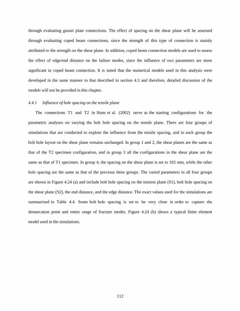
through evaluating gusset plate connections. The effect of spacing on the shear plane will be assessed

through evaluating coped beam connections, since the strength of this type of connection is mainly

attributed to the strength on the shear plane. In addition, coped beam connection models are used to assess

the effect of edge/end distance on the failure modes, since the influence of two parameters are more

significant in coped beam connection. It is noted that the numerical models used in this analysis were

developed in the same manner to that described in section 4.3 and therefore, detailed discussion of the

models will not be provided in this chapter.

Influence of hole spacing on the tensile plane

The connections T1 and T2 in Huns et al. (2002) serve as the starting configurations for the

parametric analyses on varying the bolt hole spacing on the tensile plane. There are four groups of

simulations that are conducted to explore the influence from the tensile spacing, and in each group the

bolt hole layout on the shear plane remains unchanged. In group 1 and 2, the shear planes are the same as

that of the T2 specimen configuration, and in group 3 all the configurations in the shear plane are the

same as that of T1 specimen. In group 4, the spacing on the shear plane is set to 102 mm, while the other

hole spacing are the same as that of the previous three groups. The varied parameters in all four groups

are shown in Figure 4.24 (a) and include bolt hole spacing on the tension plane (S1), bolt hole spacing on

the shear plane (S2), the end distance, and the edge distance. The exact values used for the simulations are

summarized in Table 4.4. Some bolt hole spacing is set to be very close in order to capture the

demarcation point and entire range of fracture modes. Figure 4.24 (b) shows a typical finite element

model used in the simulations.

112

S2

S2

End

dist

ance

Edge distance

Gusset plate

S1 S1

Figure 4.24 (a) Geometrical configuration of the model and (b) depiction of a typical numerical model used

Table 4.4 Gusset plate connection dimensions

Specimen Group Number of Tensile bolt lines S1 (

spacing Shear spacing

mm) S2 (mm) End distance Edge distance

G1_1 1 2 111.6 51 25 147.2 G1_2 1 3 66.15 51 25 136.85 G1_3 1 4 51 51 25 126.5 G1_4 1 5 43 .425 51 25 116.15 G2_1 2 2 95 51 25 155.5 G2_2 2 2 125.7 51 25 140.15 G2_3 2 2 126.4 51 25 139.8 G2_4 2 2 1 27 51 25 139.5 G2_5 2 2 127.2 51 25 139.4 G2_6 2 2 127.4 51 25 139.3 G2_7 2 2 129.225 51 25 138.3875 G2_8 2 2 13 2.75 51 25 136.625 G2_9 2 2 139.8 51 25 133.1

G2_10 2 2 1 68 51 25 119 G3_1 3 2 51 76 38 177.5 G3_2 3 2 75 76 38 165.5 G3_3 3 2 90 76 38 158 G3_4 3 2 1 00 76 38 153 G3_5 3 2 1 10 76 38 148 G3_6 3 2 1 20 76 38 143 G3_7 3 2 1 35 76 38 135.5 G3_8 3 2 1 50 76 38 128 G3_9 3 2 1 68 76 38 119 G4_1 4 2 51 102 51 274.5 G4_2 4 2 75 102 51 262.5 G4_3 4 2 1 50 102 51 225 G4_4 4 2 1 68 102 51 216

113

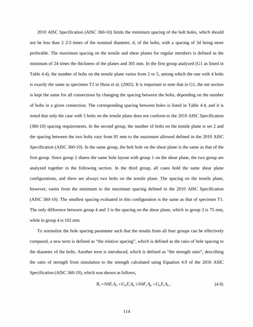
2010 AISC Specification (AISC 360-10) limits the minimum spacing of the bolt holes, which should

not be less than 2 2/3 times of the nominal diameter, d, of the bolts, with a spacing of 3d being more

preferable. The maximum spacing on the tensile and shear planes for regular members is defined as the

minimum of 24 times the thickness of the planes and 305 mm. In the first group analyzed (G1 as listed in

Table 4.4), the number of bolts on the tensile plane varies from 2 to 5, among which the one with 4 bolts

is exactly the same as specimen T2 in Huns et al. (2002). It is important to note that in G1, the net section

is kept the same for all connections by changing the spacing between the bolts, depending on the number

of bolts in a given connection. The corresponding spacing between holes is listed in Table 4.4, and it is

noted that only the case with 5 bolts on the tensile plane does not conform to the 2010 AISC Specification

(360-10) spacing requirements. In the second group, the number of bolts on the tensile plane is set 2 and

the spacing between the two bolts vary from 95 mm to the maximum allowed defined in the 2010 AISC

Specification (AISC 360-10). In the same group, the bolt hole on the shear plane is the same as that of the

first group. Since group 2 shares the same hole layout with group 1 on the shear plane, the two group are

analyzed together in the following section. In the third group, all cases hold the same shear plane

configurations, and there are always two bolts on the tensile plane. The spacing on the tensile plane,

however, varies from the minimum to the maximum spacing defined in the 2010 AISC Specification

(AISC 360-10). The smallest spacing evaluated in this configuration is the same as that of specimen T1.

The only difference between group 4 and 3 is the spacing on the shear plane, which in group 3 is 75 mm,

while in group 4 is 102 mm.

To normalize the hole spacing parameter such that the results from all four groups can be effectively

compared, a new term is defined as “the relative spacing”, which is defined as the ratio of hole spacing to

the diameter of the bolts. Another term is introduced, which is defined as “the strength ratio”, describing

the ratio of strength from simulation to the strength calculated using Equation 4.9 of the 2010 ASIC

Specification (AISC 360-10), which was shown as follows,

Rn = 0.6Fu Anv +UbsFu Ant ≤ 0.6Fy Agv +UbsFu Ant , (4.9)

114

where Fu is the ultimate strength of the material, Fy is the yielding stress of the material, Ant is the net

tension area along the tension plane, Anv is the net shear area along the shear plane, Agv and Agt are the

gross shear area and the gross tension area, respectively.

The results of strength ratio versus the relative spacing are shown in Figure 4.25 for group 1 and 2, in

Figure 4.26 for group 3, and in Figure 4.27 for group 4. From these figures, one can conclude that the

design equation in the AISC Specification (AISC 360-10) provides conservative predictions of the

ultimate strength, but the safety level is inconsistent with increase in bolt hole spacing. Specifically, with

increase in the relative spacing, the strength ratio increases gradually in the beginning until reaching a

peak value before starting to drop specifically around a relative spacing value of 5 in Figure 4.25, 4 in

Figure 4.26 and 2.6 in Figure 4.27. In addition, with increase of the shear spacing, there is a trend that the

AISC predictions lie more on the non-conservative side. Clearly, the variation in the predicted strength as

a function of bolt hole spacing suggests the presence of different failure mechanisms, as observed

numerically, which are typically omitted in design provisions. The fracture profiles, obtained from the

simulations, indicate that there are four different failure mechanisms that result from the different spacing

as shown in Figure 4.25, 4.26 and 4.27. The four mechanisms consists of four different scenarios at the

fracture initiation/ultimate strength. The mechanisms are classified, in the order of increased spacing, as 1)

fracture on the tensile plane with yielding on the shear plane (tensile fracture + shear yielding), 2) fracture

on the tensile plane and shear plane (tensile fracture + shear fracture), 3) fracture on the shear plane with

yielding on the tensile plane (tensile yielding + shear fracture), and 4) hole tearout, which is actually no

longer a block shear failure type by AISC (2010). The classifications of the four failure modes are

depicted in the space of shear and tensile spacing in Figure 4.28. The four fracture modes and their

transition are described and discussed in the following section.

115

Figure 4.25 Strength ratio versus relative spacing on the tensile plane for group 1 and 2 and the

classification of failure modes

Figure 4.26 Strength ratio versus relative spacing on the tensile plane and failure modes classification for

group 3

116

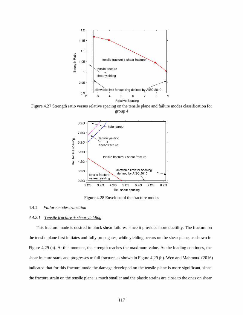
Figure 4.27 Strength ratio versus relative spacing on the tensile plane and failure modes classification for

group 4

Figure 4.28 Envelope of the fracture modes

Failure modes transition

4.4.2.1 Tensile fracture + shear yielding

This fracture mode is desired in block shear failures, since it provides more ductility. The fracture on

the tensile plane first initiates and fully propagates, while yielding occurs on the shear plane, as shown in

Figure 4.29 (a). At this moment, the strength reaches the maximum value. As the loading continues, the

shear fracture starts and progresses to full fracture, as shown in Figure 4.29 (b). Wen and Mahmoud (2016)

indicated that for this fracture mode the damage developed on the tensile plane is more significant, since

the fracture strain on the tensile plane is much smaller and the plastic strains are close to the ones on shear

117

plane. The load versus displacement curves for group 1 cases are illustrated in Figure 4.30. With the

exception of the case with two bolts on the tensile plane, the other cases are all featured with “tensile

fracture + shear yielding” failure mode. In group 3, only the case with 51 mm hole spacing on the tensile

plane belongs to this failure mode, while in group 4 none of the specimen falls into this region. In this

mode, after the tensile fracture occurs, the strength contribution from the tensile plane disappears abruptly,

so there are sudden drops in the load verses displacement curves. The residual strength is provided only

by the shear plane, and the missing portion of the strength is that of the tensile plane. This corresponds to

the philosophy in design codes in that the strength is decomposed into two portions: the tensile and shear

planes. Many experimental tests in the literature are featured with this fracture mode, such as the 28

specimens tested by Hardash and Bjorhovde (1984).

(a) (b) Figure 4.29 Fracture profiles for the failure mode: Tensile fracture + shear yielding (a) tensile fracture and

(b) full fracture

118

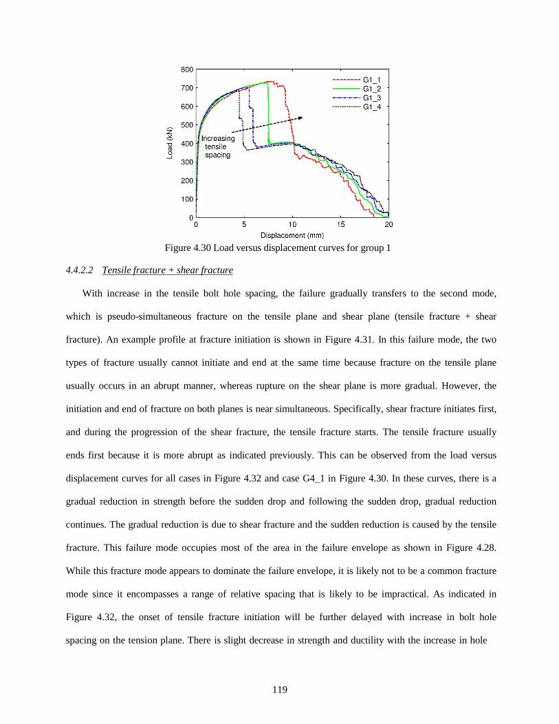
Figure 4.30 Load versus displacement curves for group 1

4.4.2.2 Tensile fracture + shear fracture

With increase in the tensile bolt hole spacing, the failure gradually transfers to the second mode,

which is pseudo-simultaneous fracture on the tensile plane and shear plane (tensile fracture + shear

fracture). An example profile at fracture initiation is shown in Figure 4.31. In this failure mode, the two

types of fracture usually cannot initiate and end at the same time because fracture on the tensile plane

usually occurs in an abrupt manner, whereas rupture on the shear plane is more gradual. However, the

initiation and end of fracture on both planes is near simultaneous. Specifically, shear fracture initiates first,

and during the progression of the shear fracture, the tensile fracture starts. The tensile fracture usually

ends first because it is more abrupt as indicated previously. This can be observed from the load versus

displacement curves for all cases in Figure 4.32 and case G4_1 in Figure 4.30. In these curves, there is a

gradual reduction in strength before the sudden drop and following the sudden drop, gradual reduction

continues. The gradual reduction is due to shear fracture and the sudden reduction is caused by the tensile

fracture. This failure mode occupies most of the area in the failure envelope as shown in Figure 4.28.

While this fracture mode appears to dominate the failure envelope, it is likely not to be a common fracture

mode since it encompasses a range of relative spacing that is likely to be impractical. As indicated in

Figure 4.32, the onset of tensile fracture initiation will be further delayed with increase in bolt hole

spacing on the tension plane. There is slight decrease in strength and ductility with the increase in hole

119

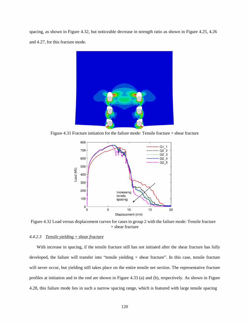
spacing, as shown in Figure 4.32, but noticeable decrease in strength ratio as shown in Figure 4.25, 4.26

and 4.27, for this fracture mode.

Figure 4.31 Fracture initiation for the failure mode: Tensile fracture + shear fracture

Figure 4.32 Load versus displacement curves for cases in group 2 with the failure mode: Tensile fracture

+ shear fracture

4.4.2.3 Tensile yielding + shear fracture

With increase in spacing, if the tensile fracture still has not initiated after the shear fracture has fully

developed, the failure will transfer into “tensile yielding + shear fracture”. In this case, tensile fracture

will never occur, but yielding still takes place on the entire tensile net section. The representative fracture

profiles at initiation and in the end are shown in Figure 4.33 (a) and (b), respectively. As shown in Figure

4.28, this failure mode lies in such a narrow spacing range, which is featured with large tensile spacing

120

and small shear spacing. This spacing requirements, although still within what is allowed by the code, is

rather unusual and this might be the reason for why this failure mode has never been captured in the

laboratory and never been reported in the literature for block shear tests.. Therefore the design equation

corresponds to this failure mode in the AISC Specification (AISC, 1999) was deleted. The final failure

profile is similar to the hole tearout failure. During this stage, with increase in hole spacing, the fracture

gradually transfer from a ductile mode to quasi-brittle mode, as shown in Figure 4.34, which would not be

desired.

(a) Fracture initiation (b) Final fracture

Figure 4.33 Fracture profiles for the failure mode: Tensile yielding + shear fracture (a) fracture initiation and (b) final fracture

121

Load

(kN

)

800

700

600

500

400

Increasing tensile spacing

300

200

100

0

G2_6 G2_7 G2_8

G2_9 0 2 4 6 8 10 12

Displacement (mm)

Figure 4.34 Load versus displacement curves for cases in group 2 with the failure mode: Tensile yielding + shear fracture

4.4.2.4 Hole tearout

The forth failure mode occurs when yielding is unable to fully develop on the tensile net section when

the shear fracture initiates. Consequently, the fourth failure mode, which is marked by hole tearout,

governs the behavior. The selective final fracture profile is shown in Figure 4.25. This mode only occurs

with large spacing, which is extremely undesired in actual design pertaining to practical application. It

does not consist of tensile and shear planes, since fracture/yielding only occurs along shear planes, as

shown in Figure 4.35, which contradicts to the assumption of block shear in Equation 4.9. Actually, AISC

(2010) defines this mode as “tearout”, a separate failure mode from block shear, and besides Equation 4.9

the strength is also limited by another bearing strength design equation. However hole, spacing pertaining

to this failure mode may still lie in the range for block shear failure allowed by the current 2010 AISC

Specification (AISC 360-10), which will render the design as non-conservative.

122

Figure 4.35 The fracture profiles for the failure mode: hole tearout

Discussion on fracture modes

There appears to be no clear classification for the four failure modes through the relative spacing. As

shown in Figure 4.25 for group 1 and 2, all four modes are identified, but only three modes are found in

Figure 4.26 for group 3, while for group 4 the second failure mode is the only one identified, as shown in

Figure 4.27. The “Tensile fracture + shear yielding” modes occupies the largest portion in Figure 4.25,

while in the other groups the second mode “Tensile fracture + shear fracture” governs most of the

geometry range, and so is the envelopes for all the allowed spacing by 2010 AISC Specification (AISC

360-10). The fracture mode transitions depend on the combination of the geometry layout in the shear and

tensile plane, suggesting a strong interaction between the two planes, which merits extensive study in the

future.

In the failure mode “Tensile fracture + shear yielding”, the ultimate strength of the connections

occurs where the fracture on the tensile plane initiates with yielding only on the shear plane. As shown in

Figure 4.29, the tensile fracture, as expected, takes place on the tensile net section. The yielded shear area,

however, is located between the net and gross sections, which is roughly (Anv+Agv)/2. This contradicts the

well-accepted code provision of yielding on the gross shear area. At the onset of the ultimate strength,

yielding on the shear plane has already fully developed, which leads to noticeable amount of hardening,

and direct use of the shear yielding strength may give conservative results.

123

The optimum geometry for the connection lies in the demarcation point of the first and second

fracture modes, where the tensile and shear fractures initiate at the same time. At this point, it is

appropriate that the design equation for predicting the ultimate block shear strength of the connection

would be based on the summation of the ultimate strength provided by both the shear and tensile planes.

The cases with the relative spacing of 5 in group 2, relative spacing of 4 in group 3, and relative spacing

of 2.6 in group 4, roughly capture this point as clearly marked by the peak strength in Figure 4.25, 4.26

and 4.27. In the second fracture mode, the fracture on the shear plane initiates first, while the tensile plane

is yielding at the same time. Thus, compared to the first failure mode, the roles of the tensile and shear

planes are reversed. The most significant difference lies in the fact that shear fracture, unlike tensile

fracture, does not occur in an abrupt manner. During the progression of shear fracture, tensile fracture

initiates and progresses promptly, and after the tensile fracture fully develops, the shear fracture continues

to propagate until total failure.

The last two failure modes are undesired from a design perspective, since the connection does not

realize its full potential in developing the full strength (i.e. the tensile plane is not being fully utilized).

Therefore, design equations for these two modes will not be discussed. Instead, spacing limitations will

be proposed to eliminate the potential for these two failure modes as will be discussed later. The two

modes share similar final fracture profiles, and therefore both modes could be considered hole tearout

failure. The difference between the two lies in the fact that the tensile plane yields in the “tensile yielding

+ shear fracture” mode, and in the fourth mode it does not. There are design equations for bearing

strength and prevention of hole tearout in the current 2010 AISC Specification (AISC 360-10). However,

for all cases in group 2, except the case with maximum tensile spacing, the block shear equation still

governs the design strength. As shown in Figure 4.28, in the allowable limits, there are still some regions

with the two fracture modes, which point the non-conservative side of the code.

Surprisingly, unlike the strength, the ductility of the connection is influenced significantly by the

spacing in which larger spacing also produces larger ductility in fracture mode “Tensile fracture + shear

yielding”. In this fracture mode, since the net sections are set to be constant, smaller spacing means more

124

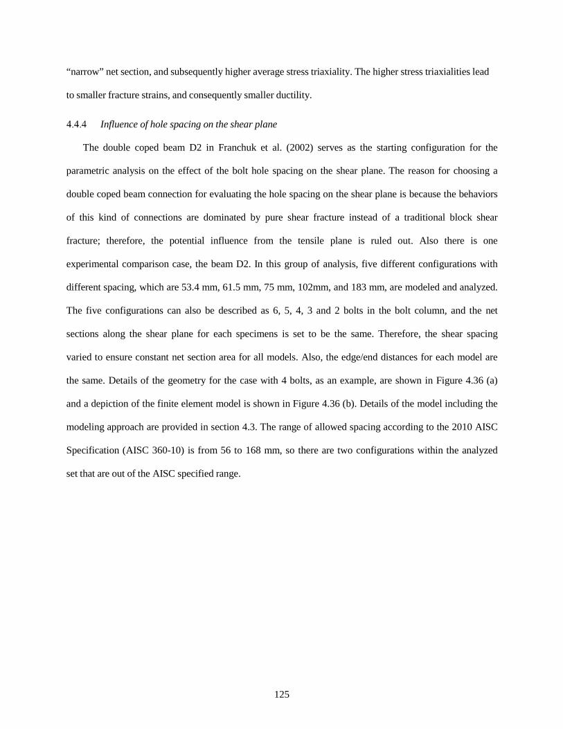
“narrow” net section, and subsequently higher average stress triaxiality. The higher stress triaxialities lead

to smaller fracture strains, and consequently smaller ductility.

Influence of hole spacing on the shear plane

The double coped beam D2 in Franchuk et al. (2002) serves as the starting configuration for the

parametric analysis on the effect of the bolt hole spacing on the shear plane. The reason for choosing a

double coped beam connection for evaluating the hole spacing on the shear plane is because the behaviors

of this kind of connections are dominated by pure shear fracture instead of a traditional block shear

fracture; therefore, the potential influence from the tensile plane is ruled out. Also there is one

experimental comparison case, the beam D2. In this group of analysis, five different configurations with

different spacing, which are 53.4 mm, 61.5 mm, 75 mm, 102mm, and 183 mm, are modeled and analyzed.

The five configurations can also be described as 6, 5, 4, 3 and 2 bolts in the bolt column, and the net

sections along the shear plane for each specimens is set to be the same. Therefore, the shear spacing

varied to ensure constant net section area for all models. Also, the edge/end distances for each model are

the same. Details of the geometry for the case with 4 bolts, as an example, are shown in Figure 4.36 (a)

and a depiction of the finite element model is shown in Figure 4.36 (b). Details of the model including the

modeling approach are provided in section 4.3. The range of allowed spacing according to the 2010 AISC

Specification (AISC 360-10) is from 56 to 168 mm, so there are two configurations within the analyzed

set that are out of the AISC specified range.

125

25

25

75

75

75

50 50

Beam flange

Beam web

Figure 4.36 (a) Representative geometry detail of the double coped connection and (b) example of the finite element model used

The strength ratios versus the relative spacing on the shear plane, for the group of analyzed double

coped beams, are shown in the Figure 4.37. As expected, due to shear lag, there is significant reduction in

the strength ratio as the relative spacing increases. With increased spacing, the strength ratio drops below

a value of one, which implies a non-conservative design equation. It is noted that the strength ratio is

inversely linearly related to the relative spacing, and the relation can be expressed in Equation 4.10 as

follows:

Strength _ ratio = −0 .0874 × Re lativeSpac

ing + 1 .635 (4.10)

Figure 4.37 Strength ratio versus relative spacing in the shear plane for the pure shear cases

126

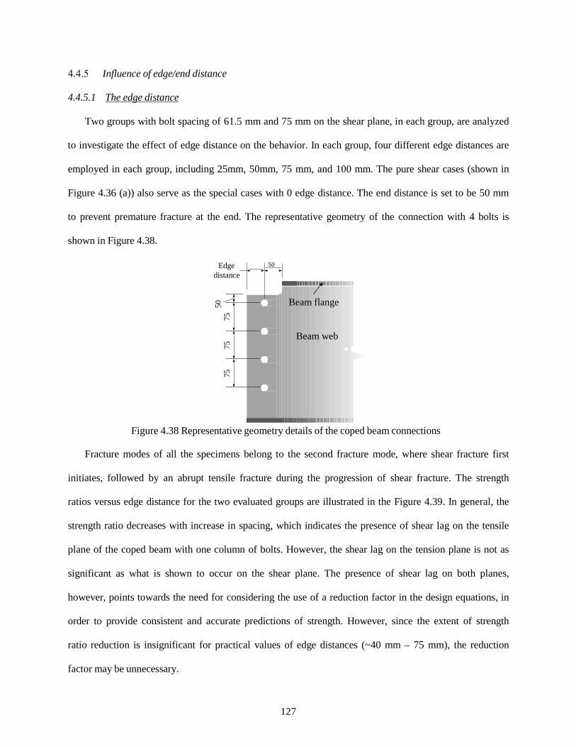
50

75

75

75

Influence of edge/end distance

4.4.5.1 The edge distance

Two groups with bolt spacing of 61.5 mm and 75 mm on the shear plane, in each group, are analyzed

to investigate the effect of edge distance on the behavior. In each group, four different edge distances are

employed in each group, including 25mm, 50mm, 75 mm, and 100 mm. The pure shear cases (shown in

Figure 4.36 (a)) also serve as the special cases with 0 edge distance. The end distance is set to be 50 mm

to prevent premature fracture at the end. The representative geometry of the connection with 4 bolts is

shown in Figure 4.38.

Edge 50 distance

Beam flange

Beam web

Figure 4.38 Representative geometry details of the coped beam connections

Fracture modes of all the specimens belong to the second fracture mode, where shear fracture first

initiates, followed by an abrupt tensile fracture during the progression of shear fracture. The strength

ratios versus edge distance for the two evaluated groups are illustrated in the Figure 4.39. In general, the

strength ratio decreases with increase in spacing, which indicates the presence of shear lag on the tensile

plane of the coped beam with one column of bolts. However, the shear lag on the tension plane is not as

significant as what is shown to occur on the shear plane. The presence of shear lag on both planes,

however, points towards the need for considering the use of a reduction factor in the design equations, in

order to provide consistent and accurate predictions of strength. However, since the extent of strength

ratio reduction is insignificant for practical values of edge distances (~40 mm – 75 mm), the reduction

factor may be unnecessary.

127

Figure 4.39 Strength ratios for different edge distances

4.4.5.2 The end distance

Two groups of coped beam connection were designed and conducted for the influence from the end

distance, and in each group there were two specimens with end distance 25 mm and 50 mm respectively,

and other settings were the same. The 25 mm is the minimum value of the required configurations defined

in AISC code, while 50 mm is serves as the comparison variable. It is logically that the ones with bigger

end distances have more strength, and there is no significant influence from the end distance on the

fracture profiles and fracture sequence, which confirms the similar conclusion in Franchuk et al (2003).

Thus there is no need to consider the effect of end distance particularly in the design.

Summary

Three different block-shear failure modes and one bolt hole tear out mode were captured in the

simulations including “tensile fracture + shear yielding”, “tensile fracture + shear fracture”, “tensile

yielding + shear fracture”, and hole tearout fracture. The classifications of the four fracture modes vary

with combinations of the shear and tensile bolt hole spacing. The first two modes are desired in the

design, while the other two should be avoided. The current design equations in major codes provide

inconsistent predictions of the strength of structural details with the potential for block shear failure,

although the strength predictions, utilizing the 2010 AISC, seems to be conservative. The allowable range

128

for the bolt hole spacing on the tensile and shear planes is sometimes not appropriate, since the

combination of large tensile spacing and small shear spacing may lead to undesired failure modes. In

addition, large bolt hole spacing on the shear plane shall be avoided since significant shear lag may occur

on the shear plane as a result of the large bolt hole spacing. Intermediate tensile spacing is favorable in

terms of both strength and ductility.

4.5 Concluding remarks

In this chapter, by employing the newly developed ductile fracture model in Chapter 3, the full

response of bolted steel connections, including the gusset plate and coped beam connections, are

simulated, up to entire failure. Excellent correlations with corresponding experimental results have been

achieved for all simulations, which validates the procedure for fracture predictions for monotonic loading

cases, and further the proposed ductile fracture model. Since the methodology has been proved to be valid,

the accuracy of further implementation of the new fracture model into structural components by using the

same methodology can be guaranteed. To that end, a parametric study was conducted with focus on

geometrical variables, including bolt spacing in the tensile and shear planes, and bolt edge/end distances,

most of which have not been fully explored by laboratory tests in the past. Relevant new findings have

been reached, which are beneficial for design codes development.

The main conclusion for this chapter can be listed as follows:

• The newly developed ductile fracture model in previous chapter is not only valid and

applicable for metals on the coupon specimen level, but also reliable on the structural

component levels, especially structural details with potential block shear failure with inherent

low and negative stress triaxialities.

• Some phenomena in block shear failure were explained physically through the ductile

fracture criterion for the first time, including detour of fracture path on the shear plane, and

the sequence of fracture progression.

129

• Parametric studies were conducted on steel connections with the potential of block shear

failure. Four different fracture modes of block shear were identified for the first time, which

provided insightful outlook onto connection behavior and also provided more information

and suggestions for future design code development.

• Compared to the experimental testing, numerical-based parametric study can be a viable

option for evaluating the effect of large number of parameters on connection response as long

as the accuracy of simulations is assured.

130

CHAPTER 5 New Models to Predict Fracture of Metals under Reverse Loading

Ductile fracture of metals resulting from large amplitude inelastic reverse straining has been the

predominant mode of failure of structural components under extreme loadings. This kind of fracture,

characterized by only a few reverse cycles with large pre-crack plastic strain, is often termed as Ultra Low

Cycle Fatigue. Ductile failure of metals has recently been recognized to be a function of stress triaxiality

and Lode angle parameter. In this section, a new fracture model with full consideration of stress triaxiality

and Lode angle parameter as well as the cut-off regions is proposed from the extension of its equivalence

for monotonic loading in Chapter 3. The underlying mechanism and determination of the cut-off region

boundary is well-defined and discussed. Additionally, the effect of load excursion on shifting the

boundary of the cut-off region and the subsequent damage evolution is assessed. The nonlinearity of

damage evolution is also studied and well characterized, and so is the history effect from the strain

reversals. The developed criterion is evaluated against data extracted from a series of multi-stress states

cyclic experimental results and excellent correlations between the proposed model and experimental

results are achieved. Comparison between the proposed model and other existing models is made and

favorable results are shown for the proposed model. The presented model can be used for predicting the

potential for ULCF failure in alloys.

5.1 Introduction

The direct stress and strain-based approaches have also been proposed and applied to the prediction of

brittle fracture under reverse loading. The most well-known examples of such are the stress-based S-N

curves developed for high-cycle fatigue and the strain-based Manson-Coffin for low-cycle fatigue. In

these two criteria, fracture often occurs after the metal has been subjected to considerable number of

cycles of reverse loading with limited or moderate pre-crack plastic strain ranges. Classification of failure

as High-Cycle Fatigue (HSF) or Low-Cycle Fatigue (LCF) depends on the number of loading cycles

before failure, which is typically on the order of millions or thousands of cycles for HSF and LCF,

131

respectively. Structural components that undergo reverse loading with considerable plastic strain demand

mostly fail in less than 100 cycles and are typically named Ultra-Low Cycle Fatigue (ULCF) or

Extremely-Low Cycle Fatigue (ELCF). Failures under ULCF, occurring after 10 or 20 cycles, are not

uncommon. Since failure under ULCF is strain-sensitive, attempts to apply the Manson-Coffin criterion

to predict ULCF life has been proven inaccurate (Kuroda, 2001; Tateishi, et al., 2007). In addition, since

strain ranges for a given loading history may significantly vary due to randomness in demand, the

traditional cycle counting techniques used for HSF life predictions may not be applicable. From a

descriptive perspective, LCF failure is due to density increase of groups of small surface cracks, which

will not exceed a limit length (Muakami and Miller, 2005) and the final failure occurs in a more of a

brittle manner. On the other hand, ULCF failure usually presents a major cup-cone type internal crack,

which is also commonly seen in ductile fracture under monotonic loading conditions. The mechanistic

and physical differences between LCF and ULCF highlight the challenges for using LCF models for

predicting ULCF life of components. Currently, there is a need for better understanding the mechanism of

ULCF and for developing new models that are capable of accurately predicting such failure.

Existing studies were mostly conducted under monotonic loading conditions for which the stress state

parameters show insignificant variations and remain almost unchanged. Therefore, this type of monotonic

loading can be termed as quasi-proportional loading. In contrast to quasi-proportional loading, models for

ductile fracture under non-proportional loading, especially reverse loading, are limited despite the fact

that failure of structural components under such loading is common.

As previously noted, there are intrinsic similarities in crack topologies that are formed under ULCF and

quasi-proportional loadings (i.e., uneven, dimple-dominated surfaces with cup-and-cone profiles),

indicated by fractographic analysis (Kanvinde and Deierlein, 2007; Voyiadjis, et al., 2013). As a result, it

is not far-fetched to presume that they also share similar crack formation characteristics including void

nucleation, growth, and coalescence. Therefore, the extension of ductile fracture criterion under quasi-

proportional loading conditions to the case of reverse loading or ULCF merits extensive consideration.

The extended ductile fracture criterion, as previously discussed, should be stress triaxiality and Lode

132

parameter dependent and should cover a broad range of these two parameters. The importance of

accounting for large strain cycles, wide range of stress triaxiality and Lode parameter, and complicated

load path lies in the fact that in structural engineering many components with varying geometries are

subjected to large cycles of reverse loading under complex loading history. For example, seismic loads

result in large strain reversals being applied to details with varying stress triaxialities including, for

example, roots of reduced beam sections, weld access holes, and panel zones. In addition, the load can be

applied in a specific angle as in the case of eccentrically braced frames, in which the Lode parameter may

be the predominant factor for initiating fracture instead of stress triaxiality.

The extension from the original quasi-proportional loading based criterion to the non-proportional

loading cases is still relatively unexplored. Bao and Treitler (2004) reported that simple direct application

of monotonic fracture models to reverse loading provided very inaccurate predictions. Bai (2008)

indicated that the linear extension is applicable for loading cases without stress reversal and that nonlinear

weighting terms should be introduced for reverse loading conditions. Hence, a proper nonlinear extension

methodology is vital for developing proper fracture criteria under ULCF loading conditions.

With respect to fracture in very negative-stress triaxiality ranges, there is a broad consensus that no

fracture can occur beyond the cut-off bounds. However, there are some differences in the literature

regarding the definition of cut-off bounds. Since fracture has been extensively observed under

intermediately negative-stress triaxialities and a variety of Lode parameters (Bao, 2003; Bao and

Wierzbicki, 2004; and Bai, 2008), the fracture bounds should thus encompass moderately negative-stress

triaxiality ranges along with the entire Lode angle parameter ranges. The cut-off bounds will also serve as

the boundary for damage evolution under complex loading conditions, especially the reverse loading

cases, in which a wide distribution of negative-stress triaxialities exists during loading reversal.

The previous discussion highlights the pressing need for developing a fracture criterion that fully

considers a wide range of stress triaxialities and Lode parameters under nonlinear damage evolution with

proper definition of the fracture cut-off bounds. The newly developed monotonic fracture criterion in

Chapter 3 is employed as the foundation for the development of the reverse loading fracture model. In this

133

=

=

p

chapter, a fracture criterion addressing reverse loading conditions is developed. The cut-off bounds of the

fracture locus in the negative-stress triaxiality range is particularly discussed and defined. The developed

criterion is evaluated against data extracted from series of multi-stress triaxiality cyclic tests conducted by

various researchers. Strong agreements between the proposed criterion and experimental data sets are

reached, indicating the validity of the newly developed model.

5.2 Description of the Stress State

Most of involved parameters are defined in section 3.2, and in this chapter, two new parameters

regarding the measure of the equivalent plastic strain, εp, which is a scalar, are employed in the fracture

modeling. The first measure is the cumulative equivalent plastic strain ε pc , also named the effective

plastic strain, and is defined by the rate form in Equation 5.1, while the second is the transient equivalent

plastic strain ε pt and is defined using Equation 5.2.

ε pc

2 ε p : ε p . (5.1)

3

ε pt

2 ε p : ε p . (5.2)

3

Under monotonic loading conditions, since there is no direction change, the cumulative and transient

equivalent plastic strains are equal and the relation ε = ε pc = ε pt holds. Under complex loading

conditions involving significant load direction changes, however, the cumulative plastic strain is an ever-

increasing scalar while its transient counterpart can decrease even under continuous plastic flow.

5.3 Discussion on the existence of a cut-off region

According to Equation 3.18, damage evolves when the material is subjected to plastic strain where

plastic strain is reached in the entire range of stress state parameters, η and θ . Fracture in every range of

θ under monotonic loading conditions has been observed and reported in many experimental studies

such as Bao (2003), Bao and Wierzbicki (2004), Barsoum and Faleskog (2007) and Li, et al. (2011). This

indicates that a cut-off limit that is solely based on the Lode angle parameter for defining the fracture

134

locus does not exist. On the other hand, a fracture cut-off region that is dependent on stress triaxiality was

highlighted in previous studies and was supported by the fact that there was no reported fracture under

monotonic loading conditions and very negative stress triaxialities.

The presence of a cut-off region in the negative stress triaxiality range was first addressed by Bao and

Wierzbicki (2005), who proposed a uniform cut-off limit with ηcutoff = −1 3 by studying a large number

of experimental results of specimens loaded under axisymmetric conditions. Kanvinde and Deierlein

(2007) also pointed out the presence of a cut-off bound with uniform stress triaxiality at ηcutoff =0 for the

Rice-Tracey model (Rice and Tracey, 1969), which was inherently included in the Gurson model (Gurson,

1977) and its extensions (Tvergaard and Needleman, 1984). However, the cut-off limits previously

proposed are challenged by the test results presented by Khan and Liu (2012) where fracture occurred

during the transition from uniaxial compression to biaxial compression with η = − 0 .495 . The fracture

cut-off region in the Mohr-Coulomb criterion is expressed as a sum of the shear stress and an additional

weighted normal stress term as follows

τ +c13σn ≤ 0

(5.3)

The Modified Mohr-Coulomb criterion in Bai and Wierzbicki (2010) and Gruben et al. (2012) are

also featured with the fracture cut-off shown in Equation 5.3.

The significance of the cut-off limit was also confirmed in Teng (2004) for the simulation of high

velocity impact. The cut-off region concept has actually already been included in several fracture models

(Cockcroft and Latham, 1968; Brozzo, et al, 1972; Oh, et al., 1979) even though this concept was not

intentionally proposed in their criteria. These models indicate that damage is assumed to only occur for

cases with maximum positive principal stresses. This means that the cut-off region is located where the

condition in Equation 5.4 is met, which can be normalized and expressed in the space of ( η , θ ,σ ),

shown in Equation 5.5.

σI ≤ 0

(5.4)

135

s η + 2 co π π

θ − ≤ 0 (5.5) 3 6 6

At the boundaries of these cut-off regions, the predicted fracture strains will tend to infinity and

damage will approach zero. These cut-off regions in the space of (η , θ ) are shown in Figure 5.1 with a

shaded area highlighting the plane stress condition. Equation 5.5 is characterized by the cut-off area

C2+C3, and Equation 5.3 by region C3. The domains C1+C2+C3 represent the uniform cut-off

assumption that ηcutoff = −1 3 .

Bampton and Raj (1982) indicated that damage due to microvoid evolution could be completely

suppressed by deforming under the maximum negative principal stress and that zero maximum principal

stress was a threshold condition for this damage type to occur, which rules out the possibility of tensile

type fracture at or below the threshold value. The occurrence of shear fracture in the critical plane with a

negative normal stress requires the shear stress in the plane of τ to overcome two obstacles, namely the

shear resistance of material τu and the friction in plane due to normal stress c13σn . The fracture then

occurs when the condition in Equation 5.6 is satisfied.

τ τ u + c13σ n

≥ 1. (5.6)

The most critical plane for the stress state with three non-positive principal stresses is the maximum

shear stress plane with zero maximum principal stress and Equation 5.6 can be written as

1 ≥ 1 . (5.7)

τ u

c13 + 2 σ

III

For ductile materials, τu is normally around 0.6 times the tensile strength and the friction coefficient,

c13, has a minimum value of 0.5 (Chang et al., 1988). This means that fracture occurs only when the

minimum principal stress reaches a magnitude of at least 4 times the shear strength or 2.4 times the tensile

strength. From a practical sense, buckling of structural metal components would have already begun

before the occurrence of such significant compressive stress. Such condition, however, is not difficult to

136

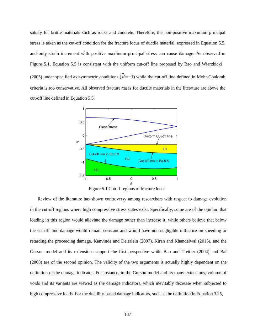
satisfy for brittle materials such as rocks and concrete. Therefore, the non-positive maximum principal

stress is taken as the cut-off condition for the fracture locus of ductile material, expressed in Equation 5.5,

and only strain increment with positive maximum principal stress can cause damage. As observed in

Figure 5.1, Equation 5.5 is consistent with the uniform cut-off line proposed by Bao and Wierzbicki

(2005) under specified axisymmetric conditions ( θ = −1) while the cut-off line defined in Mohr-Coulomb

criteria is too conservative. All observed fracture cases for ductile materials in the literature are above the

cut-off line defined in Equation 5.5.

Figure 5.1 Cutoff regions of fracture locus

Review of the literature has shown controversy among researchers with respect to damage evolution

in the cut-off regions where high compressive stress states exist. Specifically, some are of the opinion that

loading in this region would alleviate the damage rather than increase it, while others believe that below

the cut-off line damage would remain constant and would have non-negligible influence on speeding or

retarding the proceeding damage. Kanvinde and Deierlein (2007), Kiran and Khandelwal (2015), and the

Gurson model and its extensions support the first perspective while Bao and Treitler (2004) and Bai

(2008) are of the second opinion. The validity of the two arguments is actually highly dependent on the

definition of the damage indicator. For instance, in the Gurson model and its many extensions, volume of

voids and its variants are viewed as the damage indicators, which inevitably decrease when subjected to

high compressive loads. For the ductility-based damage indicators, such as the definition in Equation 3.25,

137

0

damage is always a positive variable and a predefined limit should be employed for zero damage in the

cut-off region. The two explanations are equivalent for understanding fracture delay phenomena after

compressive loading cycles while for premature fracture scenarios only the second perspective is

applicable. No attempt is made in this present study to distinguish between the two arguments. However,

since the developed criterion is founded on the ductility-based analysis in chapter 3 under quasi-

proportional loading conditions, the status of damage evolution in the cut-off regions and the subsequent

impacts follow the second perspective in which damage is always a positive variable.

5.4 Extension of the fracture criterion from monotonic loading to reverse loading

Occurrence of fracture due to large reverse pre-crack straining, often termed as ULCF, falls in

between the monotonic ductile fracture and traditional LCF fracture and shares more characteristics with

monotonic loading-based fracture.

As previously stated, the direct extension from the monotonic fracture model to reverse loading

through a linear damage evolution law provides inaccurate predictions. Hence, it is necessary to introduce

modifications describing the “fatigue” influence on the linear damage incremental rule.

The damage evolution rule is generally defined by an integral function of the stress state parameters,

shown as

D = ∫ε p f (η ,θ )d ε p , (5.8)

where the stress state parametersη(ε p ) , andθ(ε p ) , are monotonic functions of the equivalent plastic

strain and the damage indicator, D, lies in the range of [0 1], in which a value of 0 represents raw material

without degradation while a value of 1 corresponds to the initial failure state.

The damage in Equation 3.25 is postulated to accumulate in a linear fashion. The linear incremental

relationship has been widely used in the literature (Wierzbicki et al., 2005a) for the quasi-proportional

loading condition in which ε f is treated as constant since the stress state parameters are assumed to be

unchanged.

138

Perfect proportional loading is scarce in practical situations and even under classical proportional

loading η and θ cannot remain unchanged in the final unstable stage near fracture. Therefore, linearity

of the damage evolution is questionable in some sense. For the loading case without direction change, Bai

(2008) indicated that the linear incremental rule was applicable after analyzing a series of experimental

results. While this is questionable to some extent due to the mentioned changes in the stress parameters

near fracture, is understandable since no dramatic microstructural changes that will take place in the

absence of complex loading and stress reversals. It is important to emphasize, however, that the linear

incremental rule is not applicable for complex or reverse loading conditions.

For the loading cases with directional change, namely reverse loading, employing the linear damage

increment rule results in the Dc term at the limit ε p = ε f being either increased and larger than unity as in

the case of 1045 steel as reported in Bai (2008), shown in Figure 5.2 or reduced and smaller than one as in

the case for Al2024-T351 as reported in Bao and Treitler (2004). The discrepancy of fracture between the

monotonic and reverse loading conditions has also been indicated through fractographic analysis, in

which shallower dimples appear in the fracture surfaces in the case with reverse loading than the case

under monotonic loading conditions (Kanvinde and Deierlein, 2007). Therefore, changes in loading

direction play a role in damage evolution under reverse loading conditions.

It is postulated that the inconformity of damage indicators between the analytical and experimental

results under complicated loading conditions may be caused by 1) the nonlinear nature of damage

evolution, or 2) the nonlinear influence of loading history defined by reverse loading, or 3) the combined

effects of damage and loading history nonlinearities. Verification analysis for the three mentioned

speculations is conducted for several metal alloys in the verification and calibration section.

Nonlinear damage evolution rule

The linear ductility damage definition shown in Equation 3.25 is the simplest solution to Equation

3.24. Other straightforward solution with a more general format is shown as follows

139

ε ε ε ε

m m−1 ε ε dε m−1 dε D = p , dD = m pt pc = mD m pc , (5.9)

f

f f f

where m is a material constant. Equation 5.9 is actually a variant of the nonlinear damage accumulation

rule for traditional fatigue developed by Gratts (1961). The tests, identified as number 2 and 7 in the

verification and calibration section for ASTM A572 Gr.50 steel, are taken as prototypes for quasi-

proportional and reverse loading conditions, respectively, and the simulated damage evolution are plotted

by Equation 3.18 and 5.9 with m=1.9445. The value of m does not affect Dc in the quasi-proportional

loading cases, but does influence the damage magnitude before certain limit state, which may be the

starting point of loading in another direction. This is shown in the damage simulation of test 7 in Figure

5.2. For the case of quasi-proportional loading conditions, if m tends to 1, Equation 5.9 returns to

Equation 3.25. and damage evolves in a linear manner along the equivalent plastic strain. The damage at

the initial stage becomes more significant when m is less than 1 while the damage at the onset of failure is

more prominent with m larger than 1 as shown in the damage evolution simulation for Test 2 in Figure

5.2. It should be noted that in Figure 5.2 the final predicted equivalent fracture strain does not perfectly

correspond to its experimental counterpart through the calibrated parameters based on the linear damage

assumption presented in Equation 3.25 and that the constant m tends to amplify the error. The parameter

m is not redundant, although the linear increment law has been proven to be applicable to monotonic

loading cases. This is because under reverse loading conditions, the damage developed at the incipient of

plastic strain path accumulates and constitutes the total damage as shown in the plot for Test 7 in Figure

5.2 and the damage evolution rate at the initial stage is governed by the parameter m. On the other hand,

the transient equivalent plastic strain shows high sensitivity to strain reversal; and thus is taken as the

presiding measure of strain variables.

140

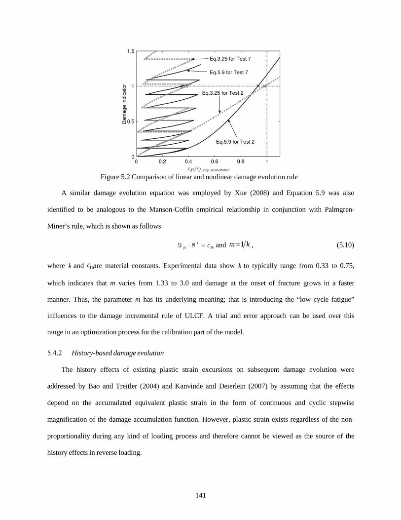
k

Figure 5.2 Comparison of linear and nonlinear damage evolution rule

A similar damage evolution equation was employed by Xue (2008) and Equation 5.9 was also

identified to be analogous to the Manson-Coffin empirical relationship in conjunction with Palmgren-

Miner’s rule, which is shown as follows

∆ε pc ⋅ N = c16 and m =1 k , (5.10)

where k and c16are material constants. Experimental data show k to typically range from 0.33 to 0.75,

which indicates that m varies from 1.33 to 3.0 and damage at the onset of fracture grows in a faster

manner. Thus, the parameter m has its underlying meaning; that is introducing the “low cycle fatigue”

influences to the damage incremental rule of ULCF. A trial and error approach can be used over this

range in an optimization process for the calibration part of the model.

History-based damage evolution

The history effects of existing plastic strain excursions on subsequent damage evolution were

addressed by Bao and Treitler (2004) and Kanvinde and Deierlein (2007) by assuming that the effects

depend on the accumulated equivalent plastic strain in the form of continuous and cyclic stepwise

magnification of the damage accumulation function. However, plastic strain exists regardless of the non-

proportionality during any kind of loading process and therefore cannot be viewed as the source of the

history effects in reverse loading.

141

It is assumed in the present study that the immense deviation from proportional loading during the

reverse loading process is the main source of the history effects on the damage evolution. A new

parameter is introduced to describe the effects on the following damage evolution from the previous non-

proportional loading history, expressed as

κ = ∫ ε pc

β dε pc , (5.11) 0

where β is defined as

3 3 3 3

∑∑σ ij ∑∑α ij

β = i =1 j =1 − i =1 j =1 , (5.12) o α 1 1

where α is the back stress tensor. The parameter β is designed to describe the stress state non-

proportionality, featured with a range of [-2, 2]. A similar but non-negative parameter was introduced by

Bai (2011). One can observe that the parameters β and κ have zero values for quasi-proportional loading

conditions, whereas the sign of depends on the initial loading sequence. For a load sequence with initial

tension followed by compression loading, as shown in Figure 5.3, the parameter κ starts from zero, then

fluctuates with decreasing mean values. This indicates that the effect of loading direction changes can be

counteracted by opposite changes whereas in the first half cycle, which is equivalent to quasi-proportional

monotonic loading conditions, κ maintains a zero value.

Figure 5.3 Schematic representation of history effects based damage evolution

142

It is postulated that the non-proportionality of the loading history affects the damage evolution law in

Equation 3.25 in the following format

dD = exp(c14κ ) dε p , (5.13) ε f (η,θ )

where c14 behaves as a weighing parameter requiring calibration and represents the effect of non-

proportionality on accelerating damage evolution when c14κ > 0, decelerating damage when c14κ < 0, and

no non-proportionality effects when c14κ = 0. When under proportional loading conditions with κ = 0 ,

Equation 5.13 will reduce to Equation 3.25. An example showing the decaying effects is presented in

Figure 5.3. From the figure, one can observe that the modification of Equation 5.13 reduces the

overestimated damage by Equation 3.25. It is noteworthy that in the first half cycle the two equations

provide the same damage increments. As discussed before, plastic strain occurring at the cut-off regions

speeds up or retards subsequent damage evolutions. It is also worth pointing out that the integral

boundaries of Equation 5.11 cover the whole range of the plastic strain paths, even in the cut-off regions.

The history effects correspond to LCF cases with negative stress ratio, R = σmin σmax < 0, as well as

the possible phenomena of fatigue crack closure. During crack closure and the simultaneous compressive

load, the crack surfaces are highly compressed, resulting in crack sharpening and subsequent acceleration

of crack growth. However, it is noted that not all the compressive load is used to collapse the voids and

sharpen the crack tip. Instead, some and perhaps most of the compressive load is dissipated during the

process of reversing the residual stresses from the preceding tensile cycle in the vicinity of the crack tip,

resulting in a subsequent decelerated crack growth. As previously stated, the acceleration and deceleration

effects are described in Equation 5.13 by c14κ > 0and c14κ < 0, respectively. If the stress ratio is always

positive, such history effects should be eliminated.

143

Damage evolution under the combined effects of nonlinearity and loading histories

Since the effects of the nonlinear increment and loading history are defined in Equation 5.9 and

Equation 5.13, a damage evolution in the format of Equation is proposed under the assumption that the

two effects behave independently and simultaneously.

m−1 ε p d ε p

dD = exp (c14κ )m (5.14) ε f ε f (η,θ )

It should be noted that the values of m and c14, calibrated using Equation 5.9 and 5.13, respectively,

may not be applicable to Equation 5.14 and new parameters have to be determined based solely on

Equation 5.14. Comparison between the three criteria, using test number 7, is shown in Figure 5.4. More

comparisons are available in Figure 5.13 and 5.14.

Figure 5.4 Comparison of the three approaches (Specimen 7 in Table 5.2)

5.5 Verification analysis and calibration of the proposed criterion

The stress triaxiality and Lode parameter dependencies have been extensively discussed in chapter 3

and modeled in Equation 3.18. Therefore such dependencies are not discussed in the verification part. The

parameters c7, c8 and c9 in Equation 3.18 will be calibrated from specimens under monotonic quasi-

proportional loading conditions since the excellent predictions by Equation 3.18, using the linear damage

incremental rule, has been verified and displayed through analysis of monotonic loading cases in chapter

144

1 ∑

3. The main objective of this chapter is to model and verify the nonlinearity and history effects resulting

from non-proportional loadings. Thus, several laboratory tests with different cyclic loading procedures are

employed as the experimental comparison groups. The parameter m and c14will be calibrated under

those reverse loading conditions and all parameters are determined using an optimization function to

minimize the relative error, shown as

Rel.Error(c7 ,c8,c9 ,c12,m,c14) =

(ε f _Predicted−ε f

N N

Experimeanlt )/ ε f Experimeanlt

(5.15)

in which N is the number of tests analyzed.

Specimens under compression-tension loading

5.5.1.1 Example 1: 1045 Steel

Bai (2011) designed and performed a series of tests using 1045 steel to study the effect of loading

history on damage evolution including monotonic and reverse loading tests with compression-tension

sequences.

The data set for monotonic loading cases comprised of a series of tests employing “classical”

notched and smooth bar specimens as well as grooved plates and tubular specimens. The experimental

fracture locus as well as the predicted locus and bounding curves according to the new criterion are

depicted in Figure 5.5, which shows strong correlations between the experimental and predicted data

points. The figure also shows inaccurate predictions when the Rice and Tracy model is used. Calibration

of the parameters of the new criterion in Equation 3.18 result in c7=0.51, c8 =-1.92 and c9 =-3.35 for 1045

steel. The reverse loading cases include notched axisymmetric specimens under differing pre-compression

strains. Since the stress state history is not provided for the data used, parallel numerical simulations are

conducted for all cases using the general-purpose finite element software ABAQUS (Simulia, 2012). The

specimens are modeled with solid element type CAX4R, and a resolution of 10 elements per mm is used

at the hot spots. Quarter model simplification is adopted to reduce the computational time. The nonlinear

isotropic/kinematic combined hardening model embedded in ABAQUS is used to simulate the

145

Bauschinger effect during reverse loading. The parameters for the constitutive equations have been

calibrated in Bai (2011) and are used in the numerical models in the present study. Comparisons of load-

displacement curves between experimental results and numerical simulations are shown in Figure 5.6. As

shown in the figure, very good correlations are achieved in all cases, highlighting accuracy of the

simulations.

Figure 5.5 Fracture locus constructed with the new criterion for 1045 steel under monotonic loading

Figure 5.6 Comparison of load-displacement curves and predicted fracture displacements for 1045 steel

The critical damage indicators at fracture for the reverse loading group are plotted in Figure 5.7 for

the linear damage increment rule in Equation 3.25. The figure clearly shows that the damage at fracture

for the pre-compression specimens is greater than one. This clearly indicates that damage for components

under reverse loading conditions does not evolve in a linear manner.

146

Simulations of damage evolution under reverse loading cases using linear, exponential nonlinear,

history-based, and combined-based approaches are all performed, and the reference fracture strain ε f in

Equation 3.25, 5.9, 5.13 and 5.14 is calculated from Equation 5.15 using the parameters calibrated from

monotonic loading cases. The reverse loading cases 1 and 3 are used for calibration while the reverse

loading case 2 is used for validation. The parameter mand c14are calculated by trial and error using a

MATLAB code and the best fits for the nonlinear approaches are also plotted in Figure 5.7, with

m = 1 .48 for Equation 5.9, c14 = −9.87 for Equation 5.13 and m = 1 .77 and c14 = −9.04 for Equation

5.14. One can observe that the linear and exponential nonlinear ductility approaches are not applicable for

the pre-compression loading conditions since the optimized limit damage indicators still diverge from

unity. The history-based approach successfully corrects the overestimation of the damage indicators for

all cases while the model based on the combined effects only slightly improves the predictions. Therefore,

it can be concluded that the history-based approach is more applicable than the exponential nonlinear

ductility-based one for 1045 steel, at least under the pre-compression conditions.

Figure 5.7 Comparison of the two correction approaches on 1045 steel

5.5.1.2 Example 2: Al 2024T351

Bao and Treitler (2004) carried out a series of tests to study crack formation and utilized

axisymmetric Al 2024 T351 specimens with three different notch radii under differing pre-compression

strains followed by tension until failure. Finite element (FE) models were also developed using ABAQUS

147

for all the cases to compute the stress/strain states in the critical fields since such information was not

included in the study by Bao and Treitler (2004). The FE modeling approach is the same as used in

Example 1. The detailed geometry and material information can be found in Bao and Treitler (2004). The

numerical versus experimental load-displacement curves for each specimen are shown in Figure 5.8 (a),

(b), and (c) for specimens A, B and C, respectively. Excellent correlations between the experimental

results and the numerical predictions are achieved.

It should be noted that experimental results for the same material conducted by different researchers

may show inevitable discrepancy. For example, results of another group of 1045 steel tested by Bai (2008)

and used to calibrate the parameters show non-negligible difference in comparison with the groups

employed in chapter 3. The same discrepancy occurs for Al 2024 T351 between the experimental results

in Bao (2003) and Bao and Treitler (2004). The predicted fracture strain for specimen A under the

monotonic tension loading and when using the parameters of Equation 3.18 that are obtained in chapter 3

and assuming quasi-proportional loading, is predicted to be 0.29. This greatly overestimates the actual

fracture strain of 0.17. This is because while the specimens’ geometry and material property may be

similar, the loading path from manufacturing and machining the specimens and the subsequent loading

protocol during the tests can differ, hence impacting the nonlinear damage evolution. Therefore, the

parameters of the fracture criterion need to be recalibrated for the data set in Bao and Treitler (2004).

Since during most of the loading path, the absolute value of θ almost remains unchanged and equals one,

Eq.15 transforms to a two-parameter criterion with two unknown parameters, c8 and c15 = c7 cos(π 6)c9 .

Calibration of the proposed model parameters is conducted, for Equation 3.25, 5.9, 5.13, and 5.14,

using the experimental results of specimen A while the results of specimen B and C are used for

validation. Coincidentally, Equation 3.25 and 5.9 yield parameters with the same values, which are c8=-

3.09, c15 =1.16 and m = 1 . Similarly, Equation 5.13 and 5.24 also share the same parameters, which are

c8=-3.09, c15 =1.16, m = 1 and c14 =1.30. Moreover, all four criteria provide reasonable predictions, shown

in Figure 5.9. The predicted accumulated equivalent plastic strains at fracture are also plotted in Figure

148

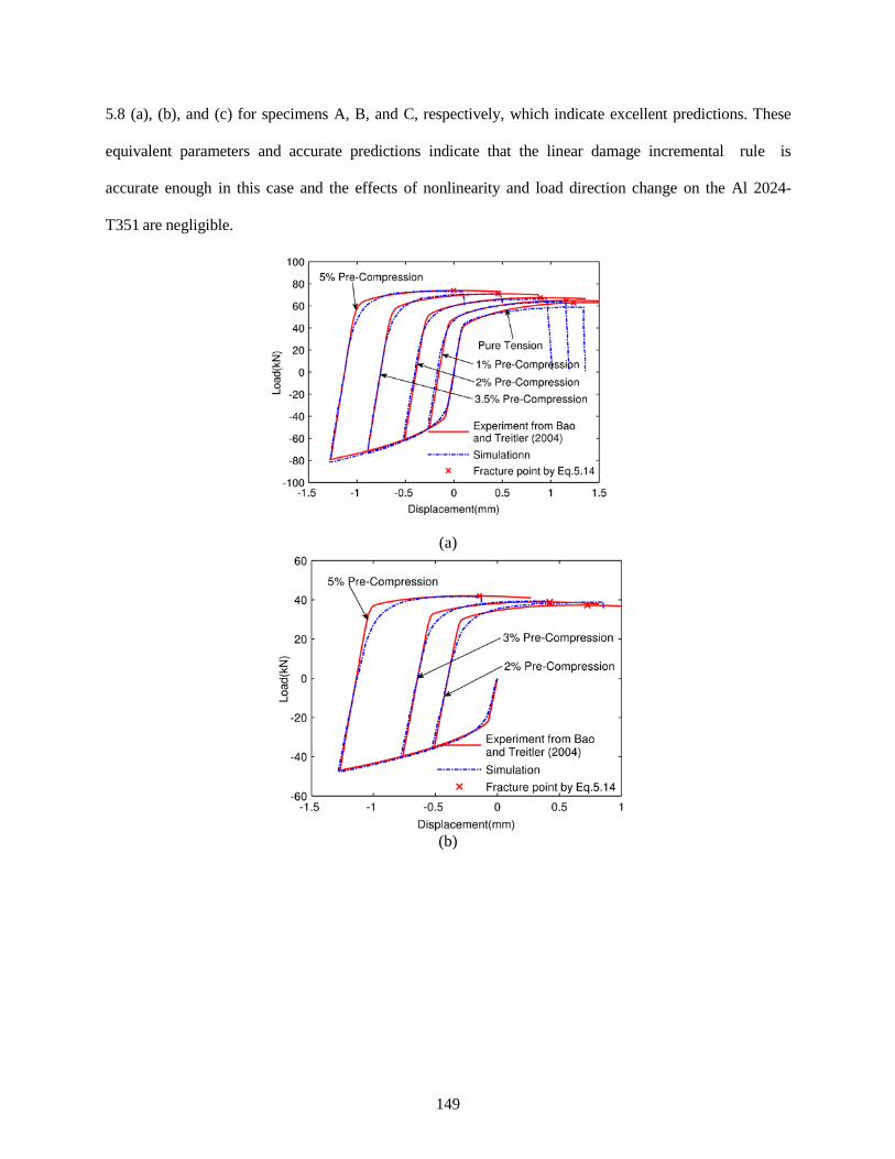
5.8 (a), (b), and (c) for specimens A, B, and C, respectively, which indicate excellent predictions. These

equivalent parameters and accurate predictions indicate that the linear damage incremental rule is

accurate enough in this case and the effects of nonlinearity and load direction change on the Al 2024-

T351 are negligible.

(a)

(b)

149

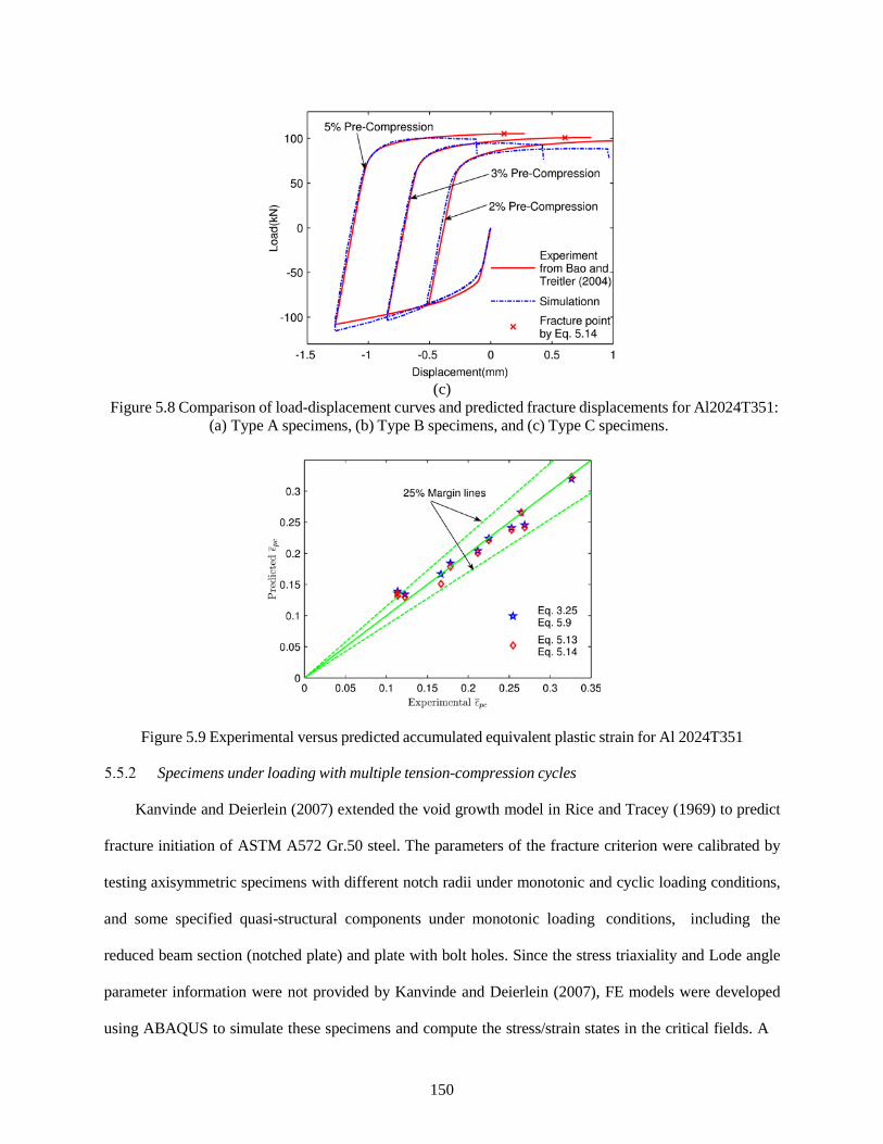
(c)

Figure 5.8 Comparison of load-displacement curves and predicted fracture displacements for Al2024T351: (a) Type A specimens, (b) Type B specimens, and (c) Type C specimens.

Figure 5.9 Experimental versus predicted accumulated equivalent plastic strain for Al 2024T351

Specimens under loading with multiple tension-compression cycles

Kanvinde and Deierlein (2007) extended the void growth model in Rice and Tracey (1969) to predict

fracture initiation of ASTM A572 Gr.50 steel. The parameters of the fracture criterion were calibrated by

testing axisymmetric specimens with different notch radii under monotonic and cyclic loading conditions,

and some specified quasi-structural components under monotonic loading conditions, including the

reduced beam section (notched plate) and plate with bolt holes. Since the stress triaxiality and Lode angle

parameter information were not provided by Kanvinde and Deierlein (2007), FE models were developed

using ABAQUS to simulate these specimens and compute the stress/strain states in the critical fields. A

150

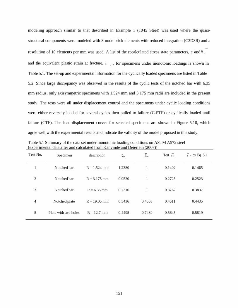
modeling approach similar to that described in Example 1 (1045 Steel) was used where the quasi-

structural components were modeled with 8-node brick elements with reduced integration (C3D8R) and a

resolution of 10 elements per mm was used. A list of the recalculated stress state parameters, η and θ ,

and the equivalent plastic strain at fracture, ε f , for specimens under monotonic loadings is shown in

Table 5.1. The set-up and experimental information for the cyclically loaded specimens are listed in Table

5.2. Since large discrepancy was observed in the results of the cyclic tests of the notched bar with 6.35

mm radius, only axisymmetric specimens with 1.524 mm and 3.175 mm radii are included in the present

study. The tests were all under displacement control and the specimens under cyclic loading conditions

were either reversely loaded for several cycles then pulled to failure (C-PTF) or cyclically loaded until

failure (CTF). The load-displacement curves for selected specimens are shown in Figure 5.10, which

agree well with the experimental results and indicate the validity of the model proposed in this study.

Table 5.1 Summary of the data set under monotonic loading conditions on ASTM A572 steel (experimental data after and calculated from Kanvinde and Deierlein (2007))

Test No. Specimen description ηav θ av Test ε f ε f by Eq. 5.1

1 Notched bar R = 1.524 mm 1.2380 1 0.1402 0.1465

2 Notched bar R = 3.175 mm 0.9520 1 0.2725 0.2523

3 Notched bar R = 6.35 mm 0.7316 1 0.3762 0.3837

4 Notched plate R = 19.05 mm 0.5436 0.4558 0.4511 0.4435

5 Plate with two holes R = 12.7 mm 0.4495 0.7489 0.5645 0.5819

151

Table 5.2 Summary of experimental data and simulations of cyclic notched bar (Experimental data after Kanvinde and Deierlein (2007))

Test

No.

Specimen

description

Load

type

Experimental fracture

displacement

Fracture displacement by

Eq. 5.9 Eq. 5.13

6 R = 1.524 mm CTF

(-0.13:0.26),[9,0.2]

(-0.13:0.26),[9,0.2]

(-0.13:0.26),[8,0.102] (-0.13:0.26),[9,0.2]

7 R = 3.175 mm CTF (-0.13:0.38),[7,0.2]

(-0.13:0.38),[7,0.3]

(-0.13:0.38),[7,0.248] (-0.13:0.38),[7,0.064]

8 R = 3.175 mm C-PTF 6(-0.13:0.25),[0.6]

6(-0.13:0.25),[0.6]

6(-0.13:0.25),[0.65] 6(-0.13:0.25),[0.3]

Note: CTF = Cyclic to failure, and C-PTF = Cyclic then pulled to failure. The specimens are cycled between displacement limits and subjected to tension load at the incipient stages. The displacement history is described with the following examples: for CTF, (-0.13:0.26),[9,0.2] refers to specimen cycled between -0.13 mm and 0.26 mm until failure is observed on the 9 cycles at a 0.2 mm displacement; for C- PTF, 6(-0.13:0.25),[0.6] refers to a specimen first subjected to 6 cycles with displacement limits of -0.13 mm and 0.25 mm, and then pulled to failure at a 0.6 mm displacement.

Figure 5.10 Load-displacement curves for selected tests (Experimental data after Kanvinde and Deierlein (2007))

The calibrated parameters in Equation 3.18 result in c7=1.18, c8=-1.90, and c9=-1.84 for ASTM A572

steel based on the experimental results from the monotonic loading conditions in Table 5.1. The new

152

criterion, as depicted in Figure 5.10, predicted very well the fracture strain through all the data points and

thus could be used to define the reference fracture strain ε f in Equation 3.25, 5.9, 5.13, and 5.14.

Applying the linear damage increment rule in Equation 3.25 and the modified evolution laws in

Equation 5.9, 5.13, and 5.14 to the reverse loading cases, the predicted equivalent fracture strains at the

fracture locations are shown and compared with each other in Figure 5.11, with m = 1.94 for Equation 5.9

and c14 = 27.52 for Equation 5.13, and m = 1.30 and c14 = 19.40 for Equation 5.14. All the three

experimental results are used for calibration and further utilized in the validation process. From Figure

5.11 one can observe that the damage indicator based on the linear damage evolution law failed to even

come close to unity, which confirms the conclusion that a linear damage incremental rule cannot

accurately predict fracture under complex loading histories. On the other hand, both of the two modified

approaches can predict the final damage with a reasonable accuracy as shown in Table 5.2 and Figure

5.11 and the combined effects criterion greatly improves the accuracy of predictions. Although the

history-based approach slightly outstepped the exponential ductility approach, no distinct difference is

noted in their comparisons in Table 5.2 and Figure 5.11.

Simulations of how damage evolves with the equivalent plastic strain using Equation 5.9, 5.13, and

5.14 during the entire loading process are depicted in Figure 5.13 and 5.14 for tests number 6 and 8,

respectively, and the same plot for Specimen 7 is presented in Figure 5.4. From the figures it is observed

that for the criterion in Equation 5.9, damage accelerates with increased equivalent strain and sometimes

reaches an unstable stage when failure is forthcoming. Conversely, damage modeled using Equation 5.13

develops rapidly at the incipient stage and then evolves at a stable rate. The damage simulated using

Equation 5.14 is situated between the other two approaches. The research on how damage evolves under

complex loading conditions is still relatively scarce and more work may be needed to identify the damage

evolution paths in the future.

153

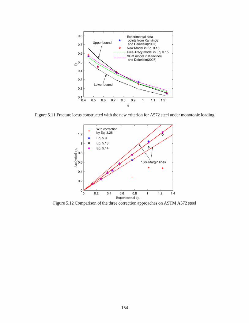
Figure 5.11 Fracture locus constructed with the new criterion for A572 steel under monotonic loading

Figure 5.12 Comparison of the three correction approaches on ASTM A572 steel

154

Figure 5.13 Damage evolution along with ε for test with number 6 (CTF)

Figure 5.14 Damage evolution along with ε for test with number 8 (C-PTF)

Summary and comparative study

The use of the combined nonlinear correction in Equation 5.14 provided the most accurate

predictions on fracture in metals. As shown in Figure 5.4, for ASTM A572 Steel, the combined approach

is more accurate than the independent nonlinear and history effect approaches and it is evident that these

two approaches still predict damage with acceptable engineering accuracy. The un-modified linear

approach is not able to provide even rough predictions. For 1045 steel, the combined criterion does not

show significant advantages over the history-based modified approach, and the nonlinear modified and

un-corrected linear approaches are simply not applicable. For Al 2024-T351, all four approaches offer

155

Parameters Eq. 3.25 Eq. 5.9 Eq. 5.13 Eq. 5.14

m 1 1.4807 1 1.7708

c14 0 0 -9.8732 -9.0393

Rel. error 55% 52.35% 0.93% 0.38%

m 1 1 1 1

c14 0 0 1.3020 1.3020

Rel. error 6.79% 6.79% 6.7% 6.7%

m 1 1.9445 1 1.2997

c14 0 0 27.5164 19.4012

Rel. error 58.89% 5.63% 4.38% 0.45%

acceptable predictions, and none of the modified versions indicated significant improvement. As shown in

Table 5.3, ASTM A572 steel is both sensitive to the nonlinear and history effect and 1045 steel is only

dependent on the history effect. For Al 2024-T351, however, neither the nonlinear nor the history effect

dependency is revealed. Thus, it can be concluded that the dependency of linear, nonlinear, or history-

based approach on damage evolution varies with different types or grades of metals. In other words, tests

specially designed under reverse loading need to be conducted for various metal classifications to assess

and calibrate such dependency.

The nonlinear approach fails in the prediction of 1045 steel and provides acceptable results for the

other two metals. The history effects approach provides predictions with engineering accuracy for all

three metals. The combined approach provides the most accurate predictions. It is evident that the history

effect is more universal than the nonlinear effect, which merits further study.

Table 5.3 Comparison of the three approaches for different metals

Examples

1045 Steel

Al 2024-T351

ASTM A572

Steel

5.6 Concluding remarks

Fracture after few reverse loading cycles, or ULCF, is one of the predominant limit states in metal

structures subjected to extreme loading cases. Based on past research, the underlying mechanisms for

ULCF are presumed to be similar to the ductile fracture mechanisms under monotonic loading conditions.

Ductile fracture has been proven sensitive to two-stress state parameters; namely the stress triaxiality and

156

Lode angle parameters. Thus, in this dissertation the fracture criterion developed in Chapter 3, with

dependency on both the stress triaxiality and Lode angle parameter, is extended for reverse loading cases.

Noteworthy, the intrinsic difference between the reverse and monotonic loading condition, mainly the

extent of variations of the stress state parameters, the fracture cut-off region, as well as the nonlinearity

and history effect on damage evolution, make the direct extension of the fracture model from monotonic

to reverse loading inapplicable.

Unlike monotonic loading conditions, the load path under ULCF can result in stress state parameters

that fall outside of the boundaries of the cut-off region. As previously discussed, this has been proven to

exist in many experimental studies. In the present study, the boundary of the cut-off region has been

determined to correspond to zero maximum principal stresses as shown in Equation 5.5. The influence of

the load expedition in the cut-off region is found to not change the current damage but speed or retard the

subsequent damage evolution.

The extension from monotonic to reverse loading conditions was achieved by the development of an

appropriate ductility-based damage evolution law. The linear damage incremental rule has been

confirmed to be only applicable to monotonic/quasi-proportional loading conditions and the difference

between the empirical and analytical prediction results when linear damage evolution is utilized is

postulated to be due to two parts, namely the nonlinear nature of the damage evolution law and the

influence of the loading history. The two parts are modeled and embedded into the ductility-based

damage incremental rule in both a separate and a combined format.

The verification analysis of the proposed model with the three damage evolution rules includes one

aluminum alloy and two steel grades. For the combined approach, satisfactory correlations are achieved

between the model predictions and experimental tests for all type of metals. For the approach with only

history effect modification, however, acceptable accuracy is attained. The nonlinear modified approach

failed to provide reasonable prediction for 1045 steel. Hence, it can be concluded that the combined

approach is valid and can be applied for metal fracture predictions and the history effect modified

approach may serve as a backup choice. The dependency on the two types of modifications varies with

157

different type or grade of metals. Model parameters for the cited metal types are calibrated and further

calibration should be conducted for evaluating the applicability of the models to other regular structural

metal types.

158

CHAPTER 6 Validation and Implementation of the New Fracture Model to Structural

Details under Cyclic Loadings

6.1 Introduction

Many natural and man-made hazards, such as earthquake, strong winds, fatigue and blast loading,

will lead to cyclic stress/straining on critical structural details and subsequent failures. There have been

many studies on the response of steel structures under elastic and small inelastic cyclic loadings, and the

corresponding predictions of such through numerical simulations are widely confirmed and well

developed since usually they do not require simulation of fracture. In cases where large inelastic demand

is expected, usually a prescriptive target performance is assigned to mark the onset of connection failure

without actually simulating fracture. The proposed ductile fracture model under cyclic loading in Chapter

5 provides a viable approach to simulate the entire fracture process. In addition to the specimen level

validation analysis in Chapter 5, in this Chapter the proposed ductile fracture model under reverse loading

is also verified on the structural details level, through comparison between numerical simulations of shear

links that are typically employed in EBFs and their experimental equivalents. The good comparisons also

further validate the developed fracture model and the modeling approach for predicting the entire

response of steel connections and buildings under any large inelastic cyclic deformations. The simulated

specimens are selected from a group of shear link experimental tests conducted by Galvez (2004), since

sufficient information was provided in their laboratory tests regarding the entire response of all specimens

up to entire failure.

6.2 Constitutive equations for metal under cyclic loading

Constitutive equations of von Mises material

The constitutive equations and associated development are briefly reviewed and derived from Dunne

and Petrinic (2005), and de Souza Neta et al. (2011), for the purpose of providing a comprehensive

159

(

σ

I II

e

understanding prior to introducing Section 6.2.2, which outlines the integration derivation for the

combined hardening plasticity model.

6.2.1.1 Basic definitions and yield criterion

The strain tensor ε is assumed the sum of the elastic part εel and plastic part ε pl , as shown in

Equation 6.1, which is often called classical additive decomposition for strain.

ε = εel + ε pl (6.1)

The elastic stress tensor, by the assumption of isotropic linear elasticity, can be given by

o = 2Gεel +λII: εel , (6.2)

where G is the shear modulus, λ is the bulk modulus, and I is the second-order identity tensor.

Plasticity commences when the equivalent stress reaches the current yield stress, and thereafter

hardening begins to develop. In this dissertation only the von Mises yield criterion is considered, which is

defined in Equation 6.3 as follows,

f = σe −σ y , (6.3)

where σe is usually named as the (von Mises) equivalent stress or effective stress, defined in Equation 6.4

in terms of principal stresses, or in terms of direct and shear stresses in Equation 6.5, or in terms of the

second stress invariant J2 in Equation 6.6. It should be noted that the yield criterion is only for un-

strained or perfectly plastic material since the yield stress is subjected to increase after hardening, and

y = σ y0 is the initial yield stress of the material.

e = 1 [(σ 2

− σ II )2 + (σ − σ III )2 +

(σ

III − σ I )2 ]1/ 2

(6.4)

3 2 2 2

2 2 2 ) 1 / 2

e = 2

σ 11 + σ 22 + σ 33 + 2σ 12 + 2σ 23 + 2σ 31

(6.5)

3 σ': σ'

2

1 / 2

=

3J 2

(6.6)

160

The von Mises yield criterion is often referred to as J2 plasticity, since the second stress invariant

J 2 = (1 2 σ': σ' )

1 / 2 is the cause for the plastic flow during yielding. Identifying the yield condition through

the yield criterion is quite straightforward, shown as follows:

If f < 0 then the material is elastic, and has elastic deformation;

If f ≥ 0 then the material has yielded, and plastic deformation occurs.

Actually, the material is somewhat subjected to hardening, which means the required stress to further

plastic deformation increases with the accumulated plastic strain p , and therefore the definition of the

equivalent stress and yield stress is altered by the hardening. For the sake of simplicity and convenience,

perfect plasticity is assumed, which represents the case of no hardening where the yielding stress always

holds its initial value, σy0. However, all metals are somehow featured with hardening after yielding

initiates. In the following sections, the hardening behavior of the metal is introduced, and so are the

changed definitions of the yield criterion.

6.2.1.2 The flow rule

The yield function in Equation 6.6 is used to determine the necessary conditions to initiate yielding,

while what occurs after yielding is controlled by flow rule. In other words, the flow rule is used to

determine the “direction” and “magnitude” of the plastic flow, which is also called plastic strain

increment. The flow rule is often defined in the following format,

d ε pl = d λ ∂g , (6.9) ∂ σ

where g is usually called plastic potential, which is a continuous differentiable function, and d λ is a

non-negative scalar and called plastic multiplier. For many materials, the plastic potential is usually the

same as the yield criterion g = f , and their plasticity model is named as the associated model since it

associates with the yielding criterion. The plasticity model with g ≠ f is called non-associated model. In

the present dissertation, only associated model is considered since most structural steels follow the

associated flow rule. The associated flow rule is therefore written in the following form,

161

d ε pl = d λ ∂f

∂ σ

. (6.10)

The associated flow rule assumes the plastic flow develops in a direction normal to the tangent to the

yield surface at the loading point, and according to the expression in Equation 6.10, the direction is

defined by ∂f ∂σ , while the magnitude is determined by the plastic multiplier. By substituting Equation

6.3 to 6.6 into Equation 6.10, gives

dε pl = 3 dλ σ' . (6.11) 2 σ e

The accumulated equivalent plastic strain p can be defined as in the incremental form as follows

1 2

dp = 2 dε pl : dε pl

, (6.12)

3

and combining Equation 6.11 and 6.12 gives

dp = d λ . (6.13)

So for the associated flow rule, the plastic multiplier turns out to be equal to the incremental equivalent

strain, and the flow rule is therefore written as

dε pl = 3 dp σ' . (6.14) 2 σ e

If we defined the direction tensor as

n =

3 σ' , (6.15) 2 σ e

which is normal to the tangent of the yield surface and called flow rule direction tensor. Combining

Equation 6.14 and 6.15, the plastic strain can be calculated as follows

dε pl = dp ⋅ n . (6.16)

By combined Equation 6.12 and 6.16, then

n : n = 3 . (6.17) 2

Since σ' is a deviatoric tensor, the n is also a deviatoric tensor, and therefore

162

I : n = 0 . (6.18)

6.2.1.3 Isotropic hardening

The yield criterion can be depicted in the space of principal stress, as shown in Figure 6.1 for plane

stress and often referred to as yield surface. The corresponding stress-strain curve obtained from uniaxial

tension tests is also depicted in the same figure. Since the stress after yielding increases with plastic strain,

the yield surface should also expand with plastic deformation. The isotropic hardening assumes that the

yield surface expands uniformly in all direction of the stress space. The amount of expansion is assumed

to be function of the accumulated equivalent plastic strain p , and then the yield criterion in Equation 6.3

becomes the following equation:

f (σ, p) =σe −σy (p), (6.19)

and the σy (p) is assumed to be in the form:

σ y (p) =σ y0 + r(p) , (6.20)

in which r(p) is often named as the isotropic hardening function.

Figure 6.1 Sketch of isotropic hardening

There are many models proposed for r(p) , and one common linear isotropic hardening function can

be written in the rate form as

163

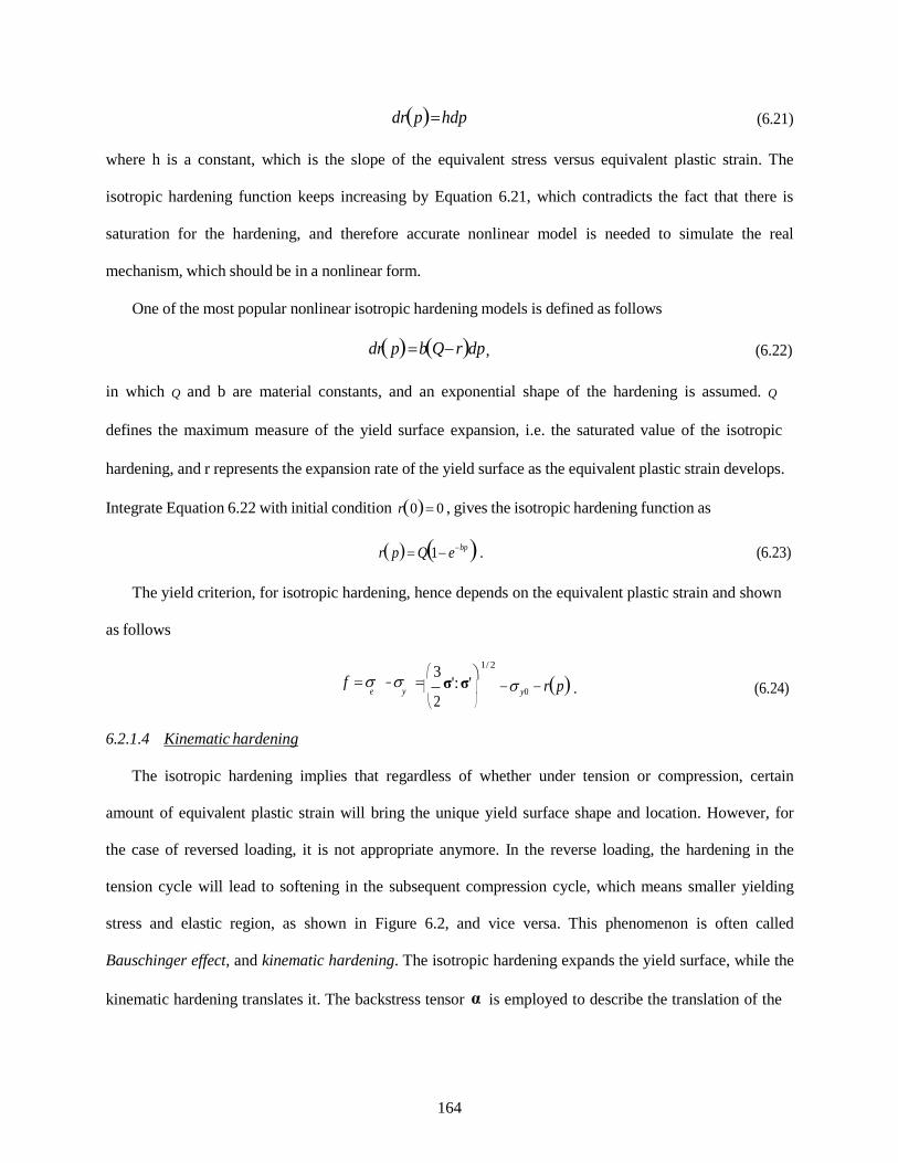
e y

dr(p) = hdp (6.21)

where h is a constant, which is the slope of the equivalent stress versus equivalent plastic strain. The

isotropic hardening function keeps increasing by Equation 6.21, which contradicts the fact that there is

saturation for the hardening, and therefore accurate nonlinear model is needed to simulate the real

mechanism, which should be in a nonlinear form.

One of the most popular nonlinear isotropic hardening models is defined as follows

dr(p) = b(Q−r)dp, (6.22)

in which Q and b are material constants, and an exponential shape of the hardening is assumed. Q

defines the maximum measure of the yield surface expansion, i.e. the saturated value of the isotropic

hardening, and r represents the expansion rate of the yield surface as the equivalent plastic strain develops.

Integrate Equation 6.22 with initial condition r(0) = 0 , gives the isotropic hardening function as

r(p) = Q(1− e−bp ) . (6.23)

The yield criterion, for isotropic hardening, hence depends on the equivalent plastic strain and shown

as follows

f = σ − σ = 3 2

1/ 2

σ': σ'

− σ y0 − r(p) . (6.24)

6.2.1.4 Kinematic hardening

The isotropic hardening implies that regardless of whether under tension or compression, certain

amount of equivalent plastic strain will bring the unique yield surface shape and location. However, for

the case of reversed loading, it is not appropriate anymore. In the reverse loading, the hardening in the

tension cycle will lead to softening in the subsequent compression cycle, which means smaller yielding

stress and elastic region, as shown in Figure 6.2, and vice versa. This phenomenon is often called

Bauschinger effect, and kinematic hardening. The isotropic hardening expands the yield surface, while the

kinematic hardening translates it. The backstress tensor α is employed to describe the translation of the

164

yield surface in stress space. Similar to isotropic hardening, various criteria have been proposed to model

kinematic hardening.

Figure 6.2 Sketch of kinematic hardening

The most popular linear kinematic hardening model is the linear Ziegler (or Prager’s) hardening law,

introduced by Prager (1956), and described in the following Equation 6.25,

dα = 2

cd ε pl

3

(6.25)

where c is a material constant and called the kinematic hardening modulus. According to Equation 6.25,

the development of the backstress is linearly related with the plastic strain. Similar to isotropic hardening,

the kinematic hardening is also featured with a saturated value for yield surface translation as the infinite

plastic deformation, and therefore linear models are not appropriate anymore.

A relaxation term (or recall term) was proposed to be added to the linear model by Armstrong and

Frederick (1966), in order to introduce nonlinearity and saturation features, which in many cases

considerably improves the accuracy of the results. The nonlinear kinematic hardening models is given as

dα = 2

cd ε pl − γαdp , (6.26) 3

in which γ is also a material constant, which defines the rate at which the kinematic hardening modulus

decreases as the plastic strain increases. Both the parameters c and γ need to be calibrated from cyclic test

data. By eliminating the translation part of the yield surface, the yield function, for kinematic hardening,

is given as follows

165

f = 3 2

(σ'−α'): (σ'−α')

1 / 2

− σ y 0 . (6.27)

The back stress α is also a deviatoric quantity, and therefore α=α’.

The hardening model in Equation 6.26, by introducing the flow direction tensor n, can be rewritten as

dα = 2

cndp − γαdp , (6.28) 3

and rearranging, gives

d (n : α)

= c − γn : α , dp

which can be integrated, taking n: α to be zero at p = 0 , we have

n : α =

c (1 − exp (− γp )) . (6.29) γ

If the material is under uniaxial loading, for monotonically increasing plastic strain εpl, Equation 6.29

can be written in terms of the magnitude, α, as follows

α = c (1 − exp (− γε pl )), (6.30)

γ

while it is easy to notice that c/γ determines the magnitude of the back stress and the final saturated value.

6.2.1.5 Combined hardening

Most materials are subjected to both isotropic hardening and kinematic hardening simultaneously, i.e.

combined hardening. By assuming the two hardening types work independently, the yield criterion can be

written as follows

f = 3 2

(σ'−α): (σ'−α)

1 / 2

− σ y 0 − r(p). (6.31)

Equation 6.31 is also sometimes called mixed hardening, since it associates with the properties of

isotropic hardening (uniform expansion of the yield surface) and kinematic hardening (translation of the

center of the yield surface in stress space). If the nonlinear hardenings from Equation 6.22 and 6.28 are

mixed, then combined hardening is usually called Chaboche-Ziegler’s formation (Lemaître and Chaboche,

1990).

166

The integration of von Mises plasticity

The objective of this chapter is to implement the newly proposed ductile fracture model into structural

details, which required the damage variable in Equation 3.25 and some other associated variables to be

embedded in the material model. The user-defined material constitutive equations can be implemented

through user subroutine VUMAT in ABAQUS/EXPLICIT. In this section, the algorithm of the user

subroutine will be introduced.

In the numerical implementation of the material constitutive model, the integration of stress, strain

and some associated state quantities needs to be conducted at every integration point over every time

increment. In the present study, an implicit scheme using the radical return method is adopted for the

integration of the constitutive equations.

In the following formulation, we shall take subscript t to be the quantities at the beginning of the time

step, and subscript t+∆t to be those at the end of the time step. For the sake of simplicity, the subscript

t+∆t is omitted. Therefore, the stress tensor at the beginning of the step, at time t, is σt , while at the end

of the time step, at time t+∆t, the stress tensor is just σ . The constitutive equations employ the popular

nonlinear combined hardening model, Chaboche-Ziegler’s formation, where isotropic hardening is

defined in Equation 6.22, and the back stress is defined in Equation 6.28.

The radial return algorithm is implemented through an elastic predictor and a following plastic

correction. The elastic predictor represents the purely elastic trial stress increment at time t+∆t, and the

stress tensor would be σtr , which is outside the yield surface if the yielding has initiated. The plastic

correction is then updated in order to bring it back onto the yield surface. If the material is still in the

elastic range, then the trial stress σtr will be still located inside the yield surface, and the stress tensor

would be the trial stress σ=σtr. The implicit scheme is shown in Figure 6.3, and the algorithm for plasticity

is introduced in the following paragraphs in detail.

167

t t

Figure 6.3 Schematic representation of implicit integration using radial return method of von Mises plasticity equations

The known quantities in the beginning of the integration include the stress at time t, σt , user-defined

state variables at time t, and the strain increment ∆ ε over the time increment ∆t. The main objective of the

integration is to update the stress and user-defined variables.

According to the classical additive decomposition for strain, the strain increment ∆ ε can be

decomposed into the elastic part ∆εel and the plastic part ∆ε pl , shown as follows

∆ε = ∆εel +∆εpl , (6.32)

and therefore

∆εel = ∆ε−∆εpl . (6.33)

Therefore the elastic strain can be written as

εel = εel + ∆εel = εel + ∆ε − ∆ε pl . t t

Substitute the Equation 6.33 into Equation 6.2, gives

( el

pl ) ( el

pl )

o = 2G εt + ∆ε − ∆ε + λII :

εt

+ ∆ε − ∆ε , (6.34)

and since the tensor ∆ε pl is a deviatoric quantity, then I : ∆εpl = 0, so Equation 6.34 can be rearranged as

o = 2G(εel

+ ∆ε)+ λII : (εel

+ ∆ε)− 2G∆ε pl . (6.35)

168

The elastic predictor σtr can be denoted by

σtr = 2G(εel + ∆ε)+ λII : (εel + ∆ε)= σ

+ 2G∆ε + λII : ∆ε , (6.36)

t t t

The elastic predictor σtr is also a known quantity at the beginning of the integration. Therefore, Equation

6.35 can be rewritten as

σ = σtr − 2G∆εpl . (6.37)

Combining Equation 6.16 and 6.37 and, we have

σ = σtr − 2G∆pn . (6.38)

The stress tensor can be expressed in terms of its deviatoric and mean part as

σ = σ '+ 1 II : σ , (6.40) 3

so the deviatoric part can be calculated as

σ ' = σ − 1 II : σ = σ tr − 2G ∆ pn −

1 II : (σ tr − 2G ∆ pn ) 3 3

= σ tr − 2G ∆ p n − 1 II : σ tr +

2G ∆ p II : n 3 3

= σ tr − 1 II : σ tr − 2G ∆ p n +

2G ∆ p II : n (6.41) 3 3

Since σ tr ' = σ tr − 1 II : σ tr , and I : n = 0 , Equation 6.41 can be rewritten as 3

σ' = σtr '−2G∆pn . (6.42)

The back stress increment, according to Equation 6.28, can be expressed as

∆α =

2 cn∆p − γα∆p , (6.43)

3

then the back stress can be updated as

α = αt + ∆α = αt + 2

cn∆p − γα∆p . 3

Rearranging gives

169

=

α

y 0

t

t

α = 1 α + 2 cn∆p . (6.44)

1 + γ∆p t 3

The equivalent stress σe can be updated through the definition of isotropic hardening, which is

function of ∆ p , as follows

σ e = σ y = σ y 0

+ r(p) = σ y 0

+ Q(1 − e−bp ) = σ + Q(1 − e−b( pt +∆p ) ) . (6.45)

For the convenience, the tensor s is defined as

s = σ'−α , (6.46)

such that

f = 3 2

1 2

s : s

−σ y

1 2 3 s : s 2

−σ y0 −Q(1− e−b( pt +∆p) ), (6.47)

and

n = 3 s

, (6.48)

2 σ e

where σe is defined at Equation 6.45.

Combining Equation 6.42, 6.44 and 6.46, gives

s = σ'−α = σtr

'−2G∆pn −

1 αt +

1 + γ∆p

2 cn∆p , 3

and rearranging gives

s = σtr '−α

− 3G∆ps +

σ e

γ∆p α 1 + γ∆p t

+ 1

1 + γ∆p

cs∆p . (6.49) σ e

Since str

= σtr

'−αt , which is also a known quantity, the Equation 6.49 can be written as

s = str − 3G∆ps + γ∆p + 1 cs∆p

σ e 1 + γ∆p 1 + γ∆p σ e ,

and rearranging gives

1 tr

γ∆p

. (6.50)

s = 3G∆p 1 +

1 c∆p s −

+ 1 + γ∆p

αt

σ e 1 + γ∆p σ e

170

t

y 0

y 0

Substituting Equation 6.50 into Equation 6.47, gives

γ∆p γ∆p 1 2

f = 1 3

str + α : str + α − σ − Q(1 − e−bpt e−b∆p ) = 0 , (6.51) 1 3G∆p 1 c∆p 2 1 + γ∆p t 1 + γ∆p t y 0

+ − σ e 1

+ γ∆p σ e

which is a closed-form function of ∆ p , and can be solved by any efficient numerical method. In the

present study, the Newton-Raphson method is adopted. From Taylor series transformation, the following

can be obtained

f + ∂f ∂∆p

d∆p + = 0 , (6.52)

and then

d∆p = − ∂f f

∂∆p

, (6.53)

while the equivalent plastic strain ∆p is then updated as

∆p( k +1) = ∆p( k ) + d∆p . (6.54)

All associated quantities are updated in the sequence as follows:

σtr = 2G(εel + ∆ε)+ λII : (εel + ∆ε)= σ + 2G∆ε + λII : ∆ε , t t t

o tr ' = σ tr − 1 II : σ tr , 3

σ e = σ y = σ y 0

+ r(p) = σ

str = σtr '−α ,

+ Q(1 − e−bp ) = σ + Q(1 − e−b( pt +∆p ) ) ,

1 tr γ∆p s = 3G∆p 1 c∆p

s

1 + − +

1 + γ∆p αt ,

σ e 1 + γ∆p σ e

n = 3 s , 2 σ e

o = σtr − 2G∆pn ,

171

t

t

α = 1 α + 2 cn∆p ,

1 + γ∆p t 3

∆ε pl = ∆p ⋅ n ,

ε pl = ε pl + ∆ε pl ,

∆εel = ∆ε − ∆ε pl ,

ε el = ε el + ∆ε el . (6.55)

The damage variables defined in Chapter 5 are then calculated after the constitutive equations have

been applied.

Implementation of the constitutive and damage equations into user- defined material subroutine

In the commercial finite element software package, ABAQUS, users can specify their own material

model through FORTRAN subroutines. In the implicit algorithm of the finite element codes, such as

ABAQUS standard, users need to provide a subroutine with the material Jacobian or tangent stiffness as

well as the plasticity constitutive equations (maybe implicit or explicit), and the subroutine is usually

called “UMAT”. The ABAQUS explicit is also featured with the function of element deletion depends on

certain variable. Therefore, in the present study, the ABAQUS explicit and its associated subroutine

“VUMAT” was adopted and programed.

In this section, the process of how to program the plasticity material model and damage criterion into

the subroutine is first introduced, and then the subroutine is validated through comparison with the

ABAQUS embed equivalent material model.

6.2.3.1 The implementation of the plasticity material model and damage criterion

At the beginning the increment, known quantities include the stress tensor, the state variables, and the

length of the time increment. The objective of the subroutine is to update the stress and state variable to

the end of the increment. An implicit material algorithm has been provided in the section and the flow

chart in Figure 6.4 shows how the algorithm is implemented in the explicit subroutine, so is the damage

criterion presented in Chapter 5.

172

Figure 6.4 Flow chart of the VUMAT subroutine

173

6.2.3.2 Validation of the material subroutine

In this section, the user-defined plasticity constitutive model (VUMAT) was validated through

comparisons with the ABAQUS built-in material model by numerically analyzing three specimens with

different scales. The first specimen only includes one element, modelled by 2 dimensional plane stress

element; the notched bar serves as the second scale specimen, modelled by the axisymmetric element

CAX; and in the third level, a full dimension shear link is modelled, with 3 dimensional shell element in

the concerned link zones.

The comparisons are conducted for the load versus displacement curve and the stress contour in

concerned areas. As shown in Figure 6.5, the results from the numerical models with two material input

methods (ABAQUS built-in versus VUMAT) correlate exceptionally well. Therefore, it can be concluded

that the integration algorithm and the corresponding subroutine programing of the user-defined plasticity

constitutive equations are correct and can be used in the following analysis.

Figure 6.5 Comparison of load versus displacement curve between VUMAT and corresponding ABAQUA embedded combined hardening material model

174

6.3 Introduction to the selected experimental specimens

An experimental program, whose test setup is shown in Figure 6.6, was conducted at the University

of Texas at Austin (Arce, 2002; Galvez, 2004; Okazaki, 2006), in order to reproduce the loading and

displacement environment on a link in an EBF with one end of the link attached to a column. As shown in

Figure 6.7 and 6.8, the link specimens were fabricated through welding heavy end plates at each end of

the W section, while the end plates were bolted into the column and beam in the experimental setup. All

sections were fabricated using ASTM A992 steel, and the material properties were obtained through

tensile coupon tests taken from flanges and webs of the specimens. The material tests were only

conducted for some of the specimens, which were not similar since it was stated that they were supplied

by different manufacturers. In addition, only the stress-strain response of the coupon tests was provided.

The main purpose of utilizing these coupon tests in this study is for calibration of the basic material

properties, including the modulus, yield and fracture stress, as well as the hardening behavior, parameters.

Therefore, the damage and hardening parameters for a similar steel grade, ASTM A572 Gr. 50, were used

as the initial parameters in the following analysis; however it should be noted that different specimens

may be featured with different yielding stress.

There were total nine specimens tested with different geometries or loading conditions in Galvez

(2004), seven with stiffeners welded to link web, two with stiffeners that only “touch” the link web. The

main objective of this chapter is to explore the implementation of the newly proposed criterion in Chapter

5, and hence only three specimens are simulated, including the two without welding, and another one with

welding. The importance of including a welded specimen lies in the fact that the effect of welding heat on

the base metal’s fracture properties has been shown in previous studies to be significant but never

quantitatively investigated. The specimen without stiffener-web welding are featured with the same

geometries but subjected to different loading protocols, denoted as specimen 1, whose geometry

configurations are shown in Figure 6.7, and this specimen corresponds to specimens 5 and 8 in Galvez

(2004), which have same configurations but different loading protocol. The configuration of another

175

specimen with stiffener-web welding is shown in Figure 6.8, and the specimen is denoted as specimen 2,

corresponding to specimens 1, 2 and 3 in Galvez (2004), which are featured with same geometry

configurations but from different manufacturer. There are two loading protocols adopted, in which the

first protocol is named as Revised Loading Protocol (RLP) used for specimen 1 shown in Table 6.1 and

Figure 6.9 (a), and the other one is called as Severe Loading Protocol (SLP) used for specimen 2 shown in

Table 6.2 and Figure 6.9 (b). It is noted that a zone on the web adjacent to the flange, named as “k-area”,

is featured with different material properties with other part of the web. The material in the “k-area” has

higher ultimate strength and smaller ductility, but the difference is quite unstable, depending on the

manufacturers. Although there exists the difference, distribution of the “k-area” is very limited, only

within around 25 mm range from the flange, and although it has been proven to be not the primary source

of the fracture initiation in web (Okazaki and Engelhardt, 2007), it may hold some effects on the fracture

propagation. Therefore a constant fracture resistance reduction factor of 0.8 is assumed for the “k-area”,

which means the parameters in Equation 3.18 except c7 are assumed to hold the same value, while the

parameter c7 only has 80% of its original value.

The results of the experimental tests are mainly shown in terms of load versus displacement curves

(shear force versus link rotation), fracture locations and initial propagations. The shear force is the force,

which acts on the shear link and can be calculated as the sum of the reaction forces in the two load cells

that support the beam. The rotation represents the rotation of the shear link, which can be determined by

the displacement difference between the two link ends over link length.

176

Figure 6.6 Details and dimensions of the test setup of the experimental program in Galvez (2004), Okazaki (2004) and Okazaki et al., (2005)

(Redrawn from Galvez (2004))

177

Figure 6.7 Geometry configurations and welding details for specimen 1 (corresponding to the specimen 5 and 8 in Galvez (2004))

Figure 6.8 Geometry configurations and welding details for specimen 2 (corresponding to the specimen 1, 2 and 3 in Galvez (2004))

178

Table 6.1 Severe Loading Protocol (SLP) used in specimen 2 Load Step Cycles Total link rotation γ

1 3 ±0.0025 rad. 2 3 ±0.005 rad.

3 4 ±0.01 rad.

4 4 ±0.02 rad.

5 4 ±0.03 rad.

6 4 ±0.04 rad.

7 4 ±0.05 rad.

8 4 ±0.06 rad.

9 4 ±0.07 rad.

10 4 ±0.08 rad.

11 4 ±0.09 rad.

Continue loading at increments of γ=±0.01 rad. with four cycles of loading at each step

Table 6.2 Revised loading protocol (SLP) used in specimen 1 (Per Richards and Uang, 2003)

Load Step Cycles Total link rotation γ

1 6 ±0.00375 rad. 2 6 ±0.005 rad.

3 6 ±0.0075 rad.

4 6 ±0.01 rad.

5 4 ±0.015 rad.

6 2 ±0.02 rad.

7 2 ±0.03 rad.

8 1 ±0.04 rad.

9 1 ±0.05 rad.

10 1 ±0.07 rad.

11 1 ±0.09 rad.

Continue loading at increments of γ=±0.02 rad. with one cycles of loading at each step

179

(a)

(b)

Figure 6.9 Loading protocols and failure initiation locations: (a) Severe Loading Protocol (SLP); and (b) Revised Loading Protocol (RLP) by Richards and Uang (2003)

180

6.4 Numerical modeling of the selected specimens

The general finite element (FE) program ABAQUS/Explicit (Simulia, 2012) was employed in the

numerical simulations in this chapter. The simulated specimens include specimens with out-of-plane

deformations and subsequent strong web-stiffener interactions (specimen 1), or welding on web-stiffener

(specimen 2), whose effects on the damage evolution cannot be ignored and make the modelling

procedure more complicated.

Modeling approach

For the purpose of reducing the computation demand, multi-scale modeling technique is adopted. As

shown in Figure 6.10, the beam and column are modelled using 3D beam element B31, while the link is

modelled with 3D shell element S4R, and the weldments are modelled with 3D solid element C3D6T, in

order to include the heat effects from welding. The beam and link are connected through coupling

constraint, and the column is attached to the link by a series of Multi-Point Constraint (MPC). In

specimen 1, since the stiffeners only “touch” the web, and out-of-plane deformations occurs on web in the

last several cycles before fracture, strong interactions between stiffener edges and web is present, and

contact is built to simulate these interactions. A friction coefficient of 0.3, representing Class C slip factor

for untreated hot rolled steel per the 2010 AISC Specifications (AISC LRFD, 2010), is adopted in these

contact simulations. It is assumed that initially there exists a gap of 0.64 mm between the stiffener edges

and link web, in order to represent the fabrication tolerances. In specimen 2, the stiffeners are welded to

the web, and the weldment configurations can be reached in Figure 6.8. In the simulations, the weldment

is modeled by solid element, and solid-shell coupling is achieved through MPC between corresponding

nodes for the constraint between weldments and web/stiffeners. The heat effects form welding on base

metal, including the effects on fracture properties and residual stress are discussed and defined in section

6.4.2 and 6.4.3. Only the welding effects between the stiffeners and link web are considered, since others

are insignificant for the fracture and deformation behavior, and therefore welding in other locations is

181

simply treated as fixed boundary conditions. The hardening parameters are defined in Equation 6.56, and

the yielding stresses are 350 Mpa for specimen 1, and 381 Mpa for specimen 2.

dr=117.2×(5−r)dp

dα = 2 × 3447 × dε pl − 38 ×

αdp 3

(6.56)

Loading procedures in the simulation exactly followed the equivalents in the corresponding

laboratory tests, in which specimen 2 is subjected to the Severe Loading Protocol (SLP) and specimen 1

is subjected to the Revised Loading Protocol (RLP). The loads are applied through the displacement ∆3 on

the two ends of the column, shown in Figure 6.10. Similar to their experimental equivalents, the loads

applied are measured from the sum of the reaction forces at the two pinned boundary conditions of the

beam, F1+F2, and the link rotations are calculated through the ratio between the difference of

displacements at the center elements of the link web at two ends, ∆1 and ∆2, and the link displacement L,

which equals to 584 mm in the present study.

182

Figure 6.10 Depiction of a typical numerical model used for EBF link (Specimen 1)

183

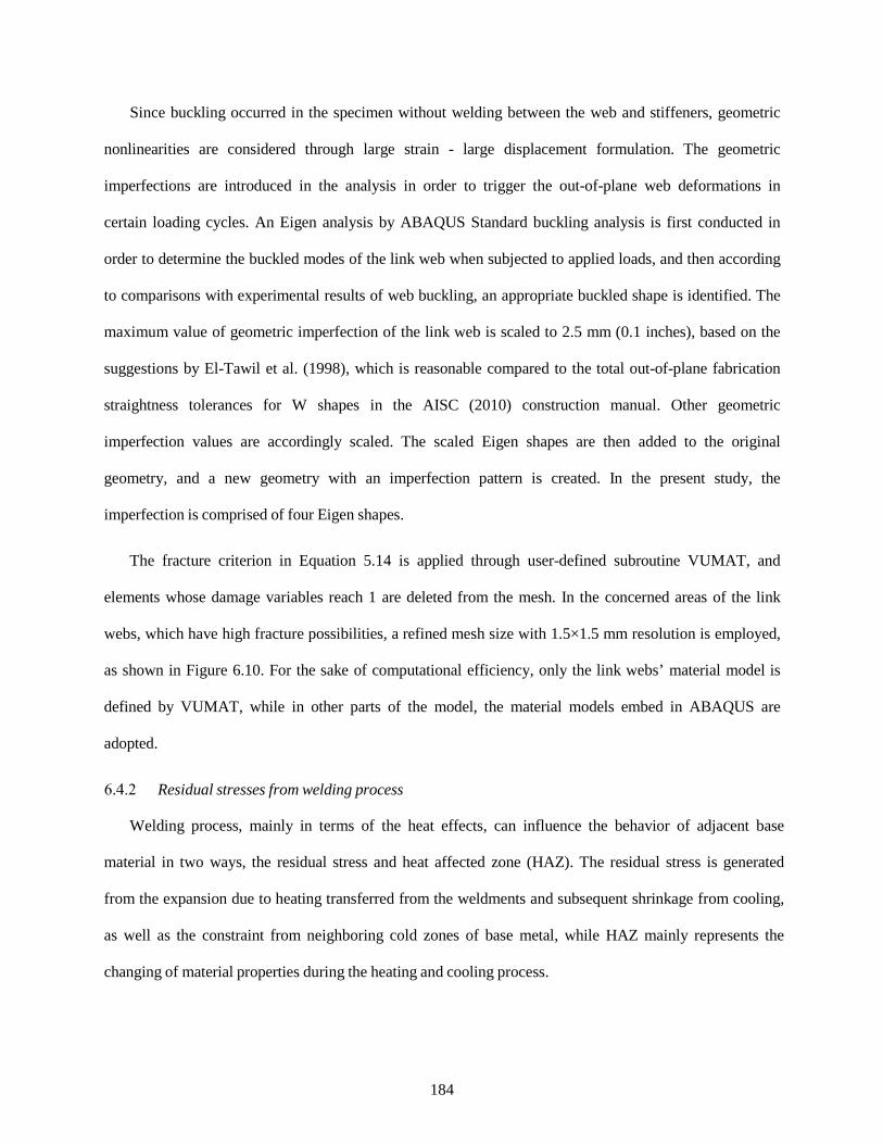
Since buckling occurred in the specimen without welding between the web and stiffeners, geometric

nonlinearities are considered through large strain - large displacement formulation. The geometric

imperfections are introduced in the analysis in order to trigger the out-of-plane web deformations in

certain loading cycles. An Eigen analysis by ABAQUS Standard buckling analysis is first conducted in

order to determine the buckled modes of the link web when subjected to applied loads, and then according

to comparisons with experimental results of web buckling, an appropriate buckled shape is identified. The

maximum value of geometric imperfection of the link web is scaled to 2.5 mm (0.1 inches), based on the

suggestions by El-Tawil et al. (1998), which is reasonable compared to the total out-of-plane fabrication

straightness tolerances for W shapes in the AISC (2010) construction manual. Other geometric

imperfection values are accordingly scaled. The scaled Eigen shapes are then added to the original

geometry, and a new geometry with an imperfection pattern is created. In the present study, the

imperfection is comprised of four Eigen shapes.

The fracture criterion in Equation 5.14 is applied through user-defined subroutine VUMAT, and

elements whose damage variables reach 1 are deleted from the mesh. In the concerned areas of the link

webs, which have high fracture possibilities, a refined mesh size with 1.5×1.5 mm resolution is employed,

as shown in Figure 6.10. For the sake of computational efficiency, only the link webs’ material model is

defined by VUMAT, while in other parts of the model, the material models embed in ABAQUS are

adopted.

Residual stresses from welding process

Welding process, mainly in terms of the heat effects, can influence the behavior of adjacent base

material in two ways, the residual stress and heat affected zone (HAZ). The residual stress is generated

from the expansion due to heating transferred from the weldments and subsequent shrinkage from cooling,

as well as the constraint from neighboring cold zones of base metal, while HAZ mainly represents the

changing of material properties during the heating and cooling process.

184

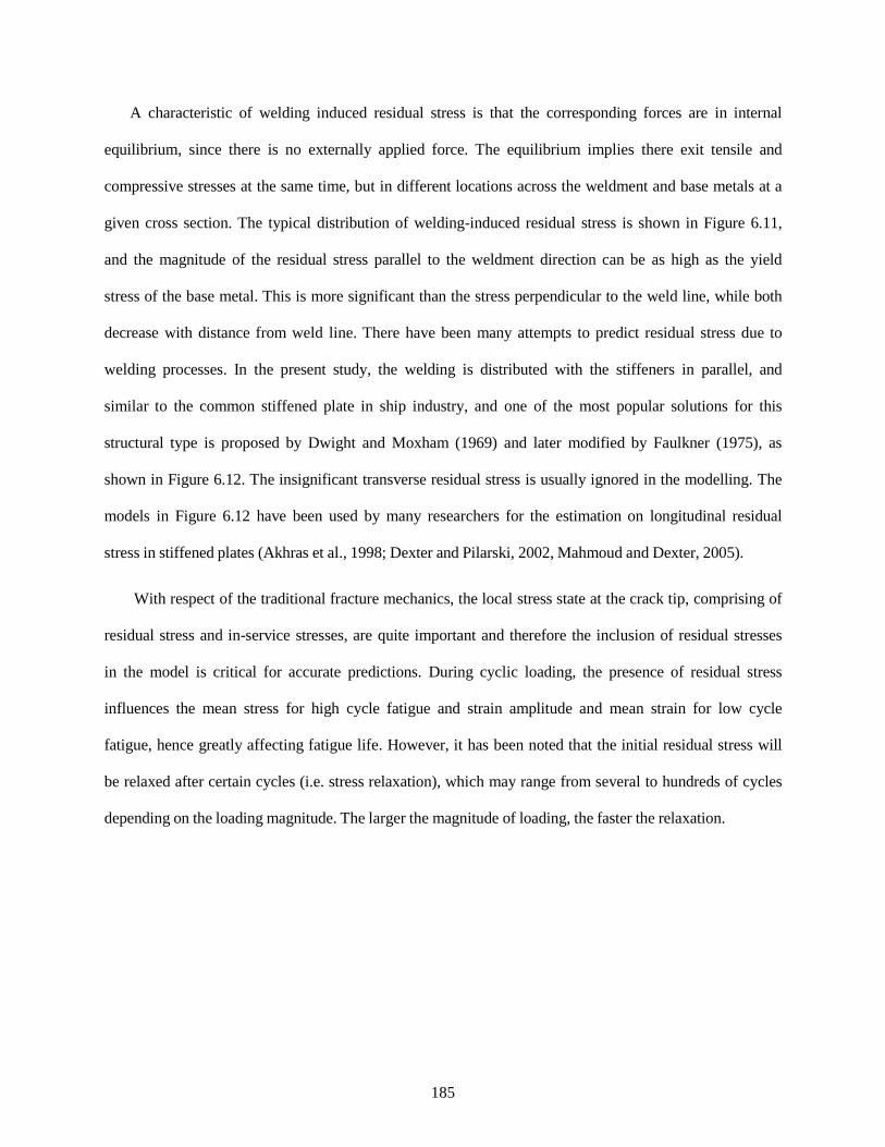
A characteristic of welding induced residual stress is that the corresponding forces are in internal

equilibrium, since there is no externally applied force. The equilibrium implies there exit tensile and

compressive stresses at the same time, but in different locations across the weldment and base metals at a

given cross section. The typical distribution of welding-induced residual stress is shown in Figure 6.11,

and the magnitude of the residual stress parallel to the weldment direction can be as high as the yield

stress of the base metal. This is more significant than the stress perpendicular to the weld line, while both

decrease with distance from weld line. There have been many attempts to predict residual stress due to

welding processes. In the present study, the welding is distributed with the stiffeners in parallel, and

similar to the common stiffened plate in ship industry, and one of the most popular solutions for this

structural type is proposed by Dwight and Moxham (1969) and later modified by Faulkner (1975), as

shown in Figure 6.12. The insignificant transverse residual stress is usually ignored in the modelling. The

models in Figure 6.12 have been used by many researchers for the estimation on longitudinal residual

stress in stiffened plates (Akhras et al., 1998; Dexter and Pilarski, 2002, Mahmoud and Dexter, 2005).

With respect of the traditional fracture mechanics, the local stress state at the crack tip, comprising of

residual stress and in-service stresses, are quite important and therefore the inclusion of residual stresses

in the model is critical for accurate predictions. During cyclic loading, the presence of residual stress

influences the mean stress for high cycle fatigue and strain amplitude and mean strain for low cycle

fatigue, hence greatly affecting fatigue life. However, it has been noted that the initial residual stress will

be relaxed after certain cycles (i.e. stress relaxation), which may range from several to hundreds of cycles

depending on the loading magnitude. The larger the magnitude of loading, the faster the relaxation.

185

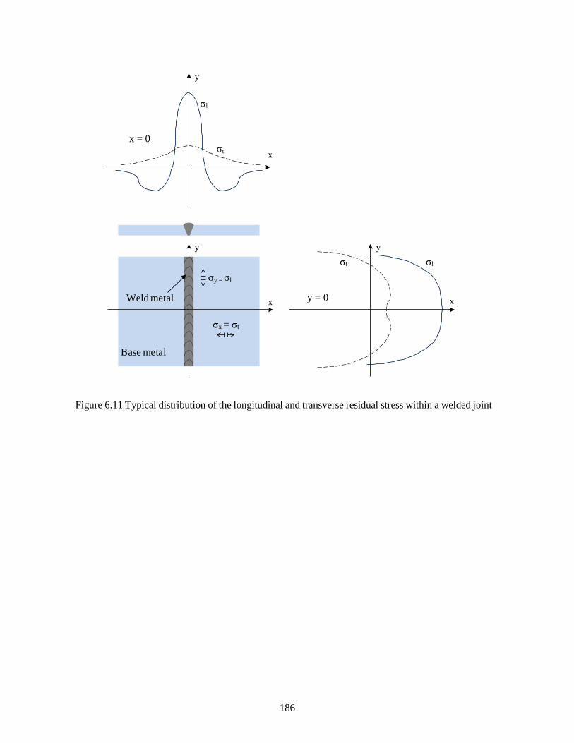
y

σl

x = 0 σt x

Weld metal

y

σy = σl

x

σx = σt

y

σt σl

y = 0 x

Base metal

Figure 6.11 Typical distribution of the longitudinal and transverse residual stress within a welded joint

186

Figure 6.12 Residual stress distribution of stiffened plate: (a) Typical stiffened plate, (b) idealized stress

distribution and (c) Faulkner stress distribution

187

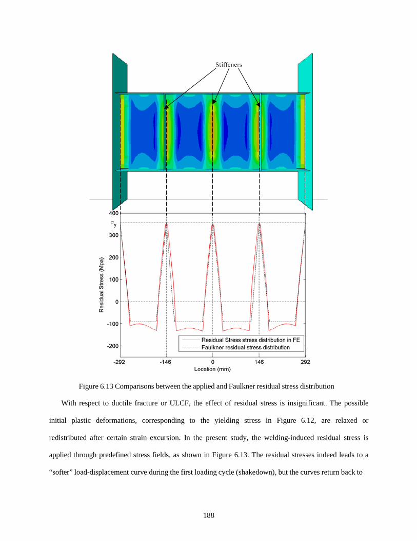
Figure 6.13 Comparisons between the applied and Faulkner residual stress distribution

With respect to ductile fracture or ULCF, the effect of residual stress is insignificant. The possible

initial plastic deformations, corresponding to the yielding stress in Figure 6.12, are relaxed or

redistributed after certain strain excursion. In the present study, the welding-induced residual stress is

applied through predefined stress fields, as shown in Figure 6.13. The residual stresses indeed leads to a

“softer” load-displacement curve during the first loading cycle (shakedown), but the curves return back to

188

the ones without consideration of residual stress only after three cycles, in which the link web is still in

the elastic range. This implies that only negligible additional difference has taken place since damage

evolution actually has not even initiated in the first several elastic cycles. The residual stresses are

removed by plastic deformations and are no longer present immediately prior to the onset of fracture. This

is similar to the opinion provided by Radaj (2002). Therefore, it can be concluded that the residual

stresses can be ignored in the process of ductile fracture predictions.

The heat affected zones (HAZ)

Although the residual stresses were proven to have insignificant effect on ductile fracture, the fracture

resistance of welded structures is admittedly degraded, which causes ductility to be one of the main

concerns for this structure type. The degradation actually comes from the exposure to temperature during

the welding process.

The heat affected zone (HAZ) is the area of base metal that does not melt but has its microstructure

and mechanical properties altered by the intensive heat from the heat related process, such as welding and

hot cutting operations. The heating and subsequent cooling process both cause the change within the

zones from weld interface to the boundary of the sensitizing temperature of the base metal. The extent of

change depends on many factors, primarily including the heat amount and input rate, the cooling

environment, and the related metals.

Many common mechanical properties, including yielding stress, modulus, ductility and hardness

change after the material experiences thermo-cycles. Since the characteristics of these cycles vary as a

function of the distance from the heat source, the material at HAZ becomes heterogeneous. Therefore, the

material and damage parameters calibrated for base metal cannot be directly applied to the HAZ material.

However, compared to the entire components, the relative dimension of the HAZ is very small, and hence

the global behavior of the link will be not greatly influenced by altering the material in HAZ, except in

terms of the failure/fracture phenomenon where local crack initiation may be located in the HAZ. Since

the HAZ is greatly restrained and usually not exceed the web thickness, corresponding to one meshed

189

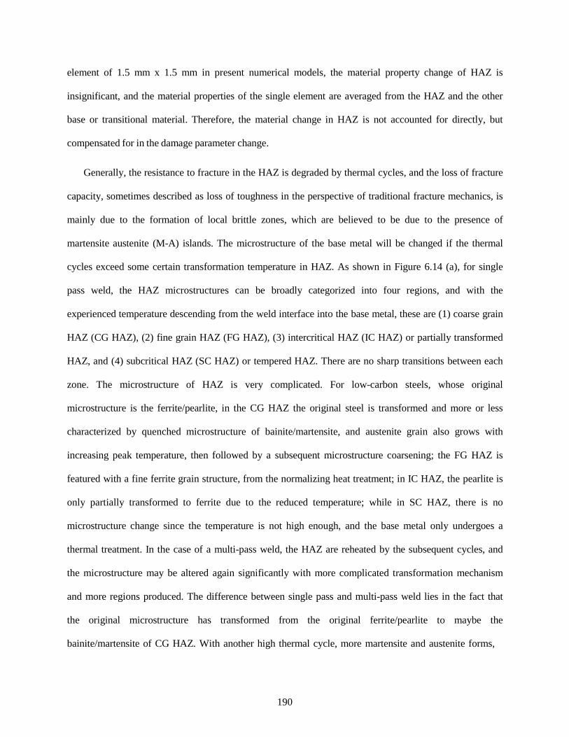
element of 1.5 mm x 1.5 mm in present numerical models, the material property change of HAZ is

insignificant, and the material properties of the single element are averaged from the HAZ and the other

base or transitional material. Therefore, the material change in HAZ is not accounted for directly, but

compensated for in the damage parameter change.

Generally, the resistance to fracture in the HAZ is degraded by thermal cycles, and the loss of fracture

capacity, sometimes described as loss of toughness in the perspective of traditional fracture mechanics, is

mainly due to the formation of local brittle zones, which are believed to be due to the presence of

martensite austenite (M-A) islands. The microstructure of the base metal will be changed if the thermal

cycles exceed some certain transformation temperature in HAZ. As shown in Figure 6.14 (a), for single

pass weld, the HAZ microstructures can be broadly categorized into four regions, and with the

experienced temperature descending from the weld interface into the base metal, these are (1) coarse grain

HAZ (CG HAZ), (2) fine grain HAZ (FG HAZ), (3) intercritical HAZ (IC HAZ) or partially transformed

HAZ, and (4) subcritical HAZ (SC HAZ) or tempered HAZ. There are no sharp transitions between each

zone. The microstructure of HAZ is very complicated. For low-carbon steels, whose original

microstructure is the ferrite/pearlite, in the CG HAZ the original steel is transformed and more or less

characterized by quenched microstructure of bainite/martensite, and austenite grain also grows with

increasing peak temperature, then followed by a subsequent microstructure coarsening; the FG HAZ is

featured with a fine ferrite grain structure, from the normalizing heat treatment; in IC HAZ, the pearlite is

only partially transformed to ferrite due to the reduced temperature; while in SC HAZ, there is no

microstructure change since the temperature is not high enough, and the base metal only undergoes a

thermal treatment. In the case of a multi-pass weld, the HAZ are reheated by the subsequent cycles, and

the microstructure may be altered again significantly with more complicated transformation mechanism

and more regions produced. The difference between single pass and multi-pass weld lies in the fact that

the original microstructure has transformed from the original ferrite/pearlite to maybe the

bainite/martensite of CG HAZ. With another high thermal cycle, more martensite and austenite forms,

190

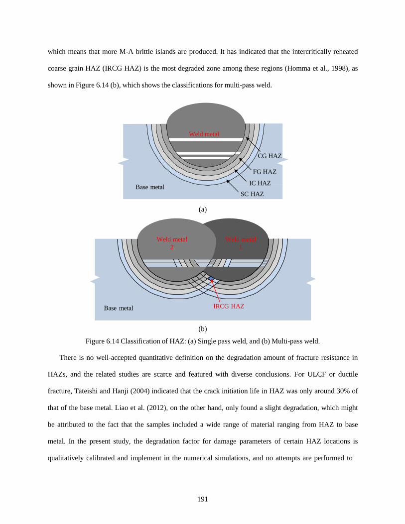
which means that more M-A brittle islands are produced. It has indicated that the intercritically reheated

coarse grain HAZ (IRCG HAZ) is the most degraded zone among these regions (Homma et al., 1998), as

shown in Figure 6.14 (b), which shows the classifications for multi-pass weld.

Weld metal

CG HAZ

Base metal

FG HAZ

IC HAZ

SC HAZ

(a)

Weld metal 2

Weld metal 1

Base metal IRCG HAZ

(b)

Figure 6.14 Classification of HAZ: (a) Single pass weld, and (b) Multi-pass weld.

There is no well-accepted quantitative definition on the degradation amount of fracture resistance in

HAZs, and the related studies are scarce and featured with diverse conclusions. For ULCF or ductile

fracture, Tateishi and Hanji (2004) indicated that the crack initiation life in HAZ was only around 30% of

that of the base metal. Liao et al. (2012), on the other hand, only found a slight degradation, which might

be attributed to the fact that the samples included a wide range of material ranging from HAZ to base

metal. In the present study, the degradation factor for damage parameters of certain HAZ locations is

qualitatively calibrated and implement in the numerical simulations, and no attempts are performed to

191

quantify a general degradation factor for structural steel. However, the quantification of such merits

extensive study in the future. The degradation factor for HAZ under single pass welding is calibrated as

0.8, and for HAZ under two pass welding is 0.8×0.8=0.64. Further study should be conducted in order to

quantitatively calibrate the degradation factors for common steel under regular welding procedure.

6.5 Simulation results and analysis

The corresponding laboratory tests were evaluated mainly from the load-displacement curves, the

buckling behavior, fracture initiation and propagation perspective. Thus, the numerical simulations

conducted in this study provide equivalent results in order to validate the damage model, numerical

modelling, and simulation procedure.

The load-displacement behavior

The numerical simulation procedure is first verified by comparisons between numerical and

experimental load-displacement curves. As previously stated, the load in this case is the shear force

applied on the EBF link, which can be calculated by the sum of the two reaction forces on the beam, and

the displacement is monitored through the rotations of the link, determined by the displacement difference

between two link ends over the link length. As shown in Figure 6.15 (a) and (b), both the curves correlate

exceptionally well with their experimental equivalents. The simulation of specimen 1 did not extend far

into the propagation stage while specimen 2 was simulated until almost complete web failure. Although

in specimen 1, the stiffeners are not rigidly tied to the web, web out-of-plane deformations are still well

restrained, since there is no obvious softening in the load versus displacement curves. In the monotonic

cases at Chapter 4, the fracture was usually indicated by sudden drop of the load versus displacement

curve, but in the cyclic loading cases, this was not the case. As shown in Figure 6.15 (b), fracture initiated

at the last cycle of step 8 (-0.06 rad.), and the fracture propagated thereafter, but only in the third cycle of

step 9 the load versus displacement curve start to “soften” and drop. The curves for shear force versus

inelastic/plastic rotations are depicted in Figure 6.16 (a) and (b) for the two specimens, since the

192

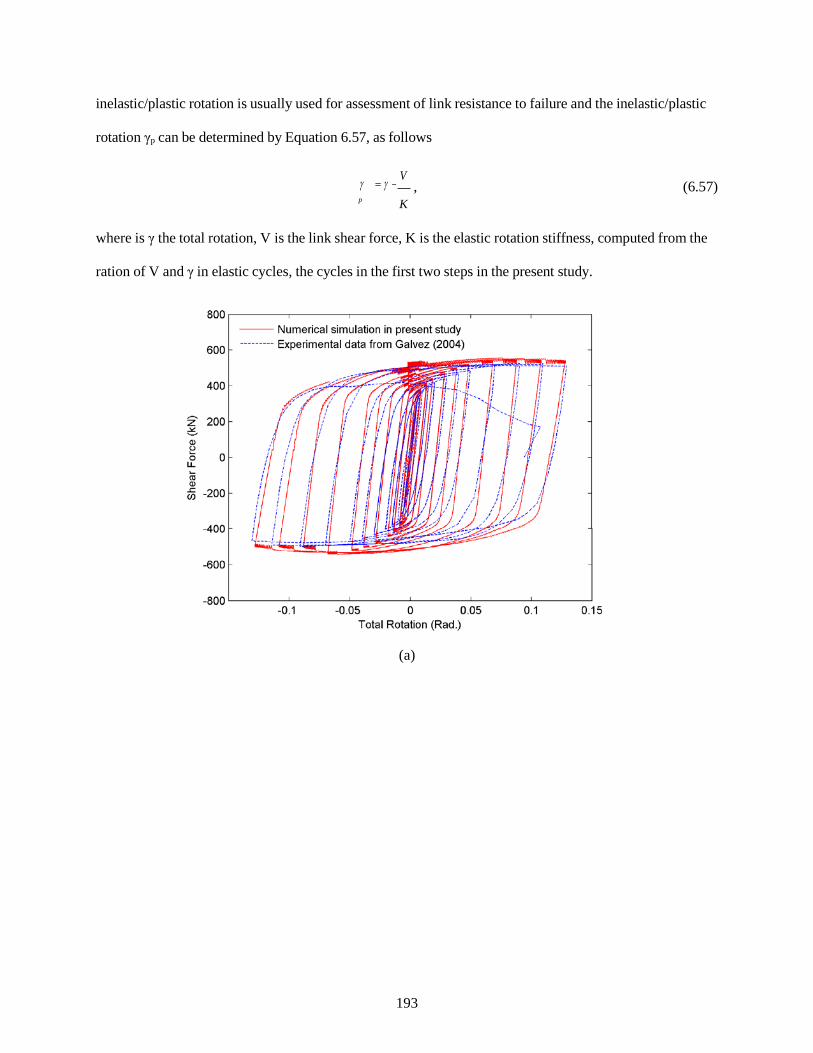
inelastic/plastic rotation is usually used for assessment of link resistance to failure and the inelastic/plastic

rotation γp can be determined by Equation 6.57, as follows

γ = γ − V

p K

, (6.57)

where is γ the total rotation, V is the link shear force, K is the elastic rotation stiffness, computed from the

ration of V and γ in elastic cycles, the cycles in the first two steps in the present study.

(a)

193

(b)

Figure 6.15 Comparisons on link shear force versus total rotation curves in numerical simulations and laboratory tests: (a) Specimen 1, and (b) Specimen 2.

(Experimental data from Gálvez (2004))

(a)

194

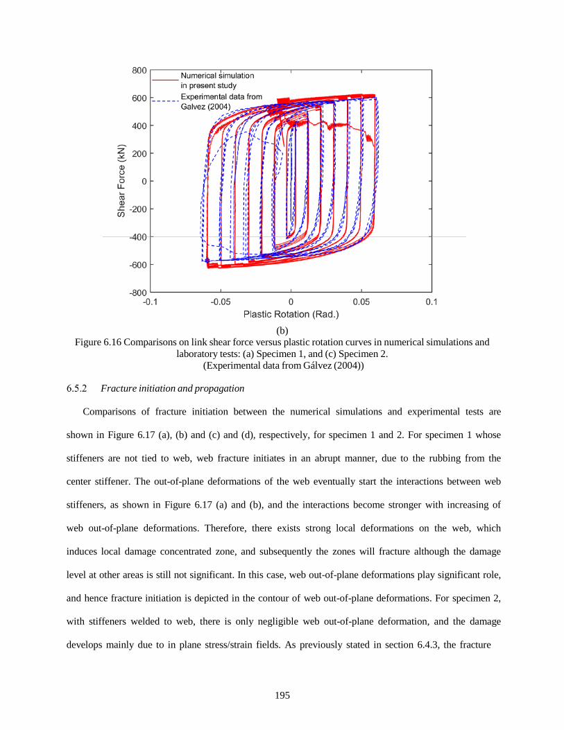
(b)

Figure 6.16 Comparisons on link shear force versus plastic rotation curves in numerical simulations and laboratory tests: (a) Specimen 1, and (c) Specimen 2.

(Experimental data from Gálvez (2004))

Fracture initiation and propagation

Comparisons of fracture initiation between the numerical simulations and experimental tests are

shown in Figure 6.17 (a), (b) and (c) and (d), respectively, for specimen 1 and 2. For specimen 1 whose

stiffeners are not tied to web, web fracture initiates in an abrupt manner, due to the rubbing from the

center stiffener. The out-of-plane deformations of the web eventually start the interactions between web

stiffeners, as shown in Figure 6.17 (a) and (b), and the interactions become stronger with increasing of

web out-of-plane deformations. Therefore, there exists strong local deformations on the web, which

induces local damage concentrated zone, and subsequently the zones will fracture although the damage

level at other areas is still not significant. In this case, web out-of-plane deformations play significant role,

and hence fracture initiation is depicted in the contour of web out-of-plane deformations. For specimen 2,

with stiffeners welded to web, there is only negligible web out-of-plane deformation, and the damage

develops mainly due to in plane stress/strain fields. As previously stated in section 6.4.3, the fracture

195

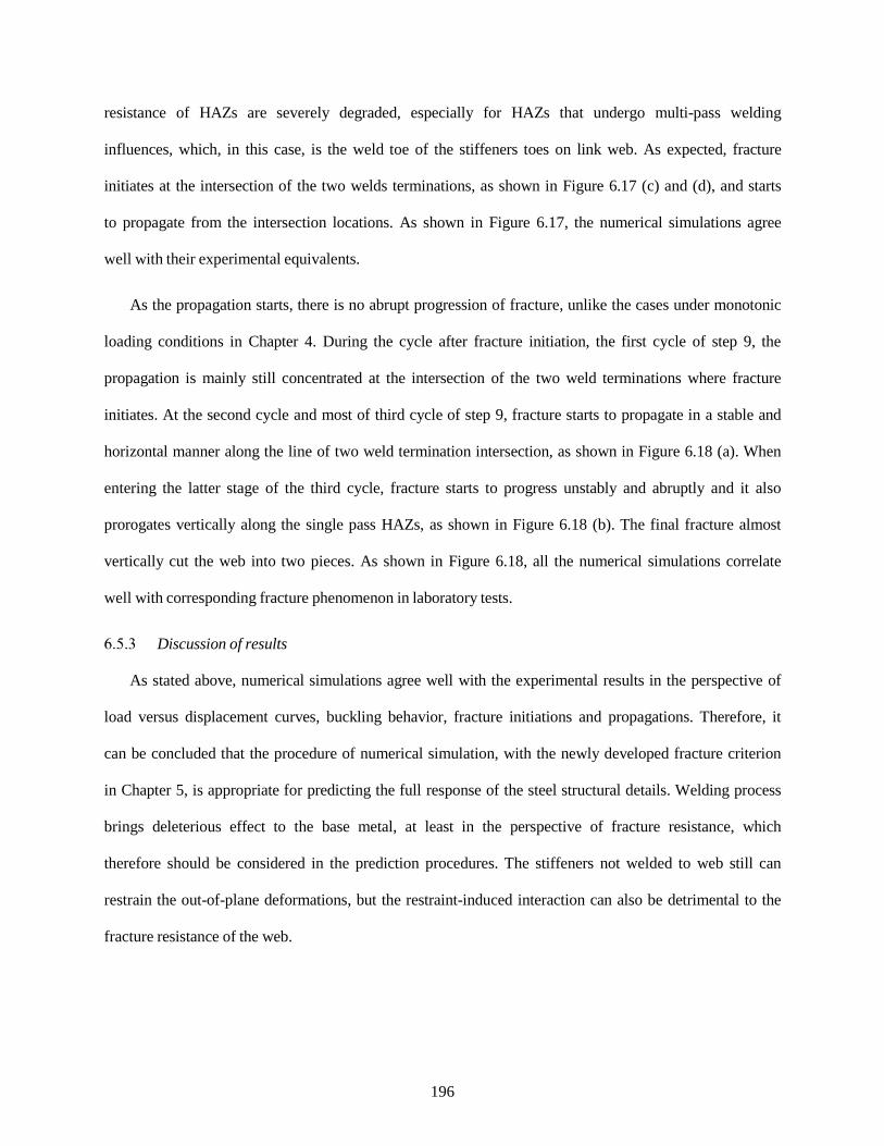
resistance of HAZs are severely degraded, especially for HAZs that undergo multi-pass welding

influences, which, in this case, is the weld toe of the stiffeners toes on link web. As expected, fracture

initiates at the intersection of the two welds terminations, as shown in Figure 6.17 (c) and (d), and starts

to propagate from the intersection locations. As shown in Figure 6.17, the numerical simulations agree

well with their experimental equivalents.

As the propagation starts, there is no abrupt progression of fracture, unlike the cases under monotonic

loading conditions in Chapter 4. During the cycle after fracture initiation, the first cycle of step 9, the

propagation is mainly still concentrated at the intersection of the two weld terminations where fracture

initiates. At the second cycle and most of third cycle of step 9, fracture starts to propagate in a stable and

horizontal manner along the line of two weld termination intersection, as shown in Figure 6.18 (a). When

entering the latter stage of the third cycle, fracture starts to progress unstably and abruptly and it also

prorogates vertically along the single pass HAZs, as shown in Figure 6.18 (b). The final fracture almost

vertically cut the web into two pieces. As shown in Figure 6.18, all the numerical simulations correlate

well with corresponding fracture phenomenon in laboratory tests.

Discussion of results

As stated above, numerical simulations agree well with the experimental results in the perspective of

load versus displacement curves, buckling behavior, fracture initiations and propagations. Therefore, it

can be concluded that the procedure of numerical simulation, with the newly developed fracture criterion

in Chapter 5, is appropriate for predicting the full response of the steel structural details. Welding process

brings deleterious effect to the base metal, at least in the perspective of fracture resistance, which

therefore should be considered in the prediction procedures. The stiffeners not welded to web still can

restrain the out-of-plane deformations, but the restraint-induced interaction can also be detrimental to the

fracture resistance of the web.

196

(a) (b)

(c) (d)

Figure 6.17 Comparisons on shear link fracture initiation between numerical simulations and laboratory tests: (a) Simulation of specimen 1, (b) experiment of specimen 1, (c) simulation of specimen 2, and (c)

experiment of specimen 2. (Experimental photos from Gálvez (2004))

197

(a)

(b) Figure 6.18 Comparisons on shear link fracture propagation between numerical simulations and

laboratory tests: (a) Horizontal crack after completing the second cycle of load step 9, and (b) final fracture

(Experimental photos from Gálvez (2004))

6.6 Summary

In this chapter, the main objective is to implement the fracture criterion designed for reverse loadings

conditions. Since the user-defined damage variables could not be applied in the adopted finite element

tool, ABAQUS, a user-defined material subroutine VUMAT was programed, through a newly derived

198

implicit radical return integration algorithm for the combined hardening material model. The VUMAT

was validated through comparisons with equivalent material model embedded in ABAQUS. The

objective for the implementation is to investigate and predict the response of three shear links in typical

eccentric braced frames, which have been experimentally tested by Galvez (2002). The final fracture of

one of the links is not dependent on the welding process but rather buckling of the link web and the

fracture of the other specimens is highly dependent on the welding that connects the stiffener to the web.

Multiscale numerical models were built to simulate all these features. The effects of welding induced

residual stress and fracture resistance degradation in HAZs were also explored. It was noted that the

effects of residual stress are insignificant for fracture under cyclic loadings with large elastic deformations,

since the induced stress fields are relaxed after only several loading cycles, while fracture resistance is

significantly degraded due to the concentrated heat input from welding and the loss of the resistance can

reach 70%.

199

CHAPTER 7 Conclusion and Future Work

The main focus in this dissertation is on the development and application of a new ductile fracture

model for predicting ductile fracture under various loading conditions. Criteria pertaining to different

loading cases were developed then validated against an ensemble of experimental data. The

implementation of these models on structural details showed excellent agreement with experimental

results, which further verified the proposed approaches. However, some aspects regarding the simulation

of ductile fracture still merit further research. The main achievements of the dissertation and the possible

improvements in future studies are summarized in the following section.

7.1 Summary of main contributions

Study on the stress triaxiality and Lode parameter effects on ductile fracture: Ductile fracture

has been known to be stress triaxiality-dependent for many years, but the role of Lode parameter has not

been realized until very recently. In the present study, the effects of stress triaxiality and Lode parameter

are explored. The two dependencies, also refer to two kinds of work hardening damage due to hydrostatic

and deviatoric stress components, respectively, are always present in any range of stress states except the

cut-off region. However, the relative contribution of the two dependencies to the total damage varies with

different stress states. With increasing stress triaxialities, the damage due to hydrostatic stress becomes

more significant, while the deviatoric stress portion decreases in terms of its relative contribution, and

vice versa. Based on the conclusion above, a three/four parameter ductile fracture model is proposed, with

the concept that the magnitude of the stress triaxiality dependency is altered by the presence of the Lode

parameter. In the newly developed model, the corresponding fracture strain locus map is shown to exhibit

a decreasing exponential function of the stress triaxiality coupled with an asymmetric cosine function of

the Lode parameter. The newly proposed criterion is validated through comparisons between the

predicted fracture strains and experimental data obtained from the literature for various types of

aluminum alloys and steel grades and good agreements have been achieved. During the verification

200

analysis, it is also shown that the extent of the two dependencies varies with different metal and some

metals are only sensitive to stress triaxiality. The proposed model also demonstrates advantages over

existing known ductile fracture criteria as shown in the comparisons.

Simulation of the block shear fracture failure in steel connections: Block shear failure is usually

featured with simultaneous tensile and shear fracture, which correspond to stress triaxiality and Lode

parameter, respectively. Therefore, block shear failure is appropriate for the implementation and further

validation of the newly proposed ductile fracture criterion. Numerical simulations on the full response of

gusset plate and coped beam connections are conducted up to and including the entire block shear failure.

Accuracy of the modeling approach and implementation of the ductile fracture model are verified through

comparisons between the numerical results and existing experimental data in terms of load versus

displacement curves, fracture profiles, and fracture sequences. Through the numerical simulations, the

inherent mechanisms of block shear in gusset plate and coped beam connections are explored and

discussed, some of which are actually explained physically for the first time.

Parametric studies of geometrical effects on block shear failure: The parametric study focused on

the geometric effects on fracture behavior through the verified numerical simulation procedure. The

geometric variables include bolt spacing on the tensile and shear planes, and bolt edge/end distances,

most of which have not been fully explored by laboratory tests in the past. Some new and relevant

findings are reached for the first time. Three different block-shear failure modes and one bolt hole tear out

mode are captured in the simulations including “tensile fracture + shear yielding”, “tensile fracture +

shear fracture”, “tensile yielding + shear fracture”, and hole tearout fracture. The classifications of the

four fracture modes vary with combinations of bolt hole spacing on the shear and tensile planes. The first

two failure modes are desired in design and typically dominate in practice due to the practicality of the

hole spacing, while the other two should be avoided. These findings are beneficial and suggestive for the

design code development.

201

Nonlinear and loading history effect on ductile fracture: Fracture after few reverse loading cycles,

or ULCF, share similar underlying mechanisms with ductile fracture under monotonic loading, and

therefore can be modeled through the extension of monotonic loading ductile fracture criteria. The newly

proposed ductile fracture model, with stress triaxiality and Lode parameter dependencies, severs as the

base model for cyclic load extension that includes damage evolution and loading history. The nonlinear

damage evolution rule is proposed and compared to the linear one that is typically employed in popular

ductile fracture models for monotonic loading. The loading history effects, which are unique to

reverse/cyclic loading cases, are explored through the introduction of a new parameter, which is

determined through stress and back stress components. Two damage evolution models, based on the

nonlinearity and history effects, respectively, are developed, and a new combined criterion with

consideration of both nonlinearity and history effects is proposed, and validated through comparisons

between the predictions and corresponding experimental results. For the combined model and the model

with only history effects, satisfactory correlations are achieved, but not for the criterion with only

nonlinearity. Therefore, it is suggested that the combined approach be utilized in the application of metal

fracture predictions under cyclic loading and the history effect modified approach may serve as a backup

choice. The analyses showed that the extent of dependencies on nonlinearity and history effects varies

with different metals and steel grades.

Application of newly developed fracture criterion to steel structures under cyclic loading: It is

essential to predict the full response of structures under cyclic loading with large inelastic deformations,

especially at the onset of the fracture. However, it is usually cumbersome to perform the fracture

simulation since available fracture prediction models are scarce. The attempts to simulate to fracture

under reverse loadings conditions by using the newly developed fracture model geared on the reverse

loading conditions is conducted in this study through the simulations of the full response of shear link in

EBF, up to and including the entire fracture. To include the fracture-associated variables, an implicit

integration algorithm is derived for the material constitutive equations with combined hardening,

accompanied with a user-defined material subroutine VUMAT, programed and validated using specimens

202

at different scales. Simulation results are compared to corresponding experimental results, in terms of

load versus displacement curves, fracture locations, and profiles and excellent agreements are achieved,

which validated the numerical simulation procedure and also further verified the developed fracture

criterion designed for cyclic loading situations, in addition to validations on the specimen level.

7.2 Suggestions for future studies

Although comprehensive analyses have been performed in this dissertation on ductile fracture under

various stress states and loading conditions, the following topics are suggested for future explorations in

order to further develop the entire fracture prediction approach.

• Mesh size effect. Fracture initiation and propagation simulation through the proposed criterion

is mesh dependent and in the present study the effects of mesh size are avoid through the

scale consistency between calibration and applications. However, if there exists a scale

difference, potential mesh size effects have to be addressed and handled appropriately. In the

future, a scale system for the mesh size effect is desired to allow the calibrated damage model

parameters to be applied in numerical models with different mesh scale.

• Coupled model. The proposed criterion is actually a non-coupled model, in which the

material’s constitutive equations or main mechanical properties, such as modulus and

yielding strength, are not influenced by the damage variable, and this kind of approach is

appropriate for some metals that are insensitive to damage evolution or whose constitutive

equations have been accurately defined regardless of damage variables. For some other

metals, the material’s constitutive equations and mechanical properties are noticeably

influenced by damage evolutions, and the influence is usually manifested though stiffness

softening and strength degradation. For these types of metals, the coupled model is more

appropriate and desired. It should be noted that, all metals are more or less subjected to the

influence of damage evolution, but the extent of such varies. It is also noted that generally the

203

non-coupled model is far more computationally efficient compared to the coupled one. So

unless critically needed, the non-coupled models should be utilized.

• Nonlocal fracture model. As stated, fracture simulation in the present study is mesh or locally

dependent, and therefore accurate predictions of fracture initiations/propagations require the

structural details to be meshed appropriately. This highly depends on the researchers’

experiences and expertise. Therefore, the development of a non-local fracture criterion is

more desired to streamline the application of the model.

• General quantitative definition on fracture resistance degradation at HAZ. In the present

study, the degradation of fracture resistance in single or multi pass HAZ is only roughly

determined, which is more likely to serve qualitative examples in the future. The problem of

degraded fracture resistance is very critical in many welded structures. A general quantitative

definition on the extent of degradation on the fracture resistance at various types of HAZ is

highly desired.

• Damage parameter calibration. Although there are many metal types and steel grades whose

damage parameters have been calibrated in this dissertation, the parameters for the majority

of engineering metals are still unknown. Therefore, in order to predict full response of

structures using these types of metals, it is desired that the damage parameters, or associated

fracture strain under various stress states, be determined and calibrated before use, at least for

major structural steels.

204

References

Aalberg, A., and Larsen, P. K. (1999) “Strength and Ductility of Bolted Connections in Normal and High

Strength Steels.” Department of Structural Engineering, Norwegian University of Science and

Technology, N-7034, Trondheim, Norway.

Akhras, G., Gibson, S., Yang, S., and Morchat, R. (1998). “Ultimate strength of a box girder simulating

the hull of a ship.” Canadian Journal of Civil Engineering, 25(5), 829-843.

American Institute of Steel Construction (1999). “Load and Resistance Factor Design Specification.”

Chicago, IL, USA.

American Institute of Steel Construction (2010). “Load and resistance factor design specification for

structural steel buildings.” Chicago, IL, USA.

Anderson, T. L. (1995). Fracture Mechanics, 2nd Edition. CRC Press, Boca Raton, FL.

Arce, G. (2002). “Impact of higher strength steels on local buckling and overstrength of links in

eccentrically braced frames.” Master’s thesis, University of Texas at Austin, Austin, TX.

Argon, A. S. and Im, J. (1975). “Separation of second phase particles in spheroidized 1045 steel, Cu-

0.6pct Cr Alloy, and maraging steel in plastic straining.” Metallurgical Transactions 6A, 839-851.

Armstrong, P. J. and Frederick, C. O. (1966). “A mathematical representation of the multiaxial

Bauschinger effect.” CEGB Report 1966, Berkeley Nuclear Laboratories.

Bampton, C. C. and Raj, R. (1982). “Influence of hydrostatic pressure and multiaxial straining on

cavitation in a superplastic aluminum alloy.” Acta Metallurgica, 30(11), 2043-2053.

205

Bai, Y. (2008). “Effect of loading history in necking and fracture.” Ph.D. dissertation, Massachusetts

Institute of Technology, Cambridge MA.

Bai, Y., Teng, X., and Wierzbicki, T. (2009). “On the application of stress triaxiality formula for plane

strain fracture testing.” Journal of Engineering Materials and Technology, 131(2), 021002.

Bai, Y., and Wierzbicki, T. (2008). “A new model of metal plasticity and fracture with pressure and Lode

dependence.” International Journal of Plasticity, 24(6), 1071-1096.

Bai, Y., and Wierzbicki, T. (2010). “Application of extended Mohr–Coulomb criterion to ductile fracture.”

International Journal of Fracture, 161(1), 1-20.

Bao, Y. (2003). “Prediction of ductile track formation in uncracked bodies.” Ph.D. dissertation,

Massachusetts Institute of Technology, Cambridge MA.

Bao, Y., and Treitler, R. (2004). “Ductile crack formation on notched Al2024-T351 bars under

compression–tension loading.” Materials Science and Engineering: A, 384(1), 385-394.

Bao, Y., and Wierzbicki, T. (2004). “On fracture locus in the equivalent strain and stress triaxiality space.”

International Journal of Mechanical Sciences, 46(1), 81-98.

Bao, Y., and Wierzbicki, T. (2005). “On the cut-off value of negative triaxiality for fracture.” Engineering

Rracture Mechanics, 72(7), 1049-1069.

Barsoum, I., and Faleskog, J. (2007). “Rupture mechanisms in combined tension and shear—experiments.”

International Journal of Solids and Structures, 44(6), 1768-1786.

Basaran, M. (2011). “Stress state dependent damage modeling with a focus on the Lode angle influence.”

Universitätsbibliothek.

Basquin, O. H. (1910). “The exponential law of endurance tests.” In Proc. Astm, 10(2), 625-630.

206

Benzerga, A. A., Besson, J., and Pineau, A. (2004). “Anisotropic ductile fracture. Part I: experiments.”

Acta Materialia 52, 4623–4638.

Benzerga, A., and Leblond, J. B. (2010). “Ductile fracture by void growth to coalescence.” Advances in

Applied Mechanics, 44, 169-305.

Benzerga, A. A. (2000). “Rupture ductile des tôles anisotropes.” Ph.D. Dissertation, Ecole Nationale

Supérieure des Mines de Paris, Paris, France.

Bermin, F. M. (1981). “Cavity formation from inclusions in ductile fracture.” Metallurgical Transactions

12 A, 723-731.

Birkemoe, P. C., and Gilmor, M. I. (1978). “Behavior of bearing-critical double-angle beam connections.”

Engineering Journal, 15(4), 109-115.

Bjorhovde, R., and Chakrabarti, S. K. (1985). “Tests of full-size gusset plate connections.” Journal of

Structural Engineering, 111(3), 667-684.

Brozzo, P., Deluca, B., and Rendina, R. (1972). “A new method for the prediction of formability limits in

metal sheets.” Proceeding, 7th Biennial Conference, International Deep Drawing Research Group,

Amsterdam, Netherlands.

Chae, D., and Koss, D.A. (2004). “Damage accumulation and failure of HSLA-100 steel.” Materials

Science and Engineering A, 366, 299-309.

Chang, W. R., Etsion, I., and Bogy, D. B. (1988). “Static friction coefficient model for metallic rough

surfaces.” Journal of Tribology, 110(1), 57-63.

Chu, C., and Needleman, A. (1980). “Void nucleation effects in biaxially stretched sheets.” Journal of

Engineering Materials and Technology 102, 249-256.

207

Clift, S. E., Hartley, P., Sturgess, C. E. N., and Rowe, G. W. (1990). “Fracture prediction in plastic

deformation processes.” International Journal of Mechanical Sciences, 32(1), 1-17.

Cockcroft, M. G., and Latham, D. J. (1968). “Ductility and the workability of metals.” Journal of the

Institute of Metals, 96(1), 33-39.

Coffin, L. (1954). “The problem of thermal stress fatigue in austenitic steels at elevated temperatures.” In

Symposium on Effect of Cyclic Heating and Stressing on Metals at Elevated Temperatures. ASTM

International.

Cui, W. (2002). “A state-of-the-art review on fatigue life prediction methods for metal structures.”

Journal of marine science and technology, 7(1), 43-56.

de Souza Neto, E. A., Peric, D., and Owen, D. R. J. (2011). Computational methods for plasticity: theory

and applications. John Wiley & Sons.

Dexter, R. J., Mahmoud, H. N., and Pilarski, P. J. (2005) “Propagation of Long Cracks in Stiffened Box-

sections under Bending and Stiffened Single Panels under Axial Tension”, International Journal of

Steel Structures, Vol.5, No.3.

Dexter, R. J., and Pilarski, P. J. (2002). “Crack propagation in welded stiffened panels.” Journal of

Constructional Steel Research, 58(5), 1081-1102.

Dexter, R. J., Pilarski, P. J., and Mahmoud, H. N. (2003) “Analysis of Crack Propagation in Welded

Stiffened Panels”, International Journal of Fatigue, Vol. 25, No. 9-11, pp. 1169-1174.

Dunand, M., and Mohr, D. (2011). “On the predictive capabilities of the shear modified Gurson and the

modified Mohr–Coulomb fracture models over a wide range of stress triaxialities and Lode angles.”

Journal of the Mechanics and Physics of Solids, 59(7), 1374-1394.

208

Dunne, F., and Petrinic, N. (2005). Introduction to computational plasticity. Oxford University Press on

Demand.

Dwight, J. B., and Moxham, K. E. (1969). “Welded steel plates in compression.” The Structural Engineer,

47(2), 49-66.

El-Tawil, S., Mikesell, T., Vidarsson, E., and Kunnath, K. (1998). “Strength and ductility of FR welded–

bolted connections.” SAC Joint Venture (p. 135). Report No. SAC/BD-98/01, Sacramento, CA.

Fang, C., Lam, A. C., Yam, M. C., and Seak, K. S. (2013). “Block shear strength of coped beams with

single-sided bolted connection.” Journal of Constructional Steel Research, 86, 153-166.

Fatemi, A., and Yang, L. (1998). “Cumulative fatigue damage and life prediction theories: a survey of the

state of the art for homogeneous materials.” International Journal of Fatigue, 20(1), 9-34.

Faulkner, D. (1975). “Compression strength of welded grillages.” Ship Structural Design Concepts, 633-

712.

Franchuk, C. R., Driver, R. G., and Grondin, G. Y. (2002). “Block shear behavior of coped steel beams.”

Structural Engineering Report 248, Department of Civil and Environmental Engineering, University

of Alberta, Edmonton, Alta., Canada.

Gao, X., Zhang, T., Hayden, M., and Roe, C. (2009). “Effects of the stress state on plasticity and ductile

failure of an aluminum 5083 alloy.” International Journal of Plasticity, 25(12), 2366-2382.

Galvez P. Investigation of factors affecting web fractures in shear links. Master’s thesis, University of

Texas at Austin, Austin, TX, USA.

209

Gologanu, M., Leblond, J. B., and Devaux, J. (1993). “Approximate models for ductile metals containing

non-spherical voids—case of axisymmetric prolate ellipsoidal cavities.” Journal of the Mechanics and

Physics of Solids, 41(11), 1723-1754.

Gologanu, M., Devaux, J., and Leblond, J. B. (1994). “Approximate models for ductile metals containing

nonspherical voids—case of axisymmetric oblate ellipsoidal cavities.” Journal of Engineering

Materials and Technology, 116(3), 290-297.

Gologanu, M., Leblond, J. B., Perrin, G., and Devaux, J. (1998). “Recent extensions of Gurson's model

for porous ductile metals.” Springer, Vienna, Austria.

Gratts, R.R. (1961). “Cumulative fatigue damage with random loading.” ASME, Journal of Basic

Engineering, 84, 403-409.

Gurson, A. L. (1977). “Continuum theory of ductile rupture by void nucleation and growth: Part I- Yield

criteria and Flow rules for porous ductile media.” Journal of Engineering Materials and Technology

99(1), 2-15.

Hardash, S. G. (1984). “Gusset plate design utilizing block-shear concepts.” The Department of Civil

Engineering and Engineering Mechanics, University of Arizona, Tucson, Arizona.

Heerens, J., and Read, D.T. (1988), “Fracture Behavior of a Pressure Vessel Steel in the Ductile-to-Brittle

Transition Region.” NISTIR 99-3099, National Institute for Standards and Technology, Boulder, CO,

December.

Homma, K., Miki, C., and Yang, H. (1998). “Fracture toughness of cold worked and simulated heat

affected structural steel.” Engineering Fracture Mechanics, 59(1), 17-28.

210

Huns, B.B.S., Grondin, G.Y., and Driver, R.G. (2002). “Block shear behavior of bolted gusset plates.”

Structural Engineering Report No. 248, Department of Civil Engineering, University of Alberta,

Edmonton, Alta., Canada.

Jablokov, V., Goto, D. M., and Koss, D. A. (2001). Damage accumulation and failure of HY-100 steel.

Metallurgical and Materials Transactions A, 32(12), 2985-2994.

Johnson, G. R., and Cook, W. H. (1985). “Fracture characteristics of three metals subjected to various

strains, strain rates, temperatures and pressures.” Engineering Fracture Mechanics, 21(1), 31-48.

Kanvinde, A. M. (2004). “Micromechanical simulation of earthquake-induced fracture in steel structures.”

Ph.D. dissertation, Stanford University.

Kanvinde, A. M., and Deierlein, G. G. (2007). “Cyclic void growth model to assess ductile fracture

initiation in structural steels due to ultra-low cycle fatigue.” Journal of Engineering Mechanics,

133(6), 701-712.

Kabir, I. R., and Islam, M. A. (2014). Hardened case properties and tensile behaviours of TMT steel bars.

American Journal of Mechanical Engineering, 2(1), 8-14.

Kao, A. S., Kuhn, H. A., Richmond, O., and Spitzig, W. A. (1990). “Tensile fracture and fractographic

analysis of 1045 spheroidized steel under hydrostatic pressure.” Journal of Materials Research, 5(01),

83-91.

Khan, A. S., and Liu, H. (2012). “A new approach for ductile fracture prediction on Al 2024-T351 alloy.”

International Journal of Plasticity, 35, 1-12.

Kiran, R., and Khandelwal, K. (2014). “A triaxiality and Lode parameter dependent ductile fracture

criterion.” Engineering Fracture Mechanics, 128, 121-138.

211

Ko, Y. K., Lee, J. S., Huh, H., Kim, H. K., and Park, S. H. (2007). “Prediction of fracture in hub-hole

expanding process using a new ductile fracture criterion.” Journal of Materials Processing

Technology, 187, 358-362.

Kuroda, M. (2001). “Extremely low cycle fatigue life prediction based on a new cumulative fatigue

damage model.” International Journal of Fatigue 24, 699-703.

Kuwamura, H., and Yamamoto, K. (1997), “Ductile crack as a trigger of brittle fracture in steel,” Journal

of Structural Engineering, June, 1997, 729-735.

Lam, A. C., Fang, C., Yam, M. C., Wang, W., and Iu, V. P. (2015). “Block shear strength and design of

coped beams with double bolt-line connections.” Engineering Structures, 100, 293-307.

Lee, B. J., and Mear, M. E. (1999). “Stress concentration induced by an elastic spheroidal particle in a

plastically deforming solid.” Journal of the Mechanics and Physics of Solids 47(6), 1301-1336.

Lemaitre, J. (1985). “A continuous damage mechanics model for ductile fracture.” Journal of Engineering

Materials and Technology, 107(1), 83-89.

Lemaitre, J., and Chaboche, J. L. (1990). Mécanique des matériaux solides, Dunod, 1985. English

translation: Mechanics of solid materials.

Li, H., Fu, M. W., Lu, J., and Yang, H. (2011). “Ductile fracture: experiments and computations.”

International Journal of Plasticity, 27(2), 147-180.

Liao, F., Wang, W., and Chen, Y. (2012). “Parameter calibrations and application of micromechanical

fracture models of structural steels.” Structural Engineering and Mechanics, 42(2), 153-174.

212

Lou, Y., Huh, H., Lim, S., and Pack, K. (2012). “New ductile fracture criterion for prediction of fracture

forming limit diagrams of sheet metals.” International Journal of Solids and Structures, 49(25), 3605-

3615.

Mahmoud, H. N. and Dexter, R. J. (2005) “Propagation Rate of Large Cracks in Stiffened Panels under

Tension Loading”, Journal of Marine Structures, Volume 18, Issue 3, pp. 265-288.

Manson, S. S. (1965). “Fatigue: a complex subject—some simple approximations.” Experimental

Mechanics, 5(7), 193-226.

McClintock, F. A. (1968). “A criterion for ductile fracture by the growth of holes.” Journal of Applied

Mechanics, 35(2), 363-371.

Matlab Version 7.13. 0.564 [Computer software]. Matick, MA, MathWorks.

McClintock, F. A. (1968). “A criterion for ductile fracture by the growth of holes.” Journal of Applied

Mechanics, 35(2), 363-371.

Miles, J. W. (1957). “On structural fatigue under random loading.” The Journal of the Acoustical Society

of America, 29(1), 176-176.

Nahshon, K., and Hutchinson, J. W. (2008). “Modification of the Gurson model for shear failure.”

European Journal of Mechanics-A/Solids, 27(1), 1-17.

Nast, T. E., Grondin, G. Y. and Cheng, J. J. R. (1999) “Cyclic Behavior of Stiffened Gusset Plate-Brace

Member Assemblies,” Structural Engineering Report 229, Department of Civil and Environmental

Engineering, University of Alberta, Edmonton, Alberta, Canada.

213

O’Dowd, N.P., and Shih, C.F. (1991). “Family of Crack-Tip Fields Characterized by a Triaxiality

Parameter-I. Structure of Fields.” Journal of the Mechanics and Physics of Solids, Vol. 39, pp. 898-

1015.

Oh, S. I., Chen, C. C., and Kobayashi, S. (1979). “Ductile fracture in axisymmetric extrusion and

drawing—part 2: workability in extrusion and drawing.” Journal of Engineering for Industry, 101(1),

36-44.

Okazaki, T. (2004). “Seismic performance of link-to-column connections in steel eccentrically braced

frames.” Ph.D. dissertation, University of Texas at Austin, Austin, TX, USA.

Okazaki, T., Arce, G., Ryu, H. C., and Engelhardt, M. D. (2005). “Experimental study of local buckling,

overstrength, and fracture of links in eccentrically braced frames.” Journal of Structural Engineering,

131(10), 1526-1535.

Okazaki, T., and Engelhardt, M. D. (2007). “Cyclic loading behavior of EBF links constructed of ASTM

A992 steel.” Journal of constructional steel Research, 63(6), 751-765.

Oyane, M., Sato, T., Okimoto, K., and Shima, S. (1980). “Criteria for ductile fracture and their

applications.” Journal of Mechanical Working Technology, 4(1), 65-81.

Paris, P. C., Gomez, M. P., and Anderson, W. E. (1961). “A rational analytic theory of fatigue.” The

Trend in Engineering, 13(1), 9-14.

Prager, W. (1956). “A new method of analyzing stresses and strains in work-hardening plastic solids.”

ASME, Journal of Applied mechanics, 23, 493-496.

Pyttel, B., Schwerdt, D., and Berger, C. (2011). “Very high cycle fatigue–is there a fatigue limit?”

International Journal of Fatigue, 33(1), 49-58.

214

Radaj, D. (2012). Heat effects of welding: temperature field, residual stress, distortion. Springer Science

& Business Media.

Rex, C. O., and Easterling, W. S. (2003). “Behavior and modeling of a bolt bearing on a single plate.”

Journal of Structural Engineering, 129(6), 792-800.

Rice, J. R. (1968). “A path independent Integral and the Approximate Analysis of Strain Concentration

for Notches and Cracks.” Journal of Applied Mechanics, 35, 379-386.

Rice, J. R., and Tracey, D. M. (1969). “On the enlargement of voids in triaxial stress fields.” Journal of

the Mechanics and Physics of Solids 17(3), 201-217.

Richards, P., and Uang, C. M. (2003). “Development of testing protocol for short links in eccentrically

braced frames.” Department of Structural Engineering, University of California, San Diego, CA.

Ricles, J. R. and Yura, J. A. (1983) “Strength of Double-Row Bolted Web Connections.” Journal of

Structural Division, ASCE, No.ST1, Vol.109, 126-142.

Seidt, J. D. (2010). “Plastic deformation and ductile fracture of 2024-T351 aluminum under various

loading conditions.” Ph.D. dissertation, Oregon State University, Corvallis, OR.

Simulia, Dassault Systèmes. ABAQUS FEA Version 6.12 [Computer software]. Providence, RI. 2012.

Stoughton, T. B., and Yoon, J. W. (2011). “A new approach for failure criterion for sheet metals.”

International Journal of Plasticity, 27(3), 440-459.

Tateishi, K., and Hanji, T. (2004). “Low cycle fatigue strength of butt-welded steel joint by means of new

testing system with image technique.” International Journal of Fatigue, 26(12), 1349-1356.

Tateishi, K., Hanji, T., and Minami, K. (2007). “A prediction model for extremely low cycle fatigue

strength of structural steel.” International Journal of Fatigue, 29, 887-896.

215

Teng, X. (2005). “High velocity impact fracture.” Ph.D. dissertation, Massachusetts Institute of

Technology, Cambridge MA.

Thomason, P. F. (1968). “A theory for ductile fracture by internal necking of cavities.” Journal of the

Institute of Metals, 96, 360-365.

Tvergaard, V., and Needleman, A. (1984). “Analysis of the cup-cone fracture in a round tensile bar.” Acta

Metallurgica, 32(1), 157-169.

Voyiadjis, G. Z., Hoseini, S. H., and Farrahi, G. H. (2012). “Effects of stress invariants and reverse

loading on ductile fracture initiation.” International Journal of Solids and Structures, 49(13), 1541-

1556.

Weck, A., Wilkinson, D. S., Maire, E., and Toda, H. (2008). “Visualization by X-ray tomography of void

growth and coalescence leading to fracture in model materials.” Acta Materialia, 56(12), 2919-2928.

Wei, F., Yam, M. C., Chung, K. F., and Grondin, G. Y. (2010). “Tests on block shear of coped beams

with a welded end connection.” Journal of Constructional Steel Research, 66(11), 1398-1410.

Wen, H., and Mahmoud, H. (2015a). “New Model for Ductile Fracture of Metal Alloys. I: Monotonic

Loading.” Journal of Engineering Mechanics, 142(2), 04015088.

Wen, H., and Mahmoud, H. (2015b). “New Model for Ductile Fracture of Metal Alloys. II: Reverse

Loading.” Journal of Engineering Mechanics, 142(2), 04015089.

Wen, H., and Mahmoud, H. (2016). Block Shear. I: Numerical Simulation & Fracture Characterization.

ASCE, Journal of Structural Engineering, under revision.

Whitmore, R. E. (1952). “Experimental investigation of stresses in gusset plates.” Bulletin No. 16,

Engineering Experiment Station, University of Tennessee, Knoxville.

216

Wierzbicki, T., Bao, Y., Lee, Y. W., and Bai, Y. (2005a). “Calibration and evaluation of seven fracture

models.” International Journal of Mechanical Sciences, 47(4), 719-743.

Wierzbicki, T., Bao, Y., and Bai, Y. (2005b). “A new experimental technique for constructing a fracture

envelope of metals under multi-axial loading.” Proceedings, 2005 SEM Annual Conference and

Exposition on Experimental and Applied Mechanics, 1295-1303.

Wierzbicki, T. and Xue, L. (2005). “On the Effect of the Third Invariant of the Stress Deviator on Ductile

Fracture.” Technical Report, Impact and Crashworthiness Lab, MIT.

Wilkins, M. L., Streit, R. D., and Reaugh, J. E. (1980). “Cumulative-strain-damage model of ductile

fracture: simulation and prediction of engineering fracture tests.” No. UCRL-53058), Lawrence

Livermore National Lab., CA (USA); Science Applications, Inc., San Leandro, CA (USA).

Xue, L. (2008). “Constitutive modeling of void shear effect in ductile fracture of porous materials.”

Engineering Fracture Mechanics, 75(11), 3343-66.

Xue, L. and Wierzbicki, T. (2008). “Ductile fracture initiation and propagation modeling using damage

plasticity theory.” Engineering Fracture Mechanics, 75(11), 3276-3293.

Xue, L., and Wierzbicki, T. (2009). “Ductile fracture characterization of aluminum alloy 2024-T351

using damage plasticity theory.” International Journal of Applied Mechanics, 1(02), 267-304.

Yam, M. C., Grondin, G. Y., Wei, F., and Chung, K. F. (2010). “Design for block shear of coped beams

with a welded end connection.” ASCE Journal of Structural Engineering, 137(8), 811-821.

Yam, M. C., Zhong, Y. C., Lam, A. C., and Iu, V. P. (2007). “An investigation of the block shear strength

of coped beams with a welded clip angle connection—Part II: Numerical study.” Journal of

Constructional Steel Research, 63(1), 116-134.

217

Yura, J. A., Birkemoe, P. C. and Ricles, J. M. (1982) “Double Angle Beam Web Connections: An

Experimental Study.” Journal of the Structural Division, ASCE, Vol. 108, No. ST2, February, pp.

311-325.

218

∫

∫

= c θ

∫ σ

∫ σ

28

Appendix I Popular Ductile Fracture Models

Forms of ductile fracture criteria used in this study if not expressed in the present paper, are

summarized in the following equations, where ci (i=17 to 38) are material constants, as follows: Cockcroft-

Latham criterion (Cockcroft and Latham, 1968)

ε f

∫ σ I dε = c17 (A.1) 0

Rice-Tracey criterion (Rice and Tracey, 1969)

ε f

ε f = c18 exp(c19η) or 0

c18 exp(c19η)dε = Dc (A.2)

Brozzo criterion (Brozzo et al., 1972)

ε f ∫ (σ 2σ I − σ ) d ε = c20 (A.3) 0 3 I m

Oh criterion (Oh et al., 1979)

ε f σ I d ε = c (A.4)

21 0

Johnson-Cook criterion (Johnson and Cook, 1985)

ε f = c22 + c23 exp(c24η) (A.5)

Ko-Huh criterion (Ko et al., 2007)

ε f σ I

1 + 3η d ε = c (A.6)

25 0

Lou-Hun criterion (Lou et al, 2012)

ε f σ −σ c

18 1+ 3η c19

I 0 σ

III 2

dε = c26 (A.7)

Modified Mohr-Coulomb criterion (Bai and Wierzbicki, 2010)

ε f 28

⋅ c29

+ 3

2 − 3 (c ax (θ )− c ) sec π θ

6

− 1

219

c

θ

6 3 6

2 1 2

( 2

31

1+ 2

⋅ 27

π θ + c

1 η +

−1

π n

θ

(A.8)

3 cos 27

6 sin

3 6

where 0 < n ≤ 1 , which describes the isotropic strain hardening according to the power law, and

1 forθ ≥ 0 cax (θ )=

c30 forθ < 0

Modified Mohr-Coulomb criterion with von Mises constitute equations (Bai and Wierzbicki, 2010)

1+ c2

π 1 π − 1

n

ε f = c32 ⋅ 3 cos θ + c31 η + sin θ (A.9)

⌠

Bai and Wierzbicki (Bai and Wierzbicki, 2008)

ε = 1 (ε + + ε − )− ε 0

θ + (ε + − ε − )θ + ε 0 f f f f

2 f f f

= 1 (c exp(−c η) + c exp(−c η ))− c exp(−c 2 1 η) θ + c exp(−c η) − c exp(−c η ))θ + c exp(−c η) 33

34 37 38 35 36 2 33 34 37 38 35 36

(A.10)

220