
Predicting the Federal Funds Rate
32
University of Lynchburg University of Lynchburg Digital Showcase @ University of Lynchburg Digital Showcase @ University of Lynchburg Undergraduate Theses and Capstone Projects Spring 5-2020 Predicting the Federal Funds Rate Predicting the Federal Funds Rate Danielle Herzberg Follow this and additional works at: https://digitalshowcase.lynchburg.edu/utcp Part of the Economics Commons, and the Statistics and Probability Commons
-
Upload
khangminh22 -
Category
Documents
-
view
3 -
download
0
Transcript of Predicting the Federal Funds Rate
University of Lynchburg University of Lynchburg
Digital Showcase @ University of Lynchburg Digital Showcase @ University of Lynchburg
Undergraduate Theses and Capstone Projects
Spring 5-2020
Predicting the Federal Funds Rate Predicting the Federal Funds Rate
Danielle Herzberg
Follow this and additional works at: https://digitalshowcase.lynchburg.edu/utcp
Part of the Economics Commons, and the Statistics and Probability Commons

Predicting the Actions of the Federal Reserve
Dani Herzberg
Senior Honors Project
Submitted in partial fulfillment of the graduation requirements of the Westover Honors College
Westover Honors College
May, 2020
_________________________________________ Jessica Scheld, PhD
_________________________________________ Mark Ledbetter, PhD
_________________________________________ Ed DeClair, PhD

ABSTRACT
This thesis examines various economic indicators to select those that are the most significant in a predictive model of the Effective Federal Funds Rate. Three different statistical models were built to show how monetary policy changed over time. These three models frame the last economic downturns in the United States; the tech bubble, the housing bubble, and the Great Recession. Many iterations of statistical regressions were conducted in order to achieve the final three models that highlight variables with the highest levels of significance. It is important to note the economic data has high levels of autocorrelation, and that these issues detract from the creation of a perfect statistical model. However, the results from the regressions showed that the Federal Reserve has altered the basis for policy over the last three recessionary periods. They tend to alter the weights of certain economic variables over others as time has progressed. More recent literature has suggested that the Fed has placed more emphasis on the Financial Markets than in years past. Historically speaking, the markets were only a fraction of the information that the Federal Reserve considered in adjusting the interest rates. However, they have more closely monitored investor sentiment in their decision making process.
1

I. INTRODUCTION
The Fed is the central banking system that works to maintain a fairly stable economic
environment. With respect to the Effective Federal Funds Rate, the Fed seeks to set a rate that
allows the economy to achieve steady growth. During times of unsustainable economic growth,
the Federal Reserve will increase the interest rate to prevent high inflation. In the alternative
situation, when growth has slowed substantially, interest rates will be cut in an attempt to
stimulate spending. On the surface it appears that the actions of the Fed are clear, but the
economy has a multitude of moving parts and in many scenarios the Fed is criticized for its
actions. This research has been conducted to reveal if there are key economic variables that
contribute to monetary policy pre and post-recession from 1990-2019. This research is important
to economics because understanding the shortcomings of historical monetary policy leads to
more informed future policy decisions.
The sections are divided as follows. Section II contains the literature review that
examines research pertaining to the Federal Reserve and monetary policy conducted by
economists. This section also allows for the explanation of previous economic policy and the
Fed’s response to economic events. Section III discusses the model development. All the
variables for consideration in the model are presented along with their expected effect on the
dependent variable, the Effective Federal Funds Rate. Section IV is description of data, here we
operationalize the variables. Section V is the methodology, the regression method and other
analysis completed is discussed. This section also describes the data collection process and
includes why certain variables were included or removed from the model. Section VI is the
results of the regression analysis and section VII is the Conclusion and Discussion. The results
section explains the statistical results from the data set and section VII connects the results back
2
to the larger economic picture. The final section also makes suggestions for future research on
this topic.
II. LITERATURE REVIEW
The actions of the Federal Reserve are highly scrutinized by the political and financial
sectors. Recently, we have entered an unprecedented time of very low interest rates late in the
market cycle. Historical research was analyzed to provide a model that would predict the actions
of the Fed.
Monetary policy of the United States first came to fruition in the mid 1800s. Although
there has been new research and publications since that period, it is crucial to understand the
roots of this policy. From literature by Bordo, a wide variety of theories are presented. One of the
earlier theories, the quantity theory of money, from Friedman in 1956 states that “a change in the
rate of growth of money will produce a corresponding but lagged change in the rate of growth of
nominal income”. This means that in the long run the changes in the price level will be evident.
The research completed in monetary history has produced findings with the behavior of money.
It was found that “secularly, a close relationship between the growth of money and nominal
income, independent of the growth of real income, is found. Cyclically, a close relationship
between the rate of change of money and of subsequent changes in nominal income is isolated”
(Bordo). In plain terms, there is a separate relationship between the growth of money and income
that is not adjusted for inflation. During the various stages of the economic cycle, changes in
money supply and nominal income is secluded. Understanding these relationships provide the
basis for comprehending monetary policy.
3

Economists agree that monetary policy, or the management of money supply and interest
rates, can regulate short-term interest rates. Per Sims work, relevant information about economic
thought, specifically pertaining to time series and monetary policy is provided. It is widely
understood that the modification of interest rates influences the levels of aggregate activity, but
economists cannot develop a concrete methodology for the measure of change. In plain terms,
professionals acknowledge that monetary policy alters economic activity but there is a wide
variance for the predicted results of the actions from the Fed. The Federal Open Market
Committee has a dual mandate; maximizing employment and price stability (Mishkin). Their
goal is to take action when the economy is running at an unsustainable rate, or when a stimulus is
needed. Following the real business cycle assumption that the economy is cyclical and goes
through periods of recessions and growth, the Fed steps in to mitigate these large fluctuations.
Per Sims, the process to determine the best practice to create a stable economy is a large source
of disunion for many economists. Those who follow the real business cycle school typically
create models that only include real variables, or variables that have been adjusted for inflation.
The inclusion of variables in real terms allows for a spurious regression to be avoided. It is noted
that “Where RBC school models have included nominal variables, it has usually been to show
that some of their correlations with real variables can be reproduced in models where nominal
aggregate demand management and monetary policy have no important role” (Sims).
A substantial issue with the Real Business Cycle School of thought is that disturbances in
monetary policy have created a large portion of the observed business cycle. This means that it is
very difficult to explain monetary aggregates when purely focusing on Real Business Cycle
models.
4

During the 1950s and 1960s, another school of thought prevailed. From Hicks, the
Investment and Savings-Liquidity and Money model, coined the ISLM model, came about. This
model is a tool that shows the relationship between the interest rates and assets markets. It is
important to note that Hicks’s work was based on the Keynes system, but with a change in the
liquidity preference section of the model (De Vroey and Hoover). Although the framework
behind the ISLM model is in many macroeconomic textbooks, this work is too static for
application in a moving economy. Sims states that the theory “uses an important idea of
disequilibrium dynamics—that trade occurs at out-of-equilibrium prices and this has real effects
– but does not have a plausible complete dynamic theory surrounding it”. Furthermore, this
theory fails to address the connection of nominal interest rates to real interest rates. It also lacks
expected inflation and the connection of investment to expected future marginal products. To
build a more complete and accurate model, both areas of thought must be fully examined. The
goal is to build upon each school of thought to fill the areas of dispersity in each of them.
_____________________________
Nominal interest rates have included inflation, thus this rate will be larger than real interest rates.
Real interest rates have been adjusted to remove inflation.
Prior to the technology bubble burst in 2001, Gavin and Mandal considered the
possibilities for predicting the actions of the Federal Reserve. The objective of the Fed is to
promote maximum sustainable growth for the economy (Mishkin). This is achieved by supplying
5
a sufficient amount of money, along with enough credit. If too little is supplied the economy will
not operate at its full potential. However, if the opposite occurs then inflation will be ignited.
Both scenarios are harmful to the economic system. It is important to note that when the Fed
acts, they do not know with full certainty the effects of its decisions on the future. Using data
from 1983 to 2000, Gavin and Mandal attempted to predict the actions of the Fed by building
two models. They examined the performance of Blue Chip stocks with growth forecasts and
inflation forecasts. The findings were that The Fed’s twice-a-year public forecasts of growth and
inflation are highly correlated with the Blue Chip consensus forecast. So, for the rest of the year,
when the Fed’s forecasts are not public the Blue Chip consensus is a useful substitute” (Gavin
and Mandal). Although this is from a very limited period, the examination of this relationship
would be interesting to research over a longer time frame. Gavin and Mandal also built a model
that depicted when gross domestic product growth and inflation sent mixed signals. They plotted
the forecast errors for GDP growth and inflation. From the beginning of 1994, GDP growth
forecast errors tended to be positive and inflation errors tended to be negative. Gavin and Mandal
predicted that the Fed would tighten monetary policy in the latter half of 2000 because the
forecast errors for both inflation and GDP growth were both positive. Their prediction was
correct, their models provided useful insights for the creation of a new predictive model that is
examined later in this work.
The Federal Reserve has a large scope of work that goes far beyond determining what the
interest rate should be. Their roles can be summarized as a “lender of last resort and as a
supervisor for the largest institutions” (Gorton and Metrick). Part of their supervisory role
includes monitoring the flow of capital through the economy. Their function of maintaining
liquidity is crucial to have a well-functioning financial system. During the 1920s the Fed had
6

failed at this and bank runs occurred because depositors did not trust that they would be able to
access their funds. The policies that were enacted in the Great Depression were flawed because
the Fed had not yet realized their role in preventing financial crises. Since then policy has
progressed. Gorton and Metrick described the 1970s as “a relatively simple business, at least
compared with today, with this simplicity supported by ceilings on the interest rates that could be
paid on time deposits, a prohibition of paying interest on demand deposits, and by restrictions on
both inter- and intrastate branching of banks”. The shift of focusing on liquidity during this time
period was apparent. Progressing forward to the Financial Crisis of 2007-2009, the Fed faced a
plethora of challenges. The Financial Crisis was marked by the housing bubble burst and the
stock market losing just over 50 percent of its value. This caused many homes to go into
foreclosure and Americans to lose their jobs. The driving factor in the Financial Crisis was the
loose restrictions placed on loans and the rise of mortgage-backed securities. These financial
products were believed to be relatively secure, but the reality was that rating agencies failed to
properly rate these assets. The most notable obstacles that the Fed had to face were obliterating
the stigma for member banks to borrow at the discount window and the expansion of “shadow
banking”. “Shadow banking” describes part of the financial sector outside of member banks,
these banks are not subject to regulatory oversight (Gorton and Metrick). The issue with this rise
is that funds were invested in bonds and other assets, which led to a high percentage of the
financial system unable to access the discount window. Banks remained reluctant to borrow even
though in August 2007 the discount-window premium decreased by 50 points. Gorton and
Metrick noted an “interesting parallel to the role of the Reconstruction Finance Corporation
during the Great Depression, many banks found an alternative source of back-up liquidity to
escape the stigma of the discount window”. This stigma was rooted in the notion that if a bank
7
had to borrow directly from the Fed, that they were having large gaps in liquidity and were in
financial distress. The Fed still faces challenges with credibility, but much progress has been
made since the first series of bank runs in the 1920s. Although managing liquidity holds
importance, this is just part of the list of concerns the Fed must manage.
One of the most relevant issues that the Fed is facing is that we are currently in a period
of very low interest rates. This is an issue because when a recession occurs, the Fed typically acts
by lowering the interest rate in the hopes of stimulating the economy. Rogoff discusses how to
address low interest rates in his research on the Zero Bound. The premise of his research
involves examining various countries and their response to different economic events. For
example, the European Central Bank cut the “short-term euro refinancing rate, by 2.5 percentage
points in the early 2000s recession and later by over 4 percentage points during the global
financial crisis” (Rogoff). Looking forward into 2017, the banks that deposited funds at the ECB
earned a negative yield, only -0.4 percent. A negative yield means that investors actually lost
money by keeping their funds in the central bank. Japan experienced a similar fate, they had a
financial crisis starting in 1992 and its policy rate has been around zero for approximately two
decades. More recently, they have slightly negative rates. Parallels can be drawn from the
European and Japan Central Banks to the Fed in the United States. This is because both banks
respond to recessions with the cutting of interest rates, the main difference is that in the United
States we have not yet entered a time of negative rates. If the United States does utilize negative
rates then this could put a great deal of pressure on the economy in the long run. This is because
borrowing money would be incentivized, while investing would be deceived. Investors would
not be rewarded for the purchase of treasuries, and this would more than likely push the returns
in the stock market down as well. Many prevalent macroeconomists have “argued central
8
bankers should abandon all pretense of long term price stability and raise their inflation targets to
4 percent” (Rogoff). This is a substantial increase from the current rates of approximately two
percent. The implications of raising the rates are unknown, but in the previous U.S. recession the
Fed cut the interest rates by an average of 5.5 percentage points. If a recession occurs and the
policy interest rate remains around its current value, the United States might enter the negative
interest rate territory. As of March 15th, 2020, the Fed responded to economic hardship caused
by the CoronaVirus Pandemic by cutting interest rates to the range of zero to a quarter percent.
They have also taken other unconventional approaches in an attempt to reduce stress on the
economy. An example of a recent unconventional approach is the Fed’s purchase of municipal
bonds. Typically, they avoid adding these items to their balance sheet, but with the recent
economic downturn this action was taken. The well-known economist, John Taylor, created the
“Taylor rule” in 1993 that suggested the normal central bank policy interest rate be four percent.
Taylor explained that the four percent came from the addition of a two percent target inflation
rate and a two percent neutral short-term real rate. Rogoff states that “Today’s near-zero nominal
short-term interest rates partly reflect the fact that central banks have been undershooting their
inflation targets, thereby muting inflation expectations”. This could prove to be very problematic
in the long run. The Fed will more than likely need to continue to utilize unconventional
monetary policy tools if a recession should arise while interest rates are close to the zero lower
bound. The recent economic downturn has forced the Fed to enter an unprecedented area of
monetary policy. They have taken strong actions to invoke economic stimulus with the hopes of
reducing extreme volatility in the economy and financial markets.
9
The studies from economists have been taken into consideration for the creation of a new
predictive model of the Federal Funds Rate. Largely, the economic variables that have been
analyzed in previous literature provided the basis for variables in my model.
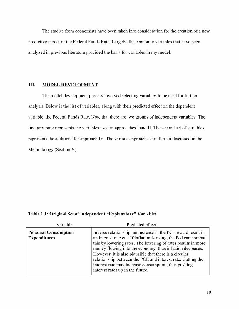
III. MODEL DEVELOPMENT
The model development process involved selecting variables to be used for further
analysis. Below is the list of variables, along with their predicted effect on the dependent
variable, the Federal Funds Rate. Note that there are two groups of independent variables. The
first grouping represents the variables used in approaches I and II. The second set of variables
represents the additions for approach IV. The various approaches are further discussed in the
Methodology (Section V).
Table 1.1: Original Set of Independent “Explanatory” Variables
Variable Predicted effect
10
Personal Consumption Expenditures
Inverse relationship; an increase in the PCE would result in an interest rate cut. If inflation is rising, the Fed can combat this by lowering rates. The lowering of rates results in more money flowing into the economy, thus inflation decreases. However, it is also plausible that there is a circular relationship between the PCE and interest rate. Cutting the interest rate may increase consumption, thus pushing interest rates up in the future.

11
Construction Spending Proportional relationship; an increase in Construction Spending would result in an interest rate cut. If construction is increasing, it is a signal that there is consumer confidence. The target interest rate would increase because the economy does not need to increase at an unsustainable rate. If construction spending decreases, then rates would be cut to stimulate the economy.
Gross Domestic Product
Proportional relationship; an increase in GDP would result in an interest rate hike. This is because if the percent change in GDP is over 2%, the target interest rate set by the Fed would increase because the economy is growing at a rate that is deemed unsustainable.
Unemployment Rate
Inverse relationship; an increase in the Unemployment Rate would result in an interest rate cut. If the unemployment rate is increasing, then more of the labor force is unemployed. The Fed should respond by lowering interest rates to stimulate the economy, or push the economy back to a “normal” level of unemployment. In economic theory, unemployment is tied closely to inflation. Thus, lowering unemployment too much can increase the inflation rate.
Volatility Index
Inverse relationship; an increase in the VIX would result in an interest rate cut. This is because if there is uncertainty in the markets, then the Fed would likely lower interest rates.
Global Price Index of All Commodities
Inverse relationship; an increase in the Global Price Index of All Commodities would result in an interest rate cut. If the global economy is experiencing economic expansion, then it is likely that the United States is experiencing the same trend. Thus, the Fed would increase interest rates.
Yield on Corporate AAA Rated Bonds
Proportional relationship; an increase in the Yield on Corporate AAA Rated Bonds would result in an interest rate hike. The yield on corporate AAA rated bonds historically has moved with the Federal Funds Rate.
M2 Money Supply
Proportional relationship; an increase in the M2 Money Supply would result in an interest rate hike. When the economy is in an expansionary period, the M2 rises and there would be an increase in the Federal Funds Rate. This rate hike would be done to control the economic expansion.
Total Reserves Except Gold on the Balance Sheet
Proportional relationship; an increase in the Total Reserves Except Gold on the Balance Sheet would result in an

Table 1.2: Additional Variables for Approach IV
Variable Predicted effect
IV. DATA DESCRIPTION
The data selection process involved reviewing models that were related to the model that
has been created for this study. The baseline model was the Taylor Rule and various leading
economic indicators were included as independent variables. Many economists have attempted to
build predictive models for the Effective Federal Funds Rate, and their work carved a pathway in
my process of collecting data. Sarno, Thornton, and Valente created predictive models which
heavily influenced my choice of variables to be included in the model developed in approaches I
and II. Approach IV analyzes a different set of variables to achieve a greater understanding of
Monetary Policy.
12
interest rate hike. The balance sheet increases during times of economic expansion, thus the Fed would respond by increasing rates.
US Dollar Overnight Repo Inverse relationship; an increase in the US Dollar Overnight Repo would result in an interest rate cut. This is because Repos are injected into the market during times of low liquidity.
S&P 500 Index Proportional relationship; an increase in the S&P 500 Index would result in an interest rate hike. If the markets are rising the Fed typically responds by interesting rates.
Conference Board US Manufacturers New Orders Nondefense Capital Good Ex Aircraft
Proportional relationship; an increase in the Conference Board US Manufacturers New Orders Nondefense Capital Good Ex Aircraft would result in an interest rate hike. When manufacturing is up, the economy is in an expansionary period and the Fed may respond by raising rates.

Approach I and II:
The data in this model was obtained from the Federal Reserve Bank of St. Louis. It
includes the Effective Federal Funds Rate, Personal Consumption Expenditures, Total
Construction Spending, Gross Domestic Product, Unemployment Rate, CBOE Volatility Index,
Global Price Index of all Commodities, Moody’s Seasoned Aaa Corporate Bond Yield, Long-
Term Government Bond Yields: 10-year: Main for the Euro Area, M2 Money Supply, and the
Total Reserves Except Gold on the Balance Sheet.
To have a complete understanding of the data utilized in this model, the definitions of all
variables must be known.
Table 2.1: Definition of Variables
13
The Effective Federal Funds Rate is the “interest rate at which depository institutions trade federal funds (balances held at the Federal Reserve Banks) with each other overnight”. This rate is central in U.S. financial markets because it influences other interest rates such as mortgages, loans, and savings. These rates in turn affect consumer wealth and confidence.
The Personal Consumption Expenditures (PCE) is a measurement of inflation that the fed utilizes in their decision to raise or lower interest rates. Since it is known that the fed uses this variable, instead of the Consumer Price Index (CPI) to measure inflation, the PCE is used in the model.
Gross Domestic Product is the “total value of goods produced and services provided in a country during one year”. This was used in the model because it is a strong indicator of the health of the economy.
Total Construction Spending is the amount of construction spending in the United States. This is a strong economic indicator because construction spending increases when consumers are confident in the growth of the economy.
The Unemployment Rate “represents the number of unemployed as a percentage of the labor force”. This was used in the model because it is a strong economic indicator.
The CBOE Volatility Index (VIX) is a measurement of “market expectations of near-term volatility conveyed by stock index option prices”. The VIX gives guidance to market expectations, as if there is a period of high volatility, the direction of the markets is uncertain. Periods of uncertainty tend to lead to lower consumer confidence in the economy.
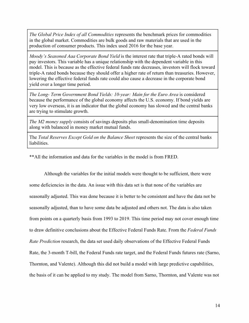
**All the information and data for the variables in the model is from FRED.
Although the variables for the initial models were thought to be sufficient, there were
some deficiencies in the data. An issue with this data set is that none of the variables are
seasonally adjusted. This was done because it is better to be consistent and have the data not be
seasonally adjusted, than to have some data be adjusted and others not. The data is also taken
from points on a quarterly basis from 1993 to 2019. This time period may not cover enough time
to draw definitive conclusions about the Effective Federal Funds Rate. From the Federal Funds
Rate Prediction research, the data set used daily observations of the Effective Federal Funds
Rate, the 3-month T-bill, the Federal Funds rate target, and the Federal Funds futures rate (Sarno,
Thornton, and Valente). Although this did not build a model with large predictive capabilities,
the basis of it can be applied to my study. The model from Sarno, Thornton, and Valente was not
14
The Global Price Index of all Commodities represents the benchmark prices for commodities in the global market. Commodities are bulk goods and raw materials that are used in the production of consumer products. This index used 2016 for the base year.
Moody’s Seasoned Aaa Corporate Bond Yield is the interest rate that triple-A rated bonds will pay investors. This variable has a unique relationship with the dependent variable in this model. This is because as the effective federal funds rate decreases, investors will flock toward triple-A rated bonds because they should offer a higher rate of return than treasuries. However, lowering the effective federal funds rate could also cause a decrease in the corporate bond yield over a longer time period.
The Long- Term Government Bond Yields: 10-year: Main for the Euro Area is considered because the performance of the global economy affects the U.S. economy. If bond yields are very low overseas, it is an indicator that the global economy has slowed and the central banks are trying to stimulate growth.
The M2 money supply consists of savings deposits plus small-denomination time deposits along with balanced in money market mutual funds.
The Total Reserves Except Gold on the Balance Sheet represents the size of the central banks liabilities.

tested for predictions over large time periods. Their model only analyzed predictions for the
short term, not over a period of years.
Approach IV:
The additional variables for this approach came from the database within the Bloomberg
Terminal.
Table 2.2: Definitions of Additional Variables
This approach utilized a new data set, but may require investigation of serial correlation
and multicollinearity because of the nature of economic data.
V. METHODOLOGY
The creation of this model has been the result of various iterations of regression models
as well as statistical tests for multicollinearity and autocorrelation. Teräsvirta’s Handbook of
Economic Forecasting was strongly utilized in this work. Three different approaches were
implemented in an attempt to build a valid statistical model. It is important to note that the first
two approaches used different statistical methods on the same data set, while the third approach
used a new set of data altogether. This was done because it was determined that the variables
15
US Dollar Overnight Repo is the interest rate that treasuries can be traded in for cash to cover short-term cash needs. Repos are typically used as a way to inject liquidity into the financial markets when other methods are insufficient (Trading Economics).
The S&P 500 Index is a stock market index that measures the performance of 500 companies that are listed on this stock exchange.
Conference Board US Manufacturers New Orders Nondefense Capital Good Ex Aircraft is a measurement conducted by the U.S. Census Bureau. In the Tech Bubble burst and the Housing Market crash this variable decreased sharply. Typically during times of economic contraction, manufactured orders fall.
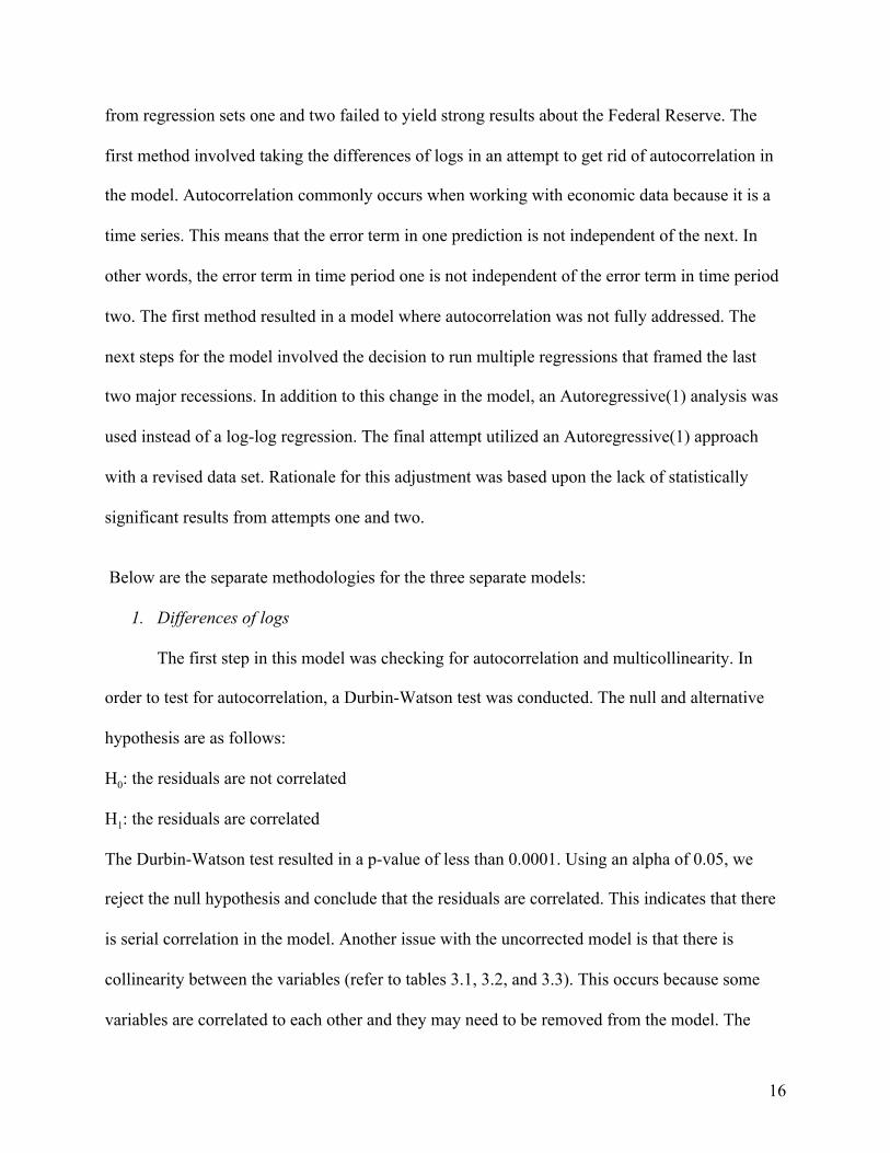
from regression sets one and two failed to yield strong results about the Federal Reserve. The
first method involved taking the differences of logs in an attempt to get rid of autocorrelation in
the model. Autocorrelation commonly occurs when working with economic data because it is a
time series. This means that the error term in one prediction is not independent of the next. In
other words, the error term in time period one is not independent of the error term in time period
two. The first method resulted in a model where autocorrelation was not fully addressed. The
next steps for the model involved the decision to run multiple regressions that framed the last
two major recessions. In addition to this change in the model, an Autoregressive(1) analysis was
used instead of a log-log regression. The final attempt utilized an Autoregressive(1) approach
with a revised data set. Rationale for this adjustment was based upon the lack of statistically
significant results from attempts one and two.
Below are the separate methodologies for the three separate models:
1. Differences of logs
The first step in this model was checking for autocorrelation and multicollinearity. In
order to test for autocorrelation, a Durbin-Watson test was conducted. The null and alternative
hypothesis are as follows:
H0: the residuals are not correlated
H1: the residuals are correlated
The Durbin-Watson test resulted in a p-value of less than 0.0001. Using an alpha of 0.05, we
reject the null hypothesis and conclude that the residuals are correlated. This indicates that there
is serial correlation in the model. Another issue with the uncorrected model is that there is
collinearity between the variables (refer to tables 3.1, 3.2, and 3.3). This occurs because some
variables are correlated to each other and they may need to be removed from the model. The
16
removal of these variables could allow for an increase in the significance of the remaining
variables. This information is derived from the T-statistics associated with each independent
variable in the model. It is also important to consider omitted variable bias, this occurs when
variables are removed from a model even though they are useful in explaining the dependent
variable. In economics, it is very difficult to fully remove multicollinearity from a model without
also removing key variables. Although multicollinearity is a valid concern, there are instances
where it is better to leave a highly correlated variable in for theoretical consideration and to
avoid this bias (McCall).
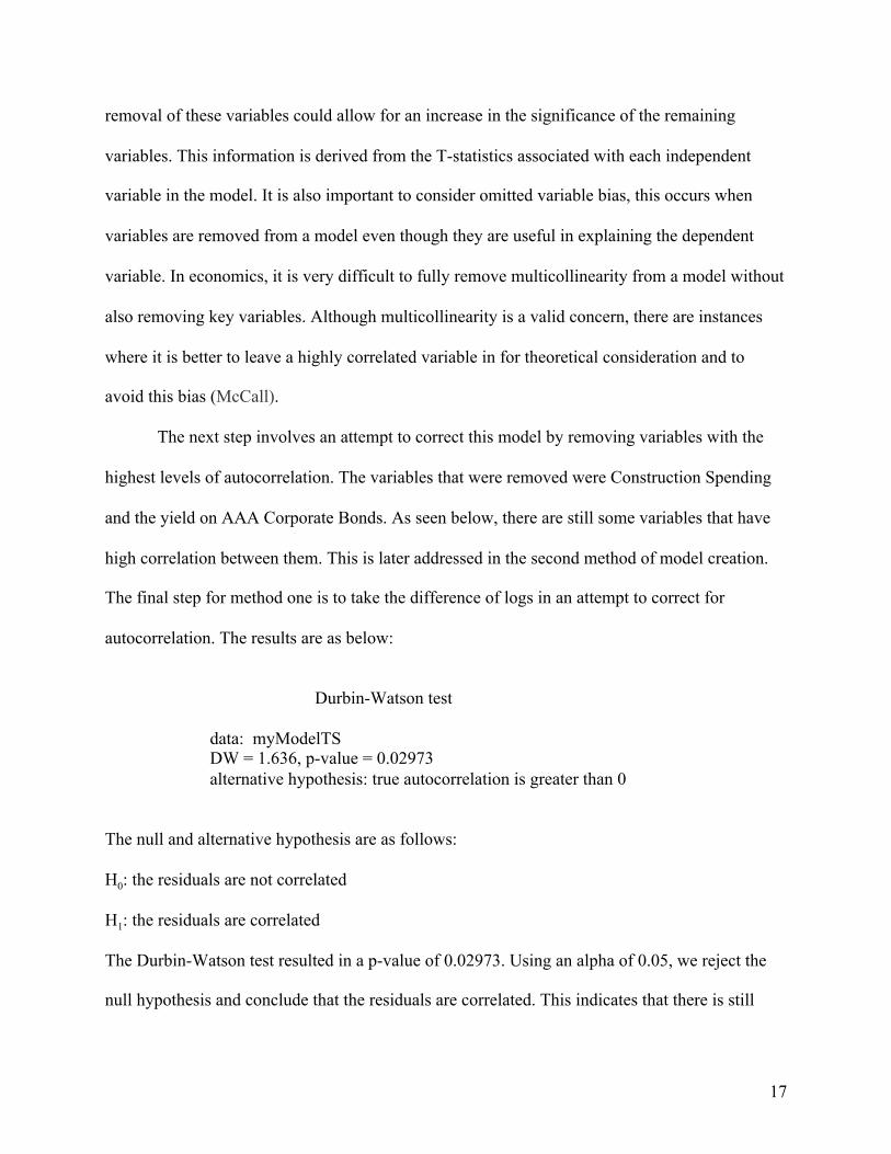
The next step involves an attempt to correct this model by removing variables with the
highest levels of autocorrelation. The variables that were removed were Construction Spending
and the yield on AAA Corporate Bonds. As seen below, there are still some variables that have
high correlation between them. This is later addressed in the second method of model creation.
The final step for method one is to take the difference of logs in an attempt to correct for
autocorrelation. The results are as below:
Durbin-Watson test
data: myModelTS DW = 1.636, p-value = 0.02973 alternative hypothesis: true autocorrelation is greater than 0
The null and alternative hypothesis are as follows:
H0: the residuals are not correlated
H1: the residuals are correlated
The Durbin-Watson test resulted in a p-value of 0.02973. Using an alpha of 0.05, we reject the
null hypothesis and conclude that the residuals are correlated. This indicates that there is still
17
serial correlation in the model. Although there was a significant improvement by the data
transformation, 0.02973 is greater than 0.0001, we are unable to state that this model is free of
autocorrelation.
2. Autoregressive(1)
The AR(1) model addresses the issues of autocorrelation in the model. The first step that
was completed for this model involved testing for multicollinearity, or correlation amongst the
variables for the three separate regressions.
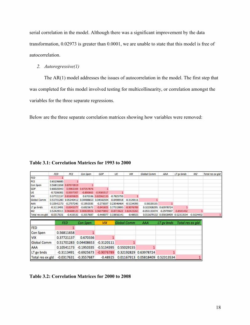
Below are the three separate correlation matrices showing how variables were removed: Table 3.1: Correlation Matrices for 1993 to 2000
Table 3.2: Correlation Matrices for 2000 to 2008
18

Table 3.3: Correlation Matrices for 2008 to 2019
19
Explanation for tables 3.1, 3.2, 3.3:
The preceding tables were created in excel to highlight the removal of correlated variables. For
each time period, any variables that had a correlation greater than the absolute value of 0.8 were
highlighted in red. This formatting was conducted to simplify the process of removing variables.
The ones across the diagonal represent that the variables are perfectly correlated with each other,
this occurred because it is the correlation between the same variables. The color coding of green
and yellow are as follows:
● Green: represents that the variable is not correlated with other variables at the 0.8 level
● Yellow: represents that the variable is correlated with other variables at the 0.8 level, but
was not removed due to omitted variable bias
Once autocorrelation has been taken into consideration, three Autoregressive(1) regressions may
be completed. The highlighted values represent variables with a correlation coefficient that is
larger than 0.8 or less than -0.8. This means that they are very highly correlated and could
introduce bias into the model. However, it is important to note that there is not a strict value for
including or removing variables in the regression.
VI. RESULTS
Below are the outputs from eViews after running three separate regressions.
Tables 4.1, 4.2, and 4.3 are the results from running Autoregressive(1) regressions in eViews
with the variables from the correlation matrices (Tables 3.1, 3.2, and 3.3).
Table 4.1: Regression Output for 1993 Q3 to 2000 Q3
20
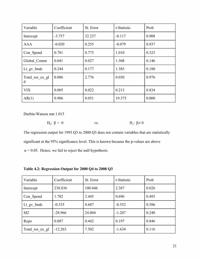
Durbin-Watson stat 1.015
H0: 0β = vs. H1: ≠ 0β
The regression output for 1993 Q3 to 2000 Q3 does not contain variables that are statistically
significant at the 95% significance level. This is known because the p-values are above
Hence, we fail to reject the null hypothesis..05. α = 0
Table 4.2: Regression Output for 2000 Q4 to 2008 Q3
21
Variable Coefficient St. Error t-Statistic Prob
Intercept -3.757 32.237 -0.117 0.908
AAA -0.020 0.255 -0.079 0.937
Con_Spend 0.781 0.773 1.010 0.323
Global_Comm 0.041 0.027 1.508 0.146
Lt_gv_bnds 0.244 0.177 1.385 0.180
Total_res_ex_gld
0.086 2.776 0.030 0.976
VIX 0.005 0.022 0.213 0.834
AR(1) 0.986 0.051 19.375 0.000
Variable Coefficient St. Error t-Statistic Prob
Intercept 238.836 100.046 2.387 0.026
Con_Spend 1.702 2.445 0.696 0.493
Lt_gv_bnds -0.335 0.607 -0.552 0.586
M2 -28.966 24.004 -1.207 0.240
Repo 0.087 0.442 0.197 0.846
Total_res_ex_gl -12.263 7.502 -1.634 0.116
Durbin-Watson stat 0.693
H0: 0β = vs. H1: ≠ 0β
The regression output for 2000 Q4 to 2008 Q3 does not contain variables that are statistically
significant at the 95% significance level. This is known because the p-values are above
Hence, we fail to reject the null hypothesis..05. α = 0
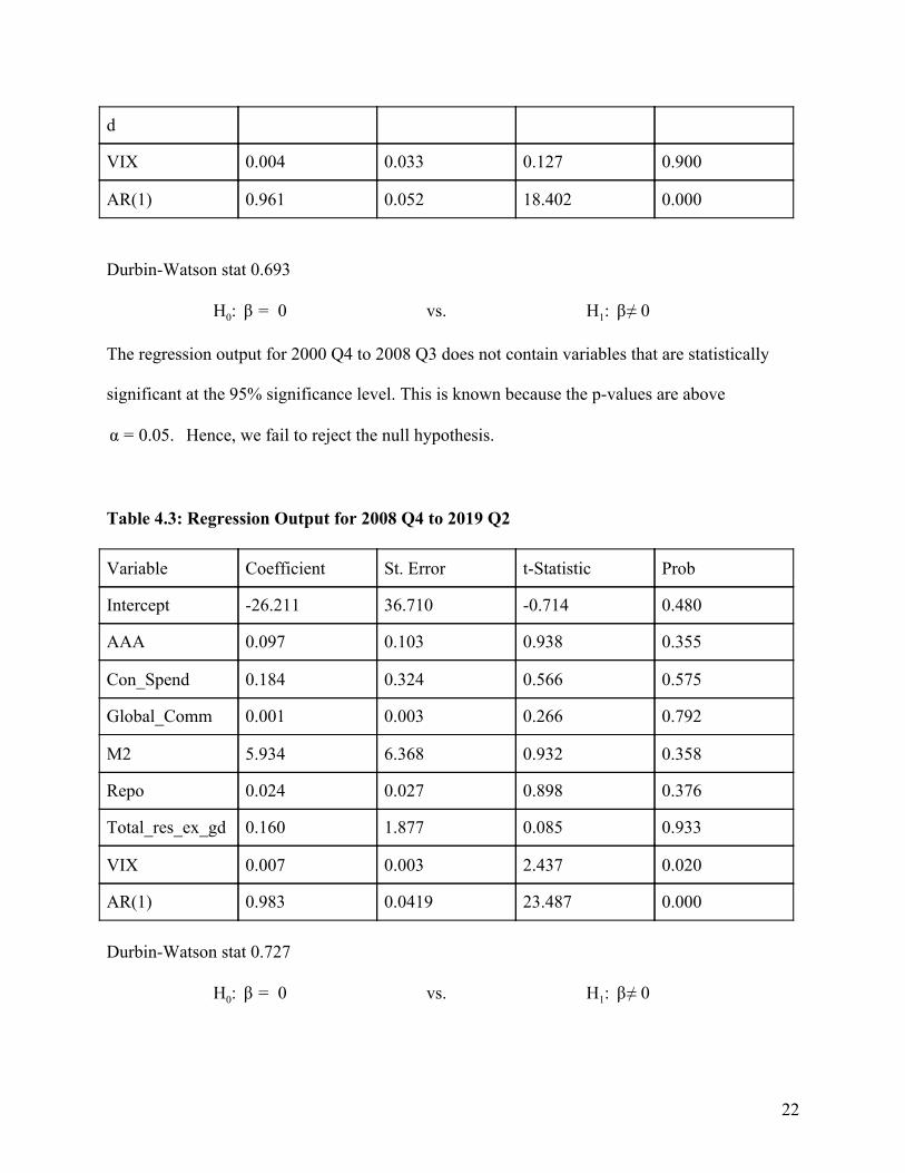
Table 4.3: Regression Output for 2008 Q4 to 2019 Q2
Durbin-Watson stat 0.727
H0: 0β = vs. H1: ≠ 0β
22
d
VIX 0.004 0.033 0.127 0.900
AR(1) 0.961 0.052 18.402 0.000
Variable Coefficient St. Error t-Statistic Prob
Intercept -26.211 36.710 -0.714 0.480
AAA 0.097 0.103 0.938 0.355
Con_Spend 0.184 0.324 0.566 0.575
Global_Comm 0.001 0.003 0.266 0.792
M2 5.934 6.368 0.932 0.358
Repo 0.024 0.027 0.898 0.376
Total_res_ex_gd 0.160 1.877 0.085 0.933
VIX 0.007 0.003 2.437 0.020
AR(1) 0.983 0.0419 23.487 0.000

The regression output for 2008 Q4 to 2019 Q2 only contains one variable that is statistically
significant at the 95% significance level. This is known because the p-values for AAA,
Con_Spend, Global_Comm, M2, Repo, and Total_res_ex_gld are above . Hence, we.05α = 0
fail to reject the null hypothesis for those variables.
The three regressions were conducted utilizing AR(1) in an attempt to control for
autocorrelation, however the model still needs further improvements. This is accepted because
the Durbin-Watson Stat is too low for all three time periods. We are testing to see if the
Durbin-Watson Stat is less than the value for the lower bound. For simplicity, the lower bound
that we are comparing to is 2.00. Since the Durbin-Watson Stat is less than 2.00, we reject the
null hypothesis and may state that there is evidence of serial correlation in the model. The main
issue that arises from serial correlation is that an error in the estimate from one time period will
bleed over into the next time periods. Other issues with my model arise because most of the
coefficients are not statistically significant from zero. The only variable that is significant in this
model is the VIX in the third regression. This is known because it has a p-value of approximately
0.020 and that is less than the Hence, we can reject the null hypothesis for this.05. α = 0
coefficient. Although the model lacked predictive findings, it still gives us insight for further
research. A possible reason for the low t-statistics is that the model is not completely void of
multicollinearity. This could explain why many of the variables are considered to be
insignificant, but it is plausible that they do actually play a role in predicting the Federal Funds
Rate.
Approach IV produced different results from the previous three regressions. This was due
to the changes in explanatory variables.
23
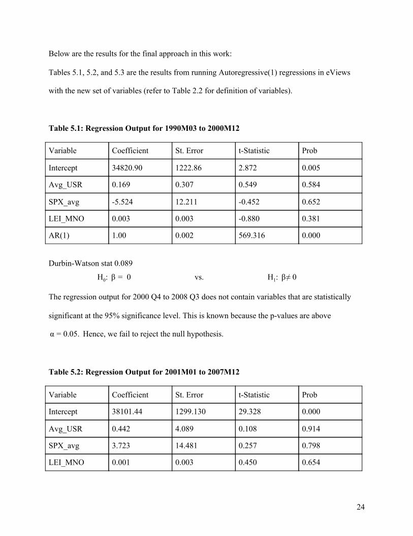
Below are the results for the final approach in this work:
Tables 5.1, 5.2, and 5.3 are the results from running Autoregressive(1) regressions in eViews
with the new set of variables (refer to Table 2.2 for definition of variables).
Table 5.1: Regression Output for 1990M03 to 2000M12
Durbin-Watson stat 0.089 H0: 0β = vs. H1: ≠ 0β
The regression output for 2000 Q4 to 2008 Q3 does not contain variables that are statistically
significant at the 95% significance level. This is known because the p-values are above
Hence, we fail to reject the null hypothesis..05. α = 0
Table 5.2: Regression Output for 2001M01 to 2007M12
24
Variable Coefficient St. Error t-Statistic Prob
Intercept 34820.90 1222.86 2.872 0.005
Avg_USR 0.169 0.307 0.549 0.584
SPX_avg -5.524 12.211 -0.452 0.652
LEI_MNO 0.003 0.003 -0.880 0.381
AR(1) 1.00 0.002 569.316 0.000
Variable Coefficient St. Error t-Statistic Prob
Intercept 38101.44 1299.130 29.328 0.000
Avg_USR 0.442 4.089 0.108 0.914
SPX_avg 3.723 14.481 0.257 0.798
LEI_MNO 0.001 0.003 0.450 0.654
Durbin-Watson stat 0.035
H0: 0β = vs. H1: ≠ 0β
The regression output for 2001M01 to 2007M12 does not contain variables that are statistically
significant at the 95% significance level. This is known because the p-values are above
Hence, we fail to reject the null hypothesis..05. α = 0
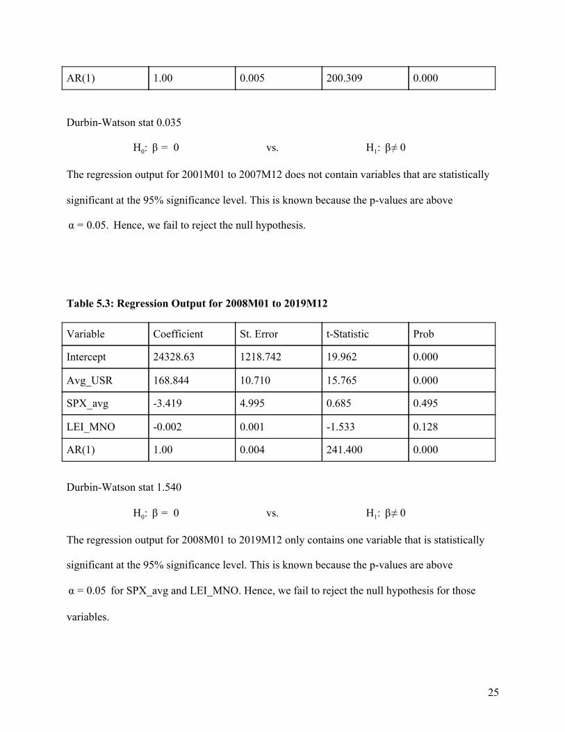
Table 5.3: Regression Output for 2008M01 to 2019M12
Durbin-Watson stat 1.540
H0: 0β = vs. H1: ≠ 0β
The regression output for 2008M01 to 2019M12 only contains one variable that is statistically
significant at the 95% significance level. This is known because the p-values are above
for SPX_avg and LEI_MNO. Hence, we fail to reject the null hypothesis for those.05 α = 0
variables.
25
AR(1) 1.00 0.005 200.309 0.000
Variable Coefficient St. Error t-Statistic Prob
Intercept 24328.63 1218.742 19.962 0.000
Avg_USR 168.844 10.710 15.765 0.000
SPX_avg -3.419 4.995 0.685 0.495
LEI_MNO -0.002 0.001 -1.533 0.128
AR(1) 1.00 0.004 241.400 0.000

___________________________________ Avg_USR: US Dollar Overnight Repo SPX_avg: The S&P 500 Index LEI_MNO: Conference Board US Manufacturers New Orders Nondefense Capital Good Ex Aircraft
The significance of the final set of regressions is that only one variable from the period
2008 to 2019 held any statistical value. Since the US Dollar Overnight Repo has a p-value of
approximately 0.000 and this is less than , we can reject the null hypothesis for this.05α = 0
coefficient. This shows how Monetary Policy has changed over time because this variable was
not statistically significant in the other regressions. The Federal Reserve has gone on to utilize
new tools to stabilize the economy. The conventional monetary policy tools involve conducting
open market operations to raise or lower the interest rate. The introduction of Repurchase
Agreements to inject liquidity into the markets is considered unconventional monetary policy,
but has become more frequently utilized during periods of economic downturn.
VII. CONCLUSION AND DISCUSSION
Upon completion of the three approaches, a conclusive predictive model has not been
obtained. The issues with the current predictive model are the lack of significance in the majority
of the variables and some levels of autocorrelation. This result is expected, as the economy has
many moving and intertwined parts. In previous economic forecasting models, the underlying
theory might hold true, but in practice models will not always hold true. This is because the
26
economic system is very dynamic, and exogenous variables can greatly disrupt forecasting
abilities. Furthermore, economists still have varying opinions about the actions of the Federal
Reserve. Rather than attempting to form a prediction of the Federal Funds Rate, it should be
suggested to forecast the economy itself. This is because the Fed adjusts the interest rate based
upon the current state of the economy and their predictions about where the economy is going.
Based on the results of my study, the responses cannot be predicted at a high degree of accuracy
for an extended time period.
Further research may be conducted in an attempt to create a more accurate model. The
current model utilizes AR(1), but the next step could be to have AR(4) and study the changes in
autocorrelation. The prediction would be that an AR(4) model would reduce the levels of
autocorrelation in the model by reducing the effects of standardized errors in the lags. The
benefit of running an AR(4) is that we would be able to lag the data four periods instead of only
one. However, this would come with costs. The two main negatives of an AR(4) would be a
reduction in the degrees of freedom and a reduction in the data points. The issue with removing
degrees of freedom is that the t-critical value would be lower. This could result in failing to reject
a null hypothesis when it should be rejected, or the variable should be considered to be
statistically significant. Another approach to the issues in the model would be altering the
variables. The regression can be re-run with removing M2 because that variable has higher levels
of serial correlation. The addition of a variable that considers the political party in power may
also be considered. Although the Federal Reserve is supposed to act independently, politicians
still put pressure on the chairman. Most notably, President Trump continually puts pressure on
the Fed to lower interest rates, even into negative territory. Trump’s rationale is that the United
States should follow suit with other countries that have adopted this change in monetary policy.
27
Furthermore, during election years the President in office wants the economy to be strong and
the stock market to flourish. This could alter the amount of downward pressure on interest rates
from the politicians. The stock market could also be an additional variable for consideration.
This is because in theory, the Fed is not supposed to be dependent on the stock market when
making interest rate decisions. Due to the wealth effect, the Fed must consider how the markets
will react to their decisions. The selection of new variables to the model and the incorporation of
AR(4) should lead to more conclusive results.
28
CITATIONS
Bauer, Christian, and Matthias Neuenkirch. “Forecast Uncertainty and the Taylor Rule.” Forecast Uncertainty and the Taylor Rule, Universitat Trier, 6 July 2017, www.uni-trier.de/fileadmin/fb4/prof/VWL/EWF/Research_Papers/2015-05.pdf.
Caunedo, Julieta, et al. “Asymmetry and Federal Reserve Forecasts.” Asymmetry and Federal Reserve Forecasts, Federal Reserve Bank of St. Louis, Nov. 2015, pdfs.semanticscholar.org/c799/f14d84892bd3768cbeb3b187b9fe16f2d457.pdf.
Gaeto, Lillian R, and Sandeep Mazumder. “Measuring the Accuracy of Federal Reserve Forecasts.” Southern Economic Journal, 2019, doi:10.1002/soef.12312.
Gamber, Edward N. “Are the Fed's Inflation Forecasts Still Superior to the Private Sector's?” Journal of Macroeconomics, vol. 31, no. 2, 2009, p. 240.
Born, Alexandra, and Zeno Enders. “Global Banking, Trade, and the International Transmission of the Great Recession.” The Economic Journal, vol. 129, no. 623, 2019, pp. 2691–2721., doi:10.1093/ej/uez010.
Moody, John. “Forecasting the Economy with Neural Nets: A Survey of Challenges and Solutions.” Lecture Notes in Computer Science Neural Networks: Tricks of the Trade, 1998, pp. 347–371., doi:10.1007/3-540-49430-8_17.
Christopher A. Sims, 1986. "Are forecasting models usable for policy analysis?," Quarterly Review, Federal Reserve Bank of Minneapolis, issue Win, pages 2-16.
Teräsvirta, Timo. “Handbook of Economic Forecasting.” Handbook of Economic Forecasting, 2013, p. iii., doi:10.1016/b978-0-444-62731-5.00023-3.
Johannsen, Benjamin K., and Elmar Mertens. “A Time Series Model of Interest Rates With the Effective Lower Bound.” Finance and Economics Discussion Series, vol. 2016, no. 33, 2016, pp. 1–46., doi:10.17016/feds.2016.033.
Gandrud, Christopher, and Cassandra Grafström. “Inflated Expectations: How Government Partisanship Shapes Monetary Policy Bureaucrats’ Inflation Forecasts.” Political Science Research and Methods, vol. 3, no. 2, 2015, pp. 353–380., doi:10.1017/psrm.2014.34.
29

Rogoff, Kenneth. “Dealing with Monetary Paralysis at the Zero Bound.” Journal of Economic Perspectives, vol. 31, no. 3, 2017, pp. 47–66., doi:10.1257/jep.31.3.47.
Bordo, Michael. “The Contribution of a Monetary History of the United States: 1867 to 1960 To Monetary History.” National Bureau of Economic Research, 1989, doi:10.3386/w2549.
Sims, Christopher A. “Interpreting the Macroeconomic Time Series Facts.” European Economic Review, vol. 36, no. 5, 1992, pp. 975–1000., doi:10.1016/0014-2921(92)90041-t.
Gorton, Gary, and Andrew Metrick. “The Federal Reserve and Panic Prevention: The Roles of Financial Regulation and Lender of Last Resort.”Journal of Economic Perspectives, vol. 27, no. 4, 2013, pp. 45–64., doi:10.1257/jep.27.4.45.
Gavin, William T., and Rachel J. Mandal. “The Art of Predicting the Federal Reserve: St. Louis Fed.” The Art of Predicting the Federal Reserve | St. Louis Fed, Federal Reserve Bank of St. Louis, 25 June, 2018, www.stlouisfed.org/publications/regional-economist/july-2000/inside-the- briefcase-the-art-of-predicting-the-federal-reserve.
Vroey, Michel De, and Kevin D. Hoover. “Introduction: Seven Decades of the IS-LM Model.” History of Political Economy, vol. 36, no. Suppl 1, 2004, pp. 1–11., doi:10.1215/00182702-36-suppl_1-1.
Mishkin, Frederic S. “Monetary Policy and the Dual Mandate.” Board of Governors of the
Federal Reserve System, 2007, www.federalreserve.gov/newsevents/speech/mishkin20070410a.htm.
“United States Overnight Repo Rate 1995-2020 Data: 2021-2022 Forecast: Calendar.” United
States Overnight Repo Rate | 1995-2020 Data | 2021-2022 Forecast | Calendar, tradingeconomics.com/united-states/repo-rate.
McCall, B. (2014). Omitted variable bias. In D. Brewer & L. Picus (Eds.), Encyclopedia of
education economics & finance (pp. 495-498). Thousand Oaks, CA: SAGE Publications, Inc. doi: 10.4135/9781483346595.n184
30