lag and attenuation parameters for routing daily flow - CORE

LAG AND ATTENUATION PARAMETERS FOR ROUTING DAILY FLOW

CHANGES THROUGH LARGE RIVER SYSTEMS

A Thesis

by

MUHAMMAD ABDUL RAHEEM SIDDIQUI

Submitted to the Office of Graduate and Professional Studies of

Texas A&M University

in partial fulfillment of the requirements for the degree of

MASTER OF SCIENCE

Chair of Committee, Ralph Wurbs

Co-Chair of Committee, Clyde Munster

Committee Member, Anthony Cahill

Head of Department, Robin Autenrieth

August 2017

Major Subject: Civil Engineering

Copyright 2017 Muhammad Abdul Raheem Siddiqui

ii

ABSTRACT

The 2007 Senate Bill 3 (SB3) initiated the establishment of environmental flow

standards and the incorporation of them in the Water Availability Modeling System (WAM)

of Texas. This led to the creation of Water Rights Analysis Package (WRAP) daily modeling

capabilities. The effects of water use and management actions propagate downstream to other

locations of interest in water availability modeling over periods ranging from several hours

to several days. Hence unlike the WRAP Monthly Simulation Model (SIM), the Daily

Simulation Model (SIMD) includes routing of the effects of flow change events to

downstream control points.

The previously developed six case study daily WAMs use routing parameters

estimated through calibration using hydrographs at upstream and downstream ends of a river

reach with computations performed with a genetic search algorithm. In this research, two

new methods have been developed to estimate routing parameters.

1. Wave Travel Velocity Equation: Motivated by Manning’s equation and

National Resources Conservation Service (NRCS) lag time equation. This

equation calculates lag time based on flow, slope, and length of the reach.

2. DFLOW program: This program calculates the lag time between upstream

and downstream control points for different flow change events in a time

series record, and provide statistical measures of the results.

The wave travel velocity equation was applied to different reaches of the Brazos

River and its tributaries and the DFLOW program was applied to the Neches, Brazos, and

Trinity River Basins. Comparative analysis of different sets of routing parameters shows that

lag times from the optimization-based parameters are unrealistically low for the Brazos and

Neches River Basins. Lag times from DFLOW and the wave travel velocity equation are

higher than optimization-based lag times and are more realistic when compared to typical

average stream velocities.

Simulation results using different simulation options and routing parameters were

compared to gauge the sensitivity of simulation results to different routing and forecasting

iii

options. Simulation results are sensitive to different routing parameters and routing and

forecasting options but do not vary dramatically for any of these options.

iv

DEDICATION

This thesis is dedicated to my parents, Abdul Wahab and Asiya.

v

ACKNOWLEDGEMENTS

I would like to thank my committee chair, Dr. Ralph Wurbs, for his guidance and

support throughout the course of this research.

My work was supported by a graduate research assistantship funded by a project

sponsored by the Texas Commission on Environmental Quality (TCEQ). The support of the

TCEQ is gratefully acknowledged. However, the information presented in this academic

thesis has not been validated by the TCEQ and does not necessarily represent the views or

policies of the TCEQ. All errors or misrepresentations found in the thesis are the

responsibility of the author, not the sponsor.

Brad Brunett of the Brazos River Authority provided some of the necessary data for

the research. I owe thanks to him as well.

Thanks also go to my friends and colleagues and the department faculty and staff for

making my time at Texas A&M University a great experience. Thanks also to my brother

Abdul Rehman for encouraging me to pursue graduate studies in a foreign country.

Finally, I would like to thank the God Almighty for giving me the strength and ability

to complete this research.

vi

CONTRIBUTORS AND FUNDING SOURCES

This work was supervised by a thesis committee consisting of Professor Dr. Ralph

Wurbs and Professor Dr. Anthony Cahill of the Department of Civil Engineering and

Professor Dr. Clyde Munster of Biological and Agricultural Engineering Department.

All work for the thesis was completed independently by the student under the

advisement of Dr. Ralph Wurbs of the Department of Civil Engineering.

My work was supported by a graduate research assistantship funded by a project

sponsored by the Texas Commission on Environmental Quality (TCEQ). Its contents are

solely the responsibility of the author and do not necessarily represent the official views of

the TCEQ.

vii

NOMENCLATURE

BRA Brazos River Authority

DFLOW Daily Flow

e-flow Environmental Flow

GIS Geographic Information System

GSA Guadalupe and San Antonio

HEC Hydrologic Engineering Center

HMS Hydrologic Modeling System

K Conveyance Factor

L Length of the Reach

LRCA Lower Colorado River Authority

NRCS National Resources Conservation Service

Q Flow

RAS River Analysis System

S Slope of the Reach

SB3 Senate Bill 3

SIM Simulation Model

SIMD Daily Simulation Model

T Time

TCEQ Texas Commission on Environmental Quality

USACE United States Army Corps of Engineers

USDA United States Department of Agriculture

USGS United States Geological Survey

VAVE Average Velocity in River

VT Travel Velocity

VW Wave Celerity

WAM Water Availability Modeling

WRAP Water Rights Analysis Package

viii

TABLE OF CONTENTS

Page

ABSTRACT ................................................................................................................ ii

DEDICATION ............................................................................................................... iv

ACKNOWLEDGEMENTS ........................................................................................... v

CONTRIBUTORS AND FUNDING SOURCES ......................................................... vi

NOMENCLATURE ...................................................................................................... vii

TABLE OF CONTENTS ............................................................................................... viii

LIST OF FIGURES ....................................................................................................... xi

LIST OF TABLES ......................................................................................................... xiii

CHAPTER I INTRODUCTION .................................................................................... 1

Water Rights Analysis Package (WRAP) ............................................................. 2

Texas Water Availability Models (WAMs) .......................................................... 3

Daily Simulation Model (SIMD) .......................................................................... 3

Literature Review.................................................................................................. 4

Flow Routing ..................................................................................................... 4

Wave Celerity .................................................................................................... 5

Muskingum Model ............................................................................................. 5

Muskingum Parameter Estimation ..................................................................... 6

Lag Model .......................................................................................................... 6

Hydraulic Routing .............................................................................................. 7

NRCS Empirical Lag Equation for Watersheds ................................................ 7

Assumptions & Limitations in Parameter Estimation ....................................... 8

Research Scope and Objectives ............................................................................ 9

CHAPTER II ROUTING AND FORECASTING IN WRAP SIMULATION MODEL 10

Routing Methods in SIMD.................................................................................... 11

Routing Parameters ............................................................................................... 13

Original Method of Calibrating Routing Parameters ............................................ 13

Issues with Routing Parameters through Replication of Hydrographs .............. 14

CHAPTER III WAVE TRAVEL VELOCITY EQUATION ........................................ 16

Theoretical Basis of Travel Time Equation .......................................................... 16

Data Collection ..................................................................................................... 17

Normal Flow Dataset ......................................................................................... 17

High Flow Datasets ............................................................................................ 19

Length of the Reaches ........................................................................................ 20

Water Surface Elevations for Slope Calculation ............................................... 20

ix

Flow ................................................................................................................ 20

K vs Q Relationship Equation through Regression .............................................. 20

Normal Flow Equation ....................................................................................... 21

High Flow Equation ........................................................................................... 22

Application of Wave Travel Velocity Equation ................................................... 23

Brazos River Basin ............................................................................................ 23

Neches River Basin ............................................................................................ 25

CHAPTER IV DEVELOPMENT OF NEW ROUTING PARAMETERS ................... 27

DFLOW Method ................................................................................................... 27

General Methodology for Application of DFLOW .............................................. 27

Application of DFLOW Program on Three Daily WAMs ................................... 28


DFLOW Methodology for Neches Basin .......................................................... 31

Results ................................................................................................................ 33


DFLOW Methodology for Brazos Basin ........................................................... 38

Results ................................................................................................................ 40

Trinity River Basin ............................................................................................ 44

DFLOW Methodology for Trinity Basin ........................................................... 46

Results ................................................................................................................ 48

Attenuation ......................................................................................................... 52

CHAPTER V COMPARATIVE ANALYSIS ............................................................... 53

Comparison of Different Sets of Routing Parameters for Neches River Basin .... 53

Comparison between Lag Values ...................................................................... 53

Comparison between River Velocities............................................................... 54

Discussion .......................................................................................................... 57

Comparison of Different Sets of Routing Parameters for Brazos River Basin..... 57



Discussion .......................................................................................................... 59

Comparison of Different Set of Routing Parameters for Trinity River Basin ...... 60



Discussion .......................................................................................................... 62

Comparison of Simulation Results ....................................................................... 62



Trinity River Basin ............................................................................................ 77

CHAPTER VI SUMMARY AND CONCLUSIONS .................................................... 82

REFERENCES .............................................................................................................. 85

APPENDIX A ................................................................................................................ 88

x

APPENDIX B ................................................................................................................ 91

APPENDIX C ................................................................................................................ 94

APPENDIX D ................................................................................................................ 97

APPENDIX E ................................................................................................................ 100

APPENDIX F ................................................................................................................ 102

APPENDIX G ................................................................................................................ 106

xi

LIST OF FIGURES

Page

Figure 3.1 Plot of K vs Q for Normal Flow Conditions in Brazos and Lower

Colorado Basin ....................................................................................... 21

Figure 3.2 Plot of K vs Q for High Flow Conditions in Brazos, Colorado, and

Trinity River Basins ................................................................................ 23

Figure 4.1 Neches River Basin Located in Texas …………………………………. 29

Figure 4.2 Neches Primary Control Points and the Reaches Formed by Them ......... 30

Figure 4.3 USGS Gauged Flows at Upstream Control Points VIKO, PISL, &

NEEV and the Downstream Control Point NEBA ………….................. 32

Figure 4.4 Lag (Days/Mile) for All Reaches of the Neches River Basin for Normal

Flows ………………………………………………………………...... 35

Figure 4.5 Brazos River Basin Located in Texas ……………………………….…. 36

Figure 4.6 Brazos Primary Control Points and the Reaches Formed by Them ......... 37

Figure 4.7 USGS Gauged Flows at U/S Point BRGR30 and D/S Point BRAQ33 39

Figure 4.8 Lag (Days/Mile) for All Reaches of the Brazos River Basin …………. 44

Figure 4.9 Trinity River Basin Located in Texas ………………………………...... 45

Figure 4.10 Trinity Primary Control Points and the Reaches Formed by Them ......... 47

Figure 4.11 Lag (Days/Mile) for All Reaches of the Trinity River Basin for Normal

Flows ………………………………………………………….……..... 51

Figure 5.1 Stream Velocity Record for NEBA from USGS (USGS Website) .......... 56

Figure 5.2 Storage in Large Reservoirs of Neches River Basin for Different

Simulation Options ………………….………………………………… 64

Figure 5.3 Storage in Large Reservoirs of Brazos River Basin for Different

Simulation Options …………….……………………………………… 68

Figure 5.4 Storage in Large Reservoirs of Trinity River Basin for Different

Simulation Options .…………………………………………………… 78

xii

LIST OF TABLES

Page

Table 1.1 Relationship between Wave Velocity and Average Velocity for Different

River Cross Sections ………………………………………….................. 5

Table 2.1 Routing Methods Used in Different River/Reservoir System

Management Models ................................................................................. 12

Table 3.1 Brazos River Authority Dataset for Travel Times Under Normal Flow

Conditions ………………………………………………………………. 18

Table 3.2 Application of Wave Travel Velocity Equation on the Brazos River Basin 24

Table 3.3 Application of Wave Travel Velocity Equation on Neches River Basin ... 26

Table 4.1 Lag and Attenuation from DFLOW for Neches River Basin …….…......... 34

Table 4.2 Lag and Attenuation from DFLOW for Brazos River Basin .……….…… 41

Table 4.3 Lag and Attenuation from DFLOW for Trinity River Basin .……………. 49

Table 5.1 Comparison of Lags Estimated with the DFLOW versus Optimization

Methods for Reaches in the Neches River Basin ………………...………. 54

Table 5.2 Corresponding Average Stream Velocities Based on Lag Values for

Reaches in the Neches River Basin .……………………………………... 56

Table 5.3 Comparison of Lags from DFLOW, Wave Travel Velocity Equation, and

Optimization Methods for Reaches in the Brazos River Basin …………... 58


Reaches in the Brazos River Basin .……………………………………… 59

Table 5.5 Comparison of lags from DFLOW and calibration method for Reaches in

the Trinity River Basin ……....................................................................... 60


Reaches in the Trinity River Basin ………………………………………. 61

Table 5.7 Instream Targets and Shortages for E-Flow Control Points of Neches .... 65

Table 5.8 Regulated Flows for E-Flow Control Points of Neches ….…………......... 66

Table 5.9 Instream Targets and Shortages for E-Flow Control Points of Brazos …... 69

Table 5.10 Regulated Flows for E-Flow Control Points of Brazos .……………….... 73

Table 5.11 Instream Targets and Shortages for E-Flow Control Points of Trinity …. 79

xiii

Table 5.12 Regulated Flows for E-Flow Control Points of Trinity .……………...… 80

1

CHAPTER I

INTRODUCTION

The Texas Commission on Environmental Quality (TCEQ) maintains a Water

Availability Modeling (WAM) System for all the river basins of Texas. The WAM consists of

the generalized modeling system Water Rights Analysis Package (WRAP) and its input

datasets for all the river basins of Texas, and related information (Wurbs 2005). The

generalized WRAP combined with an input dataset from the TCEQ WAM System is called a

water availability model (WAM). The monthly WAMs have been routinely applied in Texas

for over a decade. The TCEQ has sponsored research at Texas A&M University over the past

several years that has included the development of daily time step WRAP modeling and

corresponding daily versions of six of the 20 Texas WAMs.

The daily modeling system expands the capabilities of WRAP for simulating Senate

Bill 3 environmental flow standards and the corresponding effects on water supply reliabilities

(Wurbs and Hoffpauir 2013). The daily modeling system includes disaggregation of monthly

naturalized flows and water demands to daily units, flow forecasting and routing, simulation

of flood control reservoir operations, and recording high-flow pulses of certain frequencies for

environmental flow standards along with subsistence and base flows.

The WRAP daily modeling system is documented by the Daily Manual (Wurbs and

Hoffpauir 2015). The WRAP program for daily simulation is called SIMD. The six daily

WAMs of Texas for the Brazos, Colorado, Trinity, Neches, Sabine, and Guadalupe and San

Antonio (GSA) are in the developmental stage.

Flow routing and forecasting capabilities were added to the Daily Simulation Model as

the effects of reservoir operations and other water management and use actions usually

propagate through a river/reservoir system in less time than a month. These effects do not

transfer to the next month typically in a monthly model. Daily WAM simulations can be

performed without routing and forecasting too. Simulation results for the six daily WAMs are

changed significantly but not dramatically by completely removing routing and forecasting.

Routing and forecast parameters are necessarily approximate. Changes in values of routing and

forecast parameters can significantly affect simulation results.

2

The current techniques of determining routing parameters for daily WAMs have some

issues as described later. The purpose of this research is to develop routing parameters

determination technique(s) and to incorporate these technique(s) in the WRAP/WAM system.

This research on simulating the downstream propagation of flow changes provides an

enhanced understanding of river hydraulics as well as improved WRAP/WAM modeling

capabilities.

Water Rights Analysis Package (WRAP)

The Water Rights Analysis Package (WRAP) is a system of multiple computer

programs purposefully developed for simulating and analyzing water resources management,

allocation, development and use in a single river basin or multiple–basin region. WRAP is built

for the priority (time) based water allocation system called prior appropriation water rights. It

is used to assess the reliability of supplying water to particular water rights. These water rights

can be industrial/municipal water supply needs, hydroelectric power generation needs,

instream/environmental flow needs, and reservoir storage allocation. Flood control and

reservoir operations can also be simulated through WRAP. Additional capabilities include

tracking of salinity load and concentrations. The modeling system is general i.e. it can be

applied in any part of the world, with input files developed for the basin/region of interest

(Wurbs 2015b).

The Water Rights Analysis Package has been developed at Texas A&M University

under the supervision of Dr. Ralph Wurbs. It is implemented routinely in the state of Texas in

the United States. TCEQ maintains input files for the Texas river basins. The modeling system

supports administration of water allocation systems, regional and statewide planning, and other

water management activities.

Within the WRAP package, there are two separate simulation models based on the size

of the time step. The monthly model (SIM) was developed initially and is well established.

The monthly model is available for the public use. Sub-monthly (or daily) model (SIMD) was

developed recently and is seeing continuous improvements. The main force behind the

development of the daily model is Senate Bill 3 (SB3) environmental flow standards. WRAP

3

is documented by a Reference Manual (Wurbs 2015b), Users Manual (Wurbs 2015c), Daily

Manual (Wurbs and Hoffpauir 2015), and several other manuals.

The modeling strategy implemented in WRAP is as follows (Wurbs 2005)

1. Time-series records of naturalized flows covering the period of interests are given by

the user to the program at selected control points. The user also provides other

information such as evaporations at reservoirs, water rights priority order, water rights

diversion amount, return flows, etc. etc.

2. Naturalized flows are distributed from those control points to all control points based

on user define criteria.

3. The water management system is simulated, under the priority based allocation to each

water right.

4. Simulation results are summarized in the form of water supply reliability indices, flow,

and storage frequency relationships, and regulated and unappropriated flow records.

Texas Water Availability Models (WAMs)

The Texas commission on Environmental Quality (TCEQ) Water Availability

Modeling (WAM) system consists of WRAP and WRAP input files for the all the 23 river

basins of Texas. Three of the basins are combined with adjacent river basins. The 20 WAM

datasets are available at the TCEQ WAM website. The WAM assess availability and reliability

of water resources in a river basin based on historical hydrology and authorized (permitted) or

current conditions of human development and water use. The WAM system supports

government agencies in a wide spectrum of statewide planning and management activities.

Major applications include water rights permit evaluations and statewide planning studies. The

WAM system is currently being updated to incorporate modeling of Senate Bill 3

environmental flow standards.

Daily Simulation Model (SIMD)

The Daily Simulation Model (SIMD) is an expansion of the Monthly Simulation Model

(SIM) to enable daily time step modeling. The motivation for the development of SIMD arises

from the need of assessing water supply reliabilities after satisfying SB 3 environmental flow

4

standards. Beside the capabilities of monthly time step model, SIMD possesses the following

major additional capabilities (Wurbs and Hoffpauir 2015):

1. Disaggregation of monthly naturalized flow to daily time step.

2. Disaggregation of monthly targets of streamflow diversion, hydropower and

environmental flow to daily targets.

3. Routing and attenuation of current day flow changes to downstream control points at

later days.

4. Forecasting of available stream flows at downstream control points for future days

based on the flow changes at an upstream control point in the current day.

5. Simulation of available channel capacity for flood control reservoir operations.

6. Recording of daily and aggregated monthly simulation results.

The routing and forecasting were not required in the monthly model because the effects

of flow changes usually get transferred to all downstream control points within the same time

step. In the daily model, it is necessary to incorporate routing and forecasting to better assess

regulated flows at downstream control points and to protect senior water rights from the

diminishing effect of water use by junior water right at upstream in previous days.

Literature Review

Flow Routing

Flow routing is a technique to track the characteristics of a wave, which is

superimposed on the flow itself, in a river at different spatial locations. These characteristics

may be magnitude, time, and spread. In a typical use of flow routing, characteristics of flood

waves from different storm events are analyzed for downstream locations (Akan 2006). In

WRAP, routing is used to analyze the effects of water withdrawal or addition by upstream

users at downstream points as the wave created by flow change propagates downstream.

5

Wave Celerity

The speed of the propagation of disturbance is called celerity (or celerity of gravity

waves in shallow water), and it is estimated as 𝑐 𝑜𝑟 𝑉𝑊 = √𝑔𝐷, where D is the flow depth.

Celerity is not equal to average velocity at a river cross section.

Wave Celerity (VW) is related to average velocity as follows (USACE 1994):

Table 1.1: Relationship between Wave Velocity and Average Velocity for

Different River Cross Sections

Channel Shape VW/VAVE

Triangular 1.33

Parabolic (Wide) 1.44

Rectangular (Wide) 1.67

For natural channels, use of a conversion factor of 1.5 is acceptable because the shape

of a natural stream can be estimated as rectangular or parabolic (USACE 1994).

Muskingum Model

The Muskingum routing method, developed by McCarthy in 1938, is a hydrologic

model which applies the continuity equation and a storage versus flow relationship to route

flood flows (Fallah-Mehdipour et al. 2016). The two fundamental equations of Muskingum

routing are:

𝑑𝑆𝑡

𝑑𝑡= 𝐼𝑡 − 𝑂𝑡

𝑆𝑡 = 𝐾[𝑥𝐼𝑡 + (1 − 𝑥)𝑂𝑡]

Here, St, It, and Ot are storage, inflow, and outflow at time interval (t). Muskingum is

the most widely used method of hydrologic routing. The Muskingum method requires

parameters which must first be calibrated and then applied in the prediction phase. Muskingum

parameters K, X, and m (for nonlinear Muskingum modeling) represents the characteristics of

the river. Hence, they must first be determined using historical data (Das 2007). There are two

6

ways in which Muskingum parameters can be estimated 1: Mathematical Techniques and 2.

Phenomena-mimicking algorithms.

The x parameter of Muskingum model is not measurable, it is a weighing factor that

tells the relative importance of flows at upstream and downstream in the calculation of storage

in channel reach.

K is a storage constant that relates storage with discharge, it can also be considered as

the difference of time between similar points on inflow and outflow hydrographs which can be

peaks or centroids.

Hoffpauir incorporated Muskingum routing in the original WRAP daily simulation

model SIMD (Hoffpauir 2010).

Muskingum Parameter Estimation

The initial approach to parameter estimation was based on a graphical trial and error

method. A value of x is chosen from x= 0 to 0.5 and the storage is plotted against 𝑥𝐼𝑡 + (1 −

𝑥)𝑂𝑡. The graph generated are then compared and the value of x which forms the narrowest

loop is considered to be the most correct estimate. A line is marked to fit the loop and the slope

of this line gives the value of K. This method requires historical flow data for a storm event.

This approach is time consuming and susceptive to human error. Gill (1978) recommended a

least square method to find the parameters in Muskingum model. Karahan (2009) developed

spreadsheet and other methods to find Muskingum parameter. These methods are flexible and

easy to use. Yoon and Padmanabhan (1993) have described the different methods used for

parameter estimation. Recent methods have applied techniques such as genetic algorithm

(Mohan 1997) and harmony search (Kim et al. 2001) to calibrate the routing parameters.

Genetic algorithm approach is efficient in parameter estimation for nonlinear models.

Lag Model

The simple lag model is used in Hydrologic Engineering Center (HEC) Hydrologic

Modeling System (HMS) as well as in urban drainage applications (HEC 2000). This model is

similar to the lag and attenuation model used in WRAP except that the model does not take

into account attenuation. It is important to mention here that the attenuation parameter in most

7

reaches for modeling in WRAP is set to be 1 which means that there is no attenuation. In the

Lag Model the downstream hydrographs just get lagged without being attenuated. The lag can

be estimated the same way as K of Muskingum can be estimated. Another variation of lag

model, called ‘lag and route’, uses a similar procedure except that the flow at the outlet is

routed through a computational reservoir to provide attenuation.

Hydraulic Routing

Hydraulic routing is based on the momentum and continuity equations. In hydraulic

routing, hydrographs are calculated simultaneously at several locations along the river. Unlike

methods of hydrologic routing described above, hydraulic routing takes into consideration the

stages at different time and at different flows. Hydraulic modeling is much more complex than

hydrologic modeling and requires much more data for computation. The basic theory of

hydraulic routing methods comes from complete differential equations of one-dimensional

unsteady flow i.e. Saint-Venant equations:

𝑆𝑓 = 𝑆𝑂 −∂y

∂x−

V

g

∂V

∂x−

1

g

∂V

∂t

𝜕𝑄

𝜕𝑥+

𝜕𝐴

𝜕𝑡= 0

NRCS Empirical Lag Equation for Watersheds

The NRCS National Engineering Handbook contains an empirical equation that is

based on watershed parameters and it estimates lag time in the watershed. It is known as

National Resources Conservation Service (NRCS) lag time equation. It was developed in 1961

by Mockus. The equation is developed by using the data from 24 small watersheds.

𝐿 =𝑙0.8(𝑆 + 1)0.7

1,900𝑌0.5

Here l = flow length in feet

Y = average land slope in %

S = maximum potential retention in inches

L = lag time in hours

8

The equation is developed through regression approach (USDA 2010). It is important

to note here that this lag is different from the lag in rivers/channels on which this study is based

on. The equation to be developed in this study for lag time in rivers has used a similar empirical

approach.

Assumptions & Limitations in Parameter Estimation

Strelkoff (1980) found that the accuracy of models based on flood wave speed are

limited by assuming uniform velocity distribution. Attenuation increases with the increasing

steepness of flood wave, i.e. steep rise of inflow hydrograph, similarly the attenuation increases

for rare large overbank flood events. He also found that propagation speed of flow peaks is

nearly same as the wave speed.

Backwater effects of tributary inflows and man-made structures can cause attenuation

and lag of flood waves. No hydrologic models can simulate the effect of downstream boundary

conditions on channel routing. Hydraulic modeling will be required to achieve this feat.

The assumption made in the lag model and the Muskingum model that the lag time or

K remains constant is not valid in the real world. As flow increases the travel time decreases

because of less resistance to flow from boundaries, but when flow increases so much that it

goes into over bank floodplains, the wave speed decreases because the flow encounters

resistance from over banks that usually contain shrubs and vegetation.

The Hydrologic Engineering Center (HEC) Hydrologic Modeling System (HMS)

reference manual (HEC 2000) outlines the following conditions for data that should be used in

model calibration:

1. The mass of water should be conserved. Lateral inflows should be minimum so

that the mass entering the reach and leaving it should be approximately equal.

2. The hydrographs at upstream and downstream should be for the same time

period.

3. The size of the events on which calibration is based should be similar to the

time for which these parameters are used.

The duration of downstream should be large enough to capture the volume of the

upstream hydrograph.

9

Research Scope and Objectives

The broad objective of this research is to improve routing parameters for TCEQ daily

WAMs so as to improve overall daily modeling analyses capabilities of WRAP/WAM. The

more detailed objectives of this work are:

▪ To develop a generalized empirical equation that will calculate the travel time

of travel waves.

▪ To develop two equations through regression for relationships between

conveyance factor and normal and high flows.

▪ To select routing reaches for the selected daily WAMs.

▪ To estimate lag parameter from the developed equation.

▪ To specify a methodology to apply DAY program daily flow analysis

capabilities on different river basins and to estimate lag and attenuation

parameters using that methodology.

▪ To compare the results from different methods and suggest the best method for

use in daily WAMs.

The travel time equation is motivated by the Manning’s equation and the corresponding

two relationship equations (one for normal flows and the other for high flows) are developed

through regression of multiple data points.

The scope of the study focuses on routing parameters for the lag and attenuation method

of routing implemented in the WRAP daily simulation model SIMD.

10

CHAPTER II

ROUTING AND FORECASTING IN WRAP SIMULATION MODEL

As discussed earlier, in the real world, the effects of reservoir operations and other

water management and use actions usually propagate through a river/reservoir system to

downstream locations of interest in water availability modeling over periods ranging from

several hours to several days. Thus, this could diminish the flows for downstream users in

future days. Thus, in the daily model, everything cannot be assumed to be happening within

the same computational time step as in a monthly model. Prior upstream events affect water

supply capabilities for downstream users. Likewise, SIMD flood control operations also affect

channel flood flow capacities in future days. Flood control operations are performed keeping

in mind that the flow released from a reservoir should not cause flows at downstream locations,

located some days of travel time below the dam, to reach damaging levels.

To include these real-world effects in modeling, routing and forecasting is introduced

in the daily WRAP. The monthly model does not have these features as it is not possible and

somewhat insignificant to transfer impacts of one month to the next month because the model

does not know the distribution of flows within a month.

In both daily and monthly models, a water rights priority based computation loop is

nested within a period based computational loop. The computations progress through time. In

each time step, calculations are made for each water right (set of water control and use

requirements) based on the priority date assigned to it. The following operations are carried

out for each water right requirements within SIM and in SIMD (along with routing and

forecasting). Flow forecasting in SIMD is performed in combination with the first task given

below while routing is performed in combination with the 1st and 4th task. These tasks are

taken from the WRAP Daily Modeling Manual (Wurbs and Hoffpauir 2015):

“1. The amount of water available to that water right is determined as the minimum of

available stream flows at the control point of the water right and at control points located

downstream. In the SIMD simulation of flood control operations, the amount of channel flood

flow capacity below maximum allowable (non-damaging) limits is determined at all pertinent

control points.

11

2. The water supply diversion target, hydroelectric power generation target, minimum

instream flow limit, or non-damaging flood flow limit is set.

3. Decisions regarding reservoir storage and releases, water supply diversions, and

other water management/use actions are made; net evaporation volumes are determined, and

water balance accounting computations are performed.

4. The stream flow array used to determine water availability and remaining flood

control channel capacity at all downstream control points is adjusted for the effects of the water

management actions.”

It is not only that the water use decisions today affect future water use but the decisions

are themselves affected by future flow conditions in rivers. Forecasting addresses this issue, it

considers future flow conditions while making today's decisions. Task 1, the very first task

determines the available water for that water right by considering downstream water

availability. The available water is that quantity of water which after withdrawal does not

adversely affect the water rights that are senior to this water right. In SIM this task requires

consideration of water availability at control points located downstream alone but with flow

forecasting capabilities of SIMD, the computational algorithms also look a certain number of

days, the forecast period, into the future in determining water availability and/or remaining

flood flow capacities. The flow forecasting feature allows two simulations in each time step so

as to consider the future stream flows before making today's diversion and flood control

decisions.

Routing is performed in task 4 mentioned above where the flows at downstream control

points are adjusted for withdrawal, return flows, and reservoir management decisions occurring

upstream. Routing allows the computations to consider the delay in effects happening at

downstream due to travel time. This time can vary from less than a day for shorter reaches to

many days for longer reaches. Reverse routing occurs in combination with task 1.

Routing Methods in SIMD

Most watershed and river system models route total flow hydrographs. Conversely, the

WRAP SIMD simulation model routes changes in flows caused by return flows, reservoir

releases, and streamflow depletions for filling reservoir storage and supplying diversion

12

targets. Hydraulic (dynamic) routing as implemented in the Hydrologic Engineering Center

River Analysis System (HEC-RAS) and other hydraulic models with a computational time step

of typically less than an hour is not practical for a daily water accounting model like WRAP.

Any of the hydrologic routing methods, such as Muskingum, reported in the literature are

necessarily approximate for various reasons including having lag parameters that are constant

for all flows even though high flows typically have much faster travel times than low flows.

SIMD has two alternative routing methods: (1) the Muskingum method and (2) the lag

and attenuation method. The initial versions of SIMD included only the Muskingum method

which was developed by the United States Army Corps of Engineers (USACE) for flood

control studies decades ago and is included in many hydrology books. Computational

instabilities and other issues with applying Muskingum routing in daily SIMD simulations led

to the creation of the SIMD lag and attenuation method specifically for SIMD. The lag and

attenuation method is the recommended standard default and is applied in all six of the daily

WAMs. Improved methods for calibration of the lag and attenuation parameters is a significant

issue in this research.

Other generalized models of river/reservoir system management adopt the following

routing procedures (Wurbs 2012; Zagona et al. 2001)

Table 2.1: Routing Methods Used in Different River/Reservoir System

Management Models

Model Name Descriptive Name Methods of Routing Used

HEC-ResSim Hydrologic Engineering Center

Reservoir System Simulation

Muskingum, Muskingum-Cunge,

Modified Puls

RiverWare River and Reservoir Operations

Time Lag, Muskingum, Muskingum-

Cunge, MacCormack, Kinematic Wave,

Storage Routing

MODSIM River Basin Management Decision

Support System Lag flow

13

Routing Parameters

SIMD has input options to enter two different sets of routing parameters, one for normal

flow operations and one for flood control operations. Stream flow depletions or returns due to

the WR records (the normal flow operations) are performed under conditions of moderate to

low flows, hence the changes are routed using the normal flow routing parameters. Stream

flow depletions or returns due to the FR records (the flood control operations) are performed

during high flows, hence the associated changes are routed using the high flow routing

parameters. The lag time for higher flows is generally lower than that for moderate or low

flows.

The lag and attenuation method of routing requires two parameters for each reach.

Reach is the segment of river between an upstream control point and a downstream control

point. The lag parameter is the time it takes for effects of flow changes to arrive at the

downstream point. It can be roughly related to Muskingum K. The attenuation parameter

between two points is related to dispersion of flow change over time. The attenuation parameter

cannot be less than 1.0 day and for most of the routing reaches it is set at 1.0 day in the current

WAMs. Judgment is applied to select river reaches for which routing is applied.

One of the following set of routing parameters is inputted to SIMD via DCF files and

on RT records for each reach of interest based on the method of routing that is being used:

• LAG and ATT for normal operations and LAGF and ATTF for flood operations for

use in the SIMD lag and attenuation routing method.

• MK and MX for normal operations and MKF and MXF for flood operations for use

in the SIMD adaptation of the Muskingum routing method.

Original Method of Calibrating Routing Parameters

The current set of routing parameters used in all six daily WAMs come from calibration

studies based on hydrographs of either gaged or naturalized streamflows at upstream and

downstream control points. The original WRAP program DAY has the capability to calibrate

routing parameters based on replicating the entire hydrographs that optimize a specified

objective function using a genetic algorithm.

14

In program DAY, the user provides calibration strategies based on objective functions,

and the program comes up with a set of routing parameters after performing calibration of

routing parameters. The output file also contains a table having related input and computational

results. The DAY program is documented in the Daily Manual of WRAP.

The calibration routine of the DAY program uses optimization technique of genetic

search algorithm. It tries to find the values of best routing parameters by doing iterative

simulations. The user can control the selection of best routing parameters by specifying

objective functions that minimize deviations between computed and known downstream

hydrographs.

The five objective functions are:

1. Objective function 1 is to minimize the root mean square error.

2. Objective function 2 is to minimize the absolute mean error.

3. Objective function 3 is to minimize the mean absolute error in daily lateral inflow

volume.

4. Objective function 4 is based on minimizing the weighted average of objective function

1 and 3.

5. Objective function 5 is based on minimizing the weighted average of objective function

2 and 3.

The results of the calibration are presented in an output file as the optimized routing

parameters and the values of the corresponding objective functions.

Issues with Routing Parameters through Replication of Hydrographs

Some of the issues with the current set of routing parameters used in all six daily

WAMs that motivated this research are listed here:

1. Routing is closely connected to disaggregation of monthly flows to daily.

Calibration of routing parameters is based on the daily naturalized flows.

Therefore, a consistency in pattern and timing (lag) of the daily flows at the

upstream and downstream ends of a routing reach must be achieved in order to

have meaningful values for the routing parameters. This can be a problem

15

particularly if daily flow hydrographs at different control points are derived

from different sources.

2. Parameter calibration is complicated by flow gains and losses between the

upstream and the downstream ends of the routing reach. Channel losses include

seepage, evapotranspiration, and unaccounted diversions. Precipitation runoff

from local incremental watersheds as well as subsurface flows may enter the

river along the routing reach. The same control point may be the downstream

limit of two or more tributary streams. Multiple tributaries may enter the river

reach at various locations between its upstream and downstream ends.

Calibration is more accurate for river reaches with minimal change in volume

between the upstream and downstream ends.

3. There are two routing parameters which calibration routine calculates through

one objective function. It is possible that the DAY program gives acceptable

values of objective function but the routing parameters are far from true. This

can happen if errors in both parameters cancel out each other’s effect in

objective function calculation.

16

CHAPTER III

WAVE TRAVEL VELOCITY EQUATION

The National Resources Conservation Service (NRCS) has developed an empirical

equation to estimate lag time in a watershed. The equation is discussed in the literature review

in Chapter I. The NRCS equation provides the concept for developing an empirical equation,

called wave travel velocity equation, to calculate lag times in river reaches. The objectives of

the work documented in this chapter are:

▪ To develop a generalized empirical equation that will calculate the travel time of flood

waves based on reach parameters.

▪ To develop two equations through regression for relationships between a conveyance

factor (used in the above equation) and the normal and high flows.

The theoretical basis of travel time equation will be the Manning’s equation. The

corresponding two relationship equations (one for normal flows and the other for high flows)

required to relate travel velocity with reach parameters will be developed through regression

of multiple data points.

Theoretical Basis of Travel Time Equation

Manning’s Equation is one of the most frequently used and well-established equation

of hydraulics. It relates average velocity with roughness coefficient, hydraulic radius, and

slope.

𝑉 =1

𝑛𝑅

23√𝑆

Based on the same principle, travel velocity of a wave (VT) for a river reach is estimated

with the following equation as a function of conveyance factor (K) and slope (S) of water

surface profile.

𝑉𝑇 = 𝐾√𝑆 ……… 3.1

The conveyance factor (K) is analogous to conveyance in Manning’s equation and

roughly accounts for roughness, hydraulic radius, and other flow conditions. Eq 3.1 can be

rewritten as

17

𝑉𝑇 =𝐿

𝑇= 𝐾√𝑆

𝑇 =𝐿

𝐾√𝑆 ……… 3.2

Where T is the time required for flow wave to travel the whole reach and L is the length

of the reach.

Data Collection

Calculation of travel time from Eq. 3.2 requires length of the reach (L), slope (S), and

conveyance factor (K). Conveyance factor (K) approximately accounts for the conditions of

flow in the river. Though conditions of flow in the river are dependent on several things, the

amount of water flowing per unit time (Q) is the most important factor. It is assumed that

conveyance factor (K) is loosely related to flow (Q) and if an approximate relationship is found

between these two, for normal and high flow conditions, K can be found out for all reaches

based on the historical normal and high flows in the reach.

To develop relationships between conveyance factor and flow, for normal and high

flow conditions, reliable observed or modeled datasets of travel time in different reaches were

required.

Normal Flow Dataset

Normal flow datasets were obtained from the Brazos River Authority (BRA) Water

Management Plan. The travel time values are based on historical observations and were last

updated in 2011. These are the best estimates that BRA has with regards to travel times for

normal flow conditions, such as would be expected when BRA would be making reservoir

water supply releases for its downstream water supply customers. Table 3.1 contains the

Brazos River Authority dataset for normal flows.

18

Table 3.1: Brazos River Authority Dataset for Travel Times under Normal Flow Conditions

From To L (miles) T (days) Velocity

(miles/day)

Possum Kingdom Palo Pinto Gage 20.20 0.51 39.61

Palo Pinto Gage Dennis Gage 77.50 1.96 39.54

Dennis Gage Lake Granbury 47.30 1.53 30.92

Lake Granbury Glen Rose Gage 31.20 1.70 18.35

Glen Rose Gage Lake Whitney 68.90 4.30 16.02

Lake Whitney Aquilla Creek/Brazos

Confluence 25.30 0.56 45.18

Lake Aquilla Aquilla Creek gage 5.00 0.12 41.67

Aquilla Creek gage Aquilla creek / Brazos

Confluence 18.20 0.44 41.36

Aquilla creek / Brazos

Confluence Waco gage 16.90 0.44 38.41

Waco gage Highbank gage 53.60 1.39 38.56

Lake Proctor Leon River at Gates Ville

gage 129.10 4.27 30.23

Leon River at Gates

Ville gage Lake Belton 82.30 2.73 30.15

Lake Belton Leon River at Belton

Gage 3.50 0.19 18.42

Leon River near Belton

Gage Little River Gage 19.10 0.91 20.99

Lake Stillhouse Hollow

Dam

Lampasas River near

Belton gage 3.00 0.14 21.43

Lampasas River near

Belton gage Little River gage 18.90 0.95 19.89

Little River gage Little /San Gabriel

Confluence 51.50 1.72 29.94

Lake Georgetown N San Gabriel Gage 1.00 0.03 33.33

N San Gabriel Gage Lake Granger 35.50 0.97 36.60

Lake Granger Laneport Gage 5.00 0.13 38.46

Laneport Gage Little /San Gabriel

Confluence 26.20 0.68 38.53

Little /San Gabriel

Confluence

Little River at Cameron

Gage 10.70 0.36 29.72

19

Table 3.1: Continued

From To L (miles) T (days) Velocity

(miles/day)

Little River at Cameron

Gage Brazos /Little Confluence 33.60 1.12 30.00

Highbank gage Brazos /Little Confluence 34.60 0.90 38.44

Brazos /Little

Confluence Bryan gage 30.90 0.80 38.63

Bryan gage Brazos/Yegua

Confluence 38.10 0.99 38.48

Lake Somerville Yegua gage 1.30 0.07 18.57

Yegua gage Brazos/Yegua

Confluence 18.80 1.01 18.61

Brazos/Yegua

Confluence

Brazos/Navasota

Confluence 16.60 0.43 38.60

Lake Limestone Easterly gage 25.80 1.21 21.32

Easterly gage Brazos/Navasota

Confluence 105.70 5.31 19.91

Brazos/Navasota

Confluence Hempstead gage 33.40 0.87 38.39

Hempstead gage Richmond Gage 101.00 2.62 38.55

Richmond Gage Rosharon Gage 35.30 0.92 38.37

Rosharon Gage The Gulf of Mexico - - -

Some normal flow travel times for the lower Colorado River were also taken from the

Lower Colorado River Authority (LCRA) website. However, no other similar observed travel

time data were found in the published literature.

High Flow Datasets

High flow datasets of travel time in different river basins of Texas were obtained from

the West Gulf River Forecast Center. These travel time estimates use the maximum lag value

from a National Weather Service (NWS) watershed modeling system for each reach of interest.

These are modeled estimates, not the observed lag times.

20

Length of the Reaches

Length is one of the input parameters of the Eq. 3.2. The normal flow dataset from

BRA had the lengths of the reaches. For all the other data sets length of each reach of interest

was calculated from flowlines in the GIS files of TCEQ WAM website. The lengths of the

river reach can vary with time and with the amount of flow. The flowlines are based on river

paths for a particular snapshot in time. All lengths for the rivers in this study will be measured

in miles.

Water Surface Elevations for Slope Calculation

Another input for equation development is the slope. The slope is calculated as the

difference in elevation of water surfaces (median value for normal flows and 10% exceedance

probability value for high flows) divided by the length of the reach. In the case of the lake as

the upstream or downstream end, water surface elevations were taken from USGS historical

data records for lakes. In the case of a gage as the upstream or downstream end of the reach,

USGS gage height data were combined with the datum of the gage to get the water surface

elevations. Where there is no gage at the upstream or downstream end or the end is a

confluence, the nearest gaging station is used for that end and the slope is adjusted accordingly.

Flow

The discharge was collected for each gaging station of interest from USGS historical

data records. The median discharge was used for normal flows and 10% exceedance

probability discharge was used for high flows. Discharge of a reach is the average discharge

of upstream and downstream ends. If one end comprised of a lake or confluence, discharge of

that end is ignored. The unit of discharge is cfs throughout the calculations.

K vs Q Relationship Equation through Regression

Conveyance factor (K) is loosely related to flow (Q) through a non-linear relationship

built on the basis of regression. If we know the flow we can find K through this relationship.

21

Normal Flow Equation

Normal flow K vs Q relationship is derived using normal flow data sets. K is found for

each reach using Eq. 3.2. Length, slope and travel time of each reach is entered into Eq. 3.2 to

find conveyance factor of that reach. All conveyance factors were plotted against the

corresponding average median flow in the reach. Least square regression method is applied to

find the best fit curve. A spreadsheet of detailed calculations is attached in Appendix A. Figure

3.1 shows the plotted points and the best fit curve and its equation. The equation comes out to

be

𝐾 = 353.24 ∙ 𝑄0.278

Where Q is in cfs and the unit of K is mile/day. The R2 value for the fit is 0.475. This

generic equation can now be used to approximate conveyance factor for any reach for which

we have average median flow.

Figure 3.1: Plot of K vs Q for Normal Flow Conditions in Brazos and Lower Colorado Basin

y = 353.24x0.2778

0

1,000

2,000

3,000

4,000

5,000

6,000

0 500 1,000 1,500 2,000 2,500 3,000

Co

nve

yan

ce F

acto

r (K

)

Flow (cfs)

22

High Flow Equation

The high flow equation is derived from the NWS West Gulf River Forecasting Center

travel time estimates. Only three river basins, Brazos, Colorado, and Trinity, were used to

prepare this equation but other river basins can also be used in the future to further improve

the equation. The higher number of data points yields a better relationship between flow and

conveyance factor (K). K is found with the same procedure as followed in the normal flow

equation. Length, slope and travel time of each reach is entered into Eq. 3.2 to find the

conveyance factor of that reach. All conveyance factors were plotted against corresponding

average 10% exceedance probability flow in the reach. Regression method is applied to find

the best fit curve. A spreadsheet of detailed calculation for Brazos River basin is attached in

Appendix B, similar spreadsheets were prepared for other basins. Figure 3.2 shows the plotted

points and the best fit curve and its equation. The equation comes out to be

𝐾 = 656.84 ∙ 𝑄0.148

Where Q is in cfs and the unit of K is mile/day. The R2 value for the fit is 0.288. This

generic equation now can be used to approximate a high flow conveyance factor for any reach

for which we have average 10% exceedance probability flow.

23

Figure 3.2: Plot of K vs Q for High Flow Conditions in Brazos, Colorado, and Trinity River

Basins

Application of Wave Travel Velocity Equation

Brazos River Basin

As a pilot study, the lag parameters for the Brazos River Basin was found using the

new method for the same reaches as in the existing WRAP simulation DCF file. For these

reaches using median flow value, the relative conveyance factor was found. The conveyance

factor, length, and slope were then entered into Eq. 3.2 to find the respective lag times. The

results are compared with the old parameters found using the calibration technique. The travel

time from the Wave Travel Velocity Equation is generally significantly higher than the

calibrated lag parameter. Chapter V of this report will compare the results of this method with

other methods described in this report. Appendices C & D document the detailed calculations

for the application of normal flow and high flow wave travel velocity equations.

y = 656.84x0.1481

0

1,000

2,000

3,000

4,000

5,000

6,000

7,000

0 5,000 10,000 15,000 20,000 25,000 30,000 35,000 40,000 45,000

Co

nve

yan

ce F

acto

r (K

)

Flow (cfs)

24

Table 3.2: Application of Wave Travel Velocity Equation on the Brazos River Basin

U/S

Control

Point

WAM ID

D/S

Control

Point

WAM ID

Length Slope Avg

Flow

K ( Normal

Flows)

Normal

Flows

Lag from

Equation

High Flows

Lag from

Equation

miles cfs mile/day days days

DMAS0E BRSE1E 115 0.0006 24 854 5.38 2.69

SFAS0E BRSE1E 108 0.0006 23 841 5.17 2.63

CFNU1E CFFG1E 96 0.0007 16 768 4.71 2.53

CFFG1E BRSB2E 77 0.0004 65 1097 3.44 1.83

BRSE1E BRSB2E 97 0.0005 74 1134 4.01 2.13

BRSB23 51553R 66 0.0000 108 1249 9.32 5.16

51553R BRDE29 101 0.0003 158 1375 4.12 2.40

BRDE29 515631 46 0.0001 208 1475 5.45 2.82

51563R BRGR30 32 0.0004 148 1352 1.14 0.65

BRGR3E 515731 65 0.0001 273 1581 3.79 2.29

51573R CON070 28 0.0002 535 1875 1.08 0.64

51583R AQAQ34 - - 3 504 not

applicable

not

applicable

AQAQ34 CON070 19 0.0010 2 435 1.37 0.49

227901 NBCL36 22 0.0012 23 843 0.75 0.38

NBCL3E 509431 40 0.0007 23 843 1.80 0.91

50943R BRWA41 10 0.0004 371 1709 0.31 0.18

CON070 BRWA41 16 0.0005 735 2033 0.37 0.24

BRWA4E BRHB42 60 0.0002 829 2096 1.94 1.18

51593R LEGT47 120 0.0006 23 843 5.72 2.60

LEGT4E 516031 77 0.0003 37 951 4.47 2.09

51613R CON095 15 0.0008 14 743 0.71 0.25

CON095 LRLR53 7 0.0055 221 1498 0.06 0.04

51603R LRLR53 23 0.0008 140 1333 0.60 0.30

51623R GAGE56 5 0.0030 19 802 0.11 0.06

SGGE55 GAGE56 3 0.0028 21 823 0.07 0.04

GAGE56 516331 28 0.0010 32 916 0.99 0.57

51633R CON102 26 0.0008 52 1037 0.87 0.44

CON102 LRCA58 16 0.0006 439 1783 0.37 0.22

LRLR5E LRCA58 62 0.0004 330 1659 1.96 1.03

LRCA5E BRBR59 67 0.0002 1110 2258 1.88 1.09

BRHB42 BRBR59 68 0.0002 1352 2374 1.85 1.14

51653R NAEA66 17 0.0029 27 878 0.36 0.15

NAEA6E CON137 14 0.0002 27 878 1.04 0.36

25


U/S

Control

Point

WAM ID

D/S

Control

Point

WAM ID

Length Slope Avg

Flow

K ( Normal

Flows)

Normal

Flows

Lag from

Equation

High Flows

Lag from

Equation

miles cfs mile/day days days

CON137 NABR67 20 0.0003 54 1047 1.14 0.49

NABR67 CON145 39 0.0002 54 1047 2.50 1.00

CON145 CON231 21 - - - not

applicable

not

applicable

51643R CON129 14 0.0004 6 594 1.25 0.34

BRBR5E CON147 56 0.0002 1780 2546 1.72 1.04

CON129 CON147 23 - - - not

applicable

not

applicable

CON231 CON147 6 - - - not

applicable

not

applicable

CON147 BRHE68 32 0.0002 2410 2750 0.80 0.48

BRHE6E BRRI70 105 0.0001 2158 2673 3.25 1.88

BRRI7E BRRO72 38 0.0002 2488 2772 1.09 0.70

BRRO7E OUT 0 - 3070 2924 not

applicable

not

applicable

Neches River Basin

Using the same methodology as discussed above, the wave travel velocity equation was

applied on selected reaches of Neches River Basin. It is important to note here that most of the

data used to drive the equations were from the Brazos River basin, hence the most accurate

results are that of Brazos River Basin only. More accurate results for other river basins can be

obtained by incorporating data points from other basins in the derivation of the equation or by

having a different set of equations for each river basin.

26

Table 3.3: Application of Wave Travel Velocity Equation on Neches River Basin

U/S

Control

Point

WAM ID

D/S

Control

Point

WAM ID

Length Slope Avg.

Flow K

Normal

Flows

Lag from

Equation

miles cfs mile/day days

NENE NEAL 61 0.0244 370 1707 2.29

NEAL NEDI 75 0.0166 563 1900 3.07

NEDI NERO 47 0.0132 750 2044 2.00

NETB NEEV 53 0.0176 3105 2933 1.36

ANAL ANLU 41 0.0212 367 1703 1.65

VIKO NEBA 37 0.0134 1817 2559 1.25

PISL NEBA 31 0.0060 1690 2512 1.59

27

CHAPTER IV

DEVELOPMENT OF NEW ROUTING PARAMETERS

DFLOW Method

A new WRAP program called DFLOW (daily flow) was developed at Texas A&M

University with capabilities for analyzing flow time series, computing lag and attenuation and

performing statistical analysis. DFLOW reads input files of observed, naturalized, or simulated

daily stream flows, performs statistical, lag/attenuation, and other analyses using these

datasets, and creates output files containing datasets of daily stream flows and the results of

the various computations. Lag and attenuation analysis to support estimation of SIMD routing

parameters is a primary motivation for supplementing the original program DAY with the new

DFLOW. To perform lag and attenuation analysis, the program is provided an input file with

upstream and downstream hydrographs of observed flows. The program calculates flow

changes both upstream and downstream and then relates flow change events in terms of lag

and attenuation. The program has multiple options to limit the calculations to specific flow

change events. This is to get tailored results for routing parameter for different purposes. Using

these options, the final analysis can be filtered to ignore the lag values that are because of the

natural rain events or that are based on extreme flow events. This chapter discusses the

utilization of these resources to estimate routing parameters for different reaches of different

river reaches.

General Methodology for Application of DFLOW

The DFLOW program can be used to estimate lag and attenuation for selected stream

reaches in any river basin using the following general approach. There must be daily gauged

data available for application of DFLOW. Ideally the DFLOW approach can only be applied

on a reach if there is no reservoir and confluence between the upstream and downstream ends

of the reach, different techniques can be used to avoid these problems. A reservoir in the reach

would suppress the traveling wave, hence there would be no effect on downstream flows

because of upstream flow changes. High lateral flows or confluences can distort the correlation

between upstream and downstream flows.

28

The general methodology adopted in this research is as follows:

1. Routing reaches were selected for which DFLOW analysis is to be performed in a

particular basin.

2. Daily gauged streamflow data was downloaded from the U.S. Geological Survey

(USGS) National Water Information System (NWIS) website either directly or using

HEC-DSSVue for upstream and downstream points of these reaches.

3. A check was performed for missing data in USGS records, only periods of time where

there is no large missing data were adopted for analysis. Few odd missing values were

estimated using different techniques including the built-in option of DSSVue.

4. Simple DFLOW calculations were performed to analyze the correlation between

upstream and downstream flows, 90th percentile values of flows and median flows.

5. For reaches that have reservoir or confluences, the following techniques were used to

determine values for the routing parameters:

i. Lags from upstream and downstream reaches were used for the parts of reaches

upstream and downstream of the confluence or reservoir.

ii. For the reach having a reservoir, the data before the construction of the dam

was used.

iii. For reaches having confluences, DFLOW was used if there is a high correlation

between upstream and downstream flows.

iv. Lag/mile value was used from similar reaches if the physical and flow

characteristics of the reaches are similar.

6. A lag parameter (LP record) option in DFLOW was used to separate flood flows from

normal flow calculations and to remove rain events that contribute lateral flows and

low flow changes that might be destabilizing for the calculations.

Application of DFLOW Program on Three Daily WAMs

Neches River Basin

The Neches River Basin, as shown in Figure 4.1, is in East Texas and drains into Sabine

Lake which drains into the Gulf of Mexico. The northern and eastern sides of the basin are

29

bounded by the Sabine River Basin, and the western and southern sides are bounded by the

Trinity River Basin and Neches-Trinity coastal basin respectively. The Neches River Basin

has a drainage area of about 10,000 square miles of which about one-third is drained by the

Angelina River and two-thirds by the Neches River, Pine Island Bayou, and Village Creek.

The basin has a length of about 200 miles. The 2010 population of the Neches River Basin of

about 802,000 is projected by the Texas Water Development Board to increase by 34% by the

year 2030. The mean annual precipitation is about 49 inches/year (Wurbs et al. 2014).

Figure 4.1: Neches River Basin Located in Texas

There are 20 primary control points in the Neches water availability model (WAM) of

the Texas Commission on Environmental Quality (TCEQ) Water Availability Modeling

(WAM) System. Together these 20 control points make 19 river reaches. Figure 4.2 shows

these reaches and the average slope between the upstream and the downstream point. There

30

are 11 reservoirs within the basins with a capacity of more than 5,000 acre-feet. Sam Rayburn

Reservoir is the largest accounting for 75.2 percent of the total conservation storage capacity

(Wurbs et al. 2014).

Figure 4.2: Neches Primary Control Points and the Reaches Formed by Them

31

DFLOW Methodology for Neches Basin

River segments between all primary control points are selected to apply DFLOW

(Figure 4.2). Each reach’s lag and attenuation were calculated either using DFLOW or using

lag/mile from another similar reach or reaches. The following criteria were developed to

perform analysis for the Neches River Basin.

1. For the reaches with a confluence, DFLOW was used between upstream and

downstream control points only if there is a correlation of 0.5 or more between the

flows at two points.

2. LP record options activated in the DFLOW input file were used to refine results. The

following criteria were used to exclude or modify lags:

i. Flows below the 90th percentile were used. Lags for days having flow above

the 90th percentile was not used in the final calculation.

ii. Flows less than 100 cfs were not used. Lags for days having flow less than 100

cfs were ignored in the final calculation.

iii. Flow events with less than 30 cfs change were also ignored.

iv. If there is a change of 50% or more (compared to the change at upstream) at a

downstream control point on the same day as upstream peak day, then those

days were also ignored in the final calculation. This criterion eliminates flow

change event due to precipitation.

3. Minimum lag for each reach was assigned based on 0.01 day/mile criterion. In the

computations, if between upstream and downstream flow change events, lag is less than

(0.01 x length of reach), the calculation will shift to the next downstream flow change

event.

4. All calculations for normal flow routing parameters were performed based on flow

decreases. This is because for low and normal flows in WAMs we are more concerned

with the effect of withdrawals on flow propagations.

5. All calculations for high flow routing parameters were performed based on flow

increases. This is because for high flows/flood control operations in WAMs we are

more concerned with the effect of increase in the volume on flow propagations.

32

Discussion on Selected Stream Reaches

Consider upstream points VIKO, PISL, and NEEV, each of these control points have

NEBA as a downstream control point. DFLOW was used between NEEV and NEBA because

there is a high correlation between flows at these two control points. The other two upstream

control points are not major contributors of flow to the downstream control point and hence do

not have a high correlation with the downstream control point. Therefore, DFLOW is not used

directly for these two reaches (Figure 4.3).

Figure 4.3: USGS Gauged Flows at Upstream Control Points VIKO, PISL, & NEEV and

Downstream Control Point NEBA

In Figure 4.2, the NERO to NETB stream reach has a major confluence that is affecting

the correlation between upstream and downstream flows. To deal with this issue in this and

other streams, for the part of the reach before the confluence, the lag/mile value from the

previous stream reach (NEDI to NERO) was used and for the part of reach that is after the

confluence the lag/mile value from the next stream reach (NETB to NEEV) is used.

For the reach from PISL to NEBA, DFLOW analysis could not be performed because

the upstream control point does not have USGS daily streamflow records, so a control point in

2008 2009 2010 2011 2012 2013 2014 2015

Flo

w (

cfs

)

0

10,000

20,000

30,000

40,000

50,000

NEBA FLOW NEEV FLOW PISL FLOW VIKO FLOW

33

between these two points is used to perform DFLOW analysis on this pseudo reach. The lag

from this analysis is then projected to the remaining part of the upstream. A similar method

was used for reach between ANLU and ANSR.

High flow computation for the pseudo reach of PISL to NEBA reach had only three

flow change events for lag computation and the resulting lag was unusually high (10.97 days

for a 22-mile-long reach), therefore normal flow lag is adopted for high flows as well.

Appendix E contains information about analysis on all the 19 reaches of Neches River

Basin, resulting and adopted routing parameters, and the method adopted for each river reach.

Results

Results of the DFLOW approach applied to the Neches river system are shown in Table

4.1. Results for some of the reaches were modified for different reasons. The results show that

DFLOW lag is generally decreasing with increasing flow which is justifiable because low

flows encounter more resistance to flow because of the small hydraulic radius. High flow lag

time was higher for some reaches and lower for other, the higher lag time for high flows may

have been because of high flow extending into overbanks and having to overcome more

resistance from the flat overbanks and vegetation.

34

Table 4.1: Lag and Attenuation from DFLOW for Neches River Basin

U/S CP D/S

CP

River

Miles

Normal Flows High Flows

Lag

(days)

Attenuation

(days)

lag(days)/

mile

Lag

(days)

Attenuation

(days)

lag(days)/

mile

KIBR NEPA 31 2.06 1.00 0.067 2.14 1.00 0.069

NEPA NENE 20 1.33 1.00 0.067 1.38 1.00 0.069

NENE NEAL 61 4.07 1.00 0.067 4.22 1.00 0.069

NEAL NEDI 75 4.04 1.00 0.054 5.07 1.00 0.068

NEDI NERO 47 3.00 1.00 0.064 4.23 1.00 0.090

NERO NETB 45 2.52 1.00 0.056 3.61 1.00 0.080

NETB NEEV 53 1.96 1.00 0.037 3.00 1.00 0.057

NEEV NEBA 25 1.14 1.00 0.046 2.13 1.00 0.085

NEBA NESL 28 1.03 1.00 0.037 1.58 1.00 0.057

MUTY MUJA 26 2.72 1.00 0.105 1.56 1.00 0.060

MUJA ANAL 47 4.93 1.00 0.105 2.82 1.00 0.060

ANAL ANLU 41 2.55 1.00 0.062 3.65 1.00 0.089

ANLU ANSR 83 5.50 1.00 0.066 4.35 1.00 0.052

ANSR NETB 38 2.14 1.00 0.056 2.04 1.00 0.054

EFACU ANAL 44 4.61 1.00 0.105 2.64 1.00 0.060

ATCH ANSR 64 6.71 1.00 0.105 3.84 1.00 0.060

AYSA ANSR 35 3.67 1.00 0.105 2.1 1.00 0.060

VIKO NEBA 37 2.61 1.00 0.071 3.01 1.00 0.081

PISL NEBA 31 2.48 1.00 0.080 2.48 1.00 0.080

Lag/mile value converts the extensive lag value to intensive lag/mile value. These values for

each stream is plotted in Figure 4.4 to show how lag/mile is generally decreasing gradually

from upstream reaches to downstream reaches.

35

Figure 4.4: Lag (Days/Mile) for All Reaches of Neches River Basin for Normal Flows

36

Brazos River Basin

The Brazos River Basin, as shown in Figure 4.5, is one of the largest river basins of

Texas, and drains into the Gulf of Mexico. The upper portion of the basin is a flat arid area

with minimal contribution to stream flow. The Brazos River Basin has a drainage area of about

45,600 square miles, a small part of which is in New Mexico. The river has a length of about

900 miles. The 2010 population of the Brazos River Basin was about 2,440,000 people. The

mean annual precipitation varies greatly across the basin, increasing from 19 inches/year in the

western basin to 45 inches/year in the eastern basin (Wurbs et al. 2012).

Figure 4.5: Brazos River Basin Located in Texas

37

There are 77 primary control points in the Brazos WAM. These 77 control points define

72 river reaches, after ignoring the reaches in the coastal basins. Figure 4.6 shows these reaches

and the average slope between upstream and downstream ends. There are 37 reservoirs within

the basin with a capacity of more than 10,000 acre-feet. This include the proposed Allen’s

Creek Reservoir which is not yet constructed.

Figure 4.6: Brazos Primary Control Points and the Reaches Formed by Them

38

DFLOW Methodology for Brazos Basin

River segments between primary control points are selected to apply DFLOW (Figure

4.6). Each reach’s lag and attenuation was calculated either using DFLOW or using lag/mile

from another similar reach or reaches. The following criteria were developed to perform the

analysis for the reaches of the Brazos River and its tributaries.

1. For the reaches with a confluence, DFLOW was applied between the upstream and

downstream control points only if there is a correlation of 0.5 or more between the

flows at two points.

2. The following criteria was used to exclude or modify lags:


the 90th percentile were not used in the final calculation. For reaches that had

such low flow, that excluding the top 10th percentile flows would result in very

few flow change events feasible for lag calculations, this criterion was not used.


cfs were ignored in the final calculation. Just like previous criteria for reaches

that had such low flow, that excluding below 100 cfs flows would result in very

few flow change events feasible for lag calculations, this criterion was not used.

iii. Flow events with less than 30 cfs change were also ignored in the case of

sufficient average flows in the stream. If the average flow in the stream is low,

the 30 cfs number was either changed to 15 cfs or 0.

iv. If there is a change of 50% or more (compared to the change upstream) at a



change event due to precipitations.

3. Minimum lag to each reach was assigned based on 0.01 days/mile criteria. In


(0.01 x length of reach), the calculation will shift to the next downstream flow change

event.

39



with the effect of withdrawals on flow propagations.



more concerned with the effect of increase in the volume on flow propagations.


Consider the stream between BRGR30 and BRAQ33, Lake Whitney was created in

this stream by damming the river during 1947-1951. Once the lake is created, the flows at two

control points are not directly related anymore. Therefore, DFLOW is used only for a period

of records of 1939-1946. Figure 4.7 compares the gauged flows of the Brazos River at Aquilla

(BRAQ33, red line) and the Brazos River at Glen Rose (BRGR30, blue line). The flows at the

two sites are very similar before 1951 when the initial impoundment of Lake Whitney started.

After that, the lake is capturing the peak flows from the upstream control point i.e. BRGR30

and the downstream control point has less number of peaks and less quantity of flow.

Figure 4.7: USGS Gauged Flows at U/S point BRGR30 and D/S point BRAQ33

1940 1945 1950 1955 1960 1965

Flo

w (

cfs

)

0

2,000

4,000

6,000

8,000

10,000

BRGR30 FLOW BRAQ33 FLOW

40

For the reach BOWA40 to BRWA41, DFLOW analysis could not be performed

because the upstream control point, having comparatively low flow, is merging into the main

Brazos River having high flow. The distance between the confluence and upstream control

point is insignificant, hence the lag from the main Brazos river reach in which this stream is

draining is applied to the whole reach.

High flow computation for some of the reaches ran into erroneous results because of

lack of data points. The normal flow routing parameters were adopted for those reaches instead

of original DFLOW routing parameters for high flows. The judgment to select these reaches

was based on the number of data points for calculation, magnitude of high flow lag versus low

flow, and attenuation of high flow versus low flow. For example, the PPSA28 to BRDE29

reach had 163 flow change events in the normal flow calculations, a lag of 1.96 and attenuation

of 1. The high flow analysis for the same reach give only 7 flow change events and the lag and

attenuation of 2.6 and 1.5, which is significantly higher than normal flows. Most of reaches of

the Brazos River have high flow lag less than normal flow, therefore normal flow lag is adopted

for high flows reaches with erroneously large high flow lag and lesser number of flow change

events. Beside PPSA28 to BRDE29 reach, other reaches for which normal flow routing

parameters were adopted are CFEL22 to BRSB23, HCBR21 to CFEL22, LABE52 to LRLR53,

and GAGE56 to GALA57.

Appendix F contains information about analysis on all the 72 reaches of Brazos River


Results

Results of the DFLOW approach applied to the Brazos River and its tributaries are

shown in Table 4.2. Results for some of the reaches were modified for different reasons. The

results show that DFLOW lag is generally consistent in the main channel, and the upper reaches

of the river system have faster lag times. This could be because of high slopes in areas where

streams are initiating. High flow lag time was generally consistently lower than normal flow

lag. It is justifiable because water flowing over water will have less resistance to overcome.

This would happen as long as the channel is well defined and the high flows do not extend into

overbanks.

41

Table 4.2: Lag and Attenuation from DFLOW for Brazos River Basin

U/S CP D/S CP River

Miles


Lag

(days)

Attenuation

(days)

lag(days)/

mile

Lag

(days)

Attenuation

(days)

lag(days)/

mile

RWPL01 WRSP02 93 no

routing - -

no

routing - -

WRSP02 SFPE04 90 6.75 1.00 0.075 1.72 1.00 0.019

SFPE04 SFAS06 30 2.06 1.00 0.069 1.02 1.00 0.034

SFAS06 BRSE11 106 4.16 1.00 0.039 3.04 1.00 0.029

BRSE11 BRSB23 93 2.18 1.00 0.023 1.80 1.00 0.019

BRSB23 SHGR26 65 3.25 1.00 0.050 3.22 1.00 0.050

SHGR26 BRPP27 20 1.00 1.00 0.050 0.99 1.00 0.050

BRPP27 BRDE29 79 2.01 1.00 0.025 1.84 1.00 0.023

BRDE29 BRGR30 76 1.93 1.00 0.025 1.77 1.00 0.023

BRGR30 BRAQ33 73 1.10 1.00 0.015 0.99 1.00 0.014

BRAQ33 BRWA41 35 1.00 1.00 0.029 1.01 1.00 0.029

BRWA41 BRHB42 57 1.07 1.00 0.019 1.00 1.00 0.018

BRHB42 BRBR59 67 1.81 1.00 0.027 1.00 1.00 0.015

BRBR59 BRHE68 86 1.98 1.00 0.023 1.00 1.00 0.012

BRHE68 BRRI70 104 2.62 1.00 0.025 2.62 1.00 0.025

BRRI70 BRRO72 36 0.92 1.00 0.026 0.92 1.00 0.026

BRRO72 BRGM73 58 1.57 1.00 0.027 0.87 1.00 0.015

DUGI03 SFPE04 53 3.00 1.00 0.057 1.01 1.00 0.019

CRJA05 SFAS06 23 1.58 1.00 0.069 0.78 1.00 0.034

DMJU08 DMAS09 127 4.23 1.00 0.033 3.22 1.00 0.025

DMAS09 BRSE11 113 3.12 1.00 0.028 3.00 1.00 0.027

BSLU07 DMAS09 185 7.46 1.00 0.040 4.30 1.00 0.023

NCKN10 BRSE11 75 2.07 1.00 0.028 1.99 1.00 0.027

MSMN12 BRSB23 102 no

routing - -

no

routing - -

CFRO13 CFHA14 68 2.12 1.00 0.031 1.96 1.00 0.029

CFHA14 CFNU16 20 1.98 1.00 0.099 1.10 1.00 0.055

CFNU16 CFFG18 95 2.92 1.00 0.031 1.89 1.00 0.020

CFFG18 CFEL22 62 2.01 1.00 0.032 1.00 1.00 0.016

42


U/S CP D/S CP River

Miles


Lag

(days)

Attenuation

(days)

lag(days)/

mile

Lag

(days)

Attenuation

(days)

lag(days)/

mile

CFEL22 BRSB23 15 1.05 1.00 0.070 1.05 1.00 0.070

MUHA15 CFNU16 18 no

routing - -

no

routing - -

CAST17 CFFG18 67 2.08 1.00 0.031 1.69 1.00 0.025

HCAL19 HCBR21 16 1.15 1.00 0.072 0.78 1.00 0.049

HCBR21 CFEL22 28 2.01 1.00 0.072 1.36 1.00 0.049

BSBR20 HCBR21 17 1.22 1.00 0.072 0.83 1.00 0.049

GHGH24 SHGR26 59 1.84 1.00 0.031 1.55 1.00 0.027

CCIV25 SHGR26 35 1.82 1.00 0.052 1.32 1.00 0.038

PPSA28 BRDE29 33 1.96 1.00 0.059 1.96 1.00 0.059

PAGR31 BRAQ33 74 1.12 1.00 0.015 1.00 1.00 0.014

NRBL32 BRAQ33 42 1.09 1.00 0.026 0.85 1.00 0.020

AQAQ34 BRWA41 35 1.71 1.00 0.049 1.72 1.00 0.049

NBHI35 NBCL36 51 4.28 1.00 0.084 3.92 1.00 0.077

NBCL36 NBVM37 13 1.09 1.00 0.084 1.00 1.00 0.077

NBVM37 BOWA40 28 2.35 1.00 0.084 2.15 1.00 0.077

BOWA40 BRWA41 9 0.26 1.00 0.029 0.26 1.00 0.029

MBMG38 BOWA40 16 1.34 1.00 0.084 1.23 1.00 0.077

HGCR39 BOWA40 16 1.34 1.00 0.084 1.23 1.00 0.077

LEDL43 LEHS45 23 0.96 1.00 0.042 0.58 1.00 0.025

LEHS45 LEHM46 46 1.92 1.00 0.042 1.15 1.00 0.025

LEHM46 LEGT47 76 1.95 1.00 0.026 1.78 1.00 0.023

LEGT47 LEBE49 82 2.10 1.00 0.026 1.92 1.00 0.023

LEBE49 LRLR53 19 0.91 1.00 0.048 1.12 1.00 0.059

LRLR53 LRCA58 62 1.09 1.00 0.018 1.04 1.00 0.017

LRCA58 BRBR59 66 1.21 1.00 0.018 1.25 1.00 0.019

SADL44 LEHS45 16 0.67 1.00 0.042 0.40 1.00 0.025

COPI48 LEBE49 40 2.22 1.00 0.056 1.11 1.00 0.028

LAKE50 LAYO51 36 2.00 1.00 0.056 1.00 1.00 0.028

LAYO51 LABE52 23 1.28 1.00 0.056 0.64 1.00 0.028

43


U/S CP D/S CP River

Miles


Lag

(days)

Attenuation

(days)

lag(days)/

mile

Lag

(days)

Attenuation

(days)

lag(days)/

mile

LABE52 LRLR53 20 1.25 1.00 0.063 1.25 1.00 0.063

NGGE54 GAGE56 5 no

routing - -

no

routing - -

GAGE56 GALA57 32 1.19 1.00 0.037 1.00 1.00 0.031

GALA57 LRCA58 38 1.96 1.00 0.052 1.16 1.00 0.031

SGGE55 GAGE56 4 no

routing - -

no

routing - -

MYDB60 YCSO62 33 3.76 1.00 0.114 3.76 1.00 0.114

YCSO62 BRHE68 67 2.58 1.00 0.038 2.06 1.00 0.031

EYDB61 YCSO62 28 3.19 1.00 0.114 3.19 1.00 0.114

DCLY63 BRHE68 74 3.12 1.00 0.042 2.62 1.00 0.035

NAGR64 NAEA66 32 2.48 1.00 0.078 2.53 1.00 0.079

NAEA66 NABR67 36 2.79 1.00 0.078 2.85 1.00 0.079

NABR67 BRHE68 100 3.14 1.00 0.031 3.14 1.00 0.031

BGFR65 NAEA66 50 3.88 1.00 0.078 3.96 1.00 0.079

MCBL69 BRRI70 70 2.23 1.00 0.032 2.25 1.00 0.032

BGNE71 BRRO72 32 2.48 1.00 0.078 2.53 1.00 0.079

Lag/mile values for Brazos River reaches are plotted in Figure 4.8 which shows that

lag/mile value is generally low in main-river and high in contributing small upstream

tributaries. It can be seen just from graphical visualization of Figure 4.6 and Figure 4.8 that

even though slope of upstream reaches is steeper than main-river but the small amount of flow

in them is preventing a faster lag time.

44

Figure 4.8: Lag (Days/Mile) for all Reaches of the Brazos River Basin

Trinity River Basin

The Trinity River Basin, as shown in Figure 4.9, spans across North Central Texas to

East Texas, and drains into Galveston Bay. The northern and eastern sides of the basin are

45

bounded by the Neches River Basin, and the western and southern sides are bounded by the

Brazos River Basin. The Trinity River Basin has a drainage area of about 18,000 square miles.

The basin has a length of about 400 miles. The major concentration of population in the basin

is located in the Dallas-Fort Worth area, where water users rely primarily on surface water

sources. The mean annual precipitation varies across the basin, increasing from 29 inches/year

in the northwestern part near the Oklahoma Border to 53 inches/year in the most southeastern

point of the basin near Galveston Bay (Hoffpauir et al. 2014).

Figure 4.9: Trinity River Basin Located in Texas

46

There are 40 primary control points in Trinity Water Availability Model of the Texas

Commission on Environmental Quality (TCEQ). Together these 40 control points make 39

river reaches. Figure 4.10 shows these reaches and the average slope between upstream and

downstream point. There are 32 reservoirs within the basins with a capacity of more than 5,000

acre-feet, together these 32 reservoirs accounts for 98% of total storage in the Basin. There are

4 control points associated with SB3 environmental standards.

DFLOW Methodology for Trinity Basin

River segments between all primary control points are selected to apply DFLOW

(Figure 4.10). Each reach’s lag and attenuation were calculated either using DFLOW or using

lag/mile from another similar reach or reaches. The following criteria adopted for the Trinity

River and its tributaries are similar to the criteria employed with the other two river systems.

1. For the reaches with a confluence, DFLOW is used between upstream and downstream

control point only if there is a correlation of 0.5 or more between the flows at two

points.

2. LP records in the DFLOW input file were used to refine results. The following criteria

was used to exclude or modify lags:


90th percentile was not used in final calculation. For reaches that had such low

flow, that excluding the top 10th percentile flows would results in very few flow

change events feasible for lag calculations, this criteria was not used.


cfs were ignored in final calculation. Just like previous criteria for reaches that

had such low flow, that excluding below 100 cfs flows would results in very

few flow change events feasible for lag calculations, this criteria was not used.

iii. Flow events with less than 30 cfs change were also ignored in case of sufficient

average flows in the stream. If the average flow in the stream is low the 30 cfs

number was either changed to 15 cfs or 0.

iv. If there is a change of 50% or more (compared to the change at upstream) at a


47


change event due to precipitations.

Figure 4.10: Trinity Primary Control Points and the Reaches Formed by Them

48

3. Minimum lag for each reach was assigned based on 0.01 days/mile criteria. In


(0.01 x length of reach), calculation will shift to the next downstream flow change

event.



with the effect of withdrawals on flow propagations



more concerned with the effect of increase in volume on flow propagations.


Consider the reach between control points 8WTGP and 8TRDA which is 14 mile long.

As expected its normal flow lag is less than a day (0.35 days). When for the same reach high

flow analysis is performed, the lag was 2.99 days and the attenuation was 0.5 days. For such a

short reach these results are not acceptable hence the high flow lag was calculated based on

high flow lag/mile from the upstream reach which had the same normal flow lag/mile as this

reach. The possible reason for these erroneous results is that there are two river confluences

within this short reach which is destabilizing the calculations.

Appendix G contains information about analysis on all the 39 reaches of Trinity River


Results

Results of DFLWO approach applied to Trinity River basin is shown in Table 4.3.

Results for some of the reaches were modified for different reasons. The results show that

DFLOW lag is generally decreasing with increasing flow which is justifiable because low

flows encounter more resistance to flow because of the low hydraulic radius. High flow lag

time was higher for some reaches and lower for other, the higher lag time for high flows may

have been because of overflow into floodplains and having to overcome more resistance from

the flat overbanks and vegetation.

49

Table 4.3: Lag and Attenuation from DFLOW for Trinity River Basin

U/S CP D/S CP River

Miles


Lag

(days)

Attenuation

(days)

lag(days)/

mile

Lag

(days)

Attenuation

(days)

lag(days)/

mile

8WTJA 8WTBO 63 6.36 1.00 0.101 5.74 1.00 0.091

8WTBO 8WTFW 46 2.07 1.00 0.045 2.28 1.00 0.050

8WTFW 8WTGP 39 0.99 1.00 0.025 1.03 1.00 0.026

8WTGP 8TRDA 14 0.35 1.00 0.025 0.37 1.00 0.026

8TRDA 8TRRS 47 2.00 1.00 0.043 3.04 1.00 0.065

8TRRS 8TRTR 58 1.04 1.00 0.018 3.15 1.00 0.054

8TRTR 8TROA 76 1.96 1.00 0.026 4.05 1.00 0.053

8TROA 8TRCR 47 1.00 1.00 0.021 3.86 1.00 0.082

8TRCR 8TRMI 32 1.00 1.00 0.031 3.83 1.00 0.120

8TRMI 8TRRI 66 1.08 1.00 0.016 4.79 1.00 0.073

8TRRI 8TRRO 69 2.00 1.00 0.029 3.05 1.00 0.044

8TRRO 8TRGB 87 2.52 1.00 0.029 3.85 1.00 0.044

8BSBR 8WTBO 18 1.82 1.00 0.101 1.64 1.00 0.091

8CTAL 8CTBE 11 1.11 1.00 0.101 1.00 1.00 0.091

8CTBE 8CTFW 9 0.91 1.00 0.101 0.82 1.00 0.091

8CTFW 8WTFW 2.3 0.10 1.00 0.043 0.11 1.00 0.050

8MCGP 8TRDA 10 0.25 1.00 0.025 0.26 1.00 0.026

8ELSA 8ELLE 35 2.10 1.00 0.060 2.40 1.00 0.069

8ELLE 8TRDA 33 2.14 1.00 0.065 1.99 1.00 0.060

8IDPP 8ELLE 36 2.84 1.00 0.079 2.82 1.00 0.078

8CLSA 8ELLE 35 2.11 1.00 0.060 2.40 1.00 0.069

8DNJU 8DNGR 32 3.23 1.00 0.101 2.92 1.00 0.091

8DNGR 8TRDA 31 2.02 1.00 0.065 1.87 1.00 0.060

8WRDA 8TRRS 58 3.63 1.00 0.063 3.75 1.00 0.065

8ETMK 8ETLA 19 1.25 1.00 0.066 1.28 1.00 0.067

8ETLA 8ETFO 22 1.45 1.00 0.066 1.48 1.00 0.067

50


U/S CP D/S CP River

Miles


Lag

(days)

Attenuation

(days)

lag(days)/

mile

Lag

(days)

Attenuation

(days)

lag(days)/

mile

8ETFO 8ETCR 15 0.99 1.00 0.066 1.01 1.00 0.067

8ETCR 8TRRS 20 1.05 1.00 0.053 1.96 1.00 0.098

8SGPR 8ETLA 13 0.85 1.00 0.065 0.88 1.00 0.067

8CEKE 8CEMA 20 1.32 1.00 0.066 1.35 1.00 0.067

8CEMA 8TROA 94 3.40 1.00 0.036 5.35 1.00 0.057

8KGKA 8CEMA 21 1.38 1.00 0.066 1.41 1.00 0.067

8RIDA 8RIRI 22 0.98 1.00 0.045 1.09 1.00 0.050

8RIRI 8RIFA 29 1.30 1.00 0.045 1.44 1.00 0.050

8RIFA 8TROA 63 1.63 1.00 0.026 3.36 1.00 0.053

8WABA 8CHCO 18 2.00 1.00 0.111 1.16 1.00 0.064

8CHCO 8RIFA 31 2.82 1.00 0.091 1.86 1.00 0.060

8TEST 8TROA 63 3.88 1.00 0.062 4.49 1.00 0.071

8BEMA 8TRRI 40 1.49 1.00 0.037 2.49 1.00 0.062

Lag/mile values for Trinity River reaches are plotted in Figure 4.11 to show how

lag/mile is generally decreasing gradually from upstream reaches to downstream reaches. This

justify the argument that flow is one of the major parameter that influence lag time. The other

parameter is slope, but it can be seen just from graphical visualization of Figure 4.10 and Figure

4.11 that even though slope of upstream reaches are steeper than main-river but the small

amount of flow in them is preventing a faster lag time.

51

Figure 4.11: Lag (Days/Mile) for all Reaches of the Trinity River Basin for Normal Flows

52

Attenuation

Attenuation is 1 day for most reaches. For reaches that have no attenuation or

attenuation other than 1, it is reasonable to assume attenuation of 1 day for all practical

purposes as length of the reaches are small in all the analysis.

53

CHAPTER V

COMPARATIVE ANALYSIS

The purpose of this research is not only to develop a new method of estimating routing

parameters for daily WAMs but also to compare these new parameter values with those

currently in use with the daily WAMs and to suggest which routing parameter set is best and

should be used. The sets of new routing parameter values presented in Chapters III and IV and

the original values previously developed as discussed in Chapter II are compared and

differences are analyzed. The comparative analyses are designed to facilitate adoption of the

most appropriate methods and parameter values for the daily WAMs. The first part of this

chapter compares the results of different methods for each of the three river basins while the

later part compares the SIMD simulation results from different sets of routing parameters.

Comparison of Different Sets of Routing Parameters for Neches River Basin

Comparison between Lag Values

The DFLOW method for calibration of the lag and attenuation parameters is based on

statistical analyses of lags and attenuations observed in defined flow change events identified

in observed daily flows. The previously employed methodology for calibration of the lag and

attenuation parameters is based on applying a genetic optimization algorithm with a specified

objective function to search for parameter values that best replicate entire sequences of

observed or naturalized daily flows. The term optimization method is adopted here to refer to

this previously used technique.

Lags estimated with the DFLOW method are significantly higher than those previously

incorporated in the daily WAMs that were estimated using the optimization method. The

comparison for both is shown in Table 5.1. The old lag values are inconsistent, for example,

the PISL to NEBA reach is 31 miles long and has significantly lower flow in comparison to

the NEBA to NESL reach which is 28 miles long. The former reach has a lag of 0.66 days

while the later reach has 0 lag.

54

Table 5.1: Comparison of Lags Estimated with the DFLOW versus Optimization Methods

for Reaches in the Neches River Basin

Reach U/S CP D/S CP River

Miles

DFLOW

Lag (days)

Optimization

Lag (days)

R1 KIBR NEPA 31 2.07 0.1

R2 NEPA NENE 20 1.33 0.21

R3 NENE NEAL 61 4.07 0.13

R4 NEAL NEDI 75 4.04 0.13

R5 NEDI NERO 47 3.00 0.2

R6 NERO NETB 45 2.52 0.5

R7 NETB NEEV 53 1.96 -

R8 NEEV NEBA 25 1.14 0.3

R9 NEBA NESL 28 1.04 0

R10 MUTY MUJA 26 2.73 0

R11 MUJA ANAL 47 4.93 0.41

R12 ANAL ANLU 41 2.55 0.14

R13 ANLU ANSR 83 5.51 0.5

R14 ANSR NETB 38 2.14 0.25

R15 EFACU ANAL 44 4.62 0

R16 ATCH ANSR 64 6.71 0.4

R17 AYSA ANSR 35 3.67 0

R18 VIKO NEBA 37 2.62 0.38

R19 PISL NEBA 31 2.48 0.66

Comparison between River Velocities

As discussed in the previous section, the lags from two different methods are vastly

different. To gauge which one is more reasonable, the comparison is performed with expected

average river velocities. The average river velocities are usually in the range of 1 ft/sec for low

flows and 6 ft/sec for high flows. Table 1.1 reports ratio of wave celerity (VW) to average river

55

velocity (VAVE). For natural channels, use of a conversion factor of 1.5 is acceptable because

the shape of a stream can be estimated as rectangular or parabolic. The lag time is the travel

time of wave thus the corresponding average velocities for DFLOW lags is found out to see

whether they are in the reasonable range of velocities or not.

The corresponding average velocities in rivers is lower than 1 ft/sec for most of the

reaches. In a smaller basin like the Neches lower velocities were expected to be lower but some

of the values for upper reaches are very small. On the other hand, the corresponding average

velocities from previous lag values are very fast and cannot be justified. For the gauge on the

Neches River at the Saltwater Barrier at Beaumont (control point NEBA), the USGS has a

record for maximum and mean velocities for some days (Figure 5.2). It is the only available

gauge with velocity data among all 20 control points. The average of these values is 1.2 ft/sec.

The value of average velocity from corresponding lag is 1.102 ft/sec which is close to the

USGS measured value. Table 5.2 list the corresponding average stream velocities for each

control point.

56

Figure 5.1: Stream Velocity Record for NEBA from USGS (USGS Website)

Table 5.2: Corresponding Average Stream Velocities Based on Lag Values for Reaches in

the Neches River Basin

Reach

No. U/S CP D/S CP

River

Miles

Slope

(%)

Average Velocity of

Stream - DFLOW

(ft/sec)

Average Velocity

of Stream -

Optimization

(ft/sec)

R1 KIBR NEPA 31 0.0080 0.611 12.630

R2 NEPA NENE 20 0.0590 0.611 3.880

R3 NENE NEAL 61 0.0244 0.611 19.117

R4 NEAL NEDI 75 0.0166 0.756 23.504

R5 NEDI NERO 47 0.0132 0.638 9.574

R6 NERO NETB 45 0.0180 0.727 3.667

R7 NETB NEEV 53 0.0176 1.102 no lag

R8 NEEV NEBA 25 0.0099 0.893 3.395

57


Reach

No. U/S CP D/S CP

River

Miles

Slope

(%)

Average Velocity of

Stream - DFLOW

(ft/sec)

Average Velocity

of Stream -

Optimization

(ft/sec)

R9 NEBA NESL 28 0.0044 1.102 no lag

R10 MUTY MUJA 26 0.0358 0.388 no lag

R11 MUJA ANAL 47 0.0225 0.388 4.670

R12 ANAL ANLU 41 0.0212 0.655 11.931

R13 ANLU ANSR 83 0.0195 0.614 6.763

R14 ANSR NETB 38 0.0114 0.723 6.193

R15 EFACU ANAL 44 0.0268 0.388 no lag

R16 ATCH ANSR 64 0.0272 0.388 6.519

R17 AYSA ANSR 35 0.0586 0.388 no lag

R18 VIKO NEBA 37 0.0134 0.576 3.967

R19 PISL NEBA 31 0.0060 0.509 1.914

Discussion

The estimates of lag and attenuation from the application of DFLOW are more logical

as compared to those from the optimization method. Results are more consistent with regard

to reach parameters like slope, flow, and length. The average velocities of streams based on

the lags that were previously used in Neches daily WAM are too high and unrealistic.

Comparison of Different Sets of Routing Parameters for Brazos River Basin


Just like in the Neches River Basin, lags from DFLOW are significantly higher than

what have previously been used in the daily Brazos WAM. The comparison for both is shown

in Table 5.3. Lags using the Wave Travel Velocity Equation, developed in chapter III, are also

58

compared with the lags from the other two methods. The lags from the equation are even higher

than the DFLOW lags. While the lags from DFLOW and wave velocity equation are generally

consistent with each other, lags from the optimization method are very low in comparison. In

Table 5.3 only those reaches are presented which had lags from all three different methods.

Table 5.3: Comparison of Lags from DFLOW, Wave Travel Velocity Equation, and

Optimization Methods for Reaches in the Brazos River Basin

Reach

No. U/S CP D/S CP

River

Miles Slope (%)

Lag -

DFLOW

(days)

Lag -

Equation

(days)

Lag -

Optimization

(days)

R4 SFAS06 BRSE11 106 0.0582 4.16 5.17 0.71

R5 BRSE11 BRSB23 93 0.0515 2.18 4.01 0.79

R10 BRGR30 BRAQ33 73 0.0355 1.10 3.79 0.5

R12 BRWA41 BRHB42 57 0.0243 1.07 1.94 0.72

R15 BRHE68 BRRI70 104 0.0157 1.68 3.25 1.21

R16 BRRI70 BRRO72 36 0.0184 1.94 1.09 0.53

R21 DMAS09 BRSE11 113 0.0608 3.12 5.37 1.3

R52 LRLR53 LRCA58 62 0.0373 1.09 1.96 1.24

R53 LRCA58 BRBR59 66 0.0255 1.21 1.88 0.79


As discussed in the previous section, the lags from DFLOW and Equation 3.2 are vastly

different from lags from calibration of hydrographs. To gauge which of these sets of lags is

more reasonable, the comparison is performed with the expected average river velocities. As

discussed earlier the average river velocities are usually in the range of from 1 ft/sec for low

flows to 6 ft/sec for high flows.

The lag time is the travel time of the flow change wave. Thus, the corresponding

average river velocities for DFLOW lags are calculated to see whether they are in the

59

reasonable range of velocities or not. Table 5.4 lists the corresponding average stream

velocities for each control point.

The corresponding average velocities in rivers is in the acceptable range for all the

methods. Based on Table 5.4 it can be seen that the DFLOW river velocities are in the medium

range while average-river velocities from the equation are on the lower side, close to 1 feet per

second, the average river velocities from the calibration method are on the higher side. No

gauged data of river velocities was available for Brazos River Basin. Hence the results cannot

be compared with real data.


the Brazos River Basin

Reach

No. U/S CP D/S CP

River

Miles Slope (%)

Average

Velocity of

Stream -

DFLOW

(ft/sec)

Average

Velocity of

Stream -

Equation

(ft/sec)

Average

Velocity of

Stream -

Optimization

(ft/sec)

R4 SFAS06 BRSE11 106 0.0582 1.04 0.83 6.08

R5 BRSE11 BRSB23 93 0.0515 1.74 0.94 4.80

R10 BRGR30 BRAQ33 73 0.0355 2.70 0.78 5.95

R12 BRWA41 BRHB42 57 0.0243 2.17 1.20 3.23

R15 BRHE68 BRRI70 104 0.0157 2.52 1.30 3.50

R16 BRRI70 BRRO72 36 0.0184 0.76 1.35 2.77

R21 DMAS09 BRSE11 113 0.0608 1.48 0.86 3.54

R52 LRLR53 LRCA58 62 0.0373 2.32 1.29 2.04

R53 LRCA58 BRBR59 66 0.0255 2.22 1.43 3.40

Discussion

The estimates of lag and attenuation from the application of DFLOW and the wave

velocity equation are more reasonable as compared to the optimization method of calibrating

60

parameters based on replicating entire hydrographs. Results are more consistent with regard to

reach parameters like slope, flow, and length.

Comparison of Different Set of Routing Parameters for Trinity River Basin


In Trinity River Basin, lags from DFLOW and calibration both are close to each other

and unlike previous two basins, the calibration lags are not significantly lower than the

DFLOW lags. While DFLOW lags are generally consistent in comparison to DFLOW lags

from previous two basins, the calibration lags for Trinity River Basin are significantly high in

comparison to calibration lags from previous two basins. The comparison for both is shown in

Table 5.5, only those reaches are presented which had lags from both methods.

Table 5.5: Comparison of lags from DFLOW and calibration method for Reaches in the

Trinity River Basin

Reach

No. U/S CP D/S CP

River

Miles

Slope

(%)

Lag -

DFLOW

(days)

Lag -

Optimization

(days)

R1 8WTJA 8WTBO 63 0.0592 6.36 1.9

R5 8TRDA 8TRRS 47 0.0363 2.00 1.3

R6 8TRRS 8TRTR 58 0.0153 1.04 1.6

R10 8TRMI 8TRRI 66 0.0003 1.08 1.36

R13 8BSBR 8WTBO 18 0.0495 1.82 0.5

R16 8CTFW 8WTFW 2.3 0.2141 0.10 0.02

R24 8WRDA 8TRRS 58 0.0571 3.63 1.04

R28 8ETCR 8TRRS 20 0.0388 1.05 2.53

R30 8CEKE 8CEMA 20 0.0294 1.32 1.89

61


To assess which of the two sets of routing parameters is more reasonable, estimated

average river velocities are compared. As discussed earlier, the average river velocities

typically range from 1 ft/sec to 6 ft/sec.

The lag time is the travel time of the flow change. Thus, the corresponding average

river velocities for DFLOW lags are calculated to see whether they are in the reasonable range

of velocities or not. Table 5.6 lists the corresponding average stream velocities for each control

point.

The corresponding average velocities in rivers are lower than expected for DFLOW

lags for most of the reaches, while the average river velocities based on the optimization

method are moderate. River velocities from both methods are compared in Table 5.6. No

gauged data of river velocities was available for Trinity River Basin. Hence the results cannot

be compared with real data.


the Trinity River Basin

Reach

No. U/S CP D/S CP

River

Miles

Slope

(%)

Average

Velocity of

Stream -

DFLOW (ft/sec)

Average Velocity

of Stream –

Calibration (ft/sec)

R1 8WTJA 8WTBO 63 0.0592 0.40 1.35

R5 8TRDA 8TRRS 47 0.0363 0.96 1.47

R6 8TRRS 8TRTR 58 0.0153 2.27 1.48

R10 8TRMI 8TRRI 66 0.0003 2.49 1.98

R13 8BSBR 8WTBO 18 0.0495 0.40 1.47

R16 8CTFW 8WTFW 2.3 0.2141 0.91 4.69

R24 8WRDA 8TRRS 58 0.0571 0.65 2.27

R28 8ETCR 8TRRS 20 0.0388 0.78 0.32

R30 8CEKE 8CEMA 20 0.0294 0.62 0.43

62

Discussion

The estimates of lag and attenuation from the application of DFLOW and calibration

methods are similar for Trinity River Basin. With the limited data that is available, it is not

possible to conclude with certainty which set of routing parameters is better than the other.

Comparison of Simulation Results

Simulations were performed with the WRAP daily simulation model SIMD for the

three river basins using the latest daily WAM input files. The purpose of the simulation study

was to analyze the sensitivity of the simulation results to routing and forecasting itself and as

well as to the routing parameters. To compare results, the simulation was performed with four

different options:

1. Without routing and forecasting activated

2. With routing and without forecasting

3. With routing and forecasting using optimization-based routing parameters

4. With routing and forecasting using new DFLOW routing parameters

Total storage contents in the large reservoirs which account for most of the total storage

capacity of all reservoirs in the WAMs was compared for each option. Instream flow targets

and instream flow shortages were also compared for each of the SB3 environmental flow

control points in each river basin.

Neches River Basin

The Neches River Basin has 11 reservoirs with a capacity of more than 5,000 acre-feet

each. These major reservoirs account for the majority of the storage capacity in the basin.

Figure 5.2 compares the summation of simulated end-of-day total storage contents of the 11

reservoirs for each of the four simulation options described earlier. The total volume of water

stored in the 11 largest reservoirs in the basin at the end of each day of the 1940-2015

hydrologic period-of-analysis during authorized use scenario WAM simulations are plotted in

Figure 5.2. The simulations are based on the premise that all water right permit holders divert

and store the full amounts authorized by their permits during a repetition of 1940-2015 natural

river basin hydrology.

63

With routing and forecasting deactivated, the simulated storage plotted in Figure 5.2 is

lower than with routing and forecasting employed with either alternative set of routing

parameter values. Routing and forecasting result in more stream flow being available to refill

storage. The simulation employing the original values for routing parameters determined with

the optimization method generally result in higher storage levels. The differences in storage

between the four alternative simulations are more pronounced during extreme low and high

flow conditions.

There are five gauging stations in the Neches River Basin with Senate Bill 3 (SB3)

environmental flow standards. These instream flow requirements are incorporated in the

Neches WAM at control points ANALE, NEEVE, NENEE, NEROE, and VIKOE. As

discussed in Chapter I, the purpose of improving daily modeling capabilities is to be better

equipped to model environment flow needs. The effects of different simulation options and

routing parameters on SB3 environmental flow (e-flow) targets and shortages at these five

control points are explored in Table 5.7. The mean, median, and range of regulated flows at

these sites are compared in Table 5.8.

64

Figure 5.2: Storage in Large Reservoirs of Neches River Basin for Different Simulation Options

1940 1950 1960 1970

AC

-FT

1,500,000

2,000,000

2,500,000

3,000,000

3,500,000

4,000,000

4,500,000

5,000,000

TOTAL STORAGE WITH R & WITHOUT F TOTAL STORAGE WITH R&F OLD PARAMETERS TOTAL STORAGE WITH R&F NEW PARAMETERS

TOTAL STORAGE WITHOUT R&F

65

Table 5.7: Instream Targets and Shortages for E-Flow Control Points of Neches

Instream Targets (Ac-Ft) Instream Shortages (Ac-Ft)

Without

R&F

With R

and

Without F

With R&F

Old

Parameters

With R&F

New

Parameters

Without

R&F

With R

and

Without F

With R&F

Old

Parameters

With R&F

New

Parameters

CP ANALE ANALE ANALE ANALE ANALE ANALE ANALE ANALE

Mean 286.53 279.65 330.59 282.68 2.54 4.38 0.62 3.88

Minimum 21.8 21.8 21.8 21.8 0 0 0 0

Median 103.1 103.1 109.1 103.1 0 0 0 0

Maximum 3213.2 3213.2 3213.2 3213.2 109.1 109.1 47.36 109.1

CP NEEVE NEEVE NEEVE NEEVE NEEVE NEEVE NEEVE NEEVE

Mean 1751.36 1743.54 2201.67 1699.74 52.14 72.44 5.54 94.99

Minimum 452.2 452.2 452.2 452.2 0 0 0 0

Median 1015.5 1015.5 1150.4 1015.5 0 0 0 0

Maximum 7596.7 7596.7 7596.7 7596.7 527.6 3818.2 422.99 7596.7

CP NENEE NENEE NENEE NENEE NENEE NENEE NENEE NENEE

Mean 198.42 175.21 262.7 173.82 1.05 8.75 0.91 8.59

Minimum 23.8 23.8 23.8 23.8 0 0 0 0

Median 101.2 91.2 158.7 91.2 0 0 0 0

Maximum 1652.2 1652.2 1652.2 1652.2 101.2 101.2 25.8 101.2

CP NEROE NEROE NEROE NEROE NEROE NEROE NEROE NEROE

Mean 636.16 642.62 703.92 639.7 3.92 2.79 0.21 3.3

Minimum 41.7 41.7 41.7 41.7 0 0 0 0

Median 178.5 178.5 178.5 178.5 0 0 0 0

Maximum 6109.1 6109.1 6109.1 6109.1 132.9 132.9 38.58 132.9

CP VIKOE VIKOE VIKOE VIKOE VIKOE VIKOE VIKOE VIKOE

Mean 369.61 369.54 369.86 369.72 0.59 0.59 0.58 0.59

Minimum 81.3 81.3 81.3 81.3 0 0 0 0

Median 194.4 194.4 194.4 194.4 0 0 0 0

Maximum 3986.8 3986.8 3986.8 3986.8 61.86 61.86 61.86 61.86

66

Table 5.8: Regulated Flows for E-Flow Control Points of Neches

Regulated Flows (Ac-Ft)

Without

R&F

With R and

Without F

With R&F

Old

Parameters

With R&F

New

Parameters

CP ANALE ANALE ANALE ANALE

Mean 1379.75 1381.46 1835.46 1385.67

Minimum 0 0 0 0

Median 385.94 353.6 676.33 358.88

Maximum 99927.56 103504.28 104520.61 103504.3

CP NEEVE NEEVE NEEVE NEEVE

Mean 9302.53 9315.33 13156.82 9316.85

Minimum 0 0 29.21 0

Median 2302.09 2345.33 6106.87 1957.89

Maximum 145061.92 136479.08 189000.86 171597.53

CP NENEE NENEE NENEE NENEE

Mean 783.46 788.92 1477.03 784.66

Minimum 0 0 0 0

Median 196.18 101.39 582.68 99.84

Maximum 86403.29 87392.83 87478.89 87392.01

CP NEROE NEROE NEROE NEROE

Mean 4011.52 4017.23 4806.45 4012.46

Minimum 0 0 3.12 0

Median 1119.39 1114.55 1811.76 1091.15

Maximum 97086.88 97283.33 97892.07 97284.62

CP VIKOE VIKOE VIKOE VIKOE

Mean 1725.33 1725.33 1726.33 1725.34

Minimum 19.44 19.44 19.44 19.44

Median 648.74 648.84 649.83 648.85

Maximum 123236.86 123233.2 123228.61 123232.81

67

The general observation from the above comparisons is that regulated flows for the

simulation with the optimization-based routing parameter values are generally higher than the

regulated flows from the three other simulations. The instream flow targets are also higher with

the original parameters and the shortages are lower.

Brazos River Basin

There are 15 large reservoirs in the Brazos River Basin excluding the proposed Allen’s

Creek Reservoir. These reservoirs are responsible for about 80% of the storage capacity in the

basin. Figure 5.3 compares the storage in these reservoirs for each of the four alternative

simulation scenarios described earlier. As was the case with Neches WAM, storage levels are

lower without routing and forecasting activated. The differences are greater during extreme

low and high flow conditions in the basin. Storage is higher with the original routing parameter

values determined with the optimization method than with the new values estimated with

DFLOW.

There are nineteen gauging stations in the Brazos River Basin with SB3 environmental

flow standards. These instream flow requirements are incorporated in the Brazos WAM at

control points BRBR5E, BRGR3E, BRHE6E, BRPP2E, BRRI7E, LRLR5E, NAEA6E,

LRCA5E, BRRO7E, BRSB2E, BRSE1E, BRWA4E, CFFG1E, NBCL3E, SFAS0E, LEGT4E,

CFNU1E, DMAS0E, and LAKE5E. The effects of different simulation options and routing

parameters on SB3 environmental flow (e-flow) targets and shortages at these nineteen control

points are explored in Table 5.9. The mean, median and range of regulated flows at these sites

are compared in Table 5.10.

68

1940 1950 1960 1970

AC

-FT

0

1,000,000

2,000,000

3,000,000

4,000,000

5,000,000

TOTAL STORAGE WITHOUT R&F TOTAL STORAGE WITH R&F OLD PARAMETERS TOTAL STORAGE WITH R&F NEW PARAMETERS

TOTAL STORAGE WITH R AND WITHOUT F

Figure 5.3: Storage in Large Reservoirs of Brazos River Basin for Different Simulation Options

69

Table 5.9: Instream Targets and Shortages for E-Flow Control Points of Brazos

Instream Targets (Ac-ft) Instream Shortages (Ac-ft)

Without

R&F

With R

and

Without F

With R&F

Old

Parameters

With R&F

New

Parameters

Without

R&F

With R

and

Without F

With R&F

Old

Parameters

With R&F

New

Parameters

CP BRBR5E BRBR5E BRBR5E BRBR5E BRBR5E BRBR5E BRBR5E BRBR5E

Mean 2426.79 2408.86 2431.57 2410.7 355.79 484.45 332.47 439.27

Minimum 595 595 595 595 0 0 0 0

Median 1824.8 1824.8 1824.8 1824.8 0 0 0 0

Maximum 20628 20628 20628 20628 4608.13 4879.3 11999.08 11241.66

CP BRGR3E BRGR3E BRGR3E BRGR3E BRGR3E BRGR3E BRGR3E BRGR3E

Mean 382.28 374.94 377.28 377.92 38.08 50.74 37.32 51.78

Minimum 31.7 31.7 31.7 31.7 0 0 0 0

Median 152.7 152.7 152.7 152.7 0 0 0 0

Maximum 12853 12853 12853 12853 337.2 337.2 337.2 337.2

CP BRHE6E BRHE6E BRHE6E BRHE6E BRHE6E BRHE6E BRHE6E BRHE6E

Mean 3872.48 3862.67 3883.1 3856.41 509.03 675.89 481.98 612.27

Minimum 1011.6 1011.6 1011.6 1011.6 0 0 0 0

Median 2856.2 2856.2 2856.2 2856.2 0 0 0 0

Maximum 33322 33322 33322 33322 6455.13 11345 22211.74 26792.03

CP BRPP2E BRPP2E BRPP2E BRPP2E BRPP2E BRPP2E BRPP2E BRPP2E

Mean 246.57 246.67 241.82 245.46 36.49 43.56 38.51 45.29

Minimum 33.7 33.7 33.7 33.7 0 0 0 0

Median 142.8 142.8 142.8 142.8 0 0 0 0

Maximum 6684 6684 6684 6684 235.23 238 238 238

CP BRRI7E BRRI7E BRRI7E BRRI7E BRRI7E BRRI7E BRRI7E BRRI7E

Mean 4186.22 4181.64 4197.57 4186.5 707.66 812.22 651.07 750.97

Minimum 1090.9 1090.9 1090.9 1090.9 0 0 0 0

Median 3272.7 3272.7 3272.7 3272.7 0 0 0 0

Maximum 32331 32331 32331 32331 7888.06 12714 24595 28288.07

70



Without

R&F

With R

and

Without F

With R&F

Old

Parameters

With R&F

New

Parameters

Without

R&F

With R

and

Without F

With R&F

Old

Parameters

With R&F

New

Parameters

CP BRRO7E BRRO7E BRRO7E BRRO7E BRRO7E BRRO7E BRRO7E BRRO7E

Mean 4815.09 4802.28 4816.55 4813.13 1291.17 1377.56 1255.45 1333.62

Minimum 852.9 852.9 852.9 852.9 0 0 0 0

Median 4145.5 4145.5 4145.5 4145.5 0.04 204.81 0.02 90.27

Maximum 28165 28165 28165 28165 9391.8 20242.21 18325.31 28165

CP BRSB2E BRSB2E BRSB2E BRSB2E BRSB2E BRSB2E BRSB2E BRSB2E

Mean 143.04 142.24 143.16 142.29 21.74 25.94 21.48 25.26

Minimum 2 2 2 2 0 0 0 0

Median 119 119 119 119 0 0 0 0

Maximum 4919 4919 4919 4919 238 238 238 238

CP BRSE1E BRSE1E BRSE1E BRSE1E BRSE1E BRSE1E BRSE1E BRSE1E

Mean 51.88 51.84 51.88 51.76 6.73 6.85 6.81 7.15

Minimum 2 2 2 2 0 0 0 0

Median 37.7 37.7 37.7 37.7 0 0 0 0

Maximum 2063 2063 2063 2063 82.95 91.2 87.18 91.2

CP BRWA4E BRWA4E BRWA4E BRWA4E BRWA4E BRWA4E BRWA4E BRWA4E

Mean 800.78 784.17 808.23 795.08 56.12 110.24 68.77 107.83

Minimum 111.1 111.1 111.1 111.1 0 0 0 0

Median 495.9 495.9 495.9 495.9 0 0 0 0

Maximum 26975 26975 26975 26975 1365.19 8291 26975 26975

CP CFFG1E CFFG1E CFFG1E CFFG1E CFFG1E CFFG1E CFFG1E CFFG1E

Mean 33.97 33.57 33.9 33.42 7.96 9.35 7.91 9.52

Minimum 2 2 2 2 0 0 0 0

Median 25.8 25.8 25.8 25.8 0 1.76 0 2

Maximum 2440 2440 2440 2440 67.4 67.4 67.4 67.4

71



Without

R&F

With R

and

Without F

With R&F

Old

Parameters

With R&F

New

Parameters

Without

R&F

With R

and

Without F

With R&F

Old

Parameters

With R&F

New

Parameters

CP CFNU1E CFNU1E CFNU1E CFNU1E CFNU1E CFNU1E CFNU1E CFNU1E

Mean 16.97 16.27 16.49 16.25 2.15 5 2.15 4.83

Minimum 2 2 2 2 0 0 0 0

Median 11.9 11.9 11.9 11.9 0 0 0 0.12

Maximum 1170 1170 1170 1170 25.8 25.8 25.8 25.8

CP DMAS0E DMAS0E DMAS0E DMAS0E DMAS0E DMAS0E DMAS0E DMAS0E

Mean 14.26 14.17 14.26 14.13 2.33 2.64 2.39 2.94

Minimum 2 2 2 2 0 0 0 0

Median 6 6 6 6 0 0 0 0

Maximum 1131 1131 1131 1131 29.8 29.8 29.8 29.8

CP LAKE5E LAKE5E LAKE5E LAKE5E LAKE5E LAKE5E LAKE5E LAKE5E

Mean 64.23 64.09 64.27 64.03 12.02 12.18 11.96 12.23

Minimum 19.8 19.8 19.8 19.8 0 0 0 0

Median 53.6 53.6 53.6 53.6 0 0 0 0

Maximum 2598 2598 2598 2598 85.28 85.3 85.17 85.3

CP LEGT4E LEGT4E LEGT4E LEGT4E LEGT4E LEGT4E LEGT4E LEGT4E

Mean 50.77 50.79 51.6 50.82 8.47 10.64 8.9 11.22

Minimum 2 2 2 2 0 0 0 0

Median 39.7 39.7 39.7 39.7 0 0 0 0

Maximum 1250 1250 1250 1250 107.1 1250 1250 1250

CP LRCA5E LRCA5E LRCA5E LRCA5E LRCA5E LRCA5E LRCA5E LRCA5E

Mean 611.1 610.44 621.24 612.98 111.9 113.76 113.02 120.18

Minimum 63.5 63.5 63.5 63.5 0 0 0 0

Median 376.9 376.9 376.9 376.9 0 0 0 0

Maximum 9501 9501 9501 9501 1450.93 5334.93 9493.22 9093.35

72



Without

R&F

With R

and

Without F

With R&F

Old

Parameters

With R&F

New

Parameters

Without

R&F

With R

and

Without F

With R&F

Old

Parameters

With R&F

New

Parameters

CP LRLR5E LRLR5E LRLR5E LRLR5E LRLR5E LRLR5E LRLR5E LRLR5E

Mean 340.41 342.12 354.5 342.84 75.17 79.33 81.51 87.59

Minimum 109.1 109.1 109.1 109.1 0 0 0 0

Median 238 238 238 238 0 0 0 0

Maximum 6526 6526 6526 6526 674.4 3612.38 6526 6526

CP NAEA6E NAEA6E NAEA6E NAEA6E NAEA6E NAEA6E NAEA6E NAEA6E

Mean 48.66 48.41 48.18 49.12 3.6 5.92 3.31 5.54

Minimum 2 2 2 2 0 0 0 0

Median 27.8 27.8 27.8 27.8 0 0 0 0

Maximum 2658 2658 2658 2658 57.5 98.46 57.5 57.5

CP NBCL3E NBCL3E NBCL3E NBCL3E NBCL3E NBCL3E NBCL3E NBCL3E

Mean 37.51 37.5 37.58 37.63 4.17 4.75 4.13 4.46

Minimum 2 2 2 2 0 0 0 0

Median 23.8 23.8 23.8 23.8 0 0 0 0

Maximum 1408 1408 1408 1408 58.48 65.5 65.21 65.5

CP SFAS0E SFAS0E SFAS0E SFAS0E SFAS0E SFAS0E SFAS0E SFAS0E

Mean 8.77 8.71 8.78 8.69 1.27 1.48 1.3 1.62

Minimum 2 2 2 2 0 0 0 0

Median 4 4 4 4 0 0 0 0

Maximum 595 595 595 595 17.9 17.9 17.9 17.9

73

Table 5.10: Regulated Flows for E-Flow Control Points of Brazos

Regulated Flows (Ac-ft)

Without

R&F

With R and

Without F

With R&F

Old

Parameters

With R&F

New

Parameters

CP BRBR5E BRBR5E BRBR5E BRBR5E

Mean 8714.27 8735.82 8662.99 8688.92

Minimum 0.09 0 0 0

Median 2503.5 2283.52 2573.52 2331.11

Maximum 634275.12 700301.25 298670.12 662459.12

CP BRGR3E BRGR3E BRGR3E BRGR3E

Mean 2164.76 2161.37 2165.61 2155.8

Minimum 0 0 0 0

Median 459.53 394.49 451.2 382.47

Maximum 256915.03 250203.52 233547.45 268464.19

CP BRHE6E BRHE6E BRHE6E BRHE6E

Mean 12085.06 12110.75 12043.36 12087.14

Minimum 0.13 0 0 0

Median 3942.99 3634.2 4058.07 3757.31

Maximum 654715.75 753263 304073.44 748760.31

CP BRPP2E BRPP2E BRPP2E BRPP2E

Mean 1623.33 1638.9 1610.41 1612.95

Minimum 2.66 0 0 0

Median 353.34 287.2 339.3 283.39

Maximum 174810.06 202917.58 185702.09 192411.59

CP BRRI7E BRRI7E BRRI7E BRRI7E

Mean 12973.35 13007.58 12933.6 12978.91

Minimum 0 0 0 0

Median 3892.17 3842.97 4118.79 3932.83

Maximum 520225.72 635461 294468.66 611991.06

74



Without

R&F

With R and

Without F

With R&F

Old

Parameters

With R&F

New

Parameters

CP BRRO7E BRRO7E BRRO7E BRRO7E

Mean 12645.15 12738.83 12608.08 12690.14

Minimum 8.44 0 0 0

Median 3324.75 3197.74 3395.68 3226.86

Maximum 372546.84 382886.47 334672.06 382364.25

CP BRSB2E BRSB2E BRSB2E BRSB2E

Mean 1436.52 1441.22 1423.79 1415.27

Minimum 0 0 0 0

Median 215.58 191.16 216.79 190.92

Maximum 184254.09 184577.36 179752.94 184572.8

CP BRSE1E BRSE1E BRSE1E BRSE1E

Mean 597.12 595.98 588.08 583.32

Minimum 0 0 0 0

Median 87.94 87.11 87.17 83.41

Maximum 92764.84 92766.9 83584.77 92727.05

CP BRWA4E BRWA4E BRWA4E BRWA4E

Mean 3801.72 3791.16 3795.55 3801.96

Minimum 0 0 0 0

Median 1192.65 1028.91 1189.99 1049.84

Maximum 403305.56 409562.03 114922.61 376713.31

CP CFFG1E CFFG1E CFFG1E CFFG1E

Mean 350.19 348.91 334.87 335.66

Minimum 0 0 0 0

Median 29.06 19.64 29.49 17.1

Maximum 160242.41 160721.27 159959.7 160721.25

75



Without

R&F

With R and

Without F

With R&F

Old

Parameters

With R&F

New

Parameters

CP CFNU1E CFNU1E CFNU1E CFNU1E

Mean 177.63 179.25 162.33 169.95

Minimum 0 0 0 0

Median 30.85 10.63 31.24 10.11

Maximum 36662.69 38215.62 29378.11 37769.96

CP DMAS0E DMAS0E DMAS0E DMAS0E

Mean 250.97 249.55 237.71 231.57

Minimum 0 0 0 0

Median 19.1 16.15 18.39 10.79

Maximum 110208.44 110268.51 96482.35 110240.66

CP LAKE5E LAKE5E LAKE5E LAKE5E

Mean 316.69 316.92 316.74 316.49

Minimum 0 0 0 0

Median 52.54 52.29 52.61 51.66

Maximum 93076.46 93077 92939.51 93075.49

CP LEGT4E LEGT4E LEGT4E LEGT4E

Mean 654.61 656.74 638.74 641.2

Minimum 0 0 0 0

Median 85.94 71.54 89.54 64.54

Maximum 94353.9 94458.88 75989.27 93359.14

CP LRCA5E LRCA5E LRCA5E LRCA5E

Mean 3000.58 3024.41 2951.61 2965.03

Minimum 0 0 0 0

Median 568.38 586.09 621.79 572.94

Maximum 269230.91 294935.66 264398.22 287497.38

76



Without

R&F

With R and

Without F

With R&F

Old

Parameters

With R&F

New

Parameters

CP LRLR5E LRLR5E LRLR5E LRLR5E

Mean 1722.58 1739.78 1690.13 1697.59

Minimum 0 0 0 0

Median 284.7 301.96 323.4 278.88

Maximum 190340.41 196806.45 125557.66 182225.5

CP NAEA6E NAEA6E NAEA6E NAEA6E

Mean 656.78 658.85 660.13 672.68

Minimum 0 0 0 0

Median 36.86 28.89 39.25 28.97

Maximum 136185.78 136156.28 135624.89 136117.23

CP NBCL3E NBCL3E NBCL3E NBCL3E

Mean 449.86 447.93 450.18 449.98

Minimum 0 0 0 0

Median 40.8 37.6 40.8 39.27

Maximum 183097.48 182987.23 182822.36 183003.22

CP SFAS0E SFAS0E SFAS0E SFAS0E

Mean 173.76 172.91 169.92 168.69

Minimum 0 0 0 0

Median 12.48 10.82 12.25 9.34

Maximum 46213.51 46213.68 42798.14 46213.51

The general observation from the above comparisons is that the regulated flows for the

simulation with optimization-based routing parameters values are generally higher than the

regulated flows from the three other simulations. This pattern in the Brazos is not as consistent

as it was for the Neches River Basin. The instream flow targets and shortages are similar for

all the simulations. For some of the control points, the high regulated flows with the

77

optimization-based parameters values cause mean shortages to be lower than the other

simulations.

Trinity River Basin

The total simulated end-of-day storage from the thirteen large reservoirs of the Trinity

River Basin for different simulation options is summarized in Figure 5.4. These thirteen

reservoirs account for most of the storage capacity in the basin. With routing and forecasting

activated, the simulated storage is higher than simulated storage with routing and forecasting

deactivated. The simulation employing optimization-based routing parameters values result in

higher storage levels than the simulation with DFLOW-based routing parameters.

There are four gauging stations in the Trinity River Basin with SB3 environmental flow

standards. These instream flow requirements are incorporated in the Trinity WAM at control

points 8TRDAE, 8TROAE, 8TRROE, and 8WTGPE. As discussed in Chapter I, the purpose

of improving daily modeling capabilities is to be better equipped to model environmental flow

needs. The effects of different simulation options and routing parameters on SB3 e-flow targets

and shortages at these five control points are explored in Table 5.11. The mean, median, and

range of regulated flows at these sites are compared in Table 5.12.

78

1940 1950 1960 1970

AC

-F

T

0

1,000,000

2,000,000

3,000,000

4,000,000

5,000,000

6,000,000

7,000,000

TOTAL STORAGE WITHOUT R&F TOTAL STORAGE WITH R&F OLD PARAMETERS TOTAL STORAGE WITH R&F NEW PARAMETERS

TOTAL STORAGE WITH R AND WITHOUT F

Figure 5.4: Storage in Large Reservoirs of Trinity River Basin for Different Simulation Options

79

Table 5.11: Instream Targets and Shortages for E-Flow Control Points of Trinity


Without

R&F

With R

and

Without F

With R&F

Old

Parameters

With R&F

New

Parameters

Without

R&F

With R

and

Without F

With R&F

Old

Parameters

With R&F

New

Parameters

CP 8TRDAE 8TRDAE 8TRDAE 8TRDAE 8TRDAE 8TRDAE 8TRDAE 8TRDAE

Mean 211.8 192.78 231.51 185.54 6 17.72 23.43 24.53

Minimum 29.8 29.8 29.8 29.8 0 0 0 0

Median 99.2 79.3 99.2 73.4 0 0 0 0

Maximum 7933.9 7933.9 7933.9 7933.9 101.78 548.38 7933.9 7933.9

CP 8TROAE 8TROAE 8TROAE 8TROAE 8TROAE 8TROAE 8TROAE 8TROAE

Mean 927.96 972.2 989.43 968.05 29.76 20.99 40.57 32.81

Minimum 148.8 148.8 148.8 148.8 0 0 0 0

Median 515.7 515.7 515.7 515.7 0 0 0 0

Maximum 13884.3 13884.3 13884.3 13884.3 674.76 2772.79 13884.3 13302.06

CP 8TRROE 8TRROE 8TRROE 8TRROE 8TRROE 8TRROE 8TRROE 8TRROE

Mean 2157.59 2098.28 2128.82 2117.59 9.15 49.2 45.67 55.24

Minimum 396.7 396.7 396.7 396.7 0 0 0 0

Median 1239.7 1239.7 1239.7 1239.7 0 0 0 0

Maximum 19834.7 19834.7 19834.7 19834.7 1109.16 10503.52 19834.7 16840

CP 8WTGPE 8WTGPE 8WTGPE 8WTGPE 8WTGPE 8WTGPE 8WTGPE 8WTGPE

Mean 99.95 100.31 101.5 97.89 6.06 6.84 6.5 8.42

Minimum 37.7 37.7 37.7 37.7 0 0 0 0

Median 69.4 69.4 69.4 69.4 0 0 0 0

Maximum 2380.2 2380.2 2380.2 2380.2 89.64 410.3 2380.2 2380.2

80

Table 5.12: Regulated Flows for E-Flow Control Points of Trinity


Without R&F With R and

Without F

With R&F

Old

Parameters

With R&F

New

Parameters

CP 8TRDAE 8TRDAE 8TRDAE 8TRDAE

Mean 2673.24 2779.03 2046.89 2425.06

Minimum -2.58 0 0 0

Median 424.32 145.86 436.74 63.57

Maximum 309597.97 312169.41 166151.16 304047.28

CP 8TROAE 8TROAE 8TROAE 8TROAE

Mean 8453.81 8329.8 7518.67 7967.68

Minimum -2.29 0 0 0

Median 1910.24 2317.15 2193.3 2296.12

Maximum 357262.31 396348.91 417345.12 400782.41

CP 8TRROE 8TRROE 8TRROE 8TRROE

Mean 12840.59 12725.37 11920.67 12379.98

Minimum 0 0 0 0

Median 4348.76 4598.51 4433.53 4558.83

Maximum 416692.88 523828.53 500920.09 360382.5

CP 8WTGPE 8WTGPE 8WTGPE 8WTGPE

Mean 1057.8 1013.91 985.01 973.34

Minimum -2.58 0 0 0

Median 175.65 189.36 191.72 166.24

Maximum 131242.61 106069.29 115549.52 101622.34

The general observation from the above comparisons is entirely different from that of

the results of the Brazos and Neches River Basins. With routing and forecasting activated, the

mean of regulated flow is lower than the mean with routing and forecasting deactivated. The

median of regulated flows is similar for all the simulation options. Unlike the other river basins,

optimization-based routing parameters values were not very small and were close to the

81

DFLOW-based routing parameters values for Trinity River Basin. Instream flow targets from

all the simulations were similar. Instream flow shortages were higher for simulation with

routing and forecasting activated, this is because of low simulated regulated flows.

82

CHAPTER VI

SUMMARY AND CONCLUSIONS

Routing and forecasting capabilities are components of the daily version of the WRAP

simulation model recently developed to integrate environmental flow standards into the TCEQ

WAM System. Routing adjusts the available flows at the downstream control points for

withdrawal, return flows, and reservoir management decisions occurring upstream. Routing

allows the computations to consider the delay in effects happening at downstream due to travel

time in rivers. Forecasting considers future flow conditions while making today's decisions.

This protects downstream senior water rights in future days from negative effects of junior

upstream water rights. The forecasting computational algorithms allow model to look a certain

number of days, the forecast period, into the future in determining water availability and/or

remaining flood flow capacities.

The lag and attenuation method for routing flows is used in all six of the daily WAMs.

The lag and attenuation method of routing requires two parameters for each reach. The lag

parameter is the time taken by the effects of flow changes at upstream point to arrive at the

downstream point. The attenuation parameter between two points is related to dispersion of

flow change over time. The attenuation parameter cannot be less than 1.0 day and for most of

the routing reaches it is set at 1.0 day in the current WAMs.

The three strategies discussed in this research to estimate routing parameters are:

1. Optimization of routing parameters based on comparison of hydrographs at

upstream and downstream points. This function is available in the DAY program.

2. Wave travel velocity equation, which is developed using historical observed travel

times in Brazos River and its tributaries.

3. Statistical analysis of lags and attenuations based on the flow change events in the

time series record of upstream and downstream control points. This function is

available in the DFLOW supplementary program of DAY program.

The results of the comparisons between different routing parameters sets show that the

routing parameters currently used in the Brazos and Neches WAMs are unrealistic and cannot

be justified if compared with the physical characteristics of the reach like length, flow, slope,

83

and average river velocity. DFLOW-based routing parameters for these reaches have been

developed and should be adopted in the daily WAMs of Brazos and Neches. The Trinity

WAM’s current routing parameters have values in the same range as of the new routing

parameters from DFLOW.

The comparison of the graphs of simulated end-of-day reservoir storage in the basin

for different simulation options show a consistent trend of the storage being high for

simulations with the optimization-based routing parameters values. Generally, the simulations

employing DFLOW-based routing parameters have slightly lower storages and are closer to

the storages of simulations without routing and forecasting activated.

Similarly, the regulated flows from the simulations employing optimization-based

routing parameters values are generally high in comparison to regulated flows from the other

simulations. This is leading to fewer shortages of environmental flows at the e-flow control

points for simulation employing optimization-based routing parameters.

With very limited observed data available for lag times in the rivers, it is hard to

comment on the validity of any method and results. Future research involving comparisons

with observed data can be useful in gauging the accuracy of DFLOW method.

Wave travel velocity equation developed in this research is another alternative method

for estimating the lag times in reaches. The equation can be significantly improved by

incorporating more data points or developing separate equations for each river basin. Other

factors such as cross-sectional shape of the stream, lateral inflows, vegetation can also be

included in the equation to improve the correlation between the equation and data points.

Attenuation parameter is adopted as 1 day for all kinds of reaches in this research as

well as in previously adopted routing parameters. The research fails to find any conclusive

reason for not adopting attenuation parameter as 1 day. Less attention has been paid to the

measure of attenuation in this research as well as generally in the literature. More research is

required to justify the adoption of 1 day routing parameter for all the reaches and to suggest in

what kind of reaches the attenuation will not be 1 day.

It must be noted here that the estimation of routing parameter is approximate for any

kind of method as nothing is directly based on the laws of physics. All the research done in

this study is empirical and prone to human understanding of the subject.

84

In the continuation of this research, the DFLOW method should be applied to the

remaining three Texas Daily WAMs. The results should be analyzed to see if they are following

the same pattern as in this research. DFLOW should also be applied on reaches of the river

from other parts of the world that have observed lag times and the results should be compared

with the observed data.

85

REFERENCES

Al-Humoud, J. M., and Esen, I. I. (2006). “Approximate Methods for the Estimation of

Muskingum Flood Routing Parameters.” Water Resources Management, 20(6), 979–990.

Akan, A. O. (2006). Open Channel Hydraulics. Butterworth Heinemann, Oxford.

BRA (Brazos River Authority). (2014). Technical Report in Support of the Water

Management Plan.

Das, A. (2007). “Chance-Constrained Optimization-Based Parameter Estimation for

Muskingum Models.” Journal of Irrigation and Drainage Engineering, 133(5), 487–494.

Fallah-Mehdipour, E., Bozorg-Haddad, O., Orouji, H., and Mariño, M. A. (2016).

“Application of Genetic Programming to Flow Routing in Simple and Compound

Channels.” Journal of Irrigation and Drainage Engineering, 142(12), 04016066.

Geem, Z. W. (2006). “Parameter Estimation for the Nonlinear Muskingum Model Using the

BFGS Technique.” Journal of Irrigation and Drainage Engineering, 132(5), 474–478.

Gill, M. A. (1978). “Flood Routing by the Muskingum Method.” Journal of Hydrology,

36(3-4), 353–363.

HEC (Hydrologic Engineering Center). (2000). Hydrological Modeling System HEC-HMS

Technical Reference Manual., U.S. Army Corps of Engineer, Davis, California.

Hoffpauir, R. J. (2010). “Daily Time Step Simulation with a Priority Order Based Surface

Water Allocation Model.” dissertation, presented to Texas A&M University at College

Station, TX, in partial fulfillment of the requirements for the degree of Doctor of Philosophy.

Hoffpauir, R., Pauls, M., and Wurbs, R. (2014). Daily Water Availability Model for the

Trinity River Basin., Texas A&M University, College Station, Texas.

Kim, J. H., Geem, Z. W., and Kim, E. S. (2001). “Parameter Estimation of the Nonlinear

Muskingum Model Using Harmony Search.” Journal of the American Water Resources

Association, 37(5), 1131–1138.

Mohan, S. (1997). “Parameter Estimation of Nonlinear Muskingum Models Using Genetic

Algorithm.” Journal of Hydraulic Engineering, 123(2), 137–142.

86

Strelkoff, T. (1980). Comparative Analysis of Flood Routing Methods., Hydrologic

Engineering Center, Davis, California.

USACE (U.S. Army Corps of Engineers). (1994). Flood-Runoff Analysis., Washington, DC.

USDA (U.S. Department of Agriculture). (2010). Chapter 15: Time of Concentration. Part

630. National Engineering Handbook.

Wurbs, R. A. (2005). “Texas Water Availability Modeling System.” Journal of Water

Resources Planning and Management, 131(4), 270–279.

Wurbs, R. A. (2012). “Reservoir/River System Management Models.” Texas Water Journal,

3(1), 26–41.

Wurbs, R. A. (2015a). “Sustainable Statewide Water Resources Management in

Texas.” Journal of Water Resources Planning and Management, 141(12).

Wurbs, R. A. (2015b). Water Rights Analysis Package (WRAP) Modeling System Reference

Manual., Texas Water Resources Institute, College Station, Texas.

Wurbs, R. A. (2015c). Water Rights Analysis Package (WRAP) Modeling System Users

Manual., Texas Water Resources Institute, College Station, Texas.

Wurbs, R. A., and Hoffpauir, R. J. (2013). Environmental Flows in Water Availability

Modeling., Texas Water Resources Institute, College Station, Texas.

Wurbs, R. A., and Hoffpauir, R. J. (2015). Water Rights Analysis Package (WRAP) Daily

Modeling System., Texas Water Resources Institute, College Station, Texas.

Wurbs, R., Hoffpauir, R., Pauls, M., Ryu, M., and Bista, A. (2014). Daily Water Availability

Model for the Neches River Basin., Texas A&M University, College Station, Texas.

Wurbs, R., Hoffpauir, R., and Schnier, S. (2012). Application of Expanded WRAP Modeling

Capabilities to the Brazos WAM., Texas Water Resources Institute, College Station, Texas.

Yoon, J., and Padmanabhan, G. (1993). “Parameter Estimation of Linear and Nonlinear

Muskingum Models.” Journal of Water Resources Planning and Management, 119(5), 600–

610.

87

Zagona, E. A., Fulp, T. J., Shane, R., Magee, T., and Goranflo, H. M. (2001). “Riverware: A

Generalized Tool for Complex Reservoir System Modeling.” JAWRA Journal of the

American Water Resources Association, 37(4), 913–929.

88

APPENDIX A

89

From

Water

Surface

Elevation Flow To

Water

Surface

Elevation Flow Length Lag Slope VT

lag (days)/

mile - Avg Flow

- feet cfs - feet cfs miles days - miles/days - - cfsPossum Kingdom 866 107 Palo Pinto Gage 836 155 20 0.51 0.0003 39.61 0.025 2285 131

Palo Pinto Gage 836 155 Dennis Gage 700 207 78 1.96 0.0003 39.54 0.025 2169 181

Dennis Gage 700 207 Lake Granbury 692 - 47 1.53 0.0000 30.92 0.032 5474 207

Lake Granbury 634 22 Glen Rose Gage 567 272 31 1.70 0.0004 18.35 0.054 944 147

Glen Rose Gage 567 272 Lake Whitney 527 - 69 4.30 0.0001 16.02 0.062 1518 272

Lake Whitney 527 - Aquilla Creek/Brazos confluence - - 25 0.56 - 45.18 0.022 - -

Lake Aquilla 537 - Aquilla Creek gage 485 2 5 0.12 0.0020 41.67 0.024 937 269

Aquilla Creek gage 485 2 Aquilla creek / Brazos confluence 414 - 18 0.44 0.0007 41.36 0.024 1525 2

Aquilla creek / Brazos confluence 414 - Waco gage 352 733 17 0.44 0.0007 38.41 0.026 1454 733

Waco gage 352 733 Highbank gage 282 920 54 1.39 0.0002 38.56 0.026 2467 827

Lake Proctor 1118 9 Leon River at Gates ville gage 727 37 129 4.27 0.0006 30.23 0.033 1274 23

Leon River at Gates ville gage 727 37 Lake Belton 593 - 82 2.73 0.0003 30.15 0.033 1719 37

Lake Belton 593 - Leon River at near Belton Gage 480 58 4 0.19 0.0061 18.42 0.054 236 58

Leon River near Belton Gage 480 58 Little River Gage 403 219 19 0.91 0.0008 20.99 0.048 757 139

Lake Stillhouse Hollow Dam 622 - Lampasas River near Belton gage 482 14 3 0.14 0.0088 21.43 0.047 228 14

Lampasas River near Belton gage 482 14 Little River gage 403 219 19 0.95 0.0008 19.89 0.050 708 117

Little River gage 403 219 Little /San Gabriel confluence 305 200 52 1.72 0.0004 29.94 0.033 1575 210

Lake Georgetown 785 - N San Gabriel Gage 693 6 1 0.03 0.0173 33.33 0.030 253 6

N San Gabriel Gage 693 6 Lake Granger 504 - 36 0.97 0.0010 36.60 0.027 1152 6

Lake Granger 504 - Laneport Gage 418 52 5 0.13 0.0033 38.46 0.026 673 52

Laneport Gage 418 52 Little /San Gabriel confluence 305 200 26 0.68 0.0008 38.53 0.026 1347 126

Little /San Gabriel confluence 305 200 Little River at Cameron Gage 284 438 11 0.36 0.0004 29.72 0.034 1573 319

Little River at Cameron Gage 284 438 Brazos /Little confluence 226 - 34 1.12 0.0003 30.00 0.033 1653 438

Highbank gage 282 920 Brazos /Little confluence 226 - 35 0.90 0.0003 38.44 0.026 2186 920

Brazos /Little confluence 226 - Bryan gage 194 1780 31 0.80 0.0002 38.63 0.026 2744 1780

Bryan gage 194 1780 Brazos/Yegua confluence 174 - 38 0.99 0.0001 38.48 0.026 3892 1780

Lake SomeRiverille 238 - Yegua gage 201 6 1 0.07 0.0054 18.57 0.054 252 6

Yegua gage 201 6 Brazos/Yegua confluence 174 - 19 1.01 0.0003 18.61 0.054 1138 6

Brazos/Yegua confluence 174 - Brazos/Navasota Confluence 149 - 17 0.43 0.0003 38.60 0.026 2286 -

Lake Limestone 362 - Easterly gage 276 27 26 1.21 0.0006 21.32 0.047 846 27

Calculations for Data Points of Normal Flow Equation for Conveyance Factor

90

From

Water

Surface

Elevation Flow To

Water

Surface

Elevation Flow Length Lag Slope VT

lag (days)/

mile - Avg Flow

- feet cfs - feet cfs miles days - miles/days - - cfs

Easterly gage 276 27 Brazos/Navasota Confluence 149 - 106 5.31 0.0002 19.91 0.050 1322 27

Brazos/Navasota Confluence 149 - Hempstead gage 120 2400 33 0.87 0.0002 38.39 0.026 3005 2400

Hempstead gage 120 2400 Richmond Gage 39 1880 101 2.62 0.0002 38.55 0.026 3129 2140

Richmond Gage 39 1880 Rosharon Gage 8 3050 35 0.92 0.0002 38.37 0.026 2944 2465

Rosharon Gage 8 - Gulf of Mexico - - - - - - - - -

Mansfield Dam 490 1100 Bastrop 311 1340 84 1.00 0.0004 84.00 0.012 4181 1220

Mansfield Dam 490 1100 La Grange 214 1230 142 2.00 0.0004 71.00 0.014 3704 1165

Mansfield Dam 490 1100 Columbus 157 1530 183 3.00 0.0003 61.00 0.016 3286 1315

Mansfield Dam 490 1100 Wharton 62 1220 249 5.00 0.0003 49.80 0.020 2759 1160

Mansfield Dam 490 1100 Bay City 4 856 282 6.00 0.0003 47.00 0.021 2601 978

Calculations for Data Points of Normal Flow Equation for Conveyance Factor

91

APPENDIX B

92

From

Water

Surface

Elevation

Flow To

Water

Surface

Elevation

Flow Length Time Slope VTlag (days)/

mileAvg Flow


West Fork Trinity River near

Jacksboro875 111

Bridgeport Reservoir above

Bridgeport836 - 36 1.00 0.0002 35.90 0.028 2486 111

Bridgeport Reservoir above

Bridgeport836 - West Fork Trinity River near Boyd 671 451 28 1.25 0.0011 22.40 0.045 670 451

West Fork Trinity River near Boyd 671 451Eagle Mountain Reservoir above

Fort Worth649 - 26 1.50 0.0002 17.00 0.059 1349 451

Lake Worth above Fort Worth 594 -West Fork Trinity River at Fort

Worth521 1030 10 0.25 0.0014 40.00 0.025 1077 1030

West Fork Trinity River at Fort

Worth521 1030

West Fork Trinity River at Grand

Prairie415 1660 40 1.25 0.0005 31.92 0.031 1424 1345

West Fork Trinity River at Grand

Prairie415 1660 Trinity River at Dallas 395 5910 13 0.38 0.0003 32.89 0.030 1886 3785

Trinity River at Dallas 395 5910 Trinity River near Rosser 317 9164 50 1.75 0.0003 28.80 0.035 1684 7537

Trinity River near Rosser 317 9164 Trinity River at Trinidad 262 12900 60 2.75 0.0002 21.75 0.046 1641 11032

Trinity River at Trinidad 262 12900Trinity River near Long Lake

(Oakwood)208 15400 75 3.75 0.0001 20.00 0.050 1721 14150

Trinity River near Long Lake

(Oakwood)208 15400 Trinity River near Crockett 168 19200 46 1.50 0.0002 30.67 0.033 2364 17300

Trinity River near Crockett 168 19200 Trinity River near Riverside 133 18100 130 3.75 0.0000 34.69 0.029 4910 18650

Trinity River near Goodrich 63 23650 Trinity River at Romayor 51 23000 14 0.50 0.0002 28.60 0.035 2334 23325

Trinity River at Romayor 51 23000 Trinity River at Liberty 21 39000 47 1.00 0.0001 46.80 0.021 4246 31000

Trinity River at Liberty 21 39000 Trinity River at Moss Bluff 14 - 27 1.50 0.0001 18.00 0.056 2497 39000

Lake Alan Henry near Justiceburg 2220 -Mountain Fork Brazos River near

Aspermont1625 182 127 2.50 0.0009 50.92 0.020 1711 182

Double Mountain Fork Brazos

River near Aspermont1625 182 Brazos River at Seymour 1242 546 115 1.75 0.0006 65.71 0.015 2616 364

Brazos River at Seymour 1242 546 Brazos River near South Bend 1009 1250 97 2.00 0.0005 48.50 0.021 2278 898

Brazos River near South Bend 1009 1250Possum Kingdom Lake near

Graford999 - 66 1.00 0.0000 66.00 0.015 12012 1250

Calculations for Data Points of High Flow Equation for Conveyance Factor

93

From

Water

Surface

Elevation

Flow To

Water

Surface

Elevation

Flow Length Time Slope VTlag (days)/

mileAvg Flow


Possum Kingdom Lake near

Graford999 - Brazos River near Dennis 703 1800 101 2.25 0.0006 44.89 0.022 1904 1800

Brazos River near Dennis 703 1800 Lake Granbury near Granbury 693 - 46 0.50 0.0000 92.00 0.011 14414 1800

Lake Granbury near Granbury 693 - Brazos River near Glen Rose 569 2500 32 0.04 0.0007 800.00 0.001 29594 2500

Brazos River near Glen Rose 569 2500 Lake Whitney near Whitney 533 - 65 0.75 0.0001 86.67 0.012 8482 2500

Brazos River below Whitney Dam

near Aquilla415 3070 Brazos River at Waco 356 5020 33 0.75 0.0003 43.33 0.023 2342 4045

Brazos River at Waco 356 5020 Brazos River near Highbank 286 6240 60 1.25 0.0002 48.00 0.021 3233 5630

Brazos River near Highbank 286 6240 Brazos River at SH 21 near Bryan 202 13000 68 1.50 0.0002 45.33 0.022 2961 9620

Brazos River at Washington 158 24660 Brazos River near Hempstead 133 18300 32 1.00 0.0001 32.00 0.031 2654 21480

Brazos River near Hempstead 133 18300 Brazos River at Richmond 52 18600 105 1.50 0.0001 70.00 0.014 5784 18450

Brazos River at Richmond 52 18600 Brazos River near Rosharon 25 21500 38 0.75 0.0001 50.67 0.020 4373 20050

Calculations for Data Points of High Flow Equation for Conveyance Factor

94

APPENDIX C

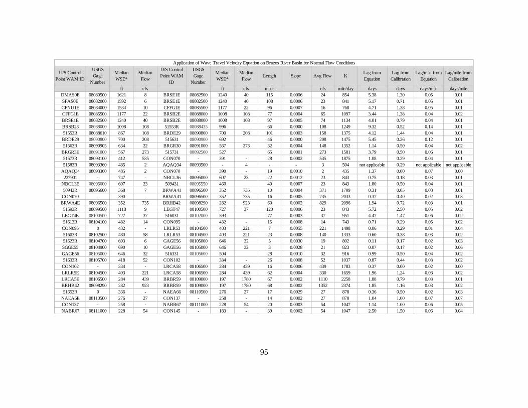
95

U/S Control

Point WAM ID

USGS

Gage

Number

Median

WSE*

Median

Flow

D/S Control

Point WAM

ID

USGS

Gage

Number

Median

WSE*

Median

FlowLength Slope Avg Flow K

Lag from

Equation

Lag from

Calibration

Lag/mile from

Equation

Lag/mile from

Calibration

ft cfs ft cfs miles cfs mile/day days days days/mile days/mile

DMAS0E 08080500 1621 8 BRSE1E 08082500 1240 40 115 0.0006 24 854 5.38 1.30 0.05 0.01

SFAS0E 08082000 1592 6 BRSE1E 08082500 1240 40 108 0.0006 23 841 5.17 0.71 0.05 0.01

CFNU1E 08084000 1534 10 CFFG1E 08085500 1177 22 96 0.0007 16 768 4.71 1.38 0.05 0.01

CFFG1E 08085500 1177 22 BRSB2E 08088000 1008 108 77 0.0004 65 1097 3.44 1.38 0.04 0.02

BRSE1E 08082500 1240 40 BRSB2E 08088000 1008 108 97 0.0005 74 1134 4.01 0.79 0.04 0.01

BRSB23 08088000 1008 108 51553R 08088435 996 66 0.0000 108 1249 9.32 0.52 0.14 0.01

51553R 08088610 867 108 BRDE29 08090800 700 208 101 0.0003 158 1375 4.12 1.44 0.04 0.01

BRDE29 08090800 700 208 515631 08090900 692 46 0.0000 208 1475 5.45 0.26 0.12 0.01

51563R 08090905 634 22 BRGR30 08091000 567 273 32 0.0004 148 1352 1.14 0.50 0.04 0.02

BRGR3E 08091000 567 273 515731 08092500 527 65 0.0001 273 1581 3.79 0.50 0.06 0.01

51573R 08093100 412 535 CON070 - 391 - 28 0.0002 535 1875 1.08 0.29 0.04 0.01

51583R 08093360 485 2 AQAQ34 08093500 - 4 - - 3 504 not applicable 0.29 not applicable not applicable

AQAQ34 08093360 485 2 CON070 - 390 - 19 0.0010 2 435 1.37 0.00 0.07 0.00

227901 - 747 - NBCL36 08095000 607 23 22 0.0012 23 843 0.75 0.18 0.03 0.01

NBCL3E 08095000 607 23 509431 08095550 460 40 0.0007 23 843 1.80 0.50 0.04 0.01

50943R 08095600 368 7 BRWA41 08096500 352 735 10 0.0004 371 1709 0.31 0.05 0.03 0.01

CON070 - 390 - BRWA41 08096500 352 735 16 0.0005 735 2033 0.37 0.40 0.02 0.03

BRWA4E 08096500 352 735 BRHB42 08098290 282 923 60 0.0002 829 2096 1.94 0.72 0.03 0.01

51593R 08099500 1118 9 LEGT47 08100500 727 37 120 0.0006 23 843 5.72 2.50 0.05 0.02

LEGT4E 08100500 727 37 516031 08102000 593 77 0.0003 37 951 4.47 1.47 0.06 0.02

51613R 08104100 482 14 CON095 - 432 - 15 0.0008 14 743 0.71 0.29 0.05 0.02

CON095 0 432 - LRLR53 08104500 403 221 7 0.0055 221 1498 0.06 0.29 0.01 0.04

51603R 08102500 480 58 LRLR53 08104500 403 221 23 0.0008 140 1333 0.60 0.38 0.03 0.02

51623R 08104700 693 6 GAGE56 08105000 646 32 5 0.0030 19 802 0.11 0.17 0.02 0.03

SGGE55 08104900 690 10 GAGE56 08105000 646 32 3 0.0028 21 823 0.07 0.17 0.02 0.06

GAGE56 08105000 646 32 516331 08105600 504 28 0.0010 32 916 0.99 0.50 0.04 0.02

51633R 08105700 418 52 CON102 - 334 - 26 0.0008 52 1037 0.87 0.44 0.03 0.02

CON102 - 334 - LRCA58 08106500 284 439 16 0.0006 439 1783 0.37 0.00 0.02 0.00

LRLR5E 08104500 403 221 LRCA58 08106500 284 439 62 0.0004 330 1659 1.96 1.24 0.03 0.02

LRCA5E 08106500 284 439 BRBR59 08109000 197 1780 67 0.0002 1110 2258 1.88 0.79 0.03 0.01

BRHB42 08098290 282 923 BRBR59 08109000 197 1780 68 0.0002 1352 2374 1.85 1.16 0.03 0.02

51653R 0 336 - NAEA66 08110500 276 27 17 0.0029 27 878 0.36 0.50 0.02 0.03

NAEA6E 08110500 276 27 CON137 - 258 - 14 0.0002 27 878 1.04 1.00 0.07 0.07

CON137 - 258 - NABR67 08111000 228 54 20 0.0003 54 1047 1.14 1.00 0.06 0.05

NABR67 08111000 228 54 CON145 - 183 - 39 0.0002 54 1047 2.50 1.50 0.06 0.04

Application of Wave Travel Velocity Equation on Brazos River Basin for Normal Flow Conditions

96

U/S Control

Point WAM ID

USGS

Gage

Number

Median

WSE*

Median

Flow

D/S Control

Point WAM

ID

USGS

Gage

Number

Median

WSE*

Median


Lag from

Equation

Lag from

Calibration

Lag/mile from

Equation

Lag/mile from

Calibration

ft cfs ft cfs miles cfs mile/day days days days/mile days/mile

CON145 - - - CON231 - - - 21 - - - not applicable 0.25 not applicable 0.01

51643R 08110000 201 6 CON129 - 176 - 14 0.0004 6 594 1.25 0.17 0.09 0.01

BRBR5E 08109000 197 1780 CON147 - 148 - 56 0.0002 1780 2546 1.72 0.64 0.03 0.01



CON147 - 156 - BRHE68 08111500 120 2410 32 0.0002 2410 2750 0.80 0.58 0.02 0.02

BRHE6E 08111500 120 2410 BRRI70 08114000 39 1905 105 0.0001 2158 2673 3.25 1.21 0.03 0.01

BRRI7E 08114000 39 1905 BRRO72 08116650 8 3070 38 0.0002 2488 2772 1.09 0.53 0.03 0.01

BRRO7E 08116650 8 3070 OUT - 0 0 - 3070 2924 not applicable 0.00 not applicable -

Application of Wave Travel Velocity Equation on Brazos River Basin for Normal Flow Conditions

* WSE = Water Surface Elevation

97

APPENDIX D

98

U/S Control

Point WAM ID

USGS

Gage

Number

Median

WSE*

Median

Flow

D/S Control

Point WAM

ID

USGS

Gage

Number

Median

WSE*

Median


Lag from

Equation

Lag from

Calibration

Lag/mile from

Equation

Lag/mile from

Calibration

ft cfs ft cfs miles cfs days days days/mile days/mile

DMAS0E 08080500 1625 182 BRSE1E 08082500 1242 546 115 0.0006 364 1573 2.91 0.00 0.03 0.00

SFAS0E 08082000 1592 110 BRSE1E 08082500 1242 546 108 0.0006 328 1549 2.81 0.00 0.03 0.00

CFNU1E 08084000 1534 101 CFFG1E 08085500 1181 272 96 0.0007 187 1425 2.55 0.00 0.03 0.00

CFFG1E 08085500 1181 272 BRSB2E 08088000 1009 1250 77 0.0004 761 1755 2.14 0.00 0.03 0.00

BRSE1E 08082500 1242 546 BRSB2E 08088000 1009 1250 97 0.0005 898 1798 2.53 0.00 0.03 0.00

BRSB23 08088000 1009 1250 51553R 08088435 999 - 66 0.0000 1250 1888 6.36 0.00 0.10 0.00

51553R 08088610 868 897 BRDE29 08090800 703 1800 101 0.0003 1349 1910 2.98 0.63 0.03 0.01

BRDE29 08090800 703 1800 515631 08090900 693 - 46 0.0000 1800 1993 3.62 0.21 0.08 0.00

51563R 08090905 636 122 BRGR30 08091000 569 2500 32 0.0004 1311 1902 0.81 0.47 0.03 0.01

BRGR3E 08091000 569 2500 515731 08092500 533 - 65 0.0001 2500 2093 3.04 0.50 0.05 0.01

51573R 08093100 415 3070 CON070 - 391 - 28 0.0002 3070 2157 0.87 0.22 0.03 0.01

51583R 08093360 487 94 AQAQ34 08093500 - 179 - - 137 1360 not applicable 0.25 - -

AQAQ34 08093360 487 94 CON070 - 390 - 19 0.0010 94 1287 0.46 0.00 0.02 0.00

227901 - 748 - NBCL36 08095000 609 344 22 0.0012 344 1560 0.41 0.18 0.02 0.01

NBCL3E 08095000 609 344 509431 08095550 463 - 40 0.0007 344 1560 0.97 0.22 0.02 0.01

50943R 08095600 372 966 BRWA41 08096500 356 5020 10 0.0004 2993 2149 0.25 0.05 0.02 0.01

CON070 - 390 - BRWA41 08096500 356 5020 16 0.0004 5020 2320 0.34 0.33 0.02 0.02

BRWA4E 08096500 356 5020 BRHB42 08098290 286 6240 60 0.0002 5630 2360 1.71 0.64 0.03 0.01

51593R 08099500 1120 310 LEGT47 08100500 730 730 120 0.0006 520 1658 2.92 1.58 0.02 0.01

LEGT4E 08100500 730 730 516031 08102000 596 - 77 0.0003 730 1744 2.44 1.19 0.03 0.02

51613R 08104100 485 779 CON095 - 432 - 15 0.0009 779 1761 0.29 0.26 0.02 0.02

CON095 0 432 - LRLR53 08104500 414 3160 7 0.0035 3160 2167 0.05 0.12 0.01 0.02

51603R 08102500 483 1920 LRLR53 08104500 414 3160 23 0.0008 2540 2098 0.40 0.38 0.02 0.02

51623R 08104700 695 164 GAGE56 08105000 647 284 5 0.0030 224 1464 0.06 0.17 0.01 0.03

SGGE55 08104900 691 99 GAGE56 08105000 647 284 3 0.0028 192 1430 0.04 0.17 0.01 0.06

GAGE56 08105000 647 284 516331 08105600 506 - 28 0.0010 284 1516 0.60 0.33 0.02 0.01

51633R 08105700 421 722 CON102 - 334 - 26 0.0009 722 1741 0.51 0.38 0.02 0.01

CON102 - 334 - LRCA58 08106500 293 4870 16 0.0005 4870 2310 0.31 0.00 0.02 0.00

LRLR5E 08104500 414 3160 LRCA58 08106500 293 4870 62 0.0004 4015 2245 1.44 1.07 0.02 0.02

LRCA5E 08106500 293 4870 BRBR59 08109000 202 13000 67 0.0003 8935 2527 1.66 0.75 0.02 0.01

BRHB42 08098290 286 6240 BRBR59 08109000 202 13000 68 0.0002 9620 2555 1.74 0.82 0.03 0.01

51653R 0 344 - NAEA66 08110500 283 824 17 0.0029 824 1775 0.18 0.50 0.01 0.03

NAEA6E 08110500 283 824 CON137 - 258 - 14 0.0003 824 1775 0.43 1.00 0.03 0.07

CON137 - 266 - NABR67 08111000 236 1480 20 0.0003 1480 1936 0.61 1.00 0.03 0.05

NABR67 08111000 236 1480 CON145 - 183 - 39 0.0003 1480 1936 1.26 1.50 0.03 0.04

Application of Wave Travel Velocity Equation on Brazos River Basin for High Flow Conditions

99

U/S Control

Point WAM ID

USGS

Gage

Number

Median

WSE*

Median

Flow

D/S Control

Point WAM

ID

USGS

Gage

Number

Median

WSE*

Median


Lag from

Equation

Lag from

Calibration

Lag/mile from

Equation

Lag/mile from

Calibration

ft cfs ft cfs miles cfs days days days/mile days/mile

CON145 - - - CON231 - - - 21 - - - not applicable 0.25 - 0.01

51643R 08110000 206 928 CON129 - 182 - 14 0.0004 928 1807 0.41 0.13 0.03 0.01

BRBR5E 08109000 202 13000 CON147 - 154 - 56 0.0002 13000 2671 1.64 0.52 0.03 0.01



CON147 - 169 - BRHE68 08111500 133 18300 32 0.0002 18300 2810 0.78 0.56 0.02 0.02

BRHE6E 08111500 133 18300 BRRI70 08114000 52 18600 105 0.0001 18450 2814 3.08 0.97 0.03 0.01

BRRI7E 08114000 52 18600 BRRO72 08116650 25 21500 38 0.0001 20050 2848 1.15 0.53 0.03 0.01

BRRO7E 08116650 25 21500 OUT - 0 0 - 21500 2878 not applicable 0.00 - -

Application of Wave Travel Velocity Equation on Brazos River Basin for High Flow Conditions

* WSE = Water Surface Elevation

100

APPENDIX E

101

Lag

(days)

Attenuation -

DFLOW

(days)

Attenuation -

Adopted

(days)

No. of Days

in DFLOW

Analysis

Lag -

DFLOW

(days)

Lag -

Adopted

(days)

Attenuation -

DFLOW

(days)

Attenuation -

Adopted

(days)

R1 KIBR NEPA 31 lag/mile from R3 2.06 - 1.00 - - 2.14 - 1.00

R2 NEPA NENE 20 lag/mile from R3 1.33 - 1.00 - - 1.38 - 1.00

R3 NENE NEAL 61 DFLOW 4.07 1.00 1.00 81 4.22 4.22 1.00 1.00

R4 NEAL NEDI 75 DFLOW 4.04 1.00 1.00 60 5.07 5.07 1.00 1.00

R5 NEDI NERO 47 DFLOW 3.00 1.00 1.00 94 4.23 4.23 0.75 1.00

R6 NERO NETB 45lag/mile from R5 before confluence and and R7 after

confluence2.52 - 1.00 - - 3.61 - 1.00

R7 NETB NEEV 53 DFLOW 1.96 0.80 1.00 196 3.00 3.00 0.83 1.00

R8 NEEV NEBA 25

DFLOW, because there is high correlation between

flows in U/S and D/S gage despite being a confluence

in between

1.14 1.50 1.00 10 2.13 2.13 1.33 1.00

R9 NEBA NESL 28 lag/mile from R7 1.03 - 1.00 - - 1.58 - 1.00

R10 MUTY MUJA 26 lag/mile from R11 2.72 - 1.00 - - 1.56 - 1.00

R11 MUJA ANAL 47

DFLOW, because there is high correlation between

flows in U/S and D/S gage despite being a confluence

in between

4.93 1.00 1.00 38 2.82 2.82 0.50 1.00

R12 ANAL ANLU 41 DFLOW 2.55 1.00 1.00 50 3.65 3.65 2.00 1.00

R13 ANLU ANSR 83DFLOW with an intermediate control point and then

projecting the lag/mile to get the total lag5.50 - 1.00 4 4.35 4.35 1.00 1.00

R14 ANSR NETB 38lag/mile from R13 before confluence and and R7 after

confluence2.14 - 1.00 - - 2.04 - 1.00

R15 EFACU ANAL 44 lag/mile from R11 as it is the most similar reach 4.61 - 1.00 - - 2.64 - 1.00

R16 ATCH ANSR 64 lag/mile from R11 as it is the most similar reach 6.71 - 1.00 - - 3.84 - 1.00

R17 AYSA ANSR 35 lag/mile from R11 as it is the most similar reach 3.67 - 1.00 - - 2.10 - 1.00

R18 VIKO NEBA 37lag/mile from R19 as it is the most similar reach before

confluence and lag/mile from R7 after confluence2.61 - 1.00 - - 3.01 - 1.00

R19 PISL NEBA 31DFLOW with an intermediate control point and then

projecting the lag/mile to get the total lag2.48 - 1.00 3 15.46 2.48 2.50 1.00

Reach

Application of DFLOW on Reaches of Neches River Basin

High FlowsNormal Flows

Method UsedRiver

MilesD/S CPU/S CP

102

APPENDIX F

103

Lag (days)

Attenuation -

DFLOW

(days)

Attenuation -

Adopted

(days)

No. of Days

in DFLOW

Analysis

Lag -

DFLOW

(days)

Lag -

Adopted

(days)

Attenuation -

DFLOW

(days)

Attenuation -

Adopted

(days)

R1 RWPL01 WRSP02 93Downstream has no gauge and there are very low

flows, hence ignoring this reachno routing - 1.00 - no routing no routing - -

R2 WRSP02 SFPE04 90Upstream has no gauge, using lag from R18 because

of similar flows6.75 - 1.00 - 0.00 1.72 - 1.00

R3 SFPE04 SFAS06 30 DFLOW 2.06 - 1.00 55 1.02 1.02 1.00 1.00

R4 SFAS06 BRSE11 106

Low correlation bewteen u/s and d/s, hence using

lag/mile form uppper reach before confluence and from

R21 after confluence

4.16 - 1.00 - 106.00 3.04 - 1.00

R5 BRSE11 BRSB23 93 DFLOW 2.18 1.00 1.00 273 1.80 1.80 1.00 1.00

R6 BRSB23 SHGR26 65 Using lag/mile from R7 3.25 - 1.00 - 0.00 3.22 - 1.00

R7 SHGR26 BRPP27 20 DFLOW 1.00 1.00 1.00 97 0.99 0.99 1.00 1.00

R8 BRPP27 BRDE29 79 DFLOW 2.01 1.00 1.00 385 1.84 1.84 1.00 1.00

R9 BRDE29 BRGR30 76Using lag/mile form R10 before confluence and from

R21 after confluence1.93 - 1.00 - 0.00 1.77 - 1.00

R10 BRGR30 BRAQ33 73 DFLOW before dam was built 1.10 1.00 1.00 24 0.99 0.99 1.00 1.00

R11 BRAQ33 BRWA41 35 DFLOW 1.00 1.00 1.00 122 1.01 1.01 1.00 1.00

R12 BRWA41 BRHB42 57 DFLOW 1.07 1.00 1.00 206 1.00 1.00 1.00 1.00

R13 BRHB42 BRBR59 67 DFLOW 1.81 1.00 1.00 82 1.00 1.00 1.00 1.00

R14 BRBR59 BRHE68 86 DFLOW 1.98 1.00 1.00 189 1.00 1.00 1.00 1.00

R15 BRHE68 BRRI70 104 DFLOW 2.62 1.00 1.00 63 5.85 2.62 0.50 1.00

R16 BRRI70 BRRO72 36 DFLOW 0.92 1.00 1.00 113 1.78 0.92 1.00 1.00

R17 BRRO72 BRGM73 58There is no down stream gauge, hence using R13

lag/mile because of simliarities1.57 - 1.00 - 0.00 0.87 - 1.00

R18 DUGI03 SFPE04 53 DFLOW 3.00 - 1.00 22 1.01 1.01 1.00 1.00

R19 CRJA05 SFAS06 23No Correlation, hence using R3 because that is the

stream which forming the major portion of this reach1.58 - 1.00 - 0.00 0.78 - 1.00

R20 DMJU08 DMAS09 127

Flows are too low and correlation is also low, using

R18 before conflence and downstream reach after

confluence

4.23 - 1.00 - 128.00 3.22 - 1.00

R21 DMAS09 BRSE11 113 DFLOW 3.12 1.00 1.00 295 3.00 3.00 1.00 1.00

R22 BSLU07 DMAS09 185 u/s is lake use, hence using similar reach 7.46 - 1.00 - 185.00 4.30 - 1.00

R23 NCKN10 BRSE11 75

No Correlation b/w u/s and d/s, hence using lag/mile

from R21 which is forming the major operation of this

reach

2.07 - 1.00 - 0.00 1.99 - 1.00

R24 MSMN12 BRSB23 102No Correlation b/w u/s and d/s also the upstream flow

is really low, hence ignoring this reachno routing - 1.00 - no routing no routing - 1.00

R25 CFRO13 CFHA14 68 DFLOW 2.12 1.00 1.00 42 1.96 1.96 0.67 1.00

R26 CFHA14 CFNU16 20 DFLOW 1.98 1.00 1.00 41 1.10 1.10 1.00 1.00

R27 CFNU16 CFFG18 95 DFLOW 2.92 1.00 1.00 425 1.89 1.89 1.00 1.00

Application of DFLOW on Reaches of Brazos River Basin


Reach U/S CP D/S CPRiver

MilesMethod Used

104

Lag (days)

Attenuation -

DFLOW

(days)

Attenuation -

Adopted

(days)

No. of Days

in DFLOW

Analysis

Lag -

DFLOW

(days)

Lag -

Adopted

(days)

Attenuation -

DFLOW

(days)

Attenuation -

Adopted

(days)

R28 CFFG18 CFEL22 62 DFLOW 2.01 1.00 1.00 85 1.00 1.00 1.00 1.00

R29 CFEL22 BRSB23 15 DFLOW 1.05 1.00 1.00 18 2.95 1.05 0.20 1.00

R30 MUHA15 CFNU16 18

No Correlation b/w d/s and u/s also the upstream CP is

really close to the dominant stream R26. Using R26

lag/mile

no routing - 1.00 - no routing no routing - 1.00

R31 CAST17 CFFG18 67No Correlation b/w d/s and u/s, using R25 lag/mile

before confluence, and R27 lag/mile after confluence2.08 - 1.00 - 67.00 1.69 - 1.00

R32 HCAL19 HCBR21 16Dam in between u/s CP and d/s CP, hence using

downstream reach lag/mile1.15 - 1.00 - 0.00 0.78 - 1.00

R33 HCBR21 CFEL22 28 DFLOW 2.01 - 1.00 8 1.36 1.36 1.00 1.00

R34 BSBR20 HCBR21 17Dam in between u/s CP and d/s CP, hence using

downstream reach lag/mile1.22 - 1.00 - 0.00 0.83 - 1.00

R35 GHGH24 SHGR26 58.5

Very low flow upstream and no correlation b/w u/s and

d/s. Using R33 lag/mile before confluence and R7

lag/mile after confluence

1.84 - 1.00 - 19695.00 1.55 - 1.00

R36 CCIV25 SHGR26 35

Very low flow upstream and no correlation b/w u/s and

d/s. Using R33 lag/mile before confluence and R7

lag/mile after confluence

1.82 - 1.00 - 5935.00 1.32 - 1.00

R37 PPSA28 BRDE29 33DFLOW, though flow is vastly different correlation is

0.51.96 - 1.00 7 2.60 1.96 1.50 1.00

R38 PAGR31 BRAQ33 74Vast flow difference, too close to dominant stream,

dam in between, hence using R10 lag/mile1.12 - 1.00 - 0.00 1.00 - 1.00

R39 NRBL32 BRAQ33 42Vast flow difference, dam in between, hence using

similar reach's lag/mile1.09 - 1.00 - 880.00 0.85 - 1.00

R40 AQAQ34 BRWA41 35Using lag/mile form R68 before confluence and from

R10 after confluence1.71 - 1.00 - 3861.00 1.72 - 1.00

R41 NBHI35 NBCL36 51Upstream has no discharge data, using downstream

reach's lag/mile4.28 - 1.00 - 0.00 3.92 - 1.00

R42 NBCL36 NBVM37 13 DFLOW 1.09 - 1.00 24 1.00 1.00 1.00 1.00

R43 NBVM37 BOWA40 28 Dam in between, using similar reach's lag/mile 2.35 - 1.00 - 0.00 2.15 - 1.00

R44 BOWA40 BRWA41 9U/s CP is very close to dominant stream R21 hence

using it's lag/mile0.26 - 1.00 - 0.00 0.26 - 1.00

R45 MBMG38 BOWA40 16 Dam in between, Use R42 1.34 - 1.00 - 0.00 1.23 - 1.00

R46 HGCR39 BOWA40 16 Dam in between, Use R42 1.34 - 1.00 - 0.00 1.23 - 1.00

R47 LEDL43 LEHS45 23 Dam in between, using downstream reach's lag/mile 0.96 - 1.00 - 0.00 0.58 - 1.00

R48 LEHS45 LEHM46 46 DFLOW 1.92 0.50 1.00 65 1.15 1.15 1.00 1.00

R49 LEHM46 LEGT47 76 DFLOW 1.95 1.00 1.00 134 1.78 1.78 1.00 1.00

R50 LEGT47 LEBE49 82Dam in between and no flow data before that, hence

using upper reach's lag/mile2.10 - 1.00 - 0.00 1.92 - 1.00

R51 LEBE49 LRLR53 19 DFLOW 0.91 1.00 1.00 43 1.12 1.12 1.17 1.00

R52 LRLR53 LRCA58 62 DFLOW 1.09 1.00 1.00 193 1.04 1.04 1.00 1.00

R53 LRCA58 BRBR59 66 DFLOW 1.21 1.00 1.00 72 1.25 1.25 1.00 1.00




MilesMethod Used

105

Lag (days)

Attenuation -

DFLOW

(days)

Attenuation -

Adopted

(days)

No. of Days

in DFLOW

Analysis

Lag -

DFLOW

(days)

Lag -

Adopted

(days)

Attenuation -

DFLOW

(days)

Attenuation -

Adopted

(days)

R54 SADL44 LEHS45 16Dam in between and no flow data before that, hence

using lower reach's lag/mile0.67 - 1.00 - 0.00 0.40 - 1.00

R55 COPI48 LEBE49 40Dam in between and no flow data before that, hence

using R56 lag/mile because of similar flows2.22 - 1.00 - 0.00 1.11 - 1.00

R56 LAKE50 LAYO51 36 DFLOW 2.00 0.80 1.00 35 1.00 1.00 0.67 1.00

R57 LAYO51 LABE52 23Dam in between and no flow data before that, hence

using upper reach's lag/mile1.28 - 1.00 - 0.00 0.64 - 1.00

R58 LABE52 LRLR53 20 DFLOW 1.25 1.00 1.00 12 2.05 1.25 2.00 1.00

R59 NGGE54 GAGE56 4.5 Very short reach for routing. Ignoring routing. no routing - 1.00 - - - - 1.00

R60 GAGE56 GALA57 32 DFLOW 1.19 1.00 1.00 14 1.00 1.00 0.50 1.00

R61 GALA57 LRCA58 38 DFLOW 1.96 0.75 1.00 100 1.16 1.16 1.00 1.00

R62 SGGE55 GAGE56 3.5 Very short reach for routing. Ignoring routing. no routing - 1.00 - - no routing - 1.00

R63 MYDB60 YCSO62 33Dam in between and no flow data before that, hence

using R65 lag/mile because of similar flows3.76 - 1.00 - 0.00 3.76 - 1.00

R64 YCSO62 BRHE68 67

Low flow corrlealtion (0.47) b/w u/s and d/s CPs, using

R68 lag/mile before confluence and R14 lag/mile after

confluence

2.58 - 1.00 - 12549.00 2.06 - 1.00

R65 EYDB61 YCSO62 28 DFLOW 3.19 1.00 1.00 5 7.05 3.19 0.60 1.00

R66 DCLY63 BRHE68 74

Low flow corrlealtion b/w u/s and d/s CPs, using R68

lag/mile before confluence and R14 lag/mile after

confluence

3.12 - 1.00 - 13830.00 2.62 - 1.00

R67 NAGR64 NAEA66 32Dam in between and no flow data before that, hence


R68 NAEA66 NABR67 36 DFLOW 2.79 1.00 1.00 183 2.85 2.85 0.83 1.00

R69 NABR67 BRHE68 100 DFLOW 3.14 1.25 1.00 76 4.12 3.14 1.50 1.00

R70 BGFR65 NAEA66 50Dam in between and no flow data before that, hence


R71 MCBL69 BRRI70 70

Low flow corrlealtion b/w u/s and d/s CPs, using R68

lag/mile before confluence and R15 lag/mile after

confluence

2.23 - 1.00 - 5490.00 2.25 - 1.00

R72 BGNE71 BRRO72 32Low flow corrlealtion b/w u/s and d/s CPs, using R68

lag/mile2.48 - 1.00 - 0.00 2.53 - 1.00




MilesMethod Used

106

APPENDIX G

107

Lag (days)

Attenuation -

DFLOW

(days)

Attenuation -

Adopted

(days)

No. of Days

in DFLOW

Analysis

Lag -

DFLOW

(days)

Lag -

Adopted

(days)

Attenuation -

DFLOW

(days)

Attenuation -

Adopted

(days)

R1 8WTJA 8WTBO 63Lake in between u/s and d/s CPs, so using R13

lag/mile because of similar flows6.36 - 1.00 - - 5.74 - 1.00

R2 8WTBO 8WTFW 46Lake in between u/s and d/s CPs, so using R33

lag/mile because of similar flows2.07 - 1.00 - - 2.28 - 1.00

R3 8WTFW 8WTGP 39 DFLOW 0.99 1.00 1.00 198 1.03 1.03 1.00 1.00

R4 8WTGP 8TRDA 14

Correlation of 0.81 is there, but two streams flow into

this reach, hence not using the original 0.214 lag/mile

but the lag/mile of upper Reach

0.35 1.00 1.00 - 2.99 0.37 0.50 1.00

R5 8TRDA 8TRRS 47 DFLOW 2.00 1.00 1.00 277 3.04 3.04 0.81 1.00

R6 8TRRS 8TRTR 58 DFLOW 1.04 1.00 1.00 135 3.15 3.15 0.65 1.00

R7 8TRTR 8TROA 76 DFLOW 1.96 1.00 1.00 74 4.05 4.05 0.83 1.00

R8 8TROA 8TRCR 47 DFLOW 1.00 1.00 1.00 60 3.86 3.86 1.07 1.00

R9 8TRCR 8TRMI 32 DFLOW 1.00 1.00 1.00 8 3.83 3.83 1.05 1.00

R10 8TRMI 8TRRI 66 DFLOW 1.08 1.00 1.00 17 4.79 4.79 1.25 1.00

R11 8TRRI 8TRRO 69 DFLOW 2.00 1.00 1.00 54 3.05 3.05 0.88 1.00

R12 8TRRO 8TRGB 87 Using upstream lag/mile 2.52 - 1.00 - - 3.85 - 1.00

R13 8BSBR 8WTBO 18 DFLOW 1.82 1.00 1.00 94 1.64 1.64 1.09 1.00

R14 8CTAL 8CTBE 11 Using R13 lag/mile 1.11 - 1.00 - - 1.00 - 1.00

R15 8CTBE 8CTFW 9 Using R13 lag/mile 0.91 - 1.00 - - 0.82 - 1.00

R16 8CTFW 8WTFW 2.3 Using R13 lag/mile 0.10 - 1.00 - - 0.11 - 1.00

R17 8MCGP 8TRDA 10Using R3 lag/mile because R4 forms the major portion

of this reach and that uses R3 lag/mile0.25 - 1.00 - - 0.26 - 1.00

R18 8ELSA 8ELLE 35 Using R21 lag/mile because it is a similar stream 2.10 - 1.00 - - 2.40 - 1.00

R19 8ELLE 8TRDA 33 DFLOW 2.14 0.75 1.00 38 1.99 1.99 0.62 1.00

R20 8IDPP 8ELLE 36 DFLOW 2.84 1.33 1.00 7 2.82 2.82 1.83 1.00

R21 8CLSA 8ELLE 35 DFLOW 2.11 1.33 1.00 15 2.40 2.40 1.24 1.00

R22 8DNJU 8DNGR 32 Using R13 lag/mile 3.23 - 1.00 - - 2.92 - 1.00

R23 8DNGR 8TRDA 31Using R19 lag/mile because R19 forms the major

portion of this reach2.02 - 1.00 - - 1.87 - 1.00

R24 8WRDA 8TRRS 58Using R36 lag/mile before confluence and R5 after

confluence3.63 - 1.00 - - 3.75 - 1.00

R25 8ETMK 8ETLA 19Using R27 lag/mile because this reach is the upstream

of R27 reach1.25 - 1.00 - - 1.28 - 1.00

R26 8ETLA 8ETFO 22Using R27 lag/mile because this reach is the upstream

of R27 reach1.45 - 1.00 - - 1.48 - 1.00

R27 8ETFO 8ETCR 15 DFLOW 0.99 1.00 1.00 120 1.01 1.01 1.00 1.00

R28 8ETCR 8TRRS 20 DFLOW 1.05 1.00 1.00 94 1.96 1.96 0.71 1.00

R29 8SGPR 8ETLA 13Using R27 lag/mile because this reach is the upstream

of R27 reach0.85 - 1.00 - - 0.88 - 1.00

Application of DFLOW on Reaches of Trinity River Basin



MilesMethod Used

108

Lag (days)

Attenuation -

DFLOW

(days)

Attenuation -

Adopted

(days)

No. of Days

in DFLOW

Analysis

Lag -

DFLOW

(days)

Lag -

Adopted

(days)

Attenuation -

DFLOW

(days)

Attenuation -

Adopted

(days)

R30 8CEKE 8CEMA 20 Using R27 lag/mile because of similarities 1.32 - 1.00 - - 1.35 - 1.00

R31 8CEMA 8TROA 94Using R27 lag/mile before confluence and R7 lag/mile

after confluence3.40 - 1.00 - - 5.35 - 1.00

R32 8KGKA 8CEMA 21 Using R27 because of same kind of stream system 1.38 - 1.00 - - 1.41 - 1.00

R33 8RIDA 8RIRI 22 DFLOW 0.98 1.00 1.00 32 1.09 1.09 1.00 1.00

R34 8RIRI 8RIFA 29 Using upstream lag/mile 1.30 - 1.00 - - 1.44 - 1.00

R35 8RIFA 8TROA 63Using R7 lag/mile because R7 forms the major portion

of this reach1.63 - 1.00 - - 3.36 - 1.00

R36 8WABA 8CHCO 18 DFLOW 2.00 0.59 1.00 12 1.16 1.16 0.67 1.00

R37 8CHCO 8RIFA 31Using R27 lag/mile before confluence and R33 lag/mile


R38 8TEST 8TROA 63Using R13 lag/mile before confluence and R7 lag/mile


R39 8BEMA 8TRRI 40Using R33 lag/mile before confluence and R10 lag/mile


Application of DFLOW on Reaches of Trinity River Basin



MilesMethod Used

lag and attenuation parameters for routing daily flow - CORE

Documents

Transcript of lag and attenuation parameters for routing daily flow - CORE