(Preprint) AAS 12-115

INVERSE PROBLEM FORMULATION COUPLED WITHUNSCENTED KALMAN FILTERING FOR STATE AND SHAPE

ESTIMATION OF SPACE OBJECTS

Laura S. Henderson∗, Pulkit Goyal† and Kamesh Subbarao‡

This work addresses issues related to resolving space objects i.e. Space SituationalAwareness (SSA). The motivation behind this paper is to further current techniquesused to estimate states associated with non-resolved space objects. Furthermore,this work deals with an inverse problem for a system of nonlinear stochastic dif-ferential equations. This system of equations corresponds to the two body orbitequations along with models accounting for effects of atmospheric drag, solar ra-diation pressure, and Earth’s aspherical shape. The present work implements anUnscented Kalman filter (UKF) in conjunction with a batch estimation loop. TheUKF estimates the states and parameters of the resident space object (RSO) untila pre-determined measurement batch size criterion is met. The estimates are thenpassed to the batch loop where a cost function is minimized to improve the esti-mates of the RSO’s parameters further. The batch loop is implemented using twomethods; the first uses the Levenberg-Marquardt technique while the second usesa Gauss-Newton algorithm. Moreover, two experiments are conducted. The firstexperiment uses the traditional UKF implementation and is treated as the bench-mark for the implementation of the batch loop. The second experiment uses theUKF along with the batch loop. The implementation of the batch loop shows aslight improvement over the traditional UKF implementation.

INTRODUCTION

For the past five decades we have been accumulating objects in space. Many of these objects

are satellites that no longer work, pieces of used rocket stages, and remnants from collisions. Over

the last decade the number of these objects has increased dramatically. This has become a critical

problem that must be addressed with urgency as it could have a detrimental effect on functioning

space assets. Objects that are placed in space such as satellites are of great importance to our

communications, national security, and economy. Much of the global connectivity technology relies

heavily on these satellites. In addition to satellites the International Space Station (ISS) is at an even

higher risk due to its large size. It is of great importance to address the issue of identifying these

objects and have the ability to predict where these objects will be at any given time and if they

pose a risk to other space objects. The motivation for this paper is the belief that it is necessary

to develop means to detect, track, identify, and predict the future intentions, actions, and positions

of space objects with adequate precision and accuracy. In addition to this, means to determine the

origin of these objects along with any change in their orbital state must be generated.

∗Graduate Student, Mechanical and Aerospace Engineering Department, University of Texas at Arlington, 500 West First

Street, Woolf Hall 106.†Visiting Student, Mechanical and Aerospace Engineering Department, University of Texas at Arlington‡Associate Professor, Mechanical and Aerospace Engineering, University of Texas at Arlington, 500 West First Street,

Woolf Hall 315G

1

This paper focuses in the area of low observables. More specifically, it deals with an inverse

problem for a system of nonlinear differential equations. Often inverse problems are studied in

linear differential equations. It is the objective of this paper to investigate inverse problem in the

context of nonlinear differential equations more specifically the inverse problem presented in Ref-

erence 1. Similar to the previously mentioned reference the short-term and long-term evolution of

space objects are studied. A system of stochastic nonlinear differential equations provide a detailed

time evolution model. The system of equations include effects from atmospheric drag, solar radia-

tion pressure, and Earth’s gravitation (including J2). Other unmodeled effects are lumped together

and represented as stochastic disturbing forces and torques. The atmospheric drag effects are mod-

eled to account for the projected frontal area of the object, which changes with time as the objects

tumble arbitrarily. The inverse problem to be addressed consists of determining the parameters that

appear in the system of stochastic nonlinear equations so that an accurate description of the position,

velocity, attitude, angular velocity and other properties of the object can be obtained. (Reference 1).

The parameters that appear in the system of differential equations characterize the object which

is assumed to be a cuboid. In other words the parameters are the length, width, and height of the

object. To estimate these parameters, the system of equations include the translational dynamics

and rigid body rotational dynamics with varying mass of moment of inertia terms so that a complete

description of the position and orientation of the object is obtained. The simulated measurements

will emulate information from the Space Surveillance Network (SSN). Lightcurve measurements

are used to determine attitude and orientation, while elevation and azimuth information are used for

position.

This paper also studies the implementation of a batch estimation methodology in conjunction with

the Unscented Kalman filter (UKF). The goal of this implementation is to improve the estimates of

the parameters that appear in the system of differential equations. This is done by estimating the

states by means of the UKF and ‘storing’ these values until a fixed batch size criterion is met. Then

these estimated state values are passed to the batch estimation algorithm which produces a new

updated value for the parameters by reducing a cost function. This is done until all the measurements

are used. Although batch estimation cannot be used in real time it has the advantage of providing

state or parameter estimates that have a lower error-covariance than sequential methods (Reference

2).

PROBLEM FORMULATION

Given time series astrometric and photometric measurements from the Space Surveillance Net-

work (SSN) as explicit and implicit functions of position, attitude, and resident space object’s (RSO)

shape and size, in addition to governing equations for the system dynamics and appropriate mea-

surement models the following problem will be solved.

• Combined Direct + Inverse Problem (References 1, 3–7) This problem aims to determine

the position, velocity, angular velocity, attitude and the Resident Space Object’s shape and

size.

2

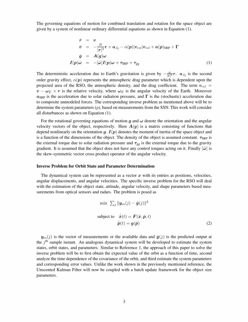
The governing equations of motion for combined translation and rotation for the space object are

given by a system of nonlinear ordinary differential equations as shown in Equation (1).

r = v

v = −µ

|r|3r + aJ2 − α(p)|vrel|vrel + a(p)SRP + Γ

g = A(g)ω

I(p)ω = −[ω]I(p)ω + τSRP + τgg (1)

The deterministic acceleration due to Earth’s gravitation is given by − µ|r|3

r. aJ2 is the second

order gravity effect, α(p) represents the atmospheric drag parameter which is dependent upon the

projected area of the RSO, the atmospheric density, and the drag coefficient. The term vrel =v − ωE × r is the relative velocity, where ωE is the angular velocity of the Earth. Moreover

aSRP is the acceleration due to solar radiation pressure, and Γ is the (stochastic) acceleration due

to composite unmodeled forces. The corresponding inverse problem as mentioned above will be to

determine the system parameters (p), based on measurements from the SSN. This work will consider

all disturbances as shown on Equation (1).

For the rotational governing equations of motion g and ω denote the orientation and the angular

velocity vectors of the object, respectively. Here A(g) is a matrix consisting of functions that

depend nonlinearly on the orientation g. I(p) denotes the moment of inertia of the space object and

is a function of the dimensions of the object. The density of the object is assumed constant. τSRP is

the external torque due to solar radiation pressure and τgg is the external torque due to the gravity

gradient. It is assumed that the object does not have any control torques acting on it. Finally [ω] is

the skew-symmetric vector cross product operator of the angular velocity.

Inverse Problem for Orbit State and Parameter Determination

The dynamical system can be represented as a vector x with its entries as positions, velocities,

angular displacements, and angular velocities. The specific inverse problem for the RSO will deal

with the estimation of the object state, attitude, angular velocity, and shape parameters based mea-

surements from optical sensors and radars. The problem is posed as

min∑

j ‖ym(j) − y(j)‖2

subject to ˙x(t) = F (x, p, t)˙p(t) = g(p) (2)

ym(j) is the vector of measurements or the available data and y(j) is the predicted output at

the jth sample instant. An analogous dynamical system will be developed to estimate the system

states, orbit states, and parameters. Similar to Reference 1, the approach of this paper to solve the

inverse problem will be to first obtain the expected value of the orbit as a function of time, second

analyze the time dependence of the covariance of the orbit, and third estimate the system parameters

and corresponding error values. Unlike the work shown in the previously mentioned reference, the

Unscented Kalman Filter will now be coupled with a batch update framework for the object size

parameters.

3

PERTURBATION EFFECTS ON THE RSO DYNAMICS

Translational and rotational acceleration perturbations are considered to model the true dynamics.

The estimator utilizes a process noise term to model these effects.

Drag Acceleration Model

Equation (3) was used to describe the drag experienced by the RSO as it orbits the Earth. The

ballistic coefficient (BC) was set up as a function of the area projected on a plane perpendicular

to the RSO’s velocity vector. As the object tumbles this area will change and so will the ballistic

coefficient. Furthermore an exponential atmospheric model was used (Reference 1 and 8 ).

aEdrag = −1

2ρatm‖vE

rel‖BCvErel (3)

J2 Acceleration Model

For most applications the assumption that Earth is a sphere is sufficient. For a more comprehen-

sive model it is necessary to model the accelerations due to the non-spherical nature of Earth as

well. An aspherical-potential function must be derived in order determine the gravitational attrac-

tion on the SRO. In this case we will use a simplification of the accelerations along each of the axis.

Given the disturbing function R2, where J2 indicates that this approximation is using the second

order zonal harmonics (J2 = 0.0010826269). Furthermore µ is Earth’s gravitational parameter

(3.896 × 105km3/s2), RE is Earth’s mean equatorial radius (RE = 6, 378km), r is the position

vector of the RSO measured from the center of the Earth, and φgc is the latitude of the object.

R2 = −3J2µ

2r

(

RE

r

)(

sin2(φgc)−1

3

)

(4)

Using sin(φgc) = rk/r where rk is the component of r along the z-axis, the following expression

can be obtained.

R2 = −3J2µR

2E

2r3

(

r2Kr2

)

+J2µR

2E

2r3(5)

Now Equation (5) can be differentiated with respect to each of the components of r to obtain the

corresponding accelerations. As an example (Equation (6))

∂R2

∂rI

= −3J2µR

2e rI

2r5

(

−5r2K + 1

r2

)

(6)

Following the same procedure Equations (8) and (9) can be obtained. This yields all three accel-

erations for this model (Reference 8).

aI = −3J2µR

2erI

2r5

(

1−5r2Kr2

)

(7)

aJ = −3J2µR

2erJ

2r5

(

1−5r2Kr2

)

(8)

aK = −3J2µR

2erK

2r5

(

3−5r2Kr2

)

(9)

4

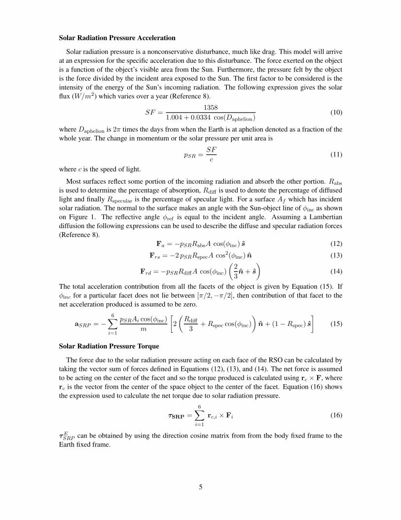
Solar Radiation Pressure Acceleration

Solar radiation pressure is a nonconservative disturbance, much like drag. This model will arrive

at an expression for the specific acceleration due to this disturbance. The force exerted on the object

is a function of the object’s visible area from the Sun. Furthermore, the pressure felt by the object

is the force divided by the incident area exposed to the Sun. The first factor to be considered is the

intensity of the energy of the Sun’s incoming radiation. The following expression gives the solar

flux (W/m2) which varies over a year (Reference 8).

SF =1358

1.004 + 0.0334 cos(Daphelion)(10)

where Daphelion is 2π times the days from when the Earth is at aphelion denoted as a fraction of the

whole year. The change in momentum or the solar pressure per unit area is

pSR =SF

c(11)

where c is the speed of light.

Most surfaces reflect some portion of the incoming radiation and absorb the other portion. Rabs

is used to determine the percentage of absorption, Rdiff is used to denote the percentage of diffused

light and finally Rspecular is the percentage of specular light. For a surface Af which has incident

solar radiation. The normal to the surface makes an angle with the Sun-object line of φinc as shown

on Figure 1. The reflective angle φref is equal to the incident angle. Assuming a Lambertian

diffusion the following expressions can be used to describe the diffuse and specular radiation forces

(Reference 8).

Fa = −pSRRabsA cos(φinc) s (12)

Frs = −2 pSRRspecA cos2(φinc) n (13)

Frd = −pSRRdiffA cos(φinc)

(

2

3n+ s

)

(14)

The total acceleration contribution from all the facets of the object is given by Equation (15). If

φinc for a particular facet does not lie between [π/2,−π/2], then contribution of that facet to the

net acceleration produced is assumed to be zero.

aSRP = −6

∑

i=1

pSRAi cos(φinc)

m

[

2

(

Rdiff

3+Rspec cos(φinc)

)

n+ (1−Rspec) s

]

(15)

Solar Radiation Pressure Torque

The force due to the solar radiation pressure acting on each face of the RSO can be calculated by

taking the vector sum of forces defined in Equations (12), (13), and (14). The net force is assumed

to be acting on the center of the facet and so the torque produced is calculated using rc × F, where

rc is the vector from the center of the space object to the center of the facet. Equation (16) shows

the expression used to calculate the net torque due to solar radiation pressure.

τSRP =

6∑

i=1

rc,i × Fi (16)

τESRP can be obtained by using the direction cosine matrix from from the body fixed frame to the

Earth fixed frame.

5

Gravity Gradient Torque

The RSO will not experience the same gravitational attraction on all points of its body. In order to

account for this phenomena a gravity gradient torque model has been introduced. Portions that are

closer to Earth will feel a stronger attraction compared to the portions of the RSO that are further

away. To calculate the net gravity gradient torque the following equation is used (Reference 9). The

size of the object considered for this study is quite small for this to be significant. Nevertheless these

models are included for modeling the true data and for possible applications wherein these torques

are not negligible.

τgg =

∫

Br × dFg (17)

r is the position vector of the infinitesimal body element with respect to the center of mass of the

SRO. dFg is the gravitational force and can be calculated using Equation (18). Me is the mass of

the Earth, dm is the body element mass, and R is the inertial relative position vector from the center

of the Earth to the RSO’s center of mass.

dFg = −GMe

|R|3Rdm (18)

Substituting Equation (18) into (17) the following expression can be obtained.

τgg = GMe Rc ×

∫

B

r

|R3|dm (19)

This equation can be generalized as shown in Equation (20). This formulation uses the truncation

of the binomial series as an approximation. Where Rc is the inertial position vector relative to the

center of the Earth. [I] is the inertia matrix.

τEgg =

3 G Me Rc

R5c

× [I]Rc (20)

MEASUREMENT MODELS

Astrometric Observation Model

The radar measurements that the observer can obtain are range ρ, azimuth Θ and elevation Φ. The

following expressions will be used to obtain the measurements. The slant range ρ is the fundamental

observation. The subscripts u, e, and n correspond to the Up-East-North components of this vector.

The full model can be found in Reference 2.

Θ = tan−1

(

ρeρn

)

(21)

Φ = sin−1

(

ρu||ρ||

)

(22)

For the problem being addressed only one optical sensor is used and we only consider the azimuth

and elevation measurements.

6

Light Curve Model

The apparent magnitude for each facet can be calculated using the model developed in Refer-

ence 10. The apparent magnitude of the RSO is taken to be the summation of the apparent magni-

tudes of all the facets.

mapp = −mapp,sun − 2.5 log10

∣

∣

∣

∣

∣

6∑

i

Fobs,i

Csun,vis

∣

∣

∣

∣

∣

(23)

Fobs is the amount of light that is impinging on the facet that then reflects to the observer. Csun,vis

is the power per square meter affecting the object caused by visible light striking the facets.

INVERSE PROBLEM SOLUTION USING UNSCENTED KALMAN FILTER WITH BATCH

ESTIMATION

In general batch estimation has the advantage of providing state estimates with a lower error

covariance than a strictly sequential method. Unfortunately batch estimation cannot always be per-

formed when the estimate is needed in real time. The process involves using multiple measurements

to estimate the states/parameters (Reference 2). The dynamics of the system can be expressed in

discrete form as

xk+1 = F(xk,wk,uk, k) (24)

yk = h(xk,uk,vk, k) (25)

with wk as Gaussian white noise process term with zero mean and Qk as the covariance. y is the

measurement vector and vk is the measurement error vector which represents zero-mean Gaussian

noise process with covariance Rk. Where x contains the states as follows

xT =[

rT vT ωB/ET gT pT

]

(26)

where, p = [length width height]T , the dimensions of the RSO.

The estimation of the attitude will require a special derivation of the UKF. Implementing the

quaternions directly would not be desired as the updated quaternions may not have a unit norm. To

avoid this a modified implementation can be used where the norm of the quaternions is forced have

a value of one. The first step is to calculate the error quaternion. This error quaternion is derived

based on the MRP sigma points. Next the attitude perturbation due to each error quaternion can

be calculated by means of quaternion composition. The addition of the perturbation and the error

form the global quaternion. Furthermore, the error quaternion related to each propagated quaternion

sigma point can be obtained by means of the quaternion composition. Finally the MRP error can be

obtained from the propagated error quaternion. This is implemented as shown in Reference 11 and

has not been shown here for the sake of brevity.

Batch Implementation with The UKF

For the batch estimation of the object parameters the maximum likelihood estimation approach is

used. This method minimizes the following cost function by means of the Gauss-Newton algorithm

J(p) =1

2

N∑

k=1

(yk − yk)T (yk − yk) (27)

7

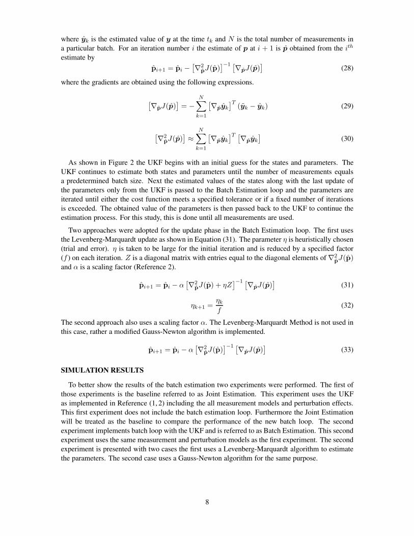
where yk is the estimated value of y at the time tk and N is the total number of measurements in

a particular batch. For an iteration number i the estimate of p at i + 1 is p obtained from the ith

estimate by

pi+1 = pi −[

∇2pJ(p)

]−1 [∇pJ(p)

]

(28)

where the gradients are obtained using the following expressions.

[

∇pJ(p)]

= −N∑

k=1

[

∇pyk

]T(yk − yk) (29)

[

∇2pJ(p)

]

≈

N∑

k=1

[

∇pyk

]T [

∇pyk

]

(30)

As shown in Figure 2 the UKF begins with an initial guess for the states and parameters. The

UKF continues to estimate both states and parameters until the number of measurements equals

a predetermined batch size. Next the estimated values of the states along with the last update of

the parameters only from the UKF is passed to the Batch Estimation loop and the parameters are

iterated until either the cost function meets a specified tolerance or if a fixed number of iterations

is exceeded. The obtained value of the parameters is then passed back to the UKF to continue the

estimation process. For this study, this is done until all measurements are used.

Two approaches were adopted for the update phase in the Batch Estimation loop. The first uses

the Levenberg-Marquardt update as shown in Equation (31). The parameter η is heuristically chosen

(trial and error). η is taken to be large for the initial iteration and is reduced by a specified factor

(f ) on each iteration. Z is a diagonal matrix with entries equal to the diagonal elements of ∇2pJ(p)

and α is a scaling factor (Reference 2).

pi+1 = pi − α[

∇2pJ(p) + ηZ

]−1 [∇pJ(p)

]

(31)

ηk+1 =ηkf

(32)

The second approach also uses a scaling factor α. The Levenberg-Marquardt Method is not used in

this case, rather a modified Gauss-Newton algorithm is implemented.

pi+1 = pi − α[

∇2pJ(p)

]−1 [∇pJ(p)

]

(33)

SIMULATION RESULTS

To better show the results of the batch estimation two experiments were performed. The first of

those experiments is the baseline referred to as Joint Estimation. This experiment uses the UKF

as implemented in Reference (1, 2) including the all measurement models and perturbation effects.

This first experiment does not include the batch estimation loop. Furthermore the Joint Estimation

will be treated as the baseline to compare the performance of the new batch loop. The second

experiment implements batch loop with the UKF and is referred to as Batch Estimation. This second

experiment uses the same measurement and perturbation models as the first experiment. The second

experiment is presented with two cases the first uses a Levenberg-Marquardt algorithm to estimate

the parameters. The second case uses a Gauss-Newton algorithm for the same purpose.

8

The set of synthetic measurements for both experiments was created with the same initial con-

ditions and object parameters. The object size for both experiment was as p = [2 3 4]T m for

length, width, and height respectively. For a Low Earth Orbit (LEO) at an inclination of 15◦ and

period of approximately 90 minutes the following initial conditions were used:

• Position and velocity initial conditions:

r(0) = [6738 0 0]T km

v(0) = [0 7.4292 1.9906]T km/s

• Angular velocity and MRP initial conditions:

ωB/E(0) =[

1.357 × 10−4 4.296 × 10−3 − 1.104 × 10−3]T

rad/s

g(0) =[

0 0 4.14213 × 10−1]T

The synthetic measurements were created using zero-mean white noise error processes with stan-

dard deviation of 2 arc-seconds for azimuth and elevation. For the light curve the error process

has a standard deviation of 0.1 magnitude. The measurements were sampled every 30 seconds. The

lightcurve model was set up using Phong specularity parameters nu and nv with a value of 10 for all

facets. The values of specular and diffusive reflection were chosen as Rspec = 0.7 and Rdiff = 0.2for three facets and Rspec = 0.6 and Rdiff = 0.2 for the remaining three. These values yield a

visible magnitude that allows the estimation of the attitude and object parameters.

Baseline - Joint Estimation (JE)

The results presented in the Appendix have been produced using the synthetic measurements as

previously described. The estimator initial conditions errors were set as: 10 Km for position error,

0.1 Km/s for velocity error, 1400 deg/hr for rotational rate error, 20 deg for attitude error, and

0.05 m for the dimension error. Furthermore, the initial conditions for the error covariance are

102 Km2 for position, 0.12 (Km/s)2 for velocity, 14002 (deg/hr)2 for rotational rate error, 202 deg2

for attitude, and 0.052 m2 for dimensions.

Figure 3 shows the projected area time history as the object travels through its orbit. As it can

be seen the area changes over time as the object tumbles. Figures 4 through 8 show the results

obtained for the Joint Estimation by averaging over 100 runs. Figure 4 shows the estimation of the

length, width, and height of the RSO. As it can be seen the filter estimates these parameters within

centimeters of the actual size of the object. These parameters are very weakly observable and in

some cases arent observable at all. Future work will investigate this in more detail. The ±3σ bounds

are shown as dotted lines in this figure and all state and parameter error figures. Moreover, Figure

5 and 6 show the estimation of the position and velocity respectively as the space object translates

through its orbit. Values for position and velocity have been estimated by the filter fairly quickly

and accurately. Figures 7 and 8 show the attitude and angular velocity estimation respectively. The

attitude has been estimated approximately with in 3 degrees of the true value. The initial condition

for the attitude estimator was about 20 degrees from the true values. The angular velocity has been

estimated with in less than a tenth of a degree per second. The corresponding initial condition

was 1400 deg/hr away from the true values. The 3σ bounds for the attitude estimation increase

and decrease as the object tumbles and the information provided by the lightcurve changes. The 3σbounds for the angular velocity remain constant through the estimation. Clearly there are times when

the 3σ bounds on the attitude errors change with the available information in the measurements.

9

Batch Estimation (BE)

Two methods were used for the Batch Estimation process. The first uses the Levenberg-Marquardt

method while the second uses the Gauss-Newton method to arrive at the estimation of the object’s

dimensions. The results presented on both of the following sections have been obtained by aver-

aging the results from 10 runs. The chosen batch size of measurements has been selected as 60

measurements per batch. A total of 181 measurements were used to obtain a total of three batches.

The batch size was chosen by investigating the observability of the states and parameters given a

batch of measurements. The observability of the ‘stacked’ batch observability matrix yields a rank

of 15. As shown on Table 1 the observability matrix has full rank (= 15) for batches greater than

10. For batches of less than 10 measurements the rank of the ‘stacked’ observability matrix was

found to be less than 15. That said, depending upon the initial conditions, the full rank condition

was always met when the batch size was 60 or more. Therefore, it was determined that a batch of

60 measurements would yield adequate results. The number of iterations per batch was set as 20

for both cases. The estimator initial conditions errors and initial conditions for the error covariance

were set to be the same as the Joint Estimation case. Similarly, the synthetic measurements were

created with the same initial conditions.

Table 1. Bach Size and Observability Matrix Rank Correlation

Batch Size Less than 10 Greater than 10

Rank of Observability Matrix Less than 15 15

Levenberg-Marquardt Method (BE-LM). The results for the Levenberg-Marquardt Bach Esti-

mation have been presented in the Appendix. These results were obtained with values of η = 100and f = 5. A scaling factor was introduced in this case as the cost function was modifying the

values for the parameters to a point where they became negative. In order to correct this α was set

as 0.1 as seen in Equation (31). This allowed the cost function to be decreased while maintaining a

non-negative value for the parameters. Figures 9 though 14 show the results obtained by averaging

the values from 10 independent runs. The first of these figures shows the estimation of the dimen-

sions of the object. No 3σ have been shown for any of the parameter estimations as these were done

by the batch estimation rather than the UKF. It can be seen the values change as the batch estimation

loop progresses. The values were estimated with in centimeters of the true value. In addition, Figure

10 shows the value of the cost function for each batch. It can be seen that the Levenberg-Marquardt

method is effective in reducing the value of the cost function with each iteration. Figure 11 shows

the estimation of the position. The 3σ bounds for this estimation are larger than those of the JE but

they quickly reduce. The final estimation value for the velocity is within 0.1 Km/s of the true value.

Figure 13 contains the results for the attitude estimation of the RSO. The 3σ bounds for the attitude

estimation vary more in this case than for the JE case, nevertheless the estimation of the attitude is

within 3 degrees of the true value. Finally the angular velocity estimation is shown in Figure 19.

The 3σ bounds for this plot increase and later oscillate as the estimation progresses.

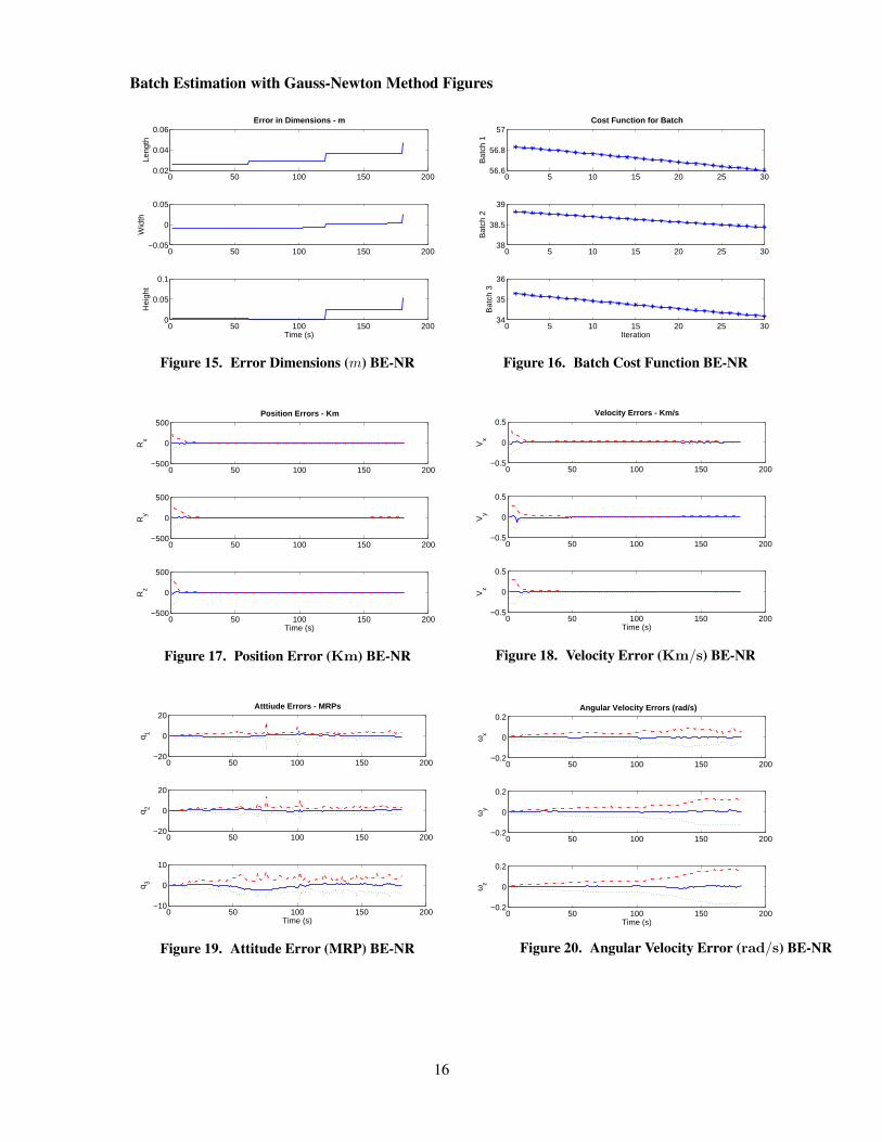
Gauss-Newton Method (BE-NR). This method was implemented with a scaling factor α = 0.001.

The results for this method are shown in Figures 15 through 20. Figure 15 clearly shows the evo-

lution of the values for the length, width, and height through each of the three batches. The batch

yields estimates within centimeters of the true value of the dimensions of the object. The cost

function for one of the runs has been shown in Figure 16. It can be seen that for each batch of

10

measurements the cost function decreases with each iteration. Moreover, Figures 17 and 18 show

the estimation of the position and velocity. The 3σ bounds for the position begin at larger values

than those for the JE, nevertheless the error for the batch estimation quickly reaches an error close

to zero. The velocity estimation is similar to that of the JE with 3σ bounds closing in slightly faster.

Figure 19 shows the attitude estimation for this case. When compared to the results obtained by the

JE it can be seen that the error is slightly larger and the 3σ vary more as well. Nevertheless, the

attitude is estimated within four degrees of the true value. Finally the angular velocity estimation

error can be seen in Figure 20. Similarly to the attitude estimation, the error in the angular velocity

is slightly higher in this case when compared to that of the JE. The 3σ bounds also increase towards

the end of the estimation.

SUMMARY AND CONCLUSIONS

The focus of this paper was to further advance the work done in Reference 1. The motivation

behind this work is to continue improving methods that can be used to identify space objects that

could pose a danger to critical space assets. A new implementation of the UKF with a batch esti-

mation loop was proposed and implemented. The UKF estimates the states and parameters for a

predetermined batch size. When the batch size is reached the estimates are passed to the batch loop.

The batch loop was implemented using two methodologies. The first of those methodologies is the

Levenberg-Marquardt. The second methodology uses a Gauss-Newton algorithm. Once the batch

estimation iterates, a new estimate of the object’s parameters is obtained. This process is followed

until all available measurements are used.

It was determined that an adequate batch size was 60 measurements. A total of 181 measure-

ments were used for a total of three batches. Two experiments were executed. The first of those

experiments was deemed Joint Estimation and was treated as the baseline. This experiment did

not use the batch loop, rather it implemented all the measurement and perturbation models to ob-

tain a benchmark behavior of the UKF. The results obtained showed the UKF converges extremely

well for the position and velocity. The attitude and angular velocity estimations are good but the

3σ bound behavior could be improved. The estimation of the parameters also behaves well. The

second experiment was the implementation of the batch loop and the UKF. The second experiment

namely the Batch Estimation had two cases. The first case dealt with the implementation of the the

Levenberg-Marquardt method. The results for this case showed an improvement on the estimation

of the RSO’s parameters. It was shown that the value for the cost function decreases for each batch.

Moreover, the estimation of the position and velocity was similar to that of the Joint Estimation. The

attitude and angular velocity estimation was slightly different than that of the baseline, specially in

the behavior of the 3σ bounds. Finally the second case for the batch estimation used the Gauss-

Newton algorithm. The estimation of the parameters was improved when compared to that of the

baseline and the first case. Nevertheless, the minimization of the cost function is not as pronounced

as in the first case. The estimation of the velocity and the position are very similar to that of the first

batch case. Similarly, the attitude and angular velocity 3σ behavior could be improved.

Although batch estimation techniques can not be used in real-time, we developed this coupled

approach to exploit their advantage in obtaining estimates with lower error-covariance than with

sequential methods. It was seen that both the Levenberg-Marquardt methodology and the Gauss-

Newton yielded a better parameter estimate than the baseline UKF. This is not conclusively proven

and more work is to be conducted to show this. It was also seen that the Gauss-Newton algorithm

yielded a slightly better results than the Levenberg-Marquardt method. This too needs to be proven

11

with additional studies. Although further work needs to be done in the estimation of the attitude

and angular velocity this is an important step towards the estimation of RSO parameters. This work

has advanced the current knowledge in the area of low observables and the investigation of inverse

problems in nonlinear stochastic differential equations. Future work will involve improving upon

the current methods presented here.

The lightcurve measurement model has not been verified/calibrated against any real data. It was

found that the model utilized by us together with the initial conditions (orbit characteristics) yielded

very little information for accurate attitude estimation. Future work will involve improving this

measurment model with appropriate calibration to improve the estimation accuracy.

REFERENCES

[1] K. Subbarao and L. Henderson, “Inverse Problems in Unresolved Space Object Identification,” SpaceFlight Mechanics Meering, No. 10-149, 2010.

[2] J. L. Crassidis and J. L. Junkins, Optimal Estimation of Dynamic Systems. New York, New York:Chapman and Hall \CRC, 2004.

[3] D. A. Vallado and S. S. Carter, “Accurate orbit determination from short-arc dense observational data,”Advances in Astronautical Sciences, Vol. 97, 1997, pp. 1587–1602.

[4] J. Matusewicz, K. Subbarao, and J. Frisbee, “Uncertainty characterization of orbital debris using sim-ulated space surveillance network measurements,” AAS/AIAA Astrodynamics Specialist Conference,Mackinac Island, Michigan, August 19-23 2007.

[5] J. Matusewicz, K. Subbarao, and J. Frisbee, “Uncertainty characterization of orbital debris using theextended Kalman filter,” AAS/AIAA Astrodynamics Specialist Conference, Mackinac Island, Michigan,August 19-23 2007.

[6] M. Kaasalainen, L. Lamberg, K. Lumme, and E. Bowell, “Interpretation of lightcurves of atmosphere-less bodies: I. General theory and new inversion schemes,” Astronomy and Astrophysics, Vol. 259, 1992,pp. 318–332.

[7] J. Durech, “Shape determination of the asteroid (6053) 1993 BW3,” Icarus, Vol. 159, 2002, pp. 192–196.

[8] D. A. Vallado, Fundamentals of Astrodynamics and Applications. El Segundo, California and Boston,Massachusetts: Microcosm Press and Kluwer Academic Publishers, 2001.

[9] H. Schaub and J. Junkins, Analytical Mechanics of Aerospace Systems. AIAA, 2009.

[10] R. Linares, J. L. Crassidis, M. K. Jah, and H. Kim, “Astrometric and Photometric Data Fusion for Resi-dent Space Object Orbit, Attitude, and Shape Determination Via Multiple-Model Adaptive Estimation,”AAS/AIAA Astrodynamics Specialists Conference, Vol. AIAA-8341, 2010.

[11] M. F. Crassidis, J. L., “Unscented Filtering for Spacecraft Attitude Estimation,” Journal of Guidance,Control and Dynamics, Vol. 26, No. 4, 2003, pp. 536–542.

12

APPENDIX: FIGURES

Figure 1. Incident solar radiation on a particular face of the space object with ab-

sorbed (Fa) and reflective (Fr) forces (Reference 8)

Figure 2. Batch Estimation Sequence for Unscented Kalman Filter

13

Joint Estimation Figures

0 10 20 30 40 50 60 70 80 90 1002.3

2.35

2.4

2.45

2.5

2.55

2.6

2.65

2.7

2.75

2.8x 10

−5 Projected Frontal Area

Time (s)

Are

a (m

2 )

Figure 3. Projected Area (m2) JE

0 20 40 60 80 100−0.2

0

0.2

Leng

th

Error in Dimensions - m

0 20 40 60 80 100−0.2

0

0.2

Wid

th

0 20 40 60 80 100−0.2

0

0.2

Time (s)

Hei

ght

Figure 4. Error Dimensions (m) JE

0 20 40 60 80 100−5

0

5 Position Errors - Km

Rx

0 20 40 60 80 100−5

0

5

Ry

0 20 40 60 80 100−5

0

5

Time (s)

Rz

Figure 5. Position Error (Km) JE

0 20 40 60 80 100−5

0

5x 10

−3 Velocity Errors - Km/s

Vx

0 20 40 60 80 100−5

0

5x 10

−3

Vy

0 20 40 60 80 100−5

0

5x 10

−3

Time (s)

Vz

Figure 6. Velocity Error (Km/s) JE

0 20 40 60 80 100−5

0

5 Atttiude Errors - (deg)

φ

0 20 40 60 80 100−5

0

5

Time

θ

0 20 40 60 80 100−5

0

5

Time (s)

ψ

Figure 7. Attitude Error (MRP) JE

0 20 40 60 80 100−5

0

5x 10

−4 Angular Velocity Errors (rad/s)

ωx

0 20 40 60 80 100−5

0

5x 10

−4

ωy

0 20 40 60 80 100−5

0

5x 10

−4

Time (s)

ωz

Figure 8. Angular Velocity Error (rad/s) JE

14

Batch Estimation with Levenberg-Marquardt Method Figures

0 50 100 150 200−0.5

0

0.5

Leng

th

Error in Dimensions - m

0 50 100 150 200−0.5

0

0.5

Wid

th

0 50 100 150 2000

1

2

Time (s)

Hei

ght

Figure 9. Error Dimensions (m) BE-LM

0 5 10 15 20 25 300

50

100

Bat

ch 1

Cost Function for Batch

0 5 10 15 20 25 300

50

Bat

ch 2

0 5 10 15 20 25 3025

30

35

Iteration

Bat

ch 3

Figure 10. Batch Cost Function BE-LM

0 50 100 150 200−500

0

500 Position Errors - Km

Rx

0 50 100 150 200−500

0

500

Ry

0 50 100 150 200−500

0

500

Time (s)

Rz

Figure 11. Position Error (Km) BE-LM

0 50 100 150 200−0.5

0

0.5 Velocity Errors - Km/s

Vx

0 50 100 150 200−0.5

0

0.5

Vy

0 50 100 150 200−0.5

0

0.5

Time (s)

Vz

Figure 12. Velocity Error (Km/s) BE-LM

0 50 100 150 200−20

0

20 Atttiude Errors - MRPs

q 1

0 50 100 150 200−20

0

20

q 2

0 50 100 150 200−20

0

20

Time (s)

q 3

Figure 13. Attitude Error (MRP) BE-LM

0 50 100 150 200−0.1

0

0.1 Angular Velocity Errors (rad/s)

ωx

0 50 100 150 200−0.2

0

0.2

ωy

0 50 100 150 200−0.1

0

0.1

Time (s)

ωz

Figure 14. Angular Velocity Error (rad/s) BE-LM

15

Batch Estimation with Gauss-Newton Method Figures

0 50 100 150 2000.02

0.04

0.06

Leng

th

Error in Dimensions - m

0 50 100 150 200−0.05

0

0.05

Wid

th

0 50 100 150 2000

0.05

0.1

Time (s)

Hei

ght

Figure 15. Error Dimensions (m) BE-NR

0 5 10 15 20 25 3056.6

56.8

57

Bat

ch 1

Cost Function for Batch

0 5 10 15 20 25 3038

38.5

39

Bat

ch 2

0 5 10 15 20 25 3034

35

36

Iteration

Bat

ch 3

Figure 16. Batch Cost Function BE-NR

0 50 100 150 200−500

0

500 Position Errors - Km

Rx

0 50 100 150 200−500

0

500

Ry

0 50 100 150 200−500

0

500

Time (s)

Rz

Figure 17. Position Error (Km) BE-NR

0 50 100 150 200−0.5

0

0.5 Velocity Errors - Km/s

Vx

0 50 100 150 200−0.5

0

0.5

Vy

0 50 100 150 200−0.5

0

0.5

Time (s)

Vz

Figure 18. Velocity Error (Km/s) BE-NR

0 50 100 150 200−20

0

20 Atttiude Errors - MRPs

q 1

0 50 100 150 200−20

0

20

q 2

0 50 100 150 200−10

0

10

Time (s)

q 3

Figure 19. Attitude Error (MRP) BE-NR

0 50 100 150 200−0.2

0

0.2 Angular Velocity Errors (rad/s)

ωx

0 50 100 150 200−0.2

0

0.2

ωy

0 50 100 150 200−0.2

0

0.2

Time (s)

ωz

Figure 20. Angular Velocity Error (rad/s) BE-NR

16