AAS YY tranport-Li Xl&Shen

ADVANCES IN ATMOSPHERIC SCIENCES, VOL. 30, NO. 5, 2013, 1320–1330

An Accurate Multimoment Constrained Finite Volume

Transport Model on Yin-Yang Grids

LI Xingliang1,2 (��), SHEN Xueshun1,2 (��), PENG Xindong1 (��),XIAO Feng3 (� �), ZHUANG Zhaorong1,2 (��),

and CHEN Chungang∗4 (��)

1State Key Laboratory of Severe Weather, Chinese Academy of Meteorological Sciences, Beijing 100081

2Center of Numerical Weather Prediction, China Meteorological Administration, Beijing 100081

3Department of Energy Sciences, Tokyo Institute of Technology, Yokohama 226-8502, Japan

4School of Human Settlement and Civil Engineering, Xi’an Jiaotong University, Xi’an 710049

(Received 5 September 2012; revised 29 November 2012; accepted 16 January 2013)

ABSTRACT

A global transport model is proposed in which a multimoment constrained finite volume (MCV) schemeis applied to a Yin-Yang overset grid. The MCV scheme defines 16 degrees of freedom (DOFs) within eachelement to build a 2D cubic reconstruction polynomial. The time evolution equations for DOFs are derivedfrom constraint conditions on moments of line-integrated averages (LIA), point values (PV), and values offirst-order derivatives (DV). The Yin-Yang grid eliminates polar singularities and results in a quasi-uniformmesh. A limiting projection is designed to remove nonphysical oscillations around discontinuities. Our modelwas tested against widely used benchmarks; the competitive results reveal that the model is accurate andpromising for developing general circulation models.

Key words: transport model, Yin-Yang grid, finite volume method, high-order scheme

Citation: Li, X. L., X. S. Shen, X. D. Peng, F. Xiao, Z. R. Zhuang, and C. G. Chen, 2013: An accuratemultimoment constrained finite volume transport model on Yin-Yang grids. Adv. Atmos. Sci., 30(5),1320–1330, doi: 10.1007/s00376-013-2217-x.

1. Introduction

With the rapid development of computer hardwareinvolving hundreds of thousands of processors, it isnow possible to use high-resolution general circula-tion models (GCM) to simulate weather and climatechanges. In developing high-performance global mod-els for such simulations, global computational mesheswith quasi-uniform grid spacing are preferred. Repre-sentative meshes of this kind include the cubed-spheregrid (Sadourny, 1972), the icosahedral grid (Sadournyet al., 1968; Williamson, 1968), and the Yin-Yang grid(Kageyama and Sato, 2004).

By projecting an icosahedron onto a sphere, spher-ical icosahedral grids possess considerable uniformity.However, the icosahedral grid is unstructured, and nu-merical models on unstructured meshes require com-

plicated numerical techniques that are very differentfrom those used for structured grids. As a result, nu-merical models on unstructured grids are often morecomputationally expensive. Further, on unstructuredgrids, it is usually nontrivial to develop high-orderschemes (more than second-order accuracy). Thegnomonic cubic grid can be constructed by project-ing an inscribed cube onto a sphere. It covers thewhole globe with six identical patches. The major dis-advantage of this grid is that the coordinate systemis not orthogonal and discontinuous local coordinatesalong patch boundaries often introduce extra numeri-cal errors. The conformal cubic grid was proposed byRancic et al. (1996) to obtain continuous local coor-dinates at patch boundaries, but at the cost of losinguniformity in grid spacing and analytical relations fortransformations.

∗Corresponding author: CHEN Chungang, [email protected]

© China National Committee for International Association of Meteorology and Atmospheric Sciences (IAMAS), Institute of AtmosphericPhysics (IAP) and Science Press and Springer-Verlag Berlin Heidelberg 2013

NO. 5 LI ET AL. 1321

(a) Yin-Yang grid (b) Yang grid (c) Yin grid

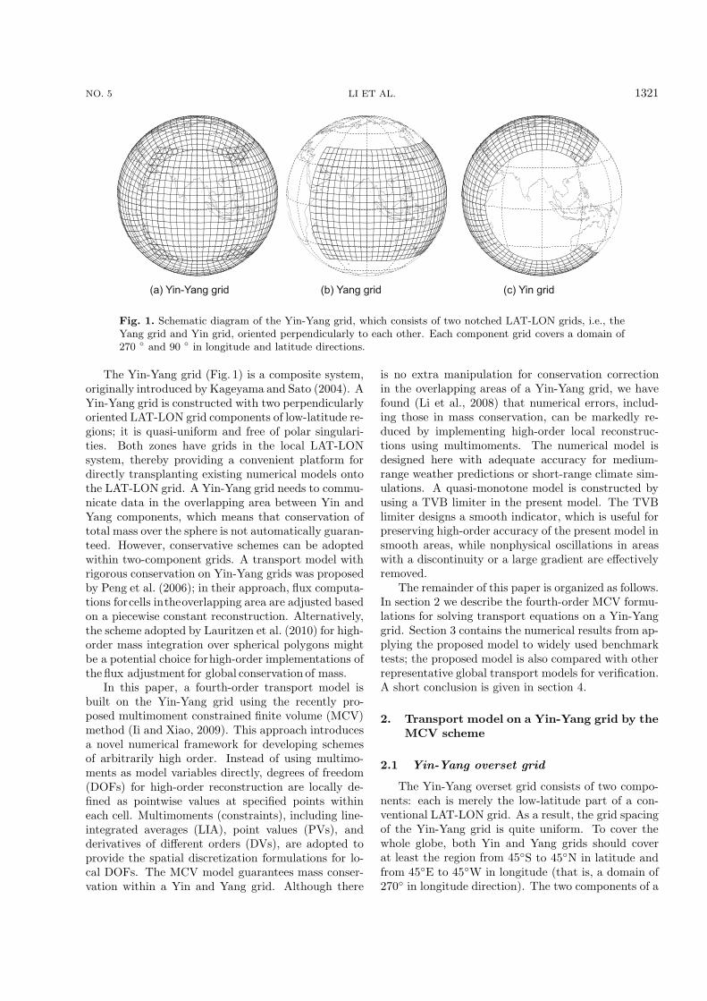
Fig. 1. Schematic diagram of the Yin-Yang grid, which consists of two notched LAT-LON grids, i.e., theYang grid and Yin grid, oriented perpendicularly to each other. Each component grid covers a domain of270 ◦ and 90 ◦ in longitude and latitude directions.

The Yin-Yang grid (Fig. 1) is a composite system,originally introduced by Kageyama and Sato (2004). AYin-Yang grid is constructed with two perpendicularlyoriented LAT-LON grid components of low-latitude re-gions; it is quasi-uniform and free of polar singulari-ties. Both zones have grids in the local LAT-LONsystem, thereby providing a convenient platform fordirectly transplanting existing numerical models ontothe LAT-LON grid. A Yin-Yang grid needs to commu-nicate data in the overlapping area between Yin andYang components, which means that conservation oftotal mass over the sphere is not automatically guaran-teed. However, conservative schemes can be adoptedwithin two-component grids. A transport model withrigorous conservation on Yin-Yang grids was proposedby Peng et al. (2006); in their approach, flux computa-tions forcells intheoverlapping area are adjusted basedon a piecewise constant reconstruction. Alternatively,the scheme adopted by Lauritzen et al. (2010) for high-order mass integration over spherical polygons mightbe a potential choice forhigh-order implementations ofthe flux adjustment for global conservation of mass.

In this paper, a fourth-order transport model isbuilt on the Yin-Yang grid using the recently pro-posed multimoment constrained finite volume (MCV)method (Ii and Xiao, 2009). This approach introducesa novel numerical framework for developing schemesof arbitrarily high order. Instead of using multimo-ments as model variables directly, degrees of freedom(DOFs) for high-order reconstruction are locally de-fined as pointwise values at specified points withineach cell. Multimoments (constraints), including line-integrated averages (LIA), point values (PVs), andderivatives of different orders (DVs), are adopted toprovide the spatial discretization formulations for lo-cal DOFs. The MCV model guarantees mass conser-vation within a Yin and Yang grid. Although there

is no extra manipulation for conservation correctionin the overlapping areas of a Yin-Yang grid, we havefound (Li et al., 2008) that numerical errors, includ-ing those in mass conservation, can be markedly re-duced by implementing high-order local reconstruc-tions using multimoments. The numerical model isdesigned here with adequate accuracy for medium-range weather predictions or short-range climate sim-ulations. A quasi-monotone model is constructed byusing a TVB limiter in the present model. The TVBlimiter designs a smooth indicator, which is useful forpreserving high-order accuracy of the present model insmooth areas, while nonphysical oscillations in areaswith a discontinuity or a large gradient are effectivelyremoved.

The remainder of this paper is organized as follows.In section 2 we describe the fourth-order MCV formu-lations for solving transport equations on a Yin-Yanggrid. Section 3 contains the numerical results from ap-plying the proposed model to widely used benchmarktests; the proposed model is also compared with otherrepresentative global transport models for verification.A short conclusion is given in section 4.

2. Transport model on a Yin-Yang grid by theMCV scheme

2.1 Yin-Yang overset grid

The Yin-Yang overset grid consists of two compo-nents: each is merely the low-latitude part of a con-ventional LAT-LON grid. As a result, the grid spacingof the Yin-Yang grid is quite uniform. To cover thewhole globe, both Yin and Yang grids should coverat least the region from 45◦S to 45◦N in latitude andfrom 45◦E to 45◦W in longitude (that is, a domain of270◦ in longitude direction). The two components of a

1322 AN ACCURATE MCV TRANSPORT MODEL ON YIN-YANG GRIDS VOL. 30

Yin-Yang grid are normal to each other, so the trans-formation equations between Yin coordinates (λ′, ϕ′)and Yang coordinates (λ, ϕ) are easily written as

⎧⎨

⎩

cosϕ cosλ = − cosϕ′ cosλ′

cosϕ sinλ = sinϕ′

sinϕ = cosϕ′ sinλ′. (1)

Bearing in mind that the Yin and Yang componentsare identical, the same numerical formulations can beindependently used on either the Yin or Yang compo-nent only if the required data in the ghost cells are in-terpolated from the adjacent component. Locations ofghost cells are calculated and stored at the beginningof the computation. The MCV scheme is constructedbased on a single-cell stencil. As a result, only one-layer of ghost cells is needed. Such a compact stencilnot only improves computational efficiency, but it alsosuppresses extra numerical errors generated by non-conforming connections between Yin and Yang com-ponents. For the sake of brevity, we restrict discussionsin the following sections to only the Yang grid.

2.2 Fourth-order transport model on a Yin-Yang grid

In this subsection, we describe numerical formula-tions of the fourth-order MCV model for global trans-port computations on a Yin-Yang grid.

2.2.1 Governing equationThe two-dimensional spherical transport equation

is written on the LAT-LON grid in conservative formas

∂tψ + ∂λe+ ∂ϕf = 0 , (2)

where ψ =√Gφ, φ is the transported field,

√G =

a2 cosϕ is the Jacobian of the transformation, a isthe radius of the Earth, λ and ϕ denote the lon-gitude and latitude directions on a sphere, e andf are the flux components in λ and ϕ directions,F = (e, f) = (uψ, vψ) is the flux vector, and v =(u, v) = (u/a cosϕ, v/a) is the angular velocity on theLAT-LON grid.

2.2.2 Configuration of DOFsA cubic spatial reconstruction over each control

volume is required to construct a fourth-order MCVmodel. As a result, for single-cell reconstruction,16 local DOFs should be defined within a 2D rect-angular control volume. As shown in the com-putational space in Fig. 2, within control volumeCij =

[λi− 1

2, λi+ 1

2

]×

[ϕi− 1

2, ϕi+ 1

2

], 16 local DOFs for

model variable ψ (λ, ϕ, t) are defined at solution pointsPi,j,m,n (denoted by solid circles) as

ψi,j,m,n (t) = ψ (λi,m, ϕj,n, t) (m = 1 . . . 4, n = 1 . . . 4) ,(3)

where i and j are indices of control volume, m andn are local indices of solution points Pi,j,m,n in λand ϕ directions within each control volume, λi,m =λi− 1

2+ (m− 1)Δλ/3 and ϕj,n = ϕj− 1

2+ (n− 1)Δϕ/3

are the locations of solution points.The discretization formulations for these local

DOFs, based on constraint conditions on multimo-ments, were developed in Ii and Xiao (2009). Here-after we describe the implementation of a fourth-orderMCV scheme for global transport computations on aYin-Yang overset grid.

To construct a high-order model, the derivatives ofthe flux vectors [the second and third terms on theleft-hand side of Eq, (2)] are first computed pointwiseat the solution points, using the MCV scheme, to ob-tain semi-discrete equations. Then time integration isperformed using a fourth-order Runge-Kutta method.

2.2.3 Spatial discretization of DOFsOn structured grids, a fully multidimensional MCV

scheme can be constructed by efficiently implementingone-dimensional formulations in different directions.Without losing generality, we consider the computa-tion of the derivative of flux component e with respectto λ to discretize the governing equation in theλ-direction as

(∂tψ)λ,(i,j,m,n) = − (∂λe)i,j,m,n . (4)

A similar procedure can be used along grid lines in

Fig. 2. For the fourth-order MCV model, equidistant lo-cal DOFs are defined within each control volume Ci,j =hλi− 1

2, λi+ 1

2

i×

hϕj− 1

2, ϕj+ 1

2

iwhere 16 local DOFs are

denoted by the solid circles. Within each control volumethere are four rows (grid lines) in the φ-direction and fourcolumns (grid lines) in the λ-direction.


the ϕ-direction by exchanging e with f and λ with ϕ.Numerical formulations are described by consid-

ering the (nth = 1 . . . 4) row of control volume Ci,j

(Fig. 2). In the following discussion, we omit the sub-scripts j and n for sake of the conciseness. A cubicreconstruction polynomial can be built for any physi-cal field using four local DOFs. For example, for modelvariable ψ (λ, φj,n, t) we get

Ψi (λ) =4∑

m=1

[lm (λ)ψi,m] , (5)

where lm (λ) is a Lagrange basis function,

lm (λ) =4∏

p=1,p�=m

λ− λi,p

λi,m − λi,p.

To build a MCV model, we first define the multimo-ment constraints, which are used to derive the spatialdiscretization equations for the DOFs. Three kindsof moments are adopted to construct a fourth-orderscheme:

Line-integrated averages (LIA) over the grid lineare defined by

ψL,i(t) =1

Δλ

λi+ 1

2∫

λi− 1

2

ψ (λ, φj,n, t)dλ . (6)

Point values (PVs) at the two endpoints of the gridline are defined by

ψP,i1(t) = ψ (λi1, ϕj,n, t) , and

ψP ,i4(t) = ψ (λi4, ϕj,n, t) . (7)

First-order derivative values (DV) with respect to λ atthe center of the grid line are defined by

ψD,iC(t) = ∂λψ (λi, ϕj,n, t) , (8)

where subscript C denotes the center of the grid line.The four DOFs and multimoment constraints

are connected through the reconstruction polynomialEq. (5)

⎡

⎢⎢⎢⎢⎢⎣

ψi1

ψi2

ψi3

ψi4

⎤

⎥⎥⎥⎥⎥⎦

=

⎡

⎢⎢⎢⎢⎢⎢⎢⎣

0 1 0 043

− 427

− 527

−4Δλ27

43

− 527

− 427

4Δλ27

0 0 1 0

⎤

⎥⎥⎥⎥⎥⎥⎥⎦

⎡

⎢⎢⎢⎢⎢⎣

ψL,i

ψP,i1

ψP,i4

ψD,iC

⎤

⎥⎥⎥⎥⎥⎦

.

(9)Once we obtain formulations for updating the mul-timoment constraints in terms of the DOFs at the

present time step, semidiscrete equations to predictthe unknown DOFs can be derived by differentiat-ing Eq. (9) with respect to time. We describe thediscretization of the governing equations for the con-straints as follows.

The LIA moment is updated from the flux-formequation by integrating the governing Eq. (4) over thegrid line,

∂t

(ψL,i

)= − 1

Δλ(ei4 − ei1) . (10)

where ei1 and ei4 are pointwise values of flux compo-nent e at the two endpoints of the grid line.

Using the reconstruction profile Eq. (5), the trans-ported field is continuous at cell interfaces. As a result,ei1 and ei4 can be directly computed by DOFs definedthere.

The PV moment is updated by the differential-formEq. (4) written at the two endpoints of the grid line.For example, at the left endpoint it is written as

∂t

(ψP,i1

)= − (∂λe)i1 . (11)

Unlike the pointwise values of flux component e, itsfirst-order derivatives are discontinuous at cell inter-faces. We determine the first-order derivative of fluxcomponent e at a cell interface by solving the deriva-tive Riemann problem (DRP),

(∂λe)i1 =12

[∂λEi−1 (λi1) + ∂λEi (λi1)] +

|ui1|2

[∂λΨi−1 (λi1) − ∂λΨi (λi1)] , (12)

where E is the spatial reconstruction for flux compo-nent e having the form in Eq. (5).

The DV moment is updated from the differential-form equation by differentiating Eq. (4) with respectto λ,

∂t

(ψD,iC

)= − (

∂2λe

)

iC, (13)

where the(∂2

λe)

iCare computed from a fourth-order

reconstruction polynomial εi for flux component e,which is determined by the following constraints,

⎧⎪⎪⎪⎪⎪⎪⎪⎨

⎪⎪⎪⎪⎪⎪⎪⎩

εi (λi1) = ei1

εi (λi4) = ei4

εi (λi) = eiC

∂λεi (λi1) = (∂λe)i1

∂λεi (λi4) = (∂λe)i4

, (14)

and eiC = Ei (λi).


Finally, the time evolution of DOFs is computedby

∂t

⎡

⎢⎢⎢⎢⎢⎣

ψi1

ψi2

ψi3

ψi4

⎤

⎥⎥⎥⎥⎥⎦

=

⎡

⎢⎢⎢⎢⎢⎢⎢⎢⎢⎣

0 0 −1 0 0

43Δλ

− 43Δλ

427

527

4Δλ27

43Δλ

− 43Δλ

527

427

−4Δλ27

0 0 0 −1 0

⎤

⎥⎥⎥⎥⎥⎥⎥⎥⎥⎦

⎡

⎢⎢⎢⎢⎢⎢⎢⎢⎣

ei1

ei4

(∂λe)i1

(∂λe)i4(∂2

λe)

iC

⎤

⎥⎥⎥⎥⎥⎥⎥⎥⎦

.

(15)To solve the problem with discontinuities or large

gradients, a limiting projection using the TVB concept(Shu, 1987) is adopted in the MCV scheme to modifythe DOFs to

ψi,m =

{ψi,m, if |ψi4 − ψi1| < MΔλ2

L (λi,m) , otherwise, (16)

where L (λ) is a linear reconstruction function writtenas

L (λ) = b0 + b (λ− λi) . (17)

Here, b0 equals the value of LIA to assure conserva-tion of the MCV model, and the slope b is determinedusing the Superbee limiter,

b = H(G(βΔψi− 12,Δψi+ 1

2), G(Δψi− 1

2, βΔψi+ 1

2)) ,(18)

with functions H (x, y) and G (x, y) defined as

H (x, y) =

⎧⎪⎪⎨

⎪⎪⎩

x, if xy > 0 and |x| > |y|y, if xy > 0 and |x| < |y|0, if xy � 0

and

G (x, y) =

⎧⎪⎪⎨

⎪⎪⎩

x, if xy > 0 and |x| < |y|y, if xy > 0 and |x| > |y|0, if xy � 0

(19)

and Δψi− 12=ψiC − ψ(i−1)C

Δλ, Δψi+ 1

2=ψ(i+1)C − ψiC

Δλ,

β = 2.In the control volume where DOFs are modified by

the above limiting projection, the continuity of trans-ported field at cell interfaces cannot be preserved. Un-der this circumstance, we solve the Riemann problemto determine the pointwise value of flux component e.For example, ei1, mentioned above, is computed by

ei1 =12

[Ei−1 (λi1) + Ei (λi1)] +

|ui1|2

[Ψi−1 (λi1) − Ψi (λi1)] . (20)

2.2.4 Time steppingAfter accomplishing spatial discretization, the or-

dinary differential equation are obtained from

∂tψi,m = L (ψ) , (21)

where L represents the spatial discretization of thegoverning equations. Equation (20) is solved by afourth-order Runge-Kutta method from step k to stepk + 1,

⎧⎪⎪⎪⎪⎪⎪⎪⎪⎪⎨

⎪⎪⎪⎪⎪⎪⎪⎪⎪⎩

ψ(1)i,m = ψk

i,m +12ΔtL(ψk

i,m)

ψ(2)i,m = ψk

i,m +12ΔtL(ψ(1)

i,m)

ψ(3)i,m = ψk

i,m + ΔtL(ψ(2)i,m)

ψk+1i,m = −1

3ψk

i,m +13ψ

(1)i,m +

23ψ

(2)i,m +

13ψ

(3)i,m

. (22)

So far, we have developed a fourth-order transportmodel on a Yin-Yang grid using the MCV scheme,which is proposed under the Eulerian framework. Inearlier work, we implemented numerical models on aYin-Yang grid for a transport model (Li et al., 2006)and for a shallow-water model (Li et al., 2008) usingsemi-Lagrangian schemes. Although semi-Lagrangianschemes are widely used in GCMs, it is not easy totreat the integration of source terms along the trajec-tory with uniformly high-order accuracy. Therefore,for general systems of conservation laws, we prefer toadopt high-order schemes developed under the Eule-rian framework.

3. Numerical tests

In this section we present results from convergencetests and from some standard and widely used bench-mark tests to evaluate the MCV transport model onthe Yin-Yang grid. Using the error measurements de-fined in Williamson et al. (1992), the global integralI (φ) on the unit earth is defined by

I (φ) =14π

7π4∫

π4

π4∫

−π4

φYa cosϕdϕdλ +

14π

7π4∫

π4

π4∫

−π4

φYi cosϕ′dϕ′dλ′ , (23)

where φYa and φYi are numerical solutions of thetransported field on Yang and Yin components, and


the normalized global errors are,

l1 =I (|φ− φT|)I (|φT|) , l2 =

I((φ− φT)2

) 12

I (φ2T)

12

,

l∞ =max (|φYa − φYa,T| , |φYi − φYi,T|)

max (|φYa,T | , |φYi,T |) , (24)

where the subscript T denotes the true value, andφYa,T and φYi,T are the true solutions on Yin andYang components.3.1 Convergence tests

A smooth initial distribution was specified for ac-curacy tests by

φ (λ, ϕ, 0) = cosϕ2 sin 2λ . (25)

Solid rotations in different directions were testedwith the following velocity field (Williamson et al.,1992),

{u = u0 (cosϕ cosα+ sinϕ cosλ sinα)

v = −u0 sinλ cosϕ, (26)

where the parameter α is the angle between the axisof the solid body rotation and the Earth’s axis, andu0 = 2πa/12.

Normalized errors (defined following Williamson etal., 1992) in the present model on a series of refinedgrids are given in Tables 1–3 for solid rotations in dif-

ferent directions. According to these results, fourth-order accuracy of the present model is achieved, asexpected.3.2 Cosine bell advection

Advection of a cosine bell, the first case inWilliamson’s set of benchmark tests (Williamson etal., 1992), is widely checked to evaluate global models.The cosine bell is initially specified by

φ (λ, ϕ, 0) =

{0.5h0

[1 + cos

(πr

R

)], if r < R =

a

30, otherwise

,

(27)where h0 = 1000 m and r = a cos−1[sinϕ0 sinϕ + cosϕ0 cosϕ cos (λ− λ0)] is the great circle distance be-tween initial center (λ0, ϕ0) = (π/2, 0) and point(λ, ϕ). The driving wind field was the same as in theprevious test. Grid spacing was 4◦ in this case, whichcorresponds to a grid resolution of (4/3)◦ in terms ofDOFs.

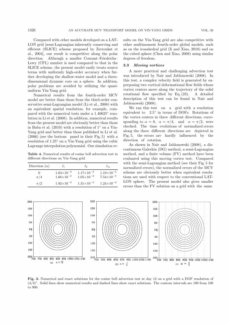
Figure 3 shows that the cosine bell returns to itsinitial position after one revolution (12 days). The nu-merical contour lines (dashed lines) are visually iden-tical to the analytic solution (solid lines). The historyof normalized errors is shown in Fig. 4 where fluctua-tions in the normalized errors are observed when thecosine bell moves across the overlapping region of theYin-Yang grid. Table 4 gives the normalized errorsafter one revolution. Normalized errors along the po-lar direction are larger than the others because, in thiscase, the advection path has more overlapping regions.

Table 1. Convergence rate of solid rotation in east direction (α = 0) on Yin-Yang grid. Normalized global errors aredefined in Eq. (23).

Resolution l1 l2 l∞

(Step) error order error order error order

11.25◦ (480) 3.69×10−4 – 3.69×10−4 – 4.15×10−4 –5.625◦ (960) 2.14×10−5 4.11 2.10×10−5 4.14 2.15×10−5 4.27

2.8125◦ (1920) 1.26×10−6 4.09 1.24×10−6 4.08 1.54×10−6 3.80

Table 2. The same as Table 1, but in northeast direction (α = π/4).


(Step) error order error order Error order

11.25◦ (480) 4.97×10−4 – 5.11×10−4 – 7.71×10−4 –5.625◦ (960) 3.14×10−5 3.98 3.21×10−5 3.99 3.94×10−5 4.29

2.8125◦ (1920) 1.94×10−6 4.02 1.97×10−6 4.03 2.42×10−6 4.03

Table 3. The same as Table 1, but in north direction (α = π/2).


(Step) error order error order Error order

11.25◦ (480) 8.94×10−4 – 1.02×10−3 – 1.24×10−3 –5.625◦ (960) 5.10×10−5 4.13 5.39×10−5 4.24 5.71×10−5 4.44

2.8125◦ (1920) 2.94×10−6 4.12 3.05×10−6 4.14 3.29×10−6 4.12


Compared with other models developed on a LAT-LON grid [semi-Lagrangian inherently conserving andefficient (SLICE) scheme proposed by Zerroukat etal., 2004], our result is competitive along the polardirection. Although a smaller Courant–Friedrichs–Lewy (CFL) number is used compared to that in theSLICE scheme, the present model easily treats sourceterms with uniformly high-order accuracy when fur-ther developing the shallow-water model and a three-dimensional dynamic core on a sphere. In addition,polar problems are avoided by utilizing the quasi-uniform Yin-Yang grid.

Numerical results from the fourth-order MCVmodel are better than those from the third-order con-servative semi-Lagrangian model (Li et al., 2008) withan equivalent spatial resolution; for example, com-pared with the numerical tests under a 1.40625◦ reso-lution in Li et al. (2008). In addition, numerical resultsfrom the present model are obviously better than thosein Baba et al. (2010) with a resolution of 1◦ on a Yin-Yang grid and better than those published in Li et al.(2006) (see the bottom panel in their Fig. 5) with aresolution of 1.25◦ on a Yin-Yang grid using the cubicLagrange interpolation polynomial. Our simulation re-

Table 4. Numerical results of cosine bell advection test indifferent directions on Yin-Yang grid.

Direction (α) l1 l2 l∞

0 1.63×10−2 1.17×10−2 1.19×10−2

π/4 1.68×10−2 1.05×10−2 7.54×10−3

π/2 1.92×10−2 1.31×10−2 1.24×10−2

sults on the Yin-Yang grid are also competitive withother multimoment fourth-order global models, suchas on the icosahedral grid (Ii and Xiao, 2010) and onthe cubed sphere (Chen and Xiao, 2008) using similardegrees of freedom.

3.3 Moving vortices

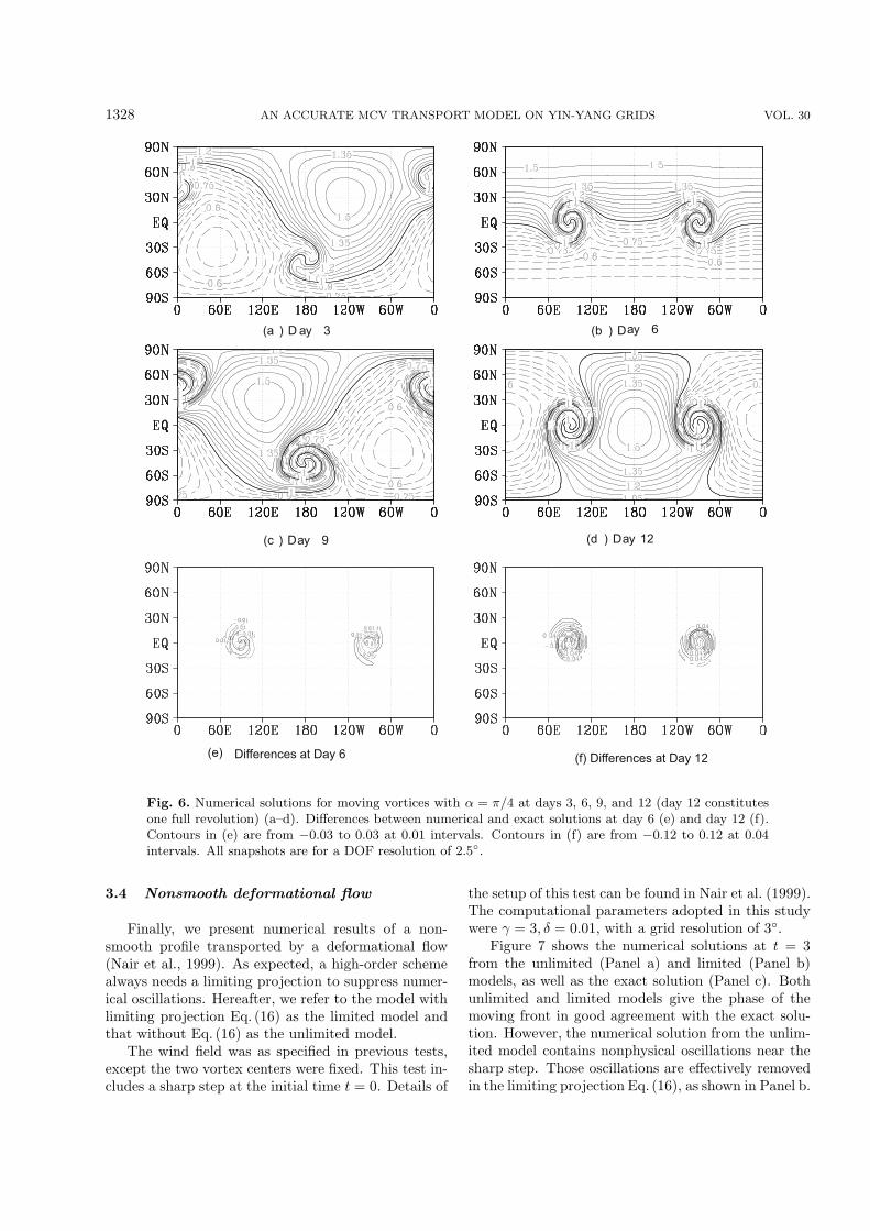
A more practical and challenging advection testwas introduced by Nair and Jablonowski (2008). Inthis test, a complex velocity field is generated by su-perposing two vortical deformational flow fields whosevortex centers move along the trajectory of the solidrotational flow specified by Eq. (23). A detaileddescription of this test can be found in Nair andJablonowski (2008).

We ran this test on a grid with a resolutionequivalent to 2.5◦ in terms of DOFs. Rotations ofthe vortex centers in three different directions, corre-sponding to α = 0, α = π/4, and α = π/2, werechecked. The time evolutions of normalized errorsalong the three different directions are depicted inFig. 5, the errors are hardly influenced by thedirection of rotation.

As shown in Nair and Jablonowski (2008), a dis-continuous Galerkin (DG) method, a semi-Lagrangianmethod, and a finite volume (FV) method have beenevaluated using this moving vortex test. Comparedwith the semi-Lagrangian method (see their Fig. 5 fornormalized errors), the normalized errors of the MCVscheme are obviously better when equivalent resolu-tions are used with respect to the conventional LAT-LON sphere. The present model also gives smallererrors than the FV solution on a grid with the same

(c) α = π2(b)(a)

Fig. 3. Numerical and exact solutions for the cosine bell advection test at day 12 on a grid with a DOF resolution of(4/3)◦. Solid lines show numerical results and dashed lines show exact solutions. The contour intervals are 100 from 100to 900.


Fig. 4. Normalized errors from the solid-body test on agrid with a DOF resolution of (4/3)◦. Normalized globalerrors are defined in Eq.(23).

resolution (see their Fig. 7 for normalized errors). Al-though the DG method shows a somewhat smallernormalized error under an equivalent resolution, theMCV scheme allows a larger CFL number for compu-tational stability (see Table 1 in Ii and Xiao, 2009).Our MCV scheme also has a competitive compu-tational efficiency since it does not involve any time-

consuming numerical integrations. Contour plots ofthe transported field φ and absolute errors are shownin Fig. 6 at different days. The location of movingvortex centers and the phase of the front of deformingvortices were accurately captured.

Fig. 5. Normalized errors for the moving vortex test ona grid with a DOF resolution of 2.5◦. Normalized globalerrors are defined in Eq.(23).


Fig. 6. Numerical solutions for moving vortices with α = π/4 at days 3, 6, 9, and 12 (day 12 constitutesone full revolution) (a–d). Differences between numerical and exact solutions at day 6 (e) and day 12 (f).Contours in (e) are from −0.03 to 0.03 at 0.01 intervals. Contours in (f) are from −0.12 to 0.12 at 0.04intervals. All snapshots are for a DOF resolution of 2.5◦.

3.4 Nonsmooth deformational flow

Finally, we present numerical results of a non-smooth profile transported by a deformational flow(Nair et al., 1999). As expected, a high-order schemealways needs a limiting projection to suppress numer-ical oscillations. Hereafter, we refer to the model withlimiting projection Eq. (16) as the limited model andthat without Eq. (16) as the unlimited model.

The wind field was as specified in previous tests,except the two vortex centers were fixed. This test in-cludes a sharp step at the initial time t = 0. Details of

the setup of this test can be found in Nair et al. (1999).The computational parameters adopted in this studywere γ = 3, δ = 0.01, with a grid resolution of 3◦.

Figure 7 shows the numerical solutions at t = 3from the unlimited (Panel a) and limited (Panel b)models, as well as the exact solution (Panel c). Bothunlimited and limited models give the phase of themoving front in good agreement with the exact solu-tion. However, the numerical solution from the unlim-ited model contains nonphysical oscillations near thesharp step. Those oscillations are effectively removedin the limiting projection Eq. (16), as shown in Panel b.


(a (b (c) Exact solution) Solution by unlimited model ) Solution by limited model

Fig. 7. Numerical solutions of nonsmooth deformational flow at t = 3 on the Yin grid. (a) from unlimited model. (b)form limited model. (c) exact solution.

(a) Solution by unlimited model (b) Solution by limited model

Fig. 8. Cutoff plots of numerical solutions for nonsmooth deformational flow along a cross section nearthe center at t = 3 on the Yin grid. Numerical solutions are denoted by open circles and exact solutionsare shown by solid lines.

The maximum and minimum values are φmax = 2.12and φmin = −0.066 in the numerical solution from un-limited model and φmax = 2.018 and φmin = −0.0019in that from the limited one.

As a clear illustration of the performance of thelimiting projection adopted in present study, Figure 8shows numerical solutions on a cross section from boththe limited and unlimited models. Nonphysical oscil-lations are invisible on the cross section from the lim-iting projection, while the steepness is well-preserved,compared to the exact solution.

4. Conclusion

A fourth-order transport model on the sphericalYin-Yang grid has been developed using the multimo-ment constrained finite volume (MCV) scheme. In

the present model, the polar singularities and con-vergence of meridians in polar regions of conventionalLAT-LON girds are completely avoided by using thequasi-uniform Yin-Yang grid. As model variables, theMCV method uses local DOFs defined within singleelements at equally spaced points. In our transportmodel, the evolution formulations for local DOFs arederived through constraint conditions on moments ofline-integrated averages (LIA), point values (PV), andfirst-order derivative values (DV). The compact localstencils used by the MCV scheme not only contributeto computational efficiency when dealing with infor-mation exchange between Yin and Yang components,but they also help reduce extra numerical errors due tooverlapping connections between two grid components.Compared with other local high-order schemes, suchas the discontinuous Galerkin scheme and the spec-


tral volume scheme, an MCV scheme offers improvedcomputational efficiency, since it allows less restrictiveCFL stability conditions, and it does not require ex-plicit volume quadrature. In addition, a limiting pro-jection can be adopted to control spurious numericaloscillations when a discontinuity or large gradient ex-ists during tracer transport. Widely used benchmarktests show that, compared with most existing models,the present model is competitive both in high-ordernumerical accuracy and computational efficiency.

Acknowledgements. This study is supported by

National Key Technology R&D Program of China (Grant

No. 2012BAC22B01), Natural Science Foundation of China

(Grant Nos. 10902116, 40805045, and 41175095) and

Grants-in-Aid for Scientific Research, Japan Society for the

Promotion of Science (Grant No. 24560187). We also ac-

knowledge that part of this paper has been presented in the

International Conference on Computational Science 2012.

REFERENCES

Baba, Y., K. Takahashi, T. Sugimura, and K. Goto, 2010:Dynamical core of an atmospheric general circula-tion model on a yin-yang grid. Mon. Wea. Rev., 138,3988–4005.

Chen, C. G., and F. Xiao, 2008: Shallow water model oncubed-sphere by multi-moment finite volume scheme.J. Comput. Phys., 227, 5019–5044.

Ii, S., and F. Xiao, 2009: High order multi-moment con-strained finite volume method. Part I: Basic formu-lation. J. Comput. Phys., 228, 3668–3707.

Ii, S., and F. Xiao, 2010: Global shallow water model us-ing high order multi-moment constrained finite vol-ume method and icosahedral grid. J. Comput. Phys.,229, 1774–1796.

Kageyama, A., and T. Sato, 2004: The “Yin-Yanggrid”: An overset grid in spherical geometry. Geo-chemistry, Geophysics, and Geosystems, 5, Q09005,doi:10.1029/2004GC000734.

Lauritzen, P. H., R. D. Nair, and P. A. Ullrich, 2010: Aconservative semi-Lagrangian multi-tracer transportscheme (CSLAM) on the cubed-sphere grid. J. Com-put. Phys., 229, 1401–1424.

Li, X. L., D. H. Chen, X. D. Peng, F. Xiao, and X. S.Chen, 2006: Implementation of the semi-Lagrangianadvection scheme on a quasi-uniform overset gridon a sphere. Adv. Atmos. Sci., 23(5), 792–801, doi:10.1007/s00376-006-0792-9.

Li, X. L., D. H. Chen, X. D. Peng, K. Takahashi, and F.Xiao, 2008: A multimoment finite-volume shallow-water model on the Yin–Yang overset spherical grid.Mon. Wea. Rev., 136, 3066–3086.

Nair, R. D., and C. Jablonowski, 2008: Moving vorticeson the sphere: A test case for horizontal advectionproblems. Mon. Wea. Rev., 136, 699–711.

Nair, R. D., J. Cote, and A. Staniforth, 1999: Cascadeinterpolation for semi-Lagrangian advection over thesphere. Quart. J. Roy. Meteor. Soc., 125(556), 1445–1468.

Peng, X. D., F. Xiao, and K. Takahashi, 2006: Conserva-tive constraint for a quasi-uniform overset grid on thesphere. Quart. J. Roy. Meteor. Soc., 132, 979–999.

Rancic, M., R. J. Purser, and F. Mesinger, 1996: Aglobal shallow-water model using an expanded spher-ical cube: gnomonic versus conformal coordinates.Quart. J. Roy. Meteor. Soc., 122(532), 959–982.

Sadourny, R., 1972: Conservative finite-difference approx-imations of the primitive equations on quasi-uniformspherical grids. Mon. Wea. Rev., 100(2), 136–144.

Sadourny, R., A. Arakawa, and Y. Mintz, 1968: Integra-tion of the nondivergent barotropic vorticity equationwith an icosahedral-hexagonal grid for the sphere.Mon. Wea. Rev., 96(6), 351–356.

Shu, C. W., 1987: TVB uniformly high-order schemes forconservation laws. Mathematics of Computation, 49,105–121.

Williamson, D. L., 1968: Integration of the barotropicvorticity equation on a spherical geodesic grid. Tel-lus, 20(4), 642–653.

Williamson, D. L., J. B. Drake, J. J. Hack, R. Jakob,and P. N. Swarztrauber, 1992: A standard test setfor numerical approximations to the shallow waterequations in spherical geometry. J. Comput. Phys.,102(1), 211–224.

Zerroukat, M., N. Wood, and A. Staniforth, 2004: SLICE-S: A semi-Lagrangian inherently conserving and effi-cient scheme for transport problems on the Sphere.Quart. J. Roy. Meteor. Soc., 130, 2649–2664.

AAS YY tranport-Li Xl&Shen

Documents

Transcript of AAS YY tranport-Li Xl&Shen