RecTree:

A Linear Collaborative Filtering Algorithm

Somy Han Seng Chee M.Sc., University of Toronto, 1992.

A THESIS SUBMIï'TED IN PARTIAL FCTLFILLMENT OF THE REQUREMENTS FOR THE DEGREE OF

MASTERS OF SCIENCE in the School

of

Computing Science

O Sonny Han Seng Chee 2000 Simon Fraser University

September, 2000

Al1 nghts reserved. This work may not be reproduced in whole or in part, by photocopy

or other means, without the permission of the author.

uisioons and Acquisitions et B' 'ographic Senrices s 8 W bibliographiques 3

The author has granteci a non- exclusive licence aiiowing the National Li- of Cana& to reproduce, loan, distribute or seil copies of this thesis in microform, paper or electronic formats.

The author retains ownersbsp of the copyright in this thesis. Neither bie tûesis nor substantial extracts fiom it may be printed or otherwise reproduced without the author's permission,

L'auteur a accordé une Licence non exciusive permettant P k Bibliothèque nationale du Canada de repmduke, prêter, distribuer ou vendre des copies de cette thèse sous la forme de microfiche/film, de reproduction sin papier ou sur format électranique.

L'auteur conserve la propriété du droit d'auteur qui pmtège cette thèse. Ni fa thése ni des extraits substantiels de celle-ci ne doivent être imphes ou autrement reproduits sans son autapisatian.

Abstract

With the ever-increasing amount of idormation available for our consumption, the problem of

information overload is becoming Uimsingly acute. Automated techniques such as information

retrieval (IR) and information filtering (IF), though useful, have provm to be inadequate. This is

clearly evident to the casual user of Intemet search engines (IR) and news clipping services (IF);

a simple query and profile can result in the retrieval of hundreds of items or the delivery of

d o m s of news clippings into his mailbox. The user is still leA to the tedious and time-

consuming task of sorting through the mass of information and evaluating each item for its

relevancy and quality. Collaborative filtering (CF) is a complirnentary technique to IRm: that

alleviates this problem by automating the sharing of human judgements ufrelevancy and quality.

Collaborative filtering has recently enjoyeâ considerable commercial success and is the

subject of active research. However, previous works have dealt with improving the accuracy OC

the algorithrns and have largely ignored the problem of scalability. This thesis introduces a new

algorithm, RecTree that to the best of ow lamwledge is the first collaborative filtering algorithm

that scales linearly with the size of the data set. RecTree is cornpared agaimt the leading nearest-

neighbur collaborative filter, CorrCF p + 9 4 ] , and found to outperfonn CorrCF in execution

time, accuracy and coverage. RecTree has good accwacy men when the item-rating density is

low - a region of difficulty for al1 previously published nearest-neighbour collaborative filters

and c&nly referred to as the sparsig problem. Our experimental and performance studies

have demonstrated the effectiveness and efficiency of this new algorithm.

Acknowledgments

1 would like to tIiank my senior supervisor, Professor Jiawei Han, for his encouragement and

guidance during my studies. His boundless enthusiasm and availability for discussion helped

shape this research during the crucial stages. My gratitude also goes to my supervisor Professor

Wo-shun Luk and the external examiner, Professor Louis Hafer for providing valuable feedback

that has served to impmve this thesis.

1 would like to thank Compaq Corporation (formerly Digital Corporation) for making the EacMovie database available online. Without this generous gesture, this research would not have been possible,

I would like to thank Geoffky Bonnycastle Glass for his meticulous pmfieading of this work. He guided me to the virtues of the present tense.

Lastly and most importantly, 1 would like to thank my sweetheart and wife for her enduring support, encouragement, and impetus for the completion of this work,

Dedication

Tu my Rat, tny RatScal and My ivfe.

Contents

CONTENTS ............................................................................................................................... V I

LIST OF TABLES ............................... " ....................................................................................... X

LIST OF FIGURES .............. ...................... .... ...................................................... ........... XI

CHAPTER 1 iNTRODUCTION .................................................................................................. 1

INFORMATION OVERLOAD ............................................................................................... I FORMATION FILTERMG/~NFORMATION RETRIEVAL ..................................................... 2

AUTOMATED COLLABORATIVE FILTERMG ...................................................................... 4 OLAP AND DATA WAREHOUSMG ................................................................................... 5 PROBLEM STATEMENT ..................................................................................................... 6

............................................................................................................... CONTRIBUTIONS 7 THESIS ORGANIZATION .................................................................................................... 8

NOMENCLATURE ............................................................................................................. 8

CHAPTER SUMMARY ........................................................................................................ 9

........................................... CEAPTER 2 RELATED WORK .............................................. .. 10

........................................ 2.1 TAPESTRY-THE FJRST COLLABORATIVE FILTERING SYSTEM 10 .............................................................................................. 2.2 COLLABORAT~VE FILTERS Il

...................................................................... 2.2.1 The GroupLens Collaborarive Filier I I ............................................................................. 2.2.7 î l e Ringo CoIlaborative Filters 12

2.2.3 Personality Diugnusts: A Probabilisfic Collaborative FiIter ................................ 14 ............................................................................ 2.2.4 The Chter Collaborative Filfer 15

2.2.5 Collaborative Filtering using Clusters .............,.................................................. 15 .................................................. 2.2.6 Bayesian Classifer for Collaborative Filiering 1 6

................................................................................................... 2.3 OPEN PROBLEMS M CF 16 ....................................................................................... 2.3.1 The EarlyRa fer Problem 17

2.3.2 TheSporsityProblem ............................................................................................. 17 ......................................................................................... 2.3.3 The Scalability Problem 17

............ 2.3.4 Corn bining Filter Bots and Persona1 Agents wiih Collaborative Filtering 17

................................................................................................................ 2.3.5 Fab 18 ....................................................................................................... 2.4 CF APPLICAT~ONS 20

................................................................................................................... 2.4.1 SiteSeer 20 ........................................................................................................... 2.4.2 Referral Web 21

................................................................................................................. 2.4.3 PHOAKS 22 ...................................................................................................... 2.5 CHAPTER SUMMARY 22

............................................................................... 3.1 OBSERVATIONS AND ASSUMPTIONS 23 ....................................................................... 3.1.1 Partiiioned Coltaburative Filtering 23

........................................................................................... 3.1.2 In-Memory Algorithm 24 ...................................... 3.1.3 Ovewiew ofRandiVeighCorr. KMeansCorr and RecTree 25

................................................................................................... 3.1.4 fiample Daia Set 25 3.1.5 Over-parririoning ............................... .. ..... .. ........................................ 26

3.2 RANDNEIGHCORR ........................................................................................................... 27

............................................................................................................................................. 29 ....................................................................................................... 3.2.3 Training Phase 29 .................................................................................................... 3.2.4 Predicrion Phase 31 ..................................................................................................... 3.2.5 Time Complerrly 34 ................................................................................................... 3.2.6 Space Complexiexity 35

................................................................................... 3.2.7 Ran&eighCorr 3 Acctiracy 35 3.3 KMEANSCORR ................................................................................................................. 37

3.3.1 Overvi ew. ................................................................................................................ 37 ................................................................................................................... 3.3.2 KMeans 38

3.3.3 K~eans' ................................................................................................................. 39 3.33.1 O v e ~ e w ............................................................................................................ 39

vii

3.3.3.2 The Missing Value Replacement Strategy ......................................................... 40 ............................................................................. 3.3.3.3 The Seed Selection Strategy 42

............................................................................................ 3 A3.4 The Distance metric 44 ..................................................................................................... 3.3.4 T h e Complerity 46 ................................................................................................... 3.3.5 Space Complexiîy 47

3.4 RECTREE ......................................................................................................................... 48 ................................................................................................................. 3.4.1 ûverview 48

....................................................................................... 3.4.2 Constructing the RecTree 48 .................................................................................................... 3.4.2.1 Node Splitting 51

3.4.2.2 The Maximum Iteration Limit, g ........................................................................ 53 3.4.2.3 TheTreeNodes .................................................................................................. 55

............................................................................... 3.4.2.4 Training on the Leaf Nodes 55 ........................................................................... 3.4.2.5 Training on the interna1 Nodes 59 ............................................................................ 3.4.2.6 Training on the Outlier Nodes 59

......................................................................................... 3.4.3 Compu ring a Prediction 60 ............................................................................................ 3.4.4 Updating the RecTree -63

..................................................................................................... 3.4.5 Time Complexity 64 ................................................................................................... 3.4.6 Space Cotnplexiîy 64

...................................................................................................... 3.5 CHAPTER SUMMARY 64

C W T E R 4 RESULTS AND DISCUSSION ....................................................................... A 6

.............................................................................................................. 4.1 METHODOLOGY 66 ......................................................................................... 4.1.1 Accuracy and Coverage 67

....................................................................................................... 4 . 2 Execuiion Time 6d

4.1.2.1 Batch-Mode .......................... .. ....................................................................... 68 ................................................................................................ 4.1 .2.2 Interactive-Mode 69

............................................................................................................ 4.1.3 Data sets 7 0 .................................................................................. 4.1 3.1 The GivenXUser Data Set 70 ............................................................................... 4.1.32 The GivenXRating Data Set 71

........................................................................... 4.1.3.3 The InteractiveXUser Data Set 71 . . . ......................................................................... 4.1.4 The Partrtion Sue Parameter /3 7 2

............................................................................................ 4.1.5 Hardware & Sofnvare 72 4.2 PERFORMANCE STUDY OF RANDNEGHCORR ................................................................. 73

* * . 4.2.1 The Partition Sue /3 ................................................................................................ 73 ............................................................................ 4.2.2 RandNeighCorr 's Running Time 74

................................................................................... 4.2.3 RanaïVeighCorr S Accurucy 76

................................................................................... 4.2.4 RancINeighCorr 's Coverage 78 .............................................................................................................. 4.2.5 Discussion 80

4.3 PERFORMANCE STUDY OF RECTREE .............................................................................. 8 1 ..................................................................................... 4.3.1 The Partition Parameter 82 ...................................................................................... 4.3.2 The Interna1 Node Limit g 82

......................................................................... 4.3.3 The Outlier Thresholk outlierSue 82 ........................................................................................ 4.3.4 RecTree Implementatio n. 83 ...................................................................................... 4.3.4.1 The Item-Rating Vector 83

4.3.4.2 The Similarity Maîrix ......................................................................................... 84 4.3.5 RecTree's Batch Mode Running Time .................................................................... 85

............................................................ 4.3.6 RecTree 's Interactive Mode Running Time 87 ................................................................................................ 4.3.7 RecTree S Accuracy 88

4.3.8 RecTree 's Coverage ............................................................................................... 90 .............................................................................................................. 4.3.9 Discussion 92

4.4 CHAPTER SUMMARY ...................................................................................................... 94

............................................................ CaAPTER 5 CONCLUSION AM) FUTURE WORK 96

................................................................................................................ 5.1 CONCLUSIONS 96 5.2 FUTURE WORK ............................................................................................................... 97

............................................................................................................... 5.2. 1 Scalability 97 ....................................................................................... 5.2.2 The Internat Node limit g 97

. * ....................................................................................... 5.2.3 The outfierslze Threshold 98 . . * ................................................................................................ 5.2.4 Smdanty Measures 98

............................................................................................................. 5.2.5 Predictions 98

List of Tables

Table 1: A compilation of movie ratings for Sammy and her &ends. A high score indicates greater preference. The letters R and A following a title denote a romantic and action title, respectively .................................................................... ,.,..................... ................................... 6

Table 2: Table of Nomenclature ..........,...,........,............................................................... . ............. ..9 Table 3: Ringo's 7-point rating scale. .................................................-........................................ 14

Table 4:The tictitious video store ratings database. The shaded cells are withheld for testing, while the iernainder of the table is subrnitted for training the collaborative Cilter. ................ 26

Table 5: A cornparison of CorrCFs MAE with al1 correlates and when only low correlates (less than O. i correlation) are used in the prediction. A lower score indicates higher accuracy. ..36

Table 6: The default vector is computed for the video dahbase using the PopAvg recommender. ......................,..................~~......,....,....................,...,......,.. m........, ,.,,. *.*.*..,.. ,.......................... 44

Table 7. A calculation of the average rating and standard deviation owr the longer history indicates that Dylan is more similar to Samrny than Beatrice .............................. .. .-..-.-.--..-... 56

Table 8. A cornparison of the correiation coefficients computed by

ComputeCorrelationSimilari~' (denoted by corumn Correlation') with those by ComputeCorrelationSimi1ariiy (denoted by column Correlation) .......................................... 58

Table 9: The GivenXUser dais set. ............... ....... ..........-... .... ... ......... ....... . ....... .... . .... . .......... .. ....... 70 Table 10: The GivenXRating data set. .............,.............................................. ..... .......... ... ..... . ..... .7 1 Table 11: The InteractiveXUser data set ............................................................................. . .......... 72

Table 12: RandhreighCF's batch mode running time with number of item-ratings. ..................... 74

List of Figures

Figure 1: The rating history for 3 users and their pair-wise correlation ........................................ 12 Figure 2: Two families of agents filter documents . Users collaborate by passing on highly rated

documents to theu neighbour's selection agents .................................................................... 19 Figure 3: SiteSeer identifies an interest neighbourhood around folders that have a high degree of

overlap in bookmarks ............................................................................................................. 21 Figure 4: The coverage for al1 nearest-neighbour collaborative filters declines with srnaller

. . training set .............................................................................................................................. 27 Figure 5: A random bi-partition of the video user base .................................................................. 29

............... Figure 6: Pair-wise similaxity weights between members of the same random partition 31 . . Figure 7: The EachMovie rating distribution ................................................................................. 33

Figure 8: Two different selections for the initial centres yield two different sets of clusters . Selecting R1 and R2 as the seeds results in cluster Cl and C2, while selecting seeds R8 and R9 results in the globally optimal clusters C3 and C4 ........................................................... 38

Figure 9: The &fault vector provides missing values .................................................................. 41 Figure 10: The default vector is computed for the video database using the PopAvg recommender .

................................................................................................................................................ 42 Figure 11: The RecTree data structure . Leaf nodes have a similarity matrix while each intemal

node maintains a rating centroid of its sub.tree . Each node has a bi-directional link wiih its .................................................................................................................................... parent- 5 1

.... Figure 12: The RecTree branches after processing the Mdeo database with pl5 itemmtings 52

Figure 13: Building a RecTree on an exponential data distriîution with P = 16 creates 4 clusters with one user each and 1 cluster with 16 users ...................................................................... 53

............. Figure 14: The RecTree's collaborative filter is trained as nodes are attached to the tree 60

............. Figure 25: The RecTree's collaborative filter is trained as nodes are attached to the tcee 62

Figure 16: RantlNeghCorr's batch mode running time with number of item.ratings ................... 75 Figure 17: CorrCFs batch mode ninning time is quadratic .......................................................... 75

..................................................... Figure 18: Accuracy of RanuNeighCorr with number of users 76

............................ Figure 19: Accuracy of RandNeighCorr with number of item-ratings per user 77 . Figure 20: Coverage of RandNeighCorr with number of users Each user has 80 itemmtings ... 79

Figure 21: Coverage for RanuNeighCorr with number of item-ratings F r user ........................... 79

Figure 22: Average maximum similarity RanuNeighCorr and CorrCF ........................................ 81

Figure 23: Baich mode m i n g time for RecTree with number of users . RecTree demonstrates a ........ linear complexity with number of users contrast to CorrCFs quadratic complexity 86

Figwe 24: RecTree batch mode running time with number of item-ratings per user .................... 86 Figure 25: RecTree's interactive mode running time ...................................................................... 87

Figure 26: Accuracy of RecTree with number of users . P is in units of users .............................. 88

Figure 27: The average similarity of advisors in RecTree ............................................................. 89 Figure 28: Accuracy of RecTree as a fhction of item-ratings per user ......................................... 90

Figure 29: Coverage of RecTree with number of users .................................................................. 91 ........................................................................ Figure 30: RecTree's coverage with rating sparsity 91

............. Figure 3 1: The contribution of correlation+ and outlier detection to RecTree's accuracy 93

Figure 32: The contribution of request delegalion to RecTree's coverage ..................................... 94

xii

Chapter

Collaborative filtering

1 Introduction

(CF) is a name used to descnie a variety of processes involving the recomrnendation of items based upon the opinions of a neighbourhood of human advisors. ~mazon' and CDNOW* are two well hown e-commerce sites that use collaborative filtering to

provide recommendations on books, music and movie titles; this sewice is provided as a means to promote customer retention, loyalty and sales [SKR99]. Despite this tremendous commercial interest, the majority of current research has focussed on irnproving the accuracy while making only passing reference to the performance and scalability issues. The fastest CF algorithms have quadratic cornplexity [RIS+94] [SM953 pHL00] [KM99a] [Pa89]. This thesis introduces, to the best of our knowledge, the first collaborative filtering algorithm, RecTree, with linear time complexity. RecTree has accuracy and coverage that is superior to the well hown correhtion- based collaborative filter [RIS+94].

1 . Information Overload

in our day-to-day activities, we are faced with an overwhelming amount of information. From

the moment we wake, we are inundated with requests for our attention and time. How do we

choose to spend our limited time on this seemingly endless Stream of demands?

We employ several sttategies. We rely on spot judgements: quite Iiterally, we judge a

book by its cover. Obviously, marketers use graphic effects and advatking to attract our

attention and to manipulate ow decision. As buyers and consumers, many of us can attest to the

mixed success of this strategy. We rely on luck: very interesting or valuable items come to our

attention serendipitously. Conversely, we can argue that luck saves us fiom wasting ow time on

very uninteresting or irrelevant items. As the name implies, this strategy cannot be relied upon.

We rely on the opinions of others: we seek advice fiom those we trust before making a

consumption decision. We ask our fiends and associates to recommend a good movie to watch.

We consult a food critic for a good restaurant to dine at. We rely on the newspaper editor to

bring us information that is relevant to us. We rely on the store manager to stock brand items that

meet our tastes. This advisory circle helps filter and recommend items for ow attention.

Advisors who consistently recommend items that we like become more trusted and their

recommendations are accorded more weight in our decision-making. Similarly, advisors whose

recommendations rarely match our preferences are given srnaller weight and eventually leave our

circle.

However, our advisory circle is necessarily fuiite and limited in experience - we can only

form a limited number of relationships in our lifetime and each member of the advisory group can

sample but a small subspace of al1 items. Consequently, we oRen make a decision with

inadequate advice. This problem has become increasingly acute with the interconnection of the

world through the Intemet. Now, we have access to an even wider selection of products and the

availability of information sources seems to grow exponentially with no limit. Obviously, our

terrestrial strategies for dealing with information overload are inadequate and we need some

automated assistance,

1.2 Information Filtering/lnformation Retrieval

idormation retrieval and information filtering 0 are a group of techniques that have

enjoyed widespread success [Sho92] [FD92]. The function of the IR system is descriied as

'4eading the user to those documents that satisfy hidher need for Uiformation" Fob8Il. IR

systems adopt the Mew that a query is an approximate expression of an information need. Users

must engage in an iterative process of modifying and refming theù query until the information

need is satisfied. By contrast, information filtering adopts the view that user's information

interests are stable and can be accurately reflected in a profile [BC92]. Documents that satisfL a

profile are extracted fiom a data stream for presentation to the user.

IF and IR use the sarne basic process for obtaining document matches. The query and

document collection/data stream are initially converted into textual surrogates, typically

keywords @3C92]. These sucrogates are then matched using one of three major alternatives:

Boolean, vector space and probabilistic retrieval models, Vector space methods represent the

query and the documents as keyword vectors in a multidimensional space. Terms are weighted by

the importance and distribution of keywords in the corpus and query. The query vector is

compared against each document vector using a similanty measure, such as the vector cosine

[SMc83]. The underlying assumption is that a high similarity of the query and a document vector

implies that the document is higtity relevant to the informational need. Extensions to the basic

vector space method attempt to capture term association and domain semantics pDF+90]

[FD92]. A detailed description of vector space and the other matching methods can be found in

[SMc83].

Despite their success, [Rm; have a number of limitations. WiR tend to retrieve many

items that are irrelevant simply because the keywords are contained in the document. This is

readily evident to any casual user of intemet search engines: a simple query string quite often

results in hundreds of matches. This problem is somewhat ameliorated by creating more

expressive queries, but most users lack either the skill or the patience to pursue this approach. in

addition, 1FiT.R can only be applied to items that are texiual or have associated textual attributes

[BC92]. It would be impassible to ask an IR system to retrieve music pieces that are "happy

sounding". Furthemore, FAR cannot readily incorporate subjective judgements into their

matches. Measures of quality and style, for example, cannot be represented. Finally, [FAR

systems suffer fiom 'horesf-exactly-the-same" syndrome. ûnly documents that match on

keywords will be presented to the user. A highly relevant document that happens to use different

keywords will never by remeved/extracted.

1.3 Automated Collaborative Filtering

Collaborative filtering (CF) is a new field of study that sprung fiom the seminal work by [GN0+92] on the Tapestry email system. Collaborative filtering seeks to automate the terrestrial advisory circle that we alluded to in an earlier section. Members of the advisory circle are identifiai based upon the similarity of their rating history to that of the user. The opinions of the advisors provide recommendations on as-yet unseen items. Unlike the terrestrial advisory circle, CF does not require that a persona1 relationship exist between the user and his advisors; in most instances, the advisors will be unknown to the user.

Whereas IF/iR seeks similarities between the queryfprofile and the items, CF seeks similarities between user nting histories and to exploit other users to rnake recommendations. CF is compIementary to FAR and does not suffer Èrom some of its limitations. Specifically, CF incorporates subjective judgements into its match. The typical CF query is of the form: "Retrieve movies that 1 may like". Secondly, CF does not require a textual representation and c m be as readily applied to textul, as well as audio and video content; any item that a humn user can evaluate and place a judgement, is amenable to CF. Finally, CF does not suffer from "more-of- exactly-the-same" syndrome. The advisory circle consists of hurnan members with individualistic tastes, which are drawn upon to make recommendations.

Unlike traditional classification and segmentation analysis, CF can be applied where user and item attributes are missing or dificult to obtain. On the Internet, accurate demographic and psychographics infomtion is notoriously difficdt to obtain. To sorne degree this may be due to user concern over priracy and the commercial use of personal information; in a survey of 10,000

households by Forrester Research Inc., two thirds had serious concerns about their privacy [FOR99]. Furthemore, when users submit sweys, over 50% [Gre99] of the applicants provide false information. These issues complicate the analysis of these online forms of data.

In contrast, users seem l e s reluctant to provide item-rating information. The EachMovie recommendation service [EM97] collected 10 or more movie preference ratings from over 60% of its mernbership. This same rnembership however responded puorly when asked their age, gender and zip code, Less than 10% of the rnembership provided al1 thtee pieces of demographic information .

1.4 OLAP and Data Warehousing

OLAP (On-Line Analytical Rocessing) and data warehousing are two complementary technologies that are enjoying considerable recent commercial success. These technologies

rapidly aggregate measures across dozens of dimensions and across al1 the dimensional permutations. Decision rnakers can use OLAP to quickly answer questions such as: "What was the number 1 selling baby product, across each province, across each store, in the last 3 years?" This type of query is prohibitively expensive for a relational database to execute. Data

warehousing is the process of cleaning data, rnaking it consistent with a data dictionary, and persisting it in a non-volatile data store. While an operational database may be pwged periodicaily (to remove lapsed customers, for example), a data warehouse will never (theoretically) erase any data. New data is appended to it, but old data is never removed. Data warehousing is a data pre-processing step to OLAP.

OLAP and data warehousing is used to implement a popular form of collaborative filtering. Many on-line retail sites customize a web page to include links like: ';Y is the most popular item of type Y' or provide statistics such as: '"T'his item has been downloaded Z times". OLAP provides the technology to compute these aggregates very rapidly; in some instances the computation can be real-time. Rovided that users supply demographic information, other interesting statistics can be computed and displayed to the user. These factoid help the user filter his selection and hopefully, for the vendor, result in a sale. An example of such a factoid is: "89% of professionals in your categoty in your state buy thisTypeOfinsurance fiom n'. Analyzing the data warehouse for interesting patterns rnay also be a usefiil technique for filtering. if a user discovers that a set of items are viewed kquently together, he may decide after viewing the first, that the remaining items in the collection are worthy of consideration; the pattern 'recomrnended' the set of items to the user, Other data mining techniques such as time series analysis, sequence analysis, clustering and classification can be applied to a data warehouse and the discovered patterns used to recommend items [JCC98].

OLAP and data mining is, however, not inextricably Iinked to data warehousing. DBMiner is a data mining-OLAP hybrid system that operates directly on relational databases [JCC97]. This system could similarly be used to mine and recommend items to users.

Multimedia-Miner is also a data mining-OLAP hybrid system that operates on multimedia databases [ZHL+98]. This system could be used to discover patterns in multimedia items such as audio or video clips. These patterns could be the basis of recomrnendations.

1.5 Problem Statement

A CF algorithm makes recommendations to the active user a based on the item ratings of 1 advisors. Denote the set of al1 items as M and the rating of user u for item i as rkf or altematively rd&). Let the vector rm denote ratings for al1 items for user u and the set Y = {rrFI), rdM), rJ@fl. .... , r,,(M}) denote the database of al1 user item-rating vectors. Defuie Su = (il id =@) as the subset of al1 items for which user u has nut yet rated and consequently for which a

collaborative filter may provide predictions. The symbol O denotes "no rating". A collaborative filter is then a hct ion f that mahs recamrnendations pu for the active user a over the set Sa of un-rated items, taking the database of item-rating vectors as input.

The function f maps items into ceal numbers or Q.

Example 1. Sammy and her friends are members of a video shop that has established a rudimentary CF system. Each rime Sarnmy and her fiends view a video, they can rate the movie on a scale of 1

to 5 indicating their level of enjoyment. A 5 indicates "1 enjoyed it very much, 1 would strongly recommend this movie" while a 1 indicates "1 hated it, don't bother". Her rating history and those of her fnends are recorded in the table below.

I I Starship Sleepless Ml- Trwper in Seattle 2 Matrix Titanic

ammy 3 4 3 L eatrice 3 4 3 1

vlan 3 4 3 3 4

Table 1: A cornplation of movie raüngs for and ber friends. A bigh score indicates greuter preference. The letiers R and A foUowing a tiUe denote a ronr~ntk and action title, respeetively.

Suppose that prior to watching the Matrix and Titanic, Sammy asked the CF system to

chmse the movie that best matches her taste. Which movie should the CF system recommend? A rudimentaq CF system could make sensible predictions using the group average. The

average rating of Matrix is 3 while Titanic has an average rating of 1414. The system would therefore recommend Titanic over Mat&. We see that this recommendation matches well with Sammy's higher rating for Zïtanic in cornparison to MatrUr.

This rudimentaq system falls well short of automating the terrestrial advisory circle. b particular, the group average algorithm implicitly assumes that al1 advisors are equally trusted and consequently, their recommendations equally weighted. An advisor's past performance is not taken into account when rnaking recommendations. However, we know that in off-line relationships, past performance is extremely relevant when judging reliability of recommendations. Equally problematic is that the group average algorithm will make the same recommendation to al1 users. Basil, who has very different viewing tastes fiom Sammy, as evidenced by his preference for action over romantic movies, will nevertheless be recommended Titanic over Matrix. In the next chapter, we will revisit this example and demonstrate how sophisticated CF algorithrns can provide more accurate and personalized recommendations.

0

1.6 Contributions

This thesis describes a new collaborative filtering data structure and algorithm called RecTree (an acronym for REComrnendation Tree) that to the best of our knowledp, is the tirst nearest- neighbour collaborative filter that can provide recommendations in linear time. The RecTree has the following characteristics:

1. RecTree cm be consîructed in linear time and space, 2. RecTree can be queried in constant tirne. 3. RecTree is more accurate than the leading nearest-neighbour collaborative fïlter, CorrCF

ptrS+94]. 4. RecTree bas a greater coverage (provides more predictions) than CorrCF. 5. RecTree does not s&er the rating sparsify problem.

We demonstrate the effectiveness and efficiency of RecTree through analysis and performance studies.

1.7 Thesis Organization

This thesis consists of five chapters, In chapter 1, we introduce collaborative filtering and the

motivation for this work. In chapter 2, we survey related work Details of the two proposed

algorithms, RandNeighCorr and RecTree are described in chapter 3. In chapter 4, we present

experimental results and discuss the strengîhs and weaknesses of each approach. Finally, in

chapter 5, we surnmarize and discuss future directions for research.

1.8 Nomenclature

Unless it is otherwise specified, this thesis uses the following table of symbols to maintain a consistent discussion:

Il rki ( The cwrent user's rating for item i. 51 The curent user's average rating. A scalar.

C The standard deviation

t 8 1 The "no rating" value. --

Table 2: Table of Nomenclature.

1.9 Chapter Summary

in this chapter we touched on the problem of information overload and the inadequacy of information retrieval and information filtering techniques for dealing with this problem. Collaborative filtering is a complementary technology that does not suffer fiom some of the limitations of IR4FIR/IF in particular, CF incorporates human judgements of relevancy and quality by automating the terrestrial advisory circle.

We introduced a database of video ratings that we will serve as a nmning example in the

chapters that follow. A formal statement of the collaborative filtering problem and summary of the contriiutions of this thesis was presented.

Chapter 2 Related Work

in this chapter we briefly survey the recent dewlopments in collaborative filtering. This is by no means an exhaustive survey.

2.1 Tapestry - the first collaborative filtering system

The phrase "collaborative filtering" originated from the Tapestry email system [GN0+92]; they define collaborative filtenng as a process where "people collaborate to help one another perform filtering by recording their reactions to documents they read." Tapestry facilitates the sharing of user opinions about documents by allowing them to annotate documents with key phrases. A user receives items by executing a complex query that selects on these annotations and the identity of the annotator. A typical query is: "Show me the documents that Sidney annotated as 'interesting"'. Tapestry could also use implicit user feedback in its queries. Knowing that Basil sends an email response to only those documents that he finds interesting, we could express a query to select on this action,

Tapestry is essentially a rich qu-g system where users benefit from the annotations contributed by others - this is the collaborative aspect of the system. The system sde r s from a number of limitations, however. Firstly, the user must be aware of the identities or have a prior relationship with his advisors, otherwise he wodd not diink to issue a query based on their annotations. Tapestry provides assistance to make the interaction of terrestrial advisory circles more efficient, but is limitcd by ais very feature. A personal relationship needs to exist ktween the advisor and advisee. Secondly, users are the to record theu reaction using any set of keywords they choose. The unlikelihood O € two users using the same set of keywords rnakes it difficult to create a mter expression that is applicable across the entire user base.

Tapestry is largely a manual system and this is the reason for its limited adoption among the users who participated in the initial shidy. in the foliowing two sections, we discuss

CHAPTER 2. RELATED WORK I l

collaborative filters that remove the "celationship requirement" and that Iimit the user's manual interaction to providing a numeric rating. In section 2.4 we present some approaches to CF that relieve the user fiom the explicit task of rating items by Uifiming endorsements h m their interactions.

A collaborative filter is an algorithm that predicts a user's preference for an item based only on how advisors have rated their preference for it. A collaborative filter diffas h m other data mining techniques in that the item's attributes and the users' demographic information are not necessary for a prediction. This very capability makes CF an attractive technology on the Internet where demographic information is difficult to obtain and anonymity is treasured.

Collaborative filters can be classified into memory-based and model-based algorithms [BHK98]. Memory-based algorithms repeatedly scan the user base to locate other users to serve as advisors. A prediction is then computed by weighting the recomrnendations of these advisors. An advisor is identified based on his similarity or neamess in tastes to the active user; consequently, these algorithms cm be equivalently called nearest-neighbour collaborative filters.

Model-based algorithms infer a user model from the database of rating histories. The user model is then consulted for predictions. Model-based algorithms require more time to train but c m provide predictions in shorter t h e in comparison to nearest-neighbour algorithms. The storage requirements for memory-based algorithms also tend to be somewhat less than those of nearest-neighbour algorithms [BHK98]. in the following sections, we describe some recent collaborative filters.

2.2 Collaborative Filters

2.2.1 The GroupLens Coilaborative Filter

The GroupLens system is one of the first automated collaborative filtering systems wS+94] to apply a statistical collaborative filter to the problem of Usenet news overload. [RIS+94] assert tbat user satisfaction with Usenet as a means of disseminating information is declining and that without some assistance to quickly sift the chaff fiom the wheat, some users are abandoning the medium.

The GroupLens system identifies advisors based on the Pearson correlation of voting history between pairs of users. The Pearson correlation measures the degree with which the rating histories of two users are Iinearly correlated. Two users may not score items identically,

but if they consistently like and dislik the same items then they will have a positive correlation score. Figure 1 shows the rating history h r 3 users and their pair-wise similarity coefficients.

An underlying assumption of the GroupLens collaborative filter is that users rate items with a Gaussian distribution; users have an ambivalent preference for most items that they encounter, while for a few items they have a strong like or dislike. The filter takes this behaviow into account by computing the prediction as a deviation from the active user's average rating 5:

The weights wa., are the pair-wise correlation coefficients between the active user u and the advisor u and the normalidon factor a is chosen such that the absolute values of the weights sum to unity.

Figure 1: The rating hlstory for 3 users and iheir pair-wise eorrelaîion.

2.2.2 The Ringo Collaborative Filters

Pearson Correlation

Ringo is a statistical collaborative filtering system [SM951 that provides on-line recommendations for music. Users provide ratings on music albums that they have listened to and the system then recommends a number of music titles. One of Ringo's most popular features is the ability for users to add to the inventory of music titles and artists; this feature was

responsible for the nearly 5-fold increase in the item inventory in the first 6 weeks of operation [SM95].

Ringo computes a prediction by taking the weighted average of the advisors' ratings. The weights are computed using one of three different similarity meûics: mean square diffaence (MSD), Pearson correlation, and constrained Pearson correlation. The MSD metric computes s i rn i lm based the mean square difference between rating histories of the users:

The Pearson correlation metric has been discussed above and will not be repeated here. The constrained Pearson correlation attempts to take into account the positive and negative endorsements of Ringo's 7-point rating scale (Table 3). Since ratings above 4 are positive endorsements while those below 4 indicate negative endorsements, the correlation metric is modified such that only when both users have rated the item positively or negatively will the correlation coefficient increase. Specifically, the constrained Pearson correlation metric is given by:

Ringo also uses an altemate prediction algorithm called artist-artist correlation. This algorithm inverts the basic collaborative filtering mechanism by treating albums as potential advisors to other albums. For example, suppose that Basil wants a prediction for the album bbAvalon**. The artist-artist correlation method computes the correlation between "Avalon" and other albums that B a d has rated and generates a prediction h m the weighted average of his scores on those albums.

[SM951 reports that the constrained Pearson correlation meûic results in the highest . accuracy and highest number of predictions (also known as coverage). The artistartist correlation

metric results in the poorest accuracy and lowest coverage.

CHAPTER 2. RELATED WORK 14

I

7 1 BOOM! One of my FAVOLRITE few! Can't live without it. 1

6 1 Solid. They are up there.

Doesn't tum me on, dwsn't bother me.

Eh. Not really my thing.

Barely talerable.

Pass the earplugs.

Table 3: Ringo's 7-point rating SC&.

23.3 Persoaality Diagnosis: A Probabilistic Collaborative Filter

Personality Diagnosis (PD) [PHLOO] is based on the assumption that user preferences can be described by a personality type or true rating vector, rim. When users rate items on different occasions, they do so with some deviation about the ûue value. Gaussian noise is assumed to sununarize al1 of the external factors that affect a rating, such as the user's mood and the context of any other titles rated in the sarne session. Specifically, the probability that user a assigns a rating score ofx on an item i is given by the normal disûiiution with mean y:

Pr(ra ( i ) = x 1 rame(i) = y) e-(x-~)2 1 2c1

The probability that the active user's true preferences are those represented by another user's ratings is used as masure of similarity and cm be cornputed by applying Bayes' rule. Specifically, the probability that the active user a is of the same personality type as another user i, is given by the product of probabilities that the active user's rating on each item is normally distriiuted about the true values as given by the user i:

The 6rst temi on the right hand side of ( 5 ) is the prior probability that the active user votes according to vector FAN) and is assumed to be a random variable with a value of '4 where Z is the number of users. Given these similacity scores, a rating probability distribution can be computed for any item and taking the most probable rating in the dismbution then generates a prediction. The probability for each rating is simply the sum of probabilities of al1 personality types that support that rating score:

~r(r,(i) = s ) = C ~ ( i , ( ~ ) = r , ( ~ ) ) Y, = (u lu E N and r,(i)=.ri) u,

PD can equivalently be interpreted as reconstructing the active user's tnie preferences by taking one of the other users at random and adding Gaussian noise to it. Given the user's rating history the probability that he is actually one of the other users is inferred. [PHLOO] ceports the accuracy of PD is competitive with those of other nearest-neighbour collaborative filters (BHK981, however the two performance studies were conducted on separate data sets.

2.2.4 The Cluster Collaborative Filter

Recently a collaborative filter based on the weighting of clusters was proposed [KM99a], This approach applies a hierarchical divisive clustering algorithm to partition the user base into successively tiner partitions until a cluster distortion threshold is satisfied. Cluster distortion is defined as the sum of the distance of al1 data points fiom the centre of the clustcr. Locatîng the leaf node where a user resides and then taking a weighted average of each cluster's recommendation on the path from the leaf partition to the root generate a prediction. A cluster recommends an item based on the average rating of al1 its members. Cluster distortion is used to weight each cluster's recommendation. W 9 9 a l reported that the overall performance was competitive with the correlation-based collaborative filter [RiS+94].

2.2.5 Collaborative Filtering using Clusters

A straightforward application of clustering techniques to ratings data was recently reported [UF98]. The authors applied the KMeans and Gibbs Sampling clustering algorithm to mate

user and item clusters. Users of the same cluster acted as recommenders for each other. The user clusters were trained by clustering on items purchased by users and item clusters were trained on the users they were purchased by. A scheme of repeated clustering was reported where a 2* and

3d iteration of user and item clustering was performed on the item and user clusters created fiom the previous iteration. The authors argue that repeated ciustering on clusters, as opposed to clustering on the actual usditems, has the potential for creating usehl neighbourhds from which recomrnendations can be drawn. initial results for repeat clustering are, however, inconclusive. Application of the clustering algorithm to the CDNow music online retail site reportedly doubled mail respondents to a music promotional.

2.2.6 Bayesian Classifier for Collaborative Filtering

The naïve Bayesian classifier computes the probability of membership in an unobserved class c based on the "naïve" asmmption that ratings are conditionally independent [BHK98]. The underlying assumption is that there are certain classes or types of users that have a common set of preferences and tastes. The probability model relating the joint probability of class membership and ratings is given below:

m

P~(C = c, r, (l),.., ra (m) ) = Pr(C = c ) n pr(ra (i) 1 C = e) i=l

The left hand side of expression (7) is the probability that a user a with the rating history r,(l),..,r,,(m) is of class c. The probability of class membership MC-c) and the conditional probabilities Pr(rd(i)(C=c) are estimated fiom the training set OP user item-ratings. However, the class labels are not directly obserwd and methods that can infer model parameters with hidden variables must be employed. The EM algorithm was selected to l e m the model structure with a fixed number of classes.

The Bayesian classifier was found to be cornpetitive with the correlation-based classifier in accuracy and coverage. However, the classifier has a significantly longer training time.

2.3 Open problems in CF

Despite the p w i n g commercial interest in collaborative filtering, there still remain a nwnber of open problems îhat have yet to be adequately resolved.

CHAPTER 2. RELATED WORK

2.3.1 The Early-Rater Problem

A collaborative filter does not provide any benefit to a user if she is the first person in her neighbourhood to rate an item. [A2971 has speculated that even if the cost of rating an item were zero, most users will still prefer to benefit fiom others ratings rather than supply ratings themselves. Without a compensation mechanism, CF systems depend upon the altruism of their rnernbers to overcome the early rater problem.

2.3.2 The Spanity Problem

Collaborative filtenng systems require a "critical mass" of users to join and provide ratings before they c m provide predictions of reasonable accuracy and coverage. Even when there is a large membership, a sufficient number of users must rate each item. The accuracy of rnany collaborative filters faIl below that of non-personalized recommendation via population averages when the rating density is low [RIS+94] [KM99a] [GSK+99] .

2.3.3 The Scalability Problem

The recent collaborative filter research has focused on improving accuracy and largely ignored the problem of execution time. We believe this may be due to two factors. Firstly, the focus of early collaborative filter research was to prove their merit through the accurate prediction of user preferences. As long the execution time was not prohibitive, accuracy was the driving factor in CF research. Secondly, the memberships in the early CF systems were relatively srnall and consequently satisfactory responses could be achieved by increasing the number of computer resources devoted to the task. However, given the quadratic time complexity of the fastest collaborative filters and the inherent less-than-linear gain in throughput for an incremental increase in computer resomes, we believe this is not a problem that can continue to be ignored.

23.4 Combining Filter Bots and Personal Agents with Collaborative Fitering

Two ment promising approaches to the eurb rater and sparsity problem attempt to increase the rating density by using bots and agents. These automatons submit ratings to the collaborative filtering system as if they are legitimate users. They differ fiom real users in that they rate every item in the inventory but never ask for recommendations. The relevancy of their recommendatioii to a human user is automatically determined by the similacity weight that the CF system computes.

[SKB+98] reports the use of %kr bots" in a Usenet application where news items are assigned ratings based upon simple d e s . The bots assign a rating based on the propohon of spelling errors, ihe length of the messages, and the lengîh of included messages. The rationde for these boîs is that Usenet m e m h prefer messages that have few spelling emn, are brief and contain more new content in comparison to included messages. Each of these bots rank the entire set of messages and ehen partitions them into 5 rating bands. Ail items within a band are assigned the same score. The proportion of news items in each band is chosen to match the human rating distniution of that newsgroup. The spell-checking bot is reported to improve the accuacy and coverage in 4 of 5 newsgroups, while the remaining bots have mixed resuits. The authow postulate that users do nos necessarily care about emr free messages, but that g d spelling correlates well with such valuable aitriiutes as carehl writing style or simple vocabdary.

[GSKW] reports the use of agents and bots in a movie recommendation application. A nurnber of simple genre bots are constructed that rate a movie with the maximum preference score of 5 if it is of a particular genre or the minimum preference score of 1 otherwise. For each user, three information filter agents are trained on only the movie cast names, the movie's keywords, or the cast names and keywords, respectiveIy. The agent profiles are constructed by cornputing the TF-IDF (term hquency-inverse document tiequency) [SMc83] vector fiom the collection of movies that the user has rated. Each movie is also converted into a TF-DF vector. The agents then score each movie by computing the vectar costne distance between their profile and the movie's TF-IDF vector. The movies are ranked and divided into 5 rating bands in proportion to the human rating distribution; al1 movies within a band are assigned the same score. The results of this study are promising and show substantial improvements in accuracy and coverage when al1 the bots and IF agents participate in the collaborative filtering system with the 50 users in the study group,

[GSK+99] noted that despite the promising results of the study, the scalability of the proposed solution had not been addressed. The MovieLens and other collaborative filtering systerns codd not cope with agents and bots that provide such a volume of recommendations nor agents that changed their ratings periodicaiiy to reflect their leaming of the user's preferences. Furthemore, these approaches are based on infonnation filtering techniques and consequently are constrained by IR'S limitations.

2.3.5 Fab

Fab is a web-page recommendation system that solves rating sparsity by computing user similarity fiom profiles rather than item-ratings [BS97I. A user profile consists of a TF-IDF vector buiIt up h m the documents that the user has rated. The vector cosine metric between user

profiles, which ranges between -1 and 1, is computed to identie advisors; a value of 1 iadicates a perfect similariiy, while -1 indicates complete dis-similarity (a user whose tastes are completely opposite to the active user), and O indicates a complete lack of interest overlap. Web pages that are highly rated by an advisor are provided to the active user as recommendations. This approach ameliorates the sparsity problem since content similarity is used as a basis of computing user similarity.

Fab's architecture, shown in Figure 2, consists of two families of agents. Collection agents gather documents fiom the web and deposit them into a central pool. SeIection agents match documents to their profiles and deliver them to their users. When a user rates a document, both the selection and the collection agents receive the relevancy feedback. Collection agents receive feedback fiom al1 users while a selection agent receives feedback fiom only its "owner". This feedback strategy results in collection agents that are ûained to serve the needs of a group of users while the selection agents are trained to serve the needs of a single user. Collection agents that consistently receive low feedback scores are periodically eliminated and agents with high feedback scores are duplicated. Fab's collaborative aspect arises when a user rates a document highly. At this point the document is fonvarded to al1 of his advisees' selection agents as recommendations. The selection agents make the final decision as to whether to forward or filter a recommended item.

Figun 2: Two families of agents alter documents. Users collaborate by passing on highly rated documents to theu neighbour's selection agents.

2.4 CF Applications

2.4.1 SiteSeer

SiteSeer is a cecornmendation system that predicts preferences for web pages [PR97]. Web-page ratings are implicitly gathered by examining a user's bookmark and bookmark folders. A bookmark is taken as a positive endorsement for a page and a folder provides a context for computing interest similarity and for providing recommendations.

SiteSeer assumes that each folder represents a distinct interest and that a high degree of overlap between users' folder contents are indicative of common interest; a user can therefore belong to as many interest neighbourhoods as bookmark folders. Recommendations are generated by taking the rnost ofien saved bookmark in the neighbourhood of folders with a high degree of overlap. SiteSeer treats the bookmarks as purely unique identifiers and does not derive any semantic value fiom the titles of folders, the bookmarks nor the contents of the web pages. The bookmark foldets, however, are used to contextualize the recommendations. in Figure 3, a neighbourhood is f o m d mund Basil's "vacation spots" folder with Sammy, Bea and Dylan. SiteSeer recornmends to Basil the link http://www.belize.org within the context of the "vacation spots" folder since it appears in al1 three of his neighbour's folders.

Using bookmarks as inputs to the collaborative tilter has a number of advantages, Bookmarks are less "noisy" data in cornparison to mouse-clicks since they represent a conscious investrnent in tirne to create and organize. Furthennore, bookmarks are contextualized by the organization of folders providing a natural means for recommendations.

Bookmarks also have a number of limitations. Valued sites are not always bookrnarked if they can be reached through other methods such as a search engine, an index page, or if it has a simple URL that can be easily remembered. in addition, bookmarks are created for a number of different reasons, ranging fiom long-tenn interest to a short-term need to retum to a page. Finally, bookmarks register positive endorsement for a page, but there is no means for cegistering partial or negative endorsement.

CHAPTER 2. RELATED WORK

Figure 3: SiteSeer identifies an interest neighbourhood around folders that have a high degree of overlap in bookmarks.

2.4.2 ReferralWeb

ReferralWeb is a system for recommending people (experts) and documents based on the social network [KSS97]. Unlike other automated collaborative filtering systems where the recommenders are anonymous, the identities of recommenders in RefenalWeb are explicit. This is crucial for a determination of ûustworthiness and quality of the information source.

RefenalWeb exposes the refenal chah as it serves two important fiinctions: it provides a reason for the expert to respond CO the requester by making the relationship explicit ( e p s they have a mutual fnend or mutual collaborator), and it provides a means by which the searcher cm evaluate the tmstworthiness or quality of the expert. ReferralWeb does not require the user Co explicitly enumerate his contacts, but builds its social network by mining documents published on the Internet.

When a user registers with the system, ReferralWeb constructs a social network by reirieving al1 documents mentionhg the user and then extracting the names of other individuals. This process is recmively applied several times and the results merged into a network. The network cm then be used to constrain and filter the search for people and documents. The social network c m be used to Uifer the quality of documents; the underlying assmption is that authors of high quality documents tend CO be collaborators or colleagues. For example: "Retrieve database documents by colleagues of J. Gray." Similarly, a query to locate an expert m the data

mining field could be expressed as: "Show me the names of individuals who have published a document about data mining that are colleagues or colleagues of colleagues of J. Han."

ReferralWebls obvious disadvantage is that it can build a social network only around individuals who have published online or are mentioned in online press releases, for example academics, CEOs, or spokespersons. However, there is a growing trend for individuals to create an online presence and this will help to extend ReferralWeb's applicability.

2.4.3 PHOAKS

PHOAKS is an on-line recommendation service that mines Usenet postings as a source of web- resource endorsement [THA+97]. Using a complex library of heuristics, the authors report an 88% accuracy in extracting web-page endorsements fiom Usenet postings. The basic strategy consists of three steps. Firstly, if the URL contains the word markers that indicate it is king recommended as opposed to king advertised or announced, it is counted as an endorsement. Secondly, if the endorsement has k e n cross-posted to many newsgroups then it is discarded - such a message is assumed to be too general to be thematically close to any of the groups. Finally, the web-page endorsement is discarded if it is part of the poster's signature file, embedded in a message or endorsed by the same user in the past; these süategies deprecate selF promotions and double counting.

PHOAK predicts the quality of a web-resource based on the number of distinct users that recommend it. The authors test this assumption of quality by comparing the recommended resources with those in newsgroups FAQs; domain experts maintain FAQs and typically direct users to high quality web pages. [THA+97] report a positive correlation between the number of distinct recommenders to the probability that it will be mentioned in a FAQ.

PHOAKS is still operational and can be accessed on-line at www.phoaks.com

2.5 Cbapter Summary

In this chapter we have summarized the recent research in collaborative filtering. We described a number of nearest-neighbour and model-based collaborative filters and indicated some of their strengths and weaknesses. We presented the open-problems in CF and some CF applications.

Chapter 3 RecTree

in this chapter, we discuss our approach to designing collaburative filters with faster execution times. We begin in Section 3.1 with a discussion of preliminary observations that motivate Our approach and the assumptions that we make. The following three sections present successive refinements to the basic approach. Section 3.4 presents RecTree, a new data structure and algorithm that can deliver recommendations in Iinear time.

in this and subsequent chapters, the tenn "item-rating vector" is used interchangeably with user since each item-rating vector is uniquely identified with a user. Therefore, when we Say the user ru, it is understood that we mean the user u associated with that item-rating vector,

3.1 Observations and Assumptions

3.1.1 Partitioned Collaborative Filtering

The fastest collaborative fiiters to date have quadratic complexity with data set size [RIS+94] [SM951 pHLoo]. Each of these algorithm differ in the mechanism of computing a prediction and the metric used to gauge similarity. However, they al1 require an exhaustive search over the database of 1 users to locate advisors. To generate predictions for a test set of q users requires lq passes over the database. Obviously, a CF system is required to make predictions for al1 subscriiing users, othemise excluded users would derive no utility from the system and hence cease to be members. The test set therefore consîsts of the same users as the database of candidate advisors - yielding the quadratic complexity.

Clearly, we cm only h o p to improve the complexity of any proposed algorithm if we can avoid or lirnit the exhaustive search for advisors. We take the latter approach and descni three algorithrns below that limit the neighbourhood over which advisors are sought. Each of these

algorithms attempts to create partitions of independent neighbo~~hoods of approximately similar users. Predictions are computed fiom only the recommendations of members of the same partition. Our general approach can thus be descnid in the following framework:

1. Phase I: Partition the data set. 2. Phase II: Train the collaborative filter. 3. Phase III. Generate predictions.

Phase ii of the framework makes no assumption about the type of collaborative filter used. Nearest-neighbour and model-based algorithms can be inseried without difficulty. A recent empirical study (BHK981 into several nearest-neighbour and model-based collaborative filters reports that both types of algorithms have comparable accuracy, Differences behveen the algorithms arise in terms of execution time and space cost; nearest-neighbour filters execute sigiificantly faster but require somewhat more disk space. We rationalize that disk space, unlike time, can always be purchased and given the continuing improvements in storage technology, at a steadily declining per unit cost. This thesis focuses on improving the execution time for nearest- neighbour collaborative filters. Phase il cm alternatively be paraphrased as: 'Train nearest- neighbourhood CF."

For this work, we assume that al1 of the rating data wili Cit into memory. This is not an unreasonable assumption, as we argue here.

The EachMovie recommendation service3 accumulated almost 3 million ratings over an eighteen-month period. The service used a 6-point rating scale that is typical of

recornrnendations systems4. The total cost to store 3 million ratings is therefore only 3 mega- bytes. if we assume an opetating system with the capability to address 1 gigabyte of memory space, an in-memory algorithm should be able to accommodate a service 300 times larger than the EachMovie service. We therefore believe that in-memory collaborative filters cm adequately serve the short and intermediate term needs of a recommendation service. It should be pointed

The EachMovie reconnnwdation service was modesîiy sized with a membership of 73,000 usea and an inventory of 1600 items. 4 There is evidence to suggest that reiiability of the data collected does not substantiaiiy increase if the number of choices e~ceeds seven [RR9 11.

out that our 1 gigabyte memory limitation is somewhat conservative - the next generation of 64-

bit operating systems will remove this limitation altogether. An extension of this work to handle very large databases is nevertheless discussed in Chapter 5.

3.13 Ovewiew of RandNeighCorr, KMeansCorr and RecTree

Starting in section 3.2 we descrii three algorithms, RanaNeighCorr, KMeansCorr and RecTree, with the potential for delivering recommendations in linear time. RandNeighCorr is the most naive approach to partitioned collaborative filtering. We present it as the baseiine algorithm against which the other two partitioned filters can be compared. RandNeighCorr partitions the data set by randomly assigning users to partitions in phase 1. In phase ii, it computes the similarity between users using the Pearson correlation measure. Finally, in phase iïi it generates predictions by taking a weighted deviation fiom the user's mean rating.

KMeansCow represents a refinement on RandNeighCow7s simpiistic partitioning strategy. It replaces the partitioning stage (phase i) with the KMeans* clustering algorithm. Phase II and Phase iü of KMeansCorr are identical to those of RandNeighCorr. A complexity analysis of KMeansCorr will reveal that despite king able to execute in isolation the partitioning and training phases in linear time, the combined action of al1 phases results in at best quadratic cornplexity.

The RecTree algorithm partitions the data in phase 1 by recursively calling KMeans' to

split the data set into child clusters. The chain of intermediate clusters leading fiom the initial data set to the final partitioning is retained in the RecTree data structure, which resembles an unbalanced binary tree. The collaborative filter is trained in Phase II by cornputing the pair-wise similarity coefficient within each leaf partition using a more accurate similarity meûic that we cal1 correlation' for clarity. The RecTree generates a prediction by employing a dual strategy. if the user is located in a partition with a suficient number of neighbours, taking the weighted deviation h m the rnean generates a prediction. if the user is located in a m l 1 neighbourhood, RecTree generates a prediction by taking the neighbourhwd's average rating.

3.1.4 Example Data Set

Throughout this chapter we &Il return to the fictitious video store, first introduced m Chapter 1,

as a running example. The values in the shaded cells are withheld as testing data and the remainder of the table is used for training the proposed collaborative filters. We will on occasion refer to the table below, without the values in the shaded cells, as the video database training set.

Sirnilarly we will refer to the shaded cells as comprising the video database test set. The prediction task will be to predict Sammy's and Basil's ratings for the movies Mat* and Tiianic.

I I -- ~ -

Starship Sleepless Trooper in Seattle MI-2 Matrix Titanic

Table 4:The flctitious video store ratings database. The sbaded cells are withheld for testing, whik the remainder of the table is submitted for training the collaborative filter.

One may imagine that by partitioning the data into smaller subsets we may be able to

obtain any desired performance. However, as Figure 4 shows, an ow-pmi~ioning of the data adversely affects the coverage (the number of predictions that can be generated); a ml1 neighbourhood means that there are fewer advisors fiom which to draw recommendations.

Figure 4: The coverage for ail nearest-neighbour collaborative filters declines with smaller training set.

3.2 RandNeigh Corr

3.2.1 Ovewiew

In this section, we present the most naïve approach to partitioned collaborative filtering to serve as the baseline. This algorithm partitions the database by randomly assigning users to k

independent partitions. Within each partition we train a correlation-based collaborative filter by computing the pair-wise similarity coefficients between members. Then, we generate a prediction by taking the weighted deviations from the rating mean.

RanaWeighCorr will serve as our baseline algorithm against which the other proposed partitioned algorithm must surpass to be worthy of M e r consideration. in the following subsections we descni each phase of RandlVeighCorr.

Alnorithm 1. ReniINdmLCBIIiYS,k~ Input: Y is the training set and is the database of al1 user item-rating vectors. Sis the test set and is the database of al1 user 'ho-rating" item vectors; each vector is the set of items for which the user has yet to rate and for which we would like RandNeighCorr tu produce predictions. k is the number of partitions to create and k 1 Il. Output: A mapping of each element of each vector of S onto a rating score or "no rating", 0. Method: The RandNeighCorr algorithm is implemented as follows. Phase 1: Partition the data set.

1. Randomly assign each member of Y to one of k partitions. Phase II: Train the collaborative filter

1. For each partition Y', cal1 ComputeComelationSimiIariiy(Y~.

Phase ük Generate predictions. 1. Cali CompureDeviu~ionFromMeanPrediction(~

3.2.2 Partitioniag Pbase

F;MM+97] reports that anecdotal evidence supports a strategy of randomly partitioning users into neighbourhoods and then applying a collaborative filter within each partition. They claimed that this strategy leads to an improvement in speed over the un-partitioned case and yields "useful predictions". However, they presented no performance results. We choose random assignment as it represents the most simplistic approach to partitioning. Our subsequent approaches to partitioning in later algorithm must result in neighbourhoods of more correlated users than random assignment, othenvise the clustering algorithm's conûiiution must be suspect.

Example 2. We take our fictitious video database and randomly assign users to one of two partitions.

Sammy

Mathew

Figure 5: A random bEpartidon of the video user base.

Corollary 1. RanuïVeighCorr's partitioning phase has O(f) complexity. Proof. A database of 1 users is randomiy assigned to k partitions in a single scan of the database.

a

3.2.3 Training Phase

In the training phase we can select fiom a number of simildty metrics to train our collaborative filter. The recently published metrics include: the mean square difference (MSD), constrained Pearson correlation [SM95], Pearson correlation wS+94], vector cosine pKK98], and personality diagnosis [PHLOO]. PHK981 reports that among the tirst three of these meirics, the Pearson correlation consistently gave the most accurate predictions. [PHLOO] subsequently reports better prediction accuracy with personali~y diagnosis (PD), but his performance studies were inconclusive as he compares the performance of PD against the other similarity meûics using different data sets.

We choose the Pearson correlation metric as it measures the linear relationship between the rating behaviour of the active user and his advisor. A iinear metric is desirable since in the prediction phase we wil1 specifi a linear bc t ion to map advisors' ratings to a recommendation. The subroutine ComputeCowelationSimiiarity~ cornputes the pair-wise correlation between

members of a partition Y. The user's mean rating L, and standard deviation a;, are computed over

the set of items that both users have rated in common.

CHAPTER 3. RECTREE

Subrou the 1 : ComputeîomloiionSiailariry(E3

Input: Y is a set of user item-rating vectors, Ontput: A square matrix of pair-wise similarity weights wu between al1 members. Method: The similarity weights are computed in the following procedure. For each user r,,. compute the pair-wise sirnilarity w,, to each other member ru in the set Y using Pearson correlation:

Example 3. We continue our running example and apply CmputeCowelationSimilan'@~ on the two random partitions fi-om Example 2. in each partition, the user's mean item-rating r, and the standard

deviation a, are computed h m the items that both users have rated in common. The correlation

between Samrny and Dylan for example is computed only over the movies, Starship Trooper, Steepless in Seattle, and M-t; we withhold Sammy's ratings for Mat?* and Titanic for testing. The correlation between Dylan and Mathew is computed over al1 movies since their ratings for al1 five movies is available for training. The similarity ma& for each of the partitions is summarized in the table below.

Figure 6: Pair-wise simllariîy welghls between mmbers of the samc random partition.

Tbeorem 1. The subroutine ComputeCo~elationSimilan@~ has 0(n2/k) complexity. Proof. The cost of computing the pair-wise similarity between members of the same partition is ~ ( n l k ) ' , where n is the data set size and k is the number of partitions. The complexity of computing îhe similady weights for al1 k partitions is then 0(n2/k). O

3.2.4 Prediction Pbase

We approximate the mapping of advisors' ratings to a user recommendation with a linear function. Recently published linear mappings include weighted average [SM95], weighted deviations h m rnean @iS+94], and most probable rating [PHLOO]. The latter approach is not applicable since we have not selected PD as our similarity metric. We now provide the rationale for selecting the weighted deviations from mean approach over the weighted average approach.

We postdate that for a mjority of users the absolute rating scale is not meaningful. Rather, users rate items on a relative scale - they rate an item in context with the ratings they have previously assigned to other items. Mathew for example, likes M-2 and likes MatrU. even more and therefore assigns scores of 3 and 4, respectively. His rating does not mean that MC-2 is a mediocre movie, but that Matrir is better. We M e r postulate that users are ambivalent about a majority of items, like or dislike a small number of items, and are passionate about even fewer items. Given these hypothesises, we expect that a user's rating distribution will resemble a bel1 curve with a man that is not n e c e s d y located at the rating scale's median value. This hypothesises is supported by a plot of the ratkg disaibution for the ~ a c h ~ o v i e ~ database in Figure 7. The rating mean is not at the scale median (between 2 and 3) - supporthg our first

The EacbMovie mvie recormnendation s d c e ran for a period of 18 months starting in 1996 and

gatherd aimost 3 million ratings fiom 73,000 mwibers.

CHAPTER 3. RECTREE

hypothesis. The rating distribution is not uniform, but shows a peak about which the votes dectine on either side - supporthg our second hypothesis. The subroutine CompteDeviationFromMeanPredictionO generates predictions that are distributed in a bel1 curve about the user's mean rating It aggregates the weighted deviations of al1 of the advisors' rating fiom their mean. The weights w, are the pair-Wise correlation coefficients computed h m the subroutine ComputeCorrelationSimilarifyO.

Subroutine 2. CompurODe~iarionFromMeanPredidion(S)

Inpuk Sis the test set and is the database of al1 user "no-rating*' item vectors; each vector is the set of items for which the user has yet to rate and for which we would like to produce predictions. Output: Each element of each vector of S is mapped into a rating score or 'ho rating", 0. Method: A predicti~np,,~ for the active user a and item i is computed fiom the weighted sum of deviations fiom the mean of al1 its advisors. The weights waeU are computed fiom the method ComputeCorrelationSimilarity(..).

Figure 7: The EacùMovie raîing distribution.

Example 4. In this example, we generate Samrny's and Basil's predictions for the movies Matrir and Titanic using the subrouthe CompirieDevia~ionFrontMeanPredicrion~. The similarity weights WC are obtained h m the tables in Example 3. The results of the calculation are summarized in the table below. The man absolute difference between the prediction and the actual rating is shown in the column labelled MAE.

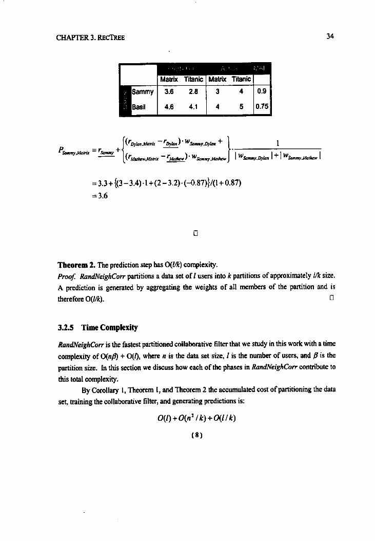
Theorem 2. The prediction step has û(l/k) complexity. Proof: RandVeighCorr partitions a data set of 1 users into k partitions of approximately I/k size. A prediction is generated by aggregating the weights of al1 members of the partition and is therefore O(l/k). U

3.2.5 Time Complexity

RandNeighCorr is the fastest partitioned coilaborative filter that we study in this work with a time

complexity of q n a ) + O(f), where n is the data set size, 1 is the number of users, and /3 is the partition size. In this section we discuss how each of the phases in RandlVeighCorr contniute to

this total complexity. By Corollary 1, Theorem 1, and Theorem 2 the accumuiated cost of partitioning the data

set, training the collaborative filter, and generating predictions is:

Theorem 3. The execution time for RafleighCorr is O(n) for constant partition size p. Proof: Let the partition size be given by n/k. Substituting for f l in ( 8 ) we obtain

RanaWeighCorrYs complexity which is linear in data set size n: O(n@ + O(I) + O(l/k) O

The constraint P is equivalent to h ing the number of item-ratings per partition and we therefore

cal1 b the partition size. By Theorem 3, we know that the execution time for RandNeigI~Corr cm

be linearized for constant values of P. In the next chapter we present out performance study into

RandlVeighCorr and demonstrate the efféct of on its pedomance.

3.2.6 Space Complexiîy

RandlVeighCorr has a space complexity of 0(12/k), where 1 is the number of users and k is the number of partitions.

In the first phase a11 of the users are distributed among k partitions. This requires at most the storage of a Cbyte partition identifier per user; for the entire data set of users this operation requires O([) disk space. in the second phase, the pair-wise similarity coefficients between al1 members of a partition are computed and saved. If there are k partitions, the average number of users in a partition is l/k and the space complexity of computing pair-wise similarity coefficients for a partition is 0(12k) and for al1 k partitions is ~(e/k). Therefore, the total space complexity of RandNeighCorr is:

3.2.7 RandNeighCorrJs Accu racy

The accuracy of a collaborative filter depends upon its ability to locate good advisors. This obvious observation is supprted by the experiment surnmarized in Table 5. In the "AH" column al1 advisors are used in the prediction, while in the ''C 0.1" column oniy advisors with correlation coefficients less than 0.1 are used for prediction. As expected, using only advisor who are p r l y correlated worsens the accuracy of predictions.

All 1 0.87 0.97

Table 5: A eomparhn of CorrCFs MAE with al1 correlates and when only low correlates ( l es than 0.1 correlation) are used in the prediction. A lower score indicates Ligber accuracy.

To improve the execution time, RanàNeighCorr limits the neighbourhwd over which advisors are sought. Intuitively we expect that the accuracy of RandNeighCorr should be affected. The following theorerns confirm this intuition and the corollary proves the result that RandNeighCorr's accuracy diminishes with increasing data set size. This result is somewhat surprising, as a collaborative filter should improve in accuracy as more data is available for it to train on.

Theorem 4. The probability of locating the f globally best advisors in a database of 1 users, which has been partitioned into k partitions of approximately equal size, is ~(llfi.

Proof: The probabiliw that a user's most similar advisor is located in his partition is equal to the probability of being located in any of the k-1 other partitions and is therefore llk, Since users are distributed into each partition randomly and the partitions are independent, the probability that each of the second and subsequent f-1 best advisors is also collocated is also llk. The total probability therefore of locating the f globally best advisors is the product of these probabilities: llkr 17

Theorem 5. The probability of locating the f globally best advisors in a partition is O@ nf) . Proof: RandNeighCorr guarantees its linear execution time by the constancy of the partition size P=nk As the data set size n increases, the number of partitions k mu t also increase to maintain

Ci's constancy. Substituting for P in Theorem 4 we have the probability of locating the f globally

best advisors in a partition: O@?/nf). CI

Coroiiary 2. The accuracy of AandNeighCorr diminishes with increasing data set size. Proof: The accuracy of a collaborative filter depends upon its ability to locate thefbest advisors to draw recommendations h m , By Theorem 5 we know ihat as the data set size increases, the probability of locating these advisors in a partition is O(n-3. 0

3.3.1 Ovewiew

KMeansCorr is a refinement on the RandVeighCorr algorithm. The random assignment strategy of phase 1 is replaced by a clustering algorithrn that subdivides the database into partitions of conelated users. There exists a collection of clustering algorithm that we can choose from F;Ri39] [EKS+96] [ZRL96] [GU981 [AGG+98] [ACW+99]. We make our selection based on the following criteria: the clustering algorithm must have quadratic time complexity or better, be applicable to high dimensional sparse data and be straighâforward to implement. The first criterion is necessary since the raison d'être of this thesis is on the development of a faster collaborative filter; a clustering algorithm that took longer than quadratic time to complete would negate the very benefit that was intended. The second criterion is a necessary applicability condition: each item will be treated as a dimension along which a clustering is sought and the number of users who may have sampled any particular item is usually quite small. The average user of the EachMovie recommendation service [Eh4971 for example, has sampled only 10 movie titles out of a possible 1628. The third criterion, though not necessary, was deemed a desirable property due to tirne constraints for the completion of this work.

Several of the recent clustering algotithms [ZRLgq [GRS98] [AGG+98] [ACW+99] were designed specifically to handle hi& dimensional data in very large databases. Thesi algorithm are disk-based and consequently very efficient when the database is larger than memory. However, this work assumes (and argues in 3.1.2) that al1 of the rating data will fit into memory; the KMeans algorithrn [KIi89] is a very fast in-memory clustering algorithm and with some modification cm serve our purposes. We cal1 this extended clustering algorithm Weuns' and describe it in detail in Algorithm 2. The CF algorithm we cal1 KMeansCow consists of replacing the partition phase (Phase I) of Algorithm 1 with K;Meansc.

It should be noted that our purpose in selecting a clustering algorithrn for phase 1 is neither to locate nor to identify the cluster structure in the data set. We partition the data because we want to improve the execution time of the collaborative filter. In section 3.2 we show that a random partitioning of the &ta resutted in Imear time complexity, but with an increasing loss in accuracy with data set size. KMeansCorr attempts to remedy the deterioration in accuracy by populating each partition with users that are bighiy correlated. Therefore, the purpose of inserting a clustering algorithm into Phase 1 is to seek a 'good' partitioning of the data such that execution

CHAPTER 3. RECTREË 38

time is linearized. impmving accuracy is a secondary objective. We are not using the clustering algorithm to identifL cluster structures in the data.

!&%leans is a straightforward and fast in-memory clustering algorithm. Selecting k random points as temporary centres initializes the algorithm. It then iterates over the steps of assigning points to temporary centres and computing new centres until either the change in computed centres falls below a threshold or the maximum number of iterations is exceeded. KMeans has a time complexity that is proportional to ktn, where k is the number of clusters, r is the maximum number of iterations and n is the number of data points. Consequently, KMeans has linear time complexity with the number of data points.

KMeans has a number of limitations. The seeding of the algorithm with k initial starting centres is problematic - given inappropriate starting centres the algorithm can be trapped by locally optimal solutions. Secondly, the initial centres are chosen by random selection;

consequently, each run of the KMeans algorithm may yield different clusters. Furthemore, KMeans cannot handle missing data. A distance calculation between a point and a candidate clustcr centre can only be canied out if both vectors have fully specified dimensions. FinaIly, KMeuns is susceptible to outliers; the algorithm has no way of detecting and removing outliers h m its calculation of the cluster centre. Figure 8 illustrates some of these conditions. In the

Following subsections we discuss how KMeans' overcomes some of these limitations.

Figure 8: Two different seleetions for the initial centres yield hvo dimerent sets of dusters. Selecting R1 and RZ as the seeds results in cluster Cl and C2, while seleethg seeds R8 and R9 results in the globdly optimal clusters C3 and C4.

333.1 Overview We denote the KMeans clustering algorithm with the extensions described below as KMeans'.

KMeans' can handle sparse data and uses correlation as the distance meüic between users. The KMeans' algorithm has a two-step initialization phase: it tint comptes a default

vector that is part of the strategy for dealing with sparse data (Step 1) and then selects k temporary centres to seed the algorithm (Step 2). It then iterates over the following steps. KMeans' scans over the data set and assigns each vector to the cluster centre that it is closest to. If a vector is missing a term, the default vector supplies it (Step 3). Once al1 the vecton are

assigned, the centroid of each cluster is cornputed fiom the average coordinate of al1 its mernbers and a global counter is incremented (Step 4-5). KMeam' iterates over these steps @tep 3-5) untii the maximum number of iterations t has been exceeded or the cluster centres have stabiIized (Step 6-7).

In the following subsections we discuss each phase of the KMeans' algorithm in detail. The KMeans' aigorithm differs fiom KMeans in its missing value replacement strategy and iis seed selection strategy (Step 1-3). KMeans does not have a way to deal with missing data and it selects seeds by random selection.

Aigoritbm 2. W d e a w , k* t, minChunge)

Input: Y is the ûaining set and is the database of al1 user item-rating-vectors. k is the number of partitions to ma te and k CC (4. minChange is the change in the cluster centres' position below which we assume the clusterhg algorith has convergd while t is the maximum number of iterations we aUow before tdnating the clustering algorithm. Output: k partitions that are characterized by theù centroids: cl, c?,.., ck Method: The partitions are computed using the following procedure:

Compute the default vector r, of Y as the cenûoid: = r , i E Y

Select k-mutualty-well-sepmted centres: cl, c ~ , .. ck

Assign each vector in Y to the cluster, Cj whose centre Cj is most correlated. Use the default vector, r, for missing value replacement. Compute the centre of each cluster from the average of its members.

CI = Lri/l(J , ie ci iterations.t-t. If iterations > t then goto Step 3

If the change in ail of the clusters' position relative to the last iteration is above the threshold, minCfmge, &en goto Step 3

d(cj, c,Pm) C minchange l l j i k STOP.

3.3.3.2 The Missing Vaiue Replacement Stralegy The item-rating vectors in CF applications are very sparse with many t e m that have the "no

rating" value, 8, This presents a problem to out clustering algorithm since a distance metric can only be computed over nurneric values. We propose to handle this problem by using a default vector for missing value replacement (Step 3). In Figure 9 we show a Euclidean distance calculation between the item-rahg vectors r, and rz with missing values replaced by the default vector r, Each ceil consists of an item identifier and rating score pair; the "?" indicates a missing value. User r, for example rates item 3 with a score 1 and has not rated items 1, 12 and 36.

A default vector is used to replace missing values in tbe user's rathg vector. It therefore represents a guess at how the user wiU rate an item once he has seen it. This replacement strategy is necessary for our clustering algodthm, which requins fd1y specified vectors,

How do we compute a default vector? By definition, a collaborative filter provides us with these rnissing ratings since its very purpose is to compute predictions for items that the user has yet to see. Selecting a petsonalized recommender for this task is circuitous; we are using a clustering algorithm to speed up a collaborative fiiter but we are using a collaborative filter to ïnitialize the clustering algocithm. Can any peirformance gain be realized with this arrangement? Personalized recommenders have at best quadratic complexity and introducing them into our algorithm would create a performance bottleneck. Selecting a non-personalized recommender is a different story however. Non-personalized recommenders have the potential to benefit the clustering algorithm since they are very fast.

We select the population average recommender, "PopAvg" for brevity, to generate the

default vector. PopAvg generates a value for each term in the default vector by computing the average rating of an item. The default vector as computed by PopAvg is equivalently the cluster centroid if we view the data set itself as a cluster. PopAvg is a fast recommender and c m compute the default vector with a single scan over the data set. The PopAvg recommender is used to compute the default vector in Step 1 of the KMeans* algorithm.

Figure 9: The dehult vector provides midng values.

Example 5. The default vecior for the video database is computed usuig the PopAvg recommender and summarized in the table below.

Star&@ Slwpless Trooper in Seattle MI-2 Matrix Titanic

3.7 3.5 3.5

Figure 10: Tbe defauL vcetor is computed for the video database using the PopAvg rccommender.

Theorem 6. The default vector is computed in O(n). ProoJ PopAvg cornputes the default vector. PopAvg requires a single scan of the database to accumulate the average rating for each item and therefore the default vector is generated in O(n) where n is the size of the data set. n

3333 The S4ed Selection Strategy The selection of the initial seeds for the KMeans algorithm is a subtle issue. Selecting poor seeds can result in the algorithm gravitating CO locally optimal solutions. One approach to overcoming this problem is to execute the KMeans algorithm severai times (selecting a new random set of seeds during each execution) and choosing the best clusters fiom the result sets. Another approach involves executing KMeans on a sub-sample of the dataset [BP98]. However, both of these approaches only impmve the probability of locating the globally optimat solution. They do not guarantee it.

Fortunately, in this work a gIobally optimal clustering is not necessary. We use the

WeansC algorithm not as a means to discover the cluster structure in the data set, but as a means to create partitions of correlated users.

Furthemore, we want the KMeanst aIgorithm to mate partitions of approximately equaI size, otherwise the partitioned collaborative filter wilt not scale Iinearly. if for example k-1 ciusters of size t and t cluster of size n-k+l are created, the cost of training the collaborative tilter will be ~(n-&+l)' - O@?. On the other hand, if k cluters each of approximately n/k size

are created, the cost of training a single partition is 0(n/k)' and the cost of training al1 k partitioning is O(&') which is linear with the data set size n.

KiMeans' selects its seeds using a strategy that we cal1 k-mutually-well-separated centres (Step 2). This procedure picks seeds, which under certain conditions (see Proposition L), increases the probability that KMeam' will create clusters of approximately equal size. The procedure we follow to achieve this is as hllows. FUst, fiom the database of user item-rating vectors Y, select the vector îhat is farthest tfom the rathg centroid (i.e. the default vector) and add it to the set P. Until p] is k, iteratively select vectors fiom the set Y-P whose sum of distances to al1 members of P is greatest. b Figure 8, the principle of k-mutually-well-separated centres would result in the selection of the points R8 and R9. Notice that this selection of seeds results in the KMeans' algorithm converging to the globally optimal clusters C3 and C in Figure 8.

This approach to seeding the Means' algorithm may be criticized for increasing its susceptibility to outliers since outliers tend to be points that are distant fiom other points [GRS98]. However, the partitioning phase oPKMeansCorr is intended to tind neighbourhoods of approximately similar users. The final computation for similarity is camed out in Phase il with a pair-wise evaluation. Consequently, a partition that includes some outliers merely results in the cost of computing their similarity to other users, but has negligiblc effect on the prediction since these users will have low sirnilarity scores.

Example 6. in this exarnple, we apply the principle of k-mutually separated centres to select two temporary seeds fiom the video database. The default vector, as computed in Example 5, is used to replace the missing values in the training data for Sammy and Basil's ratings of Matrix and Tilanic.

Gum-Fat is the furthest fiom the origin with a value of 8.54. We next compute the distance fiom Gwn-Fat to the other members of the database. Beatrice is the fiirthest fiom Gum- Fat and therefore we selected her as ihe second seed.

if we need to select three seeds, the next candidate will be selected on the basis that h iher total distance to Gum-Fat and Beatrice is the greatest.

Table 6: The default vector is computed for the video database using the PopAvg rceommender.

Thmrem 7. The cost of locating k-rnutually well-separated centres is ~(pn ) . Proof: The selection of the ih seed requires a single scan over the daiabase (of size n-i) and i-I cornparisons with the other members already in the set P. By induction, the cost to select k seeds is at most k(K-l)n - O(&). O

Proposition 1. When k=2 and the data distnlbution is Gaussian, the principle of "k-mutually well separated centres" results in two clusters of approximately equal size.

Proof For k=2 the two seeds fonn the diameter of the rating-space volume. Since the data has a Gaussian distribution, each seed lies at the opposite 'iails' of the distribution and haIf of the data will k closest to each. As a result of these conditions the KMea~is' algorithm will stabilize at two clusters of approximately equal six.

333.4 The Distance mebic The KMeans algorithm assigns each point to the cluster centre that it is closest to. However, we have yet to specify what memc will be used to compute distance. Metrics that have been used for KMeans clustering include: Manhattan distance, Euclidean distance, and the oîher Lp rnetrics [KR89]. For our application, we want neighbourhoods of users who are highly similar in rating behaviour. Since phase II of KMeansCorr uses correlation to compute similarity (Le., Compu~eComelafionSimifan~~..) ), we wiil also use correlation as the distance metric for the clustering (Step 3) to obtain partitions of highly correlated users.

Unlike the Lp metics where a smaller value denotes proximity, larger values denote proxrmity m correlation space. in correlation space the user is "closest" to the cluster centre to

which his correlation score is the highest. The comlation between ratings can range h m -1 to 1. A value of 1 denotes that the ratings are perfkctly carelated and two users occupy the same point in correlation space. A value of -1 denotes anti-correlation; the users' rating behaviour are opposite and the two users are maximally distant.

The KMeam' algorithm therefore assigns each user to the cluster centre to which his or her cotrelation caefficient is the maximum.

Example 7. in this example, we demonstrate the partitionhg of the vide0 database into two partitions using the KMeans' algorithm. The hvo-step uiitiaIization of the algorithm is shown in Example 5 and Example 6 where the default vector and the cluster seeds are selected, respectively. The training set is shown in Table 6 where the default vector has been used to replace the misshg values for Sammy and Pasil (the shaded cells). The cluster seeds are shown in the table entries for cl and c2 for the set of tables labelled Iteration 1.

lteration 1

Starship Sleeptess MI-2 Matrix Tiinic 3.0 4.0 4.0 3.0 4-0 3.0 1.0 1 .O

in the fust iteration, the correlation between each user and the cluster seeds c 1 and c2 are computed. We see that Sammy, Beatrice, and Dylan are closest to the cluster centre cl, whiIe Mathew, Gum-Fat, and Basil are dosest to c2. The new centroid of each cluster is computed from its members, yielding the new centres c3 and c4 (shown in the [teration 2 tables).

In the second iteration, the correlation calculation yields two clusters with the same members as in the previous. We c m therefore tenninate KMeans" as the cluster centres have stabilized. The &Mepnsf aigorithm therefore created two clusters with members {Sammy,

Beaûice, Dylan) and wathew, Gum-Fat, Basil) respectively.

CHAPTER 3. RECTREE

lteration 2

Theorem 8. KMeuns' has time complexity of O(n) + O(&%) + q k t n ) .

Prooj: By Theorem 6 the cost to compute the default vector is O(n), where n is the daia set size. By Theorem 7 ihe seed selection strategy has complexity qpn) where k is the number of seeds to select. During an iteration (Step 3-6) each point must be compared against k tempocary centres and a complete iteration therefore requires kn comparisons. The algoriihm is buunded by the lirnit of t iterations and consequently the complexity for the iterative phase is kln, The total complexity is linear with the size of the data set: q n ) + O(&) + O ( h ) O

3.3.4 Time Complexity

KMeansCorr has complexity of 0(n2), w h ~ e n is the data set size. Let be the average number of item-ratings per user and 1 be the number of users in the data set, then d e h e n as the size of the data set given by d.

KMeansCorr partitions the data set in Phase 1 using the KMeans' algorithm. It trains the collaborative filter in Phase €I by computing pair-wise correlation coefficients with the subroutine CumputeCorreIationSimilariiy(..) and genetates predictions in Phase III with the subroutine ComputeDeviationFromMeanPrediction(..). Theorem 8, Theorem 1, and Theorem 2 give the accumulateci cost of these phases:

Theorem 9. KMeansCorr has time complexity of 0(n2).

Proof: imposing the constraint that n/k = f l is a constant, the training and prediction phase of

KMeansCorr can be linearized. However, substituting for fl in ( 9 ) we fmd that the partitioning

phase's complexity is cubic under this constraint: O(n) + O(nJ/f) + 0(tn2fl). Therefore the best achievable time complexity is 0(n2) and is achieved by allowing the partitioning phase to complete in linear time and executing the training phase in quadratic time. Ci

KMeans"s complexity is dependant upon both the number of item-ratings n and the number of partitions k. The best achievable complexity is 0(n2) and is obtained by fnhg the nwnber of partitions k. This results in the partitioning phase completing in linear time, but the training phase completing in O($) time. Despite the disappointing result this approach is instructive and we draw a number of lessons from it:

The training and prediction phase consisting of CornputeCorrela~ionSimilariSr(..) and

ComputeDeviationFromMeanPrediction(..) can be made lincar if the partition size P is kept constant.

The partitioning phase consisting of KMeans' can be made linear if the number of partitions k can be kept constant.

The KWeansCorr algorithm has quadratic complexity at best, because it cannot optirnize the partitioning and prediction phase independently. in section 3.4, we describe a new algonthrn, RecTree, that builds upon fiNeans' and is linear in complexity.

3.3.5 Space Complexity

KMeans' has a space complexity of O(f) + qh), where 1 is the number of users in the data set, k

is the number of partitions and m is the size of the item set, M (i.e.: m = [w). During each iteration, users are assigned to the cluster centre that is closest, This operation

requires at most 4-bytes per user to store the current cluster identifier. Each iteration of the algorithm can overwcite this identifier since a history of cluster identifias is not requkd. Storing the cluster identifiers for al1 1 users therefore requires O(4.

Each of the cluster centroids may span the entire item space and therefore each centroid requires at worst O(m) storage. For k partitions the storage for al1 centroids is O(km).

3.4 Rec Tree

3.4.1 Overview

RecTree is the acronym for a new data structure and collaborative filtering algorithm called the RECommendation Tree. The RecTree algorithm partitions the data in phase 1 by recursively calling KMeans' to split the data set into child clusters. The chain of intermediate clusters leading fiom the initial data set to the final partitionhg is maintained in the RecTree data structure, which resembles an unbalanced binary tree. The collaborative filter is trained in Phase II by cornputing the pair-wise similarity coefficient within each leaf partition using a more accurate similarity metric that we cal1 correlation'. The intemal nodes are processed by the collaborative filter by computing the rating centroid based on the item-vectors in its sub-tree. The RecTree generates a prediction in Phase iIi by employing a dual strategy. if the user is loçated in a leaf partition with a suflcient number of neighbours, taking the weighted deviation fiom the mean generates a prediction. if the user is located in a small neighbourhwd, RecTree generates a prediction by retuming the neighbourhood's average rating.

A prediction request is made by passing a message directly to a tree node for pmcessing. A cecornmendation message takes the form of 2 integer identifiers and a double representing the prediction. The RecTree responds to a message by filling in the prediction Field in the message.

1 UserlD: integer 1 IternlD: integer 1 Prediction: double 1 in the subsections below we descni in detail how to construct the RecTree and then how

to query it for recommendations.

3.4.2 Constnicting the RecTree

The ConstructRecTree(.J routine builds the RecTree data structure by recursively splitting the data set Y into child clusters until stopping conditions are met. ConstmctRecTree(..) interleaves Phase 1 and Phase ii of our hmework by partitionhg the data and training the collaborative filter during the course of building the tree.

During each iteration a node is associated with the cunent data cluster and a bi- directionai Iink is created to the predecessor (Step 2-3). The routine then classifies the node as an intemal node, an outlier node, or a leaf node by checking the size of the cluster. if the node is

classified as an interna1 node, the KMeans' splits the current data cluster into two child clusters and the Constn<crRecTree(.) routine is recursively called to insert each of the child clusters into

the tree (Step 7 & 9). A node is classified as an outlier if it has fewer ratings than the threshold outliersize and

classified as a leaf if it has fewer ratings than the partition size parameter P (Step 4-5). A leaf node represents the final partitioning of the data and as such is ready to be traïned on by a collaborative filter; the subroutine ComputeCorrelationSirnilarity+(..) trains the collaborative filter on each leaf node (Step 5).

A node that is not classified as an outlier or a leaf is by definition an intemal node. intemal nodes implement the secondary prediction strategy and train an average rating vector from al1 of the members of that node.

The RecTree's construction is complete when the growth along every branch has been tenninated. In addition to outlier and leaf nodes, the global iteration threshold g can also terminate the tree growth. if the RecTree has recursed more than g times then the recursion at every branch is terminated (Step 5).

The primary pwpose of the RecTree data structure is to seek a 'good' partitioning of the data set such that the complexity of delivering recommendations is linearized. Improving the accuracy of predictions is a secondary objective. As with the KMeansCorr algorith, the partitioning phase of RecTree is not intended to identiQ nor locate cluster structures.

in the following subsections we describe details of the algorithm and discuss the rationale for the design,

Algorithm 3. ConstrucîRecTtee(parent, Y, g,outlicrS1w)

Input: parent is the parent of the current node. Y is a database of user item-rating vectors. p i s the threshold at which to stop subdividing a partition. g is the maximum number of times that this method will cal1 itself before terminating. outlierSue is the threshold at which a leaf node is marked as an outlier node, outlierSize < p. Output: The RecTree. Metbod: The RecTree is constmcted by calling this method recursively. On the first invocation, the argument, parent, is NULL. 1 . If parent is NULL then

Set global-iterations = 0. 2. Build a node V and create a bidirectional link between V and parent. 3. Assign al1 members of Y to V. 4. if IY/ < outlierSize then mark this leaf node as an outlier node; STOP. 5. if IV OR (giobai-iterations > g) then

Co~nputeCorrelationSiniiari~+(y); STOP. 6. Compute the centroid, cy of Y. 7 . Cal1 KMeans'(Y, 2, t, minchange). 8. globalitera tions*. 9. For each child cluster Y':

Cali ConsrructRecTree(V, Y', /l, g, outlierSire).

Figure 11: The RecTree data structure. Leal nodes have a similarity matrix while each internal node maintains a raîing centroid of its sub-tree. Each node has a bidirectional link with its parent.

3.4.2.1 Node Spiitting The RecTree is grown fiom the root downwards by node splitting. How do we decide

when node splitting can be terminated? Hierarchical divisive clustering methods continue splitting a cluster until a quality threshold is reached. Memcs such as minimum, maximum, and average distance have been used to control the splitting F;R89]. However, each of these mettics may lead to clusters with a small membership. This condition is not appropriate to ow application since the size of the partitions affects the coverage of the collaborative filter. A smaller

neighbourhood implies fewer candidate advisors From which we can draw recommendations (See Figure 4). Therefore, in this work we investigate the use of a minimum neighbourhood size as a

clustering control. A node that contains more item-ratings than the threshold, /3, is split.

Equivalently, a node that has fewer than /j item-ratings is classified as a leaf node and growth along that branch is terminated (Step 5).

Once the decision to subdivide a node has been made, we employ the KMeans' algorithm described in 3.3.3 to cluster the data into hvo partitions (Step 7). KiMeans' is suited to the task since it can handle sparse multidimensional data and has linea. complexity with data set size n

when the number of partitions, k, is held constant and independent of n. We satisfy this requirement in ConstructRecTree(..) by always calling Means' to split each internal node to

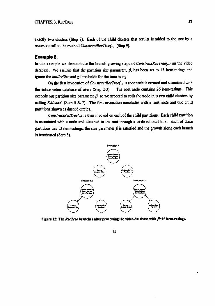
exactly two clusters (Step 7). Each of the child clusters that results is added to the tree by a recursive cal1 to the method C~nstructRecTree~.) (Step 9).

Example 8. in this example we demonsûate the branch growing steps of ConstructRecTree(..) on the video

database. We assume that the partition size parameter, p, has k e n set to 15 item-ratings and ignore the outlierSire and g thresholds for the time king.

On the first invocation of ConstmctRecTree(..), a root node is created and associated with the entire video database of users (Step 2-3). The root node contains 26 item-ratings. This

exceeds our partition size parameter so we proceed to split the node into two child clusters by

calling KMeans' (Step 5 & 7). The first invocation concludes with a root node and hvo child partitions show as dashed circles.

ConstructRecTree~.) is then invoked on each of the child partitions. Each child partition is associated with a node and attached to the root through a bidirectional link. Each of these

partitions has 13 item-ratings, the size parameter P is satisfied and the growth along each branch is terminated (Step 5).

Figure 12: The RecTree branches after processimg the video database with fi15 itemratinp.

3.4.2.2 The Maximum Iteration LMt, g

For some data disûiiutions, the hierarchical clustering we propose may result in an over- partitioning of the data. Figure 13 illustrates one hypothetical data disûiiution that would be

partitioned into n-/3 clusters of size I and one cluster of size B. Clearly the calculation of

recommendations on this pathological data distribution and others similar to it would not benefit from any form of clustering. The small clusters would be useless since they have too few advisors from which to draw recommendations. A straightforward application of a collaborative filter on the un-partitioned data would have yielded the same recomrnendations in shorter time.

We therefore propose to avoid these problematic data disûiiutions by limiting the maximum number of times that the &ta cm be subdivided using an iteration threshold, g. Each time that a node is split we increment a global iteration counter (Step 8). We then test to see if the threshold g has been exceeded on each invocation of CmstructRecTree~,) (Step 5). g can equivalently be viewed as a limit on the maximum number of intemal nodes in the RecTree, as demonsûated in Corollary 5.

Figure 13: Building a RecTree on an exponenîial data distribution with f l= 16 creates 4 clusters witb

one user each and 1 cluster with 16 users.

Lemma 1. The RecTree bas at least n/B leaf nodes. Proof. Assume that g is an arbitrarily large number. For a given data set with n item-ratings, the

RecTree partitions the data until d l nodes contains Bor fewer item-ratings. When each partition

has exactly /3 item-ratings, there are a minimum number of leaf nodes given by n@. 0

CoroUIvy 3. if the RecTree has n/p Ieafnodes then each leaf node has /3 item-ratings.

Proof: if a data set of n item-ratings is partitioned into clusters of /3 size then there are

n@ clusters. O

Lemma 2. The RecTree has at most n-&tl leaf nodes. Proof. Assume that g is an arbitrarily large number. Suppose on each of i" recursive calis to ConstmctRecTree(..J the node v~~~ with niml members is subdivided into the two child nodes v'i and V" such that 1vli[ = 1 and lvZil =ni = ni.,-l. Then ConstmcrRecTree~.) will be called n-/3 times - each recursion yielding another leaf node of size 1. On the n-fl " recursive call, two leaf

nodes are created, one of size 1 and another of size p; the total number of leaf nodes is therefore

n - p l . if during any iteration, [ ~ ' ~ l > 1 , then ConstructRecTree(.) will recurse fewer than n-B times and therefore yield fewer leaf nodes. Therefore RecTree has at most n-&tl leaf nodes.fl

Corollary 4. If the RecTree has n - p l leaf nodes then there are 2 leaf nodes whose total size is P and n-#l nodes each of size 1.

Proof: By Lemma 2 there are at most 2 leaf nodes whose size is greater than 1 otherwise the tree

has fewer than n - p l leaf nodes. I l

Lemma 3. The RecTree has at most g intemal nodes. Proof. On each cal1 to Constnr~rRecTree~,), a leaf node is split into two child nodes. The former leaf node increases the population of intemal nodes by 1. Afier the i" recursive cal1 to CorrsirucrRecTree(..), there are i intemal nodes. By induction, if the construction terminates aAer recursing at most g times, there are g intemal nodes. O

Lemma 4. The RecTree has z+l leaf nodes where z is the number of intemal nodes. Proof: On each recursive call to ConstmctRecTree(..), a leaf node is split into two child nodes. The former leaf node becomes an intemal node and the two child clusters are by definition leaf nodes and the population of leaf and interna1 nodes increases in total by 1. By induction, afier the i" recursive call to ConstnrcrRecTree(..), the population of leaf and intemal nodes has increased by i members. On the fmt invocation of ConstructRecTree(.J the tree has exactly one leaf node, the root. Therefore the total population of leaf nodes aAer the ith invocation is z+1 where z is the number of leaf nodes. O

Corollary 5. The RecTree has at most g+l leaf nodes. ProoJ: By Lemma 3 and Lemma 4

Theocem 10. The branches of the RecTree can be constructed with complexity O(gtn). Proof: The branches of the RecTree are grown by recursively calling the KMeans' algorithm to split a node into two child clusters until the partition size parameter is satisfied or a maximum recursion threshold g is exceeded. By Theorem 8 the complexity for each invocation of KMeans' to create two child clusters is: O(n) + O(4n) + 0(2tn), where n is the data set size and t is the maximum number of clustering iterations. KMeans+ is invoked at most g times and

consequently, the total complexity of inserting the branches is O(5gn) + O(2gtn) - O(gtn) since PI. a

3.4.23 The Tree Nodes Every node that is added to the RecTree has a bidirectional Iink connecting to its

predecessor and a reierence to a cluster of data (Step 2-3). The RecTree filter is trained as each node is attached to the tree. As a conseqwnce of RecTreeYs dual recommendation strategy (see 3.4.3)' the filter's training depends upon the node type. In the following three sections we

discuss how each node type is used to irain RecTree's filter.

3.4.2.4 Training on the Leal Nodes RecTree's filter is trained on the leaf nodes by computing a similarity matrix behveen al1 members of the partition. The leaf nodes provide the coefficients by which advisors' recommendations can be weighted in aggegate to generate a personalized prediction. We propose to use an enhanced version o i the correlation similarity measure, that we cal1 correlation', to compute pair-wise user similarity.

The design of correlation' is motivated by a number of observations in regard to the recently proposed similarity metrics. In the statistical collaborative filters proposed by [RIS+94] and [SMgS], pair-wise similarity is computed using only the ratings for items that both users have rated. if the item intersection set is small, then the proximity coefficients are poor measures of similarity as they are based on too iew item-rating comparisons. Furthermore, an emphasis on similarity based on the intersection set neglects the global rating behaviour that is reflected in a user's entire rating history. The following example illustrates these problems.

Example 9. Sammy and her tnends have the rating history shown in the table below. A similarity measure that considers only items in the intersection set ({Starshi$ Trooper, Sleepless in Seattle, MI-2)) would render Beatrice and Dylan indistinguishable and equally valuable advisors for Sammy-

However, if we look at the entire rating history we note that Dylan appears more similar to

CHAPTER 3. RECTREE

Sammy than Beatrice and Beatrice exhibits a greater rating volatility in cornparison to Sammy and Dylan. This intuition is confimd in the table columns that summarize the "global" average rating and standard deviation of ratings. These values are computed fiom al1 of the available rating data in the video training set.

Starship Sleepless MI- Trooper in Seattle 2 Matrix Titanic

Table 7. A calculation of the average rating and standard deviation over the longer histoiy indicates

that Dylan is more sinûlar to Sanuny than Beatrke.

We believe a coHaborative filter that took into account global nting behaviour would be more accurate. It would locate advisors that were globally more similar to the active user rather than advisors that exhibited only local similarities. We incorporate this intuition into the design of correlation'. This measure diffm from the standard correlation-based similarity calculation in that the mean rating and standard deviation a are computed over the entire set of items rated by each user.

Extending the set of items over which a similarity measwe is computed should impmve the metric's accuracy in caphuing user similarity. The i-statistic for the correlation coefficient is proportional to the square rwt of the sample set size [HM851 and therefore increasing the number of ratings increases the confidence of the correlation calculation. How do we extend the set over which the correlation is computed given that user ratings are sparse? As in the KMeans' algorithm we employ a missing value replacement strategy, We replace missing values in a user's item-rating vector by the values in a default wctor.

The semantics of the default vector in this discussion are the same as those in the means+ clusterhg algorithm. SpecificalIy, the default vector represents an estimate of the user's rating for items b t he has yet to rate. Although it would be ideal to compute a

personalized default vector for each user this approach is infeasible. Personalized recommenders have quadratic complexity at best and their operation would introduce a bottleneck into our linear recommender. We therefore select the non-personalized recommender, PopAvg, to generate the default vector. PopAvg provides the same prediction for every user and requires only a single scan to train. The default vector as generated by PopAvg is equivalently the rating centroid of the leaf partition.

The subroutine ~om~ureCorrelationSirnilarity+(..) computes a more accurate measure of user similarity with a higher confidence by using the global values of mean rating and standard deviation and by extending the intersection set wiîh a missing value replacement strategy.

Subroutine 3. ~ o m ~ ~ t e ~ o r r e k d o r r ~ i ~ ~ ) ~ a r i h + f Y )

Input: Y is a set of user item-rating vectors. Output: A square matrix of pair-wise similarity coefficients between al1 members of Y. Metbod: The similarity weights are computed in the following manner: 1. Compute the default vector r, of Y as the ceniroid:

r # = XrAq , ~ E Y 2. For each user r, compute the pair-wise similarity wa,, to each other member ru using Pearson correlation over the set of items they botb have rated (Yabu). Use the default vector to replace missing values in each user's rating vector. The average rating and standard deviation of each user is computed over the entire set of items that each user has rated (Y,)

Y, , = { k [ k ~ M u r , ~ *@orryst f @)

Example 10. The table below shows the correlation and correlation' coefficients for the video database. The correlation coefficients are computed only over the titles Starshb Trooper, Sleepless in Seattle, and MI-2. Correlation' is computed over al1 five titles with the missing ratings for Sammy and Basil estimated by the default vector.

Beaûice and Dylan are indistinguishable to the correlation metric; they are perfectly correlated to Sammy. Correlation+ captures the global similarity between these advisors and Sammy and distinguishes them by assigning a signifiçantly higher correlation coefficient to Dylan in comparison to Beaûice.

1 1 Stanhip Sleepless 1 Trwper in Seaîüe MI-2 Malrix Titanic

(R) (A) (A) (R) orrelation Correlation'

Beatrice 3 4 3 1 1 1 .O0 0.21

Dylan 3 4 3 3 4 1 .O0 0.98

Mathew 4 2 3 4 5 -0.87 -0.25

Gum-Fat 4 3 4 4 4 -1 .O0 -0.75

Tabk 8. A comparison of the correlation coefficients computed by ComputeCorrelationSimiIarity4 (denoted by column Correlation*) with those by ComputeCorrelationSimiIarity (denoted by column Correlation).

n

Proposition 2. The confidence of coefficients as computed by ConrputeCorrelationSimilariry' is higher or equal to than those computed by ComputeCorrelationSimilariry.

rJ9-2 Proof: The confidence of a correlation coefficient is given by the t-statistic [HM85]: t = - J i 7

where r is the correlation coefficient and q is the nurnber of samples. Since ComputeCorrelationSimilariry+ cornputes the correlation over the set of items that both users have rated rather than just the items that they have rated in cornmon, the confidence of the correlation coefficients generated by CompuieCorrelationSimilarity+ is higher or equal to the confidence of coefficients generated by ComputeCorrelationSimilat-ïty.

3.4.2.5 Trriining on the Interaal Nodes RecTree9s filter is trained on the interna1 nodes by computing the rating centroid of each node. The rating centroids represent the average voting preference for each item among the memôers of that neighbourhood (node). The rating centroids provide the data to support RecTree's dual recommendation strategy.

3.4.2.6 Training on the Outiier Nodes In this collaborative filtering application we consider outliers as individuals whose preferences lie outside of the main of the crrrrent membership. However, as new users join the system or existing members rate additional items, these outlying individuals may find themselves among a group of like-minded members and Chus cease to be outliers.

This perspective of outliers motivates us not to discard nor discount outhers, as cwtomary in cluster analysis. Rather, we retain them in the leaf nodes of the RecTree until such time that enough Iike-minded individuals appear. [Gui1841 recognizes outliers as data points that are distant h m other data points. [as+%] considers a point as an outlier if the regional density is below a threshold. We modify this intuition for our CF application: RecTree marks a

leaf node as an outlier node if it contains kwer than outlierSire item-ratings.

Exam pie 1 1. in this example, we demonstrate the training of the RecTree collaborative filter on the video database. During the first invocation, an intemal node is created and the fitter is trained by computing the rating centroid. In the second and third invocation, a teaf node is attached to the tree. The collaborative filter trains on the leaves by computing a similarity matnx for each leaf partition.

Figure 14: The ReeTree's collaborative filter is trained as nodes are attriched to the tree.

O

Tbeorem 11. Creating the leaf nodes in the RecTree is O(nfl. Proof; The training of the collaborative filter on a leaf node requires the population of a

similarity matrix, which is O@) where is the partition size. We estimate the complexity of

training al1 the leaf nodes by examining the case when the minimum and maximum number of leaf nodes are created. By Lertuna 1 and Corollary 3, the cost of training on the minimum

nurnber of leaf nodes is O(nS). By Lemma 2 and Corollary 4, the cost of training on the

maximum number of leaf nodes is q n - P ) + O@). The cost of training on the leaf nodes is at

therefore at worst O(@). 5

3.4.3 Computing a Prediction

RecTree employs a dual strategy for generating predictions. When the size of the neighbourhood is sufficient, a prediction is computed by taking the weighted deviation fiom the mean. When the neighbourhood is small, a recommbdation is computed by taking the rating average. RecTree's dual strategy is based on the observation that the accuracy of personalized recommenders diminishes greatly when the neighbourhood is srna11 [SKB+98] [GSK+99] EKM99aI. Furihemore, for very small neighbourhoods the accuracy of the non-personalized recommender PopAvg surpasses that of the personalized recommenders. By seIecting an appropriate value for

outlierSize, the threshold at which RecTree switches between its recommendation sûategies can be controlled.

A prediction query message consisting of a user and item identifier is passed directly to a tree node for processing. How do we locate this node? We simply follow a pointer in the user data structure that links the user record with the tree node that he resides in. The manner in which each type of node processes a request is detailed below.

Leaf nodes implement RecTree's primary prediction strategy. They compte a prediction by taking the weighted deviations from the advisors' mean. The subroutine ComputeDa,iationFromMeanPrediction(..) described in 3.2 is used for this pwpose. However the weights w, are those computed by the subroutine ComputeSimilarityWeightt(..). if a leaf cannot provide a prediction due to rating sparsity (i.e. the user's advisors have yet to rate the item of interest) then the request is delegated to the immediate parent (intemal) node.

Outlier nodes by definition have small neighbourhoods and given ow earlier discussion will generate poor predictions. An outiier node is used by RecTree to mark the transition to the second recommendation strategy, Any user that resides within an outlier node has recommendation requests bounced to the immediate parent (intemal) node.

Intemal nodes implement the secondûry prediction strategy. Each intemal node maintains an average item-rating vector that sununarizes the rating behaviour of al1 the users in its sub-tree. An interna1 node can therefore answer a recommendation request by retuming the average rating of its membership for that item.

RecTree's dual recommendation strategy is intended to overcome the deterioration in accuracy at low item-rating densities. It switches to the more robust non-personalized recommendation strategy of population averages when the size of the neighbourhood is small. When the neighbourhood is large, RecTree uses the prediction subroutine Compute13eM'utionFromMeanPrediciion(.. This subroutine is more accurate with large neighbourhoods since it has a larger pool of candidates in which to seek good advisors. When the pool of candidates is srnall, the weighted recommendations are less accurate since the subroutine has fewer advisors on which to base a recommendation.

The outlierSize threshold conaols the transition between the two recomrnendation smtegies. if the outliersue threshold is set to O, a leaf node terminates every branch of the RecTree. The leaves handle al1 of the recommendation requests and RecTree degenerates to a single prediction strategy using ConiputeDeviationFronzMeanPrediction(.(.) if outliersue is set

larger than the partition size parameter f l then an outlier node terminates each branch of the

RecTree. Al1 recornmen&tion requests are handled by retuming the neighbourhood's average

rathg for the item of interest and RecTree degenerates to non-personalized recommendation via population averages.

- -- - --- - -

Subroutine 4. OuervRecTreefSJ Input: Sis the test set and is the database of al1 user "no-rating" item vectors; each vector is the set of items for which the user has yet to rate and for which we would like RecTree to produce predictions. Output: A mapping of each element of each vector of S into a rating score or "no rating", 8. Method: A prediction is computed in the following manner: For each user r, in the test set, S:

For each item i, in r,: i. Create a recommendation message, recMess(a, i, ?) ii. Descend the RecTree to the maximum depth. iii. if the user is located in an intemal node, Ch, and ch is the node centroid then

pm,i = ~c(i)- iv. If the user is located in a leaf node Call Co~nputeDeviationFrontMeanPrediction~.) v. If the user is located in an outlier node then

ascend up the link to the parent node, Ck with centroid q.; return pusi = q(i)

Example 12. in this example we generate Basil and Sammy's predictions for Matrii and Tilanic using the RecTree. Each user's data structure has a pointer linking the user to the RecTree node that he resides in. 90th users reside in leaf nodes (see Figure 14) and so the subroutine

ComputeDeviationFromMean(.(.) is called to generate predictions. The weights for the

predictions are denved h m the similarity matrix of each leaf.

Figure 15: The RecTree's collaborative fiter is trained as nodes are attached to the tree.

Theorem 12. The RecTree generates predictions with complexity Proof: An intemal node provides a recommendation in constant time by consulting its centroid. A leaf node provides a prediction by weighting al1 of the advisors in the partition. Given that the

average size of a partition is p, the complexity is 00. O

3.4.4 Updating the RecTree

An active CF system is continually collecting new item-ratings on existing users and increasing its membership. in this section we discuss how the RecTree is updated when a new user with a history of item-ratings is added to the system. An existing user who submits additional ratings or makes changes to his existing ratings can be modelled conceptually by deleting the user and then re-inserthg the user into the RecTree.

A new user is added by descending the tree until the leaf node is reached or it is not possible to proceed. At each intemal node, the user item-rating vector is compared to the cluster centres of each child node. The branch with the closest cluster centre is descended. If both branches are equally distant from the user, then neither branch is taken. The user is associated with the tenninating node and the cluster centres on the path leading back up to the mot are updated to reflect this new member,

if the user's descent reaches a leaf node VL, a node splitting operation may be îriggered if

the node size exceeds the threshold p, othecwise the similarity rnatrix is simply updated with a

cal1 to ComputeCowelationSimilarityC(..). The ConstructRecTree(..) routine is called to grow the sub-tree beneath VL.

A user is removed from the RecTree by updating al1 the cluster centres on the path to the rmt. if the user resided in a leaf node, then the similarity maûix is updated by dekting the appropriate column and row entn'es.

CHAPTER 3. RECTIUE

3.4.5 Time Complexity

The RecTree can be constructed in O(n) and quet-ied in constant time. Let g be the average

number of item-ratings per user and 1 be the nurnber of users in the dataset, then defme n as the size of the data set given by d.

The partitioning and the collaborative training phases of our hmework are interleaved in the construction of the RecTree data structure. By Theorem 10 and Theorem I l the total

complexity of these two phases is O(@n) + O(nS), which is linear with data set six. By Theorem

12 the RecTree can be queried in 0 0 , which is independent of the size of the data set n.

3.4.6 Space Complexity

RecTree has space complexity of O(g(rn+l)) + 0(P'k/m2) where g is the maximum nurnber of

intemal nodes, nt is the number of items in the item set M, /3 is the partition size, 1 is the number of users, and k is the number of partitions.

Each branch of the tree requires constant space to store a link between a parent and a child node. From Lernma 3 and Corollary 5, we h o w that there are at most 2g+l nodes and therefore the storage requirements for the links is O@).

intemal nodes require storage for their centroids, which at worst will be required to span the entire item space. if m is the number of items in the item set M then each centroid will require O(m) storage. There are at most g intemal nodes and therefore O ( p ) storage is required to store al1 of the intemal nodes.

The leaf nodes require storage for the similarity coefficient matrix. This matrix as discussed

in section 3.2.6 requires O(f/k) storage. Substituting for /3 = ml/k the total space complexity is therefore:

3.5 Chapter Summary

In this chapter, we inîroduced three new partitioned collaborative filters with the potential for linear complexity: RandlveighCorr, KMeansCorr and RecTree. Each of these algorïthms

partitions the data into k statistically independent partitions. Since only advisors within a single partition are consulted to make a recommendation, these algorithms have the potential to scale well. A detailed complexity analysis was presented and it was discovered that while al1 three algorithms have Iinear space complexity, only RandVeighCorr and RecTree have linear time complexity; the KMeansCorr algorithm is at best quadratic in time with data set size.

RandlVeighCorr is a naïve partitioned collaborative filter. It is presented as the baseline algorithm against which the other partitioned collaborative filter will be measured against. A filter that does not surpass RandNeighCorr is not worthy of fùrther consideration. RanuNeighCorr randornly partitions the data set into k independent partitions. The correlation-based collaborative filter [RIS+94] is then applied within each partition to obtain recomrnendations.

KMeunsCow is a refinement of the RandNeighCon algorithm. It replaces RandNeighCorr's partitioning phase with the Means' clustering algorithm. It was discovered chat the partitioning phase (consisting of the Means' algorithm), filter training phase (population of a correlation similarity matrix) and the prediction phase could not be simultaneously linearized. Linearizing one component made the other component at least quadratic in time.

RecTree is a new data structure that achieves linear time complexity by decoupling the parametric dependencies of the partitioning phase from the training and prediction phase. RecTree resembles an unbalanced binary tree with the leaves of the tree representing a partitioning of the data set and the path fiom the rwt to the leaves representing successive refinements in partitioning. RecTree employs a dual prediction strategy to improve its overall accuracy and to rnake it less susceptible to the rating sparsi' problem.

CHAPTER 4Results and Discussion

Chapter 4

This chapter presents a

Results and Discussion

performance study into the accuracy, coverage and running tirne of the new collaborative filtering algorithms, RandNeighCorr and RecTree. We compare each of these algorithms against the correlrition-based collaborative filter, CorrCF [RIS+94], In summary, we find that although RandVeighCorr is the fastest algorithm with linear scalability, its accuracy can be worse than non-personalized recommendations. RecTree in contrast outperforms C m C F in accuracy, coverage and running tirne. In particutar, RecTree exhibits linear scalabiIity while CorrCF is quadratic with data set size.

This chapter is organized into 3 sections. in section 4.1 we discuss the methodology and the data set used for this study. in section 4.2 and 4.3 we present performance studies for

RanàNeighCorr and RecTree, respectively.

4.1 Methodology

We base our performance study on a cornparison with the well-hown correlation-based collaborative filter, CorrCF w+94], This filter bas k e n demonstrated to be the most accurate of the nearest neighbour filters and has been incorporated into the GroupLens [KMM+97] and MovieLens recommendation systems [SKB+98].

In each of the performance studies îhat we present, a user's rating history is partitioned into two disjoint data sets; a test set consisting of 20 randomly selected item-ratings and a training set

that comprises the remaining item-ratings. Once the collaborative filter has been trained, the test

set is subrnitted to the filter for makùig recommen&tions. We compare the filter's predictions on the test set with the user's actual rating to obtain the accuracy and coverage. A discussion of the various accuracy metrics follows.

CHAPTER AResulîs and Discussion

4.1.1 Accuracy and Coverage

The effectiveness of collaborative filters has traditionally been measured by their accuracy and their degree of coverage. Coverage is detined as the percentage of prediction requests that a filter can fulfill. Accuracy has been measured with a number of metrics that can be classified into statistical based and decision support bas& metrics.

A popular statistical accmcy metric is the mean absolute error (MM) wS+94][SM95]. This measure is computed by averaging the absolute difference between the filter's recommendation and the user's achial vote. The mean square error (MSE) is a variation on MAE wS+94]; this measure is computed by averaging the square of the difference between the prediction and the actual vote. The rationale is that users will notice large deviations and their confidence in a system's utility will be greatly diminished by predictions that are significantly different fiom their actual rating. MSE penalizes a filter for large errors. The correlation behveen the recommendations and the actual ratings has also been used as an accuracy metric [RIS+94] [SM95]. The correlation measures the degree to which the filter's predictions ûack the

user's actual ratings. Reversal rate, F-number, and ROC sensitivity are examples of decision-support accuracy

meûics. Reversal rate is the percentage of times the recommendations are very contrary to the user's actual rating. On a 5 point scale it could be defined as the percentage of predictions that deviate more than 3 points f?om the actual rating [SKB+98]. F-number is an information rehievai measure of accuracy that combines precision and recall, given by F =

2,precision-recalV(precision+recall) [SMct33]. Recision is the percentage of documents that are retrieved that are relevant and malt is the percentage of al1 relevant documents that are retrieved. in one CF application with an ascending 5 point rating scale, items with a score exceeding 4 were classified as relevant [BP99]. A F-number of 1 indicates perfect accuracy; every item that the user rated as relevant was correctly classified and only items that were relevant were presented to the user. ROC sensitivity is a signal pmessing measure fmt used by [SKB+98] to measure the decision support accuracy of the MovieLens mvie cecornmendation system. The area under the sensitivity vs. 1-specificity curve gives ik ROC sensitivity [Swe98]. Sensitivity is the

probability that a randomly selected relevant item will be categorized as a relevant item by the filter. Specificity is the probability that a randomly selected irrelevant item will be categorized as an irrelevant item by the fiIter. A ROC sensitivity of 0.5 indicates an indiscriminate filter that is no better than random predictions. A score of 1 indicates a perfect filter.

Despite the m*ad of accuracy rnetrics [GSKI99] reports that comparisons of daerent algorithms tend to be consistent regardless of the metric chosen. Given this observation, we

CHAPTER 4.Results and Discussion 68

choose MAE as our accuracy metric. It is straightfotward to implemnt and seems to enjoy the widest support in use [RiS-t94] [SM951 wi19q m i 9 7 1 [BHK98] [GSK-WJ [PKLOO].

41.2 Execution Time

The focus of this work is on the development of faster collaborative filters. The cornputationally intensive needs of traditional collaborative filters have necessitated that the similarity ma&, or user d e l s be computed off-line. The GroupLens Usenet recommendation system employs separate process pools to compute predictions and similarity weights fJCMM+97]. The rating process pool continually monitors a ratings log for new entries and assigns a process to update the similarity matrix as additionai items are rated or new users join the system. The prediction p e s s pool waits for requests and assigns a prediction process to compute a prediction using the current state of the simila~ity matrix. The recomrnendation is most accurate if the prediction process waits for any pending rating processes as this will allow the prediction process to take into account the ratings that the user has recently submitted. On the

other-hand, this strategy imposes severe performance bottlenecks and with on exception is not used: when a user first joins the CF system the similarity m a t h does not contain any references to him, consequently a prediction process cannot compute any predictions unless it waits for the similarity rnatrix to be updated by the rnting process.

4.1.2.1 Batch-Mode We present a hypothetical CF architecture whose ninning time is simpler to mode1 than

the GroupLens7 architecture. in our hypothetical system, recornrnendations for al1 possible items are pre-computed. When a user requests an item-recommendation, a lookup into the recommendation table is perfomed in essentially constant tirne. if I is the number of users, and m is the number of items, îhe storage cost of such a strategy is qln). The EacMovie recommendation site accumulateci nearly 73,000 users for 1600 movie titles over an 18-month period. Assuming that an item recommendation requires 6 bytes of storage (4 bytes to store the item id, and 2 bytes to store the numeric recomrnendation), pre-computing al1 of the item- recommendations wouid require approximately 700 megabytes of storage6 (73000xl600x6) - well

6 The storage requiremenîs will in fact be sigai6cantly Iess since the sparsity of raMgs will resuit in the 'ho-rating" prediction for a aiajority of items. The autbor's casuai inspection of the sparsity suggests that a simple compression scheme such as nui-Icngth encoding could easily accompüsh a compression factor of 10 to 1.

C W E R 4.Results and Discussion

within the storage capability of currently available commodity hard drives. We refer to this mode of opration as batch mode. When a user rates additional items, the similarity matrix and recommendations are recomputed during the next batch window,

Batch mode is simdated in our study by clearing any data structures and asking the CF

algorithm to repopulate using a new training set, Y. The CF algorithm then receives a test set, S,

for which it comptes predictions. The batch mode execution time includes the time to train on the training set and the time

to complete predictions on al1 of the test set. The test set consists of the same users as in the training set with 20 randomly withheld ratings per user. The batch mode running time for the training set of 200 users, for example, includes the tirne to train on 200 usm and the tirne to

complete 4000 predictions.

4.1.2.2 Interacîive-Mode When a new user joins the CF system we cannot wait until the next batch window to

compute al1 potential recommendations. The CF system must tespond immediately by locating his advisors and computing a prediction for the requested item. in conmst to batch mode, only a recommendation for the requested item is computed. We refer to this d e of operation as interactive mode.

Passing a single item-recornmendation request for an as-yet unseen user to the CF

algorithm simulates this interactive mode. The data stmctures are not cleared but updated as needed. The interactive mode assumes that the data structures to support tecornmendations have already been computed. This is the state of the system between batch processing windows. A

new user joins the CF service, initializes his profile by rating some items, and then expects a

recommendation. Typically, o n h e recommendation sites ask the user to provide t O to 20 ratingsTa before providing any recornrnendations. Obviously, a user cm expect more and better recommendations if she provides more ratings on joining a service. In this work we studied the execution time for providing recommen&tions to new users who were required to provide 10 ratings to Uiitialk their profile on joining the system.

7 QRate: a fiee on-üne service for movie reconitiaendatioas asks for 12 initial ratings. This service crn be accessed ai: http:f~wwwWWWqrate.com 8 Jater: an on-line service for rec~m~nding jokes asks for 15 initial ratiogs. î lûs service c m be accessed

at: http~lshadow.ieor~berke1eyyedulh~rl.

CHAPTER AResults and Discussion

4.1.3 Data sets

The data for this study is drawn fiom the EachMovie database w 9 7 ] . This database was compiled over a 18-month period fiom the online movie and video recommendation site www.eachmovie.com. More than 2.8 million numeric ratings on 1,628 movie titles were compiled fiom a membership of 72,916 user. Each movie is rated on an ascending scale of preference fiom O to 5. Users have the option of supplying their age, gender and the zip code of their residence. Over 60% of the membership submitted more than 10 item ratings while only 10% submitted al1 three pieces of demographic data. We create a working set that consists of users each of whom have rated at least 100 items. We eliminated one user fiom the working set who consistently rated every item with a score of 4.

4.1.3.1 The CivenXUser Data Set

The purpose of this work is to evaluate how data size affects algorithmic performance of the collaborative filters. There are two dimensions along which data size can be varied: the number of users and the number of item-ratings per user. dong the user dimension we drew at random 200, 400,600, 800, 1000, and 1400 users fiom the working set. We cal1 these the GivenXUser data sets where X takes on the number of users in that data set. The item ratings of each GivenXUser dataset are partitioned into a training set and a test set. The training set consists of 80 randomly drawn item-rating per user while the test set consists of 20 randomly drawn item-ratings. The GivedOOUsers data set, for example, is divided into a training set of 400 users with 80 randomly selected ratings and a test set of the same 400 users with 20 randornly drawn item ratings.

ata Se Ratings 1 Usen Rame 1 user I User 'I

Table 9: The GivenXUser data set.

CHAETER~.R~SU~~S and Discussion

4.15.2 The GivenXRathg Data Set Along the item-rating sparsity dimension, we drew at random 40,M), 80 and 100 item-ratings for each of 1400 users. We cal1 these the GivenXRatuigs data sets where X takes on the nurnber of item-ratine per user. As in the GivenXUser data sets, the item-ratings of each user are

partitioned into a training set and a test set; the test set consists of 20 randornly drawn item- ratings while the training set retains the remainder of item-ratings. The GivendORatings data set, for example, is divided into a training set of 1400 users each with 40 item rating and a test set of the same 1400 users with 20 item ratings.

Tabie 10: Tbe GivenXRiitlng data set.

4.1.33 The InteractiveXUser Data Set

RecTreels interactive mode m i n g time was tested as a Eunction of the n u m k of users in the system. As per the discussion in 4.1.2 we want to test the algorith's performance when a new user joins the system. We took the GivenXüsers &ta sets and randomly withdrew 20 users from each data set to form the InteractiveXUser data sets; for clarity we refer to the reduced data set as GivenXüser : Each InteractiveXUser data set is then partition4 into an interactive training set consisting of 10 randomly drawn item-ratings and a test set consisting of 20 randody drawn item ratings. For example, 20 users are withdrawn fiom the Given200User data set to tom the

interactive2OUser data set; each user in the hteractive20User data set has 10 item-ratings to train on and 20 item-ratings for testing.

We initially irain C d F and RecTree on the GivenXUser' data set. This initial training simulates the state of the CF system after a batch pmessing window. Once this training is

complete we submit the interactive2Nser data set to each of the filters for mteractive mode prediction.

CHAPTER 4.Results and Discussion

Set users Ratings I Usen Ratings I Vame User User 1200 20 10 20 20

Table 11: The InteractiveXUser data set.

4.1.4 The Partition Size Parameter /3

We show in 3.2.5 and 3.4.5 that RancJNeighCorr and RecTree's complexity can be linearized if

the partition size is kept constant. /3 is given by II& where 1 is the number of users, 3 is the

average number of ratings per user and k is the number of partitions. If the value of P is futed,

then each of these factors must be varied to maintain the constancy of $s value. An increase in the number of users can be adjusted for by decreasing the average number

of item-ratings in a partition, or by increasing the number of partitions k. The latter strategy is obvious and requires no M e r explanation. The former method however, is not feasible. The item-ratings for each user cannot be divided into smaller units since the entire history is required for computing similarity. Consequently, in the experiments utilizing the GivenXUser data set we

maintain constancy by vacying the number of partitions k. An increase in the number of ratings per user can be adjusted for by decreasing the

number of users in a partition or equivalently, by increasing the number of partitions. in the

experiments utilizing the GivenXRating data set, we also maintain P constancy by varying the

number of partitions k.

4.1.5 Hardware & Software

The experiments for this thesis were conducted on a laptop PC with a Pentium iil 600 MHz pracessor and 128 MB of RAM. The laptop has a 7 Gig hard drive. The laptop is running Windows 2000 Advanced Servet openting system and al1 the software is written in Java using Elorland's Jbuilder 3.5 and the Sun Java JDK 1.2.

CHAPTER 4.Results and Discussion

4.2 Performance Study of RandNeigkCorr

In this section we present a study into the performance of RandNeighCorr. in surnmary, we find

that for nondegenerate values of /3, RanaPLeighCorr is a fast Iinear collaborative filter that outperforms ConCF *s m i n g time in batch and interactive mode; CorrCF, however, always has

superior coverage and accuracy. The administrator of a CF system can chwse an operational point at which the tradesff between accuracy and running time is acceptable for his application.

The value of /3 is bounded above by the data set size, n - choosing values larger than n causes

RandVeighCorr to degenerate to ConCF in operation. P is bounded below - choosing a partition size that is too m l 1 results in recommendations that are worse than non-personalized recommendations.

RandNeighCorr's accuracy is dramatically affected by item-rating sparsity; this study fond that on data sets with fewer than 20 item-ratings per user, its accuracy was worse than non- personalized recommendations via population averages. The stability of RandNeighCorr's overall accuracy was also affected by a growing database of users. As users are added to the system, the accuracy of RanuWeighCorris predictions dechne. This phenornenon confim our analysis of 3.2.7.

4.2.1 The Partition Size /3

RandNeighCorr's m i n g time can be linearized if we constrain the partition size (B=mUk) to a

constant (see section 3.2.5). We Vary the parameter /3 and report on its effect on the algorithm's

performance. If the value of is greater t b n or equal to the size of the data set, the partitionhg phase of RandNeighCorr puts al1 the data into one partition and the algorithm's performance degenerates to that of the un-parîitioned collaborative filter, CorrCF.

We compare RanaNeighCorr's performance against CorrCF and that of PopAvg. PopAvg is a non-personalized recommendation algorithm that recommends an item based upon the average rating for that item. This algorithm rnakes no attempt to account for similarities between users in computing a prediction and comptes the sarne recommendation for every user. We intend to use PopAvg to highlight RandNeighCon's performance: at low item-rating densities.

RandlVeghCorr partitions the users into independent clusters by nndom assignment, consequently the set of candidate advisors that are available for the prediction phase changes between each run of this algorithm. In some runs, very similar users were serendipitously

CHApTER4ResuIts and Discussion

grouped into the same cluster resulting in good recommendations and in other u s , a poor

partitionhg results in poor recorrrmendations. Thecefore, for each value of we tan

RandNeighCorr 10 times and reported the average performance rneasures.

4.2.2 RundNeighCorr9s Running Time

Figure 16 and Table 12 show the ninning time of RandNeighCorr in batch mode as a function of the data set size; these experirnents were run on the GivenXUser data sets. The experiment was

repeated 10 times for each value of #? to obtain the average m i n g times. We can clearly see that RandMeighCow's m i n g time has a linear dependency on the size of the data set and the

partition size B; rhese results confirm the complexity calculations of section 3.2.5. For the

degenerate value of a = 16000 item-ratings, we see h m Table 12 that the ninning time of

RanàNeighCorr is approxitnately the same as CorrCF for the data set with 16000 item-ratings

For non-degenerate values of p, RundhreighCorr has a running time that is 4 to 36 times faster

than CorrCF. CorrCF has the slowest ninning time and is show in Figure 17 with a quadratic fit. The

running time for CorrCF is not shown in Figure 16, since it will skew the scale and hide the deiails for RarrdNeighCorr's curves.

The m i n g time Tor the non-personalized recommender PopAvg, is the fastest. This is to be expected since PopAvg requires only a single pass to compute al1 of the recommendations. PopAvg's running tirne has a linear dependency on the &ta set size.

Table 12: RaiidVeighCllCFs batch made running time with number of item-ratingo,

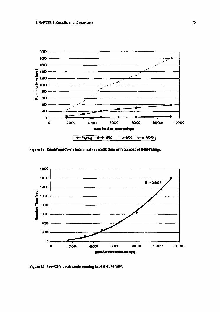
CHAPTER 4.Results and Discussion

Figure 16: RandNeighCorr9s batch mode runnhg dme with number of itemratings.

Figure 17: CorrCFs batch mode running lime Q quadraîic.

CHAPTER 4.Results and Discussion

4.23 RundNeigbCorr's Accuracy

We test the accuracy of RandVeighCorr by computing the MAE. Each experiment is repeated 10

times for each value of /? and the MAE is then averaged. Smaller values of MAE indicate greater

accuracy. In Figure 18, we show the accuracy of RanàNeighCorr d e r training on the GivenXUser data set. The accuracy of CorrCF and PopAvg are also shown for cornparison. Since the GivenXUser data set prescribes 80 item-ratings per user, we can equivalently express the partition size in terms of users. in Figure 18, the three separate runs oFRan~eiggitCorr are shown with partitions of 50,100, and 200 users.

Flgure 18: Accuracy of RandNeQhCorr witb number of users.

RandNeighCorr's accuracy improves as the partition size /?/E increases, A larger partition allows the method ComputeCorreIationSimilari&(..) more candidates 6om which to find better advisors to rnake recommendations. As fl increases to that of the data set size, the

partitionhg phase will put al1 of the &ta into a single partition and we expect RaniiNeighCorr to degenerate to collaborative filtering on un-partitioned data. This behaviour is demonstrated in

Figure 18 for l$/m = 200 users and at 200 users, where we see that RaniiNeighCorr's accuracy

matches that of CorrCF. For nondegenerate values of /?, we note that RandNeighCorr is Iess

CkWïFR 4.Results and Discussion 77

accurate than CorrCF for al1 training set sizes. Each of RanoWeighCow's curves exhibits an uverall rising MAE (declining accuraçy) with the nurnber of users in the training set.

PopAvg's accuracy monotonically improves with the number of users in the data set. It is always less accurate than CorrCF over the range of this study. PopAvg's accuracy is better than

that of RanuNeighCorr at /Y.. = 50 users and with a training set of 800 or more users, If we

extrapolate PopAvg's trend, it's accuracy will match or exceed RandlVeighCorr at P / . = 100

users on a training data set with more than 1600 users. RandNeighCorr's naïve approach to partitioning results in poor accuracy. By creating

more partitions to accommodate larger data sets, the probability of locating the best advisors for each prediction is diminished - with the consequent reduction in recommendation accuracy. This unfortunate behaviour means that as the data set gets large, the accuracy of RanuïVeighCorr will

at some point become worse than that of even non-personalized recornmendations via population averages - this phenomenon is observed for the data sets and partition sizes tested. This behaviour confums our analysis of 3.2.7.

Figure 19: Accuracy of RandNekhCorr with number of item-raîings per user.

Figure 19 shows the accuracy with the number of item-ratings available per user (the GivenXItems data set). RanfleighCorr is executed on this data set with partition sizes fixed at

CHAPTER 4.Results and Discussion 78

1400,2800,4000,7000 and 14000 item ratings. The accuracy of CorrCF and PopAvg are also plotted for cornparison.

The accuracy of RandNeighCorr and CorrCF rnonotonically improves with the number of item-ratings per user. More item-raîings allow for better recomrnendations since a more accurate calculation of sjmilanty can be cornputed fiom longer item-rating histories.

RandïVeighCorr's accuracy also improves with the size of the partition /3, but its accuracy is

always inferior to that of CorrCF. For this experirnent, none of the values chosen for /3 are

degenerate. The non-personalized recommender, PopAvg, outperforms al1 of the personalized

recommenders when the item-ratings are very sparse; PopAvg has the best accuracy at 20 item- ratings per user. PopAvg outperforms RandNeighCorr for the majority of the partition sizes

tested and is only beaten by RanàNeighCorr at /3=140ûû item ratings and at 40 or more item-

ratingduser,

4.2.4 RandNeighCorr's Coverage

The coverage of RandlVeighCorr, C o d F , and PupAvg is shown in Figure 20 as a function of the number of users in the data set, The coverage of PopAvg and CorrCF monotonically improve with more users. This occurs because more advisors are available to rnake recommendations.

The coverage of RantfNeighCorr is worse than CorrCF except for the degenerate value of P =

200 users and the data set with 200 users; Figure 20 shows that the coverage in this case is identical. RandNeighCorr's coverage improves as the size of the partitions increases. A larger partition gives thc colIaborative filter more candidates h m which advisors rnay be sought.

PopAvg's coverage is the greatest, since it can provide a recomrnendation on any item that at least one other petson has rated. The personalized filters can provide recommendations only if an advisor has rated the item of interest.

Figure 21 shows the coverage as a function of the nurnber of item-ratings per user. The coverage for al1 three algorithms monotonically improves with the number of item-ratings per user. The coverage increases since each advisor is able to provide more recommendations.

CHAPTER 4.Results and Discussion

Figure 20: Coverage of RPirdNeighCorr with number of uson. Each user has 80 itemratings.

Figure 21: Coverage for RandiVdghCon with number of item-ratings per user.

CHAPTER AResults and Discussion

4.2.5 Discussion

The accuracy of RandMeighCorr diminishes as users are added to the CF system. Our analysis of 3.2.7 shows that as the number of users increases, the probability of serendipitously putting highly correlated users in the same partition diminishes. We test this hypothesis further by plotting the average maximum similarity of advisors for each user as a fiuiction of partition and data set size in Figure 22. The plot provides more support for our hypothesis and indicates a declining average similarity as users are added to the system. The decline is sharpest for the

smallest partition size. RnndNeighCorr makes a trade-off between running time and accuracy. We obtain

predictions significantly faster in cornparison to CorrCF, but the predictions are somewhat less accurate. Choosing an appropriate value for the partition size C can set the operational point of

the algorithm. For partition sizes greater than or equal to the data set six, RandNeighCorr

degenerates in opration to CorrCF. For nondegenerate values of a, RandNeighCorr exhibits significant improvements over CorrCF in running time while sacrificing accuracy and coverage.

However, if is chosen t w small in relation to the data set size, its accuracy falls below even that

of non-personalized recommendations via PopAvg. The lower bound on /3 is determined empirically for each data set as it depends on the item-rating distribution,

PopAvg has the best accuracy, m i n g time and coverage when the item-ratings density is low: PopAvg outperfonns al1 of the pemnalized recommenders at less than 20 item-ratings per user.

C m R 4.Results and Discussion

Figure 22: Average maximum similarity RandNeighCorr and CorrCF.

4.3 Performance Study of RecTree

In this section we present a performance study into RecTree. in summary, we find that RecTree significantly outperforms CorrCF in running tirne: RecTree's linear complexity is confirmed. RecTiee has accuracy and coverage that is superior to CorrCF regardless of the number of users and item-ratings. Furthmore, RecTree performs reasonably well even when item-rating density is low. RecTree's performance can be tuned to trade-off accuracy for mmhg time by adjusting

the partition parameter p. The construction of the RecTree requires the adjusîment of three parameters: the partition

size 8, the interna1 node limit g and the outlier size limit outlierSize. In the following subsections we discuss how each of these parameters is set.

CHAPTER4.Resuits and Discussion

4.3.1 The Partition Parameter fl

There are some values of for which the RecTree is degenerate. If a is greater than or

equal to the data set size, then the partitionhg phase of ConsrmctRecTree..) is bypassed and al1 of the data is placed into a single partition. We expect then that the accuracy, cuverage and

running tinte for degenerate values of P will be identical.

4.3.2 The Interoal Node Limit g

The intemal node limit g prevents RecTree's consiruction algorithm fiom cxfiaustively partitioning pathological data distributions. Selecting a threshold that is too high may result in RecTree expending so much effort in partitioning the data that there will k no performance speed-up in cornparison to CorrCF. Selecting a threshold that is too low rnay result in RecTree abandoning the partitioning phase pre-rnaturely. We use the following heuristic for selecting g.

Lf the data set has n item-ratings and the partition size has been set to /3, then fiom Lemma 1 and Lemrna 2 we have that the minimum and maximum nurnber of partitions (leaf

nodes) that RecTree can create is L = m'fi and H = n-P+ll respectively. We want to select a value of g between these IWO extrema such that RecTree will pursue a partitioning while it is profitable. We set g to the maximum of the following two values: L*sl and L+(H-t)*s2. For this study the values of and Q='/~ yields good values for g.

Example 13. RecTree is given a training data set of 400 users, each user has 80 item-ratings to train on. The partition size has k e n set to 100 users. The minimum and maximum number of leaf nodes that

can be created are L=4 and H=301, respectively. Our heuristic dictates that g will be set to the

maximum of 6 (=@/I) and 103 (=4+(297)*'~~). g is therefore set to 1 O3 iterations.

4.3.3 Tbe Outlier Tbresbdd: oatïierSize

The outIierSize threshdd prevents RecTme fiom computing predictions on small neighbourhwds. Predictions fiom small neighbourhds tend to have poor coverage since there are relatively few potential advisors h m which to draw recommendations and the accuracy of predictions tends to be low &ce the predictiom are based on a srnall number of advisors

[HKB99]. Consequently, nodes with fewer members than outlierSize do not answer.

C~~~îWt4.Resul ts and Discussion

recommendation requests directly, but delegate such requests to their patent node. Section 3.4.3 discusses in detail how RecTree answers recommendation queries.

How do we choose an appropriate value for outlierSize? Figure 4 shows that for neighbourhoods with fewer than 20 users, the coverage declines sharply. m 9 9 ] shows that for the MovieLens &ta set, the prediction accuracy deched sharply wiîh neighbourhood sizes smalIer than 10 users. For this study we set the outliersize threshold at 20 users.

The sparsity of the item-rating space presents chalIenges ta an eficient implementation of the

RecTree. in this section we sddress the specific implementation choices chat were made in this study.

4 4 . 1 The Item-Rating Vector The user's item-ratings must be represented in a space and access-efftcient data structure.

An obvious choice for storing the item-ratings is an array. in this representation, each ceII in the

array stores either the user's rating for an item or the 'ho-rating" value O. The cell's ordinal position is the item identifier. The first ce11 in the array is special and stores the identifier of the user that "owns" this item-rnting vector. In the item-rating vector below, User36 bas rated item 1 with a score of 2 and item 3 with a score of 4. The remaining items have yet to be rated.

Arrays have the advantage of being exûemely fast to access since each ce11 in the array can be

retrieved in constant time. The EachMovie database had a membership of 72,000 users and an inventory of 1628 movie titles. Stoting the EachMovie rat@ database in an array data structure would require - SOOMB of storage. Although this storage requirement is easily met with

commodity hard drives, it is highly inefficient; only 60% of the membership provideci more than 10 movie ratings, resulting in an array of largely "no rating" value. in addition, it should be noted that the EachMovie recommendation site operated for only a brief period (approxirnately 18 months) and its membership is not large. A viable recommendation service will require signihntly more memory to accommodate its operational need to both continually increase the membmhip and the inventory of items that users c m rate-

Furthemore, it should be noted that the performance of the RecTree (and incîdentally, C o d 0 degrades significantly if the database of item-rating wctors cm not be Ioaded into

CHAPTER 4.Results and Discussion

memory in entire$, Scanning the database of itemiating vectors fiom disk is at least an order of magnitude slower than reading that information from RAM. The array representation of the EachMovie database would fit into commodity RAM but wodd have limited capacity to grow with increasing membership and item inventory.

The shortcomings of the array approach and the high sparsity of the item-rating space motivated us to pursue a compressed data representation. in this approach, only the items for which the user has submitted ratings are represented in the data structure. A numeric pair consisting of the item identifier and the rating score represents each item rating. in the rating vector below, User45 has rateci items 4, 7, 99, and 107 with the scores of 3, 2, 4, and 3

respectively. Items that the user has not rated are implicitly represented by their absence.

This new representation is significantly more space eficient, but is not amenable to direct array access. One method of access is to use binary search on the item identifiers. This approach is relatively fast with a time complexity of O(log(N)), where N is the number of item identifiers. However, the anay would need to be rnaintained in sorted order as users submit more ratings. We selected an alternative data structure, the binary tree. The binary tree also has a time complexity of O(log(N)) and the insertion and deietion of item-ratings is handled within the framework of the data structure. The Java JDK 1.2 provides an implementation of the binary tree and consequently reduced our development tirne.

4.3.4.2 The Similarity Matrix

RecTree answecs a query in 0 0 time. This complexity arises fiom having to scan through the similarity rnatrix for advisors. We improve on this search pmblem by representing the similarity matrix in a compressed format. A vector of numeric pairs represents each user's group of

advisors; the fust number is the advisor's identifier and the second number is the advisor's similarity score. in the similarity vector Mow, User88 has 3 advisor: User26, User28, and User98 with similarity scores of O.67,0.21, and 0.33 respectively.

The assumption that the en& database of item-ratiag vectors wiii fit into memory is not necessariy unreasonable. Refer to 3.1.2 for detaiied discussioa

CHAPTER 4&esults and Discussion

4.3.5 RecTree's Batch Mode Running Time

The batch mode running time for RecTree is tested as a function of the number of users (the GivenXUsers data set) and of partition size. The expriment was run 10 times for each partition size and the average running time reported in Figure 23. Each of the users in the GivenXUser

data set had 80 item-ratings, so we have equivalently expressed the partition parameter, jl in terms of number of users. The batch mode running time for CorrCF is shown for cornparison.

It can be clearly seen that RecTree outperfonns CorrCF in running time for al1 values of

8- tested. The improvement is most dramatic for data sets with 1000 or more users. The significant improvement in speed is due to the linear complexity of RecTree in cornparison to CorrCFs quadratic complexity. A Iinear fit on each of the RecTree curves yields R' of 0.99 - empirically confirming the complexity analysis of 3.4.5. A quadratic fit on CorrCF curve yields R' better than 0.99.

The running time for RecTree irnproves with smaller partition sizes. For example, at

1400 users, the running time for B/m = 300 users is 5049 seconds in cornparison to a r u ~ i n g time

of 441 1 seconds when P/m = 100 users. In particular, the ratio of the partition size in relation to

the size of the data set is an indication of the performance speedup that can be expected. The f l ~ = 200 curve at 200 users shows almost no improvement over CorrCF. However, at 1400 users, this same curve shows greater than 3 time reduction in the execution time in comparison to CorrCF.

The partition sizes p/m 2200 users are degenerate. These partition sizes equal or exceed the size of the training set with 200 users and we note that the running tirne for RecTree is identical in these two cases.

The batch running tirne for RecTree and CorrCF as a function of item-ratings per user (the GiveXRatings data set) is shown in Figure 24. RecTree significantly outperforms CorrCF's running time at al1 levels of item-ratings. RecTree's linear dependency on item-ratings is contùmed with a linear fit. Each of the RecTree curves yield a fit of R' = 0.99. This Iinear dependency is in agreement with our analysis of 3.4.5. None of the partition sizes tested were degenerate.

CHAfTER 4.Flesults and Discussion

Numkr of Uwrs

Figure 23: Batch mode running the for RecTree with number of users. RecTree demonstrates a

linemr complexiîy witb numbcr of users in ~ n l r a s t to CorrCFs quadratic complexity.

Figure 24: RecTree batch madt ruanhg time with number of itemratings per user.

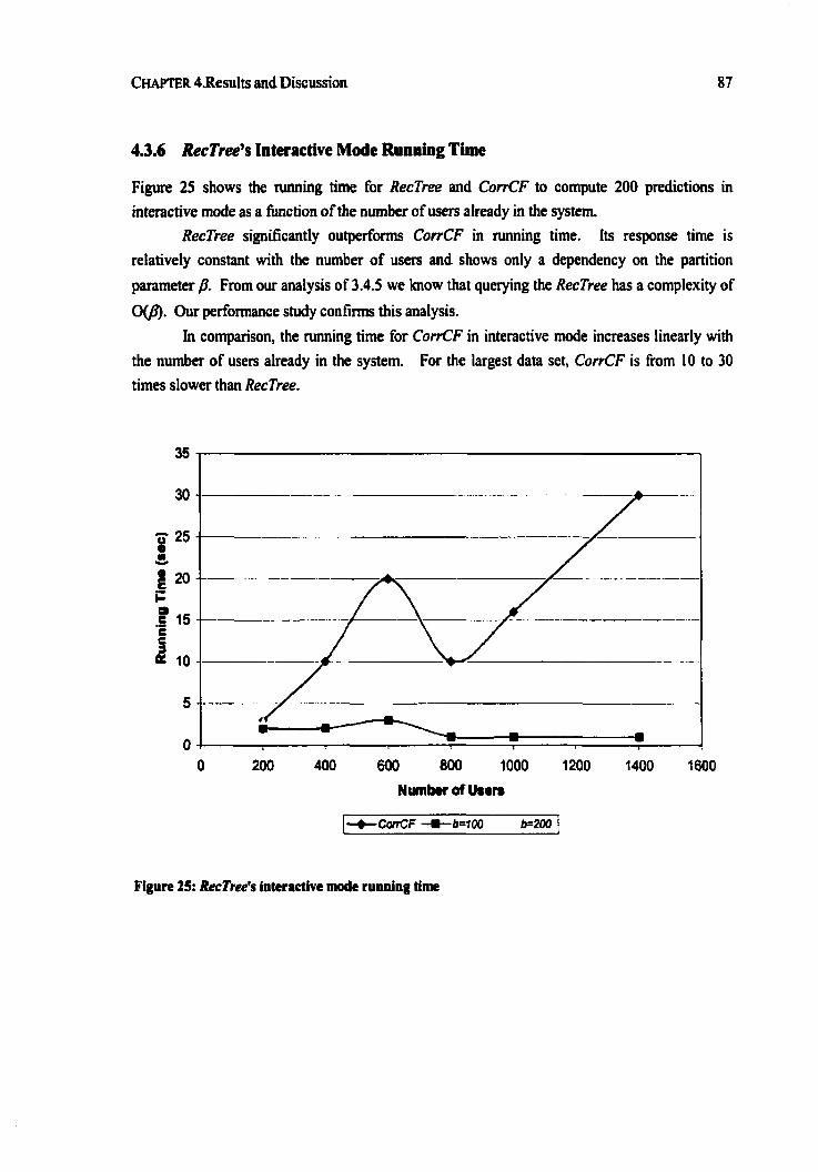
CHGPTER 4Xesults and Discussion

4.3.6 RecTree9s Interactive Mode Running Time

Figure 25 shows the m i n g time for RecTree and CorrCF to compute 200 predictions in interactive mode as a îünction of the nwnber of users already in the system.

RecTree significantly outperfonns CorrCF in running time. Its response time is relatively constant with the number of users and shows only a dependency on the partition

parameter p. From our analysis of 3A5 we know that querying the RecTree has a complexity of

00. Our performance study confirms this andysis. In comparison, the running time for CorrCF in interactive mode increases linearly with

the nwnber of users already in the system. For the largest data set, CorrCF is fiom 10 to 30

times slower than RecTree.

Figure 25: RecTree's interactive mode running time

4.3.7 RecTree9s Accuracy

The accuracy of RecTree as a iùnction of the number of users is shown in Figure 26. RecTree significantly outperforms CorrCF for almost al1 data set sizes and partition parameters

plm. RecTree's accuracy improves with Iarger partition sizes. RecdTree's intelligent partitioning eliminates the degradation in accuracy with population increases that was evident in RanaeighCorr. A larger partition allows the algorithm more candidates among whom to locate good advisors.

For partition parameter f i 8200 users, RecTree's accuracy is degenerate and we note

that these curves have identical accuracy on a training set of 200 users. The improvement in accuracy is due in part to the success of the partitioning phase of

RecTree in loçalizing highly comlated users in the same partition. Figure 27 shows that the average similarity of advisors for RecTree is always higher than that of CorrCF,

5, U g o., P

Figure 26: Accuracy of RecTree with number of users. # ts in units of users.

CHAPTER 4.Results and Discussion

O 200 400 600 800 t 000 1 ZOO 1400

Figure 2 2 The average similarity of advison in RecTree.

The accwacy of RecTree as a fiuiction of the number of item-ratings per user is tested with the GivenXRatings data set. This data set sirnulates the conditions of a CF system in the first months of operation: many users have joined the service, but each user has submitted only a few ratings. Traditionally, CF systems have poor accuracy during this period; [GSK+99] have r e f m d to this situation as the sparsity problem. in 4.2.3 we show that for very sparse data, the recommendations for the personalized recommenders CorrCF and RandNeighCow is worse than non-personalized recornmendation via population averages, PopAvg.

The accuracy of RecTree as a function of rating sparsity is shown in Figure 28, with CorrCF and PopAvg also plotted for cornparison. RecTree has very good accuracy even when the number of ratings per user is low. Its accuracy is always superior to CorrCF and PopAvg at aU levels of rating sparsity.

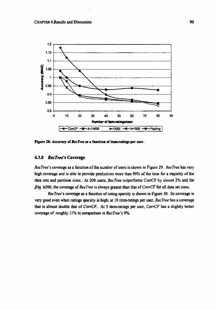
CHAPTER 4.Results and Discussion

Figure 28: Accuracy of RecTree as a funetion of itemratings pcr user,

4.3.8 RecTree's Coverage

RecTree's coverage as a fwiction of the number of users is shown in Figure 29. RecTree has very high coverage and is able to provide predictions more chan 99% of the tirne for a majority of the

data sets and partition sizes. At 200 users, RecTree outperfom CorrCF by almost 2% and for

p . 2200, the coverage of RecTree is always greatw than that of CorrCF for al1 data set sizes.

RecTree's coverage as a fimction of rating sparsity is shown in Figure 30. Its coverage is very good even when ratings sparsity is high; at 10 item-ratings per user, RecTree has a coverage that is almost double that of CorrCF. At 5 item-ratings per user, CorrCF has a slightly better coverage of roughly 11% in cornparison to RecTree's 9%.

CHAPTER 4.Results and Discussion

~ C O ~ C F +Mm=l# -;-&?=200 +~~ 1

Figure 2% Covenge of RocTree witb number of users.

Figure 30: RecTne's coverage with nling sparsity.

CHAPTER~.RCSU~S and Discussion

4.3.9 Discussion

RecTree can compute predictions in batch and interactive modes significantly faster than C o d F and other nearest-neighbour collaboraiive filters. We show that in batch mode and for the largest data set, RecTree provides predictions in appmximately 113 the time it takes CorrCF. RecTree's linear scak up with number of users and item-ratings was confinneci. As each of these quantities increase, RecTree mates more partitions to accommodate the larger data set six.

In interactive mode, RecTree's performance is even Mer : for the largest data set, predictions are provided in 1/10 to 1/30 of the time it takes CunCF. RecTreels constant query time with size of the data set was confmed.

RecTree's supaior running time arises h m its partitioning of the user base into a set of independent cluster's. Since advisors are sought only within a cluster, the time consuming task of computing similarity coefficients is substantially reduced. RecTree's ~ n n i n g time in batch mode is worse than interactive mode since it includes the time to grow the branches and the nodes of the tree. In interactive d e the existing tree is merely îraversed for predictions. The tirne to constnict the RecTree is dominated by the two processes of growing the tree branches and computing the similarity rnahix at the leaf nodes. When the partition size is small the time required ta compute the similarity matrix is reduced but more time is devoted to growing the tree. As we saw in Figure 23, Figure 24, and Figure 25, smaller partition sizes lead to improved execution time, Similarly, when the partition size is large RecTree spends less time constructing the tree branches but the time required to compute the similarity matrix increases; this sûategy ieads to increased execution times.

RecTree outperforms CuwCF in accuracy for almost al1 partition s i ~ s and &ta sets. This achievement is the result of the three complimentary strategies of creating neighbourhoods of highly correlated users, computing pair-wise similarities based on each user's entire rating history, and avoiding spurious predictions h m outlier nodes. RecTree's partitioning phase is successful as the average similarity of advisors within a partition is higher than that of advisors in the un-partitioned case (c.f. Figure 27). A plot of the contributions of each of the latter two strategies to the overall accuracy of RecTree is shown in Figure 3 1.

RecTree has good accuracy even when rhere are few item-ratings. The accuracy of 0 t h collaborative filters dimhishes greatly at low item-rating density, falling bdow even that of non- personalized recommendation via popuIation averages [KM99a]. RecTree, on the other hand, maintains good accuracy even at low item-cating density. RecTree is able to deliver on this feature by avoiding spurious recommendations h m outIier nades. Figure 3 1 shows the accuracy wiih outlier node detection disabled.

C W R 4.Results and Discussion 93

RecTree outperforms CorrCF in coverage for almost al1 partition sizes and data sets. It achieves its high coverage due to its dual prediction strategy. RecTree initially seeks predictions ffom the user's advisors in the leaf node. If the user's advisors have not rated the item in question, then they cannot provide a recommendation. RecTree then delegates the recommendation request to the parent node whm the larger group of users (to whom the user is similar to on a coarser granularity) rnay be able to satisfj the request, If the intemal node cannot satisfi the recommendation request, the prediction is returned with a "no rating" value 8. Obviously, if RecTree continued to pass the request up through the chain of parent-child links, it could increase its coverage even more. However, it was obsemed that the accuracy of the predictions degraded significantly when the prediction was delegated beyond the immediate parent node. Figure 32 shows the contribution of the delegation strategy to the ovenll coverage of RecTree.

Figure 31: The contribution oieorrelation+ and outlier deteetion to RecTree's accwacy.

CHAP'IER 4Results and Discussion 94

Figure 32: The contribution of request dekgatiou to RecTree's coverage.

4.4 Chapter Summary

In this chapter we presented a perfonnance study of RanùMeighCorr and RecTree and compared their performance against the baseline algorithm ComCF. The linear time complexity of each of these aIgorithms with data set size was c o n f i d .

RanNeighCow has the fastest execution time since it partitioned the data with a single pass over the data set. However, its naïve approach to partitioning also resulted in poor accuracy and inferior coverage in comparison to CorrCF. It was shown that as îhe data set size increases, RanrlNeighCom's accuracy (for a f ied partition size B) monotonically decreases. By creating more partitions to accommodate larger data sets, the probability of localing the best advisors for each prediction is diminished - with the consequent reduction in cecornmendation accuracy. This dommate behaviour means that as the data set gets large, the accuracy of RancINeghCorr will at some point become worse than that of even non-personalized recommendations via popuIation averages - this phenornenon is observed for the data sets and partition sizes tested.

CHAPTER 4.Results and Discussion

RecTree outperforms CorrCF in batch and interactive mode for almost al1 data sets and partition sizes tested. It not only has linear execution tirne scale-up, but also monotonic improvement in accuracy with data set size. RecTree's supecior accuracy acises fiom the success of the partitioning phase in creating neighbourhoods of highly correlated users, the use of longer rating histories for computing user similarity, and the avoidance of spucious recomrnendations fiom outlier nodes. RecTree has the unique capability among nearest-neighbow collaborative filters of providing accurate recomrnendations even when the rating density is low.

CHAPTER 5. CONCLUSION AND FUTURE WORK

Chapter 5 Conclusion and Future Work

In this chapter we surnrnarize our contributions and discuss the direction for future research to extend this study.

5.1 Conclusions

This thesis describes a new collaborative filtering data structure and algorithm called RecTree (an acronym for RECommendation Tree) that to the best of our knowledge, is the first nearest- neighbour collaborative filter that can provide recomrnendations in linear time. RecTree has the following characteristics:

1 . RecTree can be constcucted in linear time and space. 2. RecTree can be queried in constant time. 3. RecTree is more accurate than the leading nearest-neighbour collaborative filter, CorrCF

puS+94]. 4. RecTree has a greater coverage (provides more predictions) than CorrCF.

5. RecTree does not suffer the rating sparsiîy problem.

It was dernonstrated that RanùMeigkCorr's naÏve approach to partitionhg data yields clusters of un-correlated users. The resdting predictions were less accurate and the coverage was smaller than that of collaborative f i l t e ~ g on un-partîtioned data via CorrCF. RecTree by cornparison, outperforms CorrCF significantly in both accuracy and coverage. RecTree uses three strategies to achieve this result. Firstly, it partitions the user base into clusters of highly correlated users using the KMeuns' aIgotih. Secondly, it cornputes a more accurate mesure of user similarity based on the entire rating history rathec tban just the intersection set between users.

CHAPTER 5. CONCLUSION AND FUTURE WORK

Lastly, it avoids computing spurious predictions based on tw few advisors by identifling outlier clusters.

5.2 Future Work

Due to tirne constraints, only a lirnited performance study into the effectiveness and efficiency of RecTree was possible. In this section, we indicate the work that we defer to the future for the extension and improvement of the RecTree algorithm.

RecTree cannot handle large databases. in particular, if the database of item-ratings vectors can not fit into memory in entireiy, the algorithm ConsiructRecTree(..) becomes very inefficient since each clustering iteration of the KMeans' algorithm would require a complete scan of the database fiom disk. We h o p to pursue the adaptation of ment scaleable clustering algorithms [ZRLgq [GRS98] [AGCt98] [ACW+99] to RecTree to deal with very large databases.

5.2.2 The Internal Node limit g

The intemal node limit g is introduced to protect RecTree h m computing useless partitions for pathological data disûiiutions. However, a single threshold may not be flexible enough. For example, if the data was a superposition of an exponential and Gaussian distribution, a single threshold may cause RecTree to abandon the partitioning prernaturely. We leave it to future work to investigate the use of multiple thresholds for irnprowig RecTree's ability to deal flexibly with these cases.

Alternatively, we believe that studying new and more effective means of detecting pathological distriiutions is an interesting and important direction for extension to the RecTree.

CHAPTER 5. CONCLUSION AND FUTURE WORK

5.2.3 The outlierSue Tbresbold

The outlierSize threshold was set to 20 users. It would be an important improvement in RecTree's applicability if tùture work discovered a more disciplined approach to setting this important parameter.

5.2.4 Similarity Measures

RecTree uses correlation as the similarity measure between users, however other similarity measures should be investigated. The probabilistic similarity measure of PHLOO] is an interesting alternative that we leave to future work

5.2.5 Predictions

RecTree computes predictions by taking a weighted sum of deviations fiom a mean. This

prediction has proven to be quite effective, but other methods should be tested. The weighted average score [SM951 and the most probable rating [PHLOO] are two interesting alternatives that we did not pursue due to time constraints. Furthemore, previous collaborative filters have proposed only linear functions for generating predictions. It would be interesting to investigate the effectiveness of non-linear mapping functions.

While we have shown that RecTree offers improvements in accuracy, coverage and speed over its cornpetitors, it is clear that there remains room to extend this lead even further.

Bibliogr ap hy

[ACW+99] C. C. Aggawal, C, Procopiuc, I. L. Wolf, P. S. Yu, and J. S. Park, Fast Algorithms for Projected Clustering, In Proc. 1999 ACM SIGMOD [nt. Conf: Management of Data (SIGMOD '99), pages 6 1-72, Philadephia, PA, June 1999,

[AGû+98] R, Agrawal, J. Gehrke, D. Gunopulos, and P. Raghavan, Automatic Subspace Clustering in High Dimensional Data for Data Mining Applications, In Proc. 1998 ACM SIGMOD bit, Con/: Management of Data (SIGMOD'98), pages 94-105, Seattle, WA, June 1998.

[AZ97] C. Avery and R. Zeckhauser, Recommender Systems for Evaluating Computer Messages, CACM, 40(3), 88-89, March 1997.

@Cg21 N. J, Belkin and W. B. Croft, Iriforrnation Filteringa nd information Retrieval: Two sides of the Same Coin?, CACM, 35(12), 29-38, December 1992.

@F98] P. Bradley and U. Fayyad. Refining Initial Points for K-Means Clustering. htt~:llwww.reseiirch.microsofi.com~-~~ad~~~pers/icml98.hmi. July 1998.

[BHK98] J. S. Breese, D. Heckerman, and C. Kadie, ~ m ~ i r i c a l analysis of predictive algorîthms for collaborative filtering. In Proc. 14* Conf: Uncertuinry in Arfijkial Intelligence (UAI-98), pages 43-52, San Francisa, CA, July 1998.

pP99] D. Billsus and M. J, Pazzani, Learning colIaborative information filters. In Proc 15" Int. Conf. Machine Learning, pages 46-54, Madison, W, 1998.

[BS9fl M. Balbanovic and Y. Shoham, Fab: Content-based, Collaborative Recommendation, CACM, 40(3), 66-72, Mach 1997.

[DDF+9û] S. Deerwester, S. T. Dumais, G.W. Fumas, T. K. Landauer, and R. Harshman, Indexing by Latent Semantic Analysis,J. Am, Soc- Inf: Sci. 41,391-407, (1990).

mS+96] M. Ester, H-P. Kriegel, J. Sander, and X. Xu, A Densiîy-Bad Algorithm for Discovenng Clusters in Large Spatial Databases with Noise, In Proc. 2"1 hl. Conf Knowledge Discovery and Data Mining (KDD '96), pages 226-23 1, Portland, OR, 1996.

m92] P. W. Foltz and S. T. Durnais, Personalized Information Delivery: An Analysis of lnfarmation Filtering Methods, CACM, 35(12), 5 1 4 , December t992.

[FOR991 Forrester Research Inc., Forester Technographics Finds Online Customers Fearful of Privacy Violations, http://www.forrester.codERihess/Relerisd0,1769.177.FF.html, October,

[GNOt92] D. Goldberg, D. Nichols, B. M. Oki, and D. Teny, Using Collaborative Filtering to Weave an information Tapestry, CACM 3 4 12), 6 t -70, Decernber 1992.

[Gre99] B. Greenman, Liar Liar, http://www.zdnet'som/vil/content/rnap/99, 1999.

[GRS98] S. Guha, R. Rastogi, and K. Shim, CURE: An Efficient Clustering Algorithm for Large

Databases, in Proc. 1998 ACM SIGMOD Int. Conf: Management of Data (SiGMûD'98), pages 73-84, Seattle, WA, lune 1998.

[GSK+99] N. Good, J. B. Schafer, J. A. Konstan, A. Borchers, B. S a m , 1. Herlocker and J, Riedl, Combining Collaborative Filtering with Personal Agents for Better Recommendations, in Prac. 1999 Con$ American Association of Artifhl Intelligence ( M - 9 9 ) . July 1999 .

[HCC97J J. Han, J. Chiang, S. Chee, J. Chen, Q. Chen, S. Cheng, W. Gong, M. Karnber, K. Koperski, G. Liu, Y. Lu, N. Stefanovic, L. Wistone, B. Xia, O. R. Zaiane, S. Zhang, and H. Zhu, DBMiner: A System for Data Mining in Relationel Databases and Data Warehouses, In Proc. CASCONf97: Meeting of Min&, Toronto, Canada, November t997.

[HCC98] I. Han, S. Chee, and J. Y. Chiang, issues for On-Line Analytical Mining of Data Warehouses, In Proc. of 1998 SIGMODr96 Worhhop on Research Issues on Data Mining and Knowledge Discovery (DMKD'98) , Seattle, Washington, June 1998, pages 2:l-25.

[HKB+99] J. L. Herlocker, J. A. Konstan, A. Borchers, and J. RiedI, An Algorithmic Framework for Perfonning Collaborative Filtering, in Proc. 1999 Conf: Research and Development in information Retrieval, pages 230-237, Berkeley, CA, August 1999.

m85] D. L. Harnett and J. L. Murphy, Staiisticuf Analysis for Business and Econornics, third

edition, Addison Wesley, 1985.

[KM99a] A. Kohrs and B. Merialdo, Cluslering for callaborative filtering applications. in Computationaf Intelligence /or Modelling, Conrrol & Automation {CIMCAr99), Vienna. [OS Press, 1999.

m99b] h d Kohs and Bernard Merialdo, Improving Collaborative Filtering with Multimedia indexing Techniques to mate User-Adapting Web Sites, in Proc. 7th ACM Multimedia Conf, Orlando. ACM, 1999.

m f 9 7 j J. A. Konstan, B. N. Miller, D. Maltz, 3. L. Hertocker, L. R. Gordon, and J. Riedl Applying Collaborative Filtering to Usenet News, CACM, #(3), 77-87, March 1997.

m89] L. Kaufman and P. Rousseeuw, Finding Groirps in Data, An introduction fo Clustering Analysis. John Wiley and Sons, 1989.

[KSS97] H. Kautz, B. Selman, and M. Shah, ReferraI Web: Combining Social Networks and Collaborative Filtering, CACM, 40(3), 63-65, March 1997.

&iRK9TJ B. Miller, I. Riedl, and 3. Konstan, Experiences with GroupLens: Making Usenet Usehl Again. in Proc. 1997 Usenix Technicd Confi, January 1997.

[Paz991 M. Pazzani, A Framework for Collaborative, Content-Based and Demographic Fi l t e~g , Artijkial Intelligence Review, 1W9.

[PHLOO] D. M. Pemock, E. HOM@ S. Lawrence, and C. L. Giles, Collaobrative filtering by personality diagnosis: A hybrid memory and del-based approach, in Proc. I$ Con.

Uncertainîy in Art$cial Intelligence (UAI-2000), Stanford, CA, lune 2000.

wS+94] P. Resnick, N. Iacovou, M. Sushak, P. Bergsîmm, and J. Riedl, GroupLens: An open architechure for collaborative filtering of netnews. in Proc. ACM Co,$ Computer Support

Cooperative Work (CSC) 1994, New York, N'Y, pages 175-186, October 1994.

[Rob811 S. E. Robertson, The methodology of information retrieval expriment. Info~nation

Retrieval Experinient, K. S. Jones, Ed., Chapter 1, pages 9 3 1. Butterworths, 198 1,

w 9 7 3 1. Rucker and M. J. Polanco, SiteSeet: Personalized Navigation for the Web, CACM,

40(3), 73-75, March 1997.

[RR91] R Rosenthal and R. Rosnow, Essentiah of Behavioral Research: Meihod! and Data and

Analysis, McGraw Hill, second edition, 1991.

[Sho92] L. Shoshana, Architechtng Personalized Delivery of Multimedia information, CACM, 35(12), 39-50, December 1992.

[SKB+98] B. M. Sarwar, S. A. Konstan, A. Borchers, J. L. Herlocker, B. N. Miller, and J. Riedl, Using Filtering Agents to Improve Prediction Quality in the Grouplens Research Collaborative Filtering System. in Proc. ACM Con$ Computer Stipport Cooperativ Work (CSCq 1998, Seattle, WA., page 345-354 Novemer 1998.

[SKR99] 1. B. Schafer, J. Konstan, and 1. Riedl, Recommender Systems in E-Commerce, ACM

Con$ Electronic Commerce (EC-99), Denver, CO, pages 158-166, November 1999.

[SMc83] G. Salton and M. J. McGiIl, Introduction to Modern Information Reîrieval, McGraw- Hill, 1983.

[SM951 U, Shardanand and P. Maes, Social information filtering: Algorithm for automating 'îvord of mouth." in Proc. 1995 ACM Conf Human Factors in Computing Systems. New York, NY, pages 210-217,1995.

[Swe88] J. A. Swets, Measuring the accwacy of diagnostic systerns, Science, 240(4857): 1285- 1289, June 1988.

[THA+97] L. Tereen, W. Hill, B. Amento, D. McDonald, and J. Creter, PHOAKS: A System for Sharing Recomrnendations, CACM, 40(3), pages 59-62, March 1997.

[UF98] L. H, Ungar and D. P. Foster, Clustering Methods for Collaborative Filtering, In AAAl Workshop on Recommendation Systems, 1998.

[ZHL+98] O. R. Zaiane, J. Han, Z. N. Li, J. Y. Chiang, and S. Chee, MultiMedia-Miner: A System Prototype for MuhiMedia DataMining, In Proc. 1998 ACM-SIG- Conf on Management of Dutu, (system demo), Seattle, Washington, June 1998, pp. 581-583,

[ZRL96] T. Zhang, R. Ramakrishnan, and M. Livny, Birch: And Efficient Data Clustering Method for Very Large Databases, in Proc. 1996 ACM SIGMOD Int. Conf. Management of Daia, pages 103-1 14, Montreal, Canada, June 1996.