Modified tangential frequency filtering decomposition and its fourier analysis

Modified Tangential Frequency Filtering Decomposition

and its Fourier Analysis

Qiang Niu, Laura Grigori, Pawan Kumar, Frederic Nataf

To cite this version:

Qiang Niu, Laura Grigori, Pawan Kumar, Frederic Nataf. Modified Tangential FrequencyFiltering Decomposition and its Fourier Analysis. [Research Report] RR-6662, INRIA. 2008.<inria-00324378>

HAL Id: inria-00324378

https://hal.inria.fr/inria-00324378

Submitted on 24 Sep 2008

HAL is a multi-disciplinary open accessarchive for the deposit and dissemination of sci-entific research documents, whether they are pub-lished or not. The documents may come fromteaching and research institutions in France orabroad, or from public or private research centers.

L’archive ouverte pluridisciplinaire HAL, estdestinee au depot et a la diffusion de documentsscientifiques de niveau recherche, publies ou non,emanant des etablissements d’enseignement et derecherche francais ou etrangers, des laboratoirespublics ou prives.

https://hal.archives-ouvertes.fr

https://hal.inria.fr/inria-00324378

appor t de recherche

ISS

N02

49-6

399

ISR

NIN

RIA

/RR

--66

62--

FR

+E

NG

Thème NUM

INSTITUT NATIONAL DE RECHERCHE EN INFORMATIQUE ET EN AUTOMATIQUE

Modified Tangential Frequency FilteringDecomposition and its Fourier Analysis

Qiang Niu — Laura Grigori — Pawan Kumar — Frédéric Nataf

N° 6662

September 2008

Centre de recherche INRIA Saclay – Île-de-FranceParc Orsay Université

4, rue Jacques Monod, 91893 ORSAY CedexTéléphone : +33 1 72 92 59 00

Modified Tangential Frequency Filtering

Decomposition and its Fourier Analysis

Qiang Niu ∗, Laura Grigori†, Pawan Kumar ‡ , Frederic Nataf §

Theme NUM — Systemes numeriquesEquipes-Projets Grand-Large

Rapport de recherche n° 6662 — September 2008 — 24 pages

Abstract: In this paper, a modified tangential frequency filtering decomposi-tion (MTFFD) preconditioner is proposed. The optimal order of the modifica-tion and the optimal relaxation parameter are determined by Fourier analysis.With this choice of the optimal order of modification, the Fourier results showthat the condition number of the preconditioned matrix is O(h− 2

3 ), and thespectrum distribution of the preconditioned matrix can be predicted by theFourier results. The performance of MTFFD is compared with tangential fre-quency filtering (TFFD) preconditioner on a variety of large sparse matricesarising from the discretization of PDEs with discontinuous coefficients. Thenumerical results show that the MTFFD preconditioner is much more efficientthan the TFFD preconditioner.

Key-words: preconditioner; linear system; tangential frequency filtering de-composition; GMRES

∗ School of Mathematical Sciences, Xiamen University, Xiamen, 361005, P.R. China; Thework of this author was performed during his visit to INRIA, funded by China ScholarshipCouncil; (Email:[email protected])

† INRIA Saclay - Ile de France, Laboratoire de Recherche en Informatique UniversiteParis-Sud 11, France (Email:[email protected]).

‡ INRIA Saclay - Ile de France, Laboratoire de Recherche en Informatique UniversiteParis-Sud 11, France (Email:[email protected]).

§ Laboratoire J. L. Lions, CNRS UMR7598, Universite Paris 6, France; (Email:[email protected])

Preconditionnement a base de filtrage tangentiel

modifie et son analyse de Fourier

Resume : Dans ce papier nous proposons une modification du preconditionnementa base de filtrage tangentiel (MTFFD). Les valeurs optimales des parametres dela modification sont determinees par une analyse de Fourier. Avec ce choix desparametres, l’analyse de Fourier montre que le conditionnement de la matricepreconditionnee est de l’ordre de O(h− 2

3 ). Les resultats numeriques presentesmontrent que MTFFD est plus efficace que le preconditionnement a base defiltrage tangentiel TFFD.

Mots-cles : preconditionnement, systemes lineaires, GMRES

MTFFD and its Fourier Analysis 3

1 IntroductionIn this paper, we investigate preconditioning techniques for solving the linearsystem

Ax = b (1)

with

A =

D1 U1

L1 D2. . .

. . .. . . Unx−1

Lnx−1 Dnx

∈ RN×N , b ∈ RN ,

which often arises from the discretization of many PDEs by finite differenceor finite volume schemes. When preconditioned iterative methods are used forsolving (1), the convergence rate of an iterative method heavily depends onthe property of the preconditioner [36]. Therefore, developing efficient precon-ditioners has been one of the major research interests in many applications.Algebraic multigrid (AMG) methods work well for many problems in practice[21, 35]. However, conventional AMG methods may suffer from relatively ex-pensive setup time and large memory requirements, particularly for three di-mensional problems [18]. Another more general preconditioner is the multilevelincomplete block factorization [9, 37]. A theoretical comparison of algebraicmultigrid methods and algebraic multilevel methods are carried out by Y. No-tay [33] for symmetric positive definite (SPD) matrices, and generalized by C.Mense and R. Nabben [29, 30] for nonsymmetric matrices.

Tangential Frequency Filtering Decomposition (TFFD) proposed in [2] is aspecial kind of incomplete block factorization preconditioner. Similar to somepopular preconditioning techniques discussed in [1, 3, 8, 12, 13, 38, 39, 40, 42],the TFFD preconditioner can be used as a preconditioner or a smoother formultigrid methods. The preconditioner has the feature of filtering property, i.e.(M−A)f = 0 for a vector f , where M is the TFFD preconditioner. For A 0(symmetric positive semidefinite), the preconditioner satisfies M − A 0, i.e.M is a compensative matrix of A [4, 5, 24]. This is an important propertythat preconditioners of SPD coefficient matrix should possess. By combiningTFFD and ILU(0) in a multiplicative way [2], the combinative preconditioneris shown to be very efficient on several challenging problems. Therefore, it isimportant to give a deep understanding of the TFFD preconditioner. In [7, 8],the authors have presented some nice ways to analyze the properties of generalblock factorization preconditioners. For frequency filtering decomposition typepreconditioners, some analysis have been done in [1, 13, 14, 38, 39]. The boundson the spectral radii or condition numbers are derived by a couple of compli-cated inequalities. These results are useful in understanding the behavior ofthe preconditioners. However, the results have difficulty in outlining the rangeand clustering of the spectrum of the preconditioned matrix, especially whenthe matrix dimension is large. Fourier analysis is a powerful tool for analyzingthe properties of a preconditioner [15]. It has been applied successfully to lo-cal model analysis in multigrid methods [10, 11, 41], and popularized by T. F.Chan and H. C. Elman [15] for analyzing algebraic preconditioners and classicaliterative methods. Fourier analysis has been recognized as a standard tool forestimating the convergence rate of preconditioned iterative methods, see e.g. T.F. Chan et.al [16, 17], R J. Le Veque and L. N. Trefethen [23], K. Otto [34]. For

RR n° 6662

4 Q. Niu, L. Grigori, P. Kumar, and F. Nataf

point-wise incomplete factorization type preconditioners like ILU(0), MILU(0)and RILU preconditioners, Fourier analysis has been done in [15, 16, 17]. TheFourier analysis of block ILU and MILU factorization preconditioners is consid-ered in [34] for a time-dependent hyperbolic PDE problem.

The original aim of the present work is to analyze the TFFD preconditionerby means of Fourier analysis. Whereas, later we find that Fourier analysis forTFFD preconditioner is not feasible for our model problem. This is because ofan exact cancelation in the denominator of a parameter, which is determinedby symbolic computation (this will be shown in Section 3). But this does notmean that in practice TFFD is not a good preconditioner. This issue leads usto the derivation of the Modified Tangential Frequency Filtering Decomposition(MTFFD) preconditioner, in which the recursion formula of TFFD is modifiedby adding a term cΛih

q. This idea of modification comes from the MILU pre-conditioner [20], where an additional term of order O(h−2) (c 6= 0) is addedto the diagonal along with dropped fill-in. For problems arising from the dis-cretizations of second-order elliptic partial differential equations, it is known[6, 20] that the modification is able to reduce the condition number of the pre-conditioned matrix by MILU from O(h−2) (c = 0) to O(h−1) (c 6= 0). Using atwo dimensional Poisson equation as a model problem, we perform the Fourieranalysis of the MTFFD preconditioner. The optimal choice of q and c are deter-mined by this analysis, which shows that q = 4

3 and c = (4π2)23 are the optimal

choices as h tends to 0. The optimality of these parameters is illustrated by thenumerical tests. When the optimal choice of modification order q is used, theFourier analysis reveals that the condition number of the preconditioned matrixis O(h− 2

3 ). This bound is better compared with other incomplete factoriza-tion type preconditioners (c.f. [15]). To compare the preconditioning effect ofMTFFD with TFFD, we present tests on large sparse matrices arising from thediscretization of PDEs with discontinuous coefficients. The results show thatthe MTFFD preconditioner is much more efficient, and MTFFD preconditionedGMRES needs less than half of the iteration numbers of TFFD preconditionedGMRES.

We use ctridm(α, β, γ) and circm(γ1, . . . , γm) to denote the tridiagonal cir-culant matrix and circulant matrix of order m, i.e.

ctridm(α, β, γ) =

β γ α

α. . .

. . .

. . .. . . γ

γ α β

, circm(γ1, . . . , γm)

γ1 γ2 . . . γm−1 γm

γm γ1 γ2 . . . γm−1

.... . .

. . .. . .

...γ3 . . . γm γ1 γ2

γ2 γ3 . . . γm γ1

We also use tridm(α, β, γ) and Btridm(L, T, U) to denote the m×m tridiagonaland mk × mk block tridiagonal matrix with each diagonal block of size k × k

respectively, i.e.

tridm(α, β, γ) =

β γ

α. . .

. . .

. . .. . . γ

α β

and Btridm(L, T, U) =

T U

L. . .

. . .

. . .. . . U

L T

.

INRIA


The paper is organized as follows, In Section 2, a model problem is described,which will be used for Fourier analysis. In Section 3, we present the modifiedTFFD preconditioner and carry out the Fourier analysis for the MTFFD pre-conditioner. In Section 4, the performance of the MTFFD preconditioner iscompared with the TFFD preconditioner by several examples. Finally, we con-clude the paper in Section 5.

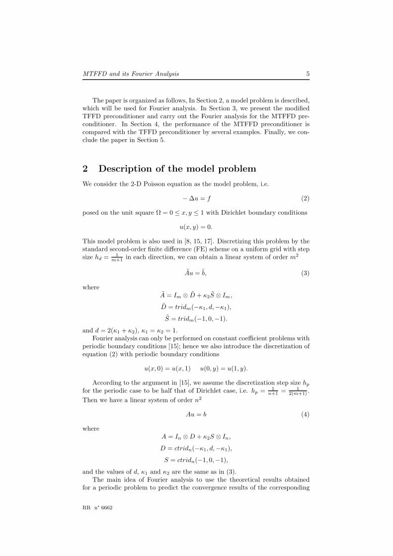
2 Description of the model problem

We consider the 2-D Poisson equation as the model problem, i.e.

− ∆u = f (2)

posed on the unit square Ω = 0 ≤ x, y ≤ 1 with Dirichlet boundary conditions

u(x, y) = 0.

This model problem is also used in [8, 15, 17]. Discretizing this problem by thestandard second-order finite difference (FE) scheme on a uniform grid with stepsize hd = 1

m+1 in each direction, we can obtain a linear system of order m2

Au = b, (3)

whereA = Im ⊗ D + κ2S ⊗ Im,

D = tridm(−κ1, d,−κ1),

S = tridm(−1, 0,−1).

and d = 2(κ1 + κ2), κ1 = κ2 = 1.Fourier analysis can only be performed on constant coefficient problems with

periodic boundary conditions [15]; hence we also introduce the discretization ofequation (2) with periodic boundary conditions

u(x, 0) = u(x, 1) u(0, y) = u(1, y).

According to the argument in [15], we assume the discretization step size hp

for the periodic case to be half that of Dirichlet case, i.e. hp = 1n+1 = 1

2(m+1) .

Then we have a linear system of order n2

Au = b (4)

whereA = In ⊗ D + κ2S ⊗ In,

D = ctridn(−κ1, d,−κ1),

S = ctridn(−1, 0,−1),

and the values of d, κ1 and κ2 are the same as in (3).The main idea of Fourier analysis to use the theoretical results obtained

for a periodic problem to predict the convergence results of the corresponding

RR n° 6662


Dirichlet problem. Therefore, we present in this paper the Fourier analysis ofthe linear system (4). In the following discussion, the equation (3) and (4) willbe referred to as Dirichlet problem and periodic problem respectively, and wealways use subscript d and p to distinguish the parameters for the Dirichlet caseand the periodic case.

Firstly, the Fourier eigenvalue of the coefficient matrix A is given by thefollowing equation [15]

Au(j,k) = λAu(j,k),

where u(j,k) is defined by

u(j,k)s,t = eisθj eitφk (5)

with

θj =2πj

n + 1, φk =

2πk

n + 1, 1 ≤ j, k ≤ n. (6)

and i is the imaginary unit.

Substituting the expression of u(j,k)s,t into the grid-equation related to A (refer

to [15]), we have

Au(j,k) = dus,t − κ1us+1,t − κ1us−1,t − κ2us,t−1 − κ2us,t+1

= (d − κ1eiθj − κ1e

−iθj − κ2eiφk − κ2e

−iφk)eisθj eitφk

= (4 − 2 cos(θj) − 2 cos(φk))eisθj eitφk

= 4(κ1 sin2(θj

2 ) + κ2 sin2(φk

2 ))u(j,k).

(7)

Thus, the Fourier eigenvalue of A corresponding to the Fourier eigenvector u(j,k)

are

λA = λj,k(A) = 4(κ1 sin2(θj

2) + κ2 sin2(

φk

2)). (8)

The expression of the Fourier eigenvalue of A will be used later in the Fourieranalysis.

3 Modified Tangential Frequency Filtering De-

compositions and its Fourier analysis

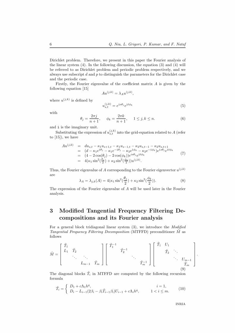
For a general block tridiagonal linear system (3), we introduce the ModifiedTangential Frequency Filtering Decomposition (MTFFD) preconditioner M asfollows

M =

T1

L1 T2

. . .. . .

Lm−1 Tm

T−11

T−12

. . .

T−1m

T1 U1

T2. . .

. . . Um−1

Tm

.

(9)The diagonal blocks Ti in MTFFD are computed by the following recursionformula

Ti =

D1 + cΛ1hq, i = 1,

Di − Li−1(2βi − βiTi−1βi)Ui−1 + cΛihq, 1 < i ≤ m.

(10)

INRIA


where Λi, 1 ≤ i ≤ m, are diagonal matrices, parameter q is the order of modi-fication, and c is a relaxation parameter. The optimal choice of q and c will bediscussed later. The matrix βi is an approximation to the inverse of Ti−1, andit can be determined by enabling M to have a filtering condition. The analysisin [2] shows that it reduce to solving

βi(Ui−1f) = T−1i−1Ui−1f, (11)

where f is a filtering vector.We can see that the MTFFD preoconditioner differs from the TFFD pre-

conditioner in that an additional term cΛihq is added in the recursion formula

(10). If Λi = Im, then the modification is similar to those done in the modifiedILU factorization [6, 20], where the modification is ch2Im. The modification in(10) is quite similar to the shifted iteration methods discussed in [43], wherethe ILU factorization of a shifted coefficient matrix is constructed and usedas a preconditioner for the original problem. For analysis purpose, we will fixΛi = Im, 1 ≤ i ≤ m, and the filtering vector is chosen as 1 = [1, . . . , 1]T .

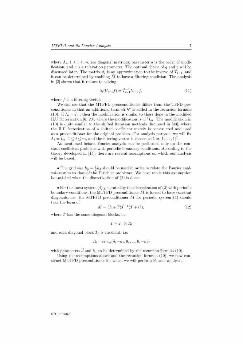
As mentioned before, Fourier analysis can be performed only on the con-stant coefficient problems with periodic boundary conditions. According to thetheory developed in [15], there are several assumptions on which our analysiswill be based,

• The grid size hp = 12hd should be used in order to relate the Fourier anal-

ysis results to that of the Dirichlet problems. We have made this assumptionbe satisfied when the discretization of (2) is done.

• For the linear system (4) generated by the discretization of (2) with periodicboundary conditions, the MTFFD preconditioner M is forced to have constantdiagonals, i.e. the MTFFD preconditioner M for periodic system (4) shouldtake the form of

M = (L + T )T−1(T + U), (12)

where T has the same diagonal blocks, i.e.

T = In ⊗ T0

and each diagonal block T0 is circulant, i.e.

T0 = circn(d,−κ1, 0, . . . , 0,−κ1)

with parameters d and κ1 to be determined by the recursion formula (10).Using the assumptions above and the recursion formula (10), we now con-

struct MTFFD preconditioner for which we will perform Fourier analysis.

RR n° 6662


Firstly, the parameters d and κ1 can be computed by solving

Ti = Di − Li−1(2βi−1 − βi−1Ti−1βi−1)Ui−1 + chqIn

=

d −κ1 −κ1

−κ1 d. . .

. . .. . . −κ1

−κ1 −κ1 d

+κ22

(d−2κ1)2

d −κ1 −κ1

−κ1 d. . .

. . .. . . −κ1

−κ1 −κ1 d

− 2κ22

(d−2κ1)In + chqIn

=

d − κ22d−2κ2

2(d−2κ1)2

(d−2κ1)−κ1 − κ2

2κ1

(d−2κ1)2−κ1 − κ2

2κ1

(d−2κ1)2

−κ1 − κ22κ1

(d−2κ1)2d − κ2

2d−2κ22(d−2κ1)

2

(d−2κ1)

. . .

. . .. . . −κ1 − κ2

2κ1

(d−2κ1)2

−κ1 − κ22κ1

(d−2κ1)2κ1 − κ2

2κ1

(d−2κ1)2d − κ2

2d−2κ22(d−2κ1)

2

(d−2κ1)

+ chqIn.

(13)From the above relationship, we have

d = d − κ22d − 2κ2

2(d − 2κ1)2

(d − 2κ1)+ chq,

κ1 = κ1 +κ2

2κ1

(d − 2κ1)2,

or(d − d)(d − 2κ1)

2 = κ22(d − 2κ1) − 2κ2

2(d − 2κ1) + 2κ1κ22, (14)

(κ1 − κ1)(d − 2κ1)2 = κ2

2κ1. (15)

By using matlab symbolic computation [27], we have

d − 2κ1 = −1 + 12 (d + chq) + 1

2

√

(d + ch)2 − 4(d + chq)

= 1 + 12chq + 1

2

√

(4 + chq)chq

= 1 + ηh,

(16)

and

κ1 =−(d+chq)−

√−4(d+chq)+(d+chq)2+(−1+ 1

2 (d+chq)+ 12

√−4(d+chq)+(d+chq)2)(d+chq)

(d+chq)(d+chq−4)

= 12 +

√(d+chq)chq( 1

2 (d+chq)−1)

chq(d+chq)

= 12 +

12 chq+1√

(4+chq)chq

= 12 + 1

2δh,

(17)

where ηh = 12chq + 1

2

√

(4 + chq)chq, δh =

√(4+chq)chq

chq+2 .From (16) and (17) we can see that κ1 → ∞ as c → 0. Thus, Fourier

analysis can not be performed on the original tangential frequency filteringdecomposition preconditioner.

By straightforward computation as in (7), the Fourier eigenvalues of L, U ,and T are

λL = −κ2e−iφk ,

λU = −κ2eiφk ,

INRIA


λT

= d − κ1 cos(θj),

respectively. Therefore, the Fourier eigenvalues of the MTFFD preconditionerM are

λ(M) = (λL + λT)λ−1

T(λU + λ

T)

=(d−2κ1 cos(θj)−κ2 cos(φk)+iκ2 sin(φk))(d−2κ1 cos(θj)−κ2 cos(φk)−iκ2 sin(φk))

d−2κ1 cos(θj).

(18)

Letting ξ = d − 2κ1 cos(θj), we have

λ(M) = 1ξ(ξ − κ2 cos(φk) + iκ sin(φk)(ξ − κ2 cos(φk) − iκ2 sin(φk))

= 1ξ((ξ − κ2 cos(φk))2 + κ2

1 sin(φk)2)

= 1ξ((ξ2 − 2ξκ2 cos(φk) + κ2

2).

(19)As we know,

λj,k(A) = 4(κ1 sin2(θj

2) + κ2 sin2(

φk

2)).

Hence

λ(M−1A) =4ξ(κ1 sin2(

θj2 )+κ2 sin2(

φk2 ))

ξ2−2ξκ2 cos(φk)+κ22

=4(d−2κ1 cos(θj))(κ1 sin2(

θj2 )+κ2 sin2(

φk2 ))

(d−2κ1 cos(θj)−κ2)2+2κ2(d−2κ1 cos(θj))(1−cos(φk))

=4(d−2κ1+4κ1 sin2(

θj2 ))(κ1 sin2(

θj2 )+κ2 sin2(

φk2 ))

(d−2κ1+4κ1 sin2(θj2 )−κ2)2+4κ2(d−2κ1+4κ1 sin2(

θj2 )) sin2(

φk2 )

=4(ηh+1+4κ1 sin2(

θj2 ))(sin2(

θj2 )+sin2(

φk2 ))

(ηh+4κ1 sin2(θj2 ))2+4κ2(ηh+1+4κ1 sin2(

θj2 )) sin2(

φk2 )

.

(20)

Thus,

λ−1(M−1A) =(ηh+4κ1 sin2(

θj2 ))2+4κ2(ηh+1+4κ1 sin2(

θj2 )) sin2(

φk2 )

4(ηh+1+4κ1 sin2(θj2 ))(sin2(

θj2 )+sin2(

φk2 ))

=16κ2

1 sin4(θj2 )+16κ1 sin2(

θj2 ) sin2(

φk2 )+η2

h+8δhκ1 sin2(θj2 )+4(1+ηh) sin2(

φk2 )

16κ1 sin4(θj2 )+16κ1 sin2(

θj2 ) sin2(

φk2 )+4(1+ηh)(sin2(

θj2 )+sin2(

φk2 ))

= 1 +16(κ1−1)κ1 sin4(

θj4 )+η2

h+8κ1ηh sin2(θj2 )−4(1+ηh) sin2(

θj2 )

16κ1 sin4(θj2 )+16κ1 sin2(

θj2 ) sin2(

φk2 )+4(1+ηh)(sin2(

θj2 )+sin2(

φk2 ))

= 1 +4(δ−1

h+1)(δ−1

h−1) sin2(

θj2 )+

η2h

sin2(θj2

)

16κ1 sin2(θj2 )+16κ1 sin2(

φk2 )+4(1+ηh)+4(1+ηh)

sin2(φk2

)

sin2(θj2

)

.

(21)As h tends to 0, we have δ−1

h ≥ 1. Then from (21) it is easy to see thatasymptotically

λ−1(M−1A) ≥ 1,

i.e. λ(M−1A) ≤ 1. This is consistent with the theoretical results obtained in[2].

Subsequently, we will derive the upper bound of λ−1(M−1A) in an analyticalway.

Let

f(s1, s2) = 1 +αs2

1 + γ

s21

βs21 + βs2

2 + es22

s21

+ e, (22)

RR n° 6662


where we use s1 = sin( θ2 ), s2 = sin(φ

2 ). It is easy to see that f(s1, s2) is a

continuous function of sin(θ2 ) and sin(φ

2 ), with ( θ2 , φ

2 ) defined in (0, π) × (0, π).

In the representation form of f(s1, s2), we have set α = 4(δ−1h + 1)(δ−1

h − 1),γ = η2

h, β = 16κ1, and e = 4(1 + ηh).

Taking partial derivation of f(s1, s2) with s2, we have

f ′s2

(s1, s2) =−2(αs2

1 + γ

s21)(β + e

s21)s2c2

(βs21 + βs2

2 + es22

s21

+ e)2

≤ 0, φ ∈ (0, π2 ),

> 0, φ ∈ (π2 , π),

(23)

where c2 = cos(φ2 ).

Thus,

maxθ,φ

(f(s1, s2)) = f(s1, 0) = f(s1, π) = 1 +αs2

1 + γ

s21

βs21 + e

.

Therefore, the maximum value of λ(M−1A) is attained on the line (j, k) withk = 1, or k = n.

Also we have

f ′s1

(s1, 0) =4αs3

1c1(βs41+es2

1)−(αs41+γ)(4βs3

1c1+2es1c1)

(βs41+es2

1)2

=2αes4

1−γ(4βs21+2e)

(βs41+es2

1)2s1c1

=32(δ−2

h−1)(1+ηh)s4

1−32η2

h(1+δh)s2

1δh

−8η2h(1+ηh)

(βs41+es2

1)2s1c1

≈ s1c1

(βs41+es2

1)2(32s4

1

δ2h

− 32η2hs2

1

δh)

≈ s1c1

(βs41+es2

1)2(32s4

1

chq − 32√

chq2 s2

1).

(24)

In the above approximation, the high-order terms are ignored as h is assumedto be sufficiently small. Subsequently, we will analyze the sign of f ′

s1(s1, 0) in

two cases:

• When q ≥ 43 , then as h → 0, we have

f ′s1

(s1, 0) is

≥ 0, θ ∈ (0, π2 ],

< 0, θ ∈ (π2 , π),

(25)

Therefore, the maximum value of λ−1(M−1A) is attained whenever j = ⌊n2 ⌋+1,

and k = 1 or k = n, where ⌊n2 ⌋ denotes the largest integer less than n

2 . At thesepoints (j, k), we have

λ−1⌊n

2 ⌋+1,k(M−1A) ≈ 1 +

4chq +chq−4

8√

chq+4

≈ 1 + 1

2√

chq2

≥ 1

2√

ch23.

(26)

• When 0 ≤ q ≤ 43 , then as h → 0, we have

f ′s1

(s1, 0) is

≤ 0, θ ∈ (0, ξh],> 0, θ ∈ (ξh, π

2 ),≤ 0, θ ∈ [π

2 , π − ξh],> 0, θ ∈ (π − ξh, π),

(27)

INRIA


where ξh the positive angle such32s4

1

chq = 32√

chq2 s2

1, i.e. s21 = c

32 h

3q2 . From the

equality, we have ξh = arcsin(c34 h

3q4 ). Therefore, in this case, the maximum

value of λ−1(M−1A) is possibly attained at one of the following three points(j, k) = (1, k), (j, k) = (n, k), or (j, k) = (⌊n

2 ⌋ + 1, k), with k = 1 or k = n. Atthe first two points, we have

λ−11,k(M−1A) = λ−1

n,k(M−1A) ≈ 1 +chq

p

8π2h2

≈ 1 + c8π2h2−q

≥ c

8π2h23.

(28)

At the third point, we have

λ−1⌊n

2 ⌋+1,k(M−1A) ≈ 1 +

4chq +chq−4

8√

chq+4

≈ 1 + 1

2√

chq2

≤ 1

2√

ch23.

(29)

Therefore, in this case the maximum value of λ−1(M−1A) is attained at (j, k) =(1, 1), or (j, k) = (n, n), i.e. the value shown by (28).

As we have shown above, the maximum eigenvalue of the preconditionedmatrix is approximately equal to 1. Therefore, the condition number of thepreconditioned matrix is approximately given by

κ(M−1A) =maxj,k λj,k(M−1A)

minj,k λj,k(M−1A)

≈ λ−1max(M−1A)

1

where λ−1max(M−1A) denotes the maximum value of λ−1(M−1A). For fixed

c, from the above analysis we can see that the optimal q that minimizes thecondition number is attained at 4

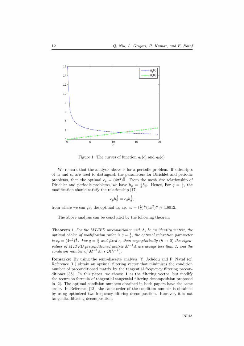
3 .Define

g1(c) = 1 + 1

2√

ch23,

g2(c) = 1 + c

8π2h23.

Then the optimal c can be determined by solving

minc

maxg1(c), g2(c). (30)

This min-max problem can be solved by their plot. In Figure 1, we give thecurve of function g1(c) and g2(c) when h

23 = 0.1. From the figure we can see

that (30) is solved whenever

g1(c) = g2(c).

From this equation, we can get the optimal c = (4π2)23 .

Suppose q is chosen as 43 , then the condition estimate of the preconditioned

linear system is

κ(M−1A) =maxj,k λj,k(M−1A)

minj,k λj,k(M−1A)

≈ λmax(M−1A)−1

1≤ 1 + max 1

2√

ch23, c

8π2h23

= O(h− 23 ).

RR n° 6662


0 5 10 15 200

2

4

6

8

10

12

14

16

c

g1(c)

g2(c)

Figure 1: The curves of function g1(c) and g2(c).

We remark that the analysis above is for a periodic problem. If subscriptsof cd and cp are used to distinguish the parameters for Dirichlet and periodic

problems, then the optimal cp = (4π2)23 . From the mesh size relationship of

Dirichlet and periodic problems, we have hp = 12hd. Hence, For q = 4

3 , themodification should satisfy the relationship [17]

cph43p = cdh

43

d ,

from where we can get the optimal cd, i.e. cd = (12 )

43 (4π2)

23 ≈ 4.6012.

The above analysis can be concluded by the following theorem

Theorem 1 For the MTFFD preconditioner with Λi be an identity matrix, theoptimal choice of modification order is q = 4

3 , the optimal relaxation parameter

is cp = (4π2)23 . For q = 4

3 and fixed c, then asymptotically (h → 0) the eigen-

values of MTFFD preconditioned matrix M−1A are always less than 1, and thecondition number of M−1A is O(h− 2

3 ).

Remarks: By using the semi-discrete analysis, Y. Achdou and F. Nataf (cf.Reference [1]) obtain an optimal filtering vector that minimizes the conditionnumber of preconditioned matrix by the tangential frequency filtering precon-ditioner [38]. In this paper, we choose 1 as the filtering vector, but modifythe recursion formula of tangential tangential filtering decomposition proposedin [2]. The optimal condition numbers obtained in both papers have the sameorder. In Reference [13], the same order of the condition number is obtainedby using optimized two-frequency filtering decomposition. However, it is nottangential filtering decomposition.

INRIA


5 6 7 8 9 10 11 12 13 140.1

0.15

0.2

0.25

0.3

0.35

0.4

0.45

0.5

Minimal eigenvalues as a function of cp

hp=1/32

hp=1/64

hp=1/128

hp=1/256

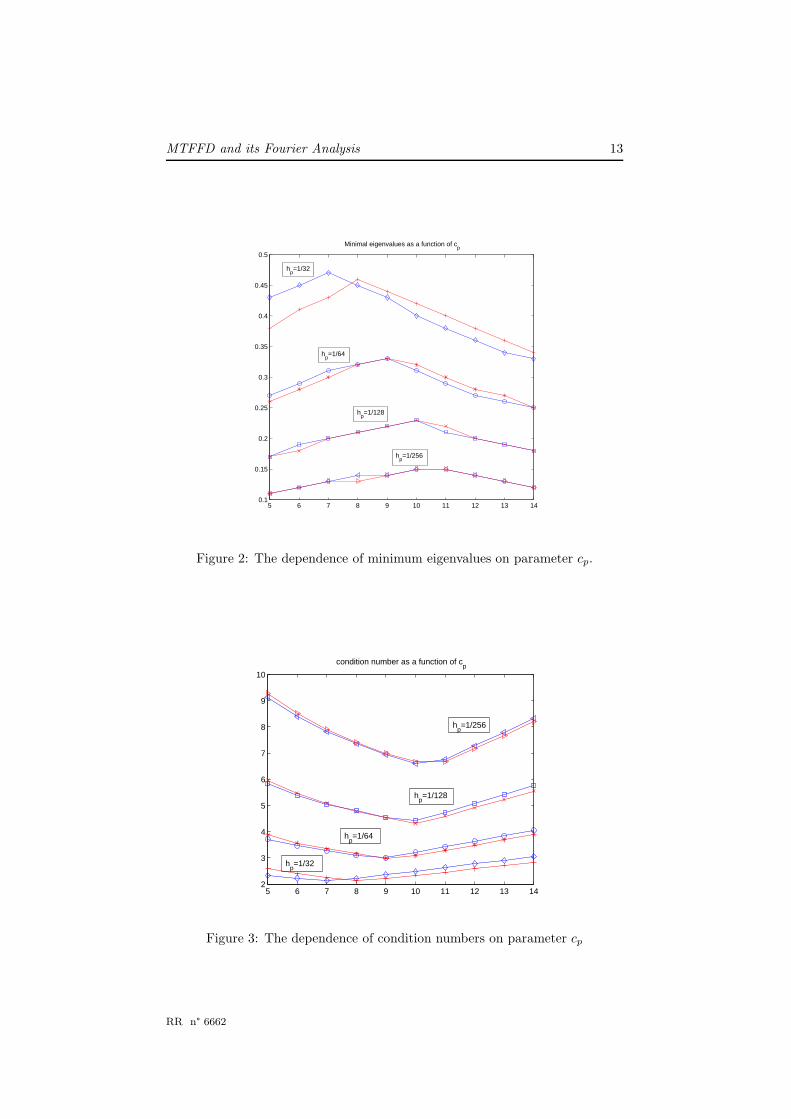
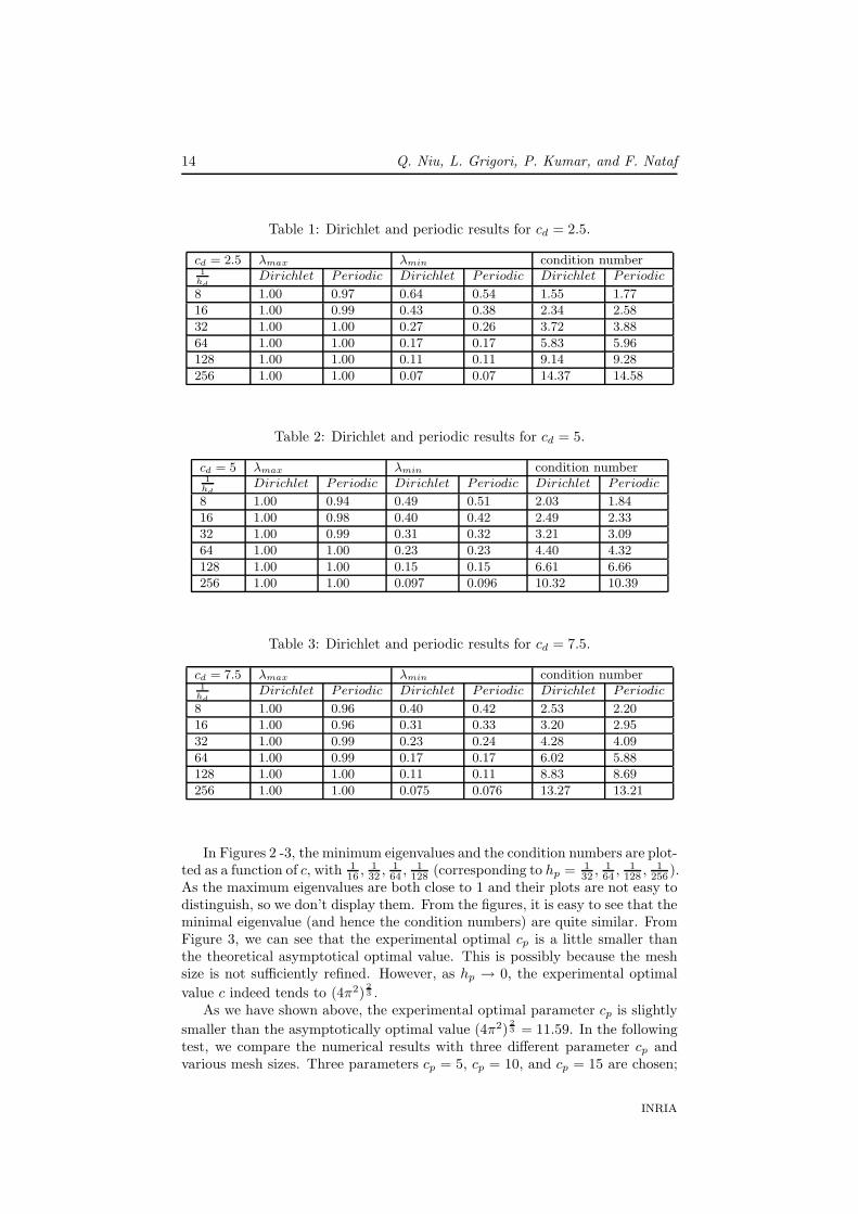
Figure 2: The dependence of minimum eigenvalues on parameter cp.

5 6 7 8 9 10 11 12 13 142

3

4

5

6

7

8

9

10

condition number as a function of cp

hp=1/256

hp=1/128

hp=1/64

hp=1/32

Figure 3: The dependence of condition numbers on parameter cp

RR n° 6662


Table 1: Dirichlet and periodic results for cd = 2.5.

cd = 2.5 λmax λmin condition number1

hdDirichlet Periodic Dirichlet Periodic Dirichlet Periodic

8 1.00 0.97 0.64 0.54 1.55 1.77

16 1.00 0.99 0.43 0.38 2.34 2.58

32 1.00 1.00 0.27 0.26 3.72 3.88

64 1.00 1.00 0.17 0.17 5.83 5.96

128 1.00 1.00 0.11 0.11 9.14 9.28

256 1.00 1.00 0.07 0.07 14.37 14.58

Table 2: Dirichlet and periodic results for cd = 5.

cd = 5 λmax λmin condition number1


8 1.00 0.94 0.49 0.51 2.03 1.84

16 1.00 0.98 0.40 0.42 2.49 2.33

32 1.00 0.99 0.31 0.32 3.21 3.09

64 1.00 1.00 0.23 0.23 4.40 4.32

128 1.00 1.00 0.15 0.15 6.61 6.66

256 1.00 1.00 0.097 0.096 10.32 10.39

Table 3: Dirichlet and periodic results for cd = 7.5.

cd = 7.5 λmax λmin condition number1


8 1.00 0.96 0.40 0.42 2.53 2.20

16 1.00 0.96 0.31 0.33 3.20 2.95

32 1.00 0.99 0.23 0.24 4.28 4.09

64 1.00 0.99 0.17 0.17 6.02 5.88

128 1.00 1.00 0.11 0.11 8.83 8.69

256 1.00 1.00 0.075 0.076 13.27 13.21

In Figures 2 -3, the minimum eigenvalues and the condition numbers are plot-ted as a function of c, with 1

16 , 132 , 1

64 , 1128 (corresponding to hp = 1

32 , 164 , 1

128 , 1256 ).

As the maximum eigenvalues are both close to 1 and their plots are not easy todistinguish, so we don’t display them. From the figures, it is easy to see that theminimal eigenvalue (and hence the condition numbers) are quite similar. FromFigure 3, we can see that the experimental optimal cp is a little smaller thanthe theoretical asymptotical optimal value. This is possibly because the meshsize is not sufficiently refined. However, as hp → 0, the experimental optimal

value c indeed tends to (4π2)23 .

As we have shown above, the experimental optimal parameter cp is slightly

smaller than the asymptotically optimal value (4π2)23 = 11.59. In the following

test, we compare the numerical results with three different parameter cp andvarious mesh sizes. Three parameters cp = 5, cp = 10, and cp = 15 are chosen;

INRIA


0 0.02 0.04 0.06 0.08 0.1 0.12 0.1410

0

101

102

curve of f=h−2/3

curve of f=0.25h−2/3

experimental condition numbers with cp=5



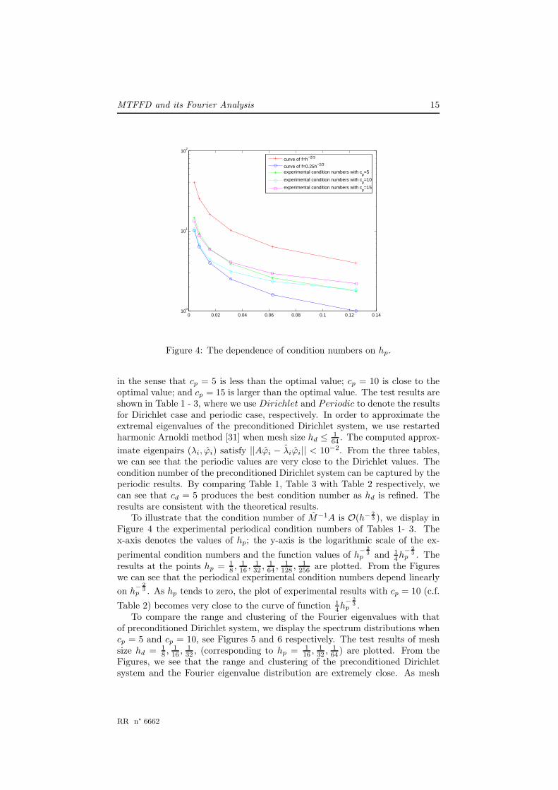
Figure 4: The dependence of condition numbers on hp.

in the sense that cp = 5 is less than the optimal value; cp = 10 is close to theoptimal value; and cp = 15 is larger than the optimal value. The test results areshown in Table 1 - 3, where we use Dirichlet and Periodic to denote the resultsfor Dirichlet case and periodic case, respectively. In order to approximate theextremal eigenvalues of the preconditioned Dirichlet system, we use restartedharmonic Arnoldi method [31] when mesh size hd ≤ 1

64 . The computed approx-

imate eigenpairs (λi, ϕi) satisfy ||Aϕi − λiϕi|| < 10−2. From the three tables,we can see that the periodic values are very close to the Dirichlet values. Thecondition number of the preconditioned Dirichlet system can be captured by theperiodic results. By comparing Table 1, Table 3 with Table 2 respectively, wecan see that cd = 5 produces the best condition number as hd is refined. Theresults are consistent with the theoretical results.

To illustrate that the condition number of M−1A is O(h− 23 ), we display in

Figure 4 the experimental periodical condition numbers of Tables 1- 3. Thex-axis denotes the values of hp; the y-axis is the logarithmic scale of the ex-

perimental condition numbers and the function values of h− 2

3p and 1

4h− 2

3p . The

results at the points hp = 18 , 1

16 , 132 , 1

64 , 1128 , 1

256 are plotted. From the Figureswe can see that the periodical experimental condition numbers depend linearly

on h− 2

3p . As hp tends to zero, the plot of experimental results with cp = 10 (c.f.

Table 2) becomes very close to the curve of function 14h

− 23

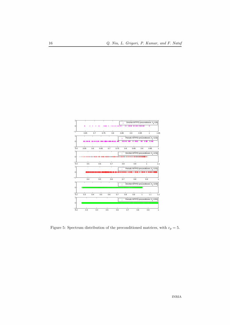
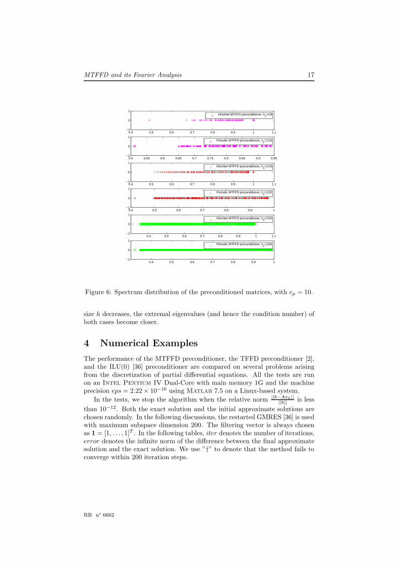
p .To compare the range and clustering of the Fourier eigenvalues with that

of preconditioned Dirichlet system, we display the spectrum distributions whencp = 5 and cp = 10, see Figures 5 and 6 respectively. The test results of meshsize hd = 1

8 , 116 , 1

32 , (corresponding to hp = 116 , 1

32 , 164 ) are plotted. From the

Figures, we see that the range and clustering of the preconditioned Dirichletsystem and the Fourier eigenvalue distribution are extremely close. As mesh

RR n° 6662


0.65 0.7 0.75 0.8 0.85 0.9 0.95 1 1.05−1

0

1

Dirichlet MTFFD preconditioner, h

d=1/8

0.5 0.55 0.6 0.65 0.7 0.75 0.8 0.85 0.9 0.95 1−1

0

1

Periodic MTFFD preconditioner, h

p=1/16

0.4 0.5 0.6 0.7 0.8 0.9 1 1.1−1

0

1


d=1/16

0.4 0.5 0.6 0.7 0.8 0.9 1−1

0

1


p=1/32

0.2 0.3 0.4 0.5 0.6 0.7 0.8 0.9 1 1.1 1.2−1

0

1


d=1/32

0.2 0.3 0.4 0.5 0.6 0.7 0.8 0.9 1−1

0

1


p=1/64

Figure 5: Spectrum distribution of the preconditioned matrices, with cp = 5.

INRIA


0.4 0.5 0.6 0.7 0.8 0.9 1 1.1−1

0

1


d=1/8

0.5 0.55 0.6 0.65 0.7 0.75 0.8 0.85 0.9 0.95−1

0

1


p=1/16

0.4 0.5 0.6 0.7 0.8 0.9 1 1.1−1

0

1

0.4 0.5 0.6 0.7 0.8 0.9 1−1

0

1

Dirichlet MTFFD preconditioner, hd=1/16

Periodic MTFFD preconditioner, hp=1/32

0.4 0.5 0.6 0.7 0.8 0.9 1 1.1−1

0

1


d=1/32

0.4 0.5 0.6 0.7 0.8 0.9 1−1

0

1


p=1/64

Figure 6: Spectrum distribution of the preconditioned matrices, with cp = 10.

size h decreases, the extremal eigenvalues (and hence the condition number) ofboth cases become closer.

4 Numerical Examples

The performance of the MTFFD preconditioner, the TFFD preconditioner [2],and the ILU(0) [36] preconditioner are compared on several problems arisingfrom the discretization of partial differential equations. All the tests are runon an Intel Pentium IV Dual-Core with main memory 1G and the machineprecision eps = 2.22 × 10−16 using Matlab 7.5 on a Linux-based system.

In the tests, we stop the algorithm when the relative norm ||b−Axk||||b|| is less

than 10−12. Both the exact solution and the initial approximate solutions arechosen randomly. In the following discussions, the restarted GMRES [36] is usedwith maximum subspace dimension 200. The filtering vector is always chosenas 1 = [1, . . . , 1]T . In the following tables, iter denotes the number of iterations,error denotes the infinite norm of the difference between the final approximatesolution and the exact solution. We use ”†” to denote that the method fails toconverge within 200 iteration steps.

RR n° 6662


Example 1. We consider the boundary value problem as in [2]

η(x)u + div(a(x)u) − div(κ(x)∇u) = f in Ωu = 0 on ∂ΩD

∂u∂n

= 0 on ∂ΩN

(31)

where Ω = [0, 1]k with k = 2, ∂ΩN = ∂Ω \ ∂ΩD, ∂ΩD = [0, 1] × 0, 1.We consider the following five different cases. As these problems are no

longer constant coefficient, we choose the additional term as cΛih43 , where Λi =

diag(Di), i.e. the diagonal matrix of the ith diagonal block of the coefficientmatrix.

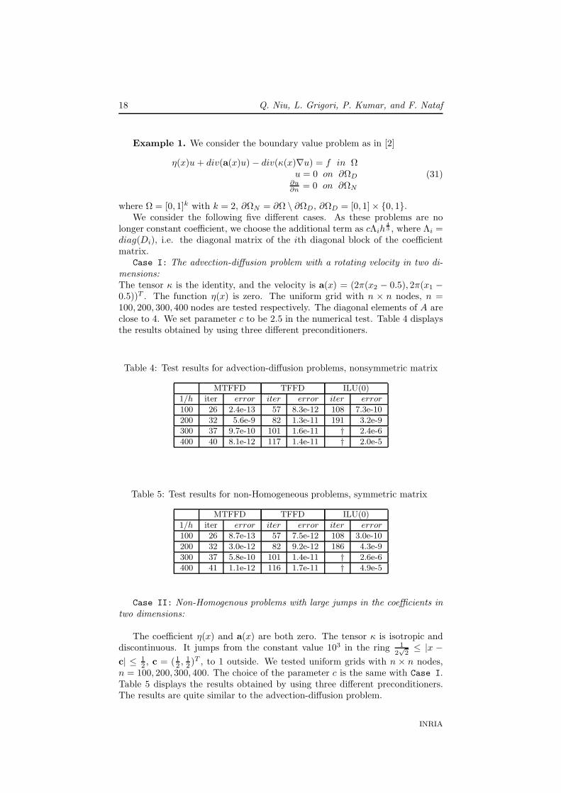
Case I: The advection-diffusion problem with a rotating velocity in two di-mensions:The tensor κ is the identity, and the velocity is a(x) = (2π(x2 − 0.5), 2π(x1 −0.5))T . The function η(x) is zero. The uniform grid with n × n nodes, n =100, 200, 300, 400 nodes are tested respectively. The diagonal elements of A areclose to 4. We set parameter c to be 2.5 in the numerical test. Table 4 displaysthe results obtained by using three different preconditioners.

Table 4: Test results for advection-diffusion problems, nonsymmetric matrix

MTFFD TFFD ILU(0)

1/h iter error iter error iter error

100 26 2.4e-13 57 8.3e-12 108 7.3e-10

200 32 5.6e-9 82 1.3e-11 191 3.2e-9

300 37 9.7e-10 101 1.6e-11 † 2.4e-6

400 40 8.1e-12 117 1.4e-11 † 2.0e-5

Table 5: Test results for non-Homogeneous problems, symmetric matrix

MTFFD TFFD ILU(0)


100 26 8.7e-13 57 7.5e-12 108 3.0e-10

200 32 3.0e-12 82 9.2e-12 186 4.3e-9

300 37 5.8e-10 101 1.4e-11 † 2.6e-6

400 41 1.1e-12 116 1.7e-11 † 4.9e-5

Case II: Non-Homogenous problems with large jumps in the coefficients intwo dimensions:

The coefficient η(x) and a(x) are both zero. The tensor κ is isotropic anddiscontinuous. It jumps from the constant value 103 in the ring 1

2√

2≤ |x −

c| ≤ 12 , c = (1

2 , 12 )T , to 1 outside. We tested uniform grids with n × n nodes,

n = 100, 200, 300, 400. The choice of the parameter c is the same with Case I.Table 5 displays the results obtained by using three different preconditioners.The results are quite similar to the advection-diffusion problem.

INRIA


From Table 4 - 5, we can see that MTFFD is much more efficient; it onlyneeds less than half of the iteration numbers that TFFD needs.

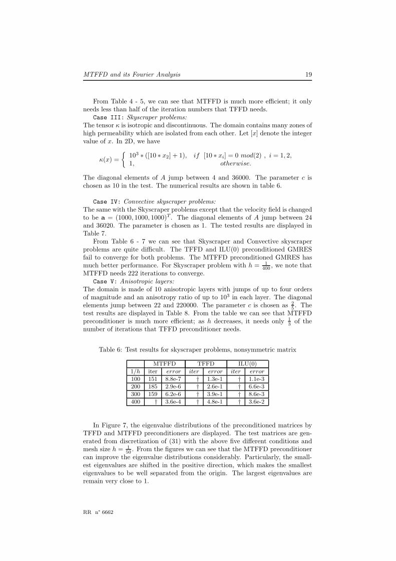
Case III: Skyscraper problems:The tensor κ is isotropic and discontinuous. The domain contains many zones ofhigh permeability which are isolated from each other. Let [x] denote the integervalue of x. In 2D, we have

κ(x) =

103 ∗ ([10 ∗ x2] + 1), if [10 ∗ xi] = 0 mod(2) , i = 1, 2,

1, otherwise.

The diagonal elements of A jump between 4 and 36000. The parameter c ischosen as 10 in the test. The numerical results are shown in table 6.

Case IV: Convective skyscraper problems:The same with the Skyscraper problems except that the velocity field is changedto be a = (1000, 1000, 1000)T . The diagonal elements of A jump between 24and 36020. The parameter is chosen as 1. The tested results are displayed inTable 7.

From Table 6 - 7 we can see that Skyscraper and Convective skyscraperproblems are quite difficult. The TFFD and ILU(0) preconditioned GMRESfail to converge for both problems. The MTFFD preconditioned GMRES hasmuch better performance. For Skyscraper problem with h = 1

400 , we note thatMTFFD needs 222 iterations to converge.

Case V: Anisotropic layers:The domain is made of 10 anisotropic layers with jumps of up to four ordersof magnitude and an anisotropy ratio of up to 103 in each layer. The diagonalelements jump between 22 and 220000. The parameter c is chosen as 2

5 . Thetest results are displayed in Table 8. From the table we can see that MTFFDpreconditioner is much more efficient; as h decreases, it needs only 1

3 of thenumber of iterations that TFFD preconditioner needs.

Table 6: Test results for skyscraper problems, nonsymmetric matrix

MTFFD TFFD ILU(0)


100 151 8.8e-7 † 1.3e-1 † 1.1e-3

200 185 2.9e-6 † 2.6e-1 † 6.6e-3

300 159 6.2e-6 † 3.9e-1 † 8.6e-3

400 † 3.6e-4 † 4.8e-1 † 3.6e-2

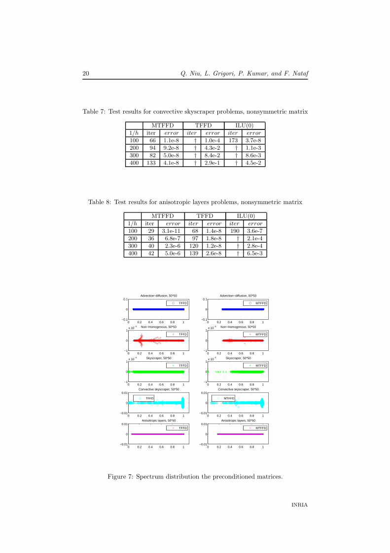
In Figure 7, the eigenvalue distributions of the preconditioned matrices byTFFD and MTFFD preconditioners are displayed. The test matrices are gen-erated from discretization of (31) with the above five different conditions andmesh size h = 1

50 . From the figures we can see that the MTFFD preconditionercan improve the eigenvalue distributions considerably. Particularly, the small-est eigenvalues are shifted in the positive direction, which makes the smallesteigenvalues to be well separated from the origin. The largest eigenvalues areremain very close to 1.

RR n° 6662


Table 7: Test results for convective skyscraper problems, nonsymmetric matrix

MTFFD TFFD ILU(0)


100 66 1.1e-8 † 1.0e-4 173 3.7e-8

200 94 9.2e-8 † 4.3e-2 † 1.1e-3

300 82 5.0e-8 † 8.4e-2 † 8.6e-3

400 133 4.1e-8 † 2.9e-1 † 4.5e-2

Table 8: Test results for anisotropic layers problems, nonsymmetric matrix

MTFFD TFFD ILU(0)


100 29 3.1e-11 68 1.4e-8 190 3.6e-7

200 36 6.8e-7 97 1.8e-8 † 2.1e-4

300 40 2.3e-6 120 1.2e-8 † 2.8e-4

400 42 5.0e-6 139 2.6e-8 † 6.5e-3

0 0.2 0.4 0.6 0.8 1−0.1

0

0.1Advection−diffusion, 50*50

TFFD

0 0.2 0.4 0.6 0.8 1−0.1

0

0.1Advection−diffusion, 50*50

MTFFD

0 0.2 0.4 0.6 0.8 1−1

0

1x 10

−3 Non−Homogenous, 50*50

TFFD

0 0.2 0.4 0.6 0.8 1−1

0

1x 10

−3 Non−Homogenous, 50*50

MTFFD

0 0.2 0.4 0.6 0.8 1−1

0

1x 10

−3 Skyscraper, 50*50

TFFD

0 0.2 0.4 0.6 0.8 1−1

0

1x 10

−3 Skyscraper, 50*50

MTFFD

0 0.2 0.4 0.6 0.8 1−0.01

0

0.01Convective skyscraper, 50*50

TFFD

0 0.2 0.4 0.6 0.8 1−0.01

0

0.01Convective skyscraper, 50*50

MTFFD

0 0.2 0.4 0.6 0.8 1−0.01

0

0.01Anisotropic layers, 50*50

TFFD

0 0.2 0.4 0.6 0.8 1−0.01

0

0.01Anisotropic layers, 50*50

MTFFD

Figure 7: Spectrum distribution the preconditioned matrices.

INRIA


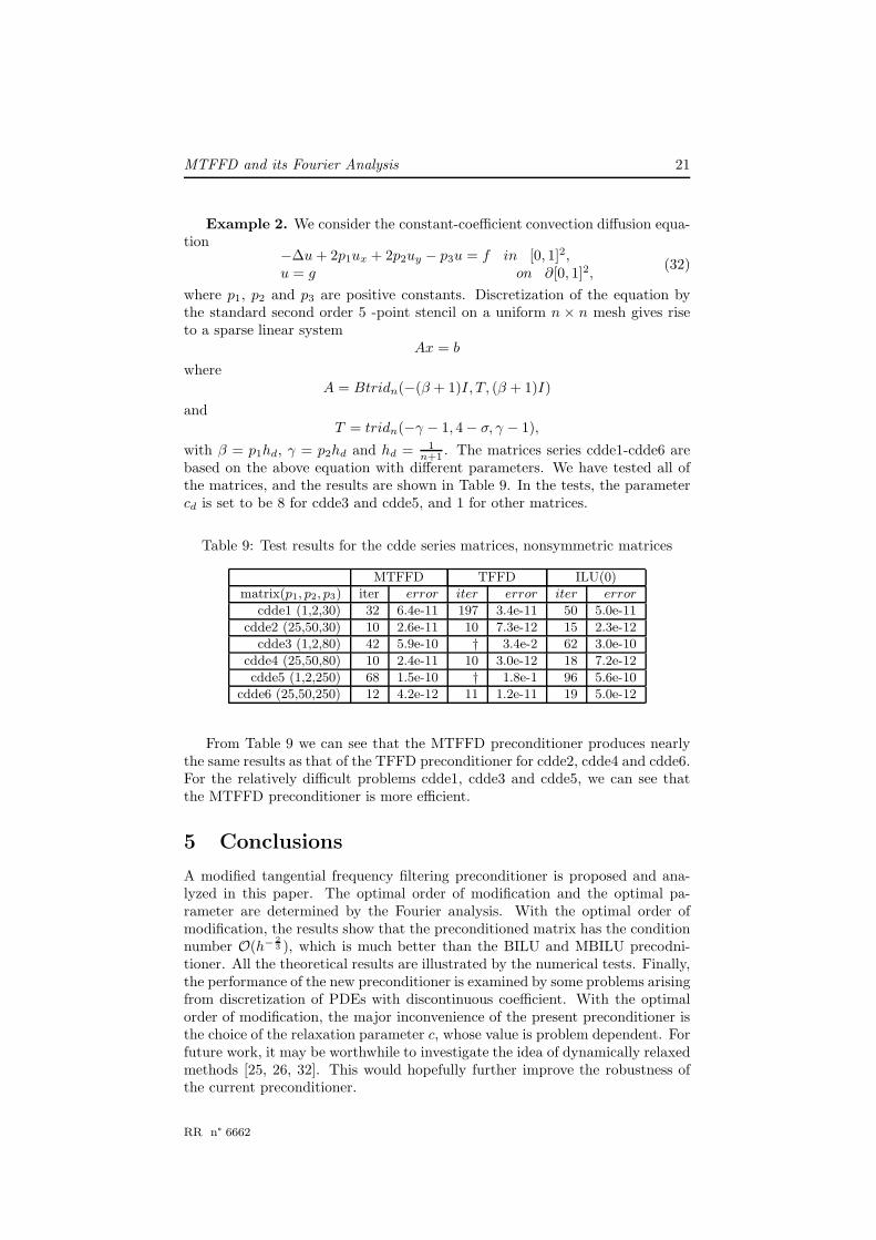
Example 2. We consider the constant-coefficient convection diffusion equa-tion

−∆u + 2p1ux + 2p2uy − p3u = f in [0, 1]2,u = g on ∂[0, 1]2,

(32)

where p1, p2 and p3 are positive constants. Discretization of the equation bythe standard second order 5 -point stencil on a uniform n × n mesh gives riseto a sparse linear system

Ax = b

whereA = Btridn(−(β + 1)I, T, (β + 1)I)

andT = tridn(−γ − 1, 4 − σ, γ − 1),

with β = p1hd, γ = p2hd and hd = 1n+1 . The matrices series cdde1-cdde6 are

based on the above equation with different parameters. We have tested all ofthe matrices, and the results are shown in Table 9. In the tests, the parametercd is set to be 8 for cdde3 and cdde5, and 1 for other matrices.

Table 9: Test results for the cdde series matrices, nonsymmetric matrices

MTFFD TFFD ILU(0)

matrix(p1, p2, p3) iter error iter error iter error

cdde1 (1,2,30) 32 6.4e-11 197 3.4e-11 50 5.0e-11

cdde2 (25,50,30) 10 2.6e-11 10 7.3e-12 15 2.3e-12

cdde3 (1,2,80) 42 5.9e-10 † 3.4e-2 62 3.0e-10

cdde4 (25,50,80) 10 2.4e-11 10 3.0e-12 18 7.2e-12

cdde5 (1,2,250) 68 1.5e-10 † 1.8e-1 96 5.6e-10

cdde6 (25,50,250) 12 4.2e-12 11 1.2e-11 19 5.0e-12

From Table 9 we can see that the MTFFD preconditioner produces nearlythe same results as that of the TFFD preconditioner for cdde2, cdde4 and cdde6.For the relatively difficult problems cdde1, cdde3 and cdde5, we can see thatthe MTFFD preconditioner is more efficient.

5 Conclusions

A modified tangential frequency filtering preconditioner is proposed and ana-lyzed in this paper. The optimal order of modification and the optimal pa-rameter are determined by the Fourier analysis. With the optimal order ofmodification, the results show that the preconditioned matrix has the conditionnumber O(h− 2

3 ), which is much better than the BILU and MBILU precodni-tioner. All the theoretical results are illustrated by the numerical tests. Finally,the performance of the new preconditioner is examined by some problems arisingfrom discretization of PDEs with discontinuous coefficient. With the optimalorder of modification, the major inconvenience of the present preconditioner isthe choice of the relaxation parameter c, whose value is problem dependent. Forfuture work, it may be worthwhile to investigate the idea of dynamically relaxedmethods [25, 26, 32]. This would hopefully further improve the robustness ofthe current preconditioner.

RR n° 6662


References

[1] Y. Achdou and F. Nataf, An iterated tangential filtering decomposition, Nu-mer. Linear Algebra Appl., 10, (2003), pp.511-539.

[2] Y. Achdou, F. Nataf, Low frequency tangential filtering decomposition, Nu-mer. Linear Algebra Appl., 14, (2007), pp.129-147

[3] J. R. Appleyard and I. M. Cheshire, Nested Factorization, SPE 12264, pre-sented at the Seventh SPE Symposium on Reservoir Simulation, San Fran-cisco, 1983.

[4] O. Axelsson, A generalized SSOR method, BIT., 13, (1972), pp. 443-467.

[5] O. Axelsson and L. Kolotilina, Diagonally compensated reduction and relatedpreconditioning methods, Numer. Linear Algebra Appl.,1, (1994), 155-177.

[6] O. Axelsson and V. A. Barker, Finite Element Solution of Boundary ValueProblems, Theory and Computation., New York: Academic Press, 1984.

[7] O. Axelsson and H. Lu, On the eigenvalue estimates for block incompletefactorization methods, SIAM. J. Matrix Anal. Appl., 16, (1995), pp. 1074-1085.

[8] O. Axelsson and G. Lindskog, On the eigenvalue distribution of a class ofpreconditioning methods, Numer. Math., 48, (1986), pp. 479-498.

[9] O. Axelsson, Iterative solution methods, Cambridge University Press, NewYork, 1994.

[10] T. Boonen, J. Van Lent and S. Vandewalle, Local Fourier analysis of multi-grid for the curl curl equation, SIAM J. Sci. Comput., 30, (2008), pp.1730-1755.

[11] A. Brandt, Rigorous local model analysis of Multigrid, Math. Comp., 31,(1977), pp. 333-390.

[12] A. Buzdin, Tangential decomposition, Computing., 61, (1998), pp.257-276.

[13] A. Buzdin and G. Wittum, Two-frequency decomposition, Numer. Math.,97, (2004), pp.269-295.

[14] A. Buzdin, D. Logashenko, and G. Wittum, IBLU decompositions based onPade approximants, Numer. Linear Algebra Appl.,15, (2008), pp.717-746.

[15] T. F. Chan and H. C. Elman, Fourier analysis of iterative methods forelliptic problems, SIAM Review., 31, (1989), pp.20-49.

[16] T. F. Chan, Fourier analysis of relaxed incomplete factorization precondi-tioners, SIAM J. Sci. Comput., 12, (1991), pp.668-690.

[17] T. F. Chan and J. M. Donato, Fourier analysis of incomplete factorizationpreconditioners for three-dimensional anisotropic problems, SIAM J. Sci. Stat.Comput., 13, (1992), pp.319-338.

INRIA


[18] I. Chihiro, Fast solver for large systems of linear equations for finite ele-ment analysis on unstructured meshes, Ph.D thesis, Swinburne University ofTechnology, 2004.

[19] P. Concus, G. H. Golub and G. Meurant, Block Preconditioning for theConjugate Gradient method, SIAM J. Sci. Statist. Comput., 6, (1985), pp.220-252.

[20] I. Gustafsson, A class of first order factorization methods, BIT., 18, (1978),pp.142-156.

[21] W. Hackbusch, Iterative solution of large sparse systems of equations,Springer, New York, 1994.

[22] B. N. Khoromskij, G. E. Mazurkevich and G. Wittum, Frequency filteringfor elliptic interface probems with lagrange multipliers, SIAM J. Sci Comput.,21, (1999), pp. 421-440.

[23] R J. Le Veque and L. N. Trefethen, Fourier anlaysis of the SOR iterations,IMA J. Numer. Anal., 8, (1988), pp.273-279.

[24] H. Lu, Matrix compensation and diagonal compensation, J. Comput. Math.Appl., 63, (1995), 237-244.

[25] M. Magolu Monga-Made, Taking Advantage of the potentialities of dynam-ically modified block incomplete factorizations, SIAM J. Sci Comput., 19,(1998), pp. 1083-1108.

[26] M. Magolu Monga-Made, Dynamically relaxed block incomplete factoriza-tions for solving two- and three-dimensional problems, SIAM J. Sci Comput.,21, (2000), pp. 2008-2028.

[27] The MathWorks, Inc. MATLAB 7, September 2004.

[28] J. A. Meijerink and H. A. van der Vorst, An iterative solution method forlinear systems of which the coefficient matrix is symmetric M-matrix, Math.Comput., 137, (1977), pp.148-162.

[29] C. Mense and R. Nabben, On algebraic multilevel methods for non-symmetric systems - comparison results Linear Algebra Appl. (2008),doi:10.1016/j.laa.2008.04.045.

[30] C. Mense and R. Nabben, On algebraic multilevel methods for non-symmetric systems - convergence results, to appear in ETNA.

[31] R.B. Morgan and M. Zeng, Harmonic Projection Methods for Large Non-symmetric Eigenvalue Problems, Numer. Linear Algebra Appl., 5, (1998) pp.33-55.

[32] Y. Notay, DRIC: A dynamic version of the RIC method, Numer. LinearAlgebra Appl.,1, (1994), 511-532.

[33] Y. Notay, Algebraic multigrid and algebraic multilevel methods: a theoreti-cal comparison, Numer. Linear Algebra Appl. 2005; 12:419-451.

RR n° 6662


[34] K. Otto, Analysis of preconditioners for hyperbolic partial differential equa-tions, SIAM J. Numer. Anal. 33, (1996), pp.2131-2165.

[35] J.W. Ruge and K. Stuben, Algebraic Multigrid (AMG), In Multigrid Meth-ods, Frontiers in Applied Mathematics, Vol 3, SIAM: Philadephia, PA, 1987,73-130.

[36] Y. Saad, Iterative Methods for Sparse Linear Systems, PWS PublishingCompany: Boston, MA, 1996.

[37] P. S. Vassilevski, Multilevel Block Factorization Preconditioners: Matrix-based Analysis and Algorithms for Solving Finite Element Equations,Springer, 2008.

[38] C. Wagner, Tangential frequency filtering decompositions for symmetricmatrices, Numer. Math., 78, (1997), pp.119-142.

[39] C. Wagner, Tangential frequency filtering decompositions for unsymmetricmatrices Numer. Math., 78, (1997), pp.143-163.

[40] C. Wagner and G. Wittum, Adaptive filtering, Numer. Math., 78, (1997),pp.305-382.

[41] R. Wienands, C. W. Oosterlee and T. Washio, Fourier analysis ofGMRES(M) preconditioned by multigrid, SIAM J. Sci. Comput., 22, (2000),pp.582-603.

[42] G. Wittum, Filternde Zerlegungen, Schnelle Loser fur große Gleichungssys-teme. Teubner Skripten zur Numerik, Band 1, Teubner-Verlag, Stuttgart,1992.

[43] G. Wittum, Shifted iterations, Numer. Math. 76, (1997), pp.265-278.

INRIA

Centre de recherche INRIA Saclay – Île-de-FranceParc Orsay Université - ZAC des Vignes

4, rue Jacques Monod - 91893 Orsay Cedex (France)

Centre de recherche INRIA Bordeaux – Sud Ouest : Domaine Universitaire - 351, cours de la Libération - 33405 Talence CedexCentre de recherche INRIA Grenoble – Rhône-Alpes : 655, avenue de l’Europe - 38334 Montbonnot Saint-Ismier

Centre de recherche INRIA Lille – Nord Europe : Parc Scientifique de la Haute Borne - 40, avenue Halley - 59650 Villeneuve d’AscqCentre de recherche INRIA Nancy – Grand Est : LORIA, Technopôle de Nancy-Brabois - Campus scientifique

615, rue du Jardin Botanique - BP 101 - 54602 Villers-lès-Nancy CedexCentre de recherche INRIA Paris – Rocquencourt : Domaine de Voluceau - Rocquencourt - BP 105 - 78153 Le Chesnay CedexCentre de recherche INRIA Rennes – Bretagne Atlantique : IRISA, Campus universitaire de Beaulieu - 35042 Rennes Cedex

Centre de recherche INRIA Sophia Antipolis – Méditerranée :2004, route des Lucioles - BP 93 - 06902 Sophia Antipolis Cedex

ÉditeurINRIA - Domaine de Voluceau - Rocquencourt, BP 105 - 78153 Le Chesnay Cedex (France)

http://www.inria.fr

ISSN 0249-6399

Modified tangential frequency filtering decomposition and its fourier analysis

Documents

Transcript of Modified tangential frequency filtering decomposition and its fourier analysis