Empirical Fourier Decomposition - arXiv

Empirical Fourier Decomposition

Wei Zhou a

Zhongren Feng a, b

Xiongjiang Wang a, ⁎

Hao Lv a

a School of Civil Engineering and Architecture, Wuhan University of Technology, Wuhan 430070, P.R.

China.

b School of Urban Construction, Wuchang Shouyi University, Wuhan 430064, P.R. China.

⁎ Corresponding author. 122 Luoshi Road, Wuhan, 430070, P.R. China.

E-mail: [email protected]

Abstract

In this paper, a novel decomposition method for non-stationary and nonlinear signals is proposed. This

method is inspired by the adaptive wavelet filter bank of the empirical wavelet transform (EWT) and Fourier

intrinsic band functions (FIBFs) of the Fourier decomposition method (FDM). Therefore, the proposed

approach is entitled as empirical Fourier decomposition (EFD). EFD is defined as the adaptive bandpass filter

bank, regarded as the adaptive FIBFs based on the segment of the Fourier spectrum. Firstly, an enhanced

segmentation technology of the Fourier spectrum based is presented. Secondly, the framework of EFD is

established both in a continuous series and a discrete series. Finally, combined with the Hilbert transform,

EFD is extended to a time-frequency representation. To verify the effectiveness of EFD, three non-stationary

multimode signals, a simulated free vibration, and one real ECG signal are tested. The results manifest that

EFD is more effective, compared with EWT and FDM, with higher processing precision, computation

efficiency and noise robustness particularly to the closely-spaced frequencies and high-frequency noise.

Keywords: Empirical wavelet transform; Fourier decomposition method; Bandpass filter bank;

Decomposition; Hilbert transform.

1. Introduction

Multicomponent non-stationary and nonlinear (NSNL) signals decomposition has drawn deep concern

in numerous fields, such as biomedical signal analysis [1–6], seismic signal analysis [7–10], vibration analysis

in engineering [11–17], speech enhancement [18–21], etc. The multicomponent signals created by real-life

physical systems frequently comprise several superposed oscillations, which are also termed as signal modes

[22], and encompass meaningful information of a physical system. Hence, it is crucial to improve the accuracy

and efficiency in signal processing.

During the past decades, several signal decomposition approaches have been proposed, among which

empirical mode decomposition (EMD) has had a significant impact [23]. Despite the limited mathematical

understanding and some obvious shortcomings, such as mode mixing and end effects, EMD is widely used in

a broad variety of time-frequency analysis applications. To overcome these difficulties, some elevated versions

of the EMD were developed, such as ensemble EMD [24], complete ensemble EMD [25], and recent method:

time-varying filter based EMD [26]. Although these approaches abate the limitations to some extent, the

performance is still not satisfactory as desired.

Jumping out of the bondage of EMD, several EMD-like signal processing methods have been proposed.

One category of the method is retrieving each signal mode in time-frequency (TF) domain. These TF analysis

methods represent the frequency of each mode versus time meaning that the time-varying frequency of non-

stationary signals can be better dealt with [22]. Introduced by Daubechies [27], Synchrosqueezing transform

(SST) is an EMD-like approach with combining wavelet analysis and reallocation technique. The reallocation

method used in the SST enhances the resolution of the TF domain so tremendous that the SST is applied

extensively. Subsequently, researchers proposed several SST-based methods, for instance, the higher order

SST [28], the matching SST for signals with fast varying instantaneous frequency [17], time-reassigned SST

with reassigned in the time direction [13], and local maximum SST for the energy concentrated in the TF

domain greatly [12], and multi-SST via multiple reallocate to achieve high concentrated TF representation

[29].

Another classify method is various adaptive filtering techniques. The empirical wavelet transform (EWT)

employs the wavelet filter bank based on the segment of the Fourier spectrum [30]. To eliminate the restriction

of the Fourier spectrum, the power spectrum based EWT methods have been developed [15,16,31]. The

variational mode decomposition (VMD) belongs to this category and is a generalization of the Wiener filter

[32]. Then, the method in [33] uses the adaptive local iterative filtering and the swarm decomposition

algorithm which is seen as the swarm filtering [34]. In addition, the Fourier decomposition method (FDM)

[35] and the recent adaptive chirp mode pursuit (ACMP) [14] are also the filter-based methods, but the FDM

is based on the Fourier transform (FT) which is a TF filter bank with the adjustable bandwidth.

Some other methods utilize an optimization model to decompose signals. For instance, the operator-based

approaches [36,37], the sparse TF method [38] and the short-time narrow-banded mode decomposition

(STNBMD) [39]. Of course, the classification is not really rigid. For example, the frameworks of VMD and

ACMP also contain optimization. However, the results of the optimization algorithms typically rely on the

initialization, like the STNBMD, of which the initial frequencies influence the results deeply to the closely-

spaced modals. Additionally, the bandwidth is regularly as the part of the objective function of the optimization

methods, always predetermined [32] and narrow [39] in the early methods but recently the ACMP enables it

adjustable.

In the aforementioned methods, two of them worth further researching, namely the EWT and the FDM.

It is because both of them depend on the FT which has been regarded as inappropriate to analyze the NSNL

signals for past decades [35]. Although the EWT method is the wavelet filter bank which is framed by the

wavelet transform, the key of the EWT is the segment based on the Fourier spectrum [30]. Therefore, the EWT

has great significance to spread the FT into the NSNL data analysis. Then, the FDM introduces the concept of

Fourier intrinsic band functions (FIBFs) to decompose signals by employing the properties of the mode: non-

negative amplitude and non-decreasing phase. The FDM applies the FT to the signals of NSNL authentically,

based on the theoretic of the FT purely. Admittedly, EWT and FDM, especially EWT, have achieved great

success and widely used in signal processing. These involved signal decomposition in the bearing fault

diagnosis [11], structural modal analysis [15,16], medical analysis [1], to name just a few examples.

Nonetheless, several limitations still persist in the EWT and FDM. With regard to the EWT, the transition

phase of the wavelet filter bank may be redundant. It causes that the adjacent components interfere with each

other, particularly the closely-spaced frequencies. For another, although it has been improved in subsequent

literature, the method of the segmentation can continue to be optimized [40]. The current method cannot match

the number of segments and the number of modes. Sometimes the first component is the residue and

sometimes is the main component, which obscures the operator. FDM is sensitive to the noise. The noise

signal can be decomposed too many components, moreover, the cost of the computation will increase

drastically. Furthermore, the signal analyzed in FDM is not expanded, resulting in a very serious end effect in

the decomposition components. These aforementioned defects all leave room for theoretical development and

improvement on the robustness of the decomposition.

In this work, a novel signal decomposition algorithm called empirical Fourier decomposition (EFD) is

proposed to address the hindrances aforementioned. Enlightened by EWT and FDM, EFD combines the idea

of the segmentation in the Fourier spectrum and the FIBFs to decompose the signal into several modes. We

propose a new method of partitioning and construct a mathematical framework of the EFD. The algorithm no

longer possesses the complex transition phase. We also illustrate that the segmentation technique matches the

number of segments and modes. Moreover, EFD optimizes performance under closely-spaced modes and

high-frequency noise, and increases computation efficiency.

The remnant of the paper is arranged as follows. In section 2, we recall the principle of the three methods:

EMD, EWT, and FDM. In section 3, we introduce the proposed method and expound its segmentation, frame

of the continuous series, discrete series, and TF representation. Section 4 shows five experiments based on

simulated and real signals. Finally, we present a conclusion for our work and some prospects for future works

in section 5.

2. Theoretical background

2.1 Empirical mode decomposition

In 1998, EMD is proposed by Huang et al. [23], it is an adaptive algorithm to decompose a signal into

several components. The components decomposed by this method are called intrinsic mode functions (IMFs).

These IMFs are amplitude-modulated-frequency-modulated (AM-FM) signals, and so the original signal is

written as:

1

cos +N

k k

k

f t f t t r t

(1)

where the envelop fk (t) is non-negative, the phase ϕk (t) is an increasing function, r (t) is the final residue, and,

N is the number of IMF. fk (t) and instantaneous frequency ωk (t) = ϕk (t) change markedly slower than ϕk (t)

does [27,30,32].

All the IMFs should satisfy two fundamental conditions [23]: (a) The difference between the number of

extreme points (minima and maxima) and the number of zero-crossings is no more than one over the entire

duration of time series. (b) At any point, the mean of the envelope defined by the local minima and local

maxima, respectively, is zero.

With these two basic conditions, the operational process of EMD is described as the following 5 steps:

1. Compute the upper and lower envelopes by using a cubic spline interpolation to fit the maxima and

minima of f (t).

2. Obtain the mean envelope and note m (t).

3. Get a candidate IMF via r1 (t) = f (t) - m (t). Generally, r1 (t) dissatisfies the two above-mentioned

conditions, then, repeat previous two steps to rk (t) (k = 1, 2, … , n-1) until the eligible candidate rn

(t) is found.

4. Define rn (t) as f1 (t), and get the next IMF by employing the same steps to (f (t)- f1 (t)).

5. Repeat the aforementioned steps to calculate the remaining IMFs.

2.2 Empirical wavelet transform

EWT is an adaptive wavelet transform algorithm based on the segmentation of the Fourier spectrum [30].

This algorithm assumes that the Fourier support [0, π] is divided into N contiguous partitions. Each segment

is denoted Sn = [ωn-1, ωn] (the ωn represents boundary, and ω0 = 0, ωN = π), then a transition zone Tn is defined

around ωn symmetrically with the double width of τn (Fig. 1). The empirical wavelets are seen as one lowpass

ϕn (ω) and N-1 bandpass filters ψn (ω) on each Sn [31].

Fig. 1. Basic construction of EWT.

Fig. 1 exhibits the lowpass and bandpass wavelet filters defined as ϕ1 (ω) and ψn (ω), where the horizontal

axis and vertical axis correspond with the boundaries and amplitude of the filters, respectively. The first

segment is the lowpass filter ϕ1 (ω) with a cut-off frequency ω1, which corresponds to the first boundary.

Except for the last bandpass filter ψN (ω) with a frequency band [ωN-1, π], other bandpass filters ψn (ω) have

a frequency band of [ωn, ωn+1].

The original segmentation technique in EWT is a local maxima approach [40]. In this method, Gilles

computes all local maxima Mi of the analyzed signal in the Fourier domain and deduces their corresponding

position ωi. Then the N-1 largest maxima are set to all corresponding ωi and re-index them as ωn where 1 ≤ n

≤ N-1. So, the set of boundaries Ʊ = {ωn}n = 0,…,N by:

1

0 if =0

= 2 otherwise

if =

n n

n

n

n N

(2)

Next, following the idea utilized in originating both of Meyer’s wavelets and Littlewood-Paley, the

empirical scaling function and empirical wavelet function defined as Eqs. (3) and (4), respectively [41].

1 if

1cos

( ) 2 2

if

0 otherwise

n n

n n

n n

n n n n

(3)

and

+1 +1

+1 +1

+1

+1 +1 +1 +1

1 if +

1cos

2 2

if ( )

1sin

2 2

if

0 otherwise

n n n n

n n

n

n n n n

n

n n

n

n n n n

(4)

where τn = γω, read this paper [30] for more details about the value of γ. β (x) is an arbitrary function with the

following properties:

0 if 0

and + 1 1 0, 1

1 if 1

x

x x x x

x

(5)

Moreover, in EWT, β (x) is the same as the most utilized in [41]:

4 2 335 85 70 20x x x x x (6)

After the tight frame wavelet filters have been established, EWT can be defined by detail coefficients and

approximation coefficients, respectively, as follows:

1, ,

f nW n t F f

(7)

1

1, ,

fW 0 t F f

(8)

where ,f

W n t

is the detail coefficients, ,f

W 0 t

is the approximation coefficients, and F-1 symbolizes the

inverse Fourier transform.

2.3 Fourier decomposition method

Proposed by Singh [35], FDM is a novel adaptive approach to process the NSNL signal. This algorithm

supposes a signal has M FIBFs and uses the FIBF to build the mono-component of a signal. M generally equals

to the number of modes of a signal. The FIBF is identified as a real part of analytic Fourier intrinsic band

functions (AFIBFs). The AFIBF is similar to a generalized Fourier expansion [23], but the limits of summation

may vary for each AFIBF. Moreover, AFIBF is defined as:

1 1 0

2AFIBF exp = exp

i

i

N

i i i k

k N

jkta t j t c

T

(9)

where i =1, 2, … , M with N0 = 0, NM = (N/2 – 1) when N is even (or if N is odd with NM = (N – 1)/2). Ni is a

vital value for AFIBF, essentially the boundary in the Fourier domain of FDM. It obtains adaptively by two

strategies: low to high-frequency scan and high to low-frequency scan.

Subsequently, each method can be divided into four steps. Owing to these steps are similar except scan

order, only the process of the low to high-frequency scan is described in the following paragraphs. For a

complete comprehensible interpretation of the algorithm, please refer to the literature [35].

Step A. Obtain FFT of f (t), i.e. F (t)=FFT{f (t)}.

Step B. Set 1 1 0

2AFIBF exp = exp

i

i

N

i i i k

k N

jkta t j t c

T

.

Step C. Get maximum number of Ni and a monotonically increasing function of phase φi(n) which such

that (Ni-1 + 1) ≤ Ni ≤ (N/2 – 1) and ωi(n) = (φi(n+1) – φi(n–1))/2 ≥ 0, n, respectively. Substitution Ni and φi(n)

to step B to get the AFIBFs.

Step D. Obtain FIBFs from the real part of AFIBFs.

3. Proposed method

The proposed method, EFD, is can be considered as a partial combination of EWT and FDM. In the frame

of this method, the ideas of segmenting Fourier spectrum in the EWT [30] and FIBF in FDM [35] are combined.

EFD employs the segmentation of the Fourier spectrum, and each partition denotes the region of a FIBF. From

Fig. 2, this method seems as a bandpass filter in each segment. Compared with EWT, EFD is more concise

and not require the cumbersome transition phase and tight frame. Then, the following subsections describe

EFD in four portions.

ω0 ω1 ωn ωn+1

1

Fig. 2. Basic construction of EFD.

3.1 Segmentation of the empirical Fourier decomposition

As same to EWT, the segment of the Fourier spectrum is significant to EFD. High quality of segmentation

is the prerequisite for the program of EFD. We propose a new segment method inspired by the local maxima

method [30] and the local minima method [40].

For the purpose of the desired performance, the separation of the Fourier spectrum should be supported

as tightly as possible. In this paper, the frequency range of the Fourier spectrum is also from 0 to π. The number

of partitions is N, which means that a total of N+1 boundaries are necessitated. To determine these boundaries,

the control points (the local maxima and initial value) are detected in the spectrum and sorted in descending

order. Then, the assumption of identified M control points is set as same to EWT [30]:

1. If M ≥ N: the method found adequate control points to support the N segments, and only the first N-

1 control points are kept.

2. If M < N: the analyzed signal has fewer modes to extract, then keeping all the control points and

resetting N to M.

Then, following the detected control point, their corresponding position ωi is deduced. Next, re-index

them as ωn where 1 ≤ n ≤ N-1, ω0 = 0 and ωN = π. Finally, we set the global minimum in [ωn-1, ωn] as boundaries

ωn, and the set of these minima is denoted as Ωn. So the Fourier boundaries is described as:

1

arg minΩ for 1 1

2

n

N Nn

n N

n N

(10)

Fig. 3 shows an example of the segmentation technique based on these three distinct methods. The

example (solid line) the Fourier spectrum demonstrates that the signal has the following features. a) The first

component of the signal concentrates in low frequency. b) The 2nd component is a flat-picked mode where

the bandwidth is wide. c) The high-frequency noise exists in the signal. Figs. 3 (a), 3 (b) and 3 (c) show results

of the local maxima method [30], the local minima method [40], and EFD. These results illustrate that the

proposed method performs better for the signals with these three characteristics. Firstly, when the signal

concentrates in the low frequency, the prior number of modes does not correspond accurately to the real

number of modes in the local maxima method [30] and the local minima method [40]. In this case, the prior

number of modes of the two methods is one less than the real number of modes. Secondly, for the flat-picked

mode, the original EWT cannot decompose the modes well, which the 1st and 3rd components are

contaminated with the 2nd. Thirdly, the proposed bound method alleviates the interference of high-frequency

noise.

Fig. 3. Three segmentation methods: (a) the local maxima method, (b) the local minima method, (c)

the proposed approach.

3.2 Continuous empirical Fourier decomposition

In this subsection, we construct a framework of continuous EFD. Firstly, let f (t) be a signal of real-valued

and time-limited (t ϵ [t1, t1+L], L>0), and φ0:=2π/L. So, the Fourier series expansion of f (t) is determined as:

1

1

1

1

1

1

0

0

0

0

0 0

1

2dt

2cos dt

2 sin dt

cos sin2

t L

t

t L

nt

t L

nt

n n

n

a f tL

a n t f tL

b n t f tL

af t a n t b n t

(11)

Then, using Euler’s formula, the complex exponential representation of the Fourier series is given by:

0

0 0

1

1 exp exp

2 2 nn

n

af t c jn t c jn t

(12)

where cn=(an-jbn) and c*

n =( an+jbn).

To give the definition of AFIBF in this proposed method, u(t), its complex conjugate u t are set as:

0

=1

0

=1

exp

exp

n

n

n

n

u t c jn t

u t c jn t

(13)

So Eq. (12) can be rewritten as:

0 Re{ }2

af t u t (14)

where Re{u(t)} is the real part of u(t).

Following the segmentation in the subsection of 3.1, the number of segment (N-1) means that u(t) can be

separated into N-1 parts, and u(t) can be computed as follows in a general Fourier expansion [23]:

1

=1

expN

i i

i

u t A j t

(15)

Finally, combining the boundaries ωn, we describe AFIBFs as:

1

0exp exp

i

i

i i nA j t c jn t

(16)

where Ai is the instantaneous amplitude and θi is the instantaneous phase of the i-th FIBF, and FIBF is a real

part of AFIBF.

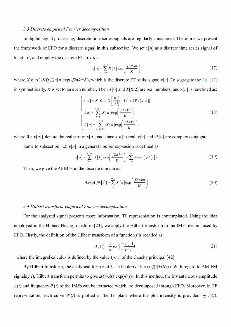
3.3 Discrete empirical Fourier decomposition

In digital signal processing, discrete time series signals are regularly considered. Therefore, we present

the framework of EFD for a discrete signal in this subsection. We set x[n] as a discrete time series signal of

length K, and employ the discrete FT to x[n]:

1

=0

2exp

K

k

j knx n X k

K

(17)

where X[k]=(1/K)∑K-1

k=0 x[n]exp(-j2πkn/K), which is the discrete FT of the signal x[n]. To segregate the Eq. (17)

in symmetrically, K is set to an even number, Then X[0] and X[K/2] are real numbers, and x[n] is redefined as:

/ 2 1

=1

1

= /2+1

0 1 2 Re2

2exp

2exp

n

K

k

K

k K

Kx n X X v n

j knv n X k

K

j knv n X k

K

(18)

where Re{v[n]} denote the real part of v[n], and since x[n] is real, v[n] and v*[n] are complex conjugate.

Same to subsection 3.2, v[n] in a general Fourier expansion is defined as:

/ 2 1 1

=1 =1

2exp exp

K N

i i

k i

j knv n X k A j t

K

(19)

Then, we give the AFIBFs in the discrete domain as:

1 2

exp expi

i

i i

j knA j t X k

K

(20)

3.4 Hilbert transform-empirical Fourier decomposition

For the analyzed signal presents more information, TF representation is contemplated. Using the idea

employed in the Hilbert-Huang transform [23], we apply the Hilbert transform to the IMFs decomposed by

EFD. Firstly, the definition of the Hilbert transform of a function f is recalled as:

1

. . df

fH t p v

t

(21)

where the integral calculus is defined by the value (p.v.) of the Cauchy principal [42].

By Hilbert transform, the analytical form z of f can be derived: z(t)=f(t)+jHf(t). With regard to AM-FM

signals f(t), Hilbert transform permits to give z(t)=A(t)exp(jθ(t)). In this method, the instantaneous amplitude

A(t) and frequency θ(t) of the IMFs can be extracted which are decomposed through EFD. Moreover, in TF

representation, each curve θi(t) is plotted in the TF plane where the plot intensity is provided by Ai(t).

Following this method, TF representation based on EFD is quite feasible.

4. Numerical studies and application

In this section, we use five examples: four artificial signals and one real-life signal, to test this proposed

method. The form of the first three signals is utilized in the EWT [30] and VMD [32], and the fourth signal

has been also applied in previous work [31]. Meanwhile, we chose EWT and FDM with applying to these

signals for comparison. In these examples, the segments of EFD are set 4, 5, 3, 4 and 11 from the first signal

to the fifth, respectively. The original EWT is used, and its selection of the segment is one less than EFD,

except for the fourth example which is the same as EFD. Additionally, due to the similar results computing by

these two methods in FDM, only the approach of low to high frequency is used in this paper.

4.1 Non-stationary multimode signals

Three non-stationary multimode signals, which primitively derive from the literature [38], are simulated

in this section. All signals are in the region of [0, 1], and sample frequency is presupposed as 1000 Hz in this

paper.

a) Example 1: The first signal has three simple components: one general linear trend and two diverse

harmonics, their functions are described as follows:

11

12

13

1 11 12 13

6

2 cos 8

cos 40

f t t

f t t

f t t

f t f t f t f t

(22)

The time series of f1(t) and its three components are shown in Fig. 4. For a direct exhibition of the

segments of FDM, the boundaries are displayed in the same way as EFD and EWT, and all their boundaries

are depicted in Fig. 5. It is worth noting that EFD is capable of separating the Fourier spectrum appropriately

in f1(t). Owing to 0 and π are also the boundaries of EWT, the boundaries of EWT and EFD are similar except

the fourth boundary where EFD is closer to the third frequency spike than EWT. Moreover, 0 is a default

boundary to FDM. The first segment of FDM is too narrow for the first component, and this deficiency induces

the first two components to interfere with each other.

Fig. 4. f1(t) and its three components: from (a) to (d) is f1(t), f11(t), f12(t),and f13(t), respectively.

Fig. 5. Boundaries of f1(t) estimated by (a) EFD, (b) EWT, and (c) FDM.

Fig. 6 demonstrates the components extracted by EFD, EWT, and FDM, respectively. The results of EFD

are shown in Fig. 6 (a), and the three modes reveal nice separation into a linear trend and two harmonics,

respectively. However, segments of EWT are quite similar to EFD, as shown in Fig. 6 (b), the first component

has a periodic fluctuate in mild because it is affected by the second component through the transition zone.

Fortunately, the other two components are quite accurate extracted by EWT. Compared with the results of

EFD and EWT, FDM shows no competitiveness in this example. As exhibited in Fig. 6 (c), except the third

component, other results present weak performance. The second component has a mild linear trend, and the

first just looks like a simple harmonic. Besides, distortions exist at both ends of the third. It is because FMD

is unable to eliminate the boundary effect. For further purpose of comparison, the error is provided in Fig. 6

(d) which defined by the difference of an original component and the corresponding extracted component in

time series. In this case, the errors of FDM are too large to compare, and only the errors of EFD and EWT are

presented. From Fig. 6 (d), it is clear that the first component of the EFD has smaller errors than the EWT

does. The other two components are in an opposite situation, but the errors of the EFD are close to the EWT.

Fig. 6. Decomposition results of f1(t) and their errors: (a) EFD, (b) EWT, (c) FDM, and (d) errors.

b) Example 2: The second signal is a composition of a quadratic trend, a linear chirp signal, and a

piecewise harmonic with two constant frequencies:

2

21

2

22

23

2 21 22 23

6

cos 15 +

cos 60 otherwise

cos 80 15 if 0.5

f t t

f t t t

tf t

t t

f t f t f t f t

(23)

The time series of f2(t) and its components are demonstrated in Fig. 7. Then, decomposing the signal by

exploiting the EFD, the EWT, and the FDM, respectively, and their boundaries are shown in Fig. 8. The

number of segments of the FDM is three, but of the other two methods is four. This is because f23 is departed

by the EFD and the EWT, and it can be deemed as two independent components due to their frequencies have

meaningful individual energy. However, the FDM keeps the entire f23, and the first segment has the same

limitation described in example 1.

Fig. 7. f2(t) and its three components: from (a) to (d) is f2(t), f21(t), f22(t),and f23(t), respectively.


Next, the components estimated via the EFD, the EWT and the FDM are displayed in Fig. 9. The results

of the EFD are displayed in Fig. 9 (a), four components seem good. But the second component has some

distortion in the middle, and the third and fourth components have not excellent performances in their

transition zone. On the contrary, the better products are provided by the second component of the EWT as Fig.

9 (b) showed. However, some distractions occur in the front half portion of the third component, actually, the

amplitude is zero in this part. Similar to example 1, it is clear depict in Fig. 9 (c) that the two first components

of the FDM are not acceptable, and only the third component is satisfactory. In addition, Fig. 9 (d) shows the

errors of the EFD and the EWT, it makes no difference in the first error. The second EFD’s error is bigger in

the middle, but the third error of the EFD is less than the EWT except for the middle transition zone.


c) Example 3: The third example embodies intra-wave frequency modulation:

31

32

3 31 32

1 1.2+ cos 2

cos 32 +0.2 cos 64

1.2+ sin 2

f tt

t tf t

t

f t f t f t

(24)

Fig. 10 presents the time series of f3(t) and its components. Again, the EFD, the EWT, and the FDM are

used to decompose f3(t), respectively. Their decomposing boundaries are shown in Fig. 11. In this case, the

boundaries of the three approaches are basically identical except the last boundary of the EFD is closer to the

third frequency spike. Hence, each component of the three methods is almost the same, as shown in Fig. 12.

Nevertheless, the difference appears in the first component, the result of EWT and FDM has fluctuation after

0.6 s. Furthermore, because of the valuable results of FDM, the errors of these three methods are exhibited in

Fig. 12 (d). The first error of the FDM seems large, but the errors are basically around 1.5. Because the entire

amplitude-modulated appears in the first component. Therefore, the first component of FDM has the same

form of f31(t). The second errors of these three methods are pretty small, among them, the errors of EFD are

minimum.

Fig. 10. f3(t) and its three components: from (a) to (d) is f3(t), f31(t), and f32(t), respectively.

4.2 Simulated free vibration signal with two closely-spaced modes and a 20 dB noise

To validate the capability of EFD in processing the closely-spaced modes and high-frequency noise, we

apply a 3-degree of freedom structural free vibration response signal with varied damping ratios, two closely-

spaced modes, and a 20 dB noise. It is utilized in [31] and given by the following equation:

23 2

1( ) cos(2 ) ( )

i if t

i i i iis t A e tf 1 n t

(25)

where Ai is the amplitude, fi is the natural frequency, ζi is the damping ratio and θi is the phase angle of the ith

frequency, respectively. To simulate the free vibration response of a real structure, the low natural frequencies

f1=1.1, f2=1.3, and f3=3.1 Hz and the varied damping ratios ζ1=2%, ζ2=1.2%, and ζ3=0.8% are introduced. In

addition, all of the amplitudes Ai=1, all of the phase angles θi=0, and n(t) is Gaussian noise with signal-to-

noise-ratio of 20 dB. The synthetic signal sampled by a frequency of 50 Hz within a period of 20 s. Fig. 13 (a)

and Fig. 13 (b) show the simulated signal with the noise of 0 dB and 20 dB, respectively.

Fig. 13. Synthetic signal: (a) 0 dB, (b) 20 dB.

Results for extracting the boundaries are showed for three the proposal employing EFD, EWT, and FDM

in Figs. 14 (a), 14 (b) and 14 (c), respectively. In this case, the segment technique of EWT is the local minima

method [40], to eliminate the effect of differ boundary between EFD and EWT in closely-spaced modes. The

number of segments in the methods of EFD, EWT, and FDM is 3, 4, and 13, respectively. However, the

segments of EWT and FDM are not matched with the actual number 3. Each frequency spike contained in the

first segment of EWT is not redundant, but the 10 extra segments of FDM are caused by Gaussian noise. The

boundaries of EWT and EFD are same in the first three, but the fourth boundary of which EFD is closer to the

third frequency spike than EWT. This difference means that the third component in EFD is less affected by

high-frequency noise than EWT does. In addition, FDM is unable to separate the first two closely-spaced

modes.

Fig. 14. Boundaries of the simulated signal estimated by (a) EFD, (b) EWT, and (c) FDM.

Next, the components of EFD and the 2nd, 3rd and 4th components of EWT and the 1st, 2nd components

of FDM are presented in Fig. 15. The first two components of EFD have a high performance. Although the

first two segments of EWT are same as EFD, the 1st and 2nd components interfere with each other. Meanwhile,

the third embodies noise in both methods. The first component of FDM is disturbed by another frequency

component, and the second component has no noise disturbance. Furthermore, the errors of EFD and EWT

are exhibited in the box plots as Fig. 15 (d), which demonstrates that the errors of EFD are less than EWT.

Fig. 15. Decomposition results of the synthetic signal and their errors: (a) EFD, (b) EWT, (c) FDM,

and (d) errors.

4.3 Real electrocardiogram signal

To exploit the proposed method to real life, in this subsection, a real electrocardiogram (ECG) signal is

introduced. This ECG signal is provided by the MIT-BIH arrhythmia database [43]. Data of 101 from 3600 to

4600 are used, and these 1000 samples are displayed in Fig. 16.

Because of substantial components, the results of EWT and FDM are just provided in the TF

representation of the next subsection. Fig. 17 shows the boundaries extracted by the proposed method. There

are 10 segments are obtained, and only one frequency spike contains in the first 9 segments. The

decomposition results are presented in Fig. 18. The first component is the trend component, while the last one

is the R wave. The other components are similar to the sinusoidal waves. More medical interpretation of these

components should be remarked by cardiologists.

Fig. 16. A sample ECG signal.

Fig. 17. Boundaries of the ECG signal estimated by EFD.

Fig. 18. Decomposition results of the ECG signal by EFD.

4.4 Time-frequency representation

Time-frequency representation is significant in signal processing, hence, the performance of EFD in the

TF domain is exhibited in this section. In this case, f3(t) and the ECG signal are applied. EWT and FDM are

also applied to these two signals for comparison.

Fig. 19 shows the TF representation of f3(t). The results of EFD, EWT, and FDM are demonstrated in

Figs. 19 (a), 19 (b) and 19 (c), respectively. From these three figures, it manifests that each method contains

two components and the corresponding component has the approximate same trend. For better comparison,

Fig. 19 (d) presents the two components of f3(t) (the bottom is f31(t) and the top is f32(t)) in the TF domain,

respectively. Based on the results in Fig. 19 (d), EFD is more effective than the other two methods. On the one

hand, the middle district of f32(t) of EWT fluctuates deeply. On the other, the energy of f31(t), as shown in Fig.

19 (d), is extremely tiny in the region of [0, 0.2] and [0.8, 1], but the results of EWT exists energy in the

regions [0.8, 0.9] and the results of FDM exists energy in [0, 0.2] and [0.8, 1].

Fig. 19. Time-frequency representation of f3(t) by: (a) EFD, (b) EWT, and (c) FDM; (d) the time-

frequency representation of f31(t) + f32(t) by the Hilbert transform.

Then, TF representation of the ECG signal is shown in Fig. 20. Corresponding to the location of the R

wave in the ECG signal, the energy of these methods are all concentrated in these sites. Moreover, the results

of EFD and EWT are basically identical, but the energy of EWT between the three R waves is sparser than

EFD. With regard to the results of FDM, it seems to provide a fruitful representation. However, it is worth

noticing that FDM is interfered by noise in the region of relatively high-frequency.

Fig. 20. Time-frequency representation of the ECG signal by (a) EFD, (b) EWT, and (c) FDM.

4.5 Discussion

Results showed in this paper indicate that EFD can provide good performance in the aforementioned

examples. Firstly, the decomposition results of EFD are nearly the same as EWT for non-stationary multimode

signals. But both of them present better than FDM. Secondly, EFD can decompose the closely-spaced

frequencies and decrease the influence of noise for the last component. Finally, TF representation of EFD

exhibits impressive performance.

The three methods: EFD, EWT, and FDM, all based on FFT. So, these methods have an equal time

complexity O(Nlog2N) [44]. However, the proposed method EFD, unlike the other, has the characteristics of

the simple framework and high computational efficiency.

Table 1 summarizes time consumption of these three methods extracting mono-component of

aforementioned examples in this paper. All the calculations are performed on a laptop with an Intel Core i7-

6700HQ CPU, 2.60GHz, 8.0GB RAM, Windows 10 Home, and software of MATLAB R2018a. Among the

three methods, EFD requires less computational time. Furthermore, it is worth noticing that FDM consumes

more computation time compared with the other. The time is increased, especially with the number of

segments, as are shown in example 4 and 5.

Table 1

Computational time for the five examples.

Example Time (s)

EFD EWT FDM

1 0.0215 0.0409 0.8400

2 0.0259 0.0576 0.9237

3 0.0221 0.0435 0.7388

4 0.0260 0.0412 1.5323

5 0.0282 0.0497 2.0460

However, there are still restrictions of EFD which all leave room for further development:

1. The number of boundaries is required in advance and is one more than the signal model order.

2. Based on FFT, the proposed method is not appropriate for high-level noise signals.

3. The signal including components with overlapped in both the frequency and time domains is unable

to be extracted.

5. Concluding remarks

In this paper, a novel approach is proposed based on EWT and FDM. The proposed method can be

considered as a bandpass filter bank based on the Fourier spectrum segmentation. Meanwhile, the rigorous

mathematical deduction based on FFT is also provided.

To substantiate the effectiveness of the proposed method, three non-stationary multimode signals, a

closely-spaced frequencies signal, and an ECG signal are presented and tested. These experiments reveal that

the proposed approach is capable of separate the aforementioned signals. Moreover, EWT and FDM are

compared. The comparison revealed that EFD can separate the closely-spaced mode, while, typically, EWT

exhibits that the extracted components cross each other. Another advantage of the proposed approach is that

the last component of EFD is less influenced by high-frequency noise compared with EWT. On the other hand,

comparing with FDM, the proposed method has higher processing precision, computation efficiency. Besides,

the TF representation of f3(t) and ECG signal is presented, which indicate that EFD enables a better

performance than the other does.

In the future, the proposed method would have wider applications in several fields. For instance, civil

engineering, mechanical engineering, earthquake engineering, etc. Moreover, we would extend EFD to a

higher dimension. For example, 2D-EFD will be able to process images. Meanwhile, the method of

segmentation should be further developed, such as the power spectrum based method [15,16,31] and the

adaptive method which likes machine learning technology [45]. It is noteworthy that each component of the

signal is linearly superposed in the Fourier domain. If a signal contains the component with the energy spread

over the whole Fourier spectrum or contains two consecutive modes are too close, these components would

be interfered by the superposing effect. The reduction of the superposition effect should be regarded as a

priority.

A MATLAB implementation of the proposed algorithm wil available at the MATLAB Central.

Acknowledgments

The authors would like to thank the people who share their contributions to the signal proceeding

community.

Conflicts of Interest: The authors declare no conflict of interest.

References

[1]A. Bhattacharyya, R.B. Pachori, A Multivariate Approach for Patient-Specific EEG Seizure

Detection Using Empirical Wavelet Transform, IEEE Trans. Biomed. Eng. 64 (2017) 2003–2015.

doi:10.1109/TBME.2017.2650259.

[2]D. Benitez, P.A. Gaydecki, A. Zaidi, A.P. Fitzpatrick, The use of the Hilbert transform in

ECG signal analysis, Comput. Biol. Med. 31 (2001) 399–406. doi:10.1016/S0010-4825(01)00009-9.

[3]A. Khaliduzzaman, S. Fujitani, A. Kashimori, T. Suzuki, Y. Ogawa, N. Kondo, A non-

invasive diagnosis technique of chick embryonic cardiac arrhythmia using near infrared light,

Comput. Electron. Agric. 158 (2019) 326–334. doi:10.1016/j.compag.2019.02.014.

[4]S.C. Wu, P.T. Chen, A.L. Swindlehurst, P.L. Hung, Cancelable Biometric Recognition with

ECGs: Subspace-Based Approaches, IEEE Trans. Inf. Forensics Secur. 14 (2019) 1323–1336.

doi:10.1109/TIFS.2018.2876838.

[5]M. Blanco-Velasco, B. Weng, K.E. Barner, ECG signal denoising and baseline wander

correction based on the empirical mode decomposition, Comput. Biol. Med. 38 (2008) 1–13.

doi:10.1016/j.compbiomed.2007.06.003.

[6]A. Sellami, H. Hwang, A robust deep convolutional neural network with batch-weighted loss

for heartbeat classification, Expert Syst. Appl. 122 (2019) 75–84. doi:10.1016/j.eswa.2018.12.037.

[7]F. Li, B. Zhang, S. Verma, K.J. Marfurt, Seismic signal denoising using thresholded

variational mode decomposition, Explor. Geophys. 49 (2017) 450–461. doi:10.1071/EG17004.

[8]Y. Chen, Z. Peng, A. Gholami, J. Yan, S. Li, Seismic signal sparse time–frequency

representation by Lp-quasinorm constraint, Digit. Signal Process. A Rev. J. 87 (2019) 43–59.

doi:10.1016/j.dsp.2019.01.010.

[9]T. Wang, M. Zhang, Q. Yu, H. Zhang, Comparing the applications of EMD and EEMD on

time-frequency analysis of seismic signal, J. Appl. Geophys. 83 (2012) 29–34.

doi:10.1016/j.jappgeo.2012.05.002.

[10]M. Schimmel, J. Gallart, The inverse S-transform in filters with time-frequency localization,

IEEE Trans. Signal Process. 53 (2005) 4417–4422. doi:10.1109/TSP.2007.896050.

[11]J. Pan, J. Chen, Y. Zi, Y. Li, Z. He, Mono-component feature extraction for mechanical fault

diagnosis using modified empirical wavelet transform via data-driven adaptive Fourier spectrum

segment, Mech. Syst. Signal Process. 72–73 (2016) 160–183. doi:10.1016/j.ymssp.2015.10.017.

[12]G. Yu, Z. Wang, P. Zhao, Z. Li, Local maximum synchrosqueezing transform : An energy-

concentrated time-frequency analysis tool, Mech. Syst. Signal Process. 117 (2019) 537–552.

doi:10.1016/j.ymssp.2018.08.006.

[13]D. He, H. Cao, S. Wang, X. Chen, Time-reassigned synchrosqueezing transform: The

algorithm and its applications in mechanical signal processing, Mech. Syst. Signal Process. 117

(2019) 255–279. doi:10.1016/j.ymssp.2018.08.004.

[14]S. Chen, Y. Yang, Z. Peng, X. Dong, W. Zhang, G. Meng, Adaptive chirp mode pursuit:

Algorithm and applications, Mech. Syst. Signal Process. 116 (2019) 566–584.

doi:10.1016/j.ymssp.2018.06.052.

[15]Y. Xin, H. Hao, J. Li, Operational modal identification of structures based on improved

empirical wavelet transform, Struct. Control Heal. Monit. 26 (2019) 1–21. doi:10.1002/stc.2323.

[16]Z. Luo, T. Liu, S. Yan, M. Qian, Revised empirical wavelet transform based on auto-

regressive power spectrum and its application to the mode decomposition of deployable structure, J.

Sound Vib. 431 (2018) 70–87. doi:10.1016/j.jsv.2018.06.001.

[17]S. Wang, X. Chen, C. Tong, Z. Zhao, Matching Synchrosqueezing Wavelet Transform and

Application to Aeroengine Vibration Monitoring, IEEE Trans. Instrum. Meas. 66 (2016) 1–13.

doi:10.1109/TIM.2016.2613359.

[18]A. Upadhyay, R.B. Pachori, Speech enhancement based on mEMD-VMD method, Electron.

Lett. 53 (2017) 502–504. doi:10.1049/el.2016.4439.

[19]P. Tanwar, A. Somkuwar, Hard component detection of transient noise and its removal using

empirical mode decomposition and wavelet-based predictive filter, IET Signal Process. 12 (2018)

907–916. doi:10.1049/iet-spr.2017.0167.

[20]Y. Laufer, S. Gannot, A Bayesian Hierarchical Model for Speech Enhancement With Time-

Varying Audio Channel, IEEE/ACM Trans. Audio, Speech, Lang. Process. 27 (2019) 225–239.

doi:10.1109/TASLP.2018.2876177.

[21]R. Henni, M. Djendi, M. Djebari, A new efficient two-channel fast transversal adaptive

filtering algorithm for blind speech enhancement and acoustic noise reduction, Comput. Electr. Eng.

73 (2019) 349–368. doi:10.1016/j.compeleceng.2018.12.009.

[22]D. Iatsenko, P.V.E. McClintock, A. Stefanovska, Nonlinear mode decomposition: A noise-

robust, adaptive decomposition method, Phys. Rev. E - Stat. Nonlinear, Soft Matter Phys. 92 (2015)

1–25. doi:10.1103/PhysRevE.92.032916.

[23]H.H.L. N.E. Huang, Z. Shen, S.R. Long, M.C. Wu, H.H. Shih, Q. Zheng, N.C. Yen, C.C.

Tung, The empirical mode decomposition and the Hilbert spectrum for nonlinear and non-stationary

time series analysis, Proc. R. Soc. London. Ser. A Math. Phys. Eng. Sci. 454 (1998) 903–995.

https://doi.org/10.1098/rspa.1998.0193.

[24]Z. Wu, N.E. Huang, Ensemble Empirical Mode Decomposition :, Adv. Adapt. Data Anal. 1

(2009) 1–41.

[25]M.E. Torres, M.A. Colominas, G. Schlotthauer, P. Flandrin, A complete ensemble empirical

mode decomposition with adaptive noise, in: ICASSP, IEEE Int. Conf. Acoust. Speech Signal

Process. - Proc., 2011: pp. 4144–4147. doi:10.1109/ICASSP.2011.5947265.

[26]H. Li, Z. Li, W. Mo, A time varying filter approach for empirical mode decomposition,

Signal Processing. 138 (2017) 146–158. doi:10.1016/j.sigpro.2017.03.019.

[27]I. Daubechies, J. Lu, H. Wu, Synchrosqueezed wavelet transforms : An empirical mode

decomposition-like tool, Appl. Comput. Harmon. Anal. 30 (2011) 243–261.

doi:10.1016/j.acha.2010.08.002.

[28]T. Representations, T. Oberlin, S. Meignen, V. Perrier, Second-Order Synchrosqueezing

Transform or Invertible Reassignment ? Towards Ideal, IEEE Trans. Signal Process. 63 (2015) 1335–

1344. doi:10.1109/TSP.2015.2391077.

[29]G. Yu, Z. Wang, P. Zhao, Multi-synchrosqueezing Transform, IEEE Trans. Ind. Electron. 66

(2019) 5441–5455. doi:10.1109/TIE.2018.2868296.

[30]J. Gilles, Empirical wavelet transform, IEEE Trans. Signal Process. 61 (2013) 3999–4010.

doi:10.1109/TSP.2013.2265222.

[31]J.P. Amezquita-Sanchez, H. Adeli, A new music-empirical wavelet transform methodology

for time-frequency analysis of noisy nonlinear and non-stationary signals, Digit. Signal Process. A

Rev. J. 45 (2015) 55–68. doi:10.1016/j.dsp.2015.06.013.

[32]K. Dragomiretskiy, D. Zosso, Variational mode decomposition, IEEE Trans. Signal Process.

62 (2014) 531–544. doi:10.1109/TSP.2013.2288675.

[33]A. Cicone, J. Liu, H. Zhou, Adaptive local iterative filtering for signal decomposition and

instantaneous frequency analysis, Appl. Comput. Harmon. Anal. 41 (2016) 384–411.

doi:10.1016/j.acha.2016.03.001.

[34]G.K. Apostolidis, L.J. Hadjileontiadis, Swarm decomposition: A novel signal analysis using

swarm intelligence, Signal Processing. 132 (2017) 40–50. doi:10.1016/j.sigpro.2016.09.004.

[35]P. Singh, S.D. Joshi, R.K. Patney, K. Saha, The Fourier decomposition method for nonlinear

and non-stationary time series analysis, Proc. R. Soc. A Math. Phys. Eng. Sci. 473 (2017).

doi:10.1098/rspa.2016.0871.

[36]S. Peng, W.L. Hwang, Null space pursuit: An operator-based approach to adaptive signal

separation, IEEE Trans. Signal Process. 58 (2010) 2475–2483. doi:10.1109/TSP.2010.2041606.

[37]S. Peng, W.L. Hwang, Adaptive signal decomposition based on local narrow band signals,

IEEE Trans. Signal Process. 56 (2008) 2669–2676. doi:10.1109/TSP.2008.917360.

[38]T.Y. Hou, Z. Shi, Adaptive data analysis via sparse time-frequency representation, Adv.

Adapt. Data Anal. 3 (2011) 1–28. doi:10.1142/S1793536911000647.

[39]S.I. McNeill, Decomposing a signal into short-time narrow-banded modes, J. Sound Vib.

373 (2016) 325–339. doi:10.1016/j.jsv.2016.03.015.

[40]J. Gilles, G. Tran, S. Osher, 2D Empirical Transforms. Wavelets, Ridgelets, and Curvelets

Revisited, SIAM J. Imaging Sci. 7 (2014) 157–186. doi:10.1137/130923774.

[41]I. Daubechies, Ten lectures on wavelets, in: CBMS-NSF Reg. Conf. Ser. Appl. Math.,

Society for Industrial and Applied Mathematics, Philadelphia, 1992: pp. 198–202.

[42]F.W. King, Hilbert transforms, Cambridge University Press Cambridge, 2009.

doi:10.1017/CBO9780511721458.

[43]G.B. Moody, R.G. Mark, The Impact of the MIT-BIH Arrhythmia Database, IEEE Eng.

Med. Biol. 20 (2001) 45–50.

[44]C.H. Papadimitriou, Optimality of the Fast Fourier Transform, J. Assoc. Comput. Mach. 26

(1979) 95–102.

[45]J. Gilles, K. Heal, A parameterless scale-space approach to find meaningful modes in

histograms - Application to image and spectrum segmentation, Int. J. Wavelets, Multiresolution Inf.

Process. 12 (2014) 1–17. doi:10.1142/S0219691314500441.

Empirical Fourier Decomposition - arXiv

Documents

Transcript of Empirical Fourier Decomposition - arXiv