Mode shape reconstruction of an impulse excited structure using continuous scanning laser Doppler...

Mode shape reconstruction of an impulse excited structureusing continuous scanning laser Doppler vibrometerand empirical mode decomposition

Yongsoo Kyong, Daesung Kim, Jedol Dayou,a� Kyihwan Park, and Semyung Wangb�

Department of Mechatronics, School of Information and Mechatronics Engineering,Gwangju Institute of Science and Technology, 1 Oryong-dong, Buk-gu, Gwangju 500-712, Republic of Korea

�Received 29 January 2008; accepted 22 May 2008; published online 3 July 2008�

For vibration testing, discrete types of scanning laser Doppler vibrometer �SLDV� have beendeveloped and have proven to be very useful. For complex structures, however, SLDV takesconsiderable time to scan the surface of structures and require large amounts of data storage. Toovercome these problems, a continuous scan was introduced as an alternative. In this continuousmethod, the Chebyshev demodulation �or polynomial� technique and the Hilbert transform approachhave been used for mode shape reconstruction with harmonic excitation. As an alternative, in thispaper, the Hilbert–Huang transform approach is applied to impact excitation cases in terms of anumerical approach, where the vibration of the tested structure is modeled using impulse responsefunctions. In order to verify this technique, a clamped-clamped beam was chosen as the test rig inthe numerical simulation and real experiment. This paper shows that with additional innovativesteps of using ideal bandpass filters and nodal point determination in the postprocessing, theHilbert–Huang transformation can be used to create a better mode shape reconstruction even in theimpact excitation case. © 2008 American Institute of Physics. �DOI: 10.1063/1.2943416�

I. INTRODUCTION

Vibration phenomena are important considerations in thedesign of machines, structures, instruments, and so on. Boththe analysis and measurement of vibration are particularlyimportant tasks because they should be performed togetherfor the modeling of a real structure. A good vibration modelhas the potential capacity for allowing further engineeringprocesses such as optimization. Among the many availablemeasurement devices, the accelerometer is the most widelyused sensor. With accelerometers and excitation such as theforce from impact hammers or electromagnetic shakers, vi-bration characteristics can be calculated by the modal param-eter estimation technique.1

Although the accelerometer has good sensitivity espe-cially in high frequency bands, it has some limitations. Be-cause of its nature as a contacting device, it can lead to massloading especially for the measurement of light structures. Ifthe structure is heavy, the accelerometer is still suitable but itcannot be attached to the rotating surface directly. In addi-tion, for mode shape measurements, many accelerometersneed to be attached in order to measure all spatial points. Inthis case, it will take some time to attach the accelerometers.For hammer roving tests, it also takes a long time to hit everymeasurement point.

Because of these limitations, in recent years noncontactmeasuring instruments such as laser Doppler vibrometer�LDV� have been more widely used.2 Compared to conven-tional contact devices, LDV does not suffer from mass load-

ing effects, and also reduces the setting time of sensors re-quired for vibration testing.2 These improvements have beenhelpful for engineers to shorten measurement time, and en-hance the spatial accuracy of measurements. LDV is defi-nitely faster than humans for testing, but when the structureis more complex, the testing process can still be timeconsuming.3

Many applications require spatially dense measurement.With conventional sensors such as accelerometers and dis-crete SLDV, the number of measurement points needs to bequite large in order to cover the whole area of a structure.This can take a relatively long time and requires a largestorage capacity. As an alternative to the discrete scanningmethod, a continuous scanning method is introduced and isreferred to in this paper as a continuous SLDV �CSLDV�.

a�Also at Vibration and Sound Research Group �VIBS�, School of Scienceand Technology, Universiti Malaysia Sabah, Locked Bag 2073, 88999Kota Kinabalu, Sabah, Malaysia.

b�Electronic mail: [email protected]. 1. Clamped-clamped beam with nondimensionalized coordinates andscan profile.

REVIEW OF SCIENTIFIC INSTRUMENTS 79, 075103 �2008�

0034-6748/2008/79�7�/075103/12/$23.00 © 2008 American Institute of Physics79, 075103-1

Downloaded 21 Mar 2009 to 203.237.43.184. Redistribution subject to AIP license or copyright; see http://rsi.aip.org/rsi/copyright.jsp

http://dx.doi.org/10.1063/1.2943416

http://dx.doi.org/10.1063/1.2943416

http://dx.doi.org/10.1063/1.2943416

http://dx.doi.org/10.1063/1.2943416

CSLDV is able to realize modal parameter estimation withonly one measurement. In terms of a “continuous” scanningmethod, many scanning schemes are available, such as theshort linear scan, the circular scan, the conical scan, and thestraight line scan.2–4 Specifically, in the sinusoidal scan, theChebyshev demodulation has been introduced by Sriramet al.;5 who have suggested the demodulation technique as apostprocessing technique to obtain the mode shapes of thevibrating structure.5–7 The resultant mode shapes are ap-proximated as a polynomial form.2–10 According to this tech-nique, approximated functional forms of natural modeshapes can be obtained based on the assumption of stationaryvelocity distribution.

However, because the Chebyshev demodulation tech-nique is based on discrete Fourier transform analysis, peri-odicity conditions should be satisfied. Also leakage problemscan degrade the results. In response to these problems, Kanget al.11 suggested an alternative method called the Hilberttransform approach. Their work investigated the Hilberttransform for the demodulation of CSLDV output, and thedeflection shape can be measured accurately. For the case ofsingle frequency excitation, they obtained good experimentalresults. However, there was no investigation about the gen-eral excitation method, in, for example, impact and randomexcitation. This is because Hilbert transform alone cannot beused for the general excitation cases.

In this paper, Hilbert–Huang transform �HHT�technology12 is proposed in order to realize the mode shapereconstruction for general excitation schemes. HHT hasproved to be capable of analyzing nonlinear and nonstation-ary signals, and has been recently used in speech communi-cation applications. This algorithm has also been used in awide range of diverse fields: geological sciences, fluid dy-namics, financial predictions, speech analysis, vibrationanalysis, and so on. This method is the combination of em-pirical mode decomposition �EMD� and the Hilbert trans-form. It can decompose a signal in the frequency-timedomain.12–15 After decomposition, modal responses can beobtained for the reconstruction of mode shapes using theHilbert transform. In order to improve the quality of modeshape reconstruction, this paper proposes two additionalsteps for the postprocessing technique; the ideal bandpassfilter in the EMD process and the instantaneous frequencyfor the determination of the nodal points of the structure.Also included in this paper are the results of the numericalsimulation and real experiment performed for the validationof this technique.

II. SYSTEM MODELING

A. Sinusoidal continuous scanning LDVs

CSLDV technology can be used on many types of struc-tures. However, for simplicity of discussion in this paper, aone-dimensional �1D� structure is used. Suppose that a 1Dstructure is scanned, and the velocity variation of the struc-

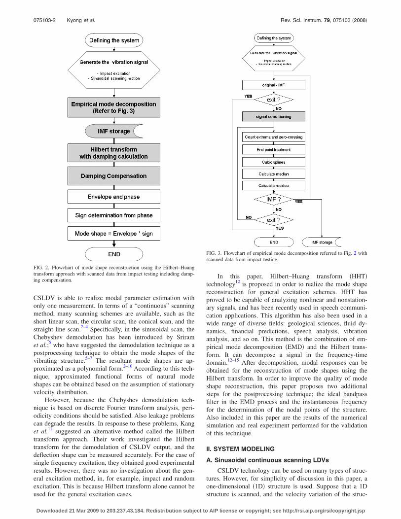
FIG. 2. Flowchart of mode shape reconstruction using the Hilbert–Huangtransform approach with scanned data from impact testing including damp-ing compensation.

FIG. 3. Flowchart of empirical mode decomposition referred to Fig. 2 withscanned data from impact testing.

075103-2 Kyong et al. Rev. Sci. Instrum. 79, 075103 �2008�


ture is statistically stationary. The scanning direction can bedenoted by the coordinate x and the scanning limits are non-dimensionalized to �1.

In this case, a laser beam reflected by a driving mirrorcan be utilized as the measuring sensor, with sensor locationdefined as

x�t� = cos��t� , �1�

where � is the laser scanning frequency, which is the sameas the mirror driving frequency.

B. 1D sinusoidal scan with impact excitation

For this case, by applying the modal approach, the timevarying velocity can be derived from the impulse responsefunction as

v�xo,t� = �q=1

Q

Yq��q�xf��q�xo�

= �q=1

Q �−�n,q

m�d,qe−�q�n,qt sin��d,qt − ��q�xf��q�xo� ,

�2�

where Q is the number of considering modes; m is the mass;Y�� is the structural modal mobility; and �q�xo� and �q�xf�denote the couplings of the qth mode shape with the observ-ing position xo and the excitation position xf, respectively.

Assuming that the structure is a clamped-clamped beam,the parameters for the velocity profile are determined, e.g.,natural frequency �n,q, damped natural frequency �d,q, cou-plings of the qth mode shape, the weighted natural frequen-cies �qL, the mode shape coefficients �q, and so on, as givenin the vibration textbook.16

�d,q = �n,q�1 − �2

�q�xf� = cosh �qxf − cos �qxf − �q�sinh �qxf − sin �qxf�

�q�xo� = cosh �qxo − cos �qxo − �q�sinh �qxo − sin �qxo� .

�3�

As has been previously mentioned, the scanning limitsare nondimensionalized to be �1; hence, some coordinateshave to be modified for the signal generation17 which are

xf =L

2�a + 1�

xo =L

2�cos �t + 1� , �4�

where a is the nondimensionalized forcing position of thestructure, as shown in Fig. 1. Finally, the velocity signal canbe expressed by combining Eqs. �2�–�4�.

III. THE HHT APPROACH FOR CSLDV

The HHT consists of two major steps: EMD and theHilbert transform seen in Fig. 2.

A. EMD „Ref. 12…

The EMD procedures decompose the measured velocitysignal into several oscillating components called intrinsicmode function �cj: IMF�. The IMF has been newly intro-duced by Huang et al. and is defined as a function satisfyingtwo conditions: �a� in the whole data set, the number ofextrema and the number of zero crossings must either equalor differ at most by one; �b� at any point, the mean value ofthe envelope defined by the local maxima and the envelopedefined by the local minima is zero.12 The first conditionensures the signs of the extrema: the local maxima are al-ways positive while the local minima are negative.13 For thesecond condition, although many researchers have studiedand suggested the appropriate method to implement it, therecent development of Huang et al. does not include theimplementation of the second condition.14

Kizhner et al. have detailed the algorithm for the EMDprocess.14 The run-configuration vector is used in this pro-cess. This vector consists of several parameters: the samplingtime interval, the maximum number of allowable IMFs, themaximum allowable number of EMD sifts for one IMF, andthe pattern prediction option. His recently developed algo-rithm is composed of many steps: �a� EMD algorithm entrypoint, �b� EMD sifting process iterative loop entry point, �c�extend, �d� spline, �e� form the median, �f� form the runningresidue, �g� the IMF criteria check, and �h� process comple-tion criteria check. Details can be found in their paper. Fromthis point, EMD procedures are explained in detail, as shownin Fig. 3.

TABLE I. Dimensions and material properties of the clamped-clampedbeam.

Property name Value

Density 7.65103 kg /m3

Young’s modulus 207 GPaWidth of cross section 3010−3 mThickness of beam 110−3 mLength of beam 45510−3 m

FIG. 4. Generated velocity signal for impact excitation with CSLDV.

075103-3 Mode shape calculation by CSLDV and EMD Rev. Sci. Instrum. 79, 075103 �2008�


1. Signal conditioning for EMD

Signal conditioning can enhance the properties of vibra-tion signals. Therefore it should be done in advance beforesignal analysis, as shown by the shaded box in Fig. 3. For thepreliminary step, from the Fourier spectrum of the originalsignal, the approximated natural frequencies can be obtainedand then the frequency ranges can be determined in advance.

Bandpass filtering. From the Fourier spectrum of theoriginal signal, the approximated natural frequencies can beobtained and then the frequency bands for the filters can bedetermined. Yang et al. noted that if the modal frequenciesare high and the signal has a high level of noise, bandpassfiltering can be a good alternative. After filtering the data, thefiltered data will be processed through EMD, and the result-ing first IMF is more similar to the one of modal responsesof the system.15

2. The IMF criteria check

The number of extrema points in the residue signalE� r�ti� � and the number of its zero crossings Z� r�ti� � haveto satisfy the condition as expressed in Eq. �5� below. That isthat the IMF must have more than 3 extrema and the differ-ence of the number of extrema and zero crossings is notmore than 1.

E�r�ti�� 3 AND �E�r�ti�� − Z�r�ti�� 1,

i � 1, ¯ ,N . �5�

If the residue signal satisfies the condition, the residue signalwill be stored in an IMF matrix and then subtracted from theoriginal signal. The subtracted signal will be the input signalof the sifting process iteratively.

3. Process completion criteria check

If the residue signal is not an IMF, it will be checkedagain for the exit criteria in Eq. �6�. If the number of extremais smaller than 4 or the number of IMF reaches the desig-nated number of IMF in the run-configuration vector, thesifting process will be finished.

E�r�ti�� 3 OR #IMFs = m . �6�

In the original EMD process, the sifting process is continueduntil that the residue becomes a monotonic function. Whenthe sifting process is repeated to obtain n IMFs, the resultingdecomposition can be shown as

v�t� = �j=1

n

cj + r , �7�

where cj is the jth intrinsic mode function and r is the resi-due. These IMFs, however, contained more than one fre-

FIG. 5. Forth order Butterworth band-pass filter for third natural mode �a�,filtered signal for third natural mode�b�, for second mode ��c� and �d��, forfirst mode ��e� and �f��.



quency component, so they are not modal responses. There-fore signal conditioning is suggested for the calculation ofmodal responses of the original signal. After the sifting stepsincluding the signal conditioning technique are finished, thesignal will be decomposed with some modal responses, someIMFs, and residue as expressed in Eq. �8�.

v�t� � �j=1

n

Mj + �j=1

m−n

cj + r . �8�

Each modal response Mj will be applied with the Hilberttransform. For a small damping ratio and high natural fre-quency, the modal properties can be obtained from its modalresponses.

B. The Hilbert transform and its application to CSLDV

The Hilbert transform can be practically applied for en-gineering purposes. It can determine the damping ratio atresonances from the impulse response function, and also es-timate the propagation time from the cross correlationfunction.18

Kang et al.11 suggested a Hilbert transform based ap-proach for the measurement of deflection shapes fromscanned data. The CSLDV output is an amplitude-modulated

vibration, thus the deflection shape can be derived from theenvelope and phase of output velocity signals.

If v�t� is the velocity output of CSLDV, v�t� which is theHilbert transform of v�t� can be expressed below

v�t� H v�t� . �9�

In order to calculate the envelope, an analytic complexfunction z�t� must be introduced,

z�t� = v�t� + jv�t� = E�t�ej��t�, �10�

then one can get the envelope and the phase presented below.

E�t� = �v2�t� + v2�t�

��t� = tan−1� v�t�v�t�� . �11�

With this information, the deflection mode shape can be plot-ted. The slope of the phase exhibits abrupt pulses at the nodepoints, at which points the mode shape changes sign.11

FIG. 6. Ideal bandpass filtering tech-nique. First bandpass filter �--� forthird natural mode and filtered spec-trum �a�, filtered signal for third natu-ral mode �b�, for second mode ��c� and�d��, for first mode ��e� and �f��.



IV. IMPROVED APPROACH OF HHT FOR CSLDV

A. Improvement in EMD „Ref. 12…

Yang et al. mentioned the bandpass filtering with an im-portant note in their work.15 They emphasized that the phaseshift of the bandpass filter used should be as small as pos-sible. In the following section of numerical simulation, theshifted signal will be discussed.

1. Signal conditioning for EMD

The bandpass filter makes the phase shift. If the signalhas shifted, the resulting mode shape would be distorted be-cause the coordinate of the mode shape is not matched to thescanning trajectory.19 Also, the phase of the signal is impor-tant in order to decide the sign changes at nodal points. Withthe bandpass filter, the changes do not occur at the nodalpoint, which contribute to additional distortion in the recon-structed mode shape.

Ideal bandpass filtering. 20 In order to improve the qual-ity of IMFs, the ideal bandpass filter is applied to thefrequency response of the signal in the frequency domain asa postprocessing technique. The frequency components out-side the bandpass filter are removed and then the velocitysignal is reconstructed by the inverse Fourier transform.There will be no phase shift in the signal, unlike the case ofthe conventional bandpass filter.

B. Hilbert transform and CSLDV

1. Phase change criteria: the determinationof nodal points

Kang et al.11 mentioned the sign of the mode shape asdiscussed below. The slope of the instantaneous phase exhib-its abrupt pulses at the node points, at which points the de-flection curve changes sign.

In the fundamentals of the Hilbert transform, the analyticsignal has to be constructed to calculate the envelope and thephase. If the structure is excited sinusoidally with a certainmode shape �x�, the instantaneous frequency can be calcu-lated from the phase, as described in Eqs. �12�–�14�.

v�t� = �x�cos �dt , �12�

��t� = tan−1� v�t�v�t�� = tan−1� �x�sin �dt

�x�cos �dt�

= tan−1�tan �dt� = �dt , �13�

d��t�dt

=d

dt �dt = �d. �14�

The abrupt changes in the phase plot become very distin-guishable in the instantaneous frequency plot which is thedifferentiation of the phase. So the locations of sign changescan be calculated with the instantaneous frequency plot, andtherefore the nodal points can be easily identified.

V. DAMPING COMPENSATION

In practice, for impact excitation, damping is alwayspresent with various magnitudes. In the time domain, theresponses have exponential decay which causes the magni-tudes of responses to decrease. The decrement of the magni-tude of responses leads to a decrease in the magnitude of theenvelopes strongly related to the mode shapes. Therefore,this damping should be compensated for, in order to achievea good quality in the reconstruction of mode shapes.

For a special case in which the damping ratio � is verysmall and the natural frequency �n is large, Yang et al.15

calculated the damped natural frequency �d from the slopeof the phase ��t�, then obtained the damping ratio from theslope of the logarithm of envelope with the damped naturalfrequency, as described in Eqs. �15� and �16�.

ln E�t� = − ��dt + constant, �15�

�n�t� =d��t�

dt= �d. �16�

Once we know the damping ratio, the mode shape can becompensated with the envelope of the response signal in thetime domain, as shown in Eq. �17�.

E��t� =E�t�

e−��dt . �17�

VI. NUMERICAL SIMULATION AND RESULTS

For validation of this technique, a clamped-clampedbeam modeled as a continuous system is used, as shown inFig. 1 and with required properties given in Table I. Withthese system properties, the first three natural frequencies areconsidered and calculated: 25.64, 71.21, and 139.57 Hz.

A. Parameters for digital signal processing

In digital signal processing, the required length of thesampled data is 2b for an efficient fast Fourier transformwhere b is a certain integer. In order to obtain coefficients at

FIG. 7. Intrinsic mode functions as modal responses with conventionalbandpass filtering �a�, IMF and residue with ideal bandpass filtering �b�.



certain frequencies, an appropriate resolution is required inthe frequency range of interest. Here, for convenience, thesampling frequency is set to 2b Hz for all cases.

B. Modal identification with scanned datafrom impact testing

For the numerical simulation of this paper, the impulseresponse function is used for generating a velocity profile.Mode shapes are then reconstructed from the velocity signalusing the HHT approach. The procedure including the damp-ing compensation is shown in Figs. 2 and 3 in the form offlowcharts, as previously discussed.

C. Validation of mode shape by using modalassurance criteria values

To evaluate how well the mode shape is reconstructed,modal assurance criteria �MAC� is used. This parameter isdefined by

MAC�theory, calculated�

=��calcT�theor�2

��calcT�calc��theorT�theor�, �18�

and this is a scalar quantity. This parameter is useful for

quantifying the degree of correlation between a theoreticalmode shape and a calculated mode shape.1

D. Results

1. For undamped case

Figure 4 shows the generated velocity signal from theimpulse response functions. Signal conditioning techniquesare used to improve the shape of the envelopes. With thisvelocity signal, a fourth order Butterworth bandpass filter isconstructed and applied to each natural frequency band ofthe velocity signal, as shown in Fig. 5. As Yang et al.15 foundin their work, the time shift which can be thought as a phaseshift, occurs at the beginning of the signal. As mentioned inSec. IV A 1, the conventional bandpass filter has a phase-shifting problem which can confuse the sign determinationand coordinate-trajectory matching. At the same time, thevelocity will undergo the innovative suggestion, which is theideal bandpass filter. The filter is applied in the frequencydomain to filter out frequency components other than thenatural frequency of interest, as shown in Fig. 6. For ex-ample, in Fig. 6�a�, the filter is applied to remove f1 and f2

leaving f3 and its sidebands, which is the interesting fre-quency components. The filter is applied over the natural

FIG. 8. Figures in the order of the pro-cess of mode shape reconstruction.IMF, its envelope, the instantaneousfrequency, and determined sign withconventional bandpass filter of the first�a�, the second �c�, and the third modalresponses �e�, the same plots with theideal bandpass filter of the first �b�, thesecond �d�, and the third modal re-sponses �f�.



frequency and the sidebands, and also to the mirroring com-ponents. The filtered signal shown at the bottom of Figs.6�a�, 6�c�, and 6�e� will undergo the EMD process. As can beseen in Figs. 6�b�, 6�d�, and 6�f�, the ideal bandpass filter isfree from phase shifting contrary to the conventional band-pass filter in Figs. 5�b�, 5�d�, and 5�f�.

After taking the HHT of the signal with both filteringtechniques, Butterworth and the ideal, three IMFs are de-composed from its vibration signal, as shown in Fig. 7, cor-responding to the three modal responses of the clamped-clamped beam. The higher frequency components aredecomposed earlier than the lower frequency componentsthrough the EMD process.

The IMFs from the EMD process are used for the modeshape reconstruction, as shown in Fig. 8. In Figs. 8�a� and8�b�, for example, the figures are presented in the order ofthe procedure of the mode shape reconstruction for the firstnatural mode. In this figure, the plots on the left representprocessing with the Butterworth filtered signal and those onthe right are from the ideal bandpass filtered signal. Theenvelope and the instantaneous frequency can be obtainedfrom the IMF given at the top of each figure. From the in-stantaneous frequency plots, abrupt changes can be obtained.These changes indicate the sign changes in mode shapes at

the nodal points. By multiplying the envelope and signchanges, the mode shape can be calculated. From the instan-taneous plots for both filtering techniques, the phase of theButterworth case is shifted and distorted, especially in themiddle, which is the location of the change in scanning di-rection from forward to backward. From the distortion of thephase, the sign of the reconstructed mode shape is deter-mined but is incorrect, while the ideal bandpass case pro-duces good results for mode shape reconstruction.

According to the results for the second and the thirdnatural modes listed in Figs. 8�c�–8�f� with the application ofthe conventional bandpass filter, the shape of the envelopesare accurately obtained, but phase shifting leads to poor de-termination of the sign of the mode shape at the nodal points.

When the mode shape is expressed in the nondimension-alized domain which is matched with the scanning trajectory,the phase shifting causes negative effects on the mode shapereconstruction. With the shifted phase, the mode shape can-not be reconstructed accurately, as shown in Fig. 9�a�. In Fig.9�c�, the MAC values show a poor correlation with the the-oretical shape. Conversely the use of the ideal bandpass filtercan make the reconstruction very accurate. It can be seen inFig. 9�b� that with the ideal bandpass filter, the reconstructedmode shapes are very similar to the theoretical shapes, and

TABLE II. MAC values of the first three natural modes of a clamped-clamped beam for impact excitation byusing the Hilbert-Huang transform approach with the ideal bandpass filter.

Simulation

Conventional band pass filter Ideal band pass filter

First Second Third First Second Third

First theory 6.2410−6 0.414 2.1810−5 0.999 1.5110−4 1.6610−4

Second theory 0.959 8.6310−5 0.521 4.4210−6 0.999 5.0910−5

Third theory 5.2310−8 0.535 2.0910−4 2.2210−4 5.3610−5 0.999

FIG. 9. Comparison between theoreti-cal mode shapes �-o-� and calculatedmode shapes �-� with conventionalbandpass filter �a�, the same as �a�with the ideal bandpass filter �b�,MAC values of the vibration modeswith bandpass filter �c�, the same as�c� with the ideal bandpass filter �d�.



therefore the MAC values are almost perfect for each mode,as shown in Fig. 9�d�. Comparisons of the MAC numericalvalues in Table II further demonstrates the improvement inthe quality of the mode shape reconstruction resulting fromthe application of the ideal bandpass filter.

2. For the damped case

If the structure is damped, the generated damped veloc-ity is shown in Fig. 10�a�. The damping ratios of the firstthree modes are 2%, 1%, and 0.5%. After the EMD processwith an ideal bandpass filter, the first three natural modalresponses are calculated. From each modal response, enve-lopes are obtained then damping is compensated using Eqs.

�15� and �16�. After the calculation of the instantaneous fre-quency, the sign of the mode shape is determined. Figure10�b�–10�d� show the calculation procedures for the first,second, and third modal responses. According to Fig. 10�e�,the compensated mode shapes are also similar to the theoret-ical mode shapes. Also the MAC values are almost perfect,as shown in Fig. 10�f� and Table III.

3. For the damped case with noise

In practice, speckle noise is always present in laserDoppler vibrometry. If the damping is high, the meaningfulcomponents of the vibration can be buried very quickly be-low the noise floor. By using the same damping ratios given

TABLE III. Comparisons of the damping compensation results with MAC values for the damped case and thenoise case.

First

Simulation

Damped Damped with noise

First Second Third First Second Third

First theory 0.999 1.2910−4 1.5310−4 0.945 5.7810−3 2.1210−3

Second theory 8.0610−6 0.999 7.7510−5 2.2610−2 0.981 8.4110−5

Third theory 1.2710−4 5.1810−5 0.999 1.1510−2 7.6610−4 0.963

FIG. 10. Generated damped velocitysignal �a�, IMF, damping compensatedenvelope, the instantaneous frequencyand determined sign of the first �b�, thesecond �c�, and the third modal re-sponses �d�, comparison between the-oretical �-o-� and calculated modeshapes �-� �e�, MAC values of the vi-bration modes �f�. Damping ratios ofeach mode are 2%, 1%, and 0.5%.



in the previous section, the vibration signal is generated, asshown in Fig. 11�a�. After half of the time span, the vibrationcomponents are buried below the noise floor. After the EMDprocess, however, the resulting modal responses are welldecomposed and show the vibration modes. In Figs.11�b�–11�d�, the envelopes are obtained with some distortionat the end of each envelope. Noise causes this distortion butthis can be resolved by spatial averages of mode shapes, asshown in Figure 11�e�. Figure 11�f� and Table III also showgood MAC values.

VII. REAL EXPERIMENT AND RESULTS

For the validation of this technique, a real experiment iscarried out, for which Fig. 12 shows the schematic diagram.A clamped-clamped beam is tested in this experiment, thedimensions of which are given in Table I. The beam isscanned by a mirror which is controlled by a dSPACE con-troller board using the proportional-integral-derivative con-trol method. While the laser is scanning the beam, the im-pulse excitation is given manually. The impact signal istriggered and acquired with the laser vibrometer’s signal andthe mirror scanning trajectory together, using a National In-strument data acquisition board and MATLAB. The scanningfrequency is 5 Hz.

The vibration data resulting after acquisition using themirror scanning trajectory are given in Fig. 13�a�. In Fig.13�a�, the real mirror scanning trajectory �solid line� and theideal sinusoidal scanning trajectory �dotted line� are shown.For ideal simulation cases, it is assumed that the laser canreach both clamped ends of the beam. In the experiment, thelaser scans the inner region of the beam with some margin atboth ends for accurate data acquisition. As a result, the scanlooks shifted and the mode shape looks cut off in Fig. 13�e�.

After the EMD process, with the modal responses, the

FIG. 11. Generated damped velocitysignal with noise �a�, IMF, dampingcompensated envelope, the instanta-neous frequency, and determined signof the first �b�, the second �c�, and thethird modal responses �d�, comparisonbetween theoretical �-o-� and calcu-lated mode shapes �-� �e�, MAC valuesof the vibration modes �f�. Dampingratios of each mode are 2%, 1%, and0.5%.

FIG. 12. Schematic diagram for the experiment using the continuous scan-ning laser Doppler vibrometer.



envelopes and instantaneous frequencies are obtained, andthen the sign of the mode shapes are calculated, as shown inFigs. 13�b�–13�d�. In Figs. 13�b�–13�d�, the envelopes aremore complicated than those in the simulation results. Thiscomplexity of shapes comes from the damping and the noiseeffect, as briefly shown in Figs. 11�b�–11�d� for the dampedcase with noise. However, this problem can be resolvedthrough spatial averaging which is performed scan by scan.

Figure 13�e� shows the comparison of mode shapes be-tween the theoretical and experimental results. In the experi-ment, the scanning mirror is paused at both ends for a veryshort period. However, during this period, the velocity dataare measured. Therefore, mode shapes calculated at bothends appear to be shifted, and the end is cut off. In spite ofthe scanning problems, the mode shapes calculated are rela-

tively accurate except at both ends. As shown in Fig. 13�f�and Table IV, the calculated mode shapes are well correlatedto the theoretical mode shapes.

VIII. SUMMARY

The HHT approach has been investigated in this paperfor the reconstruction of the mode shapes of a structurewhich has been excited using impact force. For all the cases,such as undamped, damped, damped with noise, and the realexperiment, it was shown that the HHT approach can givegood demonstrated results in comparison with theory. To fur-ther improve the mode shapes’ quality, the ideal bandpassfilter and the instantaneous frequency methods were pro-posed as a postprocessing technique. Visual inspections ofthe mode shapes and comparison of their MAC values showthat the improved HHT approach gives the accurate modeshapes with respect to the theoretical prediction.

1 D. J. Ewins, Modal Testing: Theory and Practice, 2nd ed. �ResearchStudies, England, 2000�.

2 P. Castellini, G. M. Revel, and E. P. Tomasini, Shock Vib. 30, 443 �1998�.3 M. Martarelli, Ph.D. thesis, University of London, 2001.4 A. B. Stanbridge and D. J. Ewins, Mech. Syst. Signal Process. 13, 255�1999�.

5 P. Sriram, S. Hanagud, J. Craig, and N. M. Komerath, Appl. Opt. 29, 2409�1990�.

TABLE IV. Validation of the experimental results with MAC values.

First

Experimental

First Second Third

First theory 0.935 5.5110−3 6.0310−3

Second theory 8.5710−5 0.954 8.9310−3

Third theory 2.0910−2 9.0210−4 0.923

FIG. 13. Experimental velocity datawith 5 Hz theoretical scanning trajec-tory �dotted� and real scanning trajec-tory �solid� �a�, IMF, damping com-pensated envelope, the instantaneousfrequency, and determined sign of thefirst �b�, the second �c�, and the thirdmodal responses �d�; comparison be-tween theoretical �-o-� and calculatedmode shapes �-� �e�, MAC values ofthe vibration modes �f�.



http://dx.doi.org/10.1177/058310249803000601

http://dx.doi.org/10.1006/mssp.1998.1209

6 P. Sriram, S. V. Hanagud, and J. I. Craig, AIAA J. 30, 765 �1992�.7 P. Sriram, S. Hanagud, and J. I. Craig, Int. J. Anal. Exp. Modal Anal. 7,169 �1992�.

8 A. B. Stanbridge and D. J. Ewins, Proceedings of the IMAC XIV, 1996�unpublished�, pp. 816–822.

9 A. B. Stanbridge, M. Martarelli, and D. J. Ewins, Proceedings of theIMAC XVII, 1999 �unpublished�, pp. 986–991.

10 A. B. Stanbridge, A. Z. Khan, and D. J. Ewins, Shock Vib. 7, 91 �2000�.11 M. S. Kang, A. B. Stanbridge, T. G. Chang, and H. S. Kim, Mech. Syst.

Signal Process. 16, 201 �2002�.12 N. E. Huang, Z. Shen, S. R. Long, M. C. Wu, H. H. Shih, Q. Zheng, N.-C.

Yen, C. C. Tung, and H. H. Liu, Proc. R. Soc. London, Ser. A 454, 903�1998�.

13 M. Dätig and T. Schlurmann, Ocean Eng. 31, 1783 �2004�.14 S. Kizhner, K. Blank, T. Flatley, N. E. Huang, D. Petrick, and P. Hestnes,

IEEEAC Paper No. 1345, Version 2, Updated 18 November 2005.15 J. N. Yang, Y. Lei, S. Pan, and N. Huang, Earthquake Eng. Struct. Dyn.

32, 1443 �2003�.16 D. J. Inman, Engineering Vibration, 2nd ed. �Prentice-Hall, Englewood

Cliffs, NJ, 2001�.17 Y. Kyong, M.S. thesis, Gwangju Institute of Science and Technology,

2001.18 N. Thrane, J. Wismer, H. Konstantin-Hansen, and S. Gade, Practical use

of the “Hilbert transform,” Application Note, Bruel&Kjaer.19 Y. Kyong, S. Wang, J. La, K. Park, K. S. Kang, and K. S. Kim,

Proceedings of Tenth International Congress on Sound and Vibration�ICSV�, 2003 �unpublished�, pp. 4393–4400.

20 A. V. Oppenheim, R. W. Schafer, and J. R. Buck, Discrete-Time SignalProcessing, 2nd ed. �Prentice-Hall, Englewood Cliffs, NJ, 1999�, p. 44.



http://dx.doi.org/10.2514/3.10982



http://dx.doi.org/10.1098/rspa.1998.0193

http://dx.doi.org/10.1016/j.oceaneng.2004.03.007

http://dx.doi.org/10.1002/eqe.287

https://www.researchgate.net/publication/230554866_Discrete-Time_Signal_Processing?el=1_x_8&enrichId=rgreq-fe8dd6bf87e46f5f58c39fb921a13f9a-XXX&enrichSource=Y292ZXJQYWdlOzIzMTUwNzc3O0FTOjEwMjY1MTUyNjEyMzUyN0AxNDAxNDg1NDM5OTA0




https://www.researchgate.net/publication/229057962_Engineering_Vibration?el=1_x_8&enrichId=rgreq-fe8dd6bf87e46f5f58c39fb921a13f9a-XXX&enrichSource=Y292ZXJQYWdlOzIzMTUwNzc3O0FTOjEwMjY1MTUyNjEyMzUyN0AxNDAxNDg1NDM5OTA0

https://www.researchgate.net/publication/229057962_Engineering_Vibration?el=1_x_8&enrichId=rgreq-fe8dd6bf87e46f5f58c39fb921a13f9a-XXX&enrichSource=Y292ZXJQYWdlOzIzMTUwNzc3O0FTOjEwMjY1MTUyNjEyMzUyN0AxNDAxNDg1NDM5OTA0

Mode shape reconstruction of an impulse excited structure using continuous scanning laser Doppler...

Documents

Transcript of Mode shape reconstruction of an impulse excited structure using continuous scanning laser Doppler...