an investigation of acoustic impulse response measurement

AN INVESTIGATION OF ACOUSTIC IMPULSE RESPONSE MEASUREMENT

AND MODELING FOR SMALL ROOMS

by

Zhixin Chen

A dissertation submitted in partial fulfillmentof the requirements for the degree

of

Doctor of Philosophy

in

Engineering

MONTANA STATE UNIVERSITYBozeman, Montana

November 2007

© COPYRIGHT

by

Zhixin Chen

2007

All Rights Reserved

ii

APPROVAL

of a dissertation submitted by

Zhixin Chen

This dissertation has been read by each member of the dissertation committee andhas been found to be satisfactory regarding content, English usage, format, citations,bibliographic style, and consistency, and is ready for submission to the Division ofGraduate Education.

Dr. Robert C. Maher

Approved for the Department of Electrical and Computer Engineering

Dr. Robert C. Maher

Approved for the Division of Graduate Education

Dr. Carl A. Fox

iii

STATEMENT OF PERMISSION TO USE

In presenting this dissertation in partial fulfillment of the requirements for a

doctoral degree at Montana State University, I agree that the Library shall make it

available to borrowers under rules of the Library. I further agree that copying of this

dissertation is allowable only for scholarly purposes, consistent with “fair use” as

prescribed in the U.S. Copyright Law. Requests for extensive copying or reproduction of

this dissertation should be referred to ProQuest Information and Learning, 300 North

Zeeb Road, Ann Arbor, Michigan 48106, to whom I have granted “the exclusive right to

reproduce and distribute my dissertation in and from microform along with the non-

exclusive right to reproduce and distribute my abstract in any format in whole or in part.”

Zhixin Chen

November 2007

iv

ACKNOWLEDGEMENTS

I wish to express sincere appreciation to Dr. Robert C. Maher, my doctoral

advisor, for his guidance, encouragement, friendship, and financial support, which are so

vital to a successful dissertation project.

I would like to acknowledge the other committee members, Dr. Todd Larkin, Dr.

John Paxton, Dr. Ross Snider, Dr. Richard Wolff, for their feedback and advice that

helped to shape my research skills.

I would like to thank the Electrical and Computer Engineering Department and

the College of Engineering at Montana State University for the financial support in my

graduate studies. I would like to thank my officemate, Jerry Gregoire, who helped me a

lot in my graduate studies.

I would like to express my earnest gratitude to my grandmother, my parents, and

my sister’s family for their love and support. I am deeply indebted to my dear wife,

Hongyan Li, for her love and understanding in my graduate studies. She was always

behind me and gave me her unconditional support even if that meant sacrificing the time

we spent together. Thanks to our lovely son, Richfield Wotian Chen, for the joy and the

happiness he brings to me during our many moments together.

v

TABLE OF CONTENTS

1. INTRODUCTION .....................................................................................................1

Work and Contributions .............................................................................................3Background ...............................................................................................................4

RIR Measurement Techniques .............................................................................4RIR Modeling Techniques ...................................................................................5Image Source Method ..........................................................................................8Digital Waveguide Mesh ......................................................................................9

Organization of the Dissertation ............................................................................... 10

2. MEASURING ROOM IMPULSE RESPONSES ..................................................... 11

RIR Measurement Results........................................................................................ 12Measuring RIR Using Dual Channel Method ..................................................... 12Measuring RIR Using Impulse Method .............................................................. 14Measuring RIR Using MLS Method ................................................................... 15

Additional RIR Measurements ................................................................................. 15

3. COMPARISON BETWEEN MEASURED AND IMAGE SOURCEMETHOD BASED MODELED ROOM IMPULSE RESPONSES ......................... 17

Principle of RIR Model Using Image Source Method .............................................. 17Simple RIR Model Using Image Source Method ...................................................... 19Modified RIR Model Using Image Source Method .................................................. 24

Program Initialization......................................................................................... 25Sound Source Processing ................................................................................... 26Speaker Polar Response Calculation................................................................... 26Microphone Polar Response Calculation ............................................................ 31Room Surface Reflection Coefficient Calculation .............................................. 33Image Source Processing.................................................................................... 35Room Impulse Response Calculation ................................................................. 36Simulation and Measurement Comparison ......................................................... 36

Additional Tests of the Modified RIR Model ........................................................... 38Summary on RIR Model Using Image Source Method ............................................. 40

4. ROOM IMPULSE RESPONSE MODELING USING 3-DRECTANGULAR DIGITAL WAVEGUIDE MESH ............................................... 42

Fundamentals of Digital Waveguide Mesh ............................................................... 43Update Equation ................................................................................................ 43

vi

TABLE OF CONTENTS – CONTINUED

Structures ........................................................................................................... 45Boundary Conditions ......................................................................................... 47

Analytical Expression of Impulse Response in 2-D Rectangular DWM .................... 512-D Rectangular Digital Waveguide Mesh ......................................................... 51Impulse Response Between Two Nodes in 2-D Rectangular DWM .................... 52Simulation Results ............................................................................................. 58Summary on Impulse Response Derivation ........................................................ 60

Considerations for RIR Model Using 3-D Rectangular DWM .................................. 61Frequency Response in the 3-D Rectangular DWM ............................................ 61Propagation Dispersion in the 3-D Rectangular DWM ....................................... 63Boundary Condition Performance Tests in the 3-D Rectangular DWM .............. 65

Performance Comparison between ISM and 3-D Rectangular DWM ....................... 69Performance Comparison for Small Regular Simulation Room .......................... 69Performance Comparison for Small Irregular Simulation Rooms ....................... 71

Summary on RIR Model Using Digital Waveguide Mesh ........................................ 75

5. COMPARISON BETWEEN MEASURED AND DIGITAL WAVEGUIDEMESH BASED MODELED ROOM IMPULSE RESPONSES ................................ 76

Simple RIR Model Using 3-D Rectangular DWM ................................................... 77Modified RIR Model Using 3-D Rectangular DWM ................................................ 79

Woofer Polar Response Calculation ................................................................... 80Room Surface Reflection Coefficient Calculation .............................................. 82Room Impulse Response Simulation .................................................................. 84Comparison between Simulation and Measurement............................................ 85Including Surface Detail in the RIR Model ......................................................... 86

Additional Tests of the Modified RIR Model ........................................................... 87A Subband Based Model Using 3-D Rectangular DWM .......................................... 89

Subband Decomposition Consideration .............................................................. 90Subband Based Model Using DWM ................................................................... 92Comparison between Measurement and Subband Based Model .......................... 93

Summary on Comparison between Measurement and DWM based Model ............... 94

6. CONCLUSION ....................................................................................................... 96

Work Summary ....................................................................................................... 96Future Work Discussion........................................................................................... 98

REFERENCES ............................................................................................................ 100

vii

LIST OF TABLES

Table Page

1. Delay time and magnitude of ten randomly chosen peaks in the room impulse responses measured using the dual channel, impulse, and MLS methods……………………………………………….…………………15

2. Delay time and magnitude of 7 points in the measured and thesimple modeled room impulse responses. Here the speaker isassumed to be one point source………………………………….……………..….24

3. Delay time and magnitude of 14 points in the measured and themodified modeled room impulse responses. Here the speaker isassumed to be two directional sources……………………………………………..38

4. Calculation of the frequency independent reflection coefficients from the measured frequency dependent reflection coefficients.…………….........84

viii

LIST OF FIGURES

Figure Page

1. Room impulse response measurement using the dual channel method……………..4

2. Room impulse response measurement using the impulse method…………………..5

3. Room impulse response measurement using the MLS method……………………..5

4. Room impulse response measurement system……….………………………….....12

5. Measurement result of the room impulse response using the dual channel method ……………………………………………………………………14

6. Simulation of sound propagation between two points in a rectangular room.…………………………………………………………………….……........18

7. Sound propagation simulation from a system point view…...……………………..19

8. Layout of the measurement room (plan view)..........................................................20

9. Direct sound and six first-order reflections in the measured room impulse response…………………………………………………………………...22

10. Delay time and magnitude of 7 points (direct sound and six first-order reflections) in the measured and the simple modeled room impulse responses…………………………………………………………………………...23

11. Program flowchart for the modified room impulse response model using image source method…………………………….…………………………..25

12. Measured tweeter polar responses at 2 kHz in the horizontal, vertical 1, and vertical 2 directions……………………………………………………………27

13. Measured tweeter polar responses at 5 kHz in the horizontal, vertical 1, and vertical 2 directions……………………………………………………………28

14. Measured tweeter polar responses at 10 kHz in the horizontal, vertical 1, and vertical 2 directions.…………………………………………………………...28

15. Comparison between the original and the interpolated tweeter horizontal impulse responses at the angle of 42º..…………………………………29

ix

LIST OF FIGURES – CONTINUED

Figure Page

16. Measured woofer polar responses at 500 Hz in the horizontal, vertical 1, and vertical 2 directions.……………………………………………………….…..30

17. Measured woofer polar responses at 1 kHz in the horizontal, vertical 1, and vertical 2 directions……………………………………………………………30

18. Measured woofer polar responses at 1500 Hz in the horizontal, vertical 1, and vertical 2 directions……………………………………………………………30

19. Measured microphone polar responses at 1 kHz in the vertical 1 and vertical 2 directions.……………………………………………………..…………32

20. Measured microphone polar responses at 5 kHz in the vertical 1 and vertical 2 directions.……………………………………………………..…………32

21. Measurement results of the frequency dependent room surface reflection coefficients………………………………………………………………35

22. Measurement results of the on-axis woofer and tweeter impulse responses.……………………………………………………………………..……37

23. Delay time and magnitude of 14 points (direct sound and six first-order reflections due to woofer and tweeter) in the modified modeled and the measured room impulse responses for one example speaker and microphone position in the first test room…………………………………………38

24. Delay time and magnitude of 14 points (direct sound and six first-order reflections due to woofer and tweeter) in the modified modeled and the measured room impulse responses for another example speaker and microphone position in the first test room…………………………………………39

25. Delay time and magnitude of 14 points (direct sound and six first-order reflections due to woofer and tweeter) in the modified modeled and the measured room impulse responses for an example speaker and microphone position in the second test room……………………………………...40

x


Figure Page

26. A node J with N connected neighboring nodes i, where i = 1, 2, …, N.……………………………………………………………………...44

27. Three structures of the 2-D digital waveguide mesh………………………………46

28. Reflection from a boundary in a digital waveguide mesh……....…………………48

29. In the 2-D rectangular digital waveguide mesh each node is connected to four neighbors with unit delays.……………………………………..51

30. An example source node S and an example receiver node R are located in a 2-D rectangular digital waveguide mesh.……………………………..53

31. Impulse response (left figure) and magnitude frequency response (right figure) for three example source-receiver positions in an unbounded 2-D rectangular digital waveguide mesh. Here A.U. represents arbitrary unit.…………………………………………………………...60

32. Impulse response (left figure) and magnitude frequency response (right figure) for three example source-receiver positions in an unbounded 3-D rectangular digital waveguide mesh. Here A.U. represents arbitrary unit. …………………………………………………………..63

33. Sound propagation in different directions on a circle in the 3-D rectangular digital waveguide mesh.……………………………………………….65

34. Performance tests of boundary conditions in the 3-D rectangular digital waveguide mesh.……………………………………………………………67

35. Comparison between the performances of the basic boundary condition and the modified boundary condition in three incident angles.…………………………………………………………………….68

36. Delay time and magnitude of 13 arbitrarily chosen peaks in the image source method and the 3-D rectangular digital waveguide mesh based models of the low frequency room impulse responses for a small rectangular simulation room……….………………………………….71

xi


Figure Page

37. Delay time and magnitude of 7 points (direct sound and six first-order reflections) in the low frequency room impulse responses modeled using the 3-D rectangular digital waveguide mesh for a small rectangular simulation room with a glass window in a wall and that using the image source method for the same room without the window……………………………73

38. Delay time and magnitude of 7 points (direct sound and six first-order reflections) in the low frequency room impulse responses modeled using the 3-D rectangular digital waveguide mesh for a small rectangular simulation room with three absorbing panels in a wall and that using the image source method for the same room without the absorbing panels…….…………………………………………………...……………………74

39. Delay time and magnitude of 7 points (direct sound and six first-order reflections) in the 3-D rectangular digital waveguide mesh based simple model and the real measurement of low frequency room impulse responses for a real small rectangular test room…………………………………...79

40. Measured woofer polar responses at 250 Hz in the horizontal, vertical 1, and vertical 2 directions……………………………………………………………80

41. Comparison between simulation and measurement of the source directivities in the horizontal plane.………………………………………………..82

42. Measurement results of room surface reflection coefficients in the woofer frequency range.…………………………………………………………...83

43. Delay time and magnitude of 7 points (direct sound and six first-order reflections) in the 3-D rectangular digital waveguide mesh based modified model and the real measurement of low frequency room impulse responses for a real small rectangular test room………………………….86

44. Delay time and magnitude of 7 points (direct sound and six first-order reflections) in the 3-D rectangular digital waveguide mesh based modified model (considering the effect of the window and the column) and the real measurement of low frequency room impulse responses for a real small rectangular test room………………………........................................87

xii


Figure Page

45. Delay time and magnitude of 7 points (direct sound and six first-order reflections) in the 3-D rectangular digital waveguide mesh based modified model (considering the effect of the window and the column) and the real measurement of low frequency room impulse responses for an example woofer-microphone position in the first test room……………………88

46. Delay time and magnitude of 7 points (direct sound and six first-order reflections) in the 3-D rectangular digital waveguide mesh based modified model and the real measurement of low frequency room impulse responses for an example woofer-microphone position in the second test room……………………………………………………………….89

47. The waveforms of the original signal and the synthesized signal.………………...91

48. The spectra of the original signal and the synthesized signal……………………...91

49. Spectral comparison between the original signal and the synthesized signal based room impulse response simulations.…………………………………93

50. Spectral comparison between the subband based model and the real measurement of low frequency room acoustic responses…………………………94

xiii

ABSTRACT

Room impulse response modeling has been a subject of interest to acousticians,musicians, and architects for many years. Room impulse response modeling can help topredict the acoustical characteristics of the new finished concert halls, to create a virtualstudio effect for music production without building the actual studio room, and tocompare the effect of different absorbing materials and treatments in architecture.

The goals of this dissertation are to obtain a better match between the simulationand the measurement results of small room impulse responses, and to understand why themodels and the measurements may differ even for simple cases like small rectangularrooms.

The basic image source method and digital waveguide mesh are widely used inmodeling small room impulse responses because they are relatively easy to implement.But the modeling results from these two computer models are often found to be of limitedusefulness because the source, receiver, and room surfaces in the models are usually tooidealized to match real conditions. For example, the computer models have oftenassumed the sound source to be an omni-directional point source for ease ofimplementation, but a real loudspeaker may include multiple drivers and exhibit anirregular polar response.

We develop a room impulse response computer modeling technique that extendsthe basic image source method or digital waveguide mesh by including the measuredparameters of the speaker, microphone, and room surfaces. We verify that the matchbetween the model and the measurement can be improved if we include the realmeasurement of the speaker polar response, microphone polar response, and roomsurface reflection coefficients in the model.

1

INTRODUCTION

Room acoustic response modeling has been a subject of interest to acousticians,

musicians, and architects for many years. Room acoustic responses can be modeled for

various purposes. For example, when designing new professional spaces like concert

halls, the room acoustic response model can help to predict the acoustical characteristics

of the new finished spaces. In another purpose, it may be desired to produce naturally

sounding studio effects for music production. The room acoustic response model can help

to create a virtual studio effect without building the actual room. In yet another purpose,

it may be desirable to choose the most suitable acoustical absorbers in architecture. The

room acoustic response model can help to compare the effect of different absorbing

materials and treatments.

The acoustic response received by a receiver in a room varies according to the

positions of the source and the receiver, the orientations of the source and the receiver,

and the acoustic condition of the room surfaces. The room acoustic response can be

separated into three segments: direct sound, early reflections, and late reverberation [1].

Direct sound is produced when sound wave propagates directly from the source to the

receiver. Early reflections are sparse, discrete reflected sounds from nearby surfaces. Late

reverberation is densely populated with reflected sounds.

A general approach to denote room acoustic response is based on the room

impulse response (RIR), which is the impulse response between a source and a receiver

in a room. From the modeled room impulse response, other parameters can be defined,

2

such as reverberation time (RT), early decay time (EDT), clarity (C), definition (D),

center time (CT), strength (S), and lateral energy fraction (LEF) [2]. These parameters

characterize various aspects of the room acoustics. Sometimes it is desirable that the

results of room acoustics modeling can also be auditioned, which is referred to as

“auralization” [3, 4]. In this situation, the room impulse response can be convolved with

the “dry” (anechoically recorded) audio to achieve the audible result.

There are many computer techniques for modeling room impulse responses.

However, the modeling results from these computer models are often found to be of

limited usefulness because they usually do not match the real measurement of the room

impulse responses. One reason is that the descriptions of sources, receivers, and room

surfaces in the computer models are usually too idealized to match the real conditions.

For example, the computer models have often assumed the sound source to be an omni-

directional point source for ease of implementation, but a real loudspeaker may include

multiple drivers and exhibit an irregular polar response in both the horizontal and the

vertical directions.

The goals of this dissertation are to obtain a better match between the simulation

and the measurement results of small room impulse responses, and to understand why the

models and the measurements of the room impulse responses may differ even for simple

cases like small rectangular rooms. To be more specific, this dissertation addresses the

following research questions: I. Given a real room, what parameters should be measured

to characterize the room impulse response? II. Given the answer of the previous question,

how can the room impulse response be modeled? III. According to the measured room

3

impulse response, what is the objective quality of the modeled room impulse response?

Work and Contributions

The contribution of this dissertation is to address the discrepancies found when

comparing the modeled and the measured room impulse responses. Thus, we develop a

room impulse response computer modeling technique that extends the image source

method by using the measured parameters of the speaker, microphone, and room surfaces.

We seek to obtain a better match between the modeled and the measured room impulse

responses, and to better understand why the simulations and the measurements of the

room impulse responses may differ even for simple cases like small rectangular rooms.

The image source method can be applied reliably in very simple cases like small

rectangular rooms with flat room surfaces. But there are some limitations within the

image source method itself. For example, this method is not sufficiently flexible to

handle the irregular room surfaces. In this dissertation, we use a 3-D rectangular digital

waveguide mesh in the simulation of the low frequency portion of the room impulse

responses for small rooms with irregular surfaces. We verify that we can also obtain a

better match between the 3-D rectangular digital waveguide mesh based simulation and

the real measurement of the low frequency room impulse responses for small rooms with

irregular room surfaces if we include the real measurement of the source directivity,

receiver directivity, and room surface reflection coefficients in the basic 3-D rectangular

digital waveguide mesh.

4

Background

RIR Measurement Techniques

One straightforward method to obtain the room impulse responses is to measure it

directly using an appropriate source signal [5-7]. When measuring the room impulse

responses, the room, the source, and the receiver are treated together as a system.

A room impulse response can be obtained using the dual channel method [5],

which is shown in Fig. 1. In the dual channel method, both the input and the output of the

system should be measured and processed simultaneously. The input and the output are

often transformed into the frequency domain to calculate the frequency response. The

frequency response is then transformed into the impulse response. The dual channel

method allows almost any broadband signal as the input, for example, pink noise and

white noise.

Figure 1: Room impulse response measurement using the dual channel method.

A room impulse response can also be obtained by exciting the system with an

impulse [5, 8], as shown in Fig. 2. In practice, electrical sparks, hand claps, and

computer-generated impulse signals can be used as the impulse excitation. The impulse

method is very simple but it usually cannot produce enough energy to give a reasonable

signal to noise ratio (SNR).

5

SystemInput

(Impulse)

Output(Impulse Response)

Figure 2: Room impulse response measurement using the impulse method.

A room impulse response can also be obtained by feeding the system with a

maximum length sequence (MLS) signal [9-11], which is shown in Fig. 3. The MLS

signal is a pseudo random binary sequence. The important property of the MLS signal is

that the autocorrelation of the MLS signal approximates an impulse, so the cross

correlation of the MLS signal and the output of the system approximately equals the

impulse response of the system [9]. The MLS method can give a good SNR due to its low

crest factor. But the MLS method is vulnerable to nonlinear distortion and time variance

of the measurement system [12, 13].

Figure 3: Room impulse response measurement using the MLS method.

RIR Modeling Techniques

The room impulse response can be modeled using many methods. These methods

are generally classified into three categories: physical models, scale models, and

computer models [14]. Physical models can model wave phenomena of sound but they

6

are very expensive to build. Scale models can reduce the overall size and the complexity

of testing, so they are more efficient for designing large halls. For small room impulse

responses, computer software models are used almost exclusively because the results can

be analyzed very conveniently.

There have been decades of work devoted to modeling room impulse responses

using computer software [15-17]. These computer methods are usually classified into the

ray-based methods and the wave-based methods. The ray-based methods are based on

geometric room acoustics. They assume that sound wave propagates like a plane wave, so

the wavefront propagation may be defined as a ray [3, 18]. Although this assumption is

more reasonable for high-frequency sound whose wavelength is small compared to the

dimensions of rooms, the ray-based methods are often used to solve acoustics problems

over the whole audio frequency range for rooms with simple geometries. The wave-based

methods are based on the general solution of the wave equation. They can efficiently

model the correct physics of room acoustics [3, 18, 19]. Since analytic solutions for the

wave equation are available only for very simple cases like rectangular rooms, numerical

methods must usually be applied to successfully solve different room acoustics problems.

The wave-based methods are primarily used only for low-frequency sound because the

properties of the high frequency sound may not be constant within the small elements and

the computational complexity and memory requirement may increase rapidly with

increasing simulated sound frequency bandwidth.

The ray tracing method and the image source method (ISM) are two common ray-

based methods for modeling room impulse responses [18-29]. The ray tracing method

7

finds propagation paths between a source and a receiver by generating a limited number

of rays from the source and following each ray to see if it reaches the receiver. Some

important propagation paths may be missed due to the limited number of the generated

rays. Consequently, the ray tracing method is not appropriate for the room impulse

response models when we want to compare the simulation and the measurement results

of the room impulse responses. In the image source method, the reflected path from the

real source is replaced by the direct path from the corresponding image source. The

image source method results in an impulse response with fine time resolution and only

has modest computational complexity for small rectangular rooms. So, the image source

method is suitable for modeling the room impulse responses for small rectangular rooms.

The finite element method (FEM), boundary element method (BEM), and digital

waveguide mesh (DWM) method are three known wave-based methods for modeling

room impulse responses [30-32]. The FEM divides the complete room space into small

elements and obtains a numerical solution of the partial derivative form of the wave

equation [33-35]. The BEM divides only the boundary of the room space into small

elements [33, 36]. The FEM and the BEM are the most effective choices if an

approximate solution of the wave equation is searched at a steady state to solve the

eigenvalues and eigenfunctions of an enclosure or a resonating surface. But these two

methods typically calculate frequency domain responses, so the early reflections and late

reverberation cannot be easily separated. Thus, they are not appropriate for acting as the

model because it becomes very difficult for the comparison with the measured room

impulse response. The digital waveguide mesh method is one kind of the finite difference

8

time domain (FDTD) method [37]. In the digital waveguide mesh method the derivatives

in the wave equation are replaced by the finite differences. The digital waveguide mesh

method [32] is straightforward to model room impulse responses because it solves the

wave equation directly in the time-domain.

Image Source Method

The image source method applied in room acoustics is not new [26-28, 38-40]. In

1972, Gibbs and Jones used the image source method for calculating the sound pressure

level distribution within an enclosure [26]. In 1979, Allen and Berkley used the image

source method for simulating the impulse response between two points in a small

rectangular room [27]. In 1984, Borish improved the image source method and used it in

rooms with more complex shapes [28]. Currently, the image source method is widely

used in modeling the room impulse responses for small rectangular rooms due to its fine

time resolution.

The fine time resolution of the image source method is very important when we

want to compare results with real measured impulse responses. A major drawback of the

image source method is that it cannot handle diffuse reflections and it is not sufficiently

flexible to handle the irregular room surfaces. Consequently, the image source methods

are only practical for modeling the specular reflections in rooms with simple geometries.

9

Digital Waveguide Mesh

The digital waveguide mesh was first proposed by Van Duyne and Smith in 1993

[32]. It originated from the digital waveguide, which has been popular in modeling

vibrations of different kinds of musical instruments [41-47]. The digital waveguide mesh

provides a numerical solution to the wave equation in multiple dimensions, and thus has

the benefit of incorporating the effects of diffraction and wave interference [32, 48, 49].

The 2-D and 3-D digital waveguide mesh schemes have been used to simulate wave

propagation in musical instruments [50-55], acoustic spaces [56-59], and vocal tracts [60-

62].

The rectangular mesh is the original structure of the digital waveguide mesh. It

can suffer from severe frequency and direction dependent dispersion at high frequencies.

The dispersion error can be reduced by using an interpolated mesh structure [63], or a

triangular mesh topology [50, 64]. After this, the remaining frequency-dependent error

can be rectified using the frequency warping technique [63].

We find that the frequency response is nearly uniform and the sound propagation

dispersion error is small over the low frequency range. Thus, it is feasible to use the 3-D

rectangular digital waveguide mesh for the simulation of low frequency portion of the

room impulse response for small rooms. For this investigation, we consider the low

frequency range to be from 20 Hz to 2 kHz, and the definition of a small room to be an

enclosed volume less than 30 m3.

10

Organization of the Dissertation

The remaining part of the dissertation is organized as follows. In Chapter 2, the

room impulse response measurement results using the dual channel method, the impulse

method, and the MLS method are described and shown. In Chapter 3, the room impulse

response models using the basic and the improved image source method are described

and the modeling results are compared to the measured room impulse responses. In

Chapter 4, the low frequency room impulse response model using the 3-D rectangular

digital waveguide mesh is described and the modeling results are compared to those

using the image source method. In Chapter 5, the low frequency room impulse response

model using the 3-D rectangular digital waveguide mesh is compared to the measured

room impulse response. Finally, the dissertation concludes with a summary of the results

and suggestions for future work.

11

MEASURING ROOM IMPULSE RESPONSES

Before the room impulse responses were modeled, the room impulse responses

were measured and used as a reference to compare with the modeled room impulse

responses. A practical and repeatable room impulse response measurement system

usually needs a signal generator, a speaker to create acoustical sound, a microphone to

receive sound signal, and a recording device, as shown in Fig. 4. In our measurement

system, the excitation signal is generated using a personal computer (PC) and passes

through a digital to analog converter (DAC) and an audio mixer. The sound signal is then

sent to a loudspeaker (Mackie HR824) and received by a microphone (DPA 4003). Both

the loudspeaker and the microphone are commercially available products that are typical

of standard recording studio equipment. The received signal passes through the mixer and

an analog to digital converter (ADC) to reach the PC.

Several preliminary measurements were made to make sure that the measurement

system was suitable for measuring the room impulse responses. The noise of the system

was found to be -80 dB below the full scale, which is sufficient for experiments since the

received signal magnitude is usually as large as -20 dB. There was some harmonic

distortion in the recorded sound, but the distortion components were 40 to 50 dB below

the fundamental frequency. The measurement system was linear and time invariant (LTI)

according to our verification of the time delay property, the scale property, and the

superposition property of the system. Based on the results of these preliminary

experiments, the system is suitable for the room impulse response measurements.

12

Measurement Room

Speaker

Processing Room

Audio Mixer

DAC ADC

PC

Microphone

Figure 4: Room impulse response measurement system.

We initially had limited experiences in obtaining small room impulse response

measurements, so we made several experiments to make sure the measurements were

consistent. In these experiments, the dual channel method, the impulse method, and the

MLS method were used to measure the room impulse responses for several speaker and

microphone positions. Since the measured results using these three methods were found

to be nearly identical, the impulse response measurements are deemed to be accurate and

consistent, as explained next.

RIR Measurement Results

Measuring RIR Using Dual Channel Method

The speaker and the microphone were at first set at fixed positions and the room

impulse response was measured using the SmaartLive software [65]. SmaartLive is a

software-based dual-channel audio analyzer capable of measuring the impulse response

13

between a speaker and a microphone in a room. SmaartLive contains an internal signal

generator that simplifies the measurement process by creating appropriate excitation

signals for each measurement. The excitation signals were either an internally generated

pink noise or an internally generated pink sweep.

For each excitation signal, the impulse response was measured twice. The two

measurements were found to be very consistent (the measurement variability is within

±0.5 dB) and they were averaged to increase the SNR. Thus, one averaged impulse

response for every excitation signal was obtained. Fig. 5 shows an example room impulse

response measured using SmaartLive with pink noise as source. Since the speaker and the

microphone are not omni-directional and they have irregular polar responses, the

measured room impulse response is not discrete.

To make it easier to compare the measurement results with those measured using

the pink sweep as the source, ten peaks which appear to be discrete reflections were

chosen, as indicated with arrows in Fig. 5. The respective delay times and magnitudes of

these ten peaks in every impulse response were extracted and shown in Table 1. Note that

in the table the delay time for every peak is the measured value, while the magnitude of

every peak is normalized by the magnitude of the strongest peak.

The measurement results are very close for the two input signals, which means

that room impulse response measurements using SmaartLive are repeatable and

independent of the choice of excitation signal.

14

Figure 5: Measurement result of the room impulse response using the dual channelmethod.

Measuring RIR Using Impulse Method

The room impulse response was then measured using the impulse method. To

increase the SNR, the input was fed with an impulse train with a period greater than the

length of the room impulse response to avoid time aliasing. The recorded output of the

system was the periodical impulse responses. The measurement variability of the impulse

responses is within ±0.5 dB. The periodical impulse response was then averaged

synchronously to get a final measured impulse response. The measurement results using

the impulse method are included in Table 1. The measurement results using this method

are comparable to those using the dual channel method except for a small magnitude

discrepancy (within 2 dB) of some peak values.

15

Measuring RIR Using MLS Method

The room impulse response was also measured using the MLS method. In the

measurement, the input was fed with a MLS signal with order 15 or a MLS signal with

order 16. The output signal was then recorded. The cross correlation of the input and the

output signal was then used to compute the room impulse response. The measurement

variability of the room impulse response using both MLS signals is within ±0.5 dB. The

measured results using MLS signals are also included in Table 1. It is shown that

measurement results using the MLS method are within 2 dB of those using the dual

channel method and the impulse method.

PeakNumber

Delay(ms)

Magnitude (dB)Dual Channel

Method(Pink Noise)

Dual ChannelMethod

(Pink Sweep)

ImpulseMethod

MLSMethod

(Order 15)

MLSMethod

(Order 16)1 4.71 0 0 0 0 02 7.73 -16.0 -16.0 -16.8 -16.3 -16.43 8.31 -20.2 -20.8 -20.8 -21.2 -21.14 9.06 -15.1 -15.1 -16.2 -16.0 -16.15 10.38 -13.5 -14.1 -15.0 -15.3 -15.06 12.17 -15.0 -14.8 -15.9 -15.8 -15.77 12.44 -8.8 -8.6 -9.2 -9.0 -9.18 14.38 -12.5 -12.3 -13.5 -13.2 -13.39 14.58 -6.5 -6.6 -7.5 -7.7 -7.910 14.88 -14.9 -14.8 -15.3 -15.4 -15.7

Table 1: Delay time and magnitude of ten randomly chosen peaks in the room impulseresponses measured using the dual channel, impulse, and MLS methods.

Additional RIR Measurements

Three different speaker-microphone positions were utilized with the above-

mentioned three methods to measure the room impulse responses. The measurement

results were congruent for these three methods for each position. Among these three

16

methods, the impulse method is the simplest technique to implement, but this method

needs to average many cycles of the impulse response to increase the SNR. It seems that

the MLS method is the most desired method, but the result will be affected by any

nonlinear or time variant parameters. One common disadvantage of the impulse method

and the MLS method is that they cannot report the direct transmission time between the

speaker and the microphone. Consequently, these two methods cannot be used alone to

get the final impulse response. Based on these practical considerations, we choose to use

the dual channel method in the measurement of the room impulse responses because it

can measure the delay time and the magnitude of the direct transmission and other

reflections accurately.

17

COMPARISON BETWEEN MEASURED AND IMAGE SOURCE METHOD

BASED MODELED ROOM IMPULSE RESPONSES

In this chapter, the room impulse response for an example speaker-microphone

position was measured using the dual channel method and modeled with the image

source method. If the source and the receiver are assumed to be omni-directional and the

room surfaces are assumed to be perfectly reflective, there is no surprise a large

discrepancy between the modeled and the measured room impulse responses, indicating

that this simple model is insufficient to be relied upon in a practical design situation. If

some more realistic measurement parameters like the speaker polar response, microphone

polar response, and room surface reflection coefficients are included in the model, the

discrepancy between the modeled and the measured room impulse responses is reduced

as expected. Consequently, it seems clear that the usefulness of the modeled room

impulse response can be improved by taking into account the effects of the speaker,

microphone, and room surfaces. This assertion is verified by the following tests.

Principle of RIR Model Using Image Source Method

A simulation of sound propagation from a source to a receiver within a

rectangular room is shown in Fig. 6. The sound propagation is modeled as the

superposition of the direct sound and a number of reflected sounds from the source to the

receiver. The response to an impulse at the source is then the sum of the delayed

18

impulses. Here the delay time is equal to the sound propagation path length divided by

the sound velocity.

Figure 6: Simulation of sound propagation between two points in a rectangular room.

The impulse response calculation can also be interpreted from a system point

view, as shown in Fig. 7. If the input of the system is an impulse signal, the output of the

system will be the impulse response of the system, that is, the modeled room impulse

response between the source and the receiver. The system consists of several subsystems.

Each subsystem corresponds to a sound propagation path. In reality, the property of the

subsystem is affected by the source orientation, receiver orientation, room surface

conditions, and the length of the sound propagation path.

19

Figure 7: Sound propagation simulation from a system point view.

Simple RIR Model Using Image Source Method

Before the room impulse response was modeled, the measurement room

dimensions, the speaker position, and the microphone position were measured. The

layout of the measurement room is shown in Fig. 8. The rectangular measurement room

is 3.37 meters long, 3.03 meters wide, and 2.39 meters high. The reference point for the

tweeter (the tweeter position) is the center of the tweeter, the reference point for the

woofer (the woofer position) is the center of the woofer, the reference point for the

speaker (the speaker position) is the mid-point between the tweeter position and the

woofer position, and the reference point for the microphone (the microphone position) is

the center of the diaphragm. For this experiment, the tweeter position is (1.91, 1.55, 1.11)

meters, the woofer position is (1.91, 1.55, 0.92) meters, the speaker position is (1.91, 1.55,

1.02) meters, and the microphone position is (2.78, 1.52, 1.02) meters. The temperature

20

in the measurement room was 66° Fahrenheit (19° C), giving a sound velocity of 342.8

m/s.

Figure 8: Layout of the measurement room (plan view).

It should be noted that there is a door on Wall 4, a small window on the outer side

of Wall 1, and a corner column in the corner between Wall 1 and Wall 4. The size of the

window is (0.06, 1.27, 0.36) meters and the size of the corner column is (0.16, 0.37, 2.39)

meters. The column is not considered and the window is assumed to be flat in the current

room impulse response simulation using the image source method.

The room impulse response for the example speaker and microphone position was

measured using the dual channel method with pink noise as the source and then modeled

with the image source method implemented by a MATLAB program. The speaker and

21

the microphone were at first assumed to be omni-directional and the room surfaces were

assumed to be perfectly reflective. So, only the effect of the sound propagation path

length was considered. To facilitate the analysis, only seven points were extracted from

the modeled room impulse response. These seven points correspond to the direct sound

between the speaker and the microphone and the six first-order reflections from the room

surfaces. The calculated sound pressure magnitude at these seven points was then

compared with that of the corresponding points in the measured room impulse response.

To facilitate the analysis, in the modeled and the measured room impulse responses, the

sound pressure magnitudes of the selected points are normalized by the direct sound

magnitude.

Due to the measurement variability (perhaps ±1.5 cm) of the room dimensions

and the source and receiver positions, the delay time of the magnitude peaks in the

modeled impulse response and that of the measured values may not be exactly the same.

Thus, a satisfactory match is judged to occur if the delay time difference is within 0.10

ms. According to this rule, if the delay time of a magnitude peak in the modeled impulse

response is within 0.10 ms of the measured value, the magnitude peak is verified.

Otherwise, the sample in the measured impulse response having the same delay time as

the modeled value will be chosen. For example, if the delay time of the direct sound in

the modeled impulse response is 2.52 ms and the corresponding feature in the measured

impulse response is 2.58 ms, the difference is within 0.10 ms, so the delay time is

assigned to be 2.58 ms in the measured impulse response. For another example, if the

22

modeled delay time of one of the first-order reflections is assigned to be 8.42 ms but no

peaks in the measured impulse response are within 0.10 ms of this point, the (non-peak)

sample value at time 8.42 ms in the measured impulse response is chosen. Seven points

from the measured impulse response are extracted and shown in Fig. 9.

Figure 9: Direct sound and six first-order reflections in the measured room impulseresponse.

A comparison between the modeled values and the corresponding measurements

is shown in Fig. 10 and Table 2. In Table 2, the description column represents the

reflection surface and relative orientation (the horizontal and the vertical angles) of the

sound propagation path with respect to the speaker’s axis. From Table 2 it can be seen

that the extracted values of the modeled and the measured room impulse responses are

very close (within 1 dB) for the reflected sound from Wall 3, while they differ

substantially (in the range of 10 dB to 20 dB) for other reflected sounds. Since the room

23

impulse response measurements are repeatable and the measurement variability is within

±0.5 dB, it seems that any variants cannot bridge the large gaps. The insight is that the

reflected sound from Wall 3 is nearly on the axis of the speaker while other reflections

are not. Consequently, the polar responses of the speaker and the microphone that are

presented in the measured room impulse response but not in the simple model need to be

included. Moreover, the reflection coefficients of the real room surfaces are not unity and

this must also be accounted for in the modeled result.

Figure 10: Delay time and magnitude of 7 points (direct sound and six first-orderreflections) in the measured and the simple modeled room impulse responses.

24

Measurement Image Source Method Difference DescriptionDelay(ms)

Magnitude(dB)

Delay(ms)

Magnitude(dB)

Delay(ms)

Magnitude(dB)

SoundReflection

SoundOrientation

2.58 0 2.52 0 -0.06 0 Direct Sound (1.9°, 90.0°)6.06 -6.9 5.98 -7.5 -0.08 -0.6 From wall 3 (0.8°, 90.0°)6.42 -16.4 6.44 -8.1 0.02 8.3 From floor (1.9°, 23.1°)8.42 -29.2 8.42 -10.5 0.00 18.7 From ceiling (1.9°, 162.5°)9.08 -23.6 9.10 -11.2 0.02 12.4 From wall 2 (286.1°, 90.0°)9.33 -24.4 9.31 -11.4 -0.02 13.0 From wall 4 (74.2°, 90.0°)13.71 -39.1 13.69 -14.7 -0.02 24.4 From wall 1 (179.7°, 90.0°)

Table 2: Delay time and magnitude of 7 points in the measured and the simple modeledroom impulse responses. Here the speaker is assumed to be one point source.

Modified RIR Model Using Image Source Method

The speaker polar response, microphone polar response, and room surface

reflection coefficients all affect the magnitude and the phase of the modeled room

impulse response. These parameters were measured and then incorporated into the basic

image source method. In the modified model, the small room, the speaker, and the

microphone were treated together as a linear time invariant (LTI) system. Since the input

of this system is an impulse signal, the output of this system is the impulse response of

the system, in this case the modeled room impulse response between the source and the

receiver. A MATLAB program was developed to implement the modified method to

model the room impulse response for the above-mentioned speaker-microphone position.

The program is divided into the following parts: program initialization, sound

source processing, speaker polar response calculation, microphone polar response

calculation, room surface reflection coefficient calculation, image source processing, and

finally room impulse response calculation. Fig. 11 shows the program flowchart, which is

described in more detail in the following subsections.

25

Start

Microphone PolarResponses in the Low

Frequency Range

Room Surface ReflectionCoefficients in the Low

Frequency Range

Woofer Polar Responses

Sound SourceProcessing

ProgramInitialization

Tweeter Polar Responses

Processing of the WooferDerived Image Sources

Microphone PolarResponses in the High

Frequency Range

Room Impulse ResponseCalculation

Low Frequency Range(37-1800Hz)

High Frequency Range(1800-22000Hz)

Room Surface ReflectionCoefficients in the High

Frequency Range

Processing of the TweeterDerived Image Sources

End

Figure 11: Program flowchart for the modified room impulse response model usingimage source method.

Program Initialization

In this module, values of some descriptive parameters were set. First, the room

dimensions, the woofer position, the tweeter position, and the microphone position were

specified. Next, the sound velocity was set according to the room temperature. The

sampling rate was set to 48 kHz, FFT length to 32768 samples, and simulation time

duration to 683 milliseconds (32768 samples at the sampling rate 48 kHz).

26

Sound Source Processing

A two-way loudspeaker (woofer and tweeter) was used in this experiment. When

the speaker is fed with an input signal, the crossover network directs the lower frequency

part of the input signal to the woofer and the high-frequency part to the tweeter.

According to the Mackie HR824 speaker specification, the crossover frequency of the

speaker is 1800 Hz, the woofer 3 dB bandwidth is 37 Hz to 1800 Hz, and the tweeter 3

dB bandwidth is 1800 Hz to 22000 Hz. In the simulation program, two impulse sources

were used to simulate the woofer and the tweeter respectively. The woofer polar response

and the tweeter polar response were also individually taken into account in the simulation

program.

Speaker Polar Response Calculation

To measure the tweeter polar response, the driver was located in a fixed position

and the reference point for the microphone was placed in different positions on three

circles, centered on the tweeter. The first circle is on the horizontal plane of the tweeter

(horizontal direction), the second circle is erected perpendicular to the lateral side of the

tweeter (vertical 1 direction), while the third circle is erected perpendicular to the front

side of the tweeter (vertical 2 direction). 66 different tweeter-microphone positions were

measured using a synthesized bandpass signal (1.8 kHz - 22 kHz), assuming that no

signal would come out of the woofer.

The tweeter band limited impulse responses for these 66 different tweeter-

microphone positions were then processed using a time window short enough to include

27

only the direct sound arrival. The impulse responses were then transformed into the

frequency domain using an FFT (length 512 samples) to calculate the tweeter polar

responses at different frequencies. A three-dimensional linear interpolation function was

used to interpolate the measured tweeter polar responses for several positions, where the

horizontal angles changed from 0º to 360º with 3º spacing and the vertical angles changed

from 0º to 180º with 3º spacing.

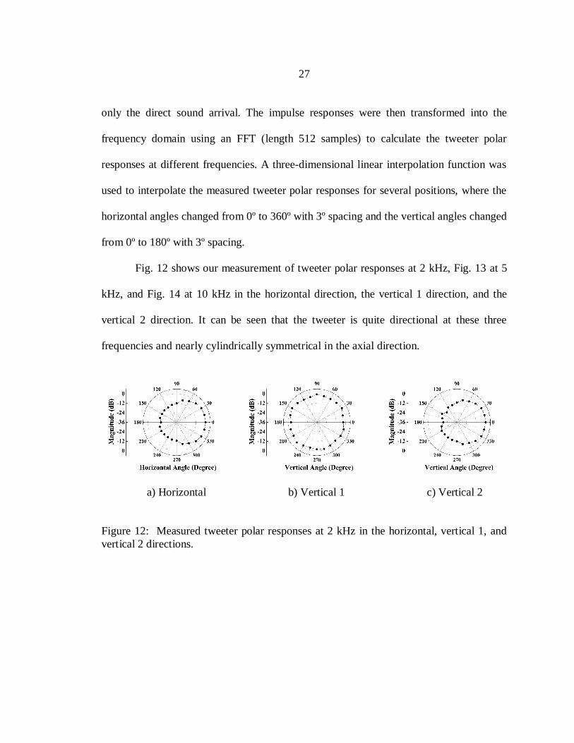
Fig. 12 shows our measurement of tweeter polar responses at 2 kHz, Fig. 13 at 5

kHz, and Fig. 14 at 10 kHz in the horizontal direction, the vertical 1 direction, and the

vertical 2 direction. It can be seen that the tweeter is quite directional at these three

frequencies and nearly cylindrically symmetrical in the axial direction.

a) Horizontal b) Vertical 1 c) Vertical 2

Figure 12: Measured tweeter polar responses at 2 kHz in the horizontal, vertical 1, andvertical 2 directions.

28





The interpolation in the simulation program was done in the time domain, which

gave very similar results to a calculation in the frequency domain according to our test.

The accuracy of the interpolation was verified as follows. The tweeter horizontal impulse

responses at the angles of 30º, 42º, and 45º were at first measured and calculated. The

measured horizontal impulse responses at the angles of 30º and 45º were then used to

interpolate the horizontal impulse response of the tweeter at the angle of 42º. The original

29

and the interpolated tweeter horizontal impulse responses at the angle of 42º were finally

compared. It is shown in Fig. 15 that they have a very small discrepancy.

a) Original b) Interpolated

Figure 15: Comparison between the original and the interpolated tweeter horizontalimpulse responses at the angle of 42º.

The woofer polar response was measured using similar procedures. The

difference is that the woofer polar response was measured using a synthesized bandpass

signal (37 Hz - 1800 Hz) and the microphone was placed in different positions on circles

centered on the woofer. Fig. 16 shows our measurement of woofer polar response at 500

Hz, Fig. 17 at 1 kHz, and Fig. 18 at 1500 Hz in the horizontal direction, the vertical 1

direction, and the vertical 2 direction. It can be seen that the woofer is also quite

directional at these frequencies and nearly cylindrically symmetrical in the axial direction.

30


Figure 16: Measured woofer polar responses at 500 Hz in the horizontal, vertical 1, andvertical 2 directions.


Figure 17: Measured woofer polar responses at 1 kHz in the horizontal, vertical 1, andvertical 2 directions.



31

Microphone Polar Response Calculation

The signal from the speaker can either go directly to the microphone or be

reflected by the room surfaces and then reach the microphone. Thus, the frequency

dependent polar response of the microphone can affect the measured signal.

The microphone polar response was at first measured for the frequency range of

the tweeter, keeping the center of the tweeter and the reference point for the microphone

fixed while the microphone was rotated around two circles. The first circle is erected

perpendicular to the lateral side of the tweeter (vertical 1 direction), while the second

circle is erected perpendicular to the front side of the tweeter (vertical 2 direction). Since

the DPA 4003 microphone is uniformly omni-directional in the horizontal plane, the

microphone horizontal polar response was not necessary to be considered in the

simulation program and therefore was not re-measured.

The microphone polar responses for 46 different tweeter-microphone orientations

were measured using a synthesized bandpass signal (1.8 kHz - 22 kHz). A three-

dimensional linear interpolation function was used to interpolate the microphone polar

responses in the frequency range of the tweeter for several positions, where the horizontal

angles changed from 0º to 360º with 3º spacing and the vertical angles changed from 0º to

180º with 3º spacing. The measurement of the microphone polar response in the woofer

frequency range was made using a similar procedure.

Fig. 19 shows our measurement of microphone polar responses at 1 kHz and Fig.

20 at 5 kHz in the vertical 1 direction and the vertical 2 direction. It can be seen that, as

expected, the receiving microphone is less directional than the loudspeaker source, but

32

the subtle microphone directionality may also be a factor in modeling room impulse

responses.

a) Vertical 1 b) Vertical 2

Figure 19: Measured microphone polar responses at 1 kHz in the vertical 1 and vertical 2directions.

a) Vertical 1 b) Vertical 2

Figure 20: Measured microphone polar responses at 5 kHz in the vertical 1 and vertical 2directions.

33

Room Surface Reflection Coefficient Calculation

The speaker output signal may be reflected by various room surfaces before

reaching the microphone. The magnitude and the phase of the speaker output signal will

thus change due to the propagation distance and the effect of the room surface reflection

coefficients. Measurements can be made to estimate the reflection coefficients of the

room surfaces for use in the simulation program.

In our test room, the room surfaces are made of or covered with several kinds of

materials. The wall and the ceiling are covered with painted wallboard, the door is made

of wood, the window is covered with glass, and the floor is coved with carpet.

To measure the low-frequency wall reflection coefficient, the center of the woofer

was first aligned with the reference point for the microphone. The positions of the woofer

and the microphone must ensure that in the measured impulse response, the reflected

sound from the measured room surface is the earliest reflection and may not be interfered

with by the reflection from other room surfaces. The speaker was then fed with a

synthesized bandpass signal (37 Hz - 1800 Hz), assuming that no signal would come out

of the tweeter. The woofer band limited impulse responses for 5 different woofer-

microphone positions were then measured. For each position, the direct sound and the

earliest reflection part were extracted from the measured impulse response and

transformed into the frequency domain using an FFT (length 512 samples) to calculate

the frequency dependent reflection coefficients for low frequencies. The measurement

method for the high-frequency wall reflection coefficient was similar, except that the

34

center of the tweeter was aligned with the reference point for the microphone and the

speaker was fed with a synthesized bandpass signal (1.8 kHz - 22 kHz).

The processing for the reflection coefficients of the other surfaces (door and

window) is similar to that for the wall. Since the walls and the ceiling of the room are

made of the same material, their reflection coefficients are considered to be equal. For

convenience, the measurement of the floor reflection coefficient was made when the

sound path from the woofer (or the tweeter) via the floor to the microphone was not on

the axis of the woofer (or the tweeter). The calculation of the floor reflection coefficient

was similar to that of the wall reflection calculation except that the polar responses of the

woofer (or the tweeter) and the microphone were considered.

Fig. 21 shows the magnitude of our measurement of frequency dependent

reflection coefficients of the wall, door, window, and floor. Here the composite room

surface reflection coefficients for the whole speaker frequency range are formed by

combining the corresponding low frequency and high frequency room surface reflection

coefficients. Because of the small size of the window and its frame, trim, and gaskets,

some part of the reflected sound from the window may be interfered with by the reflected

sound from the surrounding surfaces near the window. The window reflection coefficient

in some frequencies is therefore found to be greater than one.

35

a) Wall b) Door

c) Window d) Floor

Figure 21: Measurement results of the frequency dependent room surface reflectioncoefficients.

Image Source Processing

When a two-way speaker is fed with an impulse or another broadband signal, the

low-frequency part of the signal will be played by the woofer while the high-frequency

part will be played by the tweeter. Thus, as mentioned in the sound source processing

subsection, one source was used to simulate the woofer and the other source was used to

simulate the tweeter. The positions of the image sources due to the two drives were first

calculated. The orientation of the reflections due to the image sources, i.e., the angles

36

between the reflections and the real sources, were then computed. The orientation of the

receiver, i.e., the angles between the reflections and the receiver, were also calculated.

The intersection points between the reflection path and the room surfaces were also

calculated to judge whether the intersection points were in the wall, the ceiling, the

window, the door, or the floor. The amplitude loss and the phase change due to the

reflections from the room surfaces were finally computed for the sound sources (the real

sources and the image sources).

Room Impulse Response Calculation

In the simulation program it was assumed that the sound would propagate

spherically from the speaker directly to the microphone or via room surfaces and then to

the microphone. The amplitude loss and the phase change from the sound sources to the

receiver were computed first. The impulse responses between the receiver and the sound

sources were calculated by considering the amplitude and the phase change factors,

including the amplitude loss and the phase change due to the room surface reflection

coefficients, the woofer (or the tweeter) polar response, the microphone polar response,

and the spherical sound spreading. The impulse responses for the sound sources were

then added together to form an overall impulse response.

Simulation and Measurement Comparison

After measuring the speaker polar responses, microphone polar response, and

room surface reflection coefficients, the room impulse response was re-modeled using

these measured parameters. It should be noticed that when a two-way speaker is fed with

37

a broadband signal, the low-frequency part of the signal will be played by the woofer

while the high-frequency part will be played by the tweeter. In other words, these two

sources should be considered separately. Fig. 22 shows the on-axis woofer and tweeter

impulse responses. It can be seen that the delay time of the peaks in the woofer and the

tweeter impulse responses is different.

a) Woofer b) Tweeter

Figure 22: Measurement results of the on-axis woofer and tweeter impulse responses.

Based on the above-mentioned consideration, 14 points corresponding to the

direct sound and the six first-order reflections due to the woofer as well as the tweeter are

selected in the modeled room impulse response. The magnitude of these points was then

compared to that of the corresponding points in the measured room impulse response

using the satisfactory match procedure designed in the simple model section.

The extracted values of the modeled and the measured room impulse responses

correspond quite well (see Fig. 23 and Table 3). The discrepancies are reduced to be

within 5 dB, compared to 20 dB seen previously.

38

Figure 23: Delay time and magnitude of 14 points (direct sound and six first-orderreflections due to woofer and tweeter) in the modified modeled and the measured roomimpulse responses for one example speaker and microphone position in the first test room.

Measurement Image Source Method Differences DescriptionDelay(ms)

Magnitude(dB)

Delay(ms)

Magnitude(dB)

Delay(ms)

Magnitude(dB)

SoundSource

SoundReflection

SoundOrientation

2.58 0.0 2.63 0.0 0.05 0 Tweeter Direct Sound (1.85°, 84.0°)2.90 -10.0 2.94 -10.1 0.04 -0.1 Woofer Direct Sound (1.85°, 96.0°)6.06 -6.9 6.06 -7.1 0 -0.2 Tweeter From wall 3 (0.8°, 87.4°)6.42 -16.4 6.38 -16.8 -0.04 -0.4 Woofer From wall 3 (0.8°, 92.6°)6.71 -29.0 6.65 -28.9 -0.06 0.1 Woofer From floor (1.85°, 24.1°)6.77 -31.5 6.73 -29.8 -0.04 1.7 Tweeter From floor (1.85°, 22.2°)8.33 -23.6 8.33 -27.7 0 -4.1 Tweeter From ceiling (1.85°, 161.9°)9.00 -31.3 9.10 -29.2 0.1 2.1 Woofer From ceiling (1.85°, 163.0°)9.12 -23.6 9.19 -26.0 0.07 -2.4 Tweeter From wall 2 (286.1°, 88.3°)9.71 -28.0 9.71 -29.7 0 -1.7 Woofer From wall 2 (286.1°, 91.7°)9.33 -24.4 9.40 -23.7 0.07 0.7 Tweeter From wall 4 (74.2°, 88.4°)9.75 -28.6 9.75 -29.2 0 -0.6 Woofer From wall 4 (74.2°, 91.6°)

13.71 -39.1 13.69 -33.3 -0.02 5.8 Tweeter From wall 1 (179.7°, 88.9°)13.96 -30.7 13.96 -32.3 0 -1.6 Woofer From wall 1 (179.7°, 91.1°)

Table 3: Delay time and magnitude of 14 points in the measured and the modifiedmodeled room impulse responses. Here the speaker is assumed to be two directionalsources.

Additional Tests of the Modified RIR Model

To test the validity and the consistency of the modified model using the image

source method, the model was applied in several other speaker and microphone positions

39

in the previously mentioned test room. Fig. 24 shows that the delay time and the

magnitude of the selected points from the modeled and the measured room impulse

responses for an example speaker-microphone position also correspond quite well.

Figure 24: Delay time and magnitude of 14 points (direct sound and six first-orderreflections due to woofer and tweeter) in the modified modeled and the measured roomimpulse responses for another example speaker and microphone position in the first testroom.

The modified model was also applied in several speaker-microphone positions in

another test room, which is a little larger than the first test room. In this less decorated

test room, the walls are covered with painted concrete block, the door is made of wood,

the window is covered with a curtain, the floor is covered with brick, and the suspended

ceiling is covered with acoustical tile. Fig. 25 shows that the modified model also

performs well for an example speaker-microphone position in this test room, supporting

our conclusion that the test and the simulation procedures are robust and repeatable.

40

Figure 25: Delay time and magnitude of 14 points (direct sound and six first-orderreflections due to woofer and tweeter) in the modified modeled and the measured roomimpulse responses for an example speaker and microphone position in the second testroom.

Summary on RIR Model Using Image Source Method

The principal goal of this chapter is to verify that the discrepancies observed

between the measured room impulse response and the simulation of the room impulse

response using the popular image source method are largely attributable to the

simplifications used in the simulation. The results verify this goal. For a room impulse

response modeled using the image source method, if the source and the receiver are

assumed to be omni-directional and the room surfaces are assumed to be perfectly

reflective, there is a large discrepancy between the modeled and the measured room

impulse responses, indicating that the simple model is insufficient. The match between

the modeled and the measured room impulse responses can be improved if we include the

real measurements of speaker polar response, microphone polar response, and room

41

surface reflection coefficients in the basic image source method. Thus, the goals to obtain

a better match between the modeled and the measured room impulse responses, and to

obtain a better understanding of the differences between the simulation and the

measurement are verified.

The causes of the remaining discrepancies between the measurement and the

model of the room impulse responses are now being studied. The discrepancies may be

partly due to the irregularity of the room surfaces since there is a small window and a

corner column in the room surface. However, the image source method is not sufficiently

flexible to handle room surface irregularities. Thus, we need to find another method that

can model the room impulse response and can more easily handle the irregularity of the

room surfaces.

42

ROOM IMPULSE RESPONSE MODELING USING

3-D RECTANGULAR DIGITAL WAVEGUIDE MESH

In this chapter, the low frequency part of room impulse responses is modeled

using the 3-D rectangular digital waveguide mesh. A digital waveguide mesh provides a

numerical solution to the wave equation and incorporates diffraction and interference

effects.

The 3-D rectangular digital waveguide mesh suffers from frequency and direction

dependent dispersion for high frequency sound, but the frequency response is nearly flat

and the sound propagation dispersion error is small at low frequencies. This means that

the 3-D rectangular mesh is suitable for modeling room impulse responses for low

frequency sound. In this chapter, we use the 3-D rectangular mesh to model the room

impulse response for low frequency sound in the frequency range from 37 Hz to 1800 Hz

(the woofer frequency range).

The reason that the 3-D rectangular digital waveguide mesh is not appropriate for

simulating high frequency sound is that the frequency response is very uneven and the

sound propagation dispersion error is large over the whole frequency range. If we want to

model the room impulse response over the whole audio frequency range, we need to

oversample the impulse response (for example, by a factor of 10 or more) so that the

frequency response will be flat for the desired audio frequency range (20 Hz – 20 kHz).

Thus, the node size in the mesh would be reduced to one-tenth of the original size, and

there will be as many as one thousand times the number of nodes compared to the

43

original case. So, a digital waveguide mesh with large sample rate requires denser meshes,

more computer memory and hence takes on the order of 1000 times longer to run. This is

not suitable for current computer workstations. Thus, it is currently not appropriate to use

the 3-D rectangular digital waveguide mesh in the simulation of high frequency sounds.

In this chapter, we will first review the fundamentals of the digital waveguide

mesh. We will then show our work in the derivation of the analytical expression for the

impulse response between two nodes in 2-D rectangular digital waveguide mesh. We will

then describe the considerations for room impulse response modeling using a 3-D

rectangular digital waveguide mesh. Finally, we will compare the simulation results of

the low frequency room impulse responses using the image source method and the 3-D

rectangular digital waveguide mesh.

Fundamentals of Digital Waveguide Mesh

Update Equation

In the digital waveguide mesh, the nodes are connected with their neighboring

nodes by waveguides (bidirectional digital delay lines). Fig. 26 shows the general case of

a node J with N neighboring nodes i , where Ni ,,2,1 [32, 44, 66, 67]. The signal

JiP , represents the incoming signal to node i along the waveguide from the node J while

the signal JiP, denotes the outgoing signals from node i along the waveguide to the

node J [66, 67].

44

Jp ,1 Jp ,1

1,Jp 1,Jp

iJp , iJp ,

Jip , Jip ,

Figure 26: A node J with N connected neighboring nodes i, where i = 1, 2, …, N.

The sound pressure at a lossless node, JP , can be expressed as [66, 67]:

N

ii

N

ii

iJ

J

Z

ZP

P

1

1

,

1

2, (1)

where iJP , represents the incoming pressure signal at a connecting waveguide and iZ

represents its impedance.

Since the waveguides are bidirectional unit delay lines, the input to a node is

equal to the output from a neighboring node into the connecting waveguide at the

previous time step [66, 67]. This can be expressed as:

JiiJ PZP ,1

, . (2)

If the impedances are all equal, Eq. (1) can also be derived as an equivalent finite

difference scheme using only node pressure values [32]:

45

N

iJiJ nPnP

NnP

1)2()1(2)( , (3)

where )(nPJ denotes the sound pressure at node J at time index n . This way of

formulating the digital waveguide mesh update function is called the Kirchhoff

formulation. It has greater memory efficiency and less computational expense than Eq.

(1). Thus, we used the Kirchhoff formulation for the simulation in this dissertation.

The updating frequency or sampling frequency, sf , of a mesh and the wave

propagation velocity, c , are related to each other as [68, 69]

xNcfs , (4)

where N is the dimensions of the mesh and x is the spatial sampling interval.

Structures

The digital waveguide mesh with nodes separated with bidirectional unit delays

can be constructed in various ways like rectangular, triangular, and hexangular structures

[69, 70], as shown in Fig. 27. Among these structures, the rectangular topologies are the

easiest to handle because the regular matrices match well with the structures offered by

computer programming languages and the general shapes of simple room models.

46

a) Rectangular b) Triangular c) Hexangular

Figure 27: Three structures of the 2-D digital waveguide mesh.

One limitation of the rectangular mesh is that it has numerical dispersion, due to

the difference in the physical distances and signal path lengths. For example, in a 2-D

rectangular mesh, the spatial distance from a node to its first diagonal neighbor is 2

times the distance to an axial neighbor. However, the signal travels along the orthogonal

steps from a node to its axial neighbors in one time-step and to a diagonal neighbor, as

well as to a second axial neighbor, in two time-steps. Thus, the signal reaches locations at

physical distances of 2 spatial steps and 2 spatial steps away from the source at the

same time instant [69].

The difference in the physical distances and signal path lengths causes a

numerical error dependent on both the direction of wave propagation and the frequency

of the signal. The error is largest at high frequencies and in the axial directions of the

mesh. The dispersion can be made equal in all directions by using an interpolated mesh

scheme [63]. After this, the remaining frequency-dependent error can be rectified using

the frequency warping technique [63].

47

According to our simulation, the 3-D rectangular digital waveguide mesh has

much less numerical dispersion in the low frequency range. Thus, we used the 3-D

rectangular mesh to simulate the low frequency portion of the room impulse response in

this dissertation.

Boundary Conditions

In real rooms, sound reflections occur when the sound waves reach the room

surfaces. The complex changes of the magnitude and the phase of the sound waves at the

room surfaces depend on the surface material and structure as well as the level, frequency,

and propagation direction of the sound. Correspondingly, there should be a representation

of the boundary condition in the digital waveguide mesh.

Currently, many research centers around the world are doing research on

modeling boundary conditions in digital waveguide mesh with adjustable shape, diffusion,

and reflection characteristics [71-74]. However, there has not yet been a perfect

boundary condition implementation for the digital waveguide mesh.

For the 3-D rectangular digital waveguide mesh, there only exist two suitable

frequency and angle independent boundary conditions. One is the basic boundary

condition based on the simple impedance matching technique while the other is a

modified boundary condition proposed by Kelloniemi et al. in 2004 [73], which is based

on an improved absorbing boundary condition proposed in [66].

At the boundary of the 3-D rectangular digital waveguide mesh, an interaction

occurs between the boundary node and its immediate perpendicular neighbor within the

48

main body of the mesh structure [66]. A boundary node is generally defined as having

only one neighbor, so adjacent nodes on the mesh boundary have no direct influence on

each other.

In a real room, the effect of a room boundary is to produce a reflection of an

incident sound wave, usually with some frequency dependent absorption of the wave

energy at the boundary itself. In a digital waveguide mesh a reflection is caused by a

change in the impedance of the waveguide [66]. This can be represented by connecting a

dummy node 2 on the other side of the boundary node B , as shown in Fig. 28 [66].

BP ,1 1,BP

BP ,1 1,BP

2,BP

2,BP

Figure 28: Reflection from a boundary in a digital waveguide mesh.

The connecting waveguides on either side of the boundary have characteristic

impedances 1z and 2z respectively. If at a boundary the impedance changes from 1z to 2z ,

the reflection coefficient r is defined as [66]:

12

12

zzzzr . (5)

49

Since there is no contribution from the dummy node 2 into the boundary node B ,

the sound pressure in the boundary node can be calculated using Eqs. (1) and (2) and

expressed in the finite difference formulation as [66]

)2()1()1()( 1 nrPnPrnP BB , (6)

where r is the desired reflection coefficient, and indices B and 1 denote the boundary

node and its perpendicular neighbor, respectively. Here )1(1 nP represents the sound

pressure for the perpendicular neighbor of the boundary node one time step ago and

)2(nPB denotes the sound pressure on the boundary node two time steps ago.

In the room acoustics simulation using digital waveguide mesh, the amount of

energy reflected at the room boundary is determined by setting r equal to a value

between 0 and 1. An absorbing boundary condition is simulated with 0r and a

perfectly reflective boundary condition is simulated with 1r . This basic boundary

condition offers a satisfactory solution enabling reflection and absorption to be modeled.

But it is clearly an oversimplification of reality. In addition, this method was proved to

cause unwanted reflections at low values of reflection coefficient r [67].

To improve the performance of the basic boundary condition, in 2002, Murphy

and Mullen suggested expanding the rule obtained from Eq. (6) with 0r ,

)1()( 1, nPnP absB , (7)

into a Taylor series of the values of the nodes perpendicular to the boundary [66]. For

example, the first-order Taylor series expansion of the right hand side of Eq. (7) results in

50

)2()1(2)( 21, nPnPnP absB . (8)

Boundaries constructed this way produce significantly better absorption than the original

solution.

The basic boundary condition (6) for the perfectly reflecting case, 1r , can be

expressed as:

)2()1(2)( 1, nPnPnP BrefB . (9)

An assumption was made in [73] that reflection coefficient values between 0 and

1 could be modeled by a r-weighted linear combination of the reflecting and absorbing

solutions. The resulting new rule for adjusting the reflection coefficient r is thus written

as

)()1()()( ,, nPrnrPnP absBrefBB

))2()1(2)(1())2()1(2( 211 nPnPrnPnPr B

)2()2()1()1(2 21 nrPnPrnP B . (10)

The performance of this equation is better than those obtained with the basic boundary

condition at very low values of r .

When the basic boundary condition and the modified boundary condition are

applied in modeling low frequency room impulse responses, the modified boundary

condition performs better at lower reflection coefficients while the basic boundary

condition performs better at higher reflection coefficients.

51

Analytical Expression of Impulse Response in 2-D Rectangular DWM

Currently, in the digital waveguide mesh models, the schemes of the wave

equation are in the space-time domain, and it is not straightforward to find an analytical

expression for the impulse response between a source and a receiver in the mesh. In this

section, we derive an analytical expression for the impulse response between two nodes

in a 2-D rectangular mesh. This expression can help verify the simulation results of the

mesh.

2-D Rectangular Digital Waveguide Mesh

The rectangular digital waveguide mesh is a regular array of 1-D digital

waveguides arranged along each perpendicular dimension, interconnected at their

crossings by scattering nodes with unit delay elements. A 2-D rectangular digital

waveguide mesh was originally proposed in [32], and is illustrated in Fig. 29.

Figure 29: In the 2-D rectangular digital waveguide mesh each node is connected to fourneighbors with unit delays.

52

The difference wave equation for the 2-D rectangular mesh can be expressed

using the node values as

),1,1(),1,1([21),,( jinvjinvjinv

),,2()]1,,1()1,,1( jinvjinvjinv , (11)

where v represents the wave velocity signal of a node at rectangular coordinates ),( ji at

time index n . Here i , j , and n are arbitrary integers.

Impulse Response Between Two Nodes in 2-D Rectangular DWM

When a 2-D rectangular mesh is used for simulations, one frequently asked

question is how to obtain an expression for the impulse response between a source S at

node ),( BA and a receiver R at node ),( NBMA , i.e., how to find an expression for

the wave velocity signal at the receiver node ),( NBMA if an impulse signal is fed

into the source node ),( BA at time index 0n .

The impulse response question can also be mathematically expressed as follows.

Given a time-space impulse signal ),,( BjAin , what will be the analytical

expression of the received wave velocity signal ),,( NBMAnv for ,3,2,1,0n ?

Here the time-space impulse signal ),,( BjAin is defined as follows.

OtherwiseBjAin

BjAin0

,,01),,( .

53

The impulse response can certainly be simulated directly using Eq. (11), but an

analytical expression of the impulse response can provide helpful insights and help verify

the simulation results.

In an unbounded rectangular mesh, ),,( NBMAnv is equal to

),,( NBMAnv due to the symmetry of propagation in front of a time-space impulse

signal ),,( BjAin . Thus, without loss of generality, both M and N are assumed to

be non-negative integers here. An example source-receiver layout is shown in Fig. 30.

S

R

Figure 30: An example source node S and an example receiver node R are located in a2-D rectangular digital waveguide mesh.

It should be noticed that given an initial excitation at some node in the mesh, the

excitation energy will spread out from the excitation node more and more as the traveling

waves scatter through the nodes. This phenomenon can be described using 2-D

convolution [75]. To facilitate the analysis of the impulse response question, one 2-D

spatial signal h is defined as follow.

54

OtherwiseBmAm

mmmmhh0

1,15.0},),,({ 21

2121 .

According to Eq. (11), if an impulse signal is fed into the source node ),( BA at

time index 0n , the evolution of the wave velocity signal in the nodes over time can be

expressed as

),,2(),,1(),,( jinvjinvhjinv , (12)

where "" denotes 2-D convolution and ),,(),,( BjAinjinv for 0n . Here the

wave velocity signal ),,( jinv is viewed as a 2-D spatial signal for specific time index n .

Given ),,(),,( BjAinjinv for 0n , using Eq. (12) iteratively, the wave

velocity ),,( jinv can be written as

1)1(),,(2

0

)2( nforhCjinv

n

t

tnttn

t , (13)

where2n means the largest integer value less than or equal to

2n ,

)!2(!)!(tnt

tnC ttn

is the

binomial coefficient, andtn

tn hhhhh2

)2( means the tn 2 fold 2-D convolution

of h with itself. The calculation of wave velocity signal ),,( jinv thus needs to obtain the

value of the polynomials obtained by self-convolving h for tn 2 times. Specifically,

calculating the received wave velocity ),,( NBMAnv requires computing what the h

polynomials equal at the receiver node ),( NBMA .

If an impulse signal is fed into the source node ),( BA at time index 0n and

continuously convolved with the 2-D signal h , the evolution of the node value over time

55

becomes nh at time index n . Therefore, given ),,(),,(ˆ BjAinjinv for 0n , the

calculation of nh is actually solving ),,1(ˆ),,(ˆ jinvhjinv , i.e., solving

)]1,,1(ˆ)1,,1(ˆ),1,1(ˆ),1,1(ˆ[21),,(ˆ jinvjinvjinvjinvjinv . (14)

Von Neumann analysis can be applied to the difference equation to show the

evolution of the spatial spectrum over time by using Fourier transform theory [32, 76]. To

calculate nh at the receiver node ),( NBMA , Von Neumann analysis applied to Eq.

(14) yields

),,1(ˆ][21),,(ˆ

212222

212211 nVeeeenV cTjcTjcTjcTj , (15)

where ),,(ˆ21nV is the 2-D discrete-space Fourier transform of ),,(ˆ jinv , 1 and 2 are

the spatial frequencies, c is the sound velocity, and T is the temporal sampling interval.

Eq. (15) can be represented using a spectral amplification factor, ),( 21g .

Multiplying the Fourier transform of the solution by ),( 21g is equivalent to advancing

the solution of the time-domain scheme by one time step [32, 76]. Deriving ),( 21g

from Eq. (15) gives

),,0(ˆ),(),,(ˆ212121 VgnV n

),,0(ˆ),(][21

212112222 2211 Vgeeee ncTjcTjcTjcTj , (16)

where ),,0(ˆ21V represents the initial conditions at time index 0n . The amplification

factor ),( 21g is calculated as

56

][21][

21),( 22112211 2222

21jjjjcTjcTjcTjcTj eeeeeeeeg , (17)

where cT11 2 and cT22 2 .

According to the spatial shift theorem of the 2-D Fourier transform, to calculate

the value at the receiver node ),( NBMA , only the coefficient of 21 jNjM ee from the

polynomial ),( 21ng needs to be computed. To get the factor 21 jNjM ee , the difference in

the exponents of 1je and 1je should be equal to M and the difference in the exponents

of 2je and 2je should equal N . In the 2-D rectangular mesh, the path length of every

route between the source node ),( BA and the receiver node ),( NBMA is always an

even or an odd number of unit delays, so the coefficient of 21 jNjM ee is equal to 0 for

every other time step. In addition, the coefficient of 21 jNjM ee equals 0 for the time index

NMn since it takes NM time steps for the input to propagate from the source to

the receiver. Based on these considerations, expanding the bracketed expression in

njjjjn eeeeg )](21[),( 2211

21 , the factor 21 jNjM ee is only included in the

polynomial

222 )()()()([21

22112211 NjjNnjjNn

NjjNnjjNnn eeeeCeeeeC

])()(... 2211 MnjjMjjMnn eeeeC ,

where ,2, NMNMn . The coefficient of 21 jNjM ee in each term is calculated

as follows.

)(21

222 012

12

20 NMnNMnNMn

MnMMn

nNNnNnNNn

Nnn CCCCCCCCC

57

2

022

2 )(21

2

NMn

t

ttN

ttNn

tNnn CCC

NMn

2

0)(

21

22

2

NMn

t

tNtnn NMnNMn

NMn

CCC

nnn

NMnNMn

CC2

22

, where ,2, NMNMn . (18)

According to the shift theorem of the 2-D Fourier transform, the value of nh at

the receiver node ),( NBMA is expressed as

Otherwise

NMNMnforCCNBMAnv n

nn

NMnNMn

0

,2,2),,(ˆ

22

. (19)

Substituting the expression for ),,(ˆ NBMAnv into Eq. (13) gives the wave

velocity signal ),,( NBMAnv , i.e., the impulse response between the source node

),( BA and the receiver node ),( NBMA , which is expressed as

Otherwise

NMNMnforCCCNBMAnv

NMn

ttn

tntnt

tnt tNMntNMn

0

,2,2

)1(),,(

2

02

222

22

2

. (20)

In Eq. (20), the impulse response is analytically expressed as the summation of

combined polynomials in the time domain. The computational complexity is high in this

equation, so its practical usefulness is limited. However, for a particular case when the

receiver node is in the diagonal direction of the source node, i.e. NM , some

simplifications can be observed by successively incrementing n in Eq. (20).

58

When Nn 2 ,N

NNCNBNANv

22

2),,2( . From the calculation result in Eq.

(20), observe that an update expression for 82,42,2 NNNn can be written as

)42)(42()22)(22(),,(),,4(

NnNnNnNnNBNAnvNBNAnv and that

0),,( NBNAnv for other values of n .

According to these observations, Eq. (20) can be further simplified to the compact

form:

Otherwise

NNnforCC

NBNAnv n

Nn

Nn

Nn

Nn

0

,42,22),,(

42

22

42

22

. (21)

Note that in Eq. (21) every three out of four samples in ),,( NBNAnv are

zero-valued.

Simulation Results

The impulse responses for three arbitrary source-receiver positions were

simulated using Eq. (11) and using Eq. (20) respectively. The simulations using Eq. (11)

were made by constructing a 200200 node 2-D rectangular mesh and applying an

impulse signal into source node )120,80( . The impulse responses were then simulated at

arbitrary receiver nodes )120,80( , )122,83( , and )125,85( , which correspond to

00 NandM , 23 NandM , and 55 NandM respectively. In the

simulations, sound velocity was set to 343.5 m/s and spatial sampling interval was set to

0.0101 m, indicating an updating frequency of 48 kHz. The impulse response simulations

59

were run for 48 time steps, which ensured that the sound wave would not propagate out

of the mesh boundary. The three impulse responses were obtained, and also numerically

transformed into the corresponding frequency responses using an FFT length of 64

samples. The simulation results for the three source-receiver positions were identical to

those using Eq. (20). The simulation results for the receiver nodes )120,80( and

)125,85( were also identical to those using Eq. (21), as expected.

Fig. 31 shows the three impulse responses and the corresponding magnitude

frequency responses. In every magnitude frequency response the spectrum is symmetric

about one quarter of the updating frequency. This symmetry characteristic in the

frequency domain corresponds to the phenomenon that every other sample is zero-valued

in the time domain, as shown in Eq. (20) and in the simulated impulse responses in Fig.

31.

a) M=0 and N=0

b) M=3 and N=2

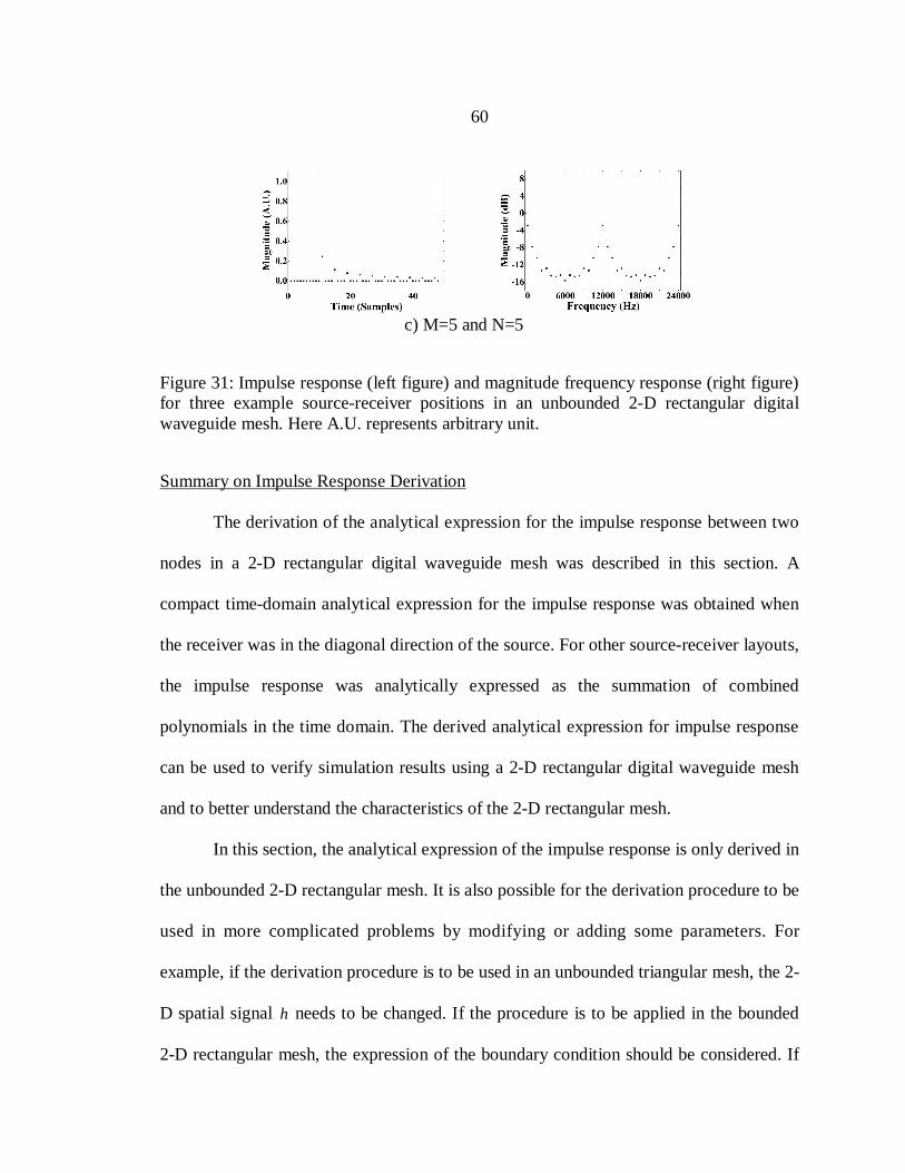
60

c) M=5 and N=5

Figure 31: Impulse response (left figure) and magnitude frequency response (right figure)for three example source-receiver positions in an unbounded 2-D rectangular digitalwaveguide mesh. Here A.U. represents arbitrary unit.

Summary on Impulse Response Derivation

The derivation of the analytical expression for the impulse response between two

nodes in a 2-D rectangular digital waveguide mesh was described in this section. A

compact time-domain analytical expression for the impulse response was obtained when

the receiver was in the diagonal direction of the source. For other source-receiver layouts,

the impulse response was analytically expressed as the summation of combined

polynomials in the time domain. The derived analytical expression for impulse response

can be used to verify simulation results using a 2-D rectangular digital waveguide mesh

and to better understand the characteristics of the 2-D rectangular mesh.

In this section, the analytical expression of the impulse response is only derived in

the unbounded 2-D rectangular mesh. It is also possible for the derivation procedure to be

used in more complicated problems by modifying or adding some parameters. For

example, if the derivation procedure is to be used in an unbounded triangular mesh, the 2-

D spatial signal h needs to be changed. If the procedure is to be applied in the bounded

2-D rectangular mesh, the expression of the boundary condition should be considered. If

61

the procedure is to be extended to the bounded 3-D rectangular mesh, the expression of a

boundary condition and a 3-D spatial signal h should be applied, and so forth.

Considerations for RIR Model Using 3-D Rectangular DWM

To apply the 3-D rectangular digital waveguide mesh in the simulation of the low

frequency part of the room impulse response, we need to know the frequency response,

the sound propagation direction dependent dispersion, and the performance of the

boundary condition of the 3-D rectangular mesh in the desired low frequency range.

The difference wave equation for the unbounded 3-D rectangular mesh can be

expressed using the node values as

),1,,1(),1,,1(),,1,1(),,1,1([31),,,( kjinPkjinPkjinPkjinPkjinP

),,,2()]1,,,1()1,,,1( kjinPkjinPkjinP , (22)

where P represents the sound pressure of a node at rectangular coordinates ),,( kji at

time index n . Here i , j , k , and n are arbitrary integers.

Frequency Response in the 3-D Rectangular DWM

We first simulated the frequency responses for several arbitrary source-receiver

positions using the difference wave equation (22) for an unbounded 3-D rectangular mesh.

The simulations using Eq. (22) were made by constructing a 200200200 node 3-D

rectangular mesh and applying an impulse signal into the source node )120,100,80( . The

impulse responses were then simulated at the receiver nodes. In the simulations, the

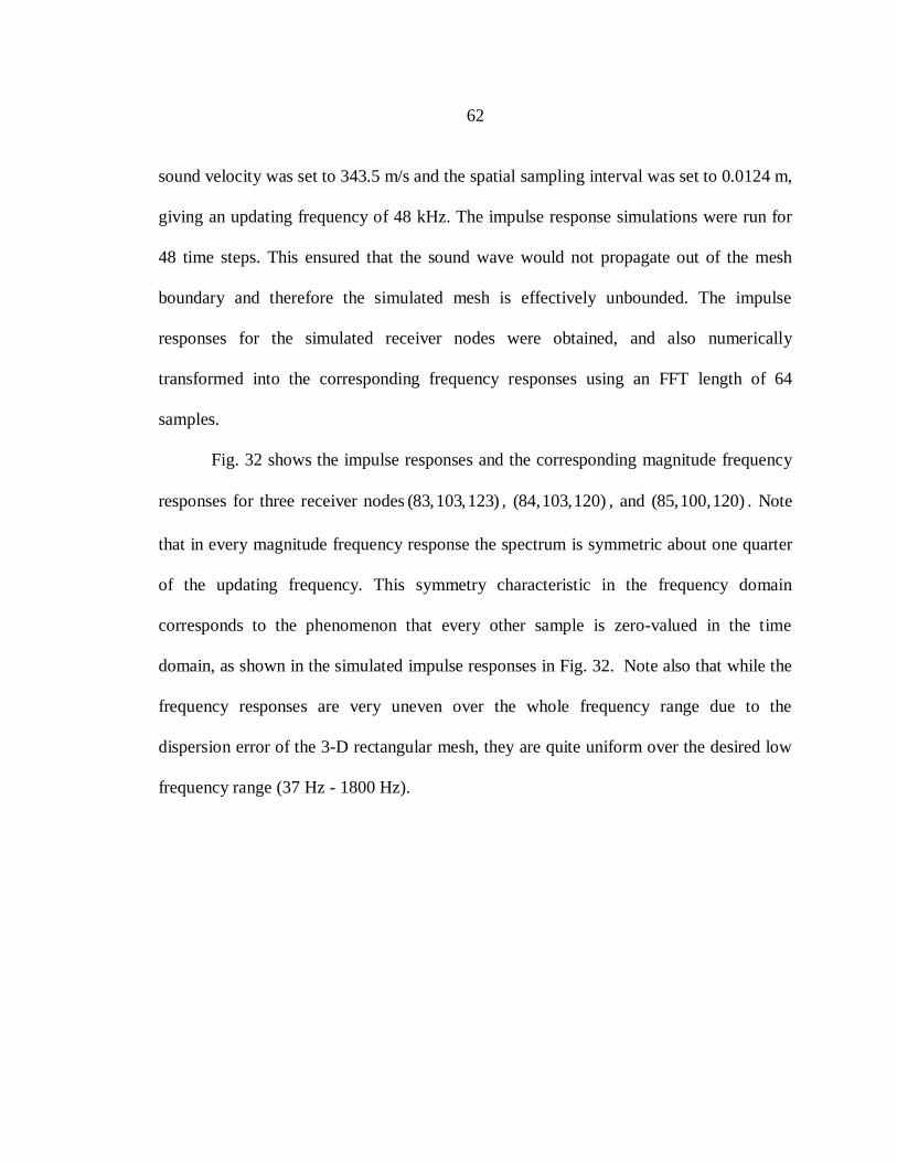
62

sound velocity was set to 343.5 m/s and the spatial sampling interval was set to 0.0124 m,

giving an updating frequency of 48 kHz. The impulse response simulations were run for

48 time steps. This ensured that the sound wave would not propagate out of the mesh

boundary and therefore the simulated mesh is effectively unbounded. The impulse

responses for the simulated receiver nodes were obtained, and also numerically

transformed into the corresponding frequency responses using an FFT length of 64

samples.

Fig. 32 shows the impulse responses and the corresponding magnitude frequency

responses for three receiver nodes )123,103,83( , )120,103,84( , and )120,100,85( . Note

that in every magnitude frequency response the spectrum is symmetric about one quarter

of the updating frequency. This symmetry characteristic in the frequency domain

corresponds to the phenomenon that every other sample is zero-valued in the time

domain, as shown in the simulated impulse responses in Fig. 32. Note also that while the

frequency responses are very uneven over the whole frequency range due to the

dispersion error of the 3-D rectangular mesh, they are quite uniform over the desired low

frequency range (37 Hz - 1800 Hz).

63

a) Receiver (83, 103, 123)

b) Receiver (84, 103, 120)

c) Receiver (85, 100, 120)

Figure 32: Impulse response (left figure) and magnitude frequency response (right figure)for three example source-receiver positions in an unbounded 3-D rectangular digitalwaveguide mesh. Here A.U. represents arbitrary unit.

Propagation Dispersion in the 3-D Rectangular DWM

The 3-D rectangular digital waveguide mesh suffers from serious direction

dependent dispersion for high frequency sound. According to our simulation, however,

the direction dependent dispersion is very small at low frequencies. When we fed a

synthesized bandpass signal (37 Hz – 1800 Hz) into a source node in the unbounded 3-D

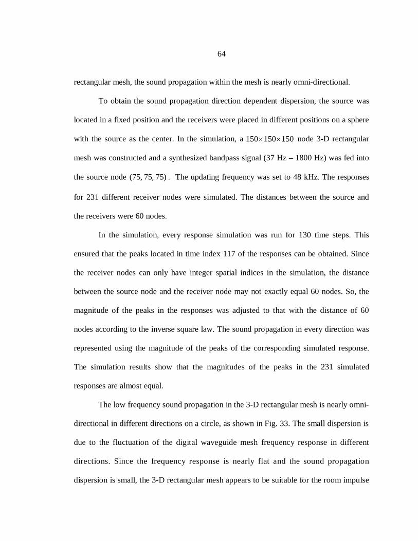
64

rectangular mesh, the sound propagation within the mesh is nearly omni-directional.

To obtain the sound propagation direction dependent dispersion, the source was

located in a fixed position and the receivers were placed in different positions on a sphere

with the source as the center. In the simulation, a 150150150 node 3-D rectangular

mesh was constructed and a synthesized bandpass signal (37 Hz – 1800 Hz) was fed into

the source node )75,75,75( . The updating frequency was set to 48 kHz. The responses

for 231 different receiver nodes were simulated. The distances between the source and

the receivers were 60 nodes.

In the simulation, every response simulation was run for 130 time steps. This

ensured that the peaks located in time index 117 of the responses can be obtained. Since

the receiver nodes can only have integer spatial indices in the simulation, the distance

between the source node and the receiver node may not exactly equal 60 nodes. So, the

magnitude of the peaks in the responses was adjusted to that with the distance of 60

nodes according to the inverse square law. The sound propagation in every direction was

represented using the magnitude of the peaks of the corresponding simulated response.

The simulation results show that the magnitudes of the peaks in the 231 simulated

responses are almost equal.

The low frequency sound propagation in the 3-D rectangular mesh is nearly omni-

directional in different directions on a circle, as shown in Fig. 33. The small dispersion is

due to the fluctuation of the digital waveguide mesh frequency response in different

directions. Since the frequency response is nearly flat and the sound propagation

dispersion is small, the 3-D rectangular mesh appears to be suitable for the room impulse

65

response modeling in the low frequency range from 37 Hz to 1800 Hz.

Figure 33: Sound propagation in different directions on a circle in the 3-D rectangulardigital waveguide mesh.

Boundary Condition Performance Tests in the 3-D Rectangular DWM

Sound reflection occurs when the sound waves reach the real room surfaces, so

there should be a corresponding representation of boundary conditions in the 3-D

rectangular mesh. Currently, there exist two suitable frequency independent boundary

conditions, which are the basic boundary condition and the modified boundary condition.

In this section, we will show the performance tests of these two boundary conditions.

The first step is to test whether or not these two boundary conditions converge. To

save simulation time, without loss of generality, a 404040 node small 3-D

rectangular mesh was constructed and a bandpass signal (37 Hz – 1800 Hz) was fed into

the source node )20,20,20( . The responses were then simulated at three arbitrary

receiver nodes )29,35,25( , )16,25,17( , and )27,31,3( using the reflection coefficients

66

0.0r , 5.0r , and 0.1r for both boundary conditions. Every response simulation

was run for 24000 time steps, which is long enough to ensure that the convergence test is

believable. According to our test, both boundary conditions converge for these three

arbitrary receiver nodes.

The second step is to test how well the simulated reflection coefficients match the

theoretical values. A test procedure proposed in [73] was used here. For reflective

boundaries, the simulated reflection coefficient is equal to the ratio of the magnitude of

the simulated reflected sound signal to that of the perfectly specular reflected sound

signal. Here the magnitude of the simulated reflected sound signal is equal to the

difference between the magnitude of the received sound signal and that of the direct

transmission sound signal between the source and the receiver. The magnitude of the

perfectly specular reflected sound signal is equal to that of the direct transmission sound

signal between the source and the mirror receiver.

A 200200200 node 3-D rectangular mesh was constructed. The simulation

was made for 11 source-receiver positions, where the incident angle from the source to

the tested boundary ranges from 0º (normal incidence) to 45º. To facilitate the

representation, we use the incident angle of 45º as an example.

A bandpass signal (37 Hz – 1800 Hz) was applied as an input over 96 time steps

at the source node S1: )10,100,90( in the mesh. The response simulation was made at the

receiver node R1: )10,100,110( . The set-up of the source node and the receiver node

made sure that the input was fed into a node located close to the tested mesh boundary

and far from any other boundary to avoid additional reflections influencing the results.

67

The output signal was received at the node located at equal distance from the tested

boundary as shown in Fig. 34 (a). The tested boundary was simulated using both the

basic boundary condition and the modified boundary condition.

a) Simulated Reflection Setup b) Direct transmission setup c) Perfect reflection setup

Figure 34: Performance tests of boundary conditions in the 3-D rectangular digitalwaveguide mesh.

The direct transmission sound signal from the source node to the receiver node

was simulated in the same 3-D rectangular mesh. The response between the source S1 and

the receiver R1 is equivalent to that between the node S2: )100,100,90( and the node R2:

)100,100,110( , as shown in Fig. 34 (b). The direct transmission sound signal was

subtracted from the output signal received at the node R1 to get the simulated reflection

signal.

In addition, the perfectly specular reflected sound signal was calculated using the

simulated response between the node S2: )100,100,90( and the node R3: )80,100,110( , as

shown in Fig. 34 (c). The simulated reflection coefficient is then calculated using the

ratio of the magnitude of the simulated reflection signal to that of the perfect specular

reflection signal.

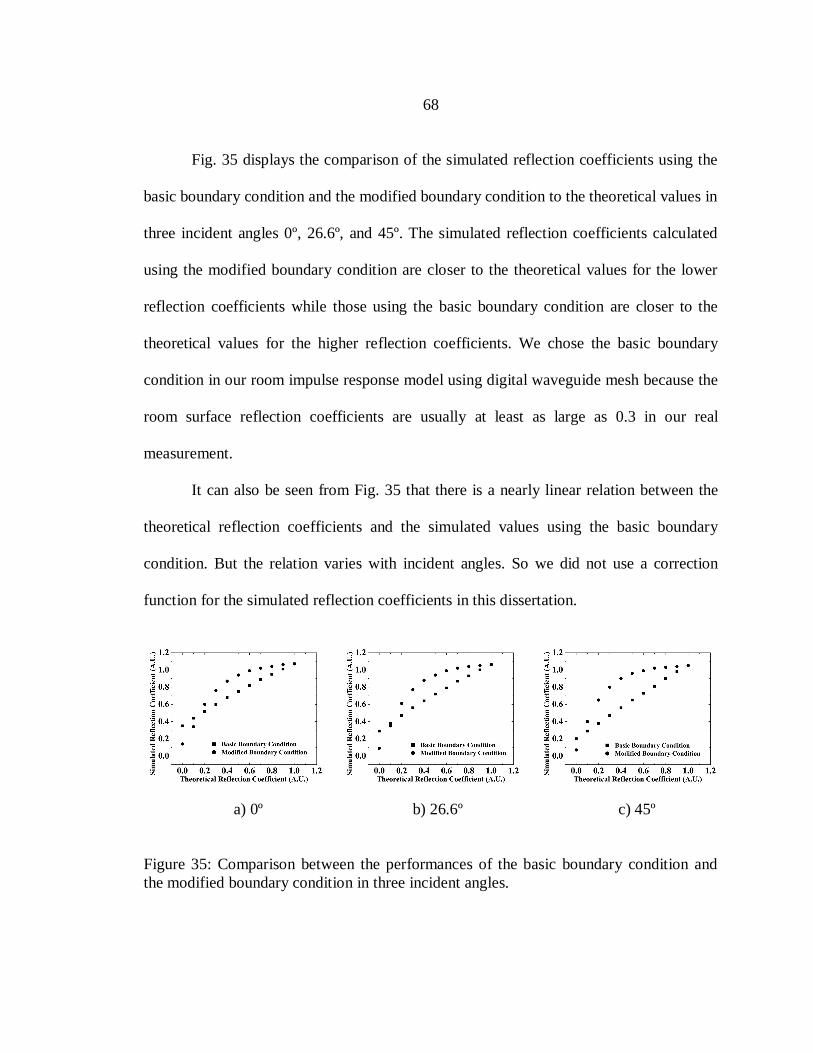
68

Fig. 35 displays the comparison of the simulated reflection coefficients using the

basic boundary condition and the modified boundary condition to the theoretical values in

three incident angles 0º, 26.6º, and 45º. The simulated reflection coefficients calculated

using the modified boundary condition are closer to the theoretical values for the lower

reflection coefficients while those using the basic boundary condition are closer to the

theoretical values for the higher reflection coefficients. We chose the basic boundary

condition in our room impulse response model using digital waveguide mesh because the

room surface reflection coefficients are usually at least as large as 0.3 in our real

measurement.

It can also be seen from Fig. 35 that there is a nearly linear relation between the

theoretical reflection coefficients and the simulated values using the basic boundary

condition. But the relation varies with incident angles. So we did not use a correction

function for the simulated reflection coefficients in this dissertation.

a) 0º b) 26.6º c) 45º

Figure 35: Comparison between the performances of the basic boundary condition andthe modified boundary condition in three incident angles.

69

Performance Comparison between ISM and 3-D Rectangular DWM

After we tested the frequency response, the sound propagation dispersion error,

and the performance of the boundary conditions of the 3-D rectangular mesh in the low

frequency range, we compared the image source method and the 3-D rectangular digital

waveguide mesh based simulation results of the low frequency impulse responses

between a source and a receiver in a small simulation room.

Performance Comparison for Small Regular Simulation Room

Before the low frequency room impulse response was modeled, the room

dimensions, the source position, and the receiver position were set. The rectangular room

was 1.24 meters long, 1.49 meters wide, and 1.74 meters high. The source position was

(0.62, 0.62, 0.62) meters and the receiver position was (0.372, 0.496, 0.62) meters. The

sound velocity was 343.5 m/s. The source and the receiver were assumed to be omni-

directional. The reflection coefficients were set to 0.8 for all the room surfaces. A

synthesized bandpass signal (37 Hz – 1800 Hz) was fed into the source and the response

in the receiver was simulated using both the image source method and the 3-D


In the simulation using the image source method, the above-mentioned room

dimensions, source position, receiver position, sound velocity, and reflection coefficients

were used directly in the program.

70

In the simulation using the 3-D rectangular digital waveguide mesh, the room was

divided into several cubic nodes with the size of 0.0124 meters. Thus, the room

dimension was (100, 120, 140) nodes in the mesh. The source was at the node (50, 50, 50)

and the receiver was at the node (30, 40, 50). In the simulation, the sound velocity was

set to 343.5 m/s, giving an updating frequency of 48 kHz. A bandpass signal (37 Hz -

1800 Hz) was fed to the source and the response at the receiver node was simulated. The

reflection coefficient in the basic boundary condition was set to 0.8.

Several arbitrary peaks were extracted from the two modeled responses. Since the

nodes in the digital waveguide mesh can only have integer spatial indices, there may be

small time shift of the delay time in the mesh. So the delay time of the peaks in the two

modeled responses may not exactly be the same. Thus, a satisfactory match described in

Chapter 3 was used. 13 peaks from the two modeled responses are extracted and shown

in Fig. 36. It can be seen that they have a very small discrepancy. Note that the peak

magnitude in the modeled response using the digital waveguide mesh is greater than that

using the image source method. This shows that the reflection coefficient calculated

using the basic boundary condition in the digital waveguide mesh is actually higher than

the theoretical value, as shown in Fig. 35 in the previous section.

71

Figure 36: Delay time and magnitude of 13 arbitrarily chosen peaks in the image sourcemethod and the 3-D rectangular digital waveguide mesh based models of the lowfrequency room impulse responses for a small rectangular simulation room.

Performance Comparison for Small Irregular Simulation Rooms

In the previous subsection, we showed that the low frequency room impulse

response simulations using the image source method and the 3-D rectangular digital

waveguide mesh were approximately equivalent for the same rectangular simulation

room. Since the image source method is not sufficiently flexible to handle the room

surface irregularities, the 3-D rectangular digital waveguide mesh can be instead used to

simulate the room impulse response for irregular rooms.

In one simulation, we added a glass window in a wall in the original rectangular

simulation room and made the room surface irregular. The window was on the outer side

of the room. The size of the window was (0.248, 0.744, 0.744) meters. The source

position, the receiver position, other room surface reflection coefficients, and the sound

velocity were kept unchanged. The length of the room changed to 1.49 meters when

72

we considered the depth of the window.

In the simulation using the digital waveguide mesh, the node size was kept

unchanged. The room dimension changed to (120, 120, 140) nodes. To fit the dimension

of this new room, the source was in the node (70, 50, 50) and the receiver was in the node

(50, 40, 50). The size of the window was (20, 60, 60) nodes and the center of the window

was in the node (10, 60, 70).

Due to the room surface irregularities, the air space within the room was not

rectangular. The irregular air space was then divided into two small rectangular air spaces,

one within the original room and the other within the window. The boundary of the

window was also considered. The reflection coefficients of the window boundaries were

set to 0.6.

Fig. 37 shows that the simulated low frequency room impulse response using the

3-D rectangular mesh now changes a lot as expected and has a large discrepancy

compared to that using the image source method for the original simulation room

(without the window), indicating the importance of including proper surface detail in the

simulation.

73

Figure 37: Delay time and magnitude of 7 points (direct sound and six first-orderreflections) in the low frequency room impulse responses modeled using the 3-Drectangular digital waveguide mesh for a small rectangular simulation room with a glasswindow in a wall and that using the image source method for the same room without thewindow.

In another simulation, we added three absorbing panels to one of the walls in the

original rectangular simulation room. To facilitate the analysis, the sizes of these three

panels were all set to (0.124, 0.248, 0.248) meters. The length of the room did not change

since the panels were all on the inner side of the room. The source position, the receiver

position, other room surface reflection coefficients, and the sound velocity were kept

unchanged.

In the simulation, the node size in the mesh was kept unchanged. The room

dimension, the source position and the receiver position were kept unchanged. The sizes

of the panels were (10, 20, 20) nodes. The center of Panel 1 was in the node (95, 60, 80),

the center of Panel 2 was in the node (95, 40, 40), and the center of Panel 3 was in the

74

node (95, 80, 40). The reflection coefficients of these panels were set to 0.3, 0.5, and 0.6

respectively.

Fig. 38 shows that the simulated low frequency impulse response using the 3-D

rectangular mesh has some discrepancies compared to that using the image source

method for the original rectangular simulation room (without the panels). But the

discrepancies are not as large as that in the window case. This is because the size of the

panels is smaller than the window and therefore has a smaller effect on the simulation

result.

Figure 38: Delay time and magnitude of 7 points (direct sound and six first-orderreflections) in the low frequency room impulse responses modeled using the 3-Drectangular digital waveguide mesh for a small rectangular simulation room with threeabsorbing panels in a wall and that using the image source method for the same roomwithout the absorbing panels.

75

Summary on RIR Model Using Digital Waveguide Mesh

In this chapter, we derived an analytical expression for the impulse response

between two nodes in a 2-D rectangular mesh. We showed that this expression can help

verify the simulation using digital waveguide mesh. We then verified that the 3-D

rectangular digital waveguide mesh is suitable for modeling the low frequency room

impulse response because the frequency response is nearly flat and the sound propagation

dispersion is small in the low frequency range in this mesh structure. We also showed

that the low frequency impulse response simulation using the image source method and

the 3-D rectangular digital waveguide mesh is approximately equivalent for the same

rectangular simulation room, but the digital waveguide mesh is also sufficiently flexible

to handle the irregular room surfaces.

76

COMPARISON BETWEEN MEASURED AND DIGITAL WAVEGUIDE

MESH BASED MODELED ROOM IMPULSE RESPONSES

In this chapter, we describe the comparison between the 3-D rectangular digital

waveguide mesh based simulation and the real measurement of the low frequency room

impulse responses for the previously mentioned measurement room (see Fig. 8).

We start with a simple model and assume that the low frequency source and

receiver are omni-directional and the room surfaces are perfectly reflective. We extract

the points corresponding to the direct sound and the six first-order reflections from the

modeled and the measured low frequency room impulse responses and then compare the

magnitudes of these chosen points. We find the expected discrepancy between the

simulation and the measurement of the room impulse responses, due to the over-

simplified model.

We then include the real measurement of the woofer polar response and the room

surface reflection coefficients in the 3-D rectangular digital waveguide mesh based model.

We do not need to include the effect of the microphone polar response because the

microphone we used is pretty omni-directional in the desired low frequency range.

The measured source directivities have nearly cardioid form over the desired

frequency range. It is feasible for us to combine three sources to simulate the directivities

of the source. The measured room surface reflection coefficients are frequency dependent,

but currently the suitable boundary conditions for the 3-D rectangular mesh are frequency

independent. One feasible way to represent the frequency dependent reflection coefficient

77

is to average the measured reflection coefficient in the desired frequency range to get a

constant value, which is then used in the boundary condition simulation.

If we include the woofer polar response and the room surface reflection

coefficients into the basic 3-D rectangular digital waveguide mesh, the discrepancy

between the simulation and the measurement of the low frequency room impulse

responses is reduced. If we include the effect of the window and the corner column of the

measurement room in the mesh, the discrepancy between the simulation and the

measurement can be further reduced.

Simple RIR Model Using 3-D Rectangular DWM

Before the room impulse response was modeled, the measurement room

dimensions, the woofer position, and the microphone position were specified. The

measurement room is 3.37 meters long, 3.03 meters wide, and 2.39 meters high, as shown

in Fig. 8 in Chapter 3. The woofer position was (1.26, 1.23, 1.16) meters and the

microphone position was (1.26, 0.41, 1.16) meters. The temperature in the measurement

room was 68° Fahrenheit (20 °C), giving a sound velocity of 343.5 m/s.

To measure the room impulse response in the low frequency range, the speaker

was then fed with a synthesized bandpass signal (37 Hz – 1800 Hz), assuming that no

signal would come out of the tweeter. The woofer band limited impulse responses for this

woofer-microphone position were then measured.

The low frequency room impulse response for this woofer-microphone position

was then modeled using the 3-D rectangular digital waveguide mesh. The low frequency

78

source and receiver were at first assumed to be omni-directional and the room surfaces

were assumed to be perfectly reflective.

In the simulation, the room was divided into several cubic nodes with the size of

0.0124 meters and the updating frequency was 48 kHz. Thus in the mesh, the room

dimension was (273, 246, 194) nodes. The source was in the node (103, 100, 94) and the

receiver was in the node (103, 34, 94). A synthesized bandpass signal (37 Hz - 1800 Hz)

was fed into to the source and the response in the receiver node was simulated. The

reflection coefficients of the room surfaces were set to 1. The impulse response

simulations were run for 20 ms.

To make it easier to perform the comparison, seven points corresponding to the

theoretical values of the direct sound and the six first-order reflections were extracted

from the modeled and the measured low frequency room impulse responses, as shown in

Fig. 39. It is evident that some discrepancies are in the range of 5 to 10 dB.

79

Figure 39: Delay time and magnitude of 7 points (direct sound and six first-orderreflections) in the 3-D rectangular digital waveguide mesh based simple model and thereal measurement of low frequency room impulse responses for a real small rectangulartest room.

Modified RIR Model Using 3-D Rectangular DWM

The woofer polar response and the room surface reflection coefficients both

affected the result of the modeled room impulse response. We did not need to include the

microphone polar response because it is nearly omni-directional in this frequency range.

The woofer polar response and the room surface reflection coefficients were measured

and then incorporated into the basic 3-D rectangular digital waveguide mesh.

A MATLAB program was developed to implement the modified room impulse

response model for the woofer-microphone position mentioned in the simple model

section. The program was divided into the following parts: woofer polar response

calculation, room surface reflection coefficients calculation, and finally room impulse

response simulation. These elements are summarized next.

80

Woofer Polar Response Calculation

The source directivity has a significant effect on the simulation result of the room

impulse response. Thus, obtaining a way to simulate the directivity characteristics of the

source is very important to the simulation. In this subsection, we show the real

measurement result of the woofer polar response and the representation of the source

directivity.

The woofer polar response was measured and calculated using the procedure

described in Chapter 3. Fig. 40 shows the woofer polar response at 250 Hz in the

horizontal direction, the vertical 1 direction, and the vertical 2 direction. The woofer is

nearly cylindrically symmetrical in the axial direction. The woofer shows a nearly semi-

cardioid characteristic in the horizontal and the vertical 2 direction and it is essentially

omni-directional in the vertical 1 direction at 250 Hz.



At 1 kHz, the woofer is also nearly cylindrically symmetrical in the axial direction

(see Fig. 17 in Chapter 3). The woofer has a nearly hyper-cardioid response in the

81

horizontal direction and the vertical 2 direction and it is nearly omni-directional in the

vertical 1 direction at 1 kHz.

The directivities of the woofer at 250 Hz and 1 kHz can be represented using

three sources, the combination of an omni-directional source and two dipole sources. The

magnitudes of these three sources were calculated according to the measured value of the

woofer polar response for the angle of 180º (the back of the woofer). Thus, at 250 Hz, the

magnitude of the omni-directional source was 0.68 and those for the dipole sources were

0.32 and -0.32. At 1 kHz, the magnitude of the omni-directional source was 0.44 and

those for the dipoles were 0.56 and -0.56. At both frequencies, the distance between the

adjacent sources was set to 1 node (0.0124 meters). This ensured that the delay time of

the selected points (the direct sound and the six first-order reflections) in the simulated

room impulse response has a smaller time shift compared to that in the measured room

impulse response.

Fig. 41 shows the comparison between the simulation and the measurement of the

source directivities at 250 Hz and 1 kHz in the horizontal plane. They correspond well in

most directions, especially on the front side of the woofer.

82

a) 250 Hz b) 1 kHz

Figure 41: Comparison between simulation and measurement of the source directivitiesin the horizontal plane.

Room Surface Reflection Coefficient Calculation

The measurement of the room surface reflection coefficients in the woofer

frequency range was described in Chapter 3. Fig. 42 shows the magnitude of the

frequency-dependent reflection coefficients of the wall, door, window, and floor in the

low frequency range. The reflection coefficients change from surface to surface.

Because of the small size of the window and its frame, trim, and gaskets, some

part of the reflected sound from the window may be interfered with by the reflected

sound from the surrounding surfaces near the window. The window reflection coefficient

at some frequencies is therefore found to be greater than 1 when using the measurement

procedure described in Chapter 3.

The measured room surface reflection coefficients at very low frequencies may

have some discrepancies compared to the real values. Since the measurements were made

in a small room, the direct sound and the earliest reflection extracted from the measured

83

impulse responses were not long enough to accurately represent the reflection

coefficients at lower frequencies. The unexpectedly large low frequency absorption of

the wall and the door will be investigated in the future.

a) Wall b) Door

c) Window b) Floor

Figure 42: Measurement results of room surface reflection coefficients in the wooferfrequency range.

To fit the frequency independent reflection coefficients in the basic boundary

condition using the mesh, the frequency dependent reflection coefficients were averaged

to get a frequency independent value for every room surface in the full band (37 Hz –

84

1800 Hz) and two subbands (37 Hz – 500 Hz and 500 Hz – 1800 Hz), as shown in Table

4.

Room Surface Reflection Coefficients (A. U.)Full Band

(37 Hz – 1800 Hz)Low Band

(37 Hz – 500 Hz)High Band

(500 Hz – 1800 Hz)Wall 0.67 0.32 0.85Door 0.67 0.30 0.86

Window 0.86 0.58 1.00Floor 0.47 0.65 0.38

Table 4: Calculation of the frequency independent reflection coefficients from themeasured frequency dependent reflection coefficients.

Room Impulse Response Simulation

The room impulse response was re-modeled by including the measured woofer

polar response and the room surface reflection coefficients in the basic boundary

condition for the 3-D rectangular digital waveguide mesh. Since 1 kHz is roughly the

center frequency in the desired frequency range (37 Hz – 1800 Hz), the source directivity

at this frequency was used to represent the directivity of the woofer in the simulation.

Three sources with the magnitude of -0.44, 0.56, and 0.44 were located in the nodes (103,

101, 94), (103, 100, 94), and (103, 99, 94) respectively. The calculated reflection

coefficients for the desired frequency band (37 Hz – 1800 Hz) were used in the

simulation. A synthesized bandpass signal (37 Hz – 1800 Hz) was fed into the source and

the response at the receiver position was simulated.

85

Comparison between Simulation and Measurement

A comparison was made between the simulated and the measured low frequency

room impulse responses. To do this, the points corresponding to the direct sound and the

six first-order reflections were extracted from the modeled room impulse response. The

magnitude of these points was then compared with that of the corresponding points in the

measured room impulse response. The extracted values of the modeled and the measured

room impulse responses correspond quite well (see Fig. 43). The discrepancies for most

points except the last point are reduced. The last point corresponds to the reflection from

the wall on the back of the speaker. One reason for the discrepancy may be that the

reflection path is blocked by the speaker and the real measurement value will thus change

due to the blockage. Another reason may be due to the effect of the window and the

corner column in the measurement room. In the real measurement, the reflection from the

window and the column may have an effect on the value of this last point. Thus, the

effect of the window and the column should also be considered to obtain a more accurate

simulation.

86

Figure 43: Delay time and magnitude of 7 points (direct sound and six first-orderreflections) in the 3-D rectangular digital waveguide mesh based modified model and thereal measurement of low frequency room impulse responses for a real small rectangulartest room.

Including Surface Detail in the RIR Model

As mentioned previously, the digital waveguide mesh can be used in the

simulation of the impulse response for a room with an irregular room surface. There is a

small window and a column in the real measurement room, making the room surface

irregular. The effect of the window and the column was considered to get a more accurate

simulation result.

In the simulation, the dimensions and the positions of the window and the corner

column were considered. Since the column was made of the same material as the walls,

their reflection coefficients were considered to be the same. Fig. 44 shows the

comparison between the magnitudes of the selected points in the simulated and the

measured low frequency room impulse responses. It is shown that the discrepancy of the

87

magnitude can be further reduced when the effect of the window and the column was

considered.

Figure 44: Delay time and magnitude of 7 points (direct sound and six first-orderreflections) in the 3-D rectangular digital waveguide mesh based modified model(considering the effect of the window and the column) and the real measurement of lowfrequency room impulse responses for a real small rectangular test room.

Additional Tests of the Modified RIR Model

To test the validity and the consistency of the modified model using the 3-D

rectangular digital waveguide mesh, the model was applied in several other woofer and

microphone positions in the previously mentioned test room. Fig. 45 shows that the

magnitudes of the selected points from the modeled and the measured room impulse

responses for an example woofer-microphone position also correspond quite well expect

for the last point. Note that the magnitude of this point in the measurement is as small as

that of the background noise. Thus, the background noise may have a very large effect on

the measurement value of this point and thus lead to the large discrepancy.

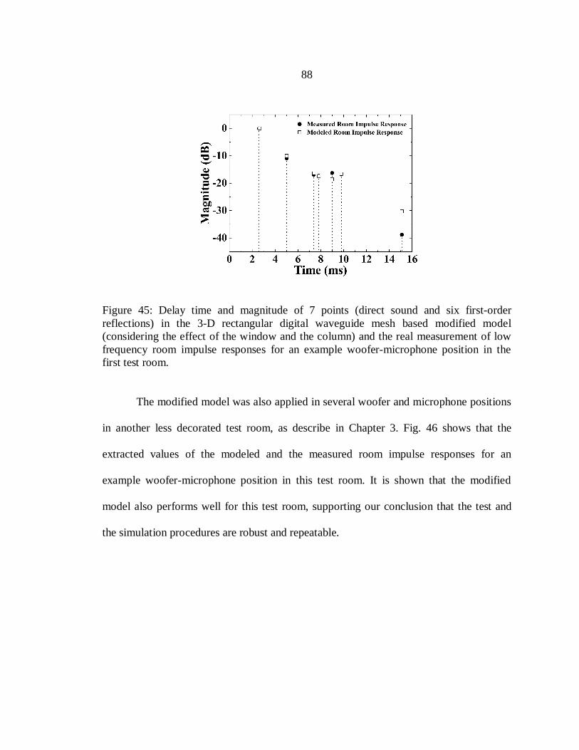
88

Figure 45: Delay time and magnitude of 7 points (direct sound and six first-orderreflections) in the 3-D rectangular digital waveguide mesh based modified model(considering the effect of the window and the column) and the real measurement of lowfrequency room impulse responses for an example woofer-microphone position in thefirst test room.

The modified model was also applied in several woofer and microphone positions

in another less decorated test room, as describe in Chapter 3. Fig. 46 shows that the

extracted values of the modeled and the measured room impulse responses for an

example woofer-microphone position in this test room. It is shown that the modified

model also performs well for this test room, supporting our conclusion that the test and

the simulation procedures are robust and repeatable.

89

Figure 46: Delay time and magnitude of 7 points (direct sound and six first-orderreflections) in the 3-D rectangular digital waveguide mesh based modified model and thereal measurement of low frequency room impulse responses for an example woofer-microphone position in the second test room.

A Subband Based Model Using 3-D Rectangular DWM

The requirement of the basic boundary condition to represent the reflection

coefficient over the whole woofer frequency range with a constant value may cause some

discrepancies between the simulation and the measurement of the low frequency room

impulse responses. An alternative way we considered to simulate the frequency

dependent boundary condition is to divide the desired woofer frequency range into

several subbands and use a constant value of reflection coefficient for each subband. The

intended advantage for the subband based method is that the reflection coefficients and

the woofer polar response will vary less in the subbands compared to in the full band.

90

Subband Decomposition Consideration

The Quadrature Mirror Filter (QMF) can be used to divide a signal into several

subbands and then obtain a perfect reconstruction of the original signal. But we need to

downsample the signal when using the QMF. This is equivalent to decreasing the

updating frequency of the digital waveguide mesh, which is undesirable because the

frequency response of the digital waveguide mesh will become uneven over the desired

frequency range (37 Hz – 1800 Hz) and the performance of the simulation result will

degrade. Therefore, we instead chose a convenient overlapped bandpass filter bank.

We instead divided the frequency range into two subbands (37 Hz – 500 Hz and

500 Hz – 1800 Hz), keeping the sampling frequency of the signals at 48 kHz. We used

these two narrower subband signals to synthesize the wider band signal (37 Hz – 1800

Hz). Fig. 47 and Fig. 48 show that the synthesized signal and the original signal have a

large discrepancy in the waveforms due to unmatched phase responses, but they have

similar spectra. Thus, the comparison between the simulation and the measurement of the

room acoustic responses was made in the frequency domain rather than in the time

domain.

91

Figure 47: The waveforms of the original signal and the synthesized signal.

Figure 48: The spectra of the original signal and the synthesized signal.

There is no standard for the number and the frequency range of the subbands in

the simulation. We can divide the frequency range into more subbands at the price of

increasing computational complexity and memory requirement. We can also divide the

frequency range into two subbands with the 3 dB bandwidth of 37 Hz to 400 Hz and 400

92

Hz to 1800 Hz respectively. In this case, the simulated source directivities and the room

surface reflection coefficients should change accordingly. One reason we chose 500 Hz

as the division boundary of the subbands is that the original signal and the synthesized

signal have a small spectra discrepancy in this way.

Subband Based Model Using DWM

In this simulation, two low frequency room impulse responses were modeled

using the 3-D rectangular digital waveguide mesh, with the original signal and the

synthesized signal as the sources. The reflection coefficients were set to 1 for all

boundaries and the source and the receiver were set to be omni-directional. These two

modeled responses were transformed into the frequency domain using an FFT with the

length of 1024 samples (the sampling frequency is 48 kHz). Fig. 49 shows the spectra

comparison between the original signal and the synthesized signal based simulation. The

spectra discrepancies are within 2 dB, which shows that the subband decomposition

method is feasible for the digital waveguide mesh based simulation.

93

Figure 49: Spectral comparison between the original signal and the synthesized signalbased room impulse response simulations.

Comparison between Measurement and Subband Based Model

The measured room surface reflection coefficients were used to calculate constant

values for every room surface in the lower and the higher subbands (shown in Table 4),

which was then applied in the basic boundary condition for the 3-D rectangular digital

waveguide mesh. The woofer polar responses at 250 Hz and 1 kHz were considered to be

the source directivities for the lower and the higher subbands, respectively.

The simulated responses were transformed into the frequency domain using an

FFT with length 1024 samples (the sampling frequency is 48 kHz). Fig. 50 shows the

spectral comparison between the subband based simulation and the real measurement.

The spectral discrepancies are within 5 dB. Future development work will be required to

assess the potential usefulness of this approach.

94

Figure 50: Spectral comparison between the subband based model and the realmeasurement of low frequency room acoustic responses.

Summary on Comparison between Measurement and DWM based Model

In this chapter, we verified that the match between the modeled and the measured

low frequency room impulse responses can be improved as expected if we include the

real measurements of the woofer polar response and the room surface reflection

coefficients in the 3-D rectangular digital waveguide mesh. We also verified that the

match can be further improved if we consider the effect of the irregular room surfaces.

We also showed that the subband based model is an alternative way for the simulation of

the low frequency room impulse response. We hoped that this subband method can help

extend the digital waveguide mesh simulation to a wider range of boundary condition.

The causes of the remaining discrepancies between the simulation and the

measurement of the low frequency room impulse responses are now being studied. For

example, they may be partly due to the scattering effect of the room surfaces. They may

95

also be partly due to the simplified representation of the boundary conditions and subtle

details of the source directivities.

96

CONCLUSION

Work Summary

To summarize this dissertation work, in the experimental part, we figured out the

experimental procedure and made experiments on measuring the room impulse responses,

speaker polar response, microphone polar response, and room surface reflection

coefficients. We developed the software to process the measurement data. In the

simulation part, we developed the MATLAB software to implement the room impulse

response models based on the image source method and digital waveguide mesh. In the

analytical part, we derived the analytical expression of impulse response in the 2D


The primary goal of this dissertation is to obtain a better match between the

simulation and the measurement of room impulse responses. In the room impulse

response model using the image source method, if the source and the receiver are

assumed to be omni-directional and the room surfaces are assumed to be perfectly

reflective, there is no surprise that a large discrepancy exists between the modeled and

the measured room impulse responses, indicating that this simple model is insufficient.

The match between the modeled and the measured room impulse responses can be

improved as expected if we include the real measurements of speaker polar response,

microphone polar response, and room surface reflection coefficients in the basic image

source method. Thus, we verified our goal to obtain a better match between the

simulation and the measurement of the room impulse responses for small rooms.

97

There are some limitations within the image source method itself. For example, it

is not sufficiently flexible to handle room surface irregularities. The digital waveguide

mesh can be used to simulate rooms with irregular room surfaces. Since the frequency

response is nearly uniform and the sound propagation dispersion error is small in the low

frequency range, the 3-D rectangular digital waveguide mesh is suitable for simulating

the low frequency part of the room impulse response. The 3-D rectangular mesh is not

appropriate for simulating sound over the whole audio frequency range because the

computational complexity and the memory requirements increase rapidly for increased

audio frequency bandwidth.

We verified that the match between the modeled and the measured low frequency

room impulse responses can be improved as expected if we included real measurements

of the woofer polar response and the room surface reflection coefficients in the 3-D

rectangular digital waveguide mesh. We also verified that the match can be further

improved if we consider the irregularity of the room surfaces. We also experimented

with a subband decomposition method for the simulation using the digital waveguide

mesh. We need to do some research to assess the potential usefulness of this approach.

At this point, we are able to better address the research questions presented in the

introduction. Given a real small empty room, the speaker polar response, microphone

polar response, and room surface reflection coefficients can be measured to characterize

the room impulse response. The room impulse response can then be modeled using the

image source method or the digital waveguide mesh, including the real measurement of

the source, receiver, and room surfaces. We may need to combine these two models if we

98

want to handle high frequency sound in an irregular room. The magnitudes of the points

corresponding to the direct sound and the six first-order reflections from the modeled and

the measured impulse responses can be compared. The discrepancies between the

simulation and the real measurement can be reduced from 10 – 20 dB in the simple model

to within 5 dB if we include the real measurement of the source, receiver, and room

surfaces in the model.

Future Work Discussion

There are some other methods that may be used to model the room impulse

response for a small room. The model using the image source method leads to an impulse

response with a fine time resolution, but this method cannot handle diffuse reflections. In

the future, we will do some research on the radiosity method [77-79], which is a ray-

based method and has been reported to be able to handle the diffuse reflection.

The boundary element method and the finite element method can also be used to

model the low frequency room acoustic responses. In the future, we will use the modeled

room acoustic responses using these methods as a reference to compare with the

modeling results using the digital waveguide mesh.

There is also some improvement that can be made in our current image source

method model or digital waveguide mesh model. First of all, we will find a more

systematic way to measure the parameters of the speaker polar response, microphone

polar response, and room surface reflection coefficients. Second, our current image

source method model does not include the processing of irregular room surfaces. This

99

will be investigated in the future. Third, in the model using the digital waveguide mesh,

the simulated reflection coefficient using the basic boundary condition has some

discrepancies with the theoretical value. In the future, we will use a correction function

for a variety of reflection coefficients (for example, range from 0.0 to 1.0 with the step of

0.1) in different directions (for example, range from 0º to 180º with the step of 1º). We

will also do research on the representation of the frequency dependent reflection

coefficients. Finally, we will do some research on the subband decomposition and the

source directivity representation in the 3-D rectangular digital waveguide mesh.

100

REFERENCES

[1] W.G. Gardner, The Virtual Acoustic Room. Master Thesis. MIT, Cambridge, 1992.

[2] T. Peltonen, A Multichannel Measurement System for Room Acoustics Analysis. Master’s thesis, Helsinki University of Technology, Espoo, Finland, 2000.

[3] M. Kleiner, B. I. Dalenbäck, and P. Svensson, “Auralization-an overview,” J. Audio Eng. Soc., vol. 41, pp. 861-875, 1993.

[4] K. H. Kuttruff, “Auralization of impulse responses modeled on the basis of ray- tracing results,” J. Audio Eng. Soc., vol. 41, pp. 876-880, 1993.

[5] P. Fausti, A. Farina, “Acoustic measurements in opera houses: Comparison between different techniques and equipment”, J. Sound and Vibration, vol. 232, pp. 213 – 229, 2000.

[6] I. Mateljan, “Signal selection for the room acoustics measurement,” Proc. 1999 IEEE Workshop on Applications of Signal Processing to Audio and Acoustics, New Paltz, New York, 1999.

[7] A. Farina, “Simultaneous measurement of impulse response and distortion with a swept sine technique,” Proc. 108th AES Convention, Paris, 2000.

[8] M. R. Schroeder, “Integrated-impulse method measuring sound decay without using impulses,” J. Acoust. Soc. Am., vol. 66, no. 2, pp. 497-500, 1979.

[9] J. Vanderkooy, “Aspects of MLS measuring systems,” J. Audio Eng. Soc., vol. 42, pp. 219-231, 1994.

[10] J. Borish and J. B. Angell, “An efficient algorithm for measuring the impulse response using pseudorandom noise,” J. Audio Eng. Soc., vol. 31, pp. 478-488, 1983.

[11] W. T. Chu, “Impulse response and reverberation decay measurements made by using a periodic pseudorandom sequence,” J. Applied Acoustics, vol. 29, pp. 193-205, 1990.

[12] C. Dunn and M. O. Hawksford, “Distortion immunity of MLS-derived impulse response measurements,” J. Audio Eng. Soc., vol. 41, pp. 314-335, 1993.

101

[13] R. Pintelon and J. Schoukens, “Measurement and modeling of linear systems in the presence of non-linear distortions,” Mechanical Systems and Signal Processing, vol. 16, no. 5, pp. 785-801, 2002.

[14] J. H. Rindel, “Modelling in auditorium acoustics: From ripple tank and scale models to computer simulations,” Forum Acusticum, Seville, Revista de Acústica XXXIII, no. 3-4, pp. 31-35, 2002.

[15] U. P. Svensson and U. R. Kristiansen, “Computational modelling and simulation of acoustic spaces,” 22nd Int. Conf. on Virtual, Synthetic and Entertainment Audio, Espoo, Finland, pp. 11-30, June 2002.

[16] C. L. Christensen and J. H. Rindel, “Predicting acoustics in classrooms,” InterNoise 2005, pp. 1782, 2005.

[17] J. H. Rindel, “The use of computer modeling in room acoustics,” Journal of Vibroengineering, vol. 3, no. 4, pp. 219-224, 2000.

[18] L. Savioja, Modeling Techniques for Virtual Acoustics. Ph.D. dissertation, Helsinki University of Technology, Espoo, Finland, 1999.

[19] A. Pietrzyk, “Computer modeling of the sound field in small rooms,” In Proc. AES 15th Int. Conf. on Audio, Acoustics & Small Spaces, Copenhagen, Denmark, pp. 24-31, 1998.

[20] A. Krokstad, S. Strom and S. Sorsdal, “Calculating the acoustical room response by the use of a ray tracing technique,” J. Sound and Vibration, vol. 8, no. 1, pp. 118- 125, 1968.

[21] R. L. Cook, T. Porter, and L. Carpenter, “Distributed ray tracing,” Computer Graphics (Proc. Siggraph 84), vol. 18, pp. 137-145, 1984.

[22] J. P. Vian and D. Van Maercke, “Calculation of the room impulse response using a ray-tracing method,” Proc. ICA Symposium on Acoustics and Theatre Planning for the Performing Arts, Vancouver, Canada , pp. 74-78, 1986.

[23] M. Vorländer, “Simulation of the transient and steady-state sound propagation in rooms using a new combined ray-tracing/image-source algorithm,” J. Acoust. Soc. Am., vol. 86, pp. 172-178, 1989.

[24] J. Arvo and D. Kirk, “A survey of ray tracing acceleration techniques,” An Introduction to Ray Tracing, A.S. Glassner ed., Academic Press, 1989.

102

[25] C. H. Séquin and E. K. Smyrl, “Parameterized ray tracing,” ACM Computer Graphics (Proc. Siggraph 89), vol. 23, pp. 307-314, 1989.

[26] B. M. Gibbs and D. K. Jones, “A Simple image method for calculating the distribution of sound pressure levels within an enclosure,” Acustica, vol. 26, pp. 24-32, 1972.

[27] J. B. Allen and D. A. Berkley, “Image method for efficiently simulating small-room acoustics,” J. Acoust. Soc. Am., vol. 65, no. 4, pp. 943-950, 1979.

[28] J. Borish, “Extension of the image model to arbitrary polyhedra,” J. Acoust. Soc. Am., vol. 75, no. 6, pp. 1827-1836, 1984.

[29] H. Lehnert, “Systematic errors of the ray-tracing algorithm,” J. Applied Acoustics, vol. 38, pp. 207-221, 1993.

[30] A. Craggs, “The use of simple 3-D acoustic elements for determining natural frequencies of complex shaped cavities,” J. Sound Vib, vol. 23, pp. 331-339, 1972.

[31] A. J. Burton and G. F. Miller, “The application of integral equation methods to the numerical solution of some exterior boundary-value problems,” Proc. R. Soc. London, Ser. A, vol. 323, pp. 201-210, 1971.

[32] S. Van Duyne and J. O. Smith, “Physical modeling with the 2-D digital waveguide mesh,” Proc. Int. Comput. Music Conf., Tokyo, Japan, pp. 40-47, Sept. 1993.

[33] S. Kopuz and N. Lalor, “Analysis of interior acoustic fields using the finite element method and the boundary element method,” J. Applied Acoustics, vol. 45, pp. 193-210, 1995.

[34] P. Davidsson, P. A. Wernberg, and G. Sandberg, “Using the finite element method for control of sound fields in room acoustics,” 15th Nordic Seminar on Computational Mechanics, Aalborg, Denmark, 2002.

[35] O. C. Zienkiewicz and R. L. Taylor, The Finite Element Method. McGraw-Hill, London, Fourth edition, 1989.

[36] R. D. Ciskowski and C. A. Brebbia, Boundary Element Methods in Acoustics. Elsevier, London, 1991.

[37] K. S. Yee, “Numerical solution of initial boundary value problems involving Maxwell’s equations in isotropic media,” IEEE Trans. Antennas Propag., vol. 14, pp. 302-307, 1966.

103

[38] U. R. Kristiansen, A. Krokstad, and T. Follestad. “Extending the image method to higher-order reflections,” J. Applied Acoustics, vol. 38, pp. 195-206, 1993.

[39] P. D. Yardley, Image Source Method for Simulating Wave Motion in Rectangular Enclosures. Master’s thesis, the University of Sheffield, 2001.

[40] T. A. Funkhouser, “A visibility algorithm for hybrid geometry- and image-based modeling and rendering,” Comput. Graph., vol. 23, no. 5, pp. 719-728, 1999.

[41] V. Välimäki, J. Pakarinen, C. Erkut, and M. Karjalainen, “Discrete-time modelling of music instruments,” Reports on Progress in Physics, vol. 69, no. 1, pp. 1-78, Jan. 2006.

[42] J. O. Smith, “A new approach to digital reverberation using closed waveguide networks,” Proc. Int. Computer Music Conf., Vancouver, Canada, pp. 47-53, 1985.

[43] J. O. Smith, “Music applications of digital waveguides,” CCRMA, Stanford Univ., Stanford, CA, Tech. Rep. STAN-M-39, 1987.

[44] J. O. Smith, “Physical modeling using digital waveguides,” Comput. Music J., Special Issue: Physical Modeling of Musical Instruments, Part I., vol. 16, no. 4, pp. 74-91, Dec. 1992.

[45] J. O. Smith, “Principles of Digital Waveguide Models of Musical Instruments,” M. Kahrs and K. Brandenburg, Ed. Norwell, MA: Kluwer, pp. 417-466, 1998.

[46] M. Karjalainen, P. Huang, and J. O. Smith, “Waveguide networks for room response modeling and synthesis,” Proc. 118th AES Convention., Barcelona, Spain, May 2005.

[47] M. Karjalainen and C. Erkut, “Digital waveguides versus finite difference structures: Equivalence and mixed modeling,” EURASIP J. Applied Signal Processing, vol. 7, pp. 978-989, June 2004.

[48] S. Van Duyne and J. O. Smith, “The 2-D digital waveguide mesh,” Proc. IEEE Workshop Applicat. Signal Process. Audio Acoust., New Paltz, NY, Oct. 1993.

[49] M. J. Beeson and D. T. Murphy, “RoomWeaver: A digital waveguide mesh based room acoustics research tool, ” Proc. 7th Int. Conf. Digital Audio Effects (DAFX04), Naples, Italy, pp. 268-273, Oct. 2004.

104

[50] F. Fontana and D. Rocchesso, “A new formulation of the 2-D waveguide mesh for percussion instruments,” Proc. XI Colloquium Musical Informatics, Bologna, Italy, pp. 27-30, Nov. 1995.

[51] M. L. Aird, L. Laird, and J. ffitch, “Modelling a drum by interfacing 2-D and 3-D waveguide meshes,” Proc. Int. Computer Music Conf., Berlin, Germany, pp. 82–85, Aug. 2000.

[52] F. Fontana and D. Rocchesso, “Signal-theoretic characterization of waveguide mesh geometries for models of two-dimensional wave propagation in elastic media,” IEEE Trans. Speech Audio Processing, vol. 9, no. 2, pp. 152-161, 2001.

[53] J. Laird, P. Masri, and N. Canagarajah, “Modeling diffusion at the boundary of a digital waveguide mesh,” Proc. Int. Computer Music Conf., Beijing, China, pp. 492-495, Oct. 1999.

[54] S. Van Duyne and J. O. Smith, “A simplified approach to modeling dispersion caused by stiffness in strings and plates,” Proc. Int. Computer Music Conf., Aarhus, Denmark, pp. 407-410, 1994.

[55] S. Van Duyne and J. O. Smith, “The 3-D tetrahedral digital waveguide mesh with musical applications,” Proc. Int. Computer Music Conf., Hong Kong, pp. 9-16, 1996.

[56] L. Savioja, T. Rinne, and T. Takala, “Simulation of room acoustics with a 3-D finite difference mesh,” Proc. Int. Computer Music Conf., Aarhus, Denmark, pp. 463-466, 1994.

[57] L. Savioja, J. Backman, A. Järvinen, and T. Takala, “Waveguide mesh method for low-frequency simulation of room acoustics,” Proc. Int. Congr. Acoustics, Trondheim, Norway, vol. 2, pp. 637-640, June 1995.

[58] A. Kelloniemi, V. Välimäki, and L. Savioja, “Simulation of room acoustics using 2-D digital waveguide meshes,” Proc. IEEE Int. Conf. Acoustics, Speech, and Signal Processing (ICASSP), Toulouse, France, vol. 5, pp. 313-316, May 2006.

[59] D. T. Murphy and D. M. Howard, “Physically modeling the acoustics of a room using a digital waveguide Mesh,” Proceedings of the 25th Euromicro Conference, Milan, Italy, pp. 82-89, Sept. 1999.

105

[60] J. Mullen, D. M. Howard, and D. T. Murphy, “Waveguide physical modeling of vocal tract acoustics: Flexible formant bandwidth control from increased model dimensionality,” IEEE Trans. Audio, Speech and Language Processing, vol. 14, no. 3, pp. 964-971, May 2006.

[61] B.H. Story, I. R. Titze, and E.A. Hoffman, “Vocal tract area functions from magnetic resonance imaging,” J. Acoust. Soc. Am., vol. 100, no. 1, pp. 537-554, 1996.

[62] J. Mullen, D. M. Howard, and D. T. Murphy, “Digital waveguide mesh modeling of the vocal tract acoustics,” IEEE Workshop on Applications of Signal Processing to Audio and Acoustics, New Paltz, NY, pp. 119-122, Oct. 2003.

[63] L. Savioja and V. Välimäki, “Reducing the dispersion error in the digital waveguide mesh using interpolation and frequency-warping techniques,” IEEE Trans. Speech Audio Process., vol. 8, pp. 184–194, 2000.

[64] S. Van Duyne and J. O. Smith, “The tetrahedral digital waveguide mesh,” IEEE Workshop on Applications of Signal Processing to Audio and Acoustics, New Paltz, NY, pp. 464-466, Oct. 1995.

[65] P. D. Henderson, “Getting started with SmaartLive: Basic measurement setup and procedures,” SIA Software Company, Inc. [Online]. Available: http://www.siasoft.com/pdf/Getting-Started-SmaartLive.pdf.

[66] D. T. Murphy and J. Mullen, “Digital waveguide mesh modelling of room acoustics: Improved anechoic boundaries,” Proc. Int. Conf. Digital Audio Effects (DAFx), Hamburg, Germany, pp. 163-168, Sept. 2002.

[67] D. T. Murphy and D. M. Howard, “2-D digital waveguide mesh topologies in room acoustics modeling,” Proc. COST G-6 Conf. Digital Audio Effects, Verona, Italy, pp. 211-216, Dec. 2000.

[68] L. Savioja, J. Huopaniemi, T. Lokki, and R. Vaananen, “Creating interactive virtual acoustic environments, ” J. Audio Eng. Soc., vol. 47, no. 9, pp. 675–705, Sept. 1999.

[69] A. Kelloniemi, Room Acoustics Modeling with the Digital Waveguide Mesh – Boundary Structures and Approximation Method. Ph.D. dissertation, Helsinki University of Technology, 2006.

http://www.siasoft.com/pdf/Getting-Started-SmaartLive.pdf.

106

[70] G.R. Campos and D.M. Howard, “On the computational efficiency of different waveguide mesh topologies for room acoustic simulation,” IEEE Trans. Speech Audio Processing, vol. 13, no. 5, pp. 1063-1072, Sept. 2005.

[71] A. Kelloniemi, “Improved adjustable boundary condition for the 3-D digital waveguide mesh,” Proc. 2005 IEEE Workshop Applications of Signal Processing to Audio and Acoustics, New Paltz, NY, pp. 191-194, Oct. 2005.

[72] A. Kelloniemi, L. Savioja, and V. Välimäki, “Spatial filter-based absorbing boundary for the 2-D digital waveguide mesh,” IEEE Signal Processing Lett., vol. 12, no. 2, pp. 126-129, Feb. 2005.

[73] A. Kelloniemi, D.T. Murphy, L. Savioja, and V. Välimäki, “Boundary conditions in a multi-dimensional digital waveguide mesh,” Proc. IEEE Int. Conf. Acoustics, Speech, and Signal Processing (ICASSP), Montreal, Canada, vol. 4, pp. 25-28, May 2004.

[74] A. Kelloniemi, “Frequency dependent boundary condition for the 3-D digital waveguide mesh,” Proc. 9th Int. Conf. Digital Audio Effects (DAFX06), Montréal, Canada, pp. 161-164, Sept. 2006.

[75] D. E. Dudgeon and R. M. Mersereau, Multidimensional Digital Signal Processing. Englewood Cliffs, NJ: Prentice-Hall, 1984.

[76] J. C. Strikwerda, Finite Difference Schemes and Partial Differential Equations. Pacific Grove, CA: Wadsworth and Brooks, 1989.

[77] H. E. Rushmeier and K. E. Torrance, “Extending the radiosity method to include specularly reflecting and translucent materials,” ACM Transactions on Graphics, vol. 9, no. 1, pp. 1-27, 1990.

[78] M. F. Cohen and J. R. Wallace, Radiosity and Realistic Image Synthesis. Academic, New York, 1993.

[79] F. X. Sillion and C. Puech, Radiosity and Global Illumination. Morgan Kaufmann, San Francisco, 1994.

an investigation of acoustic impulse response measurement

Documents

Transcript of an investigation of acoustic impulse response measurement