Characterization of Underwater Acoustic Communication ...

Characterization of Underwater Acoustic Communication ChannelsStatistical Characteristics of the Underwater

Multipath Channnels

Abraham Boayue

Master of Science in Communication Technology

Supervisor: Hefeng Dong, IET

Department of Electronics and Telecommunications

Submission date: August 2013

Norwegian University of Science and Technology

Master Thesis

August 26, 2013

Abstract

This master thesis aims at characterizing an underwater acoustic communication channelduring the two day communication experiments conducted in the Trondheim Fjord by theNTNU Acoustic Group from the 17th and 18th of June 2013. During the experiments,part of the sea trials were devoted to the transmission of a pseudorandom binary sequenceand a linear frequency modulation signal. The focus is put on the characterization of thestatistical multipath channel in which the evolution of the channel temporal impulseresponse is examined together with the spreading and scattering functions. In addition,the channel power delay profile, Doppler power spectrum, delay spread, Doppler spread,coherence bandwidth, coherence time and the maximum excess delay of the power delayprofile are presented in the form of figures and tables. Observation of the channel impulseresponse shows that the channel can be considered as a quasi-stationary channel and thatthe Doppler spread observed in the channel is mainly due to motion of the boat responsiblefor carrying the transmitter.

Acknowledgements

I would like to extend my gratitude and special appreciations to the following personsfor making this project a success. Thanks to Prof. Hefeng Dong (Professor in AcousticRemote Sensing) for allowing me undertake a project in a field that I was not so familierwith from start. Thanks to my supervisor Postdoc Alexios-Georgios Korakas for hisassistance in setting up the matlab platform and the correct estimation of the channelimpulse response need for this project.

1

Contents

1 Introduction 5

2 Statistical Multipath Channel Characteristics 62.1 Multipath fading of the Wireless Channel . . . . . . . . . . . . . . . . . . 6

2.1.1 Multipath Channel Model for Time-Variant Channels . . . . . . . 72.1.2 The Tapped Delay Line Channel Model . . . . . . . . . . . . . . . 82.1.3 Rayleigh and Ricean Fading Models . . . . . . . . . . . . . . . . . 102.1.4 Coherence Time and Coherence Bandwidth of the Channel . . . . 112.1.5 Multipath Channel Spread Factor . . . . . . . . . . . . . . . . . 112.1.6 Dispersive Characteristics of the Channel . . . . . . . . . . . . . . 11

2.2 Characteristics of Underwater Acoustic Channels . . . . . . . . . . . . . 122.2.1 Doppler Shift . . . . . . . . . . . . . . . . . . . . . . . . . . . . . 122.2.2 Multipath . . . . . . . . . . . . . . . . . . . . . . . . . . . . . . . 122.2.3 Doppler Spread . . . . . . . . . . . . . . . . . . . . . . . . . . . . 132.2.4 Delay-Spread and Doppler-Spread Functions . . . . . . . . . . . . 142.2.5 Delay-Doppler-Spread and Doppler-Delay-Spread Functions . . . 152.2.6 The Correlation Functions . . . . . . . . . . . . . . . . . . . . . . 162.2.7 Estimation of the Channel Correlation Functions and Parameters 18

3 Implementation 223.1 The Linear frequency Modulation Signal (LFM) . . . . . . . . . . . . . . 233.2 Maximal Length Sequence . . . . . . . . . . . . . . . . . . . . . . . . . . 24

4 Simulations 284.1 Trondheim Fjord Experiments . . . . . . . . . . . . . . . . . . . . . . . . 294.2 Results of Channel 4 . . . . . . . . . . . . . . . . . . . . . . . . . . . . . 31

5 Summary 43

Bibliography 44.1 Appendix A : Matlab Program Codes . . . . . . . . . . . . . . . . . . . 47.2 Appendix B : Matlab Reference Plots . . . . . . . . . . . . . . . . . . . . 57

2

List of Figures

2.1 Model for time-variant multipath channel . . . . . . . . . . . . . . . . . 92.2 Rayleigh fading signal and power, and Ricean fading signal and power . . 102.3 Simulation of a frequency selective channel, σd = [14.14, 25.22, 24.26, 24.14] 122.4 Top: Multipath trajectories in shallow-water configuration. (A) direct

path, (B) surface reflection, (C) bottom reflection, (D) surface and bottomreflection, (E) bottom and surface reflection. Bottom: Multiple paths asvisible in the envelope of a real time-domain signal. Note that the firstgroup of 4 arrivals are very clearly distinguishable-spreads about 4 ms; asecond group arrives 20 ms later with still a very significant intensity, anda more blurred time structure of the individual echoes tending to spreadand to merge into a reverberation trail. . . . . . . . . . . . . . . . . . . . 13

2.5 The Fourier transform relationships . . . . . . . . . . . . . . . . . . . . 18

3.1 Testing the ambiguity function of a chirp signal: (a)Chirp signal(b)Matchedfilter output, (c) 2-D plot of the ambiguity function (d)3-D plot of the am-biguity function . . . . . . . . . . . . . . . . . . . . . . . . . . . . . . . . 24

3.2 A plot showing : (a)M-sequence of period 511(b)The corresponding auto-correlation function, (c) The raised cosine pulse and its modulation at fc= 1000 Hz . . . . . . . . . . . . . . . . . . . . . . . . . . . . . . . . . . . 26

3.3 Testing the ambiguity function of a BPSK signal: (a)BPSK signal(b)Matchedfilter output, (c) 2-D plot of the ambiguity function (d) 3-D plot of theambiguity function . . . . . . . . . . . . . . . . . . . . . . . . . . . . . . 27

4.1 Experimental locations . . . . . . . . . . . . . . . . . . . . . . . . . . . . 294.2 Results of using a PRBS signal of length 255: (a)Temporal Impulse re-

sponse,(b)Spreading function (c) Doppler power spectrum to b., (d)Scatteringfunction , (e)Doppler power spectrum to d. (f) Power delay profile tob.(g)Power delay profile to d. . . . . . . . . . . . . . . . . . . . . . . . . 32

4.3 The spaced frequency and spaced time functions: (a)Spaced frequencyfunction using the spreading function(b)Spaced frequency function usingthe scattering function (c) Spaced time function using the spreading func-tion (d) Spaced time function using the scattering function . . . . . . . . 34

4.4 Results of using a PRBS signal of length 511: (a)Temporal Impulse re-sponse,(b)Spreading function (c) Doppler power spectrum to b., (d)Scatteringfunction , (e)Doppler power spectrum to d. (f) Power delay profile tob.(g)Power delay profile to d. . . . . . . . . . . . . . . . . . . . . . . . . 36

3


4.6 Results of using a PRBS signal of length 511: (a)Temporal Impulse re-sponse,(b)Spreading function (c) Doppler power spectrum to b., (d)Scatteringfunction , (e)Doppler power spectrum to d. (f) Power delay profile tob.(g)Power delay profile to d. . . . . . . . . . . . . . . . . . . . . . . . . 38


4.8 Results of using an LFM signal: (a)Temporal Impulse response,(b)Spreadingfunction (c) Doppler power spectrum to b., (d)Scattering function , (e)Dopplerpower spectrum to d. (f) Power delay profile to b.(g)Power delay profileto d. . . . . . . . . . . . . . . . . . . . . . . . . . . . . . . . . . . . . . . 41


1 PRBS signal of length 255: (a)3-D spreading function(b)3-D scatteringfunction (c) Doppler power spectrum of a. (d) Doppler power spectrum ofb.(e)Power delay profile of a. (f)Power delay profile of b. (g)Spaced fre-quency correlation function of e. (h)Spaced frequency correlation functionof f. . . . . . . . . . . . . . . . . . . . . . . . . . . . . . . . . . . . . . . 58



4 LFM signal : (a)3-D spreading function(b)3-D scattering function (c)Doppler power spectrum of a. (d) Doppler power spectrum of b.(e)Powerdelay profile of a. (f)Power delay profile of b. (g)Spaced frequency corre-lation function of e. (h)Spaced frequency correlation function of f. . . . . 61

4

Chapter 1

Introduction

Underwater communication and networking has become very essential both for commer-cial and military purposes. The number of research conducted in this field has increasedover the past few decades. The need to communicate between sensor nodes in sensornetwork requires the characterization of underwater acoustic channel. Because of thecomplexity of the underwater environment for communication, scientists have focused ondifferent aspects of characterizing an underwater communication channel as in [1]. Eachenvironment possesses a different characteristics that will affect the performance of a dig-ital communication system [2]; therefore, a necessary step in accessing the performanceof such systems is to be able to characterize an underwater communication channel basedon measured data from the ocean.

The propagation of sound in the ocean is very complex and must be well understood.Due to reflections on the ocean’s boundaries and refractions due to a depth varying soundspeed, sound tends to propagate through multipath trajectories; the temporal variabilityof the ocean combined with the low sound speed in water may induce significant Dopplershifts. As a result the channel is affected by time and/or frequency dispersion. Generally,an underwater communication channel can be classified as a multipath fading channel,and should be characterized statistically.

A number of efforts made in the characterization of an underwater multipath com-munication channel include the work of P. van Walree [3] , P. van Walreeand and G.Bertolotto [4], and B. Borowski [2]. The work presented in this report focuses on char-acterizing the acoustic data collected during the two day communication experimentsconducted in the Trondheim Fjord by the NTNU Acoustic Group from the 17th and18th of June 2013 to produce results similar to [3] , [4] and [2]. This report is organizedas follows: chapter 2 gives the necessary theory required for understanding and perform-ing the simulations, chapter 3 describes the method of implementation starting with abrief description of the linear frequency modulation (LFM) signal in section 3.1 and abrief description of an m-sequence and its application to a binary modulation signal toproduce a pseudorandom binary sequence (PRBS) in 3.2, chapter 4 presents the resultsof simulating a single channel with a PRBS signal for three different lengths and for anLFM signal, chapter 5 gives the conclusion, chapter 6 gives the bibliography and, finally,appendix A gives the matlab codes for producing most of the plots in the report andappendix B gives some reference plots to help aid the results obtained in chapter 4.

5

Chapter 2

Statistical Multipath ChannelCharacteristics

2.1 Multipath fading of the Wireless Channel

When a signal leaves the transmitting antenna, it can take a number of many differentpaths through a multipath communication channel to get to the receiver [5], and asa result, the transmitted signal components are scattered, reflected, diffracted, etc. byartificial or natural structures before reaching the receiver. If the transmitted signal isrepresented as i [6] and [7]:

s(t) = Re[u(t)ej2πfct

]= Re [u(t)] cos(2πfct)− Im [u(t)] sin(2πfct), (2.1)

where u(t) is the complex envelope and fc is the carrier frequency, then the received signalat the receiver may be represented as the sum of the delayed components as:

r(t) =

N(t)∑i=0

αi(t)eφDi (t)s(t− τi(t))

=Re

N(t)∑i=0

αi(t)u(t− τi(t))e−j2πτi(t) ej2φfct

(2.2)

where φDi(t) is the Doppler phase shift and amplitude αi(t) and φi(t) is the associatedphase of the ith signal component given by:

φi(t) = 2πfcτi(t)− φDi(t) (2.3)

Equation 2.2 shows that the received signal is obtained as the convolution between thetime-variant multipath channel’s impulse response and the transmitted signal if the chan-nel’s response is taken as:

6

C(τ ; t) =

N(t)∑i=0

αi(t)eφDi (t)δ(t− τi(t)) (2.4)

Equation 2.2 can be manipulated to give:

r(t) = rI(t) cos(2πfct)− rQ(t) sin(2πfct)

= a cos(2πfct+ φ(t)) (2.5)

where rI(t) and rQ(t) are the in-phase and quadrature signal components and a and φ(t)are the amplitude and phase of the received signal. The expressions for these componentsare given by:

rI(t) =Re

N(t)∑i=0

αi(t)u(t− τi(t))eφi(t) (2.6)

rQ(t) =Im

N(t)∑i=0

αi(t)u(t− τi(t))eφi(t) (2.7)

a =√r2I (t) + r2

Q(t) (2.8)

φ(t) = tan

(rQ(t)

rI(t)

)−1

(2.9)

According to [5] and [6], if the locations of the structures in the signal’s paths arecompletely random, one can assume the phase term, φi(t) will be uniformly distributedin the range (0, 2π). For large valves of the order of the multipath, N, the amplitudes,sI(t) and sQ(t) will be independently, identically Gaussian distributed, and the envelopea will have a Rayleigh distribution as:

f(a) =a

σ2e−

a2

2σ2U(a), (2.10)

where σ2 is the variance of either rI(t) or rQ(t), and U(.) is the unit step function. Underthis condition, the average power of the signal will have an exponential distribution givenby:

f(p) =1

2σ2e−

p2

2σ2U(p) (2.11)

2.1.1 Multipath Channel Model for Time-Variant Channels

The complex-valued function given in equation 2.2 can be thought of as the responseof the channel to the complex exponential function, exp(2πfct). The r.m.f (root-mean-square) spectral width of the channel, C(τ ; t) is called the Doppler spread of the channeland is denoted as Bd; which is a measure of how rapidly the channel is changing withtime. A small value of the Doppler spread results in a slowly varying of the channel withtime, while a large value gives rise to a rapidly time varying channel.

7

2.1.2 The Tapped Delay Line Channel Model

A general model for a time-variant multipath channel is illustrated in Figure 2.1 takenfrom [8]. The channel model consists of a tapped delay line with uniformly spaced taps.The tap spacing between adjacent taps is 1/W, where W is the bandwidth of the signaltransmitted through the channel. The taps coefficients of the channel are given by:

Cn(t) =cr(t) + jci(t)

=αn(t)ejφn(t), (2.12)

where αn(t) is an attenuation factor and φn(t) is a phase shift. The coefficients, cr(t)and ci(t) are usually modeled as complex-valued Gaussian processes. The length ofthe delay line corresponds to the amount of time dispersion in the multipath channel,which is usually called the multipath delay spread. The multipath spread is denotedas Tm = L/W , where L represents the maximum number of possible multipath signalcomponents.

8

Input signal

Tm

1/W 1/W 1/W

c1(t) c2(t) cL-1(t) cL(t)

+

+ Channel output

Additive noise

Figure 2.1: Model for time-variant multipath channel

9

2.1.3 Rayleigh and Ricean Fading Models

According to equation 2.12, if the coefficients of the tapped delay line channel modelis treated as a complex-valued Gaussian process, then each of the coefficients may beexpressed as:

C(t) = α(t)ejφ(t), (2.13)

where the amplitude and phase are given by:

α(t) =√c2r(t) + c2

I(t) (2.14)

φ(t) = tan−1

(cI(t)

cr(t)

)(2.15)

If the coefficients, cr(t) and cI(t) are zero mean Gaussian random variables, then theenvelope has a Rayleigh distribution as given by equation 2.2 and the phase is uniformlydistributed in the range of (0, 2π). Thus, the channel is called a Rayleigh fading channel.On the other hand, if the coefficients, cr(t) and cI(t) are nonzero mean Gaussian randomvariables, then the amplitude α(t) will have a Ricean distribution as given by:

f(α) =α

σ2e−(α2+s2)/2σ2

I0

(sασ2

)a ≥ 0, (2.16)

where 2σ2 is the average power in the multipath components, s2 = α20 is the power in

the line of sight (LOS) component, and the function I0 is the modified Bassel functionof zeroth order. A typical plot of the Rayleigh and the Ricean fading channels is shownin Figure 2.2 obtained from an exercise in [5]. The plot was obtained from a total of 11multipath components and using a random phase in generating the signal. The effect ofthe multipaths and random phase is clearly seen in the plots of the received powers; evenin the absence of noise, the received power randomly varies.

0 0.05 0.1−20

0

20Rayleigh fading signal

time ms

ampl

itude

0 0.05 0.1−50

0

50Rayleigh fading signal power

time ms

pow

er d

B

0 0.05 0.1−20

0

20Rician fading signal

time ms

ampl

itude

0 0.02 0.04 0.06 0.08 0.1−40

−20

0

20Rician fading signal power

time ms

pow

er d

B

Figure 2.2: Rayleigh fading signal and power, and Ricean fading signal and power

10

2.1.4 Coherence Time and Coherence Bandwidth of the Chan-nel

In addition to the delay spread Tm and the Doppler spread Bd, the coherence time andthe coherence bandwidth are two other parameters that can be used to characterizedfading, multipath channels. The coherence time is a measure of the time interval overwhich the channel characteristics will change very little and is given by:

Tc =1

Bd

(2.17)

Similarly, the coherence bandwidth is the bandwidth over which the channel character-istics (magnitude α(t) and phase (φ(t)) are highly correlated. All frequency componentsof a signal within this bandwidth will fade simultaneously. This bandwidth is defined asthe reciprocal of the delay time spread:

Bc =1

Tm(2.18)

2.1.5 Multipath Channel Spread Factor

The product of the multipath spread and the Doppler spread (TmBd) is known as thechannel spread factor. The channel is said to be underspread if TmBd < 1, and overspreadif TmBd > 1. In general, the estimation of the carrier phase of the channel can be verydifficult if the channel is overspread (rapid time variations Tc << Tm) due to either largemultipath spread or either Doppler spread or both, and it can be estimated with goodprecision if the channel is underspread (slow time variations Tc >> Tm).

2.1.6 Dispersive Characteristics of the Channel

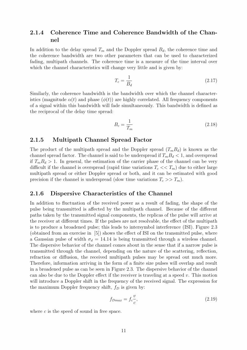
In addition to fluctuation of the received power as a result of fading, the shape of thepulse being transmitted is affected by the multipath channel. Because of the differentpaths taken by the transmitted signal components, the replicas of the pulse will arrive atthe receiver at different times. If the pulses are not resolvable, the effect of the multipathis to produce a broadened pulse; this leads to intersymbol interference (ISI). Figure 2.3(obtained from an exercise in [5]) shows the effect of ISI on the transmitted pulse, wherea Gaussian pulse of width σd = 14.14 is being transmitted through a wireless channel.The dispersive behavior of the channel comes about in the sense that if a narrow pulse istransmitted through the channel, depending on the nature of the scattering, reflection,refraction or diffusion, the received multipath pulses may be spread out much more.Therefore, information arriving in the form of a finite size pulses will overlap and resultin a broadened pulse as can be seen in Figure 2.3. The dispersive behavior of the channelcan also be due to the Doppler effect if the receiver is traveling at a speed v. This motionwill introduce a Doppler shift in the frequency of the received signal. The expression forthe maximum Doppler frequency shift, fD is given by:

fDmax = fcv

c, (2.19)

where c is the speed of sound in free space.

11

400 600 8000

0.5

1Received Pulse

400 600 8000

0.5

1Received Pulse

400 600 8000

0.5

1Received Pulse

400 500 600 700 8000

0.5

1Transmitted Pulse, σ = 14.14

Figure 2.3: Simulation of a frequency selective channel, σd = [14.14, 25.22, 24.26, 24.14]

2.2 Characteristics of Underwater Acoustic Chan-

nels

Like communication on land, underwater communication channel can be regarded as time-varying frequency selective, spatially uncorrelated channel with additive colored Gaussiannoise [9]. It is characterized by frequency dependent and range dependent absorption,which together with the multipath phenomenon results in fading. A few characteristicsof the underwater acoustic channel is described in the next few subsections.

2.2.1 Doppler Shift

A relative motion of the receiver and or the transmitter or a moving medium can changethe frequency of the sound waves propagating through the channel. The apparent changein the signal’s carrier frequency and the time domain is known as Doppler shift. Anexpression for the Doppler frequency shift is given by:

fD = fcv + c

c, (2.20)

where c is the speed of sound in free space,v speed of the observer and fc the transmittedsignal frequency known as the carrier frequency.

2.2.2 Multipath

In underwater acoustics the multipath effect is mainly caused by reflections from the seafloor and surface [9], [10]. The number of bounces determines the multipath spread. Inaddition, the channel consists of volume reflections such as plankton and fish. For a largeenough range between the transmitter and receiver, the transmitted signal propagatesto the receiver via various paths. The delay associated with each path depends on itsgeometry. The signals, while propagating, undergo successive reflections at the interfaces.Variations in the sound speed within the medium also deform the paths of the soundwaves. Due to these processes, a given signal can therefore propagate from a source to a

12

receiver along several distinct paths corresponding to different directions and durations.The main direct signal arrives along with a series of echoes, the amplitudes which decreasewith the number of reflections undergone. The process of signal taking many differentpaths to get to the receiver as a result of reflections is referred to as multipath. At highfrequencies, for short signals, the multipath effect is observable in the time domain, withtypical sequences of multiple echoes (see Figure 2.4, [10] ). While for low-frequency stablesignals, the contributions add together permanently; this creates a stable interferencepattern, with strong variations in the field amplitude.

Figure 2.4: Top: Multipath trajectories in shallow-water configuration. (A) direct path,(B) surface reflection, (C) bottom reflection, (D) surface and bottom reflection, (E) bot-tom and surface reflection. Bottom: Multiple paths as visible in the envelope of a realtime-domain signal. Note that the first group of 4 arrivals are very clearly distinguishable-spreads about 4 ms; a second group arrives 20 ms later with still a very significant inten-sity, and a more blurred time structure of the individual echoes tending to spread and tomerge into a reverberation trail.

2.2.3 Doppler Spread

The Doppler spread Bd, expresses the spectral width spreading of the received signal.In shallow water the reflections from the water surface are the primary reason for thetime-variance of the channel. The value of the Doppler spread depends on the wavesheight and frequency, wind speed, number of reflections from the sea surface and floor,and the nominal angle.

13

2.2.4 Delay-Spread and Doppler-Spread Functions

The theory of randomly time-variant linear channel was developed by Bello in his paperof 1963 [11]; he gave a full statistical characterization of the channel based on systemfunctions and their correlation functions. He made use of the concept of a communi-cation device consisting of an input and an output terminals; where the signal appliedat the input may be characterized in either the time or frequency domain and similarly,the output signal coming out of the device may be characterized in either the time orfrequency domain. Denoting x(t) and X(f) as the input time function and spectrum,and the corresponding out time function and spectrum as y(t) and Y (f), and using hisapproach and considering the underwater acoustic channel as a linear time variant filter(LTV), we can establish a mathematical relation between the input signal and the outputsignal. Since the underwater acoustic channel model to be discussed involves both delayand Doppler shifts, there exists a total of four expressions for the output signal; two forthe time function and two for the frequency spectrum. The is because the channel willtreat the signals differently depending on whether the delay operation or the Doppler-shiftoperation is applied at the input or output of the channel. For an input delay operatorapplied at the channel input, the convolution theorem gives the input-output relationshipthat exists between the input signal x(t) and output signal y(t) as:

y(t) =

∫x(t− τ)h(t, τ)dτ, (2.21)

Equation 2.21 shows that the output of the channel is expressed as the integral of thedelay elements; with the elements providing delays in the interval (τ, τ + dτ) and havinga differential amplitude of h(t, τ)dτ . Therefore, the function h(t, τ) is called the InputDelay-Spread Function of the channel and may be thought of as the response of thechannel at time t to a unit impulse input at time τ seconds in the past. Since a physicalchannel can not have an output before the input has arrived, h(t, τ) must vanish for τ < 0.The second expression for the output signal is obtain by applying the delay operator atthe output of the channel; the required expression is given by:

y(t) =

∫x(t− τ)g(t− τ, τ)dτ, (2.22)

where g(t, τ) = h(t + τ, τ) is referred to as the Output Delay-Spread-Function of thechannel and may be thought of as the response τ seconds in the future to a unit impulseat time t. For the same requirement imposed on h(t, τ), g(t, τ) must vanish for τ < 0.

The input-output relationship given by Equation 2.21 and 2.22 may be characterizedin the frequency domain by employing the input and output Doppler-Spread Functions.IfH(f, ρ) is considered to be the dual function to h(t, τ), then the frequency domain rep-resentation of the output signal is given by:

Y (f) =

∫X(f − ρ)H(f, ρ)dρ, (2.23)

where H(f, ρ) is taken as the input Doppler-Spread Function and ρ as the Doppler shiftedfrequency variable. Similarly, the frequency domain representation to the output Dopplerspread function is given by:

Y (f) =

∫X(f − ρ)G(f, ρ)dρ, (2.24)

where G(f, ρ) is taken as the output Doppler-Spread Function.

14

2.2.5 Delay-Doppler-Spread and Doppler-Delay-Spread Func-tions

Bello has demonstrated in [11] that any liner time-varying channel can be representedas a continuum of elements which simultaneously provide both a corresponding delayand Doppler shift. In his work, he classified the channel impulse response according towhether the delay operation or Doppler shift operation on the channel was at the inputor the output. Because of the existence of the two operations in the channel model, onlytwo possibilities were considered: input-delay output-Doppler-shift and input-Doppler-shift output-delay. Taking into account the former of the two possibilities, the inputdelay spread function h(t, τ) (i.e the time variance channel impulse response) can beexpressed as the inverse Fourier transform of its Doppler spectrum U(τ, ρ) (holding τ asa fix parameter) given by:

h(t, τ) =

∫U(τ, ρ)ej2πρtdρ, (2.25)

Substituting this expression into Equation 2.21 gives:

y(t) =

∫ ∫x(t− τ)U(τ, ρ)ej2πρtdρdτ, (2.26)

Equation 2.26 shows that the output of the channel is expressed as the sum of the delayand then Doppler shifted elements; with the elements providing delays in the interval(τ, τ + dτ) and Doppler shifts in the interval (ρ, ρ + dτ) and having a differential am-plitude of U(τ, ρ)dρdτ . Hence, the function U(τ, ρ) is called the Delay-Doppler-SpreadFunction of the channel.

To determine the Doppler-Delay-Spread function of the channel, we first express theinput Doppler-Spread Function as the Fourier transform of V (ρ, τ) (holding ρ as a fixedparameter):

H(f, ρ) =

∫V (ρ, τ)e−j2πτfdτ, (2.27)

Substituting this expression into Equation 2.23 gives:

Y (f) =

∫ ∫X(f − ρ)V (ρ, τ)e−j2πτfdτdρ, (2.28)

Equation 2.28 shows that the output of the channel is expressed as the sum of the Dopplershifted and then Delay elements; with the elements providing Doppler shifts in the interval(ρ, ρ + dρ) and delays in the interval (τ, τ + dτ) and having a differential amplitude ofV (ρ, τ)dτdρ. For this reason, the function V (ρ, τ) is called the Doppler-Delay-SpreadFunction of the channel. If the Fourier transform of both sides of Equation 2.26 is takenwith respect to t, and the inverse Fourier transform of both sides of Equation 2.28 is takenwith respect to f, we obtain the following two alternative expressions for the output signalof the channel in both time and frequency domains:

y(t) =

∫ ∫x(t− τ)ej2π(t−τ)ρV (ρ, τ)dτdρ (2.29)

Y (f) =

∫ ∫X(f − ρ)e−j2π(f−ρ)τU(τ, ρ)dτdρ (2.30)

15

Equations 2.29 and 2.30 show that the Delay-Doppler-Spread Function U(τ, ρ) and theDoppler-Delay-Spread Function V (ρ, τ) are related through the following equation:

U(τ, ρ) = e−j2πρτV (ρ, τ) (2.31)

2.2.6 The Correlation Functions

In this section and the rest of the report, the channel is modelled as an input-delayoutput-Doppler shift channel. Hence, all mathematical expressions involving the channelimpulse response are obtained in term of the input delay spread function h(t, τ) or equiv-alently, its inverse Fourier transform, the input Doppler spread function U(τ, ρ). Thelatter shall be called the spreading function as defined in [3]. The characteristics of amultipath channel can be defined through a number of useful correlation functions andpower spectral density functions. According to [11], if the channel is randomly time-variant, the responses of the channel discussed in the last two sections become stochasticprocesses and a practical characterization of the channel is obtained in terms of corre-lation functions. It is customary to assume as in [1] and [6] that the fading statisticsof many physical channels, including underwater acoustic channels to be approximatelystationary for time intervals sufficiently long to make it meaningful to define a subclassof channels known as Wide-Sense Stationary (WSS) channels. If in addition, the channelresponse is further considered to be uncorrelated at the delays for τ1 6= τ2, the channelcan be called a Wide-Sense Stationary Uncorrelated Scattering Channel (WSSUSC). Forsimplicity, the channel impulse response can be modeled as in Equation 2.4. The channelautocorrelation function in the time domain can be represented as :

Rh(τ1, τ2,∆t) = E [h∗(τ1, t)h(τ2, t+ ∆t]

= Rh(τ1,∆t)δ(τ2 − τ1)

= Rh(τ,∆t), (2.32)

Similarly, the channel autocorrelation function can be characterized in the frequencydomain as :

Rh(f1, f2,∆t) = E [h∗(f1, t)h(f2, t+ ∆t]

= Rh(f1,∆t)δ(f2 − f1)

= Rh(∆f,∆t) (2.33)

where the functions depend on the time variables τ1 and τ2 only through the time differ-ence τ = τ2− τ1. The most important characteristics of the wideband channel, includingthe multipath intensity profile, coherence bandwidth, coherence time, and the Dopplerpower spectrum, are derived from the autocorrelation function Rh(τ,∆t). In additionto these, the scattering function S(τ, ρ), which completely characterizes the widebandchannel if the WSSUS is assumed, can be defined; where ρ is the variable for the Dopplerfrequency shift in the frequency domain . By definition, the expression for the scatteringfunction is given as the Fourier transform of the time autocorrelation function of thechannel ( Equation 2.32) or as the Fourier transform of the inverse Fourier transform of

16

the frequency autocorrelation function ( Equation 2.33 see [6] and [4]):

Sh(τ, ρ) =

∫Rh(τ,∆t)e

−j2πρ∆td∆t

=

∫ [∫h(τ, t)h∗(τ, t+ ∆t)dt

]e−j2πρ∆td∆t

=

∫ [∫Rh(∆f,∆t)e

j2πτ∆fd∆f

]e−j2πρ∆td∆t, (2.34)

Equation 2.34 shows that the time and frequency autocorrelaton functions, Rh(τ,∆t) andRh(∆f,∆t) form a Fourier transform pair. Letting ∆t equals zero in both Equations 2.32and 2.33, an expression for the multipath intensity profile can be obtained as :

Ph(τ) =

∫Rh(∆f)ej2πτ∆fd∆f, (2.35)

where Rh(∆f) is known as the spaced frequency correlation function of the channel. Sim-ilarly, to relate the Doppler effects to the time variations of the Doppler power spectrum,we let Ac(∆f,∆t) denote the Fourier transform to the spectrum Sc(∆f, ρ) and letting∆f = 0 we get an expression for the Doppler power spectrum:

Sh(ρ) =

∫Rh(∆t)e

−j2πρ∆td∆t, (2.36)

where Rh(∆t) is known as the spaced time correlation function of the channel. TheFourier transform relationships among the correlation functions are summarized in [6]according to Figure 2.5.Having set up a model for the time variant multipath channel and derived the autocor-relation function for it in both time and frequency domain, as well as equipped with theFourier transform relationships that exist among the correlation functions, we devote afew sections in further characterization of the underwater acoustic channel.

17

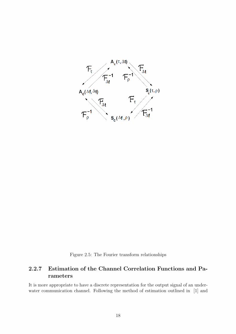
Figure 2.5: The Fourier transform relationships

2.2.7 Estimation of the Channel Correlation Functions and Pa-rameters

It is more appropriate to have a discrete representation for the output signal of an under-water communication channel. Following the method of estimation outlined in [1] and

18

[18], the discrete representation to Equation 2.26 is given by :

y(n) =L∑

(l,k)

x(n− l)U(l, k)ej2πk∆vn, (2.37)

where the L pairs (l, k) corresponds to L distinct scatterers at different delay and Doppler,and the channel is time dependent only through ej2πk∆vn, ∆v is the Doppler spacing,x(n) is the input signal and U(l, k) the delay Doppler spectrum or simply the spreadingfunction as it is called in [3] and is defined as the Fourier transform of the channelimpulse response, Equation 2.25. Hence, its discrete representation can be shown to be :

U(l, k) =N−1∑n=0

h(l, n)ej−2πnkN , (2.38)

Assuming that the wide sense stationary uncorrelated scattering assumption (WSSUS)holds, the autocorrelation function can be defined as :

RU(l,m; k, i) = E[Ul,kU∗m,i]

= S(l, k)δ(i− k)δ(m− l), (2.39)

where S(l, k) is the two dimensional power spectral density in delay and Doppler and isknown as the channel scattering function, RU(l,m; k, i) is the autocorrelation function ofthe delay-Doppler-spread of the channel and δ is the Kronecker delta function. From aphysical point of view, Ul,k can be thought of as the complex gain of the received signalarriving at delay l and Doppler k. In the real world, the strength of the scatterer changeswith time and therefore, the function Ul,k is subject to change with time : Ul,k(n). Hence,the channel is no longer a WSSUS channel. According to [1] the scattering function mustbe estimated in practice in addition to the WSSUS assumption. The scattering functioncan be estimated by transmitting a known signal; this signal must be chosen accordinglyin order to obtain a good estimate of S(l, k). The scattering function can be characterizedin terms of ambiguity functions. The definitions of the signal ambiguity function and thecross-ambiguity function are given by :

θ0(l, k) =

∣∣∣∣∣M−1∑m=0

x(m)x∗(m− l)e−j2πk∆vm

∣∣∣∣∣2

, (2.40)

(2.41)

θ(l, k) =

∣∣∣∣∣M−1∑m=0

x(m)y∗(m− l)e−j2πk∆vm

∣∣∣∣∣2

,

where x(m)y(m) is the complex baseband envelope of the transmitted and received sig-nals. [1] and [18] have pointed out that the scattering function is related to the ambiguityfunction by showing that the expectation of the cross-ambiguity function is given by :

E[θ(l, k)] =L∑

(n,m)

θ0(l + n, k +m)S(n,m). (2.42)

19

Equation 2.42 can be used to estimate the scattering function by selecting an appropriatesource signal that will cause the ambiguity function to be a unit impulse in both delayand Doppler, i.e. the ambiguity function must equal :

θ0(l, k) = δ(l)δ(k) (2.43)

An estimate of the delay power profile (multipath intensity profile) of the channel can beobtained by taking the average of the spreading function over all Doppler shifts :

Pu(l) =N−1∑k=0

|S(l, k)|2 (2.44)

The delay spread can be found by calculating the total delay of the delay power spectrum.Similarly, the Doppler power spectrum of the channel can be estimated by taking theaverage of the spreading function over all delays :

SH(k) =L−1∑l=0

|S(l, k)|2 (2.45)

The Doppler spread Bd of the channel is found to be the bandwidth of the Doppler powerspectrum SH(k). It is worth noting that Equations 2.44 and 2.45 may be valid for thespreading function |U(l, k)|2 Equation 2.38; this is because in most instances the resultsobtained by using the scattering function can be approximated with that of the spreadingfunction for most channels and hence, Equations 2.44 and 2.45 are valid for |U(l, k)|2 sincethis is easier to obtain as shall be seen in Section 3.2. From the estimates of the delaypower profile and the Doppler power spectrum, the spaced frequency correlation functionand the spaced time correlation function can be estimated by taking the Fourier transformof Equation 2.44 and the inverse Fourier transform of Equation 2.45. Hence, the requiredexpressions for these functions are :

R(∆f) =L−1∑l=0

Pu(l)e−j2π∆fl (2.46)

R(∆t) =K−1∑k=0

SH(k)ej2π∆tk, (2.47)

Channel parameters

In section 1.1.4 the coherence time and coherence bandwidth of the channel were definedaccording to Equation 2.17 and 2.18, where the former was taken as the reciprocal ofthe Doppler spread and the latter as the reciprocal of the delay spread. These quantitiescan be obtained from the estimated correlation functions as defined in the precedingparagraphs. According to [6] the delay spread Tm is defined as the value over which thedelay power profile is essentially non-zero, and the same is true for the Doppler spreadBd. Similarly, the coherence time Tc is taken as the value over which the spaced timecorrelation function is essentially non-zero, and the coherence bandwidth Bc is the valuefor which the spaced frequency correlation function is approximately zero for all ∆f > Bc.The multipath channel can also be quantified in terms of the excess delay, average delay

20

spread T̄m and the rms delay spread σTm . The mathematical expressions for the T̄m andσT̄m in terms of the delay spread Rh(τ) are given by [6] as:

T̄m =

∫∞0τPh(τ)dτ∫∞

0Ph(τ)dτ

(2.48)

σT̄m =

∫∞0

(τ − Tm)2Ph(τ)dτ∫∞0Ph(τ)dτ

, (2.49)

If Equations 2.48 and 2.49 are defined in terms of the Doppler power spectrum, by [2]the resulting equations yield the corresponding expressions for the average delay spreadand the rms delay spread in hertz:

fshift =

∫∞0ρSh(ρ)dρ∫∞

0Sh(ρ)dρ

(2.50)

σfspread =

∫∞0

(ρ− fshift)2Ph(τ)dτ∫∞0Sh(ρ)dρ

, (2.51)

where fshift and σfspread are the estimates of the maximum Doppler shift and the Dopplerspread. Another parameter of interest of the channel is the maximum excess delay of thepower delay profile. It is defined in [12] as the time delay during which the multipathenergy falls to X-dB below the maximum value of the power delay profile. This quantitycan be read from the plot of the power delay profile (see also [2]).

21

Chapter 3

Implementation

This chapter discusses some of the key points in characterizing an underwater communica-tion channel using experimental data. The chapter aims at justifying that the ambiguityfunction method of estimating the channel scattering function is appropriate. The accu-racy of the method is possible through a careful selection of the source signal. Hence, itis very useful to compute the ambiguity diagrams for various waveforms and determinewhich one of them have the desirable properties for the intended application [13]; twotypes of signals have been used to test the method. The signals are : linear frequencymodulation (LFM) signal and a binary phase shift keying signal with the bit sequencegenerated from a maximum length sequence (m-sequence). A very good understandingof the ambiguity function is covered in [14] and [13]. A study of the ambiguity diagramcan provide some insights about how different signal waveforms may be suitable for var-ious communication purposes. The ambiguity function has the following mathematicalproperties :

|θ0(τ, ρ)|2max = |θ0(0, 0)|2 = (2E)2 (3.1)

|θ0(−τ,−ρ)|2 = |θ0(τ, ρ)|2 (3.2)

|θ0(τ, 0)|2 =

∣∣∣∣∫ x(t)x(t+ τ)dt

∣∣∣∣2 (3.3)

|θ0(0, ρ)|2 =

∣∣∣∣∫ x(t)2ej2πρtdt

∣∣∣∣2 (3.4)∫ ∫|θ0(τ, 0)|2 dτdρ =(2E)2 (3.5)

Equation 3.1 states that the maximum of the ambiguity function occurs at the origin,which is the output of the matched filter that is matched perfectly to the signal reflectedfrom the target of interest; its value is equal to the square of two times the echo signalenergy. The second equation is a symmetry equation. Equation 3.3 is just the portion ofthe ambiguity function on the time delay axis, which is the square of the autocorrelationfunction of the transmitted signal. Equation 3.4 describes the behaviour of the functionalong the frequency axis and is equal to the inverse Fourier transform of the square of thesignal x(t). Finally, Equation 3.5 gives the total volume under the ambiguity diagram,and is equal to (2E)2.

22

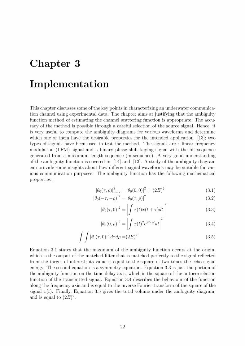
3.1 The Linear frequency Modulation Signal (LFM)

An LFM signal is commoly referred to as a chirp signal and may be expressed as a cosinesignal as in [15] and [16] :

x(t) = cos(2πf0t+ πkt2), (3.6)

where k is known as the chirp rate or the frequency slope defined as :

|k| = |f1 − f0|T

=B

T. (3.7)

Equation 3.6 and 3.7 completely characterize the chirp signal by its start frequency f0,stop frequency f1 or bandwidth B and time duration T . The following plots in Figure 3.1shows the results of a chirp signal simulated for a start frequency of f0 = 3500 Hz, stopfrequency of f1 = 4000 Hz and a period of T = 25 ms. It is clear from these plots thatthe use of the LFM signal for estimating the scattering function will yield undesirableresults; two reasons being that the output of the matched filter does not approximate animpulse along the Doppler axis, and the side lobes have very high values as opposed tothe negligible side lobe criterion.

23

0 0.005 0.01 0.015 0.02 0.025−1.5

−1

−0.5

0

0.5

1

1.5

Baseband chirp signal

(a)

−0.025 −0.02 −0.015 −0.01 −0.005 0 0.005 0.01 0.015 0.02 0.0250

50

100

150

200

250

300

350

Doppler shifts

mag

nitu

de

Output of the matched filter

(b)

Delays

Dop

pler

shi

ft−H

z

2−D representation of the ambiguity diagram

−0.025 −0.02 −0.015 −0.01 −0.005 0 0.005 0.01 0.015 0.02 0.025

−500

−400

−300

−200

−100

0

100

200

300

400

500

(c) (d)

Figure 3.1: Testing the ambiguity function of a chirp signal: (a)Chirp signal(b)Matchedfilter output, (c) 2-D plot of the ambiguity function (d)3-D plot of the ambiguity function

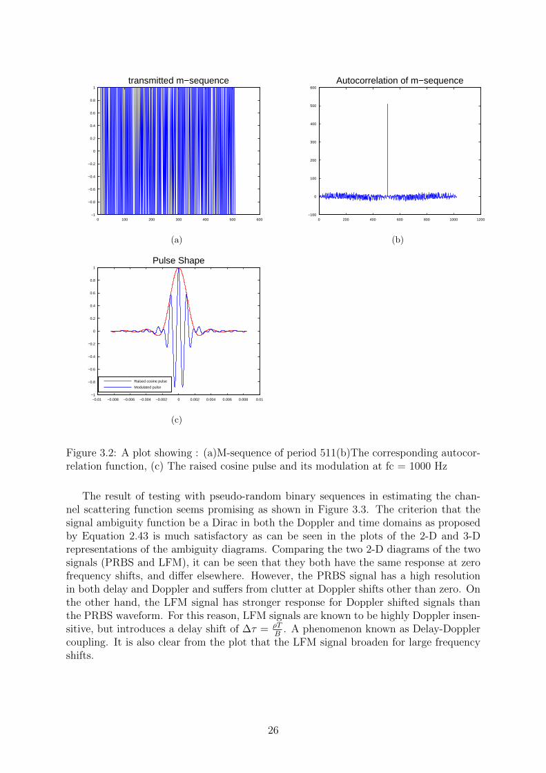
3.2 Maximal Length Sequence

A maximal length sequence (MLS) is a periodic two-level signal that can be generatedfrom a linear feedback shift register; it has a length of N = 2m − 1, where m is thenumber of stages in the shift register and N is the period. A MLS is commonly calledan m-sequence and can be generated by a polynomial G(x) of degree m, where G(x) isdefined as :

G(x) =m∑i=0

aixi, (3.8)

where the ais are the feedback taps that have values of either 0 or 1 depending on whetherthe feedback tap is connected or not. It should be noted that m-sequences are a specialcase of the output of a feedback shift register that will make every state transition of 2m

of an m-bit shift register with the exception of the all zero state. Hence, an m-sequencewill only exist only if proper feedback taps are chosen. M-Sequences have a number ofdesirable properties that make them very useful in practice; because of their optimal noise-

24

like characteristics, they can be referred to as pseudo-noise or pseudo-random sequences.The most important property of an m-sequence is its desirably periodic autocorrelationfunction. If it is mapped to an analogue time varying signal, by mapping 0 to -1 and 1to 1 or vice versa, then the resulting autocorrelation function for the resulting waveformwill be unity for zero delay, and 1/N for any delay greater than one-bit, either positiveor negative in time. The shape of the resulting autocorrelation function between +1 and-1 will be triangular and having a maximum at zero lag. Please see [17], [7] and [13]for a complete discussion of the m-sequence. The pseudo-random binary sequences usedfor testing the properties of the ambiguity function and broadcast during the experimentcan be described according to [4] by :

x(t) = cos(2πfct)N∑n=1

M∑m=1

Cmg(t−mT − nMT ), (3.9)

where g(t) is a band-limited root raised cosine pulse given by :

g(t) =T 2 cos(2πt/T )

T 2 − 16t2, (3.10)

where T denotes the bit duration and fc the carrier frequency. In Equation 3.9, thesummation creates a pseudo-random code of M bits with Cm taking on values of -1 or 1depending on whether the transmitted bit was a zero or one. The following plots shownin Figure 3.2 illustrate an m-sequence generated by a simple feedback shift register having9 stages corresponding to a period of 511; the autocorrelation function is seen to be aperfect Dirac signal except for the errors on both sides of the maximum value. A plotof the raised cosine pulse is also shown along with its modulated version at a carrierfrequency of 1000 Hz.

25

0 100 200 300 400 500 600−1

−0.8

−0.6

−0.4

−0.2

0

0.2

0.4

0.6

0.8

1

transmitted m−sequence

(a)

0 200 400 600 800 1000 1200−100

0

100

200

300

400

500

600

Autocorrelation of m−sequence

(b)

−0.01 −0.008 −0.006 −0.004 −0.002 0 0.002 0.004 0.006 0.008 0.01−1

−0.8

−0.6

−0.4

−0.2

0

0.2

0.4

0.6

0.8

1

Pulse Shape

Raised cosine pulse

Modulated pulse

(c)

Figure 3.2: A plot showing : (a)M-sequence of period 511(b)The corresponding autocor-relation function, (c) The raised cosine pulse and its modulation at fc = 1000 Hz

The result of testing with pseudo-random binary sequences in estimating the chan-nel scattering function seems promising as shown in Figure 3.3. The criterion that thesignal ambiguity function be a Dirac in both the Doppler and time domains as proposedby Equation 2.43 is much satisfactory as can be seen in the plots of the 2-D and 3-Drepresentations of the ambiguity diagrams. Comparing the two 2-D diagrams of the twosignals (PRBS and LFM), it can be seen that they both have the same response at zerofrequency shifts, and differ elsewhere. However, the PRBS signal has a high resolutionin both delay and Doppler and suffers from clutter at Doppler shifts other than zero. Onthe other hand, the LFM signal has stronger response for Doppler shifted signals thanthe PRBS waveform. For this reason, LFM signals are known to be highly Doppler insen-sitive, but introduces a delay shift of ∆τ = ρT

B. A phenomenon known as Delay-Doppler

coupling. It is also clear from the plot that the LFM signal broaden for large frequencyshifts.

26

0.2 0.4 0.6 0.8 1 1.2 1.4

−4

−3

−2

−1

0

1

2

3

4

Baseband BPSK Signal

(a)

−2 −1.5 −1 −0.5 0 0.5 1 1.5 20

1

2

3

4

5

6

7

8

9

x 104

Doppler shifts

mag

nitu

de

Output of the matched filter

(b)

Delay−Seconds

Dop

pler

shi

ft−H

z

2−D representation of the ambiguity diagram

−0.6 −0.4 −0.2 0 0.2 0.4 0.6

−60

−40

−20

0

20

40

60

(c) (d)

Figure 3.3: Testing the ambiguity function of a BPSK signal: (a)BPSK signal(b)Matchedfilter output, (c) 2-D plot of the ambiguity function (d) 3-D plot of the ambiguity function

27

Chapter 4

Simulations

This chapter presents the method and results of characterizing an underwater acousticcommunication channel based on experimental data collected from the Trondheim Fjord.During the experiments, a total of 20 channels labelled 1 to 20 were measured by trans-mitting two types of signals, an LFM signal and a BPSK signal. Of the 20 channelsmeasured, only one was chosen for the purpose of analysing the effects of characteriz-ing the channel based on the two signals chosen. An overview of the experiments andthe results of characterizing channel 4 is covered in the next subsection. The followingreferences are relevant to understanding the results presented here, [3], [4] and [2].

28

4.1 Trondheim Fjord Experiments

Figure 4.1: Experimental locations

The Trondheim Fjord experiments were carried out by the NTNU Acoustic Group fromthe 17th to 18th of June 2013. The purpose of the experiments was to broadcast signals ofdifferent wave forms and perform a measurement of the underwater communication chan-nels to be analysed at the NTNU Acoustic lab. The data for the channels was collectedfrom six different sits labeled as D1ST1 to D1ST3 and D2ST1 to D2ST3. The receiverwas deployed at the Trondheim Biological Station (TBS) as shown in Figure 4.1. Twotransducers were deployed on board the boat R/V Gunnerus from which the modulatedacoustic waves were transmitted having center frequency of 12 kHz (high frequency) and1 kHz (low frequency). During the experiment, both an m-sequence and LFM wave formswere transmitted; the receiving system was composed of a high sampling rate recorder,pre-amplifiers, filters, 1 vertical array with 8 elements and a cross array with 2 to 4 ele-ments.Table 4.1 shows the GPS coordinates, distance and bearing from TBS, and source

29

depths for sound transmission during the two day experiments.

Day No. GPS coordinates Distance and Bearing from TBS source depth (m)

1 D1ST1 63◦ 27.2’N 63◦24.7833’E 3.64 km 66.9◦ 20*

1 D1ST2 63◦28.3166’N 10◦22.5333’E 3.87 km 21. 12◦ 20*

1 D1ST3 63◦27.0085’N 10◦21.559’E 1.29 km 28. 84◦ 20*

2 D2ST1 63◦30.1833’N 10◦24.1166’E 7.53 km 20. 53◦ 20*

2 D2ST2 63◦33.2181’N 10◦26.7333’E 13.72 km 20. 98◦ 20*

2 D2ST3 63◦35.2’N 10◦29.1833’E 17.78 km 22. 72◦ 20*

* Source depths will depend on sound-speed profile and are subject to correction in caseof low quality reception

Table 4.1: The GPS coordinates, distance and bearing from TBS, and source depths forsound transmission

The data analysed in this report was collected on Day 1 of the experiments from siteD1ST3 and the results presented here were acquired from the transmission of an LFMssignal and a BPSK modulated signal as given in Equation 3.9. A few characteristics of thesignals transmitted are shown in Table 4.2. In this report, the steps involved in analysingthe data are as follows: Firstly, the passband transmitted signal was converted to anequivalent baseband signal to eliminate the dependency of the analysis on the carrierfrequency, and then re-sampled so as to reduce the very high sampling frequency usedduring transmission; a similar analysis was performed on the received signal. Secondly,the received signal was matched filtered with the transmitted signal to obtain an estimateof the impulse response for each transmission. Thirdly, the estimated impulses werestacked against the transmission time to obtain the temporal impulse response of thechannel. Finally, the temporal impulse response of the channel was used to obtain anestimate of the spreading and the scattering functions according to Equations 2.38and2.34; based on these two equations, an estimate of both the power delay profile and theDoppler power spectrum were obtained according to Equations 2.44 and 2.45 .

30

Signal ID PN8 PN9 PN10 LFMSigBandwidth (Hz) 7000 7000 7000 7000

Carrier Freq. (Hz) 10000 10000 10000 10000Bit-rate Rb (s−1) 3500 3500 3500 3500

Sequence length (M) 255 511 1023 -Sequence Duration MT(s) 0.073 0.146 0.292 -

Delay time resolution T(ms) 0.29 0.29 0.29 0.29Doppler resolution RD (m/s) - - - -

Table 4.2: Parameters of the transmitted signals

4.2 Results of Channel 4

This section presents the results of analysing channel 4 based on pseudo-random binarysequences (PRBS) as defined in Equation 3.9 and an LFM probe signal. The PRBS signalhas been generated using m-sequences for three different lengths of sequences; see Table4.2. The results obtained are shown in the form tables and figures :

• An estimate of the channel temporal impulse response

• The spreading function, |U(l, k)|2 Eq. 2.38

• The scattering function, |S(τ, ρ)|2 Eq. 2.34

• The power delay profile, Eq 2.44 based on both |U(l, k)|2 and |S(τ, ρ)|2

• The Doppler power spectrum, Eq 2.45 based on both |U(l, k)|2 and |S(τ, ρ)|2

• Tables containing estimated values of the average delay spread, rms delay spread,maximum Doppler shifts, Doppler spread ( all of these are based on Equations 2.48,2.49, 2.50 and 2.51), coherence bandwidth, the coherence time and the maximumexcess delay of the power delay profile; these are all read from their respectivefunctions

31

Simulation results for a PRBS signal of length 255

Delay (ms)

Tim

e (s

)

Temporal Impulse response

0 50 100 150 200

10

20

30

40

−10

−8

−6

−4

−2

0

(a)

Delay (ms)

Fre

quen

cy S

hift

(Hz)

Spreading Function

0 50 100 150 200

−10

−5

0

5

10 −30

−25

−20

−15

−10

−5

0

(b)

−150 −100 −50 0−10

−5

0

5

10

Power Density (dB)

Fre

q. S

hift

(Hz)

Dopppler Power Spectrum

using |U(l,k)|2

(c)

Delay (ms)

Fre

q. S

hift

(Hz)

Scattering Function

0 50 100 150 200−10

−5

0

5

10

−30

−25

−20

−15

−10

−5

0

(d)

−150 −100 −50 0−10

−5

0

5

10

Power Density (dB)

Fre

q. S

hift

(Hz)


using |S(l,k)|2

(e)

0 50 100 150 200 250−60

−50

−40

−30

−20

−10

0

Delay (ms)

Pow

er D

ensi

ty (

dB)

Power Delay Profile

using |U(l,k)|2

(f)

0 50 100 150 200 250−60

−50

−40

−30

−20

−10

0

Delay (ms)

Pow

er D

ensi

ty (

dB)

Power Delay Profile

using |S(l,k)|2

(g)

Figure 4.2: Results of using a PRBS signal of length 255: (a)Temporal Impulse re-sponse,(b)Spreading function (c) Doppler power spectrum to b., (d)Scattering function ,(e)Doppler power spectrum to d. (f) Power delay profile to b.(g)Power delay profile to d.

32

The first probe signal to be analysed on channel 4 is the PRBS signal of length 255.The results of the simulation is shown in Figure 4.2 where the temporal impulse responsehas been estimated and plotted for a time window that runs over 224 ms. The impulseresponse shows an arrival pattern that starts with the strongest arrival at a delay of about10 ms followed by a multiple arrival pattern that fluctuate rapidly on the left and rightof a 50 ms delay; after a time gap of nearly 50 ms of negligible arrival pattern, a weakerpatter of arrivals can be seen at and in the vicinity of a 200 ms delay. To exploit thestatistical model of the channel, the spreading function and the scattering function havebeen plotted as shown in Figure 4.2 (b) and (d). Although the mathematical expressionsfor these functions are very unlike, they do produce similar results for most channels ascan be seen for this channel. These functions goal is to show the plot of the expectedpower as a function of Doppler shift and delay. It is clear from the two plots that theDoppler spread pattern is exactly what is expected if they are compared to the plot of thetemporal impulse. Considering the projection of the spreading and or scattering functionon the Doppler frequency shift axis, the Doppler power spectrum has been estimated andplotted in Figure 4.2 (c) and (e) for comparison. The plots of the Doppler power spectrumresulting from these two functions are quite alike, except that the one resulting from thescattering function is more stochastic and demonstrates a more oscillatory pattern in thepower level just below about -95 dB and proceeding downward. The oscillation patternas seen in the plots are not due to noise but to fluctuations in the signal amplitude andphase; this can be due to instrument jitter or disturbances caused by wind and current tothe transducer. The Doppler spectrum is seen to be a spike between 0 and -25 dB , andthen broadened for the rest of the plot in both cases. Next, considering the projection ofthe spreading and or scattering function on the delay time axis, the power delay profilehas been estimated and plotted in Figure 4.2 (f) and (g) for comparison. The arrivalstructure is in agreement with the impulse response, where we see the first group ofarrivals having higher amplitudes between a delay of 0 and 50 ms. The middle segmentof the plots show a downward pattern of the arrivals exhibiting deep fading down toabout -50 dB and then continuing back up to about -28 dB before making a final stopat about -40 dB. Finally, taking the Fourier transform of the delay power profile and theinverse Fourier transform of the Doppler power spectrum give an estimate of the spacedfrequency and the spaced time functions. The plots of these functions are shown in Figure4.3. Finally, Tables 4.3 and 4.4 give some estimated values of the channel parameter suchas the average delay spread and the Doppler spread; it was not possible to measure thecoherence time of the two functions at the same points since they do not match at everypoint.

Tm [ms] σTm [ms] ρmax[mHz] Bd[mHz] Maximum excess delay [ms]53.5 66.7 111 77 55.552.1 47.1 19.5 103 44.4

* The second row gives the values obtained from using the spreading function and thelast from the scattering function

Table 4.3: This table shows the estimated values of the delay spread, rms delay spread,maximum Doppler shift, Doppler spread and the maximum excess delay spread

33

−10 −5 0 5 10−40

−30

−20

−10

0

∆ f (kHz)

|R(∆

f)| (

dB)

Space−frequency correlation function

using |U(l,k)|2

(a)

−10 −5 0 5 10−50

−40

−30

−20

−10

0

∆ f (kHz)

|R(∆

f)| (

dB)


using |S(l,k)|2

(b)

−2 −1 0 1 2

0.975

0.98

0.985

0.99

0.995

1

∆ t (s)

|R(∆

t)|

Space−time correlation function

using |U(l,k)|2

(c)

−2 −1 0 1 2

0.2

0.4

0.6

0.8

1

∆ t (s)

|R(∆

t)|


using |S(l,k)|2

(d)

Figure 4.3: The spaced frequency and spaced time functions: (a)Spaced frequency func-tion using the spreading function(b)Spaced frequency function using the scattering func-tion (c) Spaced time function using the spreading function (d) Spaced time function usingthe scattering function

Bc−10dB[Hz] Bc−15dB[Hz] Bc−20dB[Hz] Tc.975;.1 [s] Tc.98;.25 [s] Tc.99;.5 [s]19.5 19.7 15.7 2.44 2.98 3.4219.4 17.7 18.8 2.29 2.65 3.02


Table 4.4: This table shows the estimated values of the coherence bandwidth measuredat -15, -20 and -25 dB and the coherence time measured at 0.975, 0.98 and 0.99 in thesecond row and 0.1. 0.25 and 0.5 in the last row respectively


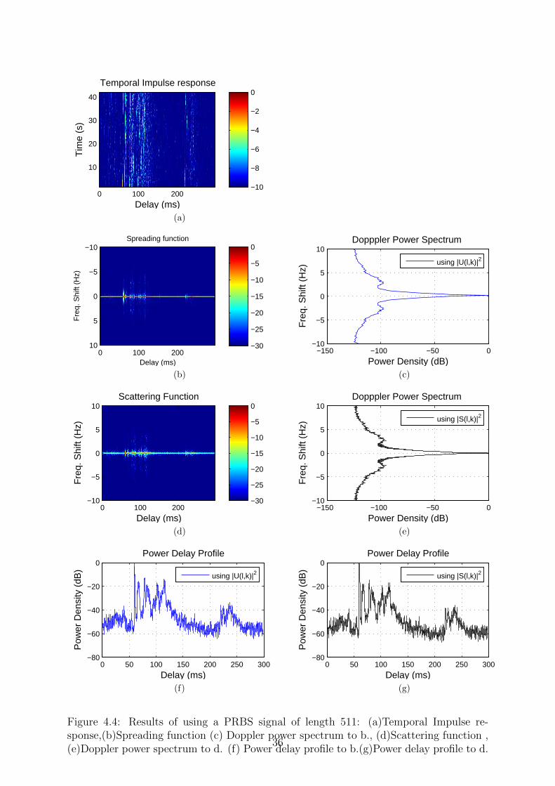
An increment in the length of the PRBS signal gives the following plots shown in Figure4.4. If the plots are now compared to that of Figure 4.2, starting with the temporalimpulse response, we observe that the strongest arrivals are no longer at the beginning;the main arrivals are now concentrated around 100 ms of which the maximum is foundto be located at about 70 ms. The plot of the impulse response here can be said to be ashifted version of Figure 4.2 (a); except for the negligible arrival patterns left of the peakarrival. The plots of the corresponding spreading and scattering functions in Figure 4.4(b) and (d) show similar effects as expected. Taking a closer look at the Doppler power

34

spectral in Figure 4.4 and (c) and (e), we see a decrease in the width of the pulse between-50 dB and -100 dB as compared to the previous plots shown in the corresponding plotsof Figure 4.2. However, the Doppler power spectra are no longer seen to be a spikebetween 0 and -25 dB; they have gained some width and in addition some side lobesas well. The power delay profiles shown in Figure 4.4 (f) and (g) now show a longerlength of fading at the beginning before featuring about three main arrivals and thenimitating the fading pattering as described for those in Figure 4.2. Next, the plots of thechannel spaced time and spaced frequency correlation have been plotted in Figure 4.5; wesee some changes in these plots if we compare them to their counterparts in Figure 4.3.For instance, the bottom of the spaced time correlation function is now smoother thanbefore. These functions were used to get an approximate estimates of the coherence timeand bandwidth of the channel. A summary of the estimates of the channel importantparameters are shown in Tables 4.5 and 4.6

Tm [ms] σTm [ms] ρmax[mHz] Bd[mHz] Maximum excess delay [ms]98.4 70.1 147 95.6 56.495.9 49.7 19.5 124 56.8






35

Delay (ms)

Tim

e (s

)Temporal Impulse response

0 100 200

10

20

30

40

−10

−8

−6

−4

−2

0

(a)

Delay (ms)

Fre

q. S

hift

(Hz)

Spreading function

0 100 200

−10

−5

0

5

10 −30

−25

−20

−15

−10

−5

0

(b)

−150 −100 −50 0−10

−5

0

5

10

Power Density (dB)

Fre

q. S

hift

(Hz)


using |U(l,k)|2

(c)

Delay (ms)

Fre

q. S

hift

(Hz)

Scattering Function

0 100 200−10

−5

0

5

10

−30

−25

−20

−15

−10

−5

0

(d)

−150 −100 −50 0−10

−5

0

5

10

Power Density (dB)

Fre

q. S

hift

(Hz)


using |S(l,k)|2

(e)

0 50 100 150 200 250 300−80

−60

−40

−20

0

Delay (ms)

Pow

er D

ensi

ty (

dB)

Power Delay Profile

using |U(l,k)|2

(f)

0 50 100 150 200 250 300−80

−60

−40

−20

0

Delay (ms)

Pow

er D

ensi

ty (

dB)

Power Delay Profile

using |S(l,k)|2

(g)


36

−10 −5 0 5 10−50

−40

−30

−20

−10

0

∆ f (Hz)

|R(∆

f)| (

dB)


using |U(l,k)|2

(a)

−10 −5 0 5 10−40

−30

−20

−10

0

∆ f (Hz)

|R(∆

f)| (

dB)


using |S(l,k)|2

(b)

−2 −1 0 1 2

0.92

0.94

0.96

0.98

1

∆ t (s)

|R(∆

t)|


using |U(l,k)|2

(c)

−2 −1 0 1 2

0.2

0.4

0.6

0.8

1

∆ t (s)

|R(∆

t)|


using |S(l,k)|2

(d)



The final of the PRBS signals to be analysed is the one of length 1023 corresponding toan m-sequence generated by a shift register of 10 stages in the register circuit. Proceedingwith our analysis as before, we see that the high level of fluctuation in the amount ofcorrelation is also present in Figure 4.6 (a) as in the case of the previous two cases andthat the arrivals have undergone deep fading with the strongest correlation componentoccurring at about 17 ms. The arrival pattern in this scenario is more stable in time andamplitude. After an empty gap of nearly 100 ms (between 100 ms to 200 ms), one strongarrival can be seen at about 178 ms followed by a couple of faded arrivals; we can alsosee some contribution to the arrival pattern from an unknown object in the vicinity of a300 ms delay. The corresponding spreading and scattering functions shown in Figure 4.6(b) and (d) show minimum spread in Doppler shifts than their counterparts in Figures4.2 and 4.4. The plots in Figure 4.6 (c) and (e) of the Doppler power spectra reveal afurther gain in the spectral width below about -20 dB, and a further increased in sidelobes having peak value at about -98 dB then those introduced in Figure 4.4. Next,comparing the plots of the power delay profile in Figure 4.6 (f) and (g) to those in Figure4.2 (f) and (g), it can be concluded that the plots obtained here are just a longer versionextending up to about 444 ms.

37

Delay (ms)

Tim

e (s


0 100 200 300 400

10

20

30

40

−10

−8

−6

−4

−2

0

(a)

Delay (ms)

Fre

q. S

hift

(Hz)

Spreading function

0 100 200 300 400

−10

−5

0

5

10 −30

−25

−20

−15

−10

−5

0

(b)

−120 −100 −80 −60 −40 −20 0−10

−5

0

5

10

Power Density (dB)

Fre

q. S

hift

(Hz)


using |U(l,k)|2

(c)

Delay (ms)

Fre

q. S

hift

(Hz)

Scattering Function

0 100 200 300 400−10

−5

0

5

10

−30

−25

−20

−15

−10

−5

0

(d)

−120 −100 −80 −60 −40 −20 0−10

−5

0

5

10

Power Density (dB)

Fre

q. S

hift

(Hz)


using |S(l,k)|2

(e)

0 100 200 300 400 500−100

−80

−60

−40

−20

0

Delay (ms)

Pow

er D

ensi

ty (

dB)

Power Delay Profile

using |U(l,k)|2

(f)

0 100 200 300 400 500−100

−80

−60

−40

−20

0

Delay (ms)

Pow

er D

ensi

ty (

dB)

Power Delay Profile

using |S(l,k)|2

(g)


38

−10 −5 0 5 10−40

−30

−20

−10

0

∆ f (Hz)

|R(∆

f)| (

dB)


using |U(l,k)|2

(a)

−10 −5 0 5 10−40

−30

−20

−10

0

∆ f (Hz)

|R(∆

f)| (

dB)


using |S(l,k)|2

(b)

−2 −1 0 1 2

0.88

0.9

0.92

0.94

0.96

0.98

1

∆ t (s)

|R(∆

t)|


using |U(l,k)|2

(c)

−2 −1 0 1 2

0.2

0.4

0.6

0.8

1

∆ t (s)

|R(∆

t)|


using |S(l,k)|2

(d)


The result of plotting the spaced frequency and spaced time correlation functions isshown next in Figure 4.9. The shape of the spaced frequency correlation function haschanged a lot as compared to those in Figures 4.3 and 4.5. On the other hand, comparingthe two plots of the spaced time correlation functions obtained from using the spreadingand scattering functions, we see that the one obtained from the spreading function seemsto be approaching the other as the length of the input signal increases. A summary ofthe estimates of the channel important parameters are shown in Tables 4.7 and 4.8

Tm [ms] σTm [ms] ρmax[mHz] Bd[mHz] Maximum excess delay [ms]60.4 102.5 109.9 130.7 5656.2 71.9 19.5 169.8 56



39




Simulation results for an LFM signal

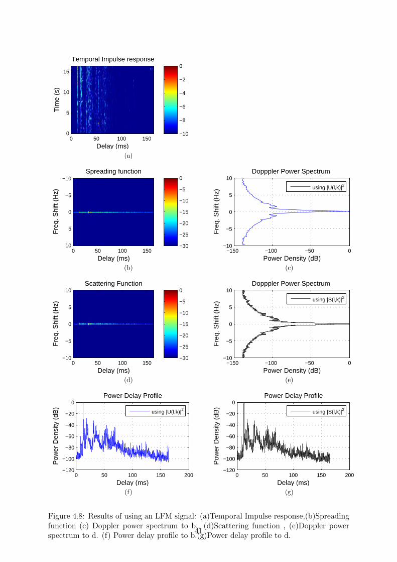
Our final signal to be analysed is the linear frequency modulation(LFM) signal. Theresults of exciting channel 4 with an LFM signal is shown in Figure 4.8. Comparing thetemporal impulse responses obtained from exciting the channel with a PRBS signal ofdifferent lengths to the one shown here in Figure 4.8 (a), we see an arrival pattern that ismore stable in both time and amplitude and concentrated in one area; even though laterarrivals show some degree of fading as in the other three cases. The strongest arrival isseen to appear at about 12 ms. The corresponding spreading and scattering functionsto this channel show the minimum spread in Doppler shift of the four cases studied.Taking a look at the Doppler power spectra in Figures (c) and (e), we see a significantincrease in the main sidelobes and a broader spectra. Next, Figure 4.8 (f) and (g) showa significant change in the arrival pattern of the power delay profiles. Only one mainarrival and a couple of weaker arrivals with insignificant amplitudes can be identified; therest have interacted with the sea floor multiple of times and can be considered as noisefloor (see appendix B?). Finally, as in the case of the PRBS signals, Figure 4.8 show plotsof the spaced frequency and spaced time correlation functions; the frequency correlationfunction can be identified as a noise-like notched filter. A summary of the estimates ofthe channel important parameters are shown in Tables 4.9 and 4.10.

Tm [ms] σTm [ms] ρmax[mHz] Bd[mHz] Maximum excess delay [ms]18.5 19.4 200 45.2 18.917.9 15 19.5 81.3 18.9



Bc−3dB[Hz] Bc−6dB[Hz] Bc−10dB[Hz] Tc.97;.1 [s] Tc.98;.25 [s] Tc.99;.5 [s]13.62 9.82 6.46 1.28 2 2.6613.38 9.24 6.22 3.14 3.32 3.52



40

Delay (ms)

Tim

e (s


0 50 100 1500

5

10

15

−10

−8

−6

−4

−2

0

(a)

Delay (ms)

Fre

q. S

hift

(Hz)

Spreading function

0 50 100 150

−10

−5

0

5

10 −30

−25

−20

−15

−10

−5

0

(b)

−150 −100 −50 0−10

−5

0

5

10

Power Density (dB)

Fre

q. S

hift

(Hz)


using |U(l,k)|2

(c)

Delay (ms)

Fre

q. S

hift

(Hz)

Scattering Function

0 50 100 150−10

−5

0

5

10

−30

−25

−20

−15

−10

−5

0

(d)

−150 −100 −50 0−10

−5

0

5

10

Power Density (dB)

Fre

q. S

hift

(Hz)


using |S(l,k)|2

(e)

0 50 100 150 200−120

−100

−80

−60

−40

−20

0

Delay (ms)

Pow

er D

ensi

ty (

dB)

Power Delay Profile

using |U(l,k)|2

(f)

0 50 100 150 200−120

−100

−80

−60

−40

−20

0

Delay (ms)

Pow

er D

ensi

ty (

dB)

Power Delay Profile

using |S(l,k)|2

(g)

Figure 4.8: Results of using an LFM signal: (a)Temporal Impulse response,(b)Spreadingfunction (c) Doppler power spectrum to b., (d)Scattering function , (e)Doppler powerspectrum to d. (f) Power delay profile to b.(g)Power delay profile to d.

41

−10 −5 0 5 10−30

−25

−20

−15

−10

−5

0

∆ f (Hz)

|R(∆

f)| (

dB)


using |U(l,k)|2

(a)

−10 −5 0 5 10−40

−30

−20

−10

0

∆ f (Hz)

|R(∆

f)| (

dB)


using |S(l,k)|2

(b)

−2 −1 0 1 2

0.97

0.98

0.99

1

∆ t (s)

|R(∆

t)|


using |U(l,k)|2

(c)

−2 −1 0 1 20

0.2

0.4

0.6

0.8

1

∆ t (s)

|R(∆

t)|


using |S(l,k)|2

(d)


Summary of the Results

Our analysis of channel 4 with the PRBS signal has shown that as the length of the signalincreases, the width of the Doppler power spectrum increases and a further increased isobserved in sidelobes which can be undesirable depending on their amplitude level. Fewerarrivals are estimated with the majority having very little amplitudes as the result of deepfading. Please see appendix B for a clearer picture of these observations. Applicationof the LFM signal to the channel reveal similar effects; the Doppler power spectrumgained its most width and only a single peak arrival is clearly seen in the plot of thepower delay profile. At this point, the choice of the transmitted signal waveform is notstraight forward. Depending on the application of the communication system and howmuch Doppler shift is to be tolerated by the receiver, according to [1] the choice betweena PRBS and an LFM waveforms is an issue that lies in the compromise of Dopplertolerance. For the sake of properly estimating the scattering function, the PRBS signalis more suitable because of its narrow ambiguity function in both delay and Doppler andin this analysis, the signal of length 255 may be preferred over the rest.

42

Chapter 5

Summary

An underwater acoustic communication channel has been characterized based on exper-imental data. The method of characterizing the channel was based on estimation ofthe channel temporal impulse response by emitting probe signals with well behave au-tocorrelation functions, and using the result to get an estimate of the channel spreadingand scattering functions; from these functions, the channel correlation functions such asthe delay power profile, the Doppler power spectrum, and the spaced time and frequencyfunctions were estimated and presented in the form of figures. The estimated values of theaverage delay spread, rms delay spread, Doppler shift, Doppler spread, coherence time,coherence bandwidth and maximum excess delay of the power delay profile are presentedin the form of tables. The channel characterized in this report was found to fluctuate inamplitude and suffered from fading; some degree of Doppler shifts were observed in thechannel and were mainly caused by the boat carrying the transmitter. Although therewere a total of 20 channels measured during the Trondheim Fjord experiments, but it wasnot necessary to analyze all of them in this master thesis. The goal of the project wasto be able to characterize an underwater communication channel based on experimentaldata with the aid of matlab. The results presented in this report were found to be consis-tent with theory and can be compared with the work found in [3], [4] and [2]. Since theprocedure for characterizing the channel in this report is quite similar to the remainingchannels, a future work will be to apply the procedure to the balance 19 channels.

43

[18]

44

Bibliography

[1] T. Eggen, A. Baggeroer, and J. Preisig, “Communication over doppler spread chan-nels. part i: Channel and receiver presentation,” IEEE Journal of Oceanic Engineer-ing, vol. 25, no. 1, pp. 62–71, 2000.

[2] B. Borowski, “Characterization of a very shallow water acoustic communicationchannel,” in OCEANS 2009, MTS/IEEE Biloxi-Marine Technology for Our Future:Global and Local Challenges, p. 110, 2009.

[3] P. van Walree, “Channel sounding for acoustic communications: techniques andshallow-water examples,” Norwegian Defence Research Establishment (FFI), Tech.Rep. FFI-rapport, vol. 7, 2011.

[4] P. A. van Walree and G. Bertolotto, “Characterization of an acoustic communicationchannel with pseudorandom binary sequences,” Proceedings of Underwater AcousticMeasurements UAM2007, Heraklion, Crete.

[5] P. M. Shankar, Introduction to wireless systems. New York: J. Wiley, 2002.

[6] A. Goldsmith, Wireless communications. Cambridge; New York: Cambridge Uni-versity Press, 2005.

[7] J. G. Proakis and M. Salehi, Digital communications. Boston: McGraw-Hill, 2008.

[8] J. G. Proakis and M. Salehi, Communication systems engineering. Upper SaddleRiver, N.J.: Prentice Hall, 2002.

[9] R. Diamant and L. Chorev, “Emulation system for underwater acoustic channel,” inInternational Undersea Defence Technology Europe conference (UDT), 2005.

[10] X. Lurton, An introduction to underwater acoustics: principles and applications.Heidelberg; New York; Oxford: Springer Verlag, published in association with PraxisPublishing, 2010.

[11] P. Bello, “Characterization of randomly time-variant linear channels,” Communica-tions Systems, IEEE transactions on, vol. 11, no. 4, p. 360393, 1963.

[12] “RMS delay spread measurement (theory) : Wireless lab : Electronics & communi-cations : IIT DELHI virtual lab.”

[13] M. I. Skolnik, Introduction to radar systems. Boston: McGraw Hill, 2001.

[14] B. R. Mahafza, Radar systems analysis and design using Matlab. Boca Raton: Chap-man & Hall/CRC, 2000.

45

[15] B. S. Sharif, J. Neasham, O. R. Hinton, and A. E. Adams, “A computationallyefficient doppler compensation system for underwater acoustic communications,”Oceanic Engineering, IEEE Journal of, vol. 25, no. 1, p. 5261, 2000.

[16] A. Quinquis, Digital signal processing using MATLAB. London; Hoboken, NJ: ISTE; Wiley, 2008.

[17] “7117992 communication systems simon haykin 4ed.”

[18] M. Smedsrud, “Acharacterization of underwater acoustic communication channelsby computer simulations,” Master’s thesis, Norwegian University of Science andTechnology, June 2005.

46

.1 Appendix A : Matlab Program Codes

C1

The purpose of this block of matlab code is to process the data and perform an estimationof the channel impulse response when it is excited by either an LFM signal of a PRBSsignal; this particular example is done for an m-sequence of length 1023.

1 function ReadData PnBPSK10 ScatteringEstimate()2

3 % Load input signal4

5 lfmpath = '..\TRANSMIT SIGNALS\M SEQ\...6 SQUARE−ROOT RAISED COSINE\M10\fc10000Hz\BPSK\Fw−over−fc 0.35\';7 lfmnam = 'Tfilter BPSK fc10000Hz Bw−fc−ratio0.35.mat';8 disp([lfmpath lfmnam])9 load([lfmpath lfmnam],'x','tx','fc','Bw','Fs')

10

11 % Duration of LFM signal (2746 samples at 192 kHz smp freq)12 Tlfm = length(x)/192000;13 % Duration of gap between 2 succesive LFM14 Tgap = 0.150;15

16 %%%%%%%%%%%%%%%%%%%%%%%%%%%%%%%%%%%%%%%%%%%%%%%%%%%%%%%%%%%%%%%%%%%%%%%17 % The signal can be processed by making use of the passband signal x ...

%18 % as it is, however, the baseband procedure is preferred. Comment ...

the %19 % baseband method if you wish to work with the passband signal. ...

%20 %%%%%%%%%%%%%%%%%%%%%%%%%%%%%%%%%%%%%%%%%%%%%%%%%%%%%%%%%%%%%%%%%%%%%%%21

22

23 % Baseband formulation of the passband signal x24

25 xb = hilbert(x).*exp(−1i*2*pi*fc.*tx);26 % figure27 % subplot(121);28 % plot(tx,real(xb));grid; %hold on;29 % title('Equivalent baseband signal sampled at fs = 192000, xb');30

31 Fs decim = 10000; % reducing the sampling frequency fs by resampling32 xb = resample(xb,Fs decim,Fs);33 tt = 0:1/Fs decim:(length(xb)−1)/Fs decim;34 % figure35 % plot(tt,real(xb),'r');grid;36 % title('Equivalent baseband signal resampled at fs = 5000, xb');37 % pause38 smf = conj(flipud(xb(:))); % matched filter to xb39 Lsm = length(smf);40 % figure41 % plot(abs(conv(xb,smf.')));42 % title('Pulse compression of xb with its matched filter at fs = 5000');43 % pause44 %45

46 % Decimation factor

47

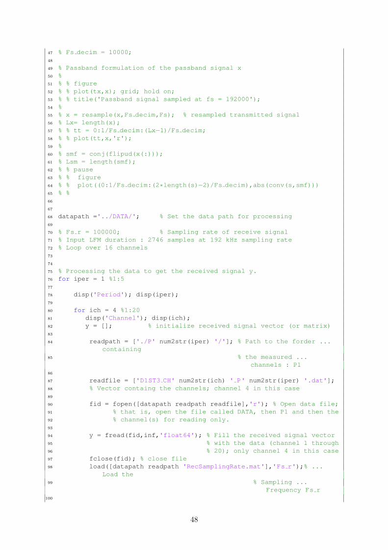
47 % Fs decim = 10000;48

49 % Passband formulation of the passband signal x50 %51 % % figure52 % % plot(tx,x); grid; hold on;53 % % title('Passband signal sampled at fs = 192000');54 %55 % x = resample(x,Fs decim,Fs); % resampled transmitted signal56 % Lx= length(x);57 % % tt = 0:1/Fs decim:(Lx−1)/Fs decim;58 % % plot(tt,x,'r');59 %60 % smf = conj(flipud(x(:)));61 % Lsm = length(smf);62 % % pause63 % % figure64 % % plot((0:1/Fs decim:(2*length(s)−2)/Fs decim),abs(conv(s,smf)))65 % %66

67

68 datapath ='../DATA/'; % Set the data path for processing69

70 % Fs r = 100000; % Sampling rate of receive signal71 % Input LFM duration : 2746 samples at 192 kHz sampling rate72 % Loop over 16 channels73

74

75 % Processing the data to get the received signal y.76 for iper = 1 %1:577

78 disp('Period'); disp(iper);79

80 for ich = 4 %1:2081 disp('Channel'); disp(ich);82 y = []; % initialize received signal vector (or matrix)83

84 readpath = ['./P' num2str(iper) '/']; % Path to the forder ...containing

85 % the measured ...channels : P1

86

87 readfile = ['D1ST3 CH' num2str(ich) ' P' num2str(iper) '.dat'];88 % Vector containg the channels; channel 4 in this case89

90 fid = fopen([datapath readpath readfile],'r'); % Open data file;91 % that is, open the file called DATA, then P1 and then the92 % channel(s) for reading only.93

94 y = fread(fid,inf,'float64'); % Fill the received signal vector95 % with the data (channel 1 through96 % 20); only channel 4 in this case97 fclose(fid); % close file98 load([datapath readpath 'RecSamplingRate.mat'],'Fs r');% ...

Load the99 % Sampling ...

Frequency Fs r100

48

101 figure, subplot(2,1,1)102 plot(y)103 title('The received signal y');104 pause(2)105

106 y = squeeze(y(1.058e7:1.498e7)).'; % Extracting portion of ...the re−

107 % ceived signal to be ...processed.

108 Ly = length(y);109 ty = 0:1/Fs r:(Ly−1)/Fs r; subplot(2,1,2)110 plot(ty,y)111

112

113 % y = resample(y,Fs decim,Fs r);114 % Ly = length(y);115 % ty = 0:1/Fs decim:(Ly−1)/Fs decim;116 %117 % figure,118 % plot(ty,y);title('A truncated version of the received ...

signal y');119 % pause120

121 % Passeband formulation of the passband received signal y122

123 % Lc = Ly + Lsm − 1; % length of convolution124 % tc = 0:1/Fs decim:(Lc−1)/Fs decim; % time vector125 % y pc = abs(conv(y,smf.'));126 %127 % figure128 % plot(tc,y pc)129 % title('Pulse Compressed signal')130 % xlabel('time [sec]')131

132

133 % Baseband formulation of the passband received signal y134

135 yb = hilbert(y).*exp(−1i*2*pi*fc.*ty); % BaseBand equivalent ...of the

136 %received signal y137 yb = resample(yb,Fs decim,Fs r);138 Lyb = length(yb);139

140 tyb = 0:1/Fs decim:(Lyb−1)/Fs decim;141 figure142 plot(tyb,real(yb));143 title('Baseband equivalent of the truncated received signal, ...

yb');144 xlabel('time [sec]');145 pause(2)146

147 Lyb = length(yb);148 Lc = Lyb + Lsm − 1; % convolution length149 tyc = 0:1/Fs decim:(Lc−1)/Fs decim;150 y pc = abs(conv(yb,smf.'));151

152 figure153 plot(tyc,y pc);

49

154 title('Pulse Compression');155 xlabel('time [sec]') ;156 pause(2)157

158

159 df = −10:0.1:10; % Doppler resolution160 Nd = length(df);161 for id = 1:Nd162 if ¬mod(id,1), disp([num2str(id) '/' num2str(Nd)]),end163 % Pulse compression (convolution with matched filter) − Baseband164 Lc = Lyb + Lsm − 1; % length of convolution165 tyc = 0:1/Fs decim:(Lc−1)/Fs decim; % time vector166 y pc(id,1:Lc) ...

=abs(conv(yb,(smf.').*exp(−1i*2*pi*df(id).*tt)));% doppler167 % matched filter168

169 % Start stacking170 % init smp = 1.69e4; %floor(1.75*Fs decim);%171 % N smp lfmgap = round((Tlfm + Tgap)*Fs decim);172 % for ilfm = 1173 % smpi = init smp + (ilfm−1)*N smp lfmgap;174 % smpf = smpi + N smp lfmgap −1;175 % n wind = smpi:1:smpf;176 % %PDP(ilfm,1:length(n wind)) = squeeze(y pc(n wind));177 % PDP(ilfm,id,1:length(n wind)) = squeeze(y pc(id,n wind));178 % end179

180 %imagesc(PDP)181 %colormap(hot)182 end183 % y pc=y pc(:,97901);184 t geo = []; % the running time185 init smp = 1.91e4; %floor(1.75*Fs decim);%186 N smp lfmgap = round((Tlfm + Tgap)*Fs decim);187 t del = 0:1/Fs decim:(N smp lfmgap−1)/Fs decim;188 for ilfm = 1:91189 smpi = init smp + (ilfm−1)*N smp lfmgap;190 t geo = [t geo smpi/Fs decim];191 smpf = smpi + N smp lfmgap −1;192 n wind = smpi:1:smpf;193 % PDP(ilfm,1:length(n wind)) = squeeze(y pc(n wind));194 %ytmp = squeeze(y pc(1:Nd,n wind));195 % PDP(ilfm,1:Nd,1:length(n wind)) = (ytmp./max(abs(ytmp)));196 PDP(ilfm,1:Nd,1:length(n wind)) =squeeze(y pc(1:Nd,n wind));197 end198 % figure, imagesc(PDP); % imagesc(squeeze(PDP(ilfm,:,:)));199 end200 end201 % %save('PulseCompression','s pc trunc','t pc trunc','Fs r')202 %203 filename = '.\RxPNBPSK10.mat'204 save(filename)

C2

The purpose of this block of matlab code is to perform estimation of the channel temporalimpulse response from which the spreading and scattering functions are obtained. Fur-

50

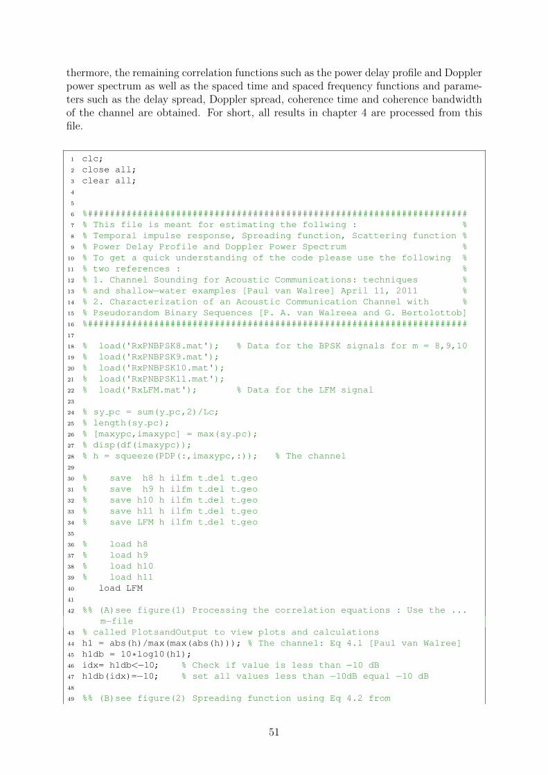
thermore, the remaining correlation functions such as the power delay profile and Dopplerpower spectrum as well as the spaced time and spaced frequency functions and parame-ters such as the delay spread, Doppler spread, coherence time and coherence bandwidthof the channel are obtained. For short, all results in chapter 4 are processed from thisfile.

1 clc;2 close all;3 clear all;4

5

6 %#####################################################################7 % This file is meant for estimating the follwing : %8 % Temporal impulse response, Spreading function, Scattering function %9 % Power Delay Profile and Doppler Power Spectrum %

10 % To get a quick understanding of the code please use the following %11 % two references : %12 % 1. Channel Sounding for Acoustic Communications: techniques %13 % and shallow−water examples [Paul van Walree] April 11, 2011 %14 % 2. Characterization of an Acoustic Communication Channel with %15 % Pseudorandom Binary Sequences [P. A. van Walreea and G. Bertolottob]16 %#####################################################################17

18 % load('RxPNBPSK8.mat'); % Data for the BPSK signals for m = 8,9,1019 % load('RxPNBPSK9.mat');20 % load('RxPNBPSK10.mat');21 % load('RxPNBPSK11.mat');22 % load('RxLFM.mat'); % Data for the LFM signal23

24 % sy pc = sum(y pc,2)/Lc;25 % length(sy pc);26 % [maxypc,imaxypc] = max(sy pc);27 % disp(df(imaxypc));28 % h = squeeze(PDP(:,imaxypc,:)); % The channel29

30 % save h8 h ilfm t del t geo31 % save h9 h ilfm t del t geo32 % save h10 h ilfm t del t geo33 % save h11 h ilfm t del t geo34 % save LFM h ilfm t del t geo35

36 % load h837 % load h938 % load h1039 % load h1140 load LFM41

42 %% (A)see figure(1) Processing the correlation equations : Use the ...m−file

43 % called PlotsandOutput to view plots and calculations44 h1 = abs(h)/max(max(abs(h))); % The channel: Eq 4.1 [Paul van Walree]45 h1db = 10*log10(h1);46 idx= h1db<−10; % Check if value is less than −10 dB47 h1db(idx)=−10; % set all values less than −10dB equal −10 dB48

49 %% (B)see figure(2) Spreading function using Eq 4.2 from

51

50 hspread = fft(h, [],1); % Eq 4.2 from ref. [1]51 hspread = fftshift(hspread,1); % Just to include ...

negative52 % center frequency53 hspread = power(abs(hspread),2); % Modulus square54 hnormsp = abs(hspread)/max(max(abs(hspread))); % Normalized to maximum55 % hnormsp = 10*log10(hnormsp); % amplitude of 156 % idx1= hnormsp<−30;57 % hnormsp(idx1)=−30;58

59

60 %% (C) see figure(3) Scattering function using Eq 4 from ref. [2]61 NFFT = 1024;62 hscatter = ifft((fft(h, NFFT).ˆ2));63 hscatter = fft(hscatter); % The scattering function eq 464 hscatter = fftshift(hscatter,1);65 hnormsc = abs(hscatter)/max(max(abs(hscatter)));66 % hnormsc = 10*log10(hnormsc);67 % idx= hnormsc<−30;68 % hnormsc(idx)=−30;69

70 %% (D) see figure(4)Power Delay Profile as defined in Eq 4.371 % using Eq 4.2 (the spreading function) [1]72 PDP4 2 = sum(abs(hspread).ˆ2);73 PDP4 2 = abs(PDP4 2)/max(max(PDP4 2)); % Normalize maximum value to 174 % PDP4 2= mag2db(PDP4 2); % dB equivalent75

76 %% (E) see figure(5)Power Delay Profile as defined in Eq 4.3 [1]77 % using 4(the scattering function) [2]78 PDP4 = sum(abs(hscatter).ˆ2);79 PDP4 = abs(PDP4)/max(max(abs(PDP4)));80 % PDP4 = mag2db(PDP4);81

82 %% (F) see figure(6) Doppler Power Spectrum as defined in Eq 4.4 [1] and83 % using the spreading function using Eq. 4.284 DPS4 2 = sum(abs(hspread').ˆ2);85 DPS4 2 = abs(DPS4 2)/max(max(abs(DPS4 2)));86 % DPS4 2 = mag2db(DPS4 2);87 fspread = −10:20/length(DPS4 2):10; % frequency resolution88 fspread = fspread(1,2:end);89

90 %% (G) see figure(7) Doppler Power Spectrum as defined in Eq 4.4 [1]91 % using the scattering function Eq 4 [2]92 DPS4 = sum(abs(hscatter').ˆ2); % Doppler power spectrum93 DPS4 = abs(DPS4)/max(max(DPS4));94 % DPS4 = mag2db(DPS4);95 fscatter = −10:20/length(DPS4):10; % frequency resolution96 fscatter = fscatter(1,2:end);97

98 %% (H)see figure(8)The space−frequency correlation function using ...the spreading function

99 fspace = (−10:20/length(PDP4 2):10); % Freq resolution in Hz100 fspace = fspace(1,2:end);101 PDPspace = fft(sum(abs(hspread).ˆ2)); % Spaced−freq. function102 PDPspace = abs(PDPspace)/max(max(abs(PDPspace)));103 % PDPspace = 10*log10(PDPspace);104

105 %% (I)see figure(9) The space frequency correlation function using ...

52

the scattering function106 fspace4 = −10:20/length(PDP4):10; % frequency resolution in Hz107 fspace4 = fspace4(1,2:end);108 PDPspace4 = fft(sum(abs(hscatter).ˆ2)); % The spaced−frequency ...

correlation function109 PDPspace4 = abs(PDPspace4)/max(max(abs(PDPspace4)));110 % PDPspace4 = 10*log10(PDPspace4);111

112 %% (J)see figure(10)The spaced time correlation function using the ...spreading function 4.2

113 DPSpacetime4 2 = ifft(sum(abs(hspread').ˆ2)); % The space time ...correlation function

114 DPSpacetime4 2 = abs(DPSpacetime4 2)/max(max(abs(DPSpacetime4 2)));115 % DPSpacetime4 2 = 10*log10(DPSpacetime4 2);116 ∆T4 2 = −2:4/(length(DPS4 2)):2;117 ∆T4 2 = ∆T4 2(1,2:end);118

119 %% (K)see figure(11) The space time correlation function using the ...scattering function

120 DPSpacetime4 = ifft(sum(abs(hscatter').ˆ2)); % The space time ...correlation function

121 DPSpacetime4 = abs(DPSpacetime4)/max(max(abs(DPSpacetime4)));122 % DPSpacetime4 = 10*log10(DPSpacetime4);123 ∆T4 = −2:4/(length(DPS4)):2;124 ∆T4 = ∆T4(1,2:end);125

126 %% (L) Estimating the delay spread, rms delay spread, maximum127 % doppler shift and Doppler spread128

129 %(1)Finding the average and rms Delay spreads using Eq. 4.2130 PDPave4 2 = sum(t del.*sum(abs(hspread).ˆ2))./sum(sum(abs(hspread).ˆ2));131 PDPrms4 2 = sqrt(sum((t del−PDPave4 2).ˆ2.*(sum(hspread).ˆ2))...132 /sum((sum(abs(hspread).ˆ2))));133

134 % (2) Finding the average and rms Delay spreads using Eq. 4135

136 PDPave4 = sum(t del.*sum(abs(hscatter).ˆ2))...137 /sum(sum(abs(hscatter).ˆ2));138 PDPrms4 = sqrt(sum((t del−PDPave4).ˆ2.*(sum(abs(hscatter).ˆ2)))...139 /sum(sum(abs(hscatter).ˆ2)));140

141 % (3)Finding the average and rms Doppler spreads (Doppler shift and ...spread)

142 % using Eq. 4.2143 Dpshift4 2 = sum(fspread.*(sum(abs(hspread').ˆ2)))...144 ./sum((sum(abs(hspread').ˆ2)));145 Dspread4 2 = sqrt(sum((fspread−Dpshift4 2).ˆ2....146 .*(sum(abs(hspread').ˆ2)))./sum((sum(abs(hspread').ˆ2))));147

148 %(4) Finding the average and rms Doppler spread (Doppler shift and ...spread)

149 % Eq. 4150 Dpshift4 = sum(fscatter.*(sum(abs(hscatter').ˆ2)))...151 /sum((sum(abs(hscatter').ˆ2)));152 Dpsread4 = sqrt(sum((fscatter−Dpshift4).ˆ2.*(sum(abs(hscatter').ˆ2)))...153 /sum((sum(abs(hscatter').ˆ2))));154 % save Bpsk8155 % save Bpsk9

53

156 % save Bpsk10157 % save LFMsig

C3

This bock of code is for plotting and performing computations of the channel’s parame-ters.

1 clear all;2 close all;3 % load Bpsk84 % load Bpsk95 % load Bpsk106 load LFMsig7 %% (A) The temporal impulse response8 figure(1);9 imagesc(1e3*t del, t geo, h1db);

10 axis xy;11 xlabel('Delay (ms)');12 ylabel('Time (s)');13 title('Temporal Impulse response');14 colorbar;15

16 %% (B) The spreading function17 figure(2);18 imagesc(1e3*t del,[−5 5],hnormsp);19 xlabel('Delay (ms)');20 ylabel('Freq. Shift (Hz)');21 title('Spreading function');22 colorbar;23

24 figure(12)25 [xsp ysp] = meshgrid(t del,fspread);26 mesh(1e3*xsp,ysp,hnormsp);27 xlabel('Delay (ms)');28 ylabel('Freq. Shift (Hz)');29 title('Spreading Function');30

31

32

33 %% (C) The scattering function34 figure(3);35 imagesc(1e3*t del,fscatter,hnormsc);36 axis xy;37 xlabel('Delay (ms)');38 ylabel('Freq. Shift (Hz)');39 title('Scattering Function');40 colorbar;41 figure(13)42 [xsc ysc] = meshgrid(t del,fscatter);43 mesh(1e3*xsc,ysc,hnormsc);44 xlabel('Delay (ms)');45 ylabel('Freq. Shift (Hz)');46 title('Scattering Function');47

48 %% (D) The power delay profile of the spreading function Eq 4.2

54

49 figure(4)50 plot(1e3*t del,PDP4 2);grid;51 xlabel('Delay (ms)');52 ylabel('Power Density (dB)');53 title('Power Delay Profile');54 % legend('using |U(l,k)|ˆ2')55 %% (E)The power delay profile of the scattering function Eq 456 figure(5)57 plot(1e3*t del,PDP4,'k');grid;58 xlabel('Delay (ms)');59 ylabel('Power Density (dB)');60 title('Power Delay Profile');61 % legend('using |S(l,k)|ˆ2');62

63 %% (F) The Doppler power spectrum of the spreading function Eq 4.264 figure(6)65 plot(fspread,DPS4 2);grid;66 xlabel('Power Density (dB)');67 ylabel('Freq. Shift (Hz)');68 title('Dopppler Power Spectrum ');69 % legend('using |U(l,k)|ˆ2')70

71 %%(G) The Doppler power spectrum of the spreading function Eq 472 figure(7)73 plot(fscatter,DPS4,'k');grid;74 xlabel('Power Density (dB)');75 ylabel('Freq. Shift (Hz)');76 title('Dopppler Power Spectrum ');77 % legend('using |S(l,k)|ˆ2')78

79 %% (H) The spaced frequency correlation function using the ...spreading function

80 figure(8)81 plot(fspace,PDPspace);grid;82 xlabel('\Delta f (Hz)');83 ylabel(' |R(\Delta f) | (dB)');84 title('Space−frequency correlation function');85 % legend('using |U(l,k)|ˆ2')86

87 %% (I) The spaced frequency correlation function using the ...scattering function

88 figure(9)89 plot(fspace4,PDPspace4,'k');grid;90 xlabel('\Delta f (Hz)');91 ylabel(' |R(\Delta f) | (dB)');92 title('Space−frequency correlation function');93 legend('using |S(l,k)|ˆ2')94 set(gcf, 'color', [0 1 0])95 %% (J) The space time correlation function using the spreading function96 figure(10)97 plot(∆T4 2,DPSpacetime4 2);grid;98 xlabel('\Delta t (s)');99 ylabel(' |R(\Delta t) | ');

100 ylim([min( DPSpacetime4 2) max( DPSpacetime4 2)]);101 title('Space−time correlation function');102 legend('using |U(l,k)|ˆ2')103 set(gcf, 'color', [1 0 1])104 %(K) The space time correlation function using the scattering function

55

105 figure(11)106 plot(∆T4,DPSpacetime4,'k');grid;107 xlabel('\Delta t (s)');108 ylabel(' |R(\Delta t) | ');109 ylim([min( DPSpacetime4) max( DPSpacetime4)]);110 title('Space−time correlation function');111 legend('using |S(l,k)|ˆ2')112 set(gcf, 'color', [1 0 1])113

114

115 %% (L) Values of the estimated delay spread, rms delay spread, ...maximum doppler

116 % Doppler shifi and doppler spread117

118 % (1) Average delay spread and rms delay spread using Eq. 4.2119 Tm4 2 = PDPave4 2120 sigma4 2 =PDPrms4 2121 % (2) Average delay spread and rms delay spread using Eq. 4122 Tm4= PDPave4123 sigma4 =PDPrms4124

125 %(3) Average delay spread and rms delay spread in Hz using Eq 4126 fd4 2 = Dpshift4 2127 Bd4 2 = Dspread4 2128

129 %(4) Average delay spread and rms delay spread in Hz using Eq 4130 fd4 = Dpshift4131 Bd4 = Dpsread4

56

.2 Appendix B : Matlab Reference Plots

This appendix includes the following plots in absolute values: The spreading and scatter-ing functions in 3-D, their corresponding Doppler power spectra and power delay profilesand the Fourier transform of the power delay profiles; in other words the spaced fre-quency correlation functions. Since the decibel representations of these plots exaggeratetheir values, an absolute value plot of them will be helpful in case of doubt.

57

M8

(a) (b)

−10 −5 0 5 100

0.2

0.4

0.6

0.8

1

Power Density (dB)

Fre

q. S

hift

(Hz)


(c)

−10 −5 0 5 100

0.2

0.4

0.6

0.8

1

Power Density (dB)

Fre

q. S

hift

(Hz)


(d)

0 50 100 150 200 2500

0.2

0.4

0.6

0.8

1

Delay (ms)

Pow

er D

ensi

ty (

dB)

Power Delay Profile

(e)

0 50 100 150 200 2500

0.2

0.4

0.6

0.8

1

Delay (ms)

Pow

er D

ensi

ty (

dB)

Power Delay Profile

(f)

−10 −5 0 5 100

0.2

0.4

0.6

0.8

1

∆ f (Hz)

|R(∆

f)| (

dB)


(g)

−10 −5 0 5 100

0.2

0.4

0.6

0.8

1

∆ f (Hz)

|R(∆

f)| (

dB)


(h)

Figure 1: PRBS signal of length 255: (a)3-D spreading function(b)3-D scattering function(c) Doppler power spectrum of a. (d) Doppler power spectrum of b.(e)Power delay profileof a. (f)Power delay profile of b. (g)Spaced frequency correlation function of e. (h)Spacedfrequency correlation function of f. 58

M9

(a) (b)

−10 −5 0 5 100

0.2

0.4

0.6

0.8

1

Power Density (dB)

Fre

q. S

hift

(Hz)


(c)

−10 −5 0 5 100

0.2

0.4

0.6

0.8

1

Power Density (dB)

Fre

q. S

hift

(Hz)


(d)

0 50 100 150 200 250 3000

0.2

0.4

0.6

0.8

1

Delay (ms)

Pow

er D

ensi

ty (

dB)

Power Delay Profile

(e)

0 50 100 150 200 250 3000

0.2

0.4

0.6

0.8

1

Delay (ms)

Pow

er D

ensi

ty (

dB)

Power Delay Profile

(f)

−10 −5 0 5 100

0.2

0.4

0.6

0.8

1

∆ f (Hz)

|R(∆

f)| (

dB)


(g)

−10 −5 0 5 100

0.2

0.4

0.6

0.8

1

∆ f (Hz)

|R(∆

f)| (

dB)


(h)

Figure 2: PRBS signal of length 511: (a)3-D spreading function(b)3-D scattering function(c) Doppler power spectrum of a. (d) Doppler power spectrum of b.(e)Power delay profileof a. (f)Power delay profile of b. (g)Spaced frequency correlation function of e. (h)Spacedfrequency correlation function of f. 59

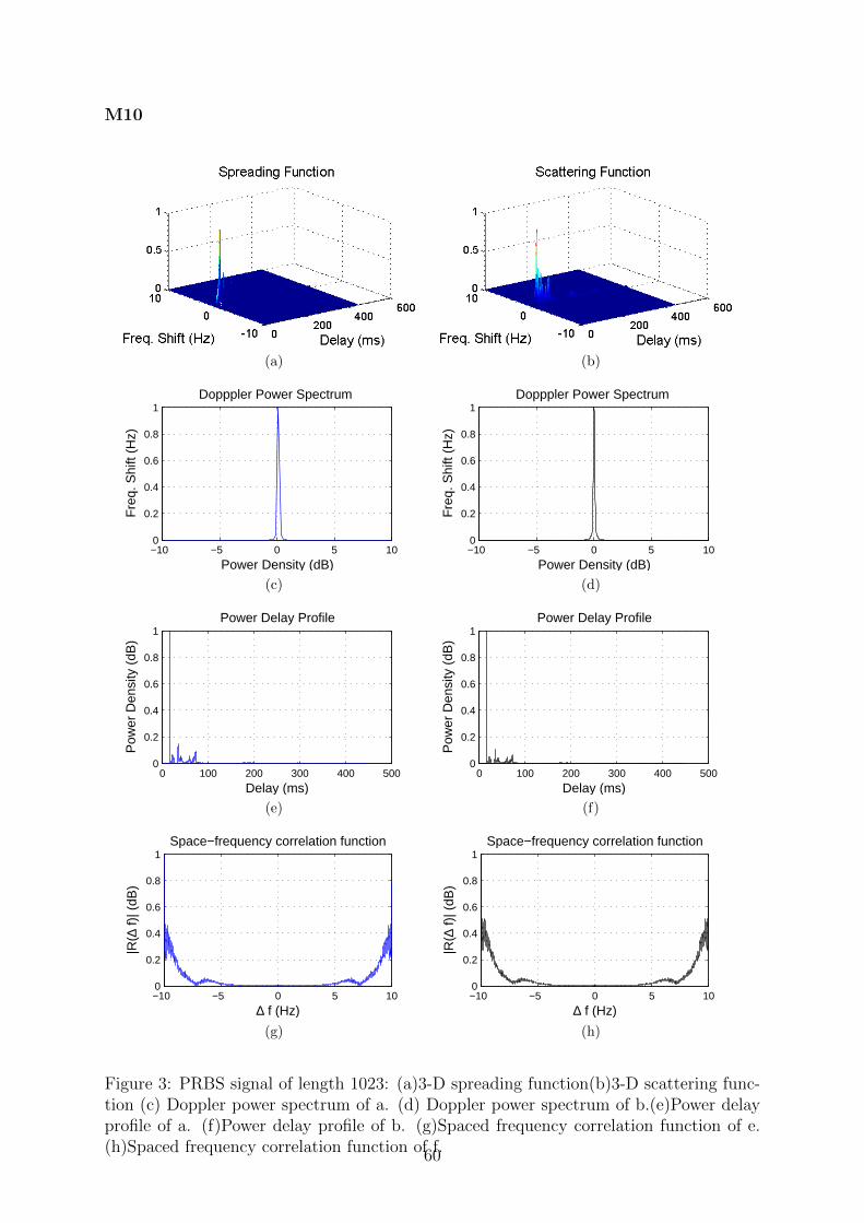
M10

(a) (b)

−10 −5 0 5 100

0.2

0.4

0.6

0.8

1

Power Density (dB)

Fre

q. S

hift

(Hz)


(c)

−10 −5 0 5 100

0.2

0.4

0.6

0.8

1

Power Density (dB)

Fre

q. S

hift

(Hz)


(d)

0 100 200 300 400 5000

0.2

0.4

0.6

0.8

1

Delay (ms)

Pow

er D

ensi

ty (

dB)

Power Delay Profile

(e)

0 100 200 300 400 5000

0.2

0.4

0.6

0.8

1

Delay (ms)

Pow

er D

ensi

ty (

dB)

Power Delay Profile

(f)

−10 −5 0 5 100

0.2

0.4

0.6

0.8

1

∆ f (Hz)

|R(∆

f)| (

dB)


(g)

−10 −5 0 5 100

0.2

0.4

0.6

0.8

1

∆ f (Hz)

|R(∆

f)| (

dB)


(h)

Figure 3: PRBS signal of length 1023: (a)3-D spreading function(b)3-D scattering func-tion (c) Doppler power spectrum of a. (d) Doppler power spectrum of b.(e)Power delayprofile of a. (f)Power delay profile of b. (g)Spaced frequency correlation function of e.(h)Spaced frequency correlation function of f.60

LFM

(a) (b)

−10 −5 0 5 100

0.2

0.4

0.6

0.8

1

Power Density (dB)

Fre

q. S

hift

(Hz)


(c)

−10 −5 0 5 100

0.2

0.4

0.6

0.8

1

Power Density (dB)

Fre

q. S

hift

(Hz)


(d)

0 50 100 150 2000

0.2

0.4

0.6

0.8

1

Delay (ms)

Pow

er D

ensi

ty (

dB)

Power Delay Profile

(e)

0 50 100 150 2000

0.2

0.4

0.6

0.8

1

Delay (ms)

Pow

er D

ensi

ty (

dB)

Power Delay Profile

(f)

−10 −5 0 5 100

0.2

0.4

0.6

0.8

1

∆ f (Hz)

|R(∆

f)| (

dB)


(g)

−10 −5 0 5 100

0.2

0.4

0.6

0.8

1

∆ f (Hz)

|R(∆

f)| (

dB)


(h)

Figure 4: LFM signal : (a)3-D spreading function(b)3-D scattering function (c) Dopplerpower spectrum of a. (d) Doppler power spectrum of b.(e)Power delay profile of a.(f)Power delay profile of b. (g)Spaced frequency correlation function of e. (h)Spacedfrequency correlation function of f. 61

Characterization of Underwater Acoustic Communication ...

Documents

Transcript of Characterization of Underwater Acoustic Communication ...