Underwater Sound Propagation and Acoustic Communication ...

UNDERWATER SOUND PROPAGATION AND

ACOUSTIC COMMUNICATION IN

A TIME-VARYING SHALLOW ESTUARINE ENVIRONMENT

by

Zheguang Zou

A dissertation submitted to the Faculty of the University of Delaware in partialfulfillment of the requirements for the degree of Doctor of Philosophy in Oceanography

Fall 2017

c© 2017 Zheguang ZouAll Rights Reserved

UNDERWATER SOUND PROPAGATION AND

ACOUSTIC COMMUNICATION IN

A TIME-VARYING SHALLOW ESTUARINE ENVIRONMENT

by

Zheguang Zou

Approved:Mark A. Moline, Ph.D.Director of the School of Marine Science and Policy

Approved:Estella Atekwana, Ph.D.Dean of the College of Earth, Ocean, and Environment

Approved:Ann L. Ardis, Ph.D.Senior Vice Provost for Graduate and Professional Education

I certify that I have read this dissertation and that in my opinion it meets theacademic and professional standard required by the University as a dissertationfor the degree of Doctor of Philosophy.

Signed:Mohsen Badiey, Ph.D.Professor in charge of dissertation


Signed:Xiaomei Xu, Ph.D.Member of dissertation committee


Signed:Lin Wan, Ph.D.Member of dissertation committee


Signed:Fabrice Veron, Ph.D.Member of dissertation committee


Signed:I. Pablo Huq, Ph.D.Member of dissertation committee

ACKNOWLEDGEMENTS

I would like to thank my advisor, Dr. Mohsen Badiey, for his help and guidance

throughout my PhD journey. He is so passionate and creative, and is always there

to help me to challenge the unknown. I would also like to thank my co-advisor, Dr.

Xiaomei Xu, for all her supports. Without her, I will not be able to come this far.

Meanwhile, I thank all my committee members, Dr. Lin Wan, Dr. Fabrice Veron, and

Dr. Pablo Huq, for their great suggestions to make this dissertation better. I also

thank my colleagues in the Ocean Acoustics Labs, Dr. Aijun Song, Dr. Entin Karjadi,

and Dr. Justin Eickmeier, for their help with this study.

In addition, a big thank you to fellow students in Robinson Hall and all my

good friends in Newark. My life in the America was so colorful because of you. I also

would like to thank my parents, family, and friends back in China. Your unconditional

love and support help me fly under the most colorful and unlimited sky.

v

TABLE OF CONTENTS

LIST OF TABLES . . . . . . . . . . . . . . . . . . . . . . . . . . . . . . . . xLIST OF FIGURES . . . . . . . . . . . . . . . . . . . . . . . . . . . . . . . xiABSTRACT . . . . . . . . . . . . . . . . . . . . . . . . . . . . . . . . . . . xvii

Chapter

1 INTRODUCTION . . . . . . . . . . . . . . . . . . . . . . . . . . . . . . 1

2 DIRECT-PATH SOUND FADING IN A SHALLOWTIDAL-STRAINING ESTUARY . . . . . . . . . . . . . . . . . . . . 8

2.1 Introduction . . . . . . . . . . . . . . . . . . . . . . . . . . . . . . . . 82.2 The Direct-Path Fading Phenomenon . . . . . . . . . . . . . . . . . . 11

2.2.1 Description of the HFA97 experiment . . . . . . . . . . . . . . 112.2.2 The observed phenomenon . . . . . . . . . . . . . . . . . . . . 13

2.3 Field Data Analysis . . . . . . . . . . . . . . . . . . . . . . . . . . . . 16

2.3.1 Environmental data . . . . . . . . . . . . . . . . . . . . . . . . 162.3.2 Acoustical data . . . . . . . . . . . . . . . . . . . . . . . . . . 192.3.3 Correlations . . . . . . . . . . . . . . . . . . . . . . . . . . . . 21

2.4 The Mechanism . . . . . . . . . . . . . . . . . . . . . . . . . . . . . . 23

2.4.1 Physical oceanography . . . . . . . . . . . . . . . . . . . . . . 242.4.2 Acoustics . . . . . . . . . . . . . . . . . . . . . . . . . . . . . 26

2.5 Acoustic Modeling . . . . . . . . . . . . . . . . . . . . . . . . . . . . 29

2.5.1 Methods . . . . . . . . . . . . . . . . . . . . . . . . . . . . . . 302.5.2 Modeling the effect of sound speed gradient . . . . . . . . . . 31

vi

2.5.3 Modeling the direct path fading in the HFA97 experiment . . 35

2.6 Discussions . . . . . . . . . . . . . . . . . . . . . . . . . . . . . . . . 38

2.6.1 Physical oceanography . . . . . . . . . . . . . . . . . . . . . . 382.6.2 Acoustics . . . . . . . . . . . . . . . . . . . . . . . . . . . . . 40

2.7 Conclusions . . . . . . . . . . . . . . . . . . . . . . . . . . . . . . . . 43

3 EFFECTS OF WIND SPEED ON SHALLOW-WATERBROADBAND ACOUSTIC TRANSMISSION . . . . . . . . . . . . 45

3.1 Introduction . . . . . . . . . . . . . . . . . . . . . . . . . . . . . . . . 453.2 Field Data Analysis . . . . . . . . . . . . . . . . . . . . . . . . . . . . 47

3.2.1 Description of the Experiment . . . . . . . . . . . . . . . . . . 47

3.2.1.1 Acoustic channel . . . . . . . . . . . . . . . . . . . . 483.2.1.2 Surface measurements . . . . . . . . . . . . . . . . . 493.2.1.3 Oceanographic measurements . . . . . . . . . . . . . 50

3.2.2 Data Analysis . . . . . . . . . . . . . . . . . . . . . . . . . . . 50

3.2.2.1 Two wind cases . . . . . . . . . . . . . . . . . . . . . 513.2.2.2 Surface roughness and Rayleigh parameter . . . . . . 533.2.2.3 Wind speed correlation . . . . . . . . . . . . . . . . . 54

3.3 Modeling . . . . . . . . . . . . . . . . . . . . . . . . . . . . . . . . . . 56

3.3.1 Modeling Methods . . . . . . . . . . . . . . . . . . . . . . . . 56

3.3.1.1 Shallow-water waves . . . . . . . . . . . . . . . . . . 573.3.1.2 Acoustic modeling . . . . . . . . . . . . . . . . . . . 58

3.3.2 Modeling Analysis . . . . . . . . . . . . . . . . . . . . . . . . 59

3.3.2.1 Two wind cases . . . . . . . . . . . . . . . . . . . . . 593.3.2.2 Roughness and Rayleigh parameter . . . . . . . . . . 603.3.2.3 Wind correlation . . . . . . . . . . . . . . . . . . . . 62

3.4 Model Prediction . . . . . . . . . . . . . . . . . . . . . . . . . . . . . 633.5 Data-Model Comparison . . . . . . . . . . . . . . . . . . . . . . . . . 673.6 Discussions . . . . . . . . . . . . . . . . . . . . . . . . . . . . . . . . 68

vii

3.7 Conclusions . . . . . . . . . . . . . . . . . . . . . . . . . . . . . . . . 70

4 MODELING ACOUSTIC COHERENT COMMUNICATIONUNDER WIND-DRIVEN OCEAN SURFACE WAVES . . . . . . 73

4.1 Introduction . . . . . . . . . . . . . . . . . . . . . . . . . . . . . . . . 734.2 Modeling Methods . . . . . . . . . . . . . . . . . . . . . . . . . . . . 75

4.2.1 Wind-impacted time-evolving acoustic channel . . . . . . . . . 764.2.2 QPSK acoustic communication system . . . . . . . . . . . . . 79

4.3 Modeling Results . . . . . . . . . . . . . . . . . . . . . . . . . . . . . 80

4.3.1 Environmental and channel variability . . . . . . . . . . . . . 824.3.2 Acoustic communication performance . . . . . . . . . . . . . . 84

4.4 Discussions . . . . . . . . . . . . . . . . . . . . . . . . . . . . . . . . 844.5 Conclusions . . . . . . . . . . . . . . . . . . . . . . . . . . . . . . . . 87

5 WIND-WAVE EFFECTS ON COHERENT ANDNON-COHERENT UNDERWATER ACOUSTICCOMMUNICATIONS: A LABORATORY EXPERIMENT . . . . 88

5.1 Introduction . . . . . . . . . . . . . . . . . . . . . . . . . . . . . . . . 885.2 The Water Tank Experiment . . . . . . . . . . . . . . . . . . . . . . . 92

5.2.1 The environment and experimental setup . . . . . . . . . . . . 935.2.2 Tested acoustic communication schemes . . . . . . . . . . . . 95

5.3 Analysis of Underwater Acoustic Channels . . . . . . . . . . . . . . . 97

5.3.1 Acoustic channel impulse response . . . . . . . . . . . . . . . 975.3.2 Channel variability . . . . . . . . . . . . . . . . . . . . . . . . 1005.3.3 Temporal coherence . . . . . . . . . . . . . . . . . . . . . . . . 103

5.4 Performance Analysis of Acoustic Communication . . . . . . . . . . . 104

5.4.1 Coherent communication . . . . . . . . . . . . . . . . . . . . . 1045.4.2 Non-coherent communication . . . . . . . . . . . . . . . . . . 108

5.5 Discussions . . . . . . . . . . . . . . . . . . . . . . . . . . . . . . . . 1125.6 Conclusions . . . . . . . . . . . . . . . . . . . . . . . . . . . . . . . . 116

viii

6 CONCLUSION . . . . . . . . . . . . . . . . . . . . . . . . . . . . . . . . 119

BIBLIOGRAPHY . . . . . . . . . . . . . . . . . . . . . . . . . . . . . . . . 122

Appendix

A COPYRIGHT PERMISSION . . . . . . . . . . . . . . . . . . . . . . . 130

ix

LIST OF TABLES

2.1 Statistical values for the water properties during the HFA97experiment . . . . . . . . . . . . . . . . . . . . . . . . . . . . . . . 19

2.2 Correlation coefficients of sound speed gradient at different depthswith tide (Rh,c) and current velocity (Ru,c). . . . . . . . . . . . . . 23

3.1 Correlation Coefficients between Surface Wind Speed andSurface-Group Pressure Amplitude . . . . . . . . . . . . . . . . . . 56

5.1 List of all wind/surface scenarios and their associated signal temporalcoherence from the tank experiment. . . . . . . . . . . . . . . . . . 103

x

LIST OF FIGURES

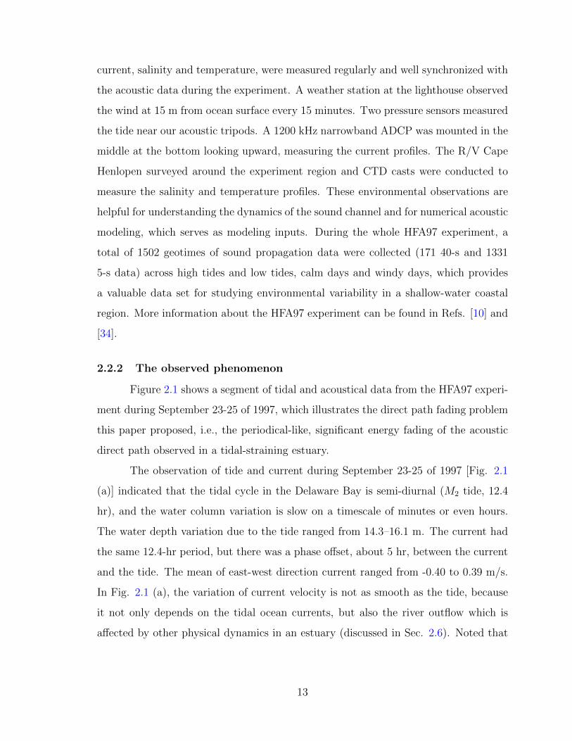
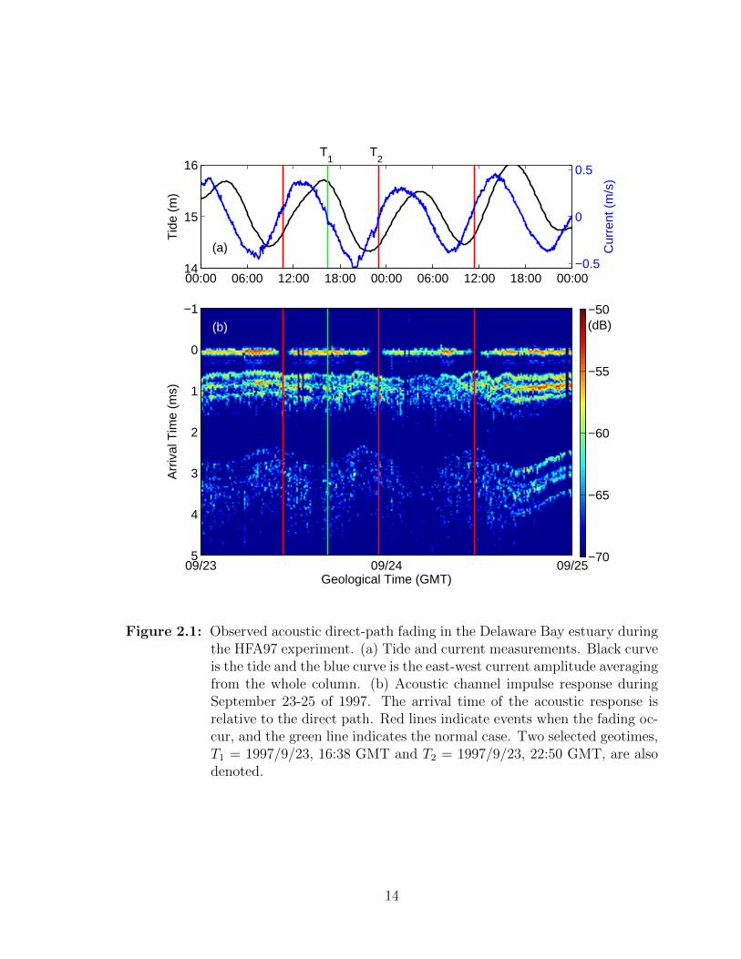
2.1 Observed acoustic direct-path fading in the Delaware Bay estuaryduring the HFA97 experiment. (a) Tide and current measurements.Black curve is the tide and the blue curve is the east-west currentamplitude averaging from the whole column. (b) Acoustic channelimpulse response during September 23-25 of 1997. The arrival time ofthe acoustic response is relative to the direct path. Red lines indicateevents when the fading occur, and the green line indicates the normalcase. Two selected geotimes, T1 = 1997/9/23, 16:38 GMT and T2 =1997/9/23, 22:50 GMT, are also denoted. . . . . . . . . . . . . . . . 14

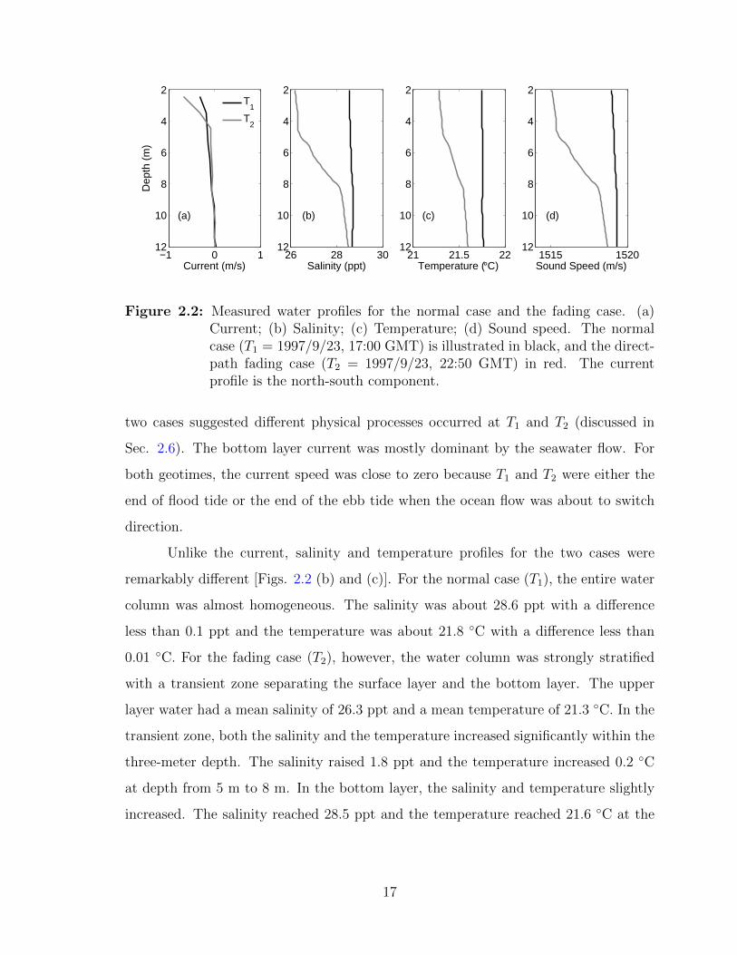
2.2 Measured water profiles for the normal case and the fading case. (a)Current; (b) Salinity; (c) Temperature; (d) Sound speed. The normalcase (T1 = 1997/9/23, 17:00 GMT) is illustrated in black, and thedirect-path fading case (T2 = 1997/9/23, 22:50 GMT) in red. Thecurrent profile is the north-south component. . . . . . . . . . . . . 17

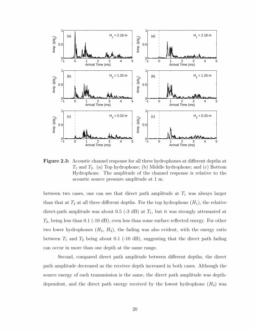
2.3 Acoustic channel response for all three hydrophones at differentdepths at T1 and T2. (a) Top hydrophone; (b) Middle hydrophone;and (c) Bottom Hydrophone. The amplitude of the channel responseis relative to the acoustic source pressure amplitude at 1 m. . . . . 20

2.4 Relation between sound speed gradient and (a) salinity gradient, and(b) temperature gradient during the HFA97 experiment. The bottomlayer data are colored in dark, the surface layer data in light, and thetransient zone in between. . . . . . . . . . . . . . . . . . . . . . . 22

2.5 Analysis of the estuary structure for different states of a tidal cycle inan estuary. (a) Ebbing; (b) Flooding. The solid lines illustrate thesalinity isolines by the end of ebbing or flooding. This structure isalso known as shear flow circulation (adopted from [36]). . . . . . 24

2.6 The critical ray circle theory. . . . . . . . . . . . . . . . . . . . . . 28

2.7 Theoretical occurrence of direct path fading for the source-receiverconfiguration (depth and range). . . . . . . . . . . . . . . . . . . . 29

xi

2.8 PE modeling of two different sound speed gradient. . . . . . . . . 32

2.9 BELLHOP ray tracing for (a) the normal case and (b) the fadingcase. . . . . . . . . . . . . . . . . . . . . . . . . . . . . . . . . . . 33

2.10 Path energy (in terms of transmission loss) as a function of soundspeed gradient. The direct path is denoted as D, and the surfacegroups are denoted as Sn, where n specifies the times of surfacebounces. . . . . . . . . . . . . . . . . . . . . . . . . . . . . . . . . . 34

2.11 Modeling acoustic channel responses for all three hydrophones atdifferent depths at T1 and T2. (a) Top hydrophone; (b) Middlehydrophone; and (c) Bottom Hydrophone. The amplitude of thechannel response is relative to the acoustic source pressure amplitudeat 1 m. . . . . . . . . . . . . . . . . . . . . . . . . . . . . . . . . . 36

2.12 PE modeling the acoustic direct-path fading in the Delaware Bayestuary during the HFA97 experiment (September 23-25 of 1997).The arrival time of the acoustic response is relative to the direct path.Red lines indicates events when the fading occur. Two selectedgeotimes, T1 = 1997/9/23, 16:38 GMT and T2 = 1997/9/23, 22:50GMT, are also denoted. . . . . . . . . . . . . . . . . . . . . . . . . 37

3.1 (a) Map of the Delaware Bay and locations of the HFA97 experiment(square) and nearby lighthouse (circle). Inset enlarges experimentallocation and shows the direction of acoustic path (AC), which is 150◦

from the north (counter-clockwise). (b) Geometry of acoustic transectwith source-receiver setup and typical acoustic surface groups for theHFA97 experiment. Note that the direct path and the single surfacebounced are not shown. (c) Mean sound speed profile in the DelawareBay during the HFA97 experiment. . . . . . . . . . . . . . . . . . 48

3.2 (color online) Directional wind histogram for wind measurementstaken by a nearby lighthouse, with each directional bin being exactly15◦ and a total bin number of 24. The observation period was from1997/9/23 08:37:11 UTC to 1997/9/29/1 01:14:47 UTC. . . . . . . 50

xii

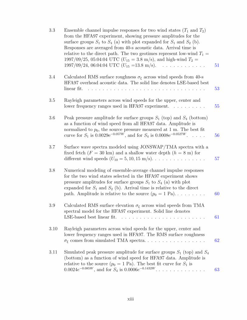
3.3 Ensemble channel impulse responses for two wind states (T1 and T2)from the HFA97 experiment, showing pressure amplitudes for thesurface groups S1 to S4 (a) with plot expanded for S1 and S2 (b).Responses are averaged from 40-s acoustic data. Arrival time isrelative to the direct path. The two geotimes represent low-wind T1 =1997/09/25, 05:04:04 UTC (U15 = 3.8 m/s), and high-wind T2 =1997/09/24, 06:04:04 UTC (U15 =13.8 m/s). . . . . . . . . . . . . 51

3.4 Calculated RMS surface roughness σξ across wind speeds from 40-sHFA97 overhead acoustic data. The solid line denotes LSE-based bestlinear fit. . . . . . . . . . . . . . . . . . . . . . . . . . . . . . . . . 53

3.5 Rayleigh parameters across wind speeds for the upper, center andlower frequency ranges used in HFA97 experiment. . . . . . . . . . 55

3.6 Peak pressure amplitude for surface groups S1 (top) and S4 (bottom)as a function of wind speed from all HFA97 data. Amplitude isnormalized to p0, the source pressure measured at 1 m. The best fitcurve for S1 is 0.0029e−0.057W , and for S4 is 0.0008e−0.0527W . . . . . 56

3.7 Surface wave spectra modeled using JONSWAP/TMA spectra with afixed fetch (F = 30 km) and a shallow water depth (h = 8 m) fordifferent wind speeds (U10 = 5, 10, 15 m/s). . . . . . . . . . . . . . . 57

3.8 Numerical modeling of ensemble-average channel impulse responsesfor the two wind states selected in the HFA97 experiment showspressure amplitudes for surface groups S1 to S4 (a) with plotexpanded for S1 and S2 (b). Arrival time is relative to the directpath. Amplitude is relative to the source (p0 = 1 Pa). . . . . . . . . 60

3.9 Calculated RMS surface elevation σξ across wind speeds from TMAspectral model for the HFA97 experiment. Solid line denotesLSE-based best linear fit. . . . . . . . . . . . . . . . . . . . . . . . 61

3.10 Rayleigh parameters across wind speeds for the upper, center andlower frequency ranges used in HFA97. The RMS surface roughnessσξ comes from simulated TMA spectra. . . . . . . . . . . . . . . . . 62

3.11 Simulated peak pressure amplitude for surface groups S1 (top) and S4

(bottom) as a function of wind speed for HFA97 data. Amplitude isrelative to the source (p0 = 1 Pa). The best fit curve for S1 is0.0024e−0.085W , and for S4 is 0.0006e−0.1432W . . . . . . . . . . . . . . 63

xiii

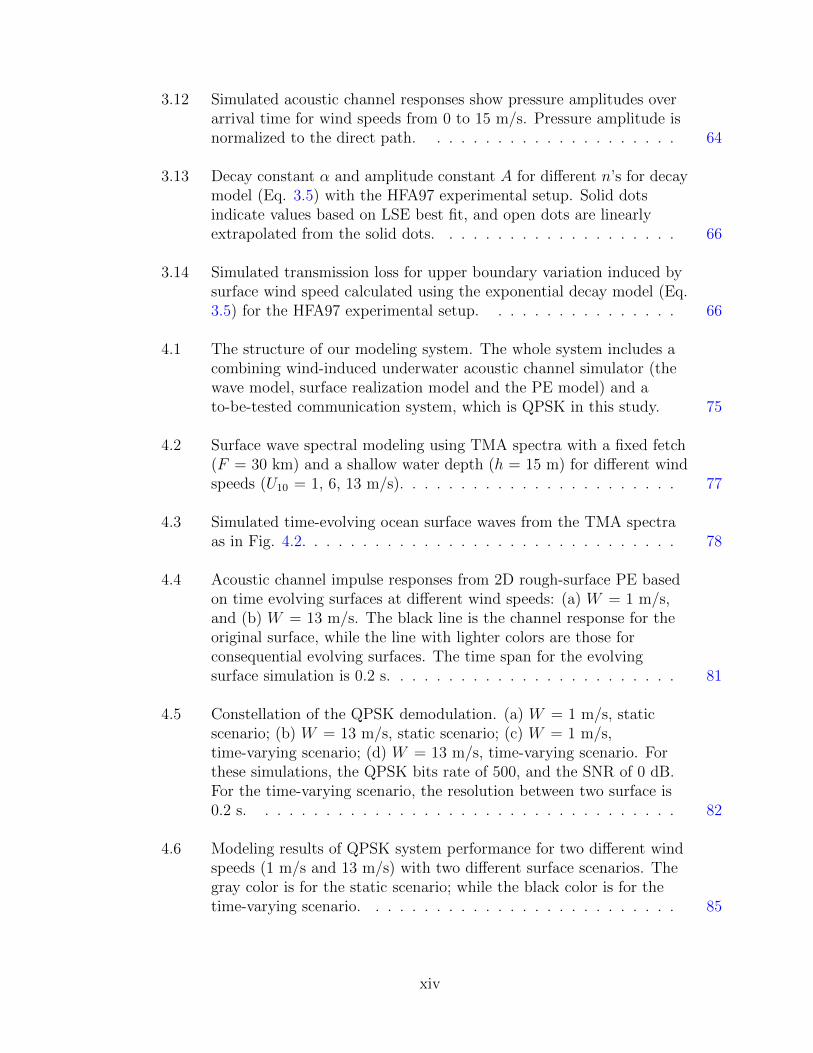
3.12 Simulated acoustic channel responses show pressure amplitudes overarrival time for wind speeds from 0 to 15 m/s. Pressure amplitude isnormalized to the direct path. . . . . . . . . . . . . . . . . . . . . 64

3.13 Decay constant α and amplitude constant A for different n’s for decaymodel (Eq. 3.5) with the HFA97 experimental setup. Solid dotsindicate values based on LSE best fit, and open dots are linearlyextrapolated from the solid dots. . . . . . . . . . . . . . . . . . . . 66

3.14 Simulated transmission loss for upper boundary variation induced bysurface wind speed calculated using the exponential decay model (Eq.3.5) for the HFA97 experimental setup. . . . . . . . . . . . . . . . 66

4.1 The structure of our modeling system. The whole system includes acombining wind-induced underwater acoustic channel simulator (thewave model, surface realization model and the PE model) and ato-be-tested communication system, which is QPSK in this study. 75

4.2 Surface wave spectral modeling using TMA spectra with a fixed fetch(F = 30 km) and a shallow water depth (h = 15 m) for different windspeeds (U10 = 1, 6, 13 m/s). . . . . . . . . . . . . . . . . . . . . . . 77

4.3 Simulated time-evolving ocean surface waves from the TMA spectraas in Fig. 4.2. . . . . . . . . . . . . . . . . . . . . . . . . . . . . . . 78

4.4 Acoustic channel impulse responses from 2D rough-surface PE basedon time evolving surfaces at different wind speeds: (a) W = 1 m/s,and (b) W = 13 m/s. The black line is the channel response for theoriginal surface, while the line with lighter colors are those forconsequential evolving surfaces. The time span for the evolvingsurface simulation is 0.2 s. . . . . . . . . . . . . . . . . . . . . . . . 81

4.5 Constellation of the QPSK demodulation. (a) W = 1 m/s, staticscenario; (b) W = 13 m/s, static scenario; (c) W = 1 m/s,time-varying scenario; (d) W = 13 m/s, time-varying scenario. Forthese simulations, the QPSK bits rate of 500, and the SNR of 0 dB.For the time-varying scenario, the resolution between two surface is0.2 s. . . . . . . . . . . . . . . . . . . . . . . . . . . . . . . . . . . 82

4.6 Modeling results of QPSK system performance for two different windspeeds (1 m/s and 13 m/s) with two different surface scenarios. Thegray color is for the static scenario; while the black color is for thetime-varying scenario. . . . . . . . . . . . . . . . . . . . . . . . . . 85

xiv

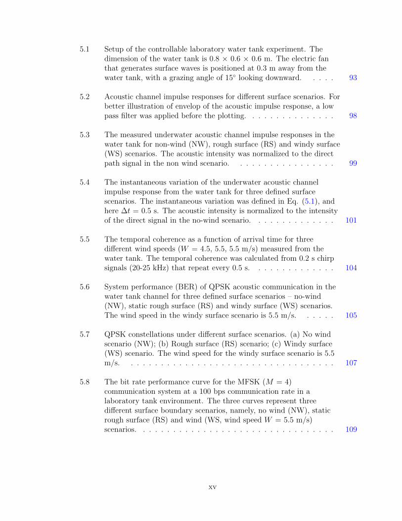
5.1 Setup of the controllable laboratory water tank experiment. Thedimension of the water tank is 0.8 × 0.6 × 0.6 m. The electric fanthat generates surface waves is positioned at 0.3 m away from thewater tank, with a grazing angle of 15◦ looking downward. . . . . 93

5.2 Acoustic channel impulse responses for different surface scenarios. Forbetter illustration of envelop of the acoustic impulse response, a lowpass filter was applied before the plotting. . . . . . . . . . . . . . . 98

5.3 The measured underwater acoustic channel impulse responses in thewater tank for non-wind (NW), rough surface (RS) and windy surface(WS) scenarios. The acoustic intensity was normalized to the directpath signal in the non wind scenario. . . . . . . . . . . . . . . . . 99

5.4 The instantaneous variation of the underwater acoustic channelimpulse response from the water tank for three defined surfacescenarios. The instantaneous variation was defined in Eq. (5.1), andhere ∆t = 0.5 s. The acoustic intensity is normalized to the intensityof the direct signal in the no-wind scenario. . . . . . . . . . . . . . 101

5.5 The temporal coherence as a function of arrival time for threedifferent wind speeds (W = 4.5, 5.5, 5.5 m/s) measured from thewater tank. The temporal coherence was calculated from 0.2 s chirpsignals (20-25 kHz) that repeat every 0.5 s. . . . . . . . . . . . . . 104

5.6 System performance (BER) of QPSK acoustic communication in thewater tank channel for three defined surface scenarios – no-wind(NW), static rough surface (RS) and windy surface (WS) scenarios.The wind speed in the windy surface scenario is 5.5 m/s. . . . . . 105

5.7 QPSK constellations under different surface scenarios. (a) No windscenario (NW); (b) Rough surface (RS) scenario; (c) Windy surface(WS) scenario. The wind speed for the windy surface scenario is 5.5m/s. . . . . . . . . . . . . . . . . . . . . . . . . . . . . . . . . . . 107

5.8 The bit rate performance curve for the MFSK (M = 4)communication system at a 100 bps communication rate in alaboratory tank environment. The three curves represent threedifferent surface boundary scenarios, namely, no wind (NW), staticrough surface (RS) and wind (WS, wind speed W = 5.5 m/s)scenarios. . . . . . . . . . . . . . . . . . . . . . . . . . . . . . . . . 109

xv

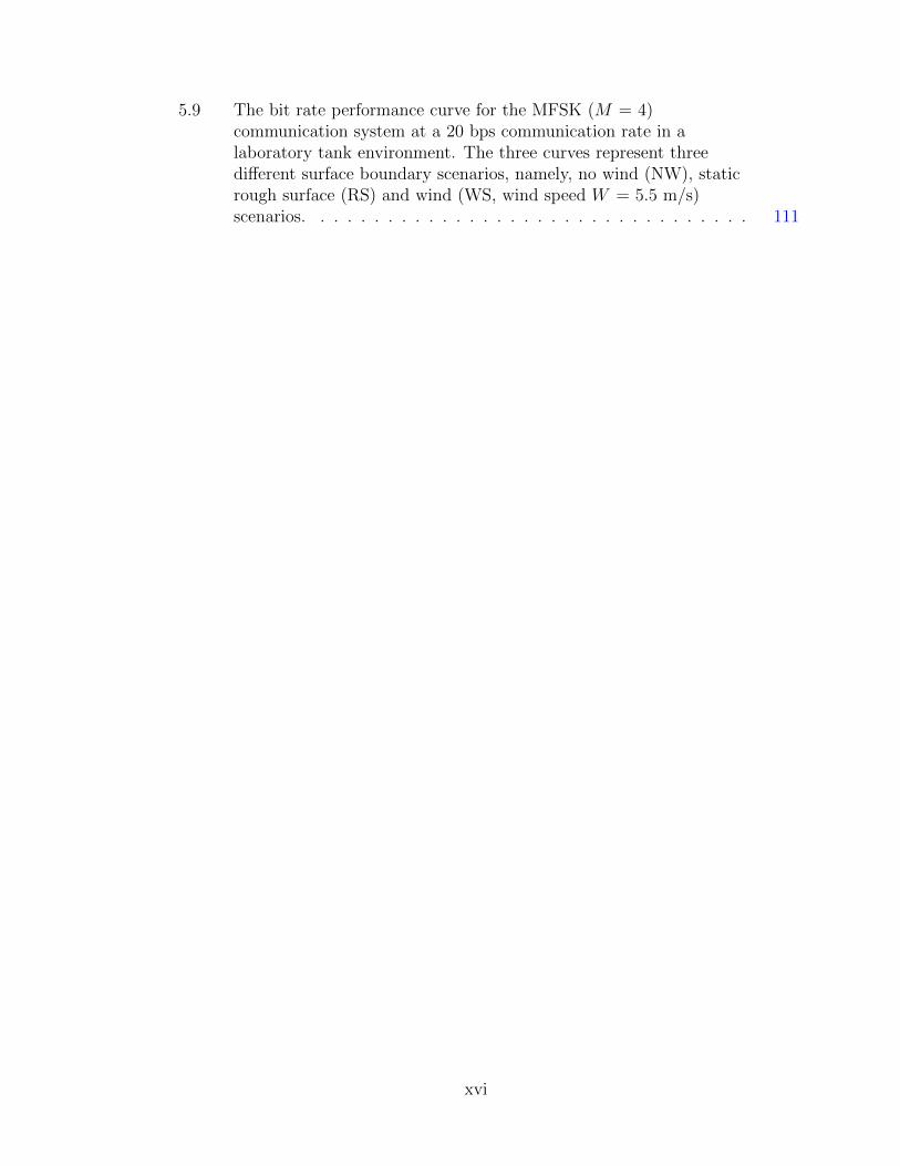
5.9 The bit rate performance curve for the MFSK (M = 4)communication system at a 20 bps communication rate in alaboratory tank environment. The three curves represent threedifferent surface boundary scenarios, namely, no wind (NW), staticrough surface (RS) and wind (WS, wind speed W = 5.5 m/s)scenarios. . . . . . . . . . . . . . . . . . . . . . . . . . . . . . . . . 111

xvi

ABSTRACT

Estuaries are water regions that connect rivers and oceans, which are very impor-

tant due to heavy traffic, fishery and other coastal engineering activities. Underwater

acoustic technology offers a series of effective applications and technical supports for

real-time monitoring and long-term preservation of the nature environment and ecosys-

tem in these regions. However, estuaries are shallow waters with complicated temporal

and spatial environmental variability, involving a variety of physical oceanographic

processes, such as tidal water mixing and ocean winds/waves, which can significantly

influence the underwater sound propagation and moreover, underwater acoustic com-

munications. In order to perform reliably and effectively in such complex time-varying

shallow-water ocean environments, next-generation underwater acoustic communica-

tion systems need an all new design based on the environmental variability of the

physical ocean, which takes the environmental physics and time-varying variability

into account and is able to adapt and switch to the optimal mode as the environ-

ment evolves. Therefore, a deep, comprehensive and thorough understanding of the

link between the time-varying ocean environment, underwater acoustic channel, and

underwater acoustic communication systems is highly required.

This dissertation investigated the relationship between the shallow-water, time-

varying environment of estuaries, the underwater sound propagation and underwater

acoustic communications, which can help the design of underwater acoustic systems

so that they can adapt the time-varying environment with wiser parameter configu-

rations. In this dissertation, field data analysis, joint numerical modeling, together

with a controllable laboratory experiment were used to study acoustic channel vari-

ability of a shallow estuary and its influence on the performance of underwater acoustic

communications. This dissertation included four aspects: (a) Effect of water-column

xvii

variation due to the tidal dynamics in an estuary on the underwater acoustic direct

path; (b) Effect of time-varying surface roughness due to the wind-driven waves on

underwater acoustic surface paths; (c) Numerically modeling the effect of time-varying

wind-driven shallow-water waves on coherent underwater acoustic communications us-

ing a combined model; (d) Conducting a controllable laboratory experiment to inves-

tigate the time-varying wind-driven water waves on the performance of coherent and

non-coherent underwater acoustic communications.

The first two aspects focused on the link between the time-varying environment

of an estuary and the underwater acoustic wave propagation. With field data analysis

and joint numerical modeling, the time-varying variability of acoustic direct paths and

surface-bounced paths from a high-frequency acoustic experiment conducted in the

Delaware Bay estuary was explored. On one hand, periodical acoustic direct path

fading was found in the tidal-straining Delaware Bay estuary, with the fading period

as same as the semi-diurnal tide. Based on physical oceanography and ocean acoustics,

the mechanism that causes the direct path fading and its link to the water dynamics of

an estuary was investigated. On the other hand, the relationship between the acoustic

surface paths and the surface wind speed was investigated, and the wind-influenced

shallow-water time-varying channel was studied using field data analysis and a joint

model combining physical oceanography and ocean acoustics. The joint numerical

model, including a wind-wave model, a surface generation algorithm and a parabolic

equation acoustic model, reproduced the relationship between the wind speed and

surface reflection signals.

The last two aspects applied the knowledge of underwater sound propagation in

shallow estuaries into analyzing the performance of underwater acoustic communica-

tion systems, i.e., investigating how the fast fluctuation of a shallow-water environment

(wind-driven waves) influences different fundamental modulation schemes for underwa-

ter acoustic communications. To better analyze the effect of environmental variability

of the physical ocean on underwater acoustic communications, the surface condition

was set as the only variation in the numerical modeling and the controllable laboratory

xviii

experiment. On one hand, a combined model including physical oceanography, ocean

acoustics, and underwater acoustic communication was used to study the time-varying

underwater acoustic channel under different wind speeds, and the performance of the

coherent acoustic communication (QPSK) system. On the other hand, a controllable

laboratory experiment was conducted to investigate bit-error-rate (BER) performance

of the MFSK (representing the non-coherent acoustic communication) and the QPSK

(representing the coherent acoustic communication) acoustic modulations.

The main conclusions of the dissertation are as follows. For the time-varying

variability of underwater acoustic channel: (a) Due to the tidal-straining water dy-

namics of an estuary, periodical water column exchange between the seawater and

the freshwater, up-refracting sound speed profile is more likely to form by the end

of ebb tide, which redirects sound signal away from the deep receivers and creates

shadow zone for the sound direct path; (b) In an open estuary, the acoustic pressure

of surface-bounced paths decreases with increased wind speed, as a result of increased

acoustic scattering due to the wind-driven surface roughness. For underwater acous-

tic communications: (c) Coherent acoustic communications are sensitive to the fast

time-varying variability, and performance decrease significantly with increased wind

speed, as a result of increased channel variability and decreased temporal coherence;

(d) Non-coherent acoustic communications are less sensitive to the channel variability,

and the reduced multipath signals due to wind-wave surface may improve the system

performance.

The key novelties of this dissertation include: (a) Using a joint model involving

physical oceanography and ocean acoustics to study the effect of time-varying estuar-

ine environment (water-column variations and wind-driven surface waves) on underwa-

ter sound propagation and the underwater acoustic channels. (b) Using an integrated

model involving physical oceanography, ocean acoustics, and underwater acoustic com-

munications to study the effect of time-varying estuarine environment (wind-driven

surface waves) on underwater acoustic communications. (c) Using field experimental

xix

data, numerical modeling and controllable laboratory experiment to study the under-

water sound propagation and underwater acoustic communications in a time-varying

ocean environment.

xx

Chapter 1

INTRODUCTION

Sounds are one of the most effective forms that can travel effectively over a

long distance in the ocean with a relatively small attenuation, much smaller than elec-

tromagnetic waves [1]. As a qualified candidate for underwater wireless applications,

acoustic waves enable many practical underwater acoustic technologies such as under-

water sonar detection [2], acoustic communication [3], and acoustic inversion [4] for

ocean exploration. Due to the wide applications in military, scientific and civil en-

gineering areas over the years, the underwater acoustic communication has received

increasing interests and attentions and become a research hotspot. Because all under-

water acoustic technologies use the propagation of acoustic waves in a water medium,

the variation of the physical ocean environment can significantly influence sound prop-

agation under the water and further, underwater acoustic communications. Thus, a

better understanding of the relationship between the physical oceanography, ocean

acoustics and underwater acoustic communications is greatly beneficial for improving

the design of next-generation underwater acoustic communication systems.

The booming of the study on underwater sound propagation began at the World

War II, for military purposes as the key driving force at the time [2]. Since active sonar

systems are mono-static, and use single-frequency continuous wave (CW) as the sound

source [2], early studies usually viewed underwater sound propagation problems based

on a sonar perspective, i.e., in terms of transmission loss, target strength, attenuation

coefficient, reverberation, etc [2, 5, 6]. Later, with increasing demand for underwater

acoustic communications, the perspective of underwater sound propagation has been

greatly extended, shifting to the underwater acoustic communication channels. Unlike

traditional sonars, acoustic communication systems are in a bistatic configuration,

1

and use broadband signals [7]. Therefore, underwater sound propagation research for

acoustic communication systems focuses on the characteristics of underwater acoustic

channels, i.e., in terms of multipath structure. Due to the high variability of nature

ocean environments, understanding the complicated underwater acoustic channel has

become an important topic for underwater acoustic communication research.

Previous studies have revealed two key challenges for the effective and reliable

acoustic communications under the water – the multipath structure of underwater

acoustic channels and the acoustic variability due to time-varying ocean environments.

On one hand, due to the existence of two nature boundaries (an air-water interface

and a seafloor) reflection and scattering of sound occurred at these two boundaries can

create more than one acoustic paths between the transmitter and receiver [8]. This

multipath effect creates later acoustic arrivals after the direct path, leading to the

amplitude variation of received sound signals, which further transfers into the spatial,

temporal and frequency domains of acoustic waves, causing problems such as spatial

diversity, temporal spreading, and selective frequency fading, etc [9]. The multipath

effect is more significant in shallow-water regions like coastal waters or estuaries, where

multiple, repeated surface-bottom reflections are more likely to occur within a short

range [10]. On the other hand, the ocean varies on a wide timescale (from milliseconds

to hundreds of years) and a broad length scale (from millimeters to thousands of

kilometers) [11]. In nature ocean environments, atmosphere-ocean dynamics (e.g.,

surface waves, swells, etc) modify the air-water boundary [12, 13, 14]; water motions

(e.g., tides, currents and upwelling/downwelling) change water column properties, such

as density, temperature, and salinity [15, 16]. Such environmental variability causes

the acoustic multipath structure to fluctuate over time, leading to decreasing temporal

coherence and shifting frequency bands [17, 18]. In short, the multipath effect and the

time-varying ability together make underwater acoustic channels highly complicated,

which are extremely challenging for underwater acoustic communications [19, 20].

One example of nature water environments that illustrates both challenges (the

shallow-water multipath and time-varying environmental variability) at the same time

2

is a shallow-water estuarine environment. Estuaries are transitional zones connecting

freshwater and seawater with high primary productivity, rich marine biological re-

sources [11, 21]. As a very important coastal ecosystem, estuaries should be monitored

for its environmental health and sustainable development. Underwater acoustic com-

munication can provide effective technical support to construct underwater monitoring

networks for long-term monitoring and protection of estuaries [22, 23]. However, the

environmental variability in an estuary is extremely strong and complicated [24], due

to the interaction of freshwater and seawater, the tidal-straining water dynamics, as

well as the atmospheric dynamics between the land and the ocean. Hence, studying

the connection between the physical ocean, ocean acoustic, and underwater acoustic

communications, as a whole system, is the key to the fundamental improvement of the

performance of underwater acoustic communication systems to apply in these highly

time-varying, shallow estuaries.

The goal of this dissertation was to investigate the relationship between the

underwater sound propagation, underwater acoustic communications, and the time-

varying physical environment of a shallow estuary, which can be used to guide the

design of future underwater acoustic communication and networking. The environ-

mental variability investigated in this dissertation includes two different timescales: a

timescale of seconds that captures fast fluctuation of acoustic surface groups due to sur-

face winds and waves, and a timescale of hours that represents slow fluctuation of both

acoustic direct path and surface groups due to water column variations. Field data

analysis, integrated numerical modeling and laboratory experiment were used in this

dissertation to explore the link between the physical oceanography, ocean acoustics,

and underwater acoustic communications.

The work of this dissertation involves the following two aspects. On one hand,

sound propagation and acoustic channel characteristics in a shallow-water estuarine

environment were studied, based on data analysis of a field experiment and numeri-

cal modeling (Chapters 2 and 3). On the other hand, the variability of underwater

acoustic channels due to the physical ocean environment was applied to the research of

3

underwater acoustic communication, to investigate the influence of the shallow-water

estuarine environment on the performance of underwater acoustic communication sys-

tems (Chapters 4 and 5).

The four major research questions in this dissertation are: (a) The effect of

water column variation due to water dynamics of a tidal-straining estuary on the vari-

ability of acoustic direct paths. (b) The effect of surface boundary variations due to

the wind-driven surface waves on the variability of acoustic surface-bounced paths.

(c) Numerically modeling the effect of wind speed on the performance of underwater

coherent acoustic communication systems using an integrated numerical model. (d)

Studying the effect of time-varying wind-driven surface waves on the performance of

underwater coherent and non-coherent acoustic communication systems from a labo-

ratory simulation experiment.

First, the effect of slow fluctuation of the water column on acoustic direct paths

was investigated with the water dynamics of a tidal-straining estuary. Acoustic direct

paths have no interactions with sea surface and seafloor and contribute the major

acoustic energy at the receiver, so they are crucial for acoustic communications due

to the stability and high energy. However, periodical intensity fading of the acoustic

direct path was observed in the Delaware Bay, a shallow tidal-straining estuary, with an

attenuation up to 20 dB. This is affected by the variation of water-column properties

itself. With field data analysis and numerical modeling, results suggested that the

repeated, significant fading in the sound direct path was the acoustic channel response

to the tidal forcing dynamics in the Delaware Bay, due to the periodicity of salinity

profile variation by the end of ebbing period, causing upward sound refraction and

creating the shadow zone for the sound direct path at the sea bottom. The direct path

fading should be taken into account in the future design of reliable underwater acoustic

systems in these regions, particularly those based on the detection of direct path energy,

which the direct path energy is crucial for signal detection and synchronization.

Second, the fast fluctuation of wind-driven surface waves on variations of acous-

tic surface paths was examined as a function of wind speed. The acoustic surface paths

4

interact with the sea surface, which has a short timescale within seconds and is highly

related to surface winds. Underwater acoustic channels in estuaries can be drastically

affected by coastal wind-wave dynamics, and the wind (or sea states) effects on un-

derwater acoustic propagation and communication systems have been reported. Field

data analysis and combined numerical modeling (including a shallow-water wind-wave

spectral method and a 2-D rough-surface parabolic equation model) were conducted

to investigated how the wind-driven surface roughness in shallow-water environments

affects the variability of mid- to high-frequency broadband acoustic channels. Mod-

eling simulations agreed with field data analyses, and together they revealed strong

correlations between wind speed and pressure amplitude of acoustic surface bounces,

indicating that increased wind-driven surface roughness is primarily responsible for the

decrease of surface-bounced acoustic energy. These findings lead to a new empirical

transmission loss formula for predicting wind-related surface acoustic energy.

Third, how the performance of underwater coherent acoustic communication

systems varies with surface wind speed was studied using integrated numerical models,

including physical oceanography, ocean acoustics, and underwater acoustic communica-

tion. Performance degradation and system failures in underwater acoustic communica-

tion were previously reported due to wind-induced surface waves, especially for coherent

communication systems which utilize phase information during the modulation. A con-

trollable numerical approach was proposed to study the effect of wind-driven surface

waves on the performance of underwater coherent acoustic communication. Realistic

acoustic channels for different wind conditions are numerically simulated with wind-

wave spectral methods and a 2-D rough-surface parabolic equation (PE) model; Then,

these time-varying acoustic channels are tested with quadrature phase-shift keying

(QPSK) modulation, one of the most fundamental modulation schemes for underwater

acoustic coherent communication in different wind conditions within a frequency band

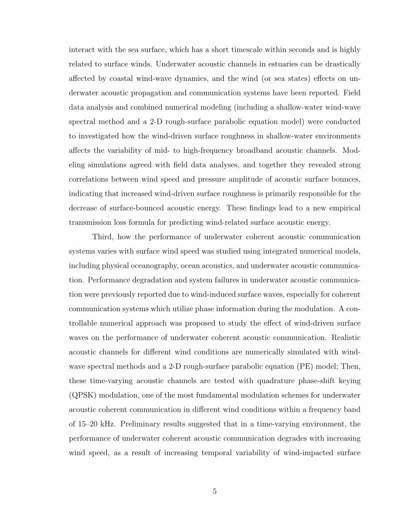
of 15–20 kHz. Preliminary results suggested that in a time-varying environment, the

performance of underwater coherent acoustic communication degrades with increasing

wind speed, as a result of increasing temporal variability of wind-impacted surface

5

waves. The proposed integrated numerical modeling method could be a helpful tool to

study acoustic communication problems in time-varying ocean environments.

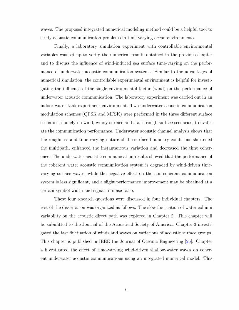
Finally, a laboratory simulation experiment with controllable environmental

variables was set up to verify the numerical results obtained in the previous chapter

and to discuss the influence of wind-induced sea surface time-varying on the perfor-

mance of underwater acoustic communication systems. Similar to the advantages of

numerical simulation, the controllable experimental environment is helpful for investi-

gating the influence of the single environmental factor (wind) on the performance of

underwater acoustic communication. The laboratory experiment was carried out in an

indoor water tank experiment environment. Two underwater acoustic communication

modulation schemes (QPSK and MFSK) were performed in the three different surface

scenarios, namely no-wind, windy surface and static rough surface scenarios, to evalu-

ate the communication performance. Underwater acoustic channel analysis shows that

the roughness and time-varying nature of the surface boundary conditions shortened

the multipath, enhanced the instantaneous variation and decreased the time coher-

ence. The underwater acoustic communication results showed that the performance of

the coherent water acoustic communication system is degraded by wind-driven time-

varying surface waves, while the negative effect on the non-coherent communication

system is less significant, and a slight performance improvement may be obtained at a

certain symbol width and signal-to-noise ratio.

These four research questions were discussed in four individual chapters. The

rest of the dissertation was organized as follows. The slow fluctuation of water column

variability on the acoustic direct path was explored in Chapter 2. This chapter will

be submitted to the Journal of the Acoustical Society of America. Chapter 3 investi-

gated the fast fluctuation of winds and waves on variations of acoustic surface groups.

This chapter is published in IEEE the Journal of Oceanic Engineering [25]. Chapter

4 investigated the effect of time-varying wind-driven shallow-water waves on coher-

ent underwater acoustic communications using an integrated numerical model. This

6

chapter was published in the Proceedings of 2016 IEEE/OES China Ocean Acous-

tics (COA) [26]. Chapter 5 conducted a controllable laboratory experiment to study

the time-varying wind-driven water waves on the performance of coherent and non-

coherent underwater acoustic communications. This chapter will be submitted to a

peer-reviewed journal soon. Finally, Chapter 6 summarized the dissertation.

7

Chapter 2

DIRECT-PATH SOUND FADING IN A SHALLOWTIDAL-STRAINING ESTUARY

Periodical fading of the acoustic direct path was observed in the Delaware Bay,

a shallow tidal-straining estuary, within a source-receiver range of 387 m and the mean

water depth of 15 m. The cycle of these fading events was about 12.4 hours and the

intensity attenuation was up to 20 dB. Data analysis suggested that the repeated, sig-

nificant fading in the sound direct path was associated with the tidal forcing dynamics

in the Delaware Bay, as a result of the periodicity of salinity profile variation, which

caused upward sound refraction and created shadow zone for the direct path near sea

floor by the end of an ebb tide. This direct path fading may occur in most tidal-

straining estuaries as long as the relation between the source-receiver configuration in

depth and theoretical sound speed gradient is satisfied, which provides a guideline for

future acoustic applications. This study also suggested that direct path fading problem

is important for underwater acoustic applications that utilize the direct path energy,

and should be taken into account for the design of reliable underwater acoustic systems

in shallow tidal-straining estuaries.

2.1 Introduction

In ocean environments, water column variations are usually very slow and grad-

ual, which influences underwater sound propagation on a large time scale, ranging from

minutes to hours, days, and even years [11]. Therefore, the underwater acoustic vari-

ability due to water column variations is much slower compared to upper boundary

variations caused by surface wind-wave dynamics, whose change is more rapid and

violent on a timescale within seconds [1, 10, 25]. It is the slow variation of ocean

8

water column that gives rise to the stability of acoustic direct paths, i.e., the paths of

sound rays that directly connect the acoustic source and receiver without interacting

with the sea surface or bottom. These acoustic direct paths are generally considered

as deterministic because they are relatively stable in time and not affected by the fast

fluctuation of ocean surface [10]. However, the effect of the water column on underwa-

ter sound propagation for a longer period cannot be ignored. In fact, a drastic change

of the water column feature may break the stability of acoustic direct paths and fail

many acoustic applications based on the detection of the direct path, and thus the

water column variability can be acoustically important.

Effects of water column variability on underwater sound propagation on large

time scales have been long noticed and widely reported in previous studies [1, 10, 2].

For instance, the diurnal solar heating in the upper layer waters leading to temperature

variation of the water column can cause significant sonar performance degradation, well

known as the Afternoon Effect [2]. Events like internal waves propagating for hours

or days can result in focusing and defocusing of acoustic energy and pose a big chal-

lenge for acoustic applications in internal wave active regions [27]. Seasonal fluctuation

of the ocean environment can be even more remarkable, accompanied by thermocline

deepening or shallowing which alters the acoustic channel and completely changes the

underwater acoustic pressure field [1]. Eventually, any acoustic variability due to the

water column will influence underwater acoustic applications that utilize sound propa-

gation in the water medium, e.g., acoustic communications, which have been received

increasing research interests these years. In one previous study [28], remarkable effects

of temperature fluctuation of internal tides on high-frequency acoustic communications

have reported, The other studied [29] revealed that underwater acoustic communica-

tion is significantly affected by tidal variations, where higher SNR is obtained at low

tides because of closer multipath components and smaller reverberation tails. How-

ever, despite the importance of these time-varying water column effects, studies that

explore the link between physical environment and underwater sound propagation,

9

even to acoustic applications, are still rare. The environmental variability of underwa-

ter acoustic channels is currently one of the biggest challenges for adaptive underwater

acoustic communication and networking systems, and improved knowledge of the phys-

ical environment can be beneficial for the design of reliable underwater acoustic systems

in the future [1].

One water environment with significant water column variability is an estuary,

i.e., a river outlet to the ocean. Estuaries are transition zones between freshwater and

seawater, and the interaction between two water bodies and the tidal dynamics can

significantly impact underwater acoustic transmissions. Moreover, coastal oceans are

highly important regions with heavy human activities such as ship traffic and/or other

coastal engineerings, and with high biological production due to strong freshwater-

seawater mixing that nourishes marine life [11]. Therefore, estuaries deserve long-term

monitoring and protection for ecosystem health and sustainability, which can use the

help of underwater acoustic techniques such as acoustic communications to broadcast

the control commands and retrieve collected in-situ data [24]. However, estuaries are

shallow waters where sound propagation has complicated multipath structure, and

moreover, the environmental variability due to coastal processes makes the acoustic

problem even more complicated. Currently, only a few acoustic studies explored these

regions [24, 10, 29, 30], and future practical underwater applications are calling for

more knowledge about the environmental variability in these particular regions.

This paper focused on the variability of acoustic direct paths which captures

only the effect from slow variations of the water column in a tidal-straining estuary.

In September of 1997, periodical-like intensity fading (up to 20 dB) of the direct path

was observed in an acoustic transmission experiment from the Delaware Bay, where the

water-column variability is significant due to the interaction between the river water

and ocean water in a tidal estuary. This direct-path fading phenomenon has been

noticed in previous studies [24, 10], but no systematic explanation was given at that

time. In this study, the cause of the direct path fading was explained based on field

data analysis and theories, e.g., sound propagation and the physical ocean dynamics

10

in a tidal-straining estuary; Acoustic modeling was applied to reconstruct underwater

acoustic pressure fields numerically with observed sound speed profiles and source and

receiver positions. Data-model analyses confirmed that the direct path fading was a

result of the periodical variation of salinity profile in the Delaware Bay due to tidal

forcing water dynamics forming upward-refracted sound speed profiles that redirected

the sound energy away from the acoustic receivers at the bottom.

The rest of the paper was organized as following. Section 2.1 introduced the

direct path fading observed in a high-frequency acoustic experiment in the Delaware

Bay. In Section 2.3, two particular events from the experiment were selected and envi-

ronmental and acoustic data were analyzed. Section 2.4 explained the mechanism that

caused the direct path fading from physical oceanography to acoustics. In Section 2.5,

acoustic modeling was presented as a verification of the proposed hypothesis. Section

2.6 discussed more on the direct path fading problem from physical oceanography and

acoustics perspectives. Finally, conclusions were made in Section 2.7.

2.2 The Direct-Path Fading Phenomenon

2.2.1 Description of the HFA97 experiment

In September of 1997, a High-Frequency Acoustic experiment (HFA97) was con-

ducted to transmit reciprocal acoustic signals for one week period in the center region

of the Delaware Bay (39◦1′N, 75◦11′W) to explore the variability of sound propaga-

tion due to the time-varying physical environment [10]. The Delaware Bay is a shallow

tidal-straining estuary located on the east coast of the United States, which is a perfect

region for this study for three reasons. First, the interaction between the river freshwa-

ter and the ocean seawater gives rise to significant water-column variability that this

study needs. Second, many physical oceanographic studies about the Delaware Bay

have been done in the past [31, 32, 33], which can help us understand the physics and

water dynamics in this region. Third, acoustic applications are highly needed for the

long-term monitoring and preservation of the Bay, which requires a better understand-

ing of the underwater sound propagation in this region.

11

Two acoustic tripods were positioned with 387 m apart on the seafloor of the

Bay to continuously transmit acoustic chirp signals. Each tripod had a transducer,

located at 3.13 m, and three hydrophones, located at 2.18, 1.33, 0.33 m, respectively,

from the seafloor. The water mean depth of the experiment region is about 15 m. Both

tripods were connected to a computer in a nearby lighthouse (39◦2′54′′N, 75◦10′56′′W)

through cables. With this source-receiver positioning, the difference of travel distance

between the direct path and the first single bottom reflection was extremely small, less

than 5 cm. In terms of acoustic arrival time, the difference was about 0.032 ms, which

cannot be well separated by the frequency resolution of source acoustic signal.

During the experiment, a series of up-sweeping acoustic chirps (1–18 kHz) were

transmitted in this shallow water region with two sampling strategies. One is to trans-

mit acoustic chirps continuously for 40 s every hour, and the other for 5 s every ten

minutes. The data samples used in this study were both, where those fast variations

less than 5 seconds, i.e., surface variations or other instantaneous interruptions, can

be averaged out so the ensemble average only reflects the slow variation of the water

column. In this study, the geological time for each sampling transmission was re-

ferred as geotime. The sampling frequency of the system was 46876 Hz. Each geotime

transmission had six channels of received data–three locally and three remotely. For

convenience, the local transmitter was denoted as S, the local hydrophones from top

to bottom were simply denoted as L1, L2 and L3, and the remote hydrophones as

H1, H2 and H3. The local top hydrophone (L1) was 1 m from the source, which was

defined as the source level for that geotime transmission. Acoustic channel responses

were obtained by matched filtering the received acoustic data with the source chirp.

Then, ensemble averaging was applied to the whole sampling duration, either 40 s or

5 s, to eliminates temporal fluctuation within seconds. Note that the 3 dB resolution

of acoustic pings was about 0.1 ms, calculated from the autocorrelation of the source

chirp, which was not small enough for the separation of the direct path and the first

single bottom reflection.

Meanwhile, atmospheric and oceanographic measurements, including wind, tide,

12

current, salinity and temperature, were measured regularly and well synchronized with

the acoustic data during the experiment. A weather station at the lighthouse observed

the wind at 15 m from ocean surface every 15 minutes. Two pressure sensors measured

the tide near our acoustic tripods. A 1200 kHz narrowband ADCP was mounted in the

middle at the bottom looking upward, measuring the current profiles. The R/V Cape

Henlopen surveyed around the experiment region and CTD casts were conducted to

measure the salinity and temperature profiles. These environmental observations are

helpful for understanding the dynamics of the sound channel and for numerical acoustic

modeling, which serves as modeling inputs. During the whole HFA97 experiment, a

total of 1502 geotimes of sound propagation data were collected (171 40-s and 1331

5-s data) across high tides and low tides, calm days and windy days, which provides

a valuable data set for studying environmental variability in a shallow-water coastal

region. More information about the HFA97 experiment can be found in Refs. [10] and

[34].

2.2.2 The observed phenomenon

Figure 2.1 shows a segment of tidal and acoustical data from the HFA97 experi-

ment during September 23-25 of 1997, which illustrates the direct path fading problem

this paper proposed, i.e., the periodical-like, significant energy fading of the acoustic

direct path observed in a tidal-straining estuary.

The observation of tide and current during September 23-25 of 1997 [Fig. 2.1

(a)] indicated that the tidal cycle in the Delaware Bay is semi-diurnal (M2 tide, 12.4

hr), and the water column variation is slow on a timescale of minutes or even hours.

The water depth variation due to the tide ranged from 14.3–16.1 m. The current had

the same 12.4-hr period, but there was a phase offset, about 5 hr, between the current

and the tide. The mean of east-west direction current ranged from -0.40 to 0.39 m/s.

In Fig. 2.1 (a), the variation of current velocity is not as smooth as the tide, because

it not only depends on the tidal ocean currents, but also the river outflow which is

affected by other physical dynamics in an estuary (discussed in Sec. 2.6). Noted that

13

00:00 06:00 12:00 18:00 00:00 06:00 12:00 18:00 00:0014

15

16T

ide

(m)

(a)

T1

T2

−0.5

0

0.5

Cur

rent

(m

/s)

Geological Time (GMT)

Arr

ival

Tim

e (m

s)

(b)

09/23 09/24 09/25

−1

0

1

2

3

4

5

(dB)

−70

−65

−60

−55

−50

Figure 2.1: Observed acoustic direct-path fading in the Delaware Bay estuary duringthe HFA97 experiment. (a) Tide and current measurements. Black curveis the tide and the blue curve is the east-west current amplitude averagingfrom the whole column. (b) Acoustic channel impulse response duringSeptember 23-25 of 1997. The arrival time of the acoustic response isrelative to the direct path. Red lines indicate events when the fading oc-cur, and the green line indicates the normal case. Two selected geotimes,T1 = 1997/9/23, 16:38 GMT and T2 = 1997/9/23, 22:50 GMT, are alsodenoted.

14

around 1997/9/24, 14:00 GMT, there was a storm tide occurred in the Bay. From

the tidal records [Fig. 2.1 (a)], one can see that the storm tide overlapped with the

semi-diurnal tide, which leads to a variation of the current pattern as well.

The acoustic channel response from the remote top hydrophone (H1) for the

period exhibited strong variability of underwater sound channels in both intensity and

arrival time responding to environmental variations [Fig. 2.1 (b)]. As this paper only

focused on the energy fluctuation of the acoustic direct path and the absolute arrival

time was out of concern, the arrival time in Fig. 2.1 (b) was plotted as relative to the

direct path for a better illustration of direct-path amplitude/intensity fluctuation. The

intensity of acoustic multipath varied between -50 and -70 dB. The first arrival was

the direct path, consisted of two individual paths (D/B). The direct path was strong

at most of the time, but it somehow attenuated significantly, e.g., around 1997/9/23,

10:50 GMT, 22:50 GMT, or 1997/9/24, 11:00 GMT, as seen in Fig. 2.1 (b). There

seemed to be a cycle for the direct path fading, about every 12.4 hours, same as the

semi-diurnal tidal cycle in the Bay, with an attenuation up to 20 dB. The fading events

sometimes lasted for more than one hour, suggesting that it was a result of slow water-

column variation. Later arrivals after the direct path were surface related paths, which

encounter at least one surface reflection. Thus, their intensity was affected by both

water column and sea surface motion, but the later was more dominant for two reasons.

On one hand, surface paths can change over seconds as a result of surface motions,

much faster than the timescale of water column variations [25]; On the other hand,

surface paths have deeper grazing angles whose intensity seemed to less subjective to

the water column variation (further explored in Secs. 2.3 and 2.5).

In short, this direct path fading problem observed in the HFA97 experiment

seemed to be a result of complicated water dynamics of an estuary rather than just the

variation of water depth. The change of water depth itself only varies the arrival time

of surface paths, but not the direct path, because it does not travel to the water surface

nor sense the water depth. However, it was more likely to link with the variation of

15

water column properties due to physical water dynamics in the Bay or other tidal-

straining estuaries. The similar period of 12.4 hr suggested that the direct path fading

was related to the tidal cycle in the Bay, particularly, the occurrences of direct path

fading were likely to associate with the end of ebbing periods. During those fading

events, the mean current was about to change direction from offshore to onshore. Even

more interestingly, by the end of September 24, 1997, the direct path fading did not

occur as expected, suggesting that the storm tide as a physical process also somehow

influenced this problem by disturbing the tidal processes.

2.3 Field Data Analysis

2.3.1 Environmental data

Two geological times were selected to the further investigation of the direct

path fading problem (marked in Fig. 2.1). One was T1 = 1997/9/23, 16:38 GMT,

when the direct path intensity was normal (referred as the normal case); The other

was T2 = 1997/9/23, 22:50 GMT, when the direct path fading was observed (referred

as the fading case). Since the fading case (T2) occurred at the end of the ebb tide, as

an opposite, the normal case at the end of a flood tide was chosen. According to the

tidal records [Fig. 2.1 (a)], for the normal case (T1), the tide was 15.7 m (close to high

tide) and the mean current was 0.08 m/s towards the south; while for the fading case

(T2), the tide was 14.4 m (close to low tide) and the mean current was about 0.10 m/s

towards the north.

Figure 2.2 displays vertical water-column profiles for current, salinity, tempera-

ture and sound speed at two selected geotimes. These profiles are all typical estuary-

type water profiles where the water column is separated into two relatively well-mixed

layers with a transient zone between them. Current profiles [Fig. 2.2 (a)] for both

cases were very similar, except for a small difference in the upper 7 m where the water

moved in the same direction but at different current speeds for the two geotimes. The

surface-layer current was mainly driven by the river outflow, which related to the physi-

cal processes such as precipitation; Therefore, the difference of surface current between

16

−1 0 1

2

4

6

8

10

12

Current (m/s)

Depth

(m

)

(a)

T

1

T2

26 28 30

2

4

6

8

10

12

Salinity (ppt)

(b)

21 21.5 22

2

4

6

8

10

12

Temperature (°C)

(c)

1515 1520

2

4

6

8

10

12

Sound Speed (m/s)

(d)

Figure 2.2: Measured water profiles for the normal case and the fading case. (a)Current; (b) Salinity; (c) Temperature; (d) Sound speed. The normalcase (T1 = 1997/9/23, 17:00 GMT) is illustrated in black, and the direct-path fading case (T2 = 1997/9/23, 22:50 GMT) in red. The currentprofile is the north-south component.

two cases suggested different physical processes occurred at T1 and T2 (discussed in

Sec. 2.6). The bottom layer current was mostly dominant by the seawater flow. For

both geotimes, the current speed was close to zero because T1 and T2 were either the

end of flood tide or the end of the ebb tide when the ocean flow was about to switch

direction.

Unlike the current, salinity and temperature profiles for the two cases were

remarkably different [Figs. 2.2 (b) and (c)]. For the normal case (T1), the entire water

column was almost homogeneous. The salinity was about 28.6 ppt with a difference

less than 0.1 ppt and the temperature was about 21.8 ◦C with a difference less than

0.01 ◦C. For the fading case (T2), however, the water column was strongly stratified

with a transient zone separating the surface layer and the bottom layer. The upper

layer water had a mean salinity of 26.3 ppt and a mean temperature of 21.3 ◦C. In the

transient zone, both the salinity and the temperature increased significantly within the

three-meter depth. The salinity raised 1.8 ppt and the temperature increased 0.2 ◦C

at depth from 5 m to 8 m. In the bottom layer, the salinity and temperature slightly

increased. The salinity reached 28.5 ppt and the temperature reached 21.6 ◦C at the

17

depth of 12 m. The in-situ salinity and temperature measurements suggested that the

direct path fading (T2) was associated with a more stratified water column while the

normal case (T1) was associated with a well-mixed water column. Also, the overall

similarity of between salinity and temperature variations suggested that the driving

factor of their variations in the Bay was the same.

The sound speed profile [Fig. 2.2 (d)] shared a pattern similar to the salinity and

temperature profiles. The sound speed was calculated from salinity and temperature

using Eq. 2.1 [35]:

c = 1449.2 + 4.6T − 0.055T 2 + 0.00029T 3 + (1.34− 0.010T )(S − 35) + 0.016z (2.1)

where, T is the temperature in ◦C, S the salinity in ppt, and z the depth in m. Like

salinity and temperature, the sound speed profile was very uniform in the normal case

(T1), but it split into two layers due to the water stratification in the fading case (T2).

The sound speed at T1 was 1519 m/s with a variation over the water column within 0.3

m/s, but at T2, the sound speed difference between the surface layer and the bottom

layer was 3.2 m/s, creating a positive sound speed gradient in the water column. Thus,

the normal case was associated with a uniform sound speed profile while the fading

case was associated with an up-refracting sound speed profile which tended to bend

acoustic rays towards the surface layer.

Table 2.1 summarizes the statistical values for the salinity, temperature and

sound speed in the surface (2–6 m), middle (6–8 m) and bottom (8–12 m) layers at

the two geotimes. At T1, all three layers had a much smaller difference and standard

deviation values for water properties than that at T2, indicating the water column

changing from uniform to non-uniform between two geotimes. Particularly, more sig-

nificant standard deviation values in the middle layer at T2 confirmed the appearance

of a steep-changing transient zone in the fading case. These variations in water column

properties between two geotimes suggested strong water mixing and stratification ac-

tivities in the Bay, which may be significant enough to affect the underwater acoustic

propagation and lead to a big change of acoustic direct path energy.

18

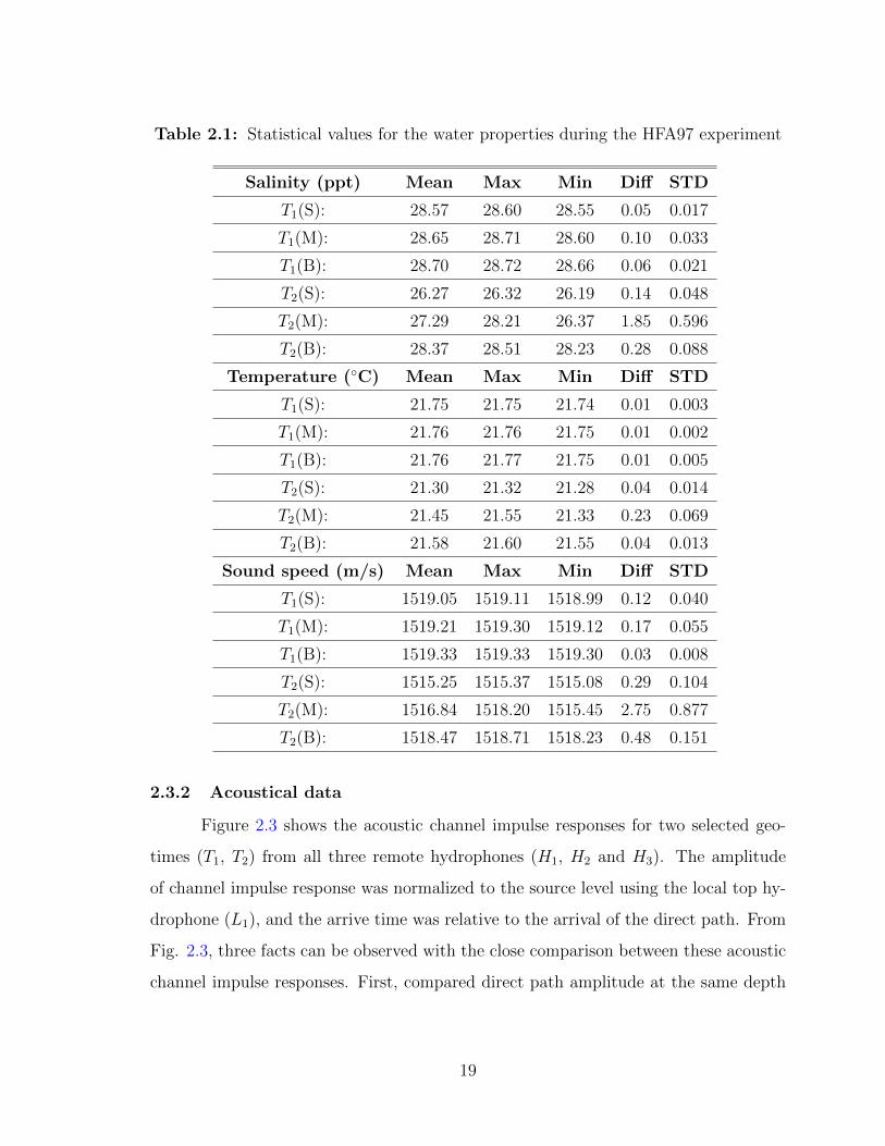
Table 2.1: Statistical values for the water properties during the HFA97 experiment

Salinity (ppt) Mean Max Min Diff STD

T1(S): 28.57 28.60 28.55 0.05 0.017

T1(M): 28.65 28.71 28.60 0.10 0.033

T1(B): 28.70 28.72 28.66 0.06 0.021

T2(S): 26.27 26.32 26.19 0.14 0.048

T2(M): 27.29 28.21 26.37 1.85 0.596

T2(B): 28.37 28.51 28.23 0.28 0.088

Temperature (◦C) Mean Max Min Diff STD

T1(S): 21.75 21.75 21.74 0.01 0.003

T1(M): 21.76 21.76 21.75 0.01 0.002

T1(B): 21.76 21.77 21.75 0.01 0.005

T2(S): 21.30 21.32 21.28 0.04 0.014

T2(M): 21.45 21.55 21.33 0.23 0.069

T2(B): 21.58 21.60 21.55 0.04 0.013

Sound speed (m/s) Mean Max Min Diff STD

T1(S): 1519.05 1519.11 1518.99 0.12 0.040

T1(M): 1519.21 1519.30 1519.12 0.17 0.055

T1(B): 1519.33 1519.33 1519.30 0.03 0.008

T2(S): 1515.25 1515.37 1515.08 0.29 0.104

T2(M): 1516.84 1518.20 1515.45 2.75 0.877

T2(B): 1518.47 1518.71 1518.23 0.48 0.151

2.3.2 Acoustical data

Figure 2.3 shows the acoustic channel impulse responses for two selected geo-

times (T1, T2) from all three remote hydrophones (H1, H2 and H3). The amplitude

of channel impulse response was normalized to the source level using the local top hy-

drophone (L1), and the arrive time was relative to the arrival of the direct path. From

Fig. 2.3, three facts can be observed with the close comparison between these acoustic

channel impulse responses. First, compared direct path amplitude at the same depth

19

−1 0 1 2 3 4 50

0.5

1

Arrival Time (ms)

Am

p. (

p/p 0) (a) H

1 = 2.18 m

−1 0 1 2 3 4 50

0.5

1

Arrival Time (ms)

Am

p. (

p/p 0) (b) H

2 = 1.33 m

−1 0 1 2 3 4 50

0.5

1

Arrival Time (ms)

Am

p. (

p/p 0) (c) H

3 = 0.33 m

−1 0 1 2 3 4 50

0.5

1

Arrival Time (ms)

Am

p. (

p/p 0) (a) H

1 = 2.18 m

−1 0 1 2 3 4 50

0.5

1

Arrival Time (ms)

Am

p. (

p/p 0) (b) H

2 = 1.33 m

−1 0 1 2 3 4 50

0.5

1

Arrival Time (ms)

Am

p. (

p/p 0) (c) H

3 = 0.33 m

Figure 2.3: Acoustic channel response for all three hydrophones at different depths atT1 and T2. (a) Top hydrophone; (b) Middle hydrophone; and (c) BottomHydrophone. The amplitude of the channel response is relative to theacoustic source pressure amplitude at 1 m.

between two cases, one can see that direct path amplitude at T1 was always larger

than that at T2 at all three different depths. For the top hydrophone (H1), the relative

direct-path amplitude was about 0.5 (-3 dB) at T1, but it was strongly attenuated at

T2, being less than 0.1 (-10 dB), even less than some surface reflected energy. For other

two lower hydrophones (H2, H3), the fading was also evident, with the energy ratio

between T1 and T2 being about 0.1 (-10 dB), suggesting that the direct path fading

can occur in more than one depth at the same range.

Second, compared direct path amplitude between different depths, the direct

path amplitude decreased as the receiver depth increased in both cases. Although the

source energy of each transmission is the same, the direct path amplitude was depth-

dependent, and the direct path energy received by the lowest hydrophone (H3) was

20

much less than top hydrophone (H1). For example, in the normal case (T1), the direct

path amplitude for H1 to H3 decreased from 0.953 to 0.034, about -29 dB; while in the

fading case (T1), it decreased from 0.05 to 0.006, about -18 dB. In other words, one

can consider the direct path faded in H3 compared to H1, especially using surface path

amplitude as a reference. Also, the attenuation of direct path amplitude over depth

in the fading case (T2) was noticeable but less significant than that in the normal case

(T2), suggesting that the direct path fading amplitude was related to the depth of the

receiver.

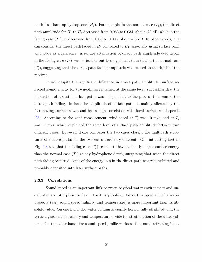
Third, despite the significant difference in direct path amplitude, surface re-

flected sound energy for two geotimes remained at the same level, suggesting that the

fluctuation of acoustic surface paths was independent to the process that caused the

direct path fading. In fact, the amplitude of surface paths is mainly affected by the

fast-moving surface waves and has a high correlation with local surface wind speeds

[25]. According to the wind measurement, wind speed at T1 was 10 m/s, and at T2

was 11 m/s, which explained the same level of surface path amplitude between two

different cases. However, if one compares the two cases closely, the multipath struc-

tures of surface paths for the two cases were very different. One interesting fact in

Fig. 2.3 was that the fading case (T2) seemed to have a slightly higher surface energy

than the normal case (T1) at any hydrophone depth, suggesting that when the direct

path fading occurred, some of the energy loss in the direct path was redistributed and

probably deposited into later surface paths.

2.3.3 Correlations

Sound speed is an important link between physical water environment and un-

derwater acoustic pressure field. For this problem, the vertical gradient of a water

property (e.g., sound speed, salinity, and temperature) is more important than its ab-

solute value. On one hand, the water column is usually horizontally stratified, and the

vertical gradients of salinity and temperature decide the stratification of the water col-

umn. On the other hand, the sound speed profile works as the sound refracting index

21

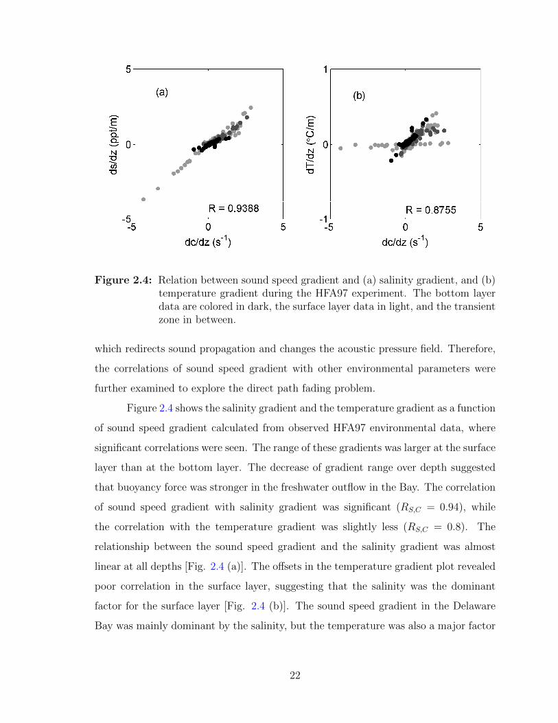
Figure 2.4: Relation between sound speed gradient and (a) salinity gradient, and (b)temperature gradient during the HFA97 experiment. The bottom layerdata are colored in dark, the surface layer data in light, and the transientzone in between.

which redirects sound propagation and changes the acoustic pressure field. Therefore,

the correlations of sound speed gradient with other environmental parameters were

further examined to explore the direct path fading problem.

Figure 2.4 shows the salinity gradient and the temperature gradient as a function

of sound speed gradient calculated from observed HFA97 environmental data, where

significant correlations were seen. The range of these gradients was larger at the surface

layer than at the bottom layer. The decrease of gradient range over depth suggested

that buoyancy force was stronger in the freshwater outflow in the Bay. The correlation

of sound speed gradient with salinity gradient was significant (RS,C = 0.94), while

the correlation with the temperature gradient was slightly less (RS,C = 0.8). The

relationship between the sound speed gradient and the salinity gradient was almost

linear at all depths [Fig. 2.4 (a)]. The offsets in the temperature gradient plot revealed

poor correlation in the surface layer, suggesting that the salinity was the dominant

factor for the surface layer [Fig. 2.4 (b)]. The sound speed gradient in the Delaware

Bay was mainly dominant by the salinity, but the temperature was also a major factor

22

especially in the bottom layer.

Table 2.2: Correlation coefficients of sound speed gradient at different depths withtide (Rh,c) and current velocity (Ru,c).

Depth (m) 2 7 12 overall

Rh,c -0.0179 -0.4440 -0.3647 -0.4740

Ru,c -0.1789 -0.2588 -0.0040 -0.1096

Table 2.2 lists correlation coefficients of the sound speed gradient for different

depths with the tide and the current velocity. Overall, the tide had a better correlation

with sound speed gradient than the current velocity. The overall correlation between

sound speed gradient and tide for the whole water column was significant (Rh,c =

−0.4740 > 0.1). The negative sign suggested that the low tide was associated with a

positive sound speed gradient while the high tide was with a negative one. The sound

speed gradient in transient and deeper layers (7 or 12 m) was much more correlated with

the tide than the surface layer (2 m). However, the surface layer sound speed gradient

correlation with the current velocity (Rh,u = −0.1789) was higher than the deeper

layer, despite the overall poor correlation of the whole water column (Rh,u = −0.1096),

indicating that the sound speed gradient in surface layer was dominant by the river

outflow, while the sound speed gradient of bottom later was more related to the tidal

cycle. Good correlation with the tide suggested that the variation of sound speed was

linked to the physical processes that with the same phase of the tide, which drives the

water column variation and further to the direct path fading problem.

2.4 The Mechanism

Theoretically speaking, the fluctuation of sound direct paths can only be in-

duced by the inhomogeneity of the water column, including a wide variety of factors

such as water properties, suspending particles biomass, etc., which redistributes the

sound energy by reflection, scattering, and refraction. Field observations and data

analysis suggested that the direct path fading was associated with a positive sound

23

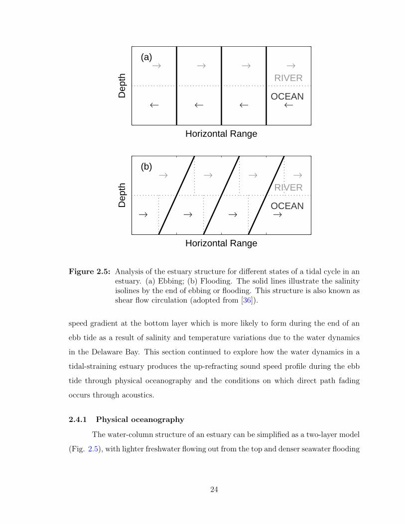
RIVER

OCEAN

(a)→ → → →

← ← ← ←

Dep

thHorizontal Range

RIVER

OCEAN

(b)→ → → →

→ → → →

Dep

th

Horizontal Range

Figure 2.5: Analysis of the estuary structure for different states of a tidal cycle in anestuary. (a) Ebbing; (b) Flooding. The solid lines illustrate the salinityisolines by the end of ebbing or flooding. This structure is also known asshear flow circulation (adopted from [36]).

speed gradient at the bottom layer which is more likely to form during the end of an

ebb tide as a result of salinity and temperature variations due to the water dynamics

in the Delaware Bay. This section continued to explore how the water dynamics in a

tidal-straining estuary produces the up-refracting sound speed profile during the ebb

tide through physical oceanography and the conditions on which direct path fading

occurs through acoustics.

2.4.1 Physical oceanography

The water-column structure of an estuary can be simplified as a two-layer model

(Fig. 2.5), with lighter freshwater flowing out from the top and denser seawater flooding

24

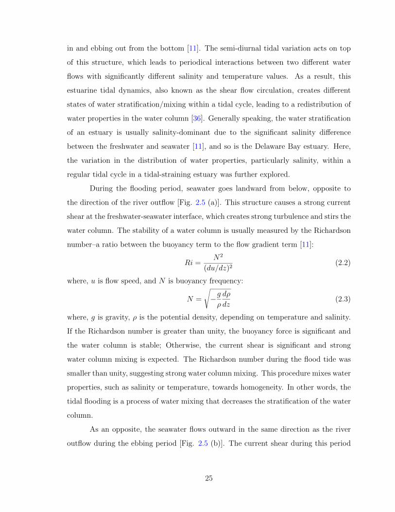
in and ebbing out from the bottom [11]. The semi-diurnal tidal variation acts on top

of this structure, which leads to periodical interactions between two different water

flows with significantly different salinity and temperature values. As a result, this

estuarine tidal dynamics, also known as the shear flow circulation, creates different

states of water stratification/mixing within a tidal cycle, leading to a redistribution of

water properties in the water column [36]. Generally speaking, the water stratification

of an estuary is usually salinity-dominant due to the significant salinity difference

between the freshwater and seawater [11], and so is the Delaware Bay estuary. Here,

the variation in the distribution of water properties, particularly salinity, within a

regular tidal cycle in a tidal-straining estuary was further explored.

During the flooding period, seawater goes landward from below, opposite to

the direction of the river outflow [Fig. 2.5 (a)]. This structure causes a strong current

shear at the freshwater-seawater interface, which creates strong turbulence and stirs the

water column. The stability of a water column is usually measured by the Richardson

number–a ratio between the buoyancy term to the flow gradient term [11]:

Ri =N2

(du/dz)2(2.2)

where, u is flow speed, and N is buoyancy frequency:

N =

√−gρ

dρ

dz(2.3)

where, g is gravity, ρ is the potential density, depending on temperature and salinity.

If the Richardson number is greater than unity, the buoyancy force is significant and

the water column is stable; Otherwise, the current shear is significant and strong

water column mixing is expected. The Richardson number during the flood tide was

smaller than unity, suggesting strong water column mixing. This procedure mixes water

properties, such as salinity or temperature, towards homogeneity. In other words, the

tidal flooding is a process of water mixing that decreases the stratification of the water

column.

As an opposite, the seawater flows outward in the same direction as the river

outflow during the ebbing period [Fig. 2.5 (b)]. The current shear during this period

25

is much less than the flooding period. Thus, the Richardson number is greater than

unity and the buoyancy force is dominant, suggesting a stable, stratified water column.

As a result, water flows move horizontally with small vertical property exchange. With

less heavy and less saline river water steadily flowing out in the surface layer without

much interaction with the deep, the salinity of upper layers continuously decreases.

Eventually, the isohaline tilts seaward during the ebbing period [Fig. 2.5 (b)] as the

time goes on. By the end of the ebb tide, the incline of the isohaline reaches the

maximum, and in terms of the vertical profile, it appears as a strong positive salinity

gradient. In other words, the ebb tide increases the stratification of the water column,

which reaches a maximum by the end of ebbing, and the water column ends up with a

strong positive salinity gradient. In terms of sound speed, which increases with salinity,

temperature and pressure (Eq. 2.1), a uniform sound speed profile is more likely to

form at the end of flood tide, while a positive sound speed gradient at the end of ebb

tide, as a result of shear flow circulation in a tidal straining estuary.

2.4.2 Acoustics

Sound bends towards the layer that has lower sound speed. The positive sound

speed gradient appearing at the end of ebb tide refracts the sound energy away from

the bottom. The possible explanations for the decrease of acoustic direct path energy

include two folds. One is due to the energy defocusing of a refracted ray cone [1].

The other is due to the existence of the bottom boundary that blocks the possible

incoming energy from below. An extreme example is the shadow zone, i.e., when the

sound speed gradient is significant enough, a direct path shadow zone will be created

near the seafloor, which can cause significant intensity fading for the direct path signal.

For the HFA97 experiment, the source and receivers were all close to the bottom, we

suggested that the cause of significant direct path fading was similar to the shadow

zone theory. However, in order for the significant direct-path fading to occur, a relation

between the geometrical condition of the acoustic source and receiver, together with

the sound speed gradient of the water column must be satisfied.

26

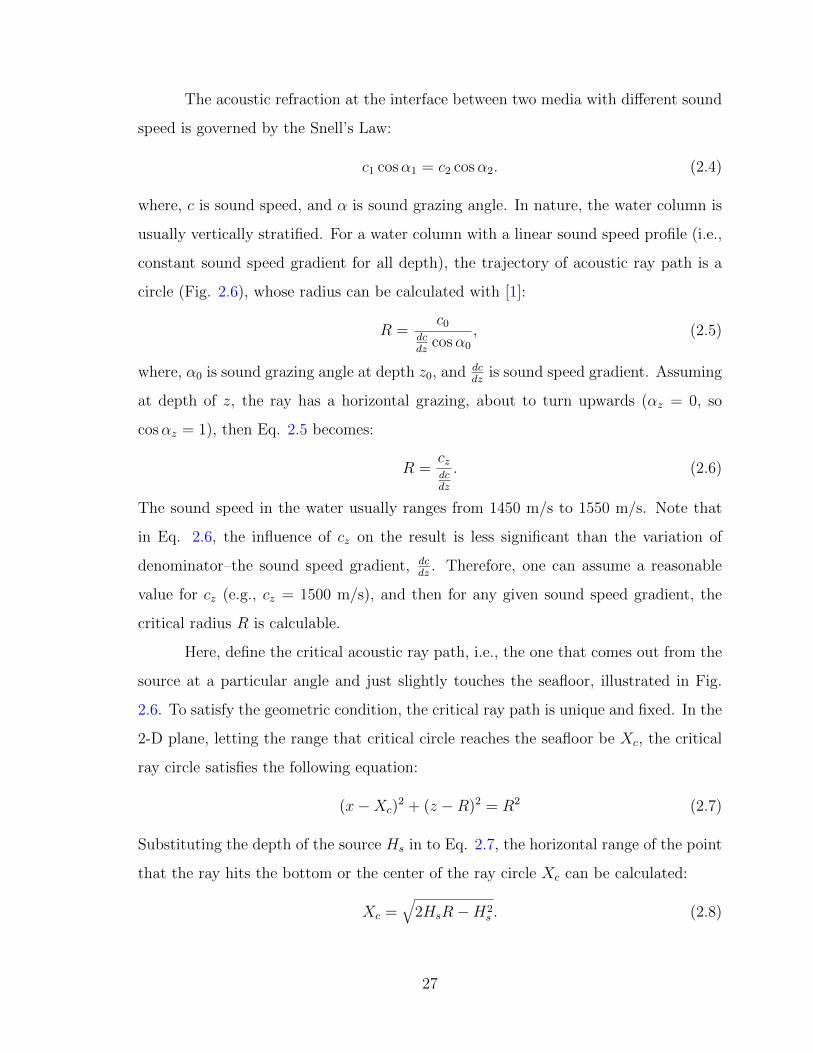
The acoustic refraction at the interface between two media with different sound

speed is governed by the Snell’s Law:

c1 cosα1 = c2 cosα2. (2.4)

where, c is sound speed, and α is sound grazing angle. In nature, the water column is

usually vertically stratified. For a water column with a linear sound speed profile (i.e.,

constant sound speed gradient for all depth), the trajectory of acoustic ray path is a

circle (Fig. 2.6), whose radius can be calculated with [1]:

R =c0

dcdz

cosα0

, (2.5)

where, α0 is sound grazing angle at depth z0, and dcdz

is sound speed gradient. Assuming

at depth of z, the ray has a horizontal grazing, about to turn upwards (αz = 0, so

cosαz = 1), then Eq. 2.5 becomes:

R =czdcdz

. (2.6)

The sound speed in the water usually ranges from 1450 m/s to 1550 m/s. Note that

in Eq. 2.6, the influence of cz on the result is less significant than the variation of

denominator–the sound speed gradient, dcdz

. Therefore, one can assume a reasonable

value for cz (e.g., cz = 1500 m/s), and then for any given sound speed gradient, the

critical radius R is calculable.

Here, define the critical acoustic ray path, i.e., the one that comes out from the

source at a particular angle and just slightly touches the seafloor, illustrated in Fig.

2.6. To satisfy the geometric condition, the critical ray path is unique and fixed. In the

2-D plane, letting the range that critical circle reaches the seafloor be Xc, the critical

ray circle satisfies the following equation:

(x−Xc)2 + (z −R)2 = R2 (2.7)

Substituting the depth of the source Hs in to Eq. 2.7, the horizontal range of the point

that the ray hits the bottom or the center of the ray circle Xc can be calculated:

Xc =√

2HsR−H2s . (2.8)

27

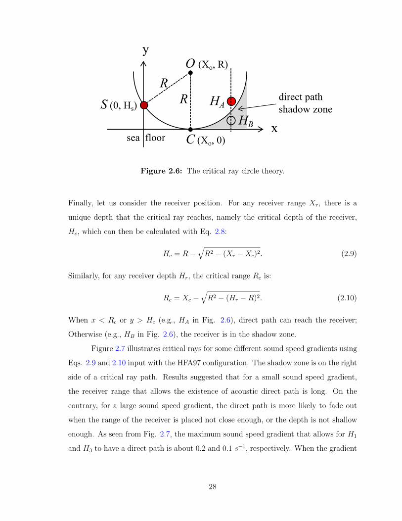
O (Xo, R)

S (0, Hs)

C (Xo, 0)x

y

HA

HB

direct path shadow zone

sea floor

RR

Figure 2.6: The critical ray circle theory.

Finally, let us consider the receiver position. For any receiver range Xr, there is a

unique depth that the critical ray reaches, namely the critical depth of the receiver,

Hc, which can then be calculated with Eq. 2.8:

Hc = R−√R2 − (Xr −Xc)2. (2.9)

Similarly, for any receiver depth Hr, the critical range Rc is:

Rc = Xc −√R2 − (Hr −R)2. (2.10)

When x < Rc or y > Hc (e.g., HA in Fig. 2.6), direct path can reach the receiver;

Otherwise (e.g., HB in Fig. 2.6), the receiver is in the shadow zone.

Figure 2.7 illustrates critical rays for some different sound speed gradients using

Eqs. 2.9 and 2.10 input with the HFA97 configuration. The shadow zone is on the right

side of a critical ray path. Results suggested that for a small sound speed gradient,

the receiver range that allows the existence of acoustic direct path is long. On the

contrary, for a large sound speed gradient, the direct path is more likely to fade out

when the range of the receiver is placed not close enough, or the depth is not shallow

enough. As seen from Fig. 2.7, the maximum sound speed gradient that allows for H1

and H3 to have a direct path is about 0.2 and 0.1 s−1, respectively. When the gradient

28

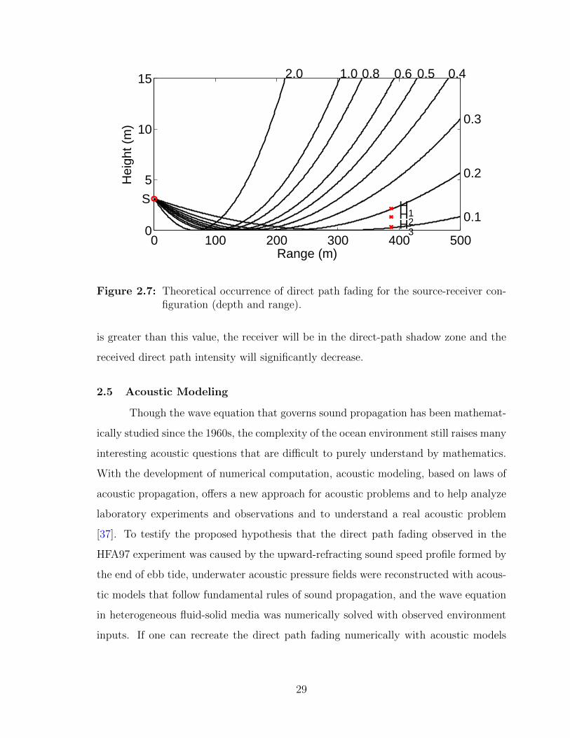
0 100 200 300 400 5000

5

10

15

0.1

0.2

0.3

0.40.50.60.81.02.0

S H1H2H3

Range (m)

Hei

ght (

m)

Figure 2.7: Theoretical occurrence of direct path fading for the source-receiver con-figuration (depth and range).

is greater than this value, the receiver will be in the direct-path shadow zone and the

received direct path intensity will significantly decrease.

2.5 Acoustic Modeling

Though the wave equation that governs sound propagation has been mathemat-

ically studied since the 1960s, the complexity of the ocean environment still raises many

interesting acoustic questions that are difficult to purely understand by mathematics.

With the development of numerical computation, acoustic modeling, based on laws of

acoustic propagation, offers a new approach for acoustic problems and to help analyze

laboratory experiments and observations and to understand a real acoustic problem

[37]. To testify the proposed hypothesis that the direct path fading observed in the

HFA97 experiment was caused by the upward-refracting sound speed profile formed by

the end of ebb tide, underwater acoustic pressure fields were reconstructed with acous-

tic models that follow fundamental rules of sound propagation, and the wave equation

in heterogeneous fluid-solid media was numerically solved with observed environment

inputs. If one can recreate the direct path fading numerically with acoustic models

29

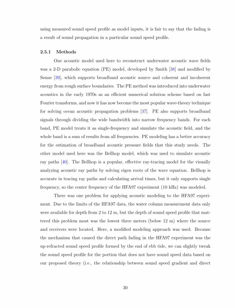
using measured sound speed profile as model inputs, it is fair to say that the fading is

a result of sound propagation in a particular sound speed profile.

2.5.1 Methods

One acoustic model used here to reconstruct underwater acoustic wave fields

was a 2-D parabolic equation (PE) model, developed by Smith [38] and modified by

Senne [39], which supports broadband acoustic source and coherent and incoherent

energy from rough surface boundaries. The PE method was introduced into underwater

acoustics in the early 1970s as an efficient numerical solution scheme based on fast

Fourier transforms, and now it has now become the most popular wave-theory technique

for solving ocean acoustic propagation problems [37]. PE also supports broadband

signals through dividing the wide bandwidth into narrow frequency bands. For each

band, PE model treats it as single-frequency and simulate the acoustic field, and the

whole band is a sum of results from all frequencies. PE modeling has a better accuracy

for the estimation of broadband acoustic pressure fields that this study needs. The

other model used here was the Bellhop model, which was used to simulate acoustic

ray paths [40]. The Bellhop is a popular, effective ray-tracing model for the visually

analyzing acoustic ray paths by solving eigen roots of the wave equation. Bellhop is

accurate in tracing ray paths and calculating arrival times, but it only supports single

frequency, so the center frequency of the HFA97 experiment (10 kHz) was modeled.

There was one problem for applying acoustic modeling to the HFA97 experi-

ment. Due to the limits of the HFA97 data, the water column measurement data only

were available for depth from 2 to 12 m, but the depth of sound speed profile that mat-

tered this problem most was the lowest three meters (below 12 m) where the source

and receivers were located. Here, a modified modeling approach was used. Because

the mechanism that caused the direct path fading in the HFA97 experiment was the

up-refracted sound speed profile formed by the end of ebb tide, we can slightly tweak

the sound speed profile for the portion that does not have sound speed data based on

our proposed theory (i.e., the relationship between sound speed gradient and direct

30

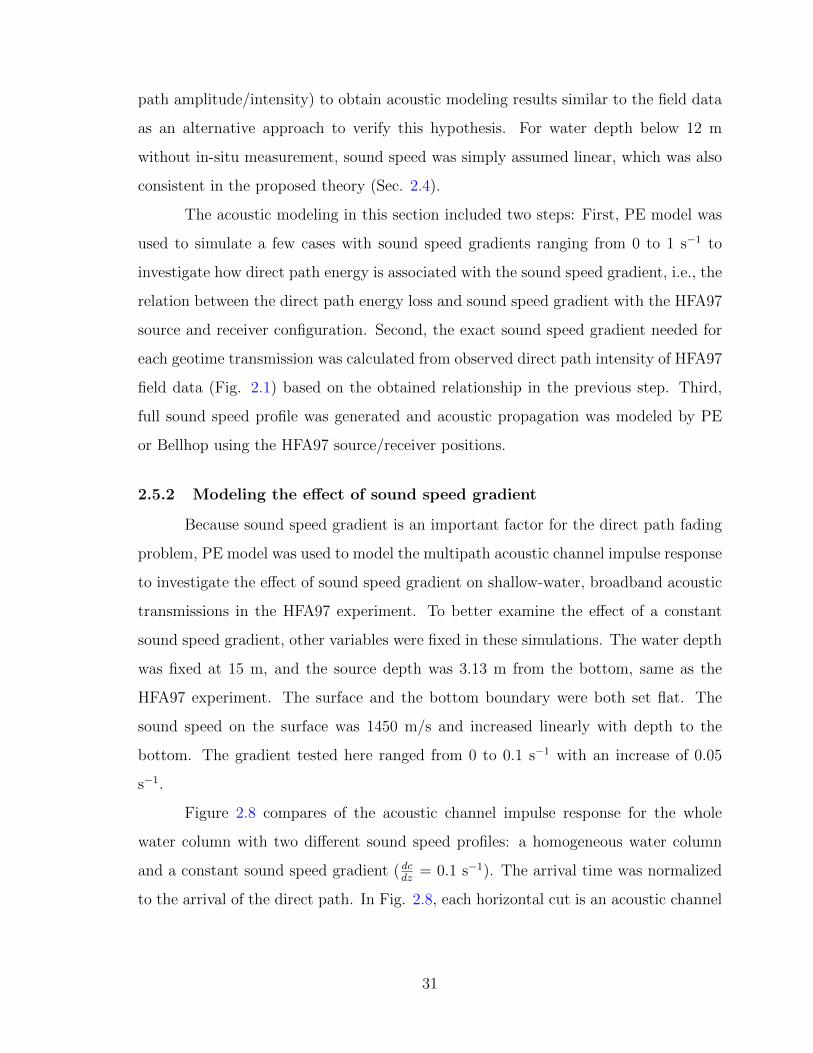
path amplitude/intensity) to obtain acoustic modeling results similar to the field data

as an alternative approach to verify this hypothesis. For water depth below 12 m

without in-situ measurement, sound speed was simply assumed linear, which was also

consistent in the proposed theory (Sec. 2.4).

The acoustic modeling in this section included two steps: First, PE model was

used to simulate a few cases with sound speed gradients ranging from 0 to 1 s−1 to

investigate how direct path energy is associated with the sound speed gradient, i.e., the

relation between the direct path energy loss and sound speed gradient with the HFA97

source and receiver configuration. Second, the exact sound speed gradient needed for

each geotime transmission was calculated from observed direct path intensity of HFA97

field data (Fig. 2.1) based on the obtained relationship in the previous step. Third,

full sound speed profile was generated and acoustic propagation was modeled by PE

or Bellhop using the HFA97 source/receiver positions.

2.5.2 Modeling the effect of sound speed gradient

Because sound speed gradient is an important factor for the direct path fading

problem, PE model was used to model the multipath acoustic channel impulse response

to investigate the effect of sound speed gradient on shallow-water, broadband acoustic

transmissions in the HFA97 experiment. To better examine the effect of a constant

sound speed gradient, other variables were fixed in these simulations. The water depth

was fixed at 15 m, and the source depth was 3.13 m from the bottom, same as the

HFA97 experiment. The surface and the bottom boundary were both set flat. The

sound speed on the surface was 1450 m/s and increased linearly with depth to the

bottom. The gradient tested here ranged from 0 to 0.1 s−1 with an increase of 0.05

s−1.

Figure 2.8 compares of the acoustic channel impulse response for the whole

water column with two different sound speed profiles: a homogeneous water column

and a constant sound speed gradient ( dcdz

= 0.1 s−1). The arrival time was normalized

to the arrival of the direct path. In Fig. 2.8, each horizontal cut is an acoustic channel

31

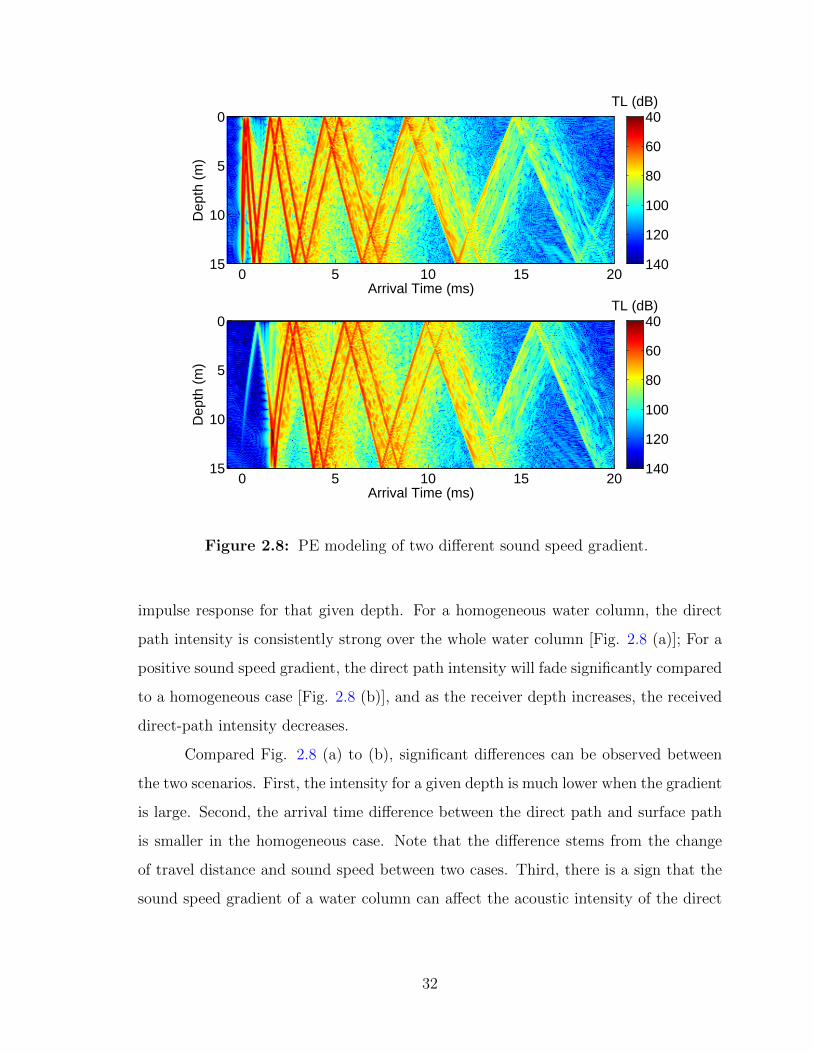
Arrival Time (ms)

De

pth

(m

)

0 5 10 15 20

0

5

10

15

TL (dB)40

60

80

100

120

140

Arrival Time (ms)

De

pth

(m

)

0 5 10 15 20

0

5

10

15

TL (dB)40

60

80

100

120

140

Figure 2.8: PE modeling of two different sound speed gradient.

impulse response for that given depth. For a homogeneous water column, the direct

path intensity is consistently strong over the whole water column [Fig. 2.8 (a)]; For a

positive sound speed gradient, the direct path intensity will fade significantly compared

to a homogeneous case [Fig. 2.8 (b)], and as the receiver depth increases, the received

direct-path intensity decreases.

Compared Fig. 2.8 (a) to (b), significant differences can be observed between

the two scenarios. First, the intensity for a given depth is much lower when the gradient

is large. Second, the arrival time difference between the direct path and surface path

is smaller in the homogeneous case. Note that the difference stems from the change

of travel distance and sound speed between two cases. Third, there is a sign that the

sound speed gradient of a water column can affect the acoustic intensity of the direct

32

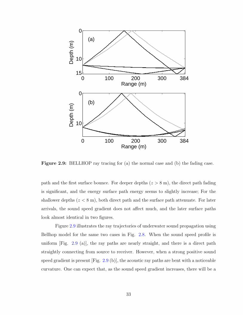
0 100 200 300 384

0

10

15

Range (m)

Dep

th (

m) (a)

0 100 200 300 384

0

10

Range (m)

Dep

th (

m) (b)

Figure 2.9: BELLHOP ray tracing for (a) the normal case and (b) the fading case.

path and the first surface bounce. For deeper depths (z > 8 m), the direct path fading

is significant, and the energy surface path energy seems to slightly increase; For the

shallower depths (z < 8 m), both direct path and the surface path attenuate. For later

arrivals, the sound speed gradient does not affect much, and the later surface paths

look almost identical in two figures.

Figure 2.9 illustrates the ray trajectories of underwater sound propagation using

Bellhop model for the same two cases in Fig. 2.8. When the sound speed profile is

uniform [Fig. 2.9 (a)], the ray paths are nearly straight, and there is a direct path

straightly connecting from source to receiver. However, when a strong positive sound

speed gradient is present [Fig. 2.9 (b)], the acoustic ray paths are bent with a noticeable

curvature. One can expect that, as the sound speed gradient increases, there will be a

33

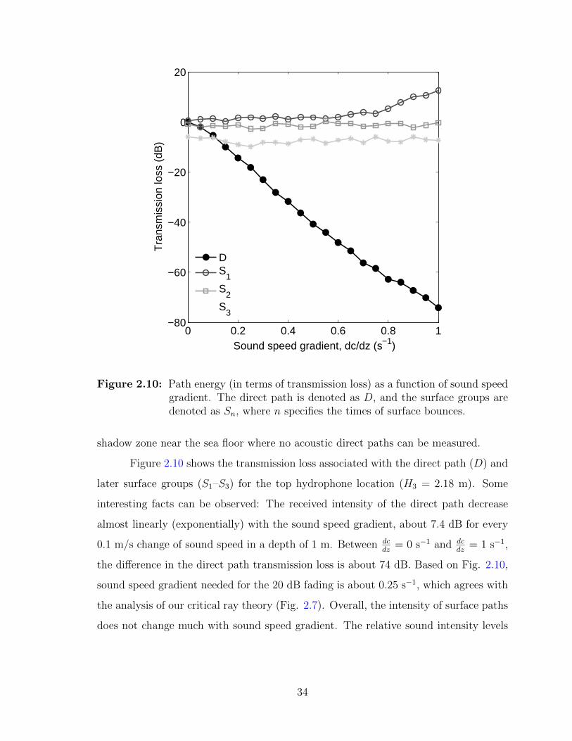
0 0.2 0.4 0.6 0.8 1−80

−60

−40

−20

0

20

Sound speed gradient, dc/dz (s−1

)

Tra

nsm

issio

n lo

ss (

dB

)

D

S1

S2

S3

Figure 2.10: Path energy (in terms of transmission loss) as a function of sound speedgradient. The direct path is denoted as D, and the surface groups aredenoted as Sn, where n specifies the times of surface bounces.

shadow zone near the sea floor where no acoustic direct paths can be measured.

Figure 2.10 shows the transmission loss associated with the direct path (D) and

later surface groups (S1–S3) for the top hydrophone location (H3 = 2.18 m). Some

interesting facts can be observed: The received intensity of the direct path decrease

almost linearly (exponentially) with the sound speed gradient, about 7.4 dB for every

0.1 m/s change of sound speed in a depth of 1 m. Between dcdz

= 0 s−1 and dcdz

= 1 s−1,

the difference in the direct path transmission loss is about 74 dB. Based on Fig. 2.10,

sound speed gradient needed for the 20 dB fading is about 0.25 s−1, which agrees with

the analysis of our critical ray theory (Fig. 2.7). Overall, the intensity of surface paths

does not change much with sound speed gradient. The relative sound intensity levels

34

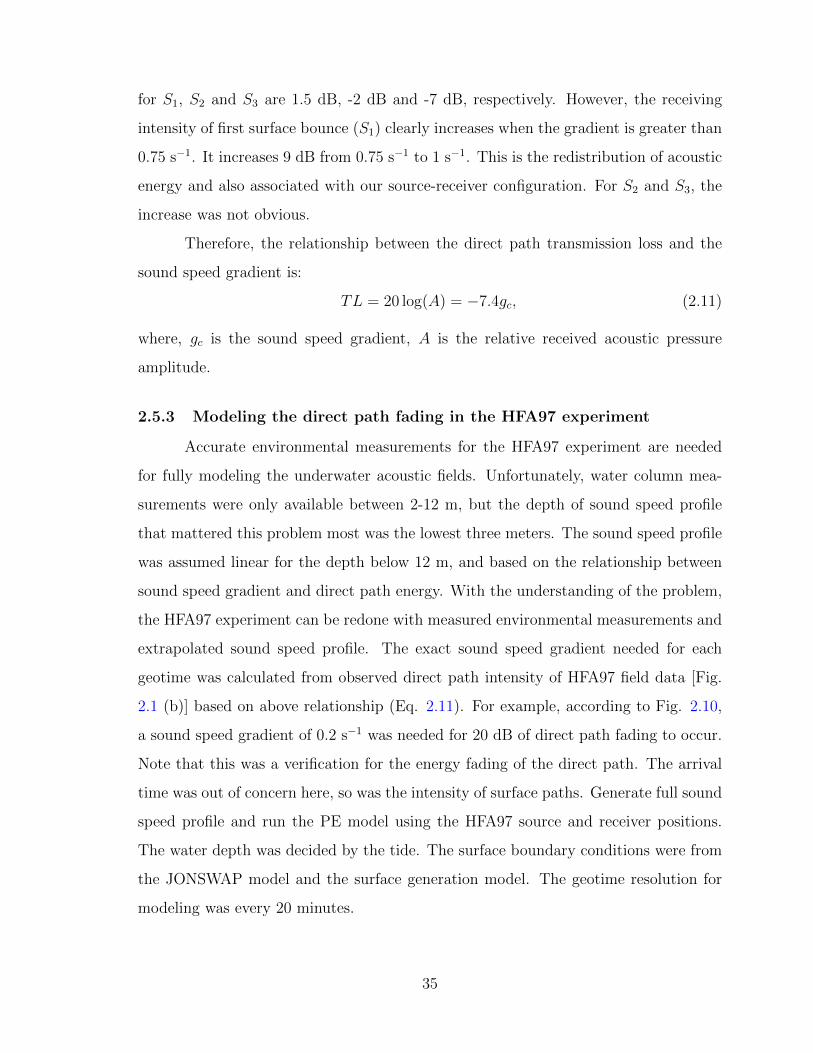
for S1, S2 and S3 are 1.5 dB, -2 dB and -7 dB, respectively. However, the receiving

intensity of first surface bounce (S1) clearly increases when the gradient is greater than

0.75 s−1. It increases 9 dB from 0.75 s−1 to 1 s−1. This is the redistribution of acoustic

energy and also associated with our source-receiver configuration. For S2 and S3, the

increase was not obvious.

Therefore, the relationship between the direct path transmission loss and the

sound speed gradient is:

TL = 20 log(A) = −7.4gc, (2.11)

where, gc is the sound speed gradient, A is the relative received acoustic pressure

amplitude.

2.5.3 Modeling the direct path fading in the HFA97 experiment

Accurate environmental measurements for the HFA97 experiment are needed

for fully modeling the underwater acoustic fields. Unfortunately, water column mea-

surements were only available between 2-12 m, but the depth of sound speed profile

that mattered this problem most was the lowest three meters. The sound speed profile

was assumed linear for the depth below 12 m, and based on the relationship between

sound speed gradient and direct path energy. With the understanding of the problem,

the HFA97 experiment can be redone with measured environmental measurements and

extrapolated sound speed profile. The exact sound speed gradient needed for each

geotime was calculated from observed direct path intensity of HFA97 field data [Fig.

2.1 (b)] based on above relationship (Eq. 2.11). For example, according to Fig. 2.10,

a sound speed gradient of 0.2 s−1 was needed for 20 dB of direct path fading to occur.

Note that this was a verification for the energy fading of the direct path. The arrival

time was out of concern here, so was the intensity of surface paths. Generate full sound

speed profile and run the PE model using the HFA97 source and receiver positions.

The water depth was decided by the tide. The surface boundary conditions were from

the JONSWAP model and the surface generation model. The geotime resolution for

modeling was every 20 minutes.

35

−1 0 1 2 3 4 50

0.5

1

H1 = 2.18 m(a)

Arrival Time (ms)

Am

p.

(p/p

0)

−1 0 1 2 3 4 50

0.5

1

H2 = 1.33 m(b)

Arrival Time (ms)

Am

p.

(p/p

0)

−1 0 1 2 3 4 50

0.5

1

H3 = 0.33 m(c)

Arrival Time (ms)

Am

p.

(p/p

0)

−1 0 1 2 3 4 50

0.5

1

H1 = 2.18 m(d)

Arrival Time (ms)

Am

p.

(p/p

0)

−1 0 1 2 3 4 50

0.5

1

H2 = 1.33 m(e)

Arrival Time (ms)

Am

p.

(p/p

0)

−1 0 1 2 3 4 50

0.5

1

H3 = 0.33 m(f)

Arrival Time (ms)

Am

p.

(p/p

0)

Figure 2.11: Modeling acoustic channel responses for all three hydrophones at differ-ent depths at T1 and T2. (a) Top hydrophone; (b) Middle hydrophone;and (c) Bottom Hydrophone. The amplitude of the channel response isrelative to the acoustic source pressure amplitude at 1 m.

Figure 2.11 shows the modeling results for acoustic channel impulse response

at two selected geotimes (T1, T2) at three hydrophone depths (H1, H2 and H3) in the

HFA97 experiment as a comparison to Fig. 2.3. Note that the amplitude of channel

impulse responses was normalized to the source level using the local top hydrophone,

and the arrival time was relative to the arrival of the direct path. Despite the amplitude

difference, modeling results (Fig. 2.11) exhibited similar features seen in the field

data (Fig. 2.3), including normal/fading difference and depth dependency, etc. The

PE model was able to capture the three facts that we observed in the field data,

including the direct path amplitude difference between two geotime cases, the direct

path amplitude decreasing over depth within the same case, and similar surface path

amplitude level. However, our model estimates less significant fading the direct path,

36

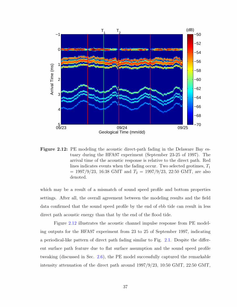
Geological Time (mm/dd)

Arr

iva

l T

ime

(m

s)

T

1T

2

09/23 09/24 09/25

−1

0

1

2

3

4

5

(dB)

−70

−68

−66

−64

−62

−60

−58

−56

−54

−52

−50

Figure 2.12: PE modeling the acoustic direct-path fading in the Delaware Bay es-tuary during the HFA97 experiment (September 23-25 of 1997). Thearrival time of the acoustic response is relative to the direct path. Redlines indicates events when the fading occur. Two selected geotimes, T1= 1997/9/23, 16:38 GMT and T2 = 1997/9/23, 22:50 GMT, are alsodenoted.

which may be a result of a mismatch of sound speed profile and bottom properties

settings. After all, the overall agreement between the modeling results and the field

data confirmed that the sound speed profile by the end of ebb tide can result in less

direct path acoustic energy than that by the end of the flood tide.

Figure 2.12 illustrates the acoustic channel impulse response from PE model-

ing outputs for the HFA97 experiment from 23 to 25 of September 1997, indicating

a periodical-like pattern of direct path fading similar to Fig. 2.1. Despite the differ-

ent surface path feature due to flat surface assumption and the sound speed profile

tweaking (discussed in Sec. 2.6), the PE model successfully captured the remarkable

intensity attenuation of the direct path around 1997/9/23, 10:50 GMT, 22:50 GMT,

37

and 1997/9/24, 11:00 GMT, confirming that the unique water column feature during

the end of ebb tide, particularly the positive sound speed gradient, was responsible for

the direct path fading phenomenon. The tidal pattern in the surface paths (Fig. 2.12)

also revealed the link with the end of the ebb tide. Our PE model was able to capture

the direct path fading with the sound speed gradient and confirmed the variation of

sound speed can cause the fading of the acoustic direct path in the HFA97 experiment

configuration. More data-model comparisons will be discussed in Sec. 2.6.

2.6 Discussions

During the HFA97 experiment, the acoustic direct path exhibited a strong ten-

dency to attenuate significantly during the end of low tide periods in the Delaware Bay

estuary (Fig. 2.1). Data analysis found significant water column differences between

the normal case and the fading case, especially that the direct path fading is associated

with a stratified water column formed during the ebbing period (Fig. 2.2). This lead

to a hypothesis that the periodical variation of salinity profile in the Delaware Bay

due to tidal-forcing water dynamics (Fig. 2.5) formed a positive sound speed gradient

that can redirect the sound energy away from our deep receivers (Figs. 2.6 and 2.7).

Then, the acoustic model was used to analyze the problem and confirm the positive

sound speed profile is able to cause the significant direct path fading feature through

reconstructing underwater acoustic pressure fields similar to the HFA97 field data us-

ing up-refracting sound speed profiles. The direct path fading is an interesting case of

acoustic propagation in the complicated, nature time-varying ocean environment. In

this section, physical oceanography and acoustic perspectives of the direct path fading

were further discussed.

2.6.1 Physical oceanography

Though the direct-path fading was more likely to occur during the later portion

of the ebb tide due to the significant water stratification forming positive sound speed

gradient at that period, the HFA97 data records (e.g., around the end of September 24,

38

1997 in Fig. 2.1) also suggested that this fading may not occur in every tidal cycle. The

truth is, the stratification of the water column is a very complicated process influenced

by local water dynamics and many other physical processes [11]. Though the main

factor for the stratification and mixing in estuaries like the Delaware Bay is the tidal

forcing, other factors could also contribute to the mixing of the water column.

First, the semi-diurnal tidal straining is the major driving factor responsible for

the direct path fading phenomenon periodically observed during the HFA97 experi-

ment. Tidal processes in the Delaware Bay influence sound speed profile on a daily

basis through modification of water column properties such as salinity and tempera-

ture. The water column modification by the shear flow circulation is the case for many

tidal-straining estuaries [36]. Previous study suggests the salinity variation is the most

prominent factor among all water column properties in a tidal estuary that causes the

water stratification [36]. The strong correlation between sound speed and the salinity

from the HFA97 field data agrees that the salinity difference is the dominant factor

that leads to this problem in the Delaware estuary. Besides, other parameters such

as temperature or pressure contributes to the variation of sound speed profile in the

Delaware Bay in a minor degree during the September 1997. The sound-speed cor-

relation coefficients for temperature and for pressure during the HFA97 experiment

were 0.5 and 0.3, respectively, suggesting they are minor factors in sound speed profile

fluctuations compared to salinity variations; However, there is a possibility that sea-

sonal variability for temperature may be significant enough to overcome the salinity

difference. For instance, if the experiment was carried out in summer, we might expect

different direct path fading pattern as the temperature difference for the ocean and

the river varies. After all, the salinity variation during the tidal forcing is the most

important factor in a tidal straining estuary.

Second, the stratification of the water column is also related to environmental

processes such as storm tide, local wind history, river discharge and precipitation, etc.

Wind blowing over the sea surface can increase water mixing, especially for a high

wind with a long period [11]. In terms of this problem, it implies that after a long

39

period of strong, consistent winds, we may not expect the direct path fading to occur,

because the water column will be increasingly well-mixed. During the low tide period

(00:00 GMT) on September 26, 1997, the measured direct path had high amplitudes

throughout the whole low tide period, because the water column was nearly well-mixed

due to a continuous 12-hr high winds (greater than 9 m/s). Moreover, precipitation

and river discharge might increase the water stratification [11], and they can result in

the direct path fading during non low-tide periods, since they are not related to tidal

forcing. For example, there was a precipitation event occurred around 00:00 GMT

1997/9/24, which strengthened the upper freshwater layer. This might be the main

reason for the low intensity seen in Fig. 2.1 at that period. Noted that the river

discharge and precipitation also have strong seasonal variability. In some cases, they

may overcome the tidal forcing effect and become a dominant factor for the direct

path fluctuation. Also, one may expect a longer direct path fading period and a more

significant direct path fading, if the current strength increases which can achieve the

positive sound speed gradient earlier and stronger.

2.6.2 Acoustics

It was once thought that the direct path fading was a result of the bottom

path and the direct path coming in opposite phases and canceling each other, but this

explanation was soon found not hold for many reasons. First, the acoustic frequencies

used in the HFA97 were broadband, and therefore it was almost impossible for the

whole frequency band with a total of 18 kHz bandwidth to cancel out at the same

time. Second, the direct path fading occurred in more than one depths of the water

column, with the direct path fading being more significant at the increased depth. This

observation can not be explained by the phase constructing/destructing theory. Third,

the bottom of the Bay was not perfectly flat where the specular reflection occurs,

so the perfect cancellation of coherent phase was almost impossible to occur in the

HFA97 field experiment. Though the phase destruction was not the major cause of the

direct path problem, this problem was indeed frequency dependent. Due to the sound

40

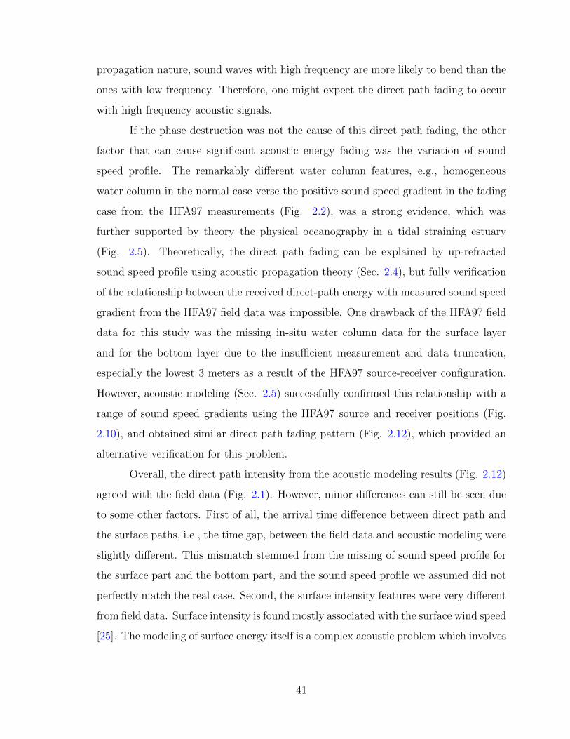
propagation nature, sound waves with high frequency are more likely to bend than the

ones with low frequency. Therefore, one might expect the direct path fading to occur

with high frequency acoustic signals.

If the phase destruction was not the cause of this direct path fading, the other

factor that can cause significant acoustic energy fading was the variation of sound

speed profile. The remarkably different water column features, e.g., homogeneous

water column in the normal case verse the positive sound speed gradient in the fading

case from the HFA97 measurements (Fig. 2.2), was a strong evidence, which was

further supported by theory–the physical oceanography in a tidal straining estuary

(Fig. 2.5). Theoretically, the direct path fading can be explained by up-refracted

sound speed profile using acoustic propagation theory (Sec. 2.4), but fully verification

of the relationship between the received direct-path energy with measured sound speed

gradient from the HFA97 field data was impossible. One drawback of the HFA97 field

data for this study was the missing in-situ water column data for the surface layer

and for the bottom layer due to the insufficient measurement and data truncation,

especially the lowest 3 meters as a result of the HFA97 source-receiver configuration.

However, acoustic modeling (Sec. 2.5) successfully confirmed this relationship with a

range of sound speed gradients using the HFA97 source and receiver positions (Fig.

2.10), and obtained similar direct path fading pattern (Fig. 2.12), which provided an

alternative verification for this problem.

Overall, the direct path intensity from the acoustic modeling results (Fig. 2.12)

agreed with the field data (Fig. 2.1). However, minor differences can still be seen due

to some other factors. First of all, the arrival time difference between direct path and

the surface paths, i.e., the time gap, between the field data and acoustic modeling were

slightly different. This mismatch stemmed from the missing of sound speed profile for

the surface part and the bottom part, and the sound speed profile we assumed did not

perfectly match the real case. Second, the surface intensity features were very different

from field data. Surface intensity is found mostly associated with the surface wind speed

[25]. The modeling of surface energy itself is a complex acoustic problem which involves

41

reflection, scattering, bubble effect, out-of-plane acoustic energy, etc. When modeling

Fig. 2.12, we focused on the direct path intensity so we simply assumed the flat surface,

but the more close modeling can be achieved in the future. Third, we assumed range-

independence in this study, but it was not the case in most estuarine environments.

In fact, the salinity and temperature distribution in an estuary is definitely range-

dependent, which will change of the curvature of the acoustic ray circle. However, the

modeling analysis we did in this paper did not account for the horizontal variation of

sound speed profile due to the limits of water column measurement, which may result

in the minor difference of direct path fading between the field data and the modeling

results. Finally, other assumptions from the PE model, e.g., 2-D plane, no bubble

effect, etc., all contributed to the data-model difference in some degrees. However, the

overall data-model agreement supported the variation of sound speed profile was the

major cause of the direct path fading.

Last but not least, this fading of sound direct path can pose serious problems

for acoustic systems that utilize the detection of acoustic direct path to apply in tidal

estuaries like the Delaware Bay. Note that the detection of the direct path in the fading

case (Fig. 2.2) was based on the tracking of direct path with previous and subsequent

sampling chirps, and as well as the calculation of the theoretical acoustic arrival time.

If there was only one single event, e.g., in real-time acoustic communication scenario,

it would be impossible to for the system to identify the direct path which may end

up with poor system performance due to so much weaker energy in direct path than

in surface paths. Though surface path energy components are strong, they are fast

fluctuated and highly time-varying (i.e., very unstable). In previous study, the tempo-

ral variability of the surface paths have been found harmful for underwater coherent

acoustic communication [26]. The fading of direct path together with fast fluctuat-

ing surface paths may be the reason for acoustic communication system failures as

previously reported due to the effects of tide [29]. If acoustic communication was per-

formed in such underwater acoustic channel, i.e., fading direct path and fluctuating,

the acoustic system can only relay on the fast changing surface path. Such a process

42

requires a series sophisticated phase tracking and channel equalization, which is a su-

per challenging topic for underwater acoustic communications. Though the HFA97 did

not transmit acoustic communication data during the experiment, we believed that

the effect of direct path fading on acoustic communication is significant and should be

further explore in the future.

2.7 Conclusions

This study explored the periodical-like intensity fading of the acoustic direct

path observed in the HFA97 experiment with a focus on the physical water dynamics

in a tidal-straining estuary as well as the acoustic propagation theory. This is a common

acoustic problem for many estuaries influenced by tidal forcing dynamics. Data and

model analyses confirmed that the periodical variation of sound speed profile due to

tidal forcing water dynamics in the Delaware Bay and the source and receiver positions

of the HFA97 experiment together are responsible for this phenomenon. Generally, the

fading of direct path increases with the increased gradient or decreased receiver depth.

Our direct path theory with source-receiver positions configuration can help to plan

future experiment or design acoustic applications in shallow tidal-straining estuaries

or similar water environments.

The direct path fading problem analyzed in this paper suggested that the acous-

tic propagation links closely with the physical environment and the processes and dy-

namics within it. Therefore, the acoustic propagation cannot be separated from the

physical environment and so does the acoustic applications that utilize the acoustic

propagation knowledge. Also, the fading of direct path found in this paper can is im-

portant for underwater acoustic communication in these regions and the environmental

variability should be considered when designing next-generation reliable underwater

acoustic systems. The effect of the direct path fading on acoustic communication and

other sonar systems will be further explored in the future.

The numerical models are useful tools for an actual time-vary acoustic problem,

which can help verify a theory and re-examine field data. This paper only used a

43

2-D PE model with range-independence. In the future, the range-dependent sound

speed profile should be taken into account in future acoustic models, as well as other

inhomogeneity (ocean currents, bubbles), for a better capture of acoustic intensity. A

joint-oceanography modeling needs for more complicated ocean acoustic problem.

44

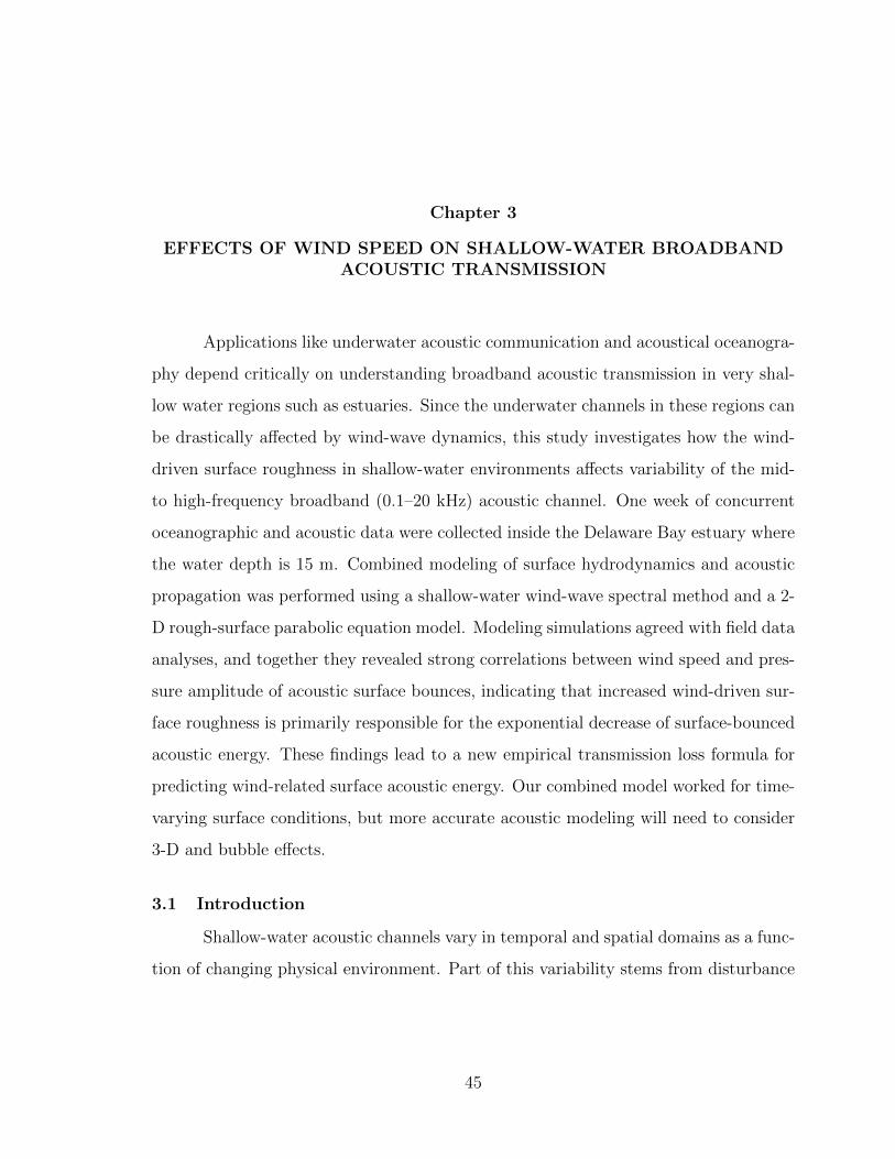
Chapter 3

EFFECTS OF WIND SPEED ON SHALLOW-WATER BROADBANDACOUSTIC TRANSMISSION

Applications like underwater acoustic communication and acoustical oceanogra-

phy depend critically on understanding broadband acoustic transmission in very shal-

low water regions such as estuaries. Since the underwater channels in these regions can

be drastically affected by wind-wave dynamics, this study investigates how the wind-

driven surface roughness in shallow-water environments affects variability of the mid-

to high-frequency broadband (0.1–20 kHz) acoustic channel. One week of concurrent

oceanographic and acoustic data were collected inside the Delaware Bay estuary where

the water depth is 15 m. Combined modeling of surface hydrodynamics and acoustic

propagation was performed using a shallow-water wind-wave spectral method and a 2-

D rough-surface parabolic equation model. Modeling simulations agreed with field data

analyses, and together they revealed strong correlations between wind speed and pres-

sure amplitude of acoustic surface bounces, indicating that increased wind-driven sur-

face roughness is primarily responsible for the exponential decrease of surface-bounced

acoustic energy. These findings lead to a new empirical transmission loss formula for

predicting wind-related surface acoustic energy. Our combined model worked for time-

varying surface conditions, but more accurate acoustic modeling will need to consider

3-D and bubble effects.

3.1 Introduction

Shallow-water acoustic channels vary in temporal and spatial domains as a func-

tion of changing physical environment. Part of this variability stems from disturbance

45

by surface winds [10]. Generally, wind raises roughness of the air-water boundary, in-

creases bubble entrainments and evokes other wave dynamics [41], causing deflection of

underlying sound propagation and fluctuation of acoustic pressure at receiver ends [2].

In shallow waters, these wind effects can be highly complex due to the multipath effect

from surface-bottom interactions that occur in depth-confined water columns [1]. Such

environmental variability makes shallow water acoustic channels extremely challeng-

ing when designing reliable, adaptive underwater acoustic communication systems or

other sonar systems [42]. Thus, improving the performance of these systems requires

understanding of the effects of wind-wave dynamics on shallow acoustic channels.

Over the recent decades, many have studied the effects of surface winds and

waves on underwater acoustics. Early research focused on acoustic backscattering from

sea surface for monostatic SONAR systems [5, 43]. However, due to increasing demands

for underwater acoustic communication, recent studies have shifted their attention to

high-frequency broadband bistatic systems, exploring the influences of wind-driven dy-

namics that include varying signal coherence [17, 44], fluctuating arrival time [45], fo-

cusing and defocusing [46], spreading angle [14], and shifting frequency [47]. Moreover,

several studies have investigated sound scattering from rough surfaces [44, 48, 14, 49].

However, a systematic examination of the wind-wave-acoustics relation has been rare

[50, 51], and only Weston and Ching [51] have focused on the single-frequency sound

propagation problem in a bistatic regime.

The complexity of this relation stems from two factors. First, differentiating

the various environmental effects in field acoustic data is difficult because this recorded

data has tangled within it many wind-related effects [10]. Second, there are presently

no well-acknowledged acoustic channel models [39] and this study requires numeri-

cal models that can handle a joint atmosphere-ocean-acoustics system. Our previous

studies explored the arrival fluctuation of surface-return paths with a JONSWAP wave

spectrum and BELLHOP ray-tracing modeling [34], and they developed a 2-D rough

surface parabolic equation (PE) model for time-evolving surface boundaries [39]. This

paper uses that 2-D rough-surface PE model and a more advanced shallow-water wave

46

spectrum for surface realization [52] in order to model acoustic propagation in shallow

water with a time-varying rough surface.

We investigate the effect of wind-driven surface dynamics on high-frequency

broadband bistatic acoustic transmission in a shallow fetch-limited estuarine environ-

ment using data from a High-Frequency Acoustic (HFA97) experiment conducted in

September 1997 in the Delaware Bay [10]. We focus on the amplitude fluctuation of

acoustic surface-bounced paths. Data and model analyses both support that pressure

amplitudes for surface groups decay exponentially when wind-driven surface roughness

increases. We propose a simple exponential decay model to predict theoretical pressure

amplitudes for higher wind speeds and higher surface groups.

The rest of the paper is organized as follows. Section II introduces the HFA97

field experiment and analyzes the field data. Section III presents the numerical models

and their comparable simulation results. Section IV predicts acoustic channel responses

for ideally increasing wind speeds using our combined model and an exponential decay

relationship that we propose predicts the theoretical amplitude for any wind speed.

Section V compares measured data to model results. Section VI discusses our findings,

and Section VII concludes the paper.

3.2 Field Data Analysis

3.2.1 Description of the Experiment

The HFA97 was a broadband acoustic field experiment conducted in the Delaware

Bay (central region: 39◦1′N, 75◦11′W; [Fig. 3.1(a)]) [10]. Two acoustic tripods were

built to transmit 0.345 s, 0.1–20 kHz acoustic chirp signals with a range of 387 m. Each

tripod had a transducer at 3.13 m and three hydrophones at 0.33 m, 1.33 m and 2.18

m from the base of the tripod. Acoustic chirps were transmitted and received with two

sampling strategies: 40-s transmission every 90 minutes, and 5-s transmission every 10

minutes. The time for each sampling task was referred as a geotime.

47

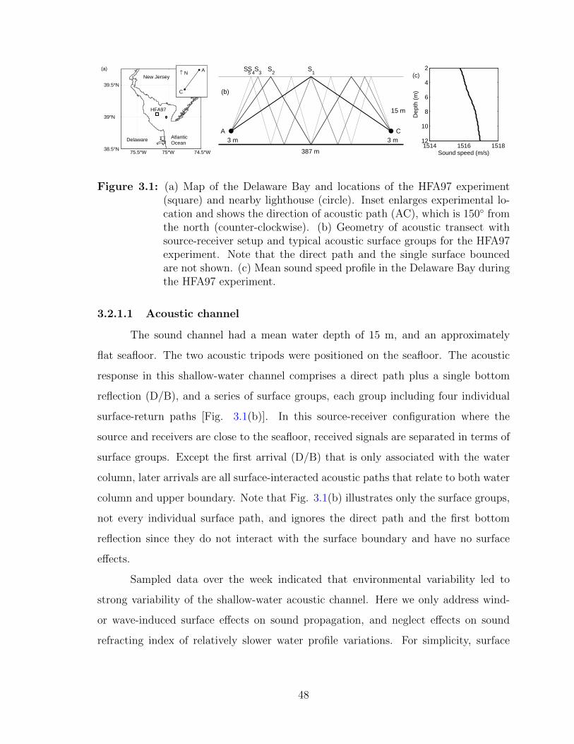
38.5°N

39°N

39.5°N

74.5°W75°W75.5°W

HFA97

AtlanticOcean

New Jersey

Delaware

C

A(a)↑ N

S5S

4S

3S

2S

1

...

A C

387 m

15 m

3 m 3 m

(b)

1514 1516 1518

2

4

6

8

10

12

Sound speed (m/s)

Dep

th (

m)

(c)

Figure 3.1: (a) Map of the Delaware Bay and locations of the HFA97 experiment(square) and nearby lighthouse (circle). Inset enlarges experimental lo-cation and shows the direction of acoustic path (AC), which is 150◦ fromthe north (counter-clockwise). (b) Geometry of acoustic transect withsource-receiver setup and typical acoustic surface groups for the HFA97experiment. Note that the direct path and the single surface bouncedare not shown. (c) Mean sound speed profile in the Delaware Bay duringthe HFA97 experiment.

3.2.1.1 Acoustic channel

The sound channel had a mean water depth of 15 m, and an approximately

flat seafloor. The two acoustic tripods were positioned on the seafloor. The acoustic

response in this shallow-water channel comprises a direct path plus a single bottom

reflection (D/B), and a series of surface groups, each group including four individual

surface-return paths [Fig. 3.1(b)]. In this source-receiver configuration where the

source and receivers are close to the seafloor, received signals are separated in terms of

surface groups. Except the first arrival (D/B) that is only associated with the water

column, later arrivals are all surface-interacted acoustic paths that relate to both water

column and upper boundary. Note that Fig. 3.1(b) illustrates only the surface groups,

not every individual surface path, and ignores the direct path and the first bottom

reflection since they do not interact with the surface boundary and have no surface

effects.

Sampled data over the week indicated that environmental variability led to

strong variability of the shallow-water acoustic channel. Here we only address wind-

or wave-induced surface effects on sound propagation, and neglect effects on sound

refracting index of relatively slower water profile variations. For simplicity, surface

48

groups are denoted as Sn, where n is the number of surface interactions, e.g., S1 is

the first surface group that includes a surface path (S), a surface-bottom path (SB), a

bottom-surface path (BS) and a bottom-surface-bottom path (BSB). Similarly, S2, S3,

S4 denote the second, the third and the fourth surface groups, respectively. Acoustic

scattering also depends on the grazing angle [51], and for S1 to S5, the theoretical

grazing angles, θ, at sea surface in a homogeneous medium are 4.43◦, 8.81◦, 13.09◦,

17.23◦ and 21.19◦, respectively. Although, these angles varied slightly due to tidal

variation of water depth and water properties, the fixed set up of this experiment was

helpful.

3.2.1.2 Surface measurements

A weather station at a nearby lighthouse [39◦2′54′′N, 75◦10′56′′W, marked as a

circle in Fig. 3.1(a)] measured the wind at 15m from ocean surface every 15 minutes

during the HFA97 experiment. A directional wind histogram (Fig. 3.2) shows that

winds blew at varying speeds and from various directions, causing strong wind-wave

interactions and dynamic surface conditions. Wind speeds (that we denote Uz with z

specifying the height in meters) ranged from 0 to 16 m/s with low-wind and high-wind

periods that evoked different stages of surface wave development. The dominant wind

directions were offshore, with high speed winds (U15 > 10 m/s) rarely coming from

southern directions.

Surface waves were measured indirectly by processing acoustic chirps received

by local hydrophones (referred to as “overhead acoustics”). Although the HFA97 ex-

periment did not directly measure surface wave spectra, a previous study [34] showed

that this overhead acoustics approach works in the Delaware Bay and can be used for

surface wind-wave spectral modeling. Waves were also captured via video and pho-

tography of the ocean surface by a fixed camera in the nearby lighthouse. All surface

photos were dated so sea state could be categorized at particular times.

49

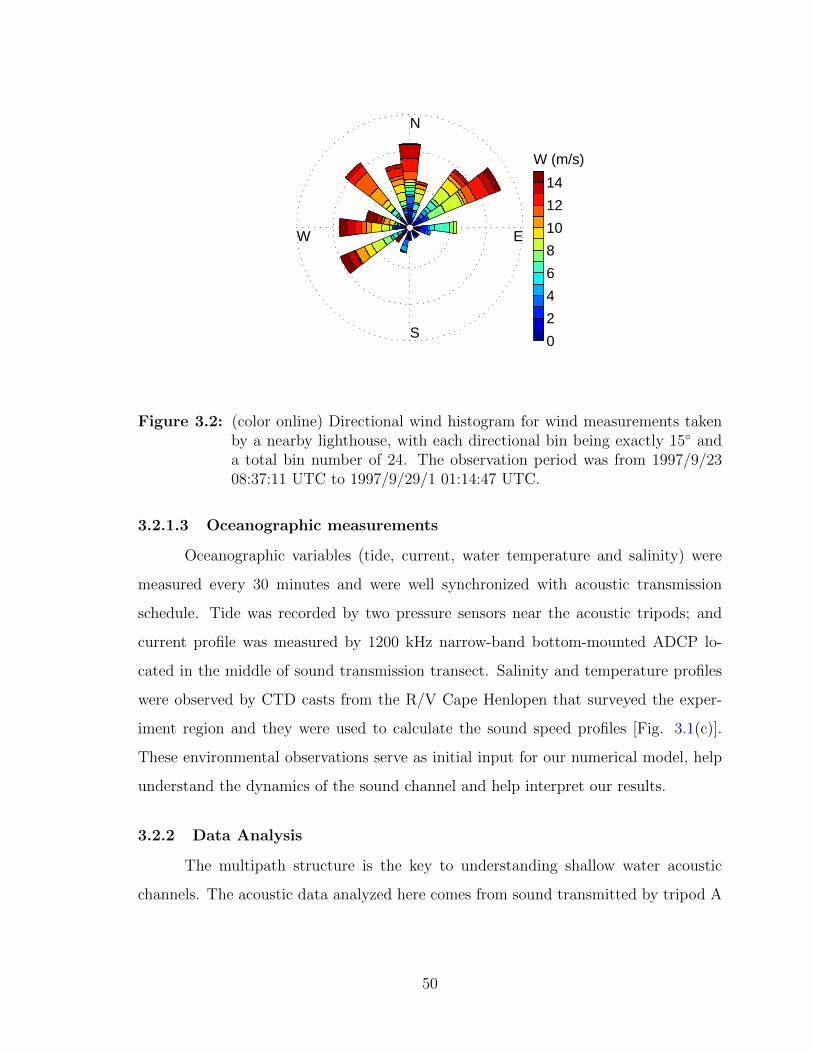
W E

S

N

0

2

4

6

8

10

12

14

W (m/s)

Figure 3.2: (color online) Directional wind histogram for wind measurements takenby a nearby lighthouse, with each directional bin being exactly 15◦ anda total bin number of 24. The observation period was from 1997/9/2308:37:11 UTC to 1997/9/29/1 01:14:47 UTC.

3.2.1.3 Oceanographic measurements

Oceanographic variables (tide, current, water temperature and salinity) were

measured every 30 minutes and were well synchronized with acoustic transmission

schedule. Tide was recorded by two pressure sensors near the acoustic tripods; and

current profile was measured by 1200 kHz narrow-band bottom-mounted ADCP lo-

cated in the middle of sound transmission transect. Salinity and temperature profiles

were observed by CTD casts from the R/V Cape Henlopen that surveyed the exper-

iment region and they were used to calculate the sound speed profiles [Fig. 3.1(c)].

These environmental observations serve as initial input for our numerical model, help

understand the dynamics of the sound channel and help interpret our results.

3.2.2 Data Analysis

The multipath structure is the key to understanding shallow water acoustic

channels. The acoustic data analyzed here comes from sound transmitted by tripod A

50

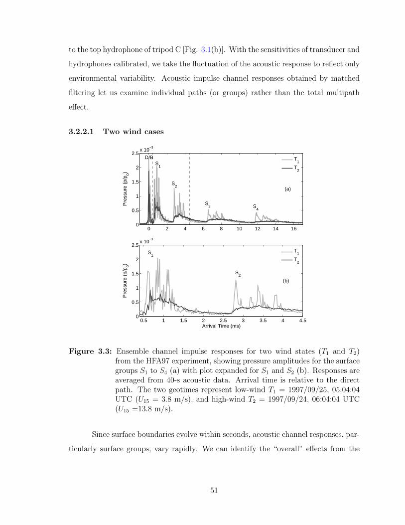
to the top hydrophone of tripod C [Fig. 3.1(b)]. With the sensitivities of transducer and

hydrophones calibrated, we take the fluctuation of the acoustic response to reflect only

environmental variability. Acoustic impulse channel responses obtained by matched

filtering let us examine individual paths (or groups) rather than the total multipath

effect.

3.2.2.1 Two wind cases

0 2 4 6 8 10 12 14 160

0.5

1

1.5

2

2.5x 10

−3

Pre

ssur

e (p

/p0)

D/B

S1

S2

S3 S

4

(a)

T1

T2

0.5 1 1.5 2 2.5 3 3.5 4 4.50

0.5

1

1.5

2

2.5x 10

−3

Pre

ssur

e (p

/p0)

Arrival Time (ms)

S1

S2

(b)

T1

T2

Figure 3.3: Ensemble channel impulse responses for two wind states (T1 and T2)from the HFA97 experiment, showing pressure amplitudes for the surfacegroups S1 to S4 (a) with plot expanded for S1 and S2 (b). Responses areaveraged from 40-s acoustic data. Arrival time is relative to the directpath. The two geotimes represent low-wind T1 = 1997/09/25, 05:04:04UTC (U15 = 3.8 m/s), and high-wind T2 = 1997/09/24, 06:04:04 UTC(U15 =13.8 m/s).

Since surface boundaries evolve within seconds, acoustic channel responses, par-

ticularly surface groups, vary rapidly. We can identify the “overall” effects from the

51

ensemble average of a series of acoustic channel responses at a given wind state. We

selected two wind cases for comparative analysis: low-wind T1 = 1997/09/25, 05:04:04

UTC (U15 = 3.8 m/s), and high-wind T2 = 1997/09/24, 06:04:04 UTC (U15 =13.8

m/s).

The ensemble channel responses for T1 and T2 (Fig. 3.3) show three notable

differences in pressure amplitudes. First, high and sharp peaks (in S1, S2, S3, etc.)

occur only in low wind not high wind. These peaks come from the part of the sound

energy that associates with each individual surface path, and can be explained by

specular reflection of sound waves from a flat/rough surface. When wind stress is

absent or weak, the sea surface is relatively calm and motionless, so the specular point

at the surface boundary is essentially fixed in position, rarely varying from ping to

ping. Thus, acoustic energy is perfectly reflected and restricted inside its original

paths. However, when wind speed increases, these peaks become blunt and cannot be

distinguished from each other because (a) wind-induced surface wave motion causes

travelling distance and time to fluctuate so peaks flatten during the averaging process;

(b) wave curvature scatters sound waves into a variety of angles so sound energy leaks

into other directions; and (c) bubbles entrained in the surface layer at high winds

attenuate sound further.

Second, the total energy of a surface group (integral over arrival time t) is

stronger at low winds than at high winds. This relates to surface roughness and signal

coherence. When two waves are coherent, they are in phase and their total pressure

is constructive and has a maximum amplitude. Then most of the acoustic energy is

in coherent paths, i.e., any acoustic reflections other than coherent reflection contain

much less energy due to smaller wave construction or deconstruction. This coherent

specular reflection produces the high amplitude seen for the relatively calm surface in

T1. Furthermore, increasing bubbles may attenuate the total energy.

Third, the tails of surface groups (e.g., during 1.4–2 ms or 4–4.5 ms in Fig.

3.3) are slightly raised in a high wind. This interesting but unexpected observation

“conflicts” with the theory of the Rayleigh parameter. We suggest that this extra tail

52

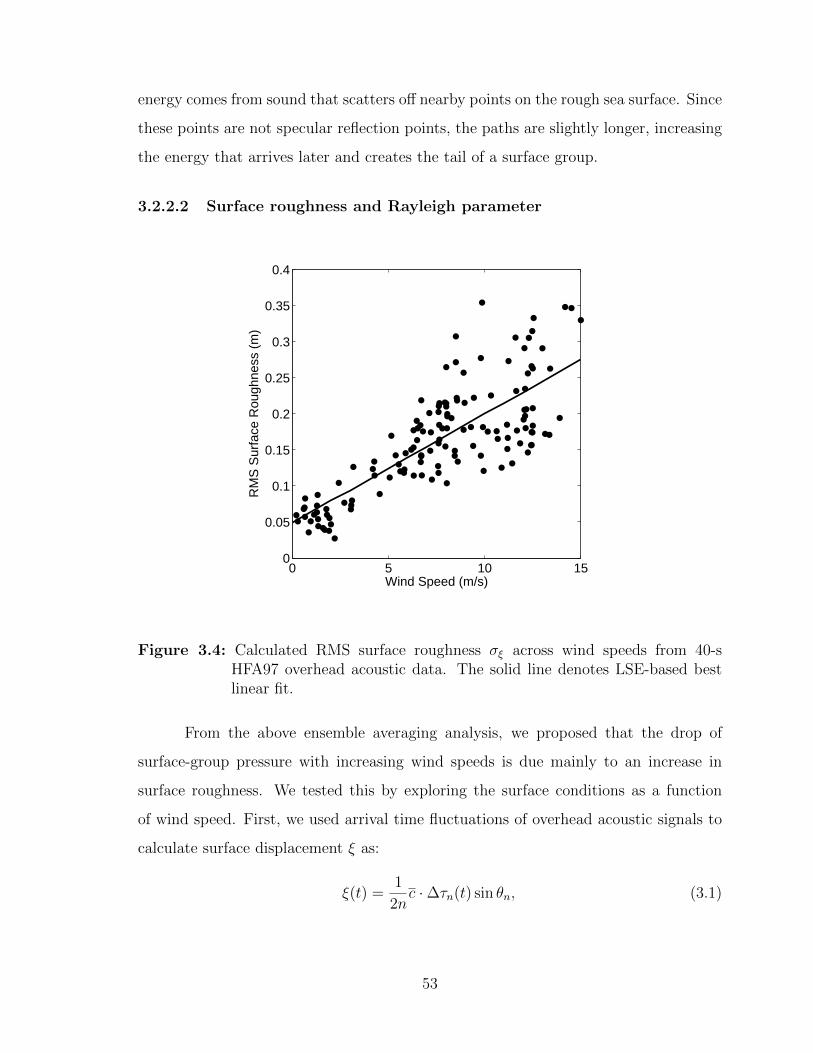
energy comes from sound that scatters off nearby points on the rough sea surface. Since

these points are not specular reflection points, the paths are slightly longer, increasing

the energy that arrives later and creates the tail of a surface group.

3.2.2.2 Surface roughness and Rayleigh parameter

0 5 10 150

0.05

0.1

0.15

0.2

0.25

0.3

0.35

0.4

Wind Speed (m/s)

RM

S S

urfa

ce R

ough

ness

(m

)

Figure 3.4: Calculated RMS surface roughness σξ across wind speeds from 40-sHFA97 overhead acoustic data. The solid line denotes LSE-based bestlinear fit.

From the above ensemble averaging analysis, we proposed that the drop of

surface-group pressure with increasing wind speeds is due mainly to an increase in

surface roughness. We tested this by exploring the surface conditions as a function

of wind speed. First, we used arrival time fluctuations of overhead acoustic signals to

calculate surface displacement ξ as:

ξ(t) =1

2nc ·∆τn(t) sin θn, (3.1)

53

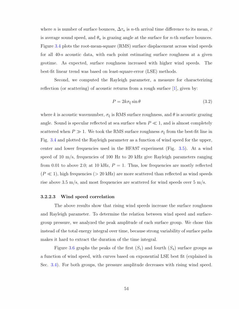
where n is number of surface bounces, ∆τn is n-th arrival time difference to its mean, c

is average sound speed, and θn is grazing angle at the surface for n-th surface bounces.

Figure 3.4 plots the root-mean-square (RMS) surface displacement across wind speeds

for all 40-s acoustic data, with each point estimating surface roughness at a given

geotime. As expected, surface roughness increased with higher wind speeds. The

best-fit linear trend was based on least-square-error (LSE) methods.

Second, we computed the Rayleigh parameter, a measure for characterizing

reflection (or scattering) of acoustic returns from a rough surface [1], given by:

P = 2kσξ sin θ (3.2)

where k is acoustic wavenumber, σξ is RMS surface roughness, and θ is acoustic grazing

angle. Sound is specular reflected at sea surface when P � 1, and is almost completely

scattered when P � 1. We took the RMS surface roughness σξ from the best-fit line in

Fig. 3.4 and plotted the Rayleigh parameter as a function of wind speed for the upper,

center and lower frequencies used in the HFA97 experiment (Fig. 3.5). At a wind

speed of 10 m/s, frequencies of 100 Hz to 20 kHz give Rayleigh parameters ranging

from 0.01 to above 2.0; at 10 kHz, P = 1. Thus, low frequencies are mostly reflected

(P � 1), high frequencies (> 20 kHz) are more scattered than reflected as wind speeds

rise above 3.5 m/s, and most frequencies are scattered for wind speeds over 5 m/s.

3.2.2.3 Wind speed correlation

The above results show that rising wind speeds increase the surface roughness

and Rayleigh parameter. To determine the relation between wind speed and surface-

group pressure, we analyzed the peak amplitude of each surface group. We chose this

instead of the total energy integral over time, because strong variability of surface paths

makes it hard to extract the duration of the time integral.

Figure 3.6 graphs the peaks of the first (S1) and fourth (S4) surface groups as

a function of wind speed, with curves based on exponential LSE best fit (explained in

Sec. 3.4). For both groups, the pressure amplitude decreases with rising wind speed.

54

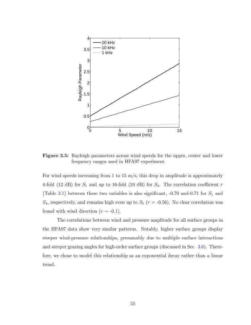
0 5 10 150

0.5

1

1.5

2

2.5

3

3.5

4

Wind Speed (m/s)

Ray

leig

h P

aram

eter

20 kHz10 kHz1 kHz

Figure 3.5: Rayleigh parameters across wind speeds for the upper, center and lowerfrequency ranges used in HFA97 experiment.

For wind speeds increasing from 1 to 15 m/s, this drop in amplitude is approximately

4-fold (12 dB) for S1 and up to 16-fold (24 dB) for S4. The correlation coefficient r

(Table 3.1) between these two variables is also significant, -0.70 and-0.71 for S1 and

S4, respectively, and remains high even up to S5 (r = -0.56). No clear correlation was

found with wind direction (r = -0.1).

The correlations between wind and pressure amplitude for all surface groups in

the HFA97 data show very similar patterns. Notably, higher surface groups display

steeper wind-pressure relationships, presumably due to multiple surface interactions

and steeper grazing angles for high-order surface groups (discussed in Sec. 3.6). There-

fore, we chose to model this relationship as an exponential decay rather than a linear

trend.

55

0 5 10 150

0.5

1

1.5

2

2.5

3

3.5

4

4.5x 10

−3

Wind Speed (m/s)

Rel

. pre

ssur

e (p

/p0)

S1

0 5 10 152

4

6

8

10

12

14

16x 10

−4

Wind Speed (m/s)

Rel

. pre

ssur

e (p

/p0)

S4

Figure 3.6: Peak pressure amplitude for surface groups S1 (top) and S4 (bottom) asa function of wind speed from all HFA97 data. Amplitude is normalizedto p0, the source pressure measured at 1 m. The best fit curve for S1 is0.0029e−0.057W , and for S4 is 0.0008e−0.0527W .

Table 3.1: Correlation Coefficients between Surface Wind Speed and Surface-GroupPressure Amplitude

S1 S2 S3 S4 S5

rDATA -0.70 -0.73 -0.65 -0.68 -0.56

rMODEL -0.40 -0.65 -0.70 -0.71 -0.60

3.3 Modeling

3.3.1 Modeling Methods

In this section, we combined wind, wave and acoustic models to simulate acoustic

propagation under a time-varying wind-wave surface. Modeling this problem requires

two necessary steps: (a) realizing shallow-water surface waves from winds, and (b)

reconstructing underwater acoustic pressure fields from a rough surface boundary.

56

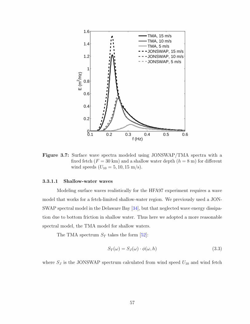
0.1 0.2 0.3 0.4 0.5 0.60

0.2

0.4

0.6

0.8

1

1.2

1.4

1.6

f (Hz)

E (

m2 /H

z)

TMA, 15 m/sTMA, 10 m/sTMA, 5 m/sJONSWAP, 15 m/sJONSWAP, 10 m/sJONSWAP, 5 m/s

Figure 3.7: Surface wave spectra modeled using JONSWAP/TMA spectra with afixed fetch (F = 30 km) and a shallow water depth (h = 8 m) for differentwind speeds (U10 = 5, 10, 15 m/s).

3.3.1.1 Shallow-water waves

Modeling surface waves realistically for the HFA97 experiment requires a wave

model that works for a fetch-limited shallow-water region. We previously used a JON-

SWAP spectral model in the Delaware Bay [34], but that neglected wave energy dissipa-

tion due to bottom friction in shallow water. Thus here we adopted a more reasonable

spectral model, the TMA model for shallow waters.

The TMA spectrum ST takes the form [52]:

ST (ω) = SJ(ω) · φ(ω, h) (3.3)

where SJ is the JONSWAP spectrum calculated from wind speed U10 and wind fetch

57

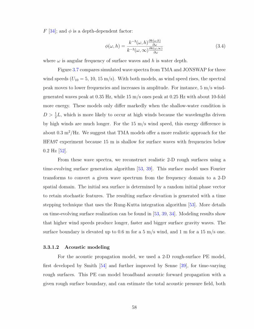
F [34]; and φ is a depth-dependent factor:

φ(ω, h) =k−3(ω, h)∂k(ω,h)

∂ω

k−3(ω,∞)∂k(ω,∞)∂ω

(3.4)

where ω is angular frequency of surface waves and h is water depth.

Figure 3.7 compares simulated wave spectra from TMA and JONSWAP for three

wind speeds (U10 = 5, 10, 15 m/s). With both models, as wind speed rises, the spectral

peak moves to lower frequencies and increases in amplitude. For instance, 5 m/s wind-

generated waves peak at 0.35 Hz, while 15 m/s ones peak at 0.25 Hz with about 10-fold

more energy. These models only differ markedly when the shallow-water condition is

D > 12L, which is more likely to occur at high winds because the wavelengths driven

by high winds are much longer. For the 15 m/s wind speed, this energy difference is

about 0.3 m2/Hz. We suggest that TMA models offer a more realistic approach for the

HFA97 experiment because 15 m is shallow for surface waves with frequencies below

0.2 Hz [52].

From these wave spectra, we reconstruct realistic 2-D rough surfaces using a

time-evolving surface generation algorithm [53, 39]. This surface model uses Fourier

transforms to convert a given wave spectrum from the frequency domain to a 2-D

spatial domain. The initial sea surface is determined by a random initial phase vector

to retain stochastic features. The resulting surface elevation is generated with a time

stepping technique that uses the Rung-Kutta integration algorithm [53]. More details

on time-evolving surface realization can be found in [53, 39, 34]. Modeling results show

that higher wind speeds produce longer, faster and bigger surface gravity waves. The

surface boundary is elevated up to 0.6 m for a 5 m/s wind, and 1 m for a 15 m/s one.

3.3.1.2 Acoustic modeling

For the acoustic propagation model, we used a 2-D rough-surface PE model,

first developed by Smith [54] and further improved by Senne [39], for time-varying

rough surfaces. This PE can model broadband acoustic forward propagation with a

given rough surface boundary, and can estimate the total acoustic pressure field, both

58

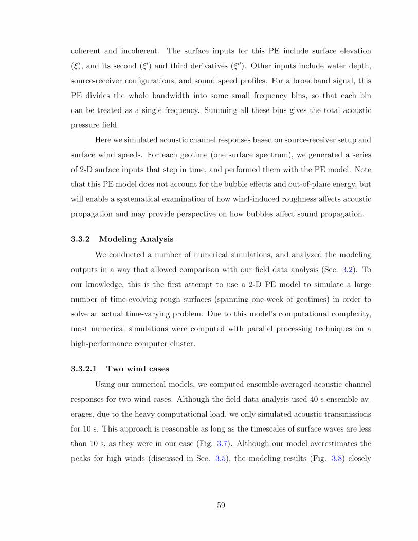
coherent and incoherent. The surface inputs for this PE include surface elevation

(ξ), and its second (ξ′) and third derivatives (ξ′′). Other inputs include water depth,

source-receiver configurations, and sound speed profiles. For a broadband signal, this

PE divides the whole bandwidth into some small frequency bins, so that each bin

can be treated as a single frequency. Summing all these bins gives the total acoustic

pressure field.

Here we simulated acoustic channel responses based on source-receiver setup and

surface wind speeds. For each geotime (one surface spectrum), we generated a series

of 2-D surface inputs that step in time, and performed them with the PE model. Note

that this PE model does not account for the bubble effects and out-of-plane energy, but

will enable a systematical examination of how wind-induced roughness affects acoustic

propagation and may provide perspective on how bubbles affect sound propagation.

3.3.2 Modeling Analysis

We conducted a number of numerical simulations, and analyzed the modeling

outputs in a way that allowed comparison with our field data analysis (Sec. 3.2). To

our knowledge, this is the first attempt to use a 2-D PE model to simulate a large

number of time-evolving rough surfaces (spanning one-week of geotimes) in order to

solve an actual time-varying problem. Due to this model’s computational complexity,

most numerical simulations were computed with parallel processing techniques on a

high-performance computer cluster.

3.3.2.1 Two wind cases

Using our numerical models, we computed ensemble-averaged acoustic channel

responses for two wind cases. Although the field data analysis used 40-s ensemble av-

erages, due to the heavy computational load, we only simulated acoustic transmissions

for 10 s. This approach is reasonable as long as the timescales of surface waves are less

than 10 s, as they were in our case (Fig. 3.7). Although our model overestimates the

peaks for high winds (discussed in Sec. 3.5), the modeling results (Fig. 3.8) closely

59

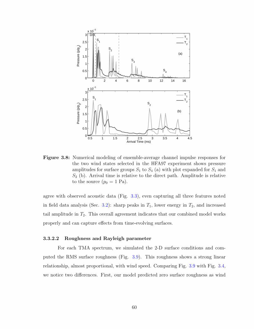
0 2 4 6 8 10 12 14 160

0.5

1

1.5

2

2.5

3x 10

−3

Pre

ssur

e (p

/p0)

D/B

S1

S2

S3

S4

(a)

T1

T2

0.5 1 1.5 2 2.5 3 3.5 4 4.50

0.5

1

1.5

2

2.5

3x 10

−3

Pre

ssur

e (p

/p0)

Arrival Time (ms)

S1

S2

(b)

T1

T2

Figure 3.8: Numerical modeling of ensemble-average channel impulse responses forthe two wind states selected in the HFA97 experiment shows pressureamplitudes for surface groups S1 to S4 (a) with plot expanded for S1 andS2 (b). Arrival time is relative to the direct path. Amplitude is relativeto the source (p0 = 1 Pa).

agree with observed acoustic data (Fig. 3.3), even capturing all three features noted

in field data analysis (Sec. 3.2): sharp peaks in T1, lower energy in T2, and increased

tail amplitude in T2. This overall agreement indicates that our combined model works

properly and can capture effects from time-evolving surfaces.

3.3.2.2 Roughness and Rayleigh parameter

For each TMA spectrum, we simulated the 2-D surface conditions and com-

puted the RMS surface roughness (Fig. 3.9). This roughness shows a strong linear

relationship, almost proportional, with wind speed. Comparing Fig. 3.9 with Fig. 3.4,

we notice two differences. First, our model predicted zero surface roughness as wind

60

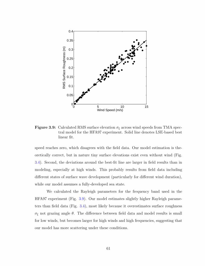
0 5 10 150

0.05

0.1

0.15

0.2

0.25

0.3

0.35

0.4

Wind Speed (m/s)

RM

S S

urfa

ce R

ough

ness

(m

)

Figure 3.9: Calculated RMS surface elevation σξ across wind speeds from TMA spec-tral model for the HFA97 experiment. Solid line denotes LSE-based bestlinear fit.

speed reaches zero, which disagrees with the field data. Our model estimation is the-

oretically correct, but in nature tiny surface elevations exist even without wind (Fig.

3.4). Second, the deviations around the best-fit line are larger in field results than in

modeling, especially at high winds. This probably results from field data including

different states of surface wave development (particularly for different wind duration),

while our model assumes a fully-developed sea state.

We calculated the Rayleigh parameters for the frequency band used in the

HFA97 experiment (Fig. 3.9). Our model estimates slightly higher Rayleigh parame-

ters than field data (Fig. 3.4), most likely because it overestimates surface roughness

σξ not grazing angle θ. The difference between field data and model results is small

for low winds, but becomes larger for high winds and high frequencies, suggesting that

our model has more scattering under these conditions.

61

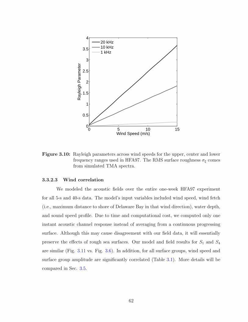
0 5 10 150

0.5

1

1.5

2

2.5

3

3.5

4

Wind Speed (m/s)

Ray

leig

h P

aram

eter

20 kHz10 kHz1 kHz

Figure 3.10: Rayleigh parameters across wind speeds for the upper, center and lowerfrequency ranges used in HFA97. The RMS surface roughness σξ comesfrom simulated TMA spectra.

3.3.2.3 Wind correlation

We modeled the acoustic fields over the entire one-week HFA97 experiment

for all 5-s and 40-s data. The model’s input variables included wind speed, wind fetch

(i.e., maximum distance to shore of Delaware Bay in that wind direction), water depth,

and sound speed profile. Due to time and computational cost, we computed only one

instant acoustic channel response instead of averaging from a continuous progressing

surface. Although this may cause disagreement with our field data, it will essentially

preserve the effects of rough sea surfaces. Our model and field results for S1 and S4

are similar (Fig. 3.11 vs. Fig. 3.6). In addition, for all surface groups, wind speed and

surface group amplitude are significantly correlated (Table 3.1). More details will be

compared in Sec. 3.5.

62

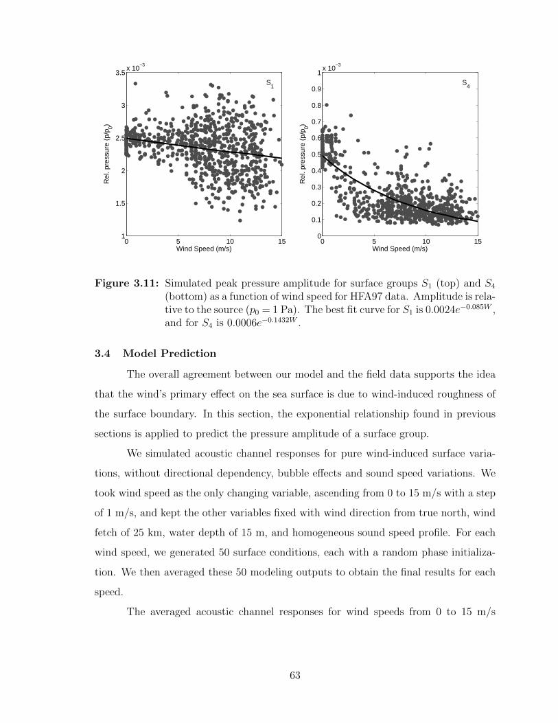
0 5 10 151

1.5

2

2.5

3

3.5x 10

−3

Wind Speed (m/s)

Rel

. pre

ssur

e (p

/p0)

S1

0 5 10 150

0.1

0.2

0.3

0.4

0.5

0.6

0.7

0.8

0.9

1x 10

−3

Wind Speed (m/s)

Rel

. pre

ssur

e (p

/p0)

S4

Figure 3.11: Simulated peak pressure amplitude for surface groups S1 (top) and S4

(bottom) as a function of wind speed for HFA97 data. Amplitude is rela-tive to the source (p0 = 1 Pa). The best fit curve for S1 is 0.0024e−0.085W ,and for S4 is 0.0006e−0.1432W .

3.4 Model Prediction

The overall agreement between our model and the field data supports the idea

that the wind’s primary effect on the sea surface is due to wind-induced roughness of

the surface boundary. In this section, the exponential relationship found in previous

sections is applied to predict the pressure amplitude of a surface group.

We simulated acoustic channel responses for pure wind-induced surface varia-

tions, without directional dependency, bubble effects and sound speed variations. We

took wind speed as the only changing variable, ascending from 0 to 15 m/s with a step

of 1 m/s, and kept the other variables fixed with wind direction from true north, wind

fetch of 25 km, water depth of 15 m, and homogeneous sound speed profile. For each

wind speed, we generated 50 surface conditions, each with a random phase initializa-

tion. We then averaged these 50 modeling outputs to obtain the final results for each

speed.

The averaged acoustic channel responses for wind speeds from 0 to 15 m/s

63

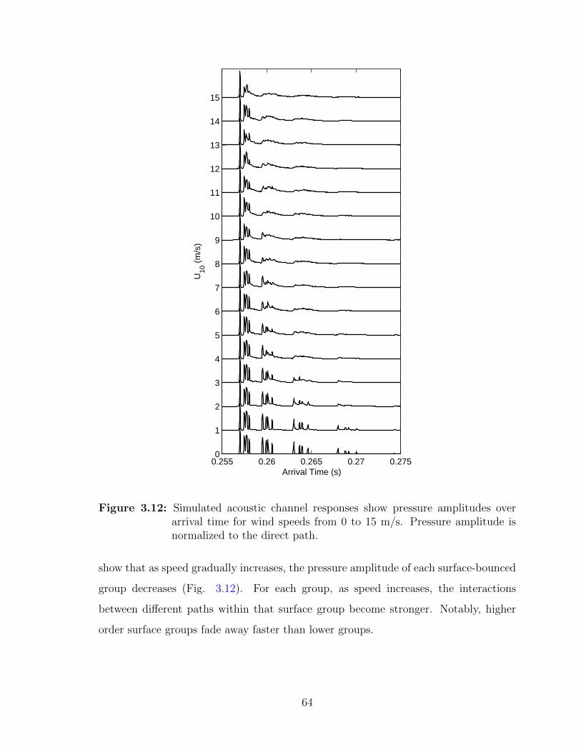
0.255 0.26 0.265 0.27 0.2750

1

2

3

4

5

6

7

8

9

10

11

12

13

14

15

Arrival Time (s)

U10

(m

/s)

Figure 3.12: Simulated acoustic channel responses show pressure amplitudes overarrival time for wind speeds from 0 to 15 m/s. Pressure amplitude isnormalized to the direct path.

show that as speed gradually increases, the pressure amplitude of each surface-bounced

group decreases (Fig. 3.12). For each group, as speed increases, the interactions

between different paths within that surface group become stronger. Notably, higher

order surface groups fade away faster than lower groups.

64

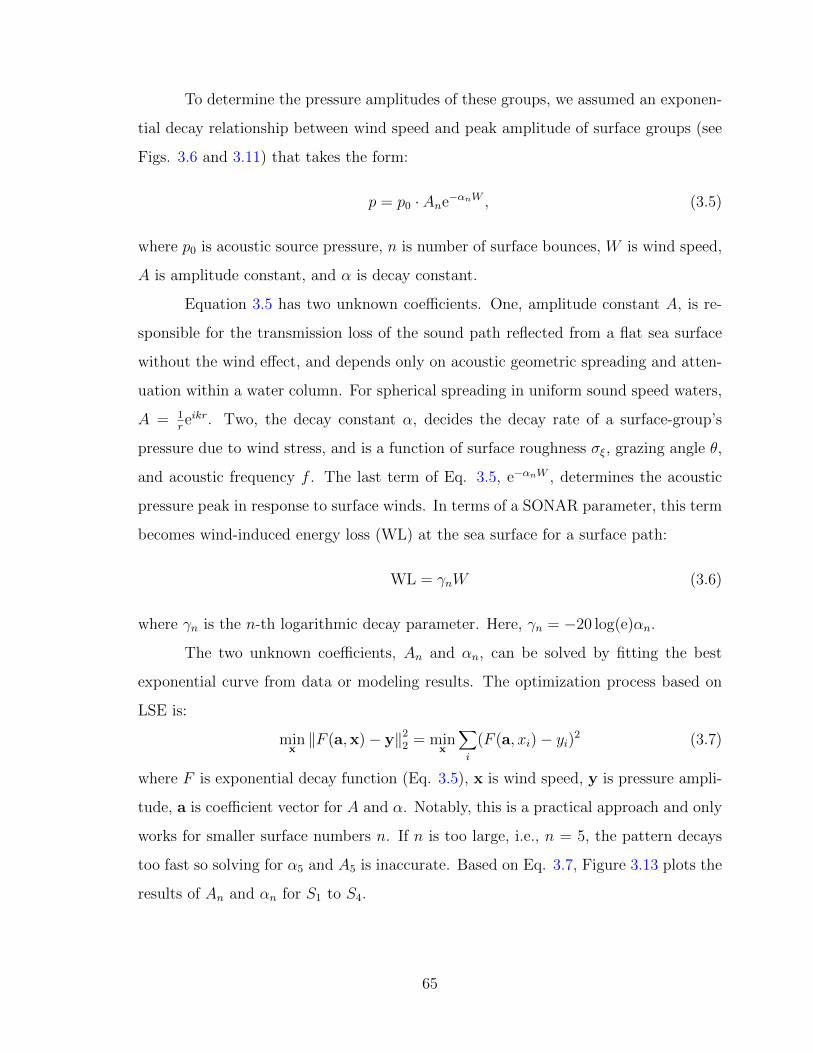
To determine the pressure amplitudes of these groups, we assumed an exponen-

tial decay relationship between wind speed and peak amplitude of surface groups (see

Figs. 3.6 and 3.11) that takes the form:

p = p0 · Ane−αnW , (3.5)

where p0 is acoustic source pressure, n is number of surface bounces, W is wind speed,

A is amplitude constant, and α is decay constant.

Equation 3.5 has two unknown coefficients. One, amplitude constant A, is re-

sponsible for the transmission loss of the sound path reflected from a flat sea surface

without the wind effect, and depends only on acoustic geometric spreading and atten-

uation within a water column. For spherical spreading in uniform sound speed waters,

A = 1reikr. Two, the decay constant α, decides the decay rate of a surface-group’s

pressure due to wind stress, and is a function of surface roughness σξ, grazing angle θ,

and acoustic frequency f . The last term of Eq. 3.5, e−αnW , determines the acoustic

pressure peak in response to surface winds. In terms of a SONAR parameter, this term

becomes wind-induced energy loss (WL) at the sea surface for a surface path:

WL = γnW (3.6)

where γn is the n-th logarithmic decay parameter. Here, γn = −20 log(e)αn.

The two unknown coefficients, An and αn, can be solved by fitting the best

exponential curve from data or modeling results. The optimization process based on

LSE is:

minx‖F (a,x)− y‖22 = min

x

∑i

(F (a, xi)− yi)2 (3.7)

where F is exponential decay function (Eq. 3.5), x is wind speed, y is pressure ampli-

tude, a is coefficient vector for A and α. Notably, this is a practical approach and only

works for smaller surface numbers n. If n is too large, i.e., n = 5, the pattern decays

too fast so solving for α5 and A5 is inaccurate. Based on Eq. 3.7, Figure 3.13 plots the

results of An and αn for S1 to S4.

65

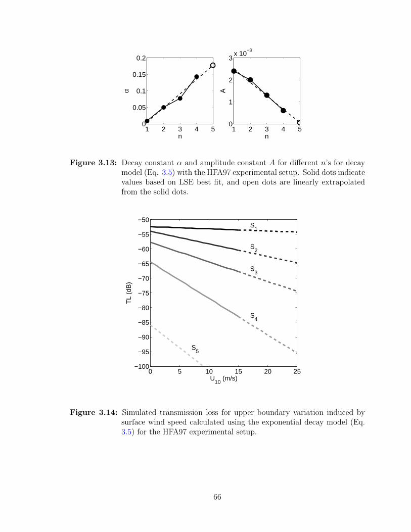
1 2 3 4 50

0.05

0.1

0.15

0.2

n

α1 2 3 4 5

0

1

2

3x 10

−3

n

A

Figure 3.13: Decay constant α and amplitude constant A for different n’s for decaymodel (Eq. 3.5) with the HFA97 experimental setup. Solid dots indicatevalues based on LSE best fit, and open dots are linearly extrapolatedfrom the solid dots.

0 5 10 15 20 25−100

−95

−90

−85

−80

−75

−70

−65

−60

−55

−50S

1

S2

S3

S4

S5

U10

(m/s)

TL

(dB

)

Figure 3.14: Simulated transmission loss for upper boundary variation induced bysurface wind speed calculated using the exponential decay model (Eq.3.5) for the HFA97 experimental setup.

66

Substituting these solved coefficients into Eq. 3.5 gives the transmission loss for

S1 to S4 for wind speeds from 0 to 15 m/s (solid lines in Fig. 3.14). These αn and

An estimates also let us predict transmission loss for any wind speed (dashed lines in

Fig. 3.14). Furthermore, these results allow us to make predictions for higher-order

surface groups where coefficients An and αn are difficult to solve. Since αn increases

with n, while An decreases (Fig. 3.13), we can linearly extrapolate to obtain for S5 the

coefficients A5 = 0.0006 and α5 = 0.1432 (Fig. 3.13). With these values, we can solve

the decay pattern for S5 (Fig. 3.14).

Although this section only showcases one simple application of the wind-acoustics

relationship, this approach can be very practical for acoustic channel prediction.

3.5 Data-Model Comparison

Our model assumes full development of surface gravity waves, no bubble for-

mation, no out-of-plane scattering, uniform medium attenuation, no Doppler effect

from surface waves, simple rigid bottom properties, and no biological effects. These

assumptions must be kept in mind when comparing modeling and field data results.

Overall, our numerical results closely agree with our field data. Modeling en-

semble averages for two geotimes (Fig. 3.8) reproduced three main features seen in

the field data (Fig. 3.3). Modeling of surface roughness (Fig. 3.9) and Rayleigh pa-

rameter (Fig. 3.10) predicted the same trends as field data (Figs. 3.4 and 3.5). Most

importantly, our modeling showed decay patterns similar to field data (Figs. 3.6 and

3.11). These agreements indicate that wind-induced surface roughness plays a key role

in attenuating acoustic surface returns.

However, some disagreements were seen that might stem from minor factors

other than surface roughness. First, at high wind speeds (U10 > 7 m/s), our model

(Fig. 3.11) predicts higher pressures than field observations (Fig. 3.6). We assert that

this is mainly because the PE model we used did not account for bubble effects [39].

Air bubbles attenuate acoustic energy [14] and are more likely to form in the surface

water layer (via wave breaking) at high wind speeds [2]. Thus, at these speeds, they are

67

more likely to lead to discrepancies between modeling and field data results. Moreover,

bubble attenuation is more prominent for small grazing angles [55], and thus for small

surface groups like S1. Consequently, it may explain our model’s overestimation of S1

in high-wind scenarios (Fig. 3.8).

Second, at low wind speeds, the model (Fig. 3.11) predicts lower pressure

amplitudes than field data (Fig. 3.6). This disagreement could arise for many reasons:

the field data could have more surface roughness at low winds (see Fig. 3.4); the ocean

surface in nature could have pre-existing bubbles that rise from the water column or

ocean bottom and overtake small surface scatterings at low winds [51, 55]; and the sea

state [56] in field data could be less developed than the fully-developed state our model

assumes.

Third, our model results (Fig. 3.11) fluctuate less at low winds but more at

high winds than the field results (Fig. 3.6). This discrepancy stems from us performing

insufficient simulations due to the computational complexity of the problem. Instead of

modeling ensemble averages over time (as in Fig. 3.6), we only simulated one acoustic

channel response for each individual rough surface. This causes focusing and defocusing

of sound energy [46] and thus leads to the fluctuation at high winds (Fig. 3.11).

Fourth, our numerical models slightly underestimate the overall acoustic am-

plitude of the surface groups (Fig. 3.11 vs. Fig. 3.6). This difference could be due

to a mismatch of medium attenuation in the model, or to a 2-D model that neglects

out-of-plane acoustic energy, or more complicated water column properties and bot-

tom properties. Fortunately, however, since the influences of these factors on sound

propagation are independent of wind speed, they should not affect our conclusions on

wind effect.

3.6 Discussions

In this paper, we confirmed, both with HFA97 field data and numerical mod-

eling, that all surface-bounced sound energy decreases with increasing wind speeds

68

because of greater wind-generated surface roughness, results consistent with many pre-

vious field experiments [51, 55, 57, 58]. Since our modeling, which only incorporates

surface roughness, agreed overall with field data, we conclude that among all wind ef-

fects, surface roughness is the major factor that decreases surface-return sound waves in

the HFA97 experiment. Other factors that influence sound propagation are discussed

below.

Number of surface groups

Both our field (Fig. 3.6) and modeling (Figs. 3.11 and 3.12) results indicate that

higher surface groups (e.g., S4, S5) experience more surface effects, i.e., more atten-

uation than lower surface groups due to multiple, repeated interactions with surface

fluctuation. Furthermore, for a given source level, the maximum number of surface

groups n decreases as wind speed increases, as shown in our model (Figs. 3.12 and

3.14), and reported in a previous study [51].

Bubble effects

Bubbles play a much smaller role in attenuating acoustic intensity than the

scattering loss caused by surface roughness. However, our data-model comparison

indicates that air bubbles have a stronger effect on lower surface groups (smaller n).

In a fixed acoustic setup like HFA97, the grazing angle decreases as number of surface

bounces n increases, and small grazing angles cause more significant bubble attenuation

[43]. Hence, we expect greater bubble attenuation in S1 than in S4. Indeed, we find

that our model displays much more overestimation for S1 than for S4 (Fig. 3.3 vs. Fig.

3.3, and Fig. 3.6 vs. Fig. 3.11), most likely due to the PE model not including bubble

effects.

Sound frequency

Wind effects on sound propagation are frequency-dependent [51]. Surface rough-

ness (Figs. 3.5 and 3.10) and bubble attenuation [1] affect high frequencies more

strongly than low frequencies, even at high wind speeds. Unfortunately, the HFA97

69

experiment transmitted broadband acoustic chirps so our results could not demonstrate

frequency dependency. However, the Rayleigh parameter analysis suggests that using

frequencies under 10 kHz would significantly reduce these wind-induced surface effects

for a region like the Delaware Bay, where wind speeds remain mostly below 15 m/s

(Fig. 3.2).

Wind direction

The HFA97 experiment demonstrated no clear relationship between wind di-

rection and sound attenuation. However, other studies have shown that the direction

of wind on the surface might play a role [58]. In our experiment, all wind directions

produced a range of surface-group intensities, with the exception of directions between

120◦ to 200◦ that only evoked high intensities. In the Delaware Bay the wind in these

directions was fairly low speed (Fig. 3.2), so our decay pattern predicts a high acoustic

intensity. Directional dependency in a fetch-limited estuary is more likely to contribute

combination effects of directional waves and of varying fetch length [59] due to bay ge-

ometry, both interesting problems that deserve further research.

Wind fetch and wind duration

Other wind properties can also affect underwater sound propagation by evoking

different developments of the sea state. Generally, a longer fetch with enough duration

has the potential to develop a rougher sea surface, and thus leads to smaller surface-

returned acoustic energy [59]. Although these effects on surface roughness are much

smaller than wind speed, they still account for some fluctuations in surface roughness

(Figs. 3.4 and 3.9) and surface group pressures (Figs. 3.6 and 3.11), especially at high

winds.

3.7 Conclusions

Our analysis leads to the following explanation for the effects of wind on acoustic

wave propagation. Wind generates ocean surface gravity waves, causing rough bound-

ary conditions of the sound channel (Figs. 3.4 and 3.9) and entrainment of air bubbles

70

during wave breaking, both of which can attenuate surface-returned sound. As wind

speeds increase, the ocean surface is dominated by more complex waves, with lower

peak frequencies, extended spectral range and intensified wave energy (Fig. 3.7). This

wave motion gives rise to fluctuations in sound arrivals [34] as the acoustic wavefront

captures the surface curvature [58]. Increased roughness results in incoherent scattering

of the sound waves [1], i.e., higher Rayleigh parameters (Figs. 3.4 and 3.5). Meanwhile,

breaking of surface waves leads to further acoustic energy attenuation as sound waves

pass the surface layer waters. Thus, as wind speed increases, the surface-returned

acoustic pressure decreases (Fig. 3.12).

Here we examined the sea surface roughness and broadband sound fluctuation

in a shallow estuary as a function of wind speed, using both field data analysis and

numerical modeling. Results from both conclude that wind affects shallow-water sound

propagation as follows: (a) wind-induced surface roughness, among all wind effects, is

primarily responsible for acoustic attenuation with an exponential decay relationship;

(b) bubble attenuation is the second major factor, and its effects should be incorporated

in future acoustic models, especially in high wind cases; and (c) wind direction, fetch

and duration may jointly affect this problem and require further investigation.

Numerical modeling offers a useful tool for studying acoustic propagation prob-

lems in highly dynamic environments that have a variety of factors influencing sound

propagation. Overall agreement between our model and field results establishes that

our approach works for acoustic modeling under a time-evolving surface. With 2-D

rough surface PE, we were able to examine in-plane acoustic fields which are the dom-

inant part of energy components, but more accurate modeling will need to consider

out-of-plane scatterings in a 3-D PE. Also, since this problem is inherently linked to

physical ocean dynamics, full understanding will require a joint oceanography-acoustics

model.

Future study will be extended to underwater acoustic communication whose

performance decreases at high winds. Our realistic wind-impacted acoustic channel

model and the better understanding of channel variability will help design a more

71

reliable communication system for shallow-water time-varying acoustic channels.

72

Chapter 4

MODELING ACOUSTIC COHERENT COMMUNICATION UNDERWIND-DRIVEN OCEAN SURFACE WAVES

Winds raise time-varying roughness on the air-sea interface, which deflects un-

derlying sound and modifies underwater acoustic channel in short timescale. Perfor-

mance degradations and system failures in underwater acoustic communication were

reported due to wind-induced surface waves, especially for coherent communication

systems which utilize phase information during the modulation. Here, we propose a

controllable numerical approach for this problem: Realistic acoustic channels for differ-

ent wind conditions are numerically simulated with wind-wave spectral methods and a

2-D rough-surface parabolic equation (PE) model; Then, these time-varying acoustic

channels are tested with quadrature phase-shift keying (QPSK) modulation, one of the

most fundamental modulation schemes for underwater acoustic coherent communica-

tion. Preliminary results suggest that in consideration of a time-varying environment,

system performance for coherent communication degrades with increasing wind speed,

as a result of increasing temporal variability of wind-impacted surface waves. Our

numerical modeling method could be a helpful tool to study acoustic communication

problems in time-varying ocean environments.

4.1 Introduction

Underwater acoustic communication in shallow waters has been a challenging re-

search topic over recent decades, due to the complexity of acoustic multipath structure

in nature time-varying environment [60, 61]. There has been a series of schemes and

methods proposed for acoustic communication in such challenging regions. Most pop-

ular communication schemes are based on coherent methods, where data modulation

73

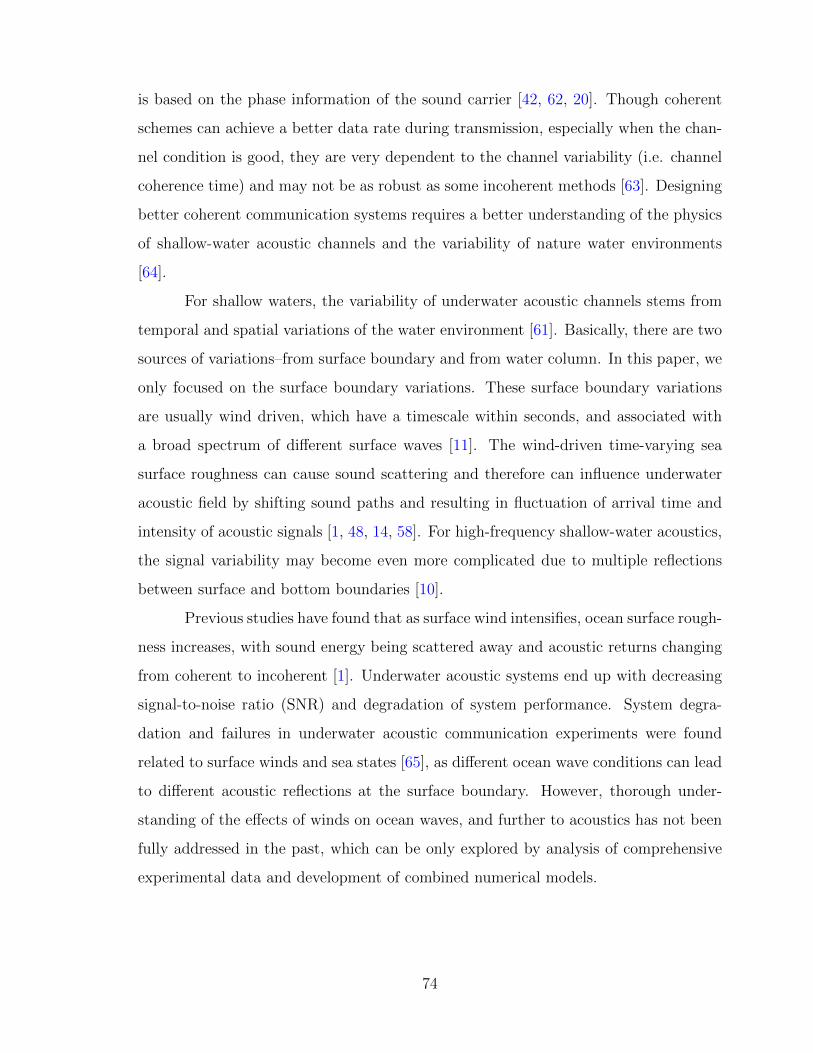
is based on the phase information of the sound carrier [42, 62, 20]. Though coherent

schemes can achieve a better data rate during transmission, especially when the chan-

nel condition is good, they are very dependent to the channel variability (i.e. channel

coherence time) and may not be as robust as some incoherent methods [63]. Designing

better coherent communication systems requires a better understanding of the physics

of shallow-water acoustic channels and the variability of nature water environments

[64].

For shallow waters, the variability of underwater acoustic channels stems from

temporal and spatial variations of the water environment [61]. Basically, there are two

sources of variations–from surface boundary and from water column. In this paper, we

only focused on the surface boundary variations. These surface boundary variations

are usually wind driven, which have a timescale within seconds, and associated with

a broad spectrum of different surface waves [11]. The wind-driven time-varying sea

surface roughness can cause sound scattering and therefore can influence underwater

acoustic field by shifting sound paths and resulting in fluctuation of arrival time and

intensity of acoustic signals [1, 48, 14, 58]. For high-frequency shallow-water acoustics,

the signal variability may become even more complicated due to multiple reflections

between surface and bottom boundaries [10].

Previous studies have found that as surface wind intensifies, ocean surface rough-

ness increases, with sound energy being scattered away and acoustic returns changing

from coherent to incoherent [1]. Underwater acoustic systems end up with decreasing

signal-to-noise ratio (SNR) and degradation of system performance. System degra-

dation and failures in underwater acoustic communication experiments were found

related to surface winds and sea states [65], as different ocean wave conditions can lead

to different acoustic reflections at the surface boundary. However, thorough under-

standing of the effects of winds on ocean waves, and further to acoustics has not been

fully addressed in the past, which can be only explored by analysis of comprehensive

experimental data and development of combined numerical models.

74

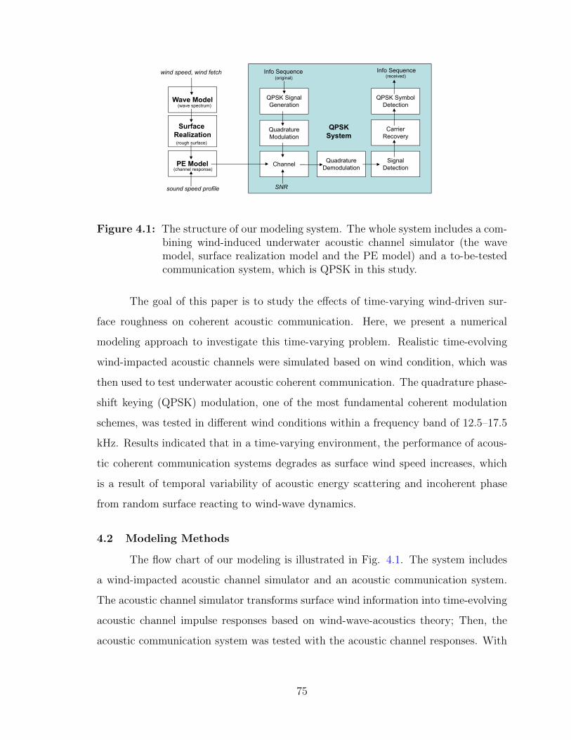
Wave Model

PE Model

Surface Realization

(channel response)

wind speed, wind fetch Info Sequence

Channel

QuadratureModulation

QuadratureDemodulation

QPSK SignalGeneration

SignalDetection

CarrierRecovery

QPSK SymbolDetection

(rough surface)

(wave spectrum)

sound speed profile SNR

Info Sequence(original) (received)

QPSKSystem

Figure 4.1: The structure of our modeling system. The whole system includes a com-bining wind-induced underwater acoustic channel simulator (the wavemodel, surface realization model and the PE model) and a to-be-testedcommunication system, which is QPSK in this study.

The goal of this paper is to study the effects of time-varying wind-driven sur-

face roughness on coherent acoustic communication. Here, we present a numerical

modeling approach to investigate this time-varying problem. Realistic time-evolving

wind-impacted acoustic channels were simulated based on wind condition, which was

then used to test underwater acoustic coherent communication. The quadrature phase-

shift keying (QPSK) modulation, one of the most fundamental coherent modulation

schemes, was tested in different wind conditions within a frequency band of 12.5–17.5

kHz. Results indicated that in a time-varying environment, the performance of acous-

tic coherent communication systems degrades as surface wind speed increases, which

is a result of temporal variability of acoustic energy scattering and incoherent phase

from random surface reacting to wind-wave dynamics.

4.2 Modeling Methods

The flow chart of our modeling is illustrated in Fig. 4.1. The system includes

a wind-impacted acoustic channel simulator and an acoustic communication system.

The acoustic channel simulator transforms surface wind information into time-evolving

acoustic channel impulse responses based on wind-wave-acoustics theory; Then, the

acoustic communication system was tested with the acoustic channel responses. With

75

this regime, system performance of underwater acoustic communication can be numer-

ically simulated with adjustable environmental parameters, such as wind speed, wind

fetch, water depth and ambient noise level.

4.2.1 Wind-impacted time-evolving acoustic channel

The acoustic channel simulator includes three numerical models–a wave spec-

tral model, a surface realization model, and a full-wave acoustic propagation model

(left three components in Fig. 4.1). This acoustic channel simulator has been used in

previous studies to investigate effects of surface winds on time-varying acoustic prop-

agation [39, 25]. Basically, the wave model converts wind information to wave energy

spectrum; the surface realization model generates surface elevation from the wave spec-

trum; and the PE acoustic propagation model constructs acoustic pressure field with

rough surface boundary.

First of all, the spectrum of wind-driven surface waves was generated by a wave

model based on environmental variables. The wind-wave spectral method adopted here

was the TMA model [66]. TMA is an empirical wind-driven ocean wave model, par-

ticularly optimized for shallow waters. It estimates the theoretical wave spectrum for

fully-developed wind-driven surface gravity waves, with an adjustment term validated

from field data, and a depth-dependent factor accounting for the wave dissipation due

to limited water depth [52]. TMA is more suitable for shallow water studies than

other wave models that do not consider the water depth, because acoustic multipaths

and rough ocean waves would have even more effects on acoustic channel in these

shallow regions [25]. Using this model, wave spectra were numerically generated with

controllable environmental inputs, i.e. wind speed, wind fetch, and water depth.

Second, time-varying surface waves were generated by the surface model. With

a given wind-wave spectrum, 2-D rough sea surfaces was realized by a surface model

[53]. The surface model converts a frequency-dependent wave spectrum to surface

wave heights using Fourier transform pairs, from the frequency domain to the spatial

domain. Furthermore, due to the nature evolution of ocean waves, this problem is

76

10−1

100

101

0

0.2

0.4

0.6

0.8

1

f (Hz)

E (

m2 /H

z)

13 m/s6 m/s1 m/s

Figure 4.2: Surface wave spectral modeling using TMA spectra with a fixed fetch(F = 30 km) and a shallow water depth (h = 15 m) for different windspeeds (U10 = 1, 6, 13 m/s).

a time-evolving problem, where the following surface wave is related to the previous

surface wave. For such wave evolution, this model initializes random phases for the first

surface; For following surface elevations, the model adopts the Rung-Kutta integration

algorithm to step in time from the previous surface roughness [53]. Note that this

model can simulate both time-evolving or randomly-varying surface elevations for a

same surface wave spectrum, which enables us to study acoustic communications with

different scenarios.

77

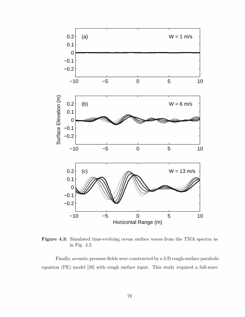
−10 −5 0 5 10

−0.2

−0.1

0

0.1

0.2 (a) W = 1 m/s

−10 −5 0 5 10

−0.2

−0.1

0

0.1

0.2 (b) W = 6 m/s

Sur

face

Ele

vatio

n (m

)

−10 −5 0 5 10

−0.2

−0.1

0

0.1

0.2 (c) W = 13 m/s

Horizontal Range (m)

Figure 4.3: Simulated time-evolving ocean surface waves from the TMA spectra asin Fig. 4.2.

Finally, acoustic pressure fields were constructed by a 2-D rough-surface parabolic

equation (PE) model [39] with rough surface input. This study required a full-wave

78

acoustic model which can handle broadband acoustic transmission and rough surface

scattering. This PE used in this study is based on a 2-D split-step Fourier transforma-

tion and range-marching algorithm, and more importantly, it accounts for the surface

scattering caused by rough surface conditions [39]. For acoustic scattering from a rough

surface, the pressure release boundary is shifted from a flat surface to a rough surface,

which modifies the reflection angles and the reflected energy. Therefore, this model

is capable of computing acoustic arrival time and pressure amplitude under rough sea

surfaces [39].

4.2.2 QPSK acoustic communication system

The incoherent components of acoustic signals, caused by acoustic scattering

from time-varying rough sea surface, can influence underwater acoustic coherent com-

munication, where phase information of received acoustic signals is the key to demodu-

late the transmitted data [25, 20, 61]. Here, we focused on phase shift keying – the most

fundamental acoustic coherent scheme, which many other more sophisticated coherent

communications were built on. The system we tested here was the quadrature phase

shift keying (QPSK) [20]. Note that we only tested the basics of the QPSK scheme

with simple carrier recovery; while we did not apply further adaptive mechanism to

track and compensate the temporal variability of acoustic channel (i.e. examples in

[63]).

The QPSK system was demonstrated in the box of Fig. 4.1. The transmitter

had two main components–signal generation and quadrature modulation. The system

first generates to-be-transmitted signals for the QPSK modulation, which include a

chirp signal (for signal detection), a single-frequency signal (for carrier recovery), a

known M-sequence (for fine time synchronization and signal recovery), and the data

series (also modulated by the M-sequence). Next, all these signals were transformed

from baseband (0-5 kHz) to passband (12.5-17.5 kHz) via carrier modulation in both

real and imaginary components.

79

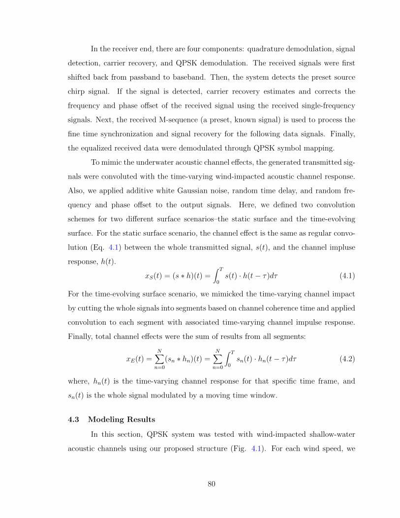
In the receiver end, there are four components: quadrature demodulation, signal

detection, carrier recovery, and QPSK demodulation. The received signals were first

shifted back from passband to baseband. Then, the system detects the preset source

chirp signal. If the signal is detected, carrier recovery estimates and corrects the

frequency and phase offset of the received signal using the received single-frequency

signals. Next, the received M-sequence (a preset, known signal) is used to process the

fine time synchronization and signal recovery for the following data signals. Finally,

the equalized received data were demodulated through QPSK symbol mapping.

To mimic the underwater acoustic channel effects, the generated transmitted sig-

nals were convoluted with the time-varying wind-impacted acoustic channel response.

Also, we applied additive white Gaussian noise, random time delay, and random fre-

quency and phase offset to the output signals. Here, we defined two convolution

schemes for two different surface scenarios–the static surface and the time-evolving

surface. For the static surface scenario, the channel effect is the same as regular convo-

lution (Eq. 4.1) between the whole transmitted signal, s(t), and the channel impluse

response, h(t).

xS(t) = (s ∗ h)(t) =∫ T

0s(t) · h(t− τ)dτ (4.1)

For the time-evolving surface scenario, we mimicked the time-varying channel impact

by cutting the whole signals into segments based on channel coherence time and applied

convolution to each segment with associated time-varying channel impulse response.

Finally, total channel effects were the sum of results from all segments:

xE(t) =N∑n=0

(sn ∗ hn)(t) =N∑n=0

∫ T

0sn(t) · hn(t− τ)dτ (4.2)

where, hn(t) is the time-varying channel response for that specific time frame, and

sn(t) is the whole signal modulated by a moving time window.

4.3 Modeling Results

In this section, QPSK system was tested with wind-impacted shallow-water

acoustic channels using our proposed structure (Fig. 4.1). For each wind speed, we

80

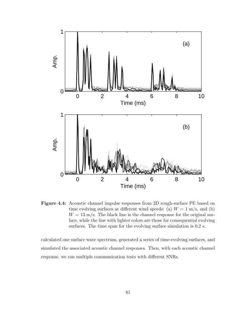
0 2 4 6 8 100

1

Am

p.

Time (ms)

(a)

0 2 4 6 8 100

1

Am

p.

Time (ms)

(b)

Figure 4.4: Acoustic channel impulse responses from 2D rough-surface PE based ontime evolving surfaces at different wind speeds: (a) W = 1 m/s, and (b)W = 13 m/s. The black line is the channel response for the original sur-face, while the line with lighter colors are those for consequential evolvingsurfaces. The time span for the evolving surface simulation is 0.2 s.

calculated one surface wave spectrum, generated a series of time-evolving surfaces, and

simulated the associated acoustic channel responses. Then, with each acoustic channel

response, we ran multiple communication tests with different SNRs.

81

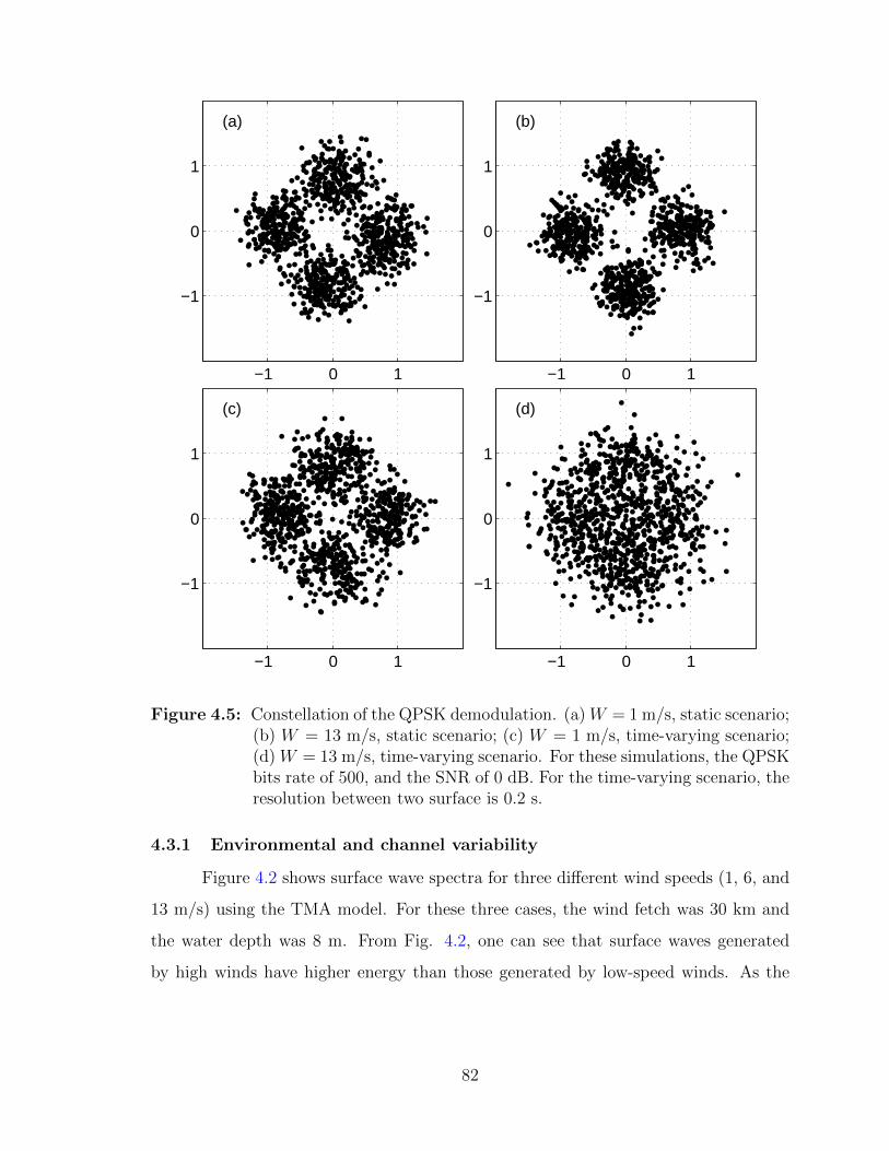
−1 0 1

−1

0

1

(a)

−1 0 1

−1

0

1

(b)

−1 0 1

−1

0

1

(c)

−1 0 1

−1

0

1

(d)

Figure 4.5: Constellation of the QPSK demodulation. (a) W = 1 m/s, static scenario;(b) W = 13 m/s, static scenario; (c) W = 1 m/s, time-varying scenario;(d) W = 13 m/s, time-varying scenario. For these simulations, the QPSKbits rate of 500, and the SNR of 0 dB. For the time-varying scenario, theresolution between two surface is 0.2 s.

4.3.1 Environmental and channel variability

Figure 4.2 shows surface wave spectra for three different wind speeds (1, 6, and

13 m/s) using the TMA model. For these three cases, the wind fetch was 30 km and

the water depth was 8 m. From Fig. 4.2, one can see that surface waves generated

by high winds have higher energy than those generated by low-speed winds. As the

82

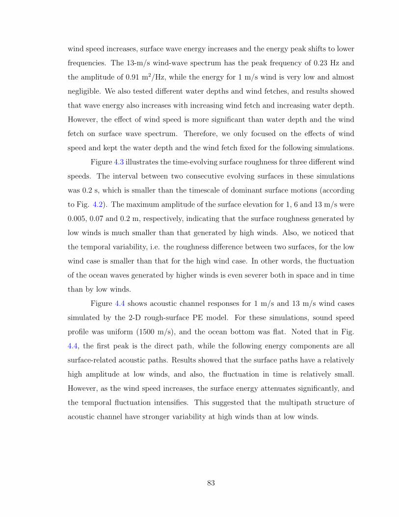
wind speed increases, surface wave energy increases and the energy peak shifts to lower

frequencies. The 13-m/s wind-wave spectrum has the peak frequency of 0.23 Hz and

the amplitude of 0.91 m2/Hz, while the energy for 1 m/s wind is very low and almost

negligible. We also tested different water depths and wind fetches, and results showed

that wave energy also increases with increasing wind fetch and increasing water depth.

However, the effect of wind speed is more significant than water depth and the wind

fetch on surface wave spectrum. Therefore, we only focused on the effects of wind

speed and kept the water depth and the wind fetch fixed for the following simulations.

Figure 4.3 illustrates the time-evolving surface roughness for three different wind

speeds. The interval between two consecutive evolving surfaces in these simulations

was 0.2 s, which is smaller than the timescale of dominant surface motions (according

to Fig. 4.2). The maximum amplitude of the surface elevation for 1, 6 and 13 m/s were

0.005, 0.07 and 0.2 m, respectively, indicating that the surface roughness generated by

low winds is much smaller than that generated by high winds. Also, we noticed that

the temporal variability, i.e. the roughness difference between two surfaces, for the low

wind case is smaller than that for the high wind case. In other words, the fluctuation

of the ocean waves generated by higher winds is even severer both in space and in time

than by low winds.

Figure 4.4 shows acoustic channel responses for 1 m/s and 13 m/s wind cases

simulated by the 2-D rough-surface PE model. For these simulations, sound speed

profile was uniform (1500 m/s), and the ocean bottom was flat. Noted that in Fig.

4.4, the first peak is the direct path, while the following energy components are all

surface-related acoustic paths. Results showed that the surface paths have a relatively

high amplitude at low winds, and also, the fluctuation in time is relatively small.

However, as the wind speed increases, the surface energy attenuates significantly, and

the temporal fluctuation intensifies. This suggested that the multipath structure of

acoustic channel have stronger variability at high winds than at low winds.

83

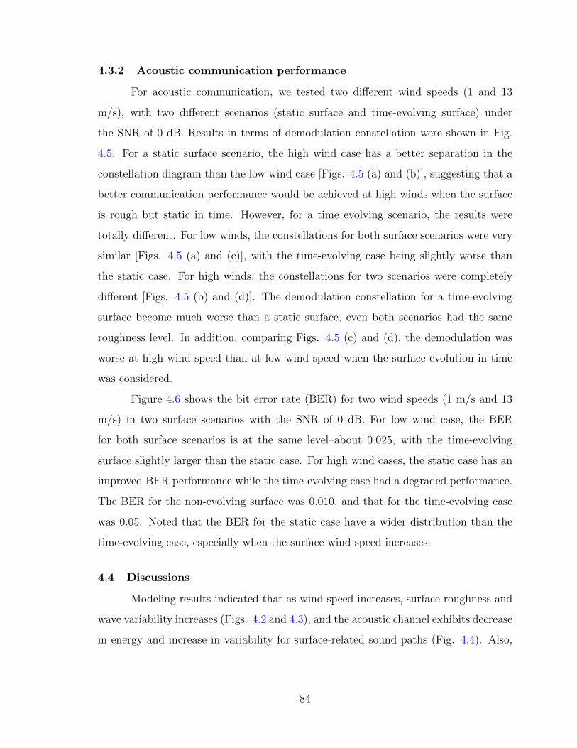
4.3.2 Acoustic communication performance

For acoustic communication, we tested two different wind speeds (1 and 13

m/s), with two different scenarios (static surface and time-evolving surface) under

the SNR of 0 dB. Results in terms of demodulation constellation were shown in Fig.

4.5. For a static surface scenario, the high wind case has a better separation in the

constellation diagram than the low wind case [Figs. 4.5 (a) and (b)], suggesting that a

better communication performance would be achieved at high winds when the surface

is rough but static in time. However, for a time evolving scenario, the results were

totally different. For low winds, the constellations for both surface scenarios were very

similar [Figs. 4.5 (a) and (c)], with the time-evolving case being slightly worse than

the static case. For high winds, the constellations for two scenarios were completely

different [Figs. 4.5 (b) and (d)]. The demodulation constellation for a time-evolving

surface become much worse than a static surface, even both scenarios had the same

roughness level. In addition, comparing Figs. 4.5 (c) and (d), the demodulation was

worse at high wind speed than at low wind speed when the surface evolution in time

was considered.

Figure 4.6 shows the bit error rate (BER) for two wind speeds (1 m/s and 13

m/s) in two surface scenarios with the SNR of 0 dB. For low wind case, the BER

for both surface scenarios is at the same level–about 0.025, with the time-evolving

surface slightly larger than the static case. For high wind cases, the static case has an

improved BER performance while the time-evolving case had a degraded performance.

The BER for the non-evolving surface was 0.010, and that for the time-evolving case

was 0.05. Noted that the BER for the static case have a wider distribution than the

time-evolving case, especially when the surface wind speed increases.

4.4 Discussions

Modeling results indicated that as wind speed increases, surface roughness and

wave variability increases (Figs. 4.2 and 4.3), and the acoustic channel exhibits decrease

in energy and increase in variability for surface-related sound paths (Fig. 4.4). Also,

84

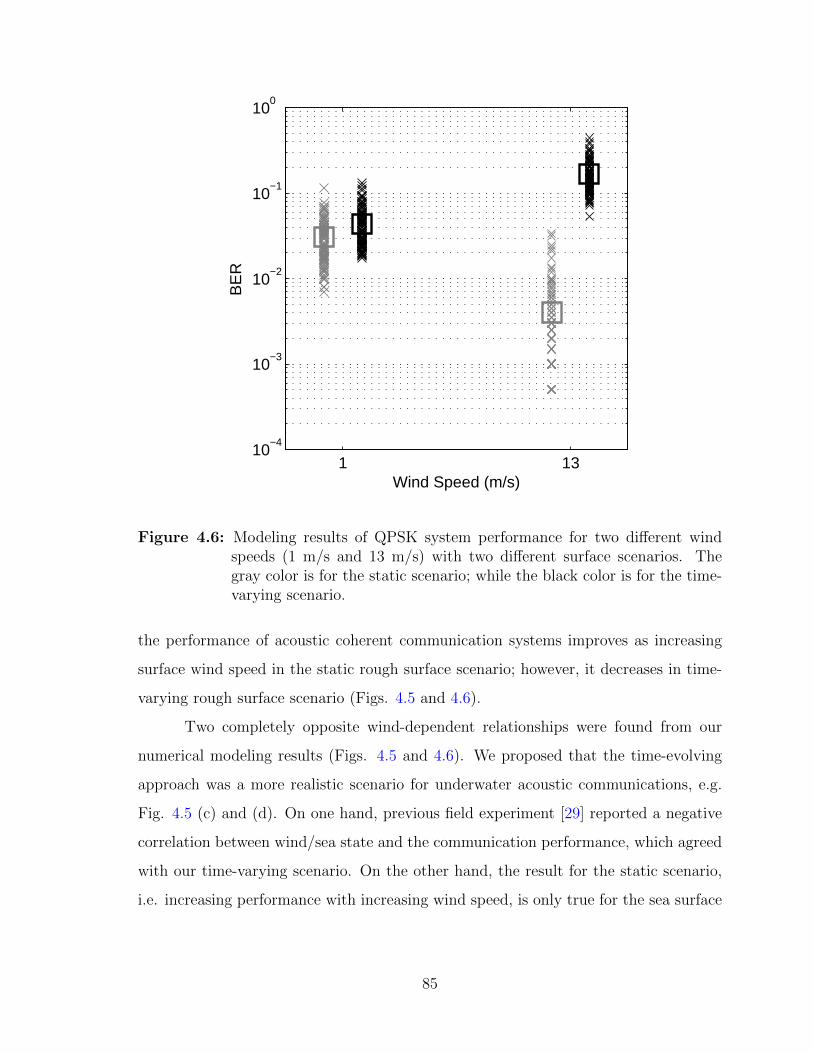
1 1310

−4

10−3

10−2

10−1

100

BE

R

Wind Speed (m/s)

Figure 4.6: Modeling results of QPSK system performance for two different windspeeds (1 m/s and 13 m/s) with two different surface scenarios. Thegray color is for the static scenario; while the black color is for the time-varying scenario.

the performance of acoustic coherent communication systems improves as increasing

surface wind speed in the static rough surface scenario; however, it decreases in time-

varying rough surface scenario (Figs. 4.5 and 4.6).

Two completely opposite wind-dependent relationships were found from our

numerical modeling results (Figs. 4.5 and 4.6). We proposed that the time-evolving

approach was a more realistic scenario for underwater acoustic communications, e.g.

Fig. 4.5 (c) and (d). On one hand, previous field experiment [29] reported a negative

correlation between wind/sea state and the communication performance, which agreed

with our time-varying scenario. On the other hand, the result for the static scenario,

i.e. increasing performance with increasing wind speed, is only true for the sea surface

85

which has a roughness but is still motionless. In real nature, however, the rough

sea surface is impossible to be static due to the gravity. We argued that to model

a realistic communication performance for a rough surface boundary, time-varying

acoustic channels should be used instead of static acoustic channels.

We suggest that the cause of the decrease of communication performance at

high winds is due to the increasing temporal variability of surface waves, not due to

the increasing incoherent signals from rough surface scattering. Actually, the increas-

ing roughness does not degrade the performance of acoustic communication systems

[Fig. 4.5 (a) and (b)]; Instead, it can improve the performance by providing a simpler

multipath structure for underwater acoustic communication. Considering an extreme

case, if the surface boundary is extremely rough and all surface energy are completely

scattered away, there will be a very little surface return which leaves only a strong

direct path component, which is perfect for the communication system. The temporal

variability, however, can degrade the system performance by failing the carrier recov-

ery and channel equalization. For this reason, coherent communication system requires

well-designed channel adaptive methods whose reaction time should be shorter than

the coherence time of the physical channel [63]. In our basic QPSK system, we did not

adopt such mechanism to compensate the variability of channel in time, so the carrier

recovery processing was based on the channel at the beginning moment, which did not

account for the channel variability for following moments, so that it leads to failure of

phase recovery and therefore the decrease of system performance.

In addition, there were some aspects we did not consider in this study which

might affect the communication results. We did not account for the bubble effect in our

PE modeling. Bubble forming is inevitable at high sea states along with wave breaking,

which causes attenuation of acoustic intensity but it is usually considered having little

effects on forward scattering problem. Also, the realistic sound transmission in the

ocean is a 3-D problem, but we limited our analysis and discussion in a 2-D PE model,

which did not account for the out-of-plane acoustic reflection and scattering. However,

this is still a realistic approach as our 2-D PE mimics the most energy component of the

86

acoustic fields, because the out-of-plane acoustic energy is relatively small comparing

to the in-plane energy [14, 25].

4.5 Conclusions

This study presented a combined numerical modeling approach to investigate the

wind-wave effects on acoustic coherent communication. With time-varying nature of

ocean surface waves, the QPSK performance will decrease with increasing wind speed,

due to the increasing temporal variability of surface paths at high winds, instead of the

increasing roughness of the ocean surface itself. As the system performance of under-

water acoustic communication is strongly related to the physical environment, which

is complex and time-varying, the full understanding of the time-varying environment

on acoustic communication will need further work on realistic oceanography-acoustics

combined models. Future study will be continued on effects of QPSK system with chan-

nel tracking, and how acoustic communication performance links with signal coherence

time and water environment variability. Also, effects on other acoustic communication

methods and coding schemes will be further explored.

87

Chapter 5

WIND-WAVE EFFECTS ON COHERENT AND NON-COHERENTUNDERWATER ACOUSTIC COMMUNICATIONS: A LABORATORY

EXPERIMENT

Atmospheric winds raise surface water waves that can cause fast fluctuations

of underwater acoustic channels and further influence underwater acoustic commu-

nications. The link between winds and underwater acoustic communications is an

extremely complicated inter-discipline study, which is not well understood yet, mostly

because directly studying this problem from ocean acoustic experiments, where envi-

ronmental variables are difficult to control or separate, is extremely challenging. In this

paper, a laboratory water tank experiment is proposed to provide a fresh look of this

problem. Two fundamental modulations schemes (one coherent, one non-coherent) are

investigated in a controllable laboratory environment, where wind is the only changing

environmental variable. Results show that, the performance of coherent communica-

tions decreases at high winds due to increased acoustic channel variations and decreased

temporal coherence, while the performance of non-coherent communications may in-

crease as a result of smaller acoustic surface returns and less channel sensitivity of

the non-coherent detection method. Results also suggest that winds effect on com-

munication performance depends critically on modulation schemes, which should be

considered differently for modeling and design of underwater acoustic networks in the

future.

5.1 Introduction

Rapid developments of marine sciences and ocean explorations promote a se-

ries of underwater technologies and applications for ocean engineering. Underwater

88

acoustic communications, which enable wireless data and information exchange among

underwater devices, have been a research hotspot for many years due to the extensive

usage in civil engineering and scientific research [67]. Underwater information trans-

mission with high data rate and reliability has been the goal for underwater acoustic

communication researches. For recent decades, the data rate of underwater acoustic

communications has greatly improved from only a few bits per second (bps) to several

thousand bps, with system reliability increasing steadily as well.

Currently, the top challenge that hinders the further improvement of underwater

acoustic communications stems from complex nature ocean environments, which are

extremely diverse and highly time-varying [61]. For instance, variation of sea surface

roughness driven by surface winds and waves [25, 26], water mixing and stratification

driven by tidal forcing [68, 28], variation of thermocline due to the internal wave

[27, 69], noise interruption from marine life and human activities [70, 71], etc, can

all affect the variability of time-varying underwater acoustic channels and further the

performance of underwater acoustic communication systems. Until today, there are

still no effective acoustic communication schemes existed that can work in all ocean

environments and guarantee high data rate and reliability at the same time. The leap

of underwater acoustic communication performance requires a deeper understanding

of the connection between physical ocean environments, underwater acoustic channels

and acoustic communication systems [10, 61, 25].

Among all environmental variability, winds and surface waves at the air-sea

interface are the most common one for the fast fluctuation of underwater acoustic

channels, which has a significant influence on underwater acoustic communications.

Driven by atmospheric winds, sea surface waves increase the roughness of the air-

sea interface and alter sound paths under the water, which has been challenging the

design of underwater acoustic communication systems for a while. Evidences that

winds, surface waves or sea states influence the performance of underwater acous-

tic communication have been widely reported in previous studies (e.g., on underwa-

ter acoustic channels [10, 2, 51, 61, 67, 72, 73, 74, 75, 76, 60, 77], field experiments

89

[78, 29, 79, 80, 81, 82, 83, 84, 85], numerical modeling [86, 87, 88], etc). As a complex

and inter-discipline scientific research problem, the inside link between the wind/wave

and the performance of underwater acoustic communication systems has not been fully

understood yet [26]. Next-generation underwater acoustic communication systems are

calling for a physics-based design that offers a better adaptability of time-varying

physical ocean environments, which can use a better understanding of the relationship

between the physical oceanography, ocean acoustics, and underwater acoustic commu-

nication.

Many wind-related effects on underwater acoustics have been previously stud-

ied, and the two key effects are the increased ambient noise due to surface wind-wave

dynamics, and the increased acoustic scattering due to wind-driven surface waves, both

of which can influence underwater acoustic communications. On one hand, the spec-

trum of wind-generated ambient noise ranges from 10 to 104 Hz [89], well overlapped

with the frequency bands used by mid- to large-range underwater acoustic communica-

tions [61]. When the wind force strengthens, ambient noise increases within its entire

spectrum, with noise peak slightly shifting to lower frequencies. Louder background

noise in a windy environment reduces the signal-to-noise ratio (SNR) at the receiver

end, posing a negative effect on the underwater acoustic demodulation. On the other

hand, wind blowing on top of the water causes water wave dynamics at the interface,

changes underwater sound propagation paths, and eventually causes fluctuations of

phase, arrival time and intensity of received acoustic signals on a wide timescale, rang-

ing from a millisecond to tens of seconds [25]. Due to the complexity of the wind-wave

mechanism itself [41, 53], which involves a series of complicated processes including

wind built, wave dynamics and wave breaking, the wind-related effects on underwater

acoustic channels, and the performance of acoustic communication systems are still

not clear at this point [44, 57].

Most studies that focused on these wind or surface wave effects on underwa-

ter sound propagation and acoustic communication channels are too complicated for

practical applications in real underwater communication systems. Direct studies on

90

the link between the wind and underwater acoustic communications (with either field

experiments or numerical modeling) are very rare, due to lack of the ability to con-

trol environmental variables in field experiments and lack of realistic acoustic channel

simulators that can handle this complicated time-evolving problem [39]. This problem

needs an intermediary method that bridging the gap between field experiments and

realistic numerical simulations.

Currently, underwater acoustic communications can be classified into two ma-

jor categories: coherent communications, which modulate the to-be-transmitted data

into the phase of acoustic carriers, and non-coherent communications, which use other

acoustic information such as frequency and/or amplitude of sound carriers to carry

data information. In general, coherent communications can achieve higher data trans-

mission rates due to its higher bandwidth efficiency, but they are more sensitive to

channel variability; Besides, maintaining high performance in a highly time-varying

ocean environment requires a series of sophisticated equalization and tracking of un-

derwater acoustic channels [60, 20]. Non-coherent communications, on the other hand,

achieve lower data rates, but they are very robust and the systems are generally easy to

implement, which make them very reliable and suitable for underwater communications

in the ocean [60, 63]. So far, there have been a variety of ideas or methods proposed

to solve the communication problem for time-varying ocean channels, but there are

still no perfect solutions at this moment. At current stage, most popular underwater

communication schemes are based on coherent methods [42, 62, 20], but non-coherent

methods are still widely used for reliable communications (such as transmitting control

commands) in the commercial acoustic modems. In short, the underwater non-coherent

acoustic communications are robust and the coherent communications are sensitive to

acoustic channels. Therefore, how the surface wind wave dynamics influence the un-

derwater coherent and non-coherent acoustic communications (e.g., will the coherent

methods perform better than the coherent method?) is a question that requires further

investigation.

The goal of this paper was to explore how winds above plays a role in coherent

91

and non-coherent acoustic communications in the water through the effect of time-

varying wind-driven surface waves. This study is helpful for understanding how wind

waves can affect the underwater acoustic communication systems and which can be

used to guide the system design or switch schemes based on wind/wave conditions.

With a laboratory water tank experiment, three different surface scenarios (non-wind,

windy and static roughness surface) were compared to investigate how the time-varying

surface variation driven by surface wind on the coherent and non-coherent commu-

nication. The quadrature phase shift keying (QPSK) modulation, one fundamental

coherent scheme, and the multiple frequency shift keying (MFSK), one fundamental

non-coherent scheme, were tested inside a water tank with different preset wind/surface

conditions. Results indicated that the wind affects very differently on coherent and

non-coherent acoustic communications: the performance of coherent acoustic commu-

nications downgrades with increased wind speed due to higher channel variations and

lower signal temporal coherence at high wind, while non-coherent communication per-

formance increases with the increased winds due to smaller multipath energy.

The rest of the paper was organized as follows. Section 5.2 introduced the setup

of the water tank experiment and the two tested acoustic communication schemes.

Section 5.3 analyzed the characteristics of underwater acoustic channels for each surface

scenarios in the water tank. Section 5.4 presented the results of QPSK and MFSK

acoustic communication with preliminary analyses. Section 5.5 discussed the effect of

the wind on the two modulations schemes based on the results. Finally, conclusions

were drawn in Sec. 5.6.

5.2 The Water Tank Experiment

To investigate the effect of wind-driven surface waves on the performance of

underwater acoustic communications straightforward, a laboratory water tank experi-

ment was designed as a controllable environment where two representative modulation

schemes – QPSK and MFSK were tested and compared. The main consideration of

conducting a laboratory experiment instead of a field experiment was to minimize the

92

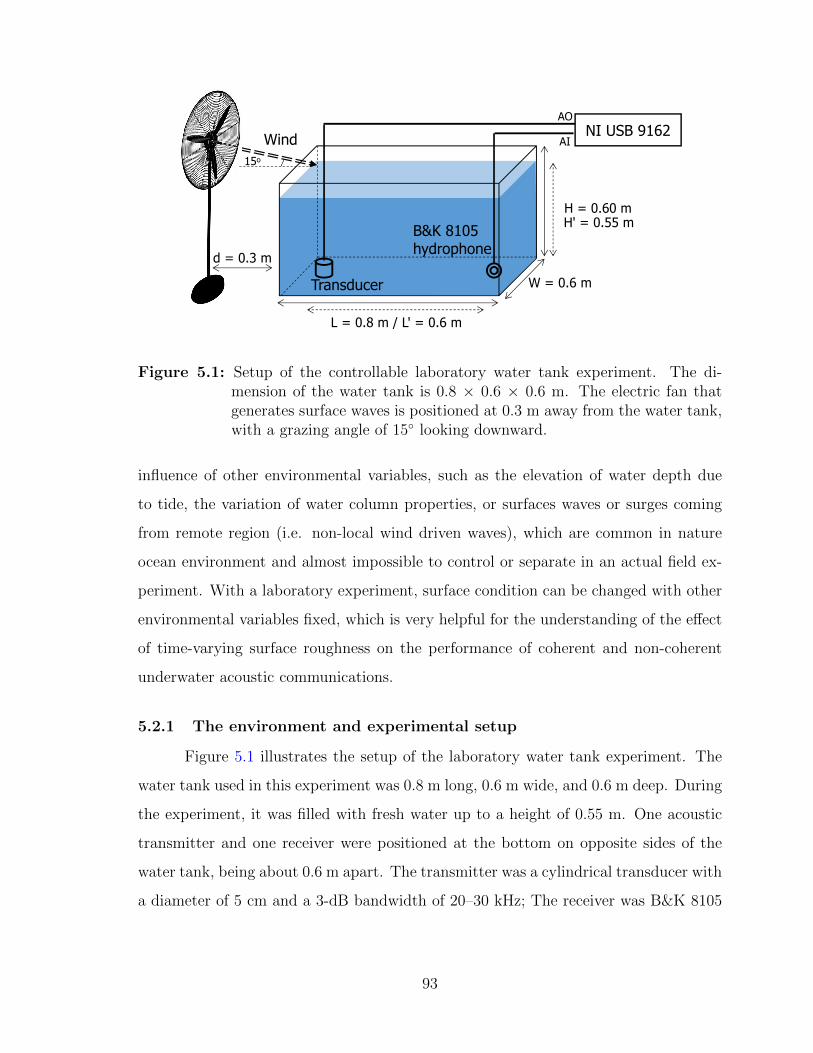
Transducer

B&K 8105hydrophone

NI USB 9162

L = 0.8 m / L' = 0.6 m

W = 0.6 m

H = 0.60 m H' = 0.55 m

AO

AIWind

d = 0.3 m

15o

Figure 5.1: Setup of the controllable laboratory water tank experiment. The di-mension of the water tank is 0.8 × 0.6 × 0.6 m. The electric fan thatgenerates surface waves is positioned at 0.3 m away from the water tank,with a grazing angle of 15◦ looking downward.

influence of other environmental variables, such as the elevation of water depth due

to tide, the variation of water column properties, or surfaces waves or surges coming

from remote region (i.e. non-local wind driven waves), which are common in nature

ocean environment and almost impossible to control or separate in an actual field ex-

periment. With a laboratory experiment, surface condition can be changed with other

environmental variables fixed, which is very helpful for the understanding of the effect

of time-varying surface roughness on the performance of coherent and non-coherent

underwater acoustic communications.

5.2.1 The environment and experimental setup

Figure 5.1 illustrates the setup of the laboratory water tank experiment. The

water tank used in this experiment was 0.8 m long, 0.6 m wide, and 0.6 m deep. During

the experiment, it was filled with fresh water up to a height of 0.55 m. One acoustic

transmitter and one receiver were positioned at the bottom on opposite sides of the

water tank, being about 0.6 m apart. The transmitter was a cylindrical transducer with

a diameter of 5 cm and a 3-dB bandwidth of 20–30 kHz; The receiver was B&K 8105

93

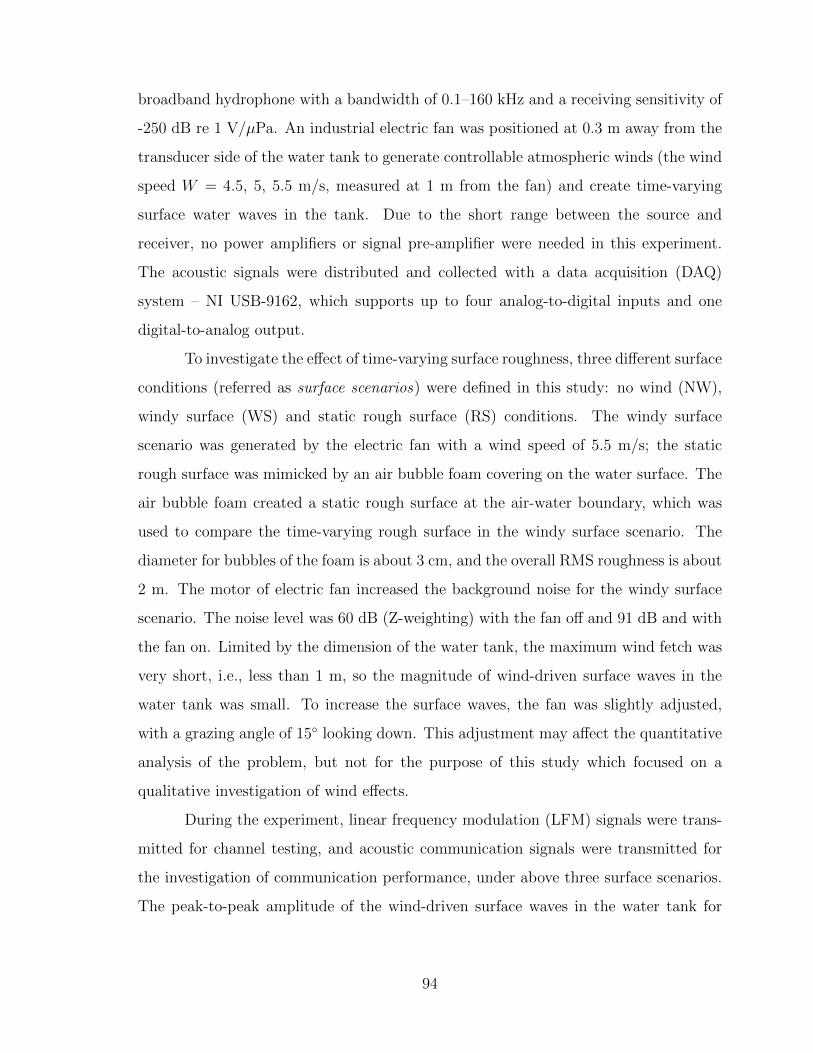
broadband hydrophone with a bandwidth of 0.1–160 kHz and a receiving sensitivity of

-250 dB re 1 V/µPa. An industrial electric fan was positioned at 0.3 m away from the

transducer side of the water tank to generate controllable atmospheric winds (the wind

speed W = 4.5, 5, 5.5 m/s, measured at 1 m from the fan) and create time-varying

surface water waves in the tank. Due to the short range between the source and

receiver, no power amplifiers or signal pre-amplifier were needed in this experiment.

The acoustic signals were distributed and collected with a data acquisition (DAQ)

system – NI USB-9162, which supports up to four analog-to-digital inputs and one

digital-to-analog output.

To investigate the effect of time-varying surface roughness, three different surface

conditions (referred as surface scenarios) were defined in this study: no wind (NW),

windy surface (WS) and static rough surface (RS) conditions. The windy surface

scenario was generated by the electric fan with a wind speed of 5.5 m/s; the static

rough surface was mimicked by an air bubble foam covering on the water surface. The

air bubble foam created a static rough surface at the air-water boundary, which was

used to compare the time-varying rough surface in the windy surface scenario. The

diameter for bubbles of the foam is about 3 cm, and the overall RMS roughness is about

2 m. The motor of electric fan increased the background noise for the windy surface

scenario. The noise level was 60 dB (Z-weighting) with the fan off and 91 dB and with

the fan on. Limited by the dimension of the water tank, the maximum wind fetch was

very short, i.e., less than 1 m, so the magnitude of wind-driven surface waves in the

water tank was small. To increase the surface waves, the fan was slightly adjusted,

with a grazing angle of 15◦ looking down. This adjustment may affect the quantitative

analysis of the problem, but not for the purpose of this study which focused on a

qualitative investigation of wind effects.

During the experiment, linear frequency modulation (LFM) signals were trans-

mitted for channel testing, and acoustic communication signals were transmitted for

the investigation of communication performance, under above three surface scenarios.

The peak-to-peak amplitude of the wind-driven surface waves in the water tank for

94

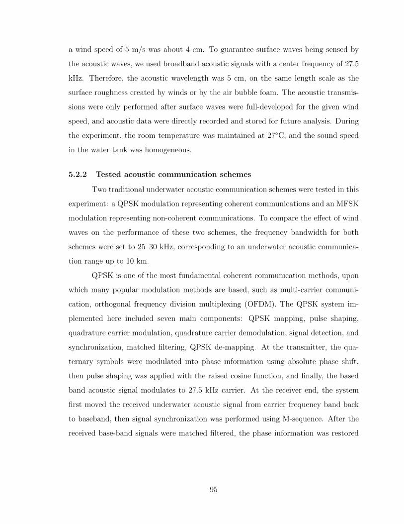
a wind speed of 5 m/s was about 4 cm. To guarantee surface waves being sensed by

the acoustic waves, we used broadband acoustic signals with a center frequency of 27.5

kHz. Therefore, the acoustic wavelength was 5 cm, on the same length scale as the

surface roughness created by winds or by the air bubble foam. The acoustic transmis-

sions were only performed after surface waves were full-developed for the given wind

speed, and acoustic data were directly recorded and stored for future analysis. During

the experiment, the room temperature was maintained at 27◦C, and the sound speed

in the water tank was homogeneous.

5.2.2 Tested acoustic communication schemes

Two traditional underwater acoustic communication schemes were tested in this

experiment: a QPSK modulation representing coherent communications and an MFSK

modulation representing non-coherent communications. To compare the effect of wind

waves on the performance of these two schemes, the frequency bandwidth for both

schemes were set to 25–30 kHz, corresponding to an underwater acoustic communica-

tion range up to 10 km.

QPSK is one of the most fundamental coherent communication methods, upon

which many popular modulation methods are based, such as multi-carrier communi-

cation, orthogonal frequency division multiplexing (OFDM). The QPSK system im-

plemented here included seven main components: QPSK mapping, pulse shaping,

quadrature carrier modulation, quadrature carrier demodulation, signal detection, and

synchronization, matched filtering, QPSK de-mapping. At the transmitter, the qua-

ternary symbols were modulated into phase information using absolute phase shift,

then pulse shaping was applied with the raised cosine function, and finally, the based

band acoustic signal modulates to 27.5 kHz carrier. At the receiver end, the system

first moved the received underwater acoustic signal from carrier frequency band back

to baseband, then signal synchronization was performed using M-sequence. After the

received base-band signals were matched filtered, the phase information was restored

95

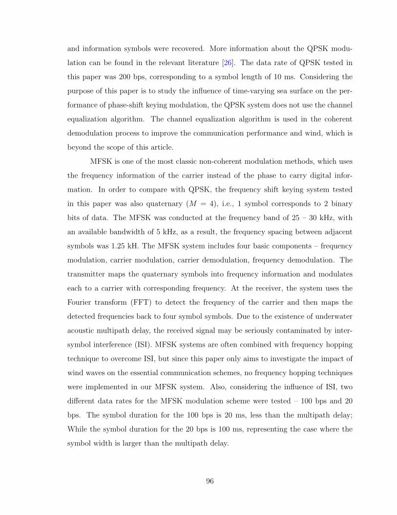
and information symbols were recovered. More information about the QPSK modu-

lation can be found in the relevant literature [26]. The data rate of QPSK tested in

this paper was 200 bps, corresponding to a symbol length of 10 ms. Considering the

purpose of this paper is to study the influence of time-varying sea surface on the per-

formance of phase-shift keying modulation, the QPSK system does not use the channel

equalization algorithm. The channel equalization algorithm is used in the coherent

demodulation process to improve the communication performance and wind, which is

beyond the scope of this article.

MFSK is one of the most classic non-coherent modulation methods, which uses

the frequency information of the carrier instead of the phase to carry digital infor-

mation. In order to compare with QPSK, the frequency shift keying system tested

in this paper was also quaternary (M = 4), i.e., 1 symbol corresponds to 2 binary

bits of data. The MFSK was conducted at the frequency band of 25 – 30 kHz, with

an available bandwidth of 5 kHz, as a result, the frequency spacing between adjacent

symbols was 1.25 kH. The MFSK system includes four basic components – frequency

modulation, carrier modulation, carrier demodulation, frequency demodulation. The

transmitter maps the quaternary symbols into frequency information and modulates

each to a carrier with corresponding frequency. At the receiver, the system uses the

Fourier transform (FFT) to detect the frequency of the carrier and then maps the

detected frequencies back to four symbol symbols. Due to the existence of underwater

acoustic multipath delay, the received signal may be seriously contaminated by inter-

symbol interference (ISI). MFSK systems are often combined with frequency hopping

technique to overcome ISI, but since this paper only aims to investigate the impact of

wind waves on the essential communication schemes, no frequency hopping techniques

were implemented in our MFSK system. Also, considering the influence of ISI, two

different data rates for the MFSK modulation scheme were tested – 100 bps and 20

bps. The symbol duration for the 100 bps is 20 ms, less than the multipath delay;

While the symbol duration for the 20 bps is 100 ms, representing the case where the

symbol width is larger than the multipath delay.

96

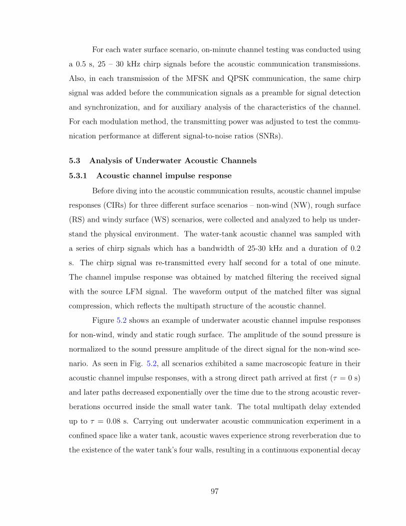
For each water surface scenario, on-minute channel testing was conducted using

a 0.5 s, 25 – 30 kHz chirp signals before the acoustic communication transmissions.

Also, in each transmission of the MFSK and QPSK communication, the same chirp

signal was added before the communication signals as a preamble for signal detection

and synchronization, and for auxiliary analysis of the characteristics of the channel.

For each modulation method, the transmitting power was adjusted to test the commu-

nication performance at different signal-to-noise ratios (SNRs).

5.3 Analysis of Underwater Acoustic Channels

5.3.1 Acoustic channel impulse response

Before diving into the acoustic communication results, acoustic channel impulse

responses (CIRs) for three different surface scenarios – non-wind (NW), rough surface

(RS) and windy surface (WS) scenarios, were collected and analyzed to help us under-

stand the physical environment. The water-tank acoustic channel was sampled with

a series of chirp signals which has a bandwidth of 25-30 kHz and a duration of 0.2

s. The chirp signal was re-transmitted every half second for a total of one minute.

The channel impulse response was obtained by matched filtering the received signal

with the source LFM signal. The waveform output of the matched filter was signal

compression, which reflects the multipath structure of the acoustic channel.

Figure 5.2 shows an example of underwater acoustic channel impulse responses

for non-wind, windy and static rough surface. The amplitude of the sound pressure is

normalized to the sound pressure amplitude of the direct signal for the non-wind sce-

nario. As seen in Fig. 5.2, all scenarios exhibited a same macroscopic feature in their

acoustic channel impulse responses, with a strong direct path arrived at first (τ = 0 s)

and later paths decreased exponentially over the time due to the strong acoustic rever-

berations occurred inside the small water tank. The total multipath delay extended

up to τ = 0.08 s. Carrying out underwater acoustic communication experiment in a

confined space like a water tank, acoustic waves experience strong reverberation due to

the existence of the water tank’s four walls, resulting in a continuous exponential decay

97

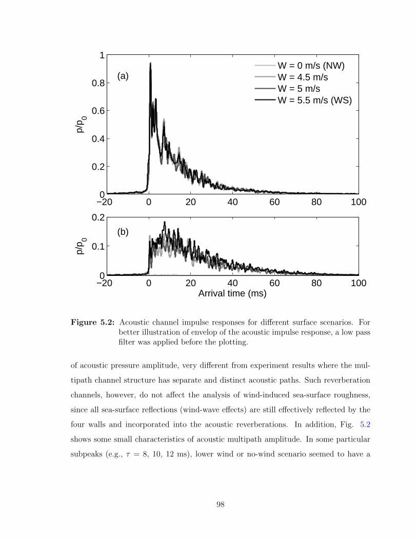
−20 0 20 40 60 80 1000

0.2

0.4

0.6

0.8

1

p/p

0

(a)W = 0 m/s (NW)

W = 4.5 m/s

W = 5 m/s

W = 5.5 m/s (WS)

−20 0 20 40 60 80 1000

0.1

0.2

Arrival time (ms)

p/p

0

(b)

Figure 5.2: Acoustic channel impulse responses for different surface scenarios. Forbetter illustration of envelop of the acoustic impulse response, a low passfilter was applied before the plotting.

of acoustic pressure amplitude, very different from experiment results where the mul-

tipath channel structure has separate and distinct acoustic paths. Such reverberation

channels, however, do not affect the analysis of wind-induced sea-surface roughness,

since all sea-surface reflections (wind-wave effects) are still effectively reflected by the

four walls and incorporated into the acoustic reverberations. In addition, Fig. 5.2

shows some small characteristics of acoustic multipath amplitude. In some particular

subpeaks (e.g., τ = 8, 10, 12 ms), lower wind or no-wind scenario seemed to have a

98

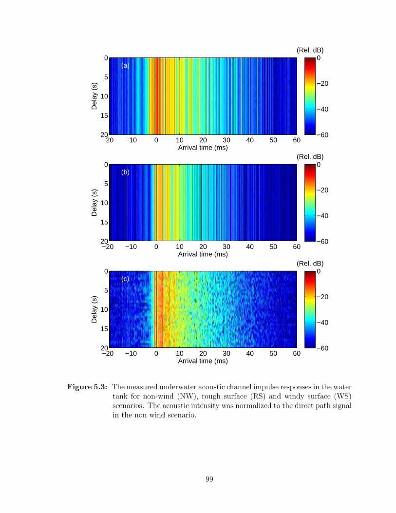
Arrival time (ms)

Dela

y (

s)

(a)

−20 −10 0 10 20 30 40 50 60

0

5

10

15

20

(Rel. dB)

−60

−40

−20

0

Arrival time (ms)

Dela

y (

s)

(b)

−20 −10 0 10 20 30 40 50 60

0

5

10

15

20

(Rel. dB)

−60

−40

−20

0

Arrival time (ms)

Dela

y (

s)

(c)

−20 −10 0 10 20 30 40 50 60

0

5

10

15

20

(Rel. dB)

−60

−40

−20

0

Figure 5.3: The measured underwater acoustic channel impulse responses in the watertank for non-wind (NW), rough surface (RS) and windy surface (WS)scenarios. The acoustic intensity was normalized to the direct path signalin the non wind scenario.

99

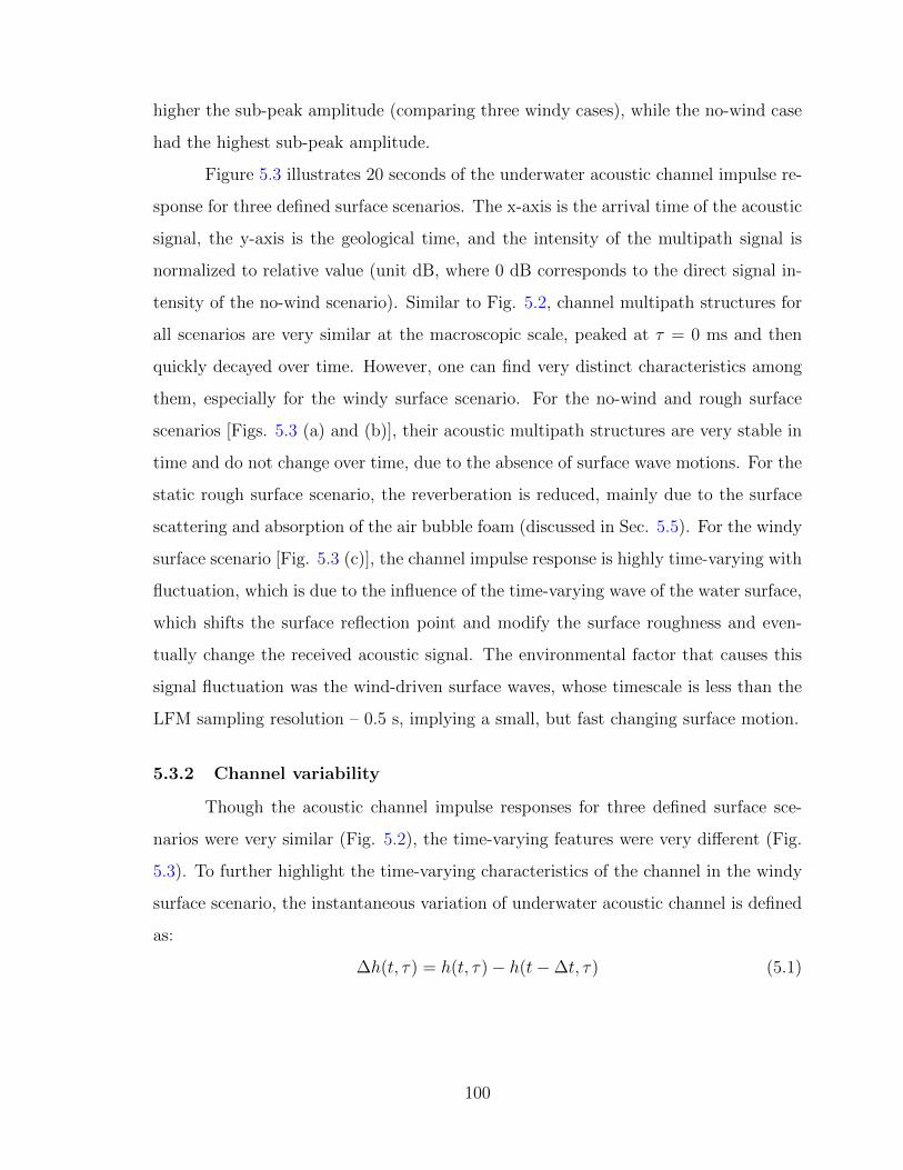
higher the sub-peak amplitude (comparing three windy cases), while the no-wind case

had the highest sub-peak amplitude.

Figure 5.3 illustrates 20 seconds of the underwater acoustic channel impulse re-

sponse for three defined surface scenarios. The x-axis is the arrival time of the acoustic

signal, the y-axis is the geological time, and the intensity of the multipath signal is

normalized to relative value (unit dB, where 0 dB corresponds to the direct signal in-

tensity of the no-wind scenario). Similar to Fig. 5.2, channel multipath structures for

all scenarios are very similar at the macroscopic scale, peaked at τ = 0 ms and then

quickly decayed over time. However, one can find very distinct characteristics among

them, especially for the windy surface scenario. For the no-wind and rough surface

scenarios [Figs. 5.3 (a) and (b)], their acoustic multipath structures are very stable in

time and do not change over time, due to the absence of surface wave motions. For the

static rough surface scenario, the reverberation is reduced, mainly due to the surface

scattering and absorption of the air bubble foam (discussed in Sec. 5.5). For the windy

surface scenario [Fig. 5.3 (c)], the channel impulse response is highly time-varying with

fluctuation, which is due to the influence of the time-varying wave of the water surface,

which shifts the surface reflection point and modify the surface roughness and even-

tually change the received acoustic signal. The environmental factor that causes this

signal fluctuation was the wind-driven surface waves, whose timescale is less than the

LFM sampling resolution – 0.5 s, implying a small, but fast changing surface motion.

5.3.2 Channel variability

Though the acoustic channel impulse responses for three defined surface sce-

narios were very similar (Fig. 5.2), the time-varying features were very different (Fig.

5.3). To further highlight the time-varying characteristics of the channel in the windy

surface scenario, the instantaneous variation of underwater acoustic channel is defined

as:

∆h(t, τ) = h(t, τ)− h(t−∆t, τ) (5.1)

100

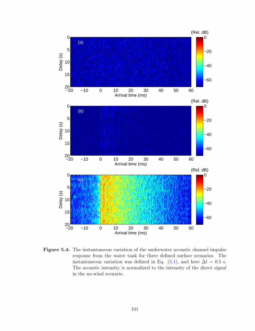
Arrival time (ms)

Dela

y (

s)

(a)

−20 −10 0 10 20 30 40 50 60

0

5

10

15

20

(Rel. dB)

−60

−40

−20

0

Arrival time (ms)

Dela

y (

s)

(b)

−20 −10 0 10 20 30 40 50 60

0

5

10

15

20

(Rel. dB)

−60

−40

−20

0

Arrival time (ms)

Dela

y (

s)

(c)

−20 −10 0 10 20 30 40 50 60

0

5

10

15

20

(Rel. dB)

−60

−40

−20

0

Figure 5.4: The instantaneous variation of the underwater acoustic channel impulseresponse from the water tank for three defined surface scenarios. Theinstantaneous variation was defined in Eq. (5.1), and here ∆t = 0.5 s.The acoustic intensity is normalized to the intensity of the direct signalin the no-wind scenario.

101

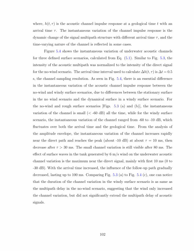
where, h(t, τ) is the acoustic channel impulse response at a geological time t with an

arrival time τ . The instantaneous variation of the channel impulse response is the

dynamic change of the signal multipath structure with different arrival time τ , and the

time-varying nature of the channel is reflected in some cases.

Figure 5.4 shows the instantaneous variation of underwater acoustic channels

for three defined surface scenarios, calculated from Eq. (5.1). Similar to Fig. 5.3, the

intensity of the acoustic multipath was normalized to the intensity of the direct signal

for the no-wind scenario. The arrival time interval used to calculate ∆h(t, τ) is ∆t = 0.5

s, the channel sampling resolution. As seen in Fig. 5.4, there is an essential difference

in the instantaneous variation of the acoustic channel impulse response between the

no-wind and windy surface scenarios, due to differences between the stationary surface

in the no wind scenario and the dynamical surface in a windy surface scenario. For

the no-wind and rough surface scenarios [Figs. 5.3 (a) and (b)], the instantaneous

variation of the channel is small (< -60 dB) all the time, while for the windy surface

scenario, the instantaneous variation of the channel ranged from -60 to -10 dB, which

fluctuates over both the arrival time and the geological time. From the analysis of

the amplitude envelope, the instantaneous variation of the channel increases rapidly

near the direct path and reaches the peak (about -10 dB) at about τ = 10 ms, then

decrease after τ > 30 ms. The small channel variation is still visible after 80 ms. The

effect of surface waves in the tank generated by 6 m/s wind on the underwater acoustic

channel variation is the maximum near the direct signal, mainly with first 10 ms (0 to

-30 dB). With the arrival time increased, the influence of the follow-up path gradually

decreased, lasting up to 100 ms. Comparing Fig. 5.3 (a) to Fig. 5.4 (c), one can notice

that the duration of the channel variation in the windy surface scenario is as same as

the multipath delay in the no-wind scenario, suggesting that the wind only increased

the channel variation, but did not significantly extend the multipath delay of acoustic

signals.

102

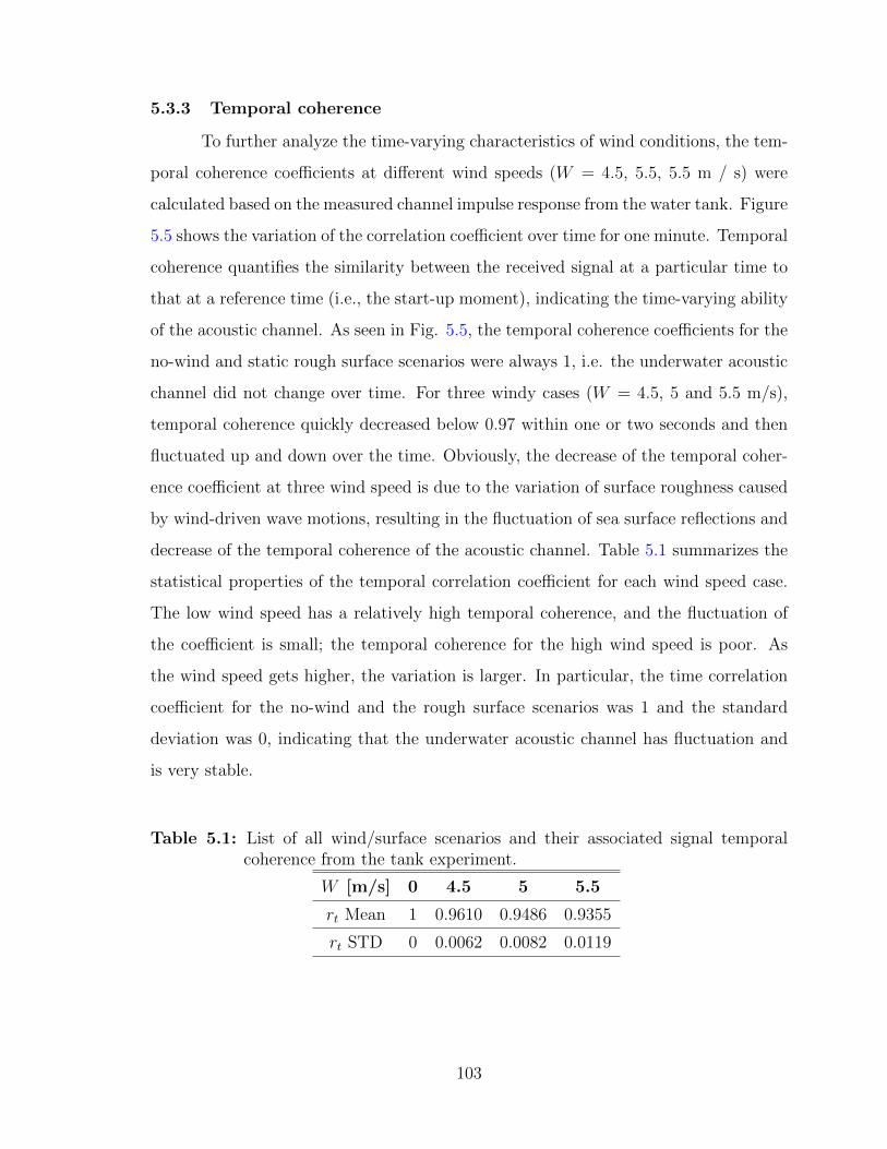
5.3.3 Temporal coherence

To further analyze the time-varying characteristics of wind conditions, the tem-

poral coherence coefficients at different wind speeds (W = 4.5, 5.5, 5.5 m / s) were

calculated based on the measured channel impulse response from the water tank. Figure

5.5 shows the variation of the correlation coefficient over time for one minute. Temporal

coherence quantifies the similarity between the received signal at a particular time to

that at a reference time (i.e., the start-up moment), indicating the time-varying ability

of the acoustic channel. As seen in Fig. 5.5, the temporal coherence coefficients for the

no-wind and static rough surface scenarios were always 1, i.e. the underwater acoustic

channel did not change over time. For three windy cases (W = 4.5, 5 and 5.5 m/s),

temporal coherence quickly decreased below 0.97 within one or two seconds and then

fluctuated up and down over the time. Obviously, the decrease of the temporal coher-

ence coefficient at three wind speed is due to the variation of surface roughness caused

by wind-driven wave motions, resulting in the fluctuation of sea surface reflections and

decrease of the temporal coherence of the acoustic channel. Table 5.1 summarizes the

statistical properties of the temporal correlation coefficient for each wind speed case.

The low wind speed has a relatively high temporal coherence, and the fluctuation of

the coefficient is small; the temporal coherence for the high wind speed is poor. As

the wind speed gets higher, the variation is larger. In particular, the time correlation

coefficient for the no-wind and the rough surface scenarios was 1 and the standard

deviation was 0, indicating that the underwater acoustic channel has fluctuation and

is very stable.

Table 5.1: List of all wind/surface scenarios and their associated signal temporalcoherence from the tank experiment.

W [m/s] 0 4.5 5 5.5

rt Mean 1 0.9610 0.9486 0.9355

rt STD 0 0.0062 0.0082 0.0119

103

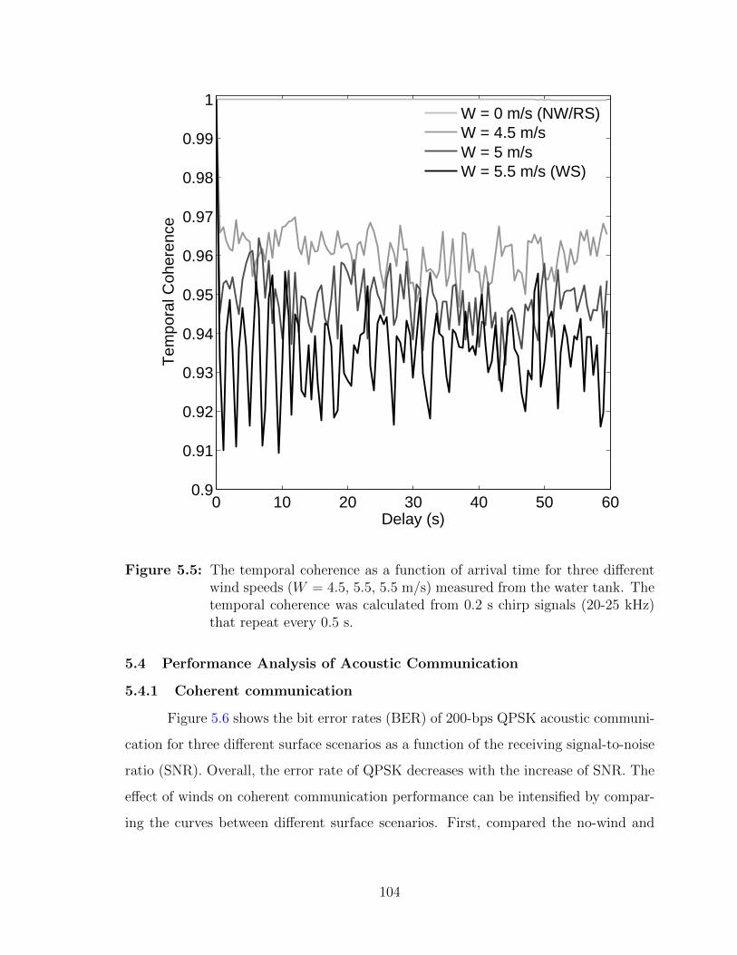
0 10 20 30 40 50 600.9

0.91

0.92

0.93

0.94

0.95

0.96

0.97

0.98

0.99

1

Delay (s)

Tem

pora

l C

ohere

nce

W = 0 m/s (NW/RS)

W = 4.5 m/s

W = 5 m/s

W = 5.5 m/s (WS)

Figure 5.5: The temporal coherence as a function of arrival time for three differentwind speeds (W = 4.5, 5.5, 5.5 m/s) measured from the water tank. Thetemporal coherence was calculated from 0.2 s chirp signals (20-25 kHz)that repeat every 0.5 s.

5.4 Performance Analysis of Acoustic Communication

5.4.1 Coherent communication

Figure 5.6 shows the bit error rates (BER) of 200-bps QPSK acoustic communi-

cation for three different surface scenarios as a function of the receiving signal-to-noise

ratio (SNR). Overall, the error rate of QPSK decreases with the increase of SNR. The

effect of winds on coherent communication performance can be intensified by compar-

ing the curves between different surface scenarios. First, compared the no-wind and

104

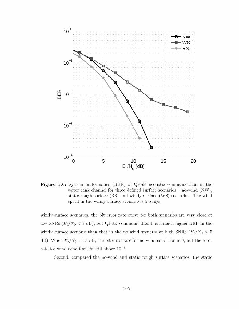
0 5 10 15 2010

−4

10−3

10−2

10−1

100

Eb/N

0 (dB)

BE

R

NW

WS

RS

Figure 5.6: System performance (BER) of QPSK acoustic communication in thewater tank channel for three defined surface scenarios – no-wind (NW),static rough surface (RS) and windy surface (WS) scenarios. The windspeed in the windy surface scenario is 5.5 m/s.

windy surface scenarios, the bit error rate curve for both scenarios are very close at

low SNRs (Eb/N0 < 3 dB), but QPSK communication has a much higher BER in the

windy surface scenario than that in the no-wind scenario at high SNRs (Eb/N0 > 5

dB). When Eb/N0 = 13 dB, the bit error rate for no-wind condition is 0, but the error

rate for wind conditions is still above 10−3.

Second, compared the no-wind and static rough surface scenarios, the static

105

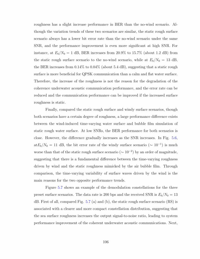
roughness has a slight increase performance in BER than the no-wind scenario. Al-

though the variation trends of these two scenarios are similar, the static rough surface

scenario always has a lower bit error rate than the no-wind scenario under the same

SNR, and the performance improvement is even more significant at high SNR. For

instance, at Eb/N0 = 1 dB, BER increases from 20.9% to 15.7% (about 1.2 dB) from

the static rough surface scenario to the no-wind scenario, while at Eb/N0 = 13 dB,

the BER increases from 0.14% to 0.04% (about 5.4 dB), suggesting that a static rough

surface is more beneficial for QPSK communication than a calm and flat water surface.

Therefore, the increase of the roughness is not the reason for the degradation of the

coherence underwater acoustic communication performance, and the error rate can be

reduced and the communication performance can be improved if the increased surface

roughness is static.

Finally, compared the static rough surface and windy surface scenarios, though

both scenarios have a certain degree of roughness, a large performance difference exists

between the wind-induced time-varying water surface and bubble film simulation of

static rough water surface. At low SNRs, the BER performance for both scenarios is

close. However, the difference gradually increases as the SNR increases. In Fig. 5.6,

atEb/N0 = 11 dB, the bit error rate of the windy surface scenario (∼ 10−1) is much

worse than that of the static rough surface scenario (∼ 10−2) by an order of magnitude,

suggesting that there is a fundamental difference between the time-varying roughness

driven by wind and the static roughness mimicked by the air bubble film. Through

comparison, the time-varying variability of surface waves driven by the wind is the

main reasons for the two opposite performance trends.

Figure 5.7 shows an example of the demodulation constellations for the three

preset surface scenarios. The data rate is 200 bps and the received SNR is Eb/N0 = 13

dB. First of all, compared Fig. 5.7 (a) and (b), the static rough surface scenario (RS) is

associated with a clearer and more compact constellation distribution, suggesting that

the sea surface roughness increases the output signal-to-noise ratio, leading to system

performance improvement of the coherent underwater acoustic communications. Next,

106

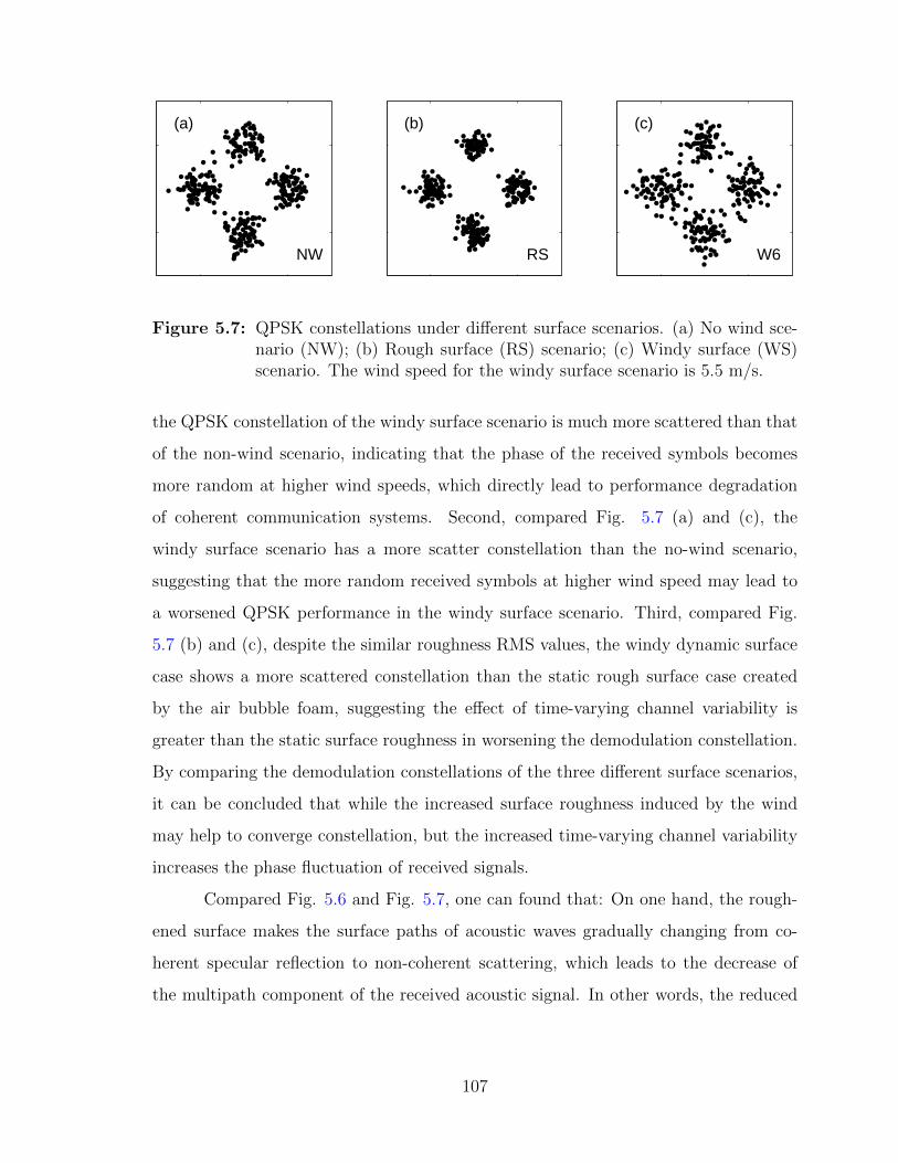
(a)

NW

(b)

RS

(c)

W6

Figure 5.7: QPSK constellations under different surface scenarios. (a) No wind sce-nario (NW); (b) Rough surface (RS) scenario; (c) Windy surface (WS)scenario. The wind speed for the windy surface scenario is 5.5 m/s.

the QPSK constellation of the windy surface scenario is much more scattered than that

of the non-wind scenario, indicating that the phase of the received symbols becomes

more random at higher wind speeds, which directly lead to performance degradation

of coherent communication systems. Second, compared Fig. 5.7 (a) and (c), the

windy surface scenario has a more scatter constellation than the no-wind scenario,

suggesting that the more random received symbols at higher wind speed may lead to

a worsened QPSK performance in the windy surface scenario. Third, compared Fig.

5.7 (b) and (c), despite the similar roughness RMS values, the windy dynamic surface

case shows a more scattered constellation than the static rough surface case created

by the air bubble foam, suggesting the effect of time-varying channel variability is

greater than the static surface roughness in worsening the demodulation constellation.

By comparing the demodulation constellations of the three different surface scenarios,

it can be concluded that while the increased surface roughness induced by the wind

may help to converge constellation, but the increased time-varying channel variability

increases the phase fluctuation of received signals.

Compared Fig. 5.6 and Fig. 5.7, one can found that: On one hand, the rough-

ened surface makes the surface paths of acoustic waves gradually changing from co-

herent specular reflection to non-coherent scattering, which leads to the decrease of

the multipath component of the received acoustic signal. In other words, the reduced

107

multi-path energy from the sea-surface reflection highlights the energy of the main

direct-path signal, which helps to reduce inter-symbol interference and improve the

communication performance. On the other hand, the wind caused by the wave has

a high time-varying channel variability, which continues to affect the amplitude and

phase of the received signal, severely reducing the stability of the QPSK phase infor-

mation, and ultimately disrupt the coherent communication in the underwater signal

coherence required. Therefore, the performance degradation of coherent underwater

acoustic communication in the presence of wind is not caused by wind-induced envi-

ronmental noise or roughness increase, but rather by increased instantaneous channel

variation and reduced temporal coherence. Moreover, for coherent acoustic communi-

cation, the negative influence caused by time-varying is greater than positive influence

caused by wind-induced sea roughness.

5.4.2 Non-coherent communication

Figure 5.8 shows the bit error rate performance of the underwater acoustic

communication system in no-wind, static rough surface, and wind surface scenarios for

the acoustic MFSK (M = 4) system. The data rate here is 100 bps and the associated

symbol duration is 20 ms, while the multipath delay of the water tank channel is more

than 80 ms (Fig. 5.2), which is the longer than the symbol duration. First, comparing

the no-wind and windy surface scenarios, the BER performances for both are very

similar, both decrease with the increase of SNR, and eventually remain at 0.04 when

Eb/N0 > 20 dB. One can see that the wind-driven surface waves in the laboratory

water tank environment have little effect on the performance of MFSK non-coherent

communication systems. Second, comparing the no-wind and static rough surface

scenarios, the stationary, rough surface boundary in the static rough surface scenario

improves the BER performance of non-coherent communication systems. When the

SNR is low (Eb/N0 < 6 dB), the performance of the static rough surface scenario is

similar to that of the no-wind scenario, but with the increased SNR, the BER of the

static rough surface scenario decreases rapidly and reaches zero error at Eb/N0 = 18

108

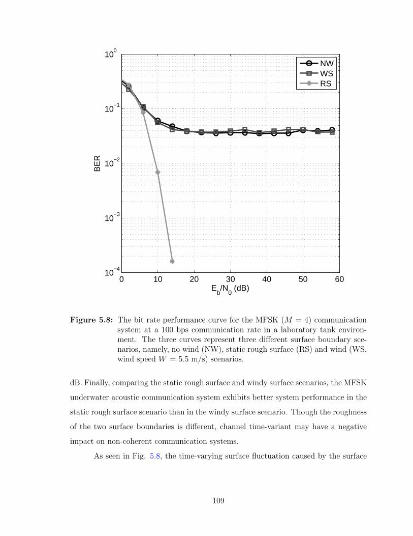
0 10 20 30 40 50 6010

−4

10−3

10−2

10−1

100

Eb/N

0 (dB)

BE

R

NW

WS

RS

Figure 5.8: The bit rate performance curve for the MFSK (M = 4) communicationsystem at a 100 bps communication rate in a laboratory tank environ-ment. The three curves represent three different surface boundary sce-narios, namely, no wind (NW), static rough surface (RS) and wind (WS,wind speed W = 5.5 m/s) scenarios.

dB. Finally, comparing the static rough surface and windy surface scenarios, the MFSK

underwater acoustic communication system exhibits better system performance in the

static rough surface scenario than in the windy surface scenario. Though the roughness

of the two surface boundaries is different, channel time-variant may have a negative

impact on non-coherent communication systems.

As seen in Fig. 5.8, the time-varying surface fluctuation caused by the surface

109

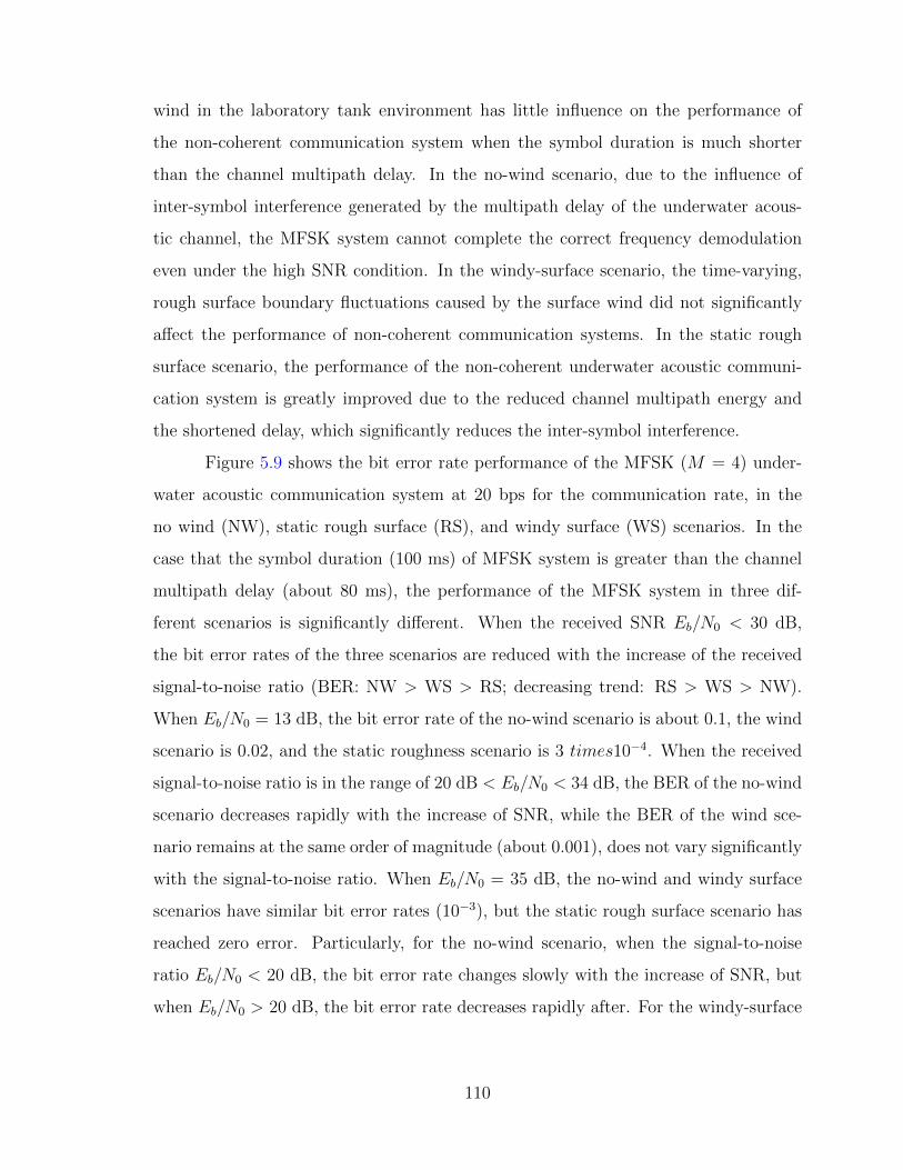
wind in the laboratory tank environment has little influence on the performance of

the non-coherent communication system when the symbol duration is much shorter

than the channel multipath delay. In the no-wind scenario, due to the influence of

inter-symbol interference generated by the multipath delay of the underwater acous-

tic channel, the MFSK system cannot complete the correct frequency demodulation

even under the high SNR condition. In the windy-surface scenario, the time-varying,

rough surface boundary fluctuations caused by the surface wind did not significantly

affect the performance of non-coherent communication systems. In the static rough

surface scenario, the performance of the non-coherent underwater acoustic communi-

cation system is greatly improved due to the reduced channel multipath energy and

the shortened delay, which significantly reduces the inter-symbol interference.

Figure 5.9 shows the bit error rate performance of the MFSK (M = 4) under-

water acoustic communication system at 20 bps for the communication rate, in the

no wind (NW), static rough surface (RS), and windy surface (WS) scenarios. In the

case that the symbol duration (100 ms) of MFSK system is greater than the channel

multipath delay (about 80 ms), the performance of the MFSK system in three dif-

ferent scenarios is significantly different. When the received SNR Eb/N0 < 30 dB,

the bit error rates of the three scenarios are reduced with the increase of the received

signal-to-noise ratio (BER: NW > WS > RS; decreasing trend: RS > WS > NW).

When Eb/N0 = 13 dB, the bit error rate of the no-wind scenario is about 0.1, the wind

scenario is 0.02, and the static roughness scenario is 3 times10−4. When the received

signal-to-noise ratio is in the range of 20 dB < Eb/N0 < 34 dB, the BER of the no-wind

scenario decreases rapidly with the increase of SNR, while the BER of the wind sce-

nario remains at the same order of magnitude (about 0.001), does not vary significantly

with the signal-to-noise ratio. When Eb/N0 = 35 dB, the no-wind and windy surface

scenarios have similar bit error rates (10−3), but the static rough surface scenario has

reached zero error. Particularly, for the no-wind scenario, when the signal-to-noise

ratio Eb/N0 < 20 dB, the bit error rate changes slowly with the increase of SNR, but

when Eb/N0 > 20 dB, the bit error rate decreases rapidly after. For the windy-surface

110

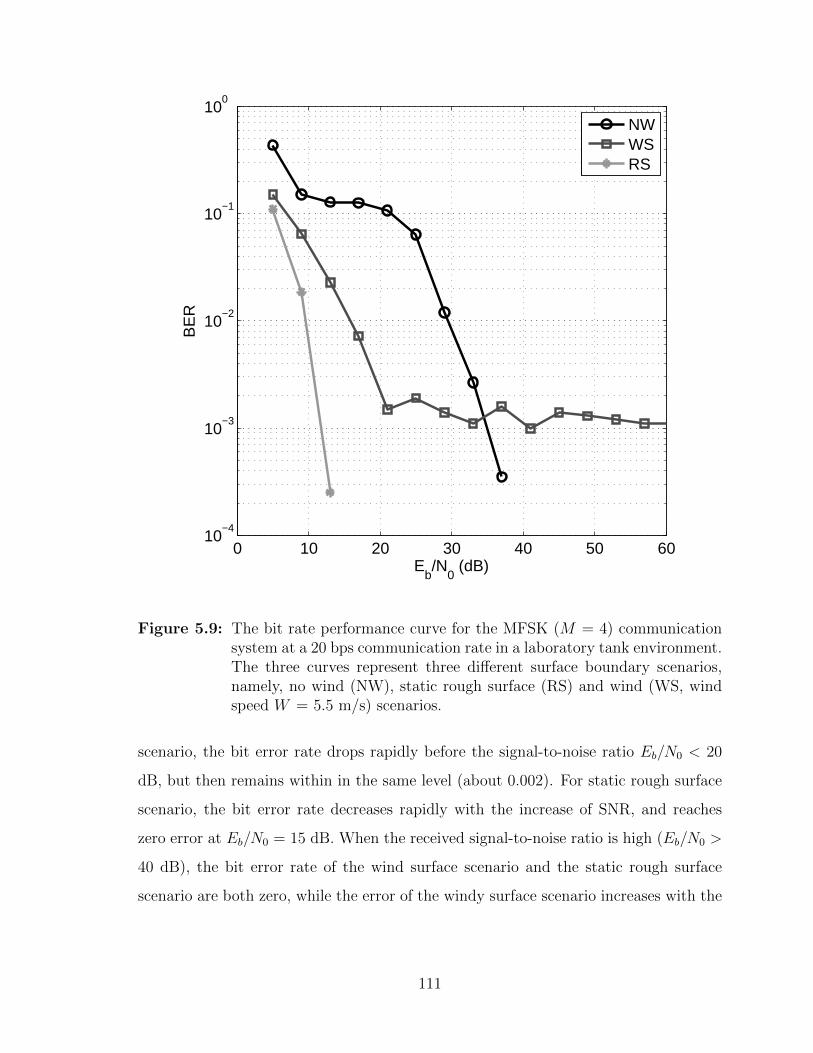
0 10 20 30 40 50 6010

−4

10−3

10−2

10−1

100

Eb/N

0 (dB)

BE

R

NW

WS

RS

Figure 5.9: The bit rate performance curve for the MFSK (M = 4) communicationsystem at a 20 bps communication rate in a laboratory tank environment.The three curves represent three different surface boundary scenarios,namely, no wind (NW), static rough surface (RS) and wind (WS, windspeed W = 5.5 m/s) scenarios.

scenario, the bit error rate drops rapidly before the signal-to-noise ratio Eb/N0 < 20

dB, but then remains within in the same level (about 0.002). For static rough surface

scenario, the bit error rate decreases rapidly with the increase of SNR, and reaches

zero error at Eb/N0 = 15 dB. When the received signal-to-noise ratio is high (Eb/N0 >

40 dB), the bit error rate of the wind surface scenario and the static rough surface

scenario are both zero, while the error of the windy surface scenario increases with the

111

signal-to-noise ratio, ending at about 10−3.

The effect of wind speed on the performance of non-coherent communication

systems is less pronounced than that of coherent communication systems. Rough

surface roughness caused by wind waves improves or decreases the performance of non-

coherent communication systems, which also depends on a number of other conditions,

such as the relationship between the symbol width and the multipath delay of the

channel, or the received signal-to-noise ratio of the system.

5.5 Discussions

Two classical and representative underwater acoustic communication modula-

tion schemes (MFSK and QPSK) were tested and analyzed in a three surface boundary

scenarios, i.e., no-wind and static rough surface and windy surface scenarios through

a laboratory simulation experiment platform with controllable environment variables.

Results show that the time-varying roughness boundary caused by wind-driven surface

waves will lead to the performance degradation of the coherent water acoustic commu-

nication system (Figs. 5.6 and 5.7), while the performance of the non-coherent under-

water acoustic communication system is less influenced (Fig. 5.8), and there can be a

slight performance increase (Fig. 5.9) with low signal-to-noise ratio and longer symbol

delay than channel multipath. Acoustic channel analysis revealed that in the windy

surface scenario, surface boundary condition becomes rougher and more dynamic due

to surface winds, and received acoustic signals experience a smaller surface-returned en-

ergy, a stronger channel variation (Fig. 5.4) and a lower temporal coherence (Fig. 5.5).

Here, the effect of the wind as a common physical environment variable on underwater

acoustic and underwater acoustic communication systems is further discussed.

First, the results of QPSK underwater acoustic communication experiment ob-

tained in the lab water tank experiment are in agreement with the previous simulation

results [26], and the other sea test results [29, 79, 80], on the negative correlation be-

tween surface wind speed (or sea state) and the performance of underwater coherent

acoustic communications. However, based on the analysis of the experimental results

112

from no-wind, static rough surface and windy surface scenarios, we did not fully agree

with some previous research on the explanation of the adverse effects of wind and waves

on coherent communications. For example, van Walree [29] claimed the main reason

for the decrease in the coherence of underwater acoustic communication was due to

winds/waves is the decrease of the coherent energy of the signal caused by the increase

of environmental background noise and the increase of sea surface roughness. Results

show that, on the one hand, the effect of wind noise on the performance of coherent

underwater acoustic communication is far less than that of wind-induced time-varying

sea surface roughness. In the laboratory tank experiments, the wind-induced back-

ground noise is small. However, previous research [89] showed that wind-induced noise

is mainly concentrated at low frequencies (10 kHz or less), which will not have a signif-

icant impact on the performance of medium and high frequency underwater acoustic

communication systems. Therefore, the increase of wind-induced noise is not the main

cause of deterioration of coherent communication performance. On the other hand,

comparing the demodulation constellation and the BER curve (Figs. 5.6 and 5.7), one

can see that the increase of the static roughness not only does not reduce the perfor-

mance of coherence communication system. Instead, it improves the performance. In

addition to the increase of roughness, the wind generated by the wave has a higher

time-varying, affecting the stability of signal phase in the coherent communications,

destroying the coherent communication system underwater acoustic signal coherence

required for demodulation. Therefore, the increase of channel variability and the de-

crease of signal correlation are the main reasons for the negative correlation between

the sea surface wind velocity and the performance of the coherent water acoustic com-

munication in the sea-trial experiment of the coherent communication system.

The experimental results show that the time-varying rough boundary caused

by the wind does not significantly reduce the performance of non-coherent underwater

acoustic communication. Under some certain condition (based on symbol duration

and SNR), the performance of incoherent underwater acoustic communication systems

may be improved to a certain extent. The results of the MFSK underwater acoustic

113

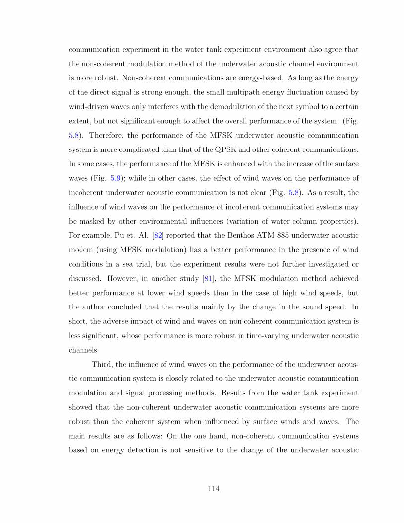
communication experiment in the water tank experiment environment also agree that

the non-coherent modulation method of the underwater acoustic channel environment

is more robust. Non-coherent communications are energy-based. As long as the energy

of the direct signal is strong enough, the small multipath energy fluctuation caused by

wind-driven waves only interferes with the demodulation of the next symbol to a certain

extent, but not significant enough to affect the overall performance of the system. (Fig.

5.8). Therefore, the performance of the MFSK underwater acoustic communication

system is more complicated than that of the QPSK and other coherent communications.

In some cases, the performance of the MFSK is enhanced with the increase of the surface

waves (Fig. 5.9); while in other cases, the effect of wind waves on the performance of

incoherent underwater acoustic communication is not clear (Fig. 5.8). As a result, the

influence of wind waves on the performance of incoherent communication systems may

be masked by other environmental influences (variation of water-column properties).

For example, Pu et. Al. [82] reported that the Benthos ATM-885 underwater acoustic

modem (using MFSK modulation) has a better performance in the presence of wind

conditions in a sea trial, but the experiment results were not further investigated or

discussed. However, in another study [81], the MFSK modulation method achieved

better performance at lower wind speeds than in the case of high wind speeds, but

the author concluded that the results mainly by the change in the sound speed. In

short, the adverse impact of wind and waves on non-coherent communication system is

less significant, whose performance is more robust in time-varying underwater acoustic

channels.

Third, the influence of wind waves on the performance of the underwater acous-

tic communication system is closely related to the underwater acoustic communication

modulation and signal processing methods. Results from the water tank experiment

showed that the non-coherent underwater acoustic communication systems are more

robust than the coherent system when influenced by surface winds and waves. The

main results are as follows: On the one hand, non-coherent communication systems

based on energy detection is not sensitive to the change of the underwater acoustic

114

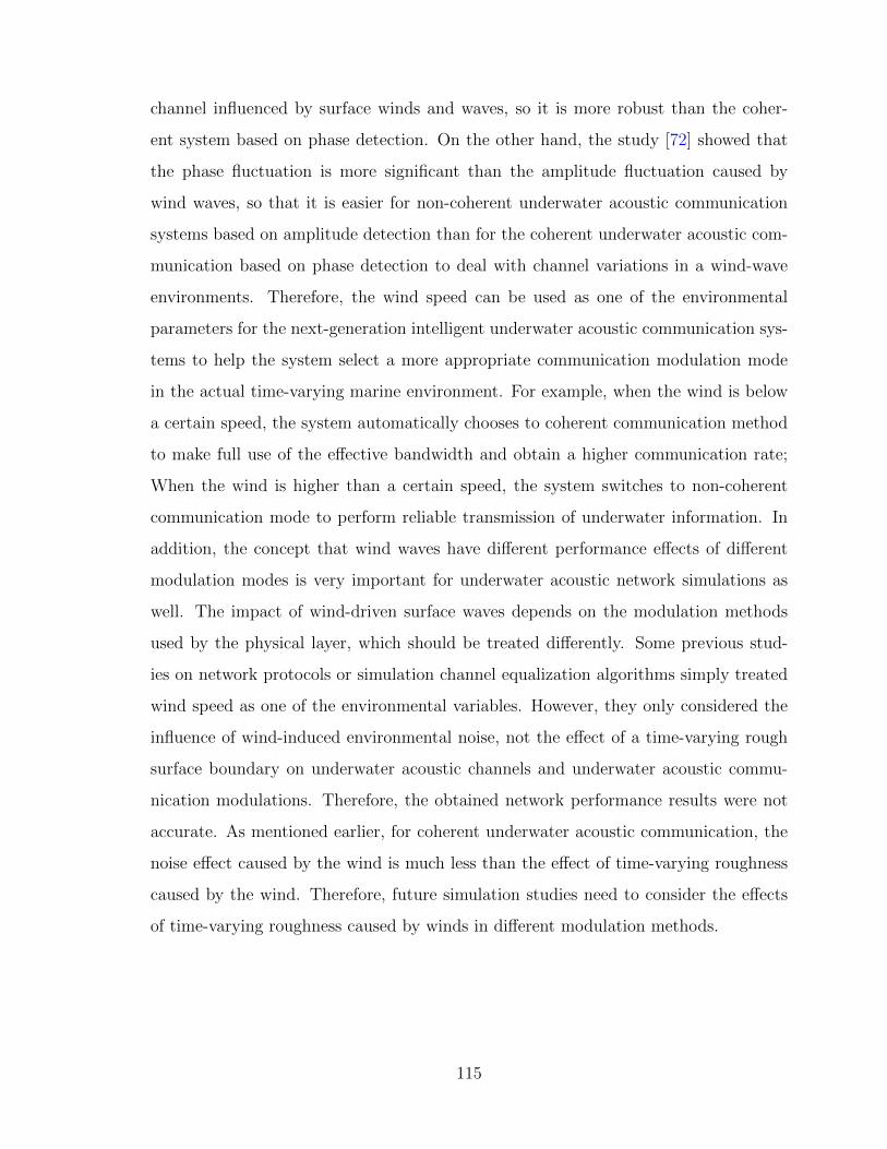
channel influenced by surface winds and waves, so it is more robust than the coher-

ent system based on phase detection. On the other hand, the study [72] showed that

the phase fluctuation is more significant than the amplitude fluctuation caused by

wind waves, so that it is easier for non-coherent underwater acoustic communication

systems based on amplitude detection than for the coherent underwater acoustic com-

munication based on phase detection to deal with channel variations in a wind-wave

environments. Therefore, the wind speed can be used as one of the environmental

parameters for the next-generation intelligent underwater acoustic communication sys-

tems to help the system select a more appropriate communication modulation mode

in the actual time-varying marine environment. For example, when the wind is below

a certain speed, the system automatically chooses to coherent communication method

to make full use of the effective bandwidth and obtain a higher communication rate;

When the wind is higher than a certain speed, the system switches to non-coherent

communication mode to perform reliable transmission of underwater information. In

addition, the concept that wind waves have different performance effects of different

modulation modes is very important for underwater acoustic network simulations as

well. The impact of wind-driven surface waves depends on the modulation methods

used by the physical layer, which should be treated differently. Some previous stud-

ies on network protocols or simulation channel equalization algorithms simply treated

wind speed as one of the environmental variables. However, they only considered the

influence of wind-induced environmental noise, not the effect of a time-varying rough

surface boundary on underwater acoustic channels and underwater acoustic commu-

nication modulations. Therefore, the obtained network performance results were not

accurate. As mentioned earlier, for coherent underwater acoustic communication, the

noise effect caused by the wind is much less than the effect of time-varying roughness

caused by the wind. Therefore, future simulation studies need to consider the effects

of time-varying roughness caused by winds in different modulation methods.

115

Finally, in the real marine environment, the wind effect on underwater communi-

cations is more complicated than the effect of wind-induced surface reflection on acous-

tic communication performance based on our results. In our water tank experiment,

only the influence of surface boundary variation on the performance of underwater

acoustic communication under the condition of uniform wave growth was considered,

but the ocean wind wave involves many complicated marine environmental variables.

For example, a consistent, strong wind blowing on the sea surface will increase water

mixing, deepening the thermocline, and thus affecting the speed of sound profile, and

ultimately change the entire underwater sound field and channel multipath structure

completely. On a larger time scale, the changes in the water column (e.g., temperature

or salinity variations) may exceed the effect of wind-induced time-varying sea-surface

roughness and completely alter the underwater sound field (as reported in [81, 76]).

Besides, the high-speed conditions of the wave breaking and underwater bubble gener-

ation, scattering, absorption of sound energy, resulting in the further multipath energy

losses at the receiver end. Though in the laboratory water tank environment, the wind

waves are small and there is no wave breaking or bubble forming, research showed that

the influence of air bubbles on the underwater acoustic channel is mainly increased

energy attenuation and increased background noise. Therefore, the underwater air

bubbles caused by wind and waves will also lead to multipath energy attenuation,

reduce the signal to noise ratio of the received signal. In addition, Bubbles motion

and breaking will produce a certain channel instantaneous change. Based on our re-

sults from time-varying surface waves, it can be deduced that air bubbles may have a

negative effect on the coherent underwater acoustic communication system, but does

not affect much on the performance of incoherent underwater acoustic communication

systems. This conclusion will be further studied in the future.

5.6 Conclusions

In this paper, a controllable experimental environment was constructed, and

a laboratory tank experiment was used to investigate the problem. The goal of this

116

paper was to explore the effect of wind-induced time-varying sea surface on coherent

and non-coherent underwater acoustic communication modulation schemes through a

controllable method and analyze the performance of the two modulation methods in

response to surface winds and waves. Results show that the influence of the wind on

coherent and non-phase acoustic communication is very different: the performance of

coherent underwater acoustic communication decreases remarkably with the increase

of wind speed, which is mainly due to the increased channel variability and the reduced

signal temporal coherence under high wind speed; and the presence of wind does not

result in a significant decrease in the performance of non-coherent communication due

to its less sensitivity to the channel variability, and in some cases, smaller multipath

reflected signals at high wind speed can even increase the performance of non-coherent

communications.

The influence of the wind on the underwater acoustic communication includes

two aspects: on the one hand, the increase of roughness, on the other hand, increases

the time-varying channel variability. The increase of roughness is beneficial to commu-

nication, while the increase of time-varying is not. Coherent communication is much

more sensitive to time-varying channel variability than non-coherent communication.

Coherent communication performance degraded under wind waves, while non-coherent

communication performance remained unaffected, but performance may be improved

due to increased roughness. Therefore, in the presence of wind, non-coherent commu-

nication can guarantee the higher reliability of the system, especially when the SNR is

low; In the absence of wind conditions, switching to coherent communication mode can

take full advantage of effective bandwidth to achieve a higher transmission rate. This

study is helpful for guiding the design of underwater acoustic communication system,

such as to assist the selection of communication modes according to the present wind-

wave condition. However, the relationship between the performance of different wind

speed, especially the effect of the bubble forming under high wind speed, still needs to

be further studied.

Future study may include following aspects. Since the tank channel is still very

117

different from the actual ocean time-varying environment, the performance variation of

underwater acoustic communication due to the wind effect in the real ocean should be

studied. Also, the impact of the wind on many sub-components of the communication

system will be investigated, such as synchronization, signal detection, and channel

equalization schemes of coherent underwater acoustic communication systems.

118

Chapter 6

CONCLUSION

The reliable acoustic communication in a highly time-varying ocean environment

is an extremely challenging research topic. Because underwater sound propagation is

closely related to the physical processes and water dynamics of the ocean, underwater

acoustic communication research should not be isolated from the variability of the

physical environment. However, it was treated as a separate research topic under

electrical engineering, which lacks consideration of the nature of the physical ocean

and hinders the development of underwater acoustic communication systems. This

dissertation focused on the link of underwater acoustics with the physical environment.

Studying the sound propagation in estuaries, where environmental variability is strong

due to the interaction between the freshwater and seawater, can significantly help

the understanding of underwater acoustic channel characteristics and the design of

next-generation underwater acoustic communication systems. Field experiment data

analysis, integrated numerical modeling, and a laboratory experiment were combined

together to study the internal link between physical oceanography, ocean acoustics and

underwater acoustic communications in a shallow tidal-straining estuary.

On the environmental variability of underwater acoustic channel in a tidal-

straining estuary, acoustic direct path and surface-bounced paths were found affected

by very different time-varying physical processes: (a) Influenced by tidal water dy-

namics, acoustic direct paths exhibit periodical intensity fading, as a result of water

column variation (water mixing and stratification) in a tidal-straining estuary. (b) Af-

fected by surface winds and waves, the pressure amplitude of acoustic surface-bounced

paths is highly correlated with surface wind speed, as a result of increased wind-driven

119

surface roughness at high winds significantly scattering away the acoustic energy of

surface-bounced paths.

On the link between the environmental variability and underwater acoustic com-

munications, the effect of the fast fluctuation of wind-induced surface waves on the per-

formance of underwater acoustic communications was investigated. Numerical model-

ing and laboratory experiment results suggested that, the increase roughness at high

winds is beneficial for the system performance; while the increased channel variability

is not. How wind-driven surface waves influence the performance of underwater acous-

tic communication is a result of the competition between these two factors: (a) For

coherent acoustic communication, the system performance may decrease remarkably

with increasing wind speed, due to the increased channel variability and the reduced

temporal coherence; (b) For the non-coherent acoustic communication, the system per-

formance may not decrease because the non-coherent modulation is less sensitive to

the channel variation, and moreover, the performance of non-coherent communication

may improve at high winds because of the reduced multipath energy.

This dissertation focused on the relationship between physical oceanography,

ocean acoustics and underwater acoustic communications. Each of the four research

questions in this dissertation represents an additional small step towards the goal of this

relationship. To fully understand the influence of time-varying environment on acous-

tic communication, it is necessary to continue to develop integrated numerical models

that can handle physical oceanography, ocean acoustics and underwater acoustic com-

munications at the same time. Considering the great potential and future applications

of underwater acoustic communication and underwater acoustic network, the link be-

tween physical oceanography, ocean acoustics and underwater acoustic communications

deserves more attention and further study.

Future study includes but is not limited to the following aspects: Explore the

link with field experiment that including data from long-term ocean observations, un-

derwater acoustic transmissions, underwater acoustic communications; Study the influ-

ence of time-varying characteristics of marine environment on more underwater acoustic

120

communication schemes; Study the influence of time-varying characteristics of marine

environment on individual components in an underwater acoustic communication sys-

tem, such as synchronization, signal detection, equalization, etc.

121

BIBLIOGRAPHY

[1] L. Brekhovskikh and Y. Lysanov, Fundamentals of Ocean Acoustics. New York:Springer, 3 ed., 2003.

[2] R. J. Urick, Principles of underwater sound. USA: McGraw-Hill Ryerson, 3 ed.,1983.

[3] M. Stojanovic, “Underwater acoustic communication,” in Wiley Encyclopedia ofElectrical and Electronics Engineering, pp. 1–7, New York: John Wiley & Sons,2015.

[4] H. Medwin and C. Clay, Fundamentals of acoustical oceanography. Boston: Aca-demic Press, 1998.

[5] C. Eckart, “The scattering of sound from the sea surface,” The Journal of theAcoustical Society of America, no. 52, pp. 566–570, 1953.

[6] R. P. Chapman and J. H. Harris, “Surface backscattering strengths measured withexplosive sound sources,” Journal of the Acoustical Society of America, vol. 34,no. 1960, pp. 1592–1597, 1962.

[7] M. Stojanovic, J. Proarkis, J. Rice, and M. D. Green, “Spread spectrum under-water acoustic telemetry,” in OCEANS ’98 Conference Proceedings, pp. 650–654,1997.

[8] J. W. Caruthers, Fundamentals of marine acoustics. New York: Elsevier, 1977.

[9] B. G. Katsnelson, V. Petnikov, and J. Lynch, Fundamentals of shallow wateracoustics. New York: Springer, 2012.

[10] M. Badiey, J. A. Simmen, and S. E. Forsythe, “Signal variability in shallow-watersound channels,” IEEE Journal of Oceanic Engineering, vol. 25, pp. 492–500, oct2000.

[11] R. Stewart, Introduction to Physical Oceanography. Minneapolis: Texas A & MUniversity, 2008.

[12] M. Badiey, J. Eickmeier, and A. Song, “Arrival-time fluctuations of coherent re-flections from surface gravity water waves,” The Journal of the Acoustical Societyof America, vol. 135, no. 5, pp. EL226–EL231, 2014.

122

[13] O. Bergem, N. Pace, and D. D. Lorio, “Surface wave influence on acoustic propaga-tion in very shallow water,” in OCEANS 1999. MTS/IEEE. Conference Proceed-ings, vol. 1, (Seattle, Washington, USA), pp. 434–438, IEEE & Marine Technol.Soc, 1999.

[14] P. H. Dahl, “High-frequency forward scattering from the sea surface: the charac-teristic scales of time and angle spreading,” IEEE Journal of Oceanic Engineering,vol. 26, no. 1, pp. 141–151, 2001.

[15] M. Siderius, P. L. Nielsen, J. Sellschopp, M. Snellen, and D. Simons, “Experimen-tal study of geo-acoustic inversion uncertainty due to ocean sound-speed fluctua-tions,” The Journal of the Acoustical Society of America, vol. 110, no. 2, pp. 769–781, 2001.

[16] M. Siderius, M. Porter, and K. Group, “Impact of thermocline variability on un-derwater acoustic communications: Results from KauaiEx,” in American Instituteof Physics, vol. 728, pp. 358–365, 2004.

[17] T. C. Yang, “Measurements of temporal coherence of sound transmissions throughshallow water,” The Journal of the Acoustical Society of America, vol. 120, no. 5,pp. 2595–2614, 2006.

[18] S. Li, H. Wu, Y. Xu, C. Peng, L. Fang, M. Lin, L. Xing, and P. Zhang, “Mid- tohigh-frequency noise from high-speed boats and its potential impacts on hump-back dolphins,” The Journal of the Acoustical Society of America, vol. 138, no. 2,pp. 942–952, 2015.

[19] M. Stojanovic, L. Freitag, and M. Johnson, “Channel-estimation-based adaptiveequalization of underwater acoustic signals,” in OCEANS ’99 MTS/IEEE, vol. 2,(Seattle, Washington, USA), pp. 590–595, 1999.

[20] J. C. Preisig, “Performance analysis of adaptive equalization for coherent acous-tic communications in the time-varying ocean environment,” The Journal of theAcoustical Society of America, vol. 118, no. 1, p. 263, 2005.

[21] E. D. Houde and E. S. Rutherford, “Recent trends in estuarine fisheries-predictionsof fish production and yeild,” Estuaries, vol. 16, no. 2, pp. 161–176, 1993.

[22] K. Dyer, Estuaries: a physical introduction. New York: John Wiley & Sons, 2 ed.,1997.

[23] M. Badiey, L. Lenain, K. C. Wong, R. Heitsenrether, and A. Sundberg, “Long-termacoustic monitoring of environmental parameters in estuaries,” in Proceedings ofOCEANS 2003 MTS/IEEE, vol. 1, (San Diego), pp. 366–369, IEEE, 2003.

123

[24] M. Badiey, J. A. Simmen, and S. E. Forsythe, “Frequency dependence of broad-band propagation in coastal regions,” The Journal of the Acoustical Society ofAmerica, vol. 101, pp. 3361–3370, jun 1997.

[25] Z. Zou and M. Badiey, “Effects of wind speed on shallow-water broadband acoustictransmission,” IEEE Journal of Oceanic Engineering, pp. 1–13, 2017.

[26] Z. Zou, M. Badiey, and X. Xu, “Modeling acoustic coherent communication underwind-driven ocean surface waves,” in 2016 IEEE/OES China Ocean Acoustics(COA), (Harbin), pp. 1–6, IEEE, 2016.

[27] M. Badiey, B. G. Katsnelson, J. F. Lynch, S. Pereselkov, and W. L. Siegmann,“Measurement and modeling of three-dimensional sound intensity variations dueto shallow-water internal waves,” The Journal of the Acoustical Society of Amer-ica, vol. 117, no. 2, pp. 613–625, 2005.

[28] N. M. Carbone and W. S. Hodgkiss, “Effects of tidally driven temperature fluc-tuations on shallow-water acoustic communications at 18 kHz,” IEEE Journal ofOceanic Engineering, vol. 25, pp. 84–94, jan 2000.

[29] P. A. van Walree, J. A. Neasham, and M. C. Schrijver, “Coherent acoustic com-munication in a tidal estuary with busy shipping traffic.,” The Journal of theAcoustical Society of America, vol. 122, pp. 3495–506, dec 2007.

[30] S. Kamimura, H. Ogasawara, K. Mori, and T. Nakamura, “Tidal effect insmall-scale sound propagation experiment,” Japanese Journal of Applied Physics,vol. 51, no. 7, pp. 1–7, 2012.

[31] E. H. Pape and R. W. Garvine, “The subtidal circulation in Delaware Bay andadjacent shelf waters,” Journal of Geophysical Research, vol. 87, no. 2, pp. 7955–7970, 1982.

[32] K.-C. Wong and X. Lu, “Low-frequency variability in Delaware’s inland bays,”Journal of Geophysical Research, vol. 99, no. C6, pp. 12683–12695, 1994.

[33] P. Castellano and J. Kirby, “Validation of a hydrodynamic model of DelawareBay and the adjacent coastal region,” tech. rep., University of Delaware, Newark,2011.

[34] E. A. Karjadi, M. Badiey, J. T. Kirby, and C. Bayindir, “The effects of surfacegravity waves on high-frequency acoustic propagation in shallow water,” IEEEJournal of Oceanic Engineering, vol. 37, pp. 112–121, jan 2012.

[35] K. V. Mackenzie, “Nine-term equation for sound speed in the oceans,” The Journalof the Acoustical Society of America, vol. 70, no. 3, pp. 807–812, 1981.

124

[36] J. H. Simpson, J. Brown, J. Mattews, and G. Allen, “Tidal straining, densitycurrents, and in the control of stirring stratification estuarine,” Estuaries, vol. 13,no. 2, pp. 125–132, 1990.

[37] F. B. Jensen, Computational ocean acoustics. New York: Springer, 1994.

[38] K. Smith, “Convergence, stability, and variability of shallow water acoustic pre-dictions using a split-step Fourier parabolic equation model,” Journal of Compu-tational Acoustics, vol. 9, pp. 243–285, mar 2001.

[39] J. Senne, A. Song, M. Badiey, and K. B. Smith, “Parabolic equation modeling ofhigh frequency acoustic transmission with an evolving sea surface.,” The Journalof the Acoustical Society of America, vol. 132, pp. 1311–8, sep 2012.

[40] M. B. Porter, “Gaussian beam tracing for computing ocean acoustic fields,” TheJournal of the Acoustical Society of America, vol. 82, no. 4, pp. 1349–1359, 1987.

[41] F. Veron and K. Melville, “Experiments on the stability and transition of wind-driven water surfaces,” Journal of Fluid Mechanics, vol. 446, pp. 25–65, 2001.

[42] D. Rouseff, M. Badiey, and A. Song, “Effect of reflected and refracted signals oncoherent underwater acoustic communication: Results from the Kauai experiment(KauaiEx 2003),” The Journal of the Acoustical Society of America, vol. 126,pp. 2359–66, nov 2009.

[43] R. Urick and R. Hoover, “Backscattering of sound from the sea surface: Its mea-surement, causes, and application to the prediction of reverberation levels,” TheJournal of the Acoustical Society of America, vol. 28, no. 6, pp. 1038–1042, 1956.

[44] P. H. Dahl, “On the spatial coherence and angular spreading of sound forwardscattered from the sea surface: Measurements and interpretive model,” The Jour-nal of the Acoustical Society of America, vol. 100, no. 2, pp. 748–758, 1996.

[45] C. Park, W. Seong, P. Gerstoft, and W. S. Hodgkiss, “Fluctuating arrivals ofshort-range acoustic data.,” The Journal of the Acoustical Society of America,vol. 129, pp. 98–103, jan 2011.

[46] C. T. Tindle and G. B. Deane, “Shallow water sound propagation with surfacewaves,” The Journal of the Acoustical Society of America, vol. 117, no. 5, pp. 2783–2794, 2005.

[47] M. Siderius and M. B. Porter, “Modeling broadband ocean acoustic transmissionswith time-varying sea surfaces.,” The Journal of the Acoustical Society of America,vol. 124, pp. 137–50, jul 2008.

[48] P. H. Dahl, “On bistatic sea surface scattering: Field measurements and model-ing,” The Journal of the Acoustical Society of America, vol. 105, no. 4, pp. 2155–2169, 1999.

125

[49] P. H. Dahl, “Observations and modeling of angular compression and vertical spa-tial coherence in sea surface forward scattering,” The Journal of the AcousticalSociety of America, vol. 127, pp. 96–103, jan 2010.

[50] H. Medwin, “Specular scattering of underwater sound from a wind-driven surface,”The Journal of the Acoustical Society of America, vol. 41, no. 6, pp. 1485–1495,1967.

[51] D. E. Weston and P. A. Ching, “Wind effects in shallow-water acoustic transmis-sion,” The Journal of the Acoustical Society of America, vol. 86, no. 4, pp. 1530–1545, 1989.

[52] E. Bouws, H. Gonther, W. Rosenthal, and C. L. Vincent, “Similarity of the WindWave Spectrum in Finite Depth Water,” Journal of Geophysical Research: Oceans,vol. 90, no. C1, pp. 975–986, 1985.

[53] C. Bayindir, Implementation of a computational model for random directional seasand underwater acoustics. PhD thesis, University of Delaware, 2009.

[54] K. B. Smith, “A three-dimensional propagation algorithm using finite azimuthalaperture,” The Journal of the Acoustical Society of America, vol. 106, pp. 3231–3239, dec 1999.

[55] S. McDaniel, “Sea surface reverberation: A review,” The Journal of the AcousticalSociety of America, vol. 94, no. 4, pp. 1905–1922, 1993.

[56] M. Donelan, “Directional spectra of wind-generated waves,” Mathematical andPhysical Sciences, vol. 315, no. 1534, pp. 509–562, 1985.

[57] P. H. Dahl, J. W. Choi, N. J. Williams, and H. C. Graber, “Field measurementsand modeling of attenuation from near-surface bubbles for frequencies 1-20 kHz,”The Journal of the Acoustical Society of America, vol. 124, no. 3, pp. EL163–EL169, 2008.

[58] G. B. Deane, J. C. Preisig, C. T. Tindle, A. Lavery, and M. D. Stokes, “Determin-istic forward scatter from surface gravity waves,” The Journal of the AcousticalSociety of America, vol. 132, pp. 3673–86, dec 2012.

[59] S. McDaniel and D. McCammon, “Composite-roughness theory applied to scatter-ing from fetch-limited seas,” Journal of the Acoustical Society of America, no. 2,pp. 1712–1719, 1987.

[60] D. B. Kilfoyle and a. B. Baggeroer, “The state of the art in underwater acoustictelemetry,” IEEE Journal of Oceanic Engineering, vol. 25, no. 1, pp. 4–27, 2000.

[61] M. Stojanovic and J. Preisig, “Underwater acoustic communication channels:Propagation models and statistical characterization,” Communications Magazine,IEEE, vol. 47, no. 1, pp. 84–89, 2009.

126

[62] J. C. Preisig and G. B. Deane, “Surface wave focusing and acoustic communica-tions in the surf zone,” The Journal of the Acoustical Society of America, vol. 116,pp. 2067–2080, oct 2004.

[63] L. Freitag, M. Stojanovic, S. Singh, and M. Johnson, “Analysis of channel effectson direct-sequence and frequency-hopped spread-spectrum acoustic communica-tion,” IEEE Journal of Oceanic Engineering, vol. 26, no. 4, pp. 586–593, 2001.

[64] T. C. Yang, “Properties of underwater acoustic communication channels in shallowwater,” The Journal of the Acoustical Society of America, vol. 131, no. 1, pp. 129–145, 2012.

[65] P. A. van Walree, “Propagation and scattering effects in underwater acousticcommunication channels,” IEEE Journal of Oceanic Engineering, vol. 38, no. 4,pp. 614–631, 2013.

[66] S. Hughes, “The TMA shallow-water spectrum description and applications,” tech.rep., US Army Corps of Engineers, Washington DC, 1984.

[67] M. Stojanovic, “Recent advances in high-speed underwater acoustic communica-tions,” IEEE Journal of Oceanic engineering, vol. 21, no. 2, pp. 125–136, 1996.

[68] D. B. Reeder, “Acoustic propagation characteristics of the estuarine salt wedge,”in Proceedings of Meetings on Acoustics ICA2013, pp. 1–6, AIP, jun 2013.

[69] J. Luo and M. Badiey, “Frequency dependent beating patterns and amplitudeincrease during the approach of an internal wave packet,” The Journal of theAcoustical Society of America, vol. 131, no. February 2012, pp. EL145–EL149,2012.

[70] L. Sha and L. W. Nolte, “Effects of environmental uncertainties on sonar detec-tion performance prediction,” The Journal of the Acoustical Society of America,vol. 117, pp. 1942–1953, apr 2005.

[71] H. Bailey, B. Senior, D. Simmons, J. Rusin, G. Picken, and P. M. Thompson,“Assessing underwater noise levels during pile-driving at an offshore windfarmand its potential effects on marine mammals,” Marine Pollution Bulletin, vol. 60,no. 6, pp. 888–897, 2010.

[72] R. Galvin and L. S. Wang, “Measured channel characteristics and the correspond-ing performance of an underwater acoustic communication system using paramet-ric transduction,” in IEEE Proceedings-Radar, Sonar and Navigation, 2000.

[73] M. N. Anagnostou, J. A. Nystuen, E. N. Anagnostou, A. Papadopoulos, andV. Lykousis, “Passive aquatic listener (PAL): An adoptive underwater acousticrecording system for the marine environment,” Nuclear Instruments and Methodsin Physics Research, vol. 626, no. A, pp. S94–S98, 2011.

127

[74] K. G. Kebkal, a. G. Kebkal, and S. G. Yakovlev, “A frequency-modulated-carrierdigital communication technique for multipath underwater acoustic channels,”Acoustical Physics, vol. 50, no. 2, pp. 177–184, 2004.

[75] J. Park, J. R. Yoon, and J. S. Park, “Frequency and temporal coherence variationfor sea surface fluctuation,” Japanese Journal of Applied Physics, vol. 48, pp. 5–8,2009.

[76] S.-U. Son, H. Kim, J. Joo, and J. W. Choi, “Multipath Effects on High-FrequencyCoherent Acoustic Communications in Shallow Water,” Japanese Journal of Ap-plied Physics, vol. 52, pp. 1–7, 2013.

[77] M. Porter, V. McDonald, P. Baxley, and J. Rice, “SignalEx: linking environmentalacoustics with the signaling schemes,” in OCEANS 2000 MTS/IEEE Conferenceand Exhibition. Conference Proceedings, vol. 1, pp. 595–600, 2000.

[78] D. Rouseff, S. Member, D. R. Jackson, W. L. J. Fox, C. D. Jones, J. A. Ritcey, andD. R. Dowling, “Underwater acoustic communication by passive-phase conjugation: Theory and experimental results,” IEEE Journal of Oceanic Engineering, vol. 26,no. 4, pp. 821–831, 2001.

[79] L. Freitag and S. Singh, “Performance of micro-modem PSK signaling under vari-able conditions during the 2008 RACE and SPACE experiments,” in OCEANS2009, (Biloxi), pp. 1–8, IEEE, 2009.

[80] F. Qu and L. Yang, “Rate and reliability oriented underwater acoustic commu-nication schemes,” in Digital Signal Processing Workshop and 5th IEEE SignalProcessing Education Workshop, (Marco Island, FL, USA), pp. 144–149, IEEE,2009.

[81] M. Siderius, M. B. Porter, P. Hursky, and V. McDonald, “Effects of ocean ther-mocline variability on noncoherent underwater acoustic communications,” TheJournal of the Acoustical Society of America, vol. 121, pp. 1895–1908, apr 2007.

[82] L. Pu, Y. Luo, H. Mo, S. Le, Z. Peng, J. H. Cui, and Z. Jiang, “Comparingunderwater MAC protocols in real sea experiments,” Computer Communications,vol. 56, pp. 47–59, 2015.

[83] T. Jenserud and S. Ivansson, “Measurements and modeling of effects of out-of-plane reverberation on the power delay profile for underwater acoustic channels,”IEEE Journal of Oceanic Engineering, vol. 40, no. 4, pp. 807–821, 2015.

[84] M. Chitre, I. Topor, R. Bhatnagar, and V. Pallayil, “Variability in link perfor-mance of an underwater acoustic network,” in OCEANS 2013 MTS/IEEE Bergen:The Challenges of the Northern Dimension, 2013.

128

[85] J. Flynn, J. Ritcey, W. L. J. Fox, and D. Rouseff, “Performance of reduced-complexity multi-channel equalizers for underwater acoustic communications,” inConference Record of the Thirty-Sixth Asilomar Conference on Signals, Systemsand Computers, vol. 1, 2002.

[86] H. Chatha, A. Kumar, and R. Bahl, “Simulation studies of underwater commu-nication system in shallow oceanic channel,” in Oceans ’02 MTS/IEEE, vol. 4,pp. 2401–2408, 2002.

[87] D. Chizhik, A. P. Rosenberg, and Q. Zhang, “Coherent and differential acous-tic communication in shallow water using transmitter and receiver arrays,” inOCEANS’10 IEEE Sydney, OCEANSSYD 2010, pp. 4–8, 2010.

[88] X. Huang and V. B. Lawrence, “Effect of wind-generated bubbles on OFDM powerloading for time-varying shallow water acoustic channels with limited feedback,”in OCEANS 2011 IEEE - Spain, no. 2, 2011.

[89] G. M. Wenz, “Acoustic ambient noise in the ocean: Spectra and sources,” TheJournal of the Acoustical Society of America, vol. 34, no. 12, pp. 1936–1956, 1962.

129

Appendix A

COPYRIGHT PERMISSION

130

2017/11/16 Rightslink® by Copyright Clearance Center

https://s100.copyright.com/AppDispatchServlet#formTop 1/1

Title: Modeling acoustic coherentcommunication under wind-driven ocean surface waves

ConferenceProceedings:

Ocean Acoustics (COA), 2016IEEE/OES China

Author: Zheguang ZouPublisher: IEEEDate: Jan. 2016Copyright © 2016, IEEE

If you're acopyright.com user,you can login toRightsLink using yourcopyright.comcredentials.Already a RightsLinkuser or want to learnmore?

Thesis / Dissertation Reuse

The IEEE does not require individuals working on a thesis to obtain a formal reuse license, however,you may print out this statement to be used as a permission grant:

Requirements to be followed when using any portion (e.g., figure, graph, table, or textual material) of an IEEEcopyrighted paper in a thesis:

1) In the case of textual material (e.g., using short quotes or referring to the work within these papers) usersmust give full credit to the original source (author, paper, publication) followed by the IEEE copyright line © 2011IEEE.

2) In the case of illustrations or tabular material, we require that the copyright line © [Year of originalpublication] IEEE appear prominently with each reprinted figure and/or table.

3) If a substantial portion of the original paper is to be used, and if you are not the senior author, also obtain thesenior author's approval.

Requirements to be followed when using an entire IEEE copyrighted paper in a thesis:

1) The following IEEE copyright/ credit notice should be placed prominently in the references: © [year of originalpublication] IEEE. Reprinted, with permission, from [author names, paper title, IEEE publication title, andmonth/year of publication]

2) Only the accepted version of an IEEE copyrighted paper can be used when posting the paper or your thesison-line.

3) In placing the thesis on the author's university website, please display the following message in a prominentplace on the website: In reference to IEEE copyrighted material which is used with permission in this thesis, theIEEE does not endorse any of [university/educational entity's name goes here]'s products or services. Internal orpersonal use of this material is permitted. If interested in reprinting/republishing IEEE copyrighted material foradvertising or promotional purposes or for creating new collective works for resale or redistribution, please go tohttp://www.ieee.org/publications_standards/publications/rights/rights_link.html to learn how to obtain a Licensefrom RightsLink.

If applicable, University Microfilms and/or ProQuest Library, or the Archives of Canada may supply single copiesof the dissertation.

Copyright © 2017 Copyright Clearance Center, Inc. All Rights Reserved. Privacy statement. Terms andConditions. Comments? We would like to hear from you. E-mail us at [email protected]

2017/10/10 Rightslink® by Copyright Clearance Center

https://s100.copyright.com/AppDispatchServlet#formTop 1/1

Title: Effects of Wind Speed onShallow-Water BroadbandAcoustic Transmission

Author: Zheguang ZouPublication: Oceanic Engineering, IEEE

Journal ofPublisher: IEEEDate: Dec 31, 1969Copyright © 1969, IEEE

If you're acopyright.com user,you can login toRightsLink using yourcopyright.comcredentials.Already a RightsLinkuser or want to learnmore?

Thesis / Dissertation Reuse

The IEEE does not require individuals working on a thesis to obtain a formal reuse license, however,you may print out this statement to be used as a permission grant:

Requirements to be followed when using any portion (e.g., figure, graph, table, or textual material) of an IEEEcopyrighted paper in a thesis:

1) In the case of textual material (e.g., using short quotes or referring to the work within these papers) usersmust give full credit to the original source (author, paper, publication) followed by the IEEE copyright line © 2011IEEE.

2) In the case of illustrations or tabular material, we require that the copyright line © [Year of originalpublication] IEEE appear prominently with each reprinted figure and/or table.

3) If a substantial portion of the original paper is to be used, and if you are not the senior author, also obtain thesenior author's approval.

Requirements to be followed when using an entire IEEE copyrighted paper in a thesis:

1) The following IEEE copyright/ credit notice should be placed prominently in the references: © [year of originalpublication] IEEE. Reprinted, with permission, from [author names, paper title, IEEE publication title, andmonth/year of publication]

2) Only the accepted version of an IEEE copyrighted paper can be used when posting the paper or your thesison-line.

3) In placing the thesis on the author's university website, please display the following message in a prominentplace on the website: In reference to IEEE copyrighted material which is used with permission in this thesis, theIEEE does not endorse any of [university/educational entity's name goes here]'s products or services. Internal orpersonal use of this material is permitted. If interested in reprinting/republishing IEEE copyrighted material foradvertising or promotional purposes or for creating new collective works for resale or redistribution, please go tohttp://www.ieee.org/publications_standards/publications/rights/rights_link.html to learn how to obtain a Licensefrom RightsLink.

If applicable, University Microfilms and/or ProQuest Library, or the Archives of Canada may supply single copiesof the dissertation.

Copyright © 2017 Copyright Clearance Center, Inc. All Rights Reserved. Privacy statement. Terms andConditions. Comments? We would like to hear from you. E-mail us at [email protected]

Underwater Sound Propagation and Acoustic Communication ...

Documents

Transcript of Underwater Sound Propagation and Acoustic Communication ...