TIME-FREQUENCY SIGNAL ANALYSIS 775

Adaptive Windowed Fourier TransformIgor Djurovic, LJubisa Stankovic

Abstract– Adaptive Fourier transform witha data-driven window function is proposed inthe paper. The algorithm, based on the confi-dence intervals intersection, is used for deter-mination of the window length. It producesan adaptive, close to optimal, bias-to-variancetrade-off. Generalization for the case of time-varying signals is given. Numerical examplesand statistical analysis illustrate and confirmthe presented theory.

I. Introduction

In biased estimators the bias value is usuallyproportional to an estimator parameter. Inmany cases the estimation variance caused bya stochastic influence is inversely proportionalto the same parameter. In these cases there ex-ists a bias-to-variance trade-off which resultsin the minimal mean squared error (MSE).The MSE is defined as a sum of the squaredbias and the variance.The bias usually cannot be determined in

advance since it depends on the estimatedvalue and its derivatives. Thus, the opti-mal estimation parameter, producing a bias-to-variance trade-off, cannot be used in prac-tical realizations. In order to produce an esti-mate of this parameter, as close as possible tothe optimal one, the non-parametric algorithmis proposed [1]. It is based on the intersectionof the confidence intervals (ICI). Algorithmorigins are in non-parametric regression [2].The algorithm is applied on the instantaneousfrequency (IF) estimation based on theWignerdistribution and on other time-frequency (TF)distributions [1], [3]. Other algorithm applica-tions are: signal and image filtering [4], [5], sig-nal denoising [6], [7], determination of the TFdistributions’ values [8], variable-step LMS al-gorithms, and the direction-of-arrival estima-tion [9].In this paper, the algorithm is applied on

the calculation of the Fourier transform (FT).Namely, the bias-to-variance trade-off exists in

Signal Processing, Vol.82, No.1, Jan.2003.

the case of the FT. This fact is noted in the fa-mous book [10], where optimal window widthin the FT is derived. It cannot be used in cal-culations since the bias of the FT depends onits unknown derivatives. Note that an optimalsmoothed periodogram, based on the bias-to-variance trade-off, is proposed in [11]. How-ever, method for derivation, background the-ory, and application field of the approach from[11], is quite different than the approach pro-posed in this paper.The paper is organized as follows. Optimal

window width in the case of the FT is derivedin Section II. Algorithm for the optimal win-dow width estimation is given in Section III.The FT produced with estimate of the opti-mal window width is called adaptive windowedFourier transform. Numerical examples andstatistical analysis are presented in Section IV.

II. Optimal Window Width in theFourier Transform

Consider signal f(n) corrupted by a whiteGaussian noise ν(n) with the variance σ2,N (0,σ2). The goal is to estimate the FT ofsignal f(n):

F (ω) =N−1Xn=0

f(n)e−jωn, (1)

based on the noisy signal x(n) observations.Here, the estimation will be performed by us-ing the windowed FT:

X(ω) =N−1Xn=0

x(n)w(n)e−jωn. (2)

Variance of the windowed FT (2):

σ2(w) = E{|X(ω)|2}− |E{X(ω)}|2 =

σ2N−1Xn=0

w2(n) (3)

776 TIME-FREQUENCY SIGNAL ANALYSIS

is window dependent. For a Hanning window,that will be used in numerical examples, thevariance is:

σ2(N) =3

8σ2N. (4)

It is proportional to the window width. Simi-lar conclusion holds for all window forms usedin practice.The bias and variance of the FT can be con-

sidered separately since

E{X(ω)} =N−1Xn=0

f(n)w(n)e−jωn. (5)

The bias can be derived from:

E{X(ω)} =N−1Xn=0

f(n)w(n)e−jωn =

1

2π

Z π

−πW (θ)F (ω − θ)dθ. (6)

By expanding the FT F (ω) into the Taylorseries around ω:

F (ω − θ) = F (ω) +∞Xk=1

(−1)kF (k)(ω)θkk!

, (7)

expression (6), for even and symmetric windowfunction, can be written as:

E{X(ω)} = F (ω)+1

2π

∞Xk=1

F (2k)(ω)

(2k)!

Z π

−πW (θ)θ2kdθ, (8)

where the second term on the right hand sideof (8) represents the bias. By neglecting thehigher-order derivatives of the FT, F (k)(ω) =0 for k > 2, we get

E{X(ω)} ≈ F (ω) + F00(ω)4π

Z π

−πW (θ)θ2dθ =

F (ω)− F00(ω)2

w00(0). (9)

For Hanning window holds w00(0) = 2π2/N2,and the bias is:

bias{X(ω)} = E{X(ω)}−F (ω) = − π2

N2F 00(ω).

(10)

The MSE of the FT estimate is:

MSE(ω;N) = bias2{X(ω)}+ σ2(N) =

π4

N4[F 00(ω)]2 +

3

8σ2N. (11)

The optimal window width, producing mini-mal MSE value, follows from

∂MSE(ω;N)

∂N|N=Nopt(ω) = 0,

−4π4

N5[F 00(ω)]2 +

3

8σ2 = 0, (12)

resulting in:

Nopt(ω) =5

r32π4[F 00(ω)]2

3σ2. (13)

Similar relationship is derived in [10]. How-ever, the optimal window width determinationwas not discussed. As it can be seen, expres-sion (13) contains the unknown FT derivative,F 00(ω). Thus, it cannot be used for a direct‘optimal’ FT calculation. Next we will presenta method for the parameter Nopt(ω) estima-tion without knowing the value of F 00(ω).

III. Non-parametric Algorithm

An adaptive algorithm, based on the ICIrule, for the IF estimation has been developedin [1]. It can be used when the MSE, in termsof parameter N , is of the form:

MSE(ω, N) = BNn +A(ω)

Nm, (14)

whereσ2(N) = BNn, (15)

is the estimation variance, while the secondterm in (14) represents the squared bias

bias2(ω, N) = A(ω)/Nm. (16)

The MSE is a relatively slow varying functionaround its minimum [12]. It means that satis-factory results can be obtained by consideringa set with relatively small number of the para-meter N values. In the IF estimation case, thesame as in our case of the adaptive FT calcu-lation, the parameter N is the window width.For implementation of the FFT algorithms it is

ADAPTIVE WINDOWED FOURIER TRANSFORM 777

0 1000 2000

0

2

4

0 1000 2000 30000

500

1000

0 1000 2000 30000

500

1000

0 1000 2000 30000

1000

2000

0 1000 2000

0

2

4

0 1000 2000 30000

500

1000

0 1000 2000 30000

500

1000

0 1000 2000 30000

1000

2000

0 1000 2000

0

2

4

0 1000 2000 30000

500

1000

0 1000 2000 30000

500

1000

0 1000 2000 30000

1000

2000

log10MSE log10MSE log10MSE

N N N

|X(ω)| |X(ω)| |X(ω)|

ω ω ω

|F(ω)|

ω

|F(ω)|

ω

|F(ω)|

ω

Nopt

ω

Nopt

ω

Nopt

ω

a) b) c)

d) e) f)

g) h) i)

j) k) j)

Fig. 1. Adaptive FT for a sum of three complex sinusoids: First column - σ = 0.1; second column - σ = 1; thirdcolumn - σ = 2. First row - logarithm of the MSE as function of the window width, thick line representsMSE for the adaptive algorithm; second row - FTs with the constant window width: N = 2048 - dashedline; N = 128 - thick line; third row - adaptive FT; fourth row - adaptive window width.

suitable that the windows have dyadic widths.Define a set N with such window widths:

N = {N (s)|N (s) = 2N(s−1), s = 1, 2, ..., J}.(17)

staring with a very narrow window N(1), upto a very wide window N (J).

Let F (ω) be the true value of the esti-mated variable (true FT). The estimates ob-tained with parameters from set N are de-noted by FN(s)(ω), s = 1, 2, ..., J . For an esti-

mate FN(s)(ω) as a random variable, with biasbias(ω, N (s)) and standard deviation σ(N (s)),like for any other random variable, the follow-

ing inequality can be written as

|F (ω)−(FN(s)(ω)−bias(ω, N (s)))| ≤ κσ(N (s)).(18)

This inequality is holds with probability P (κ).We will assume that parameter κ is such thatthe probability P (κ) is very close to 1.The confidence interval around the estimate

is

Ds ∈ [FN(s)(ω)− (κ+∆κ)σ(N (s)),

FN(s)(ω) + (κ+∆κ)σ(N (s))]. (19)

Values κ and ∆κ determine algorithm accu-racy and they depend on m and n in (14).

778 TIME-FREQUENCY SIGNAL ANALYSIS

0 0.5 1 1.5 2 2.5 3-0.5

0

0.5

1

1.5

2

2.5

3

3.5

4

N=2048N=1024N=16(κ+∆κ)=1(κ+∆κ)=1.25(κ+∆κ)=1.5(κ+∆κ) varying

σ

log10MSE

Fig. 2. MSE for various constant window widths, and for adaptive algorithm with various (κ+∆κ) for the caseof a sum of three complex sinusoids.

Details on determination of κ and ∆κ can befound in [13].Basic idea of the algorithm: When the bias

is small, i.e., F 00(ω)/N2 can be neglected,then the confidence intervals intersect sinceFN(s)(ω) are unbiased estimates. Therefore,the true FT F (ω) belongs to these intervalswith probability P (κ +∆κ) → 1. This is al-ways true for extremely wide windows. Fornarrow windows the bias is dominant with re-spect to the variance and the confidence in-tervals do not intersect. The optimal win-dow is somewhere between these two extremecases, for finite and nonzero values of F 00(ω)and σ2. It can be shown that the parametersκ and ∆κ can be determined in such a waythat the intersection of the confidence intervals(Ds ∩Ds−1) works as an indicator of the win-dow width close to the optimal one, for a givenfrequency ω. A detailed analysis, which maybe applied here, in a straightforward manner,can be found in [13].It has been derived that the values of κ and

∆κ should satisfy:

∆κ =

rm

n2m/2

2n/2 − 12m/2 + 1

, (20)

κ <

rm

n2m/2−1

2n/2 − 12m/2 + 1

(2(m+n)/2 − 1).(21)

The adaptive value of N is determined as thesmallest N(s) ∈N where two consecutive con-fidence intervals intersect:

|FN(s)(ω)− FN(s−1)(ω)| ≤

(κ+∆κ)[σ(N (s)) + σ(N(s−1))]. (22)

Note that in practical considerations the ex-act value of the estimation standard devia-tion σ(N (s)) is not known. Therefore, it isnecessary to estimate the standard deviationσ(N (s)). Estimation procedure depends on theparticular problem nature.

A. Algorithm

Based on the facts from this section, the fol-lowing algorithm for the adaptive FT determi-nation can be defined.1. Consider a set of the window widthsN =

{N (s)|N (s) = 2N (s−1), s = 1, 2, ..., J}.2. Calculate the FT for each window from

the set N, Xs(ω), s = 1, 2, ..., J .3. The initial guess is the FT produced with

the widest window from the set N, XJ(ω).Note that this FT has the smallest bias fromall FTs obtained with windows from the con-sidered set.4. The adaptive FT, F (ω), for a consid-

ered ω, is the one produced with the narrow-est window from the setN where the following

ADAPTIVE WINDOWED FOURIER TRANSFORM 779

0 1000 20000

2

4

0 1000 2000 30000

500

1000

0 1000 2000 30000

500

1000

0 1000 2000 30000

1000

2000

0 1000 20000

2

4

0 1000 2000 30000

500

1000

0 1000 2000 30000

500

1000

0 1000 2000 30000

1000

2000

0 1000 20000

2

4

0 1000 2000 30000

500

1000

0 1000 2000 30000

500

1000

0 1000 2000 30000

1000

2000

log10MSE log10MSE log10MSE

N N

|X(ω)| |X(ω)| |X(ω)|

ω ω ω

|F(ω)|

ω

|F(ω)|

ω

|F(ω)|

Nopt Nopt

ω

Nopt

a) b) c)

d) e) f)

g) h) i)

j) k) j)

ω

ω ω

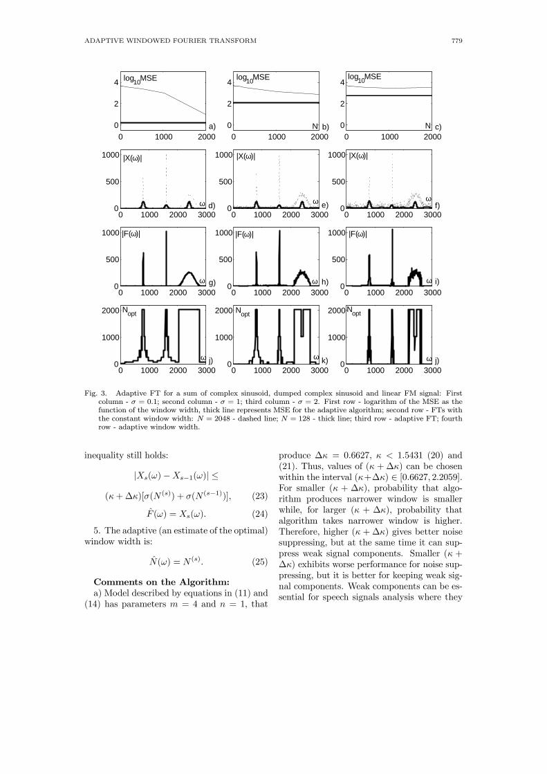
Fig. 3. Adaptive FT for a sum of complex sinusoid, dumped complex sinusoid and linear FM signal: Firstcolumn - σ = 0.1; second column - σ = 1; third column - σ = 2. First row - logarithm of the MSE as thefunction of the window width, thick line represents MSE for the adaptive algorithm; second row - FTs withthe constant window width: N = 2048 - dashed line; N = 128 - thick line; third row - adaptive FT; fourthrow - adaptive window width.

inequality still holds:

|Xs(ω)−Xs−1(ω)| ≤

(κ+∆κ)[σ(N (s)) + σ(N(s−1))], (23)

F (ω) = Xs(ω). (24)

5. The adaptive (an estimate of the optimal)window width is:

N(ω) = N (s). (25)

Comments on the Algorithm:a) Model described by equations in (11) and

(14) has parameters m = 4 and n = 1, that

produce ∆κ = 0.6627, κ < 1.5431 (20) and(21). Thus, values of (κ +∆κ) can be chosenwithin the interval (κ+∆κ) ∈ [0.6627, 2.2059].For smaller (κ + ∆κ), probability that algo-rithm produces narrower window is smallerwhile, for larger (κ + ∆κ), probability thatalgorithm takes narrower window is higher.Therefore, higher (κ +∆κ) gives better noisesuppressing, but at the same time it can sup-press weak signal components. Smaller (κ +∆κ) exhibits worse performance for noise sup-pressing, but it is better for keeping weak sig-nal components. Weak components can be es-sential for speech signals analysis where they

780 TIME-FREQUENCY SIGNAL ANALYSIS

0 0.5 1 1.5 2 2.5 30

0.5

1

1.5

2

2.5

3

3.5

4

N=2048N=1024N=16(κ+∆κ)=1(κ+∆κ)=1.25(κ+∆κ)=1.5(κ+∆κ) varying

σ

log10MSE

Fig. 4. MSE for various constant window widths and for adaptive algorithm with various (κ+∆κ) for the caseof the sum of complex sinusoids, dumped complex sinusoid and linear FM signal.

are very important for the audio quality. Thus,the choice of (κ+∆κ) depends on the consid-ered application. Its influence will be analyzedwithin the numerical examples.b) The unknown standard deviation σ(N (s))

of the FT (23) should be estimated. It can bedone on numerous ways. For the FM signalit can be done as in [1], while for the speechsignal it can be done by considering the speechsignal pause, as it is described in [14].c) The adaptive FT for the Hanning window

can be written as:

X(ω) =N−1Xn=0

x(n)w(n,ω)e−jωn (26)

where:

w(n,ω) =1

2

Ã1− cos 2πn

N(ω)

!. (27)

B. Application in Time-Frequency Analysis

For signals with time variations of the spec-tral content, the short-time Fourier transform(STFT):

STFT (n,ω) =N−1Xm=0

x(n+m)w(m)e−jωm,

(28)can be used instead of the standard FT. Theadaptive STFT can be calculated with the

same algorithm as in the previous subsection,for each time-instant. For an instant n, thealgorithm can be performed by using samplesx(n + m), m ∈ [0,N), where N is a widthof the widest window from the considered setN. Resulting adaptive FT can be further usedfor calculation of distributions from the Cohenclass according to [15], [16], [17].

IV. Numerical Examples

Example 1. Consider a signal:

f(t) = exp(j256πt)+

1

2exp(j512πt) +

1

4exp(j768πt), (29)

sampled with ∆t = 1/1024, within t ∈ [−1, 1].Signal is corrupted by

ν(n) =σ√2(ν1(n) + jν2(n)), (30)

where νi(n), i = 1, 2 are mutually independentwhite Gaussian noises with unitary variance.The adaptive algorithm is applied on the setof the Hanning windows whose widths are:

N = [2048 1024 512 256 128 64 32 16 8 4].(31)

Results obtained with the proposed algorithmfor (κ + ∆κ) = 1 are summarized in Fig.1. The first column represents a small noise

ADAPTIVE WINDOWED FOURIER TRANSFORM 781

0 1000 2000-3

-2

-1

0

1

0 1000 2000 30000

5

10

0 1000 2000 30000

5

10

0 1000 2000 30000

1000

2000

0 1000 2000-3

-2

-1

0

1

0 1000 2000 30000

5

10

0 1000 2000 30000

5

10

0 1000 2000 30000

1000

2000

0 1000 2000-3

-2

-1

0

1

0 1000 2000 30000

5

10

0 1000 2000 30000

5

10

0 1000 2000 30000

1000

2000

log10MSE log10MSE log10MSE

N N N

|X(ω)| |X(ω)| |X(ω)|

ω ω ω

|F(ω)|

ω

|F(ω)|

ω

|F(ω)|

ω

Nopt

ω

Nopt

ω

Nopt

ω

a) b) c)

d) e) f)

g) h) i)

j) k) j)

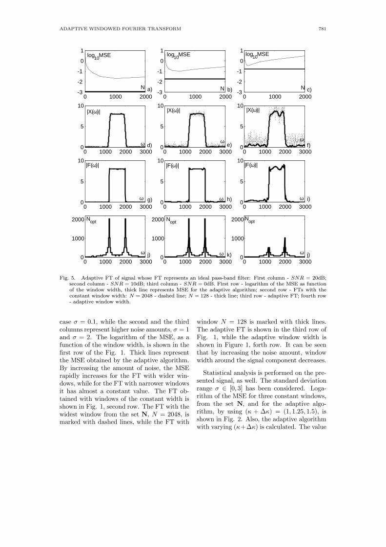
Fig. 5. Adaptive FT of signal whose FT represents an ideal pass-band filter: First column - SNR = 20dB;second column - SNR = 10dB; third column - SNR = 0dB. First row - logarithm of the MSE as functionof the window width, thick line represents MSE for the adaptive algorithm; second row - FTs with theconstant window width: N = 2048 - dashed line; N = 128 - thick line; third row - adaptive FT; fourth row- adaptive window width.

case σ = 0.1, while the second and the thirdcolumns represent higher noise amounts, σ = 1and σ = 2. The logarithm of the MSE, as afunction of the window width, is shown in thefirst row of the Fig. 1. Thick lines representthe MSE obtained by the adaptive algorithm.By increasing the amount of noise, the MSErapidly increases for the FT with wider win-dows, while for the FT with narrower windowsit has almost a constant value. The FT ob-tained with windows of the constant width isshown in Fig. 1, second row. The FT with thewidest window from the set N, N = 2048, ismarked with dashed lines, while the FT with

window N = 128 is marked with thick lines.The adaptive FT is shown in the third row ofFig. 1, while the adaptive window width isshown in Figure 1, forth row. It can be seenthat by increasing the noise amount, windowwidth around the signal component decreases.

Statistical analysis is performed on the pre-sented signal, as well. The standard deviationrange σ ∈ [0, 3] has been considered. Loga-rithm of the MSE for three constant windows,from the set N, and for the adaptive algo-rithm, by using (κ + ∆κ) = (1, 1.25, 1.5), isshown in Fig. 2. Also, the adaptive algorithmwith varying (κ+∆κ) is calculated. The value

782 TIME-FREQUENCY SIGNAL ANALYSIS

05101520-3

-2.5

-2

-1.5

-1

-0.5

0

0.5

1

N=2048N=1024N=16(κ+∆κ)=1(κ+∆κ)=1.25(κ+∆κ)=1.5(κ+∆κ) varying

SNR [dB]

log10MSE

Fig. 6. MSE for various constant window widths and for adaptive algorithm with various (κ+∆κ) for the caseof the ideal pass-band filter.

(κ + ∆κ) = 1.75 is used for ω = 0. Value of(κ+∆κ) is linearly decreased toward the max-imal frequency, where (κ + ∆κ) = 1 is used.Performance of the adaptive algorithm with(κ+∆κ) = (1, 1.25, 1.5), and with a frequencyvarying (κ+∆κ) are almost the same. It showsthat all values of (κ+∆κ) from the proposedrange produce similar performance. The adap-tive algorithms perform better than the FTwith any constant window from the consideredset.Example 2. Consider a sum of the complex

sinusoid, damped complex sinusoid, and linearFM signal:

f(t) = 2 exp(j256πt) exp(−32t2)+exp(j512πt) + 2 exp(j64πt2 + j768πt). (32)

The numerical tests and the statistical analysisare performed under the same assumptions, asin the previous example. Results are given inFigs. 3 and 4.Example 3. Consider a signal:

f(t) = 8 exp(j512πt)sin(128πt)

πt, (33)

that represents an ideal passband filter:

F (ω) =

½8 ω ∈ [384π, 640π],0 elsewhere.

(34)

Signal is sampled with ∆t = 1/1024. Applica-tion of the proposed algorithm for signal (33),

embedded in (30) with SNR equal to 20dB,10dB and 0dB is shown in the columns of Fig.5, respectively. Algorithm parameters are thesame as in Example 1. It can be seen from thefirst two columns that a wide adaptive windowis taken only around the cut-off frequencies,where |F 00(ω)| is different from zero. This isin a full agreement with the proposed theory.However, outside this region the adaptive algo-rithm took narrow window since |F 00(ω)| ≈ 0.In a heavier noise environment, third columnin Fig. 5, adaptive window length aroundthe cut-off frequencies is decreased in order toavoid noise influence. Statistical analysis forthis case is shown in Fig. 6.Example 4. TF analysis is performed on

the signal

f(t) = 2 exp(j256πt) exp(−32t2)+

exp(−j384πt) exp(−8t2), (35)

corrupted by a white complex Gaussian noise(30) with σ = 1.5. The STFT of non-noisysignal (35), produced with the widest windowfrom the considered set N = 512, is shownin Fig. 7a, while for the noisy signal it isshown in Fig. 7b. The adaptive algorithmwith (κ+∆κ) = 1.25 is applied. The MSE forwindows with constant widths, as well as forthe adaptive algorithm, is shown in Fig. 7c.The adaptive STFT is shown in Fig. 7d, while

ADAPTIVE WINDOWED FOURIER TRANSFORM 783

Fig. 7. Adaptive TF representation: a) STFT of the non-noisy signal calculated with the widest window; b)STFT of noisy signal; c) MSE as a function of the window width; d) adaptive STFT; e) adaptive windowwidth; f) S-method calculated by using the adaptive STFT.

the adaptive window width is shown in Fig.7e. The S-method, as a distribution from theCohen class that can be realized by using theadaptive STFT [16]

SM(n,ω) =LX

l=−LSTFT (n,ω + l∆ω)×

STFT ∗(n,ω − l∆ω), (36)

where ∆ω is the frequency step, is shown inFig. 7f. The value of L = 3 is used.

V. Conclusion

Non-parametric algorithm for determina-tion of the adaptive FT is presented. The

algorithm produces adaptive window lengththat gives a bias-to-variance trade-off, withthe MSE smaller than for any constant win-dow from the considered set. Generalizationof the algorithm to the TF analysis of thesignal with varying spectral content is done.The frequency-varying algorithm parameter(κ +∆κ) is introduced in order to keep weaksignal components that can be very importantfor audio quality of the speech signals. Thealgorithm produces almost the same MSE fora wide range of (κ+∆κ) values.

784 TIME-FREQUENCY SIGNAL ANALYSIS

VI. Acknowledgment

The work of I. Djurovic is supported bythe Postdoctoral Fellowship for Foreign Re-searchers of Japan Society for the Promotionof Science and the Ministry of Education, Cul-ture, Sports, Science and Technology underGrant 01215. The work of LJ. Stankovic issupported by the Volkswagen Stiftung, Fed-eral Republic of Germany.

References

[1] V. Katkovnik and LJ. Stankovic: “Instantaneousfrequency estimation using the Wigner distri-bution with varying and data driven windowlength,” IEEE Trans. Sig. Proc., Vol.46, No.9,Sept. 1998, pp.2315-2325.

[2] A. Goldenshluger and A. Nemirovski: “On spatialadaptive estimation of nonparametric regression,”Math. Methods of Statistics, Vol.6, No.2, 1970,pp.135-170.

[3] B. Barkat: “Instantaneous frequency estimationof nonlinear frequency-modulated signals in thepresence of multiplicative and additive noise,”IEEE Trans. Sig. Proc., Vol.49, No.10, Oct. 2001,pp.2214-2222.

[4] LJ. Stankovic: “On the time-frequency analysisbased filtering,” Ann. Telecom., Vol.55, No.5-6,May 2000, pp.216-225.

[5] LJ. Stankovic, S. Stankovic and I. Djurovic:“Space/spatial frequency analysis based filter-ing,” IEEE Trans. Sig. Proc., Vol.48, No.8, Aug.2000, pp.2343-2352.

[6] K. Egiazarian, V. Katkovnik and J. Astola:“Adaptive-window size image denoising based onthe ICI rule,” in Proc. IEEE ICASSP’2001, Vol.3,2001, pp.1869-1872.

[7] V. Katkovnik: “A new method for varying adap-tive bandwidth selection,” IEEE Trans. Sig.Proc., Vol.47, No.9, Sept. 1999, pp.2567-2571.

[8] LJ. Stankovic and V. Katkovnik: “The Wignerdistribution of noisy signals with adaptive time-freqyency varying window,” IEEE Trans. Sig.Proc., Vol.47, No.2, Apr. 1999, pp.1099-1108.

[9] A.B. Gershman, LJ. Stankovic and V. Katkovnik:“Sensor array signal tracking using a data-drivenwindow approach,” Sig. Proc., Vol.80, 2000,pp.2507-2515.

[10] A. Papoulis: Signal analysis, McGraw Hill, 1977.[11] P. Stoica and T. Sundin: “Optimal smoothed pe-

riodogram,” Sig. Proc., Vol.78, 1999, pp.253-264.[12] LJ. Stankovic and V. Katkovnik: “Instantaneous

frequency estimation using higher order distrib-utions with adaptive order and window length,”IEEE Trans. Inf. Th., Vol.46, No.1, Jan. 2000,pp.302-311.

[13] LJ. Stankovic and V. Katkovnik: “Algorithmfor the instantaneous frequency estimation usingtime-frequency distributions with variable win-dow width,” IEEE Sig. Proc. Let., Vol.5, No.9,Sept. 1998. pp.224-228.

[14] S. Stankovic: “About time-variant filtering ofspeech signals with time-frequency distributionsfor hands-free telephone systems,” Sig. Proc.,Vol.80, No.9, Sept. 2000, pp.1777-1785.

[15] G.S. Cunningham and W.J. Williams: “Kerneldecomposition of time-frequency distributions,”IEEE Trans. Sig. Proc., Vol.42, No.6, June 1994,pp.1425-1442.

[16] LJ. Stankovic: “A method for time-frequency sig-nal analysis,” IEEE Trans. Sig. Proc., Vol.42,No.1, Jan. 1994, pp.225-229.

[17] F. Cakrak and P.J. Loughlin: “Multiwindowtime-varying spectrum with instantaneous band-width and frequency constraints,” IEEE Trans.Sig. Proc., Vol.49, No.8, Aug. 2001, pp.1656-1666.