Adaptive Color Space Transform using IndependentComponent Analysis

Esteban Vera Sergio Torres

Department of Electrical EngineeringUniversity of Concepcion, Chile

ABSTRACT

In this paper, a novel color space transform is presented. It is an adaptive transform based on the application ofindependent component analysis to the RGB data of an entire color image. The result is a linear and reversiblecolor space transform that provides three new coordinate axes where the projected data is as much as statisticallyindependent as possible, and therefore highly uncorrelated. Compared to many non-linear color space transformssuch as the HSV or CIE-Lab, the proposed one has the advantage of being a linear transform from the RGBcolor space, much like the XYZ or YIQ. However, its adaptiveness has the drawback of needing an estimate ofthe transform matrix for each image, which is sometimes computationally expensive for larger images due to thecommon iterative nature of the independent component analysis implementations. Then, an image subsamplingmethod is also proposed to enhance the novel color space transform speed, efficiency and robustness. The newcolor space is used for a large set of test color images, and it is compared to traditional color space transforms,where we can clearly visualize its vast potential as a promising tool for segmentation purposes for example.

Keywords: Color Image Processing, Color Space Transform, Independent Component Analysis

1. INTRODUCTION

Computer vision is mainly about retrieving useful information from images, generally simulating the way theHuman Vision System (HVS) performs it. In this way, color images are the natural information source andthey are normally captured in the trichromatic RGB color space. Although widely used due to its simplicity,the RGB color space suffers from a high degree of correlation between its color channels, making harder theinformation extraction process from them. Therefore, many different color spaces have been suggested1, 2 andthey are often used for achieving better results in several computer vision tasks such as color quantization,segmentation, compression, noise reduction, contrast enhancement, etc. . . 3–8

Color space transforms are commonly based on fixed linear or non-linear operations from the RGB color space,with their respective advantages and drawbacks regarding for example the proportionality between the coordi-nates distance and the color difference, similarity to the HVS perception, separation of chromatic and achromaticchannels, etc. . . . Nevertheless, none of the generic color spaces available such as HSV, HSI, YUV, YIQ, CIE-Labor CIE-Luv, can really adapt to the color image content, performing in different ways for different computervision tasks, so none of them is a real optimum for any kind of color images, having to choose by try anderror which color space best fits to every specific application.9–12 For this reason, the seek for new color spacetransforms is a constant concern in the color image processing research community. For example, and based onthe color opponent model of the HVS, new color spaces have been defined in order to match the needs of colorimage segmentation13 and quantization14 algorithms.

However, in the specific case of adaptive color spaces, special attention is given to the X1X2X3 color spacebased on the discrete Karhunen-Loeve (K-L) Transform,2 which is commonly achieved by applying PrincipalComponent Analysis (PCA) to the RGB color space data. It has the main advantage of being a linear trans-formation that leads to three new orthogonal channels that are uncorrelated to each other. This color space iswidely accepted for image compression applications10 and it has been extended to other applications such asLocal Contrast Enhancement15 and Face Recognition.16

Further author information: E-mail: esteban.vera@udec.cl, Address: Casilla 160-C, Concepcion, Chile.

Image Processing: Algorithms and Systems V, edited by Jaakko T. Astola, Karen O. Egiazarian, Edward R. Dougherty Proc. of SPIE-IS&T Electronic Imaging, SPIE Vol. 6497, 64970P, © 2007 SPIE-IS&T · 0277-786X/07/$18

SPIE-IS&T/ Vol. 6497 64970P-1

Nonetheless, in the early 80’s, and after applying X1X2X3 color space to a large amount of data for segmentationpurposes, Ohta el al.9 found an approximation to the K-L Transform by a fixed transform matrix, leading to theOhta’s color space I1I2I3, which usually allows very similar results at much less computational cost, in despite ofthe loose of adaptiveness. Lately, a similar approximation has been performed after applying the K-L transformto the CIE-Lab space as well.17

Thinking in the constraints of the K-L color space, and also based on the successful applications to multispectralimagery,18, 19 in this paper we propose a novel color space transform based on the direct use of independentcomponent analysis20, 21 (ICA) to entire RGB color space images. Lately, ICA has already being used in colorimage processing for many applications, but it has being used with small patches of color images to find basisfunctions that are finally useful for feature extraction and denoising.22, 23 However, in this particular newadaptive color space case, ICA finds a linear, but not necessarily orthogonal coordinate system where the RGBdata is projected onto three new variables that are as statistically independent as possible from each other.Therefore ICA is a generalization of PCA and, like PCA, it has proven to be a useful tool for finding structurein data, so there are no reasons why not applying ICA to an entire color image and don’t expect that at leastthe obtained results might equal or outperform the ones obtained by the K-L color space. Nonetheless, ICA hasthe disadvantage of being obtained by an iterative algorithm.

We test the proposed color space transform by applying it to different kind of images, and then comparing itsresults to the ones obtained by commonly used color spaces such as the HSI, CIE-Lab, I1I2I3 and X1X2X3.From the results, we describe some special properties of the new color space, and we also show some potentialapplications.

This paper is organized as follows. In Section 2, a brief description of independent component analysis ispresented. In Section 3 the new color space is described. A comparison between the proposed color space andclassical ones applied to color images is shown in Section 4 . The conclusions of the paper are finally summarizedin Section 5.

2. INDEPENDENT COMPONENT ANALYSIS

In this section an overview of independent component analysis20, 21 is presented. First the basics of the ICAmodel is described. Then, the fundamental principles of statistical independence are reinforced and characterizedby higher order statistics. In this way several methods for achieving ICA are mentioned, and finally the usedimplementation is explained.

2.1. Definition of ICA

Assume that we observe n linear mixtures x1, . . . , xn of n independent components

xj = aj1s1 + aj2s2 + . . . + ajnsn,∀j (1)

where each mixture xj and each independent component si is a zero-mean random variable. In vector notationthe above mixing model is written as

x = As (2)

where A is the mixing matrix whose elements are the coefficients aij . This statistical model is called independentcomponent analysis, or ICA model. The ICA model is a generative model that describes how the observed dataare generated by a process of mixing the components si, that cannot be directly observed otherwise. The mixingmatrix is also assumed to be unknown, so all we observe is the random vector x, and we must estimate both Aand s from it.

The starting point for ICA is that the components si are statistically independent, which finally implies thatthe independent components must have nongaussian distributions. If we assume a square mixing matrix, so wehave same number of observations than independent components, then after estimating the matrix A we cancompute its inverse W, and thus obtain the independent components by:

s = Wx (3)

SPIE-IS&T/ Vol. 6497 64970P-2

2.2. Statistical Independence

Considering two scalar-valued random variables y1 and y2, then this variables are independent if the informationon the value of y1 does not give any information on the value of y2, and vice versa. In statistical terms,independence can be defined by probabilities densities. Let us denote by p(y1, y2) the joint probability densityfunction (pdf) of y1 and y2, and denote by p1(y1) and p2(y2) the marginal pdf of y1 and y2 respectively:

p1(y1) =∫

p(y1, y2)dy2

p2(y2) =∫

p(y1, y2)dy1(4)

Then, y1 and y2 are independent if and only if its joint pdf is factorizable as

p(y1, y2) = p1(y1)p2(y2) (5)

From the definition of independence above it can be derived the most important property of independent randomvariables. Given two functions h1 and h2, we always have

E{h1(y1)h2(y2)} = E{h1(y1)}E{h2(y2)} (6)

If we know that two random variables are uncorrelated if their covariance is zero, then

E{y1y2} − E{y1}E{y2} = 0 (7)

Therefore, if the variables are independent, they are uncorrelated. On the other hand, uncorrelatedness does notimply independence.

2.3. ICA Implementation

The key for estimating the ICA model is nongaussianity. Following the Central Limit Theorem, a sum ofindependent random variables tends toward a gaussian distribution. Thus, a sum of two independent randomvariables has a distribution that is closer to gaussian than any of the two original random variables. If we assumethat the data vector x is a mix of independent components, then the distribution of each mixed vector is moregaussian than any of the independent components in s. Therefore if we can choose the unmixing matrix Win order to maximize the nongaussianity of each estimated component, then they will finally correspond to theindependent components.

Thus, a measure of nongaussianity is needed in order to estimate the ICA model. Using a statistical approach,kurtosis will define if a distribution is subgaussian or supergaussian, and therefore is a good measure of thenongaussianity degree. On the other hand, by using an information theory approach, negentropy is an adequatechoice.

Other approaches to solve the ICA model are related to minimization of mutual information, maximum likelihoodby infomax, and projection pursuit, but they are very related to the maximization of nongaussianity at the end.

In this case we will make use of the widely used and accepted ICA algorithm called FastICA.24 The preprocessingsteps to apply the ICA method is basically: centering the data, or removing its mean value leading to zero-meanvariables; and whitening the data, leading to uncorrelated unit variance data. Centering is a very trivial step,and whitening can be easily achieved by Principal Component Analysis, or PCA. The algorithm is of an iterativenature, and basically it needs to setup initially the startup for the unmixing matrix W and the selection of thenonlinear function used to estimate an approximation value for the negentropy.

3. NEW COLOR SPACE TRANSFORM

The adaptive color space transform here proposed is based on the application of independent component analysisto a RGB color image. At the end this is an improved, and generalized natural extension of the X1X2X3

Karhunen-Loeve color space obtained by using PCA.2

SPIE-IS&T/ Vol. 6497 64970P-3

3.1. Description

In this particular color space transform case, each RGB channel is treated as a sample measurement witha different point-of-view of the same scene, which can lead us to discover up to three different independentcomponents that are supposed to be mixed in each observation in the R, G and B channels. The only bigassumption is that the statistical distributions of the unknown independent components are nongaussian, thenwhat the ICA algorithm pursues is to find the best tridimensional linear projection into the RGB cube thatmaximize the nongaussianity of each estimated component, that can be at the end statistically independent fromeach other.

We are assuming that each of the three RGB channels has a mix of three independent (nongaussian) components,which might not be necessarily true, so what we are finally doing at the end is seeking for three componentsthe most independent as possible. Every resulting estimated independent component is expected to be moreuncorrelated to each other compared to the original RGB channels, and also to other color spaces. Of course, eachof these three supposed independent components can contain a mix of even more real independent components,because we will commonly have more independent components than mixtures, but we are finally constrained toestimate a maximum of three.

3.2. Practical Considerations

To apply the proposed transform first we reorder each RGB channel of a given image into a vector, and then oncewe apply the independent component analysis algorithm (FastICA24) to the three vectors we get as a result theseparation (unmixing) matrix W, which will define our color space transform matrix for a particular image, likeany linear color space transform. This separation matrix, and its inverse (the mixing matrix A), can be furtherused to perform the color space transform back and forth for the same image. Then, some clear advantagesof the adaptive color space proposed here are: the linearity of the transform and, of course, its adaptiveness.In addition, we should state as a major advantage the lack of constraints regarding the orthogonality of theprojections, such as in PCA, which is an extra degree of freedom to perform an estimation that fits better thedata distribution in the statistical independence sense. However this extra degree of freedom is also addingcomplexity to the ICA algorithm itself, which sometimes leads that the tuning of the FastICA algorithm canbecome tricky. However, the worst result we could get is as good or bad as performing only the whitening onthe data, obtaining the same result as the K-L only transformation.

Typically we choose as a starting mixing matrix for the iteration algorithm the identity matrix, but a randomvector could also be used. The main difference is that if we apply the algorithm several times to the same image,the order of the estimated independent components can change randomly as well, but generally the same resultsare achieved. The other important point is the selection of the nonlinearity for the algorithm. We typicallyselected the tanh, but normally any other choice used to work well in the same way. The only problem wasrelated when no convergence was achieved, so the change of nonlinearity sometimes helped in making it work.

Additionally, for larger images the convergence time in a normal Personal Computer (PC) can be too long forcertain difficult images in particular, so a subsampling scheme helped to accelerate the convergence time, andalso helped in making the estimation more robust. At the beginning we tried fractal subsampling scanning asproposed in,25 but at the end using normal vector downsampling was enough to guarantee proper and repeatableresults. In all the test images used, we tried with good confidence up to a factor of 100 in downsampling leadingto similar results, but with a significative reduction on the number of iterations needed, increasing even furtherthe speed up of the convergence time. It seems that there are less distraction points that used to confuse thealgorithm, avoiding local minima for example.

Finally, it is worth to mention that the FastICA algorithm includes the mean removal for the initial data vectorsand also realizes the whitening to the data through PCA, so the preprocessing step is the entire K-L X1X2X3

color space transform.

4. RESULTS

In order to test the behavior of the new adaptive color space transform, we applied it to a large collection of colorimages extracted from the Berkeley Segmentation Database,26 the Image Quality Assessment Database,27 and

SPIE-IS&T/ Vol. 6497 64970P-4

the USC-SIPI Image Database28 where we extracted some classical color test image processing such as Lenna,Peppers and Mandrill.

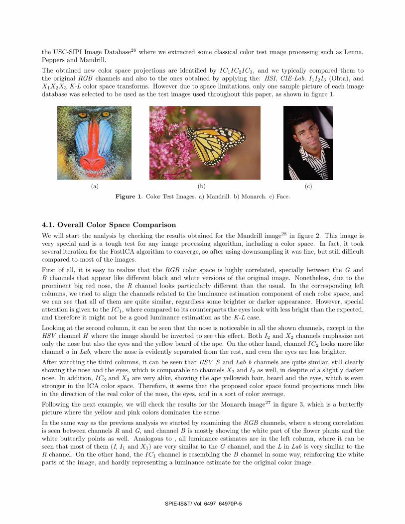
The obtained new color space projections are identified by IC1IC2IC3, and we typically compared them tothe original RGB channels and also to the ones obtained by applying the: HSI, CIE-Lab, I1I2I3 (Ohta), andX1X2X3 K-L color space transforms. However due to space limitations, only one sample picture of each imagedatabase was selected to be used as the test images used throughout this paper, as shown in figure 1.

(a) (b) (c)

Figure 1. Color Test Images. a) Mandrill. b) Monarch. c) Face.

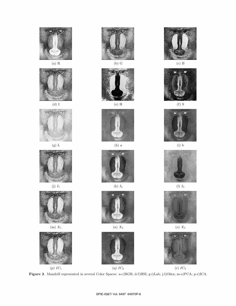
4.1. Overall Color Space ComparisonWe will start the analysis by checking the results obtained for the Mandrill image28 in figure 2. This image isvery special and is a tough test for any image processing algorithm, including a color space. In fact, it tookseveral iteration for the FastICA algorithm to converge, so after using downsampling it was fine, but still difficultcompared to most of the images.

First of all, it is easy to realize that the RGB color space is highly correlated, specially between the G andB channels that appear like different black and white versions of the original image. Nonetheless, due to theprominent big red nose, the R channel looks particularly different than the usual. In the corresponding leftcolumns, we tried to align the channels related to the luminance estimation component of each color space, andwe can see that all of them are quite similar, regardless some brighter or darker appearance. However, specialattention is given to the IC1, where compared to its counterparts the eyes look with less bright than the expected,and therefore it might not be a good luminance estimation as the K-L case.

Looking at the second column, it can be seen that the nose is noticeable in all the shown channels, except in theHSV channel H where the image should be inverted to see this effect. Both I2 and X2 channels emphasize notonly the nose but also the eyes and the yellow beard of the ape. On the other hand, channel IC2 looks more likechannel a in Lab, where the nose is evidently separated from the rest, and even the eyes are less brighter.

After watching the third columns, it can be seen that HSV S and Lab b channels are quite similar, still clearlyshowing the nose and the eyes, which is comparable to channels X2 and I2 as well, in despite of a slightly darkernose. In addition, IC3 and X3 are very alike, showing the ape yellowish hair, beard and the eyes, which is evenstronger in the ICA color space. Therefore, it seems that the proposed color space found projections much likein the direction of the real color of the nose, the eyes, and in a sort of color average.

Following the next example, we will check the results for the Monarch image27 in figure 3, which is a butterflypicture where the yellow and pink colors dominates the scene.

In the same way as the previous analysis we started by examining the RGB channels, where a strong correlationis seen between channels R and G, and channel B is mostly showing the white part of the flower plants and thewhite butterfly points as well. Analogous to , all luminance estimates are in the left column, where it can beseen that most of them (I, I1 and X1) are very similar to the G channel, and the L in Lab is very similar to theR channel. On the other hand, the IC1 channel is resembling the B channel in some way, reinforcing the whiteparts of the image, and hardly representing a luminance estimate for the original color image.

SPIE-IS&T/ Vol. 6497 64970P-5

(a) R (b) G (c) B

(d) I (e) H (f) S

(g) L (h) a (i) b

(j) I1 (k) I2 (l) I3

(m) X1 (n) X2 (o) X3

(p) IC1 (q) IC2 (r) IC3

Figure 2. Mandrill represented in several Color Spaces: a-c)RGB; d-f)HSI; g-i)Lab; j-l)Ohta; m-o)PCA; p-r)ICA.

SPIE-IS&T/ Vol. 6497 64970P-6

WY

(a) R (b) G (c) B

(d) I (e) H (f) S

(g) L (h) a (i) b

(j) I1 (k) I2 (l) I3

(m) X1 (n) X2 (o) X3

(p) IC1 (q) IC2 (r) IC3

Figure 3. Monarch represented in several Color Spaces: a-c)RGB; d-f)HSI; g-i)Lab; j-l)Ohta; m-o)PCA; p-r)ICA.

SPIE-IS&T/ Vol. 6497 64970P-7

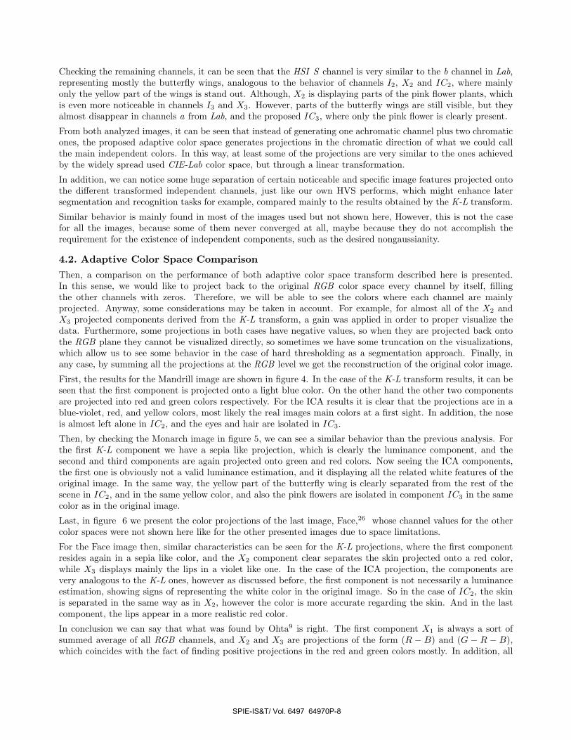
Checking the remaining channels, it can be seen that the HSI S channel is very similar to the b channel in Lab,representing mostly the butterfly wings, analogous to the behavior of channels I2, X2 and IC2, where mainlyonly the yellow part of the wings is stand out. Although, X2 is displaying parts of the pink flower plants, whichis even more noticeable in channels I3 and X3. However, parts of the butterfly wings are still visible, but theyalmost disappear in channels a from Lab, and the proposed IC3, where only the pink flower is clearly present.

From both analyzed images, it can be seen that instead of generating one achromatic channel plus two chromaticones, the proposed adaptive color space generates projections in the chromatic direction of what we could callthe main independent colors. In this way, at least some of the projections are very similar to the ones achievedby the widely spread used CIE-Lab color space, but through a linear transformation.

In addition, we can notice some huge separation of certain noticeable and specific image features projected ontothe different transformed independent channels, just like our own HVS performs, which might enhance latersegmentation and recognition tasks for example, compared mainly to the results obtained by the K-L transform.

Similar behavior is mainly found in most of the images used but not shown here, However, this is not the casefor all the images, because some of them never converged at all, maybe because they do not accomplish therequirement for the existence of independent components, such as the desired nongaussianity.

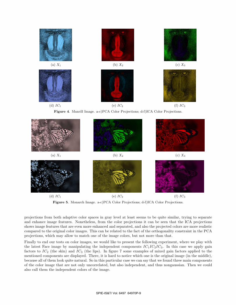
4.2. Adaptive Color Space ComparisonThen, a comparison on the performance of both adaptive color space transform described here is presented.In this sense, we would like to project back to the original RGB color space every channel by itself, fillingthe other channels with zeros. Therefore, we will be able to see the colors where each channel are mainlyprojected. Anyway, some considerations may be taken in account. For example, for almost all of the X2 andX3 projected components derived from the K-L transform, a gain was applied in order to proper visualize thedata. Furthermore, some projections in both cases have negative values, so when they are projected back ontothe RGB plane they cannot be visualized directly, so sometimes we have some truncation on the visualizations,which allow us to see some behavior in the case of hard thresholding as a segmentation approach. Finally, inany case, by summing all the projections at the RGB level we get the reconstruction of the original color image.

First, the results for the Mandrill image are shown in figure 4. In the case of the K-L transform results, it can beseen that the first component is projected onto a light blue color. On the other hand the other two componentsare projected into red and green colors respectively. For the ICA results it is clear that the projections are in ablue-violet, red, and yellow colors, most likely the real images main colors at a first sight. In addition, the noseis almost left alone in IC2, and the eyes and hair are isolated in IC3.

Then, by checking the Monarch image in figure 5, we can see a similar behavior than the previous analysis. Forthe first K-L component we have a sepia like projection, which is clearly the luminance component, and thesecond and third components are again projected onto green and red colors. Now seeing the ICA components,the first one is obviously not a valid luminance estimation, and it displaying all the related white features of theoriginal image. In the same way, the yellow part of the butterfly wing is clearly separated from the rest of thescene in IC2, and in the same yellow color, and also the pink flowers are isolated in component IC3 in the samecolor as in the original image.

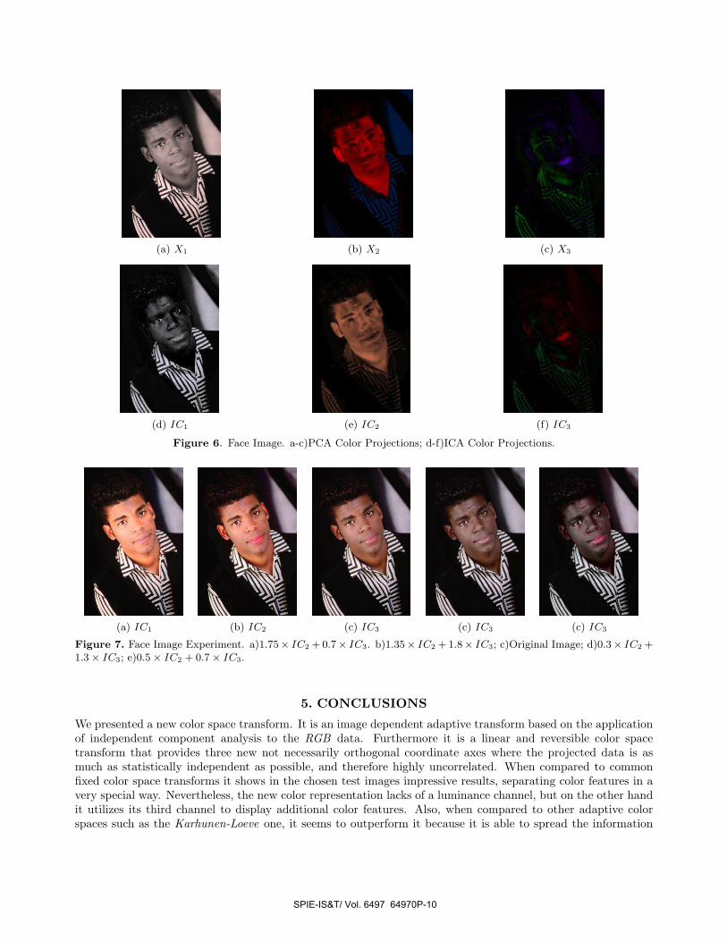
Last, in figure 6 we present the color projections of the last image, Face,26 whose channel values for the othercolor spaces were not shown here like for the other presented images due to space limitations.

For the Face image then, similar characteristics can be seen for the K-L projections, where the first componentresides again in a sepia like color, and the X2 component clear separates the skin projected onto a red color,while X3 displays mainly the lips in a violet like one. In the case of the ICA projection, the components arevery analogous to the K-L ones, however as discussed before, the first component is not necessarily a luminanceestimation, showing signs of representing the white color in the original image. So in the case of IC2, the skinis separated in the same way as in X2, however the color is more accurate regarding the skin. And in the lastcomponent, the lips appear in a more realistic red color.

In conclusion we can say that what was found by Ohta9 is right. The first component X1 is always a sort ofsummed average of all RGB channels, and X2 and X3 are projections of the form (R − B) and (G − R − B),which coincides with the fact of finding positive projections in the red and green colors mostly. In addition, all

SPIE-IS&T/ Vol. 6497 64970P-8

(a) X1 (b) X2 (c) X3

(d) IC1 (e) IC2 (f) IC3

Figure 4. Manrill Image. a-c)PCA Color Projections; d-f)ICA Color Projections.

(a) X1 (b) X2 (c) X3

(d) IC1 (e) IC2 (f) IC3

Figure 5. Monarch Image. a-c)PCA Color Projections; d-f)ICA Color Projections.

projections from both adaptive color spaces in gray level at least seems to be quite similar, trying to separateand enhance image features. Nonetheless, from the color projections it can be seen that the ICA projectionsshows image features that are even more enhanced and separated, and also the projected colors are more realisticcompared to the original color images. This can be related to the fact of the orthogonality constraint in the PCAprojections, which may allow to match one of the image colors, but not more than that.

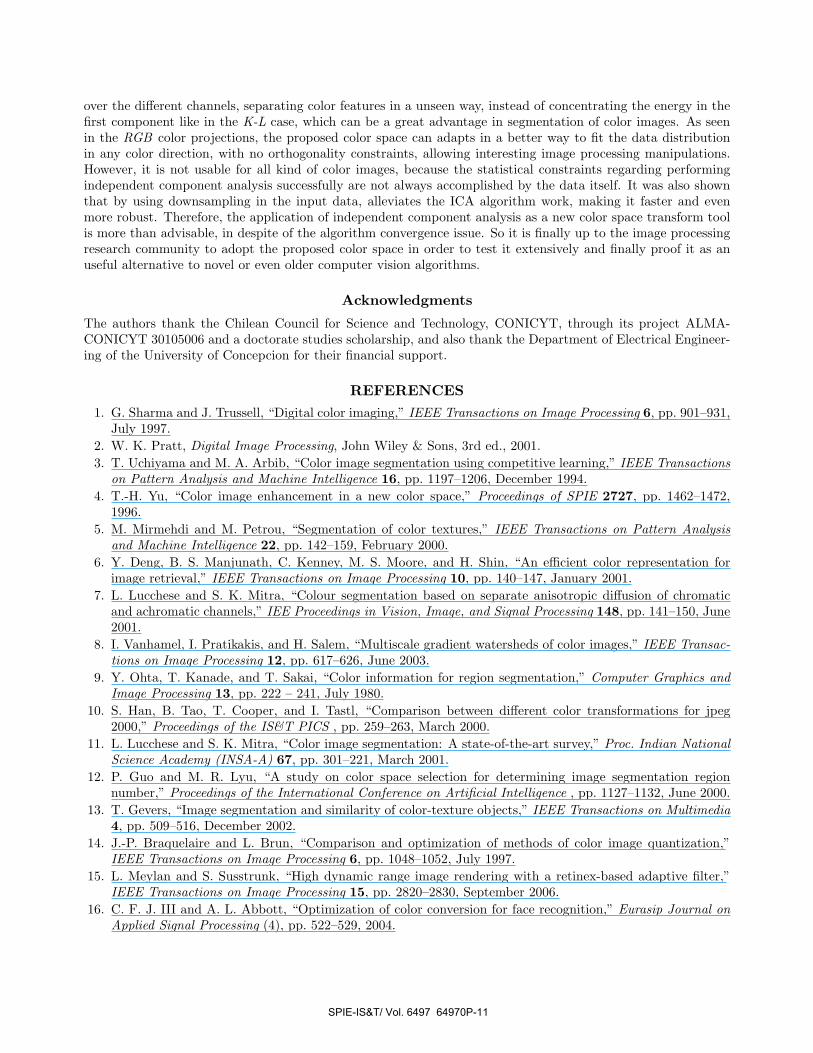
Finally to end our tests on color images, we would like to present the following experiment, where we play withthe latest Face image by manipulating the independent components IC1IC2IC3. In this case we apply gainfactors to IC2 (the skin) and IC3 (the lips). In figure 7 some examples of mixed gain factors applied to thementioned components are displayed. There, it is hard to notice which one is the original image (in the middle),because all of them look quite natural. So in this particular case we can say that we found three main componentsof the color image that are not only uncorrelated, but also independent, and thus nongaussian. Then we couldalso call them the independent colors of the image.

SPIE-IS&T/ Vol. 6497 64970P-9

(a) X1 (b) X2 (c) X3

(d) IC1 (e) IC2 (f) IC3

Figure 6. Face Image. a-c)PCA Color Projections; d-f)ICA Color Projections.

(a) IC1 (b) IC2 (c) IC3 (c) IC3 (c) IC3

Figure 7. Face Image Experiment. a)1.75× IC2 + 0.7× IC3. b)1.35× IC2 + 1.8× IC3; c)Original Image; d)0.3× IC2 +1.3 × IC3; e)0.5 × IC2 + 0.7 × IC3.

5. CONCLUSIONS

We presented a new color space transform. It is an image dependent adaptive transform based on the applicationof independent component analysis to the RGB data. Furthermore it is a linear and reversible color spacetransform that provides three new not necessarily orthogonal coordinate axes where the projected data is asmuch as statistically independent as possible, and therefore highly uncorrelated. When compared to commonfixed color space transforms it shows in the chosen test images impressive results, separating color features in avery special way. Nevertheless, the new color representation lacks of a luminance channel, but on the other handit utilizes its third channel to display additional color features. Also, when compared to other adaptive colorspaces such as the Karhunen-Loeve one, it seems to outperform it because it is able to spread the information

SPIE-IS&T/ Vol. 6497 64970P-10

over the different channels, separating color features in a unseen way, instead of concentrating the energy in thefirst component like in the K-L case, which can be a great advantage in segmentation of color images. As seenin the RGB color projections, the proposed color space can adapts in a better way to fit the data distributionin any color direction, with no orthogonality constraints, allowing interesting image processing manipulations.However, it is not usable for all kind of color images, because the statistical constraints regarding performingindependent component analysis successfully are not always accomplished by the data itself. It was also shownthat by using downsampling in the input data, alleviates the ICA algorithm work, making it faster and evenmore robust. Therefore, the application of independent component analysis as a new color space transform toolis more than advisable, in despite of the algorithm convergence issue. So it is finally up to the image processingresearch community to adopt the proposed color space in order to test it extensively and finally proof it as anuseful alternative to novel or even older computer vision algorithms.

Acknowledgments

The authors thank the Chilean Council for Science and Technology, CONICYT, through its project ALMA-CONICYT 30105006 and a doctorate studies scholarship, and also thank the Department of Electrical Engineer-ing of the University of Concepcion for their financial support.

REFERENCES1. G. Sharma and J. Trussell, “Digital color imaging,” IEEE Transactions on Image Processing 6, pp. 901–931,

July 1997.2. W. K. Pratt, Digital Image Processing, John Wiley & Sons, 3rd ed., 2001.3. T. Uchiyama and M. A. Arbib, “Color image segmentation using competitive learning,” IEEE Transactions

on Pattern Analysis and Machine Intelligence 16, pp. 1197–1206, December 1994.4. T.-H. Yu, “Color image enhancement in a new color space,” Proceedings of SPIE 2727, pp. 1462–1472,

1996.5. M. Mirmehdi and M. Petrou, “Segmentation of color textures,” IEEE Transactions on Pattern Analysis

and Machine Intelligence 22, pp. 142–159, February 2000.6. Y. Deng, B. S. Manjunath, C. Kenney, M. S. Moore, and H. Shin, “An efficient color representation for

image retrieval,” IEEE Transactions on Image Processing 10, pp. 140–147, January 2001.7. L. Lucchese and S. K. Mitra, “Colour segmentation based on separate anisotropic diffusion of chromatic

and achromatic channels,” IEE Proceedings in Vision, Image, and Signal Processing 148, pp. 141–150, June2001.

8. I. Vanhamel, I. Pratikakis, and H. Salem, “Multiscale gradient watersheds of color images,” IEEE Transac-tions on Image Processing 12, pp. 617–626, June 2003.

9. Y. Ohta, T. Kanade, and T. Sakai, “Color information for region segmentation,” Computer Graphics andImage Processing 13, pp. 222 – 241, July 1980.

10. S. Han, B. Tao, T. Cooper, and I. Tastl, “Comparison between different color transformations for jpeg2000,” Proceedings of the IS&T PICS , pp. 259–263, March 2000.

11. L. Lucchese and S. K. Mitra, “Color image segmentation: A state-of-the-art survey,” Proc. Indian NationalScience Academy (INSA-A) 67, pp. 301–221, March 2001.

12. P. Guo and M. R. Lyu, “A study on color space selection for determining image segmentation regionnumber,” Proceedings of the International Conference on Artificial Intelligence , pp. 1127–1132, June 2000.

13. T. Gevers, “Image segmentation and similarity of color-texture objects,” IEEE Transactions on Multimedia4, pp. 509–516, December 2002.

14. J.-P. Braquelaire and L. Brun, “Comparison and optimization of methods of color image quantization,”IEEE Transactions on Image Processing 6, pp. 1048–1052, July 1997.

15. L. Meylan and S. Susstrunk, “High dynamic range image rendering with a retinex-based adaptive filter,”IEEE Transactions on Image Processing 15, pp. 2820–2830, September 2006.

16. C. F. J. III and A. L. Abbott, “Optimization of color conversion for face recognition,” Eurasip Journal onApplied Signal Processing (4), pp. 522–529, 2004.

SPIE-IS&T/ Vol. 6497 64970P-11

17. Y. Chen, P. Hao, and A. Dang, “Optimal transform in perceptually uniform color space and its applicationin image coding,” Lecture Notes in Computer Science 3211, pp. 269–276, 2004.

18. S. Rajagopalan and R. A. Robb, “Independent component analysis assisted unsupervised multispectralclassification,” Proceedings of the SPIE 5029(1), pp. 725–733, SPIE, 2003.

19. Q. Du, I. Kopriva, and H. Szu, “Independent-component analysis for hyperspectral remote sensing imageryclassification,” Optical Engineering 45(1), p. 017008, 2006.

20. A. Hyvarinen, J. Karhunen, and E. Oja, Independent Component Analysis, John Wiley & Sons, 2001.21. J. V. Stone, Independent Component Analysis: A Tutorial Introduction, MIT press, 2004.22. P. Hoyer and A. Hyvrinen, “Independent component analysis applied to feature extraction from colour and

stereo images,” Network: Computation in Neural Systems 11, pp. 191–210, August 2000.23. T.-W. Lee and M. S. Lewicki, “Unsupervised image classification, segmentation and enhancement using ica

mixture models,” IEEE Transactions on Image Processing 11, pp. 270–279, March 2002.24. A. Hyvrinen, “Fast and robust fixed-point algorithms for independent component analysis,” IEEE Trans-

actions on Neural Networks 10, pp. 626–634, May 1999.25. N. Papamarkos, A. E. Atsalakis, and C. P. Strouthopoulos, “Adaptive color reduction,” IEEE Transactions

on Systems, Man, and Cybernetics-Part B: Cybernetics 32, pp. 44–56, February 2002.26. D. Martin, C. Fowlkes, D. Tal, and J. Malik, “A database of human segmented natural images and its

application to evaluating segmentation algorithms and measuring ecological statistics,” in Proc. 8th Int’lConf. Computer Vision, 2, pp. 416–423, July 2001.

27. H. R. Sheikh, Z. Wang, L. Cormack, and A. C. Bovik, “Live image quality assessment database,”http://live.ece.utexas.edu/research/quality .

28. A. G. Weber, “The usc-sipi image database,” http://sipi.usc.edu/database/ .

SPIE-IS&T/ Vol. 6497 64970P-12