FAST ALGORITHMS OF FOURIER AND HARTLEYTRANSFORM AND THEIR IMPLEMENTATION IN MATLABVíTÌZSLAV VESELÝAbstract. This paper is mainly intended as survey article on construction offast algorithms for the computation of the discrete Fourier transform (DFT)and discrete Hartley transform (DHT), all in relation to discrete linear andcyclic convolution which are fundamental operations in many data processingtasks. The exposition prefers purely algebraic approach to explain the basicideas in concise but clear manner. The bene�ts of author's new algebraicsetting of generalized Kronecker product are demonstrated in deriving fastalgorithms of Cooley-Tukey type for the computation of multidimensionalfast Fourier and Hartley transform. These algorithms have been implementedas FORTRAN MEX-�les in MATLAB which makes it easy to use them andevaluate their performance. Compared with other commonly used proceduresthe results of performance tests exhibit equal or better numerical stabilityand for most larger transform lengths time e�ciency superior to that of thecomparative procedures. The results concerning the new algorithm for fastHartley transform are stated without proofs and will be published elsewherein more detail. 1. IntroductionDiscrete Fourier transform (DFT), its alternative discrete Hartley transform(DHT) and discrete convolution (DC) play fundamental role in many �elds ofmathematics and applied sciences, the traditional one being digital signal process-ing . This is evidenced by a large number of monographs devoted to this topic[7, 9, 10, 11, 13, 16, 17, 23, 32, 35, 36]. DC stands behind linear techniques fordata processing which are widely used under synonyms moving average method orlinear digital �ltration. The basic idea is to achieve a desired modi�cation of thedata sequence simply by replacing each entry with a weighted average of values inits neighbourhood. The weights remain �xed and \move" along the data sequence.DC is closely connected with DFT, actually either of DC or DFT may be com-puted via the latter operation. DFT and DHT themselves are a useful tool for�nding an approximate Fourier expansion of the data sequence and play a funda-mental role of their own in the spectral representation of signals. Thus the problemof fast computation is mainly reduced to the problem of �nding fast algorithm forDate: September 2, 1998.1991 Mathematics Subject Classi�cation. Primary: 65T20; Secondary: 65F30,15A36.Key words and phrases. fast Fourier transform, fast Hartley transform, factorization of ma-trices, generalized Kronecker product of matrices, performance tests.Research supported by the GA of the Czech Republic under grant number 201/96/0665.1

2 VíTÌZSLAV VESELÝDFT or DHT known as fast Fourier transform (FFT) or fast Hartley transform(FHT), respectively.In this paper we shall review basic results concerning the interconnection be-tween DFT, DHT and DC. Using a clear algebraic setting, standard principles forconstruction of FFTs in form of a sparse factorization of the DFTmatrix will be ex-plained, the multidimensional case inclusively. The Kronecker product of matricesand its certain generalization is presented as an e�ective tool for �nding such fac-torizations. Special attention will be paid to factorizations of Cooley-Tukey typeboth for FFT and FHT which have been derived using the new algebraic approachbased on generalized Kronecker product. Their MATLAB [45] implementation inthe form of FORTRANMEX-�les exhibits a very good performance. Performancetests prove equal or better numerical stability, and especially for lengths exceed-ing 1000 samples also a signi�cantly better time e�ciency of the new algorithmswhen compared with standard MATLAB command fft or some other widely usedalgorithms. 2. Notation and introductory remarksWe write s := v or v =: s to indicate that expression v will be denoted by thesymbol s.2.1. Sets, numbers, vectors and matrices.� N;Z;R;C : : : set of all natural numbers, integers, real and complex numbers,respectively.� Z(+; �) : : : ring of integers with addition + and multiplication �.� ZN := f0; 1; : : : ; N � 1g : : : the set of residues modulo N 2 N.� ZN(�;�), ZN(�) : : : the residue class ring modulo N 2 N, its additivegroup, respectively, with operations of addition � and multiplication� mod-ulo N .� Re c; Im c : : : real, imaginary part of complex number c, respectively.� int(r) : : : integer part of real number r.� hniN : : : n modulo N (remainder of n after division by N ).Clearly h�iN : Z(+; �)! ZN(�;�) is the canonical residue class homomor-phism. We shall apply the same notation when working with polynomialsover C instead of integers: hQ(z)iP (z) denotes the remainder of polynomialQ(z) after division by polynomial P (z).� n j m; n - m : : : integer n is, is not, a divisor of integer m, respectively.� gcd(n;m) : : : the greatest common divisor of integers n and m.� fi : jg := fi; i + 1; : : : ; jg : : : interval of integers (i; j 2 Z), fi : jg = ; forj < i.� Ni:j := NiNi+1 : : :Nj : : : ordered product of m factors Nk 2 N (k 2 fi : jg),Ni:j = 1 for j < i. In particular N = Ni:j denotes (ordered) factorization ofN .� x := [x0; x1; : : : ; xN�1]T : : : column vector of length N 2 N with entriesxi 2 C (T stands for transpose).

FFT AND FHT ALGORITHMS AND THEIR MATLAB IMPLEMENTATION 3� 1N := [1; 1; : : : ; 1]T : : : column vector of length N 2 N with all entries equalto one.� X(z) = x0 + x1z + � � � + xN�1zN�1 : : : polynomial associated with thecoe�cient vector x = [x0; x1; : : : ; xN�1]T .� deg(X) : : : degree of polynomialX(z).� z := x�y : : : Hadamard product (or element-by-element product) of vectorsx and y of equal size N � 1 or 1 � N is a vector z of the same size withzn = xnyn; n = 0; 1; : : : ; N � 1.� M(N �K) : : : the set of all matrices A = [an;k] of size N �K (N;K 2 N)with entries an;k 2 C . Alternatively we write A(n; k) instead of an;k for theentry in (n + 1)-row and (k + 1)-column (n 2ZN; k 2ZK). Of course, thesame convention will be adopted when denoting entries of vectors which arespecial matrices.� A� : : : conjugate transpose of matrix A.� jAj : : : determinant of a square matrix A.� IN : : : identity matrix of order N .� �i;j ; �(i; j) : : : Kronecker's symbol: �i;j = �(i; j) = (1 for i = j0 for i 6= j .� P(M ) : : : permutation group of the set M .Lemma 2.1. Let us associate with every 0 6= a 2ZN; gcd(a;N ) = 1, a transla-tion mapping ta de�ned by the rule ta(x) = haxiN ; x 2ZN.Then ta : ZN(�) ! ZN(�) is a group automorphism. In particular there exists0 6= a0 2 ZN, gcd(a0; N ) = 1, such that haa0iN = 1. We say therefore that a0 isinverse to a modulo N and write a0 = hai�1N . Moreover ta0 = t�1a de�nes theinverse automorphism.Proof. Clearly, ta is a group endomorphism on ZN(�). Injectivity is straightfor-ward following the implications:haxiN = hayiN ; x; y 2ZN ) ha(x � y)iN = 0 ) N j a(x� y) ) N j (x� y)because gcd(a;N ) = 1 ) x = y because 0 � jx�yj � N �1. From the �nitenessofZN we can conclude also that ta is surjective, and in particular there must existx = a0 which is mapped onto 1 by ta, i.e. 1 = ta(a0) = haa0iN . Hence we concludethat gcd(a0; N ) = 1 because it is a divisor of 1.2.2. Mixed-radix integer representation.� N := (N1; N2; : : : ; Nm) : : : ordered m-tuple denoting (�nite) mixed-radixnumber system where Ni 2 N is the size of the i-th radix (i = 1; 2; : : : ;m),i = 1 is related to the most signi�cant radix position, i = m to the leastsigni�cant one.� N0 := (Nm; Nm�1; : : : ; N1) : : : mixed-radix number system reversed to thenumber system N.� Ni:j := (Ni; Ni+1; : : : ; Nj) : : : partial mixed-radix number system of N,1 � i � j � m.

4 VíTÌZSLAV VESELÝGiven a factorization N = N1:m then the associated number system N =(N1; N2; : : : ; Nm) denoted by the same script letter will be assumed by defaultlater on if not stated explicitly. We shall also agree on using by default the samearabic capital letter with subscript i for i-th radix if a number system was speci�edonly by its script letter (N versus Ni, K versus Ki, etc.).Theorem 2.2 (MIR-representation of ZN).Let N = N1:m. Then the mapping MIRN(�) de�ned by the ruleMIRN(n1; n2; : : : ; nm) := n1N2:m + n2N3:m + � � �+ nm�1Nm + nm (2.1)is a one-to-one mapping ZN1 �ZN2 � � � � �ZNm !ZN.Proof. Injectivity of MIRN(�) is easily proved by induction on m (cf. [48, Lemma1.4]). As ZN is �nite, the mapping is also surjective.De�nition 2.3.The mapping MIRN(�) is called mixed-radix integer representation with respect tothe number system N and the ordered m-tuple (n1; n2; : : : ; nm) is said to be themixed-radix integer representation of number n := MIRN(n1; n2; : : : ; nm) 2 ZNwith respect to the number system N, n1 is the most signi�cant and nm the leastsigni�cant digit.In case B := N1 = N2 = � � � = Nm we obtain the usual base-B represen-tation for numbers 0 � n � Bm � 1. For example the number system N =(10; 10; 10) leads to standard decadic representation of any number 0 � n � 999:n = MIRN(n1; n2; n3) = n1100 + n210 + n3.Allowing for di�erent radices Ni, we arrive at a generalized concept of 2.3 whereranges for digits 0 � ni � Ni � 1 are varying with their position.Identifying multiindices (n1; n2; : : : ; nm) 2ZN1 �ZN2 � � � � �ZNm withMIRN(n1; n2; : : : ; nm) 2 ZN1:m one can view MIRN(�) as a mapping reorderingmultiindices into lexicographic order. This is related to the usual method of storingmultidimensional array to the computer memory in linear order as one-dimensionalarray.De�nition 2.4 (Digit reversal).Let us have number system N associated with the factorization N = N1:m andde�ne a permutation mapping SN 2 P(ZN) bySN(MIRN(n1; n2; : : : ; nm)) := MIRN0 (nm; nm�1; : : : ; n1) = (2.2):= nmN1:m�1 + nm�1N1:m�2 + � � �+ n2N1 + n1:Then SN is called digit reversal with respect to the number system N. The corre-sponding permutation matrix denoted by the same bold-face letter is introducedas SN = [�(n; SN(k))] 2M(N � N ).We shall omit the subscript N and write simply MIR(n1; n2; : : : ; nm); S or Swhenever there is no danger of ambiguity. Given x = [x0; x1; : : : ; xN�1]T thenSx = [y(0); y(1); : : : ; y(N � 1)]T where y(S(k)) = xk, i.e. xk is moved to the

FFT AND FHT ALGORITHMS AND THEIR MATLAB IMPLEMENTATION 5position S(k). Consider for illustration digit reversal with respect to the decadicnumber system N = (10; 10; 10) which maps every 3-digit decadic number to anumber with decadic digits in reversed order, for example S(458) = 854.Lemma 2.5 (Associativity of nested mixed-radix integer representations).Let N := N1:m; m � 2. Then for each i 2 f1 : m � 1g it holdsMIRN3(MIRN1(n1; n2; : : : ; ni);MIRN2(ni+1; ni+2; : : : ; nm))= MIRN(n1; n2; : : : ; nm) (2.3)where N1 = N1:i; N2 = Ni+1:m and N3 = (N1:i; Ni+1:m).Proof.We have MIRN1(n1; n2; : : : ; ni) 2ZN1:i;MIRN2(ni+1; ni+2; : : : ; nm) 2ZNi+1:m andN = N1:iNi+1:m. HenceMIRN3(MIRN1(n1; n2; : : : ; ni);MIRN2(ni+1; ni+2; : : : ; nm))= MIRN1(n1; n2; : : : ; ni)Ni+1:m +MIRN2(ni+1; ni+2; : : : ; nm)= (n1N2:i + n2N3:i + � � �+ ni)Ni+1:m + ni+1Ni+2:m + � � �+ nm�1Nm + nm= MIRN(n1; n2; : : : ; nm):2.3. Integer representation by the Chinese Remainder Theorem (CRT).Theorem 2.6 (CRT-representation of ZN(�;�)).Let N = N1:m where gcd(Ni; Nj) = 1 for i 6= j (factors Ni are pairwise prime).If we put Mi = NNi and M 0i = hMii�1Ni for i 2 f1 : mg, then the mapping CRT(�)de�ned by the ruleCRT(n1; n2; : : : ; nm) := hn1M 01M1 + n2M 02M2 + � � �+ nmM 0mMmiN (2.4)is a ring isomorphism ZN1(�;�)�ZN2(�;�)�� � ��ZNm(�;�)!ZN(�;�), theinverse of which is computed byCRT�1(n) = (hniN1 ; hniN2 ; : : : ; hniNm ): (2.5)Proof. Observe �rst that M 0i is correctly de�ned because hMii�1Ni exists by lemma2.1. Indeed, gcd(Ni; Nj) = 1 for i 6= j ) gcd(Mi; Ni) = 1 in view of Mi = NNi .The next step is to show, that the mapping de�ned by (2.5) is a ring isomor-phism. Obviously that mapping is a ring homomorphismbecause it is composed ofcanonical homomorphisms h�iN1 �h�iN2 �� � �� h�iNm . To prove injectivity, assumeCRT�1(k) = CRT�1(n); k; n 2ZN. Then we gethkiNi = hniNi 8i ) Ni j (k � n) 8i ) N j (k � n) ) k � n = 0 because0 � jk� nj � N � 1. CRT�1(�) is also surjective because ZN1 �ZN2 � � � � �ZNmand ZN have equal �nite cardinality N .Now put n = hn1M 01M1 + n2M 02M2 + � � �+ nmM 0mMmiN . Choose i 2 f1 : mgarbitrary but �xed. Then Ni jMj 8j 6= i ) hnjM 0jMjiNi = 0 8j 6= i ) hniNi =

6 VíTÌZSLAV VESELÝhniM 0iMiiNi = hni hM 0iMiiNi| {z }1 iNi = niand we conclude that (2.5) de�nes inverse mapping to CRT(�).Corollary 2.7 (Second Integer Representation (SIR) of ZN(�)).Let N = N1:m where gcd(Ni; Nj) = 1 for i 6= j (factors Ni are pairwise prime).If we put Mi = NNi and M 0i = hMii�1Ni for i 2 f1 : mg, then the mapping SIR(�)de�ned by the ruleSIR(n01; n02; : : : ; n0m) := hn01M1 + n02M2 + � � �+ n0mMmiN (2.6)is a group isomorphism ZN1(�) �ZN2(�) � � � � �ZNm(�)!ZN(�), the inverseof which is computed bySIR�1(n) = (hM 01niN1 ; hM 02niN2 ; : : : ; hM 0mniNm ): (2.7)Proof. If we set n0i := hniM 0i iNi 2:1= tM 0i (ni); ni 2ZNi i 2 f1 : mg, thenSIR(tM 01 (n1); tM 02(n2); : : : ; tM 0m(nm)) =hhn1M 01iN1M1 + hn2M 02iN2M2 + � � �+ hnmM 0miNmMmiN (�)=hn1M 01M1 + n2M 02M2 + � � �+ nmM 0mMmiN (2.4)= CRT(n1; n2; : : : ; nm): (2.8)To verify the above equality (�) we argue for every i 2 f1 : mg as follows:Ni j (niM 0i � hniM 0i iNi) ) NiMi j (niM 0iMi � hniM 0i iNiMi) where NiMi =N . Consequently both sums are congruent modulo N , which proves the desiredequality.We have expressed CRT as a composite mapping CRT = SIR�(tM 01�tM 02�� � ��tM 0m )where the product-mapping (tM 01 � tM 02 � � � � � tM 0m) is a group automorphism onZN1(�)�ZN2(�)�� � ��ZNm(�) by lemma 2.1 with inverse (tM1�tM2�� � ��tMm ).Hence we conclude that SIR = CRT � (tM1 � tM2 � � � � � tMm ) is also a groupautomorphism with inverse SIR�1 = (tM 01 � tM 02 � � � � � tM 0m ) � CRT�1, which is(2.7) in view of (2.5) and due to the evident equality hM 0ihniNi iNi = hM 0iniNi ; i 2f1 : mg.3. Kronecker product of matrices in usual and generalized senseKronecker product is a useful matrix operation which can be found in almost anymonograph on matrix calculus such as [31]. Among them the Graham's book [26]is exceptional in dealing with Kronecker products almost exclusively and supplyingdetails usually not mentioned elsewhere.By de�nition, the Kronecker product A = BC of matrices B = [B(n1; k1)] 2M(N1�K1) and C = [C(n2; k2)] 2M(N2�K2) in the usual sense is a N1�K1block matrix A := [B(n1; k1)C] 2 M(N � K) with total of N = N1N2 rowsand K = K1K2 columns. Consider an entry A(n; k) of A which is at (n2; k2)-th

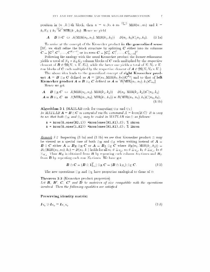
FFT AND FHT ALGORITHMS AND THEIR MATLAB IMPLEMENTATION 7position in (n1; k1)-th block, then n = n1N2 + n2 (2.1)= MIR(n1; n2) and k =k1K2 + k2 (2.1)= MIR(k1; k2). Hence we yieldA = B C , A(MIR(n1; n2);MIR(k1; k2)) = B(n1; k1)C(n2; k2): (3.1a)To arrive at the concept of the Kronecker product in the generalized sense[48], we shall re�ne the block structure by splitting C either into its columnsC = [C0;C1; : : : ;CK2�1] or its rows C = [CT0 ;CT1 ; : : : ;CTN2�1]T .Following the analogy with the usual Kronecker product the former re�nementyields a total of N1 �K1K2 column blocks of C each multiplied by the respectiveelement of B 2M(N1 �K1K2), while the latter one yields a total of N1N2 �K1row blocks of C each multiplied by the respective element of A 2M(N1N2�K1).The above idea leads to the generalized concept of right Kronecker prod-uct A = B R C de�ned as A = [B(n1;MIR(k1; k2))Ck2 ] and to that of leftKronecker product A = B L C de�ned as A = [B(MIR(n1; n2); k1)Cn2 ].Hence we getA = B R C , A(MIR(n1; n2);MIR(k1; k2)) = B(n1;MIR(k1; k2))C(n2; k2)A = B L C , A(MIR(n1; n2);MIR(k1; k2)) = B(MIR(n1; n2); k1)C(n2; k2):(3.1b)Algorithm 3.1 (MATLAB code for computing R and L).In MATLAB A = BC is computed via the command A = kron(B,C). It is easyto see that both R and L may be coded in MATLAB via as follows:A = kron(B,ones(N2,1)).*kron(ones(N1,K1),C); % rkronA = kron(B,ones(1,K2)).*kron(ones(N1,K1),C); % lkronRemark 3.2. Inspecting (3.1a) and (3.1b) we see that Kronecker product maybe viewed as a special case of both R and L when writing instead of A =B C either A = BR R C or A = BL L C where BR(n1;MIR(k1; k2)) =BL(MIR(n1; n2); k1) = B(n1; k1) holds for all n1 2ZN1; n2 2ZN2; k1 2ZK1; k2 2ZK2. Thus BR is obtained from B by repeating each column K2-times and BLfrom B by repeating each row N2-times. We have gotB C = (B 1TK2 )R C = (B 1N2) L C: (3.2)The new operations R and L have properties analogical to those of .Theorem 3.3 (Kronecker product properties).Let B, B0, C, C0 and D be matrices of size compatible with the operationsinvolved. Then the following equalities are satis�ed.Preserving identity matrix:IN1 IN2 = IN1N2 (3.3)

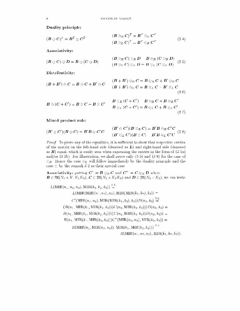
8 VíTÌZSLAV VESELÝDuality principle:(B C)T = BT CT (B R C)T = BT L CT(B L C)T = BT R CT (3.4)Associativity:(B C)D = B (C D) (B R C) RD = B R (C R D)(B L C)L D = B L (C LD) (3.5)Distributivity:(B +B0)C = B C +B0 C (B +B0)R C = B R C +B0 R C(B +B0)L C = B L C +B0 L C(3.6)B (C +C 0) = B C +B C0 B R (C +C 0) = B R C +B R C 0B L (C +C0) = B L C +B L C 0(3.7)Mixed product rule:(B0 C 0)(B C) = B0B C 0C (B0 C 0)(B R C) = B0B R C 0C(B0 L C 0)(B C) = B0B L C0C (3.8)Proof. To prove any of the equalities, it is su�cient to show that respective entriesof the matrix on the left-hand side (denoted as L) and right-hand side (denotedas R) equal, which is easily seen when expressing the entries in the form of (3.1a)and/or (3.1b). For illustration, we shall prove only (3.5) and (3.8) for the case ofR. Hence the case L will follow immediately by the duality principle and thecase by the remark 3.2 as their special case.Associativity: putting C 0 := B R C and C00 := C RD whereB 2M(N1�K1K2K3), C 2M(N2�K2K3) and D 2M(N3�K3), we can writeL(MIR(n1; n2; n3);MIR(k1; k2; k3)) 2:5=L(MIR(MIR(n1; n2); n3);MIR(MIR(k1; k2); k3)) =C 0(MIR(n1; n2);MIR(MIR(k1; k2); k3))D(n3; k3) 2:5=�B(n1;MIR(k1;MIR(k2; k3)))C(n2;MIR(k2; k3))�D(n3; k3) =B(n1;MIR(k1;MIR(k2; k3)))�C(n2;MIR(k2; k3))D(n3; k3)� =B(n1;MIR(k1;MIR(k2; k3)))C00(MIR(n2; n3);MIR(k2; k3)) =R(MIR(n1;MIR(n2; n3));MIR(k1;MIR(k2; k3))) 2:5=R(MIR(n1; n2; n3);MIR(k1; k2; k3)):

FFT AND FHT ALGORITHMS AND THEIR MATLAB IMPLEMENTATION 9Mixed Product Rule: putting A := B R C, A0 := B0 C 0, D := B0B andE := C 0C where B0 2M(N1 �K1), B 2M(K1 � L1L2), C 0 2M(N2 �K2) andC 2M(K2 � L2), we can writeL(MIR(n1; n2);MIR(l1; l2)) 2:2=K1�1Xk1=0 K2�1Xk2=0 A0(MIR(n1; n2);MIR(k1; k2))A(MIR(k1; k2);MIR(l1; l2)) =K1�1Xk1=0 K2�1Xk2=0 (B0(n1; k1)C 0(n2; k2))(B(k1;MIR(l1; l2))C(k2; l2)) =�K1�1Xk1=0 B0(n1; k1)B�k1;MIR(l1; l2)���K2�1Xk2=0 C0(n2; k2)C(k2; l2)� =D(n1;MIR(l1; l2))E(n2; l2) = R(MIR(n1; n2);MIR(l1; l2)):In view of associativity of ; R and L we may write multiple Kroneckerproducts of any type, omitting parentheses. Let N = N1:m; K = K1:m; n :=MIR(n1; n2; : : : ; nm) 2 ZN; k := MIR(k1; k2; : : : ; km) 2 ZK; ni 2 ZNi andki 2 ZKi for any i 2 f1 : mg. Then it is easy to see by induction on m andin view of lemma 2.5 that the equations (3.1a) and (3.1b) attain a more generalform:A = A1 A2 : : :Am , A(n; k) = A1(n1; k1)A2(n2; k2) : : :Am(nm; km)where A 2M(N �K) and Ai 2M(Ni �Ki) for i 2 f1 : mg, (3.9a)A = A1 R A2 R : : :R Am ,A(n; k) = A1(n1;MIR(k1; : : : ; km))A2(n2;MIR(k2; : : : ; km)) : : :Am(nm; km)where A 2M(N �K) and Ai 2M(Ni �Ki:m) for i 2 f1 : mg, (3.9b)A = A1 L A2 L : : :L Am ,A(n; k) = A1(MIR(n1; : : : ; nm); k1)A2(MIR(n2; : : : ; nm); k2) : : :Am(nm; km)where A 2M(N �K) and Ai 2M(Ni:m �Ki) for i 2 f1 : mg. (3.9c)Theorem 3.4 (Almost commutativity of ).Let Ai 2M(Ni �Ki) for i 2 f1 : mg, thenAm : : :A1 = SN(A1 : : :Am)STK (3.10)where N = (N1; : : : ; Nm) and K = (K1; : : : ;Km).Proof. Put A := A1 : : :Am and A0 := Am : : :A1, then it holds for eachn = MIRN(n1; : : : ; nm) and k = MIRK(k1; : : : ; km):A0(SN(n); SK(k)) = A0(MIRN0 (nm; : : : ; n1);MIRK0 (km; : : : ; k1)) (3.9a)=

10 VíTÌZSLAV VESELÝAm(nm; km) : : :A1(n1; k1) = A1(n1; k1) : : :Am(nm; km) (3.9a)=A(MIRN(n1; : : : ; nm);MIRK(k1; : : : ; km)) = A(n; k).Theorem 3.5 (Canonical sparse factorizations of Kronecker products).A = A1 A2 : : :Am = A(m)A(m�1) : : :A(1) whereA(i) = IN1:i�1 Ai IKi+1:m 2M(N1:iKi+1:m � N1:i�1Ki:m) (3.11a)A = A1 R A2 R : : :R Am = A(m)A(m�1) : : :A(1) whereA(i) = IN1:i�1 (Ai R IKi+1:m ) 2M(N1:iKi+1:m �N1:i�1Ki:m) (3.11b)A = A1 L A2 L : : :L Am = A(1)A(2) : : :A(m) whereA(i) = IK1:i�1 (Ai L INi+1:m ) 2M(K1:i�1Ni:m �K1:iNi+1:m) (3.11c)Proof. The mixed product rule (3.8) plays the key role in the derivation of theabove factorizations. Let us demonstrate the main idea for R in case of m = 2:A = A1 R A2 = IN1A1 R A2IK2 ) (IN1 A2)(A1 R IK2 ). To prove (3.11b)for m > 2 we proceed by induction on m using associativity (3.5):A = A1RA02 = (IN1 A02)(A1R IK2:m ) where by induction hypothesis A02 :=A2R : : :RAm = A0 (m)2 A0 (m�1)2 : : :A0 (2)2 ; A0 (i)2 = IN2:i�1 (AiR IKi+1:m ); i 2f2 : mg. Applying mixed product rule (m � 1)-times to we arrive atIN1 A02 = (IN1 A0 (m)) : : : (IN1 A0 (2)).To obtain (3.11b) it is su�cient to putA(1) := A1R IK2:m and A(i) := IN1 A0(i) = IN1 (IN2:i�1 (AiR IKi+1:m )) =IN1:i�1 (Ai R IKi+1:m ) for i 2 f2 : mg, where we have used (3.3) and (3.5).Finally, (3.11a) follows from (3.11b) by 3.2 and (3.11c) by the duality principle(3.4).De�nition 3.6. For any � 2 ZKi+1:m let Ai;� 2 M(Ni � Ki) be the submatrixof Ai 2M(Ni �Ki:m) from (3.9b) with entries Ai;�(ni; ki) := Ai(ni;MIR(ki; �)).Similarly for any � 2 ZNi+1:m let Ai;� 2 M(Ni � Ki) be the submatrix of Ai 2M(Ni:m � Ki) from (3.9c) with entries Ai;�(ni; ki) := Ai(MIR(ni; �); ki). Ai;�(or Ai;�) is said to be the �-th (�-th) elementary submatrix of Ai. Theassociated linear transform is called �-th (�-th) elementary transform of Ai.Remark 3.7.Now we are going to analyze the structure of A(i) from (3.11b) (or (3.11c)) inmore detail. Clearly, A(i) is a block-diagonal matrix with equal blocks eAi :=Ai R IKi+1:m (or eAi := Ai L INi+1:m ) repeated N1:i�1 times (or K1:i�1 times)along the diagonal.Each of these equal blocks eAi consists ofNi �Ki diagonal blocks of sizeKi+1:m�Ki+1:m (or Ni+1:m � Ni+1:m). The (ni; ki)-th diagonal block has the formdiag(Ai(ni;MIRKi(ki; 0)); : : : ; Ai(ni;MIRKi (ki;Ki+1:m � 1)))�or diag(Ai(MIRNi(ni; 0); ki); : : : ; Ai(MIRNi(ni; Ni+1:m � 1); ki))� (3.12)

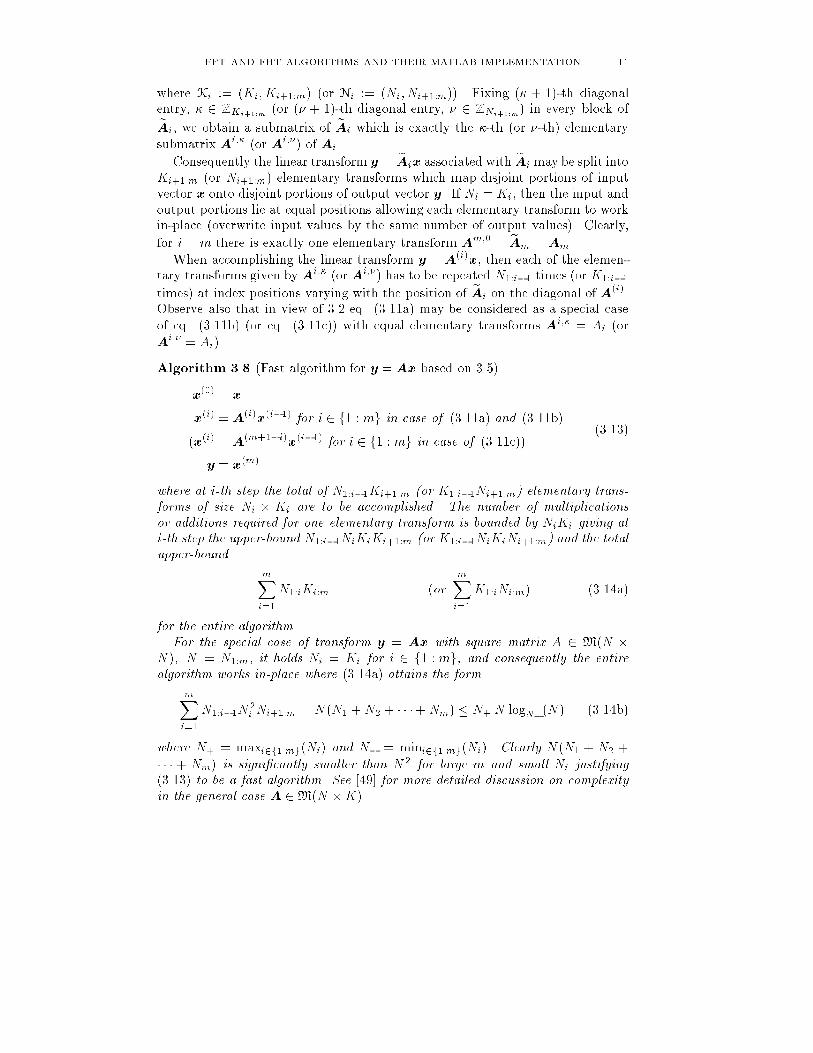
FFT AND FHT ALGORITHMS AND THEIR MATLAB IMPLEMENTATION 11where Ki := (Ki;Ki+1:m) (or Ni := (Ni; Ni+1:m)). Fixing (� + 1)-th diagonalentry, � 2 ZKi+1:m (or (� + 1)-th diagonal entry, � 2 ZNi+1:m) in every block ofeAi, we obtain a submatrix of eAi which is exactly the �-th (or �-th) elementarysubmatrix Ai;� (or Ai;�) of Ai.Consequently the linear transform y = eAix associated with eAi may be split intoKi+1:m (or Ni+1:m) elementary transforms which map disjoint portions of inputvector x onto disjoint portions of output vector y. If Ni = Ki, then the input andoutput portions lie at equal positions allowing each elementary transform to workin-place (overwrite input values by the same number of output values). Clearly,for i = m there is exactly one elementary transform Am;0 = eAm = Am.When accomplishing the linear transform y = A(i)x, then each of the elemen-tary transforms given by Ai;� (or Ai;�) has to be repeated N1:i�1 times (or K1:i�1times) at index positions varying with the position of eAi on the diagonal of A(i).Observe also that in view of 3.2 eq. (3.11a) may be considered as a special caseof eq. (3.11b) (or eq. (3.11c)) with equal elementary transforms Ai;� = Ai (orAi;� = Ai).Algorithm 3.8 (Fast algorithm for y = Ax based on 3.5).x(0) = xx(i) = A(i)x(i�1) for i 2 f1 : mg in case of (3.11a) and (3.11b)(x(i) = A(m+1�i)x(i�1) for i 2 f1 : mg in case of (3.11c))y = x(m) (3.13)where at i-th step the total of N1:i�1Ki+1:m (or K1:i�1Ni+1:m) elementary trans-forms of size Ni � Ki are to be accomplished. The number of multiplicationsor additions required for one elementary transform is bounded by NiKi giving ati-th step the upper-bound N1:i�1NiKiKi+1:m (or K1:i�1NiKiNi+1:m) and the totalupper-bound mXi=1 N1:iKi:m (or mXi=1K1:iNi:m) (3.14a)for the entire algorithm.For the special case of transform y = Ax with square matrix A 2 M(N �N ); N = N1:m; it holds Ni = Ki for i 2 f1 : mg, and consequently the entirealgorithm works in-place where (3.14a) attains the formmXi=1 N1:i�1N2i Ni+1:m = N (N1 + N2 + � � �+ Nm) � N+ N logN� (N ) (3.14b)where N+ = maxi2f1:mg(Ni) and N� = mini2f1:mg(Ni). Clearly N (N1 + N2 +� � � + Nm) is signi�cantly smaller than N2 for large m and small Ni justifying(3.13) to be a fast algorithm. See [49] for more detailed discussion on complexityin the general case A 2M(N �K).

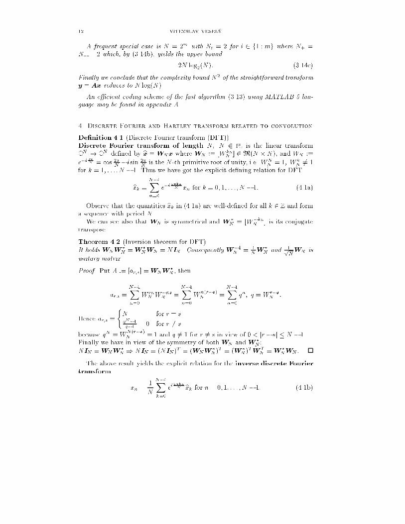
12 VíTÌZSLAV VESELÝA frequent special case is N = 2m with Ni = 2 for i 2 f1 : mg where N+ =N� = 2 which, by (3.14b), yields the upper-bound2N log2(N ): (3.14c)Finally we conclude that the complexity bound N2 of the straightforward transformy = Ax reduces to N log(N ).An e�cient coding scheme of the fast algorithm (3.13) using MATLAB 5 lan-guage may be found in appendix A.4. Discrete Fourier and Hartley transform related to convolutionDe�nition 4.1 (Discrete Fourier transform (DFT)).Discrete Fourier transform of length N; N 2 N, is the linear transformCN ! CN de�ned by bx = WNx where WN := [W knN ] 2M(N � N ), and WN :=e�i 2�N = cos 2�N �i sin 2�N is the N -th primitive root of unity, i.e. WNN = 1; W kN 6= 1for k = 1; : : : ; N � 1. Thus we have got the explicit de�ning relation for DFTbxk = N�1Xn=0 e�i 2�knN xn for k = 0; 1; : : : ; N � 1: (4.1a)Observe that the quantities bxk in (4.1a) are well-de�ned for all k 2Zand forma sequence with period N .We can see also that WN is symmetrical and W �N = [W�knN ] is its conjugatetranspose.Theorem 4.2 (Inversion theorem for DFT).It holds WNW �N =W �NWN = NIN . Consequently W�1N = 1NW �N and 1pNWN isunitary matrix.Proof. Put A := [ar;s] =WNW �N , thenar;s = N�1Xn=0 W rnN W�nsN = N�1Xn=0 Wn(r�s)N = N�1Xn=0 qn; q = W r�sN :Hence ar;s = (N for r = sqN�1q�1 = 0 for r 6= sbecause qN = WN(r�s)N = 1 and q 6= 1 for r 6= s in view of 0 < jr � sj � N � 1.Finally we have in view of the symmetry of both WN andW �N :NIN =WNW �N ) NIN = (NIN )T = (WNW �N )T = (W �N )TW TN =W �NWN :The above result yields the explicit relation for the inverse discrete Fouriertransform xn = 1N N�1Xk=0 ei 2�knN bxk for n = 0; 1; : : : ; N � 1: (4.1b)

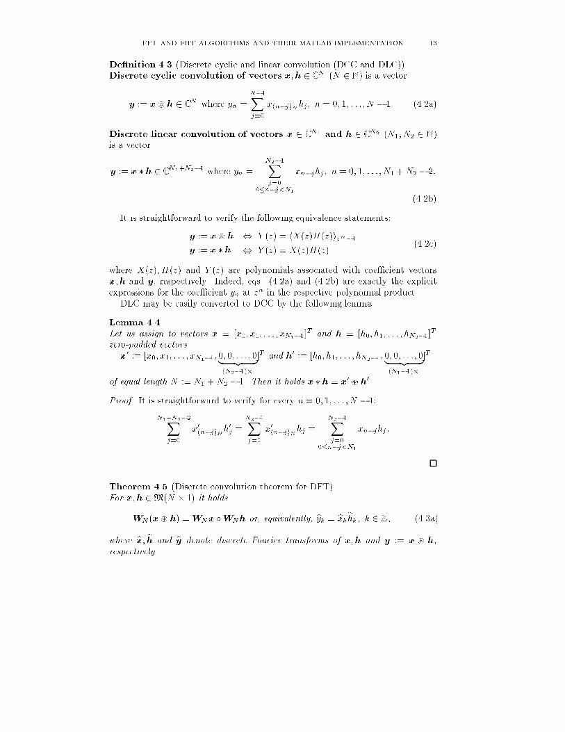
FFT AND FHT ALGORITHMS AND THEIR MATLAB IMPLEMENTATION 13De�nition 4.3 (Discrete cyclic and linear convolution (DCC and DLC)).Discrete cyclic convolution of vectors x;h 2 CN (N 2 N) is a vectory := x ~ h 2 CN where yn = N�1Xj=0 xhn�jiNhj; n = 0; 1; : : :; N � 1: (4.2a)Discrete linear convolution of vectors x 2 CN1 and h 2 CN2 (N1; N2 2 N)is a vectory := x � h 2 CN1+N2�1 where yn = N2�1Xj=00�n�j<N1 xn�jhj; n = 0; 1; : : : ; N1 + N2 � 2:(4.2b)It is straightforward to verify the following equivalence statements:y := x ~ hy := x � h , Y (z) = hX(z)H(z)izN�1, Y (z) = X(z)H(z) (4.2c)where X(z);H(z) and Y (z) are polynomials associated with coe�cient vectorsx;h and y, respectively. Indeed, eqs. (4.2a) and (4.2b) are exactly the explicitexpressions for the coe�cient yn at zn in the respective polynomial product.DLC may be easily converted to DCC by the following lemma.Lemma 4.4.Let us assign to vectors x = [x0; x1; : : : ; xN1�1]T and h = [h0; h1; : : : ; hN2�1]Tzero-padded vectorsx0 := [x0; x1; : : : ; xN1�1; 0; 0; : : :; 0| {z }(N2�1)� ]T and h0 := [h0; h1; : : : ; hN2�1; 0; 0; : : :; 0| {z }(N1�1)� ]Tof equal length N := N1 + N2 � 1. Then it holds x � h = x0 ~ h0.Proof. It is straightforward to verify for every n = 0; 1; : : : ; N � 1:N1+N2�2Xj=0 x0hn�jiNh0j = N2�1Xj=0 x0hn�jiNhj = N2�1Xj=00�n�j<N1 xn�jhj:Theorem 4.5 (Discrete convolution theorem for DFT).For x;h 2M(N � 1) it holdsWN (x ~ h) =WNx �WNh or, equivalently, byk = bxkbhk; k 2Z; (4.3a)where bx; bh and by denote discrete Fourier transforms of x;h and y := x ~ h,respectively.

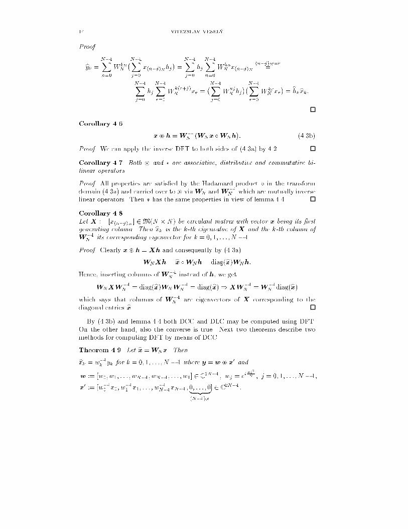
14 VíTÌZSLAV VESELÝProof.byk = N�1Xn=0 W knN �N�1Xj=0 xhn�jiNhj� = N�1Xj=0 hj N�1Xn=0 W knN xhn�jiN hn�jiN=r=N�1Xj=0 hj N�1Xr=0 W k(r+j)N xr = �N�1Xj=0 W kjN hj��N�1Xr=0 W krN xr� = bhkbxk:Corollary 4.6. x~ h =W�1N (WNx �WNh): (4.3b)Proof. We can apply the inverse DFT to both sides of (4.3a) by 4.2.Corollary 4.7. Both ~ and � are associative, distributive and commutative bi-linear operators.Proof. All properties are satis�ed by the Hadamard product � in the transformdomain (4.3a) and carried over to ~ viaWN andW�1N which are mutually inverselinear operators. Then � has the same properties in view of lemma 4.4.Corollary 4.8.Let X := [xhn�jiN ] 2M(N � N ) be circulant matrix with vector x being its �rstgenerating column. Then bxk is the k-th eigenvalue of X and the k-th column ofW�1N its corresponding eigenvector for k = 0; 1; : : : ; N � 1.Proof. Clearly x~ h = Xh and consequently by (4.3a)WNXh = bx �WNh = diag(bx)WNh:Hence, inserting columns ofW�1N instead of h, we getWNXW�1N = diag(bx)WNW�1N = diag(bx))XW�1N =W�1N diag(bx)which says that columns of W�1N are eigenvectors of X corresponding to thediagonal entries bx.By (4.3b) and lemma 4.4 both DCC and DLC may be computed using DFT.On the other hand, also the converse is true. Next two theorems describe twomethods for computing DFT by means of DCC.Theorem 4.9. Let bx =WNx. Thenbxk = w�1k yk for k = 0; 1; : : : ; N � 1 where y = w ~ x0 andw := [w0; w1; : : : ; wN�1; wN�1; : : : ; w1] 2 C 2N�1 ; wj = ei�j2N ; j = 0; 1; : : : ; N � 1;x0 := [w�10 x0; w�11 x1; : : : ; w�1N�1xN�1; 0; : : : ; 0| {z }(N�1)� ] 2 C 2N�1 :

FFT AND FHT ALGORITHMS AND THEIR MATLAB IMPLEMENTATION 15Proof. After substituting �2kn = (k � n)2 � n2 � k2 into (4.1a), we getbxk = e�i�k2N N�1Xn=0 ei�(k�n)2N e�i�n2N xn = w�1k 2N�2Xn=0 ei�(k�n)2N x0n:Theorem 4.10 (Rader [38]).Let bx = WNx where N = p is a prime number. Then ZN � f0g is cyclic groupof order N � 1 with respect to �. Let 0 6= g 2 ZN be a generator (arbitrary but�xed) and g�1 := hgi�1N its inverse modulo N (cf. lemma 2.1). Thenbx0 = x0 + x1 + : : :xN�1;bxhgriN = x0 + yr for r = 0; 1; : : : ; N � 2 where y = w ~ x0 andw := [w0; w1; : : : ; wN�2] 2 CN�1 ; wj = W gjN for j = 0; 1; : : : ; N � 2;x0 := [x00; x01; : : : ; x0N�2]; x0j = xhg�j iN :Proof. It is a well-known result from number theory that ZN � f0g is a cyclicgroup with respect to multiplication modulo N if N = p is a prime | see [27, 35].Then ZN � f0g = fhgniN jn = 0; 1; : : : ; N � 2g where g is a generator of thatgroup. Consequently, for any k = 1; 2; : : : ; N � 1 there exists r 2ZN�1 such thatk = hgriN and one can rewrite (4.1a) as followsbx0 = x0 + x1 + : : : xN�1 for k = 0, andbxk = bxhgriN = N�1Xn=0 W knN xn = x0 + N�1Xn=1 W knN xn = x0 + N�2Xs=0 W hgriN hgsiNN x(hgsiN ) =x0 + N�2Xs=0 W ghr+siN�1N x(hgsiN ) s=h�jiN�1= x0 + N�2Xj=0 W ghr�jiN�1N x(hg�jiN ) =x0 + N�2Xj=0 whr�jiN�1x0j = x0 + yr for 0 6= k = hgriN 2ZN; r = 0; 1; : : :; N � 2:Observe that a real vector x 2 RN is not transformed by DFT to a real vectorbx in general. Clearly, for x 2 RN we get by (4.1a) a complex vector bx satisfyingsymmetry bxk = N�1Xn=0 xn cos 2�nkN � iN�1Xn=0 xn sin 2�nkN = bx�k; k 2Z: (4.4)Consequently, there is a data redundancy in the transform domain where onlyone half of the 2N real values representing the real and imaginary parts of bxk; k =0; 1; : : : ; N �1, are carrying an useful information. Now we are going to show thata slight modi�cation in the de�nition of DFT can remove this drawback. Wesimply replace the complex kernel e�i 2�nkN = cos 2�nkN � i sin 2�nkN by the real

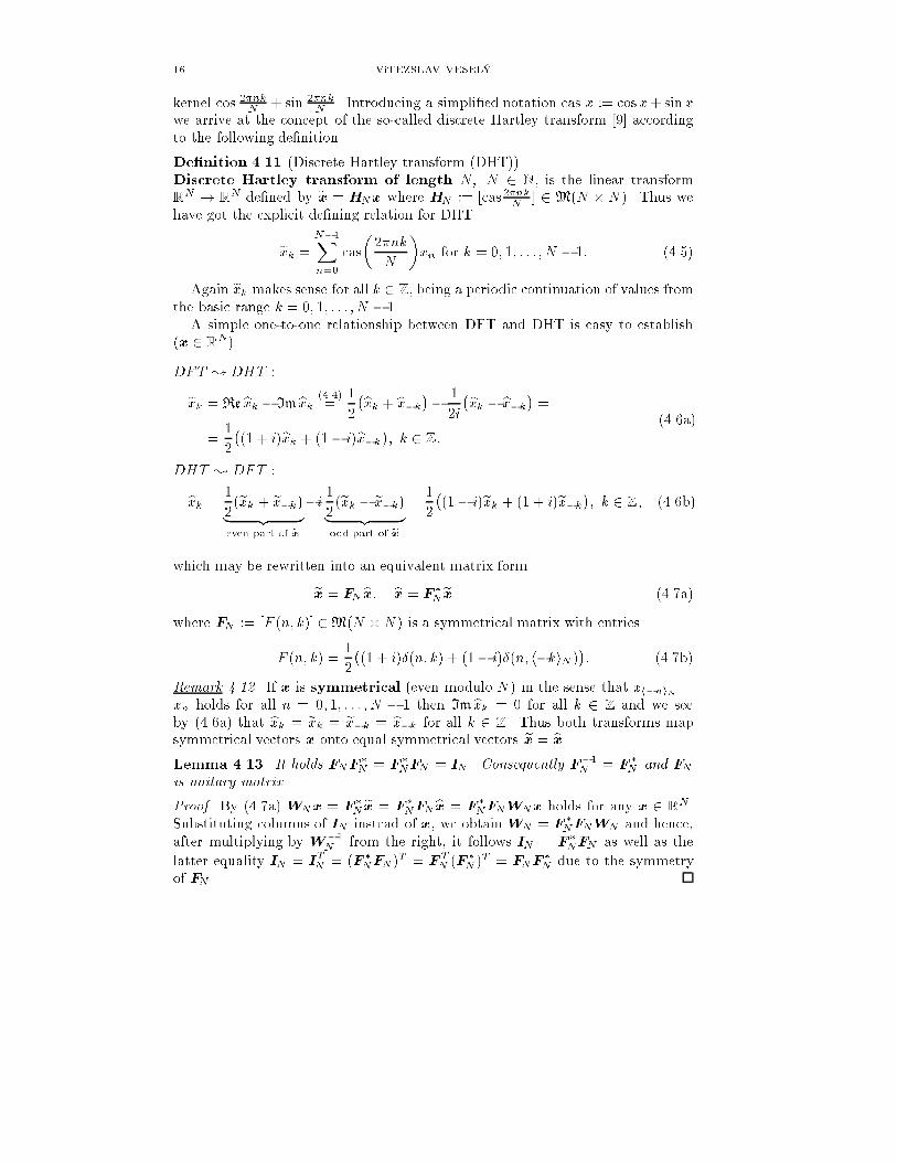
16 VíTÌZSLAV VESELÝkernel cos 2�nkN + sin 2�nkN . Introducing a simpli�ed notation cas x := cosx+ sinxwe arrive at the concept of the so-called discrete Hartley transform [9] accordingto the following de�nition.De�nition 4.11 (Discrete Hartley transform (DHT)).Discrete Hartley transform of length N; N 2 N, is the linear transformRN ! RN de�ned by ex = HNx where HN := [cas2�nkN ] 2M(N � N ). Thus wehave got the explicit de�ning relation for DHTexk = N�1Xn=0 cas�2�nkN �xn for k = 0; 1; : : : ; N � 1: (4.5)Again exk makes sense for all k 2Z, being a periodic continuation of values fromthe basic range k = 0; 1; : : : ; N � 1.A simple one-to-one relationship between DFT and DHT is easy to establish(x 2 RN).DFT ; DHT :exk = Re bxk � Im bxk (4.4)= 12�bxk + bx�k�� 12i�bxk � bx�k� == 12�(1 + i)bxk + (1 � i)bx�k�; k 2Z: (4.6a)DHT ; DFT :bxk = 12(exk + ex�k)| {z }even part of ex �i 12(exk � ex�k)| {z }odd part of ex = 12�(1� i)exk + (1 + i)ex�k�; k 2Z; (4.6b)which may be rewritten into an equivalent matrix formex = FN bx; bx = F �N ex (4.7a)where FN := [F (n; k)] 2M(N � N ) is a symmetrical matrix with entriesF (n; k) = 12�(1 + i)�(n; k) + (1� i)�(n; h�kiN )�: (4.7b)Remark 4.12. If x is symmetrical (even modulo N ) in the sense that xh�niN =xn holds for all n = 0; 1; : : : ; N � 1 then Im bxk = 0 for all k 2 Zand we seeby (4.6a) that bxk = exk = ex�k = bx�k for all k 2 Z. Thus both transforms mapsymmetrical vectors x onto equal symmetrical vectors ex = bx.Lemma 4.13. It holds FNF �N = F �NFN = IN . Consequently F�1N = F �N and FNis unitary matrix.Proof. By (4.7a) WNx = F �N ex = F �NFN bx = F �NFNWNx holds for any x 2 RN.Substituting columns of IN instead of x, we obtain WN = F �NFNWN and hence,after multiplying by W�1N from the right, it follows IN = F �NFN as well as thelatter equality IN = ITN = (F �NFN )T = F TN (F �N )T = FNF �N due to the symmetryof FN .

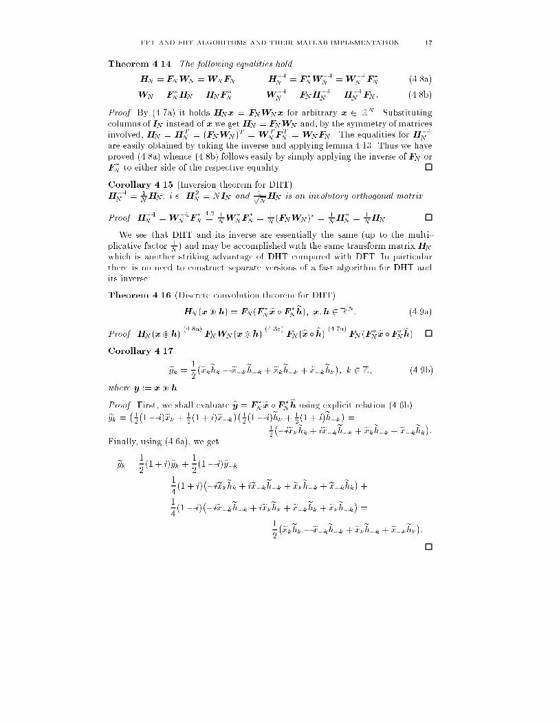
FFT AND FHT ALGORITHMS AND THEIR MATLAB IMPLEMENTATION 17Theorem 4.14. The following equalities holdHN = FNWN =WNFN H�1N = F �NW�1N =W�1N F �N (4.8a)WN = F �NHN =HNF �N W�1N = FNH�1N =H�1N FN : (4.8b)Proof. By (4.7a) it holds HNx = FNWNx for arbitrary x 2 RN. Substitutingcolumns of IN instead of x we getHN = FNWN and, by the symmetry of matricesinvolved, HN = HTN = (FNWN )T = W TN FTN = WNFN . The equalities for H�1Nare easily obtained by taking the inverse and applying lemma 4.13. Thus we haveproved (4.8a) whence (4.8b) follows easily by simply applying the inverse of FN orF �N to either side of the respective equality.Corollary 4.15 (Inversion theorem for DHT).H�1N = 1NHN , i.e. H2N = NIN and 1pNHN is an involutory orthogonal matrix.Proof. H�1N =W�1N F �N 4:2= 1NW �NF �N = 1N (FNWN )� = 1NH�N = 1NHN .We see that DHT and its inverse are essentially the same (up to the multi-plicative factor 1N ) and may be accomplished with the same transform matrixHNwhich is another striking advantage of DHT compared with DFT. In particularthere is no need to construct separate versions of a fast algorithm for DHT andits inverse.Theorem 4.16 (Discrete convolution theorem for DHT).HN (x~ h) = FN (F �N ex � F �N eh); x;h 2 RN: (4.9a)Proof. HN (x~h) (4.8a)= FNWN (x~h) (4.3a)= FN (bx � bh) (4.7a)= FN (F �N ex �F �N eh).Corollary 4.17.eyk = 12�exkehk � ex�keh�k + exkeh�k + ex�kehk�; k 2Z; (4.9b)where y := x~ h.Proof. First, we shall evaluate by = F �N ex �F �N eh using explicit relation (4.6b).byk = � 12(1� i)exk + 12 (1 + i)ex�k��12(1� i)ehk + 12 (1 + i)eh�k� =12��iexkehk + iex�keh�k + exkeh�k + ex�kehk�:Finally, using (4.6a), we geteyk = 12(1 + i)byk + 12(1� i)by�k =14(1 + i)��iexkehk + iex�keh�k + exkeh�k + ex�kehk�+14(1� i)��iex�keh�k + iexkehk + ex�kehk + exkeh�k� =12�exkehk � ex�keh�k + exkeh�k + ex�kehk�:

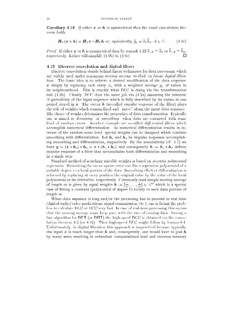
18 VíTÌZSLAV VESELÝCorollary 4.18. If either x or h is symmetrical then the usual convolution the-orem holds.HN (x ~ h) =HNx �HNh or, equivalently, eyk = exkehk; k 2Z: (4.9c)Proof. If either x or h is symmetrical then by remark 4.12 ex�k = exk or eh�k = ehk,respectively. Either will simplify (4.9b) to (4.9c).4.19. Discrete convolution and digital �ltersDiscrete convolution stands behind linear techniques for data processing whichare widely used under synonyms moving average method or linear digital �ltra-tion. The basic idea is to achieve a desired modi�cation of the data sequencex simply by replacing each entry xn with a weighted average yn of values inits neighbourhood. This is exactly what DLC is doing via the transformationrule (4.2b). Clearly, DCC does the same job via (4.2a) assuming the inherentN -periodicity of the input sequence which is fully described by its values in oneperiod stored in x. The vector h (so-called impulse response of the �lter) playsthe role of weights which remain �xed and \move" along the input data sequence.The choice of weights determines the properties of data transformation. Typicallyone is aimed at denoising or smoothing when data are corrupted with somekind of random errors. Another example are so-called di�erential �lters whichaccomplish numerical di�erentiation. As numerical di�erentiation results in in-crease of the random noise level, special weights can be designed which combinesmoothing with di�erentiation. Let hs and hd be impulse responses accomplish-ing smoothing and di�erentiation, respectively. By the associativity (cf. 4.7) wehave y = (x � hs) � hd = x � (hs � hd) and consequently h := hs � hd de�nesimpulse response of a �lter that accomplishes both di�erentiation and smoothingin a single step.Standard method of searching suitable weights is based on stepwise polynomialregression. Minimizing the mean square error one �ts a regression polynomial of asuitable degree to a local portion of the data. Smoothing e�ect or di�erentiation isachieved by replacing at every position the original value by the value of the localpolynomial or its derivative, respectively. Commonly used simple moving averageof length m is given by equal weights h := [ 1m ; : : : ; 1m ] 2 Rm which is a specialcase of �tting a constant (polynomial of degree 0) locally to each data portion oflength m.When data sequence is long and/or the processing has to proceed in real time(digital audio/video applications, signal transmission, etc.), one is facing the prob-lem to calculate DLC or DCC very fast. In case of real-time processing this meansthat the moving average must keep pace with the rate of coming data. Having afast algorithm for DFT (or DHT) the high-speed DCC is obtained via the convo-lution theorem 4.6 (or 4.16). Then high-speed DLC might follow by lemma 4.4.Unfortunately, in digital �ltration this approach is impractical because typicallythe input x is much longer than h and, consequently, one would have to pad hby many zeros resulting in redundant computational load and extreme memory

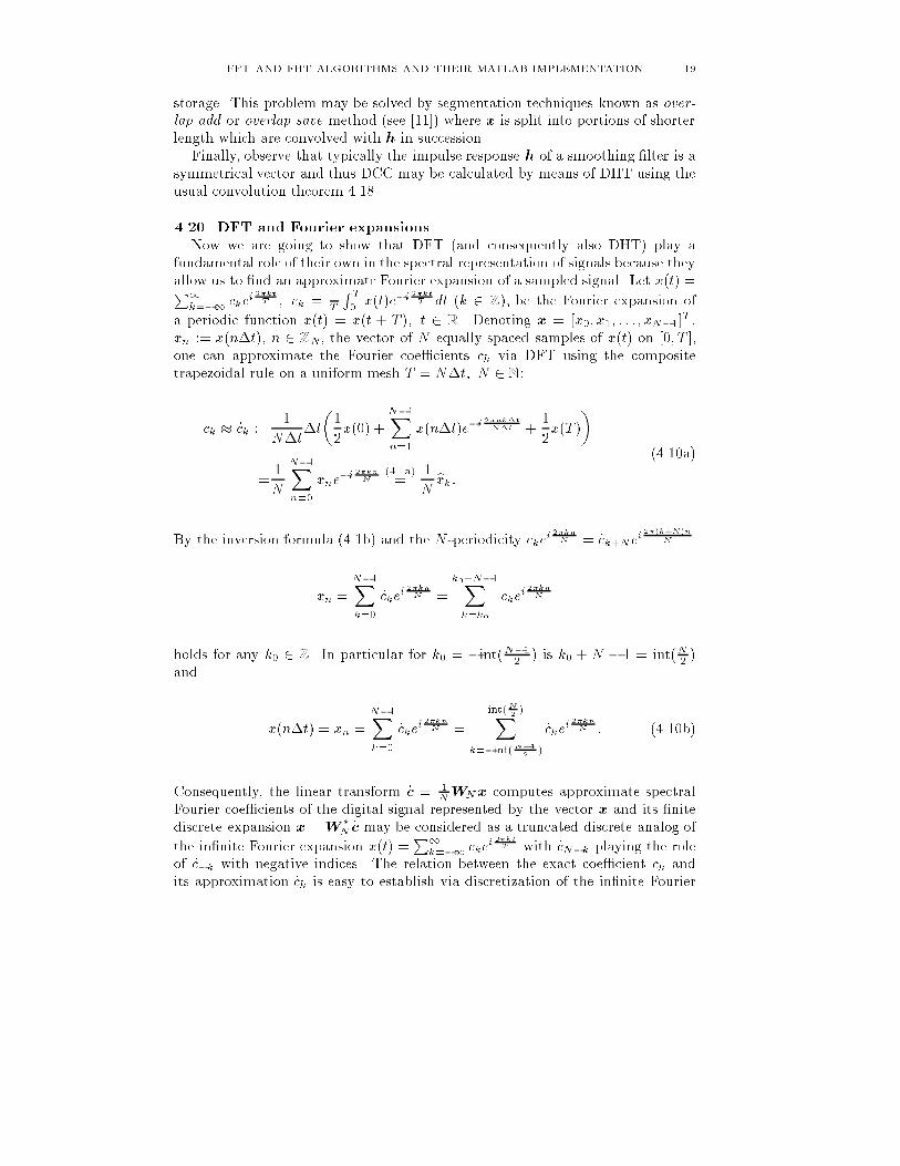
FFT AND FHT ALGORITHMS AND THEIR MATLAB IMPLEMENTATION 19storage. This problem may be solved by segmentation techniques known as over-lap-add or overlap-save method (see [11]) where x is split into portions of shorterlength which are convolved with h in succession.Finally, observe that typically the impulse response h of a smoothing �lter is asymmetrical vector and thus DCC may be calculated by means of DHT using theusual convolution theorem 4.18.4.20. DFT and Fourier expansionsNow we are going to show that DFT (and consequently also DHT) play afundamental role of their own in the spectral representation of signals because theyallow us to �nd an approximate Fourier expansion of a sampled signal. Let x(t) =P1k=�1 ckei 2�ktT ; ck = 1T R T0 x(t)e�i 2�ktT dt (k 2 Z), be the Fourier expansion ofa periodic function x(t) = x(t + T ); t 2 R. Denoting x = [x0; x1; : : : ; xN�1]T ,xn := x(n�t), n 2ZN, the vector of N equally spaced samples of x(t) on [0; T ],one can approximate the Fourier coe�cients ck via DFT using the compositetrapezoidal rule on a uniform mesh T = N�t; N 2 N:ck � _ck := 1N�t�t�12x(0) + N�1Xn=1 x(n�t)e�i 2�nk�tN�t + 12x(T )�= 1N N�1Xn=0 xne�i 2�knN (4.1a)= 1N bxk: (4.10a)By the inversion formula (4.1b) and the N -periodicity _ckei 2�knN = _ck+Nei 2�(k+N)nNxn = N�1Xk=0 _ckei 2�knN = k0+N�1Xk=k0 _ckei 2�knNholds for any k0 2 Z. In particular for k0 = �int(N�12 ) is k0 + N � 1 = int(N2 )and x(n�t) = xn = N�1Xk=0 _ckei 2�knN = int(N2 )Xk=�int(N�12 ) _ckei 2�knN : (4.10b)Consequently, the linear transform _c = 1NWNx computes approximate spectralFourier coe�cients of the digital signal represented by the vector x and its �nitediscrete expansion x =W �N _c may be considered as a truncated discrete analog ofthe in�nite Fourier expansion x(t) =P1k=�1 ckei 2�ktT with _cN�k playing the roleof _c�k with negative indices. The relation between the exact coe�cient ck andits approximation _ck is easy to establish via discretization of the in�nite Fourier

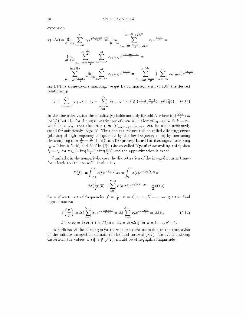
20 VíTÌZSLAV VESELÝexpansion.x(n�t) = limK!1 KXk=�K ckei 2�kn�tN�t (�)= limM!1 int(N2 )+MNXk=�int(N�12 )�MN ckei 2�knN =limM!1 int(N2 )Xk=�int(N�12 ) MXm=�M ck+mNei 2�(k+mN)nN =int(N2 )Xk=�int(N�12 ) limM!1 MXm=�M ck+mNei 2�knN = int(N2 )Xk=�int(N�12 )� 1Xm=�1 ck+mN �ei 2�knN :As DFT is a one-to-one mapping, we get by comparison with (4.10b) the desiredrelationship_ck = 1Xm=�1 ck+mN = ck + 1Xm=�1m6=0 ck+mN for k 2 f�int(N�12 ) : int(N2 )g: (4.11)In the above derivation the equality (�) holds not only for odd N where int(N�12 ) =int(N2 ) but also for the asymmetric case of even N in view of ck ! 0 with k !1,which also says that the error term Pm2Z�f0g ck+mN can be made arbitrarilysmall for su�ciently large N . Thus one can reduce this so-called aliasing error(aliasing of high-frequency components by the low-frequency ones) by increasingthe sampling rate 1�t = NT . If x(t) is a frequency band limited signal satisfyingck = 0 for jkj � K, and K � int(N2 ) (the so-calledNyquist sampling rate) then_ck = ck for k 2 f�int(N�12 ) : int(N2 )g and the approximation is exact.Similarly, in the nonperiodic case the discretization of the integral Fourier trans-form leads to DFT as well. EvaluatingX(f) :=Z 1�1 x(t)e�i2�ftdt � Z T0 x(t)e�i2�ftdt ��t�12x(0) + N�1Xn=1 x(n�t)e�i2�fn�t + 12x(T )�for a discrete set of frequencies f = kT ; k = 0; 1; : : : ; N � 1, we get the �nalapproximationX� kT � � �tN�1Xn=0 xne�i 2�kn�tN�t = �tN�1Xn=0 xne�i 2�knN = �t bxk (4.12)where x0 = 12 (x(0) + x(T )) and xn = x(n�t) for n = 1; : : : ; N � 1:In addition to the aliasing error there is one error more due to the truncationof the in�nite integration domain to the �nal interval [0; T ]. To avoid a strongdistortion, the values jx(t)j; t =2 [0; T ], should be of negligible magnitude.

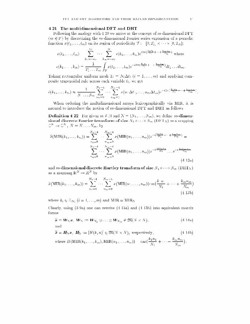
FFT AND FHT ALGORITHMS AND THEIR MATLAB IMPLEMENTATION 214.21. The multidimensional DFT and DHTFollowing the analogy with 4.20 we arrive at the concept ofm-dimensional DFT(m 2 N) by discretizing the m-dimensional Fourier series expansion of a periodicfunction x(t1; : : : ; tm) on its region of periodicity T := [0; T1]� � � � � [0; Tm]:x(t1; : : : ; tm) = 1Xk1=�1 � � � 1Xkm=�1 c(k1; : : : ; km)ei2�( k1t1T1 +���+ kmtmTm ) wherec(k1; : : : ; km) = 1T1 : : :Tm ZT x(t1; : : : ; tm)e�i2�( k1t1T1 +���+ kmtmTm )dt1 : : :dtm:Taking rectangular uniform mesh Ti = Ni�ti (i = 1; : : : ;m) and applying com-posite trapezoidal rule across each variable ti, we get_c(k1; : : : ; km) � 1N1 : : :Nm N1�1Xn1=0 � � �Nm�1Xnm=0 x(n1�t1; : : : ; nm�tm)e�i2�( k1n1N1 +���+ kmnmNm ):When ordering the multidimensional arrays lexicographically via MIR, it isnatural to introduce the notion of m-dimensional DFT and DHT as follows.De�nition 4.22. For given m 2 N and N = (N1; : : : ; Nm), we de�ne m-dimen-sional discrete Fourier transform of size N1�� � ��Nm (DFTN) as a mappingCN ! CN ; N = N1 : : :Nm, bybx(MIR(k1; : : : ; km)) =N1�1Xn1=0 � � �Nm�1Xnm=0 x(MIR(n1; : : : ; nm))e�( k1n1N1 +���+ kmnmNm ) =N1�1Xn1=0 � � �Nm�1Xnm=0 x(MIR(n1; : : : ; nm))e�i 2�k1n1N1 : : : e�i 2�kmnmNm(4.13a)andm-dimensional discrete Hartley transformof size N1�� � ��Nm (DHTN)as a mapping RN ! RN byex(MIR(k1; : : : ; km)) = N1�1Xn1=0 � � �Nm�1Xnm=0 x(MIR(n1; : : : ; nm))cas�k1n1N1 + � � �+ kmnmNm �(4.13b)where ki 2ZNi (i = 1; : : : ;m) and MIR = MIRN.Clearly, using (3.9a) one can rewrite (4.13a) and (4.13b) into equivalent matrixformsbx =WNx; WN :=WN1 : : :WNm 2M(N � N ); (4.14a)andex =HNx; HN := [H(k; n)] 2M(N �N ); respectively; (4.14b)where H(MIR(k1; : : : ; km);MIR(n1; : : : ; nm)) = cas�k1n1N1 + � � �+ kmnmNm �:

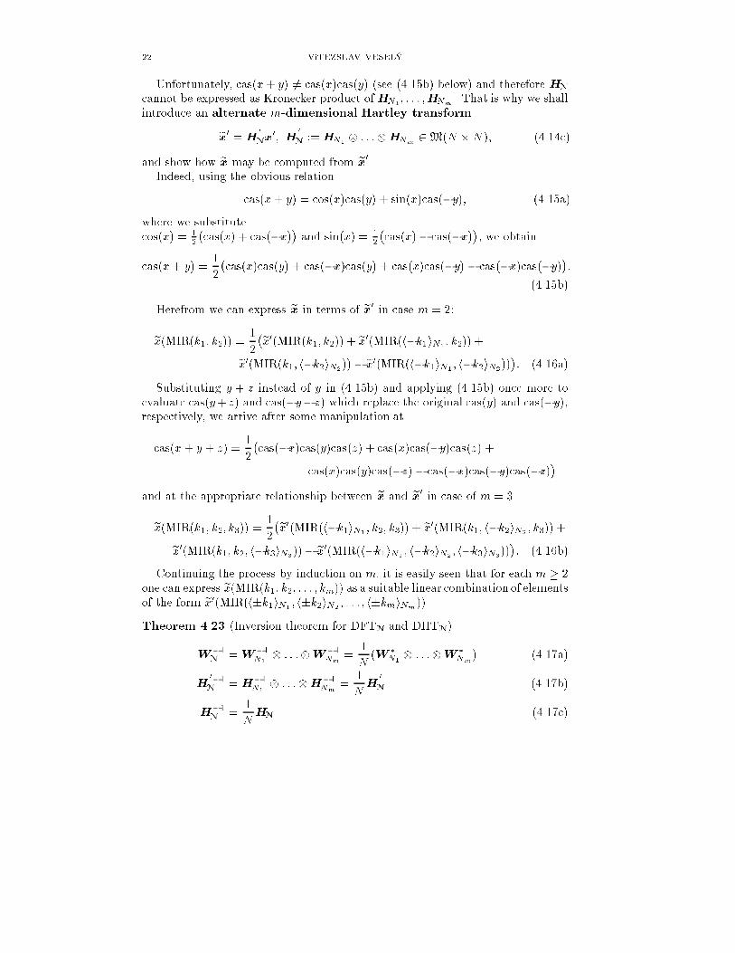
22 VíTÌZSLAV VESELÝUnfortunately, cas(x+ y) 6= cas(x)cas(y) (see (4.15b) below) and therefore HNcannot be expressed as Kronecker product ofHN1 ; : : : ;HNm . That is why we shallintroduce an alternate m-dimensional Hartley transformex0 =H 0Nx0; H 0N :=HN1 : : :HNm 2M(N � N ); (4.14c)and show how ex may be computed from ex0.Indeed, using the obvious relationcas(x+ y) = cos(x)cas(y) + sin(x)cas(�y); (4.15a)where we substitutecos(x) = 12�cas(x) + cas(�x)� and sin(x) = 12�cas(x)� cas(�x)�, we obtaincas(x+ y) = 12�cas(x)cas(y) + cas(�x)cas(y) + cas(x)cas(�y) � cas(�x)cas(�y)�:(4.15b)Herefrom we can express ex in terms of ex0 in case m = 2:ex(MIR(k1; k2)) = 12�ex0(MIR(k1; k2)) + ex0(MIR(h�k1iN1 ; k2)) +ex0(MIR(k1; h�k2iN2 )) � ex0(MIR(h�k1iN1 ; h�k2iN2 ))�: (4.16a)Substituting y + z instead of y in (4.15b) and applying (4.15b) once more toevaluate cas(y+ z) and cas(�y� z) which replace the original cas(y) and cas(�y),respectively, we arrive after some manipulation atcas(x + y + z) = 12�cas(�x)cas(y)cas(z) + cas(x)cas(�y)cas(z) +cas(x)cas(y)cas(�z) � cas(�x)cas(�y)cas(�z)�and at the appropriate relationship between ex and ex0 in case of m = 3ex(MIR(k1; k2; k3)) = 12�ex0(MIR(h�k1iN1 ; k2; k3)) + ex0(MIR(k1; h�k2iN2 ; k3)) +ex0(MIR(k1; k2; h�k3iN3 ))� ex0(MIR(h�k1iN1 ; h�k2iN2 ; h�k3iN3))�: (4.16b)Continuing the process by induction on m, it is easily seen that for each m � 2one can express ex(MIR(k1; k2; : : : ; km)) as a suitable linear combination of elementsof the form ex0(MIR(h�k1iN1 ; h�k2iN2 ; : : : ; h�kmiNm )).Theorem 4.23 (Inversion theorem for DFTN and DHTN).W�1N =W�1N1 : : :W�1Nm = 1N (W �N1 : : :W �Nm ) (4.17a)H 0�1N =H�1N1 : : :H�1Nm = 1NH 0N (4.17b)H�1N = 1NHN (4.17c)

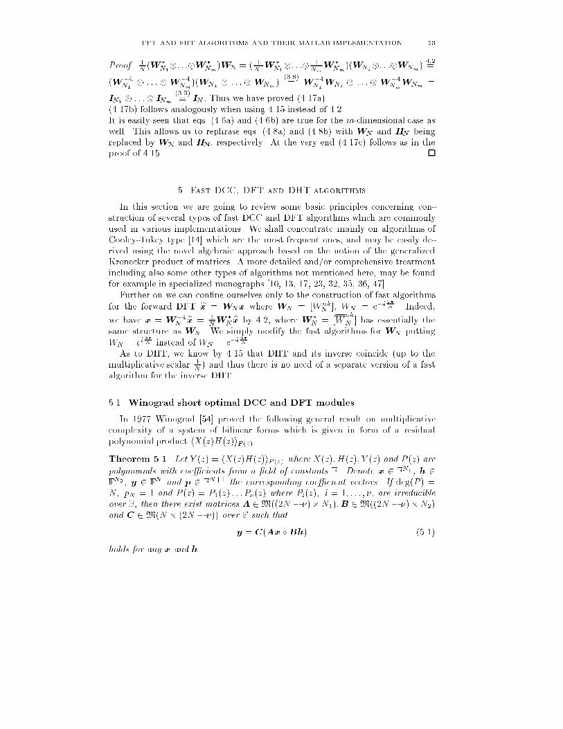
FFT AND FHT ALGORITHMS AND THEIR MATLAB IMPLEMENTATION 23Proof. 1N (W �N1: : :W �Nm )WN = ( 1N1W �N1: : : 1NmW �Nm )(WN1: : :WNm ) 4:2=(W �1N1 : : : W�1Nm )(WN1 : : : WNm ) (3.8)= W�1N1 WN1 : : : W�1NmWNm =IN1 : : : INm (3.3)= IN : Thus we have proved (4.17a).(4.17b) follows analogously when using 4.15 instead of 4.2.It is easily seen that eqs. (4.6a) and (4.6b) are true for the m-dimensional case aswell. This allows us to rephrase eqs. (4.8a) and (4.8b) with WN and HN beingreplaced by WN and HN, respectively. At the very end (4.17c) follows as in theproof of 4.15. 5. Fast DCC, DFT and DHT algorithmsIn this section we are going to review some basic principles concerning con-struction of several types of fast DCC and DFT algorithms which are commonlyused in various implementations. We shall concentrate mainly on algorithms ofCooley-Tukey type [14] which are the most frequent ones, and may be easily de-rived using the novel algebraic approach based on the notion of the generalizedKronecker product of matrices. A more detailed and/or comprehensive treatmentincluding also some other types of algorithms not mentioned here, may be foundfor example in specialized monographs [10, 13, 17, 23, 32, 35, 36, 47].Further on we can con�ne ourselves only to the construction of fast algorithmsfor the forward DFT bx = WNx where WN = [WnkN ], WN = e�i 2�N . Indeed,we have x = W�1N bx = 1NW �N bx by 4.2, where W �N = [WnkN ] has essentially thesame structure as WN . We simply modify the fast algorithms for WN puttingWN = ei 2�N instead of WN = e�i 2�N .As to DHT, we know by 4.15 that DHT and its inverse coincide (up to themultiplicative scalar 1N ) and thus there is no need of a separate version of a fastalgorithm for the inverse DHT.5.1. Winograd short optimal DCC and DFT modules.In 1977 Winograd [54] proved the following general result on multiplicativecomplexity of a system of bilinear forms which is given in form of a residualpolynomial product hX(z)H(z)iP (z) .Theorem 5.1. Let Y (z) = hX(z)H(z)iP (z) where X(z);H(z); Y (z) and P (z) arepolynomials with coe�cients from a �eld of constants F. Denote x 2 FN1 , h 2FN2 , y 2 FN and p 2 FN+1 the corresponding coe�cient vectors. If deg(P ) =N; pN = 1 and P (z) = P1(z) : : : P�(z) where Pi(z); i = 1; : : : ; �, are irreducibleover F, then there exist matrices A 2M((2N � �)�N1);B 2M((2N � �)�N2)and C 2M(N � (2N � �)) over F such thaty = C(Ax �Bh) (5.1)holds for any x and h.

24 VíTÌZSLAV VESELÝSketch of the proof (see [35, 54] for more details).The proof is based on the polynomial version of the Chinese Remainder Theo-rem which allows us to replace the polynomial product hX(z)H(z)iP (z) of highmodular degree N by � polynomial products hXi(z)Hi(z)iPi(z) of lower modulardegrees deg(Pi) where Xi(z) = hX(z)iPi(z) and Hi(z) = hH(z)iPi(z). The productXi(z)Hi(z) is evaluated using Lagrange interpolation on a set of 2(deg(Pi)�1)+1mesh points. Thus we need 2deg(Pi) � 1 multiplications for each i giving a totalof 2P�i=1(deg(Pi) � 1) = deg(P ) � � multiplications which are accomplished bythe Hadamard product of (5.1).The number 2N � � is the best possible (minimal) multiplicative complexity ofY (z) = hX(z)H(z)iP (z) over F when neglecting multiplications by �xed constantsfrom the �eld F. These constants are exactly the signi�cant entries of the matri-ces A;B and C (entries not belonging to f0;�1; 1g). The construction of thesematrices depends on the choice of the mesh for Lagrange interpolation (cf. proof)and is thus not unique. Moreover, number � depends on the choice of the �eld F.In practice, the algorithm (5.1) can be useful only if the matrices A;B and C areas simple as possible (most entries being 0,1 or -1) and at the same time 2N �� isreasonably small. It is a hard optimization problem to balance both requirementsbecause with decreasing 2N�� the size of matrices A;B and C decreases as well,giving thus less chance for a simple structure.We see from the de�ning relations (4.2a) and (4.2b) that both DCC and DLCmay be viewed as systems of bilinear forms which are represented as polynomialproducts (4.2c). While for DCC we have to put P (z) = zN �1, in case of DLC wemay choose any polynomialP (z), deg(P ) > deg(X)+deg(H) = N1�1+N2�1 =N1 + N2 � 2, which will guarantee hX(z)H(z)iP (z) = X(z)H(z). Clearly, by 4.4P (z) = zN �1 with N = N1+N2�1 is a natural choice for DLC. Then, of course,having representation (5.1) for y = x0 ~ h0 = C(Ax0 �Bh0), we get right away arepresentation for y = x � h = C(Ax �Bh) where A and B are submatrices ofA0 and B0 formed by their leading N1 and N2 columns, respectively. That is whywe can henceforth con�ne ourselves to DCC only.As zN � 1 has only integer coe�cients from the minimal �eld E := f0; 1;�1g,our choice of F is limited only to a �eld satisfying F � C because E � F isalways true. Let us have representation (5.1) of DCC for such a �eld F and denotecn the (n + 1)-row of matrix C (n = 0; 1; : : :; N � 1), then PN�1j=0 xhn�jiNhj =cn(Ax�Bh) holds for any x;h 2 FN . Denote �i := [�i;0; : : : ; �i;N�1]T 2 EN � FNfor i = 0; 1; : : : ; N � 1. Putting x = �i and h = �j we see that the bilinearforms on the left-and right-hand side have equal coe�cient at xihj for any i; j 2f0; 1; : : : ; N � 1g. Consequently, both bilinear forms must attain equal values forany x;h 2 CN . Our conclusion is that only the structure of matrices A;B andC depends on the choice of F, not a�ecting validity of (5.1) for some x 2 CN orh 2 CN that does not belong to FN .Observe that we can think of (5.1) to be a generalized form of the convolutiontheorem (4.3b) where � = N corresponds to the choice F = C . Indeed, thepolynomial zN � 1 is decomposed into � = N irreducible linear factors over C

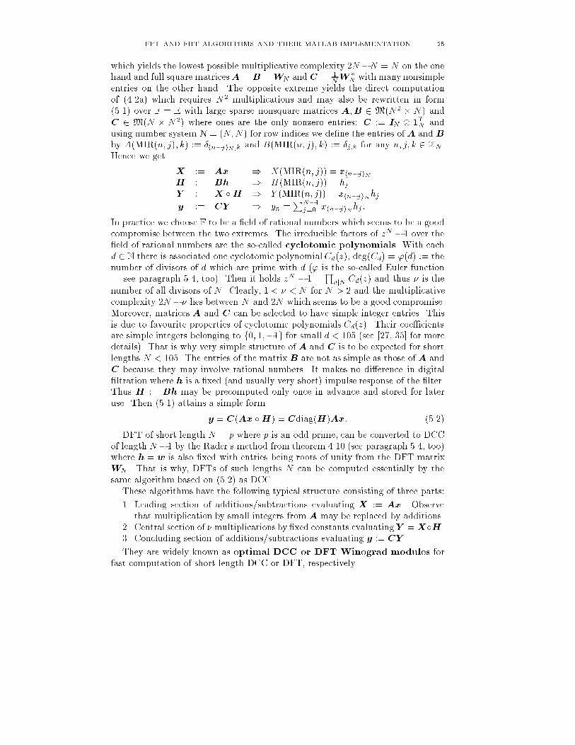
FFT AND FHT ALGORITHMS AND THEIR MATLAB IMPLEMENTATION 25which yields the lowest possible multiplicative complexity 2N �N = N on the onehand and full square matricesA = B =WN andC = 1NW �N with many nonsimpleentries on the other hand. The opposite extreme yields the direct computationof (4.2a) which requires N2 multiplications and may also be rewritten in form(5.1) over F = E with large sparse nonsquare matrices A;B 2 M(N2 � N ) andC 2 M(N � N2) where ones are the only nonzero entries: C := IN 1TN andusing number system N = (N;N ) for row indices we de�ne the entries of A and Bby A(MIR(n; j); k) := �hn�jiN ;k and B(MIR(n; j); k) := �j;k for any n; j; k 2ZN.Hence we get X := Ax ) X(MIR(n; j)) = xhn�jiNH := Bh ) H(MIR(n; j)) = hjY := X �H ) Y (MIR(n; j)) = xhn�jiNhjy := CY ) yn =PN�1j=0 xhn�jiNhj :In practice we choose F to be a �eld of rational numbers which seems to be a goodcompromise between the two extremes. The irreducible factors of zN � 1 over the�eld of rational numbers are the so-called cyclotomic polynomials. With eachd 2 N there is associated one cyclotomic polynomialCd(z), deg(Cd) = '(d) := thenumber of divisors of d which are prime with d (' is the so-called Euler function| see paragraph 5.4, too). Then it holds zN � 1 = QdjN Cd(z) and thus � is thenumber of all divisors of N . Clearly, 1 < � < N for N > 2 and the multiplicativecomplexity 2N �� lies between N and 2N which seems to be a good compromise.Moreover, matrices A and C can be selected to have simple integer entries. Thisis due to favourite properties of cyclotomic polynomials Cd(z). Their coe�cientsare simple integers belonging to f0; 1;�1g for small d < 105 (see [27, 35] for moredetails). That is why very simple structure of A and C is to be expected for shortlengths N < 105. The entries of the matrix B are not as simple as those of A andC because they may involve rational numbers. It makes no di�erence in digital�ltration where h is a �xed (and usually very short) impulse response of the �lter.Thus H := Bh may be precomputed only once in advance and stored for lateruse. Then (5.1) attains a simple formy = C(Ax �H) = Cdiag(H)Ax: (5.2)DFT of short length N = p where p is an odd prime, can be converted to DCCof length N �1 by the Rader's method from theorem 4.10 (see paragraph 5.4, too)where h = w is also �xed with entries being roots of unity from the DFT matrixWN . That is why, DFTs of such lengths N can be computed essentially by thesame algorithm based on (5.2) as DCC.These algorithms have the following typical structure consisting of three parts:1. Leading section of additions/subtractions evaluating X := Ax. Observethat multiplication by small integers from A may be replaced by additions.2. Central section of � multiplications by �xed constants evaluatingY = X�H.3. Concluding section of additions/subtractions evaluating y := CY .They are widely known as optimal DCC or DFT Winograd modules forfast computation of short length DCC or DFT, respectively.

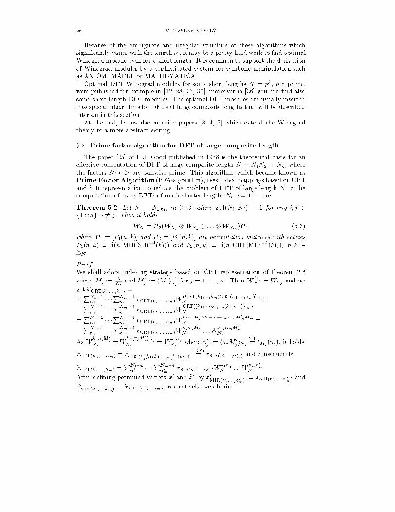
26 VíTÌZSLAV VESELÝBecause of the ambiguous and irregular structure of these algorithms whichsigni�cantly varies with the length N , it may be a pretty hard work to �nd optimalWinograd module even for a short length. It is common to support the derivationof Winograd modules by a sophisticated system for symbolic manipulation suchas AXIOM, MAPLE or MATHEMATICA.Optimal DFT Winograd modules for some short lengths N = pk, p a prime,were published for example in [12, 28, 35, 36], moreover in [36] you can �nd alsosome short length DCC modules. The optimal DFT modules are usually insertedinto special algorithms for DFTs of large composite lengths that will be describedlater on in this section.At the end, let us also mention papers [3, 4, 5] which extend the Winogradtheory to a more abstract setting.5.2. Prime factor algorithm for DFT of large composite length.The paper [25] of I. J. Good published in 1958 is the theoretical basis for ane�ective computation of DFT of large composite length N = N1N2 : : :Nm wherethe factors Ni 2 N are pairwise prime. This algorithm, which became known asPrime Factor Algorithm (PFA-algorithm), uses index mappings based on CRTand SIR representation to reduce the problem of DFT of large length N to thecomputation of many DFTs of much shorter lengths Ni, i = 1; : : : ;m.Theorem 5.2. Let N = N1:m, m � 2, where gcd(Ni; Nj) = 1 for any i; j 2f1 : mg, i 6= j. Then it holdsWN = P 2(WN1 WN2 : : :WNm )P 1 (5.3)where P 1 = [P1(n; k)] and P 2 = [P2(n; k)] are permutation matrices with entriesP1(n; k) = �(n;MIR(SIR�1(k))) and P2(n; k) = �(n;CRT(MIR�1(k))), n; k 2ZN.Proof.We shall adopt indexing strategy based on CRT representation of theorem 2.6where Mj := NNj and M 0j := hMji�1Nj for j = 1; : : : ;m. Then WMjN = WNj and weget bxCRT(k1;:::;km) ==PN1�1n1 � � �PNm�1nm xCRT(n1;:::;nm)W hCRT(k1;:::;km)CRT(n1;:::;nm)iNN ==PN1�1n1 � � �PNm�1nm xCRT(n1;:::;nm)WCRT(hk1n1iN1 ;:::;hkmnmiNm )N ==PN1�1n1 � � �PNm�1nm xCRT(n1;:::;nm)W k1n1M 01M1+���+kmnmM 0mMmN ==PN1�1n1 � � �PNm�1nm xCRT(n1;:::;nm)W k1n1M 01N1 : : :W kmnmM 0mNm .As W kjnjM 0jNj =W kj hnjM 0jiNjNj = W kjn0jNj where n0j := hnjM 0jiNj 2:1= tM 0j (nj), it holdsxCRT(n1;:::;nm) = xCRT(t�1M01(n01);:::;t�1M0m (n0m)) (2.8)= xSIR(n01;:::;n0m) and consequentlybxCRT(k1;:::;km) =PN1�1n01 � � �PNm�1n0m xSIR(n01;:::;n0m)W k1n01N1 : : :W kmn0mNm .After de�ning permuted vectors x0 and bx0 by x0MIR(n01;:::;n0m) := xSIR(n01;:::;n0m) andbx0MIR(k1;:::;km) := bxCRT(k1;:::;km), respectively, we obtain

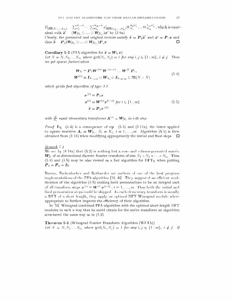
FFT AND FHT ALGORITHMS AND THEIR MATLAB IMPLEMENTATION 27bx0MIR(k1;:::;km) =PN1�1n01 � � �PNm�1n0m x0MIR(n01;:::;n0m)W k1n01N1 : : :W kmn0mNm , which is equiv-alent with bx0 = (WN1 : : :WNm )x0 by (3.9a).Clearly, the permuted and original vectors satisfy bx = P 2bx0 and x0 = P 1x andthus bx = P 2(WN1 : : :WNm )P 1x.Corollary 5.3 (PFA-algorithm for bx =WNx).Let N = N1N2 : : :Nm where gcd(Ni; Nj) = 1 for any i; j 2 f1 : mg, i 6= j. Thenwe get sparse factorizationWN = P 2W (m)W (m�1) : : :W (1)P 1;W (i) = IN1:i�1 WNi INi+1:m 2M(N � N ) (5.4)which yields fast algorithm of type 3.8x(0) = P 1xx(i) =W (i)x(i�1) for i 2 f1 : mgbx = P 2x(m) (5.5)with NNi equal elementary transforms Ai;� =WNi in i-th step.Proof. Eq. (5.4) is a consequence of eqs. (5.3) and (3.11a), the latter appliedto square matrices Ai = WNi , Ni = Ki, i = 1; : : : ;m. Algorithm (5.5) is thenobtained from (3.13) when modifying appropriately the initial and �nal steps.Remark 5.4.We see by (4.14a) that (5.3) is nothing but a row- and column-permuted matrixWN of m-dimensional discrete Fourier transform of size N1�N2�� � ��Nm. Thus(5.4) and (5.5) may be also viewed as a fast algorithm for DFTN when puttingP 1 = P 2 = IN .Burrus, Eschenbacher and Rothweiler are authors of one of the best programimplementations of the PFA-algorithm [12, 40]. They suggested an e�cient mod-i�cation of the algorithm (5.5) making both permutations to be an integral partof all transform steps x(i) =W (i)x(i�1), i = 1; : : : ;m. Thus both the initial and�nal permutation steps could be skipped. As each elementary transform is usuallya DFT of a short length, they apply an optimal DFT Winograd module whereappropriate to further improve the e�ciency of their algorithm.In [53] Winograd combined PFA-algorithm with the optimal short-length DFTmodules in such a way that he could obtain for the entire transform an algorithmstructured the same way as in (5.2).Theorem 5.5 (Winograd Fourier Transform Algorithm (WFTA)).Let N = N1N2 : : :Nm where gcd(Ni; Nj) = 1 for any i; j 2 f1 : mg, i 6= j. If

28 VíTÌZSLAV VESELÝWNi = CiDiAi, Di = diag(H i), is a factorization (5.2) describing the appropri-ate optimal DFT Winograd module, then WN = CDA whereA = (A1 A2 : : :Am)P 1;D = D1 D2 : : :Dm;C = P 2(C1 C2 : : :Cm): (5.6)Proof. WN (5.3)= P 2(WN1 WN2 : : :WNm )P 1 =P 2(C1D1A1 C2D2A2 : : :CmDmAm)P 1 (3.8)=P 2(C1C2: : :Cm)(D1D2: : :Dm)(A1A2: : :Am)P 1 = CDA:The diagonal matrix D concatenates all constants from the multiplication sec-tions of all elementary transforms. Similarly the matrices A and C cumulate�xed constants from the leading and concluding sections, respectively. This pro-cess allows for further complexity reduction compared with the standard approachwhere Ai, Di and Ci are applied to separate elementary transforms. Silverman'sprogram [41] (reprinted in [35], too) is a recognized implementation of WFTA.Unfortunately, this program did not become widely spread because practical testscould not prove WFTA to be superior to other fast DFT algorithms. The mainreason is inherent to WFTA, namely that the row size of A signi�cantly exceedsN which results in increased memory storage and disables in-place processing.More details concerning WFTA and related topics can be found in [52], too.5.3. Cooley-Tukey DFT and DHT algorithm for large composite length.World-wide Cooley-Tukey's algorithm for fast computation of DFT becameknown under the abbreviation FFT (Fast Fourier Transform)1. Its originalversion [14]2 was limited to DFT of power-of-two length N = 2m. Later onCooley-Tukey's idea was generalized to arbitrary composite length N = N1 : : :Nm.Occasionally such algorithms are also calledmixed radix FFTs to stress the roleof the Mixed Radix Integer Representation in their construction. Unlike the PFAalgorithm there are no restrictions on factors Ni allowing for wider choice of lengthsN .We shall give a new purely algebraic derivation of the sparse factorization stand-ing behind FFT which is based on the notion of generalized Kronecker product[48, 49]. Let us start with an auxiliary statement concerning the digit reversal.Theorem 5.6 (Digit reversal decomposition).Let N := N1:m; m � 2, then it holds for each i 2 f1 : m� 1gSN = SN3(SN1 SN2) = (SN2 SN1)SN3 (5.7)where N1 = N1:i; N2 = Ni+1:m and N3 = (N1:i; Ni+1:m).1Often FFT is used in wider sense to denote any fast DFT algorithm.2The latest historical study of M. T. Heideman, C. S. Burrus and D. H. Johnson [9] tracesthe origin of the method back to a paper by C. F. Gauss published in 1805.

FFT AND FHT ALGORITHMS AND THEIR MATLAB IMPLEMENTATION 29Proof. We have S0 := SN3(SN1 SN2) = SN3(IN1:i SN2)(SN1 INi+1:m ) bythe mixed-product rule (3.8). Let S; S0; S1; S2 and S3 be permutation mappingsassociated with permutation matrices SN;S0;SN1INi+1:m ; IN1:i SN2 and SN3,respectively. We are going to show S = S0. Choose n = MIRN(n1; : : : ; nm)arbitrary but �xed then S0(n) = S3�S2�S1(MIRN(n1; : : : ; nm))�� (2.3)=S3�S2�S1(MIRN3(MIRN1(n1; : : : ; ni);MIRN2(ni+1; : : : ; nm)))�� =S3�S2(MIRN3(MIRN01 (ni; : : : ; n1);MIRN2(ni+1; : : : ; nm)))� =S3(MIRN3(MIRN01 (ni; : : : ; n1);MIRN02 (nm; : : : ; ni+1))) =MIRN03(MIRN02(nm; : : : ; ni+1);MIRN01(ni; : : : ; n1)) (2.3)= MIRN0 (nm; : : : ; n1).The other equality follows by almost commutativity 3.4:SN3(SN1 SN2) = SN3(SN1 SN2)STN3SN3 (3.10)= (SN2 SN1)SN3 .Theorem 5.7 (Veselý [49]).Let N = N1:m, m � 2, thenWN = SN(WR;1 R : : :RWR;m) = (WL;1 L : : :LWL;m)STN (5.8)where WR;i = [WR;i(ni; k)] 2 M(Ni � Ni:m), WL;i = W TR;i and WR;i(ni; k) =WN1:i�1nikN = WnikNi:m for i = 1; : : : ;m, k 2ZNi:m. In particular we have WR;m =WL;m =WNm . For every � 2ZNi+1:m the �-th elementary submatrix ofWR;i andWL;i attains the form W i;�R = D�WNi and W i;�L = WNiD�, respectively, whereD� = diag(Wni�Ni:m )ni2ZNi .Proof. We shall proceed by induction on m to prove (5.8).� m = 2: N = N1N2; n; k 2 ZN, n = MIRN(n1; n2), S(n) = MIRN0 (n2; n1)and k = MIRN(k1; k2)) S(n)k = (n2N1+n1)k = n1k +n2N1(k1N2+k2) =n1k + n2N1k2 + n2k1N ) hS(n)kiN = n1k +N1n2k2. HenceWS(n)kN =Wn1MIR(k1;k2)N WN1n2k2N = WR;1(n1;MIR(k1; k2))WR;2(n2; k2) (3.9b))WN = S(WR;1 RWR;2) = S(WR;1 RWN2 ).� m > 2: N = N1N 02 where N 02 = N2:m. Let SN1, SN2 and SN3 be the digitreversal permutation matrices of 5.6 for the case i = 1. Clearly SN1 = IN1and applying the induction hypothesis we getWN = SN3(WR;1RWN 02) = SN3�WR;1RSN2(WR;2R: : :RWR;m)� (3.8)=SN3(IN1 SN2)(WR;1 RWR;2 R : : :RWR;m) (5.7)=SN(WR;1 R : : :RWR;m).The other equality is obtained by matrix transpose (3.4):WN = W TN = �SN(WR;1 R : : :R WR;m)�T = (W TR;1 L : : : L W TR;m)STN =(WL;1 L : : :LWL;m)STN:Finally, by de�nition 3.6 and with Ni := (Ni; Ni+1:m), we getW i;�R (ni; ki) = WR;i(ni;MIRNi(ki; �)) = Wni(kiNi+1:m+�)Ni:m = Wni�Ni:mWnikiNi+1:mNi:m =Wni�Ni:mWnikiNi which is equivalent with W i;�R = D�WNi .Clearly W i;�L = (W i;�R )T =WNiD�.

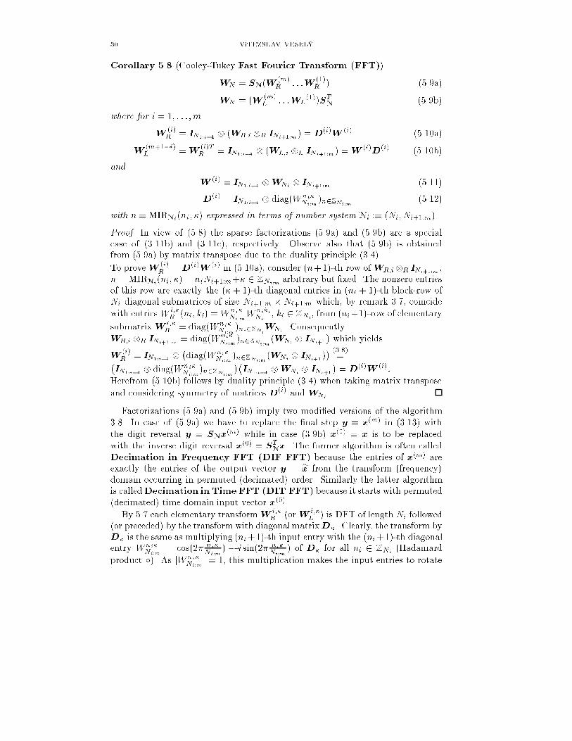
30 VíTÌZSLAV VESELÝCorollary 5.8 (Cooley-Tukey Fast Fourier Transform (FFT)).WN = SN(W (m)R : : :W (1)R ) (5.9a)WN = (W (m)L : : :WL(1))STN (5.9b)where for i = 1; : : : ;mW (i)R = IN1:i�1 (WR;i R INi+1:m ) = D(i)W (i) (5.10a)W (m+1�i)L =W (i)TR = IN1:i�1 (WL;i L INi+1:m ) =W (i)D(i) (5.10b)and W (i) = IN1:i�1 WNi INi+1:m (5.11)D(i) = IN1:i�1 diag(Wni�Ni:m )n2ZNi:m (5.12)with n = MIRNi(ni; �) expressed in terms of number system Ni := (Ni; Ni+1:m).Proof. In view of (5.8) the sparse factorizations (5.9a) and (5.9b) are a specialcase of (3.11b) and (3.11c), respectively. Observe also that (5.9b) is obtainedfrom (5.9a) by matrix transpose due to the duality principle (3.4).To proveW (i)R = D(i)W (i) in (5.10a), consider (n+1)-th row ofWR;iR INi+1:m ,n = MIRNi(ni; �) = niNi+1:m+� 2ZNi:m arbitrary but �xed. The nonzero entriesof this row are exactly the (� + 1)-th diagonal entries in (ni + 1)-th block-row ofNi diagonal submatrices of size Ni+1:m � Ni+1:m which, by remark 3.7, coincidewith entries W i;�R (ni; ki) = Wni�Ni:mWnikiNi , ki 2ZNi, from (ni+1)-row of elementarysubmatrixW i;�R = diag(Wni�Ni:m )ni2ZNiWNi . ConsequentlyWR;i R INi+1:m = diag(Wni�Ni:m )n2ZNi:m (WNi INi+1 ) which yieldsW (i)R = IN1:i�1 �diag(Wni�Ni:m )n2ZNi:m (WNi INi+1 )� (3.8)=�IN1:i�1 diag(Wni�Ni:m )n2ZNi:m��IN1:i�1 WNi INi+1� = D(i)W (i):Herefrom (5.10b) follows by duality principle (3.4) when taking matrix transposeand considering symmetry of matrices D(i) and WNi .Factorizations (5.9a) and (5.9b) imply two modi�ed versions of the algorithm3.8. In case of (5.9a) we have to replace the �nal step y = x(m) in (3.13) withthe digit reversal y = SNx(m) while in case (3.9b) x(0) = x is to be replacedwith the inverse digit reversal x(0) = STNx. The former algorithm is often calledDecimation in Frequency FFT (DIF FFT) because the entries of x(m) areexactly the entries of the output vector y = bx from the transform (frequency)domain occurring in permuted (decimated) order. Similarly the latter algorithmis calledDecimation in Time FFT (DIT FFT) because it starts with permuted(decimated) time domain input vector x(0).By 5.7 each elementary transformW i;�R (orW i;�L ) is DFT of length Ni followed(or preceded) by the transform with diagonalmatrixD�. Clearly, the transform byD� is the same as multiplying (ni+1)-th input entry with the (ni+1)-th diagonalentry Wni�Ni:m = cos(2� ni�Ni:m ) � i sin(2� ni�Ni:m ) of D� for all ni 2 ZNi (Hadamardproduct �). As jWni�Ni:m j = 1, this multiplication makes the input entries to rotate

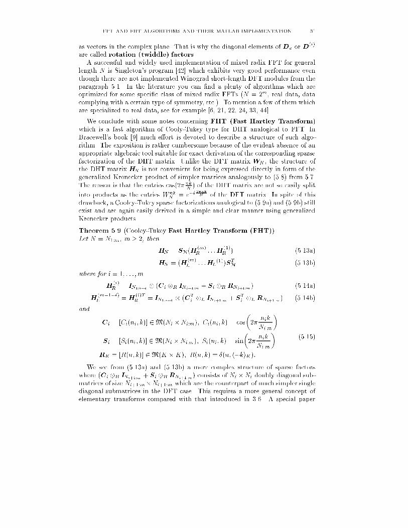
FFT AND FHT ALGORITHMS AND THEIR MATLAB IMPLEMENTATION 31as vectors in the complex plane. That is why the diagonal elements of D� or D(i)are called rotation (twiddle) factors.A successful and widely used implementation of mixed radix FFT for generallength N is Singleton's program [42] which exhibits very good performance eventhough there are not implemented Winograd short-length DFT modules from theparagraph 5.1. In the literature you can �nd a plenty of algorithms which areoptimized for some speci�c class of mixed radix FFTs (N = 2m, real data, datacomplying with a certain type of symmetry, etc.). To mention a few of them whichare specialized to real data, see for example [6, 21, 22, 24, 33, 44].We conclude with some notes concerning FHT (Fast Hartley Transform)which is a fast algorithm of Cooly-Tukey type for DHT analogical to FFT. InBracewell's book [9] much e�ort is devoted to describe a structure of such algo-rithm. The exposition is rather cumbersome because of the evident absence of anappropriate algebraic tool suitable for exact derivation of the corresponding sparsefactorization of the DHT matrix. Unlike the DFT matrix WN , the structure ofthe DHT matrixHN is not convenient for being expressed directly in form of thegeneralized Kronecker product of simpler matrices analogously to (5.8) from 5.7.The reason is that the entries cas(2�nkN ) of the DHT matrix are not so easily splitinto products as the entries WnkN = e�i 2�nkN of the DFT matrix. In spite of thisdrawback, a Cooley-Tukey sparse factorizations analogical to (5.9a) and (5.9b) stillexist and are again easily derived in a simple and clear manner using generalizedKronecker products.Theorem 5.9 (Cooley-Tukey Fast Hartley Transform (FHT)).Let N = N1:m, m � 2, thenHN = SN(H(m)R : : :H(1)R ) (5.13a)HN = (H(m)L : : :HL(1))STN (5.13b)where for i = 1; : : : ;mH(i)R = IN1:i�1 (Ci R INi+1:m + Si R RNi+1:m ) (5.14a)H (m+1�i)L =H(i)TR = IN1:i�1 (CTi L INi+1:m + STi L RNi+1:m ) (5.14b)and Ci = [Ci(ni; k)] 2M(Ni �Ni:m); Ci(ni; k) = cos�2� nikNi:m�Si = [Si(ni; k)] 2M(Ni �Ni:m); Si(ni; k) = sin�2� nikNi:m�RK = [R(n; k)] 2M(K �K); R(n; k) = �(n; h�kiK): (5.15)We see from (5.13a) and (5.13b) a more complex structure of sparse factorswhere (Ci R INi+1:m + Si R RNi+1:m ) consists of Ni �Ni doubly diagonal sub-matrices of size Ni+1:m�Ni+1:m which are the counterpart of much simpler singlediagonal submatrices in the DFT case. This requires a more general concept ofelementary transforms compared with that introduced in 3.6. A special paper

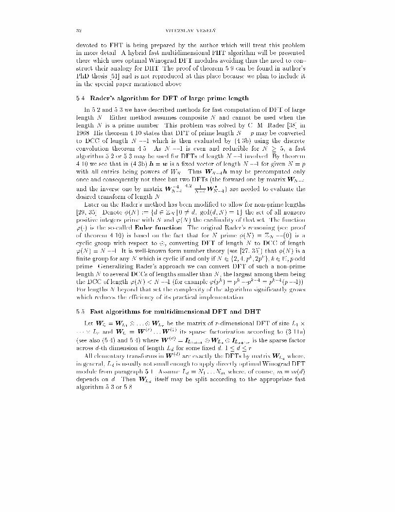
32 VíTÌZSLAV VESELÝdevoted to FHT is being prepared by the author which will treat this problemin more detail. A hybrid fast multidimensional FHT algorithm will be presentedthere which uses optimal Winograd DFT modules avoiding thus the need to con-struct their analogy for DHT. The proof of theorem 5.9 can be found in author'sPhD thesis [51] and is not reproduced at this place because we plan to include itin the special paper mentioned above.5.4. Rader's algorithm for DFT of large prime length.In 5.2 and 5.3 we have described methods for fast computation of DFT of largelength N . Either method assumes composite N and cannot be used when thelength N is a prime number. This problem was solved by C. M. Rader [38] in1968. His theorem 4.10 states that DFT of prime length N = p may be convertedto DCC of length N � 1 which is then evaluated by (4.3b) using the discreteconvolution theorem 4.5. As N � 1 is even and reducible for N � 5, a fastalgorithm 5.2 or 5.3 may be used for DFTs of length N � 1 involved. By theorem4.10 we see that in (4.3b) h = w is a �xed vector of length N � 1 for given N = pwith all entries being powers of WN . Thus WN�1h may be precomputed onlyonce and consequently not three but two DFTs (the forward one by matrixWN�1and the inverse one by matrix W�1N�1 4:2= 1N�1W �N�1) are needed to evaluate thedesired transform of length N .Later on the Rader's method has been modi�ed to allow for non-prime lengths[29, 35]. Denote �(N ) := fd 2 ZN j 0 6= d; gcd(d;N ) = 1g the set of all nonzeropositive integers prime with N and '(N ) the cardinality of that set. The function'(�) is the so-called Euler function. The original Rader's reasoning (see proofof theorem 4.10) is based on the fact that for N prime �(N ) = ZN � f0g is acyclic group with respect to �, converting DFT of length N to DCC of length'(N ) = N � 1. It is well-known form number theory (see [27, 35]) that �(N ) is a�nite group for any N which is cyclic if and only if N 2 f2; 4; pk; 2pkg; k 2 N; p oddprime. Generalizing Rader's approach we can convert DFT of such a non-primelength N to several DCCs of lengths smaller than N , the largest among them beingthe DCC of length '(N ) < N � 1 (for example '(pk) = pk � pk�1 = pk�1(p� 1)).For lengths N beyond that set the complexity of the algorithm signi�cantly growswhich reduces the e�ciency of its practical implementation.5.5. Fast algorithms for multidimensional DFT and DHT.Let WL =WL1 : : :WLr be the matrix of r-dimensional DFT of size L1 �� � � � Lr and WL = W (r) : : :W (1) its sparse factorization according to (3.11a)(see also (5.4) and 5.4) where W (d) = IL1:d�1 WLd ILd+1:r is the sparse factoracross d-th dimension of length Ld for some �xed d, 1 � d � r.All elementary transforms inW (d) are exactly the DFTs by matrixWLd where,in general, Ld is usually not small enough to apply directly optimalWinograd DFTmodule from paragraph 5.1. Assume Ld = N1 : : :Nm where, of course, m = m(d)depends on d. Then WLd itself may be split according to the appropriate fastalgorithm 5.3 or 5.8.

FFT AND FHT ALGORITHMS AND THEIR MATLAB IMPLEMENTATION 33We can write in general WLd =W (m+1)d W (m)d : : :W (1)d W (0)d where W (i)d havethe structure related to the corresponding fast algorithm. In particularW (0)d andW (m+1)d are the appropriate permutation matrices (P 1, P 2, SN, STN or ILd) andW (i)d , i = 1; : : : ;m, look like (5.4), (5.10a) or (5.10b) when using the appropriateKronecker products , R or L.To be more speci�c, assume DIF FFT withW (i)d = IN1:i�1 (WR;iR INi+1:m )for i = 1; : : : ;m. Then, by the mixed-product rule (3.8), we getW (d) = IL1:d�1 (W (m+1)d : : :W (0)d ) ILd+1:r ) =:W (d;m+1) : : :W (d;0)where W (d;i) = IL1:d�1 W (i)d ILd+1:r . Clearly, againW (d;0) andW (d;m+1) arecertain permutation matrices and for i = 1; : : : ;mW (d;i) =IL1:d�1 IN1:i�1 (WR;i R INi+1:m ) ILd+1:r (3.3)=IL1:d�1N1:i�1 �(WR;i R INi+1:m ) ILd+1:r � 3:7(3.12)=IL1:d�1N1:i�1 (W 0R;i R INi+1:mLd+1:r ) (5.16a)where W 0R;i 2 M(Ni � Ni:mLd+1:r) is obtained from WR;i 2 M(Ni � Ni:m) byrepeating Ld+1:r-times each column inWR;i, i.e. W 0R;i =WR;i 1TLd+1:r .The case DIT FFT follows by matrix transpose:W (d;i) =IL1:d�1N1:i�1 (W 0L;i L INi+1:mLd+1:r ) (5.16b)where W 0L;i =W 0TR;i =W TR;i 1Ld+1:r 5:7= WL;i 1Ld+1:r .In case of PFA we have instead of R andWNi instead ofWR;i, which yieldsW (d;i) =IL1:d�1N1:i�1 WNi INi+1:mLd+1:r : (5.16c)We see that elementary steps of the m-dimensional fast DFT algorithm haveessentially the same structure as those in the one-dimensional case. See MATLABcoding scheme in appendix B which clari�es the implementation details.Cooley-Tukey factorization of the matrix H 0L of the alternate m-dimensionalHartley transform is obtained analogously from (4.14c) and 5.9.5.6. Number theoretic and polynomial transforms.The circumstance that both DFT and DCC may be introduced also over datastructures other than the �led of complex or real numbers stimulated new ideas inthe e�ort to improve the e�ciency of the existing algorithms. Choosing residue ringof integers, residue ring of polynomials (modulo cyclotomic polynomial) or �nite(Galois) �eld instead of C we obtain a generalized DFT concept known as numbertheoretic transform (NTT), polynomial transform or Galois transform,respectively. L. Skula [43] studied such transforms from the theoretical point ofview in a more general framework, namely over a commutative ring with unity.Another abstract approach generalizes DFT to group algebras [7].In contrast to DFT these transforms have usually no interpretation of their ownbut they serve as an important tool for extremely fast computation of DCC andDLC in real-time digital �ltration (cf. 4.19).

34 VíTÌZSLAV VESELÝOne can see that most constructions of fast algorithms described above in para-graphs 5.1{5.5 may be carried over3. Moreover additional reduction of computa-tional load may be achieved when exploiting speci�c properties of operations onthe particular data structure.NTTs are suitable for implementation in specialized microprocessor controlledhardware which uses modular arithmetic (bit length 8,16,32, etc.). Then usingNTTs over residue ring of integers with modulus close to power of two (28; 216; 232,etc.) allows one to replace most operations of multiplication by simple and ex-tremely fast binary shifts. A special case of NTTs are the so-called Fermattransforms (moduli are Fermat numbers Fn = 22n + 1) or Mersenne trans-forms (moduli are Mersenne numbers Mp = 2p � 1, p odd prime). Basic papersconcerning NTTs and related topics may be found in [35], some more are [2, 8, 39].NTTs are mostly applied to DCC evaluation in hardware-supported digital �ltra-tion (the discrete convolution theorem 4.5 remains valid) [15, 30]. When combinedwith methods converting DFT to DCC such as 4.9 or the Rader's method 4.10(see paragraph 5.4 as well) NTTs may be utilized also for approximate fast com-putation of classical DFT (see [1]). There exist also other applications, e.g. exactsolution of the deconvolution problem [20]. Coding theory is a typical applicationarea for Galois transforms.Polynomial transforms were introduced by H. J. Nussbaumer already in 1977.Basics of their construction can be found in [23, 36] along with references to fun-damental papers, see also [34, 37, 46]. In principle the polynomial transforms arean analogy to NTTs except that they operate over the residue ring of polynomi-als instead of integers. They are important in multidimensional signal processingbecause they enable us to reduce the dimension of DCC and DFT by one.5.7. Some implementation re�nements.In this paragraph we are going to list some implementation tricks which furtherimprove the performance of algorithms mentioned above.a) DFT of real data: In applying the FFT, we often consider only real vec-tors x in the time domain whereas the vectors bx are still complex withredundancy (4.4). This redundancy says that just N real numbers (and not2N ) are su�cient to determine real and imaginary parts of bx if x is realof length N . When using an algorithm for complex DFT, we must set theimaginary parts of x to zero which is ine�cient in that the computer pro-gram will still perform all operations involving imaginary parts even thoughthey are zero. In [11, p.188] there are described two techniques solving thisproblem.� DFT of two real vectors x1 and x2 of equal length N simultaneouslyputting y := x1 + ix2. Then it is easy to show that bx1 and bx2 may be3cf. [48, 49] where both generalizedKronecker product and mixed radix FFTs withWN beingany root of unity are considered over a commutative ring of unity.

FFT AND FHT ALGORITHMS AND THEIR MATLAB IMPLEMENTATION 35computed from by := byR + ibyI , byR := Re by, byI := Im by, using formulasbx1(k) = byR(k) + byR(�k)2 + i byI (k) � byI(�k)2bx2(k) = byI(k) + byI (�k)2 � i byR(k)� byR(�k)2 (5.17)for k 2Z.� DFT of real vector x of even length 2N via DFT of complex vector y :=x1 + ix2 where x1(n) := x(2n) and x2(n) := x(2n + 1) are respectivelythe even and odd numbered entries of x, n = 0; 1; : : : ; N � 1. Againbx = xR + ixI may be computed back from by bybxR(k) = byR(k) + byR(�k)2 + cos �kN �byI(k) + byI (�k)2 ��sin �kN �byR(k)� byR(�k)2 �bxI(k) = byI(k)� byI(�k)2 � cos �kN �byR(k) � byR(�k)2 ��sin �kN �byI(k) + byI (�k)2 � (5.18)for k = 0; 1; : : :; N where bxR(k) := Re bx(k) and bxI(k) := Im bx(k) arerespectively the real and imaginary parts of the entries of the 2N pointdiscrete transform bx. When computing the inverse DFT, then the aux-iliary transform (5.18) has to be inverted using similar formulas wherebx(k) and by(k) interchange their roles and the cosine terms invert theirsign.� If neither of the above methods can be used (we have one real vector xof odd length N ), then FHT and (4.6b) is the best solution.b) In-place transform and parallelism: As WN is a square matrix of sizeN � N , both PFA and FFT work in-place by remark 3.7 because each el-ementary transform accomplished in a single step maps a portion of inputonto the same portion on output. Moreover these portions are disjoint fordi�erent elementary transforms allowing parallelism in the processing. Onmultiprocessor hardware several elementary transforms may be accomplishedat the same time which results in a signi�cant time reduction by a factorapproximately equal to the number of processors involved.c) Fast digit reversal: In the DIF FFT (5.9a) or DIT FFT (5.9b) algorithmand their FHT counterparts (5.13a) or (5.13b) we need data to be permutedaccording to the digit reversal by matrix SN or its inverse by matrix STN,respectively. There exist various techniques for fast digit reversal. One ofthem, the so-called cell-structured algorithm for digit reversal [50], isbased on the digit reversal decomposition (5.7). This allows us to replacea digit reversal of large length by several digit reversals of much shorterlengths. In some cases the original lengthN may be reduced up to a cube root3pN . For a certain level of symmetry in the factorization of N = N1 : : :Nm

36 VíTÌZSLAV VESELÝ(none, partial or full), the cell-structured algorithm allows no, partial or fullin-place permutation. Extensive timing tests accomplished in [50] prove thecell-structured algorithm to be for large composite lengths superior to othercommonly used techniques.d) DCC via FFT or FHT avoiding digit reversal: One can fully avoidthe digit reversal permutation in the computation of DCC via the discreteconvolution theorem for DFT or DHT. Indeed, when applying in (4.3b)DIF FFT for the forward transforms WNx and WNh, and DIT FFT forthe inverse transform by matrixW�1N , we see that digit reversal in the laststep of the forward DFTs and its inverse in the �rst step of the inverseDFT may be cancelled. It is because the Hadamard product WNx �WNhpreserves the permuted order.If either x or h is symmetrical, we can proceed by 4.18 in the sameway when combining the FHT algorithms (5.13a) and (5.13b) in the DCCcomputation via (4.9c).e) Recursive sin-cos generator for rotation factors: We have to evaluatea plenty of cosines and sines when calculating the rotation factors (5.12)which participate in elementary transforms of an FFT or FHT algorithm.It would be extremely time consuming to call library cosine and sine func-tions. That is the reason why various recurrent schemes are used in prac-tice. K. Dobe¹ suggested an e�cient two-step recurrent sin-cos generator[19] requiring only two additions and two multiplications per step. Usingthe well-known goniometric identities sin(k�1)� = sin k� cos��cos k� sin�and cos(k�1)� = cos k� cos��sink� sin� we get sin(k+1)��sin(k�1)� =2 sin� cos k� and cos(k+1)�� cos(k� 1)� = �2 sin� sink�, and hence thedesired two-step recurrent formulassin(k + 1)� = sin(k � 1)�+ 2 sin� cos k�cos(k + 1)� = cos(k � 1)�� 2 sin� sin k�: (5.19)We apply the recurrent scheme twice in succession as follows:(i) First, when looping in the i-th step through elementary transforms for� = 0; : : : ; Ni+1:m � 1, we put � = 2�Ni:m and k = � to evaluate sin 2��Ni:mat the transition step �; �+ 1.(ii) Second, when evaluating the rotation factors cos 2��Ni:m ni � i sin 2��Ni:m nifor the �-th elementary transform, we put � = 2��Ni:m and k = ni to getcos 2��Ni:m ni and sin 2��Ni:m ni at the transition step ni ; ni + 1. Observethat sin� entering into (5.19) are exactly those sines which have beencomputed in (i) using the sin-cos generator as well.The recursion of (i) may be pretty long and thus there is a danger ofround-o� error cumulation when using low-precision and/or truncated oat-ing point arithmetic. In such cases it is recommended to multiply each cosinecos k� and sine sin k� evaluated via (5.19) by a scaling factor e � 1 whichtries to correct the violation of the identity sin2k�+ cos2k� = 1. One of the

FFT AND FHT ALGORITHMS AND THEIR MATLAB IMPLEMENTATION 37following strategies is frequently applied for e:e = 2� (sin2k�+ cos2k�)e = 1:5� 0:5(sin2k�+ cos2k�)e = 0:5=(sin2k�+ cos2k�) + 0:5e = 0:5�3� (sin2k�+ cos2k�)�: (5.20)6. Performance tests of FFT algorithmsIn this section we present results of performance tests of two groups of Coo-ley-Tukey FFT and FHT algorithms which were implemented as compiled com-mands in the widely used matrix-oriented numeric computation system MATLAB5.1 for WINDOWS'95.One group referred to as innovative procedures uses algorithms newly designedaccording to the theory of generalized Kronecker product:FFT1C: Multidimensional DIF FFT Cooley-Tukey algorithm (5.9a) for com-plex data using optimal Winograd modules 5.1 of lengths up to 25, re-cursive sin-cos generator 5.7e) and optional cell-structured digit reversal5.7c). Symmetrized length factorizations (see table 1) are optimized forthe cell-structured digit reversal taking into account the available lengths ofWinograd modules.FFT2C: Multidimensional DIT FFT Cooley-Tukey algorithm (5.9b) with thesame additional features as FFT1C.FFT1R: Multidimensional DIF FFT Cooley-Tukey algorithm for real dataof even length 2N based on (5.18) from 5.7a). There FFT1C is used toaccomplish the substitutive complex DFT of half length N .FHT1, FHT2: FHT1 and FHT2 are respectively the multidimensional FHTcounterparts of FFT1C and FFT2C. In principle they are designed for realdata according to (5.13a) and (5.13b) where, compared with FFT1C andFFTC2, a more sophisticated technique had to be applied to integrate op-timal Winograd modules. Along with (4.6b) they yield a fast DFT for realdata with the same wide range of lengths which FFT1C and FFT2C supplyfor the complex data, the odd lengths inclusively.All procedures described above are designed for both forward and inverse multi-channel in-place transforms with prescribed indexing increment. Suppressing theoptional digit reversal allows faster DCC by 5.7d).To properly evaluate the e�ciency of the above novel algorithms, they wereconfronted with some other commonly used algorithms of the same type. Theyare referred to as comparative FFT procedures and comprise:FFTC: Modi�ed version of Singleton's well-known FFT program [42] for com-plex data where the faster sin-cos generator 5.7e) was adopted for evaluationof rotation factors.fft: Built-in MATLAB 5.1 function for multi-channel FFT of real or complexdata of arbitrary length.

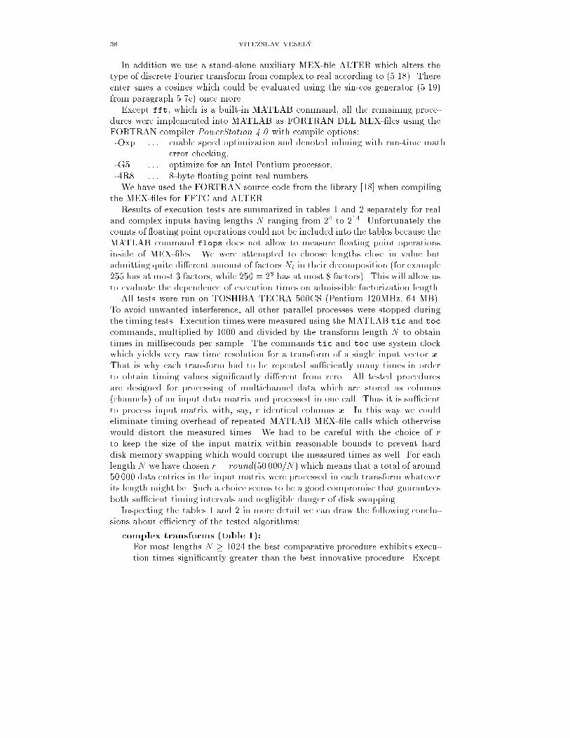
38 VíTÌZSLAV VESELÝIn addition we use a stand-alone auxiliary MEX-�le ALTER which alters thetype of discrete Fourier transform from complex to real according to (5.18). Thereenter sines a cosines which could be evaluated using the sin-cos generator (5.19)from paragraph 5.7e) once more.Except fft, which is a built-in MATLAB command, all the remaining proce-dures were implemented into MATLAB as FORTRAN DLL MEX-�les using theFORTRAN compiler PowerStation 4.0 with compile options:-Oxp : : : enable speed optimization and denoted inlining with run-time matherror checking,-G5 : : : optimize for an Intel Pentium processor,-4R8 : : : 8-byte oating point real numbers.We have used the FORTRAN source code from the library [18] when compilingthe MEX-�les for FFTC and ALTER.Results of execution tests are summarized in tables 1 and 2 separately for realand complex inputs having lengths N ranging from 24 to 214. Unfortunately thecounts of oating point operations could not be included into the tables because theMATLAB command flops does not allow to measure oating point operationsinside of MEX-�les. We were attempted to choose lengths close in value butadmitting quite di�erent amount of factors Ni in their decomposition (for example255 has at most 3 factors, while 256 = 28 has at most 8 factors). This will allow usto evaluate the dependence of execution times on admissible factorization length.All tests were run on TOSHIBA TECRA 500CS (Pentium 120MHz, 64 MB).To avoid unwanted interference, all other parallel processes were stopped duringthe timing tests. Execution times were measured using the MATLAB tic and toccommands, multiplied by 1000 and divided by the transform length N to obtaintimes in milliseconds per sample. The commands tic and toc use system clockwhich yields very raw time resolution for a transform of a single input vector x.That is why each transform had to be repeated su�ciently many times in orderto obtain timing values signi�cantly di�erent from zero. All tested proceduresare designed for processing of multichannel data which are stored as columns(channels) of an input data matrix and processed in one call. Thus it is su�cientto process input matrix with, say, r identical columns x. In this way we couldeliminate timing overhead of repeated MATLAB MEX-�le calls which otherwisewould distort the measured times. We had to be careful with the choice of rto keep the size of the input matrix within reasonable bounds to prevent harddisk memory swapping which would corrupt the measured times as well. For eachlength N we have chosen r = round(50 000=N ) which means that a total of around50 000 data entries in the input matrix were processed in each transform whateverits length might be. Such a choice seems to be a good compromise that guaranteesboth su�cient timing intervals and negligible danger of disk swapping.Inspecting the tables 1 and 2 in more detail we can draw the following conclu-sions about e�ciency of the tested algorithms:complex transforms (table 1):For most lengths N � 1024 the best comparative procedure exhibits execu-tion times signi�cantly greater than the best innovative procedure. Except

FFT AND FHT ALGORITHMS AND THEIR MATLAB IMPLEMENTATION 39N = 512, innovative procedures are never worse than the comparative ones.For highly composite lengths other then power-of-two (see for example 2052,2520, 4104, 5040 and 8208) the innovative procedures are only slightly faster,for lengths decomposable into a small number of prime factors (see for ex-ample 1573, 1859, 2057 and 5491) the di�erences are more striking givingfor comparative procedures times longer by more than 50%. The probableexplanation for that phenomenon is that both FFTC and fft have not im-plemented optimal Winograd short DFT modules. The same argumentationmight justify the surprisingly much better performance of innovative proce-dures for large power-of-two lengths which are expected to be well-optimizedin the comparative procedures. Indeed, in the innovative algorithms there isthe strategy to minimize the number of factors at the expense of their mag-nitude, so that Winograd module of the largest available length in the rangeup to 25 can be applied for the short DFT associated with each particularfactor. The bene�ts of this approach are most apparent for power-of-twolength 4096 which is factorized as 16 � 16 � 16 allowing thus to utilize thelargest available Winograd module of power-of-two length 16. In that casethe execution time could be reduced as much as to one half.real transforms (table 2):The three columns entitled complex DFT+ALTER list performance resultsof real DFT of length N by the method (5.18) from paragraph 5.7a). Thecomplex FFT of even length N2 is computed by means of one of the threeprocedures FFT1C, FFT2C or FFTC and then converted to the real FFTof length N by a separate MATLAB call of MEX-�le ALTER. Observethat the algorithms of FFT1R and FFT2R are essentially the same as thoseof FFT1C+ALTER and FFT2C+ALTER, respectively, the only di�erencebeing that ALTER is not called at the MATLAB level but is integrated di-rectly into the MEX-�les FFT1R and FFT2R. We see that the times forFFT1C+ALTER and FFT2C+ALTER are by about 0.0030{0.0040 largerthan those of FFT1R and FFT2R. This di�erence must be due to theMEX-calling overhead of procedure ALTER. Thus for maximum speed werecommend to concentrate all code of any fast DFT algorithm into oneMEX-�le. Otherwise there is a danger that much of the computationalpower of the algorithm will go lost. In spite of this drawback the times inDFT+ALTER columns are still a little bit shorter than those of the built-infft for lengths other than power of two. As expected, the time proportionsof real FFT algorithms are in accordance with those of complex FFTs fromtable 1. Again N = 1024 (corresponding to N = 512 in table 1) is the ex-ceptional length where fft shows best performance. The FHT1 and FHT2procedures are absolute winners with most times being signi�cantly belowthose of the concurrent procedures.round-o� error propagation (both tables):To be able to estimate round-o� error propagation, we have used specialinput vector x = [x0; x1; : : : ; xN�1]T the entries of which form a geometricsequence xn = Qn where 0 < jQj < 1. Then we easily derive a simple

40 VíTÌZSLAV VESELÝformula for bxk, k = 0; 1; : : : ; N � 1:bxk =N�1Xn=0 QnWnkN = N�1Xn=0(QW kN )n = 1� (QW kN )N1�QW kN = 1�QNW kNN1�QW kN =1� QN1�QW kN : (6.1)If y = [y0; y1; : : : ; yN�1]T is a FFT result corrupted with round-o� errors,then we evaluate the relative error of the k-th entry yk by Rk = yk�bxkjykjand put R = maxk(Rk) to indicate relative error of the whole transform.Then Rmax in the last row of both tables denotes the maximal relative errorfrom all transforms in each column. Thus Rmax re ects quite reliably thenumerical stability of each particular FFT procedure. We have used x withquotient Q = 0:7. As x is a real vector, it had to be replaced by x + ix toobtain a true complex input for the transforms in table 1. The innovativealgorithms show favourable round-o� error around 5 � 10�14 which is closeto the least signi�cant digit of mantissa. The built-in fft exhibits the worstnumerical stability with a round-o� error 9 �10�13 � 10�12 loosing 2 decadicdigits more. 7. ConclusionWe have presented a self-contained survey of basic techniques for construction offast algorithms for discrete Fourier and Hartley transform along with those for theclosely connected operations of discrete linear and cyclic convolution. All necessarymathematical background mainly from number theory and matrix calculus was�rst explained, and later on applied to the derivation of the fast algorithms.A special attention was paid to the Cooley-Tukey class of fast FFT and FHTalgorithms which are the most widely used ones in practical applications. Thenew algebraic concept of generalized Kronecker product of matrices proved to bean e�ective tool for clear and transparent derivation and structural description ofsparse factors associated with this type of algorithms.This new insight into the sparse structure contributed to an improved designand, �nally, to a more e�cient practical implementation of the algorithms of thattype. This was con�rmed by performance tests of innovated implementations ofmultidimensonal FFT and FHT in form of FORTRAN DLL MEX-�les which,for most lengths exceeding 1000 samples, exhibit time e�ciency superior both tobuilt-in MATLAB command fft and the standard improved Singleton's proce-dure. The round-o� error propagation is comparable with Singleton's procedureand by two decadic digits better than with MATLAB command fft.

FFT AND FHT ALGORITHMS AND THEIR MATLAB IMPLEMENTATION 41Time [msec per sample]Innovative ComparativeN = N1 � � � � �Nm complex DFT complex DFTFFT1C FFT2C FFTC fft16 = 16 0.0000 0.0000 0.0000 0.000032 = 16 � 2 0.0000 0.0000 0.0000 0.000063 = 7 � 9 0.0000 0.0000 0.0000 0.000064 = 8 � 8 0.0000 0.0000 0.0000 0.000070 = 7 � 5 � 2 0.0000 0.0000 0.0000 0.000072 = 9 � 8 0.0000 0.0000 0.0139 0.0000126 = 7 � 9 � 2 0.0079 0.0079 0.0079 0.0079128 = 8 � 2 � 8 0.0078 0.0078 0.0078 0.0078130 = 13 � 5 � 2 0.0077 0.0077 0.0077 0.0077140 = 7 � 4 � 5 0.0071 0.0071 0.0071 0.0071252 = 7 � 9 � 4 0.0040 0.0040 0.0079 0.0079255 = 17 � 5 � 3 0.0078 0.0078 - 0.0078256 = 16 � 16 0.0039 0.0039 0.0039 0.0039504 = 2 � 7 � 9 � 2 � 2 0.0079 0.0079 0.0119 0.0079507 = 13 � 3 � 13 0.0059 0.0039 0.0079 0.0099512 = 16 � 2 � 16 0.0059 0.0059 0.0078 0.0039560 = 4 � 7 � 5 � 4 0.0071 0.0071 0.0089 0.00891024 = 16 � 4 � 16 0.0059 0.0059 0.0078 0.00781573 = 11 � 13 � 11 0.0064 0.0051 0.0089 0.01211026 = 3 � 19 � 3 � 2 � 3 0.0097 0.0097 0.0117 0.01171680 = 4 � 7 � 5 � 3 � 4 0.0089 0.0101 0.0107 0.01071859 = 13 � 11 � 13 0.0065 0.0054 0.0097 0.01242048 = 16 � 8 � 16 0.0054 0.0054 0.0122 0.00882052 = 2 � 3 � 19 � 3 � 3 � 2 0.0122 0.0112 0.0132 0.01222057 = 11 � 17 � 11 0.0068 0.0068 0.0102 0.01462520 = 2 � 3 � 7 � 5 � 2 � 3 � 2 0.0119 0.0111 0.0131 0.01074096 = 16 � 16 � 16 0.0056 0.0056 0.0103 0.00904104 = 2 � 3 � 19 � 3 � 2 � 3 � 2 0.0134 0.0134 0.0144 0.01445040 = 3 � 4 � 7 � 5 � 4 � 3 0.0097 0.0097 0.0129 0.01195491 = 17 � 19 � 17 0.0098 0.0102 0.0111 0.01886137 = 19 � 17 � 19 0.0090 0.0103 0.0112 0.01898192 = 16 � 16 � 2 � 16 0.0089 0.0089 0.0125 0.01258208 = 3 � 4 � 19 � 3 � 4 � 3 0.0122 0.0124 0.0144 0.01568320 = 8 � 13 � 5 � 2 � 8 0.0099 0.0099 0.0154 0.01548400 = 4 � 5 � 7 � 3 � 5 � 4 0.0110 0.0098 0.0131 0.014316384 = 16 � 8 � 8 � 16 0.0102 0.0087 0.0134 0.0134Rmax 4e-015 5e-014 4e-015 9e-013Table 1Performance of FFT algorithms for complex data

42 VíTÌZSLAV VESELÝTime [msec per sample]Innovative ComparativeN real DFT DHT complex DFT + ALTER DFTFFT1R FFT2R FHT1 FHT2 FFT1C FFT2C FFTC fft16 0.0000 0.0000 0.0000 0.0000 0.0000 0.0000 0.0000 0.000032 0.0000 0.0000 0.0000 0.0000 0.0000 0.0000 0.0000 0.000063 - - 0.0000 0.0000 - - - 0.000064 0.0000 0.0000 0.0000 0.0000 0.0000 0.0000 0.0000 0.000070 0.0000 0.0000 0.0000 0.0000 0.0000 0.0000 0.0000 0.000072 0.0000 0.0000 0.0000 0.0000 0.0000 0.0000 0.0000 0.0000126 0.0000 0.0000 0.0000 0.0000 0.0079 0.0079 0.0079 0.0079128 0.0000 0.0000 0.0000 0.0000 0.0078 0.0078 0.0078 0.0000130 0.0000 0.0077 0.0000 0.0000 0.0077 0.0077 0.0077 0.0077140 0.0071 0.0071 0.0000 0.0000 0.0071 0.0071 0.0071 0.0071252 0.0040 0.0040 0.0040 0.0040 0.0079 0.0079 0.0079 0.0079255 - - 0.0039 0.0039 - - - 0.0078256 0.0039 0.0039 0.0039 0.0039 0.0078 0.0078 0.0078 0.0039504 0.0040 0.0040 0.0040 0.0040 0.0079 0.0079 0.0079 0.0079507 - - 0.0039 0.0039 - - - 0.0079512 0.0039 0.0039 0.0039 0.0039 0.0078 0.0078 0.0078 0.0020560 0.0054 0.0054 0.0036 0.0036 0.0107 0.0107 0.0089 0.00711024 0.0039 0.0039 0.0029 0.0020 0.0088 0.0088 0.0098 0.00201573 - - 0.0032 0.0032 - - - 0.01211026 0.0058 0.0058 0.0039 0.0039 0.0097 0.0107 0.0107 0.01171680 0.0065 0.0065 0.0042 0.0042 0.0095 0.0095 0.0095 0.00951859 - - 0.0032 0.0032 - - - 0.01182048 0.0044 0.0044 0.0034 0.0034 0.0088 0.0088 0.0103 0.00342052 0.0068 0.0058 0.0068 0.0068 0.0097 0.0112 0.0112 0.01222057 - - 0.0034 0.0044 - - - 0.01362520 0.0067 0.0063 0.0067 0.0075 0.0107 0.0099 0.0111 0.01194096 0.0044 0.0044 0.0034 0.0032 0.0090 0.0090 0.0125 0.00444104 0.0078 0.0080 0.0066 0.0080 0.0122 0.0112 0.0122 0.01345040 0.0065 0.0077 0.0056 0.0056 0.0097 0.0099 0.0099 0.01215491 - - 0.0056 0.0055 - - - 0.01786137 - - 0.0044 0.0055 - - - 0.01918192 0.0045 0.0055 0.0045 0.0045 0.0089 0.0088 0.0112 0.00578208 0.0089 0.0079 0.0067 0.0065 0.0134 0.0124 0.0134 0.01468320 0.0056 0.0054 0.0054 0.0056 0.0088 0.0088 0.0111 0.01448400 0.0065 0.0065 0.0065 0.0054 0.0099 0.0098 0.0110 0.011916384 0.0067 0.0067 0.0057 0.0045 0.0099 0.0087 0.0112 0.0055Rmax 4e-015 8e-015 4e-015 1e-014 4e-015 8e-015 4e-015 9e-013Table 2Performance of FFT and FHT algorithms for real data

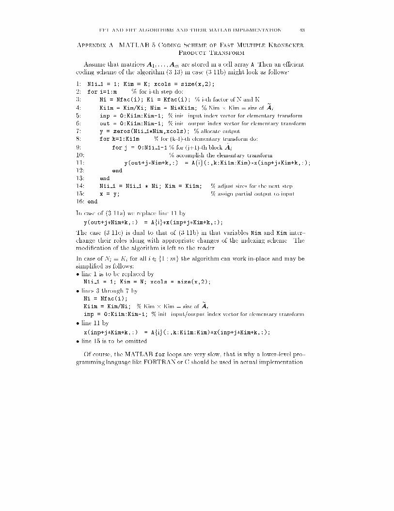
FFT AND FHT ALGORITHMS AND THEIR MATLAB IMPLEMENTATION 43Appendix A. MATLAB 5 Coding Scheme of Fast Multiple KroneckerProduct TransformAssume that matrices A1; : : : ;Am are stored in a cell array A. Then an e�cientcoding scheme of the algorithm (3.13) in case (3.11b) might look as follows:1: N1i 1 = 1; Kim = K; xcols = size(x,2);2: for i=1:m % for i-th step do:3: Ni = Nfac(i); Ki = Kfac(i); % i-th factor of N and K4: Ki1m = Kim/Ki; Nim = Ni�Ki1m; % Nim � Kim = size of eAi5: inp = 0:Ki1m:Kim-1; % init. input index vector for elementary transform6: out = 0:Ki1m:Nim-1; % init. output index vector for elementary transform7: y = zeros(N1i 1�Nim,xcols); % allocate output8: for k=1:Ki1m % for (k-1)-th elementary transform do:9: for j = 0:N1i 1-1 % for (j+1)-th block eAi10: % accomplish the elementary transform11: y(out+j�Nim+k,:) = Afig(:,k:Ki1m:Kim)�x(inp+j�Kim+k,:);12: end13: end14: N1i 1 = N1i 1 � Ni; Kim = Ki1m; % adjust sizes for the next step15: x = y; % assign partial output to input16: endIn case of (3.11a) we replace line 11 byy(out+j�Nim+k,:) = Afig�x(inp+j�Kim+k,:);The case (3.11c) is dual to that of (3.11b) in that variables Nim and Kim inter-change their roles along with appropriate changes of the indexing scheme. Themodi�cation of the algorithm is left to the reader.In case of Ni = Ki for all i 2 f1 : mg the algorithm can work in-place and may besimpli�ed as follows:� line 1 is to be replaced byN1i 1 = 1; Kim = N; xcols = size(x,2);� lines 3 through 7 byNi = Nfac(i);Ki1m = Kim/Ni; % Kim � Kim = size of eAiinp = 0:Ki1m:Kim-1; % init. input/output index vector for elementary transform� line 11 byx(inp+j�Kim+k,:) = Afig(:,k:Ki1m:Kim)�x(inp+j�Kim+k,:);� line 15 is to be omitted.Of course, the MATLAB for loops are very slow, that is why a lower-level pro-gramming language like FORTRAN or C should be used in actual implementation.

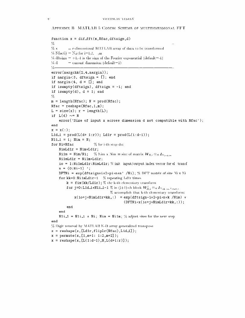
44 VíTÌZSLAV VESELÝAppendix B. MATLAB 5 Coding Scheme of multidimensional FFTfunction x = dif fft(x,Nfac,dftsign,d)%||||||||||||||||||||||||||||||||-% x = r-dimensional MATLAB array of data to be transformed% Nfac(i) = N i for i=1,2,. . .,m% dftsign = +1,-1 is the sign of the Fourier exponential (default=-1)% d = current dimension (default=1)%||||||||||||||||||||||||||||||||-error(nargchk(2,4,nargin));if nargin<3, dftsign = []; endif nargin<4, d = []; endif isempty(dftsign), dftsign = -1; endif isempty(d), d = 1; end%m = length(Nfac); N = prod(Nfac);Nfac = reshape(Nfac,1,m);L = size(x); r = length(L);if L(d) �= Nerror('Size of input x across dimension d not compatible with Nfac');endx = x(:);L1d 1 = prod(L(d+ 1:r)); Ld1r = prod(L(1:d-1));N1i 1 = 1; Nim = N;for Ni=Nfac % for i-th step do:NimLd1r = Nim�Ld1r;Ni1m = Nim/Ni; % Nim x Nim = size of matrix WR;i R INi+1:mNi1mLd1r = Ni1m�Ld1r;io = 1:Ni1mLd1r:NimLd1r; % init. input/output index vector for el. transf.n = (0:Ni-1).';DFTNi = exp(dftsign�i�2�pi�n�n'./Ni); % DFT matrix of size Ni x Nifor kk=0:Ni1mLd1r-1 % repeating Ld1r timesk = fix(kk/Ld1r);% the k-th elementary transformfor j=0:L1d 1�N1i 1-1 % in (j+1)-th block W 0R;i R INi+1:mLd+1:r% accomplish that k-th elementary transform:x(io+j�NimLd1r+kk,:) = exp(dftsign�i�2�pi�n�k./Nim).�...(DFTNi�x(io+j�NimLd1r+kk,:));endendN1i 1 = N1i 1 � Ni; Nim = Ni1m; % adjust sizes for the next stepend% Digit reversal by MATLAB N-D array generalized transposex = reshape(x,[Ld1r,fliplr(Nfac),L1d 1]);x = permute(x,[1,m+1:-1:2,m+2]);x = reshape(x,[L(1:d-1),N,L(d+1:r)]);

FFT AND FHT ALGORITHMS AND THEIR MATLAB IMPLEMENTATION 45The MATLAB function listed above accomplishes r-dimensional DIF FFT ofsize L1 �L2 � � � �� Lr across the speci�ed dimension d. The function applies thefast algorithm from paragraph 5.5 for the in-place partial transform x = W (d)xusing the sparse factorization (5.16a) of the matrixW (d) = IL1:d�1WLdILd+1:r .Putting L=size(x) and N=L(d) then, up to the round-o� error, the MATLABcalls fft(x,[],d) and dif fft(x,factor(N),[],d) yield the same results.Similarly both ifft(x,[],d) and dif fft(x,factor(N),1,d)./N accomplishinverse DFT across the dimension d.Consequently the loopsfor d=1:length(L), y=dif fft(y,factor(L(d)),[],d); end;andfor d=1:length(L), y=dif fft(y,factor(L(d)),1,d)./L(d); end;compute respectively a complete r-dimensional forward and inverse DFT so as dothe MATLAB commands fftn(x) and ifftn(x).References[1] R. Adhami and R. J. Polge, Fast Fourier transformation based on number theoretic trans-forms, J. Franklin Inst. 325 (1988), no. 5, 547{557.[2] R. C. Agarwal and J. W. Cooley, New algorithms for digital convolution, IEEE Trans. onASSP 25 (1977), no. 5, 392{409.[3] L. Auslander and S. Winograd, The multiplicative complexity of certain semilinear systemsde�ned by polynomials, Adv. in Appl. Math. 1 (1980), no. 3, 257{299.[4] L. Auslander, E. Feig and S. Winograd, Abelian semi-simple algebras and algorithms forthe discrete Fourier transform, Adv. in Appl. Math. 5 (1984), no. 1, 31{55.[5] , The multiplicative complexity of the discrete Fourier transform, Adv. in Appl.Math. 5 (1984), no. 1, 87{109.[6] G.D. Bergland,A radix-eight fast Fourier transform subroutine for real-valued series, IEEETrans. on Audio and ElectroacousticsAU-17 (1969), no. 2, 138{144.[7] T. Beth, Verfahren der schnellen Fourier-Transformation, B. G. Teubner, Stuttgart, 1984(German).[8] D. T. Birtwistle, The eigenstructure of the number theoretic transforms, Signal Processing4 (1982), no. 4, 287{294.[9] Ronald N. Bracewell, The Hartley transform, Oxford University Press, New York, 1986.[10] William L. Briggs and Van Emden Henson, The DFT. An owner's manual for the discreteFourier transform, SIAM, Philadelphia, Pennsylvania, 1995.[11] E. Oran Brigham, The fast Fourier transform and its applications, Prentice-Hall, Engle-wood Cli�s, NJ, 1988.[12] C. S. Burrus and P. W. Eschenbacher, An in-place, in-order prime factor FFT algorithm,IEEE Trans. on ASSP 29 (1981), no. 4, 806{817.[13] C. S. Burrus and T. W. Parks, DFT/FFT and convolution algorithms, Wiley-Interscience,Wiley & Sons, New York, 1985.[14] J. W. Cooley and J. W. Tukey, An algorithm for machine calculation of complex Fourierseries, Math. of Comput. 19 (1965), 297{301.[15] R. Creutzburg and H. J. Grundmann, Die Fermattransformation und ihre Anwendung beider schnellen Berechnung digitaler Faltungen, Rostock. Math. Kolloq. 24 (1983), 77{98(German).[16] Václav Èí¾ek, Diskrétní Fourierova transformace a její pou¾ití, SNTL, Praha, 1981 (Czech).[17] Eh. E. Dagman and G. A. Kukharev, Bystrye diskretnye ortogonal'nye preobrazovaniya,Nauka, Novosibirsk, 1983 (Russian).

46 VíTÌZSLAV VESELÝ[18] K. Dobe¹, Discrete signal processing program library, vol. 1:"Fast Fourier Transforms",Geophysical Institute, Prague, 1984.[19] , Fast Fourier transforms with recursively generated trigonometric functions, Com-puting 29 (1982), 263{276.[20] G. Drauschke and M. Tasche, Exact deconvolution using number-theoretic transforms, Com-put. Math. Appl. 15 (1988), no. 9, 757{768.[21] P. Duhamel and H. Hollman, Split radix FFT algorithm, Electr. Letters 20 (1984), no. 1,14{16.[22] P. Duhamel and M. Vetterli, Improved Fourier and Hartley transform algorithms: Appli-cation to cyclic convolution of real data, IEEE Trans. on ASSP 35 (1987), no. 6, 818{824.[23] Douglas F. Elliott and K. Ramamohan Rao, Fast transforms. Algorithms, analyses, appli-cations, Academic Press, New York, 1982.[24] O. K. Ersoy, Representation of real discrete Fourier transform in terms of a new set offunctions based upon Möbius inversion, BIT 25 (1985), no. 3, 541{556.[25] I. J. Good, The interaction algorithm and practical Fourier analysis, J. Roy. Stat. Soc. B20 (1958), 361{372, see also same journal, 22 (1960), 372{375.[26] A. Graham,Kronecker products and matrix calculus with applications, John Wiley & Sons,Rexdale, Ontario, 1981.[27] K. Ireland and M. Rosen, A classical introduction to modern number theory, Springer-Verlag, New York, 1982.[28] H. W. Johnson and C. S. Burrus, Large DFT modules: 11, 13, 17, 19 and 25, E. E. TechnicalReport 8105, Dept. of Electrical Engineering, Rice University, Houston, USA, Dec 13 1981.[29] D. P. Kolba and T. W. Parks, A prime factor FFT algorithm using high speed convolution,IEEE Trans. on ASSP 25 (1977), 281{294.[30] R. Kuèera, Computing discrete convolution using number theoretic transforms, Elektrotech.èas. 38 (1987), no. 1, 50{60 (Czech).[31] P. Lancaster, Theory of matrices, Academic Press, New York, 1969.[32] Charles Van Loan, Computational frameworks for the fast Fourier transform, SIAM,Philadelphia, Pennsylvania, 1992.[33] J. B. Martens,Discrete Fourier transform algorithms for real-valued sequences, IEEETrans.on ASSP 32 (1984), no. 2, 390{396.[34] , Two-dimensional convolutions by means of number theoretic transforms overresidue class polynomial rings, IEEE Trans. on ASSP 32 (1984), no. 4, 862{871.[35] J. H. McClellan and C. M. Rader, Number theory in digital signal processing, Prentice-Hall,Englewood Cli�s, NJ, 1979, Russian translation in 1983.[36] H. J. Nussbaumer, Fast Fourier transform and convolution algorithms, 2-nd ed., Springer-Verlag, Berlin, 1982.[37] , New polynomial transform algorithms for multidimensional DFT's and convolu-tions, IEEE Trans. on ASSP 29 (1981), no. 1, 71{83.[38] C. M. Rader, Discrete Fourier transforms when the number of data samples is prime, Proc.IEEE 56 (1968), 1107{1108.[39] I. S. Reed, T. K. Truong, B. Benjauthrit and C. Wu, A fast algorithm for computing acomplex-number theoretic transform for long sequences, IEEE Trans. on ASSP 29 (1981),no. 1, 122{124.[40] J. H. Rothweiler, Implementation of the in-order prime factor transform for variable sizes,IEEE Trans. on ASSP 30 (1982), 105.[41] H. F. Silverman, An introduction to programming the Winograd Fourier transform algo-rithm (WFTA), IEEE Trans. on ASSP 25 (1977), 152{165.[42] R. C. Singleton, An algorithm for computing the mixed radix fast Fourier transform, IEEETrans. on Audio and ElectroacousticsAU-17 (1969), no. 2, 93{103.[43] L. Skula, Linear transforms and convolution, Math. Slovaca 37 (1987), no. 1, 9{30.[44] H. V. Sorensen, D. L. Jones, M. T. Heideman and C. S. Burrus, Real-valued fast Fouriertransform algorithms, IEEE Trans. on ASSP 35 (1987), no. 6, 849{863.

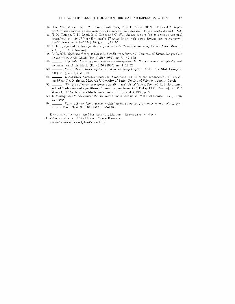
FFT AND FHT ALGORITHMS AND THEIR MATLAB IMPLEMENTATION 47[45] The MathWorks, Inc., 24 Prime Park Way, Natick, Mass. 01760, MATLAB. High-performance numeric computation and visualization software { User's guide, August 1992.[46] T. K. Truong, T. K. Reed, R. G. Lipes and C. Wu, On the application of a fast polynomialtransform and the Chinese Remainder Theorem to compute a two-dimensional convolution,IEEE Trans. on ASSP 29 (1981), no. 1, 91{97.[47] E. E. Tyrtyshnikov,On algorithms of the discrete Fourier transform, Collect. Artic. Moscow(1981), 10{26 (Russian).[48] V. Veselý, Algebraic theory of fast mixed-radix transforms: I. Generalized Kronecker productof matrices, Arch. Math. (Brno) 25 (1989), no. 3, 149{162.[49] , Algebraic theory of fast mixed-radix transforms: II. Computational complexity andapplications, Arch. Math. (Brno) 26 (1990), no. 1, 19{26.[50] , Fast cell-structured digit reversal of arbitrary length, SIAM J. Sci. Stat. Comput.12 (1991), no. 2, 298{310.[51] , Generalized Kronecker product of matrices applied to the construction of fast al-gorithms, Ph.D. thesis, Masaryk University of Brno, Faculty of Science, 1989, in Czech.[52] ,Winograd Fourier transform algorithm and related topics, Proc. of the 6-th summerschool "Software and algorithms of numerical mathematics", Doksy 1985 (Prague), JÈSMF(Society of Czechoslovak Mathematicians and Physicists), 1986, p. 67.[53] S. Winograd, On computing the discrete Fourier transform, Math. of Comput. 32 (1978),175{199.[54] , Some bilinear forms whose multiplicative complexity depends on the �eld of con-stants, Math. Syst. Th. 10 (1977), 169{180.Department of Applied Mathematics, Masaryk University of BrnoJanáèkovo nám. 2a, 662 95 Brno, Czech RepublicE-mail address: vesely@math.muni.cz