Appendix A Fourier Transforms

Appendix AFourier Transforms

A Fourier transformation is a mathematical technique that determines the amplitude andfrequencies of oscillatory signals contained within a time dependent function. In the case ofNMR, the Fourier transform is used to converts the time domain NMR signal, or FID, to afrequency domain signal, otherwise known as the NMR spectrum. For example, if the timedependent signal is given by the following equation,

f(t) = Acos(ωt) (A.1)

then the Fourier transform of this signal will provide both the frequency of the oscillation, (ω),as well as the amplitude of the component at that frequency (A).

The Fourier transformation algorithm that is used in most NMR processing software is thefast Fourier transform, or FFT [44]. From the perspective of this text, the most important featureof this technique is the requirement for 2N data points in the time domain data.

A.1 Fourier SeriesThe Fourier series is a useful starting point to understand some concepts of Fourier trans-

forms. The Fourier series describes any time dependent periodic function, f(t), in terms ofdiscrete frequency components: ω, 2ω, 3ω . . .. If a function has a period of 2π then it can berepresented by the following sum, or Fourier series representation of f(t):

f(t) =ao

2+

∞∑n=1

ancos(nt) + bnsin(nt) (A.2)

The above indicates that we can represent an arbitrary function as a linear combination of aseries of basis functions (cosine and sine), just as we might write an arbitrary vector in termsof its x-, y-, and z-components. As with any other set of basis functions, these functions areorthogonal:∫ π

−π

sin(mt)sin(nt)dt = πδmn

∫ π

−π

cos(mt)cos(nt)dt = πδmn∫ π

−π

sin(mt)cos(nt)dt = 0

(A.3)

δmn = 1 if m = n, otherwise, δmn = 0.

476 PROTEIN NMR SPECTROSCOPY

nb

2 4 6 8 10 12 14 16 180

n

Figure A.1 Fourier components of asquare wave. The coefficients, bn

are plotted as a function of frequency,ωn. The strongest frequency com-ponent corresponds to ω, the secondstrongest is 3ω, etc. Note that only dis-crete values of ω are allowed since asquare wave is a periodic function.

These orthogonal relationships can be used to calculate the coefficients of the Fourier seriesrepresentation of f(t):

an =1

π

∫ π

−π

f(t)cos(nt)dt (A.4)

bn =1

π

∫ π

−π

f(t)sin(nt)dt (A.5)

an and bn are the amplitudes of the various frequency components that sum to give f(t). Notethat bo is always zero since sin(0) = 0.

For well behaved functions, as n gets larger both an and bn approach zero. For example,coefficients for the Fourier series representation of a square wave are given in Fig. A.1 andthe Fourier representation of the square wave is given in Fig. A.2. How well a Fourier seriesrepresents its function depends on the nature of the function. In general, functions with sharpedges (i.e. square wave) require a large number of terms to adequately represent the function,as illustrated in Fig. A.2.

A.2 Non-periodic Functions - The Fourier TransformOnce the function becomes non-periodic it is necessary to utilize a continuous transform,

called the Fourier transform:

F (ω) =1√2π

∫ ∞

−∞f(t)eiωtdt (A.6)

In this case, the non-periodic time domain signal f(t) is represented by a continuous functionin the frequency domain, F (ω). F (ω) gives the amplitude of the frequency components which

0 2 4 -2Time

0 2 4 -2Time

A B

Figure A.2 Fourier series ofa square wave. The Fourierseries that represents a squarewave is shown as the sum ofthe first 3 terms of the se-ries (panel A) and as the sumof the first 7 terms of the se-ries (panel B). Note that therepresentation of the squarewave becomes more accurateas the number of terms in-creases. The square wave isdrawn with a dotted line whilethe Fourier sums are shown asa continuous line.

APPENDIX A: Fourier Transforms 477

are present in the time domain signal. If F (ω) exists, then it is possible to calculate the inverseFourier transform of a function:

f(t) =1√2π

∫ ∞

−∞F (ω)e−iωtdw (A.7)

A.2.1 Examples of Fourier TransformsA.2.1.1 Cosine and Sine

These two functions describe the time evolution of the detected magnetization from themagnetic dipoles in the x-y plane as they precess about Bo. The Fourier transforms of thesetwo functions are shown in Fig. A.3

Cosine.f(t) = cos(ωot) (A.8)

F (ω) =

∫ ∞

−∞cos(ωot)e

iωtdt

=

∫ ∞

−∞cos(ωot)[cos(ωt) + isin(ωt)]dt (A.9)

The complex term is zero since sin is an odd function, its integral from −∞ to +∞ is zero.Therefore:

F (ω) =

∫ ∞

−∞cos(ωot)cos(ωt)dt (A.10)

this integral can be evaluated by taking the limits to be from −a to +a:

F (ω) =

∫ +a

−a

cos(ωot)cos(ωt)dt

=1

2

∫ +a

−a

[cos([ωo − ω]t) + cos([ωo + ω]t)] dt

=sin(ωo − ω)a

(ωo − ω)+

sin(ωo + ω)a

(ωo + ω)(A.11)

This function becomes large when ω = ±ωo. In the limit, as a → ∞, it consists of two δfunctions, one at +ωo and a second at −ωo

1.This result can also be obtained by expressing cos(ωt) as a sum of complex exponentials:

F (ω) =

∫ ∞

−∞cos(ωot)e

iωtdt

=1

2

∫ ∞

−∞

[eiωot + e−iωot

]eiωtdt

=1

2[δ(ω − ωo) + δ(ω + ωo)] (A.12)

1A delta function is a special function that is infinitely narrow and infinitely high at a single point. Forexample, such a peak at x = 2 would be written as δ(x − 2); the delta function is found at the value of xthat makes the argument, x − 2, zero, i.e. δ(0) = ∞.


A B

-5 -4 -3 -2 -1 0 1 2 3 4 5

Frequency [rad/sec] -5 -4 -3 -2 -1 0 1 2 3 4 5

Frequency [rad/sec]

Figure A.3. Fourier transform of cos(ωt) and sin(ωt). Fourier transform of cos(ωt) (PanelA) and sin(ωt) (Panel B). All of these peaks are delta functions. Also note that the Fouriertransform of sin(ωt) is imaginary.

Sine. The Fourier transform of sine is very similar to that of a cosine:

F (ω) =

∫ ∞

−∞sin(ωot)e

iωtdt

=1

2i

∫ ∞

−∞

[eiωot − e−iωot

]eiωtdt

=1

2i[δ(ω − ωo) − δ(ω + ωo)] (A.13)

Note that this function is imaginary.

A.2.1.2 Square-Wave

-10 -8 -6 -4 -2 0 2 4 6 8 10

-1

0

1

2

3

4

Frequency [rad/sec]

Figure A.4. Effect of pulse width on Sinc func-tion. Sinc functions for two different valuesof a are shown. The solid line corresponds toa = 2 and the dotted line to a = 5.0.

A single pulse that is centered about zerowith a width of 2a has the following Fouriertransform:2

F (ω) =1√2π

∫ a

−a

1eiωtdt

=eiωa

iω√

2π− e−iωa

iω√

2π

=

√2sin(ωa)

ω√

π(A.14)

This function is called a sinc function andits shape is shown in Fig. A.4. The width ofthis function, measured as the distance be-tween the first zero-crossing points, is:

∆ω =2π

a(A.15)

The position of the first zero-crossing pointis π

ain rad/sec or 1

2ain Hz3. Note that as

2∫

eaxdx = eax

a.

3Frequencies are given in two common units, rad/sec and Hz. The former is usually associated with thesymbol ω while the latter is associated with the symbol ν or f . The two are related as follows: ω = 2πν.


the value of a decreases (the square pulse becomes narrower) the width of the sinc functionincreases. This inverse relationship between a function and its Fourier transform is quite generaland of importance in both NMR spectroscopy and X-ray diffraction.

A.2.1.3 Exponential DecayNMR signals decay exponentially: e−at. The Fourier transform of this function is:

F (ω) =

∫ ∞

0

e−ateiωtdt

=

∫ ∞

0

e−(a−iω)tdt

=1

a − iω

=a + iω

(a − iω)(a + iω)

=a + iω

(a2 + ω2)(A.16)

F (ω) =T2

1 + T 22 ω2

(A.17)

A B

-10 -8 -6 -4 -2 0 2 4 6 8 10

0.00

1.00

2.00

Frequency [rad/sec] -10 -8 -6 -4 -2 0 2 4 6 8 10

-1.00

0.00

1.00

Frequency [rad/sec]

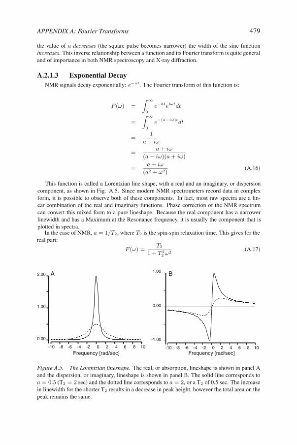
Figure A.5. The Lorentzian lineshape. The real, or absorption, lineshape is shown in panel Aand the dispersion, or imaginary, lineshape is shown in panel B. The solid line corresponds toa = 0.5 (T2 = 2 sec) and the dotted line corresponds to a = 2, or a T2 of 0.5 sec. The increasein linewidth for the shorter T2 results in a decrease in peak height, however the total area on thepeak remains the same.

This function is called a Lorentzian line shape, with a real and an imaginary, or dispersioncomponent, as shown in Fig. A.5. Since modern NMR spectrometers record data in complexform, it is possible to observe both of these components. In fact, most raw spectra are a lin-ear combination of the real and imaginary functions. Phase correction of the NMR spectrumcan convert this mixed form to a pure lineshape. Because the real component has a narrower

plotted n pectra.i sIn the case of NMR, a = 1/T2, where T2 is the spin-spin relaxation time. This gives for the

real part:

linewidth and has a Maximum at the Resonance frequency, it is usually the component that is


Note the dependence of the linewidth on the T2. The smaller (shorter) T2 is, the broader theline. In fact, the full width of this line at half-height is:

∆ν =1

πT2(A.18)

A.2.1.4 Fourier Transform of a Comb FunctionA comb function is just an infinite series of equally spaced delta functions, similar to the teeth

of the comb. Comb functions occur in both the time domain and the frequency domains in NMRspectroscopy. The digital NMR signal, or free induction decay (FID) is simply the product of acomb function, with teeth spaced τdw apart, and the continuous signal from the probe. Similarly,the spectrum is simply a convolution of the NMR spectrum and a comb function, with the teethspaced 1/τdw apart. Convolution functions are explained in more detail in Section A.2.3. TheFourier transform of a comb function in the time domain is:

F (ω) =

∫ ∞

o

f(t)eiωtdt

=

∫ k=+∞∑k=−∞

δ(t − kτdw) eiωtdt

=

k=+∞∑k=−∞

∫δ(t − kτdw) eiωtdt (A.19)

The integral of a product of a delta function with another function is simply the value of thatfunction at the position of the delta function, i.e.:∫

δ(t − kτdw) eiωtdt = eiω(kτdw) (A.20)

Therefore the Fourier transform is:

F (ω) =

k=+∞∑k=−∞

eiω(kτdw) (A.21)

The above is an infinite sum of complex functions eiωkτdw . This function can be represented ascosine and sine functions4:

F (ω) =

k=+∞∑k=−∞

[cos(ωkτdw) + i sin(ωkτdw)] (A.22)

Now, summation of cos(ωkτdw) for values of k ranging from −∞ to +∞ will in general bezero because for every positive value of cos(ωkτdw), there exists a negative value to cancel it.The exception to this is when cos(ωkτdw) is always one, regardless of the value of k. Thisoccurs when:

ωkτdw = 0, 2π, 4π... = 2nπ (A.23)

Thus, ωτdw must be restricted to even multiples of π, such that the product of ωkτdw is always amultiple of 2π. This restriction forces the complex part of the sum to zero, since sin(2nπ) = 0.Therefore:

ω = 2lπ/τdw l ∈ I (A.24)

4Recall eiθ = cosθ + isinθ.


or in Hz (ω = 2πν):

ν = l/τdw l ∈ I (A.25)

Equation A.25 defines another comb function, with teeth spaced 1/τdw apart. Note the recip-rocal relationship between the teeth spacing. The Fourier transform of a comb function in time,with teeth spaced τ apart, will generate a comb function in frequency, with the teeth spaced 1/τapart.

A.2.2 LinearityIf the Fourier transform of two functions, g(t) and h(t) are known, then the Fourier trans-

form of any linear combination of these two functions is just the sum, or combination, of theirindividual transforms:

G(ω) =1√2π

∫ ∞

−∞g(t)eiωtdt (A.26)

H(ω) =1√2π

∫ ∞

−∞h(t)eiωtdt (A.27)

aG(ω) + bH(ω) = a1√2π

∫ ∞

−∞g(t)eiωtdt + b

1√2π

∫ ∞

−∞h(t)eiωtdt (A.28)

A.2.3 Convolutions: Fourier Transform of the Product ofTwo Functions

A common task is to calculate the Fourier transform of a product of two functions. If theFourier transform of each of the individual functions is known then the Fourier transform of theproduct is the convolution of the two individual Fourier transforms.

F ⊗ G(ω) =1√2π

∫ ∞

−∞G(ω′)F (ω − ω′)dω′ (A.29)

The convolution of two functions can be difficult to visualized. Consider the example shown inFig. A.6, where g(x) is some complex shape (a cat) located at the origin and h(x) is a deltafunction located at x = 2, i.e. h(x) = δ(x − 2). The convolution of g and h is particularlystraight-forward since h(x) is a delta function. Evaluating g ⊗ h at x=2:

g ⊗ h(x = 2) =

∫ ∞

−∞g(x′)h(2 − x′)dx′

g ⊗ h(x = 2) =

∫ ∞

−∞g(x′)δ([2 − x′] − 2)dx′

g ⊗ h(x = 2) =

∫g(x′)δ(−x′)dx′

= g(0) (A.30)

The last step used the fact that δ(−x′) is only non-zero when x′ = 0. Therefore, the convolutionof g(x) with h(x) has essentially moved the shape (g(x)) from the origin to the position of thedelta function (h(x)).


−2 −1 1 2

−2 −1 1 2

−2 −1 1 2

g(x)

h(x)

h(x)g(x)

0

0

0

Figure A.6. Convolution of two functions. The convolution of one function, a cat at the origin(g(x)), with a delta function at x = 2 (h(x)), moves the first function such that it is centered atx = 2.

As another example, consider the tail of the cat, which is located at x = 0.25 in g(x) and atx = 2.25 in g ⊗ h:

g ⊗ h(x = 2.25) =

∫ ∞

−∞g(x′)h(2.25 − x′)dx′

g ⊗ h(x = 2.25) =

∫ ∞

−∞g(x′)δ(2.25 − x′ − 2)dx′

g ⊗ h(x = 2.25) =

∫ ∞

−∞g(x′)δ(0.25 − x′)dx′ (A.31)

The last integral is only non-zero for x′ = 0.25, therefore:

g ⊗ h(x = 2.25) = g(0.25) (A.32)

A.2.3.1 Convolution with a Lattice FunctionIn the above example, h(x), was a single δ function. A particularly useful extension of this

example occurs when h(x) is a series of equal spaced δ functions (a comb function). In thiscase the convolution of g and h places an image of g at each position of the delta functions of h(see Fig. A.7).


=−2 −1 1 2

g(x) h(x)

−1 1 2

g(x) h(x)−2

00

0

Figure A.7. Convolution with a comb function. The convolution of a function, g(x), with acomb function, h(x), produces an image of g(x) at every tooth of the comb.

A.2.3.2 Application of Convolution in NMR SpectroscopyThe detected NMR signal is:

cos(ωot)e−t/T2 (A.33)

where ωo is the resonance frequency and T2 is the spin-spin relaxation time,or the time constantfor decay of the FID.

To calculate the Fourier transform of the FID the following steps are taken:

1 The Fourier transform of a cosine function, or pure harmonic wave, is:

f(t) = cos(ωot)

G(ω) = δ(ω − ωo) + δ(ω + ωo) (A.34)

G(ω) consists of two delta functions, one at ω = +ωo and the other at ω = −ωo.

2 The Fourier transform of the second function is (real part only):

f(t) = e−tT2

H(ω) =T2

1 + T22ω2

(A.35)

3 The convolution of these functions produces a Lorentzian line positioned at δ(ω − ωo) andδ(ω + ωo), as shown in Fig. A.8.

=−2 −1 1 2 −2 −1 1 2

G(w) H(w) G(w) H(w)0 0 0

Figure A.8. Fourier transform of cos(ωot)e−t/T2 . The Fourier transform of the product of

cos(ωot) and e−t/T2 is given by the convolution of their respective transforms.

Appendix BComplex Variables, Scalars, Vectors, and Tensors

B.1 Complex Numbers

0 10 20 30 40 50

-1

0

1

Time

Am

plitu

de

Figure B.1. Representation of pulses withcomplex variables. Two excitation pulsesare shown. Both pulses have the same fre-quency, but differ in phase. The solid line has aphase shift of 0◦, while the dotted line is shifted−120◦. Both of these pulses can be representedby eiωt+φ, where φ = 0 and −120◦, respec-tively.

Complex numbers are widely used inNMR theory as a convenient method ofkeeping track of the frequency and phasesof pulses and signals. For example, supposean excitation pulse consisted of one of thetwo signals shown in Fig. B.1. These areboth oscillatory functions, but with differ-ent starting points, or phase shifts. Com-plex numbers can be used to represent boththe frequency as well as any phase shiftassociated with the signal. For example,the solid line can be represented as eiωt

while the dotted line can be represented asei(ωt−120◦).

The symbol i is defined as i =√−1. A

complex number is of the form z = a + ib,where a and b are real numbers. Thereare various ways to represent complex num-bers. one of the most useful is a Argand di-agram, shown in Fig. B.2. In the Arganddiagram the real (a) and imaginary (b) com-ponents of the complex number define theposition of the point in a Cartesian systemwith the real and imaginary axis as the two basis, or coordinate axis. It is also possible to repre-sent complex numbers in polar coordinates. The two representations are, of course, equivalent.The latter representation is more useful in NMR because the phase of the NMR signal can beobtained directly from the size of θ.

The representation of the complex number in polar coordinates gives the following defini-tion:

z = r(cosθ + isinθ) (B.1)


which leads directly to Euler’s identity:

eiθ = cosθ + isinθ (B.2)

This can be seen from the series expansion of eiθ , cosθ, and sinθ.

cosθ = 1 − θ2

2!+

θ4

4!− . . . sinθ =

θ

1!− θ3

3!+

θ5

5!. . . (B.3)

eiθ = 1 +iθ

1!+

(iθ)2

2!+

(iθ)3

3!+

(iθ)4

4!+ . . .

= 1 +iθ

1!+

i2θ2

2!+

i3θ3

3!+

i4θ4

4!+ . . .

= 1 +iθ

1!+

−θ2

2!+

−iθ3

3!+

θ4

4!+ . . .

=

[1 +

−θ2

2!+

θ4

4!+ . . .

]+

[iθ

1!+

−iθ3

3!+ . . .

]= cosθ + isinθ

B.2 Representation of Signals with Complex NumbersAn electrical signal, whether it is a pulse or the induced current from the probe, consists of

a time dependent oscillation of voltage. This oscillation can be characterized by an amplitude(A), frequency(ω), and phase (φ). Complex numbers provide a way of representing all three ofthese parameters in a concise manner:

S(t) = Aei(ωt+φ) (B.4)

This function can be imagined as a vector that rotates in the Argand plane with a frequency ω.In terms of the observable signal, only the real component of the complex function exists. Itsimaginary component simply provides a way of incorporating the phase shift of the signal.

Phase Shifts. Application of a phase shift, ψ, to the above signal can be evaluated bysimply taking the product of the signal and eiψ:

ei(ωt+φ+ψ) = eiψeiωt+φ (B.5)

θ

i

r

ri

r

Figure B.2. Representation of complex numbers with an Argand diagram. An Argand di-agram is shown on the left and the representation in polar coordinates is shown on the right.The real and imaginary axis are labeled with r and i, respectively. In polar coordinates,r =

√a2 + b2 and θ = atan(b/a), where a is the real coordinate and b is the imaginary

coordinate. Note that this ’r’ refers to the length of the vector from the origin to the position ofthe point, not the real axis. In this particular example, a = 1, b = 3, r =

√10, and θ = 71.56◦.

APPENDIX B: Complex Variables, Scalars, Vectors, and Tensors 487

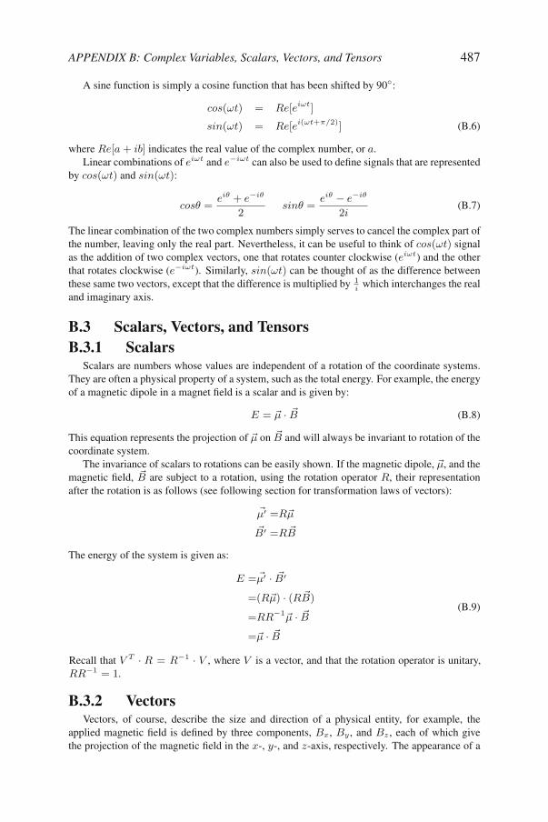
A sine function is simply a cosine function that has been shifted by 90◦:

cos(ωt) = Re[eiωt]

sin(ωt) = Re[ei(ωt+π/2)] (B.6)

where Re[a + ib] indicates the real value of the complex number, or a.Linear combinations of eiωt and e−iωt can also be used to define signals that are represented

by cos(ωt) and sin(ωt):

cosθ =eiθ + e−iθ

2

eiθ − e−iθ

2i(B.7)

The linear combination of the two complex numbers simply serves to cancel the complex part ofthe number, leaving only the real part. Nevertheless, it can be useful to think of cos(ωt) signalas the addition of two complex vectors, one that rotates counter clockwise (eiωt) and the otherthat rotates clockwise (e−iωt). Similarly, sin(ωt) can be thought of as the difference betweenthese same two vectors, except that the difference is multiplied by 1

iwhich interchanges the real

and imaginary axis.

B.3 Scalars, Vectors, and TensorsB.3.1 Scalars

Scalars are numbers whose values are independent of a rotation of the coordinate systems.They are often a physical property of a system, such as the total energy. For example, the energyof a magnetic dipole in a magnet field is a scalar and is given by:

E = �µ · �B (B.8)

This equation represents the projection of �µ on �B and will always be invariant to rotation of thecoordinate system.

The invariance of scalars to rotations can be easily shown. If the magnetic dipole, �µ, and themagnetic field, �B are subject to a rotation, using the rotation operator R, their representationafter the rotation is as follows (see following section for transformation laws of vectors):

�µ′ =R�µ

�B′ =R �B

The energy of the system is given as:

E =�µ′ · �B′

=(R�µ) · (R �B)

=RR−1�µ · �B

�

(B.9)

B.3.2 VectorsVectors, of course, describe the size and direction of a physical entity, for example, the

applied magnetic field is defined by three components, Bx, By , and Bz , each of which givethe projection of the magnetic field in the x-, y-, and z-axis, respectively. The appearance of a

sinθ =

=µ� · B

Recall that V T · R = R−1 · V , where V is a vector, and that the rotation operator is unitary,RR−1 = 1.


vector is changed by a rotation of the coordinate system. For example, if the magnetic field isdefined to be along the z-axis in one coordinate frame: �B = |B|(0, 0, 1), then a rotation of thecoordinate system about the x-axis by 90◦will cause the magnetic field to be aligned along they-axis in the new coordinate frame, with component �B = |B|(0, 1, 0). Note that vector itselfhas not changed, simply its representation by the coordinate system.

The transformation of a vector from one coordinate frame to another can be written as:

′ = RV (B.10)

where V is the vector in the original frame, R is a rotation matrix, and V ′ is the representationof the vector in the new coordinate frame.

B.3.3 TensorsTensors are mathematical entities that are useful for describing the anisotropic properties of

physical systems. Recall that J-coupling arises from an alteration in the local magnetic fieldof one spin due to the magnetic dipole of the coupled spin. This effect is transmitted throughthe intervening electrons that join the two atoms. Since the electron distribution is, in general,anisotropic, the coupling should depend on the relative orientation of the two spins with respectto the electron distribution. This orientational information is conveniently represented by atensor. This tensor is written as a 3 × 3 array:

J̃ =

⎡⎣Jxx Jxy Jxz

Jyx Jyy Jyz

Jzx Jzy Jzz

⎤⎦ (B.11)

Tensors that describe physical interactions are symmetric, i.e. Jyx = Jxy , Jzx = Jxz , andJyz = Jzy , therefore there are only six independent components that define a tensor.

The Hamiltonian, or energy, due to the J- or scalar-coupling between two spins, I and S, isgiven as:

H = �I · J̃ · �S (B.12)

The two terms of the right, J̃ · �S represent the local magnetic field at the I spin due to the Sspin:

�Bloc = J̃ · �S

=

⎡⎣Jxx Jxy Jxz

Jyx Jyy Jyz

Jzx Jzy Jzz

⎤⎦

⎡⎣Sx

Sy

Sz

⎤⎦

=

⎡⎣JxxSx + JxySy + JxzSz

JyxSx + JyySy + JyzSz

JzxSx + JzySy + JzzSz

⎤⎦ (B.13)

The energy of interaction between the I spin and this local magnetic field is �I · Bloc .

B.3.3.1 Transformation properties of TensorsThe rotation of the coordinate system transforms a tensor as follows, using the example of

the coupling tensor:J ′ = R · J · R−1 (B.14)

where J ′ is the form of the tensor in the new coordinate systems.The transformation law for tensors can be proven using the above expression for the coupling

energy, H = �I · J̃ · �S. Since the energy is a scalar, it must be invariant to rotations. Beginning

V

APPENDIX B: Complex Variables, Scalars, Vectors, and Tensors 489

with the transformed spin angular momentum vectors and the tensor, it is possible to show thatthis is equal to the same expression written with the untransformed vectors and tensors:

H = �I ′ J̃ ′ �S′

= [R �I] [R J̃ R−1] [R �S]

= R �I R J̃ �S

= R R−1 �I J̃ �S

= �I J̃ �S (B.15)

If a tensor is symmetric, then there is a coordinate transformation that will produce a diagonalform of the tensor. The orientation of the coordinate system in which the tensor is diagonal isoften called the principal axis system, or PAS. The J-coupling tensor in the coordinate systemis:

JPAS =

⎡⎣Jxx 0 0

0 Jyy 00 0 Jzz

⎤⎦ (B.16)

Note that six components are still required to specify this form of the tensor, Jxx, Jyy, Jzz , andthe three angles that describe the orientation of the principle axis system.

O

z

x

y C N

π

σ

π

Figure B.3. Effect of molecularorbitals on J-coupling. The effectof the anisotropic distribution ofmolecular orbitals on the J-couplingtensor is illustrated using the cou-pling between the nitrogen and car-bonyl carbon.

As an example, consider the coupling between thecarbonyl carbon and the amide nitrogen. The couplingbetween the nuclear spins is due to the electrons in theσ bond as well as in the π orbital that is formed fromthe individual pz orbitals (see Fig. B.3). The later bondgives the peptide bond its partial double bond character.

If the coordinate system was defined such that the y-axis was along the C-N bond and the z-axis was in thedirection of the pz orbitals, then the J-coupling tensorwould have the following form:

JNC =

⎡⎣0 0 0

0 Jyy 00 0 Jzz

⎤⎦ (B.17)

where Jyy would be related to the electron density in theσ bond and Jzz would be related to the electron densityin the π bond. Since the bonding σ and π orbitals arein the y- and z-direction, these components of the J-coupling tensor would be larger than the x-component,which has been set to zero in this simple example.

Appendix CSolving Simultaneous Differential Equations:Laplace Transforms

Simultaneous linear differential equations often describe the time dependence of systems.For example, in the case of chemical exchange between two sites the following equations de-scribe the time dependence of the concentrations of A and B:

dA

dt= −k1[A] + k2[B]

dB

dt= +k2[A] − k2[B] (C.1)

Examples of exchange reactions in NMR include chemical exchange (Chapter 18) and exchangeof magnetization by dipolar coupling (Chapters 16 and 19).

C.1 Laplace TransformsA straight forward method of solving simultaneous differential equations is by the use of

Laplace transforms. This method automatically allows the inclusion of initial conditions andgenerally yields solutions in closed form that are suitable for simulations or data fitting. TheLaplace transform, L, of a function, F (t), is:

L[F (t)] = f(s) =

∫ ∞

o

e−stF (t)dt (C.2)

Table C.1. Inverse Laplace transforms.

f(s) F (t)

1s−a

eat

1(s−a)(s−b)

1a−b

(eat − ebt)

s(s−a)(s−b)

1a−b

(aeat − bebt)


The Laplace transform of the derivative of a function is:

L[F ′(t)] = sf(s) − F (o) (C.3)

where F (0) is the value of F at t = 0. Differential equations are solved by first obtaining theLaplace transform of the equations, solve for f(s) and then obtain the solution, F (t) from theinverse transform. A few useful inverse transforms are shown in Table C.1.

C.1.1 Example CalculationAs a simple example, consider the following equation:

dF (t)

dt= −a F (t)

sf − Fo = −af

f(s + a) = Fo

f =Fo

s + a

Using the inverse transform given in Table C.1 gives the final solution:

F (t) = Foe−at

Returning to the general case of two simultaneous equations:

dU

dt= a11U + a12V (C.4)

dV

dt= a21U + a22V (C.5)

Taking the Laplace transform of both gives:

s u − Uo = a11u + a12v (C.6)

s v − Vo = a21u + a22v (C.7)

Eliminating v gives:

−Uo(a22 − s) + Voa12 = u [(a11 − s)(a22 − s) − a21a12]

Solving for u:

u =−Uo(a22 − s) + Voa12

[a11a22 − a11s − a22s + s2 − a21a12](C.8)

The denominator is a quadratic function with two roots, λ1, and λ2:

λ1 =(a11 + a22) ±

√(a11 + a22)2 − 4(a11a22 − a21a12)

2

λ2 =(a11 + a22) ±

√(a11 − a22)2 + 4a21a12

2(C.9)

Note: (a11 + a22)2 − 4a11a22 = (a11 − a22)

2.

Therefore,

u = −Uoa221

(s − λ1)(s − λ2)+ Uo

s

(s − λ1)(s − λ2)+ Voa12

1

(s − λ1)(s − λ2)(C.10)

Taking the inverse transform gives:

U(t) = Uo

[−a22

eλ1t − eλ2t

λ1 − λ2+

λ1eλ1t − λ2e

λ2t

λ1 − λ2

]+ Voa12

eλ1t − eλ2t

λ1 − λ2(C.11)

The equation for V(t) is obtained by simply interchanging U and V as well as the indices on aij :

V (t) = Vo

[−a11

eλ1t − eλ2t

λ1 − λ2+

λ1eλ1t − λ2e

λ2t

λ1 − λ2

]+ Uoa21

eλ1t − eλ2t

λ1 − λ2(C.12)

C.1.2 Application to Chemical ExchangeThe correspondence between the general coefficients, aij , and the kinetic rate constants is

as follows:

a11 = −RA − k1 a12 = +k2

a21 = +k1 a22 = −RB − k2(C.13)

The intensity of the two selfpeaks (IAA, IBB) and the two crosspeaks (IAB , IBA) can beobtained if we define the magnetization associated with the ’A’ environment as U(t) and thatassociated with the ’B’ environment as V(t).

If the spin-lattice relaxation rates of both environments is the same, then:

λ1 = −kex − R (C.14)

λ2 = −R (C.15)

λ1 − λ2 = −kex (C.16)

The magnetization that gives rise to the selfpeak at (ωA, ωA) begins in environment ’A’ andremains in the same environment after the mixing time:

IAA(t) = IoA(k2 + R)

e(−kex−R)t − e−Rt

−kex+

(−kex − R)e(−kex−R)t − (−R)e−Rt

−kex

= IoA

[k2 + (kex − k2)e

−kext]e−Rt

kex

= IoA(fA + fBe−kext) e−Rt (C.17)

The intensity of the crosspeak, IBA, representing magnetization that began in environmentB, but was transferred to environment A, is:

IBA(τ) = IoBa12

e−λ1t − e−λ2t

λ1 − λ2

= IoB

k2

−kex

[e−kexte−Rt − e−Rt

]= Io

Bk2

−kex

[e−kext − 1

]e−Rt

= IoBfA

[1 − e−kext

]e−Rt (C.18)

APPENDIX C: Solving Simultaneous Differential Equations 493


The equation for the other self- and crosspeak are obtained by exchanging A and B. SubstitutingfA for Io

B and fB for IoB , gives the complete solution for all four peaks:

IAA(t) = fA

[fA + fBe−kext

]e−Rt (C.19)

IBB(t) = fB

[fB + fAe−kext

]e−Rt (C.20)

IBA(t) = fBfA

[1 − e−kext

]e−Rt (C.21)

IBA(t) = fAfB

[1 − e−kext

]e−Rt (C.22)

C.1.3 Application to Spin-lattice RelaxationC.1.3.1 Two Identical SpinsThe Solomon equations for two coupled identical spins (ρI = ρS) are:

dIz

dt= −ρ(Iz − Io

z ) − σ(Sz − Soz ) (C.23)

dSz

dt= −σ(Iz − Io

z ) − ρ(Sz − Soz ) (C.24)

Making the substitution, U(t) = Iz(t) − Ioz and V (t) = Sz(t) − So

z gives:

dU

dt= −ρU − σV

dV

dt= −σU − ρV (C.25)

Therefore,

a11 = −ρ a12 = −σ (C.26)

a21 = −σ a22 = −ρ (C.27)

The two roots are:λ1 = −(ρ + σ) λ2 = −(ρ − σ) (C.28)

and λ1 − λ2 = −2σ.The time dependence of U(t) is:

U(t) = Uo

[−a22

eλ1t − eλ2t

λ1 − λ2+

λ1eλ1t − λ2e

λ2t

λ1 − λ2

]+ Voa12

eλ1t − eλ2t

λ1 − λ2

=eλ1t

λ1 − λ2[Uo(λ1 − a22) + Voa12] +

eλ2t

λ1 − λ2[Uo(a22 − λ2) − Voa12]

=eλ1t

−2σ[Uo(−σ) + Vo(−σ)] +

eλ2t

−2σ[Uo(−σ) − Vo(−σ)]

=eλ1t

2[Uo + Vo] +

eλ2t

2[Uo − Vo] (C.29)

Substituting U(t) = Iz(t)−Ioz , V (t) = Sz(t)−So

z , and setting the equilibrium values (Ioz , So

z )to Mo gives:

Iz(t) − Mo =e−(ρ+σ)t

2[Iz(0) + Sz(0) − 2Mo] +

e−(ρ−σ)t

2[Iz(0) − Sz(0)] (C.30)

APPENDIX C: Solving Simultaneous Differential Equations 495

The above equation shows that the relaxation of the spin is, in general, multi-exponential. How-ever, if both spins inverted at the begining of the measurement (Iz(0) = Sz(o) = −Mo), thetime dependence of Iz and Sz are:

Iz(t) = Mo(1 − 2e−(ρ+σ)t) Sz(t) = Mo(1 − 2e−(ρ+σ)t) (C.31)

and the longitudinal magnetization relaxes with a single time constant:

1

T1= σ + ρ = (W2 − W0) + (W0 + 2W1 + W2) = 2(W1 + W2) (C.32)

C.1.4 Spin-lattice Relaxation of Two Different SpinsIn general the spin-lattice relaxation of a heteronuclear spin that is coupled to a proton is alsomulti-exponential. However, if the attached proton is saturated while the longitudinal magneti-zation is changing, the relaxation becomes a single exponential, with a rate constant of ρS . Thisresult is conveniently obtained using Laplace transforms.

If the protons are saturated, Iz = 0 and dIz/dt=0. Therefore the Solomon equation be-comes:

dSz

dt= −σIo

z − ρs(Sz − Soz ) (C.33)

Substituting V (t) = Sz(t) − Soz gives:

dV

dt= −σIo

z − ρsV (C.34)

The Laplace transform of this is:

sv − Vo =−σIo

z

s− ρs v (C.35)

Solving for v:

v =−Vo

(s + ρs)+ σIo

1

s(s + ρ)(C.36)

Taking the inverse transform, and substituting Sz(t) − SoZ , gives

Sz(t) − Soz = e−ρSt

[Sz(0) − So

Z − σ

ρsIo

]+

σ

ρsIo (C.37)

The usual initial condition for the relaxation measurement is to begin with Sz(0) = 0, giving:

Sz(t) = e−ρSt

[−So

z − σ

ρsIo

]+ So

z +σ

ρsIo

=

[So

z +σ

ρsIo

](1 − eρst) (C.38)

Appendix DBuilding Blocks of Pulse Sequences

Chapters 13 and 14 contain a number of complex pulse sequences. These sequences aregenerally constructed from small segments, with each segment performing a specific function.Consequently, the easiest way to understand many of these experiments is to first recognizeeach segment within the sequence and then consider the effect of each these segments onthe flow of magnetization through the entire sequence. This appendix offers a brief reviewof the product operator treatment of the density matrix and provides a summary of the mostcommon segments that are found in pulse sequences.

D.1 Product operatorsD.1.1 Pulses

x

y

z

y

x

II

I

B1

β

−I−I

Figure D.1. Effect of a β = 90◦

y-pulse on Iz .

Pulses transform magnetization by a rotation of themagnetization by an angle of β about the axis of theapplied magnetization. Usually the right-handed rule isadopted, i.e. the direction of the change of magnetizationfollows the curvature of the fingers when the pulse is ap-plied along the direction of the thumb. For example:

Iz

Pβx→ Izcos(β) − Iysin(β) is a pulse of flip angle β, along the x-axis, applied to Iz

Iz

Pβy→ Izcos(β) + Ixsin(β) is a pulse of flip angle β, along the y-axis, applied to Iz

D.1.2 Evolution by J-coupling

Jtπ

y zx

x

y z

z

−I

2I SI

−2I S

Figure D.2. Effect of scalarcoupling on the evolution of thedensity matrix Ix.

A spin, I , that is transverse and coupled to anotherspin, S, will oscillate between in-phase (e.g. Ix) and anti-phase magnetization (2IySz) as follows (see Fig. D.2):

IxJ→ Ixcos(πJt) + 2IySzsin(πJt)

IyJ→ Iycos(πJt) − 2IxSzsin(πJt)

(D.1)

Note that a density matrix corresponding to the product oftwo-transverse operators does not evolve under J-coupling,for example:

2IxSyJ→ 2IxSy (D.2)


D.1.3 Evolution by Chemical Shift

xIyI

z

ω t

Figure D.3. Effect of chemicalshift on the evolution of the den-sity matrix.

Only transverse magnetization will evolve due to chem-ical shift. The evolution is equivalent to a rotation aboutthe z-axis by an angle ωt, as illustrated in Fig. D.3. Forexample:

Ix → Ixcos(ωIt) + Iysin(ωIt) (D.3)

Anti-phase terms evolve according to the chemical shift ofthe transverse spin:

2IxSz → 2IxSzcos(ωIt) + 2IySzsin(ωIt) (D.4)

D.2 Common Elements of Pulse SequencesThe following discusses a number of common elements that are found in a variety of het-

eronuclear and 15N separated homonuclear sequences. In the following figures the narrow barsrepresent 90◦ pulses and the wider bars 180◦ pulses. All pulses are along the x-axis unlessotherwise noted.

D.2.1 INEPT Polarization Transfer

∆ ∆

S

I

y

∆ =1/(4J)

Figure D.4. INEPTpolarization transfer.

The INEPT element, shown in Fig. D.4, transfers polarizationfrom spin I to S and vice-versa. In the process in-phase magnetiza-tion is converted to anti-phase or the reverse. The delay ∆ is set to1/(4J), however shorter values are often used to reduce signal lossdue to relaxation. The 180◦ pulses are applied to both types of spinstherefore the J-coupling is active during the entire 2∆ period andthe transfer of magnetization is represented by:

−Iy2∆−→ −Iycos(πJ2

1

4J) + 2IxSzsin(πJ2

1

4J)

= −Iycos(π/2) + 2IxSzsin(π/2)

= 2IxSz

P90I,S−→ 2IzSy (D.5)

Note that chemical shift evolution of the transverse spin (e.g. I) isrefocused by the centered 180◦ pulse:

−Iy∆→ −Iycos(ω∆) + Ixsin(ω∆)

180x→ +Iycos(ω∆) + Ixsin(ω∆)

∆→ cos(ω∆)[Iycos(ω∆) − Ixsin(ω∆)]

+ sin(ω∆)[Ixcos(ω∆) + Iysin(ω∆)]

= Ix[−cos(ω∆)sin(ω∆) + cos(ω∆)sin(ω∆)]

+ Iy[cos2(ω∆) + sin2(ω∆)]

= Iy

(D.6)

APPENDIX D: Building Blocks of Pulse Sequences 499

D.2.2 HMQC Polarization Transfer

Figure D.5. HMQCpolarization transfer.

The HMQC (heteronuclear multiple quantum) segment alsotransfers polarization, however the resultant magnetization is rep-resented by a multiple quantum term because of the absence of the90◦ pulse on the I-spins:

−Iy∆−→ 2IxSz

P90S−→ 2IxSy. (D.7)

the delay ∆ is set to 1/(2J). Note that the chemical shift evolution ofthe I spins is not refocused by this segment. However, a 180◦ pulseis usually placed at a later time in the sequence, such as in the middleof the indirect time evolution domain, to refocus this chemical shiftevolution.

D.2.3 Constant Time Evolution

Figure D.6. Constanttime evolution.

A constant time segment permits the density matrix to evolveaccording to chemical shift, but during a fixed time period, 2T. The180◦ pulse, which is initially centered in the 2T period is system-atically moved in one direction by an amount t/2, generating a nettime increment of t for chemical shift evolution. Evolution due to J-coupling would be prevented by the application of decoupling to theS-spins. The chemical shift evolution can be calculated in two ways,by a tedious product operator analysis or by simply keeping track ofthe phase change of the magnetization. The product operator analy-sis proceeds as follows, beginning from transverse magnetization1:

IyT−t/2→ Iycos(ω[T − t

2]) − Ixsin(ω[T − t

2])

P180x→ −Iycos(ω[T − t

2]) − Ixsin(ω[T − t

2]) (D.8)

T+t/2→ −cos(ω[T − t

2])

[Iycos(ω[T +

t

2]) − Ixsin(ω[T +

t

2])

]

−sin(ω[T − t

2])

[Ixcos(ω[T +

t

2]) + Iysin(ω[T +

t

2])

]

= Iy

[−cos(ω[T − t

2])cos(ω[T +

t

2]) − sin(ω[T − t

2])sin(ω[T +

t

2])

]

+Ix

[cos(ω[T − t

2])sin(ω[T +

t

2]) − sin(ω[T − t

2])cos(ω[T +

t

2])

]= −Iycos(ωt) + Ixsin(ωt) (D.9)

this is the same evolution that would be obtained by precession during a delay of 2 t2

: Iy →Iycos(ωt) − Ixsin(ωt), with a simple inversion of sign.

1The final step uses the following trigonometric identities: cos(α−β) = cosαcosβ+sinαsinβ, sin(α−β) = sinαcosβ − cosβsinβ.


The above evolution of the magnetization can be obtained in a more straight-forward mannerby considering the phase of the magnetization. This approach is illustrated in Fig. D.7 and therelevant equations are given below.

IyT−t/2→ Iyeiθ1 : θ1 = ω [T − t/2]

Iyeiθ1 P180x−→ Iyei(π−θ1)

Iyeiθ1 T+t/2−→ Iyei(π−θ1+θ2) : θ2 = ω [T + t/2] (D.10)

The π term in the final phase angle can be ignored since it simply reflects an inversion of thesignal, therefore the total phase angle is: −θ1 + θ2 = ω [−(T − t/2) + (T + t/2)] = ωt.

2tT−

2tT+P180

x

x

y

x

y

x

y

x

yθ1

π−θ1 π−θ +θ1 2

θ2

Figure D.7. Analysis of constant time evolution using phase angles. The use of phase anglesto quickly analyze constant time evolution is illustrated. During the first delay, T − t/2, themagnetization precesses by an angle θ1, the 180◦ pulse essentially negates this phase angle, andthe following T + t/2 period adds θ2 to the phase, giving a net rotation of −θ1 + θ2 = ωt,neglecting the constant phase shift of π.

D.2.4 Constant Time Evolution with J-coupling

−Tt2

+Tt2

2T

C

N

Figure D.8. Constanttime with J-couplingevolution.

This pulse sequence element simultaneously permits chemicalshift evolution to occur for a period equal to t and J-coupling toevolve for a period of 2T . A typical application is to record thenitrogen (N -spin) chemical shift while generating anti-phase mag-netization between the nitrogen and the carbonyl-carbon (C-spin),such as in the HNCO experiment.

The analysis of the evolution of the chemical shift of the nitro-gen is identical to that discussed above since the 180◦ pulse on thecarbons cannot affect the nitrogen-spin. The evolution of the systemdue to J-coupling can be analyzed using the following two rules:

1. A single 180◦ pulse will reverse the direction of evolution dueto J-coupling since it flips the spin-state of one of the coupledpartners.

2. 180◦ pulses, when applied to both spins, do not change the evolution of the J-coupling.Thus, evolution due to J-coupling is active for the entire period of 2T .

The second rule applies here, so the total evolution period for J-coupling is 2T . Therefore thetotal evolution of the density matrix is:

NyωN→ Nycos(ωN t) − Nxsin(ωN t)

JNC→ −2NxCzcos(ωN t) − 2NyCzsin(ωN t)

assuming 2T = 1/(2JNC). Note that the same result is obtained if evolution according toJ-coupling is considered first.


D.2.5 Sequential Chemical Shift & J-coupling Evolution

2∆

2t

2∆

2tH

C

Figure D.9. Sequential chemi-cal shift and J-coupling evolu-tion.

Constant time evolution with J-coupling is an effi-cient way of simultaneously allowing evolution due toJ-coupling and chemical shift. However, the period 2Tis often too short for the desired time for chemical shiftevolution. This is particularly true for CH groups, dueto the strong J-coupling of 140 Hz, which gives an upperlimit on the evolution time of 3.5 msec. Consequently, thechemical shift evolution of the protons is done separatelyfrom the J-coupling in a sequential fashion. The net resultof the sequence shown to the right is:

IzP90H→ −Iy

ωH ,JCH−→ 2IxCzcos(ωHt) + 2IyCzsin(ωHt) (D.11)

assuming ∆ = 1/(2J).This result can be readily obtained by following the phase changes due to evolution by

chemical shift and J-coupling. The total evolution of proton magnetization by chemical shift is(neglecting the phase change of π, see Section D.2.3):

ΘCS = −θ1 + θ2

= −ωH

[t

2+

∆

2+

t

2

]+ ωH

[∆

2

]= −ωHt (D.12)

Evolution due to J-coupling is obtained in the same fashion, using the two rules described abovein Section D.2.4. The phase will evolve in one direction prior to the 180◦ carbon-pulse. The180◦ carbon-pulse, because it is applied to only one of the coupled spins, will reverse the senseof evolution for the period t/2. The 180◦ proton pulse reverses this change in direction duringthe last time period, ∆/2, giving a total phase evolution of:

ΘJ = θ1 − θ2 + θ3

= πJ

[t

2+

∆

2− t

2+

∆

2

]= πJ∆ (D.13)

If ∆ = 1/(2J), then −IyJ→ Iycos(π/2) + 2IxCzsin(π/2) = 2IxCz . Of course, both

chemical shift evolution and J-coupling occur at the same time, giving the final result shown inEq. D.11.

The sequential evolution of chemical shift and J-coupling can reduce the overall sensitivityof the experiment because the proton magnetization is transverse for a total time of t + ∆.Since the proton spin-spin relaxation rate (R2) is usually fast, the extended time period can leadto signal loss due to relaxation. The amount of time the proton spends in the x-y plane can bereduced by the use of semi-constant time methods, as discussed below.

above, evolution of chemical shift for a time t and evolution of J-coupling for a time ∆. The keydifference is that the longest time the proton is transverse is equal to t, instead of t + 1/(2J).

D.2.6 Semi-constant Time Evolution of Chemical Shift& J-coupling

The semi-constant time evolution [70] has the same outcome as the sequential evolution described


ta tctb ta tb tcH

C

iiH

C

i Figure D.10 Semi-constanttime evolution. Two differ-ent ways of implementing thisbuilding block are shown (iand ii).

This is accomplished by incorporating the time required for evolution of J-coupling into thetime allotted for chemical shift evolution.

Two versions of this pulse segment are used, and both are shown in Fig. D.10. Version idiffers from ii in the order of the 180◦ pulses. The initial values (t0) and the increments (δt) foreach delay are given in Table D.1.

Considering the first version (i), the value of the delays for the nth data point are:

where ∆t is the dwell time. Note that ta and tb increase with each data point while tc decreasesto zero length at the last data point of the FID (N ).

The total evolution of the density matrix from chemical shift is:

ΘCS = [θa + θb − θc] ωH

=

[∆

2+ n

∆t

2+ n

∆t

2− n

∆

2

1

N− ∆

2+ n

∆

2

1

N

]ωH

= n∆tωH (D.15)

Similarly, the total phase due to evolution via J-coupling is:

ΘJ = θa − θb + θc

=∆

2+ n

∆t

2− n

∆t

2+ n

∆

2

1

N+

∆

2− n

∆

2

1

N= ∆ (D.16)

Therefore the total evolution of the density matrix is:

IxJCH−→ 2IyCz

ωH−→ 2Cz [IycosωHt − IxsinωHt] (D.17)

The derivation of the delays and increments is straight-forward. For example, with versioni, the following constraints hold for the initial time point:

ΘCS(t = 0) = t0a + t0b − t0c = 0

ΘJ(t = 0) = t0a − t0b + t0c = ∆ (D.18)

Table D.1. Delays for semi-constant time evolution.

Version ta tb tc

i t0a = ∆2

t0b = 0 t0c = ∆2

δta = ∆t2

δtb = ∆t2

− ∆2

1N

δtc = −∆2

1N

ii t0a = ∆2

t0b = 0 t0c = ∆2

δta = −∆2

1N

δtb = ∆t2

− ∆2

1N

δtc = ∆t2

∆ = 1/2J , ∆t = dwell time, N=index of last data point.

ta = t0a + nδta tb = t0b + nδtb tc = t0c + nδtc

= ∆2

+ n∆t2

= 0 = ∆2− n∆

21N

(D.14)[∆t

2− ∆

2

1

N

]

+ n


Adding these two equations together gives t0a = ∆/2 and defining t0b = 0 gives t0c = ∆/2.The increment in ΘCS must be equal to the dwell time (∆t) and the increment in ΘJ must

be zero.

∆ΘCS = δta + δtb − δtc = ∆t

∆ΘJ = δta − δtb + δtc = 0 (D.19)

Adding these two equations together gives δta = ∆t/2. To fix the value of δtb, the incrementin tc is set to -∆/(2N), such that the delay tc goes to zero at the last point (n = N ) to minimizethe total time of the segment. This gives δtb = ∆t/2 − ∆/(2N).

References

[1] A. Abragam. The Principles of Nuclear Magnetism. Oxford, 1961.

[2] H. Akaike. A new look at the statistical model identification. IEEE transactions onautomatic control, AC-19:716–723, 1974.

[3] M. Akke and A.G. Palmer. Monitoring macromolecular motions on microsecond to mil-lisecond time scales by R1ρ−R1 constant relaxation time NMR spectroscopy. Journalof the American Chemical Society, 118:911–912, 1996.

[4] A. Allerhand and E. Thiele. Analysis of Carr-Purcell spin-echo NMR experimentson multiple-spin systems. II. The effect of chemical exchange. Journal of ChemicalPhysics, 45:902–916, 1966.

[5] HMQC and HSQC experi-ments with water flip-back optimized for large proteins. Journal of Biomolecular NMR,11:279–288, 1998.

[6] S. J. Archer, M. Ikura, D. A. Torchia, and A. Bax. An alternative 3D NMR techniquefor correlating backbone 15N with side chain Hβ resonances in larger proteins. Journal

[7] H. Barkhuijsen, R. de Beer, W. M. M. J. Bovee, and D. van Ormondt. Retrieval offrequencies, amplitudes, damping factors, and phases from time-domain signals using alinear least-squares procedure. Journal of Magnetic Resonance, 61:465–481, 1985.

[8] I.L. Barsukov and L.-Y. Lian. Structure determination from NMR data I, NMR of Macro-molecules:A Practical Approach, Editor G.C.K. Roberts, pages 315–357. IRL Press,1993.

[9] A. Bax, G. M. Clore, and A. M. Gronenborn. 1H-1H correlation via isotropic mixing of13C magnetization, a new three-dimensional approach for assigning 1H and 13C spectraof 13C-enriched proteins. Journal of Magnetic Resonance, 88:425–431, 1990.

[10] A. Bax, R.H. Griffey, and B.L. Hawkins. Correlation of proton and 15N chemical-shiftsby multiple quantum NMR. Journal of Magnetic Resonance, 55:301–315, 1983.

[11] A. Bax and S. Grzesiek. Methodological advances in protein NMR. Accounts of Chem-ical Research, 26:131–138, 1993.

of Magnetic Resonance, 95:636–641, 1991.

P. Andersson, B. Gsell, B. Wipf, H. Senn, and G. Otting.

506 REFERENCES

[12] A. Bax, M. Ikura, L.E. Kay, D.A. Torchia, and R. Tschudin. Comparison of differentmodes of 2-dimensional reverse-correlation NMR for the study of proteins. Journal ofMagnetic Resonance, 86:304–318, 1990.

[13] A. Bax, G. Kontaxis, and N. Tjandra. Dipolar couplings in macromolecular structuredetermination. Methods in Enzymology, 339:127–174, 2001.

[14] A. Bax and D. Marion. Improved resolution and sensitivity in 1H-detected heteronuclearmultiple-bond correlation spectroscopy. Journal of Magnetic Resonance, 78:186–191,1988.

[15] A. Bax and S.S. Pochapsky. Optimized recording of heteronuclear multidimensionalNMR spectra using pulsed field gradients. Journal of Magnetic Resonance, 99:638–643, 1992.

[16] N.J. Baxter and M.P. Williamson. Temperature dependence of 1H chemical shifts inproteins. Journal of Biomolecular NMR, 9:359–369, 1997.

[17] P. R. Bevington. Data Reduction and Error Analysis for the Physical Sciences.McGraw-Hill, 1992.

[18] F. Bloch. Nuclear induction. Physical Review, 70:460–474, 1946.

[19] F. Bloch and A. Siegert. Magnetic resonance for non-rotating fields. Physical Review,57:522–527, 1940.

[20] G. Bodenhausen, H. Kogler, and R.R. Ernst. Selection of coherence-transfer pathwaysin NMR pulse experiments. Journal of Magnetic Resonance, 58:370–388, 1984.

[21] G. Bodenhausen and D. Ruben. Natural abundance 15N NMR by enhanced heteronu-clear spectroscopy. Chemical Physics Letters, 69:185–189, 1980.

[22] B. A. Borgias, M. Gochin, D.J. Kerwood, and T.L. James. Relaxation matrix analysisof 2D NMR data. Progress in NMR spectroscopy, 22:83–100, 1990.

[23] A.A. Bothner-By and J. Dadok. Useful manipulations of the free induction decay. Jour-nal of Magnetic Resonance, 72:540–543, 1987.

[24] L. Braunschweiler and R.R. Ernst. Coherence transfer by isotropic mixing - applicationto proton correlation spectroscopy. Journal of Magnetic Resonance, 53:521–528, 1983.

[25] D.M. Briercheck, T.C. Wood, T.J. Allison, J.P. Richardson, and G.S. Rule. The NMRstructure of the RNA binding domain of E. coli rho factor suggests possible RNA-proteininteractions . Nature Structural Biology, 5:393–399, 1998.

[26] A. T. Brünger. X-PLOR: Version 3.1, A System for X-ray Crystallography and NMR.Yale University Press, 1992.

[27] H. Y. Carr and E. M. Purcell. Effects of diffusion on free precession in nuclear magneticresonance experiments. Physical Review, 94:630–638, 1954.

[28] J.P. Carver and R.E. Richards. A general two-site solution for the chemical exchangeproduced dependence of T2 upon the Carr-Purcell pulse sequence. Journal of MagneticResonance, 6:89–105, 1972.

REFERENCES 507

[29] J. Cavanagh, W. J. Chazin, and M. Rance. The time dependence of coherence transfer inhomonuclear isotropic mixing experiments. Journal of Magnetic Resonance, 87:110–131, 1990.

[30] J. Cavanagh, W. J. Fairbrother, A. G. Palmer III, and N. J. Skelton. Protein NMR Spec-troscopy. Academic Press, 1996.

[31] J. Cavanagh, A.G. Palmer, P.E. Wright, and M. Rance. Sensitivity improvement inproton-detected 2-dimensional heteronuclear relay spectroscopy. Journal of MagneticResonance, 91:429–436, 1991.

[32] J. Cavanagh and M. Rance. Suppression of cross-relaxation effects in TOCSY spectra

1993.

[33] S.-L. Chang, A. Szabo, and N. Tjandra. Temperature dependence of domain motionsof calmodulin probed by NMR relaxation at multiple fields. Journal of the AmericanChemical Society, 125:11379–11384, 2003.

[34] J. Chen, C.L. Brooks III, and P.E. Wright. Model-free analysis of protein dynamics:assessment of accuracy and model selection protocols based on molecular dynamicssimulation. Journal of Biomolecular NMR, 29:243–257, 2004.

[35] G. M. Clore, A. Bax, P. C. Driscoll, P. T. Wingfield, and A. M. Gronenborn. Assignmentof the side-chain 1H and 13C resonances of interleukin-1β using double- and triple-resonance heteronuclear three-dimensional NMR spectroscopy. Biochemistry, 29:8172–8184, 1990.

[36] G. M. Clore, P. C. Driscoll, P. T. Wingfield, and A. M. Gronenborn. Analysis of the back-bone dynamics of interleukin-1β using two-dimensional inverse detected heteronuclear1H-15N NMR spectroscopy. Biochemistry, 29:7387–7401, 1990.

[37] G. M. Clore, A. Szabo, A. Bax, L. E. Kay, P. C. Driscoll, and A. M. Gronenborn. De-viations from the simple two-parameter model-free approach to the interpretations ofnitrogen-15 nuclear magnetic relaxation of proteins. Journal of the American ChemicalSociety, 112:4989–4991, 1990.

[38] G.M. Clore, A.M. Gronenborn, and A. Bax. A robust method for determining the magni-tude of the fully asymmetric alignment tensor of oriented macromolecules in the absenceof structural information. Journal of Magnetic Resonance, 133:216–221, 1998.

[39] R. T. Clubb, V. Thanabal, and G. Wagner. A constant-time three-dimensional triple-resonance pulse scheme to correlate intra-residue 1HN , 15N, and 13C’ chemical shiftsin 15N-13

[40] R. T. Clubb, V. Thanabal, and G. Wagner. A new 3D HN(CA)HA experiment for obtain-ing fingerprint HN -Hα crosspeaks in 15N- and 13C-labeled proteins. J. BiomolecularNMR, 2:203–210, 1992.

[41] R. T. Clubb and G. Wagner. A triple-resonance pulse scheme for selectively correlatingamide 1HN and 15N nuclei with the 1Hα proton of the preceding residue. Journal ofBiomolecular NMR, 2:389–394, 1992.

C-labeled proteins. Journal of Magnetic Resonance, 97:213–217, 1992.

via a modified DIPSI-2 mixing sequence. Journal of Magnetic Resonance, A105 : 328,

508 REFERENCES

[42] C. Cohen-Tannoudji, B. Diu, and F. Laloë. Quantum Mechanics. John Wiley & Sons,1977.

[43] W. W. Conover. Magnetic shimming. Acorn NMR: http://www.acornnmr.com, 2004.

[44] J.W. Cool y and J.W. Tukey. An algorithm for the machine calculation of complexFourier series. Mathematics of Computation ,19:297–301, 1965.

[45] F. Cordier and S. Grzesiek. Direct observation of hydrogen bonds in proteins by inter-residue 3HJNC scalar couplings. Journal of the American Chemical Society, 121:1601–1602, 1999.

[46] E.J. d’Auvergne and P.R. Gooley. The use of model selection in the model-free analysisof protein dynamics. Journal of Biomolecular NMR, 25:25–39, 2003.

[47] D.G. Davis, M.E. Perlman, and R.E. London. Direct measurements of the dissociation-rate constant for inhibitor-enzyme complexes via the T1ρ and T2(CPMG) methods.Journal of Magnetic Resonance, 104B:266–275, 1994.

[48] E. de Alba and N. Tjandra. NMR dipolar couplings for the structure determinationof biopolymers in solution. Progress in Nuclear Magnetic Resonance Spectroscopy,

[49] D.E. Demco, P. Van Hecke, and J.S. Waugh. Phase-shifted pulse sequence for measure-ment of spin-lattice relaxation in complex systems. Journal of Magnetic Resonance,16:467–470, 1974.

[50] C.E. Dempsey. Hydrogen exchange in peptides and proteins using NMR spectroscopy.Progress in Nuclear Magnetic Resonance Spectroscopy, 39:135–170, 2001.

[51] C. Deverell, R.E. Morgan, and J.H. Strange. Studies of chemical exchange by nuclearmagnetic relaxation in the rotating frame. Molecular Physics, 18:553–559, 1970.

[52] J.F. Doreleijers, S. Mading, D. Maziuk, K. Sojourner, L. Yin, J. Zhu, J.L. Markley JL,and E.L. Ulrich. BioMagResBank (BMRB) database with sets of experimental NMRconstraints corresponding to the structures of over 1400 biomolecules deposited in theprotein data bank. Journal of Biomolecular NMR, 26:139–146, 2003.

[53] R. R. Ernst, G. Bodenhausen, and A. Wokaun. Principles of Nuclear Magnetic Reso-nance in One and Two Dimensions. Oxford, 1987.

[54] N. A. Farrow, R. Muhandiram, A. U. Singer, S. M. Pascal, C. M. Kay, G. Gish, S. E.Shoelson, T. Pawson, J. D. Forman-Kay, and L. E. Kay. Backbone dynamics of a freeand a phosphopeptide-complexed Src homology 2 domain studied by 15N relaxation.Biochemistry, 33:5984–6003, 1994.

[55] S. W. Fesik, H. L. Eaton, E. T. Olejniczak, E. R. P. Zuiderweg, L. P. McIntosh, and F. W.Dahlquist. 2D and 3D NMR spectroscopy employing 13C-13C magnetization transfer byisotropic mixing. Spin system identification in large proteins. Journal of the AmericanChemical Society, 112:886–888, 1990.

[56] R. Freeman. Spin Choreography: Basic Steps in High Resolution NMR. SpektrumAcademic Publishers, 1997.

e

40:175–197, 2002.

REFERENCES 509

[57] D. B. Fulton, R. Hrabal, and F. Ni. Gradient-enhanced TOCSY experiments with im-proved sensitivity and solvent suppression. Journal of Biomolecular NMR, 8:213–218,1996.

[58] D. Fushman and D. Cowburn. Nuclear magnetic resonance relaxation in determinationof residue-specific 15N chemical shift tensors in proteins in solution: protein dynamics,structure, and applications of transverse relaxation optimized spectroscopy. Methods inEnzymology, 339:109–126, 2001.

[59] D. Fushman, N. Tjandra, and D. Cowburn. Direct measurement of 15N chemical shiftanisotropy in solution. Journal of the American Chemical Society, 120:10947–10952,1998.

[60] J. Garcia de la Torre, M.L. Huertas, and B. Carrasco. HYDRONMR: Prediction ofNMR relaxation of globular proteins from atomic-level structures and hydrodynamiccalculations. Journal of Magnetic Resonance, 147:138–146, 2000.

[61] H. Geen and R. Freeman. Band-selective radiofrequency pulses. Journal of MagneticResonance, 93:93–141, 1991.

[62] S. J. Glaser and G. P. Drobny. Assessment and optimization of pulse sequences forhomonuclear isotropic mixing. Advances in Magnetic Resonance, 14:35–58, 1990.

[63] M. Goldman. Quantum Description of High-Resolution NMR in Liquids. Oxford Sci-ence Publications, 1988.

[64] N.K. Goto, K.H. Gardner, G.A. Mueller, R.C. Willis, and L.E. Kay. A robust and cost-effective method for the production of Val, Leu, Ile(δ1) methyl-protonated 15N-, 13C-,2H-labeled proteins. Journal of Biomolecular NMR, 13:369–374, 1999.

[65] S. Grzesiek, J. Anglister, and A. Bax. Correlation of backbone amide and aliphaticside-chain resonances in 13C/15N-enriched proteins by isotropic mixing of 13C magne-tization. Journal of Magnetic Resonance, B101:114–119, 1993.

[66] S. Grzesiek and A. Bax. Correlating backbone amide and side chain resonances in largerproteins by multiple relayed triple resonance NMR. Journal of the American ChemicalSociety, 114:6291–6293, 1992.

[67] S. Grzesiek and A. Bax. An efficient experiment for sequential backbone assignment ofmedium-sized isotopically enriched proteins. Journal of Magnetic Resonance, 99:201–207, 1992.

[68] S. Grzesiek and A. Bax. Improved 3D triple-resonance NMR techniques applied to a31-kDa protein. Journal of Magnetic Resonance, 96:432–440, 1992.

[69] S. Grzesiek and A. Bax. The origin and removal of artifacts in 3D HCACO spectra ofproteins uniformly enriched with 13C. Journal of Magnetic Resonance, B102:103–106,1992.

[70] S. Grzesiek and A. Bax. Amino-acid type determination in the sequential assignmentprocedure of uniformly 13C/15N-enriched proteins. Journal of Biomolecular NMR,3:185–204, 1993.

510 REFERENCES

[71] S. Grzesiek, P. Wingfield, S. Stahl, J. D. Kaufman, and A. Bax. Four-dimensional 15N-separated NOESY of slowly tumbling perdeuterated 15N-enriched proteins. Applica-tions to HIV-1 Nef. Journal of the American Chemical Society, 117:9594–9595, 1995.

[72] M.R. Hansen, L. Mueller, and A. Pardi. Tunable alignment of macromolecules by fila-mentous phage yield dipolar coupling interactions. Nature Structural Biology, 5:1065–1074, 1998.

[73] T.K. Hitchens, S.A. McCallum, and G.S. Rule. A J(CH)-modulated 2D (HACACO)NHpulse scheme for quantitative measurement of 13Cα −1 Hα couplings in 15N, 13C-labeled proteins. Journal of Magnetic Resonance, 109:281–284, 1999.

[74] T.-L. Hwang, M. Kadkhodaei, A. Mohebbi, and A. J. Shaka. Coherent and incoherentmagnetization transfer in the rotating frame. Magnetic Resonance in Chemistry, 30:S24–S34, 1992.

[75] M. Ikura, L. E. Kay, and A. Bax. A novel-approach for sequential assignment of 1H,13C, and 15N spectra of larger proteins. Heteronuclear triple-resonance 3-dimensionalNMR-spectroscopy: Application to calmodulin. Biochemistry, 29:4659–4667, 1990.

[76] R. Ishima, J. M. Lois, and D. A. Torchia. Transverse 13C relaxation of CHD2 methylisotopmers to detect slow conformational changes of protein side chains. Journal of theAmerican Chemical Society, 121:11589–11590, 1999.

[77] R. Ishima, J.M. Louis, and D. A. Torchia. Optimized labeling of 13CHD2 methyl iso-topomers in perdeuterated proteins: Potential advantages for 13C relaxation studies ofmethyl dynamics of larger proteins. Journal of Biomolecular NMR, 121:167–71, 2001.

[78] J. Jeener. Pulse pair techniques in high resolution NMR. Ampere International SummerSchool, Basko Poljie, Yugoslavia, 1971.

[79] J. Jeener, B. H. Meier, P. Bachmann, and R. R. Ernst. Investigation of exchangeprocesses by 2-dimensional NMR-spectroscopy. Journal of Chemical Physics, 71:4546–4553, 1979.

[80] M. Karplus. Contact electron-spin coupling of nuclear magnetic moments. Journal ofChemical Physics, 30:11–16, 1959.

[81] L. E. Kay, M. Ikura, R. Tschudin, and A. Bax. 3-Dimensional triple-resonance NMRspectroscopy of isotopically enriched proteins. Journal of Magnetic Resonance, 89:496–514, 1990.

[82] L. E. Kay, P. Keifer, and T. Saarinen. Pure absorption gradient enhanced heteronuclearsingle quantum correlation spectroscopy with improved sensitivity. Journal of AmericanChemical Society, 114:10663–10665, 1992.

[83] L. E. Kay, D. Marion, and A. Bax. Practical aspects of 3D heteronuclear NMR ofproteins. Journal of Magnetic Resonance, 84:72–84, 1989.

[84] L. E. Kay, D. A. Torchia, and A. Bax. Backbone dynamics of proteins as studied by15N inverse detected heteronuclear NMR spectroscopy: Application to staphylococcalnuclease. Biochemistry, 28:8972–8979, 1989.

REFERENCES 511

[85] L. E. Kay, G. Y. Xu, A. U. Singer, D. R. Muhandiram, and J. D. Forman-Kay. A gradient-enhanced HCCH-TOCSY experiment for recording side-chain 1H and 13C correlationsin H2O samples of proteins. Journal of Magnetic Resonance, B 101:333–337, 1993.

[86] L. E. Kay, G. Y. Xu, and T. Yamazaki. Enhanced-sensitivity triple-resonance spec-troscopy with minimal H2O saturation. Journal of Magnetic Resonance, A 109:129–133, 1994.

[87] A. E. Kelly, H. D. Ou, R. Withers, and V. J. Dotsch. Low-conductivity buffers for high-sensitivity NMR measurements. Journal of American Chemical Society, 124:12013–12019, 2002.

[88] D. M. Korzhnev, E. V. Tischenko, and A. S. Arseniev. Off-resonance effects in 15N T2

CPMG measurements. Journal of Biomolecular NMR, 17:231–237, 2000.

[89] C.D. Kroenke, M. Rance, and A.G. Palmer III. Variability of the 15N chemical shiftanisotropy in Escherichia coli Ribonuclease H in solution. Journal of the AmericanChemical Society, 121:10119–10125, 1999.

[90] H. Kuboniwa, S. Grzesiek, F. Delaglio, and A. Bax. Measurement of HN -Hα J couplingsin calcium-free calmodulin using new 2D and 3D water-flip-back methods. Journal ofBiomolecular NMR, 4:871–878, 1994.

[91] A. Kumar, G. Wagner, R. R. Ernst, and K. Wüthrich. Studies of J-connectivities andselective 1H-1H Overhauser effects in H2O solutions of biological macromolecules bytwo-dimensional NMR experiments. Biochemical Biophysical Research Communica-tions, 96:1156–1163, 2000.

[92] J. Kuszewski, J. Qin, A.M. Gronenborn, and G. M. Clore. The impact of direct re-finement against 13Cα and 13Cβ chemical shifts on protein structure determination byNMR. Journal of Magnetic Resonance, 106B:92–96, 1995.

[93] W. E. Lamb. The theory of chemical shielding in atoms. Physical Review, 60:817, 1941.

[94] M.H. Levitt, R. Freeman, and T. Frenkiel. Broad-band heteronuclear decoupling. Jour-nal of Magnetic Resonance, 47:328–330, 1982.

[95] Y.-C. Li and G.T. Montelione. Solvent saturation-transfer effects in pulsed-field-gradientheteronuclear single-quantum-coherence (PFG-HSQC) spectra of polypeptides and pro-teins. Journal of Magnetic Resonance, B101:315–319, 1993.

[96] J C Lindon and A G Ferrige. Digitization and data processing in Fourier transformNMR. Progress in NMR Spectroscopy, 14:27–66, 1980.

[97] G. Lipari and A. Szabo. Model-free approach to the interpretation of nuclear magneticresonance relaxation in macromolecules. 1. Theory and range of validity. Journal of theAmerican Chemical Society, 104:4546–4559, 1982.

[98] G. Lippens, C. Dhalluin, and J.-M. Wieruszeski. Use of water flip-back pulse in thehomonuclear NOESY experiment. Journal of Biomolecular NMR, 5:327–331, 1995.

[99] M. Liu, X. Mao, C. Ye, H. Huang, J. K. Nicholson, and J. C. Lindon. Improved WA-TERGATE pulse sequences for solvent suppression in NMR spectroscopy. Journal ofMagnetic Resonance, 132:125–129, 1998.

512 REFERENCES

[100] P. Luginbuhl and K. Wüthrich. Semi-classical nuclear spin relaxation theory revisitedfor use with biological macromolecules. Progress in Nuclear Magnetic Resonance Spec-troscopy, 40:199–247, 2002.

[101] Z. Luz and S. Meiboom. Nuclear magnetic resonance study of the photolysis of thetrimethylammonium ion in aqueous solution - Order of the reaction with respect to sol-vent. Journal of Chemical Physics, 39:366–370, 1963.

[102] A. M. Mandel, M. Akke, and A. G. Palmer III. Backbone dynamics of Escherichia coliribonuclease H1:Correlations with structure and function in an active enzyme. Journalof Molecular Biology, 246:144–163, 1995.

[103] A. De Marco, M. Llinas, and K. Wüthrich. Analysis of H-1 NMR spectra of ferrichromepeptides. 1. Non-amide protons. Biopolymers, 17:617–636, 1978.

[104] D. Marion, P.C. Driscoll, L.E. Kay, P.T. Wingfield, A. Bax, A.M. Gronenborn, and G.M.Clore. Overcoming the overlap problem in the assignment of 1H NMR spectra of largerproteins by use of three-dimensional heteronuclear 1H-15N Hartmann-Hahn multiplequantum coherence and nuclear Overhauser-multiple quantum coherence spectroscopy:Application to interleukin 1β. Biochemistry, 28:6150–6156, 1989.

[105] D. Marion, M. Ikura, R. Tschudin, and A. Bax. Rapid recording of 2D NMR spec-tra without phase cycling. application to the study of hydrogen exchange in proteins.Journal of Magnetic Resonance, 85:393–399, 1989.

[106] D. Marion and K. Wüthrich. Application of phase sensitive two-dimensional correlatedspectroscopy (COSY) for measurements of 1H-1H spin-spin coupling constants in pro-teins. Biochemical Biophysical Research Communications, 113:967, 1983.

[107] J.L. Markley, A. Bax, Y. Arata, C.W. Hilbers, R. Kaptein, B.S. Sykes, P.E. Wright, andK. Wüthrich. Recommendations for the presentation of NMR structures of proteins andnucleic acids. Pure and Applied Chemistry, 70:117–142, 1998.

[108] J.L. Markley, W.J. Horsley, and M.P. Klein. Spin-lattice relaxation measurements inslowly relaxing complex spectra. Journal of Chemical Physics, 55:3604, 1971.

[109] H.M. McConnell. Reaction rates by nuclear magnetic resonance. Journal of ChemicalPhysics, 28:430–431, 1958.

[110] M. A. McCoy and L. Mueller. Selective shaped pulse decoupling in NMR: Homonuclear[13C] carbonyl decoupling. Journal of the American Chemical Society, 1992:2108–2112, 1992.

[111] S. Meiboom and D. Gill. Modified spin-echo method for measuring nuclear relaxationtimes. Review of Scientific Instruments, 29:688–691, 1958.

[112] B. H. Meier and R. R. Ernst. Elucidation of chemical-exchange networks by 2-dimensional NMR-spectroscopy - Heptamethylbenzenonium ion. Journal of the Amer-ican Chemical Society, 101:6441–6442, 1979.

[113] B. A. Messerle, G. Wider, G. Otting, C. Weber, and K. Wüthrich. Solvent suppressionusing a spin lock in 2D and 3D NMR spectroscopy with H2O solutions. Journal ofMagnetic Resonance, 85:608–614, 1989.

REFERENCES 513

[114] O. Millet, J.P. Loria, C.D. Kroenke, M. Pons, and A.G. Palmer III. The static magneticfield dependence of chemical exchange linebroadening defines the NMR chemical shifttime scale. Journal of American Chemical Society, 122:2867–2877, 2000.

[115] N. Müller, R. R. Ernst, and K. Wuthrich. Multiple-quantum-filtered two-dimensionalcorrelated NMR spectroscopy of proteins. Journal of the American Chemical Society,108:6482–6492, 1986.

[116] D. R. Muhandiram and L. E. Kay. Gradient-enhanced triple-resonance three-dimensional NMR experiments with improved sensitivity. Journal of Magnetic Res-onance, 1994:203–216, 1994.

[117] F.A.A. Mulder, P.J.A.van Tilborg, R. Kaptein, and R. Boelens. Microsecond time scaledynamics in the RXR DNA-binding domain from a combination of spin-echo and off-resonance rotating frame relaxation measurements. Journal of Biomolecular NMR,13:275–288, 1999.

[118] D. Neuhaus and M. Williamson. The Nuclear Overhauser Effect in Structural and Con-formational Analysis. VCH Publishers, Inc., New York, 1989.

[119] J. S. Nowick, O. Khakshoor, M. Hashemzadeh, and J. O. Brower. DSA: A new internalstandard for NMR studies in aqueous solution. Organic Letters, 2003:3511–3513, 1992.

[120] T. G. Oas, C. J. Hartzell, F. W. Dahlquist, and G. P. Drobny. The amide 15N chemicalshift tensors of four peptides determined from 13C dipole-coupled chemical shift powderpatterns. Journal of the American Chemical Society, 109:5962–5966, 1987.

[121] M. Ottiger, F. Delaglio, and A. Bax. Measurement of J and dipolar couplings fromsimplified two-dimensional NMR spectra. Journal of Magnetic Resonance, 131:373–378, 1998.

[122] A. W. Overhauser. Paramagnetic relaxation in metals. Physical Review, 89:689–700,1953.

[123] A.G. Palmer, C.D. Kronenke, and J.P. Loria. Nuclear magnetic resonance methods forquantifying microsecond-to-millisecond motions in biological macromolecules. Meth-ods in Enzymology, 339:204–238, 2001.

[124] A. Pardi, M. Billeter, and K. Wüthrich. Calibration of the angular dependence of theamide proton-C alpha proton coupling constants, 3JHN−α, in globular protein. use of3JHN−α for identification of helical secondary structure. Journal of Molecular Biology,180:741–751, 1984.

[125] S. L. Patt. Single- and multiple-frequency-shifted laminar pulses. Journal of MagneticResonance, 96:94–102, 1992.

[126] N. H. Pawley, C. Wang, S. Koide, and L. K. Nicholson. An improved method for dis-tinguishing between anisotropic tumbling and chemical exchange in analysis of 15Nrelaxation parameters. Journal of Biomolecular NMR, 20:149–165, 1988.

[127] J. W. Peng, V. Thanabal, and G. Wagner. 2D heteronuclear NMR measurements ofspin-lattice relaxation times in the rotating frame of X-nuclei in heteronuclear HX spinsystems. Journal of Magnetic Resonance, 94:82–100, 1991.

514 REFERENCES

[128] K. Pervushin. Impact of Transverse Relaxation Optimized Spectroscopy TROSY onNMR as a technique in structural biology. Quarterly Reviews of Biophysics, 33:161–197, 2000.

[129] K. Pervushin, R. Riek, G. Wider, and K. Wüthrich. Attenuated T2 relaxation by mu-tual cancellation of dipople-dipole coupling and chemical shift anisotropy indicates anavenue to NMR structures of very large biological macromolecules in solution. Proceed-ings of the National Academy of Sciences of the United States of America, 94:12366–12371, 1997.

[130] K. Pervushin, R. Riek, G. Wider, and K. Wüthrich. Transverse relaxation-optimizedspectroscopy (TROSY) for NMR studies of aromatic spin systems in 13C-labeled pro-teins. Journal of the American Chemical Society, 120:6394–6400, 1998.

[131] U. Piantini, O. W. Sorensen, and R. R. Ernst. Multiple quantum filters for elucidatingNMR coupling networks. Journal of the American Chemical Society, 104:6800–6801,1982.

[132] M. Piotto, V. Saudek, and V. Sklenar. Gradient-tailored excitation for single-quantumNMR-spectroscopy of aqueous solutions. Journal of Biomolecular NMR, 2:661–665,1992.

[133] P. Plateau and M. Gueron. Exchangeable proton NMR without base-line distortion, us-ing new strong-pulse sequences. Journal of the American Chemical Society, 104:7310–7311, 1982.

[134] J. A. Pople. Proton magnetic resonance of hydrocarbons. Journal of Chemical Physics,24:1111, 1956.

[135] D. S. Raiford, C. L. Fisk, and E. D. Becker. Calibration of methanol and ethylene-glycolnuclear magnetic resonance thermometers. Analytical Chemistry, 51:2050–2051, 1979.

[136] M. Rance and J. Cavanagh. RF phase coherence in rotating-frame NMR experiments inisotropic solutions. Journal of Magnetic Resonance, 87:363–371, 1990.

[137] M.K. Rosen, K.H. Gardner, R.C. Willis, W.E. Parris, T. Pawson, and L.E. Kay. Selec-tive methyl group protonation of perdeuterated proteins. Journal of Molecular Biology,263:627–636, 1996.

[138] A. Ross, M. Czisch, and G. C. King. Systematic errors associated with the CPMG pulsesequence and their effect on motional analysis of biomolecules. Journal of MagneticResonance, 124:355–365, 1997.

[139] S. P. Rucker and A. J. Shaka. Broadband homonuclear cross polarization in 2D NMRusing DIPSI-2. Molecular Physics, 68:509–517, 1989.

[140] M. Salzmann, K. Pervushin, G. Wider, H. Seen, and K. Wüthrich. TROSY in triple-resonance experiments: New perspectives for sequential NMR assignment of large pro-teins. Proceedings of the National Academy of Sciences of the United States of America,95:13585–12590, 1998.

[141] C.R. Sanders and J.P. Schwonek. Characterization of magnetically orientable bilayersin mixtures of dihexanoylphosphatidylcholine and dimyristoylphosphatidylcholine bysolid-state NMR. Biochemistry, 31:8898–8905, 1992.

REFERENCES 515

[142] M. Sattler, J. Schleucher, and C. Griesinger. Heteronulear multidimensional NMR ex-periments for the structure determination of proteins in solution employing pulsed fieldgradients. Progress in Nuclear Magnetic Resonance Spectroscopy, 34:93–158, 1999.

[143] J.M. Schurr, H.P. Babcock, and B.S. Fujimoto. A test of the model-free formulas. Effectsof anisotropic rotational diffusion and dimerization. Journal of Magnetic Resonance,105:211–224, 1994.

[144] G. Schwarz. Estimating the dimension of a model. The annals of statistics, 6:461–464,1978.

[145] C.D. Schwieters, J.J. Kuszewski, N. Tjandra, and G.M. Clore. The Xplor-NIH NMRmolecular structure determination package. Journal of Magnetic Resonance, 160:65–73, 2003.

[146] A. J. Shaka, P. B. Barker, and R. Freeman. Computer-optimized decoupling schemefor wideband applications and low-level operation. Journal of Magnetic Resonance,64:547–552, 1985.

[147] A. J. Shaka, J. Keeler, and R. Freeman. Evaluation of a new broadband decouplingsequence: WALTZ-16. Journal of Magnetic Resonance, 53:313–349, 1983.

[148] A. J. Shaka, C. J. Lee, and A. Pines. Iterative schemes for bilinear operators; applicationsto spin decoupling. Journal of Magnetic Resonance, 77:274–293, 1988.

[149] N.J. Skelton, A.G. Palmer III, M. Akke, J. Kordel, M. Rance, and W.J. Chazin. Practicalaspects of two-dimensional proton-detected 15N spin relaxation measurements. Journalof Magnetic Resonance, B 102:253–264, 1993.

[150] V. Sklenar, M. Piotto, R. Leppik, and V. Saudek. Gradient-tailored water suppressionfor 1H-15N HSQC experiments optimized to retain full sensitivity. Journal of MagneticResonance, A102:241–245, 1993.

[151] C. P. Slichter. Principles of Magnetic Resonance. Springer-Verlag, Berlin, 1990.

[152] I. Solomon. Relaxation processes in a system of two spins. Physical Review, 99:559–565, 1955.

[153] O.W. Sorensen, G.W. Eich, M.H. Levitt, G. Bodenhausen, and R.R. Ernst. Productoperator-formalism for the description of NMR pulse experiments. Progress in NuclearMagnetic Resonance Spectroscopy, 16:163–192, 1983.

[154] D. J. States, R. A. Haberkorn, and D. J. Ruben. A two-dimensional nuclear overhauserexperiment with pure absorption phase in four quadrants. Journal of Magnetic Reso-nance, 48:286–292, 1982.

[155] T. J. Swift and R. E. Connick. NMR-relaxation mechanism of 17O in aqueous solutionsof paramagnetic cations and the lifetime of water molecules in the first coordinationsphere. The Journal of Chemical Physics, 37:307–320, 1962.

[156] N. Tjandra and A. Bax. Direct measurement of distances and angles in biomolecules byNMR in a dilute liquid crystalline medium. Science, 278:1111–1114, 1997.

[157] N. Tjandra, S. Grzesiek, and A. Bax. Magnetic field dependence of nitrogen-proton Jsplittings in 15N-enriched human ubiquitin resulting from relaxation interference and

516 REFERENCES

residual dipolar coupling. Journal of the American Chemical Society, 118:6264–6272,1996.

[158] N. Tjandra, P. T. Wingfield, S. Stahl, and A. Bax. Anisotropic rotational diffusion ofperdeuterated HIV protease from 15N NMR relaxation measurements at two magneticfield strengths. Journal of Biomolecular NMR, 8:273–284, 1996.

[159] J.R. Tolman, H.M. Al-Hashimi, L.E. Kay, and J.H. Prestegard. Structural and dynamicanalysis of residual dipolar coupling data for proteins. Journal of the American Chemi-cal Society, 123:1416–1424, 2001.

[160] L. A. Trimble and M. A. Bernstein. Application of gradients for water suppression in 2Dmultiple-quantum-filtered COSY spectra of peptides. Journal of Magnetic Resonance,B105:67–72, 1994.

[161] V. Tugarinov and L.E. Kay. Ile, Leu, and Val methyl assignments of the 723-residuemalate synthase G using a new labeling strategy and novel NMR methods. Journal ofthe American Chemical Society, 125:13868–13878, 2003.

[162] G. W. Vuister and A. Bax. Quantitative J correlations: A new approach for measuringhomonuclear three-bond J(HnHα) coupling constants in 15N-enriched proteins. Journalof the American Chemical Society, 115:7772–7777, 1993.

[163] A.C. Wang, P. J. Lodi, J. Qin, G. W. Vuister, A. M. Gronenborn, and G. M. Clore. An ef-ficient triple-resonance experiment for proton-directed sequential backbone assignmentsof medium-sized proteins. Journal of Magnetic Resonance, B105:196–198, 1994.

[164] Y.-X. Wang, J. Jacob, F. Cordier, P. Wingfield, S. Stahl, S. Lee-Huang, D. Torchia,S. Gresiek, and A. Bax. Measurement of 3HJNC connectivities across hydrogen bondsin a 30 kDa protein. Journal of Biomolecular NMR, 14:181–184, 1999.

[165] Y. Wei, D.-K. Lee, and A. Ramamoorthy. Solid-state 13C NMR chemical shiftanisotropy tensors of polypeptides. Journal of the American Chemical Society,123:6118–6126, 2001.

[166] D. S. Wishart, C. G. Bigam, J. Yao, F. Abildgaard, H. J. Dyson, E. Oldfield, J. L.Markley, and B. D. Sykes. 1H, 13C, 15N chemical shift referencing in biomolecularNMR. Journal of Biomolecular NMR, 6:135–140, 1993.

[167] D. S. Wishart and B. D. Sykes. The 13C chemical-shift index: A simple method for theidentification of protein secondary structure using 13C chemical-shift data. Journal ofBiomolecular NMR, 4:171–180, 1994.

[168] M. Wittekind and L. Mueller. HNCACB, a high-sensitivity 3D NMR experiment to cor-relate amide-proton and nitrogen resonances with the alpha- and beta-carbon resonancesin proteins. Journal of Magnetic Resonance, B 101:201–205, 1993.

[169] D.E. Woessner. Nuclear spin relaxation in ellipsoids undergoing rotational brownianmotion. Journal of Chemical Physics, 37:647, 1962.

[170] K. Wüthrich, M. Billeter, and W. Braun. Polypeptide secondary structure determinationby nuclear magnetic resonance observation of short proton-proton distances. Journal ofMolecular Biology, 180:715–740, 1984.

REFERENCES 517

[171] K. Wüthrich and G. Wagner. Nuclear magnetic resonance of labile protons in basicpancreatic trypsin inhibitor. Journal of Molecular Biology, 130:1–18, 1979.

[172] T. Yamazaki, W. Lee, , M. Revington, D. L. Mattiello, F. W. Dahlquist, C. H. Arrow-smith, and L. E. Kay. An HNCA pulse scheme for the backbone assignment of 15N, 13C,2H-labeled proteins: Application to a 27-kDa Trp repressor-DNA complex. Journal ofthe American Chemical Society, 116:6464–6465, 1994.

[173] T. Yamazaki, W. Lee, C. H. Arrowsmith, D. R. Muhandiram, and L. E. Kay. A suite oftriple resonance NMR experiments for the backbone assignment of 15N, 13C, 2H labeledproteins with high sensitivity. Journal of the American Chemical Society, 116:11655–11666, 1994.

[174] D. Yang and L. E. Kay. Improved lineshape and sensitivity in the HNCO-family of tripleresonance experiments. Journal of Biomolecular NMR, 14:273–276, 1999.

[175] J. X. Yang and T. F. Havel. An evaluation of least-squares fits to COSY spectra asa means of estimating proton-proton coupling constants. I. Simulated test problems.Journal of Biomolecular NMR, 4:807–826, 1994.

[176] O. W. Zhang, L. E. Kay, J. P. Olivier, and J. D. Forman-Kay. Backbone 1H and 15Nresonance assignments of the N-terminal SH3 domain of DRK in folded and unfoldedstates using enhanced-sensitivity pulsed field gradient NMR techniques. Journal ofBiomolecular NMR, 4:845–858, 1994.

[177] G. Zhu, D.A. Torchia, and A. Bax. Discrete Fourier transformation of NMR signals. Therelationship between sampling delay time and spectral baseline. Journal of MagneticResonance, 105A:219–222, 1993.

[178] S. Zinn-Justin, P. Berthault, M. Guenneugues, and H. Desvaux. Off-resonance RF-fieldin heteronuclear NMR: Application to the study of slow motions. Journal of Biomolec-ular NMR, 10:363–372, 1997.

[179] M. Zweckstetter and A. Bax. Prediction of sterically induced alignment in a diluteliquid crystalline phase: Aid to protein structure determination by NMR. Journal of theAmerican Chemical Society, 122:3791–3792, 2000.

Index

α-helixJHN Hα , 138NOE, 255

α-ketobutyrate, for labeling of methyl groups,301

α-ketoisovalerate, for labeling of methylgroups, 301

β-strand/sheetJHN Hα , 138NOE, 255

χ1 torsional angle, measurement from scalarcoupling, 389

1H chemical shifts, 2113C chemical shifts, 2115N

chemical shifts, 21homonuclear techniques, 253isotopic labeling, 4spectrum, referencing, 86

180◦ pulsesemi-selective, 283

180◦ pulsecoherence changes, 233composite, 132CPMG, 415decoupling, 145elimination of artifacts with gradients,

224selective, 297selective, excitation profile, 297spin-echo, 203TOCSY experiment, 188

2Dchemical exchange, 411for measuring T1ρ, 424measurement of chemical exchange, 420

90◦ pulse, 10, 13calibration, 46coherence changes, 226selective, 294

selective excitation, 45selective, excitation profile, 296

AB system, 142Absorption lineshape, 45Acquisition parameters

T1, 328T2, 328

Acquisition time, 54delayed, 82direct, 8indirect, 172

Active coupling, 185Adiabatic pulse, 424Adjoint

Hermitian operator, 97operator, 95

Aliasing, 48, 340carbon spectrum, 344

Alignment tensoraxial component, 374

Amide exchange, 315rates, used to identify hydrogen bonds,

389pH effect, 315

Amide nitrogenchemical shift tensor, 437

Amide protonchemical shift, effect of temperature, 390linebroadening from exchange, 315saturation by presat, 317saturation in HNCO experiment, 288water saturation, 456

Amino acidchemical shift range in proteins, 24rate of exchange for sidechain protons,

315spin system, 251TOCSY crosspeak intensity, 193

Angle

520

phase, change due to evolution, 501pulse flip angle, 12

Angular momentum, 3, 6spin, 3

Angular momentum operatormatrix form (Sx, Sy , Sz), 104Pauli spin matrices, 108raising and lowering, 103Sz , 103

Anisotropic chemical shift, see Chemical shiftanisotropy

Anisotropic diffusionT1/T2 ratio, 455

Anti-phase magnetization, 165Apodization, 74–78

cos2, 77exponential multiplication, 75exponential multiplication, effect on

noise, 74linebroadening, 75lorentzian to Gaussian transform, 75removal of truncation artifacts, 74sin2, 77trigonometric functions, 77

Aromatic ringeffect on chemical shift, 23flipping, averaging of chemical shift, 25

Artifactaxial peak suppression, 243clipped FID, 53residual dipolar coupling measurements,

378sinc wiggles, 69solvent resonance, 47truncation, 68zero frequency spike, 61zero-filling, 68

Artifact suppressionin 180◦ pulses, 224coherence editing, 213DC offset, 61linear prediction, 71phase cycle, 61quadrature imbalance, 62z-gradient filters, 223

Asparagine, sidechain amide resonances inrefocused-HSQC experiment, 211

Assignmentchemical shifts, 252correlation of sidechain atoms to main-

chain, 301general method, 251mainchain, 278molecular weight limitations, 253sidechain, 300stereo-specific, 389use of NOESY, 267

Attenuation, pulse power, 35Autocorrelation function, 440

axially symmetric diffusion, 449Random isotropic motion, 448

Autopeak, 170Average chemical shift, fast exchange, 405Average relaxation rate, 421AX system, 140Axial component, alignment tensor, 374Axial peak, 243

B1 field, 7Backbone, see MainchainBacteriophage, for residual dipolar coupling,

369Bandwidth, 45

selective 180◦ pulse, 297selective 90◦ pulse, 296water flip-back pulses, 323

Basis function, 90Basis set, spherical, 214Bicells, for residual dipolar coupling, 369Bloch equations, 18

chemical exchange, 407Bloch-Siegert shift, 292Boltzmann distribution, 6

equilibrium density matrix, 126Bond lengths, in structure refinement, 391Brownian motion, effect on relaxation, 441Bulk magnetization, 10

Calibrationheteronuclear pulses, 326RF-pulse, 46water flip-back pulse, 326

Carbon spectrumaliasing, 344chemical shifts, protein, 24

Carbonyl carbonchemical shift tensor, 437

Carrier frequency, 34Channel, RF, 34, 325Chemical exchange, 403

averaging of scalar coupling, 388Bloch equations, 407distinguishing fast from slow, 425effect of temperature, 425effect on linewidth, 406effect on spin-spin relaxation, 446fast, 414general theory, 407intermediate exchange, 414intermediate, lineshape, 409ligand binding, 427magnetic field dependence, 426measurement using CPMG, 416measurement with T1ρ, 421

INDEX

521

relaxation dispersion, 414slow exchange, 413slow, measurement with exchange spec-

troscopy, 411time scale, 404very slow, 411

Chemical shift, 19, 43513C, 2115N, 21amino acid, 21, 24assignment, 25, 252averaged by fast exchange, 414degenerate, 25effect of electronic structure, 21effect of secondary structure on, 391evolution of density matrix, 498isotropic, 435proton, 21ring current effect, 23structural constraint, 390temperature dependence of HN , 390

Chemical shift anisotropy, 17, 434, 435Chemical shift evolution

aliased peaks, 340calculating initial delay, 341determining delays for constant time, 344determining delays for non-constant time,

342Chemical shift reference, 86–87Chemical shift tensor, 435

amide nitrogen, 437carbonyl carbon, 437

Chemical shift, dispersion, 26Clipped FID, receiver gain, 53Coherence level

changes due to 180◦ pulse, 233HMQC experiment, 233induced by 90◦ pulse, 226NOESY experiment, 362

Coherence pathway, 218COSY experiment, 218DQF-COSY, 222

Coherence selection, 213, 216comparison of phase cycling and pulsed-

field gradients, 214phase cycling, 225principles, 214pulsed-field gradient, 218

Coherence, correspondence to elements densitymatrix, 155

Coherent spins, 13, 128Coil

Helmholtz, 7RF, 7shim, 40

Commutator, 100Complex number, 485

Argand diagram, 485Euler’s identity, 486

Composite pulse, 132decoupling scheme, 147

Conformational exchange, see Chemical ex-change

Constant time evolutiondescription, 499HNHA experiment, 263HNHB experiment, 266in HNCO experiment, 287semi, 501with scalar coupling, 500

Constraints/residue, effect on structure determi-nation, 400

Continuous wave (CW) NMR, 7Contour plot, 174

HSQC, 199Convolution theory, and Fourier transforms, 481Correlated spectroscopy, see COSYCorrelation function, auto, 440COSY experiment, 173

analysis using density matrix, 175anti-phase crosspeaks, 181appearance of spectrum, 180change in density matrix, 176coherence levels, 216experiment diagram, 175glycine crosspeak, 187methyl crosspeak, 187origin of crosspeaks, 178origin of diagonal peaks, 179phase cycle, 232pulse sequence code, 175signal cancellation in large proteins, 187use in structure determination, 387

Coupled spins, energy level diagram, 443Coupling

dipolar, 353scalar, 135

Coupling constantheteronuclear, 277homonuclear, effect of secondary struc-

ture on, 388CPMG

measurement of chemical exchange, 415quantitative description, 416

Cross correlation, 456Crosspeak, 170Cryoprobe, effect of salt on sensitivity, 314CSA, see Chemical shift anisotropyCyclops, phase cycle, 63

DC offset, 61, 66Dead-time, receiver, 84Decibels (dB), 35Decoupling, 145

INDEX

522

bandwidth, 147DIPSI, 146efficiency, 147GARP-1, 146MLEV-16, 146schemes, bandwidth, 148schemes, performance, 148selective with SEDUCE, 298super-cycle, 147WALTZ-16, 146

Decoupling in the presence of scalar interac-tions, see Decoupling, DIPSI

Decoupling schemes, guide to use, 149Degenerate chemical shift, 25Delay

for semi-constant time evolution, 502optimization of polarization transfer, 338

Delta function, 15Density matrix

average, 124calculation of expectation values, 123coherent spins, 128definition, 122description of ensembles, 122direct product, 156effect of pulses, 127equilibrium, 126evolution by chemical shift, 498evolution by scalar coupling, 497evolution during free precession, 128incoherent spins, 125observable magnetization, 156time evolution, 161time evolution of elements, 154two coupled spins, 153

Detectiondirect, 172quadrature, 36

Detection period, 114multi-dimensional, 172

Deuteriumlock solvent, 315selective labeling of methyl groups, 301use in assignment of large proteins, 253

Diagonal peaks, 170Diffusion tensor, determining from relaxation

data, 464Digital FT, errors, 79Digital resolution, 54

increase by zero filling, 67Digitizer, dynamic range, 54Dipolar coupling, 353, 443

averaging by molecular tumbling, 356bond orientation, 353effect of anisotropic tumbling, 357energy of interaction, 353heteronuclear, 438

inter-proton distance, 353interproton distances, 358–368relaxation, 437residual, see Residual dipolar couplingtheory, 353–356transition rates, effect of molecular size,

358DIPSI decoupling, 146Dirac notation, 94

expectation values, 96operators, 96scalar product, 96wavefunctions, 94

Direct product, 156Discrete Fourier Transform, 15Dispersion, chemical shift, 26Dispersive

lineshape, 45lineshape, COSY experiment, 181

Distance constraints, see NOE constraintsDistance geometry, 395–397Distance matrix, 396

smoothing, 396Double quantum filtered correlated spec-

troscopy, see DQF-COSYDoublet, 136DQF-COSY experiment, 173, 182–185

apodization, 77appearance of spectrum, 185change in density matrix, 183coherence selection with gradients, 221phase cycle, 215product operator treatment, 182pulse sequence with WATERGATE for

solvent suppression, 320use in assignments, 254

DSA, chemical shift reference, 86DSS, chemical shift reference, 86Dummy scans, 57Dwell time, 15, 48

TPPI, 242Dynamics, internal motion, 449

Echo-antiecho, see N-P selectionEffective magnetic field, 19Eigenfunction, 90Eigenvalue

definition, 90determining, 97

Energy function, 385experimental, 385–391structure determination, 391

Energy minimization, 393Equilibrium binding constant, 429Euler’s identity, 486Evolution

due to chemical shift, 498

INDEX

523

due to scalar-coupling, 497Evolution diagram, product operators, 164Evolution period, 172Evolution time, due to Hamiltonian, 90Exchange broadening, 414Exchangeable protons, effect on relaxation mea-

surements, 456Excitation period, 114Excitation, null, 46Expectation value, 93Exponential multiplication, 75Extreme narrowing, 446

F test, 470Fast exchange

lineshape analysis, 414qualitative description, 404

Fast motion limit, 446FFT, see Fourier transformField gradient, see Pulsed-field gradientFlip angle, pulse, 12Flip-back pulse

Gaussian, 323Half-Gaussian, 323rectangular, 323sine, 323

Folded peaks, 241Folding, 48Force field, see Energy functionForward-backward linear prediction, 72Fourier series, 475Fourier transform, 15, 476

comb function, 480convolution theory, 481cosine function, 477exponential decay, 479linearity, 481missing points, 80sine function, 478square wave, 478two-dimensional, 172

Free Induction Decay(FID), 8

GARP-1 decoupling, 146Gaussian selective pulse, 297Glutamine, sidechain amide resonances in

refocused-HSQC experiment, 211Glycine

COSY crosspeak, 187filtering of peaks in TQF-COSY, 237

Gradient, see Pulsed-field gradientGyromagnetic ratio

effect on heteronuclear sensitivity, 198heteronuclear, 4polarization transfer, 201properties of nuclei, 4

Hamiltonian, 5

definition, 90diagonalization, 97effective, during pulse, 116evolution in one-pulse experiment, 114rotating frame, during pulse, 118scalar coupling, 140Zeeman, 6

HCCH-TOCSY experiment, 302–308pulse sequence, 304

Helmholtz coil, 7Hermite selective pulse, 297Hermitian operator, 97Heteronuclear

dipolar coupling, 438gyromagnetic ratio, 4instrument configuration, 324scalar coupling constants, 137

Heteronuclear NMRcoherence selection with gradients, 222sensitivity, 198

Heteronuclear NOE, 432, 447, 462effect of internal motion, 451measurement, 462

Heteronuclear relaxationCSA, 445dipolar coupling, 445T1, 445

HMQCas experiment building block, 499

HMQC experiment, 199–204coherence level, 233comparison to HSQC and refocused-

HSQC, 209–210product operator analysis, 200pulse sequence, 200pulse sequence code, 200

HMQC, heteronuclear multiple quantum coher-ence, 198

HN(CA)CBmagnetization pathway, 281

HN(CA)COmagnetization pathway, 281

HN(CO)CA experiment, 291–292pulse sequence, 292

HN(COCA)CBmagnetization pathway, 281

HNCA experiment, 290–291magnetization pathway, 281sensitivity relative to HNCO, 291

HNCO experiment, 282–290data collection scheme, 285magnetization pathway, 281phase cycle, 289product operator, 285pulse sequence, 283pulse sequence code, 284sensitivity relative to HNCA, 291

INDEX

524

water management, 288HNHA experiment, 262–265

calculation of coupling constant, 265crosspeak intensity, 263product operator analysis, 263pulse sequence, 263

HNHB experiment, 265–267pulse sequence, 266

Homogeneityof magnetic field during spin-lock, 317

HomonuclearJ-correlated spectra, 173scalar coupling constants, 137

HSQC experiment, 204–2072D 15N, 258–259behavior of XH2 systems, 210comparison to HMQC and refocused-

HSQC, 209–210for measuring residual dipolar coupling,

377phase cycle, 234product operator analysis, 204pulse sequence, 205, 258pulse sequence, artifact suppression with

gradients, 224pulse sequence, coherence selection with

gradients, 223pulsed-field gradients, 222sensitivity enhanced, 245

HSQC TOCSY, see TOCSYHSQC, heteronuclear single quantum coher-

ence, 198Hydrogen bonding

method to identify, 390structure determination, 389

Hydrogen exchange, see Amide exchangeHydroxyl proton, saturation by presat, 317Hypercomplex quadrature detection, 242–244

IBURP, selective pulse, 297Identity matrix, 155Identity operator, 129Impedance, 41In-phase magnetization, 165Incoherent spins, 125Indirect detection, sampling, 342INEPT

as experiment building block, 498HSQC experiment, 205optimal transfer time, 210optimization of delay, 338reverse in HSQC experiment, 205transfer function for CH, CH2, CH3, 211

Inter-proton distancefrom NOESY experiment, 358measurement errors, 367

Intermediate exchange, 414

Intermediate frequency (IF), 34Internal motion

correlation time, 449effect on T1, T2, hnNOE, 451

Interscan delay time, 56IPAP, residual dipolar coupling measurement,

378Isotopic label

methyl groups, 301Isotopic labeling, 198Isotropic chemical shift, 20, 435Isotropic mixing, 190

HCCH-TOCSY experiment, 302Isotropic mixing scheme

DIPSI-2, 192DIPSI-3, 192FLOPSY-8, 192

J-coupling, see Scalar coupling

Karplus curve, 138Karplus curve, use in structure determination,

387Karplus equation

for Cα-Cβ bond, 389for N-Cα bond, 388

Laboratory frame, 10Lamb formula, 19Laplace transform, 491Larmor equation, 6Ligand binding

chemical exchange, 427exchange time scale, 428fast exchange, 429intermediate exchange, 429ligand titration, 428slow exchange, 428

Linear prediction, 67forward-backward, 72root-reflection, 71selection of parameters, 73theory, 69

Linebroadening, 75Lineshape

absorption, 15, 45absorptive, 479anti-phase, 181chemical exchange, 409dispersion, 45dispersive, 479Gaussian, 75Lorentzian, 15, 479phase-twisted, 247sinc, 478

Lineshape analysis, 414Linewidth

INDEX

525

effect of chemical exchange, 406effect of temperature, 332in HMQC, HSQC, and refocused-HSQC

experiment, 209Lipari-Szabo

analysis of relaxation, 449Lock

field-frequency, 33solvent, 33

Longitudinalmagnetization, 10

Lorentzian lineshape, 15, 479effect on apodization, 75

Lorentzian to Gaussian transform, 75

Magnetquench, 29superconducting, 29

Magnet, actively shielded, 29Magnetic dipole, 3, 6Magnetic field

effect on chemical exchange, 426homogeneity, 34medical devices, 29shim, 34

Magnetic susceptibility, 39Magnetization

bulk, 10longitudinal, 10transverse, 10

Mainchain assignments, 278triple-resonance experiments, 280

Matrix, trace, 123McConnell equations, 407Medical devices, safety in magnetic field, 29Methyl groups

COSY crosspeak, 187specific labeling, 301

Methyl rotation, averaging of chemical shift, 25Microcell, NMR tube, 314Mixing period, 172MLEV-16 decoupling, 146Model-free analysis, 449

fitting parameters, 466Molecular alignment tensor, 375Molecular dynamics

use in refinement, 394Multiplet, 136

N-P selection, quadrature detection, 247–251NMR spectrometer

block diagram, 30NMR tube

cleaning, 313microcell, 314

NOE constraintsbi-harmonic, 385

square-well, 385structure determination, 385

NOE, heteronuclear, 462NOESY

peak intensity, 363spin diffusion, 368

NOESY experiment2D pulse sequence, 3602D pulse sequence with WATERGATE,

3223D 15N separated

inter-residue connectivities, 268pulse sequence, 268

4D 15N separated, 269pulse sequence, 270semi-constant time, 270

CN-NOESY, magnetization transfer path,338

phase cycle for 2D experiment, 362product operator treatment, 360use in sequential assignments, 267

Nuclear Overhauser effect, 432Nuclei,spin-1/2, 4Nyquist frequency, 48

Observable, 93time evolution, 100

Observable magnetizationdensity matrix, 156product operator, 159

Off-resonance, 42Off-resonance FID(free induction decay), 14On-resonance, 42On-resonance FID(free induction decay), 14One-pulse experiment, 8

density matrix treatment, 159Product operator treatment, 165quantum mechanical description, 113

Operatorangular momentum (Sx, Sy , Sz), 104commuting, 100definition, 90Dirac notation, 96exponential, 101exponential hermitian, 101Hermitian, 97identity, 129raising and lowering, 103rotation, 105rotation operator, 108Sz , 103trace, 100unitary, 101

Order parameter, 449, 450diffusion on the surface of a cone, 450extended model-free, 450

Oscillatory, excitation field, 8

INDEX

526

Out-and-back experiment, triple-resonance, 279

Particle in a Box, 92Parts-per-million (ppm), 20Passive coupling, 185Pauli spin matrices, 108PFG, see Pulsed-field gradientPhase

coherence, 16receiver, 60

Phase correctionfirst-order, 85zero-order, 85

Phase cycle, 582D NOESY experiment, 362coherence selection, 213, 225COSY experiment, 232Cyclops, 63DQF-COSY, 215HNCO experiment, 289HSQC experiment, 234pulsed-field gradients, 213removal of axial peaks, 243

Phase shifts, origin, 83Phase, induced by pulsed field-gradients, 219Phase-twisted lineshape, 247Phasing, spectrum, 82–85Phenomenological relaxation, 16ppm, parts-per-million, 20Pre-amplifier, 32Precession, 10Preparation period, 114, 172Principal axis system, 489

chemical shift tensor, 435, 436Principal coordinate frame

scalar coupling tensor, 140Probe, 31

deuterium lock, 31excitation coil, 7gradient coils, 32heteronuclear, 31inverse, 31, 324inverse, coil position, 325tuning, 324tuning and matching, 41

Processingfrequency reversal, 351shifting peak positions, 351

Processing, 3D data, 346–351data structure, 346defining spectral matrix, 346directly detected domain, 348indirectly detected domain, 348

Product operator, 155, 497analysis of HMQC experiment, 200analysis of HSQC, 204detectable magnetization, 159

evolution diagram, 164in one-pulse experiment, 131notation, 129

Proteinrotational correlation time, 329

Proton chemical shifts, 21Proton relaxation

effect of molecular weight and magneticfield, 330

Pulse90◦, 10, 13bandwidth, 45calibration, 326

flip-back, 326heteronuclear, 326heteronuclear, pulse sequence, 327

flip angle, 12flip-back

Gaussian, 323Half-Gaussian, 323rectangular, 323sine, 323

frequency shifted, 299heteronuclear calibration, use of for-

mamide, 327heteronuclear calibration, use of glycine,

327quadrature, 240selective 180◦, 297selective 90◦, 294shaped, 35

Pulse sequencebuilding block, 498–503

constant time evolution, 499HMQC, 499INEPT, 498semi-constant time, 501

heteronuclear NOE measurement, 462heteronuclear pulse calibration, 327heteronuclear T1 measurement, 458heteronuclear T2 measurement, 461TROSY, 337

Pulse sequence codeCOSY experiment, 175HNCO experiment, 284indirect evolution period, 342one-dimensional acquisition, 57

Pulsed NMR, 8Pulsed-field gradient

artifact suppression 180◦ pulse, 224coherence editing, 218–221coils, 218DQF-COSY, 222HSQC experiment, 222induced phase shifts, 219recovery time, 219triple-axis, 218

INDEX

527

use in N-P selection, 248use of z-filters for artifact suppression,

223z-gradient, 218

Pyruvate, for labeling of methyl groups, 301

Quadrature detection, 14, 36channel phases, 82hypercomplex, 242–244N-P selection, 247–251sensitivity enhancement, 245–246TPPI, 240–242

Quadrature image, 62Quadrature imbalance, 62Quadrature pulse, 240Quantum mechanics, 89Quartet, 136Quench

magnet, 29

R1ρ, 422chemical exchange, 421T2 measurement, 460

Rabi formula, transition probabilities, 119Radiation damping, 319, 456

in 3D 15N NOESY, 269suppression by gradients, 456

Random isotropic motionautocorrelation function, 448spectral density function, 448

Receiver, 36dead-time, 84gain, 53phase, 60

Reference framerotating, 9

Refocused-HSQC experiment, 198, 207–208comparison to HSQC and HMQC, 209–

210pulse sequence, 207

RelaxationBloch equations, 18CSA, 434dipolar coupling, 437effect of anisotropic motion, 454effect on INEPT transfer time, 210effect on TOCSY experiment, 193extended model-free analysis, 450fast motion limit, 446heteronuclear NOE, 447heteronuclear spin-lattice, effect of CSA,

445heteronuclear T1 measurement, 457heteronuclear, data analysis, 463model-free analysis, 449multi-exponential, 445phenomenological, 16Solomon equations, 444

spin-lattice, 16, 432, 442spin-lattice, like spins, 445spin-lattice, unlike spins, 445spin-spin, 17, 432, 446spontaneous emission, 432stimulated emission, 432

Relaxation analysiserror propagation, 472fitting T1 and T2, 468model fitting, 468statistical tests, 468

Relaxation datasystematic errors, 467

Relaxation dispersion, 414Relaxation, heteronuclear

effect of internal motion, 451Residual dipolar coupling, 368

alignment media, 369bacteriophage, 369bicells, 369

alignment tensor, 375estimation of alignment tensor, 380introduction during refiment, 397measurement, 375–379measurement using IPAP, 378pulse sequences for measurement, 377rhombicity of alignment tensor, 375theory, 371–375use in structure determination, 386

Resolutiondigital, 54

Resonance assignmentchemical shift, 25

Resonance frequency, 6RF

channel, 34coil, 7excitation of transitions, 7radio-frequency, 3

RF-filter, 52RF-Pulse

calibration, 46effect on coherence levels, 226

Rhombicity, see Residual dipolar couplingRight-hand rule, 12Ring current, 23RMSD (root-mean squared deviation), 401Root-reflection, 71Rotating

frame, 9reference frame, 9

Rotationgroups, 105magnetization, right-hand rule, 12operator, 105operators, 110wavefunction, 109

INDEX

528

Rotation angle, pulse, 12Rotational correlation time, 441

calculation from structure, 464effect of temperature, 329Stokes-Einstein Equation, 329

Rotational diffusionanisotropic, 454axially symmetric, 449

Rotational diffusion constantfrom ratio of T1 to T2, 464obtaining from relaxation data, 463

Sample preparation, 313–316pH, 314salt, 314

Sample temperature, 39Sample tube

cleaning, 313microcell, 314

Sampling, indirect detection, 342Scalar coupling, 135

AB system, 142averaging by conformational exchange,

388AX system, 140evolution of density matrix, 497heteronuclear constants, 277Karplus curve, 138measurement with HNHA experiment,

262multiple heteronuclear spins, 140multiplet, 136Pascal’s triangle, 139principle coordinate frame, 140typical coupling constants, 137use in structure determination, 387

Scalar product, 91Scalar, definition, 487Scan repetition rate, 56Scatchard plot, analysis of ligand binding, 429Schrödinger Equation, 89SE-HSQC, see Sensitivity enhancementSecondary structure

inter-proton distances, 256SEDUCE, selective decoupling, 298Selective excitation, 45Selective pulse

90◦, 294excitation profile of 90◦ pulse, 296excitation profile, 180◦ pulse, 297Guassian, 297Hermite, 297IBURP, 297

selfpeak, 170Semi-constant time

in 4D NOESY experiment, 270setting of delays, 502

Sensitivity enhancement, 245–246Sensitivity, heteronuclear NMR, 198Shaped pulses, 35Shielding, 5, 6, 19, 434

tensor, 19Shifted laminar pulse, 299Shim, magnetic field, 34Shimming, 34, 40

optimizing lock level, 40optimizing with FID, 40optimizing with lineshape, 40

Signal-to-noise, 56increase with cryoprobe, 314

Simulated annealing, in structure refinement,393

Sinc function, 478Sinc wiggles, 69Slow exchange, 413

ligand binding, 428qualitative description, 405

Solomon equations, 444Solvent suppression, 316–324

coherence selection, 318heteronuclear spin-lock, 317jump-and-return, 321linear prediction, 78presaturation, 316WATERGATE, 319

Spectral densityrelationship to dipolar coupling, 358

Spectral density functiondefinition, 440internal motion, 451Random isotropic motion, 448

Spectral Resolution, 54Spectral width, 48Spin diffusion, effect on NOESY crosspeak in-

tensities, 368Spin, one-half, 4Spin-echo, HMQC experiment, 203Spin-lattice relaxation, 16

isolated spin, 442like spins, 445scan repetition rate, 56unlike spins, 445

Spin-lock, measurement of chemical exchange,416

Spin-spin relaxation, 17, 446like spins, 446unlike spins, 447unlike spins, CSA effect, 447

Spin-spin relaxation rate, effect of exchange,414

Spin-system, 25, 169, 251Spinning, sample, 31Spins

coherent, 128

INDEX

529

incoherent, 125Spontaneous emission, 3, 432States quadrature detection, see Hypercomplex

quadrature detectionStates-TPPI, axial peak suppression, 243Stern and Gerlach, 102Stimulated emission, 432Stokes-Einstein Equation, 329Structure determination

bond length constraints, 391chemical shift constraints, 390constraints/residue, 400energy minimization, 393hydrogen bond constraints, 389NOE constraints, 385refinement, 397residual dipolar coupling, 386simulated annealing, 393torsional angle, 387, 391van der Waals interactions, 392X-PLOR, 385

Super-cycle, decoupling, 147Sweepwidth, 48

T1, 16effect of internal motion, 451

T1, protoneffect of magnetic field, 330effect of molecular weight, 330

T2, 16effect of internal motion, 451effect of temperature, 332measurement with CPMG, 461

T2 star, 18T2, heteronuclear

measurement with T1ρ, 460offset errors CPMG method, 459

T2, protoneffect of magnetic field, 330effect of molecular weight, 330

T1ρ, 422chemical exchange, 421T2 measurement, 460

Temperatureeffect on chemical exchange, 425effect on linewidth, 332effect on tuning, 325sample, 39

Tensordefinition, 488molecular alignment, 375residual dipolar coupling, 375shielding, 19

Tensor product, 156Three-dimensional NMR, general description,

170Time domain, 8, 15

Time proportional phase increment, see TPPITMS, trimethyl silane, chemical shift reference,

86TOCSY, 187–194

2D pulse sequence with WATERGATE,322

3D 15N separated, 259–262appearance of spectra, 257product operator, 260pulse sequence, practical, 260resolution improvement over 2D, 256water saturation, 262

effect of resonance off-set, 192effective J-coupling constant, 192evolution of density matrix, 190isotropic mixing schemes, 191magnetization transfer time for amino

acids, 193Torsional angle

energy function for refinement, 391from scalar coupling, 387

Total correlation spectroscopy, see TOCSYTPPI, quadrature detection, 240–242TQF-COSY, 235

filtering of peaks, 237Trace

matrix, 123operator, 100

Transition probabilities, Rabi formula, 119Transmitter, 34

defining frequency, 345Transverse magnetization, 10, 17Trigonometric functions

use in apodization, 77Triple-quantum filtered COSY, 235Triple-resonance experiments

assignment of sidechains, 301Bloch-Siegert shifts, 292for mainchain assignments, 280magnetization transfer pathways, 281out-and-back, 279use in assignments, 253

Triplet, 136TROSY

comparison to HSQC, 333extending molecular weight range for as-

signments, 254pulse sequence, 337sensitivity, 335theory, 332transverse relaxation optimized spec-

troscopy, 198Truncation artifacts, 68Truncation, FID, 66Tuning

order of nuclei, 326probe, 324

INDEX

530

Tuning and matching, probe, 41Two-dimensional NMR

general description, 170

Unitary operator, 101

van der Waals, use in structure refinement, 392Vector, definition, 487Viscosity

effect of temperature, 332effect on rotational correlation time, 329

WALTZ-16 decoupling, 146Water saturation, flip-back pulses, 321

Water suppression, T2 CPMG experiment, 460WATERGATE, solvent suppression, 319Wavefunction, 90Wiggles, sinc lineshape, 478Window function, 74

X-PLOR, computer package for structure refine-ment, 385

z-filter, artifact suppression, 223Zeeman, Hamiltonian, 6Zero-filling, 67

artifacts, 68

INDEX

FOCUS ON STRUCTURAL BIOLOGY

1. S.R. Kiihne and H.J.M. de Groot (eds.): Perspectives on Solid State NMR in Biology. 2001ISBN 0-7923-7102-X

2. J.N. Housby (ed.): Mass Spectrometry and Genomic Analysis. 2001 ISBN 0-7923-7173-9

3. C. Dennison: A Guide to Protein Isolation. 2003 ISBN 1-4020-1224-1

4.ISBN 1-4020-3586-1

5.ISBN 1-4020-3499-7

springeronline.com

O.M. Becker and M. Karplus (eds.): Guide to Biomolecular Simulations. 2005

G.S. Rule and T.K. Hitchens: Fundamentals of Protein NMR Spectroscopy. 2006

Appendix A Fourier Transforms

Documents

Transcript of Appendix A Fourier Transforms