PHYS 391 – Lab 5: Fourier Transform

Key Concepts

• Fast Fourier Transforms

• Frequency Resolution of FFTs

• Aliasing

• Harmonic Overtones

5.1 Introduction

This lab will explore the experimental aspects of using the Fast Fourier Transform (FFT). This is going to bea much more qualitative lab than the past few labs in the sense that the idea here is to let you explore someof these concepts from videos and collected data files rather than just relying on a mathematical descriptions.There really isn’t much data to collect in this lab, so you will be graded mostly on how well you can explainyour answers to posed questions and assigned tasks in boldface and how you can relate this to the theoryof the Fourier Transform.

With the exception of some coding tasks, the majority of work for this lab entails writing and draw-ing/labeling figures. Please find on our Canvas site a lab response template (named: Lab5template.docx) Plan to download this word document and use it to answer questions posed in this lab. You’re welcometo neatly draw graphs and figures that support your answers on the document (allow space), then scan thisand hand in the scan. This file is in addition to any coding work that you can turn in separately.

5.2 Vernier Setup

We will use Vernier Logger Pro connected to a microphone and voltage probe via a LabPro interface (orsimilar) to detect time-varying voltages supplied to a speaker by a Pasco Function Generator. Both datachannels to Logger Pro (the microphone input and voltage from the probe) will be displayed as both timedomain graphs and Fourier transform plots.

Recall that all observed data is discrete, and that time series are time-domain data sampled at regulartime steps, ∆t. This time-domain data is also sometimes called a “waveform”. Recall, also, that the sam-pling frequency (νs) is related to ∆t by the expression:

νs = 1∆t

The output from the function generator has been wired to drive a basic speaker over which audio signalscan be heard. The Vernier microphone probe senses these signals. The voltage probe is also connected so asto monitor, directly, the voltages produced by the function generator.

5.3 Frequency Domain Setup

We’ll set up the LoggerPro by setting up the critical parameters controlling both the resolution of the signalin the time domain: νs and N . These are the sampling frequency and number of samples analyzed (andacquired in this case) per window. As LoggerPro doesn’t let us control directly the value for N , we need touse the LoggerPro Duration setting in its Data Collection dialog to set this.

a) Question: for Figure 1, how can we derive the N value shown in the Data Collection dialogbox in Figure 1

Using these acquisition parameters, we will first look at an input microphone signal driven at 500 Hz.The time-domain waveform is shown in Figure 2.

b) Verify from Figure 2 that the frequency is indeed 500 Hz. Measure the period fromthe graph and show your work to find the frequency (i.e. what did you measure to determine

1

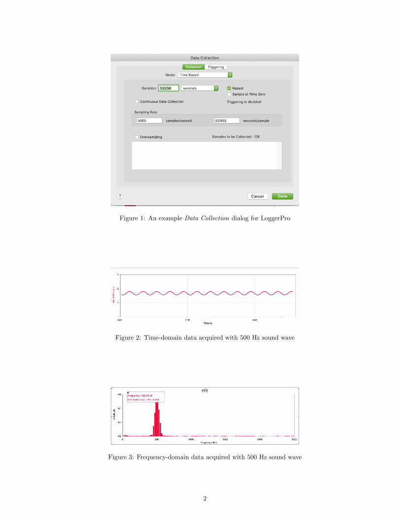
Figure 1: An example Data Collection dialog for LoggerPro

Figure 2: Time-domain data acquired with 500 Hz sound wave

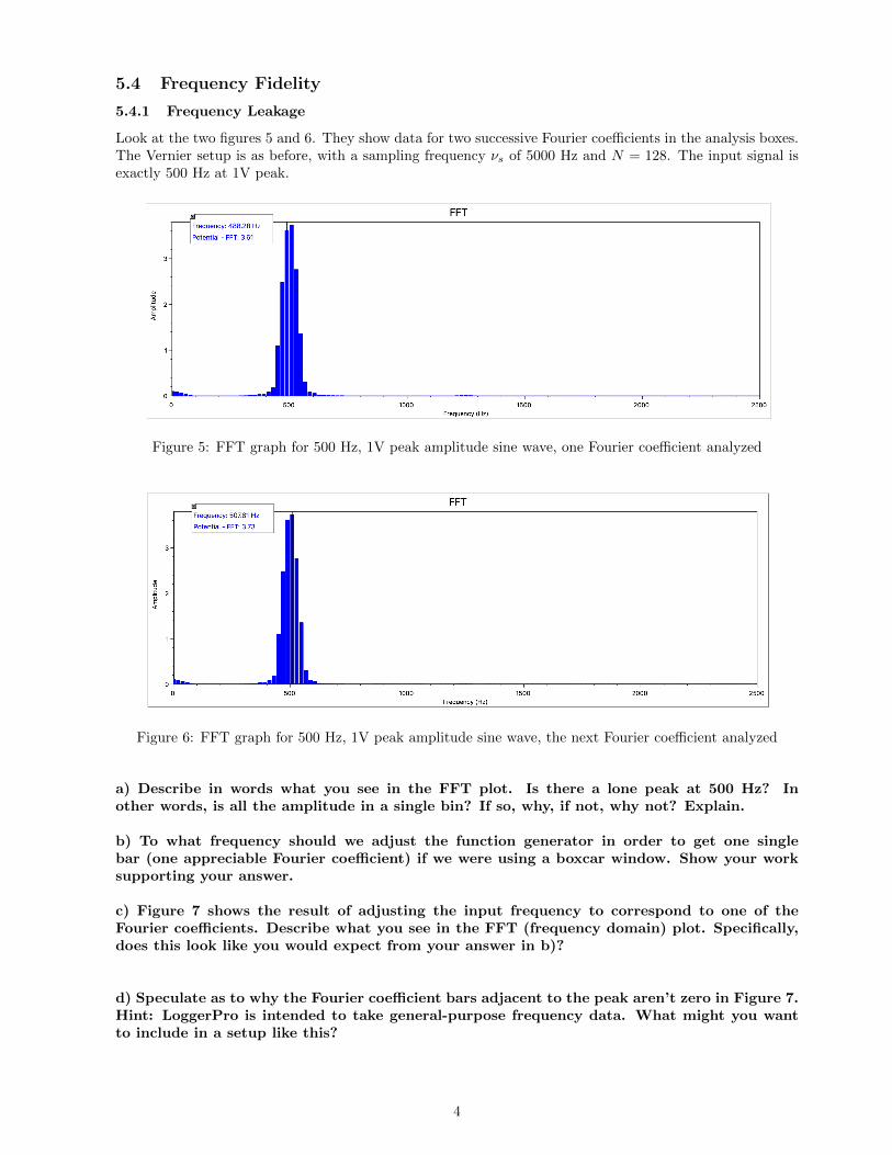
Figure 3: Frequency-domain data acquired with 500 Hz sound wave

2

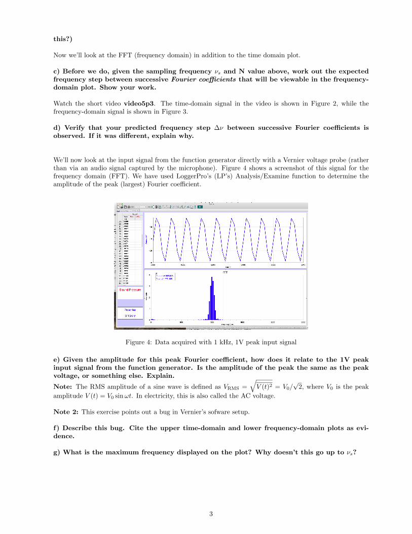
this?)

Now we’ll look at the FFT (frequency domain) in addition to the time domain plot.

c) Before we do, given the sampling frequency νs and N value above, work out the expectedfrequency step between successive Fourier coefficients that will be viewable in the frequency-domain plot. Show your work.

Watch the short video video5p3. The time-domain signal in the video is shown in Figure 2, while thefrequency-domain signal is shown in Figure 3.

d) Verify that your predicted frequency step ∆ν between successive Fourier coefficients isobserved. If it was different, explain why.

We’ll now look at the input signal from the function generator directly with a Vernier voltage probe (ratherthan via an audio signal captured by the microphone). Figure 4 shows a screenshot of this signal for thefrequency domain (FFT). We have used LoggerPro’s (LP’s) Analysis/Examine function to determine theamplitude of the peak (largest) Fourier coefficient.

Figure 4: Data acquired with 1 kHz, 1V peak input signal

e) Given the amplitude for this peak Fourier coefficient, how does it relate to the 1V peakinput signal from the function generator. Is the amplitude of the peak the same as the peakvoltage, or something else. Explain.

Note: The RMS amplitude of a sine wave is defined as VRMS =

√V (t)2 = V0/

√2, where V0 is the peak

amplitude V (t) = V0 sinωt. In electricity, this is also called the AC voltage.

Note 2: This exercise points out a bug in Vernier’s sofware setup.

f) Describe this bug. Cite the upper time-domain and lower frequency-domain plots as evi-dence.

g) What is the maximum frequency displayed on the plot? Why doesn’t this go up to νs?

3

5.4 Frequency Fidelity

5.4.1 Frequency Leakage

Look at the two figures 5 and 6. They show data for two successive Fourier coefficients in the analysis boxes.The Vernier setup is as before, with a sampling frequency νs of 5000 Hz and N = 128. The input signal isexactly 500 Hz at 1V peak.

Figure 5: FFT graph for 500 Hz, 1V peak amplitude sine wave, one Fourier coefficient analyzed

Figure 6: FFT graph for 500 Hz, 1V peak amplitude sine wave, the next Fourier coefficient analyzed

a) Describe in words what you see in the FFT plot. Is there a lone peak at 500 Hz? Inother words, is all the amplitude in a single bin? If so, why, if not, why not? Explain.

b) To what frequency should we adjust the function generator in order to get one singlebar (one appreciable Fourier coefficient) if we were using a boxcar window. Show your worksupporting your answer.

c) Figure 7 shows the result of adjusting the input frequency to correspond to one of theFourier coefficients. Describe what you see in the FFT (frequency domain) plot. Specifically,does this look like you would expect from your answer in b)?

d) Speculate as to why the Fourier coefficient bars adjacent to the peak aren’t zero in Figure 7.Hint: LoggerPro is intended to take general-purpose frequency data. What might you wantto include in a setup like this?

4

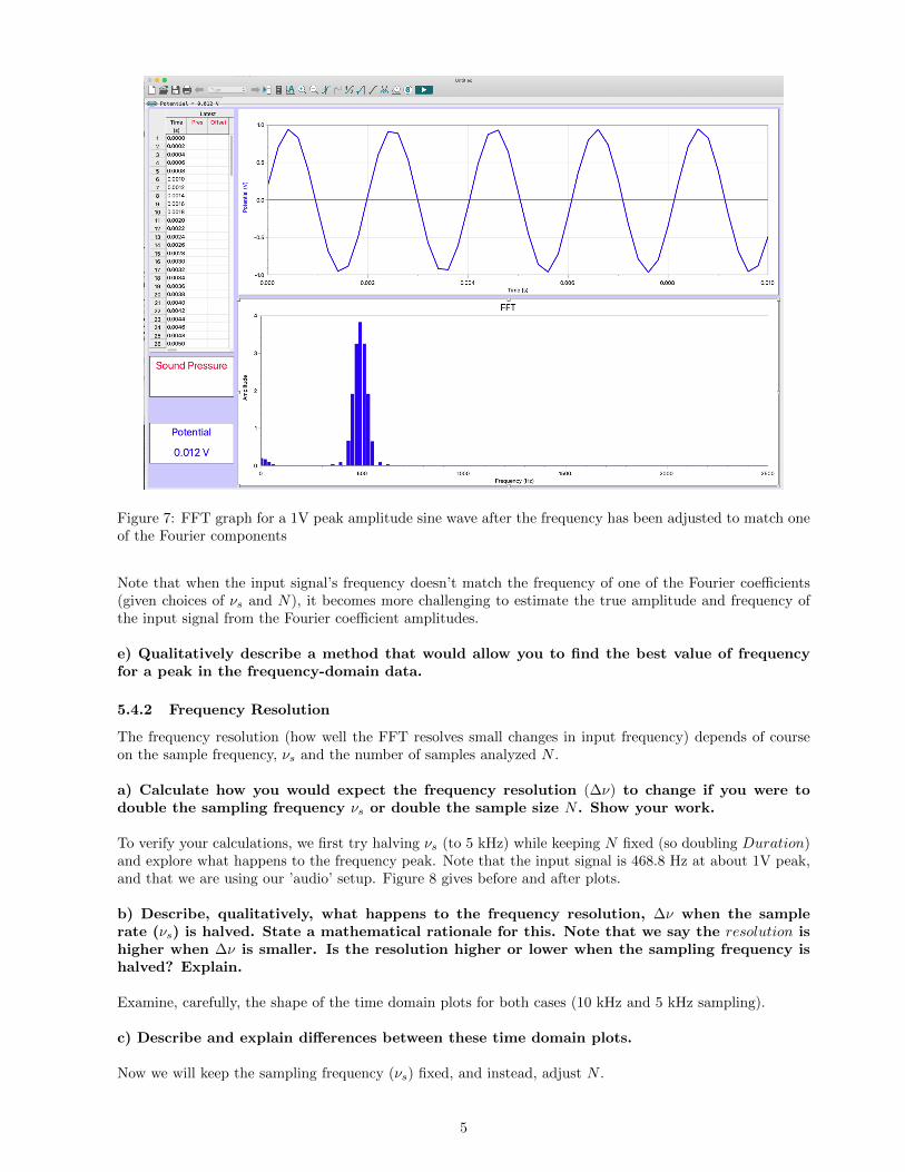
Figure 7: FFT graph for a 1V peak amplitude sine wave after the frequency has been adjusted to match oneof the Fourier components

Note that when the input signal’s frequency doesn’t match the frequency of one of the Fourier coefficients(given choices of νs and N), it becomes more challenging to estimate the true amplitude and frequency ofthe input signal from the Fourier coefficient amplitudes.

e) Qualitatively describe a method that would allow you to find the best value of frequencyfor a peak in the frequency-domain data.

5.4.2 Frequency Resolution

The frequency resolution (how well the FFT resolves small changes in input frequency) depends of courseon the sample frequency, νs and the number of samples analyzed N .

a) Calculate how you would expect the frequency resolution (∆ν) to change if you were todouble the sampling frequency νs or double the sample size N . Show your work.

To verify your calculations, we first try halving νs (to 5 kHz) while keeping N fixed (so doubling Duration)and explore what happens to the frequency peak. Note that the input signal is 468.8 Hz at about 1V peak,and that we are using our ’audio’ setup. Figure 8 gives before and after plots.

b) Describe, qualitatively, what happens to the frequency resolution, ∆ν when the samplerate (νs) is halved. State a mathematical rationale for this. Note that we say the resolution ishigher when ∆ν is smaller. Is the resolution higher or lower when the sampling frequency ishalved? Explain.

Examine, carefully, the shape of the time domain plots for both cases (10 kHz and 5 kHz sampling).

c) Describe and explain differences between these time domain plots.

Now we will keep the sampling frequency (νs) fixed, and instead, adjust N .

5

Figure 8: The same signal sampled at 10kHz (red) and 5kHz (blue) with N=100 in both cases

d) Given your ”mathematical rationale” from above, what will happen when you double Nwith constant νs? Explain.

To verify your calculations, we’ve set νs to 5 kHz and started with N=100. Saving these plots, we thendoubled N, and then doubled N again,. while keeping νs fixed. Note that the input signal is 468.8 Hz atabout 1V peak, and that we are using our ‘audio’ setup. Figure 9 gives before and after plots.

Figure 9: The same signal sampled at 5 kHz for N’s of 100 (blue), 200 (red) and 400 (green)

e) Did doubling N while keeping the sampling frequency fixed have the effect you predicted?Explain. What happens to the frequency resolution as N is increased. Why?

f) Can you think of a case where increasing N alone without increasing νs wouldn’t actu-ally lead to any improvement? What would happen if you had a transient, non-periodic signallike a short single pulse? What would the effective “sample time” be in this case?

6

5.5 Aliasing

Aliasing is an interesting phenomenon, for example, causing wagon wheels to appear to move counterclock-wise in old westerns. We will explore aliasing by watching a pre-made video. Look at the short videovideo5p5. Write down the values for input (function generator) frequency and amplitude and those givenfor particular Fourier coefficients that are pointed out as the video progresses. as the video progresses. Thevideo begins with the sampling frequency set to 1 kHz and N = 100.

Questions:a) As we scanned the input frequency of the function generator up to the Nyquist frequencyfor this setup, what did you see? Particularly, what did you see when the input frequency wasset to 200 Hz?

b) What happened as the input frequency approached the Nyquist limit?

c) Describe what happened in the frequency plot (FFT) after the input frequency surpassedthe Nyquist limit and approached the sampling frequency. I asked a question about the ap-parent 400 Hz signal observed after the frequency surpassed the Nyquist limit in the video,answer it here.

d) Describe what happened after the input frequency exceeded the sampling frequency at1 kHz.

e) Finally, does a pattern become apparent? If the input frequency is 750 Hz, what would theexpected observed (and aliased) frequency be? Explain.

5.6 Frequency Overtones

Recall that when using Fourier synthesis in your homework (5) you could construct standard waveforms,for example triangle and square waves, by adding overtones, defined as integer multiples of some fundamentalfrequency, together. The trick was in determining whether odd, even or both integers (e.g. 3, 5, 7 times thefundamental) were needed. Another important piece of information is how the amplitudes of the overtonescompared to that of the fundamental (the latter being the frequency input by the function generator).Aside: for an excellent simulator for the construction of waveforms using Fourier series, seethis excellent web site, particularly: http://www.falstad.com/fourier/

To explore frequency overtones, we’ll set the sampling frequency (νs) to 1 kHz and N = 1000. We be-gin by setting input frequency at 200 Hz with 1V-P amplitude. Look at the short video video5p6audio.Here we explore the differences in observed waveforms given stated changes in the input signal between sine,triangle, and square waves, initially using our ‘audio’ setup.

Questions:a) How faithful is the representation of the sine wave given our (audio: speaker + microphone)system for monitoring the input signal? Cite evidence observed in the video.

b) Does the triangle wave look like what you expected? Explain.

c) The square wave observed with our system does not look much like a square wave. Specu-late as to why that might be.

Look at another short video video5p6voltage. Here we do the same exploration of waveforms, butusing a voltage probe to monitor input signals.

d) is the observed waveform of the input square wave improved using the new setup, a voltageprobe? Explain why this might be so.

Now to analyze these signals. We start with the same parameters as above (for the videos). In Figure 10we show both time- and frequency-domain plots for a 200 Hz sine wave (amplitude ∼ 1 V peak) using the

7

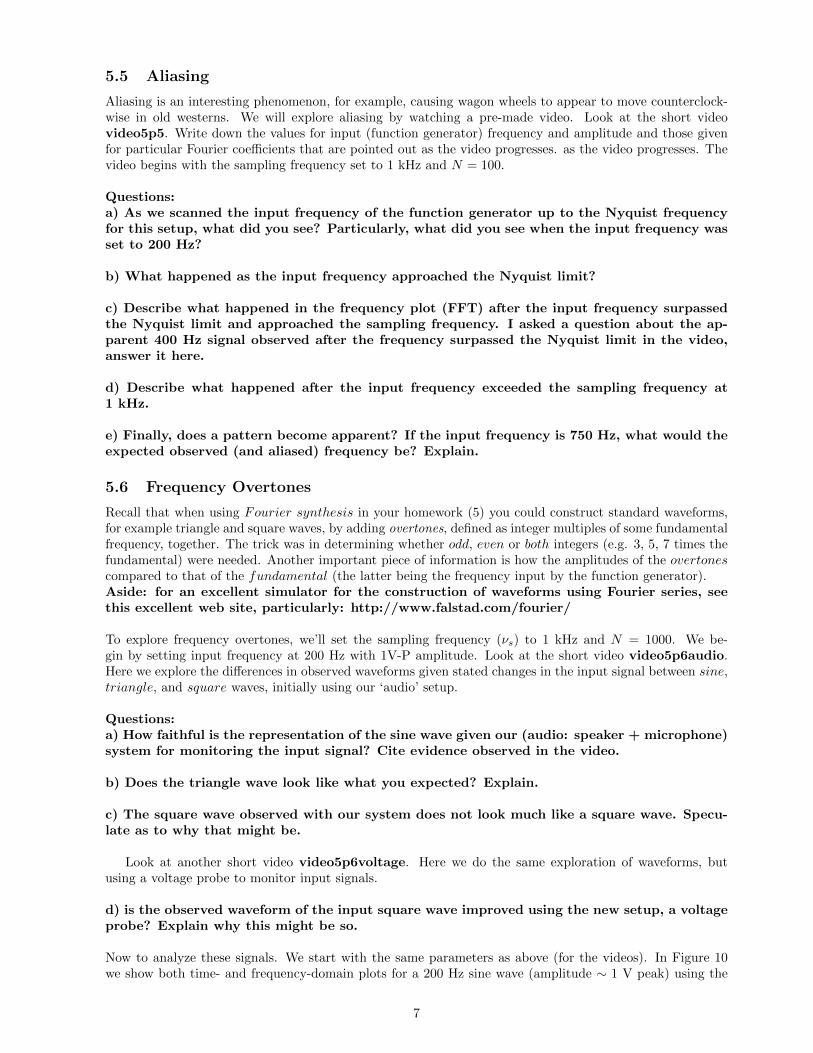
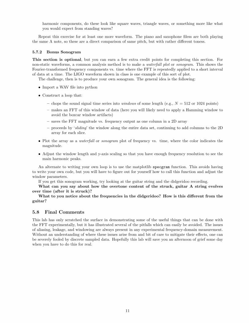
Voltage Probe. In Figures 11-12 we show the same type of plot for a triangle wave with Fourier peaks pickedat 200 Hz and 400 Hz. In Figures 13-15 we do the same for the square wave, but pick also the peak Fouriercoefficient near 0 Hz as well.

Figure 10: 200 Hz, 1V-P sine wave signal analyzed near 200 Hz.

Figure 11: 200 Hz, 1V-P triangle wave signal analyzed near 200 Hz.

More Questions:

e) What are the expected overtone frequencies for the triangle wave (compared to that ofthe fundamental frequency of 200 Hz)? Find a mathematical expression for these and state ithere (you can look this up).

f) What about the square wave? Note, you calculated this in HW5.

g) What has happened to the overtones that have frequencies above the Nyquist limit? Ex-plain.

h) Does it seem like a good idea to have the Nyquist frequency be an integer multiple ofyour primary frequency?

8

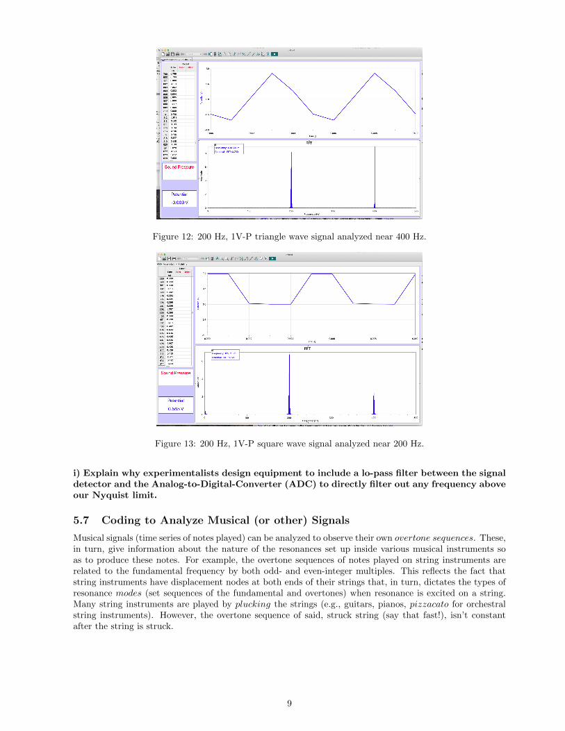
Figure 12: 200 Hz, 1V-P triangle wave signal analyzed near 400 Hz.

Figure 13: 200 Hz, 1V-P square wave signal analyzed near 200 Hz.

i) Explain why experimentalists design equipment to include a lo-pass filter between the signaldetector and the Analog-to-Digital-Converter (ADC) to directly filter out any frequency aboveour Nyquist limit.

5.7 Coding to Analyze Musical (or other) Signals

Musical signals (time series of notes played) can be analyzed to observe their own overtone sequences. These,in turn, give information about the nature of the resonances set up inside various musical instruments soas to produce these notes. For example, the overtone sequences of notes played on string instruments arerelated to the fundamental frequency by both odd- and even-integer multiples. This reflects the fact thatstring instruments have displacement nodes at both ends of their strings that, in turn, dictates the types ofresonance modes (set sequences of the fundamental and overtones) when resonance is excited on a string.Many string instruments are played by plucking the strings (e.g., guitars, pianos, pizzacato for orchestralstring instruments). However, the overtone sequence of said, struck string (say that fast!), isn’t constantafter the string is struck.

9

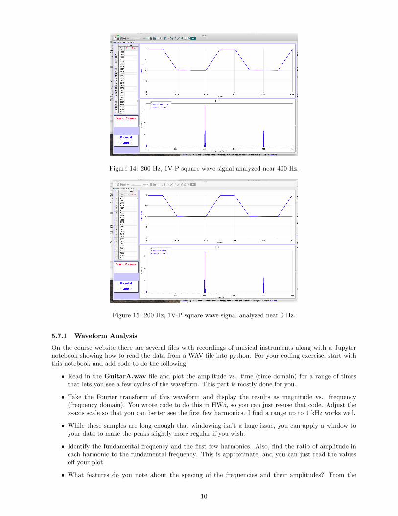
Figure 14: 200 Hz, 1V-P square wave signal analyzed near 400 Hz.

Figure 15: 200 Hz, 1V-P square wave signal analyzed near 0 Hz.

5.7.1 Waveform Analysis

On the course website there are several files with recordings of musical instruments along with a Jupyternotebook showing how to read the data from a WAV file into python. For your coding exercise, start withthis notebook and add code to do the following:

• Read in the GuitarA.wav file and plot the amplitude vs. time (time domain) for a range of timesthat lets you see a few cycles of the waveform. This part is mostly done for you.

• Take the Fourier transform of this waveform and display the results as magnitude vs. frequency(frequency domain). You wrote code to do this in HW5, so you can just re-use that code. Adjust thex-axis scale so that you can better see the first few harmonics. I find a range up to 1 kHz works well.

• While these samples are long enough that windowing isn’t a huge issue, you can apply a window toyour data to make the peaks slightly more regular if you wish.

• Identify the fundamental frequency and the first few harmonics. Also, find the ratio of amplitude ineach harmonic to the fundamental frequency. This is approximate, and you can just read the valuesoff your plot.

• What features do you note about the spacing of the frequencies and their amplitudes? From the

10

harmonic components, do these look like square waves, triangle waves, or something more like whatyou would expect from standing waves?

Repeat this exercise for at least one more waveform. The piano and saxophone filess are both playingthe same A note, so these are a direct comparison of same pitch, but with rather different toness.

5.7.2 Bonus Sonogram

This section is optional, but you can earn a few extra credit points for completing this section. Fornon-static waveforms, a common analysis method is to make a waterfall plot or sonogram. This shows theFourier-transformed frequency components vs. time where the FFT is repeatedly applied to a short intervalof data at a time. The LIGO waveform shown in class is one example of this sort of plot.

The challenge, then is to produce your own sonogram. The general idea is the following:

• Import a WAV file into python

• Construct a loop that:

– chops the sound signal time series into windows of some length (e.g., N = 512 or 1024 points)

– makes an FFT of this window of data (here you will likely need to apply a Hamming window toavoid the boxcar window artifacts)

– saves the FFT magnitude vs. frequency output as one column in a 2D array

– proceeds by ‘sliding’ the window along the entire data set, continuing to add columns to the 2Darray for each slice.

• Plot the array as a waterfall or sonogram plot of frequency vs. time, where the color indicates themagnitude.

• Adjust the window length and y-axis scaling so that you have enough frequency resolution to see themain harmonic peaks.

An alternate to writing your own loop is to use the matplotlib specgram function. This avoids havingto write your own code, but you will have to figure out for yourself how to call this function and adjust thewindow parameters.

If you get this sonogram working, try looking at the guitar string and the didgeridoo recording.What can you say about how the overtone content of the struck, guitar A string evolves

over time (after it is struck)?What to you notice about the frequencies in the didgeridoo? How is this different from the

guitar?

5.8 Final Comments

This lab has only scratched the surface in demonstrating some of the useful things that can be done withthe FFT experimentally, but it has illustrated several of the pitfalls which can easily be avoided. The issuesof aliasing, leakage, and windowing are always present in any experimental frequency-domain measurement.Without an understanding of where these issues arise from and bit of care to mitigate their effects, one canbe severely fooled by discrete sampled data. Hopefully this lab will save you an afternoon of grief some daywhen you have to do this for real.

11