ISSN 2347-3487

1135 | P a g e N o v e m b e r 1 4 , 2 0 1 4

Physics of Climate Change: Harmonic and exponential processes from in situ ocean time series observations show rapid asymmetric warming.

J. Brian Matthews and J. B. Robin Matthews Drs J B and J B R Matthews, Douglas, Isle of Man, British Isles

drs-matthews@manx.net Dept of Physics and Physical Oceanography, Memorial University of Newfoundland, St Johns, NL, Canada.

ABSTRACT Analyses of rare ocean timeseries in the top few meters show logarithmic and exponential processes control anthropogenic global warming (AGW) of which 93% is in the oceans. Processes result in asymmetric heat capture in the North and South tropical Pacific. A new Lagrangian paradigm established a global ocean surface freshwater and heat conveyor. Climate research wrongly assumed atmospheric pan-evaporation at sea as over land, a 10m well-mixed surface layer, and ignored that seawater density depends on both salinity and temperature. In situ observations show two different heat-capture and evaporation regimes exist dependent on surface temperature and salinity. The tropical North Pacific is temperature dominant, but other tropical oceans are salinity dependent. Incident solar radiation is cyclical and greenhouse gas (GHG) heat-capture is exponential and cumulative.

The rate of GHG-caused climate change is disputed and not quantitatively evaluated. A target limit of total atmospheric temperature rise of <2°C is forecast from 30 to 100 years, or not at all. It is based on doubling of total carbon emissions from the long-term stable 280ppm to 560ppm.

Here we show solar cycles became less significant compared to exponentially rising GHG heat capture after the 1957 solar maximum Keeling Point. The doubling time for exponential warming is ~20 years at -0.030-0.037°Cyr

-1. GHG

warming of is now ~1°C. At present rates, exponential increases add +1°C in ~20yr, +2°C in ~40yr, +4°C in ~60yr, 8°C in ~80yr above existing levels. Post-1957 carbon dioxide concentration GHG forcing is also doubling in ~20yrs at 0.0268ppmyr

-1. It rose from 1957-1976 by 17.1ppm, and from 1977-1996 by 34.4ppm. A further doubling by 68.4ppm

would bring total emissions to 435ppm by 2017. It exceeded 400ppm in 2014. Carbon dioxide accounts for three quarters of the GHGs. Of the others, methane and HCFCs already may be out of control.

Ocean surface temperature anomalies are close to the proposed +2°C limit. Century-long records in 5yr anomalies in the North Pacific show peaks of +1.6°C at the surface in 1995, and +1.3°C at 5m. North Atlantic peaks were +1.12°C in 2005 consistent Arctic freshwater fluxes. Central England temperature (CET) 5-yr peak air anomaly was +1.3°C in 2004 consistent with a rapid response in air due to low heat capacity. 2014 is a record year for temperatures and carbon dioxide total emissions.

Pacific sub-surface water warmed faster than at the surface. The freshwater lid that thickened limits heat loss. The annual cycled heat increased by 3MJm

-3 over 100yr at Isle of Man, by 1MJm

-3 over 88yr at Scripps Pier surface, and by 4MJm

-3

over 78yr at 5m. The post-1986 annual Arctic ice heat cycle decreased by -2,633MJm-3

. Before 1986 tropical heat was offset against polar melt and runoff at Port Erin. After, exponentially decreasing Arctic ice reduced thickness from 1.9m-1.4m but surface area decreased more slowly than volume. This accounts for the observed increased polar ice formation surface layer at <4°C and <24.7‰ in Polar Seas.

Process rate differences derive from the ~3000x greater heat capacity of water to air (3.9x106: 1.3x10

3Jm

-3°C

-1), and the

~1000x greater density (1023: 1.2 kgm-3

). The top 10m operates on decadal timescales. Heat is trapped under a surface freshwater lid. Sub-surface heat penetration is on centennial and millennial timescales. It takes ~250yr since the industrial revolution for two thirds of AGW to reach ~300m. The flux of heat and freshwater through Bering Strait doubled from 2000-2007. It accounts for one third of surface layer meltwater fluxes into the Labrador Current at a rate of ~0.85Sv. The Atlantic inflow of ~8.5Sv accounts for the remainder with an Arctic residence time above the halocline of ~2.5-6 years. This is consistent with the three and half years at the Isle of Man between the seasonal 1959 October high and the record 1963 February low. The Equatorial Undercurrent (EUC) compensates the land-locked Pacific surface layer bringing warm salty water under the Panama freshwater warm pool.

We suggest the doubled warming of the North Pacific led to a quasi-permanent loop in the sub-polar jet stream. Warm air driven over Beringia displaces cold polar air to the North American mid-west. This resulted in continuous extreme weather over central North America in 2013-2014. In the southern hemisphere high evaporation resulted in record precipitation that temporarily reduced sealevels in 2012. Changed ocean ecological systems have been reported. The Pacific warming led to enhanced hurricane frequency from the Panama warm pool as well as super typhoons in the western North Pacific. North America now has hurricane seasons on both coasts and Hawaii, and extreme weather year-round. The warm tropical Gulf Stream/Columbus and Viking polar gyre boundary shifted northwards in the mid 1990s. It shows at Port Erin in a 1990s high seasonal salinity. After the millennium until records ceased in 2006, a seasonal freshwater layer was observed, consistent with a thickened freshwater lid over high salinity tropical water. Most long-term continuous records in the top 5m ceased in the mid 1980s. We suggest the ocean layer is warming exponentially and freshening.

Global Ocean warming is known as the tragedy of the commons. Solutions include individual ownership and responsibility through, for example, managing fisheries by individual transferable quotas. The Zero Marginal Cost Society, the adopted goal of the UN and world leaders, requires a painful paradigm transition from a Newtonian to a Thermodynamic stable

ISSN 2347-3487

1136 | P a g e N o v e m b e r 1 4 , 2 0 1 4

sustainable no-growth system. The option of population control cannot succeed in time. The EU leaders‟ commitment to reduce GHG requires reduction of ~8.9ppmyr

-1 for the next 16 years to 2030. It is the only viable solution. However, it

requires binding global commitments to a new paradigm conserving thermodynamic principles of maximized use of Earth‟s natural resources. In economic terms this means narrowing the gap between rich and poor and deflation to stability of zero growth. Without immediate implementation, we suggest the exponential growth will continue, and may already be beyond control.

Our work needs further experimental verification in the near-surface ocean on short space and timescales especially along meridional transects. The Isle of Man and Galapagos Islands, with both tropical and polar water, are ideal to establish constant monitoring of temperature, salinity, pH currents, and sealevel at 1, 2, 3, 5, 7, and 10m along with standard Met observations including pan evaporation and precipitation on purpose-build piers. Ocean-side measurements allow data to be collected efficiently with calibrated instruments if part of well-funded independent University–level research. This way a new generation of young scientists well trained in classical physics can establish the scientific truth through experimental verification. This could proceed as part of a crash program to develop alternative natural energy resources based on geothermal heat exchange, pumped storage, tides and tidal currents, solar, winds and renewable carbon until nuclear fusion comes online as the ultimate solution.

Indexing terms/Keywords

2°C AGW air temperature global limit; 20th century solar maximum; 20-year doubling time AGW; 400yr solar maximum;

Abrupt Climate Shifts; Adaptive research management; AGW counter measures; AGW decadal exponential surface change; AGW doubling time 20 years; AGW five meter doubling time 22 years; AGW great underestimation; AGW ice age timescales deep ocean; AGW North Atlantic 1.1°C; AGW North Pacific 5m 1.3°C; AGW North Pacific surface 1.6°C; AGW ocean surface layer monitoring; AGW surface doubling time 18 years; Aleut Gyre; All but Pacific Ocean Salt control heat capture; Antarctic ice melt; Anthropogenic global warming (AGW); Arctic icemelt; Arctic water residence time; Asymmetric heat trap North Pacific to other tropical oceans; Bad Science at Sea Surface; Basal icemelt buffer; Basal icemelt moderator for AGW; Carbon dioxide doubling time 20 years; Carbon dioxide EU Limit; Centennial ocean heat; Centennial surface air-sea exchange; Central England air temperature (CET); Century-long seasurface timeseries; Challenger temperatures; Circumpolar Current; Claudius-Clapeyron sea evaporation; Climate Change Atlantic Ocean; Climate Change Europe v North America; Climate Change North Pacific v South Pacific; Climate Change Physics; Coincidence v Correlation; Columbus Gyre; Correlation without verification is Coincidence; Counter-rotating ocean cells; Cumulative exponential AGW; Cyclical AGW; Daily ocean heat; Daily surface air-sea exchange; Data analysis; Decadal ocean heat; Decadal surface air-sea exchange; Ebbesmeyer-Ingraham-Carmack ocean surface circulation; Ekman and Log Wind-driven currents; Equatorial Undercurrent (EUC) Panama freshwater warm pool circulation; European v North American Climate Change; Evaporation Measurement; Experimental ground truth; Exponential AGW; Exponential solar heat trap; Extreme precipitation 2012; Extreme temperatures 2014; Extreme weather 2013-2014; Extreme weather and jet stream; Fisheries exponential crash; Fisheries ocean acidification; Fishery management; Flood and precipitation extremes; Freshening ocean surface; Freshwater freezing at temperature <2°C and salinity <24.7‰; Global warming and Ocean Tides; Global warming in ocean surface; Global warming underestimated; Global warming without lull; Greenhouse gas (GHG) ocean heat capture; Haiyan super typhoon; Harmonic solar radiation; HCFC Greenhouse gas; Heyerdahl Gyre; Hourly ocean heat; Hourly surface air-sea exchange; Hurricane Category 5; Ice age surface air-sea exchange; Individual transferable fishing quotas; Innovative Science; IPCC 2°C AGW global limit; IPCC Carbon Limit global limit; Isell hurricane; Islip NY rainfall extreme; Jet Stream loop; Keeling Point 1957; Lagrangian coherent water mass slabs or snarks; Lagrangian surface and heat transport system; Last Glacial Maximum change; Latent heat asymmetric heat trap; Local and community solutions; Log Inverse of Exponential; Lull in global warming; Majid Gyre; Marine air temperature (MAT); Maverick Science; Melville Gyre; Meridional Overturning Tropical Cells; Methane AGW; Millennial ocean heat; Millennial surface air-sea exchange; Millennium Climate Shift; Monthly surface air-sea exchange; Newtonian Economics; North Pacific asymmetric warming; North Pacific Climate shift; North Pacific surface heat and freshwater trap; North Pacific thermal controls of heat capture; Nuclear fusion; Ocean Acidification; Ocean Surface Conveyor; Ocean Surface Freshening; Ocean Surface Warming; Pan evaporation; Panama freshwater warm pool; Paradigm shift Newtonian to Thermodynamic; Peer review; Penguin Gyre; Physics of Climate Change; Polar Amplification; Polar Bear Gyre; Post-1957 AGW; Post-1976 AGW; Post-1986 AGW; Post-millennial AGW; Raindrop shape; Rainfall extreme; Regime shift since Last Glacial Maximum (LGM); Scientific Method Geophysics experimental ground truth; Sea evaporation; Sea Surface temperature (SST); Snarks or Lagrangian coherent water mass slabs; Snarks; Solutions to tragedy of the commons; ; Storkerson Gyre; Substitution of SST for MAT; Super typhoon; Surface Frontal jets; Surface warming ~0.038°Cyr

-1;

Thermodynamics of Climate Change; Tidal pumping; Tides and climate change; Tragedy of the Commons; Tropical Freshwater Warm Pools; Tropical North Pacific Ocean heat trap; Tropical South Pacific Ocean high evaporation; Turtle Gyre; UN 2°C AGW global limit; UN Carbon dioxide Limit global limit; UN Montreal Protocol HCFC limit; Viking Gyre; Warming lull due to ice melt; Warming ocean surface; Wrong 10m mixed-layer theories; Wrong Pan evaporation at sea assumption; Zero Marginal Cost Society;

ISSN 2347-3487

1137 | P a g e N o v e m b e r 1 4 , 2 0 1 4

Academic Discipline And Sub-Disciplines

Physics of top of ocean; Exponential and cyclical change; Climate change physics; experimental in situ ocean science; anthropogenic global warming (AGW); solar radiation forcing; Greenhouse gas forcing; exponential warming; climate shifts; Solutions to global warming and tragedy of the commons.

SUBJECT CLASSIFICATION

Physical oceanography; Air-Sea interaction: Climate Change; Greenhouse Gas Heat Trap

TYPE (METHOD/APPROACH)

Experimental fieldwork; analysis and review

Council for Innovative Research

Peer Review Research Publishing System

Journal: JOURNAL OF ADVANCES IN PHYSICS

Vol. 6, No. 2

www.cirjap.com, japeditor@gmail.com

ISSN 2347-3487

1138 | P a g e N o v e m b e r 1 4 , 2 0 1 4

1. INTRODUCTION

Climate studies hitherto have concentrated on the atmosphere. Recent research suggests that future studies must concentrate on the top few meters of oceans to understand climate change [1][2]. Anthropogenic global warming (AGW) for the past 250 years can be explained through the interaction of exponential and solar harmonic processes in the top 2m of oceans. Solar radiation in the top of oceans and seas is crucial to all processes. Oceans occupy over 70% of Earth‟s surface including the 8.5% in shelf and coastal seas up to depths of 200m. Ninety nine percent of biological living space is in the 3-dimensional oceans compared to the mostly 2-dimensional colonized surface over land [3]. Life evolved in the oceans with the buoyant surface layer playing a vital part in biological diversity, evolution, hybridogenesis and transport [4].

1.1 Physics Chemistry and General Biology

The physics, chemistry and general biology were well defined in 1942 in a single classic volume by Sverdrup, Johnson and Fleming (1942) [5]. The concept of fetch, the logarithmic buildup of surface waves and currents over time and distance was introduced. Ocean circulation dependent density, a function of temperature and salinity, and density- stratified oceans was set out. The freezing of water from the surface at maximum density <4°C and <24.7‰ was demonstrated (Figure 1).

1.2 Ocean and estuaries

The post-war expansion of oceanography saw the separation of oceanography from meteorology as well as other branches of ocean science. Estuarine, coastal and shelf seas studies gradually separated from open ocean research that concentrated on deep oceans. Estuaries were defined by boundary layers and by stratification in the 1960s with a positive estuary having a freshwater runoff and precipitation layer over colder salty seawater [6]. A negative estuary was defined as having evaporation exceeding precipitation. The North Pacific was known to be a positive estuary from this time [1].

Fig 1: Clausius-Clapeyron evaporation and seawater density T-S diagram.

We became interested in the impacts of ocean surface on climate change from our investigation of discrepancies between sea surface temperature datasets [7][8]. We made the first in situ measurement of evaporation in the mid-Pacific between Tahiti and Hawaii. We reported that the boundary between the North Pacific freshwater stratified thermohaline circulation and Carmack‟s salt dominant circulation was determined by salinity greater than 35‰ [1][2][9]. In the central tropical Pacific this was at temperatures >28°C and >36‰ in northern mid-summer 2008. Our findings are summarized in Figure 1.

1.3 Pan evaporation versus Clausius Clapeyron exponential evaporation

We found that climatologists used sea surface temperatures (SST) from unknown depths, assumed temperatures were uniform in the top 10m, and that pan evaporation applied to the sea surface [8]. Further analysis of in situ ocean data confirmed that evaporation was dependent only on the exponential Clausius Clapeyron relationship (Figure 1) [1]. This was not previously reported. Moreover, reliable SSTs averaged over the top 100m were only available from the 1990s. Their distribution, quantity and quality tapering to almost zero back to 1955 when routine SST sampling began [7]. Salinity and temperature in the top 10m were never routine meteorological data.

Meteorologists have good long continuous records of weather measurements over land. The UK has detailed rainfall data as well as standard meteorological temperatures, pressures and winds. These were often collected by keen well-informed amateurs. The longest continuous daily weather records are the Central England Temperatures (CET) from 1659 [2]. Wet and dry bulb temperatures, pressure, 10m winds, rain gauge and pan evaporation were routinely collected. Evaporation pans are ~1m diameter shallow trays that are automatically topped up with measured volumes. Evaporation is computed as the top-up volume less the measured precipitation. It was found to depend on relative humidity and windspeed because

ISSN 2347-3487

1139 | P a g e N o v e m b e r 1 4 , 2 0 1 4

water could only come from the open pan and not through the land surface. It is of great significance to agricultural interests especially those remote from ocean weather.

The UK Met Office extended data collection to lighthouses, weatherships and marine stations in late 19th century to

facilitate shipping forecasts [7][2]. Rainfall and evaporation was not measured at these stations. However, sea surface temperatures, some salinity, and other measurements were made on weatherships, lighthouses, and at marine stations. Climatologists subsequently used the temperature timeseries data to investigate rapid climate change from greenhouse gas infrared heat trap.

Our analysis revealed the significance of the exponential trend of evaporation dependent on temperature. Evaporation increases by ~7 percent per °C while precipitation is reported to increase by 2-3 percent [1]. The exponential trends to infinity at the boiling point ~100°C. The inverse log end of the exponential trends to zero or a constant. Moreover, evaporation and trapped incident solar heat was found to be asymmetrically dependent on salinity and temperature that determine density (Figure 1). The salinity dependence of South Pacific hypersaline (>35‰) caused heat extraction by evaporation to be double that of the heat of evaporation and precipitation of the North Pacific. However, the thermal circulation of the North Pacific sequestered twice the heat of the hypersaline ocean surface layer. Previous climate work concentrated solely on temperature as heat proxy without regard to the fact that heat is carried in the water mass with density a function of both temperature and salinity.

1.4 Surface layer circulation

Air-sea interaction in the sea surface buoyant layer is the most securely verified of all ocean processes. The Ebbesmeyer-Ingraham OSCURS wind-driven transport model of Lagrangian coherent water masses is a well-verified surface circulation system [10][11]. It comprises eleven interconnected counter-rotating convergent-divergent gyres, and eight garbage patches (Figure 2) [1]. Forecasts and hindcasts of surface water transport derive from daily surface air pressure fields.

Fig 2: Ebbesmeyer –Ingraham verified interconnected counter-rotating divergent (blue)/convergent (red) Lagrangian coherent surface gyres on an equal area projection.

Surface wind drift coefficients were verified for passive plankton-carrying watermasses and surface drifters, self-propelled drifters. Those with appreciable sail areas are enhanced by 30-50%. A WWII aircraft plastic identity tag found in an Albatross chick on Midway Island was found to have circulated in the Aleut Gyre for 60 years (https://www.youtube.com/watch?v=QHJK5ISKR2Q last accessed 12 September 2014). Flotsam from Malaysia Airline flight MH370 lost on 8 March 2014 is likely to be found in the almost unknown Majid gyre (Figure 2). High windage flotsam, such as Portuguese man-of-war jellyfish and debris from the 2011 Fukushima Japan tsunami, travel at higher than average Eulerian speeds and are calibrated into the OSCURS model. This gyre system was found to be the basis of asymmetric global warming through transport of freshwater and heat from the tropics to the poles [1][9]. Brine from tropical evaporation and polar freezing processes are the sources of ocean benthic waters.

Analysis of the century-long sea surface records at Port Erin Marine Biological Station (PEMBS) showed both tropical water of salinity up to 36‰, and polar water as low as 31‰ are coherent and stable at the same density (Figure 1). They balanced different temperatures and salinities at the same density [2]. A front at 11°N in the north Pacific had ~2.5°C temperature range over 12km [1]. There were no geostrophic currents across the front because the density anomaly of ~23 balanced the salinity/temperature differences. Standard seawater is defined as salinity 35‰, and standard density 1023kgm

-3 at 25°C. Similar fronts in both the north Pacific and north Atlantic are found at ~10°C. They form a wall against

divergent/convergent gyres: in the Pacific between the Aleut/Turtle gyres and in the Atlantic between the Viking/Columbus gyre and Gulf Stream (Figure 2) [12][1].

1.5 Coherent Lagrangian water masses, snarks or slabs

Coherent water masses are known to persist for long periods in stratified estuaries and oceans. Lagrangian coherent water masses were called snarks, slabs or parcels when first found from a detailed timeseries of salinity-temperature-depth (STD) system [13]. It used a fine 3D grid at 1km×1km×2m intervals over an 18km×60m fjord region. The ocean surface is occupied by these snarks or slabs and is not the uniform mass seen from space [10]. Meridional tropical cells (MTCs) form long coherent surface water masses from the daily solar warming/cooling process (Figure 3) [14]. We

ISSN 2347-3487

1140 | P a g e N o v e m b e r 1 4 , 2 0 1 4

discussed the evidence for the interaction of an extended set of MTCs with equatorial upwelling and countercurrents to derive the schematic in Figure 3 [1]. We reported details of meridional depth profiles, surface gradients, and currents [8].

Tropical slabs travel zonally along gyres at ~6nmdy-1

(~11kmdy-1

), meridionaly in cells at a few tenths of cms-1

(~1kmdy-1

), and are a few meters thick [13][10]. We suggest slabs, 11km×1km×1m, and travel around gyres in resonance with solar diurnal, annual and longer cycles as well as under varying wind regimes driving the gyre system [1].

Fig 3: Tropical circulation schematic of surface layer processes and daily fluxes. Equatorial upwelling separates north and south Pacific along the eastbound Equatorial Undercurrent (EUC). Vertical Meridional Tropical Cells (MTCs) flow north south in counter-rotating currents an order of magnitude smaller than zonal Heyerdahl and Turtle eastbound currents. Hypersaline water >36‰ and >28°C has high evaporation and lower trapped heat.

1.6 Solar cycles, sea surface temperature and basal Arctic Icemelt

The PEMBS temperatures and salinities suggested resonance with solar cycles with a remarkable maximum/minimum temperature cycle of 1959/1963 (Figure 2 in [2]). This corresponded to the 400-year solar maximum in 1957 (Figure 3 in [2]). The gyre system transported warm tropical water to PEMBS 2 years later in the annual 1959 October maximum. We suggested resultant cold polar waters from Arctic basal icemelt and runoff reached PEMBS 3½ years later in record cold water in the annual 1963 February minimum. This corresponds to the record cold north European winter of 1962-3.

This is consistent with three phases of greenhouse gas warming buffered by Arctic icemelt. First came the melting of deep keels of glacial icebergs to 1939 such as the 1912 Titanic iceberg. Then followed a mid-century of cooling 1940-1986 where melting on deep-keel ice islands and multi-year ice led to overall cooling. Finally, there is the observed modern exponentially rising melting of annual ice at a rate of ~0.037°Cyr

-1 or more than 1°C in 20 years [2]. There was no lull in

rising sea temperatures. Moreover, the rapid rising trend in both Arctic icemelt and sea surface temperatures coincides with rapid falling trend in incident solar radiation after the 20

th century solar maximum ended in 2008 [2].

1.7 Deep water heat penetration on centennial and millennial timescales

Heat trapped in the ocean penetrates to ocean depths on centennial and millennial timescales and is difficult to extract. There is no radiative heat loss from below the surface skin [7][1]. Tropical storms can only remove heat through sustained winds over several days from the top few meters [5][15]. Speed-over-ground (SOG) of the cyclone is the critical factor. SOG >4.5ms

-1 leaves too short a time to cool the surface waters thus powering tropical cyclones to potential Category 5

storms [15].

Suggestions that ocean heat can be removed in 30-year cycles do not take account of the density and thermal gradients. Observed temperatures from modern and Challenger datasets showed surface temperatures from 1872-76 over 135 years, rose at the surface by 0.59±0.12°C, at ~366m by two thirds (0.39±0.18°C), and by one fifth (0.12±0.07°C) at ~1,000m [16]. Meltwaters from the last glacial maximum (LGM) are reported to reach abyssal depths over a period of ~1,750yr with the Pacific lagging Atlantic deep waters by ~4,000yr [17]. These logarithmically declining values suggest that rapid surface warming takes centuries to reach 100s of meters depth and millennia to influence deeper waters.

This is not the conventional view of the ocean conveyor system. Moreover, extensive investigations for the International Panel on Climate Change (IPCC) of atmospheric and ocean climate processes from 1997-2008 failed to make measurements in the crucial top 5m even with Argos floats [16][18]. Climate models continue to assume a well-mixed surface layer and evaporation dependent on windspeed and relative humidity. No surface measurements of tropical evaporation derived from temperature and salinity hourly data, other than ours, have been published. As recently as October 2012, it was speculated that ocean evaporation measurement would be solved by large groups of people applying a range of methods including satellite and buoy data, and large computer models [19]. Our simple Pacific experiment of four years earlier was still unpublished [1]. We are not aware of any follow-up at the time of writing.

We discovered evaporation depended on both temperature and salinity. This emphasizes the need for simple field verification even for apparently well-known processes. A background in classical physics is preferable to technological,

ISSN 2347-3487

1141 | P a g e N o v e m b e r 1 4 , 2 0 1 4

engineering or modelling expertise. Focus on simple questions is the essence of physics experimental research. Large-scale experiments conducted by large teams are least likely to find something unexpected. We investigated sea surface temperature and found asymmetric heating due to hypersalinity, salinity, and temperature dependent evaporation.

Southern Hemisphere enhanced evaporation and precipitation is exemplified by the world‟s largest hypersaline estuary, the Araruama Lagoon (22ºS) [20][1]. The long-term mean salinity is ~52‰ and surface temperature 28.4ºC. Unusually heavy precipitation in 1989-90 caused salinity to fall as low as 36‰ in this shallow south Atlantic lagoon [21]. It subsequently recovered but was ~2‰ salinity lower than its long-term value. Surface precipitation effectively puts a lid on the estuarine circulation to Ekman depth ~150m ensuring heat remains trapped. Thus, enhanced precipitation has been ongoing for the last 25 years ago. Moreover, hypersaline waters foster unique halophilic genera and cyanobacteria [22].

1.8 Atmospheric hiatus and ‘missing heat’ and data collection by non-scientists

Climate scientists debate why there is a 21st century lull or hiatus in atmospheric warming [23]. Alternatively, they suggest „missing heat‟ is in the Atlantic or Pacific and will return to the surface in 20 or 30 years [24]. Another that varying solar radiation accounts for the mid-twentieth century warming-cooling-warming cycle [25]. There is even an absurd suggestion that statistically modeled data are so good they can replace missing observations on, for example, mid-twentieth century precipitation [26]. There are no precipitation observations from the ocean surface so no amount of statistics without verified field data can provide meaningful results. Correlations without physics are merely coincidence. It is a particular prevalent in atmospheric physics and generally so in geophysics where experiments cannot be repeated at will [2][72].

Part of the problem is the development of tight disciplinary post-WW2 boundaries. It is significant that we are using data collected at marine biological stations, not by meteorologists or oceanographers. Moreover, when the routine global monitoring for fisheries research was mooted in 1899, establishment scientists warned that good scientists would be unlikely to be satisfied doing routine monitoring [27]. We use data from two marine stations where data was collected by or under the supervision of active research scientists using calibrated instruments. In contrast, the global VOS SST data is routinely collected by drafted seamen never checked or supervised by qualified scientists [2][8]. All experimental physicists know it is essential to be familiar with every detail of data collection including actually doing the collection oneself. We believe the rate of global warming has been underestimated because it has been left to statisticians, modelers and desk-bound scientists. Both authors have extensive experience at sea in experimental observation as well as in further analysis and modeling of verification data.

The objective of this paper is to develop our hypotheses of ocean climate change further from high quality timeseries of solar cycles, carbon dioxide concentration, near-surface temperature and salinity, and Arctic icemelt. We relate these to known physical processes in global heat balance in respect of asymmetric heat capture in the tropical North Pacific and enhanced evaporation and precipitation elsewhere. We examine the rare Scripps Pier daily timeseries of temperature and salinity at the surface and 5m from 1917, and at the significance of hypersaline water found in PEMBS data in the 1990s. We assess the trends of exponential increase in greenhouse gases on global warming, rapid polar icemelt, and the impacts on mid-latitude Northern Hemisphere weather patterns.

Wherever possible we use calibrated daily timeseries arranged into 365-day years without leap day 29 February. This allows computation of comparable daily, monthly, annual, and longer maximum, minimum, means and trends.

2 RESULTS

2.1 Solar radiation and global warming

Cornelius De Jager et al., (2010) [28] showed three grand episodes in sunspot numbers calibrated to total solar irradiance: the 1630-1721 Maunder Minimum (blue bars), the Regular Episode, and 1923-2008 C20

th Maximum (red bars) (Figure 4

redrawn by kind permission of Cornelius De Jager, personal communications).

Fig 4: 350yr record a) Maximum sunspot numbers b) Northern hemisphere land-air temperatures. 1630-1721 Maunder Minimum (blue bars), 1923-2008 C20

th Maximum (red bars), 1957 peak (red), 1986 transition (green bars).

(Data courtesy of De Jager et al., (2010) [28] redrawn by permission, personal communication).

Data are smoothed over 18 year periods that effectively removed the well known ~11yr sunspot solar irradiance cycle of half the 22yr Hale period. The curve around the peak solar irradiance is on 24 December 1957 solar irradiance (red). The

ISSN 2347-3487

1142 | P a g e N o v e m b e r 1 4 , 2 0 1 4

rapid decline is post-1986 (green bar). The rising temperature trend coincided with the abrupt falling trend in solar irradiance/sunspot numbers. The mean of several 18yr mean northern hemisphere atmospheric temperature records, including the CET, is shown in Figure 4b.

This led to our suggestion that Arctic basal icemelt and ocean surface processes were responsible [1,2]. The long rising trend in air temperatures for 250 years confirms the exponential GHG top of the atmosphere infrared heat trap suggested by Berkeley Earth physicists [29]. Volcanism radiation impacts are now negligible compared to greenhouse gases. The mid-century lull or hiatus with slight cooling is clearly visible in the record. Air temperature rises preceded the post-1986 abrupt upturn in sea temperatures observed at PEMBS (Figure 2 in [2]).

There are clearly two separate warming processes, 1) the long-term solar irradiance, and 2) exponential infrared heat trap.

2.2 Solar radiation and Carbon Dioxide concentration

The interaction between the logarithmic increase in top-of-the-atmosphere carbon dioxide GHG heat trap and long-term solar radiation variations is shown in Figure 5. Data on CO2 are a composite from Mauna Loa by Keeling 1958-2008 [30] supplemented to 2014 by NOAA data (http://www.esrl.noaa.gov/gmd/ccgg/trends/#mlo_full), and Antarctic ice core spot values from 1890-1957 [31]. Mean monthly sunspot numbers (pink), proxy for solar irradiance, and CO2 ppm concentration (blue) are overlaid from http://sidc.oma.be/sunspot-data/dailyssn.php One standard deviation from the mean sunspot numbers 58±49 (dashed) is shaded (pink). The 1923-2008 C20th Maximum is marked (vertical red dash).

Fig 5: 1890-2014 Mean monthly sunspot numbers (pink) with standard deviation about the long mean (shaded), carbon dioxide concentrations (blue), and C20

th Maximum (red dash).

2.2.1 Variations in natural incident solar radiation cannot account for AGW

Attempts by climate change skeptics to relate AGW to natural variations in total incident solar irradiance or sunspot numbers are clearly not supported by observational data. Total irradiance, used in climate models, is relatively constant through the 400-years of climate observations with well known ~11yr cycles. It has a mean 1890-2008 of 1366.0±0.3wm

-2.

This is little different from 1610-2008 mean of 1365.8±0.3wm-2

. The mean encompasses both the Maunder Minimum and the C20

th Maximum [32]. There is a small falling trend from 1987-2008 of –0.011wm

-2yr

-1. That is the fall of –0.2 wm

-2yr

-1

from the mean of 1366.1±0.4wm-2

. The slight downturn is at the end of the C20th Maximum, and a return to within the 400-

year standard deviation. Moreover, the November 2011 sunspot high of 97 is within one standard deviation (Figure 5).

Moreover, the marked warming in 1959 in the 1904-2013 PEMBS surface temperatures was 2-3 standard deviations above the long-term mean (Figures 2, 3 in [2]). Seawater data are much more securely based in physics. It has ~3000x times the heat capacity of air (3.9x10

6: 1.3x10

3Jm

-3°C

-1). Peak ocean warming was after the 24 December 1957 400-year

maximum of solar irradiance/sunspots and at peak of the ~11yr Schwabe cycles. Resultant hot water reached Port Erin during 10 of 12 months above average temperatures in 1959. The peak was in October, the warmest seawater month (Figure 3 in[2]). It is consistent with water on the Gulf Stream Columbus gyre reaching PEMBS ~2yr after the solar peak.

2.2.2 Exponential rise of CO2 concentration from the Keeling Point

We name the date from which exponential growth took off the Keeling Point (Figure 5). The exponential rise of CO2 concentration became clear when Keeling began his carefully calibrated Mauna Loa Hawaii observations undertaken as

ISSN 2347-3487

1143 | P a g e N o v e m b e r 1 4 , 2 0 1 4

part of the 1957 International Geophysical Year (IGY) (Figure 5) [33]. By coincidence or design, it began around the sunspot high of 355 on 24 December 1957 [2]. The annual cycle of biological uptake and release of CO2 mainly in the northern hemisphere was demonstrated from daily measurements for the first time. His careful calibrated observations were instrumental in overturning the then-established negative consensus on AGW. Parallel records in Antarctica and at Scripps Institute of Oceanography confirm that these represent global values.

The key result is characteristic of exponential growth - annual rising values each higher than the previous records. Each successive annual May high or September-October low was higher than every preceding one. The 2014 May high of 401.75ppm is the highest recorded to date. The log trend 1958-2014 is 1.0042 ppm yr

-1, and the mean annual rate is

1.47±0.77ppm yr-1

. However, the highest annual mean increment was 2.8ppmyr-1

in 1998. The lowest annual increment was 0.1ppmyr

-1 in 1958 and since the millennium 1.01ppmyr

-1 in 2009. That is likely due to the global recession. The

2.43ppm in 2013 is less the 2.54ppm in 2003. The log trend 1999-2013 is 1.0051ppm yr-1

. This is steeper than for the record from 1957. It suggests the exponential trend in infrared GHG heat-trap is increasing. Present levels of ~400ppm are 43% above the long-term mean of ~280ppm.

The post-1957 linear trend of 0.0268ppmyr-1

suggests a doubling time of the order of ~20 years, similar to that found for warming at PEMBS. Indeed CO2 increased during 1957-1976 by 17.1ppm, and subsequently from 1977-1996 by 34.4ppm. A further doubling by 68.4ppm would bring total emissions to 435ppm. This is not far below present 2014 levels and is clearly exponential growth. Both GHG forcing and ocean surface layer warming have ~20yr doubling times.

2.3 Solar harmonic and Exponential Interactions

We are interested in the resonance between solar harmonics and oceans at the same time as exponential/log trends in heat capture. Solar incident radiation varies in cycles from minutes to millennia. Modern exponential GHG heating runs only over the last 250yr since the industrial revolution.

2.3.1 Ice age and millennial cycles

Solar daily and seasonal cycles depend on Earth‟s annual period of rotation and axis tilt. Earth has an elliptic orbit around the Sun, and precession from perihelion to perihelion determines long-term solar radiation variations. Earth‟s axis completes one full cycle every 26kyr. Combined with the slower elliptical orbit precession, it creates resonances at every ~21kyr. It is believed that the great ice ages varied in proportion to changes in insolation caused by small fluctuations in the Earth‟s orbital eccentricity, obliquity and precession (longitude of perihelion), which have predominant periods of 100, 41 and 23kyr, respectively [34]. The connection to observed climate change is little understood. However, measurable solar variations on ice age timescales are only likely to be significant on millennial timescales in the deep ocean significant over several ice ages [17]. As we noted earlier, solar radiation is effectively constant over the last ~400yr cycle.

However, Sun‟s astronomical orbit also impacts ocean and atmospheric tides as well as cyclones and storm surges on centennial and shorter timescales.

2.3.2 Solar and Lunar Astronomical Resonance

Tidal gravitational attraction is proportional to the mass and inversely proportional to the square of the distance between the two bodies. The Sun has by far the greatest mass but its influence is secondary on tides because of the inverse square of the distance apart reduces its relative gravitational attraction. Solar and lunar cycles and resonances have been known and predicted for millennia [35]. The 2000-year old Antikythera mechanism computed many conjunctions of Earth, Moon and Sun with great accuracy. We think it may be the first portable tidal computer since it is packed in a portable wooden box similar to a navigation sextant. As practical sailors in tidal seas, we would find it very useful in cruise planning.

Tides depend on phases of the moon from full moon to full moon over a solar month. The lunar day is longer than the Earth day because the Moon orbits in the same direction the Earth spins. The Moon takes about 24 hours and 50 minutes to return to the same location in the sky. A solar month is approximately 28 solar days. The return to the same phase of the Moon on the same date in the year occurs in a Metatonic cycle of 19 solar years or 235 lunar months. After the cycle, the Sun, Moon and Earth are back in nearly the same relative orientations. The Moon appears to return to the same point in the sky relative to the zodiac in a sidereal month. In 19 years, there are 235+19, or 254 sidereal months. The Antikythera mechanism has gears with 235 and 254 gear cogs with pin and slot to give eccentric obits [35]. The 76-year Callippic cycle is four Metonic cycles minus one day, and improves the accuracy of reconciling solar years with whole numbers of lunar months. The mechanism was sufficiently sophisticated it even described the color of full moons, and could predict eclipses 78 years into the future. A dial showed the four-year of Olympic and Corinth Games cycles so voyages could be planned well ahead of time. It was likely developed and used over several millennia for ocean voyages.

Tidal pumping results from conjunctions of sun and moon are important ocean processes as well as important for safe navigation. The first printed tidal predictions for Liverpool in 1924 were made for Liverpool ship owners with 10 harmonics on a 10-geared Kelvin Tidal Machine [36]. Later the UK Admiralty standard tidal analysis and prediction used 43 harmonics [37]. The process was computerized in the late 1960s. We used the US standard 37 harmonics in our upper Gulf of California, Sea of Cortez computer harmonic analysis and prediction program [38]. The nineteen-year correction was applied as an annual modifier on circular gear wheels in analog machines or in annual tabulated amplitude adjustments for harmonic numerical models. The Antikythera pin and slot mechanism was a more sophisticated solution to the problem of elliptical orbits and long-term variations.

ISSN 2347-3487

1144 | P a g e N o v e m b e r 1 4 , 2 0 1 4

2.3.3 Ocean Tides, tidal pumping and brine formation

Ocean tidal ranges in meters from principal lunar and solar semi-diurnal and diurnal harmonic amplitudes, 2x(M2+S2+K1+O1), are shown in Figure 6 (courtesy National Tidal Centre, Australian Bureau of Meteorology).

Fig 6: Ocean tidal range meters, courtesy of National Tidal Centre, Australian Bureau of Meteorology.

Tidal ranges >5m (red) are significant in many parts of the ocean. They are not usually incorporated in ocean climate models, but play an important part in ocean circulation. Ocean tides in resonant seas (e.g. Irish, North, and Red Seas and the Sea of Cortez-northern Gulf of California), and non-resonant seas (e.g. Mediterranean and Baltic Seas), affect ocean circulation differently. They are clearly significant in Antarctic Atlantic sector Bight. The interactions with high evaporation in inverse estuaries such as the Gulf of California are particularly important for surface and deepwater circulation.

2.3.4 Gulf of California Pacific and Mediterranean Atlantic Ocean Circulation

The subtropical Gulf of California (22-32ºN) inverse estuary has estimated evaporation ~1.4myr-1

in south, and seasonal ~1.1myr

-1 in northern subtropical part [39]. The northern Gulf of California has tidal range similar to Irish Sea [2]. Indeed,

because tides are measured on solar time, we are able to use the graphic Sea of Cortez Tidal Calendar for Isle of Man tides of similar range (http://www.cedointercultural.org/content/view/60/52/lang,en/) [38]. The hypersaline upper Gulf has salinity ~2‰ higher than Pacific Ocean at the same latitude [40]. Summer water temperatures were ~32ºC and salinity >39‰. It is seasonally stratified with vertical brine-driven mixing to ~30m. The halocline descends to ~250m under winter cooling and tidal mixing. This results in a year-round net outflow into north Pacific at ~250m. Herguera et al. (2003) [41] showed the Gulf of California seasonal outflow was ongoing for at least the last ~300 years. Winter SST from paleo-temperature records were similar to instrumental records for last 170 years, while from 1700-1830 they showed alternating cooler and warmer winters. This suggests that solar cycles dominated before the industrial revolution. Significantly, they found the late 20

th SST increase seen in north Pacific [1][42], was not seen in tropical Pacific where salinity was a constant

~35‰. However, significant warming of subsurface waters to 250m was found.

Vertical circulation is determined by halocline and topography. Simpson et al. (1990) [43], in a classic paper, showed that freshwater buoyancy and tidal current shear produce both periodic and enduring stratification. Periodic stratification increases on the ebb and decreases on the flood. A revised and extended stratification model quantified seasonal Gulf circulation pattern where seasonal wind-driven surface waters replace evaporate over a year-round tidal circulation [44]. Tidal and seasonal wind renewal resulted in high nutrient flow and higher productivity than seen in the Mediterranean Sea that is also an inverse estuary.

The Mediterranean has an annual cycle with no tidal pumping. Like the Gulf of California, it is a high evaporative basin surrounded by a semi-arid zone. However, water warms throughout the summer and cools in winter. Surface water is replaced by water through the Strait of Gibraltar. The annual peak outflow to the Atlantic is at 1500m. Brine in the Med only sinks on annual cooling. In the tidally pumped northern Gulf of California, it is year-round. The Gulf of California contribution to the Pacific over the last 170 years shows significant warming at 250m. This is within the ⅔ of AGW found in the top 366m found over the 135-year Challenger records [16].

ISSN 2347-3487

1145 | P a g e N o v e m b e r 1 4 , 2 0 1 4

2.4 Scripps Pier North Pacific (32°N) records

Scripps Pier La Jolla, California, USA, 32° 52.0'N, 117° 15.5'W has rare and valuable geophysical timeseries of daily surface and 5m records from 1916 (Figure 7). Staff aquarists and volunteers collect data with the Birch Aquarium at Scripps Institute of Oceanography (SIO) (http://shorestation.ucsd.edu/index.html). The Pier is on the southbound Turtle convergent gyre of the California Current (Figure 2) [1].

Fig 7: Mean annual temperatures and trends for CET, PEMBS and Scripps Pier.

Comparative annual temperatures and trends for the Central England (CET) land air, Isle of Man Port Erin Marine Biological station (PEMBS) and Scripps Pier at the surface and 5m are shown in Figure 7.

2.4.1 The mid-twentieth century solar maximum

The 1959 Keeling Point associated with the 400-year solar maximum appears in all three records confirming it is a global event. The solar irradiance peak is the principal cause. However, cooling consistent with Arctic meltwaters in February 1963 is present in CET and PEMBS records, but not in the Scripps record. This is expected since the north Pacific is almost land-locked and has no Arctic water. Surface freshwater and heat flows from the North Pacific northwards through Bering Strait. However, Pacific surface waters during this time were moderated by runoff, basal icemelt and rapid retreat of Alaskan tidewater glaciers rather than full Arctic Ocean icemelt [45][46]. Two distinct seasonal water masses were reported. Glacial retreat was recorded from about 1850 when Glacier Bay opened. The modern rapid retreat of Pacific tidewater glaciers is known to be related to climate change though the processes are not fully understood in detail [47]. However, the basic mechanisms of tidal pumping and basal icemelt were first quantified in the Glacier Bay studies [45][46]. The basic physics principles of freshwater ice melt releasing latent heat at 0°C into seawater of known salinity and temperature were used. Two equations for heat and salinity allowed quantification of both. Scripps Pier on the southbound California Current and the Turtle Gyre is likely to receive pulses of cold meltwaters freshwaters from the Aleut Gyre illustrated in the Ebbesmeyer-Ingraham tracks (Figure 3).

ISSN 2347-3487

1146 | P a g e N o v e m b e r 1 4 , 2 0 1 4

2.4.2 Century-long three phase warming-cooling-warming

The three warming-cooling-warming regimes, present in all three regimes with different transition boundaries (green bars Figure 7), were:

1) Surface warming: Scripps +0.019°Cyr-1

1917-41, 5m +0.028°Cyr-1

1929-1941, and PE +0.018°C yr-1

1904-39.

2) Surface cooling: Scripps -0.007°Cyr-1

1942-76, 5m -0.004°Cyr-1

, and PE -0.002°Cyr-1

1940-86, and

3) Surface warming: +0.012°Cyr-1

1977-2013, 5m +0.005°Cyr-1

, and PE +0.031°C yr-1

1987-2013.

The modern rapid warming and overall century trends and total rises at Port Erin and in CET air were:

4) Port Erin warming for past 37 years is +0.031°Cyr-1

for ~0.9°C overall, and CET +0.012°Cyr-1

for ~0.3°C

5) Port Erin surface rate for 110 years is +0.009°Cyr-1

for ~1°C overall, and CET+0.009°Cyr-1

for ~1°C.

6) Scripps surface rate for 97 years is +0.010°Cyr-1

for ~1°C overall but only +0.5°C over the past 37 years.

7) Scripps rate at 5m for 87 years is +0.015°Cyr-1

for +1.3°C overall but only +0.2°C over the past 37 years.

We note that Port Erin SST mean temperature 1904-2014 is 10.47±0.52°C and CET 9.6±0.6°C for a mean difference of +0.9°C. Thus, SST means are always warmer than air temperature. Net heat loss is from water to air. Moreover, the correlation coefficient CET to SST is only 0.8. Thus, SST is not a good proxy for Marine Air Temperature (MAT).

2.4.3 Pacific warming greater at 5m than at the surface

The north Pacific water at 5m has warmed over 87 years by 1.3°C, about 30% more than at the surface 1.02°C. This supports our observations of the differential heat capture of the north Pacific of ~12MJ: 6MJ day

-1 (Figure 2) [1]. We were

alerted to a 0.3°C discrepancy in Hadley Centre and GISS mid-Pacific SST climate datasets in 2008 in our weekly EOS AGU geophysics newsletter [48]. This led to our designing and carrying out the Pacific meridional hourly timeseries that led to our discovering discrepancies in the established sea surface mechanisms [5][8][1][2]. Any discrepancy between datasets looks likely to be due to differential warming from the top down, and to double the subsurface-trapped heat in the North as in the South Pacific. However, we recommended that samples collected by non-scientists from unknown depths should not be included in any datasets [8]. Moreover, the correlation coefficient between bucket temperatures and MAT was 0.45 between Tahiti to 2°N. Thus, in the tropical mid-Pacific, SST is a very poor proxy for tropical MAT used in climate models. This persistent surface temperature gradient is the likely cause of discrepancies in some SST datasets.

June is the month of peak solar radiation at the summer solstice; October is the month of highest SST (Figure 8).

Fig 8: Mean June temperatures and trends for Scripps Pier.

Scripps June data are shown in Figure 8. June temperatures declined until 1976 when the trend shifted abruptly to a warming trend of +0.038°Cyr

-1 for a trend rise of 1.4°C over 38 years. The corresponding trend at 5m is +0.032°Cyr

-1 for a

rise of 1.2°C. This is consistent with heating from above. It confirms a doubling time of the order of 18-22yrs. The persistent gradient confirms thermal diffusion coefficients measured in the mid-Pacific and the California Current as referenced in [1]. Moreover, it compares to Port Erin trend rate 1986-2014 of +0.031°Cyr

-1 for a rise of 0.9°C and doubling

time of the order of 22yr [2]. Port Erin is warmed by tropical water and cooled by Labrador Current/Viking Gyre water.

The June warming rate at Scripps is driven by incident and trapped solar radiation. This suggests the global warming rate of sea surface temperatures after the mid-century solar maximum is of the order of +0.031°Cyr

-1.

ISSN 2347-3487

1147 | P a g e N o v e m b e r 1 4 , 2 0 1 4

2.4.4 The North Pacific 1976/77 abrupt temperature shift

The North Pacific abrupt transition to rapid warming in 1976/77 was some ten years before the north Atlantic upward shift. A rise +0.9°C from 1958-2005 in the 10-50m deep layer in the North Pacific was reported along Line P through the northbound Aleut subpolar gyre [42]. Most of the rise was in 1976/7. There was no data above 10m (Bill Crawford, personal communication). The atmospheric climate of the North Pacific region, including Alaska, also underwent a dramatic shift in 1976/7 [49]. There were great increases in winter and spring temperatures, and lesser increases in summer and autumn, when compared to the previous 25yr. Alaskan air temperature timeseries from 1951-2001 show an abrupt shift in 1976 from a cooler to a warmer regime. The century-mean annual temperatures 1906-2006 in Fairbanks (64˚49' N, 147˚52' W), altitude 141m rose by 1.4°C from –3.6°C to –2.2°C [50]. The frequency of very low temperatures, less than -40°C or -40°F, has decreased substantially confirming Polar Amplification (Figure 8 in [2]). We note that 1926 had the highest mean annual temperature in the century timeseries. Moreover, the abrupt upward shift in air temperature was from 1972-1973 in both annual and 5-year means. This is four years ahead of the Pacific SST shift (Figure 3 in [50]). Moreover, the1926 Fairbanks means were the highest temperature in the century record, while 1931, 18.5° at Scripps was also the highest. Scripps SST appears to lag Fairbanks air by 4-5 years. The CET air temperature upward shift led the North Atlantic SST shift at Port Erin. Air moves across oceans in days while water masses take months and years. It is simply down to differences in density and heat capacity. It may lead to the mistaken concept that heat flows from air to water. However, water temperatures are always warmer than air temperatures as we showed in PEMBS and mid-Pacific records. Air temperature regimes are driven by SST that lags by months of travel time to the observation. Moreover, PEMBS SSTs are moderated by Arctic icemelt and runoff. Surface water forms a lid that reduces radiative and storm heat loss. We have no continuous subsurface data from PEMBS. North Pacific temperatures respond to higher heat capture below the surface also moderated by the buoyant lid over the whole basin.

2.5 Salinity and density anomalies The two temperature regime shifts, 1941/2 and 1976/7 show as abrupt low salinity and density anomalies (Figure 9). The 1941 regime shift from warming to cooling begins in ~1941 with an abrupt low mean salinity shift of 33.31‰. The 1959 temperature high at peak solar radiation is followed in 1964 by maximum salinity 33.83‰. The 1976-77 transition from cooling to warming starts with high surface salinity of 33.72‰ in 1976 to a low of 33.42‰ in 1978. Note that salinity at 5m is lower than at the surface i.e. it is fresher. This is seen in the densities that must always preserve surface buoyancy (Figure 9).

Fig 9: Scripps Pier mean annual surface (red) and 5m (blue) salinity and density trends.

ISSN 2347-3487

1148 | P a g e N o v e m b e r 1 4 , 2 0 1 4

Scripps Pier records also show the most marked shifts in temperature and salinity regimes in the first half of the twentieth century. The warm year 1931, with mean temperature 18.5°C exceeds even the mean of 18.3°C for 1959 at the solar maximum. The subsequent cold year, 1933 has mean temperature at the surface of 15.7°C, and 14.7°C at 5m. The warm year 1931 also has high salinity 33.80‰. This support the concept of warm water carried on higher salinity tropical subsurface waters. This was observed at Port Erin and we believe, contributed to the melting deep-keel Arctic icebergs such as the one that sank SS Titanic in 1912 (Figure 7) [2]. Further, we note the 1927 high lags the 1926 temperature high in the central Alaska temperatures. Here, the 1927 salinity high 33.46‰ and temperature high is followed by the 1931 33.80‰ salinity lows, suggesting about a 4-year high-low cycle at Scripps Pier.

The mid-twentieth century solar maximum high is seen as the 1959 high SST and low salinity anomaly in Scripps data. It was followed by the century-low year, 1964 maximum mean annual salinity of 33.83‰ (Figure 9). Indeed, the highest daily surface temperatures, salinities and densities were all recorded before the great 1976-77-regime shift. The highest surface temperature of 25.80°C was recorded on 30 July 1931 (Table 1a). The highest surface salinity of 34.86‰ was on 27 October 1917 and the highest density 2 March 1971.

The low salinity anomalies in the north Atlantic were the result of surface layers of polar meltwaters circulating in Viking gyres, measured from weatherships, and cross the ocean to make landfall in the English Channel near Lands End, England [50]. They are part of the freshwater flux through the Arctic to subarctic seas [52]. They are an essential part of Carmack‟s alpha/beta circulation system that links the north Pacific to the north Atlantic [9]. We showed the annual heat cycle above the decade mean of 10.1±2.5°C in 1904-2013 was 7% more than for the 2004-2013 decade mean of 11.2±2.6°C (Figure 4 in [2]. This suggests an exponential increment on top of the warming over the past century of 1.1°C. We showed this produced a marked warming winter circulation regime. There was also a marked shift in wind regimes from two five-year periods 1960-64 to 2000-2004 (Figure 6 in [2]).

2.6 Arctic Ocean circulation

Our observations are consistent with shifts in North Atlantic regimes are similar to those reported in the north Pacific [2]. Pacific and Arctic freshwater and heat flux into the Arctic from before and during the IPY has been discussed in detail by Beszczynska-Möller, A., et al., (2011) [53]. Figure 10 shows exchanges through the main oceanic gateways to the Arctic Ocean reprinted by permission of The Oceanography Society from Figure 1 in Beszczynska-Möller, A., et al., 2011, [53].

Fig 10: A schematic of the main pathways of the Atlantic inflows (red line) and modified Atlantic water in Arctic circulation (red dashed), and Pacific inflow (yellow line) and freshwater outflow (yellow dashed) from a mixture of

Pacific, river and icemelt waters. Other markings are for moorings locations and other details not shown here. (Reprinted by permission of The Oceanography Society from Figure 1 in Beszczynska-Möller, et al., (2011), doi:

10.5670/oceanog.2011.59 [53].)

The schematic shows the main Atlantic inflows (red line) and modified Atlantic water in Arctic circulation. Pacific inflows are shown by yellow lines and freshwater outflow by yellow dashed lines. The latter is a mixture of Pacific, river and icemelt waters. Atlantic influx of warm saline waters across the Greenland-Scotland ridge is estimated to be 8.5Sv (1Sv = 10

6m

3/s). Only the upper part of the Atlantic water layer travels into the Barents Sea. Large areas of the Barents Sea are

ice-free year-round because of the large Atlantic heat flux. The increased warm water fluxes are impacting Arctic Ocean dynamics. The study also found that the front between the Pacific and Atlantic water had shifted from the Lomonosov Ridge location in 1991 to the Mendeleyev Ridge in 1994.

Bering Strait through flow is order of magnitude smaller than the Atlantic water at ~ 0.8Sv. However, it transports one-third of the freshwater entering the Arctic Ocean, and is a major source of nutrients. Outflows are through the Canadian

ISSN 2347-3487

1149 | P a g e N o v e m b e r 1 4 , 2 0 1 4

Archipelago and Denmark Strait and are concentrated in narrow strong freshwater surface layers estimated from mooring at ~50m. The exceptional year for the transport of warm and freshwater to the Arctic was 2007 [53].

Residence times of water masses in the Arctic Ocean were determined from isotope studies of river runoff, sea ice meltwater and the boundary between Pacific and Atlantic water [54]. The mean

3H-

3He ages is 4.3±1.7yr in the halocline

within the salinity surface of 33.1±0.3‰. It is 9.6±4.6 years below the 34.2±0.2‰ salinity surface. The low salinity surface water appears to have a residence time ~2.5-6 years. This is within the Port Erin period between the seasonal warm peak in October and cold water and the February cold flush 3.5 years later.

Data from instrumented seals has shown that under-ice melt of East Greenland Glaciers is continuous year-round [55] (Figure 4 red arrows). The warm water from the Gulf Stream sweeps towards the Greenland west coast under the tidewater glaciers. This has refocused attention on the importance of basal icemelt to climate change after our earlier work in Glacier Bay [45][46]. The warm water stream sweeps northbound under the surface freshwater lens to melt East Greenland glaciers [56]. This extends to the tidewater glaciers of the entire Canadian Archipelago where rapid irreversible mass loss has been reported [57]. All meltwaters travel south and east along the shelf edge to run along Ebbesmeyer et al. (2011) wall to make landfall on the European shelf from the English Channel (~50N) northwards (Figure 2) [12].

2.7 Solar radiation, ocean and atmosphere regimes

2.7.1 Keeling Point 1957 shift from solar cycles to exponential greenhouse gas trap

The „Keeling Point‟ in 1957 marks a boundary between dominant natural radiation cycles and the exponentially increasing greenhouse gas heat trap dominance. It marks is the onset of what is now known as AGW. Solar radiation, carbon dioxide and surface temperatures are shown as anomalies timeseries first 10-year means (Figure 11, and Table 1).

Fig 11: Anomalies of 5-year mean temperatures CET, PEMBS, Scripps, and mean annual Sunspot percentage above maximum and atmospheric CO2 ppm.

For example, annual mean sunspot numbers are shown as percentage of the solar maximum in 1957 above 10-year mean for 1891-1901 (Figure 11, black/yellow circles). The ~11-year sunspot cycles are marked and shaded. The 1957 maximums are 100% of the 400-year maximum and 80% above the 1891-91 10-year mean. The 2013 sunspot maximum is well below the long-term mean, and is comparable to the 1905 sunspot maximum.

Table 1: Means and maximum anomalies of Sunspot percentage, atmospheric CO2 ppm, and mean temperatures from CET, PEMBS, Scripps.

Base decade Value Year max Max Anomaly

Sunspot% 1891-1900 24±16 1957 76%

CO2 ppm 1891-1900 296±0.7 2006 86ppm

CET °C 1891-1900 9.3±0.6 2004 1.30°C

PEMBS 0.5m °C 1904-1913 10.86±0.29 2005 1.12°C

Scripps 0.5m °C 1917-1926 16.95±0.50 1995 1.59°C

Scripps 5m °C 1927-1936 16.23±0.83 1995 1.29°C

Mean annual CO2 1891-1901 was only 20ppm above the long-term pre-industrial level of 280ppm (Figure 11, black yellow dots). The abrupt upturn in the exponential rise coincided with Keeling‟s International Geophysical Year (IGY), well-calibrated carbon dioxide timeseries monitoring (Figure 5) [30][33]. Values of CO2 concentration before 1957 are not part of well-calibrated series of measurements. The logarithmic trend reported by the Berkeley Earth physics group is at the beginning of the record [29]. Means, and decadal base years and values at peaks are shown in Table 1.

ISSN 2347-3487

1150 | P a g e N o v e m b e r 1 4 , 2 0 1 4

The North Pacific is warmed to a maximum anomaly of 1.59°C in 1997 supporting the observation that it traps twice the heat of the South Pacific. PEMBS water reached a maximum of 1.12°C in 2005. It is cooled by Arctic meltwaters. Temperatures anomalies shown are from centered smoothing 5-year means from first 10 years of each record (Figure 10). This supports our mid-Pacific finding that heat sequestration in standard seawater of salinity <35‰ is twice that in hypersaline water (Figure 1 and 3). The differential heating is seen below the buoyant surface layer. Scripps surface temperatures rose from a mean of 16.7±3.2°C in 1917 (16.9±2.4°C in 1927), to 17.6±2.6°C in 2013. The corresponding temperatures at 5m are a mean of 15.9±1.8°C in 1927 to 17.1±2.5°C in 2013. Thus, since 1927 5m water has warmed by 1.2°C compared with 0.7°C at the surface.

The 1995 5-year peak anomaly has mean temperature 17.4±1.9°C at 5m and 17.8±2.0°C at the surface. The annual mean in 1997 was 18.75±2.65°C at 5m, and 19.16±2.83°C at the surface. Temperatures at 5m were at the century minimum in 1933 with 14.7±1.9°C, and at the surface minimum was in 1975 with 15.6±2.4°C. This clearly demonstrates differential warming at 5m after the mid-20

th century 1957 Keeling Point (Figures 5, 10).

3 DISCUSSION

3.1 Basal icemelt key moderator of ocean warming

3.1.1 Volumetric ice melt.

Basal icemelt continues year-round through the double diffusion mechanism under the ice or buoyant surface freshwater lid. Scripps data show the buoyant lid is increasingly less salty and dense since the great shift of 1976/7. The early 20

th

century saw the greatest surface changes probably due to the basin-wide impacts of Alaskan tidewater glacier retreat.

In the Port Erin, north Atlantic data showed two seasonal water mass cycles of polar and tropical water showed three phases of warming and cooling that we attribute to basal icemelt. The most recent is the post-1986 exponential melting (Figure 7) [2]. We attributed this to the melting of the thin layer of Arctic annual ice after deeper ice had melted over the previous century. We calculated net annual reduction in ice volume post-1986 was -0.4 x10

3km

3 (Figure 7 in [2]). Rapid

exponential icemelt was shown from about 1979-1986. The annual ice melt is the difference between maximum and minimum ice volume. It increased for two 8yr periods at the beginning and end of the records from 16.2±0.9 to 17.8±0.9 x10

3km

3yr

-1. It is now melting at a rate of ~1.6x10³km³yr

-1 more ice than in the previously relatively stable period before

1986. However, the same quantity of heat or more is available now to melt a lower starting volume. As warming continues rising and volumes decreasing, there is excess heat available to warm surface waters. This amounts to potential additional surface warming of ~2.7x10

21J at the rate of ~1x10

20Jyr

-1. There is a positive feedback mechanism of increased summer

open water later into the freeze-up season and potential for enhanced basal ice melt through the winter.

We also showed the annual heat cycle had significantly increased over the past century (Figure 4 in [2]). For two ten year periods, 1904-1913 and 2004-2013, the annual cycle increased from 1280 degree-days over a mean of 10.1±2.5°C to 1370 degree-days over a mean of 11.2±2.6°C. This is a 7% increase of annual heating cooling over a warmer mean temperature of 1.1°C. This confirms exponential heating by which each annual increment is added to the existing total.

In seawater, the ratio of the latent heat of evaporation at 25ºC to the latent heat of fusion is 24.4: 3.42x10

2MJm

-3. The

tropics through evaporation absorb 7.1 times as much heat to evaporate 1m as it loses to freeze it. Thus, the low latent heat of fusion allows the Arctic ice sheet to form quickly and thus limit sea-air heat loss from November to April. Arctic shelf seas and lagoons in the early period 1979-1986 were seasonally hypersaline with brine from ice formation reaching >40‰ with reports of salinities as high as 180‰ in newly formed bottom brine [60]. The abrupt spring runoff flushing with freshwater (~0°C, 0‰) was followed in July by marine surface water of salinity ~24‰ that became more saline ~31‰ during the open-water season.

The rate of winter ice formation November-December was found to be ~0.8-1.0cm day-1

[61]. The salinity increase immediately below the ice was 0.04‰ day

-1 from water of mean salinity 6-13‰ in coastal lagoons under landfast ice [62].

This is well below the salinity for maximum density of ~24.7‰ so water of lower salinity freezes at 4ºC without vertical circulation as in freshwater lakes (Figure 1). A numerical study verified these Arctic near-shore brine rejection processes [63]. Modern studies suggest the brine drainage mechanism has contrasting but different effects on climate change in the Arctic and Antarctic [64]. Indeed, Robin Muench et al., (2009) [65] showed deep outflow of Antarctic brine from the shelf in a 200m thick band moving at ~0.6ms

−1 at depths ~500-1600m. There was evidence of tidal pumping (see Figure 6 above).

Bulk vertical diffusion rates were estimated to be ~10− 3

ms−1

or ~100m day−1

. The sinking of brine brings buoyant surface replacement water under the ice similar to that measured in the Arctic [61]. Hitherto, emphasis was placed on summer icemelt being due primarily to summer sunlight and low albedo [66]. It is clear that the subsurface water has far higher heat capacity and is thus a more likely source of cycles in the melting and freezing of floating-ice.

We calculated net annual reduction in ice volume post-1986 was -0.4 x103km

3 (Figure 7 in [2]). Rapid exponential icemelt

was shown to begin from about 1979-1986. The annual ice melt, the difference between maximum and minimum ice volume, for two 8yr periods at the beginning and end of the records increased from 16.2±0.9 to 17.8±0.9 x10

3km

3yr

-1. It is

now melting at a rate of ~1.6x10³km³yr-1

more ice than in the previously relatively stable period before 1986. However, the same quantity of heat or more is available now to melt a lower starting volume. As warming continues rising and volumes decreasing, there is excess heat available to warm surface waters. This amounts to potential additional surface warming of ~2.7x10

21J at the rate of ~1x10

20Jyr

-1. There is a positive feedback mechanism of increased summer open water later

into the freeze-up season and potential for enhanced basal ice melt through the winter.

ISSN 2347-3487

1151 | P a g e N o v e m b e r 1 4 , 2 0 1 4

We also showed the annual heat cycle had significantly increased over the past century (Figure 4 in [2]). For two ten year periods, 1904-1913 and 2004-2013, the annual cycle increased from 1280 degree-days over a mean of 10.1±2.5°C to 1370 degree-days over a mean of 11.2±2.6°C. This is a 7% increase of annual heating cooling over a warmer mean temperature of 1.1°C. This confirms exponential heating by which each annual increment is added to the existing total.

We are interested in trying to find details of other examples of excess melting of Arctic ice results from unusual warming of 3½ years earlier. This was well demonstrated by the 1959/1963 warm event at Port Erin. The exceptional year for the transport of warm and freshwater to the Arctic was 2007 [53]. Low salinity surface water appears to have a residence time ~2.5-6 years. At Port Erin 3.5yr elapsed between seasonal warm water in October and cold water in February.

The volume of Arctic floating ice allows computation of heat from latent heat considerations [2]. Data from the PIOMAS (Pan-Arctic Ice-Ocean Modeling and Assimilation System) Data Sets timeseries of ice volumes show exponential decay (data courtesy of http://psc.apl.washington.edu/wordpress/research/projects/arctic-sea-ice-volume-anomaly/, [58][59]) (Figure 12).

Fig 12: Pan-Arctic Ice-Ocean Modeling and Assimilation System (PIOMAS) Exponential Arctic Ice volume decrease 1975-2014 (Data courtesy of Zhang and Rothrock 2003[58], and Schweiger et al., 2011 [59]).

Low minimum volumes of Arctic ice are marked for years 1981 1993, 1995, 2007 and 2012. There is a period from 1996-2007 of high anomalies in temperatures in CET and PEMBS data (Figure 10). The Port Erin low temperature observed in 2010 may be related to the anomaly in low ice volume from 2007. That could also relate to the high inputs of Pacific and Atlantic freshwater for 2007 mentioned earlier [53]. Pacific water account for one third the total Arctic icemelt and is significant at the Isle of Man in the eastern north Atlantic.

Port Erin data showed a strong warming to the 5yr peak in centered on 2005 (Figures 10,7). The PEMBS 2007 peak is 11.63±2.41ºC. The highest summer seawater temperature was 16.10ºC on 28 July in the previous year 2006. Three and a half years later, on 9 March 2010 we saw the coldest water at 5.8ºC 2010. This produced unusually heavy spring snowfall and blizzard conditions along the west coast of the Isle of Man, but almost none on the east coast. Snow formed along the junction of cold polar air front over the relatively warmer west coast seawater. The coldest mean seawater temperatures since 1991 was at 10.65±2.95ºC in 2010. This confirms the circulation of water from Port Erin through the Arctic and back as a spring pulse of freshwater 3½ years later.

The temperature on 6 August 2014 was 16.20ºC, warmer than the previous high of 16.10ºC in 2006. The record cold water in spring 2010 followed. This suggests a likely cold spring meltwater runoff in spring 2018.

3.1.2 Areal ice melt.

Heavy brine produced during freezing sinks rapidly as demonstrated across the Arctic and Antarctic shelves [65][60]. The deepwater brine replacement by buoyant surface water gives the mistaken idea that ices volume is increasing when the thin surface layer freezes ~<4ºC. Indeed, Barber et al., (2009) [67] showed that porous, rotten annual ice and compact multi-year ice have identical satellite radiometric signals despite having very different properties and melt rates. Only field observation showed the actual ground truth.

[1] We computed the ice thickness from volume/area for the two post-1986 Arctic ice periods (Table 8 in [2]). We found the mean ice thickness had decreased by 0.5m, from 1.9m to 1.4m [2]. However, the mean areal reduction rate only rose from 0.04x10

6km

2yr

-1 to 0.05x10

6km

2yr

-1. This is because the maximum area is now increasing at a rate of

+0.04x106km

2yr

-1

ISSN 2347-3487

1152 | P a g e N o v e m b e r 1 4 , 2 0 1 4

whereas it formerly fell at about the same rate. Thus, there is a greater area of thinner ice. This demonstrates the freezing of the brackish low salinity 0-24.7‰ surface waters that freeze from 4ºC to –1.7ºC without vertical mixing (Figure 1) [5]). We showed this is consistent with Polar Amplification, a warming Arctic and weakening of the North-South temperature gradient with impacts on the jet stream (Figure 8 in [2]).

3.2 Heat cycle anomalies in north Pacific, Atlantic and Arctic sea ice.

Heating cycle anomalies in the Scripps Pier, PEMBS and Arctic PIOMAS ice volumes are shown in Figure 13 and Table 2.

Fig 13: Heat Cycle Anomalies for Port Erin, Scripps Pier and Arctic Ice Volumes.

Port Erin surface temperature anomalies are in a sinusoidal cycle with seasonal warming from tropical and cooling from polar water as previously reported [2]. The 2004-13 decade has a higher temperature cycle than the one a century earlier in 1904-13 showing an increase in the annual heat cycle. The heating and freezing cycles are out of phase i.e. the heating sine to the cosine of seasonal ice volume.

At the beginning of the century, the warming was practically identical to that at Scripps Pier. The PEMBS 1904-13 decade showed surface water warming with mean anomaly 3.53±2.49°C and maximum 7.61°C on a decadal mean date of ~18 August. However, PEMBS 2004-13 decade showed surface water warming with mean anomaly 3.72±2.60°C and maximum 7.72°C on a decadal mean date of ~22 August. We note that maximum warming is later and maximum cooling earlier. There were 1289°C-Days of heating in the 1904-13 cycle compared to 1356°C-Days for the 2014-13 decade.

Table 2. Heating cycle anomalies from decadal means for PEMBS, Scripps Pier temperatures (°C) and Arctic Ice volumes (Km

3 x 10

3).

Temperature

°C PEMBS PEMBS SIO 0.5 SIO 0.5 SIO 5m SIO 5m

Ice Volume

Km3 x 10

3

Decade 1904-13 2004-13 1917-26 2004-13 1927-36 2004-13 Decade 1979-88 2004-13

Date Min 9-Mar 28-Feb 25-Jan 24-Jan 24-Jan 8-Mar Date Min 10-Sep 15-Sep

Mean Anom. 3.53±2.49 3.72±2.60 3.63±2.49 3.27±2.43 2.54±1.73 2.75±1.99 Mean Anom. 8.6±5.8 9.1±6.4

Max 7.61 7.72 8.31 7.64 6.06 6.83 Max 16.2 17.8

Date Max 18-Aug 22-Aug 2-Aug 28-Jul 24-Jul 28-Jul Date Max 21-Apr 19-Apr

Real Mean 10.45±2.54 11.16±2.60 17.07±2.37 17.79±2.43 16.24±1.73 17.17±1.99 Real Mean 23.5±5.8 15.8±6.4

°C-Days 1289 1356 1324 1192 925 1003 Annual Cycle 3123 3320

The Scripps Pier 1917-26 decade showed surface water warming with mean anomaly 3.63±2.49°C and maximum 8.31°C on a decadal mean date of ~28 July. This is the highest of all temperature anomalies. Subsurface seawater at 5m for the 1927-36 decade warmed much less with mean anomaly 2.54±1.73°C and maximum 6.06°C on a decadal mean date of ~24 July. There were 1324°C-Days of surface heating in the 1917-26 cycle compared to only 925°C-Days for the 2004-13

decade. Thus, the heating/cooling cycle was larger at Scripps than PEMBS in the early part of the 20th

century. We suggest this represents greater ice buffered cooling during annual cycles.

ISSN 2347-3487

1153 | P a g e N o v e m b e r 1 4 , 2 0 1 4

However, the heating cycle at 5m was greater for 2004-13 at 1003°C-Days compared with the earlier decade 1927-36 with a low 925°C-Days. There is greater warming at depth due the thermohaline heat trap. Moreover, the 5m seawater had

greater date variability for decadal minimum temperatures. For 1927-36 it was 24 January, and for 2004 on 8 March. However, for the 1979-88 decade minimum was as early as 26 December but from 1958-67, it was 5 March. This is a similar shift to spring minimums in March from winter coolest in February seen in Port Erin data (Figure 4 in [2]). The date of the minimum volume was later from 10 September to 15 September while maximum volumes are earlier on 19 April from 21 April.

3.3 Century heat cycle shifts in north Pacific, Atlantic and Arctic sea ice.

The differences in decadal annual heat cycles are shown Table 3. The heat values are computed for a cubic meter of seawater using the specific heat (3.9MJm

-3ºC

-1) and latent heat of fusion/melting (342MJ m

-3).

Table 3. Decadal annual cycle heating mean differences for PEMBS, Scripps Pier and Arctic Ice MJm-3

.

Differences PE 100yr SIO 0.5m 88yr SIO 5m 78yr Differences Ice Vol. 26yr

Days -9 -1 43 Date Min 5

Mean Anom. ºC 0.19 -0.36 0.21 Mean Anom. 0.54

Max ºC 0.11 -0.67 0.77 Max 1.54

Max Days 4 -5 4 Date Max -2

Real Mean ºC 0.71 0.71 0.93 Mean Volume -7.70

Heat MJm-3

3 1 4 Heat MJm-3

-2,633

Degree-day 68 -131 78 Volume 197

Heat MJm-3

264 -513 303 Heat MJm-3

67,396

Decadal heat cycled at Port Erin, Scripps surface and 5m has increased by 3, 1, and 4MJm-3

. The real mean temperatures have increased by 0.71ºC at the surface and 0.93ºC at 5m at Scripps over 78 years. However, the decadal anomaly differences were +0.19ºC, -0.36ºC and +0.21ºC respectively. The 5m Scripps seawater warmed faster than the surface waters as expected from the heat trap mechanism in thermohaline circulation. Moreover, Scripps surface water has not kept up the pace of warming during the early record even though overall warming is identical to that at Port Erin.

3.4 Buffering of warming by ice melt.

The enormous cooling capacity of thawing ice is clearly shown in the ice cycle changes over 26 years. The total volume increased by 197km

310

3 for an increased heat cycled in the melt-thaw cycle to 67.4x10

3MJm

-3. Heat used in the annual

ice meltwater cycle has decrease by –2,633MJm-3

over the 26 years since the rapid retreat began. This is >200% more than the warming at Port Erin or Scripps. Port Erin annual cycled heat over the century has increased by 264MJm

-3

compared with Scripps 5m water over 78 years of 303MJm-3

. We attribute the heat difference to seasonal cooling by Arctic meltwaters at Port Erin.

A consequence of annual ice volume decreasing exponentially is that the buffering or cooling of sea surface temperatures decrease. Thus, we expect warming trend to continue increasing in surface and near-surface water in North Atlantic.

3.5 Confirmation of Surface Gradients

3.5.1 Tropical Mid-Pacific temperatures

A fundamental tenet of climate temperature datasets is that the top 10m of the oceans are uniformly well mixed [8]. Our equatorial Pacific finding of large perpetual gradients in the top 3m was not well received in online peer-review discussions [70][2]. This is normal for scientific experiments reporting results contrary to established views. We believe our work is the first to challenge to the use of pan evaporation instead of the correct Clausius Clapeyron temperature relation [1]. It is still assumed to apply in definitive texts (see [71] and references in [1][2][7][8]). Climatologists especially apply bulk statistics to determine supposed evaporation from windspeed and relative humidity. Statistics on geophysical data are often misused to alter unusual experimental data to fit established notions [72]. Keeling commented on the use of „calibrated‟ reviewers for his groundbreaking research [33]. Thus, it is important, in the context of rapid climate change that the evidence is presented more fully.

3.5.2 Substitution of Sea Surface Temperatures for Marine Air Temperatures (MAT).

Sea surface temperatures, often from unknown depth, were substituted for marine air temperature (MAT). In the mid-Pacific, we found mean sea surface temperatures from standard bucket measurements of 28.54±0.75

oC were warmer

than mean dry bulb air temperatures of 28.1±1.4oC (Table 4) [8]. Bucket measurements were taken to 2

oN in hypersaline

water. Nighttime air temperatures at 27.5±0.9oC were colder than the sea surface temperatures seawater and 3m

temperatures of 28.17±0.67oC. We had expected nighttime cooling would lead to nocturnal surface cooling. The salinity

became dominant for salinity >35‰ at temperatures ~28oC (Figure 1).

ISSN 2347-3487

1154 | P a g e N o v e m b e r 1 4 , 2 0 1 4

Table 4: Tropical mid-Pacific Tahiti to 2oN surface temperatures May-June 2008.

May-June 2008 ToC Air T

oC Night Air T

oC bucket T

oC 3m

Min 25.0 25.0 26.37 26.27

Latitude of min -8.98 -8.98 0.53 0.46

Day & Time min 21-May-08 03.00 21-May-08 03.00 30-May-08 22.00 30-May-08 21.00

Mean 28.1±1.4 27.5±0.9 28.54±0.75 28.16±0.67 Max 33.0 33.0 30.10 29.25

Latitude of max -13.70 -3.39 -12.14 -11.99

Day & Time max 14-May-08 13.00 28-May-08 02.00 16-May-08 13.00 16-May-08 16.00

Total No. 432 223 432 432

Correlation 0.45 0.6 Correlation 1.0

The substitution of SST for MAT is not a reliable indicator. The correlation coefficient of surface bucket temperatures to air temperature is 0.45 for all air, and 0.6 for nocturnal air temperatures. However, subsurface 3m temperatures correlate completely (1.0) with sea surface temperatures, but with a persistent logarithmic decline with depth (Figure 7 in [8]).

3.5.3 Assumption of a 10m well-mixed layer.

SST is always warmer than air, nighttime air and water at 3m in the mid-Pacific. Temperature differences were persistent but highly variable (Table 5). Temperature differences from the surface to 3m were 0.4±0.2

oC, to air temperatures

0.4±1.2oC, and to nighttime air 0.9±0.7

oC. Minimum temperatures were recorded a few hours after midnight.

Table 5: Tropical mid-Pacific, Tahiti to 2oN, surface temperatures May-June 2008.

May-June 2008 ΔT°C 0-3m ΔT°C 0-Air ΔT°C 0-Night Air

Minimum °C -0.2 -4.8 -4.8

Latitude of min -0.4 -3.4 -3.4

Day & Time min 30-May-08 03.00 28-May-08 02.00 28-May-08 02.00

Mean 0.4±0.2 0.4±1.2 0.9±0.7 Maximum °C 0.98 3.4 3.3

Latitude of max -10.2 -2.8 -9.0

Day & Time max 19-May-08 13.00 28-May-08 10.00 21-May-08 03.00

Surface temperature gradients were reported from all world oceans by Soviet Russian scientists in the 1980s [71]. Air shows great variability because of the 3000x lower heat capacity. We observed heat exchange from water to air, but from air to water were undetectably small [1]. Thus, the substitution of SST in both atmospheric and ocean datasets needs very careful re-evaluation.

3.5.4 Scripps Pier temperature, salinity and density gradients.

Scripps Pier data verifies that surface differences are persistent and variable (Table 6).

Table 6: 1927-2014 Scripps surface and 5m temperature, salinity and density maximum, minimum, means and differences, and Sunspot numbers.

1927-2013 ToC 5m S‰ 5m σ kg m

-3 ΔT

oC 0-5m ΔS‰ 0-5m Δσ 0-5m Sunspots

Min 10.00 30.40 21.85 -3.68 -3.80 -3.38

Day min 2-Mar-1971 9-Jan-2006 9-Jan-2006 27-Apr-1993 27-Sep-1967 27-Sep-1967

Mean 16.61±2.38 33.56±0.17 24.36±0.55 0.58±1.06 0.02±0.07 -0.13±0.25 67±58

Max 25.00 34.33 25.83 8.30 2.91 2.51 355

Day Max 27-Jul-1931 30-May-1961 2-Mar-1971 6-Aug-1971 9-Jan-2006 9-Jan-2006 24-Dec-1957

The mean temperature, from 0.5-5m from 1927-2013, was warmer at the surface by +0.58±1.06oC. The mean

temperature difference was –0.12±0.21oCm

-1 practically the same as the –0.13±0.06

oCm

-1 measured in the tropical mid-

Pacific (Figure 7 in [8], Figure 4 in [1]).

However, salinity was higher at the surface by 0.02±0.07‰, but the density lower by -0.13±0.25 kgm-3

. This is the basic buoyancy requirement (Figure 1). We include the sunspot maximum number of 355 on 24 December 1957 for comparison. This is the peak solar radiation and Keeling Point in our analysis.

There were some notable inversions. It is normal to examine extraordinary data points for potential errors. However, we looked at data on either side of the extreme values. They were part of consistent patterns reconcilable with the basic physical processes. For example, the temperature at the surface was colder than at 5m by –3.68

oC on 27 April 1993. This

could to due to cold spring runoff. Another extreme event, when surface water reached a maximum difference of +8.30oC,

on 6 August 1971. This may be due to the maximum summer heating carried from the south on strong wind-driven surface currents over the cold water at 5m. This is before the great shift of 1976-7. Northbound wind-driven currents drive ocean surface water to the coast for downwelling circulation.

The mean salinity difference is 0.02±0.07‰ and the density anomaly -0.13±0.25 kg m-3

, i.e. the surface is buoyant at all times. Any deviations from these normal trends may be related to weather or current shifts over a few days. For example on 9 January 2006 the surface had density 24.36 (33.31‰ at 15.8

oC), when at 5m the density had a strong inversion at

ISSN 2347-3487

1155 | P a g e N o v e m b e r 1 4 , 2 0 1 4

21.85 (30.40‰ at 16.0oC). The low salinity water ~30.40‰ appeared on 7-9 January with 33.31‰ salinity on days before

and after the event. These suggest a subsurface coherent slab or snark passed during this period. It is beyond the scope of this paper to investigate further. However, we present these data summaries to show that gradients in the surface layer are always present and quite variable. We are not tempted to alter them without further evidence in response to Kinsman‟s warning [72].

Spot readings at random times and places are unlikely to yield datasets as reliable as those at fixed locations such as Scripps Pier and Port Erin, Isle of Man. Satellite data have large footprints and variable time intervals, do not measure below the surface, and are therefore useful only as crude estimates of ocean surface temperatures. Scripps data suggest there are many interesting processes just below the surface that have not yet been recorded. For example, sustained NW winds observed along the Washington-Oregon-California coast drove surface water offshore and brought acidic cold water to the surface [73]. Since 2007 similar upwelling has prevented Pacific oysters from seeding naturally along the US Pacific Northwest coast. Inversions in coastal timeseries may reveal similar effects when examined in more detail.

3.6 Surface salinity and the ocean surface layer.

The surface layer appears to be reducing in salinity and thickening to leave uniform salinity and density over the top 5m i.e. a deepening of the thermocline-halocline-pycnocline. Salinity decrease compensated for higher heating at 5m than at the surface to maintain the density gradient. The maximum annual salinity was observed in 1964 at 33.83±0.1‰ at the surface, and 33.80±0.1‰ at 5m. These anomalous high salinities follow century maximum temperatures in 1959 associated with the solar maximum. Salinity minimum was in 1993 at 33.2±0.3‰ at the surface and at 5m. This confirms two different regimes at the surface and 5m.

This is likely a global phenomenon as higher surface temperatures lead to higher evaporation, precipitation and runoff. Indeed, we pointed out that enhanced precipitation was reported in the southern hemisphere [1]. From early 2010 to late 2011 record rainfall on land over Australia, Southeast Asia, and South America resulted and flooding and a global fall in sea level by 7mm[68]. Previously sealevel had been rising by ~3mm per year.

3.7 Confirmation of thermohaline circulation for 35‰<Salinity>35‰.

3.7.1 Mid-Pacific thermohaline circulation for 35‰<Salinity>35‰.

The mid-Pacific observations showed salinity is the clear control for values greater than 35‰. This is Carmack‟s salt dominant system [9]. The two groups for 35‰<salinity>35‰ are shown in Table 7. All data were taken at 3m. Negative latitudes are in the southern hemisphere. All hypersaline samples were south of 2°N with the exception of a few near Hawaii ~21.2°N at 35‰. The 451 samples from the hypersaline tropical South Pacific had density correlation +0.0 with temperature and +0.6 with salinity. The highest salinity observed was 36.42‰ at 16.6°S at 1700hrs: the highest temperature 29.25°C at 12.0°S at 1600hrs. Observed means were for density 23.00±0.24, temperature 28.05±0.24°C and salinity 35.77±0.44‰. This has been described as a deep hypersaline layer that deepens westwards along the equator. It appears under the fresh warm pools of east and west tropical Pacific. The two regimes are shown in Figure 1 and more detail in [1].

Table 7. Tropical Pacific temperature, salinity and density correlations

Local Date TºC S‰>=35 S‰>=35 σ S>=35 Local Date TºC S‰<35 S‰<35 σ S<S35

No 451 451 451 No 289 289 289

Minimum 24.80 35.00 22.45 Min 24.38 34.42 21.94

Date Min 12-Jun-08 9.00 14-Jun-08 6.00 31-May-08 18.00 Date Min 8-Jun-08 7.00 8-Jun-08 7.00 2-Jun-08 17.00

Lat Min 21.2 21.2 2.0 Lat Min 16.0 16.0 5.3

Mean 28.05±0.87 35.77±0.44 23.00±0.24 Mean 25.97±1.16 34.68±0.14 22.75±0.35 Maximum 29.25 36.42 23.49 Max 28.24 35.00 23.24

Date Max 16-May-08 16.00 11-May-08 17.00 12-Jun-08 9.00 Date Max 1-Jun-08 15.00 14-Jun-08 4.00 12-Jun-08 7.00

Lat Max -12.0 -16.6 21.2 Lat Max 3.6 21.2 21.2

Correlation 0.0 0.6 Correlation -0.9 -0.0 For the 289 samples with salinity <35‰, all in the northern hemisphere, temperature was dominant. Density correlation was –0.9 with temperature and +0.0 with salinity. This is Carmack‟s temperature controlled thermohaline circulation [9]. The highest salinity observed was 35.00‰ at 21.1°n at 0400hrs: the highest temperature 28.24°C at 3.6°N at 1500hrs. Observed means were for density 22.75±0.35, temperature 25.97±1.16°C and salinity 34.68±0.14‰.

3.7.2 North Atlantic anomalies

The North Atlantic shelf seas are usually considered stratified estuaries with temperature dominated thermohaline circulation. However, we observed anomalously high salinity at Port Erin >36‰ between 1992-1996 (Figure 5 and Table 7 in [2]). Extremes were comparable and even higher than those found in the mid-tropical Pacific. This supports our interpretation that high salinity tropical water reached the Irish Sea seasonally alternating with polar origin Labrador Sea water. Observations of temperature and salinity were collected from 1982-2006. The marine station closed in 2006 and only surface temperatures observations maintained by the Isle of Man government on a nearby data logger [2].

The 1982-2007 seasonal cycle had low density ~25, low salinity ~31‰, high temperature, ~12oC in November, and high

density ~27, high salinity ~35‰, low temperature, <9oC in March. Earlier work had found salinity was stable at ~34‰

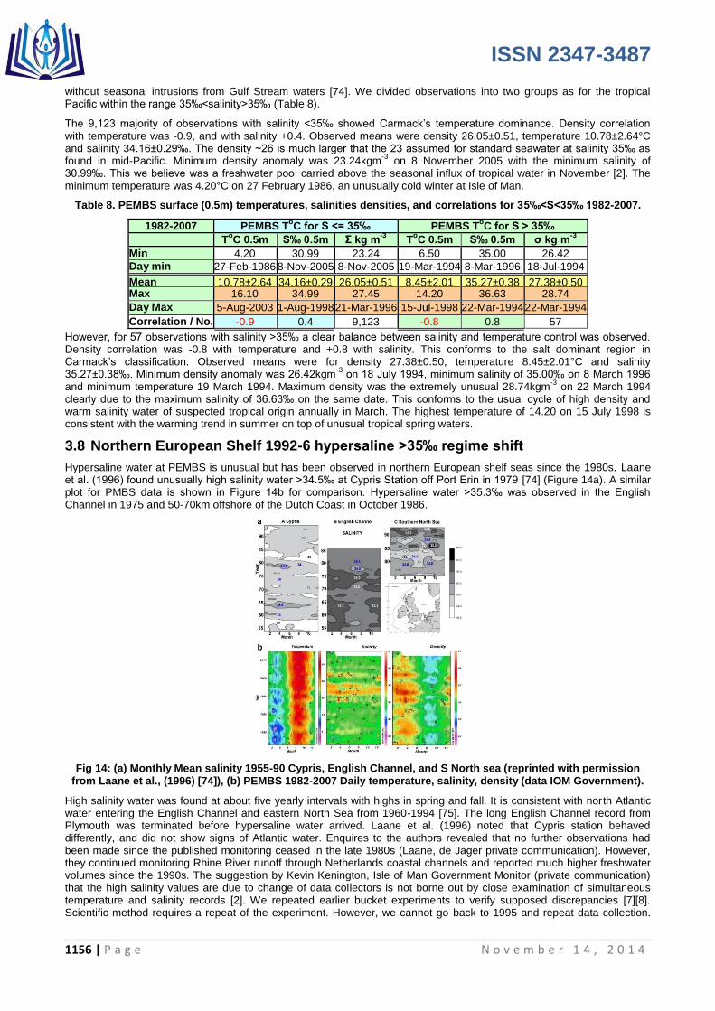
ISSN 2347-3487

1156 | P a g e N o v e m b e r 1 4 , 2 0 1 4

without seasonal intrusions from Gulf Stream waters [74]. We divided observations into two groups as for the tropical Pacific within the range 35‰<salinity>35‰ (Table 8).

The 9,123 majority of observations with salinity <35‰ showed Carmack‟s temperature dominance. Density correlation with temperature was -0.9, and with salinity +0.4. Observed means were density 26.05±0.51, temperature 10.78±2.64°C and salinity 34.16±0.29‰. The density ~26 is much larger that the 23 assumed for standard seawater at salinity 35‰ as found in mid-Pacific. Minimum density anomaly was 23.24kgm

-3 on 8 November 2005 with the minimum salinity of

30.99‰. This we believe was a freshwater pool carried above the seasonal influx of tropical water in November [2]. The minimum temperature was 4.20°C on 27 February 1986, an unusually cold winter at Isle of Man.

Table 8. PEMBS surface (0.5m) temperatures, salinities densities, and correlations for 35‰<S<35‰ 1982-2007.

1982-2007 PEMBS ToC for S <= 35‰ PEMBS T

oC for S > 35‰

ToC 0.5m S‰ 0.5m Σ kg m

-3 T

oC 0.5m S‰ 0.5m σ kg m

-3

Min 4.20 30.99 23.24 6.50 35.00 26.42

Day min 27-Feb-1986 8-Nov-2005 8-Nov-2005 19-Mar-1994 8-Mar-1996 18-Jul-1994

Mean 10.78±2.64 34.16±0.29 26.05±0.51 8.45±2.01 35.27±0.38 27.38±0.50 Max 16.10 34.99 27.45 14.20 36.63 28.74

Day Max 5-Aug-2003 1-Aug-1998 21-Mar-1996 15-Jul-1998 22-Mar-1994 22-Mar-1994

Correlation / No. -0.9 0.4 9,123 -0.8 0.8 57

However, for 57 observations with salinity >35‰ a clear balance between salinity and temperature control was observed. Density correlation was -0.8 with temperature and +0.8 with salinity. This conforms to the salt dominant region in Carmack‟s classification. Observed means were for density 27.38±0.50, temperature 8.45±2.01°C and salinity 35.27±0.38‰. Minimum density anomaly was 26.42kgm

-3 on 18 July 1994, minimum salinity of 35.00‰ on 8 March 1996

and minimum temperature 19 March 1994. Maximum density was the extremely unusual 28.74kgm-3

on 22 March 1994 clearly due to the maximum salinity of 36.63‰ on the same date. This conforms to the usual cycle of high density and warm salinity water of suspected tropical origin annually in March. The highest temperature of 14.20 on 15 July 1998 is consistent with the warming trend in summer on top of unusual tropical spring waters.

3.8 Northern European Shelf 1992-6 hypersaline >35‰ regime shift

Hypersaline water at PEMBS is unusual but has been observed in northern European shelf seas since the 1980s. Laane et al. (1996) found unusually high salinity water >34.5‰ at Cypris Station off Port Erin in 1979 [74] (Figure 14a). A similar plot for PMBS data is shown in Figure 14b for comparison. Hypersaline water >35.3‰ was observed in the English Channel in 1975 and 50-70km offshore of the Dutch Coast in October 1986.

Fig 14: (a) Monthly Mean salinity 1955-90 Cypris, English Channel, and S North sea (reprinted with permission from Laane et al., (1996) [74]), (b) PEMBS 1982-2007 Daily temperature, salinity, density (data IOM Government).

High salinity water was found at about five yearly intervals with highs in spring and fall. It is consistent with north Atlantic water entering the English Channel and eastern North Sea from 1960-1994 [75]. The long English Channel record from Plymouth was terminated before hypersaline water arrived. Laane et al. (1996) noted that Cypris station behaved differently, and did not show signs of Atlantic water. Enquires to the authors revealed that no further observations had been made since the published monitoring ceased in the late 1980s (Laane, de Jager private communication). However, they continued monitoring Rhine River runoff through Netherlands coastal channels and reported much higher freshwater volumes since the 1990s. The suggestion by Kevin Kenington, Isle of Man Government Monitor (private communication) that the high salinity values are due to change of data collectors is not borne out by close examination of simultaneous temperature and salinity records [2]. We repeated earlier bucket experiments to verify supposed discrepancies [7][8]. Scientific method requires a repeat of the experiment. However, we cannot go back to 1995 and repeat data collection.

ISSN 2347-3487

1157 | P a g e N o v e m b e r 1 4 , 2 0 1 4

The scientific solution is to design a well-focused experiment. Continuously measure temperature, salinity, pH and currents at 1, 2, 3, 5, 7, and 10m on a purpose-built platform with full Met Station Stevenson Screen, anemometer mast, evaporation pan and tide gauge. Original data collected by others may be re-interpreted but never altered. Unexpected discoveries usually arise from carefully conducted experiments.

The Port Erin data show steadily increasing summer high and decreasing spring low temperatures throughout the record. However, high salinity appears in annual pulses between 1994-2002 (Table 5b in [2]. These high salinity values can only come from the tropics as shown in correlation coefficients (Table 8). These are real mathematical relationships from the density equation [1]. Without verified physical causality, correlation coefficients are merely coincidence [72]. Hypersaline surface waters >36‰ were reported to depth of ~500m in Gulf Stream at 26ºN between 2004-2012 (Figure 4 in [76]). Indeed, there are indications that surface water could be as high as 37‰. However, sampling data were not published for the all-important surface layer. This is the probable origin for PEMBS hypersaline water Gulf Stream surface waters.

3.9 Problem of abandonment of surface timeseries monitoring

Figure 14 captures the major problem of ceasing collecting long continuous daily timeseries of ocean surface data. The Manx record shows tropical hypersaline water entered the Irish Sea for the first time. It peaked around 1995. Thereafter, the surface water has a freshwater layer. We suggest that derives from the higher evaporation and precipitation as in Pacific freshwater warm pools. We need surface data to confirm this. The English Channel and North Sea data monitoring cessation is a major blow to understanding the surface physics of the North European shelf seas. We expect the same changes to apply but have no data, nor any means to obtain it retrospectively.

Since 2002, surface temperatures continued to rise, but salinity reduced. Seasonal tropical water now has a freshwater buoyant surface layer (Figure 14). This is consistent with increased runoff observed over the northern hemisphere and Europe since 2000. The salinity at Port Erin is likely reduced also because of a thicker surface layer originating on polar meltwaters from the Labrador Sea and Arctic. Indeed one of us JBRM running trials with Slocum profiling gliders in the Labrador Current north of Newfoundland in August 2014 encountered the stratification lid at 10m. The density anomaly was 24, temperature 8°C and salinity 31‰. The device was programmed to expect surface density of 24. It was reprogrammed closer to the extreme of 23.24 seen at PEMBS (Table 8). However, Arctic runoff and meltwaters are much closer to freshwater during the seasonal breakup as observed in Arctic lagoons ([60]).

3.10 Poleward shift after the Last Glacial Maximum

Polar amplification was attributed to differential warming since the last glacial maximum(LGM) [77] (Figure 15).

Fig 15: Poleward shift of jet streams since last glacial Maximum. (Reprinted by permission from Toggweiler and Russell, (2008) Nature.[77]).

It forecast a poleward shift of sub-polar jet streams from latitude range 45-50° to 50-55°. In the Antarctic, the shift coincides with the deep Antarctic Circumpolar Channel. This leads to stronger sustained circumpolar E-W winds and greater upwelling along the Penguin Gyre (Figure 3). However, in the northern hemisphere it coincides with the Isle of Man at 54°N and the northern entrance to the Western Irish Sea fjord estuary shelf sea (Figure 1 in [2]). We suggest the differential Pacific heat trap strengthened the E-W gradient. This led to the observed sub-polar jet stream loop described above, and in strengthened warm inflows to the Arctic and cold fresh outflows to the Atlantic (Figure 10). Woodgate et al., (2010) [80] used the observed Bering Strait volume and heat transport between 1991 and 2007 in numerical flow models. Both volume and heat transport 2007 values were record highs; 2007 heat flux ~5-6x10

20Jyr

-1 was twice 2001 measured

ISSN 2347-3487

1158 | P a g e N o v e m b e r 1 4 , 2 0 1 4

flux. The authors suggest interannual flow variability ~0.2Sv. They note that the incoming Pacific Ocean heat flux is sufficient to account for one third the seasonal Arctic ice loss or to melt an ice sheet 1m thick over an area of 1-2x10

6km

2.

4 CONSEQUENCES

We believe that the physics of climate change can be understood as the interaction of long-term cyclical and exponential processes. Hitherto, climate research wrongly assumed atmospheric pan-evaporation as over land, a 10m well-mixed surface layer, and ignored the significance of both temperature and salinity in determining density and the transport of heat and freshwater. The failure to recognize the importance of exponential processes has led to underestimates of the pace of warming. It is striking that all the processes have an exponential component (see Figures 1, 5, and 10).

4.1 Logarithmic Growth – the Essential Exponential

The eminent physicist and teacher Albert A. Bartlett (1923-2013) stated, “The greatest shortcoming of the human race is our inability to understand the exponential function.” [81]. He pointed out that all growth is unsustainable where resources are finite, and that even small increments lead to infinity. Bartlett‟s lectures are among the most viewed on the internet (https://www.youtube.com/watch?v=3hsKWJGtEFc Last upload 19 October 2014). He used log “Law of 70” to help understand the process. The doubling time in years T2, from any steady compounding rate R% is:

T2 = (ln(2))/R.

Natural log of two is actually 69.3 but 70 is a simple approximation. Physicists use the Law of 72 because it is divisible by two, three, and four, and easier to make quick mental estimates. Bartlett applied to rule to the limits on fossil fuel, population growth and food supplies. On climate change he stated, “If any of the observed global warming can be attributed to the action of humans, this is all the proof your need the world is overpopulated” (https://www.youtube.com/watch?v=F8ZJCtL6bPs last access 21 October 2014). His first law of sustainability is: You cannot sustain population growth, You cannot sustain growth in rates of consumption of resources. Simple arithmetic denies sustainability of growth. Steady state is the best possible sustainable state. The inverse of exponentials is logarithmic functions. The exponential function trends to infinity while at the inverse log trends to zero. This ties together population growth, consumption of Earth‟s resources and sustainability.

4.1.1 Exponential Evaporation

Evaporation due to Claudius-Clapeyron thermodynamics is an exponential function of temperature (Figure 1)[1]. Evaporation approximately increases at ~7%°C

-1. It doubles for every ~10°C temperature rise. Thus, evaporation at 18°C

(saturated vapor pressure of 21hPa) is twice that at 8°C (SVP 11hPa); evaporation at 28°C (SVP 38hPa) doubles again. Measured evaporation measured was ~4.5mmdy

-1 (~1.6myr

-1, SVP 34hPa) at 26°C, and at 28°C ~7.1mmdy

-1 (~2.6myr

-1,

SVP 38hPa) [1]. Enhance evaporation at higher temperature was due to the effect of salinity on density.

Salinity controls brine sinking processes for hypersaline water. Nocturnal cooling was not sufficient to cool brine to allow settling to deeper water. Evaporation is negligibly small in the Humboldt Current alongside the world‟s driest desert the Atacama. At the cold log end of the scale, at low SVP, carbon dioxide can be readily dissolved in seawater. Thus, cold Polar Regions are a source of ocean acidification, and evaporation is negligible. Deepwater brine from surface freezing carries acidified water down slope to interleave along isopycnals, as discussed above.

4.2 Asymmetric ocean warming

The combination of exponential evaporation and asymmetry between normal and hypersaline seawater (<35‰) leads to asymmetric ocean warming and evaporation. Thermal controlled circulation at salinity <35‰ captures twice the heat below the surface layer than salinity controlled circulation at salinity >35‰. Conversely, hypersaline water evaporates approximately twice as much precipitation and heat as normal or brackish water (Figure 3)[1]. This applied in the tropical Pacific Ocean between northern and southern hemispheres. It also applies between the north Pacific and north Atlantic. The differential warming leads to polar amplification and changes to both N-S and W-E jet streams. These changes result in different impacts of warming over North America and Europe.

4.3 Cyclical and exponential solar radiation

Greenhouse gas heat trap is rising exponentially just as the solar radiation is falling after the 20th

century high (Figure 5). Exponential warming of the ocean continues despite the reduction in incident radiation. Carbon dioxide is the principal measure of greenhouse gases and makes up about three-quarters of the total annual emissions, ~50Gt (37.5Tg ≈ 400ppm CO2 equivalent). Other gases such as methane, nitrous oxide and complex man-made chemicals such as chloroflouro carbons (CFCs) make up the total. Indeed, it has been estimated that if the Montreal Protocol in 1997 had not banned CFCs, the CO2 equivalent would now be 135Gt (~1440ppm) [82]. The substitution of hydrochloroflouro carbons (HCFC) for CFCs resulted in the closing of the polar ozone holes. It is estimated to have reduced the 2014 level by ~85ppm. We noted above that the exponential doubling time for carbon dioxide is about ~20 years would bring total emissions to 435ppm (Section 2.2.2). Thus, without the Montreal Protocol we would almost certainly have exceeded the GHG total 2°C warming. Moreover, it has recently been discovered that though HCFCs are ozone-friendly, they are powerful greenhouses gases in their own right. There is pressure to extend the Protocol to HCFCs.

Increasing atmospheric CO2 may only be a warning of far worse GHG warming. NOAA Annual GHG Index (AGGI) shows long-lived greenhouse gasses increased by 1.5% in one year and by 34% since 1990

ISSN 2347-3487

1159 | P a g e N o v e m b e r 1 4 , 2 0 1 4

(http://research.noaa.gov/News/NewsArchive/LatestNews/TabId/684/ArtMID/1768/ArticleID/10553/Greenhouse-gases-continue-rising-in-2013-34-percent-increase-since-1990.aspx). Tundra and sub sea anhydrous methane is already being released. The increased influx of tropical water into the Arctic is likely to lead to positive feedback from methane release from quasi-stable methane hydrates at ~400m [83]. Better understanding of seasonal cycles would aid in determining methane Arctic impact [84]. The warming Arctic climate is melting permafrost and releasing methane with many significant feedbacks to the climate system [85]. Arctic lakes no longer freeze to the bottom so melting of permafrost continues year-round (see freshwater cycle Fig. 1). These methane releases alone suggest a potential step increase in ocean heating from infrared GHG heat trapping. The mis-handling of any of the GHGs could to irreversible exponential AGW.

4.4 Ocean heat trapped by a buoyant lid and buffered by icemelt

Both Pacific and Atlantic heat anomalies in ocean and air show exponential warming from the Keeling Point (Figure 12). In the north Atlantic Port Erin surface data, has both tropical and polar water. Polar icemelt is in three phases over the past 100 years. Icemelt post1986 had increased exponentially (Figure 11). Tropical water at Port Erin at a peak in October travels through the Arctic Ocean with a residence time of ~4 years. Polar meltwater appears in seasonal cold meltwaters at Port Erin in February 3½ years after tropical warm water. This reduces the warming in the north Atlantic water exemplified by Port Erin records. The temperature anomaly peaked in 2004-5 at 1.12°C. This compares with a 2004 Central England temperature (CET) peak in 2004 of +1.3°C.

By contrast, the Pacific water showed evidence of rapid warming and ice melt that we attribute to retreating Alaskan tidewater glaciers in the first half of the twentieth century (Figure 13). After the Keeling Point heat trapped by thermal circulation at salinity <35‰ reached a peak in 1995 of 1.6°C at the surface and 1.3°C at 5m.

The cooling or lull reported from 2010-12 is likely due to Arctic icemelt 3-4 years earlier. Air responds rapidly to melting ice by cooling rapidly. It has 3000x lower heat capacity than seawater. This makes seawater less responsive to rapid change but allows it to rapidly melt subsurface ice. All records show warming is at record levels in 2014. We anticipate cool meltwaters to appear in the north Atlantic in spring 2017-8. Thus, any lull or hiatus in warming is a response to the thermal properties of seawater and air during the melting of land and sea ice.

4.5 Millennial, centennial and decadal timescales

4.5.1 Millennial and ice age timescales

Deep ocean circulation operates on millennial timescales taking ~1750yr to reach the abyssal plain and ~4000yr between oceans [17]. Until the last great Holocene glacial retreat and flooding Bering Strait was closed and Isle of Man connected to the European landmass [87][88][89]. The last three glacial maximum ice extents 20kyrBP, 38kyrBP, and 65kyBP were highly variable. Only the most recent covered the British Isles, and Alaska was ice-free throughout the last glaciation [90][91]. At the end of the last ice age, Lake Agassiz flowed through Canadian archipelago and into north Atlantic [92]. Ice rafted debris was found in the European Atlantic[93]. The last great flood from the melting of the Laurentide ice sheet was about ~7,900yrBP [94].

Thermal dominant heat trapping is likely a millennial-scale process. The North Pacific Ocean was landlocked until ~8kyBP so influx of freshwater and heat is a recent phenomenon. A relatively warm north Pacific is the most likely reason Alaska remained ice-free. The distortion of the jet stream in a northward loop is likely Rayleigh instability due to increased forcing at higher temperatures. This is probably the long-term condition that kept Alaska ice-free.

4.5.2 Centennial timescales

Over the last 250 years since beginning of the industrial revolution AGW has reached only to ~300m [16]. Surface heat anomalies were close to long-term means at the beginning of the twentieth century (Figure 10). We found that modern rapid AGW took off exponentially only after the mid-century Keeling Point from 1957. The nature of exponential growth is that each increment adds to the previous total. This places the emphasis on decadal and year-to-year increments.

4.6 Decadal and annual timescales in exponential growth

The shift in jet streams in response to asymmetry between the north Pacific and north Atlantic appears to be key to understanding modern rapid climate change. The first author, JBM first became aware of the jet stream loops in 1982 at the Geophysical Institute, University of Alaska. February is usually the coldest month with temperatures ~-30°C. A warm spell in February melted an outdoor ice-cream stock. It was too short a warm spell to melt measurable amounts accumulated snow and ice, but was enough to melt ice cream. Meteorologist Sue Ann Bowling explained to the author that occasionally a 5-lobed jet stream assumed a stable position that brought unusual warm tropical air to the cold Interior. The warm air flux displaced polar air southwards along the McKenzie River and into the Canadian and US Midwest.

The jet stream loop has occurred more frequently as the Pacific Ocean warmed especially after the millennium. The warm water passing through Bering Strait between 2000-2007 doubled as we reported above. In December 2013, Fairbanks Alaska was briefly warmer than Miami Florida. Throughout much of 2014, the loop persisted carrying cold polar air to the interior central and southern states.

Francis and Vavrus (2012) [95] reported the blocking mechanism whereby the cold polar air meets the warm Gulf of Mexico air. Long highly dynamic fronts form between cold and warm air masses. In the winter, extreme snowfall around the unfrozen Great Lakes result in record snowfalls in New York and other states to the south. Tornadoes, storms and

ISSN 2347-3487

1160 | P a g e N o v e m b e r 1 4 , 2 0 1 4

floods are so common along the long frontal system that on the short ABC World News weather warnings from Meteorologist Ginger Zee are broadcast almost every day.

There is ample evidence of weather setting new records for rainfall, winds, early and late snow, hurricanes on both coasts and flooding in semi arid deserts of the Southwest. Since this is a physics journal, we have included screenshots taken from ABC World News broadcast on BBC TV on 13 August 2014 (Figure 16). It illustrates the interaction of cold polar air with warm ocean air (cold fronts are blue, warm fronts red, cyclonic lows L with arrows).

Fig 16: Coastal frontal jet trapped over Islip, Long Island NY 13 August 2014 drops record 13.27in of rain in 24hrs (from ABC World News, USA as broadcast on BBC TV, UK 13 August 2014).

The cold front (left) in the radar plot of rainfall had penetrated through the mid-west to form a linear frontal system on 12 August. The warm front from the Gulf forms the cyclonic storm. Record flooding was reported in Nebraska, Michigan, and Illinois. Heavy rain and storms are forecast for the next 48 hours. The radar plot (middle) for Wednesday, 13 August shows the cyclonic low frontal system over the ocean off New Jersey and New York. The storm stalled over Islip, Long Island NY (right) with a measured record 24hr rainfall of 13.27in (337mm). These pictures bring out important processes.

4.6.1 Slow moving cyclones over sea decline in intensity but not over land

The cyclone was trapped over land so could not draw up cold subsurface water as found in detailed hurricane studies by Mei et al., (2010) (Section 3.3 in [1], [14]) for slow moving hurricanes. However, warm air over land collided with the cold front and precipitation was continuous at ~0.55inhr

-1 (14mmhr

-1). Meanwhile only five miles to the east over the sea,

precipitation was only 1-2in (25-50mm) in 24 hr. In the cold air on the west coast of Long Island and over Long Island Sound, the rainfall gradient more gradually reduced. This clearly illustrates the different behavior of cyclones over land and sea.

Over sea, slow moving storms decay from upwelled coldwater over 24hrs or more [1]. It is fast moving storms that build in strength and do most damage. Thus, the warming of the Pacific warm pools to ~32°C creates intense hurricanes and typhoons. This suggests a strengthening of the warm eastern boundary current in the North Pacific (see references in [1]). Super typhoons with record-breaking winds made landfall in the Philippines in November 2013 (Haiyan) and Japan in October 2014 (Vongfong). A category 5 hurricane on the Saffir-Simpson scale has 1-minute sustained winds of at least 70ms

-1: super typhoon at least 65ms

-1. Container shipping companies such as Maersk, trading out of China, now use two

new levels above standard Hurricane Force 12 on the Beaufort scale. Only days before the Islip NY record, on 8-9 August 2014, two hurricanes Iselle and Julio passed over Hawaii. They were the first for 26 years. In August, September and October 2014 tropical storms appeared simultaneously over the Gulf of California and Gulf of Mexico to produce record floods through the southern US and Northern Mexican States.

4.6.2 West and northwards shift of Atlantic gyres

The landfall of hurricanes north of Cape Hatteras may indicate a warm eastern boundary is becoming a regular feature of North Atlantic circulation as in the north Pacific. This would be consistent with the warming trend of both oceans. The storm system of 12-13 August 2014 passed along the coast all the way to New England. Hurricane tracks more usually leave the coast at Cape Hatteras following the Gulf Stream. However, with warming Gulf Stream and north Atlantic, storms more frequently take an easterly route along the coast. This has meant that the jet stream continues a northwards bend in the North Atlantic as in the North Pacific. It results from a strong northwards push of cyclonic winds that held the warm Atlantic air in contact with the cold polar air. This suggests a warm eastern northwards boundary current is developing in the North Atlantic as well as in the North Pacific. Exponential surface warming has resulted in high surface temperatures persisting later in the season. The rule with hurricanes used to be Always in August, Sometimes in September, Occasionally in October, and Never in November. Haiyan super typhoon with the greatest winds to make landfall of ~90msms

-1, was in November 2013. Atlantic hurricanes are more common in October. Moreover, Halloween 2014 saw

record cold temperatures and early snow in North America while the United Kingdom enjoyed record warm temperatures. St Cloud Minnesota had record cold temperature on 31 October of 15°F (-9.5°C) compared with a normal 35°F (1.5°C). The coastal frontal jet brought snow from the Carolinas to Newfoundland on 1 November. UK enjoyed the warmest ever October temperature of 22.5°C recorded near London against a normal 11°C. This is consistent with exponential warming of the North Atlantic and Pacific Oceans, the persistent jet stream loop, and the northward shift of Polar Amplification.

ISSN 2347-3487

1161 | P a g e N o v e m b e r 1 4 , 2 0 1 4

4.7 Enhanced Greenland and Canadian Archipelago tidewater glacial basal ice melt

The cold polar air displaced by the western Atlantic loop displaces polar air southwards over Europe. The unusual cold water observed in March 2010 is a consequence of this process. The west and northwards shift of the Columbus/Viking gyre boundary is likely to continue.

The north and westwards shift of Atlantic gyres is likely to enhance the under ice melting of Greenland glaciers that is already well advanced as reported above [2]. This will change the volume of meltwaters in the Viking gyre. However, we suspect the cold meltwater anticipated for spring 2017-18 at Isle of Man, may not reach the island if the Columbus/Viking gyre boundary has moved further north and west. The Isle of Man is likely to spend more time in the warm Gulf Stream/Columbus gyre flows.

4.7.1 Antarctic basal icemelt

Rapid basal Antarctic icemelt is reported to be widespread [96]. There is strong tidal pumping of surface freshwater from sinking of brine to deep waters was reported (see Figure 6). Models of under ice circulation were developed to investigate important under-ice circulation processes [97][63]. However, the divergent Penguin Gyre coupled with enhanced Antarctic Circumpolar winds is likely to drive surface water away from the continent. Satellite observations show increased surface ice spreading northwards. Measurements of near-surface meridional vertical circulation are very difficult to perform in the Southern Ocean. The best approach is to continue investigating under-ice circulation using novel techniques such as instrumented seal and torpedo robots.

4.8 Forecasting chaotic climate systems

Scientific truth is verified from experiment evidence to test assumptions, statistics and models. Coupled tide and surge

models followed early success with tidal models where the largest surges were found to coincide with spring tides [98]. In

extreme conditions, reversal of prevailing winds was able to reverse normal cyclonic circulation for example in the North Sea (Figure 4 in [99]). These techniques were applied to the world‟s first operational coupled ocean/atmosphere model used to control the UK Thames Barrier in co-operation with other North Sea nations to minimize flood risk for all [100].

Ocean modelers at the time had expected similar techniques would be applied to the open ocean with subsequent verification [101]. For example, numerical techniques such as using variable boundary meshes in model grids could reduce numerical turbulence in transitions from ocean to coastal or estuarine model scales [102]. Sadly, this has not happened. Nor has the recommendation in Richardson‟s (1922)[103] pioneering work on weather prediction by numerical process to place experimental observation points uniformly as far as possible at the center of model grid cells. It has been applied to some extent over land. However, most of the essential ocean stations were abandoned in the 1990s with a few notable exceptions such as Ocean Station Papa (P) and Line P (Section 2.4.4, [42]) The result led to greater dependence on satellite observations with very few stations continuously recording simultaneous atmospheric and near-surface observations. The weaknesses in ocean observation systems was brought home in the Fastnet race disaster when many racing sailors lost their lives and boats [104]. It a simple fact that predictions of dynamic weather conditions is difficult on land even with good observational networks. Even here, the forecasts shown in Figure 16 are only moderately accurate for a few days. Indeed, reversion to Admiral Fitzroy‟s method has resumed using numerical computer models (Section 1.2 in [2], [105]). Fitzroy, founder of the UK Met Office, collected weather charts and chose a current chart that most resembled a previous one. Earlier sequences were followed to produce daily-published forecasts. Fortunately, they were right more times than they were wrong. However, forecasts are only valid for the following day. Conditions can change as we saw with the stalling of the cyclone over Islip NY. With high-speed computers is it possible to run global models several times and choose the predictions that occur most frequently. This is now the accepted technique. UK Met Office abandoned long-range forecasts because of some prominent wrong ones.

4.9 El Niño Southern Oscillation (ENSO) forecasting

Problems with the Central Pacific ENSO forecasts for the regions of our tropical experiment at ~140W are illustrated in Figure 17 [1].Sea surface temperature (SST) anomalies forecast for Niño 3.4 region (5ºN-5ºS, 120ºW-170ºW based on observed values from July and August 2010, from 14 dynamical and 10 statistical models. Forecasts are overlaid by observed values September 2010-January 2011 (red circles). (Figures courtesy International Research Institute (IRI) for Climate and Society and Climate Prediction Centre, NOAA/NWS, MD. The figure on the right is the forecast fro mid-August from 16 dynamical and nine statistical models. The yellow line is a weighted mean. We note that after 5 months in January 2011, actual anomalies diverged away from observations. The consensus was for a warming trend from cold anomalies.

The consensus for 2014-15 is for a warming trend from an almost neutral anomaly to a falling trend at the end. The statistical models take no account of temperature, salinity and Clausius Clapeyron evaporation. Most dynamic models do not incorporate the near-surface dynamics detailed in this paper.

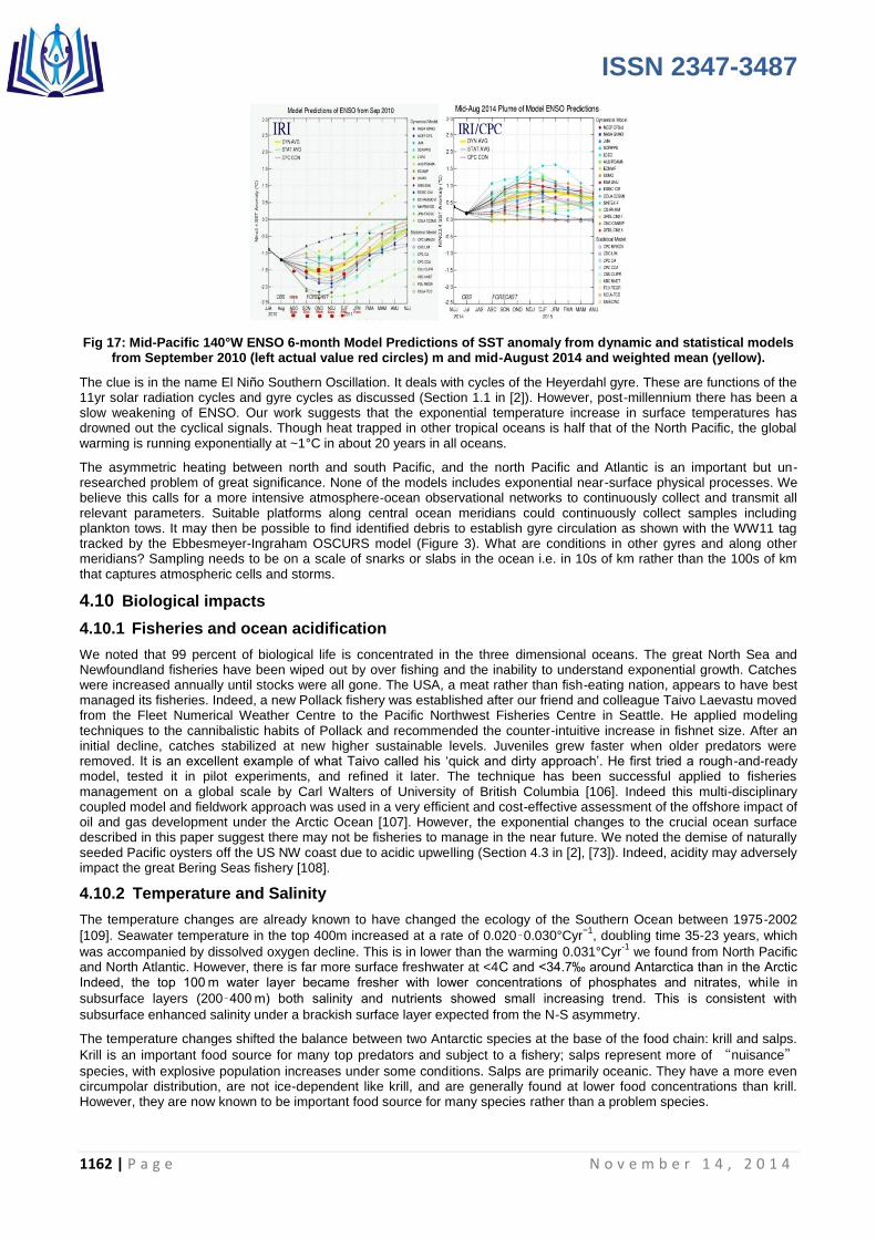
ISSN 2347-3487

1162 | P a g e N o v e m b e r 1 4 , 2 0 1 4

Fig 17: Mid-Pacific 140°W ENSO 6-month Model Predictions of SST anomaly from dynamic and statistical models from September 2010 (left actual value red circles) m and mid-August 2014 and weighted mean (yellow).

The clue is in the name El Niño Southern Oscillation. It deals with cycles of the Heyerdahl gyre. These are functions of the 11yr solar radiation cycles and gyre cycles as discussed (Section 1.1 in [2]). However, post-millennium there has been a slow weakening of ENSO. Our work suggests that the exponential temperature increase in surface temperatures has drowned out the cyclical signals. Though heat trapped in other tropical oceans is half that of the North Pacific, the global warming is running exponentially at ~1°C in about 20 years in all oceans.

The asymmetric heating between north and south Pacific, and the north Pacific and Atlantic is an important but un-researched problem of great significance. None of the models includes exponential near-surface physical processes. We believe this calls for a more intensive atmosphere-ocean observational networks to continuously collect and transmit all relevant parameters. Suitable platforms along central ocean meridians could continuously collect samples including plankton tows. It may then be possible to find identified debris to establish gyre circulation as shown with the WW11 tag tracked by the Ebbesmeyer-Ingraham OSCURS model (Figure 3). What are conditions in other gyres and along other meridians? Sampling needs to be on a scale of snarks or slabs in the ocean i.e. in 10s of km rather than the 100s of km that captures atmospheric cells and storms.

4.10 Biological impacts

4.10.1 Fisheries and ocean acidification

We noted that 99 percent of biological life is concentrated in the three dimensional oceans. The great North Sea and Newfoundland fisheries have been wiped out by over fishing and the inability to understand exponential growth. Catches were increased annually until stocks were all gone. The USA, a meat rather than fish-eating nation, appears to have best managed its fisheries. Indeed, a new Pollack fishery was established after our friend and colleague Taivo Laevastu moved from the Fleet Numerical Weather Centre to the Pacific Northwest Fisheries Centre in Seattle. He applied modeling techniques to the cannibalistic habits of Pollack and recommended the counter-intuitive increase in fishnet size. After an initial decline, catches stabilized at new higher sustainable levels. Juveniles grew faster when older predators were removed. It is an excellent example of what Taivo called his „quick and dirty approach‟. He first tried a rough-and-ready model, tested it in pilot experiments, and refined it later. The technique has been successful applied to fisheries management on a global scale by Carl Walters of University of British Columbia [106]. Indeed this multi-disciplinary coupled model and fieldwork approach was used in a very efficient and cost-effective assessment of the offshore impact of oil and gas development under the Arctic Ocean [107]. However, the exponential changes to the crucial ocean surface described in this paper suggest there may not be fisheries to manage in the near future. We noted the demise of naturally seeded Pacific oysters off the US NW coast due to acidic upwelling (Section 4.3 in [2], [73]). Indeed, acidity may adversely impact the great Bering Seas fishery [108].

4.10.2 Temperature and Salinity

The temperature changes are already known to have changed the ecology of the Southern Ocean between 1975-2002

[109]. Seawater temperature in the top 400m increased at a rate of 0.020–0.030°Cyr−1

, doubling time 35-23 years, which

was accompanied by dissolved oxygen decline. This is in lower than the warming 0.031°Cyr-1

we found from North Pacific and North Atlantic. However, there is far more surface freshwater at <4C and <34.7‰ around Antarctica than in the Arctic Indeed, the top 100 m water layer became fresher with lower concentrations of phosphates and nitrates, whi le in

subsurface layers (200–400 m) both salinity and nutrients showed small increasing trend. This is consistent with

subsurface enhanced salinity under a brackish surface layer expected from the N-S asymmetry.

The temperature changes shifted the balance between two Antarctic species at the base of the food chain: krill and salps.

Krill is an important food source for many top predators and subject to a fishery; salps represent more of “nuisance”

species, with explosive population increases under some conditions. Salps are primarily oceanic. They have a more even circumpolar distribution, are not ice-dependent like krill, and are generally found at lower food concentrations than krill. However, they are now known to be important food source for many species rather than a problem species.

ISSN 2347-3487

1163 | P a g e N o v e m b e r 1 4 , 2 0 1 4

In general, abundance of krill and salps showed opposite trends to each other. Krill abundance was greater in years with lower seawater temperature, greater sea-ice extent and higher nutrient concentration, while salps showed the opposite pattern. The circumpolar-scale distribution of Antarctic krill is now relatively well documented. The distribution is strongly

asymmetrical, with over 75% of the population concentrated into the Atlantic sector 0–90°W, a sector of elevated food

concentrations. This is the sector with tidal pumping (Figure 6, Section 3.1).

Krill is a major food source for whales and as well as commercial fisheries. The shift to warmer temperatures, lower salinities and more ice-free conditions is likely to have profound effects in both south and north polar oceans. The warm summer water at the Isle of Man in 2014 coincided with a sharp decline in basking shark sightings (manxbaskingsharkwatch.com). Few were sighted during the season that usually ends by 1 September. However, there were unusual sightings in September off the west coast of the island. While at the northern end of the North Channel of the western Irish See off the Isle of Mull there were a record number of sightings (BaskingSharkScotland.co.uk). This suggests the plankton food stock had shifted to the north. Indeed, on 30 September the carcass of a starving baby basking shark washed up on the Ards Peninsula, Northern Ireland in the western Irish Sea facing Isle of Man. It is thought that plankton peaked early in the season. The baby carcass is under investigation for a death apparently caused by starvation. This is the first opportunity to study changes at the base of the food chain caused by seawater temperature and salinity shifts. There are likely many more biological impacts in the vast oceans that go unseen from lack of sampling.

4.11 Innovative and Maverick Science

New discoveries are usually found by scientists working alone or in pairs rather than by large teams. Establishment scientists who regulate research dominate large multinational multidisciplinary studies and tend to reject work that is contrary to accepted wisdom. Charles Keeling started groundbreaking research as part of the IGY but his desire to follow through was almost thwarted by „calibrated‟ reviewers in funding agencies [33]. He persisted, and now the greenhouse gas theory of heat entrapment is the proven basis for exponential global warming.

The discovery of temperature and salinity control of evaporation and heat capture was made following a simple experiment to find the scientific truth about discrepancies in mid-tropical Pacific SST datasets [1]. The discrepancies were found in data collected under VOS program of WMO using wrong assumptions about the sea surface since 1955 [69][70]. Indeed, the program continues to collect SST and subsurface temperatures that used as proxy for MAT. We could find no climatologists or meteorologists who had gone to sea to test the assumptions since 1926 [69]. Moreover, one reviewer with a stake in the established IPCC community recommended our research not be published.

We are shocked that field verification, the only basis for establishing scientific truth, should be so treated in favor of statistics with no proven causality. Papers suggesting problems from wrong assumptions on the ocean surface heat trap were ignored. Unfortunately, ocean scientists tend to concentrate on the Deep Ocean. Even Argo floats sample below upper 10m until very recently.

The wrong assumptions were made following G I Taylor‟s substitution in his famous buoyancy work investigating the meteorology and oceanography off Newfoundland following the Titanic disaster [110]. It was a reasonable assumption in the thick buoyant cold surface layer off Newfoundland. Indeed, one of us (JBRM) found this pycnocline-thermocline-halocline barrier at 10m at density 24 (8°C, 31‰) in August 2014 off Newfoundland in the Labrador Current. Taylor formulated his buoyancy parameters for the air-land boundary in 1931 [111]. It is based on the simple facts that at the boundary heat and mass behave differently. He invented the terms eddy diffusion and eddy viscosity to get round the problems of a turbulent boundary layer. Mass cannot pass through the land surface boundary. Taylor had expected later to include the air-sea boundary, but Ekman beat him to it [112]. So, the air-land equations and the tenuous assumptions of a uniform ocean boundary layer have continued in use without question or experimental verification.

We are quite sure Taylor would have designed the simple experiment that we performed in the tropical Pacific. He was a keen sailor and would have jumped at the opportunity. He liked simple experiments with easily demonstrable results. Indeed, one of us (JBM) found Taylor had quoted the surface tension of a bubble as 2T/r instead of 4T/r. In private correspondence, he readily accepted the error, and was most interested in our work on raindrops [113]. Indeed, raindrops are still quoted as being teardrops when we re-discovered the fact they fell flat-bottomed, blew up into bubbles with annular rings that developed Rayleigh instabilities on final bursting. Indeed, we pointed out that both the belief in the teardrop-shaped rain drop, and evaporation dependence on relative humidity are key pieces of meteorology bad science (http://www.ems.psu.edu/~fraser/BadScience.html) [1].

It is now six years since our Pacific experiment. We had expected a rush of similar follow-up experiments. It is important that our findings be verified and the experimental procedure improved. Annual meridional transects in both directions are conducted annually by the Sea Education Association that generously sponsored our work and allowed use of the data. We would like to see more transects in other oceans between Iceland and Ascension or Tristan da Cunha Islands, or from Sri Lanka southwards. A mid-Atlantic meridional transect from Iceland southwards should be top priority.

The work presented here clearly verifies discoveries of key modern scientists: Keeling, Ebbesmeyer, Carmack, Williamson, etc. We believe our work will most likely be followed up by dedicated classical scientists well grounded in the use of models for dynamically adjusting ongoing fieldwork in the adaptive management program devised by Carl Walters [106][107]. Large programs are too diffuse and concentrate on everything, leaving little room to for individual discovery at the heart of science. The Alaska pipeline project, for example, studied everything from the sea at Valdez, in Prince William Sound to Prudhoe Bay on the Arctic shore. When the project was built, the biggest problem had not been addressed. Test water for the 4ft (1.25m) pipeline contained anti-freeze that had huge impact on the permafrost. No one had consulted

ISSN 2347-3487

1164 | P a g e N o v e m b e r 1 4 , 2 0 1 4

engineers in advance. A similar mistake was avoided from the subsequent waterflood project that used adaptive management [107].

We hope that scientists and funding agencies will take these points seriously. The IPCC and even the International Polar Year failed to study the top few meters of ocean. Any fieldwork should be managed dynamically by a small group of scientists chosen for their expertise and ability to work in response to multi-disciplinary demands. The present publish or perish system is a major obstacle. We suggest, like the Council for Innovative Research, articles be restricted to no more than three authors. We adopted a point score of one for single author, half for two authors, and zero for all others. If models, statistics and assumptions are presented without verification experiments, they should be rejected. Field observations should be the focus. The proposed Indian Ocean could be a major test bed for these cost effective measures [114].

4.12 Innovative Solutions

The next generation of young scientists are asking questions about how we got to this crisis and coming up with solutions. Undergraduate researchers at Guelph University asked why the Grand Banks cod fishery collapsed despite continuous oversight by government fisheries experts [115]. The first answer was too many boats chasing too few fish. Fish stocks were grossly underestimated while technology moves so fast that every fish could be found through side-looking sonar. The pressure to increase catches exponentially without responsibility to maintain stocks is known as the tragedy of the commons. All the world‟s fisheries could face the same fate as Grand Banks cod, North and Irish Sea herring, Mediterranean and Gulf of California tuna and fisheries of the Southern Oceans. This is a similar question asked by JBRM when an undergraduate: Why are there discrepancies in mid-Pacific SSTs and is it caused by measurement methods as suggested? The experimental research voyage of discovery from that question led to findings revealed in this paper. The answers will come from young scientists untroubled by established beliefs. The key is individual and family responsibility for conserving and managing finite resources. This may extend to regions and countries until the global establishes self sufficient cells that make a global pattern. It is parallel to the snarks that together make up the ocean surface circulation.

4.13 Fisheries Solution to the Tragedy of the Commons – Individual Transferable Quotas

Rutherford (2008) [115] concludes „Establishing private property rights using methods such as individual transferable quotas is occurring in several parts of the world to avoid the tragedy of depleted fish stocks. Well-defined property rights, through the implementation of individual transferable quotas, ensure that fisheries internalize the cost and benefits of management decisions. Individual transferable fishing quotas have proven effective to increase conservation efforts and reduce overcapacity, which is often produced with increased legislation. Individual transferable quotas are not only a viable solution for reducing overfishing and preventing stock collapses, but the best solution available.‟

The principle of individual responsibility to deal with the fundamental problem of exponential growth must be extended. Continuous growth is impossible in a finite world. It applies most importantly to carbon fuels. Once this is adopted no one will waste invaluable chemicals made over millions of years by merely burning them. Exponential growth will give way to perpetual stability. This is the Goldilocks solution – not too hot and not too cold. However, there is a dangerous transition period to negotiate for this major paradigm shift.

4.14 Final Solution? – The Zero Marginal Cost Society

Rifkin (2014) [116] extended his earlier work to suggest the solution to the tragedy of the commons is the Collaborative Commons, shared ownership of finite resources. The UN, European Union and leading economists have adopted the concept. It already has brought convergence of many previously distinct fields including ecological sciences, chemistry, biology, engineering, architecture, urban planning information technology and challenges the standard economic theory, The Zero Marginal Cost Society is predicts the inevitable Eclipse of Capitalism based on the fact the sustainable growth Is impossible in a finite world. Standard capitalist theory is grounded on the metaphor of Newtonian physics wedded to growth as the engine of economic activity. But the most one can achieve is stability and deflation as the desirable outcome. Since this inevitably reduces the wealth of the richest 85 people who control more resources than the poorest two billion, it will be a difficult battle. The future of the planet depends on successful Goldilocks outcome.

Rifkin shows the Collaborative Commons is grounded in the Laws of Thermodynamics. The total energy content of the universe is constant and the total entropy is continually increasing. Fossil fuel once used is unavailable for further user. All economic activity depends on harnessing all available energy in nature. The inevitable solution is the maximization of finite resources. The Internet of Things allows resources to be shared with almost zero marginal cost. Humans are only custodian of limited resources and are already sharing through the collaborative commons to form the Third Industrial Revolution.

The problem is how to make the transition from standard free-market capitalism to a near-zero cost society with minimal disruption. It is already happening and the results more widely seen. Corporate profits are reducing, property rights weakening, banks giving way to uncontrolled electronic currency, and gradual move towards easily accessible abundance. Economists expect the transition to take place in the next fifty years. However, that estimate is based on present rates of fossil fuel use and global warming estimates. Exponential doubling of AGW in 20 years requires much more urgent action.

4.15 Population Growth and reversing over-consumption of natural resources

Bartlett warned that human exponential growth in consumption of Earth‟s natural resources inevitably led to climate change. The problem will be solved in the long-term in the Third Industrial Revolution. There are two clear paths to follow.

ISSN 2347-3487

1165 | P a g e N o v e m b e r 1 4 , 2 0 1 4

Recent research suggests that even large-scale epidemics killing billions or a global one-child policy are unlikely to limit population growth by 2100 [117]. This only leaves limiting consumption of natural resources.

4.16 Global Targets for Greenhouse Gas Management

4.16.1 Atmospheric Targets

Atmospheric target aims to limit GHG warming to 2°C. It is likely to be reached by about 2017-2020. We already achieved 1.3°C in CET temperatures with 2014 the warmest to date. The target is based on doubling the long-term stable ~280ppm atmospheric carbon dioxide concentration to no more than 560ppm. However, we showed exponential increase in the ninety three percent of AGW in the oceans. Exponential increases are cumulative (Section 2.2.2). Atmospheric carbon dioxide doubles in 20yr: from 1957-1976 it increased by 17.1ppm, and from 1977-1996 by 34.4. This is slightly more than double the first 17.1. A further doubling by 68.4ppm would bring total emissions to 435ppm by 2017. It exceeded 400ppm in 2014. Carbon dioxide accounts for three quarters of the GHGs. Of the others, methane and HCFCs already may be out of control. These figures show that serious reductions in GHG are required immediately.

4.17 European Union Targets for Greenhouse Gas Management

European Union leaders agreed to reduce annual carbon dioxide emissions to 40 percent of 1990 levels by 2030. The 1990 level was 354ppm and 40% is 141.7. That is a reduction rate of –8.9ppmyr

-1 (Table 9). This is a real significant

reduction that will make a big difference if achieved. It will give time to develop alternative fuels until the ultimate nuclear fusion achieves limitless energy. Our friend and colleague Malcolm Haines achieved a sustained 200 million degrees in his laboratory. Research is progressing in UK and USA with the potential it may produce sustained high output. The EU initiative could lead to a global recognition of the importance of concentration on making real contributions to conservation of resources. But how likely is the target to be achieved? Table 9 sets out the EU target.

Table 9. EU Target 40% of 1990 values by 2030 and previous 6 years carbon dioxide concentration ppm.

Yr Ppm ΔYrppm Max-Min Δppm yr

1990 354.2±2.0 1.3 6.2 1.2

40% in 16yr 141.7 -8.9

2008 385.3±1.8 1.8 5.7 2.0 2009 386.4±1.9 1.0 5.8 1.7

2010 388.6±2.0 2.3 6.2 2.4

2011 390.7±1.7 2.1 5.3 2.1

2012 392.7±1.9 2.0 5.8 2.1

2013 395.2±1.9 2.4 6.3 2.5

2014 (397.5)

2008-13 ΔYrppm Max-Min Δppm yr

Mean 1.9±0.5 5.8±0.4 2.1±0.3 The reduction by -8.9ppm would require an addition decrease per year of ~3ppm beyond the annual seasonal cycle in addition to a reversal of the trend of +2ppm to. For the past six years emissions increased by an average of +1.9±0.5ppmyr

-1 with a mean annual seasonal cycle of 5.8±0.4ppm. Annual emissions increased from a low in 2009 due

to global recession of 1.0 to 2013 high 2.4ppm. The present year 2014 has seen record high emission level in May. Falling global petroleum prices suggests total emissions well also be at a high level.

These data suggest the „binding‟ target could only be reached if no further emissions of green house gases were achieved immediately with a further annual reduction of ~3ppm. The capitalist system is driven based on burning fossil fuels to produce continuous growth on the Newtonian system. However, the laws of thermodynamics require maximization of natural energy sources the only achievable growth of zero emissions. USA, Canada and Australia are already seeing the results of global warming in extreme weather and precipitation and floods. They are also the nations with the greatest per capita fossil fuel use. However, they are also the nations that have fought hard to deny or restrict the scientific truth that climate change is exponential and dependent on population growth and fossil fuel consumption.

East Asian countries achieve industrialization in ten years compared with the first industrial revolution of a hundred years. They are also founded on very ancient civilizations with a deep understanding of the collaborative commons. Millions of people are now concentrating on the meaning and philosophy of life rather than boring wealth accumulation. Couple this with deep interest in education, conserving living resources and the environment, there is a good chance the far eastern nations, especially China may reach the global consensus of zero emissions reductions. It is based on family, country and individual responsibility to manage the commons collaboratively for the benefit of the Planet.

The concern of all nations should be to address the total emissions of which carbon dioxide represents only three quarter of the total as discussed in Section 4.3. It may already be too late to stop natural methane release. The Montreal protocol may be extended to reduce HCFCs. However, our work suggests that exponentially warming is well advanced. The cold northern Europe winter of 2010 resulted from the exception warm year of 2007. The current year 2014 is the warmest on record with record storms, floods, tornados and multiple hurricanes on east and west coasts of North America. Snow come two months early to the central mid-west in September 2014. This suggests the North Atlantic is and Northern Europe is likely to see record cold winter meltwaters by spring 2018. Australia and South America are likely to see further extreme precipitation, evaporation and floods.

ISSN 2347-3487

1166 | P a g e N o v e m b e r 1 4 , 2 0 1 4

The scientific response should be to institute continuous monitoring of surface waters for temperature, salinity, pH, oxygen, and currents at 1, 2, 3, 5, 7 and 10m from a purpose built piers with fully standard Stevenson Screen Met Station, anemometer mast and pan evaporator and tide gauge. Port Erin is an ideal pilot station having polar and tropical waters and an existing long record. It needs duplication at many other stations. The work need supervision by University research scientists based on site with calibrated instruments and well funded independent research programs. Research into the top 10m of ocean including climate change, ocean acidification and alternative energy require focused interdisciplinary research. The natural energy mix will vary for each community. However, conservation of limited resources and funding solar, geothermal, tidal barrages, turbines and pumped storage, as well as renewable energy sources will be developed until fusion power is achieved. The aim every human enterprise to conserve Earth‟s limited resources to become carbon free in accord with UN and EU plans to achieve the goal of the Zero Marginal Cost Society [116]. This is the only available solution before final catastrophic global warming arrives from uncontrollable emissions of methane from tundra and the ocean.

5 CONCLUSIONS

Warming in the ninety three percent in the top meter of ocean is increasing at an exponential doubling of 1°C in twenty years. It is clearly due to GHG heat trapped in the ocean with carbon dioxide heat trap also doubling in twenty years. Population reduction in the next century is unlikely. The only recourse to save the planet is to reverse the consumption of natural recourses to produce annual decreases of the order of –9ppm in carbon gases as in the binding agreement of the European Union leaders.

ACKNOWLEDGMENTS

We are grateful to the dedicated data collectors from Scripps Pier Birch Aquarium, Port Erin Marine Biological Station, PIOMAS ice volume group at APL University of Washington, Seattle, and sunspot monitors over the past 400 years. Sea Education Association (sea.org) was invaluable in providing comprehensive education in the sea and seamanship as well as helping run the essential meridional timeseries data collection between Tahiti to Hawaii upon which our research is founded. JBM thanks his mentor BJ Mason, a former Director General of UK Met Office, who taught him the value of both negative and positive results in experimental physics. Also, Taivo Laevastu, former director of the US Fleet Numerical Center and later Pacific Northwest fisheries, and Carl Walters, of the University of British Columbia, for teaching the value of ecological modelling for designing cost-effective and simple verification field experiments. We thank our friend and colleague Malcolm Haines of Imperial College who introduced us to the difficulties of attaining the ultimate sustainable fusion and his Z-pinch effect. Finally, JBM is especially grateful to the teachers of Urmston Grammar School who fed his curiosity in a wide range of subjects, recreation and music. The Science staff, the two „Johnny Nicks‟ Nicholson and Mr. W. Rosenberg taught through weekly experiments how to conduct experiments and handle dangerous chemicals safely. Mr. Paterson taught geography and photography that gave a lasting base for global studies. Mr. Bill Hutchinson deserves special mention for making pure and applied mathematics a real treat in classes taught through love, laughter and

learning. Finally we are indebted to Nina Matthews whose love and support made this work possible. This work

is entirely self-funded.

REFERENCES

[1] Matthews, J. Brian, & Matthews, J. B. Robin, 2014, In situ measurement shows ocean boundary layer physical processes control catastrophic global warming, Journal Of Advances In Physics, 5(1), 681-704, http://www.cirjap.com/ojs/index.php/jap/article/view/72i/pdf_61.

[2] Matthews, J. B. and Matthews, J. B. R. 2014, Possible signals of poleward surface ocean heat transport, of Arctic basal ice melt, and of the twentieth century solar maximum in the 1904–2012 Isle of Man daily timeseries, Ocean Sci. Discuss. 11, 47–122, doi: 10.5194/osd-11-47-2014, Supplement C54, C193, C238.

[3] Ryan, Frank, 2011, The Mystery of Metamorphosis, A Scientific Detective Story, with Foreword by Dorian Sagan and Lynn Margulis, ISBN-978-1-60358-341-1, Chelsea Green Pub. Vermont, USA.

[4] Williamson, D. I., 2014, The Origin of Barnacle (Thecostraca, Cirripedia), Crustaceana, 87(6), 755-765, doi: 10.1163/1565403-00003303.

[5] Sverdrup, H. U., Johnson, M. W., and Fleming, R. H., 1942, The Oceans Their Physics, Chemistry, and General Biology, Prentice-Hall, NY, http://ark.cdlib.org/ark:/13030/kt167nb66r/.

[6] Hansen, D. V. and Rattray Jr., M. 1966, New Dimensions in Estuary Classification, Limnol. Oceanogr., 11, 319-326.

[7] Matthews, J. B. R. 2013, Comparing historical and modern methods of sea surface temperature measurement – Part 1: Review of methods, field comparisons and dataset adjustments, Ocean Sci., 9, 683-694, doi: 10.5194/os-9-683-2013.

[8] Matthews, J. B. R. and Matthews, J. B. 2013, Comparing historical and modern methods of Sea Surface Temperature Measurement – Part 2: Field Comparison in the central tropical Pacific, Ocean Sci., 9, 695-711, doi: 10.5194/os-9-695-2013.

[9] Carmack, E. C., 2007, The alpha/beta ocean distinction: A perspective on freshwater fluxes, convection, nutrients, and productivity in high-latitude seas, Deep-Sea Res., 54, 2578-2598, doi: 10.1016/j.dsr2.2007.08.018.

ISSN 2347-3487

1167 | P a g e N o v e m b e r 1 4 , 2 0 1 4

[10] Ebbesmeyer, C. and Scigliano, E. 2009, Flotsametrics and the floating world, Harper Collins Pub. Co., ISBN 978-0-06-155841-2.

[11] Ingraham Jr., J. 1997, Getting to know OSCURS, REFMS‟s Ocean Surface Current Simulator, Status of Stocks and Multispecies, Quarterly Report, Alaska Fisheries Science Canter, June 1997, http://www.afsc.noaa.gov/REFM/docs/oscurs/get_to_know.htm.

[12] Ebbesmeyer, C.C., Belkin, I. M., Drost, H. E., Zimmermann, S., and Carmack, E. C.: Wall across the Atlantic: Drift bottles released by students confirm that the Gulf Stream prevents subarctic surface drifters from escaping south, Oceanography, 24(1), 172–174, doi: 10.5670/oceanog.2011.15, 2011.

[13] Ebbesmeyer, C. C., et al., 1975, Application of an advective-diffusive equation to a water parcel observed in a fjord, Estuar Coastal Mar Sci, 3(3), 249-268, doi: 10.1016/0302-3524(75)90027-4.

[14] Perez, R. C., et al., 2010, Tropical Cells and a Secondary Circulation near the Northern Front of the Equatorial Pacific Cold Tongue, J. Phys. Oceanogr, 40, 2091-2106, doi:10.1175/2010JPO4366.1.

[15] Mei, W., et al., F.: The effect of translation speed upon the intensity of tropical cyclones over the tropical ocean, Geophys. Res. Lett. 39, L07801, doi: 10.1029/2011GL050765, 2012.

[16] Roemmich, D., et al., 2012, 135 years of global ocean warming between the Challenger expedition and the Argo Programme, Nature Climate Change, 2, 425–428, doi: 10.1038/nclimate1461.

[17] Gebbie, G. 2012, Tracer transport timescales and the observed Atlantic-Pacific lag in the timing of the Last Termination, Paleoceanography, 27(3), PA3225, 14pp, doi: 10.1029/2011PA002273.

[18] Schiller, A. and Brassington, G. B. (Eds), 2011, Operational Oceanography in the 21st Century, ISBN-978-94-0331-5,

doi: 10.1007/978-94-007-0332-2, Springer Dordrecht.

[19] Lippsett, L., 2012, Calculating Evaporation from the Ocean: Scientists strive to unravel a mix of dynamic factors, Oceanus, 49, 24-25.

[20] Kjerfve, B., et al., 1996, Hydrology and Salt Balance in a Large, Hypersaline Coastal Lagoon: Lagoa de Araruama, Brazil, Estuar. Coast. Shelf Sci., 42, 701-725, doi:10.1006/eccss.1966.0045.

[21] Moreira-Turcq, P. F., 2000, Impact of a low salinity year on the metabolism of a hypersaline coastal lagoon (Brazil), Hydrobiologia, 429, 133-140, doi:10.1023/A:1004037624787.

[22] Clementino, M. M., et al., 2008, Prokaryotic diversity in one of the largest hypersaline coastal lagoons in the world, Extremophiles, 12:595–604, doi: 10.1007/s00792-008-0162-x.

[23] Kintisch, E. 2014, Is Atlantic holding Earth's missing heat? 2014, Science, 345(6199), 860-861, doi: 10.1126/science.345.6199.860.

[24] Chen, X., and Tung, K. 2014, Varying planetary heat sink led to global-warming slowdown and acceleration, Science, 345(6199), 897-903, doi: 10.1126/science.1254937.

[25] Tung, K., and Zhou, J. 2013, Using data to attribute episodes of warming and cooling in instrumental records, PNAS, 110(6), doi: 10.1073/pnas.1212471110.

[26] Osborne, J., and Lambert, H.: The missing aerosol response in twentieth century mid-latitude precipitation observations, Nature Climate Change, doi: 10.1038/nclimat e2173, 2014.

[27] Allen, E. J., 1899, The Stockholm Fisheries Conference, Nature, 61(1568), 54.

[28] De Jager, C., et al., 2010, Quantifying and specifying the solar influence on terrestrial surface temperature, J. Atmos. Sol-Terr. Phy. 72. 926–937, doi: 10.1016/j.jastp.2010.04.011.

[29] Rohde, R., et al., 2012, A new estimate of the average earth surface land temperature spanning 1753 to 2011, Geoinfor Geostat: An Overview, 1, 1, 7pp, doi: 10.4172/gigs.1000101.

[30] Keeling, R.F., et al., 2009, Atmospheric CO2 records from sites in the SIO air-sampling network. In Trends: A Compendium of Data on Global Change. Carbon Dioxide Information Analysis Center, Oak Ridge National Laboratory, U.S. Department of Energy, Oak Ridge, Tenn., U.S.A. doi: 10.3334/CDIAC/atg.035, http://cdiac.ornl.gov/trends/co2/sio-mlo.html.

[31] Etheridge, D. M., et al., 1996, Natural and anthropogenic changes in atmospheric CO2 over the last 1000 years from air in Antarctic ice and firn, J. Geophys. Res., 101(D2), 4115-4128, doi: 10.1029/95JD03410.

[32] Lean, J., et al., 1995, Reconstruction of solar irradiance since 1610: Implications for climate change, Geophys Res Lett, 22(23), 3195-3198, 95GL03093, doi: 10.1029/95GL03093.

[33] Keeling, C. D. 1998, Rewards and Penalties of Monitoring the Earth, Ann Rev Energy Env, 23(1), 25-82, doi: 10.1146/annurev.energy.23.1.25.

[34] Rial, J. A. 2004, Earth‟s orbital eccentricity and the rhythm of the Pleistocene ice ages: the concealed pacemaker, Global and Planetary Change, 41, 81–93, doi: 10.1016/j.gloplacha.2003.10.003.

ISSN 2347-3487

1168 | P a g e N o v e m b e r 1 4 , 2 0 1 4

[35] Freeth, T., et al., 2006, Decoding the ancient Greek astronomical calculator known as the Antikythera Mechanism, Nature, 444, 587-591, doi: 10.1038/nature05357.

[36] Doodson, A. T. 1924, The Tides and Work of the Tidal Institute, Liverpool, Geogr. J., 63(1), 134-147.

[37] Doodson, A. T. and Warburg, H. D. 1941, Admiralty Manual of Tides, Hydrographic Department, Admiralty, London, UK.

[38] Matthews, J. B.: The Tides of Puerto Peñasco, Gulf of California, J. Arizona Acad. Sci., 5, 131-134, doi: 10.2307/40024617, 1968.

[39] Lavín, M. F., et al., 1998, Inverse-estuarine Features of the Upper Gulf of California, Estuar. Coast. Shelf S. 47, 769-795, doi: 10.1006/e ss.1998.0387.

[40] Roden, G. I., 1972, Thermohaline structure and baroclinic flow across the Gulf of California entrance and in the Rivilla Gigedo Islands region, J. Phys. Oceanogr, 2, 177-183, doi: 10.1175/1520-0485(1972)002<0177:TSABFA>2.0.CO;22.

[41] Herguera, J. J., et al., 2003, Decadal surface ocean variability in the lower Gulf of California Records for the past 300 years, Geofis. Int., 42(3), 397-406.

[42] Crawford, W., et al., Line P ocean temperature and salinity, 1956–2005, Prog. Oceanogr. 75, 161-178, doi: 10.1016/j.pocean.2007.08.017, 2007.

[43] Simpson, J. H., et al., 1990, Tidal straining, density currents, and stirring in the control of estuarine stratification, Estuaries, 13(2), 125-132.

[44] Marinone, S. G., et al., 2011, A quantitative characterization of the seasonal Lagrangian circulation of the Gulf of California from a three-dimensional numerical model, Cont. Shelf Res. 31(14), 1420-1426, doi: 10.1016/j.csr.2011.05.014.

[45] Matthews, J. B., and Quinlan, A. V., 1975, Seasonal characteristics of water masses in Muir Inlet, a fjord with tidewater glaciers, J. Fish Res Board Can., 32(10), 1693-1703, doi: 10.1139/f75-203.

[46] Matthews, J. B. 1981, The seasonal circulation of the Glacier Bay, Alaska fjord system, Estuar. Coast. Shelf S., 12(6), 679-700, doi: 10.1016/S0302-3524(81)80065-5.

[47] Post, A., Motyka, R. J., and Streveler, G. 2011, A Complex Relationship Between Calving Glaciers and Climate, Eos Trans. AGU, 92(37), 305-312, doi: 10.1029/2011EO370001.

[48] Vecchi, G. A., et al., 2008, Examining the tropical Pacific‟s response to global warming, Eos Trans. AGU, 89(9), 81, 83, doi: 10.1029/2008EO090002.

[49] Hartmann, B., and Wendler, G. 2005, The Significance of the 1976 Pacific Climate Shift in the Climatology of Alaska, J. Clim. 18(22), 4824-4839, doi: 10.1175/JCLI3532.1.

[50] Wendler, G., and Shulski, M., 2009, A Century of Climate Change for Fairbanks, Alaska, Arctic, 62(3), 295-300.

[51] Dickson, R. R., et al., 1988, The “Great Salinity Anomaly” in the Northern North Atlantic 1968-1982, Prog. Oceanogr, 20, 103-151.

[52] Dickson, R., et al., 2007, Current estimates of freshwater flux through Arctic and subarctic seas, Prog. Oceanogr, 73, 210–230, doi: 10/1016/j.pocean.2006.12.003.

[53] Beszczynska-Möller, A., et al., 2011, A synthesis of exchanges through the main oceanic gateways to the Arctic Ocean. Oceanography 24(3), 82–99, doi: 10.5670/oceanog.2011.59, 2011.

[54] Ekwurzel, B., et al., 2001, River runoff, sea ice meltwater, and Pacific water distribution and mean residence times in the Arctic Ocean, J. Geophys Res, 106(C5), 9075-9092, doi: 10.1029/1999JC000024.

[55] Straneo, F., Hamilton, G. S., Sutherland, D. A., Stearns, L.A., Davidson, F., Hammill, M. O., Stenson, G. B. and Rosing-Asvid, A. 2010, Rapid circulation of warm subtropical waters in a major glacial fjord in East Greenland, Nature Geoscience, 3, 182-186, doi: 10.1038/NGEO764.

[56] Mernild, S. H., et al., 2012, Climate-driven fluctuations in freshwater flux to Sermilik Fjord, East Greenland, during the last 4000 years, Holocene, 22, 155, doi: 10.1177/0959683611431215.

[57] Lenaerts, J. T. et al., 2013, Irreversible mass loss of Canadian Arctic Archipelago glaciers, Geophys. Res. Lett, 40, 870–874, doi: 10.1002/grl.50214.

[58] Zhang, J., and Rothrock, D. A., 2003 Modeling global sea ice with a thickness and enthalpy distribution model in generalized curvilinear coordinates, Mon. Wea. Rev., 131(5), 681-697.

[59] Schweiger, A., et al., 2011 Uncertainty in modeled arctic sea ice volume, J Geophys Res, 116(C8), doi: 10.1029/2011JC007084.

[60] Matthews, J. B. and Stringer, W. J., 1984, Spring breakup and flushing of an Arctic lagoon estuary, J. Geophys. Res.-Oceans, 89, 2073-2079, doi: 10.1029/JC089iC02p02073.

ISSN 2347-3487

1169 | P a g e N o v e m b e r 1 4 , 2 0 1 4

[61] Matthews, J. B., 1981, Observations of under-ice circulation in a shallow lagoon in the Alaskan Beaufort Sea, Ocean Manage, 6, 223-234, doi: 10.1016/0302-184X(81)90040-8.

[62] Matthews, J. B., 1981, Observations of surface and bottoms currents in the Beaufort Sea near Prudhoe Bay, Alaska, J. Geophys. Res., 86(C7), 6653-6660, doi: 10.1029/JC086iC07p06653.

[63] Kowalik, Z. and Matthews, J. B., 1983, Numerical study of the water movement driven by brine rejection from nearshore Arctic ice, J. Geophys. Res.-Oceans, 88, 2953-2958, doi: 10.1029/JC088iC05p02953.

[64] Turner, J. and Overland, J., 2009, Contrasting climate change in the two polar regions, Polar Res., 28(2), 146-164, doi: 10.1111/j.1751-8369.2009.00128.x.

[65] Muench, R et al., A. 2009, A dense water outflow from the Ross Sea, Antarctica: Mixing and the contribution of tides, J. Mar. Systems, 77, 369-397, doi: 10.1016/J.jmarsys.2008.11.003.

[66] Perovich, D. K., Richter-Menge, J. A. Jones, K. F. and Light, B., 2008, Sunlight, water, and ice: Extreme Arctic sea ice melt during the summer of 2007, Geophys. Res. Lett, 35, L11501,

[67] Barber, D. G., et al., 2009, Perennial pack ice in the southern Beaufort Sea was not as it appeared in the summer of 2009, Geophys. Res. Lett, 36, L24501, doi: 10.1029/2009GL041434.

[68] Fasullo, J., 2013, Australia's record rains lowered sea level, Nature, 500(7464), 504, doi: 10.1038/500504a.

[69] Matthews, J. B. R., 2012, Comparing historical and modern methods of Sea Surface Temperature measurement – Part 1: Review of methods, field comparisons and dataset adjustments, Ocean Sci. Discuss, 9, 2951–2974, doi: 10.5194/osd-9-2951-2012.

[70] Matthews, J. B. R., and Matthews, J. B., 2012, Comparing historical and modern methods of Sea Surface Temperature measurement – Part 2: Field comparison in the Central Tropical Pacific, Ocean Sci. Discuss, 9, 2975–3019, doi: 10.5194/osd-9-2975-2012.

[71] Soloviev, A. and Lukas, R., 2006, The Near-Surface Layer of the Ocean: Structure, Dynamics and Applications, Springer, Dordrecht, The Netherlands.

[72] Kinsman, B. 1957, Proper and improper use of statistics in geophysics, Tellus, 9(3), 408-418, doi: 10.1111/j.2153-3490.1957.tb01897.x.

[73] Waldbusser, G. G., et al., 2013, A developmental and energetic basis linking larval oyster shell formation to acidification sensitivity, Geophys. Res. Lett, 40, 2171–2176, doi: 10.1002/grl.50449.4

[74] Laane, R. W., et al., 1996, Changes and causes of variability in salinity and dissolved inorganic phosphate in the Irish Sea, English Channel, and Dutch coastal zone, ICES Journal of Marine Science, 53(6), 933-944, doi: 10.1006/jmsc.1996.0115.

[75] Visser, M. et al., 1996, Time series analysis of monthly mean data of temperature, salinity, nutrients, suspended matter, phyto-and zoo-plankton at eight locations on the Northwest European Shelf, Deutsche Hydrographische Zeitschrift, German Journal of Hydrography, 48(3/4), 299-323, doi: 10.1007/BF02799376.

[76] Smeed, D. A., et al., 2014, Observed decline of the Atlantic meridional overturning circulation 2004–2012, Ocean Sci., 10, 29-38, doi: 10.5194/os-10-29-2014.

[77] Toggweiler, J. R. and Russell, J., 2008, Ocean circulation in a warming climate, Nature, 451, 296-8, doi: 10.1038/nature06590.

[78] Danielson, S., et al., 2012, Wind-induced reorganization of the Bering shelf circulation, Geophys. Res. Lett. 39, L08601, doi: 10.1029/2012GL051231.

[79] Screen, J. A., and Simmonds, I., 2013, Exploring links between Arctic implication and mid-latitude weather, Geophys. Res. Lett, 40, doi: 10.1002/grl.50174.

[80] Woodgate, R. A., et al., 2010, The 2007 Bering Strait oceanic heat flux and anomalous Arctic sea-ice retreat, Geophys. Res. Lett, 37, L01602, doi: 10.1029/2009GL041621.

[81] Bartlett, Albert A., 2004, The Essential Exponential! For the future of our planet, ISBN 0-9758973-0-6, Center for Science, Mathematics and Computer Education, University of Nebraska-Lincoln, USA.

[82] Velders, et al., 2014, The large contribution of projected HFC emissions to future climate forcing, Nat. Inst. Pub Health and Environ, Bilthoven, NL, http://www.wcrp-climate.org/vconference2011/posters/C35/C35_Velders_Th12A.pdf.

[83] Archer, D., 2007, Methane hydrate stability and anthropogenic climate change, Biogeosciences, 4, 521–544.

[84] Kort, E. A., et al., 2012 Atmospheric observations of Arctic Ocean methane emissions up to 82º north, Nature Geoscience, 5, 318-321, DOI: 10.1038/NGEO1452.

[85] Olefeldt, D., et al., 2013, Environmental and physical controls on northern terrestrial methane emissions across permafrost zones, Global Change Biology, 19, 589–603, doi: 10.1111/gcb.12071.

ISSN 2347-3487

1170 | P a g e N o v e m b e r 1 4 , 2 0 1 4

[86] Olefeldt, D., et al., 2013, Environmental and physical controls on northern terrestrial methane emissions across permafrost zones, Global Change Biology, 19, 589–603, doi: 10.1111/gcb.12071.

[87] Meiri, M., et al., 2014, Faunal record identifies Bering isthmus conditions as constraint to end-Pleistocene migration to the New World, Proc. Roy. Soc B, Proc. R. Soc. B, 281(1776), 20132167, doi: 10.1098/rspb.2013.2167.

[88] Cunliffe, B., 1997, The Oxford Illustrated History of Prehistoric Europe, Oxford University Press, ISBN: 978-0-19-285441-4, 523pp.

[89] Turney, C. S. M., and Brown, H., 2007, Catastrophic early Holocene sea level rise, human migration and the Neolithic transition in Europe, Quaternary Sci. Rev., 26(17-18), 2036-2041, doi: 10.1016/j.quascirev.2007.07.003.

[90] Rasmussen, S. O., et al., 2006, A new Greenland ice core chronology for the last glacial termination. J. Geophys. Res., 111, doi: 10.1029/2005JD006079.

[91] Cook, J., 2013, Ice Age art: arrival of the modern mind, British Museum Press, ISBN: 978-0-7141-2333-2, 288pp.

[92] Murton, J. B., et al. 2010, Identification of Younger Dryas outburst flood path from Lake Agassiz to the Arctic Ocean, Nature, 464, doi: 10.1038/nature08954.

[93] Bond, G., et al., 1997, A Pervasive Millennial-Scale Cycle in North Atlantic Holocene and Glacial Climates, Science, 278(5341), 1257-1266, doi: 10.1126/science.278.5341.1257.

[94] Kennett, D. J., et al., 2008, Wildfire and abrupt ecosystem disruption on California's Northern Channel Islands at the Ållerød–Younger Dryas boundary (13.0–12.9 ka), Quaternary Sci. Rev., 27(7–28), 2530–2545, doi: 10.1016/j.quascirev.2008.09.006.

[95] Francis, J. A., and Vavrus, S. J., 2012 Evidence linking Arctic amplification to extreme weather in mid-latitudes, Geophys. Res. Lett, 39, L06801, doi: 10.1029/2012GL051000.

[96] Rignot, E., and Jacobs, S. S. 2002, Rapid bottom melting widespread near Antarctic ice sheet grounding lines, Science, 296(5575), 2020-2023, doi: 10.1126/science.1070942.

[97] Jenkins, Adrian, 2011, Convection-Driven Melting near the Grounding Lines of Ice Shelves and Tidewater Glaciers. J. Phys. Oceanogr, 41, 2279–2294 doi: 10.1175/JPO-D-11-03.1.

[98] Prandle, D. and Wolf, J. 1978, The interaction of surge and tide in the North Sea and River Thames, Geophysical J. Roy. Astron. Soc., 55(1), 203-216 doi: 10.1111/j.1365-246X.1978.tb04758.x.

[99] Sündermann, J and Pohlmann, T.: A brief analysis of North Sea physics, Oceanologia, 53(3), 663-689, doi: 10.5697/oc.53-3.663, 2011.

[100] McRobie, A., Spencer, T. and Gerritsen, H. 2005, The Big Flood: North Sea Storm Surge, Theme Issue, Phil. Trans. R. Soc. A, 363(1831), 1261-1493, doi: 10.1098/rsta.2005.1567.

[101] Matthews, J. B. and Laevastu, T., 1975, Hydrodynamical-numerical models for coastal and open ocean areas, Eos, Trans AGU, 56(9), 580, doi: 10.1029/EO056i009p00580.

[102] Matthews, J. B. and Mungall, J. C. H., 1970, Variable Boundary, Two Dimensional Tidal Model, Nature, 226, 835-836, doi: 10.1038/226835a0, 1970.

[103] Richardson, L. F. 1922, Weather Prediction by Numerical Process, Cambridge University Press, http://ia600302.us.archive.org/12/items/weatherpredictio00richrich/weatherpredictio00richrich.pdf .

[104] Forbes, H., Laing, M., Myatt, J, 1979 Fastmet Race Inquiry, http://www.blur.se/images/fastnet-race-inquiry.pdf .

[105] Mellersh, H. E. L., 1974, Fitzroy of the Beagle, Mason & Lipscomb Pub, New York, NY, USA.

[106] Walters, C. J. and Martell, S. J. D.: Fisheries Ecology and Management, Princeton University Press, Princeton, NJ, USA, 2004.

[107] Matthews, J. B., 1980, pp220-232, In Mathematical Modelling of Estuarine Physics, Sündermann, J., and Holz, K.

-P. (Eds), ISBN: 9781118669075, doi: 10.1029/LN001p0220/, Springer (AGU).

[108] Mathis, J. T., et al., 2011, The role of ocean acidification in systemic carbonate mineral suppression in the Bering Sea, Geophys. Res. Lett. 38, L19602, doi: 10.1029/2011GL048884.

[109] Lee, C.I., et al., 2010, Long-Term Relationships between the Marine Environment, Krill and Salps in the Southern Ocean, J Mar Biol., 2010, Article ID 410129, 18pp, doi: 10.1155/2010/410129.

[110] Taylor, G. I.: Effect of Variation in Density on the Stability of Superposed Streams of Fluid, Proc. Roy. Soc. Lond, 132(820), 499-523, doi:10.109/rspa.1931.0015, 1931.

[111] Taylor, G. I.: Eddy motion in the atmosphere, Phil. Trans. R. Soc. Lond, A215, 1-26, 1915.

[112] Batchelor, G. K., 1976, Geoffrey Ingram Taylor. 7 March 1886 – 27 June 1975, Biogr. Mems Fell. R. Soc. 565-633 22 doi: 10.1098/rsbm.1976.0021.

ISSN 2347-3487

1171 | P a g e N o v e m b e r 1 4 , 2 0 1 4

[113] Matthews, J. B., and Mason, 1964, Electrification produced by the rupture of large water drops in an electric field, Q J Roy Met Soc, 90, 275-286.

[114] Hood, R. R., McPhaden, M. J., and Urban, E., 2014, New Indian Ocean Program Builds on a Scientific Legacy, Eos, 95(39), 349-350, doi: 10.1002/2014EO590001.

[115] Rutherford, J., 2008, Too many boats chasing too few fish: The collapse of the Atlantic groundfish fishery and the avoidance of future collapses through free market environmentalism, Studies by Undergraduate Researchers at Guelph, 2(1), 11-17, https://journal.lib.uoguelph.ca/index.php/surg/article/view/803/1208. Last accessed: 20 Oct. 2014.

[116] Rifkin, J, 2014, The Zero Marginal Cost Society: The Internet of Things, the Collaborative Commons, and the Eclipse of Capitalism, Palgrave Macmillan, NY, ISBN: 978-1-137-27846-3.

[117] Corey J. Bradshaw, A., and Brook, B. W., 2014, Human population reduction is not a quick fix for environmental problems, PNAS, 1410465111v1-201410465, doi: 10.1073/pnas.1410465111.