PHYS. 321 - ELECTROMAGNETIC THEORY - PART 2

October 5, 2015

[ELECTROMAGNETIC THEORY - PHY321 - ASH. OCT. 2015 RUH]

of 43

Department of Physics - Al Imam Mohammed Ibn Saud Islamic University - Riyadh / KSA

PHY 321

ELECTROMAGNETIC THEORY

PART TWO

Compiled by

Prof. Dr. Ali S. Hennache

RUH- KSA , Oct. 2015

October 5, 2015


of 43

1.6 Differential and Integrals

When integrating along lines, over surfaces, or throughout volumes, the

ranges of the respective variables define the limits of the respective integrations.

In order to evaluate these integrals, we must properly define the differential

elements of length, surface and volume in the coordinate system of interest. The

definition of the proper differential elements of length (dl for line integrals) and

area (ds for surface integrals) can be determined directly from the definition of

the differential volume (dv for volume integrals) in a particular coordinate system.

It is more interesting to be concerned not with individual vectors, but with

scalars and vectors which are defined over regions in space — scalar and vector

fields. When a scalar function u(r) is determined or defined at each position r in

some region, we say that u is a scalar field in that region. Similarly, if a vector

function v(r) is defined at each point, then v is a vector field in that region. As you

will see, in field theory our aim is to derive statements about the bulk properties

of scalar and vector fields, rather than to deal with individual scalars or vectors.

(a)

(b)

Figure 1: Examples of (a) a scalar field (pressure); (b) a vector field (wind velocity) .

1.7 Differential Elements of Length, Surface, and Volume

In our study of electromagnetism we will often be required to perform line, surface, and volume integrations. The evaluation of these integrals in a particular coordinate system requires the knowledge of differential elements of length, surface, and volume. In the following subsections we describe how these differential elements are constructed in each coordinate system.

1.7.1 Rectangular coordinate system

A differential volume element in the rectangular coordinate system is generated by making differential changes dx, dy, and dz along the unit vectors

October 5, 2015


of 43

x, y and z, respectively, as illustrated in Figure 1a. The differential volume is given by the expression

Figure 1 : Differential elements in a rectangular coordinate system

The volume is enclosed by six differential surfaces. Each surface is defined by a unit vector normal to that surface. Thus, we can express the differential surfaces in the direction of positive unit vectors (see Figure 1b) as

The general differential length element from P to Q is

October 5, 2015


of 43

1.7.2 Cylindrical coordinate system Figure 2. a shows the differential volume bounded by the surfaces

at ?, ? + d ?, , + d , z, and z + dz. The differential volume enclosed is

The differential surfaces in the positive direction of the unit vectors (Fig. 2.b) are

Figure 2.: Differential elements in a cylindrical coordinate system

The differential length vector from P to Q is

October 5, 2015


of 43

1.7.3 Cylindrical coordinate system

Exercise 01

Using the appropriate differential elements, show that

(a.) the circumference of a circle of radius

(b.) the surface area of a sphere of radius

(c.) the volume of a sphere of radius

Solution

(a.)

http://www.globalspec.com/Goto/GotoWebPage?gotoUrl=http%3A%2F%2Fwww%2Ebooks24x7%2Ecom%2Fpromo%2Fglobalspec&gotoType=bookpurchase&srcProspectId=0

http://www.globalspec.com/Goto/GotoWebPage?gotoUrl=http%3A%2F%2Fwww%2Ebooks24x7%2Ecom%2Fpromo%2Fglobalspec&gotoType=bookpurchase&srcProspectId=0

October 5, 2015


of 43

(b.)

(c.)

October 5, 2015


of 43

Exercise 02 A three-dimensional solid is described in spherical coordinates

according to (a.) Sketch the solid. (b.) Determine the volume of the solid.

(c.) Determine the surface area of the solid.

Solution

(a.)

October 5, 2015


of 43

(b.)

(c.)

1.8 Line Integrals of Vectors

October 5, 2015


of 43

Certain parameters in electromagnetic are defined in terms of the line integral of a vector field component in the direction of a given path. The component of a vector along a given path is found using the dot product. The resulting scalar function is integrated along the path to obtain the desired result. The line integral of the vector A along a the path L is then defined as

where

dl = al dl al _ unit vector in the direction of the path L

dl _ differential element of length along the path L

Whenever the path L is a closed path, the resulting line integral of A is defined as the circulation of A around L and written as

1.9 Line integrals through fields Line integrals are concerned with measuring the integrated interaction with a field as you move through it on some defined path. Eg, given a map showing the pollution density field in Oxford, you may wish to work out how much pollution you breath in when cycling from college to the Department via different routes.

October 5, 2015


of 43

First recall the definition of an integral for a scalar function f (x) of a single scalar

variable x. One assumes a set of n samples fi = f (xi ) spaced by . One

forms the limit of the sum of the products as the number of samples tends to infinity

For a smooth function, it is irrelevant how the function is subdivided. In a vector line integral, the path (a space curve!) L along which the integral is to

be evaluated is split into a large number of vector segments . Each line segment is then multiplied by the quantity associated with that point in space, the products are then summed and the limit taken as the lengths of the segments tend to zero. There are three types of integral we have to think about, depending on the nature of the product: 1. Integrand U(r) is a scalar field, hence the integral is a vector.

2. Integrand a(r) is a vector field dotted with dr hence the integral is a scalar.

3. Integrand a(r) is a vector field crossed with dr hence vector result.

Note immediately that unlike an integral in a single scalar variable, there are many paths L from start point rA to end point rB, and in general the integral will depend on the path taken.

October 5, 2015


of 43

Figure 4: Line integral. In the diagram F(r) is a vector field, but it could be replace with scalar field U(r).

1.9.1 Physical examples of line integrals i) The total work done by a force F as it moves a point from A to B along a given path C is given by a line integral of type 2 above. If the force acts at point r and the instantaneous displacement along curve C is dr then the infinitesimal work

done is dW = F · dr, and so the total work done traversing the path is

ii) Ampere's law relating magnetic intensity H to linked current can be written as

where I is the current enclosed by the closed path C. iii) The force on an element of wire carrying current I, placed in a magnetic field of strength B, is dF = Idr x B. So if a loop C of this wire is placed in the field, the total force will be and integral of type 3 above:

October 5, 2015


of 43

Note that the expressions above are beautifully compact in vector notation, and are all independent of coordinate system. Of course when evaluating them we need to choose a coordinate system: often this is the standard Cartesian coordinate system (as in the worked examples below), but need not be.

Exercise 03

A force acts on a body at it moves between (0; 0) and (1; 1). Determine the work done when the path is 1. along the line y = x.

2. along the curve 3. along the x axis to the point (1; 0) and then along the line x = 1.

Solution

This is an example of the “type 2” line integral. In plane Cartesians

Then the work done is

1. For the path y = x we find that dy = dx. So it is easiest to convert all y references to x.

October 5, 2015


of 43

2. For the path we find that , so again it is easiest to convert all y references to x.

3. This path is not smooth, so break it into two. Along the first section, y = 0 and dy = 0, and on the second x = 1 and dx = 0, so

So in general the integral depends on the path taken. Notice that answer (1) is the same as answer (2) when n = 1, and that answer (3) is the limiting value of

answer (2) as .

Exercise 04

Repeat part (2) using the Force

Solution

For the path we find that , so

In exercise 04, the line integral has the same value for the whole range of paths. We now prove that it is wholly independent of path.

October 5, 2015


of 43

Consider the function g(x; y ) = x²y ²/2. Using the definition of the perfect or total differential

and in this case

So our line is actually

This depends solely on the value of g at the start and end points, and not at all on the path used to get from A to B. Such a vector field is called conservative.

If F is a conservative field, the line integral is independent of path. An immediate corollary is that

If F is a conservative field, the line integral around a closed path is zero..

Exercise 05 Using plane polars, repeat path 3 of the earlier (Exercise 03)

line integral example where the a force acts on a body at it moves between (0; 0) and (1; 0) then from (1; 0) to (1;1).

October 5, 2015


of 43

Solution

First change the functions and the vectors from Cartesian to plane polars:

Must break the path into two. Along the first part of the path, the integrand is zero

as . Along the second part, , and hence

1.9.2 Differential Lengths on Arbitrary Paths Line integrals on paths in arbitrary directions may be defined using general differential lengths or differential displacements. The general differential displacements in rectangular, cylindrical and spherical coordinates are

These differential lengths are valid for integration in any general direction but the resulting integrands must be parameterized in terms of only one variable (the variable of integration).

Exercise 06

October 5, 2015


of 43

Given , evaluate the line integral of H along the path L made up of the three straight line paths shown below.

Solution

on

on

on

October 5, 2015


of 43

1.9.3 Surface Integrals of Vectors Certain parameters in electromagnetic are defined in terms of the surface integral of a vector field component normal to the surface. The component of a vector normal to the surface is found using the dot product. The resulting scalar function is integrated over the surface to obtain the desired result. The surface integral of the vector A over the surface S (also called as the flux of A through S) is then defined as

where

October 5, 2015


of 43

ds = an ds

an _ unit vector normal to the surface S

ds _ differential surface element on S

An _ component of A normal to the surface S

For a closed surface S, the resulting surface integral of A is defined as the net outward flux of A through S assuming that the unit normal an is an the outward pointing normal to S.

Exercise 07

(Surface integral / net outward flux)

Given , determine the net outward flux (Surface integral / net outward flux) through the closed hemispherical surface defined by

, and 0 S = S1 + S2 S1 _ hemispherical surface (ro = 5) S2 _ circular surface (θo = 90°)

Solution

spherical coordinate differential volume

October 5, 2015


of 43

on

on

October 5, 2015


of 43

1.10 Del operator

One of the most important and useful mathematical constructs is the

"del operator", usually denoted by the symbol (which is called the "nabla"). This can be regarded as a vector whose components in the three principle directions of a Cartesian coordinate system are partial differentiations with respect to those three directions. Of course, the partial differentiations by themselves have no definite magnitude until we apply them to some function of the coordinates. Letting i, j, k denote the basis vectors in the x,y,z directions, the del operator can be expressed as

1.11 Main Operations of Vector Calculus

All the main operations of vector calculus, namely, the divergence, the gradient, the curl, and the Laplacian can be constructed from this single operator. The entities on which we operate may be either scalar fields or vector fields. A scalar field is just a single-valued function of the coordinates x,y,z. For example, the static pressure of air in a certain region could be expressed as a scalar field p(x,y,z), because there is just a single value of static pressure p at each point. On the other hand, a vector field assigns a vector v to each point in space. An example of this would be the velocity v(x,y,z) of the air throughout a

October 5, 2015


of 43

certain region.

1.11.1 The gradient

If we simply multiply a scalar field such as p(x,y,z) by the del operator, the result is a vector field, and the components of the vector at each point are just the partial derivatives of the scalar field at that point, i.e.,

This is called the gradient of p.

1.11.2 The divergence

The dot product of and a vector field v(x,y,z) = vx(x,y,z)i + vy(x,y,z)j +

vz(x,y,z)k gives a scalar, known as the divergence of v, for each point in space:

1.11.3 The curl

The cross product of and a vector field v(x,y,z) gives a vector, known as the

curl of v, for each point in space:

Notice that the gradient of a scalar field is a vector field, the divergence of a

vector field is a scalar field, and the curl of a vector field is a vector field.

1.11.4 "div grad" of a scalar field

This is sometimes called the "div grad" of a scalar field, and is given by

October 5, 2015


of 43

1.11.5 The Laplacian operator

For convenience we usually denote this operator by the symbol ², and it is

usually called the Laplacian operator, because Laplace studied physical

applications of scalar fields (x,y,z) (such as the potential of an inverse-square

force law) that satisfy the equation , i.e.,

Exercise 08

Determine the gradient of the function ƒ (x,y) = x + y2

Solution

∇ƒ (x,y) = (∂ƒ/∂x )i + ( ∂ƒ/∂y) j

= [∂/∂x] (x + y2)i + [∂/∂y] (x + y2)j

= (1 + 0)i + (0 + 2y)j

= i + 2yj

Exercise 09

Choose the gradient of f (x, y) = x2 y2

(a) 2xi + 3y2j

(b) x2i + y3j

(c) 2xy3i + 3x2y2j

(d) y3i + x2j

Solution

October 5, 2015


of 43

Exercise 10

Calculate the gradient of the following functions:

(a) ƒ (x,y) = x + 3y2

(b)

(c) ƒ (x,y,z) = 3x2√y + cos (3z)

(d) ƒ (x,y,z) =1/(√x2 + y2 + z2 )

(e) ƒ (x,y) (4y)/(x2 + 1)

(f)

Solution

(a)

(b)

October 5, 2015


of 43

(c)

(d)

October 5, 2015


of 43

(e)

(f)

Definition: if is a unit vector, then ⋅ ∇ƒ is called the directional derivative of ƒ in the direction .

The directional derivative is the rate of change of ƒ in the direction .

Exercise 11 Find the directional derivative of f (x,y,z) = x² y z in the direction 4i - 3k at the point (1,-1,1).

Solution

October 5, 2015


of 43

Exercise 12

Calculate the directional derivative of the following functions in the given

directions and at the stated points:

(a) ƒ = 3x2 − 3y2 in the direction j at (1, 2, 3).

(b) ƒ = √x2 + y2 in the direction 2i + 2j + k at (0, −2, 1).

(c) ƒ = sin (x) + cos (y) + sin (z) in the direction πi + πj at (π, 0, π).

Solution

(a)

October 5, 2015


of 43

(b)

(c)

Exercise 13

October 5, 2015


of 43

What is the correct gradient of the scalar field ƒ(x, y, z) = xy2 − yz?

(a) i + (2x − z)j − yk

(b) 2xyi + 2xyj + yk

(c) y2i − 2zj − yk

(d) y2i + (2xy − z)j − yk

Solution

Exercise 14

What is the divergence of F(x, y) = xyi + (2x − 3y)j? (a) 1/y − 3

(b) ( − x/ y2 ) + 2

(c) (1/y) − (x/ y2)

(d) −2

Solution

Exercise 15

October 5, 2015


of 43

Calculate the divergence of the vector fields F(x, y) and G(x, y, z):

(a) F = xi + yj

(b) F = y2i + xyj

(c) F = 3x2i − 6xyj

(d) G= x2i + 2zj − yk

(e)

(f)

Solution

(a)

(b)

If the vector field is F = y3i + xyj, its components are

October 5, 2015


of 43

(c)

(d)

(e)

October 5, 2015


of 43

(f)

The curl of a vector field, F(x, y, z), in three dimensions may be

written: curl F(x, y, z) = ∇ × F(x, y, z):

∇ × F(x, y, z) = ( ∂F3/∂y − ∂F2/∂z )i − ( ∂F3/∂x − ∂F1/∂z )j +( ∂F2/∂x − ∂F1/∂y )k

=

i j k

∂/∂x ∂/∂y ∂/∂z

F1 F2 F3

October 5, 2015


of 43

Exercise 16

Which of the following is the curl of F(x, y,z) = xi + yj + zk? (a) 2i − 2j + 2k

(b) xi + yj + zk

(c) 0

(d) i + j + k

Solution

Exercise 17

Calculate the curl of F(x, y, z) = 3x2i + 2zj − xk ?

Solution

∇ × F(x, y, z) = ( ∂F3∂y − ∂F2∂z )i − ( ∂F3∂x − ∂F1∂z )j + ( ∂F2∂x − ∂F1∂y )k

=

i j k ∂∂x ∂∂y ∂∂z

3x2 2z −x

= ( ∂(−x)∂y − ∂(2z)∂z )i − ( ∂(−x)∂x − ∂(3x3)∂z )j + ( ∂(2z)∂x − ∂(3x2)∂y )k

= (0 − 2)i − (−1 − 0)j + (0 − 0)k = −2i + j

Exercise 18

Find the divergence of V = (3x, 2xy, 4z)

October 5, 2015


of 43

Solution

Then divergence of V is given as,

∇.V= (∂Vx /∂x) + (∂Vy /∂y)+ (∂Vz/∂z).

Where,

. ∂Vx /∂x = 3,

∂Vy /∂y = 2y and

∂Vz /∂z = 4

∇.V = 3 + 2x + 4.

= 7 + 2x.

The divergence of V = 7 + 2x.

Exercise 19

Find the gradient of V (4y, 3xz, and 2 x)?

Solution

The gradient of A is given as,

Where,

∇A = i (∂A /∂x) + j(∂A /∂y) + k(∂A /∂z).

(∂A /∂x) = 0

(∂A /∂y) = 3z

(∂A /∂z) = 0

∇A = 3zj.

The gradient of A = 3zj

1.12 Green’s Theorem

In this section we are going to investigate the relationship between certain kinds of line integrals (on closed paths) and double integrals.

Let’s start off with a simple (recall that this means that it doesn’t cross itself) closed curve C and let D be the region enclosed by the curve. Here is a sketch of such a curve and region.

October 5, 2015


of 43

First, notice that because the curve is simple and closed there are no holes in the region D. Also notice that a direction has been put on the curve. We will use the convention here that the curve C has a positive orientation if it is traced out in a counter-clockwise direction. Another way to think of a positive orientation (that will cover much more general curves as well see later) is that as we traverse the path following the positive orientation the region D must always be on the left.

Let C be a positively oriented, piecewise smooth, simple, closed curve and let D be the region enclosed by the curve. If P and Q have continuous first order partial derivatives on D then,

Before working some examples there are some alternate notations that we need to acknowledge. When working with a line integral in which the path satisfies the condition of Green’s Theorem we will often denote the line integral as,

Exercise 20

Use Green’s Theorem to evaluate where C is the triangle with

vertices , , with positive orientation.

Solution

Let’s first sketch C and D for this case to make sure that the conditions of Green’s Theorem are met for C and will need the sketch of D to evaluate the double integral.

October 5, 2015


of 43

So, the curve does satisfy the conditions of Green’s Theorem and we can see that the following inequalities will define the region enclosed.

We can identify P and Q from the line integral. Here they are.

So, using Green’s Theorem the line integral becomes,

Exercise 21

Evaluate where C is the positively oriented circle of radius 2 centered at the origin.

Solution

October 5, 2015


of 43

A circle will satisfy the conditions of Green’s Theorem since it is closed and simple and so there really isn’t a reason to sketch it. Let’s first identify P and Q from the line integral.

Be careful with the minus sign on Q! Now, using Green’s theorem on the line integral gives,

where D is a disk of radius 2 centered at the origin. Since D is a disk it seems like the best way to do this integral is to use polar coordinates. Here is the evaluation of the integral.

Exercise 22

Evaluate where C are the two circles of radius 2 and radius 1 centered at the origin with positive orientation.

Solution

Notice that this is the same line integral as we looked at in the second example and only the curve has changed. In this case the region D will now be the region between these two circles and that will only change the limits in the double integral so we’ll not put in some of the details here. Here is the work for this integral.

October 5, 2015


of 43

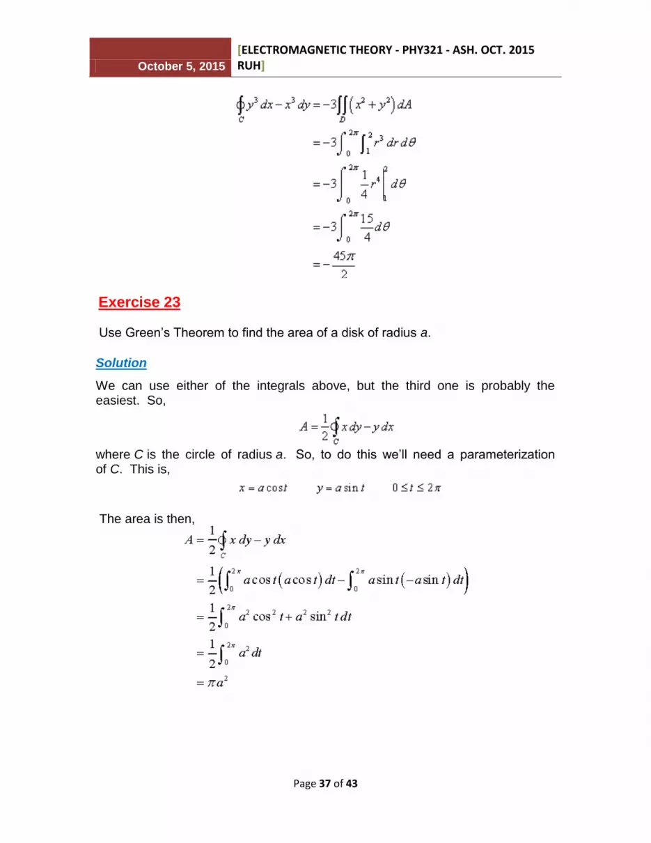
Exercise 23

Use Green’s Theorem to find the area of a disk of radius a.

Solution

We can use either of the integrals above, but the third one is probably the easiest. So,

where C is the circle of radius a. So, to do this we’ll need a parameterization of C. This is,

The area is then,

October 5, 2015


of 43

1.13 Stokes’ Theorem

In this section we are going to take a look at a theorem that is a higher dimensional version of Green's Theorem. In Green’s Theorem we related a line integral to a double integral over some region. In this section we are going to relate a line integral to a surface integral. However, before we give the theorem we first need to define the curve that we’re going to use in the line integral.

Let’s start off with the following surface with the indicated orientation.

Around the edge of this surface we have a curve C. This curve is called

the boundary curve. The orientation of the surface S will induce the positive

orientation of C. To get the positive orientation of C think of yourself as walking

along the curve. While you are walking along the curve if your head is pointing in

the same direction as the unit normal vectors while the surface is on the left then

you are walking in the positive direction on C.

Let S be an oriented smooth surface that is bounded by a simple, closed, smooth

boundary curve C with positive orientation. Also let be a vector field then,

In this theorem note that the surface S can actually be any surface so long as its

boundary curve is given by C. This is something that can be used to our

advantage to simplify the surface integral on occasion.

Exercise 23

October 5, 2015


of 43

Use Stokes’ Theorem to evaluate where

and S is the part of above the plane . Assume that S is

oriented upwards.

Solution

Let’s start this off with a sketch of the surface.

In this case the boundary curve C will be where the surface intersects the

plane and so will be the curve

So, the boundary curve will be the circle of radius 2 that is in the plane . The

parameterization of this curve is,

The first two components give the circle and the third component makes sure

that it is in the plane .

October 5, 2015


of 43

So, the boundary curve will be the circle of radius 2 that is in the plane . The

parameterization of this curve is,

The first two components give the circle and the third component makes sure

that it is in the plane .

Using Stokes’ Theorem we can write the surface integral as the following line

integral.

So, it looks like we need a couple of quantities before we do this integral. Let’s

first get the vector field evaluated on the curve. Remember that this is simply

plugging the components of the parameterization into the vector field.

Next, we need the derivative of the parameterization and the dot product of this

and the vector field.

We can now do the integral.

October 5, 2015


of 43

Exercise 24

Use Stokes’ Theorem to evaluate where and C is the

triangle with vertices , and with counter-clockwise rotation.

Solution

We are going to need the curl of the vector field eventually so let’s get that out of

the way first.

Now, all we have is the boundary curve for the surface that we’ll need to use in

the surface integral. However, as noted above all we need is any surface that

has this as its boundary curve. So, let’s use the following plane with upwards

orientation for the surface.

October 5, 2015


of 43

Since the plane is oriented upwards this induces the positive direction on C as

shown. The equation of this plane is,

Now, let’s use Stokes’ Theorem and get the surface integral set up.

Okay, we now need to find a couple of quantities. First let’s get the gradient.

Recall that this comes from the function of the surface.

Note as well that this also points upwards and so we have the correct direction.

Now, D is the region in the xy-plane shown below,

We get the equation of the line by plugging in into the equation of the

plane. So based on this the ranges that define D are,

October 5, 2015


of 43

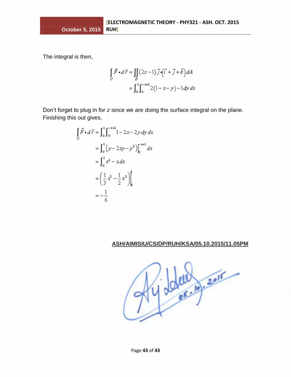
The integral is then,

Don’t forget to plug in for z since we are doing the surface integral on the plane.

Finishing this out gives,

ASH/AIMISIU/CS/DP/RUH/KSA/05.10.2015/11.05PM

PHYS. 321 - ELECTROMAGNETIC THEORY - PART 2

Documents

Transcript of PHYS. 321 - ELECTROMAGNETIC THEORY - PART 2