PHYS 239Spatiotemporal Dynamics in Biological Systems

Winter 2022

Solution of Homework #1

Prepared by Leonardo Pacciani-Morilpaccianimori@physics.ucsd.edu

January 19th, 2022

1. Phase diagram and phase transitions in dynamical systemsIn class, we studied a model of growth and predation. Let the density of an organism be ρ(t). If the growth of the organismis described by a logistic term and the e�ect of predation by a hyperbolic term, then the dynamics is given by the followingODE:

dρ

dt= rρ ·

(1− ρ

ρ

)− δ · ρ

1 + ρρK

where r is the maximal replication rate and δ is the maximal predation rate. Of the two remaining parameters, ρ describesthe carrying capacity and ρK describes the saturating density for predation.

Upon introducing dimensionless variables, u := ρ/ρ, τ := rt, the above equation becomes

du

dτ= u(1− u)− αu

1 + uκ

with two dimensionless parameters α := δ/r and κ = ρK/ρ.

(a) Write a general expression for the fixed point u∗(κ, α) at which du/dτ = 0, and show that the nature of the solution u∗

depends importantly on whether the relative predation rate α is smaller or larger than

αc(κ) =1

2+κ

4+

1

4κ

Show that αc(κ) has a single minimum at κ = 1. The point (κ = 1, α = αc(1) is called the “critical point” due to thespecial behavior exhibited by the system in the vicinity of this point as we will see below.

SolutionThe value u∗ at which du/dτ = 0 is obtained by solving:

0 = u∗(1− u∗)− αu∗

1 + u∗

κ

⇒ u∗(1− u∗) = αu∗

1 + u∗

κ

1

One solution is u∗ = 0. Assuming u∗ 6= 0 and dividing by u∗ on both sides we get:

1− u∗ = α

1 + u∗

κ

⇒ (1− u)(1 +

u∗

κ

)= α ⇒ 1 +

u∗

κ− u∗ − (u∗)2

κ= α ⇒

⇒ (u∗)2

κ+ u∗

(1− 1

κ

)+ (α− 1) = 0 ⇒ (u∗)2 + u∗(κ− 1) + κ(α− 1) = 0

and the solution of this quadratic equation is:

u∗± =−(κ− 1)±

√(κ− 1)2 − 4κ(α− 1)

2=

(1− κ)±√κ2 + 1− 2κ− 4κα+ 4κ

2=

=(1− κ)±

√κ2 + 2κ− 4κα

2=

(1− κ)±√

(κ+ 1)2 − 4κα

2

So, values u∗ at which du/dτ = 0 are:

u∗0 = 0 u∗± =(1− κ)±

√(κ+ 1)2 − 4κα

2(1)

Let’s consider the expression of u∗±: depending on the sign of (κ + 1)2 − 4κα, we might have two distinctreal solution (> 0), one degenerate1 real solution (= 0) or two complex conjugate solutions (< 0). The onlyphysically acceptable solutions in our systems are u∗ ≥ 0: in fact, u = ρ/ρ where ρ is a positive parameter andρ is the population density, which by definition cannot be negative.Therefore, if (κ+ 1)2 − 4κα < 0 the only physically acceptable solution will be u∗ = 0. This happens when:

(κ+ 1)2 − 4κα < 0 ⇒ 4κα > (κ+ 1)2 ⇒ α >2κ+ κ2 + 1

4κ⇒

⇒ α >1

2+κ

4+

1

4κ= αc(κ)

The physical meaning of this result is that when the predation rate is su�ciently larger than the replication rate(remember that α = δ/r), then the population will not survive (i.e., the only possible equilibrium is u∗ = 0,which is extinction). In other words, the replication rate must be su�ciently larger than the predation rate forthe system to be able to sustain a non-zero population.Let us now find the minima of αc(κ):

dαcdκ

= 0 ⇒ d

dκ

(1

2+κ

4+

1

4κ

)= 0 ⇒

⇒ 1

4− 1

4κ2= 0 ⇒

⇒ 1

4κ2=

1

4⇒ κ2 = 1 ⇒ κ = ±1

However, κ is a positive parameter (κ = ρK/ρ, with both ρK and ρ positive parameters), so the only acceptablesolution is κ = 1. To check that this is indeed a minimum, we evaluate the second derivative of αc(κ) in κ = 1:

d2αcdκ2

∣∣∣∣κ=1

=d

dκ

(1

4− 1

4κ2

)∣∣∣∣κ=1

= − 1

4· −2κ3

∣∣∣∣κ=1

= −1

4· −2(1)3

=2

4=

1

2> 0

1This is just the mathematical term to indicate two solutions of a quadratic equation with the same value.

2

Here is a plot of αc(κ):

κ

αc(κ)

κ = 1

αc(1) = 1

(b) For κ = 1, find u∗(α) vs α. [Hint: there are two non-negative real values for u∗(α) for α < αc, and only one forα > αc. Ignore any imaginary solutions which are irrelevant.] To see which of the fixed points is stable/unstable, plotdu/dτ vs u for κ = 1 and the following values of α: (i) α . αc(1), (ii) α = αc(1), (iii) α & αc(1). For each case,plot the “flow”, i.e. the direction of du/dτ as arrows for di�erent regions of u. The type of phase transition which occursat the critical point here is called a “supercritical bifurcation”.SolutionFor κ = 1, the expression of the equilibria u∗ become (from Eq (1)):

u∗0 = 0 u∗± = ±√1− α

We can reject the negative solution (u∗ ≥ 0) and the complex solution (α > 1 = αc(1)), so in the end we have:

u∗0 = 0 u∗ =√1− α with α ≤ 1

This is the plot of u∗(α):

α

u∗(α)

αc = 1

If we now set κ = 1 in the equation of our system we get:

du

dτ= u(1− u)− αu

1 + u

Let’s now plot du/dτ for three values of α as required and determine the stability of the equilibria with astreamplot (i.e., a plot of the “flow”):

i. α . αc : we choose α = 0.95. The streamplot we obtain is the following:

3

u

du/dτ

u∗ = 0

u∗ =√1− α

Therefore, u∗0 = 0 is an unstable equilibrium, while u∗ =√1− α is stable. As soon as the initial condition

is larger than 0, the population will always tend towards u∗ =√1− α

ii. α = αc : we have α = 1. The streamplot we obtain is the following:

u

du/dτ

u∗0 = 0

Therefore, the only equilibrium u∗0 = 0 is stable (u∗ =√1− α =

√1− 1 = 0). Whatever the ini-

tial condition, the population will always tend towards 0 (i.e., the populaton will ultimately always go toextinction).

iii. α & αc : we choose α = 1.1. The streamplot we obtain is the following:

u

du/dτ

u∗0 = 0

Therefore, also in this case the only equilibrium u∗0 = 0 is stable (u∗ =√1− α is not an acceptable

equilibrium in this case).

This is a supercritical pitchfork bifurcation. The bifurcation diagram is:

4

α

u∗(α)

stable

unstable

stable

We can’t see the full “pitchfork” because we are restricting u∗ to non-negative values. To show that this is indeeda supercritical bifurcation, we can expand the equation of the system around u∗ = 0:

du

dt= u(1− u)− αu

(1− u

κ+u2

κ2+ · · ·

)=

= u− u2 − αu+α

κu2 − α

κ2u3 + · · · =

= u(1− α)− u2(ακ− 1)− α

κ2u3 + · · ·

If we now set κ = 1 we are left with:

du

dτ≈ u(1− α) + u2(α− 1)− αu3 (2)

Despite not having the same form of the “prototypical” example of supercritical bifurcation (i.e., x = rx−x3),the behavior of this system is qualitatively the same:

u

du/dτ

α > 1

u

du/dτ

α = 1

u

du/dτ

α < 1

(c) Sketch (i.e., plot the approximate dependence by hand, not by computer) the dependence of the stable fixed point u∗ in thevicinity of the critical point αc(1). The robustness of the system can be characterized by the sensitvity of the densityu∗ to small changes in the environment. Let S := du∗/dα be a measure of the change in population density when thepredation rate changes. Sketch S(α) in the vicinity (i.e., on both sides) of the critical point, and describe the behavior inwords.SolutionThe dependence of the stable fixed point u∗ around αc is taken simply from the bifurcation diagram shownabove:

5

α

u∗

αc

Where the curve on the left of αc is√1− α. Notice that u∗(α) is continuous but not smooth (i.e., not di�er-

entiable) in αc.The sensitivity S(α) = du∗/dα will surely be equal to 0 for α > αc (since u∗(α) is constant for α > αc).For α < αc, S(α) will always be negative (u∗ decreases as α increases), and will decrease tending to2 −∞ forα→ αc:

α

S(α)

αc

Therefore, the sensitivity S(α) undergoes an abrupt, discontinuous change in α = αc.

(d) For κ = 1/2, show that there are three solutions for u∗(α) for a range of α at α0 ≤ α ≤ αc(1/2), where α0 is apositive number you need to determine. To see which of the solutions are stable/unstable, plot du/dτ vs u for κ = 1/2and the following values of α: (i) α . αc(1/2), (ii) α = αc(1/2), (iii) α & αc(1/2), (iv) α . α0, (v) α = α0, (vi)α & α0. For each case, plot the “flow” as in (b). Indicate the stable and unstable fixed points which arise in each case. Incases where there are multiple stable fixed points for the same value of α, what determines the value of u∗, the steady-statedensity?SolutionThe general expression of the equilibria of the system is given by Eq (1):

u∗0 = 0 u∗± =(1− κ)±

√(κ+ 1)2 − 4κα

2

We will have three solutions if i) the two solutions u∗± are real (i.e. α < αc) and if ii) they are both non-negative.

2In fact, the derivative of√1− α is−(2

√1− α)−1, which tends to−∞ for α→ 1

6

This happens when the smaller solution, u∗−, is non-negative, i.e.:

(1− κ)−√

(κ+ 1)2 − 4κα

2≥ 0 ⇒ (1− κ)

2≥√

(κ+ 1)2 − 4κα

2⇒

⇒ (1− κ) ≥√

(κ+ 1)2 − 4κα ⇒ (1− κ)2 ≥ (k + 1)2 − 4κα ⇒

⇒ 1 + κ2 − 2κ ≥ 1 + κ2 + 2κ− 4κα ⇒ 4κα ≥ 4κ ⇒ α ≥ 1 := α0

Therefore, we will have three distinct solutions for 1 ≤ α ≤ αc(1/2) = 9/8 = 1.125.

Let’s now plot du/dτ for κ = 1/2 and the required values of α to determine the stability of the equilibria witha streamplot:

i. α . α0: we choose α = 0.95. The streamplot we obtain is the following:

u

du/dτ

u∗0 = 0

u∗+ = 14(1 +

√9− 8α)

so we have one unstable equilibrium at u∗ = 0 and one stable one at u∗+ > 0. As soon as the initialcondition is larger than 0, the population will tend towards u∗+.

ii. α = α0: we have α = 1. The streamplot we obtain is the following:

u

du/dτ

u∗0 = 0

u∗+ = 12

and so the situation is the same as the previous point.iii. α & α0: we choose α = 1.05. The streamplot we obtain is the following:

7

u

du/dτ

u∗ = 0

u∗− = 14(1−

√9− 8α)

u∗+ = 14(1 +

√9− 8α)

Now a new equilibrium has emerged, and u∗ = 0 is now stable. Therefore, if the initial condition is0 < u(0) < u∗−, the system will end up in u∗ = 0; in other words, if the initial population is smallerthan a threshold (u∗−), the population will die out. On the other hand, if u(0) > u∗−, the population willalways tend towards u∗+. This population size e�ect (i.e., the fact that in order to have a non-zero stationarypopulation the initial population must be larger than a threshold) is known as the Allee e�ect.

iv. α . αc(1/2): we choose α = 1.12. The streamplot we obtain is the following:

u

du/dτ

u∗0 = 0

u∗− = 14(1−

√9− 8α) u∗+ = 1

4(1 +√9− 8α)

The situation is the same as before; the two equilibria u∗± > 0 are approaching each other.v. α = αc(1/2): we have α = 1.125. The streamplot we obtain is the following:

u

du/dτ

u∗0 = 0

u∗+ = 14

The two equilibria u∗ > 0 have now merged into a saddle point. If the initial population is u(0) > u∗+,the system will slowly tend towards u∗+, but as soon as the population is pushed below u∗+ it will go toextinction.

vi. α & αc(1/2): we choose α = 1.13. The streamplot we obtain is the following:

u

du/dτ

u∗ = 0

8

Now the only possible equilibrium is u∗ = 0, and so the population will go to extinction independently ofthe initial condition.

(e) For the nonzero stable fixed point u∗ obtained in (d), use Taylor expansion to obtain the leading dependence on α in thevicinity of αc(1/2) and in the vicinity of α0. From these results, obtain the sensitivity S(α) of this fixed point andsketch both u∗(α) and S(α) in the vicinity of α0. The type of phase transition which occurs at αc(1/2) is called a“saddle-point bifurcation”, while the phase transition which occurs at α0 is called a “subcritical bifurcation”. Describe inwords how they are di�erent from each other and from the supercritical bifurcation encountered in (b).SolutionThe expression of the non-zero fixed point is:

u∗± =(1− κ)±

√(κ+ 1)2 − 4κα

2

By plugging κ = 1/2 we get:

u∗± =1− 1/2±

√(1/2 + 1)2 − 4α · 1/2

2=

1/2±√(3/2)2 − 2α

2=

1

4± 1

2

√9

4− 2α =

=1

4± 1

2

√9− 8α

4=

1

4± 1

2· 12

√9− 8α =

1

4(1±

√9− 8α)

The bifurcation diagram (i.e., the plot of the dependence of u∗ on α) is the following:

α

u∗

α0 αc(1/2)

Therefore, at αc(1/2) a new fixed point emerges, and splits into two fixed points for α . αc(1/2). Further-more, the absolute value of the derivative S(α) = du∗/dα diverges to∞ for3 α→ αc(1/2)

−:

|S(α)| =∣∣∣∣du∗dα

∣∣∣∣ = ∣∣∣∣14(1 +√9− 8α)

∣∣∣∣ = ∣∣∣∣− 1√9− 8α

∣∣∣∣ = 1√9− 8α

α→αc(1/2)−−−−−−−→ +∞ (3)

and so a Taylor expansion around αc(1/2) is not possible. The plot of |S(α)| is the following:

α

|S(α)|

αc(1/2)

3The expression “α→ αc(1/2)−” means that α is approaching αc(1/2) “from below”, i.e. from values smaller than αc(1/2).

9

On the other hand, u∗+(α) and S(α) are continuous and di�erentiable at α0 = 1, so we can perform a Taylorexpansion around that point. Expanding u∗+:

u∗+ =1

4(1 +

√9− 8α) =

= u∗+(α = 1) +du∗+dα

∣∣∣∣α=1

(α− 1) +1

2

d2u∗+dα2

∣∣∣∣α=1

(α− 1)2 +1

6

d3u∗+dα3

∣∣∣∣α=1

(α− 1)3 + · · · =

=1

4(1 +

√9− 8α)

∣∣∣∣α=1

+

(− 1

9− 8α

)∣∣∣∣α=1

(α− 1) +1

2·[− 4

(9− 8α)3/2

]∣∣∣∣α=1

(α− 1)2+

+1

6·[− 48

(9− 8α)5/2

]∣∣∣∣α1

(α− 1)3 + · · · =

=1

2+(−1)(α−1)+1

2·(−4)(α−1)2+1

6·(−48)(α−1)3+· · · = 1

2−(α−1)−2(α−1)2−8(α−1)3+· · ·

Neglecting all terms beyond leading order in α we get:

u∗ =3

2− α

If we now consider u∗−(α), this functon will be continuous but not smooth4 inα0. The expansion must thereforebe written separately for α . α0 and for α & α0:

u∗− ≈

0 α < α0

u∗−(α = 1) +du∗−dα

∣∣∣α=1

(α− 1) + · · · α > α0⇒ u∗− ≈

{0 α < α0

(α− 1) α > α0

The first important di�erence between these two transitions is that the transition at α0 is continuous, whilethe one at αc(1/2) is discontinuous.

The di�erence between the subcritical bifurcation found here and the supercritical bifurcation found in (b) isthat in this case as the parameterα is changed an unstable equilibrium (u∗0 = 0) “splits” into multiple equilibria,while in a supercritical bifurcation it is a stable equilibrium that “splits” into more.

(f) For κ = 2, show that there are two non-negative solutions u∗(α) for α < α1, where α1 is a number smaller than αc(2),and one solution for α > α1. Determine which of the fixed points is stable by plotting du/dτ vs u for κ = 2 and thefollowing values of α: (i) α . α1. (ii) α = α1, (iii) α & α1. For each case, plot the “flow” and indicate the stable andunstable fixed points as above. Using Taylor expansion, find the leading dependence of the stable fixed point u∗ on α inthe vicinity of α1. From this result, find the sensitivity S(α), and sketch u∗(α), S(α) in the vicinity of α1. The phasetransition which occurs at α1 is called a “transcritical bifurcation”. Describe in words again how it is di�erent from thebifurcations encountered in (b) and (e)Solution

4We are looking at the “merging” of the unstable branch into the equilibrium u∗ = 0 in the bifurcation diagram above.

10

For κ = 2, the expression of the non-zero fixed points is:

u∗± =(1− κ)±

√(κ+ 1)2 − 4κα

2

∣∣∣∣∣κ=2

=−1±

√32 − 4 · 2 · α2

=1

2(−1±

√9− 8α)

Now, u∗− is always negative and so the only two possible equilibria are u∗0 = 0 and u∗+. This last fixed point willbe non-negative when5:

1

2(−1 +

√9− 8α) ≥ 0 ⇒

√9− 8α > 1 ⇒ 9− 8α ≥ 1 ⇒ −8α ≥ −8 ⇒ α ≤ 1 := α1

Therefore, we have two non-negative solutions (u∗0 and u∗+) for α < α1 and only one solution (u∗0) for α > α1.

Let’s now plot du/dτ for the three values of α as required and determine the stability of the equilibria with astreamplot:

i. α . α1 : we choose α = 0.95. The streamplot we obtain is the following:

u

du/dτ

u∗0 = 0

u∗+ = 12(−1 +

√9− 8α)

Therefore, u∗0 = 0 is an unstable equilibrium, while u∗+ is stable. As soon as the initial condition is largerthan 0, the population will tend towards u∗+.

ii. α = α1 : we have α = 1. The streamplot we obtain is the following:

u

du/dτ

u∗0 = 0

The only equilibrium, u∗0 = 0 is stable. Whatever the initial condition, the population will always go toextinction.

iii. α & α1 : we choose α = 1.1. The streamplot we obtain is the following:

5Notice: the fact that α1 = α0 is just a coincidence.

11

u

du/dτ

u∗0 = 0

Like in the previous case, the only equilibrium u∗0 = 0 is stable.

The bifurcation diagram is the following:

α

u∗

stableunstable

and so the dependence of the stable fixed point u∗+ on α is:

α

u∗

α1

where the curve on the left of α1 is 12(−1 +

√9− 8α). This curve is not smooth in α1, so we have again to

write the Taylor expansion for α < α1 and α > α1 separately. We get:

u∗+ ≈

{−2(α− 1) α < α1

0 α > α1

Therefore, in this case the sensitivity S(α), while still being discontinuous, does not diverge for α→ α−1 :

S =du∗

dα=

d

dα

1

2(−1 +

√9− 8α) = − 2√

9− 8α

α→α−1−→ −2

12

α

S(α)

α1

−2

The di�erence between this transcritical bifurcation and the subcritical and saddle-point bifurcations encoun-tered before are the following:

• A transcritical bifurcation is continuous, like a subcritical one and unlike a saddle-point bifurcation• The sensitivity in a transcritical bifurcation is discontinuous but it does not diverge close to the critical

point• Subcritical (and also supercritical) bifurcations and saddle-point bifurcations involve the creation/destruction

of fixed points. In a transcritical bifurcation, on the other hand, two fixed points cross each other, “exchang-ing” their stability. In this particular system we can’t see the full picture because u∗ > 0. If we also allowu∗ to be negative, the bifurcation diagram in the vicinity of α1 looks like this:

α

u∗

α1 stableunstable

(g) Based on the results obtained in (a)-(f) above, sketch the phase diagram in the parameter space (κ.α) as follows: draw theline (actually a curve)αc(κ) and put down the special points (κ, α) = (1, αc(1)), (1/2, αc(1/2)), (1/2, α0), (2, α1).With the additional knowledge that the critical values α0 and α1 are κ-independent (you don’t need to derive this), youcan obtain 2 lines that divide the entire parameter space into three distinct regions. Show the two lines in the space of(κ, α) and give a verbal description of the three “phases” separated by these lines. Indicate the nature of phase transitions(bifurcations) upon crossing each line separating the three phases.SolutionLet’s call the special points:

a = (1, αc(1)) = (1, 1) b =

(1

2, αc

(1

2

))=

(1

2,9

8

)

c =

(1

2, α0

)=

(1

2, 1

)d = (2, α1) = (2, 1)

and plot them together with αc(κ) (and a few lines for reference):

13

κ

α

ab

c d

(1/2, 0)(1, 0) (2, 0)

(0, 1)

Let’s now use all the information we have gathered in the previous points to understand how does the phasediagram look:

• If we move along any of the the segments (1/2, 0) → c, (1, 0) → a and (2, 0) → d, we have that thefixed points of the system are u∗0 and u∗+; we are in the situation where as soon as the initial condition isu(0) > 0, the system will tend towards u∗+. Therefore, we can infer that in the whole region α < 1 thesystem exhibits a nontrivial equilibrium u∗+, to which the population will always tend to if u(0) > 0. Wecall this phase S for “survival”:

κ

α

S

• Above the curve outlined by αc(κ), the only possible fixed point is u∗0. In this area of the parameter spacethe population wil always go to extinction, no matter the initial condition. If we move on the segment(2, 0)→ d this is also true between d and the curve αc(κ). Therefore, this will happen in all the area of theparameter space that is between the curve αc(κ) and the region S. We call this phase E for “extinction”:

14

S

E

κ

α

• Finally, if we move along the segment c→ b the system will exhibit the Allee e�ect (i.e., we needu(0) > u∗−in order to have a non-zeo stationary population). We call this phase A from “Allee”:

S

E

A

κ

α

Therefore, the phase diagram of the system (and the two lines that divide it into three regions) are:

15

S

E

A

κ

α

κ = 1

The transition S ←→ A is a subcritical bifurcation and the transition A←→ E is a saddle-point bifurcation.Finally, the transition S ←→ E for κ = 1 is a supercritical bifurcation while for κ > 1 is a transcriticalbifurcation.

2. Oscillatory genetic circuitA genetic circuit in a cell involves two transcription factors, an “activator” and a “repressor”. The activator activates theexpression of itself and the repressor, while the repressor represses the expression of the activator. This circuit is known asthe “predator-prey” circuit. Denoting the concentrations of the activator and the repressor by [A] and [R], respectively, wecan write down a simple set of equations describing their dynamics:

d[A]

dt= αA

[A]

[A] +KA· KR

[R] +KR− µ[A]

d[R]

dt= αR

[A]

[A] +KA− µ[R]

In the above, the parameters KA and KR are the dissociation constant for the binding of the activator and the repressorto the promoter regions, respectively, αA and αR characterize the activity of the two promoter, and µ is the rate of cellgrowth (which serves here to dilute the concentrations of the transcription factors). In this problem, you will find conditionsunder which this circuit sustains oscillation.

(a) Make these equations dimensionless using u = [A]/KA, v = [R]/KR, and τ = µt. Write down the dependences of thetwo remaining dimensionless parameters, σA ∝ αA and σR ∝ αR, in terms of the original parameters of the problem.Solution

16

Let’s first consider the equation for [A], and plug in it [A] = uKA, [R] = vKR and t = τ/µ:

d

d(τ/µ)(uKA) = αA

uKA

uKA +KA· KR

vKR +KR− µuKA ⇒

⇒ µKAdu

dτ= αA

u

u+ 1· 1

v + 1− µuKA ⇒

⇒ du

dτ=

αAµKA

· u

u+ 1· 1

v + 1− u

We can therefore define σA := αA/(µKA) (note that σA ∝ αA). Similarly, for [R] we get:

d

d(τ/µ)(vKR) = αR

uKA

uKA +KA− µvKR ⇒

⇒ µKRdv

dt= αR

u

u+ 1− µvKR ⇒

⇒ dv

dτ=

αRµKR

· u

u+ 1− v

and we can define σR := αR/(µKR) (note that σR ∝ αR). This way, the equations of our system become:

du

dτ= σA

u

u+ 1· 1

v + 1− u dv

dτ= σR

u

u+ 1− v

Notice that, by definition, both σA > 0 and σR > 0 (αA, αR, KA, KR and µ are all positive parameters).

(b) In (u, v) space, sketch the two null clines (i.e., the relation between u and v that makes du/dτ = 0 or dv/dτ = 0).Indicate each sub-regions of (u, v) space partitioned by the two null clines whether du/dτ and dv/dτ are positive ornegative. Sketch qualitatively the “flow” of u and v by arrows in the (u, v) space.

SolutionIn order to make it easier to plot them, we express the null clines as v = · · · . From the equation for uwe obtain:

du

dτ= 0 ⇒ σA

u

u+ 1· 1

v + 1= u

Therefore, one possible solution is u = 0. Assuming u 6= 0 and dividing by u on both sides:

σA1

u+ 1= v + 1 ⇒ v = σA

1

u+ 1− 1

and du/dτ is positive when v is smaller than this expression. Therefore, the plot of this nulllcline and of theregions where du/dτ is positive/negative is the following:

17

u

v

(0, σA − 1)

(σA − 1, 0)

u > 0

u < 0

From the equation for v we obtain:

dv

dτ= 0 ⇒ σR

u

u+ 1= v ⇒ v = σR

u

u+ 1

and dv/dτ is positive when v is smaller than this expression. Therefore, the plot of this nulllcline and of theregions where dv/dτ is positive/negative is the following:

u

v

v > 0

v < 0(0, σR)

The combined plot of both null clines is:

u

v

u < 0

v < 0

u > 0

v < 0

u > 0

v > 0

u < 0

v > 0

18

Therefore, the qualitative flow of the system is the following:

u

v

The solutions of this system will oscillate around the nontrivial fixed point of the system (which is the intersec-tion of the two null clines). It remains to be seen if the solutions spiral away from or towards this point, or if theygo around it in closed orbits (the qualitative analysis we’re doing here does not allow us to distinguish betweenthese cases).

(c) Find the fixed point(s) (u∗, v∗) where du/dτ = 0 and dv/dτ = 0. Show conditions on the parameters σA and σRin order for there to be a “nontrivial” fixed point u∗ > 0 and v∗ > 0. Obtain how the nontrivial fixed point (u∗, v∗)depends on the parameters (σA, σR).SolutionIn order to find the nontrivial fixed points (i.e., with u∗, v∗ 6= 0), we must solve:

σAu∗

u∗ + 1· 1

v + 1− u∗ = 0 σR

u∗

u∗ + 1− v∗ = 0 (4)

which corresponds to finding the intersection point of the null clines shown above. From the first equation in(4) we get:

σAu∗

u∗ + 1· 1

v + 1= u∗ ⇒ u∗ =

σAv∗ + 1

− 1 (5)

where in we have divided by u∗ on both sides since we assuming u∗ 6= 0. From the second equation in (4) weget simply:

v∗ = σRu∗

u∗ + 1

Substituting u∗ from equation (5) we get:

v∗ = σR

(σA

v∗ + 1− 1

)v∗ + 1

σA=σRσA

(σA − v∗ − 1) = σR −σRσA

v∗ − σRσA

⇒

⇒ v∗(1 +

σRσA

)= σR

(1− 1

σA

)⇒ v∗(σA + σR) = σR(σA − 1) ⇒ v∗ =

σR(σA − 1)

σA + σR

19

If we now plug this expression of v∗ into u∗ from equation (5), we get:

u∗ =σA

σRσA−σRσA+σR

+ 1− 1 =

σAσRσA − σR + σA + σR

(σA + σR)− 1 =σA

σRσA + σA(σA + σR)− 1 =

=σA

σA(σR + 1)(σA + σR)− 1 =

σA + σRσR + 1

− 1 =σA + σR − σR − 1

σR + 1=σA − 1

σR + 1

Therefore, the general expression of the nontrivial fixed point of the system is:

(u∗, v∗) =

(σA − 1

σR + 1,σR(σA − 1)

σA + σR

)In order for this fixed point to be really nontrivial, we need that the parameters σA and σR are such that u∗ > 0and v∗ > 0. Therefore, we need:

u∗ > 0 ⇒ σA − 1

σR + 1> 0 ⇒ σA > 1

(since σR > 0) and:

v∗ > 0 ⇒ σR(σA − 1)

σA + σR⇒ σA > 1

(since again σR > 0). Therefore, we need σA > 1 in order to have u∗, v∗ > 0.(d) In the vicinity of the nontrivial fixed point obtained in (c), use Taylor expansion to linearize the dynamical equations for

x(t) = u(t)− u∗, y(t) = v(t)− v∗. Find the two eigenvalues λ for the linearized system.SolutionFirst of all, we can rewrite our system as:

d~z

dτ= f(~z) (6)

where:

~z =

(uv

)f(~z) =

(f1(~z)f2(~z)

)=

(σA

uu+1 ·

1v+1 − u

σRuu+1 − v

)This way, the linearization of our system around (u∗, v∗) looks like:

d~z

dτ= f(~z∗) + J(~z∗)(~z − ~z∗)

where we are neglecting all terms beyond the first order, andJ(~z∗) is the jacobian matrix of the system computedin ~z∗ = (u∗, v∗):

J(~z∗) =

∂f1∂u

∂f1∂v

∂f2∂u

∂f2∂v

∣∣∣∣∣∣(u∗,v∗)

Let’s compute the partial derivatives:

∂f1∂u

∣∣∣∣(u∗,v∗)

=∂

∂u

(σA

u

u+ 1· 1

v + 1− u)∣∣∣∣

(u∗,v∗)

= σA

(1

u+ 1− u

(u+ 1)2

)1

v − 1− 1

∣∣∣∣(u∗,v∗)

=

=σA

(u∗ + 1)2(v∗ + 1)− 1 = · · · = 1− σA

σA + σR

20

∂f1∂v

∣∣∣∣(u∗,v∗)

=∂

∂v

(σA

u

u+ 1· 1

v + 1− u)∣∣∣∣

(u∗,v∗)

= −σAu∗

u∗ + 1· 1

(v∗ + 1)2− u∗ =

= · · · = (σA + σR)(1− σA)σA(σR + 1)2

∂f2∂u

∣∣∣∣(u∗,v∗)

=∂

∂u

(σR

u

u+ 1− v)∣∣∣∣

(u∗,v∗)

=σR

(u∗ + 1)2= · · · = σR(σR + 1)2

(σA + σR)2

∂f2∂v

∣∣∣∣(u∗,v∗)

=∂

∂v

(σR

u

u+ 1− v)∣∣∣∣

(u∗,v∗)

= −1

Therefore, we have:

J(~z∗) =

1−σAσA+σR

(σA+σR)(1−σA)σA(σR+1)2

σR(σR+1)2

(σA+σR)2−1

and we can write the linearization of the system around (u∗, v∗) as:dx/dτ

dy/dτ

=

1−σAσA+σR

(σA+σR)(1−σA)σA(σR+1)2

σR(σR+1)2

(σA+σR)2−1

xy

If we call for simplicity:

A =1− σAσA + σR

B =(σA + σR)(1− σA)

σA(σR + 1)2C =

σR(σR + 1)2

(σA + σR)2

the eigenvalues of the linearized system are found by solving:

det

[(A BC −1

)−(λ 00 λ

)]= 0 ⇒ det

(A− λ BC −(λ+ 1)

)= 0 ⇒

⇒ −(A− λ)(λ+ 1)−BC = 0 ⇒ λ2 + λ(1−A) +BC −A = 0

The solution of this quadratic equation is given by:

λ± =1

2

[−(1−A)±

√(1−A)2 − 4(BC −A)

]= · · ·

· · · = 1

2(σA + σR)

[1− 2σA − σR ±

√1 + σR(6− 4σA) +

(4

σA− 3

)σ2R

]

21

(e) Based on whether the eigenvalues λ found in (d) has nonzero imaginary component, and whether the real component of λ ispositive or negative, find regions of the parameter space (σA, σR) where you expect the circuit to exhibit stable oscillation,damped oscillation, or stable coexistence.SolutionLet us first determine under which conditions Reλ± > 0. This happens when:

1− 2σA − σR2(σA + σR)

> 0 ⇒ 1− 2σA − σR > 0 ⇒ σR < 1− 2σA

However, we always have 1 − 2σA < 0 because σA > 1 (notice that we can’t even have Reλ± = 0 becauseof the same reason). Therefore, this inequality can’t be solved (σR > 0 by defintion) and we will always haveReλ± < 0: the nontrivial equilibrium (u∗, v∗) is always stable, and all the initial conditions (whether theyoscillate or not) will tend towards it.

Let us then determine under which conditions there are oscillations at all. The system will exhibit oscillationsif Imλ± 6= 0, which happens if6:

g(σR) := σ2R

(4

σA− 3

)+ σR(6− 4σA) + 1 < 0

The function g(σR) is a parabola, and therefore:

• if it is convex (i.e., the sign of what multiplies σ2R is positive, therefore 3 − 4/σA > 0 ⇒ σA < 4/3),g(σR) < 0 if σR is in the region between the two zeroes of the parabola

• if it is concave (i.e., the sign of what multiplies σ2R is negative, therefore 3− 4/σA < 0 ⇒ σA > 4/3),g(σR) < 0 if σR is smaller than the smallest zero or largest than the largest zero of the parabola

σR

g(σR)

The parabola is convex, σA < 4/3

σR

g(σR)

The parabola is concave, σA > 4/3

The zeroes of a parabola described by g(σR) are:

σ±R =3σA − 2σ2A ± 2

√σA(σA − 1)3

3σA − 4

Therefore, for a convex parabola we have:

σA <4

3σ−R < σR < σ+R

6Remember: in order for the eigenvalues λ± to have a nonzero imaginary part, the term in their expression under the square root(i.e., the discriminant) must be negative.

22

while for a concave one:σA >

4

3σR < σ−R and σR > σ+R

Looking at, the expression of σ±R , σA(σA − 1)3 is positive for σA < 0 and σA > 1. Since we are assumingσA > 1, the content of the square root is always positive and so σ±R are both real. We therefore need to checkwhen σ±R are both positive. Since σ−R < σ+R , we can first check when7 σ−R > 0:

σ−R =3σA − 2σ2A − 2

√σA(σA − 1)3

3σA − 4> 0 ⇒

{3σA − 4 > 0

3σA − 2σ2A − 2√σA(σA − 1)3 > 0

The first equation yields σA > 4/3. This means that σ−R could be positive only when the parabola is concave.Solving the second equation:

3σA − 2σ2A > 2√σA(σA − 1)3 ⇒ (3σA − 2σ2A)

2 > 4σA(σA − 1)3 ⇒

⇒ 9σ2A + 4σ4A − 12σ3A > 4σA(σ3A − 3σ2A + 3σA − 1) = 4σ4A − 12σ3A + 12σ2A − 4σA ⇒

⇒ 3σ2A − 4σA < 0 ⇒ σA(3σA − 4) < 0

This last inequality is true if σA > 0 and 3σA − 4 < 0 ⇒ σA < 4/3. Thus:

σ−R > 0 ⇒

{σA > 4/3

σA < 4/3

This means that the inequality σ−R > 0 does not have any solution: σ−R < 0 for any value of σA.

Similarly, we can check when σ+R > 0:

σ+R =3σA − 2σ2A + 2

√σA(σA − 1)3

3σA − 4> 0 ⇒

{3σA − 4 > 0

3σA − 2σ2A + 2√σA(σA − 1)3 > 0

⇒

⇒

{σA > 4/3

2√σA(σA − 1)3 > 2σ2A − 3σA

Solving the second equation:

4σA(σ3A − 3σ2A + 3σA − 1) = 4σ4A − 12σ3A + 12σ2A − 4σA > 4σ4A + 9σ2A − 12σ3A ⇒

⇒ 3σ2A − 4σA > 0 ⇒ σA(3σA − 4) > 0

This inequality is true if σA > 0 and 3σA − 4 > 0 ⇒ σA > 4/3, and so:

σ+R > 0 ⇒

{σA > 4/3

σA > 4/3⇒ σA >

4

3

Therefore:7Because in that case we know that both σ±

R > 0. If σ−R < 0 we could still have either σ+

R > 0 or σ+R < 0.

23

– For σA < 4/3 (i.e., the parabola is convex), σ±R < 0

– For σA > 4/3 (i.e., the parabola is concave), σ−R < 0 and σ+R > 0

Therefore, the system will exhibit oscillations (i.e., g(σR) < 0 ⇒ Imλ± 6= 0) only when:

σA >4

3and σR > σ+R =

3σA − 2σ2A + 2√σA(σA − 1)3

3σA − 4

On the other hand, the system will not exhibit oscillations (i.e., g(σR > 0) ⇒ Imλ± = 0) when:

σA <4

3or σA >

4

3and σR ≤ σ+R =

3σA − 2σ2A + 2√σA(σA − 1)3

3σA − 4

The phase diagram of the system is the following:

D.O.S.C.

σA

σR

(4/3, 0)(1, 0)

In phase S.C. (which includes the line that separates the two phases) the system exhibits stable coexistence (i.e.,Reλ± < 0, Imλ± = 0): there are no oscillations and therefore the solutions will simply tend towards thenontrivial fixed point (u∗, v∗). In phaseD.O., on the other hand, the solutions will also oscillate and thereforethe system will exhibit damped oscillations (i.e., Reλ± < 0, Imλ± 6= 0). There are no regions in the parameterspace where the system exhibits stable oscillations (i.e., Reλ± = 0, Imλ± 6= 0).

3. Rock-scissor-paper gameThis classic “game” insolves three species R, S and P interacting in a population. S stimulates the growth of R whileP stimulates the death of R. Also, P stimulates the growth of S while R stimulates the death of S, and R stimulatesthe growth of P while S stimulates the death of P . Let p1, p2, p3 denote respectively the frequency of R, S, P in apopulation, with p1 + p2 + p3 = 1. In the simplest case where the gain (cost) of winning (losing) is unity, the dynamicsof the system is governed by the following ODES:

dp1dt

= p1 · (p2 − p3)

dp2dt

= p2 · (p3 − p1)

24

dp3dt

= p3 · (p1 − p3)

In this problem, you will work out the conditions under which the R-S-P game sustains oscillations.

(a) Show that the above equations admit a conserved quantity, p1p2p3 := C , where C is a positive constant fixed by theinitial condition, i.e. C = p1(0) · p2(0) · p3(0).SolutionIn order to show that C = p1p2p3 is conserved, we simply have to verify that its time derivative is null, i.e.dC/dt = 0:

dC

dt=

d

dt(p1p2p3) =

dp1dt· p2p3 + p1

d

dt(p2p3) =

= p1p2p3 + p1(p2p3 + p2p3) = p1p2p3 + p1p2p3 + p1p2p3 =

= p1(p2 − p3)p2p3 + p1p2(p3 − p1)p3 + p1p2p3(p1 − p2) =

= (p1p2 − p1p3)p2p3 + p1p2(p23 − p1p3) + p1p2(p1p3 − p2p3) =

= ����p1p22p3 −

HHHHp1p2p23 +HHHHp1p2p

23 −��

��HHHHp21p2p3 +����HHHHp21p2p3 −��

��p1p22p3 = 0

Since C is constant, its value will be fixed by its initial condition: C(t) = C(0) = p1(0) · p2(0) · p3(0).(b) Introducing xi = p1 − 1/3 to describe the deviation from the symmetric point p1 = p2 = p3 = 1/3, write down

the two constrains on pi (on their sum and product) in terms of xi. Further introducing y = p2 − p3, write down theconstraint p1p2p3 = C in terms of x1 and y (we will change x1 to x below to further simplify the notation).SolutionFrom xi = pi − 1/3 we have pi = xi + 1/3, and by substituting in the constraint p1 + p2 + p3 = 1 we get:

1 = p1 + p2 + p3 = x1 +1

3+ x2 +

1

3+ x3 +

1

3= x1 + x2 + x3 + 1 ⇒ x1 + x2 + x3 = 0

On the other hand, substituting in the expression for C :

C = p1p2p3 =

(x1 +

1

3

)(x2 +

1

3

)(x3 +

1

3

)=

(x1x2 +

x13

+x23

+1

9

)(x3 +

1

3

)=

= x1x2x3 +1

3x1x2 +

1

3x1x3 +

1

9x1 +

1

3x2x3 +

1

9x2 +

1

9x3 +

1

27=

= x1x2x3 +1

3(x1x2 + x2x3 + x1x3) +

1

9(x1 + x2 + x3︸ ︷︷ ︸

=0

) +1

27=

= x1x2x3 +1

3(x1x2 + x2x3 + x1x3) +

1

27

25

If we now call x = p1 − 1/3 and y = p2 − p3 we have:

p1 = x+1

3

{p2 + p3 = 1− p1 = 2/3− xp2 − p3 = y

From the second equation in the system we have p2 = p3+ y, and plugging this expression in the first equationwe obtain:

p3 + y + p3 =2

3− x ⇒ 2p3 =

2

3− x− y ⇒ p3 =

1

2

(2

3− x− y

)Plugging this expression for p3 back in the previous system of equations we get:

p2 =1

2

(2

3− x− y

)+ y =

1

2

(2

3− x+ y

)We can now use these results to write C in terms of x and y:

C = p1p2p3 =

(x+

1

3

)1

2

(2

3− x− y

)1

2

(2

3− x+ y

)=

=1

4

(x+

1

3

)[(2

3− x)2

− y2]=

1

4

(x+

1

3

)(4

9+ x2 − 4

3x− y2

)=

=1

4

(4

9x+ x3 − 4

3x2 − xy2 + 4

27+

1

3x2 − 4

9x− 1

3y2)

=

=1

9x+

1

4x3 − 1

3x2 − 1

4xy2 +

1

27+

1

12x2 − 1

9x− 1

12y2 =

=1

27+

1

4x3 − 1

4x2 − 1

12y2(1 + 3x) =

=1

27− 1

4x2(1− x)− 1

12y2(3x+ 1)

(c) From the constraint on x and y obtained in (b), show that there is a unique maximum for C(x, y) in the allowed space0 < pi < 1. What is the value C0 := C(x0, y0) at the maximum? And what does the location of the maximum(x0, y0) corresponds to in terms of the frequencies pi? Show that for C . C0 (i.e. , for 0 < C0 − C � C0), the stableorbits are ellipses centered at (x0, y0), i.e. of the form a(x − x0)2 + b(y − y0)2 = c. How does the size of the ellipsedepend on the value of c0 − C?SolutionTo find the maximum of C by “brute force”, we have to see where the partial derivatives of C are equal to zero:

∂C

∂x= −1

4

(2x(1− x) + x2(−1)

)− 1

12y2 · 3 = −1

2x2 +

3

4x− 1

4y2

26

∂C

∂y= − 1

12· 2y(3x+ 1) = −1

6y − 1

2xy{

∂C/∂x = 0

∂C/∂y = 0⇒

{−1

2x2 + 3

4x−14y

2 = 0

−16y −

12xy = 0

⇒

{3x2 − 2x− y2 = 0

y(3x+ 1) = 0

From the second equation we have either y = 0 or x = −1/3. If we set y = 0 in the first equation we get:

3x2 − 2x = 0 ⇒ x(3x− 2) = 0 ⇒

{x = 0

x = 2/3

On the other hand, if we set x = −1/3 in the same equation we obtain:

3 · 19+ 2

1

3− y2 = 0 ⇒ y2 = 1 ⇒ y = ±1

(notice that, from the definitions of x and y and from the fact that 0 ≤ pi ≤ 1 we have −1/3 ≤ x ≤ 2/3 and−1 ≤ y ≤ 1).Therefore, the points where the derivative of C is null are (0, 0), (2/3, 0) and (−1/3,±1). In order to checkwhich one of them is a maximum, we have to compute the so-called “hessian matrix” of C , i.e.:

H(x, y) =

∂2C∂x2

∂2C∂x∂y

∂2C∂y∂x

∂2C∂y2

and evaluate it in (0, 0), (2/3, 0), (−1/3,−1) and (−1/3, 1). Remember that a point (x0, y0) of a functionf(x, y) is a maximum if H(x0, y0) is negative definite (i.e., all its eigenvalues are negative).For our system, we have:

∂2C

∂x2= −1

2+

3

2x

∂2C

∂x∂y=

∂2C

∂y∂x= −1

2y

∂2C

∂y2= −1

2(3x+ 1)

Therefore:

H(x, y) =

−12 + 3

2x −12y

−12y −1

2(3x+ 1)

Let’s first evaluate it in (2/3, 0):

H(2/3, 0) =

−12 + 3

2 ·23 −1

2 · 0

−12 · 0 −1

2(3 ·23 + 1)

=

12 0

0 −32

The eigenvalues of this matrix are 1/2 and−3/2, so the matrix is neither positive definite nor negative definite.In (−1/3,−1) we have:

H(−1/3,−1) =

−12 + 3

2 ·(−1

3

)−1

2 · (−1)

−12 · (−1) −1

2

[3 ·(−1

3

)+ 1] =

−1 12

12 0

27

The eigenvalues of this matrix are λ± = 12(−1±

√2), where λ+ > 0 and λ− < 0 so again the matrix is neither

positive definite nor negative definite. Similarly, for (−1/3, 1) we have:

H(−1/3, 1) =

−12 + 3

2 ·(−1

3

)−1

2 · 1

−12 · 1 −1

2

[3 ·(−1

3

)+ 1] =

−1 12

12 0

and its eigenvalues are again λ± = 1

2(−1±√2).

Finally, in (0, 0) we have:

H(0, 0) =

−12 + 3

2 · 0 −12 · 0

−12 · 0 −1

2(3 · 0 + 1)

=

−12 0

0 −12

This matrix is indeed negative definite, because its (only) eigenvalue is −1/2. Therefore, (x = 0, y = 0) is themaximum of C . From the expression of C we also have C0 = C(0, 0) = 1/27.

There is, however, a smarter way to get to the same conclusions without computing all the derivatives shownabove. Let’s take a look again at how C is written as a function of x and y:

C(x, y) =1

27− 1

4x2(1− x)− 1

12y2(3x+ 1)

Now, from the definitions of x and y we have −1/3 ≤ x ≤ 2/3 and −1 ≤ y ≤ 1, and so x2, (1− x), y2 and(3x+1) will always be positive. Therefore, C ≤ 1/27 because−x2(1− x)/4 < 0 and−y2(3x+1)/12 < 0.Thus, 1/27 is the maximum value of C . Since C0 = C(0, 0) = 1/27, the point (0, 0) will be its maximum.

From the original expression of our equations, the point (x0 = 0, y0 = 0) corresponds to p1 = p2 = p3 = 1/3.

To determine the stable orbits around (x0, y0), we rewrite the expression of C as:

C = C0 −1

4x2 +

1

4x3 − 1

4xy2 − 1

12y2

If we now call δC = C0−C and neglect all the terms in the equation beyond the leading order (because x andy will be small, since we are studying the system close to (x0 = 0, y0 = 0)), we get:

−1

4x2 − 1

12y2 + δC = 0

and we can rewrite it as:

1

4x2 +

1

12y2 = δC ⇒ x2

4δC+

y2

12δC= 1 ⇒

(x

2√δC

)2

+

(y

2√3δC

)2

= 1

This is the equation of an ellipse that is centered in (0, 0) and has semiaxes of lengths 2√δC (along x) and

2√3δC (along y).

28

(d) For an arbitrary value of the constant C in the range 0 < C < C0, show that x(t) is bounded in the range xmin(C)and xmax(C) (in the sense that for the ellipse in (c), x(t) is bounded between±

√c/a). Find the values of xmin and xmax

in the limit C → 0 and show that the trajectory is composed of three straight-line segments in this limit. Express thesesegments in the original variables (p1, p2, p3) and explain in words what is happening along each trajectory. Sketch thistrajectory in the (x, y) space, along with the direction of the dynamics. Add to the plot the ellipse in (c) obtained in thelimit C → C0. Finally, sketch your guess of what the trajectories should look like for intermediate values of C .SolutionWe’ve just shown that xmin ≤ x ≤ xmax when δC ≈ 0, i.e. when C ≈ C0. To show that this is true for anyvalue of 0 < C < C0, let’s use the geenral expression of C to write y2 as a function of x:

C − C0 = −1

4x2(1− x)− 1

12y2(3x+ 1) ⇒ 1

12y2(3x+ 1) = C0 − C −

1

4x2(1− x) ⇒

⇒ y2 =12

3x+ 1

[C0 − C −

1

4x2(1− x)

]Since y2 ≥ 0, we need this expression to be larger or equal to 0. Since 3x + 1 > 0 (remember that from thedefinition of x we have −1/3 ≤ x ≤ 2/3), we will need:

C − C0 −1

4x2(1− x) ≥ 0 ⇒ 1

4x2(1− x) ≤ C0 − C

The term on the left hand side is a cubic function. Therefore, we need to determine when the cubic functionassumes values lower or equal to C0 − C . It’s not necessary to solve the cubic equation (i.e., the equationwith the equality sign “=” instead of “≤”), also because it would be very complicated. We can simply plotf(x) = x2(1− x)/4 and C0 − C to understand how the system behaves:

x

f(x)

−1/3 2/3

C0 − C

C0

xmin xmax

Therefore, we immediately see thatx2(1−x)/4 ≤ C0−C whenxmin ≤ x ≤ xmax for any value of 0 < C < C0.

If we now take the limit C → 0, we get:

1

4x2(1− x) = C0 =

1

27

We could solve the cubic equation, but from the plot above we can see that asC → 0we will haveC0−C → C0

and therefore xmin → −1/3 and xmax → 2/3.

29

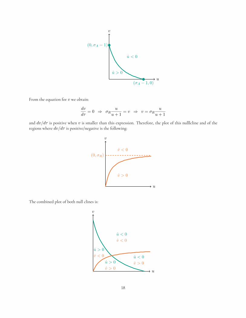
To find the three straight-line segments, we notice that in (b) during some calculations we have written C as:

C =1

4

(x+

1

3

)[(2

3− x)2

− y2]

This expression is useful now because in the limit C → 0 we will have:

1

4

(x+

1

3

)[(2

3− x)2

− y2]= 0

This equation has three solutions:• x = −1/3 with any value for y• y = 2/3− x• y = −2/3 + x

These solutions are represent by three lines in the (x, y) plane. The points in which these three lines intersectare given by: {

x = −1/3y = 2/3− x

{x = −1/3y = −2/3 + x

{y = 2/3− xy = −2/3 + x

By solving these simple linear systems we obtain:{x = −1/3y = 1

{x = −1/3y = −1

{x = 2/3

y = 0

Therefore, this is the plot of the three segments that delineate the orbits of the system in the limit C → 0:

x

y

(−1/3, 1)

(−1/3,−1)

(2/3, 0)

Now, in terms of the original variables (p1, p2, p3) the three points correspond to8:p1 = 0

p2 = 1

p3 = 0

p1 = 0

p2 = 0

p3 = 1

p1 = 1

p2 = 0

p3 = 0

8For example, for the point (−1/3, 1) we have x = −1/3 ⇒ p1 = 1/3− 1/3 = 0 and then:{y = p2 − p3 = 1

p1 + p2 + p3 = 0⇒

{p2 − p3 = 1

p2 + p3 = 0⇒

{p2 = 1

p3 = 0

And similarly for the other points.

30

Therefore, the three points correspond to states where only one of the populations is present. When we movefrom one point to the other along the segment, one population is replacing the other: for example, if we movealong the segment (−1/3, 1)→ (2/3, 0) the population p1 is replacing populations p2.To determine the direction of the dynamics (i.e., if the orbits are going clockwise or counterclockwise) we cansimply rewrite the equation for p1 in terms of x and y:

x =

(x+

1

3

)y (7)

Since x+ 1/3 > 0, we have that x > 0 when y > 0 and viceversa:

x

y

(−1/3, 1)

(−1/3,−1)

(2/3, 0)

Therefore, the orbits are going clockwise. The stream plot of these orbits and of the ones obtained in (c) will be:

x

y

(−1/3, 1)

(−1/3,−1)

(2/3, 0)

31

The intermediate orbits will have a shape that is something in between the ellipse and the triangle (since C is acontinuous function, they will be a continuous deformation from the ellipse to the triangle). For example:

x

y

(−1/3, 1)

(−1/3,−1)

(2/3, 0)

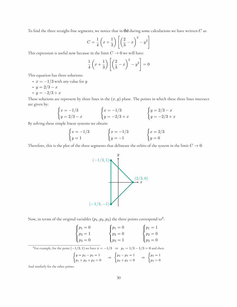
The actual streamplot of this system9, plotted with Mathematica10, is shown in Figure 1.

(e) Bonus for the more mathematically inclined: find the period of oscillation for C → 0. You should be able to write youranswer in terms of ln(1/C). [Hint: you will need to obtain deviations of the trajectories from the straight-line segments,and most importantly, the turning points for small but non-zero C . As the three pieces are symmetrical, you just need towork out one of them.]

9It is not required by the homework, but the equations of which I am plotting the streamplot in this figure can be obtained fromthe original equations by simply plugging the definitions of x and y:

p1 = p1(p2 − p3)p2 = p2(p3 − p1)p3 = p3(p1 − p2)

⇒

x =

(x+ 1

3

)y

y = ddt(p2 − p3) = p2p3 − p2p1 − p1p3 + p2p3 = 2p2p3 − p1(p2 + p3)

From the definitions y = p2− p3 and x = p1− 1/3, and from the constraint p1 + p2 + p3 = 1 we find p2 = 1/3− x/2+ y/2 andp3 = 1/3− x/2− y/2. Plugging these expressions in the equation for y, in the end we obtain:

x =

(x+

1

3

)y y =

3

2x2 − x− 1

2y2

10This plot shows the flow for any initial condition on x and y, so also for (x, y) outside of the triangle we’ve studied in this point(which are non-physical solutions of the system).

32

-0.4 -0.2 0.0 0.2 0.4 0.6

-1.0

-0.5

0.0

0.5

1.0

x

y

Figure 1: Streamplot of the rock-scissor-paper system.

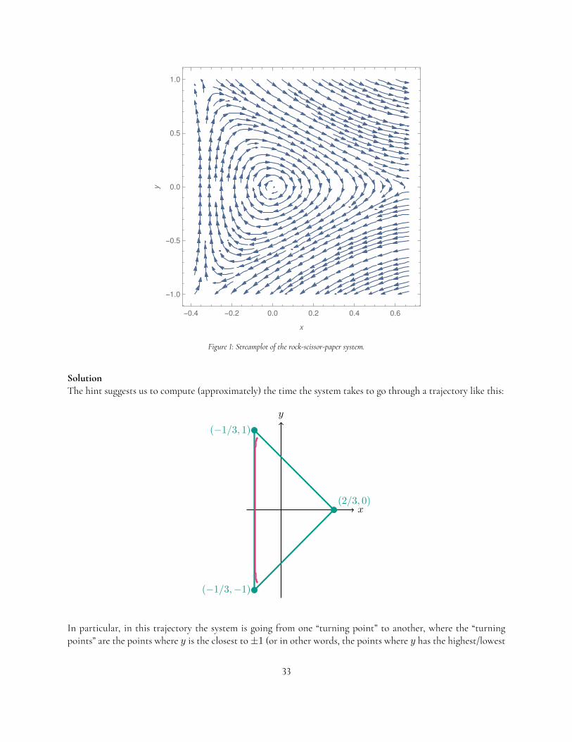
SolutionThe hint suggests us to compute (approximately) the time the system takes to go through a trajectory like this:

x

y

(−1/3, 1)

(−1/3,−1)

(2/3, 0)

In particular, in this trajectory the system is going from one “turning point” to another, where the “turningpoints” are the points where y is the closest to±1 (or in other words, the points where y has the highest/lowest

33

value). Thanks to the symmetry of the problem, once we compute the time tsegment that the system takes to gothrough one of this “pieces” of trajectory, the period T of the complete orbit will be T = 3tsegment.

To compute tsegment, we solve the equations of the system close to one of the segments, and since the system issymmetrical we can choose any of the three segments. We choose to work near (−1/3,−1) → (−1/3, 1) (asin the figure above), so we set x = −1/3 + ε (with ε > 0 small) in the equations of the system and we get:

x =(x+ 1

3

)y

y = 32x

2 − x− 12y

2

⇒

x =

(−1

3 + ε+ 13

)y

y = 32

(19 + ε2 − 2

3ε)− 1

3 + ε− 12y

2

⇒

⇒

x = ε · y ≈ 0

y = 12 + 3

2ε2 − 1

2y2 ≈ 1

2(1− y2)

where we have neglected the terms containing ε, since it is small. The first equation expresses the fact that thesystem remains close to the segment (since x ≈ 0 means that x does not change), while the second one is theequation we have to solve in order to determine tsegment. We do so by separating the variables:

dy

dt=

1

2(1− y2) ⇒ 2

dy

1− y2= dt

We now integrate both sides; the right hand side is integrated from t = 0 (our initial time) to t = tsegment, whilesince we are moving “up” the segment the left hand side is integrated from y = −1 + δ to y = 1 − δ, whereδ > 0 is small and will depend on ε:∫ 1−δ

−1+δ2

dy

1− y2=

∫ tsegment

0dt ⇒

∫ 1−δ

−1+δ2dy

(1

1− y+

1

1− y

)= tsegment ⇒

⇒ tsegment = 2 ln

(1 + y

1− y

)∣∣∣∣1−δ−1+δ

= 2 ln2

δ

Now, δ gives a measure of how close y gets to±1 at the turning points (as stated above, y goes from−1 + δ to1−δ), and we want to express how it depends onC in the limitC → 0. To do this, we start from the expressionof C in terms of x and y:

C =1

4

(x+

1

3

)[(2

3− x)2

− y2]

and we set11 x = −1/3 + ε, y = 1− δ:

C =1

4

(−1

3+ ε+

1

3

)[(2

3+

1

3− ε)2

− (1− δ)2]=

1

4ε(1 + ε2 − 2ε− 1− δ2 + 2δ

)⇒

⇒ 4C = −ε3 − 2ε2 − εδ2 + 2εδ

11Notice that our results do not change even if we choose y = −1 + δ, since C depends on y2.

34

If we neglet all terms beyond leading orders in δ and ε:

4C = −2ε2 + 2εδ ⇒ 2C = εδ − ε2 ⇒ δ = ε+2C

ε

The turning point corresponds to the minimum value of δ as a function of ε:

x

y

ε∗

δ∗

0 =∂

∂εδ(ε) = 1− 2C

ε2⇒ ε∗ =

√2C ⇒ δ∗ = 2

√2C

Therefore, the period of the orbits for C → 0 will be:

T = 3tsegment = 3 · 2 ln 2

δ∗= 6 ln

2

2√2C

= 6 ln1√2C

= 3 ln1

2C

35