Advanced Mechanics I. Phys 302
146
Advanced Mechanics I. Phys 302 Artem G. Abanov This work is licensed under the Creative Commons Attribution 3.0 Unported License. To view a copy of this license, visit http://creativecommons.org/licenses/by/3.0/ or send a letter to Creative Commons, 444 Castro Street, Suite 900, Mountain View, California, 94041, USA.
-
Upload
khangminh22 -
Category
Documents
-
view
0 -
download
0
Transcript of Advanced Mechanics I. Phys 302

Advanced Mechanics I. Phys 302Artem G. Abanov
This work is licensed under the Creative CommonsAttribution 3.0 Unported License. To view a copy of thislicense, visit http://creativecommons.org/licenses/by/3.0/or send a letter to Creative Commons, 444 Castro Street,Suite 900, Mountain View, California, 94041, USA.


ContentsAdvanced Mechanics I. Phys 302 1
Lecture 1. Introduction. Vectors. 1
Lecture 2. Coordinates. Frames of references. Newton’s first and second laws. 32.1. Coordinates, scalars, vectors. 32.2. Frames of reference. 4
Lecture 3. Newton’s laws. 7
Lecture 4. Air resistance. 9
Lecture 5. Air resistance. 11
Lecture 6. Oscillations. Oscillations with friction. 13
Lecture 7. Oscillations with external force. Resonance. 157.1. Different limits. 157.2. External force. 16
Lecture 8. Resonance. Response. 178.1. Resonance. 178.2. Useful points. 18
Lecture 9. Momentum Conservation. Rocket motion. Charged particle in magneticfield. 19
9.1. Momentum Conservation. 199.2. Rocket motion. 209.3. Charged particle in magnetic field. 21
Lecture 10. Kinematics in cylindrical/polar coordinates. 23
Lecture 11. Angular velocity. Angular momentum. 2711.1. Angular velocity. Rotation. 2711.2. Angular momentum. 28
Lecture 12. Moment of inertia. Kinetic energy. 2912.1. Angular momentum. Moment of inertia. 2912.2. Kinetic energy. 31
Lecture 13. Work. Potential energy. 3313.1. Mathematical preliminaries. 3313.2. Work. 34
3

4 FALL 2014, ARTEM G. ABANOV, ADVANCED MECHANICS I. PHYS 302
13.3. Conservative forces. Energy conservation. 34
Lecture 14. Energy Conservation. One-dimensional motion. 3714.1. Change of kinetic energy. 3714.2. 1D motion. 38
Lecture 15. Spherical coordinates. Central forces. 4115.1. Spherical coordinates. 4115.2. Central force 44
Lecture 16. Effective potential. Kepler orbits. 4516.1. Central force. General. 4516.2. Motion in under central force. 4516.3. Kepler orbits. 46
Lecture 17. Kepler orbits continued. 4917.1. Kepler’s second law 5117.2. Kepler’s third law 51
Lecture 18. Another derivation. Conserved Laplace-Runge-Lenz vector. 5318.1. Another way. 5318.2. A hidden symmetry. 5318.3. Conserved vector ~A. 54
Lecture 19. Change of orbits. Virial theorem. Kepler orbits for comparable masses. 5719.1. Kepler orbits from ~A. 5719.2. Change of orbits. 5719.3. Spreading of debris after a satellite explosion. 5819.4. Virial theorem 5819.5. Kepler orbits for comparable masses. 58
Lecture 20. Panegyric to Newton. Functionals. 6120.1. How to see F = GMm
r2 from Kepler’s laws. 6120.2. Difference between functions and functionals. 6220.3. Examples of functionals. 62
Lecture 21. More on functionals. 6521.1. Examples of functionals. Continued. 6521.2. General form of the functionals. 6621.3. Discretization. Fanctionals as functions. 66
Lecture 22. Euler-Lagrange equation 6722.1. Minimization problem 6722.2. Minimum of a function. 6722.3. The Euler-Lagrange equations 6822.4. Example 70
Lecture 23. Euler-Lagrange equation continued. 7123.1. Example 7123.2. Reparametrization 72

FALL 2014, ARTEM G. ABANOV, ADVANCED MECHANICS I. PHYS 302 523.3. The Euler-Lagrange equations, for many variables. 72
Lecture 24. Lagrangian mechanics. 7324.1. Problems of Newton laws. 7324.2. Newton second law as Euler-Lagrange equations 7324.3. Hamilton’s Principle. Action. 7324.4. Lagrangian. 7424.5. Examples. 74
Lecture 25. Lagrangian mechanics. 7725.1. General strategy. 7725.2. Examples. 77
Lecture 26. Lagrangian mechanics. 7926.1. Examples. 79
Lecture 27. Lagrangian mechanics. 8327.1. Example. 8327.2. Small Oscillations. 84
Lecture 28. Lagrangian mechanics. 8728.1. Generalized momentum. 8728.2. Ignorable coordinates. Conservation laws. 8728.3. Momentum conservation. Translation invariance 8828.4. Non uniqueness of the Lagrangian. 88
Lecture 29. Lagrangian’s equations for magnetic forces. 9129.1. Electric and magnetic fields. 9129.2. The Lagrangian. 92
Lecture 30. Energy conservation. 9530.1. Energy conservation. 95
Lecture 31. Hamiltonian. 9931.1. Hamiltonian. 9931.2. Examples. 100
Lecture 32. Hamiltonian equations. 10332.1. Hamiltonian equations. 10332.2. Examples. 104
Lecture 33. Hamiltonian equations. Examples 10733.1. Lagrangian→Hamiltonian, Hamiltonian→Lagrangian. 10733.2. Examples. 108
Lecture 34. Hamiltonian equations. Examples. Phase space. 11334.1. Examples. 11334.2. Phase space. Hamiltonian vector field. Phase trajectories. 114
Lecture 35. Liouville’s theorem. Poincaré recurrence theorem. Area law. 11735.1. Liouville’s theorem. 117

6 FALL 2014, ARTEM G. ABANOV, ADVANCED MECHANICS I. PHYS 302
35.2. Poincaré recurrence theorem. 11835.3. Area law. 118
Lecture 36. Adiabatic invariants. 12136.1. Examples. 123
Lecture 37. Poisson brackets. Change of Variables. Canonical variables. 12537.1. Poisson brackets. 12537.2. Change of Variables. 12637.3. Canonical variables. 127
Lecture 38. Hamiltonian equations. Jacobi’s identity. 12938.1. Hamiltonian mechanics 12938.2. New formulation of the Hamiltonian mechanics. 12938.3. How to compute Poisson brackets for any two functions. 13038.4. The Jacobi’s identity 13138.5. Commutation of Hamiltonian flows. 131
Lecture 39. Integrals of motion. Angular momentum. 13339.1. Time evolution of Poisson brackets. 13339.2. Integrals of motion. 13439.3. Angular momentum. 134
Lecture 40. Hamilton-Jacobi equation. 13740.1. Momentum. 13740.2. Energy. 13840.3. Hamilton-Jacobi equation 13940.4. Connection to quantum mechanics. 139

LECTURE 1. INTRODUCTION. VECTORS. 1
LECTURE 1Introduction. Vectors.
Preliminaries.• Contact info.• Syllabus. Homework 40%, First exam 30%, Final 30%.• Attendance policy.• Zoom. Mute. Use space bar. Pin video. No video.• Lecture, feedback. Going too fast, etc.• Office hours (Mondays 12 pm on Zoom)• Canvas.• Homework submissions through Canvas. PDF SINGLE FILE.• Homeworks due by Wednesday’s lectures.• Homework session. Wednesday 12pm on Zoom.• Homeworks: To cheat or not to cheat? collaborations!!!!! make study groups, mis-takes, etc.• Honors problems. Indicate if you are an Honors student on top of your homework.• Homework sessions (Wednesday 12pm on Zoom)• Grading. Every assignment is 100 pt. The points split equally between the problemsin a given assignment.• Exams. The same point system as in homework assignments. First exam is takehome. Most of the problems are taken from the problem bank. The bank is on theweb.• Book. Lecture notes. Zoom and lecture notes.• Language.• Course content and philosophy.• Questions: profound vs. stupid.• Lecture is a conversation.


LECTURE 2Coordinates. Frames of references. Newton’s first and
second laws.
2.1. Coordinates, scalars, vectors.• Coordinates. Coordinate systems. You chose a coordinate system to describe aprocess (positions, motion, fields, etc) The physical process does not depend on thesystem of coordinates you use!• Scalars. Vectors.• Vector components.• Vectors and scalars are independent of the coordinate systems. Vector componentsdo depend on the coordinate system which you use.• What can be done with vectors? Linearity, scalar (dot) product, vector (cross)product. The idea is to keep their independence from the coordinate system.– Scalar (dot) product. Coordinate independent definition. Bilinear. Symmetric.
~a ·~b = |~a||~b| cos(φ) =3∑i=1
aibi ≡ aibi — Einstein notations.
– Vector (cross) product. Coordinate independent definition.
~c = ~a×~b, |~c| = |~a||~b| sin(φ), Direction — right hand rule.Bilinear. Antisymmetric – RHR, this is why it is sin(φ) and not cos(φ). Deter-minant.
• Symbol Levi-Chivita.– Useful formulas:
εijkεijl = 2δkl, εijkεilm = δjlδkm − δjmδkl.Notice the use of Einstein notations.• Examples:
– Vector product ~c = ~a×~b:ci = [~a×~b]i = εijkajbk
cx = [~a×~b]x = εxyzaybz + εxzyazby = aybz − azby, etc.Importance of the order of indexes.
3
4 FALL 2014, ARTEM G. ABANOV, ADVANCED MECHANICS I. PHYS 302
– Scalar product of two vector products:[~a×~b] · [~c× ~d] = [~a×~b]i[~c× ~d]i = εijkεilmajbkcldm =
(δjlδkm − δjmδkl
)ajbkcldm =
ajcjbkdk − ajdjbkck = (~a · ~c)(~b · ~d)− (~a · ~d)(~b · ~c)– Triple vector product:
[~a× [~b× ~c]]i = εijkεklmajblcm = εkijεklmajblcm =(δilδjm − δimδjl
)ajblcm = biajcj − cibjaj =
[~b(~a · ~c)− ~c(~a ·~b)
]iso
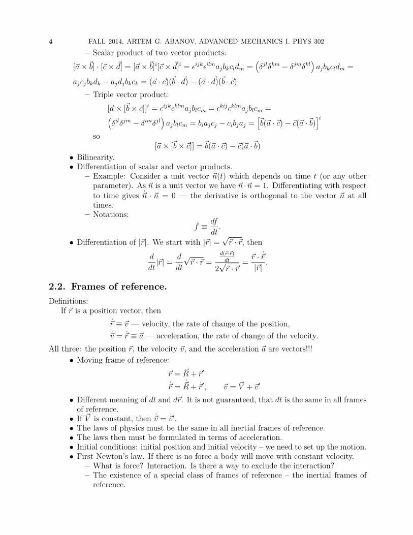
[~a× [~b× ~c]] = ~b(~a · ~c)− ~c(~a ·~b)• Bilinearity.• Differentiation of scalar and vector products.
– Example: Consider a unit vector ~n(t) which depends on time t (or any otherparameter). As ~n is a unit vector we have ~n ·~n = 1. Differentiating with respectto time gives ~n · ~n = 0 — the derivative is orthogonal to the vector ~n at alltimes.
– Notations:f ≡ df
dt.
• Differentiation of |~r|. We start with |~r| =√~r · ~r, then
d
dt|~r| = d
dt
√~r · ~r =
d(~r·~r)dt
2√~r · ~r
= ~r · ~r|~r|
.
2.2. Frames of reference.Definitions:
If ~r is a position vector, then~r ≡ ~v — velocity, the rate of change of the position,~v = ~r ≡ ~a — acceleration, the rate of change of the velocity.
All three: the position ~r, the velocity ~v, and the acceleration ~a are vectors!!!• Moving frame of reference:
~r = ~R + ~r′
~r = ~R + ~r′, ~v = ~V + ~v′
• Different meaning of dt and d~r. It is not guaranteed, that dt is the same in all framesof reference.• If ~V is constant, then ~v = ~v′.• The laws of physics must be the same in all inertial frames of reference.• The laws then must be formulated in terms of acceleration.• Initial conditions: initial position and initial velocity – we need to set up the motion.• First Newton’s law. If there is no force a body will move with constant velocity.
– What is force? Interaction. Is there a way to exclude the interaction?– The existence of a special class of frames of reference – the inertial frames ofreference.

LECTURE 2. COORDINATES. FRAMES OF REFERENCES. NEWTON’S FIRST AND SECOND LAWS.5• Force, as a vector measure of interaction.• Point particle and mass.• The requirement that the laws of physics be the same in all inertial frames of refer-ences. The second Newton’s law: ~F = m~a.


LECTURE 3Newton’s laws.
• Second Newton’s law. You must have/identify the object! Forces are vectors. Su-perposition.• ~F = m~a — tree second order non-linear differential equations.• Third Newton’s law.
In the following I give very simple examples of the use of the Newton’s Laws. ~F = m~a worksboth ways.
• Given the motion we can find the total force.– Going around a circle.– Archimedes law.
• Given the force we can find the motion.– Vertical motion.– Wedge.– Wedge with friction.– Pulley.
7

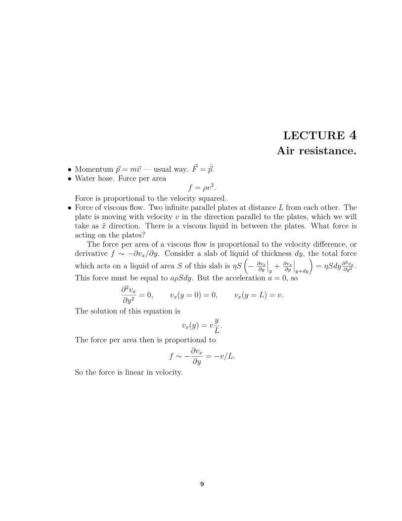
LECTURE 4Air resistance.
• Momentum ~p = m~v — usual way. ~F = ~p.• Water hose. Force per area
f = ρv2.
Force is proportional to the velocity squared.• Force of viscous flow. Two infinite parallel plates at distance L from each other. Theplate is moving with velocity v in the direction parallel to the plates, which we willtake as x direction. There is a viscous liquid in between the plates. What force isacting on the plates?
The force per area of a viscous flow is proportional to the velocity difference, orderivative f ∼ −∂vx/∂y. Consider a slab of liquid of thickness dy, the total forcewhich acts on a liquid of area S of this slab is ηS
(− ∂vx
∂y
∣∣∣y
+ ∂vx∂y
∣∣∣y+dy
)= ηSdy ∂
2vx∂y2 .
This force must be equal to aρSdy. But the acceleration a = 0, so∂2vx∂y2 = 0, vx(y = 0) = 0, vx(y = L) = v.
The solution of this equation is
vx(y) = vy
L.
The force per area then is proportional to
f ∼ −∂vx∂y
= −v/L.
So the force is linear in velocity.
9


LECTURE 5Air resistance.
• Air resistance. We consider two model cases: the air resistance is proportional tov, or to v2 – linear, or quadratic. These forms of the air resistance should not betaken literary. These two cases are just models we will use to learn how the motiondepends on the forms of the air resistance.– Linear: F = −γv. Finite distance.Units of [γ] = kg/s.
mv = −γv, v(t = 0) = v0, l(t = 0) = 0,
v(t) = v0e− γmt, l(t) =
∫ t
0v(t′)dt′ = mv0
γ(1− e−
γmt), l(t→∞) = mv0
γ.
If γmt 1, then
v(t) ≈ v0 − v0γt
m,
l(t) ≈ v0t−12v0t
γt
m.
– Quadratic: F = −γ|v|v. Infinite distance.Units of [γ] = kg/m
mv = −γv2, v(t = 0) = v0, l(t = 0) = 0,
m
v= γt+ m
v0, v(t) = v0
1 + v0γmt, l(t) = m
γlog
(1 + v0γ
mt).
If v0γmt 1, then
v(t) ≈ v0 − v0v0γ
mt,
l(t) ≈ v0t− v0t12v0γ
mt.
• Air resistance and gravity. Linear case.
mv = −mg − γv, v(t = 0) = v0, l(t = 0) = 0.11

12 FALL 2014, ARTEM G. ABANOV, ADVANCED MECHANICS I. PHYS 302
sov(t) = v0e
− γmt + mg
γ
(e−
γmt − 1
).
l(t) = v0m
γ
(1− e−
γmt)− mg
γ
(m
γ
(e−
γmt − 1
)+ t
)– Limit of γt/m 1:
v ≈ v0 − gt
l(t) ≈ v0t−gt2
2In our condition γt/m 1 what t should we use? – depends on the problem.
– Time to the top. Height. At the top vT = 0,
T = m
γlog
(1 + γv0
mg
),
for γv0mg 1
T ≈ m
γ
γv0
mg− 1
2m
γ
(γv0
mg
)2
= v0
g− 1
2v0
g
γv0
mg,
l(T ) ≈ 12v2
0g− 1
3γv3
0mg2
– Terminal velocity.
t→∞, v∞ = −mgγ, mg = −v∞γ

LECTURE 6Oscillations. Oscillations with friction.
Oscillations.• Equation:
mx = −kx, mlφ = −mg sinφ ≈ −mgφ, −LQ = Q
C,
All of these equation have the same form
x = −ω20x, ω2
0 =
k/mg/l1/LC
, x(t = 0) = x0, v(t = 0) = v0.
• The general solution isx(t) = A sin(ω0t) +B cos(ω0t) = C sin(ω0t+ φ),
whereA andB are arbitrary constants. C =√A2 +B2 —amplitude; φ = tan−1(A/B)
— phase.• The velocity as a function of time is
v(t) = x = ω0A cos(ω0t)− ω0B sin(ω0t).• Our initial conditions give
x(t = 0) = B = x0, v(t = 0) = Aω0 = v0,
so the arbitrary constants are given by
B = x0, A = v0
ω0.
(check units)• Oscillates forever. The frequency of oscillations does not depend on the initial con-ditions and can be read straight from the equation of motion. This is the propertyof harmonic oscillations. It also means, that the frequency is the property of thesystem itself, not of the way we set up the motion.• Energy. Conserved quantity: E = x2
2 + ω20x
2
2 . It stays constant on a trajectory!dE
dt= x
(x+ ω2
0x)
= 0.
Oscillations with friction:13

14 FALL 2014, ARTEM G. ABANOV, ADVANCED MECHANICS I. PHYS 302
• Equation of motion.
mx = −kx− γx, −LQ = Q
C+RQ,
• Considerx = −ω2
0x− 2γx, x(t = 0) = x0, v(t = 0) = v0.
• Units of γ are s−1 – the same as for ω0.• Dissipation
dE
dt= x
(x+ ω2
0x)
= −2γx2 < 0.If γ > 0, the energy is decreasing! – dissipation!• Solution: This is a linear equation with constant coefficients. We look for the solutionin the form x = <Ce−iωt, where ω and C are complex constants.
ω2 + 2iγω − ω20 = 0, ω = −iγ ±
√ω2
0 − γ2
• Two solutions, two independent constants.• Two cases: γ < ω0 and γ > ω0.• In the first case γ < ω0 (underdamping):
x = e−γt<[C1e
iΩt + C2e−iΩt
]= Ce−γt sin (Ωt+ φ) , Ω =
√ω2
0 − γ2
Decaying oscillations. Shifted frequency. For γ ω0 we can use the Taylor expansion
Ω ≈ ω0 −12γ2
ω0
• In the second case γ > ω0 (overdamping):
x = Ae−Γ−t +Be−Γ+t, Γ± = γ ±√γ2 − ω2
0 > 0, Γ+ > Γ−.• For the initial conditions x(t = 0) = x0 and v(t = 0) = 0 we find
A = x0Γ+
Γ+ − Γ−, B = −x0
Γ−Γ+ − Γ−
For t→∞ the B term can be dropped as Γ+ > Γ−, then x(t) ≈ x0Γ+
Γ+−Γ− e−Γ−t.

LECTURE 7Oscillations with external force. Resonance.
7.1. Different limits.— Overdamping:We found before that in the overdamped case:
x = Ae−Γ−t +Be−Γ+t, Γ± = γ ±√γ2 − ω2
0 > 0Consider a limit γ →∞. Then we have
Γ+ ≈ 2γ, Γ− ≈ω2
0γ
x+(t) ≈ Be−2γt, x−(t) ≈ Ae−ω02γ t.
Let’s see where these solutions came from. In the equationx = −ω2
0x− 2γxin the limit γ →∞ the last term is huge. It must be compensated by one of the others terms.Let’s see what will happen if we drop the ω2
0x term. Then we get the equation x = −2γx.Its solution is x = Be−2γt. After one more integration we see, that we will get the x+(t)solution.
Now let’s see what will happen if we drop the x term. We get the equation x = −ω20
2γx.
Its solution is x = Ae−ω2
02γ t – this is our x−(t) solution.
— Case of γ = 0, ω0 → 0:In this case the equation is
x = −ω20x→ 0
Se we expect to have x = 0, or x(t) = v0t+ x0.Let’s see how we get it out of the exact solution:
x(t) = A sin(ω0t) +B cos(ω0t)If we naively take ω0 → 0 we will get x(t) = B, which is incorrect. What we need to do is tofirst impose the initial conditions: x(t = 0) = x0 and v(t = 0) = v0. Then we get
x(t) = v0
ω0sin(ω0t) + x0 cos(ω0t).
15

16 FALL 2014, ARTEM G. ABANOV, ADVANCED MECHANICS I. PHYS 302
Now the limit ω0 → 0 is not so trivial, as in the first term zero is divided by zero. So weneed to use the Taylor expansion sin(ω0t) ≈ ω0t. Then we get
x(t) = v0t+ x0.
7.2. External force.In equilibrium everything is at the minimum of the potential energy, so we have the harmonicoscillator with dissipation. All we measure are the response functions, so we need the knowhow the harmonic oscillator behaves under external force.
• Let’s add an external force:x+ 2γx+ ω2
0x = f(t), x(t = 0) = x0, v(t = 0) = v0.
• The full solution is the sum of the solution of the homogeneous equation with anysolution of the inhomogeneous one. This full solution will depend on two arbitraryconstants. These constants are determined by the initial conditions.• Let’s assume, that f(t) is not decaying with time. Any solution of the homogeneousequation will decay in time. There is, however, a solution of the inhomogeneousequation which will not decay in time. So in a long time t 1/γ the solutionof the homogeneous equation can be neglected. In particular this means that theasymptotic of the solution does not depend on the initial conditions.• Let’s now assume that the force f(t) is periodic with some period. It then can berepresented by a Fourier series. As the equation is linear the solution will also be aseries, where each term corresponds to a force with a single frequency. So we needto solve
x+ 2γx+ ω20x = f sin(Ωf t),
where f is the force’s amplitude.
LECTURE 8Resonance. Response.
8.1. Resonance.— Resonance:
• In the previous lecture we found that for arbitrary f(t) we need to solve:x+ 2γx+ ω2
0x = f sin(Ωf t),where f is the force’s amplitude.• Let’s look at the solution in the form x = −f=Ce−iΩf t, and use sin(Ωf t) = −=e−iΩf t.We then get
C = 1ω2
0 − Ω2f − 2iγΩf
= |C|eiφ,
|C| = 1[(Ω2
f − ω20)2 + 4γ2Ω2
f
]1/2 , tanφ = 2γΩf
ω20 − Ω2
f
x(t) = −f=|C|e−iΩf t+iφ = f |C| sin (Ωf t− φ) ,• Resonance frequency for the position measurement
Ωrf =
√ω2
0 − 2γ2.
• Phase changes sign at Ωφf = ω0.
• Role of the phase: delay in response. The force is zero at t = 0, the response x(t)is zero at t = φ/Ωf > 0, so if φ > 0 the response is “delayed” in comparison to theforce.
— Resonance in velocity measurement• The velocity is given by
v(t) = x(t) = f=iΩfCe−iΩf t.
• The velocity amplitude is given by
fΩf |C| = fΩf[
(Ω2f − ω2
0)2 + 4γ2Ω2f
]1/2 = f1
[(Ωf − ω20/Ωf )2 + 4γ2]1/2
17

18 FALL 2014, ARTEM G. ABANOV, ADVANCED MECHANICS I. PHYS 302
• The maximum is when Ωf − ω20/Ωf = 0, so the resonance frequency for the velocity
is ω0 — without the damping shift.• Current is velocity.
— Analysis for small γ.• To analyze resonant response we analyze |C|2.• The most interesting case γ ω0, then the response|C|2 has a very sharp peak at Ωf ≈ ω0:
|C|2 = 1(Ω2
f − ω20)2 + 4γ2Ω2
f
≈ 14ω2
0
1(Ωf − ω0)2 + γ2 ,
so that the peak is very symmetric.• |C|2max ≈ 1
4γ2ω20.
• to find HWHM we need to solve (Ωf − ω0)2 + γ2 =2γ2, so HWHM = γ, and FWHM = 2γ.• Q factor (quality factor). The good measure ofthe quality of an oscillator is Q = ω0/FWHM =ω0/2γ. (decay time) = 1/γ, period = 2π/ω0, soQ = πdecay time
period .• Quality factor Q is the property of the resonator.• For a grandfather’s wall clock Q ≈ 100, for thequartz watch Q ∼ 104.
0 1 2 30
2
4
6
γ=0.8γ=0.6γ=0.4γ=0.2
0 1 2 30
1000
2000
3000
γ=0.01
Figure: Resonantresponse. For insert
Q = 50.
8.2. Useful points.• The complex response function
C(Ωf ) = 1ω2
0 − Ω2f − 2iγΩf
as a function of complex frequency Ωf has simple poles at Ωpf = −iγ ±
√ω2
0 − γ2.Both poles are in the lower half plane of the complex Ωf plane. This is always so forany linear response function. It is the consequence of causality!• The resonator with a high Q is a filter. One can tune this filter by changing theparameters of the resonator.• By measuring the response function and its HWHM we can measure γ. By changingthe parameters such as temperature, fields, etc. we can measure the dependence of γon these parameters. γ comes from the coupling of the resonator to other degrees offreedom (which are typically not directly observable) so this way we learn somethingabout those other degrees of freedom.
LECTURE 9Momentum Conservation. Rocket motion. Charged
particle in magnetic field.
9.1. Momentum Conservation.It turns out that the mechanics formulated by Newton implies certain conservation laws.These laws allows us to find answers to many problems/questions without solving equationsof motion. Moreover, they are very useful even when it is impossible to solve the equationsof motion, as happens, for example, in Stat. Mech. But the most important aspect of theconservation laws is that they are more fundamental than the Newtonian mechanics itself. InQuantum mechanics or Relativity, or quantum field theory the very same conservation lawsstill hold, while the Newtonian mechanics fails.
• Momentum conservation. Consider a system of N interacting bodies• We number the bodies with indexes i = 1, . . . N , etc.,• All bodies interact with each other and with something outside of our system.• A body j acts on a body i with a force ~Fij.• A body i experiences an external force ~F ex
i — this is the force with which whateveris outside of our system acts on the body i.• Then for each of the bodies we have
~pi = ~Fi = ~F exi +
∑j
~Fij.
We take Fii = 0 — no self action.• According to the Newton’s third law ~Fij = −~Fji.• Consider the total momentum of the whole system ~P = ∑
i ~pi, then
~P =∑i
pi =∑i
~F exi +
∑i,j
~Fij =∑i
~F exi .
because ∑i,j~Fij = 0 as in this sum for every term ~Fij there is a term ~Fji.
• So internal forces in a system do not contribute to the change of the total momentum.• The momentum of a closed system (when there is no interaction with outside ~F ex
i = 0)is conserved ~P = 0.• Important points:
19
20 FALL 2014, ARTEM G. ABANOV, ADVANCED MECHANICS I. PHYS 302
– It is of paramount importance to clearly define what your system is and whatthe “outside” is.
– The statement is only about the total momentum of the system.– The nature of the forces does not matter. They can be dissipative, or non-dissipative it will still work.
– It is only the sum of all outside forces that leads to the change of the totalmomentum.
– The momentum is a vector! there are three conservation laws — one for eachcomponent..
– If only some components of the total external force are zero, then only thecorresponding components of the total momentum will be conserved.
• Examples of the momentum conservation law.
9.2. Rocket motion.Statement of the problem:
• A rocket burns fuel. The spent fuel is ejected with velocity V in the frame ofreference of the rocket.• Both the mass of the rocket m(t) and its velocity v(t) are functions of time t. Thefunction m(t) is in our hands – this is how we burn the fuel – how hard we press onthe gas pedal.• We want to find the function v(t) — the rocket velocity as a function of time.• The initial mass of the rocket is minitial. The initial velocity of the rocket is vinitial.
Solution:• At some time t the velocity of the rocket is v and its mass is m.• Its momentum at this moment is mv.• The engine fires constantly. At time t+dt the mass of the rocket changes and becomesm+ dm (where dm is negative), its velocity becomes v + dv. The momentum of therocket is (m+ dm)(v + dv) ≈ mv +mdv + vdm• The spent fuel has a mass dmf and has velocity v−V , so its momentum is (v−V )dmf .• As the total mass of a rocket with the fuel does not change dm + dmf = 0. So themomentum of the burned fuel is −(v − V )dm.• As there is no external forces acting on the system rocket+fuel the total momentumof this system must be conserved, or the total momentum mv at time t, must beequal to the total momentum mv +mdv + vdm− (v − V )dm at time t+ dt.
mv = mv +mdv + vdm− (v − V )dm,mdv = −V dm,
dv = −V dmm,
vfinal = vinitial + V log minitial
mfinal.
• Notice, that the answer does not depend on the exact form of the function m(t). Itdepends only on the ratio of the initial mass to the final mass.

LECTURE 9. MOMENTUM CONSERVATION. ROCKET MOTION. CHARGED PARTICLE IN MAGNETIC FIELD.21• As final moment is arbitrary we can write
v(t) = vinitial + V log minitial
m(t)• Consider now that there is an external force Fex acting on the rocket. Then we willhave
mdv = −V dm+ Fexdt, mdv
dt= Fex − V
dm
dt.
• This equation looks like the second Newton law if we say that there is a new force“thrust”= −V dm
dt, which acts on the rocket. Notice, that dm
dt< 0, so this force is
positive.
9.3. Charged particle in magnetic field.• Lorentz force: ~F = q~v × ~B + q ~E.• No electric field — ~F ⊥ ~v, so there is no component of the force ~F along the vectorof velocity ~v, so |~v| = const.. Trajectories. gvB = mω2R = mωv, I used ωR = v.Cyclotron frequency ωc = qB
m. Cyclotron radius Rc = mv
qB.
• Boundary effect.


LECTURE 10Kinematics in cylindrical/polar coordinates.
In this lecture we will consider different coordinate systems in flat 2D space.• What are coordinates?
– The Cartesian coordinates are given by the origin and two unit vectors ex andey.
– These vectors have the following properties.
e2x = e2
y = 1, ex · ey = 0.
– These two vectors ex and ey are the same in any point of space. (It is possibleto define such vectors only because the space is flat.)
– Any vector can be represented as
~r = xex + yey.
– Any point can be described by the components x and y.– For a moving particle differentiating ~r we find its velocity
~v = xex + yey, vx = x vy = y
– Differentiating the vector of the velocity we find the vector of acceleration
~a = ~v = xex + yey, ax = x ay = y
– A trajectory is given by x(t) and y(t), where t is a parameter – usually time. Ifwe are not interested on the time dependence, then we can give the trajectoryas a function y(x).
– The polar coordinates are given by the origin and two vectors er and eφ.– Both er and eφ are different in different points of space. These vectors are notdefined at the origin.
– These vectors have the following properties at every point of space
(10.1) e2r = e2
φ = 1, er · eφ = 0.
– In the polar coordinates we use r and φ to describe the position. However, theposition vector ~r is not given by simple components as in Cartesian coordinates.Instead it is given by
~r = rer(r, φ)23

24 FALL 2014, ARTEM G. ABANOV, ADVANCED MECHANICS I. PHYS 302
• In 2D we can use r and φ as coordinates. Our unit vectors er and eφ can be repre-sented through the Cartesian vectors ex and ey at every point.
er = ex cosφ+ ey sinφeφ = −ex sinφ+ ey cosφ ; ex = er cosφ− eφ sinφ
ey = er sinφ+ eφ cosφ• Differentiating these relationships with respect to a parameter (time) t we get
er = φeφ, eφ = −φer• Notice, that if we differentiate the relationships (10.1), then we get
er · er = eφ · eφ = 0, er · eφ = −eφ · erThe first two relations show that a derivative of a unit vector must be orthogonalto that vector (its length must not change) The second relation shows how theorthogonal unit vector must change in order to keep their orthogonality.• The radius vector ~r = rer. Let’s calculate the vector of velocity
~v = ~r = rer + rer = rer + rφeφ.
We see that the components of the velocity are given byvr = r, vφ = rφ
• Acceleration – we must differentiate the vector of the velocity!~a = ~v =
(r − rφ2
)er +
(rφ+ 2rφ
)eφ, ar = r − rφ2, aφ = rφ+ 2rφ
• In the case r = const, φ = ω, ~a = −rω2er + rωeφ.• Notice, if φ = ω = const, then aφ = 2rω – this is the origin of the Coriolis force.
Free motion. There is no forces, so ~a = 0.• In Cartesian coordinates it gives
x = 0, y = 0, x(t) = vx,0t+ x0, y(t) = vy,0t+ y0.
• Or the trajectoryy = y0 + vy,0
vx,0(x− x0).
This is the equation for a straight line in the Cartesian coordinates.• In the polar coordinates. ~a = 0, so both components of ~a must be zero
rφ+ 2rφ = 0r − rφ2 = 0 ,
r2φ = const = A
r − A2
r3 = 0• Notation
∂
∂x≡ ∂x
• Now I will do the following trick. Instead of two functions r(t) and φ(t) I will considera function r(φ) — the trajectory — and use∂
∂t= ∂φ
∂t
∂
∂φ= φ
∂
∂φ= A
r2∂φ; r = A
r2∂φr = −A∂φ1r
; r = −A2
r2 ∂2φ
1r,
then we getA2
r2 ∂2φ
1r− A2
r3 = 0, ∂2φ
1r
= −1r,
1r
= B cos(φ− φ0)

LECTURE 10. KINEMATICS IN CYLINDRICAL/POLAR COORDINATES. 25• This is the equation of the straight line in the polar coordinates.


LECTURE 11Angular velocity. Angular momentum.
Consider a rigid body which can rotate around an axis which goes through its center ofmass. We apply a force ~F to some point of the body.
• Depending on the direction of the force the body may or may not rotate with in-creasing frequency.• In any case the body as a whole will not move.• It means that the axis must apply a force −~F to the body.• So the sum of all forces applied to the body is zero.• What then causes the angular velocity to change?• Consider a small piece of the body.• Its velocity is changing! So there must be a net force acting on it.• This is the force of interaction of our small piece with the rest of the body.• Such forces are very difficult to compute, but• If the body is rigid, then me know that the relative position of the points of the bodydoes not change.• It turns out that this observation is enough to construct the theory of the motion ofa rigid body without the reference to the internal forces.
11.1. Angular velocity. Rotation.• Vector of angular velocity ~ω. For |~r| = const.:
~v = ~ω × ~r.• Sum of two vectors
~v13 = ~v12 + ~v23, (~ω13 − ~ω12 − ~ω23)× ~r = 0, ~ω13 = ~ω12 + ~ω23
• We have a frame rotating with angular velocity ~ω with respect to the rest frame. Avector ~l constant in the rotating frame will change with time in the rest frame and
~l = ~ω ×~l.• ω = dφ
dt, if ω is a vector ~ω, then dφ must be a vector ~dφ. Notice, that φ is not a
vector!• If we rotate one frame with respect to another by a small angle ~dφ, then a vector ~lwill change by
d~l = ~dφ×~l.27

28 FALL 2014, ARTEM G. ABANOV, ADVANCED MECHANICS I. PHYS 302
11.2. Angular momentum.• Consider a vector ~J = ~r × ~p – vector of angular momentum.• Consider a bunch of particles which interact with central forces: ~Fij ‖ ~ri− ~rj. Thereis also external force ~F ex
i acting on each particle.• Consider the time evolution of the vector of the total angular momentum ~J = ∑
i ~ri×~pi:
~J =∑i
~ri × ~pi +∑i
~ri × ~pi =∑i
~ri ×
∑j 6=i
~Fij + ~F exi
=∑i 6=j
~ri × ~Fij +∑i
~ri × ~F exi
• The sum ∑i ~ri × ~F ex
i is called torque. Here it is the torque of external forces ~τ ex.• if a force ~F is applied to a point with the position ~r with respect to the origin, thenthe torque of this force with respect to the same origin is given by
~τ ≡ ~r × ~F .
• Consider now the first sum in the RHS. Remember that ~Fij = −~Fji∑i 6=j
~ri × ~Fij = 12∑i 6=j
~ri × ~Fij + 12∑i 6=j
~rj × ~Fji = 12∑i 6=j
(~ri − ~rj)× ~Fij = 0
• So we have~J = ~τ ex
• If the torque of external forces is zero, then the angular momentum is conserved.

LECTURE 12Moment of inertia. Kinetic energy.
In the previous lecture we considered a set of particles and showed, that if they interactthrough the central forces the rate of change of angular momentum equals to the total torqueof external forces only. In proving this statement the condition of rigidity was not used atall. The statement ~J = ~τ ex is very general.
In this lecture we show how to compute the angular momentum and the kinetic energyfor a rigid body. Remember, that the condition of rigidity is very strong. The equation
~v = ~ω × ~r.allows us to compute the velocity of every point of the body by knowing only one vector ~ω.So both the angular momentum and the kinetic energy will depend only on the vector ~ω andsome property of the body itself.
12.1. Angular momentum. Moment of inertia.• Consider a ridged set of particles of masses mi — the distances between the particlesare fixed and do not change. The whole system rotates with the angular velocity ~ω.Each particle has a radius vector ~ri. Let’s calculate the angular momentum of thewhole system.
~J =∑i
mi~ri × ~vi =∑i
mi~ri × [~ω × ~ri] =∑i
mi
(~ω~r2
i − ~ri(~ω · ~ri))
or in components (Einstein notations are assumed over Greek indexes)
Jα =∑i
mi
(ωα~r2
i − rαi ωβrβi
)=∑i
mi
(δαβ~r2
i − rai rβi
)ωβ = Iαβωβ,
Iαβ =∑i
mi
(δαβ~r2
i − rai rβi
)• The moment of inertia is a positive definite symmetric 3× 3 tensor!
I =
Ixx Ixy IxzIyx Iyy IyzIzx Izy Izz
, Iαβ = Iβα.
It transforms one vector into another:~J = I~ω.
29

30 FALL 2014, ARTEM G. ABANOV, ADVANCED MECHANICS I. PHYS 302
As for any symmetric tensor:– There are special coordinate axes in which the tensor has a diagonal form – onlydiagonal elements are nonzero, while all the off diagonal elements are zero.
– These diagonal elements are called principle moments of inertia. The corre-sponding axes are called principal axes of inertia.
– If all the principal moments are different, then the principle axes are orthogonalto each other.
– In a degenerate case these cases can be chosen to be orthogonal.– These principle axes are “attached” to the body, so if the body is rotating, thenthese axes are also rotating with the body.
• The direction of the angular momentum ~J and direction of the angular velocity ~ωdo not in general coincide!• It is ~J which is constant when there are no external torques, not ~ω! Let me repeatit: If there are no external torques the vector ~ω may change with time — both itsdirection and magnitude. But the angular momentum vector ~J will remain constant.
Contrast this to the usual momentum-velocity relation~p = m~v
where the conservation of momentum means that the velocity is also constant. Thisis because the mass m is a scalar, not tensor.• This last statement makes even the kinematics (motion with no external forces) of arigid body very complicated and highly non-trivial.• Moment of inertia of a continuous body.
Iαβ =∫ (
δαβ~r2 − rαrβ)dm =
∫ (δαβ~r2 − rαrβ
) dmdV
dV =∫ (
δαβ~r2 − rαrβ)ρ(~r)dV,
where ρ(~r) is the mass density of the material at point ~r – it must be know as thisis a characteristic of the body.• How to compute the moment of inertia of an arbitrary body.
– First you chose a system of coordinates registered with the body.– You chose which component of the tensor of inertia you want to compute. Youhave to compute all of them, but you need to start with something. Let’s say itis Ixy.
– Then in the expression∫ (δαβ~r2 − rαrβ
)ρ(~r)dV we have α = x and β = y.
– The first term under the integral is then zero, as δxy = 0.– In the second term rα = x, and rβ = y, so we have
Ixy = −∫∫∫
xyρ(x, y, z)dxdydz.
– Let’s say we want to compute Ixx. Then α = x, and β = x, so the first termδαβ~r2 = x2 + y2 + z2, as δxx = 1, and ~r2 = x2 + y2 + z2. The second term is justx2. So we need to compute
Ixx =∫∫∫ (
y2 + z2)ρ(x, y, z)dxdydz.
• Examples.– A thin ring: Izz = mR2, Ixx = Iyy = 1
2mR2, all off diagonal elements vanish.
– A disc: Izz = 12mR
2, Ixx = Iyy = 14mR
2, all off diagonal elements vanish.

LECTURE 12. MOMENT OF INERTIA. KINETIC ENERGY. 31– A sphere: Ixx = Iyy = Izz = 2
5mR2, all off diagonal elements vanish.
– A stick at the end: Ixx = Iyy = 13mL
2.– A stick at the center: Ixx = Iyy = 1
12mL2.
• Role of symmetry.
12.2. Kinetic energy.• Consider the kinetic energy of the moving body.
K = 12∑i
mi~v2i = 1
2∑i
mi[~ω × ~ri]2 = 12∑i
mi[~ω2~r2 − (~ω · ~r)2] = 12∑i
mi[δαβ~r2 − rαrβ]ωαωβ.
so we get
K = Iαβωαωβ
2(this also shows that I is positive definite)• In terms of angular momentum:
K = 12(I−1
)αβJαJβ.


LECTURE 13Work. Potential energy.
13.1. Mathematical preliminaries.• Functions of many variables, say U(x, y)• Differential of a function of many variables.
dU = ∂U
∂xdx+ ∂U
∂ydy.
• Consider an expressionδG = A(x, y)dx+B(x, y)dy.
where A and B are some arbitrary functions. The question is: is this a differentialof some function? The answer is: not necessarily. The proof:– Let’s assume that δG is a differential of some function U , then we must have
A = ∂U
∂x, B = ∂U
∂y.
– But then∂A
∂y= ∂2U
∂x∂y= ∂B
∂x.
– So δG is a differential of some function if (and only if)∂A
∂y= ∂B
∂x
– In other words, if the condition above is satisfied, then there exists a functionU(x, y) such that
A(x, y) = ∂U(x, y)∂x
, B(x, y) = ∂U(x, y)∂y
.
– Then the statement that the form δG is a differential is a very strong statement,as it tells you that in order to know two functions A(x, y) and B(x, y) you needto know only one function U(x, y).
• Examples.– δG = xdy + ydx is a differential U = xy.– δG = xdy − ydx is not a differential. The function U does not exist.
33

34 FALL 2014, ARTEM G. ABANOV, ADVANCED MECHANICS I. PHYS 302
13.2. Work.
• A work done by a force: δW = ~F · d~r.• Notice, that although δW = Fxdx+ Fydy + Fzdz this is not necessarily a full differ-ential.• Superposition. If there are many forces, the total work is the sum of the works doneby each.• Finite displacement. Line integral.• In general case work depends on path!!!!!
13.3. Conservative forces. Energy conservation.
• Fundamental forces. Depend on coordinate, do not depend on time.• Work done by the forces over a closed loop is zero.• It means that work is independent of the path.• Consider two paths: first dx, then dy; first dy then dx
δW1 = Fx(x, y)dx+ Fy(x+ dx, y)dyδW2 = Fy(x, y)dy + Fx(x, y + dy)dx.
• The works must be equal to each other, so
Fx(x, y)dx+ Fy(x, y)dy + ∂Fy∂x
dydx = Fy(x, y)dy + Fx(x, y)dx+ ∂Fx∂y
dydx

LECTURE 13. WORK. POTENTIAL ENERGY. 35
where we used Fy(x + dx, y) ≈ Fy(x, y) + ∂Fy∂xdx, and Fx(x, y + dy) ≈ Fx(x, y)dx +
∂Fx∂ydydx. So in order for the works to be equal to each other we must have
∂Fy∂x
∣∣∣∣∣x,y
= ∂Fx∂y
∣∣∣∣∣x,y
• So a small work done by a conservative force:
δW = Fxdx+ Fydy,∂Fy∂x
= ∂Fx∂y
is a full differential!• So there exist a function U such that
δW = −dU(the minus sign is for further convenience)• It means that there is such a function of the coordinates U(x, y), that
Fx = −∂U∂x
, Fy = −∂U∂y
, or ~F = −gradU ≡ −~∇U.


LECTURE 14Energy Conservation. One-dimensional motion.
• Last lecture we found, that there exists a special class of forces (which depend onlyon coordinates) which are called “conservative forces”.– Not all forces are conservative! Friction!– All fundamental forces are conservative.
• A conservative force is such a force that its work around any closed loop is zero.• Last lecture we found that for a conservative (zero work on a closed loop) force thereexists a function U — called “potential energy” such that
Fx = −∂U∂x
, Fy = −∂U∂y
, or ~F = −gradU ≡ −~∇U.
Such function is not unique as one can always add an arbitrary constant to thepotential energy.• Under a small displacement d~r a work done by such a force is
δW = ~F · d~r = Fxdx+ Fydy + Fzdz = −dU.
• If the force ~F (~r) is known, then there is a test for if the force is conservative.
∇× ~F = 0.
14.1. Change of kinetic energy.• If a body of mass m moves under the force ~F , then.
md~v
dt= ~F , md~v = ~Fdt, m~v · d~v = ~F · ~vdt = ~F · d~r = δW.
So we havedmv2
2 = δW
• The change of kinetic energy K = mv2
2 equals the total work done by all forces.• In general case this is not very useful, as we need to know the path in order tocompute work.
W =∫
ΓA→B~F · d~r.
In order to know the path we need to solve the equations of motion.37

38 FALL 2014, ARTEM G. ABANOV, ADVANCED MECHANICS I. PHYS 302
14.1.1. Conservative forces.
• So on a trajectory: dK = δW = −dU , or
d
(mv2
2 + U
)= 0, K + U = const.
• Examples.
14.2. 1D motion.
• In 1D the force that depends only on the coordinate is always conservative.• In 1D in the case when the force depends only on coordinates the equation of motioncan be solved in quadratures.• The number of conservation laws is enough to solve the equations.• If the force depends on the coordinate only F (x), then there exists a function —potential energy — with the following property
F (x) = −∂U∂x
Such function is not unique as one can always add an arbitrary constant to thepotential energy.• The total energy is then conserved
K + U = const., mx2
2 + U(x) = E
• Energy E can be calculated from the initial conditions: E = mv20
2 + U(x0)• As mv2
2 > 0 the allowed areas where the particle can be are given by E − U(x) > 0.• Picture. Turning points — the solutions of the equation E = U(x). Prohibitedregions.• Notice, that the equation of motion depends only on the difference E − U(x) =
mv20
2 + U(x0) − U(x) of the potential energies in different points, so the zero of thepotential energy (the arbitrary constant that was added to the function) does notplay a role.• We thus found that
dx
dt= ±
√2m
√E − U(x)
• Energy conservation law cannot tell the direction of the velocity, as the kinetic energydepends only on absolute value of the velocity. In 1D it cannot tell which sign touse “+” or “−”. You must not forget to figure it out by other means.
LECTURE 14. ENERGY CONSERVATION. ONE-DIMENSIONAL MOTION. 39• We then can solve the equation
±√m
2dx√
E − U(x)= dt, t− t0 = ±
√m
2
∫ x
x0
dx′√E − U(x′)
• Examples:– Motion under a constant force.– Oscillator.– Pendulum.
• Periodic motion. Period between two turning points xL and xR.
T = 2√m
2
∫ xR
xL
dx′√E − U(x′)


LECTURE 15Spherical coordinates. Central forces.
15.1. Spherical coordinates.
15.1.1. Coordinate vectors of spherical coordinates.
• The spherical coordinates are given by
x = r sin θ cosφy = r sin θ sinφz = r cos θ
.
• The coordinates r, θ, and φ can be used to denote any point.• There are corresponding unit vectors er, eθ, and eφ at each point (r, θ, φ).
– The vector ~er is the unit vector along the direction where our point shifts if wechange the coordinate r, while keeping θ and φ constant.
– The vector ~eθ is the unit vector along the direction where our point shifts if wechange the coordinate θ, while keeping r and φ constant.
– The vector ~eφ is the unit vector along the direction where our point shifts if wechange the coordinate φ, while keeping θ and r constant.
• With such definitions of er, eθ, and eφ we see, that– If we change only coordinate r to r + dr, then the position vector ~r changes byd~r = ~erdr.
41

42 FALL 2014, ARTEM G. ABANOV, ADVANCED MECHANICS I. PHYS 302
– If we change only coordinate θ to θ + dθ, then the position vector ~r changes byd~r = ~eθrθ.
– If we change only coordinate φ to φ+ dφ, then the position vector ~r changes byd~r = ~eφr sin θdφ.
• The vector d~r then is expressed through the dr, dθ and dφ asd~r = ~erdr + ~eθrdθ + ~eφr sin θdφ.
• In Cartesian coordinates the similar expression isd~r = ~exdx+ ~eydy + ~ezdz.
• Notice, that in this formulation we do not need to have the position vector ~r. Wecan do everything with the coordinate vectors defined locally.
15.1.2. Connecting Spherical and Cartesian.
Here I show how to connect ~ex, ~ey, ~ez, to ~er, ~eθ, ~eφ using only local relations.• Using the definition of the spherical coordinates we have locally
dx = dr sin θ cosφ+ dθr cos θ cosφ− dφr sin θ sinφdy = dr sin θ sinφ+ dθr cos θ sinφ+ dφr sin θ cosφdz = dr cos θ − dθr sin θ
• Using these expressions in d~r is Cartesian coordinates we findd~r = (~ex sin θ cosφ+ ~ey sin θ sinφ+ ~ez cos θ) dr + (~exr cos θ cosφ+ ~eyr cos θ sinφ− ~ezr sin θ) dθ+ (~eyr sin θ cosφ− ~exr sin θ sinφ) dφ• Comparing this to the d~r in spherical coordinates we get
~er = ~ex sin θ cosφ+ ~ey sin θ sinφ+ ~ez cos θ~eθ = ~ex cos θ cosφ+ ~ey cos θ sinφ− ~ez sin θ~eφ = −~ex sinφ+ ~ey cosφ
15.1.3. Coordinate independent definition of the gradient.
• Imagine now a function of coordinates U . We want to find the components of avector ~∇U in the spherical coordinates.• Consider a function U as a function of Cartesian coordinates: U(x, y, z). Then
dU = ∂U
∂xdx+ ∂U
∂ydy + ∂U
∂zdz = ~∇U · d~r.
Notice, that we have a coordinate independent definition of the vector gradient. Thevector of gradient ~∇U is such a vector that for any vector d~r we have:
dU = ~∇U · d~r — definition of ~∇U.It is coordinate independent as it is a scalar/dot product which doe not depend oncoordinates.• I want to make a few points about this definition.
– This definition is constructive – it allows on to find the vector of gradient in anysystem of coordinates. For this it is important that d~r is arbitrary infinitesimalvector.

LECTURE 15. SPHERICAL COORDINATES. CENTRAL FORCES. 43– It connects calculus dU with geometry — the scalar product of two vectors.– It thus gives the geometrical meaning/picture to calculus. In particular one cansee that if one chooses a vector d~r⊥ which is perpendicular to the vector of thegradient at some particular point, then the function U will not change along thedirection of d~r⊥ (in the infinitesimal neighborhood of that point).
• Let’s see how this definition works in Cartesian coordinates.– In particular, if we use the standard Cartesian coordinates and write the vectorof gradient as
~∇U = (~∇U)x~ex + (~∇U)y~ey + (~∇U)z~ez,
where (~∇U)x, (~∇U)y, and (~∇U)z are the components of the vector ~∇U in Carte-sian coordinates. These are the components which we want to find.
– Using the vector d~r in Cartesian coordinate we finddU = ~∇U · d~r = (~∇U)xdx+ (~∇U)ydy + (~∇U)zdz
– Consider a function U as the function of Cartesian coordinates U(x, y, z), weknow from the standard calculus
dU = ∂U
∂xdx+ ∂U
∂ydy + ∂U
∂zdz
– Comparing these to results for dU (both are valid for arbitrary infinitesimal dx,dy, and dz) we find
(~∇U)x = ∂U
∂x, (~∇U)y = ∂U
∂y, (~∇U)z = ∂U
∂z.
– This is our standard formulas for the gradient in Cartesian coordinates.• Now we can use this procedure for any other system of coordinates, as long as weknow how to express d~r in the corresponding coordinate vectors.
15.1.4. Gradient in spherical coordinates.
• Let’s write the vector ~∇U in the spherical coordinates.~∇U = (~∇U)r~er + (~∇U)θ~eθ + (~∇U)φ~eφ,
where (~∇U)r, (~∇U)θ, and (~∇U)φ are the components of the vector ~∇U in the spher-ical coordinates. It is those components that we want to find.• By the definition of the gradient vector, and using d~r in spherical coordinates we get
dU = ~∇U · d~r = (~∇U)rdr + (~∇U)θrdθ + (~∇U)φr sin θdφ• On the other hand if we now consider U as a function of the spherical coordinatesU(r, θ, φ), then
dU = ∂U
∂rdr + ∂U
∂θdθ + ∂U
∂φdφ
• Comparing the two expressions for dU we find(~∇U)r = ∂U
∂r
(~∇U)θ = 1r∂U∂θ
(~∇U)φ = 1r sin θ
∂U∂φ
.

44 FALL 2014, ARTEM G. ABANOV, ADVANCED MECHANICS I. PHYS 302
• The vector of gradient in spherical coordinates is then written as
~∇U = ∂U
∂r~er + 1
r
∂U
∂θ~eθ + 1
r sin θ∂U
∂φ~eφ
• In particular if U is the potential energy, then
~F = −~∇U = −∂U∂r~er −
1r
∂U
∂θ~eθ −
1r sin θ
∂U
∂φ~eφ.
15.2. Central force• Consider a motion of a body under central force. Take the origin in the center offorce.• A central force is given by
~F = F (r)~er.• Such force is always conservative: ~∇× ~F = 0, so there is a potential energy:
~F = −~∇U = −∂U∂r~er,
∂U
∂θ= 0, ∂U
∂φ= 0,
so that potential energy depends only on the distance r, U(r).
LECTURE 16Effective potential. Kepler orbits.
16.1. Central force. General.• Last lecture we started to consider a motion of a body under central force.• A central force is given by
~F = F (r)~er.
• Such force is always conservative: ~∇× ~F = 0,• The potential energy U(r) is a function of the distance r only.
F (r) = −∂U∂r
• The torque of the central force τ = ~r× ~F = 0, so the angular momentum is conserved:~J = const.
16.2. Motion in under central force.Consider now a particle of mass m which is moving in the central force field. The field iscompletely described by the potential energy function U(r). We set this function such, thatU(r →∞)→ 0.
In order to set up the problem we must also specify the initial conditions. So we knowthat at some time t = 0 the velocity of the particle is ~v0 and the position is ~r0.
• The vector of angular momentum can be computed from initial conditions ~J = ~r0×~p0.• The energy can also be computed from the initial conditions E = m~v2
02 + U(r0).
• Both ~J and E are conserved. They are also independent conserved quantities.• The direction of ~J is perpendicular to the initial momentum and initial coordinate.• During the motion its direction will not change — it is conserved.• So during the motion at any moment the momentum and position vectors will be inthe same plane perpendicular to ~J .• The motion is all in one plane! The plane which contains the vector of the initialvelocity and the initial radius vector.• We take the direction of ~J as our z axis. The plane of motion is then x− y plane.
45

46 FALL 2014, ARTEM G. ABANOV, ADVANCED MECHANICS I. PHYS 302
• The angular momentum is ~J = J~ez, where J = | ~J | = const.. This constant is givenby initial conditions J = m|~r0 × ~v0|.• In the x − y plane θ = π/2 we can use only r and φ coordinates — the polarcoordinates.• Writing the value of the angular momentum in the polar coordinates we get
mr2φ = J, φ = J
mr2
• The velocity in these polar coordinates is
~v = r~er + rφ~eφ = r~er + J
mr~eφ
• The kinetic energy then is
K = m~v2
2 = mr2
2 + J2
2mr2
• The total energy then is
E = K + U = mr2
2 + J2
2mr2 + U(r).
• If we introduce the effective potential energy
Ueff (r) = J2
2mr2 + U(r),
then we havemr2
2 + Ueff (r) = E, mr = −∂Ueff∂r
• This is a one dimensional motion which was solved before.
16.3. Kepler orbits.Historically, the Kepler problem —the problem of motion of the bod-ies in the Newtonian gravitationalfield — is one of the most impor-tant problems in physics. It is thesolution of the problems and exper-imental verification of the resultsthat convinced the physics commu-nity in the power of Newton’s newmath and in the correctness of hismechanics. For the first time peo-ple could understand the observedmotion of the celestial bodies andmake accurate predictions. Thewhole theory turned out to be much
simpler than what existed before.• In the Kepler problem we want to consider the motion of a body of mass m in thegravitational central force due to much larger mass M .

LECTURE 16. EFFECTIVE POTENTIAL. KEPLER ORBITS. 47• As M m we ignore the motion of the larger mass M and consider its positionfixed in space (we will discuss what happens when this limit is not applicable later)• The force that acts on the mass m is given by the Newton’s law of gravity:
~F = −GmMr3 ~r = −GmM
r2 ~er
where ~er is the direction from M to m.• The potential energy is then given by
U(r) = −GMm
r, −∂U
∂r= −GmM
r2 , U(r →∞)→ 0
• The effective potential is
Ueff (r) = J2
2mr2 −GMm
r,
where J is the angular momentum.• For the Coulomb potential we will have the same r dependence, but for the likecharges the sign in front of the last term is different — repulsion.• In case of attraction for J 6= 0 the function Ueff (r) always has a minimum for somedistance r0. It has no minimum for the repulsive interaction.• Looking at the graph of Ueff (r) we see, that
– for the repulsive interaction there can be no bounded orbits. The total energyE of the body is always positive. The minimal distance the body may have withthe center is given by the solution of the equation Ueff (rmin) = E.
– for the attractive interaction there is a minimum of the effective potential energyat some r0 = J2
Gm2M(this is the solution of the equation ∂Ueff/∂r = 0), and
U(r0) < 0, where U(r →∞)→ 0. Then, from the graph U(r) we see∗ if E > 0, then the motion is not bounded. The minimal distance thebody may have with the center is given by the solution of the equationUeff (rmin) = E.∗ if Ueff (r0) < E < 0, then the motion is bounded between the two realsolutions of the equation Ueff (r) = E. One of the solution is larger thanr0, the other is smaller.∗ if Ueff (r0) = E, then the only solution is r = r0. So the motion is aroundthe circle with fixed radius r0. For such motion we must havemv2
r0= GmM
r20
,J2
mr30
= GmM
r20
, r0 = J2
Gm2M.
Notice, that this is exactly r0 that we found before. Also
Ueff (r0) = E = mv2
2 − GmM
r0= −1
2GmM
r0.


LECTURE 17Kepler orbits continued.
• In the motion the angular momentum and the energy are conserved• All motion happens in one plane.• In that plane we describe the motion by two time dependent polar coordinates r(t)and φ(t). The dynamics is given by the angular momentum conservation and theeffective equation of motion for the r coordinate
φ = J
mr2 , mr = −∂Ueff (r)∂r
,
where Ueff (r) is given by
Ueff (r) = J2
2mr2 −GMm
r.
• For now I am not interested in the time evolution and only want to find the trajectoryof the body. This trajectory is given by the function r(φ).• However, if we know r(φ), we can solve φ = J
mr2(φ) and find φ(t). Then we will alsohave r(φ(t)). Thus one can consider finding of r(φ) as the first step in full solution.• In order to find r(φ) I will use the trick we used before
r = dr
dt= dφ
dt
dr
dφ= J
mr2dr
dφ= − J
m
d(1/r)dφ
,d2r
dt2= dφ
dt
dr
dφ= − J2
m2r2d2(1/r)dφ2
• On the other hand∂Ueff∂r
= −J2
m(1/r)3 +GMm (1/r)2 .
49

50 FALL 2014, ARTEM G. ABANOV, ADVANCED MECHANICS I. PHYS 302
• Now I denote u(φ) = 1/r(φ) and get
−J2
mu2 d
2u
dφ2 = J2
mu3 −GMmu2
or, denoting d2udφ2 ≡ u′′
u′′ = −u+ GMm2
J2 .
• The general solution of this equation is
u = GMm2
J2 + A cos(φ− φ0),
where A and φ0 are arbitrary constants.• We can put φ0 = 0 by redefinition.• Before I do that, I want to point out that this is cheating. The constants A andφ0 should be obtained from the initial conditions. So unless we know how to get φ0from the initial conditions we cannot redefine our system of coordinates to measurethe angle from the direction of φ0. However, we know that such redefinition exists.We will discuss the issue of finding φ0 from the initial conditions later and now wejust go ahead and redefine φ.• So by setting φ0 = 0 we have
1r
= γ + A cosφ, γ = GMm2
J2
If γ = 0 this is the equation of a straight line in the polar coordinates.• A more conventional way to write the trajectory is
1r
= 1c
(1 + ε cosφ) , c = J2
GMm2 = 1γ
where ε > 0 is dimentionless number. This is the equation of ellipse in polar coordi-nates. ε is called the eccentricity of the ellipse, it controls the “shape” of the ellipse,while c has a dimension of length and it controls the “size” of the ellipse.• We see that
– If ε < 1 the orbit is periodic.– If ε < 1 the minimal and maximal distance to the center — the perihelion andaphelion are at φ = 0 and φ = π respectively.
rmin = c
1 + ε, rmax = c
1− ε– If ε > 1, then the trajectory is unbounded.– If ε → ∞ the trajectory is the straight line. (the only way to make this limitmeaningful is to also take c→∞, which means J →∞. So the planet is eithermoving too far, or moving too fast.)
• If we know c and ε we know the orbit, so we must be able to find out J and E fromc and ε. By definition of c we find J2 = cGMm2. In order to find E, we notice, thatat r = rmin, r = 0, so at this moment v = rminφ = J/mrmin, so the kinetic energyK = mv2/2 = J2/2mr2
min, the potential energy is U = −GmM/rmin. So the total

LECTURE 17. KEPLER ORBITS CONTINUED. 51energy is
E = K + U = −1− ε22
GmM
c, J2 = cGMm2,
Indeed we see, that if ε < 1, E < 0 and the orbit is bounded.• The ellipse can be written as
(x+ d)2
a2 + y2
b2 = 1,
witha = c
1− ε2 , b = c√1− ε2
, d = aε, b2 = ac.
• One can check, that the position of the large mass M is one of the focuses of theellipse — NOT ITS CENTER!• This is the first Kepler’s law: all planets go around the ellipses with the sun atone of the foci.
17.1. Kepler’s second lawThe conservation of the angular momentum reads
12r
2φ = J
2m.
We see, that in the LHS rate at which a line from the sun to a comet or planet sweeps outarea:
dA
dt= J
2m.
This rate is constant! So• Second Kepler’s law: A line joining a planet and the Sun sweeps out equal areasduring equal intervals of time.
17.2. Kepler’s third lawConsider now the closed orbits only. There is a period T of the rotation of a planet aroundthe sun. We want to find this period.
The total area of an ellipse is A = πab, so as the rate dA/dt is constant the period is
T = A
dA/dt= 2πabm
J,
Now we square the relation and use b2 = ac and c = J2
GMm2 to find
T 2 = 4π2m2
J2 a3c = 4π2
GMa3
Notice, that the mass of the planet and its angular momentum canceled out! so• Third Kepler’s law: For all bodies orbiting the sun the ratio of the square of theperiod to the cube of the semimajor axis is the same.
This is one way to measure the mass of the sun. For all planets one plots the cube of thesemimajor axes as y and the square of the period as x. One then draws a straight line throughall points. The slope of that line is GM/4π2.


LECTURE 18Another derivation. Conserved Laplace-Runge-Lenz
vector.
18.1. Another way.• Another way to solve the problem is starting from the following equations:
φ = J
mr2(t) ,mr2
2 + Ueff (r) = E, Ueff (r) = J2
2mr2 + U(r).
• For now we am not interested in the time evolution and only want to find the tra-jectory of the body. This trajectory is given by the function r(φ). In order to findit we express r from the second equation and divide it by φ from the first. We thenfind
r
φ= dr
dφand r
φ= r2
√2mJ2
√E − Ueff (r),
orJ√2m
dr
r2√E − Ueff (r)
= dφ,J√2m
∫ r
r(φ0
dr′
r′2√E − Ueff (r′)
= φ− φ0,
where E, ~J , φ0, and r(φ0) (total 6) are given by initial conditions.• These formulas give the trajectory for any central potential U(r).• For the ∼ 1/r potential the integral becomes a standard one after substitution x =
1/r.
18.2. A hidden symmetry.Let’s assume, that we have some central attractive potential U(r), which decays to zero atinfinity.
• The problem is mapped to a one dimensional problem for the coordinate r andeffective potential energy Ueff (r) = J2
2mr2 + U(r).• For total energy E < 0 we have bounded motion for r between rmin and rmax.
53

54 FALL 2014, ARTEM G. ABANOV, ADVANCED MECHANICS I. PHYS 302
• We can compute the time Tr for a particle to go from rmin to rmax and back
Tr =√
2m∫ rmax
rmin
dr√E − Ueff (r)
, where rmin and rmax are the solutions of E = Ueff (r).
• We can also compute r(t).• We then can compute the time Tφ it takes for the angle φ to change by 2π
2π = J
m
∫ Tφ
0
dt
r2(t) .
• The two times Tr and Tφ do not necessarily coincide.• It is also a very special condition that Tr and Tφ coincide for ANY E and J !
If Tr 6= Tφ the orbit is bounded, but not closed — this is the general situation.It is a very special property of the gravitational (or Coulomb) potential that Tr = Tφ for
ANY E and J . This symmetry requires an explanation.
If U(r) is the gravitation potential energy with a small correction this discrepancy betweenTr and Tφ is small. The orbit is almost closed, or one can say that it precesses.
18.3. Conserved vector ~A.The Kepler problem has an interesting additional symmetry. This symmetry ensures thatTr = Tφ (for any E and J). As usual this symmetry also leads to the conservation of theLaplace-Runge-Lenz vector ~A. If the gravitational force is ~F = − k
r2~er, then we define:
~A = ~p× ~J −mk~er,
where ~J = ~r × ~p. This vector can be defined for both gravitational and Coulomb forces:k > 0 for attraction and k < 0 for repulsion.
An important feature of the “inverse square force” is that this vector is conserved. Let’scheck it. First we notice, that ~J = 0, so we need to calculate:
~A = ~p× ~J −mk~er

LECTURE 18. ANOTHER DERIVATION. CONSERVED LAPLACE-RUNGE-LENZ VECTOR. 55Now using
~p = ~F , ~er = ~ω × ~er = 1mr2
~J × ~erWe then see
~A = ~F × ~J − k
r2~J × ~er =
(~F + k
r2~er
)× ~J = 0
So this vector is indeed conserved.The question is: Is this conservation of vector ~A an independent conservation law? There
are three components of the vector ~A are there three new conservation laws?The answer is that not all of them are independent.
• As ~J = ~r × ~p is orthogonal to ~er, we see, that ~J · ~A = 0. So the component of ~Aperpendicular to the plane of the planet rotation is always zero.• Now let’s calculate the magnitude of this vector
~A · ~A = ~p2 ~J2 − (~p · ~J)2 +m2k2 − 2mk~er · [~p× ~J ] = ~p2 ~J2 +m2k2 − 2mkr
~J · [~r × ~p]
= 2m(~p2
2m −k
r
)~J2 +m2k2 = 2mE ~J2 +m2k2.
So we see, that the magnitude of ~A is not an independent conservation law.• Using the relation between the eccentricity ε with ~J2 and E from the last lecture wefind, that
| ~A| =√~A · ~A = εkm
• We are left with only the direction of ~A within the orbit plane. Let’s check thisdirection. As the vector is conserved we can calculate it in any point of orbit.• So let’s consider the perihelion. At perihelion ~pper ⊥ ~rper ⊥ ~J , where the subscriptper means the value at perihelion.• Simple examination shows that ~pper × ~J = pperJ~eper. Then at the perihelion ~A =
(pperJ −mk)~eper.• However, vector ~A is a constant of motion, so if it has this magnitude and directionin one point it will have the same magnitude and direction at all points!• We computed its magnitude before | ~A| = εkm, so
~A = mkε~eper.
We see, that for Kepler orbits ~A points to the point of the trajectory where the planetor comet is the closest to the sun.• So we see, that ~A provides us with only one new independent conserved quantity.• It also means, that if we know the velocity and the position of a planet or a cometat any time, we can compute the vector ~A at this moment of time and immediatelyknow the position of the perihelion. And this position is constant — no precession.
We can also compute rmin, so we will know close, say, a comet will come to the sun andwhere the point of the closest approach will be. We can compute this from just the initialconditions and without solving any differential equations.But we can do more!


LECTURE 19Change of orbits. Virial theorem. Kepler orbits for
comparable masses.
19.1. Kepler orbits from ~A.Last lecture we showed, that for the central force ~F =− kr2~er the vector
~A = ~p× ~J −mk~er,
is conserved.The existence of an extra conservation law sim-
plifies many calculations. For example we can deriveequation for the trajectories without solving any dif-ferential equations. Let’s do just that.
Let’s derive the equation for Kepler orbits (trajectories) from our new knowledge of theconservation of the vector ~A. For this we consider ~r · ~A.
~r · ~A = ~r · [~p× ~J ]−mkr = J2 −mkrOn the other hand
~r · ~A = rA cos θ, so rA cos θ = J2 −mkrOr
1r
= mk
J2
(1 + A
mkcos θ
), c = J2
mk, ε = A
mk.
19.2. Change of orbits.Consider a problem to change from an circular orbit Γ1 of a radius R1 to an orbit Γ2 with aradius R2 > R1.
• For the transition we will use an elliptical orbit γ with rmin = R1 and rmax = R2.• We need two boosts. One to go from Γ1 to γ, and the second one to go from γ to Γ2.• The final speed on Γ2 will be less than that on Γ1.
57

58 FALL 2014, ARTEM G. ABANOV, ADVANCED MECHANICS I. PHYS 302
19.3. Spreading of debris after a satellite explosion.19.4. Virial theoremLet’s consider a collection of N particles interacting with each other. Let’s assume that theyundergo some motion with a period T — it also means that we are in the center of mass frameof reference. Then we can define an averaged quantities as follows: Let’s imagine that wehave a quantity P (~ri, ~ri) which depends on the coordinates and the velocities of all particles.Then we define an average
〈P 〉 = 1T
∫ T
0P (~ri, ~ri)dt
Now let’s calculate average total kinetic energy K = ∑imi~ ir
2
2
〈K〉 = 1T
∫ T
0
∑i
mi~r2i
2 dt =∑i
mi
21T
∫ T
0~r2i dt =
∑i
mi
21T
∫ T
0~ri · ~ridt
Taking the last integral by parts and using the periodicity to cancel the boundary terms weget
〈K〉 = −12∑i
1T
∫ T
0~ri ·mi~ridt = −1
2∑i
1T
∫ T
0~ri · ~Fidt = −1
21T
∫ T
0
∑i
~ri · ~Fidt,
where ~Fi is the total force which acts on the particle i.So we find
2〈K〉 = −⟨∑
i
~ri · ~Fi⟩.
So far it was all very general. Now lets assume that all the forces are the forces ofCoulomb/Gravitation interaction between the particles.
~Fi =∑j 6=i
~Fij, ~Fij = − k
r2ij
~eij,
where ~eij is a unit vector pointing from j to i and rij = |~ri − ~rj|. We then have for anymoment of time∑
i
~ri · ~Fi =∑i 6=j
~ri · ~Fij =∑i>j
(~ri − ~rj) · ~Fij = −∑i>j
rijk
r2ij
= U,
where U is the total potential energy of the system of the particles at the given moment oftime. So we have
2〈K〉 = −〈U〉This is called the virial theorem. It also can be written as E = −〈K〉.
It is important, that the above relation is stated for the AVERAGES only. for examplein the perihelion of a Kepler orbit we know that 2Kper(1 + ε) = −Uper.
On the other hand for the circular orbit kinetic and potential energies are constant intime, so the averages are just the values.
19.5. Kepler orbits for comparable masses.

LECTURE 19. CHANGE OF ORBITS. VIRIAL THEOREM. KEPLER ORBITS FOR COMPARABLE MASSES.59If the bodies interact only with one another and noexternal force acts on them, then the center of masshas a constant velocity. We then can attach our frameof reference to the center of mass and work there. Thisway we will only be studying the relative motion of thebodies.
Let’s now consider two bodies with masses m1 andm2 interacting by a gravitational force. We will use center of mass system of reference andplace our coordinate origin at the center of mass. If the position of m1 is given by ~r1 and theposition of m2 is given by ~r2, then as the center of mass is in the origin we have
m1~r1 +m2~r2 = 0,then the vector ~r from the mass m2 to the mass m1 is
~r = ~r1 − ~r2 = m1 +m2
m2~r1.
Then the equation of motion for the mass m1 is
m1~r1 = − kr2~er,
m1m2
m1 +m2~r = − k
r2~er, µ~r = − kr2~er,
where µ is a “reduced mass”µ = m1m2
m1 +m2We then see, that the problem has reduced to a motion of a single body of a “reduced mass”µ under the same force. This is our standard problem, that we have solved before.
In the case of gravitation we can go further and us k = Gm1m2 = G m1m2m1+m2
(m1 + m2) =GµM , where M = m1 +m2 — the total mass. So the equation of motion is
µ~r = −GµMr2 ~er,
Or just a motion of a particle of mass µ in the gravitational field of a fixed (immovable) massM .
What one must not forget, though, is that after ~r(t) is found one still need to find~r1(t) = µ
m1~r(t) and ~r2(t) = − µ
m2~r(t) to know the positions and motions of the real bodies.


LECTURE 20Panegyric to Newton. Functionals.
20.1. How to see F = GMmr2 from Kepler’s laws.
Here I will show how the Newton’s gravity could be derived from the Kepler’s laws. Keplerfound Kepler’s laws from the observations of the planet’s motion. It is clear that thereshould be some attraction between the planets and the sun. How do we find the force of thisattraction if we only know the Kepler’s laws/observations and the Newton’s laws of mechanics.In other words how could Newton figure out that the force of gravity is F = GMm
r2 ?The crucial observations made by Kepler were• All planets move along ellipses with the sun in the focus. Different planet’s ellipseshave different eccentricity and different size.• The ratio of the square of the period of orbit T to the cube of the large semi-axis aof the ellipses is the same for all planets — this ration does not depend on the massof the planet or the eccentricity of the planet’s orbit.
The argument, then is the following:• As the ratio T 2/a3 does not depend on eccentricity, it must be the same if a planethad a perfectly circular orbit. The radius of this orbit r will play the role of the largesemi-axis.• Let’s consider this orbit of radius r. There is a force that acts on the planet F (r),and we must have
mv2
r= F (r),
where m is the mass of the planet and v is its velocity.• The period of rotation is
T = 2πrv.
• SoT 2
r3 = (2π)2 r2
v21r3 = m(2π)2 1
r2F (r) .
• As this ratio must not depend neither on mass m nor on the radius r, we then musthave
F (r) ∼ m
r2
61

62 FALL 2014, ARTEM G. ABANOV, ADVANCED MECHANICS I. PHYS 302
• If the sun attracts the planet with such a force, then the planet must attract the sunwith the same force. But then, according to the above formula the force must beproportional to the mass of the sun. So we have
F (r) = GMm
r2 ,
where G is just some constant.This is not the complete proof. We need to take the force we found, compute the arbitraryorbits, and show, that they are ellipses — just as Kepler observed.
20.2. Difference between functions and functionals.• A function establishes a correspondence/map between elements of one set with ele-ments of another. Usually for a number x it gives back a (single) number y accordingto some rule: y = f(x), where f denotes this rule. So a function is a rule accordingto which if I give it a number it returns back a number. For example the functionf(x) = x2 — it is a rule, according to which if I have a number x, I need to square itand return the result back. Two different x′ may return back the same number. Forthe previous example the numbers x and −x will return the same value of f(x).
f : number −→ number.A function of many variables is a rule by which it takes a few numbers and returnsone number.• A functional establishes a correspondence/map between functions and numbers. Nor-mally one has to restrict the space of functions. So a functional is a rule which oneapplies to a function from established space receives back a number. Or if you givea function to a functional it returns back a number. In order to define a func-tional we must define the space of functions it can act on and a rule by which itreturns/computes a number if we give it a function from that space.
F : function −→ number.A functional can take more than one function as an argument.• An operator takes a function from defined subspace and returns back a function (fromthe same subspace).
O : function −→ function.We will not be dealing with operators.
20.3. Examples of functionals.• Everyday examples.• Area under the graph: for a (integrable) functions on interval [a, b] we can define afunctional
A[f(x)] =∫ b
af(x)dx.
That means, that if you have a function f(x) which belongs to our space (it isintegrable on the interval [a, b]) we can construct the number — the area under thegraph. This is the rule which defines out functional.

LECTURE 20. PANEGYRIC TO NEWTON. FUNCTIONALS. 63• Length of a path.
– Our space is the space of smooth functions on the interval [a, b].– For any graph y(x) we can compute its length
L[y(x)] =∫ b
a
√√√√1 +(dy
dx
)2
dx.
– Let’s now take a path x(t), y(t), where t ∈ [a, b] is a parameter. Both x(t), y(t)are smooth. Then the length of this path is
L[x(t), y(t)] =∫ b
a
√√√√(dxdt
)2
+(dy
dt
)2
dt.
It is important to specify the space of functions.


LECTURE 21More on functionals.
21.1. Examples of functionals. Continued.• Length of a path. Invariance under reparametrization.
– In the last lecture we considered a path x(t), y(t), where t ∈ [a, b] is a parameter.Both x(t), y(t) are smooth. Then the length of this path is
L[x(t), y(t)] =∫ b
a
√√√√(dxdt
)2
+(dy
dt
)2
dt.
– Let’s now change this parameter. Namely we take t to be a function of anotherparameter τ : t(τ). The very same graph is given by x(τ) = x(t(τ)) and y(τ) =y(t(τ)). Then the length is
L[x(τ), y(τ)] =∫ bτ
aτ
√√√√(dxdτ
)2
+(dy
dτ
)2
dτ,
where t(aτ ) = a, t(bτ ) = b. Using the chain rule we get dxdτ
= dxdt
dtdτ
and the samefor dx
dτ, as well as dτ = dτ
dtdt we will get exactly the same expression as before.
So the length – the functional – is invariant under reparametrization.– In N dimensional space a curve is given by smooth functions xi(t), i = 1 . . . N .The (Euclidean) length of this curve is given by
L[xi(t)] =∫ b
a
√dxidt
dxidtdt.
It is a functional on N functions.• Energy of a horizontal string in the gravitational field.
– Consider a rope linear density ρ and length L. We attach it to two nails distancel < L apart which are on the same height. What is the potential energy of therope which has a shape given by a function y(x)? (y-vertical, x-horizontal)
65

66 FALL 2014, ARTEM G. ABANOV, ADVANCED MECHANICS I. PHYS 302
– Consider a small piece of the rope. It has a mass ρ√
(dx)2 + (dy)2. The potentialenergy of this piece is ρgy
√(dx)2 + (dy)2 . So the total potential energy is
U [y(x)] = ρg∫ l
0y(x)
√1 + (y′)2dx.
– It is a functional on a space of smooth functions y(x) in the interval [0, l] whichsatisfy the constraint
L = L[y(x)]• Value at a point as functional. The functional which for any function returns thevalue of the function at a given point.• Functions of many variables. Area of a surface. Invariance under reparametrization.
It is important to specify the space of functions.
21.2. General form of the functionals.• We need to establish a rule which will allow to compute a number for a function.• General form
∫ x2x1L(x, y, y′, y′′, . . . )dx. Important: In function L the y, y′, y′′ and so
on are independent variables. It means that we consider a function L(x, z1, z2, z3, . . . )of normal variables x, z1, z2, z3, . . . and for any function y(x) at some point x wecalculate y(x), y′(x), y′′(x), . . . and plug x and these values instead of z1, z2, z3, . . . inL(x, z1, z2, z3, . . . ). We do that for all points x, and then do the integration.
21.3. Discretization. Fanctionals as functions.Let’s consider a functional A[f(x)] acting on the functions from some well defined space, let’ssay on smooth functions on the interval [a, b]. We can do the following trick.
• Consider the variable x to be discretized: instead of thinking of x as a continuousvariable we will select N points xi in the interval [a, b]. Lat’s also take x1 = a,xN = b.• Eventually we will need to take a limit N →∞. This limit should be taken in sucha way, that max(∆xi)→ 0.• A function f(x) is then represented by its values fi at xi: fi = f(xi).• Then the functional A[f(x)] can be thought as a function of the values fi: A[f(x)] =A(f1, . . . , fN).• We then can deal with the functional as a with the function of many variables.• At the end we must take the limit N →∞ as described above, and make sure, thatsuch limit does exist.
In many non-trivial cases this procedure allows one to make sense out of the calculations.If you are to compute the value of a functional numerically, then this procedure is exactly
what you have to do.

LECTURE 22Euler-Lagrange equation
22.1. Minimization problemWhat kind of problems can we state with the functionals?
One of the most important problem (but not the only one) is stated as following: givena functional A[f(x)] (remember, that the space the functional works on is a part of itsdefinition) which function (from the defined space) will give the smallest (or the largest)value of the functional? How do we find this function?
For an arbitrary functional such function may not exist. Moreover, generally if you changethe space you will find a different answer. In many cases, if you change the space the questionwill not have an answer.
Notice, that this is exactly the same situation as with functions. A function may or maynot have minimum or maximum on a given interval. This statement depends on the interval.For example a function 1/x has no maximum or minimum in the interval [−1, 1], but it has aminimum and a maximum in the interval [1, 2]. The position of the maximum and minimumdepends on the interval boundaries.
In the following examples notice the importance of defining the space of functions.• Minimal distance between two points.• Minimal time of travel. Ferma Principe.• Minimal potential energy of a string.• etc.
22.2. Minimum of a function.Before we derive the equation for the function which minimizes a functional. Let’s rememberhow it is done for functions.
The questions is: if we have a function f(x) how do we find the position x0 of its minimum?There are different ways to think about it. I want to emphasize the following line of
arguments:• Let’s assume, that we know the position of the minimum x0.• Let’s consider x which is very close to x0.
67
68 FALL 2014, ARTEM G. ABANOV, ADVANCED MECHANICS I. PHYS 302
• We know that if x is close enough to x0 the value of the function at x0 can berepresented as a series (δx ≡ x− x0)
f(x) = f(x0) + a1δx+ a2(δx)2 + . . .
where the coefficients a1, a2, etc. are the coefficients of the Taylor expansion. Theyare some fixed numbers!• In this series for δx small enough the term a1δx is dominant. And it’s dominance isthe larger then smaller δx is.• So for very small δx we can write
δf = f(x)− f(x0) ≈ a1δx.
• As f(x0) is the minimum, for small enough δx we must have δf > 0. This must betrue for both positive and negative δx!• The only way to have ensure this inequality is to have
a1 = 0.
• Then the Taylor expansion starts with the term a2(δx)2 which is positive if a2 > 0for any δx.• According to Taylor expansion a1 = ∂f
∂x
∣∣∣x=x0
. So to find the minimum we need tosolve the equation
∂f
∂x
∣∣∣∣∣x=x0
= 0
Notice, that the condition for leads to the equation above is that the change of the functionin the first order in δx is zero!
22.3. The Euler-Lagrange equations• The functionalA[y(x)] =
∫ x2x1L(y(x), y′(x), x)dx with the boundary conditions y(x1) =
y1 and y(x2) = y2.• The problem is to find a function y(x) which is the stationary “point” of the functionalA[y(x)].• The stationary “point” of a functional A[y(x)] =
∫ x2x1L(x, y(x), y′(x))dx for the func-
tions satisfying y(x1) = y1, y(x2) = y2 is given by the solution of Euler-Lagrangeequation.• Euler-Lagrange equation is the second order differential equation with boundaryconditions y(x1) = y1, y(x2) = y2.• Derivation of the Euler-Lagrange equation.
– Let’s assume, that we found the function y0(x) which gives as a minimum of thefunctional A[y(x)] =
∫ x2x1L(x, y(x), y′(x))dx for the functions satisfying y(x1) =
y1, y(x2) = y2.– Lets shift this function a little and consider the function y(x) = y0(x) + δy(x),where δy(x) is small/infinitesimal.
– The new function y(x) must be from the same space, so me must have
(22.1) δy(x1) = 0, δy(x2) = 0.

LECTURE 22. EULER-LAGRANGE EQUATION 69– The value of our functional on the new function is
A[y0(x) + δy(x)] =∫ x2
x1L(x, y0(x) + δy(x), y′0(x) + δy′(x))dx
– Let’s compute A[y0(x) + δy(x)] up to the linear order in δy(x):
A[y0(x) + δy(x)] ≈∫ x2
x1
L(x, y0(x), y′0(x)) + ∂L
∂y
∣∣∣∣∣y=y0(x)
δy + ∂L
∂y′
∣∣∣∣∣y′=y′0(x)
δy′
dxHere I treated L(x, y, y′) as just a function of its INDEPENDENT variables x,y, and y′, differentiated it with respect to these variables and then plugged y0instead of y and y′0 instead of y′.
– To shorten notations I will use ∂L∂y0
to mean ∂L∂y
∣∣∣y=y0(x)
, and the same for theprimed term.
– Notice, that after this substitution y = y0(x) the functions ∂L∂y0
and ∂L∂y′0
are thefunctions of x only!
– The first term under the integral is what is in A[y0(x)] — the value of thefunctional at the minimum.
A[y0(x) + δy(x)] ≈ A[y0(x)] +∫ x2
x1
[∂L
∂y0δy + ∂L
∂y′0δy′]dx
– Let’s call δA = A[y0(x)+δy(x)]−A[y0(x)]. It is called variation of the functional.
δA ≈∫ x2
x1
∂L
∂y0δy(x)dx+
∫ x2
x1
∂L
∂y′0
dδy(x)dx
dx
– Notice, that in the last term in dδy(x)dx
it is a full derivative over x. The function∂L∂y′0
is a function of x only, as we already plugged y0(x) instead of y and y′0(x)instead of y′.
– I will use the partial integration on that term
δA ≈∫ x2
x1
∂L
∂y0δy(x)dx+ δy(x) ∂L
∂y′0
∣∣∣∣∣x2
x1
−∫ x2
x1δy(x) d
dx
∂L
∂y′0dx.
Notice that in this step ddx
∂L∂y′
assumes full differentiation over x.– Now we use the boundary conditions (22.1) and see that
δy(x) ∂L∂y′0
∣∣∣∣∣x2
x1
= 0.
– So we have
δA ≈∫ x2
x1δy(x)
[∂L
∂y0− d
dx
∂L
∂y′0
]dx.
– This equation tells us how the value of the functional A[y(x)] changes, when wechange the function from the minimum y0(x) by an ARBITRARY infinitesimalfunction δy (subject, of course to (22.1)).
– As the function δy(x) is arbitrary, the value of the integral∫ x2x1δy(x)
[∂L∂y0− d
dx∂L∂y′0
]dx
can be either positive or negative.

70 FALL 2014, ARTEM G. ABANOV, ADVANCED MECHANICS I. PHYS 302
– But the function y0(x) is the minimum! If we shift from the minimum we canonly go up, so the value δA must always be positive! (or non-negative in thelinear order – it will become positive in the quadratic order)
– The only way to ensure that δA is non-negative for ARBITRARY δy(x) is todemand, that
∂L
∂y0− d
dx
∂L
∂y′0= 0.
The statement then is that the function y0(x) must be such as to satisfy thisequation.
• The Euler-Lagrange equation readsd
dx
∂L
∂y′= ∂L
∂y, y(x1) = y1, y(x2) = y2
This is the second order differential equation with boundary conditions y(x1) = y1,y(x2) = y2.
22.4. Example• Shortest path
∫ x2x1
√1 + (y′)2dx, y(x1) = y1, and y(x2) = y2.
L(y(x), y′(x), x) =√
1 + (y′)2,∂L
∂y= 0, ∂L
∂y′= y′√
1 + (y′)2.
the Euler-Lagrange equation isd
dx
y′√1 + (y′)2
= 0, y′√1 + (y′)2
= const., y′(x) = const., y = ax+ b.
The constants a and b should be computed from the boundary conditions y(x1) = y1and y(x2) = y2.

LECTURE 23Euler-Lagrange equation continued.
23.1. Example• Shortest time to fall – Brachistochrone.
– What path the rail should be in order for the car to take the least amount oftime to go from point A to point B under gravity if it starts with zero velocity.
– Lets take the coordinate x to go straight down and y to be horizontal, with theorigin in point A.
– The boundary conditions: for point A: y(0) = 0; for point B: y(xB) = yB.– The time of travel is
T =∫ ds
v=∫ xB
0
√1 + (y′)2√
2gx dx.
– We have
L(y, y′, x) =
√1 + (y′)2√
2gx ,∂L
∂y= 0, ∂L
∂y′= 1√
2gxy′√
1 + (y′)2.
– The Euler-Lagrange equation is
d
dx
1√x
y′√1 + (y′)2
= 0, 1x
(y′)2
1 + (y′)2 = 12a, y′(x) =
√x
2a− x
– So the path is given by
y(x) =∫ x
0
√x′
2a− x′dx′
– The integral is taken by substitution x = a(1− cos θ). It then becomes a∫
(1−cos θ)dθ = a(θ − sin θ). So the path is given by the parametric equations
x = a(1− cos θ), y = a(θ − sin θ).
the constant a must be chosen such, that the point xB, yB is on the path.71

72 FALL 2014, ARTEM G. ABANOV, ADVANCED MECHANICS I. PHYS 302
23.2. ReparametrizationThe form of the Euler-Lagrange equation does not change under the reparametrization.
Consider a functional and corresponding E-L equation
A =∫ x2
x1L(y(x), y′x(x), x)dx, d
dx
∂L
∂y′x= ∂L
∂y(x)Let’s consider a new parameter ξ and the function x(ξ) converts one old parameter x toanother ξ. The functional
A =∫ x2
x1L(y(x), y′x(x), x)dx =
∫ ξ2
ξ1L
(y(ξ), y′ξ
dξ
dx, x
)dx
dξdξ,
where y(ξ) ≡ y(x(ξ)). So that
Lξ = L
(y(ξ), y′ξ
dξ
dx, x
)dx
dξ
The E-L equation then isd
dξ
∂Lξ∂y′ξ
= ∂Lξ∂y(ξ)
Using∂Lξ∂y′ξ
= dx
dξ
∂L
∂y′x
dξ
dx= ∂L
∂y′x,
∂Lξ∂y(ξ) = dx
dξ
∂L
∂y(x)we see that E-L equation reads
d
dξ
∂L
∂y′x= dx
dξ
∂L
∂y(x) ,d
dx
∂L
∂y′x= ∂L
∂y(x) .
So we return back to the original form of the E-L equation.What we found is that E-L equations are invariant under the parameter change.
23.3. The Euler-Lagrange equations, for many variables.If we have a functional of two functions y(x) and z(x)
A =∫ x2
x1L(x, y(x), z(x), y′(x), z′(x))dx
then, as we derived the Euler-Lagrange equation working with the functional variations onlyin the linear order, we have simply the E-L equation for each of the function
d
dx
∂L
∂y′= ∂L
∂y
d
dx
∂L
∂z′= ∂L
∂zAnd so on.

LECTURE 24Lagrangian mechanics.
24.1. Problems of Newton laws.• Not invariant when we change the coordinate system:
Cartesian:mx = Fxmy = Fy
, Cylindrical:
m(r − rφ2
)= Fr
m(rφ+ 2rφ
)= Fφ
.
• Too complicated, too tedious. Consider two pendulums.• Difficult to find conservation laws.• Symmetries are not obvious.• Cannot be used in non-classical world.
24.2. Newton second law as Euler-Lagrange equationsSecond order differential equation.
24.3. Hamilton’s Principle. Action.For each conservative mechanical system there exists a functional, called action, which isminimal on the solution of the equation of motion
This functional — Action — has the following form:
A[qi(t)] =∫ tf
tiL(t, qi(t), qi(t))dt.
Let’s see what it means.• qi — a set of numbers which describes the configuration/position of our system.These numbers are called generalized coordinates.– A set of numbers which ambiguously describe the configuration of the system.– These numbers must be independent.– These numbers must provide the complete description.
• During the motion these generalized coordinates change as functions of time t. Icollectively denoted the full set of these functions as qi(t).• Correspondingly, there are generalized velocities: qi = dqi
dtfor each of the coordinates.
I collectively denote them as qi(t).73
74 FALL 2014, ARTEM G. ABANOV, ADVANCED MECHANICS I. PHYS 302
• ti is initial moment of time, tf is the final moment.• The function L(t, qi(t), qi(t)) of time t, generalized coordinates qi(t), and gen-eralized velocities qi(t)) is called the Lagrangian of the system.• The integration is done over time t.
The Hamilton’s principle is not constructive. It states that such functional — ActionA[qi(t)] — exists. We still need to construct this functional. This means, that for anysystem, after we have chosen the coordinates qi, we need to be able to construct theLagrangian L(t, qi(t), qi(t)).
24.4. Lagrangian.Before I show how to construct the Lagrangian, I want to emphasize two important points:
• Lagrangian is not energy. We do not minimize energy. We do not even minimize theLagrangian. We minimize action!• Lagrangian is a function of generalized coordinates qi and generalized velocitiesqi. There must be no momenta in Lagrangian.
The Lagrangian is constructed bu the following procedure:• After we have chosen the generalized coordinates qi and assuming, that we knowthe generalized velocities qi(t) we compute the kinetic energy of our system: K(t, qi, qi)— it may or may not explicitly depend on time.• We also compute the potential energy U(t, qi) — it also may or may not explicitlydepend on time.• The Lagrangian then is given by:
L(t, qi, qi) = K(t, qi, qi)− U(t, qi).After we constructed the Lagrangian, we can write the equation of motion for each of
generalized coordinates:d
dt
∂L
∂qi= ∂L
∂qi.
24.5. Examples.• Free fall.
– We chose our standard y vertical coordinate, to describe the position of thebody.
– The kinetic energy is K = my2
2 .– The potential energy is U = mgy.– The Lagrangian is
L(y, y) = K − U = my2
2 −mgy.
– The Lagrange equation isd
dt
∂L
∂y= ∂L
∂y.
ormy = −mg.
• Motion of a particle in an arbitrary potential U(~r).

LECTURE 24. LAGRANGIAN MECHANICS. 75– We chose our standard Cartesian coordinates.– The kinetic energy is K = m~r2
2 .– The potential energy is U(~r).– The Lagrangian is
L = m~r2
2 − U(~r).
– The Lagrange equation for the component x is
mx = −∂U∂x
.
– The same are for the other components, so we can write
m~r = −~∇U.
This is Newton’s equation ~F = m~a! So we indeed reproduced the Newtoniandynamics!
• A mass on a stationary wedge. No friction.– There is only one coordinate here y.– The kinetic energy is my2
2 .– The potential energy is −mgy sinα.– The Lagrangian is L = my2
2 +mgy sinα.– The Lagrange equation is
my = mg sinα.
Notice, we did not need any forces to find this!
• A mass on a moving wedge. No friction.– The coordinates are x and y – see figure.– The kinetic energy of the wedge is Mx2
2 .– Let’s compute the kinetic energy of the mass m. Its horizontal position isx+y cosα, it’s vertical position is −y sinα, so its horizontal velocity componentvhor = x + y cosα, its vertical velocity component is vver = −y sinα. So itsvelocity squared is given v2 = v2
hor + v2ver = x2 + y2 + 2xy cosα.
– So the total kinetic energy is
K = M
2 x2 + m
2(x2 + y2 + 2xy cosα
).
– Total potential energy is −mgy sinα.– The Lagrangian is
L = M +m
2 x2 + m
2 y2 +mxy cosα +mgy sinα.

76 FALL 2014, ARTEM G. ABANOV, ADVANCED MECHANICS I. PHYS 302
– There are two Lagrange equations, for x and y(M +m)x+my cosα = 0my +mx cosα = mg sinα

LECTURE 25Lagrangian mechanics.
25.1. General strategy.ONLY IF ALL THE FORCES ARE CONSERVATIVE!!!
• Choose generalized coordinates qi.• Generalized coordinates:
– A set of numbers which ambiguously describe the configuration of the system.– These numbers must be independent.– These numbers must provide the complete description.
• Write the total kinetic energy K of the system in terms of the generalized coordinatesand their time derivatives: qi and qi.• Write the total potential energy U in terms of the generalized coordinates qi.• Both kinetic and potential energy may or may not depend on time explicitly.• Define the Lagrangian L = K(qi, qi)− U(qi).• Write down the Lagrange equations for all/every generalized coordinates
d
dt
∂L
∂qi= ∂L
∂qi.
• Set up the initial conditions for all generalized coordinates qi and generalizedvelocities qi.• Solve the equations.
25.2. Examples.25.2.1. A pendulum.
• The coordinate is φ — the angle the pendulum makes with the vertical line.• The Lagrangian is
L = ml2φ2
2 −mgl(1− cosφ).
– The first term is the rotational kinetic energy Iω2
2 , where I = ml2 — the momentof inertia, and ω = φ — angular velocity.
– The second term is simply the potential energy.77

78 FALL 2014, ARTEM G. ABANOV, ADVANCED MECHANICS I. PHYS 302
• The Lagrange equation isd
dt
∂L
∂φ= ∂L
∂φ,
∂L
∂φ= Iφ,
∂L
∂φ= −mgl sinφ
φ = −gl
sinφ.
25.2.2. A pendulum on a cart.
• The coordinate x — the position of the Cart and φ — the angle of the pendulumare good generalized coordinates.• The kinetic energy of the cart is Mx2/2.• To find the kinetic energy of the pendulum we need to find the velocity of the ball mthrough our generalized coordinates. The x position of the ball is xm = x+l sinφ, they position of the ball is ym = l cosφ. Then for the ball we have vx = xm = x+φl cosφ,and vy = ym = −φl sinφ. So v2 = v2
x + v2y = (x + φl cosφ)2 + φ2l2 sin2 φ. And the
total kinetic energy is
K = Mx2
2 + m
2(x2 + 2xφl cosφ+ l2φ2
).
• The potential energy is U = −mgym = −mgl cosφ.• The Lagrangian is
L = K − U = Mx2
2 + m
2(x2 + 2xφl cosφ+ l2φ2
)+mgl cosφ.
• We need to write two equations for x and φ.– For x we have:
∂L
∂x= 0, ∂L
∂x= Mx+mx+mφl cosφ, d
dt
∂L
∂x= Mx+mx+mφl cosφ−mφ2l sinφ.
– The first Lagrange equation isMx+mx+mφl cosφ−mφ2l sinφ = 0.
– For φ we have∂L
∂φ= −mxφl sinφ−mgl sinφ, ∂L
∂φ= mxl cosφ+ml2φ, d
dt
∂L
∂φ= mxl cosφ−mxφl sinφ+l2φ.
– The second Lagrange equation ismxl cosφ−mxφl sinφ+ml2φ = −mxφl sinφ−mgl sinφ
• So the Lagrange equations areMx+mx+mφl cosφ−mφ2l sinφ = 0mxl cosφ+ml2φ = −mgl sinφ
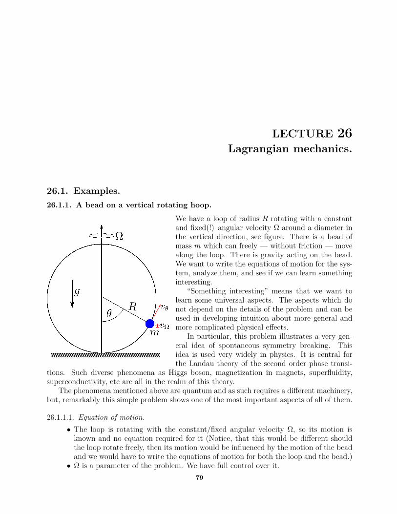
LECTURE 26Lagrangian mechanics.
26.1. Examples.26.1.1. A bead on a vertical rotating hoop.
We have a loop of radius R rotating with a constantand fixed(!) angular velocity Ω around a diameter inthe vertical direction, see figure. There is a bead ofmass m which can freely — without friction — movealong the loop. There is gravity acting on the bead.We want to write the equations of motion for the sys-tem, analyze them, and see if we can learn somethinginteresting.
“Something interesting” means that we want tolearn some universal aspects. The aspects which donot depend on the details of the problem and can beused in developing intuition about more general andmore complicated physical effects.
In particular, this problem illustrates a very gen-eral idea of spontaneous symmetry breaking. Thisidea is used very widely in physics. It is central forthe Landau theory of the second order phase transi-
tions. Such diverse phenomena as Higgs boson, magnetization in magnets, superfluidity,superconductivity, etc are all in the realm of this theory.
The phenomena mentioned above are quantum and as such requires a different machinery,but, remarkably this simple problem shows one of the most important aspects of all of them.
26.1.1.1. Equation of motion.• The loop is rotating with the constant/fixed angular velocity Ω, so its motion isknown and no equation required for it (Notice, that this would be different shouldthe loop rotate freely, then its motion would be influenced by the motion of the beadand we would have to write the equations of motion for both the loop and the bead.)• Ω is a parameter of the problem. We have full control over it.
79

80 FALL 2014, ARTEM G. ABANOV, ADVANCED MECHANICS I. PHYS 302
• The position of the bead at any moment of time is then fully described by just onegeneralized coordinate — the angle θ.• Lagrangian. We need potential and kinetic energies:
– The potential energy U(θ) = mgR(1− cos θ).– For the kinetic energy we notice, that the total vector velocity of the beadhas to components vθ — the velocity along the loop, and vΩ — the velocityperpendicular to the plane of the loop, see figure. We also see that vθ = Rθ,and vΩ = ΩR sin θ. The two components are perpendicular to each other, thetotal velocity of the bead is v2 = R2θ2 + Ω2R2 sin2 θ. The kinetic energy then isK(θ, θ) = m
2 R2θ2 + m
2 Ω2R2 sin2 θ.So the Lagrangian is
L = m
2 R2θ2 + m
2 Ω2R2 sin2 θ −mgR(1− cos θ).
• Equation of motion.Rθ = (Ω2R cos θ − g) sin θ.
26.1.1.2. Analysis of the motion. The motion of the bead depends on the initial conditions.If one wants to know the full solution one has to set up initial conditions and then solve theequation of motion. This exact solution is fairly complicated and not very illuminating.
Instead we want to consider the motion around the equilibrium positions of the bead. Weexpect this motion to be a harmonic motion and have some universal features.
• There are four equilibrium points — points where θ = 0 — the bead can remainstationary on the loop.
sin θ = 0, or cos θ = g
Ω2R
• Critical Ωc. The second two equilibriums are possible only ifg
Ω2R< 1, Ω > Ωc =
√g/R.
• The most interesting regime is Ω ∼ Ωc and θ small.• Effective potential energy for Ω ∼ Ωc. From the Lagrangian we can read the effectivepotential energy:
Ueff (θ) = −m2 Ω2R2 sin2 θ +mgR(1− cos θ).
Assuming Ω ∼ Ωc we are interested only in small θ. So
Ueff (θ) ≈12mR
2(Ω2c − Ω2)θ2 + 3
4!mR2Ω2
cθ4
Ueff (θ) ≈ mR2Ωc(Ωc − Ω)θ2 + 34!mR
2Ω2cθ
4,
One should notice, that there are two terms: one of the order of (Ω−Ωc)θ2 and theother is of the order of θ2. It seems unreasonable to keep only these terms and dropthe rest. However, we will see below, that θ2 ∼ (Ω − Ωc), so in fact both terms areof the same order (Ω− Ωc)2 and the rest of them are of the higher order.• Spontaneous symmetry breaking. Plot the function Ueff (θ) for Ω < Ωc, Ω = Ωc, and
Ω > Ωc. Discuss universality.

LECTURE 26. LAGRANGIAN MECHANICS. 81• Small oscillations around θ = 0, Ω < Ωc
mR2θ = −mR2(Ω2c − Ω2)θ, ω =
√Ω2c − Ω2.
• Small oscillations around θ0, Ω > Ωc.
Ueff (θ) = −m2 Ω2R2 sin2 θ +mgR(1− cos θ),
∂Ueff∂θ
= −mR(Ω2R cos θ − g) sin θ, ∂2Ueff∂θ2 = mR2Ω2 sin2 θ −mR cos θ(Ω2R cos θ − g)
∂Ueff∂θ
∣∣∣∣∣θ=θ0
= 0, ∂2Ueff∂θ2
∣∣∣∣∣θ=θ0
= mR2(Ω2 − Ω2c)
So the Tylor expansion gives
Ueff (θ ∼ θ0) ≈ const + 12mR
2(Ω2 − Ω2c)(θ − θ0)2
The frequency of small oscillations then is
ω =√
Ω2 − Ω2c .
26.1.1.3. Universality.• The effective potential energy for small θ and |Ω− Ωc|
Ueff (θ) = 12a(Ωc − Ω)θ2 + 1
4bθ4.
• θ0 for the stable equilibrium is given by ∂Ueff/∂θ = 0
θ0 = 0 for Ω < Ωc√
ab(Ω− Ωc) for Ω > Ωc
Plot θ0(Ω). Non-analytic behavior at Ωc.• Response: how θ0 responses to a small change in Ω.
∂θ0
∂Ω =
0 for Ω < Ωc12
√ab
1√(Ω−Ωc)
for Ω > Ωc
Plot ∂θ0∂Ω vs Ω. The response diverges at Ωc.


LECTURE 27Lagrangian mechanics.
27.1. Example.Here we consider one more example — a double pendulum. The strategyis same as always
• Choosing the generalized coordinates.• Write the potential energy.• Kinetic energy. Normally, most trouble for students.
Here the most natural choice of coordinates are the angles φ1 and φ2. Itis also convenient to use the auxiliary x and y for the intermediate steps.So that we have
x1 = l1 sinφ1, x2 = l1 sinφ1 + l2 sinφ2
y1 = −l1 cosφ1, y2 = −l1 cosφ1 − l2 cosφ2
• Now we can write the potential energyU = m1gy1 +m2gy2 = −(m1 +m2)gl1 cosφ1 −m2gl2 cosφ2
• In order to find the kinetic energy we need velocitiesv1x = x1 = l1φ1 cosφ1, v2x = x2 = l1φ1 cosφ1 + l2φ2 cosφ2
v1y = y1 = l1φ1 sinφ1, v2y = y2 = l1φ1 sinφ1 + l2φ2 sinφ2
sov2
1 = v21x + v2
1y = l21φ21
v22 = v2
2x + v22y = l21φ
21 + l22φ
22 + 2l1l2φ1φ2 cos(φ1 − φ2)
and the kinetic energy
K = (m1 +m2)l212 φ2
1 + m2l22
2 φ22 +m2l1l2φ1φ2 cos(φ1 − φ2)
• The Lagrangian then is
L = (m1 +m2)l212 φ2
1 + m2l22
2 φ22 +m2l1l2φ1φ2 cos(φ1− φ2) + (m1 +m2)gl1 cosφ1 +m2gl2 cosφ2.
83

84 FALL 2014, ARTEM G. ABANOV, ADVANCED MECHANICS I. PHYS 302
• Now we write the Lagrangian equations. We first compute the partial derivatives:
∂L∂φ1
= (m1 +m2)l21φ1 +m2l1l2φ2 cos(φ1 − φ2), ∂L
∂φ1= −m2l1l2φ1φ2 sin(φ1 − φ2)− (m1 +m2)gl1 sinφ1
∂L∂φ2
= m2l22φ2 +m2l1l2φ1 cos(φ1 − φ2), ∂L
∂φ2= +m2l1l2φ1φ2 sin(φ1 − φ2)−m2gl2 sinφ2
and then the full derivative for each
(m1 +m2)l21φ1 +m2l1l2φ2 cos(φ1 − φ2) +m2l1l2φ22 sin(φ1 − φ2) = −(m1 +m2)gl1 sinφ1
m2l22φ2 +m2l1l2φ1 cos(φ1 − φ2)−m2l1l2φ
21 sin(φ1 − φ2) = −m2gl2 sinφ2
(some terms which appeared originally have canceled each other)These are the equations of motion. They are second order coupled nonlinear differentialequations. In order to complete them we need to supply also the initial conditions for bothvariables.
Such equations are hard to solve or analyze. Typically we are mainly interested in thesmall oscillations around the equilibrium position. In this case the equilibrium position isobvious: φ1,eq = φ2,eq = 0. So we need to linearize our equations around this point.
Linearizaton means that you only keep the linear terms in φ1−φ1,eq and in φ2−φ2,eq andtheir derivatives. In our case we then have
(m1 +m2)l21φ1 +m2l1l2φ2 = −(m1 +m2)gl1φ1
m2l22φ2 +m2l1l2φ1 = −m2gl2φ2
These are much simpler — they are still coupled, but at least they are linear! They can besolved by a simple Fourier transform.
27.2. Small Oscillations.We will study the problem of small oscillation in the next semester. Here is just an overview.
A system will always have some dissipation. In many cases the dissipation can be consid-ered to be very small. However, no matter how small it is if one waits long enough the systemwill find one of its equilibrium positions (there can be several.) Such equilibrium positionsare the minimums of the potential energy. If qi are the set of N generalized coordinatesand U(qi) is the potential energy, then the equilibrium positions qi,eq are the solutionsof N algebraic equations
∂U
∂qi
∣∣∣∣∣qi=qi,eq
= 0.
After one solves these equations, then for each solution one must make sure, that this isindeed the minimum, not the maximum or a saddle point.
In many cases the equilibrium position can be guessed form the problem itself, but notalways!!! One has to be careful.
The Lagrangian equations of motion contain the derivative of the Lagrangian ∂L∂qi
and ∂L∂qi
.So in order for the equations of motion to be linear in the displacement of the generalizedcoordinates from the equilibrium positions qi − qi,eq and generalized velocities one needsto write the Lagrangian in quadratic order in displacement of generalized coordinates andgeneralized velocities.
LECTURE 27. LAGRANGIAN MECHANICS. 85For example, for the problem of the double pendulum the equilibrium position is obvious
φ1,eq = φ2,eq = 0. We can write the Lagrangian in the quadratic order in φ1 − φ1,eq = φ1,φ2 − φ2,eq = φ2 and in φ1, φ2.
L = (m1 +m2)l212 φ2
1 + m2l22
2 φ22 +m2l1l2φ1φ2 −
12(m1 +m2)gl1φ2
1 −12m2gl2φ
22.
(I dropped the constant terms from the Lagrangian.) One can see, that our linearized equa-tions can be obtained from this Lagrangian right away, by the standard procedure.


LECTURE 28Lagrangian mechanics.
28.1. Generalized momentum.• Definition: For a coordinate q the generalized momentum is defined as
p ≡ ∂L
∂q
• Examples:– For a particle in a potential field L = m~r2
2 − U(~r) we have
~p = ∂L
∂~r= m~r
The generalized momentum is just the usual momentum.– For a rotation around a fixed axis L = Iφ2
2 − U(φ), then
p = ∂L
∂φ= Iφ = J.
The generalized momentum is just an angular momentum.
28.2. Ignorable coordinates. Conservation laws.If one chooses the coordinates in such a way, that the Lagrangian does not depend on sayone of the coordinates q1 (but it still depends on q1, then the corresponding generalizedmomentum p1 = ∂L
∂q1is conserved as
d
dtp1 = d
dt
∂L
∂q1= ∂L
∂q1= 0
• Problem of a freely horizontally moving cart of mass M with hanged pendulum ofmass m and length l.
L = Mx2
2 + m
2(x2 + 2xφl cosφ+ l2φ2
)+mgl cosφ.
We see right away, that there is no x (remember x and x are different variables forthe Lagrangian) in the Lagrangian. So x is ignorable variable. It means, that the
87

88 FALL 2014, ARTEM G. ABANOV, ADVANCED MECHANICS I. PHYS 302
corresponding generalized momentum px = ∂L∂x
is conserved. So we can write one ofthe equations of motion as
px = (M +m)x+mφl cosφ = const.
This constant should be obtained from the initial conditions.
28.3. Momentum conservation. Translation invarianceLet’s consider a translationally invariant problem. For example all interactions depend onlyon the distance between the particles. The Lagrangian for this problem is L(~r1, . . . ~ri, ~r1, . . . ~ ir).Then we add a constant vector ε to all coordinate vectors and define
Lε(~r1, . . . ~ri, ~r1, . . . ~ ir,~ε) ≡ L(~r1 + ~ε, . . . ~ri + ~ε, ~r1, . . . ~ ir)
It is clear, that in the translationally invariant system the Lagrangian will not change undersuch a transformation. So we find
∂Lε∂~ε
= 0.
But according to the definition∂Lε∂~ε
∣∣∣∣∣~ε=0
=∑i
∂L
∂~ri.
Hence ∑i
∂L
∂~ri= 0.
On the other hand the Lagrange equations tell us that∑i
∂L
∂~ri= d
dt
∑i
∂L
∂~ri= d
dt
∑i
~pi,
sod
dt
∑i
~pi = 0,∑i
~pi = const.
We see, that the total momentum of the system is conserved!
28.4. Non uniqueness of the Lagrangian.For any problem and any given set of generalized coordinates the Lagrangian is not uniquelydefined. This is similar to the fact that the potential energy is not uniquely defined — onecan always add a constant to it.
In the same way as two potential energy functions which differ only by a constant givethe same equations of motion, two Lagrangians for the same problem must give the sameequations of motion. So two Lagrangians are equivalent if the resulting Lagrangian equationsare the same.
• Let’s take a Lagrangian L(q, q, t).• Let’s take an arbitrary function G(q, t).• Let’s construct a new Lagrangian L(q, q, t) = L+ q ∂G
∂q+ ∂G
∂t.
• The statement is that the two Lagrangians L and L are equivalent.

LECTURE 28. LAGRANGIAN MECHANICS. 8928.4.1. Proof of equivalence.
• The Lagrange equationd
dt
∂L
∂q= ∂L
∂q.
Let’s use our definition of L and see how it works∂L
∂q= ∂L
∂q+ ∂G
∂q,
∂L
∂q= ∂L
∂q+ q
∂2G
∂2q+ ∂2G
∂t∂q
thend
dt
∂L
∂q= d
dt
∂L
∂q+ q
∂2G
∂2q+ ∂2G
∂q∂tand we see
d
dt
∂L
∂q− ∂L
∂q= d
dt
∂L
∂q− ∂L
∂q.
• So we see, that the equation we obtain using L is exactly the same as the equationwe obtain using L.
d
dt
∂L
∂q= ∂L
∂q.
28.4.2. The reason.
We want to understand why the above transformation of the Lagrangian does not change theequations of motion.
• The reason for this is the following: the expression I added to the Lagrangian q ∂G∂q
+ ∂G∂t
is a full derivative q ∂G∂q
+ ∂G∂t
= dGdt
as can be seen using the chain rule. So L = L+ dGdt.
But then the Action changes by
A =∫ tf
tiLdt =
∫ tf
tiLdt+
∫ tf
ti
dG
dtdt =
∫ tf
tiLdt+G(q(tf ), tf )−G(q(ti), ti) = A+ const.
So the variation of the Action does not change, and thus the condition for the ex-tremum — the Euler-Lagrange equation — also does not change.
So one can always add a full time derivative to a Lagrangian.The last statement is correct only in the classical mechanics. In quantum mechanics the
Action itself has its own meaning (unlike the classical mechanics where we are only interestedin its minimum.) and addition of a constant to the Action is not necessarily harmless.


LECTURE 29Lagrangian’s equations for magnetic forces.
The equation of motion ism~r = q( ~E + ~r × ~B)
The question is what Lagrangian gives such equation of motion?
29.1. Electric and magnetic fields.In order to answer the question above we need to know a bit more about electric and magneticfields. Classically these fields are completely described by the Maxwell equations. There arefour of thes equations, but we will need only two of them: magnetic Gauss law and Faraday’slaw
∇ · ~B = 0, ∇× ~E = −∂~B
∂t.
Notice, that these are the two Maxwell equations which do not have matter — charge orcurrent densities.
Consider first magnetic Gauss law. Which is the statement that there are no magneticcharges.
∇ · ~B = 0This equation is satisfied by the following solution
~B = ∇× ~A,
for any vector field ~A(~r, t).The Faraday’s Law
∇× ~E = −∂~B
∂tthen gives
~E = −∇φ− ∂ ~A
∂t,
where φ is the electric potential and is again an arbitrary function.The vector potential ~A and the potential φ are not uniquely defined. One can always
choose another potential~A′ = ~A+∇F, φ′ = φ− ∂F
∂t91

92 FALL 2014, ARTEM G. ABANOV, ADVANCED MECHANICS I. PHYS 302
and obtain exactly the same electric and magnetic fields. As the other two Maxwell equationscontain only electric and magnetic fields (and not the potentials) they will also not fix thisfreedom.
Moreover, in any experiment we can only measure electric ~E and magnetic ~B fields. Thismeans that the potentials — vector potential ~A and scalar potential φ cannot be measuredby itself.
Such fields are called gauge fields. The freedom of choice is called gauge freedom. Thetransformation from one set of fields ~A and φ to ~A′ and φ′ is called gauge transformation.The fact, that no physical results must depend on the choice of gauge (physical quantitiesmust be invariant under the gauge transformation) is called gauge symmetry.
Such gauge symmetries are extremely important in physics. A lot of constructions inmodern physics involve some sort of gauge symmetry.
As any continuous symmetry gauge symmetry leads to conservation laws. In the case ofelectromagnetism it leads to the charge conservation law (we will not discuss it any furtherin this class).
Notice, that if ~B and ~E are zero, the gauge fields do not have to be zero. For example if~A and φ are constants, ~B = 0, ~E = 0.
29.2. The Lagrangian.Now we can write the Lagrangian:
L = m~r
2 − q(φ− ~r ·~A)
I note, that this Lagrangian has a simpler and more transparent form in the notations adoptedin the special and general relativity — four dimensional space-time with Minkovskii metric.
• It is impossible to write the Lagrangian in terms of the physical fields ~B and ~E!• The expression
φdt− d~r · ~Ais a full differential if and only if
−∇φ− ∂ ~A
∂t= 0, ∇× ~A = 0,
which means that it is full differential, and hence can be thrown out, only if thephysical fields are zero!
The generalized momenta are
~p = ∂L
∂~r= m~r + q ~A
(Notice, that the generalized momentum is not the same as usual momentum. Moreover, itis not gauge invariant!)
The Lagrange equations are:d
dt~p = ∂L
∂~rLet’s consider the x component
d
dtpx = ∂L
∂x,
LECTURE 29. LAGRANGIAN’S EQUATIONS FOR MAGNETIC FORCES. 93
mx+ qx∂Ax∂x
+ qy∂Ax∂y
+ qz∂Ax∂z
+ q∂Ax∂t
= −q∂φ∂x
+ qx∂Ax∂x
+ qy∂Ay∂x
+ qz∂Az∂x
mx = q
(−∂φ∂x− ∂Ax
∂t+ y
[∂Ay∂x− ∂Ax
∂y
]− z
[∂Ax∂z− ∂Az
∂x
])mx = q (Ex + yBz − zBy)


LECTURE 30Energy conservation.
30.1. Energy conservation.We also have the time translation invariance in many systems. It means that the Lagrangiandoes not explicitly depend on time. So we have L(q, q), and not L(q, q, t). However, thecoordinate q(t) does depend on the time. So let’s see how the Lagrangian on a trajectorydepends on time.
Let me clarify the question. Assume that we have a Lagrangian L(q, q). We then writeLagrangian equation of motion d
dt∂L∂q
= ∂L∂q
with some initial conditions q(t = 0) = q0,q(t = 0) = v0. Then we solve this equation an obtained q(t) and hence we also obtainedq(t) = dq(t)
dt. We then take these functions and plug them into the Lagrangian L(q(t), q(t)).
Now the Lagrangian becomes a function of time on the trajectory. We want to see how itdepends on time.
In our standard definition it means that we are interested in the full time derivative ofthe Lagrangian.d
dtL(q(t), q(t)) = ∂L
∂qq+ ∂L
∂qq = ∂L
∂qq+ d
dt
(∂L
)− q d
dt
∂L
∂q= d
dt
(∂L
)+ q
(∂L
∂q− d
dt
∂L
∂q
)But as we are looking at the real trajectory — the function q(t) is the solution of the Lagrangeequation. So according to the Lagrange equation the last term is zero, so we have
d
dt
(∂L
∂qq − L(q, q)
)= 0
or∂L
∂qq − L(q, q) = const = E
Using generalized momentum we can writepq − L = E, Constant on trajectory.
If we have many variables qi, thenE =
∑i
piqi − L
This is another conserved quantity.Examples:
95

96 FALL 2014, ARTEM G. ABANOV, ADVANCED MECHANICS I. PHYS 302
• A particle in a potential field.– The Lagrangian
L = m~r2
2 − U(~r)
– The momenta
px = ∂L
∂x= mx, py = ∂L
∂y= my, pz = ∂L
∂z= mz.
– The Energy
E = xpx + ypy + zpz − L = m~r2
2 + U(~r)
• A particle on a circle.– The Lagrangian
L = mR2
2 φ2 − U(φ).
– Generalized momentum
pφ = ∂L
∂φ= mR2φ.
– The Energy
E = φpφ − L = mR2
2 φ2 + U(φ)
• A cart (mass M) with a pendulum (mass m, length l).– The Lagrangian:
L = M +m
2 x2 +mφxl cosφ+ m
2 l2φ2 −mgl(1− cosφ).
– The generalized momenta:
px = ∂L
∂x= (M +m)x+mφl cosφ, pφ = ∂L
∂φ= mxl cosφ+ml2φ.
– The Energy
E = xpx + φpφ − L = M +m
2 x2 +mφxl cosφ+ m
2 l2φ2 +mgl(1− cosφ)
• A string with tension and gravity:– The Functional ∫ L
0(ρgy − T )
√1 + (y′)2dx.
– One can thin of it as an Action of some mechanical system. Then for this systemwe identify the “Lagrangian”
L = (ρgy − T )√
1 + (y′)2.
We also use the letter x to denote the time in that mechanical system.– So the “generalized momentum” is
p = ∂L
∂y′= ρgy − T√
1 + (y′)2y′.
LECTURE 30. ENERGY CONSERVATION. 97– And conserved “energy”
E = y′p− L = ρgy − T√1 + (y′)2
.
This is now a first order differential equation which can be solved much easier,than the second order Euler-Lagrange equation.
– This conserved quantity has a physical meaning for the initial problem of therope. It is the x component of the tension force.


LECTURE 31Hamiltonian.
In this lecture we will construct a function of generalized momenta and coordinates, whichis called Hamiltonian. In this lecture I will not describe how it is used — this will be donelater. Here we just construct this function and consider a few examples.
31.1. Hamiltonian.Given a Lagrangian L(qi, qi) the energy
E =∑i
piqi − L, pi = ∂L
∂qi
is a number defined on a trajectory! One can say that it is a function of initial conditions.We can construct a function a function of p and q in the following way: we first solve
the set of equationspi = ∂L
∂qiwith respect to qi, we then have these functions
qi = qi(qj, pj)and define a function H(qi, pi)
H(qi, pi) =∑i
piqi(qj, pj)− L(qi, qi(qj, pj)),
• Notice, that in this construction we have never used the equations of motion! wehave treated q, q and p simply as variables, not as some functions of time.
This function is called a Hamiltonian! The Hamiltonian is a function of coordinates andmomenta! THERE MUST BE NO VELOCITIES IN THE HAMILTONIAN!
• Hamiltonian is NOT energy. Energy is a number on a trajectory. Hamiltonian is afunction of p and q — it, by itself, knows nothing about trajectories.• Hamiltonian and energy are related to each other. The value of the Hamiltonian ona trajectory is energy.
The importance of variables:• We have three kinds of variables:
generalized coordinates — qi, generalized velocities — qi, generalized momenta — pi.
• A Lagrangian is a function of generalized coordinates and velocities: qi and qi.99

100 FALL 2014, ARTEM G. ABANOV, ADVANCED MECHANICS I. PHYS 302
• A Hamiltonian is a function of the generalized coordinates and momenta: qi andpi.
Here are the steps to get a Hamiltonian from a Lagrangian(a) Write down a Lagrangian L(qi, qi) – it is a function of generalized coordinates
and velocities qi, qi(b) Find generalized momenta
pi = ∂L
∂qi.
(c) Treat the above definitions as equations and solve them for all qi, so for each velocityqi you have an expression qi = qi(qj, pj).
(d) Substitute these function qi = qi(qj, pj) into the expression∑i
piqi − L(qi, qi).
The resulting function H(qi, pi) of generalized coordinates and momenta is called aHamiltonian.
31.2. Examples.• A particle in a potential field.
– The Lagrangian
L = m~r2
2 − U(~r)– The momenta
px = ∂L
∂x= mx, py = ∂L
∂y= my, pz = ∂L
∂z= mz.
– The velocity~r = ~p
m– The Hamiltonian
H(~r, ~p) = xpx + ypy + zpz − L = ~p2
m− L = ~p2
2m + U(~r)
• A particle on a circle.– The Lagrangian
L = mR2
2 φ2 − U(φ).– Generalized momentum
pφ = ∂L
∂φ= mR2φ.
– The velocityφ = pφ
mR2
– The Hamiltonian
H(φ, pφ) = φpφ − L =p2φ
2mR2 + U(φ)
• A cart (mass M) with a pendulum (mass m, length l).

LECTURE 31. HAMILTONIAN. 101– The Lagrangian:
L = M +m
2 x2 +mφxl cosφ+ m
2 l2φ2 −mgl(1− cosφ).
– The generalized momenta:
px = ∂L
∂x= (M +m)x+mφl cosφ, pφ = ∂L
∂φ= mxl cosφ+ml2φ.
– The generalized velocities
x = 1l
lpx − pφ cosφM +m sin2 φ
, φ = 1ml2
(M +m)pφ −mlpxM +m sin2 φ
.
– The Hamiltonian
H = xpx + φpφ − L = 12ml2
ml2p2x − 2mlpxpφ cosφ+ (m+M)p2
φ
M +m sin2 φ+mgl(1− cosφ)
• Central symmetric potential in 3D. (Kepler problem)– We need to write the Lagrangian in spherical coordinates. We know
d~r = ~erdr + ~eθrdθ + ~eφr sin θdφ.Dividing this by dt we get
~v = ~err + ~eθrθ + ~eφrφ sin θ,so
v2 = r2 + r2θ2 + r2φ2 sin2 θ.
The Lagrangian is
L = m
2 r2 + m
2 r2θ2 + m
2 r2φ2 sin2 θ − U(r)
– The generalized momenta are
pr = ∂L
∂r= mr, pθ = ∂L
∂θ= mr2θ, pφ = ∂L
∂φ= mr2φ sin2 θ.
– The generalized velocities
r = prm, θ = pθ
mr2 , φ = pφmr2 sin2 θ
.
– The Hamiltonian
H = rpr + θpθ + φpφ − L = p2r
2m + p2θ
2mr2 +p2φ
2mr2 sin2 θ+ U(r)


LECTURE 32Hamiltonian equations.
32.1. Hamiltonian equations.• If Lagrangian explicitly depends on time. . .• New notation for the partial derivatives. What do we keep fixed?
– The notation explicitly keeps the notion of what is kept fixed.– The definition of momentum then is
p =(∂L
∂q
)q
.
– The Lagrangian equation of motiond
dt
(∂L
∂q
)q
=(∂L
∂q
)q
etc.• Derivation of the Hamiltonian equations.
– Let’s differentiate the Hamiltonian H(p, q) with respect to momentum p, whilekeeping the coordinate q fixed.
– We will use H = pq − L(q, q), but we will remember, that q is the function of pand q, i.e. q(p, q).
– So we differentiate the function H(p, q) = pq(p, q)− L(q, q(p, q)).– We will also remember, that by definition p =
(∂L∂q
)q.
– So we have:(∂H
∂p
)q
= q + p
(∂q
∂p
)q
−(∂L
∂q
)q
(∂q
∂p
)q
= q + p
(∂q
∂p
)q
− p(∂q
∂p
)q
= q
This is the first Hamiltonian equation.– Now lets differentiate the Hamiltonian with respect to q, while keeping p fixed.– Again we must remember that q(p, q) is the function of p and q.– So using H(p, q) = pq(p, q)− L(q, q(p, q)) we have(
∂H
∂q
)p
= p
(∂q
∂q
)p
−(∂L
∂q
)q
−(∂L
∂q
)q
(∂q
∂q
)p
= −(∂L
∂q
)q
+p− (∂L
∂q
)q
(∂q∂q
)p
.
103

104 FALL 2014, ARTEM G. ABANOV, ADVANCED MECHANICS I. PHYS 302
– Using the definition of momentum p =(∂L∂q
)q, we see, that the last term is zero.
So we have (∂H
∂p
)p
= −(∂L
∂q
)q
.
– According to the Lagrangian equation of motion(∂L∂q
)q
= ddt
(∂L∂q
)q
= p. Thelast equality comes from the definition of momentum. So we have(
∂H
∂q
)p
= −p.
This is the second Hamiltonian equation.• The two Hamiltonian equation together are
q = ∂H
∂p,
p = −∂H∂q
.
• Notice, that the equations are “self-contained” there is no notion of the generalizedvelocities. Everything is written in terms of the coordinates, momenta and their timedependence.• If we have many degrees of freedom, then this pair of equations is written for eachdegree of freedom.
32.2. Examples.• Energy conservation.
– Energy is the value of the Hamiltonian on the trajectory!!!!– What it means, is that we take a Hamiltonian, write the Hamilton equations,solve them for some initial conditions q(t = 0) = q0, p(t = 0) = p0 (and so forthif we have more degrees of freedom). We then have two functions q(t) and p(t).
– We now substitute these functions into the Hamiltonian H(p, q, t) and obtain afunction of time H(p(t), q(t), t).
– Now lets differentiate this function with respect to time. This is a full derivativenowdH
dt= ∂H
∂pp+ ∂H
∂qq + ∂H
∂t= −∂H
∂p
∂H
∂q+ ∂H
∂q
∂H
∂p+ ∂H
∂t= ∂H
∂t
where we used the Hamilton equations for the functions p(t) and q(t).– So we see, that if the Hamiltonian does not explicitly depend on time (in lesswords ∂H
∂t= 0), then
dH
dt= 0.
or the value of the Hamiltonian on a trajectory is constant.– Notice the importance of the minus sign in the second of the Hamilton equations!
• Velocity.– In many cases the Hamiltonian is the starting point.

LECTURE 32. HAMILTONIAN EQUATIONS. 105– The dependence of the velocity on momentum is then given by the Hamiltonequation
q = ∂H
∂p.
– In particular if we have a normal “kinetic energy” E(p) = p2
2m , then this equationsgives
x = ∂E
∂p= p/m.
This is the usual p = mv.– The kinetic energy as a function of momentum E(p) is called dispersion relation.– It is the dispersion relation which gives the relation between the velocity andmomentum, by the Hamilton equation.
– There are cases where this is very nontrivial. For example in liquid Helium thedispersion of “exitations” is similar to the one shown in the picture. One cansee, that at p = p0 the momentum is not zero (it is p0), but the velocity is zero!


LECTURE 33Hamiltonian equations. Examples
The Hamiltonian and Lagrangian formulations of mechanics are equivalent to each other.Namely, if we know the Lagrangian we will know the Hamiltonian and if we know the Hamil-tonian we will know the Lagrangian.
33.1. Lagrangian→Hamiltonian, Hamiltonian→Lagrangian.33.1.1. L→ H
• We are given a Lagrangian L(qi, qi) as a function of coordinates qi and veloc-ities qi. There are no momenta in the Lagrangian!• We write the definition of momenta
pi = ∂L
∂qi.
• We treat these equations as equations for all velocities qi and solve them withrespect to the velocities
qj = qj(pi, qi).• We construct the Hamiltonian
H(pi, qi) =∑j
pj qj(pi′, qi′)− L(qj′, qj′(pi′, qi′)).
The Hamiltonian thus constructed is the function of all coordinates qi and all momentapi. There are must be no velocities in the Hamiltonian!
33.1.2. H → L
• We are given a Hamiltonian H(pi, qi) as a function of all coordinates qi andall momenta pi. There are no velocities in the Hamiltonian!• We write the definition of velocity for each momentum
qi = ∂H
∂pi.
• We treat these equations as equations for all momenta pi and solve them withrespect to the momenta
pj = pj(qi, qi).107
108 FALL 2014, ARTEM G. ABANOV, ADVANCED MECHANICS I. PHYS 302
• We construct the LagrangianL(qi, qi) =
∑j
qjpj(qi′, qi′)−H(pj′(qi′, qi′), qj′)
The Lagrangian thus constructed is the function of all coordinates qi and all velocities qi.There are must be no momenta in the Lagrangian!
33.1.3. Equations of motion.
If we have a Lagrangian and a Hamiltonian which are connected by the procedures describedabove, then the Lagrangian and Hamiltonian equations are equivalent — they describe thesame motion!
L(qi, qi) ⇐⇒ H(pi, qi)d
dt
∂L
∂qi= ∂L
∂qi⇐⇒
qi = ∂H∂pi
pi = −∂H∂qi
qi(t = 0) = qi0, qi(t = 0) = vi0 ⇐⇒ qi(t = 0) = qi0, pi(t = 0) = pi0.
Given equivalent initial conditions these equations will give exactly the same qi(t)!
33.2. Examples.33.2.1. A particle in a potential field.
• Lagrangian→Hamiltonian, Hamiltonian→Lagrangian.– The Lagrangian
L(~r, ~r) = m~r
2 − U(~r).– The momentum
~p = ∂L
∂~r= m~r.
– The velocity~r = ~p
m– The Hamiltonian
H(~p, ~r) = ~p · ~r − L = ~p2
2m + U(~r)
– From the Hamiltonian
~r = ∂H
∂~p= ~p
m.
– The momentum~p = m~r.
– The Lagrangian
L(~r, ~r) = ~r · ~p−H = m~r
2 − U(~r).
• We found the Hamiltonian from the Lagrangian and then from Hamiltonian we foundthe same Lagrangian.• The equations of motion:

LECTURE 33. HAMILTONIAN EQUATIONS. EXAMPLES 109– The Lagrangian equations of motion
m~r = −∂U∂~r
.
– The Hamiltonian equations of motion
~r = ∂H
∂~p= ~p
m, ~p = −∂H
∂~r= −∂U
∂~r.
– Taking the time derivative of the first equation we find ~p = m~r. Using this inthe second equation we find
m~r = −∂U∂~r
.
– We see, that the Hamiltonian and Lagrangian equations give the same ~r(t)!
33.2.2. Rotation around a fixed axis.
• Lagrangian→Hamiltonian, Hamiltonian→Lagrangian.
L(φ, φ) = Iφ2
2 − U(φ).
– The momentumpφ = Iφ.
– Velocityφ = pφ
I– The Hamiltonian
H(pφ, φ) = pφφ− L =p2φ
2I + U(φ).
– The velocity
φ = ∂H
∂pφ= pφ
I.
– The momentumpφ = Iφ.
– The Lagrangian
L(φ, φ) = Iφ2
2 − U(φ)
• The equations of motion– Lagrangian equation
Iφ = −∂U∂φ
– The Hamiltonian equations
φ = ∂H
∂pφ= pφ
I, pφ = −∂H
∂φ= −∂U
∂φ

110 FALL 2014, ARTEM G. ABANOV, ADVANCED MECHANICS I. PHYS 302
Differentiating the first equation with respect to time and using the result inthe second equation we get
Iφ = −∂U∂φ
– We see, that the Hamiltonian and Lagrangian equations give the same φ(t)!An example of the system considered above is a pendulum.
33.2.3. Motion in a central symmetric field.
• Lagrangian→Hamiltonian, Hamiltonian→Lagrangian.– The Lagrangian is
L = m
2 r2 + m
2 r2θ2 + m
2 r2φ2 sin2 θ − U(r)
– The momenta:
pr = ∂L
∂r= mr, pθ = ∂L
∂θ= mr2θ, pφ = ∂L
∂φ= mr2φ sin2 θ.
– The velocities
r = prm, θ = pθ
mr2 , φ = pφmr2 sin2 θ
.
– The Hamiltonian
H = rpr + θpθ + φpφ − L = p2r
2m + p2θ
2mr2 +p2φ
2mr2 sin2 θ+ U(r).
– The velocities
r = ∂H
∂pr= prm, θ = ∂H
∂pθ= pθmr2 , φ = ∂H
∂pφ= pφmr2 sin2 θ
.
– The momenta
pr = ∂L
∂r= mr, pθ = ∂L
∂θ= mr2θ, pφ = ∂L
∂φ= mr2φ sin2 θ.
– The Lagrangian
L = rpr + θpθ + φpφ −H = m
2 r2 + m
2 r2θ2 + m
2 r2φ2 sin2 θ − U(r)
• The equations of motion– The Lagrangian equations of motion
mr = mrθ2 +mrφ2 sin2 θ − ∂U
∂r
mr2θ + 2mrrθ = mr2φ2 sin θ cos θmφr2 sin2 θ +mφrr sin2 θ + 2r2φθ sin θ cos θ = 0

LECTURE 33. HAMILTONIAN EQUATIONS. EXAMPLES 111– The Hamiltonian equations of motion
r = ∂H∂pr
= prm
pr = −∂H∂r
= p2θ
mr3 +p2φ
mr3 sin2 θ− ∂U
∂r
θ = ∂H∂pθ
= pθmr2 pθ = −∂H
∂θ=
p2φ cos θ
mr2 sin3 θ
φ = ∂H∂pφ
= pφmr2 sin2 θ
. pφ = −∂H∂φ
= 0
– You are welcome to check that these equations are equivalent to the Lagrangianequations.
33.2.4. Relativistic particle.
Consider a Hamiltonian H(p, x) = ε(p) = c√p2 +m2
0c2 in 1D. We do not consider any field
so the Hamiltonian does not depend on x.• Equations of motion.
p = −∂H∂x
= 0, x = ∂H
∂p= cp√
p2 +m20c
2
So we see, that the momentum is conserved, but the velocity has a nontrivial depen-dence on momentum. In particular if p→∞ we have x→ c. Moreover, the velocitycan never exceed c!• The momentum. From the last equation
p = m0cx√c2 − x2
.
Notice, if we introduce a “mass” as m = m0√1−x2/c2
, then we have p = mx – the usualformula. Now if we use this notation to write the energy, then we get ε = mc2.• Lagrangian.
L(x, x) = xp−H = −m0c√c2 − x2
• Action. It is very instructive to write the Action for this problem
S = −m0c∫ √
c2 − x2dt = −m0c∫ √
(cdt)2 − (dx)2.
• Geometrical meaning of Action. Notice, that the action above is the length of the
interval in the space-time (ct, x) with the metric(
1 00 −1
):
(ds)2 = (cdt, dx)(
1 00 −1
)(cdtdx
)
The Action then isA = −m0c
∫ds

112 FALL 2014, ARTEM G. ABANOV, ADVANCED MECHANICS I. PHYS 302
• One now can easily extend this construction to the full 3 + 1 space by using theMinkovskii metric
1 0 0 00 −1 0 00 0 −1 00 0 0 −1
• Moreover, one is not restricted to the flat Minkovskii space and can write the Actionfor a particle in a curved space-time — the space-time with Einstein’s gravity.

LECTURE 34Hamiltonian equations. Examples. Phase space.
34.1. Examples.• General case for the kinetic energy quadratic in velocities
L = 12 qiMij(qk)qj − U(qk),
where Mij(qk) – a symmetric q-dependent positive definite matrix.– The momenta
pi = ∂L
∂qi= Mij(qk)qj.
– The velocitiesqi =
(M−1(qk)
)ijpj.
– The Hamiltonian
H = 12pi
(M−1(qk)
)ijpj + U(qk)
– The Hamiltonian equations
qi = ∂H
∂pi=(M−1(qk)
)ijpj
pk = −∂H∂qk
= −12pi
(∂M−1(qk′)
∂qk
)ij
pj −∂U
∂qk
Derivative of a matrix(∂M−1(qk′)
∂qk
)ijmeans simply the matrix where each matrix
element is the derivative of the original matrix elements (M−1(qk))ij.• A cart (mass M) with a pendulum (mass m, length l).
L = M +m
2 x2 +mφxl cosφ+ m
2 l2φ2 −mgl(1− cosφ).
This is a particular case of the example above.– The coordinates/velocities (
xφ
)113

114 FALL 2014, ARTEM G. ABANOV, ADVANCED MECHANICS I. PHYS 302
– The matrix M
M =(M +m ml cosφml cosφ ml2
)– The inverse M−1
M−1 = 1ml2
1M +m sin2 φ
(ml2 −ml cosφ
−ml cosφ m+M
)– The Hamiltonian
H = 12ml2
ml2p2x − 2mlpxpφ cosφ+ (m+M)p2
φ
M +m sin2 φ+mgl(1− cosφ).
– etc.
34.2. Phase space. Hamiltonian vector field. Phase trajectories.Hamiltonian equations are the first order differential equations! We double the number ofvariables and the number of equations, but each equation is now the first order differentialequations. We still need two initial conditions for each degree of freedom.
• The space of all q and all p is called a phase space of the Hamiltonian system.Let’s consider a one dimensional problem with time independent Hamiltonian. So we haveonly one generalized coordinate q. The phase space is then two dimensional: (q, p). For agiven Hamiltonian the equations of motion are
q = ∂H
∂p
p = −∂H∂q
Let’s assume that a system had a phase space coordinates (qt, pt) at time t. The equationsof motion show that at time t+ dt the system will be at the point
qt+dt = qt + ∂H
∂pdt
pt+dt = pt −∂H
∂qdt
Let’s now define the Hamiltonian vector field by
~H =(
∂H∂p
−∂H∂q
).
Then we see, that a point (qt, pt) after time dt shifts to(qt+dtpt+dt
)=(qtpt
)+ ~Hdt
So the vector ~H is a vector of velocity in the phase space.• We can plot the vector field ~H at every point of the phase space.• Notice, that we do not need to solve any differential equations for that. We just needto differentiate the Hamiltonian!• This vector field will show the velocity in the phase space for our system.

LECTURE 34. HAMILTONIAN EQUATIONS. EXAMPLES. PHASE SPACE. 115A trajectories of the system in the phase space are simply the lines which are tangential tothe Hamiltonian vector field at every point of the line. Different trajectories correspond todifferent initial conditions.
This construction is very similar to the electric field and electric field lines.• Motion in the phase space: we can consider the motion of a system in the phasespace: we start from an initial point (qi, pi) and continue along the Hamiltonianvector field — along phase space trajectories.• Trajectories do not intersect (except in isolated singular points). This is the sameas for electric field lines. The phase space trajectories (electric field lines) can haveone tangential vector at each point, except the points where ~H = 0 — the singularpoints — all the derivatives of the Hamiltonian are zero.• On the phase trajectories the Hamiltonian is constant — the energy is conserved!
These simple rules allow one to construct the phase space trajectories for many (usually 1D)systems. Here are the couple of examples.
• Harmonic oscillator.– The Hamiltonian of the Harmonic oscillator is
H = p2
2m + mω2x2
2 .
– On the phase space trajectories the Hamiltonian is constant. The lines in (x, p)space given by
p2
2m + mω2x2
2 = E
are ellipses with the semiaxes√
2mE and√
2E/mω2. (The area of these ellipsesis 2πE/ω = ET , where T is the period.)
– The Hamiltonian vector field is
~H =(p/m−mω2x
)
• Pendulum.– When energy is small the pendulum is a harmonic oscillator, so for small energiesthe trajectories are ellipses.
– When energy grows the ellipses grow.
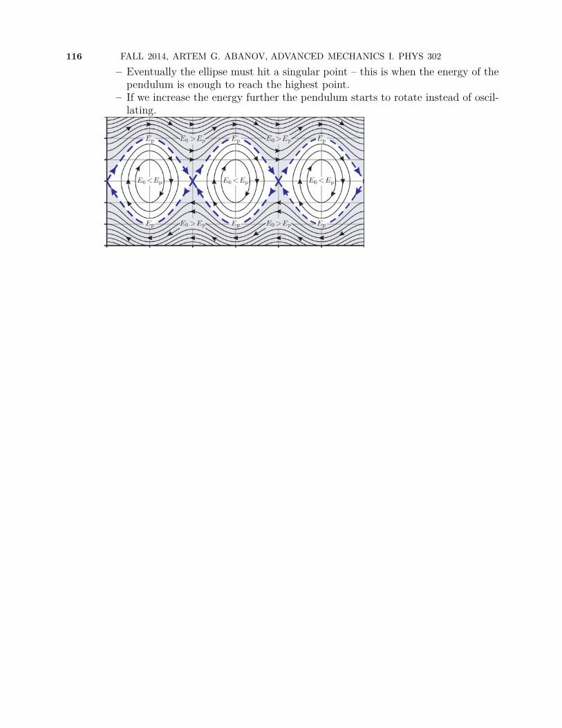
116 FALL 2014, ARTEM G. ABANOV, ADVANCED MECHANICS I. PHYS 302
– Eventually the ellipse must hit a singular point – this is when the energy of thependulum is enough to reach the highest point.
– If we increase the energy further the pendulum starts to rotate instead of oscil-lating.

LECTURE 35Liouville’s theorem. Poincaré recurrence theorem.
Area law.
35.1. Liouville’s theorem.
Theorem: The phase space volume is conserved under the Hamiltonian flow.Proof: As the trajectories do not intersect, we can consider the Hamiltonian flow as a mapof the phase space on itself: any initial point (q0, p0) is mapped to a point (q(t), p(t)) aftertime t, where q(t) and p(t) are the solutions of the Hamiltonian equations with (q0, p0) asinitial conditions.
For a small time interval dt the map is given by
q1 = q0 + ∂H
∂p0dt, p1 = p0 −
∂H
∂q0dt
We can consider these equations as the equations for the change of variables from (q0, p0) to(q1, p1).
Consider a piece of volume at time t = 0: A0 =∫dq0dp0. After time dt, this volume
becomes A1 =∫dq1dp1. We want to compute the change of this volume dA = A1 −A0.
dA =∫dq1dp1 −
∫dq0dp0 =
∫ (∂q1
∂q0
∂p1
∂p0− ∂q1
∂p0
∂p1
∂q0
)dq0dp0 −
∫dq0dp0.
117

118 FALL 2014, ARTEM G. ABANOV, ADVANCED MECHANICS I. PHYS 302
Using the formulas for our change of variables we find
∂q1
∂q0= 1 + ∂2H
∂p0∂q0dt,
∂p1
∂p0= 1− ∂2H
∂p0∂q0dt,
∂q1
∂p0= ∂2H
∂p20dt,
∂p1
∂q0= −∂
2H
∂q20dt.
Or (∂q1
∂q0
∂p1
∂p0− ∂q1
∂p0
∂p1
∂q0
)= 1−
(∂2H
∂p0∂q0
∂2H
∂p0∂q0− ∂2H
∂p20
∂2H
∂q20
)(dt)2
so that dA ∼ (dt)2. It means, that dAdt∼ dt, so when we take the limit dt→ 0 we get
dAdt
= 0, A = const.
• This is Liouville’s theorem. It states, that the volume of phase space is unchangedunder the map on itself induced by the equations of motion.• It is also correct for any number of degrees of freedom.• Notice the importance of the minus sign in the Hamiltonian equations.
35.2. Poincaré recurrence theorem.If the available phase space for the system is finite. Let’s starts the motion at some pointof the phase space. Let’s consider an evolution of some finite but small neighborhood ofthis point. The volume of the neighborhood is constant, so eventually it will cover all of theavailable volume. Then the tube of the trajectories must intersect itself. But it cannot, astrajectories do not intersect. It means that it must return to the starting neighborhood (orintersect it at least partially.)
It means that under Hamiltonian dynamics the system will always return arbitrary closeto the initial starting point.
The time it will take for the system to return is another matter.
35.3. Area law.This law is valid only in 1D. Let’s consider a Hamiltonian motion in 1D. We will assume,that the motion is periodic — in 1D the motion is either periodic, or unbounded. In thephase space picture the periodic motion means that the phase space trajectory is a closedloop (without self-crossings). We then can compute the area of the phase space A =
∫dpdq
of the loop inside the phase space trajectory of a motion with energy E. We thus will havea function A(E).

LECTURE 35. LIOUVILLE’S THEOREM. POINCARÉ RECURRENCE THEOREM. AREA LAW.119
If we change the energy by dE the area will change. Consider two trajectories one withthe energy E and the other with the energy E + dE. We want to compute the differencebetween the areas for the two trajectories.
The change of the area is the sum of the vector product of the vectors (dq, dp) and( ∂q∂EdE, ∂p
∂EdE), so
dA = −dE∮ (
∂q
∂Edp− ∂p
∂Edq
)= −dE
∮ (∂q
∂Ep− ∂p
∂Eq
)dt = dE
∮ (∂q
∂E
∂H
∂q+ ∂p
∂E
∂H
∂p
)dt
= dE∮ (
∂H
∂q
∂q
∂E+ ∂H
∂p
∂p
∂E
)dt.
The Hamiltonian is the function of coordinate q and momentum p. The Hamiltonian in thelast formula is the Hamiltonian on the trajectory. The trajectory depends on the energy E,so we have H(q(t, E), p(t, E)). This function does not depend on time t, as it is conserved.So we can look at the last formula above as if it is a chain rule for the derivative dH/dE. Butthis derivative is 1, as the value of the Hamiltonian on a trajectory is energy! So we have.
dA = dE∮ dH
dEdt = dE
∮dt = TdE.
Thus we have our Area Law:dAdE
= T (E).• In particular for oscillator we saw that A = 2πE/ω = ET .• Connection to Bohr’s quantum mechanics.


LECTURE 36Adiabatic invariants.
We want to consider the following problem:• We have a conservative 1D system with slowly varying parameter.• The system is described by a Hamiltonian H(p, q;λ), where λ is a parameter, say aspring constant, etc.• The system undergoes a periodic motion with some period T which depends onenergy E and the value of the parameter λ.• We now start to slowly change the parameter λ as a function of time.• What can we say about the motion?
Before we do anything we need to understand what does it mean to change the parameter“slowly”. The natural definition is that the change of the parameter ∆λ during one periodT is small in comparison to the value of the parameter itself:
Tdλ
dt λ.
Rewriting this asT λ/λ
we see, that there are two vastly different time scales: T — typical time for the motion; λ/λ— typical time of change of the parameter λ.
What do we expect:• If the parameter is a function of time the energy is no longer conserved.• The rate of change of the energy averaged over the period of the motion will be veryslow.• The averaged rate of change of the energy will be proportional to λ. If λ = 0 — theparameter is constant — then the energy does not change, it is conserved.
So we have rapid oscillations and slow change of the parameter. Let’s compute how theenergy is changing. Energy is the value of the Hamiltonian on a trajectory.
dE
dt=(∂H
∂t
)p,q
=(∂H
∂λ
)p,q
dλ
dt.
Where in the RHS in(∂H∂λ
)p,q
we must substitute the solution of the equation of motion p(t)and q(t). The p and q are changing rapidly with time — the typical time of change is the
121

122 FALL 2014, ARTEM G. ABANOV, ADVANCED MECHANICS I. PHYS 302
period T . We want to average the above expression over the period T . As dλdt
almost doesnot change during the period we can take it out of the averaging
dE
dt= dλ
dt
(∂H
∂λ
)p,q
While λ in ∂H∂λ
is changing just a little during the period we can do the averaging in ∂H∂λ
assuming λ to be constant.• So from now on we can consider the Hamiltonian system with constant λ. Whichalso means constant energy E.
The averaging means∂H
∂λ= 1T
∫ T
0
(∂H(p(t), q(t), λ)
∂λ
)p,q,E
dt.
According to the Hamiltonian equation (remember λ is fixed)
q =(∂H
∂p
)q,λ,E
, or dt = dq
(∂H/∂p)q,λ,E.
so we have
T =∫ T
0dt =
∮ dq
(∂H/∂p)q,λ,E,
∫ T
0
∂H
∂λdt =
∮ (∂H/∂λ)p,q,E(∂H/∂p)q,λ,E
dq,
where∮means integrating there and back. We thus have:
dE
dt= dλ
dt
∮ (∂H/∂λ)p,q,E(∂H/∂p)q,λ,E
dq∮ dq(∂H/∂p)q,λ
.
In the RHS the integrals must be taken on some particular trajectory. The trajectorydepends on the energy E and on the parameter λ.
• This is an important point. All the integrals in the RHS are taken along a trajectoryat fixed E and fixed λ!• So we solve the Hamiltonian equations for some fixed E and λ, and find p(t;E, λ) andq(t;E, λ) — this is a parametric form (t is a parameter) of a phase space trajectoryfor given E and λ.• On this trajectory the momentum p can be considered to be a function of the coor-dinate q. The phase space trajectory is given by p(q;E, λ).
Also on a trajectory, at fixed λ the energy is conserved and E = H(q, p(q;E, λ), λ) Takingthe derivative of this equation with respect to λ for fixed E and q we find(
∂H
∂λ
)q,p,E
+(∂H
∂p
)q,λ,E
(∂p
∂λ
)q,E
= 0,
or(∂H/∂λ)p,q,E(∂H/∂p)q,λ,E
= −(∂p
∂λ
)q,E
.

LECTURE 36. ADIABATIC INVARIANTS. 123
Also on a trajectory ∂H∂p
= ∂E∂p. So together we have
dE
dt= −dλ
dt
∮ ( ∂p∂λ
)q,E
dq∮ ( ∂p∂E
)q,λdq
or ∮ ( ∂p∂E
)q,λ
dE
dt+(∂p
∂λ
)q,E
dλ
dt
dq = 0.
Again, considering p as p(q;E, λ), where the dependence of p on q comes from the solutionof the Hamiltonian equations at FIXED E and λ we can write (for fixed q) dp(q;E, λ) =(∂p∂E
)q,λdE +
(∂p∂λ
)q,E
dλ. (As energy is conserved, there is no distinction between E and Ein this procedure.) The above equation then is
d
dt
∮p(q;E, λ)dq = 0.
So the quantityI = 1
2π
∮pdq
is called adiabatic invariant. This quantity does not change during the adiabatic change ofthe parameters.
Let me repeat the story:• We have a conservative 1D system with.• The system is described by a Hamiltonian H(p, q;λ), where λ is a parameter, say aspring constant, etc.• The system undergoes a periodic motion.• The Hamiltonian equations of motion for FIXED parameter λ conserve the energyE.• From the equation E = H(p, q, λ) we find p(q;E, λ)• We compute the quantity
I(E, λ) = 12π
∮pdq = 1
2π
∮p(q;E, λ)dq
Notice, that all this is done at FIXED E and λ — we are solving the equations fora purely conservative system!• If we now start to slowly change the parameter λ with time, the energy of the systemwill be changing in such a way, that
I(E(t), λ(t)) = const.will remain constant.
36.1. Examples.36.1.1. A particle in a box.
• A free 1D particle in a box of length L.• We want to see how the energy of the particle depends on L if we slowly change L.Namely, we start with the particle of some particular energy E at some length L.We then slowly change the length L. How the energy of the particle will change?

124 FALL 2014, ARTEM G. ABANOV, ADVANCED MECHANICS I. PHYS 302
We start at fixed E and L. At fixed E the momentum of the particle is p =√
2mE. Theadiabatic invariant then is
I = 12π
∮ √2mEdq =
√2mE2π
∮dq =
√2mE2π 2L.
So the combination√EL will remain constant if we slowly change L. So will remain the
combination EL2.In particular, lets assume, that we slowly changed L to L + dL. As EL2 = const.,
differentiating this with respect to L we finddEL2 + 2ELdL = 0,
ordE = −2E
LdL.
Notice, that this also can be written as (E = mv2
2 = 12pv)
dE = −2p v2LdL = −2pTdL.
but 2p/T is the average change of the particle’s momentum during one period, so it is anaverage force f which the particle exerts on the wall. Then fdL is work which the systemdid while the wall was moving from L to L+ dL. Accordingly, the energy of the particle hasdecreased by exactly the work the particle has done.
36.1.2. Oscillator.
The Hamiltonian isH = p2
2m + mω2
2 x2.
We want to see how the energy changes if we slowly change the frequency ω.Considering the motion at fixed E and ω we write
p = ±√
2mE −m2ω2x2
The adiabatic invariant is (xE =√
2Emω2 )
I = 12π2
∫ xE
−xE
√2mE −m2ω2x2dx = E
ω.
So if we slowly change ω the energy will always stay proportional to the frequencyE ∼ ω.

LECTURE 37Poisson brackets. Change of Variables. Canonical
variables.• Students’ evaluations.
37.1. Poisson brackets.Consider a function of time, coordinates and momenta: f(t, q, p). We want to knowhow the value of this function changes with time on the solutions of the equations of motion.Namely, we have a Hamiltonian H(p, q) and the Hamiltonian equations of motion
qi = ∂H
∂pi, pi = −∂H
∂qi.
We want to solve them with some initial conditions and find the functions qi(t) and pi(t).We then plug these functions in the function f and get f(t, q(t), p(t)), which is now afunction of time – the value of the function f of the trajectory. We want to see how thisvalue changes with time.
So we want to compute dfdt:
df
dt= ∂f
∂t+∑i
(∂f
∂qiqi + ∂f
∂pipi
)= ∂f
∂t+∑i
(∂f
∂qi
∂H
∂pi− ∂f
∂pi
∂H
∂qi
)= ∂f
∂t+ H, f
where we defined the Poisson brackets for any two functions g and f
g, f =∑i
(∂g
∂pi
∂f
∂qi− ∂g
∂qi
∂f
∂pi
).
• Notice, that the Poisson brackets are defined for any two functions f and g.In particular we see, that
pi, qk = δi,k.
According to the definition Poisson brackets are• Antisymmetric.• Bilinear.• For a constant c, f, c = 0.• f1f2, g = f1f2, g+ f2f1, g.• Jacobi’s identity. (we will talk about it later.)
125

126 FALL 2014, ARTEM G. ABANOV, ADVANCED MECHANICS I. PHYS 302
37.2. Change of Variables.We want to answer the following question. What change of variables will keep the Hamilton-ian equations intact? Namely We have our original variables p and q and the originalHamiltonian H(p, q). The Hamiltonian equations are
qi = ∂H
∂pi, pi = −∂H
∂qi.
We want to find the new variables P and Q, such that the form of the Hamiltonianequations for the new variables is the same
Qi = ∂H
∂Pi, Pi = − ∂H
∂Qi
.
Let’s consider an arbitrary transformation of variables: Pi = Pi(p, q), and Qi =Qi(p, q). We then have
Pi = H,Pi, Qi = H,Qi.
or
Pi =∑k
[∂H
∂pk
∂Pi∂qk− ∂H
∂qk
∂Pi∂pk
].
At this point I want to make the change of variables in the Hamiltonian. For that I in-vert/solve the equations for the change of variables to get pi = pi(P, Q) and qi =qi(P, Q) and substitute these functions into the original Hamiltonian H(p, q)
H(p(P, Q), q(P, Q)) ≡ H(P, Q)
we then have by the chain rule
∂H
∂pk=∑α
(∂H
∂Pα
∂Pα∂pk
+ ∂H
∂Qα
∂Qα
∂pk
),
∂H
∂qk=∑α
(∂H
∂Pα
∂Pα∂qk
+ ∂H
∂Qα
∂Qα
∂qk
)
Substituting this into our equation for Pi we get
Pi =∑k,α
[(∂H
∂Pα
∂Pα∂pk
+ ∂H
∂Qα
∂Qα
∂pk
)∂Pi∂qk−(∂H
∂Pα
∂Pα∂qk
+ ∂H
∂Qα
∂Qα
∂qk
)∂Pi∂pk
]
= −∑α
[∂H
∂PαPi, Pα+ ∂H
∂Qα
Pi, Qα]
Analogously,
Qi = −∑α
[∂H
∂Qα
Qi, Qα+ ∂H
∂PαQi, Pα
]We see, that the Hamiltonian equations keep their form if
Pi, Qα = δi,α, Pi, Pα = Qi, Qα = 0
• So in order for the Hamiltonian equation to have the same form in the new variablesthe Poisson brackets of the new variables must be the same as the Poisson bracketsof the old variables.
LECTURE 37. POISSON BRACKETS. CHANGE OF VARIABLES. CANONICAL VARIABLES.12737.3. Canonical variables.The Poisson brackets
Pi, Qα = δi,α, Pi, Pα = Qi, Qα = 0are called canonical Poisson brackets.
The variables that have such Poisson brackets are called the canonical variables, they arecanonically conjugated. Transformations that keep the canonical Poisson brackets are calledcanonical transformations.
• Non-uniqueness of the Hamiltonian.• Coordinates and momenta obtained from Lagrangian are always canonically conju-gated.• L = pq −H only if p and q are canonical variables.• Canonical Poisson brackets are encoded in the pq term.


LECTURE 38Hamiltonian equations. Jacobi’s identity.
• Last week. The lecture time next Monday will be a help session.• Evaluations.
38.1. Hamiltonian mechanics• The Poisson brackets are property of the phase space and have nothing to do withthe Hamiltonian.• The Hamiltonian is just a function on the phase space.• Given the phase space pi, qi, the Poisson brackets and the Hamiltonian. We canconstruct the equations of the Hamiltonian mechanics:
pi = H, pi, qi = H, qi.• In this formulation there is no need to distinguish between the coordinates andmomenta. So we can use ξ1 . . . ξ2N instead of q1 . . . qN and p1 . . . pN , with givenPoisson brackets ξi, ξj.• The equations of motion are then
ξi = H, ξi.• Time evolution of any function f(ξ, t) is given by the equation
df
dt= ∂f
∂t+ H, f.
difference between the full and the partial derivatives!
38.2. New formulation of the Hamiltonian mechanics.Here is the new formulation of mechanics:
• We have a phase space with coordinates ξi.• This phase space is equipped with Poisson brackets.Poisson brackets are– Antisymmetric.– Bilinear.– For a constant c, f, c = 0.– f1f2, g = f1f2, g+ f2f1, g.– Jacobi’s identity. (we will talk about it later.)
129

130 FALL 2014, ARTEM G. ABANOV, ADVANCED MECHANICS I. PHYS 302
• Any function on the phase space H(ξ, t) can be a Hamiltonian (which functionyou take as a Hamiltonian depends on the problem you are solving.)• Time evolution of any function f(ξ, t) is given by the equation
df
dt= ∂f
∂t+ H, f.
In this formulation the phase space and the Poisson brackets play the major role. They areindependent of a Hamiltonian (the are defined before the Hamiltonian even introduced) Ifwe know the Hamiltonian we can also construct the Hamiltonian equations of time evolutionof any function.
In particular the time evolution of the Hamiltonian itself is given bydH
dt= ∂H
∂t+ H,H = ∂H
∂t
as H,H = 0 due to antisymmetry of the Poisson brackets. So if the Hamiltonian does notexplicitly depend on time, then it is conserved on the trajectories.
38.3. How to compute Poisson brackets for any two functions.In order to use our formulation we need a way to compute the Poisson bracket between anytwo functions f and g if we know all ξi, ξj. In general the Poisson bracket ξi, ξj is thefunction of all the phase space coordinates. We only require that all the properties listed indefinition hold.
The answer is:f, g = ∂f
∂ξi
∂g
∂ξjξi, ξj.
(summation over the repeated indexes is implied.) Notice the order of indexes. It is impor-tant.
Let’s prove this formula.• We start with the Poisson bracket of ξj, g.• In order to compute it we consider ξj as our Hamiltonian. This Hamiltonian thengives a flow
dg
dt= ξj, g.
• On the other hand, by the chain ruledg
dt= ∂g
∂ξi
dξidt
= ∂g
∂ξiξj, ξi.
• Comparing the two results we see, that
ξj, g = ∂g
∂ξiξj, ξi
• To compute the Poisson bracket g, f we consider the function g as the Hamiltonian,then
df
dt= g, f.

LECTURE 38. HAMILTONIAN EQUATIONS. JACOBI’S IDENTITY. 131• On the other hand, by the chain rule
df
dt= ∂f
∂ξj
dξjdt
= ∂f
∂ξjg, ξj = − ∂f
∂ξj
∂g
∂ξiξj, ξi
so thatf, g = ∂f
∂ξj
∂g
∂ξiξj, ξi.
• Using this rule we see, that if all the requirements for the Poisson brackets aresatisfied for all ξi, ξj, then these requrements are satisfied for any functions f andg.
There is one more identity the Poisson brackets must satisfy – the Jacobi’s identity.
38.4. The Jacobi’s identityUsing the definition of the Poisson brackets in the canonical coordinates it is easy, but lengthyto prove, that for any three functions f , g, and h:
f, g, h+ g, h, f+ h, f, g = 0As it holds for any functions this is the property of the phase space and the Poisson brackets.
Let’s take ξ1 . . . ξ2N , to be canonical coordinates, so that ξi, ξj = const. Then we canwrite
h, f, g = ∂h
∂ξp
∂
∂ξl
(∂f
∂ξi
∂g
∂ξjξi, ξj
)ξp, ξl.
Taking the derivative, remembering that ξi, ξj = const and cycle permuting the functionswe get
h, f, g = ∂h
∂ξp
∂2f
∂ξi∂ξl
∂g
∂ξjξi, ξjξp, ξl+ ∂h
∂ξp
∂f
∂ξi
∂2g
∂ξj∂ξlξi, ξjξp, ξl
g, h, f = ∂g
∂ξp
∂2h
∂ξi∂ξl
∂f
∂ξjξi, ξjξp, ξl+ ∂g
∂ξp
∂h
∂ξi
∂2f
∂ξj∂ξlξi, ξjξp, ξl, p→ j, j → l, l→ i, i→ p
f, g, h = ∂f
∂ξp
∂2g
∂ξi∂ξl
∂h
∂ξjξi, ξjξp, ξl+ ∂f
∂ξp
∂g
∂ξi
∂2h
∂ξj∂ξlξi, ξjξp, ξl
Combining the terms with the same second derivatives, relabeling the indexes, and usingantisymmetry of the Poisson brackets we see, that the Jacobi identity is satisfied.
• As it holds for any functions this is the property of the phase space and the Poissonbrackets themselves.• If the Poisson brackets are not constants, one can show (the same way as above) thatif Jacoby’s identity is satisfied by the phase space coordinates Poisson bracketsξi, ξj,then it is satisfied for any functions.
38.5. Commutation of Hamiltonian flows.For a Hamiltonian H we can introduce the operator ζH of the Hamiltonian flow by thefollowing definition: for any function g
ζHg ≡ H, g

132 FALL 2014, ARTEM G. ABANOV, ADVANCED MECHANICS I. PHYS 302
Let’s now consider two Hamiltonians H1 and H2 and compute the commutator of their flows.Namely, for any function g we have (using Jacobi’s identity)
ζH1 ζH2g − ζH2 ζH1g = H1, H2, g − H2, H1, g = H1, H2, g = ζH1,H2g.
As this is true for any function g we haveζH1 ζH2 − ζH2 ζH1 = ζH1,H2.
So the commutator of the Hamiltonian flows is also a Hamiltonian flow.

LECTURE 39Integrals of motion. Angular momentum.
39.1. Time evolution of Poisson brackets.Consider two arbitrary functions f(q, p, t) and g(q, p, t). We want to compute the full timederivative of their Poisson bracket
d
dtf, g.
It means, that we have a phase space with Poisson brackets. We also have a Hamiltonian. Wesolve the Hamiltonian equations of motion and find p(t), q(t) (or ξ(t) if we do not distinguishbetween coordinates and momenta) We compute the Poisson bracket f, g – it will be somefunction of all ξ. We substitute the solutions ξ(t) in this function and then take the timederivative.
Our general procedure allows us to do it much simpler, but before we do that I want tocompute
∂
∂tf, g.
This is partial derivative. So we just consider the explicit dependence of f, g on time. Wekeep fixed all other variables except t, so I will leave them out to shorten the formulasf(t+∆t), g(t+∆t)−f(t), g(t) = f(t+∆t), g(t+∆t)−f(t), g(t+∆t)+f(t), g(t+∆t)−f(t), g(t) = f(t+∆t), g(t+∆t)−g(t)+f(t+∆t)−f(t), g(t)so, dividing by ∆t and taking the limit ∆t→ 0 we get
∂
∂tf, g =
∂f
∂t, g
+f,∂g
∂t
.
Notice• The only property of the Poisson brackets which we used is its bi-linearity.
Now Let’s compute the full time evolution of the Poisson bracket f, g under the Hamil-tonian H.
d
dtf, g = ∂
∂tf, g+ H, f, g =
∂f
∂t, g
+f,∂g
∂t
+ H, f, g+ f, H, g
=∂f
∂t+ H, f, g
+f,∂g
∂t+ H, g
Notice, that in this derivation we used
133

134 FALL 2014, ARTEM G. ABANOV, ADVANCED MECHANICS I. PHYS 302
• the Jacobi’s identity,• the antisymmetry,• and the bi-linearity
Of the Poisson brackets.So we get
d
dtf, g =
df
dt, g
+f,dg
dt
.
• Notice, that these are the full derivatives, not partial!!
39.2. Integrals of motion.A conserved quantity is such a function f(q, p, t), that df
dt= 0 under the evolution of a
Hamiltonian H. So we have if we have two conserved quantities f(q, p, t) and g(q, p, t), thend
dtf, g =
df
dt, g
+f,dg
dt
= 0
So if we have two conserved quantities we can construct a new conserved quantity! Sometimesit will turn out to be an independent conservation law!
39.3. Angular momentum.This is an example of a case where the Poisson brackets do not have a global canonical form.
39.3.1. Poisson Brackets.
Let’s calculate the Poisson brackets for the angular momentum: ~M = ~r × ~p.Coordinate ~r and momentum ~p are canonically conjugated so
pi, rj = δij, pi, pj = ri, rj = 0.As our coordinates and momenta are canonical, we can use the definition of the Poisson
brackets through derivatives — the way they were introduced from the very beginning. How-ever, I will show that we can compute the Poisson brackets between the angular momentumcomponents algebraically — using only the properties of the Poisson brackets.
Using M i = εijkrjpk we write
M i,M j = εilkεjmnrlpk, rmpn = εilkεjmn(rlpk, rmpn+ pkrl, rmpn
)=
εilkεjmn(rlpnpk, rm+ rlrmpk, pn+ pkpnrl, rm+ pkrmrl, pn
)=
εilkεjmn(rlpnδkm − pkrmδln
)=(εilkεjkn − εiknεjlk
)pnrl = pirj − ripj = −εijkMk
(I used εilkεjnk = δijδln − δinδlj). In short the result is
M i,M j = −εijkMk
Notice:• The components of the angular momentum construct their own phase space closedunder the Poisson brackets!• Unlike the usual phase space this phase space looks odd (3) dimensional!

LECTURE 39. INTEGRALS OF MOTION. ANGULAR MOMENTUM. 135• This puzzle is resolved by the following observation:
M i, ~M2 = M i,MkMk = 2M i,MkMk = −2εikjM jMk = 0.
• So for any Hamiltonian which depends on ~M only, the ~M2 will be conserved!•
d ~M2
dt= H, ~M2 = ∂H
∂M iM i, ~M2 = 0.
• So in 3D space of ~M all motion will happen on the spheres ~M2 = cons..• The sphere is 2D – even dimension.• There is no way to construct global canonical coordinates on this space.
39.3.2. Spin in magnetic field.
We can now consider a Hamiltonian mechanics, say for the HamiltonianH = ~h · ~M.
In this caseM i = H,M i = hjM j,M i = −hjεjikMk,
or~M = ~h× ~M.
Notice:• M2 = ~M · ~M = ~M ·
[~h× ~M
]= 0.
• This equation (Bloch equation) describes a vector ~M rotating with constant angularvelocity around the direction of ~h.
39.3.3. Euler equations
Consider a free rigid body with tensor of inertia I. The Hamiltonian is just the kinetic energy.
H = 12M
i(I−1)ijM j.
The equations of motion then is
Mk = H,Mk = 12M
i,Mk(I−1)ijM j + 12M
i(I−1)ijM j,Mk = εkilM l(I−1)ijM j.
Let’s write this equation in the system of coordinates of the principal axes of the body. Thenthe tensor of inertia is diagonal, and for x component we get
Mx = M zI−1yy M
y −MyI−1zz M
z.
or, using that Mx = IxxΩx, etc we getIxxΩx = (Izz − Iyy)ΩzΩy,
and two more equations under the cyclic permutations.• Three degrees of freedom. We must have three second order differential equationsfor complete description. We have only three first order equations. Three moreequations are missing.• The equations are written for the components of ~Ω in the non-internal system ofcoordinates which is rotating with ~Ω.

136 FALL 2014, ARTEM G. ABANOV, ADVANCED MECHANICS I. PHYS 302
• In order to find the orientation of the rigid body as a function of time we need towrite and solve three more first order differential equations.• We will do it at some point next semester.

LECTURE 40Hamilton-Jacobi equation.
This is the last lecture for the class. In this lecture we will tie together the concepts ofAction, Lagrangian, and Hamiltonian.
40.1. Momentum.
Consider an action
S =∫ t1
t0L(q, q, t)dt, q(t0) = q0, q(t1) = q1.
Consider the value of the action on the trajectory as a function of q1. What it means is thefollowing:
• We have an action and thus we have a Lagrangian.• We write the Lagrangian equations of motion with the boundary conditions: q(t0) =q0 and q(t1) = q1.• We solve these equation of motion (with the boundary conditions) and find thefunctions q(t; t0, q0, t1, q1) – those are coordinates as function of time, the boundaryconditions are the parameters the function depends on.• We substitute those functions q(t; t0, q0, t1, q1) into the action and take the integralover time t.• The result will be a function — the value of the action on the trajectory. Thisfunction will depend on t0, q0, t1, and q1 .
137

138 FALL 2014, ARTEM G. ABANOV, ADVANCED MECHANICS I. PHYS 302
• We are interested in how this function depends on q1 with all other parameters fixed.If we change the upper limit from q1 to q1 + dq1 the trajectory will also change from q(t)
to q(t) + δq(t), where δq(t0) = 0, and δq(t1) = dq1. The change of the action then is
dS =∫ t1
t0L(q + δq, q + δq, t)dt−
∫ t1
t0L(q, q, t)dt =
∫ t1
t0
(∂L
∂qδq(t) + ∂L
∂qδq(t)
)dt =
∫ t1
t0
(∂L
∂q− d
dt
∂L
∂q
)δq(t)dt+ ∂L
∂qδq(t)
∣∣∣∣∣t1
t0
= ∂L
∂qδq(t)
∣∣∣∣∣t1
t0
= pdq1.
So we have∂S∂q
= p.
• I want to emphasize ones more: S here is not a functional! We already substitutedthe solution in. It is here the function of the upper (and lower) boundary conditions.
40.2. Energy.
Consider an action
S =∫ t1
t0L(q, q, t)dt, q(t0) = q0, q(t1) = q1.
Consider the value of the action on the trajectory as a function of t1.Notice, that t1 is there in two places: as the upper limit of integration and in the boundary
condition. We do not change the value of q at the upper limit! but the trajectory changes!.So we have
S(t1 + dt1) =∫ t1+dt1
t0L(q + δq, q + δq, t)dt = Ldt1 +
∫ t1
t0L(q + δq, q + δq, t)dt.
Using the usual trick we will getdS = Ldt1 + pδq|t1t0 = Ldt1 − pqdt1,
where I used δq(t1) = −q(t1)dt1 — see picture.So we have
∂S∂t
= −H.

LECTURE 40. HAMILTON-JACOBI EQUATION. 139• Notice, that this is all on a trajectory. So in the right hand side it is the value ofthe Hamiltonian on the trajectory. If energy is conserved, then it is just a number— energy.
40.3. Hamilton-Jacobi equationWe have on a trajectory
−∂S∂t
= H(p, q, t),
but on a trajectory we also have p = ∂S∂q, so we can write
−∂S∂t
= H
(∂S∂q, q, t
).
This is a partial differential equation for the function S(q, t). This equation is called Hamilton-Jacobi equation.
The function S(q, t) at any moment of time defines a N − 1 dimensional hypersurfaceS(q, t) = const. in the N dimensional coordinate space — the space of all coordinates. Withtime this surface changes. One can imagine these as propagation of wave fronts — theHamilton-Jacobi equation then is the non-linear wave equation. The rays corresponding tothese hypersurfaces are different trajectories (for different initial conditions).
Let’s imagine, that we solved this equation and found the function S(q, t, α1 . . . αN), whereN is the number of the coordinates. Let’s see how ∂S
∂αidepends on time.
d
dt
∂S∂αi
= q∂2S∂q∂αi
+ ∂
∂t
∂S∂αi
= q∂2S∂q∂αi
− ∂
∂αiH
(∂S∂q, q, t
)= q
∂2S∂q∂αi
−∂H∂p
∂2S∂q∂αi
= q∂2S∂q∂αi
−q ∂2S∂q∂αi
.
Where we used the Hamilton-Jacobi equation and the Hamiltonian equation ∂H∂p
= q . So wesee, that
d
dt
∂S∂αi
= 0.
So all ∂S∂αi
do not change with time and are constants. Then the N equations∂S∂αi
= βi
are implicit definitions of the solutions of the equations of motions q(t, αi, βi) that dependon 2N arbitrary constants, which are given by initial conditions.
40.4. Connection to quantum mechanics.The quasiclassical approximation of quantum mechanics ~ → 0 transfers the Schrödingerequation into the Hamilton-Jacobi equation.
• H(p, x) is a polynomial of p.• Substitute p → p ≡ −i~ ∂
∂xinto the Hamiltonian and obtain the operator H =
H(p, x). This operator is called Hamiltonian operator.• Consider a function Ψ = e
i~S .
• Notice, p2Ψ = −i~S ′′e i~S + S ′2e i~S .• Notice, that at ~→ 0 we have p2Ψ→ S ′2e i~S = Ψ
(∂S∂x
)2.

140 FALL 2014, ARTEM G. ABANOV, ADVANCED MECHANICS I. PHYS 302
• It is clear, that the same will happen for any (positive integer) power of p, namelyat ~→ 0 we have pnΨ→ Ψ
(∂S∂x
)n.
• As H(p, x) is a polynomial of p we will have HΨ = ΨH(∂S∂x, x).
• Also i~ ∂∂t
Ψ = −Ψ∂S∂t.
• So we see that the equation
i~∂
∂tΨ = HΨ
at the limit ~→ 0 goes to
−∂S∂t
= H
(∂S∂x
, x
).
• The first equation is the Schrödinger equation. The second one is the Hamilton-Jacobi equation.
Closing remarks• No lecture on Monday.• Student evaluation.• How much you have learned.