A Soft Decision Tree

A soft decision tree

Hung Son Nguyen

Institute of Mathematics,Warsaw University,Banacha 2, Warsaw 02095, Poland

Abstract. Searching for binary partition of attribute domains is an importanttask in Data Mining, particularly in decision tree methods. The most importantadvantage of decision tree methods are based on compactness and clearness ofpresented knowledge and high accuracy of classification. In case of large data tables,the existing decision tree induction methods often show to be inefficient in bothcomputation and description aspects. The disadvantage of standard decision treemethods is also their instability, i.e., small deviation of data perhaps cause a totalchange of decision tree. We present the novel ”soft discretization” methods using”soft cuts” instead of traditional ”crisp” (or sharp) cuts. This new concept allows togenerate more compact and stable decision trees with high classification accuracy.We also present an efficient method for soft cut generation from large data bases.

Key words: Data Mining, Rough set, Decision tree, Soft Discretization.

1 Introduction

The main step in methods of decision tree construction is to fine optimal par-titions of the set of objects. The problem of searching for optimal partitionsof real value attributes, defined by so called cuts, has been studied by manyauthors (see e.g. [1,2,10],[4]), where optimization criteria are defined by e.g.height of the obtained decision tree, the number of cuts or the classificationaccuracy of decision tree on new unseen objects. In general, all those prob-lems are hard from computational point of view. Hence numerous heuristicshave been investigated to develop approximate solutions of these problems.One of the major tasks of these heuristics is to define approximate measuresestimating the quality of extracted cuts. In rough set and Boolean reason-ing based methods, the quality is defined by the number of pairs of objectsdiscerned by the partition.

One can mention some problems occurring in existing decision tree in-duction algorithms. The first is related to efficiency of searching for optimalpartition of real value attributes assuming that the large data table is repre-sented in relational data base. Using straightforward approach to the optimalpartition selection (with respect to a given measure), the number of necessaryqueries is of order O(N), where N is the number of pre-assumed partitions ofthe searching space. In such case, even the linear complexity is not acceptablebecause of the time needed for one step. The critical factor for time complex-ity of algorithms solving the discussed problem is the number of simple SQL

queries like SELECT COUNT FROM ... WHERE attribute BETWEEN ...(related to some interval of attribute values) necessary to construct suchpartitions. Moreover, the existing (traditional) methods are using crisp con-ditions for object discerning. This can lead to misclassification of new objectswhich are, e.g., close to the separating boundary, and this fact can provideto low quality of new object classification.

The first problem is a big challenge for data mining researchers. Almostall existing methods are based on sampling technique, i.e., building a decisiontree for small, randomly chosen subset of data, and then evaluate the qualityof decision tree for whole data [3]. If the quality of generated decision tree isnot sufficient enough, we have to repeat this step for new sample.

We propose a novel approach based on soft cuts which make possible toovercome the second problem. Decision trees using soft cuts as test functionsare called soft decision tree. The new approach leads to new efficient strategiesin searching for the best cuts (both soft and crisp cuts) using the wholedata. We show some properties of considered optimization measures allowingto reduce the size of searching space. Moreover, we prove that using onlyO(log N) simple queries, one can construct the partition very close to optimal.

2 Basic notions

An information system [8] is a pair A = (U,A), where U is a non-empty,finite set called the universe and A is a non-empty finite set of attributes, i.e.,a : U → Va for a ∈ A, where Va is called the value set of a. Elements of U arecalled objects. Two objects x, y ∈ U are said to be discernible by attributesfrom A if there exists an attribute a ∈ A such that a(x) 6= a(y).

Any information system of the form A = (U,A∪ {dec}) is called decisiontable where dec /∈ A is called decision. Without loss of generality we assumethat Vdec = {1, . . . , d}. Then the set DECk = {x ∈ U : dec(x) = k} will becalled the kth decision class of A for 1 ≤ k ≤ d. Any pair (a, c), where a isan attribute and c is a real value, is called a cut. We say that ”the cut (a, c)discerns a pair of objects x, y” if either a(x) < c ≤ a(y) or a(y) < c ≤ a(x).

2.1 Decision tree construction from Decision tables

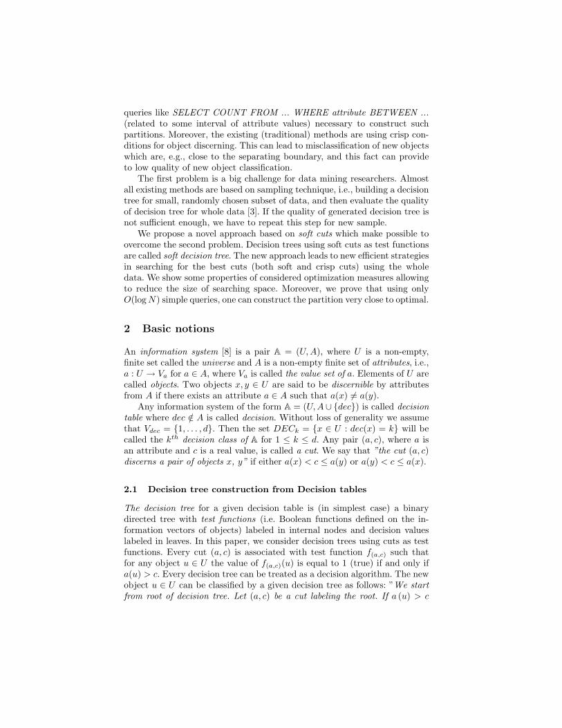
The decision tree for a given decision table is (in simplest case) a binarydirected tree with test functions (i.e. Boolean functions defined on the in-formation vectors of objects) labeled in internal nodes and decision valueslabeled in leaves. In this paper, we consider decision trees using cuts as testfunctions. Every cut (a, c) is associated with test function f(a,c) such thatfor any object u ∈ U the value of f(a,c)(u) is equal to 1 (true) if and only ifa(u) > c. Every decision tree can be treated as a decision algorithm. The newobject u ∈ U can be classified by a given decision tree as follows: ”We startfrom root of decision tree. Let (a, c) be a cut labeling the root. If a (u) > c

we go to the right subtree and if a (u) ≤ c we go to the left subtree of thedecision tree. The process will be continued for any node until we reach anyexternal node.” The decision tree is called consistent with the decision table

µ´¶³(a, c)

¡¡

¡ª

@@@R

¢¢

¢¢ A

AA

A ¢¢

¢¢ A

AA

A

?

a(u) > ca(u) ≤ c

u

L R

Fig. 1. Decision tree approach.

A if it classifies properly all objects from A. The decision tree is called op-timal with A if it has a smallest height among decision tree consistent withA. The cut c on attribute a is called optimal cut if (a, c) labels one of inter-nal nodes of optimal decision trees. Developing some decision tree inductionmethods [2,10] we should often solve the following problem: ”For a given setof candidate cuts {c1, ..., cN} on an attribute a, find a cut ci belonging to theset of optimal cuts with highest probability”. Usually, we use some measure(or quality functions) F : {c1, ..., cN} → R to estimate the quality of cuts.For a given measure F , the straightforward algorithm should compute thevalues of F for all cuts: F (c1), .., F (cN ). The cut cBest which optimizes thevalue of function F is selected as the result of searching process. The typicalalgorithm for decision tree induction can be described as follows:

1. For a given set of objects U , select a cut (a, cBest) of high quality amongall possible cuts and all attributes;

2. Induce a partition U1, U2 of U by (a, cBest) ;3. Recursively apply Step 1 to both sets U1, U2 of objects until some stop-

ping condition is satisfied.

We consider the set of all relevant cuts Ca = {c1, ..., cN} on an attribute a.

Definition 1. The d-tuple of integers 〈x1, ..,xd〉 is called class distributionof the set of objects X ⊂ U iff xk = card(X ∩DECk) for k ∈ {1, ..., d}. If theset of objects X is defined by X = {u ∈ U : p ≤ a(u) < q} for some p, q ∈ Rthen the class distribution of X is called the class distribution in [p; q).

In next sections we recall the most frequently used measures for decision treeinduction like ”Entropy Measure” and ”Discernibitity Measure”, respectively.

Entropy measure uses class-entropy as a criterion to evaluate the list ofbest cuts which together with the attribute domain induce the desired in-tervals. The class information entropy of the set of N objects X with classdistribution 〈N1, ..., Nd〉, where N1 + ... + Nd = N , is defined by Ent(X) =−∑d

j=1Nj

N log Nj

N . Hence, the entropy of the partition induced by a cut pointc on attribute a is defined by

E (a, c;U) =|UL|n

Ent (UL) +|UR|n

Ent (UR)

where {UL, UR} is a partition of U defined by c. For a given feature a, the cutcmin which minimizes the entropy function over all possible cuts is selected seeFigure 2. The methods based on information entropy are reported in [2,10].

��

��

��

��

��

��

��

��

��

��

��

��

��

��

��

��

��

��

� � ��

��

��

��

��

��

��

��

��

��

��

��

��

� ��

�

� ��

��

� � ��

��

� � ��

��

� � ��

� ��

��

� ��

� ��

��

� ��

��

��

��

��

��

� �

��

��

��

��

��

��

� ��

Fig. 2. The illustration of Entropy measure (left) discernibility measure(right) forthe same data set. On horizontal axes: ID of consequent cuts; on vertical axes:values of corresponding measures

Discernibility measure is based on Rough Set and Boolean reasoningapproach. Intuitively, energy of the set of objects X ⊂ U can be defined bythe number of pairs of objects from X to be discerned called conflict(X). Let〈N1, ..., Nd〉 be a class distribution of X, then conflict(X) can be computedby conflict(X) =

∑i<j NiNj . The cut c which divides the set of objects U

into U1, and U2 is evaluated by

W (c) = conflict(U)− conflict(U1)− conflict(U2)

i.e. the more is number of pairs of objects discerned by the cut (a, c), thelarger is chance that c can be chosen to the optimal set of cut. This algorithmis called Maximal-Discernibility heuristics or the MD-heuristics for decisiontree construction. Figures 2 illustrate the values of Entropy and Discernibilityfunctions over set of possible cuts on one of attributes of SatImage data. Onecan see that the cuts preferred by both measures are quite similar. The highaccuracy of decision trees constructed by using discernibility measure andtheir comparison with Entropy-based methods has been reported in [4].

2.2 Soft cuts

We have presented so far decision tree methods working with cuts treated assharp classifiers such, that real values are partitioned by them into disjointintervals. One can observe that in some situations objects which are closeone to other, can be treated as very different. In this section we introducesome notions of soft cuts which discern two given values if those values arefar enough from the cut. The formal definition of soft cuts is following:

Definition 2. A soft cut is any triple p = 〈a, l, r〉, where a ∈ A is an at-tribute, l, r ∈ < are called the left and right bounds of p (l ≤ r); the valueε = r−l

2 is called the uncertain radius of p. We say that a soft cut p discernspair of objects x1, x2 if a (x1) < l and a (x2) > r.

The intuitive meaning of p = 〈a, l, r〉 is such that there is a real cutsomewhere between l and r. So we are not sure where one can place the realcut in the interval [l, r]. Hence for any value v ∈ [l, r] we are not able to checkif v is either on the left side or on the right side of the real cut. Then we saythat the interval [l, r] is an uncertain interval of the soft cut p. Any normalcut can be treated as soft cut of radius equal to 0.

Any set of soft cuts splits the real axis into intervals of two categories: theintervals corresponding to new nominal values and the intervals of uncertainvalues called boundary regions. The problem of searching for minimal set ofsoft cuts with a given uncertain radius can be solved in a similar way to thecase of sharp cuts. We propose some heuristic for this problem in the lastsection of the paper. The problem becomes more complicated if we want toobtain as small as possible set of soft cuts with the radius as large as possible.We will discuss this problem in the next paper.

2.3 Soft Decision Tree

The test functions defined by cuts can be Here we propose two strategiesbeing modifications of that method by using described above soft cuts (fuzzyseparated cuts). They are called fuzzy decision tree and rough decision tree.

In fuzzy decision tree method instead of checking the condition a (u) > cwe have to check how strong is hypothesis that u is on the left or right side ofthe cut (a, c). This condition can be expressed by µL (u) and µR (u), whereµL and µR are membership function of left and right intervals (respectively).The values of those membership functions can be treated as a probabilitydistribution of u in the node labeled by soft cut (a, c − ε, c + ε). Then onecan compute the probability of the event that object u is reaching a leaf. Thedecision for u is equal to decision labeling the leaf with largest probability.

In the case of rough decision tree, when we are not able to decide toturn left or right (the value a(u) is too close to c) we do not distribute theprobability to children of considered node. We have to compare their answerstaking into account the numbers of supported by them objects. The answerwith most number of supported objects is a decision of given object.

3 Searching for best cuts in large data tables

In this section we present the efficient approach to searching for optimal cutsin large data tables. There are modifications of our MD-heuristic describedin previous sections. We describe some techniques which have been presentedin previous papers (see [5]).

3.1 Tail cuts can be eliminated

In [5] we have shown the following techniques for irrelevant cut eliminating.For given set of candidate cuts Ca = {c1, .., cN} on a such that c1 < c2... <cN , by median of the kth decision class we mean the cut c ∈ Ca which mini-mizes the value |Lk−Rk|. The median of the kth decision class will be denotedby Median(k). Let cmin = mini{Median(i)} and cmax = maxi{Median(i)}.We have shown in [5] the following theorem.

Theorem 1 The quality function W : {c1,..,cN} → N defined over the setof cuts is increasing in {c1, ..., cmin} and decreasing in {cmax, ..., cN}. HencecBest ∈ {cmin, ..., cmax}

This property is interesting because one can use only O(d log N) queries todetermine the medians of decision classes by using Binary Search Algorithm.Hence the tail cuts can be eliminated by using using O(d log N) SQL queries.Let us also observe that if all decision classes have similar medians thenalmost all cuts can be eliminated.

3.2 Divide and Conquer Strategy

The main idea is to apply the ”divide and conquer” strategy to determine thebest cut cBest ∈ {c1, ..., cn} with respect to a given quality function. Firstwe divide the set of possible cuts into k intervals (e.g. k = 2, 3, ..). Thenwe choose the interval to which the best cut may belong with the highestprobability. We will use some approximating measures to predict the intervalwhich probably contains the best cut with respect to discernibility measure.This process is repeated until the considered interval consists of one cut. Thenthe best cut can be chosen between all visited cuts.The problem arises how to define the measure evaluating the quality of the in-terval [cL; cR] having class distributions: 〈L1, ..., Ld〉 in (−∞; cL); 〈M1, ..., Md〉in [cL; cR); and 〈R1, ..., Rd〉 in [cR;∞). This measure should estimate thequality of the best cut among those belonging to the interval [cL; cR].

In previous papers (see [5,7]) we proposed the following measures to esti-mate the quality of the best cut in [cL; cR]

Eval ([cL; cR]) =W (cL) + W (cR) + conflict([cL; cR])

2+ ∆ (1)

where the value of ∆ is defined by:

∆ =[W (cR)−W (cL)]2

8 · conflict([cL; cR])(in the dependent model)

∆ = α ·√

D2(W (c)) for some α ∈ [0; 1]; (in the independent model)

The choice of ∆ and the value of parameter α from [0; 1] can be tuned inlearning process or are given by expert. One can see that to determine thevalue Eval ([cL; cR]) we need only O(d) simple SQL queries of the form:

SELECT COUNTFROM data_tableWHERE (a BETWEEN c_L AND c_R) GROUPED BY d.

3.3 Local and Global Search

We present two strategies of searching for the best cut using formula 1 calledlocal and global search. In local search algorithm, first we discover the bestcuts on every attribute separately. Then we compare them to find out theglobal best one. The details of local algorithm can be described as follows:

Algorithm 1: Searching for semi-optimal cutParameters: k ∈ N and α ∈ [0; 1].Input: attribute a; the set of candidate cuts Ca = {c1, .., cN} on a;Output: The optimal cut c ∈ Ca

beginLeft ← min; Right ← max; {see Theorem 1}while (Left < Right)1.Divide [Left; Right] into k intervals with equal length by (k+1) boundary

points i.e.

pi = Left + i ∗ Right− Left

k;

for i = 0, .., k.2.For i = 1, .., k compute Eval([cpi−1 ; cpi ], α) using Formula (1). Let

[pj−1; pj ] be the interval with maximal value of Eval(.);3.Left ← pj−1; Right ← pj ;

endwhile;Return the cut cLeft;

end

Hence the number of queries necessary for running our algorithm is of orderO(dk logk N). In practice we set k = 3 because the function f(k) = dk logk Nhas minimum over positive integers for k = 3. For k > 2, instead choosing the

best interval [pi−1; pi], one can select the best union [pi−m; pi] of m consecu-tive intervals in every step for a predefined parameter m < k. The modifiedalgorithm needs more – but still of order O(log N) – simple questions only.

The global strategy is searching for the best cut over all attributes. At thebeginning, the best cut can belong to every attribute, hence for each attributewe keep the interval in which the best cut can be found (see Theorem 1), i.e.we have a collection of all potential intervals

Interval Lists = {(a1, l1, r1), (a2, l2, r2), ..., (ak, lk, rk)}Next we iteratively run the following procedure

• remove the interval I = (a, cL, cR) having highest probability of contain-ing the best cut (using Formula 1);

• divide interval I into smaller ones I = I1 ∪ I2... ∪ Ik;• insert I1, I2, ..., Ik to Interval Lists.

This iterative step can be continued until we have one–element interval orthe time limit of searching algorithm is exhausted. This strategy can besimply implemented using priority queue to store the set of all intervals,where priority of intervals is defined by Formula 1.

3.4 Example

We consider a randomly generated data table consisting of 12000 records. Ob-jects are classified into 3 decision classes with the distribution 〈5000, 5600, 1400〉,respectively. One real value attribute has been selected and N = 500 cutson its domain has generated class distributions as shown in Figure 3. Themedians of three decision classes are c166, c414 and c189, respectively. The me-dian of every decision class has been determined by binary search algorithmusing log N = 9 simple queries. Applying Theorem 1 we conclude that it isenough to consider only cuts from {c166, ..., c414}. Thus 251 cuts have beeneliminated by using 27 simple queries only.

In Figure 3 we show the graph of W (ci) for i ∈ {166, ..., 414} and weillustrated the outcome of application of our algorithm to the reduce set ofcuts for k = 2 and ∆ = 0. First the cut c290 is chosen and it is necessaryto determine to which of the intervals [c166, c290] and [c290, c414] the bestcut belongs. The values of function Eval on these intervals is computed:Eval([c166, c290]) = 23927102, Eval([c290, c414]) = 24374685. Hence, the bestcut is predicted to belong to [c290, c414] and the search process is reduced tothe interval [c290, c414]. The above procedure is repeated recursively until theselected interval consists of single cut only. For our example, the best cut c296

has been successfully selected by our algorithm. In general the cut selectedby the algorithm is not necessarily the best. However, numerous experimentson different large data sets shown that the cut c∗ returned by the algorithmis close to the best cut cBest (i.e. W (c∗)

W (cBest)· 100% is about 99.9%).

Distribution for first class

0

1020

3040

50

0 50 100 150 200 250 300 350 400 450

Distribution for second class

0

1020

3040

5060

70

0 50 100 150 200 250 300 350 400 450

Distribution for third class

01020

0 50 100 150 200 250 300 350 400 450

Median(1)

Median(2)

Median(3)

19000000

20000000

21000000

22000000

23000000

24000000

25000000

26000000

166 197 228 259 290 321 352 383 414

Fig. 3. Distributions for decision classes 1, 2, 3 and graph of W (ci) for i ∈{166, .., 414}

3.5 Searching for soft cuts

One can modify the Algorithm 1 presented in the previous section to deter-mine ”soft cuts” in large data bases. The modification is based on changingthe stop condition. In every iteration of the Algorithm 1, the current interval[Left; Right] is divided equally into k smaller intervals and the best smallerinterval will be chosen as the current interval. In the modified algorithm onecan either select one of smaller intervals as the current interval or stop thealgorithm and return the current interval as a result.

Intuitively, the Divide and Conquer Algorithm is stopped and results theinterval [cL; cR] if the following conditions hold:

• The class distribution in [cL; cR] is too stable, i.e. there is no sub-intervalof [cL; cR] which is considerably better than [cL; cR] him self;

• The interval [cL; cR] is sufficiently small, i.e. it contains a small numberof cuts;

• The interval [cL; cR] does not contain too much objects; (because thelarge number of uncertain objects cans result in larger decision tree andthen prolongs the time of decision tree construction)

4 Conclusions

The problem of optimal binary partition of continuous attribute domain forlarge data sets stored in relational data bases has been investigated. We showthat one can reduce the number of simple queries from O(N) to O(log N)to construct the partition very close to the optimal one. We plan to extendthese results for other measures.

Acknowledgement: This paper has been partially supported by PolishState Committee of Research (KBN) grant No 8T11C02519 and grant of theWallenberg Foundation.

References

1. Dougherty J., Kohavi R., Sahami M.: Supervised and unsupervised discretiza-tion of continuous features. In. Proc. of the 12th International Conference onMachine Learning, Morgan Kaufmann, San Francisco, CA, 1995, pp. 194–202.

2. Fayyad, U. M., Irani, K.B.: On the handling of continuous-valued attributes indecision tree generation. Machine Learning 8, 1992, pp. 87–102.

3. John, G. H., Langley, P.: Static vs. dynamic sampling for data mining. Pro-ceedings of the Second International Conference of Knowledge Discovery andData Mining, Portland, AAAI Press 1996, pp. 367–370.

4. Nguyen, H. S.: Discretization Methods in Data Mining. In L. Polkowski, A.Skowron (Eds.): Rough Sets in Knowledge Discovery 1, Springer Physica-Verlag, Heidelberg, 1998, pp. 451–482.

5. Nguyen, H. S.: Efficient SQL-Querying Method for Data Mining in Large DataBases. Proc. of 16th International Joint Conference on Artificial Intelligence,IJCAI-99, Morgan Kaufmann Publishers, Stockholm, Sweden, 1999, pp. 806-811.

6. Nguyen, H. S.: On Efficient Construction of Decision tree from Large Databases.Proc. of the Second International Conference on Rough Sets and CurrentTrends in Computing (RSCTC’2000). Springer-Verlag, pp. 316-323.

7. Nguyen, H. S.: On Efficient Handling of Continuous Attributes in Large DataBases, Fundamenta Informatica 48(1), pp. 61-81

8. Pawlak Z.: Rough sets: Theoretical aspects of reasoning about data, KluwerDordrecht, 1991.

9. Polkowski, L., Skowron, A. (Eds.): Rough Sets in Knowledge Discovery Vol.1,2, Springer Physica-Verlag, Heidelberg, 1998.

10. Quinlan, J. R. C4.5. Programs for machine learning. Morgan Kaufmann, SanMateo CA, 1993.

11. Skowron, A., Rauszer, C.: The discernibility matrices and functions in informa-tion systems. In. R. SÃlowinski (ed.). Intelligent Decision Support – Handbookof Applications and Advances of the Rough Sets Theory, Kluwer AcademicPublishers, Dordrecht, 1992, pp. 311–362

A Soft Decision Tree

Documents

Transcript of A Soft Decision Tree