Medical Decision Support System for Diagnosis of Soft Tissue Tumors based on Distributed...
29
A. Subasi, Medical decision support system for diagnosis of neuromuscular disorders using DWT and fuzzy support vector machines, Computers in Biology and Medicine 42, 806–815, 2012. Medical Decision Support System for Diagnosis of Neuromuscular Disorders using DWT and Fuzzy Support Vector Machines Abdulhamit Subasi International Burch University, Faculty of Engineering and Information Technologies, 71000, Sarajevo, Bosnia and Herzegovina. E-mail: [email protected] Abstract The motor unit action potentials (MUAPs) in an electromyographic (EMG) signal provide a significant source of information for the assessment of neuromuscular disorders. In this work, different types of machine learning methods were used to classify EMG signals and compared in relation to their accuracy in classification of EMG signals. The models automatically classify the EMG signals into normal, neurogenic or myopathic. The best averaged performance over 10 runs of randomized cross-validation is also obtained by different classification models. Some conclusions concerning the impacts of features on the EMG signal classification were obtained through analysis of the classification techniques. The comparative analysis suggests that the fuzzy SVM modelling is superior to the other machine learning methods in at least three points: slightly higher recognition rate; insensitivity to overtraining; and consistent outputs demonstrating higher reliability. The combined model with DWT and Fuzzy-SVM achieves the better performance for internal cross validation (External cross validation) with the area under the ROC curve (AUC) and accuracy equal to 0.996 (0.993) and 97.41% (97%), respectively. These results show that the proposed model have the potential to obtain a reliable classification of EMG signals, and to assist the clinicians for making a correct diagnosis of neuromuscular disorders. Keywords:Electromyography (EMG); Motor unit action potentials (MUAPs); Discrete Wavelet Transform (DWT); Artificial Neural Network (ANN); Radial Basis Function Networks (RBFN); C4.5 Decision Tree; Linear Discriminant Analysis (LDA); Support Vector Machine (SVM); Fuzzy SVM. 1. Introduction The Electromyography (EMG) is generated by the electrical activity of the muscle fibers and it can be detected using intramuscular electrodes. Neuromuscular diseases are a group of disorders whose most important characteristic is that they cause muscular weakness and/or muscle tissue wasting. These disorders have an effect on the motor nuclei of the cranial nerves, the anterior horn cells of the spinal cord, the nerve
Transcript of Medical Decision Support System for Diagnosis of Soft Tissue Tumors based on Distributed...
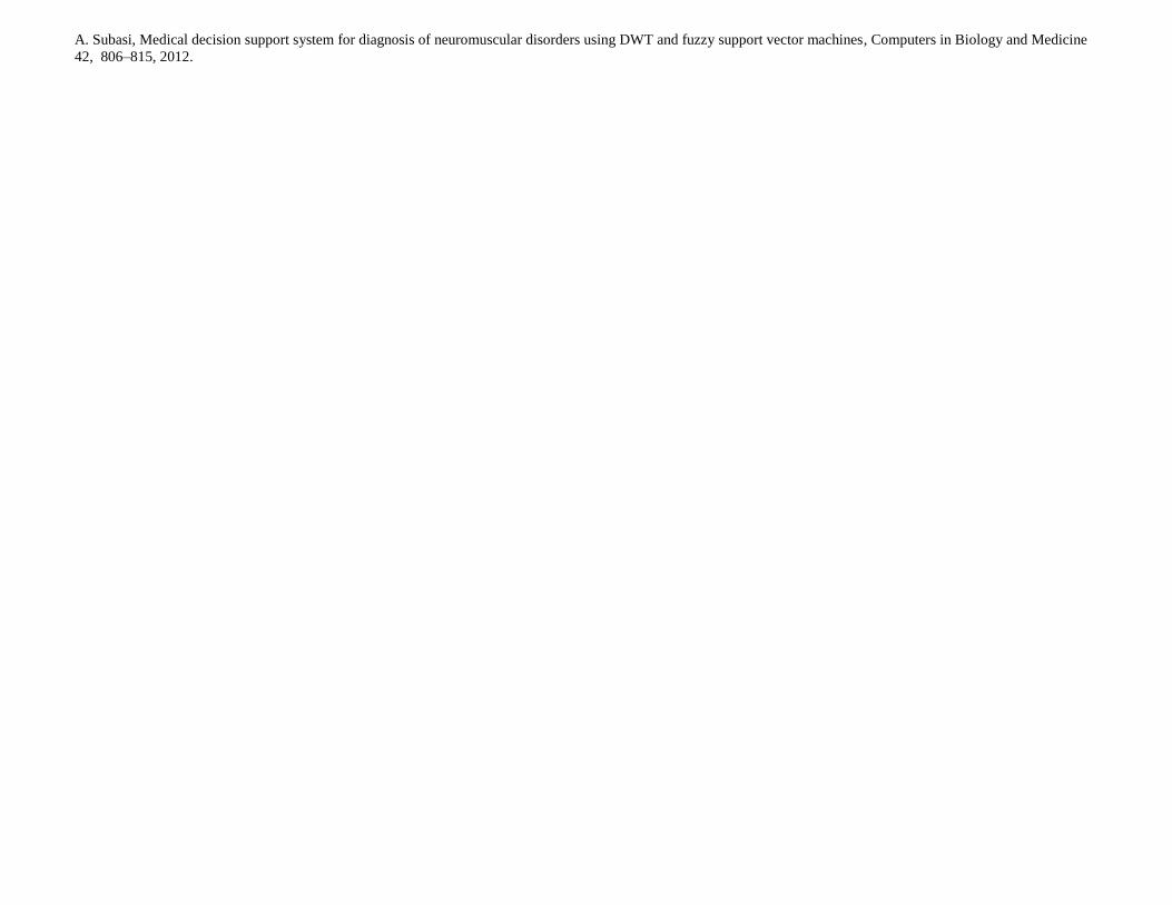
A. Subasi, Medical decision support system for diagnosis of neuromuscular disorders using DWT and fuzzy support vector
machines, Computers in Biology and Medicine 42, 806–815, 2012.
Medical Decision Support System for Diagnosis of Neuromuscular Disorders using DWT and
Fuzzy Support Vector Machines
Abdulhamit Subasi
International Burch University, Faculty of Engineering and Information Technologies, 71000, Sarajevo,
Bosnia and Herzegovina.
E-mail: [email protected]
Abstract
The motor unit action potentials (MUAPs) in an electromyographic (EMG) signal provide a significant
source of information for the assessment of neuromuscular disorders. In this work, different types of
machine learning methods were used to classify EMG signals and compared in relation to their accuracy in
classification of EMG signals. The models automatically classify the EMG signals into normal, neurogenic
or myopathic. The best averaged performance over 10 runs of randomized cross-validation is also obtained
by different classification models. Some conclusions concerning the impacts of features on the EMG signal
classification were obtained through analysis of the classification techniques. The comparative analysis
suggests that the fuzzy SVM modelling is superior to the other machine learning methods in at least three
points: slightly higher recognition rate; insensitivity to overtraining; and consistent outputs demonstrating
higher reliability. The combined model with DWT and Fuzzy-SVM achieves the better performance for
internal cross validation (External cross validation) with the area under the ROC curve (AUC) and accuracy
equal to 0.996 (0.993) and 97.41% (97%), respectively. These results show that the proposed model have
the potential to obtain a reliable classification of EMG signals, and to assist the clinicians for making a
correct diagnosis of neuromuscular disorders.
Keywords:Electromyography (EMG); Motor unit action potentials (MUAPs); Discrete Wavelet Transform
(DWT); Artificial Neural Network (ANN); Radial Basis Function Networks (RBFN); C4.5 Decision Tree;
Linear Discriminant Analysis (LDA); Support Vector Machine (SVM); Fuzzy SVM.
1. Introduction
The Electromyography (EMG) is generated by the electrical activity of the muscle fibers and it can
be detected using intramuscular electrodes. Neuromuscular diseases are a group of disorders whose most
important characteristic is that they cause muscular weakness and/or muscle tissue wasting. These disorders
have an effect on the motor nuclei of the cranial nerves, the anterior horn cells of the spinal cord, the nerve
A. Subasi, Medical decision support system for diagnosis of neuromuscular disorders using DWT and fuzzy support vector
machines, Computers in Biology and Medicine 42, 806–815, 2012.
roots and spinal nerves, the peripheral nerves, the neuromuscular junction, and the muscle itself. In
neurogenic disorders, some motor neurons degenerate, the surviving motor neurons grow new axonal
sprouts establishing synaptic contacts with the denervated muscle fibers. Needle electromyography is the
most suitable way for the detection of changes in motor unit size and its internal structure. Hence needle
EMG differentiate between other types of normal and abnormal spontaneous activity. From the point of
view of signal analysis, the electrical activity recorded by needle EMG may be pseudorandom and the
frequency content of the recorded signal depends on quite a lot of aspects. Since the electrical properties of
intramuscular tissues affect volume conduction, the higher frequencies within the signal will be attenuated
considerably more than the lower ones. The frequency content of the EMG signal has a physiological
significance, and frequency analysis has been used in different studies of neuromuscular disorders. In
needle EMG, a shift toward high frequencies is a characteristic feature in myopathies, while a shift toward
low frequencies is often well-known in neurogenic conditions [1].
Hence, the resulting information can be used to find out the origin of the diseases, i.e. neurogenic or
myopathic [2-4]. It is typical clinical practice to examine the MUAPs from visual inspection and from
listening to their audio characteristics. Nevertheless, subjective MUAP assessment, even if satisfactory for
the detection of obvious abnormalities, may not be sufficient to describe less apparent deviations or mixed
patterns of abnormalities [5]. Consequently, for an effective automated EMG signal classification, a
systematic treatment of EMG signals must be carried out. For this reason, a number of computer-based
quantitative EMG analysis algorithms have been developed. Pattichis and Pattichis [6] have investigated
the usefulness of the wavelet transform (WT), which provides a linear time-scale representation for
describing motor unit action potential (MUAP) morphology and three different neural networks, the
backpropagation (BP), the radial-basis function network (RBF), and the self-organizing feature map
(SOFM). Pattichis and Elia [7] used autoregressive and cepstral analyses combined with time domain
analysis in classification of EMG signals. Pattichis et al. [8] used MUAP parameters as input to a sequential
parametric pattern recognition classifier. Subasi et al. [9] investigated the practicality of using an
autoregressive model and wavelet neural network to extract classifiable features from EMG. Katsis et al.
used Support vector machines (SVM) [10], RBFN and DecisionTree (DT) [11] for MUAP classification.
Pino et al. [12] used Naive Bayesian (NB), DT, and pattern discovery (PD) classifiers for MUAP
classification and characterization. Yan et al. [13] used mutual information-based feature selection in
surface EMG and applied fuzzy LS-SVM in motion classification. Kamavuako et al. [14] tried to determine
the relationship between grasping force and features of single-channel intramuscular EMG signals.
Recently, Dobrowolski et al. [15] used MUAPs decomposition using wavelet and SVM for the
classification of neuromuscular disorders.
A. Subasi, Medical decision support system for diagnosis of neuromuscular disorders using DWT and fuzzy support vector
machines, Computers in Biology and Medicine 42, 806–815, 2012.
Nevertheless, in some of the studies done before, the EMG signals were acquired from surface
EMG and the classification is realized on the basis of different feature extraction methods. Actually, there
exist so many differences between intramuscular EMG (iEMG) signals and surface EMG (sEMG) signals
that it cannot be guaranteed that the effective algorithms used in sEMG scenario also work well in iEMG
scenario. Besides, the feature extraction methods are also very important in the classification of EMG
signals. In this paper, FSVM classifier combined with statistical features extracted from DWT are
compared different machine learning methods to classify EMG signals. To contribute to the quantification
of the routine needle EMG examination, a methodology has been developed for EMG signal classification
which consists of three steps. In the first step, the EMG signals are decomposed into different frequency
bands using discrete wavelet transform (DWT). In the second step, statistical features extracted from these
subband decomposed EMG signals to get better accuracy for diagnosis of neuromuscular disorder. In the
last step, an unknown EMG signal is classified as normal, myopathic or neurogenic using different machine
learning methods. Also we compared the performances of different machine learning techniques such as
LDA, ANN, RBFN, C4.5 decision tree, SVM and FSVM.
The remainder of the paper is organized as follows. In the next section, information is given about
the subjects and the methods applied in each step of the EMG signal classification process are presented.
Section 3 provides a complete experimental study of the different machine learning methods for diagnosis
of neuromuscular disorders, in which the impact of feature set and algorithmic issues are compared with
respect to classification performance. Section 4 gives some discussion on the results. Finally, the
conclusions are summarized in Section 5.
2. Materials and Methods
2.1. Subjects and Data Acquisition
An EMG system (Keypoint; Medtronic Functional Diagnostics, Skovlunde, Denmark) with standard
settings was used. The EMG signal was acquired from the biceps brachii muscle using a concentric needle
electrode (0.45 mm diameter with a recording surface area 0.07 mm2; impedance at 20 Hz below 200 kΩ).
The signal was band-pass filtered at 5 Hz to 10 kHz and sampled at 20 kHz for 5 s with 12-bit resolution.
All the measurements from patients and control group were done in Neurology Department of University of
Gaziantep. The electrode is usually advanced at least 3-5 mm into the muscle before recording. The
electrode is also moved at least 3-5 mm between recordings to make sure that different MUAP’s are
recorded. The electrode is advanced until the medial or posterior border of the muscle is reached. The
electrode is then pulled out to the fascial and inserted to a new radial direction.
A. Subasi, Medical decision support system for diagnosis of neuromuscular disorders using DWT and fuzzy support vector
machines, Computers in Biology and Medicine 42, 806–815, 2012.
The EMG signals were recorded from the biceps brachii muscle at force levels approximately 30%
of maximum voluntary contraction (MVC) under isometric conditions. Patient diagnoses were based on a
range of clinical information included a general examination and clinical history of the patient, and EMG
and nerve conduction tests. Muscle biopsies were not taken in the majority of cases, on ethical grounds, as
they are only considered in EMG clinic in cases where diagnosis is uncertain or for specific clinical reasons.
In this study, EMG data collected from 27 subjects have been analysed. Data were recorded from seven
healthy subjects (three males, four females) with ages ranging from 10 to 43 years (mean age±standard
deviation (S.D.): 30.2±10.8 years), seven myopathic subjects (four males, three females) with ages ranging
from 7 to 46 years (mean age±standard deviation (S.D.): 21.5±13.3 years) and thirteen neurogenic subjects
(eight males, five females) with ages ranging from 7 to 55 years (mean age±standard deviation (S.D.):
25.1±17.2 years) as in Subasi et al. [9].
2.2. Feature extraction using discrete wavelet transform
The wavelet transform (WT) allows the discrimination of non-stationary signals with different
frequency features [16]. The wavelet transform decomposes a signal into a set of basic functions called
wavelets. The wavelets are obtained from a single function ψ, the mother wavelet, by dilations and
translations as [17,18].
a
bt
atba
1, (1)
for positive a . Conventionally, a is 1 for the mother wavelet and increasing a > 1 dilates the wavelet,
expanding the interval over which it takes non-zero values. This model leads to the definition of the
equation for the continuous wavelet transform (CWT):
,1
)(),( dta
bt
atxbaW
(2)
where b operate to translate the function across x(t) just the same as t does in the equations above, and the
variable a acts to adjust the time scale of the probing function, ψ.
The discrete wavelet transform (DWT) is used to decompose a signal by using filters to extract
interesting frequency resolution components within the signal. The DWT possesses compact support in
both time and frequency domain [19-22]. The DWT is a signal-processing tool that finds many engineering
and scientific applications. DWT analyzes the signal at different frequency bands, with different resolutions
by decomposing the signal into a coarse approximation and detail information. DWT employs two sets of
functions called scaling functions and wavelet functions, which are related to low-pass and high-pass filters,
A. Subasi, Medical decision support system for diagnosis of neuromuscular disorders using DWT and fuzzy support vector
machines, Computers in Biology and Medicine 42, 806–815, 2012.
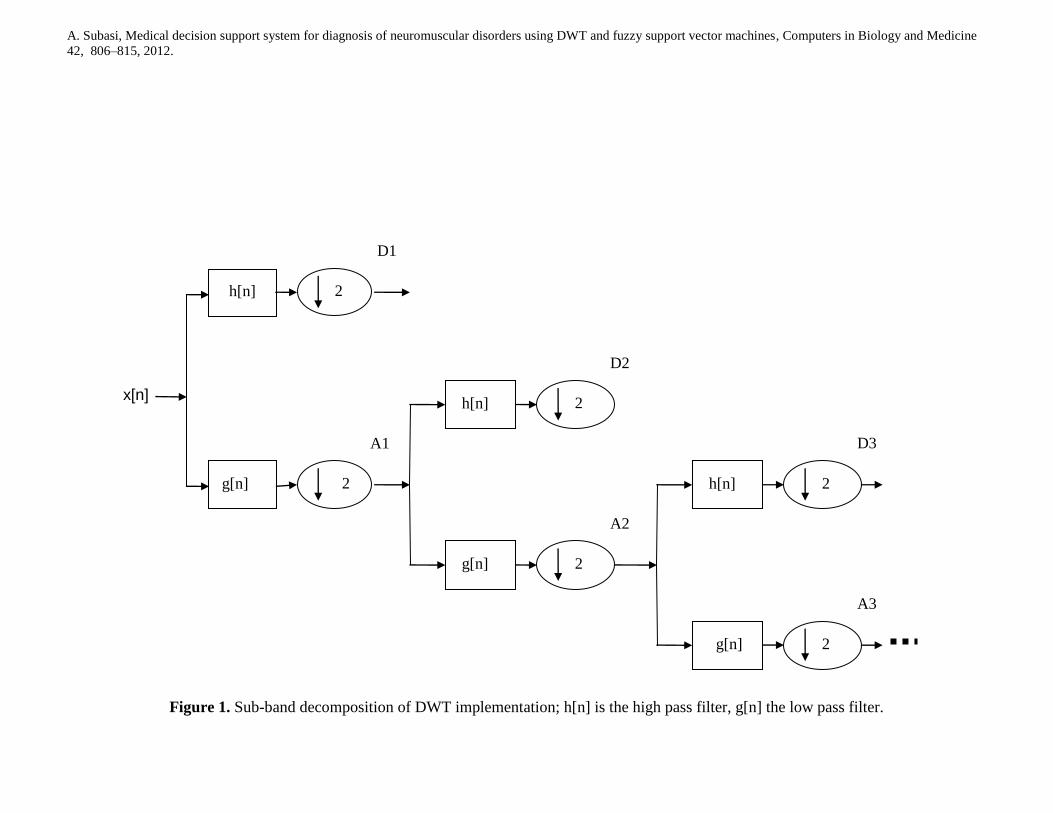
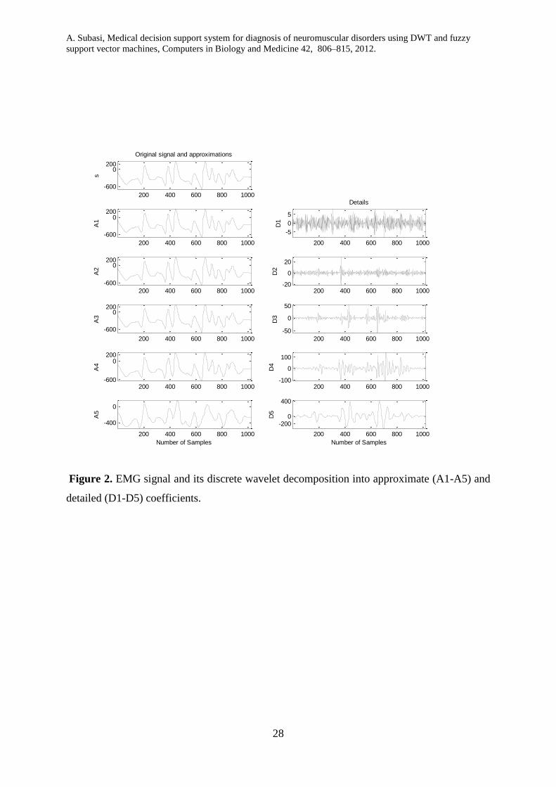
respectively. Each stage of this scheme consists of two digital filters and two down-samplers by 2. The
down-sampled outputs of first high-pass and low-pass filters provide the detail, D1 and the approximation,
A1, respectively. The first approximation, A1 is further decomposed and this process is continued as in Fig.
1. These approximation and detail records are reconstructed from the Daubechies 4 (DB4) wavelet filter.
Details are given in [19-26].
The extracted wavelet coefficients provide a compact representation that shows the energy
distribution of the EMG signal in time and frequency. In order to decrease the dimensionality of the
extracted feature vectors, statistics over the set of the wavelet coefficients were used [27]. The following
statistical features were utilized to represent the time-frequency distribution of the EMG signals:
(1) Mean of the absolute values of the coefficients in each sub-band.
(2) Average power of the wavelet coefficients in each sub-band.
(3) Standard deviation of the coefficients in each sub-band.
(4) Ratio of the absolute mean values of adjacent sub-bands.
Features 1 and 2 represent the frequency distribution of the signal and the features 3 and 4 the
amount of changes in frequency distribution. Total 15 feature are extracted, which are 4 different values for
features (1), (2) and (3); 3 values for feature (4). These feature vectors, calculated for the frequency bands
A5 and D3–D5 and were used as an input to classifiers.
2.3. Linear Discriminant Analysis (LDA)
Linear discriminant analysis (LDA) is a technique that produces discriminant functions that are
linear in the input variables. It is also used in a particular sense to refer to the technique in which a
transformation is required, which maximises between class separability and minimizes within class
variability.
There are different ways of generalising the criterion to the multiclass case. Optimisation of these
criteria yields transformations that reduce to Fisher’s linear discriminant in the two-class case and that
maximise the between-class scatter and minimise the within-class scatter [28]. Standard LDA classifier of
RapidMiner [29] machine learning tool is used in our study.
2.4. Artificial Neural Networks (ANN)
Artificial neural networks (ANNs) are appropriate for solving problems in biomedical engineering
and, particularly, in analyzing biomedical signals, because of their variety of applicability and their
capability to learn complex and nonlinear relations. ANNs are trained by example instead of rules. When
used in diagnosis of neuromuscular disorders, they are not affected by factors such as human fatigue,
A. Subasi, Medical decision support system for diagnosis of neuromuscular disorders using DWT and fuzzy support vector
machines, Computers in Biology and Medicine 42, 806–815, 2012.
emotional states, and habituation. They are capable of rapid identification, analysis of conditions, and
diagnosis in real time [30]. The most frequently used training algorithm in classification problems is the
backpropagation (BP) algorithm which is used in this work also. There are many different types and
architectures of neural networks varying fundamentally in the way they learn; the details of which are well
documented in the literature [31, 32]. MLP classifier of RapidMiner [29] machine learning tool was used
with a three-layer backpropagation neural network with 9 tansig neurons in the hidden layer and purelin
neuron in the output layer is used. The network training function is the traingdx. Besides, the learning rate
and momentum rate is set to 0.1 and 0.2. The accepted average squared error is 0.005 and the training
epochs are 1000. These parameters are obtained by trial and error.
2.5. Radial Basis Function Networks (RBFN)
Since RBFN has a simpler structure and a much faster training process, it is a popular alternative to
the MLP. The RBFN has network architecture similar to the classical regularization network [33]. Each
node in the hidden layer of RBFN uses an RBF as its nonlinear activation function. The hidden layer carries
out a nonlinear transform of the input, and hence the output layer is a linear combiner mapping the
nonlinearity into a new space. The biases of the output layer neurons can be modeled by an extra neuron in
the hidden layer. The learning of the RBFN necessitates the determination of the RBF centers and the
weights. The centers can be placed on a random subset of the training examples, or determined by
clustering or by means of a learning procedure. For classification problems, RBF units map input patterns
from a nonlinearly separable space to a linearly separable space, and the responses of the RBF units form
new feature vectors. Each RBF prototype is a cluster serving mainly a certain class. The RBFN is
insensitive to the order of the appearance of the adjusted signals, and consequently more appropriate for
online or succeeding adaptive adjustment [34]. Standard RBF classifier of RapidMiner [29] machine
learning tool was used in the experiments.
2.6. C4.5 Decision Tree (DT)
Any decision tree will increasingly divide the set of training examples into smaller and smaller
subsets. If all the samples in each subset had the same category label, we would say that each subset was
pure, and could terminate that part of the tree. However, there is a mixture of labels in each subset, and thus
for each branch we must make a decision either to stop dividing and accept an imperfect decision, or
instead choose a different property and grow the tree further [35].
The C4.5 algorithm has the prerequisite for pruning based on the rules derived from the learned tree.
Each leaf node has an associated rule which is the conjunction of the decisions leading from the root node,
A. Subasi, Medical decision support system for diagnosis of neuromuscular disorders using DWT and fuzzy support vector
machines, Computers in Biology and Medicine 42, 806–815, 2012.
through the tree, to that leaf. A technique called C4.5 Rules deletes redundant antecedents in such rules.
The information corresponding to nodes near the root can be pruned by C4.5Rules. This is more general
than impurity based pruning methods, which instead merge leaf nodes [35, 36]. Standard J48 classifier of
RapidMiner [29] machine learning tool was used in the experiments.
2.7. Support vector machines (SVM)
In this section, some basic work on Support vector machines (SVM) is shortly reviewed, for further
details refer to [36-38]. SVM are one of the recently developed classifiers in statistical learning theory [39].
SVM present a solution to the binary classification problem. The algorithm separates the two classes by a
hyperplane that maximizes the distance between the hyperplane and the nearest sample of each class. They
are focus of interest in biomedical applications, because of their accuracy. Most of the prior classifiers
separate classes using hyperplanes. But SVM widen the idea of hyperplane separation to data that cannot be
separated linearly, by mapping the predictors onto a new, higher-dimensional space in which they can be
separated linearly. It is achievable to separate the classes in any training set while running the risk of
finding trivial solutions that over-fit the data. As a result, the SVM algorithm includes methods that intend
to avoid this over-fitting. This is accomplished by using an iterative optimisation algorithm. Generally,
these misclassifications only arise if the wrong kernel function has been selected or there are cases in
different classes. The method’s name derives from the support vectors, which are lists of the predictor
values taken from cases that lie close to the decision boundary separating the classes. It is practical to
assume that these cases have the greatest impact on the location of the decision boundary. Computationally,
finding the best location for the decision plane is an optimisation problem to facilitate a kernel function to
create linear boundaries through non-linear transformations [37, 40, 41]. Since RBF kernel function gives
better accuracy, it was selected as a kernel function for the SVM classifier. For training the SVM classifier
with the RBF kernel function, the kernel parameter γ and the trade-off parameter C that could be chosen
based on training data. First the original algorithm of SVM was used to find the optimal γ value and the
trade-off parameter C. These parameters were sought in the two-dimension grid by C = (1, 2, 10, 50, 100,
1000) and a set of 100 equidistant values of γ between 10-2
and 102. A low number of support vectors were
used as the criterion for choosing C and γ. For too low values of C, a large number of support vectors were
obtained. Such a solution was less economical and required more computations for evaluating the decision
function. The chosen example values of C between 50 and 500 should provide good and economical
solutions. The minimal number of support vectors obtained was 42 corresponding to C = 300, γ = 0.2.
Therefore, the RBF kernel parameter γ of 0.2 and the trade-off parameter C of 300 were chosen for the
RBF kernel function in the SVM classifier.
A. Subasi, Medical decision support system for diagnosis of neuromuscular disorders using DWT and fuzzy support vector
machines, Computers in Biology and Medicine 42, 806–815, 2012.
2.8. Fuzzy Support Vector Machines (FSVM)
SVM is a powerfull machine learning method for solving classification problems [37], but there are
still some restrictions of this theory. From the training set and formulations, each training sample belongs
to either one class or the other. For each class, we can simply verify that all training samples of this class
are treated uniformly in the theory of SVM. In many real-world applications, the effects of the training
samples are different. Also some training samples are more imperative than others in the classification
problem. It would be required that the significant training samples must be classified correctly and would
not be cared about some training samples like noise whether they are misclassified or not. This means that,
each training sample no more exactly belongs to one of the two classes. It may possibly 90% belong to one
class and 10% be meaningless, and it may possibly 20% belong to one class and 80% be meaningless. In
other words, there is a fuzzy membership 0 < si ≤ 1 associated with each trainging sample xi. This fuzzy
membership can be regarded as the attitude of the related training sample toward one class in the
classification problem and the value (1 − si) can be regarded as the attitude of meaningless. Lin and Wang
[42] extend the concept of SVM with fuzzy membership and make it an FSVM. Even though in the
formulation of the problem the fuzzy membership is assumed to be given in advance, it is helpful to have
the parameters of membership being automatically setting up in the course of training [42, 43].
The major difference among SVM and FSVM is that the cost C of FSVM is multiplied by fuzzy
membership si. In FSVM model, the theory behind is to set a fuzzy membership to every input point and to
reformulate SVM in such a way that different input points can make different contributions to the learning
of the decision surface. Besides, FSVM is based on the maximization of the margin similar to the classical
SVM. On the other hand, it uses fuzzy membership function instead of fixed weights to prevent noisy data
points from getting narrower margins. The procedure becomes more complicated for the multi-class
classification problems since the outputs could be more than one class and must be divided into N mutually
exclusive classes. Actually, there are some ways to solve multi-class classification problems for SVM such
as one-against-one (OAO) classifiers and one-against-all (OAA) classifiers [44].
2.8.1. Generating the Fuzzy Memberships
In order to choose the proper fuzzy memberships in a given problem is straightforward. First, the
lower bound of fuzzy memberships must be defined, and then, the main property of data set needs to be
selected and made connection between this property and fuzzy memberships [42, 43]
Both in binary class and in multi-class classification problem, it is not easy to define the target value
of classification and the fuzzy membership function of training data during the implementation of the OAA
A. Subasi, Medical decision support system for diagnosis of neuromuscular disorders using DWT and fuzzy support vector
machines, Computers in Biology and Medicine 42, 806–815, 2012.
classifier in which a key issue is to the success of the classification system. Generally, for a k-class
classification problem, the OAA contains k decision functions when the OAA classifier is operated and the
jth decision function is trained to separate class j (labeled +1) examples from the rest examples (labeled -1).
To solve the multi-class EMG signal classification problem, OAA-FSVM classifier can be defined
as, an EMG signal belongs to class j if the element of column j is 1, while another signal does not belong to
class j if the element of column j is -1. We can assign higher weight to each positive example and lower
weight to each negative example. Consequently, the membership function ssij for each of the n EMG
signals in k classes’ problem can be defined as
1
1
ijij
ijij
ijvifss
vifssss (3)
where
,10
ijss ,10
ijss i=1,…,n, j=1,…,k (4)
For the experimental study, the symbol OAA-FSVM (
ijss ,
ijss ) can be defined as the fuzzy membership
function of OAA-FSVM classifier. The target values of proposed EMG signal classification system will be
transformed into multi-dimensional bipolar values. Besides, every training data point has its different
weights at each set of classification and the setting of fuzzy membership function is decided by its target
value [44].
For training the FSVM classifiers with the RBF kernel functions, the kernel parameter γ and the
trade-off parameter C could be determined based on training data. First the parameters were sought in the
two-dimension grid by C = (1, 2, 10, 50, 100, 1000) and a set of 100 equidistant values of γ between 10-3
and 103 as it is done in SVM. A low number of support vectors were used as the criterion for choosing C
and γ. For too low values of C, a large number of support vectors were taken. The selected example values
of C between 50 and 500 give effective solutions. The minimal number of support vectors obtained was 32
corresponding to C = 250, γ = 0.2. Therefore, the RBF kernel parameter γ of 0.2 and the trade-off
parameter C of 250 were chosen for the RBF kernel function in the FSVM classifiers. The value of the
tuning membership parameter r for the FSVM classifier using the RBF kernel function (C = 250, γ = 0.2)
was searched in the set of r = (1, 1/2, 1/4, 1/8, 1/16) based on training data [44]. The value of r associated
with the minimal number of support vectors was selected. The minimal number of support vectors obtained
was 32 corresponding to r=1.
3. Experimental Results
A. Subasi, Medical decision support system for diagnosis of neuromuscular disorders using DWT and fuzzy support vector
machines, Computers in Biology and Medicine 42, 806–815, 2012.
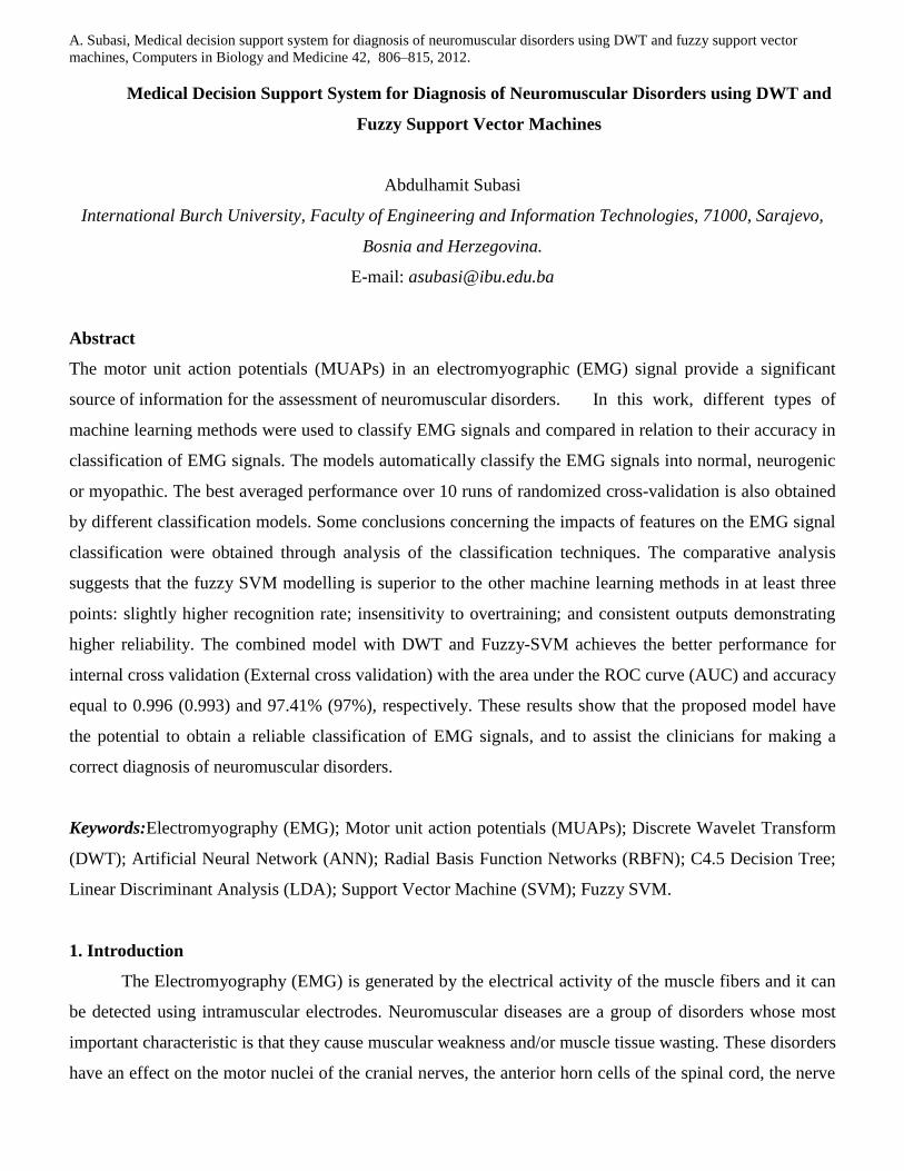
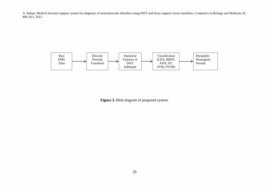
To contribute to the quantification of the routine needle EMG examination, a methodology has been
developed for EMG signal classification which consists of three steps. In the first step, the EMG signals are
decomposed into different frequency bands using discrete wavelet transform (DWT) as shown in Figure 2.
In the second step, statistical features extracted from these subband decomposed EMG signals to get better
accuracy for diagnosis of neuromuscular disorder. In the last step, an unknown EMG signal is classified as
normal [0 0 1], myopathic [0 1 0] or neurogenic [1 0 0] by different classification methods namely Linear
discriminant analysis (LDA), radial basis function networks (RBFN), multilayer perceptron artificial neural
networks (MLPANN), C4.5 decision tree (C4.5 DT), Support Vector Machines (SVM) and Fuzzy SVM
(Fig.3.). Out of these classifiers, FSVM combined with statistical features extracted from DWT gave the
best performance result for EMG signal classification. Besides, this technique tries to extract the most
valuable characteristic input features by minimizing redundancy and exclude noise from the EMG signal.
The problem of predicting performance based on limited data is an interesting, and controversial.
Different techniques encountered, of which one—cross-validation—is gaining ascendance and is possibly
the assessment technique of choice in most practical limited-data situations. Comparing the performance of
different machine learning techniques on a particular problem is another matter that is not as easy as it
sounds. In most practical classification techniques the cost of a misclassification error depends on the
nature of error it is—whether, for instance, a positive example was erroneously classified as negative or
vice versa. While doing classification, and evaluating its performance, it is often crucial to take these costs
into account. For classification problems, it is natural to measure a classifier’s performance in terms of the
error rate [45].
In order to calculate the performance of a classifier on independent dataset called the test set, its
error rate on a dataset that played no part in the creation of the classifier need to be assessed. In some
circumstances, three different datasets can be mentioned: the training data, the validation data, and the test
data. The training data is used to train the classifier. The validation data is used to adjust parameters of the
classifier. Then the test data is used to calculate the error rate of the final method. All of the three sets need
to be chosen individually: the validation set must be different from the training set to achieve better
performance in the selection stage, and the test set must be different from both to get a reliable estimate of
the true error rate. If lots of data exists, a large sample can be used for training; then another, independent
large sample of different data can be used for testing. As long as both samples are representative, the error
rate on the test set will give a true indication of future performance. And the larger the test sample, the
more precise the error estimate. The accuracy of the error estimate can be computed statistically [45].
If the amount of data for training and testing is limited, it is common to hold out one-third of the
data for testing and use the remaining two-thirds for training. In this case, if the sample used for training (or
A. Subasi, Medical decision support system for diagnosis of neuromuscular disorders using DWT and fuzzy support vector
machines, Computers in Biology and Medicine 42, 806–815, 2012.
testing) is not representative, it should be ensured that the random sampling is done in such a way as to
guarantee that each class is appropriately represented in both training and test sets. This technique is called
stratification, and it provides only a primitive precaution against uneven representation in training and test
sets. A more general approach to mitigate any bias caused by the individual sample chosen for holdout is to
repeat the whole process, training and testing, several times with different random samples. In each step, a
certain amount of the data is randomly selected for training, possibly with stratification, and the remainder
used for testing. The error rates on the different iterations are averaged to yield an overall error rate. This is
the repeated holdout method of error rate estimation. In a single holdout process, one might consider
swapping the roles of the testing and training data—that is, train the system on the test data and test it on
the training data—and average the two results, consequently reducing the effect of uneven representation in
training and test sets. On the other hand, a simple alternative forms the basis of an important statistical
technique called cross-validation. In cross-validation, the data is split into k approximately equal partitions
and each in turn is used for testing and the remainder is used for training. This is called k-fold cross-
validation, and if stratification is adopted as well and it is called stratified k-fold cross-validation [45].
Since the usual approach for calculating the error rate of a classification technique given a single,
fixed sample of data was to use stratified 10-fold cross-validation, the EMG data has been divided
randomly into 10 parts in which the class has been represented in approximately the same amounts as in the
full dataset. Tests have also shown that the use of stratification improves results slightly. Therefore the
typical assessment technique in situations where only limited data is available is stratified 10-fold cross-
validation. Note that neither the stratification nor the division into 10 folds has to be exact, because
statistical evaluation is not an exact science. Moreover, stratification reduces the variation, but it certainly
does not eliminate it entirely [45].
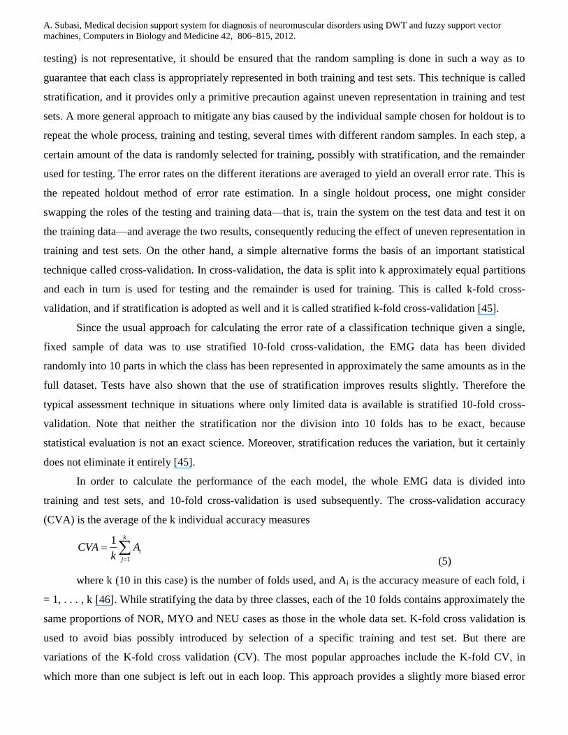
In order to calculate the performance of the each model, the whole EMG data is divided into
training and test sets, and 10-fold cross-validation is used subsequently. The cross-validation accuracy
(CVA) is the average of the k individual accuracy measures
k
j
iAk
CVA1
1
(5)
where k (10 in this case) is the number of folds used, and Ai is the accuracy measure of each fold, i
= 1, . . . , k [46]. While stratifying the data by three classes, each of the 10 folds contains approximately the
same proportions of NOR, MYO and NEU cases as those in the whole data set. K-fold cross validation is
used to avoid bias possibly introduced by selection of a specific training and test set. But there are
variations of the K-fold cross validation (CV). The most popular approaches include the K-fold CV, in
which more than one subject is left out in each loop. This approach provides a slightly more biased error
A. Subasi, Medical decision support system for diagnosis of neuromuscular disorders using DWT and fuzzy support vector
machines, Computers in Biology and Medicine 42, 806–815, 2012.
estimate, but with reduced variability, mainly due to more subjects being left-out [47]. If the results
obtained are used only to report prediction error estimates, the CV is called External (ECV), and the second
sample is a true test set. If the error obtained from the second sample is used to choose the best of the
derived models, then the CV is called Internal (ICV), since it is part of model development, and the second
sample is a second training set. Therefore, ICV can lead to erroneous conclusions if one refers to its results
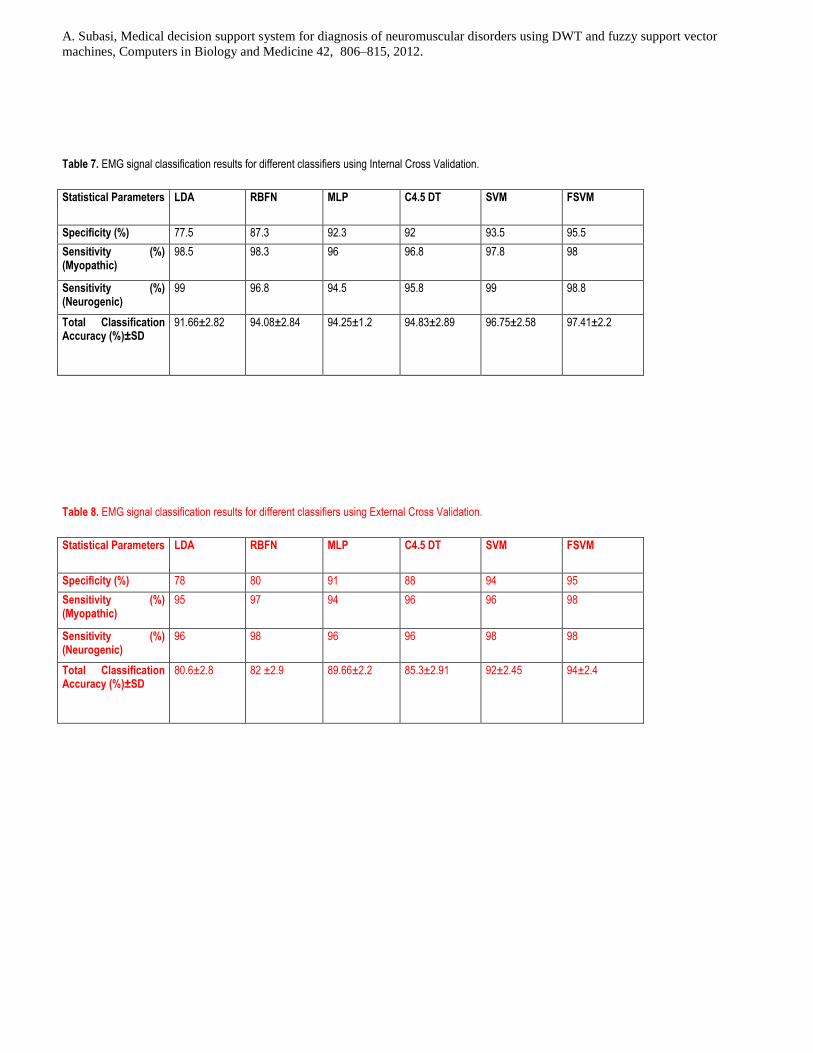
as error estimates. On the other hand, ECV gives an unbiased error estimate of a model [47, 48]. The results
for ECV and ICV are shown in table 7 and 8.
Receiver operating characteristic (ROC) curve is a graphical technique for evaluating classification
performance and represent the performance of a classifier without regard to class distribution or error costs.
They plot the number of positives enclosed in the sample on the vertical axis, expressed as a percentage of
the total number of positives, versus the number of negatives involved in the sample, defined as a
percentage of the total number of negatives, on the horizontal axis. This is one approach of using cross-
validation to generate ROC curves. A simpler approach is to accumulate the predicted probabilities for all
the numerous test sets, along with the true class labels of the corresponding instances, and make a single
ranked list based on this data. This is the easier method to implement, because for each fold of a 10-fold
cross-validation, weight the instances for a selection of different cost ratios, train the scheme on each
weighted set, count the true positives and false positives in the test set, and plot the resulting point on the
ROC axes. The area under the curve (AUC) is used instead because, roughly speaking the larger the area
the better the model [45]. In this study, the second method was used in the calculation of AUC.
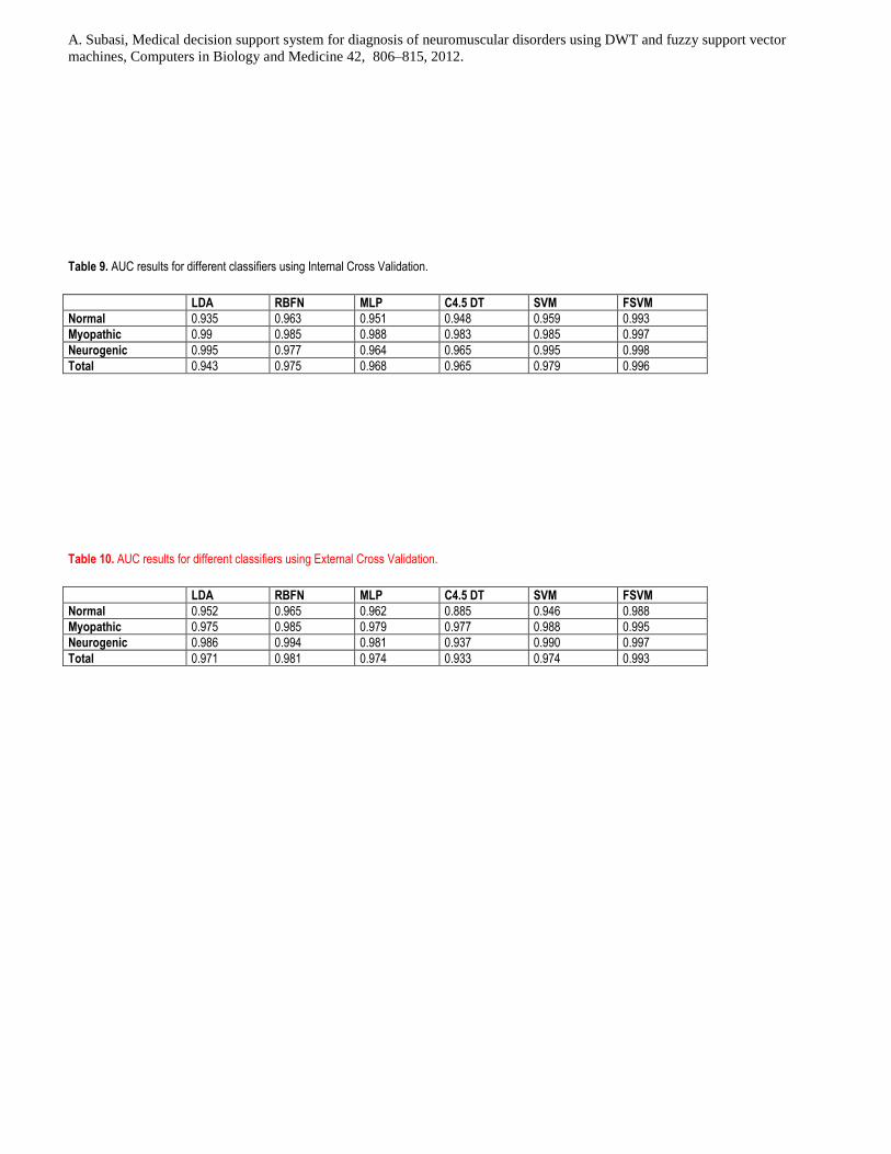
ROC analysis was used to evaluate the discrimination ability of the classifiers. The classification
performance was then measured by the mean area under the ROC curve (AUC). The mean AUC, as an
average performance, gives an indication of a typical AUC obtained using the given input data, and
indicates how reliably result is estimated [49-54]. The AUC is usually taken as the index of performance
because it gives a single measure of overall accuracy that is independent of any particular threshold [41,
51]. In spite of its advantages, the ROC plot does not give a rule for the classification of cases.
The test performances of the models were determined by the computation of the following statistical
parameters:
Specificity: number of correct classified healthy subjects/number of total healthy subjects.
Sensitivity (myopathy): number of correct classified subjects suffering from myopathy/number of
total subjects suffering from myopathy.
Sensitivity (neurogenic): number of correct classified subjects suffering from neurogenic
disorder/number of total subjects suffering from neurogenic disorder.
Total classification accuracy: number of correct classified subjects/number of total subjects.
A. Subasi, Medical decision support system for diagnosis of neuromuscular disorders using DWT and fuzzy support vector
machines, Computers in Biology and Medicine 42, 806–815, 2012.
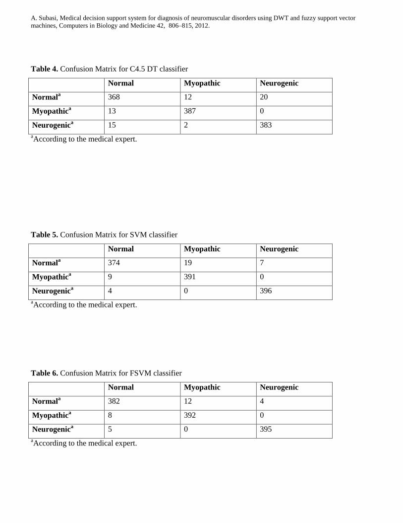
In general, all techniques accomplished a good performance with mean AUCs up to 0.996. A
slightly lower performance was observed when applying LDA as compared to other machine learning
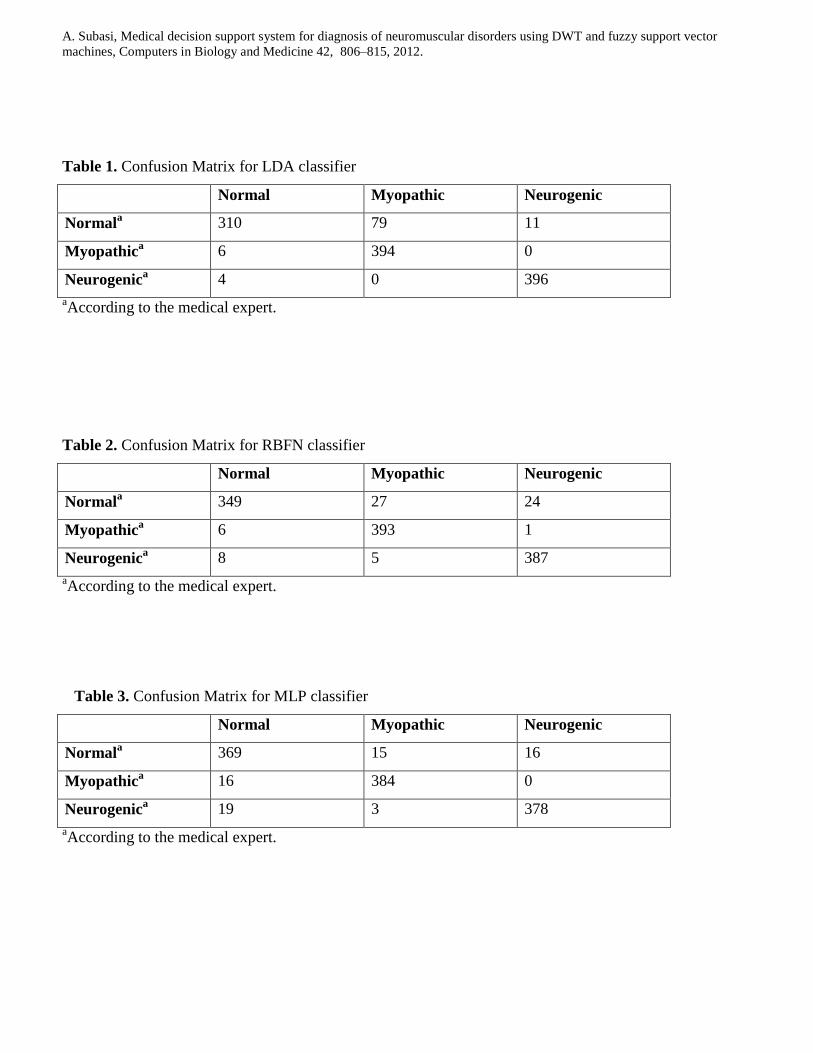
methods. Tables 1-6 show confusion matrices for each classifier and Tables 7-10 shows the ICV and ECV
performances of these classifiers using the statistical features of DWT subbands as input. The ICV and
ECV results do not show much more difference (1-2 %) in the FSVM, SVM and ANN. For ICV (ECV) test
the correct classification rate of 91.66% (89.6%) for LDA, 94.08% (93 %) for RBFN, 94.25% (93.66) for
MLPANN, 94.83% (93.3%) for C4.5 DT, 96.75% (96%) for SVM and 97.41% (97%) for FSVM have been
reached after the first step for all classification techniques. As it can be seen from tables, the specificity,
sensitivity values gave similar results. The EMG signal classification rate of RBFN was superior to the
classification rate of LDA in a normal group; but classification rate of LDA was superior to the
classification rate of RBFN for pathological cases. If EMG signal classification accuracy obtained using
RBFN, MLPNN and C4.5 DT are compared; they are almost equal classification accuracies. Although
classification accuracy of LDA is the worst, it has superior sensitivity (for both myopathic and neurogenic
pathological cases) compared to the other classification techniques. FSVM has the best classification
performance if compared to the other classification techniques.
Accurate identification of EMG signal is important for both diagnosis and treatment evaluation. The
FSVM classifier identified the groups with an overall accuracy of 95.4% (ROC area=0.965). Classification
accuracy improved significantly when statistical features of DWT subbands were used, providing 97.41%
accuracy. This effect also resulted in an improvement of ROC area (AUC=0.996) and the accuracy of
FSVM was higher than with an LDA, RBFN, C4.5 DT, MLPNN and SVM based classifier. The enhanced
classification accuracy of the FSVM using statistical features of DWT subbands as basic EMG signal
parameters makes it an attractive alternative for diagnosing of neuromuscular disorders and evaluating the
effectiveness of treatment.
4. Discussion
Similar studies of LDA, C4.5. DT, MLPNN and SVM as an EMG signal classifier can be found in
different studies [10-15]. If we compare the results taken from this study with the previous results [6-15],
the results taken from this study is 3% better than the previous results. Because statistical features extracted
from DWT subbands of EMG signals eliminates the noise in the data, extracts the best features for EMG
data and provides unbiased estimator. Hence the procedure represented in this study contributes better
results than the previous studies. When differentiating EMG signals, performance can be expressed using
cross-validation accuracy rates and ROC area. Classification performance has been found to be
significantly enhanced when statistical features of DWT subbands and FSVM method are used to train and
A. Subasi, Medical decision support system for diagnosis of neuromuscular disorders using DWT and fuzzy support vector
machines, Computers in Biology and Medicine 42, 806–815, 2012.
test the classifiers. Feature selection and classification method appears, therefore, to be important when
dealing with EMG signal classification; this can also reduce the dimensionality of input data with less
computational complexity.
The main advantage of the SVM approach is that this flexibility is largely controlled by the
algorithm itself on the training data. For the RBF kernel, two parameters have to be selected beforehand:
the trade-off parameter C and the kernel parameter γ. They can be optimised for an optimal generalisation
performance in the traditional way by using an independent test set or k-fold cross-validation [54]. On the
other hand, the generalisation behaviour can be estimated directly and thus the parameters can be chosen
solely based on the training data. In order to test these last two criteria to parameter selection, they were
applied on a single realisation of a small training set and subsequently evaluated on a large validation set of
samples. It can be seen that the parameter C produces the maximal amplitude of any Gaussian basis
function in the decision function. For a chosen width parameter γ, C therefore controls the maximal
distance at which a support vector can contribute significantly to the decision function. Hence, for too low
values of C, a large number of support vectors were obtained. Such a solution is less economical and needs
more computations for evaluating the decision function, as it corresponds to an RBF-network with a larger
number of nodes. Therefore, a low number of support vectors can be used as criterion for choosing C.
Examining the number of support vectors as function of C and γ within a reasonable range shows that
starting from a sufficiently high value of C the number of support vectors does not decrease anymore.
Empirically, it is found that even for lower values of C a good generalisation ability is achieved, provided
that the width γ is readjusted appropriately. For different settings of γ, different final values for the margin
on the generalisation error are obtained. This can be used for choosing γ for a given value of C [55-57].
Concerning the estimation of the prediction error by 10-fold cross-validation, it can be seen that 10-
fold CV error has little bias for EMG data set. It would be of significance to consider this for the current
problem, where there is also feature-selection bias to be corrected for. As to be expected for training
samples of twice or near twice the size, the (estimated) bias was smaller: between 1 and 3% for the EMG
data set. The estimated prediction rate according to 10-fold CV error remains essentially constant as
statistical features are deleted in the classifier. Hence feature selection provides essentially little
improvement in the performance of the classifier for the EMG data set; also it confirms that the number of
features does not affect the prediction error which is almost zero. The 10-fold CV error, which has the
selection bias removed, is approximately equal to 1% for 15 features. Although the feature vectors have
been generated independently of the class labels, a classifier can be formed that has not only an average
zero error but also an average CV error close to zero. Also it is important to note that if a test set is used to
estimate the prediction error, then there will be a selection bias if this test set was used also in the feature
A. Subasi, Medical decision support system for diagnosis of neuromuscular disorders using DWT and fuzzy support vector
machines, Computers in Biology and Medicine 42, 806–815, 2012.
selection process. Thus the test set must play no role in the feature selection process for an unbiased
estimate to be obtained. Concerning the former approach, an internal cross-validation (ICV) is not
sufficient. Hence, an external cross-validation (ECV) must be done whereby at each stage of the validation
process with the deletion of a subset of the observations for testing, the classifier must be trained on the
retained subset of observations by performing the same feature selection procedure used to train the rule in
the first instance on the full training set [47]. Hence besides ICV, ECV is used to get sufficient results (see
tables 8-10).
Based on the results of the present work and familiarity in EMG signal classification problems, the
followings can be emphasized:
i. The high classification accuracy of the FSVM classifier gives insights into the features used for defining
the EMG signals. The conclusion drawn in the applications demonstrated that the DWT coefficients are
the features, which well represent the EMG signals, and by the usage of these features a good distinction
between classes can be obtained.
i. LDA, RBFN, MLPANN, C4.5 DT, SVM based classifiers are appropriate for use in diognosis of
neuromuscular disorders; but, FSVM has an advantage over other classification methods based on its
higher classification accuracy.
ii. The high sensitivity of the LDA method confirms that LDA is an acceptable classification method. On
the other hand, LDA does not have good classification accuracy and cannot easily handle nominal data
types.
iii. C4.5 DT classifier uses an error reduction based training algorithm and as a result provide rules that are
used to reduce classification error. This can results to large trees and over-fitting problems. C4.5 DT
method cannot find relationships among multiple features.
iv. SVM is based on preprocessing the data to represent patterns in a high dimension — typically much
higher than the original feature space. With an appropriate nonlinear mapping to a sufficiently high
dimension, data from different categories can always be separated by a hyperplane. As a result, while the
original features bring sufficient information for good classification, mapping to a higher dimensional
feature space make available better discriminatory evidence that are absent in the original feature space.
The problem of training an SVM is to select the nonlinear functions that map the input to a higher
dimensional space. Often this choice will be informed by the designer’s knowledge of the problem
domain. Polynomials, Gaussians or other basis functions might be used in the absense of such
information. The dimensionality of the mapped space can be arbitrarily high. For training the SVM,
appropriate kernel parameters C, and were selected by using trail and error method. The optimal C, and
values can only be ascertained after trying out diffrent values. In addition, the choice of parameter in
A. Subasi, Medical decision support system for diagnosis of neuromuscular disorders using DWT and fuzzy support vector
machines, Computers in Biology and Medicine 42, 806–815, 2012.
the SVM is crucial in order to have a suitably trained SVM. The SVM has to be trained for different
kernel parameters until to get the best result.
v. Although accuracy across the five methods did not differ significantly for the clinical data, FSVM had a
significant advantage in its ability to maximize the classification accuracy. The classification results and
the values of statistical parameters indicated that the FSVM had considerable success in the EMG signals
classification by comparing with other classification methods.
vi. The FSVM classifier is robust to dynamic noise by setting lower fuzzy membership for the data points
with the noises or outliers, whereas the SVM classifier is sensitive to the noise. Some data points with
outliers and noises could be support vectors in the SVM classifier.
vii. The proposed FSVM classifier has lower computation cost than the SVM classifier due to the fewer
support vectors, which is critical for online classification of EMG signals. The present study has shown
that the proposed FSVM classifier is very effective for diagnosis of neuromuscular disorders.
5. Conclusion
In this paper, we developed an efficient combination of classifier and features, which proved by the
different experiments is applicable for the classification of the EMG signals. This was accomplished using
LDA, RBFN, MLPNN, C4.5 DT, SVM and FSVM techniques with statistical features extracted from DWT
subbands. Because the experiments proved, the combination represented as the Fuzzy SVM and the
statistical features extracted from DWT subbands can achieve a better performance than others classifier
over the three EMG signal patterns: normal, myopathic and neurogenic. The experiment shows that the
feature set extracted from DWT has superior subject-independent, and intrinsic excellent separability in
contrast to those conventional known time and frequency domain features. Also as a classifier, the Fuzzy
SVM classifier demonstrated better generalization ability and more rapid execution speed than the other
classifier. Besides the proposed Fuzzy SVM classifier with statistical features extracted from DWT
subbands meets the requirements for normal, myopathic and neurogenic MUAP characterization and is
capable of classifying the EMG signals with a high degree of accuracy and repeatability, invariant of the
level of motor impairment. Furthermore the proposed Fuzzy SVM classifier shows promise as a clinically
useful method of providing numerical inputs to the next step of the interpretation phase of an EMG
examination. This demonstrates that the Fuzzy SVM classifier can be valuable for the capture and
expression of knowledge useful to a clinician. These results provide encouragement to develop and
evaluate a Fuzzy SVM method for quantifying the level of contribution of a neuromuscular disorder.
Acknowledgements
A. Subasi, Medical decision support system for diagnosis of neuromuscular disorders using DWT and fuzzy support vector
machines, Computers in Biology and Medicine 42, 806–815, 2012.
The author thanks to Dr. Mustafa Yilmaz at University of Gaziantep, Neurology Department for
providing the EMG data utilized in this research. This research has been supported by International Burch
University (IBU Project no: IBU2010-PRD001).
References
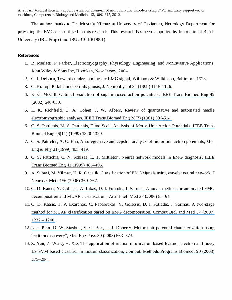
1. R. Merletti, P. Parker, Electromyography: Physiology, Engineering, and Noninvasive Applications,
John Wiley & Sons Inc, Hoboken, New Jersey, 2004.
2. C. J. DeLuca, Towards understanding the EMG signal, Williams & Wilkinson, Baltimore, 1978.
3. C. Krarup, Pitfalls in electrodiagnosis, J. Neurophysiol 81 (1999) 1115-1126.
4. K. C. McGill, Optimal resolution of superimposed action potentials, IEEE Trans Biomed Eng 49
(2002) 640-650.
5. E. K. Richfield, B. A. Cohen, J. W. Albers, Review of quantitative and automated needle
electromyographic analyses, IEEE Trans Biomed Eng 28(7) (1981) 506-514.
6. C. S. Pattichis, M. S. Pattichis, Time-Scale Analysis of Motor Unit Action Potentials, IEEE Trans
Biomed Eng 46(11) (1999) 1320-1329.
7. C. S. Pattichis, A. G. Elia, Autoregressive and cepstral analyses of motor unit action potentials, Med
Eng & Phy 21 (1999) 405–419.
8. C. S. Pattichis, C. N. Schizas, L. T. Mittleton, Neural network models in EMG diagnosis, IEEE
Trans Biomed Eng 42 (1995) 486–496.
9. A. Subasi, M. Yilmaz, H. R. Ozcalik, Classification of EMG signals using wavelet neural network, J
Neurosci Meth 156 (2006) 360–367.
10. C. D. Katsis, Y. Goletsis, A. Likas, D. I. Fotiadis, I. Sarmas, A novel method for automated EMG
decomposition and MUAP classification, Artif Intell Med 37 (2006) 55–64.
11. C. D. Katsis, T. P. Exarchos, C. Papaloukas, Y. Goletsis, D. I. Fotiadis, I. Sarmas, A two-stage
method for MUAP classification based on EMG decomposition, Comput Biol and Med 37 (2007)
1232 – 1240.
12. L. J. Pino, D. W. Stashuk, S. G. Boe, T. J. Doherty, Motor unit potential characterization using
―pattern discovery‖, Med Eng Phys 30 (2008) 563–573.
13. Z. Yan, Z. Wang, H. Xie, The application of mutual information-based feature selection and fuzzy
LS-SVM-based classifier in motion classification, Comput. Methods Programs Biomed. 90 (2008)
275–284.
A. Subasi, Medical decision support system for diagnosis of neuromuscular disorders using DWT and fuzzy support vector
machines, Computers in Biology and Medicine 42, 806–815, 2012.
14. E. N. Kamavuako, D. Farina, K. Yoshida, W. Jensen, Relationship between grasping force and
features of single-channel intramuscular EMG signals, Journal of Neuroscience Methods 185
(2009) 143–150
15. A. P. Dobrowolski, M. Wierzbowski, K. Tomczykiewicz, Multiresolution MUAPs decomposition
and SVM-based analysis in the classification of neuromuscular disorders, Comput. Methods
Programs Biomed. (2011), doi:10.1016/j.cmpb.2010.12.006
16. I. Daubechies, The wavelet transform, time–frequency localization and signal analysis, IEEE
Trans. Inform. Theory 36(5) (1990) 961–1005.
17. I. Daubechies, S. Mallat, A.S. Willsky, Introduction to the special issue on wavelet transforms and
multiresolution signal analysis, IEEE Trans. Inform. Theory 38 (1992) 529-532.
18. M. Vetterli, C. Herley, Wavelets and filter banks: theory and design, IEEE Trans. Signal Process.
40 (1992) 2207-2232.
19. S. Mallat, A Wavelet Tour of Signal Processing, Second Edition (Wavelet Analysis & Its
Applications), Academic Press, 1999.
20. B. P. Marchant, Time-Frequency Analysis for Biosystem Engineering, Biosystems Engineering
85(3) (2003) 261-281.
21. J. L. Semmlow, Biosignal and Biomedical Image Processing, MATLAB-Based Applications,
Marcel Dekker Inc, 270 Madison Avenue, New York, 2004.
22. L. Sornmo, P. Laguna, Bioelectrical Signal Processing in Cardiac and Neurological Applications,
Elsevier Academic Press, 2006.
23. H. Adeli, Z. Zhou, N. Dadmehr, Analysis of EEG records in an epileptic patient using wavelet
transform, Journal Neurosci Meth 123 (2003) 69–87.
24. M. Akay, Wavelet applications in medicine, IEEE Spectrum 34(5) (1997)50–56.
25. A. Subasi, Automatic recognition of alertness level from EEG by using neural network and wavelet
coefficients, Expert Systems with Applications 28 (2005) 701–711.
26. A. Subasi, EEG signal classification using wavelet feature extraction and a mixture of expert model,
Expert Systems with Applications 32 (2007) 1084–1093.
27. A. Kandaswamy, C. S. Kumar, R. P. Ramanathan, S. Jayaraman, N. Malmurugan, Neural
classification of lung sounds using wavelet coefficients, Comput Biol Med 34(6) (2004) 523-537.
28. A. R. Webb, Statistical Pattern Recognition, John Wiley & Sons Ltd, West Sussex 2002.
29. Rapid Miner machine learning tool, http://www.rapidminer.com/
30. E. Micheli-Tzanakou, Neural Networks in Biomedical Signal Processing, (2000), in: J. D. Bronzino
(Ed.), The Biomedical Engineering Handbook, CRC Press LLC, Boca Raton.
A. Subasi, Medical decision support system for diagnosis of neuromuscular disorders using DWT and fuzzy support vector
machines, Computers in Biology and Medicine 42, 806–815, 2012.
31. L. Fausett, Fundamentals of neural networks architectures, algorithms, and applications, Prentice
Hall, Englewood Cliffs, NJ, 1994.
32. S. Haykin, Neural networks: A comprehensive foundation, Macmillan, New York, 1994.
33. T. Poggio, F. Girosi, Networks for approximation and learning, Proc IEEE 78(9) (1990) 1481–1497.
34. K. L. Du, M. N. S. Swamy, Neural Networks in a Softcomputing Framework, Springer-Verlag
London Limited, 2006
35. R. O. Duda, P. E. Hart, D. Stork, Pattern lassification, 2nd Edition, John Wiley & Sons, 2002.
36. J. Quinlan, Improved use of continuous attributes in C4.5, J Artific Intelligence Research 4 (1996)
77–90.
37. V. Vapnik, Statistical learning theory, Wiley, New York , 1998.
38. C. J. C. Burges, A tutorial on support vector machines for pattern recognition, Data Mining &
Knowledge Discov 2(2) (1998) 121–167.
39. J. A. K. Suykens, J. De Brabanter, L. Lukas, J. Vandewalle, Weighted least squares support vector
machines: robustness and sparse approximation, Neurocomputing 48 (2002) 85–105.
40. S. Abe, Support Vector Machines for Pattern Classification, Springer London, 2005.
41. A. H. Fielding, Cluster and Classification Techniques for the Biosciences, Cambridge University
Press, The Edinburgh Building, Cambridge, UK, 2007.
42. C. F. Lin, S. D. Wang, Fuzzy Support Vector Machines, IEEE Transactions on Neural Networks
13(2) (2002) 464-471.
43. C. F. Lin, S. D. Wang, Fuzzy Support Vector Machines with Automatic Membership Setting,
(2005) ,in: L. Wang (Ed.), Support Vector Machines: Theory and Applications, Springer-Verlag,
Berlin Heidelberg, 2005, pp. 233–254.
44. T.-Y. Wang, H.-M. Chiang, Fuzzy support vector machine for multi-class text categorization,
Information Processing and Management 43 (2007) 914–929
45. I. H. Witten, E. Frank, Data Mining, Practical Machine Learning Tools and Techniques, Second
Edition, Morgan Kaufmann Publishers (Elsevier), San Francisco, CA, 2005.
46. R. Zhang, G. McAllister, B. Scotney, S. McClean, G. Houston, Combining Wavelet Analysis and
Bayesian Networks for the Classification of Auditory Brainstem Response, IEEE Trans Info Tech
Biomed 10(3) (2006) 458-467.
47. C. Ambroise, G. J. McLachlan, Selection bias in gene extraction on the basis of microarray gene-
expression data. Proc Natl Acad Sci USA 99(10) (2002) 6562-6566.
48. E. Karageorgiou, The Logic of Exploratory and Confirmatory Data Analysis, Cognitive Critique
(2011) 35-48.
A. Subasi, Medical decision support system for diagnosis of neuromuscular disorders using DWT and fuzzy support vector
machines, Computers in Biology and Medicine 42, 806–815, 2012.
49. J. A. Hanley, B. J. McNeil, The meaning and use of the area under a receiver operating
characteristic (ROC) curve, Radiology 143 (1982) 29–36.
50. N. A. Obuchowski, Receiver operating characteristic curves and their use in radiology, Radiology
229 (2003) 3–8.
51. J. A. Swets, ROC analysis applied to the evaluation of medical imaging techniques, Invest Radiol
14(2) (1979) 109–121.
52. A. Devos, L. Lukas, J. A. K. Suykens, L. Vanhamme, A. R. Tate, F. A. Howe, C. Majos, A.
Moreno-Torres, M. van der Graaf, S. Arus, S. Van Huffel, Classification of brain tumours using
short echo time H MR spectra, Journal of Magnetic Resonance 170 (2004) 164–175.
53. J. M. Deleo, Receiver operating characteristic laboratory (ROCLAB): software for developing
decision strategies that account for uncertainty. In Proceedings of the Second International
Symposium on Uncertainty Modelling and Analysis. College Park, MD: IEEE, Computer Society
Press, (1993) 318-325.
54. M. H. Zweig, G. Campbell, Receiver-operating characteristic (ROC) plots: a fundamental
evaluation tool in clinical medicine, Clinical Chemistry 39 (1993) 561-577.
55. N. Christiani, J. Shawe-Taylor, An Introduction to Support Vector Machines, Cambridge Univ.
Press, Cambridge, 2000.
56. D.L. Massart, B.G.M. Vandeginste, L.M.C. Buydens, S. De Jong, P.J. Lewi, J. Smeyers-Verbeke,
Handbook of Chemometrics and Qualimetrics, Part A, Elsevier, Amsterdam, 1997.
57. A.I. Belousov, S.A. Verzakov, J. von Frese, A flexible classification approach with optimal
generalisation performance: support vector machines, Chemometrics and Intelligent Laboratory
Systems 64 (2002) 15– 25.
A. Subasi, Medical decision support system for diagnosis of neuromuscular disorders using DWT and fuzzy support vector
machines, Computers in Biology and Medicine 42, 806–815, 2012.
Table 1. Confusion Matrix for LDA classifier
Normal Myopathic Neurogenic
Normala 310 79 11
Myopathica 6 394 0
Neurogenica 4 0 396
aAccording to the medical expert.
Table 2. Confusion Matrix for RBFN classifier
Normal Myopathic Neurogenic
Normala 349 27 24
Myopathica 6 393 1
Neurogenica 8 5 387
aAccording to the medical expert.
Table 3. Confusion Matrix for MLP classifier
Normal Myopathic Neurogenic
Normala 369 15 16
Myopathica 16 384 0
Neurogenica 19 3 378
aAccording to the medical expert.
A. Subasi, Medical decision support system for diagnosis of neuromuscular disorders using DWT and fuzzy support vector
machines, Computers in Biology and Medicine 42, 806–815, 2012.
Table 4. Confusion Matrix for C4.5 DT classifier
Normal Myopathic Neurogenic
Normala 368 12 20
Myopathica 13 387 0
Neurogenica 15 2 383
aAccording to the medical expert.
Table 5. Confusion Matrix for SVM classifier
Normal Myopathic Neurogenic
Normala 374 19 7
Myopathica 9 391 0
Neurogenica 4 0 396
aAccording to the medical expert.
Table 6. Confusion Matrix for FSVM classifier
Normal Myopathic Neurogenic
Normala 382 12 4
Myopathica 8 392 0
Neurogenica 5 0 395
aAccording to the medical expert.
A. Subasi, Medical decision support system for diagnosis of neuromuscular disorders using DWT and fuzzy support vector
machines, Computers in Biology and Medicine 42, 806–815, 2012.
Table 7. EMG signal classification results for different classifiers using Internal Cross Validation.
Statistical Parameters LDA RBFN MLP C4.5 DT SVM FSVM
Specificity (%) 77.5 87.3 92.3 92 93.5 95.5
Sensitivity (%) (Myopathic)
98.5 98.3 96 96.8 97.8 98
Sensitivity (%) (Neurogenic)
99 96.8 94.5 95.8 99 98.8
Total Classification Accuracy (%)±SD
91.66±2.82 94.08±2.84 94.25±1.2 94.83±2.89 96.75±2.58 97.41±2.2
Table 8. EMG signal classification results for different classifiers using External Cross Validation.
Statistical Parameters LDA RBFN MLP C4.5 DT SVM FSVM
Specificity (%) 78 80 91 88 94 95
Sensitivity (%) (Myopathic)
95 97 94 96 96 98
Sensitivity (%) (Neurogenic)
96 98 96 96 98 98
Total Classification Accuracy (%)±SD
80.6±2.8 82 ±2.9 89.66±2.2 85.3±2.91 92±2.45 94±2.4
A. Subasi, Medical decision support system for diagnosis of neuromuscular disorders using DWT and fuzzy support vector
machines, Computers in Biology and Medicine 42, 806–815, 2012.
Table 9. AUC results for different classifiers using Internal Cross Validation.
LDA RBFN MLP C4.5 DT SVM FSVM
Normal 0.935 0.963 0.951 0.948 0.959 0.993
Myopathic 0.99 0.985 0.988 0.983 0.985 0.997
Neurogenic 0.995 0.977 0.964 0.965 0.995 0.998
Total 0.943 0.975 0.968 0.965 0.979 0.996
Table 10. AUC results for different classifiers using External Cross Validation.
LDA RBFN MLP C4.5 DT SVM FSVM
Normal 0.952 0.965 0.962 0.885 0.946 0.988
Myopathic 0.975 0.985 0.979 0.977 0.988 0.995
Neurogenic 0.986 0.994 0.981 0.937 0.990 0.997
Total 0.971 0.981 0.974 0.933 0.974 0.993

A. Subasi, Medical decision support system for diagnosis of neuromuscular disorders using DWT and fuzzy support vector
machines, Computers in Biology and Medicine 42, 806–815, 2012.
A. Subasi, Medical decision support system for diagnosis of neuromuscular disorders using DWT and fuzzy support vector machines, Computers in Biology and Medicine
42, 806–815, 2012.
Figure 1. Sub-band decomposition of DWT implementation; h[n] is the high pass filter, g[n] the low pass filter.
x[n]
g[n]
h[n] 2
2
D1
A1
h[n]
g[n]
D2
2
2
A2
2
2
h[n]
g[n]
D3
A3
A. Subasi, Medical decision support system for diagnosis of neuromuscular disorders using DWT and fuzzy support vector machines, Computers in Biology and Medicine
42, 806–815, 2012.
A. Subasi, Medical decision support system for diagnosis of neuromuscular disorders using DWT and fuzzy
support vector machines, Computers in Biology and Medicine 42, 806–815, 2012.
28
200 400 600 800 1000
-600
0200
Original signal and approximations
s
200 400 600 800 1000
-600
0200
A1
200 400 600 800 1000
-600
0200
A2
200 400 600 800 1000
-600
0200
A3
200 400 600 800 1000-600
0200
A4
200 400 600 800 1000
-400
0
A5
Number of Samples
200 400 600 800 1000
-5
0
5
Details
D1
200 400 600 800 1000-20
0
20
D2
200 400 600 800 1000
-50
0
50
D3
200 400 600 800 1000-100
0
100
D4
200 400 600 800 1000
-2000
400
Number of Samples
D5
Figure 2. EMG signal and its discrete wavelet decomposition into approximate (A1-A5) and
detailed (D1-D5) coefficients.
A. Subasi, Medical decision support system for diagnosis of neuromuscular disorders using DWT and fuzzy support vector machines, Computers in Biology and Medicine 42,
806–815, 2012.
29
Figure 3. Blok diagram of proposed system.
Raw
EMG
Data
Discrete
Wavelet
Transform
Statistical
Features of
DWT
Subbands
Classification
(LDA, RBFN,
ANN, DT,
SVM, FSVM)
Myopathic
Neurogenic
Normal