An Exact Probability Metric for Decision Tree Splitting and Stopping

Machine Learning, 28, 257–291 (1997)c© 1997 Kluwer Academic Publishers. Manufactured in The Netherlands.

An Exact Probability Metric for Decision TreeSplitting and Stopping

J. KENT MARTIN [email protected] of Information and Computer Science, University of California, Irvine, Irvine, CA 92692

Editor: Doug Fisher

Abstract. ID3’s information gain heuristic is well-known to be biased towards multi-valued attributes. Thisbias is only partially compensated for by C4.5’s gain ratio. Several alternatives have been proposed and areexamined here (distance, orthogonality, a Beta function, and two chi-squared tests). All of these metrics arebiased towards splits with smaller branches, where low-entropy splits are likely to occur by chance. Both classicaland Bayesian statistics lead to the multiple hypergeometric distribution as the exact posterior probability of thenull hypothesis that the class distribution is independent of the split. Both gain and the chi-squared tests arise inasymptotic approximations to the hypergeometric, with similar criteria for their admissibility. Previous failuresof pre-pruning are traced in large part to coupling these biased approximations with one another or with arbitrarythresholds; problems which are overcome by the hypergeometric. The choice of split-selection metric typicallyhas little effect on accuracy, but can profoundly affect complexity and the effectiveness and efficiency of pruning.Empirical results show that hypergeometric pre-pruning should be done in most cases, as trees pruned in this wayare simpler and more efficient, and typically no less accurate than unpruned or post-pruned trees.

Keywords: pre-pruning, post-pruning, hypergeometric, Fisher’s Exact Test

1. Introduction and Background

Top-Down Induction of Decision Trees, TDIDT (Quinlan, 1986), is a family of algorithmsfor inferring classification rules (in the form of a decision tree) from a set of examples.TDIDT makes a greedy choice of a candidate split (decision node) for a data set andrecursively partitions each of its subsets. Splitting terminates if all members of a subset arein the same class or the set of candidate splits is empty.

Some algorithms, e.g., ID3 (Quinlan, 1986), have included criteria to stop splitting whenthe incremental improvement is deemed insignificant. These stopping criteria are sometimescollectively referred to as pre-pruning criteria. Other algorithms have added recursiveprocedures for post-pruning (replacing a split with a terminal node). Some proceduresdescribed as post-pruning go beyond mere pruning by replacing a split with some othersplit, typically with a child of the replaced node, as in C4.5 (Quinlan, 1993).

Note that there are more than1013 ways to partition a set containing only 20 items.Practical algorithms can explore only a small portion of such a vast space. Greedy hill-climbing is a general strategy for reducing search, but here it must operate in the context ofexploring only a tiny subset of the possible splits. TDIDT builds complex trees by recursiverefinement of simpler trees, and it explores only simple splits at each decision node. At eachdecision node, split selection is addressed as two separate but interdependent subproblems:

1. choosing a set of candidate splits

2. selecting a split (or, perhaps, none of them, if pre-pruning is used)

258 J.K. MARTIN

The earliest TDIDT algorithms such as CART (Breiman, Friedman, Olshen, & Stone,1984), ID3 (Quinlan, 1986), and C4.5 (Quinlan, 1993) restricted the candidates to splitson the values of a single attribute having a small number of distinct values and only binarysplits for continuous attributes. More recent algorithms extend the candidate space invarious ways, including lookahead (e.g., Elder, 1995; Murthy & Salzberg, 1995; Quinlan& Cameron-Jones, 1995), multi-way splits for continuous attributes (e.g., Fayyad & Irani,1992b, 1993; Fulton, Kasif, & Salzberg, 1995), combinations of two discrete attributes(Murphy & Pazzani, 1991), and linear combinations of continuous attributes (e.g., John,1995; Murthy, Kasif, Salzberg, & Beigel, 1993; Park & Sklansky, 1990).

Choosing a split from among the candidates takes place in the context of, and mayinteract strongly with, the choice of a set of candidates. At each decision point, both ofthese processes take place in the context of all of the choices made at higher levels in thetree. The interactions between the two phases of split selection, between the two phasesand the context created by earlier choices, and between the two phases, the context, and thegreedy search strategy create a very complex environment; one in which it is very difficultto determine what the impact would be of changing some aspect of a procedure. It is equallydifficult to determine which aspects of a procedure may be responsible for poor or goodperformance on any particular problem.

An important facet of the changing context for split selection is that the mean subset sizedecreases with the depth of the decision node. A fundamental principle of inference is thatthe degree of confidence with which one is able to choose between alternatives is directlyrelated to the number of examples. There is thus a strong tendency for inferences madenear the leaves of a TDIDT decision tree to be less reliable than those made near the root.

The strong interaction between the choice of the set of candidates and the selection amongcandidates is exemplified by pre-pruning the exclusive-or (XOR) of two Boolean attributes.Neither attribute, taken alone, appears to have any utility in separating the classes; yet thecombination of the two will completely separate the classes. If only single-attribute splitsare allowed, and pre-pruning based on apparent local utility is used, the resulting tree willhave a single leaf of only 50% accuracy (assuming equally frequent classes).

This example is often cited as an argument against pre-pruning. The difficulty is actuallythe result of the interaction of pre-pruning and allowing only single-attribute splits, andone could easily argue against a very restricted choice of a candidate set. For any givenset of candidates, pre-pruning will tend to preclude discovering a significantly better treefor problems where the correct concept definition contains compound features similar toXOR1. There are, however, at least two approaches which might lead to discovering a betterdecision tree. One approach is not to pre-prune but, rather, to post-prune as appropriate.The other approach is to expand the set of candidates. Both of these approaches increase thelearning time — if both ultimately discover equivalent trees, we should prefer the approachentailing the least additional work.

Though we have mentioned expanding the candidate set as a possible means of dealingwith XOR and other difficulties arising from exploring only single-attribute splits, and willtouch on it again at the end of the paper, this paper does not explore this phase of splitselection experimentally. The main focus of this paper is on the second phase of split selec-tion, the use of heuristic functions to select a split from among a set of candidates. Anotherobjective is to explore causes (other than the XOR difficulty) of the poor performance of

AN EXACT PROBABILITY METRIC 259

50 50B

0 25 25 12A

25 13A

25 0 0 12 0 13 25 050 50

A

25 23B

25 27B

0 10 25 0 0 13 0 15 0 12 25 0

0 1 2

0 1 0 1

0 1

0 1 2 0 1 2

Figure 1. Alternative Splits

pre-pruning in early empirical studies (Breiman, et al., 1984; Fisher & Schlimmer, 1988;Quinlan, 1986).

Evaluation criteria for split selection involve tradeoffs of accuracy and complexity. Thereis no single measure which combines these appropriately for every application. Measuresof complexity include the number of leaves and their average depth (weighted according tothe sample fraction covered by each leaf), and the time complexity of the algorithm. Thefollowing terms will be used to distinguish between these: complexity≡ number of leaves;efficiency≡ average depth (expected classification cost); and practicality≡ tree building,pruning, and cross-validation time.

In referring to classifier accuracy, an important distinction is made between thepopulation(all of the instances in the problem’s domain) and thesample(the classifier’s training/testingdata). The dominant goal is usually to infer trees where the population instances covered byeach leaf are, as nearly as possible, members of the same class. If each leaf is labeled withsome predicted class, the accuracy of the leaf is defined as the percentage of the coveredpopulation instances for which the class is correctly predicted. The accuracy of the treeis defined as the average accuracy of the leaves, weighted according to the fraction of thepopulation covered by each leaf. In most cases, accuracy can only be estimated, and it isimportant to report a variance or confidence interval as well as the point estimate. Typically,cross-validation (Breiman, et al., 1984) is used to estimate accuracy.

2. Impact of Different Choices Among Candidate Splits

Figure 1 shows two different decision trees for the same data set, choosing a different splitat the root. In this case, the accuracy of the two trees is the same (100%, if this is the entirepopulation), but one of the trees is more complex and less efficient than the other. For thisproblem, the set of candidate splits is sufficient to fully separate the classes, and each of the

260 J.K. MARTIN

candidate splits is necessary. The choice of one split over another is a matter of complexityand efficiency, rather than of accuracy.

A set of candidate splits might be insufficient because of missing data, noise, or somehidden feature. After introducing noise2 into the population of Figure 1, the average resultsof splitting onA first versus splitting onB first are shown in Table 1a (averaged over 100independent samples randomly drawn from this noisy population, each sample of size 100).Here also, the difference between the alternative split orderings is a matter of complexityand efficiency, not accuracy.

Returning to the noise-free population of Figure 1, if we add an irrelevant variable3 Xand split onA first thenB, or onB first thenA, we get the same trees shown in Figure 1(the first two lines in Table 1b) and attributeX will not be used. The effects of splitting onattributeX first, or splitting onX between the splits onA andB are also shown in Table 1b.Again, the difference between the alternative split orderings is a matter of complexity andefficiency, not accuracy.

Rather than the irrelevant attributeX, suppose that we added a binary attributeY , whichis equal to the classification 99% of the time, but opposite to the class 1% of the time,

Table 1.Effects of Split Order

a. Effects of Noise

Error Rate No. of Nodes No. of Leaves Wtd. Avg. DepthA first 2.5% 9 6 2B first 2.5% 8.7 5.4 1.8

b. Effects of An Irrelevant/Redundant Attribute

Error Rate No. of Nodes No. of Leaves Wtd. Avg. DepthA,B 0 9 6 2B,A 0 8 5 1.8X,A,B 0 19 12 3X,B,A 0 17 10 2.8

X,AB/BA 0 18 11 2.9X,BA/AB 0 18 11 2.9A,X,B 0 19 12 3B,X,A 0 16 9 2.5

c. Combined Effects of Noise and Redundancy

37.5% Noise Level 10% Noise LevelError No. of No. of Avg. Error No. of No. of Avg.

% Nodes Leaves Depth % Nodes Leaves DepthA,B,Z 2.6 13.3 8.2 2.4 2.8 13.3 8.2 2.4B,A,Z 2.8 13.0 7.5 2.8 2.8 13.0 7.5 2.2A,Z,B 2.8 19.0 12.0 3.0 4.0 18.1 11.4 3.0B,Z,A 3.0 17.2 9.6 2.6 3.9 16.3 9.2 2.5Z,A,B 2.8 19.0 12.0 3.0 4.3 18.1 11.4 3.0Z,B,A 2.8 17.7 10.3 2.8 3.9 16.6 9.8 2.7

Z,AB/BA 2.9 18.3 11.1 2.9 3.9 17.3 10.6 2.8Z,BA/AB 2.8 18.3 11.1 2.9 3.9 17.7 10.8 2.9


randomly. Splitting on this attribute alone would give 99% accuracy, so it is clearly relevant,but redundant (since the pair of attributesA andB give 100% accuracy). The results forsplitting onA, B, andY in different orders are identical to those given in Table 1b forA,B, andX.

As a final example in this vein, consider the effects of adding both noise and irrelevantor redundant attributes. Add a third attributeZ to the noisy population of Table 1a, onethat is just a noisier version of the original attribute underlying the noisy attributeA. If thelevel of noise in this attribute is varied, its behavior ranges from being irrelevant at a 50%noise level to being redundant as its noise level approaches that ofA (1%). (Note that, evenat 1% noise, attributeZ taken alone is less predictive of the class than was the redundantattributeY in the previous paragraph). The effects of splitting onA, B, andZ in variousorders are shown in Table 1c. When attributeZ is more nearly irrelevant (37.5% noise),the order of the attribute splits is largely a matter of complexity and efficiency, rather thanaccuracy. AsZ becomes more relevant, but redundant (10% noise), splitting on attributeZ before or between the splits on attributesA andB has a significant negative impact onaccuracy as well as on efficiency and complexity.

From the foregoing examples, for unpruned trees, the order in which various splits aremade is largely a matter of complexity and efficiency, rather than of accuracy. Accuracymay be significantly affected when attributes are noisy and strongly correlated (i.e., redun-dant). Insofar as the accuracy of unpruned trees is concerned, the ordering of the splits isnot a significant factor in most cases. This is one of the factors underlying the frequentobservations (e.g., Breiman, et al., 1984; Fayyad & Irani, 1992a) that various heuristicfunctions for choosing among candidate splits are largely interchangeable.

It is important to note that if significant differences in accuracy occur, the difference inaccuracy would typically be of overriding importance. When the accuracies of various treesare equivalent, however, there is certainly a preference for simpler and more efficient trees.The differences in complexity and efficiency in the examples given above, and indeed in mostof the applications in the UCI data depository (Murphy & Aha, 1995), are relatively minor.For more complex applications involving scores of attributes and thousands of instances,these effects will be compounded, and may have a much greater impact. It should alsobe noted that all of these differences in accuracy and complexity are being explored inthe context of having severely restricted the set of candidate splits for the sole purpose ofreducing an intractable problem to manageable proportions. Differences in complexity andefficiency may be greatly magnified as the set of candidate splits is expanded.

Liu and White (1994) discuss the importance of discriminating between attributes whichare truly ‘informative’ and those which are not. The examples in Figure 1 and Table 1 donot consider the possible effects of pruning. Consider the effects of pruning in Table 1c.From Table 1a, we know that splitting on the noisy attributesA andB alone (and ignoringattributeZ) achieves an error rate of 2.5%. Subsequently splitting on attributeZ does notimprove accuracy (it appears to be harmful), and adds significantly to the complexity of thetrees. There is strong evidence that the final split on attributeZ overfits the sample dataand should be pruned.

When the split on attributeZ does not come last, then simple pruning will not correctthe overfitting (it would, in fact, be very harmful). The pruning strategy used in Quinlan’s(1993) C4.5 algorithm, replacing the split with one of its children and merging instances

262 J.K. MARTIN

from the other children, would be beneficial here. This kind of tree surgery is by far lesspractical than simple pruning (Martin & Hirschberg, 1996a), and could be avoided if thecandidate selection heuristic chose to split onZ last. The presence of this kind of treesurgery in an algorithm suggests that the algorithm’s heuristic does not choose splits in thebest order from the point of view of efficient pruning.

This strong dependence of the effectiveness and efficiency of either pre- or post-pruningon the order in which the splits are made appears to have been overlooked in previousmachine-learning studies comparing various split selection metrics, e.g., CART (Breiman,et al., 1984) and Fayyad and Irani (1992a), which have consistently found various metrics tobe largely interchangeable with regard to the resulting tree’s accuracy. The examples givenhere indicate that different split orderings can profoundly affect how effective a simple pre-or post-pruning algorithm will be, and whether more elaborate and expensive algorithmssuch as C4.5’s can be avoided.

Thus, we suggest that the following three criteria should be considered in choosing aheuristic:

1. It should prefer splits that most improve accuracy and avoid those which are harmful.

2. For equivalent accuracies, it should prefer splits leading to simpler and more efficienttrees.

3. It should order the splits so as to permit effective simple pruning.

3. Functions for Selection Among Candidates

A natural approach is to label each of the split subsets according to their largest class andchoose the split which has the fewest errors. There are several problems with this approach,see, e.g., CART (Breiman, et al., 1984), the most telling being that it simply has not workedout well empirically.

Various other measures of split utility have been proposed. Virtually all of these measuresagree as to the extreme points, i.e., that a split in which the classes’ proportions are the samein every subset (and, thus, the same as in the parent set) has no utility, and a split in whicheach subset is pure (each contains only one class) has maximum utility. Intermediate casesmay be ranked differently by the various measures. Most of the measures fall into one ofthe following categories:

1. Measures of the difference between the parent and the split subsets on some functionof the class proportions (such as entropy). These measures emphasize the purity of thesubsets, and CART (Breiman, et al., 1984) terms theseimpurity functions.

2. Measures of the difference between the split subsets on some function of the classproportions (typically a distance or an angle). These measures emphasize thedisparityof the subsets.

3. Statistical measures of independence (typically aχ2 test) between the class propor-tions and the split subsets. These measures emphasize the weight of the evidence, thereliability of class predictions based on subset membership.


Suppose, for instance, that we randomly choose 64 items from a population and observethat 24 items are classified positive and 40 negative. If we then observe that 1 of thepositive items is red and all other items (positive or negative) are blue, how reliable isan inference that all red items are positive, or even a weaker inference that red itemstend to have a different class than blue ones?

Fayyad and Irani (1992a) cite several studies showing that various impurity measures arelargely interchangeable, i.e., that they result in very similar decision trees, and CART(Breiman, et al., 1984) finds that the final (unpruned) tree’s properties are largely insensitiveto the choice of a splitting rule (utility measure).

A great variety of differing terminology, representations, and notation for splits is usedin the machine learning literature. To facilitate comparisons of the different metrics, onlyone representation and notation is used here. A convenient representation for splits is acontingency, or cross-classification, table:

sub-1 · · · sub-V Totalcat-1 f11 · · · f1V n1

......

. . ....

...cat-C fC1 · · · fCV nCTotal m1 · · · mV N

C is the number of categoriesV is the number of subsets in the splitmv is the no. of instances in subsetvfcv is the no. of those which are in classcN is the total no. in the parentnc is the total no. in classc

3.1. Approximate Functions for Selection Among Candidates

Variants of the information gain impurity heuristic used in ID3 (Quinlan, 1986) have becomethede factostandard metrics for TDIDT split selection. Information gain is the difference(decrease) between the entropy at the parent and the weighted average entropy of the subsets.

gain =

(C∑c=1

[−(ncN

)log2

(ncN

)])(1)

−(

V∑v=1

(mv

N

) C∑c=1

[−(fcvmv

)log2

(fcvmv

)])The gain ratio function used in C4.5 (Quinlan, 1993) partially compensates for the known

bias of gain towards splits having more subsets (largerV ).

gain ratio= gain

/V∑v=1

[−(mv

N

)log2

(mv

N

)](2)

Lopez de Mantaras (1991) proposes a different normalization, a distance metric (1− d)

1− d = gain

/V∑v=1

C∑c=1

[−(fcvN

)log2

(fcvN

)](3)

264 J.K. MARTIN

Fayyad and Irani (1992a) give an orthogonality (angular disparity) metric for binaryattributes

ORT = 1−(

C∑c=1

fc1 · fc2

) / [(C∑c=1

f2c1

)(C∑c=1

f2c2

)]1/2

(4)

Unlike gain ratio and1− d, ORT is not a function of gain.Buntine (1990) derives a Beta-function splitting rule

e−W (α) =Γ(Cα)V

Γ(α)CV

V∏v=1

∏Cc=1 Γ(fcv + α)Γ(mv + Cα)

(5)

The parameter,α, is user-specified (typicallyα = 0.5 or α = 1), and describes theassumed prior distribution of the contingency table cells. Information gain appears as partof an asymptotic approximation to this function4.

In addition to the above heuristics from the machine learning literature, the analysis ofcategorical data has long been studied by statisticians. The Chi-squared statistic (Agresti,1990)

X2 =C∑c=1

V∑v=1

(fcv − ecv)2

ecv, whereecv = (nc mv/N) (6)

is distributedapproximatelyasχ2 with (C − 1) × (V − 1) degrees of freedom5. Thequantitiesecv are the expected values of the frequenciesfcv under thenull hypothesisthat the class frequencies are independent of the split. This test is admissible6 only whenCochran’s criteria(Cochran, 1952) are met (all of theecv are greater than 1 and no morethan 20% are less than 5). We note that because of the recursive partitioning inherent inTDIDT, Cochran’s criteriacannotbe satisfied by all splits in a tree of depth> log2(N0/5)(whereN0 is the size of the tree’s training set), and the criteria are unlikely to be satisfiedeven in shallower trees with unbalanced splits.

The Likelihood-Ratio Chi-squared statistic (Agresti, 1990)

G2 = 2C∑c=1

V∑v=1

fcv ln(fcvecv

)(7)

is alsoapproximatelyχ2 with (C − 1) × (V − 1) degrees of freedom. The convergenceof G2 is slower thanX2, and theχ2 approximation forG2 is usually poor wheneverN < 5 CV (Agresti, 1990), as was also the case forX2.

Replacingecv by (nc mv/N) in Equation 7 and rearranging the terms leads toG2 =2 ln(2)N gain. In the arguments supporting adoption of information gain, minimum de-scription length (MDL), and general entropy-based heuristics, the product of the parent setsize and the information gain from splitting (N × gain) is approximately the number ofbits by which the split would compress a description of the data. The gain approximationis closely related to conventional maximum likelihood analysis, and message compressionhas a limitingχ2 distribution that converges less quickly than the more familiarX2 test.


Mingers (1987) discusses theG2 metric, and White and Liu (1994) recommend that theχ2

approximation to eitherG2 or X2 be used instead of gain, gain ratio, etc. We note againthat Cochran’s criteria for applicability of theχ2 approximation are seldom satisfied for allsplits in a decision tree.

3.2. An Exact Test

Fisher’s Exact Test for2× 2 contingency tables (Agresti, 1990) is based on the hypergeo-metric distribution, which gives the exact probability of obtaining the observed data underthe null hypothesis, conditioned on the observed marginal totals (nc andmv).

P0 ≡(n1

f11

)(n2

f21

) / (Nm1

)(8)

The achieved level of significance,α (the confidence level of the test is1 − α), is thesum of the hypergeometric probabilities for the observed data and for all hypothetical datahaving the same marginal totals (nc andmv) which would have given a lower value forP0. Fisher’s test is uniformly the most powerful unbiased test (Agresti, 1990), i.e., in thesignificance level approach to hypothesis testing, no other test will out-perform Fisher’sexact test (the power of a test is the probability that the null hypothesis will be rejectedwhen some alternative hypothesis is really true).

White and Liu (1994) note that Fisher’s exact test should be used for smallecv instead oftheχ2 approximation, and suggest that a similar test for larger tables could be developed.The extension of Fisher’s test for tables larger than2 × 2 is the multiple hypergeometricdistribution (Agresti, 1990)

P0 =

(∏Cc=1 nc!N !

)V∏v=1

(mv!∏Cc=1 fcv!

)(9)

This exact probability expression can be derived either from classical statistics, as the prob-ability of obtaining the observed data given that the null hypothesis is true (Agresti, 1990),or from Bayesian statistics (Martin, 1995), as the probability that the null hypothesis istrue given the observed data. The Bayesian derivation ofP0 differs from Buntine’s Betaderivation primarily by conditioning on both the row and column totals of the contingencytable, and by eliminating theα parameter.

For choosing among several candidate splits of the same set of data,P0 is a more ap-propriate metric than the significance level. If we are seeking the split for which it is leastlikely that the null hypothesis is true, that is measured directly byP0, whereas significancemeasures the cumulative likelihood of obtaining the given split or any more extreme split.(This is consistent with Minger’s (1987) suggested use ofG2).

The following approximate relationships can be derived (Martin, 1995), showing thatX2,G2, and gain arise as terms in alternative approximations to the statistical reliability of classpredictions based on split subset membership (split reliability):

2 ln(2) N gain≈ −2 ln(P0) − (C − 1)(V − 1) ln(2πN)+ (terms increasing as the interaction sum of squares)∗ (10)

266 J.K. MARTIN

X2 ≈ −2 ln(P0) − (C − 1)(V − 1) ln(2πN)+ (terms increasing as the main-effects sum of squares)∗ (11)

∗In neither case should it be assumed that these terms vanish, even asN→∞.Both factors are positive, indicating that these measures tend to overestimate thereliability of very non-uniform splits. The sum of squares terminology used herearises in analysis of variance (ANOVA) — main-effects refers to the variances ofthe marginal totals,mv andnc, and interaction refers to the additional variance ofthefcv terms over that imposed by themv andnc totals.

3.3. Some Other Measures of Attribute Relevance

This section reviews two noteworthy measures of attribute relevance which are not intendedto be used for selecting a split attribute or for stopping, but rather to screen out irrelevantattributes or to predict whether stopping would result in reduced accuracy.

Fisher and Schlimmer (1988) propose a variation of Gluck and Corter’s (1985)categoryutility measure (which is itself the basis of Fisher’s (1987) COBWEB incremental learningsystem):

F-S= average of∑v

{mv

N

∑c

[(fcvmv

)2

−(ncN

)2]}

Category utility expresses the extent to which knowledge of one attribute’s value predictsthe values of all of the other attributes (including the class). This variant (F-S) focuses onpredicting only the class, and averages the utility of the other attributes in this regard. F-Sis not proposed for choosing the split feature, nor for stopping, but to determine the averagerelevance of a candidate set as a predictor of whether a stopped tree would be less accuratethan an unpruned tree (using information gain for splitting andχ2 for stopping).

In that same context, Fisher (1992) proposes using the average value of Lopez de Mantaras(1991)(1− d) distance measure (Equation 3), rather than F-S, as the predictor for(1− d)-splitting andχ2-stopping. Thoughd has the mathematical properties of a distance metric,it is perhaps easier to understand in information-theoretic terms. Maximizing informationgain minimizes the average number of bits needed to specify the class once it is knownwhich branch of the decision tree was taken. A similar question asks how many bits areneeded on the average to specify the branch given the class.d is the sum of the number ofbits needed to specify the class knowing the branch and the number needed to specify thebranch knowing the class, normalized to the interval [0,1]. Maximizing(1− d) minimizesthis collective measure.

Kira and Rendell’s (1992) RELIEF algorithm proposes a somewhat different measure (K-R), again not for choosing the split feature, nor for stopping, but for eliminating irrelevantattributes from the candidate set.

K-R = average overm randomly chosen items,i, of:∑[diff(i,Mi)2 − diff(i,Hi)2

](12)


whereHi is the Euclidean nearest neighbor which has the same class as instancei; Mi isthe nearest neighbor which has the opposite class from instancei; for a nominal attribute

diff(i, j) ={

0, if instancesi andj have the same value1, if instancesi andj have different values

and, for a numeric attribute

diff(i, j) = |value(i)− value(j) | / | range|

This K-R measure is nondeterministic because of the random choice ofm instances fromthe sizeN sample, and because of tie-breaking when choosingHi andMi. This nondeter-minism can lead to a very high variance of K-R for small data sets, and in some cases thedecision whether to exclude an attribute from the candidate set can change depending onthe random choices made.

Kononenko (1994) proposes extensions of K-R as metrics for choosing the split attribute,primarily lettingm = N for small datasets and averaging overk nearest instancesHi andk nearestMi. Unfortunately, Kononenko’s paper mis-states Kira and Rendell’s formula(compare Equation 12) as:

K-R = average overm randomly chosen items,i, of:∑[diff(i,Mi)− diff(i,Hi)]

which could have a profound effect for numeric attributes (though not for the binary at-tributes tested by Kononenko). Kononenko’s results indicate that a localized metric such asK-R may have an advantage in problem domains such as parity, where XOR-like featuresare common. However, neither Kononenko nor Kira and Rendell seem to have tested theirproposed measures on numeric data, so that it is not clear how well these measures willwork for numeric data.

4. Correlations Among the Various Measures

Values of each of the primary measures (P0, gain, gain ratio, distance, orthogonality, chi-squared, and Beta) were calculated for over 1,0002 × 2 tables7. These data (see Martin,1995) confirmed the analyses given above (see the discussions around Equations 6 through11 in Sections 3.1 and 3.2):

• when Cochran’s criteria are satisfied (in this case, alleij ≥ 5), G2 ≈ X2 andX2 ≈−2.927 − 2 ln(P0); when they are not,X2 andG2 tend to be spuriously high, andoverestimate split reliability

• a similar linear relation toln(P0) is found for the other measures, with an even strongertendency to overestimate split reliability whenX2 ≈ χ2 is not valid

• very high values of information gain and the other measures occur frequently whenthe null hypothesis cannot be rejected(P0 ≥ 0.5) — occurrence of these high valuesis strongly correlated with circumstances under which theX2 ≈ χ2 approximation isinvalid

268 J.K. MARTIN

Table 2.A Troublesome Data Set

Cat Attr A Attr B Attr C Attr D Attr E Attr F Attr G Attr H

0 1 0 1 0 1 0 1 0 1 0 1 0 1 0 1P 23 1 17 7 19 5 3 21 11 13 18 6 15 9 9 15N 40 0 34 6 35 5 10 30 25 15 35 5 31 9 21 19

Total 63 1 51 13 54 10 13 51 36 28 53 11 46 18 30 34

Attr min info gain 1− d ORT W(1) G2 X2 P0

eij gain ratio ÷N

A ¶ 0.4 .022 .193 .021 .502 .686 1.99 1.69 .375B 4.9 .020 .028 .012 .078 .693 1.81 1.86 .101C 3.8 .009 .014 .006 .041 .700 .77 .79 .185D 4.9 .017 .024 .010 .051 .697 1.53 1.45 .131E 10.5 .019 .019 .010 .045 .697 1.69 1.69 .090F 4.1 .018 .027 .011 .079 .694 1.60 1.65 .119G 6.8 .018 .022 .010 .056 .696 1.64 1.67 .099H 11.3 .015 .015 .008 .034 .700 1.37 1.36 .106

¶ TheX2 andG2 tests are unreliable here.

Attr Normalized Rank (apparent best = 1, worst = 8)info gain 1− d ORT W(1) G2 X2 P0

gain ratio

A 1 1 1 1 1 1 2.1 8B 2.0 7.4 5.0 7.3 4.4 2.0 1 1.3C 8 8 8 7.9 7.8 8 8 3.3D 3.6 7.6 5.7 7.8 6.5 3.6 3.7 2.0E 2.7 7.8 6.1 7.8 6.6 2.7 2.1 1F 3.2 7.5 5.5 7.3 4.8 3.2 2.4 1.7G 3.0 7.7 5.9 7.7 5.9 3.0 2.2 1.2H 4.6 7.9 6.9 8 8 4.6 4.3 1.4

• whenX2 ≈ χ2 (Cochran’s criteria) is valid, all of the measures converge (rank splitsin roughly the same order, though differing in detail) — whenX2 ≈ χ2 is invalid, thesplit rankings can be quite divergent

Consider a data set which produces the trial splits shown at the top of Table 2. The middleportion of the table gives the values of each of the split selection metrics (forW (1) andP0,the lower the value the better the split is taken to be; for the other metrics, the higher thevalue the better). For easier comparison, the bottom portion of the table gives a normalizedrank, 1 indicating the heuristic’s best split and 8 the poorest split. The rank,R, is definedasRi = a+ bXi, whereXi is the split’s heuristic value and

b ={−7/ (max(Xi)−min(Xi)) if max(Xi) is best+7/ (max(Xi)−min(Xi)) if min(Xi) is best


a ={

1− bmax(Xi) if max(Xi) is best1− bmin(Xi) if min(Xi) is best

i.e.,a andb assign the value 1 to the best split and 8 to the poorest split, and rank the othersplits linearly between them.

Note the strong correlation (0.999) between gain ratio and orthogonality. Likewise,(1−d)andW (1) are strongly correlated (0.965), as are gain,G2, andX2 (1.000 forG2 vs. gainand 0.950 forX2 vs. either gain orG2). The correlation of gain,G2, andX2 followsfrom their definitions and was noted in the previous section. The strength of the correlationbetween gain ratio and orthogonality and that between(1− d) andW (1) was unexpected,as it is not obvious in their definitions that this should be the case.

Information gain chooses attributeA for the first split, as do all of the metrics exceptX2

andP0 (gain,G2, andX2 differ primarily over the question of which of the attributesAandB is best and which second best).

There is but a single instance ofA = 1 in these data. Intuitively, splitting off singleinstances in this fashion is hardly efficient. Suppose there wereno instances ofA = 1,either because of noise or random chance in drawing the sample. Then, clearly, attributeA would be of no use in separating the data and would have had the lowest gain (zero).Likewise, if there were two instances ofA = 1, one in each class, attributeA would againhave the lowest gain. Apparently, when the relative frequencies of the attribute values arevery non-uniform, as here, information gain is hyper-sensitive to noise and to samplingvariation.

Gain ratio, distance, orthogonality, and the Beta function allemphaticallychoose attributeA for these data (especially gain ratio and orthogonality), evidence that these measures alsosuffer (even more) from this hyper-sensitivity. Mingers (1989b) has previously noted andexpressed concern about this tendency to favor unbalanced splits.

This attribute (A) is clearly more suited to making subtle distinctions at the end of a chainof other tests than to making coarser cuts near the root of the tree. OnlyP0 is qualitativelydifferent from the other metrics, ranking attributeA dead last and clearly a poorer choicethan the other attributes.

Hypothesis 1 —The chi-squared statistics, information gain, gain ratio, distance, andorthogonality all implicitly assume an infinitely large sample — i.e., that continuous pop-ulation parameters are adequately approximated by their discrete sample estimates (e.g.,substitutingnc/N for pc, the proportion of classc in the population), and that a discrete (e.g.,binomial) distribution is adequately approximated by a continuous normal distribution.

When Cochran’s criteria are not satisfied, these assumptions may be incorrect, and theseheuristics inadmissible. For such ill-conditioned data, use of these metrics entails a highlikelihood of rejecting the null hypothesis when it is really true. (A data set is ill-conditionedfor an analysis when slight changes in the observations would cause large perturbations ofthe estimated quantities.)

Hypothesis 2 —Buntine’s Beta function derivation explicitly assumes that the classdistributions in the subsets of a split area priori independent of one another. While thisassumption can be admitted for a single split considered in isolation, it is not appropriatewhen comparing alternative splits of a given population.

For example, given a population where each item has 3 binary attributes:

class = (pos, neg)

270 J.K. MARTIN

color = (blue, red) size= (large, small)

Let α(i, j) = Prob{class= i | color = j} γ(j) = Prob{color = j}β(i, k) = Prob{class= i | size= k} δ(k) = Prob{size= k}

and θ(i) = Prob{class= i}Now, θ(i) = α(i, blue) × γ(blue) + α(i, red) × γ(red) (13)

= β(i, small) × δ(small) + β(i, large) × δ(large)

Because of Equation 13, the two statements “α(i, blue) is independent ofα(i, red)” and“β(i, small) is independent ofβ(i, large)” cannot both be true of the same population.

Hypothesis 3 —The null hypothesis probability functionP0 appears to be a measurewhich properly incorporates all these factors (finite sample size, a discrete, non-normaldistribution, Cochran’s criteria, and the non-independence of split subsets), and may be amore suitable split selection metric than gain, gain ratio, distance, orthogonality, Beta, orchi-squared.

Viewing these hypotheses in terms of our three criteria for choosing a heuristic function(prefer splits which improve accuracy, prefer splits leading to simpler and more efficienttrees, and order the splits to permit practical pruning), since none of the metrics directlymeasures either accuracy or complexity, the conjecture in Hypothesis 3 must be testedempirically, rather than analytically. Because pruning is a very complex (and often contro-versial) subject, we chose to do a partial evaluation at this point for the first two criteria interms of unpruned decision trees, and to defer evaluation of the third criteria (the effective-ness and efficiency of pruning) until later in the paper, after a more extensive discussion ofpruning issues.

5. Empirical Comparisons of the Measures for Unpruned Binary Trees

A Common Lisp implementation of ID3 obtained from Dr. Raymond Mooney was used inthe experiments described here, substituting different split selection and pruning methodsfor ID3’s information gain andχ2 tests.

Sixteen data sets were used to evaluate the split metrics. They are described in a technicalreport (Martin, 1995), and were chosen to give a good variety of application domains,sample sizes, and attribute properties. None of the data sets has any missing values. Twoissues arise with respect to the attributes:

• Numeric attributes must be converted to a form having only a few distinct values, i.e.,cut into a small number of sub-ranges. Various procedures have been proposed for this,differing along dimensions of

1. arbitrary vs. data-driven cuts

2. once-and-for-all vs. re-evaluating cut-points at every level in the tree

3. a priori (considering only the attribute’s distribution) vs.ex postcut-points (alsoconsidering the classification)

4. multi-valued vs. binary cuts

5. the function used to evaluate potential cut-points


The particular method used may have important consequences for both efficiency andaccuracy, and can interact with selection and stopping criteria in unpredictable ways.

• Orthogonality is defined (Equation 4) only for binary splits, and each attribute havingV > 2 values must be converted to binary splits for this measure. This can be donemost simply by creatingV binary attributes. Quinlan (1993) describes a procedure foriteratively merging branches of a split using gain or gain ratio. Other procedures aregiven by Breiman, et al. (1984) and Cestnik, Kononenko, and Bratko (1987).

In order to control the splitting context and to avoid bias in comparing the selection metrics,two a priori, once-and-for-all, multi-valued strategies were used here to convert a numericattribute to a discrete attribute:

1. ‘natural’ cut-points determined by visual examination of smoothed histograms

2. arbitrary cut-points at approximately the quartiles (approximate because the cut-pointsare not allowed to separate instances with equal values — quartiles because the ‘natural’cut-points typically give about 4 subsets per attribute).

The resulting cut-points are not intended to be optimum (and may not even be “good”),merelya priori, consistent, and unbiased. Results obtained here should be compared onlyto one another, and not to published results using other (especiallyex post) strategies on thesame data set.

These two procedures were applied to every attribute in each of the ten datasets whichcontained numeric attributes, resulting in 20 new datasets which contained only discreteattributes. With the 6 original datasets which had no numeric attributes, there were 26discrete-attribute datasets to be evaluated.

All but two of these datasets (Word Sense and natural cut-points WAIS, for which allattributes are binary) have some attributes with arityV > 2. For all 24 of these datasets,a new dataset was created in which all attributes havingV > 2 values were replacedwith V binary attributes. The 26 all-binary datasets permitted a fair comparison of theorthogonality measure to the other measures using exactly the same binary candidate sets.This binarization imposes a significant time penalty for tree-building and post-pruningrelative to trees built from the un-binarized data set (see Section 8 and Martin and Hirschberg(1996a)).

In each experiment, a tree was grown using all of the instances, and the complexity andefficiency of this tree were determined. The accuracy of this tree was then estimated by10-fold cross-validation (Martin and Hirschberg (1996b) show that 10-fold or greater cross-validation usually gives a nearly unbiased estimate of the accuracy oftheclassifier inferredfrom the entire sample).

It is hard to make a rigorous statement about the significance of the difference in accuracybetween any two of the trees because the trees and accuracy estimates repeatedly sub-samplethe same small dataset and are not statistically independent (see Martin & Hirschberg(1996c) for a full discussion of this question). In this study, we use the 2-SE heuristictest for significance proposed by Weiss and Indurkhya (1994) — the difference in twoaccuracy estimates,A1 andA2, is heuristically significant at the 95% confidence level if|A2−A1 | ≥ 2 SE, where SE=

√A(1−A)/N andA = (A1 +A2)/2.

272 J.K. MARTIN

The results for unpruned trees using the various metrics are shown in Table 3. Onlysummaries of complexity, efficiency, and practicality are shown here, full results are givenin a technical report (Martin, 1995). Two values are shown for the Beta metric’sαparameter:1, the uniform prior; and 0.5, the Jeffreys prior recommended by Buntine. TheG2 andX2

trees were built without regard to significance or to admissiblity (Cochran’s criteria).

None of the differences in accuracy between split metrics is statistically significant atthe 95% level. The accuracy summary figures are averages weighted by the sample sizes.These averages are sensitive to systematic differences between the metrics. The ‘overall’figure includes the six datasets which do not have a natural/quartiles distinction, and istherefore not simply the average of the natural and quartiles averages. The difference inaccuracy between arbitrary and ‘natural’ nominalizations is very small, except for the Glassand WAIS data, and sometimes positive, sometimes negative.

Except for two of the datasets, the trees inferred using the various metrics all have about thesame number of leaves. For the BUPA liver disease and Pima diabetes datasets, the numberof leaves varies more widely between the metrics, with theG2 andX2 trees consistentlyhaving the fewest leaves for these two datasets. Note the large difference between theoverall total number of leaves and the sum of the natural and quartiles totals — the trees forthe Word Sense and the Solar Flare C and M datasets are very complex (around 250 leavesfor Word Sense, and 60-80 leaves each for the Solar Flare trees).

All of the measures build shallower trees with more leaves for the quartiles splits thanfor the natural splits. This reflects the fact that a classifier must be more complex to dealwith an arbitrary (quartiles) division into subsets. The quartile trees are all about the samedepth. For the natural cut-points, theP0 trees are consistently shallower and the gain ratioand orthogonality trees are consistently deeper than those of the other metrics for all of thedatasets, reflecting a tendency for all the metrics exceptP0 to be ‘fooled’ into using splitswith one or more very small subsets (which occur frequently in the natural subsets data).

With a single exception (the WAIS data, where the natural subsets are binary), the quar-tile subsets reduce training time, 40-50% on the average. This time savings is directlyattributable to the reduced dimensionality (number of attribute-value pairs) of the quartilesubsets. The large difference between the overall total time and the sum of the natural andquartile totals is due almost entirely to the Word Sense dataset — in every case, this onedataset (which has 100 binary attributes) took longer than all of the others combined.

P0 is more practical (faster) in virtually every case (the sole exception being the quartilesBUPA dataset, where theX2 andG2 metrics were slightly faster).P0 reduced training timeby 30% on the average over the nearest competitor (X2) and by 60% over the least practical(gain ratio). Martin and Hirschberg (1996a) give a theoretical analysis of the worst-caseand average-case time complexity of TDIDT, which was confirmed empirically using thedetailed data underlying Table 3.

These data support the conjecture that in virtually every case unpruned trees grown usingP0 are less complex (in terms of the number of leaves), more efficient (expected classificationtime) and more practical (learning time), and no less accurate than trees grown using theother metrics. They also reinforce the conclusion that for unpruned trees, the choice ofmetric is largely a matter of complexity and efficiency, and has little effect on accuracy.


Table 3.Unpruned Trees, Binary Splits

Data Set Gain Gain 1− d Ort W (1) W (.5) G2 X2 P0

Ratio

Cross-Validation Accuracy, %

BUPA Nat 54 56 51 52 58 59 54 55 60Qua 66 59 60 59 64 62 61 62 62

Finance 1 Nat 77 75 75 71 71 71 73 79 75Qua 72 77 75 77 65 73 77 77 75

Finance 2 Nat 91 92 95 94 94 91 91 95 92Qua 86 95 91 91 94 92 92 94 92

Solar Flare C 87 87 87 86 87 85 85 86 86Solar Flare M 85 85 84 82 83 85 87 83 85Solar Flare X 97 96 96 97 96 97 97 97 97Glass Nat 51 50 50 50 50 47 51 51 53

Qua 72 70 69 72 69 72 70 66 70Iris Nat 95 95 93 96 96 95 94 94 95

Qua 91 91 91 92 91 89 91 91 90Obesity Nat 56 58 56 60 51 49 53 47 58

Qua 40 51 49 47 56 44 44 51 51Pima Nat 72 71 73 70 70 71 72 71 70

Qua 65 67 68 64 66 67 69 67 65Servo Motors 95 95 95 96 95 96 93 95 95Soybean 98 98 98 98 98 98 98 98 98Thyroid Nat 91 91 90 90 91 90 91 91 89

Qua 93 93 93 92 93 92 93 94 93WAIS Nat 84 84 84 84 82 84 84 84 80

Qua 61 67 61 65 57 63 67 71 65Wine Nat 91 92 89 86 91 92 90 94 91

Qua 93 90 89 89 89 94 92 94 89Word Sense 64 64 64 63 64 63 64 65 64

Overall 75.1 74.9 74.8 73.7 74.7 74.8 75.3 75.3 75.0Natural 72.8 72.6 72.1 70.9 72.5 72.4 72.5 72.9 73.0

Quartiles 73.2 73.1 73.1 71.9 73.0 73.5 74.3 73.8 72.6

Total Number of Leaves

Overall 1295 1267 1191 1351 1318 1272 1070 1061 1213Natural 371 365 371 369 324 311 262 259 298

Quartiles 531 488 424 562 536 527 421 421 502

Weighted Average Depth

Overall 9.9 14.0 10.1 15.8 10.3 9.1 8.1 9.1 7.3Natural 13.6 16.6 13.9 17.1 10.6 9.6 8.9 9.0 6.6

Quartiles 6.5 6.7 5.9 7.5 6.7 6.5 5.8 5.8 6.2

Total Run Time (sec)

Overall 5852 7883 6585 7394 5004 4956 4490 4410 3028Natural 1236 1711 1606 1242 1036 1049 998 943 746

Quartiles 778 936 959 655 621 652 606 536 428

274 J.K. MARTIN

6. Stopping Criteria

A characteristic of these kinds of inductive algorithms is a tendency to overfit noisy data(noise in the form of sampling variance, incorrect classifications, errors in the attributevalues, or the presence of irrelevant attributes). Breiman, et al. (1984) initially searched fora minimum gain threshold to prevent this overfitting. Since(N × gain) has approximatelyaχ2 distribution (which has very complex thresholds), setting a simple threshold for gainwas not successful.

Quinlan (1986) originally proposed that theX2 ≈ χ2 significance test (Equation 6) beused to prevent overfitting in ID3 by stopping the process of splitting a branch if the ‘best’split so produced were not statistically significant. Besides the unfortunate interactionexemplified by the XOR problem, there are two reasons that this strategy does not workwell:

1. theχ2 approximation toX2 should not be used for splits with smallecv components(there are similar difficulties withG2 and with gain) — the divide-and-conquer strategyof TDIDT creates ever smaller subsets, so that this difficulty is certain to arise after atmostlog2(N0/5) splits have been made (N0 is the size of the entire data set)

2. X2 and gain converge at different rates and may rank splits in different orders — gainprobably does not order the splits correctly for pre-pruning byX2

Both of these approaches were abandoned in favor of some form of post-pruning, such ascost-complexity pruning (CART, Breiman, et al., 1984), reduced-error pruning (Quinlan,1988), or pessimistic pruning (C4.5, Quinlan, 1993). There have been a number of studiesin this area (e.g., Buntine & Niblett, 1992; Cestnik & Bratko, 1991; Fisher & Schlimmer,1988; Mingers, 1989a, 1989b; Niblett, 1987; Niblett & Bratko, 1986; Schaffer, 1993).Among the notable findings are:

• in general, it seems better to post-prune using an independent data set than to pre-pruneas originally proposed in ID3

• k-fold cross-validation seems to work better for pruning than point estimates such asX2

• the decision to prune is a form of bias — whether pruning will improve or degradeperformance depends on how appropriate the bias is to the problem at hand

• pruning, whether byX2 or cross-validation, may have a negative effect on accuracywhen the training data are sparse (i.e., ill-conditioned)

Note— A decision to prune the data opens the possibility of committingType II errors(accepting the null hypothesis when some alternative hypothesis is really true, as in pre-pruning in the XOR problem). A decision not to prune when using real data almost certainlyintroducesType Ierror (overfitting — rejecting the null hypothesis when it is really true).

Consider, for example, the following potential splits:


(A)=.00271(B)=.00290split on B

(A)=0.5841split on A

P 1/9

N2/1

(A)=.0016split on A

P?185/205

N?312/285

SPLIT=GAINSTOP=NONE

B=0 B=1

A=0 A=1 A=0 A=1

POSTPRUNEto N?

497/490(A)=.0079(B)=.0343split on A

(B)=.0164split on B

P 1/9

P?184/206

(B)=.3935STOPN?

315/285

SPLIT=PSTOP=P

B=0 B=1

A=0 A=1

0

0

Figure 2. Alternative Split/Stop Strategies

AttributeA AttributeBA = 0 A = 1 Total B = 0 B = 1 Total

ClassN 185 315 500 ClassN 3 497 500ClassP 215 285 500 ClassP 10 490 500

Total 400 600 1000 Total 13 987 1000info. gain=.00271 info. gain=.00290

X2=3.750 P0=.0079 X2=3.819 P0=.0343

Attribute B has a slightly larger gain (.00290) than does attributeA (.00271), and soattributeB would be chosen for the first split of an unpruned ID3 tree (gain ratio, orthog-onality, (1− d), andW (1) all also would choose attributeB). X2 for this split (3.819) isslightly below the 95% confidence cut-off (3.841), as isX2 for attributeA (3.75), and soboth splits are disallowed by this criterion and ID3 (splitting on gain and stopping onX2)stops without generating any tree.

Splitting on gain and post-pruning (by C4.5’s pessimistic method) leads to the rule[(B =0) ∧ (A = 0) ⇒ (ClassP )] (see the left-hand tree in Figure 2) .P0 < 0.05 for bothsplits, and the more balanced attributeA is the better choice (.008 forA versus .034 forB). Splitting and stopping usingP0 (see the right-hand tree in Figure 2) leads to the moregeneral rule[(A = 0)⇒ (ClassP )] more directly, without generating and later pruning asubtree on the right hand branch of the root.

Hypothesis 4 —The previous negative results concerning pre-pruning (e.g., Breiman,et al., 1984; Quinlan, 1988; Schaffer, 1993) may be due to use of different inadmissiblestatistics for split selection and stopping, and to interaction with the restricted split can-didates set, rather than to any inherent fault of pre-pruning. Use of theP0 function forboth selection and stopping might permit more practical construction of simpler and moreefficient decision trees without loss of predictive accuracy (except for problems such asparity, where the XOR problem might require an expanded candidate set if the tree is to bestopped).

276 J.K. MARTIN

7. Empirical Studies of Pre- and Post-Pruning

As was the case for our earlier conjecture (see Hypothesis 3, p. 270), the conjecture inHypothesis 4 must be tested empirically. In this section we present and contrast resultsfrom post-pruning using C4.5’s pessimistic pruning method (Quinlan, 1993); splitting andpre-pruning usingP0; and splitting using one of the other metrics and pre-pruning using aχ2 criterion.

7.1. Effects of Post-Pruning

Quinlan’s (1993) pessimistic post-pruning method (C4.5) was used at the default 0.25confidence factor level. The results are summarized in Table 4. Some of the noteworthyfeatures of these data are:

1. Using the 2-SE criterion (Section 5), there are no significant differences in accuracybetween unpruned and post-pruned trees, nor between the various metrics. That is, thechoice of a splitting heuristic and whether or not to post-prune are largely matters ofcomplexity, efficiency, and practicality, not of accuracy.

2. The differences in complexity and efficiency between metrics are much smaller afterpost-pruning. The trees that ‘overfit’ most benefit most from post-pruning, though some‘overfitting’ remains after post-pruning.

3. Post-pruning had virtually no effect on the complexity and efficiency of the trees builtusingP0 as the splitting metric, and very little effect on the trees built usingG2 andX2. Post-pruning these trees was largely wasted effort.

4. Post-pruning can be very expensive, and is not cost-effective. Trees with comparableaccuracy, complexity, and efficiency can be obtained at half the run-time (or less) byusingP0 as the splitting metric without post-pruning, rather than using another metricand post-pruning.

It was somewhat surprising that C4.5’s pessimistic pruning method was not more effective.Pessimistic post-pruning had little effect (less than 6% reduction in the total number ofleaves) on the quartiles cut-points trees for any of the metrics. For the natural cut-points,by contrast, the number of leaves was reduced by 28-34% for the gain, gain ratio,1 − d,and orthogonality trees (the reduction was lower for the other metrics, and only 2% for theP0 trees).

It appears that the pessimistic post-pruning method is fairly effective in dealing with thevery unbalanced splits which are common in the natural cut-points data (especially whenusing gain or gain ratio and similar metrics), but is less effective in pruning the more balancedtrees built usingP0, G2, orX2. That is, while gain and gain ratio, etc. are biased towardschoosing very unbalanced splits, pessimistic post-pruning has the opposite bias (against theunbalanced splits) and offsets the bias of these metrics to achieve in the end a tree withroughly the same complexity as the unprunedG2,X2, andP0 trees. This cancelling of thebiases illustrates our third criterion (see Section 2) for choosing a split selection heuristic,i.e., that the heuristic should order the splits so as to permit effective simple pruning.


Table 4.Post-Pruned Trees, Binary Splits

Data Set Gain Gain 1− d Ort W (1) W (.5) G2 X2 P0

Ratio


BUPA Nat 59 57 54 59 59 58 53 55 59Qua 60 63 59 61 63 62 60 59 64

Finance 1 Nat 71 75 67 67 73 71 71 71 73Qua 71 83 69 69 69 69 75 77 71

Finance 2 Nat 94 94 94 95 94 94 91 94 94Qua 89 92 92 89 92 94 89 91 91

Solar Flare C 87 85 86 87 87 89 86 85 86Solar Flare M 85 86 86 85 87 85 85 86 84Solar Flare X 95 96 96 96 98 97 98 97 97Glass Nat 48 54 52 52 52 50 51 50 51

Qua 70 69 68 72 69 66 73 70 66Iris Nat 95 95 95 95 95 95 95 95 96

Qua 90 92 93 91 91 91 92 92 91Obesity Nat 51 49 53 51 53 58 58 64 51

Qua 53 38 53 44 56 51 56 58 58Pima Nat 71 72 72 71 71 72 73 72 71

Qua 65 67 65 65 64 68 67 68 66Servo Motors 95 95 93 96 95 94 95 96 95Soybean 98 98 98 98 98 98 98 98 98Thyroid Nat 90 89 90 88 91 91 90 90 91

Qua 94 93 93 92 92 94 95 93 92WAIS Nat 84 84 84 84 84 84 80 84 84

Qua 69 59 59 61 65 63 65 65 59Wine Nat 90 93 92 84 90 91 89 90 91

Qua 89 90 92 89 91 92 91 92 89Word Sense 65 64 63 64 63 64 65 64 64

Overall 74.7 75.3 74.5 74.6 75.0 75.5 75.4 75.2 75.1Natural 72.5 73.4 72.7 72.2 73.1 73.3 72.4 72.9 73.2

Quartiles 72.2 73.3 72.1 72.3 72.5 73.8 74.0 73.8 73.0


Overall 1155 1051 1039 1142 1141 1171 1025 1019 1203Natural 267 240 253 263 257 262 243 244 292

Quartiles 504 462 410 529 519 521 406 409 499


Overall 7.6 10.0 8.1 10.3 8.4 8.1 7.7 8.6 7.2Natural 7.0 9.9 8.5 9.5 7.7 7.5 7.9 8.1 6.4

Quartiles 6.4 6.2 5.7 7.0 6.5 6.5 5.7 5.8 6.2


Overall 7448 26868 9165 43506 9301 7787 6676 9794 5261Natural 1769 4669 2539 5783 2189 1960 1727 1717 1086

Quartiles 1244 1340 1255 1135 1017 1016 1000 866 867

278 J.K. MARTIN

The run-times for tree building and post-pruning are roughly proportional to the dataset size and exponential in the (weighted average) unpruned tree depth8. The post-prunedtrees built usingP0 had the shortest run-times in all but one case (the quartiles BUPA data,as in Table 3). The gain ratio and orthogonality metrics consistently have above-averagerun-times, though this is somewhat exaggerated in the summary figures due to extremelylong run-times for these two metrics on the Word Sense and Pima (natural cut points) datasets — both are large samples with many attributes and several very small split subsets.

7.2. Effects of Stopping

The effects of stopping based onP0 are summarized in Table 5. Though accuracy for theServo and Obesity problems is reduced by pruning at the 0.05 level, the differences are notstatistically significant by our 2-SE heuristic (see Section 5). The improved accuracy of thepre-pruned quartiles Pima data is highly significant (the difference is approximately 5-SE,where≥ 2-SE is deemed significant).

The decreased accuracy for the Servo data is largely due to pruning an XOR-like subtree.As mentioned earlier, pre-pruning when the candidate set is univariate is subject to thisXOR difficulty. Post- rather than pre-pruning, or lookahead, or some other scheme forexpanding the candidate set (see Section 10) would be beneficial for this dataset.

For the Obesity data, linear discriminant analysis fails, suggesting that the classes are nothomogeneous (this will be discussed further in Section 10, and see Figure 7). The Obesityattributes are very noisy and correlated, and the data are very sparse (only 45 instances)relative to the concept being studied. A pruning strategy of varying the pruning thresholdaccording to sample size would be beneficial for this dataset (this strategy will be discussedlater, in Section 9).

The overall accuracy in Table 5 is mildly concave, peaking at around theP0 = 0.05 level.Growing and stopping decision trees usingP0 at the 0.05 level usually does no harm andmay, in fact, be mildly beneficial to accuracy.

At the 0.05 level, the number of leaves is reduced by 75% from the unprunedP0 and gaintrees. The average depth is reduced by 35% over the unprunedP0 trees, and by 50% overunpruned gain trees. Training time is reduced by 30% over unprunedP0 trees, by 60% overunpruned gain trees, and by 75% over post-pruned gain trees.

The overall effects of splitting and stopping usingP0 versus splitting using the variousmetrics and then post-pruning by the pessimistic method are shown in Figure 3. Thex-axislabels in Figure 3 indicate which metric was used to select splits in building the trees.

The overall summary figures from Tables 3, 4, and 5 are plotted on they-axes of Figure 3as three bars for each metric, showing the results for unpruned, post-pruned, and pre-prunedtrees. Note that they-axis scale in Figure 3d is logarithmic, and equal increments on thisaxis represent a doubling of the learning time.

TheP0 trees in Figure 3 were pre-pruned usingP0 at the 0.05 level. Trees for the othermetrics were pre-pruned using theχ2 criterion provided in Mooney’s ID3 implementation(disallow a split if Cochran’s criteria are satisfied andX2 is less than the 95% critical valueofχ2 for the split, but stopiff all candidates are disallowed). Thisχ2 rule rarely resulted in atree different from the unpruned tree —χ2-stopping was largely ineffective because theχ2

test is rarely admissible (Cochran’s criteria are rarely met) after the first few splits (i.e., the


Table 5.Effects of Stopping, Binary Splits

Unpruned Pruning Threshold Leveldata set Nominalize conf. limits 0.5 0.1 0.05 0.01 0.005 0.001


BUPA Natural 60 53-67 58 61 57 54 58 58Quartiles 62 55-69 65 59 57 64 62 54

Finance 1 Natural 75 57-90 73 77 77 65 69 60Quartiles 75 57-90 79 79 79 71 64 ¶ 44

Finance 2 Natural 92 80-99 97 94 94 94 94 94Quartiles 92 80-99 88 97 97 92 97 94

Solar Flare C 86 80-91 89 88 88 89 89 89Solar Flare M 85 79-90 85 89 90 90 90 90Solar Flare X 97 94-99 98 98 98 98 98 98Glass Natural 53 44-62 50 52 52 52 44 46

Quartiles 70 61-78 68 67 70 65 61 63Iris Natural 95 89-99 95 95 95 96 96 96

Quartiles 90 82-96 91 92 92 94 94 92Obesity Natural 58 37-77 47 44 49 40 ¶ 33 ¶ 13

Quartiles 51 31-71 42 49 49 40 ¶ 29 36Pima Natural 70 65-74 70 72 72 70 73 71

Quartiles 65 60-70 68 § 73 § 73 § 74 § 74 § 75Servo Motors 95 89-98 93 91 89 89 90 ¶ 81Soybean 98 88-100 98 98 96 98 98 98Thyroid Natural 89 82-94 91 93 93 91 91 90

Quartiles 93 87-97 94 93 92 92 91 91WAIS Natural 80 62-93 82 84 84 78 76 76

Quartiles 65 45-82 67 65 63 63 74 76Wine Natural 91 84-96 92 93 92 92 86 87

Quartiles 89 82-95 90 89 88 86 89 85Word Sense 64 59-68 65 66 66 67 65 64

Overall 75.0 73.4-76.4 75.3 76.4 76.4 75.9 75.5 74.1Natural 73.0 70.2-75.6 72.5 74.0 73.4 71.7 71.7 70.7

Quartiles 72.6 69.8-75.2 74.0 74.9 75.1 75.0 74.8 73.1

¶ below the 95% confidence limits § above the 95% confidence limits


Overall 1213 895 406 295 192 164 125Natural 298 231 122 82 58 48 39

Quartiles 502 394 151 109 68 60 44


Overall 7.30 6.71 5.21 4.78 3.83 3.57 2.96Natural 6.67 5.78 4.29 4.12 3.16 2.95 2.40

Quartiles 6.22 6.06 4.77 4.19 3.30 2.99 2.42


Overall 3028 2799 2387 2242 1960 1889 1733Natural 746 684 569 520 461 437 386

Quartiles 428 409 335 307 259 252 221

280 J.K. MARTIN

a. Cross-validation Accuracy (%)

Post-pruned Unpruned Pre-pruned

gain ratio 1-d ORT W(1) W(.5) G^2 X^2 P073

74

75

76

77b. Number of Leaves



400

800

1200

c. Weighted Average Depth



4

8

12

16d. CPU Time (Hrs)



2

4

8

16

32

Figure 3. Stopping vs. Post-Pruning

most beneficial splits) have been made.χ2-stopping was effective only for the trees builtusing Buntine’s Beta function and the quartiles trees (but not the natural cut-points trees)built using information gain. The fact thatP0 is always admissible butχ2 rarely is accountsfor the large difference in the effectiveness ofP0-stopping versusχ2-stopping in Figure 3.χ2-stopping likely would have resulted in smaller trees if theχ2 criterion informed pruningirrespective of Cochran’s criteria, although probably not as small as when usingP0 sincesplits tend to look more informative whenχ2 is not admissible. Another option to considerwould be to always prune in cases where Cochran’s criteria are not satisfied.

Splitting and stopping usingP0 was more practical, and resulted in trees which weresimpler, more efficient, and typically no less accurate than splitting using any of the othermetrics and eitherχ2-stopping or pessimistic post-pruning.

8. Binary vs. Multi-way Splits

An additional set of experiments was conducted to determine the effects of having usedbinary as opposed to multi-way splits. These data are summarized in Table 6. The multi-way trees have two or three times as many leaves as the binary trees, are only one-half toone-third as deep, and reduce training and validation time by 80-85%. The time savings is


a straightforward consequence of the increased branching factor reducing the height of thetree and of roughly halving the dimensionality.

A substantial time penalty is incurred whenV -ary attributes are forced intoV binarysplits. Overall, learning time increases quadratically in the dimensionality of the data.Approaches such as those suggested by Weiss and Indurkhya (1991) to reduce dimension-ality and optimum binarization techniques such as those used in C4.5 (Quinlan, 1993) andASSISTANT (Cestnik, et al., 1987) should be pursued. With thecaveatthat the method ofhandling numeric attributes and steps to reduce dimensionality can influence accuracy andinteract with stopping in unpredictable ways.

There is a slight decrease in accuracy for the multi-way splits which becomes smaller asthe stopping threshold level decreases (and, in fact, is sometimes reversed below the 0.01level). The effect is more pronounced for data sets with lower accuracy. Shavlik, Mooney,and Towell (1991) report a similar increase in accuracy of ID3 for binary encoding of theattributes.

The loss in accuracy and the better performance of pre-pruning when using the multi-waysplits can be explained by taking note of the very large number of leaves typically foundin the multi-way trees. Each multi-way split has more subsets and, on the average, smallersubsets than a binary split. Subsequently splitting the smaller subsets is more likely tooverfit due to chance attribute/class association, andP0-stopping is effective in preventingoverfitting in these over-fragmented trees.

These findings suggest that a strategy such as that available as an option in C4.5 (Quinlan,1993) for merging the values of an attribute to reduce its arity and produce more nearlybalanced splits would be beneficial. Finding an optimum or near-optimum strategy basedonP0 rather than on C4.5’s gain ratio test is a promising topic for future research.

9. When and How Strongly to Pre-prune

Fisher and Schlimmer (1988) and Fisher (1992) report thatχ2-stopping tends to improveaccuracy if the average relevance of a candidate set’s attributes is very low, and tends to bedetrimental otherwise with an increasing detriment as the average relevance increases. Inthose studies, average relevance was measured either by the average of Lopez de Mantaras’s(1 − d) measure or by the F-S measure of the candidate set (see Section 3.3), and theχ2

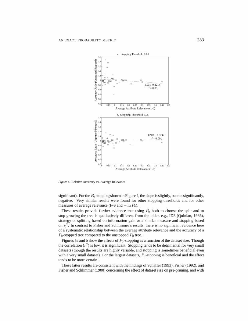
test was applied without regard to Cochran’s criteria.Figures 4a and b show the results of a similar study forP0-stopping. They-axis in Figure 4

is the ratio of the unprunedP0 tree’s accuracy to the accuracy of theP0-stopped tree (datataken from Table 5). Ay value of 1 indicates no difference in accuracy; a value< 1 thatstopping improved accuracy; and a value> 1 that stopping reduced accuracy. Thex-axisvalue in Figure 4 is the average of(1− d) over each split considered at the root of the treefor each data set.

The intercept of the regression line in Figure 4a is> 1, suggesting thatP0-stopping isharmful when the average attribute relevance is low. The negative slope of the regressionline indicates thatP0-stopping slowly becomes more effective as the average relevanceincreases.

In Fisher’s (1992) study for trees built using1−d and pruned usingχ2, the correspondingregression line was0.944 + 1.085x, with r2 = 0.438 (the positive slope+1.085 was

282 J.K. MARTIN

Table 6.Binary vs. Multi-way Splits

Data Set Binary Multi-wayunpruned P0 pruned unpruned P0 pruned

Gain P0 0.05 0.01 0.005 Gain P0 0.05 0.01 0.005

Cross-Validation Accuracy %

BUPA Nat 54 60 57 54 58 55 57 59 51 57Qua 63 62 57 63 62 57 58 57 58 57

Finance 1 Nat 77 75 ¶ 77 65 69 67 65 ¶ 58 67 54Qua ¶ 72 75 79 ¶ 71 64 ¶ 52 71 71 ¶ 52 56

Finance 2 Nat 91 92 94 94 94 95 92 91 91 92Qua 86 92 97 92 97 89 89 97 97 97

Flare C 87 76 88 89 89 85 87 88 88 88Flare M 85 85 90 89 89 85 85 89 89 90Flare X 97 97 98 98 98 97 97 97 97 97Glass Nat 51 ¶ 53 52 52 44 47 ¶ 44 51 50 50

Qua 72 70 70 65 61 66 69 62 62 57Iris Nat 95 95 95 96 96 95 93 97 97 97

Qua 91 90 92 94 94 92 90 90 93 93Obesity Nat 56 58 49 § 40 § 33 51 58 56 § 62 § 56

Qua 40 51 49 40 § 29 49 40 44 58 § 63Pima Nat 72 70 72 70 73 70 70 71 72 72

Qua 68 65 73 74 74 67 67 71 74 74Servo 95 95 89 89 90 96 95 93 92 93Soybean 98 98 96 98 98 98 98 96 98 98Thyroid Nat 91 89 93 91 91 91 91 91 91 91

Qua 93 93 92 92 91 92 93 92 92 92WAIS † Qua 61 65 63 63 73 65 67 73 71 71Wine Nat 90 90 92 92 86 89 90 88 91 90

Qua 93 89 89 § 86 93 91 92 90 § 93 91

Overall 77.1 76.7 78.0 77.4 77.4 75.5 76.1 77.1 77.5 77.4Natural 72.6 72.8 73.2 71.6 71.6 71.0 71.1 72.6 71.9 72.2

Quartiles† 74.1 72.7 75.4 75.3 74.9 71.9 72.7 73.1 75.0 74.1

¶ binary is better (95% confidence level) § multi-way is better (95% confidence level)

Number of Leaves

Overall 944 955 216 140 120 2155 2384 717 487 425Natural 366 292 80 56 46 880 911 311 237 199

Quartiles† 422 502 109 68 60 975 1136 327 210 186


Overall 8.8 6.2 3.9 3.0 2.7 3.5 3.6 2.6 2.3 2.1Natural 13.9 6.8 4.2 3.2 3.0 4.3 4.2 3.0 2.7 2.5

Quartiles† 5.8 6.2 4.2 3.3 3.0 3.1 3.3 2.6 2.3 2.2

Training & Validation Time (sec)

Overall 2074 1354 944 809 771 323 201 170 159 156Natural 1234 745 519 460 436 127 83 72 68 67

Quartiles† 585 428 307 259 252 127 72 64 58 57

† Not included in Quartiles summary. WAIS (Natural) and Word Sense are binary.


a. Stopping Threshold 0.01

0 0.05 0.1 0.15 0.2 0.25 0.3 0.35 0.4 0.45 0.5

Average Attribute Relevance (1-d)

0.5

0.6

0.7

0.8

0.9

1

1.1

1.2

1.3

1.4

1.5

Acc

urac

y R

atio

(U

npru

ned/

Sto

pped

)

1.031 0.221xr = 0.032

b. Stopping Threshold 0.05

0 0.05 0.1 0.15 0.2 0.25 0.3 0.35 0.4 0.45 0.5

Average Attribute Relevance (1-d)

0.5

0.6

0.7

0.8

0.9

1

1.1

1.2

1.3

1.4

1.5

Acc

urac

y R

atio

(U

npru

ned/

Sto

pped

)

0.998 0.024xr = 0.0012

Figure 4. Relative Accuracy vs. Average Relevance

significant). For theP0 stopping shown in Figure 4, the slope is slightly, but not significantly,negative. Very similar results were found for other stopping thresholds and for othermeasures of average relevance (F-S and− lnP0).

These results provide further evidence that usingP0 both to choose the split and tostop growing the tree is qualitatively different from the older, e.g., ID3 (Quinlan, 1986),strategy of splitting based on information gain or a similar measure and stopping basedonχ2. In contrast to Fisher and Schlimmer’s results, there is no significant evidence hereof a systematic relationship between the average attribute relevance and the accuracy of aP0-stopped tree compared to the unstoppedP0 tree.

Figures 5a and b show the effects ofP0-stopping as a function of the dataset size. Thoughthe correlation (r2) is low, it is significant. Stopping tends to be detrimental for very smalldatasets (though the results are highly variable, and stopping is sometimes beneficial evenwith a very small dataset). For the largest datasets,P0-stopping is beneficial and the effecttends to be more certain.

These latter results are consistent with the findings of Schaffer (1993), Fisher (1992), andFisher and Schlimmer (1988) concerning the effect of dataset size on pre-pruning, and with

284 J.K. MARTIN

Fisher’s (1992) suggestion of a more optimistic (non-pruning) strategy for small datasetsand a more pessimistic (strong pre-pruning) strategy for large datasets. Figure 5c showsthe generally beneficial net effects of the following simple strategy of varying the stoppingthreshold with the dataset size:

Dataset P0-stoppingSize Threshold

N < 50 do not stop50 ≤ N < 100 0.5100 ≤ N < 200 0.1200 ≤ N < 500 0.05

N ≥ 500 0.01

Comparing Figure 5c to Figures 5a and b, note that in Figures 5a and b the outcome is veryuncertain for the smallest datasets, but stopping is slightly harmful on the average for thesesmall datasets (more uncertain and more harmful on the average the more severely the treeis pruned, i.e., the lower theP0 threshold). The variable strategy in Figure 5c eliminatesboth the uncertainty and the slightly harmful average effect by simply not stopping for thevery small datasets.

For the largest data sets, the effects of stopping are more certain and more certain not tobe harmful to accuracy, even for fairly severe pruning (0.01P0 threshold). The variablestrategy maintains both this advantage and the reduced complexity the pruning yields.

For the intermediate dataset sizes, the primary effect of the variable threshold strategyis to reduce the uncertainty of the accuracy outcome, as evidenced by the lower scatter ofFigure 5c relative to Figures 5a and b in the region100 ≤ N ≤ 200, while maintaining theadvantage of reduced complexity.

The high level of uncertainty in Figures 5a and b is largely a consequence of the factthatP0 and the other metrics are discrete variables, though we treat them as if they werecontinuous. For small samples, the increments between the discrete values ofP0 are largeand small perturbations of the data may cause a large change inP0, affecting both the choiceof the split attribute and whether to stop. The statistics on which our decisions are made arevery sensitive to noise and unstable under the perturbations caused by cross-validation re-sampling in small samples, and the variable threshold strategy simply takes this sensitivityand instability into account.

In Fisher’s (1992) terminology, the variable threshold strategy is optimistic for the smallestdatasets, and more pessimistic as dataset size increases. The strategy can also be viewedfrom the standpoint of risk management. Defining risk as the likelihood that stopping willresult in reduced accuracy and uncertainty as the variance of they-axis in Figure 5, thestrategy is more cautious when the risk and uncertainty of stopping are high (i.e., for verysmall datasets) and increasingly bold as the risk and uncertainty decrease with increasingdataset size.


a. Stopping Threshold 0.01

0 100 200 300 400 500 600 700 800 900

Dataset Size (N)

0.5

0.6

0.7

0.8

0.9

1

1.1

1.2

1.3

1.4

1.5

Acc

urac

y R

atio

(U

npru

ned/

Sto

pped

)

1.083 0.00021xr = 0.0642

b. Stopping Threshold 0.05

0 100 200 300 400 500 600 700 800 900

Dataset Size (N)

0.5

0.6

0.7

0.8

0.9

1

1.1

1.2

1.3

1.4

1.5

Acc

urac

y R

atio

(U

npru

ned/

Sto

pped

)

1.042 0.00013xr = 0.0562

c. Variable Stopping Threshold

0 100 200 300 400 500 600 700 800 900

Dataset Size (N)

0.5

0.6

0.7

0.8

0.9

1

1.1

1.2

1.3

1.4

1.5

Acc

urac

y R

atio

(U

npru

ned/

Sto

pped

)

1.008 0.000064xr = 0.0982

Figure 5. Relative Accuracy vs. Dataset Size

10. Impact of Different Choices of Candidate Split Sets

We have seen in the XOR example that the choice of a candidate set can interact strongly withother factors, particularly with pre-pruning, to preclude or strongly bias against discoveringaccurate decision trees for some problems. Figure 6 illustrates a different aspect of thechoice of candidate sets. Here, there are 2 continuous attributes (x andy) and 2 classes,and the boundary between the two classes is linear (class = 1 if y > x, else class = 0).If the candidate splits are restricted to splitting on a single attribute, each of the decisiontree leaves covers a rectangular area with sides parallel to the axes. The oblique boundarybetween the two classes can at best be approximated as a step function, and the accuracyof the tree is directly related to the complexity of the tree and to the sample size (the moreleaves and the smaller the area covered by each leaf, the better — the shaded area in Figure 6is equal to the error rate in the region0 ≤ x ≤ 1 and0 ≤ y ≤ 1). If the splits are furtherrestricted so as to allow only binary splits on continuous attributes, a deeper tree will berequired in order to achieve the same accuracy.

286 J.K. MARTIN

class 0

class 1

0 0.1 0.2 0.3 0.4 0.5 0.6 0.7 0.8 0.9 1

x

0

0.1

0.2

0.3

0.4

0.5

0.6

0.7

0.8

0.9

1

y

Figure 6. Linear Class Boundaries

a. Linear Class Boundaries

Class 0

Class 1

0 0.1 0.2 0.3 0.4 0.5 0.6 0.7 0.8 0.9 1

x

0

0.1

0.2

0.3

0.4

0.5

0.6

0.7

0.8

0.9

1

y

b. Typical Tree Boundaries

Class 0

Class 1

0 0.1 0.2 0.3 0.4 0.5 0.6 0.7 0.8 0.9 1

x

0

0.1

0.2

0.3

0.4

0.5

0.6

0.7

0.8

0.9

1

y

Figure 7. Linear Class Boundaries and XOR

If splits on linear combinations of continuous attributes (e.g., discriminant functions) areallowed, then, for the same sample size, both better accuracy and a simpler tree can beobtained, and trees with accuracy equivalent to single attribute splits can be obtained fromsmaller samples. See, for instance, Weiss and Indurkhya (1991), Murthy, et al. (1993),Park and Sklansky (1990), and John (1995) for some approaches to handling such linearcombinations.

Another feature of this problem is that if only binary splits on a single attribute are allowed,the incremental improvement that could be achieved by any particular split is small. Pre-pruning might preclude splits on continuous attributes in these cases. Again, this is causedby the interaction of pre-pruning with the restrictions on candidate splits, rather than bypre-pruningper se.


The choice of a candidate set defines a language for describing the boundaries betweenclasses. If an accurate description of the true class boundaries in this language is verycomplex (as in XOR or approximating a linear boundary with a step function), then pre-pruning is likely to have a deleterious effect because pre-pruning may prevent discovery ofthese very complex decision trees.

The point of pruning is to prevent or correct overfitting, the building of trees that are morecomplex than can be supported by the available data using principles of sound statisticalinference. When only very simple candidate splits are allowed, empirical evidence fromearlier studies (Breiman, et al., 1984; Quinlan, 1986) indicates that better results are obtainedfrom building overly complex trees and post-pruning than from pre-pruning. The results ofour analysis of the XOR and linear boundaries problems indicates that both better accuracyand simpler trees might be obtained by expanding the set of candidate splits. It is not clearwhether it is more effective in general to expand the candidate splits and pre-prune, to buildmore complex trees and post-prune, or to combine the two approaches.

Expanding the set of candidate splits is not a panacea. In the first place, exhaustive searchis impractical. Further, when continuous attributes are involved, the set of possible functionscombining several attributes is unbounded. It is still necessary to restrict the candidatesto relatively simple functions by bounding the number of attributes in a combination andlimiting continuous functions to, for instance, linear or quadratic forms.

Expanding the candidate set is not always straightforward. In Figure 7, for instance (class= 1 if | y − x |> 0.2, else class = 0), the class boundaries are linear. Linear discriminantanalysis (Weiss & Indurkhya, 1991) fails in this case (all of the instances are predicted to beclass 1, a 40% error rate) because the simple discriminant analysis assumptions (that eachclass is adequately described by a single multivariate normal distribution, and that the classmeans are different) do not hold for these data. This problem (Figure 7) is called the ‘par-allel oblique lines’ problem and is dealt with effectively in the OC1 (Murthy, et al., 1993)algorithm.

In addition to having linear class boundaries, this problem has a trait in common with theXOR problem — diagonally opposite corners of the attribute space have the same class.Ordinary linear discriminant analysis seeks a single line separating two classes, and mayfail to find a satisfactory boundary when two lines are required. In this case, the effect oflinear discriminant analysis is the same as the effect of pre-pruning in the XOR problem.

In summary, expanding the set of candidate splits is a very powerful tool and can per-mit discovering decision trees that are both more accurate and less complex. In terms ofincreasing the number of problems for which reasonably accurate and simple trees canbe learned, expanding the set of candidates (within reasonable bounds on the increasedsearch space) is likely to be more effective than is using post-pruning. However, thereare no guarantees, and there is no one-size-fits-all strategy for expanding the candidateset. There have also recently been some disquieting results on the effectiveness of looka-head (Murthy & Salzberg, 1995), and on the potentially harmful effects of over-expandingthe candidate set, termed ‘oversearching’ by Quinlan and Cameron-Jones (1995).

288 J.K. MARTIN

11. Conclusions

The following conclusions are drawn from the results and analyses of the experimentsperformed here:

1. Information gain, gain ratio, distance, orthogonality, chi-squared, and Beta each down-play some part of the influence of the marginal totals of the classes and attribute values.Whenever one or more of the expected values in a split is small, these measures areprone to overestimate the reliability of the split. The divide-and-conquer strategy ofbuilding classification trees often leads to very small subtrees where these measures areinadmissible.

2. TheP0 null hypothesis probability measure proposed here overcomes the difficultiesencountered when the classes and attribute values are unevenly distributed or the ex-pected frequencies are small. The unpruned treesP0 builds are typically simpler, moreefficient, and no less accurate than those built by the other measures.

3. The ordering of the attribute splits within a tree can profoundly affect the effectivenessand efficiency of pruning (either pre- or post-pruning). This is particularly the casewhen different heuristics are used for selecting the split and deciding whether to pruneor stop splitting.

4. TheP0 measure can be used to stop splitting. This is more practical than post-pruning,particularly C4.5’s pessimistic post-pruning routine (Quinlan, 1993), and the resultingtrees are typically simpler, more efficient, and no less accurate than unpruned or post-pruned trees. A stopping threshold level which decreases (prunes more severely) as thesample size increases is recommended.

5. The arguments against stopping are equally arguments against use of very sparse (orotherwise ill-conditioned) data, biased heuristics, different inadmissible heuristics forsplitting and stopping, and very restricted candidate sets. Assuming a sample size of 50or more, there is no point in continuing the inductive process when the class distributionis probably independent of the candidate splits (P0 > 0.5), and in most domains thereis little point in continuing whenP0 > 0.05.

The paper also describes the biases of the various heuristic splitting and stopping metricsand why they are inadmissible. It also largely explains the reasons (other than the well-known XOR problem) for the failure of attempts to formulate a satisfactory stopping strategyusing these inadmissible heuristics.

Acknowledgments

The Common Lisp implementation of TDIDT (ID3) used here (substituting various heuris-tics for information gain andX2) is due to, and copyright by Dr. Raymond Mooney,University of Texas. Dr. Mooney’s copyright notice acknowledges the contributions ofothers, and gives permission to modify the program provided that the original copyrightnotice is retained. The comments and suggestions of editor Doug Fisher and several anony-mous reviewers are also gratefully acknowledged.


Notes

1. XOR is prototypical of themyopiaof greedy search, a symptom which may be alleviated by lookahead, as inpost-pruning rather than stopping. TDIDT’s search strategy is also irrevocable and narrowly focused, problemswhich may not be alleviated by lookahead and post-pruning.

2. We introduce noise by randomly reversing the class of 1% of the instances, by reversing 1% of the values ofAindependently of the class noise, and by altering 1% of the values ofB independently of the class and attributeA noise, lettingB = 0 andB = 2 change to 1, andB = 1 change to either 0 or 2 with equal likelihood.

3. The irrelevant variable is one which is binary and random, and completely independent of the class and of thevalues ofA andB.

4. In this regard, it should be noted that the incomplete Beta function also has a strong relationship to theχ2,hypergeometric, binomial, Student’st, andF (variance-ratio) distributions. Which is to say that all sensiblemeasures of split utility asymptotically rank attributes in the same order. Hence the repeated empirical findings(e.g., Breiman, et al., 1984; Fayyad & Irani, 1992a) that the various measures are largely interchangeable.

5. If X1, . . . , Xν are independent random variables, each having a standard (zero mean, unity variance) normaldistribution, then

∑ν

i=1X2i has a chi-squared (χ2) distribution with ν degrees of freedom. Here, the

Xi ≡ (fcv − ecv)/√ecv terms are approximately standard normaliff the null hypothesis is true and all of

theecv are large.6. We say that a statistical procedure isrobustif the actual significance level is close to the procedure’s estimated

level, even under deviations from assumptions. An inference procedure isbiasedif its mean deviation from theactual confidence level is not zero. A non-robust biased procedure isinadmissible, otherwise, the procedureis admissible.

7. N = (2, 4, 8, . . . , 64), n1 = (1 . . . N/2),m1 = (1 . . . n1), f11 = (0 . . .m1).

8. See Martin and Hirschberg (1996a) for a thorough analysis of the time complexity of this post-pruningalgorithm.

References

Agresti, A. (1990).Categorical data analysis. New York: John Wiley & Sons.Breiman, L., Friedman, J. H., Olshen, R. A., & Stone, C. J. (1984).Classification and regression trees. Pacific

Grove, CA: Wadsworth & Brooks.Buntine, W. L. (1990).A theory of learning classification rules. PhD thesis. University of Technology, Sydney.Buntine, W. & Niblett, T. (1992). A further comparison of splitting rules for decision-tree induction.Machine

Learning, 8, 75–85.Cestnik, B., Kononenko, I. & Bratko, I. (1987). ASSISTANT 86: A knowledge-elicitation tool for sophisticated

users. InProgress in Machine Learning, EWSL-87. Wilmslow: Sigma Press.Cestnik, B. & Bratko, I. (1991). On estimating probabilities in tree pruning. InMachine Learning, EWSL-91.

Berlin: Springer-Verlag.Cochran, W. G. (1952). Some methods of strengthening the commonχ2 tests.Biometrics, 10, 417-451.Elder, J. F. (1995). Heuristic search for model structure. In Fisher, D. & Lenz, H-J. (Eds.)Learning from Data:

Artificial Intelligence and Statistics V, Lecture Notes in Statistics, v. 112 (pp. 131-142). New York: Springer.Fayyad, U. M., & Irani, K. B. (1992a). The attribute selection problem in decision tree generation.Proceedings of

the 10th National Conference on Artificial Intelligence, AAAI-92(pp. 104–110). Cambridge, MA: MIT Press.Fayyad, U. M., & Irani, K. B. (1992b). On the handling of continuous-valued attributes in decision tree generation.

Machine Learning, 8, 87-102.Fayyad, U. M., & Irani, K. B. (1993). Multi-interval discretization of continuous-valued attributes for classification

learning.Proceedings of the 13th International Joint Conference on Artificial Intelligence (IJCAI-93)(pp. 1022-1027). San Mateo, CA: Morgan Kaufmann.

Fisher, D. H. (1987). Knowledge acquisition via incremental conceptual clustering.Machine Learning, 2,139-172.

Fisher, D. H. (1992). Pessimistic and optimistic induction. Technical Report CS-92-22, Department of ComputerScience, Vanderbilt University, Nashville, TN.

Fisher, D. H., & Schlimmer, J. C. (1988). Concept simplification and prediction accuracy.Proceedings of the 5thInternational Conference on Machine Learning (ML-88)(pp. 22–28). San Mateo, CA: Morgan-Kaufmann.

290 J.K. MARTIN

Fulton, T., Kasif, S., & Salzberg, S. (1995). Efficient algorithms for finding multi-way splits for decision trees.Machine Learning: Proceedings of the 12th International Conference (ML-95)(pp. 244-251). San Francisco:Morgan Kaufmann.

Gluck, M. A., & Corter, J. E. (1985). Information, uncertainty, and the utility of categories.Proceedings of the7th Annual Conference of the Cognitive Society(pp. 283–287). Hillsdale, NJ: Lawrence Erlbaum.

John, G. H. (1995). Robust linear discriminant trees. In Fisher, D. & Lenz, H-J. (Eds.)Learning from Data:Artificial Intelligence and Statistics V, Lecture Notes in Statistics, v. 112 (pp. 375-386). New York: Springer.

Kira, K. & Rendell, L. A. (1992). A practical approach to feature selection.Machine Learning: Proceedings ofthe 9th International Conference (ML-92)(pp. 249-256). San Mateo, CA: Morgan Kaufmann.

Kononenko, I. (1994). Estimating attributes: Analysis and extensions of RELIEF.Proceedings of the EuropeanConference on Machine Learning (ECML-94), (pp. 171-182). Berlin: Springer.

Liu, W. Z., & White, A. P. (1994). The importance of attribute-selection measures in decision tree induction.Machine Learning, 15, 25–41.

Lopez de Mantaras, R. (1991). A distance-based attribute selection measure for decision tree induction.MachineLearning, 6, 81–92.

Martin, J. K. (1995). An exact probability metric for decision tree splitting and stopping. Technical Report 95-16,Department of Information & Computer Science, University of California, Irvine, CA.

Martin, J. K. & Hirschberg, D. S. (1996a). On the complexity of learning decision trees.Proceedings Fourth Inter-national Symposium on Artificial Intelligence and Mathematics, AI/MATH-96(pp. 112-115). Fort Lauderdale,FL.

Martin, J. K. & Hirschberg, D. S. (1996b). Small sample statistics for classification error rates I: Error rate mea-surements. Technical Report 96-21, Department of Information & Computer Science, University of California,Irvine, CA.

Martin, J. K. & Hirschberg, D. S. (1996c). Small sample statistics for classification error rates II: Confidenceintervals and significance tests. Technical Report 96-22, Department of Information & Computer Science,University of California, Irvine, CA.

Mingers, J. (1987). Expert systems — rule induction with statistical data.Journal of the Operational ResearchSociety, 38, 39–47.

Mingers, J. (1989a). An empirical comparison of pruning measures for decision tree induction.Machine Learning,4, 227–243.

Mingers, J. (1989b). An empirical comparison of selection measures for decision tree induction.MachineLearning, 3, 319–342.

Murphy, P. M., & Aha, D. W. (1995).UCI Repository of Machine Learning Databases. (machine-readable datadepository). Department of Information & Computer Science, University of California, Irvine, CA.

Murphy P. M. & Pazzani, M. J. (1991). ID2-of-3: Constructive induction of M-of-N concepts for discriminatorsin decision trees.Machine Learning: Proceedings of the 8th International Workshop (ML-91)(pp. 183-187).San Mateo, CA: Morgan Kaufmann.

Murthy, S., Kasif, S., Salzberg, S., & Beigel, R. (1993). OC-1: Randomized induction of oblique decision trees.Proceedings of the 11th National Conference on Artificial Intelligence (AAAI-93)(pp. 322-327). Menlo Park,CA: AAAI Press.

Murthy, S. & Salzberg, S. (1995). Lookahead and pathology in decision tree induction.Proceedings of the 14thInternational Joint Conference on Artificial Intelligence (IJCAI-95)(pp. 1025-1031). San Mateo, CA: MorganKaufmann.

Niblett, T. (1987). Constructing decision trees in noisy domains. InProgress in Machine Learning, EWSL-87.Wilmslow: Sigma Press.

Niblett, T., & Bratko, I. (1986). Learning decision rules in noisy domains. InProceedings of Expert Systems 86.Cambridge: Cambridge University Press.

Park, Y. & Sklansky, J. (1990). Automated design of linear tree classifiers.Pattern Recognition, 23, 1393-1412.Quinlan, J. R. (1986). Induction of decision trees.Machine Learning, 1, 81–106.Quinlan, J. R. (1988). Simplifying decision trees. In B. R. Gaines & J. H. Boose (Eds.).Knowledge Acquisition

for Knowledge-Based Systems. San Diego: Academic Press.Quinlan, J. R. (1993).C4.5: Programs for Machine Learning. San Mateo, CA: Morgan Kaufmann.Quinlan, J. R. & Cameron-Jones, R.M. (1995). Oversearching and layered search in empirical learning.Pro-

ceedings of the 14th International Joint Conference on Artificial Intelligence (IJCAI-95)(pp. 1019-1024). SanMateo, CA: Morgan Kaufmann.

Schaffer, C. (1993). Overfitting avoidance as bias.Machine Learning, 10, 153–178.


Shavlik, J. W., Mooney, R. J., & Towell, G. G. (1991). Symbolic and neural learning algorithms: An experimentalcomparison.Machine Learning, 6, 111-143.

Weiss, S. M. & Indurkhya, N. (1991). Reduced complexity rule induction.Proceedings of the 12th InternationalJoint Conference on Artificial Intelligence, IJCAI-91(pp. 678–684). San Mateo, CA: Morgan Kaufmann.

Weiss, S. M. & Indurkhya, N. (1994). Small sample decision tree pruning.Proceedings of the 11th InternationalConference on Machine Learning (ML-94), (pp. 335-342). San Francisco: Morgan-Kaufman.

White, A. P. & Liu, W. Z. (1994). Bias in information-based measures in decision tree induction.MachineLearning, 15, 321–329.

Received November 8, 1996Accepted April 28, 1997Final Manuscript May 7, 1997

An Exact Probability Metric for Decision Tree Splitting and Stopping

Documents

Transcript of An Exact Probability Metric for Decision Tree Splitting and Stopping