arX

iv:h

ep-t

h/02

0908

9v2

12

Sep

2002

Preprint typeset in JHEP style. - HYPER VERSION SWAT-350

Exact Superpotentials from Matrix Models

Nick Dorey, Timothy J. Hollowood, S. Prem Kumar and Annamaria Sinkovics

Department of Physics, University of Wales Swansea, Swansea, SA2 8PP, UK

E-mail: t.hollowood@swan.ac.uk, n.dorey@swan.ac.uk

s.p.kumar@swan.ac.uk, a.sinkovics@swan.ac.uk

Abstract: Dijkgraaf and Vafa (DV) have conjectured that the exact superpotential

for a large class of N = 1 SUSY gauge theories can be extracted from the planar

limit of a certain holomorphic matrix integral. We test their proposal against existing

knowledge for a family of deformations of N = 4 SUSY Yang-Mills theory involving

an arbitrary polynomial superpotential for one of the three adjoint chiral superfields.

Specifically, we compare the DV prediction for these models with earlier results based

on the connection between SUSY gauge theories and integrable systems. We find

complete agreement between the two approaches. In particular we show how the DV

proposal allows the extraction of the exact eigenvalues of the adjoint scalar in the

confining vacuum and hence computes all related condensates of the finite-N gauge

theory. We extend these results to include Leigh-Strassler deformations of the N = 4

theory.

1. Introduction

Theories with N = 1 supersymmetry in four dimensions are of considerable interest.

Apart from their potential phenomenological relevance, they provide a field theoretic

laboratory where physical phenomena such as confinement and dynamical symmetry

breaking can be studied in a controlled setting. This is possible largely because these

theories contain a special class of observables whose dependence on the parameters

of the theory is constrained to be holomorphic. These quantities, which include the

vacuum expectation values of chiral operators and the tensions of BPS saturated

domain walls, are governed by a holomorphic superpotential which can sometimes

be determined exactly. Although exact results for many different models have been

obtained, a general recipe for computing the superpotential for an arbitrary N = 1

model has remained elusive. In recent work [1–4], Dijkgraaf and Vafa (DV) have

proposed a solution to this problem which applies to a large class of N = 1 theories.

Specifically, they claim that the superpotentials for these theories can be extracted

from the planar limit of a certain holomorphic matrix integral. In this paper, we

will perform a detailed test of their proposal against known results for a family of

N = 1 preserving deformations of N = 4 SUSY Yang-Mills theory with gauge group

SU(N) (or U(N)). For this family of theories there is an alternative method for

computing the exact superpotential, given in [5–8]. In fact, the superpotential can

be deduced from the value of the Lax matrix of a certain classical integrable system

in its equilibrium position. Remarkably, we will find that these two seemingly very

different recipes give exactly the same result. The comparison will also shed light on

both approaches. In the remainder of this introductory section, we will review both

the DV proposal and the results of [8] based on the connection to integrable systems

and present our main conclusions.

We begin by considering N = 4 SUSY Yang-Mills theory with gauge group G =

SU(N) and bare complex coupling τ = 4πi/g2Y M +θ/2π. In the standard language of

N = 1 superfields, the theory contains three adjoint-valued chiral multiplets, which

we will label Φ+, Φ− and Φ. We will consider the deformation of the N = 4 theory

obtained by adding an N = 2 preserving mass term for Φ±, together with a general

polynomial superpotential for Φ which preserves N = 1 supersymmetry.The classical

superpotential then reads,

W (Φ) = Tr

(

iΦ[Φ+, Φ−] + Φ+Φ− +N∑

p=2

gpΦp

)

(1.1)

Setting gp = 0 for p ≥ 3 corresponds to the N = 1∗ deformation but we will not

limit ourselves to this case.

1

This theory already has a rich vacuum structure at the classical level. In partic-

ular, there is a large set of classical vacua in which the adjoint scalar fields acquire

vacuum expectation values (VEVs) spontaneously breaking some or all of the gauge

symmetry. In this paper we will focus on SUSY vacua in which the full SU(N) gauge

symmetry is unbroken. At the classical level this corresponds to setting the adjoint

scalar VEVs to zero1. The qualitative behaviour of the corresponding quantum the-

ory in these vacua is well known: at energy scales much less than the mass scale set by

the deformations, the chiral multiplets decouple leaving the theory of a single SU(N)

vector multiplet which is in the same universality class as N = 1 SUSY Yang-Mills.

The theory is therefore in a confining phase with a mass gap and gluino condensation.

There are N supersymmetric vacua denoted |k〉 with k = 0, 1, 2, . . . , N −1, each with

a non-zero expectation value for the gluino bilinear which is the lowest component of

the superfield S = Tr (WαW α)/32π2. In fact, the action of S-duality, inherited from

the underlying N = 4 theory, dictates that the vacuum states |k〉 and |k + 1〉 are

simply related by a 2π shift in the vacuum angle: τ → τ + 1. Hence it will suffice to

consider the k = 0 vacuum, |0〉, in the following. Our aim will be to determine the

exact effective superpotential in this vacuum, 〈0|Weff |0〉. The vacuum expectation

values of the operators up = Tr Φp can then be obtained by differentiating with

respect to the parameters gp appearing in (1.1).

1.1 The integrable system approach

An exact formula for the effective superpotential can be obtained from a slight

extension of the results presented in [8]. This approach relies on the connection

between SUSY gauge theories and integrable systems first discovered in [9–11]. In

the present case the relevant integrable system is the elliptic Calogero-Moser (ECM)

system. This is a system of N non-relativistic particles with complex positions and

momenta, Xj and Pj , j = 1, 2, . . . , N , which live on a torus Eτ of complex structure

τ and its tangent space respectively. Time evolution is governed by the quadratic

Hamiltonian,

H2 =

N∑

j=1

P 2j

2+∑

j>k

℘(Xj − Xk) (1.2)

where ℘ is the Weierstrass function (see Appendix A.1) which is elliptic with respect

to the torus Eτ . The system has a Lax formulation involving two N×N matrices Ljk

and Mjk, in terms of which Hamilton’s equations can be rewritten as iL̇ = [M, L].

This immediately implies the existence of N conserved quantities Hp = Tr Lp for

1In general, the adjoint scalar fields can and will acquire VEVs in the quantum theory without

breaking the gauge symmetry.

2

p = 1, . . . , N . These quantities can also be thought of as a set of Poisson-commuting

Hamiltonians each generating a distinct time-evolution of the system.

We will now state the relation between the deformed N = 4 theory and the

ECM theory (for more details see [8]). Firstly, for each value of p, the conserved

quantity Hp is identified with the expectation value of the operator up = Tr Φp

introduced above2. As explained in [6], the supersymmetric vacua of the theory then

correspond to the equilibrium configurations of the ECM particles. In particular,

for the theory with an arbitrary polynomial deformation, as in Eq.(1.1) we must

consider equilibrium configurations with respect to the time-evolution generated by

the Hamiltonian H =∑N

p=2 gpHp.

In the general case, finding these configurations is not straightforward. However,

the massive vacua of the theory have a very special property: they correspond to

static configurations which simultaneously stationarize each of the Hamiltonians 3

Hp, for p = 2, . . . , N . In particular, the vacuum |0〉 introduced above corresponds to

a configuration where the particles are evenly spaced around one cycle of the torus:

Xj = (2πiτ/N)j − iπτ(N − 1)/N ; Pj = 0 for j = 1, . . . , N . As each Hamiltonian is

stationary, the same configuration corresponds to a SUSY vacuum for all values of the

deformation parameters. The eigenvalues of the Lax matrix Lab in this equilibrium

configuration were calculated explicitly in [8]. The result is

λ̃j = −1

2

θ′3(π/2 − πj/N |τ/N)

θ3(π/2 − πj/N |τ/N)

(1.3)

where j = 1, 2, . . . , N . The vacuum expectation values of the operators, up, can

then be determined via the relation 〈0|up|0〉 =∑N

j=1 λ̃pj . As the resulting formulae

are completely independent of the deformation parameters gp, we find that that the

vacuum value of the effective superpotential is simply given by,

〈0|Weff |0〉 =N∑

p=2

gp〈0|up|0〉 =N∑

p=2

N∑

j=1

gpλ̃pj (1.4)

2To restrict to the SU(N) theory where u1 vanishes we consider the ECM system in its center-

of-momentum frame where H1 =∑N

j=1Pj = 0.

3In the field theory this is related to the fact that massive vacua preserving N = 1 supersymmetry

correspond to the maximal degenerations of the Riemann surface which governs the Coulomb branch

of the N = 2 theory obtained by setting all the deformation parameters to zero. However, it can

also be demonstrated directly using the Lax representation for the equations of motion of the ECM

system. This is shown in Appendix B.

3

1.2 The Dijkgraaf-Vafa Approach

Dijkgraaf and Vafa have proposed an exact recipe for calculating the exact effective

superpotential Weff as a function of the gluino condensate (the expectation value

of the superfield S). Specifically, they relate the superpotential to the following

holomorphic matrix integral:

Z =

∫

[dΦ][dΦ+][dΦ−] exp

(

− 1

gsW (Φ)

)

(1.5)

where gs is a coupling constant. The integral is to be understood as a multi-variable

contour integral. As for any adjoint SU(N) theory the free energy F has a ’t Hooft

expansion where the Feynman diagrams are organised according to their genus g ≥ 0.

F =∑

g≥0

g2g−2s Fg(λ) (1.6)

where λ = gsN is the matrix model ’t Hooft coupling. DV predict that the exact

superpotential of the above N = 1 perturbation of the N = 4 theory only depends

on the leading term in this expansion: F0(λ). This term may be evaluated by

taking the ’t Hooft limit of the matrix model, N → ∞, gs → 0 with λ held fixed,

which isolates the planar Feynman diagrams. Fortunately the matrix model can

be solved exactly in this limit using standard saddle-point technology. In the case

of a quadratic deformation, the solution has been already been given by Kazakov,

Kostov and Nekrasov [13]. Generalization of their solution to an arbitrary polynomial

deformation is straightforward and is given below.

The proposed dictionary between matrix model and field theory quantities identi-

fies the ’t Hooft coupling λ = gsN with the expectation value of the gluino bilinear

superfield S. From now on we will use the symbol S to denote both the matrix model

’t Hooft coupling and the gluino condensate of the field theory and assume that the

interpretation is clear from the context. The resulting expression for the field theory

superpotential is,

Weff(S) = N∂F0

∂S− 2πiτS (1.7)

The supersymmetric vacua may be found be extremising Weff as a function of S.

The expectation value of Weff in each vacuum is simply its value at the corresponding

the extremum. The main aim of this paper is to compare the resulting formulae with

the exact field theory predictions Eqs. (1.3) and (1.4). We find that the DV prescrip-

tion allows us to extract the field theory eigenvalues λ̃j and we find precise agreement

between the two approaches, for arbitrary values of the deformation parameters gp,

4

up to the known ambiguities in the definition of the operators up [5]. Agreement in

the case of a quadratic superpotential has previously been checked in [4].

Several features of our result are worthy of further comment. A remarkable

consequence of Dijkgraaf and Vafa’s proposal is that the holomorphic quantities of

the deformed N = 4 theory are large-N exact. Although this property is far from

obvious in the integrable systems approach it nevertheless seems to be true that 1/N

corrections to all physical quantities vanish up to the usual operator mixing ambigu-

ities! On another hand there are some features of the field theory results which are

not apparent at the outset in the DV prescription, for example the linear dependence

of the exact superpotential (1.4) on the deformation parameters gp. Nevertheless, we

are able to prove that for the class of deformations considered the DV prescription

automatically implies this linearity in the confining vacuum.

We also extend our study to include a different class of deformations of the

N = 4 theory, namely the Leigh-Strassler deformations. We use the DV proposal

to compute the exact effective superpotential for these deformations and extract the

eigenvalues λ̃j in the confining vacuum of the theory. Remarkably, we find once again

that these are independent of the deformation parameters gp.

2. Superpotentials and eigenvalue distributions from matrix

models

According to the Dijkgraaf-Vafa proposal [1–3] superpotentials for a large class of

N = 1 supersymmetric field theories at finite N are computed by corresponding

large-N matrix models. Assuming the validity of this conjecture for arbitrary de-

formations of the N = 4 theory, we will demonstrate that for such deformations,

in the confining vacuum of the resulting theory the matrix model in fact yields the

correct eigenvalue distribution for the adjoint scalar field in the theory. This tests

the Dijkgraaf-Vafa proposal for a large class of deformations of the N = 4 the-

ory. Furthermore, it provides a general prescription for extracting QFT eigenvalue

distributions from the matrix model and also demonstrates that the matrix model

computes all condensates in the holomorphic sector of the theory.

2.1 Deformations of N = 4 theory

In the N = 1 language, the N = 4 U(N) theory with coupling constant τ ≡4πi/g2

Y M + θ/2π has three adjoint chiral superfields Φ+, Φ− and Φ. We consider a

5

general class of deformations of the N = 4 theory specified by a tree level superpo-

tential

W =1

g2Y M

Tr[

iΦ[Φ+, Φ−] + Φ+Φ− + V (Φ)]

(2.1)

where V (Φ) is a general polynomial

V (Φ) ≡∑

p

gp Φp. (2.2)

Note that for the sake of simplicity we have set any and all mass scales to unity. (For

V (Φ) = Φ2 we obtain the N = 1∗ theory.)

As a direct consequence of the proposal of Dijkgraaf and Vafa [1–3], in a given

vacuum the exact effective superpotential for the above class of deformations of the

N = 4 theory is computed by the planar diagram expansion, i.e. a large-N limit, of

the three-matrix model partition function expanded around that vacuum

Z =

∫

[dΦ+][dΦ−][dΦ] exp− 1

gsTr[

iΦ[Φ+, Φ−] + Φ+Φ− + V (Φ)]

(2.3)

with Φ+ = (Φ−)†.

The confining vacua of the field theory correspond to the classical solution Φ =

Φ± = 0 which preserves the full U(N) gauge symmetry. In order to implement the

Dijkgraaf-Vafa proposal for extracting the field theory superpotential in the confining

vacua we therefore need to solve the matrix model Eq. (2.3) around the trivial vacuum

Φ = Φ± = 0. As noted for example in [13], the key fact that permits the solution of

these matrix models is that one may integrate out Φ± exactly to obtain a one-matrix

integral to be solved in the large-N limit

Z =

∫

[dΦ]e−

1gs

TrV (Φ)

det(AdjΦ + i). (2.4)

2.2 Solution of the large-N matrix model

The above one-matrix model actually becomes tractable in the large-N limit by

going to an eigenvalue basis and performing a large-N saddle-point approximation

to the integral. The details of this procedure have been extensively discussed in the

literature. We refer the reader to [13], and references therein, for details.

The main feature of the solution is that the eigenvalues λj of Φ interact via a

repulsive effective potential and form a continuum in the large-N limit and condense

into a cut along the real axis. The actual extent of the cut and the density of

6

eigenvalues ρ(λ) along the cut is self-consistently determined by the saddle point

equation in terms of the parameters of the deformation V (Φ) and the matrix model

’t Hooft coupling S = gsN . The saddle point equation in the large-N limit is most

conveniently written in terms of the resolvent function

ω(z) =

∫ +α

−α

ρ(λ)

z − λdλ λ ∈ [−α, α];

∫ +α

−α

ρ(λ)dλ = 1. (2.5)

The resolvent ω(z) is an analytic function on the complex z-plane whose only sin-

gularity is a branch cut with the discontinuity across the cut given precisely by the

spectral density

ω(λ + iǫ) − ω(λ − iǫ) = −2πiρ(λ); λ ∈ [−α, α]. (2.6)

The saddle point equation essentially encodes the condition that the force on a

test eigenvalue due to the remaining large-N equilibrium distribution of eigenvalues

vanishes along the cut where the eigenvalues condense. The matrix model effective

action yields this force on a test eigenvalue at position z in the complex plane as

F (z) =1

2i[G(z + i

2) − G(z − i

2)] (2.7)

where

G(z) = U(z) + iS(ω(z + i2) − ω(z − i

2)). (2.8)

and U(z) is a polynomial in z such that

V ′(z) =1

i[U(z + i

2) − U(z − i

2)]. (2.9)

The analytic properties of the function G(z) are central to the solution of the

model and its subsequent physical interpretation. The defining equation for G(z)

Eq. (2.8) implies that G(z) is an analytic function with two branch cuts between

[−α + i2, α + i

2] and [−α − i

2, α − i

2]. The matrix model saddle point equation

identifies the values of G(z) along the two cuts via

G(λ + i2± iǫ) = G(λ − i

2∓ iǫ); λ ∈ [−α, α]. (2.10)

Thus the saddle point equation may be viewed as a ‘gluing’ condition for the two

cuts on the z-plane. In addition G(z) = G(z∗)∗ and G(z) = G(−z). The function

G(z) is then uniquely determined by its asymptotic behaviour at z → ∞ which is

specified by the polynomial U(z) in Eq. (2.8).

Given the density of eigenvalues ρ(λ) in the matrix model one may use it to com-

pute expectation values of various quantities in the matrix model. However, at the

7

A

CA’

CB

CA

CA’

CB

C

l

ab

cd

a b dc

i

k

i j k l

02w

w

-w2

2

1

z u

j

Figure 1: The z-plane and its pre-image in the u-plane. The cuts in the z-plane are

indicated by the dotted lines with Roman letters to dictate how they are mapped from the

u-plane. Three representative closed contours CA, CB and CA′ are illustrated.

outset we would like to point out these expectation values are distinct from vacuum

expectation values of the corresponding observables in field theory. In particular,

expectation values of the quantities Tr Φn in the matrix model are defined in the

obvious way:

〈〈TrΦn〉〉 =

∫ α

−α

ρ(λ)λn dλ . (2.11)

Using the formulae above one can relate these expectation values to the terms in the

large-z expansion of G(z). However these expectation values 〈〈Tr Φn〉〉 are not to be

identified with the corresponding condensates 〈TrΦn〉in the field theory,

〈Tr Φn〉QFT 6= 〈〈TrΦn〉〉. (2.12)

2.3 Emergence of the τ̃-torus

The two-cut structure of the z-plane (from the analytic properties of G(z)) and the

gluing conditions Eq. (2.10) uniquely specify a torus which we denote by Eτ̃ where

τ̃ is defined to be the complex structure parameter of this torus. The contour CA

in the z-plane enclosing the cut [−α + i2, α + i

2] maps to the A-cycle of the torus

while the contour CB joining the two cuts maps to the B-cycle of the torus. We also

define CA′ as the contour enclosing the lower cut. Note that CA + CA′ can be pulled

away from the cuts to enclose the point at infinity. These contours in the z-plane

are indicated in Figure 1.

The torus Eτ̃ may be thought of as usual, as a quotient of the complex plane, say

the u-plane (this auxiliary variable u will lead to the required elliptic parametriza-

8

tion), by a lattice with periods 2ω1 and 2ω2 with ω2/ω1 = τ̃ . The physical signifi-

cance of this torus will become apparent upon implementing the procedure of [1–3]

for computing the field theory superpotential. In fact τ̃ will be identified with τ/N ,

signalling a low-energy SL(2, Z) duality symmetry in τ/N where τ is the coupling of

the N = 4 theory. This duality, dubbed S̃-duality in [5] is distinct from the SL(2, Z)

symmetry of the N = 4 theory although it is of course a consequence of the latter.

The map z(u) from the u-plane to the z-plane is specified by the requirements

that going around CA (the A-cycle of the torus) returns z to its original value, while

traversing the contour CB (the B-cycle of the torus) causes z to jump by an amount

i, which is the distance between the two cuts in the z-plane. Both these operations

leave G unchanged which is therefore an elliptic function on the u-plane. Thus

A − cycle : z(u + 2ω1) = z(u); G(z(u + 2ω1)) = G(z(u)) , (2.13a)

B − cycle : z(u + 2ω2) = z(u) + i; G(z(u + 2ω2)) = G(z(u)). (2.13b)

These requirements (along with the power law behaviour of G(z) at large z)

specify z(u) uniquely and we find that

z(u) = −ω1

π

[

ζ(u) − ζ(ω1)

ω1

u

]

≡ −1

2

θ′1(πu2ω1

|τ̃)

θ1(πu2ω1

|τ̃). (2.14)

Here ζ(z) is the Weierstrass zeta function and θ1 is the Jacobi theta function (see [14]

and the Appendix for details). Note that the map from the torus to the eigenvalue

plane is completely independent of the choice of the field theory deformation V (Φ).

Different deformations imply different asymptotic properties of the elliptic function

G(z(u)) as z → ∞ and hence lead to elliptic functions with different orders.

2.3.1 An Example

For the simplest deformation, i.e. the quadratic one corresponding to the N = 1∗

theory, the asymptotics determine G(z(u)) uniquely:

V (Φ) = Φ2 : G(z(u)) =ω2

1

π2

[

℘(u) − 2ζ(ω1)

ω1

]

. (2.15)

G(z(u)) will involve higher powers of the Weierstrass-℘ function for more complicated

deformations.

Let us see how in the simplest example which was first discussed and solved

in [3, 4], V (Φ) = Φ2, τ̃ gets identified with τ/N . To see this we integrate the one-

form G(z)dz over the A-cycle and B-cycle to obtain the total number of eigenvalues S

9

and ∂F0/∂S respectively, the latter being the variation in the genus zero free energy

of the matrix model upon transporting an eigenvalue to infinity,

ΠA = 2πiS = −i

∫

A

G(z(u))dz(u)

dudu =

1

12

dE2(τ̃ )

dτ̃, (2.16a)

ΠB =∂F0

∂S= −i

∫

B

G(z(u))dz(u)

dudu =

τ̃

12

dE2(τ̃)

dτ̃− 1

12E2(τ̃). (2.16b)

Then the effective superpotential Weff for the N = 1∗ theory in the confining vacuum

is obtained by extremizing the following expression with respect to S,

Weff = NΠB − τΠA . (2.17)

Using our expressions for the respective integrals over the cycles it is easy to see that,

∂Weff

∂S= 0 =⇒ τ̃ =

τ

N. (2.18)

and

Weff = −N

12E2(τ/N) . (2.19)

Upon restoring the mass scales in the problem this result agrees precisely, up to

an additive constant with the expressions of [6, 7]. The fact that S in Eq.(2.16a)

automatically comes out as the τ -derivative of the effective superpotential is in line

with the identification of S with gluino condensate of the gauge theory.

The identification of the complex structure τ̃ of the matrix model torus with

τ/N in the confining vacuum of the field theory in fact holds for all possible choices

of V (Φ) and indeed, seems to work for a completely different class of deformations

namely the Leigh-Strassler deformations which will be discussed in detail below. The

emergence of a torus with complex structure τ/N , controlling the low-energy physics

of the confining vacua of deformations of the N = 4 theory, has been well understood

from the point of view of Seiberg-Witten theory in [5, 12]. It is quite remarkable to

see this structure emerge from the matrix model.

2.4 QFT eigenvalues and general superpotentials

Before embarking on a discussion of the eigenvalues below, we should emphasize a

subtle point that will emerge in due course. It will turn out that the distribution of

eigenvalues in the matrix model described by the density ρ(λ) is not to be identified

with the distribution of eigenvalues of Φ in the field theory at large N . In fact, the

main result of this section is that the Dijkgraaf-Vafa proposal is tantamount to iden-

tifying the eigenvalues of the adjoint scalar in the confining vacuum of the field theory

10

with the function z(u) in Eq. (2.14) (after a simple shift of its argument), distributed

evenly over a cycle on the Eτ̃ torus. In contrast the matrix model eigenvalues are

not uniformly distributed along this cycle.

The function z(u) that we have obtained above is a map from the torus Eτ̃ to

the plane of eigenvalues z. In particular, z(u) maps the A cycle of the torus to the

cut enclosed by CA,

CA ≃ z(2ω1x + ω2) = −1

2

θ′3(πx|τ̃)

θ3(πx|τ̃)+

i

2; x ∈ [−1

2, 1

2]. (2.20)

This cut extends from −α + i2

to α + i2

and represents the possible values of the

eigenvalues λ of Φ shifted by i/2 (the i/2 shift is deduced simply from Eq. (2.8)). In

view of this we define the function

λ(x) = −1

2

θ′3(πx|τ̃ )

θ3(πx|τ̃ ); x ∈ [−1

2, 1

2] . (2.21)

At first sight, this is simply a map from the A cycle of the torus to the interval

[−α, α] in which the eigenvalues are distributed. However, we will soon find that

λ(x) has greater significance. Before we uncover this, we note that given the map

λ(x) we can ask how the eigenvalues of the matrix model are distributed along the

A cycle of the torus. The answer is rather complicated being given by

dn

dx= ρ(λ(x))

dλ

dx, (2.22)

with −x0 ≤ x ≤ x0 where λ(x0) = α.4

In contrast, we will now show how the proposal of [4] automatically implies that

eigenvalues of Φ in the confining vacuum of the field theory at large N are uniformly

distributed over the x-interval [−12, 1

2] and are given precisely by the function λ(x).

To see this we simply note that the function z′′(u) = ω1

π℘′(u) is elliptic on the torus

and thus the following integral vanishes

∫

CA+C′

A

G(z(u))z′′(u)du = 0. (2.23)

Using the definition of G(z) in Eq. (2.8) this implies

S

∫

CA+C′

A

(ω(z + i2) − ω(z − i

2))z′′(u)du = i

∫

CA+C′

A

U(z)z′′(u)du. (2.24)

The periodicity of z(u) along the A-cycle allows us to reduce the left hand side of

this expression to a contour integral around u = 0 picking out the residue at u = 0.4Notice that the A cycle covers the interval [−α, α] twice, so one must choose one of the branches.

11

Using z(2ω1x ± ω2) = λ(x) ± i2, and Eq. (2.9) and the heat equation for the Jacobi

theta functions (A.9) we find that

S = − 1

2iπ

d

dτ̃

∫ 1/2

−1/2

V (λ(x)) dx. (2.25)

with λ(x) given by Eq. (2.21) Since the proposal of [4] implies the identification

τ̃ = τ/N and 2πiS = −dWeff/dτ so that S is the gluino condensate, we must have

Weff = N

∫ 1/2

−1/2

V (λ(x)) dx; λ(x) = −1

2

θ′3(πx|τ̃)

θ3(πx|τ̃). (2.26)

This proves that the eigenvalues of the adjoint scalar Φ in the confining vacuum

of the field theory at large N are given by the function λ(x) and are uniformly

distributed over the interval x ∈ [−12, 1

2] independent of the deformation V (Φ). Note

that, on the contrary the distribution of eigenvalues of the matrix model depends on

the deformation in a complicated way.

We should also emphasize that the result (2.26) is also, according to Dijkgraaf

and Vafa, true at finite N . At finite N the eigenvalues of Φ in the confining vacuum

have been computed from a completely different approach using the connection be-

tween N = 1∗ theories and integrable systems in [8]. The eigenvalues found in [8]

depend on a discrete index j and were given as

λ̃j = −1

2

θ′3(π/2 − πj/N |τ/N)

θ3(π/2 − πj/N |τ/N); j = 1, . . . , N . (2.27)

(Notice that these, as explained above, are not to be identified with the eigenvalues

λj of the matrix model!) The Dijkgraaf-Vafa prediction from the matrix model above

in Eq. (2.26) agrees precisely with the results of [8] upon taking the large-N limit

where the discrete label j in Eq.(2.27) is replaced by the continuous variable x. In

particular the eigenvalues are uniformly distributed in x. This demonstrates that

using the recipe of [1–3] the matrix model indeed computes the superpotentials for

the entire class of deformations considered above, provided N is large. Alternatively,

for any given deformation it also computes all the condensates 〈Tr Φn〉 via

〈TrΦn〉 = N

∫ 1/2

−1/2

λn(x) dx . (2.28)

In concert with all our previous warning 〈Tr Φn〉, the condensate of the field theory

is not to be identified with the expectation values in the matrix model (2.11):

〈〈TrΦn〉〉 6= 〈Tr Φn〉 . (2.29)

12

As we have already mentioned, the eigenvalues and hence all the condensates in

the confining vacuum are completely independent of the actual choice of deforma-

tions. This is in complete accord with expectations from field theory. The defor-

mations of the N = 4 theory that we have discussed may be thought of as N = 1

perturbations of the N = 2∗ theory. The confining vacua of the resulting theories

arise from points on the Coulomb branch where the Seiberg-Witten curve for the

N = 2∗ theory degenerates maximally into a torus of complex structure τ/N . The

location of such a point in moduli space given by condensates 〈Tr Φn〉, is completely

independent of the choice of V (Φ). This is in fact expected to be true in all massive

vacua of the N = 1 theory.

Although we have seen a remarkable agreement between the matrix model recipe

and the field theory results of [8], strictly this agreement appears when the eigenvalues

form a continuous distribution and can happen only in the large-N limit of the field

theory. Indeed, the appearance of integrals over a continuous label rather discrete

sums in Eq. (2.26) suggests that we are really doing a large-N calculation from the

point of view of the field theory. So does the large-N matrix model, or the planar

graphs of the matrix model really compute the holomorphic sector of the finite-N

field theory? The resolution of this puzzle will be the subject of Section 3.

2.5 Some explicit examples

We have computed the superpotentials from the matrix model by explicitly obtaining

G(z(u)) for V (Φ) = Φ2 and Φ4 and computing S, ∂F0/∂S as the integrals of G(z)dz

over the A and B cycles. These results match with a direct computation of the

superpotential using the eigenvalue distribution following Eq. (2.26). We quote the

results for these cases below

(i) V (Φ) = Φ2:

G(z(u)) =ω2

1

π2℘(u) − 2w1ζ(ω1)

π2, (2.30a)

ΠA =dh(τ̃)

dτ̃; ΠB = τ̃

dh(τ̃ )

dτ̃− h(τ̃ ). (2.30b)

Weff = −Nh(τ/N) = −N

12E2(τ/N). (2.30c)

The additive normalization of Weff can be fixed by a direct computation of Eq. (2.26)

which gives

Weff = N

∫ 1/2

−1/2

λ2(x) dx = −N

12

(

E2(τ/N) − 1)

. (2.31)

13

(ii) V (Φ) = Φ4:

G(z(u)) =ω4

1

π4℘(u)2 +

ω21

2π4

(

π2 − 8ω1ζ(ω1))

℘(u)

− ω1

6π4

(

g2ω31 + 6π2ζ(ω1) − 36ω1ζ(ω1)

2)

, (2.32a)

ΠA =dh(τ̃ )

dτ̃; ΠB = τ̃

dh(τ̃)

dτ̃− h(τ̃). (2.32b)

Weff = −Nh(τ/N) =N

720(10E2(τ/N)2 − E4(τ/N) − 30E2(τ/N)). (2.32c)

The additive normalization of Weff can be fixed by a direct computation of Eq. (2.26)

which gives

Weff = N

∫ 1/2

−1/2

λ4(x) dx =N

720

(

10E2(τ/N)2 − E4(τ/N) − 30E2(τ/N) + 21)

. (2.33)

2.6 Summary

In summary, in this section we have verified that the Dijkgraaf-Vafa prescription

for computing N = 1 superpotentials from matrix models works for a large class of

deformations of the N = 4 theory. In particular it appears to provide a recipe for ex-

tracting quantum field theory eigenvalue distributions from the matrix model which

therefore permits an exact computation of all higher condensates and superpoten-

tials for general deformations of the type discussed above. Our check of this proposal

rests on the precise agreement between these field theory eigenvalues extracted from

the matrix model, and those computed independently from a completely different

approach in [8].

It must be emphasized that the field theory eigenvalue distributions are not

identical to the matrix model distributions. The spectral densities of the two systems

are different although there exists a recipe for extracting the QFT distributions from

those of the matrix model.

3. Large N versus finite N

As we have mentioned, one remarkable consequence of the Dijkgraaf-Vafa hypothesis

is that the exact superpotential is captured by a large-N analysis. This presents a

real puzzle: we have already remarked that the matrix model yields the distribution

of eigenvalues of Φ which agrees with the large-N limit of the distribution computed

14

from the integrable system approach in [8]; however, surely when we calculate the

condensates 〈Tr Φn〉 using the finite-N distribution of [8], we will find differences

from the large-N result.

Put another way, the large-N matrix model (DV) result for the condensates

(2.28) are given by an integral along one of the cycles on the torus which can be

written in terms of an integral over theta functions using Eqs. (2.21) and (2.28):

〈Tr Φn〉DV = N

∫ 1/2

−1/2

(

−1

2

θ′3(πx|τ/N)

θ3(πx|τ/N)

)n

dx , (3.1)

while, in the same normalization, the condensates at finite-N can be calculated from

the exact eigenvalues that follow from the integrable system. In the confining vacuum

these are given in Eq. (2.27). Hence, the condensate which follows from the integrable

system analysis is

〈Tr Φn〉int =N∑

j=1

(

−1

2

θ′3(π/2 − πj/N |τ/N)

θ3(π/2 − πj/N |τ/N)

)n

. (3.2)

Clearly, (3.1) and (3.2) differ at finite N and so, one might think, that at finite N

the whole Dijkgraaf-Vafa hypothesis is called into question.

However, it is well-known that the condensates of the N = 1∗ theory are plagued

by mixing ambiguities [5, 15]. There is no canonical definition of the operator Φn

and different approaches can lead to expressions which differ by admixtures of Φp,

p < n (including the identity operator p = 0). What is important, however, is

that the mixing coefficients should be vacuum independent. This means that the

mixing coefficients should only depend on modular functions involving the torus

whose complex structure is the bare coupling τ rather than the effective coupling in

the confining vacuum τ/N . It simply would not make sense if the mixing coefficients

between two approaches depended on the vacuum—in the present case the confining

one. Having appreciated the possibility of mixing we can now see how the Dijkgraaf-

Vafa hypothesis can be correct even though (3.1) and (3.2) are manifestly different

at finite N . The resolution is that definitions of 〈TrΦn〉DV and 〈Tr Φn〉int differ by

vacuum independent mixings.

Although we have no general proof of this, we can present very strong arguments

for its verisimilitude. Firstly consider n = 2. In this case, the sum (3.2) gives

〈Tr Φ2〉int = −N

12

(

E2(τ/N) + (N − 2)E2(τ) − (N − 1)E2(τ/2))

. (3.3)

Notice that (3.3) actually vanishes for N = 2 which follow from the fact that the

two eigenvalues vanish in this case. Notice also that it differs from (2.31) by terms

15

which involve modular functions of τ and τ/2, rather than τ/N and, therefore, one

suspects that they differ by a vacuum independent constant which corresponds to

mixing with the identity operator.

At this point we should remind the reader that the class of theories we are

considering have a large number of vacua with a mass gap, where the theory is realised

in different phases. The canonical examples are the Higgs vacuum where the gauge

group is broken completely by the Higgs mechanism, and the confining vacuum where

classically the full gauge symmetry is unbroken although quantum mechanically there

are no massless states due to strong coupling effects which cause the elementary

degrees of freedom to confine and generate a mass gap. It is well-known that the

Higgs and confining vacua are actually related by an S-duality, τ → −1/τ , while

more general modular transformations map to other massive vacua [6, 7, 17]. This

provides us with a natural definition for the condensates.

One way to disentangle the operator ambiguities is to note there exists a natural

definition of the condensates, which we denote simply as 〈Tr Φn〉, that have “good”

modular properties. What we mean by this is that the value of the condensate in

the Higgs vacuum is given by taking the value in the confining vacuum with the S-

duality replacement τ → −1/τ and then by multiplying by the factor τ−n [5,6]. The

values in other vacua are also related by other modular transformations. That such

a basis of operators with good modular properties should exist follows ultimately

from the fact that we are considering a deformation of the N = 4 theory, which is

self-dual under modular transformations, by operators which can be chosen to have

a definite weight. By assigning a compensating modular weight to the couplings

the resulting deformed theory is then modular invariant. However, the vacua of

the theory spontaneously break the modular symmetry. The modular symmetry

then simply permute the vacua. We can also establish the existence of the modular

covariant basis of operators directly from the integrable system: this tells us how

〈Tr Φn〉 is related to 〈Tr Φn〉int and therefore, using (3.3) and its generalization to

arbitrary deformation, how 〈Tr Φn〉 is related to 〈TrΦn〉DV.

For the Φ2 operator, the modular covariant definition of the condensate is related

to the matrix one by the vacuum independent—so involving modular functions of τ

rather than τ/N—shift

〈Tr Φ2〉 = 〈TrΦ2〉DV +N

12

(

NE2(τ) − 1)

. (3.4)

This then yields the modular covariant value of the condensate derived in [6] in the

confining vacuum:

Confining: 〈Tr Φ2〉 = −N

12

(

E2(τ/N) − NE2(τ))

. (3.5)

16

The expression for the condensate in the Higgs vacuum derived in [6] is

Higgs: 〈TrΦ2〉 = −N2

12

(

NE2(τN) − E2(τ))

. (3.6)

As explained above, the expressions (3.5) and (3.6) are related by

〈Tr Φ2〉∣

∣

∣

Higgs= τ−2

(

〈Tr Φ2〉∣

∣

∣

Conf

)

τ→−1/τ. (3.7)

In order to see this one uses the modular transformation property of the Eisenstein

series (A.14).

Now consider the Φ4 deformation. In this case the sum (3.2) gives

〈Tr Φ4〉int =N

720

(

10E2(τ/N)2 − E4(τ/N))

+1

6

(

(2N − 3)E2(τ/2) − (2N − 6)E2(τ))

〈TrΦ2〉int

+N

720

(

5N(N − 1)E2(τ/2)2 − 10N(N − 2)E2(τ)2

− (N − 1)(N − 3)2E4(τ/2) + N2(N − 2)E4(τ))

.

(3.8)

In the large-N limit one can easily see that (3.8) goes over to (2.33). In addition it

vanishes for N = 2 as remarked above. Notice that the difference between 〈Tr Φ4〉DV

and 〈Tr Φ4〉int is again by a vacuum independent, i.e. τ/N -independent, admixture

of Tr Φ2 and the identity operator. Once again there is a natural modular covariant

definition of the condensate which can be established by investigating the integrable

system and establishing a relation between 〈Tr Φ4〉 and 〈TrΦ4〉int. Using (3.8) one

eventually finds

〈Tr Φ4〉 = 〈TrΦ4〉DV +1

12

(

6 − NE2(τ))〈Tr Φ2〉DV

+N

720

(

N2E4(τ) − 5N2E2(τ)2 − 35NE2(τ) + 9)

.

(3.9)

The result (2.33), then gives the value of the condensate in the confining vacuum:

Confining: 〈Tr Φ4〉 =N

720

(

10E2(τ/N)2 − E4(τ/N)

− 5N2E2(τ)2 + N2E4(τ) − 5NE2(τ)E2(τ/N))

.(3.10)

The value in the Higgs vacuum follows by taking τ → −1/τ and multiplication by

τ−4 yielding

Higgs: 〈Tr Φ4〉 =N

720

(

10N4E2(τN)2 − N4E4(τN)

− 5N2E2(τ)2 + N2E4(τ) − 5N3E2(τ)E2(τN))

.(3.11)

17

4. Perturbation of the Leigh-Strassler deformation

We now turn to an application of the techniques of Dijkgraaf and Vafa to a very

different class of deformations of the U(N) N = 4 theory. We consider the N = 4

theory perturbed both by a certain exactly marginal operator (the Leigh-Strassler

deformation [18]) and certain mass terms. (The authors of [4] have pointed out

that such deformations can accessed via known matrix models.) The Leigh-Strassler

deformations of the N = 4 theory lead to a 3-dimensional fixed manifold of N = 1

theories, via special trilinear perturbations of the N = 4 superpotential. Among

these marginal deformations, of particular interest is the so-called “q-deformation”

of the N = 4 superpotential,

W = Tr(

iΦ[Φ+, Φ−]β)

≡ Tr(

iΦ[Φ+Φ−eiβ/2 − Φ−Φ+e−iβ/2])

. (4.1)

We consider a special perturbation of this theory via the superpotential

W = Tr(

iΦ[Φ+, Φ−]β + Φ+Φ− + Φ2)

(4.2)

We choose this particular form for the mass perturbation as the corresponding large-

N matrix model can be solved [19] around the trivial classical solution Φ = Φ± = 0.

This trivial solution corresponds of course to the confining vacuum of the N = 1

gauge theory.

As demonstrated in [19], expanding around the trivial vacuum the fields Φ±

can be integrated out and the corresponding one-matrix model can be solved in the

large-N limit by going to an eigenvalue basis and a change of variables. We simply

quote this change of variables here, without further explanation. In particular the

eigenvalues λi of Φ are redefined in terms of new variables δi

λi = −eδi +1

2sin(β/2)(4.3)

The eigenvalues experience a force that causes them to condense and expand out

into a cut in the large-N limit. The complex z-plane in which the δi’s live turns out

to be a cylinder with two cuts and gluing conditions on the two cuts implied by the

saddle point equation for the function G(z).

4.1 The τ̃ torus

The key point for us is that large-N matrix model solution once again leads to the

emergence of a torus. The z-plane being a two-cut cylinder with certain gluing

18

conditions, there is a natural map to a torus Eτ̃ with 2 marked points. As before, we

think of this torus as the complex u-plane modded out by lattice translations. The

map z(u) and G(z(u)) can be determined precisely using in particular the asymptotic

behaviour of G(z(u)). We refer the reader to [19] for the details of these asymptotic

properties. Using these properties we are able to determine G(z(u)) and the map

z(u) in the elliptic parametrization as

G(z(u)) =ω2

1

π2

cos(β/2)

2sin3(β/2)

θ1(β/2)2

θ′1(β/2)2

[

℘(u + ω1β/2π) − ℘(ω1β/π)]

(4.4)

and

exp z(u) =1

2cot(β/2)

θ′1(0)

θ′1(β2)

θ1(πu/2ω1 − β/4)

θ1(πu/2ω1 + β/4). (4.5)

Note that G(z(u)) is elliptic while z(u) is periodic only along the A-cycle while

B-cycle shifts lead to shifts in z(u),

z(u + 2ω1) = z(u); z(u + 2ω2) = z(u) + iβ. (4.6)

This encodes the gluing conditions implied by the saddle point equation satisfied by

G(z). Note that the points u = ±βω1/2π are the two marked points on the τ̃ -torus

and they map to the points z = ∓∞. Note also that in the β → 0 limit z(u) and

G(z(u)) reduce to Eqs.(2.14) and (2.15) after a simple rescaling of z(u) by β.

4.2 The effective superpotential

We can now use the Dijkgraaf-Vafa prescription to compute the effective superpoten-

tial for the relevant deformation of the Leigh Strassler theory. We have to compute

the integrals of the one-form G(z)dz over the A and B cycles of the τ̃ -torus. The

integrals are surprisingly simple and we find

ΠA = −i

∫

A

G(z(u))z′(u)du =dh(τ̃)

dτ̃; ΠB = −i

∫

B

G(z(u))z′(u)du = τ̃dh(τ̃)

dτ̃−h(τ̃ )

(4.7)

where

h(τ̃) =cos(β/2)

4sin3(β/2)

θ1(β/2|τ̃)

θ′1(β/2|τ̃). (4.8)

Thus we find the same structure as before for S and ∂F0/∂S which guarantees that

dWeff/dS = 0 =⇒ τ̃ = τ/N (4.9)

and

Weff = −Nh = −Ncos(β/2)

4sin3(β/2)

θ1(β/2|τ/N)

θ′1(β/2|τ/N)(4.10)

19

up to an additive constant. A quick check confirms that as β → 0 this result

reproduces the superpotential for N = 1∗ theory.5

4.3 QFT eigenvalues and condensates

We recall that in the deformations considered in Section 2, the map from the A-cycle

of the the torus Eτ̃ to the z-plane turned out to yield the field theory eigenvalues

distributed uniformly on this cycle of Eτ̃ . We can ask if a similar picture emerges

for perturbations of the Leigh-Strassler theory. We first note that we need to take

into account the field redefinition Eq.(4.3) and so we need to consider the function

− exp z(u)+1/(2sin(β/2)) evaluated along the A-cycle of the torus, and we find that

the relevant function (after a shift of z by iβ/2) is

λ(x) = −1

2cot(β

2)

θ′1(0)

θ′1(β/2)

θ3(πx − β/4)

θ3(πx + β/4)+

1

2sin(β/2); x ∈ [−1

2, 1

2]. (4.11)

It is quite remarkable that for the quadratic deformation considered in this sec-

tion we find that indeed,

Weff = N

∫ 1/2

−1/2

λ2(x)dx = −Ncos(β/2)

4sin3(β/2)

θ1(β/2|τ/N)

θ′1(β/2|τ/N)+

N

4sin2(β/2)(4.12)

Although we don’t have a general proof, the above leads us to believe that λ(x)

indeed yields the eigenvalues of the adjoint scalar in the confining vacuum of the field

theory, distributed uniformly over the interval [−12, 1

2]. In other words, replacing x

by a discrete index as in the previous section would precisely yield the eigenvalues

of the adjoint scalar in the confining vacuum of the finite N field theory. We further

conjecture that our conclusions in Section 3 on the relation between the field theory

quantities at large-N and finite N should also hold for the deformations of the Leigh-

Strassler theories. Note also that our earlier comments on the distinction between

field theory eigenvalue densities and matrix model eigenvalue densities apply in this

case as well.

A potential test involving S-duality:

Although not completely understood in the context of this class of theories,

one expects the Higgs and confining phases of these theories to be related by S-

5Actually there is a τ -independent additive constant which diverges in the β → 0 limit which

is a consequence of the linear shift of variables introduced in [19]. Strictly speaking, the resultant

shift in the matrix model action N/(4sin2(β/2)) needs to be reintroduced into Weff which would

then get rid of the offending additive term in the β → 0 limit.

20

duality i.e. τ → −1/τ . A possible non-trivial test of our results for the superpo-

tential and eigenvalue distributions in the confining vacuum is a comparison with

classical eigenvalues in the Higgs vacuum after performing S-duality on the confin-

ing vacuum and taking the semiclassical limit. It is not difficult to see that the

classical eigenvalues in the Higgs vacuum are distributed on a circle with λ̃j ∼exp(−i(N +1−2j)β/2)/cos(Nβ/2); j = 1, . . . N . After an S-duality transformation,

and redefining β ′ = τβ, in the semiclassical τ → i∞ limit our result Eq.(4.11) also

yields a uniform circular distribution of eigenvalues λ(x) ∼ exp(−iβ ′Nx)/cos(βN/2);

x ∈ [−1/2, 1/2]. This gives a hint of how S-duality should act on the Leigh-Strassler

deformation parameter. Indeed the Leigh-Strassler family of N = 1 CFTs are not

self-dual under SL(2, Z) [18]. Our observations here could provide a starting point

for further investigation into these issues.

5. Conclusions

In this article we have performed a test of the proposal of [1–3] for a large class of

N = 1 preserving deformations of the N = 4 theories in their confining phase. We

have shown that the Dijkgraaf-Vafa proposal translates into a rather simple recipe

for extracting eigenvalues of the adjoint scalar Φ in the confining vacuum from the

corresponding matrix model, thereby yielding all the relevant condensates including

the superpotential in that vacuum. We find that the eigenvalues extracted using this

recipe match precisely with the results of [8] wherein the relevant eigenvalues were

obtained from a completely different approach involving the connection of N = 1∗

theories with integrable models. Although at first sight the matrix model recipe yields

large-N field theory results, we demonstrate through certain nontrivial examples that

these large-N results are simply related to their finite N counterparts via vacuum

independent field redefinitions or operator mixings. Thus the large-N matrix model

indeed computes the holomorphic observables of the field theory at finite N in its

confining vacuum.

We also compute the effective superpotential in the confining vacuum of a mass

deformation of the Leigh-Strassler CFT. We demonstrate that for this class of de-

formations, the matrix model once again yield the field theory eigenvalues and con-

densates via a simple recipe. A potential test of our results in the confining vacuum

involves utilising S-duality to obtain the eigenvalues in the Higgs vacuum in the

classical limit. The latter can be computed independently and we find nontrivial

agreement if we assume that the Leigh-Strassler deformation parameter transforms

with modular weight one, under S-duality.

21

An interesting question concerns whether the matrix model approach can capture

the full vacuum structure of the N = 1∗ theory, including the Higgs vacuum. We

answer this in the affirmative in a separate publication.

Acknowledgements We would like to thank R. Dijkgraaf and C. Vafa for ex-

tensive stimulating discussions. S.P.K. would like to acknowledge support from a

PPARC Advanced Fellowship.

AppendixA: Some Properties of Elliptic Functions

In this appendix we provide some useful—but far from complete—details of ellip-

tic functions and their near cousins. For definitions and a more complete treatment,

we refer the reader to one of the textbooks, for example [14]. An elliptic function

f(u) is a function on the complex plane, periodic in two periods 2ω1 and 2ω2. We

will define the lattice Γ = 2ω1Z⊕ 2ω2Z and define the basic period parallelogram as

D ={

u = 2µω1 + 2νω2, 0 ≤ µ < 1, 0 ≤ ν < 1}

. (A.1)

The complex structure of the torus defined by identifying the edges of D is

τ = ω2/ω1 (A.2)

and we also define

q = eiπτ . (A.3)

A.1 The Weierstrass function

The archetypal elliptic function is the Weierstrass ℘(u) function. It is an even func-

tion which is analytic throughout D, except at u = 0 where it has a double pole:

℘(u) =1

u2+

∞∑

k=1

ck+1u2k ,

c2 =g2

20, c3 =

g3

28, ck =

3

(2k + 1)(k − 3)

k−2∑

j=2

cjck−j k ≥ 4 .

(A.4)

The Weierstrass function satisfies the fundamental identity

( d

du℘(u)

)2

= 4℘(u)3 − g2℘(u) − g3 (A.5)

which defines the Weierstrass invariants g2,3 = g2,3(ωℓ) associated to the torus.

22

A.2 The Weierstrass zeta function

We are also interested in other functions which are only quasi-elliptic. First we have

ζ(u). It is an odd function with the quasi-elliptic property:

ζ(u + 2ωℓ) = ζ(u) + 2ζ(ωℓ) . (A.6)

Its derivative gives minus the Weierstrass function

℘(u) = −ζ ′(u) . (A.7)

It follows that ζ(u) has a simple pole at u = 0. Useful identities are

ω2ζ(ω1) − ω1ζ(ω2) =πi

2, (A.8a)

ζ(ω1 + ω2) = ζ(ω1) + ζ(ω2) , (A.8b)

℘(ω1 + ω2) + ℘(ω1) + ℘(ω2) = 0 . (A.8c)

A.3 The Jacobi theta functions

We are also interested in the Theta functions θi(x|τ), or θi(x, q), i = 1, 2, 3, 4. They

are also quasi-elliptic functions on D when x = πu/2ω1. Each of them satisfies the

heat equation

πi∂2θi(x|τ)

∂x2+ 4

∂θi(x|τ)

∂τ= 0 . (A.9)

They are related to the previous functions; for instance, two relations that we need

are

ζ(u)− ζ(ω1)

ω1u =

π

2ω1

θ′1(x|τ)

θ1(x|τ)

∣

∣

∣

∣

x=πu/2ω1

≡ − iπ

2ω1+

π

2ω1

θ′3(x|τ)

θ3(x|τ)

∣

∣

∣

∣

x=π(u−ω1−ω2)/2w1

,

(A.10)

where the derivative is with respect to x.

A.4 The Eisenstein series

Finally, we introduce the Eisenstein series and their relation to elliptic functions.

There are a number of ways to define these series: see [16]6; for instance

Ek(τ) =1

2

∑

m,n∈Z

(m,n)=1

1

(mτ + n)k, (A.11)

6Beware, the definition of q in that reference is the square of ours.

23

where (m, n) denotes the greatest common divisor. Each series has a q-expansion;

for example

E2(τ) = 1 − 24∑

n=1

σ1(n)q2n ,

E4(τ) = 1 + 240∑

n=1

σ3(n)q2n ,

E6(τ) = 1 − 504∑

n=1

σ5(n)q2n,

(A.12)

where σj(n) is a sum over each positive integral divisor of n raised to the jth power.

Useful identities are

E ′2 =

πi

6

(

E22 − E4

)

,

E ′4 =

2πi

3

(

E4E2 − E6

)

,

E ′6 = πi

(

E6E2 − E24

)

,

(A.13)

where the derivatives are defined with respect to τ . Under a S-duality transformation

we have

E2(−1/τ) = τ 2E2(τ) +6τ

πi, Ek(−1/τ) = τkEk(τ) k ≥ 4 . (A.14)

The relations of the Eisenstein series to the elliptic functions defined previously

appears through the identities

ζ(w1)w1 =π2

12E2(τ) , g2(2w1)

4 =4π4

3E4(τ) , g3(2w1)

6 =8π8

27E6(τ) . (A.15)

AppendixB: Stationary points of the Hamiltonians

In this Appendix we show that the configuration of the ECM system considered in the

text is an equilibrium point with respect to each of the Hamiltonians Hp = TrLp. In

each case Hamilton’s equations read ∂Pj/∂t = −∂Hp/∂Xj and ∂Xj/∂t = ∂Hp/∂Pj .

Thus we need to show that the right hand side of both these equations vanishes

in the configuration of interest where Xj = 〈Xj〉 = 2πij/N for j = 1, 2 . . .N and

Pj = 〈Pj〉 = 0. (Note that here for simplicity we present the requisite proof for the

equilibrium positions that correspond to the Higgs vacuum of the gauge theory. The

proof for the confining vacuum can be obtained along the same lines by using the Lax

matrix appropriate for that vacuum and equilibrium positions Xj = 〈Xj〉 = 2πiτj/N

for j = 1, 2 . . .N and Pj = 〈Pj〉 = 0.)

24

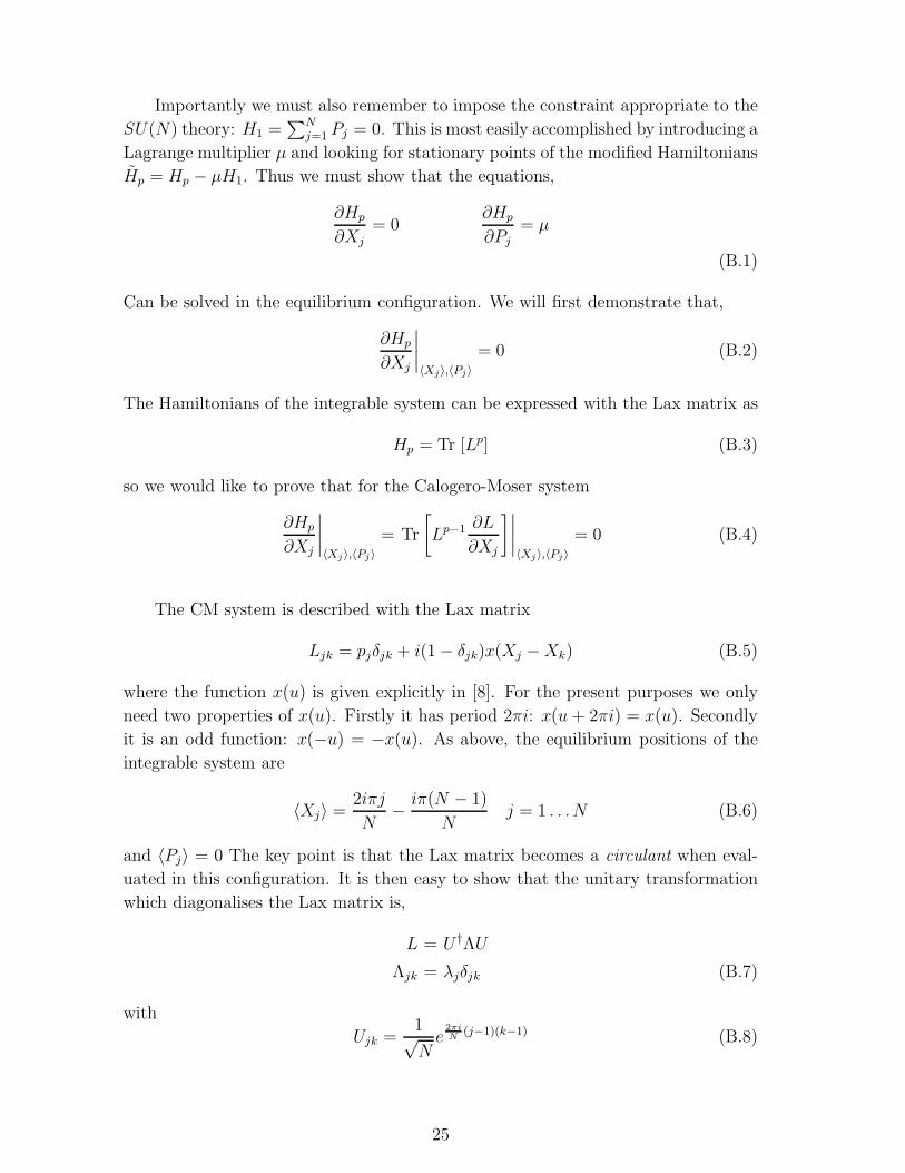
Importantly we must also remember to impose the constraint appropriate to the

SU(N) theory: H1 =∑N

j=1 Pj = 0. This is most easily accomplished by introducing a

Lagrange multiplier µ and looking for stationary points of the modified Hamiltonians

H̃p = Hp − µH1. Thus we must show that the equations,

∂Hp

∂Xj= 0

∂Hp

∂Pj= µ

(B.1)

Can be solved in the equilibrium configuration. We will first demonstrate that,

∂Hp

∂Xj

∣

∣

∣

∣

〈Xj〉,〈Pj〉

= 0 (B.2)

The Hamiltonians of the integrable system can be expressed with the Lax matrix as

Hp = Tr [Lp] (B.3)

so we would like to prove that for the Calogero-Moser system

∂Hp

∂Xj

∣

∣

∣

∣

〈Xj〉,〈Pj〉

= Tr

[

Lp−1 ∂L

∂Xj

]∣

∣

∣

∣

〈Xj〉,〈Pj〉

= 0 (B.4)

The CM system is described with the Lax matrix

Ljk = pjδjk + i(1 − δjk)x(Xj − Xk) (B.5)

where the function x(u) is given explicitly in [8]. For the present purposes we only

need two properties of x(u). Firstly it has period 2πi: x(u + 2πi) = x(u). Secondly

it is an odd function: x(−u) = −x(u). As above, the equilibrium positions of the

integrable system are

〈Xj〉 =2iπj

N− iπ(N − 1)

Nj = 1 . . . N (B.6)

and 〈Pj〉 = 0 The key point is that the Lax matrix becomes a circulant when eval-

uated in this configuration. It is then easy to show that the unitary transformation

which diagonalises the Lax matrix is,

L = U †ΛU

Λjk = λjδjk (B.7)

with

Ujk =1√N

e2πiN

(j−1)(k−1) (B.8)

25

The trace then can be written

Tr

[

Lp−1 ∂L

∂Xj

]∣

∣

∣

∣

〈Xj〉,〈Pj〉

= Tr

[

Λp−1U∂L

∂Xj

∣

∣

∣

∣

〈Xj〉,〈Pj〉

U †

]

(B.9)

Substituting the expressions for the Lax matrix and for U the explicit form of

the trace is

Tr

[

Λp−1U∂L

∂Xj

∣

∣

∣

∣

〈Xj〉,〈Pj〉

U †

]

= − 2

N

N∑

k=1

λp−1k

N∑

l=1,l 6=j

x′(Xj − Xl) sin2π

N(k − 1)(j − l)

(B.10)

Using that x′(u) is an even function and is periodic in ω1 = 2πi we find the terms in

the summation pairwise cancel. Thus the summation gives zero and we conclude

∂Hp

∂Xj

∣

∣

∣

∣

〈Xj〉,〈Pj〉

= 0 (B.11)

Similarly its easy to show that the second equation in (B.1) is solved by choosing

µ = Hp−1. This completes the proof.

References

[1] R. Dijkgraaf and C. Vafa, “Matrix models, topological strings, and supersymmetric

gauge theories,” [hep-th/0206255].

[2] R. Dijkgraaf and C. Vafa, “On geometry and matrix models,” [hep-th/0207106].

[3] R. Dijkgraaf, Talk at “Strings 2002”, Cambridge,

[http://www.damtp.cam.ac.uk/strings02/avt/dijkgraaf/]

[4] R. Dijkgraaf and C. Vafa, “A perturbative window into non-perturbative physics,”

[hep-th/0208048]

[5] O. Aharony, N. Dorey and S. P. Kumar, JHEP 0006, 026 (2000) [hep-th/0006008].

[6] N. Dorey, JHEP 9907, 021 (1999) [hep-th/9906011].

[7] N. Dorey and S. P. Kumar, JHEP 0002, 006 (2000) [hep-th/0001103].

[8] N. Dorey and A. Sinkovics, JHEP 0207, 032 (2002) [hep-th/0205151].

[9] R. Donagi and E. Witten, Nucl. Phys. B 460, 299 (1996) [hep-th/9510101].

[10] A. Gorsky, I. Krichever, A. Marshakov, A. Mironov and A. Morozov, Phys. Lett. B

355, 466 (1995) [hep-th/9505035].

26

[11] E. J. Martinec and N. P. Warner, Nucl. Phys. B 459, 97 (1996) [hep-th/9509161];

E. J. Martinec, Phys. Lett. B 367, 91 (1996) [hep-th/9510204].

[12] N. Dorey, T. J. Hollowood and S. Prem Kumar, Nucl. Phys. B 624, 95 (2002)

[hep-th/0108221].

[13] V. A. Kazakov, I. K. Kostov and N. A. Nekrasov, Nucl. Phys. B 557, 413 (1999)

[hep-th/9810035].

[14] E. T. Whittaker, G. N. Watson, A course of Modern Analysis, 4th edn., Cambridge

University Press, 1927.

[15] N. Dorey, V. V. Khoze and M. P. Mattis, Phys. Lett. B 396, 141 (1997)

[hep-th/9612231].

[16] N. Koblitz, “Introduction to Elliptic Curves and Modular Forms”. Springer-Verlag,

2nd Edition 1993.

[17] C. Vafa and E. Witten, Nucl. Phys. B 431, 3 (1994) [hep-th/9408074].

[18] R. G. Leigh and M. J. Strassler, Nucl. Phys. B 447, 95 (1995) [hep-th/9503121].

[19] I. K. Kostov, Nucl. Phys. B 575, 513 (2000) [hep-th/9911023].

27