Algorithms: Matrix-Matrix Multiplication - University of Illinois
29
UNIVERSITY OF ILLINOIS AT URBANA-CHAMPAIGN Algorithms: Matrix-Matrix Multiplication
-
Upload
khangminh22 -
Category
Documents
-
view
1 -
download
0
Transcript of Algorithms: Matrix-Matrix Multiplication - University of Illinois

UNIVERSITY OF ILLINOIS AT URBANA-CHAMPAIGN
Algorithms: Matrix-Matrix Multiplication

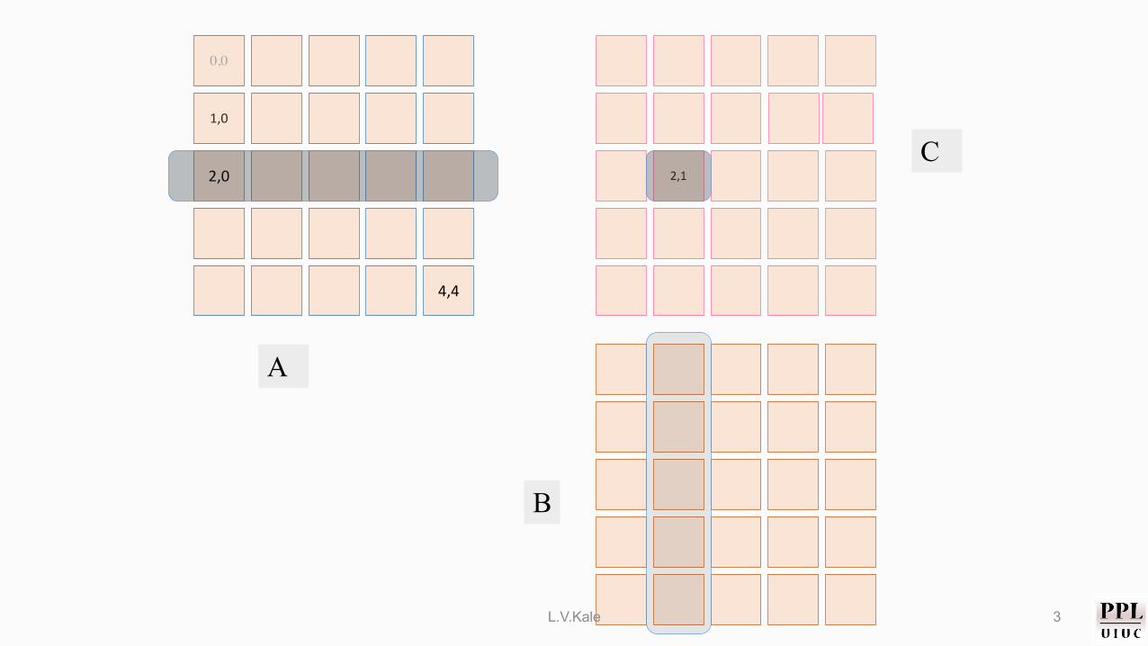
Simple Algorithm• A X B => C, matrices of size NxN, using p = q2 procs• Start with a 2D (block) decomposition of A, B and C
• Each process gets a (N/q)x(N/q) block
L.V.Kale 2
1,0
0,0
2,0
4,4
2,1
A
C
B
L.V.Kale 3

Simple Algorithm• A X B => C, matrices of size NxN, using P = q2 procs• Start with a 2D (block) decomposition of A, B and C
• Each process gets a ( ⁄" #)x( ⁄" #) block
• Each processsor broadcasts it’s A piece along its row, and its B piecealong its column
• Use sub-communicators for this purpose, as we learned
L.V.Kale 4

Simple Algorithm: Analysis• Isoefficiency
• Using communication volume (i.e. # of bytes) as the communication cost• Assume, for now, broadcasting M bytes takes O(M) time
• Communication: 2 𝑝 &'
(
• Computation: &)
(
• *+,,-./*01/+.*+,(-101/+.
= 3 (&'
&)= 3 (
&= k (1)
• W = N3 ; i.e N = W1/3
• Substituting for N in (1): 3 (4 56 )
= k
• So, W = 89)𝑝:.< So, i.e. W ∝ 𝑝:.<
L.V.Kale 5

Simple Algorithm: Analysis• Isoefficiency
• Using communication volume (i.e. # of bytes) as the communication cost• Assume, for now, broadcasting M bytes takes O(M) time
• O(p1.5), which is ok
• What is the problem with this algorithm?• Memory on each processor increases to (q-1) times its original value..
• q-1 blocks of A and q-1 blocks of B!
L.V.Kale 6

Cannon’s Matrix Multiplication Algorithm• Idea is to keep only one tile of B and C on every processor at any step• Tile movements are like a well-choreographed dance• Recall : q is 𝑝• Phase 1:
• Shift each tile of A , Ai,j , leftwards by i steps (i.e. send it to Pi , (j-i)%q )• Shift each tile of B, Bi,j , upwards by j steps
• Phase 2: • Repeat q times:
• Multiply available tiles and add to the local C tile• Shift A tile leftwards and B tile upwards
L.V.Kale 7

0,0
A
C
B
0,1 0,2 0,3 0,4
2,0
3,0
4,0
1,1
2,2
3,3
4,44,1 4,2 4,3
3,1
2,1
1,2 1,3 1,4
2,3 2,4
3,2 3,4
0,0 0,1 0,1 0,3 0,4
2,0
3,0
4,0
1,1
2,2
3,3
4,44,1 4,2 4,3
3,1
2,1
1,2 1,3 1,4
2,3 2,4
3,2 3,4
C[1,0] +=A[1,1]*B[1,0]
C[1,1] +=A[1,2]*B[2,1]
C[1,2] +=A[1,3]*B[3,2]
C[1,3] +=A[1,4]*B[4,3]
C[0,0] +=A[0,0]*B[0,0]
C[0,1] +=A[0,1]*B[1,1]
C[0,2] +=A[0,2]*B[2,2]
C[0,3] +=A[0,3]*B[3,3]
C[2,0] +=A[2,2]*B[2,0]
C[2,1] +=A[2,3]*B[3,1]
C[2,2] +=A[2,4]*B[4,2]
C[2,4] +=A[2,1]*B[1,4]
C[3,0] +=A[3,3]*B[3,0]
C[3,1] +=A[3,4]*B[4,1]
C[3,2] +=A[3,0]*B[0,2]
C[3,3] +=A[3,1]*B[1,3]
C[4,0] +=A[4,4]*B[4,0]
C[4,1] +=A[4,0]*B[0,1]
C[4,2] +=A[4,1]*B[1,2]
C[4,3] +=A[4,2]*B[2,3]
C[4,4] +=A[4,3]*B[3,4]
C[0,4] +=A[0,4]*B[4,4]
C[1,4] +=A[1,0]*B[0,4]
C[2,3] +=A[2,0]*B[0,3]
C[3,4] +=A[3,2]*B[2,4]
1,0
1,0
L.V.Kale 8

A(0,0) A(0,1) A(0,2)
A(1,0) A(1,1) A(1,2)
A(2,0) A(2,1) A(2,2)
B(0,0) B(0,1) B(0,2)
B(1,0) B(1,1) B(1,2)
B(2,0) B(2,1) B(2,2)
C(0,0) C(0,1) C(0,2)
C(1,0) C(1,1) C(1,2)
C(2,0) C(2,1) C(2,2)
L.V.Kale 9

A(0,0) A(0,1) A(0,2)
A(1,0) A(1,1) A(1,2)
A(2,0) A(2,1) A(2,2)
B(0,0) B(0,1) B(0,2)
B(1,0) B(1,1) B(1,2)
B(2,0) B(2,1) B(2,2)
C(0,0) C(0,1) C(0,2)
C(1,0) C(1,1) C(1,2)
C(2,0) C(2,1) C(2,2)
C[0,0] =
L.V.Kale 10

A(0,0) A(0,1) A(0,2)
A(1,0) A(1,1) A(1,2)
A(2,0) A(2,1) A(2,2)
B(0,0) B(0,1) B(0,2)
B(1,0) B(1,1) B(1,2)
B(2,0) B(2,1) B(2,2)
C(0,0) C(0,1) C(0,2)
C(1,0) C(1,1) C(1,2)
C(2,0) C(2,1) C(2,2)
C[0,0] = A[0,0]*B[0,0]
L.V.Kale 11
A(0,0) A(0,1) A(0,2)
A(1,0) A(1,1) A(1,2)
A(2,0) A(2,1) A(2,2)
B(0,0) B(0,1) B(0,2)
B(1,0) B(1,1) B(1,2)
B(2,0) B(2,1) B(2,2)
C(0,0) C(0,1) C(0,2)
C(1,0) C(1,1) C(1,2)
C(2,0) C(2,1) C(2,2)
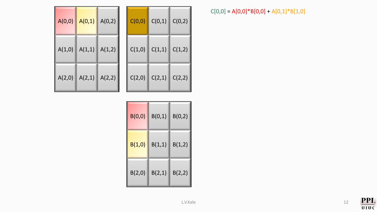
C[0,0] = A[0,0]*B[0,0] + A[0,1]*B[1,0]
L.V.Kale 12

A(0,0) A(0,1) A(0,2)
A(1,0) A(1,1) A(1,2)
A(2,0) A(2,1) A(2,2)
B(0,0) B(0,1) B(0,2)
B(1,0) B(1,1) B(1,2)
B(2,0) B(2,1) B(2,2)
C(0,0) C(0,1) C(0,2)
C(1,0) C(1,1) C(1,2)
C(2,0) C(2,1) C(2,2)
C[0,0] = A[0,0]*B[0,0] + A[0,1]*B[1,0] + A[0,2]*B[2,0]
L.V.Kale 13

Cannon’s Algorithm
L.V.Kale 14

A(0,0) A(0,1) A(0,2)
A(1,0) A(1,1) A(1,2)
A(2,0) A(2,1) A(2,2)
B(0,0) B(0,1) B(0,2)
B(1,0) B(1,1) B(1,2)
B(2,0) B(2,1) B(2,2)
0
1
2
0 1 2
0
1
2
0 1 2
L.V.Kale 15

A(0,0) A(0,1) A(0,2)
A(1,1) A(1,2)
B(0,0) B(0,1) B(0,2)
B(1,0) B(1,1) B(1,2)
B(2,0) B(2,1) B(2,2)
0
1
2
0 1 2
0
1
2
0 1 2
A(2,1) A(2,2)A(2,0)
A(1,0)
L.V.Kale 16

A(0,0) A(0,1) A(0,2)
A(1,2) A(1,0)
B(0,0) B(0,1) B(0,2)
B(1,0) B(1,1) B(1,2)
B(2,0) B(2,1) B(2,2)
0
1
2
0 1 2
0
1
2
0 1 2
A(2,2) A(2,0)A(2,1)
A(1,1)
L.V.Kale 17
A(0,0) A(0,1) A(0,2)
A(1,2) A(1,0)
B(0,0)
B(1,0) B(1,1)
B(2,0) B(2,1)
0
1
2
0 1 2
0
1
2
0 1 2
A(2,0) A(2,1)A(2,2)
A(1,1)
B(0,1)
B(1,2)
B(2,2)
B(0,2)
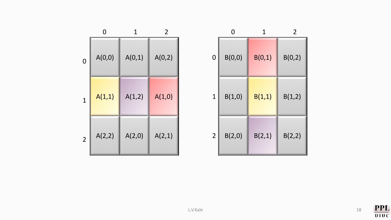
L.V.Kale 18

A(0,0) A(0,1) A(0,2)
A(1,2) A(1,0)
B(0,0)
B(1,0) B(2,1)
B(2,0) B(0,1)
0
1
2
0 1 2
0
1
2
0 1 2
A(2,0) A(2,1)A(2,2)
A(1,1)
B(1,1)
B(2,2)
B(0,2)
B(1,2)
L.V.Kale 19

A(0,0) A(0,1) A(0,2)
A(1,2) A(1,0)
A(2,0) A(2,1)A(2,2)
A(1,1)
B(0,0)
B(1,0) B(2,1)
B(2,0) B(0,1)
B(1,1)
B(0,2)
B(1,2)
B(2,2) C[1,1] =
*
=
C(0,0) C(0,1) C(0,2)
C(1,0) C(1,1) C(1,2)
C(2,0) C(2,1) C(2,2)
L.V.Kale 20

A(0,0) A(0,1) A(0,2)
A(1,2) A(1,0)
A(2,0) A(2,1)A(2,2)
A(1,1)
B(0,0)
B(1,0) B(2,1)
B(2,0) B(0,1)
B(1,1)
B(0,2)
B(1,2)
B(2,2) C[1,1] = A[1,2]*B[2,1] +
*
=
C(0,0) C(0,1) C(0,2)
C(1,0) C(1,1) C(1,2)
C(2,0) C(2,1) C(2,2)
L.V.Kale 21

A(0,1) A(0,2)
A(1,2) A(1,0)
A(2,0) A(2,1)
B(1,0) B(2,1)
B(2,0) B(0,1)
B(0,2)
B(1,2)
C[1,1] = A[1,2]*B[2,1] +
*
=
C(0,0) C(0,1) C(0,2)
C(1,0) C(1,1) C(1,2)
C(2,0) C(2,1) C(2,2)
A(0,0)
A(2,2)
A(1,1)
B(0,0) B(1,1) B(2,2)
L.V.Kale 22

A(0,2) A(0,0)
A(1,0) A(1,1)
A(2,1) A(2,2)
B(2,0) B(0,1)
B(0,0) B(1,1)
B(1,2)
B(2,2)
C[1,1] = A[1,2]*B[2,1] + A[1,0]*B[0,1] +
*
=
C(0,0) C(0,1) C(0,2)
C(1,0) C(1,1) C(1,2)
C(2,0) C(2,1) C(2,2)
A(0,1)
A(2,0)
A(1,2)
B(1,0) B(2,1) B(0,2)
L.V.Kale 23

A(0,0) A(0,1)
A(1,1) A(1,2)
A(2,2) A(2,0)
B(0,0) B(1,1)
B(1,0) B(2,1)
B(2,2)
B(0,2)
C[1,1] = A[1,2]*B[2,1] + A[1,0]*B[0,1] + A[1,1]*B[1,1]
*
=
C(0,0) C(0,1) C(0,2)
C(1,0) C(1,1) C(1,2)
C(2,0) C(2,1) C(2,2)
A(0,2)
A(2,1)
A(1,0)
B(2,0) B(0,1) B(1,2)
L.V.Kale 24

Cannon’s Algorithm: analysis• Same amount of communication
• Think about what data comes in to a processor• So, same isoefficiency: O(p1.5)
L.V.Kale 25

Johnson’s 3D Matrix Multiplication• How can we reduce communication?• The matrix multiplication (sequential) has 3 nested loops, and we
tiled only the outer 2. • What if we tile the 3rd (k) loop as well?
• What does that mean in distributed memory context?• Note that the k loop is involves a reduction
• Basic idea: • organize processes in a 3D cube of cubes, • distribute A on one face of the process cube• Distribute B on another phase of the process cube• Collect C on the 3rd phase of the process cube
L.V.Kale 26

C on this
surface
A on this surface
B on this surface
Tile size = &> 56 )
x &> 56 )
3D Matrix Multiplication

3D Matrix Multiplication: Analysis• Tile size = &
> 56 )x &
> 56 )
• Assuming pipelined broadcast, and ignoring per-message cost (because messages are large), each process receives 2 tiles:
• Communication volume proportional to &∗&> 5' )
• Computation, as always: &)
(
• Exercise: calculate isoefficiency• Memory pressure:
• More than Cannon’s but less than the original (multicast based) version• Each tile is duplicated in 𝑝:/A places (as opposed to 𝑝 places in
L.V.Kale 28

Another new Algorithm: 2.5D matrix mpy• Optional reading for interested students• Edgar Solomonic (now at UIUC), and J. Demmel (Berkeley)
• Communication-optimal parallel 2.5D matrix multiplication and LU factorization algorithms, 2011
L.V.Kale 29