Modular Multiplication in the Residue Number System
191
Modular Multiplication in the Residue Number System A DISSERTATION SUBMITTED TO THE SCHOOL OF ELECTRICAL AND ELECTRONIC ENGINEERING OF THE UNIVERSITY OF ADELAIDE BY Yinan KONG IN PARTIAL FULFILLMENT OF THE REQUIREMENTS FOR THE DEGREE OF DOCTOR OF PHILOSOPHY July 2009
-
Upload
khangminh22 -
Category
Documents
-
view
4 -
download
0
Transcript of Modular Multiplication in the Residue Number System

Modular Multiplication in the
Residue Number System
A DISSERTATION SUBMITTED TO
THE SCHOOL OF ELECTRICAL AND ELECTRONIC ENGINEERING
OF THE UNIVERSITY OF ADELAIDE
BY
Yinan KONG
IN PARTIAL FULFILLMENT OF THE REQUIREMENTS FOR
THE DEGREE OF DOCTOR OF PHILOSOPHY
July 2009

Declaration of Originality
Name: Yinan KONG Program: Ph.D.
This work contains no material which has been accepted for the award
of any other degree or diploma in any university or other tertiary institution
and, to the best of my knowledge and belief, contains no material previously
published or written by another person, except where due reference has been
made in the text.
I give consent to this copy of my thesis, when deposited in the Univer-
sity Library, being made available for loan and photocopying, subject to the
provisions of the Copyright Act 1968.
The author acknowledges that copyright of published works contained
within this thesis (as listed below) resides with the copyright holder/s of
those works.
Signature: Date:
i

ii

AcknowledgmentsMy supervisor, Dr Braden Jace Phillips, is an extremely hard working and
dedicated man. So, first and foremost, I would like to say “thank you” to
him, for his critical guidance, constant sustainment and role modelling as a
supervisor. It is my true luck that I have been able to work with him for
these years. This has been a precious experience which deserves my cherish-
ing throughout my whole life.
I am also grateful to Associate Professor Cheng-Chew Lim and Dr Alison
Wolff for their guidance through important learning phases of this complex
technology. Throughout the course of my study I have received considerable
help from my colleagues Daniel Kelly and Zhining Lim, who have been, and
will remain, my great friends.
Acknowledgement is given to the Australian Research Council (ARC) as
this work has been supported by the ARC Discovery Project scheme.
Thanks to the support from my family and friends. I have been relying
on you throughout my candidature. Thanks are due to Mum, Dad, Ranran,
Zhaozhao and Jingdong JU, who flew over 5000 miles to take care of me. I
would definitely not have been able to get to this point without your encour-
agement. You are the real pearls lying on the bottom of my mind.
Mother, thank you for giving birth to me as well as cultivating me through
those tough years. This thesis has your sweat in it.
My love, BEN YA, you are my greatest inspiration. Thank you for all
you have done for me.
Yinan KONG
November 2008
iii

iv

AbstractPublic-key cryptography is a mechanism for secret communication be-
tween parties who have never before exchanged a secret message. This thesis
contributes arithmetic algorithms and hardware architectures for the modu-
lar multiplication Z = A × B mod M . This operation is the basis of many
public-key cryptosystems including RSA and Elliptic Curve Cryptography.
The Residue Number System (RNS) is used to speed up long word length
modular multiplication because this number system performs certain long
word length operations, such as multiplication and addition, much more ef-
ficiently than positional systems.
A survey of current modular multiplication algorithms shows that most
work in a positional number system, e.g. binary. A new classification is de-
veloped which classes these algorithms as Classical, Sum of Residues, Mont-
gomery or Barrett. Each class of algorithm is analyzed in detail, new devel-
opments are described, and the improved algorithms are implemented and
compared using FPGA hardware.
Few modular multiplication algorithms for use in the RNS have been
published. Most are concerned with short word lengths and are not appli-
cable to public-key cryptosystems that require long word length operations.
This thesis sets out the hypothesis that each of the four classes of modular
multiplication algorithms possible in positional number systems can also be
used for long word length modular multiplication in the RNS; moreover using
the RNS in this way will lead to faster implementations than those which re-
strict themselves to positional number systems. This hypothesis is addressed
by developing new Classical, Sum of Residues and Barrett algorithms for
modular multiplication in the RNS. Existing Montgomery RNS algorithms
are also discussed.
The new Sum of Residues RNS algorithm results in a hardware im-
v

plementation that is novel in many aspects: a highly parallel structure using
short arithmetic operations within the RNS; fully scalable hardware; and
the fastest ever FPGA implementation of the 1024-bit RSA cryptosystem at
0.4 ms per decryption.
vi
Publications1. Yinan Kong and Braden Phillips, “Fast Scaling in the Residue Number
System”, accepted by IEEE Transactions on VLSI Systems in Decem-
ber 2007.
2. Yinan Kong and Braden Phillips, “Simulations of modular multipliers
on FPGAs”, Proceedings of the IASTED Asian Conference on Mod-
elling and Simulation, Beijing, China, Oct. 2007, pp. 11281131.
3. Yinan Kong and Braden Phillips, “Comparison of Montgomery and
Barrett modular multipliers on FPGAs”, 40th Asilomar Conference
on Signals, Systems and Computers. Pacific Grove, CA, USA: IEEE,
Piscataway, NJ, USA, Oct. 2006, pp. 16871691.
4. Yinan Kong and Braden Phillips, “Residue number system scaling
schemes”, in Smart Structures, Devices, and Systems II, ser. Proc.
SPIE, S. F. Al-Sarawi, Ed., vol. 5649, Feb. 2005, pp. 525536.
5. Yinan Kong and Braden Phillips, “A classical modular multiplier for
RNS channel operations”, The University of Adelaide, CHiPTec Tech.
Rep. CHIPTEC-05-02, November 2005.
6. Yinan Kong and Braden Phillips, “A Montgomery modular multiplier
for RNS channel operations”, The University of Adelaide, CHiPTec
Tech. Rep. CHIPTEC-05-02, November 2005.
vii

Publications in Submission1. Yinan Kong and Braden Phillips, “Modular Reduction and Scaling
in the Residue Number System Using Multiplication by the Inverse”,
submitted to IEEE Transactions on VLSI Systems in November 2008.
2. Yinan Kong and Braden Phillips, “Low latency modular multiplica-
tion for public-key cryptosystems using a scalable array of parallel pro-
cessing elements”, submitted to 19th IEEE Computer Arithmetic in
October 2008.
3. Braden Phillips and Yinan Kong, “Highly Parallel Modular Multiplica-
tion in the Residue Number System using Sum of Residues Reduction”,
submitted to Journal of Applicable Algebra in Engineering, Communi-
cation and Computing in June 2008.
4. Yinan Kong and Braden Phillips, “Revisiting Sum of Residues Mod-
ular Multiplication”, submitted to International Journal of Computer
Systems Science and Engineering in May 2008.
viii

Nomenclature
〈X〉M The operation X mod M .
D The dynamic range of a RNS.
M The modulus of a modular multiplication, typically n bits.
mi The ith RNS channel modulus.
N The number of RNS channels.
n The wordlength of M .
w The RNS channel width.
�X� The ceiling of X. The smallest integer greater than or equal to X.
�X� The floor of X. The largest integer smaller than or equal to X.
BE Base Extension.
CRT Chinese Remainder Theorem.
DSP Digital Signal Processing.
ECC Elliptic Curve Cryptography.
LUC Look-Up Cycle.
LUT Look-Up Table.
LUT Look-Up Table
ix

MRS Mixed Radix Number System.
QDS Quotient Digit Selection.
RNS Residue Number System.
RSA RSA Cryptography.
x

Contents
1 Introduction 1
1.1 Thesis Outline . . . . . . . . . . . . . . . . . . . . . . . . . . 2
1.2 Contribution . . . . . . . . . . . . . . . . . . . . . . . . . . . 4
2 Background 7
2.1 Residue Number Systems . . . . . . . . . . . . . . . . . . . . . 8
2.1.1 RNS Representation . . . . . . . . . . . . . . . . . . . 8
2.1.2 Conversion between RNS and Positional Number Sys-
tems . . . . . . . . . . . . . . . . . . . . . . . . . . . . 9
2.1.3 RNS Arithmetic . . . . . . . . . . . . . . . . . . . . . 14
2.1.4 Moduli Selection . . . . . . . . . . . . . . . . . . . . . 15
2.1.5 Base Extension . . . . . . . . . . . . . . . . . . . . . . 16
2.2 RSA Public-Key Cryptography . . . . . . . . . . . . . . . . . 18
2.2.1 Public-Key Cryptography . . . . . . . . . . . . . . . . 18
2.2.2 The RSA Cryptosystem . . . . . . . . . . . . . . . . . 19
2.2.3 Exponentiation . . . . . . . . . . . . . . . . . . . . . . 20
3 Four Ways to Do Modular Multiplication in a Positional
Number System 25
3.1 Introducing Four Ways to Do Modular Multiplication . . . . 26
3.1.1 Classical Modular Multiplication . . . . . . . . . . . . 27
3.1.2 Sum of Residues Modular Multiplication . . . . . . . . 29
3.1.3 Barrett Modular Multiplication . . . . . . . . . . . . . 30
3.1.4 Montgomery Modular Multiplication . . . . . . . . . . 31
xi

CONTENTS
3.2 Reinvigorating Sum of Residues . . . . . . . . . . . . . . . . . 33
3.2.1 Tomlinson’s Algorithm . . . . . . . . . . . . . . . . . . 33
3.2.2 Eliminating the Carry Propagate Adder . . . . . . . . 35
3.2.3 Further Enhancements . . . . . . . . . . . . . . . . . . 37
3.2.4 High Radix . . . . . . . . . . . . . . . . . . . . . . . . 40
3.2.5 Summary of the Sum of Residues Modular Multiplica-
tion . . . . . . . . . . . . . . . . . . . . . . . . . . . . 40
3.3 Bounds of Barrett Modular Multiplication . . . . . . . . . . . 42
3.3.1 Bound Deduction . . . . . . . . . . . . . . . . . . . . 42
3.3.2 Performance at Different Word Lengths . . . . . . . . 45
3.4 Montgomery Modular Multiplication on FPGA . . . . . . . . 47
3.4.1 Separated Montgomery Modular Multiplication Algo-
rithm . . . . . . . . . . . . . . . . . . . . . . . . . . . 47
3.4.2 High Radix Montgomery Algorithm . . . . . . . . . . 47
3.4.3 Bound Deduction . . . . . . . . . . . . . . . . . . . . 54
3.4.4 Interleaved vs. Separated Structure . . . . . . . . . . . 57
3.4.5 Trivial Quotient Digit Selection . . . . . . . . . . . . . 58
3.4.6 Quotient Digit Pipelining . . . . . . . . . . . . . . . . 62
3.5 Modular Multiplications within RNS Channels . . . . . . . . . 69
4 Four Ways to Do Modular Multiplication in the Residue
Number System 71
4.1 Short Word Length RNS Modular Multiplications using Look-
Up Tables . . . . . . . . . . . . . . . . . . . . . . . . . . . . . 73
4.1.1 RNS Modular Reduction, Scaling and Look-Up Tables 74
4.1.2 Existing RNS Scaling Schemes using Look-Up Tables . 75
4.1.3 A New RNS Scaling Scheme using Look-Up Tables . . 88
4.2 RNS Classical Modular Multiplication . . . . . . . . . . . . . 93
4.2.1 The Core Function . . . . . . . . . . . . . . . . . . . . 93
4.2.2 A Classical Modular Multiplication Algorithm in RNS
using the Core Function . . . . . . . . . . . . . . . . . 97
4.2.3 Examples . . . . . . . . . . . . . . . . . . . . . . . . . 105
xii

CONTENTS
4.3 RNS Sum of Residues Modular Multiplication . . . . . . . . . 109
4.3.1 Sum of Residues Reduction in the RNS . . . . . . . . . 109
4.3.2 Approximation of α . . . . . . . . . . . . . . . . . . . . 110
4.3.3 Bound Deduction . . . . . . . . . . . . . . . . . . . . . 115
4.3.4 The RNS Sum of Residues Modular Multiplication Al-
gorithm . . . . . . . . . . . . . . . . . . . . . . . . . . 117
4.4 RNS Barrett Modular Multiplication . . . . . . . . . . . . . . 121
4.4.1 RNS Modular Reduction using Barrett Algorithm . . . 121
4.4.2 The Algorithm . . . . . . . . . . . . . . . . . . . . . . 127
4.5 RNS Montgomery Modular Multiplication . . . . . . . . . . . 133
4.5.1 Montgomery Modular Reduction in RNS . . . . . . . . 133
4.5.2 The Algorithm . . . . . . . . . . . . . . . . . . . . . . 136
4.5.3 A Comparison between RNS Barrett and Montgomery
Modular Multiplication . . . . . . . . . . . . . . . . . . 136
5 Implementation of RNS Sum of Residues Modular Multipli-
cation 141
5.1 A Scalable Structure for Sum of Residues Modular Multipli-
cation in RNS . . . . . . . . . . . . . . . . . . . . . . . . . . . 142
5.1.1 A 4-Channel Architecture . . . . . . . . . . . . . . . . 143
5.1.2 The Scaled Architecture for Modular Multiplication . . 144
5.2 Implementation Results . . . . . . . . . . . . . . . . . . . . . 149
6 Conclusion and Future Perspectives 153
6.1 Conclusion . . . . . . . . . . . . . . . . . . . . . . . . . . . . 154
6.2 Future Perspectives . . . . . . . . . . . . . . . . . . . . . . . 154
Bibliography 157
xiii

CONTENTS
xiv

List of Figures
2.1 Conversion from the RNS to the Mixed Radix Number System
(MRS) . . . . . . . . . . . . . . . . . . . . . . . . . . . . . . . 12
3.1 An Architecture for Tomlinson’s Modular Multiplication Al-
gorithm [Tomlinson89] . . . . . . . . . . . . . . . . . . . . . . 34
3.2 Modified Sum of Residues Modular Multiplier Architecture . . 36
3.3 n-bit Carry Save Adders . . . . . . . . . . . . . . . . . . . . . 37
3.4 New Sum of Residues Modular Multiplier Architecture . . . . 38
3.5 An Example for New Sum of Residues Modular Multiplication
n = 4, A = (1111)2, B = (1011)2 and M = (1001)2 . . . . . . . 39
3.6 New High-Radix Sum of Residues Modular Multiplier Archi-
tecture . . . . . . . . . . . . . . . . . . . . . . . . . . . . . . . 41
3.7 Delays and Areas of Improved Barrett Modular Multiplication
Algorithm . . . . . . . . . . . . . . . . . . . . . . . . . . . . . 46
3.8 Delays of Montgomery Modular Multiplication at Different
Radices. . . . . . . . . . . . . . . . . . . . . . . . . . . . . . . 54
3.9 Delays and Areas of Interleaved and Separated Montgomery
Modular Multiplication at Different Radices . . . . . . . . . . 59
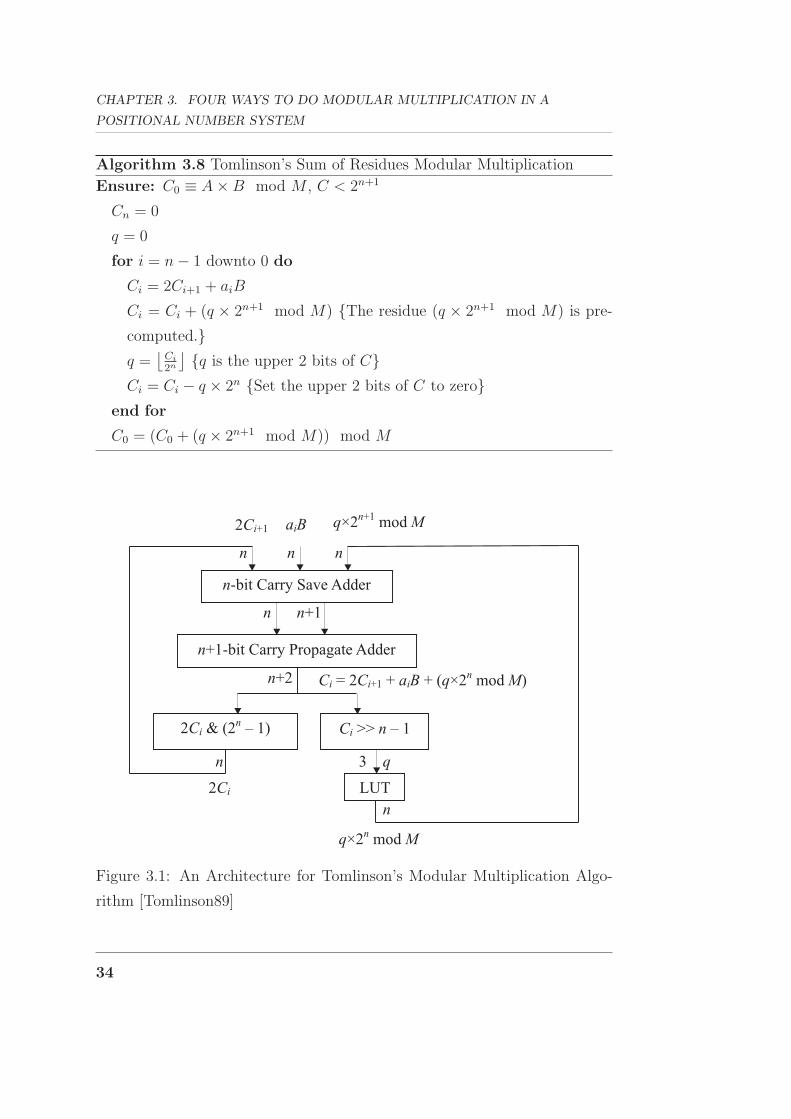
3.10 Shortest Delays of Separated Montgomery Multiplication Al-
gorithm using Trivial QDS at n from 12 to 32 . . . . . . . . . 62
3.11 Shortest Delays of Separated Montgomery Multiplication Al-
gorithm using Quotient Digit Pipelining at n from 13 to 32 . . 67
xv

LIST OF FIGURES
3.12 Shortest Delays of Separated Montgomery Multiplication Al-
gorithm with & without Quotient Digit Pipelining at n from
13 to 32 . . . . . . . . . . . . . . . . . . . . . . . . . . . . . . 68
3.13 Delays and Areas of Four Classes of Modular Multipliers in
Binary . . . . . . . . . . . . . . . . . . . . . . . . . . . . . . . 70
4.1 RNS Scaling using Look-Up Tables. . . . . . . . . . . . . . . . 75
4.2 The 3 Modulus RNS Scaler . . . . . . . . . . . . . . . . . . . 77
4.3 RNS Scaling using Estimation for Channels S + 1 ≤ i ≤ N . . 80
4.4 RNS Scaling using a Decomposition of the CRT (two redun-
dant channels with channel mi) . . . . . . . . . . . . . . . . . 83
4.5 RNS Scaling using Parallel Base Extension (BE) Blocks . . . . 85
4.6 Parallel Architecture to Perform Y =⌊
XM
⌋ ≈∑Ni=1 f(xi). . . . 86
4.7 One Channel of a Parallel Residue Arithmetic Process using
Memories with Addressing Capacity = r. . . . . . . . . . . . . 87
4.8 A New Architecture to Perform Short Word length Scaling in
RNS . . . . . . . . . . . . . . . . . . . . . . . . . . . . . . . . 90
4.9 A Typical Core Function C(X): D = 30030; C(D) = 165 . . . 95
4.10 The h Least Significant Bits to be Maintained during the Mod-
ular Multiplication 〈xiC(σi)〉2h . . . . . . . . . . . . . . . . . . 102
4.11 An End-Around Adder to Compute 〈θi + θi+1〉2k−1. . . . . . . 126
4.12 Architecture for Scaling by 2 in RNS . . . . . . . . . . . . . . 128
4.13 High-Radix Architecture for Scaling by 2l in RNS . . . . . . . 129
4.14 Delay of Channel-Width Multiplication and Addition modulo
a General Modulus and Multiplication and Addition modulo
2k − 1 used for RNS Barrett Algorithm against RNS Channel
Width w . . . . . . . . . . . . . . . . . . . . . . . . . . . . . . 132
4.15 Delay of Barrett and Montgomery RNS Modular Multiplica-
tion against RNS Channel Width w . . . . . . . . . . . . . . . 138
5.1 A 4-Channel RNS Modular Multiplier . . . . . . . . . . . . . . 145
xvi

LIST OF FIGURES
5.2 A 4-Channel Modular Multiplier Block Suitable for a Scalable
Array of Blocks . . . . . . . . . . . . . . . . . . . . . . . . . . 146
5.3 A 12-Channel Modular Multiplier Built from a 3× 3 Array of
4-Channel Blocks . . . . . . . . . . . . . . . . . . . . . . . . . 148
xvii

LIST OF FIGURES
xviii

List of Tables
2.1 The Pre-Computed Constants of RNS {3, 5, 7} . . . . . . . . . 9
2.2 An Example of Right-to-Left Modular Exponentiation . . . . . 23
3.1 Montgomery Modular Reduction Process at Radix 2 . . . . . . 49
3.2 Montgomery Modular Reduction Process at Radix 4 . . . . . . 50
3.3 Montgomery Modular Reduction Process at Radix 8 (l =⌈
nk
⌉) 52
3.4 Montgomery Modular Reduction Process at Radix 8 (l =⌊
nk
⌋) 53
3.5 The k-boundary of Montgomery Reduction for n from 12 to 32 61
3.6 Shortest Delays of Separated Montgomery Multiplication Al-
gorithm using Trivial QDS at n from 12 to 32 . . . . . . . . . 61
3.7 k and d in Quotient Digit Pipelining of Montgomery Algorithm
for n from 12 to 25 . . . . . . . . . . . . . . . . . . . . . . . . 66
3.8 Shortest Delays of Separated Montgomery Multiplication Al-
gorithm using Quotient Digit Pipelining at n from 13 to 32 . . 67
4.1 A Comparison of 6 Short Word length RNS Scaling Schemes
using LUTs . . . . . . . . . . . . . . . . . . . . . . . . . . . . 92
4.2 An Example of Pre-Computed Parameters for the Classical
Modular Reduction Algorithm in RNS using the Core Function106
4.3 An Example of the Classical Modular Reduction Algorithm in
RNS using the Core Function for a case in which �Mag(X)� ≥ 1107
4.4 An Example of the Classical Modular Reduction Algorithm in
RNS using the Core Function for a case in which �Mag(X)� < 1108
xix

LIST OF TABLES
4.5 The Maximum Possible N against w in RNS Sum of Residues
Reduction . . . . . . . . . . . . . . . . . . . . . . . . . . . . . 113
5.1 The Pre-Computed Constants for the RNS Sum of Residues
Modular Multiplication Algorithm in Algorithm 4.2 . . . . . . 144
xx

Chapter 1
Introduction
The purpose of this chapter is to outline the thesis by chapters and present
the contribution this thesis makes.
1

CHAPTER 1. INTRODUCTION
1.1 Thesis Outline
In the information age, cryptography has become a cornerstone for informa-
tion security. Cryptography allows people to carry established notions of
trust from the physical world to the electronic world; it allows people to do
business electronically without worries of deceit and deception; and it estab-
lishes trust for people through open, standards-based, security technology
that withstands the test of time.
In the distant past, cryptography was used to assure only secrecy. Wax
seals, signatures, and other physical mechanisms were typically used to assure
integrity of the message and authenticity of the sender. When people started
doing business online and needed to transfer funds electronically, the use of
cryptography for integrity began to surpass its use for secrecy. Hundreds of
thousands of people interact electronically every day, whether it is through e-
mail, e-commerce, ATM machines, or cellular phones. The constant increase
of information transmitted electronically has led to an increased reliance on
the transport of trust made possible by public-key cryptography, a mechanism
for secret communication between parties who have never before exchanged
a secret message.
One can argue that public-key cryptosystems become more secure as the
hardware used to perform cryptography increases in speed. Take the RSA
cryptosystem as an example [Rivest78]. The effort of cracking the RSA code,
via factorization of the product of two large primes, approximately doubles
for every 35 bits at key lengths around 210 bits [Crandall01]. However, adding
35 bits to the key increases the work involved in decryption by only 10%!
Thus speeding up the cryptography hardware by just 10% enables the use of
a cryptosystem that is twice as strong with no compromise in performance
[Koblitz87]. Speed, therefore, is an important goal for public-key cryptosys-
2

1.1. THESIS OUTLINE
tems. Indeed it is essential not just for cryptographic strength but also to
clear the large number of transactions performed by central servers in elec-
tronic commerce systems.
This thesis contributes to the modular multiplication operation Z =
A × B mod M , the basis of many public-key cryptosystems including RSA
[Rivest78] and Elliptic Curve Cryptography (ECC) over a prime finite field
[Hankerson04]. The Residue Number System (RNS) [Omondi07] is used to
speed up long word length modular multiplication.
Chapter 2 provides the background to the Residue Number System and
the RSA cryptosystem.
Chapter 3 defines a new classification of current modular multiplication
algorithms in a positional number system. The four classes in this definition
are Classical, Sum of Residues, Barrett and Montgomery. Further develop-
ments are made to these algorithms and implementations are prepared for the
modular multiplications within RNS channels that will appear in Chapter 5.
Chapter 4 is the core of this thesis. Firstly it surveys existing modular
multiplication algorithms in the RNS. Most of these schemes are designed
for short word length operands and hence are not applicable in public-key
cryptosystems that require long word length moduli. One reason for this
incompatibility is that their architectures are typically based on Look-Up
Tables (LUT). For long word length operands, these tables become infeasi-
bly large. However, they are still useful for other applications of RNS, e.g.
Digital Signal Processing (DSP). A new scheme of this kind is then derived
and decreases hardware complexity compared to previous schemes without
affecting time complexity.
Chapter 4 then explores the possibility that each of the four classes of
modular multiplication algorithms for positional number systems can be
3

CHAPTER 1. INTRODUCTION
adopted for modular multiplication in the RNS. The goal is a long word
length operation that is faster than working in a positional number system.
Ideally all intermediate processes will be short word length operations en-
tirely within RNS channels.
Chapter 5 illustrates a highly parallel and scalable architecture for the
RNS sum of residues modular multiplication algorithm discussed in Chap-
ter 4. This architecture is then implemented on a Xilinx Virtex5 FPGA plat-
form using results from Chapter 3 for RNS channel operations. The delay for
a 64-bit RNS modular multiplier is 81.7 ns. 0.4 μs and 0.73 μs are required
to perform 1024-bit and 2048-bit modular multiplication respectively. The
corresponding speed of a 1024-bit RSA system is 0.4 ms per decryption.
Chapter 6 concludes the work and suggests some areas for further study.
1.2 Contribution
The following contributions are presented in this thesis:
• A new classification of existing modular multiplication algorithms in a
positional number system. New developments are made and improved
algorithms are implemented on FPGA platforms.
• Existing algorithms performing short word length modular multipli-
cation in RNS are characterized in terms of Look-Up Cycles (LUC)
and Look-Up Tables (LUT) within a consistent framework. A new
LUT-based algorithm that is applicable in DSP achieves less hardware
complexity compared to existing algorithms.
• New algorithms are developed for Classical, Sum of Residues and Bar-
rett classes for a long word length modular multiplication in the Residue
4

1.2. CONTRIBUTION
Number System. All the intermediate operations are kept within RNS
channels, which leads to a highly parallel architecture performing a fast
long word length modular multiplication in the RNS in hardware.
• The fastest ever FPGA implementation of the 1024-bit RSA cryptosys-
tem. It achieves 0.4 ms per decryption.
5

CHAPTER 1. INTRODUCTION
6

Chapter 2
Background
The purpose of this chapter is to introduce the Residue Number System and
RSA cryptography. The Residue Number System is the main mathematical
tool used to improve the performance of public-key cryptosystems in this
thesis. The background on the Residue Number System is the basis of tech-
nical developments made in later chapters, particularly in Chapter 4. The
introduction of RSA cryptography aims to show the significance of improving
the efficiency of the long word length modular multiplication operation.
7

CHAPTER 2. BACKGROUND
2.1 Residue Number Systems
2.1.1 RNS Representation
What number has the remainders of 2, 3 and 2 when divided by the numbers
3, 5 and 7 respectively? This question is probably the first documented use
of residue arithmetic in representing numbers, recorded by a Chinese Scholar
Sun Tsu over 1500 years ago [Jenkins93]. The question basically asks us to
convert the coded representation {2, 3, 2} in a residue number system, based
on the moduli {3, 5, 7}, back to its normal decimal format.
A Residue Number System [Szabo67] is characterized by a set of N co-
prime moduli {m1,m2, . . . , mN} with m1 < m2 < · · · < mN . In the RNS a
number X is represented in N channels: X = {x1, x2, . . . , xN}, where xi is
the residue of X with respect to mi, i.e. xi = 〈X〉mi= X mod mi. Hence a
RNS has digit sets {[0,m1 − 1], [0,m2 − 1], [0,m3 − 1], . . . ,[0,mN − 1]} in its
N channels. For example, in the RNS with the modulus set {3, 5, 7} above,
X = {2, 3, 2}. The word length of the largest channel mN is defined as the
channel width w.
Within a RNS: there is a unique representation of all integers in the range
0 ≤ X < D where D = m1m2 . . . mN . Also, D is the number of different
representable values in the RNS and is therefore known as the dynamic range
of the RNS. Hence D = 3×5×7 = 105 is the total number of distinct values
that are representable in the example above. These 105 available values can
be used to represent numbers 0 through 104, -52 through +52 or any other
interval of 105 consecutive integers. This thesis considers the non-negative
numbers from 0 to D − 1 only, as the RNS is used for positive modular
arithmetic.
There are two other important values in a RNS, Di and 〈D−1i 〉mi
. Di =
8

2.1. RESIDUE NUMBER SYSTEMS
Table 2.1: The Pre-Computed Constants of RNS {3, 5, 7}N 3
D 105
i 1 2 3
mi 3 5 7
Di 35 21 15
〈Di〉mi2 1 1
〈D−1i 〉mi
2 1 1
Dmi
and 〈D−1i 〉mi
is its multiplicative inverse with respect to mi such that
〈Di × D−1i 〉mi
= 1. These values are constants for a particular modulus set
and can be pre-computed before any actual computations are performed in
a RNS. For example, in RNS {3, 5, 7}, the Di set is {35, 21, 15} and the
〈D−1i 〉mi
set is {2, 1, 1}. Thus, each RNS has a table of known constants that
might be useful in future computations. Table 2.1 lists some of the constants
of RNS {3, 5, 7}.
2.1.2 Conversion between RNS and Positional Num-
ber Systems
Conversion from Binary to RNS
The binary-to-RNS conversion is quite a simple problem compared with the
conversion in the opposite direction. All that is required is to find the residue
of X mod mi for each modulus. Computing X mod mi for binary values
X and m is a typical modular reduction problem and will be discussed in
detail in Chapter 3.
For example, if X = 23 is to be converted into its RNS format based on
the moduli {3, 5, 7}, then x1 = 〈23〉3 = 2, x2 = 〈23〉5 = 3 and x3 = 〈23〉7 = 2.
9

CHAPTER 2. BACKGROUND
Conversion from RNS to Positional Number Systems using the
Mixed Radix Number System (MRS)
Associated with any RNS {m1,m2, . . . , mN} is a Mixed Radix Number System
(MRS) {m1,m2, . . . , mN} [Soderstrand86], which is an N -digit positional
number system with position weights
1, m1, m1m2, m1m2m3, . . . , m1m2m3 . . .mN−1
and digit sets {[0,m1 − 1], [0,m2 − 1], [0,m3 − 1], . . . , [0,mN − 1]} in its
N digit positions. Hence, the MRS digits are in the same ranges as the
RNS residues. For example, the MRS {3, 5, 7} has position weights 1, 3 and
3 × 5 = 15.
The RNS-to-MRS conversion is to determine the gi digits of MRS, given
the xi digits of RNS, so that {g1, g2, . . . , gN} = {x1, x2, . . . , xN}. From the
definition of MRS, we have
X = g1 + g2m1 + g3m1m2 + · · · + gNm1m2m3 . . . mN−1.
A modular reduction, with respect to m1, of both sides of this equation yields
〈X〉m1 = g1.
Hence g1 = x1. Subtracting x1 and dividing both sides by m1 yields
X − g1
m1
= g2 + g3m2 + · · · + gNm2m3 . . . mN−1.
Now reduction modulo m2 yields g2 as
g2 = 〈(X − g1)m−11 〉m2 = 〈(x2 − g1)m
−11 〉m2
because the equality 〈X−g1
m1〉m2 = 〈(X−g1)m
−11 〉m2 holds according to a prop-
erty in number theory [Richman71]. A prerequisite for this is that m1 and
10

2.1. RESIDUE NUMBER SYSTEMS
m2 must be co-prime so that 〈m−11 〉m2 exists. This is exactly what happens
in a RNS.
Following a similar procedure,
X−g1
m1− g2
m2
= g3 + g4m3 + · · · + gNm3 . . . mN−1,
g3 can be obtained as
g3 = 〈((X − g1)m−11 − g2)m
−12 〉m3 = 〈((x3 − g1)m
−11 − g2)m
−12 〉m3 .
Continuing this process, the mixed radix digits, gi, can be retrieved from
RNS residues as
g1 = x1
g2 = 〈(x2 − g1)m−11 〉m2
g3 = 〈((x3 − g1)m−11 − g2)m
−12 〉m3
. . .
gN = 〈((. . . ((xN − g1)m−11 − g2)m
−12 . . . )m−1
N−2 − gN−1)m−1N−1〉mN
All the 〈m−1i 〉mj
are constants that can be pre-computed. Figure 2.1 illus-
trates this process implemented using N(N−1)2
modular blocks. Each block
performs an operation like 〈(xj −gi)m−1i 〉mj
. As can be seen from Figure 2.1,
the disadvantage of this algorithm is the sequentiality of the structure. The
computation of gi has to wait for the result of gi−1.
Take X = {2, 3, 2} in RNS {3, 5, 7} as an example. Pre-computed con-
stants include
〈m−11 〉m2 = 2,
〈m−11 〉m3 = 5,
and 〈m−12 〉m3 = 3.
11

CHAPTER 2. BACKGROUND
1x
2x
3x Nx
2m�
3m�
Nm�
Nm�
Nm�
……
1g
3m�
……
……
……
……
2g 3
g Ng
Figure 2.1: Conversion from the RNS to the Mixed Radix Number System
(MRS)
12

2.1. RESIDUE NUMBER SYSTEMS
Then the corresponding MRS digits are
g1 = x1 = 2
g2 = 〈(x2 − g1)m−11 〉m2 = 〈(3 − 2) × 2〉5 = 2
g3 = 〈((x3 − g1)m−11 − g2)m
−12 〉m3 = 〈((2 − 2) × 5 − 2) × 3〉7 = 1
Therefore {2,2,1} in MRS is equal to {2,3,2} in RNS, and the decimal form
can be obtained by computing an inner product of the MRS digit set and
weight set as
X = 2 × 1 + 2 × 3 + 1 × 15 = 23.
Conversion from RNS to Binary using Chinese Remainder Theo-
rem (CRT)
Instead of deriving the mixed radix representation of a RNS and then using
the weights in the MRS to complete the conversion, the position weights
for a RNS can be directly derived using the Chinese Remainder Theorem
(CRT). The CRT is important in residue arithmetic as it is the basis of
almost all of the operations of a RNS, including conversion to binary, scaling
and comparison [Szabo67, Elleithy91]. It is also referred to in later sections
of this thesis such as in Section 4.1.2, 4.2.1 and 4.4.1. Using the CRT, an
integer X can be expressed as
X =
⟨N∑
i=1
Di〈D−1i xi〉mi
⟩D
, (2.1)
where D, Di and 〈D−1i 〉mi
are pre-computed constants introduced in Sec-
tion 2.1.1.
13

CHAPTER 2. BACKGROUND
For X = {2, 3, 2} in RNS {3, 5, 7}, the pre-computed constants are
D = 3 × 5 × 7 = 105,
Di = {35, 21, 15},and 〈D−1
i 〉mi= {2, 1, 1}.
Then following Equation (2.1),
X =
⟨3∑
i=1
Di〈D−1i xi〉mi
⟩D
= 〈35 × 〈2 × 2〉3 + 21 × 〈1 × 3〉5 + 15 × 〈1 × 2〉7〉105 = 23.
The disadvantage of the CRT is its dependence on a modulo D operation
[Omondi07]. Given that D is a large integer, this reduction incurs a sig-
nificant hardware overhead. This will be discussed in Chapter 4 in more
detail.
2.1.3 RNS Arithmetic
If A, B and C have RNS representations given by A = {a1, a2, . . . , aN},B = {b1, b2, . . . , bN} and C = {c1, c2, . . . , cN}, then denoting * to represent
the operations +, -, or ×, the RNS version of C = 〈A * B〉D satisfies
C = {〈a1 * b1〉m1 , 〈a2 * b2〉m2 , . . . , 〈aN * bN〉mN}.
Again take the simple RNS {3, 5, 7} as an example. If A = 23 = {2, 3, 2}and B = 40 = {1, 0, 5}, then
Csum = 〈A + B〉D = {〈2 + 1〉3, 〈3 + 0〉5, . . . , 〈2 + 5〉7} = {0, 3, 0}= 〈23 + 40〉105 = 〈63〉105 = 63, (2.2)
Cdiff = 〈A − B〉D = {〈2 − 1〉3, 〈3 − 0〉5, . . . , 〈2 − 5〉7} = {1, 3, 4}= 〈23 − 40〉105 = 〈−17〉105 = 88, (2.3)
and Cprod = 〈A × B〉D = {〈2 × 1〉3, 〈3 × 0〉5, . . . , 〈2 × 5〉7} = {2, 0, 3}= 〈23 × 40〉105 = 〈920〉105 = 80. (2.4)
14

2.1. RESIDUE NUMBER SYSTEMS
The correct values of A − B and A × B in (2.3) and (2.4) are −17 and 920
respectively; however these overflow the dynamic range [0, 104], and so they
have to be reduced modulo D = 105 to form the results representable by
RNS. Therefore, the equality C = A * B holds if it can be assured that
A * B falls in the dynamic range D as in (2.2).
Thus addition, subtraction and multiplication can be concurrently per-
formed on the N residues within N parallel channels, and it is this high
speed parallel operation that makes the RNS attractive. There is, however,
no such parallel form of modular reduction within RNS and this problem
has long prevented wider adoption of RNS. Hence, this becomes the main
issue of this thesis. As an aside, note that a Maple package to perform basic
RNS arithmetic operations was developed to support the research described
in this thesis. This tool, RNSpack, can be found at:
http://gforge.eleceng.adelaide.edu.au/gf/project/rnspack/
2.1.4 Moduli Selection
RNS moduli need to be co-prime. Hence one common practice is to select
prime numbers for the RNS moduli. Sometimes, however, a set of non-prime
numbers can also be co-prime, and therefore, RNS moduli selection becomes
a case-specific problem.
In our application, RNS is used to accelerate a 1024-bit modular mul-
tiplication. This means that binary inputs to the RNS are all 1024 bits.
Therefore, the dynamic range D of the RNS should be no smaller than 2048
bits so that the product of two 1024-bit numbers does not overflow.
The other rule to be considered is the even distribution of this 2048-bit
dynamic range into the N moduli. The smaller the RNS channel width w, the
15

CHAPTER 2. BACKGROUND
faster the computation within RNS and the more remarkable the advantage
of RNS. Therefore, we want w as small as possible. On the other hand,
suppose the N RNS moduli are m1,m2, . . . ,mN . If m1 is 16 bits and m2 is
64 bits long, the computation in the m2 channel can be much slower than
in the m1 channel. Thus, in this thesis, the N moduli are selected to be the
same word length. This means that the dynamic range of the RNS system
is evenly distributed into the N moduli.
The remaining work is to make sure N co-prime w-bit moduli exist. For
example, suppose w = 9, N =⌈
20489
⌉= 228, i.e. 228 co-prime moduli must
be found within the range from 28 = 256 to 29 − 1 = 511. Because there
are only 128 odd integers from 256 to 511, it is impossible to find 228 co-
prime numbers. Now, w = 10. N =⌈
204810
⌉= 205 channels and these 205
co-prime moduli should be within the range from 29 = 512 to 210−1 = 1023,
included. However, according to our search algorithm, there are only 83
co-prime numbers found among the 256 odd numbers within [512, 1023], so
w = 10 is invalid. Similarly when w = 11. For the case of w = 12, a set of
268 co-prime numbers have been found within [211, 212 −1] = [2048, 4095], in
which there are 255 primes. Thus even the number of primes is enough for
the requirement of the number of moduli, N =⌈
204812
⌉= 171.
In addition, redundancy in dynamic range, i.e. more redundant channels,
is always required in building a RNS system. Consequently, to construct a
RNS system with 2048-bit dynamic range and equal word length moduli, the
minimal channel width w is very likely to be 12 bits.
2.1.5 Base Extension
So far it has been assumed that once the modulus set has been determined,
all operations are carried out with respect to that set only. This is not al-
16

2.1. RESIDUE NUMBER SYSTEMS
ways so. A frequently occurring computation is that of base extension(BE),
which is defined as follows [Omondi07]. Given a residue representation
{x1, x2, . . . , xN} in RNS {m1, m2, . . . , mN} and an additional set of moduli,
{mN+1,mN+2, . . . , mN+s}, such that m1,m2, . . . , mN , mN+1, . . . , mN+s are all
co-prime, the residue representation {x1, x2, . . . , xN , xN+1, . . . , xN+s} is to be
computed. This is also described as “base extend X to the new modulus set
m1,m2, . . . , mN ,mN+1, . . . , mN+s”. Base extension is very useful in dealing
with difficult operations of conversion to positional systems, scaling, division
and dynamic range extension.
Efficient algorithms for base extension are presented in [Szabo67, Barsi95,
Shenoy89b] and [Posch95]. The scheme in [Szabo67] uses the MRS conversion
introduced in Section 2.1.2 which is relatively slow and costly; [Shenoy89b]
employs two extra RNS channels with moduli both greater than N ; [Posch95]
performs an approximate extension; and [Barsi95] achieves exact scaling
without any extra RNS channel but can be as slow as the MRC in some
rare cases. These algorithms are discussed in further detail in Section 4.1,
4.4 and 4.5.
17

CHAPTER 2. BACKGROUND
2.2 RSA Public-Key Cryptography
2.2.1 Public-Key Cryptography
Public-key cryptography is a mechanism for secret communication between
parties who have never before exchanged a secret message [Schneier96]. Its
counterpart is private-key cryptography, in which both sender and receiver
must have knowledge of a shared private key and must have firstly secretly
exchanged the private key before exchanging secret messages. Public-key
cryptography eliminates this initial secret exchange step.
A very important application of public-key cryptography is key exchange
for a private-key system. The first example of public-key cryptography, pub-
lished by Diffe and Hellman in 1976 [Diffie76], was in fact a key exchange
scheme. Their public-key distribution system allows two parties to exchange
a private key over a public channel. In this way a public-key system is used
to initiate a private-key system, which is subsequently used to encrypt data.
This is a good combination of private and public-key systems in that private-
key systems are usually simpler and faster than public-key systems at a given
level of security.
The generation of digital signatures is another significant application of
public-key cryptography. Like a conventional signature, a digital signature is
affixed to a message to prove the identity of its sender. A public-key digital
signature, however, has many more merits apart from this [Boyd93]. These
include: integrity (which makes a signature unique for a particular docu-
ment), concurrence (which provides proof that two parties were in agreement
or disagreement), nonrepudiation (which prevents denial that a message was
sent or that it was received) and timeliness (which provides proof of the time
of a message’s transmission). All of these properties are of great importance
18

2.2. RSA PUBLIC-KEY CRYPTOGRAPHY
in applications such as electronic commerce transactions.
2.2.2 The RSA Cryptosystem
The RSA cryptosystem [Rivest78] is a simple and widely used public-key
cryptosystem. It is based on one of the mathematical trapdoor problems: it
is easy to multiply two large primes but hard to factorize the product.
The RSA cryptosystem has been described many times in literature with
a tradition that a couple, Alice and Bob, act as the secretive pair exchanging
messages. Now let us also begin the description of RSA with these conspir-
ators.
Before Alice starts receiving any messages, she has to establish her private
and public keys. This is done by selecting two large prime numbers, U and
V , of approximately equal length such that their product M = U × V has a
required n-bit word length. Alice must also choose an integer e which is less
than M and relatively prime to (U − 1)(V − 1). Alice’s public key consists
of two numbers, M and e. Finally Alice must compute her private key, the
modular inverse k = e−1 mod (U−1)(V −1) and either dispose of the prime
factors U and V or keep them secret.
To send a secret message to Alice, Bob performs the encryption
G = F e mod M,
where F is the n-bit plaintext message and G is the cyphertext. To decrypt
this message, Alice computes
F = Gk mod M.
Note that the encryption uses the public key pair only. This means anyone
can send Alice a message. Decryption requires the knowledge of the private
19

CHAPTER 2. BACKGROUND
key k, which means only Alice can see the plaintext of messages sent to her.
The generation of a cryptographic signature is a reverse of the process
above. This is because the nature of a signature requires that anyone can
verify that the signature is correct, yet only the holder of the private key can
generate a signature. Since Alice is the “private key holder” in the case above,
she can sign a message by performing an operation equivalent to decryption,
S = F k mod M,
where F is the n-bit message to be signed and S is her signature. Bob can
verify the signature S by encrypting it with the public key and comparing
the result with the original message F using
F = Se mod M.
As can be seen from these equations, only one kind of operation is in-
volved in RSA encryption and decryption, namely modular exponentiation.
Modular exponentiation is equivalent to a series of modular multiplications
[Knuth69]. Therefore, the performance of RSA depends largely on the effi-
ciency of the modular multiplication operation. Most practical RSA systems
today use keys which are 1024 bits long [Schneier96]. Hence the focus of this
thesis, is to improve 1024-bit modular multiplication.
2.2.3 Exponentiation
Modular exponentiation is classified as single exponentiation and multi-exponentiation.
RSA cryptography uses single exponentiation
C = AB mod M.
Multi-exponentiation takes the form
C =l∏
i=1
ABii mod M.
20

2.2. RSA PUBLIC-KEY CRYPTOGRAPHY
This is also widely used in public-key cryptosystems. For example, the
product of two modular exponentiations are needed in the digital signa-
ture proposed by Brickell and McCerley in [Brickell91], the DSS standard
[Standards91], and Schnorr’s identity verification of smart card [Schnorr89].
Three modular exponentiations are used in ElGamal’s scheme [ElGamal85].
Modular exponentiation can be performed using repeated modular multi-
plications in the same way as exponentiation can be performed with repeated
multiplications. Algorithms for multi-exponentiation appear in [ElGamal85,
Chang94, Yen93] and [Yen94]. Fewer new algorithms for single exponentia-
tion have appeared in recent years. This is probably because single modular
exponentiation seems to be ‘sequential’ in nature, and using extra hardware
does not seem to help much [Rivest85]. It is possible to prove that log2 B
is a lower bound on the number of multiplications required to evaluate AB
[Knuth97]. [Knuth97, Menezes97] and [Dhem98] provide good surveys for
modular exponentiations. The following subsections introduce the two well-
known methods for single exponentiation in both hardware and software:
the left-to-right and right-to-left methods. The focus is on single modular
exponentiation as this is required for RSA. Note, however, that modular
multiplication is the basis of both single and multi-exponentiation.
Left-to-Right Exponentiation
The left-to-right algorithm [Knuth97] is described in Algorithm 2.1.
Evaluation requires n− 1 modular squares (the very first modular square
is trivial) and nz(B)−1 modular multiplications, where nz(B) is the number
of non-zero bits in B. Take B = 23 = (10111)2 as an example and nz(B) = 4.
The process is illustrated in Equation (2.5).
1 → A → A2 → (A4 × A)2 → (A10 × A)2 → A22 × A = A23, (2.5)
21

CHAPTER 2. BACKGROUND
Algorithm 2.1 Left-to-Right Exponentiation
Ensure: C ≡ AB mod M , B is n-bit long
C = 1
for i = n − 1 downto 0 do
C = C × C mod M
if bi = 1 then
C = C × A mod M
end if
end for
where 4 modular squares and 3 modular multiplications are used.
Right-to-Left Exponentiation
The right-to-left algorithm [Knuth97] is described in Algorithm 2.2.
Algorithm 2.2 Right-to-Left Exponentiation
Ensure: C ≡ AB mod M , B is n-bit long
C = 1
D = A
for i = n − 1 downto 0 do
if bi = 1 then
C = C × D mod M
end if
D = D × D mod M
end for
Again n− 1 modular squares and nz(B)− 1 modular multiplications are
required and this is the same as the left-to-right algorithm. However, this
algorithm has an advantage when parallel hardware is available: the square
and multiplication can be performed in parallel [Rivest85, Orup91, Chiou93].
22

2.2. RSA PUBLIC-KEY CRYPTOGRAPHY
Table 2.2: An Example of Right-to-Left Modular Exponentiation
i bi C D
1 A
0 1 1 × A A2
1 1 A × A2 A4
2 1 A3 × A4 A8
3 0 A7 A16
4 1 A7 × A16 = A23
In Algorithm 2.1, when bi = 1, the statement C = C ×A mod M needs the
result of C from the previous operation C = C × C mod M to continue,
and so these two statements have to be performed in series. Thus, the right-
to-left algorithm has a shorter delay within each loop than the left-to-right
algorithm though they both have the same number of loops. [Chiou93] gave
an implementation using this to obtain a speed benefit of 30%.
The example of B = 23 = (10111)2 is illustrated in Table 2.2.
Now that we have algorithms for modular exponentiation, our attention
turns to modular multiplication, the major topic of this thesis.
23

CHAPTER 2. BACKGROUND
24

Chapter 3
Four Ways to Do Modular
Multiplication in a Positional
Number System
The purpose of this chapter is to survey existing modular multiplication algo-
rithms in a positional number system. They are into 4 new classes: Classical,
Sum of Residues, Barrett and Montgomery. Each of the class of algorithm
is analyzed in detail and further developments are made to the Montgomery,
Sum of Residues and Barrett algorithm. Implementations are also prepared
for the channel modular multipliers within the long wordlength RNS modu-
lar multiplication algorithm implemented in Chapter 5.
25

CHAPTER 3. FOUR WAYS TO DO MODULAR MULTIPLICATION IN A
POSITIONAL NUMBER SYSTEM
3.1 Introducing Four Ways to Do Modular
Multiplication
To develop a first algorithm for modular multiplication, let us begin with a
simple schoolbook multiplication. Consider two integers A and B with digits
ai and bi in radix r:
A =l∑
i=0
airi
B =l∑
i=0
biri
Then a simple multiplication is computed in Equation (3.1).
C = A × B
= blArl + bl−1Arl−1 + · · · + b1Ar + b0A
= (. . . ((blAr + bl−1A)rbl−2A)r + · · · + b1A)r + b0A. (3.1)
A and B are both l-digit integers and the product C is 2l digits. Equa-
tion (3.1) forms an algorithm suitable for an iterative implementation as
illustrated in Algorithm 3.1. Note that as the loop is from l − 1 down to 0,
Ci+1 denotes the value Ci in the previous iteration.
Algorithm 3.1 A Basic MultiplicationEnsure: C0 = A × B
Cl = 0
for i = l − 1 to 0 do
Ci = biA + rCi+1 {Partial product accumulation}end for
Now the modular reduction step has to be included so that we perform a
modular multiplication as in Equation (3.2)
C = A × B mod M (3.2)
26

3.1. INTRODUCING FOUR WAYS TO DO MODULAR MULTIPLICATION
One way is to complete the multiplication and then modulo reduce the result
in a separate step as in Equation (3.3) and Algorithm 3.2.
C = A × B mod M
= (. . . ((blAr + bl−1A)r + bl−2A)r
+ · · · + b1A)r + b0A mod M (3.3)
Algorithm 3.2 Separated Modular Multiplication
Ensure: C0 = A × B mod M
Cl = 0
for i = l − 1 to 0 do
Ci = biA + rCi+1 {Partial product accumulation}end for
C0 = C0 mod M {Modular reduction step}
The other way is to place the modular reduction step inside every pair
of brackets as in Equation (3.4). This corresponds to the insertion of the
statement Ci = Ci mod M into the end of each iteration in Algorithm 3.1
and results in Algorithm 3.3, an interleaved modular multiplication algorithm.
C = A × B mod M
= (. . . ((blAr + bl−1A mod M)r + bl−2A mod M)r
+ · · · + b1A mod M)r + b0A mod M (3.4)
3.1.1 Classical Modular Multiplication
The way in which the modular reduction step in Algorithm 3.3, Ci = Ci
mod M , is implemented defines the class of modular multiplication algo-
rithm. For a Classical algorithm, this step is performed by subtracting a
27

CHAPTER 3. FOUR WAYS TO DO MODULAR MULTIPLICATION IN A
POSITIONAL NUMBER SYSTEM
Algorithm 3.3 Interleaved Modular Multiplication
Ensure: C0 = A × B mod M
Cl = 0
for i = l − 1 to 0 do
Ci = biA + rCi+1 {Partial product accumulation}Ci = Ci mod M {Modular reduction step}
end for
multiple of the modulus at each iteration as shown in Algorithm 3.4, where
QDS stands for quotient digit selection.
Algorithm 3.4 Classical Modular MultiplicationEnsure: C0 = A × B
Cl = 0
for i = l − 1 to 0 do
Ci = biA + rCi+1 {Partial product accumulation}q = QDS(Ci,M) {Quotient digit selection}Ci = Ci − qM {Reduction step}
end for
Papers that take this approach include [Blakley83, Brickell83, Orup91]
and [Walter92]. Reduction in this way can be understood as a division in
which the quotient is discarded and the remainder retained. Development of
modular multipliers along this line has closely followed the development of
division, especially SRT division (as originally in [Robertson58]).
The quotient digit selection function (QDS) has received a great deal of
attention to: permit quotient digits (q) to be trivially estimated from only
the most significant bits of the partial result C; allow the partial result to
be stored in a redundant form; and move the QDS function from the critical
path (e.g. [Orup91, Walter92]).
The two methods from [Orup91, Walter92] were combined and imple-
28

3.1. INTRODUCING FOUR WAYS TO DO MODULAR MULTIPLICATION
mented in Section 3.5 for comparison.
3.1.2 Sum of Residues Modular Multiplication
Some early modular multipliers [Kawamura88, Findlay90, Tomlinson89, Su96,
Chen99] perform the modular reduction step in Algorithm 3.3 by accumulat-
ing residues modulo M instead of by adding or subtracting multiples of the
modulus as in the case for Classical or Montgomery modular multiplication.
This results in the Sum of Residues (SOR) algorithm shown in Algorithm 3.5,
in which the residues q×rl+1 mod M are accumulated modulo M . They may
be pre-computed and retrieved from a table ([Kawamura88, Tomlinson89])
or evaluated recursively during the modular multiplication ([Findlay90]).
Algorithm 3.5 Sum of Residues Modular Multiplication
Ensure: C0 = A × B mod M
Cl = 0
q = 0
for i = l − 1 to 0 do
Ci = biA + rCi+1 {Partial product accumulation}Ci = Ci + (q × rl+1 mod M) {Residues accumulation}q =
⌊Ci
rl
⌋Ci = Ci − q × rl {Quotient digit selection and reduction}
end for
C0 = (C0 + (q × rl+1 mod M)) mod M
Section 3.2 examines this algorithm in further detail and presents some
improvements to it.
29

CHAPTER 3. FOUR WAYS TO DO MODULAR MULTIPLICATION IN A
POSITIONAL NUMBER SYSTEM
3.1.3 Barrett Modular Multiplication
The relationship between division and modular multiplication is made ex-
plicit in Equation (3.5).
C = A × B mod M = A × B −⌊
A × B
M
⌋× M. (3.5)
A and B are two n-bit multiplicands and M denotes the n-bit modulus.
This equation suggests an alternative mechanism: one may perform the di-
vision⌊
A×BM
⌋by multiplying by M−1. Papers that follow this line include
[Barrett87, Walter94] and [Dhem98]. A typical example is the improved Bar-
rett algorithm based on [Barrett84], developed in [Barrett87] and improved
in [Dhem98] by introducing more variable parameters.
The Improved Barrett modular multiplication described in [Dhem98] is
a separated modular multiplication scheme in which the product A × B
is modular reduced using multiplication by a pre-computed inverse of the
modulus. If we let C0 = A × B and Y =⌊
A×BM
⌋=⌊
C0
M
⌋, Equation (3.5)
becomes
C = A × B mod M = C0 − Y × M. (3.6)
The advantage of Improved Barrett modular multiplication lies in the fast
computation of Y as
Y =
⌊C0
M
⌋=
⌊C0
2n+v2n+u
M
2u−v
⌋,
where u and v are two parameters. Furthermore, the quotient Y can be
estimated with an error of at most 1 from
Y =
⎢⎢⎢⎣⌊
C0
2n+v
⌋ ⌊2n+u
M
⌋2u−v
⎥⎥⎥⎦ .
The value K =⌊
2n+u
M
⌋is a constant and can be pre-computed. The algorithm
is shown in Algorithm 3.6.
30

3.1. INTRODUCING FOUR WAYS TO DO MODULAR MULTIPLICATION
Algorithm 3.6 Improved Barrett Modular Multiplication
Require: u, v {Pre-defined parameters}Require: K =
⌊2n+u
M
⌋{A pre-computed constant}
Ensure: C ≡ A × B mod M
C0 = A × B
C1 =⌊
C0
2n+v
⌋ {Right shift by n + v}C2 = C1 × K
Y =⌊
C2
2u−v
⌋ {Right shift by u − v}C = C0 − Y × M
3.1.4 Montgomery Modular Multiplication
In recent years the Montgomery modular multiplication algorithm [Montgomery85]
has been the most popular [Orup95, Walter99, Batina02] of the 4 classes of
modular multiplication algorithms. It computes C = A × B × R−1 mod M
rather than a fully reduced residue C = A × B mod M . Here A, B, C and
M are all n-bit integers and R = 2n. An extra modular multiplication can
be used to convert the result to a fully reduced residue:
C = A × B mod M = (A × B × R−1) × (R2) × R−1 mod M.
Another way is to use the Montgomery residues AR mod M and BR mod M
instead of A and B as the multiplicands fed into the algorithm. Computation
can then proceed with Montgomery residues as an internal representation.
The result of a Montgomery modular multiplication is itself a Montgomery
residue ABR mod M = (AR) × (BR) × R−1 mod M , which can be fed
directly into a subsequent Montgomery modular multiplication. Inputting
ABR mod M and 1 into a Montgomery modular multiplier produces a fully
reduced residue as AB mod M = (ABR) × 1 × R−1 mod M .
This algorithm has evolved a great deal since its introduction in 1985
[Montgomery85]. Improvements include the use of a higher radix and inter-
31

CHAPTER 3. FOUR WAYS TO DO MODULAR MULTIPLICATION IN A
POSITIONAL NUMBER SYSTEM
leaved structures. The algorithm can be rewritten to permit trivial QDS or
to move the QDS from the critical path [Walter99, Batina02].
A binary Montgomery modular multiplication calculates
A × B × R−1 mod M
= A × B × 2−n mod M
= (a0B + a1B2 + a2B22 + · · · + an−1B2n−1) × 2−n mod M
= a0B2−n + a1B2−(n−1) + a2B2−(n−2) + · · · + an−1B2−1 mod M
= (. . . ((a0B2−1 + a1B)2−1 + a2B)2−1 + · · · + an−1B)2−1 mod M
This equation describes an interleaved modular multiplier with the partial
result Ci in the ith iteration satisfying Ci+1 = (Ci + aiB)2−1 mod M . This
can be computed in another way [Montgomery85]. If M is odd, then
qi = Ci × (−M(0)−1) mod 2
and Ci2−1 mod M = (Ci + qiM)/2.
Here −M(0)−1 is the least significant bit of 〈−M−1〉2. Thus,
Ci+1 = (Ci + aiB + qiM)/2 mod M
holds. This means by choosing appropriate quotient digit qi, the least sig-
nificant bit of C can be made 0 by adding qiM . The the division by 2 is
simply done by right shifting C by one bit. This simple algorithm is shown
in Algorithm 3.7.
A comparison of Algorithm 3.3 and Algorithm 3.5 with Algorithm 3.7
gives the main difference from the Classical and the Sum of Residues algo-
rithms to the Montgomery algorithm. The former two reduces partial prod-
ucts from the most significant digits to the least while the latter works the
reverse way. Further development and implementation of the Montgomery
modular multiplication algorithm is made in Section 3.4.
32

3.2. REINVIGORATING SUM OF RESIDUES
Algorithm 3.7 Interleaved Montgomery Modular Multiplication at Radix 2
Require: R = 2n
Ensure: Cn ≡ A × B × R−1 mod M
C0 = 0
for i = 0 to n − 1 do
C = Ci + aiB {Partial product accumulation}qi = Ci × (−M(0)−1) mod 2 {Quotient digit selection}Ci+1 = (C + qiM)/2 {Reduction step}
end for
3.2 Reinvigorating Sum of Residues
3.2.1 Tomlinson’s Algorithm
In recent years, Sum of Residues algorithms have either been overlooked
[Walter99] or incorporated within one of the other class of reduction algo-
rithms [Chen99]. In this section, we revisit this distinct class of algorithms
and make some development on it.
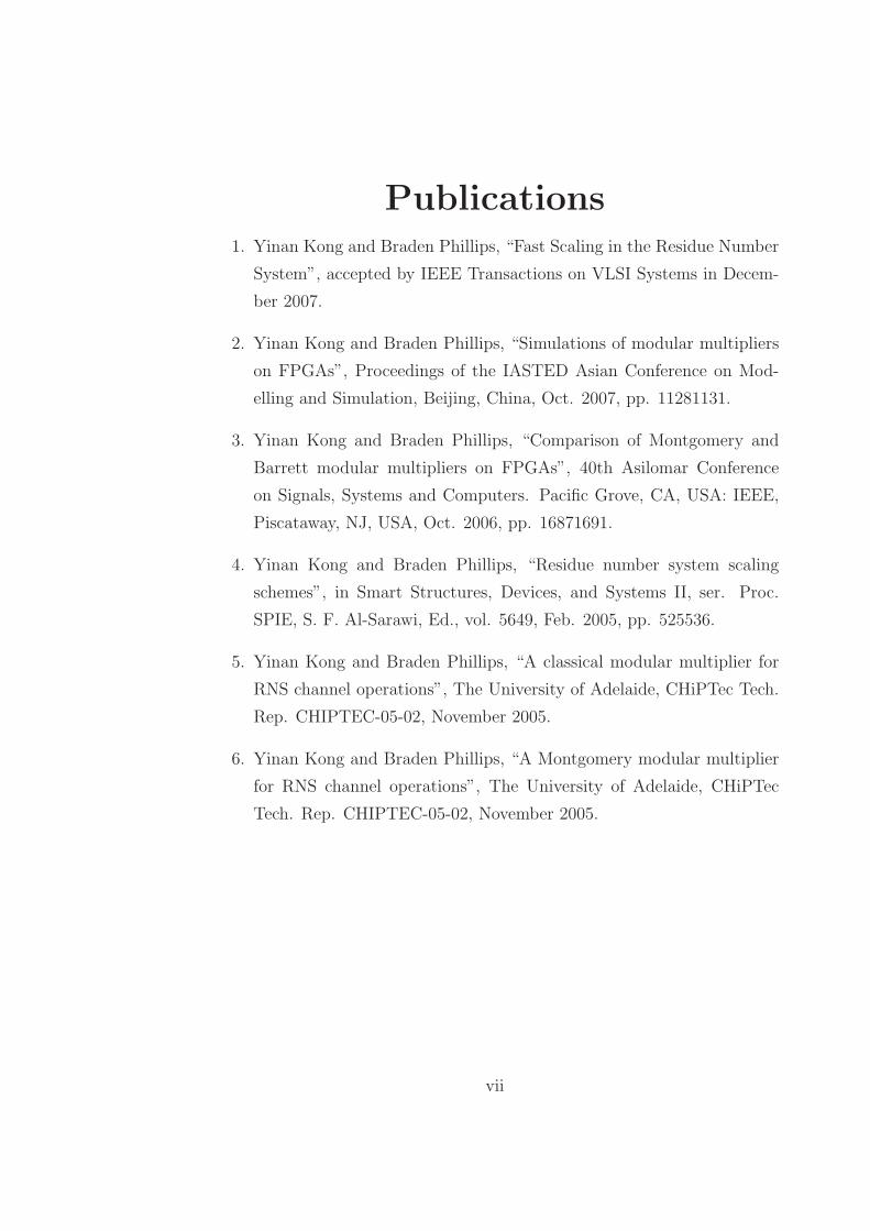
A typical SOR algorithm was proposed by Tomlinson in [Tomlinson89]
and is shown in Algorithm 3.8. Tomlinson’s algorithm performs the reduction
by setting the most significant bits to zero and accounting for this change
by adding the pre-computed residue (q × 2n+1 mod M). We take a slightly
improved architecture, illustrated in Figure 3.1, of this algorithm as a starting
point for further development. A Carry Save Adder (CSA) [Burks46] is used
to perform the three-term addition Ci = 2Ci+1 + aiB + (q × 2n+1 mod M).
To make sure 2Ci+1 is n bits long, the same as the other two addends, q is
set to be the upper 3 bits of the current partial result instead of 2.
[Chen99] gives a similar algorithm but sets q only two bits long. This
means that the partial result Ci may be n + 1 bits long. To bound it within
33
CHAPTER 3. FOUR WAYS TO DO MODULAR MULTIPLICATION IN A
POSITIONAL NUMBER SYSTEM
Algorithm 3.8 Tomlinson’s Sum of Residues Modular Multiplication
Ensure: C0 ≡ A × B mod M , C < 2n+1
Cn = 0
q = 0
for i = n − 1 downto 0 do
Ci = 2Ci+1 + aiB
Ci = Ci + (q × 2n+1 mod M) {The residue (q × 2n+1 mod M) is pre-
computed.}q =
⌊Ci
2n
⌋ {q is the upper 2 bits of C}Ci = Ci − q × 2n {Set the upper 2 bits of C to zero}
end for
C0 = (C0 + (q × 2n+1 mod M)) mod M
q
n-bit Carry Save Adder
2Ci+1
q×2n
mod M
Ci >> n – 1
Ci = 2Ci+1 + aiB + (q×2n
mod M)
aiB
2Ci & (2n
– 1)
LUT2Ci
n+1-bit Carry Propagate Adder
n n n
q×2n+1
mod M
n+1
n+2
n
3
n
n
Figure 3.1: An Architecture for Tomlinson’s Modular Multiplication Algo-
rithm [Tomlinson89]
34

3.2. REINVIGORATING SUM OF RESIDUES
n bits, a subtracter is used to constantly subtract M until Ci has only n bits.
This redundant step greatly increases the latency of the algorithm.
3.2.2 Eliminating the Carry Propagate Adder
There are two obvious demerits of the architecture in Figure 3.1. Firstly,
a Carry Propagate Adder (CPA) is used to transform the redundant rep-
resentation of Ci to its non-redundant form. This is required because the
upper 3 bits of Ci have to be known to look up q × 2n mod M before the
next iteration. The CPA delay contributes significantly to the latency of the
implementation. The second problem is that the look-up of q × 2n mod M
is on the critical path.
Both of these problems can be solved by keeping the intermediate result in
a redundant carry save form. The CPA of Figure 3.1 is eliminated so that the
calculation of the partial result becomes C1i + C2i = C1i+1 + C2i+1 + aiB +
((q1+q2)×2n mod M), where C1i and C2i are the redundant representation
of Ci as sum and carry terms respectively. A modified architecture is shown
in Figure 3.2. The CPA is replaced by a second CSA.
The pre-computed residue (q1+q2)×2n mod M , which must be retrieved
from a look-up table (LUT), can be sent to the second CSA rather than the
first. All three addends to the first CSA are available at the beginning of
each iteration and the table look-up step can be performed in parallel with
the first CSA.
In Figure 3.1 it can be seen that the carry output of the first CSA is
n + 1 bits wide. This can not be input directly to the second CSA which
is only n-bits wide. Thus, in Figure 3.2 the MSB of the (n + 1)-bit carry is
sent to the LUT circuit instead. The LUT retrieves two possible values of
35

CHAPTER 3. FOUR WAYS TO DO MODULAR MULTIPLICATION IN A
POSITIONAL NUMBER SYSTEM
(q1+q2)×2n
mod M
q1 = C1i >> n – 1
q2 = C2i >> n – 1
2C1i = 2C1i & (2n
– 1)
2C2i = 2C2i & (2n
– 1)
LUT
2C1i q1
n-bit Carry Save Adder
2C2i
n
n+1
n
n n+1
q2
C1i C2i
n n1
2
q1q2
1 2
1
n
MUX
n-bit Carry Save Adder
aiB
n n n
2C2i+1
2C1i+1
Figure 3.2: Modified Sum of Residues Modular Multiplier Architecture
36

3.2. REINVIGORATING SUM OF RESIDUES
(q1 + q2) × 2n mod M corresponding to the case of either a 0 or 1 in the
MSB of the carry output from the first CSA. A MUX selects the appropriate
value of (q1 + q2) × 2n mod M once the MSB is available. Thus, although
the LUT executes in parallel with the first CSA, an additional MUX appears
on the critical path.
3.2.3 Further Enhancements
If the second CSA in Figure 3.2 can be modified to accept an (n+1)-bit input,
the MUX can be eliminated. The left of Figure 3.3 shows a conventional n-bit
CSA. Note that the output sum is only n bits wide. To accept an (n + 1)-
bit input, we can just copy the MSB of the (n + 1)-bit input to the MSB
of output sum. This is illustrated in the right of Figure 3.3. This modified
CSA accepts 1 (n+1)-bit input and 2 n-bit inputs and produces 2 (n+1)-bit
outputs.
Figure 3.3: n-bit Carry Save Adders
Figure 3.4 shows the resulting modular multiplication architecture. The
algorithm corresponding to this new architecture is given as Algorithm 3.9.
The CPA has been eliminated from the iteration and the residue lookup has
been shifted from the critical path. Also, no subtraction is needed at the end
of the algorithm to bound the output within n + 1 bits. If C10 and C20 are
37

CHAPTER 3. FOUR WAYS TO DO MODULAR MULTIPLICATION IN A
POSITIONAL NUMBER SYSTEM
simply summed using a CPA, the resulting output C0 could be n + 2 bits,
which needs some further subtraction to be reduced. Therefore the same
technique as in the loop is applied. Both C10 and C20 are set to n − 1 bits
and the n-bit residue corresponding to the 2 upper reset bits is retrieved from
another LUT. The final sum yields an (n + 1)-bit output C0.
n-bit Carry Save Adder
2C1i+1
(q1+q2)×2n
mod M
q1 = C1i >> n – 1
q2 = C2i >> n – 1
aiB
2C1i = 2C1i & (2n
– 1)
2C2i = 2C2i & (2n
– 1)
LUT
2C1i q1
n-bit Carry Save Adder
2C2i
n n n
n n+1n
n+1 n+1
q2
C1i C2i
2C2i+1
n n2
2
q1 q2
2 2
T1i T2i
Figure 3.4: New Sum of Residues Modular Multiplier Architecture
The LUTs have a 4-bit input and a n-bit output so that a (24 × n)-bit
ROM can be used. For example, a 64-bit modular multiplier only needs a
1K-bit ROM, which is reasonable for a RNS channel modular multiplier .
Figure 3.5 shows an example of the new algorithm for the case r = 2,
n = 4, A = 15 = (1111)2, B = 11 = (1011)2 and M = 9 = (1001)2. It is also
noted that at the last step a second LUT of the same size is needed.
38

3.2. REINVIGORATING SUM OF RESIDUES
i n= - 1 = 3
i n= - 2 = 2
i n= - 3 = 1
i n= - 4 = 0
4-bit Carry Save Adder
(q1+q2)×24
mod 1001
q1 = 01011 >> 3
q2 = 00000 >> 3
1011
2C13 = 010110 & (1111)
2C23 = 000000 & (1111)
000000 mod 1001
2C13 q1
4-bit Carry Save Adder
2C23
1011 00000 0000
01011
q2
0000
0110 0000 01 00
q1 q2
00 000000
00000
C13 C23
2C14 2C24 a3B
4-bit Carry Save Adder
q1 = 11110 >> 3
q2 = 00010 >> 3
1011
2C11 = 111100 & (1111)
2C21 = 000100 & (1111)
2C11 q1
4-bit Carry Save Adder
2C21
0011 11000 0101
11110
q2
0100
1100 0100 11 00
1100
00010
C11 C21
2C12 2C22 a1B
(q1+q2)×24
mod 1001
100000 mod 1001
q1 q2
01 01
4-bit Carry Save Adder
1011
4-bit Carry Save Adder
0011 11000 0011
11000
01001100
00110
C10 C20
2C11 2C21 a0B
(q1+q2)×24
mod 1001
110000 mod 1001
q1 q2
11 00
3-bit Carry Propagate Adder
while C0 M do C0 = C0 – M
0110
C0
0011
q1 = 11000 >> 3
q2 = 00110 >> 3
C10 = 11000 & (111)
C20 = 00110 & (111)
C10 C20 q2
000 110 11 00
11000 mod 1001
(q1+q2)×23
mod 1001
4-bit Carry Propagate Adder
0110
01100
q1
4-bit Carry Save Adder
q1 = 01110 >> 3
q2 = 01010 >> 3
1011
2C12 = 011100 & (1111)
2C22 = 010100 & (1111)
2C12 q1
4-bit Carry Save Adder
2C22
1101 01000 0111
01110
q2
0000
1100 0100 01 01
0110
01010
C12 C22
2C13 2C23 a2B
(q1+q2)×24
mod 1001
010000 mod 1001
q1 q2
01 00
�
Figure 3.5: An Example for New Sum of Residues Modular Multiplication
n = 4, A = (1111)2, B = (1011)2 and M = (1001)2
39

CHAPTER 3. FOUR WAYS TO DO MODULAR MULTIPLICATION IN A
POSITIONAL NUMBER SYSTEM
Algorithm 3.9 New Sum of Residues Modular Multiplication
Ensure: C0 ≡ A × B mod M , C < 2n+1
C1n = C2n = q1 = q2 = 0
for i = n − 1 downto 0 do
{T1i, T2i} = 2C1i+1 + 2C2i+1 + aiB {Carry save addition}{C1i, C2i} = T1i +T2i +((q1+q2)×2n mod M) {Carry save addition}{The residue ((q1 + q2) × 2n mod M) is precomputed}{q1, q2} = {C1i >> (n − 1), C2i >> (n − 1)} {q1 and q2 are the upper
2 bits of C1i and C2i respectively.}{C1i, C2i} = {2C1i & (2n − 1), 2C2i & (2n − 1)} {Set the upper 2 bits
of C1i and C2i to zero}end for
{C10, C20} = {2C10, 2C20} {Right shift so they are both n − 1 bits}C0 = C10 + C20 + ((q1 + q2) × 2n−1 mod M)
3.2.4 High Radix
A radix-r version of the algorithm can be produced as in Figure 3.6. If r = 2k
this version executes in n/k iterations; however a larger LUT and (n+k)-bit
CSAs are required.
3.2.5 Summary of the Sum of Residues Modular Mul-
tiplication
In this section, we set out to invigorate the Sum of Residues modular mul-
tiplication algorithms. We developed a new structure (shown in Figure 3.4)
of this distinct class of modular multiplication algorithm based on Tomlin-
son’s Algorithm [Tomlinson89]. This new algorithm will be implemented in
Section 3.5 for a comparison with other classes of algorithms.
40

3.2. REINVIGORATING SUM OF RESIDUES
n+k-bit Carry Save Adder
rC1i+1
(q1+q2)×2n+k
mod M
q1 = C1i >> n
q2 = C2i >> n
aiB
rC1i = rC1i & (2n+k
– 1)
rC2i = rC2i & (2n+k
– 1)
LUT
rC1i q1
n+k-bit Carry Save Adder
rC2i
n+k
n+k+1 n
n+k+1
q2
C1i C2i
rC2i+1
k+1
q1 q2
n+k n+k
n+k
n+k+1
n+k n k
k+1
k+1k+1
+
Figure 3.6: New High-Radix Sum of Residues Modular Multiplier Architec-
ture
41

CHAPTER 3. FOUR WAYS TO DO MODULAR MULTIPLICATION IN A
POSITIONAL NUMBER SYSTEM
3.3 Bounds of Barrett Modular Multiplica-
tion
In Section 3.1.3, the Improved Barrett modular multiplication algorithm is
introduced. In this section, the bounds of the output and input of the al-
gorithm are derived, and hence the range of the two parameters u and v is
given. Implementations are also made on Xilinx Virtex2 FPGA platform and
the delay and area of this algorithm are simulated.
3.3.1 Bound Deduction
Bounds on the Estimated Quotient
The estimated quotient Y is at most 1 less than the actual quotient Y if u
and v are chosen appropriately, as shown below.
Recall Y =⌊
C0
M
⌋=
⌊C0
2n+v2n+u
M
2u−v
⌋and Y =
⌊� C02n+v �
⌊2n+u
M
⌋2u−v
⌋, then
Y ≥ Y >
⌊C0
2n+v
⌋ ⌊2n+u
M
⌋2u−v
− 1
>( C0
2n+v − 1)(2n+u
M− 1)
2u−v− 1
=C0
M− C0
2n+u− 2n+v
M+
1
2u−v− 1
≥⌊
C0
M
⌋− C0
2n+u− 2n+v
M+
1
2u−v− 1
⇔ Y ≥ Y > Y − C0
2n+u− 2n+v
M+
1
2u−v− 1 (3.7)
because x ≥ �x� > x − 1 always holds for any natural x.
Because M is the n-bit modulus, A and B are two n-bit multiplicands
42

3.3. BOUNDS OF BARRETT MODULAR MULTIPLICATION
and C0 = A × B, C0 is 2n bits long. Thus,
2n−1 ≤ M ≤ 2n − 1 < 2n and 22n−1 ≤ C0 ≤ 22n − 1 < 22n.
Then (3.7) becomes
Y ≥ Y > Y − 22n
2n+u− 2n+v
2n−1+
1
2u−v− 1
⇔ Y ≥ Y > Y − (2n−u + 2v+1 + 1 − 2v−u) (3.8)
If we choose u ≥ n + 1 and v ≤ −2, then 0 < 2n−u ≤ 12, 0 < 2v+1 ≤ 1
2and
0 < 2n−u − 2v−u ≤ 12. Thus, 1 < 2n−u + 2v+1 + 1− 2v−u < 2. Therefore, (3.8)
becomes
Y ≥ Y > Y − 1.xx.
Because Y is an integer, Y = Y or Y = Y − 1. Namely, the maximal error
on the estimated quotient is limited to 1 by choosing u ≥ n + 1 and v ≤ −2.
Bounds on the Output
The worst-case word length of the estimated output C will be checked below.
Recall Equation (3.6) C = A×B mod M = C0 −Y ×M and the remainder
C is certainly no more than n bits long. Now Y is replaced by Y and (3.6)
becomes
C = C0 − Y × M (3.9)
If Y = Y , (3.9) will be the same as (3.6) and the result C is at most n
bits long. If Y = Y − 1, (3.9) will be C = A × B − (Y − 1) × M =
A × B − Y × M + M = C + M . Because both C and M are n bits long at
most, the output is n + 1 bits long at most. Consequently, the output of the
Improved Barrett Modular Multiplication Algorithm is n + 1 bits.
43

CHAPTER 3. FOUR WAYS TO DO MODULAR MULTIPLICATION IN A
POSITIONAL NUMBER SYSTEM
Bounds on the Input
Because the output is likely to be the input of another modular multiplier,
which will itself use Improved Barrett Modular Multiplication, we should
ensure output C is n + 1 bits when there are two n + 1 bit inputs, A and B.
We will now show that this consistency exists if u and v are appropriately
selected.
Recall Equation (3.7)
Y ≥ Y > Y − C0
2n+u− 2n+v
M+
1
2u−v− 1.
Now M is n bits and A and B become n + 1 bits, and so C0 = A × B is
2n + 2 bits long. Thus,
2n−1 ≤ M ≤ 2n − 1 < 2n and 22n+1 ≤ C0 ≤ 22n+2 − 1 < 22n+2.
Then Equation (3.7) becomes
Y ≥ Y > Y − 22n+2
2n+u− 2n+v
2n−1+
1
2u−v− 1
⇔ Y ≥ Y > Y − (2n−u+2 + 2v+1 + 1 − 2v−u) (3.10)
If we choose u − 2 ≥ n + 1 i.e. u ≥ n + 3 and also v ≤ −2, then (3.10)
becomes the same as (3.8):
Y ≥ Y > Y − 1.xx.
Therefore, Y = Y or Y = Y − 1 and the output C is still n + 1 bits long in
the case of n + 1-bit inputs by choosing u ≥ n + 3 and v ≤ −2.
Now, Y ≤ Y =⌊
C0
M
⌋ ≤ ⌊22n+2
2n−1
⌋= 2n+3. While M cannot be 2n+1 because
it is usually odd, Y < 2n+3. Therefore, the bound on the estimated quotient
Y is n+3 bits. In conclusion, the bounds on the quotient inputs and output
are n + 3, n + 1 and n + 1 respectively. To save hardware, the parameters
are suggested to be u = n + 3 and v = −2.
44

3.3. BOUNDS OF BARRETT MODULAR MULTIPLICATION
3.3.2 Performance at Different Word Lengths
As stated in Section 2.1.4, the RNS channel width n should be at least 12
bits in a RNS system with 2048-bit dynamic range. The delay of a modular
multiplier is expected to increase as the word length n increases. This is
apparent in the results from the algorithm implemented and evaluated in
terms of speed and area on an FPGA platform using Xilinx tools.
A Xilinx Virtex2 FPGA was used as the implementation target. All
of the implementations were performed using the Xilinx ISE environment
using XST for synthesis and ISE standard tools for place and route. Speed
optimization with standard effort was used for all of the implementations:
Target FPGA: Virtex2 XC2V1000 with a -6 speed grade, 1M gates,
5120 slices and 40 embedded 18 × 18 multipliers
Xilinx 6.1i: XST - Synthesis
ISE - Place and Route
Optimization Goal: Speed
Language: VHDL
Pure delays of the combinatorial circuit were measured excluding those
between pads and pins. They were generated from the Post-Place and Route
Static Timing Analyzer with a standard place and route effort level.
The results of the Improved Barrett Modular Multiplier from 12 bit to
24 bits are shown in Figure 3.7(a). As can be seen from Figure 3.7, the
performance in terms of both speed and space complexity is best at n = 12.
This multiplier is used for the RNS channel modular multiplication in the
final implementation of the RNS in Chapter 5.
45

CHAPTER 3. FOUR WAYS TO DO MODULAR MULTIPLICATION IN A
POSITIONAL NUMBER SYSTEM
Delays at Different Wordlengths
10
15
20
25
30
35
40
12 14 16 18 20 22 24
n
ns Delays
(a) Delays
Areas at Different Wordlengths
0
20
40
60
80
100
12 14 16 18 20 22 24
n
sli
ces
Areas
(b) Areas
Figure 3.7: Delays and Areas of Improved Barrett Modular Multiplication
Algorithm
46

3.4. MONTGOMERY MODULAR MULTIPLICATION ON FPGA
3.4 Montgomery Modular Multiplication on
FPGA
In this section, published techniques of the Montgomery modular multiplica-
tion algorithm are analyzed, including interleaved/separated structure, high
radix, trivial quotient digit selection and quotient pipelining. They are also
implemented on the same FPGA platform described in Section 3.3.2.
3.4.1 Separated Montgomery Modular Multiplication
Algorithm
In contrast to interleaved Montgomery modular multiplication in Algorithm 3.7,
a separated Montgomery modular multiplier performs the multiplication and
then reduces the product using the Montgomery algorithm. Recall n is the
word length of modulus M and suppose C0 is the 2n-bit product of A × B.
The Montgomery modular reduction algorithm calculates
C0 × R−1 mod M
= C0 × 2−n mod M
= (. . . ((C02−1)2−1)2−1 . . . )2−1 mod M
= (. . . (((C0 + q0M)/2 + q1M)/2 + q2M)/2 + · · · + qn−1M)/2 mod M
The algorithm is shown in Algorithm 3.10
3.4.2 High Radix Montgomery Algorithm
Algorithm 3.11 shows an interleaved modular multiplication at a radix r and
Algorithm 3.12 shows a separated version of this algorithm. The radix is
47

CHAPTER 3. FOUR WAYS TO DO MODULAR MULTIPLICATION IN A
POSITIONAL NUMBER SYSTEM
Algorithm 3.10 Separated Montgomery Modular Multiplication at Radix
2Require: R = 2n
Ensure: Cn ≡ A × B × R−1 mod M
C0 = A × B
for i = 0 to n − 1 do
qi = Ci × (−M(0)−1) mod 2 {Quotient digit selection}Ci+1 = (Ci + qiM)/2 {Reduction step}
end for
chosen to be a power of 2, i.e. r = 2k, k = 0, 1, 2, . . .. Note −M(0)−1 is the
least significant digit of 〈−M−1〉r in base r.
Radix-2
Consider the case r = 2 in Algorithm 3.12. The product C0 yet to be reduced
modulo M is 2n bits and M is n bits long. There are n iterations and exactly
one bit is reduced in each iteration since the least significant bit of the current
Ci is made 0 by adding qi×M . After n iterations, the result will be presented
as Cn. Table 3.1 illustrates the process for the case of n = 8. To show the
reduction process more clearly, assume there is no word length growth on
the partially reduced results Ci. However, this is impossible and the bound
of the growth will be calculated in Section 3.4.3.
Radix-r
Now consider the case when k > 1, r > 2, and assume that n bits are
equivalent to l digits. Then there is 1 digit, i.e. k bits, to be reduced in
each iteration. For example, if k = 2, we have radix 4 and 2 bits will be
reduced in one iteration; there will be l = 8/2 = 4 iterations in the case of
48

3.4. MONTGOMERY MODULAR MULTIPLICATION ON FPGA
Table 3.1: Montgomery Modular Reduction Process at Radix 2
Bits 15 14 13 12 11 10 9 8 7 6 5 4 3 2 1 0
C0 * * * * * * * * * * * * * * * *
q0M * * * * * * * *
C0 + q0M * * * * * * * * * * * * * * * 0
C1 * * * * * * * * * * * * * * *
q1M * * * * * * * *
C1 + q1M * * * * * * * * * * * * * * 0
C2 * * * * * * * * * * * * * *
q2M * * * * * * * *
C2 + q2M * * * * * * * * * * * * * 0
C3 * * * * * * * * * * * * *
q3M * * * * * * * *
C3 + q3M * * * * * * * * * * * * 0
C4 * * * * * * * * * * * *
q4M * * * * * * * *
C4 + q4M * * * * * * * * * * * 0
C5 * * * * * * * * * * *
q5M * * * * * * * *
C5 + q5M * * * * * * * * * * 0
C6 * * * * * * * * * *
q6M * * * * * * * *
C6 + q6M * * * * * * * * * 0
C7 * * * * * * * * *
q7M * * * * * * * *
C7 + q7M * * * * * * * * 0
C8 * * * * * * * *
=< C0 × 2−8 >M
49

CHAPTER 3. FOUR WAYS TO DO MODULAR MULTIPLICATION IN A
POSITIONAL NUMBER SYSTEM
Table 3.2: Montgomery Modular Reduction Process at Radix 4
Bits 15 14 13 12 11 10 9 8 7 6 5 4 3 2 1 0
C0 * * * * * * * * * * * * * * * *
q0M * * * * * * * *
C0 + q0M * * * * * * * * * * * * * * 0 0
C1 * * * * * * * * * * * * * *
q1M * * * * * * * *
C1 + q1M * * * * * * * * * * * * 0 0
C2 * * * * * * * * * * * *
q2M * * * * * * * *
C2 + q2M * * * * * * * * * * 0 0
C3 * * * * * * * * * *
q3M * * * * * * * *
C3 + q3M * * * * * * * * 0 0
C4 * * * * * * * *
=< C0 × r−4 >M
=< C0 × 2−8 >M
n = 8. This reduction process is illustrated in Table 3.2 with the assumption
that no word length grows during the process. The corresponding interleaved
and separated algorithms are shown in Algorithm 3.11 and Algorithm 3.12
respectively.
A complication arises if n is not divisible by k. In these cases, the number
of iterations l can be l =⌈
nk
⌉or l =
⌊nk
⌋with some additional correction
steps after l iterations. This is just what the function Cn = Correct(Cl) does
in Algorithm 3.11 and Algorithm 3.12. Take n = 8 and k = 3 as an example
for the version of separated modular multiplication in Algorithm 3.12, where
one digit equals 3 bits and hence 3 bits are reduced in each iteration.
Let us consider how many iterations are required. If l =⌈
nk
⌉=⌈
83
⌉= 3,
50

3.4. MONTGOMERY MODULAR MULTIPLICATION ON FPGA
Algorithm 3.11 Interleaved Montgomery Modular Multiplication at Radix
rRequire: R = 2n, r = 2k and l =
⌊nk
⌋Ensure: Cn ≡ A × B × R−1 mod M
C0 = 0
for i = 0 to l − 1 do
C = Ci + aiB {Partial product accumulation}qi = Ci × (−M(0)−1) mod r {Quotient digit selection}Ci+1 = (C + qiM)/r {Reduction step}
end for
Cn = Correct(Cl) {Correction step}
Algorithm 3.12 Separated Montgomery Modular Multiplication at Radix
rRequire: R = 2n, r = 2k and l =
⌊nk
⌋Ensure: Cn ≡ A × B × R−1 mod M
C0 = A × B
for i = 0 to l − 1 do
qi = Ci × (−M(0)−1) mod r {Quotient digit selection}Ci+1 = (Ci + qiM)/r {Reduction step}
end for
Cn = Correct(Cl) {Correction step}
51

CHAPTER 3. FOUR WAYS TO DO MODULAR MULTIPLICATION IN A
POSITIONAL NUMBER SYSTEM
Table 3.3: Montgomery Modular Reduction Process at Radix 8 (l =⌈
nk
⌉)
Bits 15 14 13 12 11 10 9 8 7 6 5 4 3 2 1 0
C0 * * * * * * * * * * * * * * * *
q0M * * * * * * * *
C0 + q0M * * * * * * * * * * * * * 0 0 0
C1 * * * * * * * * * * * * *
q1M * * * * * * * *
C1 + q1M * * * * * * * * * * 0 0 0
C2 * * * * * * * * * *
q2M * * * * * * * *
C2 + q2M * * * * * * * 0 0 0
C3 * * * * * * *
=< C0 × r−3 >M
=< C0 × 2−9 >M
Corrected C3 * * * * * * * 0
=< 2 × C0 × 2−9 >M
=< C0 × 2−8 >M
9 bits will be reduced and the result is C0 × 2−9 mod M instead of C0 × 2−8
mod M . Then C0 × 2−9 mod M is multiplied by 2 in the correction step to
obtain the correct answer. This is shown in Table 3.3.
Rather than having l =⌈
nk
⌉, let us now consider l =
⌊nk
⌋=⌊
83
⌋= 2.
In this case, 6 bits will be reduced and the result is C0 × 2−6 mod M .
Then C0 × 2−6 mod M is further reduced to C0 × 2−8 mod M either by
two additional radix-2 iterations or one radix-4 iteration. This is shown in
Table 3.4 with one radix-4 iteration added at the end as a correction step.
Of the two cases considered, l =⌊
nk
⌋is better because the result from
l =⌈
nk
⌉is likely not to be fully reduced. This is proved in Section 3.4.3.
Therefore, the version of l =⌊
nk
⌋iterations is adopted in Algorithm 3.11 and
52

3.4. MONTGOMERY MODULAR MULTIPLICATION ON FPGA
Table 3.4: Montgomery Modular Reduction Process at Radix 8 (l =⌊
nk
⌋)
Bits 15 14 13 12 11 10 9 8 7 6 5 4 3 2 1 0
C0 * * * * * * * * * * * * * * * *
q0M * * * * * * * *
C0 + q0M * * * * * * * * * * * * * 0 0 0
C1 * * * * * * * * * * * * *
q1M * * * * * * * *
C1 + q1M * * * * * * * * * * 0 0 0
C2 * * * * * * * * * *
q2M * * * * * * * *
C2 + q2M * * * * * * * * 0 0
Corrected C2 * * * * * * * *
< C0 × 2−8 >M
Algorithm 3.12 with one n mod k correction step added at the end when n
is not divisible by k.
The performance of the multipliers using different radices are compared in
Figure 3.8 using the Xilinx FPGA simulation described on page 45. Following
the word length in the tables above, n = 16 bits is chosen here, which is
greater than 12 bits, the lower bound of n derived in Section 2.1.4. As
can be seen from Figure 3.8, the higher the radix r = 2k, the faster the
modular multiplier runs, especially when k becomes close to the word length
n. However, very high radices can be impossible to implement, as proved in
Section 3.4.5 below, and, therefore, the radix is often selected to be as high
as possible under some further conditions.
53

CHAPTER 3. FOUR WAYS TO DO MODULAR MULTIPLICATION IN A
POSITIONAL NUMBER SYSTEM
Delays at Different Radices
05
10152025303540455055
0 1 2 3 4 5 6 7 8 9 10 11 12 13 14 15 16 17
k
ns n = 16
Figure 3.8: Delays of Montgomery Modular Multiplication at Different
Radices.
3.4.3 Bound Deduction
In this section we consider the magnitudes of the intermediate results of
Montgomery modular multiplication algorithm and reduce their bounds.
Bounds of Interleaved Montgomery Modular Multiplication Algo-
rithm
Recall the Interleaved Montgomery Modular Multiplication Algorithm in Al-
gorithm 3.11. The partial result Ci in the current iteration has the following
relationship with Ci+1 in next iteration:
rCi+1 = Ci + aiB + qiM, (3.11)
where B and M are n bits long, ai and qi are to be no more than k bits long
and r = 2k. We want the word length of Ci and Ci+1 to be consistent and
certainly as short as possible to save hardware.
54

3.4. MONTGOMERY MODULAR MULTIPLICATION ON FPGA
If Ci is x bits long, the worst case of the right side of (3.11), Ci+aiB+qiM
is 2x−1+(2k−1)(2n−1)+(2k−1)(2n−1) = 2x−1+2(2k−1)(2n−1) = 2kCi+1.
If Ci and Ci+1 are the same word length, then Ci+1 ≤ 2x − 1 should hold.
Thus,
2x − 1 + 2(2k − 1)(2n − 1) ≤ 2k(2x − 1),
which gives
2x ≥ 2n+1 − 1.
Because n > 0, 1 < 2n = 2n+1 − 2n, hence 2n < 2n+1 − 1 and 2x >
2n+1 − 1, x ≥ n + 1. To minimize hardware choose x = n + 1. In other words
n+1 bits is sufficient for the partial result Ci of the interleaved Montgomery
modular multiplier. It can also be seen that the final result Cn is at most
n + 1 bits long regardless of n and k.
Bounds of Separated Montgomery Modular Multiplication Algo-
rithm
Recall the Separated Montgomery Modular Multiplication Algorithm in Al-
gorithm 3.12 on page 51. The partial result Ci in the current iteration has
the following relationship with Ci+1 in its next iteration.
rCi+1 = Ci + qiM, (3.12)
where M is n bits long, qi is k bits long at most and r = 2k. Again assuming
that Ci is x bits long, the right side of (3.12), Ci + qiM can be 2x − 1 +
(2k − 1)(2n − 1) = 2kCi+1 in the worst case. If Ci and Ci+1 are consistent,
Ci+1 ≤ 2x − 1 should hold. Thus,
2x − 1 + (2k − 1)(2n − 1) ≤ 2k(2x − 1),
which gives
x ≥ n.
55

CHAPTER 3. FOUR WAYS TO DO MODULAR MULTIPLICATION IN A
POSITIONAL NUMBER SYSTEM
This means for all the word lengths greater than or equal to n bits Ci and
Ci+1 are consistent. However, the word length of Ci cannot be shorter than
2n, because A × B is assigned to C0 at the very first step. Therefore, the
partial result Ci of the separated modular multiplier is 2n bits long.
Now the range of the final result Cn is to be determined. There are two
alternations for the number of iterations l, i.e. l =⌈
nk
⌉and l =
⌊nk
⌋, as
discussed in Section 3.4.2 above.
If l =⌈
nk
⌉, then let kl = n + p, where 0 ≤ p ≤ k − 1. All of the l
iterations in Algorithm 3.12 up to the line Cn = Correct(Cl) are connected
and expressed in the equation below:
rlCl = C0 + q0M + rq1M + r2q2M + · · · + rl−1ql−1M,
where M is n bits long, qi is k bits long at most, C0 is 2n bits long and
r = 2k. Thus,
2klCl ≤ (22n − 1) + (r − 1)(2n − 1) + r(r − 1)(2n − 1) + r2(r − 1)(2n − 1)
+ · · · + rl−1(r − 1)(2n − 1)
= (22n − 1) + (r − 1)(2n − 1)(1 + r + r2 + · · · + rl−1)
= (22n − 1) + (2n − 1)(2kl − 1)
⇒ 2klCl ≤ (22n − 1) + (2n − 1)(2kl − 1) (3.13)
Because kl = n + p, (3.13) becomes
2n+pCl ≤ (22n − 1) + (2n − 1)(2n+p − 1)
⇒ 2pCl ≤ (2n − 1)(2p + 1) < 2p(2n+1 − 1)
⇒ Cl ≤ 2n+1 − 1.
Therefore, Cl = C02−kl mod M is n + 1 bits long at most. However, we
need Cn = C02−n mod M , so C02
−kl mod M should be left-shifted by p bits
56

3.4. MONTGOMERY MODULAR MULTIPLICATION ON FPGA
to produce Cn = C02−n mod M . In other words, the process Correct(Cl)
adds p “0”s to the end of C02−kl mod M . Consequently, the final result Cn
is n + p + 1 bits long, where p = k − (n mod k). Hence the result is not
fully Montgomery modular reduced. For example, if n = 16, and k = 7, then
p = k − (n mod k) = 5 and n + p + 1 = 16 + 5 + 1 = 22 bits. This is why
this approach is not used in Algorithm 3.11 and Algorithm 3.12.
If l =⌊
nk
⌋, then let kl + p = n, where 0 ≤ p ≤ k − 1. All of the l
iterations in Algorithm 3.12, along with the Correct(Cl) line, are connected
and expressed in the equation below:
2nCn = C0 + q0M + rq1M + r2q2M + · · · + rl−1ql−1M + rlq′lM,
where q′l is p bits long at most, M is n bits long, qi is k bits long at most, C0
is 2n bits long and r = 2k. Thus,
2nCn ≤ (22n − 1) + (r − 1)(2n − 1) + r(r − 1)(2n − 1) + r2(r − 1)(2n − 1)
+ · · · + rl−1(r − 1)(2n − 1) + rl(2p − 1)(2n − 1)
= (22n − 1) + (2kl − 1)(2n − 1) + 2kl(2p − 1)(2n − 1)
= 2n+1(2n − 1)
⇒ Cn ≤ 2n+1 − 2 < 2n+1 − 1.
Therefore, Cn = C02−n mod M is at most n+1 bits, which means it is fully
reduced.
3.4.4 Interleaved vs. Separated Structure
Figure 3.9 shows the comparison between interleaved and separated multi-
pliers in terms of delays and areas respectively. Various radices are included
and n is chosen to be 16. In Figure 3.9(a), the separated modular multiplier
is obviously faster than the interleaved one at k < 8, i.e. when k is less than
57

CHAPTER 3. FOUR WAYS TO DO MODULAR MULTIPLICATION IN A
POSITIONAL NUMBER SYSTEM
n/2, while when k becomes larger than n/2, this advantage becomes vague.
However, as proved in Section 3.4.5 below, k cannot be too large. (Typi-
cally k must not be greater than n/2.) Therefore, the separated structure
is recommended to implement the Montgomery Modular Multiplier because
it is faster than the interleaved structure at most of the possible values of
k. Although our main optimization goal is speed, Figure 3.9(b) shows that
the separated structure also gains some advantage over the interleaved one
in hardware area.
3.4.5 Trivial Quotient Digit Selection
Techniques have been published to improve performance by making the
quotient digit selection step trivial and moving it from the critical path
[Shand93, Walter95]. Recall the Separated Montgomery Modular Multipli-
cation Algorithm shown in Algorithm 3.12 on page 51. In each iteration,
qi is computed using qi = Ci × (−M(0)−1) mod r, where −M(0)−1 is the
least significant bit of 〈−M−1〉2. This step is called quotient digit selection
(QDS). If M is always selected to guarantee that M mod r = r − 1 , then
−M(0)−1 mod r = M(0)M(0)−1 mod r = 1 can also be guaranteed, and
thus qi = Ci(0) holds and the QDS step examines only the least significant
digit of the partial result Ci. This is known as trivial QDS and is included
in Algorithm 3.13.
However, this brings a restriction on the radix r = 2k. Because M should
always satisfy M mod r = r−1, which means that the least significant digit
of M must satisfy M(0) = r − 1 = 2k − 1, i.e. there should be k “1”s at
the end of M . Thus for n = 8, M should be in the form *******1 if r = 2,
******11 if r = 4 and *****111 if r = 8.
Recall the conclusion from Section 2.1.4: to construct a RNS system with
58

3.4. MONTGOMERY MODULAR MULTIPLICATION ON FPGA
Delays for Interleaved vs Separated Structure
(n = 16)
0
10
20
30
40
50
60
70
80
0 1 2 3 4 5 6 7 8 9 10 11 12 13 14 15 16 17
k
ns Separated
Interleaved
(a) Delays
Areas for Interleaved vs Separated Structure
(n = 16)
0
50
100
150
200
250
300
350
0 1 2 3 4 5 6 7 8 9 10 11 12 13 14 15 16 17
k
sli
ces
Separated
Interleaved
(b) Areas
Figure 3.9: Delays and Areas of Interleaved and Separated Montgomery
Modular Multiplication at Different Radices
59

CHAPTER 3. FOUR WAYS TO DO MODULAR MULTIPLICATION IN A
POSITIONAL NUMBER SYSTEM
Algorithm 3.13 Separated Montgomery Modular Multiplication Algorithm
with Trivial QDS
Require: R = 2n, r = 2k and l =⌊
nk
⌋Ensure: Cn ≡ A × B × R−1 mod M
C0 = A × B
for i = 0 to l − 1 do
Ci+1 = (Ci + Ci(0)M)/r {Reduction step with trivial QDS}end for
Cn = Correct(Cl) {Correction step}
2048-bit dynamic range using equal word length moduli, the channel width
n should be at least 12 bits.
However, if trivial QDS is used, the range of the available integers may
not be enough for the co-prime moduli to be found. For example, if n = 12
and r = 4, i.e. k = 2, 171 co-prime moduli must be found from the set,
{y|y = 4x+3, 29 ≤ x ≤ 210−1}, which has 210−29 = 512 integers. Only 132
co-prime numbers can be found in these 512 integers∗, and this is not enough.
Therefore, n = 12 can only be feasible in the case of radix-2, i.e. k = 1. We
name this kind of set a “range set”, and obviously there is a unique range
set for each pair of n and k. Similarly, if n = 13, N =⌈
204812
⌉= 158 co-prime
numbers are needed. If k = 2, 242 co-prime numbers have been found in its
range set {y|y = 4x + 3, 210 ≤ x ≤ 211 − 1}, which means k = 2 is feasible.
However if k = 3, only 126 co-prime numbers can be found in its range set
{y|y = 8x + 7, 29 ≤ x ≤ 210 − 1}, which means k = 3 is not feasible and
k = 2 is the largest k that suits n = 13. Thus, for each value of word length
n, there will be a largest feasible k. We name this the k-boundary. Table 3.5
lists the k-boundary for n from 12 to 32.
Recall the result from Figure 3.8 in Section 3.4.2. The higher the radix
∗This result was obtained using a bruteforce search in Maple.
60

3.4. MONTGOMERY MODULAR MULTIPLICATION ON FPGA
Table 3.5: The k-boundary of Montgomery Reduction for n from 12 to 32
n 12 13 14 15 16 17 18 19 20 21 22
k-boundary 1 2 3 4 5 6 7 9 10 11 12
n 23 24 25 26 27 28 29 30 31 32
k-boundary 13 14 15 16 17 18 19 20 21 23
Table 3.6: Shortest Delays of Separated Montgomery Multiplication Algo-
rithm using Trivial QDS at n from 12 to 32
n 12 13 14 15 16 17 18
k 1 1 3 4 5 6 7
delays 32.087 34.282 34.100 27.646 22.297 25.085 24.869
n 19 20 21 22 23 24 25
k 9 10 10 11 13 14 15
delays 22.006 23.684 24.403 25.133 25.583 25.858 25.720
n 26 27 28 29 30 31 32
k 16 17 18 19 20 21 23
delays 25.479 28.483 28.896 27.924 28.217 29.916 31.953
r = 2k, the faster the modular multiplier runs, especially when k becomes
roughly the same as the word length n. Nonetheless, here we can see that to
use trivial QDS, k cannot be that large, because k cannot be greater than the
k-boundary in each word length. Thus, k should always be selected to be one
of those values close to the k-boundary or just the k-boundary itself. This
was also proved in our implementation, where trivial QDS gave a speed-up
of 2 over the non-trivial QDS version. All the possible values of k for n from
12 to 32 were simulated and the shortest delays at each word length n are
listed in Table 3.6 and shown in Figure 3.10.
61
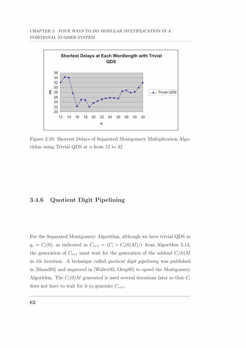
CHAPTER 3. FOUR WAYS TO DO MODULAR MULTIPLICATION IN A
POSITIONAL NUMBER SYSTEM
Shortest Delays at Each Wordlength with Trivial
QDS
20
22
24
26
28
30
32
34
36
12 14 16 18 20 22 24 26 28 30 32
n
ns Trivial QDS
Figure 3.10: Shortest Delays of Separated Montgomery Multiplication Algo-
rithm using Trivial QDS at n from 12 to 32
3.4.6 Quotient Digit Pipelining
For the Separated Montgomery Algorithm, although we have trivial QDS as
qi = Ci(0), as indicated in Ci+1 = (Ci + Ci(0)M)/r from Algorithm 3.13,
the generation of Ci+1 must wait for the generation of the addend Ci(0)M
in ith iteration. A technique called quotient digit pipelining was published
in [Shand93] and improved in [Walter95, Orup95] to speed the Montgomery
Algorithm. The Ci(0)M generated is used several iterations later so that Ci
does not have to wait for it to generate Ci+1.
62

3.4. MONTGOMERY MODULAR MULTIPLICATION ON FPGA
Recall the equation of Montgomery Modular Reduction:
C × R−1 mod M
= (. . . (((C + C0(0)M)/r + C1(0)M)/r + C2(0)M)/r
+ · · · + Cl−1(0)M)/r mod M
= (. . . (((C − C0(0) + C0(0)(M + 1))/r − C1(0) + C1(0)(M + 1))/r − C2(0)
+C2(0)(M + 1))/r − · · · − Cl−1(0) + Cl−1(0)(M + 1))/r mod M
= ((. . . ((((((C − C0(0))/r − C1(0))/r − C2(0) + C0(0)(M + 1))/r2)/r
−C3(0) + C1(0)(M + 1))/r2)/r − C4(0) + C2(0)(M + 1)/r2)/r
− · · · − Cl−2(0) + Cl−4(0)(M + 1)/r2)/r − Cl−2(0)
+Cl−4(0)(M + 1)/r2)/r − Cl−1(0) + Cl−3(0)(M + 1)/r2)/r
+Cl−2(0)(M + 1)/r2 + Cl−1(0)(M + 1)/r mod M (3.14)
As can be seen from (3.14), because Ci +Ci(0)M will set the least significant
digit of the result to 0, Ci + Ci(0)M can be split into two parts, Ci − Ci(0)
and Ci(0) + Ci(0)M = Ci(0)(M + 1), i.e. Ci + Ci(0)M = [Ci − Ci(0)] +
[Ci(0)(M +1)]. These two parts are computed in parallel in the ith iteration.
So Ci(0)(M + 1)/r2 is planned to be added to Ci+2 two iterations later, and
Ci−Ci(0) is added by Ci−2(0)(M+1)/r2 already computed two iterations ago
without waiting for the computation of Ci(0)(M + 1). The level of quotient
digit pipelining d indicates how many iterations Ci(0)M is added after it
was calculated. In the previous example d = 2. The cost of quotient digit
pipelining is that Cl−2(0)(M + 1)/r2 + Cl−1(0)(M + 1)/r mod M has to be
computed after l iterations. This is reasonable compared with the advantage
in speed of the algorithm. The algorithm is shown in Algorithm 3.14.
The selection of d depends on the speed to compute Ci(0)(M + 1)/rd.
d = 2 or 3 was enough in the FPGA implementation studied here. When d
was set greater, no remarkable change was observed in speed.
The biggest disadvantage is the limitation quotient digit pipelining im-
63

CHAPTER 3. FOUR WAYS TO DO MODULAR MULTIPLICATION IN A
POSITIONAL NUMBER SYSTEM
Algorithm 3.14 Separated Montgomery Modular Multiplication Algorithm
with Trivial QDS and Quotient Digit Pipelining
Require: R = 2n, r = 2k and l =⌊
nk
⌋Ensure: Cn ≡ A × B × R−1 mod M
C0 = A × B
for i = −d to −1 do
Ci(0) = 0 {Initialisation of quotient digit}end for
for i = 0 to l − 1 do
Ci+1 = (Ci−Ci(0)+Ci−d(0)(M+1)/rd)/r {Reduction step with quotient
digit generated previously}Ci(0)(M + 1)/rd {Generation of quotient digit to be used d iterations
later}end for
Cl−d = (Cl) {Initialisation of Cl−d for the final loop}for i = l − d to l − 1 do
Ci+1 = Ci + Ci(0)(M + 1)/rl−i {Reduction step with quotient digit
generated previously}end for
Cn = Correct(Cl) {Correction step}
64

3.4. MONTGOMERY MODULAR MULTIPLICATION ON FPGA
poses on the radix r = 2k. The largest possible k will be smaller than the
k-boundary of the version without quotient digit pipelining. The reason is
that in the ith iteration,
Ci+1 = (Ci−Ci(0)+Ci−d(0)(M+1)/rd)/r = (Ci−Ci(0))/r+Ci−d(0)(M+1)/rd+1
should be computed. This means the last d + 1 least significant digits of
Ci(0)(M + 1) should be 0. Therefore,
Ci(0)(M + 1) = 0 mod rd+1 ⇔ M = −1 mod rd+1
Thus, there should be k(d + 1) “1”s at the end of M instead of k “1”s in
the version without quotient digit pipelining above. Similarly, k(d + 1) ≤ k-
boundary instead of k ≤ k-boundary. If d = 2, k should be no more than
one third of the k-boundary. Table 3.7 lists the possible values of k and d
for n from 12 to 25.
This is obviously a bad effect because the decrease in k slows the multiplier
as discussed in Section 3.4.2 and 3.4.5. However, the use of quotient digit
pipelining speeds up the algorithm, and therefore, we expect a tradeoff point
in the implementation where the speed is highest.
All the possible values of k and d for n from 12 to 32 were simulated and
the shortest delays at each word length n are listed in Table 3.8 and shown
in Figure 3.11 below.
n = 24 has the shortest delay across all word lengths. To judge if the
quotient digit pipelining technique really accelerates the modular multiplier,
consider Figure 3.12. The version without quotient digit pipelining is faster
than the quotient digit pipelining version within the interval [16, 26]. This
means the advantage the greater k brings about in the version without quo-
tient digit pipelining overwhelms the advantage the quotient digit pipelining
technique brings. Overall, the shortest delay is 22.006(ns) and this occurs for
65

CHAPTER 3. FOUR WAYS TO DO MODULAR MULTIPLICATION IN A
POSITIONAL NUMBER SYSTEM
Table 3.7: k and d in Quotient Digit Pipelining of Montgomery Algorithm
for n from 12 to 25n 12 13 14 15 16 17 18
k-boundary 1 2 3 4 5 6 7
k 1 1 1 1 2 1 2 1 2 3 1
d NA 1 1,2 1–3 1 1–4 1 1–5 1,2 1 1–6
n 18 19 20
k-boundary 7 9 10
k 2 3 1 2 3 4 1 2 3 4 5
d 1,2 1 1–8 1–3 1,2 1 1–9 1–4 1,2 1 1
n 23 24
k-boundary 13 14
k 1 2 3 4 5 6 1 2 3 4 5
d 1–12 1–5 1–3 1,2 1 1 1–13 1–6 1–3 1,2 1
n 24 25
k-boundary 14 15
k 6 7 1 2 3 4 5 6 7
d 1 1 1–14 1–6 1–4 1,2 1,2 1 1
66
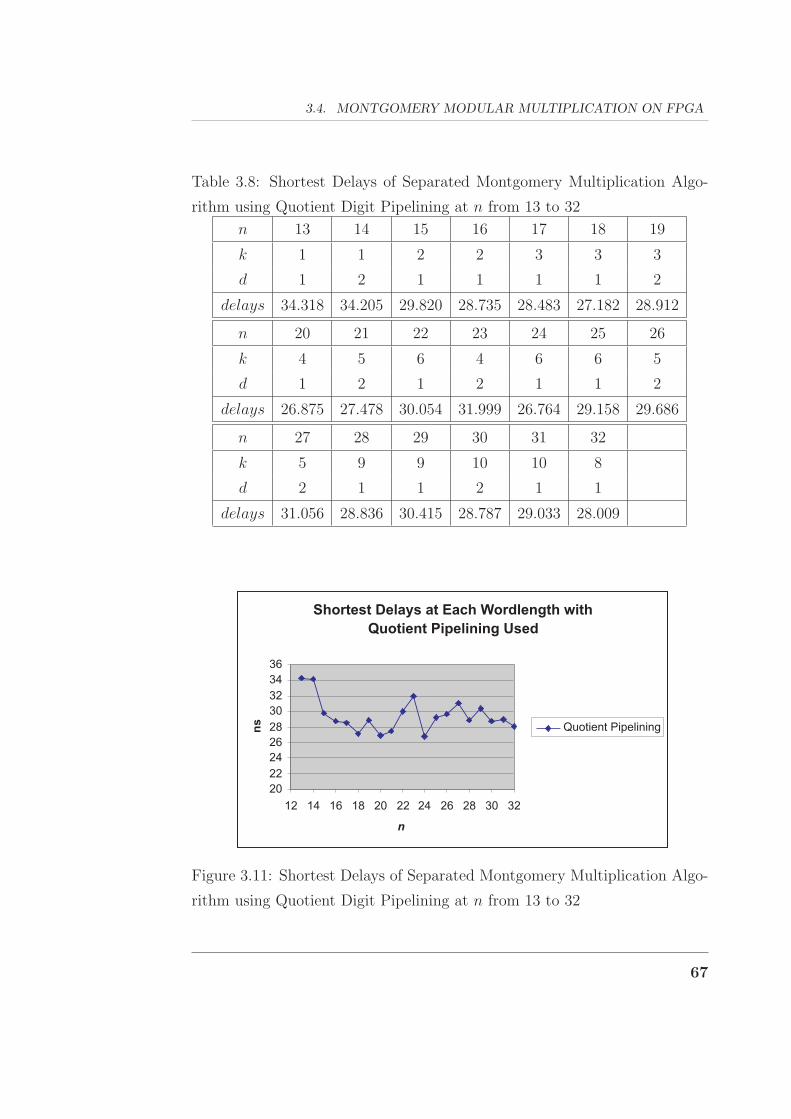
3.4. MONTGOMERY MODULAR MULTIPLICATION ON FPGA
Table 3.8: Shortest Delays of Separated Montgomery Multiplication Algo-
rithm using Quotient Digit Pipelining at n from 13 to 32
n 13 14 15 16 17 18 19
k 1 1 2 2 3 3 3
d 1 2 1 1 1 1 2
delays 34.318 34.205 29.820 28.735 28.483 27.182 28.912
n 20 21 22 23 24 25 26
k 4 5 6 4 6 6 5
d 1 2 1 2 1 1 2
delays 26.875 27.478 30.054 31.999 26.764 29.158 29.686
n 27 28 29 30 31 32
k 5 9 9 10 10 8
d 2 1 1 2 1 1
delays 31.056 28.836 30.415 28.787 29.033 28.009
Shortest Delays at Each Wordlength with
Quotient Pipelining Used
20
22
24
26
28
30
32
34
36
12 14 16 18 20 22 24 26 28 30 32
n
ns Quotient Pipelining
Figure 3.11: Shortest Delays of Separated Montgomery Multiplication Algo-
rithm using Quotient Digit Pipelining at n from 13 to 32
67

CHAPTER 3. FOUR WAYS TO DO MODULAR MULTIPLICATION IN A
POSITIONAL NUMBER SYSTEM
None QP vs. QP
20
22
24
26
28
30
32
34
36
12 14 16 18 20 22 24 26 28 30 32
n
ns
None Quotient
Pipelining
Quotient Pipelining
Figure 3.12: Shortest Delays of Separated Montgomery Multiplication Algo-
rithm with & without Quotient Digit Pipelining at n from 13 to 32
a separated Montgomery modular multiplier with n = 19 and k = 9 without
quotient digit pipelining.
Finally, a conclusion of Montgomery modular multiplication algorithm is
obtained: high radix and trivial QDS are both beneficial while the quotient
digit pipelining technique is not suitable for FPGA implementations.
68
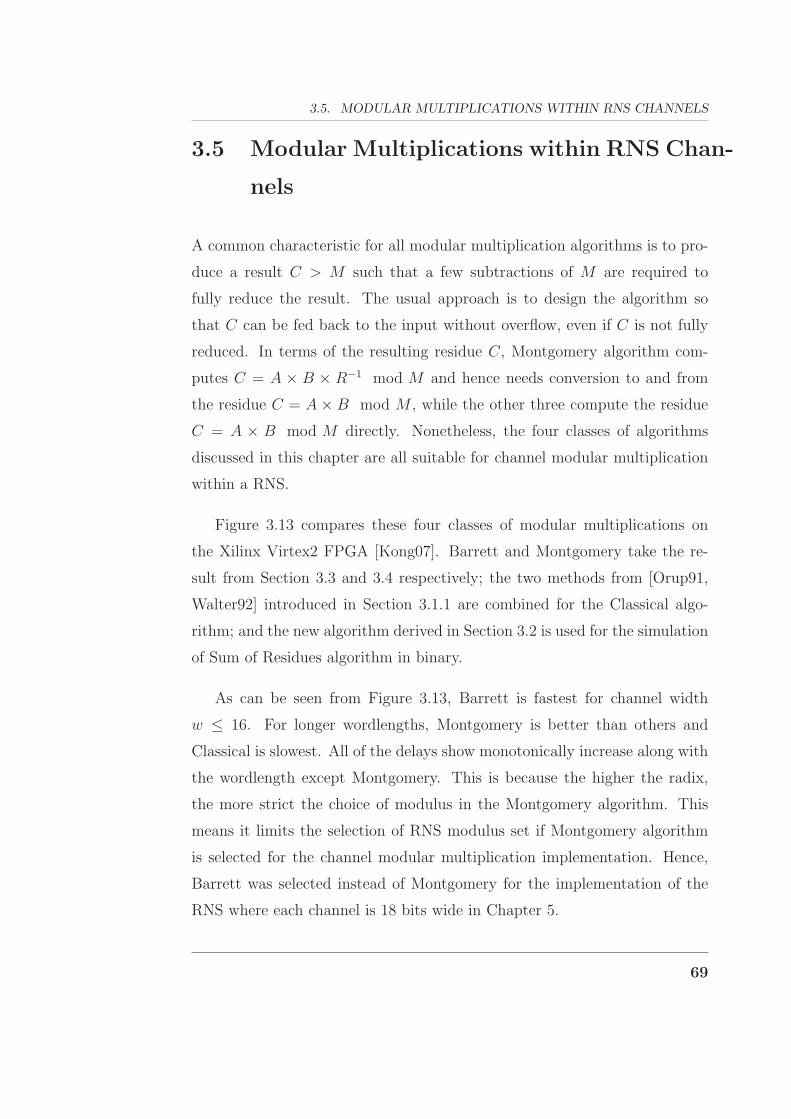
3.5. MODULAR MULTIPLICATIONS WITHIN RNS CHANNELS
3.5 Modular Multiplications within RNS Chan-
nels
A common characteristic for all modular multiplication algorithms is to pro-
duce a result C > M such that a few subtractions of M are required to
fully reduce the result. The usual approach is to design the algorithm so
that C can be fed back to the input without overflow, even if C is not fully
reduced. In terms of the resulting residue C, Montgomery algorithm com-
putes C = A × B × R−1 mod M and hence needs conversion to and from
the residue C = A × B mod M , while the other three compute the residue
C = A × B mod M directly. Nonetheless, the four classes of algorithms
discussed in this chapter are all suitable for channel modular multiplication
within a RNS.
Figure 3.13 compares these four classes of modular multiplications on
the Xilinx Virtex2 FPGA [Kong07]. Barrett and Montgomery take the re-
sult from Section 3.3 and 3.4 respectively; the two methods from [Orup91,
Walter92] introduced in Section 3.1.1 are combined for the Classical algo-
rithm; and the new algorithm derived in Section 3.2 is used for the simulation
of Sum of Residues algorithm in binary.
As can be seen from Figure 3.13, Barrett is fastest for channel width
w ≤ 16. For longer wordlengths, Montgomery is better than others and
Classical is slowest. All of the delays show monotonically increase along with
the wordlength except Montgomery. This is because the higher the radix,
the more strict the choice of modulus in the Montgomery algorithm. This
means it limits the selection of RNS modulus set if Montgomery algorithm
is selected for the channel modular multiplication implementation. Hence,
Barrett was selected instead of Montgomery for the implementation of the
RNS where each channel is 18 bits wide in Chapter 5.
69

CHAPTER 3. FOUR WAYS TO DO MODULAR MULTIPLICATION IN A
POSITIONAL NUMBER SYSTEM
Comparison of the Delays of Four Modular
Multipliers
15
20
25
30
35
40
45
50
55
60
65
12 14 16 18 20 22 24
w
ns
Montgomery
Barrett
Sum of
Residues
Classical
(a) Comparison of Delays of Four Modular Multipliers in Binary
Comparison of the Area of Four Modular
Multipliers
0
50
100
150
200
12 14 16 18 20 22 24
w
Sli
ces
Montgomery
Barrett
Sum of
Residues
Classical
(b) Comparison of Areas of Four Modular Multipliers
Figure 3.13: Delays and Areas of Four Classes of Modular Multipliers in
Binary
70

Chapter 4
Four Ways to Do Modular
Multiplication in the Residue
Number System
The purpose of this chapter is to explore the application of the four classes of
modular multiplication algorithms from positional number systems to long
word length modular multiplication in a RNS. Section 4.1 surveys modular
multiplication algorithms currently available in the RNS. Each of the subse-
quent 4 sections discusses one of the four classes of algorithms. New Classical,
Sum of Residues and Barrett algorithms are developed for modular multipli-
cation in the RNS. Existing Montgomery RNS algorithms are also discussed.
71

CHAPTER 4. FOUR WAYS TO DO MODULAR MULTIPLICATION IN THE
RESIDUE NUMBER SYSTEM
Chapter 2 states some facts: the long word length modular multiplica-
tion Z = A × B mod M , where A, B and the modulus M are all n-bit
positive integers, is the most frequent operation in Elliptic Curve Cryp-
tosystems (ECC) [Doche06]; in RSA, it is the only operation required to
implement the modular exponentiations which constitute encryption and de-
cryption [Rivest78]; and the Residue Number System (RNS) [Soderstrand86]
offers advantages for long word length arithmetic of this kind by representing
integers in independent short word length channels. Therefore, implement-
ing public-key cryptosystems using RNS becomes an interesting avenue of
research [Kawamura88, Bajard04b]. The drawback to this approach is RNS
modular reduction which is a computationally complex operation. Thus, the
modular reduction Z = X mod M , also denoted as 〈X〉M , is the focus of
this chapter.
Early publications [Szabo67] avoided RNS modular reduction altogether
by converting from RNS representation to a positional system, performing
modular reduction there, and converting the result back into RNS. This
approach was discussed in Section 2.1.2. Later, algorithms using look-up
tables were proposed to perform short word length modular reduction. Most
of these avoided converting numbers from RNS to positional systems, but
were limited to 32-bit inputs, as surveyed in Section 4.1. More recently,
variations of Montgomery’s reduction algorithm [Montgomery85] have been
developed for long word length modular reduction, which work entirely within
a RNS [Kawamura00, Freking00, Bajard04a].
Montgomery’s reduction algorithm is only one of the alternatives available
in positional number systems [Kong05]. This raises a question: can any of the
other reduction algorithms from positional number systems be applied to the
RNS? This chapter provides an answer in the affirmative by presenting RNS
reduction algorithms using the other three classes of algorithms: Classical,
72
4.1. SHORT WORD LENGTH RNS MODULAR MULTIPLICATIONS USING
LOOK-UP TABLES
Sum of Residues and Barrett.
4.1 Short Word Length RNS Modular Mul-
tiplications using Look-Up Tables
This section will examine existing modular reduction algorithms in RNS, and
then give a new algorithm for doing short word length modular multiplica-
tion in RNS. All of these algorithms use look-up tables (LUTs) and only
perform short word length modular multiplication in RNS, typically a mod-
ulus M ≤ 32 bits. They cannot be used to do encryptions and decryptions of
public-key cryptosystems because sufficiently large LUTs would not only be
slow, but infeasibly large in existing technology. Nonetheless, there are other
applications for short word length RNS such as Digital Signal Processing
(DSP) [Alia84, Barraclough89].
The fast RNS operations, additions and multiplications, have been used
for DSP and it has proved to be most profitable to speed up computations
in DSP. Some architectures were designed with a very high degree of pro-
cessing parallelism and communication parallelism tailored to the response
time of adders and multipliers. [Parhami96] uses longer intermediate pseudo-
residues for look-up table implementations. [Alia98] proposes a high speed
pipelined Fast Fourier Transform (FFT) algorithm with relatively optimal
VLSI complexity. Several adder and multiplier units were conceived with dif-
ferent characteristics, such as multiply-accumulate units (MAC) [Preethy99]
and power-of-2 scaling units [Mahesh00]. Furthermore, general purpose DSP
chips were shown to achieve great higher data processing bandwidth when
incorporated with RNS processors [Bhardwaj98]. For these applications, a
new LUT-based RNS scaling algorithm is described in Section 4.1.3.
73
CHAPTER 4. FOUR WAYS TO DO MODULAR MULTIPLICATION IN THE
RESIDUE NUMBER SYSTEM
4.1.1 RNS Modular Reduction, Scaling and Look-Up
Tables
To perform the modular reduction Z = X mod M , one may use
X mod M = X −⌊
X
M
⌋× M.
This modular reduction will be easily done in the RNS if the scaling step
Y =
⌊X
M
⌋
can be performed effectively within the RNS as subtraction and multiplica-
tion can both be accomplished by efficient RNS channel operations. Note
that in the scaling step, the scaling factor M is a known constant.
RNS Scaling using Look-Up Tables
Most of the RNS scaling schemes from the literature operate using look-up
tables. Scaling results are pre-computed and stored in a network of ROM
tables as shown in Figure 4.1. The various schemes lead to different structures
in the ROM network and, in general, trade reduced latency (achieved through
exploiting parallelism within the network) against hardware cost. All LUTs
in an implementation are assumed to have the same size. The number of
look-up cycles (LUCs) is typically used as a measure of the latency of the
scaling algorithm and the number of look-up tables as the hardware cost.
Sizing Look-Up Tables
Both the time and space complexity are heavily dependent on the size of
the ROMs selected as well as the width of each RNS modulus. Therefore,
to make a uniform base for comparison of them, r is used to denote the
74

4.1. SHORT WORD LENGTH RNS MODULAR MULTIPLICATIONS USING
LOOK-UP TABLES
…… ……
1x ix Nx
Look-up tables
1y iy Ny
…… ……
Figure 4.1: RNS Scaling using Look-Up Tables.
number of residue inputs addressing each LUT and it is assumed that r
remains the same for all of the LUTs within an implementation. Take the
5-bit moduli {19, 23, 29, 31} as an example. If ROMs with an address space
of 32K = 4K× 8 bits are used, then r =⌊
log2 4K5
⌋= 2 because each memory
can accommodate two residue inputs at most.
The size of LUTs increases sharply as the modulus word length goes up.
Large LUTs are not only slow but are not commercially available. This is
exactly why the algorithms based on LUTs are not applicable to long word
length modular reduction. In Section 2.1.4, it was shown that the channel
width w of a RNS needs to be at least 12 bits for a 1024-bit RSA system.
Given r = 2, the size of one LUT will reach 2r×w × w = 16M × 12 ≈ 200M
bits, and this is not acceptable for any hardware system to be constructed
with thousands of such LUTs.
4.1.2 Existing RNS Scaling Schemes using Look-Up
Tables
Scaling by Conversion to and from a Positional Representation
A straightforward approach to scaling a RNS number X is to first convert
it to a positional number system where it is scaled by M . The result is
75

CHAPTER 4. FOUR WAYS TO DO MODULAR MULTIPLICATION IN THE
RESIDUE NUMBER SYSTEM
converted back to RNS representation. The last two steps are fairly conve-
nient and the most time-consuming step is to convert a RNS number into a
positional system. As stated in Section 2.1.2, there are two common conver-
sion techniques [Szabo67]: conversion using the Chinese Remainder Theorem
(CRT) and using the Mixed Radix System (MRS).
As illustrated in Figure 2.1, N(N−1)2
LUTs and N − 1 LUCs are used to
complete a MRS conversion. To accomplish the whole scaling by conversion
to and from a positional representation, the latency and complexity of per-
forming Y =⌊
XM
⌋in that positional system and the conversion back to RNS
system should be added. Thus, such a scaling method based on MRS can be
both complex and slow.
Scaling in the 3 Modulus RNS
The RNS with modulus set {2k−1, 2k, 2k+1} has been the topic of considerable
interest as efficient hardware mechanisms exist for reduction with respect to
these moduli. An autoscale multiplier is described in [Taylor82] for this
modulus set. The autoscale multiplier performs the operation⌊
KXM
⌋where
K is a constant, which may lead to overflow of the product KX.
One of the motives of [Taylor82] was to incorporate the whole scaling
process for each output digit, into one look-up table. However, at the time of
publication, commercially available memory of an appropriate speed category
was limited to a 12-bit address space. If this memory was used to implement
scaling by conversion to a positional representation, the system would achieve
a dynamic range that was considered too small for most applications.
To extend the dynamic range, [Taylor82] presented a scaling structure
that is based on a partial conversion from the RNS to a positional binary
representation using MRS conversion. The conversion is truncated at the
76

4.1. SHORT WORD LENGTH RNS MODULAR MULTIPLICATIONS USING
LOOK-UP TABLES
point at which the result is within the addressing capacity of a high-speed
memory. This truncation introduces some errors to the scaling. For the MRS
conversion, x is defined as
x = 〈X − x1〉D = {0, 〈x2 − x1〉m2 , 〈x3 − x1〉m3} = {0, x2, x3}.
Thus, the two residues x2 and x3 can represent an approximation to x. Fig-
ure 4.2 shows the autoscale architecture.
+- - -
+ +
ROM
1mM
Kx
2m
�3
m�
+
2y
3y
1y
ROM
2mM
KxROM
3mM
Kx
2x
1x
3x
Figure 4.2: The 3 Modulus RNS Scaler
Using 12-bit ROMs an autoscale multiplier can be built with dynamic
range 12NN−1
bits. Note however, that this scaling technique is most attractive
for systems with 3 moduli as the effective dynamic range decreases with
increased number of moduli. For example when N = 3, the system using
12-bit ROMs has an effective dynamic range of 18 bits; however the effective
dynamic range is only 14 bits when N = 7.
This scaling algorithm works with an arbitrary value of M and requires
only O(N) LUTs and 1 LUC. This remarkably low latency is achieved at the
cost of limited dynamic range. Also note that the scaling is not completed
77

CHAPTER 4. FOUR WAYS TO DO MODULAR MULTIPLICATION IN THE
RESIDUE NUMBER SYSTEM
entirely within the RNS: the difference of residues from adjacent channels is
required to address the LUTs.
Scaling using Estimation
Recall the Chinese Remainder Theorem (CRT) introduced in Section 2.1.2
on page 13. The Chinese Remainder Equation (2.1) is re-written here:
X =
⟨∑i
Di〈D−1i xi〉mi
⟩D
. (2.1)
Also recall the definitions for RNS dynamic range D = m1m2 . . .mN , Di = Dmi
and 〈D−1i 〉mi
in Section 2.1.1. For the RNS with moduli {m1, . . . , ms}, the
CRT in (2.1) becomes
〈X〉M =
⟨S∑
i=1
Mi〈M−1i xi〉mi
⟩M
, (4.1)
where Mi = Mmi
and 〈M−1i 〉mi
is its multiplicative inverse with respect to mi.
Many of the schemes surveyed [Jullien78, Griffin89, Shenoy89a, Barsi95] take
M to be a product of several of the moduli because this permits the rapid
evaluation of 〈X〉M from (4.1).
From Y =⌊
XM
⌋= X−〈X〉M
M,
yi = 〈Y 〉mi=
⟨X − 〈X〉M
M
⟩mi
=⟨〈X − 〈X〉M〉mi
× 〈M−1〉mi
⟩mi
, (4.2)
where 〈M−1〉miis the multiplicative inverse of M with respect to mi. A
sufficient condition for the existence of 〈M−1〉miis that M and mi are co-
prime and M �= 0 [Richman71]. Since M =S∏
i=1
mi, then 〈M−1〉midoes not
exist for 1 ≤ i ≤ S. Hence the choice of M as a product of a subset of the
moduli has come at a cost: while Equation (4.2) above can be used to deduce
yi for S + 1 ≤ i ≤ N , a different method must be applied for 1 ≤ i ≤ S.
78

4.1. SHORT WORD LENGTH RNS MODULAR MULTIPLICATIONS USING
LOOK-UP TABLES
In [Jullien78], an estimation algorithm with an absolute error of S+12
is
used to derive yi for S + 1 ≤ i ≤ N . The estimated result is
yi =
⟨S∑
j=1
Ai(xj) + Ai(xi)
⟩mi
where Ai(xj) =
⟨D〈D−1
j xj〉Mmj
⟩mi
. This can be pre-computed and entered into
the LUTs as illustrated in Figure 4.3. For this figure it is assumed that r = 2,
N = 6 and S = 3 such that M =3∏
i=1
mi. It is possible to see that it takes
�logr(S + 1)� LUCs and (N−S)⌈
Sr−1
⌉LUTs to estimate yi for S+1 ≤ i ≤ N .
Finding yi for 1 ≤ i ≤ S is a typical process of base extension (BE), as
introduced in Section 2.1.5. Note that the scaled result Y <S∏
i=1
mi and can
therefore be uniquely represented by {yS+1, . . . , yN} in the RNS with moduli
{mS+1, . . . , mN}. Base extending this (N − S)-channel representation of Y
back into the original N -channel RNS gives yi for the whole RNS modulus set
1 ≤ i ≤ N . In the scaling scheme in [Jullien78], the BE is accomplished using
a partial MRS conversion in a recursive form, as discussed in Section 2.1.2.
This requires N − S + �logr(N − S)� LUCs and⌈
(N+S)(N−S−1)2
⌉LUTs.
Because the base extension technique to generate yi for 1 ≤ i ≤ S depends
on the values of yi for S + 1 ≤ i ≤ N , it must occur subsequent to the
estimation of these results, rather than in parallel. Therefore, �logr(S+1)�+
N −S�logr(N −S)� = N −S + �logr(N + 1)�+ 1 LUCs are required for the
scaling process, i.e. a time complexity of O(N). A total of (N − S)⌈
Sr−1
⌉+⌈
(N+S)(N−S−1)2
⌉LUTs are required, i.e. space complexity of O(N2). With
O(N) LUCs and O(N2) LUTs, this scaling scheme is an improvement over
the one using MRS; however the error of up to ±S+12
is larger than most other
scaling schemes. Moreover, the base extension method processes numbers of
long word lengths outside of the RNS and this decreases the parallelism
available in the second half of the scaling process.
79

CHAPTER 4. FOUR WAYS TO DO MODULAR MULTIPLICATION IN THE
RESIDUE NUMBER SYSTEM
4m
�1x2
x3x
4x
6m
�
4y
5m
�5
m�
5m
�
4m
�
4m
�
4
)(
)(
24
14
mx
Ax
A�
6
)(
)(
26
16
mx
Ax
A�
4
)(
)(
44
34
mx
Ax
A�
5
)(
)(
55
35
mx
Ax
A�
5
)(
)(
25
15
mx
Ax
A�
6
)(
)(
66
36
mx
Ax
A�
6m
�
6m
�
5x6x
5y
6y
Figure 4.3: RNS Scaling using Estimation for Channels S + 1 ≤ i ≤ N
80

4.1. SHORT WORD LENGTH RNS MODULAR MULTIPLICATIONS USING
LOOK-UP TABLES
Scaling using a Decomposition of the CRT
The scaling schemes in [Shenoy89a, Griffin89] and [Aichholzer93] are based
on a decomposition of the CRT. The scheme from [Shenoy89a] achieves the
more remarkable effect in reducing the latency within the scaling process. It
also represents a significant advance towards the goal of performing as much
of the scaling as possible within the RNS. It decreases the required number
of LUTs to O(logr N) by expressing the scaled integer Y as a summation of
terms that can be evaluated in parallel:
Y =
⌊X
M
⌋≈
N∑i=1
f(xi). (4.3)
This equation is typical of residue arithmetic processes that achieve O(logr N)
time complexity. This will be deduced shortly in the last subsection.
Once again the scaling in [Shenoy89a] is performed by a product of some
of the moduli M =S∏
i=1
mi. Substituting the two CRT equations (2.1) and
(4.1) into Y =⌊
XM
⌋= X−〈X〉M
Myields
Y =
⟨∑Ni=1 Di〈D−1
i xi〉mi
⟩D−⟨∑S
i=1 Mi〈M−1i xi〉mi
⟩M
M. (4.4)
Two parameters, rx and rx, are then introduced [Shenoy89b] to reduce the
two large modulo operations, 〈∑i ·〉D and 〈∑i ·〉M , in (4.4). It can be derived
that
Y = rx − rxD
M+
N∑i=S+1
Di
M〈D−1
i xi〉mi+
S∑i=1
1
mi
(D
M〈D−1
i xi〉mi− 〈M−1
i xi〉mi).
(4.5)
By a novel decomposition of the CRT [Shenoy89b], rx and rx can be calcu-
lated by constructing 2 redundant channels in the RNS scaler as
rx =
⟨D−1(
N∑i=1
⟨Di〈D−1
i xi〉mi
⟩mr
− xr)
⟩mr
81

CHAPTER 4. FOUR WAYS TO DO MODULAR MULTIPLICATION IN THE
RESIDUE NUMBER SYSTEM
and
rx =
⟨M−1
⟨S∑
i=1
Mi〈M−1i xi〉mi
− 〈x〉mr
⟩mr
⟩mr
,
where mr and mr are additional RNS moduli. The channel mr with its
residue xr needs to be maintained during other operations. This is because
the x required to deduce rx can be obtained through the original residues,
xi, by
x = Ml
⟨S∑
i=1
〈M−1i xi〉mi
Ml
⟩ml
=
⟨S∑
i=1
Mi〈M−1i xi〉mi
⟩Ml
where ml is chosen to be the modulus among the S moduli such that ml ≥S. This leads to a maximum error of ±1 in the scaled result [Shenoy89a].
The factors rx and rx need only be computed once within the scaling and
can then be broadcast to all of the channels. The output residues yi, can
then be obtained by performing a modulo mi operation on both sides of
Equation (4.5). By implementing the channels in parallel it is possible to
compute yi in O(logr N) LUCs. Figure 4.4 shows the block diagram of one
modulus channel and the two redundant channels of this scaler for the case
r = 2, N = 4 and S = 2.
It is also proved [Shenoy89b] that the sum of xr and xr is at most log2(NS)
bits long. Hence for the example shown in Figure 4.4, the sum of xr and xr
is at most 3 bits. Thus, even though r = 2, it is possible to input xr,
xr and the result of the sum terms into a single ROM in the last look-
up cycle. Note that the size of the two redundant channels increases with
the number of moduli in the RNS system. For example, in the RNS with
modulus set {7, 11, 13, 17, 19, 23}, if S = 3 then the redundant channel width
is log2(NS) ≈ 4.17 bits. Given D = 7436429 ≈ 22.83 bits the redundant
channels represent 18.27% percent of dynamic range.
The total number of look-up tables is⌈
N2+(r+2)N+r−2r−1
⌉which is O(N2).
The major advantage of this scheme is its speed. Scaling by a product
82

4.1. SHORT WORD LENGTH RNS MODULAR MULTIPLICATIONS USING
LOOK-UP TABLES
rm
�1x2
x3x
4x
rm
��
iy
im
�i
m�
im
�
rm
�
rm
�
rm
��
rm
��
xr
xr�
im
�
� �
�
4
3
1
im
ii
i
i
xD
MD� �
��
�
2
1
11
)(
1
im
ii
mi
i
ii
i
xM
xD
MD
m
rx
rm
�
Figure 4.4: RNS Scaling using a Decomposition of the CRT (two redundant
channels with channel mi)
83
CHAPTER 4. FOUR WAYS TO DO MODULAR MULTIPLICATION IN THE
RESIDUE NUMBER SYSTEM
of several moduli is achieved within �logr(N + 1)� + �logr 3� LUCs which
is O(logr N). However, two extra moduli are employed in two redundant
channels that require extra hardware. This represents a hardware overhead
of logD(NS) percent (typically > 10%). Moreover, the channel mr should
be maintained in other RNS operations such that the modulus set become
{m1, . . . , mN ,mr}.
Scaling using Parallel Base Extension
The scaling scheme shown in Figure 4.3 takes a product of some moduli
as the scaling factor M and uses MRS to base extend {yS+1, . . . , yN} to
{m1, . . . , mS}. The scaling scheme in [Barsi95] uses the same form of M but
this time a base extension is used to generate all of the yi. The simplicity
of this scaling scheme is due to the innovation of a parallel base extension
technique. One of the significant goals of the authors was to perform scal-
ing without the two redundant channels required by the scheme shown in
Figure 4.4 and without increasing the latency and hardware overhead.
Scaling by M =S∏
i=1
mi can be achieved with two base extension steps.
Firstly the representation of 〈X〉M in {x1, x2, . . . , xS} is base extended to
the moduli {mS+1,mS+2, . . . , mN} to obtain a representation of 〈X〉M in the
whole dynamic range [0, M). In the base extension scheme of [Barsi95] this
costs O(logr S) LUCs. One can then use:
Y =
⌊X
M
⌋=
X − 〈X〉MM
=
⟨X − 〈X〉M
M
⟩DM
=⟨⟨
M−1⟩
DM
(〈X〉 DM− 〈〈X〉M〉 D
M)⟩
DM
to deduce {yS+1, yS+2, . . . , yN}. This requires one LUC and N − S LUTs.
Finally one can base extend this result back to {y1, y2, . . . , yS} to obtain the
final representation of y. This base extension takes O(logr(N − S)) LUCs.
84

4.1. SHORT WORD LENGTH RNS MODULAR MULTIPLICATIONS USING
LOOK-UP TABLES
The entire scaling process requires O(logr S)+O(logr(N−S))+1 ≈ O(logr N)
LUCs and is shown in Figure 4.5 where the BE blocks perform base extensions
using the hardware structure described in [Barsi95]. A total of O(N2) LUTs
are required.
...
1x Sx Nx
BES+1
…… ……
BEN
1�Sx
LUTLUT
……
BE1 BES……
Sy1
y
……
1�Sy Ny
……
...
Figure 4.5: RNS Scaling using Parallel Base Extension (BE) Blocks
Note that another two publications [Ulman98] and [Garcia99] take al-
ternative approaches to this same problem but both of them involve larger
LUTs. The latter replaces the base extension blocks with large LUTs with
up to S + 1 inputs. For a RNS with more than 3 5-bit channels, such large
LUTs are not available and hence the scheme is only viable in some specific
cases as stated in [Garcia99].
85

CHAPTER 4. FOUR WAYS TO DO MODULAR MULTIPLICATION IN THE
RESIDUE NUMBER SYSTEM
…… ……
…… ………… …… …… ……
LUTs to generate yi
1y iy Ny
ix1
x Nx
LUTs to generate yNLUTs to generate y1
Figure 4.6: Parallel Architecture to Perform Y =⌊
XM
⌋ ≈∑Ni=1 f(xi).
The Time Complexity of O(logr N)
A ROM network to perform (4.3)
Y =
⌊X
M
⌋≈
N∑i=1
f(xi) (4.3)
is shown in Figure 4.6. A more detailed diagram appears in Figure 4.7. This
is a typical architecture of residue arithmetic processes that achieve O(logr N)
time complexity. Many scaling schemes [Shenoy89a, Barsi95, Garcia99, Posch95,
Ulman98, Aichholzer93] can be implemented with this structure. In this
subsection, the time complexity of residue arithmetic structures following
Equation (4.3) is derived.
Suppose each available LUT can accept only r inputs at most while gen-
erating only one output as discussed in Section 4.1.1 above. Then, each
channel of the parallel scaling structure in Figure 4.6 can be drawn as a tree
as in Figure 4.7, where it is assumed that there are N input residues and l
look-up cycles are consumed to accomplish the scaling in channel i.
In the first cycle, the number of LUTs is �N/r�. Thus, there are �N/r�input residues to the LUTs in the second cycle, where the number of LUTs
will be ��N/r�/r�. This proceeds recursively until only one LUT is needed,
i.e. �. . . ��N/r�/r� . . . /r� = 1 as illustrated in Figure 4.7. Using the result
from Number Theory [Richman71], �N/r2� = ��N/r�/r�, gives the number
86

4.1. SHORT WORD LENGTH RNS MODULAR MULTIPLICATIONS USING
LOOK-UP TABLES
……
……
……
……
……
……
……
……
……
…… …
…
……
……
……
……
iy
Nx
1�
rx
�
rr
rN
x�
/
LU
TL
UT
LU
T
rx
21x
rx
�
1)
2/
(�
�r
rN
x�
1
)1
/(
��
rr
Nx
LU
T
rx
31
2�
rx
LU
TL
UT
LU
T
LU
T
Nu
mb
er
of
LU
Ts
ineach
LU
C
�
rN
/
�
�
rr
N/
/ 1
Figure 4.7: One Channel of a Parallel Residue Arithmetic Process using
Memories with Addressing Capacity = r.
87

CHAPTER 4. FOUR WAYS TO DO MODULAR MULTIPLICATION IN THE
RESIDUE NUMBER SYSTEM
of LUTs as �N/r� in the first cycle, �N/r2� in the second and so on, until the
last cycle, where �. . . ��N/r�/r� . . . /r� = �N/rl� = 1. Then from N/rl ≤�N/rl� = 1, we have, N/rl ≤ 1 ⇒ l ≥ logr N .
If 0 < N/rl−1 ≤ 1, then �N/rl−1� = 1. This means only l − 1 cycles are
needed and this contradicts our original assumption that l cycles are required.
Therefore, N/rl−1 > 1 ⇒ l < logr N +1 and logr N ≤ l < logr N +1, so that
l = �logr N�.
This represents the exact time complexity of the i-th channel of the residue
arithmetic process shown in Figure 4.7. Because all N channels run in par-
allel, �logr N� is also the exact time complexity of the scaling scheme con-
structed using r-input LUTs.
It can also be proved that the exact space complexity of each channel is⌈N−1r−1
⌉and so the exact space complexity of the whole arithmetic process is
N⌈
N−1r−1
⌉, which is at the level of O(N2).
4.1.3 A New RNS Scaling Scheme using Look-Up Ta-
bles
This section presents a new RNS short word length scaling scheme using
LUTs. For those schemes surveyed in Section 4.1.2, O(logr N) and O(N2)
are the lowest time and hardware complexity respectively. Furthermore, the
scaling factor M is usually chosen to be a product of some of the moduli
M =S∏
i=1
mi. This scheme decreases hardware complexity to O(N) without
affecting time complexity. Also, it allows M to be any number co-prime to
the RNS moduli.
88

4.1. SHORT WORD LENGTH RNS MODULAR MULTIPLICATIONS USING
LOOK-UP TABLES
The New Scaling Scheme
Consider Equation (4.2)
yi =⟨〈X − 〈X〉M〉mi
× 〈M−1〉mi
⟩mi
.
This is equivalent to
yi =⟨〈xi − 〈X〉M〉mi
× 〈M−1〉mi
⟩mi
. (4.6)
Because M is co-prime with all mi, 〈M−1〉mialways exists and (4.6) can be
used to evaluate yi in every channel. For a constant M , 〈M−1〉mican be pre-
computed and stored in a LUT. Note that [Meyer-Base03] presents a similar
scheme by fixing M = 2.
The first step in this scheme is to evaluate 〈X〉M from the RNS repre-
sentation of X, i.e. {x1, x2, . . . , xN}. This again is a typical base extension
problem as long as M is not too large. The base extension approach in
[Barsi95] can then be used.
As there are only two inputs to (4.6), xi and 〈X〉M , (4.6) can be im-
plemented using a single LUT for each output residue yi provided the word
length of M is at most (r − 1) times the RNS channel width w. In this case
the scaling step only uses 1 LUC and N LUTs.
For example, if r = 3 and the channel width is w = 5 bits, the addressing
capacity of each LUT is 23×5 × 5 = 32K × 5 bits. In this case M can be
as large as (r − 1) × 5 = 10 bits. M can be made larger if a larger LUT
is used or several LUTs are concatenated to allow more addressing capacity.
In the example above, if the largest available LUT is 512K = 64K × 8, i.e.
2M+5 ≤ 64K, then the scaling factor M can be as large as log2 64+10−5 = 11
bits.
The scaling scheme is illustrated in Figure 4.8. The base extension block
89

CHAPTER 4. FOUR WAYS TO DO MODULAR MULTIPLICATION IN THE
RESIDUE NUMBER SYSTEM
costs O(logr N) LUCs and O(N) LUTs, and the scaling step consumes 1
LUC and N LUTs. Thus the time complexity of this new scaling process is
O(logr N) + 1 = O(logr N) and the space complexity is O(N) + N = O(N).
The latter is an improvement for the scaling problem in RNS using LUTs
since all other methods incur a hardware cost of O(N2). The main reason
is they need O(N) LUTs to scale in one channel. When scaling over N
channels, their space complexities become O(N2).
More specifically, suppose the base extension block in Figure 4.5 is used,
which has an exact time complexity of logr N + 2 and an exact space com-
plexity of 2⌈
N−1r−1
⌉+4. The exact time complexity of this new scaling process
is logr N + 3 and the exact space complexity is 2⌈
N−1r−1
⌉+ N + 4.
……
……
……
1x
LUTs for
base extension
2x
1x Nx
LUT
Kx
2x
LUT LUT
Nx
1y
2y Ny
Figure 4.8: A New Architecture to Perform Short Word length Scaling in
RNS
An Example
As an example, consider the RNS moduli m1 = 23, m2 = 25, m3 = 27, m4 =
29 and m5 = 31, and suppose the integer X = 578321 = {9, 21, 8, 3, 16} is to
be scaled by M = 1039. 〈M−1〉mihas been pre-computed as {6, 9, 25, 23, 2}
90

4.1. SHORT WORD LENGTH RNS MODULAR MULTIPLICATIONS USING
LOOK-UP TABLES
for 1 ≤ i ≤ 5. Base extend X to M to compute 〈X〉M = 637. Then, according
to (4.6), the scaled residues are computed as y1 = 〈〈9 − 637〉23 × 6〉23 =
4, y2 = 〈〈21 − 637〉25 × 9〉25 = 6, y3 = 〈〈8 − 637〉27 × 25〉27 = 16, y4 =
〈〈3 − 637〉29 × 23〉29 = 5, and y5 = 〈〈16 − 637〉31 × 2〉31 = 29. Thus, Y =
{4, 6, 16, 5, 29} = 556 =⌊
5783211039
⌋. Note that in this example all operations
can be performed using 64K × 8 bit LUTs.
Evaluation
Table 4.1 shows a comparison between the 5 surveyed scaling schemes with
the new one.
Note that none of these schemes can be used for modular multiplication
of over 1024 bits because their LUT implementations are not suitable for
the RNS with long dynamic ranges and wide channel widths. Long word
length modular multiplication is discussed in more detail in the following 4
sections.
91

CHAPTER 4. FOUR WAYS TO DO MODULAR MULTIPLICATION IN THE
RESIDUE NUMBER SYSTEM
Table 4.1: A Comparison of 6 Short Word length RNS Scaling Schemes using
LUTsScaling Scaling LUCs LUTs Limitation
scheme factor M
Scaling using Any integer
MRS conversion within [0, D) O(N) O(N2) High overhead
[Szabo67]
3 modulus Any integer Narrow D;
scaling within [0, D) 1 O(N) only suitable
[Taylor82] for 3 moduli
Scaling using A product Large error of S+12
;
estimation of some O(N) O(N2) high complexity
[Jullien78] moduli generating yi
for 1 ≤ i ≤ S
Scaling using a A product Two redundant
decomposition of some O(logr N) O(N2) channels;
of the CRT moduli one to be
[Shenoy89a] maintained
Scaling using A product High overhead
parallel base of some O(logr N) O(N2) in some
extension moduli rare cases
[Barsi95]
Any integer Low hardware
The new < (r − 1)w O(logr N) O(N) complexity;
scaling and co-prime dependent on
to mi base extension
92

4.2. RNS CLASSICAL MODULAR MULTIPLICATION
4.2 RNS Classical Modular Multiplication
This section describes a Classical algorithm for modular multiplication in
the Residue Number System. Recall the Classical modular multiplication
algorithm for modular multiplication in a positional system introduced in
Section 3.1.1. In the Classical algorithm, the modular reduction is performed
by subtracting a multiple of the modulus from the current partial product, as
in Algorithm 3.4. Typically X mod M = X−Y ×M is evaluated following a
step called quotient digit selection to decide the multiple Y =⌊
XM
⌋. Quotient
digit selection involves a comparison between the magnitudes of X and M .
Thus a way is sought to quickly determine the relative magnitudes of RNS
numbers. This is not easy in a RNS. The solution developed here uses the
Core Function [Akushskii77, Miller83] for this purpose.
Existing RNS algorithms using the Core Function for scaling and conver-
sion between RNS and positional systems can be found in [Burgess97] and
[Burgess03]. Their drawback is that they do not support sufficiently long
word lengths for public-key cryptography.
4.2.1 The Core Function
The Core C(X)
The core function [Gonnella91] for a RNS {m1,m2, . . . , mN} is defined for
an integer X as
C(X) =∑
i
wi
⌊X
mi
⌋=∑
i
(X − xi)wi
mi
= X∑
i
wi
mi
−∑
i
xiwi
mi
(4.7)
where xi is the channel residue of X mod mi. The wis are arbitrary con-
stants known as the channel weights. Setting X = D, where D is the dynamic
93

CHAPTER 4. FOUR WAYS TO DO MODULAR MULTIPLICATION IN THE
RESIDUE NUMBER SYSTEM
range of the RNS, in (4.7) gives
C(D) =∑
i
wi
⌊D
mi
⌋=∑
i
wiD
mi
= D∑
i
wi
mi
. (4.8)
Hence,C(D)
D=∑
i
wi
mi
. (4.9)
Substituting (4.9) into (4.7) gives
C(X) =XC(D)
D−∑
i
xiwi
mi
. (4.10)
This is the commonly used form of the core function. It shows a nearly
linear plot of C(X) against X with a slope C(D)D
and some noise due to the
summation term∑
ixiwi
mi[Soderstrand86], as illustrated in Figure 4.9 from
[Burgess03]. Therefore, C(X) could be used as a rough representation of
the magnitude of X, as required for a classical modular reduction algorithm.
The magnitude of the noise depends on the magnitudes of the weights wi
and the specific value of C(D) for a given RNS [Burgess97].
Let Mag(X) = XC(D)D
and Noise(X) =∑
ixiwi
mi, then (4.10) becomes
Mag(X) = C(X) + Noise(X). (4.11)
Therefore,C(X)
C(M)≈ Mag(X)
Mag(M)=
X
M. (4.12)
The Chinese Remainder Theorem for a Core Function
In this subsection, let us derive the Chinese Remainder Theorem for a Core
Function, as in [Soderstrand86]. From (4.8), we have
C(D) =∑
i
wiD
mi
=∑
i
Diwi. (4.13)
94

4.2. RNS CLASSICAL MODULAR MULTIPLICATION
0 0.5 1 1.5 2 2.5 3
x 104
−20
0
20
40
60
80
100
120
140
160
180
X
C(X
)
Figure 4.9: A Typical Core Function C(X): D = 30030; C(D) = 165
A modular reduction, with respect to mj, of both sides of this equation yields
〈C(D)〉mj=
⟨∑i
Diwi
⟩mj
= 〈Djwj〉mj.
Then,
wj =⟨C(D)D−1
j
⟩mj
. (4.14)
Hence, the weights can be decided once C(D) has been chosen so long as
Equation (4.13) is satisfied. This implies that some of the weights must be
negative to ensure C(D) � D.
Again recall the Chinese Remainder Theorem (CRT) introduced in Sec-
95

CHAPTER 4. FOUR WAYS TO DO MODULAR MULTIPLICATION IN THE
RESIDUE NUMBER SYSTEM
tion 2.1.2 on page 13. The Chinese Remainder Equation (2.1) gives
X =
⟨∑i
Di〈D−1i xi〉mi
⟩D
, (2.1)
where D, Di and 〈D−1i 〉mi
are pre-computed constants. Let σi = Di〈D−1i 〉mi
,
which can also be pre-computed, so that the CRT equation becomes
X =
⟨∑i
σixi
⟩D
=∑
i
σixi − αD, (4.15)
where α is an unknown integer. Substituting (4.15) into the basic core func-
tion (4.10) yields
C(X) =C(D)
D(∑
i
σixi − αD) −∑
i
xiwi
mi
=∑
i
xi(σiC(D)
D− wi
mi
) − αC(D).
Setting X = σi = Di〈D−1i 〉mi
in (4.10),
C(σi) =σiC(D)
D−∑
j
〈DiD−1i 〉mj
wj
mj
=σiC(D)
D− wi
mi
=D−1
i C(D) − wi
mi
. (4.16)
Therefore,
C(X) =∑
i
xiC(σi) − αC(D).
Then we have the Chinese Remainder Theorem for a core function as
〈C(X)〉C(D) =
⟨∑i
xiC(σi)
⟩C(D)
, (4.17)
where C(σi) can be pre-computed using (4.16).
96

4.2. RNS CLASSICAL MODULAR MULTIPLICATION
An example should make things clearer. Consider a RNS {17, 19, 23,
25, 27, 29, 31}, giving D = 4508102925 and 〈D−1i 〉mi
= {1, 15, 13, 3, 8, 4, 1}.Choose C(D) = 28 = 256. Then, from (4.14), the weights are found as
w1 = 〈256 × 1〉17 = 1 or − 16
w2 = 〈256 × 15〉19 = 2 or − 17
w3 = 〈256 × 13〉23 = 16 or − 7
w4 = 〈256 × 3〉25 = 18 or − 7
w5 = 〈256 × 8〉27 = 3 or − 4
w6 = 〈256 × 4〉29 = 9 or − 20
w7 = 〈256 × 1〉31 = 8 or − 23
In order to minimize the noise in the core function, weights with small mag-
nitudes should be chosen. In this example, the weight set is selected as
wi = {1, 2,−7,−7,−4, 9, 8}. For w5, -4 is selected rather than 3 because
w5 needs to be negative to offset the positive magnitude of the sum of the
other 6 weights. The legitimacy of these weights can be checked against
Equation (4.13):
C(D) = 1 × 265182525 + 2 × 237268575 − 7 × 196004475 − 7 × 180324117
−4 × 166966775 + 9 × 155451825 + 8 × 145422675
= 256,
as required.
4.2.2 A Classical Modular Multiplication Algorithm in
RNS using the Core Function
This section presents a new algorithm for modular multiplication in RNS
using the Core Function. Following an efficient RNS multiplication X =
97

CHAPTER 4. FOUR WAYS TO DO MODULAR MULTIPLICATION IN THE
RESIDUE NUMBER SYSTEM
A×B, the RNS modular reduction is to compute X mod M = X −Y ×M ,
where
Y =
⌊X
M
⌋=
⌊Mag(X)
Mag(M)
⌋(4.18)
as Mag(X) = XC(D)D
and Mag(M) = MC(D)D
. An algorithm implementing this
depends on the efficiency of computing Mag(X) using (4.11) as Mag(M) can
be pre-computed. Note that for a modular reduction the algorithm does not
have to produce the exact Y . The result will satisfy X mod M ≡ X−Y ×M
and for many applications it is sufficient that the word length of the result
is consistent from each round of modular multiplication.
The advantage of the core function lies in the fact that a number C(X),
computed through Equation (4.17), is used to approximate the scaled magni-
tude of X, Mag(X), as shown in (4.12). Therefore, Y =⌊
Mag(X)Mag(M)
⌋≈⌊
C(X)C(M)
⌋is always used in previously published RNS scaling techniques using core
functions. However, there are two unsolved problems as stated below.
Two Problems with the Core Function used in RNS Modular Re-
duction
First, because C(X) has to be large enough to minimize the error incurred
by the noise term in (4.11), it has to be very large for a long word length
X as used in public-key cryptosystems. Second, the modular reduction
〈C(X)〉C(D) has to be performed in (4.17). This is hard to do in a RNS. These
are the reasons why most of the previously published techniques for RNS scal-
ing using the core function [Burgess97, Burgess03, Miller83, Soderstrand86]
are difficult to apply to long word length operations. The following work gives
a Classical Modular Reduction Algorithm for RNS using the Core Function
which addresses these two problems.
First, both terms, C(X) and Noise(X), are computed in the algorithm
98

4.2. RNS CLASSICAL MODULAR MULTIPLICATION
instead of the former only, namely, Y =⌊
Mag(X)Mag(M)
⌋≈⌊
C(X)+Noise(X)Mag(M)
⌋. This
requires an efficient algorithm to find Noise(X). A suitable algorithm for
this is described later. The advantage of this approach is that C(X) does
not need to be very large as Mag(X) can be accurately derived. Also, C(D)
can be selected to be a power of 2 so that 〈C(X)〉C(D) can be computed
efficiently outside the RNS.
Pre-Computations
Let C(D) = 2h < M , then Equation (4.16) becomes C(σi) =2hD−1
i −wi
mi.
Both C(σi) and Mag(M) = 2hMD
can be pre-computed. As in [Miller83],
the dynamic range D of the RNS is selected to satisfy√
D > M and then
Mag(M) = 2hMD
< 1. Therefore,⌊
1Mag(M)
⌋has to be pre-computed instead
of Mag(M). Then Equation (4.18) becomes
Y =
⌊X
M
⌋=
⌊Mag(X)
Mag(M)
⌋≈ �Mag(X)� ×
⌊1
Mag(M)
⌋. (4.19)
This will give Y a small error of⌈Mag(X) + 1
Mag(M)
⌉at most. This means
that the final result from (4.19) may, on occasion, be too great by several
factors of M . In an implementation of RSA cryptography, for example, this
error can be carried through a long series of modular multiplications and
only corrected at the end. In this case the user must ensure that the dynamic
range of the RNS, D, is sufficiently large to hold intermediate values without
overflow. Typically this incurs a cost of a few extra RNS channels.
Although⌊
1Mag(M)
⌋is pre-computed, unfortunately sometimes Mag(X) =
2hXD
< 1, which makes �Mag(X)� = 0. A scaling factor L is needed to increase
Mag(X) so that Equation (4.19) becomes
Y =
⌊X
M
⌋=
⌊L × Mag(X)
L × Mag(M)
⌋≈ �L × Mag(X)� ×
⌊1
L × Mag(M)
⌋, (4.20)
99

CHAPTER 4. FOUR WAYS TO DO MODULAR MULTIPLICATION IN THE
RESIDUE NUMBER SYSTEM
where L is an integer such that L×Mag(X) > 1 and L×Mag(M) < 1. This
makes both �L × Mag(X)� > 0 and⌊
1L×Mag(M)
⌋> 0. Here L is the least pos-
sible integer such that L×Mag(X) > 1 and for the convenience of computa-
tion, L = 2l is chosen, where l is the number of “0”s in front of the first non-
zero fractional bit of Mag(X). Using the example on page 97, suppose the
modulus M = 32767 and the pre-computed Mag(M) = 2hMD
= 0.0021367 =
(0.00000000100011)2. Mag(X) = 0.0326 = (0.00001000010110)2 gives l =
5 and L = 25 as 25 × (0.00001000010110)2 = (1.000010110)2 > 1 and
25 × (0.00000000100011)2 = (0.000100011)2 < 1. 5 is selected instead of
7 or 8 is because the smaller the L × Mag(M), the larger the 1L×Mag(M)
and the less error⌊
1L×Mag(M)
⌋incurs. For example,
⌊Mag(X)Mag(M)
⌋=⌊
0.03260.0021367
⌋=⌊
(0.00001000010110)2(0.00000000100011)2
⌋= 15. �25 × (0.00001000010110)2�×
⌊1
25×(0.00000000100011)2
⌋=
1×14 = 14 and �28 × (0.00001000010110)2�×⌊
128×(0.00000000100011)2
⌋= 8×1 =
8.
During the pre-computation, the possible values of L are not known when
Mag(M) = (0.00000000100011)2 is calculated. Therefore,⌊
12l×Mag(M)
⌋is pre-
computed for l = 1, 2, . . . , 8 and the correct value will be selected once l is
found during the actual computation process.
The required pre-computations are:
• 〈D−1i 〉mi
for each RNS channel.
• wi for each RNS channel.
• C(D) = 2h.
• C(σi) =2hD−1
i −wi
miin binary.
• −⌊
1Mag(M)
⌋× M in the RNS.
• −⌊
12l×Mag(M)
⌋× M for l = 1 . . . h in the RNS.
100
4.2. RNS CLASSICAL MODULAR MULTIPLICATION
Core Computation
Equation (4.17) becomes C(X) = 〈∑i xiC(σi)〉2h after setting C(D) = 2h.
Then C(X) = 〈∑i〈xiC(σi)〉2h〉2h is used to compute C(X). The inner
multiplication 〈xiC(σi)〉2h is actually a sum of w h-bit numbers as xi is
bounded by the channel width w bits. This is because only the least sig-
nificant h bits of each partial product generated during this multiplication
need to be kept, as shown within the dotted rectangle in Figure 4.10. These
trimmed partial products can be easily obtained by discarding the top j bits
of C(σi) and adding j “0”s to its end if the j-th bit of xi is 1. For exam-
ple, if h = 8, C(σi) = 202 = (11001010)2 and xi = 18 = (10010)2, then
〈xiC(σi)〉2h = (10010100)2 + (10100000)2 because xi has “1”s at the 1st and
4th bits respectively.
These w h-bit partial products can be summed in O(log w) complexity
using an h-bit tree [Wallace64, Dadda65]. Such a basic tree [Weinberger81,
Santoro89, Ohkubo95, Itoh01] is normally composed of a few h-bit Carry Save
Adders (as described in Section 3.2 on page 37) followed by a h-bit Carry
Propagate Adder [Weinberger58]. Note that it is only necessary to keep the
h least significant bits while dropping any carry-outs above the h − 1-th bit
because of the reduction modulo 2h to follow. Compared with array adders
[Baugh73, Hatamian86, Sutherland99, Weste04], these trees achieve higher
speed at the price of irregular layout and some long interconnect wires during
implementation. Various hybrid structures have also been proposed that
offer tradeoffs between these two extremes [Zuras86, Hennessy90, Mou90,
Dhanesha95, Weste04]. They can achieve nearly as few levels of logic as the
Wallace tree while offering more regular wiring.
The rest of the work is to perform the consecutive modular addition⟨∑Ni=1 •
⟩2h
. Once again the addition tree method can be used to arrive at
101

CHAPTER 4. FOUR WAYS TO DO MODULAR MULTIPLICATION IN THE
RESIDUE NUMBER SYSTEM
... ...
... ...
... ...
... ...
... ... }}
w partial products
h bits
Figure 4.10: The h Least Significant Bits to be Maintained during the Mod-
ular Multiplication 〈xiC(σi)〉2h
a low complexity of O(log N), where N is the number of RNS channels.
Noise Computation
Noise(X) =∑
ixiwi
miis to be computed at the same time as the core compu-
tation. This seems to be hard as it involves division, which is much harder
than the multiplication within a RNS channel. However, note that wi
mican
be pre-computed, and so this is actually a RNS channel multiplication with
errors incurred by the inaccuracy of wi
mi. The following paragraphs describe a
simple way to do this multiplication by examining the precision of the noise.
Let fi = xiwi
mi, then Noise(X) =
∑Ni=1 fi. Each fi is truncated or rounded
up to maintain the precision needed, as it is not an integer. Here rounding fi
towards −∞ is chosen, for example, 2.568 → 2.5, 27.66 → 27.6, −1.210 →−1.3, etc. Define fi = main(fi) + trivial(fi), where main(fi) is the rounded
result, i.e. 2.5, 27.6 and -1.3 respectively in the 3 cases above; trivial(fi) is the
part of value discarded from fi, i.e. 0.068, 0.06 and 0.090 in the cases. Note
that trivial(fi) is always positive. Then, Noise(X) =∑
i fi =∑
i(main(fi)+
102

4.2. RNS CLASSICAL MODULAR MULTIPLICATION
trivial(fi)) =∑
i main(fi) +∑
i trivial(fi). Thus, Noise(X)−∑i main(fi) =∑i trivial(fi) > 0, is the error of main(fi) as an estimate to the noise.
If∑
i trivial(fi) < 1, then 0 < Noise(X) −∑i main(fi) < 1. Hence,
�Noise(X)� = �∑i main(fi)� or �∑i main(fi)�+1. This implies the �Mag(X)�needed in (4.19) has an error of at most 1 because from (4.11), �Mag(X)� =
�C(X)+Noise(X)� and C(X) is an integer. One way to achieve∑N
i=1 trivial(fi)
< 1 is to ensure each trivial(fi) is less than 1/N , where N is the num-
ber of RNS modulus channels. In the example on page 97, N = 7 and
1/N = 0.142857. Thus keeping �log10 N� = 1 fractional digit in main(fi) will
make trivial(fi) < 0.1 < 1/7, and hence �Noise(X)� = �∑i main(fi)�. Simi-
larly in binary, �log2 N� = 3 fractional bits in main(fi) will make trivial(fi) <
(0.001)2 < (0.001001 . . . )2 = 1/7.
In fact, to keep xi × wi
mia fast short word length multiplication, only
w + �log2 N� + 1 bits of the pre-computed wi
miare stored. This is because
xi is w bits long and can increase the inaccuracy by at most w times. Now
the estimate to wi
miis only �log2 N� + 1 bits more than the channel width w
and xi × wi
miis only a short multiplication. Therefore, the noise computation,
Noise(X) =∑
ixiwi
mi, is expected to have only a similar delay to a RNS
channel modular multiplication.
Again take the RNS with 7 channels of 5-bit width as in the example on
page 97. 5 + �log2 7� + 1 = 9 fractional bits of wi
miare to be kept. Hence
14-bit xiwi
miand Noise(X) =
∑7i=1
xiwi
miadd up to 14 + �log2 7� = 17 bits with
8 integer bits all exact and 3 out of 9 fractional bits exact. This is why the
xiwi
mivalues are kept to 4 decimal fractional digits in the examples in Table 4.3
and Table 4.4 shown on page 107 and 108, respectively.
103

CHAPTER 4. FOUR WAYS TO DO MODULAR MULTIPLICATION IN THE
RESIDUE NUMBER SYSTEM
The Algorithm
The Classical Modular Reduction Algorithm in RNS using the Core Function
is shown in Algorithm 4.1.
Algorithm 4.1 The Classical Modular Reduction Algorithm in RNS using
the Core FunctionRequire: M,N, h, {m1, . . . ,mN} as described above.
Require: pre-computed values C(D) = 2h
Require: pre-computed tables 〈D−1i 〉mi
, wi
mi, C(σi) =
2hD−1i −wi
mi,⟨
−⌊
1Mag(M)
⌋× M
⟩mi
for i = 1 . . . N and⟨−⌊
12l×Mag(M)
⌋× M
⟩mi
for
i = 1 . . . N and l = 1 . . . h
Ensure: Z ≡ A × B mod M
1: X = A × B {1 RNS multiplication in N channels}2: C(X) =
⟨∑Ni=1〈xiC(σi)〉2h
⟩2h
| Noise(X) =∑N
i=1xiwi
mi{Two parallel
computations with Core using fast tree structure and Noise equivalent to
1 RNS channel multiplication}3: �Mag(X)� = �C(X) + Noise(X)�4: if �Mag(X)� ≥ 1 then
5: 〈�Mag(X)�〉mifor i = 1 . . . N {Convert �Mag(X)� to its residue rep-
resentation}6: Z = X + �Mag(X)� × (−
⌊1
Mag(M)
⌋× M) {1 RNS multiplication and
1 RNS addition in N channels}7: else
8: Choose l so that �2l × Mag(X)� = 1
9: Z = X + (−⌊
12l×Mag(M)
⌋× M) {1 RNS multiplication and 1 RNS
addition in N channels}10: end if
104

4.2. RNS CLASSICAL MODULAR MULTIPLICATION
4.2.3 Examples
To provide some examples of the new algorithm, consider once again the RNS
modulus set {17, 19, 23, 25, 27, 29, 31} with dynamic range D = 4508102925,
M = 37627, 〈D−1i 〉mi
= {1, 15, 13, 3, 8, 4, 1}, C(D) = 28 = 256, and the
weight set wi = {1, 2,−7,−7,−4, 9, 8}. Table 4.2 lists the pre-computed pa-
rameters. To demonstrate the process for �Mag(X)� ≥ 1, take A = 65537
and B = 65535. The calculation of Z = A × B mod M = 65537 ×65535 mod 37627 = 33380 using Algorithm 4.1 is listed in Table 4.3. This
gives Z = {2, 18, 0, 22, 21, 8, 22} = 15874347 ≡ 33380 mod 37627. For
the case of �Mag(X)� ≤ 1, suppose A = 167 and B = 3463, then Z =
167 × 3463 mod 37627 = 13916 is listed in Table 4.4. This gives Z =
{16, 15, 0, 18, 0, 10, 21} = 51543 ≡ 13916 mod 37627.
105

CHAPTER 4. FOUR WAYS TO DO MODULAR MULTIPLICATION IN THE
RESIDUE NUMBER SYSTEM
Table 4.2: An Example of Pre-Computed Parameters for the Classical Mod-
ular Reduction Algorithm in RNS using the Core Function
N 7
D 4508102925 (33 bits)
h 8
C(D) 28 = 256
M 37627 (16 bits)
Mag(M) 0.002136710754 = (0.00000000100011)2
i 1 2 3 4 5 6 7
mi 17 19 23 25 27 29 31
〈D−1i 〉mi
1 15 13 3 8 4 1
wi 1 2 -7 -7 -4 9 8
C(σi) =2hD−1
i −wi
mi15 202 145 31 76 35 8
−⌊
1Mag(M)
⌋× M 14 11 8 14 18 2 21
l = 1 7 15 4 7 9 1 26
l = 2 12 17 2 16 18 15 13
l = 3 9 12 12 9 17 0 3
−⌊
12l×Mag(M)
⌋× M l = 4 13 6 6 17 22 0 17
l = 5 1 16 14 22 19 7 5
l = 6 9 8 7 11 23 18 18
l = 7 16 17 3 19 6 16 21
l = 8 11 12 1 23 11 15 7
106

4.2. RNS CLASSICAL MODULAR MULTIPLICATION
Tab
le4.
3:A
nE
xam
ple
ofth
eC
lass
ical
Modula
rR
educt
ion
Alg
orit
hm
inR
NS
usi
ng
the
Cor
eFunct
ion
for
aca
se
inw
hic
h�M
ag(X
)�≥
1
i1
23
45
67
A2
610
128
263
B0
48
106
241
X=
A×
B0
511
2021
153
〈xiC
(σi)〉 2h
024
259
108
6013
24
C(X
)=
〈∑ ix
iC(σ
i)〉 2h
250
xiw
i
mi
0.00
000.
5263
-3.3
479
-5.6
000
-3.1
112
4.65
510.
7741
Noi
se(X
)=∑ i
xiw
i
mi
-6.1
036
Mag
(X)
=C
(X)+
Noi
se(X
)24
3.89
64>
1
�Mag
(X)�
243
Z=
X+�M
ag(X
)�×(−⌊
1M
ag(M
)
⌋ ×M
)2
180
2221
822
107

CHAPTER 4. FOUR WAYS TO DO MODULAR MULTIPLICATION IN THE
RESIDUE NUMBER SYSTEM
Tab
le4.
4:A
nE
xam
ple
ofth
eC
lass
ical
Modula
rR
educt
ion
Alg
orit
hm
inR
NS
usi
ng
the
Cor
eFunct
ion
for
aca
se
inw
hic
h�M
ag(X
)�<
1
i1
23
45
67
A14
156
175
2212
B12
513
137
1222
X=
A×
B15
189
218
316
〈xiC
(σi)〉 2h
225
5225
139
9610
512
8
C(X
)=
〈∑ ix
iC(σ
i)〉 2h
2x
iw
i
mi
0.88
231.
8947
-2.7
392
-5.8
800
-1.1
852
0.93
104.
1290
Noi
se(X
)=∑ i
xiw
i
mi
-1.9
674
Mag
(X)
=C
(X)+
Noi
se(X
)0.
0326
=(0
.000
0100
0010
110)
2<
1
Choos
el
5
L=
2l25
Choos
e−⌊
12
l ×M
ag(M
)
⌋ ×M
116
1422
197
5
Z=
X+
(−⌊
12
l ×M
ag(M
)
⌋ ×M
)16
150
180
1021
108

4.3. RNS SUM OF RESIDUES MODULAR MULTIPLICATION
4.3 RNS Sum of Residues Modular Multipli-
cation
Recall the Sum of Residues modular reduction algorithm in Section 3.2. X
is reduced modulo M by finding a sum of residues modulo M [Findlay90,
Tomlinson89]. If X =∑
i xi then∑
i〈xi〉M ≡ X mod M is obtained. Al-
though this does not produce a fully reduced result, it is possible to determine
bounds for intermediate values such that the output from one modular mul-
tiplication can be used as the input to subsequent modular multiplications
without overflow. This section uses this sum of residues method for modular
multiplication in the RNS, with the advantage that all of the residues 〈xi〉Mcan be evaluated in parallel.
4.3.1 Sum of Residues Reduction in the RNS
To derive a RNS algorithm for sum of residues reduction, we start again with
the Chinese Remainder Theorem (CRT). Using the CRT, an integer X can
be expressed as
X =
⟨∑i
Di〈D−1i xi〉mi
⟩D
, (2.1)
where D, Di and 〈D−1i 〉mi
are pre-computed constants. Defining γi = 〈D−1i xi〉mi
in (2.1) yields
X =
⟨N∑
i=1
γiDi
⟩D
=N∑
i=1
γiDi − αD. (4.21)
Actually Equation (4.21) has already appeared in a different style as Equa-
tion (4.15) in Section 4.2.1 on page 96. The difference is it was used then for
109

CHAPTER 4. FOUR WAYS TO DO MODULAR MULTIPLICATION IN THE
RESIDUE NUMBER SYSTEM
core function to form a classical RNS algorithm while here it gives rise to a
RNS modular reduction algorithm using a sum of residues. Reducing (4.21)
modulo M yields
Z =N∑
i=1
γi〈Di〉M − 〈αD〉M (4.22)
=N∑
i=1
Zi − 〈αD〉M≡ X mod M
for Zi = γi〈Di〉M . Thus X can be reduced modulo M using a sum of the
residues Zi and a correction factor 〈αD〉M .
Note that γi = 〈D−1i xi〉mi
can be found using a single RNS multiplication
in channel i as 〈D−1i 〉mi
is just a pre-computed constant. All N γis can be
produced simultaneously in their respective channels in the time of a single
RNS multiplication. Similarly, only one RNS multiplication is needed for
Zi = γi〈Di〉M as 〈〈Di〉M〉mican be pre-computed.
4.3.2 Approximation of α
Now α becomes the only value yet to be found. In this section, let us deduce
the solution provided by [Kawamura00] in a different perspective and try to
improve it by decomposing its approximations. This is the first improvement
over [Kawamura00] and gives more accuracy by permitting exact γi.
Dividing both sides of (4.21) by D yields
α +X
D=
∑Ni=1 γiDi
D=
N∑i=1
γi
mi
. (4.23)
Since 0 ≤ X/D < 1, α ≤∑Ni=1
γi
mi< α + 1 holds. Therefore,
α =
⌊N∑
i=1
γi
mi
⌋. (4.24)
110

4.3. RNS SUM OF RESIDUES MODULAR MULTIPLICATION
In subsequent discussions, α is used to approximate α. Firstly, an approx-
imation of α = α or α − 1 will be given. Secondly, some extra work will
exactly assure α = α under certain prerequisites.
Deduction of α = α or α − 1
The first approximation is introduced here: a denominator mi in (4.24) is
replaced by 2w, where w is the RNS channel width and 2w−1 < mi ≤ 2w.
Then the estimate of (4.24) becomes
α =
⌊N∑
i=1
γi
2w
⌋. (4.25)
The error incurred by this denominator’s approximation is denoted as
εi =(2w − mi)
2w.
Then,
2w =mi
1 − εi
.
Recall that according to the definition of a RNS in Section 2.1.1, the RNS
moduli are ordered such that mi < mj for all i < j. Therefore, the largest
error
ε = max(εi) =(2w − m1)
2w.
Let us now investigate the accuracy of α:
0 ≤ γi ≤ mi − 1
⇒ 0 ≤ γi
mi
≤ mi − 1
mi
< 1
⇒ 0 ≤N∑
i=1
γi
mi
< N. (4.26)
111

CHAPTER 4. FOUR WAYS TO DO MODULAR MULTIPLICATION IN THE
RESIDUE NUMBER SYSTEM
Therefore,
N∑i=1
γi
2w=
N∑i=1
γi(1 − εi)
mi
(4.27)
≥N∑
i=1
γi(1 − ε)
mi
= (1 − ε)N∑
i=1
γi
mi
=N∑
i=1
γi
mi
− ε
N∑i=1
γi
mi
⇒N∑
i=1
γi
2w>
N∑i=1
γi
mi
− Nε. (4.28)
The last inequality holds due to Equation (4.26). If 0 ≤ Nε ≤ 1, then∑Ni=1
γi
mi− Nε >
∑Ni=1
γi
mi− 1. Thus,
∑Ni=1
γi
2w >∑N
i=1γi
mi− 1. In addition,
obviously∑N
i=1γi
2w <∑N
i=1γi
mi. Therefore,
N∑i=1
γi
mi
− 1 <
N∑i=1
γi
2w<
N∑i=1
γi
mi
. (4.29)
Then,
α =
⌊N∑
i=1
γi
2w
⌋=
⌊N∑
i=1
γi
mi
⌋= α,
or,
α =
⌊N∑
i=1
γi
mi
⌋− 1 = α − 1.
when 0 ≤ Nε ≤ 1.
This raises the question: is it easy to satisfy the condition 0 ≤ Nε ≤ 1 in
a RNS? The answer is: the larger the dynamic range of the RNS, the easier.
This is contrary to most published techniques that are only applicable to
RNS with small dynamic range as surveyed in Section 4.1.
Given 0 ≤ Nε ≤ 1 and ε = (2w−m1)2w ,
N − 1
N≤ m1
2w≤ 1,
112

4.3. RNS SUM OF RESIDUES MODULAR MULTIPLICATION
Table 4.5: The Maximum Possible N against w in RNS Sum of Residues
Reductionw (bits) 2–4 5 6 7 8 9 10
Maximum N 2 3 3 5 7 9 12
D (bits) 4–8 15 18 35 56 81 120
w (bits) 11 12 13 14 15 16 17
Maximum N 17 26 52 80 123 211 376
D (bits) 187 312 676 1120 1845 3376 6392
w (bits) 18 19 20 21 22 23 24
Maximum N 524 732 1044 1526 2307 3574 5256
D (bits) 9432 13908 20880 32046 50754 82202 126144
which means there must be at least N co-prime numbers existing within
the interval I = [N−1N
2w, 2w] for the use of RNS moduli. Take w = 32 and
N = 69 as an example. Then the dynamic range D > 31 × 69 = 2139 bits
> 2048 bits, which gives sufficient word length for a 1024-bit modulus M .
I = [6869
232, 232] has a rough span of 107, and there are 2807426 primes found
within it, which is much larger than the required number, N = 69. Another
example could be a RNS with 10 8-bit moduli. I = [ 910
28, 28] = [231, 256],
which spans 26 integers with only 4 primes among them, much less than
N = 10.
Table 4.5 lists the maximum N against different w from 2 to 24, which
witnesses the fact that the number of channels N available increases drasti-
cally along with the linear increase of the channel width w. This is because
the span of interval I is 2w − N−1N
2w = 2w
N. 2w increases much faster than
N , which gives a sharp increase of the span of I with more primes existing
within it as the dynamic range D of the RNS increases.
Apart from this, it is also easy to satisfy the harsher condition 0 ≤ Nε ≤
113

CHAPTER 4. FOUR WAYS TO DO MODULAR MULTIPLICATION IN THE
RESIDUE NUMBER SYSTEM
12. This requires
2N − 1
2N≤ m1
2w≤ 1,
which can be derived using the process above. This will be used for further
developments in next subsection.
The actual problem now is α could be α or α− 1. From Equation (4.21),
X could be X or X + D. Then two values of X mod M will result and it is
difficult to tell the correct one. Thus, α needs to be the exact α.
Ensuring α = α
To make sure α =⌊∑N
i=1γi
2w
⌋in (4.25) is equal to α instead of α − 1, a
correction factor Δ can be added to the floor function. Equation (4.25)
becomes
α =
⌊N∑
i=1
γi
2w+ Δ
⌋. (4.30)
Substituting Equation (4.23) into Equation (4.28) and Equation (4.29)
yields
α +X
D− Nε <
N∑i=1
γi
2w< α +
X
D.
Adding Δ on both sides yields
α +X
D− Nε + Δ <
N∑i=1
γi
2w+ Δ < α +
X
D+ Δ. (4.31)
If Δ ≥ Nε, then Δ−Nε ≥ 0 and α+ XD−Nε+Δ ≥ α. If 0 ≤ X < (1−Δ)D,
then XD
+ Δ < 1 and α + XD
+ Δ < α + 1. Hence,
α <
N∑i=1
γi
2w+ Δ < α + 1. (4.32)
Therefore,
α =
⌊N∑
i=1
γi
2w+ Δ
⌋= α
114

4.3. RNS SUM OF RESIDUES MODULAR MULTIPLICATION
holds. The two prerequisites from the deduction above are
⎧⎨⎩Nε ≤ Δ < 1
0 ≤ X < (1 − Δ)D(4.33)
It has already been shown in the previous section that the first condition
Nε < Δ < 1 is easily satisfied as long as Δ is not too small. For example, Δ
could be 12. The second one is not that feasible at first sight as it requires X
be less than half the dynamic range D in the case of Δ = 12. However, 1
2D
is just one bit shorter than D, which is a number over two thousand bits.
Therefore, this can be easily achieved by extending D by several bits to cover
the upper bound of X. This is deduced in the following section. Hence, we
have obtained an α = α.
4.3.3 Bound Deduction
The RNS dynamic range to do a 1024-bit multiplication should at least be
2048 bits. However as stated in Section 2.1.4, algorithms always require some
redundant RNS channels. This section is dedicated to confirming how many
channels are actually needed for the new RNS Sum of Residues algorithm.
Equation (4.22), the basis of the RNS Sum of Residues algorithm, is rewritten
here:
Z =N∑
i=1
γi〈Di〉M − 〈αD〉M . (4.22)
Note that the result Z may be greater than the modulus M and would
require subtraction of a multiple of M to be fully reduced. Instead, the
dynamic range D of the RNS can be made large enough that the results
of modular multiplications can be used as operands for subsequent modular
multiplications without overflow.
115

CHAPTER 4. FOUR WAYS TO DO MODULAR MULTIPLICATION IN THE
RESIDUE NUMBER SYSTEM
Given that γi < mi < 2w, 〈Di〉M < M and 〈αD〉M ≥ 0,
Z =N∑
i=1
γi〈Di〉M − 〈αD〉M < N2wM. (4.34)
Thus, take operands A < N2wM and B < N2wM such that X = A × B <
N222wM2.
According to Equation (4.33), we must ensure that X does not overflow
(1 − Δ)D. If it is assumed M can be represented in h channels so that
M < 2wh, then
X < N222wh+2w.
X < (1 − Δ)D is required for
D > 2N(w−1),
which will be satisfied if
N222wh+2w < (1 − Δ)2N(w−1).
This is equivalent to
N > 2h + 2 +2 log2
N1−Δ
+ N
w.
For example, for w ≥ 32, N < 128 and Δ = 12, it will be sufficient to choose
N ≥ 2h + 7. Note that this bound is conservative and fewer channels may
be sufficient for a particular RNS, as in the example on page 119. This is
because the bound of Z can be directly computed as
Z =N∑
i=1
γi〈Di〉M − 〈αD〉M ≤N∑
i=1
(mi − 1)〈Di〉M .
using the pre-computed RNS constants, mi and 〈Di〉M , instead of worst case
bounds N and M as in (4.34).
116

4.3. RNS SUM OF RESIDUES MODULAR MULTIPLICATION
4.3.4 The RNS Sum of Residues Modular Multiplica-
tion Algorithm
Another Approximation
Equation (4.24) giving the exact α is rewritten here:
α =
⌊N∑
i=1
γi
mi
⌋. (4.24)
2w has been used to approximate the denominator mi to form Equation (4.25)
and Equation (4.30). Note that a numerator γi can also be simplified by being
represented using its most significant q bits, where q < w. Hence,
γi = 2w−q⌊ γi
2w−q
⌋. (4.35)
The error incurred by this numerator’s approximation is denoted as
δi =γi − γi
mi
.
Then
γi = γi − δimi.
The largest possible error will be
δ =2w−q − 1
m1
.
Note that this approximation, treated as a necessary part of the computa-
tion of α in [Kawamura00], is actually not imperative. It has been shown
the algorithm works fine without this approximation in previous discussions
although it does simplify the computations in hardware.
Replacing the γi in Equation (4.30) by γi yields
α =
⌊N∑
i=1
γi
2w+ Δ
⌋. (4.36)
117

CHAPTER 4. FOUR WAYS TO DO MODULAR MULTIPLICATION IN THE
RESIDUE NUMBER SYSTEM
Then, Equation (4.27) becomes
N∑i=1
γi
2w=
N∑i=1
(γi − δimi)(1 − εi)
mi
=N∑
i=1
γi(1 − εi)
mi
−N∑
i=1
(1 − εi)δi
≥ (1 − ε)N∑
i=1
γi
mi
− Nδ
N∑i=1
γi
2w>
N∑i=1
γi
mi
− N(ε + δ). (4.37)
This is because
0 < 1 − εi =mi
2w< 1
⇒ 0 <
N∑i=1
(1 − εi) < N,
and Equation (4.26)
0 ≤N∑
i=1
γi
mi
< N.
Note that the only difference between Equation (4.28) and (4.37) is that the
ε in the former is replaced by the ε + δ in the latter. Following a similar
development to Section 4.3.2, Equation (4.31) becomes
α +X
D− N(ε + δ) + Δ <
N∑i=1
γi
2w+ Δ < α +
X
D+ Δ. (4.38)
The two prerequisites in (4.33) are now⎧⎨⎩N(ε + δ) ≤ Δ < 1
0 ≤ X < (1 − Δ)D(4.39)
This will again guarantee
α =
⌊N∑
i=1
γi
2w+ Δ
⌋= α.
118

4.3. RNS SUM OF RESIDUES MODULAR MULTIPLICATION
Substituting (4.35) into Equation (4.36) yields
α =
⌊N∑
i=1
⌊γi
2w−q
⌋2q
+ Δ
⌋. (4.40)
This is the final equation used in the new algorithm to estimate α.
An example
To demonstrate the applicability of this scheme to, for example, 1024-bit
RSA cryptography, consider the set of consecutive 32-bit prime moduli [m1,
m2, . . ., m69] = [4294965131, 4294965137, . . . , 4294966427]. For h = 33,⌊log2
(∏hi=1 mi
)⌋= 1055 and the RNS has over 1024 bits of dynamic range
for the modulus M . Choosing N = 69 gives �log2 D� = 2207 bits of
dynamic range. The maximum value of the intermediate product X is(∑Ni=1(mi − 1)〈Di〉M
)2
such that �log2 X� ≤ 2188 and X < D as required.
Selecting q = 7 and Δ = 0.75 ensures 0 ≤ N(ε + δ) ≤ Δ < 1 and
0 ≤ X < (1 − Δ)D as required for exact determination of α.
The Algorithm
The Sum of Residues modular multiplication algorithm in RNS is shown in
Algorithm 4.2. It computes Z ≡ A × B mod M using Equation (4.22).
Z =
N∑i=1
γi〈Di〉M − 〈αD〉M .
Note that from Equation (4.24) and (4.26), α < N . Thus, 〈αD〉M can be
pre-computed in RNS for α = 0 . . . N − 1.
An implementation of this algorithm is described in Chapter 5.
119

CHAPTER 4. FOUR WAYS TO DO MODULAR MULTIPLICATION IN THE
RESIDUE NUMBER SYSTEM
Algorithm 4.2 The Sum of Residues Modular Multiplication Algorithm in
RNS
Require: M,N,w, Δ, q, {m1, . . . , mN}, (N2wM)2 < (1 − Δ)D,N( (2w−m1)2w +
2w−q−1m1
) ≤ Δ < 1.
Require: pre-computed table 〈D−1i 〉mi
for i = 1, . . . , N
Require: pre-computed table 〈〈Di〉M〉mjfor i, j = 1, . . . , N
Require: pre-computed table 〈〈αD〉N〉mifor α = 1, . . . , N − 1 and i =
1, . . . , N − 1
Require: A < N2wM,B < N2wM
Ensure: Z ≡ A × B mod M
1: X = A × B
2: γi = 〈xiD−1i 〉mi
for i = 1, . . . , N
3: Zi = γi × 〈Di〉M for i = 1, . . . , N
4: Z =∑N
i=1 Zi
5: α =⌊∑N
i=1
⌊γi
2w−q
⌋/2q + Δ
⌋6: Z = Z − 〈αD〉M
120
4.4. RNS BARRETT MODULAR MULTIPLICATION
4.4 RNS Barrett Modular Multiplication
This section presents a RNS modular multiplication algorithm in which the
reduction modulo a long word length M is performed by multiplying by the
inverse of the modulus.
Section 3.1.3 proposes Equation (3.5)
X mod M = X −⌊
X
M
⌋× M (3.5)
for modular multiplication in binary. The scaling step Y = �XM� is achieved
by multiplying X by M−1 using Barrett algorithm. The following sections
use this to develop a RNS reduction algorithm in which all of intermediate
operations occur within the RNS.
4.4.1 RNS Modular Reduction using Barrett Algorithm
Since multiplication and subtraction are both trivial in RNS, the scaling �XM�
in (3.5) again becomes the key problem. An instance of the Improved Barrett
algorithm in [Dhem98] is used, as described in Section 3.1.3:
Y =
⌊X
M
⌋=
⎢⎢⎢⎣⌊
X2n+v
⌋ ⌊2n+u
M
⌋2u−v
⎥⎥⎥⎦+ ε (4.41)
where n is the word length of modulus M . Setting u = n + 3 and v = −2
bounds the error term ε within 1, as shown in Section 3.3.1. Then, (4.41)
becomes
Y =
⌊X
M
⌋=
⌊⌊X
2n−2
⌋× K
2n+5
⌋. (4.42)
where K = �22n+3/M� is a constant and can be computed and stored in
advance.
121

CHAPTER 4. FOUR WAYS TO DO MODULAR MULTIPLICATION IN THE
RESIDUE NUMBER SYSTEM
Subsections below examine the following steps involved in RNS scaling
using Barrett’s algorithm in the following order:
• Scaling by a power of 2:⌊
X2u
⌋=
⌊� X2u−1 �
2
⌋.
• Scaling by 2:⌊
X2
⌋= (X − 〈X〉2) × 2−1.
• Reduction modulo 2: 〈X〉2 = 〈γ1〉2 ⊕ 〈γ2〉2 ⊕ . . . 〈γN〉2 ⊕ 〈α〉2, where
γi = 〈D−1i × xi〉mi
.
• Calculation of 〈α〉2: 〈α〉2 = 〈〈∑Ni=1 θi−φ〉mr〉2, where θi = 〈D−1Diγi〉mr ,
φ = 〈D−1xr〉mr and mr is a redundant RNS channel.
Scaling by a power of 2
To apply Barrett’s equation (4.42), scaling by the binary powers 2n−2 and
2n+5 must be performed in RNS. Since
⌊� X2a−1 �
2
⌋=⌊
X2a
⌋[Richman71], X
can be scaled by 2a by iteratively being scaled by 2. Higher radix versions
are also possible in which X is iteratively scaled by a power 2l. Subsequent
subsections assume scaling by 2 but the issue of high-radix versions will be
revisited on page 127.
Scaling by 2
Scaling by 2 is achieved by using⌊
X2
⌋= (X − 〈X〉2) × 2−1. In the RNS
channels this is performed as
yi = 〈⌊
X
2
⌋〉mi
= 〈(xi − 〈X〉2) × 〈2−1〉mi〉mi
(4.43)
where 〈2−1〉mihas been pre-computed.
122

4.4. RNS BARRETT MODULAR MULTIPLICATION
Reduction modulo 2
The next problem is to find 〈X〉2. To do this a redundant modulus mr is
introduced into the RNS. mr ≥ N is chosen and mr is co-prime with all of
the members of the original modulus set {m1, ...,mN}. The original input
X is therefore represented as X = {x1, x2, ..., xN , xr}. Note that a similar
solution from [Shenoy89a] is discussed in Section 4.1.2; however in that case
two redundant moduli are used instead of one.
From the Chinese Remainder Theorem,
X = 〈N∑
i=1
Diγi〉D
= D1γ1 + D2γ2 + ... + DNγN − αD (4.44)
where γi = 〈D−1i xi〉mi
and α is an unknown integer. Note that this equation
is identical to Equation (4.21) which is then used to perform the reduction
modulo M . However, in this section it will be used to perform a reduction
modulo the redundant channel modulus mr to obtain α. Reducing both sides
of (4.44) modulo mr yields
xr =
⟨N∑
i=1
〈〈Di〉mr〈γi〉mr〉mr− 〈αD〉mr
⟩mr
⇒ 〈α〉mr =
⟨⟨N∑
i=1
〈〈Di〉mr〈γi〉mr〉mr− xr
⟩mr
× 〈D−1〉mr
⟩mr
.
Since Equation (4.26) in Section 4.3.2 gives
0 ≤N∑
i=1
γi
mi
< N, (4.26)
it can then be shown that 0 ≤ α < N because
α =
⌊N∑
i=1
γi
mi
⌋. (4.24)
123

CHAPTER 4. FOUR WAYS TO DO MODULAR MULTIPLICATION IN THE
RESIDUE NUMBER SYSTEM
Now that mr ≥ N and α < N , α = 〈α〉mr . So
α =
⟨N∑
i=1
⟨〈D−1〉mr〈Di〉mr〈γi〉mr
⟩mr
− 〈〈D−1〉mrxr〉mr
⟩mr
(4.45)
⇒ 〈α〉2 = 〈〈N∑
i=1
〈〈D−1〉mr〈Di〉mr〈γi〉mr〉mr
−〈〈D−1〉mrxr〉mr〉mr〉2. (4.46)
where 〈Di〉mr and 〈D−1〉mr can both be pre-computed.
From (4.44):
〈X〉2 = 〈〈D1γ1〉2 + 〈D2γ2〉2 + ... + 〈DNγN〉2 − 〈αD〉2〉2. (4.47)
As 〈a〉2 ∈ {0, 1}, 〈ab〉2 = 〈a〉2〈b〉2 is valid for any integers a and b. Also,
working modulo 2, both addition ′+′ and subtraction ′−′ operations can be
performed using Boolean addition ′⊕′ (which is equivalent to a logic XOR).
Hence Equation (4.47) can be re-written as
〈X〉2 = 〈D1〉2〈γ1〉2 ⊕ 〈D2〉2〈γ2〉2 ⊕ ... ⊕ 〈DN〉2〈γN〉2 ⊕ 〈α〉2〈D〉2.
If all of the RNS moduli mi are primes other than 2, then Di and D are all
odd and hence
〈X〉2 = 〈γ1〉2 ⊕ 〈γ2〉2 ⊕ ... ⊕ 〈γN〉2 ⊕ 〈α〉2. (4.48)
As γi = 〈D−1i xi〉mi
is only an efficient RNS channel modular multiplica-
tion, 〈X〉2 can be computed from (4.48) given 〈α〉2 from (4.46). The compu-
tation of 〈α〉2 is obviously slower than other steps which just involve short
modular multiplications in RNS channels and boolean XOR operations. The
next subsection will, therefore, explore ways to accelerate the evaluation of
〈α〉2.
124

4.4. RNS BARRETT MODULAR MULTIPLICATION
Computation of 〈α〉2
The computation of 〈α〉2 is slower than other intermediate computations but
two strategies can be used to break this bottleneck.
The first strategy is to ensure that (4.48) does not wait for evaluation of
(4.46). To do this 〈X〉2 is found using (4.48) for both possible cases: 〈α〉2 = 0
and 〈α〉2 = 1. Then two results for �X2� can be found from (4.43). Finally,
when the result from (4.46) is available, it is used to select the correct value
of �X2�.
A second strategy is to speed up the evaluation of (4.46) using careful
selection of the redundant modulus mr. If we set θi = 〈D−1Diγi〉mr and
φ = 〈D−1xr〉mr , (4.46) becomes a series of N additions modulo mr:
〈α〉2 = 〈〈N∑
i=1
θi − φ〉mr〉2. (4.49)
One might consider choosing mr = 2k to accelerate this. In that case, how-
ever, 〈2−1〉mr does not exist and the scaled residue yr = 〈⌊X2
⌋〉mr cannot
be computed for the next round of scaling using 〈(xr − 〈X〉2) × 〈2−1〉mr〉mr .
Therefore mr = 2k − 1 is chosen.
Then, one addition modulo mr in (4.49) becomes 〈θi+θi+1〉2k−1 = 〈s〉2k−1,
where 0 ≤ s ≤ 2mr − 2 as 0 ≤ θi ≤ mr − 1 and 0 ≤ θi+1 ≤ mr − 1. Suppose
t = 〈s〉mr , then
s = l × (2k − 1) + t = l × 2k + (t − l). (4.50)
It can be seen that l is the most significant bit of the k + 1-bit number s.
Reducing both sides of (4.50) modulo 2k gives
t = 〈s〉2k + l, (4.51)
where 〈s〉2k is actually the least significant k bits of s. Thus, an addition
modulo 2k − 1 can be conveniently performed using an end-around adder
125

CHAPTER 4. FOUR WAYS TO DO MODULAR MULTIPLICATION IN THE
RESIDUE NUMBER SYSTEM
End-Around
Adder
i1�i
outC inC
121�
�� kii
Figure 4.11: An End-Around Adder to Compute 〈θi + θi+1〉2k−1.
[Parhami00] in which the carry output l from a conventional adder is fed
back into the carry input at the least significant end of the adder. The
latency is only marginally longer than ordinary addition.
Figure 4.11 shows the scheme. Note that the end-around adder can be
used in the RNS channels directly, because the two inputs θi and θi+1 are
both less than mr = 2k−1, which makes the output bounded by the modulus
mr = 2k − 1 too.
If a binary tree of adders is used, only �log2(N)� levels of addition are
required to evaluate (4.49).
Moreover, the modular multiplication units computing θi = 〈D−1Diγi〉mr
and φ = 〈D−1xr〉mr will also be much faster than units for general modular
multiplication because of the special modulus mr [Beuchat03]. In the case of
θi, Equation (4.51) still holds as
θi = t = 〈s〉2k +⌊ s
2k
⌋, (4.52)
where s = 〈D−1Di〉mr × 〈γi〉mr [Zimmermann99]. (4.52) can be easily imple-
mented using a multiplier followed by an adder.
126

4.4. RNS BARRETT MODULAR MULTIPLICATION
Figure 4.12 gives the architecture for the whole process of scaling by 2.
High-Radix Architecture
In the high-radix version of the scaling algorithm, Equation (4.43) becomes
yi = 〈⌊
X
2l
⌋〉mi
= 〈(xi − 〈X〉2l) × 〈2−l〉mi〉mi
(4.53)
where 2l = r is the radix and 〈2−l〉mihas been pre-computed. Equation (4.47)
becomes
〈X〉2l = 〈〈D1γ1〉2l + 〈D2γ2〉2l + ... + 〈DNγN〉2l − 〈αD〉2l〉2l , (4.54)
and Equation (4.49) becomes
〈α〉2l = 〈〈N∑
i=1
θi − φ〉mr〉2l . (4.55)
Only the final 〈•〉2 operation in Equation (4.49) is replaced by 〈•〉2l in (4.55).
This means the time to compute Equation (4.55) is almost independent of
the radix. Hence this algorithm is suitable for high-radix implementations
where the radix can be selected higher to reduce the number of iterations to
compute⌊
XM
⌋. Figure 4.13 gives the high-radix architecture for the scaling
by 2l process.
4.4.2 The Algorithm
The RNS Barrett modular multiplication algorithm at radix-2 is shown in
Algorithm 4.3.
All the operations in this algorithm are short word length and within
the RNS. When the channel moduli are not too large, the evaluation time is
127
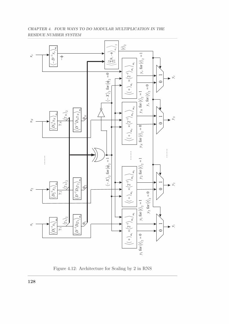
CHAPTER 4. FOUR WAYS TO DO MODULAR MULTIPLICATION IN THE
RESIDUE NUMBER SYSTEM
1fo
r2
1�
ty
……
……
……
……
0fo
r2
�t
yr
0fo
r2
�t
yN
1fo
r2
�t
yr
1fo
r2
�t
yN
0fo
r2
2�
ty
1fo
r2
2�
ty
0fo
r2
1�
ty
1xr
x
1y2
yN
y
2x
Nx
0fo
r2
2�
�X
11
1
12
mm
m
�
��
2
1
N
rm
rx
D1
��
��
21
rm
N ii
�
�� �
2t
ry
22
2
12
mm
m
�
��
NN
Nm
mm
12
�
��
rr
rm
mm
12
�
��
01
01
01
01
1
for
22
��
X
1
1
1
1m
xD
�
2
2
1
2m
xD
�
Nm
NN
xD
1�
rm
DD
11
1�
�
1�
21
�2
2�
2�
2N
�
N�
rm
DD
22
1�
�
rm
NN
DD
�1
�
Figure 4.12: Architecture for Scaling by 2 in RNS
128

4.4. RNS BARRETT MODULAR MULTIPLICATION
……
……
……
12
,..
.,
1,0
for
2
�
�
l
rl
y
12
,..
.,
1,0
for
2 �
�
l
Nl
y
12
,..
.,
1,0
for
22
�
�
l
ly
12
,..
.,
1,0
for
21
�
�
l
ly
1y2
yN
y
11
1
2
mm
l
m
��
�
lr
m
N ii
21
�
�� �
l2
ry
22
2
2
mm
l
m
��
�
NN
Nm
m
l
m
��
�2
rr
rm
m
l
m
��
�2
MU
XM
UX
MU
XM
UX
12
,..
.,
1,0
at
22
��
�l
ll
X
……
1xr
x2
xN
x
2
1
N
rm
rx
D1
��
��
1
1
1
1m
xD
�
2
2
1
2m
xD
�
Nm
NN
xD
1�
rm
DD
11
1�
�
1�
2�
N�
rm
DD
22
1�
�
rm
NN
DD
�1
�
lN
2�
l2
2�
l2
1�
ll
ll
DD
DD
NN
22
22
22
11
...
�
��
��
��
�
Figure 4.13: High-Radix Architecture for Scaling by 2l in RNS
129

CHAPTER 4. FOUR WAYS TO DO MODULAR MULTIPLICATION IN THE
RESIDUE NUMBER SYSTEM
Algorithm 4.3 The Barrett Modular Multiplication Algorithm in RNS
Require: M,N,w, {m1, . . . , mN ,mr} as described above.
Require: pre-computed values 〈D−1〉mr and 〈2−1〉mr
Require: pre-computed table 〈Di〉mi, 〈D−1Di〉mr , 〈M〉mi
and 〈2−1〉mifor
i = 1, . . . , N
Ensure: Z ≡ A × B mod M
1: xi = 〈ai × bi〉mifor i = 1, . . . , N
2: φ = 〈D−1xr〉mr
3: γi = 〈D−1i xi〉mi
for i = 1, . . . , N
4: θi = 〈D−1Diγi〉mr for i = 1, . . . , N
5: 〈X〉2 = 〈γ1〉2 ⊕ 〈γ2〉2 ⊕ ... ⊕ 〈γN〉26: y′
i = 〈(xi − 〈X〉2) × 〈2−1〉mi〉mi
for i = 1, . . . , N
7: y′′i = 〈(xi − NOT(〈X〉2)) × 〈2−1〉mi
〉mifor i = 1, . . . , N
8: 〈α〉2 = 〈〈∑Ni=1 θi − φ〉mr〉2
9: if 〈α〉2 == 0 then
10: yi = y′i for i = 1, . . . , N
11: else
12: yi = y′′i for i = 1, . . . , N
13: end if
14: zi = 〈xi − yi × 〈M〉mi〉mi
for i = 1 . . . N
130

4.4. RNS BARRETT MODULAR MULTIPLICATION
dominated by the modular accumulation 〈〈∑Ni=1 θi − φ〉mr〉2l in the redun-
dant channel with its special modulus of the form 2k − 1. A benefit of the
algorithm is that modular addition and multiplication operations within this
channel are much faster than for a general modulus. If these are referred
to as fast modular operation steps, then algorithm requires (2n + 3)/l fast
modular multiplications, (2n + 3)/l multiplications modulo general mi and
�log2(N)�(2n + 3)/l fast modular additions.
Figure 4.14 compares the latency for the 2 fast channel modular opera-
tions with 2 operations modulo general mi. The RNS channel word length
w starts from 12 bits because this is the minimum w required to construct
a RNS system with 2048-bit dynamic range and equal word length moduli
as stated in Section 2.1.4. The Xilinx Virtex2 FPGA used in Section 3.3.2
on page 45, XC2V1000 with a -6 speed grade, is used again. The Barrett
algorithm in binary discussed in Section 3.1.3 and 3.3 is used for general
modular multiplication and addition within the channels. The result from
Section 3.3.2 is taken for general modular multiplication.
It can be seen that on the FPGA, a fast modular multiplication is even
faster than a general modular addition. Also, a fast modular addition has
roughly the same latency as an addition. At the end of next section, these
results will be used to compare the RNS Barrett and RNS Montgomery
algorithm as the latter uses general modular multiplications and additions,
but fewer of them.
131

CHAPTER 4. FOUR WAYS TO DO MODULAR MULTIPLICATION IN THE
RESIDUE NUMBER SYSTEM
Delays of channel-width multiplication,
multiplication modulo 2^k - 1, addition modulo a
general modulus and end-around addition vs
RNS channel widths
0
5
10
15
20
25
30
35
40
12 14 16 18 20 22 24
w (bits)
ns
modular multiplication multiplication modulo 2^k-1modular addtion endaround addition
Figure 4.14: Delay of Channel-Width Multiplication and Addition modulo
a General Modulus and Multiplication and Addition modulo 2k − 1 used for
RNS Barrett Algorithm against RNS Channel Width w
132

4.5. RNS MONTGOMERY MODULAR MULTIPLICATION
4.5 RNS Montgomery Modular Multiplica-
tion
Existing schemes for multiplication modulo a long word length modulus in
RNS [Posch95, Freking00, Bajard98, Bajard01, Phillips01a, Phillips03] are
based on Montgomery reduction [Montgomery85]. Most of them are quite
similar and this section will examine these techniques.
Recall the Montgomery algorithm in Section 3.1.4. Montgomery reduc-
tion of X × R−1 modulo M proceeds by adding a multiple of M according
to 〈X〉M . This approach works well in the RNS as 〈X〉M can be found easily
for some values of R.
4.5.1 Montgomery Modular Reduction in RNS
In the RNS, the value R is chosen to be the dynamic range D =∏N
i=1 mi.
This is consistent in all of the existing RNS Montgomery algorithms. Hence
the RNS Montgomery reduction computes
Z ≡ X × D−1 mod M, (4.56)
where Z, X and M are all represented in the RNS with modulus set Ω =
{m1,m2, . . . , mN}. As in the Montgomery algorithm in binary in Section 3.1.4,
an integer q is sought such that q < D and X+qM is a multiple of D. Hence,
the resulting division X+qMD
is exact and easily performed in RNS by multi-
plying X + qM by D−1 since Z ≡ 〈X × D−1〉M = X+qMD
[Montgomery85].
Therefore, the RNS Montgomery modular reduction algorithm is composed
of 4 steps:
• Find q in Ω such that 〈X + qM〉D = 0.
133

CHAPTER 4. FOUR WAYS TO DO MODULAR MULTIPLICATION IN THE
RESIDUE NUMBER SYSTEM
• Base extend q from Ω to q in Ω.
• Find Z = (X + qM)D−1 in Ω.
• Base extend Z from Ω to Ω noting that Z ≡ X × D−1 mod M .
Details of these steps will be examined below.
Because X +qM is a multiple of D, the representation of X +qM in RNS
Ω is {0, 0, . . . , 0} [Bajard00]. This means
〈xi + qi〈M〉mi〉mi
= 0 for i = 1, . . . , N.
Then
qi = 〈xiM−1〉mi
for i = 1, . . . , N
where 〈M−1〉miis pre-computed. Thus, q is obtained such that X + qM
is divisible by D. However, this means (X + qM) × D−1 cannot be com-
puted because D−1 does not exist in Ω as D =∏N
i=1 mi. Therefore, it is
necessary to perform this computation in another RNS with modulus set
Ω = {mN+1,mN+2, . . . , m2N}, where D =∏2N
j=N+1 mj and D has to be co-
prime to D. Again, this becomes a typical issue of base extension: q needs
to be base extended from {q1, q2, . . . , qN} to {qN+1, qN+2, . . . , q2N}.
Base Extension I
The technique in [Bajard01] improves this base extension based on previous
publications [Posch95, Kawamura00]. From CRT,
q =
⟨N∑
i=1
Di〈D−1i qi〉mi
⟩D
=N∑
i=1
Di〈D−1i qi〉mi
− αD,
where α < N from Equation (4.24) and (4.26). Set
q = q + αD =N∑
i=1
Di〈D−1i qi〉mi
.
134
4.5. RNS MONTGOMERY MODULAR MULTIPLICATION
Reducing q modulo mj for j = N + 1, . . . , 2N yields
qj =
⟨N∑
i=1
〈Di〉mj〈D−1
i qi〉mi
⟩mj
, (4.57)
where 〈D−1i 〉mi
and 〈Di〉mjcan both be pre-computed. Therefore,
Z = (X + qM)D−1 = (X + qM)D−1 + αM, (4.58)
and then
Z ≡ X × D−1 mod M.
[Bajard04a] gives conditions for this result by assuming X < DM . From
α < N , q < D and q = q + αD, q < (N + 1)D. Then, Z < (DM + (N +
1)DM)D−1 = (N + 2)M . Thus, both (N + 2)M < D and (N + 2)M <
D have to be satisfied to assure Z < D and Z < D such that Z has a
valid RNS representation in Ω and Ω. Moreover, to be able to reuse the
result Z < (N + 2)M as inputs for the next round of RNS Montgomery
modular multiplication, ((N + 2)M)2 < DM has to be satisfied. This gives
(N + 2)2M < D. Note that this has already implied (N + 2)M < D. Thus,
the prerequisites for this algorithm are⎧⎨⎩(N + 2)2M < D
(N + 2)M < D.
These are easy to satisfy. Note that D can be greater or less than D.
Base Extension II
The last step is to base extend Z ≡ X × D−1 mod M back to RNS Ω. For
this base extension, all RNS Montgomery algorithms [Posch95, Bajard98,
Kawamura00, Bajard01, Phillips01b, Phillips03] take a method similar to
[Shenoy89a], which has been discussed in Section 4.4.1. A redundant modulus
135

CHAPTER 4. FOUR WAYS TO DO MODULAR MULTIPLICATION IN THE
RESIDUE NUMBER SYSTEM
channel mr > N is introduced with mr co-prime to mi for i = 1, . . . , 2N .
〈M〉mr and 〈D−1〉mr are pre-computed. xr = 〈X〉mr must be input from the
beginning and qr has to be computed using Equation (4.57). Following CRT,
Z =2N∑
j=N+1
Dj
⟨〈Dj
−1〉mjZj
⟩mj
− βD. (4.59)
β can be obtained similarly to Equation (4.45) as
β =
⟨2N∑
j=N+1
⟨〈D−1Dj〉mr
⟨⟨〈Dj
−1〉mjZj
⟩mj
⟩mr
⟩mr
− ⟨〈D−1〉mrZr
⟩mr
⟩mr
where Zj for j = N + 1, . . . , 2N and r is computed from Equation (4.58) as
Zj =⟨⟨
xj + qj〈M〉mj
⟩mj
〈D−1〉mj
⟩mj
.
Given β, Zi is evaluated by reducing both sides of (4.59) modulo mi for all
i = 1, . . . , N ,
Zi =
⟨2N∑
j=N+1
〈Dj〉mi
⟨〈Dj
−1〉mjZj
⟩mj
− 〈βD〉mi
⟩mi
.
4.5.2 The Algorithm
The RNS Montgomery modular multiplication algorithm is shown in Algo-
rithm 4.4. There are N + 5 RNS channel multiplications and N − 2 chan-
nel additions needed to perform a RNS Montgomery modular multiplication
[Bajard01, Bajard04a].
4.5.3 A Comparison between RNS Barrett and Mont-
gomery Modular Multiplication
Recall that the RNS Barrett algorithm shown in Algorithm 4.3 has the advan-
tage that most of its modular multiplications and modular additions on the
136

4.5. RNS MONTGOMERY MODULAR MULTIPLICATION
Algorithm 4.4 The Montgomery Modular Multiplication Algorithm in RNS
Require: M,N, Ω = {m1, . . . , mN}, Ω = {mN+1, . . . ,m2N},mr as described
above.
Require: (N + 2)2M < D =∏N
i=1 mi and (N + 2)M < D =∏2N
j=N+1 mj
Require: pre-computed values 〈D−1〉mr and 〈2−1〉mr
Require: pre-computed table 〈M−1〉mi, 〈M〉mj
, 〈D−1i 〉mi
, 〈Di〉mj, 〈Dj〉mi
,
〈Dj−1〉mj
, 〈Dj〉mr , 〈D〉mi, 〈D−1〉mj
and 〈D−1〉mr for i = 1, . . . , N and
j = N + 1, . . . , 2N and r
Ensure: Z ≡ A × B mod M
1: xi = 〈ai × bi〉mifor i = 1, . . . , 2N and r
2: qi = 〈xiM−1〉mi
for i = 1, . . . , N
3: qj =⟨∑N
i=1〈Di〉mj〈D−1
i qi〉mi
⟩mj
for j = N + 1, . . . , 2N and r
4: Zj =⟨⟨
xj + qj〈M〉mj
⟩mj
〈D−1〉mj
⟩mj
for j = N + 1, . . . , 2N and r
5: β =
⟨∑2Nj=N+1
⟨〈D−1Dj〉mr
⟨⟨〈Dj
−1〉mjZj
⟩mj
⟩mr
⟩mr
− ⟨〈D−1〉mrZr
⟩mr
⟩mr
6: Zi =
⟨∑2Nj=N+1〈Dj〉mi
⟨〈Dj
−1〉mjZj
⟩mj
− 〈βD〉mi
⟩mi
for i = 1, . . . , N
137

CHAPTER 4. FOUR WAYS TO DO MODULAR MULTIPLICATION IN THE
RESIDUE NUMBER SYSTEM
Delays of Barrett and Montgomery RNS modular
reduction algorithm
vs RNS channel widths
4000
5000
6000
7000
8000
12 14 16 18 20 22 24
w (bits)
ns
Barrett
Montgomery
Figure 4.15: Delay of Barrett and Montgomery RNS Modular Multiplication
against RNS Channel Width w
critical path are modulo its special modulus of the form 2k −1 within the re-
dundant channel. Figure 4.14 shows these fast modular operations are indeed
faster than multiplications and additions modulo general moduli. However,
the RNS Barrett algorithm requires (2n + 3)/l fast modular multiplications,
(2n + 3)/l multiplications modulo a general mi and �log2(N)�(2n + 3)/l fast
modular additions. These are much more than the RNS Montgomery algo-
rithm, which needs N + 5 and N − 2 for general modular multiplication and
addition respectively.
Figure 4.15 shows the delay of the Barrett RNS algorithm and the Mont-
gomery RNS algorithm for reduction of a 2048-bit product by a 1024-bit
modulus at radix-16 on the same FPGA platform as in Section 3.3.2. These
results are produced by adding the delays of channel operations in Figure 4.14
for the two algorithms.
It can be seen from Figure 4.15 that the RNS Barrett algorithm is faster
when the RNS channels are less than 18 bits. As the width of the chan-
nels increases, the cost of channel operations increases while the number of
138

4.5. RNS MONTGOMERY MODULAR MULTIPLICATION
channels N decreases, and hence the Montgomery approach becomes faster.
Note that in next chapter, the implementation of RNS Sum of Residues
algorithm shows a better performance than both of these two implementa-
tions.
139

CHAPTER 4. FOUR WAYS TO DO MODULAR MULTIPLICATION IN THE
RESIDUE NUMBER SYSTEM
140

Chapter 5
Implementation of RNS Sum of
Residues Modular
Multiplication
The purpose of this chapter is to give an implementation for a long word
length RNS modular multiplier on an FPGA platform. The Sum of Residues
algorithm is chosen to achieve this. It forms a highly parallel and scalable
architecture which can perform 1024-bit RSA decryption with the fastest
published rate of 0.4 ms per decryption on a Xilinx Virtex5 device.
141

CHAPTER 5. IMPLEMENTATION OF RNS SUM OF RESIDUES MODULAR
MULTIPLICATION
An implementation of a RNS modular multiplication algorithm depends
heavily on the size of the hardware used. A hardware platform able to hold a
1024-bit RNS modular multiplication may become obsolete as demand grows
for 2048-bit encryption. Thus, the RNS Sum of Residues algorithm is selected
to be implemented because it is suitable for a scalable architecture and also
because of its parallelism.
5.1 A Scalable Structure for Sum of Residues
Modular Multiplication in RNS
Recall Algorithm 4.2 described in Section 4.3.4 as below:
Algorithm 5.1 The Sum of Residues Modular Multiplication Algorithm in
RNS
Require: M,N,w, Δ, q, {m1, . . . , mN}, (N2wM)2 < (1 − Δ)D,N( (2w−m1)2w +
2w−q−1m1
) ≤ Δ < 1.
Require: pre-computed table 〈D−1i 〉mi
for i = 1, . . . , N
Require: pre-computed table 〈〈Di〉M〉mjfor i, j = 1, . . . , N
Require: pre-computed table 〈〈αD〉N〉mifor α = 1, . . . , N − 1 and i =
1, . . . , N − 1
Require: A < N2wM,B < N2wM
Ensure: Z ≡ A × B mod M
1: X = A × B
2: γi = 〈xiD−1i 〉mi
for i = 1, . . . , N
3: Zi = γi × 〈Di〉M for i = 1, . . . , N
4: Z =∑N
i=1 Zi
5: α =⌊∑N
i=1
⌊γi
2w−q
⌋/2q + Δ
⌋6: Z = Z − 〈αD〉M
142
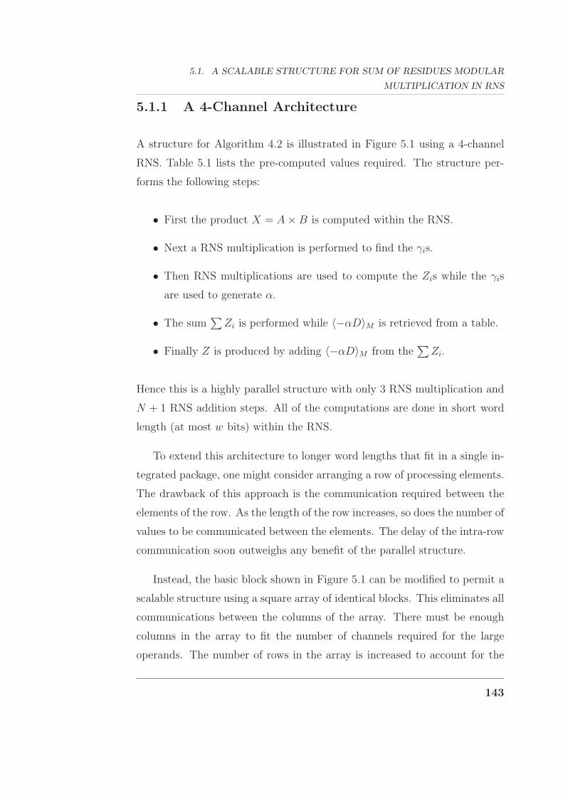
5.1. A SCALABLE STRUCTURE FOR SUM OF RESIDUES MODULAR
MULTIPLICATION IN RNS
5.1.1 A 4-Channel Architecture
A structure for Algorithm 4.2 is illustrated in Figure 5.1 using a 4-channel
RNS. Table 5.1 lists the pre-computed values required. The structure per-
forms the following steps:
• First the product X = A × B is computed within the RNS.
• Next a RNS multiplication is performed to find the γis.
• Then RNS multiplications are used to compute the Zis while the γis
are used to generate α.
• The sum∑
Zi is performed while 〈−αD〉M is retrieved from a table.
• Finally Z is produced by adding 〈−αD〉M from the∑
Zi.
Hence this is a highly parallel structure with only 3 RNS multiplication and
N + 1 RNS addition steps. All of the computations are done in short word
length (at most w bits) within the RNS.
To extend this architecture to longer word lengths that fit in a single in-
tegrated package, one might consider arranging a row of processing elements.
The drawback of this approach is the communication required between the
elements of the row. As the length of the row increases, so does the number of
values to be communicated between the elements. The delay of the intra-row
communication soon outweighs any benefit of the parallel structure.
Instead, the basic block shown in Figure 5.1 can be modified to permit a
scalable structure using a square array of identical blocks. This eliminates all
communications between the columns of the array. There must be enough
columns in the array to fit the number of channels required for the large
operands. The number of rows in the array is increased to account for the
143

CHAPTER 5. IMPLEMENTATION OF RNS SUM OF RESIDUES MODULAR
MULTIPLICATION
Table 5.1: The Pre-Computed Constants for the RNS Sum of Residues Mod-
ular Multiplication Algorithm in Algorithm 4.2
i 1 2 3 4
〈D−1i 〉mi
〈D−11 〉m1 〈D−1
2 〉m2 〈D−13 〉m3 〈D−1
4 〉m4
〈〈D1〉M〉m1〈〈D1〉M〉m2
〈〈D1〉M〉m3〈〈D1〉M〉m4
〈〈Dj〉M〉mi〈〈D2〉M〉m1
〈〈D2〉M〉m2〈〈D2〉M〉m3
〈〈D2〉M〉m4
〈〈D3〉M〉m1〈〈D3〉M〉m2
〈〈D3〉M〉m3〈〈D3〉M〉m4
〈〈D4〉M〉m1〈〈D4〉M〉m2
〈〈D4〉M〉m3〈〈D4〉M〉m4
〈〈−D〉M〉m1〈〈−D〉M〉m2
〈〈−D〉M〉m3〈〈−D〉M〉m4
〈〈−αD〉M〉mi〈〈−2D〉M〉m1
〈〈−2D〉M〉m2〈〈−2D〉M〉m3
〈〈−2D〉M〉m4
〈〈−3D〉M〉m1〈〈−3D〉M〉m2
〈〈−3D〉M〉m3〈〈−3D〉M〉m4
residues Zi which must be computed (in parallel) and accumulated (in series).
For example, Figure 5.2 shows a 4-channel block arranged for the scalable
array. This is a modified version of Figure 5.1 with extra input and output
ports to account for communication down a column.
5.1.2 The Scaled Architecture for Modular Multipli-
cation
A 12-channel modular multiplication can be built with a 3 × 3 array of the
block in Figure 5.2. The resulting structure is shown in Figure 5.3. The
leftmost column performs calculations in channels m1 to m4; the middle
column is for m5 to m8; and the rightmost for m9 to m12. The columns
execute independently. This is achieved by computing γ1 to γN and α in
each of the columns.
144

5.1. A SCALABLE STRUCTURE FOR SUM OF RESIDUES MODULAR
MULTIPLICATION IN RNS
x 12
x 3x 4
a 1,b1
a 4,b4
×<D
1-1> m1
…<D
4-1> m4
<<D
2> M> m1
…<<
D2> M
> m4×
<<D
3> M> m1
…<<
D3> M
> m4×
<<D
4> M> m1
…<<
D4> M
> m4×
<×> m1
…<×
> m4
<Z2> m1
…<Z
2> m4<Z
3> m1…
<Z3> m4
<Z4> m1
…<Z
4> m4
<+> m1
…<+
> m4…
…
��
��
i
qw
i2/
�a
<<D
1> M> m1
…<<
D1> M
> m4×
<Z1> m1
…<Z
1> m4
<<-D
> M> m1
…<<
-D> M
> m4<<
-aD>
M> m1
…<<
-aD>
M> m4
<+
> m1…
<+
> m4<Z
> m1…
<Z> m4
×
<Z> m1
<Z> m4
…
<Z 1.
.4> m1
<Z 1.
.4> m4
��1�
2�
3�
4�
x
Fig
ure
5.1:
A4-
Chan
nel
RN
SM
odula
rM
ult
iplier
145

CHAPTER 5. IMPLEMENTATION OF RNS SUM OF RESIDUES MODULAR
MULTIPLICATION
a 1,b1
a 4,b4
×<D
1-1> m1
…<D
4-1> m4
<<D
2> M> m1
…<<
D2> M
> m4×
<<D
3> M> m1
…<<
D3> M
> m4×
<<D
4> M> m1
…<<
D4> M
> m4×
<×> m1
…<×
> m4
<Z2> m1
…<Z
2> m4<Z
3> m1…
<Z3> m4
<Z4> m1
…<Z
4> m4
<+> m1
…<+
> m4…
…
��
��
i
qw
i2/
�<<
D1> M
> m1…
<<D
1> M> m4
×<Z
1> m1…
<Z1> m4
<<-D
> M> m1
…<<
-D> M
> m4<<
-aD>
M> m1
…<<
-aD>
M> m4
<+
> m1…
<+
> m4<Z
> m1…
<Z> m4
×
<Z> m1
<Z> m4
…
<Z 1.
.4+Z
in> m1
a 5..8
+a in
Z in
a 1..8
a out
Z out
<Z 1.
.4+Z
in> m4
��
�
�
1�
2�
3�
4�
x 12
x 3x 4
x
Fig
ure
5.2:
A4-
Chan
nel
Modula
rM
ult
iplier
Blo
ckSuit
able
for
aSca
lable
Arr
ayof
Blo
cks
146

5.1. A SCALABLE STRUCTURE FOR SUM OF RESIDUES MODULAR
MULTIPLICATION IN RNS
The rows of the array in Figure 5.3 evaluate the residues. The first row
finds Z1 to Z4 and∑4
i=1 Zi; the second row Z5 to Z8, the sum∑8
i=5 Zi
and∑8
i=1 Zi =∑4
i=1 Zi +∑8
i=5 Zi; and the last row finds Z9 to Z12, the
sum∑12
i=9 Zi and∑8
i=1 Zi +∑12
i=9 Zi. The sum of the residues is found by
accumulating the results down a column. This comes at a cost of latency
but bounds the number of I/O pins for the blocks and ensures the array is
scalable. A similar scheme is used to accumulate the terms required to find
α. This is off the critical path of the modular multiplication. Note that each
row produces outputs for the result Z but these will be meaningless for all
but the last row.
The indices in Figure 5.2 are arranged to illustrate the first block in the
second row of Figure 5.3. First {γ5, . . . , γ8} are computed from the inputs
{a5b5, . . . , a8b8}. Then RNS multiplications with {〈D5〉M , . . . , 〈D8〉M} mod-
ulo {m1, . . . , m4} are used to compute {〈Z5〉m1 , . . . , 〈Z5〉m4} . . .
{〈Z8〉m1 , . . . , 〈Z8〉m4}. These results are added to{〈∑Z1...4〉m1
, . . . , 〈∑Z1...4〉m4
}(available at the Zin input) to generate
{〈∑Z1...8〉m1, . . . , 〈∑Z1...8〉m4
}. These
values are sent to the next element down the column via the Zout output.
The critical path is shown on the middle column in Figure 5.3. The
latency of the modular multiplier is given by
d1 + (k − 2)dz + dn, (5.1)
where k is the number of rows in the array, d1 is the delay from the ai and bi
inputs to Zout of the first block, dz is the delay from Zin to Zout of any block
between the first and the last block, and dk is the delay from Zin of the last
block to the final output Z.
147

CHAPTER 5. IMPLEMENTATION OF RNS SUM OF RESIDUES MODULAR
MULTIPLICATION
a1,b
1a
4,b
4…
0
<�
Z1..4>
m1
…
<�
Z1..4>
m4
0
�a
1..4
a5,b
5a
8,b
8…
�a
1..8
a9,b
9a
12,b
12
…
<Z
>m
1<
Z>
m4
…
<�
Z1..8>
m1
…
<�
Z1..8>
m4
a1,b
1a
4,b
4…
<�
Z1..4>
m5
…
<�
Z1..4>
m8
�a
1..4
a5,b
5a
8,b
8…
�a
1..8
a9,b
9a
12,b
12
…
<Z
>m
5<
Z>
m8
…
<�
Z1..8>
m5
…
<�
Z1..8>
m8
a1,b
1a
4,b
4…
<�
Z1..4>
m9
…
<�
Z1..4>
m12
�a
1..4
a5,b
5a
8,b
8…
�a
1..8
a9,b
9a
12,b
12
…
<Z
>m
9<
Z>
m12
…
<�
Z1..8>
m9
…
<�
Z1..8>
m12
a1,b
1a
4,b
4…
a1,b
1a
4,b
4…
a1,b
1a
4,b
4…
a1,b
1a
4,b
4…
a1,b
1a
4,b
4…
a1,b
1a
4,b
4…
a1,b
1a
4,b
4…
a1,b
1a
4,b
4…
a1,b
1a
4,b
4…
<Z
>m
1<
Z>
m4
…<
Z>
m1
<Z
>m
4…
<Z
>m
1<
Z>
m4
…
Zin
Zout
ain
aout
Zin
Zout
ain
aout
Zin
ain
Zin
ain
Zin
Zout
ain
aout
Zin
Zout
ain
aout
Zin
Zout
ain
aout
Zin
Zout
ain
aout
Zin
ain
00
00
Cri
tical
Path
1d
zd
kd
Fig
ure
5.3:
A12
-Chan
nel
Modula
rM
ult
iplier
Built
from
a3×
3A
rray
of4-
Chan
nel
Blo
cks
148

5.2. IMPLEMENTATION RESULTS
5.2 Implementation Results
To utilize the hardware efficiently, each block shown in Figure 5.2 has to
hold as many channels as possible. This depends largely on the size of the
hardware used. Thus, the latest version of the Xilinx Virtex5 FPGA is
used as the implementation target to evaluate the performance of the RNS
modular multiplier. The implementation was performed using the Xilinx ISE
environment using XST for synthesis and ISE standard tools for place and
route. Speed optimization with standard effort has been used.
Target FPGA: Virtex5 XC5VSX95T with a -3 speed
grade, 14720 CLB (Configurable Logic
Blocks) slices and 640 DSP slices
Xilinx 9.1i: XST - Synthesis
ISE - Place and Route
Optimization Goal: Speed
Language: VHDL
The largest RNS modular multiplier this FPGA can accommodate was
found to be 64 bits. Repeated modular multiplication of 64-bit inputs can
be performed without overflow in a 10-channel RNS where each channel is
18 bits wide. The pin-to-pin delay was measured from the Post-Place and
Route Static Timing Analyzer with a standard place and route effort level.
The modular multiplications within the 18-bit channels is performed using
the Barrett algorithm discussed Sections 3.1.3 and 3.3 and optimized for the
Xilinx Virtex2 FPGA platform used in Sections 3.3 and 3.4. The performance
of this modular multiplier has already been shown in Figure 3.7 on page 46.
The latency of a single block of this 64-bit modular multiplier is 81.7 ns
and the component delays for Equation (5.1) were d1 = 77.18 ns, dz =
149

CHAPTER 5. IMPLEMENTATION OF RNS SUM OF RESIDUES MODULAR
MULTIPLICATION
20.87 ns and dk = 25.45 ns. This was done by using the consecutive prime
moduli [m1,m2, . . . , m10] = [262051, 262069, . . . , 262139], q = 5 and Δ = 0.5.
The final design consumed 78% of the DSP slices on Virtex5 but only 10%
of the CLB slices. This is because the channel modular multipliers make
extensive use of the hardware multipliers available in the DSP slices of the
FPGA. With more DSP slices it would have been possible to include more
channels within each FPGA.
Modular multiplication of 1024-bit inputs can be performed with a 16×16
array of 64-bit blocks using the consecutive prime moduli [m1,m2, . . . ,m160] =
[260017, 260023, . . . , 262139], q = 10 and Δ = 0.6. From Equation (5.1) the
delay for this array can be estimated to be 77.18 + 20.87 × 14 + 25.45 =
394.8 ns ≈ 0.4 μs. Similarly a 2048-bit modular multiplication can be per-
formed with an 32 × 32 array using the consecutive prime moduli
[m1,m2, . . . , m320] = [258101, 258107, . . . , 262139], q = 10 and Δ = 0.8. The
delay in this case is 77.18 + 20.87 × 30 + 25.45 = 728.7 ns.
According to Section 2.2.3, the number of multiplications required to
evaluate a RSA decryption C = AB mod M is log2 B on parallel hardware.
Then a 1024-bit RSA decryption could be achieved in 394.8 ns × 1024 ≈0.4 ms and a 2048-bit in 728.7 ns × 2048 ≈ 1.5 ms.
This can be compared with some previously published low latency results.
• The design in [Blum99] can complete a 1024-bit modular multiplica-
tion in 8.2 μs on a Xilinx XC4000 FPGA. The Montgomery modular
multiplication algorithm [Montgomery85] discussed in Section 3.4 is
implemented on systolic arrays with all the operations performed in
binary.
• The design in [McIvor04] can perform the same operation in 2.6 μs on
the same FPGA. This design again uses Montgomery algorithm in a
150

5.2. IMPLEMENTATION RESULTS
positional system and improves the speed by using redundant repre-
sentations for intermediate results.
• The design in [Nozaki01] is the only published implementation based on
the Montgomery modular multiplication in RNS [Posch95]. It uses the
RNS Montgomery algorithm discussed in Section 4.5 with a Cox-Rower
architecture from [Kawamura00]. This is implemented on a 0.25 μm LSI
prototype and achieves 2.34 μs for a 1024-bit modular multiplication
at its fastest speed.
• Finally, Figure 4.15 shows the speed of a 1024-bit modular multipli-
cation in RNS using RNS Barrett and RNS Montgomery algorithms
discussed in Section 4.4 and 4.5. They are both over 4 μs at w = 18.
Moreover, these results are relatively theoretical because they are pro-
duced from a theoretical sum of the results of implemented channel
modular operators only. The actual speed could be lower.
151

CHAPTER 5. IMPLEMENTATION OF RNS SUM OF RESIDUES MODULAR
MULTIPLICATION
152

Chapter 6
Conclusion and Future
Perspectives
The purpose of this chapter is to conclude this thesis by reflecting on its
original objectives and contributions. Some suggestions for further study are
made.
153

CHAPTER 6. CONCLUSION AND FUTURE PERSPECTIVES
6.1 Conclusion
The four classes of modular multiplication algorithms possible in positional
number systems can also be used for long word length modular multiplication
in the RNS; moreover, using the RNS in this way will lead to faster implemen-
tations than those which restrict themselves to positional number systems.
This outcome was the foremost objective of this thesis and was demonstrated
through developing new Classical, Barrett and Sum of Residues algorithms
for modular multiplication in the RNS and implementing the RNS Sum of
Residues algorithm on an FPGA.
In Chapter 3, four classes of positional modular multiplication algorithms
are analyzed, improved and implemented. Chapter 4 uses RNS to speed
up long word length modular multiplication. This is achieved by devising
new algorithms of Classical, Barrett and Montgomery classes that restrict
all intermediate operations within short word length RNS channels. This is
further demonstrated by the implementation in Chapter 5.
6.2 Future Perspectives
The RNS modular multiplication algorithms show good performance in speed-
ing up long word length modular multiplication for the RSA Cryptosystem on
an FPGA. As the word length of public-key systems increases over time, El-
liptic Curve Cryptography, which uses shorter keys and moduli, will probably
become another interesting application of the RNS in the future. Apart from
the multiplication modulo a long word length modulus, the Elliptic Curve
system involves modular additions and inversions, which also challenge the
capacity of the RNS.
154

6.2. FUTURE PERSPECTIVES
The benefits of the RNS to public-key systems may not be limited to
speed. Investigations can proceed in other aspects of a public-key system
based on the RNS, such as security. The parallel architectures possible with
RNS are different to the relatively serial procedures possible in a positional
system. To what extent can a RNS help a public-key system circumvent
power and timing attacks by disguising internal operations through its par-
allel nature? This may not only be of theoretical interest.
155

CHAPTER 6. CONCLUSION AND FUTURE PERSPECTIVES
156

Bibliography
[Aichholzer93] O. Aichholzer and H. Hassler. A fast method for modulus
reduction in residue number system. In Proc. Economical
Parallel Processing, pages 41–54, Vienna, Austria, 1993.
[Akushskii77] I. J. Akushskii, V. M. Burcev, and I. T. Pak. A new po-
sitional characteristic of non-positional codes and its appli-
cation. In Coding Theory and the Optimization of Complex
Systems. 1977.
[Alia84] G. Alia, F. Barsi, and E. Martinelli. A fast near optimum
vlsi implementation of fft using residue number system. The
VLSI Journal, 2:133–147, 1984.
[Alia98] G. Alia, F. Barsi, and E. Martinelli. Optimal vlsi complexity
design for high speed pipeline fft using rns. Computers &
Electrical Engineering, 24:167–182, 1998.
[Bajard98] J. C. Bajard, L. S. Didier, and P. Kornerup. An rns mont-
gomery modular multiplication algorithm. IEEE Trans.
Comput., 47(7):766–776, July 1998.
[Bajard00] J.C. Bajard, L.S. Didier, P. Kornerup, and F. Rico. Some
improvements on rns montgomery modular multiplication.
157

BIBLIOGRAPHY
In Proc. SPIE, International Symposium on Optical Science
and Technology, August 2000.
[Bajard01] J. C. Bajard, L. S. Didier, and P. Kornerup. Modular mul-
tiplication and base extensions in residue number systems.
In Proc. 15th IEEE Symposium on Computer Arithmetic,
volume 2, pages 59–65, 2001.
[Bajard04a] J. C. Bajard and L. Imbert. A full RNS implementation of
RSA. IEEE Trans. Comput., 53(6), June 2004.
[Bajard04b] J. C. Bajard, L. Imbert, P. Y. Liardet, and Y. Teglia. Leak
resistant arithmetic. Cryptographic Hardware and Embedded
System (CHES), pages 62–75, 2004.
[Barraclough89] S. R. Barraclough. The design and implementation of the
ims a110 image and signal processor. In Proc. IEEE CICC,
pages 24.5/1–4, San Diego, May 1989.
[Barrett84] Paul Barrett. Communications authentication and security
using public key encryption - a design for implementation.
Master’s thesis, Oxford University, September 1984.
[Barrett87] Paul Barrett. Implementing the Rivest, Shamir and Adle-
man public-key encryption algorithm on a standard digital
signal processor. In Advances in Cryptology - Crypto 86,
volume 263 of Lecture Notes in Computer Science, pages
311–323. Springer, Berlin/Heidelberg, Germany, 1987.
[Barsi95] F. Barsi and M. C. Pinotti. Fast base extension and precise
scaling in RNS for look-up table implementations. IEEE
Trans. Signal Processing, 43(10):2427–2430, October 1995.
158

BIBLIOGRAPHY
[Batina02] L. Batina and G. Muurling. Montgomery in practice: How
to do it more efficiently in hardware. In B. Preneel, edi-
tor, Proceedings of RSA 2002 Cryptographers’ Track, num-
ber 2271 in Lecture Notes in Computer Science, pages 40–52.
Springer, San Jose, USA, Feb 2002.
[Baugh73] C. Baugh and B. Wooley. A two’s complement paral-
lel array multiplication algorithm. IEEE Trans. Comput.,
22(12):1045–1047, December 1973.
[Beuchat03] Jean-Luc Beuchat, Laurent Imbert, and Arnaud Tisserand.
Comparison of modular multipliers on fpgas. In Proceedings
of SPIE, volume 5205, pages 490–498, 2003.
[Bhardwaj98] M. Bhardwaj and B. Ljusanin. The renaissance – a residue
number system based vector co-processor. In Proc. 32nd
Asilomar Conference on Signals, Systems and Computers,
pages 202–207, 1998.
[Blakley83] G. R. Blakley. A computer algorithm for calculation the
product ab modulo m. IEEE Trans. Comput., C-32:497–500,
June 1983.
[Blum99] T. Blum and C. Paar. Montgomery modular exponentiation
on reconfigurable hardware. In Proc. 14th IEEE Symposium
on Computer Arithmetic, Adelaide, Australia, April 1999.
[Boyd93] C. Boyd. Modern data encryption. Electronics and Commu-
nication Engineering, pages 271–278, 1993.
[Brickell83] Ernest F. Brickell. A fast modular multiplication algorithm
with application to two key cryptography. In Advances in
Cryptology - Crypto 82, Lecture Notes in Computer Science.
Springer, Berlin/Heidelberg, Germany, 1983.
159

BIBLIOGRAPHY
[Brickell91] E. F. Brickell and K. S. McCurley. Interactive identification
and digital signature. AT & T Technical Journal, pages 78–
86, 1991.
[Burgess97] Neil Burgess. Scaled and unscaled residue number system
to binary conversion techniques using the core function. In
Proc. 13th IEEE Symposium on Computer Arithmetic, pages
250–257, June 1997.
[Burgess03] N. Burgess. Scaling an RNS number using the core function.
In Proc. 16th IEEE Symposium on Computer Arithmetic,
2003.
[Burks46] A. Burks, H. Golodstine, and J. von Neumann. Preliminary
discussion of the logical desing of an electronic computing
instrument, volume 1. Princeton, advanced study edition,
1946.
[Chang94] C. C. Chang, W. J. Horng, and D. J. Buehrer. A cascade
exponentiation evaluation scheme based on the lempel-ziv-
welch compression algorithm. Journal of Information Sci-
ence and Engineering, 1994.
[Chen99] Chien-Yuan Chen and Chin-Chen Chang. A fast modular
multiplication algorithm for calculating the product ab mod-
ulo n. Information Processing Letters, 72:77–81, 1999.
[Chiou93] C. W. Chiou. Parallel implementation of the RSA public -
key cryptosystem. International Journal of Computer Math-
ematics, 48(153-155), 1993.
[Crandall01] R. Crandall and C. Pomerance. Prime Numbers, A Compu-
tational Perspective. Springer-Verlag, 2001.
160

BIBLIOGRAPHY
[Dadda65] L. Dadda. Some schemes for parallel multipliers. In Alta
Frequenza, volume 34, pages 349–356, May 1965.
[Dhanesha95] H. Dhanesha, K. Falakshahi, and M. Horowitz. Array-of-
arrays architecture for parallel floating point multiplication.
In Proc. Conf. Advanced Research in VLSI, pages 150–157,
1995.
[Dhem98] J.-F. Dhem. Design of an efficient public-key cryptographic
library for RISC based smart cards. PhD thesis, Universite
Catholique de Louvain, May 1998.
[Diffie76] W. Diffie and M. E. Hellman. New directions in cryptogra-
phy. IEEE Transactions on Information Theory, 22:644–654,
November 1976.
[Doche06] C. Doche and L. Imbert. Extended double-base number
system with applications to elliptic curve cryptography. In
Progress in Cryptology - INDOCRYPT 2006, volume 4329.
Springer, November 2006.
[ElGamal85] T. ElGamal. A public key cryptosystem and a signature
scheme based on discrete logarithms. IEEE Trans. Inform.
Theory, 31(4):469–472, 1985.
[Elleithy91] K.M. Elleithy and M.A. Bayoumi. A massively parallel RNS
architecture. In 25th Asilomar Conference, 1991, volume 2
of Conference Record of the Asilomar Conference on Sig-
nals, Systems and Computers, pages 408–412 vol. 1, Pacific
Grove, CA, Nov 1991. Institute of Electrical and Electronics
Engineers Computer Society.
[Findlay90] P. A. Findlay and B. A. Johnson. Modular exponentiation
using recursive sums of residues. In Advances in Cryptology
161

BIBLIOGRAPHY
- Crypto 89, volume 435 of Lecture Notes in Computer Sci-
ence, pages 371–386. Springer, Berlin/Heidelberg, Germany,
1990.
[Freking00] W. L. Freking and K. K. Parhi. Modular multiplication in
the residue number system with application to massively-
parallel public-key cryptography systems. In Proc. 34th
Asilomar Conference on Signals, Systems and Computers,
volume 2, pages 1339–1343, 2000.
[Garcia99] A. Garcia and A. Lloris. A look-up scheme for scaling in the
RNS. IEEE Trans. Comput., 48(7):748–751, July 1999.
[Gonnella91] J. Gonnella. The application of core functions to residue
number systems. IEEE Trans. Signal Processing, 39:284–
288, 1991.
[Griffin89] M. Griffin, M. Sousa, and F. Taylor. Efficient scaling in
the residue number system. In IEEE International Confer-
ence on Acoustics, Speech, and Signal Processing, volume 89,
1989.
[Hankerson04] Darrel Hankerson, Alfred J. Menezes, and Scott Vanstone.
Guide to Elliptic Curve Cryptography. Springer, 2004.
[Hatamian86] M. Hatamian and G. Cash. A 70-mhz 8-bit × 8-bit parallel
pipelined multiplier in 2.5-μm cmos. JSSC, 21(4):505–513,
August 1986.
[Hennessy90] J. Hennessy and D. Patterson. Computer Architecture: A
Quantitative Approach. Morgan Kaufmann, San Mateo,
1990.
162

BIBLIOGRAPHY
[Itoh01] N. Itoh and et al. A 600-mhz 54 × 54-bit multiplier with
rectangular-styled wallace tree. IEEE Journal of Solid-State
Circuits, 36(2):249–257, February 2001.
[Jenkins93] W. K. Jenkins. Finite arithmetic concepts. In S. K. Mi-
tra and J. F. Kaiser, editors, Handbook for Digital Signal
Processing, pages 611–675. Wiley, 1993.
[Jullien78] G. A. Jullien. Residue number scaling and other operations
using rom arrays. IEEE Trans. Comput., 27(4):325–336,
April 1978.
[Kawamura88] Shin-Ichi Kawamura and Kyoko Hirano. A fast modu-
lar arithmetic algorithm using a residue table. In Ad-
vances in Cryptology - Eurocrypt 88, volume 330 of Lec-
ture Notes in Computer Science, pages 245–250. Springer,
Berlin/Heidelberg, Germany, 1988.
[Kawamura00] S. Kawamura, M. Koike, F. Sano, and A. Shimbo. Cox-
rower architecture for fast parallel montgomery multiplica-
tion. In Advances in Cryptology - Eurocrypt 2000, volume
1807 of Lecture Notes in Computer Science, pages 523–538.
Springer, 2000.
[Knuth69] D. E. Knuth. The Art of Computer Programming, volume 2.
Addison - Wesley, 1969.
[Knuth97] D. E. Knuth. The Art of Computer Programming, volume 2.
Addison - Wesley, third edition, 1997.
[Koblitz87] N. Koblitz. A Course in Number Theory and Cryptography.
Graduate Texts in Mathematics 114. Springer-Verlag, 1987.
163

BIBLIOGRAPHY
[Kong05] Y. Kong and B. Phillips. Residue number system scaling
schemes. In S. F. Al-Sarawi, editor, Proc. SPIE, Smart
Structures, Devices, and Systems II, volume 5649, pages
525–536, February 2005.
[Kong07] Y. Kong and B. Phillips. Simulations of modular multipli-
ers on fpgas. In Proceedings of the IASTED Asian Confer-
ence on Modelling and Simulation, page 11281131, Beijing,
China, October 2007.
[Mahesh00] M. N. Mahesh and M. Mehendale. Low power realization of
residue number system based fir filters. In 13th Int. Conf.
On VLSI Design, pages 30–33, Bangalore, India, January
2000.
[McIvor04] C. McIvor, M. McLoone, and J. V. McCanny. Modified
montgomery modular multiplication and RSA exponentia-
tion techniques. IEE Proceedings Computers and Digital
Techniques, 151(6), November 2004.
[Menezes97] A. J. Menezes, P. V. Oorschot, and S. Vanstone. Handbook
of Applied Cryptography. CRC Press, 1997.
[Meyer-Base03] U. Meyer-Base and T. Stouraitis. New power-of-2 RNS scal-
ing scheme for cell-based ic design. IEEE Trans. VLSI Syst.,
11(2):280–283, April 2003.
[Miller83] D. D. Miller, J. N. Polky, and J. R. King. A survey of soviet
developments in residue number theory applied to digital
filtering. In Proceedings of the 26th Midwest Symposium on
Circuits and Systems, 1983.
164

BIBLIOGRAPHY
[Montgomery85] P. L. Montgomery. Modular multiplication without trial di-
vision. Mathematics of Computation, 44(170):519–521, April
1985.
[Mou90] Z. Mou and F. Jutand. A class of close-to-optimum adder
trees allowing regular and compact layout. In Proc. IEEE
Intl. Conf. Computer Design, pages 251–254, 1990.
[Nozaki01] H. Nozaki, M. Motoyama, A. Shimbo, and S. Kawamura.
Implementation of RSA algorithm based on RNS mont-
gomery multiplication. In Proceedings of Cryptographic
Hardware and Embedded Systems (CHES 2001), pages 364–
376, September 2001.
[Ohkubo95] N. Ohkubo and et al. A 4.4 ns cmos 54 × 54-bit multiplier
using pass-transistor multiplexer. IEEE Journal of Solid-
State Circuits, 30(3):251–257, 1995.
[Omondi07] A. Omondi and B. Premkumar. Residue Number Systems –
Theory and Implementation, volume 2 of Advances in Com-
puter Science and Engineering: Texts. Imperial College
Press, UK, 2007.
[Orup91] Holger Orup and Peter Kornerup. A high-radix hardware al-
gorithm for calculating the exponential me modulo n. In Pro-
ceedings of the 10th IEEE Symposium on Computer Arith-
metic, volume 576, pages 51–57, 1991.
[Orup95] Holger Orup. Simplifying quotient determination in high-
radix modular multiplication. In Proceedings of the 12th
IEEE Symposium on Computer Arithmetic, pages 193–199,
1995.
165

BIBLIOGRAPHY
[Parhami96] B. Parhami. A note on digital filter implementation using
hybrid rns-binary arithmetic. Signal Processing, 51:65–67,
1996.
[Parhami00] B. Parhami. Computer Arithmetic – Algorithms and Hard-
ware Designs. Oxford University Press, 2000.
[Phillips01a] B. Phillips. Modular multiplication in the montgomery
residue number system. In Proc. 35th Asilomar Conference
on Signals, Systems and Computers, volume 2, pages 1637–
1640, 2001.
[Phillips01b] B. Phillips. Montgomery residue number systems. Electron-
ics Letters, 37(21):1286–1287, 2001.
[Phillips03] B. Phillips. Scaling and reduction in the residue number sys-
tem with pairs of conjugate moduli. In Proc. 37th Asilomar
Conference on Signals, Systems and Computers, volume 2,
pages 2247– 2251, 2003.
[Posch95] K. C. Posch and R. Posch. Modulo reduction in residue num-
ber systems. IEEE Trans. Parallel Distrib. Syst., 6(5):449–
454, May 1995.
[Preethy99] A. P. Preethy and D. Radhakrishnan. A 36-bit balanced
moduli mac architecture. In Proc. IEEE Midwest Symposium
On Circuits and Systems, pages 380–383, 1999.
[Richman71] F. Richman. Number Theory : An Introduction to Algebra.
Contemporary undergraduate mathematics series. 1971.
[Rivest78] R. L. Rivest, A. Shamir, and L. M. Adleman. A method for
obtaining digital signatures and public-key cryptosystems.
Communications of the ACM, 21(2):120–126, February 1978.
166

BIBLIOGRAPHY
[Rivest85] R. L. Rivest. RSA chips (past/present/future). In Advances
in Cryptology - Eurocrypt 84, volume 209 of Lecture Notes
in Computer Science, pages 159–165. Springer, New York,
1985.
[Robertson58] J. E. Robertson. A new class of digital division methods. IRE
Transactions on Electronic Computers, 7:218–222, Septem-
ber 1958.
[Santoro89] M. Santoro. Design and Clocking of VLSI Multipliers. Ph.d.
thesis, Stanford University, CSL-TR-89-397, 1989.
[Schneier96] B. Schneier. Applied Cryptography: Protocols, Algorithms,
and Source Code in C. John Wiley & Sons, Inc., 2nd edition,
1996.
[Schnorr89] C. P. Schnorr. Efficient identification and signature for smart
cards. In Advances in Cryptology - Crypto 89, Lecture Notes
in Computer Science. Springer, New York, 1989.
[Shand93] M. Shand and J. Vuillemin. Fast implementations of RSA
cryptography. In Proc. 11th IEEE Symposium on Computer
Arithmetic, pages 252–259, 1993.
[Shenoy89a] A. Shenoy and R. Kumaseran. A fast and accurate RNS
scaling technique for high speed signal processing. IEEE
Trans. Acoust., Speech, Signal Processing, 37(6):929–937,
June 1989.
[Shenoy89b] A. Shenoy and R. Kumaseran. Fast base extension using a re-
dundant modulus in RNS. IEEE Trans. Comput., 38(2):292–
297, February 1989.
167

BIBLIOGRAPHY
[Soderstrand86] M. A. Soderstrand, W. Jenkins, and G. Jullien. Residue
number system arithmetic: Modern applications. Digital
Signal Processing, 1986.
[Standards91] National Institute Standards and Technology. A proposed
federal information processing standard for digital signature
standard (dss). In Federal Register, volume 56, pages 42980–
42982. 1991.
[Su96] F. F. Su and T. Hwang. Comments on iterative modular
multiplication without magnitude comparison. In Proc. 6th
National Conference on Information Security, pages 21–22,
Taichung Taiwan, 1996.
[Sutherland99] I. S. Sutherland, B. Sproull, and D. Harris. Logical Effort:
Designing Fast CMOS Circuits. Morgan Kaufmann, San
Francisco, CA, 1999.
[Szabo67] N. S. Szabo and R. H. Tanaka. Residue Arithmetic and its
Applications to Computer Technology. McGraw Hill, New
York, 1967.
[Taylor82] F. J. Taylor and C. H. Huang. An autoscale residue multi-
plier. IEEE Trans. Comput., 31(4):321–325, April 1982.
[Tomlinson89] A. Tomlinson. Bit-serial modular multiplier. Electronics
Letters, 25(24):1664, November 1989.
[Ulman98] Z. D. Ulman and M. Czyzak. Highly parallel, fast scaling of
numbers in nonredundant residue arithmetic. IEEE Trans.
Signal Processing, 46:487–496, February 1998.
168

BIBLIOGRAPHY
[Wallace64] C. Wallace. A suggestion for a fast multiplier. IEEE Trans-
actions on Electronic Computers, pages 14–17, February
1964.
[Walter92] C. D. Walter. Faster multiplication by operand scaling. In
Advances in Cryptology - Crypto 91, volume 576 of Lec-
ture Notes in Computer Science, pages 313–323. Springer,
Berlin/Heidelberg, Germany, 1992.
[Walter94] C. D. Walter. Logarithmic speed modular multiplication.
Electronics Letters, 30(17):1397–1398, August 1994.
[Walter95] C. D. Walter. Still faster modular multiplication. Electronics
Letters, 31(4):263–264, February 1995.
[Walter99] C. D. Walter. Montgomery’s multiplication technique: how
to make it smaller and faster. In C.-K. Koc and C. Paar, ed-
itors, Cryptographic Hardware and Embedded Systems, First
International Workshop, CHES’99 Worcester, MA, USA,
August 12-13, 1999 Proceedings, volume 1717 of Lecture
Notes in Computer Science, pages 80–93. Springer-Verlag,
Berlin, Germany, 1999.
[Weinberger58] A. Weinberger and J. Smith. A logic for high-speed addi-
tion. In System Design of Digital Computer at the National
Bureau of Standards: Methods for High-Speed Addition and
Multiplication, volume 23 of Circular 591, chapter 1, pages
3–12. National Bureau of Standards, February 1958.
[Weinberger81] A. Weinberger. 4-2 carry-save adder module. In IBM Tech-
nical Disclosure Bulletin, volume 23, pages 3811–3814. Jan-
uary 1981.
169

BIBLIOGRAPHY
[Weste04] N. Weste and D. Harris. CMOS VLSI Design – A Circuit
and Systems Perspecitive. Addison Wesley, third edition,
2004.
[Yen93] S. M. Yen and C. S. Laih. The fast cascade exponentiation
algorithm and its application on cryptography. In Advances
in Cryptology - Auscrypt 92, Lecture Notes in Computer
Science. Springer, New York, 1993.
[Yen94] S. M. Yen, C. S. Laih, and A. K. Lenstra. Multi-
exponentiation. In IEE Proc. Computers and Digital Tech-
niques, volume 141, pages 325–326, 1994.
[Zimmermann99] R. Zimmermann. Efficient vlsi implementation of mod-
ulo (2n1) addition and multiplication. In Koren and Ko-
rnerup, editors, Proceedings 14th IEEE Symposium on Com-
puter Arithmetic, pages 158–167, Adelaide, Australia, 1999.
IEEE Computer Society Press.
[Zuras86] D. Zuras and W. McAllister. Blalanced delay trees and com-
binatorial division in vlsi. IEEE Journal of Solid-State Cir-
cuits, 21(5):814–819, October 1986.
170