PREPRINT SOURCE http://www.jenskoeplinger.com/P

NOTICE: this is the authors’ version of a work that was accepted for publication in Applied Mathematics and Computation.

Changes resulting from the publishing process, such as peer review, editing, corrections, structural formatting, and other quality

control mechanisms may not be reflected in this document. Changes may have been made to this work since it was submitted for

publication. A definitive version was subsequently published in Appl. Math. Computation (2010) doi: 10.1016/j.amc.2010.04.069

Elliptic complex numbers with dual multiplication

John A. Shuster

210 Grand Ave, Las Vegas, NM 87701, USA

Jens Köplinger

105 E Avondale Dr, Greensboro, NC 27403, USA

Abstract

Investigated is a number system in which the square of a basis number: (w)2, and the square of its additive inverse: (−w)2, are not

equal. Termed W space, a vector space over the reals, this number system will be introduced by restating defining relations for complex

space C, then changing a defining conjugacy relation from conj(z) + z = 0 in the complexes to conj(z) + z = 1 for W space. This change

produces a dual represented vector space consisting of two dual, isomorphic fields, which are unified under one “context-sensitive”

multiplication. Fundamental algebraic and geometric properties will be investigated. W space can be interpreted as a generalization of

the complexes but is characterized by an interacting duality which seems to produce two of everything: two representations, two

multiplications, two norm values, and two solutions to a linear equation. W space will be compared to a previous suggestion of a similar

algebra, and then possible applications will be offered, including a W space fractal.

Key words: elliptic complex number, vector space, duality, fractal, hypernumber

1 Introduction

In this paper we propose to establish an algebra, W space, as a dual representational vector space with a vector

multiplication. By first revisiting characteristic relations in complex number algebra, this will allow us to modify a relation

between conjugates, and key algebraic properties of the proposed W space will become evident.

Two representations: +W and −W of this space, with linear bases {1, (w)} and {1, (−w)}, respectively, are introduced,

each of which will yield an algebraically closed field with its own multiplication. On products with a factor from each of the

two fields, the unifying algebra of W space will prove to be predictable with respect to commutativity, associativity, and

distributivity.

Using the example of the squares of the optional linear basis numbers ((w) or (−w)), a key characteristic of W space will

be isolated by defining a context-sensitive multiplication: When multiplying two factors, the product depends on (is “sensitive”

to) the representation (“context”) of each factor. This approach will allow us to provide an unambiguous and consistent

algebra, which will permit further analysis.

Geometrical investigation will suggest W space as mapped onto two dual planes, which can be visualized as one dual-layered

(or two-sided transparent) plane: One layer (or side) depicts +W representation, and the other depicts −W in this model.

The dual conjugate in W space results in a non-standard norm with generalized formula x2 + (rep)xy + y2, which offers

two norm values depending on the representation (rep) of an element in W. In general, W space algebra will be characterized

as having “two of everything”, including two distinct solutions to a linear equation.

W space is compared to a similar system proposed by C. Musès [1,2,3,4,5,6], “w numbers”, which we acknowledge as an

important preceding concept, but which we comment on their apparent inconsistency and lack of formal definition.

Finally, some interpretations are made and possible applications of W space will be suggested, including a unique fractal

that results from multiplication in W space.

Email addresses: johnashuster@yahoo.com (John A. Shuster), jens@prisage.com (Jens Köplinger).

URL: http://www.jenskoeplinger.com (Jens Köplinger).

Private version, all rights reserved by the authors May 9, 2010

2 Circular complex versus elliptic complex spaces

2.1 Revisiting C: the circular complex field

Development of complex space, the complex field C, was achieved under full acceptance that {i,−i} could exist to solve the

relation z2 = −1. This acceptance brought a definition of a consistent multiplication, and the emergence of a circular

(Euclidean) multiplicative norm, and its implied conjugate relation: conj (z) = −z. These findings can be distilled into two

essential characteristic relations that generate C under a commutative addition and vector distribution with:

Definition 1 Defining relations for C

{i,−i} is the solution set to: (C: DR-0)

conj (z) + z = 0, (C: DR-1)

conj (z) · z = 1 = z · conj (z) . (C: DR-2)

The space C = {a + bi, where a, b are real} is seen to be a vector space under addition (+) and a scalar multiplication (·).Multiplication is extended to define a vector operation 1 over any pair in C × C.

Assuming a linear conjugacy operator in the vector space 〈C, +, ·〉, the relations conj (i) = −i and conj (−i) = − (−i) = i

determine the general conjugate of z = x + yi as:

conj (z) = conj (x + yi) = x + y conj (i) = x + y (−i) = x + (−y) i = x − yi. (1)

Thus,

conj (z) · z = (x − yi) · (x + yi) = x2 + y2, (2)

z · conj (z) = (x + yi) · (x − yi) = x2 + y2 = conj (z) · z. (3)

This allows defining a multiplicative norm such that for any two vectors the norm of the product is the product of the

norms. Any such z with norm = 1 lie on the circle: x2 + y2 = 1. For this reason, the standard complex space C will now be

referred to as circular complex numbers, and under addition (+) and its multiplication (·), these numbers form a

mathematical field.

2.2 Introducing W: the elliptic complex space

In order to introduce another type of complex space, we now consider a change in the conjugacy relation and postulate a

solution set {(w) , (−w)}. Hence, we consider a vector space W defined and generated by a commutative addition and vector

distribution with:

Definition 2 Defining relations for W

{(w) , (−w)} is the solution set to: (W: DR-0)

conj (z) + z = 1, (W: DR-1)

conj (z) · z = 1 = z · conj (z) . (W: DR-2)

Expressed in terms of the solution set {(w) , (−w)}, the additive inverse of (w) shall be denoted as either − (w) or (−w);

consequently, the additive inverse of (−w) are either − (−w) or (w). While distinction between − (i) = (−1) i and (−i) would

be trivial and unneeded in C, it becomes required for W when considering multiplication later. The two members of the

solution set {(w) , (−w)} will therefore be carefully separated, before considering mixed multiplication between factors

containing both (w) and (−w) terms.

1 Note that conj (z) = −z implies that conj (z) · z = (−z) · z = 1 for z = i and −i. Thus, (−i) · i = 1 and [− (−i) · (−i)] = i · (−i) = 1,

which requires a commutative multiplication in C. And, (−z) · z = −z · z = 1 implies z2 = −1 for both i and −i, so the squares i2 = −1

and (−i)2 = −1 are equal.

2

2.3 Derived relations within W

Since conj (z) = 1− z, we have conj (z) · z = (1 − z) · z = 1. Using distributivity of multiplication over a sum and difference,

this implies

z2 := z · z = z − 1, (4)

(−z) · z = z · (−z) = (−1) z · z = 1 − z. (5)

These results are true for both w and (−w) of the solution set, so substituting into equations (4) and (5) yields fundamental

behavior of multiplication in W:

(w)2= (w) − 1, (6)

(−w)2= (−w) − 1, (7)

and

(− (w)) · (w) = 1 − (w) , (8)

(− (−w)) · (−w) = 1 − (−w) . (9)

It is apparent that multiplication (·) requires distinction of (w) versus (−w), as it differentiates − (w) from (−w), both of

which denote the additive inverse of (w).

The following sections will therefore introduce two fields +W and −W, to handle multiplication for (w) and (−w),

respectively. After this, both fields will be joined to form W space as a unified, dual elliptic complex vector space.

2.4 Defining +W: an elliptic complex field

The space +W := {a + b (w) , where a, b are real} is seen to be a vector space under addition (+) and a scalar

multiplication, with a + b (w) also being denoted as coefficients (a, b). A vector multiplication is introduced over any pair in

(+W) × (+W) and denoted as “×”. Letting A := a + b (w) and B := c + d (w) we define:

A × B := [a + b (w)] × [c + d (w)] = [a] [c + d (w)] + [b (w)] × [c + d (w)]

= [ac + ad (w)] + [bc (w) + bd ((w) × (w))] = [ac + ad (w)] + [bc (w) + bd ((w) − 1)]

= [ac − bd] + [ad + bc + bd] (w) (10)

Since conj (w) = 1 − (w), any z = x + y (w) in the vector space 〈+W, +,×〉 has a conjugate (assuming a linear conjugacy

operator):

conj (z) = conj (x + y (w)) = x + y conj (w) = x + y (1 − (w)) = x + y − y (w) . (11)

Therefore, we obtain for the product of any z with its conjugate:

conj (z) × z = [(x + y) − y (w)] × [x + y (w)] = x2 + xy + y2 (12)

Similarly, z × conj (z) = x2 + xy + y2. This product lets us define a norm of any z = x + yw in +W:

‖z‖+ := z × conj (z) = x2 + xy + y2, (13)

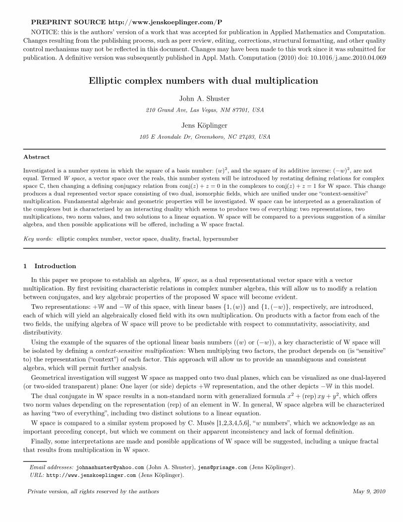
which can be shown to be a multiplicative norm. Any such z with norm = 1 lies on the ellipse: x2 + xy + y2 = 1 (see figure 1).

We discover that the integral powers of (w) lie on this same ellipse:

(w)1= (w) ; (w)

2= (w) − 1; (w)

3= −1;

(w)4=− (w) ; (w)

5= 1 − (w) ; (w)

6= 1. (14)

Thus, (w) is a sixth-root of unity, which lies on the fundamental (w)-axis, and all real powers of (w) appear anti-clockwise

on the plot. Hence, this ellipse can also be called the “power orbit” of (w) under ×: {(w)n

for all real n} (see appendix C).

Summarizing, the complex space +W can be referred to as the elliptic complex numbers, with

A−1 = conj (A) / ‖z‖+ = [x + y − y (w)] / ‖z‖+. Under + and × multiplication, these numbers form an algebraic field.

Furthermore, the mapping i 7→ (1 − 2 (w)) /√

3 shows that the complex field C is isomorphic to the 〈+W, +,×〉 field, and, as

one might expect, under this mapping the unit circle in C is mapped onto the unit ellipse in +W.

3

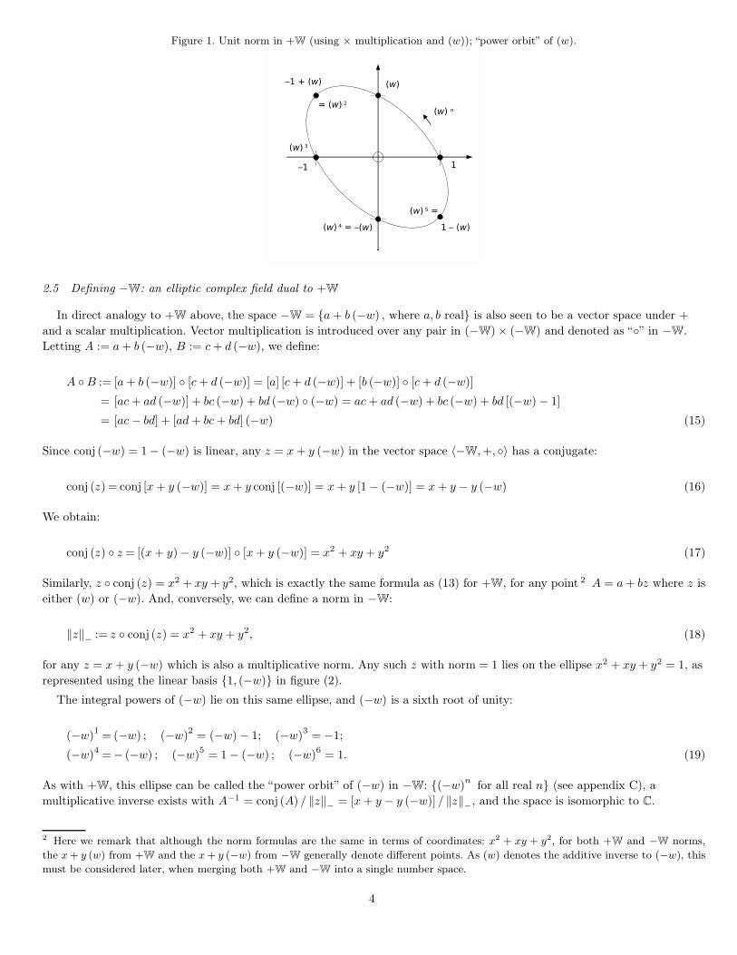
Figure 1. Unit norm in +W (using × multiplication and (w)); “power orbit” of (w).

2.5 Defining −W: an elliptic complex field dual to +W

In direct analogy to +W above, the space −W = {a + b (−w) , where a, b real} is also seen to be a vector space under +

and a scalar multiplication. Vector multiplication is introduced over any pair in (−W) × (−W) and denoted as “◦” in −W.

Letting A := a + b (−w), B := c + d (−w), we define:

A ◦ B := [a + b (−w)] ◦ [c + d (−w)] = [a] [c + d (−w)] + [b (−w)] ◦ [c + d (−w)]

= [ac + ad (−w)] + bc (−w) + bd (−w) ◦ (−w) = ac + ad (−w) + bc (−w) + bd [(−w) − 1]

= [ac − bd] + [ad + bc + bd] (−w) (15)

Since conj (−w) = 1 − (−w) is linear, any z = x + y (−w) in the vector space 〈−W, +, ◦〉 has a conjugate:

conj (z) = conj [x + y (−w)] = x + y conj [(−w)] = x + y [1 − (−w)] = x + y − y (−w) (16)

We obtain:

conj (z) ◦ z = [(x + y) − y (−w)] ◦ [x + y (−w)] = x2 + xy + y2 (17)

Similarly, z ◦ conj (z) = x2 + xy + y2, which is exactly the same formula as (13) for +W, for any point 2 A = a + bz where z is

either (w) or (−w). And, conversely, we can define a norm in −W:

‖z‖−

:= z ◦ conj (z) = x2 + xy + y2, (18)

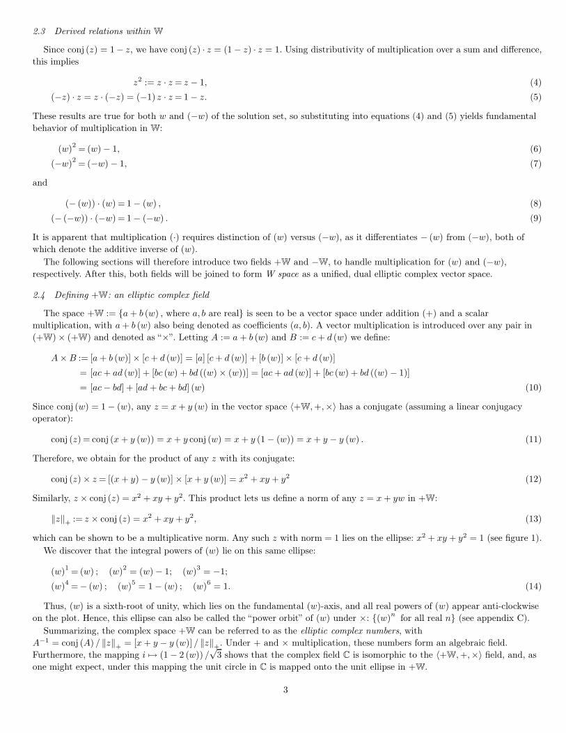
for any z = x + y (−w) which is also a multiplicative norm. Any such z with norm = 1 lies on the ellipse x2 + xy + y2 = 1, as

represented using the linear basis {1, (−w)} in figure (2).

The integral powers of (−w) lie on this same ellipse, and (−w) is a sixth root of unity:

(−w)1= (−w) ; (−w)

2= (−w) − 1; (−w)

3= −1;

(−w)4 =− (−w) ; (−w)5 = 1 − (−w) ; (−w)6 = 1. (19)

As with +W, this ellipse can be called the “power orbit” of (−w) in −W: {(−w)n

for all real n} (see appendix C), a

multiplicative inverse exists with A−1 = conj (A) / ‖z‖−

= [x + y − y (−w)] / ‖z‖−

, and the space is isomorphic to C.

2 Here we remark that although the norm formulas are the same in terms of coordinates: x2 + xy + y2, for both +W and −W norms,

the x + y (w) from +W and the x + y (−w) from −W generally denote different points. As (w) denotes the additive inverse to (−w), this

must be considered later, when merging both +W and −W into a single number space.

4

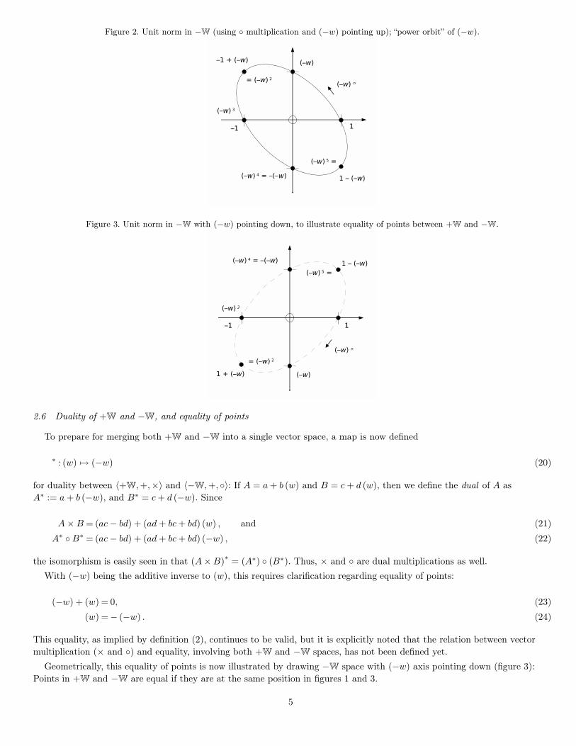
Figure 2. Unit norm in −W (using ◦ multiplication and (−w) pointing up); “power orbit” of (−w).

Figure 3. Unit norm in −W with (−w) pointing down, to illustrate equality of points between +W and −W.

2.6 Duality of +W and −W, and equality of points

To prepare for merging both +W and −W into a single vector space, a map is now defined

∗ : (w) 7→ (−w) (20)

for duality between 〈+W, +,×〉 and 〈−W, +, ◦〉: If A = a + b (w) and B = c + d (w), then we define the dual of A as

A∗ := a + b (−w), and B∗ = c + d (−w). Since

A × B = (ac − bd) + (ad + bc + bd) (w) , and (21)

A∗ ◦ B∗ = (ac − bd) + (ad + bc + bd) (−w) , (22)

the isomorphism is easily seen in that (A × B)∗

= (A∗) ◦ (B∗). Thus, × and ◦ are dual multiplications as well.

With (−w) being the additive inverse to (w), this requires clarification regarding equality of points:

(−w) + (w) = 0, (23)

(w) =− (−w) . (24)

This equality, as implied by definition (2), continues to be valid, but it is explicitly noted that the relation between vector

multiplication (× and ◦) and equality, involving both +W and −W spaces, has not been defined yet.

Geometrically, this equality of points is now illustrated by drawing −W space with (−w) axis pointing down (figure 3):

Points in +W and −W are equal if they are at the same position in figures 1 and 3.

5

3 W space: unified dual elliptic complex space

3.1 Overview

We now define W space (W) as consisting of elements which are both (w) and (−w) represented, as an algebraic joining of

the two elliptic complex fields +W and −W. W space consists of two dual elliptic complex fields, with a general multiplication

defined within each field and between elements of each field.

While both +W and −W fields have been introduced separately so far, additional consideration must now be taken for the

general product that may involve factors from either space, i.e., one factor containing a (w) term, and the other factor

containing a (−w) term. It will be shown that this algebra is no longer a field, but can be regarded as a dual-represented,

dual-normed vector space over the reals, with a vector multiplication which may distribute over a vector sum. To do this, a

left-factor or right-factor rule must be supplemented, describing a W1 and W2 space, respectively. Rules on how and when

substitution of equal quantities can occur will be termed sensitivity.

3.2 Context domains of × and ◦, and general multiplication in W space

Multiplication ◦ has only been defined in −W (equation 15) between two factors A := a + b (−w) and B := c + d (−w),

using (−w) from definition 2, (W1: DR-0). This will now be called (−w) representation, or −W representation of points in W.

For A′ := a − b (w) and B′ := c − d (w) (i.e., using (w) representation of the same two points), the ◦ multiplication is not

defined; instead, the × operation from +W must be used (equation 10). We have

A′ × B′ = [a + (−b) (w)] × [c + (−d) (w)] = (ac − bd) + (−ad − bc + bd) (w) , (25)

A ◦ B = [a + b (−w)] ◦ [c + d (−w)] = (ac − bd) + (ad + bc + bd) (−w) . (26)

Clearly, A′ × B′ 6= A ◦ B even though A′ = A and B′ = B. Hence, × and ◦ are different operations, each depending on the

representation of its factors in +W or −W space, respectively.

Operation × is defined on the domain of (+W) × (+W) elements of W, while ◦ is defined on the domain of (−W) × (−W)

elements of W. Conversely, the general multiplication operation in W must reduce to × multiplication when restricted to the

(+W) × (+W) domain, and it must reduce to ◦ multiplication when restricted to the (−W) × (−W) domain. These domains

will now be interpreted as the two contexts in which general multiplication within W must operate, and this multiplication

will be termed sensitive to the representation of its factors. In short, W space has a context-sensitive multiplication.

The remaining context domains of the general multiplication are: (−W) × (+W) and (+W) × (−W). The union of all four

domains is W × W, the entire domain of general multiplication in W space.

3.3 General multiplication in W1 space

We define a W1 version of W space as W1 ≡ 〈W1, +, (·)〉 := {〈+W, +,×〉 joined with 〈−W, +, ◦〉} so that the general

multiplication (·) of W1 is extended to all four context domains (cases) of (A, B) ∈ W × W:

(1) A (·) B := A × B when (·) is restricted to elements of the +W field; i.e., (·) : (+W) × (+W) 7→ (+W), so (·) = ×.

(2) A (·) B := A ◦ B when (·) is restricted to elements of the −W field; i.e., (·) : (−W) × (−W) 7→ (−W), so (·) = ◦.(3) A (·) B := A′ ×B when (·) is restricted to elements of the −W field as left factor, and an element of the +W field as right

factor, with left factor taking on the same representation (A′) as the right factor. Then, (·) : (−W) × (+W) 7→ (+W), so

(·) = {×, with left factor represented in + W as A′}.(4) A (·) B := A′ ◦ B when (·) is restricted to elements of the +W field as left factor, and an element of the −W field as right

factor, with left factor taking on the same representation (A′) as the right factor. Then, (·) : (+W) × (−W) 7→ (−W), so

(·) = {◦, with left factor represented in − W as A′}.Cases 1 and 2 have already been discussed and follow from (W: DR-0) through (W: DR-2) in definition 2. A supplemental

definition for cases 3 and 4 in W1 space is now given:

Definition 3 Supplemental definition for W1 space

W1 space is defined by (W: DR-0) through (W: DR-2) and the following supplements:

(−w) (·) (w) := − (w) × (w) , (W1: DR-3)

(w) (·) (−w) := − (−w) ◦ (−w) . (W1: DR-4)

6

We now recall derived result: (−z) z = 1 − z (equation 5). This relation is true for both (w) and (−w) of the solution set, so

substituting them into this equation yields the mixed-factor basis behavior of multiplication in W1, revealing

non-commutativity:

(−w) (·) (w) = − (w) × (w) = 1 − (w) , (27)

(w) (·) (−w) = − (−w) ◦ (−w) = 1 − (−w) , (28)

(w)2:= (w) × (w) = −1 + (w) , (29)

(−w)2:= (−w) ◦ (−w) = −1 + (−w) . (30)

Relations (27) and (28) characterize this W1 version of W space. It is especially noted that the squares of (w) and (−w) are

defined unambiguously as the product with itself (equations 29 and 30).

3.4 W2 space

Just as in the W1 version of W space, we define a counterpart W2 ≡ 〈W2, +, (·)〉 := {〈+W, +,×〉 joined with 〈−W, +, ◦〉}as:

Definition 4 Supplemental definition for W2 space

W2 space is defined by (W: DR-0) through (W: DR-2) and the following supplements:

(−w) (·) (w) := − (−w) ◦ (−w) , (W2: DR-3)

(w) (·) (−w) := − (w) × (w) . (W2: DR-4)

This yields:

(−w) (·) (w) = − (−w) ◦ (−w) = 1 − (−w) , (31)

(w) (·) (−w) = − (w) × (w) = 1 − (w) , (32)

(w)2:= (w) × (w) = −1 + (w) , (33)

(−w)2 := (−w) ◦ (−w) = −1 + (−w) . (34)

Relations (31) and (32) exhibit non-commutativity in W2, as a type of “mirrored” dual to W1 space 3 relations (27) and (28).

It appears that W1 space is different from W2 space only where a vector product involves factors which contain both (w)

and (−w) terms. In order to clarify and further discuss this situation, we will now introduce a representation function rep (A),

representational equality (r=), and the terms copoint and dual point.

3.5 Representation function, representational equality, copoint and dual point

In performing a general multiplication in W (not specified by either × or ◦), we have seen that the representation of each

factor matters. To handle this key aspect of W space, we introduce the following notions and notation.

3.5.1 The representation function

Given any element A ∈ W we shall determine its representation using the rep function:

rep (A) :=

1, if A is non-real and represented by (w) ,

0, if A is real, and

−1, if A is non-real and represented by (−w) .

(35)

3.5.2 Representational equality

An equation A = B in W does not necessarily imply that AD1 = BD2 for any D1 = D2 when performing the general

multiplication (for definition of equality, =, see section 2.6, “equality of points”). What is required is that either the

multiplication be specified by × or ◦, or that the multipliers D1 and D2 must be equal and of the same representation. Thus,

we say “D1 is representationally equal to D2”, or:

D1r= D2 ⇐⇒ {D1 = D2, and rep (D1) = rep (D2)} (36)

3 However, W2 space is not an “isomorphic” dual to W1 space.

7

3.5.3 Copoint

The following notation will specify an opposite (or alternate) representation of a given element A ∈ W. Suppose a, b, c, d

real and A := a + bw, then we designate the copoint of A as A′ := a + (−b) (−w). Similarly, if B := c + d (−w), then

B′ := c − d (w). In general, for non-real D ∈ W we define:

D′ := {D′ = D, and rep (D′) 6= rep (D)} (37)

In addition, if D is any non-real point in W space, we wish to be able to specify D represented under (w) or under (−w):

D+ := {D+ = D, and rep (D+) = 1} (38)

D− := {D− = D, and rep (D−) = −1} (39)

For real D we define the trivial case D′ = D+ = D− = D, as representational equality (r=) and equality of points (as in

section 2.6) reduce to ordinary equality in the reals.

For non-real D we still have equality of points D′ = D+ = D− = D, but also:

(D+)′r= D−,

D+r

6= D−,

Dr

6= D′,

(D−)′r= D+,

rep (D+) = −rep (D−) ,

rep (D) = −rep (D′) .

(40)

3.5.4 Dual point

We now apply the dual notation (∗) on a general point D with real coefficients a, b by defining D∗ as the dual point of D:

D∗ :=

a + b(−w), if D is non-real and represented as a + b(w),

a, if D is real, and

a + b(w), if D is non-real and represented as a + b(−w).

(41)

Thus, D∗ = D only if D is real, whereas in general rep (D∗) = −rep (D), and:

[a + b (w)]∗ r= a + b (−w) , (42)

[a + b (−w)]∗ r= a + b (w) . (43)

3.6 Examples for multiplying factors of unlike representation

The following gives a few examples for general multiplication in W1 and W2 space, respectively. For readability, we will

leave out the explicit multiplication symbol (·) between two factors, and write it as an implied product:

(w) (·) (−w)≡ (w) (−w) , (44)

A (·)B ≡AB, (45)

and so forth. As long as we specify whether multiplication is executed in W1 or W2, the multiplication result will be unique

(per definitions 3 and 4).

Clearly, the non-commutativity of (w) and (−w) follows from the general multiplication in W being defined in terms of two

different specific operations. All following examples will be in W1 (definition 3).

The most simple product between two numbers of different representation is:

(−w) (w)r= (−w) × (w) 6= (w) ◦ (−w)

r= (w) (−w) . (46)

More general, by letting A := a − b (−w) and B := c + d (w), we compute the product AB straight-forward. Note that

multiplication distributes over addition, only requiring that the representation rep (A) and rep (B) does not change.

Substituting (−w) (w)r= 1 − (w), we obtain:

ABr= [a − b (−w)] [c + d (w)]

r= a [c + d (w)] − b (−w) [c + d (w)]

r= ac + ad (w) − bc (−w) − bd (−w) (w)

7→ ac + ad (w) + bc (w) − bd (1 − (w))r= (ac − bd) + (ad + bc + bd) (w) . (47)

8

Table 1

Multiplication in W1

A ∈ B ∈ rep (A) rep (B) AB ≡ rep (AB)

+W +W +1 +1 A × B +1

−W +W −1 +1 A′ × B +1

+W −W +1 −1 A′ ◦ B −1

−W −W −1 −1 A ◦ B −1

As the change arrow indicates, the representation of one of the terms was changed

−bc (−w) 7→ [−bc (−w)]′r= bc (w) , (48)

as multiplication in W1 requires the representation of a product to be in the representation of the right factor. In the above

example, we had rep (B) = 1, and therefore the sum ad (w) − bc (−w) had to be represented as in terms of (w) as well.

Next, we observe that this result is exactly the same as computing A′ × B where A′r= [a − b (−w)]′

r= a + b (w):

A′ × Br= [a + b (w)] × [c + d (w)]

r= (ac − bd) + (ad + bc + bd) (w) . (49)

But, the product A ◦ B′r= (ac − bd) + (−ad − bc + bd) (−w) 6= AB. In other words, we have in W1:

ABr= A′ × B

r= (A+) × (B+) , (50)

when rep (A) = −1 and rep (B) = 1 (conversely, in W2 we have ABr= A ◦ B′

r= (A−) ◦ (B−) for the same A, B).

Therefore, multiplication in W1 corresponds to the field multiplication of the right-hand factor’s representation field, and

the left factor (and product) is then represented in that same field. These properties are summarized in Table 1.

As representation of a factor determines the outcome of a multiplication result, this can be interpreted as context-sensitive

multiplication. Nevertheless, general multiplication in W is a well-defined, single valued function from W × W 7→ W.

Multiplication in W1 is governed entirely by the representation of the right factor, and conversely, multiplication in W2

(definition 4) is governed entirely by the representation of the left factor, as can easily be shown.

3.7 A note about non-commutativity

For z1, z2 ∈ {(w) , (−w)}, it can be verified that zi = rep (zi) (w), rep2 (zi) = 1, and z1z2 = rep (z1) rep (z2) [z2 − 1]. Using

these identities, the general product in W1 between any two factors A := a + bz1 and B := c + dz2, i.e. of any representation,

can also be expressed as:

ABr= ac + (ad) z2 + (bc) z1 + bd z1z2

7→ (ac − rep (z1) rep (z2) bd) + (ad + rep (z1) rep (z2) (bc + bd)) z2, (51)

BAr= ac + (ad) z2 + (bc) z1 + bd z2z1

7→ (ac − rep (z1) rep (z2) bd) + (bc + rep (z1) rep (z2) (ad + bd)) z1. (52)

Since z1 = rep (z1) (w), rep (z2) z1 = rep (z1) [rep (z2) (w)] = rep (z1) z2, therefore (1) z1 = rep (z1) rep (z2) z2, and we can

express the general difference, in various representations:

BA − AB = (bc + rep (z1) rep (z2) (ad + bd)) z1 − (ad + rep (z1) rep (z2) (bc + bd)) z2

= (rep (z1) rep (z1) bc + (ad + bd)) z2 − (ad + rep (z1) rep (z2) (bc + bd)) z2

= bd (1 − rep (z1) rep (z2)) z2

= bd (rep (z1) rep (z2) − 1) z1

= bd (rep (z2) − rep (z1)) (w)

= bd (rep (z1) − rep (z2)) (−w) . (53)

Obviously, when A and B are in the same field representation, rep (z1) = rep (A) = rep (B) = rep (z2), there is BAr= AB, and

multiplication in W1 is commutative within either +W or −W field. However, when the multiplication is between oppositely

represented factors, i.e., rep (A) = −rep (B), then BA − AB = bd (rep (A) − rep (B)) (w) = ±2bd (w). In this case, we have

shown that multiplication in W1 is “predictably” non-commutative since, knowing AB, we can predict that:

9

BA = AB + bd (rep (A) − rep (B)) (w) , (54)

where:

rep (A) = 1 =⇒ BAr= (B+) × A, (55)

rep (A) = −1 =⇒ BAr= (B−) ◦ A, (56)

rep (B) = 1 =⇒ ABr= (A+) × B, (57)

rep (B) = −1 =⇒ ABr= (A−) ◦ B. (58)

Of course, identical reasoning applies to W2 as well, where all non-commutativity rules are determined by the left factor (as

opposed to the right-factor rules in W1 which were just demonstrated).

3.8 Multiplication and substitution rules in W

In W space we have shown multiplication to be context sensitive, depending on the representation of multiplication factors.

Therefore, substitution of multiplication factors is generally not permissible. Only when the multiplication is made explicit, as

either × or ◦, is such substitution permissible, as the product is governed by the field properties of either +W or −W,

respectively. The following theorems give a concise description of the substitution rules inW1 space.

3.8.1 Substitution for products in W1

For any A, B ∈ W1 their product is: ABr= (A+) × B if rep (B) = 1, or AB

r= (A−) ◦ B if rep (B) = −1. Since rep (B)

determines the representation of A, to be (A+) or (A−) respectively, one may substitute A′ for A (i.e., substitute the left

factor with its copoint: A′ = A where rep (A′) = −rep (A)), without changing product AB.

3.8.2 Equations and multiplication in W1

The following rules govern equations for any A, B, C ∈ W1:

Ar= B =⇒ AC

r= BC and CA

r= CB, (59)

A = B =⇒ ACr= BC, (60)

A′ r= B and A, B, C /∈ R =⇒ AC

r= BC but CA 6= CB. (61)

The two trivial cases (A, B ∈ R, and C ∈ R) reduce to scalar multiplication, which is always allowed in vector space equations.

Equations (59) through (61) can quickly be confirmed from right factor multiplication: As long as the same multiplication

(× or ◦) is executed on both sides of an equation, the equality is preserved. Notably, equation (61) describes a situation where

the seemingly trivial operation of “multiplying an equation on both sides with the same factor” may not always be allowable,

as it breaks equality if the representations are not compatible.

3.8.3 Substitution in W1 expressions

It should be emphasized that distinction between point equality (A = B) and representational equality (Ar= B) is

important in W space, as point equality A = B includes both cases: Ar= B or A′

r= B. In a simple example, the identity

CBr= CB (62)

would be broken by substituting B with B′ on one side of the equation (A, B, C /∈ R), per equation (61).

In general, substitution of multiplication factors is allowable only if the underlying field multiplication (× or ◦, from +W or

−W, respectively) remains unchanged.

3.8.4 Restating expressions in W with use of explicit multiplication, and choice of representation

Any expression stated in W can be restated according to the rules of general multiplication, into a specific multiplication

(× or ◦), and then the field properties of +W or −W can be applied to that expression.

It is noted that no preference for one representation over the other is given: Both point and copoint are equal, A = A′, and

it is vector multiplication that required us to introduce the stronger representational equality, e.g. A′

r

6= A for non-real A.

The particular formulation of a problem has to determine which representation to choose, or a convention has to be set. An

example that demonstrates this need is:

10

Figure 4. A visualization of W space.

A := (w) − (−w) . (63)

The point A could be represented either as (A+)r= 2 (w) or (A−)

r= −2 (−w), there is no preferred choice of representation

within the algebra. As will be discussed later, additional representation conventions can be introduced, with varying

complexity, for modeling different kinds of scenarios for which one might want to use such algebras. At first, though, more of

the common properties of W will be discussed, before proposing extensions.

3.9 Where are +C, −C, C1 or C2 in the complex space C?

There is a simple reason why there are no +C, −C, C1, or C2 spaces in the complexes: C multiplication is commutative

and has equal squares: i2 = −1 = (−i)2. There is no 〈+C, +,×〉 that would be discernible from 〈−C, +, ◦〉. The real powers of

(i) and (−i) are the same unit circle. A more subtle observation is that the conjugacy operator (conj) and the dual operator

(dual) ≡ (∗) are the same for any element A in C:

conj (A) = dual (A) = A∗. (64)

Similarly, because of commutativity in C, there is no distinction between C1 and C2 spaces since both define C identically.

Thus, the non-zero sum of (±w) and its conjugate is what allows W space to become a dual represented, two dimensional

vector space, that can be equipped with two dual, non-commutative vector multiplications. One might say, in a more pointed

way, that a “conjugal symmetry” in C becomes a characteristic asymmetry in W.

4 Geometric and algebraic properties of W space

4.1 Geometric interpretation

Since each representation of W is a two dimensional vector space, one may think of W as consisting of two dual planes: +W

with linear basis {1, (w)}, and −W with basis {1, (−w)}. These planes are identical except for the representation of the w axis

as either (w) or (−w): Figures 1 and 2 have identical geometry: a point A := a + b (w) and its dual point A∗ = a + b (−w)

would show at the same position in the respective graph.

In order to illustrate W as a vector space, the equality of point and copoint A = A′ = a − b (−w) requires a flip of the −W

plane across the real axis, as is shown in figure 3.

This procedure is sketched in figure 4, with two arbitrary points A, B and their copoints A′, B′. Several interpretations of

this graph are possible: The −W plane is flipped and placed above (or below) the +W plane (making point and copoint on

top of each other); or W space is one transparent plane, where each side of such a plane represents +W or −W.

11

Regardless of what interpretation one may prefer (if any), figure 4 illustrates the geometric aspect of multiplication with

mixed factors: Multiplication in W1 is sensitive to the representation of its right factor, therefore the product AB as shown

would be evaluated as A′ ◦ B (as B is −W represented). Similarly, in W2, that same product would become A × B′.

If one were to visualize this, one could say that multiplication is executed in one of the two planes, or on one side of a

transparent plane. No preference of visualization is given, and it is not necessary to interpret multiplication in such a way.

4.2 Associativity

When a product of any number of factors is such that the entire expression will be evaluated in either the +W or −W field,

then multiplication will remain associative. If, however, factors of different representation are multiplied with each other, the

product is generally not associative anymore, as the right-factor (or left-factor) rules of W1 (or W2) apply to pairwise

multiplication only.

Specifically, taking three non-real points A, B, C with rep (A) = rep (B) = rep (C), we have in W1:

A (BC)r= A × (B × C)

r= (A × B) × C

r= (AB) C (65)

A′ (B′C′)r= A′ ◦ (B′ ◦ C′)

r= (A′ ◦ B′) ◦ C′ r

= (A′B′)C′ (66)

A (B′C)r= A × (B × C)

r

6= (A′ ◦ B′) × Cr= (AB′)C (67)

The last equation (representational inequality) indicates non-associativity, as the expression (AB′)C must be evaluated to

(A′ ◦ B′) × C due to the right-factor representation rule in W1.

We conclude that multiplication is generally not associative in W space, but within +W or −W it is associative, just as

multiplication is generally non-commutative in W space, but within +W or −W it is commutative. Non-associativity arises

from the choice of representation of the factors, and is therefore predictable.

4.3 A note about distributivity

It is remarked that both × and ◦ multiplication in W1 and W2 distribute over addition, as both 〈+W, +,×〉 and

〈−W, +, ◦〉 are a field. Implicit multiplication, however, does not distribute over addition in general, as such expressions

provide insufficient information about the representation of each of the terms:

A × (B + C) = D ⇔ A × B + A × C = D (68)

A ◦ (B + C) = E ⇔ A ◦ B + A ◦ C = E (69)

A (B + C) = F < AB + AC = F (70)

Relations (68) and (69) hold true, as multiplication has been stated explicitly (× or ◦ ). In relation (70), multiplication is

implicitly determined by the chosen representation of A, B and C, which is not distributive.

For example: If A := (w), B := (w) and C := (−w), we have in W1:

A (B + C) = (w) ((w) + (−w))

= (w) (0) = 0, (71)

AB + AC = (w) (w) + (w) (−w)

= (−1 + (w)) + (1 − (−w))

= 2w. (72)

As clarified in section (3.8.4), W space does not give a preferred representation of a point in the {1, w} plane. Instead, the

formulation must provide this information, by either explicitly stating multiplication to be × and ◦, or by stating the

representation of each point. If explicit multiplication is not provided by the formulation, then it is generally not distributive.

We do note, however, that distributivity holds in W if the sum to be distributed is uniformly represented, i.e, if all terms in

the sum are entirely +W represented, or entirely −W represented. In this sense, distributivity in W is also predictable.

12

Figure 5. Lines of isonorm in +W (left) and −W (right), for k ∈ {0.5, 1, 2}.

4.4 Geometry of norms in W space

Earlier, the two elliptic complex fields +W and −W, with multiplications × and ◦, lead to two conjugates (relations 11 and

16):

conj (x + y (w))r= x + y − y (w) , (73)

conj (x + y (−w))r= x + y − y (−w) . (74)

For a general point A := x + y (w) with copoint A′ = x − y (−w), the norms from relations (13) and (18) then are:

‖A‖+ = A × conj (A) = x2 + xy + y2, (75)

‖A‖−

= A′ ◦ conj (A′) = x2 − xy + y2. (76)

Figure 5 shows lines of isonorm samples: k2 = ‖A‖+ and k2 = ‖A‖−

, for k = 12 , 1, and 2.

In general, a point A in W space has two norm values, depending on the chosen representation of A:

‖A‖ ={

‖A‖+ , ‖A‖−

}

={

x2 + xy + y2, x2 − xy + y2}

={

x2 + rep (A)xy + y2}

. (77)

Geometrically, if interpreting the norm as “distance from the origin”, this could be viewed as a “short way” and a “long way”,

depending on the factor rep (A) xy. When measuring distances ‖A − B‖1

2 between two points A and B, then there are two

solutions in general:

‖A − B‖1

2 ={

‖A − B‖1

2

+ , ‖A − B‖1

2

−

}

. (78)

It can easily be shown that the product norm property holds for ‖A × B‖+ = ‖A‖+ ‖B‖+ and ‖A ◦ B‖−

= ‖A‖−‖B‖

−,

but not for other combinations of ×, ◦, ‖·‖+ and ‖·‖−

, in general. It is concluded that W space is a metric space only for

expressions evaluated in either +W or −W.

4.5 Dual solutions of linear equations

As W space does not suggest a preferred representation of a general point, there is a curious consequence for linear

equations, if multiplication isn’t stated explicitly: They have two solutions in general. For two given points A and B, and an

unknown point X , the relation AX = B may become:

(A+) × (X+) = (B+) , or (79)

(A−) ◦ (X−) = (B−) . (80)

For non-real A, these two expressions generally evaluate to a different point X .

13

Table 2

Comment on w numbers after C. Musès in the example of squaring.

# Description schematic in w numbers in W space

1 assume an equality A = B assume: (−1)w = (−w) assume: (−1) w = (−w)

2 multiply on left by A AA = AB [(−1) w] [(−1) w] = [(−1) w] (−w) [(−1)w] × [(−1) w]r= [(−1)w] × (−w)

3 substitute B for A (right) AA = BB [(−1) w] [(−1) w] = (−w) (−w) [(−1)w] × [(−1) w]r= (−w) × (−w)

4 represent (−w) under ×... [(−1)w] × [(−1) w]

r= [(−1)w] × [(−1) w]

5 use “square” notation A2 = B2 [(−1) w]2 = (−w)2...

6 reorder coefficients (vector space) (−1)2 w2 = (−w)2 (−1)2 (w × w)r= (−1)2 (w × w)

7 w2 = (−w)2 w × wr= w × w

8 interpretation contradicts with definitions no contradiction

9 conclusion assumption (#1) is false choice of × or ◦ possible

10 w numbers not a vector space vector space, 2 vector multiplications

5 Remarks on “w numbers” after Charles Muses

In the 1970’s, a system called “w numbers” (or “w arithmetic”) was proposed by Charles Musès[1,2,3,4]. This system

appears to exhibit geometric and algebraic properties similar to W space (or more specifically, W1) of this paper. We will now

comment on Musean w numbers, and distinguish them from W space.

5.1 Defining relations for w numbers

In [1] Musès writes: “When we come to w defined by w2 = −1 + w (42) and (−w)2

= −1 − w (43) we [...] are now able to

distinguish arithmetically between (+x)2

and (−x)2. [...] Hence, we further define −w, unless explicitly otherwise stated, to

mean (+1) [(−1)w] and not (−1) [(+1)w]”. This notation is clarified in [4]: “Thus, (+1) [(−1)w] = + (−w), but

[(+1) (−1)] w = − (+w). Though +1 (−w) and −1 (+w) are the same in additive context, they are not the same

multiplicatively.”

We comment that these definitions appear insufficient, as they seem to imply an underlying vector space (“... +1 (−w) and

−1 (+w) are the same in additive context ...”), however, they offer a contradicting statement at the same time (“... they are

not the same multiplicatively.”) It is not clear how two points could simultaneously be equal but not be the same

“multiplicatively.” Musès also writes[1]: “(w) (−w) = (−w)4(−w) = (−w)

5(45) = 1 − (−w) = 1 + w if only addition is

considered (46); and similarly, (−w) (w) = (w)4(w) = (w)

5= 1 − w (47)”.

Likewise, it is unclear how equality in a vector space could be realized (“1 − (−w) = 1 + w if only addition is considered”).

Musès introduces terms like “almost distributive” and “almost commutative” [3] and gives examples as in [2]:

“w (−w + w) = 2w whereas (−w + w)w = 0”, or [1,3]: “w (w − w) = w (0) = 0” whereas prior distribution of the addends

would yield “w (w − w) = −1 + w + 1 + w = 2w”.

We acknowledge that these are examples of an algebraic situation requiring clarification, however, no apparent clarification

has been offered by Musès.

5.2 Isolating the problematic contention

Equality of the vector elements 1 (−w) = −1 (w) is required for building a vector space over the reals. If only a single

multiplication operation is defined, one has (−w)2 = [(−1)w] [(−1)w] = (−1) (−1)w2 = w2, which is in direct contradiction

to the defining relations from [1], equations (42) and (43): “w2 = −1 + w” and “(−w)2 = −1 − w”. This is detailed in table 2,

and leads to the problematic conclusion that Musean w numbers cannot be a vector space.

Incidentally, since A × B − A′ ◦ B′ = ±2bd (w), we recognize that A × B = A′ ◦ B′ only if A or B is real (b = 0 or d = 0).

Hence, A2 = A × A = A′ ◦ A′ = (A′)2

only if A = A′ is real.

In [1] Musès notes: “. . . hypernumbers can be perceived not as ’disobeying laws’ but rather as becoming sensitive to

distinctions among phenomena previously only lumped together in less sensitive arithmetics”. Though in a different manner,

this paper has implemented his note via the “context-sensitive” vector multiplication defined for W space.

14

Figure 6. Unit locus for min norm, ‖A‖min

.

6 Possible algebraic variants of W space

6.1 A commutative multiplication?

We have observed that for two points A := a + b (w) and B := c + d (w), the products AB and A′B′ only differ in a ±bd (w)

term, which is the same term that arises from non-commutativity in factors of different representations (e.g. equation 54).

Thus, one can define a new multiplication on all of W × W as:

A ⊙ B :=1

2[(A+) × (B+) + (A−) ◦ (B−)]

= (ac − bd) + (bc + ad)w. (81)

The binary operation, multiplication ⊙, is easily seen to be commutative on all of W. Furthermore, if W space were mapped

onto the complex plane using a map h (w) = i, then h (A ⊙ B) = h (A)h (B) under commutative multiplication in C.

6.2 Uniform “min” norm (dmin metric) for all of W space?

Earlier we have introduced two norm choices (section 4.4, “Geometry of norms in W space”), making W dual-normed space.

It might just as well be useful to define a single, uniform norm instead, to make W a metric space. Such a choice of norm for a

general point A = x + yw (regardless of representation) to be:

‖A‖min := x2 − |xy| + y2 = min{

‖A‖+ , ‖A‖−

}

. (82)

The corresponding metric, defined for A − B = (∆x) + (∆y)w by:

dmin (A, B) :=√

‖A − B‖min =

√

(∆x)2 − |∆x∆y| + (∆y)2. (83)

Its unit locus (figure 6) is like a swollen unit locus of the city-block metric: dcity (A, B) = |∆x| + |∆y|. It is easily shown that

dmin is a valid metric in W and that d2min = (3/2)d2

Eucl − (1/2)d2city, where dEucl is the Euclidean metric:

dEucl :=

√

(∆x)2 + (∆y)2. Unfortunately, however, the min norm does not obey the norm product property, i.e., it is not a

multiplicative norm.

Compared to the dual ‖A‖+ and ‖A‖−

implied metrics, one could geometrically interpret ‖A‖min = min{

‖A‖+ , ‖A‖−

}

to

consider only the “shorter way”, or minimum distance selection for all of W.

6.3 Possible joint W12 := W1 ∪ W2 space?

Given the core of similarity between W1 and W2, it may be possible to extend W space to a joint W12 space where this

core is fully-exploited, and the joint possibilities of both multiplication in W1 and W2 would generally result in a product that

is a set with two members, one member for each representation, i.e.:

(w) (−w) := {1 − (w) , 1 − (−w)} , (84)

(−w) (w) := {1 − (−w) , 1 − (w)} . (85)

15

One could then even declare the result an unordered set, which makes:

(w) (−w) = (−w) (w) = − (w)2

= − (−w)2= {1 − (w) , 1 − (−w)} , (86)

thereby giving every product of two non-real factors a result set that consists of two points.

At this point we only remark that such set multiplication will cause proliferation of results in repeated multiplication, and

in particular, for infinite sums such as the Taylor series of a function; this requires further investigation and clarification.

6.4 Possible U space?

We note a possible U space as a way of completing options for the defining relation: conj (z) + z := {0, 1, or − 1}. The

choice of 0 yields C, the choice of 1 yields W of this paper, and choosing −1 would yield U. Similar to W space, the defining

relations of U space would be:

Definition 5 Defining relations for U

{(u) , (−u)} is the solution set to: (U: DR-0)

conj (z) + z = −1, (U: DR-1)

conj (z) · z = 1 = z · conj (z) . (U: DR-2)

Interestingly, these two relations imply that the third powers of (u) and (−u) are unity: (u)3

= 1 = (−u)3, and that the power

ellipse for u is: x2 − xy + y2 = 1. On first look, U space appears to have a context sensitive multiplication similar to W, and

again, could result in a U1 and a U2 version of U space.

7 Summary, possible applications of W space, and outlook

In this paper we have introduced W space as a dual elliptic complex vector space with context sensitive multiplication.

Algebraic rules that govern such multiplication have been specified, and appropriate notification thereof was introduced. W

space was demonstrated to contain two dual fields: +W and −W, which can be unified in two similar ways that lead to a W1

or W2 space. Geometrically, the space was found to be dual normed, with the ‖·‖+ and ‖·‖−

norms representing squares of

distances in the +W and −W component fields, respectively. The relation of W space to a predecessor concept, “w numbers”

after C. Musès, was then discussed, and we remarked how we believe that W space addresses certain issues. Finally, possible

algebraic variants of W space were drafted for further examination.

In [6] Musès originally chose the symbol “w” as a “referent of consciousness”, and it was claimed that the properties of w

and (−w) make such w numbers well-suited for use in the social as well as physical sciences. In this final section, we will

speculate on how W space could provide more tangible realizations, and offer suggestions where it may help explain both

physical and human behavior.

Generally, W space may be useful with systems that intrinsically have two dual mechanisms that may result in different

outcomes, where it is not predictable in these systems when one behavior (or outcome) will be evident as compared to the

other. This could include, e.g., spin- 12 behavior in quantum physics, or spontaneous decision making in sociology or psychology.

In physics, a spin- 12 particle (e.g., an electron) is described as having an intrinsic property, its “spin”, that is not tied to

space or time. Upon measurement, such spin- 12 particle will spontaneously assume one of two possible states, resulting in two

distinct measurement outcomes. The Stern–Gerlach experiment is a famous demonstration of this quantum effect. W space

could aid in modeling this physical behavior, by mapping the particle’s spin to ±W representation of the space-time

coordinates used. The product norm property within +W and −W may warrant relativity as in [7,8].

In sociology or psychology, W space could be applicable for scenarios in which a test group is placed in an environment

with ongoing opportunity of taking one action over another, where no reasonably accurate prediction is apparent for the

action that the test group might take. One might even speculate on applicability for an individual subject, e.g., a person who

has a split personality disorder. W space might be able to model decision outcomes for that individual that might otherwise

seem irrational.

One interesting aspect of the dual multiplication arises when one does not mandate, up front, one of the multiplication

results over the other, but allows carrying forward both results. Due to the inherent proliferation of possible results in a

sequential algorithm, one can realize fractal shapes when letting the number of algorithmic steps go against infinity. While

investigation into these opportunities is largely outstanding, we have added the multi-star fractal in appendix A as a first

result, and remark here only that one could expect interesting outcomes when evaluating the exponential function through its

Taylor polynomial (appendix B).

16

The primary goal of this paper has been to establish W space on a sound mathematical footing. Using defining relations,

we have shown that this system, with a well-defined context sensitive multiplication, contains within it a duality that does not

prevent or restrict its consistency. This way, W space is perhaps the next step beyond circular complex space.

On a humorous note, one might say that early in our math education we were taught that “a minus times a minus always

equals a plus”. Paradoxically, W space represents somewhat of a departure from this hitherto conventional wisdom, and on a

more serious note, it might help establish a new convention in terms of its context sensitive algebra. It is our hope that this

system will be more fully explored and used in the future.

Acknowledgements

The authors thank Charles Musès for his inspiring writings on w numbers. We also extend our appreciation to Kevin

Carmody for numerous discussions and contributions regarding Musean w numbers.

References

[1] C. Musès, Hypernumbers-II. Further concepts and computational applications, Appl. Math. Comput. 4 (1978) 45-66.

[2] C. Musès, Computing in the bio-sciences with hypernumbers: a survey. Int. J. Bio-Medical Computation. 10 (1979) 519-525.

[3] C. Musès, Hypernumbers and quantum field theory with a summary of physically applicable hypernumber arithmetics and their

geometries. Appl. Math. Comput. 6 (1980) 63-94.

[4] C. Musès, Hypernumbers applied, or how they interface with the physical world. Appl. Math. Comput. 60 (1994) 25-36.

[5] K. Carmody, Elliptic complex numbers: the Musèan hypernumber w. Monograph (withdrawn), previously at URL:

http://kevincarmody.com/math/surveyw.pdf (retrieved 6 February 2005).

[6] C. Musès, Psychotronic quantum theory; a proposal for understanding mass/space/time/consciousness transductions in terms of a

radically extended quantum theory. Proceedings of International Association for Psychotronic Research (1975).

[7] J. Köplinger, Hypernumbers and relativity. Appl. Math. Comput. 188 (2007) 954-969.

[8] J. Köplinger, Gravity and electromagnetism on conic sedenions, Appl. Math. Comput. 188 (2007) 948-953.

[9] W space multi-star and Exp(Z) fractals (bitmap samples, and C source code), http://jenskoeplinger.com/W .

APPENDIX

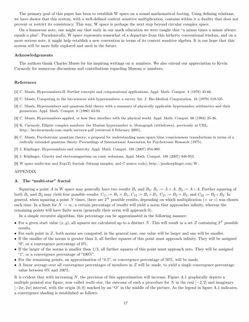
A The “multi-star” fractal

Squaring a point A in W space may generally have two results B1 and B2: B1 := A × A, B2 := A ◦ A. Further squaring of

both B1 and B2 may yield four possible results: C11 := B1 × B1, C12 := B1 ◦ B1, C21 := B2 × B2, and C22 := B2 ◦ B2. In

general, when squaring a point N times, there are 2N possible results, depending on which multiplication (× or ◦) was chosen

each time. In a limit for N → ∞, a certain percentage of results will yield a norm that approaches infinity, whereas the

remaining points will have finite norm (generally their norm will approach 0).

In a simple recursive algorithm, this percentage can be approximated in the following manner:

• For a given start value (x, y), all squares are calculated up to a distinct N . This will result in a set Z containing 2N possible

results.

• For each point in Z, both norms are computed; in the general case, one value will be larger and one will be smaller.

• If the smaller of the norms is greater than 3, all further squares of this point must approach infinity. They will be assigned

“0”, or a convergence percentage of 0%.

• If the larger of the norms is smaller than 1/3, all further squares of this point must approach zero. They will be assigned

“1”, or a convergence percentage of “100%”.

• For the remaining points, an approximation of “0.5”, or convergence percentage of 50%, will be made.

• A linear average over all convergence percentages of members in Z will be made, to yield a single convergence percentage

value between 0% and 100%.

It is evident that with increasing N , the precision of this approximation will increase. Figure A.1 graphically depicts a

multiple pointed star figure, now called multi-star, the outcome of such a procedure for N in the real [−2, 2] and imaginary

[−2w, 2w] interval, with the origin (0, 0) marked by an “O” in the middle of the picture. As the legend in figure A.1 indicates,

a convergence shading is established as follows:

17

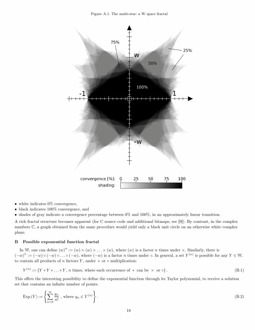
Figure A.1. The multi-star: a W space fractal

• white indicates 0% convergence,

• black indicates 100% convergence, and

• shades of gray indicate a convergence percentage between 0% and 100%, in an approximately linear transition.

A rich fractal structure becomes apparent (for C source code and additional bitmaps, see [9]). By contrast, in the complex

numbers C, a graph obtained from the same procedure would yield only a black unit circle on an otherwise white complex

plane.

B Possible exponential function fractal

In W, one can define (w)n := (w) × (w) × . . . × (w), where (w) is a factor n times under ×. Similarly, there is

(−w)n := (−w) ◦ (−w) ◦ . . . ◦ (−w), where (−w) is a factor n times under ◦. In general, a set Y (n) is possible for any Y ∈ W,

to contain all products of n factors Y , under × or ◦ multiplication:

Y (n) := {Y ∗ Y ∗ . . . ∗ Y , n times, where each occurrence of ∗ can be × or ◦} . (B.1)

This offers the interesting possibility to define the exponential function through its Taylor polynomial, to receive a solution

set that contains an infinite number of points:

Exp (Y ) :=

{

∞∑

n=0

yn

n!, where yn ∈ Y (n)

}

. (B.2)

18

The notation{∑ yn

n!

}

indicates summation over all possible members yn of Y (n), with one yn from each Y (n).

As the sum for Exp(Y ) is convergent, the infinite solution sets for n → ∞, plotted in the two dimensional plane, exhibit a

rich fractal structure (for samples and source code, see [9]).

C Exponential, logarithm, polar forms, and ellipse area in W space

This appendix restates the results originally derived by Kevin Carmody in [5]. We present his and our results using W

space notation as established in the current paper, while sometimes deriving them differently, e.g., by using the isomorphism

between +W and C. Replacing (w) with (−w) in this section will yield the identical relations, as −W and C are isomorphic as

well. We will therefore only discuss +W, while all statements will be valid for −W without loss of generality. It is noted,

however, that the following derivations are generally not valid for multiplication of factors of mixed representation.

C.1 Derivation of (w)q

for real q

The map:

P (i) :=1 − 2 (w)√

3from C 7→ (+W) , (C.1)

or conversely,

Q (w) :=1

2− i

√3

2= exp

(

− iπ

3

)

from (+W) 7→ C (C.2)

establishes the isomorphism between (+W) and C. We shall now show that for any real q:

(w)q=

2√3

[

cos(πq

3+

π

6

)

+ (w) sinπq

3

]

. (C.3)

PROOF. Letting (w)q

:= a + b (w) we have

Q ((w)q) = [Q (w)]

q=

[

exp

(

− iπ

3

)]q

= exp

(

− iπq

3

)

= cos(

−πq

3

)

+ i sin(

−πq

3

)

. (C.4)

Also,

Q ((w)q) = Q (a + bw) = a + bQ (w) = a + b

(

1

2− i

√3

2

)

=

(

a +b

2

)

+ i

(

−b√

3

2

)

, (C.5)

so:

(

a +b

2

)

+ i

(

−b√

3

2

)

= cos(

−πq

3

)

+ i sin(

−πq

3

)

, with parts: (C.6)

a +b

2= cos

(

−πq

3

)

, and − b√

3

2= sin

(

−πq

3

)

. (C.7)

This implies:

b =2√3

sin(πq

3

)

, and a = cos(πq

3

)

− 1√3

sin(πq

3

)

. (C.8)

Using the cosine of angle sum relation, we find:

cos(πq

3+

π

6

)

= cos(πq

3

)

cos(π

6

)

− sin(πq

3

)

sin(π

6

)

=

√3

2cos(πq

3

)

− 1

2sin(πq

3

)

=

√3

2a, (C.9)

(w)q = a + b (w) =2√3

[

cos(πq

3+

π

6

)

+ (w) sinπq

3

]

. (C.10)

This concludes the proof. �

19

Figure C.1. Area swept by angle θ

C.2 Polar forms

Relation (C.3) for (w)q suggests a polar form for elements of (+W), using a modulus |A|+ :=√

‖A‖+ of a general point

A := a + (w) br= (A+) ∈ (+W), defined through the ‖·‖+ norm from relation (13). Then, the polar form of A is:

Ar= |A|+ (w)

q, where (C.11)

q =3

π

[

tan−1 a + 2b

a√

3− π

6

]

. (C.12)

Thus, we can write × multiplication between two points A and B in polar form:

A × B = |A|+ (w)q |B|+ (w)s = |A|+ |B|+ (w)q (w)s = |A|+ |B|+ (w)q+s . (C.13)

C.3 Exponential and logarithm

We summarize results from Carmody [5] for the exponential function in (+W):

e(a+b(w)) := 1 +

∞∑

k=1

(a + b (w))k

k!

= eaeb(w) = ea+ b2 (w)

b 3√

3

2π . (C.14)

For the special case b = −2a we have:

(w)q = e−

qπ

3√

3(1−2(w))

= e−qπ

3P (i), (C.15)

where P (i) = (1 − 2 (w)) /√

3 from relation (C.1) above, the image of the complex i under the map C 7→ (+W).

The last relation allows us to write the natural logarithm:

ln (A+) := ln |A|+ − qπ

3P (i) =

1

2ln(

a2 + ab + b2)

− qπ

3√

3(1 − 2 (w)) . (C.16)

C.4 Real exponent of (w) proportional to area swept under ellipse

We conclude with another finding of Carmody. Figure C.1 shows (w)q

at angle θ and radius r. A triangular sector of area is

dA = 12r2dθ, where r2 = 1/ (1 + sin θ cos θ) since 1 = x2 + y2 + xy = r2 + r2 sin θ cos θ.

Integrating over angle 0 to θ, we find the Euclidean area A (θ) swept by the radius vector:

A (θ) =1

2

∫ θ

0

r2dθ′ =1

2

∫ θ

0

1

1 + sin θ′ cos θ′dθ′ =

1

2

∫ θ

0

1

1 + 12 sin 2θ′

dθ′

=1√3

tan−1

(

2 tan θ + 1√3

)

− π

6√

3=

1√3

[

tan−1

(

1√3

+2 tan θ√

3

)

− π

6

]

. (C.17)

20

From relation (C.12) we have:

q =3

π

[

tan−1 a + 2b

a√

3− π

6

]

=3

π

[

tan−1

(

1√3

+2 tan θ√

3

)

− π

6

]

=3√

3

πA (θ) , (C.18)

and therefore see that the area A (θ) swept by the radius vector is proportional to the real exponent q of (w)q, which

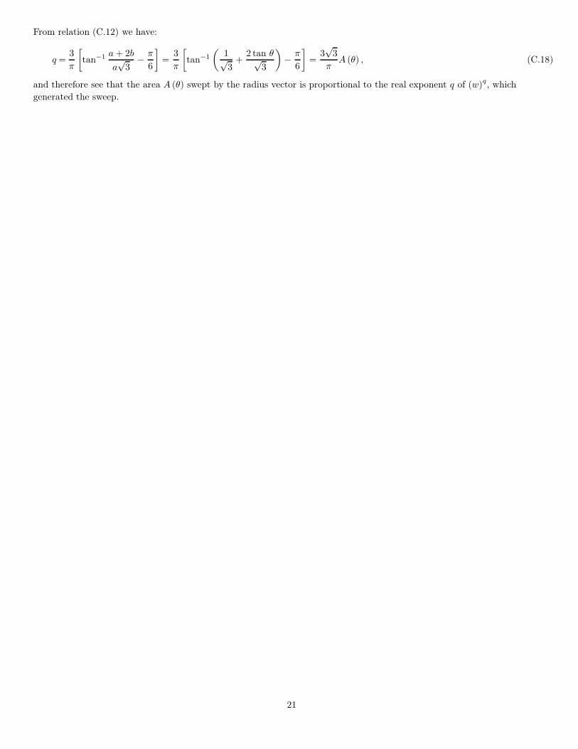
generated the sweep.

21