
17x bits Elliptic Curve Scalar Multiplication over GF(2 - CORE
97
17x bits Elliptic Curve Scalar Multiplication over GF(2 , using Optimal Normal Basis TANG KO CHEUNG, SIMON ([email protected]) ‘ A Thesis Submitted in Partial Fulfillment of the Requirements for the Degree of Master of Philosophy in Information Engineering © The Chinese University of Hong Kong May 2001 The Chinese University of Hong Kong holds the copyright of this thesis. Any person(s) intending to use a part or whole of the materials in the thesis in a proposed publication must seek copyright release from the Dean of the Graduate School. i
-
Upload
khangminh22 -
Category
Documents
-
view
1 -
download
0
Transcript of 17x bits Elliptic Curve Scalar Multiplication over GF(2 - CORE

17x bits Elliptic Curve Scalar Multiplication over
GF(2,us ing Optimal Normal Basis
TANG K O CHEUNG, SIMON
A Thesis Submitted in Partial Fulfillment
of the Requirements for the Degree of
Master of Philosophy
in
Information Engineering
© The Chinese University of Hong Kong
May 2001
The Chinese University of Hong Kong holds the copyright of this thesis. Any
person(s) intending to use a part or whole of the materials in the thesis in a proposed
publication must seek copyright release from the Dean of the Graduate School.
i

/ L f
| ( I 1 APR 2i 1
~UNIvIRSiiY s y s t e w ^ 纷

Abstract
Elliptic Curve Scalar Multiplication is the dominant computation of Elliptic
Curve Cryptography, and each usual ECC cryptographic operation takes just one
or two Elliptic Curve Multiplications. Using Optimal Normal Basis in GF{2'^),
we achieve 60ms to 88ms per iteration for bits length ranges from 173 to 179 on a
Pentium II-400Mhz PC in C without using assembly. No such result using ONB
has ever been reported in the literature before. The competitive performance
is due to an adaptation of the Almost Inverse Algorithm for an implementation
of fast field inverses for ONB. Since we have only used the standard addition-
subtraction method for Scalar Multiplication, vast improvements can still be
possible.
In the final chapter, we present our findings of a particular extension of the RSA
public-key cryptosystem from using integers modulo n to a version using matrices
whose entries are integers modulo n, where n is the product of two large primes.
Acknowledgment
I wish to thank Prof. Wei for his help, advice, generous support and genuine
academic freedom. In addition, his contribution to the last chapter is very much
appreciated.
i i
橢圓曲線數量乘法是橢圓曲線密碼學之主要運算,而一個一般
的橢圓曲線密碼操作只需要一至兩個橢圓曲線數量乘法。
在 有 限 體 G F ( 2 A m ) 使 用 最 適 正 規 基 , 對 1 7 3 至 1 7 9 位 元 長
度,一個橢圓曲線數量乘法只需要0.060-0.088秒。這是使用
C語言,在奔騰二 •四百百萬赫個人電腦上作出的,而且沒
有使用過組合語言。
使用正規基,沒有這樣的結果在文獻上出現過。
其良好的性能是由於在使用最適正規基,履行了一個快速的
逆,這是把差不多逆算法改編而作出的。
對數量乘法’因爲我們只是使用過加減算法,故還有很多改
良的空間。
在最後--章,我們推廣RSA公開密碼系統至矩陣,其元素是
整數模n,n係兩個大質數之乘積。
Contents
1 Theory of Optimal Normal Bases 3
1.1 Introduction 3
1.2 The minimum number of terms 5
1.3 Constructions for optimal normal bases 7
1.4 Existence of optimal normal bases 10
2 Implementing Multiplication in 爪) 13
2.1 Defining the Galois fields GF(2饥) 13
2.2 Adding and squaring normal basis numbers in GF{2'^) 14
2.3 Multiplication formula I5
2.4 Construction of Lambda table for Type I ONB in GF{2'^) 16
2.5 Constructing Lambda table for Type II ONB in GF{2'^) 21
2.5.1 Equations of the Lambda matrix 21
2.5.2 An example of Type Ila ONB 23
2.5.3 An example of Type l ib ONB 24
2.5.4 Creating the Lambda vectors for Type II ONB 26
2.6 Multiplication in practice 28
3 Inversion over optimal normal basis 33
3.1 A straightforward method 33
3.2 High-speed inversion for optimal normal basis 34
3.2.1 Using the almost inverse algorithm 34
1
2 CONTENTS
3.2.2 Faster inversion, preliminary subroutines 37
3.2.3 Faster inversion, the code 41
4 Elliptic Curve Cryptography over 49
4.1 Mathematics of elliptic curves 49
4.2 Elliptic Curve Cryptography 52
4.3 Elliptic curve discrete log problem 56
4.4 Finding good and secure curves 58
4.4.1 Avoiding weak curves 58
4.4.2 Finding curves of appropriate order 59
5 The performance of 17x bit Elliptic Curve Scalar Multiplication 63
5.1 Choosing finite fields 63
5.2 17x bit test vectors for onb 65
5.3 Testing methodology and sample runs 68
5.4 Proposing an elliptic curve discrete log problem for an 178bit curve 72
5.5 Results and further explorations 74
6 On matrix RSA 77
6.1 Introduction 77
6.2 2 by 2 matrix RSA scheme 1 80
6.3 Theorems on matrix powers 80
6.4 2 by 2 matrix RSA scheme 2 83
6.5 2 by 2 matrix RSA scheme 3 84
6.6 An example and conclusion 85
Bibliography 9 1

Chapter 1
Theory of Optimal Normal Bases
1.1 Introduction
In this chapter the theory of optimal normal bases in the finite fields GF{p^) is presented. We explain the use of an optimal normal basis so as to reduce the com-plexity of multiplying field elements. Constructions for these bases in and extensions of the results to GF{p^) are presented. Important applications of finite field arithmetic include: cryptography [Men93] and error correction coding [Ber68], since a reduction in the complexity of multiplying and exponentiating elements of G厂(2爪)is achieved for many values of m, some prime.
A normal basis in GF{p爪、is a basis N of the form N = {P, pP, f3P\ ..., f }.
It is well known that a normal basis exists in every finite field. Every B e GF{p^)
may be uniquely expressed in terms of A/" as S = X]二丄 , hi e GF{p).
Further,let A = ;C S ^ a,',and let C = AB = J^TJq^ aftp' ’ where c is referred to as a product digit. Now C = {YTJo^ a , * �
=ET=~q ET=o ^ibjPP'P^' • The expressions are referred to as cross-product terms. Since iV is a basis for the vector space, we can write / p'/ p" = Y!k=o Aijfc/ P知,
Xijk e GF{p). Substitution yields
m—1m—1 ^ijkCiihj. (1.1)
i=0 j=Q
For X e let X = . . . ,Xm-i) denote the coordinate vector for X
3

4 CHAPTER 1. THEORY OF OPTIMAL NORMAL BASES
in the basis N. Since N is normal, we have A^'' = (a_fc,a_fc+i,. •. ’a—jt—i) where the subscripts are taken modulo m.
Also =
广 - 、 广 ” ’ . . . ’ � 爪 广广一))’ so equating co-efficients yields Ck{A,B) = co{Ap"' '\
Therefore viewing c^ as a bilinear form, the form Ck is obtained from cq by an A;—fold cyclic shift of the variables involved.
Define a matrix Tn as follows: index the rows of Tn by the ordered pairs (i, j ) , 0 < hj < m - 1 . In row column k put Xijk, the coefficient of pp" in the expansion of pP'pP'' • Let Cn denote the number of nonzero terms in the form cq, and therefore Cfc, in the basis N.
As an example, consider the finite field GF{2^) as generated by the irreducible polynomial f{x) = + 1. If we choose a to be a zero of f{x) and set (3 =
then N = {fi, , (3'^''] is a normal basis. The matrix Tn for this basis
is given in Table 1.1a. The value of Cn in this example is 15. If = o;, then {从/52,/322’ 卢23’ 沪 i s again a normal basis. Its matrix is given in Table 1.1b, and Cat = 9 for this basis.

1.1. INTRODUCTION 5
Table 1.1a. Tn for a normal basis N in GF{2^) with Cn = 15.
2fc
2 ^ 2 � 1 2 4 8 16
1 1 0 1 0 0 0 1 2 0 1 1 1 0
1 4 1 1 1 0 1
1 8 1 0 1 1 1
1 16 1 1 1 0 0
~ ~ 2 1 ~ ~ 1 1 ^
2 2 0 0 1 0 0
2 4 0 0 1 1 1
2 8 1 1 1 1 0
2 16 1 1 0 1 1
1 1 1 1 0 r
4 2 0 0 1 1 1
4 4 0 0 0 1 0
4 8 1 0 0 1 1
4 16 0 1 1 1 1
~ ~ 8 1 r ~ o r ~ i r
8 2 1 1 1 1 0
8 4 1 0 0 1 1
8 8 0 0 0 0 1
8 16 1 1 0 0 1
~ 1 6 1 1 1 1 0 ^
16 2 1 1 0 1 1
16 4 0 1 1 1 1
16 8 1 1 0 0 1
16 16 1 0 0 0 0

6 CHAPTER 1. THEORY OF OPTIMAL NORMAL BASES
Definition 1 We define N to be an optimal normal basis of GF{p^) if and only
if Cn = 2m — 1.
Table 1.1b. T^ for an optimal normal basis N in GF{2^).
2fc 2' 1 2 4 8 16
1 1 0 1 0 0 0
1 2 1 0 0 1 0
1 4 0 0 0 1 1
1 8 0 1 1 0 0
1 16 0 0 1 0 1
2 1 1 0 0 1 0
2 2 0 0 1 0 0
2 4 0 1 0 0 1
2 8 1 0 0 0 1
2 16 0 0 1 1 0
4 1 0 0 0 1 1
4 2 0 1 0 0 1
4 4 0 0 0 1 0
4 8 1 0 1 0 0
4 16 1 1 0 0 0
8 1 0 1 1 0 0
8 2 1 0 0 0 1
8 4 1 0 1 0 0
8 8 0 0 0 0 1
8 16 0 1 0 1 0
~ i 6 1 o ~ ~ o ~ ~ 1 0 r 16 2 0 0 1 1 0
16 4 1 1 0 0 0
16 8 0 1 0 1 0
16 16 1 0 0 0 0
1.2 The minimum number of terms
We prove that 2m - 1 is the minimum possible number of terms in equation (1.1),
Cfc = Zl E Xijkaibj. The proof of the following theorem is based on an examina-i=0 j=0
tion of m rows of a submatrix of T^.

1.3. CONSTRUCTIONS FOR OPTIMAL NORMAL BASES 7
Theorem 2 If N is a normal basis for GF{p^) with matrix Tn, then Cn � 2 m — 1 .
Proof . Let N = . . . and, for simplicity, denote by A . m—1
Since N is a normal basis, ^ /5i = trace (3. i=0
Let b denote trace f3. Consider the m x m submatrix To of Tn consisting of the
m rows of Tn corresponding to the elements /5o/3i,0 < i < m — 1. Now bj3o = m—l m—1
Po Pi — Ylt PoPi. Therefore, the sum of the rows of To is an m—tuple with t = 0 i=0
a 6 in position 1 and zeros elsewhere. Hence, each column of To contains at least two nonzero elements with the possible exception of column 1 because each column of To must contain at least one nonzero element since the rows of To are linearly independent or equivalently, {PoPi : 0 < i < m - 1} is a basis for G F { p ^ ) .
Therefore, the total number of nonzero elements in To is at least 2m — 1. If we
define Tj to be the matrix obtained from To by raising each element (associated
with a row) of To to the jP th power, then PoPi in To becomes mod m in
Tj for 0<i,j <m- 1.
Prom the definition of a normal basis, Tj must also contain a total of at least
2m — 1 nonzero elements. Thus, the total number of nonzero elements in Tn is at
least m{2m — 1) and since each column has Cn nonzero elements, Cm�2m — 1. 口
Corollary 3 Given an optimal normal basis in GF(j/^),for every 0 < k <m — l, m—l m—l
equation (1.1), i.e., Ck = ^ ^ XijkfHbj will contain two occurrences of subscript i=0 j=o
i for every 0 < i < m — 1, and one occurrence of subscript j. This is also true for
the subscripts j.
1.3 Constructions for optimal normal bases
By appropriately choosing (3, we can generate an optimal normal basis N =
{(3, /5P, � . . . , 广 - 1 } in GF(p饥),for certain values of m.
Lemma 4 Suppose that K = GF[p爪)contains {m + l)st roots of unity. If the m
nonunit roots of unity are linearly independent, then K contains an optimal normal
basis.
Proo f . Let (3 denote a primitive (m + l)st root of unity in K. Then the con-
jugates of P are pp,pp\...,广.Since N = {/3, /3p’ 妒 、 . . ” 广 } is linearly
independent, it is a normal basis for K. But N is the set of zeros of p{x)=
(工 m+i _ l)/(x- 1); that is, N is the set of nonunit roots of unity in K. Let = (3,

8 CHAPTER 1. THEORY OF OPTIMAL NORMAL BASES
and /3i — i = 1 ,2 , . . . ,m - 1. Recall that the number of nonzero terms in the
bilinear form for cq is also the number of nonzero terms in the expansion of the
set {PoPi : 0 < z < m - 1} in the basis N. But if pi ^ then 隨 = P j for m—1
some exponent j (depending on i) whereas Pq/Sq^ 二 E Hence there are 2m — 1 i=0
nonzero terms in the expansion, and N is optimal. •
The above can be restated as below.
Theorem 5 The field K = GF{p^) contains an optimal normal basis consisting
of the nonunit (m + l)st roots of unity if and only if m + I is a prime and p is
primitive in Zm+i •
Proof. If m + 1 is prime, then m+1 divides 广 — 1 and K contains a primitive (m + l)st root of unity (3. Since p is primitive in 1 ’ the minimal polynomial of P is - l)/{x — 1) and the nonunit (m + l)st roots are linearly independent.
Conversely if these roots are independent in K then p has order m modulo m + 1 and m + 1 is prime. •
The above theorem cannot produce optimal normal bases in GF{p^) for prime m unless m = 2. This liability can be overcome in extensions of in some
instances by the following theorem.
Theorem 6 If
(a) 2 is primitive in Z2m+i, or
(b) 2m + 1 is a prime, congruent to 3 modulo 4 and 2 generates the quadratic residues in Z2m+i,
then there exists an optimal normal basis in G_F(2爪).
Proof. Since 2m + 1|22爪-1’ there exists a primitive (2m + l)st root of unity, 7 in L e t = 7 + 7 -1 .
Since 2爪三 士 1 mod (2m + 1), either 7 - 1 二- or 7 = 72"*. Now " 2 ” ' = + 7-1)2"" = — + = 7 + 7-1 = 尽
Hence, (3 is an element of the subfield
We claim that {/?, an optimal normal basis of the subfield. m—1 m—1 i i
If = 0,then E 从 千 I + 7 - 2 ' ) = 0. Now since either 2 is a generator i=0 i=0
of the multiplicative group of GF{2m + 1) or 2 generates the quadratic residues of GF{2m + 1) with 2m + 1 三 3 mod 4 then + - E S ^ W +

1.3. CONSTRUCTIONS FOR OPTIMAL NORMAL BASES 9
m_l i 2m Ya=o = Yj where each \ occurs in {/Xi,/X2,... ,/U2m}- Therefore 7 j=i
2m-l is a zero of the polynomial j{X) = ^ /J^+iX�Since f(j) = 0’ the minimal
z = 0 polynomial of 7’ m^{X) divides f(X).
If hypothesis (a) holds then m^{X) = 1 + Jj: + +... + ;:之爪 since m^{X)\f{X)
we conclude that f{X) = 0 and all Xi = 0.
If hypothesis (b) holds then m^{X) has degree m as does m^-i(X) and ;爪+1 _ 1 = (X-l)m^(X)m^-i(X). But m^(X) since / ( 7 ) = 0 and m ^ - i ( X ) \f(X)
since / ( 7 - 1 ) = 0 and, hence, 1 + + •. • + 义2爪|八义)implying that f{X)三 0 and that all A = 0. Therefore, we conclude that N is & normal basis for GF{2"^).
The cross-product terms are P^' = + + 7 - 2 ^ ) = � + 2 ” +
(2'+2J)) + ⑵—2” + ⑵-2勺).Now if 2 is primitive modulo 2m + 1 then each nonzero residue has the form 2 知 for some integer k satisfying 0 < k < 2m - 1,
whereas if 2 generates the quadratic residues modulo 2m + 1 and is congruent to 3 modulo 4, then each nonzero residue has the form of either 2知 or —2知 for some integer k satisfying 0 < A; < m - 1.
Therefore if 2' ^ ±2" ' mod (2m + 1), then there exist integers k and k' such that 2' + = ±2知 and 2' - 2) = 士 f o r at least one choice of the + or — sign in each case. In this event, P ^ ' = + .
One the other hand, if 2' = ±2) mod {2m + 1), then one of 2' + is not zero modulo 2m + 1, and so there exists a k such that at least one of the equations 2' + 力 = 2 " , + 2) = — - 2) - - = -2& is satisfied. In this case, since we are in a field of characteristic 2, = .
Let Pi = i = 0 , l , 2 , . . . , m - 1. Then, since (/3of = there are at most 2m — 1 terms in the expansion of the set in terms of the basis N, and
therefore there are precisely 2m - 1 such terms and iV is an optimal normal basis. •
The minimal polynomial M/3(X) as defined in the above Theorem can be easily
determined recursively. Over GF(2), define the sequence of polynomials fi{X), i =
0,1,2,... as follows. Let fo{X) = 1’ / i ( X ) = X + 1, and ft{X) = Xft-i{X) +
f t - 2 { X ) , i > 2. If m is such that the hypotheses of the theorem are satisfied, then
fm{X) is the minimal polynomial of P. Indeed, it is easily shown by induction that
M Y + 广 1) = 1 + E l i ( y ' + 广”.Therefore 副 = 1 + J:T=i(Y + 7""” =
1 + J2i=i 7 ' = 0, since 7 is a primitive (2m + l)st root of unity.

10 CHAPTER 1. THEORY OF OPTIMAL NORMAL BASES
Definition 7 Let N = {(3, } be a normal basis over Let
= i = 0,1,... ,m - 1. The basis N will be said to be of type I if with the
exception of one value of i, 0 < i < m - 1, there exists an integer ki satisfying
0 <ki <m-l such that /3oA = /5fc..
The basis N is said to be of type II if, for every i, satisfying 1 < i < m - 1, there
exists integers ki and rrii such that 二 +
Clearly every optimal basis constructed by the method of Theorem 5 is a type-I basis and every optimal basis constructed by the methods of Theorem 6 is a type-II basis.
It is easily shown that every type-I basis can be obtained by the construction of Theorem 5. It can be shown that every type-II basis can be obtained by the construction of Theorem 6,[MOVW89].
1.4 Existence of optimal normal bases
It is known, see [MOVW89], that
• 2 is primitive in Zp for a prime p ii p = 4q + 1 and q is an odd prime,
• 2 is primitive in Zp for a prime p ii p = 2q + 1 where g is a prime congruent to 1 modulo 4,
• 2 is a generator of the quadratic residues in Zp if p = + 1 where ^ is a prime congruent to 3 modulo 4, and
• 2 cannot be primitive modulo p if p is a prime congruent to 1 modulo 8.
In view of these results, the testing of the hypotheses in Theorems 5 and 6 becomes easier in certain cases. Computer searches give a complete list of m < 1200 for which we can construct an optimal normal basis in Table 1.4, has 23% of
all possible values of m.
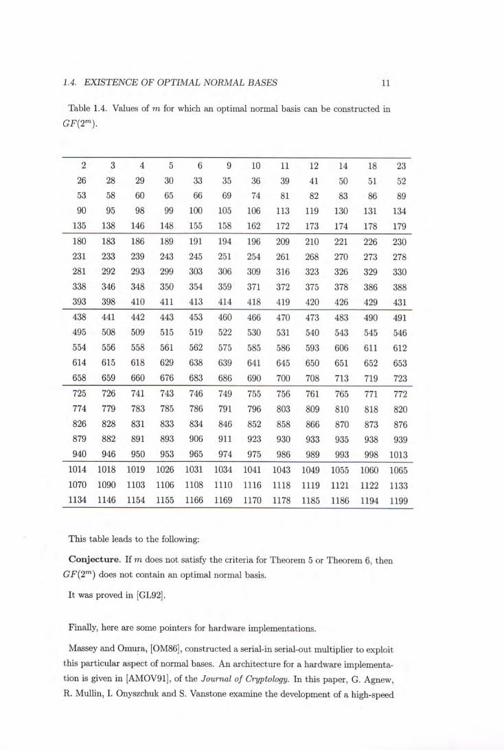
1.4. EXISTENCE OF OPTIMAL NORMAL BASES 11
Table 1.4. Values of m for which an optimal normal basis can be constructed in
2 3 4 5 6 9 10 11 12 14 18 23
26 28 29 30 33 35 36 39 41 50 51 52
53 58 60 65 66 69 74 81 82 83 86 89
90 95 98 99 100 105 106 113 119 130 131 134
135 138 146 148 155 158 162 172 173 174 178 179
180 183 186 189 191 194 196 209 210 221 226 230
231 233 239 243 245 251 254 261 268 270 273 278
281 292 293 299 303 306 309 316 323 326 329 330
338 346 348 350 354 359 371 372 375 378 386 388
393 398 410 411 413 414 418 419 420 426 429 431
438 441 442 443 453 460 466 470 473 483 490 491
495 508 509 515 519 522 530 531 540 543 545 546
554 556 558 561 562 575 585 586 593 606 611 612
614 615 618 629 638 639 641 645 650 651 652 653
658 659 660 676 683 686 690 700 708 713 719 723
725 726 741 743 746 749 755 756 761 765 771 772
774 779 783 785 786 791 796 803 809 810 818 820
826 828 831 833 834 846 852 858 866 870 873 876
879 882 891 893 906 911 923 930 933 935 938 939
940 946 950 953 965 974 975 986 989 993 998 1013
1014 1018 1019 1026 1031 1034 1041 1043 1049 1055 1060 1065
1070 1090 1103 1106 1108 1110 1116 1118 1119 1121 1122 1133
1134 1146 1154 1155 1166 1169 1170 1178 1185 1186 1194 1199
� This table leads to the following:
Conjecture. If m does not satisfy the criteria for Theorem 5 or Theorem 6, then GF{2^) does not contain an optimal normal basis.
It was proved in [GL92].
Finally, here are some pointers for hardware implementations.
Massey and Omura, [OM86] ’ constructed a serial-in serial-out multiplier to exploit this particular aspect of normal bases. An architecture for a hardware implementa-tion is given in [AM0V91], of the Journal of Cryptology. In this paper, G. Agnew, R. Mullin, I. Onyszchuk and S. Vanstone examine the development of a high-speed
12 CHAPTER 1. THEORY OF OPTIMAL NORMAL BASES
implementation of a system to perform exponentiation in fields of the form 爪). The use of optimal normal bases and observations on the structure of multiplica-tions have led to the development of an architecture which is of low complexity and high-speed. Using this architecture a multiplication can be performed in m clock cycles.

Chapter 2
Implementing Multiplication i n GF{2爪)
2.1 Defining the Galois fields GF(2爪)
A normal basis can be found for any finite field GF{p^), see chapter 1. For com-puters we use p = 2, i.e., 广 — . . A n element e in a field GF{2^)
written in a normal basis 朋:e = + . . . + + 已工沪 i + 己。卢
Here is the first header file, called field2n.li,which helps to define Galois Fields for the C code.
/*•* f i e l d 2 n . h ••*/
#def ine WORDSIZE ( s i z e o f ( i n t ) * 8 ) #def ine NUMBITS 173
#def ine NUMWORD (NUMBITS/WORDSIZE)
#define UPRSHIFT (NUMBITS7.W0RDSIZE) #def ine MAXLONG (NUMWORD+1)
#def ine MAXBITS (MAXLONG*WORDSIZE)
#def ine MAXSHIFT (WORDSIZE-1)
#def ine MSB (1L«MAXSHIFT)
#def ine UPRBIT (1L«(UPRSHIFT-1))
#def ine UPRMASK (-1L«UPRSHIFT))
#def ine SUMLOOP(i) f o r ( i = 0 ; KMAXLONG; i++)
1 3

14 CHAPTER 2. IMPLEMENTING MULTIPLICATION IN GF{2^)
typedef short in t INDEX;
typedef unsigned long ELEMENT;
typedef s t r u c t {
ELEMENT e[MAXLONG];
} FIELD2N;
WORDZISE is the number of bits in a machine word. NUMB ITS is the number of bits
the normal basis math will be expected to work on. NUMWORD is the maximum index
of machine words into a normal basis coefficients array. UPRSHIFT is the number of
left shifts needed to get to the most significant bit in the zero offset of the coefficient
list. MAXLONG is the number of machine words to hold the normal basis coe伍dents.
The term MAXBITS is used in a few places; it is the maximum number of bits we
can store in MAXLONG machine words. The term MAXSHIFT is the largest number of
shifts we need to move the most significant bit to the least in a single bit block.
Since we are doing a lot of shifting, this will be useful later. MSB is a mask for the
most significant bit in a WORDZISE block of bits.
The term UPRSHIFT is used to compute the most significant bit position, and
UPRBIT, a mask for the high-order ELEMENT UPRMASK. We will use UPRBIT for rota-
tions and UPRMASK to clear bits after rotations and shifts.
SUMLOOP is a macro. An INDEX is used for bookkeeping. We call an unsigned long
an ELEMENT, because it is the simplest thing we can work with. An ELEMENT is one
machine word in size.
Finally,we define the fields storage structure FIELD2N. This comes from the math-
ematical symbols, which means a field of characteristic 2 and vector length
m. Since we are going to reference each field element in the array, we use a single
letter "e, “ for ELEMENT. The coefficients are in big-endian order. This is an arbitrary
choice, so if one changes the order, make sure he changes it everywhere.
2.2 Adding and squaring normal basis numbers in
In base 2, all the coefficients can only be 0 or 1, and addition is simply an exclusive^ or,XOR operation. For m = 8,16,32,or 64 we would have perfect word-size align-ment for
any processor. Unfortunately, these are too small for cryptographic pur-poses and not mathematically optimal-

2.3. MULTIPLICATION FORMULA 15
The nicest aspect of this representation is that squaring a number amounts to a rotation. There are two reasons for this: 1 . ( 沪 下 = / 5 2 … 2 . = p. The first statement is obvious. The second statement comes from the rules of finite fields and is similar to Fermat's Little Theorem. So squaring e amounts to shifting each coefficient up to the next term and rotating the last coefficient down to 0 position. Squaring is thus very fast in a normal basis.
The first weird or interesting thing to recognize is what 1 is in a normal basis: 护 • In other words, the fundamental constant, 1’ is represented as "all
bits set" in a normal basis. So, adding 1 to a normal basis number amounts to flipping all the bits~not counting as we are used to.
2.3 Multiplication formula
Multiplication over a normal basis gets a touch complicated and is the main theme of this chapter. The basics are the same in any mathematical system, just multiply coefficients and sum over all those that have the same power of x. What makes optimal normal bases slick is that most of those terms are 0.
To show how multiply works, let us recall those material in Chapter 1, section 1 first.
Take two elements in GF(2,: A = E t ' o ' a n d B = ZT=o'The formal multiplication is C = AB = ZTJo' ET=o a扣萨 but C = ZT=o CkP''
by definition of an element in a normal basis. So the double sum in the first equation has to match the single sum in the second equation. In fact, we must have each cross-product term map to a sum over the basis terms
m—1 � = \ijk(3^\ Xijk e GF{2).
k=0
The Xijk coefficient is called "the lambda matrix" or "multiplication table."
If we substitute the multiplication table formula into the C = AB formula, we get a mess. FVom that mess we can find the solution to each Ck coefficient of in C = EETqI Cfc卢 ’ which is "only" a double sum:
m—1m—1 Cfc = [ [ aibjXijk.
i=0 j=0
which is equation 1.1 in Chapter 1 section 1.
16 CHAPTER 2. IMPLEMENTING MULTIPLICATION IN GF{2^)
The equation Ck = "yI E cLi^j^ijk can be transmogrified into a form that requires i=0 j=0 . .
only Xijo. From the discussions following equation 1.1 of Chapter 1 section 1’ it is
readily seen that m—1m—1
Cfc = ^ ^ ai+fc&j+fcAijO. (2-1) i=0 二 0
That reduces the amount of work required to construct the 入 matrix (multiplication
table). What makes equation 2.1 so awesome is that all we need to do is shift the
inputs by the correct amount and all coefficients can be computed in parallel.
Because there is no carry, even high-level languages can reasonably implement
normal basis math using very little memory. Of course, assembler and hardware
will always be faster.
An "optimal" normal basis has the minimum number of nonzero terms. This
number is called the "complexity" of the multiplication table. For fields GF{2" ' )
the optimal (minimum) complexity is 2m — 1’ chapter 1 theorem 1.
Recall that there are two types of optimal normal basis over GF�2爪、mentioned in
Chapter 1’ Section 3. They are called Type I and Type II. The only real difference
between them is the way we find which bits in the 入 matrix are set. For Type I
ONB we only need to store one vector; for Type II ONB we'll need to store two
vectors. For the code here, we'll make them both look the same so that the multiply
routine will work in either case. A Type I ONB multiply could be made quicker
with a few math tricks.
2.4 Construction of Lambda table for Type I ONB
in
According to Chapter 1’ Section 3’ the rules for creating Type I Optimal Normal
Basis in the field are:
1. m + 1 must be prime,
2. 2 must be primitive in hm-vi-
Rule 2 means that 2 raised to any power in the range 0 . . . m - 1 modulo m + 1
must result in a unique integer in the range 1 . . . m . Z is used to mean the set of
integers.
We need to find the cross-product terms of in 萨 = 入 i j f c / ^ 2 知 , X i j k e

2.4. CONSTRUCTION OF LAMBDA TABLE FOR TYPE I ONB IN GF{2^) 1 7
GF{2) to make the multiplication work. Because we can transform the A matrix to
A; = 0 for all cross-terms, we really only need to solve the equation: = (3 .
There is also the special case: P ^ — 1, when 2' + is congruent to 0 modulo
m+1.
To proceed, we need to know some math rules. For all the above to work optimally
we must have P be an element of order m + 1 in GF{T^) . Since 2 is primitive
in Zm+i, mod m + 1 will run through all the integers between 1 and m as i
runs through all values 0,1,...,m — 1. The combination 产 is just another way of
counting through all powers of (3, which is what generates our basis. The order is
scrambled compared to , but all powers of the generator are accounted for. These
are just simple matters, see [Ros98], p.80.
The easy way to solve equations = /^i, and also = 1 is to rewrite
them as modulo m + 1 and to "step into the exponent." We only need to solve:
+ = 1 mod m + 1,
2' + = 0 mod m + 1 .
Let's start with i = 0. = 1 and 二 1, since m + 1 is prime. This last point
comes from Fermat's Little Theorem. The first equation + = I mod m + 1
cannot have a solution for z = 0. Only the second equation 2 � + = 0 mod m + 1
can.
This second equation + 2- = 0 mod m + 1, can be solved, like this: If we take
the square root of = 1, we find: 2—2 = mod m + 1. But we already know
that 2® = +1, and, since 2 generates all the numbers mod m + 1, there is only one
choice: T 丨 1 = —1 mod m + 1. The equation + V = 0 mod m + 1 thus has a
solution for i = 0’ which is: 2 � 2 — 2 二 • mod m + 1 . We mentioned previously that
the Type I ONB only needs a single vector to keep track of all the cross-product
terms. The first entry in the table is at offset 0 (we are programming in C) and
has value m/2. We don't need to store any more of the values to solutions of this
equation, because we can multiply equation 2° + — • mod m + 1 by 2 and still
have 0 on the right-hand side. For every i, the nonzero element Xijo element from
the equation + = 0 mod m + 1 will always be: j = m/2 + i mod m.
Now for the first equation + = 1 mod m + 1, we do have to tabulate the values
from this equation once and then use those to look up the correct shift amounts.
The first value for i = 1 is easy, since: 2 + = 1,or = —1,so j = m/2. After
that we need to use antilog and log tables so we can find mod m + 1 easily and
j from 1 — 2 mod m + 1 just as easily.
18 CHAPTER 2. IMPLEMENTING MULTIPLICATION IN GF{2^)
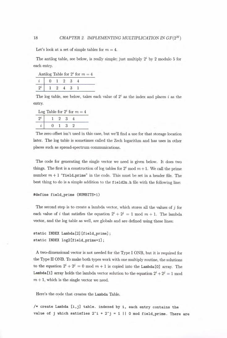
Let's look at a set of simple tables for m = 4.
The antilog table, see below, is really simple; just multiply by 2 modulo 5 for
each entry.
Antilog Table for 2七 for m = 4
i 0 1 2 3 4
2' 1 2 4 3 1
The log table, see below, takes each value of as the index and places i as the entry.
Log Table for 2' for m = 4
2' 1 2 3 4
i 0 1 3 2
The zero offset isn't used in this case, but we'll find a use for that storage location
later. The log table is sometimes called the Zech logarithm and has uses in other
places such as spread-spectrum communications.
The code for generating the single vector we need is given below. It does two
things. The first is a construction of log tables for 2' mod m + 1 . We call the prime
number m + 1 “f ield_prime” in the code. This must be set in a header file. The
best thing to do is a simple addition to the f i e ld2n .h file with the following line:
#de f ine f i e ld_pr ime (NUMBITS+1)
The second step is to create a lambda vector, which stores all the values of j for
each value of i that satisfies the equation + = 1 mod m + 1 . The lambda
vector, and the log table as well, are globals and are defined using these lines:
s t a t i c INDEX Lambda[2][f ield_prime];
s t a t i c INDEX l o g 2 [ f i e l d _ p r i m e + l ];
A two-dimensional vector is not needed for the Type I ONB, but it is required for
the Type II ONB. To make both types work with one multiply routine, the solutions
to the equation 2' + = 0 mod m + 1 is copied into the Lambda [0] array. The
Lambda [1] array holds the lambda vector solution to the equation 2' + 2^ = 1 mod
m + 1 , which is the single vector we need.
Here's the code that creates the Lambda Table.
/ • c reate Lambda [ i , j ] t a b l e , indexed by i , each entry contains the
value of j which s a t i s f i e s 2 " i + 2 " j = 1 || 0 mod f ield一prime. There are
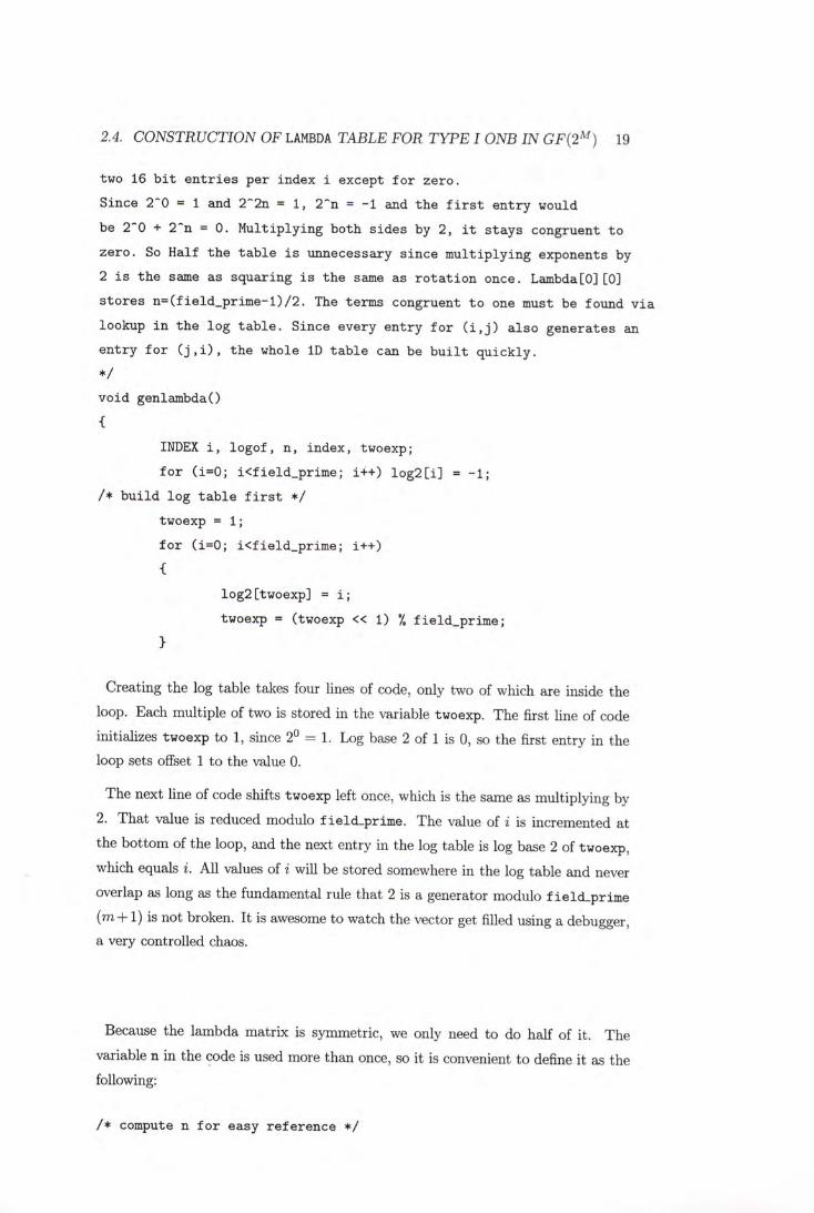
2.4. CONSTRUCTION OF LAMBDA TABLE FOR TYPE I ONB IN GF{2^) 19
two 16 b i t e n t r i e s per index i except f o r z e r o .
Since 2"0 = 1 and 2~2n = 1, 2~n = - 1 and the f i r s t entry would
be 2^0 + 2~n = 0. Mult ip ly ing both s ides by 2, i t s tays congruent t o
z e r o . So Half the t a b l e i s unnecessary s ince mul t ip ly ing exponents by
2 i s the same as squaring i s the same as r o t a t i o n once. Lambda[0][0]
s t o r e s n = ( f i e l d一p r i m e - l ) / 2 . The terms congruent t o one must be found v i a
lookup in the l o g t a b l e . Since every entry f o r ( i , ; j ) a l s o generates an
entry f o r ( j , i ) , the whole ID t a b l e can be b u i l t q u i c k l y .
* /
v o id genlambdaO {
INDEX i , l o g o f , n, index, twoexp;
f o r ( i=0 ; i<f ield一prime; i++) l o g 2 [ i ] = - 1 ;
/ * b u i l d l o g t a b l e f i r s t •/
twoexp = 1;
f o r ( i = 0 ; i< f i e ld_pr in ie ; i++)
•C
log2[twoexp] = i ;
twoexp = (twoexp « 1) % f ield—prime;
}
Creating the log table takes four lines of code, only two of which are inside the
loop. Each multiple of two is stored in the variable twoexp. The first line of code
initializes twoexp to 1’ since 2° 二 1. Log base 2 of 1 is 0’ so the first entry in the
loop sets offset 1 to the value 0.
The next line of code shifts twoexp left once, which is the same as multiplying by
2. That value is reduced modulo field—prime. The value of i is incremented at
the bottom of the loop, and the next entry in the log table is log base 2 of twoexp,
which equals i. All values of i will be stored somewhere in the log table and never
overlap as long as the fundamental rule that 2 is a generator modulo f ield_prime
(m + 1 ) is not broken. It is awesome to watch the vector get filled using a debugger,
a very controlled chaos.
Because the lambda matrix is symmetric, we only need to do half of it. The
variable n in the code is used more than once, so it is convenient to define it as the
following:
/ • compute n f o r easy r e f e r e n c e •/

20 CHAPTER 2. IMPLEMENTING MULTIPLICATION IN GF{2^)
n = (field—prime — l ) / 2 ;
/ • f i l l in f i r s t vector with indices s h i f t e d by half tab le s i ze * / Lambda[0] [0] = n; f o r ( i = l ; i<field_p:rime; i++) Lambda[0] [ i ] = (Lambda [0] [ i - 1 ] + 1) •/• NUMBITS ;
The above code fills in the Lambda [0] table. Starting with i = 0 in equation + 二 0 mod m + 1, each succeeding value is just 1 plus the previous value
modulo NUMBITS. For memory-constrained systems using only Type I ONB math, only one vector is needed.
Here is the code that generates the single important lambda vector.
/ * i n i t i a l i z e second vector with known values •/
Lambda[1][0]= - 1 ; / * never used * /
Lambda[1] [1] = n;
Lambda [1] [n] = 1;
/ * loop over resu l t space. Since we want 2 " i + = 1 mod f ie ld_pr ime
i t ' s a ton eas ier to loop on 2 " i and look up i than so lve the s i l l y
equations. Think about i t , make a t a b l e , and i t ' l l be obvious. •/
f o r ( i=2; i<=n; i++) {
index = l og2 [ i ];
logof = l og2 [ f i e ld_pr ime - i + 1 ] ;
Lambda[1][index] = logof;
Lambda[1][logof] = index; }
/ • l a s t term, i t ' s the only one which equals i t s e l f . •/
Lambda[1] [ l og2 [n+ l ] ] = log2[n+l];
}
Let's see how this works. The first thing to recognize is that equation 2' + 2) = 1
mod m + 1 is symmetric. If entry A^o = 1, then 入jio = 1 too. The counter i is
taken as the value of 2'. Because we'll hit every value only once, the counter steps
through every possible value of 2' (mod m + 1). The variable index is log base 2 of
i , so that tells us where to store the value of i in the Lambda vector.
Since 1 — 2 modulo f ield_prime does not change if we add f ield_prime, we can write the equation as: = f ield_prime + 1 - 2 \ Take log base 2 of both sides, and we have the second line of code in the loop. This eliminates negative lookups, which would give the code some major headaches.

2.4. CONSTRUCTION OF LAMBDA TABLE FOR TYPE I ONB IN GF{2^) 2 1
The last two lines in the loop simply set the entry point index to the value of j
(called logof in the code) and entry point j to the value of index. The very last
line in the above listing fills in the only nonsymmetric term.
2.5 Constructing Lambda table for Type II ONB in
2.5.1 Equations of the Lambda matrix
For a Type II optimal normal basis we have the same number of terms. But both sets are scrambled, so we end up with two sets of vectors. There are two possible Type II ONBs: let us call them Type Ila and Type lib.
According to Chapter 1’ Section 3. A Type II optimal normal basis over can be created if :
1 2m + 1 is prime and either
2a 2 is primitive in Z2m+i
or
2b 2m + 1 = 3 mod 4 and 2 generates the quadratic residues in Z2m+i.
What does 2a mean? If we take mod 2m + 1 for /c = 0,1, 2 , . . . , 2m - 1 then we
get every value in the range [1 . . . 2m] back. What does 2b mean? The first part is
simple: The last two bits are set in the binary representation of the prime 2m + 1.
The second part means that even if 2知 mod 2m + 1 does not generate every element
in the range [1 . . . 2m], we can at least take the square root mod 2m + 1 of 2''.
For Type II ONB we need to modify the f i e l d 2 n . h header file again. To make life a bit simpler, we add some additional code. This allows all the modifications to work when needed. By simply changing TYPE2 to TYPEl in one place the entire code package will compile correctly.
#def ine TYPE2
# i fde f TYPE2
#def ine field—prime ((NUMBITS«1)+1) #e lse
#def ine f ie ld_pr ime (NUMBITS+1) #endif
22 CHAPTER 2. IMPLEMENTING MULTIPLICATION IN GF{2^)
To generate a Type II ONB we use two field elements from two different fields. First pick an element 7 of order 2m + 1 in We use that to find (5, which
is in the field We won't actually have to find the 7 element; we are just going to use it symbolically to help us create the A matrix. Form the sum of 7 + 7 " ^ This element gives us the first element, of our normal basis, recall Chapter 1’ Section 3.
The cross-product terms of P � ' ' a r e = + =
(7(2妨)+ 7—⑵+2勺)+ ⑵-2勺 + (2^2勺).Since = (y + , we get
裕 i _ / + if ^ ±2). mod (2m + 1) , " " = i & if 2 � 士 m o d (2m + 1 ) . 於 肌 � / c are two possible
solutions to the multiplication of any two basis elements. That is what makes this
normal basis optimal: It has the minimum number of possible terms. In the case of = ±2 ) , the terms + 7 - � c a n c e l , because the exclusive-or of anything with itself is 0.
In the case of — ±2) mod (2m + 1), at least one of these equations:
+ 力 = m o d (2m + 1)
21 + 2•? = - 2 ^ mod (2m + 1) will have a solution, and at least one of these equations:
- -- mod ( 2 m + 1 )
2' 一 = -2'= mod (2m + 1) also has a solution.
In the case of = mod (2m + 1 ) , at least one of the following four equations has a solution:
+ T = 2知 mod (2m + 1)
- 义 = 2 知 mod (2m + 1) + V = 一2& mod (2m + 1)
T + = - 2 ^ mod ( 2 m + 1 ) .
In the first set of equations, there are two possible solutions, and in the second
set of equations, there is only one possible solution. It is easy to see that, [Ros98],
p.87, the equations are all similar, so instead of working with two different sets we
can combine them and work with just one group of four equations. To build our A

2.4. CONSTRUCTION OF LAMBDA TABLE FOR TYPE I ONB IN GF{2^) 2 3
matrix, we set /c = 0 and find solutions to:
2' + = 1 mod (2m+1),
2' + = - 1 mod (2m+1),
2' - = 1 mod ( 2 m + 1 ) , 2i - 23 = - 1 mod ( 2 m + 1 ) .
2.5.2 An example of Type Ila ONB
As an example of Type Ila, take 2m + 1 = 19. Then our field size m = 9. This will be the length of the A matrix. The first thing we need to build are log and antilog tables.
Powers of mod 19 (antilog)
i 0 1 2 3 4 5 6 7 8 9 10 11 12 13 14 15 16 17 18
2' 1 2 4 8 16 13 7 14 9 18 17 15 11 3 6 12 5 10 1
The antilog table, see above, takes an index, i, and returns I = mod 2m + 1.
The log table, see below, takes an index, I, and returns the value of i.
Log base 2 of i mod 19 (log table)
J 1 2 3 4 5 6 7 8 9 10 11 12 13 14 15 16 17 18 Log2(i) — 0 1 13 2 16 14 6 3 8 17 12 15 5 7 11 4 1 0 V
The code to compute the log table is as follows:
twoexp = 1;
f o r ( i=0 ; i<NUMBITS; i++) {
log2[twoexp] = i;
twoexp = (twoexp « 1) •/• field—prime;
}
Note that the log table is built using modulo field—prime as the subscript, and the loop counter i is the value. This builds the log table in the order of the antilog table.
To continue the example, let us start with i = 1 in the equations
2' + 2^ =1 mod ( 2 m + 1), 2' + = - 1 mod (2m+1),
=1 mod ( 2 m + 1 ) ,
2' - = - 1 mod ( 2 m + 1 ) .
24 CHAPTER 2. IMPLEMENTING MULTIPLICATION IN GF{2^)
Writing down all four equations mod 19 and subtracting 2 from both sides gives 2' = -l = 18 j = 9
= - 3 = 16 = A -2^ = - 1 = > j = 0
us the following: -2^ = - 3 力•二 13
Since the A matrix has only nine entries per column, the solutions for j must be in the range of 0 . . . 8. Only two terms for j are less than 9. These are the two terms we need. So we have our first nonzero entries in the A matrix: Ai,o = 1 and Ai,4 = 1. All other entries X i j must be 0.
Continuing in this manner we can find two values of j for each value of i, which
give us nonzero entries in the A matrix. We'll mark these with two vectors: Aq and
Ai,and call them Lambda[0] [] and Lambda[l][] in the code. Each position in the A
table corresponds to a value of i in cross-product term and each entry is
the matching value of j, which gives one of the terms in equation
j + P�' if ^ ±2 ) mod (2m + 1) , p p = S that has k or k 二 0. The
[ i f 2' = 土2) mod (2m + 1) results are shown below.
i Aq = ji A I = j2
~0 1
1 4 0
2 4 7
3 6 8 A Vectors for m = 9
4 2 1
5 6 7
6 5 3
7 2 5
_8 8 ^
The choice of value in either column for any row does not really matter, since we are going to combine matching coefficients in the multiply routine eventually. Note that there are a total of 2m - 1 terms. The zero entry will always be 1 for any Type II ONB. We fill in this spot just to make the code simple, but we will take advantage of it when we do the actual multiply.
2.5.3 An example of Type lib ONB
Now, ley us look at a Type lib ONB. When the field—prime is 23,for example, we have a Type l ib ONB, which is congruent to 3 mod 4 and in which 2 generates the quadratic residues of mod 23. Look at the antilog table below to see what this

2.4. CONSTRUCTION OF LAMBDA TABLE FOR TYPE I ONB IN GF{2^) 2 5
really means.
Powers of mod 23 (antilog)
i 0 1 2 3 4 5 6 7 8 9 10
2' 1 2 4 8 16 9 18 13 3 6 12
i 11 12 13 14 15 16 17 18 19 20 21 22
2' 1 2 4 8 16 9 18 13 3 6 12 T
Note that only half the values of 1 . . . 22 appear in the anti-log table. But if we take 23 - 2' for all values greater than 11, we get the results shown in the following table, that is fairly straightforward, [Ros98], p.89.
Powers of 2' mod 23 (antilog)
i 0 1 2 3 4 5 6 7 8 9 10
2' 1 2 4 8 7 9 5 10 3 6 11
1 11 12 13 14 15 16 17 18 19 20 21 22 2 叫 1 2 4 8 7 9 5 10 3 6 1 1 ~ ~ T
Now, 23 - 2' modulo 23 is just -2\ It, after building half the log table, we find
that twoexp ( = 2 ” equals 1’ then we know we will cycle through the same values
of 2' that we just finished. To solve this problem we can restart at i = 0 but do the
subscript on negative values of 2\ Since subscripts need to be positive (for us to fill
in a useful table relative to the rest of the code anyway), we can start with twoexp
= f i e l d - r i m e - 1 = 2*NUMBITS, which is congruent to - 1 . This following code
then fills in the rest of the log table.
i f (twoexp == 1) / * i f so , then deal with quadratic res idues * / {
twoexp = 2*NUMBITS;
f o r ( i=0 ; i<NUMBITS; i++) {
log2[twoexp] = i ;
twoexp = (twoexp « 1) % f i e l d . p r i m e ;
} }
The final Log table is shown here.
Log base 2 of i mod 23 (log table)
J 1 2 3 4 5 6 7 8 9 10 " T T
Log2{i) | 0 1 8 2 6 9 4 3 5 7 10

26 CHAPTER 2. IMPLEMENTING MULTIPLICATION IN GF{2^)
_ i 12 13 14 15 16 17 18 19 20 21 2 �
Log2{i) I 10 7 5 3 4 9 6 2 8 1 ~ 0 ~
All we are doing is bookkeeping: tracking all the coefficients we need to add in
order to compute the multiplication of two normal basis numbers. Since all we had
to solve for was k = 0’ instead of a complete 入 matrix, we only need to store two
vectors.
2.5.4 Creating the Lambda vectors for Type II ONB
Once we have the log and antilog tables, creating the vectors is easy. Here is the
code for generating the vectors for a Type II ONB.
/ * Type 2 ONB i n i t i a l i z a t i o n . F i l l s 2D Lambda matr ix . •/
v o i d genlambda2() {
INDEX i , l o g o f [ 4 ] , n , index , j , k , twoexp;
/ * b u i l d l o g t a b l e f i r s t . For the case where 2 generates the quadrat i c
r e s i d u e s ins tead of the f i e l d , d u p l i c a t e a l l the e n t r i e s t o ensure
p o s i t i v e and negat ive matches in the lookup t a b l e ( that i s , - k mod
f ield一prime i s congruent t o entry f ield一prime - k ) . •/
twoexp = 1;
f o r ( i = 0 ; i<NUMBITS; i++) {
l og2[ twoexp] = i ;
twoexp = (twoexp « 1) % f ie ld一prime;
} i f (twoexp == 1) / • i f s o , then dea l with quadrat i c r e s i d u e s * / {
twoexp = 2*NUMBITS;
f o r ( i = 0 ; i<NUMBITS; i++) {
l og2[ twoexp] = i ;
twoexp = (twoexp « 1) % f ie ld一prime;
} } e l s e

2.5. CONSTRUCTING LAMBDA TABLE FOR TYPE II ONB IN GF{2^) 27 {
f o r (i=NUMBITS; i<field一prime—1; i++) {
l og2 [twoexp] = i;
twoexp = (twoexp « 1) % f ie ld一prime;
} }
/ • f i r s t element in v e c t o r 0 always = 1 • /
Lambda [0] [0] = 1;
Lambda [1] [0] = -1;
/ * again compute n = ( f ield一prime - l ) / 2 but t h i s time we use i t t o see i f an equat ion a p p l i e s • /
n = ( f i e l d _ p r i m e - l ) / 2 ;
/ * as in genlambda f o r Type I we can l o o p over 2- i i idex and l ook up index
from the l o g t a b l e p r e v i o u s l y b u i l t . But we have t o work with 4
equat ions ins tead of one and only two of those are u s e f u l . Look up
a l l f o u r s o l u t i o n s and put them i n t o an array . Use two c o u n t e r s , one
c a l l e d j t o s tep thru the 4 s o l u t i o n s and the o ther c a l l e d k t o t r a c k
the two v a l i d ones .
For the case when 2 generates quadrat i c r e s i d u e s only 2 equat ions are
r e a l l y needed. But the same math works due t o the way we f i l l e d the
l o g 2 t a b l e .
*/ twoexp = 1;
f o r ( i = l ; i<n; i++) {
twoexp = ( t w o e x p « l ) % f ie ld—prime;
l o g o f [ 0 ] = l og2 [ f i e ld一pr ime + 1 - twoexp];
l o g o f [ 1 ] = l og2 [ f i e ld一pr ime - 1 - twoexp];
l ogo f[2] = log2[ twoexp - 1];
l o g o f [ 3 ] = l o g 2 [twoexp + 1];
k = 0 ;
•j = 0;
whi le (k<2) {
28 CHAPTER 2. IMPLEMENTING MULTIPLICATION IN GF{2^)
i f ( l o g o f [ j ] < n) {
Lambda[k] [ i ] = logof [ j ];
k++;
}
} }
The genlambda2 routine is very similar to the previous genlambda routine. The main difference is that we now have to check four equations instead of one. The four equations are solved as a look up in the log table and saved in the logo f [] array.
Since there are two solutions and four variables to check, we use two counters. The variable j counts over the logof [] array, and the variable k counts over the solutions. A solution is valid only if less than n. For Type l ib that is automatic, and only the first two equations will ever be used. But anything modulo f ield_prime will give us an index into the array in the range of 1.. .2+NUMBITS, and for Type Ila we have to check that we get the right two solutions.
Going from 1 to m - 1 and getting two solutions gives us 2m — 2 terms. The first term is already known and is set at offset 0 in Lambda [0] [] • So we have found all the terms, Chapter 1, Section 2.
2.6 Multiplication in practice
The starting point for multiplication is the multiplication formula m—1m—1
Cfc = Z) Z ] ai+kbj+kXijo in section 2.3. i=0 j=0
Prom the previous efforts we know that there are only two values of j for each value of i (or vice versa, since multiplication is independent of order). Note that each subscript of a and b is shifted by the same value of k. This means we can shift all the a coefficients and all the b coefficients for any particular values of i and j to find one term for all the c coefficients.
An example will help. Let's take the i = 2 index of the Type Ila GF{2^) example worked out before.
2.6. MULTIPLICATION IN PRACTICE 29
i AQ = ji A I = j2
0 1
1 4 0 2 4 7 3 6 8
A Vectors for m = 9 4 2 1
5 6 7
6 5 3
7 2 5
_8 8 ^
Prom this table we have Ao’2 = 4 and Ai’2 = 7. Consider one explicit term of the multiplication formula, which looks like this: Cfc = +a2+fc(64+fc + 67+fc) +
For k = 0, the partial sum is £12(64 + 67)- For k = 1, the partial sum is 03(65 + 63) and so one through k = 8. All of these bitwise manipulations can be done in parallel. What we have to do is rotate the A vector right two places and multiply it with the sum of the B vector rotated right four and seven places. As an example, graphically this appears as follows:
di ao as ay QQ a^ (24 <23 ai
H H BI BO BG 67 BE 65 H +
be &5 h 63 62 bo bg 67
i i i i i i i i i C8 Cj C6 C5 C4 C3 C2 Ci Co
The addition is performed by using exclusive-or XOR. The multiplication is per-formed using AND. Depending on machine size, we can do 8’ 16’ 32’ or 64 coefficients simultaneously.
Since multiplication is commutative, we can choose either A or B to be summed. In the code, we shift B once for each term and use the count of that offset as the index into the lambda vector table to find each proper shift of A.
The first routine we need is a rotate. Going right, the least significant bit needs to be placed into the most significant bit. Going left we do the opposite. Here are single bit rotation routines.
vo id r o t _ l e f t ( a ) FIELD2N •a;
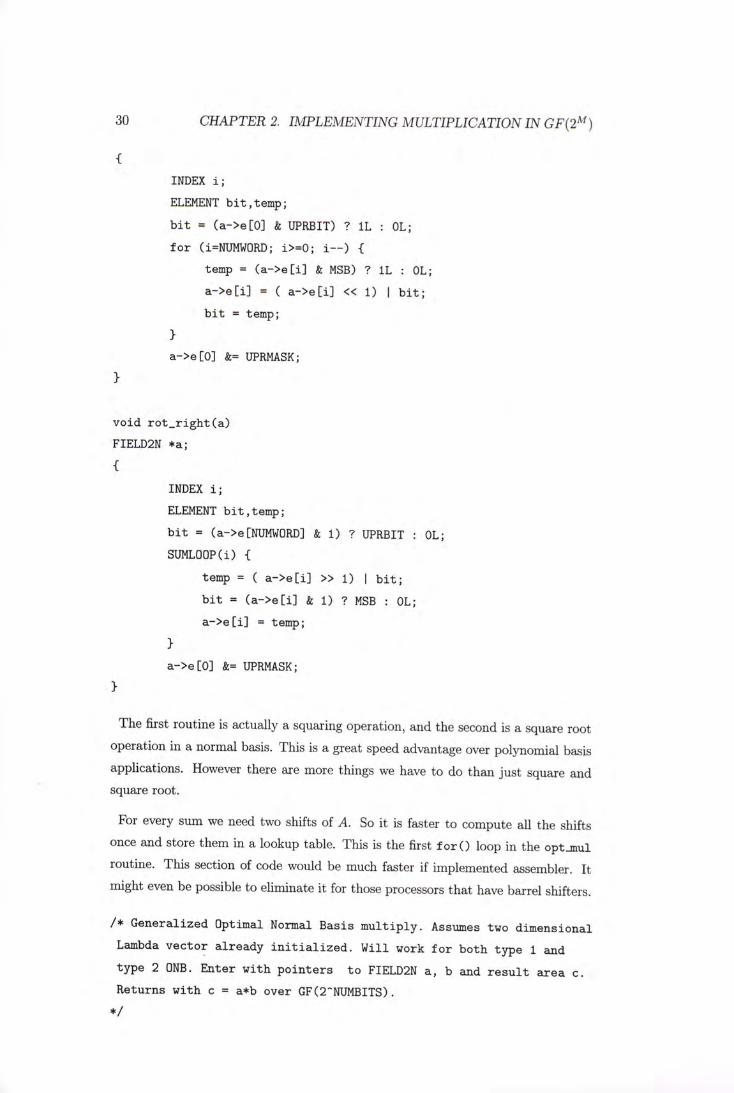
30 CHAPTER 2. IMPLEMENTING MULTIPLICATION IN GF{2^)
{ INDEX i ; ELEMENT bit , temp;
b i t = (a->e[0] & UPRBIT) ? IL : OL; f o r (i=NUMWORD; i>=0; i一一) •[
temp = ( a - > e [ i ] & MSB) ? IL : OL; a - > e [ i ] = ( a - > e [ i ] « 1) | b i t ; b i t = temp;
} a->e[0] &= UPRMASK;
}
void rot—right(a) FIELD2N •a; {
INDEX i ;
ELEMENT bit , temp;
b i t = (a->e[NUMWORD] & 1) ? UPRBIT : OL;
SUMLOOP(i) {
temp = ( a - > e [ i ] >> 1 )丨 b i t ; b i t = ( a - > e [ i ] & 1) ? MSB : OL; a - > e [ i ] = temp;
} a->e [0] &= UPRMASK;
} The first routine is actually a squaring operation, and the second is a square root
operation in a normal basis. This is a great speed advantage over polynomial basis applications. However there are more things we have to do than just square and
‘ square root.
For every sum we need two shifts of A. So it is faster to compute all the shifts once and store them in a lookup table. This is the first f o r ( ) loop in the opt_mul routine. This section of code would be much faster if implemented assembler. It might even be possible to eliminate it for those processors that have barrel shifters.
/ * Generalized Optimal Normal Basis mult ip ly . Assumes two dimensional Lambda vec tor already i n i t i a l i z e d . Wil l work f o r both type 1 and type 2 ONB. Enter with po inters to FIELD2N a, b and r e s u l t area c . Returns with c = a*b over GF(2~NUMBITS).
*/
2.6. MULTIPLICATION IN PRACTICE 31
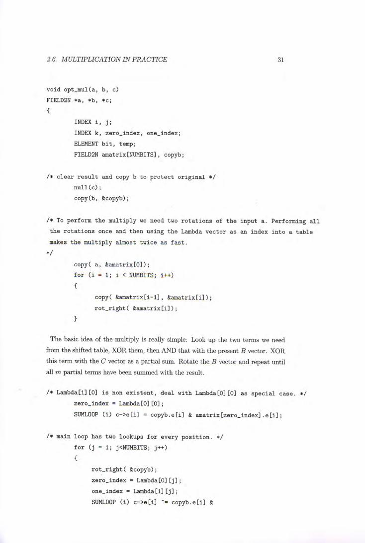
vo id opt_mul(a, b , c )
FIELD2N •a, •b, * c ; {
INDEX i , j ;
INDEX k, zero_ index , one_index;
ELEMENT b i t , temp;
FIELD2N amatrix[NUMBITS], copyb;
/ * c l e a r r e s u l t and copy b t o p r o t e c t o r i g i n a l * /
n u l l ( c );
copy(b , ©b);
/ * To perform the mult ip ly we need two r o t a t i o n s of the input a. Performing a l l
the r o t a t i o n s once and then using the Lambda v e c t o r as an index in to a t a b l e
makes the mult ip ly almost twice as f a s t .
* /
copy( a, feamatrix;[0]); f o r ( i = 1; i < NUMBITS; i++) {
copy( & a m a t r i x [ i - l ] , &amatr ix [ i ] ) ;
r o t _ r i g h t ( feamatrix[i]);
}
The basic idea of the multiply is really simple: Look up the two terms we need
from the shifted table, XOR them, then AND that with the present B vector. X O R
this term with the C vector as a partial sum. Rotate the B vector and repeat until
all m partial terms have been summed with the result.
/ • Lambda[1][0] i s non e x i s t e n t , deal with Lambda[0][0] as s p e c i a l case . •/ zero—index = Lambda[0][0];
SUMLOOP ( i ) c - > e [ i ] = c o p y b . e [ i ] & amatr ix [zero . index ] . e [ i ] ;
/ * main l oop has two lookups f o r every p o s i t i o n . •/ f o r ( j = 1; j<NUMBITS; j++) {
r o t _ r i g h t ( fecopyb);
zero—index = Lambda[0][j];
one一index = Lambda[1][j];
SUMLOOP ( i ) c - > e [ i ] c o p y b . e [ i ] &

32 CHAPTER 2. IMPLEMENTING MULTIPLICATION IN GF{2^)
(amatrix [zero—index:] . e [ i ] "amatrix [one_index] . e [ i ] ) ; }
}
Optimizing the code for speed is obviously important but implementation depen-dent. For a Type I ONB, there is no need for two lookup vectors. In fact, we only need to perform the multiplication (AND) of A rotated half its length with B and take the "trace" of the result, which gets summed with the single lookup vector result for a very high speed Type I ONB algorithm. The trace function for ONB it is identical to a parity bit calculation, see [Ros98], p.95.

Chapter 3
Inversion over optimal normal basis
3.1 A straightforward method
To begin with, let us look at a very straightforward method of inversion over a
normal basis. Observe that if a e GF(2爪),a ^ 0, then using Fermat's Little
Theorem, a—i = =(“广一‘—�• At this point we could just exponentiate
directly. But this would require m squarings and m - 1 multiplies. For m on the
order of 200 this would be exceptionally slow.
The following is a way around the problem. The most efficient technique, from the
point of view of minimizing the number of multiplications, was proposed by Itoh,
Teechai and Tsujii in 1986.
If m is odd, then since 2爪—i — 1 = (2(爪一丄)"-1)(2——1)/2 + 1 ) ’ we have =
- 1 ) . Hence it takes only one multiplication to evaluate
once the quantity ”Z2-i j ^ g been computed (we are ignoring the cost of squar-
ing).
If m is odd, then we have ! 一 丄 = ^ ^ ^ consequently
it takes two multiplications to evaluate once ^ ^ been com-
puted. The procedure is then repeated recursively.
Here is an example: Consider the field We have
2155 —2 = 2(277 — 1)(277 + 1),
277 — 1 = 2(219 - 1)(219 十 1)(238 + 1) + 1’
3 3

34 CHAPTER 3. INVERSION OVER OPTIMAL NORMAL BASIS
219 —1 = 2(29 _1) (29 + 1) + 1 ’
29 - 1 = 2(2+ 1)(22 + 1)(24 + 1) + 1,
so an inversion in takes ten multiplications.
It can easily be verified by induction that this method requires exactly I{m)=
[log2(m - 1)J + - 1) - 1 field multiplications, where w { m - l ) denotes the number of l,s in the binary expansion of m - 1,see [Men93].
3.2 High-speed inversion for optimal normal basis
3.2.1 Using the almost inverse algorithm
The following method combines polynomial basis and optimal normal basis to im-
plement a very high speed inversion algorithm. Most research into elliptic curve
crypto systems over the past few years has concentrated on finding mathematical
tricks to increase throughput. Many of these tricks rely on the structure of certain
fields. Others rely on finding specific irreducible polynomials.
In finite field arithmetic, most inversion routines require two to five times as long as a multiply. The routine presented here was first developed by Dave Dahm, see [Ros98]. This inversion routine is as fast as a single optimal normal basis multiply. But notice, however that special polynomial bases can be made much faster in general..
Dahm's inversion algorithm is based on [SOOS95] for the "almost inverse algorith-m" and on the results of Chapter 1 for the irreducible polynomial, which converts from Type I and Type II ONB to polynomial basis. The "almost inverse algorithm" is based on Euclid's algorithm, but it leaves a final factor of a;知,which has to be divided out. Fortunately, this is a trivial operation for ONB, so the conversion to and from polynomial basis and the elimination of the final factor turns out to be much faster than the inversion algorithm described in section 1 of this chapter.
The basic idea of the almost inverse algorithm is the same as polynomial inversion. We keep the following formula constant, see [Ros98], p.285: B • F + C G = 1 mod M , where M is the prime polynomial. For an ONB the prime polynomial is very specific; we will describe it later.
The almost inverse algorithm is initialized with:
B = 1

3.2, HIGH-SPEED INVERSION FOR OPTIMAL NORMAL BASIS 35
C = 0
F ^Source Polynomial
G = M =Prime Polynomial
A: = 0
The variables B,C,F, and G are polynomials, and k is an integer. The almost
inverse algorithm proceeds by repeating the following steps:
While the last bit of F is 0:
shift F right (divide by a:)
shift C left (multiply by x)
increment k by 1. “ If F = 1, return B,k. (3.1)
If degree(F) < degree(G), then exchange F, G and B, C.
F = F + G.
B = B + C.
Repeat entire loop.
The reason this is an "almost" inverse routine is that we have the final result with an extra factor of x'', which must be divided out. For optimal normal basis this factor is very easy to find, and we don't need a full-scale multiply to remove it.
There are additional tricks that Schroeppel et al. [SOOS95] include in their paper to help speed up the algorithm. These include using two separate loops rather than exchanging polynomials, using registers, and expanding structures to explicitly named variables. Many of these tricks reduce portability but increase throughput.
In Chapter 1’ Section 3’ an irreducible polynomial for a Type Ila optimal normal basis, for which 2 is primitive in Z2m+i, is: Mjja = l + x + +
It follows that for a Type I ONB (with 2 primitive in Zm+i) an irreducible poly-nomial is given by: M / = 1 + ;r + re? + … + x"".
For the Type l ib optimal normal basis, for which 2 generates the quadratic
residues, the polynomial Mua = 1 + a: + + . . . + has two factors, so it
is not irreducible. Fortunately, the almost inverse algorithm will still work. This is
due to the requirement that the source polynomial be relatively prime to the basis
polynomial M. This will always be the case for sources of Type II ONB.
Let us look at how to convert a Type I normal basis representation to a polynomial basis representation. Each term in a normal basis is of the form: aiX^\ But since

36 CHAPTER 3. INVERSION OVER OPTIMAL NORMAL BASIS
2 is a generator modulo m + 1, we can also write this term as: aix''. Since Mi = 1 + a; + ;r2 + . . . + a:饥’ we can move the i th coe伍dent of Type I ONB to the k
position to convert form normal to polynomial basis. This is just a permutation of all the bits, and we only have to move the ones that are set.
The only problem we have is when 2' 二 m. This term is not represented in the polynomial basis, because it has the power of the most significant coefficient in M/ = 1 + a; + a;2 + .. • + In the normal basis case, there is no representation for x®. For this case, we map the coefficient of the most significant bit of the ONB to the least significant bit of the polynomial representation, and nothing is lost. Here is Rosing's explanation: As vector spaces, the basis vectors are exactly the same (except for order) at all places except 1. Each set of basis vectors contains
.. • ,0;爪—1. The only difference is that ONB contains x"^ and polynomial basis contains 1. In the Type I field these two representations are related by: 1 + a: + + . . . + = 0.
For a Type II optimal normal basis, things are almost as easy, [Ros98], p.287. The polynomial basis is twice as long as the normal basis. For each bit in the ONB we will have 2 bits in the polynomial basis. It turns out that the 2 bits are palindromes; if bit i is set, then so is bit 2m + 1 — i.
In chapter 1, section 3’ we took the basis to be of the form: 7 + 7 - 1 _
The combination of these two terms created a new one, which was the basis for
the Type II ONB. Using this, along with the polynomial Mua = 1 + x + x^ i-
. . . + we can derive a simple conversion scheme to go from Type II ONB to
polynomial representation and back by flipping just 2 bits in a known permutation.
Since the permutation is predefined for any ONB, we can create a lookup table at
initialization, along with the creation of the multiplication vectors.
For simplicity, let p = 2m + 1. Since we are doing base 2 field math, we have: (7 + 7-1)2' = + 7-2* = ^ r + ^ p - r j^g^ as with the Type I ONB, we have a permutation form the coefficient of each term to a corresponding one in the polynomial representation. But there are now 2 bits that we have to map: one that maps 2' to k and one that maps p - to p - k.
By creating the permutation map as a set of indices and bit masks, the conversion is very fast. The almost inverse algorithm is then simple to invoke. The whole process is identical for both Type I and Type II (other than the number of bits needed).

3.2, HIGH-SPEED INVERSION FOR OPTIMAL NORMAL BASIS 37
3.2.2 Faster inversion, preliminary subroutines
There are several steps to creating this faster inversion routine. The first is a pair of
tables used in the conversion from normal basis to polynomial and back. Another
is the multiplication of re—知 as the final step in the almost inverse algorithm. Then
there is the inversion routine itself. The latter has been expanded using some of
the suggestions in [SOOS95].
Let us start with some new constants, which are defined in a header file:
#de f ine LONGWORD (field_prime/WORDSIZE)
#def i i ie LONGSHIFT ((field一prime—1)%W0RDSIZE)
#de f ine LONGBIT (1L«(L0NGSHIFT-1))
#de f ine LONGMASK C (-1L«L0NGSHIFT))
These are used to create the polynomial basis representation, as we will see below.
LONGWORD is the number of ELEMENTS needed to hold the polynomials we will be
using. LONGSHIFT is the number of left shifts needed to get to the most significant
bit in the most significant ELEMENT of the polynomial representation. LONGBIT is
the most significant bit we will need in the polynomial basis, and LONGMASK is a
mask that keeps the most significant bits in the most significant ELEMENT of the
polynomial basis.
Next comes some additional initialization code, which needs to be called only once.
The initializations are for the following arrays, which need to be added to the .c file
(chapter 3 subroutines):
s t a t i c INDEX l o g 2 [ f i e l d _ p r i m e + l ];
s t a t i c INDEX two一 inx[field—prime];
s t a t i c ELEMENT two一bit [field一;prime];
s t a t i c unsigned char shi f t一by[256] ;
The variable l og2 is the same; it is just global for use in the conversion process.
The two arrays two_* are used to find specific bits. Rather than save the bit position,
as in the l og2 array, we save the ELEMENT index and bit offset within an ELEMENT.
This speeds execution with only a minor increase in memory requirements. The
array sh i f t _by is used as one of the speed enhancements. Instead of shifting the F
polynomial only once and incrementing k as stated in the algorithm, we do several
shifts at once if possible.
We have seen the genlambda routines before; the only change there is the removal
of variable log2, because it is now global. The routine i n i t . t w o fills in the arrays
38 CHAPTER 3. INVERSION OVER OPTIMAL NORMAL BASIS
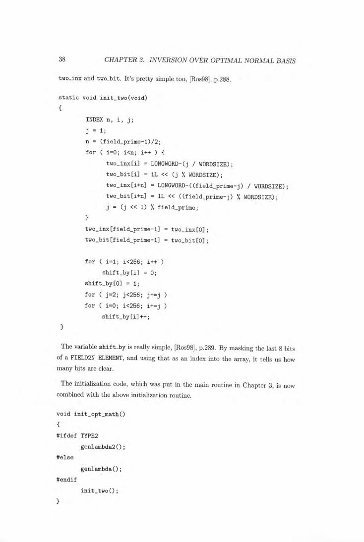
two-inx and two_bit. It's pretty simple too, [Ros98], p.288.
s t a t i c vo id init—two(void) {
INDEX n, i , j ;
j = 1;
n = ( f i e l d _ p r i m e - 1 ) / 2 ;
f o r ( i=0 ; i<ii; i++ ) {
t w o _ i n x [ i ] = LONGWORD-(j / WORDSIZE);
two一bit [ i ] = IL « ( j 7, WORDSIZE);
two一inxlii+ii] = LONGWORD —((field一prime—j) / WORDSIZE);
•two一bit [ i+n] = IL « ( ( f i e l d . p r i m e - j ) •/• WORDSIZE);
j = ( j « 1) 7, f i e l d - p r i m e ;
} two一inx [field一prime—1] = two_inx[0];
•two_bit [ f ield一prime-1] = two_bit [0];
f o r ( i = l ; i<256; i++ )
s h i f t _ b y [ i ] = 0;
shi f t—by[0] = 1;
f o r ( j = 2 ; j<256; j+= j )
f o r ( i=0 ; i<256; i+=j )
sh i f t—by[ i ] ++;
}
The variable s h i f t . b y is really simple, [Ros98], p.289. By masking the last 8 bits
of a FIELD2N ELEMENT, and using that as an index into the array, it tells us how
many bits are clear.
The initialization code, which was put in the main routine in Chapter 3’ is now
combined with the above initialization routine.
vo id in i t_opt_math( ) {
# i f d e f TYPE2
genlainbda2();
# e l s e
genlambdaO ;
#endif
iiii1;_two();
}

3.2, HIGH-SPEED INVERSION FOR OPTIMAL NORMAL BASIS 39
There is yet another type of variable. It is used to hold double-size arrays for
Type II optimal normal basis conversions to "customary" polynomial basis repre-
sentations. For Type I optimal normal basis, it is the same size as FIELD2N, but
this makes the code more general.
typedef s t r u c t {
ELEMENT e [LONGWORD+1];
} CUSTFIELD;
Basic operations on this structure are similar to operations on FIELD2N and DBLFIELD
structures. To copy values from one CUSTFIELD to another, we use the following
code segment:
vo id copy一cust ( a , b )
CUSTFIELD * a , * b ; {
INDEX i ;
f o r ( i = 0 ; i<=LONGWORD; i++) b - > e [ i ] = a - > e [ i ];
}
And to clear out a variable, the following routine is used.
vo id n u l l _ c u s t ( a )
CUSTFIELD *a; {
INDEX i ;
f o r ( i=0 ; i<=LONGWORD; i++) a - > e [ i ] = 0;
}
The last step of the almost inverse algorithm is the multiplication of the extra
factor Let us see how this routine works.
/ * se t b = a * u~n, where n>0 and n <= field一;prime * /
vo id cus一times_u_to一ii(CUSTFIELD •a, int n, CUSTFIELD •b) {
#de f ine SIZE (2+L0NGW0RD+2)
ELEMENT w, t [SIZE+l];
INDEX i , j , n l , n2, n3;
40 CHAPTER 3. INVERSION OVER OPTIMAL NORMAL BASIS
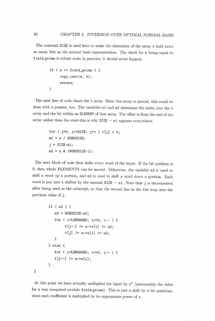
The constant SIZE is used here to make the dimension of the array t hold twice as many bits as the normal basis representation. The check for n being equal to f ie ld-pr ime is robust code; in practice, it should never happen.
i f ( n == field—prime ) { copy_cust(a, b);
return;
}
The next line of code clears the t array. Since this array is special, this could be done with a pointer, too. The variables nl and n2 determine the index into the t array and the bit within an ELEMENT of that array. The offset is from the end of the array rather than the start-this is why SIZE - nl appears everywhere.
f o r ( j=0 ; j<=SIZE; j++ ) t [ j ] = 0;
nl = n / WORDSIZE;
j = SIZE-nl;
n2 = n & (WORDSIZE-1);
The next block of code then shifts every word of the input. If the bit position is 0, then whole ELEMENTS can be moved. Otherwise, the variable n3 is used to shift a word up a portion, and n2 is used to shift a word down a portion. Each word is put into t shifted by the amount SIZE - nl. Note that j is decremented after being used as the subscript, so that the second line in the f o r loop uses the previous value of j .
i f ( n2 ) {
n3 = W0RDSIZE-n2;
f o r ( i=LONGWORD; i>=0; i — ) {
t [ j ~ ] 1= a - > e [ i ] « n2;
t [ j ] 1= a - > e [ i ] » n3;
} } e l s e {
f o r ( i=LONGWORD ; i>=0; i — ) {
t [ j — ] 1= a - > e [ i ] ;
} }
At this point we have actually multiplied the input by x"" (presumably the value for n was computed modulo f ie ld-prime) . This is just a shift by n bit positions, since each coefficient is multiplied by its appropriate power of x.

3.2, HIGH-SPEED INVERSION FOR OPTIMAL NORMAL BASIS 41
The next block of code then shifts the upper portion by the correct amount to
account for the fact that the field size does not fill a complete word. This moves
the upper portion of an ELEMENT at an offset, which holds the most significant
bits of the result back to the least significant ELEMENT position. The code works
because: x^ - 1 = (x - 1)M, where M is Mi or Mua as discussed before. Now
x^ = l + {x - 1)M. Multiply both sides by x'^ and reduce modulo M, we have the
relationship: = x^. So every reduced modulo M will simply be x^.
n3 = LONGSHIFT+1;
i = SIZE-LONGWORD;
f o r ( j=SIZE; j>=SIZE-nl; j — ) {
t [ j ] 1= t [ i — ] » n3;
t [ j ] 1= t [ i ] « (W0RDSIZE-n3);
}
The final step is to move the data from the t array to the output b array. This includes one important check: If the coefficient to is set, we can reduce this power by adding in the rest of M (since M = 0 mod M) . This is just all bits set, and the variable w is used to contain these bits for each ELEMENT.
w = t[SIZE-LONGWORD] & (IL « LONGSHIFT ) ? : 0;
f o r ( i=0; i<=LONGWORD; i++ )
b - > e [ i ] = t[i+SIZE-LONGWORD] b ->e[0] &= LONGMASK;
#undef SIZE }
Finally, the upper bits are cleared to complete the operation and clean up the output. (The term SIZE was previously defined at the beginning of the routine. Since the name is common, it is good to limit the scope.)
3.2.3 Faster inversion, the code
The fast inversion algorithm does not translate into pretty code. It uses all the
methods described previously, including the conversion from optimal normal basis
to polynomial basis and back using Mi or Mua. The almost inverse algorithm is
included, along with several speed ups mentioned in [SOOS95].
/ * This algorithm i s the Almost Inverse Algorithm of Schroeppel , et a l . given in ‘ ' F a s t Key Exchange with E l l i p t i c Curve Systems‘ ‘

42 CHAPTER 3. INVERSION OVER OPTIMAL NORMAL BASIS
* / vo id opt_inv(FIELD2N *a, FIELD2N *dest ) {
CUSTFIELD f , b , c , g ;
INDEX i , j , k, m, n, f _ t o p , c_ top ;
ELEMENT b i t s , t , mask;
/ * f , b , c , and g are not in optimal normal b a s i s format: they are held
in ‘customary f o r m a t ' , i . e . aO + a l * u " l + a2*u"2 + . . .; For the
comments in t h i s r o u t i n e , the polynomials are assumed t o be
polynomials in u. •/
The first thing is to initialize G to the prime polynomial M , as in the algorithm
3.1. This is all bits set, including 1 extra bit past the defined limit of LONGSHIFT.
/ • Set g t o polynomial ( u " p - l ) / ( u - l ) * /
f o r ( i = l ; i<=LONGWORD; i++ )
g . e [ i ] = "0 ;
g . e [ 0 ] = LONGMASK I (IL « LONGSHIFT);
The next chunk of code converts the input value a from normal basis to polynomial
basis using the predefined offset and bit masks created in init_two. For a Type II
normal basis we need 2 bits set.
/ * Convert a t o ,customary f o r m a t ) , put t ing answer in f * /
nu l l _ cus t (&f );
j = 0;
f o r ( k=NUMWORD; k>=0; k— ) {
b i t s = a->e[k];
m = k>0 ? WORDSIZE : UPRSHIFT;
f o r ( i=0 ; Km; i++ ) {
i f ( b i t s & 1 ) {
f . e [ t w o . i n x [ j ] ] |= two一bit [ j ];
# i f d e f TYPE2
f . e [two一inx [ j +NUMBITS] ] I = two一bit [ j +NUMBITS];
#endif
}

3.2, HIGH-SPEED INVERSION FOR OPTIMAL NORMAL BASIS 43
b i t s » = 1;
} }
After initializing the remaining variables of algorithm 3.1. We then eliminates powers of x (which called u here), as stated in the first step of the almost inverse algorithm. The variables c_top and f_top are used to track the unused (zeroed out) ELEMENTS in b, c and f , g, respectively. This also helps speed up the code, since it eliminates loop executions, which have null results.
/ * Set c t o 0, b t o 1, and n to 0 * / null_cust(&c);
null_cust(&b);
b.eCLONGWORD] = 1; n = 0;
/ * Now f i n d a polynomial b , such that a*b = u~n •/
/ * f and g shrink, b and c grow. The code takes advantage of t h i s .
c_top and f _ t o p are the var iables which contro l t h i s behavior * /
c_top = LONGWORD; f一 t op = 0 ;
do {
i = s h i f t _ b y [ f .eliLONGWOIlD] k Oxff];
n+=i;
/ * Sh i f t f r ight i (d iv ide by u " i ) * /
m = 0;
f o r ( j = f _ t o p ; j<=LONGWORD; j++ ) {
b i t s = f . e [ j ];
f . e [ j ] = ( b i t s » i ) I ((ELEMENT) m << (WORDSIZE-i)); m = b i t s ;
} } while ( i == 8 && (f.e[LONGWORD] & 1) == 0 ) ;
Everything is now initialized, and we're ready for the main loop.
li F = 1’ then the routine is finished. This will happen on occasion if you enter with a single bit set; the above code shifts the bit down and the main routine would not be needed. We check for that here.

44 CHAPTER 3. INVERSION OVER OPTIMAL NORMAL BASIS
f o r ( j=0 ; j<LONGWORD; j++ )
i f ( f . e [ j ] ) break;
i f ( j<LONGWORD I| f.e[LONGWORD] != 1 ) {
Assuming F is not equal to 1,we enter the "almost inverse algorithm's" main loop.
/ * There are two loops here: whenever we need t o exchange f with g and
b with c , jump t o the other loop which has the names reversed! * / do {
/ • Shorten f and g when p o s s i b l e •/
while ( f . e [ f一 t op ] == 0 kk g .e [ f一 top] == 0 ) f _ top++ ;
/ * f needs to be b igger - i f no t , exchange f with g and b with c .
(Actual ly jump t o the other l oop instead of doing the exchange)
The published algorithm requires deg f >= deg g , but we d o n ' t
need t o be so f i n e * /
i f ( f . e [ f _ t o p ] < g . e [ f _ t o p ] ) goto loop2 ; l o o p l :
/ * f = f + g , making f d i v i s i b l e by u •/
f o r ( i = f _ t o p ; i<=LONGWOIlD; i++ )
f . e C i ] -= g . e [ i ] ;
/ • b = b+c * /
f o r ( i=c_ top ; i<=LONGWOIlD; i++ )
b . e [ i ] c . e [ i ];
do {
i = shift_by[f.e[LONGWORD] & Oxff ];
/ * S h i f t c l e f t i (mult iply by u~i), lengthening i t i f needed * / m = 0;
f o r ( j=LONGWORD; j>=c_top ; j — ) {
b i t s = c . e [ j ];
c . e [ j ] = ( b i t s « i ) | m;
m = b i t s » (WORDSIZE—i);
} i f ( m ) c . e [ c _ t o p = j ] = m;
/ * S h i f t f r i gh t i ( d i v i d e by u ' i ) * /
m = 0;
f o r ( j = f _ t o p ; j<=LONGWORD; j++ ) {

3.2, HIGH-SPEED INVERSION FOR OPTIMAL NORMAL BASIS 45
b i t s = f . e [ j ];
f . e [ j ] = ( b i t s » i ) I ((ELEMENT) m « (WORDSIZE-i)); m = bits;
} } while ( i == 8 && (f.e[LONGWORD] & 1) == 0 ) ;
/ • Check i f we are done ( f = l ) * /
f o r ( j = f _ t o p ; j<LONGWORD; j++ )
i f ( f .e [ j ] ) break;
} while ( j<LONGWORD || f•e[LONGWORD] != 1 ) ;
There are two loops here that are identical; only the variable names have been
flipped to do the correct operations. The last step in the loop is to check to see if
F = 1. If it is, then the above while loop ends. Note that if we exit the loop this
way, the value of j will always be equal to LONGWORD. The use of goto's may violate
most C programming styles, but it is very useful here.
i f ( j>0 )
goto done;
do {
/ • Shorten f and g when poss ib le •/
while ( g . e [ f _ t o p ] == 0 && f . e [ f _ t o p ] == 0 ) f_top++;
/ * g needs to be bigger - i f not , exchange f with g and b with c .
(Actual ly jump to the other loop instead of doing the exchange)
The published algorithm requires deg g >= deg f , but we don ' t
need to be so f i n e •/
i f ( g . e [ f _ t o p ] < f . e [ f _ t o p ] ) goto l oop l ;
loop2:
/ • g = f+g , making g d i v i s i b l e by u * /
f o r ( i = f _ t o p ; i<=L0NGW0RD5 i++ )
g . e [ i ] � f . e [ i ] ;
/ * c = b+c * /
f o r ( i=c_top ; i<=LONGWOIlD; i++ ) c . e C i ] 八 = b . e [ i ];
do {
i = sliift_by[g.e[LONGWORD] & Oxff];
n+=i ;
/ * Sh i f t b l e f t i (multiply by u ~ i ) , lengthening i t i f needed •/ m = 0; f o r ( j=LONGWORD; j>=c_top; j — ) {

46 CHAPTER 3. INVERSION OVER OPTIMAL NORMAL BASIS
b i t s = b.eCj];
b . e [ j ] = ( b i t s « i ) I m;
m = b i t s » (WORDSIZE-i);
} i f ( m ) b . e [ c _ t o p = j ] = m;
/ * Sh i f t g r ight i (d iv ide by u~i) •/
m = 0;
f o r ( j = f _ t o p ; j<=LONGWORD; j++ ) {
b i t s = g . e [ j ];
g . e [ j ] = (b i t s>>i ) I ((ELEMENT)m << (WORDSIZE-i)); m = bits;
} } while ( i == 8 && (g.e[LONGWORD] & 1) == 0 ) ;
/ • Check i f we are done (g=l ) * /
f o r ( j = f _ t o p ; j<LONGWORD; j++ )
i f ( g . e [ j ] ) break;
} while ( j�LONGWORD || g.e[LONGWORD] != 1 ) ;
copy_cust(&c, &b);
}
The guts of the routine are straightforward executions of the almost inverse algo-
rithm. The variable c_top and f_top are both adjusted along the way to reduce
the number of execution loops as the procedure progresses. If we exit the last loop,
then we have to swap b and c so we can finish the algorithm correctly. The shifting
is done using the least significant byte of f or g as an index into the shi f t_by array.
Instead of calling a subroutine, we has made the code inline for this shift.
The final stage is to multiply b by the appropriate power of x and then convert that value back to normal basis so we'll get the right answer.
done:
/ • Now b i s a polynomial such that a*b = u~n, so mult iply b by u~(-n) •/
cus_times_u_to_n(&b, field一prime - n •/• field一prime, &b);
/ * Convert b back to optimal normal bas is form ( in to dest ) * /
i f ( b.e[LONGWORD] & 1 ) one(dest);

3.2, HIGH-SPEED INVERSION FOR OPTIMAL NORMAL BASIS 47
e l se
nul l (dest );
j = 0; f o r ( k=NUMWORD; k>=0; k_- ) {
b i t s = 0; t = 1;
mask = k > 0 ? "0 : UPRMASK; do {
i f ( b . e [ t w o _ i n x [ j ] ] & two 一 b i t [ j ] ) b i t s "= t ;
t « = 1;
} while ( t&mask );
dest ->e[k] b i t s ;
}
} / • opt一inv * /
This version of the inverse algorithm requires about as much time to compute as
a normal basis multiply. This routine is at least ten times faster than the
straightforward method found in section 1 of this chapter. So, although it looks
messy, it is much quicker to execute. As usual, it takes up more code space to reduce
run time, but inversion is called by every elliptic sum or doubling, see chapter 4. It
is extremely useful to use this if one has ROM to spare.

48 CHAPTER 3. INVERSION OVER OPTIMAL NORMAL BASIS

Chapter 4
Elliptic Curve Cryptography over
Elliptic curve cryptography (ECC) was proposed independently by Victor Miller
and Neil Koblitz in the mid-eighties. 160bit ECC are considered to be of the same
security level as 1024bit RSA. Elliptic curve Cryptography offers many advantages
over RSA. For the same level of security, especially over 160bit, ECC is faster,
requires less computing power, permits reduction in key and certificate size which
saves memory and bandwidth.
ECC has received increased commercial acceptance as evidenced by its inclusion in
standards by accredited standards organizations such as IEEE (Institute of Electri-
cal and Electronics Engineers), ISO (International Standards Organization), NIST
(National Institute of Standards and Technology), and ANSI (American National
Standards Institute), see [ECC standard]. It is being promoted as the best method
for implementing digital signatures for banking smartcard applications.
4.1 Mathematics of elliptic curves
There are several kinds of defining equations for elliptic curves, but the most com-
mon are the Weierstrass equations. For the binary finite fields GF{2^), the Weier-
strass equation is
y^ + xy ^x^ + ax^ + b (4.1)
where a and b are elements of GF{2^) with b # 0.
There is another kind of Weierstrass equation over GF(2"^), giving what are called
super singular curves. However, these curves are cryptographically weak, see section
4 9

50 CHAPTER 4. ELLIPTIC CURVE CRYPTOGRAPHY OVER GF{2^)
3 below; thus they are omitted.
Given a Weierstrass equation, the elliptic curve E consists of the solutions {x, y)
over GF{2饥、to the defining equation, along with an additional element called the
point at infinity (denoted The points other than are called finite points. The
number of points on E (including t^) is called the order of E and is denoted by
There is an addition operation on the points of an elliptic curve which possesses the algebraic properties of ordinary addition (e.g. commutativity and associativity). This operation can be described geometrically as follows.
Define the inverse of the point P = (x, y) to be (x, x + y). Then the sum P + Q of the points P and Q is the point R with the property that P, Q, and -R lie on a common line. The point at infinity d plays a role analogous to that of the number 0 in ordinary addition. Thus P + ^ P, p + ( _ p ) = ^ for all points P. Under this addition operation, it can be shown that E forms a group.
When implementing the formulae for elliptic curve addition, it is necessary to distinguish between doubling (adding a point to itself) and adding two distinct points that are not inverses of each other, because the formulae are different in the two cases. Besides this, there are also the special cases involving By full addition is meant choosing and implementing the appropriate formula for the given pair of points. Algorithms for full addition are given here:

4.1. MATHEMATICS OF ELLIPTIC CURVES 51
Full Addition
Input: a field GF{2'^)- coefficients a, b for an elliptic curve
E -{-xy = + +b over points Po = {xo,yo) and Pi = {xi,yi) on E.
Output: the point P2 := Pq + Pi.
1. If 尸0 = then output P2 <— Pi and stop 2. If Pi = 1?, then output 尸2 Po and stop 3. If xo / xi then
3.1 set A — (yo + yi)/(a:o + ;ri) 3.2 set X2 — a + 入2 + 入 + + 工1
3.3 go to step 7 4. If yo + yi then output P2 —必 and stop
5. If a:! = 0 then output P2 —必 and stop 6. Set
6.1 A <— a:! +2/1/a;!
6.2 0:2 — a + A2 + A 7. y2 卜(a;! + a:2)A + X2 + 2/1
8- P2 一(32 ’y2) The above algorithm requires 2 general multiplications, a squaring, and a multi-
plicative inversion. To subtract the point P = (a:,y), one adds the point -P =
Elliptic curve points can be added but not multiplied. It is, however, possible to perform scalar multiplication, which is another name for repeated addition of the same point. If /c is a positive integer and P a point on an elliptic curve, the scalar multiple kP is the result of adding k copies of P. Thus, for example, ^P = P + P + P + P + P. The notion of scalar multiplication can be extended to zero and the negative integers via OF = 'd, {-k)P = k{-P).
Scalar multiplication can be performed efficiently by the addition-subtraction method outlined below.

52 CHAPTER 4. ELLIPTIC CURVE CRYPTOGRAPHY OVER GF{2^)
Elliptic Curve Scalar Multiplication
Input: an integer k and an elliptic curve point P.
Output: the elliptic curve point kP.
1. If A; = 0 then output and stop. 2. lik <0 the set Q — ( - P ) and K — {-k), else set Q ^ P and ^ /c. 3. Let hihi-i . . . hiho be the binary representation of 3K, where the most
significant bit hi is 1.
4. Let KiKi-i... KiKo be the binary representation of K.
5. Set S ^Q.
6. For i from I — 1 downto 1 do Set S <- 25. If /li = 1 and Ki —0 then compute 5 <— 5 + Q. If /li = 0 and Ki = I then compute S S — Q .
7. Output S.
There are several modifications that improve the performance of this algorithm.
These methods are summarized in [Gor98]. Elliptic Curve Multiplication is the
computation that dominates the operations of Elliptic Curve Cryptography.
4.2 Elliptic Curve Cryptography
Let us explain some more terms of Elliptic Curves first.
If u is the order of an elliptic curve over GF{2^), then the Hasse bound is + 1 — < u < + 1 + Thus the order of an elliptic curve over G i ^ ( 2 1 ’
#£;(Gi^(2"^))’ is approximately 2爪.
The order of a point P on an elliptic curve is the smallest positive integer n
such that nP = d. The order always exists and divides the order of the curve
If k and I are integers, then kP = IP if and only if k三I mod n.
Suppose that the point P on E has large prime order n where r? does not divide the order of the curve P is called a base point of the curve. Then a key pair can the defined as follows. (However, one needs to know what are good and secure curves, see section 4 below.)

4.2. ELLIPTIC CURVE CRYPTOGRAPHY 53
EC key pair generation
Input: elliptic curve E with base point P of order n.
Output: private key d and the corresponding public key Q
1. select a statistically unique and unpredictable integer d
in the interval [ 1 . . .n — 1]
2. compute the point Q = dP on the curve E.
3. the private key is d, the public key is Q.
Of course, public key is public, the curve is also public, and a user must kept his own secret key secret.
It is necessary to compute an elliptic curve discrete logarithm, see section 3 below, in order to derive a private key from its corresponding public key. For this reason, public-key cryptography based on key pairs of this type relies for its security on the difficulty of the elliptic curve discrete logarithm problem, ECDLP. 160 bits Elliptic Curve Cryptography are being viewed as equivalent to 1024bits RSA in terms of security. It is still extremely difficult to break them in the year 2000 even if one hundred thousands of computers can be used together, see section 3 below.
Now we briefly outline how elliptic curves can be useful in cryptography. See the standards [ECC standard] for more details, nevertheless these are simple protocols.
For encrypting or decrypting a file, it is important to note that these are essentially carried out by traditional secret key algorithm, such as DEA. The key for use with the traditional secret key algorithm is generated randomly in a particular session, and is called a session key. The role of ECC is to encrypt or decrypt this session key only. For 160bit ECC, we should choose a 80bit session key for a comparable security level, see [ECC standard].
The advantage of public key cryptography here is that no key management is
necessary. When Alice wants to send a message to Bob, he only needs to find out
the public key of Bob, which is of course publicly available. Alice can then encrypt
messages using this public key, none can decrypt them except Bob, as only Bob
processes the private key of Bob. The reader can then imagine what would the
situation be if traditional secret key algorithm was used when each of his Bob's
(girl) friends wanted to communicate to Bob.
Digital Signature are the electronic equivalent of traditional handwritten signa-
tures. Digital Signature is hard to forge. One of its main function is authentication,
another is data integrity.
How can Bob proves that a message is written by Bob himself?

54 CHAPTER 4. ELLIPTIC CURVE CRYPTOGRAPHY OVER GF{2^)
Answer: Bob applies his private key, Privatebob, to the message using a digital
signature algorithm to generate a digital signature, see below. He then sends the
message along with the digital signature to Alice. Alice checks, or verifies, the
signature by applying Bob's public key, Publicbob, to the signature using a digital
signature verification algorithm. Since only Bob is in possession of Privatebob, Alice
knows: if in case the signature verification passes, the message was from Bob and
that the data has not been changed.
How can Bob proves that he is Bob, to Alice?
Answer: By the process of random challenge. Alice randomly chooses a message
and ask Bob to sign it. Alice can then verify the signature. Since none except Bob,
as only Bob processes Privatebob, can produce a valid signature, Alice knows that
he is Bob if the verification passes.

4.2. ELLIPTIC CURVE CRYPTOGRAPHY 55
ECDSA signature generation Input: message M, private key d,
elliptic curve E with base point P of order n. Output: signature for M.
1. select a statistically unique and unpredictable integer k
in the interval [1. . . n — 1]
2. compute kP = {xi,yi)
3. compute r = xi mod n
4. compute e =Hash(M)
5. compute s = + dr) mod n
6. the signature for M is (r, s)
ECDSA signature verification
Input: message M, signature for message (r, 5 ) , public key Q,
elliptic curve E with base point P of order n.
Output: accept or reject the signature.
1. compute e =Hash(M)
2. compute s—1 mod n
3. compute ui = e - mod n
4. compute U2=r • mod n
5. compute u i P + U2Q = (x i ,y i )
6. compute v = xi mod n
7. accept the signature ii v = r
Hash is a one-to-one function that maps a message M to a integer of length 160bit,
it is also called a message digest function and runs very fast, see [ECC standard].
Since hash functions or modulus computations are relatively cheap, it is clear
that Elliptic Curve Scalar Multiplication is the computation that dominates elliptic
� curve cryptography.
Signature ~1 single EC point multiplication,
Signature verification ~1.5 times of a single EC point multiplication,
Encryption ~2 EC point multiplications
Decryption "slightly > a single EC point multiplication,
The reason for the number 1.5 rather than 2 in signature verification is due to the
time taken to do a simultaneous elliptic curve multiplications.

56 CHAPTER 4. ELLIPTIC CURVE CRYPTOGRAPHY OVER GF{2^)
4.3 Elliptic curve discrete log problem
Let E be an elliptic curve defined over a finite field Let P € E{GF{2"'))
be a point of order n, where n is a prime number and n > 2)60.
The elliptic curve discrete logarithm problem (ECDLP) is the following: given the curve E, P and Q G E{GF{2'^)), determine the integer l,0<l <n-l, such that Q 二 IP, provided that such an integer exists.
The best general algorithms known to date for ECDLP are the Pollard-p method
and the Pollard-入 method, [Pol78]. The Pollard-p method takes about y^7rn/2 steps,
where each step is an elliptic curve addition. The Pollard-/? can be parallelized (see
[OW99]) so that if m processors are used, then the expected number of steps by each
processor before a single discrete logarithm is obtained is y/Trn/2/m. The PoUard-A
method takes about 3.2S^/n steps. It can also be parallelized (see [OW99]) so that if
m processors are used, then the expected number of steps by each processor before
a single discrete logarithm is obtained is about 2y/n/m.
Some special classes of elliptic curves, including supersingular curves, see section 1,
have been prohibited in the ECC standards, see [ECC standard], by the requirement
of the MOV condition [MOV93]. These curves have been prohibited because there
is a method for efficiently reducing the discrete logarithm problem in these curves
to the discrete logarithm problem in a finite field, which is much easier.
Also, the special class of elliptic curves called GF(2"")-anomalous curves have been
prohibited by the requirement of the Anomalous condition (see section 4 below) be-
cause there is an efficient algorithm for computing discrete logarithms in E{GF{2'^))
where E is an anomalous curve over (i.e. = 2"^).
Assume that a 1 MIPS (Million Instructions Per Second) machine can perform 4 X 10⁴ elliptic curve additions per second. (This estimate is indeed high, an ASIC (Application Specific Integrated Circuit) built for performing elliptic curve oper-ations over the field has a 40 MHz clock-rate and can perform roughly 40,000 elliptic additions per second.) Then, the number of elliptic curve additions that can be performed by a 1 MIPS machine in one year is (4 x 10^) • (60 x 60 x 24 X 365) « 1.261 x 10^2
The following table shows the computing power required to compute a single
discrete logarithm for various values of n with the PoUard-p method.

4.3. ELLIPTIC CURVE DISCRETE LOG PROBLEM 57
Field size Size of n MIPS years
(in bits) (in bits)
163 160 280 8.5 x lO^
191 186 293 7.0 X 10¹⁵ 239 234 2117 1.2 x lO^^
359 354 2177 1.3 x
431 426 2213 9.2 x ICP
Note: The strength of any cryptographic algorithm relies on the best methods that are known to solve the hard mathematical problem that the cryptographic algorithm is based upon, The discovery and analysis of the best methods for any hard mathematical problem is a continuing research topic. The state of the art in solving the ECDLP is subject to change as time goes by.
To put the numbers in the above table into some perspective, the following ta-ble, [Odl95], shows the computing power required to factor integers with the 1995 versions of the general number field sieve.
Size of integer to be factored (in bits) MIPS years
512 3 X 10⁴
768 2 X 10⁸
1024 3 X IQii
1280 1 X 10¹⁴
1546 3 X IOI6
2048 3 X 10²O
Odlyzko, [Odl95] has estimated that if 0.1% of the world's computing power were available for one year to work on a collaborative effort to break some challenge cipher, then the computing power available would be 10^ MIPS years in 2004 and IQio to lOii MIPS years in 2014.
As an example, if 10,000 computers each rated at 1,000 MIPS are
available, and n « then an elliptic curve discrete logarithm can be
computed in 85,000 years. Take a look of
http://cristal.inria.fr/~harley/ecdl7/readMe.html http://cristal.inria.fr/bin/ecdldb?m=AP
http://cristal.inria.fr/bin/ecdldb?m=P;i=501
to see how this can be possible in the future.
A Pentium 11-400 is a many-splendored Thing but it is at most a 800 MIPS machine. The fact that the chip has 400 Million cycles per second and that at most 2 instructions can be started per second means I have a machine capable of 800

58 CHAPTER 4. ELLIPTIC CURVE CRYPTOGRAPHY OVER GF{2^)
MIPS by definition of the numbers. (The Pentium has two pipelines for processing instructions, so 2 instructions can start in each cycle.) But MIPS is a bad number because it only tells how many instructions begin in a second, and has nothing to do with how long it takes fully execute the instructions.
On the other hand, how weak is 32bits ECC?
On January 2000, I wrote a program in MAPLE implementing the Pollard-p
method. It broke the 32 bits ECDLP over GF(p), where p is a prime, in 2.5
minutes and for 40bits in 1.5 hours on a Pentium 11-400. Since 32 bits is the
usual wordsize of a processor, it might be the case that many students
in many parts of the world are still going on to implementing 32bits
Elliptic Curve Cryptography. Yet no explicit evidence as to how weak
32bits E C C are, probably because it is too small, that the usual research
journals simply chose to forget it! But this was why I wrote this program. So
although this M A P L E program was rather simple, at least on a second
thought, there is still of value in trying to publish it.
4.4 Finding good and secure curves
4.4.1 Avoiding weak curves
To guard against existing attacks on ECDLP, one should select an elliptic curve E
over such that:
1. The order is divisible by a large prime n > 2i60;
2. The MOV condition holds; and
3. The Anomalous condition holds.
� The MOV Condition
The reduction attack of Menezes, Okamoto and Vanstone, [MOV93] reduces the
discrete logarithm problem in an elliptic curve over G_F(2爪)to the discrete loga-
rithm in the finite field for some B>1. The attack is only practical if B
is small; this is not the case for most elliptic curves. The MOV condition ensures
that an elliptic curve is not vulnerable to these reduction attacks. Most elliptic
curves over a field will indeed satisfy the MOV condition.
Before performing the algorithm, it is necessary to select an MOV threshold. This is a positive integer B such that taking discrete logarithms over is at least
as difficult as taking elliptic discrete logarithms over G_F(2爪).A value of B > 20 is
4.4. FINDING GOOD AND SECURE CURVES 59
required. Selecting B > 20 also limits the selection of curves to non-supersingulax curves, section 1. Suppose E is an elliptic curve defined over and n is a
prime divisor of
The MOV Condition
Input: An MOV threshold B, q = 2爪,and a prime n.
Output: The message true if the MOV condition is satisfied for an elliptic curve over GF{2'^) with a base point of order n; the message false otherwise.
1. Set i = 1
2. For i from 1 to 5 do
2.1 Set t = t • q mod n
2.2 lft = l, then output "false" and stop 3. Output "true"
The Anomalous Condition
Smart [Sma99] and Satoh and Araki [SA98] showed that the elliptic curve discrete
logarithm problem in anomalous curves can be efficiently solved. An elliptic curve
E defined over GF{2"') is said to be GF(2"')-anomalous if # E ( a F ( 2 " " ) ) = 2爪.
The Anomalous condition checks that #五 ( 6 ^ ( 2 爪 ) ) / this ensures that an
elliptic curve is not vulnerable to the Anomalous attack. Most elliptic curves over
a field will indeed satisfy the Anomalous condition.
4.4.2 Finding curves of appropriate order
In order to perform EC-based cryptography it is necessary to be able to find an elliptic curve. The task is as follows: given a field size 2饥 and lower and upper bounds Tmin and Vmax for base point order, find an elliptic curve E over and a prime n in the interval r饥�„ < n < r^ax, which is the order of a point on E. Since factor large numbers are difficult in general, a trial division bound Uax is chosen and the search is restricted to nearly prime curve orders.
There are four approaches to selecting such a curve:
1. Select curve coefficients with particular desired properties, compute the curve
order by using formulae, and repeat the process until an appropriate order is found.
2- If m is divisible by a small integer d, then select a curve defined over 勺
and compute its order over GF{2^) by using formulae. Repeat if possible until an appropriate order is found.
3. Select a curve at random, compute its order directly, and repeat the process

60 CHAPTER 4. ELLIPTIC CURVE CRYPTOGRAPHY OVER GF{2^)
until an appropriate order is found.
4. Search for an appropriate order, and construct a curve of that order.
These material are highly technical and the mathematics involved is far from being trivial, especially if one demands a program that can produce reliable results in a reasonable amount of time. See [SSB99] and the standards [ECC standard] for more details.
For the first and second approach, attention must be paid to a new kind of attack, [GHS2000], since m might be composite here. The fourth approach is implemented using the complex multiplication (or CM) method. The third approach: Selecting a curve at random, is considered to be the best. Since, to guard against possible future attacks against special classes of non-supersingular curves, it is prudent to select an elliptic curve at random.
We briefly outline how "Selecting a curve at random" can be accomplished. The main difficulty is point-counting, which is omitted. To explain them need another thesis. Despite this, even an outline can be quite cumbersome.
We explain the input parameters first:
1. Tmin shall be selected so that Tmin > The security level of the resulting elliptic curve discrete logarithm problem can be increased by selecting a larger Tmin (e.g. T f j i i f i � 2 ).
2. The order u of an elliptic curve E over satisfies + 1 - <
w < + 1 + and u is even. Hence for a given Vmin should be <
3. Imax is typically a small integer (e.g. 1麵工=255) .

4.4. FINDING GOOD AND SECURE CURVES 61
Selecting an appropriate curve and point at random
Input: A field size q = 2爪,lower bound rmin, and trial division bound Imax-
Output: Field elements a,6 e G_F(2爪)which define an elliptic curve over GT(2爪),
a point P of prime order n > rmin, n > the curve,
and the cofactor h =
1. Generate an elliptic curve verifiably at random, see note 1 below
2. Compute the order u of the curve defined by a and b, see note 2 below
3. Verify that 6 0,
the curve equation is E : y^ + xy = x^ ax^ + b over GF{2'^)
4. Test u for near primality,
if the result is not nearly prime, then go to step 1. Otherwise, u = h • n,
where h is /^ax-smooth, and n > Vmin, n > is probably prime,
see note 3 below
5. Check the MOV condition, with inputs B >20, q = and n,
if the result is false, then go to step 1
6. Check the Anomalous condition,
if the result is false, then go to step 1
7. Find a point P on E of order n, see note 4 below
8. Output the curve E, the point P , the order n, and the cofactor h
Note:
1. select parameters {SEED, a, b) arbitrarily, see [ECC standard], to understand
what "verifiably at random" means.
2. the order #E(J3F{2饥Y) can be computed by using Schoof's algorithm, [Sch87]
and its modifications. Although the basic algorithm is quite inefficient, several dra-
matic improvements and extensions of this method have been discovered in recent
years. In 1998, it was feasible to compute orders of elliptic curves over G_F(2饥)
where m was as large as 1300. Cryptographically suitable elliptic curves over fields
as large as could be randomly generated in about 5 hours on a worksta-
tion, [Ler97]. In 2000,M. Fouquet, P. Gaudry and R. Harley could count the points
on a curve of cryptographic size in seconds. Their program could also be combined
with an early-abort strategy to examine lots of random curves until a secure one is
found. E.g., generating a secure 163-bit curve took about 20 seconds on an Alpha
750 server, [FGH2000].
3. Given a trial division bound Imax, a positive integer h is said to be Z爪aa:-smooth
if every prime divisor of h is at most Imax- Given a positive integer Vmin, the positive
integer u is said to be nearly prime if w = /i • n for some probable prime value of n
such that n > Tmin and some Imax-smooth integer h.

62 CHAPTER 4. ELLIPTIC CURVE CRYPTOGRAPHY OVER GF{2^)
4. If the order u = of an elliptic curve E is nearly prime, the following algorithm efficiently produces a random point on E whose order is the large prime factor n of u = hn.
1. Generate a random point R (not 'd) on E
2. Set P = hR
3. If P = i9, then go to step 1, otherwise output P.
Chapter 5
The performance of 17x bit Elliptic Curve Scalar Multiplication
5.1 Choosing finite fields
There are specific values of m for which an optimal normal basis exists in G_F(2爪).
Prom chapter 1’ section 4; chapter 2, section 4 and 5’ we have the following:
m for which a Type I ONB exists in
100, 106’
130’ 138’ 148’
162,172,178, 180,
196’ 210’
226,
268,
292,316,
346, 348,
372,378,
388,
418, 420, 442
460, 466
6 3
64CHAPTER 5. THE PERFORMANCE OF 17X BIT ELLIPTIC CURVE SCALAR MULTIPLICATION
m for which a Type II ONB exists in GF{2'^)
105’ 113’ 119’
131’ 134’ 135’ 146,155’ 158,
173, 174, 179, 183,186, 189,191,
194, 209,221’
230, 231,233, 239, 243, 245,251,254, 261, 270, 273,278, 281,
293,299,303, 306,309,
323’ 326, 329, 330,338, 350,
354,359, 371, 375,
386,393, 398, 410, 411, 413,414,
419,426’ 429, 431,438, 441, 443,
453, 470, 473
Those m < 100 have all been deleted since the Certicom ECDL challenge has been solved up to ECC2K-108 on 4th April 2000.
See http://www.certicom.com/research/ecc_challenge.html
for the number of machines, time and computing power that was involved.
How about leObit ECC? Would the news of ECC2K-108 influence our belief t o wards the security of 160bit ECC?
Answer: V ^ / V ^ = 2 6 « 67,000’ 000. See section 3 of this chapter.
Those m < 160 are included here for reference only. Notice that I have classified the table into rows. The rationale for this arrangement is after taking into account of the size of a 32bit processor, so that we have a category of 161 to 192 bits, the next row would then be 193 to 224 bits.
It should be pointed out that a new kind of attack was discovered recently, [GHS2000] and they recommended to choose m that was prime so that this at-tack would not work. However, this will eliminate many many interesting field sizes, such as all field sizes with Type I ONB exists. Whether their attack will work practically to some or all curves on these field sizes is not clear. For this reason, in the above two tables, I have marked those field sizes with m prime with a bold-faced type.
Now for our work on testing the "The performance of Elliptic Curve Scalar Mul-tiplication" :
For type II ONB, we choose GF(2爪)with m = 173,179.
For type I ONB, we choose m = 178. Note that 178 = 2-89 which is nearly prime.

5.2. 17X BIT TEST VECTORS FOR ONB 65
5.2 17x bit test vectors for onb
According to the information in the section "Finding good and secure curves," we found secure curves according to the standard, [ECC standard].
Numbers are presented in hexadecimal form. Each hexadecimal digit expands in the natural way to four bits, except possibly the most significant digit, which expands to the approximate number of bits. Once expanded, the bits are from high orders to low orders, left to right.
Example 8 m=173 bits
use Type II ONB in
The curve is y^ ^ xy = x^ + ax^ + b over
a = IFFF FFFFFFFF FFFFFFFF FFFFFFFF FFFFFFFF FFFFFFFF
b = 020 65676EBA 2BD7E13A EE225240 52D30C43 B66CFC30
Base point P
^ = 1F51 4AC1C477 27B9B985 57195120 7A62EE52 66A287DC y = 1EF2 A6F631E0 7D953066 289BC9AA F04EF67F 82137C2E Order of P (size is 173 bits) n = 1000 00000000 00000000 005A7FC9 654DD68B 04AFBC97 h = 2
Example 9 m=173 bits
use Type II O N B in
The curve is y^ xy = x^ + ax^ + b over
0
b = C69 7988DD3E 2FE085BD 2C1472AB 067B8F0C F119704E
Base point P
^ = 171F E4505005 1C356898 A5D9508B 81C0B3C7 CF9F7A2E y = C5F 0165A54D 14B2590D FC6C4EB6 4B3347AB F50CFCF4 Order of P (size is 171 bits) n = 7FF FFFFFFFF FFFFFFFF FFE2DC3A 3FBDB80E 5A93E6B3 h = 4

66CHAPTER 5. THE PERFORMANCE OF 17X BIT ELLIPTIC CURVE SCALAR MULTIPLICATION
Example 10 m=178 bits
use Type I ONB in
The curve is y^ + xy = x^ + ax^ + b over
a = 1
6 = 2C7E5 439E4C8B 270D7F84 475F527A D5B2AB28 5804C450
Base point P
^ = ICAAC 5F88C818 29548641 B2908BB2 EE5AAE1A CE99E7AB y = D2CD A4044CA1 0EB0E98D 7C4E2934 1FF24D75 49861AD5 Order of P (size is 178 bits)
20000 00000000 00000000 01A9C35E A2EBCADC A3E11E47 h = 2
Example 11 m=178 hits
use Type I ONB in
The curve is y^ + xy = x^ + ax^ + b over
a = 0
b = 21BE6 CB54480A E8FF68F3 CFBD12B5 C1DDEF59 77635C79
Base point P
^ = 104CB 99623987 82FDE024 19DD68ED 63E5463E 2425A7E6 y = F175 A82716AE 6B52049E 317B951A 8C90C9D0 C3A3E564 Order of P (size is 177 bits)
n = 10000 00000000 00000000 00AD9B22 331C2A11 F16A0F29 h = 4
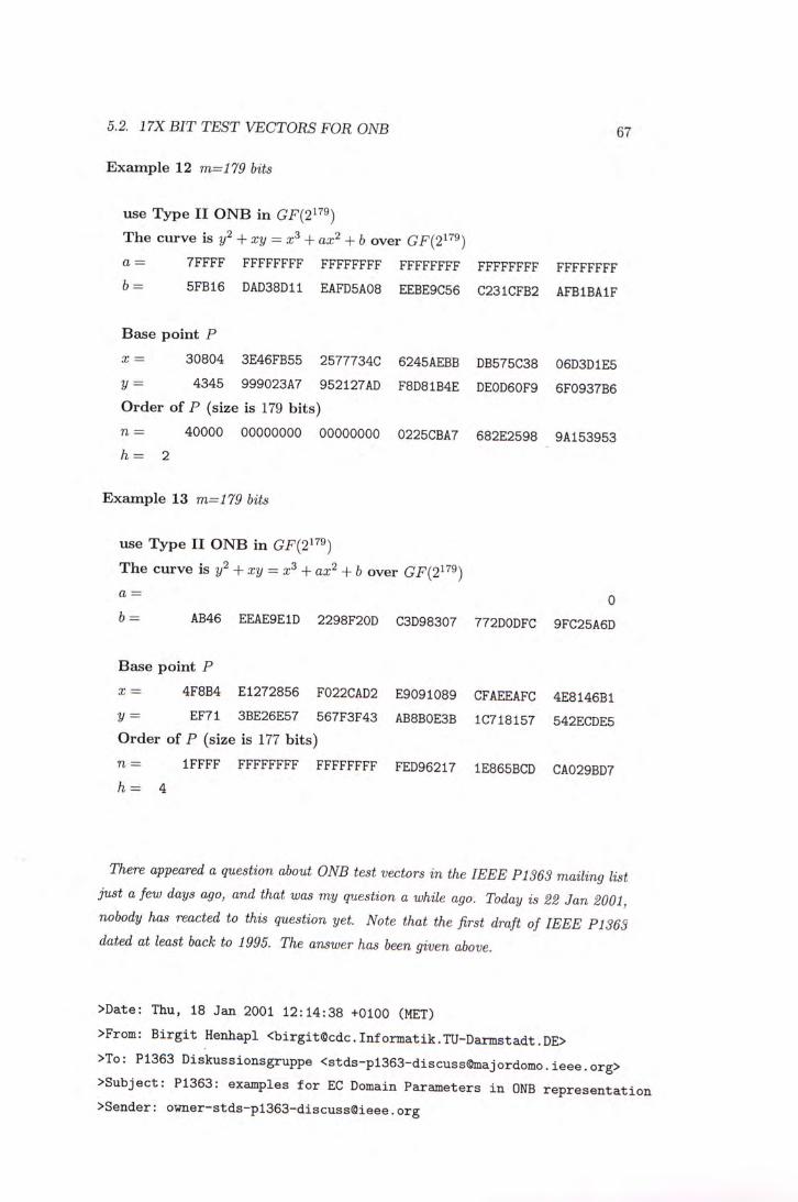
5.2. 17X BIT TEST VECTORS FOR ONB 67
Example 12 m=179 bits
use Type II ONB in
The curve is y^ + xy = x^ + ax^ + b over
a = 7FFFF FFFFFFFF FFFFFFFF FFFFFFFF FFFFFFFF FFFFFFFF
b = 5FB16 DAD38D11 EAFD5A08 EEBE9C56 C231CFB2 AFBIBAIF
Base point P
^ = 30804 3E46FB55 2577734C 6245AEBB DB575C38 06D3D1E5 y = 4345 999023A7 952127AD F8D81B4E DE0D60F9 6F0937B6 Order of P (size is 179 bits) n = 40000 00000000 00000000 0225CBA7 682E2598 9A153953 h= 2
Example 13 m=179 bits
use Type II ONB in
The curve is y^ + xy = x^ i- ax^ + b over
0
b = AB46 EEAE9E1D 2298F20D C3D98307 772D0DFC 9FC25A6D
Base point P
a: = 4F8B4 E1272856 F022CAD2 E9091089 CFAEEAFC 4E8146B1 y = EF71 3BE26E57 567F3F43 AB8B0E3B 1C718157 542ECDE5 Order of P (size is 177 bits) n = IFFFF FFFFFFFF FFFFFFFF FED96217 1E865BCD CA029BD7 h = 4
There appeared a question about ONB test vectors in the IEEE PI363 mailing list
a /e犯 days ago, and that was my question a while ago. Today is 22 Jan 2001,
nobody has reacted to this question yet. Note that the first draft of IEEE PI363
dated at least back to 1995. The answer has been given above.
>Date: Thu, 18 Jan 2001 12:14:38 +0100 (MET)
>From: B i r g i t Henhapl <birgit®cdc.Informatik.TU-Darmstadt.DE>
>To: P1363 Diskussionsgruppe <[email protected]> >Subject: P1363: examples f o r EC Domain Parameters in ONB representat ion
>Sender: owner-stds-pl363-discussQieee .org
68CHAPTER 5. THE PERFORMANCE OF 17X BIT ELLIPTIC CURVE SCALAR MULTIPLICATION
>X-Resent-To: Multiple Recipients <stds-pl363-discuss0majordomo.ieee.org> >X-Info: [Un] Subscribe requests to [email protected]
>X-Moderator-Address: stds-pl363-discuss-approval(3maj ordomo. i eee . org
>This i s a s tds -p l363-d iscuss broadcast. See the IEEE P1363 web page
> ( h t t p : / / g r o u p e r . i e e e . o r g / g r o u p s / 1 3 6 3 / ) f o r more information. For l i s t
> in fo , see http : / /grouper . ieee .org /groups /1363/WorkingGroup/mai l l i s t .html
> >Hi,
>I,m implementing ECDSA over GF(2~n) in ONB-representation. I need to f i n d
>some t e s tvec to r s in order to v e r i f y my implementations.
>P1363 unfortunatly does not include any t e s t v e c t o r s .
>The only examples I found are those of X9.62-1998, but I 'm not able to
>extract the y -coordinate based on the given (compressed) basepoint . My
> f i n i t e - f i e l d - a r i t h i n e t i c seems to be correc t ( I got some t e s t v e c t o r s ) .
>Can e i ther anybody give me the y -coordinates of the X9.6* examples (J4 .3 ,
>exc. 4 + 5, p. 109/110) or any other examples WITH y -coord inate or at
>least confirm that the given x -coordinates of the base po ints are not
>correc t . >
>Many thanks,
> B i rg i t Henhapl
>Birgit Henhapl b irg i tQcdc . informatik . tu-darmstadt .de
>Technische Universitaet Darmstadt phone: +49 6151 16 5541 >FB Informatik fax : +49 6151 16 6036
>Inst i tut fl ier Theoretische Inf ormatik
>Lehrstuhl Pro f . J. Buchmann
>Alexanderstr. 10 >64283 Darmstadt >Gemany]
5.3 Testing methodology and sample runs
For each bit length,
• Two SECURE, according to the IEEE P1363 November 1999 documents, curves were generated.

5.3. TESTING METHODOLOGY AND SAMPLE RUNS 69
• Verify the sample curve parameters matched with each other. See note 1 below.
• 1000 times of ( m ) • P, P is the base point, where rn is a random number satisfies 0 < = rn < order of P, were performed.
• Several runs on each of the two curves were then followed. See note 2 below.
Note:
• 1. Check that the order of P was correctly specified in the data of a sample curve.
Now P = {x, y), and let pnt.order be the order of P as specified in the data of a sample curve. It suffices to check that [pnt-order — 1) . P = (re, a; + y).
Reason: If {pnt.order - 1) • P = (x, a: + y) then {pnt.order - i ) . p ^ _ p by the
inverse formula. Therefore (pnt.order) • P = {pnt.arder-I) • P + P =-P + P =
Since pnt-order is a prime number, so from simple group theory, the actual order
of P is either 1 or pnt.order. Obviously P is not i9, therefore the actual order of P is indeed pnt.order.
• 2. But no significant variance was observed.
Here is a sample run of the "Elliptic Curve Scalar Multiplication" C program for
the 178 bit curve of example 3 in the last section on a Pentium II-400Mhz PC.
po int P
X : Icaac 5f88c818 29548641 b2908bb2 eeSaaela ce99e7ab
y : d2cd a4044cal 0eb0e98d 7c4e2934 I f f24d75 4986lad5
X XOR y
: 1 1 8 6 1 fb8c84b9 27e46fcc cedea286 f la8e36 f 871f fd7e
(pnt_order - 1 ) P
X : Icaac 5f88c818 29548641 b2908bb2 eeSaaela ce99e7ab
y : 11861 fb8c84b9 27e46fcc cedea286 f la8e36 f 871f fd7e
User time: 0.0500000000 seconds
Real t ime: 0.0000000000 seconds

70CHAPTER 5. THE PERFORMANCE OF 17X BIT ELLIPTIC CURVE SCALAR MULTIPLICATION
random seed i s 1046851076 I am running . . • (random)P . . . f o r 1000 times
User time: 59.6650000000 seconds
Real t ime: 60.0000000000 seconds
FYI, the l a s t rn i s
: c l c 6 a f8c5ca l 105348ab 78a8d9f0 ea4e4672 5f35caab
FYI, the l a s t (rn)P i s
X : 398e9 daf7da6b 448a3b6b be f ce5c5 50125580 414fbe52
y : 19361 4ba20af5 bebdbl24 ad61b0b5 72bc0ad9 c7244fa9
random seed i s 975226737 I am running •.• (random)P . . . f o r 1000 times
User time: 59.7760000000 seconds
Real t ime: 59.0000000000 seconds
FYI, the l a s t rn i s
: 1 6 8 e f 95ca9911 029ble le b8209691 5d224c8d 2f814c26
FYI, the l a s t (rn)P i s
X : 36424 05a78ce8 a291512c 6602839c 19a6232b 50192993
y : 729d afe77al9 75bdaf94 24009e23 13756bc6 7036f514
random seed i s 2632629705 I am running . . . (random)P . . . f o r 1000 times
User t ime: 59.8160000000 seconds
Real t ime: 60.0000000000 seconds
FYI, the l a s t rn i s
: 1 5 e c 6 c889e808 c f e c l 8 4 1 9334e3de 60e6665a 01b4ebb7
FYI, the l a s t (rn)P i s
X : a336 6 9 2 c f 5 f f 9aa fd2 f l 31d390d6 a589e724 a3d09639

5-3. TESTING METHODOLOGY AND SAMPLE RUNS 71
y : 14641 b82b0083 dbf2f57d 260ee831 43199f65 885c030e
random seed i s 1527782800 I am running .•. (random)P . . . f o r 1000 times
User time: 59.6660000000 seconds
Real time: 60.0000000000 seconds
FYI, the l a s t rn i s
: a c 8 8 3 f 7 9 b l f d 68588745 d9b50ea8 56c9f7b8 6a548ad9
FYI, the l a s t (rn)P i s
X : f379 56ea7a2e 7b5b00ad 3379c485 346caaaf 759bb29f
y : 23908 c6158fa3 02229a57 a46f271f 2celded7 dbb8c38b
random seed i s < s t u f f d e l e t e d �
I am running . . . (random)P . . . f o r 1000 times
User time: 59.8460000000 seconds
Real t ime: 60.0000000000 seconds
FYI, the l a s t rn i s
: < f o r ECDL problem >
FYI, the l a s t (rn)P i s
X : 35b7a lc281adf 93562c4c f0506c lb ec8dfb28 d0031c81
y : 342fc 94043645 1283a0d2 e8a35d41 2a3a4207 03aeld98
s t u f f de le ted
Notice that (random) . P took 0.060 seconds per iteration.

72CHAPTER 5. THE PERFORMANCE OF 17X BIT ELLIPTIC CURVE SCALAR MULTIPLICATION
5.4 Proposing an elliptic curve discrete log prob
lem for an 178bit curve
Once we have the "Elliptic Curve Scalar Multiplication" C program working, it is
very easy to propose an elliptic curve discrete log problem- simply look at the last
few lines of the previous section. This 178 bit curve is considered secure according
to the standard of IEEE P1363 November 1999 documents. But why do we need
to propose an elliptic curve discrete log problem? Because there was a new kind
of attack discovered by Nigel Smart, et al. in January 2000. The following is an
excerpt, see [GHS2000] for details of the attack.
>From [email protected] Sat Jan 15 08:34:24 2000
>Date: Fri, 14 Jan 2000 15:38:18 +0000
> From: Nigel Smart <[email protected]>
>To: [email protected], [email protected] .hp.com
>Subject: P1363: ECC Stuff
> > I think it would be a good idea for the P1363 document to recommend
>that in ECC systems in char 2 that the finite field used should be
>chosen to be of the PRIME degree over F _2.
> > It is has been suspected by the experts for some time that curves
>over fields of composite degree over F _2 could be weaker. Indeed G .
>Frey gave a talk in Waterloo in 1998 which mentioned this idea, as
> have a number of other people in other meetings over the last couple
>of years.
> > Just before Xmass at a meeting in Cirencester (UK) on "Coding and
> Cryptography" , Steven Galbraith presented a joint paper with me
>describing further details of the possible problems with such
> curves. (The proceedings are available as an LNCS volume).
> > At this conference we also announced that Florian Hess (Uni.
>Sydney), Pierrick Gaudry (\'{E}cole Poly technique) and myself have
>discovered the following fact.. ..
> Let q=2
At and fix an integer n>=4.
Consider an elliptic curve over F _{ qAn}. Then for "most"
such curves one can solve the dlog problem on E(F _{ qAn}) in

5.4. PROPOSING AN ELLIPTIC CURVE DISCRETE LOG PROBLEM FOR AN 178BIT CURVE 73
time 0 ( q A {2+epsilon}) this should be compared to Pollard
rho which would give a time of O(qA {n/2}).
> It should be pointed out that "random" curves defined over
> i) A prime field F_p
>or
> ii) A field of prime degree over F_2, F_{2 Ap}
> >ARE NOT AFFECTED IN ANY WAY by this new result. Neither are
>Koblitz type curves defined over fields of any degree over F_2.
> > Making P1363 recommend only prime fields or those of prime degree
>over F _2 would bring P1363 into line with the recently recommended
> NIST curves and the way the ANSI standards are progressing. Hence
>such a move would make sense not only from the security perspective
> but also from the standards and interoperability perspective.
> >Nigel
> >Nigel P. Smart I mail: [email protected]
The important points have been high-lighted by me. Notice that it was a very
serious and strong attack, provided it worked! However, there have been no
further discussions on this attack and its improvements in the IEEE P1363 mailing
list since then. Notice that 178 = 2 . 89 which is not prime, nearly prime though,
and may as well be subject to this attack. It would be valuable to know the answer
because the program under consideration on Scalar Multiplication over a field with
Type I ONB exists is always faster than that of over a field with Type II ONB exists,
for similar bit lengths, see section 5 below. The reason is due to the differences in
their polynomial basis representation for the implementation of the Fast Inverse,
chapter 3, section 3.2.1.
Now we propose the following elliptic curve discrete log problem:

74CHAPTER 5. THE PERFORMANCE OF 17X BIT ELLIPTIC CURVE SCALAR MULTIPLICATION
ECDLP on a 178bit curve (178 = 2 * 89)
Find the integer l, 0:::; l :::; n - 1, such that Q = lP, where n , Q, P
and the curve are defined as follows:
use Type I ONB in GF(2178 )
The curve is y2 + xy = x3 + ax2 + b over GF(2178 )
a = 1
b= 2C7E5 439E4C8B 270D7F84 475F527A D5B2AB28 5804C450
Base point P
x = 1CAAC 5F88C818 29548641 B2908BB2 EE5AAE1A CE99E7AB
y = D2CD A4044CA1 OEBOE98D 7C4E2934 1FF24D75 49861AD5
Order of P (size is 178 bits)
n = 20000 00000000 00000000 01A9C35E A2EBCADC A3E11E47
h= 2
Point Q x= 35b7a lc281adf 93562c4c f0506clb ec8dfb28 d0031c81
y = 342fc 94043645 1283aOd2 e8a35d41 2a3a4207 03ae1d98
Let us know the answer so that we will then stop to use GF(2178 ).
5.5 Results and further explorations
Platform
Pentium II-400MHz, compiled with Microsoft VC++ Version 6.0, with
standard /02 compiler optimization. No assembly was being used.
The performance of Elliptic Curve Scalar Multiplication over GF(2m)
bit length onb Elliptic Curve Scalar Multiplication r . P
173 type II 0.082 seconds per iteration
178 type I 0.060 seconds per iteration
179 type II 0.088 seconds per iteration
This result was also posted on http://itec.erg.cuhk.edu.hk/wb/r/wb.html
It is the scalar multiplication that dominates the computations of elliptic curve
cryptography, chapter 4, section 2. Since an usual elliptic curve cryptographic
operation only requires 1 or 2 elliptic curve multiplications, ECC based on this
scalar multiplication program is thus fully functional on a Pentium II-400Mhz Pc.
Yet only the addition-subtraction method was used for scalar multiplication, one

5.5. RESULTS AND FURTHER EXPLORATIONS 75
obvious way to improve the performance is to use better methods of Multiplication, [Gor98]. Other techniques that might as well benefit normal basis arithmetic such as point-halving and Probenius expansions, [SSB99] might also be valuable.
However, our next target is to make Elliptic Curve Cryptography runs smoothly on embedded devices, such as a smart card, PDA or mobile phone. That is perhaps a long journey.

76CHAPTER 5. THE PERFORMANCE OF 17X BIT ELLIPTIC CURVE SCALAR MULTIPLICATION

Chapter 6
On matrix RSA
In this chapter, we present our findings of a particular extension of the RSA pubUc-
key cryptosystem from using integers modulo n to a version using matrices whose
entries are integers modulo n, where n is the product of two large primes. In
contrast to the methods found in the existing literature, our schemes do not require
matrices of a special form, such as triangular matrices, and essentially work on
all plaintext message matrices, whether non-singular or not. The derivation of the
theorems on matrix powers depends on the consideration of eigenvalues of matrices
over GF{p) and GF(n) , rather than on counting the number of matrices that form
a group under matrix multiplication. Several numbers are encrypted and decrypted
in a single run. By using the Cayley-Hamilton theorem, our method reduces the
computation of a matrix exponentiation with a large exponent to the computation
of an exponentiation of x modulo the characteristic polynomial of a matrix, which
can be accomplished by the square and multiply method or any other methods of
fast exponentiations. Thus computational saving can be achieved.
6.1 Introduction
In the RSA public-key cryptosystem, integers modulo n, where n is the product of
two large primes p and q�are used. The public key consists of the integer n and
the encryption exponent e. The private key consists of the decryption exponent
丄 It is required that d . e 三 1 mod (p — - 1). Note that a slightly different
version requires that d • e 三 1 mod l.c.m.[(p — 1),(g - 1)]. Let integer x, 0 < x < n
denote the plaintext. The encryption process computes the cyphertext y = mod
n, 0 S y < n. Given a cyphertext y, the decryption process computes x = p^ mod n.
77
78 CHAPTER 6. ON MATRIX RSA
Note that the encryption process or the decryption process computes the expo-nentiation of integers modulo the integer n.
In the matrix extension of RSA, we compute the exponentiations of matrices, rather than integers, in the encryption or the decryption process. The central idea is to use matrices whose entries are integers modulo n. The plaintext shall take on the form of a k-hy-k matrix X, and the cyphertext shall also take on the form of a k-hy-k matrix Y. The entries of either matrix are integers modulo n where n is the product of two large primes p and q. Given a plaintext matrix X ’ the encryption process computes the cyphertext 三 Ji:巨 mod n. Given a cyphertext y, the decryption process computes the plaintext X 三 mod n.
The motivation of using matrix extensions of RSA public-key cryptography is that it has the potential of speeding up the RSA encryption and decryption computa-tions, particularly when multiple rounds of integer encryption and decryption are present. One may use the square and multiply technique for matrices exponentia-tion mod n [V085], but because of the Cayley-Hamilton Theorem, exponentiation of matrices with a large exponent can be reduced to the computation of a matrix poly-nomial of moderate degree, [CD90]. By using the Cayley-Hamilton theorem, our method reduces the computation of a matrix exponentiation with a large exponent to the computation of an exponentiation of x modulo the characteristic polynomial of a matrix, which can be accomplished by the square and multiply method or any other methods of fast exponentiations, section 6.
Attention must be paid to ensure that the encryption and the decryption process
returns the original plaintext under all conditions of relevance. For example, the
relationship between the encryption exponent e and the decryption exponent d
become modified. Additional constraints on usable plaintext X also arise.
Our proposed 2 by 2 matrix RSA scheme 1 is our first step towards an extension of
RSA scheme to matrices. Three numbers can be encrypted and decrypted in each
single run. However, it requires the sender to check whether a plaintext message
matrix is non-singular or not: if it is singular, he cannot encrypt that particular
message. This is not very appropriate for cryptographic application although the
proportion of singular matrices over Z„ , where for instance n = p • ^ and p, ^ are
large distinct primes, is very much close to zero. It is not good to restrict arbitrary
plaintext matrices to be non-singular. This problem was also mentioned in [V085]
and [CD90]. In order to solve this problem, they used upper triangular matrices.
In our proposed 2 by 2 matrix RSA scheme 2 and 3,we can stiU use matrices
without a special form over Z^. The condition for the sender to check is just one or
two gcd computations of n with an integer depending on the entries on the plaintext

6.1. INTRODUCTION 79
matrix. What are required are only those gcd's would not equal to one. This will
always be the case for otherwise n would get factored, as we know that factoring
large numbers is hard. Hence it is not a demanding assumption.
In section 3,some theorems of matrix powers over GF{p) and GF(n) , are ex-
plained. These theorems look similar to Fermat's little theorem. But unlike the
usual approach by counting the number of matrices that form a group, [V085]’ the
derivation of these theorems depends on the consideration of eigenvalues of matrices.
Given a square matrix A, the characteristic polynomial of A is det(Ai - A), where
det denotes the determinant of A. For example, \i A = \ ^ ^ \ , then the char-\ c d 厂
acteristic polynomial of A is det (A/ — A), which is A^ - (a + d)A + {ad — be).
The Cayley-Hamilton Theorem: Every matrix satisfies its only characteristic poly-
nomial. For example: “ ^ j , then A^-{a + d)A + {ad-hc)I = 0 ’ where
/ here denotes 2 by 2 identity matrix, and O denotes 2 by 2 zero matrix.
Throughout this chapter, we let p, q be large primes, ajidn=pxq.
80 CHAPTER 6. ON MATRIX RSA
6.2 2 by 2 matrix RSA scheme 1
Key preparation:
1. Choose two large strong primes p and q. Compute n = p x q.
2. Choose a random large integer e such that 0 < e < 2(p - l ) (g - 1) and is relatively prime to 2 ( p - - 1).
3. Calculate d such that e-d=l mod 2{p - - 1).
Note: e stands for encrypt, d stands for decrypt.
Public key is (n,e). Secret key is d.
P and q should be discarded or kept secret.
Encryption:
1. Suppose a, b, c are non-negative integers less than n, with
+ 6c 0 mod n.
_ ( a h \ Let X = I ^ ^ j be the plaintext message matrix.
2. X is encrypted to r 三 X互 mod n, where modulo n is taken element-wisely.
Decryption:
Y^ mod n. ‘
Note that three integers are encrypted and decrypted in a single run. For matrix
exponentiations mod n, we may use the standard square and multiply method.
However, notice that = (a^ + 6c) / . So y 三 X 芒 三 ( a � + b c ) ^ X mod n.
Moreover, 三(X),= {{a^+ mod n. But X一议=+ mod
n, so Y^ = ((a2 + he)^ f{a? + hc)^X mod n. Now {{o?+ hc)^f{o?+ 三
(a2 + be疗三一 1 mod n If a^ + be mod n. This last fact comes from the definitions of e, d and the theory of basic RSA scheme.
In this way, encryption and decryption of a matrix take just a single exponentiation of numbers modulo n.
6.3 Theorems on matrix powers
We let p, q be large primes, a n d n ^ p x g . I denotes 2 by 2 identity matrix.

6.3. THEOREMS ON MATRIX POWERS 81
Lemma 14 Let A be a 2 by 2 matrix whose entries are elements of GF{p). Let
fix) e GF{p)[x]. Then
( / ( A 2 ) - / ( A I ) . A 2 / ( A I ) - A I / ( A 2 ) R -R . , . A2-A1 A 十 A,-Ai ] y T
m = <
� / ' ( A i M + ( / (Ai ) - A i f ( A i ) ) / if Ai =入 2
where Ai and X2 are eigenvalues of A in GF{p'^) and f'{x) is the formal derivative
affix).
Proof: Suppose Ai ^ A2, there exists Q{x) e GF{p)[x], e,h e GF{p) such that f � = ( x - 入 - 入 2 ) Q ( a : ) + ex + h. Thus / (A i ) = eAi + h, /(A2) = eAs + h, and e = h = W • 胸 , ^ h e result then follows from the Cayley-
Hamilton theorem.
For the case Ai = X2, there exists Q(x) e GF{p)[x], e,h e GF{p) such that / � = M)^Q(x) + e x + h. So f'{x) = 2(x - Xi)Q(x) + (x -入丄尸^‘⑷ + e. Thus / (A i ) = eAi + h, / ' ( A i ) = e. Therefore h = / (A i ) - Ai / ' (Ai ) , and the result follows from the Cayley-Hamilton theorem. •
Theorem 15 Let A be a 2 by 2 matrix whose entries are elements of GF{p). Sup-pose A has no zero eigenvalue,
(1) Then 三 / modp if A has distinct eigenvalues in GF{p^), and Ap(p-i)三 /
mod p if A has repeated eigenvalues in GF{p^).
(2) 1)三 / modp.
Proof: Let f{x) = x^ in the above lemma.
Suppose Ai + A2, where Ai,入2 € G F { p � . = ^ ^ + ^ ' ^ Z ^ f ^ 1. Since Ai,
A2 € Ai 0, A2 — 0’ then A^p'—i) = =1 in G F ( p ' ) . We have
� 二 + - / • Thus 三 I mod p.
Suppose Ai = A2, in this case Ai actually equals to ^ ’ which is in GF{p). Using the above lemma, we have A'' = /c. + (入卜 Ai = +
Thus 乂P(P-i)三 0 . A f - i J + (Ar^)P(l — 0 ) / 三 / mod p.
This proves (1). (2) follows easily from (1). •
Theorem 16 Let A be a 2 by 2 matrix whose entries are non-negative integers.
^ P-eigenvalue of A means an eigenvalue of A mod p, where modulo p is taken
element-wisely, in GF{p^). Let p, q be two large primes, n = p • q.
� // the p-eigenvalues of A are non-zero and the q-eigenvalues of A are non-zero,
then 三 J mod n.
(V // the p-eigenvalues of A are non-zero and distinct, and the q-eigenvalues of A

82 CHAPTER 6. ON MATRIX RSA
are non-zero and distinct, then i )三 j 誦歧化
Proof: Let Ap 三 4 mod p. Since Ap has no zero eigenvalue, from the above theorem, ] ? ( ”二 i )三 I mod p. Thus " (p ' - i )三趟(”‘一”三 j mod p. Similarly
jWf—1)三 1)三 一_i)三 /modp’andAP(p2_i)9(92 — i )三
J mod q. Hence 三 / mod pq. This proves (1). The proof of (2) is similar. •
Remark 1 Suppose 01,02,03,04 are non-negative integers, and A = ( ^^ ^^ \ . V 0,4 J
Let p, q be two large primes, n = p • q.
If gcd{n, aia4 - (22*23} = 1 then the p-eigenvalues and q-eigenvalues of A are non-zero.
Proof: The characteristic equation of A mod p is obtained from A - (a i+a4)A + (aia4 - 0203)三 0 by taking each coefficients mod p. If A has zero /^eigenvalue’ then aia4 - a2az 三 0 mod p. So gcd{n, 0104 - 0203} g 1•口
Remark 2 Suppose ai,a2,a3,a4 are integers, and A = ( \ . Let p, q be V 04 J
two large odd primes, n = p • q.
^f9cd{n, (ai — a4)2 + 4a2a3} = 1 then the p-eigenvalues (and q-eigenvalues as well) of A are distinct.
Proof: The characteristic equation of A mod p is obtained from 入2 - (ai + 04) A +
(aia4 - 0203)三 0 by taking each coefficients mod p. Suppose A has repeated p-
eigenvalues, A - (ai + a4)A + {a^a^ - asag)三(A _ Ai)(A — Ai) mod p. So Ai + Ai
三 ai + a4, . 三 aiCH - a2a3 mod p. Thus (ai + “4)2 - 4(0104 — 0303)三 0 or
(ai - a4)2 + 40203 = 0 mod p. Thus gcd{n, (ai — a^f + 40203} ^ 1. •
6.4. 2 BY 2 MATRIX RSA SCHEME 2 83
6.4 2 by 2 matrix RSA scheme 2
Key preparation:
1. Choose two large strong primes p and q. Compute n = p x q.
2. Choose a random large integer e such that 0 < e < — 1)^(^2 _ i ) 肌 」
is relatively prime to — —丄).
3. Calculate d such that e . d 三 1 mod - l)q{q'^ - 1).
Note: e stands for encrypt, d stands for decrypt.
Public key is (n,e). Secret key is d.
P and q should be discarded or kept secret.
Encryption:
1. Suppose ai,a2,a3,04 are non-negative integers less than n,
with gcd{n, aia4 - 02as} = 1.
/ ai a2 \ Let X = be the plaintext message matrix.
\ < 3 «4 / 2. X is encrypted to F = mod n, where modulo n is taken element-wisely.
Decryption:
Y^ mod n.
Prom theorem 16, part (1) in the last section, it is easily seen that Y^ =
=X I = X mod n if gcd{n, aia4 — 0203} = 1. Thus this method works.
Notice that in the encryption step, the assumption on the gcd is not demanding.
The probability of plaintexts not satisfying the assumption is securely small. The
cost of the adversary exploiting this deficiency is high. There are also additional
techniques to shore up this shortcoming. Reserve a few bits in the plaintext group
{ai’a2’a3,a4} for redundant random bits. For example, let the last few bits of 04
be bits randomly generated by the encoder which do not carry any useful infor-
mation. The encoder checks if the plaintexts { a ! ’ � 2 ’ a] ’ a j satisfy the encryption
assumption. If the assumption is not met, the encoder re-generate the redundant
bits anew using random methods. The process is iterated until the encryption con-
ditions are met. This way, the encryption-decryption process are guaranteed to
recover the original plaintexts. The random and redundant bits are then discarded
after decryption. Another alternative is to use our matrix RSA encryption without
checking whether the assumption is satisfied. The errors that are caused in the rare

84 CHAPTER 6. ON MATRIX RSA
event when the assumption fails can be controlled by some higher-level error-control protocols. Or, this scheme can be used in non-critical application when some rare errors can be tolerated, such as in the transmission of audio or video signals.
6.5 2 by 2 matrix RSA scheme 3
Key preparation:
1. Choose two large strong primes p and q. Compute n=pxq.
2. Choose a random large integer e such that 0 < e < (p^ - - 1) and is relatively prime to (p^ - - 1).
3. Calculate d such that e • d= 1 mod {p^ — — 1).
Note: e stands for encrypt, d stands for decrypt.
Public key is (n,e). Secret key is d.
p and q should be discarded or kept secret.
Encryption:
1. Suppose ai ’ (22, a3’04 are non-negative integers less than n, with
9cd{n, aia4 - 0203} = 1 and gcd{n, (ai - a^f + 40203} = 1.
I ai \ , Let A = be the plaintext message matrix.
\ 0,4 J 2. X is encrypted to 三 mod n, where modulo n is taken element-wisely.
Note: the assumptions on the gcd's are not demanding, for otherwise n
could be factored, as we know factoring large integers is hard.
Decryption: Y^ mod n. ‘ ‘
Recall theorem 16 part (2), 三 / mod n if JC has non-zero distinct p-
eigenvalues and non-zero distinct q-eigenvalues. The remarks following the theorem tell us that gcd{n, aia4 - a s a s } = 1 ensures that the ^^eigenvalues and ^-eigenvalues of X are non-zero; gcd{n, (ai — a4)2 + 4�2仃3} = 1 ensures that the ^^eigenvalues (and ^-eigenvalues as well) of X are distinct. Hence = 三;i: • / 三;j: mod n.

6.6. AN EXAMPLE AND CONCLUSION 85
6.6 An example and conclusion
We give an example of the 2 by 2 matrix RSA scheme 3 of which n is of 309 decimal
digits or 1026 bits.
Key preparation:
1. Choose two large strong primes p and q. Compute n = p x q.
P =
5896965768945957659506848854848456584565846475464756523090596596 5759675495657595758959659655689586570457399239597056573484643584 56348684568232904355043
q =
6993473047856239092735783473460784738934658993465248946347456458 9465473465894576458884940690326373646740564390234237692264589340 623456789347854789346458038027 n =
4124027116925439711126060931808648993334089023057628654438782005
8490963316778489586544982873192444063098900835306669287267394571
9731718556494282326143641378318068862636587831418262182791117543
5090643859085237746617164309199463151765154957393221400334174850
09909257489839125067993249361919927504159141603220161
2. Choose a random large integer e such that 0 < e < {p^ — — 1)
and is relatively prime to {p^ - - 1).
e =
5478965967947956697584956247457459475905983467348484685484648546 45636458462373647464579579

86 CHAPTER 6. ON MATRIX RSA
3. Calculate d such that e • 3 三 1 mod {p^ - - 1). d =
9923240211909365778848877528951513579922604194672572727019940456
8570790644969068642922856211895221823541150145226513378196320128
3973253102175776758252065837326375454719634284015552559687447152
1419955052608189812387599741311101262220303205164690763165145997
6134826814726292911624908280764774329459542546838255418437615505
0827240132064784647435316534458968175815024683545843608689025382
3045517035957219202519910398519269670128273506121035205851522651
2580395121854814468020236757564466643666393093837073145085485797
3427320724523756765789123475013954336481784447403658305767772709
77068980148177871561262555536450906903795
Encryption:
1- Suppose ai,<22’ 03,a4 are non-negative integers less than n, with 9cd{n, aia4 — 0203} = 1 and gcd{n, {ai 一 04)^ + 40203} = 1.
f ai a2 \ Let X — be the plaintext message matrix. \ 0,3
f 11454 12565 \ Now we l e t X =
\ 21566 22383 J
2. X is encrypted ioY = mod n, where modulo n is taken element-wisely.
The c h a r a c t e r i s t i c polynomial of X i s x^-33837-x-14601908,
by taking each c o e f f i c i e n t s modulo n.
The remainder when x^ is divided by x2-33837 x-14601908, i s :
1950829288770222018713629364393431717125995418211561487348386417
7998443221197765240714027731325654830308510663222278016130569737
1207648203670098683402302473623738437900475281628660334889206598
0718977792084010607705294682580058868663904246382026578750567602
83600912527505492708551092326071870815155941496043064 • x +
2513987506549215393273510133287053898679067857850315308532004913
5062914548305648648416756665365023519291716222337612263216339872
3897373644751479230764877481927864943224713226853503062854373911
5404713054275266136342984918286601678709456239313681950605182315
31831808880491331160236681720786664014304539197822364
Computation i s carr ied out by the square and mult iply method, and by taking modulo n.

6.6. AN EXAMPLE AND CONCLUSION 87
Using the Cayley-Hamilton theorem,
- [hi \>2 \ Y = X mod n = , where b i , b2, ba, b4 i s given by:
\ bs b4 y bi =
3333741578639862858186121356393695975736261126843541647629126702
5192319841652135886173184312753516003128127078775810608018317902
9848759396040155874488422640930834890235718377384472521551897494
9467915060714655620992051947589527091459135142572567949047167362
08326818980025196517023141665827763276229228628245122
b2 =
3076857509951461914572845864668558303641365796782995202793878893
8644082735356636734925228724157875829668819160387698450482805685
8496297869270092678269869737990221570230431545384955555269343699
0259502992025357671220197046030173821640944002249179814880795495
54748645992595603860594119202927635216626349843682337
bs =
2383821862197562381183307128720030538175064939665132225286244604
8109713893632908893351764332950182761453542088314296457174922048
0880165551174197262769445946922684005817455305996255568439432682
5817057555262512530692006377825950449413257106533692525823276900
52943914334540934013720363120785529725630809215855863
b4 =
2726844043872998857706427361493636908499937553058893429641316597
1897936567237289212220805565899350223523846899572033726585037794
5251040231109040615626230970352202873370982864597787495613107880
8547453276187437221418159303828408093417514128786407386316523744
51838609619278406746811972179278705612751750234659208
Decryption:
Y^ mod n.
By taking each c o e f f i c i e n t s modulo n, the c h a r a c t e r i s t i c polynomial of Y i s x^+g-x+h, where g =
2187468611338017706359573145729965102431979366212822231607120711
9891670224667554074695975867732021899545827692265494239931433446
4363637485839368162172629145353099961666474420854264348417229711
2165919381268382650824117366980991118653660643427467465304658593
59653086380374646872151384878733386119337304343535992
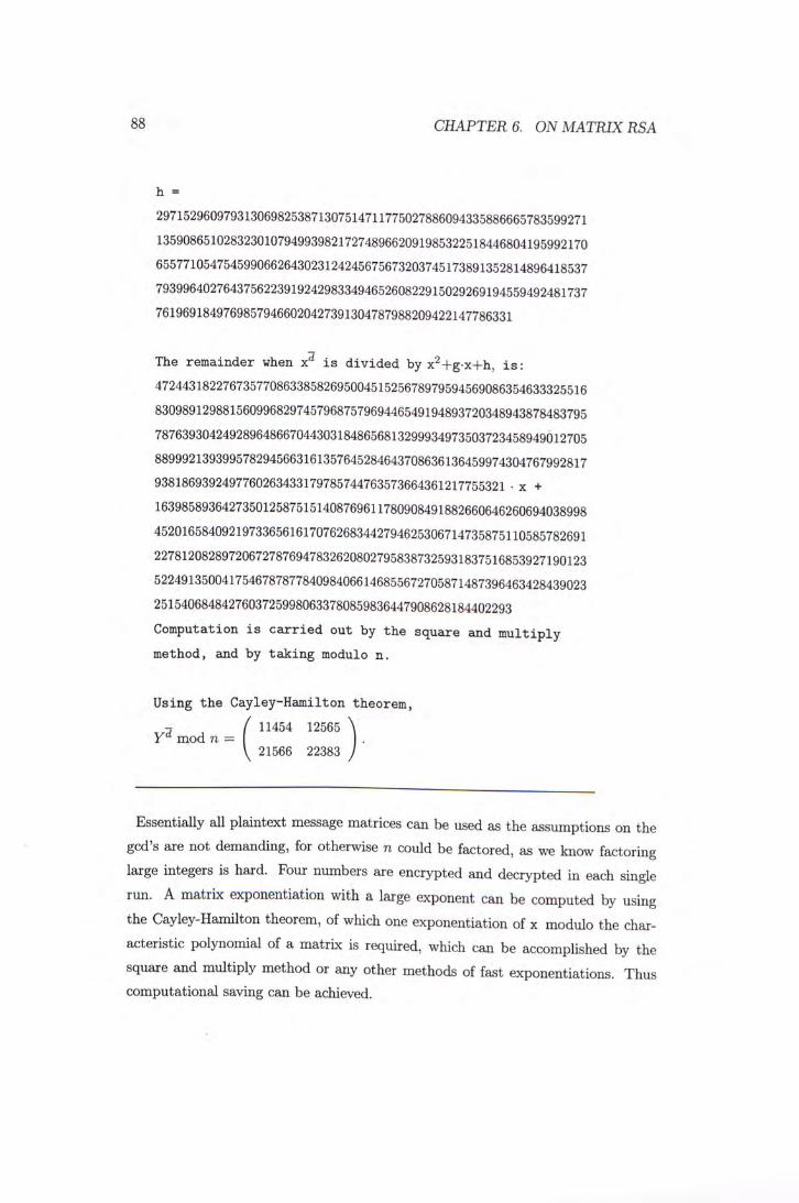
88 CHAPTER 6. ON MATRIX RSA
h =
2971529609793130698253871307514711775027886094335886665783599271 1359086510283230107949939821727489662091985322518446804195992170 6557710547545990662643023124245675673203745173891352814896418537 7939964027643756223919242983349465260822915029269194559492481737 76196918497698579466020427391304787988209422147786331
The remainder when x^ is divided by x^+g-x+h, is:
4724431822767357708633858269500451525678979594569086354633325516 8309891298815609968297457968757969446549194893720348943878483795 7876393042492896486670443031848656813299934973503723458949012705 8899921393995782945663161357645284643708636136459974304767992817 9381869392497760263433179785744763573664361217755321 . x + 1639858936427350125875151408769611780908491882660646260694038998 4520165840921973365616170762683442794625306714735875110585782691 2278120828972067278769478326208027958387325931837516853927190123 5224913500417546787877840984066146855672705871487396463428439023 25154068484276037259980633780859836447908628184402293 Computation is carried out by the square and multiply
method, and by taking modulo n.
Using the Cayley-Hamilton theorem,
] (11454 12565 \ mod n 二 .
\ 21566 22383 /
Essentially all plaintext message matrices can be used as the assumptions on the gcd's are not demanding, for otherwise n could be factored, as we know factoring large integers is hard. Four numbers are encrypted and decrypted in each single run. A matrix exponentiation with a large exponent can be computed by using the Cayley-Hamilton theorem, of which one exponentiation of x modulo the char-acteristic polynomial of a matrix is required, which can be accomplished by the square and multiply method or any other methods of fast exponentiations. Thus computational saving can be achieved.

Bibliography
[ABV89] D. W. Ash, I. F. Blake, and S. A. Vanstone, "Low Complexity
Normal Bases," in Discrete Applied Math, vol. 25 (Amsterdam: Elsevier Science Publishers/North-Holland, 1989), 191-210.
[AM0V91] G. Agnew, R. Mullin, I. Onyszchuk and S. Vanstone, "An imple-mentation for a fast public-key cryptosystem", Journal of Cryptol-
ogy, 3 (1991), 63-69.
[Ber68] E. Berlekamp, Algebraic Coding Theory, McGraw-Hill, 1968.
[CD90] C.C. Chuang and J.G. Dunham, "Matrix extensions of the RSA
algorithm", in advances in cryptology: Crypto '90 (Santa Barbara, CA,1990), 140—155’ Lecture Notes in Computer Science, Springer, Berlin, 1991. ‘
[ECC standard] Elliptic Curve Cryptography Standard a) ANSI X9.62, Public Key Cryptography for the Financial Ser-
Industry: The Elliptic Curve Digital Signature Algorithm (ECDSA), 1999.
b) ANSI X9.63, Public Key Cryptography for the Financial Ser-
Industry: Elliptic Curve Key Agreement and Key Transport Protocols, working draft, August 1999.
c) IEEE P1363, Standard Specications for Public-Key Cryptogra-phy, 2000.
d) ISO/IEC 14888-3, Information Technology - Security Tech-
几 — - D i g i t a l Signatures with Appendix — Part 3: Certicate
Based-Mechanisms, 1998.
e) ISO/IEC 15946, Information Technology - Security Techniques
• _ Cryptographic Techniques Based on Elliptic Curves, Committee Draft (CD), 1999.
f ) National Institute of Standards and Technology, Digital Signa-
t观 Standard, FIPS Publication 186-2,February 2000.
8 9

90 BIBLIOGRAPHY
[FGH2000] M. Fouquet, P. Gaudry and R. Harley, "On Satoh's algorithm and its implementation", Ecole Polytechnique Research Report
Lix/RR/00/06, June 29, 2000.
[GL92] S. H. Gao and H. W. Lenstra, "Optimal normal bases," Designs,
Codes and Cryptography 2 (1992), 315-323.
[Gor98] D. M. Gordon, "A survey of fast exponentiation methods" ’ Journal
of Algorithms 27 (1998),129- 146.
[GHS2000] P. Gaudry, F. Hess, and N. P. Smart. "Constructive and Destruc-tive Facets of Weil Descent on Elliptic Curves," to appear in Jour-nal of Cryptology.
[Ler97] R. Lercier, "Finding good random elliptic curves for cryptosystems
defined over In Advances in Cryptology: EuroCrypt 97,
pages 379-392, 1997.
[Men93] A.J. Menezes, Elliptic Curve Public Key Cryptosystems (Boston:
Kluwer Academic Publishers, 1993).
[MOV93] A. Menezes, T. Okamoto and S. Vanstone, "Reducing elliptic curve
logarithms to logarithms in a finite field", IEEE Transactions on
Information Theory 39 (1993), 1639-1646.
[MOVW89] R. C. Mullin, I.M. Onyszchuk, S.A. Vanstone, and R. M. Wilson, "Optimal Normal Bases in G F ( p - ) , " in Discrete Applied Math,
vol.22 (Amsterdam: Elsevier Science Publishers/North-Holland, 1988), 149-161. ‘
[Odl95] A. Odlyzko, "The Future of Integer Factorization", Cryptobytes,
volume 1,number 2’ summer 1995, 5-12.
[OM86] J. Omura and J. Massey, "Computational method and apparatus
for finite field arithmetic", U.S. patent number 4,587,627, May 1986.
[OW99] P. van Oorschot and M. Wiener, "Parallel collision search with
cryptanalytic applications", Journal of Cryptology, (1999) 12:1-28.
[Pol78] J- Pollard, "Monte Carlo methods for index computation mod p" ’ Mathematics of Computation, 32 (1978), 918-924.
[Ros98] M. Rosing, Implementing Elliptic Curve Cryptography, Manning
Publications Company, 1998.

BIBLIOGRAPHY 91
[Sch87] R. Schoof. "Elliptic curves over finite fields and the computation
of square roots mod p". Mathematics of Computation, 44, pages 483-494, 1987.
[SA98] T. Satoh and K. Araki, "Fermat quotients and the polynomial time
discrete log algorithm for anomalous elliptic curves", Commentarii
Mathematici Universitatis Sancti Pauli 47 (1998), 81-92. Errata: ibid. 48(1999), 211-213.
[Sma99] N.P. Smart, "The Discrete Logarithm Problem on Elliptic Curves
of Trace One", Journal of Cryptology, 1999,12:193-196.
[SOOS95] R. Schroeppel, H. Orman, S. O'Malley, and O. Spatscheck "Fast Key Exchange with Elliptic Curve Systems", Crypto '95 (New York: Springer-Verlag, 1995), 43-56.
[SSB99] G. Seroussi, N. Smart and I.F. Blake, Elliptic Curves in Cryptog-
— y,L o n d o n Mathematical Society Lecture Note Series, Cam-bridge University Press, 1999.
[V085] V. Varadharajan and R. Odoni, "Extension of RSA cryptosystems
to matrix rings", Cryptologia 9 (1985), no. 2’ 140-153.
The End

#
%
« •

hDhT(L9EQD
I MMMMim i saLJBjqin 州门3