Five-brane superpotentials in heterotic M-theory
58
arXiv:hep-th/0102046v3 25 Aug 2001 UPR 926T hep-th/0102046 February 2001 Five-Brane Superpotentials in Heterotic M -theory Eduardo Lima 1,2 , Burt Ovrut 1,3 and Jaemo Park 1 1 David Rittenhouse Laboratory Department of Physics and Astronomy University of Pennsylvania, Philadelphia, Pennsylvania 19104 2 Departamento de Fisica Universidade Federal do Cear´ a, Fortaleza, Brazil 3 Institut Henri Poincar´ e Universit´ e Pierre et Marie Curie 75231 Paris, CEDEX 05 ABSTRACT The open supermembrane contribution to the non-perturbative superpotential of bulk space five-branes in heterotic M -theory is presented. We explicitly compute the super- potential for the modulus associated with the separation of a bulk five-brane from an end-of-the-world three-brane. The gauge and κ-invariant boundary strings of such open supermembranes are given and the role of the holomorphic vector bundle on the orbifold fixed plane boundary is discussed in detail. Research supported in part by DOE grant DE-AC02-76ER03071
-
Upload
independent -
Category
Documents
-
view
0 -
download
0
Transcript of Five-brane superpotentials in heterotic M-theory

arX
iv:h
ep-t
h/01
0204
6v3
25
Aug
200
1
UPR 926T
hep-th/0102046
February 2001
Five-Brane Superpotentials in Heterotic M-theory
Eduardo Lima 1,2, Burt Ovrut 1,3 and Jaemo Park 1
1David Rittenhouse Laboratory
Department of Physics and Astronomy
University of Pennsylvania, Philadelphia, Pennsylvania 19104
2Departamento de Fisica
Universidade Federal do Ceara, Fortaleza, Brazil
3Institut Henri Poincare
Universite Pierre et Marie Curie
75231 Paris, CEDEX 05
ABSTRACT
The open supermembrane contribution to the non-perturbative superpotential of bulk
space five-branes in heterotic M -theory is presented. We explicitly compute the super-
potential for the modulus associated with the separation of a bulk five-brane from an
end-of-the-world three-brane. The gauge and κ-invariant boundary strings of such open
supermembranes are given and the role of the holomorphic vector bundle on the orbifold
fixed plane boundary is discussed in detail.
Research supported in part by DOE grant DE-AC02-76ER03071
1 Introduction
One of the principal problems obstructing attempts to obtain the standard model from M -
theory, that is, how to obtain chiral fermions in the low energy effective theory, was solved in
several papers by Horava-Witten [1, 2] and Witten [3]. These authors compactified eleven-
dimensional N = 1 supergravity on the orbifold S1/ZZ2, producing chiral fermions on each
of the two ten-dimensional orbifold fixed planes. They then showed that cancellation of
the gravitational anomalies induced by these chiral fermions uniquely requires that each
orbifold fixed plane supports an N = 1, E8 super-Yang-Mills multiplet. Horava-Witten
theory, therefore, is a theory with an eleven-dimensional “bulk” space bounded on two
sides by ten-dimensional S1/ZZ2 orbifold planes. The relation of this theory to N = 1 four-
dimensional theories was explored in [3, 4, 5], but these papers compactified Horava-Witten
theory directly to four-dimensions.
In a series of papers [6]–[9], it was shown that it is natural to compactify Horava-Witten
theory, not directly to four-dimensions, but, rather, on a Calabi-Yau threefold to a theory
with a five-dimensional bulk space bounded, on each end of the orbifold, by four-dimensional
BPS three-branes. In this compactification, called heterotic M -theory, our observable world
arises as the worldvolume theory of one of the boundary three-branes, the other boundary
brane forming a hidden sector. Heterotic M -theory represents a fundamental realization
of a “brane universe” directly from M -theory. It was demonstrated explicitly in [10]–[14]
that both grand unified theories of particle physics and the standard model can arise on
the observable three-brane by appropriately specifying semi-stable, holomorphic E8 vector
bundles on the associated Calabi-Yau space. These Yang-Mills “instantons” break E8 to
phenomenologically interesting gauge groups, such as SU(3) × SU(2) × U(1), and lead to
three families of quarks and leptons. However, it was shown in these papers that, generically,
anomaly cancellation requires the existence of BPS five-branes, wrapped on holomorphic
curves in the Calabi-Yau threefold, in the bulk space. These five-branes represent new, non-
perturbative physics that might have dramatic effects both in low energy particle physics
and in cosmology [15]–[24]. Therefore, it is of importance to have a detailed understanding
of their dynamics.
With this in mind, in a recent paper [25], we computed the superpotential induced
at low energy by the exchange of open supermembranes between the two orbifold fixed
planes. This superpotential is an explicit holomorphic function of the (1, 1)-moduli of
the Calabi-Yau threefold. In addition, we showed that this superpotential is only non-
vanishing under restrictive topological conditions on the end-of-the-world orbifold plane
1

instantons, namely, that the restriction of each vector bundle to the holomorphic curve
around which the supermembrane is wrapped be trivial. In this paper, we extend these
results to compute the low energy N = 1 superpotential induced by the exchange of open
supermembranes between one end-of-the-world BPS three-brane and a wrapped five-brane
in the bulk space. This calculation, although related to the one performed for the two
orbifold fixed planes, has many features that are unique to the bulk space five-brane. We
find that the superpotential is a holomorphic function of a new, composite modulus. This
modulus is a specific combination of the translation modulus of the five-brane, the real
and imaginary parts of the (1, 1)-modulus associated with the holomorphic curve on which
the five-brane is wrapped and the “axion” modulus, which is related to the worldvolume
two-form of the five-brane. Again, we find that this superpotential is only non-vanishing if
the vector bundle associated with the end-of-the-world three-brane is trivial when restricted
to the holomorphic curve on which the five-brane and open supermembrane are wrapped.
Specifically, we do the following. In Section 2 we discuss supermembranes and five-branes
in both eleven-dimensional supergravity and in Horava-Witten theory. The κ-invariant
action for an open supermembrane with one boundary string on an orbifold fixed plane and
the other on a bulk space five-brane is studied in detail in Section 3. Section 4 is devoted to
a discussion of the compactification of this theory on a Calabi-Yau threefold to heterotic M -
theory and the further dimensional reduction on the S1/ZZ2 orbifold. The effective action is
shown to reduce to that of the heterotic superstring coupled to one E8 gauge background, a
Neveu-Schwarz five-brane and wrapped on a holomrphic curve in the Calabi-Yau manifold.
In Section 5, we review the relevant moduli in heterotic M -theory and their reduction to
the four-dimensional effective theory. We discuss in detail the (1, 1)-modulus T associated
with the holomorphic curve and the translational chiral multiplet Y that will appear in
the superpotential. We also discuss the method for calculating the superpotential from the
open supermembrane contribution to the relevant fermion two-point function. Section 6
is devoted to the explicit calculation of the non-perturbative corrections to this two-point
function using a saddle point approximation. We present a careful discussion of gauge fixing
and zero-modes, calculate the bosonic holomorphic contribution and compute the formal
expressions for the determinants associated with quadratic fluctuation terms. In Section
7 we calculate the Wess-Zumino-Witten determinant related to quadratic fluctuations in
the background of an E8 gauge instanton. It is shown that this determinant is only non-
vanishing if the restriction of the holomorphic vector bundle to the curve on which the
heterotic string is wrapped is trivial. Finally, we extract the complete expression for the
2
superpotential associated with the five-brane translation modulus in Section 8. Our notation
and conventions are discussed in the Appendix.
Our work, both in this paper and in [25], is based on the ground-breaking formalism
presented in [26, 27]. Recently, a paper due to Moore, Peradze and Saulina [29] appeared
which studied topics similar to those presented here and in [25]. Some of our results are
similar to theirs and much is new or complementary. We acknowledge their work and appre-
ciate their pre-announcement of our independent study of this subject. We want to point
out and emphasize the paper of Derendinger and Sauser [28] on the perturbative low energy
effective theory of five-branes in heterotic M -theory. These authors elucidated the relevant
moduli associated with five-brane dynamics and computed their contribution to the four-
dimensional Kahler potential. In this paper, we add the non-perturbative superpotential
contributions. We note that the same moduli naturally arise in our calculation, in a very
different context.
2 Membranes and Five-Branes in Horava-Witten Theory:
Eleven-Dimensional Supergravity, Membranes and Five-Branes:
N = 1 supersymmetry in eleven-dimensions has 32 supercharges and consists of a single
supergravity multiplet [30] containing as its component fields a graviton gMN , a three-form
CMNP and a Majorana gravitino ΨM . The field strength of the three-form, defined by
G = dC, has as its components GMNP Q = 24∂[M CNP Q]. We denote the coordinates of the
real eleven manifold M11 as (x0, . . . , x9, x11). The associated action is invariant under the
supersymmetry transformations of the component fields. For our purposes, we need only
specify the supersymmetry variation of the gravitino field ΨM , which is given by
δεΨM = DM ε+
√2
288(Γ NP QR
M− 8δN
MΓP QR)εGN P QR + · · · , (2.1)
where ε is the Majorana supersymmetry parameter and the dots denote terms that involve
the fermion fields of the theory. The eleven-dimensional spacetime Dirac matrices ΓM
satisfy ΓM , ΓN = 2gMN . N = 1 eleven-dimensional supergravity can be formulated in a
superspace with coordinates
zM = (xM , θµ), (2.2)
where xM , M = 0, . . . , 9, 11 are the bosonic coordinates introduced above and θµ, µ =
1, . . . , 32 are anti-commuting coordinates in a thirty-two component Majorana spinor. In
3

this formulation, the graviton and three-form appear as the lowest components of the super-
elfbein EA
Mand the super-three-form C
CBArespectively. The gravitino arises at order θ in
the expansion of EA
M.
It is well-known that there is a 2 + 1-dimensional “electrically charged” membrane
solution of the M -theory equations of motion that preserves one-half of the supersymmetries
[31], that is, 16 supercharges. The worldvolume action for this supermembrane coupled
to background eleven-dimensional supergravity is known [32]. It is given, in the target
superspace formulation, by
SSM = −TM∫
Σd3σ(
√
− det gı −1
6εıkΠ A
ı Π B Π C
kC
CBA), (2.3)
where
TM = (2π2/κ2)1/3 (2.4)
is the membrane tension of mass dimension three and σı, ı = 0, 1, 2 are the intrinsic coor-
dinates of the membrane worldvolume Σ. Parameter κ is the eleven-dimensional Newton
constant. Furthermore,
gı = Π Aı Π B
ηAB , Π Aı = ∂ıZ
ME
A
M, (2.5)
where ZM represents the superembedding Z : Σ3|0 → M11|32, whose bosonic and fermionic
component fields are the background coordinates
ZM(σ) = (XM (σ), Θµ(σ)), (2.6)
respectively. The action is a sigma-model since the super-elfbeins EA
Mand the super-three-
form CCBA
both depend on the superfields ZM. The super-elfbeins have, as their first bosonic
and fermionic component in the Θ expansion, the bosonic elfbeins E AM
and the gravitino Ψ αM
respectively, while the super-three-form has the bosonic three-form from eleven-dimensional
supergravity as its leading field component.
The fact that the membrane solution of M -theory preserves one-half of the supersymme-
tries translates, when speaking in supermembrane worldvolume language, into the fact that
the action (2.3) exhibits a local fermionic invariance, κ-invariance, that is used to gauge
away half of the fermionic degrees of freedom. Specifically, the supermembrane action is
invariant under the local fermionic symmetries
δκΘ = 2P+κ+ · · · , δκXM = 2
¯ΘΓM P+κ+ · · · , (2.7)
where κ(σ) is an eleven-dimensional local spinor parameter and P± are the projection
operators
P± ≡ 1
2(1 ± 1
6√
− det gıεıkΠ A
ı Π B Π C
kΓABC), (2.8)
4

obeying
P 2± = P±, P+P− = 0, P+ + P− = 1. (2.9)
It follows from the first equation in (2.7) that the P+Θ component of spinor Θ can be trans-
formed away by a κ-transformation. Note that (2.7) includes only the leading order terms
in Θ, which is all that is required to discuss the supersymmetry properties of the membrane.
It can be shown that the membrane action (2.3) will be invariant under transformations
(2.7) if and only if the background superfields EA
Mand C
CBAsatisfy the eleven-dimensional
supergravity constraint equations. However, the general bosonic membrane configuration
X(σ) is not invariant under global supersymmetry transformations
δεΘ = ε, δεXM = ¯εΓMΘ, (2.10)
where ε is an eleven-dimensional spinor independent of σ. Nevertheless, one-half of the
supersymmetries will remain unbroken if and only if (2.10) can be compensated for by a
κ-transformation with a suitable parameter κ(σ). That is
δΘ = δεΘ + δκΘ
= ε+ 2P+κ(σ) = 0. (2.11)
In order for this to be satisfied, a necessary condition is that
P−ε = 0. (2.12)
In addition to the supermembrane, it is well-known that there is a six-dimensional
“solitonic” five-brane solution ofM -theory that preserves one-half of the supersymmetries [],
that is, 16 supercharges. The worldvolume action for this five-brane coupled to background
eleven-dimensional supergravity is known [33], but it is not necessary to give its explicit
form in this paper. Here, it suffices to note the following. The scale of the action is set by
T5, which is the five-brane tension of mass dimension six given by
T5 = (4π/κ4)1/3. (2.13)
It follows from (2.4) that the relation between T5 and TM is
T5 =2π
κ2
1
TM. (2.14)
The five-brane worldvolume M 6 has the six intrinsic coordinates ξr, r = 0, . . . , 5 and world-
volume metric
grs
= ΠAr Π
Bs ηAB , Π
A
r = ∂rYM
EA
M, (2.15)
5

where YM
represents the superembedding Y : M6|06 → M11|32 with
YM
(ξ) = (YM
(ξ), Ξµ(ξ)). (2.16)
In addition to YM
and Ξµ, the five-brane theory also requires the introduction of a world-
volume two-form, Drs(ξ), whose field strength is anti-self-dual. Finally, we note that the
five-brane action contains explicit couplings to the super-elfbeins EA
Mand super-three-form
CCBA
of the eleven-dimensional background supergravity.
As for the supermembrane, the five-brane worldvolume action exhibits a κ-invariance
that can be used to gauge away half of the fermionic degrees of freedom. Specifically, the
action is invariant under
δκΞ = 2P+κ+ · · · , δκYM
= 2¯ΞΓMP+κ+ · · · , δκDrs = 2CrsµP+κ
µ, (2.17)
where κ(ξ) is an eleven-dimensional local spinor parameter,
Crsµ = ΠA
r ΠB
s CµBA(2.18)
and P± are projection operators. In general, these operators depend in a complicated way
on the three-form
Hrst = (dD)rst − Crst, (2.19)
where
Crst = ΠA
r ΠB
s ΠC
t CCBA
(2.20)
is the pullback of the supergravity super-three-form onto the five-brane worldvolume. If,
however, one chooses
Hrst = 0, (2.21)
which we will do for the remainder of this paper, then these projection operators simplify
and are given by
P± =1
2
1 ± 1
6!√
− det grs
εr1...r6ΠA1
r1. . . Π
A6
r6
ΓA1...A6
. (2.22)
Note that (2.17) includes only the leading order terms in Ξ, which is all that is required
to discuss the supersymmetry properties of the five-brane. It can be shown that the five-
brane action will be invariant under κ-transformation (2.17) if and only if the background
superfields EA
Mand C
CBAsatisfy the constraint equations of eleven-dimensional supergrav-
ity. Using a κ-transformation with a suitable parameter κ(ξ), the global supersymmetry
transformations
δεΞ = ε, δεYM
= ¯εΓM Ξ, (2.23)
6

where ε is an eleven-dimensional spinor independent of ξ, can be compensated for to leave
one-half of the supersymmetries unbroken. That is
δΞ = ε+ 2P+κ(ξ) = 0. (2.24)
For this to be satisfied, a necessary condition is that
P−ε = 0. (2.25)
It is well-known that after fixing this κ-gauge, the 16 unbroken supercharges arrange them-
selves as a six-dimensional (2,0) supersymmetry and that the worldvolume theory of the
five-brane consists of a single tensor multiplet. This supermultiplet contains as its compo-
nent fields
(Drs, Yp, χ), p = 6, . . . , 9, 11, (2.26)
where the field strength of Drs is anti-self-dual, the five scalars Yp
label the transverse
translational modes of the five-brane and χ are the associated fermions.
We now turn to a discussion of supermembranes and five-branes in Horava-Witten the-
ory.
Five-Branes and Membranes in Horava-Witten Theory:
When M -theory is compactified on S1/ZZ2, it describes the low energy limit of the strongly
coupled heterotic string theory [1, 2]. We choose x11 as the orbifold direction and parametrize
S1 by x11 ∈ [−πρ, πρ] with the endpoints identified. The ZZ2 symmetry acts by further
identifying any point x11 with −x11 and, therefore, gives rise to two ten-dimensional fixed
hyperplanes at x11 = 0 and x11 = πρ. We will denote the manifold of either of them by
M10. Since, at each ZZ2 hyperplane, only the field components that are even under the ZZ2
action can survive, the eleven-dimensional supergravity in the bulk space is projected into
N = 1 ten-dimensional chiral supergravity on each boundary. N = 1 supersymmetry in
ten-dimensions preserves 16 supercharges. Furthermore, cancellation of the chiral anomaly
in this theory requires the existence of an N = 1, E8 super-Yang-Mills multiplet on each
fixed hyperplane [1, 2]. Therefore, the effective action for M -theory on S1/ZZ2 describes the
coupling of two ten-dimensional E8 super-Yang-Mills theories, one on each hyperplane, to
eleven-dimensional supergravity in the bulk space. In order to cancel all chiral anomalies
on the hyperplanes, the action has to be supplemented by the modified Bianchi identity1
(dG)11MNPQ = − 1
4π(κ
4π)2/3
(
J (1)δ(x11) + J (2)δ(x11 − πρ))
MNPQ, (2.27)
1The normalization of G adopted here differs from [1] by a factor of√
2 but it agrees with [35], in which
one considers, as we will do in this paper, the superfield version of the Bianchi identities.
7

where
J (n) = trF (n) ∧ F (n) − 1
2trR ∧R, (2.28)
for n = 1, 2 and M,N = 0, . . . , 9. The solutions to the equations of motion must re-
spect the ZZ2 orbifold symmetry. For the purposes of this paper, we need only specify the
transformation property of the gravitino under ZZ2. This is given by
ΨM(x11) = Γ11ΨM(−x11), Ψ11(x11) = −Γ11Ψ11(−x11). (2.29)
where Γ11 = Γ0Γ1 · · · Γ9. In order for the supersymmetry transformations of the gravitino
to be consistent with the ZZ2 symmetry, the eleven-dimensional Majorana spinor ε in (2.1)
must satisfy
ε(x11) = Γ11ε(−x11). (2.30)
This equation does not restrict the number of independent components of the spinor fields
ε at any point in the bulk space. However, at each of the ZZ2 hyperplanes, constraint (2.30)
becomes the ten-dimensional chirality condition
1
2(1 − Γ11)ε = 0, at x11 = 0, πρ. (2.31)
This condition implies that the theory exhibits N = 1 supersymmetry on each of the ten-
dimensional orbifold fixed planes.
Five-brane solutions were explicitly constructed for Horava-Witten theory in [36]. There,
the five-brane solution of eleven-dimensional supergravity was shown to satisfy the equations
of motion of the theory subject to the ZZ2 constraints. There are two different ways to orient
the five-brane with respect to the orbifold direction, that is, x11 can be either a transverse
coordinate or a coordinate oriented in the direction of the five-brane. In the first case, the
five-brane is parallel to the hyperplanes. In the second case, it intersects each of them along
a 4+1 dimensional brane. Note, however, that there is no BPS 4-brane in ten-dimensional
heterotic string theory. It follows that the second orientation cannot preserve supercharges
compatible with the N = 1 supersymmetry on the boundary hyperplanes. Hence, such
five-branes are not of interest from the point of view of this paper, and we consider only five-
branes parallel to the orbifold fixed planes. We now show that these parallel five-branes do
conserve supercharges compatible with the boundary hyperplane supersymmetry. As shown
above, for any orientation of the five-brane, one half of the supersymmetries will remain
unbroken if and only if the target supersymmetry transformation with spinor parameter ε
can be compensated for by a κ-transformation with a suitable parameter κ(ξ). For this to
be the case ε must satisfy P−ε = 0, where P− is given in (2.22). Now choose the orientation
8

of the fivebrane to be parallel to the orbifold fixed planes. In this case, we can take the
fields Y and Ξ such that
Yp′
= δp′
r ξr, p′, r = 0, . . . , 5,
Yp
= 0, p = 6, . . . , 9,
Y11
= Y, Ξ = 0, (2.32)
where Y is the location of the five-brane along the orbifold direction. Expression (2.25)
then becomes
P−ε =1
2(1 − Γ012345)ε = 0, (2.33)
where Γ012345 = Γ0 · · · Γ5. Note that the 16 supercharges preserved on the five-brane world-
volume by chirality condition (2.33) form a (2,0)-supersymmetry on the five-brane.
As discussed previously, the five-brane worldvolume fields form a tensor supermultiplet
of (2,0)-supersymmetry. This contains, among other things, a two-form Drs whose field
strength is anti-self-dual. It is important to note that the presence of an anti-self-dual
tensor in six-dimensions leads to a gravitational anomaly on the five-brane worldvolume.
This must be canceled by adding the appropriate higher dimensional interactions to the
eleven-dimensional supergravity theory and by modifying Bianchi identity (2.27) to
(dG)11MNPQ = − 1
4π(κ
4π)2/3
(
J (1)δ(x11) + J (2)δ(x11 − πρ) + J5δ(x11 − Y )
)
MNPQ,
(2.34)
where J5 is the four-form source that is Poincare dual to the homology class of the complex
curve on which the five-brane is wrapped.
Now consider supermembranes in the Horava-Witten context. We begin by assuming
there are no five-branes in the bulk space. There are two different ways to orient the mem-
brane with respect to the orbifold direction, that is, x11 can either be a transverse coordinate
or a coordinate oriented in the direction of the membrane. In the first case, the membrane
is parallel to the hyperplanes. In the second case, it extends between the two hyperplanes
and intersects each of them along a 1 + 1-dimensional string. This latter configuration is
sometimes referred to as an open supermembrane. It was shown in [36] that the parallel
configuration cannot preserve supercharges compatible with the N = 1 supersymetry on
the boundary hyperplanes. This is readily understood once one notices that a such a par-
allel membrane would correspond to a BPS membrane in ten-dimensional heterotic string
theory. However, no such membrane exists and, therefore, parallel membranes are not of
interest in this paper. Henceforth, we only consider open supermembrane configurations.
9

We now show that these configurations do preserve supercharges compatible with the N = 1
supersymmetry on the orbifold planes.
We have seen in (2.12) that, in order for supersymmetry to be preserved, the global
supersymmetry parameter ε of the membrane worldvolume theory must satisfy P−ε = 0,
where P− is given in (2.8). An open submembrane is oriented perpendicular to the ten-
dimensional hyperplanes. Therefore, we can choose the fields such that
X 0 = σ0, X 1 = σ1, X 11 = σ2,
Xm = 0, m = 2, 3, . . . , 9 Θ = 0, (2.35)
so that P−ε = 0 now becomes
P−ε =1
2(1 − Γ0Γ1Γ11)ε = 0. (2.36)
This is as far as one can go in the bulk space. However, on the orbifold boundary planes,
(2.31) can be substituted in (2.36) to give
1
2(1 − Γ01)ε = 0, at x11 = 0, πρ. (2.37)
This expression implies that the eleven-dimensional Majorana spinor ε, when restricted
to the 1 + 1-dimensional boundary strings, is a non-vanishing Majorana-Weyl spinor, as it
should be.2 We see, therefore, that this configuration preserves supercharges consistent with
the supersymmetry on the ZZ2 hyperplanes. Therefore, we conclude that a configuration
in which the supermembrane is oriented parallel to the orbifold hyperplanes breaks all
supersymmetries. On the other hand, the configuration for the open supermembrane is
such that the hyperplane and membrane supersymmetries are compatible. Below, we will
analyze the exact role of chiral projection (2.37).
Now assume there is a bulk space five-brane oriented parallel to the orbifold planes,
and that the open supermembrane stretches between one orbifold plane and the five-brane.
The previous discussion continues to hold on the two-dimensional boundary string, which we
denote by ∂Σ9, contained in the orbifold plane. What happens at the other two-dimensional
boundary string, ∂Σ5, embedded in M6? Clearly (2.36) must remain true on ∂Σ5. It is
not hard to show that this expression is compatible with the five-brane spinor chirality
constraint (2.33) and, hence, preserves supercharges compatible with the supersymmetry
2When we switch to Euclidean space later in this paper, we must regard ε as an eleven-dimensional Dirac
spinor and ε as a ten-dimensional Weyl spinor, since in these dimensions one cannot impose the Majorana
condition.
10

on the orbifold fixed plane. Below, we will analyze the exact role of chiral projection (2.36)
on the supercharges of ∂Σ5.
We conclude that the configuration consisting of an open supermembrane with two-
dimensional boundary strings on an orbifold plane and a parallel five-brane respectively,
preserves supercharges consistent with the supersymmetry on the Horava-Witten fixed hy-
perplanes.
3 κ-Invariant Action for Open Membranes:
We have shown that for a supermembrane to preserve supersymmetries consistent with the
boundary fixed planes and witha parallel oriented five-brane, the membrane must be open.
That is, it must be stretched between the two ZZ2 hyperplanes or, as we will be concerned
with in this paper, between one of the ZZ2 hyperplanes and the bulk space five-brane. In
this section, we want to find the action associated with such a membrane. Action (2.3)
is a good starting point. However, it is not obvious that it will correspond to the desired
configuration, even in the bulk space. For this to be the case, one needs to ask whether
this action respects the ZZ2 symmetry of Horava-Witten theory. The answer was provided
in [36], where it was concluded that, for an appropriate extension of the ZZ2 symmetry to
the worldvolume coordinates and similar constraints for the worldvolume metric, the open
supermembrane equations of motion are indeed ZZ2 covariant if the supergravity background
is ZZ2 invariant. Therefore, we can retain action (2.3). Does it suffice, however, to completely
describe the open membrane configuration? Note that the intersection, which we denote by
∂Σ9, of one end of the open membrane with the orbifold fixed plane is a two-dimensional
string embedded in the ten-dimensional boundary plane M10. We denote by σi, i = 1, 2,
the worldsheet coordinates of this string. Intuitively, one expects extra fields, which we
generically denote by φ(σ), to appear on this boundary string in addition to the bulk fields
ZM(σ). These would naturally couple to the pullback onto the boundary string of the
background E8 super-gauge fields AM. As we will see in this section, new supermembrane
fields are indeed required and form a chiral Wess-Zumino-Witten multiplet of the E8 gauge
group.3 Furthermore, the intersection, which we denote by ∂Σ5, of the other end of the open
supermembrane with the bulk space five-brane is also a 1 + 1-dimensional string. However,
this string is embedded in the six-dimensional five-brane worldvolume M6. As we will see
below, unlike the intersection string on the orbifold plane, it is not necessary to have extra
fields on the five-brane intersection string in addition to the bulk fields ZM(σ). These bulk
3This section follows closely the original proof in [35].
11

fields suffice, through their derivatives along the worldsheet directions, to couple to the
pullback onto the string worldsheet of the five-brane super-two-form fields DRS.
Let us first consider the intersection of the open membrane with the boundary hyper-
plane. As discussed previously, the supergravity theory of the background fields exhibits
both gauge and gravitational anomalies that can only be canceled by modifying the Bianchi
identity as in (2.34). Integrating (2.34) along the x11 direction in the neighborhood of the
orbifold plane, and promoting the result to superspace, we find that
GMNPQ |M10= − 1
8πTM(trF ∧ F)MNPQ, (3.1)
where F is the super-field-strength of the fields A. Note that we have dropped the curvature
term proportional to trR∧R. The reason for this is that this term is associated, for anomaly
cancellation, with higher dimensional terms in the eleven-dimensional supergravity action.
However, the brane actions used here couple only to the background fields whose dynamics
are given by the usual, low dimensional supergravity theory. Hence, the trR ∧R terms are
of higher order from this point of view. The reason for expressing the integrated Bianchi
identity in superspace is to make it compatible with the bulk part of supermembrane action
(2.3), which is written in terms of the pullbacks of superfields EA
Mand C
CBAonto the
worldvolume. Recalling that, locally, G = dC, it follows from (3.1) that on the orbifold
plane
CMNP |M10= − 1
8πTMΩMNP(A), (3.2)
where
ΩMNP(A) = 3!
(
tr(A ∧ dA) +2
3tr(A ∧ A ∧ A)
)
MNP
(3.3)
is the Chern-Simons three-form of the super-one-form A.
Note that each A is a super-gauge-potential and, as such, transforms under super-gauge
transformations as
δLAaM = ∂ML
a + fabcAbML
c, (3.4)
with a, b, c = 1, . . . , 248. If we define the pullback of A as
Ai ≡ ∂iZM
AM, (3.5)
the gauge transformation in superspace (3.4) induces a gauge transformation on the string
worldsheet, which acts on the pullback of A as
δLAai = (DiL)a = ∂iL
a + fabcAbiL
c, (3.6)
12

where L = L(ZM(σ)). It follows from (3.2), (3.3) and (3.4) that, on the boundary fixed
plane,
δLCMNP|M10= − 3
4πTM
[
δL
(
tr(A ∧ dA) +2
3tr(A ∧ A ∧ A)
)
MNP
]
= − 3
4πTMtr(∂[ML∂NAP]).
(3.7)
Note that, since the supergauge fields A live only on the orbifold plane,
δLCMNP = 0 (3.8)
everywhere else on the open supermembrane, including its intersection with the bulk space
five-brane. Now consider the variation of the supermembrane action (2.3) under a super-
gauge transformation. Clearly, a non-zero variation arises from the second term in (2.3)
δLSSM =TM6
∫
Σd3σ εık∂ıZ
M∂ZN∂kZ
PδLCPNM
=1
8π
∫
∂Σ9
d2σ εij∂iZM∂jZ
Ntr(L∂NAM), (3.9)
where we have integrated by parts. Therefore, action (2.3) is not invariant under gauge
transformations. This symmetry is violated precisely at the boundary plane. It follows that
to restore gauge invariance, one must add an appropriate boundary term to the superme-
mbrane action.
Before doing that, however, let us consider the transformation of the action SSM under
a κ-transformation, taking into account the boundary expression (3.2). Note that the κ-
transformation acts on the super-three-form C as
δκC = LκC = iκ dC + (diκ) C , (3.10)
where Lκ is the Lie derivative in the κ-direction and the operator iκ is defined, for any
super-l-form O, as
iκO =1
l!O
M1···Mliκ(dZ
Ml ∧ · · · ∧ dZM1)
=1
(l − 1)!O
M1···Ml−1µ(P+κ
µ)(dZMl−1 ∧ · · · ∧ dZM1). (3.11)
Importantly, we use the positive projection P+ of κ, as defined in (2.7), in order to remain
consistent with the previous choices of supersymmetry orientation. Varying action (2.3)
under (3.10), and under the full κ-variations of Z, we observe that κ-symmetry is also
violated at the boundaries
δκSSM = −1
6TM
∫
∂Σd2σ εij∂iZ
M∂jZNCNMµP+κ
µ (3.12)
13

where ∂Σ = ∂Σ9 + ∂Σ5 is the sum over the two strings on the boundary of the open
supermembrane. Using (3.2), this can be written as
δκSSM =1
48π
∫
∂Σ9
d2σ εij∂iZM∂jZ
NΩNMµ(A)P+κµ
−1
6TM
∫
∂Σ5
d2σ εij∂iZM∂jZ
NCNMµP+κ
µ (3.13)
In deriving this expression, we have used the eleven-dimensional supergravity constraints. It
proves convenient to consider, instead of this κ-transformation, the modified κ-transformation
∆κ = δκ − δLκ , (3.14)
where δLκ is a super-gauge transformation with the special gauge parameter
Lκ = iκA = 2AµP+κµ. (3.15)
Note that, although this modifies the transformation of the three-form CMNP on ∂Σ9, it fol-
lows from (3.8) that this modified transformation is identical to the original κ-transformation
everywhere else, including ∂Σ5. Under this transformation, the supermembrane action be-
haves as
∆κSSM =1
8π
∫
∂Σ9
d2σ εij∂iZM∂jZ
NFNµP+κ
µAM
−1
6TM
∫
∂Σ5
d2σ εij∂iZM∂jZ
NCNMµP+κ
µ (3.16)
It is important to note that modified κ-invariance of SSM has two independent obstructions,
one on the orbifold boundary string ∂Σ9 and one on the five-brane string ∂Σ5. Both of these,
along with the obstruction to gauge invariance on ∂Σ9 specified in (3.9), must somehow be
canceled if the theory is to be consistent. Before doing that, it is also useful to record that
the pullback of the boundary background field A transforms as
∆κAi = 2∂iZM
FMµP+κµ (3.17)
under this modified κ-transformation, where we have used the fact that
δκA = LκA (3.18)
is the κ-transformation of A, just as in (3.10).
We now turn to the question of canceling both the gauge and modified κ-transformations
on both ∂Σ9 and ∂Σ5. We begin with the intersection string ∂Σ9 of the orbifold plane
and the membrane. It was shown in [35] that the gauge and modified κ-anomalies on
14

∂Σ9, given in (3.9) and the first term in (3.16), can be canceled if the supermembrane
action is augmented to include a chiral level one Wess-Zumino-Witten model on the orbifold
boundary string of the membrane. The fields thus introduced will couple to the pullback of
the background field A at that boundary.
On ∂Σ9, the new fields can be written as
g(σ) = eφa(σ)Ta , (3.19)
where T a, a = 1, . . . , 248 are the generators of E8 and φa(σ) are scalar fields that transform
in the adjoint representation, and parametrize the group manifold, of E8. Note that g is a
field living on the worldsheet of the orbifold boundary string. The left-invariant Maurer-
Cartan one-forms ωi(σ) are defined by
ωi = g−1∂ig. (3.20)
The variation of g(σ) under gauge and modified κ-transformations can be chosen to be
δLg = gL, ∆κg = 0, (3.21)
where L = L(Z(σ)). The coupling of this model to the external gauge fields is accomplished
by replacing the left-invariant Maurer-Cartan one-form ωi = g−1∂ig by the “gauged” version
g−1Di g = ωi − ∂iZM
AM, (3.22)
where Di is the covariant derivative for the right-action of the gauge group.
An action that is gauge- and κ-invariant on the membrane bulk space worldvolume and
on ∂Σ9, but not yet on the five-brane boundary string, can be obtained by adding to the
bulk action SSM given in (2.3) the Wess-Zumino-Witten action
SWZW =1
8π
∫
∂Σ10
d2σ tr[1
2
√−ggij(ωi − ∂iZM
AM) · (ωj − ∂jZNAN) + εij∂jZ
MωiAM]
− 1
24π
∫
Bd3σ εıkΩkı(ω), (3.23)
where
Ωkı(ω) = tr(ω ∧ ω ∧ ω)kı (3.24)
and we use ε012 = +1. The first term in (3.23) describes the kinetic energy for the scalar
fields φa(σ) and their interactions with the pullback of the super-gauge potential A. The
second term is the integral, over the three-ball B with boundary ∂Σ9, of the Wess-Zumino-
Witten three-form, constructed in (3.24) from a one-form ω = g−1dg, where g : B → E8.
The map g must satisfy
g |∂Σ9= g, (3.25)
15

but is otherwise unspecified. That such a g exists was shown in [38]. Note that we have
implicitly assumed that
∂Σ9 = CP1 = S2, (3.26)
as we will do later in this paper when computing the superpotential. It is straightfor-
ward to demonstrate that the variation of SWZW under both gauge and local modified
κ-transformations, δL and ∆κ respectively, exactly cancels the variations of the bulk action
SSM given in (3.9) and the first term in (3.16), provided we choose the parameter κ on ∂Σ9
to obey
P−κ = 0, (3.27)
where the projection operators P± are defined as
P± ≡ 1
2(1 ± 1
2√
− det gijεijΠA
i ΠBj ΓAB) (3.28)
Note that this is consistent with (2.37). On the orbifold boundary string we can denote κ
by κ. In proving this cancellation, it is necessary to use the super-Yang-Mills constraints
on the boundary hyperplane. We conclude that by adding SWZW to the action, we have
completely canceled the gauge anomaly (3.9) and the ∂Σ9 term in the modified κ-anomaly
(3.16). We now turn to the question of canceling the remaining obstruction to modified
κ-invariance, namely, the ∂Σ5 term in (3.16).
Before doing this, it is necessary to discuss the embedding coordinates of the boundary
string on the five-brane. First note that, when restricted to the intersection between the
membrane and the five-brane,
ZM(σ) = Y
M(σ). (3.29)
Furthermore, it follows from the static gauge choice (2.32) of the five-brane that all su-
percoordinates YM(σ) vanish except for those given in terms of the intrinsic worldvolume
supercoordinates as
YR(σ) = (ξr(σ),Θµ(σ)), (3.30)
where Θµ is a 16-component spinor of (2,0)-supersymmetry in six-dimensions. In terms of
the supercoordinates in (3.30), the five-brane tensor supermultiplet (2.26) can be expressed
as a super-two-form DRS satisfying
Drs |Θµ=0= Drs (3.31)
and another constraint that we will specify below. It is useful to note that the second term
in (3.16) can now be written as
− 1
6TM
∫
∂Σ5
d2σ εij∂iYR∂jY
SCSRµP+κ
µ, (3.32)
16

where we have used the fact that the string can only move within the five-brane worldvolume
and, therefore, κ must be projected as in (2.33).
It was shown in [39] that the ∂Σ5 term in (3.16), that is, the obstruction to κ-invariance
on the intersection string of the membrane and five-brane, can be canceled if one adds to
the action SSM + SWZW another term, supported only on ∂Σ5, given by
S5 =1
6TM
∫
∂Σ5
d2σεijDij (3.33)
where i, j = 0, 1 and
Dij = deliYR∂jY
SDSR (3.34)
is the pullback of the five-brane worldvolume super-two-form DRS onto the boundary string
∂Σ5. It is important to note that, unlike the case of the Wess-Zumino-Witten action (3.23),
it is not necessary to introduce any new dynamical degrees of freedom on ∂Σ5 in order to
couple this string to the background five-brane worldvolume two-form superfield. Clearly,
this piece of the action does not involve the E8 supergauge fields of the orbifold boundary
in any way and, hence, the gauge anomaly continues to vanish. However, DRS does have a
non-trivial transformation under modified κ-transformations. This is given by
∆κD = δκD = iκdD + (diκ)D (3.35)
where the action of iκ on any super-l-form is defined in (3.11). Varying S5 under the
modified κ-transformation, we find that
∆κS5 =1
6TM
∫
∂Σ5
d2σεij∂iYR∂jY
S(dD)SRµP+κµ. (3.36)
Using (3.32), we can add this variation to the ∂Σ5 term in (3.16) giving
∆κSSM |∂Σ5+∆κS5 =
1
6TM
∫
∂Σ5
d2σεij∂iYR∂jY
SHSRµP+κ
µ, (3.37)
where
H = dD − C. (3.38)
This variation will vanish and modified κ-invariance will be restored if and only if we impose
the constraint
HSRµ = 0. (3.39)
This constraint reduces the large reducible multiplet in DRS to the irreducible tensor super-
multiplet specified in (2.26).
17

Thus far, we have demonstrated that the combined action for the open supermembrane
with boundary strings
SOM = SSM + SWZW + S5 (3.40)
is invariant under both E8 gauge transformations on ∂Σ9 and modified κ-transformations
everywhere. We have, however, yet to check that this action is invariant under the Abelian
transformations
δΛD = dΛ (3.41)
of the super two-form on ∂Σ5. As in the case of E8 supergauge transformations, there are
two potential sources of δΛ anomalies. First, integrate the modified Bianchi identity (2.34)
along the x11 direction in the neighborhood of the five-brane. We find that
GMNPQ |M6= 0 (3.42)
Exactly as for the trR∧R term at the orbifold boundary M10, we have dropped the contri-
bution from the five-brane source J5 on the right hand side of (2.34). Again, the reason for
doing this is that this term is associated, for anomaly cancellation, with higher dimensional
terms in the eleven-dimensional supergravity action. However, the five-brane action used
here couples only to background fields associated with the usual, low dimension terms in
this supergravity theory. Hence, the J5 terms are higher order from this point of view. It
follows from (3.42) that
CMNP |M5= (dD)MNP (3.43)
where D is some super-two-form on M6 unrelated to D. Note that this expression is con-
sistent with the constraint equation (3.39). It follows that
δΛCMNP |M6= 0 (3.44)
and, hence, SSM is invariant. Second, note that since the variation of its integrand is a total
divergence, S5 is invariant under Abelian transformation (3.41). Combining these results,
we conclude that
δΛSOM = 0. (3.45)
4 Low-Energy Limit and the Heterotic Superstring:
In this paper, we are interested in obtaining an effective four-dimensional theory with N = 1
supersymmetry. In particular, we want to compute non-perturbative corrections to the
superpotential of the theory. These corrections arise from the non-perturbative interaction
18

between the background and the open supermembrane embedded in it. The total action of
this theory is
STotal = SHW + SOM = (SSG + SYM ) + (SSM + SWZW + S5) (4.1)
where SSG, SYM can be found in [25] and SSM , SWZW and S5 are given in (2.3), (3.23) and
(3.33) respectively. In addition to compactifying on S1/ZZ2, which takes eleven-dimensional
supergravity to the Horava-Witten theory, there must be a second dimensional reduction
on a real six-dimensional manifold. This space, which reduces the theory from ten- to four-
dimensions on each orbifold boundary plane, and from eleven- to five-dimensions in the bulk
space, is taken to be a Calabi-Yau threefold, denoted CY3. A Calabi-Yau space is chosen
since such a configuration will preserve N = 1 supersymmetry in four-dimensions. That
is, we now consider M -theory, open supermembranes and five-branes on the geometrical
background
M11 = R4 × CY3 × S1/ZZ2 (4.2)
where R4 is four-dimensional, flat space.
It is essential that this theory be Lorentz invariant in four-dimensions. Consider a five-
brane located in the bulk space and oriented parallel to the orbifold fixed planes. It is clear
that to maintain Lorentz invariance, the manifold of the five-brane must be of the form
M6 = R4 × C (4.3)
where C is a real two-dimensional surface with the property that
C ⊂ CY3 (4.4)
It was shown in [9] that, in order to preserve N = 1 four-dimensional supersymmetry on R4,
C must be a holomorphic curve in CY3. Now consider an open supermembrane stretched
between one orbifold plane and the bulk space five-brane. Any such membrane must have
an embedding geometry given by
Σ = C × I (4.5)
where C is a real, two-dimensional surface and I ⊂ S1/ZZ2 is the interval in the orbifold
direction between the orbifold plane and the five-brane. Clearly, the requirement of four-
dimensional Lorentz invariance implies that
C ⊂ CY3 (4.6)
19

Since CY3 is purely space-like, it follows that we must, henceforth, use the Euclidean ver-
sion of supermembrane theory.4 It was shown in [25] that, in order to preserve N = 1
supersymmetry in four-dimensions, it is necessary to choose C to be a holomorphic curve in
CY3. Clearly, since Σ has a boundary in M6 we must have
Σ = C × I (4.7)
In this section, we take the limit as the radius ρ of S1 becomes small and explicitly
compute the open supermembrane theory in this limit. The result will be the heterotic
superstring, coupled to one E8 gauge background and to a Neveu-Schwarz five-brane, em-
bedded in the ten-dimensional space
M10 = R4 × CY3, (4.8)
and wrapped around a holomorphic curve C ⊂ CY3.
We begin by rewriting the action (3.40) for an open supermembrane with boundary
strings on one orbifold plane and a bulk space five-brane as
SOM = TM
∫
Σd3σ(
√
det Π Aı Π B
ηAB − i
6εıkΠ A
ı Π B Π C
kC
CBA)
− 1
8π
∫
∂Σ9
d2σ tr[1
2
√ggij(ωi − Ai) · (ωj − Aj) + iεijωiAj]
+1
24π
∫
Bd3σiεijkΩkj i(ω) − 1
6TM
∫
∂Σ5
d2σiεijDij . (4.9)
An i appears multiplying the epsilon symbols because we are in Euclidean space. Further-
more, it is important to note that the requirement that we work in Euclidean space changes
the sign of each term in (4.9) relative to the Minkowski signature action given by (3.23) and
(3.33). The boundary terms describe the gauged chiral Wess-Zumino-Witten model on the
orbifold string and the coupling to the super-two-form on the five-brane string. Since they
are defined only on the boundary, they are not affected by the compactification on S1/ZZ2.
As for the bulk action, we identify
X 11 = σ2 (4.10)
and for all remaining fields keep only the dependence on σ0, σ1. The explicit reduction of
the bulk action was carried out in [25], to which we refer the reader. Here, we will simply
state the result. We find that the first part of action (4.9) reduces in the small ρ limit to
the string action
SS = TSY
πρ
∫
Cd2σ(φ
√
det ΠAi ΠB
j ηAB − i
2εijΠA
i ΠBj BBA), (4.11)
4Another reason to Euclideanize the theory is that, in this paper, we will perform the calculation of
quantum corrections using the path-integral formalism.
20
where
TS = TMπρ ≡ (2πα′)−1 (4.12)
is the string tension of mass dimension two, super-two-form BBA and dilaton superfield φ
are defined below and Y is the location coordinate of the five-brane in the S1/Z2 orbifold
interval. This coordinate is chosen so that when Y → 0, the length of the open membrane
shrinks to zero. This important factor arises from the fact that, by assumption, no fields
depend on intrinsic coordinate σ2 and that
∫
d3σ =
∫ Y
0dσ2
∫
d2σ = Y
∫
d2σ (4.13)
Before we can write the total action for the open supermembrane compactified on S1/ZZ2,
we must discuss the boundary terms in (4.9). In the limit that the radius ρ of S1 shrinks
to zero, the orbifold fixed plane and the five-brane coincide. Generically, the two different
boundaries of the supermembrane need not be identified. However, since our supersym-
metric embedding Ansatz (4.10) assumes all quantities to be independent of the orbifold
coordinate, the two boundary strings coincide as the zero radius limit is taken. This has
further implications beyond the fact that, at low energy, we are dealing with a single string.
To see this, begin by considering the full orbifold before taking the small ρ limit and before
compactifying on CY3. Note that, prior to the embedding Ansatz, the membrane bound-
ary on the orbifold fixed plane, ∂Σ9, can be any two-dimensional subset of M10. However,
Ansatz (4.10) implies that
∂Σ9 ⊂M6 ⊂M10, (4.14)
where M6 is the induced embedding of the five-brane manifold into M10. This constraint
limits the bosonic target space coordinates of ∂Σ9 to lie in a six-dimensional submanifold
of M10 and will have important implications that will be discussed later in this paper. Fur-
thermore, the restriction of ∂Σ9 to M6 ⊂ M10 implies that the five-brane chiral constraint
(2.33) now applies to the supercharges on ∂Σ9, in addition to the ZZ2 induced chiral con-
straint (2.31). This reduces from 16 to 8 the number of preserved supercharges on ∂Σ9.
The embedding Ansatz, however, prior to taking the small ρ limit has no effect on the
coordinates, bosonic or fermionic, of ∂Σ5.
Now take the limit that ρ → 0. In this limit, there is no change on ∂Σ9. However, in
the small radius limit, the ZZ2 projection (2.31) applies to supercharges on ∂Σ5 in addition
to the chiral constraint (2.33), reducing them from 16 to 8. They are given by exactly the
same supercharges as on ∂Σ9. The small ρ limit does not affect the bosonic coordinates of
∂Σ5 which, by definition, will satisfy ∂Σ5 ⊂M6 ⊂M10.
21

Note that our analysis of the supercharges of both ∂Σ9 and ∂Σ5, in the small ρ limit,
remains incomplete. As discussed previously, prior to taking ρ small, the supercharges on
∂Σ9 are further restricted by chiral constraint (2.37) and those on ∂Σ5 by chiral constraint
(2.36). In the ρ → 0 limit, these constraints become identical. This constraint further
reduces the number of supercharges from 8 to 4. We conclude that, as ρ→ 0, the boundary
strings coincide so that
C = ∂Σ9 = ∂Σ5 (4.15)
and satisfy
C ⊂M6 ⊂M10 (4.16)
with four preserved supercharges. These restrictions are important, as we will see below.
Putting everything together, we find that the resulting action is
SC = TSY
πρ
∫
Cd2σ(φ
√
det ΠAi ΠB
j ηAB − i
2εijΠA
i ΠBj BBA)
− 1
8π
∫
Cd2σ tr[
1
2
√ggij(ωi − Ai) · (ωj − Aj) + iεijωiAj]
+1
24π
∫
Bd3σiεıkΩkı(ω) − 1
6TS
∫
Cd2σiεijDij, (4.17)
where
ΠAi = ∂iZ
ME
AM . (4.18)
and
BMN = CMN11, φ = E1111. (4.19)
Note that in the last term of (4.17) we have used (4.12) and absorbed a factor of 1/πρ into the
definition of the superfield D so that it now has mass dimension zero. For ease of notation,
we have written (4.17) in terms of the ten-dimensional superembedding coordinates
ZM = (XM ,Θµ), (4.20)
where spinor Θ satisfies the Weyl chirality constraint
1
2(1 − Γ11)Θ = 0. (4.21)
However, as we have just discussed, the superembedding is to be considered further re-
stricted to
ZR = Y
R = (ξr,Θµ), (4.22)
where r = 0, 1, . . . , 5 and Θ satisfies the additional, gauge-fixing conditions that
1
2(1 + iΓ012345)Θ = 0,
1
2(1 + iΓ01)Θ = 0. (4.23)
22

The chiral projections in (4.21) and (4.23) reduce the number of independent components
of spinor Θ to four. We note in passing that the dilaton superfield φ satisfies
g1111 = φ2. (4.24)
This expression will be useful in the next section when discussing low energy moduli fields.
We recognize the action (4.17) as that of the heterotic superstring coupled to one E8 gauge
background, a Neveu-Schwarz five-brane and wrapped on a holomorphic curve C ⊂ CY3. In
this paper, the curve C is restricted to
C = CP1 = S2. (4.25)
This follows from expressions (3.26) and (4.15).
5 Superpotential in 4D Effective Field Theory:
It is essential when constructing superpotentials to have a detailed understanding of all
the moduli in five-dimensional heterotic M -theory. Furthermore, we must know explicitly
how they combine to form the moduli of the four-dimensional low-energy theory. The
compactification of Horava-Witten theory to heterotic M -theory on a Calabi-Yau threefold
with G-flux, but without bulk five-branes, was carried out in [6, 8], and reviewed in [40].
The further compactification of this theory on S1/ZZ2, arriving at the N = 1 sypersymmetric
action of the effective four-dimensional theory was presented originally in [8] and, again,
was reviewed in [40]. We refer the reader to these papers for all necessary details. Here,
we discuss only those relevant moduli not reviewed in [40], namely, the moduli associated
with the translation of the bulk-space five-brane. We emphasize that, throughout this
paper, we take the bosonic components of all superfields to be of dimension zero, both in
five-dimensional heterotic M -theory and in the associated four-dimensional effective theory.
First, consider the compactification from Horava-Witten theory to heterotic M -theory.
This compactification is carried out as follows. Consider the metric
ds211 = V −2/3guvdyudyv + gU V dy
UdyV , (5.1)
where yu, u = 2, 3, 4, 5, 11 are the coordinates of the five-dimensional bulk space of heterotic
M -theory, yU , U = 0, 1, 6, 7, 8, 9 are the Calabi-Yau coordinates and gU V is the metric on
the Calabi-Yau space CY3. The factor V −2/3 in (5.1) has been chosen so that metric guv is
the five-dimensional Einstein frame metric. The Calabi-Yau volume modulus V = V (yu) is
defined by
V =1
v
∫
CY3
√
g, (5.2)
23

where g is the determinant of the Calabi-Yau metric gU V and v is a dimensionful parameter
necessary to make V dimensionless.
These fields all must be the bosonic components of specific N = 1 supermultiplets in
five-dimensions. These supermultiplets are easily identified as follows.
1. Supergravity: the bosonic part of this supermultiplet is
(guv,Au, . . .). (5.3)
This accounts for guv. The origin of the graviphoton component Au was discussed in [8].
2. Universal Hypermultiplet: the bosonic part of this supermultiplet is
(V,Cuvw, ξ, . . .), (5.4)
which accounts for the Calabi-Yau volume modulus V . The remaining zero-modes com-
ponents were discussed in [8]. Having identified the appropriate N = 1, five-dimensional
superfields, one can read off the zero-mode fermion spectrum to be precisely those fermions
that complete these supermultiplets.
Thus far, we have not said anything about the bulk space five-brane. As discussed in
Section 2, after fixing the κ-gauge the worldvolume theory of the five-brane exhibits (2, 0)-
supersymmetry. The worldvolume fields of the five-brane form a tensor supermultiplet.
3. Tensor Supermultiplet: The complete supermultiplet is
(Drs, Yp, χ), p = 6, . . . , 9, 11, (5.5)
where the field-strength of Drs is anti-self-dual, there are five scalars Yp
and χ are the
associated fermions. For a five-brane oriented parallel to the orbifold fixed planes, four of
the scalars Y p, p = 6, . . . , 9 are moduli in the Calabi-Yau direction and we can ignore them.
The fifth scalar Y 11, which we now simply refer to as Y , is the translational mode of the
five-brane in the orbifold direction and is of principal interest in this paper. All of these
fields are functions of the six worldvolume coordinates ξr, r = 0, 1, . . . , 5.
We now move to the discussion of the compactification of heterotic M -theory in five-
dimensions to the effective N = 1 supersymmetric theory in four-dimensions. This com-
pactification, without the five-brane, was carried out in detail in [8] and reviewed in [40].
Here, we simply state the relevant four-dimensional zero-modes and their exact relationship
to the five-dimensional moduli of heterotic M -theory. The bulk space zero-modes coincide
with the ZZ2-even fields. One finds that the metric is
ds25 = R−1guvdyudyv +R2(dy11)2, (5.6)
24
where guv is the four-dimensional metric, R = R(yu) is the volume modulus of S1/ZZ2 and
yu, u = 2, 3, 4, 5 are the four-dimensional coordinates. The Calabi-Yau volume modulus
reduces to
V = V (yu). (5.7)
It is conventional to incorporate this field into the complex dilaton S as
S = V + i√
2σ (5.8)
where scalar field σ was discussed in [8]. Furthermore, there are an additional h1,1 (1, 1)-
moduli, denoted by T I , which arise in the context of superpotentials and were defined in
detail in [8]. Of importance in this paper is a particular linear combination of these (1, 1)-
moduli, which we denote by T . Modulus T is related to the (1, 1)-moduli T I as follows.
Recall that the cohomology group H(1,1) on CY3 has a basis of harmonic (1, 1)-forms ωI ,
I = 1, . . . , h1,1. These are naturally dual to a basis CI , I = 1, . . . , h1,1 of curves in H(1,1)
where1
vC
∫
CI
ωJ = δIJ . (5.9)
We have introduced a parameter vC of mass dimension minus two to make the integral
dimensionless. Parameter vC can be taken to be the volume of curve C. Any holomorphic
curve can be expressed as a linear combination of the CI curves. For example, the curve Caround which our heterotic string is wrapped can be written
C =
h1,1∑
I=1
cICI (5.10)
for some complex coefficients cI , I = 1, . . . , h1,1. The dual to this expression is the harmonic
(1, 1)-form
ωC =1
(∑h1,1
K=1 c2K)
h1,1∑
I=1
cIωI , (5.11)
where1
vC
∫
CωC = 1. (5.12)
This form can be extended to a basis of H(1,1). Denote the remaining h1,1 − 1 basis forms
by ω′i, with the property
1
vC
∫
Cω′i = 0. (5.13)
Now, note from the discussion in [25] that
RV −1/3ω =
h1,1∑
I=1
ReT IωI , (5.14)
25

where ω is the Kahler form on CY3. Similarly, one can define ReT by
RV −1/3ω = ReT ωC +h1,1−1∑
i=1
βiω′i. (5.15)
Equating these two expressions and integrating over C using (5.9), (5.10), (5.12) and (5.13),
we find that
ReT =
h1,1∑
I=1
cIReT I . (5.16)
Furthermore, from the discussion in [25] we note that
B =
h1,1∑
I=1
ImT IωI , (5.17)
where Bmn = Cmn11 is the bosonic component of superfield BMN defined in (4.19). Similarly,
one can define ImT by
B = ImT ωC +h1,1−1∑
i=1
γiω′i. (5.18)
Integrating these two expressions over C using (5.9), (5.10), (5.12) and (5.13), we find that
ImT =h1,1∑
I=1
cI ImTI . (5.19)
Putting equations (5.16) and (5.19) together, we conclude that
T =
h1,1∑
I=1
cITI . (5.20)
The exact form of the four-dimensional N = 1 translational supermultiplet of the five-
brane has to be carefully discussed at this point. It was shown in [9] that, when a five-brane
is compactified to four-dimensions on a holomorphic curve C of genus g, there are two
types of N = 1 zero-mode supermultiplets that arise. First, there are g Abelian vector
superfields. Since we are concerned with superpotentials in this paper, these superfields are
not of interest to us and we will mention them no further. The second type of multiplet
that arises is associated with the translational scalar mode, now reduced to
Y = Y (yu). (5.21)
In addition, one must consider the four-dimensional modulus associated with the two-form
Drs. This is found by expanding
D = 3aωC , (5.22)
26

where a = a(yu). It was shown in [28], in an entirely different context, that the N = 1
translational supermultiplet of the five-brane is a chiral multiplet whose bosonic component
is given by
Y =Y
πρReT + i(a+
Y
πρImT ). (5.23)
The divisor πρ renders Y/πρ and, hence, Y dimensionless.
It is then easily seen that these modes form the following four-dimensional, N = 1
supermultiplets.
1. Supergravity: the full supermultiplet is
(guv, ψαu ), (5.24)
where ψαu is the gravitino.
2. Dilaton and T-Moduli Chiral Supermultiplets: the full multiplets are
(S, λS), (T I , λIT ), (5.25)
where I = 1, . . . , h1,1 and λS , λIT are the dilatino and T-modulinos, respectively. In partic-
ular, the T modulus is the lowest component of chiral superfield
(T , λT ) (5.26)
3. Five-Brane Translation Chiral Supermultiplet: the full multiplet is
(Y, λY) (5.27)
where λY is the associated Weyl fermion. The fermions completing these supermultiplets
arise as zero-modes of the fermions of five-dimensional heterotic M -theory. The action
for the effective, four-dimensional, N = 1 theory has been derived in detail in [8]. Here we
simply state the result. The relevant terms for a general discussion of the superpotential are
the kinetic terms for the S, T I and Y moduli and the bilinear terms of their superpartner
fermions. If we collectively denote S, T I and Y as Y I′ , where I ′ = 1, . . . , h1,1 +2, and their
fermionic superpartners as λI′, then the component Lagrangian is given by
L4D = KI′J ′∂uYI′∂uY J ′
+ eκ2pK
(
KI′J ′
DI′WDJ ′W − 3κ2p|W |2
)
+KI′J ′λI′
∂/λJ′ − eκ
2pK/2(DI′DJ ′W )λI
′
λJ′
+ h.c. (5.28)
Here κ2p is the four-dimensional Newton’s constant,
KI′J ′ = ∂I′∂J ′K (5.29)
27

are the Kahler metric and Kahler potential respectively, and
DI′W = ∂I′W + κ2p
∂K
∂Y I′W (5.30)
is the Kahler covariant derivative acting on the superpotential W . The Kahler potential, ex-
cluding the five-brane translational mode Y, was computed in [8]. This result was extended
to include Y in [28]. In terms of the S, T I and Y moduli, it is given by
κ2pK = − ln(S + S − τ
16
(Y + Y)2
T + T ) − ln
1
6
h1,1∑
I,J,K=1
dIJK(T + T )I(T + T )J (T + T )K
,
(5.31)
where τ is the dimensionless parameter
τ = T5vC(πρ)2κ2
4. (5.32)
It is useful at this point to relate the low energy fields of the heterotic superstring action
derived in Section 4 to the four-dimensional moduli derived here from heterotic M -theory.
Specifically, we note from (4.24) that
g1111 |Θ=0 = φ2 |Θ=0, (5.33)
and from (5.1) and (5.6) that
ds211 = · · · +R2V −2/3(dy11)2. (5.34)
Identifying them implies
φ |Θ=0 = RV −1/3 . (5.35)
We will use this identification in the next section.
Following the approach of [26] and [27], we will calculate the non-perturbative superpo-
tential by computing instanton induced fermion bilinear interactions and then comparing
these to the fermion bilinear terms in the low energy effective supergravity action. In this
paper, the instanton contribution arises from open supermembranes wrapping on a product
of an interval I ⊂ S1/ZZ2 and a holomorphic curve C ⊂ CY3. Specifically, we will calculate
this instanton contribution to the two-point function of the fermions λY associated with
the Y moduli. The two-point function of four-dimensional space-time fermions λY located
at positions yu1 , yu2 is given by the following path integral expression
〈λY(yu1 )λY(yu2 )〉 =
∫
DΦe−S4DλY(yu1 )λY(yu2 ) ·∫
DZDωe−SΣ(Z,ω;E A
M,C
MNP,AM,DRS), (5.36)
28

where SΣ is the open supermembrane action given in (4.9). Here Φ denotes all super-
gravity fields in the N = 1 supersymmetric four-dimensional Lagrangian (5.28) and Z, ω
are the worldvolume fields on the open supermembrane. In addition, the path-integral is
performed over all supersymmetry preserving configurations, (E A
M, C
MNP,AM,DRS), of the
membrane in the eleven-dimensional Horava-Witten background with a bulk five-brane,
compactified down to four-dimensions on CY3 ×S1/ZZ2. The integration will restore N = 1
four-dimensional supersymmetry. The result of this calculation is then compared to the
terms in (5.28) proportional to (DYDYW )λYλY and the non-perturbative contribution to
W extracted.
6 String Action Expansion:
In this paper, we are interested in the non-perturbative contributions of open supermem-
brane instantons to the two-point function (5.36) of chiral fermions in the four-dimensional
effective field theory. In order to preserve N = 1 supersymmetry, the supermembrane must
be of the form Σ = C × I, where curve C ⊂ CY3 is holomorphic and I ⊂ S1/ZZ2. As we
have shown in previous sections, this is equivalent, in the low energy limit, to considering
the non-perturbative contributions of heterotic superstring instantons to the same fermion
two-point function in the effective four-dimensional theory. Of course, in this setting, the
superstring must wrap completely around a holomorphic curve C ⊂ CY3 in order for the
theory to be N = 1 supersymmetric.
Since we are interested only in non-perturbative corrections to the two-point function
〈λY(yu1 )λY(yu2 )〉, the perturbative contributions to this function, which arise from the inter-
action terms in the effective four-dimensional action S4D in (5.36), will not be considered in
this paper. Therefore, we keep only the kinetic terms of all four-dimensional dynamic fields
in S4D. Furthermore, we can perform the functional integrations over all these fields except
λY, obtaining some constant determinant factors which we need not evaluate. Therefore,
we can rewrite (5.36) as
〈λY(yu1 )λY(yu2 )〉 ∝∫
DλY e−∫
d4yλY∂/λYλY(yu1 )λY(yu2 )
·∫
DZDωe−SC(Z,ω;E AM,BMN,φ,AM,DRS), (6.1)
where SC is the heterotic superstring action given in (4.17). As we will see shortly, the
functional dependence of SC on the fields λY comes from the interaction between the su-
perstring fermionic field Θ and the five-brane fermion X (from which λY is derived in the
29
compactification). Recall that both of these fermions are Weyl spinors in ten-dimensions.5
Clearly, to perform the computation of the two-point function (6.1), we must write the
action SC in terms of its dynamical fields and their interactions with the dimensionally
reduced background fields. This means that we must first expand all superfield expressions
in terms of component fields. We will then expand the action in small fluctuations around its
extrema (solutions to the superstring equations of motion), corresponding to a saddle-point
approximation. We will see that because there exists two fermionic zero-modes arising from
Θ, their interaction with the five-brane fermion X will produce a non-vanishing contribution
to (6.1). Therefore, when performing the path-integrals over the superstring fields, we must
discuss the zero-modes with care. The next step will be to consider the expression for the
superstring action and to write it in terms of the complex five-brane translation modulus.
Finally, we will perform all remaining path integrals in the saddle-point approximation,
obtaining the appropriate determinants.
We start by expanding the ten-dimensional superfields in the action SC in terms of the
component fields.
Expanding in Powers of Θ:
In this section, for ease of notation, we take the superembedding coordinates to be Z =
(X,Θ) where (1 − Γ11)Θ = 0 as in (4.21). The required restrictions of X to ξ and Θ to
satisfy (1 + iΓ012345)Θ = 0, as in (4.23), will be carried out in the next section along with
further gauge fixing choices.
We begin by rewriting action SC in (4.17) as
SC = SS + S5 + SWZW , (6.2)
where
SS(Z; E AM(Z),BMN(Z), φ(Z)) = TS
Y
πρ
∫
Cd2σ(φ
√
det ∂iZMEAM∂jZ
NEBN ηAB
− i
2εij∂iZ
ME
AM∂jZ
NE
BN BBA) (6.3)
is the supermembrane bulk action dimensionally reduced on I ⊂ S1/ZZ2,
S5(Z; DRS(Z)) =i
6TS
∫
Cd2σεij∂iZ
R∂jZSDSR (6.4)
is the action of the boundary string where the membrane meets the five-brane and
SWZW (Z, ω; AM(Z)) = − 1
8π
∫
Cd2σ tr[
1
2
√ggij(ωi − Ai) · (ωj − Aj) + iεijωiAj]
5Note that in Euclidean space one does not have Majorana-Weyl spinors in ten-dimensions.
30

+1
24π
∫
Bd3σiεıkΩkı(ω). (6.5)
is the gauged Wess-Zumino-Witten action on the other boundary string, where
Ai = ∂iZM
AM(Z). (6.6)
Note that this action is a functional of Z(σ) = (X(σ),Θ(σ)). We now want to expand the
superfields in (6.2) in powers of the fermionic coordinate Θ(σ). For the purposes of this
paper, we need only keep terms up to second order in Θ. We begin with SS + S5 given in
(6.3) and (6.4). Using an approach similar to [41] and using the results in [42], we find that,
to the order in Θ required, the super-zehnbeins are given by
EAM =
E AM
14ω
CDM (ΓCD)ανΘ
ν
−iΓAµνΘν δαµ
, (6.7)
where E AM (X(σ)) are the bosonic zehnbeins and ω CD
M (X(σ)) is the ten-dimensional spin
connection, defined in terms of derivatives of E AM (X). We turn off the gravitino background
in this expression for simplicity. We will discuss below its contribution to the two-point func-
tion of the fermion related to five-brane translation. The super-two-form fields associated
with the membrane are, up to the order in Θ required,
BMN = BMN − 1
4φΘΓ[MΓCDΘωN ]CD,
BMµ = −iφ(ΓMΘ)µ,
Bµν = 0. (6.8)
In addition, we rewrite (5.35)
φ |Θ=0= RV −1/3. (6.9)
Now consider the two-form DRS associated with the five-brane. Much of the required infor-
mation can be obtained from the global supersymmetry transformation, which can be read
off from the five-brane action after choosing the static gauge. The result is
Drs = Drs − XΓrsΘ
Drµ = 0
Dµν = 0, (6.10)
where X is the 32-component spinor satisfying (1− Γ11)X = (1 + iΓ012345)X = 0. Its eight
independent components form the spinor χ of the (2, 0) tensor multiplet on the five-brane
worldvolume M 6. Finally, we find that
Y
πρφ =
Y
πρRV −1/3 + XΘ, (6.11)
31

where we have used (6.9). At this point, motivated by the formalism in [28], we make the
field redefinition
X = RV −1/3XY . (6.12)
Expression (6.11) can then be written as
Y
πρφ = RV −1/3
Y, (6.13)
where
Y =Y
πρ+ XYΘ. (6.14)
Hence, fermion XY is directly related to the pure translation modulus Y . Substituting these
expressions into actions (6.3) and (6.4), they can be written as
SS + S5 = S0 + SΘ + SΘ2, (6.15)
where S0 is purely bosonic
S0(X;E AM (X),Drs(X)) = TS
Y
πρ
∫
Cd2σ(RV −1/3
√
det ∂iXM∂jXNE AME
BN ηAB
− i
2εij∂iX
M∂jXNBNM )
− i
6TS
∫
Cd2σεij∂iX
r∂jXsDsr, (6.16)
and SΘ and SΘ2 are the first two terms (linear and quadratic) in the Θ expansion. Straight-
forward calculation gives6
SΘ(X,Θ;E AM (X),XY (X)) = TS
∫
Cd2σRV −1/3
√
det ∂iXM∂jXNE AME
BN ηAB
·12(XY V − VXY ) (6.17)
and
SΘ2(X,Θ;E AM (X)) = TS
Y
πρ
∫
Cd2σRV −1/3
√
det ∂iXM∂jXNE AME
BN ηAB
(gij + iǫij)ΘΓiDjΘ, (6.18)
where DiΘ is the covariant derivative
DiΘ = ∂iΘ + ∂iXNω AB
N ΓABΘ, (6.19)
6In a space with Minkowski signature, where the spinors are Majorana-Weyl, the fermion product would
be XY V. However, in Euclidean space, the fermions are Weyl spinors only and this product becomes the
hermitian sum 1
2(XY V − VXY ).
32

Γi is the pullback of the eleven-dimensional Dirac matrices
Γi = ∂iXMΓM , (6.20)
and V is the vertex operator for the five-brane fermion XY , given by
V = (1 +i
2ǫij∂iX
r∂jXsΓrs)Θ. (6.21)
The symbol ǫij is the totally antisymmetric tensor in two-dimensions, given in terms of the
numeric εij by
ǫij =εij
√
det gij. (6.22)
Now consider the expansion of the superfields in SWZW given in (6.5). Here, we need only
consider the bosonic part of the expansion
S0WZW (X,ω;AM (X), E AM (X)) = − 1
8π
∫
Cd2σ tr[
1
2
√ggij(ωi −Ai) · (ωj −Aj) + iεijωiAj ]
+1
24π
∫
Bd3σiεıkΩkı(ω), (6.23)
where Ai(σ) = ∂iXMAM (X(σ)) is the bosonic pullback of AM. For example, the expansion
of AM to linear order in Θ contains fermions that are not associated with the moduli of
interest in this paper. Hence, they can be ignored. Similarly, we can show that all other
terms in the Θ expansion of SWZW are irrelevant to the problem at hand.
Note that, in terms of the coordinate fields X and Θ, the path integral measure in (6.1)
becomes7
DZDω = DXDΘDω. (6.24)
We can now rewrite the two-point function as
〈λI(yu1 )λJ(yu2 )〉 ∝∫
DλY e−∫
d4yλY∂/λYλY(yu1 )λY(yu2 )
·∫
DXDΘe−(S0+SΘ+SΘ2) ·
∫
Dωe−S0WZW . (6.25)
The last factor∫
Dωe−S0WZW (6.26)
behaves somewhat differently and will be discussed in the next section. Here, we simply note
that it does not contain the fermion λY and, hence, only contributes an overall determinant
to the superpotential. This determinant, although physically important, does not affect
the rest of the calculation, to which we now turn. To perform the X,Θ path integral, it is
essential that we fix any residual gauge freedom in the X and Θ fields.7Since we are working in Euclidean space, the spinor fields Θ are complex. To be consistent, one must
use the integration measure DΘDΘ. In this paper, we write the integration measure DΘ as a shorthand for
DΘDΘ.
33

Fixing the X and Θ Gauge:
As stated at the beginning of the last section, we have, for simplicity, thus far taken the
superembedding coordinates to be Z = (X,Θ) where (1−Γ11)Θ = 0. Henceforth, however,
we must impose the required restrictions of X to ξ and Θ to satisfy (1 + iΓ012345)Θ = 0.
In addition, we will also impose a further choice of gauge. We begin by considering the
bosonic coordinates. As discussed in Section 3, we must take all values of XM to vanish
with the exception of
Xr(σ) = ξr(σ), r = 0, 1, . . . , 5. (6.27)
Having done this, it is convenient to fix the gauge of the non-vanishing bosonic coordinates
by identifying
Xr′(σ) = δr′
i σi, (6.28)
where r′ = 0, 1. This choice, which corresponds to orienting the X0 and X1 coordinates
along the string worldvolume, can always be imposed. This leaves four real bosonic degrees
of freedom, which we denote as
Xu(σ) ≡ yu(σ), (6.29)
where u = 2, . . . , 5. Now consider the fermionic coordinate fields Θ. First make an two-eight
split in the Dirac matrices
ΓA = (τa′ ⊗ γ, 1 ⊗ γa′′), (6.30)
where a′ = 0, 1 and a′′ = 2, . . . , 9 are flat indices and τa′ and γa′′ are the two- and eight-
dimensional Dirac matrices, respectively. Then Γ11 ≡ −iΓ0Γ1 · · ·Γ9 can be decomposed
as
Γ11 = τ ⊗ γ (6.31)
where γ = γ2γ3 · · · γ9 and
τ = −iτ0τ1 =
1 0
0 −1
. (6.32)
More explicitly,
Γ11 =
γ 0
0 −γ
. (6.33)
Also note that
− iΓ012345 =
γ2345 0
0 −γ2345
. (6.34)
34

In general, the Weyl spinor Θ can be written in a generic basis as
Θ =
Θ1
Θ2
. (6.35)
However, as discussed previously, Θ satisfies
Γ11Θ = Θ and iΓ012345Θ = Θ, (6.36)
so that the first condition implies
γΘ1 = Θ1, γΘ2 = −Θ2, (6.37)
and the second one gives
γ2345Θ1 = Θ1, γ2345Θ2 = −Θ2 (6.38)
From the first equation of (6.36), we conclude that Θ is in the representation 16+ of SO(10).
In the presence of the five-brane, SO(10) is broken to SO(4) × SO(6) ≈ SU(2) × SU(2) ×SO(6) under which
16+ = (2+,1,4+) ⊕ (1,2−,4−). (6.39)
The second projection in (6.36) then implies that Θ is in the representation (2+,1,4+).
Here, the ± on 2 denote SO(4) chirality and the ± on 4 denote SO(6) chirality. Under the
bosonic gauge fixing X0 = σ0 and X1 = σ1, SO(6) is reduced to SO(4)× SO(2), for which
4+ = 2
+ ⊗ 1+ ⊕ 2
− ⊗ 1−. (6.40)
Having applied all the chirality constraints, we can now discuss the decomposition of Θ
under the fermionic gauge fixing conditions.
Recall from our discussion of κ-symmetry in Section 2 that, because we can use the κ-
invariance of the worldvolume theory to gauge away half of the independent components of
Θ, only half of these components represent physical degrees of freedom. For the superstring
in Euclidean space, we can define the projection operators
P± =1
2(1 ± i
2√gεijΠA
i ΠBj ΓAB) (6.41)
and write
Θ = P+Θ + P−Θ. (6.42)
Now, note from (2.7) that P+Θ can be gauged away while the physical degrees of freedom
are given by P−Θ. Using (6.32), it follows that Θ2 in (6.35) can be gauged to zero, leaving
35
only Θ1 as the physical degrees of freedom. We thus can fix the fermion gauge so that
Θ =
θ
0
, (6.43)
where θ satisfies
γθ = θ, γ2345θ = θ, (6.44)
and transforms in the representation
(2+,1,2+,1+) (6.45)
under SU(2)×SU(2)×SO(4)×SO(2). This corresponds to choosing 1+ under the SO(2)
chirality of the string worldsheet, which implies that the physical Θ is the right-moving
mode. We conclude that the physical degrees of freedom contained in Z = (X,Θ) are
yu(σ), θAα (σ), (6.46)
where u = 2, . . . , 5 indexes R4, A = 1, 2 is the SU(2) index and α denotes the 2+ of
the SO(4) symmetry of R4. Therefore, the X,Θ path-integral measures in (6.25) must be
rewritten as
DXDΘ ∝ DyDθ, (6.47)
where there is an unimportant constant of porportionality representing the original gauge
redundancy.8
Equations of Motion:
We can now rewrite the two-point function (6.25) as
〈λY(yu1 )λY(yu2 )〉 ∝∫
DλY e−∫
d4yλY∂/λYλY(yu1 )λY(yu2 )
·∫
DyDθe−(S0+SΘ+SΘ2) ·
∫
Dωe−S0WZW . (6.48)
In this paper, we want to use a saddle-point approximation to evaluate these path-integrals.
We will consider small fluctuations δy and δθ of the superstring degrees of freedom around
a solution y0 and θ0 to the equations of motion
y = y0 + δy, θ = θ0 + δθ. (6.49)
However, before expanding the action using (6.49), we need to discuss the equations of
motion for the fields y and θ, as well as their zero-modes.
8Here, again, we write Dθ as a shorthand for DθDθ.
36

Consider first the equations of motion for the bosonic fields y(σ). The bosonic action
(6.16) can be written as
S0 = TSY
πρ
∫
Cd2σ(RV −1/3
√
det gij +i
2εijbij) − TS
∫
Cd2σ
i
6εijdij , (6.50)
where
gij = ∂iXr∂jX
sgrs, bij = ∂iXr∂jX
sBrs, dij = ∂iXr∂jX
sDrs. (6.51)
We now assume that the background two-form field BMN (X) satisfies dB = 0. This can
be done if we neglect corrections of order α′. Then, locally, B = dΛ, where Λ is a one-
form. Thus, the second term in (6.50) can be written as a total derivative and so does not
contribute to the equations of motion. Next, note that, similarly, the five-brane two-form
Drs(X) satisfies dD = 0. This can be seen as follows. Recall from (2.21) that (dD)rst = Crst.
However, the field components CMNP vanish in the low energy limit of heterotic M -theory
because of their ZZ2 properties. The result then follows. Therefore, locally, D = dΛ, where
Λ is a one-form. Hence, the third term in (6.50) can also be written as a total derivative
and so does not contribute to the equations of motion. Varying the action, we obtain the
bosonic equations of motion
1
2
√
det gijgkl∂kX
r∂lXs∂grs∂Xt
−∂k(√
det gijgkl∂lX
rgrt) = 0, (6.52)
where gij is the inverse of the induced metric gij , gijgjk = δik. Now fix the bosonic gauge
(6.28) and choose a system of coordinates such that the metric tensor restricted to the
holomorphic curve C can be written locally as
grs |C=
hr′s′(σ) 0
0 ηuv
, (6.53)
where ηuv is the flat metric of R4. Then equation (6.52) becomes
∂k
(
√
det gijδkr′δ
ls′h
r′s′∂lyu0
)
= 0. (6.54)
Next, consider the equations of motion for the fermionic degrees of freedom. In action
(6.3) the terms that contain Θ are (6.17) and (6.18), whose sum can be written as
2TSY
πρ
∫
Cd2σRV −1/3
√
det gijΘΓiDiΘ+1
2TS
∫
Cd2σRV −1/3
√
det gij(XY V −VXY ), (6.55)
where we have fixed the gauge as in (6.28) and (6.43), so that V is given by
V = (1 +i
2ǫij∂iX
r∂jXsΓrs)Θ
= 2Θ (6.56)
37

It follows from the gauge fixing condition (6.43) that only half of the eight independent
components of the five-brane fermion XY couple to the physical degrees of freedom in Θ,
namely
P+XY =1
2(1 + iΓ01)XY ≡ X+
Y . (6.57)
In fact, the equations of motion for Θ are given by
2Y
πρΓiD0iΘ0 = X+
Y , (6.58)
where we have used (6.30) and
D0iΘ0 = ∂iΘ0 + δr′
i ωKLr′ ΓKLΘ0. (6.59)
Of course, we must consider only the physical degrees of freedom θ0 in Θ0.
Zero-Modes:
The saddle-point calculation of the path-integrals Dy and Dθ around a solution to the
equations of motion can be complicated by the occurrence of zero-modes. First consider
bosonic solutions yu0 (σ), u = 2, . . . , 5 of the equations of motion (6.54). By construction,
all such solutions are maps from a holomorphic curve C to R4. Clearly, these can take any
value in R4, so we can write
yu0 ≡ xu, (6.60)
where xu are coordinates of R4. Therefore, any solution yu0 (σ) of the equations of motion
will always have these four translational zero-modes. Are additional zero-modes possible?
To avoid this possibility, we will assume in this paper that
C = CP1 = S2, (6.61)
where S2 are rigid spheres isolated in CY3. It follows that for a saddle-point calculation of
the path-integrals around a rigid, isolated sphere, the bosonic measure can be written as
Dyu = d4xDδyu, (6.62)
where we have expanded
yu = yu0 + δyu (6.63)
for small fluctuations δyu.
Now consider fermionic solutions θ0 of the equation of motion (6.58). To any Θ0 can
always be added a solution of the homogeneous six-dimensional Dirac equation
ΓiD0iΘ′ = 0. (6.64)
38

This equation has the general solution
Θ′ = ϑ⊗ η−, (6.65)
where η− is the covariantly constant spinor on CY3, which is broken by the embedding
of the membrane as discussed in [25], restricted to C and ϑ is an arbitrary Weyl spinor
satisfying the Weyl equation in R4. Note that ϑ has negative four-dimensional chirality,
since Θ′ satisfies (1−Γ11)Θ′ = 0. Therefore, any solution θ0 of the equations of motion will
always have two complex component fermion zero-modes ϑα, α = 1, 2. The rigid, isolated
sphere has no additional fermion zero-modes. Hence, for a saddle-point calculation of the
path integrals around a rigid, isolated sphere the fermionic measure can be written as
Dθ = dϑ1dϑ2 Dδθ, (6.66)
where we have expanded
θ = θ0 + δθ (6.67)
for small fluctuations δθ. To conclude, in the saddle-point approximation the y, θ part of
the path integral measure can be written as
DyuDθ = d4x dϑ1dϑ2 DδyuDδθ. (6.68)
Saddle-Point Calculation:
We are now ready to calculate the two-point function (6.48), which can be rewritten as
〈λY(yu1 )λY(yu2 )〉 ∝∫
DλY e−∫
d4yλY∂/λYλY(yu1 )λY(yu2 )
·∫
d4x dϑ1dϑ2 DδyuDδθ e−(S0+SΘ+SΘ2)
·∫
Dω e−S0WZW . (6.69)
Substituting the fluctuations (6.49) around the solutions y0 and θ0 into
S = S0 + SΘ + SΘ2, (6.70)
we obtain the expansion
S = S0 + S2, (6.71)
where, schematically
S0 = S |y0,θ0 (6.72)
39
and
S2 =δ2Sδyδy
|y0,θ0 (δy)2 + 2δ2Sδyδθ
|y0,θ0 (δyδθ) +δ2Sδθδθ
|y0,θ0 (δθ)2. (6.73)
The terms in the expansion linear in δy and δθ each vanish by the equations of motion.
To avoid further complicating our notation, we state in advance the following simplifying
facts. First, note that all terms in S2 contribute to the two-point function to order α′ on the
superstring worldsheet. Therefore, we should evaluate these terms only to classical order in
yu0 and θ0. To classical order, one can take θ0 = 0 since, to this order, the background X−Y
field on the right-hand side of (6.58) vanishes. Therefore, S2 simplifies to
S2 =δ2Sδyδy
|y0,θ0=0 (δy)2 +δ2Sδθδθ
|y0,θ0=0 (δθ)2. (6.74)
It is useful to further denote
S0 = Sy0 + Sθ0 , (6.75)
where
Sy0 = (S0) |y0 , Sθ0 = (SΘ + SΘ2) |y0,θ0, (6.76)
and to write
S2 = Sy2 + Sθ2 , (6.77)
with
Sy2 =δ2Sδyδy
|y0,θ0=0 (δy)2, Sθ2 =δ2Sδθδθ
|y0,θ0=0 (δθ)2. (6.78)
We can then rewrite two-point function (6.69) as
〈λY(yu1 )λY(yu2 )〉 ∝∫
DλY e−∫
d4yλY∂/λYλY(yu1 )λY(yu2 )
·∫
d4x e−Sy0 ·
∫
dϑ1dϑ2 e−Sθ0
·∫
Dδyu e−Sy2 ·
∫
Dδθ e−Sθ2 ·
∫
Dω e−S0WZW . (6.79)
We will now evaluate each of the path-integral factors in this expression one by one. We
begin with∫
d4x e−Sy0 .
The Sy0 Term:
It follows from (6.76) that Sy0 is simply S0, given in (6.50) and (6.51), evaluated at a solution
of the equations of motion yu0 . That is
Sy0 = TSY
πρ
∫
Cd2σ(RV −1/3
√
det gij +i
2εijbij) +
i
6TS
∫
Cd2σεijdij , (6.80)
40

where
gij = ∂iyr0∂jy
s0grs, bij = ∂iy
r0∂jy
s0Brs, dij = ∂iy
r0∂jy
s0Drs. (6.81)
Let us evaluate the term involving gij . To begin, we note that
∫
Cd2σ
√
det gij =1
2
∫
Cd2σ
√ggij∂iy
r0∂jy
s0grs, (6.82)
where the first term is obtained from the second using the worldvolume metric equation of
motion. Noting that gij is conformally flat and going to complex coordinates z = σ0 + iσ1,
z = σ0 − iσ1, it follows from (6.82) that
∫
Cd2σ
√
det gij =1
2
∫
Cd2z∂zy
r0∂zy
s0ωrs =
1
2
∫
Cd2zωzz, (6.83)
where ωrs = igrs is the Kahler form restricted to C. Using the expansion (5.15) and the
orthonormal conditions (5.12), (5.13), it follows from (6.83) that
∫
Cd2σRV −1/3
√
det gij =vC2
ReT . (6.84)
Next consider the second term in (6.80) involving bij. Note that
i
2
∫
Cd2σεijbij =
i
2
∫
Cd2z∂zy
r0∂zy
s0Brs =
i
2
∫
Cd2zBzz. (6.85)
Recall from (5.18) that
Bzz = ImT ωCzz + · · · , (6.86)
where the dots indicate terms that vanish upon integration over C. It follows from (5.12)
and (6.85) thati
2
∫
Cd2σεijbij =
i
2vCImT . (6.87)
Finally, consider the third term in (6.80) involving dij . First, we note that
i
6
∫
Cd2σεijdij =
i
6
∫
Cd2z∂zy
r0∂zy
s0Drs =
i
6
∫
Cd2zDzz. (6.88)
Remembering from (5.22) that
Dzz = 3aωCzz, (6.89)
it follows from (5.12) and (6.88) that
i
6
∫
Cd2σεijdij =
i
2vCa. (6.90)
Putting (6.84), (6.87) and (6.90) together in (6.80), we see that
Sy0 =T
2
(
Y
πρReT + i(a+
Y
πρImT )
)
, (6.91)
41

where
T = TSvC = TMπρ vC (6.92)
is a dimensionless parameter. Recalling from (5.23) that the Y modulus is defined by
Y =Y
πρReT + i(a+
Y
πρImT ), (6.93)
it follows that we can write Sy0 as
Sy0 =T
2Y. (6.94)
We conclude that the∫
d4xe−Sy0 factor in the path-integral is given by
∫
d4x e−Sy0 =
∫
d4xe−T2Y. (6.95)
We next evaluate the path integral factor∫
dϑ1dϑ2e−Sθ0 .
The Sθ0 Term and the Fermionic Zero-Mode Integral:
It follows from (6.76) that Sθ0 is the sum of SΘ and SΘ2 , given in (6.55), evaluated at a
solution of the equations of motion yu0 , θ0. Varying (6.55) with respect to Θ leads to the
equation of motion (6.58). Inserting the equation of motion into (6.55), we find
Sθ0 = TS
∫
Cd2σRV −1/3
√
det gijXYΘ0. (6.96)
As discussed above, any solution Θ0 can be written as the sum
Θ0 = Θ0 + Θ′, (6.97)
where Θ′ is a solution of the purely homogeneous Dirac equation (6.64) and has the form
(6.65). Since, in the path-integral, we must integrate over the two zero-modes ϑα, α = 1, 2
in Θ′, it follows that terms involving Θ0 can never contribute to the fermion two-point
function. Therefore, when computing the superpotential, one can simply drop Θ0. Hence,
Sθ0 is given by (6.96) where Θ0 is replaced by Θ′.
Next, we note that the Kaluza-Klein Ansatz for the ten-dimensional fermion XY is given
by
XY = −iλY ⊗ η−, (6.98)
where λY (yu) are the fermionic superpartners of the complex modulus Y with four-dimensional
negative chirality. Using (6.65) and (6.98), one can evaluate the product XYΘ′, which is
found to be
XY Θ′ = −i · (λY ϑ), (6.99)
42

where λY ϑ = λY αϑα and we used the fact that the CY3 covariantly constant spinor η− is
normalized to one. Substituting this expression into (6.96) and using (6.84) then gives
Sθ0 = T ReT λY ϑ. (6.100)
However, we are note quite finished. Thus far, in this section, we have ignored the gravitino
for notational simplicity and because we have presented the gravitino formalism in detail
in [25]. Using that formalism, it is straightforward to compute the contribution of the
gravitino to Sθ0 , which we find to be
TY
πρλT ϑ, (6.101)
where λT is the fermionic superpartner of modulus T discussed in Section 5. Combining
(6.100) with (6.101), we have the complete result that
Sθ0 = TλYϑ, (6.102)
where
λY = ReT λY + Y λT (6.103)
is the fermionic superpartner of modulus Y. It is gratifying that this expression for λY, as
well as expression (6.93) for Y, are consistent with those found, in a different context, in
[28]. It follows that the∫
dϑ1dϑ2 e−Sθ0 factor in the path-integral is
∫
dϑ1dϑ2e−Sθ0 =
∫
dϑ1dϑ2e−T λYϑ. (6.104)
Expanding the exponential, and using the properties of the Berezin integrals, we find that
∫
dϑ1dϑ2e−Sθ0 =
T 2
2λYλY, (6.105)
where we have suppressed the spinor indices on λYλY. Collecting the results we have
obtained thus far, two-point function (6.79) can now be written as
〈λY(yu1 )λY(yu2 )〉 ∝∫
DλY e−∫
d4yλY∂/λYλY(yu1 )λY(yu2 )
·∫
d4x e−T2Y(x) λY(x)λY(x)
·∫
Dδyu e−Sy2 ·
∫
Dδθ e−Sθ2 ·
∫
Dω e−S0WZW . (6.106)
Next, we evaluate the bosonic path-integral factor∫
Dδyue−Sy2 .
43

The Sy2 Quadratic Term:
It follows from (6.78) that Sy2 is simply the quadratic term in the y = y0 + δy expansion
of S0, given in (6.50) and (6.51). Note that SΘ + SΘ2 does not contribute since the second
derivative is to be evaluated for θ0 = 0. Furthermore, since this contribution to the path-
integral is already at order α′, S0 should be evaluated to lowest order in α′. As discussed
above, to lowest order dB = 0 and, hence, the bij term in (6.50) is a total divergence which
can be ignored. In addition, as discussed above, dD = 0 and, thus, the dij term in (6.50) is
also a total divergence which can be ignored. Performing the expansion in what is left, we
find that
Sy2 = TSY
πρ
∫
Cd2σRV −1/3
√
det gij
(
1
2gij(Diδy
u)(Djδyv)ηuv
)
. (6.107)
The induced covariant derivative of δy is a simple ordinary derivative
Diδyu = ∂iδy
u + ω ui vδyv = ∂iδy
u, (6.108)
since the connection components vanish along R4. Integrating the derivatives by parts then
gives
Sy2 = TSY
πρ
∫
Cd2σRV −1/3
(
−1
2δyu[ηuv
√ggijDi∂j ]δy
v
)
(6.109)
where the symbol Di indicates the covariant derivative with respect to the worldvolume
connection on C. Generically, the fields R,V and Y are functions of xu. However, as
discussed above, at the level of the quadratic contributions to the path-integrals all terms
should be evaluated at the classical values of the background fields. Since R,V and Y are
moduli, these classical values can be taken to be constants, rendering Y RV −1/3 independent
of xu. Hence, the factor TSYπρRV
−1/3 can simply be absorbed by a redefinition of the δy’s.
Using the relation∫
Dδy e− 1
2
∫
d2σ δyOδy ∝ 1√detO
, (6.110)
we conclude that∫
Dδyue−Sy2 ∝ 1√
detO1(6.111)
where
O1 = ηuv√ggijDi∂j (6.112)
We next turn to the evaluation of the∫
Dδθ e−Sθ2 factor in the path-integral.
44
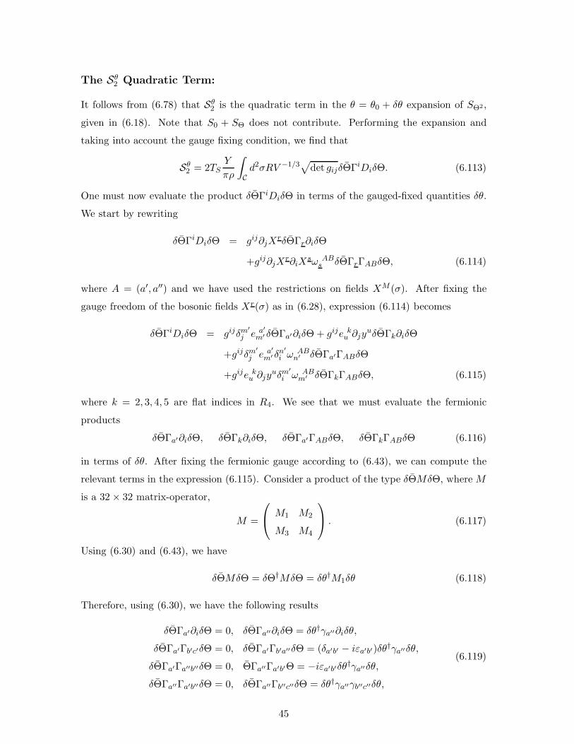
The Sθ2 Quadratic Term:
It follows from (6.78) that Sθ2 is the quadratic term in the θ = θ0 + δθ expansion of SΘ2,
given in (6.18). Note that S0 + SΘ does not contribute. Performing the expansion and
taking into account the gauge fixing condition, we find that
Sθ2 = 2TSY
πρ
∫
Cd2σRV −1/3
√
det gijδΘΓiDiδΘ. (6.113)
One must now evaluate the product δΘΓiDiδΘ in terms of the gauged-fixed quantities δθ.
We start by rewriting
δΘΓiDiδΘ = gij∂jXrδΘΓr∂iδΘ
+gij∂jXr∂iX
sω ABs δΘΓrΓABδΘ, (6.114)
where A = (a′, a′′) and we have used the restrictions on fields XM (σ). After fixing the
gauge freedom of the bosonic fields Xr(σ) as in (6.28), expression (6.114) becomes
δΘΓiDiδΘ = gijδm′
j e a′
m′ δΘΓa′∂iδΘ + gije ku ∂jy
uδΘΓk∂iδΘ
+gijδm′
j e a′
m′ δn′
i ωABn′ δΘΓa′ΓABδΘ
+gije ku ∂jyuδm
′
i ω ABm′ δΘΓkΓABδΘ, (6.115)
where k = 2, 3, 4, 5 are flat indices in R4. We see that we must evaluate the fermionic
products
δΘΓa′∂iδΘ, δΘΓk∂iδΘ, δΘΓa′ΓABδΘ, δΘΓkΓABδΘ (6.116)
in terms of δθ. After fixing the fermionic gauge according to (6.43), we can compute the
relevant terms in the expression (6.115). Consider a product of the type δΘMδΘ, where M
is a 32 × 32 matrix-operator,
M =
M1 M2
M3 M4
. (6.117)
Using (6.30) and (6.43), we have
δΘMδΘ = δΘ†MδΘ = δθ†M1δθ (6.118)
Therefore, using (6.30), we have the following results
δΘΓa′∂iδΘ = 0, δΘΓa′′∂iδΘ = δθ†γa′′∂iδθ,
δΘΓa′Γb′c′δΘ = 0, δΘΓa′Γb′a′′δΘ = (δa′b′ − iεa′b′)δθ†γa′′δθ,
δΘΓa′Γa′′b′′δΘ = 0, ΘΓa′′Γa′b′Θ = −iεa′b′δθ†γa′′δθ,δΘΓa′′Γa′b′′δΘ = 0, δΘΓa′′Γb′′c′′δΘ = δθ†γa′′γb′′c′′δθ,
(6.119)
45

with a′′ = (k,K), k = 2, 3, 4, 5 are flat indices in R4 and K = 6, 7, 8, 9 are flat indices in the
supspace CY⊥ ⊂ CY3 orthogonal to C. Substituting these expressions into (6.115) yields
δΘΓiDiδΘ = gije ku ∂jyu[δθ†γk∂iδθ − iδm
′
i ω a′b′
m′ εa′b′δθ†γkδθ + δm
′
i ω KLm′ δθ†γkγKLδθ]
+gijδm′
j e a′
m′ δn′
i ωb′Kn′ (δa′b′ − iεa′b′)δθ
†γKδθ. (6.120)
Then (6.113) becomes
Sθ2 = 2TSY
πρ
∫
Cd2σRV −1/3δθ†√ggije k
u ∂jyu[γk∂i − iδm
′
i ω a′b′
m′ εa′b′γk
+δm′
i ω KLm′ γkγKL] +
√ggijδm
′
j e a′
m′ δn′
i ωb′Kn′ (δa′b′ − iεa′b′)γKδθ. (6.121)
As discussed in the previous section, at the level of the quadratic contributions to the
path-integrals, all terms should be evaluated at the classical values of the backgound fields.
Therefore, the factor 2TSYπρRV
−1/3 can be absorbed by a redefinition of the δθ’s. Next, we
use the relation∫
Dδθ e∫
d2σδθ†Oδθ ∝ detO. (6.122)
Note, however, that when going to Euclidean space, we have doubled the number of fermion
degrees of freedom. Therefore, one must actually integrate over only one half of these degrees
of freedom. This amounts to taking the square-root of the determinant on the right-hand
side of (6.122). Hence, we conclude that∫
Dδθ e−Sθ2 ∝
√
detO/3, (6.123)
where
O/3 =√ggijγke k
u ∂jyu[∂i − iδm
′
i ω a′b′
m′ εa′b′ + δm′
i ω KLm′ γKL]
+γKδm′
j e a′
m′ δn′
i ωb′Kn′ (δa′b′ − iεa′b′). (6.124)
Note that because of the projections (6.44) that reduce the number of independent com-
ponents of θ from 16 to 4, the operator O/3 must be projected accordingly. We implicitly
assume this.
Collecting the results we have obtained thus far, two-point function (6.79) can now be
written as
〈λY(yu1 )λY(yu2 )〉 ∝√
detO/3√detO1
·∫
DλY e−∫
d4yλY∂/λYλY(yu1 )λY(yu2 )
·∫
d4x e−T2Y λY(x)λY(x)
·∫
Dω e−S0WZW . (6.125)
It remains, therefore, to evaluate the∫
Dω e−S0WZW factor in the path-integral, which we
now turn to.
46

7 The Wess-Zumino-Witten Determinant:
In this section, we will discuss the E8 Wess-Zumino-Witten part of the action, its quadratic
expansion and one loop determinant. Here we follow the exposition in [25] closely.
Recall from (6.23) that the relevant action is
S0WZW = − 1
8π
∫
Cd2σ tr[
1
2
√ggij(ωi −Ai) · (ωj −Aj) + iεijωiAj ]
+1
24π
∫
Bd3σiεıkΩkı(ω), (7.1)
where ω = g−1dg is an E8 Lie algebra valued one-form and g is given in (3.19). In order to
discuss the equation of motion and the chirality of this action, it is convenient to use the
complex coordinates z = σ0 + iσ1, z = σ0− iσ1 on C and to define the complex components
of A by A = Azdz +Azdz. Then action (7.1) can be written as
S0WZW = − 1
8π
∫
Cd2z tr
(
g−1∂zgg−1∂zg − 2Azg
−1∂zg +AzAz)
+1
24π
∫
Bd3σiεıkΩkı(ω). (7.2)
It is useful to define the two E8 currents
Jz = (Dzg)g−1, Jz = g−1Dzg, (7.3)
where Dz and Dz are the E8 covariant derivatives. In order to perform the path-integral
over ω, it is necessary to fix any residual gauge freedom in the ω fields. Recall from the
discussion in Section 3 that the entire action is invariant under both local gauge and modified
κ-transformations, δL and ∆k respectively. It follows from (3.21) and (3.14) that
δκg = gikA. (7.4)
It is not difficult to show that using this transformation, one can choose a gauge where
Jz = 0. (7.5)
Henceforth, we work in this chiral gauge. It follows from (7.2) that the g equations of
motion are
∂zJz = 0, DzJz + Fzz = 0, (7.6)
where Fzz is the E8 field strength. Note that this is consistent with the gauge choice (7.5)
and, hence, that the first equation in (7.6) is vacuous. Thus, the on-shell theory we obtain
from the gauged Wess-Zumino-Witten action is an E8 chiral current algebra at level one.
47

The level can be read off from the coefficient of the Chern-Simons term in (7.2). We would
now like to evaluate the Wess-Zumino-Witten contribution to the path-integral using a
saddle-point approximation. To do this, we should expand g as small fluctuations
g = g0 + δg (7.7)
around a classical solution g0 of (7.6). However, it is clearly rather difficult to carry out the
quadratic expansion and evaluate the determinant in this formalism. Luckily, there is an
equivalent theory which is more tractable in this regard, which we now describe.
As discussed in [25], if the gauge field background is restricted to lie within an SO(16)
subgroup of E8, then the equivalent action is given by the free fermion theory coupled to the
SO(16) gauge field background. As described in [25], realistic heterotic M -theory models
can always be chosen to have the gauge instanton within the SO(16) subgroup of E8. Here,
we consider only such restricted backgrounds. We can now write the action for SO(16)
fermions coupled to background gauge fields. It is given by [47]–[51]
Sψ =
∫
Cd2σψaD/abA ψ
b (7.8)
where ψa denotes the set of SO(16) fermions with a,= 1, . . . , 16 and
D/abA =√gτ i(Diδ
ab −Aabi ) (7.9)
is the covariant derivative on C with Aabi the set of SO(16) background gauge fields. The
matrices τ i are the Dirac matrices in two-dimensions. It follows from the above discussion
that we can write∫
Dω e−S0WZW ∝∫
Dψa e−Sψ , (7.10)
where the gauge fixing of variable ω described by (7.5) is inherent in the ψa formalism, as
we will discuss below. The equations of motion are given by
D/abA ψb = 0. (7.11)
We now expand
ψa = ψa0 + δψa (7.12)
around a solution ψa0 of (7.11) and consider terms in Sψ up to quadratic order in the
fluctuations δψa. We find that
Sψ = S0ψ + S2ψ, (7.13)
where
S0ψ =
∫
Cd2σψa0D/
abA ψ
b0 (7.14)
48

and
S2ψ =
∫
Cd2σδψaD/abA δψ
b. (7.15)
The terms linear in δψ vanish by the equations of motion. It follows immediately from
(7.11) that S0ψ = 0. Then, using (6.122), one finds from (7.15) that∫
Dδψa e−Sψ ∝√
detD/A. (7.16)
Note, again, that by going to Euclidean space we have doubled the number of fermionic
degrees of freedom. Therefore, one must actually integrate over only one half of these
degrees of freedom. This requires the square-root of the determinants to appear in (7.16).
It is important to discuss how the chiral gauge fixing condition (7.5) is manifested in the ψa
formalism. Condition (7.5) imposes the constraint that g couples only to the Az component
of the gauge fields and not to Az. It follows that in evaluating detD/A, we should keep only
the Az components of the gauge fields. That is, we should consider the Dirac determinants
of SO(16) holomorphic vector bundles on the Riemann surface C. Gauge fixing condition
(7.5) also imposes a constraint on the definition of determinant detD/A as follows. Recall
that on the Euclidean space C, each spinor ψ is a complex two-component Weyl spinor
ψ =
ψ+
ψ−
. (7.17)
Rescaling this basis to
ψ+
ψ−
=
(gzz)−1/4ψ+
(gzz)1/4ψ−
(7.18)
and using the standard representation for τ0, τ1 then, locally, one can write
D/A =
0 D−A
D+A 0
, (7.19)
where
D−A = (gzz)3/4
(
(gzz)−1/2 ∂
∂z(gzz)
1/2 −Az
)
, D+A = (gzz)1/4 ∂
∂z. (7.20)
Since the operator D/A must be Hermitean, it follows that D+A = D†−A. Now, in addition
to disallowing any coupling to Az, gauge condition (7.5) imposes the constraint that
ψa+ = 0 (7.21)
for all a = 1, . . . , 16. Then, using the fact that
detD/A =√
det(D/A)2 (7.22)
49

and gauge condition (7.21), we see that the proper definition of the determinant is
detD/A =
√
detD†−AD−A. (7.23)
In this paper, it is not necessary to determine the exact value of detD/A. We need only
compute whether it vanishes or is non-zero, and the conditions under which these two
possibilities occur. To do this, we must examine the global properties of the holomorphic
vector bundle. As we did throughout the paper, we will restrict
C = CP1 = S2. (7.24)
With this restriction, the condition for the vanishing of detD/A can be given explicitly, as
we now show.
It follows from (7.21) that the chiral fermions realizing the SO(16) current algebra
are elements of the negative chiral spinor line bundle S− of the sphere. Note from (7.19)
that D−A is the part of the Dirac operator which acts on S−. With respect to a non-trivial
SO(16) holomorphic vector bundle background A, the complete operator we should consider
is
D−A : S− ⊗A→ S+ ⊗A, (7.25)
where S+ denotes the positive chiral spinor bundle on the sphere. This is the global de-
scription of the local D−A operator defined in (7.19) and (7.20). In order to have nonzero
determinant detD/A, it is necessary and sufficient that D−A should not have any zero-modes.
This follows from the index theorem which, for SO(16), implies that
cokerD†−A = kerD−A. (7.26)
As was shown in [25], D−A does not have any zero-modes if and only if the restriction
of the SO(16) holomorphic vector bundle A to C is trivial. Therefore, in order to have a
non-zero superpotential for the five-brane, we must have a special type of the gauge bundle
on the Calabi-Yau threefold. Bundles of this type are straightforward to construct. We will
present a number of phenomenologically relevant examples in a forthcoming paper [52].
8 Final Expression for the Superpotential:
We are now, finally, in a position to extract the final form of the non-perturbative superpo-
tential from the fermion two-point function. Combining the results of the previous section
50

with expression (6.125), we find that
〈λY(yu1 )λY(yu2 )〉 ∝√
detO/3√detO1
·√
detD/A
·∫
DλY e−∫
d4yλY∂/λYλY(yu1 )λY(yu2 )
·∫
d4x e−T2Y(x) λY(x)λY(x). (8.1)
Comparing this with the purely holomorphic part of the quadratic fermion term in the
four-dimensional effective Lagrangian (5.28)
(∂Y∂YW )λYλY, (8.2)
we obtain
W ∝√
detO/3√detO1
·√
detD/A · e−T2Y. (8.3)
In this expression, the dimensionless field Y is defined by
Y =Y
πρReT + i(a+
Y
πρImT ), (8.4)
where Y and a are the translational and axionic moduli of the five-brane respectively and
τ is the complex (1, 1)-modulus associated with curve C. T is a dimensionless parameter
given by
T = TMπρ vC , (8.5)
with TM the membrane tension and πρ the S1/ZZ2 interval length. The operators O1 and
O/3 are presented in (6.112) and (6.124), respectively. The operator D/A and its determinant
detD/A are defined in (7.9), (7.19), (7.20) and (7.23). This determinant and, hence, the
superpotential W will be non-vanishing if and only if the pullback of the associated SO(16)
holomorphic vector bundle A to the curve C is trivial. All the determinants contributing to
W are non-negative real numbers. We emphasize that W given in (8.3) is the contribution
of open supermembranes wrapped once around C × I, where C = S2 is a sphere isolated
in the Calabi-Yau threefold CY3 and I ⊂ S1/ZZ2. The generalization to supermembranes
wrapped once around I but n-times around C is straightforward. One simply replaces the
exponential term in (8.3) by
e−nT2
Y. (8.6)
Further generalizations and discussions of the complete open supermembrane contributions
to the non-perturbative superpotential in heterotic M -theory will be presented elsewhere
[52].
51

A Notation and Conventions:
We use a notation such that symbols and indices without hats represent fields in the ten-
dimensional fixed hyperplanes of Horava-Witten theory (as well as the two-dimensional
heterotic string theory), while hatted indices relate to quantities of eleven-dimensional bulk
space (and the three-dimensional open membrane theory). In addition, underlined symbols
and indices refer to the five-brane worldvolume.
Bosons:
For example,
XM , M = 0, 1, . . . , 9, and XM , M = 0, 1, . . . , 9, 11, (A.1)
are, respectively, the coordinates of ten- and eleven-dimensional spacetimes. We do not
change notation when switching from Minkowskian signature to Euclidean signature.
Eleven-dimensional space is, by assumption, given by
M11 = R4 × CY3 × S1/ZZ2, (A.2)
while the ten-dimensional space obtained by compactifying it on S1/ZZ2 is, clearly,
M10 = R4 × CY3. (A.3)
The membrane worldvolume Σ is decomposed as
Σ = C × I, (A.4)
where the holomorphic curve C lies within CY3 and I ⊂ S1/ZZ2.
The two-dimensional heterotic string theory is represented by fields with worldsheet
coordinates σi, with i = 0, 1. Bosonic indices of ten-dimensional spacetime are split into
indices parallel to the worldsheet (m′ = 0, 1) and indices perpendicular to it (m′′ = 2, . . . , 9).
The space normal to the worldsheet is an eight-dimensional space. Since it is assumed that
the worldsheet is wrapped on a curve C contained in the Calabi-Yau threefold CY3, these
eight directions ym′′
can be split in two sets of four. The first set parametrizes the subset
CY⊥ ⊂ CY3 which is normal to curve C. The coordinates are denoted yU , U = 6, 7, 8, 9.
The second set consists of the coordinates yu, u = 2, 3, 4, 5 of R4.
The five-brane worldvolume M6 is embedded in M10 as
M10 = CY⊥ ×M6, (A.5)
52

where
M6 = R4 × C. (A.6)
Indices in the five-brane super-worldvolume are given by R = (r, µ), with r = 0, 1, . . . , 5 and
µ = 1, . . . , 16. Note that one has a (2, 0)-supersymmetry on the five-brane worldvolume.
Coordinates of CY3 are denoted by
yU = (Xr′ , yU ), with U = 0, 1, 6, 7, 8, 9, r′ = 0, 1, (A.7)
or, using the complex structure notation,
ym, ym, m = 1, 2, 3, m = 1, 2, 3. (A.8)
The bosonic indices in (A.1)-(A.8) are coordinate (or “curved”) indices. The corre-
sponding tangent space (or “flat”) indices are given in the following table,
M10 M11 M 6 C M⊥ R4 CY⊥
M,N M, N r, s r′, s′ m′′, n′′ u, v U, V
A,B A, B a, b a′, b′ a′′, b′′ k, l K,L
where M⊥ is the subspace of M10 perpendicular to C.
Spinors:
In ten-dimensional spacetime with Euclidean signature, the 32×32 Dirac matrices ΓA satisfy
ΓA,ΓB = 2ηAB (A.9)
or, with curved indices, (since ΓA = e MA ΓM)
ΓM ,ΓN = 2gMN . (A.10)
One defines ten-dimensional chirality projection operators 12(1 ± Γ11), where
Γ11 = −iΓ0Γ1 · · ·Γ9. (A.11)
A useful representation for ΓA is given by the two-eight split
ΓA = (τa′ ⊗ γ, 1 ⊗ γa′′), (A.12)
where the two-dimensional Dirac matrices τ0, τ1 and their product defined by τ = −iτ0τ1are explicitly given by
τ0 =
0 1
1 0
, τ1 =
0 −ii 0
, τ =
1 0
0 −1
. (A.13)
53

These ten-dimensional Dirac matrices are more explicitly written as
Γ0 =
0 γ
γ 0
Γ1 =
0 −iγiγ 0
Γa′′ =
γa′′ 0
0 γa′′
Γ11 =
γ 0
0 −γ
(A.14)
where γa′′ are 16 × 16 Dirac matrices, and the product
γ = γ2γ3 · · · γ9 (A.15)
is used in the definition of eight-dimensional chirality projection operators 12(1 ± γ). Note
that Γ211 = 1, γ2 = 1, and τ2 = 1. In eleven-dimensions, the 32 × 32 Dirac matrices are
given by
ΓA = ΓA, (A = 0, 1, . . . , 9), and Γ11 = Γ11. (A.16)
References
[1] P. Horava and E. Witten, “Heterotic and Type I String Dynamics from Eleven Dimen-
sions”, Nucl. Phys. B460 (1996) 506, hep-th/9603142.
[2] P. Horava and E. Witten, “Eleven-Dimensional Supergravity on a Manifold with
Boundary”, Nucl. Phys. B475 (1996) 94, hep-th/9510209.
[3] E. Witten, “Solutions of Four-Dimensional Field Theories via M -Theory”, Nucl. Phys.
B507 (1997) 3, hep-th/9703166.
[4] T. Banks and M. Dine, Nucl. Phys. B479 (1996) 173.
[5] A. Lukas, B.A. Ovrut and D. Waldram, “On the Four-Dimensional Effective Action
of Strongly Coupled Heterotic String Theory”, Nucl. Phys. B532 (1998) 43, hep-
th/9710208.
[6] A. Lukas, B.A. Ovrut, K. Stelle and D. Waldram, “The Universe as a Domain Wall”,
Phys. Rev. D59 (1999) 086001, hep-th/9803235.
[7] A. Lukas, B.A. Ovrut and D. Waldram, “Cosmological Solutions of Horava-Witten
Theory”, Phys. Rev. D60 (1999) 086001, hep-th/9806022.
[8] A. Lukas, B.A. Ovrut, K. Stelle and D. Waldram, “Heterotic M -theory in Five Dimen-
sions”, Nucl. Phys. B552 (1999) 246, hep-th/9806051.
54

[9] A. Lukas, B.A. Ovrut and D. Waldram, “Non-Standard Embedding and Five-Branes
in Heterotic M -theory”, Phys. Rev. D59 (1999) 106005, hep-th/9808101.
[10] R. Donagi, T. Pantev, B.A. Ovrut and D. Waldram, “Holomorphic Vector Bundles
and Nonperturbative Vacua in M -theory”, JHEP 9906 (1999) 34, hep-th/9901009.
[11] R. Donagi, B.A. Ovrut, T. Pantev and D. Waldram, “Standard Models from Heterotic
M -theory”, hep-th/9912208.
[12] R. Donagi, B.A. Ovrut, T. Pantev and D. Waldram, “Standard Model Bundles on
Nonsimply Connected Calabi-Yau Threefolds”, hep-th/0008008.
[13] R. Donagi, B.A. Ovrut, T. Pantev and D. Waldram, “Standard Model Bundles”, math-
ag/0008010.
[14] R. Donagi, B.A. Ovrut, T. Pantev and D. Waldram, “Spectral Involutions on Rational
Elliptic Surfaces”, math-ag/0008011.
[15] H.P. Nilles, M. Olechowski and M. Yamaguchi, “Supersymmetry Breakdown at a Hid-
den Wall”, hep-th/9801030.
[16] E. Sharpe, “Boundary Superpotentials”, hep-th/9611196.
[17] E.A. Mirabelli and M.E. Peskin, “Transmission of Supersymmetry Breaking from a
Four-dimensional Boundary”, hep-th/9712214.
[18] L. Randall and R. Sundrum, Phys. Rev. Lett. 83 (1999) 3370, hep-th/9905221.
[19] L. Randall and R. Sundrum, Phys. Rev. Lett. 83 (1999) 4690, hep-th/9906064.
[20] A. Lukas and B.A. Ovrut, “U-Duality Invariant M -theory Cosmology”, hep-
th/9709030.
[21] K. Benakli, “Cosmological Solutions in M -theory on S1/ZZ2”, hep-th/9804096.
[22] K. Benakli, “Scales and Cosmological Application in M -theory”, hep-th/9805181.
[23] A. Lukas, B.A. Ovrut and D. Waldram, “Cosmological Solutions of Horava-Witten
Theory”, Phys. Rev. D60 (1999) 086001, hep-th/9806022.
[24] J. Ellis, Z. Lalak, S. Pokorski and W. Pokorski, “Five-Dimensional Aspects ofM -theory
and Supersymmetry Breaking”, hep-th/9805377.
55

[25] E. Lima, B. Ovut, J. Park and R. Reinbacher, “Non-Perturbative Superpotential from
Membrane Instantons in Heterotic M -theory”, hep-th/0101049.
[26] K. Becker, M. Becker and A. Strominger, “Fivebranes, Membranes and Non Perturba-
tive String Theory”, Nucl. Phys. B456 (1995) 130, hep-th/9507158.
[27] J. Harvey and G. Moore, “Superpotentials and Membrane Instantons”, hep-
th/9907026.
[28] J.-P. Derendinger and R. Sauser, “A Five-brane Modulus in the Effective N=1 Super-
gravity of M -theory”, hep-th/0009054.
[29] G. Moore, G. Peradze and N. Saulina, “Instabilities in Heterotic M -theory Induced by
Open Membrane Instantons”, hep-th/0012104.
[30] E. Cremmer, B. Julia and J. Scherk, Phys. Lett. B76 (1978) 409.
[31] M.J. Duff and K.S. Stelle, Phys. Lett. B253 (1991) 113.
[32] E. Bergshoeff, E. Sezgin and P.K. Townsend, Phys. Lett. B189 (1987) 75.
[33] I. Bandos, K. Lechner, A. Nurmagambetov, P. Pasti, D. Sorokin and M. Tonin, Phys.
Rev. Lett. 78 (1997) 4332.
[34] E. Cremmer and S. Ferrara, Phys. Lett. B91 (1980) 61.
[35] M. Cederwall, “Boundaries of 11-Dimensional Membranes”, hep-th/9704161.
[36] Z. Lalak, A. Lukas and B.A. Ovrut, “Soliton Solutions of M -theory on an Orbifold”,
hep-th/9709214.
[37] P. Candelas, Lectures on Complex Manifolds, in Trieste 1987 Proceedings.
[38] E. Witten, Comm. Math. Phys. 92 (1984) 455.
[39] C.S. Chu and E. Sezgin, “M-Fivebrane from the Open Supermembrane”, JHEP 9712
(1997) 1.
[40] B. Ovrut, “N=1 Supersymmetric Vacua in Heterotic M -theory”, hep-th/9905115.
[41] B. de Wit, K. Peeters and J. Plefka, “Superspace Geometry for Supermembrane Back-
grounds”, hep-th/9803209.
56

[42] E. Bergshoeff, M. de Roo, B. de Wit and P. van Nieuwenhuizen, Nucl. Phys. B195
(1982) 97.
[43] S.S. Chern, “Minimal Submanifolds in a Riemannian Manifold”, University of Kansas,
Dept. of Mathematics, 1968.
[44] M. Green, J. Schwartz and E. Witten, Superstring Theory, Vol.1, Cambridge University
Press, 1987.
[45] L. Alvarez-Goume, G. Moore and C. Vafa, Comm. Math. Phys. 106 (1986) 81.
[46] D. Freed, “On Determinant Line Bundles”, in Mathematical Aspects of String Theory,
edited by S. Yau (World Scientific, 1987).
[47] D.Vecchia, B. Durhuus and J.L. Petersen, Phys. Lett. B144 (1984) 245.
[48] A.N. Redlich and H. Schnitzer, Nucl. Phys. B183 (1987) 183.
[49] A.N. Redlich and H. Schnitzer, Nucl. Phys. B167 (1986) 315.
[50] A.N. Redlich, H. Schnitzer and K. Tsokos, Nucl. Phys. B289 (1989) 397.
[51] H. Schnitzer and K. Tsokos, Nucl. Phys. B291 (1989) 429.
[52] E. Lima, B.A. Ovrut, J. Park and R. Reinbacher, In preparation.
57